Dynamic Occlusion Analysis in Optical Flow Fieldsthompson/publications/Thompson:1985:DOA.pdf · DynamicOcclusion Analysis in Optical Flow Fields ... THOMPSON,MEMBER,IEEE,KATHLEENM.MUTCH,MEMBER,IEEE,

IEEE TRANSACTIONS ON PATTERN ANALYSIS AND MACHINE INTELLIGENCE, VOL. PAMI-7, NO. 4, JULY 1985

Dynamic Occlusion Analysis in Optical Flow Fields

WILLIAM B. THOMPSON, MEMBER, IEEE, KATHLEEN M. MUTCH, MEMBER, IEEE,

AND VALDIS A. BERZINS, MEMBER, IEEE

Abstract-Optical flow can be used to locate dynamic occlusion bound-aries in an image sequence. We derive an edge detection algorithm sensi-tive to changes in flow fields likely to be associated with occlusion. Thealgorithm is patterned after the Marr-Hildreth zero-crossing detectorscurrently used to locate boundaries in scalar fields. Zero-crossing de-tectors are extended to identify changes in direction and/or magnitudein a vector-valued flow field. As a result, the detector works for flowboundaries generated due to the relative motion of two overlappingsurfaces, as well as the simpler case of motion parallax due to a sensormoving through an otherwise stationary environment. We then showhow the approach can be extended to identify which side of a dynamicocclusion boundary corresponds to the occluding surface. The funda-mental principal involved is that at an occlusion boundary, the imageof the surface boundary moves with the image of the occluding surface.Such information is important in interpreting dynamic scenes. Resultsare demonstrated on optical flow fields automatically computed fromreal image sequences.

Index Terms-Dynamic occlusion, dynamic scene analysis, edge de-tection, optical flow, visual motion.

I. INTRODUCTION

AN optical flow field specifies the velocity of the imageof points on a sensor plane due to the motion of the sen-

sor and/or visible objects. Optical flow can be used to estimateaspects of sensor and object motion, the position and orienta-tion of visible surfaces relative to the sensor, and the relativeposition of different objects in the field of view. As a result,the determination and analysis of optical flow is an importantpart of dynamic image analysis. In this paper, we develop anoperator for finding occlusion boundaries in optical flow fields.We deal exclusively with dynamic occlusions in which flowproperties differ on either side of the boundary. The operatoris effective for both motion parallax, when a sensor is movingthrough an otherwise stationary environment, and for moregeneral motion in which multiple moving objects can be in thefield of view. The multiple moving object situation is more dif-ficult because boundaries are marked by almost arbitrary com-binations of changes in magnitude and/or direction of flow.

Manuscript received June 1, 1984; revised February 14, 1985. Rec-ommended for acceptance by W. E. L. Grimson. This work was sup-ported by the National Science Foundation under Grant MCS-81-05 215,the Air Force Office of Scientific Research under Contract F49620-83-0140, and by Zonta International.W. B. Thompson and V. A. Berzins are with the Department of Com-

puter Science, University of Minnesota, Minneapolis, MN 55455.K. M. Mutch was with the Department of Computer Science, Univer-

sity of Minnesota, Minneapolis, MN 55455. She is now with the Depart-ment of Computer Science, Arizona State University, Tempe, AZ85287.

The technique is extended so that a determination may bemade about which side of a dynamic occlusion boundary corre-sponds to the occluding surface. Such a determination is ofgreat importance for interpreting the shape and spatial organi-zation of visible surfaces. Results are demonstrated on realimage sequences with flow fields computed using the tokenmatching technique described in [1] . Reliability is obtainedby dealing only with methods able to integrate flow field in-formation over relatively large neighborhoods so as to reducethe intrinsic noise in fields determined from real imagesequences.

II. BOUNDARY DETECTION

Conventional edge operators detect discontinuities in imageluminence. These discontinuities are difficult to interpret,however, because of the large number of factors that can pro-duce luminence changes. Boundaries in optical flow can arisefrom many fewer causes and, hence, are often more informa-tive. If a sensor is moving through an otherwise static scene, adiscontinuity in optical flow occurs only if there is a discon-tinuity in the distance from the sensor to the visible surfaceson either side of the flow boundary [2]. Discontinuities inflow will occur for all visible discontinuities in depth, exceptfor viewing angles directly toward or away from the directionof sensor motion. If objects are moving with respect to oneanother in the scene, then all discontinuities in optical flowcorrespond either to depth discontinuities or surface bound-aries, and most depth discontinuities correspond to flowdiscontinuities.The use of local operators to detect discontinuities in optical

flow has been suggested by others. Nakayama and Loomis [3]propose a "convexity function" to detect discontinuities inimage plane velocities generated by a moving observer. Theirfunction is a local operator with a center-surround form. Thatis, the velocity integrated over a band surrounding the centerof the region is subtracted from the velocity integrated overthe center. The specifics of the operator are not preciselystated, but a claim is made [3, Fig. 3] that the operator returnsa positive value at flow discontinuities. (In fact, most reason-able formulations of their operator would yield a value of 0 atthe boundary, with a positive value to one side or the other.)Clocksin [2] develops an analysis of optical flow fields gen-erated when an observer translates in a static environment. Heshows that, in such circumstances, discontinuities in the mag-nitude of flow can be detected with a Laplacian operator. Inparticular, singularities in the Laplacian occur at discontinuitiesin the flow. He also showed that, in this restricted environ-

0162-8828/85/0700-0374$01.00 © 1985 IEEE

374

Authorized licensed use limited to: IEEE Xplore. Downloaded on February 28, 2009 at 10:34 from IEEE Xplore. Restrictions apply.

THOMPSON et al.: DYNAMIC OCCLUSION ANALYSIS IN OPTICAL FLOW FIELDS

ment, the magnitude of optical flow at a particular image pointis inversely proportional to distance, and the distances can berecovered to within a scale factor of observer speed. It is thustrivial to determine which of two surfaces at an edge is occlud-ing, for example, by simply comparing magnitudes of the twosurface velocities, even when observer speed is unknown.For this restricted situation in which a sensor moves through

an otherwise static world

flow ('fl=)_ A + rt(l) (1)

where at an image point xk, flow(xZ) is the optical flow (a two-dimensional vector), fr is the component of the flow due tothe rotation of the scene with respect to the sensor, ft is de-pendent on the translational motion of the sensor and theviewing angle relative to the direction of translation, and r isthe distance between the sensor and the surface visible at x[4] . For a fixed x, flow varies inversely with distance. Bothfr and ft vary slowly (and continuously) with x. Discontinu-ities in flow thus correspond to discontinuities in r. Further-more, it is sufficient to look only for discontinuities in themagnitude of flow. This relationship holds only for relativemotion between the sensor and a single, rigid structure. Whenmultiple moving objects are present, (1) must be modified sothat there is a separate f (') and f i) specifying the relative mo-tion between the sensor and each rigid object. Discontinuitiesassociated with object boundaries may now be manifested inthe magnitude and/or direction of flow.Boundary detectors for optical flow fields should satisfy two

criteria: 1) sensitivity to rapid spatial change in one or both ofthe magnitude and direction of flow, and 2) operation over asufficiently large neighborhood to reduce sensitivity to noisein computed flow fields. It is desirable to achieve the secondcriterion without an unnecessary loss of spatial resolution inlocating the boundary or a need for postprocessing to reducethe width of detected boundaries. The zero-crossing detectorsof Marr and Hildreth [5] may be extended to optical flowfields in a manner that achieves both objectives [6] . For scalarfields (e.g., intensity images), zero-crossing edge detection pro-ceeds as follows. 1) Smooth the field using a symmetrical Gauss-ian kernel. 2) Compute the Laplacian of the smoothed func-tion. 3) Look for directional zero crossings of the resultingfunction (e.g., look for points at which, along some direction,the function changes sign). Under a set of relatively weak as-sumptions, these zero crossings can be shown to correspond topoints of most rapid change in some direction in the originalfunction. The convolution with a Gaussian provides substan-tial noise reduction and, in addition, allows tuning of themethod for edges of a particular scale. Steps 1) and 2) involveevaluating the function V 2G * I, where G is a Gaussian kernel,* is the convolution operation, and I is the original image. Theeffect of the V2G operator can be approximated by blurringthe original function with two different Gaussian kernels ofappropriate standard deviation, and then taking the differenceof the result. This formulation results in computational simpli-fications [7], [8] and also corresponds nicely to several phys-iological models that have been proposed for early visualprocessing.

The effect of this approach is to identify edge points wherethe intensity of the blurred image is locally steepest. Moreprecisely, an edge can be defined as a peak in the first direc-tional derivative, or as a zero crossing in the second directionalderivative. At an edge, the second directional derivative haszero crossings in almost all directions, but the preferred direc-tion is normal to the locus of the zero crossings, which is thesame as the direction where the zero crossing is steepest forlinearly varying fields [5]. For vector images such as opticalflow fields, the directional derivatives are vector valued, andwe want the magnitude of the first directional derivative tohave a peak.This extension to two-dimensional flow fields is relatively

straightforward. The optical flow field is first split into sepa-rate scalar components corresponding to motion in the x andy directions. The V2G operator is applied to each of thesecomponent images, and the results combined into a component-wise Laplacian of the original flow field. (The Laplacian is avector operator which can be expressed in arbitrary coordinatesystems. For convenience, we choose a Cartesian coordinatesystem.) This componentwise Laplacian operation is imple-mented by subtracting two componentwise blurred versions ofthe original. With the proper set of weak assumptions, discon-tinuities in optical flow correspond to zeros in both of thesecomponent Laplacian fields. At least one of the componentswill have an actual zero crossing. The other will have either azero crossing or will have a constant zero value in a neighbor-hood of the discontinuity. If the componentwise Laplaciansare treated as a two-dimensional vector field, discontinuitiesare indicated by directional reversals in the combined field.Because of the discrete spatial sampling and a variety of noisesources, the zeros or zero crossings in the two components ofthe field may not actually be exactly spatially coincident. Thus,exact reversal is not expected, and a range of direction changesof about 180° is accepted. A threshold on the sum of the vec-tor magnitudes at the location of the flip is used to ensure thatthe zero crossing is of significant slope. This is analogous tothe threshold on zero-crossing slope which is often used in prac-tice when zero-crossing techniques are used on intensity im-ages, and serves to filter out small discontinuities.

The approximations made by the computations describedabove will be good if the variation of the field parallel to theedge is much more uniform than the variation normal to theedge. For scalar images, exact results will be obtained if theintensity varies at most linearly along the edge contour [5].For vector images, the field must vary at most linearly in someneighborhood of the edge contour, so that the assumptions re-quired are slightly stronger than for scalar images. Appendix Icontains the analysis for the case of vector images.Two examples of this technique applied to real images are

shown below. In both examples, the objects are toy animalswith flat surfaces, shown moving in front of a textured back-ground. In Fig. l(a), the tiger translates parallel to the imageplane from right to left between frames 1 and 2. The elephantrises off its front legs between frames 1 and 2, effectively ro-tating about an axis at its hind feet oriented perpendicularly tothe image plane. The elephant also translates slightly to theleft parallel to the image plane. The optical flow vectors, shown

375



(DI

(c)

Fig. 1. (a) Image pair. (b) Optical flow. (c) Detected edge overlaid ontoflow field. (d) Dectected edge overlaid onto first frame of sequence.

in Fig. 1(b), were obtained by relaxation labeling token match-ing, as described in [1] . Notice that the flow vectors on theelephant and tiger have approximately the same magnitude butdiffer in direction. Each component of this flow field was con-

volved with approximated Gaussians of standard deviations3.65 and 5.77. The ratio of these standard deviations is 1 :1.6.The two convolved flow fields were subtracted, and the re-

sulting vector field was searched for reversals in vector direc-tion. A boundary strength threshold was chosen to eliminatenoise points due to small, local variations in estimated flow.In Fig. l(c), the points where reversals were found are shown

(U)Fig. 2. (a) Image pair. (b) Optical flow. (c) Detected edge overlaid onto

flow field. (d) Detected edge overlaid onto first frame of sequence.

overlaid on the original flow field, and in Fig. 1(d) the pointsare overlaid in white on the first image of the pair. The edgepoints form a good boundary between the discontinuous opti-cal flow vector fields [Fig. 1(c)] ; but because these fields areso sparse, the edge points match only the approximate loca-tions of the true edges [Fig. I (d)] .In Fig. 2(a), both the tiger and elephant are translating to

the right, parallel to the image plane between frames 1 and 2.The flow field shown in Fig. 2(b) was obtained in the samemanner as in Fig. l(b). The direction of the flow vectors onboth animals is approximately the same, but there is a dis-

376



continuity in magnitude. Two Gaussian filtered versions ofthe flow fields were obtained with standard deviations of 3.16and 5.16-a ratio of 1: 1.6. The locations of vector reversalsresulting from differencing the two filtered fields are shownin Fig. 2(c) and (d).The width of the Gaussian kernel used in the V 2G operator,

the density of the computed optical flow field, and the spatialvariability of flow all interact to affect the performance of theboundary detection. As with the use of zero-crossing detectorsfor scalar fields, it may be desirable to use a range of kernelsizes and then combine the results to obtain a more robust in-dicator for the presence of a boundary. While zero-crossingcontours are, in principle, connected, the use of a thresholdon the slope at the zero crossing results in some portions ofthe boundary being missed. In practice, zero-crossing bound-ary detection for both scalar and vector fields often requiressuch thresholds to avoid significant problems with false bound-ary indications in slowly varying regions of the fields. Workstill needs to be done on better techniques for selecting zerocrossings that correspond to true boundaries.

III. IDENTIFYING OCCLUDING SURFACES

When analyzing edges between dissimilar image regions thatarise due to occlusion boundaries, it is important to determinewhich side of the edge corresponds to the occluding surface.Occlusion boundaries arise due to geometric properties of theoccluding surface, not the occluded surface. Thus, while theshape of the edge provides significant information on the struc-ture of the occluding surface, it says little or nothing about thestructure of the surface being occluded. In situations where asensor is translating through an otherwise static scene, any sig-nificant local decrease in r in (1) increases the magnitude offlow. Thus, at a flow boundary, the side having the larger mag-nitude of flow will be closer, and thus will be occluding thefarther surface. Sensor rotation complicates the analysis, whileif objects in the field of view move with respect to each other,there is no direct relationship between magnitude offlow andr. Surfaces corresponding to regions on opposite sides of aboundary may move in arbitrary and unrelated ways. However,by considering the flow values on either side of the boundaryand the manner in which the boundary itself changes over time,it is usually possible to find which side of the boundary corre-sponds to the occluding surface, although the depth to the sur-faces on either side cannot be determined.The principle underlying the approach is that the image of the

occluding contour moves with the image of the occluding sur-face. Fig. 3 illustrates the effect for simple translational mo-

tion. Shown on the figure are the optical flow of points oneach surface and the flow of points on the image of the bound-ary. In Fig. 3(a), the left surface is in front and occluding thesurface to the right. In Fig. 3(b), although the flow values asso-ciated with each surface are the same, the left surface is nowbehind and being occluded by the surface to the right. Theoccluding surface cannot be determined using only the flowin the immediate vicinity of the boundary. The two cases canbe distinguished because, in Fig. 3(a), the flow boundary deter-mined by the next pair of images will be displaced to the left,while in Fig. 3(b) it will be displaced to the right.

time to .-

(a)

. w

time t1 - -

(b)Fig. 3. Optical flow at a boundary at two instants in time. (a) Surface

to the left is in front. (b) Surface to the right is in front.

To formalize the analysis, we need to distinguish the opticalflow of the boundary itself from the optical flow of surfacepoints. The flow of the boundary is the image plane motionof the boundary, which need not have any direct relationshipto the optical flow of regions adjacent to the boundary. Themagnitude of the optical flow of boundary points parallel tothe direction of the boundary typically cannot be determined,particularly for linear sections of boundary. Thus, we will limitthe analysis in this section to the component of optical flowperpendicular to the direction of the image of occlusion bound-aries. As a result, if the flow on both sides of the boundary isparallel to the boundary, the boundary will still be detectable,but the method given here will provide no useful informationabout which surface is occluding.We can now state the basic principle more precisely. Choose

a coordinate system in the image plane with the origin at a par-ticular boundary point and the x axis oriented normal to theboundary contour, with x > 0 for the occluding surface. Thecamera points in the z direction, and the image plane is atz = 0. Let f,(x, y) be the x component of optical flow at thepoint (x, y). Let fb be the x component of the flow of theboundary itself at the origin (i.e., ftb is the image plane veloc-ity of the boundary in a direction perpendicular to the bound-ary). Then, for rigid objects,

(2)xb= lim f+(X, )=fx(0,0)-x o++

We will show that this relationship is true for arbitrary rigidbody motion under an orthographic projection. For a singlesmooth surface, perspective projections are locally essentiallyequivalent to a rotation plus a scale change, although the anal-ysis is more complex. Equation (2) specifies a purely local con-straint and, as the limit is taken from only one side of theboundary, is dependent on flow values on a single surface.Thus, the limit result will hold as well for perspective projec-tions. Algorithms which utilize the result in (2) may suffer,however, if properties of more than a truly local area of thefield are utilized. The instantaneous motion of a rigid objectrelative to a fixed coordinate system can be described with re-spect to a six-dimensional, orthogonal basis set. Three valuesspecify translational velocity, the other three specify angularvelocity. These six coordinates of motion can be convenientlyclassified into four types: translation at constant depth, transla-tion in depth, rotation at constant depth, and rotation in depth.Translation at constant depth is translation in a direction par-allel to the image plane. Translation in depth is translation per-

377



pendicular to the image plane. Rotation at constant depth isrotation around an axis perpendicular to the image plane. Ro-tation in depth is rotation around an axis parallel to the imageplane. Any instantaneous motion can be described as a com-bination of these four types. For orthographic projections,translation in depth has no effect on the image. Thus, we needto show that the above relationship relating boundary and sur-face flow holds for the three remaining motion types.A point on the surface of an object in the scene that projects

into a boundary point in the image will be referred to as a gen-erating point of the occlusion boundary. The family of gen-erating points defines a generating contour, which lies alongthe extremal boundary of the object with respect to the sen-sor. For both translation and rotation at constant depth, thegenerating contour remains fixed to the occluding surface overtime. Thus, the boundary and adjacent points move with ex-actly the same motion. As a result, the projection of the sur-face flow in the direction normal to a particular boundary pointis identical to the projection of the boundary flow in the samedirection. (The result is strictly true only for instantaneousflow. Over discrete time steps, boundary curvature will affectthe projected displacement of the boundary.)The analysis of rotation in depth is complicated by a need to

distinguish between sharp and smooth occlusion boundaries,based on the curvature of the occluding surface. The intersec-tion of the surface of the object and a plane passing throughthe line of sight to the generating point and the surface normalat the generating point defines a cross section contour. Thecross section contour and the generating contour cross at rightangles at the generating point. Sharp boundaries occur whenthe curvature of the cross section contour at a generating pointis infinite. Smooth boundaries occur when the curvature isfinite.Sharp generating contours will usually remain fixed on the

object surface over time. (Exceptions occur only in the infre-quent situations in which, due to changes in the line of sightwith respect to the object, either sharp boundary becomessmooth or a flat face on one side of the generating point linesup with the line of sight.) Smooth generating contours willmove along the surface of the object any time the surface ori-entation at a point fixed to the surface near the extremal bound-ary is changing with respect to the line of sight. Fig. 4 showsexamples of both possibilities. The figure shows a view fromabove, with the sensor looking in the plane of the page and theobjects rotating around an axis perpendicular to the line ofsight. In Fig. 4(a), an object with a square cross section is beingrotated. Fig. 4(b) shows an object with a circular cross section.For sharp boundaries, a surface point close to a generating

point in three-space projects onto the image at a location closeto the image of the generating point. The surface point andthe generating point move as a rigid body. For rigid body mo-tion, differences in flow between the image of two points goto zero as the points become coincident in three-space. As aresult, surface points arbitrarily close to the generating pointproject to the same flow values as the generating point itself.For smooth boundaries, the situation is more complex. The

surface points corresponding to the boundary may change overtime, so that points on the surface near the generating point

generating point -J

(a) (b)

line of sight

Fig. 4. (a) Generating contour at a sharp boundary remains fixed to theobject surface. (b) Generating contour at a smooth boundary movesrelative to the object surface.

and the generating point itself may not maintain a fixed rela-tionship in three-space. The property described in (2) stillholds for rotation in depth, however. The formal proof ofthis assertion is relatively complex and is given in Appendix B.(The Appendix actually shows that the limit of surface flow isequal to boundary flow for rotation of smooth objects aroundan arbitrarily oriented axis.) Informally, the result holds be-cause the surface is tangent to the line of sight at the generatingpoint, so that any motion of the generating point with respectto a point fixed to the surface is along the line of sight. Thedifference between the motion of the surface near the generat-ing point and the motion of the generating point itself is a vec-tor parallel to the line of sight and, hence, does not appear inthe projected flow. This means that the motion of the bound-ary in the x direction will be the same as that of a point fixedto the surface at the instantaneous location of the generatingpoint. The limit property holds because the surface flow variescontinuously with x in the vicinity of the generating point, aslong as we restrict our attention to points that are part of thesame object.To develop an algorithm for actually identifying the occlud-

ing surface at a detected boundary, we will start by assumingonly translational motion is occurring. (Violations of thisassumption are discussed below.) According to (2), we needonly look at the flow at the edge point and immediately toeither side to determine which side corresponds to the occlud-ing surface. In practice, however, this in inadequate. Edgeswill be located imprecisely in each frame due to a variety ofeffects. This imprecision is compounded when the location ofedge points is compared across frames to determine the flowof the edge. By considering the pattern of change in theLaplacian of the optical flow field, however, a simple binarydecision test can be constructed to determine which surfacevelocity most closely matches that of the edge. As before, wewill use a coordinate system with its origin at the location ofsome particular boundary point at a time to, the x axis orientednormal to the orientation of the boundary, and consider onlyflowx, the projection of flow onto the x axis. In this new co-ordinate system, positive velocity values will correspond tomotion to the right. We will assume that the flow field in thevicinity of the edge can be approximated by a step function.The algorithm developed here is unaffected by constants addedto the flow field or by applying positive multiples to the mag-nitude of flow. Therefore, to simplify analysis, normalize theflow field by subtracting a constant value fa such that the pro-

378



(3)

jected velocities of the two surfaces have equal magnitudes andopposite signs, and then multiply by a positive scale factor f,such that the magnitudes will be normalized to 1 and -1 [i.e.,flow' = fs(flowx - fa)] . The resulting step edges can have oneof two possible shapes, depending upon whether the surface tothe left is, after scaling and normalizing, moving to the left orto the right (see Fig. 5).When the two possible velocity functions are convolved with

a Gaussian blurring kernel, the resulting functions are shownin Fig. 5(a) and (b). The Laplacian of these functions in thedirection perpendicular to the edge is equal to the second deriva-tive, and is shown in Fig. 5(c) and (d). These two cases maybe described analytically as follows.Case 1: Given the step function

1 x<0s(x) x>0

convolve s(x) with a Gaussian blurring function g(x).

h(x) =g * s.

Let s(x) = - 2u(x) + 1 where

0, x<0u(x) =

1,~ x>0.

Then

h(x)= 1- 2 e-A/20 dCA (5)

h"(x) =x

e-X2/2U2 (6)a3- _27r

Therefore,

h"(x)<0 when x<O

h"(x) > 0 when x >0. (7)

Case 2: The step function for case 2 is - s(x),where s(x) andu(x) are defined above

h"(x) = -2x e2/2a2 (9)

Therefore,

h"(x) > O when x <O

h"(x)<0 when x>0. (10)

At some later time t1, the entire second derivative curveh"(x) will have shifted right or left, depending upon whetherthe edge moves with the surface moving to the right or left.Based upon the analysis above, in case 1, if the left surfaceis occluding, the second derivative curve will be moving to theright and the sign at the origin will become negative, while ifthe right surface is occluding, the curve will be moving left andthe sign at the origin will be positive. In case 2, if the left sur-face is occluding, the curve will be moving to the left and thesign at the origin will be negative; while if the right surface isoccluding, the curve will be moving to the right and the sign

(a)

(c)

(b)

(d)

R L L R

I3)

(e) (f )(4) Fig. 5. Smoothed magnitude of flow for (a) case 1 and (b) case 2. (c)

and (d) Laplacian of the functions in (a) and (b). (e) and (f) Twopossible locations of the Laplacian curves after an interval of time.The dashed curve indicates the location of the curve if the edge moveswith the surface to the right. The solid curve indicates the location ofthe curve if the edge moves with the surface to the left.

at the origin will be positive. Note that in both cases, whenthe left surface is the occluding surface, the sign at the originwill become negative, and when the right surface is occluding,the sign at the origin will become positive. This is illustratedin Fig. 5(e) and (f). In the original, unrotated coordinate sys-tem, this is equivalent to stating that at time t1 the directionnormal to the edge for which the second directional derivativeof optical flow is positive, evaluated at the location of the edgeat to, points toward the occluding surface. (The approach issimilar to that used in [9] to determine the direction of mo-tion of an intensity contour.) This analysis may be extendedto the general case where the original step function has not beennormalized. The direction of the second derivative at t1 mustnow, however, be evaluated at the point (xO , YO) + (ti - to)fa.(As fa is the average flow of the surfaces on either side of theboundary, this point may be thought of as lying half-way be-tween the two possible image locations of the boundary attime t1.)

In practice, difficulties may arise for very large differentialflows between the two surfaces. The second derivative functionh "(x) approaches zero away from the zero crossing. Noise sen-sitivity of the classification technique is likely to increase whenthe value is small. It is useful to determine a guideline for thesize of the Gaussian blurring kernel to ensure that the curvewill be observed near its extrema, where the sign is more likelyto be correct. The form of the function h"(x) may be simplifiedby substitution for analysis purposes. Let

b=- x

Then, in case 1,

2and =

2 (12)

h"(x) = f(b) = cbe-b(

379

(13)



f'(b) = ce-b2 (1 - 2b2). (14)

The extrema off(b) will occur at b = ± 1/v, and the extremaof h "(x) occur at x = ± a. The ratio

h"(2.7a) =0.12h"'(0) (15)

indicates that at ±2.7a the magnitude of h"(x) is 12 percent ofits magnitude at the extrema, and thus is relatively close tozero. If the noise is such that the sign will be accurate whenthe expected Laplacian value is at least 10 percent of the ex-

trema value, then a Gaussian blurring kernel should be used ofstandard deviation at least 1/2.7 of the maximum expectedmagnitude of flow of the edge. For cases where the noise pre-

sents more of a problem, a Gaussian of larger standard devia-tion should be used. The analysis for case 2 can be performedsimilarly with the same result.The algorithm is implemented as follows. Optical flow fields

are obtained for two temporally adjacent image pairs. Approx-imation to the Laplacians of Gaussian blurred versions of theseflow fields are calculated by computing the difference of theflow fields convolved with two different Gaussian kemels.(Again, the componentwise Laplacian is used.) As before, edgepoints are found in the first flow field by searching for vectorreversals in the Laplacian of the field. At such points, the valueof the smoothed flow field obtained from the larger of theGaussian kernels is considered to approximate the average flowof the two surface regions on either side of the edge. Thisaverage flow is used to find the appropriate offset to add tothe edge location to find P, a point midway between the twopossible edge locations in the second Laplacian field. Next,the direction perpendicular to the edge point is estimated byfinding the direction of greatest change in the Laplacian of thefirst flow field. The Laplacian of the second flow field at thepoint P is then examined. The Laplacian component in thesecond field perpendicular to the edge orientation points to-ward the occluding surface.An example of this technique applied to an image sequence

is shown in Fig. 6. The leopard translates from left to rightapproximately equally between frames 1, 2, and 3 in Fig. 6(a).The edge points shown in Fig. 6(b) are obtained as describedin Section II. At each edge point, an offset based on the flowvector from the smoother version of the field at that point isadded to the location of the edge point. The resulting locationis examined in the Laplacian of the second flow field. Thecomponent of this Laplacian perpendicular to the edge willpoint toward the occluding surface. Shown in Fig. 6(c) are theedge points, each of which has an associated line segment. Theline segment projects in the direction of the occluding surface,as determined by the algorithm. The correct classification ismade for all except a few points at the bottom of the edge. Inthis region, several nearby tokens were matched in one framepair but not the other, significantly affecting the smoothedflow fields in the neighborhood of the boundary.

IV. ROTATIONAL MOTIONRotation in depth introduces several complexities for the

analysis of optical flow at occlusion boundaries. The first is an

Fig. 6. (a) Image sequence. (b) Dectected boundary overlaid onto firstframe of sequence. (c) Identification of occluding surface. Each edgepoint has a line segment projecting from it toward the occludingsurface.

unexpected corollary of (2): in certain situations, there is nodiscontinuity in flow at occlusion boundaries. This occurs forpure rotation in depth of objects that are circularly symmetric,rotating about their axis of symmetry, and otherwise stationarywith respect to the background. In such cases, the image ofthe boundary over time maintains a fixed position with respectto the background. As a consequence of (2), the projected sur-

face flows on either side of the boundary are identical and are

the same as the boundary flow itself. Fortunately, the zero-

crossing-based boundary detection method is still usually appli-cable, although the detected location of the boundary may bedisplaced.The second complication involves the determination of oc-

cluding surfaces. Rotations in depth produce a dynamic self-occlusion-the rotating object occludes sections of itself overtime. In the situation described in the previous paragraph, self-occlusion is the only dynamic occlusion occurring. In thesecircumstances, the relationship in (2) is of no direct value inidentifying the occluding surface. No information is availableon which side of the boundary corresponds to a true occludingsurface. (The situation is truly ambiguous in that two very dif-ferent classes of spatial organizations can produce the same flowpattern.) If the rotating object is also translating relative to thebackground, if the object is not rotationally symmetric, or if it

ta)

380


THOMPSON etal.: DYNAMIC OCCLUSION ANALYSIS IN OPTICAL FLOW FIELDS

is not rotating around an axis of symmetry, then (2) will, inprinciple, correctly identify the occluding surface. Difficultiesarise in practice, however, because the algorithm given abovedepends on surface flow in the neighborhood of the boundary,not just at the edge. In the presence of rotation in depth, mis-classifications are possible, particularly if no translation relativeto the background is occurring and/or the rotating object issmall, leading to rapidly changing flow values near the extremalboundary.Rotation also complicates inferences about relative depth

based on the analysis of occlusion boundaries. For translationalmotion, the occluding surface on one side of a boundary is nec-essarily in front of the occluded surface. For rotation in depth,the occluded and occluding surfaces are on the same side ofthe boundary, and no definitive information is available aboutthe surface on the other side of the boundary. (Reference[10] shows an example in which a nonrotating surface onone side of a boundary is in front of a rotating surface on theother side of the boundary.) One approach to determining theactual relative depth involves first determining whether or notrotation in depth is actually occurring. Such as analysis is be-yond the scope of this paper (see [11 ] ). As an alternative, ananalysis of surface regions that are appearing or disappearingdue to dynamic occlusion gives information about the occludedsurfaces at a boundary [10] . The method described here givesinformation about the occluding surface. By combining thetwo approaches, self-occlusion is recognized by noting a bound-ary where one side is marked as both occluding and occluded.

V. CONCLUSION

Motion-based boundary detection is sensitive only to depthdiscontinuities and/or object boundaries. Thus, unlike inten-sity-based edge detection, all detected edge points are of directsignificance to the interpretation of object shape. On the otherhand, significant edges will not be detected unless there is per-ceived motion between the surfaces on either side. Motion-based analysis offers another significant advantage. In mostcases, the side of a boundary corresponding to the occludingsurface can be identified. As we have shown, this is possiblefor general motion, not just for a sensor moving through anotherwise static environment. This determination is quite dif-ficult using only static information, and has received only littleattention (e.g., [ 12] ).

APPENDIX A

The following is an analysis of the appropriateness of usingzero crossings in the componentwise Laplacian of a flow fieldto detect contours of maximal rate of change in the flow field.Theorem: Let V be a twice continuously differentiable vec-

tor field, let N be an open neighborhood containing the originsuch that a V/ay is constant on N, let L be the intersection ofN and the y axis, and let u be a unit vector. Then |VV. u12has an extremum in the x direction on L if and only if ux(U * V V) _ V 2 V has a zero crossing on L.Justification. The magnitude of the directional derivative in

the u direction is

IVV- U2=(VV- u)2 +(VV u)2 (16)

The partialfollows:

aa, vx 2

=ux av 2y av

~ LL a Iy L a fli+[ x axy +ayavy

[ _V ] 2 +[ar,] 211

2 a_ x ax aVV+ 2uXuL--+-vxIv

2V]ax2 [aV ] 2]

(17)

(18)

= aU2 aVav av 2aV2u ax +2uxuy a- +uY ay

(19)

derivative of this quantity can be simplified as

~aV a2V- ay a2Vl

aX IVV.UIj22U2Lax aX2] +2uxuyLaY aX2i

(20)

av av- a2V= 2u UX a + Uy a ,

-2ux *a VV a: aX

a2 V=-2ux(u -VV) ax2

(21)

(22)

since av/ay is constant on N. For the same reason,a2V/ay2 =0 and a2 V/ax2 = V2V. Therefore, a/ax |VV u12 has a zerocrossing whenever uX(u - V V) . V2 V does. But VV.u 12 hasan extremum in the x direction whenever a/ax |VV. u12 hasa zero crossing. N

Whenever the Laplacian V2V has a zero crossing, so mustux(u _ VV) - V2V, except when ux(u * VV) = 0, which is un-likely because real edges are places with steep gradients. Zerocrossings in the Laplacian will therefore almost always corre-spond to extrema in the magnitude of the directional deriva-tive, with respect to almost all directions. It is possible for themagnitude of the directional derivative to have an extremumwithout a zero in the Laplacian because the component at rightangles to the preferred direction defined by u - V V need notbe small. If there is no variation of the field parallel to theedge, then the steepest directional derivative occurs in the direc-tion normal to the edge; and if the variation parallel to the edgeis much less than that normal to the edge, as we expect formost images, then the steepest directional derivative occurs ina direction nearly normal to the edge. If we choose u in the xdirection, then u *V V will be parallel to a V/ax, so that theabove theorem states the component of the Laplacian in thedirection parallel to the difference in the flow on both sidesof the boundary will have a zero crossing. The Laplacian canfail to have a direction reversal at an edge only if the compo-nent of the Laplacian at right angles to the flow difference isnot small, which occurs when the normal component of theflow gradient at an edge is changing in direction more rapidly

381



than it is changing in magnitude. Such situations do not appearto be common in real optical flows, and can occur only whenthe unfiltered flow is changing appreciably in a neighborhoodof the edge for at least one of the two surfaces. For the caseof a boundary between two surfaces with distinct uniformflows on each surface, the smoothed Laplacian has a directionalzero crossing in all directions except along the boundary. Inthat direction, the value of the smoothed Laplacian is zero.The extremum can be either a maximum or a minimum. A

maximum is of course desired, and minima are discarded inpractice by requiring the slope of the zero crossing to be suffi-ciently steep. While this is not a guaranteed test, it works inalmost all cases because of the Gaussian filtering applied tothe images before the Laplacian is calculated. Minima in thegradient usually correspond to areas where the field is uniform,and due to the tails on a Gaussian curve, gradients near theminima tend to be small, with small values for derivatives ofall orders.

APPENDIX B

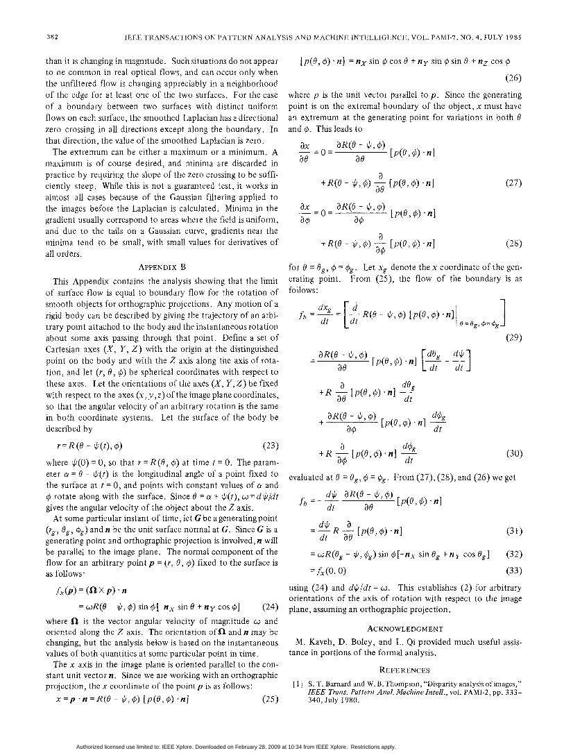
This Appendix contains the analysis showing that the limitof surface flow is equal to boundary flow for the rotation ofsmooth objects for orthographic projections. Any motion of arigid body can be described by giving the trajectory of an arbi-trary point attached to the body and the instantaneous rotationabout some axis passing through that point. Define a set ofCartesian axes (X, Y, Z) with the origin at the distinguishedpoint on the body and with the Z axis along the axis of rota-tion, and let (r, 0, 41) be spherical coordinates with respect tothese axes. Let the orientations of the axes (X, Y, Z) be fixedwith respect to the axes (x,y,z) of the image plane coordinates,so that the angular velocity of an arbitrary rotation is the samein both coordinate systems. Let the surface of the body bedescribed by

[p(9, 4) n] = nx sin 4 cos 0 + ny sin 4 sin 0 + nz cos 4

(26)

where p is the unit vector parallel to p. Since the generatingpoint is on the extremal boundary of the object, x must havean extremum at the generating point for variations in both 0and 4. This leads to

DX= 0 = 3R(O ; 5) [p(O, 1) - n]

+R(d - ,)3

[p(0,0)an]

ax = 0 = 3R(0 - 1,) f p(O, 0) n]

+R(O - ;, 0) a.; [ p(o, ¢) - n]ao

(27)

(28)

for 0 = 0g, 4 = 41g. Let xg denote the x coordinate of the gen-erating point. From (25), the flow of the boundary is asfollows:

fb - g R(0 - 4,)[p(0,) n]|dt Idt g =o-

(29)

3R( 4141 [dOg do1=aR(0 ;)¢) p(O,) n]Et d]

a dO+R a- [p(0,)n] dg+ a dt

+ [RO-o)p(O,4n]doa41 dtr= R ( - j(t),4) (23)

where 4(0) = 0, so that r = R (0, 4) at time t = 0. The param-eter ax= 0 - 4(t) is the longitudinal angle of a point fixed tothe surface at t = 0, and points with constant values of ax and4 rotate along with the surface. Since 0 = ax + 41(t), X = d4/dtgives the angular velocity of the object about the Z axis.At some particular instant of time, let G be a generating point

(rg, Og, 4g) and n be the unit surface normal at G. Since G is agenerating point and orthographic projection is involved, n willbe parallel to the image plane. The normal component of theflow for an arbitrary point p = (r, 0, 0) fixed to the surface isas follows:

f(p)= (flX p) n

-cR(6 - 4, 4) sin 4[-nx sin 0 + n y cos41] (24)where fQ is the vector angular velocity of magnitude X andoriented along the Z axis. The orientation of Qi and n may bechanging, but the analysis below is based on the instantaneousvalues of both quantities at some particular point in time.The x axis in the image plane is oriented parallel to the con-

stant unit vector n. Since we are working with an orthographicprojection, the x coordinate of the point p is as follows:x=p n=R(6 -4 ,41) [p(6,1) -n (25)

+R - [p(, ) * n] dta4 dt(30)

evaluated at 0 = Og, 4 = Og. From (27), (28), and (26) we get

d,; aR(0-41,4)fb d= ao [p(6,41) -n]

=d R [p(O,41) *n]dt aO

(31)

= (R(Og - 4, 4g) sin 4[-nx sin Og + ny cos Og] (32)

= fx(0, ) (33)using (24) and d4/dt = cu. This establishes (2) for arbitraryorientations of the axis of rotation with respect to the imageplane, assuming an orthographic projection.

ACKNOWLEDGMENTM. Kaveh, D. Boley, and L. Qi provided much useful assis-

tance in portions of the formal analysis.

REFE RENCES

[1] S. T. Barnard and W. B. Thompson, "Disparity analysis of images,"IEEE Trans. Pattern Anal. Machine Intell., vol. PAMI-2, pp. 333-340, July 1980.

382


THOMPSON etal.: DYNAMIC OCCLUSION ANALYSIS IN OPTICAL FLOW FIELDS

[21 W. F. Clocksin, "Perception of surface slant and edge labels fromoptical flow: A computational approach," Perception, vol. 9,pp. 253-269, 1980.

[31 K. Nakayama and J. M. Loomis, "Optical velocity patterns, veloc-ity sensitive neurons, and space perception: A hypothesis," Per-ception, vol. 3, pp. 63-80, 1974.

[4] H. C. Longuet-Higgins and K. Prazdny, "The interpretation of amoving retinal image," in Proc. Roy. Soc. London, vol. B-208,1980, pp. 385-397.

[51 D. Marr and E. Hildreth, "Theory of edge detection," in Proc.Roy. Soc. London, vol. B-207, 1980, pp. 187-217.

[6] W. B. Thompson, K. M. Mutch, and V. A. Berzins, "Edge detec-tion in optical flow fields," in Proc. 2nd Nat. Conf. Artif. Intell.,Aug. 1982.

[71 J. L. Crowley and R. M. Stern, "Fast computation of the differ-ence of low-pass transform," IEEE Trans. Pattern Anal. MachineInteP., vol. PAMI-6, pp. 212-222, Mar. 1984.

[8] P. J. Burt, "Fast filter transforms for image processing," Comput.Graph. Image Processing, vol. 16, pp. 20-51, 1981.

[9] D. Marr and S. Ullman, "Directional selectivity and its use inearly visual processing," in Proc. Roy. Soc. London, vol. B-211,pp. 151-180, 1981.

[101 K. M. Mutch and W. B. Thompson, "Analysis of accretion anddeletion at boundaries in dynamic scenes," IEEE Trans. PatternAnal. MachineIntell., vol. PAMI-7, pp. 133-138, 1985.

[111 W. B. Thompson, K. M. Mutch, and V. A. Berzins, "Analyzingobject motion based on optical flow," in Proc. 7th Int. Conf.Pattern Recog., July 1984.

[121 A. P. Witkin, "Intensity-based edge classification," in Proc.2nd Nat. Conf. Artif. Intell., Aug. 1982.

William B. Thompson (S'72-M'75) received theSc.B. degree in physics from Brown University,

Providence, RI, in 1970, and the M.S. andPh.D. degrees in computer science from theUniversity of Southern California, Los Angeles,in 1972 and 1975, respectively.He is currently an Associate Professor in the

Department of Computer Science at the Univer-sity of Minnesota, Minneapolis. Previously, hewas a member of the Image Processing Instituteat the University of Southern California. His

primary research interest is in the area of computer vision, with anemphasis on the development of techniques for perceiving spatial orga-razation. In addition, he is a principal in the expert problem solvingresearch group at the University of Minnesota.Dr. Thompson is a member of the American Association for Artificial

Intelligence and the Association for Computing Machinery.

Kathleen M. Mutch (S'80-M'83) received theM.S. and Ph.D. degree in computer science fromthe University of Minnesota, Minneapolis, in1981 and 1983, respectively.She is currently an Assistant Professor in the

Department of Computer Science at ArizonaState University, Tempe. Her research interestsinclude time-varying image analysis and applica-tions of computer vision.Dr. Mutch is a member of the Association for

Computing Machinery, SIGART, SIGCAPH,and the American Association for Artificial Intelligence.

Valdis A. Berzins (S'76-M'78) received the S.B.degree in physics and the S.M. and E.E. degreesin electrical engineering in 1975, and the Ph.D.degree in computer science in 1979, all fromthe Massachusetts Institute of Technology,Cambridge.He is presently Assistant Professor of Com-

puter Science at the University of Minnesota.His research interests include database supportfor computer aided design, software engineering,and image analysis.

383


Documents

Dynamic Occlusion Analysis in Optical Flow Fieldsthompson/publications/Thompson:1985:DOA.pdf · DynamicOcclusion Analysis in Optical Flow Fields ... THOMPSON,MEMBER,IEEE,KATHLEENM.MUTCH,MEMBER,IEEE,