Embed Size (px)
Citation preview

Dynamic Portfolio Optimization with Transaction
Costs: Heuristics and Dual Bounds
David B. Brown and James E. Smith∗
Fuqua School of Business
Duke University
Durham, NC 27708-0120
[email protected], [email protected]
First version: August 10, 2010This version: February 3, 2011
Abstract
We consider the problem of dynamic portfolio optimization in a discrete-time, finite-horizon set-ting. Our general model considers risk aversion, portfolio constraints (e.g., no short positions), returnpredictability, and transaction costs. This problem is naturally formulated as a stochastic dynamic pro-gram. Unfortunately, with non-zero transaction costs, the dimension of the state space is at least as largeas the number of assets and the problem is very difficult to solve with more than one or two assets.
In this paper, we consider several easy-to-compute heuristic trading strategies that are based onoptimizing simpler models. We complement these heuristics with upper bounds on the performance withan optimal trading strategy. These bounds are based on the dual approach developed in Brown, Smithand Sun (2009). In this context, these bounds are given by considering an investor who has access toperfect information about future returns but is penalized for using this advance information. Theseheuristic strategies and bounds can be evaluated using Monte Carlo simulation.
We evaluate these heuristics and bounds in numerical experiments with a risk-free asset and threeor ten risky assets. In many cases, the performance of the heuristic strategy is very close to the upperbound, indicating that the heuristic strategies are very nearly optimal.
Subject Classifications: Dynamic Programming, Portfolio Optimization
∗We thank the anonymous Associate Editor and referees for their helpful comments.

1. Introduction
Dynamic portfolio theory – dating from the seminal work of Mossin (1968), Samuelson (1969) and Merton
(1969, 1971) – provides a rigorous framework for determining optimal investment strategies in idealized
environments that assume there are no transaction costs. The solutions to these models rely heavily on
the absence of transaction costs. For example, in some models, the optimal solutions recommend holding
constant fractions of the investor’s wealth in different assets. To implement such a strategy, an investor must
continually buy and sell assets in order to maintain the target fractions as asset prices fluctuate. In practice,
transactions are costly and continual rebalancing can be quite expensive. If expected returns vary over time,
the situation may be even worse as the investor continually trades to adjust to a moving target.
Constantinides (1979) studied a general discrete-time model of portfolio optimization with transaction
costs and obtained the strongest structural results in the setting with power utility, proportional transaction
costs, and two assets. Specifically, he showed that there is a two-dimensional convex cone of asset positions
where it is optimal to not trade and that, when the asset position is outside of this cone, it is optimal to
trade to bring the asset position to the boundary of the cone. Davis and Norman (1990) and Shreve and
Soner (1994) analyzed continuous-time versions of this model with one risky and one risk-free asset and
established analogous results. Muthuraman (2006) and others have developed numerical methods for the
case with a single risky asset.
Of course, practitioners must actually contend with multiple risky assets and, unfortunately, this problem
is much more difficult to solve. The portfolio optimization problem is naturally formulated as a stochastic
dynamic program. With no transaction costs, the optimal investments typically depend on the investor’s
wealth but not the investor’s asset positions. However, with transaction costs, the optimal investments
depend on the investor’s initial asset positions and the dimension of the state space is at least as large as
the number of assets considered. The resulting dynamic program suffers from the “curse of dimensionality”
and is very difficult to solve with more than one or two risky assets.1
In this paper, we consider the problem of dynamic portfolio optimization in a discrete-time, finite-horizon
setting. Our general model considers risk aversion (we maximize the expected utility of terminal wealth),
portfolio constraints (e.g., no short positions), the possibility of predictable returns, and convex transaction
costs. We introduce several easy-to-compute heuristic trading strategies that are based on solving simpler
optimization problems. The first heuristic is a “cost-blind” strategy that follows the trading strategy given
by ignoring transaction costs; this is considered primarily as a benchmark for evaluating the performance
of the other heuristics and bounds. The second heuristic is a “one-step” strategy that can be viewed
1The special case with a quadratic utility and quadratic transaction costs and no portfolio constraints can be formulatedas a linear quadratic control problem that is straightforward to solve; see Garleanu and Pedersen (2009).
1

as approximating the dynamic programming recursion by taking the continuation value to be the value
function for the model that ignores transaction costs; transaction costs are considered in the current period
only. Finally, we consider a “rolling buy-and-hold” strategy where, in each period, we solve an optimization
problem with transaction costs with the simplifying assumption that there will be no further opportunities
to trade over a fixed horizon; the continuation value at the end of the horizon is again taken to be the value
function for the model that ignores transaction costs.
We complement these heuristics with upper bounds on the performance with an optimal trading strategy.
These bounds are based on the dual approach developed in Brown, Smith and Sun (2009). In this context, the
bounds are given by considering an investor who has access to perfect information about future returns but is
penalized for using this advance information. The dual approach of Brown, Smith and Sun (2009) generalizes
the dual approach developed for option pricing problems by Rogers (2002), Haugh and Kogan (2004), and
Andersen and Broadie (2004) (see also related earlier work by Davis and Karatzas (1994)) to consider general
stochastic dynamic programs; this generalization is essential for the application to portfolio optimization
problems. In this paper, we generate penalties using the approach for “good penalties” suggested in Brown,
Smith and Sun (2009) and develop a new gradient-based approach for generating penalties that exploits the
convex structure of the underlying stochastic dynamic program. These heuristic strategies and bounds can
be simultaneously evaluated using Monte Carlo simulation.
We evaluate these heuristics and bounds in numerical experiments with a risk-free asset and three risky
assets (with predictable returns) or with ten risky assets (without predictability). The results are promising:
the run times are reasonable and, in many cases, the performance of the heuristic strategy is very close to
the upper bound, indicating that the heuristic strategies are very nearly optimal.
Brandt (2009) provides a recent survey of research in portfolio optimization and touches briefly on
issues related to transaction costs. Closer to this paper, Akian, Menaldi and Sulem (1996), Leland (2000),
Muthuraman and Kumar (2006) and Lynch and Tan (2009) consider portfolio choice problems with multiple
risky assets and transaction costs in various settings. These papers develop analytic frameworks for the case
with many assets, but focus on numerical examples with two risky assets; the numerical methods employed
are based on grid approximations of the state space and do not scale well for problems with more risky assets.
Muthuraman and Zha (2008) describe a numerical procedure that scales better: their procedure assumes a
particular form of trading strategy, estimates the value function given this trading strategy using simulation,
and then updates the trading strategy. The computational effort required by this scheme scales polynomially
in the number of assets. Their example with seven risky assets requires approximately 62 hours to compute
a trading strategy; there is no guarantee that the resulting strategy is optimal or any indication of how
much better one might do with an optimal strategy. Chryssikou (1998) studies portfolio optimization with
2

quadratic transaction costs and no constraints using a pair of heuristic strategies, one of which is similar to
our rolling buy-and-hold strategy.
We view our contributions to be (i) the study of some easy-to-compute heuristic trading strategies that
may be useful in practice and (ii) the development of a dual bounding approach that can be used to evaluate
the quality of these and other heuristics. Both the heuristics and dual bounds are fairly flexible and can be
adapted to problems with different forms of utility functions, different forms of transaction costs (provided
they are convex), different forms of portfolio constraints and different models of returns.
There is also a recent literature that uses dual methods to evaluate portfolio strategies with portfolio
constraints. For example, Haugh, Kogan, and Wang (2006) and Haugh and Jain (2010), following Cvitanic
and Karatzas (1992) and others, use Lagrange multiplier methods to “dualize” portfolio constraints in
continuous time portfolio allocation models; see Rogers (2003) for a review and synthesis of related theory.
In contrast, we treat portfolio constraints directly and “dualize” the nonanticipativity constraints that require
the investor to use only the information available at the time a decision is made; our penalties can be viewed
as Lagrange multipliers associated with these nonanticipativity constraints. This interpretation is discussed
in more detail in Brown, Smith and Sun (2009).
In the next section of the paper, we describe our basic model and note some structural properties of
the model. In §3, we describe our heuristics. In §4, we describe our approach to dual bounds in general
and discuss the specific bounds we consider in our numerical experiments. In §5, we describe our numerical
experiments and results. The appendix contains proofs the propositions in the paper as well as some detailed
assumptions and results for the numerical experiments.
2. The Portfolio Optimization Model
Time is discrete and indexed as t = 0, . . . , T , with t = 0 being the current period and T being the terminal
period. There are n risky assets and a risk-free asset (cash). The risk-free rate rf is assumed to be known
and constant over time. The returns of the risky assets are stochastic and denoted by rt = (rt,1, . . . , rt,n)
where rt,i ≥ 0 is the (gross) return on asset i from period t-1 to period t.
The monetary values of the risky asset holdings at the beginning of period t are described by the vector
xt = (xt,1, . . . , xt,n); the cash position in period t is denoted ct. We let the trade vector at = (at,1, . . . , at,n)
denote the amounts of risky assets bought (if at,n > 0) or sold (if at,n < 0) in period t. The transaction costs
associated with trade vector at are given by κ(at). In our general analysis and approach, we will assume that
κ(at) is a nonnegative and convex function of the trades at with κ(0) = 0. In our numerical experiments,
3

we will focus on the special case of proportional transaction costs with
κ(at) =
n∑i=1
(δ+i a
+t,i − δ
−i a−t,i
), (1)
where a+t,i = max(at,i, 0) and a−t,i = min(at,i, 0) denote the positive and negative components of the trades
and δ+i , δ−i ≥ 0 are the proportional costs for buying and selling (respectively) asset i. Alternatively, we
could use a quadratic function for transaction costs to capture a “linear price impact,” where trades lead to
temporary linear changes in prices. Many other forms are also possible.
Taking transaction costs into account, the asset holdings and cash position evolve according to:
xt+1 = rt+1 · (xt + at), (2)
ct+1 = rf (ct − 1′at − κ(at)). (3)
Here · denotes the componentwise product of two vectors (so xt+1,i = rt+1,i(xt,i + at,i)) and 1 is an n-vector
of ones. The investor’s wealth wt in period t is the sum of the total dollar holdings across the risky assets
and cash, i.e.,
wt = 1′xt + ct. (4)
The investor’s goal is to maximize the expected utility of terminal wealth, E [U(wT )], where U is a non-
decreasing and concave utility function. Note that in this formulation, we define wealth in terms of the
market value of the portfolio. We could have instead defined wealth in terms of the liquidation value
of the portfolio, including the transaction costs associated with liquidation. In this case, we would take
wt = 1′xt − κ(−xt) + ct. Our general approach works in either case, though the numerical results would
obviously be somewhat different.
We will assume that the investor’s trades at in period t are restricted to a closed, convex set At(xt, ct).
In our numerical experiments, we will focus on the case where the investor is not allowed to have short
positions in risky assets or cash, so given an asset position (xt, ct), the allowed trades are
At(xt, ct) = {at ∈ Rn : xt + at ≥ 0, ct − 1′at − κ(at) ≥ 0} . (5)
We will also consider numerical results for the case where short positions are allowed, but there is a margin
requirement that limits the total (long or short) position in risky assets to be no more than ` times the
4
investor’s post-trade wealth. In this case, the set of allowed trades is also convex and can be written:
At(xt, ct) =
{at ∈ Rn :
n∑i=1
|xt,i + at,i| ≤ ` (1′xt + ct − κ(at))
}. (6)
In general, we consider sets of allowed trades At(xt, ct) defined in terms of a set Ht of allowed final positions
(or holdings): at ∈ At(xt, ct) if and only if (xt +at, ct−1′at−κ(at)) ∈ Ht. We assume that the allowed set
of final positions Ht is closed, convex and nondecreasing in ct (if (xt, c1t ) ∈ Ht and c1t ≤ c2t then (xt, c
2t ) ∈ Ht).
This implies that At(xt, ct) is convex for each (xt, ct).
We will allow the possibility that returns exhibit some degree of predictability. To model this, we let zt
denote a vector of observable market state variables that provides information about the returns rt+1 of the
risky assets. We will assume that zt follows a Markov process. The returns rt+1 may depend on zt but,
given zt, the returns are assumed to be conditionally independent of prior returns and earlier values of the
market state variable.
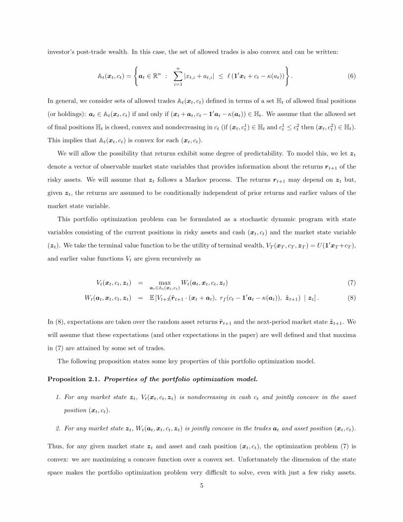
This portfolio optimization problem can be formulated as a stochastic dynamic program with state
variables consisting of the current positions in risky assets and cash (xt, ct) and the market state variable
(zt). We take the terminal value function to be the utility of terminal wealth, VT (xT , cT , zT ) = U(1′xT+cT ),
and earlier value functions Vt are given recursively as
Vt(xt, ct, zt) = maxat∈At(xt,ct)
Wt(at,xt, ct, zt) (7)
Wt(at,xt, ct, zt) = E [Vt+1(rt+1 · (xt + at), rf (ct − 1′at − κ(at)), zt+1) | zt] . (8)
In (8), expectations are taken over the random asset returns rt+1 and the next-period market state zt+1. We
will assume that these expectations (and other expectations in the paper) are well defined and that maxima
in (7) are attained by some set of trades.
The following proposition states some key properties of this portfolio optimization model.
Proposition 2.1. Properties of the portfolio optimization model.
1. For any market state zt, Vt(xt, ct, zt) is nondecreasing in cash ct and jointly concave in the asset
position (xt, ct).
2. For any market state zt, Wt(at,xt, ct, zt) is jointly concave in the trades at and asset position (xt, ct).
Thus, for any given market state zt and asset and cash position (xt, ct), the optimization problem (7) is
convex: we are maximizing a concave function over a convex set. Unfortunately the dimension of the state
space makes the portfolio optimization problem very difficult to solve, even with just a few risky assets.
5
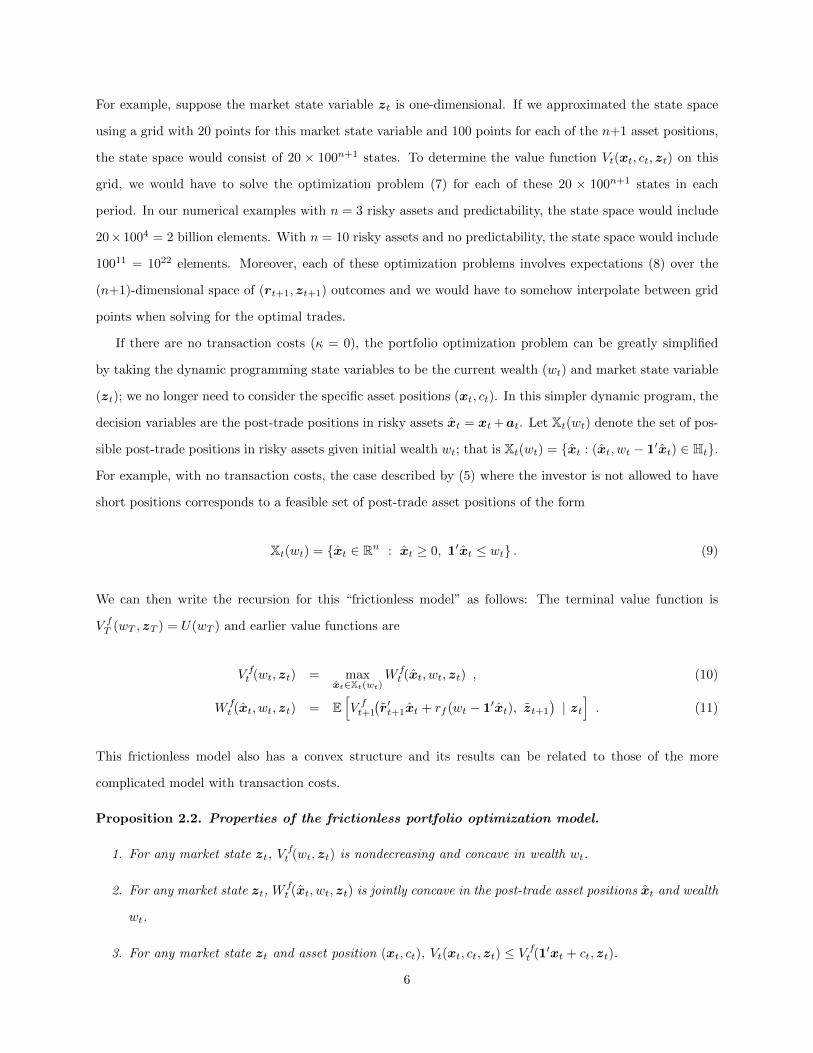
For example, suppose the market state variable zt is one-dimensional. If we approximated the state space
using a grid with 20 points for this market state variable and 100 points for each of the n+1 asset positions,
the state space would consist of 20 × 100n+1 states. To determine the value function Vt(xt, ct, zt) on this
grid, we would have to solve the optimization problem (7) for each of these 20 × 100n+1 states in each
period. In our numerical examples with n = 3 risky assets and predictability, the state space would include
20× 1004 = 2 billion elements. With n = 10 risky assets and no predictability, the state space would include
10011 = 1022 elements. Moreover, each of these optimization problems involves expectations (8) over the
(n+1)-dimensional space of (rt+1, zt+1) outcomes and we would have to somehow interpolate between grid
points when solving for the optimal trades.
If there are no transaction costs (κ = 0), the portfolio optimization problem can be greatly simplified
by taking the dynamic programming state variables to be the current wealth (wt) and market state variable
(zt); we no longer need to consider the specific asset positions (xt, ct). In this simpler dynamic program, the
decision variables are the post-trade positions in risky assets xt = xt +at. Let Xt(wt) denote the set of pos-
sible post-trade positions in risky assets given initial wealth wt; that is Xt(wt) = {xt : (xt, wt − 1′xt) ∈ Ht}.
For example, with no transaction costs, the case described by (5) where the investor is not allowed to have
short positions corresponds to a feasible set of post-trade asset positions of the form
Xt(wt) = {xt ∈ Rn : xt ≥ 0, 1′xt ≤ wt} . (9)
We can then write the recursion for this “frictionless model” as follows: The terminal value function is
V fT (wT , zT ) = U(wT ) and earlier value functions are
V ft (wt, zt) = maxxt∈Xt(wt)
W ft (xt, wt, zt) , (10)
W ft (xt, wt, zt) = E
[V ft+1
(r′t+1xt + rf (wt − 1′xt), zt+1
)| zt]. (11)
This frictionless model also has a convex structure and its results can be related to those of the more
complicated model with transaction costs.
Proposition 2.2. Properties of the frictionless portfolio optimization model.
1. For any market state zt, Vft (wt, zt) is nondecreasing and concave in wealth wt.
2. For any market state zt, Wft (xt, wt, zt) is jointly concave in the post-trade asset positions xt and wealth
wt.
3. For any market state zt and asset position (xt, ct), Vt(xt, ct, zt) ≤ V ft (1′xt + ct, zt).
6

Thus, to solve the frictionless model, we need to solve a convex optimization problem for each market state
zt and wealth wt. For example, if the market state variable zt is one-dimensional, we could solve this
dynamic program on a two-dimensional grid involving zt and wt. The expectations over (rt+1, zt+1) in
(11) will still be high-dimensional if we have many assets, but can be evaluated using various methods. In
our numerical experiments, we will approximate these expectations using discrete approximations of the
underlying distributions; see §5.1 below.
If the investor has a power utility function, the frictionless model simplifies further. Specifically, suppose
U(wT ) =1
1− γw1−γT , (12)
where γ > 0 is the coefficient of relative risk aversion; in the case where γ = 1, U(wT ) = ln(wT ). We can
then write the value function as
V ft (wt, zt) =1
1− γw1−γt φt(zt) , (13)
where φt(zt) is defined recursively with φT (zT ) = 1 and
1
1− γφt(zt) = max
θt∈Xt(1)E[
1
1− γ(r′t+1θt + rf (1− 1′θt))
1−γ φt+1(zt+1) | zt]. (14)
Here θt = (θ1, . . . , θn) are the post-trade fractions of wealth wt invested in the risky assets. In this case, the
dimension of the state space is equal to the dimension of the market state variable zt.
Note that if the next-period market state zt+1 and the returns rt+1 are independent given zt, then
equation (14) factors and it is optimal to pursue a myopic trading strategy that maximizes the expected
utility of next period’s wealth. However, if the next-period market state zt+1 and the returns rt+1 are not
independent and the investor has a relative risk aversion coefficient γ > 1 (as is considered to be typical),
the optimal trading strategies will include some degree of hedging against unfavorable changes in the market
state variable: compared to the myopic strategies, these strategies tend to have higher next-period wealth
in scenarios with poor future prospects (i.e., with high values of φt+1(zt+1)) and lower next-period wealth
in scenarios with better future prospects (i.e., with low values of φt+1(zt+1)).
3. Some Heuristic Trading Strategies
Given that the portfolio optimization model with transaction costs is difficult to solve, it is natural to
consider heuristic trading strategies based on solutions to approximate models that are simpler to solve. We
will consider several such heuristic strategies.
7

3.1. Cost-Blind Strategies
First, we consider cost-blind strategies that ignore transaction costs and simply follow the optimal trading
strategy recommended by the frictionless model. To simulate such a strategy, we need to first solve the
dynamic program for the frictionless model (10) to find the optimal post-trade asset positions xt or fractions
θt = xt/wt for each period t, market state zt and wealth level wt; we do this once and store the results. In
the body of the simulation, in each period, we choose trades at to move to the investor to the recommended
fractions θt for the current market state zt and wealth level wt. Given this trade, we generate random
returns rt+1 for the risky assets and calculate next-period asset positions (xt+1, ct+1) using equations (2)
and (3), deducting transaction costs from the cash position. We then generate the next-period market state
zt+1 and continue the simulation process for the next period.
Though this cost-blind strategy may perform reasonably well when the transaction costs are small or
when it is optimal to put all of the investor’s wealth in a single asset, with larger transaction costs and more
balanced investments we would expect this strategy to trade too much in pursuit of marginal improvements
in asset positions that do not exceed the cost of executing the trade.
3.2. One-Step Strategies
Second, we consider a heuristic strategy where the investor uses the value function from the frictionless
model as an approximate continuation value, but includes transaction costs in the current period. In this
case, in each period, the investor chooses trades at that solve:
maxat∈At(xt,ct)
E[V ft+1
(r′t+1(xt + at) + rf (ct − 1′at − κ(at)), zt+1
)| zt]. (15)
To simulate such a one-step strategy, we first solve the dynamic program for the frictionless model (10)
to determine the value function V ft (wt, zt); we do this in advance of the simulation and store the value
function. In the body of the simulation, for each period in each trial, we solve the optimization problem (15)
to find the recommended trade at for the then-prevailing (xt, ct, zt) scenario. We then generate random
returns rt+1 for the risky assets, calculate next-period asset positions (xt+1, ct+1) using equations (2) and
(3), generate a new market state zt+1 and continue to the next period. Note that the objective function in
(15) is concave in the trades at (this follows from the assumption that the transaction cost function κ(at)
is convex and the fact that V ft (wt, zt) is nondecreasing and concave in wealth wt; see Proposition 2.2), so
(15) is a convex optimization problem. The optimization problem is, however, complicated by the presence
of the high-dimensional expectation in (15): these expectations must be evaluated to calculate the objective
function for any candidate trade at.
8

While the cost-blind strategies are likely to trade too much because they neglect the costs of trading,
we would expect these one-step strategies to trade too little because they underestimate the benefits of
moving towards the optimal position without transaction costs. Or, put another way, the frictionless model
underestimates the cost of being out of the optimal position because it assumes the investor can costlessly
adjust the position in the next period. If the optimal asset positions change slowly over time, moving towards
the optimal position in one period may provide benefits in future periods as well as the current one.
Though we would have to solve the full portfolio optimization problem (7) to exactly capture the long-term
impacts of adjusting portfolio positions, we can perhaps approximate this effect by reducing the transaction
costs κ(at) appearing in the objective function in (15). There are a variety of ways we might modify these
costs and we can experiment to find a good modification. In our numerical experiments, we consider monthly
trades and focus on the case where we adjust the transaction costs by dividing κ(at) by dividing by a time-
dependent constant. Specifically, we focus on the case where we divide by the smaller of 6 or the number
of periods remaining (T − t). The intuitive interpretation of this adjustment is that the benefit of adjusting
the asset positions lasts approximately 6 months. We will call these trading strategies modified one-step
strategies and consider alternative divisors in §5.4.
3.3. Rolling Buy-and-Hold Strategies
Finally, we consider a heuristic trading strategy where, in each period, the investor chooses trades to maximize
the expected utility of wealth at some horizon h periods into the future, taking transaction costs into account,
but assuming that there will be no opportunities to adjust the portfolio over this time horizon. As in the one-
step strategy, the continuation value at the horizon is approximated by the value function for the frictionless
model. That is, in period t, the investor chooses trades at that solve:
maxat∈At(xt,ct)
E[V ft+h
((rt+h · . . . · rt+1)′(xt + at) + rhf (ct − 1′at − κ(at)), zt+h
)| zt], (16)
with the understanding that we use the terminal utility U(wT ) in place of V ft+h(wT+h) whenever t+ h > T .
Though this objective function assumes that there are no future opportunities to adjust the portfolio over
this time horizon, when simulating or executing this strategy, the investor solves the same problem in the
next period. As with the one-step strategies, the objective function in (16) is concave in at and, when
simulating with this strategy, we must solve the convex optimization problem (16) once for each period of
each simulated trial.
As with the modification of the one-step strategies, some degree of experimentation may be required to
identify a good horizon h for a particular problem. In our numerical experiments with monthly trading, we
9

will focus on the case where the horizon h is 6 months, but will consider alternatives in §5.4. We will refer to
these heuristic trading strategies as the rolling buy-and-hold strategies. Chryssikou (1998) studies a similar
heuristic but with the horizon fixed at the terminal period T , i.e., with terminal utility U(wT ) in place of
V ft+h(wT+h) in (16).
4. Dual Bounds
We can evaluate the heuristic strategies of §3 using simulation and we can rerun these simulations with
variations of these strategies (e.g., adjusting the modification of transaction costs for the one-step strategies or
the horizon for the rolling buy-and-hold strategies) in an attempt to improve their performance. When doing
these experiments, it would be helpful to know how much better we could possibly do. The frictionless model
provides an upper bound on performance (see Proposition 2.2), but when transaction costs are substantial,
this “no transaction cost bound” may be rather weak.
In this section, we will derive upper bounds on performance using the dual approach developed in Brown,
Smith and Sun (2009). This dual approach consists of two elements: (i) we relax the “nonanticipativity”
constraints that require the trading decisions to depend only on the information available at the time the
decision is made and (ii) we impose penalties that punish violations of these nonanticipativity constraints.
We first describe this dual approach in general and then describe the penalties we will use in our numerical
experiments. As we will see, these dual bounds are typically tighter than the bound given by the model that
ignores transaction costs.
4.1. The Dual Approach
In our discussion of the dual bounds, it helps to introduce notation to describe the full sequences of market
states z = (z0, . . . ,zT ), returns r = (r1, . . . , rT ) and trades a = (a0, . . . ,aT−1). Using this notation, we
write the pre-trade asset and cash positions as xt(a, r) and ct(a) and wealth as wt(a, r); these are calculated
according to equations (2)-(4) and are given by
xt(a, r) =
t−1∑τ=0
(rt · . . . · rτ+1) · aτ + (rt · . . . · r1) · x0
ct(a) =
t−1∑τ=0
rt−τf (−1′aτ − κ(aτ )) + rtfc0
and wt(a, r) = 1′xt(a, r) + ct(a). Similarly, we write the set of feasible trade sequences a as A(r). Note
that, for any given return sequence r, the position in risky assets xt(a, r) is linear in the trade sequence
a and, with convex transaction costs, the cash position ct(a) and wealth wt(a, r) are concave in the trade
sequence a.
10

A trading strategy can be viewed as a function α(r, z) that maps from sequences of returns r and market
states z to a trade sequence a. A trading strategy α is feasible if (i) α(r, z) is in A(r) for each (r, z), and
(ii) α is nonanticipative in that the trade at selected in period t depends only on what is known in period
t; that is, at depends on the market states (z0, . . . ,zt) and the asset returns (r1, . . . , rt), but not the future
market states or returns. We let A denote this set of feasible strategies. In this notation, we can rewrite the
portfolio optimization problem (7) compactly as
maxα∈A
E [U(wT (α(r, z), r))] . (17)
Here the expectations are taken over sequences of returns r and market states z, with trading strategy α
selecting trades in each (r, z) scenario.
In deriving dual upper bounds for this problem, we will focus on a “perfect information relaxation” that
assumes the investor knows all market states z and all asset returns r before making any trading decisions.
The penalties π(a, r, z) depend on the sequence of trades a, returns r, and market states z in a given
scenario; we say a penalty π is dual feasible if E [π(α(r, z), r, z)] ≤ 0 for any feasible trading strategy α. We
can then state the duality result as follows.
Proposition 4.1. Dual bound. For any feasible trading strategy α and any dual feasible penalty π,
E [U(wT (α(r, z), r))] ≤ E[
maxa∈A(r)
{U(wT (a, r))− π(a, r, z)
}]. (18)
The problem on the right of (18) is perhaps easiest to understand by considering how we estimate this
expression using simulation. In each trial of the simulation, we generate a sequence of market states z and
asset returns r, drawing samples according to their joint stochastic process. We then solve a deterministic
“inner problem” of the form:
maxa∈A(r)
{U(wT (a, r))− π(a, r, z)
}(19)
to find the sequence of trades a in A(r) that maximizes the penalized objective, U(wT (a, r)) − π(a, r, z),
assuming perfect foresight, i.e., assuming that the full sequences of market states z and asset returns r are
known. We obtain an estimate of the dual bound (18) by averaging the optimal values from these inner
problems across the trials of the simulation. Note that since wealth wT (a, r) is concave in the trade sequence
a and the utility function is increasing and concave in wealth, the utility of final wealth is concave in a for
a given return sequence r. If we consider penalties π(a, r, z) that are convex in the trade sequence a for
11

given sequences of returns r and market states z, the inner problem (19) will be a deterministic convex
optimization problem in a and will not be difficult to solve.
It is not hard to see that inequality (18) holds with any dual feasible penalty, for any feasible strategy
α. To see this, note:
E [U(wT (α(r, z), r))] ≤ E [U(wT (α(r, z), r))− π(α(r, z), r, z)] (20)
≤ E[
maxa∈A(r)
{U(wT (a, r))− π(a, r, z)
}].
The first inequality follows from the assumption that π is dual feasible; since α is assumed to be a feasible
trading strategy, this implies E [π(α(r, z), r, z)] ≤ 0. The second inequality follows from the fact that the
value with perfect foresight must meet or exceed the value of any feasible trading strategy α: The investor
with perfect foresight could choose the sequence of trades that would be chosen by α in each scenario and
obtain the same value. However, the investor with perfect foresight can usually do better by choosing a
different sequence of trades that maximizes the penalized objective in the given scenario.
The bound (18) is a special case of the weak duality result from Brown, Smith and Sun (2009). Brown,
Smith and Sun (2009) also show that strong duality holds in this framework in that there exists an optimal
penalty π∗ such that the inequality in (18) will hold with equality with this π∗ and an optimal strategy
α∗; “complementary slackness” also holds in that an optimal penalty π∗ will lead to trades a in the dual
problem that match those of an optimal strategy.
Note that the penalty π = 0 is trivially dual feasible. In this case, the inner problem (19) amounts to
finding an optimal trading strategy given perfect knowledge of all future returns and the dual bound (18)
is the expected utility with perfect information. This inner problem is straightforward to solve, but the
bound is typically quite weak. To obtain tighter bounds, we need to choose a penalty that reduces the
benefit provided by having advance knowledge of future market states and returns. In addition, to ensure
reasonable computational times, the penalties should be easy to compute and lead to an inner problem (19)
that is easy to solve. We will consider two types of penalties. First we will consider penalties that are
constructed following the prescription for “good penalties” from Brown, Smith and Sun (2009). Second, we
will consider a new type of penalty that exploits the convex structure of the primal problem.
4.2. Penalties Based on Approximate Value Functions
Brown, Smith and Sun (2009) suggest constructing penalties by choosing a sequence of generating functions
(g0, . . . , gT ) that approximate the continuation value functions for the dynamic programming model. In this
context, the generating functions gt(a, r, z) may depend on the full sequences of returns r and market states
12

z, but depend only on trades up to period t, (a0, . . . ,at). The penalty is then taken to be
π(a, r, z) =
T∑t=0
(gt(a, r, z)− E [gt(a, r, z) | r1, . . . , rt, z0, . . . ,zt]) . (21)
Brown, Smith and Sun (2009) show that penalties constructed this way are dual feasible. Moreover, if we
take the generating functions gt(a, r, z) to be the optimal continuation values Vt+1(xt+1(a, r), ct+1(a), zt+1)
for the original portfolio optimization program (7), the resulting “ideal penalty” is optimal: it provides a
dual bound equal to the optimal value for the primal and the optimal trades in the dual problem are feasible
and optimal for the primal problem.
We can approximate this ideal penalty using approximations of the continuation values as generating
functions. For example, consider the continuation values for the one-step strategies; we could approximate
the continuation value using the continuation value from the frictionless model (10) by taking the generating
function gt(a, r, z) to be V ft+1(wt+1(a, r), zt+1). Though this frictionless value function is reasonably easy to
compute, it leads to an inner problem that is not easy to solve: V ft+1(wt+1(a, r), zt+1) is a concave function
of the trades a but when used to generate a penalty π using (21), V ft+1 enters into the objective for the inner
problem with both positive and negative signs, leading to an objective function that is neither convex nor
concave and an inner problem that is generally not easy to solve.
To overcome this difficulty, we will take gt(a, r, z) to be a linear approximation of V ft+1(wt+1(a, r), zt+1)
based on a first-order Taylor series expansion in the trades a around the trades a∗ given by some fixed
trading strategy. For example, in the case with proportional transaction costs given by equation (1), the
linear approximation of V ft+1 yields a generating function of the form
gt(a, r, z) = V ft+1(wt+1(a∗, r), zt+1) (22)
+ V f ′t+1(wt+1(a∗, r), zt+1)
t∑τ=1
n∑i=1
(∂wt+1
∂a+τ,i
(a+τ,i − a
∗+τ,i
)+∂wt+1
∂a−τ,i
(a−τ,i − a
∗−τ,i
)),
where V f ′t+1 denotes the derivative of V ft+1 with respect to wealth and a+t,i, a−t,i, a
∗+t,i , and a∗+t,i denote the positive
and negative components of a and a∗. With a power utility function, V ft+1 can be calculated analytically as
V f ′t (wt, zt) = w−γt φt(zt), where φt(zt) is determined when solving the frictionless model (14); in other cases,
13

V ft+1 may have to be estimated numerically. The partial derivatives in (22) are given by:
∂wt+1
∂a+τ,i=
t+1∏τ ′=τ+1
rτ ′,i − rt+1−τf
(1 + δ+i
)∂wt+1
∂a−τ,i=
t+1∏τ ′=τ+1
rτ ′,i − rt+1−τf
(1− δ−i
).
With a generating function of the form of (22), using (21) we obtain a dual feasible penalty π that is linear
in the trades a (or, more precisely, linear in the positive and negative components of a), for any sequence
of returns r and market states z. The objective for the inner problem (19) is then concave in a and the
resulting inner problem is a deterministic convex optimization problem that is not difficult to solve. Note
that there are high-dimensional expectations (over returns rt+1 and the market state zt+1) in the definition
of the penalty (21); however, these expectations only affect the weights associated with the trades in this
linear penalty and the weights need only be calculated once when solving the inner problem in a simulated
scenario. In our numerical experiments, we will consider bounds generated by penalties of this form, taking
a∗ to be the trades suggested by the modification of the one-step heuristic strategy. We will call these
bounds the modified one-step bounds.
We can construct a similar penalty using a generating function based on the analogue of the continuation
value used to determine the rolling buy-and-hold strategy,
E[V ft+h
((rt+h · . . . · rt+2)′xt+1(a, r) + rh−1f ct+1(a), zt+h
)| zt+1
]. (23)
Note that this is a function of the period-t+1 market-state zt+1 (by conditioning) and returns rt+1 (through
xt+1), but does not depend on later market states or returns as these are integrated out in the expectations.
Here too we will consider a generating function based on a first-order Taylor series expansion of (23) in the
trades a around the trades a∗ given by some heuristic strategy; the details are provided in the appendix. As
with the modified one-step penalty, this leads to a dual feasible penalty π that is linear in the positive and
negative components of a for any sequence of returns r and market states z. In our numerical experiments,
we will consider bounds generated by penalties of this form, taking a∗ to be the trades suggested by a rolling
buy-and-hold strategy. We will call these the rolling buy-and-hold dual bounds.
4.3. Gradient-Based Penalties
We will also consider gradient-based penalties that exploit the convex structure of the primal optimization
problem. To understand the motivation for this approach, assume (for the sake of this motivating discussion)
that the utility of terminal wealth U(wT (a, r)) is differentiable in the sequence of trades a and that an optimal
14
trading strategy α∗ for the portfolio optimization problem with transaction costs is known. Then suppose
we take the penalty π(a, r, z) to be
π(a, r, z) = ∇aU(wT (α∗(r, z), r))′ (a− α∗(r, z)) (24)
where ∇aU(wT (a, r)) is the gradient of terminal utility with respect to the trade sequence a, for a given
sequence of returns r. Note that this penalty is linear in the trade sequence a.
We can view the primal problem (17) as a convex optimization problem with the decision variables
being the trading strategy α; this will be formalized in the proof of the proposition below. The first-order
conditions for this optimization problem can be shown to imply that
E [π(α(r, z), r, z)] = E [∇aU(wT (α∗(r, z), r))′ (α(r, z)− α∗(r, z))] ≤ 0 (25)
for any feasible strategy α. This means the penalty (24) is dual feasible.
Now consider the deterministic inner problem (19) given by this penalty:
maxa∈A(r)
{U(wT (a, r))−∇aU(wT (α∗(r, z), r))′ (a− α∗(r, z))
}. (26)
Since the penalty is linear in the trade sequence a, the inner problem (26) is a convex optimization problem
and its first-order conditions are necessary and sufficient for an optimal solution. The gradient of the objective
function in (26) with respect to the trade sequence a is
∇aU(wT (a, r))−∇aU(wT (α∗(r, z), r)) . (27)
Now note that if we take the trade sequence to be that selected by the optimal strategy, i.e., a = α∗(r, z),
the gradient (27) is equal to zero. Since this a is in A(r) and it sets the gradient equal to zero, this a
must be an optimal solution for the inner problem (26). Moreover, with a = α∗(r, z), the penalty (24)
is zero and the objective for the inner problem (26) reduces to U(wT (α∗(r, z), r)) and the dual bound is
E [U(wT (α∗(r, z), r))]. Thus, the penalty (24) is optimal: it yields a dual trading strategy that is optimal
for the primal problem and a dual bound equal to the optimal value for the primal.
Of course, in practice we do not know the optimal strategy α∗ for the portfolio optimization problem and
cannot use the penalty (24). We can, however, approximate the original problem and use similar penalties
based on the optimal solution to this approximate problem. For example, we can approximate the original
problem by considering the frictionless model (10). If we take wT (a, r) to be the terminal wealth without
15

transaction costs and A to be the set of feasible trading strategies without transaction costs (and let A(r)
be the set of feasible trades in the approximate model given returns r), we can then write the approximate
optimization problem based on the frictionless model as
maxα∈A
E [U(wT (α(r, z), r))] . (28)
Let α∗(r, z) be an optimal trading strategy for this approximating frictionless model and consider a gradient-
based penalty of the form of (24), but with wT in place of wT and α∗ in place of α∗, i.e.,
π(a, r, z) = ∇aU(wT (α∗(r, z), r))′ (a− α∗(r, z)) . (29)
The argument leading to (25) requires the strategy to be optimal for the chosen wealth function (i.e., for
(28)), but it does not require the strategy to be optimal for the true wealth function with transaction
costs. If the set of feasible strategies for the approximate model A includes those for the real model A (i.e.,
A(r) ⊆ A(r) for all r), then E [π(α(r, z), r, z)] will hold for all α in A and this approximate penalty π will
be dual feasible for the original problem. However, the inner problem with this approximate penalty,
maxa∈A(r)
{U(wT (a, r))−∇aU(wT (α∗(r, z), r))′(a− α∗(r, z))
}, (30)
will generally not be optimized by taking the trade sequence to be a = α∗(r, z). Nevertheless, because the
penalty is dual feasible, the dual problem with this approximate penalty will provide a valid upper bound
on the performance of any feasible trading strategy.
We can use this gradient-based approach with a variety of approximations of the wealth function as long
as the approximate wealth function is concave and we can identify an optimal strategy for the approximate
problem. The following proposition formalizes this gradient-based approach to penalties.
Proposition 4.2. Gradient-based penalties. Let α∗ be an optimal trading strategy for the portfolio choice
problem (28) with modified terminal wealth wT (a, r), assumed concave in a, and modified allowable trades
A(r), assumed convex and satisfying A(r) ⊆ A(r) for each return sequence r. Consider the penalty π given
by equation (29):
1. π is dual feasible.
2. If wT (a, r) = wT (a, r) and A(r) = A(r) for each return sequence r, then the dual bound (18) holds
with equality with penalty π.
16

3. If wT (a, r) ≤ wT (a, r), then,
maxa∈A(r)
{U(wT (a, r))− π(a, r, z)
}≤ U(wT (α∗(r, z), r)). (31)
The first two parts of the proposition formalize the results discussed earlier. We will discuss the last part
of the proposition in a moment. Note that our definition of gradient-based penalties π in equation (29)
implicitly assumes that U and wT are differentiable so the necessary gradients exist and π corresponds to a
directional derivative. If the gradient does not exist, we can define π in terms of the directional derivative
instead; this directional derivative will exist whenever U ◦wT is concave. The use of the directional derivatives
is discussed in more detail in the proof of the result in the appendix.
In our numerical experiments, we will consider two examples of gradient-based penalties. The first is
based on the frictionless model, as discussed above. In this case, the approximate terminal wealth wT (a, r)
is given by taking the transaction costs to be zero and the allowable trade sequences A(r) are the same as
in the original model but without the transaction costs: A(r) ⊆ A(r) then follows from our assumption that
the set of feasible asset positions Ht is nondecreasing in cash. In this frictionless model, the gradient of the
utility of terminal wealth is ∇aU(wT (a, r)) = U ′(wT (a, r))∇awT (a, r), where U ′ is the derivative of the
utility function and ∇awT (a, r) is a nT × 1 vector with entries corresponding to trade at given by
∇atwT (a, r) = (rT · . . . · rt+1)− rT−tf 1 .
We will call the resulting penalty the frictionless gradient-based penalty.
Note that with this approximation, the wealth with transaction costs wT (a, r) are less than or equal to
the wealth without transaction costs wT (r, z) (for all r and z), so the last part of Proposition 4.2 applies:
the optimal values for the inner problems with this penalty (on the left side of (31)) will be less than or
equal to the utility of final wealth with no transaction costs (on the right side of (31)) for every r and z.
This implies that the dual bounds using this frictionless gradient penalty must be at least as tight as the no
transaction cost bound given by the value function for the frictionless model.
Although the frictionless gradient penalty leads to tighter bounds than the frictionless model, we can
perhaps do better if we somehow incorporate the effects of transaction costs in the approximate model.
The key for the gradient penalty approach is to do this in a way that still allows us to find the optimal
solution for the approximate model. One way to do this is to consider a variation of the original model
where the transaction costs depend on the post-trade asset positions rather than the trades. In this case,
the transaction costs are of the form κ(xt), where xt = xt + at and the cash position evolves according to
17

ct+1 = rf (ct − 1′at − κ(xt + at)), rather than equation (3). In such a case, we can represent the portfolio
problem as a dynamic program like that of the frictionless model (10) with wealth wt and the market state
zt as state variables and post-trade asset positions xt as decision variables, without considering the specifics
of the asset positions (xt, ct).
In our numerical experiments, we will consider a modified gradient-based penalty where we take κ(xt)
to be proportional to the post-trade asset positions xt. Specifically, we will take the proportional fee for
the asset positions to be equal to the proportional fee for trades divided by the number of periods (T ) in
the model. More generally, we could consider κ(xt) that assume transaction costs are proportional to the
difference between the post-trade position xt and some reference position. For example, we might take this
reference position to be the asset allocation recommended by the frictionless model for the same market
state or, alternatively, the initial (period 0) asset position. Our modified gradient bound can be viewed as
an example of this general form where the reference position is taken to be a zero position (i.e., with zero
investment in each risky asset), which is the assumed initial position in the experiments. Of course, there
are a number of possible variations on these ideas and we could experiment to perhaps find better bounds.
5. Numerical Experiments
In this section, we describe the experiments that we use to test the proposed trading strategies and dual
bounds. We first describe the details of the models considered and then discuss the run times and numerical
results. We then consider variations on the heuristics and bounds as well as the constraints.
5.1. Model Details
We will test the heuristic strategies and dual bounds by evaluating these heuristics and bounds in a series
of simulations with varying parameter values. In all cases, we begin by solving the dynamic program for
the frictionless model (equations (10) and (11)) for the given parameter values; we also solve the analogous
dynamic program used to determine the modified gradient penalty of §4.3. We then repeatedly generate
random sequences of market states and returns. For each sequence of market states and returns, we “run” the
heuristic strategies of §3, determining the sequence of trades selected by the heuristic and the corresponding
terminal wealth and utility. We also solve the inner problem for each of the dual bounds in this same
scenario. We repeat this simulation process for a given number of trials.
In our experiments, we assume monthly time steps, proportional transaction costs κ(at) = δ∑ni=1 |at,i|,
and power utilities. We will consider a variety of parameters:
• time horizons T of 6, 12, 24, and 48 months;
• transaction cost rates δ of 0.5%, 1.0% and 2.0%;
18

• relative risk aversion coefficients γ of 1.5, 3.0 or 8.0, reflecting low, medium and high degrees of risk
aversion.
In the next three subsections, we will focus on the case with constraint (5) ruling out short positions; we
consider limited leverage constraints of the form of (6) in §5.5. In all cases, we assume the investor starts
with all wealth invested in cash and normalize wealth to one, i.e., we assume x0 = 0 and c0 = 1. We will
consider 1000 trials in each simulation.
We consider two different models of returns. The first highlights the role of predictability and the second
considers a larger number of risky assets.
Model with Three Risky Assets and Predictability. We first consider a model with three risky
assets and one market state variable, based on Lynch (2001); Lynch studied the impact of predictability on
portfolio choices, without considering transaction costs. Specifically, letting ρt = ln rt, the model assumes
returns and market states evolve according to
ρt+1
zt+1
=
ar + brzt
az + bzzt
+
et+1
vt+1
, (32)
where the stochastic increments (et+1 vt+1) are multivariate normal with mean zero and covariance Σev. The
three risky assets correspond to value-weighted equity portfolios sorted by the size of the underlying firms
(i.e, small-, medium- and large-cap stocks) and the market state variable is a normalized index reflecting the
term spread (specifically, the difference between 20-year and one-month treasury bonds). Lynch estimates
this model using data from 1927 to 1996. The returns are inflation-adjusted and the risk-free rate rf is
1.00042. The other numerical assumptions are discussed in the appendix.
In this model, the market state variable has a significant impact on expected returns. With no transaction
costs and medium risk aversion (γ = 3.0), we find that with high values of zt (i.e., with a large term spread),
the investor should invest heavily in a mix of small- and medium-sized stocks and hold no cash. With zt = 0,
the investor should invest in a mix of all three assets, while holding substantial reserves in cash. With negative
values for zt, the investor should invest most of his wealth in cash. In our numerical experiments, we will
assume the initial market state is neutral (i.e., z0 = 0).
We follow Lynch (2001) and use discrete approximations of the uncertainties to calculate expectations.
We approximate the market state variable using a grid with 19 points. The idiosyncratic returns (et+1 in
equation (32)) are approximated using a Gaussian quadrature approach with three points per asset. This
Gaussian quadrature approximation exactly matches the mean and covariance structure for log returns ρt
and matches higher-order moments (3rd-5th) of this joint distribution as well. (See, e.g., Judd 1998, for an
19

introduction to Gaussian quadrature methods.) Taken together, the joint distribution for returns and the
market-state variable is approximated using a four-dimensional grid with a total of 33 × 19 = 513 elements.
This discrete approximation scheme is used to calculate the expectations required to solve the dynamic
programming model for the frictionless model, to evaluate the expectations in the optimization problems for
the heuristic trading strategies (in §3), and to evaluate the expectations appearing in the penalties based
on approximate value functions (in §4.2). For consistency, we also use this discrete approximation in the
simulations, i.e., we generate sample returns and market states from this grid according to the probabilities
of the discrete approximation.
Model with Ten Risky Assets and No Predictability. We also consider examples with ten risky
assets and no predictability. In this case, we assume that the asset returns follow a discrete-time multivariate
geometric Brownian motion process, a special case of (32) with ρt = ln rt evolving according to ρt+1 =
ar + et+1 where the stochastic increments et+1 are multivariate normal with mean zero and covariance
Σe. In this example, the ten risky assets correspond to five equity indices (S&P 500, Russell 2000 Value,
MSCI World Gross, Russell 1000 Value Index, Russell MidCap Index), three bond indices (Lehman Brothers’
US government and corporate bond indices and Lehman Brothers’ Fixed Rate Mortgage Backed Securities
Index), a real estate index trust (NAREIT), and a composite index of 1-5 Year US Treasuries. The parameters
were estimated using monthly return data from 1981-2006 and are provided in the appendix. The risk-free
rate rf = 1.0048 is the average return on three-month US treasuries, estimated from the same data set.
These returns are not inflation-adjusted.
We also use discrete approximations of the uncertainties to calculate expectations in this model. The
idiosyncratic returns (et+1) are approximated using a multidimensional quadrature (or cubature) formula in
Stroud (1971, p. 317) that includes 2n + 2n points and exactly matches the first five moments of the return
distribution. With 10 assets, the return distribution is approximated using a ten-dimensional grid with a
total of 1044 elements. There are a variety of different approaches we could use to calculate expectations
in these models and there is a tradeoff between the accuracy of the approximation and the amount of work
involved. Stroud (1971) provides a comprehensive review of multidimensional quadrature formulas; one such
formula matches three moments of the underlying distribution and involves only 2n points. Alternatively,
we might consider evaluating these expectations using Monte Carlo or Quasi Monte Carlo methods; see, e.g.,
Judd (1998) or Glasserman (2004) for discussions of these approaches.
5.2. Run Times
Table 1 provides the run times for evaluating the heuristics and dual bounds in a simulation with 1000 trials
for the two different return models and four different time horizons (T ). In all cases, we consider the case
20

Horizon (T)
No Trans. Cost
Modified Trans. Cost Model Cost Blind One‐Step
Modified One‐Step
Rolling Buy‐and‐Hold
Zero Penalty
Modified One‐Step
Rolling Buy‐and‐Hold
Frictionless
Gradient Based
Modified Gradient
6 5.1 5.3 5.7 293.1 291.1 285.2 9.1 12.0 13.6 9.0 10.8 12 10.1 10.4 10.2 622.3 591.9 583.9 12.2 17.0 21.3 12.0 14.7 24 20.0 20.8 20.0 1214.8 1180.9 1215.4 21.6 33.0 41.8 22.2 29.9 48 39.9 41.8 40.9 2482.6 2363.9 2558.7 72.2 80.0 105.1 62.4 89.8
6 0.8 0.8 9.5 743.0 839.0 870.2 10.3 14.8 20.6 12.4 13.1 12 1.5 1.5 16.9 1485.5 1643.7 1784.9 20.4 25.5 34.4 21.3 22.2 24 2.8 3.1 34.0 3020.5 3243.0 3354.9 55.4 60.3 77.8 57.7 62.9 48 5.6 6.3 66.6 6150.6 6742.6 7238.9 269.0 221.4 250.1 253.4 291.4
Ten‐Asset Model without Predictability
Simple DP Models
Table 1: Run Times (seconds) Required to Evaluate Heuristic Strategies and Dual Bounds
Three‐Asset Model with Predictability
Heuristic Strategies Dual Bounds
with risk aversion coefficient γ = 3 and the transaction cost rate δ = 0.01; changes in these two parameters
do not appreciably affect the run times. These computations were run on a Dell personal computer with a
2.55GHz Intel Core 2 Quad CPU processor and 3.25GB of RAM, running Windows XP. The calculations
were done using Matlab with a single processor; the run times were estimated using Matlab’s Profiler utility.
In our calculations, we used the general purpose MOSEK optimization toolbox for Matlab to solve the convex
optimization problems. We could almost certainly improve the run times by developing more specialized
code for the particular forms of optimization problems that we consider.
The first two columns in Table 1 report the time required to solve the dynamic program for the frictionless
model. We also show the time required to solve the dynamic program with modified transaction costs that
is used to calculate the modified gradient bound. These models must be solved once, before running the
simulation. As expected, the run times for these two models are quite similar and grow linearly with the
number of periods in the model. The models without predictability take less time to solve: though they
have more assets (10 rather 3), they do not involve a market state variable and there is only one scenario to
evaluate in each period, as opposed to the 19 market states considered in the model with predictability.
Most of the time in the simulation is spent evaluating the heuristic strategies. The cost-blind heuristic is
quite easy to evaluate, as we simply move to the post-trade asset allocations recommended by the frictionless
model. The other heuristics require solving a convex optimization problem in each period to determine the
trades that optimize the heuristic’s objective in that scenario. The run times thus grow linearly with the
number of periods and the number of trials. The complexity of each of these convex optimization problems
grows more than linearly in the number of assets (in theory no worse than polynomially), but this depends
on the details of the optimization methods used.
The dual bounds take less time to calculate. Here we solve one deterministic inner problem for each
trial; the number of decision variables is the number of assets n times the number of periods T or 2nT
when we decompose the trades into their positive and negative components. The run times grow linearly
21

in the number of trials and the complexity of the convex optimization problem grows more than linearly
in the number of decision variables involved (nT or 2nT ); this polynomial growth is evident in the run
times in Table 1 for the dual problems with increasing horizon T . The run times required to evaluate the
heuristic strategies are longer than the run times for the dual problems because the optimization problems for
the heuristic strategies involve high-dimensional expectations (over returns and market states) to calculate
objective function values for each setting of the decision variables.
Finally, remember that the run times in Table 1 are the times required to evaluate the quality of the
heuristic strategies and dual bounds. In practice, if we want to use the modified one-step or rolling buy-
and-hold heuristics to recommend a trade, we need only solve the corresponding optimization problems once
for the current state and period. Dividing the run times in Table 1 by the 1000 trials in the simulation and
the number of periods considered (T ), we see that trades recommended by these heuristic strategies can be
determined in a fraction of a second on a desktop PC.
5.3. Results
In each simulation, for each heuristic and dual bound, we calculate
• the average utility of final wealth or value for the dual bound,
• the mean “turnover,” defined as the average volume of trade in each period, 1T
∑T−1t=0
∑ni=1 |at,i|
To simplify the interpretation of the results, we will convert the utilities and bounds to annualized certainty
equivalent returns. Given a time horizon of T months and a mean utility calculated in a simulation of µ,
the annualized certainty equivalent return is defined as the constant annual return r that yields utility µ,
i.e., the r that solves:
µ = U(w0 r
T/12)
(33)
where w0 is the initial wealth. We estimate mean standard errors for these certainty equivalent returns
and the duality gaps (the differences between upper and lower bounds on optimal returns) using the “delta
method” (see, e.g., Casella and Berger 2002, p. 240) based on a first-order Taylor series expansion of the
certainty equivalent formula (i.e., the inverse of equation (33)).
To reduce the variance in our estimates of the expected utilities, we use a simple control variate tech-
nique (see, e.g., Glasserman 2004, p. 185) using the utilities for the frictionless model as a control variate.
22

Specifically, for a given strategy α, we estimate its expected utility as
µ =1
S
S∑s=1
{U(wT (α(rs, zs), rs)) + β
(V f0 (w0, z0)− U(wfT (αf (rs, zs), rs))
)}(34)
where S is the number of trials, rs and zs are the sequences of returns and market states in trial s, α(rs, zs)
and αf (rs, zs) are the trades for the chosen strategy and frictionless strategy in trial s, and wT and wfT are
the terminal wealths with and without transaction costs. V f0 (w0, z0) is the expected utility for the frictionless
model in the initial state; this is computed before we begin the simulation. The term inside the parentheses
in (34) has zero mean, so adjusting the estimate of expected utility by adding this term does not bias the
estimate. The regression coefficient β in (34) is given as (σy/σx)ρxy where σx is the standard deviation
of U(wfT (αf (rs, zs), rs)), σy is the standard deviation of U(wT (α(rs, zs), rs)) and ρxy is the correlation
between these quantities. The estimates for the gradient-based dual bounds of §4.3 are similarly adjusted
using control variates.
Table 2 shows the simulation results for the three-asset model with predictability, for a time horizon (T )
of 12 months; results for the other time horizons are shown in Table A3 in the appendix. Figure 1 summarizes
the results for all time horizons, transaction costs, and risk aversion levels, showing the certainty equivalent
returns for the best heuristic policy (the bottom end of the error bars) and the best dual bound (the upper
end of the error bar); the length of the error bar thus represents the duality gap for a particular set of
parameters. In these results, the annualized certainty returns are stated in percentage terms. For example,
in the first row of Table 2, we see that in the case with risk aversion coefficient γ = 1.5 and transaction
cost rate δ = 0.5%, the modified one-step heuristic has an annualized certainty equivalent return quoted as
6.55 percent; this corresponds to an estimated value of r in equation (33) of 1.0655. The mean standard
errors are also quoted in percentage terms; the 95-percent confidence interval on r for the modified one-step
strategy in this case is 1.0655± 1.96× 0.0012. The turnover means that an investor following the modified
one-step strategy would execute trades averaging 10.6% of his initial wealth in each period.
In Table 2, we see that the modified one-step and rolling buy-and-hold heuristic strategies perform
similarly and consistently outperform the cost-blind strategy and the (unmodified) one-step strategy. The
rolling buy-and-hold strategy “wins” in most cases, but its performance is typically only slightly better than
the modified one-step strategies. In most of these cases, the cost-blind strategies perform substantially worse
than these two heuristic strategies with larger differences occurring when the transaction costs are larger
and when the investor is less risk averse (has a low value of γ). Looking at the turnover, we see that, as
expected, the modified one-step and rolling buy-and-hold strategies trade less than the cost-blind strategy,
but more than the (unmodified) one-step strategy.
23

Horizon
(T)
Risk
Aversion
Coeff. (γ)
Trans.
Cost Rate
(δ)
Cost Blind
One
‐Step
Mod
ified
One
‐Step
Rolling
Buy
‐and‐Hold
Zero
Penalty
Mod
ified
One
‐Step
Rolling
Buy
‐and‐Hold
Frictio
nless
Gradien
t Ba
sed
Mod
ified
Gradien
t
No Trans.
Cost
Boun
dBe
st
Strategy
Best Upp
er
Boun
dGap
Best Perform
ance
Parameters
Heu
ristic Strategies
Dual Bou
nds
Table 2: Re
sults fo
r the Three‐Asset M
odel with
Predictability
1215
05%
CERe
turn
(%)
435
593
655
654
5453
673
741
694
674
724
655
673
018
121.5
0.5%
CE Return (%
)4.35
5.93
6.55
6.54
54.53
6.73
7.41
6.94
6.74
7.24
6.55
6.73
0.18
Mean Std. Error (%
)0.02
0.21
0.12
0.14
0.48
0.00
0.02
0.01
0.00
0.12
Turnover (%
)46.8
6.6
10.6
9.5
70.3
8.1
19.3
4.5
7.1
47.5
121.5
1.0%
CE Return (%)
1.55
3.03
5.90
5.93
50.04
6.26
6.47
6.68
6.27
7.24
5.93
6.26
0.32
Mean Std. Error (%
)0.05
0.21
0.14
0.16
0.46
0.01
0.02
0.01
0.01
0.16
Turnover (%
)46.1
3.1
9.1
8.4
54.3
7.2
10.1
4.1
6.9
47.5
121.5
2.0%
CE Return (%
)‐3.85
0.52
4.91
4.93
43.42
5.42
5.36
6.22
5.41
7.24
4.93
5.36
0.42
MStdE
(%)
009
001
020
020
043
001
001
002
001
020
Rlli
BR
lliB
Rolling
Buy
‐and‐Hold
Mod
ified
One
‐Step
Mod
ified
One
‐Step
Mod
ified
One
‐Step
Mean Std. Error (%
)0.09
0.01
0.20
0.20
0.43
0.01
0.01
0.02
0.01
0.20
Turnover (%
)44.7
0.0
7.1
6.7
40.2
6.5
7.9
3.5
6.5
47.5
123
0.5%
CE Return (%)
2.73
3.20
3.46
3.49
50.72
3.79
4.62
3.83
3.72
4.01
3.49
3.72
0.23
Mean Std. Error (%
)0.01
0.12
0.07
0.08
0.49
0.00
0.02
0.00
0.00
0.08
Turnover (%
)20.9
3.5
7.5
6.3
70.3
5.3
19.5
2.7
5.6
21.0
123
1.0%
CE Return (%)
1.48
1.76
3.13
3.20
46.45
3.57
3.75
3.68
3.46
4.01
3.20
3.46
0.26
Mean Std. Error (%
)0.02
0.10
0.10
0.11
0.47
0.01
0.02
0.01
0.00
0.11
Rolling
Buy
‐Mod
ified
Rolling
Buy
‐and‐Hold
Mod
ified
Gradien
t
Rolling
Buy
‐and‐Hold
Rolling
Buy
‐and‐Hold
Turnover (%
)20.7
1.5
5.6
4.8
54.3
4.8
9.1
2.5
5.4
21.0
123
2.0%
CE Return (%
)‐0.99
0.51
2.63
2.66
40.09
3.15
3.09
3.40
3.01
4.01
2.66
3.01
0.35
Mean Std. Error (%
)0.03
0.01
0.14
0.13
0.43
0.01
0.01
0.01
0.01
0.13
Turnover (%
)20.4
0.0
3.8
3.4
40.2
4.6
6.5
2.2
5.0
21.0
128
0.5%
CE Return (%)
1.33
1.50
1.58
1.60
40.86
1.76
2.56
1.74
1.70
1.80
1.60
1.70
0.10
Mean Std. Error (%
)0.00
0.05
0.03
0.03
0.56
0.00
0.02
0.00
0.00
0.03
Turnover
(%)
7.8
1.3
2.9
2.4
70.3
3.3
18.7
1.0
3.2
7.8
Rolling
Buy
‐and‐Hold
Mod
ified
Gradien
t
Rolling
Buy
‐and‐Hold
Mod
ified
Gradien
t
gy
and‐Hold
Gradien
t
Turnover (%
)7.8
1.3
2.9
2.4
70.3
3.3
18.7
1.0
3.2
7.8
128
1.0%
CE Return (%)
0.86
0.98
1.46
1.49
37.27
1.70
1.87
1.68
1.61
1.80
1.49
1.61
0.12
Mean Std. Error (%
)0.01
0.04
0.04
0.04
0.51
0.01
0.01
0.00
0.00
0.04
Turnover (%
)7.8
0.6
2.2
1.8
54.3
3.0
7.6
0.9
3.1
7.8
128
2.0%
CE Return (%
)‐0.08
0.51
1.28
1.30
31.81
1.62
1.59
1.58
1.45
1.80
1.30
1.45
0.15
Mean Std. Error (%
)0.01
0.00
0.05
0.05
0.43
0.01
0.01
0.01
0.00
0.05
Turnover (%
)7.7
0.0
1.5
1.3
40.2
3.0
4.7
0.8
3.0
7.8
Rolling
Buy
‐and‐Hold
Mod
ified
Gradien
t
and‐Hold
Gradien
t
Rolling
Buy
‐and‐Hold
Mod
ified
Gradien
t
Average
0.24
Minim
um0.10
Maxim
um0.42
24

8.0Risk aversion coefficient (γ) = 1.5
T ti t t
8.0Risk aversion coefficient (γ) = 1.5
Transaction cost rate: δ = 0 0%
7.0
8.0Risk aversion coefficient (γ) = 1.5
Transaction cost rate: δ = 0.0%
7.0
8.0
%)
Risk aversion coefficient (γ) = 1.5Transaction cost rate:
δ = 0.0%
δ = 0.5%6.0
7.0
8.0
turn (%
)
Risk aversion coefficient (γ) = 1.5Transaction cost rate:
δ = 0.0%
δ = 0.5%
δ = 1.0%
5.0
6.0
7.0
8.0
ent R
eturn (%
)
Risk aversion coefficient (γ) = 1.5Transaction cost rate:
δ = 0.0%
δ = 0.5%
δ = 1.0%
5.0
6.0
7.0
8.0
ivalen
t Return (%
)
Risk aversion coefficient (γ) = 1.5
Risk aversion coefficient (γ) = 3.0
Transaction cost rate: δ = 0.0%
δ = 0.5%
δ = 1.0%
δ = 2.0%
4.0
5.0
6.0
7.0
8.0
nty Eq
uivalent Return (%
)
Risk aversion coefficient (γ) = 1.5
Risk aversion coefficient (γ) = 3.0
Transaction cost rate: δ = 0.0%
δ = 0.5%
δ = 1.0%
δ = 2.0%
4.0
5.0
6.0
7.0
8.0
tainty Equ
ivalen
t Return (%
)
Risk aversion coefficient (γ) = 1.5
Risk aversion coefficient (γ) = 3.0
Transaction cost rate: δ = 0.0%
δ = 0.5%
δ = 1.0%
δ = 2.0%
3.0
4.0
5.0
6.0
7.0
8.0
ed Certainty Equ
ivalen
t Return (%
)
Risk aversion coefficient (γ) = 1.5
Risk aversion coefficient (γ) = 3.0
Transaction cost rate: δ = 0.0%
δ = 0.5%
δ = 1.0%
δ = 2.0%
2.0
3.0
4.0
5.0
6.0
7.0
8.0
nnua
lized
Certainty Equ
ivalen
t Return (%
)
Risk aversion coefficient (γ) = 1.5
Risk aversion coefficient (γ) = 3.0
Risk aversion coefficient (γ) = 8.0
Transaction cost rate: δ = 0.0%
δ = 0.5%
δ = 1.0%
δ = 2.0%
2.0
3.0
4.0
5.0
6.0
7.0
8.0
Ann
ualized
Certainty Equ
ivalen
t Return (%
)
Risk aversion coefficient (γ) = 1.5
Risk aversion coefficient (γ) = 3.0
Risk aversion coefficient (γ) = 8.0
Transaction cost rate: δ = 0.0%
δ = 0.5%
δ = 1.0%
δ = 2.0%
1.0
2.0
3.0
4.0
5.0
6.0
7.0
8.0
Ann
ualized
Certainty Equ
ivalen
t Return (%
)
Risk aversion coefficient (γ) = 1.5
Risk aversion coefficient (γ) = 3.0
Risk aversion coefficient (γ) = 8.0
Transaction cost rate: δ = 0.0%
δ = 0.5%
δ = 1.0%
δ = 2.0%
1.0
2.0
3.0
4.0
5.0
6.0
7.0
8.0
Ann
ualized
Certainty Equ
ivalen
t Return (%
)
Risk aversion coefficient (γ) = 1.5
Risk aversion coefficient (γ) = 3.0
Risk aversion coefficient (γ) = 8.0
Transaction cost rate: δ = 0.0%
δ = 0.5%
δ = 1.0%
δ = 2.0%
0.0
1.0
2.0
3.0
4.0
5.0
6.0
7.0
8.0
0 5 10 15 20 25 30 35 40 45 50
Ann
ualized
Certainty Equ
ivalen
t Return (%
)
Risk aversion coefficient (γ) = 1.5
Risk aversion coefficient (γ) = 3.0
Risk aversion coefficient (γ) = 8.0
Transaction cost rate: δ = 0.0%
δ = 0.5%
δ = 1.0%
δ = 2.0%
0.0
1.0
2.0
3.0
4.0
5.0
6.0
7.0
8.0
0 5 10 15 20 25 30 35 40 45 50
Ann
ualized
Certainty Equ
ivalen
t Return (%
)
Horizon (T)
Risk aversion coefficient (γ) = 1.5
Risk aversion coefficient (γ) = 3.0
Risk aversion coefficient (γ) = 8.0
Transaction cost rate: δ = 0.0%
δ = 0.5%
δ = 1.0%
δ = 2.0%
0.0
1.0
2.0
3.0
4.0
5.0
6.0
7.0
8.0
0 5 10 15 20 25 30 35 40 45 50
Ann
ualized
Certainty Equ
ivalen
t Return (%
)
Horizon (T)
Risk aversion coefficient (γ) = 1.5
Risk aversion coefficient (γ) = 3.0
Risk aversion coefficient (γ) = 8.0
Transaction cost rate: δ = 0.0%
δ = 0.5%
δ = 1.0%
δ = 2.0%
0.0
1.0
2.0
3.0
4.0
5.0
6.0
7.0
8.0
0 5 10 15 20 25 30 35 40 45 50
Ann
ualized
Certainty Equ
ivalen
t Return (%
)
Horizon (T)
Risk aversion coefficient (γ) = 1.5
Risk aversion coefficient (γ) = 3.0
Risk aversion coefficient (γ) = 8.0
Transaction cost rate: δ = 0.0%
δ = 0.5%
δ = 1.0%
δ = 2.0%
0.0
1.0
2.0
3.0
4.0
5.0
6.0
7.0
8.0
0 5 10 15 20 25 30 35 40 45 50
Ann
ualized
Certainty Equ
ivalen
t Return (%
)
Horizon (T)
Risk aversion coefficient (γ) = 1.5
Risk aversion coefficient (γ) = 3.0
Risk aversion coefficient (γ) = 8.0
Transaction cost rate: δ = 0.0%
δ = 0.5%
δ = 1.0%
δ = 2.0%
0.0
1.0
2.0
3.0
4.0
5.0
6.0
7.0
8.0
0 5 10 15 20 25 30 35 40 45 50
Ann
ualized
Certainty Equ
ivalen
t Return (%
)
Horizon (T)
Risk aversion coefficient (γ) = 1.5
Risk aversion coefficient (γ) = 3.0
Risk aversion coefficient (γ) = 8.0
Transaction cost rate: δ = 0.0%
δ = 0.5%
δ = 1.0%
δ = 2.0%
0.0
1.0
2.0
3.0
4.0
5.0
6.0
7.0
8.0
0 5 10 15 20 25 30 35 40 45 50
Ann
ualized
Certainty Equ
ivalen
t Return (%
)
Horizon (T)
Risk aversion coefficient (γ) = 1.5
Risk aversion coefficient (γ) = 3.0
Risk aversion coefficient (γ) = 8.0
Transaction cost rate: δ = 0.0%
δ = 0.5%
δ = 1.0%
δ = 2.0%
0.0
1.0
2.0
3.0
4.0
5.0
6.0
7.0
8.0
0 5 10 15 20 25 30 35 40 45 50
Ann
ualized
Certainty Equ
ivalen
t Return (%
)
Horizon (T)
Risk aversion coefficient (γ) = 1.5
Risk aversion coefficient (γ) = 3.0
Risk aversion coefficient (γ) = 8.0
Transaction cost rate: δ = 0.0%
δ = 0.5%
δ = 1.0%
δ = 2.0%
0.0
1.0
2.0
3.0
4.0
5.0
6.0
7.0
8.0
0 5 10 15 20 25 30 35 40 45 50
Ann
ualized
Certainty Equ
ivalen
t Return (%
)
Horizon (T)
Risk aversion coefficient (γ) = 1.5
Risk aversion coefficient (γ) = 3.0
Risk aversion coefficient (γ) = 8.0
Transaction cost rate: δ = 0.0%
δ = 0.5%
δ = 1.0%
δ = 2.0%
0.0
1.0
2.0
3.0
4.0
5.0
6.0
7.0
8.0
0 5 10 15 20 25 30 35 40 45 50
Ann
ualized
Certainty Equ
ivalen
t Return (%
)
Horizon (T)
Risk aversion coefficient (γ) = 1.5
Risk aversion coefficient (γ) = 3.0
Risk aversion coefficient (γ) = 8.0
Transaction cost rate: δ = 0.0%
δ = 0.5%
δ = 1.0%
δ = 2.0%
Figure 1: Bounds on optimal returns in the three-asset example.
Examining the dual bounds, we see that the zero-penalty bound performs very poorly, as expected:
an investor with perfect foresight can achieve high returns, even with transaction costs. The bounds with
penalties are much better and are also substantially better than the simple no-transaction-cost bound given
by using the value function for the frictionless model. There is no consistent winner among the dual bounds:
the modified one-step, modified gradient, and rolling buy-and-hold bounds all perform best in some cases.
The modified gradient bounds win more often with higher levels of risk aversion (higher values of γ); this
may be because the quality of the first-order Taylor series approximation underlying the modified-one-step
and rolling buy-and-hold bounds degrades with higher levels of risk aversion. The frictionless gradient-based
bound consistently outperforms the no-transaction cost bound (as it must, based on Proposition 4.2(c)), but
is never the best of the dual bounds. Examining the mean standard errors, we see that the dual bounds
with penalties are quite precisely estimated; the mean standard errors are typically much smaller than the
mean standard errors associated with the modified one-step and rolling buy-and-hold heuristic strategies.
The duality gaps – the difference between certainty equivalent returns for the best bound and best
strategy – are often quite small. In these case, there is relatively little room for improvement on the heuristic
strategies. In Table 2, the gaps range from 0.10% to 0.42% and average 0.24%. The results are somewhat
better for shorter time horizons and somewhat worse for the longer time horizons. With T = 48 months, the
gaps for the three-asset case average 0.39%. The duality gaps also appear to increase with higher transaction
25

costs and with lower risk aversion. The worst gap for all of the three-asset cases is 0.79% for the low risk
aversion, large transaction cost case (γ = 1.5; δ = 0.02) with the long time horizon (T = 48). The mean
standard errors for the duality gaps are close to the mean standard errors for the heuristic strategies, as the
mean standard errors for the heuristic strategies dominate those of the dual bound.
Table 3 shows the simulation results for the ten-asset model without predictability, for a time horizon
(T ) of 12 months; results for the other time horizons are shown in Table A4 in appendix. These results
are summarized in Figure 2. Here we find that the cost-blind strategy performs much better, because, with
no predictability, the cost-blind strategies trade much less: there is some rebalancing of the portfolio in
response to idiosyncratic gains or losses on particular assets but no large scale changes in the asset positions
in response to changes in the market state variable. For example, in the low risk aversion cases (γ = 1.5),
the cost-blind strategy calls for placing all wealth in two assets, rebalancing these positions over time in
response to idiosyncratic gains or losses. The modified one-step and rolling buy-and-hold heuristics place all
of their wealth in these same two assets, but do not rebalance in subsequent periods. In many cases, the
duality gap is very close to zero, suggesting the heuristic strategies are nearly optimal.2
5.4. Tuning the Heuristics
In general, we find the results of §5.3 encouraging, particularly given how little effort has been made to fine
tune the heuristics and penalties used. In many cases, the duality gaps are quite small and the heuristic
strategies are probably good enough for most practical applications. Where the duality gaps are larger,
we may be able to improve performance by varying the heuristics and/or tighten the bounds by varying
the penalties. For example, in the modified one-step strategy we reduced the transaction costs in the
optimization problem (15) by dividing the costs by the smaller of 6 and the number of periods remaining.
This rule apparently performs reasonably well in most cases considered here, but we could perhaps do better
with different scaling rules. Similarly, we took the horizon h in the rolling buy-and-hold objective (16) to be
6; again, we could perhaps do better with a different horizon.
In Table 4, we report results with varying divisors and horizons for two cases where the duality gaps were
largest. In the case with the largest duality gap for the three-asset model (γ = 1.5; δ = 0.02, T = 48), we can
cut the gap of 0.79% to 0.53% by considering a longer horizon or larger divisor. Similarly, for the case with
the largest gap in Table 3 (γ = 8.0; δ = 0.02, T = 12) with a gap of 0.52%, we can improve the performance
of the heuristics and reduce the gap to 0.03%. In this case, it appears that a rolling buy-and-hold strategy
with a longer time horizon is nearly optimal.
2There are a few cases were the estimated duality gap is slightly negative. In these cases, the estimated gaps are smallcompared to their mean standard errors. In these cases, we believe the true gap is very close to zero and the negative estimateis a result of sampling error.
26

Horizon
(T)
Risk
Aversion
Coeff. (γ)
Trans.
Cost Rate
(δ)
Cost Blind
One
‐Step
Mod
ified
One
‐Step
Rolling
Buy
‐and‐Hold
Zero
Penalty
Mod
ified
One
‐Step
Rolling
Buy
‐and‐Hold
Frictio
nless
Gradien
t Ba
sed
Mod
ified
Gradien
t
No Trans.
Cost
Boun
dBe
st
Strategy
Best Upp
er
Boun
dGap
Table 3: Re
sults fo
r the Ten‐Asset M
odel with
out P
redictability
Best Perform
ance
Parameters
Heu
ristic Strategies
Dual Bou
nds
1215
05%
CERe
turn
(%)
1113
1176
1306
1306
5376
1306
1306
1337
1308
1362
1306
1306
000
121.5
0.5%
CE Return (%
)11.13
11.76
13.06
13.06
53.76
13.06
13.06
13.37
13.08
13.62
13.06
13.06
0.00
Mean Std. Error (%
)0.15
0.04
0.00
0.00
0.31
0.00
0.00
0.00
0.00
0.00
Turnover (%
)26.5
6.5
8.3
8.3
121.0
8.3
8.3
3.8
7.6
8.9
121.5
1.0%
CE Return (%)
9.45
5.91
12.50
12.50
46.07
12.50
12.50
13.16
12.55
13.62
12.50
12.50
0.00
Mean Std. Error (%
)0.15
0.00
0.00
0.00
0.27
0.00
0.00
0.01
0.00
0.00
Turnover (%
)26.3
0.0
8.3
8.3
90.0
8.3
8.3
3.2
7.6
8.9
121.5
2.0%
CE Return (%)
7.23
5.91
11.39
11.39
36.40
11.39
11.39
12.83
11.48
13.62
11.39
11.39
0.00
MStdE
(%)
013
000
000
000
024
000
000
002
000
000
Rlli
BR
lliB
Rolling
Buy
‐and‐Hold
Rolling
Buy
‐and‐Hold
Rolling
Buy
‐and‐Hold
Rolling
Buy
‐and‐Hold
Mean Std. Error (%
)0.13
0.00
0.00
0.00
0.24
0.00
0.00
0.02
0.00
0.00
Turnover (%
)22.3
0.0
8.2
8.2
49.6
8.2
8.2
2.5
7.5
8.9
123
0.5%
CE Return (%)
11.26
8.81
11.34
11.34
52.32
11.37
11.36
11.71
11.38
11.91
11.34
11.36
0.02
Mean Std. Error (%
)0.00
0.06
0.01
0.01
0.28
0.00
0.00
0.00
0.00
0.01
Turnover (%
)9.8
3.3
8.3
8.3
121.0
8.3
8.3
3.2
7.6
9.8
123
1.0%
CE Return (%)
10.62
5.92
10.79
10.79
44.84
10.82
10.81
11.54
10.85
11.91
10.79
10.81
0.02
Mean Std. Error (%
)0.00
0.00
0.01
0.01
0.25
0.00
0.00
0.01
0.00
0.01
Mod
ified
Ro
lling
Buy
‐
Mod
ified
One
‐Step
Rolling
Buy
‐and‐Hold
Rolling
Buy
‐and‐Hold
Rolling
Buy
‐and‐Hold
Turnover (%
)9.7
0.0
8.3
8.3
90.0
8.3
8.3
2.9
7.6
9.8
123
2.0%
CE Return (%)
9.35
5.91
9.24
9.23
35.36
9.81
9.81
11.23
9.80
11.91
9.35
9.80
0.45
Mean Std. Error (%
)0.00
0.00
0.04
0.04
0.22
0.00
0.00
0.02
0.00
0.00
Turnover (%
)9.7
0.0
6.0
5.9
49.6
8.2
8.2
2.5
7.5
9.8
128
0.5%
CE Return (%)
9.09
7.00
9.16
9.16
48.05
9.25
9.22
9.60
9.21
9.74
9.16
9.21
0.05
Mean Std. Error (%
)0.00
0.05
0.01
0.01
0.33
0.00
0.00
0.00
0.00
0.01
Turnover
(%)
9.9
1.3
8.3
8.3
121.0
8.3
8.3
2.4
7.8
9.9
Cost Blind
Mod
ified
Gradien
t
One
‐Step
gy
and‐Hold
Rolling
Buy
‐and‐Hold
Mod
ified
Gradien
tTurnover (%
)9.9
1.3
8.3
8.3
121.0
8.3
8.3
2.4
7.8
9.9
128
1.0%
CE Return (%)
8.45
5.91
8.49
8.49
41.26
8.75
8.74
9.47
8.68
9.74
8.49
8.68
0.19
Mean Std. Error (%
)0.00
0.00
0.03
0.03
0.29
0.00
0.00
0.01
0.00
0.03
Turnover (%
)9.9
0.0
6.8
6.8
90.0
8.3
8.3
2.3
7.8
9.9
128
2.0%
CE Return (%)
7.19
5.91
7.15
7.14
32.45
8.64
8.60
9.24
7.71
9.74
7.19
7.71
0.52
Mean Std. Error (%
)0.00
0.00
0.08
0.08
0.25
0.01
0.01
0.01
0.00
0.00
Turnover (%
)9.8
0.0
2.3
2.3
49.6
8.1
8.2
2.1
7.7
9.9
Cost Blind
Mod
ified
Gradien
t
and‐Hold
Gradien
t
Mod
ified
One
‐Step
Mod
ified
Gradien
t
Average
0.14
Minim
um0.00
Maxim
um0.52
27

15.015.0
Risk aversion coefficient (γ) = 1 5Transaction cost rate: 14.0
15.0
Risk aversion coefficient (γ) = 1.5Transaction cost rate: δ = 0.0%
13.0
14.0
15.0
%)
Risk aversion coefficient (γ) = 1.5Transaction cost rate: δ = 0.0%
δ = 0.5%δ = 1 0%
12.0
13.0
14.0
15.0
turn (%
)Risk aversion coefficient (γ) = 1.5
Risk aversion coefficient (γ) = 3.0
Transaction cost rate: δ = 0.0%
δ = 0.5%δ = 1.0%
δ = 2.0%
11 0
12.0
13.0
14.0
15.0
ent R
eturn (%
)Risk aversion coefficient (γ) = 1.5
Risk aversion coefficient (γ) = 3.0
Transaction cost rate: δ = 0.0%
δ = 0.5%δ = 1.0%
δ = 2.0%
11.0
12.0
13.0
14.0
15.0
ivalen
t Return (%
)Risk aversion coefficient (γ) = 1.5
Risk aversion coefficient (γ) = 3.0
Transaction cost rate: δ = 0.0%
δ = 0.5%δ = 1.0%
δ = 2.0%
10.0
11.0
12.0
13.0
14.0
15.0
nty Eq
uivalent Return (%
)Risk aversion coefficient (γ) = 1.5
Risk aversion coefficient (γ) = 3.0
Risk aversion coefficient (γ) = 8.0
Transaction cost rate: δ = 0.0%
δ = 0.5%δ = 1.0%
δ = 2.0%
10.0
11.0
12.0
13.0
14.0
15.0
tainty Equ
ivalen
t Return (%
)Risk aversion coefficient (γ) = 1.5
Risk aversion coefficient (γ) = 3.0
Risk aversion coefficient (γ) = 8.0
Transaction cost rate: δ = 0.0%
δ = 0.5%δ = 1.0%
δ = 2.0%
9.0
10.0
11.0
12.0
13.0
14.0
15.0
ed Certainty Equ
ivalen
t Return (%
)Risk aversion coefficient (γ) = 1.5
Risk aversion coefficient (γ) = 3.0
Risk aversion coefficient (γ) = 8.0
Transaction cost rate: δ = 0.0%
δ = 0.5%δ = 1.0%
δ = 2.0%
8.0
9.0
10.0
11.0
12.0
13.0
14.0
15.0
nnua
lized
Certainty Equ
ivalen
t Return (%
)Risk aversion coefficient (γ) = 1.5
Risk aversion coefficient (γ) = 3.0
Risk aversion coefficient (γ) = 8.0
Transaction cost rate: δ = 0.0%
δ = 0.5%δ = 1.0%
δ = 2.0%
7.0
8.0
9.0
10.0
11.0
12.0
13.0
14.0
15.0
Ann
ualized
Certainty Equ
ivalen
t Return (%
)Risk aversion coefficient (γ) = 1.5
Risk aversion coefficient (γ) = 3.0
Risk aversion coefficient (γ) = 8.0
Transaction cost rate: δ = 0.0%
δ = 0.5%δ = 1.0%
δ = 2.0%
6 0
7.0
8.0
9.0
10.0
11.0
12.0
13.0
14.0
15.0
Ann
ualized
Certainty Equ
ivalen
t Return (%
)Risk aversion coefficient (γ) = 1.5
Risk aversion coefficient (γ) = 3.0
Risk aversion coefficient (γ) = 8.0
Transaction cost rate: δ = 0.0%
δ = 0.5%δ = 1.0%
δ = 2.0%
6.0
7.0
8.0
9.0
10.0
11.0
12.0
13.0
14.0
15.0
Ann
ualized
Certainty Equ
ivalen
t Return (%
)Risk aversion coefficient (γ) = 1.5
Risk aversion coefficient (γ) = 3.0
Risk aversion coefficient (γ) = 8.0
Transaction cost rate: δ = 0.0%
δ = 0.5%δ = 1.0%
δ = 2.0%
5.0
6.0
7.0
8.0
9.0
10.0
11.0
12.0
13.0
14.0
15.0
0 5 10 15 20 25 30 35 40 45 50
Ann
ualized
Certainty Equ
ivalen
t Return (%
)Risk aversion coefficient (γ) = 1.5
Risk aversion coefficient (γ) = 3.0
Risk aversion coefficient (γ) = 8.0
Transaction cost rate: δ = 0.0%
δ = 0.5%δ = 1.0%
δ = 2.0%
5.0
6.0
7.0
8.0
9.0
10.0
11.0
12.0
13.0
14.0
15.0
0 5 10 15 20 25 30 35 40 45 50
Ann
ualized
Certainty Equ
ivalen
t Return (%
)
Horizon (T)
Risk aversion coefficient (γ) = 1.5
Risk aversion coefficient (γ) = 3.0
Risk aversion coefficient (γ) = 8.0
Transaction cost rate: δ = 0.0%
δ = 0.5%δ = 1.0%
δ = 2.0%
Figure 2: Bounds on optimal returns in the ten-asset example.
Horizon (h) or Divisor 3 6 9 12 15 18 21 24
HeuristicModified One‐Step 5.62 6.01 6.05 6.02 5.98 5.94 5.90 5.87Rolling Buy‐and‐hold 5.53 6.00 6.13 6.18 6.20 6.19 6.19 6.18
BoundsModified One‐Step 7.07 6.87 6.80 6.73 6.73 6.73 6.75 6.75Rolling Buy‐and‐hold 7.01 6.79 6.90 7.12 7.33 7.48 7.57 7.64
GapsMean 1.38 0.79 0.67 0.55 0.53 0.54 0.56 0.57Std. Error 0.14 0.10 0.10 0.10 0.10 0.10 0.11 0.11
HeuristicModified One‐Step 6.26 7.15 7.54 7.61Rolling Buy‐and‐hold 6.27 7.14 7.54 7.61
BoundsModified One‐Step 11.63 8.64 7.93 7.83Rolling Buy‐and‐hold 11.71 8.60 7.86 7.64
GapsMean 5.36 1.45 0.32 0.03Std. Error 0.08 0.08 0.05 0.03
Table 4: Certainty Equivalent Returns (%) with Varying Parameters for Heuristics
Three assets without predictability, T =48, γ=1.5, δ=0.02
Ten assets without predictability, T =12, γ=8, δ=0.02
28

Leverage Limit ( l ) Cost Blind One‐Step
Modified One‐Step
Rolling Buy‐and‐Hold
Zero Penalty
Modified One‐Step
Rolling Buy‐and‐Hold
Frictionless
Gradient Based
Modified Gradient
No Trans. Cost Bound
Best Strategy
Best Upper Bound Gap
1.0 Best Divisor/Horion 6 6 6 6CE Return (%) 10.62 5.91 10.79 10.79 74.46 10.82 10.81 11.54 10.85 11.91 10.79 10.81 0.02
Table 5: Results for the Ten‐Asset Example with Varying Leverage Limit
Heuristic Strategies Dual Bounds Best Performance
CE Return (%) 10.62 5.91 10.79 10.79 74.46 10.82 10.81 11.54 10.85 11.91 10.79 10.81 0.02Mean Std. Error (%) 0.00 0.00 0.01 0.01 0.46 0.00 0.00 0.01 0.00 0.00
Turnover (%) 9.8 0.0 8.3 8.3 166.5 8.3 8.3 2.9 7.6 9.8
2.0 Best Divisor/Horion 6 6 6 6CE Return (%) 12.14 5.91 12.38 12.37 174.12 12.68 12.73 14.45 12.84 15.03 12.38 12.68 0.31
Mean Std. Error (%) 0.00 0.00 0.01 0.01 1.42 0.00 0.00 0.01 0.00 0.01Turnover (%) 21.3 0.0 18.7 18.7 417.4 16.4 16.7 4.8 14.7 21.8
3 0 Best Divisor/Horion 9 9 9 9
Modified One‐Step
Modified One‐Step
Modified One‐Step
Rolling Buy‐and‐Hold
3.0 Best Divisor/Horion 9 9 9 9CE Return (%) 12.09 5.92 13.14 13.18 314.06 13.60 13.53 16.10 13.54 16.89 13.18 13.53 0.35
Mean Std. Error (%) 0.01 0.00 0.04 0.04 3.21 0.01 0.01 0.02 0.00 0.05Turnover (%) 35.4 0.0 24.2 23.8 788.7 22.5 24.2 6.9 21.8 36.6
4.0 Best Divisor/Horion 12 12 12 12CE Return (%) 10.96 5.92 13.23 13.24 504.62 14.07 13.62 16.83 13.63 17.73 13.24 13.62 0.38
Mean Std. Error (%) 0.01 0.00 0.11 0.10 6.27 0.03 0.01 0.03 0.00 0.10Turnover (%) 50.0 0.0 25.7 24.8 1325.6 23.3 15.8 8.0 28.6 52.4
Rolling Buy‐and‐Hold
Rolling Buy‐and‐Hold
Rolling Buy‐and‐Hold
Rolling Buy‐and‐Hold
5.0 Best Divisor/Horion 12 12 12 12CE Return (%) 9.72 5.92 13.12 13.15 757.54 14.21 13.61 17.39 13.72 18.33 13.15 13.61 0.47
Mean Std. Error (%) 0.02 0.00 0.15 0.13 11.24 0.07 0.01 0.03 0.01 0.13Turnover (%) 63.5 0.0 25.7 24.8 2081.9 26.3 16.8 8.5 35.3 67.3
Rolling Buy‐and‐Hold
Rolling Buy‐and‐Hold
5.5. Results with Short Sales and Borrowing
In the numerical experiments presented thus far, we have focused exclusively on the case where short positions
and borrowing are not allowed. Alternatively, we can consider cases where borrowing and short positions are
allowed and the investor faces a constraint on the total leverage allowed, i.e., a constraint of the form of (6)
for a given leverage limit `. The set of feasible trades is larger in this case (and grows larger as ` increases)
and one might wonder how the heuristics and dual bounds perform with leverage.
To investigate this, we conducted a series of numerical experiments where we consider leverage constraints
with varying limits. We focus on the ten-asset model without predictability and the case with T = 12,
γ = 3, and δ = 1.0% and consider leverage limits ` varying from 1 to 5. In this study, we varied the divisors
and horizons for the modified-one step and rolling buy and hold heuristics and dual bounds (as in §5.4),
considering values of 6, 9, and 12. The results are presented in Table 5.
In Table 5, we see that the certainty equivalent returns for the dual bounds and no-transaction cost
bounds are all increasing with the leverage limit, reflecting the larger set of feasible trades.3 The zero
penalty bound in particular increases greatly with higher leverage limits as the larger feasible sets allow
the investor with advance knowledge of asset returns to more effectively exploit the arbitrage opportunities
provided by such information. The performance of the modified one-step and rolling buy-and-hold heuristic
strategies need not improve with larger feasible sets; the larger feasible sets lead to higher values for the
3Note that with power utility and a return model with log-normal returns, it is never optimal to borrow or take short positionsas these positions lead to a positive probability of an infinite negative utility. However, with our discrete approximations of thereturn distribution, it is optimal to borrow and take short positions in this numerical example.
29

heuristics’ objective function (in (15) and (16)), but this may not actually lead to better performance.
Overall, the duality gaps widen with higher leverage limits; the worst case is with a leverage limit ` = 5.0
which has a gap of 0.47%. Though we could perhaps do better with more sophisticated heuristics and
bounds, we note that in this worst case, the modified one-step and rolling buy-and-hold heuristics (with
certainty equivalent returns of approximately 13.15%) greatly outperform the cost-blind strategy (return of
9.72%) and the dual bounds with penalties (13.61%) are much tighter than the no-transaction cost bound
(18.33%). Thus these heuristics and dual bounds greatly outperform strategies and bounds that simply
ignore transactions costs.
6. Conclusion
In this paper, we have studied some easy-to-compute heuristics for managing portfolios with transaction
costs and developed a dual approach for examining the quality of these heuristics. The approach is general
in that we can consider a variety of utility functions, a variety of forms for transaction costs (provided they
are convex functions), a variety of constraint sets (provided they are convex) as well as a variety of different
models for returns. Our numerical experiments are promising: the run times, even without using customized
optimization software, are reasonable and, in many cases, the performance of the heuristic strategy is very
close to the upper bound, indicating that the heuristic strategies are very nearly optimal.
Frankly, we were surprised that these heuristics performed so well. At a high level, the key issue is to
manage the tradeoff between improving asset positions and minimizing transaction costs. These heuristics
capture this tradeoff in a relatively crude but apparently effective manner. In studying these heuristics,
we find the dual upper bounds particularly helpful: when the bounds tell us that the performance of these
heuristics is nearly optimal, we know that there is little to be gained by considering more complicated
heuristics. Given the complexity of the full dynamic programming model with transaction costs, we find this
quite reassuring.
30

References
[1] Akian, M., J. L. Menaldi, A. Sulem. 1996. On an Investment-Consumption Model with TransactionCosts. SIAM Journal on Control and Optimization 34(1), 329-364.
[2] Andersen, L., M. Broadie. 2004. Primal-dual simulation algorithm for pricing multidimensional Ameri-can options. Management Science 50(9), 1222-1234.
[3] Brandt, M. W. 2009. Portfolio choice problems, in Y. Ait-Sahalia, and L. P. Hansen (eds.), Handbookof Financial Econometrics. St. Louis, MO: Elsevier.
[4] Brown, D.B., J. Smith, P. Sun. 2009. Information Relaxations and Duality in Stochastic DynamicPrograms. Operations Research 58(4), 785-801.
[5] Casella, G. R.L. Berger. 2004. Statistical Inference: Second edition. Duxbury Press, Pacific Grove,California.
[6] Chryssikou, E. 1998. Multiperiod Portfolio Optimization in the Presence of Transaction Costs, Ph.D.Dissertation, Sloan School of Management, MIT.
[7] Constantinides, G. 1979. Multiperiod consumption and investment behavior with convex transactioncosts. Management Science 25(11), 1127-1137.
[8] Cvitanic, J., I. Karatzas. 1992. Convex duality in constrained portfolio optimization. Annals of AppliedProbability 2(4), 767-818.
[9] Davis, M.H.A., I. Karatzas. 1994. “A deterministic approach to optimal stopping.” in Probability, Statis-tics and Optimization: A Tribute to Peter Whittle., edited by F.P. Kelly. Chichester: John Wiley andSons, 455-466.
[10] Davis, M.H.A., A. Norman. 1990. Portfolio selection with transaction costs. Mathematics of OperationsResearch 15(4), 676-713.
[11] Garleanu, N., L. Pedersen. 2009. Dynamic tading with predictable returns and transaction costs. Work-ing paper.
[12] Glasserman, P. 2004. Monte Carlo Methods in Financial Engineering. Springer-Verlag: New York.
[13] Haugh, M.B., A. Jain. 2010. The dual approach to portfolio evaluation: a comparison of the static,myopic and generalized buy-and-hold strategies. Quantitative Finance, to appear.
[14] Haugh, M.B., L. Kogan. 2004. Pricing american options: a duality approach. Operations Research 52(2),258-270.
[15] Haugh, M.B., L. Kogan, J. Wang. 2006. Evaluating portfolio policies: a duality approach. OperationsResearch 54(3), 405-418.
[16] Judd, K.L. 1998. Numerical Methods in Economics MIT Press: Cambridge, MA.
[17] Leland, H. E. 2000. Optimal portfolio management with transaction costs and capital gains taxes. HaasSchool of Business Technical Report.
[18] Lynch, A.W. 2001. Portfolio choice and equity characteristics: characterizing the hedging demandsinduced by return predictability. Journal of Financial Economics 62(1), 67-130.
[19] Lynch, A.W., S. Tan. 2009. Multiple risky assets, transaction costs and return predictability: allocationrules and implications for U.S. investors. Journal of Financial and Quantitative Analysis, to appear.
31

[20] Merton, R. C. 1969. Lifetime portfolio selection under uncertainty: the continuous time case. The Reviewof Economics and Statistics 51(3), 247-257.
[21] Merton, R. C. 1971. Optimum consumption and portfolio rules in a continuous time model. Journal ofEconomic Theory 3(4), 373-413.
[22] Mossin, J. 1968. Optimal multiperiod portfolio policies. The Journal of Business 41(2), 215-229.
[23] Muthuraman, K. 2007. A computational scheme for optimal investment-consumption with proportionaltransaction costs. Journal of Economic Dynamics and Control 31(4), 1132-1159.
[24] Muthuraman, K., S. Kumar. 2006. Multi-dimensional portfolio optimization with proportional transac-tion costs. Mathematical Finance 16(2), 301-335.
[25] Muthuraman, K., H. Zha. 2008. Simulation based portfolio optimization for large portfolios with trans-action costs. Mathematical Finance 18(1), 115-134.
[26] Rogers, L.C.G. 2002. Monte Carlo Valuation of American Options. Mathematical Finance 12(3), 271-286.
[27] Rogers, L.C.G. 2003. Duality in constrained optimal investment and consumption problems: a synthesis.Paris-Princeton Lectures on Mathematical Finance 2002, (Springer Lecture Notes in Mathematics 1814),Springer, Berlin, 95-131.
[28] Samuelson, P. 1969. Lifetime portfolio selection by dynamic stochastic programming. The Review ofEconomics and Statistics 51(3), 239-246.
[29] Shreve, S. E., H. M. Soner. 1994. Optimal investment and consumption with transaction costs. Annalsof Applied Probability, 4(3), 609-692.
[30] Stroud, A. H. 1971. Approximate calculation of multiple integrals. Prentice-Hall: Englewood Cliffs, NJ.
32

A. Appendix
A.1. Proofs and Detailed Derivations
Proof of Proposition 2.1. The proof is by induction. For the terminal case, VT (xT , cT , zT ) = U(1′xT +cT ) is nondecreasing in cT and concave in (xT , cT ) because the utility function is assumed to be nondecreasingand concave in wealth. We now assume the result of the proposition holds for period t+1 and show that itmust also hold for period t.
For monotonicity in ct: Assume c1t ≤ c2t . Then by the induction hypothesis, for any xt and at,
Wt(at,xt, c1t , zt) = E
[Vt+1
(rt+1 · (xt + at), rf (c1t − 1′at − κ(at)), zt+1
)| zt]
≤ E[Vt+1
(rt+1 · (xt + at), rf (c2t − 1′at − κ(at)), zt+1
)| zt]
= Wt(at,xt, c2t , zt).
This implies
Vt(xt, c1t , zt) = max
at∈At(xt,c1t )Wt(at,xt, c
1t , zt)
≤ maxat∈At(xt,c1t )
Wt(at,xt, c2t , zt)
≤ maxat∈At(xt,c2t )
Wt(at,xt, c2t , zt)
= Vt(xt, c2t , zt).
The second inequality here follows from our assumption that the set of allowed final asset positions Ht isnondecreasing in ct: this implies that At(xt, c1t ) ⊆ At(xt, c2t ).
For concavity: For any positions (x1t , c
1t ) and (x2
t , c2t ) and trading strategies a1
t and a2t , let (xαt , c
αt ) =
α(x1t , c
1t ) + (1− α)(x2
t , c2t ) and let aαt = αa1
t + (1− α)a2t . Then we have
Wt(aαt ,x
αt , c
αt , zt) = E [Vt+1(rt+1 · (xαt + aαt ), rf (cαt − 1′aαt − κ(aαt )), zt+1) | zt]
≥ E[Vt+1
(rt+1 · (xαt + aαt ), rf (cαt − 1′aαt − ακ(a1
t )− (1− α)κ(a2t )), zt+1
)| zt]
≥ αE[Vt+1
(rt+1 · (x1
t + a1t ), rf (c1t − 1′a1
t − κ(a1t )), zt+1
)| zt]
+(1− α)E[Vt+1
(rt+1 · (x2
t + a2t ), rf (c2t − 1′a2
t − κ(a2t )), zt+1
)| zt]
= αWt(a1t ,x
1t , c
1t , zt) + (1− α)Wt(a
2t ,x
2t , c
2t , zt).
The first inequality follows by using the assumption that the transaction cost function κ(at) is convex in atand then using the nondecreasing in ct part of the induction hypothesis. The next inequality follows fromthe concavity part of the induction hypothesis.
Suppose a1∗t and a2∗
t are optimal trades given positions (x1t , c
1t ) and (x2
t , c2t ) and let aα∗t = αa1∗
t + (1−α)a2∗
t . The concavity result above then implies
Vt(xαt , c
αt , zt) = max
at∈At(xαt ,cαt )Wt(at,x
αt , c
αt , zt)
≥ Wt(aα∗t ,xαt , c
αt , zt)
≥ αWt(a1∗t ,x
1t , c
1t , zt) + (1− α)Wt(a
2∗t ,x
2t , c
2t , zt)
= αVt(x1t , c
1t , zt) + (1− α)Vt(x
2t , c
2t , zt)
The first inequality above follows from our assumption that the set of allowed final asset positions Htis convex: this implies that aα∗t is in At(xαt , cαt ) and is thus feasible but not necessarily optimal for theoptimization problem in the first line above.
Proof of Proposition 2.2. Proofs for the first two parts of this proposition can be constructed in muchthe same way as the proof of Proposition 2.1 given above.
33

Part 3: Given asset position (xt, ct) and market state zt consider a trading strategy starting in this state thatis optimal with transaction costs and achieves the value Vt(xt, ct, zt). This trading strategy is feasible for themodel without transaction costs (because the sets of possible asset positions is assumed to be nondecreasing incash) and, without transaction costs, would yield an expected utility µ that is at least as large as Vt(xt, ct, zt).Since this strategy is feasible but not necessarily optimal in the model without transaction costs, we knowV ft (1′xt + ct, zt) ≥ µ ≥ Vt(xt, ct, zt).
Proof of Proposition 4.1. A proof of a more general version of this result may be found in Brown, Smith,and Sun (2009); a proof for this version of the result is given in the discussion following the Proposition.
Derivation of Rolling-Buy-and-Hold Penalty. Assuming proportional transaction costs given by equa-tion (1), the Taylor series expansion of (23) about a∗ yields a generating function of the form
gt(a, r, z) = E[V ft+h
((rt+h · . . . · rt+2)′xt+1(a∗, r) + rh−1f ct+1(a∗), zt+h
)| zt+1
](35)
+
t∑τ=1
n∑i=1
E[V f ′t+h(−)(rt+h,i . . . rt+2,i) | zt+1
](∂xt+1,i
∂a+τ,i
(a+τ,i − a
∗+τ,i
)+∂xt+1,i
∂a−τ,i
(a−τ,i − a
∗−τ,i
))
+
t∑τ=1
n∑i=1
E[V f ′t+h(−) | zt+1
]rh−1f
(∂ct+1,i
∂a+τ,i
(a+τ,i − a
∗+τ,i
)+∂ct+1,i
∂a−τ,i
(a−τ,i − a
∗−τ,i
))
where
V f ′t+h(−) = V f ′t+h
((rt+h · . . . · rt+2)′xt+1(a∗, r) + rh−1f ct+1(a∗), zt+h
)∂xt+1,i
∂a+τ,i=
t+1∏τ ′=τ+1
rτ ′,i
∂xt+1,i
∂a−τ,i=
t+1∏τ ′=τ+1
rτ ′,i
∂ct+1,i
∂a+τ,i= − rt+1−τ
f
(1 + δ+i
)∂ct+1,i
∂a−τ,i= − rt+1−τ
f
(1− δ−i
)As with the modified-one-step penalty, using a generating function of the form of (35) with the formulafor a “good” penalty (21), we obtain a dual feasible penalty π that is linear in the positive and negativecomponents of a for any sequence of returns r and market states z. To calculate the “good” penalty, we needto evaluate the expectations (over returns rt+1 and the market state zt+1). The equations for the generatingfunction (35) are more complicated than the generating functions for the modified one-step penalty (22)because (35) involves expectations of the frictionless value function and its derivatives over period t to t+h;these will be calculated using a quadrature scheme. This additional complication leads to these bounds beingsomewhat more time-consuming to compute than the modified one-step bounds; see Table 1 in §5.2.
Proof of Proposition 4.2. Part (a): To streamline our notation, we define f(α, r, z) = U(wT (α(r, z), r))and F (α) = E [f(α, r, z)] = E [U(wT (α(r, z), r))]. Note that since wT is a concave function and U is concaveand nondecreasing, f(α, r, z) is concave in α for each (r, z); this implies that F (α) is also concave in α. The(one-sided) directional derivatives of f and F at α in direction δ are defined as
f ′(α, δ, r, z) = limε→0+
f(α+ εδ, r, z)− f(α, r, z)
ε
F ′(α, δ) = limε→0+
F (α+ εδ)− F (α)
ε
34

The concavity of f(α, r, z) and F (α) in α implies these directional derivatives exist (in the extended realnumbers). If U(w) is differentiable in w at wT (α(r, z), r) and wT (a, r) is differentiable in a at (α(r, z), r),then the gradient of U ◦ wT exists at this point and f ′(α, δ, r, z) = ∇aU(wT (α(r, z), r))
′δ.
Let A denote the set of feasible trading strategies for the real model and A denote the set of feasibletrading strategies for the modified model. Since At ⊆ At, the set of trading strategies in the modified modelis no smaller than that of the true model, i.e., A ⊆ A. Moreover, the sets At are convex, so the set of feasibletrading strategies A is also convex.
Given the concavity of F and convexity of A, a necessary and sufficient condition for α∗ to maximizeF (α) over A is that the directional derivatives of F at α∗ are nonpositive for all feasible directions:
F ′(α∗, α− α∗) ≤ 0 (36)
for all α in A; see, e.g., Friedlen and Nashed (1968).4 A result of Bertsekas (1973; Prop 2.1)5 says that
F ′(α, δ) = E [f ′(α, δ, r, z)] . (37)
Bertsekas’s result relies on the fact that f(α, r, z) is convex in α for each (r, z) and assumes f(α, r, z) isintegrable for each α (i.e., E [|f(α, r, z)|] <∞), but does not require any other differentiability or integrabilityassumptions. (Bertsekas assumes that α lies in Rn but his proof also goes through when α lies in an infinite-dimensional convex set.) Combining (36) and (37) and using the fact that A ⊆ A, we have
E [f ′(α∗, α− α∗, r, z)] ≤ 0 (38)
for all α in A.If U ◦ wT is differentiable, then (38) is equivalent to
E [π(α(r, z), r, z)] = E [∇aU(wT (α∗(r, z), r))′ (α(r, z)− α∗(r, z))] ≤ 0 (39)
for all α in A. Thus, the gradient-based penalty π given by equation (29) is dual feasible.If U ◦ wT is not differentiable, we can define the penalty π directly in terms of the directional derivative,
π(a, r, z) = limε→0+
U(wT (α∗(r, z) + ε(a− α∗(r, z)), r))− U(wT (α∗(r, z), r))
ε. (40)
The existence of these directional derivatives follows from concavity alone and, in this case, we have
E [π(α(r, z), r, z)] = E [f ′(α∗, α− α∗, r, z)] , (41)
which is less than or equal to 0 by (38). Thus this π is also dual feasible.
Part (b): The proof for the case where U(w) and wT (a, r) are differentiable is given in the text beforethe proposition, near equations (26) and (27). Here we show the result without assuming U and wT aredifferentiable,
We first focus on a (r, z) particular scenario and for ease of notation, we will suppress the dependenceon (r, z): we let α∗ = α∗(r, z) and define the function u : RnT → R1 as u(a) = U(wT (a, r)) and denote itsdirectional derivative (in direction d) by u′(a,d). The penalty π in this case is π(a) = u′(α∗,a − α∗), andthe inner problem is
maxa∈A(r)
{u(a)− u′(α∗,a− α∗)} .
Following standard results in convex analysis (e.g., Rockafellar 1970; Thm. 23.4),6 we can express the
4Friedlen, D.M. and M.Z. Nashed, 1968. A note on one-sided directional derivatives, Mathematics Magazine 41(3), 147-150.5Bertsekas, D.P., 1973. Stochastic optimization Problems with nondifferentiable cost functionals, Journal of Optimization
Theory and Applications 12(2), 218-231.6Rockafellar, R.T., 1970. Convex Analysis, Princeton University Press, Princeton, NJ.
35

directional derivative for the concave function u as
u′(a,d) = infh∈∂u(a)
d′h,
where ∂u(a) is the superdifferential of u at a, defined as the set of all supergradients at this point:
∂u(a) ={h ∈ RnT : u(a) + h′(b− a) ≥ u(b) for all b ∈ RnT
}.
We thus have:
maxa∈A(r)
{u(a)− u′(α∗,a− α∗)} = maxa∈A(r)
{u(a)− inf
h∈∂u(α∗)(a− α∗)′h
}= max
a∈A(r)sup
h∈∂u(α∗)
{u(a) + h′(α∗ − a)
}= sup
h∈∂u(α∗)
{h′α∗ + max
a∈A(r)
{u(a)− h′a
}}= sup
h∈∂u(α∗)
{h′α∗ + u(α∗)− h′α∗
}= u(α∗) .
The fourth equality follows from the fact that for any h ∈ ∂u(α∗), the definition of a supergradient implies
u(a)− h′a ≤ u(α∗)− h′α∗,
and since α∗ = α∗(r, z) ∈ A(r), a = α∗(r, z) is feasible and attains the maximum value.Returning to the original notation, we have established that, for any (r, z),
maxa∈A(r)
{U(wT (a, r))− π(a, r, z)} = U(wT (α∗(r, z), r)) .
Taking expectations of this, we have:
E[
maxa∈A(r)
{U(wT (a, r))− π(a, r, z)}]
= E [U(wT (α∗(r, z), r))] .
Part(c): We have
maxa∈A(r)
{U(wT (a, r))− π(a, r, z)} ≤ maxa∈A(r)
{U(wT (a, r))− π(a, r, z)}
= U(wT (α∗(r, z), r)).
The inequality follows from A(r) ⊆ A(r) and the condition wT ≤ wT . The next equality follows by argumentsanalogous to that part (b) that show the choice a = α∗(r, z) must attain the maximum and the observationthat π(α∗(r, z), r, z) = 0.
36

A.2. Detailed Assumptions and Results for Numerical Experiments
Assumptions for model with three risky assets and predictability, from Lynch (2001):
Large‐cap Mid‐cap Small‐cap Term spreadMean (ar, az) 0.0053 0.0067 0.0072 0.0000Regression coeff. (br, bz) 0.0038 0.0058 0.0072 0.8700
Covariance (Σev)Large‐cap Mid‐cap Small‐cap Term spread
Large‐cap 0.002894 0.003532 0.003910 ‐0.000135 Mid‐cap 0.004886 0.005712 ‐0.000170 Small‐cap 0.007259 ‐0.000191
Term spread 0.072900
Table A1: Data for Three‐Asset Model with Predictability
Note Lynch (2001) considers four different models, each with three risky assets and a one-dimensional marketstate variable. His three risky assets correspond to portfolios of stocks that are either sorted by firm size(which we use) or by book-to-market ratio; the market state variable is either the term spread (which weuse) or a dividend yield.
Assumptions for model with ten risky assets and no predictability:
SP500 R1000V RMidC R2000V MSCIW NAREIT LBUSGv LBUSCp LBMortBnd USTreasBndMean (ar) 0.009850 0.010672 0.010868 0.011173 0.009073 0.009432 0.007239 0.008111 0.007828 0.006424
Covariance (Σe)SP500 R1000V RMidC R2000V MSCIW NAREIT LBUSGv LBUSCp LBMortBnd USTreasBnd
SP500 0.001887 0.001659 0.001897 0.001592 0.001531 0.000742 0.000112 0.000243 0.000194 0.000054R1000V 0.001650 0.001721 0.001549 0.001339 0.000821 0.000109 0.000233 0.000183 0.000052RMidC 0.002199 0.001995 0.001549 0.000968 0.000097 0.000242 0.000183 0.000039R2000V 0.002194 0.001318 0.001166 0.000048 0.000189 0.000121 0.000011MSCIW 0.001738 0.000634 0.000083 0.000188 0.000147 0.000041NAREIT 0.001269 0.000110 0.000206 0.000142 0.000060LBUSGv 0.000224 0.000259 0.000231 0.000128LBUSCp 0.000346 0.000308 0.000150
LBMortBnd 0.000336 0.000144USTreasBnd 0.000082
Table A2: Data for the Ten‐Asset Model without Predictability
These parameters were estimated as the means and covariances of historical returns for these indices usingmonthly return data from 1981-2006. The indices are, from left to right, 5 stock indices: the S&P 500, theRussell 1000 Value Index, Russell MidCap Index, Russell 2000 Value, and MSCI World Gross index; LehmanBrothers’ US government and corporate bond indices; Lehman Brothers’ Fixed Rate Mortgage BackedSecurities Index, a real estate index trust (NAREIT), and a composite index of 1-5 Year US Treasuries.
37

Numerical Results for Other Parameter Values:
Horizon
(T)
Risk
Aversion
Coeff. (γ)
Trans.
Cost Rate
(δ)
Cost Blind
One
‐Step
Mod
ified
One
‐Step
Rolling
Buy
‐and‐Hold
Zero
Penalty
Mod
ified
One
‐Step
Rolling
Buy
‐and‐Hold
Frictio
nless
Gradien
t Ba
sed
Mod
ified
Gradien
t
No Trans.
Cost
Boun
dBe
st
Strategy
Best Upp
er
Boun
dGap
615
05%
CERe
turn
(%)
380
558
598
601
5508
624
660
655
613
713
601
613
012
Best Perform
ance
Parameters
Heu
ristic Strategies
Dual Bou
nds
Table A3: Re
sults fo
r the Three‐Asset M
odel with
Predictability
61.5
0.5%
CE Return (%
)3.80
5.58
5.98
6.01
55.08
6.24
6.60
6.55
6.13
7.13
6.01
6.13
0.12
Mean Std. Error (%
)0.03
0.23
0.17
0.18
0.68
0.01
0.03
0.01
0.00
0.18
Turnover (%
)53.2
11.6
17.6
17.2
61.2
13.5
19.7
8.3
14.0
53.7
61.5
1.0%
CE Return (%)
0.58
2.19
5.04
5.06
50.60
5.41
5.43
6.08
5.24
7.13
5.06
5.24
0.18
Mean Std. Error (%
)0.05
0.21
0.19
0.20
0.65
0.02
0.03
0.02
0.01
0.20
Turnover (%
)52.7
4.3
15.6
15.3
48.2
11.4
13.9
7.0
13.4
53.7
61.5
2.0%
CE Return (%
)‐5.56
0.51
3.57
3.56
43.93
3.84
3.64
5.35
3.80
7.13
3.57
3.64
0.08
MStdE
(%)
010
001
022
022
060
003
002
004
001
022
Rolling
Buy
‐and‐Hold
Mod
ified
Gradien
t
Rolling
Buy
‐and‐Hold
Mod
ified
Gradien
t
Mdifi
dR
lliB
Mean Std. Error (%
)0.10
0.01
0.22
0.22
0.60
0.03
0.02
0.04
0.01
0.22
Turnover (%
)51.8
0.0
11.8
11.4
37.0
9.4
11.0
5.3
12.0
53.7
63
0.5%
CE Return (%)
2.40
3.03
3.25
3.26
51.20
3.48
3.81
3.57
3.36
3.91
3.26
3.36
0.09
Mean Std. Error (%
)0.01
0.13
0.10
0.11
0.67
0.01
0.02
0.01
0.00
0.11
Turnover (%
)24.6
5.9
10.3
9.8
61.2
8.0
16.3
5.0
10.6
24.7
63
1.0%
CE Return (%)
0.92
1.35
2.78
2.77
46.97
3.03
3.01
3.29
2.89
3.91
2.78
2.89
0.12
Mean Std. Error (%
)0.02
0.10
0.14
0.14
0.63
0.01
0.02
0.01
0.00
0.14
Mod
ified
Gradien
t
Mod
ified
One
‐Step
Rolling
Buy
‐and‐Hold
Mod
ified
Mod
ified
Rolling
Buy
‐and‐Hold
Turnover (%
)24.5
2.1
8.2
7.9
48.2
7.2
8.7
4.3
10.0
24.7
63
2.0%
CE Return (%
)‐1.98
0.51
1.99
1.99
40.62
2.23
2.07
2.85
2.18
3.91
1.99
2.07
0.08
Mean Std. Error (%
)0.04
0.00
0.15
0.15
0.58
0.02
0.01
0.03
0.01
0.15
Turnover (%
)24.2
0.0
6.0
5.7
37.0
6.3
6.0
3.3
8.8
24.7
68
0.5%
CE Return (%)
1.21
1.44
1.50
1.51
41.17
1.65
1.89
1.64
1.57
1.77
1.51
1.57
0.06
Mean Std. Error (%
)0.00
0.05
0.04
0.04
0.62
0.00
0.02
0.00
0.00
0.04
Turnover
(%)
9.3
2.2
3.9
3.7
61.2
4.8
12.3
1.9
5.9
9.3
One
‐Step
Gradien
t
Mod
ified
One
‐Step
Rolling
Buy
‐and‐Hold
Rolling
Buy
‐and‐Hold
Mod
ified
Gradien
tTurnover (%
)9.3
2.2
3.9
3.7
61.2
4.8
12.3
1.9
5.9
9.3
68
1.0%
CE Return (%)
0.65
0.82
1.33
1.33
37.66
1.51
1.45
1.54
1.40
1.77
1.33
1.40
0.07
Mean Std. Error (%
)0.01
0.04
0.05
0.05
0.57
0.01
0.01
0.00
0.00
0.05
Turnover (%
)9.3
0.8
3.1
3.0
48.2
4.3
4.6
1.6
5.7
9.3
68
2.0%
CE Return (%
)‐0.46
0.51
1.04
1.04
32.33
1.23
1.09
1.38
1.14
1.77
1.04
1.09
0.04
Mean Std. Error (%
)0.01
0.00
0.06
0.06
0.50
0.01
0.00
0.01
0.00
0.06
Turnover (%
)9.2
0.0
2.2
2.1
37.0
3.9
2.5
1.2
5.3
9.3
Mod
ified
Gradien
t
Mod
ified
One
‐Step
Rolling
Buy
‐and‐Hold
Mod
ified
One
‐Step
and‐Hold
Gradien
t
Average
0.09
Minim
um0.04
Maxim
um0.18
38

Horizon
(T)
Risk
Aversion
Coeff. (γ)
Trans.
Cost Rate
(δ)
Cost Blind
One
‐Step
Mod
ified
One
‐Step
Rolling
Buy
‐and‐Hold
Zero
Penalty
Mod
ified
One
‐Step
Rolling
Buy
‐and‐Hold
Frictio
nless
Gradien
t Ba
sed
Mod
ified
Gradien
t
No Trans.
Cost
Boun
dBe
st
Strategy
Best Upp
er
Boun
dGap
Best Perform
ance
Parameters
Heu
ristic Strategies
Dual Bou
nds
Table A3: Re
sults fo
r the Three‐Asset M
odel with
Predictability
2415
05%
CERe
turn
(%)
469
625
668
669
5364
702
787
717
706
730
669
702
033
241.5
0.5%
CE Return (%
)4.69
6.25
6.68
6.69
53.64
7.02
7.87
7.17
7.06
7.30
6.69
7.02
0.33
Mean Std. Error (%
)0.02
0.17
0.09
0.11
0.34
0.00
0.02
0.00
0.00
0.11
Turnover (%
)44.3
3.9
7.6
5.9
90.4
4.6
20.6
2.3
3.6
45.5
241.5
1.0%
CE Return (%)
2.14
4.00
6.29
6.35
49.20
6.76
6.97
7.04
6.83
7.30
6.35
6.76
0.41
Mean Std. Error (%
)0.04
0.18
0.10
0.12
0.33
0.00
0.01
0.01
0.00
0.12
Turnover (%
)43.1
2.1
6.1
5.0
68.0
4.2
8.9
2.2
3.5
45.5
241.5
2.0%
CE Return (%
)‐2.79
0.57
5.68
5.70
42.66
6.36
6.29
6.80
6.38
7.30
5.70
6.29
0.59
MStdE
(%)
007
002
016
017
031
001
001
001
001
017
Rolling
Buy
‐and‐Hold
Mod
ified
One
‐Step
Rolling
Buy
‐and‐Hold
Mod
ified
One
‐Step
Rlli
BR
lliB
Mean Std. Error (%
)0.07
0.02
0.16
0.17
0.31
0.01
0.01
0.01
0.01
0.17
Turnover (%
)40.9
0.0
4.5
3.9
48.6
3.9
4.4
2.0
3.4
45.5
243
0.5%
CE Return (%)
2.92
3.38
3.65
3.68
50.13
3.98
5.13
3.98
3.92
4.06
3.68
3.92
0.24
Mean Std. Error (%
)0.01
0.11
0.05
0.06
0.37
0.00
0.02
0.00
0.00
0.06
Turnover (%
)19.2
2.2
6.3
4.8
90.4
3.4
21.7
1.4
2.9
19.4
243
1.0%
CE Return (%)
1.80
2.25
3.37
3.45
45.87
3.89
4.18
3.90
3.79
4.06
3.45
3.79
0.34
Mean Std. Error (%
)0.01
0.09
0.07
0.08
0.35
0.00
0.01
0.00
0.00
0.08
Rolling
Buy
‐and‐Hold
Rolling
Buy
‐and‐Hold
Rolling
Buy
‐and‐Hold
Mod
ified
Gradien
t
Rolling
Buy
‐Mod
ified
Turnover (%
)19.0
1.0
4.5
3.4
68.0
3.3
8.8
1.3
2.9
19.4
243
2.0%
CE Return (%
)‐0.42
0.54
3.01
3.07
39.58
3.73
3.71
3.75
3.54
4.06
3.07
3.54
0.48
Mean Std. Error (%
)0.03
0.01
0.11
0.11
0.33
0.01
0.01
0.01
0.01
0.11
Turnover (%
)18.6
0.0
2.8
2.1
48.6
3.2
4.3
1.2
2.8
19.4
248
0.5%
CE Return (%)
1.40
1.56
1.66
1.67
41.01
1.83
3.14
1.79
1.77
1.82
1.67
1.77
0.10
Mean Std. Error (%
)0.00
0.04
0.02
0.02
0.50
0.00
0.03
0.00
0.00
0.02
Turnover
(%)
7.1
0.9
2.4
1.8
90.6
2.3
21.6
0.5
1.7
7.1
Rolling
Buy
‐and‐Hold
Mod
ified
Gradien
t
gy
and‐Hold
Gradien
t
Rolling
Buy
‐and‐Hold
Mod
ified
Gradien
tTurnover (%
)7.1
0.9
2.4
1.8
90.6
2.3
21.6
0.5
1.7
7.1
248
1.0%
CE Return (%)
0.97
1.15
1.55
1.58
37.28
1.83
2.22
1.76
1.73
1.82
1.58
1.73
0.14
Mean Std. Error (%
)0.00
0.04
0.03
0.03
0.48
0.01
0.02
0.00
0.00
0.03
Turnover (%
)7.0
0.4
1.7
1.3
68.1
2.2
8.7
0.5
1.7
7.1
248
2.0%
CE Return (%)
0.13
0.52
1.42
1.44
31.74
1.86
1.94
1.70
1.64
1.82
1.44
1.64
0.20
Mean Std. Error (%
)0.01
0.00
0.04
0.04
0.42
0.01
0.01
0.00
0.00
0.04
Turnover (%
)7.0
0.0
1.1
0.8
48.6
2.3
3.7
0.5
1.7
7.1
and‐Hold
Gradien
t
Rolling
Buy
‐and‐Hold
Mod
ified
Gradien
t
Rolling
Buy
‐and‐Hold
Mod
ified
Gradien
t
Average
0.31
Minim
um0.10
Maxim
um0.59
39

Horizon
(T)
Risk
Aversion
Coeff. (γ)
Trans.
Cost Rate
(δ)
Cost Blind
One
‐Step
Mod
ified
One
‐Step
Rolling
Buy
‐and‐Hold
Zero
Penalty
Mod
ified
One
‐Step
Rolling
Buy
‐and‐Hold
Frictio
nless
Gradien
t Ba
sed
Mod
ified
Gradien
t
No Trans.
Cost
Boun
dBe
st
Strategy
Best Upp
er
Boun
dGap
Best Perform
ance
Parameters
Heu
ristic Strategies
Dual Bou
nds
Table A3: Re
sults fo
r the Three‐Asset M
odel with
Predictability
4815
05%
CERe
turn
(%)
485
633
679
678
5385
716
817
727
722
734
679
716
037
481.5
0.5%
CE Return (%
)4.85
6.33
6.79
6.78
53.85
7.16
8.17
7.27
7.22
7.34
6.79
7.16
0.37
Mean Std. Error (%
)0.02
0.12
0.06
0.08
0.24
0.00
0.02
0.00
0.00
0.06
Turnover (%
)46.1
2.5
6.6
4.4
160.0
3.3
24.7
1.2
1.9
48.5
481.5
1.0%
CE Return (%)
2.42
4.53
6.54
6.57
49.35
6.99
7.23
7.21
7.10
7.34
6.57
6.99
0.43
Mean Std. Error (%
)0.03
0.15
0.07
0.08
0.23
0.00
0.01
0.00
0.00
0.08
Turnover (%
)43.9
1.3
4.9
3.5
115.6
2.5
9.9
1.2
1.8
48.5
481.5
2.0%
CE Return (%
)‐2.28
0.61
6.01
6.00
42.70
6.87
6.79
7.09
6.88
7.34
6.01
6.79
0.79
MStdE
(%)
006
003
011
012
022
001
001
001
001
010
Mod
ified
One
‐Step
Mod
ified
One
‐Step
Rolling
Buy
‐and‐Hold
Mod
ified
One
‐Step
Mdifi
dR
lliB
Mean Std. Error (%
)0.06
0.03
0.11
0.12
0.22
0.01
0.01
0.01
0.01
0.10
Turnover (%
)39.7
0.0
3.3
2.4
76.6
2.3
2.6
1.1
1.8
48.5
483
0.5%
CE Return (%)
3.01
3.37
3.70
3.72
50.36
4.11
5.59
4.04
4.02
4.09
3.72
4.02
0.30
Mean Std. Error (%
)0.01
0.08
0.03
0.04
0.28
0.00
0.03
0.00
0.00
0.04
Turnover (%
)19.4
1.6
6.0
4.2
160.0
2.9
26.8
0.7
1.6
19.8
483
1.0%
CE Return (%)
1.94
2.46
3.46
3.53
46.06
4.12
4.46
4.00
3.95
4.09
3.53
3.95
0.42
Mean Std. Error (%
)0.01
0.08
0.05
0.06
0.26
0.01
0.01
0.00
0.00
0.06
Mod
ified
One
‐Step
Rolling
Buy
‐and‐Hold
Rolling
Buy
‐and‐Hold
Mod
ified
Gradien
t
Rolling
Buy
‐Mod
ified
Turnover (%
)19.0
0.7
4.1
2.8
115.6
2.5
10.5
0.7
1.6
19.8
483
2.0%
CE Return (%
)‐0.17
0.56
3.12
3.17
39.66
4.16
4.10
3.92
3.83
4.09
3.17
3.83
0.66
Mean Std. Error (%
)0.02
0.01
0.08
0.08
0.24
0.01
0.01
0.01
0.00
0.08
Turnover (%
)18.2
0.0
2.3
1.5
76.6
2.4
3.1
0.7
1.5
19.8
488
0.5%
CE Return (%)
1.43
1.55
1.67
1.68
41.73
1.91
3.91
1.81
1.80
1.83
1.68
1.80
0.12
Mean Std. Error (%
)0.00
0.03
0.01
0.02
0.46
0.00
0.05
0.00
0.00
0.02
Turnover
(%)
6.9
0.7
2.2
1.6
153.2
2.8
26.4
0.3
0.9
6.9
Mod
ified
Gradien
t
gy
and‐Hold
Gradien
t
Rolling
Buy
‐and‐Hold
Mod
ified
Gradien
t
Rolling
Buy
‐and‐Hold
Turnover (%
)6.9
0.7
2.2
1.6
153.2
2.8
26.4
0.3
0.9
6.9
488
1.0%
CE Return (%)
1.03
1.22
1.58
1.61
38.07
1.98
2.53
1.79
1.78
1.83
1.61
1.78
0.17
Mean Std. Error (%
)0.00
0.03
0.02
0.02
0.42
0.01
0.02
0.00
0.00
0.02
Turnover (%
)6.8
0.3
1.6
1.1
112.9
2.4
10.9
0.3
0.9
6.9
488
2.0%
CE Return (%)
0.23
0.52
1.46
1.48
32.42
2.14
2.24
1.76
1.74
1.83
1.48
1.74
0.26
Mean Std. Error (%
)0.01
0.00
0.03
0.03
0.39
0.02
0.01
0.00
0.00
0.03
Turnover (%
)6.7
0.0
0.9
0.6
75.9
2.3
3.5
0.3
0.9
6.9
Gradien
t
Rolling
Buy
‐and‐Hold
Mod
ified
Gradien
t
Rolling
Buy
‐and‐Hold
Mod
ified
Gradien
t
and‐Hold
Average
0.39
Minim
um0.12
Maxim
um0.79
40

Horizon
(T)
Risk
Aversion
Coeff. (γ)
Trans.
Cost Rate
(δ)
Cost Blind
One
‐Step
Mod
ified
One
‐Step
Rolling
Buy
‐and‐Hold
Zero
Penalty
Mod
ified
One
‐Step
Rolling
Buy
‐and‐Hold
Frictio
nless
Gradien
t Ba
sed
Mod
ified
Gradien
t
No Trans.
Cost
Boun
dBe
st
Strategy
Best Upp
er
Boun
dGap
615
05%
CERe
turn
(%)
1054
1126
1249
1249
5450
1249
1249
1313
1252
1362
1249
1249
000
Table A4: Re
sults fo
r the Ten‐Asset M
odel with
out P
redictability
Best Perform
ance
Parameters
Heu
ristic Strategies
Dual Bou
nds
61.5
0.5%
CE Return (%
)10.54
11.26
12.49
12.49
54.50
12.49
12.49
13.13
12.52
13.62
12.49
12.49
0.00
Mean Std. Error (%
)0.29
0.06
0.00
0.00
0.44
0.00
0.00
0.01
0.00
0.00
Turnover (%
)17.1
12.8
16.6
16.6
105.7
16.6
16.6
6.3
15.1
17.2
61.5
1.0%
CE Return (%)
9.42
5.91
11.38
11.38
46.90
11.38
11.38
12.79
11.44
13.62
11.38
11.38
0.00
Mean Std. Error (%
)0.28
0.00
0.00
0.00
0.39
0.00
0.00
0.02
0.00
0.00
Turnover (%
)17.0
0.0
16.5
16.5
81.4
16.5
16.5
4.6
14.9
17.2
61.5
2.0%
CE Return (%)
7.84
5.91
9.21
9.21
37.05
9.21
9.21
12.36
9.30
13.62
9.21
9.21
0.00
MStdE
(%)
020
000
001
000
033
000
000
004
001
000
Rlli
BR
lliB
Rolling
Buy
‐and‐Hold
Rolling
Buy
‐and‐Hold
Rolling
Buy
‐and‐Hold
Rolling
Buy
‐and‐Hold
Mean Std. Error (%
)0.20
0.00
0.01
0.00
0.33
0.00
0.00
0.04
0.01
0.00
Turnover (%
)16.8
0.0
16.3
16.3
47.4
16.3
16.3
2.7
14.6
17.2
63
0.5%
CE Return (%)
10.72
8.49
10.79
10.79
52.99
10.81
10.80
11.51
10.83
11.91
10.79
10.80
0.01
Mean Std. Error (%
)0.00
0.08
0.01
0.01
0.40
0.00
0.00
0.01
0.00
0.01
Turnover (%
)17.9
6.5
16.6
16.6
105.7
16.6
16.6
5.7
14.7
18.0
63
1.0%
CE Return (%)
9.54
5.91
9.69
9.70
45.62
9.72
9.71
11.20
9.76
11.91
9.70
9.71
0.01
Mean Std. Error (%
)0.00
0.00
0.01
0.01
0.36
0.00
0.00
0.02
0.00
0.01
Rolling
Buy
‐and‐Hold
Rolling
Buy
‐and‐Hold
Rolling
Buy
‐Ro
lling
Buy
‐
Mod
ified
One
‐Step
Rolling
Buy
‐and‐Hold
Turnover (%
)17.8
0.0
16.5
16.5
81.4
16.5
16.5
4.6
14.6
18.0
63
2.0%
CE Return (%)
7.24
5.91
7.60
7.60
35.99
7.78
7.70
10.75
7.81
11.91
7.60
7.70
0.09
Mean Std. Error (%
)0.00
0.00
0.06
0.06
0.31
0.00
0.00
0.03
0.01
0.06
Turnover (%
)17.6
0.0
11.8
11.7
47.4
11.0
11.9
3.2
14.5
18.0
68
0.5%
CE Return (%)
8.56
6.83
8.62
8.63
48.56
8.68
8.65
9.46
8.67
9.74
8.63
8.65
0.02
Mean Std. Error (%
)0.00
0.07
0.01
0.01
0.43
0.00
0.00
0.01
0.00
0.01
Turnover
(%)
18.0
2.5
16.6
16.6
105.7
16.5
16.6
4.3
14.7
18.1
gy
and‐Hold
gy
and‐Hold
Rolling
Buy
‐and‐Hold
Rolling
Buy
‐and‐Hold
Rolling
Buy
‐and‐Hold
Rolling
Buy
‐and‐Hold
Turnover (%
)18.0
2.5
16.6
16.6
105.7
16.5
16.6
4.3
14.7
18.1
68
1.0%
CE Return (%)
7.39
5.91
7.58
7.58
41.88
7.75
7.63
9.23
7.68
9.74
7.58
7.63
0.05
Mean Std. Error (%
)0.00
0.00
0.03
0.03
0.38
0.00
0.00
0.01
0.00
0.03
Turnover (%
)17.9
0.0
13.4
13.3
81.4
10.3
7.4
3.8
14.6
18.1
68
2.0%
CE Return (%)
5.12
5.91
6.45
6.45
32.97
6.71
6.58
8.87
6.70
9.74
6.45
6.58
0.12
Mean Std. Error (%
)0.00
0.00
0.10
0.10
0.33
0.01
0.00
0.02
0.00
0.10
Turnover (%
)17.8
0.0
4.4
4.4
47.4
9.0
3.3
3.0
14.8
18.1
Rolling
Buy
‐and‐Hold
and‐Hold
and‐Hold
Rolling
Buy
‐and‐Hold
Rolling
Buy
‐and‐Hold
Rolling
Buy
‐and‐Hold
Average
0.03
Minim
um0.00
Maxim
um0.12
41

Horizon
(T)
Risk
Aversion
Coeff. (γ)
Trans.
Cost Rate
(δ)
Cost Blind
One
‐Step
Mod
ified
One
‐Step
Rolling
Buy
‐and‐Hold
Zero
Penalty
Mod
ified
One
‐Step
Rolling
Buy
‐and‐Hold
Frictio
nless
Gradien
t Ba
sed
Mod
ified
Gradien
t
No Trans.
Cost
Boun
dBe
st
Strategy
Best Upp
er
Boun
dGap
Table A4: Re
sults fo
r the Ten‐Asset M
odel with
out P
redictability
Best Perform
ance
Parameters
Heu
ristic Strategies
Dual Bou
nds
2415
05%
CERe
turn
(%)
1240
1204
1334
1334
5325
1334
1334
1350
1336
1362
1334
1334
000
241.5
0.5%
CE Return (%
)12.40
12.04
13.34
13.34
53.25
13.34
13.34
13.50
13.36
13.62
13.34
13.34
0.00
Mean Std. Error (%
)0.08
0.03
0.00
0.00
0.21
0.00
0.00
0.00
0.00
0.00
Turnover (%
)15.0
3.3
4.1
4.1
155.3
4.1
4.1
2.1
3.9
4.8
241.5
1.0%
CE Return (%)
11.52
5.92
13.06
13.06
45.55
13.06
13.06
13.38
13.10
13.62
13.06
13.06
0.00
Mean Std. Error (%
)0.08
0.00
0.00
0.00
0.18
0.00
0.00
0.00
0.00
0.00
Turnover (%
)14.9
0.0
4.1
4.1
110.7
4.1
4.1
2.0
3.9
4.8
241.5
2.0%
CE Return (%)
10.39
5.91
12.50
12.51
36.00
12.50
12.50
13.18
12.58
13.62
12.51
12.50
0.00
MStdE
(%)
007
000
000
000
016
000
000
001
000
000
Rolling
Buy
‐and‐Hold
Rolling
Buy
‐and‐Hold
Rolling
Buy
‐and‐Hold
Rolling
Buy
‐and‐Hold
Rlli
BR
lliB
Mean Std. Error (%
)0.07
0.00
0.00
0.00
0.16
0.00
0.00
0.01
0.00
0.00
Turnover (%
)12.6
0.0
4.1
4.1
57.9
4.1
4.1
1.8
3.9
4.8
243
0.5%
CE Return (%)
11.54
8.99
11.63
11.63
51.81
11.65
11.65
11.82
11.65
11.91
11.63
11.65
0.02
Mean Std. Error (%
)0.00
0.05
0.01
0.01
0.19
0.00
0.00
0.00
0.00
0.01
Turnover (%
)5.8
1.7
4.1
4.1
155.3
4.2
4.1
1.8
4.0
5.9
243
1.0%
CE Return (%)
11.16
5.92
11.35
11.35
44.32
11.38
11.37
11.72
11.40
11.91
11.35
11.37
0.02
Mean Std. Error (%
)0.00
0.00
0.01
0.01
0.17
0.00
0.00
0.00
0.00
0.01
Rolling
Buy
‐and‐Hold
Rolling
Buy
‐and‐Hold
Mod
ified
One
‐Step
Rolling
Buy
‐and‐Hold
Mod
ified
Ro
lling
Buy
‐Turnover (%
)5.8
0.0
4.1
4.1
110.7
4.1
4.1
1.7
3.9
5.9
243
2.0%
CE Return (%)
10.42
5.91
10.07
10.04
34.96
10.90
10.91
11.55
10.88
11.91
10.42
10.88
0.46
Mean Std. Error (%
)0.00
0.00
0.03
0.03
0.15
0.00
0.00
0.01
0.00
0.00
Turnover (%
)5.7
0.0
3.1
3.0
57.9
4.1
4.1
1.6
3.9
5.9
248
0.5%
CE Return (%)
9.36
7.09
9.45
9.45
47.47
9.55
9.54
9.67
9.48
9.74
9.45
9.48
0.03
Mean Std. Error (%
)0.00
0.04
0.01
0.01
0.29
0.00
0.00
0.00
0.00
0.01
Turnover
(%)
5.9
0.6
4.2
4.1
155.3
4.5
4.4
1.3
4.1
6.0
Rolling
Buy
‐and‐Hold
Mod
ified
Gradien
t
Cost Blind
Mod
ified
Gradien
t
One
‐Step
gy
and‐Hold
Turnover (%
)5.9
0.6
4.2
4.1
155.3
4.5
4.4
1.3
4.1
6.0
248
1.0%
CE Return (%)
8.98
5.92
8.96
8.95
40.72
9.31
9.30
9.60
9.22
9.74
8.98
9.22
0.23
Mean Std. Error (%
)0.00
0.00
0.02
0.02
0.25
0.00
0.00
0.00
0.00
0.00
Turnover (%
)5.9
0.0
3.5
3.4
110.7
4.2
4.1
1.3
4.0
6.0
248
2.0%
CE Return (%)
8.24
5.91
7.47
7.47
32.08
9.95
10.00
9.48
8.70
9.74
8.24
8.70
0.46
Mean Std. Error (%
)0.00
0.00
0.06
0.06
0.20
0.02
0.02
0.01
0.00
0.00
Turnover (%
)5.8
0.0
1.2
1.2
57.9
4.3
4.3
1.3
4.0
6.0
and‐Hold
Gradien
t
Cost Blind
Mod
ified
Gradien
t
Cost Blind
Mod
ified
Gradien
t
Average
0.13
Minim
um0.00
Maxim
um0.46
42

Horizon
(T)
Risk
Aversion
Coeff. (γ)
Trans.
Cost Rate
(δ)
Cost Blind
One
‐Step
Mod
ified
One
‐Step
Rolling
Buy
‐and‐Hold
Zero
Penalty
Mod
ified
One
‐Step
Rolling
Buy
‐and‐Hold
Frictio
nless
Gradien
t Ba
sed
Mod
ified
Gradien
t
No Trans.
Cost
Boun
dBe
st
Strategy
Best Upp
er
Boun
dGap
Table A4: Re
sults fo
r the Ten‐Asset M
odel with
out P
redictability
Best Perform
ance
Parameters
Heu
ristic Strategies
Dual Bou
nds
4815
05%
CERe
turn
(%)
1300
1227
1348
1348
5319
1348
1348
1356
1350
1362
1348
1348
000
481.5
0.5%
CE Return (%
)13.00
12.27
13.48
13.48
53.19
13.48
13.48
13.56
13.50
13.62
13.48
13.48
0.00
Mean Std. Error (%
)0.04
0.02
0.00
0.00
0.15
0.00
0.00
0.00
0.00
0.00
Turnover (%
)9.6
1.7
2.1
2.1
262.5
2.1
2.1
1.2
2.0
2.9
481.5
1.0%
CE Return (%)
12.54
5.92
13.34
13.34
45.45
13.34
13.34
13.51
13.37
13.62
13.34
13.34
0.00
Mean Std. Error (%
)0.04
0.00
0.00
0.00
0.13
0.00
0.00
0.00
0.00
0.00
Turnover (%
)9.5
0.0
2.1
2.1
174.4
2.1
2.1
1.2
2.0
2.9
481.5
2.0%
CE Return (%)
11.83
5.91
13.06
13.06
35.87
13.06
13.06
13.40
13.13
13.62
13.06
13.06
0.00
MStdE
(%)
003
000
000
000
011
000
000
000
000
000
Rolling
Buy
‐and‐Hold
Rolling
Buy
‐and‐Hold
Rolling
Buy
‐and‐Hold
Rolling
Buy
‐and‐Hold
Rlli
BR
lliB
Mean Std. Error (%
)0.03
0.00
0.00
0.00
0.11
0.00
0.00
0.00
0.00
0.00
Turnover (%
)8.4
0.0
2.0
2.0
82.2
2.0
2.0
1.1
2.0
2.9
483
0.5%
CE Return (%)
11.67
9.19
11.76
11.76
51.77
11.80
11.80
11.87
11.79
11.91
11.76
11.79
0.03
Mean Std. Error (%
)0.00
0.04
0.01
0.01
0.14
0.00
0.00
0.00
0.00
0.01
Turnover (%
)4.0
0.9
2.1
2.1
262.5
2.4
2.4
1.0
2.0
4.1
483
1.0%
CE Return (%)
11.44
5.92
11.62
11.62
44.25
11.66
11.65
11.82
11.67
11.91
11.62
11.65
0.03
Mean Std. Error (%
)0.00
0.00
0.01
0.01
0.13
0.00
0.00
0.00
0.00
0.01
Rolling
Buy
‐and‐Hold
Rolling
Buy
‐and‐Hold
Mod
ified
One
‐Step
Mod
ified
Gradien
t
Mod
ified
Ro
lling
Buy
‐Turnover (%
)4.0
0.0
2.1
2.1
174.4
2.1
2.1
1.0
2.0
4.1
483
2.0%
CE Return (%)
10.96
5.91
10.55
10.51
34.85
11.48
11.50
11.73
11.42
11.91
10.96
11.42
0.46
Mean Std. Error (%
)0.00
0.00
0.03
0.03
0.11
0.00
0.00
0.01
0.00
0.00
Turnover (%
)4.0
0.0
1.6
1.5
82.2
2.0
2.0
1.0
2.0
4.1
488
0.5%
CE Return (%)
9.49
7.17
9.57
9.58
47.24
9.76
9.76
9.70
9.61
9.74
9.58
9.61
0.03
Mean Std. Error (%
)0.00
0.04
0.02
0.02
0.24
0.01
0.01
0.00
0.00
0.02
Turnover
(%)
4.1
0.3
2.2
2.1
249.5
3.4
3.5
0.8
2.1
4.1
Cost Blind
Mod
ified
Gradien
t
Rolling
Buy
‐and‐Hold
Mod
ified
Gradien
t
One
‐Step
gy
and‐Hold
Turnover (%
)4.1
0.3
2.2
2.1
249.5
3.4
3.5
0.8
2.1
4.1
488
1.0%
CE Return (%)
9.25
5.92
9.22
9.19
40.69
9.64
9.64
9.67
9.49
9.74
9.25
9.49
0.24
Mean Std. Error (%
)0.00
0.00
0.02
0.02
0.20
0.00
0.00
0.00
0.00
0.00
Turnover (%
)4.1
0.0
1.9
1.8
171.6
2.7
2.7
0.8
2.1
4.1
488
2.0%
CE Return (%)
8.77
5.91
7.63
7.62
31.95
12.02
12.29
9.61
9.24
9.74
8.77
9.24
0.47
Mean Std. Error (%
)0.00
0.00
0.05
0.05
0.17
0.07
0.07
0.00
0.00
0.00
Turnover (%
)4.1
0.0
0.6
0.6
82.0
6.0
6.1
0.8
2.0
4.1
Cost Blind
Mod
ified
Gradien
t
and‐Hold
Gradien
t
Cost Blind
Mod
ified
Gradien
t
Average
0.14
Minim
um0.00
Maxim
um0.47
43