Embed Size (px)
Citation preview
Dynamic Programming Algorithms for Planning and Robotics
in Continuous Domainsand the Hamilton-Jacobi Equation
Ian MitchellDepartment of Computer Science
University of British Columbia
research supported by the Natural Science and Engineering Research Council of Canada
and Office of Naval Research under MURI contract N00014-02-1-0720
22 Sept 2008 Ian Mitchell, University of British Columbia 2
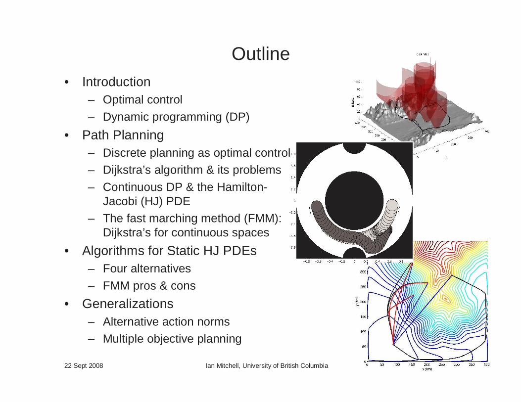
Outline• Introduction
– Optimal control
– Dynamic programming (DP)
• Path Planning– Discrete planning as optimal control– Dijkstra’s algorithm & its problems
– Continuous DP & the Hamilton-Jacobi (HJ) PDE
– The fast marching method (FMM): Dijkstra’s for continuous spaces
• Algorithms for Static HJ PDEs– Four alternatives
– FMM pros & cons
• Generalizations– Alternative action norms– Multiple objective planning
22 Sept 2008 Ian Mitchell, University of British Columbia 3
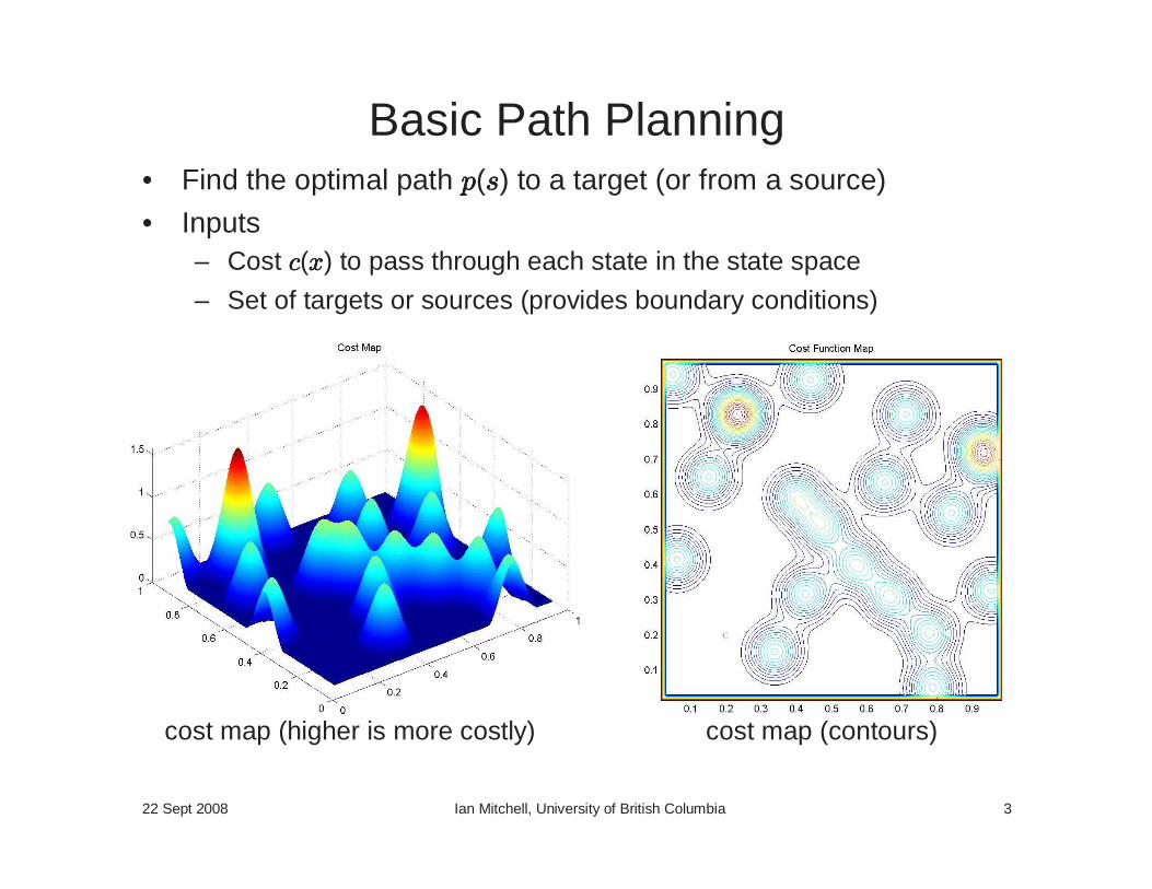
Basic Path Planning• Find the optimal path pppp(ssss) to a target (or from a source)
• Inputs– Cost cccc(xxxx) to pass through each state in the state space
– Set of targets or sources (provides boundary conditions)
cost map (higher is more costly) cost map (contours)
22 Sept 2008 Ian Mitchell, University of British Columbia 4
Discrete vs Continuous• Discrete variable
– Drawn from a countable domain, typically finite– Often no useful metric other than the discrete metric
– Often no consistent ordering
– Examples: names of students in this room, rooms in this building, natural numbers, grid of Rd, …
• Continuous variable– Drawn from an uncountable domain, but may be bounded– Usually has a continuous metric
– Often no consistent ordering– Examples: Real numbers [ 0, 1 ], Rd, SO(3), …
22 Sept 2008 Ian Mitchell, University of British Columbia 5
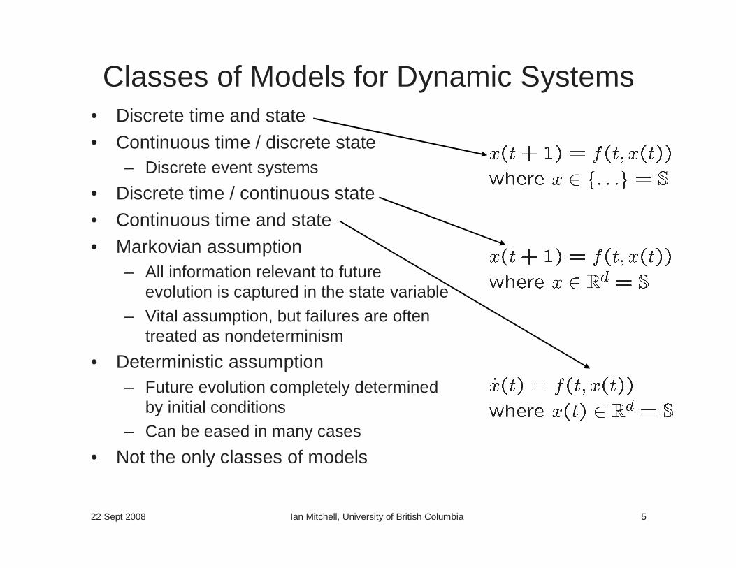
Classes of Models for Dynamic Systems• Discrete time and state
• Continuous time / discrete state– Discrete event systems
• Discrete time / continuous state
• Continuous time and state
• Markovian assumption– All information relevant to future
evolution is captured in the state variable– Vital assumption, but failures are often
treated as nondeterminism
• Deterministic assumption– Future evolution completely determined
by initial conditions– Can be eased in many cases
• Not the only classes of models
22 Sept 2008 Ian Mitchell, University of British Columbia 6
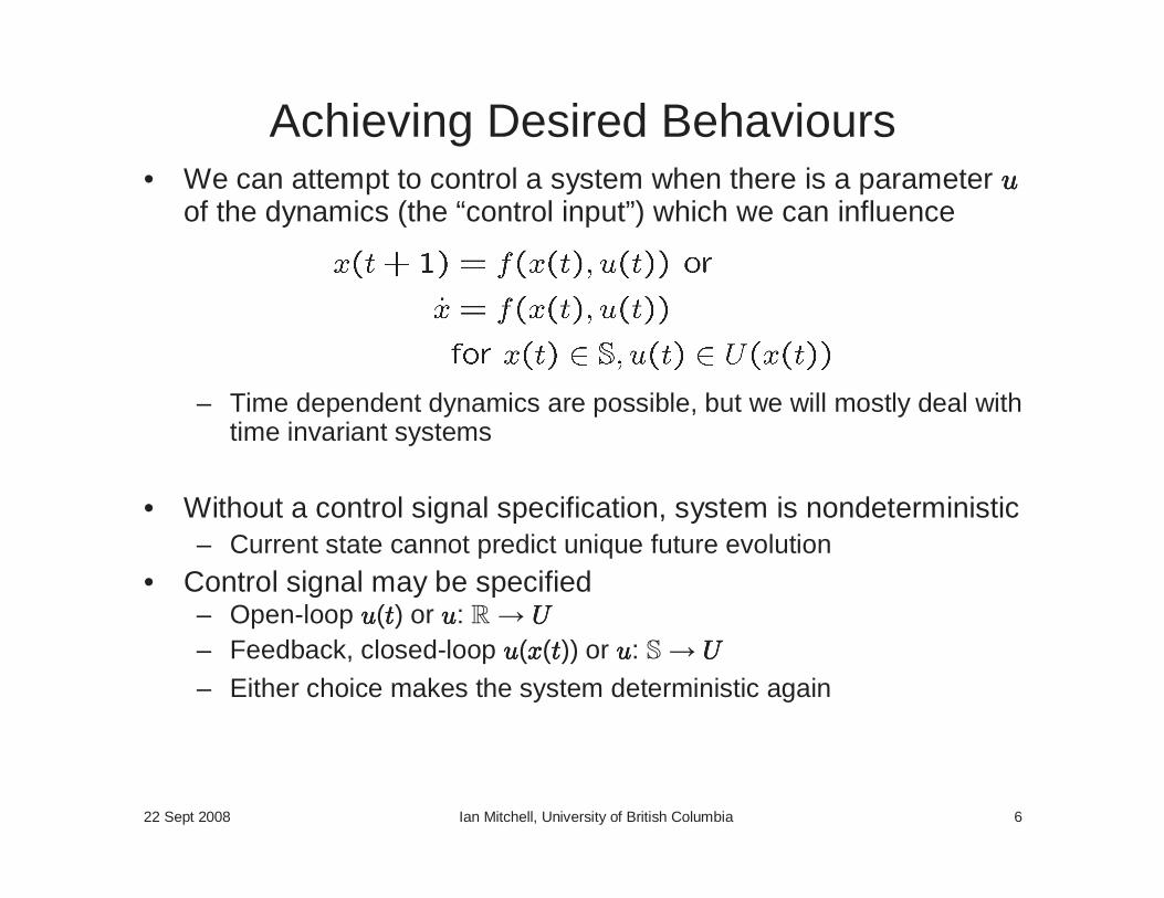
Achieving Desired Behaviours• We can attempt to control a system when there is a parameter uuuu
of the dynamics (the “control input”) which we can influence
– Time dependent dynamics are possible, but we will mostly deal with time invariant systems
• Without a control signal specification, system is nondeterministic– Current state cannot predict unique future evolution
• Control signal may be specified– Open-loop uuuu(tttt) or uuuu: R UUUU
– Feedback, closed-loop uuuu(xxxx(tttt)) or uuuu: S UUUU
– Either choice makes the system deterministic again
22 Sept 2008 Ian Mitchell, University of British Columbia 7
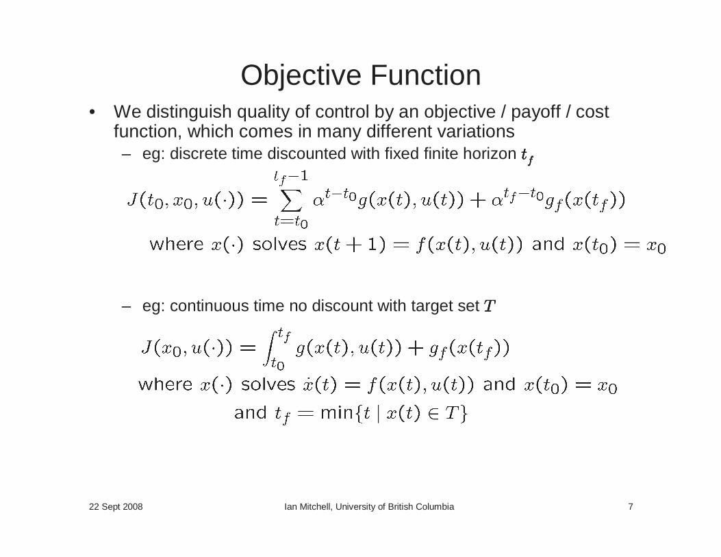
Objective Function• We distinguish quality of control by an objective / payoff / cost
function, which comes in many different variations– eg: discrete time discounted with fixed finite horizon ttttffff
– eg: continuous time no discount with target set TTTT
22 Sept 2008 Ian Mitchell, University of British Columbia 8
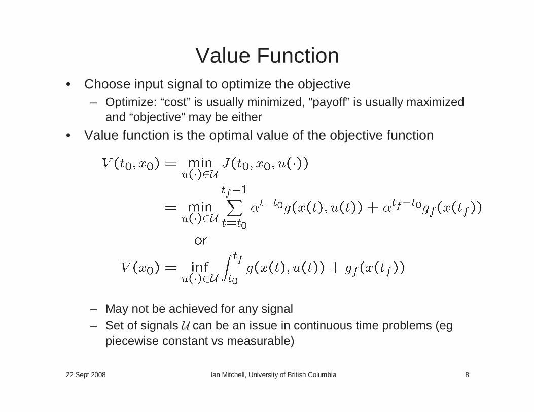
Value Function• Choose input signal to optimize the objective
– Optimize: “cost” is usually minimized, “payoff” is usually maximized and “objective” may be either
• Value function is the optimal value of the objective function
– May not be achieved for any signal– Set of signals U can be an issue in continuous time problems (eg
piecewise constant vs measurable)
22 Sept 2008 Ian Mitchell, University of British Columbia 9
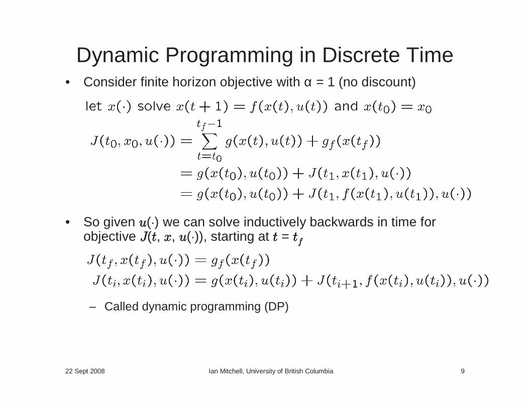
Dynamic Programming in Discrete Time• Consider finite horizon objective with α = 1 (no discount)
• So given uuuu(·) we can solve inductively backwards in time for objective JJJJ(tttt, xxxx, uuuu(·)), starting at tttt = ttttffff
– Called dynamic programming (DP)
22 Sept 2008 Ian Mitchell, University of British Columbia 10
DP for the Value Function• DP can also be applied to the value function
– Second step works because uuuu(tttt0) can be chosen independently of uuuu(tttt) for tttt > tttt0
22 Sept 2008 Ian Mitchell, University of British Columbia 11
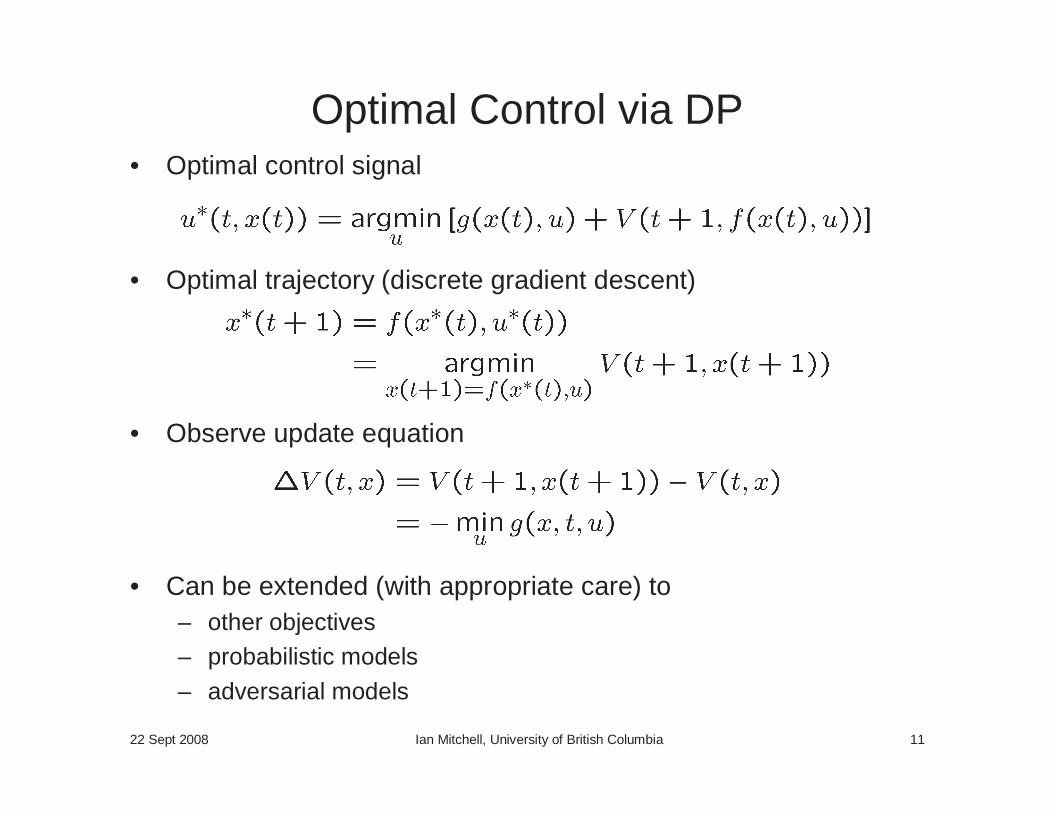
Optimal Control via DP• Optimal control signal
• Optimal trajectory (discrete gradient descent)
• Observe update equation
• Can be extended (with appropriate care) to – other objectives– probabilistic models
– adversarial models

22 Sept 2008 Ian Mitchell, University of British Columbia 12
Outline• Introduction
– Optimal control
– Dynamic programming (DP)
• Path Planning– Discrete planning as optimal control– Dijkstra’s algorithm & its problems
– Continuous DP & the Hamilton-Jacobi (HJ) PDE
– The fast marching method (FMM): Dijkstra’s for continuous spaces
• Algorithms for Static HJ PDEs– Four alternatives
– FMM pros & cons
• Generalizations– Alternative action norms– Multiple objective planning

22 Sept 2008 Ian Mitchell, University of British Columbia 13
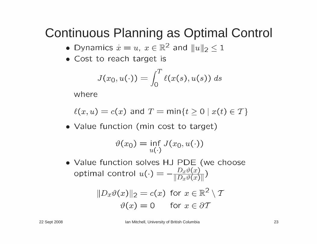
Basic Path Planning (reminder)• Find the optimal path pppp(ssss) to a target (or from a source)
• Inputs– Cost cccc(xxxx) to pass through each state in the state space
– Set of targets or sources (provides boundary conditions)
cost map (higher is more costly) cost map (contours)
22 Sept 2008 Ian Mitchell, University of British Columbia 14
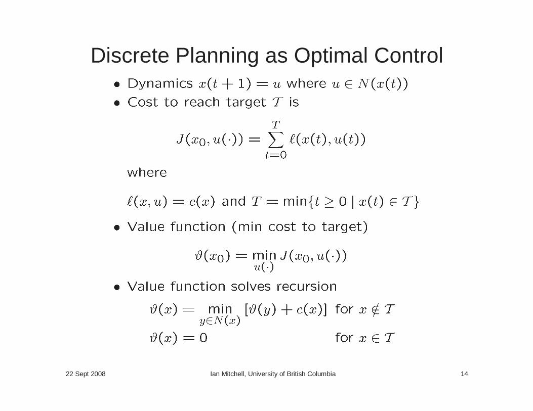
Discrete Planning as Optimal Control
22 Sept 2008 Ian Mitchell, University of British Columbia 15
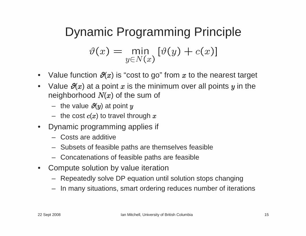
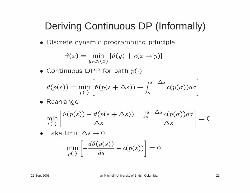
Dynamic Programming Principle
• Value function ϑϑϑϑ(xxxx) is “cost to go” from xxxx to the nearest target
• Value ϑϑϑϑ(xxxx) at a point xxxx is the minimum over all points yyyy in the neighborhood NNNN(xxxx) of the sum of– the value ϑϑϑϑ(yyyy) at point yyyy– the cost cccc(xxxx) to travel through xxxx
• Dynamic programming applies if– Costs are additive– Subsets of feasible paths are themselves feasible
– Concatenations of feasible paths are feasible
• Compute solution by value iteration– Repeatedly solve DP equation until solution stops changing– In many situations, smart ordering reduces number of iterations
22 Sept 2008 Ian Mitchell, University of British Columbia 16
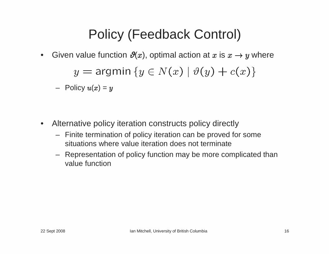
Policy (Feedback Control)• Given value function ϑϑϑϑ(xxxx), optimal action at xxxx is xxxx→→→→ yyyy where
– Policy uuuu(xxxx) = yyyy
• Alternative policy iteration constructs policy directly– Finite termination of policy iteration can be proved for some
situations where value iteration does not terminate
– Representation of policy function may be more complicated than value function
22 Sept 2008 Ian Mitchell, University of British Columbia 17
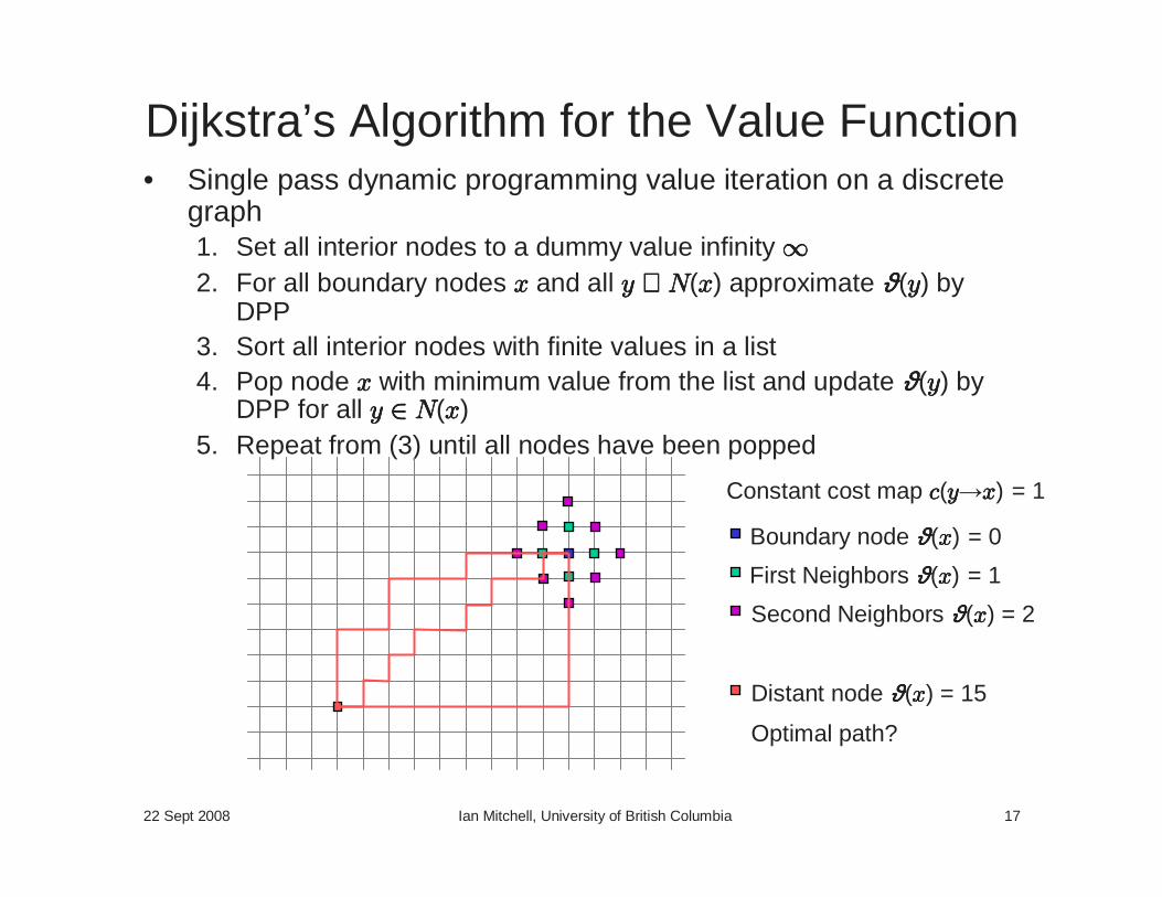
Dijkstra’s Algorithm for the Value Function• Single pass dynamic programming value iteration on a discrete
graph1. Set all interior nodes to a dummy value infinity ∞∞∞∞2. For all boundary nodes xxxx and all yyyy ∈∈∈∈ NNNN(xxxx) approximate ϑϑϑϑ(yyyy) by
DPP3. Sort all interior nodes with finite values in a list4. Pop node xxxx with minimum value from the list and update ϑϑϑϑ(yyyy) by
DPP for all yyyy ∈∈∈∈ NNNN(xxxx)5. Repeat from (3) until all nodes have been popped
Boundary node ϑϑϑϑ(xxxx) = 0
Constant cost map cccc(yyyy xxxx) = 1
First Neighbors ϑϑϑϑ(xxxx) = 1
Second Neighbors ϑϑϑϑ(xxxx) = 2
Distant node ϑϑϑϑ(xxxx) = 15
Optimal path?
22 Sept 2008 Ian Mitchell, University of British Columbia 18
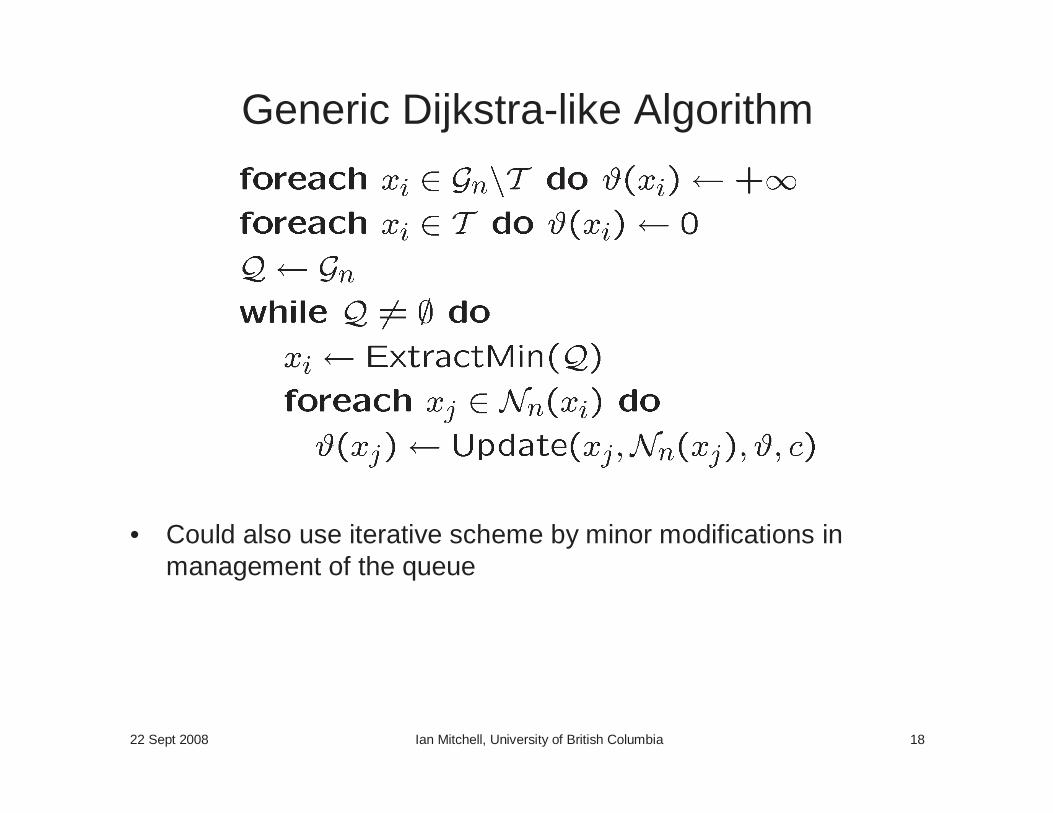
Generic Dijkstra-like Algorithm
• Could also use iterative scheme by minor modifications in management of the queue
22 Sept 2008 Ian Mitchell, University of British Columbia 19
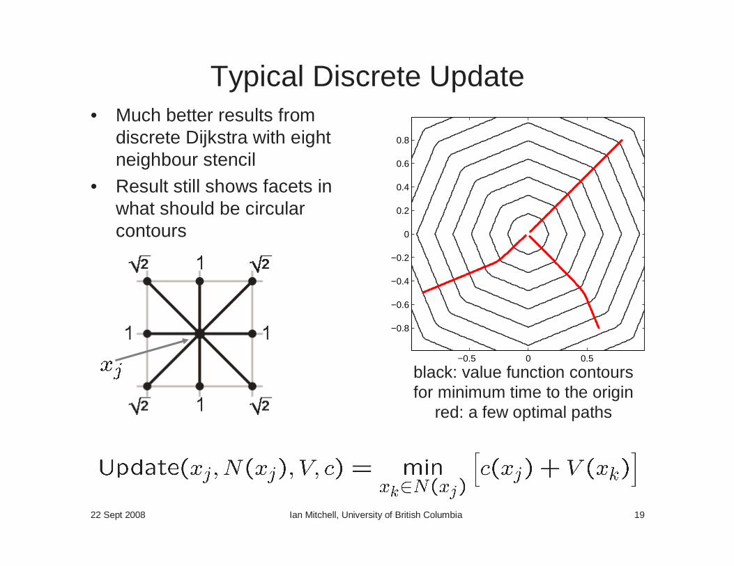
Typical Discrete Update• Much better results from
discrete Dijkstra with eight neighbour stencil
• Result still shows facets in what should be circular contours
−0.5 0 0.5
−0.8
−0.6
−0.4
−0.2
0
0.2
0.4
0.6
0.8
black: value function contoursfor minimum time to the origin
red: a few optimal paths
22 Sept 2008 Ian Mitchell, University of British Columbia 20
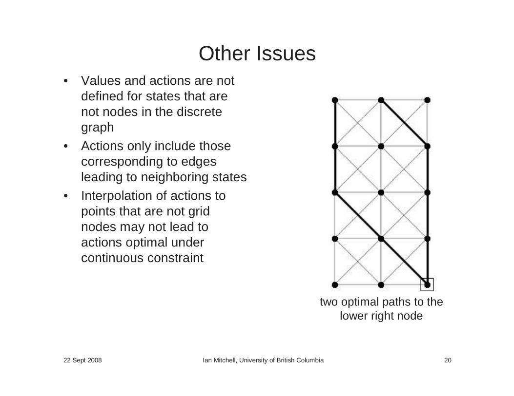
Other Issues• Values and actions are not
defined for states that are not nodes in the discrete graph
• Actions only include those corresponding to edges leading to neighboring states
• Interpolation of actions to points that are not grid nodes may not lead to actions optimal under continuous constraint
two optimal paths to thelower right node
22 Sept 2008 Ian Mitchell, University of British Columbia 21
Deriving Continuous DP (Informally)
22 Sept 2008 Ian Mitchell, University of British Columbia 22
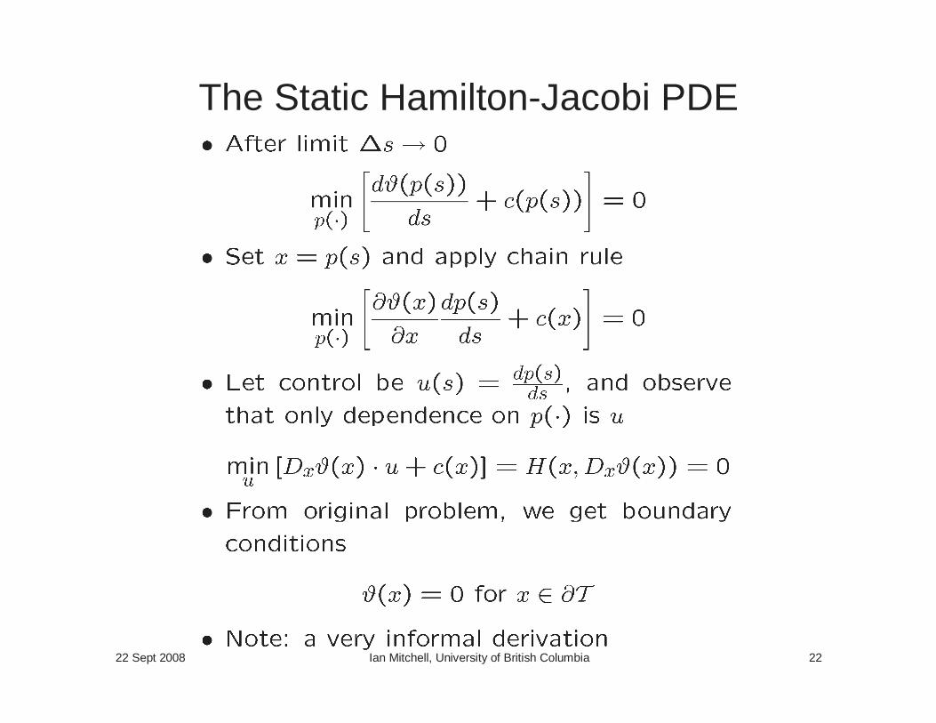
The Static Hamilton-Jacobi PDE
22 Sept 2008 Ian Mitchell, University of British Columbia 23
Continuous Planning as Optimal Control
22 Sept 2008 Ian Mitchell, University of British Columbia 24
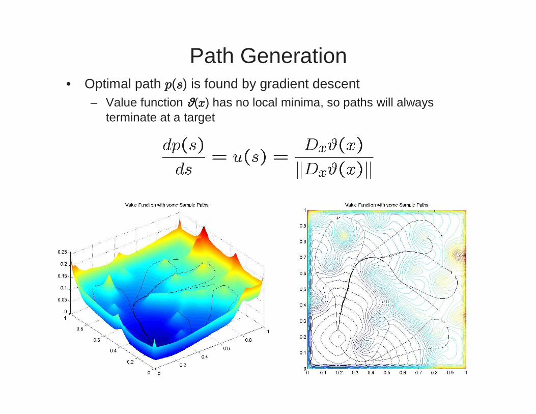
Path Generation• Optimal path pppp(ssss) is found by gradient descent
– Value function ϑϑϑϑ(xxxx) has no local minima, so paths will always terminate at a target
22 Sept 2008 Ian Mitchell, University of British Columbia 25
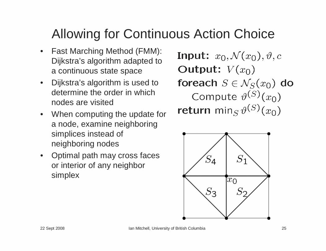
Allowing for Continuous Action Choice• Fast Marching Method (FMM):
Dijkstra’s algorithm adapted to a continuous state space
• Dijkstra’s algorithm is used to determine the order in which nodes are visited
• When computing the update for a node, examine neighboring simplices instead of neighboring nodes
• Optimal path may cross faces or interior of any neighbor simplex
22 Sept 2008 Ian Mitchell, University of British Columbia 26
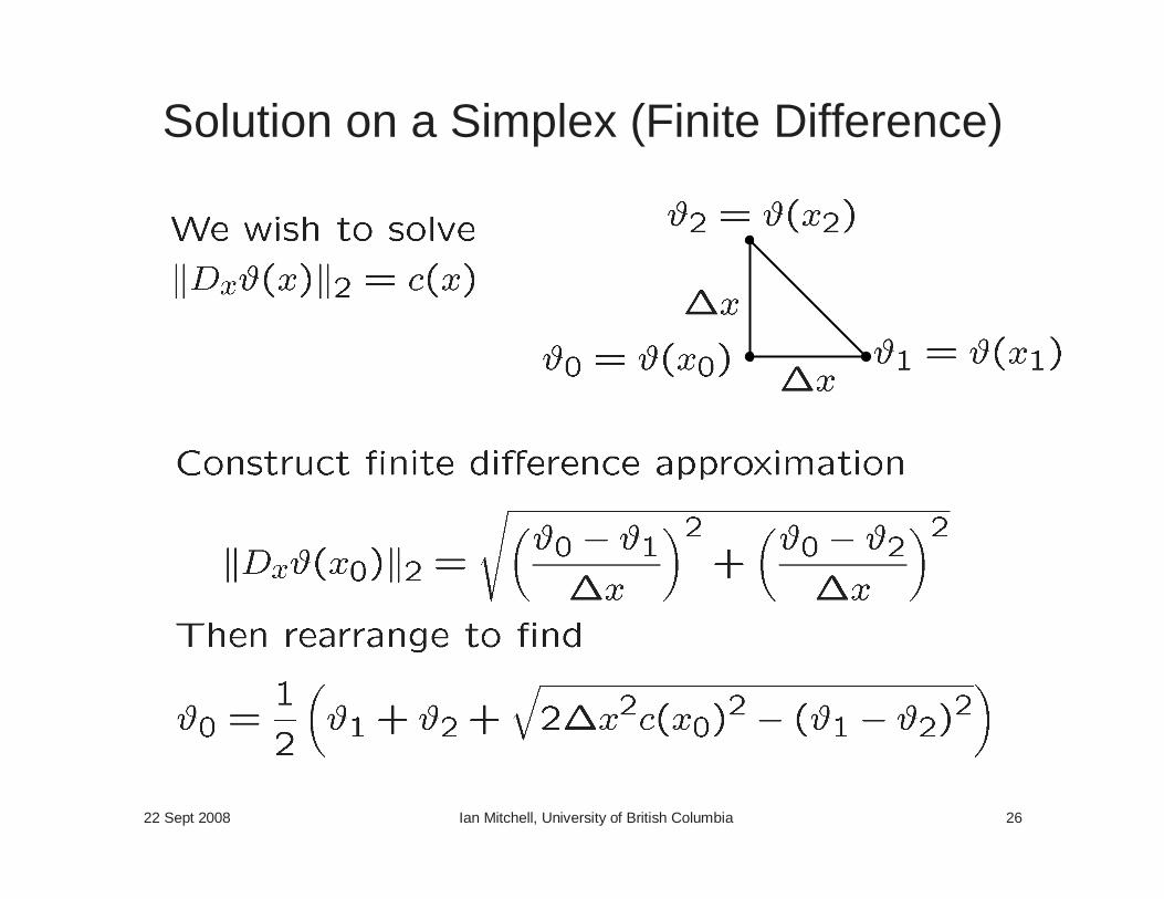
Solution on a Simplex (Finite Difference)
22 Sept 2008 Ian Mitchell, University of British Columbia 27
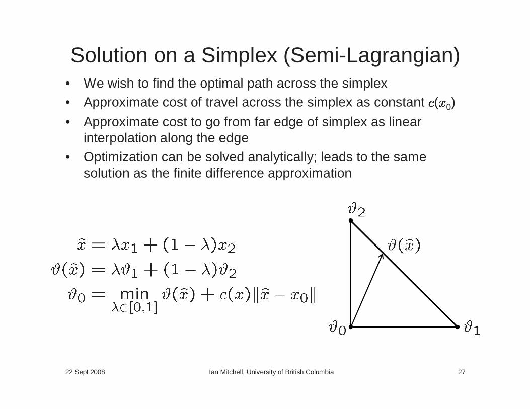
Solution on a Simplex (Semi-Lagrangian)• We wish to find the optimal path across the simplex• Approximate cost of travel across the simplex as constant cccc(xxxx0)
• Approximate cost to go from far edge of simplex as linear interpolation along the edge
• Optimization can be solved analytically; leads to the same solution as the finite difference approximation
22 Sept 2008 Ian Mitchell, University of British Columbia 28
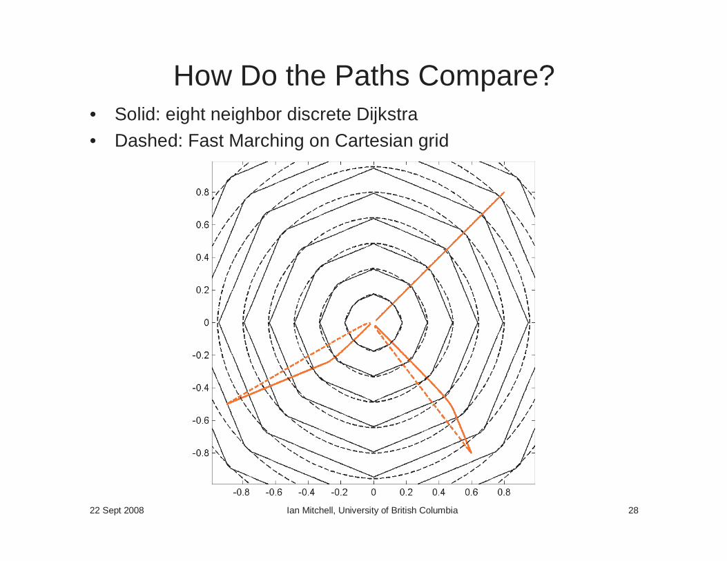
How Do the Paths Compare?• Solid: eight neighbor discrete Dijkstra
• Dashed: Fast Marching on Cartesian grid
22 Sept 2008 Ian Mitchell, University of British Columbia 29
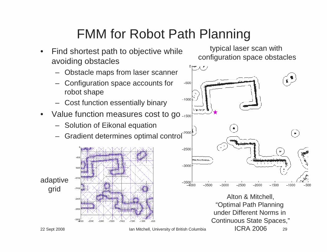
FMM for Robot Path Planning• Find shortest path to objective while
avoiding obstacles– Obstacle maps from laser scanner
– Configuration space accounts for robot shape
– Cost function essentially binary
• Value function measures cost to go– Solution of Eikonal equation
– Gradient determines optimal control
typical laser scan with configuration space obstacles
adaptivegrid
Alton & Mitchell,“Optimal Path Planning
under Different Norms in Continuous State Spaces,”
ICRA 2006
22 Sept 2008 Ian Mitchell, University of British Columbia 30
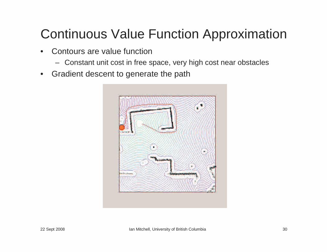
Continuous Value Function Approximation• Contours are value function
– Constant unit cost in free space, very high cost near obstacles
• Gradient descent to generate the path
22 Sept 2008 Ian Mitchell, University of British Columbia 31
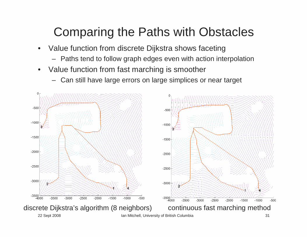
Comparing the Paths with Obstacles• Value function from discrete Dijkstra shows faceting
– Paths tend to follow graph edges even with action interpolation
• Value function from fast marching is smoother– Can still have large errors on large simplices or near target
discrete Dijkstra’s algorithm (8 neighbors) continuous fast marching method
22 Sept 2008 Ian Mitchell, University of British Columbia 32
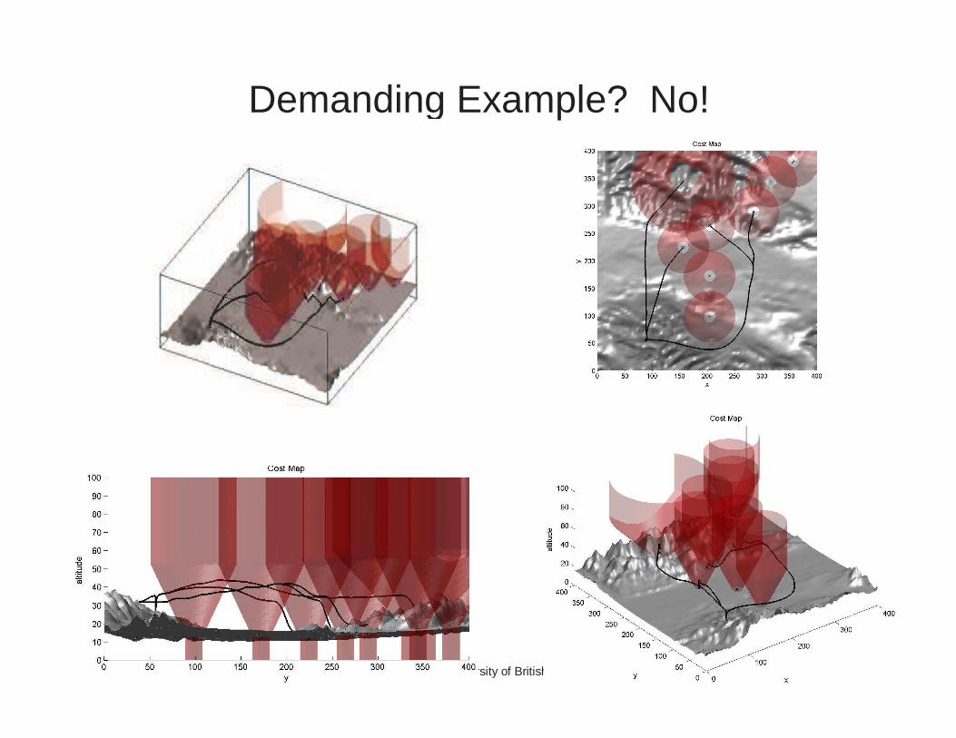
Demanding Example? No!

22 Sept 2008 Ian Mitchell, University of British Columbia 33
Outline• Introduction
– Optimal control
– Dynamic programming (DP)
• Path Planning– Discrete planning as optimal control– Dijkstra’s algorithm & its problems
– Continuous DP & the Hamilton-Jacobi (HJ) PDE
– The fast marching method (FMM): Dijkstra’s for continuous spaces
• Algorithms for Static HJ PDEs– Four alternatives
– FMM pros & cons
• Generalizations– Alternative action norms– Multiple objective planning
22 Sept 2008 Ian Mitchell, University of British Columbia 34
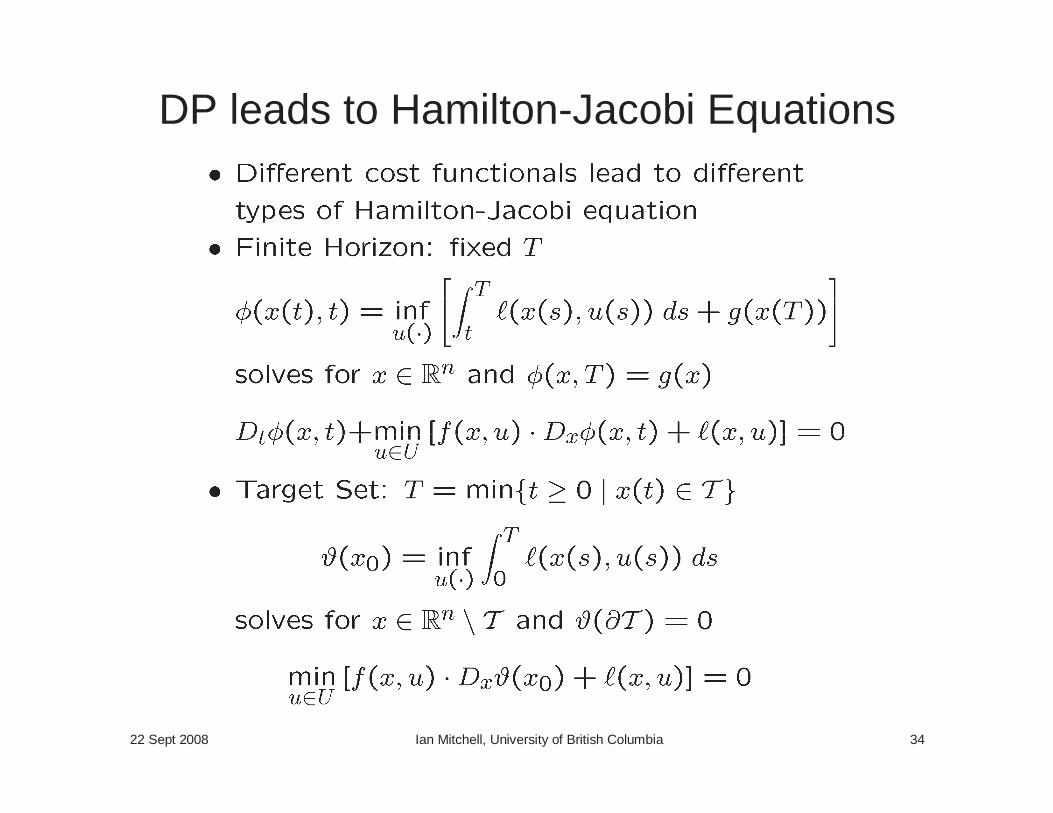
DP leads to Hamilton-Jacobi Equations
22 Sept 2008 Ian Mitchell, University of British Columbia 35
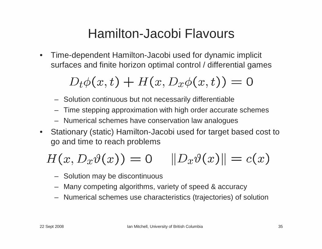
Hamilton-Jacobi Flavours
• Time-dependent Hamilton-Jacobi used for dynamic implicit surfaces and finite horizon optimal control / differential games
– Solution continuous but not necessarily differentiable
– Time stepping approximation with high order accurate schemes– Numerical schemes have conservation law analogues
• Stationary (static) Hamilton-Jacobi used for target based cost to go and time to reach problems
– Solution may be discontinuous– Many competing algorithms, variety of speed & accuracy– Numerical schemes use characteristics (trajectories) of solution
22 Sept 2008 Ian Mitchell, University of British Columbia 36
Solving Static HJ PDEs• Two methods available for using time-dependent techniques to
solve the static problem– Iterate time-dependent version until Hamiltonian is zero– Transform into a front propagation problem
• Schemes designed specifically for static HJ PDEs are essentially continuous versions of value iteration from dynamic programming– Approximate the value at each node in terms of the values at its
neighbours (in a consistent manner)– Details of this process define the “local update”– Eulerian schemes, plus a variety of semi-Lagrangian
• Result is a collection of coupled nonlinear equations for the values of all nodes in terms of all the other nodes
• Two value iteration methods for solving this collection of equations: marching and sweeping– Correspond to label setting and label correcting in graph algorithms
22 Sept 2008 Ian Mitchell, University of British Columbia 37
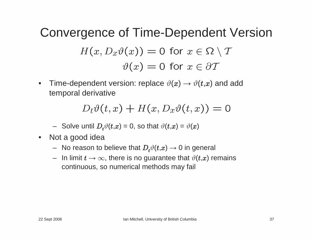
Convergence of Time-Dependent Version
• Time-dependent version: replace ϑ(xxxx) ϑ(tttt,xxxx) and add temporal derivative
– Solve until DDDDttttϑ(tttt,xxxx) = 0, so that ϑ(tttt,xxxx) = ϑ(xxxx)
• Not a good idea– No reason to believe that DDDDttttϑ(tttt,xxxx) 0 in general– In limit tttt ∞, there is no guarantee that ϑ(tttt,xxxx) remains
continuous, so numerical methods may fail
22 Sept 2008 Ian Mitchell, University of British Columbia 38
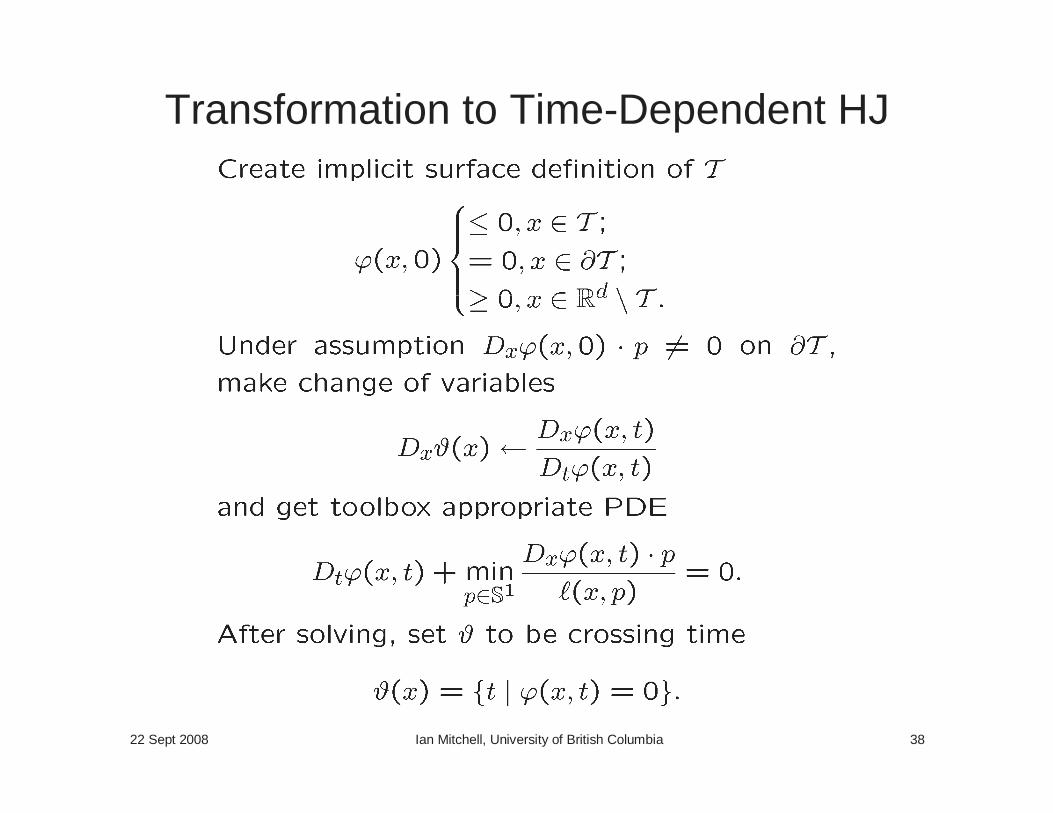
Transformation to Time-Dependent HJ
22 Sept 2008 Ian Mitchell, University of British Columbia 39
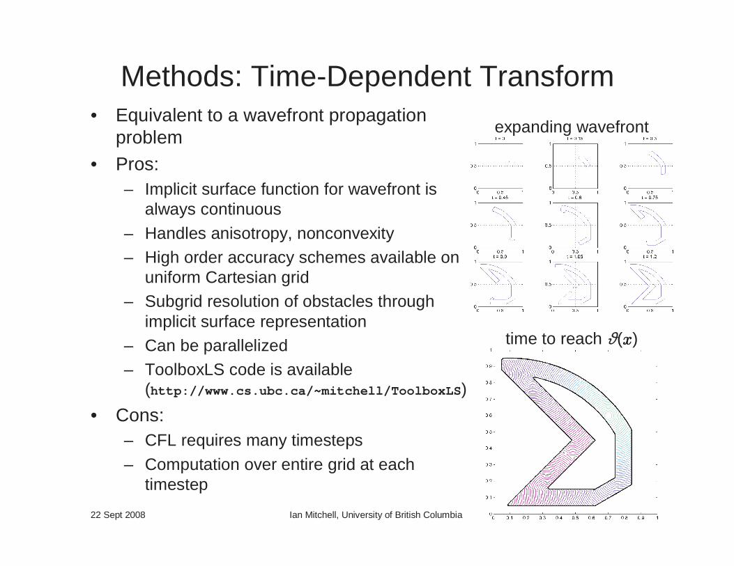
Methods: Time-Dependent Transform• Equivalent to a wavefront propagation
problem
• Pros: – Implicit surface function for wavefront is
always continuous
– Handles anisotropy, nonconvexity– High order accuracy schemes available on
uniform Cartesian grid– Subgrid resolution of obstacles through
implicit surface representation– Can be parallelized– ToolboxLS code is available
(http://www.cs.ubc.ca/~mitchell/ToolboxLS)
• Cons: – CFL requires many timesteps
– Computation over entire grid at each timestep
expanding wavefront
time to reach ϑ(xxxx)
22 Sept 2008 Ian Mitchell, University of British Columbia 40
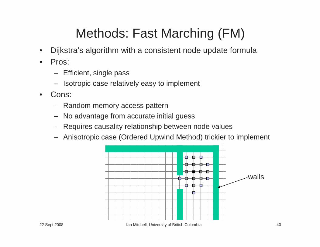
Methods: Fast Marching (FM)• Dijkstra’s algorithm with a consistent node update formula
• Pros:– Efficient, single pass
– Isotropic case relatively easy to implement
• Cons:– Random memory access pattern– No advantage from accurate initial guess – Requires causality relationship between node values
– Anisotropic case (Ordered Upwind Method) trickier to implement
walls
22 Sept 2008 Ian Mitchell, University of British Columbia 41
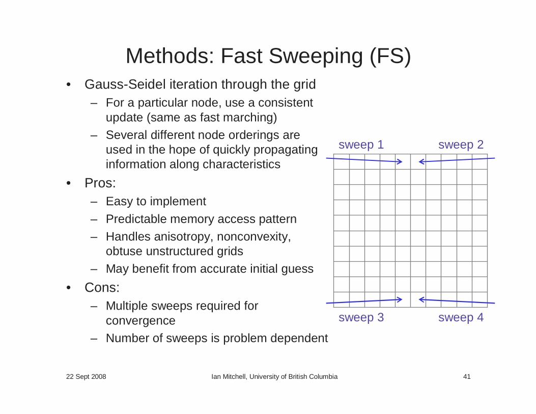
Methods: Fast Sweeping (FS)• Gauss-Seidel iteration through the grid
– For a particular node, use a consistent update (same as fast marching)
– Several different node orderings are used in the hope of quickly propagating information along characteristics
• Pros:– Easy to implement
– Predictable memory access pattern– Handles anisotropy, nonconvexity,
obtuse unstructured grids– May benefit from accurate initial guess
• Cons:– Multiple sweeps required for
convergence– Number of sweeps is problem dependent
sweep 3 sweep 4
sweep 1 sweep 2
22 Sept 2008 Ian Mitchell, University of British Columbia 42
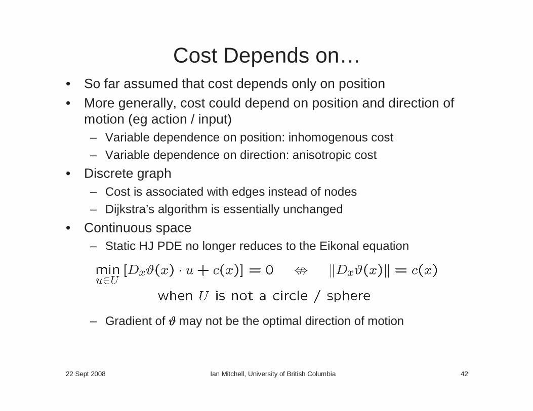
Cost Depends on…• So far assumed that cost depends only on position
• More generally, cost could depend on position and direction of motion (eg action / input)– Variable dependence on position: inhomogenous cost
– Variable dependence on direction: anisotropic cost
• Discrete graph– Cost is associated with edges instead of nodes– Dijkstra’s algorithm is essentially unchanged
• Continuous space– Static HJ PDE no longer reduces to the Eikonal equation
– Gradient of ϑϑϑϑ may not be the optimal direction of motion
22 Sept 2008 Ian Mitchell, University of British Columbia 43
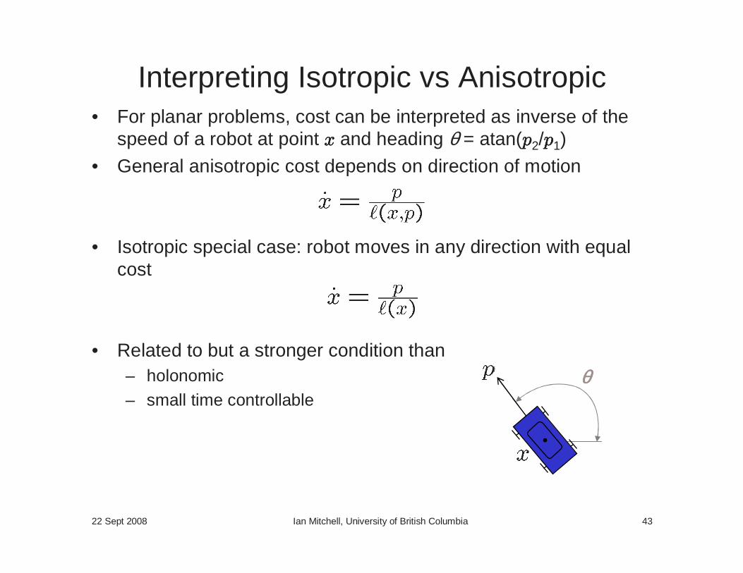
Interpreting Isotropic vs Anisotropic• For planar problems, cost can be interpreted as inverse of the
speed of a robot at point xxxx and heading θ = atan(pppp2/pppp1)
• General anisotropic cost depends on direction of motion
• Isotropic special case: robot moves in any direction with equal cost
• Related to but a stronger condition than– holonomic– small time controllable
θθθθ
22 Sept 2008 Ian Mitchell, University of British Columbia 44
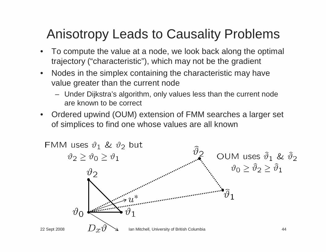
Anisotropy Leads to Causality Problems• To compute the value at a node, we look back along the optimal
trajectory (“characteristic”), which may not be the gradient
• Nodes in the simplex containing the characteristic may have value greater than the current node– Under Dijkstra’s algorithm, only values less than the current node
are known to be correct
• Ordered upwind (OUM) extension of FMM searches a larger set of simplices to find one whose values are all known
22 Sept 2008 Ian Mitchell, University of British Columbia 45
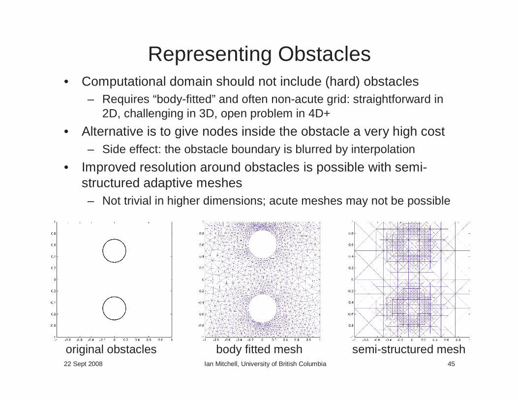
Representing Obstacles
original obstacles
• Computational domain should not include (hard) obstacles– Requires “body-fitted” and often non-acute grid: straightforward in
2D, challenging in 3D, open problem in 4D+
• Alternative is to give nodes inside the obstacle a very high cost– Side effect: the obstacle boundary is blurred by interpolation
• Improved resolution around obstacles is possible with semi-structured adaptive meshes– Not trivial in higher dimensions; acute meshes may not be possible
semi-structured meshbody fitted mesh
22 Sept 2008 Ian Mitchell, University of British Columbia 46
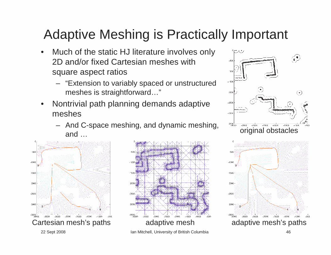
Adaptive Meshing is Practically Important• Much of the static HJ literature involves only
2D and/or fixed Cartesian meshes with square aspect ratios– “Extension to variably spaced or unstructured
meshes is straightforward…”
• Nontrivial path planning demands adaptive meshes– And C-space meshing, and dynamic meshing,
and …
Cartesian mesh’s paths adaptive mesh’s paths
original obstacles
adaptive mesh
22 Sept 2008 Ian Mitchell, University of British Columbia 47
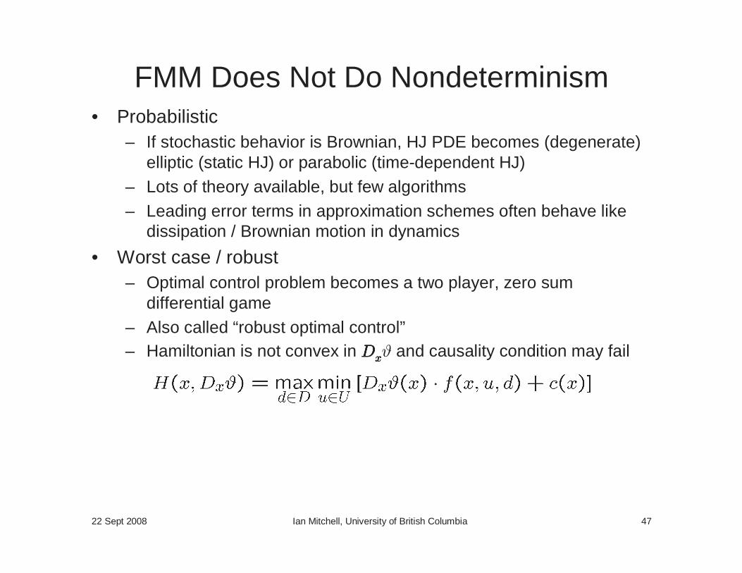
FMM Does Not Do Nondeterminism• Probabilistic
– If stochastic behavior is Brownian, HJ PDE becomes (degenerate) elliptic (static HJ) or parabolic (time-dependent HJ)
– Lots of theory available, but few algorithms– Leading error terms in approximation schemes often behave like
dissipation / Brownian motion in dynamics
• Worst case / robust– Optimal control problem becomes a two player, zero sum
differential game– Also called “robust optimal control”– Hamiltonian is not convex in DDDDxxxxϑ and causality condition may fail
22 Sept 2008 Ian Mitchell, University of British Columbia 48
Other FMM Issues• Initial guess
– FMM gets little benefit from a good initial guess because each node’s value is computed only when it might be completely correct
– Changing the value of any node can potentially change any other node with a higher value, so an efficient updating algorithm is not trivial to design
• Focused algorithms (when given source and destination)– A* is a version of Dijkstra’s algorithm that ignores some nodes
which cannot be on the optimal path
– FMM updates depend on neighboring simplices rather than individual nodes, so there is no straightforward adaptation of A*
• Non-holonomic– The value function may not be continuous if some directions of
motion are forbidden– Without continuity on a simplex, interpolation should not be used in
the local updates

22 Sept 2008 Ian Mitchell, University of British Columbia 49
Outline• Introduction
– Optimal control
– Dynamic programming (DP)
• Path Planning– Discrete planning as optimal control– Dijkstra’s algorithm & its problems
– Continuous DP & the Hamilton-Jacobi (HJ) PDE
– The fast marching method (FMM): Dijkstra’s for continuous spaces
• Algorithms for Static HJ PDEs– Four alternatives
– FMM pros & cons
• Generalizations– Alternative action norms– Multiple objective planning
22 Sept 2008 Ian Mitchell, University of British Columbia 50
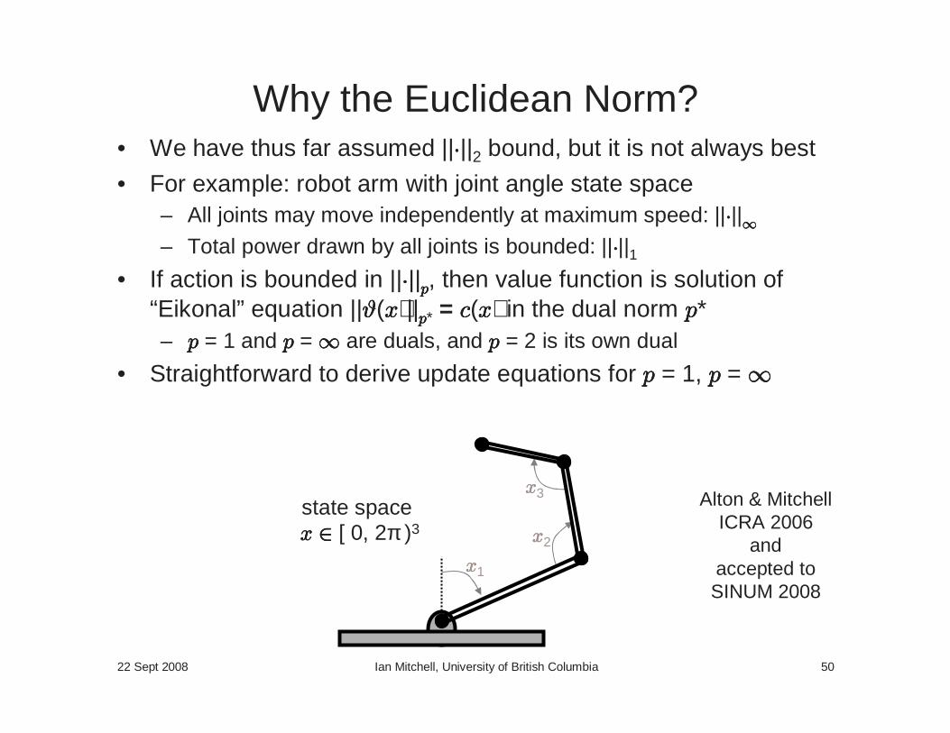
Why the Euclidean Norm?
state spacexxxx ∈∈∈∈ [ 0, 2π )3
• We have thus far assumed ||····||2 bound, but it is not always best
• For example: robot arm with joint angle state space– All joints may move independently at maximum speed: ||····||
∞∞∞∞
– Total power drawn by all joints is bounded: ||····||1• If action is bounded in ||····||pppp, then value function is solution of
“Eikonal” equation ||ϑϑϑϑ(xxxx)||pppp* = cccc(xxxx) in the dual norm pppp*– pppp = 1 and pppp = ∞∞∞∞ are duals, and pppp = 2 is its own dual
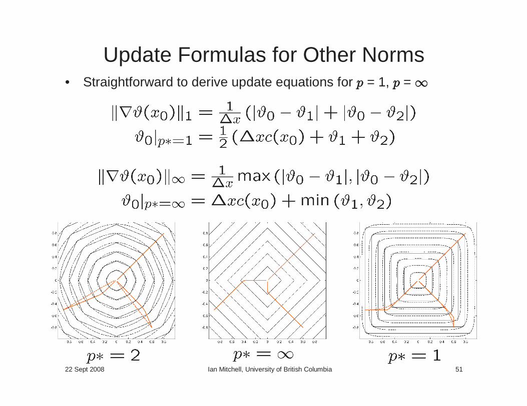
• Straightforward to derive update equations for pppp = 1, pppp = ∞∞∞∞
xxxx1
xxxx2
xxxx3 Alton & MitchellICRA 2006
andaccepted toSINUM 2008
22 Sept 2008 Ian Mitchell, University of British Columbia 51
Update Formulas for Other Norms• Straightforward to derive update equations for pppp = 1, pppp = ∞∞∞∞
22 Sept 2008 Ian Mitchell, University of British Columbia 52
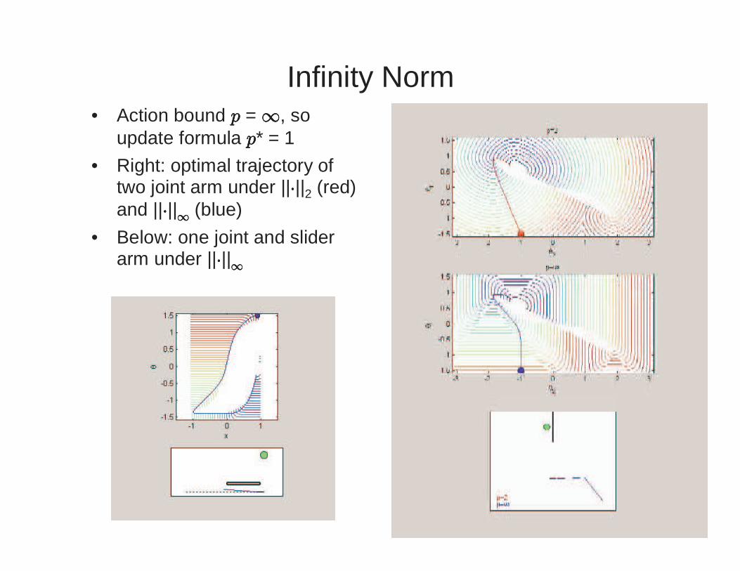
Infinity Norm• Action bound pppp = ∞∞∞∞, so
update formula pppp* = 1
• Right: optimal trajectory of two joint arm under ||····||2 (red) and ||····||
∞∞∞∞(blue)
• Below: one joint and slider arm under ||····||
∞∞∞∞
22 Sept 2008 Ian Mitchell, University of British Columbia 53
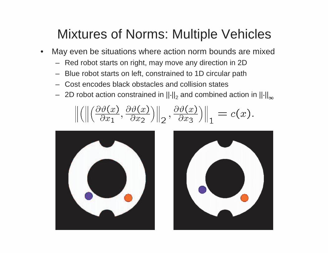
Mixtures of Norms: Multiple Vehicles• May even be situations where action norm bounds are mixed
– Red robot starts on right, may move any direction in 2D
– Blue robot starts on left, constrained to 1D circular path– Cost encodes black obstacles and collision states– 2D robot action constrained in ||····||2 and combined action in ||····||
∞∞∞∞
22 Sept 2008 Ian Mitchell, University of British Columbia 54
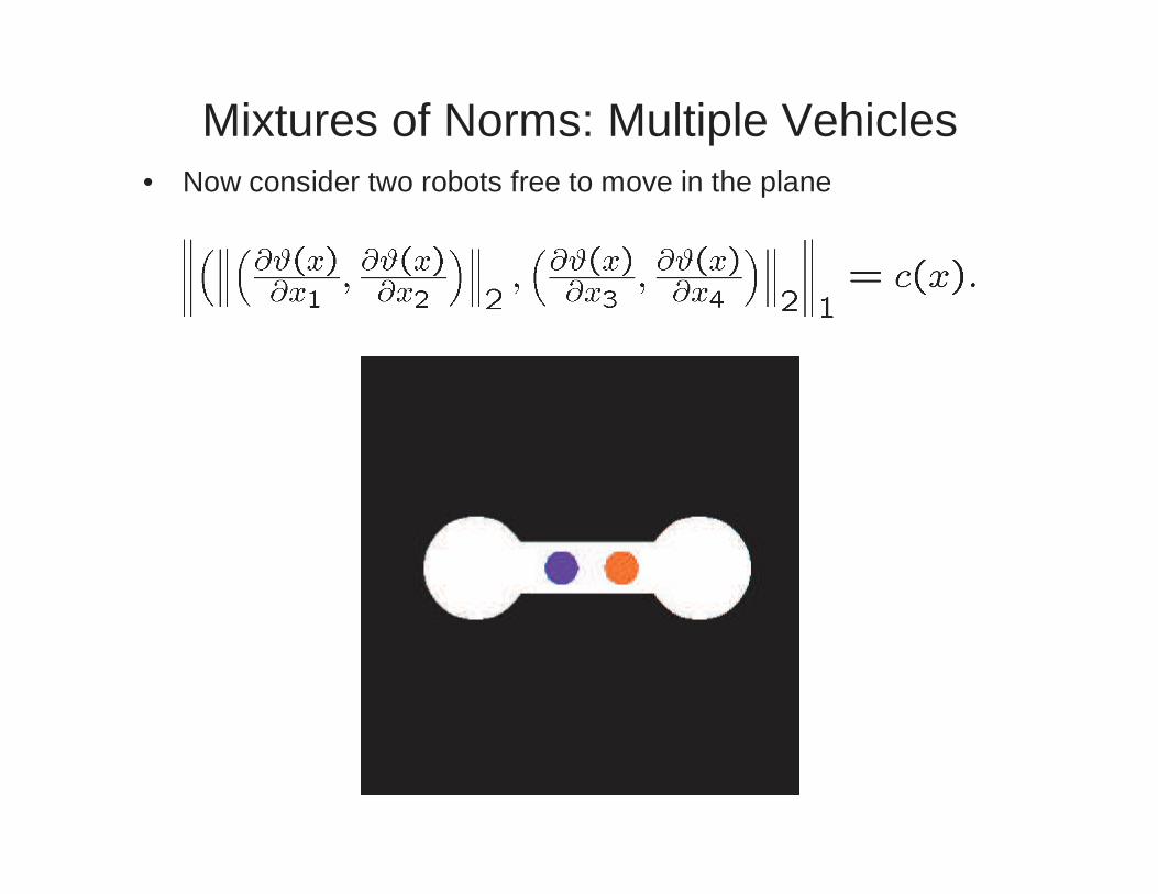
Mixtures of Norms: Multiple Vehicles• Now consider two robots free to move in the plane
22 Sept 2008 Ian Mitchell, University of British Columbia 55
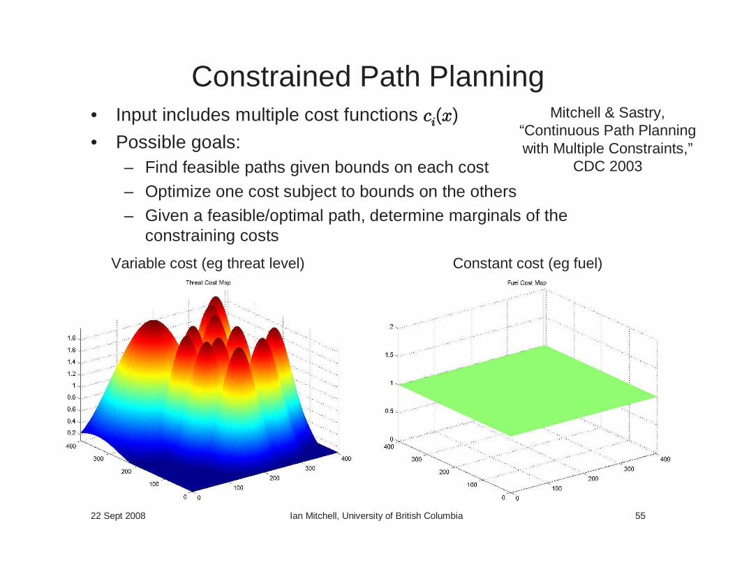
Constrained Path Planning• Input includes multiple cost functions cccciiii(xxxx)
• Possible goals:– Find feasible paths given bounds on each cost
– Optimize one cost subject to bounds on the others– Given a feasible/optimal path, determine marginals of the
constraining costs
Constant cost (eg fuel)Variable cost (eg threat level)
Mitchell & Sastry,“Continuous Path Planningwith Multiple Constraints,”
CDC 2003
22 Sept 2008 Ian Mitchell, University of British Columbia 56
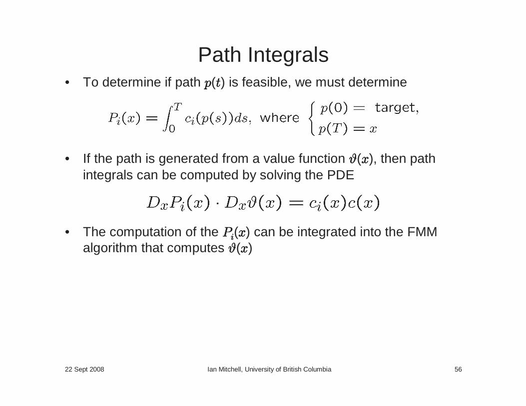
Path Integrals• To determine if path pppp(tttt) is feasible, we must determine
• If the path is generated from a value function ϑϑϑϑ(xxxx), then path integrals can be computed by solving the PDE
• The computation of the PPPPiiii(xxxx) can be integrated into the FMM algorithm that computes ϑϑϑϑ(xxxx)
22 Sept 2008 Ian Mitchell, University of British Columbia 57
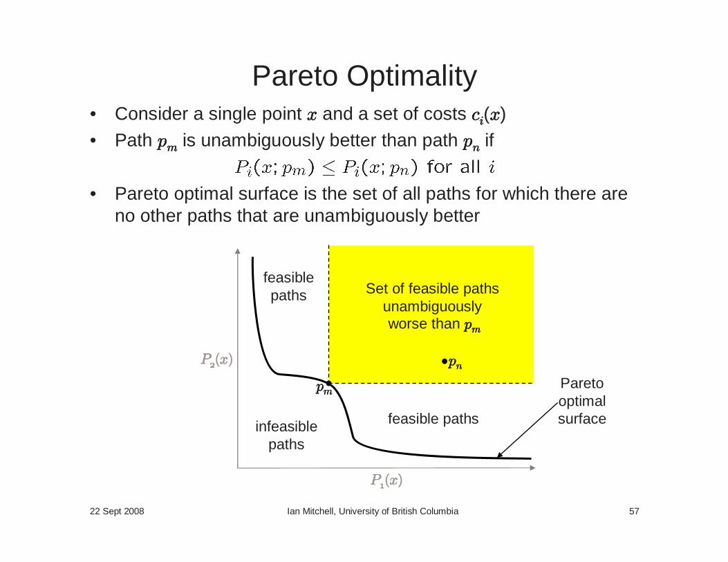
Pareto Optimality• Consider a single point xxxx and a set of costs cccciiii(xxxx)
• Path ppppmmmm is unambiguously better than path ppppnnnn if
• Pareto optimal surface is the set of all paths for which there are no other paths that are unambiguously better
PPPP(xxxx)
ppppnnnnPPPP(xxxx)
ppppmmmm
Set of feasible paths unambiguously worse than ppppmmmm
Paretooptimalsurfaceinfeasible
paths
feasible paths
feasiblepaths
22 Sept 2008 Ian Mitchell, University of British Columbia 58
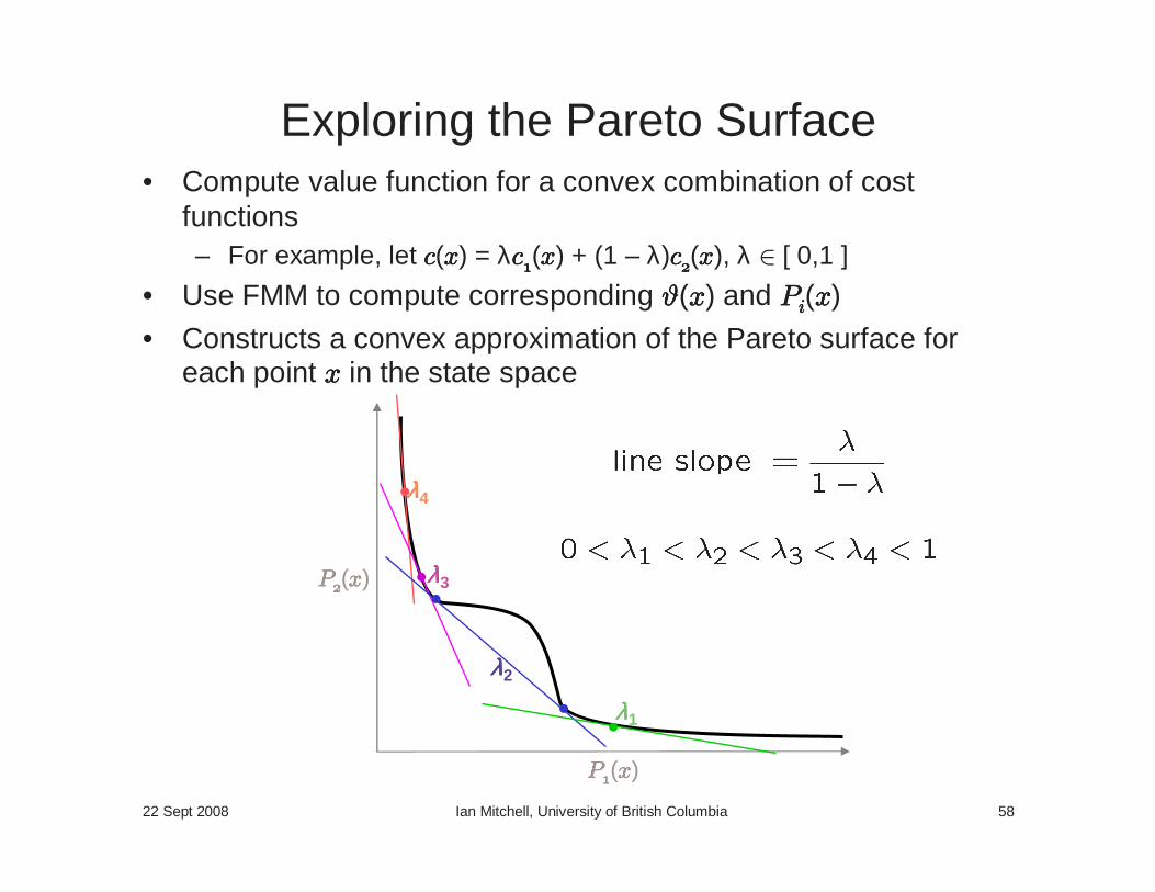
Exploring the Pareto Surface• Compute value function for a convex combination of cost
functions– For example, let cccc(xxxx) = λcccc(xxxx) + (1 – λ)cccc(xxxx), λ ∈ [ 0,1 ]
• Use FMM to compute corresponding ϑϑϑϑ(xxxx) and PPPPiiii(xxxx)
• Constructs a convex approximation of the Pareto surface for each point xxxx in the state space
PPPP(xxxx)
PPPP(xxxx)
λλλλ4
λλλλ3
λλλλ2
λλλλ1
22 Sept 2008 Ian Mitchell, University of British Columbia 59
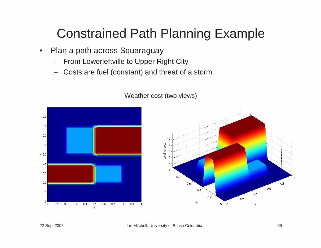
Constrained Path Planning Example• Plan a path across Squaraguay
– From Lowerleftville to Upper Right City
– Costs are fuel (constant) and threat of a storm
Weather cost (two views)
22 Sept 2008 Ian Mitchell, University of British Columbia 60
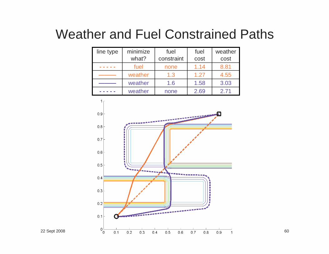
Weather and Fuel Constrained Pathsweather
costfuel cost
fuel constraint
minimizewhat?
line type
2.712.69noneweather- - - - -3.031.581.6weather———4.551.271.3weather———8.811.14nonefuel- - - - -
22 Sept 2008 Ian Mitchell, University of British Columbia 61
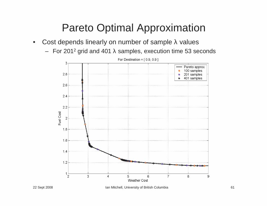
Pareto Optimal Approximation• Cost depends linearly on number of sample λ values
– For 2012 grid and 401 λ samples, execution time 53 seconds
22 Sept 2008 Ian Mitchell, University of British Columbia 62
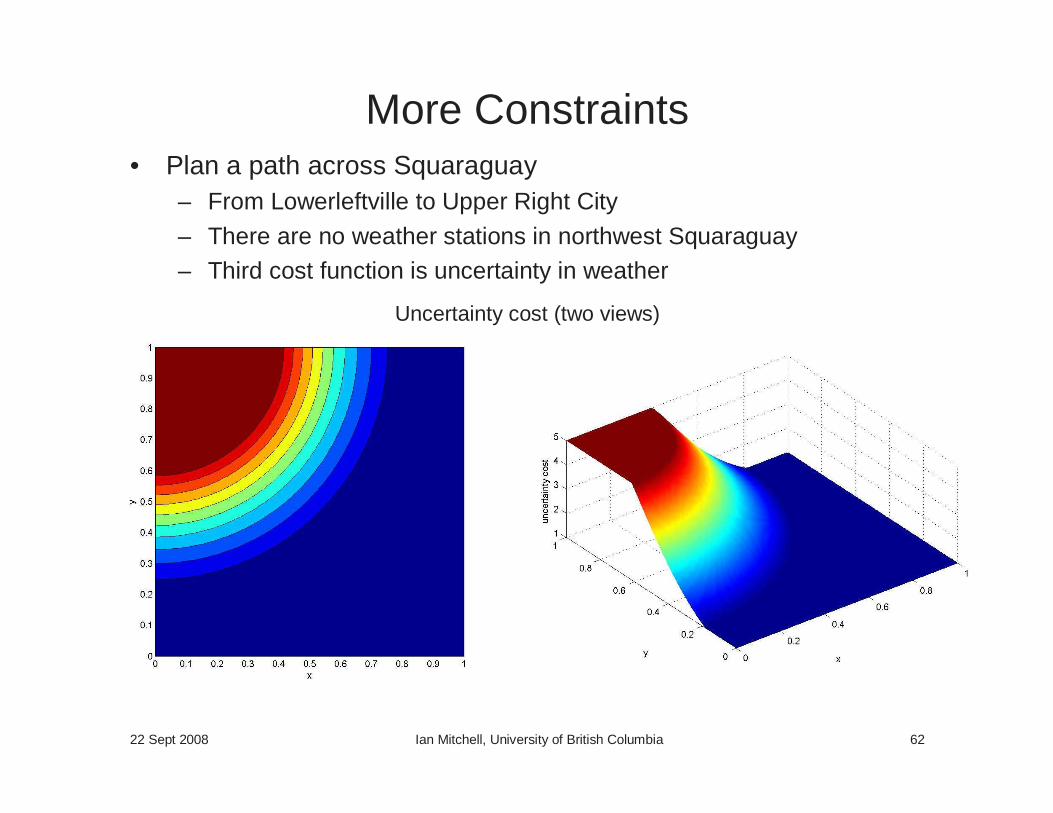
More Constraints• Plan a path across Squaraguay
– From Lowerleftville to Upper Right City
– There are no weather stations in northwest Squaraguay– Third cost function is uncertainty in weather
Uncertainty cost (two views)
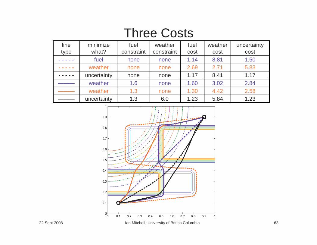
22 Sept 2008 Ian Mitchell, University of British Columbia 63
Three Costs
2.843.021.60none1.6weather———2.584.421.30none1.3weather———
5.84
8.412.718.81
weather cost
1.3
nonenonenone
fuel constraint
6.0
nonenonenone
weather constraint
1.23
1.175.831.50
uncertainty cost
fuel cost
minimize what?
line type
1.23uncertainty———
1.17uncertainty- - - - -2.69weather- - - - -1.14fuel- - - - -
22 Sept 2008 Ian Mitchell, University of British Columbia 64
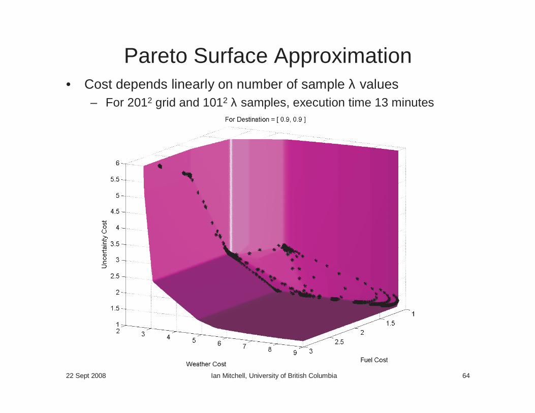
Pareto Surface Approximation• Cost depends linearly on number of sample λ values
– For 2012 grid and 1012 λ samples, execution time 13 minutes
22 Sept 2008 Ian Mitchell, University of British Columbia 65
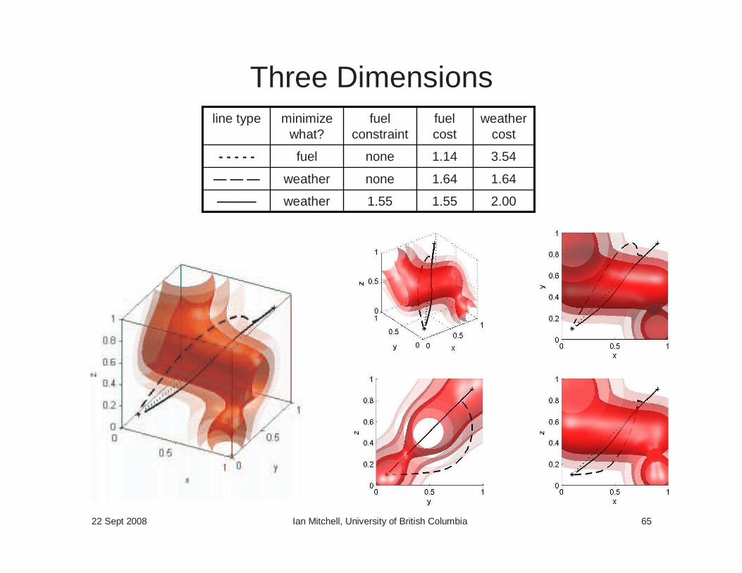
Three Dimensionsweather
costfuel cost
fuel constraint
minimize what?
line type
2.001.551.55weather———
1.641.64noneweather— — —
3.541.14nonefuel- - - - -
22 Sept 2008 Ian Mitchell, University of British Columbia 66
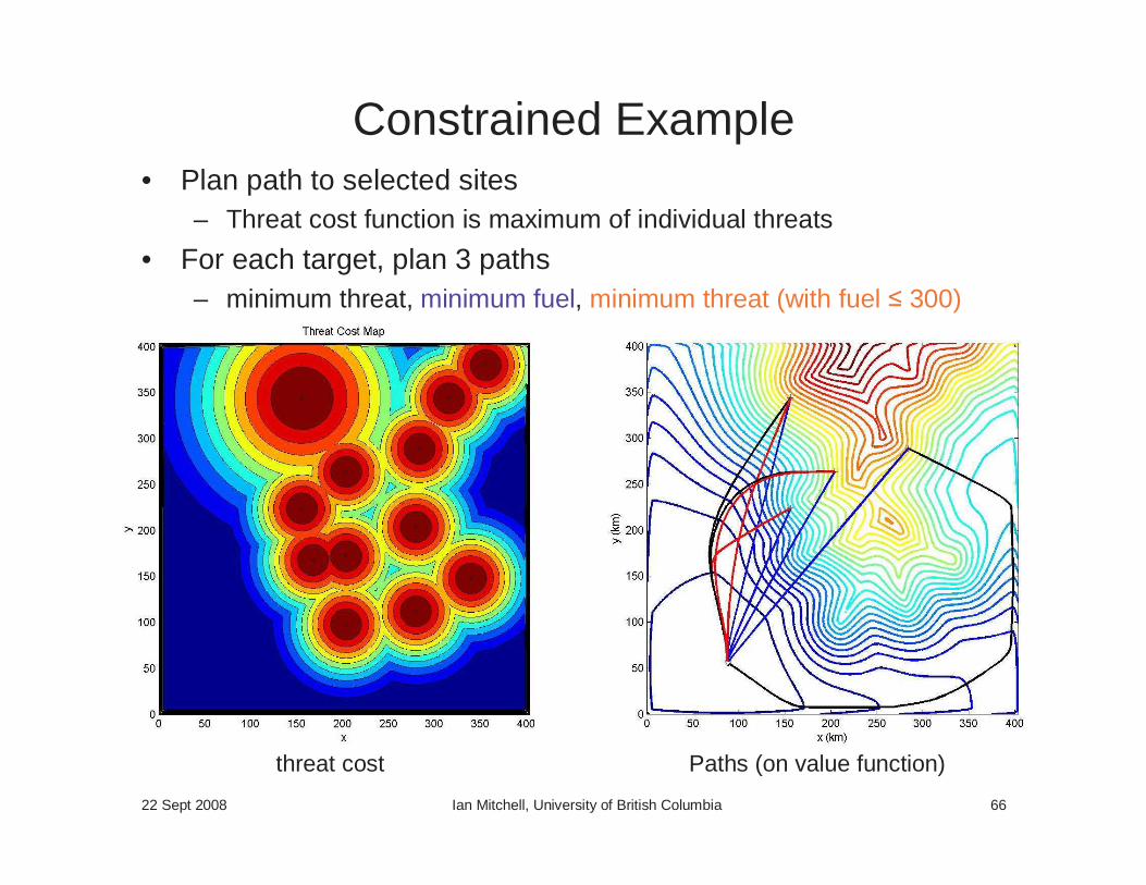
Constrained Example• Plan path to selected sites
– Threat cost function is maximum of individual threats
• For each target, plan 3 paths– minimum threat, minimum fuel, minimum threat (with fuel 300)
threat cost Paths (on value function)
22 Sept 2008 Ian Mitchell, University of British Columbia 67
Future Work• Fast Sweeping and Marching code
– Python & C++– Interfaced to time-dependent HJ Toolbox and Matlab
• Robotic applications– Mesh refinement strategies
– Integration with localization algorithms
– Practical implementation
• Higher dimensions?– Taking advantage of special structure
– Integration with suboptimal but scalable techniques
22 Sept 2008 Ian Mitchell, University of British Columbia 68
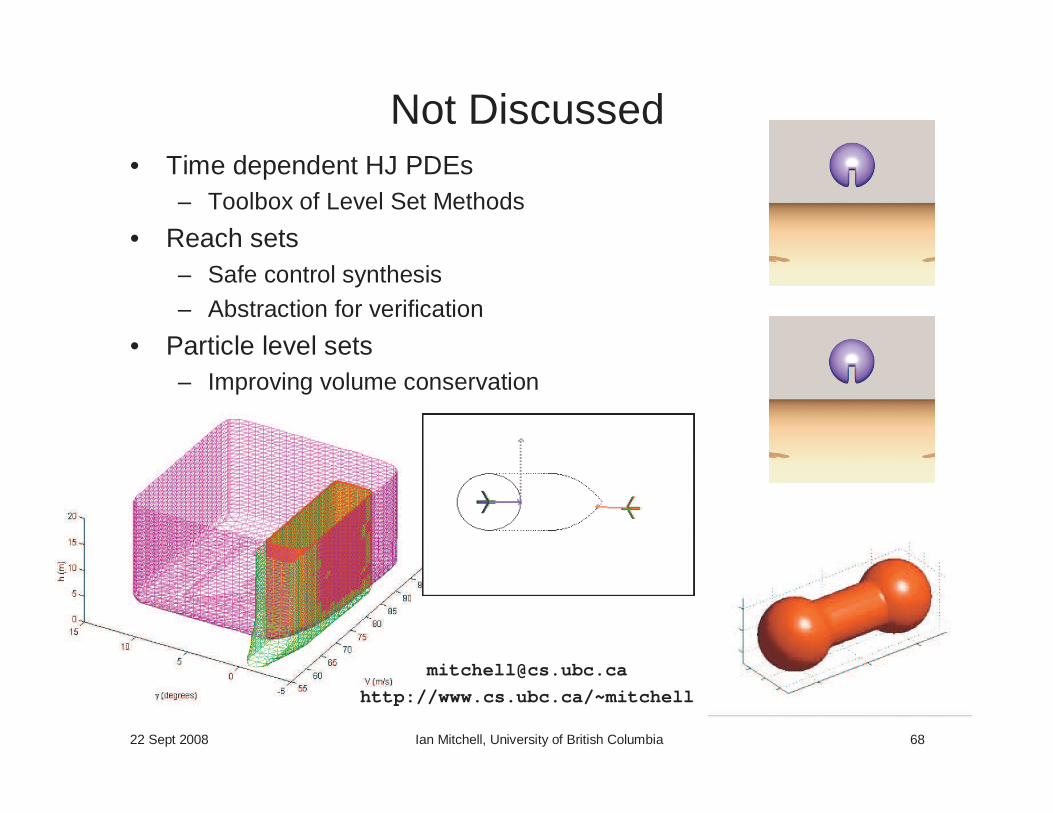
Not Discussed• Time dependent HJ PDEs
– Toolbox of Level Set Methods
• Reach sets– Safe control synthesis – Abstraction for verification
• Particle level sets– Improving volume conservation
http://www.cs.ubc.ca/~mitchell
22 Sept 2008 Ian Mitchell, University of British Columbia 69
DP & HJ PDE References• Dynamic programming
– Dynamic Programming & Optimal Control, Bertsekas (3rd ed, 2007)
• HJ PDEs and viscosity solutions– Crandall & Lions (1983) original publication– Crandall, Evans & Lions (1984) current formulation– Evans & Souganidis (1984) for differential games
– Crandall, Ishii & Lions (1992) “User’s guide” (dense reading)– Viscosity Solutions & Applications in Springer’s Lecture Notes in
Mathematics (1995), featuring Bardi, Crandall, Evans, Soner & Souganidis (Capuzzo-Dolcetta & Lions eds)
– Optimal Control & Viscosity Solutions of Hamilton-Jacobi-Bellman Equations, Bardi & Capuzzo-Dolcetta (1997)
– Partial Differential Equations, Evans (1998)
22 Sept 2008 Ian Mitchell, University of British Columbia 70
Static HJ PDE Algorithm References• Time-dependent transforms
– Osher (1993)
– Mitchell (2007): ToolboxLS documentation
• Fast Marching– Tsitsiklis (1994, 1995): first known description, semi-Lagrangian– Sethian (1996): first finite difference scheme
– Kimmel & Sethian (1998): unstructured meshes– Kimmel & Sethian (2001): path planning– Sethian & Vladimirsky (2000): anisotropic FMM (restricted)
– Sethian & Vladimirsky (2001, 2003): ordered upwind methods
• Fast Sweeping– Boue & Dupuis (1999): sweeping for MDP approximations– Zhao (2004), Tsai et. al (2003), Kao et. al. (2005), Qian et. al.
(2007): sweeping with finite differences for static HJ PDEs
22 Sept 2008 Ian Mitchell, University of British Columbia 71
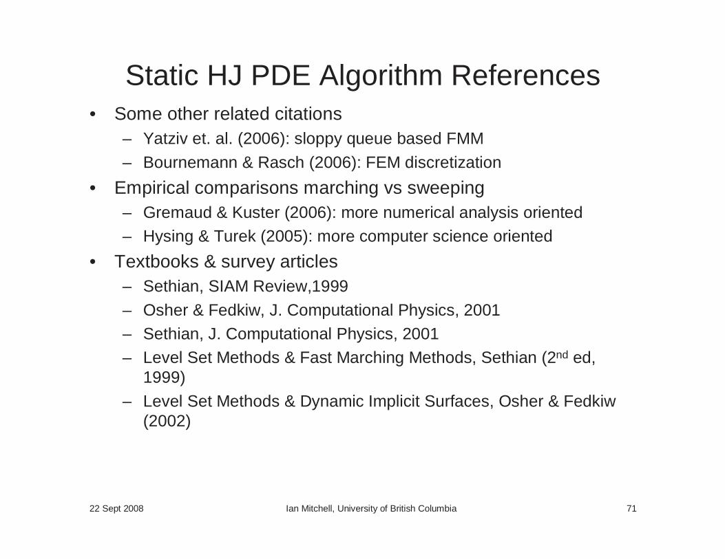
Static HJ PDE Algorithm References• Some other related citations
– Yatziv et. al. (2006): sloppy queue based FMM
– Bournemann & Rasch (2006): FEM discretization
• Empirical comparisons marching vs sweeping– Gremaud & Kuster (2006): more numerical analysis oriented– Hysing & Turek (2005): more computer science oriented
• Textbooks & survey articles– Sethian, SIAM Review,1999
– Osher & Fedkiw, J. Computational Physics, 2001– Sethian, J. Computational Physics, 2001– Level Set Methods & Fast Marching Methods, Sethian (2nd ed,
1999)
– Level Set Methods & Dynamic Implicit Surfaces, Osher & Fedkiw(2002)
For more information contact
Ian MitchellDepartment of Computer ScienceThe University of British Columbia
http://www.cs.ubc.ca/~mitchell
Dynamic Programming Algorithms for Planning and Robotics
in Continuous Domainsand the Hamilton-Jacobi Equation


![Dynamic Programming - Princeton University Computer Science · 3 Dynamic Programming History Bellman. [1950s] Pioneered the systematic study of dynamic programming. Etymology. Dynamic](https://img.pdfslide.net/doc/110x75/6046dbfc71b5767bc03138ec/dynamic-programming-princeton-university-computer-3-dynamic-programming-history.jpg)