International Journal of InnovativeComputing, Information and Control ICIC International c⃝2012 ISSN 1349-4198Volume 8, Number 3(B), March 2012 pp. 2347–2358

DYNAMIC SENSOR BIAS CORRECTION FOR ATTITUDEESTIMATION USING UNSCENTED KALMAN FILTER

IN AUTONOMOUS VEHICLE

Mikio Bando, Yukihiro Kawamata and Toshiyuki Aoki

Department of Smart Systems ResearchHitachi Research Laboratory, Hitachi Ltd.

1-1, Omika-cho, Hitachi-shi, Ibaraki-ken, Japanmikio.bando.bt@hitachi.com

Received March 2011; revised September 2011

Abstract. This paper describes a method for estimating sensor biases by using a low-dimensional Unscented Kalman Filter (UKF) to maintain the positional estimation ac-curacy of an autonomous vehicle (AV). It is difficult to estimate attitude accurately ina blind situation (such as with no GPS satellites and no landmarks), because of sensorbias. We developed a dead reckoning system for an embedded system using the UKF.The UKF has high computational effort, so, we decreased the number of dimensions inthe UKF by excluding sensor biases term. On the presumption that AV drives steadily,we derived equations for the relationship between the averages of angular accelerationand gyro bias, and corrected the sensor output. Instead of using high-dimensional UKF,we corrected sensor biases by using these equations. This method quickly and accuratelyestimated attitude.Keywords: Sensor bias estimation, Unscented Kalman filter, Localization

1. Introduction. The development of autonomous vehicles (AVs) has made great progr-ess recently. For example, the Defense Advanced Research Projects Agency (DARPA) inthe U.S.A organized Grand Challenge [1] and Urban Challenge [2], which are long distanceraces in which autonomously controlled vehicles participate. Some companies are expectedto put these technologies into practical use in the transport or factory.

AVs are classified broadly into two categories. One is a guided AV which follows apre-established route, and the other is a self-directed AV which does not. Almost allself-directed AVs have an environmental recognition function for noticing pedestrians orobstacles near the vehicle, a control planning function for avoiding these pedestrians andobstacles, and other functions [3]. To use these functions, the AV always estimates itsposition. This is because localization function is one of the most important functions torealize autonomous running.

However, developing features that can recognize the environment or calculate localiza-tion for AVs is expensive. Practically applying the autonomous technology will be animportant factor in reducing these costs. There are some studies on localization usinglow-cost sensors [4,5], but we know of no studies on accurate localization at low calculationcost.

We are going to devise localization logic of low calculation cost with the goal of installingthe localization logic in embedded equipment such as the in-vehicle controller.

This paper describes results of a low calculation cost method for maintaining localiza-tion accuracy for practical application of the autonomous technology.

2347

2348 M. BANDO, Y. KAWAMATA AND T. AOKI

2. Localization Model.

2.1. Dead reckoning model. To estimate vehicle position, this study used dead reck-oning model as shown in Figure 1.

SensorFusion(PositionCorrection)DeadReckoningGPS・Landmarks(LM)VelocityAttitude

Localization

Distancetraveled(Velocity)DirectionPosition calculatedon basis ofdistance traveledand direction.This method gatherserrors by gradation.

Dead ReckoningSensor Fusion

GPSpositioningGPSerror ellipse

Estimatedposition( after fusion )Estimatedposition( before fusion )Estimatedpositioningerrorellipse

Figure 1. Dead reckoning model

The dead reckoning method estimates the vehicle’s position on the basis of distancetraveled (velocity) and the direction. The dead reckoning model influences the non-holonomic constraint of 4-wheel vehicle; thus the vehicle cannot move sideways.Let the position of a vehicle be (x(t), y(t), z(t)) at the step t and let its velocity and

angular velocity be v(t) and ω(t), respectively. Then, during the time increment δt second,the variation of the vehicle position, (δx(t), δy(t), δz(t)), is given by

δx(t) = v(t) cos θy(t) cos θp(t)δt (1)

δy(t) = v(t) sin θy(t) cos θp(t)δt (2)

δz(t) = v(t) sin θp(t)δt (3)

where θy(t), θp(t) are the yaw and pitch angles at step t. Thus, the vehicle position(x(t+ 1), y(t+ 1), z(t+ 1)) at the next step t+ 1 is estimated in the following manner:x(t+ 1)

y(t+ 1)z(t+ 1)

=

x(t) + δx(t)y(t) + δy(t)z(t) + δz(t)

(4)

In this way, we can calculate vehicle position if we know the vehicle velocity and atti-tude.

2.2. Attitude calculation model. The dead reckoning model needs vehicle velocityand attitude. The velocity can often be observed directly with measurement devices.However, in a lot of cases, all parts of the vehicle attitude (yaw, roll, pitch ) cannot alwaysbe observed directly. Therefore, we calculate the vehicle attitude using the followingmethod.

ϕ(t) =

√ωr(t)

2 + ωp(t)2 + ωy(t)

2 (5)

λ(t) =

λ1(t)λ2(t)λ3(t)

=

ωr(t)ϕ(t)ωp(t)

ϕ(t)ωy(t)

ϕ(t)

(6)

DYNAMIC SENSOR BIAS CORRECTION FOR ATTITUDE ESTIMATION 2349

∆CEV (t) = I cosϕ(t) + λ(t) sinϕ(t)

+ λ(t)λ(t)T (1− cosϕ(t)) (7)

λ(t) =

0 −λ3(t) λ2(t)λ3(t) 0 −λ1(t)−λ2(t) λ1(t) 0

CEV (t) = ∆CEV (t)CEV (t− 1) (8)

θ(t) =

θy(t)θr(t)θp(t)

= CEV (t)θ(0) (9)

where t is an observing step, θy(t), θr(t), θp(t) is the attitude, θ(0) is initial attitude vector,ωy(t), ωr(t), ωp(t) is the anglar velocity (yaw, roll, pitch), CEV is a rotation matrix fromthe topocentric tangent plane coordinate system to vehicle coordinate system, and ∆CEV

is a tiny rotation matrix.

3. Attitude Calculation Modeling Using UKF.

3.1. Attitude calculation without gyro sensor. When the vehicle attitude is cal-culated in an actual situation, dead reckoning positioning accumulates errors because ofgyro sensor errors. Therefore, we consider how to eliminate the positioning errors usinganother sensor, for example, accelerometer and GPS.

When accelerometer is used, pitch angle and roll angle are calculated using the followingmethod expressing gravity term:

G(t) = α(t) +CTEV (t)g + ϵG(t), (10)

where G is output value of accelerometer, α is acceleration of the vehicle, and g isacceleration of gravity.

A yaw angle can be directly observed by the GPS direction term. Thus we can ob-serve all components of vehicle attitude (yaw, roll, pitch), and occasionally eliminate theaccumulating attitude errors.

3.2. Unscented Kalman filtering (UKF) modeling. The vehicle attitude is calcu-lated by the UKF which has robust nonlinear output of sensors, because gyro sensor andaccelerometer are predicted to output strongly nonlinear responses in outdoor areas whereAVs are driving around.

The UKF algorithm uses arbitrary nonlinear function. The extended Kalman filter usesJacobian matrix, while the UKF does the “sigma points”. The UKF algorithm will bestated below [6].

The state vector x(t) and observed vector y(t) at time t are defined by

x(t) = [θ(t),ω(t),α(t), ω(t), α(t), bω, bα] (11)

y(t) = [Θ(t),Ω(t),V (t),G(t)] (12)

where θ is the attitude vector, ω is the angular velocity vector, bω is the bias term vectorof gyro sensor, bα is the bias term vector of accelerometer. ω(t), α(t) are able to calculatefrom thire time constant [7,8]. Θ is the attitude calculating from Equation (10) and GPSdirection, and Ω is the output value vector of gyro sensor.

2350 M. BANDO, Y. KAWAMATA AND T. AOKI

Given the state vector at the step t− 1, we calculate the prediction of sigma points asfollows:

χ0(t|t− 1) = f(x(t− 1|t− 1), t− 1)

χ(t|t− 1) =[χ0(t|t− 1), Q(t|t− 1), R(t|t− 1)

]yi = h(χi(t|t− 1), t− 1) , i = 0, 1, . . . , 2n

t = t0 + 1, t0 + 2, . . .

where

Q(t|t− 1) = [q1(t|t− 1), q2(t|t− 1), . . . , qi(t|t− 1)]

R(t|t− 1) = [r1(t|t− 1), r2(t|t− 1), . . . , ri(t|t− 1)]

qi(t|t− 1) = χ0(t|t− 1) + γ(√

GWGTi

)ri(t|t− 1) = χ0(t|t− 1)− γ

(√GWGT

i

)G = G(x(t− 1|t− 1), t− 1)

W = W (t− 1)

i = 1, 2, . . . , 2n

x(t|t) = x(t|t− 1) +K(t)e(t) (13)

e(t) = y(t)− y(t|t− 1) (14)

K(t) = L(t|t− 1)H−1(t|t− 1) (15)

x(t|t− 1) =2n∑i=0

wiχi(t|t− 1) (16)

y(t|t− 1) =2n∑i=0

wiyi(t|t− 1) (17)

G = G(x(t− 1|t− 1), t− 1)

W = W (t− 1)

M(t|t− 1) =2n∑i=0

wi[χi(t|t− 1)− x(t|t− 1)]

[χi(t|t− 1)− x(t|t− 1)]T +GWGT (18)

L(t|t− 1) =2n∑i=0

wi[χi(t|t− 1)− x(t|t− 1)]

[yi(t|t− 1)− y(t|t− 1)]T (19)

H(t|t− 1) =2n∑i=0

wi[yi(t|t− 1)− y(t|t− 1)]

[yi(t|t− 1)− y(t|t− 1)]T + V (t) (20)

t = t0 + 1, t0 + 2, . . .

x(t0|t0) = E[x(t0)] (21)

The UKF has a higher computation load than the extended Kalman filtering, insteadof a higher nonlinear tracking capability [6].

DYNAMIC SENSOR BIAS CORRECTION FOR ATTITUDE ESTIMATION 2351

The UKF has O(N3) computational effort in the number of states N [6,7]. CPU powerof our embedded system assumes 500MHz, and attitude estimation function can use lessthan 0.01% of the CPU power. In the case of our situation N = 21, the computational ef-fort is too great for using in the embedded system. Figure 2 shows calculation componentsof the positioning system.

UKF< State variable: 21 >Gyro sensor

EstimatedvalueAccelerometerSpeedometerGPS Computational effort order: 213--

Figure 2. Calculation components of positioning system

Thus, we propose a method to decentralize calculation of state variables to lessen thecomputational effort like a bank of Kalman filters [11]. The state variables (11) areclassified into two groups: one largely alters in value from moment to moment, whilethe other slightly alters. The latter is sensor bias terms (6 variables), so they can becalculated by linear theories that need only low computational effort. Figure 3 shows ourproposed component architecture.

UKF< State variable: 15>

Gyro sensorEstimatedvalue

AccelerometerSpeedometerGPS Computational effort order: 153

Sensor bias estimation< State variable: 6 >Computational effort order: 63--

Figure 3. Decentralized positioning system

The proposed component architecture, which has a calculation number of times 153

order, decreases computational effort around 65 % compared with centralized architecture,which has a calculation number of times 213, like in Figure 2.

Thus, we have to design the UKF without sensor bias term, but there are no studies ondecentralized sensor bias architecture. Many studies set up bias equations as a componentof the Kalman filtering [9-12]. Therefore, we developed the expression for the relationshipbetween the gyro bias and the other estimated variables of the UKF.

2352 M. BANDO, Y. KAWAMATA AND T. AOKI

4. Bias Estimating Principle.

4.1. Theory of bias estimation. The gyro sensor bias is calculated by angular accel-eration. We developed the following expressions for the relationship between the gyrosensor bias and the angular acceleration:

ωg(t) = ω(t) + bω(t) + ϵ(t) (22)

ωg(t)− ω(t− 1) = ω(t)− ω(t− 1) + bω(t) + ϵ(t) (23)

= δω(t− 1) + bω(t) + ϵ(t) (24)

where t is step, ωg is observed angular velocity of gyro sensor, ω is estimated angularvelocity, δω is variation of the angular velocity, bω is bias of gyro sensor, and ϵ is noise.Also δω, bω and ϵ are all independent.Taking the average of both sides of (24), we have

E[ωg(t)− ω(t− 1)] = E[δω(t) + bω(t) + ϵ(t)]

= E[δω(t)] + E[bω(t)] + E[ϵ(t)] (25)

E[δω(t)] =1

nδt

t−1∑i=0

δω(i)

=(ω(1)− ω(0)) + (ω(2)− ω(1)) + . . .+ (ω(t)− ω(t− 1))

nδt

=ω(t)− ω(0)

nδt(26)

When the average noise is assumed to be 0, and the steadily moving vehicle in finitetime (ω(t) = ω(0)) observes the average angular acceleration to be 0, Equation (25)changes as shown below.

E[ωg(t)− ω(t− 1)] = E[bω] (27)

bω(t) = nE[bω(t)]−n−1∑i=0

bω(i)

= nE[ωg(t)− ω(t− 1)]−n−1∑i=0

bω(i) (28)

We can calculate the gyro bias from Equation (28), and these equations require lesscomputational effort than estimating all state variables at once.

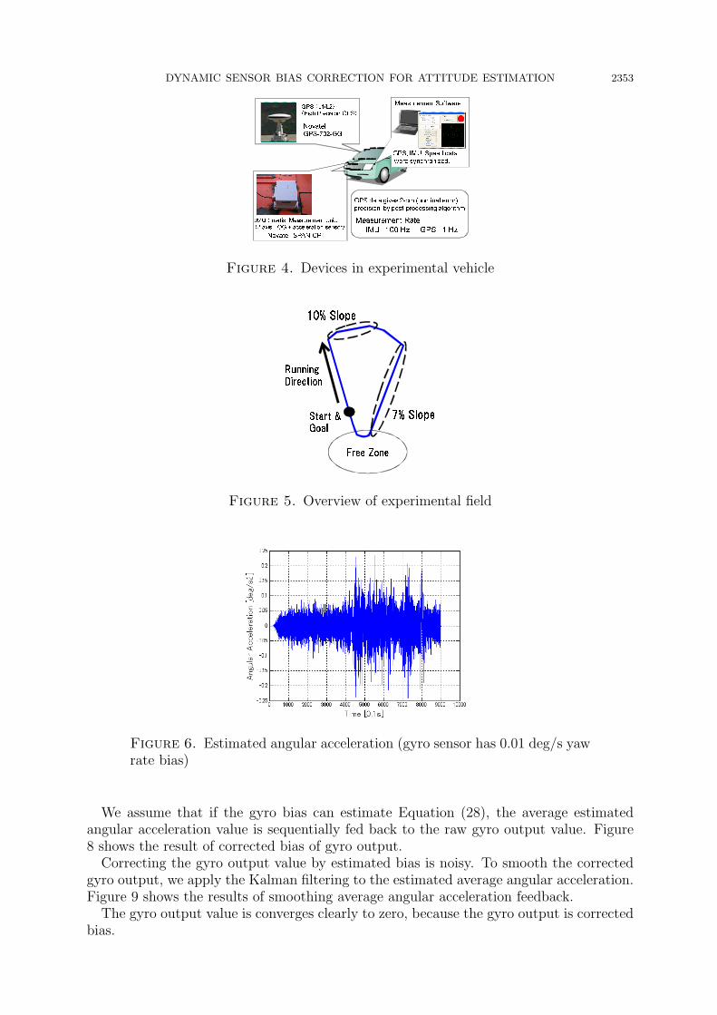
4.2. Result of bias estimating simulations. To examine the above decentralizingmethod, we simulated bias estimating capability. We collected sensor data from a movingdump truck used as an experimental vehicle to verify our methods. The vehicle had thefollowing devices: GPS, gyro, and acceleration and speed sensors (see Figure 4).The GPS was used to obtain a reference position. The vehicle traveled on a sand

experimental field, in a circle course of around 2 km for 6 minutes. An overview of theexperimental field is shown in Figure 5.We gathered simulation data, which were added arbitrary bias to yaw angular velocity

of gyro sensor output. Using these data, estimating state variables by the UKF simulationindicated the following results.Figure 6 shows the estimated angular acceleration (yaw). It is difficult to distinguish

between the sensor bias and the angular acceleration. However, the average angularacceleration converges on the gyro bias value (see Figure 7).

DYNAMIC SENSOR BIAS CORRECTION FOR ATTITUDE ESTIMATION 2353

ＧＰＳ （L1/L2）（High Precision GPS）

ＩＭＵ （Inertial Measurement Unit）（3 axis FOG + acceleration sensor）

NovatelGPS-702-GG

Novatel SPAN-CPT

Measurement Software

Measurement RateIMU： 100 Hｚ， GPS： 1 HzGPS data gives 2-cm (nominal error)precision by post-processing algorithm

GPS, IMU, Speed data were synchronized.

Figure 4. Devices in experimental vehicle

7% Slope

10% SlopeRunningDirection

Start &Goal Free ZoneFigure 5. Overview of experimental field

Figure 6. Estimated angular acceleration (gyro sensor has 0.01 deg/s yawrate bias)

We assume that if the gyro bias can estimate Equation (28), the average estimatedangular acceleration value is sequentially fed back to the raw gyro output value. Figure8 shows the result of corrected bias of gyro output.

Correcting the gyro output value by estimated bias is noisy. To smooth the correctedgyro output, we apply the Kalman filtering to the estimated average angular acceleration.Figure 9 shows the results of smoothing average angular acceleration feedback.

The gyro output value is converges clearly to zero, because the gyro output is correctedbias.

2354 M. BANDO, Y. KAWAMATA AND T. AOKI

Figure 7. Average estimated angular acceleration (gyro sensor has 0.01deg/s yaw rate bias)

Inputted BiasCorrected Bias by Estimated BiasFigure 8. Corrected bias of gyro sensor under fed back average of esti-mated angular acceleration (gyro sensor has 0.01 deg/s yaw rate bias)

Inputted BiasCorrected Bias by Estimated BiasFigure 9. Estimated bias of gyro sensor under fed back Kalman filteringestimated angular acceleration (gyro sensor has 0.01 deg/s yaw rate bias)

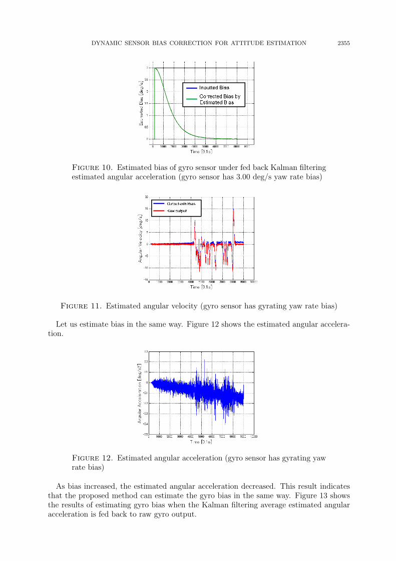
Also, we simulated a low-cost gyro sensor that had 3 deg/s bias. Figure 10 shows thecorrected gyro sensor output under 3 deg/s bias. These results indicate that our biasestimation method can correspond to not only small but also large bias.Next, we checked our method for time varying bias adaptivity. We simulated the same

way but added bias was increased 10−3 per second. Figure 11 compares raw gyro sensoroutput and output of adding bias.

DYNAMIC SENSOR BIAS CORRECTION FOR ATTITUDE ESTIMATION 2355

Inputted BiasCorrected Bias by Estimated Bias

Figure 10. Estimated bias of gyro sensor under fed back Kalman filteringestimated angular acceleration (gyro sensor has 3.00 deg/s yaw rate bias)

Output with BiasRaw output

Figure 11. Estimated angular velocity (gyro sensor has gyrating yaw rate bias)

Let us estimate bias in the same way. Figure 12 shows the estimated angular accelera-tion.

Figure 12. Estimated angular acceleration (gyro sensor has gyrating yawrate bias)

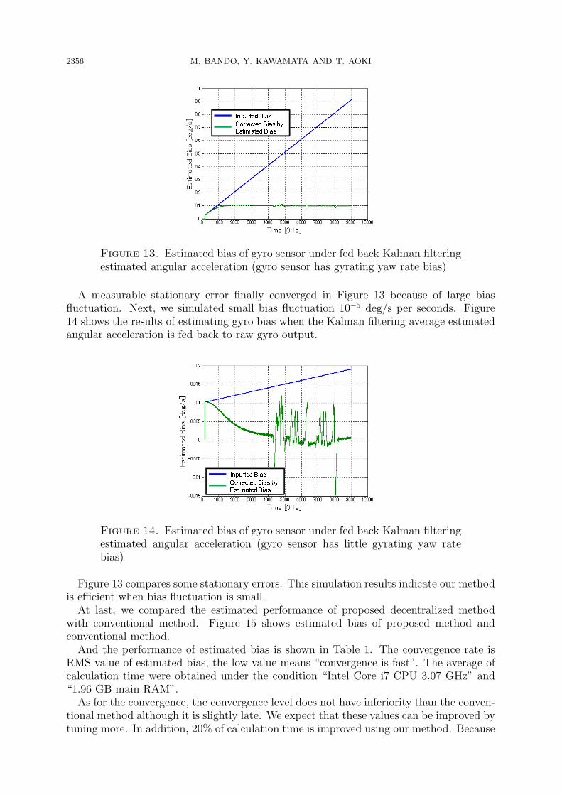
As bias increased, the estimated angular acceleration decreased. This result indicatesthat the proposed method can estimate the gyro bias in the same way. Figure 13 showsthe results of estimating gyro bias when the Kalman filtering average estimated angularacceleration is fed back to raw gyro output.

2356 M. BANDO, Y. KAWAMATA AND T. AOKI

Inputted BiasCorrected Bias by Estimated Bias

Figure 13. Estimated bias of gyro sensor under fed back Kalman filteringestimated angular acceleration (gyro sensor has gyrating yaw rate bias)

A measurable stationary error finally converged in Figure 13 because of large biasfluctuation. Next, we simulated small bias fluctuation 10−5 deg/s per seconds. Figure14 shows the results of estimating gyro bias when the Kalman filtering average estimatedangular acceleration is fed back to raw gyro output.

Inputted BiasCorrected Bias by Estimated BiasFigure 14. Estimated bias of gyro sensor under fed back Kalman filteringestimated angular acceleration (gyro sensor has little gyrating yaw ratebias)

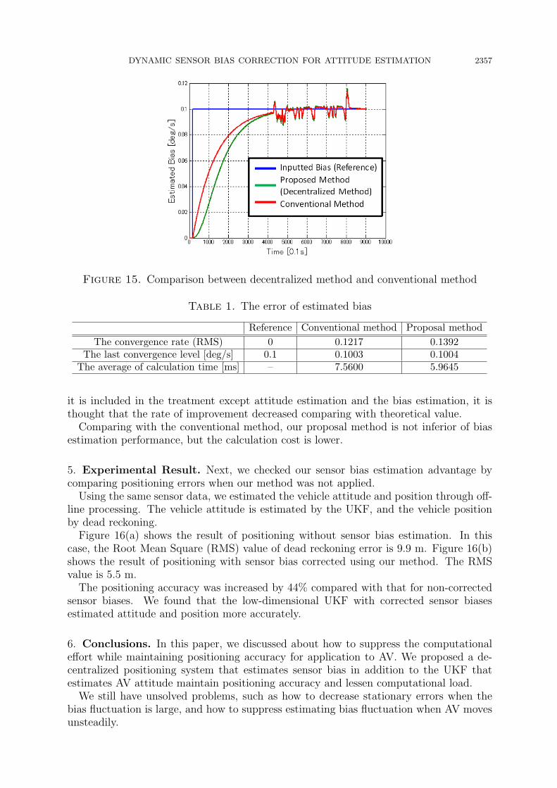
Figure 13 compares some stationary errors. This simulation results indicate our methodis efficient when bias fluctuation is small.At last, we compared the estimated performance of proposed decentralized method

with conventional method. Figure 15 shows estimated bias of proposed method andconventional method.And the performance of estimated bias is shown in Table 1. The convergence rate is

RMS value of estimated bias, the low value means “convergence is fast”. The average ofcalculation time were obtained under the condition “Intel Core i7 CPU 3.07 GHz” and“1.96 GB main RAM”.As for the convergence, the convergence level does not have inferiority than the conven-

tional method although it is slightly late. We expect that these values can be improved bytuning more. In addition, 20% of calculation time is improved using our method. Because

DYNAMIC SENSOR BIAS CORRECTION FOR ATTITUDE ESTIMATION 2357

Figure 15. Comparison between decentralized method and conventional method

Table 1. The error of estimated bias

Reference Conventional method Proposal method

The convergence rate (RMS) 0 0.1217 0.1392The last convergence level [deg/s] 0.1 0.1003 0.1004

The average of calculation time [ms] – 7.5600 5.9645

it is included in the treatment except attitude estimation and the bias estimation, it isthought that the rate of improvement decreased comparing with theoretical value.

Comparing with the conventional method, our proposal method is not inferior of biasestimation performance, but the calculation cost is lower.

5. Experimental Result. Next, we checked our sensor bias estimation advantage bycomparing positioning errors when our method was not applied.

Using the same sensor data, we estimated the vehicle attitude and position through off-line processing. The vehicle attitude is estimated by the UKF, and the vehicle positionby dead reckoning.

Figure 16(a) shows the result of positioning without sensor bias estimation. In thiscase, the Root Mean Square (RMS) value of dead reckoning error is 9.9 m. Figure 16(b)shows the result of positioning with sensor bias corrected using our method. The RMSvalue is 5.5 m.

The positioning accuracy was increased by 44% compared with that for non-correctedsensor biases. We found that the low-dimensional UKF with corrected sensor biasesestimated attitude and position more accurately.

6. Conclusions. In this paper, we discussed about how to suppress the computationaleffort while maintaining positioning accuracy for application to AV. We proposed a de-centralized positioning system that estimates sensor bias in addition to the UKF thatestimates AV attitude maintain positioning accuracy and lessen computational load.

We still have unsolved problems, such as how to decrease stationary errors when thebias fluctuation is large, and how to suppress estimating bias fluctuation when AV movesunsteadily.

2358 M. BANDO, Y. KAWAMATA AND T. AOKI

EstimatedpositionRTK-GPS EstimatedpositionRTK-GPS

(a) Positioning without bias correction (b) Positioning with bias correction

Figure 16. Positioning result

Acknowledgment. The authors also gratefully acknowledge the helpful comments andsuggestions of the reviewers, which have improved the presentation.

REFERENCES

[1] http://www.darpa.mil/grandchallenge05/index.html.[2] http://www.darpa.mil/grandchallenge/index.asp.[3] M. Tanaka, Reformation of particle filters in simultaneous localization and mapping problems, Inter-

national Journal of Innovative Computing, Information and Control, vol.5, no.1, pp.119-128, 2009.[4] H. Rehbinder and X. Hu, Drift-free attitude estimation for accelerated rigid bodies, Automatica,

vol.40, pp.653-659, 2004.[5] A. E. Hadri and A. Benallegue, Sliding mode observer to estimate both the attitude and the gyro-

bias by using low-cost sensors, Proc. of the 2009 IEEE/RSJ International Conference on IntelligentRobots and Systems, pp.2867-2872, 2009.

[6] J. J. LaViola Jr., A comparison of unscented and extended Kalman filtering for estimating quaternionmotion, Proc. of 2003 American Control Conference, 2003.

[7] T. Aoki, Y. Shimagaki, T. Ikki, M. Tanikawara, S. Sugimoto, Y. Kubo and K. Fujimoto, Cycle slipdetection in kinematic GPS with a jerk model for land vehicles, International Journal of InnovativeComputing, Information and Control, vol.5, no.1, pp.153-166, 2009.

[8] T. Aoki and S. Sugimoto, Dynamical models for automobile movements, International Journal ofInnovative Computing, Information and Control, vol.6, no.1, pp.3-14, 2010.

[9] S. A. Holmes, G. Klein and D. W. Murray, An O(N2) square root unscented Kalman filter for visualsimultaneous localization and mapping, IEEE Trans. on Pattern Analysis and Machine Intelligence,vol.31, no.7, 2009.

[10] M. S. Pierre and D. Gingras, Comparison between the unscented Kalman filter and the extendedKalman filter for the position estimation module of an integrated navigation information system,Proc. of IEEE Intelligent Vehicles Symposium, 2004.

[11] W. Xue, Y.-Q. Guo and X.-D. Zhang, Application of a bank of Kalman filters and a robust Kalmanfilter for aircraft engine sensor/actuator fault diagnosis, International Journal of Innovative Com-puting, Information and Control, vol.4, no.12, pp.3161-3168, 2008.

[12] N. Metni, J. M. Pfimlin and T. Hamel, Attitude and gyro bias estimation for a flying UAV, Proc. ofthe 2005 IEEE International Conference on Intelligent Robots and Systems, 2005.

[13] C. Fan and Z. You, Highly efficient sigma point filter for spacecraft attitude and rate estimation,Mathmatical Problems in Engineering, vol.2009, 2009.

[14] P. D. Burns and W. D. Blair, Sensor bias estimation from measurements of known trajectories, Proc.of the 37th Southeastern Symposium on System Theory, pp.373-377, 2005.

[15] X. Suo, L. Chen and A. Sheng, Asynchronous multi-sensor bias estimation with sensor locationuncertainty, Proc. of 2009 Chinese Control and Decision Conference, pp.4317-4322, 2009.