Embed Size (px)
Citation preview
1
Dynamic simulations of urban policies for sustainable food
securitization: Dynamics of Urban Development, Agriculture Sector
Growth, and Price Mechanisms
15 February 2015
Jose Ma. Luis P. Montesclaros
Associate Research Fellow, Centre for Non-Traditional Security Studies
S. Rajaratnam School of International Studies
Nanyang Technological University, Singapore
Abstract:
Global trends show decreasing global food security (measured by the ratio of food supply to demand) over the past years, but the future outcome is not something that can be defined based on statistical trends. Rather, there are non-linear dynamics that will eventually lead to a bouncing up back up of food production. This was uncovered by assessing how the current food insufficiency situation has developed, with the primary lenses of urban development, rural production, and price dynamics. Wages in agriculture have been consistently lower than those in industry and services sectors, leading to increasing migration to cities where the latter sectors are based. This migration has led to decreasing food production, as labor is required to till the agricultural land in rural areas. However, by this same mechanism, food scarcity increases, and the price of food eventually increases. Governments eventually find the need to give priority to ensuring food sufficiency for their constituents, as is the case in many developing countries wherein more funds are allocated for encouraging food production. This leads sequentially to an increase in wages in agriculture, migration back to agricultural jobs, and a bouncing back up of food production. However, the combination of 1) market failures shaping the allocation of resources, 2) investment delays from poor spread of knowledge of appropriate investments, and 3) delays in product delivery from producers to consumers, will prevent this bouncing back up from happening. The sooner these issues are addressed, the better the capability of the market’s price mechanism to mobilize actors. Policy recommendations showed three potential scenarios for the extent of time (in years) under which the urban food insecurity situation will be resolved. The fact that the problem remains to be a persistent one shows that the feedback loops for addressing it are not yet triggered; as such, the price mechanism is not yet functioning properly. The set of policy recommendations, derived from the causal analysis, may be applied to systemically improve the dynamics shaping the future of food security globally and by extension, in urban areas.
Word Counts
Text (excluding tables and figures): less than 5000 words
Figures: around 500 words
Appendix: Model Documentation for Reference Model: 1756 words
2
Content
I. Introduction
II. Problem Statement
III. State of Knowledge and Global Trends on Impending Food Insecurity
IV. Dynamic Analysis with Causal Loops: Development of Urban Areas
V. Urban-Rural Food (URF) Model Description: Why Don’t Rural Areas Produce More?
VI. URF Model Simulation Output
VII. Linking up Incentives: Actors and Incentives in Food Production
VIII. Theories of Industrial Growth and Consumer Demand
IX. Dynamic Analysis on Root Problem: Delays in Agricultural Sector Growth
X. Policy Recommendations and Policy Simulation
XI. Conclusion
XII. References
XIII. Appendix
XIV. Table of Figures
3
I. Introduction
In development planning parlance, the carrying capacity of an area is the maximum size of the population it can
maintain (“carry”) before negative impacts are felt. This phenomenon is evident not only for locations but also to
sectors and products: a point always occurs where further increases are not viable. In sociology, there is likewise
always a threshold, or a tipping point, beyond which societal changes occur. However, the process of transition is
never neutral: there are always gainers and losers.
Over the past decades of industrialization, massive changes have occurred. Cities, have been growing because they
have provided “urbanization economies”, or more efficient spatial arrangements which help firms reduce transport
costs for consumers, and transactions costs from matching labor demand and supply. On the population/demand side,
life spans have been increasing, triggering higher birth rates and population booms. Along with these, the value of
food has been shadowed by luxury items, given large extents of agricultural surplus during the “green revolution” that
started in the 1970s. Relatedly, on the production/supply side there, desires of higher wages have led to increasing
labor migration geographically towards urban areas and away from rural areas. Sectorally, workers and firms alike
have been moving to higher value-added sectors (namely, manufacturing and services) and away from agriculture.
City governments, with the desire of desire of creating more jobs and achieving economic growth, have expanded
their urban industrial/post-industrial areas, encroaching on rural agricultural areas. Last, capital for research and
development had been invested in non-agricultural sectors, at the expense of agriculture, especially in the 1980s and
1990s. Overall, the tagline has been (economic) “catch-up”.
However, a tipping point is being reached. The current rates of rapid industrialization and urbanization are impacting
on urban food sufficiency, leading to an outcome of a decline in food supply amid growing demand. Food sufficiency
(expressed as a ratio of supply to demand) is going down. Yet, economists also note that a requirement for cities to
continue to exist is sufficient food surplus from the countryside. A shrinking surplus would therefore defeat the
purpose of urbanization. One response to this is that demand, supply and price dynamics (“ the invisible hand”) ensure
that sufficient incentive is provided for the desired basket of goods (which includes sufficient food) to emerge. Food
prices, undoubtedly, will bounce back up to trigger back food investments. However, how will the urban dwellers
cope in this transition?
II. Problem Statement
Given the background, the problem that remains to be addressed is:
What explains the growing urban food insecurity in the context of urban development, and what policies can
be implemented to address it systemically?
4
III. State of Knowledge and Global Trends on Impending Food Insecurity
Global Food Scarcity
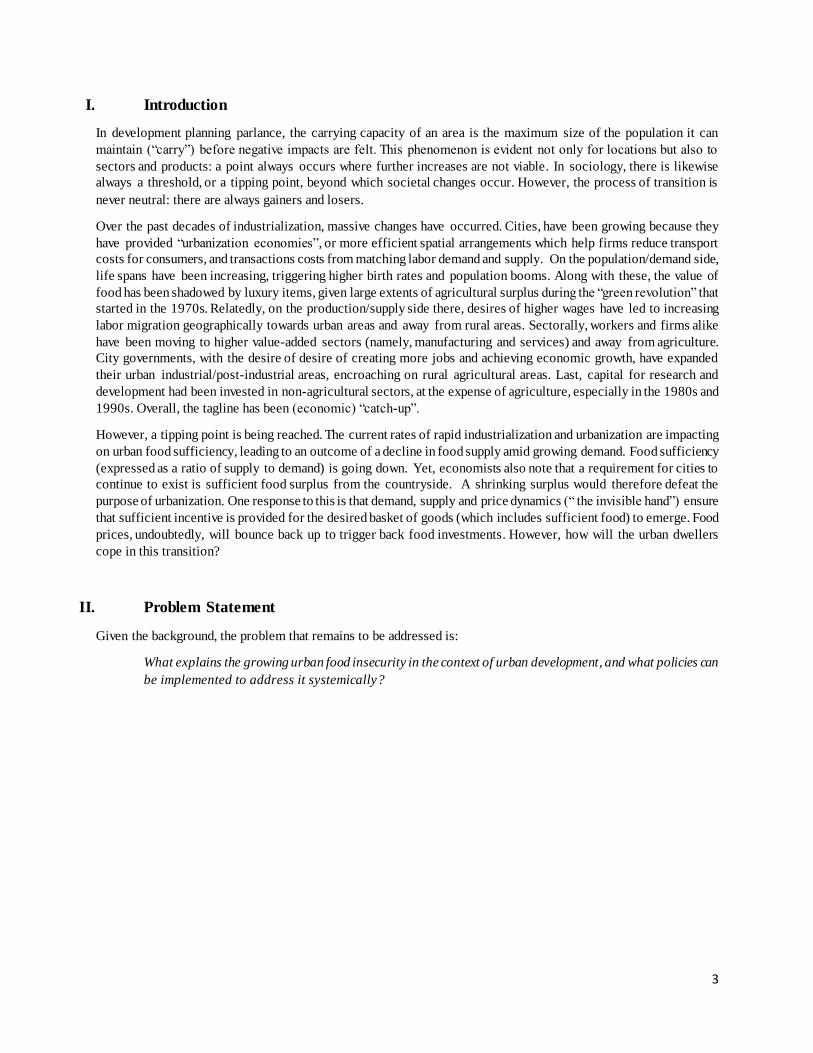
Globally, the problem of food scarcity is growing. The International Rice Research Institute (IRRI) has projected that,
given population growth trends, food demand is to increase by 26% from 430 metric tons (mt) in 2010 to 496 mt in
2020 and 555 mt in 2030. In order to meet this demand, food production should increase by 8 to 10 metric tons
annually, an increase of 1.2 to 1.5%.
Figure 1 Global Consumption Trends
Source: Copied from Rice Almanac, 4 th Edition (IRRI, 2013)
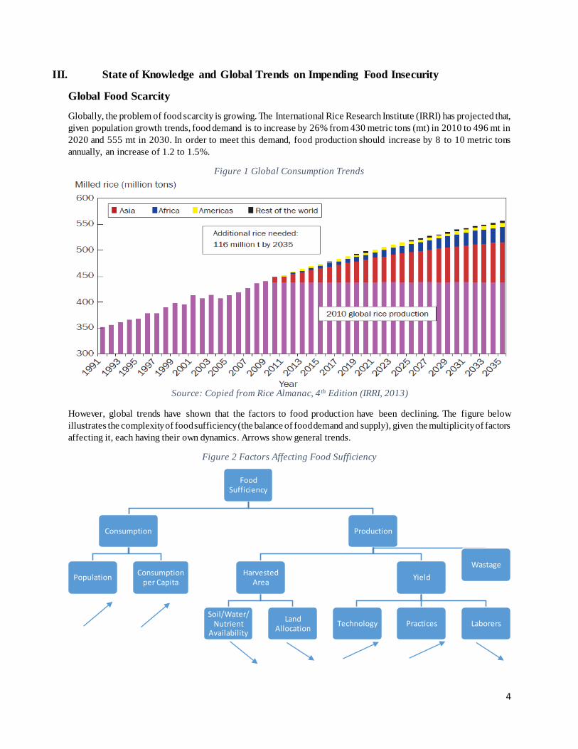
However, global trends have shown that the factors to food production have been declining. The figure below
illustrates the complexity of food sufficiency (the balance of food demand and supply), given the multiplicity of factors
affecting it, each having their own dynamics. Arrows show general trends.
Figure 2 Factors Affecting Food Sufficiency
Food Sufficiency
Consumption
PopulationConsumption
per Capita
Production
Harvested Area
Soil/Water/ Nutrient
Availability
Land Allocation
Yield
Technology Practices Laborers
Wastage
5
Land
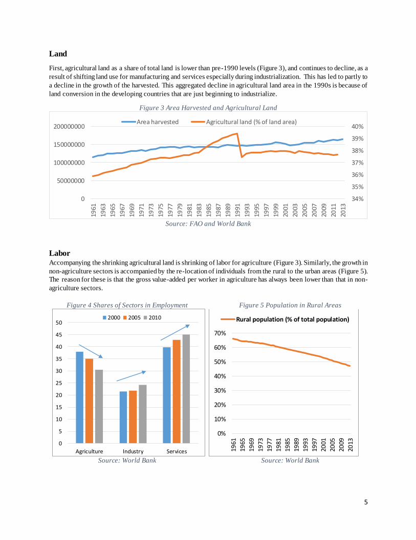
First, agricultural land as a share of total land is lower than pre-1990 levels (Figure 3), and continues to decline, as a
result of shifting land use for manufacturing and services especially during industrialization. This has led to partly to
a decline in the growth of the harvested. This aggregated decline in agricultural land area in the 1990s is because of
land conversion in the developing countries that are just beginning to industrialize.
Figure 3 Area Harvested and Agricultural Land
Source: FAO and World Bank
Labor Accompanying the shrinking agricultural land is shrinking of labor for agriculture (Figure 3). Similarly, the growth in
non-agriculture sectors is accompanied by the re-location of individuals from the rural to the urban areas (Figure 5).
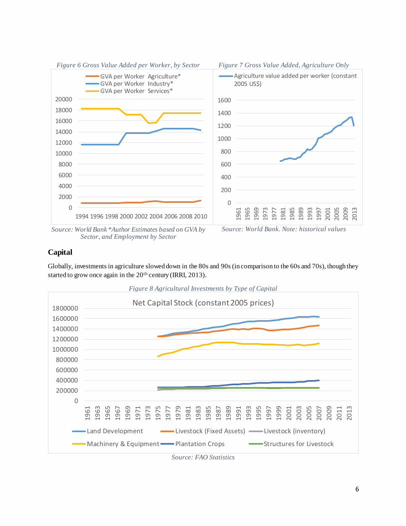
The reason for these is that the gross value-added per worker in agriculture has always been lower than that in non-
agriculture sectors.
Figure 4 Shares of Sectors in Employment Figure 5 Population in Rural Areas
Source: World Bank Source: World Bank
34%
35%
36%
37%
38%
39%
40%
0
50000000
100000000
150000000
200000000
1961
1963
1965
1967
1969
1971
1973
1975
1977
1979
1981
1983
1985
1987
1989
1991
1993
1995
1997
1999
2001
2003
2005
2007
2009
2011
2013
Area harvested Agricultural land (% of land area)
0
5
10
15
20
25
30
35
40
45
50
Agriculture Industry Services
2000 2005 2010
0%
10%
20%
30%
40%
50%
60%
70%
1961
1965
1969
1973
1977
1981
1985
1989
1993
1997
2001
2005
2009
2013
Rural population (% of total population)
6
Figure 6 Gross Value Added per Worker, by Sector Figure 7 Gross Value Added, Agriculture Only
Source: World Bank *Author Estimates based on GVA by
Sector, and Employment by Sector Source: World Bank. Note: historical values
Capital
Globally, investments in agriculture slowed down in the 80s and 90s (in comparison to the 60s and 70s), though they
started to grow once again in the 20 th century (IRRI, 2013).
Figure 8 Agricultural Investments by Type of Capital
Source: FAO Statistics
0
2000
4000
6000
8000
10000
12000
14000
16000
18000
20000
1994 1996 1998 2000 2002 2004 2006 2008 2010
GVA per Worker Agriculture*GVA per Worker Industry*GVA per Worker Services*
0
200
400
600
800
1000
1200
1400
1600
1961
1965
1969
1973
1977
1981
1985
1989
1993
1997
2001
2005
2009
2013
Agriculture value added per worker (constant2005 US$)
0
200000
400000
600000
800000
1000000
1200000
1400000
1600000
1800000
1961
1963
1965
1967
1969
1971
1973
1975
1977
1979
1981
1983
1985
1987
1989
1991
1993
1995
1997
1999
2001
2003
2005
2007
2009
2011
2013
Net Capital Stock (constant 2005 prices)
Land Development Livestock (Fixed Assets) Livestock (inventory)
Machinery & Equipment Plantation Crops Structures for Livestock
7
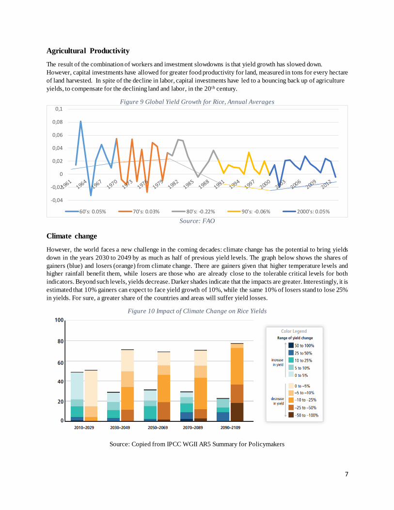
Agricultural Productivity
The result of the combination of workers and investment slowdowns is that yield growth has slowed down.
However, capital investments have allowed for greater food productivity for land, measured in tons for every hectare
of land harvested. In spite of the decline in labor, capital investments have led to a bouncing back up of agriculture
yields, to compensate for the declining land and labor, in the 20th century.
Figure 9 Global Yield Growth for Rice, Annual Averages
Source: FAO
Climate change
However, the world faces a new challenge in the coming decades: climate change has the potential to bring yields
down in the years 2030 to 2049 by as much as half of previous yield levels. The graph below shows the shares of
gainers (blue) and losers (orange) from climate change. There are gainers given that higher temperature levels and
higher rainfall benefit them, while losers are those who are already close to the tolerable critical levels for both
indicators. Beyond such levels, yields decrease. Darker shades indicate that the impacts are greater. Interestingly, it is
estimated that 10% gainers can expect to face yield growth of 10%, while the same 10% of losers stand to lose 25%
in yields. For sure, a greater share of the countries and areas will suffer yield losses.
Figure 10 Impact of Climate Change on Rice Yields
Source: Copied from IPCC WGII AR5 Summary for Policymakers
-0,04
-0,02
0
0,02
0,04
0,06
0,08
0,1
60's: 0.05% 70's: 0.03% 80's: -0.22% 90's: -0.06% 2000's: 0.05%
8
In sum, the current state seems to point to impending greater food scarcity and potential insufficiency in the future,
unless actions are taken to reverse the current trajectories.
IV. Dynamic Analysis with Causal Loops: Development of Urban Areas
The trends just shown seem to paint a bleak picture of food sufficiency globally. Stochastic modelling, which predicts
future values based on past values would paint such a picture. However, a dynamic approach would help to understand
the dynamics of what led to this problem in the first place, and the implications for the future.
Urban Development: Causal Loops
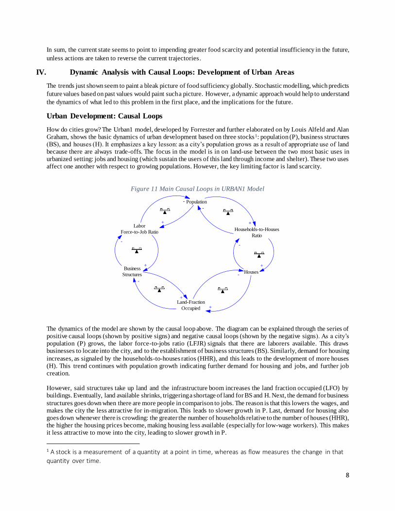
How do cities grow? The Urban1 model, developed by Forrester and further elaborated on by Louis Alfeld and Alan Graham, shows the basic dynamics of urban development based on three stocks1: population (P), business structures (BS), and houses (H). It emphasizes a key lesson: as a city’s population grows as a result of appropriate use of land because there are always trade-offs. The focus in the model is in on land-use between the two most basic uses in urbanized setting: jobs and housing (which sustain the users of this land through income and shelter). These two uses affect one another with respect to growing populations. However, the key limiting factor is land scarcity.
Figure 11 Main Causal Loops in URBAN1 Model
The dynamics of the model are shown by the causal loop above. The diagram can be explained through the series of positive causal loops (shown by positive signs) and negative causal loops (shown by the negative signs). As a city’s population (P) grows, the labor force-to-jobs ratio (LFJR) signals that there are laborers available. This draws businesses to locate into the city, and to the establishment of business structures (BS). Similarly, demand for housing
increases, as signaled by the households-to-houses ratios (HHR), and this leads to the development of more houses (H). This trend continues with population growth indicating further demand for housing and jobs, and further job creation. However, said structures take up land and the infrastructure boom increases the land fraction occupied (LFO) by buildings. Eventually, land available shrinks, triggering a shortage of land for BS and H. Next, the demand for business
structures goes down when there are more people in comparison to jobs. The reason is that this lowers the wages, and makes the city the less attractive for in-migration. This leads to slower growth in P. Last, demand for housing also goes down whenever there is crowding: the greater the number of households relative to the number of houses (HHR), the higher the housing prices become, making housing less available (especially for low-wage workers). This makes it less attractive to move into the city, leading to slower growth in P.
1 A stock is a measurement of a quantity at a point in time, whereas as flow measures the change in that
quantity over time.
Population
Labor
Force-to-Job RatioHouseholds-to-Houses
Ratio
Business
StructuresHouses
Land-Fraction
Occupied
+
+
+
-
-
-
+
+
+
-
-
-
9
Urban Development: Model Behaviour
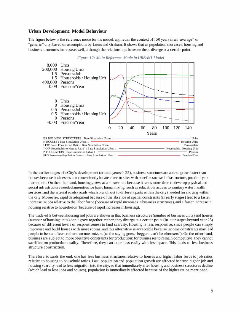
The figure below is the reference mode for the model, applied in the context of 150 years in an “average” or
“generic” city, based on assumptions by Louis and Graham. It shows that as population increases, housing and
business structures increase as well, although the relationships between these diverge at a certain point.
Figure 12: Main Reference Mode in URBAN1 Model
In the earlier stages of a City’s development (around years 0-25), business structures are able to grow faster than
houses because businesses can conveniently locate close to sites with benefits such as infrastructure, proximity to
market, etc. On the other hand, housing grows at a slower rate because it takes more time to develop physical and
social infrastructure needed amenities for basic human living, such as education, access to sanitary water, health
services, and the arterial roads (roads which branch out to different parts within the city) needed for moving within
the city. Moreover, rapid development because of the absence of spatial constraints (in early stages) lead to a faster
increase in jobs relative to the labor force (because of rapid increases in business structures), and a faster increase in
housing relative to households (because of rapid increases in housing).
The trade-offs between housing and jobs are shown in that business structures (number of business units) and houses (number of housing units) don’t grow together: rather, they diverge at a certain point (in later stages beyond year 25) because of different levels of responsiveness to land scarcity. Housing is less responsive, since people can simply
improvise and build houses with more rooms, and this alternative is acceptable because income constraints may lead people to be satisficers rather than maximizers (as the saying goes, “beggars can’t be choosers”). On the other hand, business are subject to more objective constraints for production: for businesses to remain competitive, they cannot sacrifice on production quality. Therefore, they can cope less easily with less space. This leads to less business structure construction.
Therefore, towards the end, one has less business structures relative to houses and higher labor force to job ratios relative to housing to household ratios. Last, population and population growth are affected because higher job and housing scarcity lead to less migration into the city, so that immediately after housing and business structures decline (which lead to less jobs and houses), population is immediately affected because of the higher ratios mentioned.
Urban1 Reference Mode
8,000 Units200,000 Housing Units
1.5 Persons/Job1.5 Households / Housing Unit
400,000 Persons0.09 Fraction/Year
0 Units0 Housing Units
0.5 Persons/Job0.5 Households / Housing Unit
0 Persons-0.03 Fraction/Year
0 20 40 60 80 100 120 140
YearsBS BUSINESS STRUCTURES : Base Simulation Urban 1 Units
H HOUSES : Base Simulation Urban 1 Housing Units
LFJR Labor Force to Job Ratio : Base Simulation Urban 1 Persons/Job
"HHR Households-to-Houses Ratio" : Base Simulation Urban 1 Households / Housing Unit
P POPULATION : Base Simulation Urban 1 Persons
PPG Percentage Population Growth : Base Simulation Urban 1 Fraction/Year
10
V. Urban-Rural Food (URF) Model Description: Why Don’t Rural Areas Produce More?
A Shift in View
The narrative above seems to be the dominant way of seeing things, given the “growth” mindset over the past years. It has been taken for granted that there will be sufficient food, given the surpluses in agriculture especially during the green revolution. We now venture into this narrative, and into the task of integrating the food security component into
the urban development model, to develop an Urban-Rural Food (URF) model. In building a model bottom up, a simple model is desirable. We build on the original assumptions in the Urban1 model, as documented in Appendix 1: Urban1
Model of this paper (said dynamics were briefly described in the previous section). We basically assume this to be the “average” or “generic” city as a starting point for modelling.
Focus: Urban and Rural Areas within a Region
The original city dynamics point to the impact of jobs and housing on migration towards a particular city. However, it disregards the impact of urban migration on rural agricultural production and food distribution. We therefore add this element to the model. The Urban-Rural Food (URF) model builds on the Urban1 model, but alters the treatment of the variables. Namely, we use the Urban1 model as the dynamics for migration into the urbanized cities within
regions, and add the component of rural areas within regions.
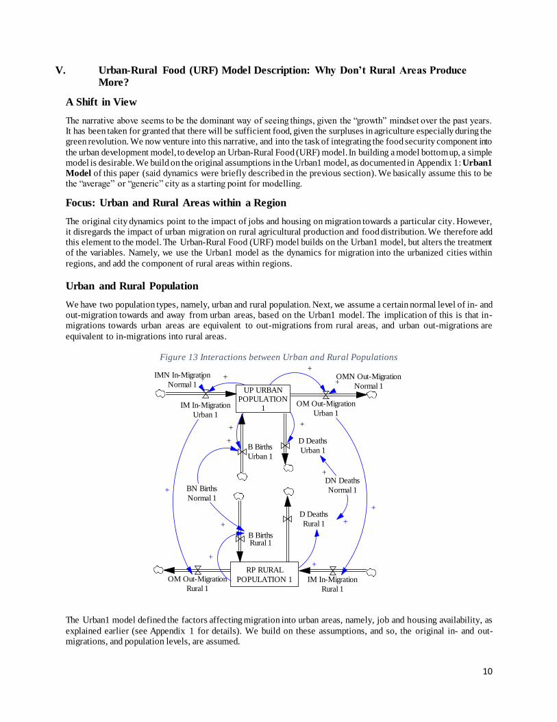
Urban and Rural Population
We have two population types, namely, urban and rural population. Next, we assume a certain normal level of in- and out-migration towards and away from urban areas, based on the Urban1 model. The implication of this is that in-migrations towards urban areas are equivalent to out-migrations from rural areas, and urban out-migrations are
equivalent to in-migrations into rural areas.
Figure 13 Interactions between Urban and Rural Populations
The Urban1 model defined the factors affecting migration into urban areas, namely, job and housing availability, as
explained earlier (see Appendix 1 for details). We build on these assumptions, and so, the original in- and out-migrations, and population levels, are assumed.
UP URBANPOPULATION
1IM In-Migration
Urban 1
OM Out-Migration
Urban 1
B Births
Urban 1
D Deaths
Urban 1
BN Births
Normal 1
+
+ +
DN Deaths
Normal 1
+
OMN Out-Migration
Normal 1
IMN In-Migration
Normal 1 ++ ++
RP RURAL
POPULATION 1 IM In-Migration
Rural 1
OM Out-Migration
Rural 1
D Deaths
Rural 1
B BirthsRural 1
+ +
++
+
+
11
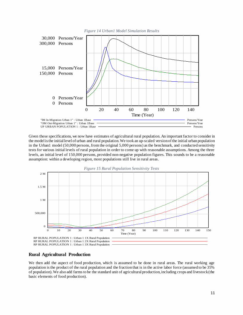
Figure 14 Urban1 Model Simulation Results
Given these specifications, we now have estimates of agricultural rural population. An important factor to consider in the model is the initial level of urban and rural population. We took an up-scaled version of the initial urban population in the Urban1 model (50,000 persons, from the original 5,000 persons) as the benchmark, and conducted sensitivity tests for various initial levels of rural population in order to come up with reasonable assumptions. Among the three
levels, an initial level of 150,000 persons, provided non-negative population figures. This sounds to be a reasonable assumption: within a developing region, most populations still live in rural areas.
Figure 15 Rural Population Sensitivity Tests
Rural Agricultural Production
We then add the aspect of food production, which is assumed to be done in rural areas. The rural working age population is the product of the rural population and the fraction that is in the active labor force (assumed to be 35% of population). We also add farms to be the standard unit of agricultural production, including crops and livestock (the basic elements of food production).
Selected Variables
30,000 Persons/Year
300,000 Persons
15,000 Persons/Year
150,000 Persons
0 Persons/Year
0 Persons
0 20 40 60 80 100 120 140
Time (Year)"IM In-Migration Urban 1" : Urban 1Base Persons/Year
"OM Out-Migration Urban 1" : Urban 1Base Persons/Year
UP URBAN POPULATION 1 : Urban 1Base Persons
2 M
1.5 M
1 M
500,000
0
0 10 20 30 40 50 60 70 80 90 100 110 120 130 140 150
Time (Year)
RP RURAL POPULATION 1 : Urban 1 1X Rural Population
RP RURAL POPULATION 1 : Urban 1 2X Rural Population
RP RURAL POPULATION 1 : Urban 1 3X Rural Population
12
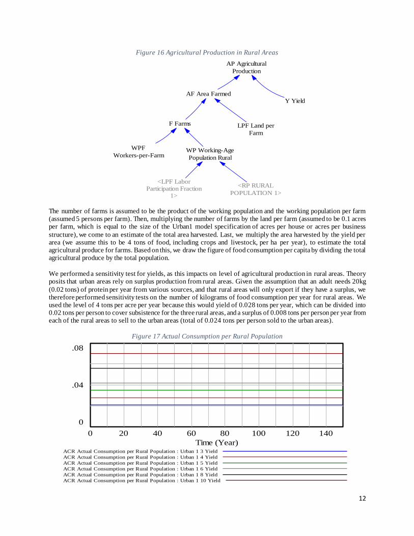
Figure 16 Agricultural Production in Rural Areas
The number of farms is assumed to be the product of the working population and the working population per farm (assumed 5 persons per farm). Then, multiplying the number of farms by the land per farm (assumed to be 0.1 acres per farm, which is equal to the size of the Urban1 model specification of acres per house or acres per business
structure), we come to an estimate of the total area harvested. Last, we multiply the area harvested by the yield per area (we assume this to be 4 tons of food, including crops and livestock, per ha per year), to estimate the total agricultural produce for farms. Based on this, we draw the figure of food consumption per capita by dividing the total agricultural produce by the total population.
We performed a sensitivity test for yields, as this impacts on level of agricultural production in rural areas. Theory posits that urban areas rely on surplus production from rural areas. Given the assumption that an adult needs 20kg
(0.02 tons) of protein per year from various sources, and that rural areas will only export if they have a surplus, we therefore performed sensitivity tests on the number of kilograms of food consumption per year for rural areas. We used the level of 4 tons per acre per year because this would yield of 0.028 tons per year, which can be divided into 0.02 tons per person to cover subsistence for the three rural areas, and a surplus of 0.008 tons per person per year from each of the rural areas to sell to the urban areas (total of 0.024 tons per person sold to the urban areas).
Figure 17 Actual Consumption per Rural Population
AF Area FarmedY Yield
<LPF LaborParticipation Fraction
1>
WP Working-Age
Population Rural
WPF
Workers-per-Farm
LPF Land per
Farm
AP Agricultural
Production
F Farms
<RP RURAL
POPULATION 1>
ACR Actual Consumption per Rural Population
.08
.04
0
0 20 40 60 80 100 120 140
Time (Year)ACR Actual Consumption per Rural Population : Urban 1 3 Yield
ACR Actual Consumption per Rural Population : Urban 1 4 Yield
ACR Actual Consumption per Rural Population : Urban 1 5 Yield
ACR Actual Consumption per Rural Population : Urban 1 6 Yield
ACR Actual Consumption per Rural Population : Urban 1 8 Yield
ACR Actual Consumption per Rural Population : Urban 1 10 Yield
13
VI. URF Model Simulation Output
Urbanization Outcomes
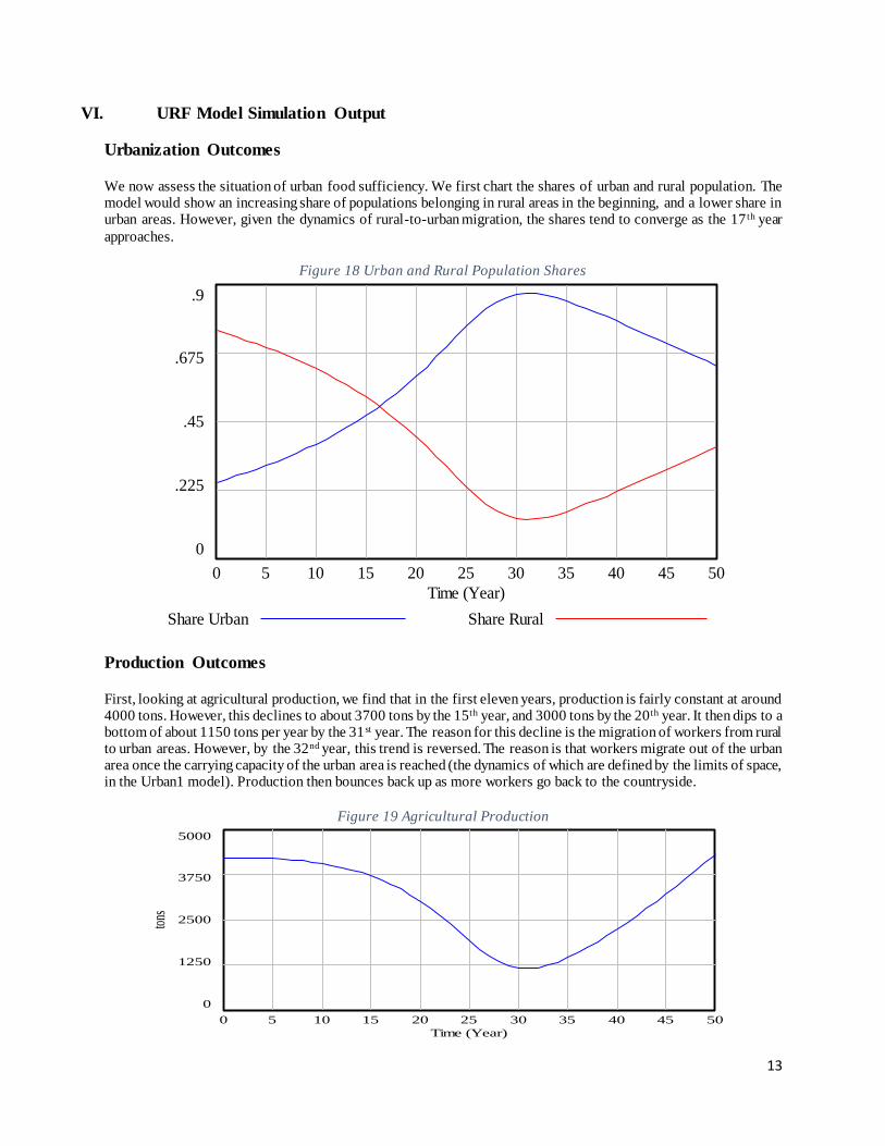
We now assess the situation of urban food sufficiency. We first chart the shares of urban and rural population. The model would show an increasing share of populations belonging in rural areas in the beginning, and a lower share in urban areas. However, given the dynamics of rural-to-urban migration, the shares tend to converge as the 17 th year
approaches.
Figure 18 Urban and Rural Population Shares
Production Outcomes
First, looking at agricultural production, we find that in the first eleven years, production is fairly constant at around 4000 tons. However, this declines to about 3700 tons by the 15th year, and 3000 tons by the 20th year. It then dips to a bottom of about 1150 tons per year by the 31st year. The reason for this decline is the migration of workers from rural to urban areas. However, by the 32nd year, this trend is reversed. The reason is that workers migrate out of the urban area once the carrying capacity of the urban area is reached (the dynamics of which are defined by the limits of space, in the Urban1 model). Production then bounces back up as more workers go back to the countryside.
Figure 19 Agricultural Production
Shares of Urban and Rural Population
.9
.675
.45
.225
0
0 5 10 15 20 25 30 35 40 45 50
Time (Year)
Share Urban Share Rural
AP Agricultural Production
5000
3750
2500
1250
0
0 5 10 15 20 25 30 35 40 45 50
Time (Year)
tons
AP Agricultural Production : Urban 1 4 Yield

14
Consumption Outcomes
What are the implications of these trends on food consumption per capita? After sales from urban to rural, consumption per rural population is constant at 0.02 (since rural areas produce for subsistence purposes), urban consumption per
capita declines for the next 30 years and plateaus at the 31 st /32nd year. However, what is important to note is that urban consumption per capita diminishes towards extremely low levels. By the 13 th year, urban consumers are only consuming 10 kg (0.01 tons) per year. This average consumption can be broken down into consumption between the poor and the rich, for instance, and one can see that the same ratio can be achieved if the rich may consume the 20kg per year sufficiency amount, while the poorer ones consume as low as 3-5 tons per year.
Figure 20 Consumption per Urban and Rural Population
After the 35th year, production bounces back up. By the 40 th, it is already beyond the sufficient food level per capita.
The reason, however, is not because of urban food sufficiency, but rather, because of the falling attractiveness of
urban areas, as explained in the previous section (Dynamic Analysis with Causal Loops: Development of Urban
Areas).
While this may paint a bleak picture on production, it is nonetheless a realistic picture if urbanization and rural
production are not coordinated in taking food security concerns into consideration. Yes, production may indeed
bounce back up, but this is predicated on the decline in attractiveness of urban areas. However, given the income
differences between the gross value-added per worker in agricultural and non-agricultural production, urbanization
trends are expected to continue.
The disconnect between urbanization policies by cities and regions that support them on one hand, and rural
production on the other, results in large shares of urban populations who live in hunger (as shown by the urban food
consumption per capita falling below the sufficiency level). However, this is not a necessary outcome, if the
incentives of the actors are tweaked. Feedback mechanisms from urbanization back to rural production need to be
installed to align incentives of actors. We tackle this in the next section.
Consumption per Urban and Rural Population
.2
.15
.1
.05
0
0 5 10 15 20 25 30 35 40 45 50
Time (Year)Agri Supply per Person in Urban Area after Sales : Urban 1 4 Yield Revised
Agri Supply Rural Area per person after Sales : Urban 1 4 Yield Revised
15
VII. Linking up Incentives: Actors and Incentives in Food Production
Agricultural Sector Growth
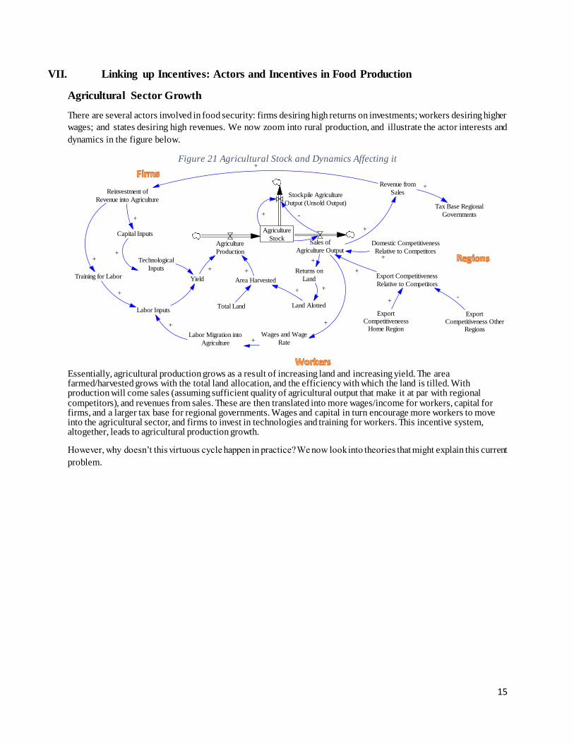
There are several actors involved in food security: firms desiring high returns on investments; workers desiring higher
wages; and states desiring high revenues. We now zoom into rural production, and illustrate the actor interests and
dynamics in the figure below.
Figure 21 Agricultural Stock and Dynamics Affecting it
Essentially, agricultural production grows as a result of increasing land and increasing yield. The area farmed/harvested grows with the total land allocation, and the efficiency with which the land is tilled. With production will come sales (assuming sufficient quality of agricultural output that make it at par with regional competitors), and revenues from sales. These are then translated into more wages/income for workers, capital for firms, and a larger tax base for regional governments. Wages and capital in turn encourage more workers to move into the agricultural sector, and firms to invest in technologies and training for workers. This incentive system, altogether, leads to agricultural production growth.
However, why doesn’t this virtuous cycle happen in practice? We now look into theories that might explain this current
problem.
Agriculture
StockAgriculture
Production
Yield Area Harvested
+ +
Sales of
Agriculture Output
Stockpile Agriculture
Output (Unsold Output)
Domestic Competitiveness
Relative to Competitors
Export Competitiveness
Relative to Competitors
+
+
-+
ExportCompetitiveness Other
Regions
ExportCompetitiveneess
Home Region
+-
Technological
Inputs
Capital Inputs
Labor Inputs
+
Revenue from
Sales
+
Reinvestment of
Revenue into Agriculture
+
+
+
Wages and Wage
Rate
+
+
Land Alotted
Returns on
Land
+
++
Training for Labor
+
Labor Migration into
Agriculture
+
Total Land
Tax Base Regional
Governments
+
16
VIII. Theories of Industrial Growth and Consumer Demand
There are two core theories that can explain the issues in rural production growth. We begin by describing the
dynamics of sector growth and of price, and summarize with the hypothesis that the price system is not functioning
sufficiently to motivate stakeholders to go into agricultural production.
Incentive Mechanisms for Capacity Growth
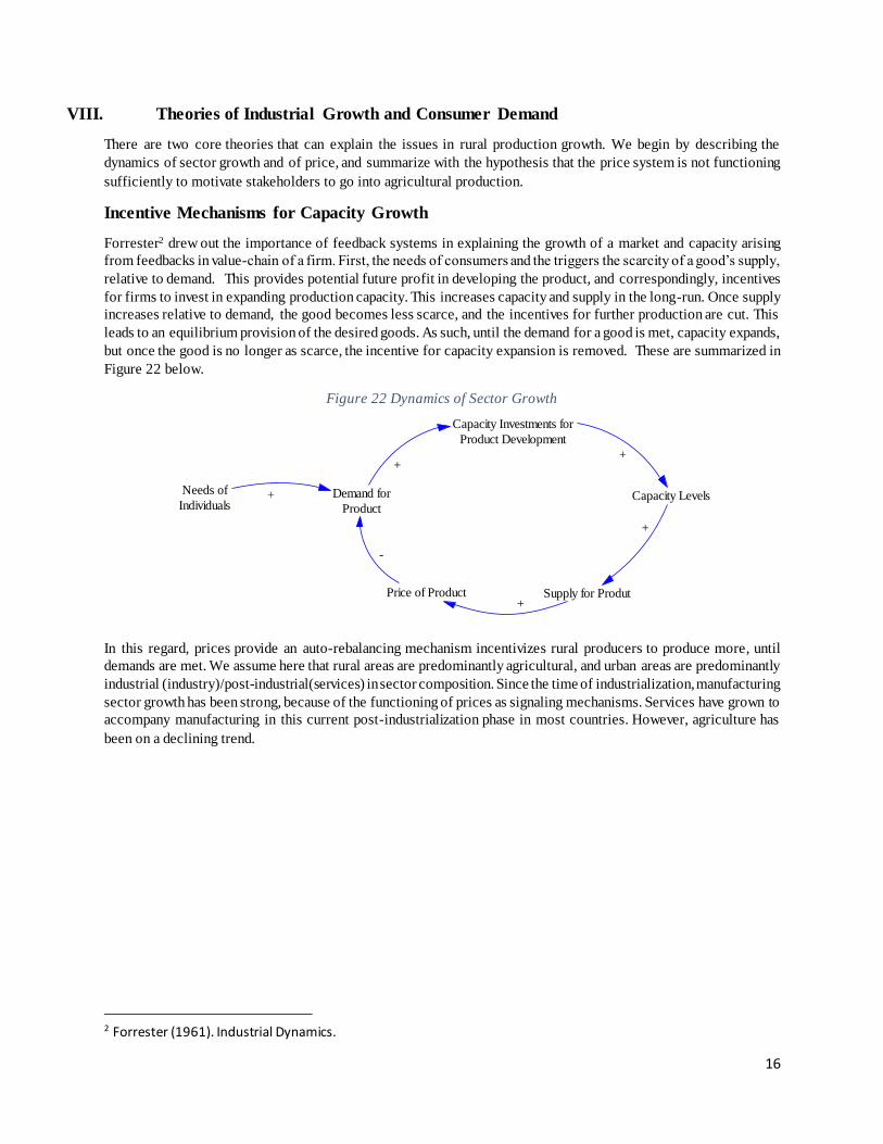
Forrester2 drew out the importance of feedback systems in explaining the growth of a market and capacity arising
from feedbacks in value-chain of a firm. First, the needs of consumers and the triggers the scarcity of a good’s supply,
relative to demand. This provides potential future profit in developing the product, and correspondingly, incentives
for firms to invest in expanding production capacity. This increases capacity and supply in the long-run. Once supply
increases relative to demand, the good becomes less scarce, and the incentives for further production are cut. This
leads to an equilibrium provision of the desired goods. As such, until the demand for a good is met, capacity expands,
but once the good is no longer as scarce, the incentive for capacity expansion is removed. These are summarized in
Figure 22 below.
Figure 22 Dynamics of Sector Growth
In this regard, prices provide an auto-rebalancing mechanism incentivizes rural producers to produce more, until
demands are met. We assume here that rural areas are predominantly agricultural, and urban areas are predominantly
industrial (industry)/post-industrial(services) in sector composition. Since the time of industrialization, manufacturing
sector growth has been strong, because of the functioning of prices as signaling mechanisms. Services have grown to
accompany manufacturing in this current post-industrialization phase in most countries. However, agriculture has
been on a declining trend.
2 Forrester (1961). Industrial Dynamics.
Demand for
Product
Capacity Investments for
Product Development
Capacity Levels
Supply for ProdutPrice of Product
++
+
+
-
Needs of
Individuals+
17
Issues in Capacity Growth
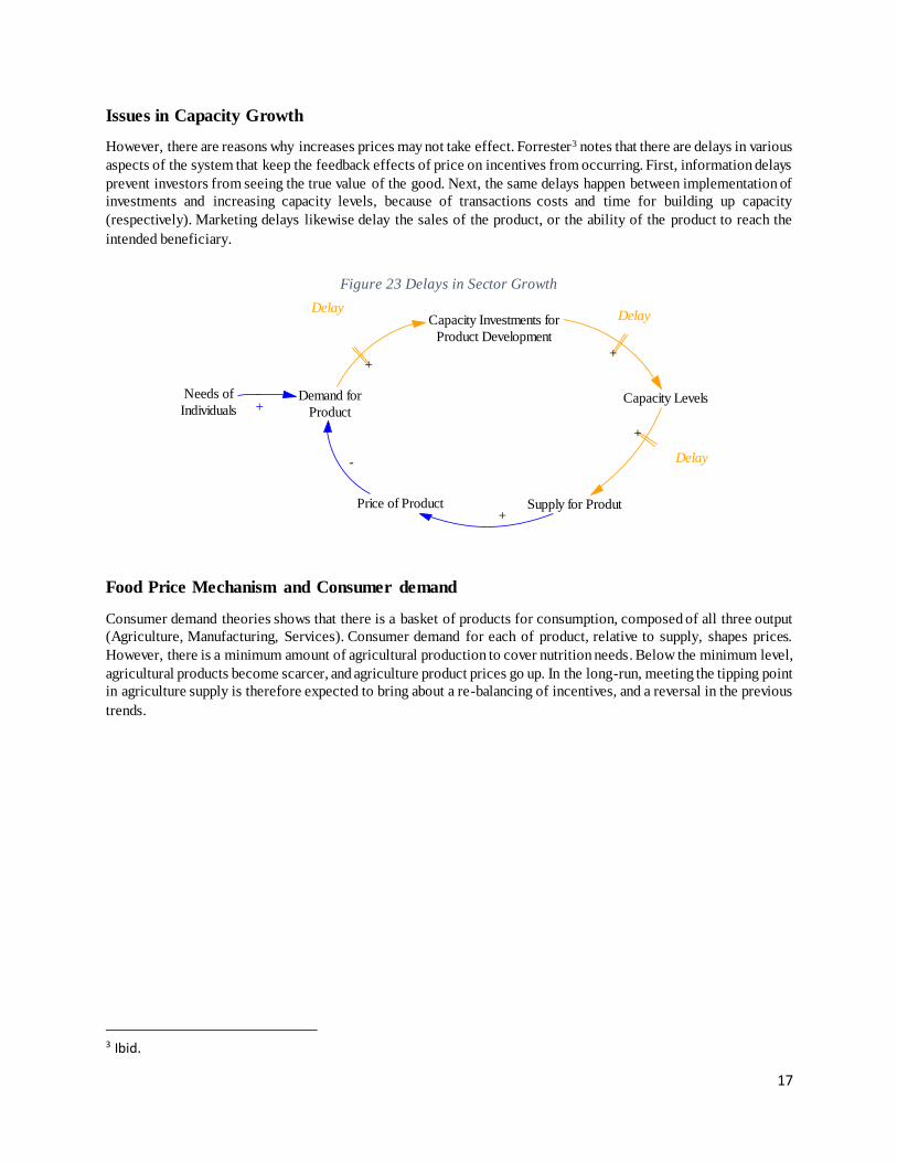
However, there are reasons why increases prices may not take effect. Forrester3 notes that there are delays in various
aspects of the system that keep the feedback effects of price on incentives from occurring. First, information delays
prevent investors from seeing the true value of the good. Next, the same delays happen between implementation of
investments and increasing capacity levels, because of transactions costs and time for building up capacity
(respectively). Marketing delays likewise delay the sales of the product, or the ability of the product to reach the
intended beneficiary.
Figure 23 Delays in Sector Growth
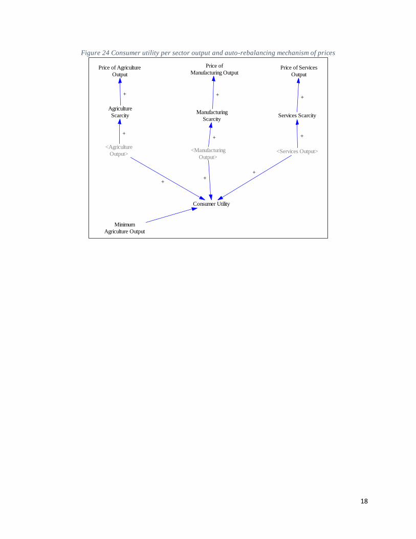
Food Price Mechanism and Consumer demand
Consumer demand theories shows that there is a basket of products for consumption, composed of all three output
(Agriculture, Manufacturing, Services). Consumer demand for each of product, relative to supply, shapes prices.
However, there is a minimum amount of agricultural production to cover nutrition needs. Below the minimum level,
agricultural products become scarcer, and agriculture product prices go up. In the long-run, meeting the tipping point
in agriculture supply is therefore expected to bring about a re-balancing of incentives, and a reversal in the previous
trends.
3 Ibid.
Demand for
Product
Capacity Investments for
Product Development
Capacity Levels
Supply for ProdutPrice of Product
++
+
+
-
Needs of
Individuals +
DelayDelay
Delay
18
Figure 24 Consumer utility per sector output and auto-rebalancing mechanism of prices
<Agriculture
Output><Manufacturing
Output><Services Output>
Consumer Utility
++
+
Minimum
Agriculture Output
Agriculture
ScarcityManufacturing
ScarcityServices Scarcity
++ +
Price of Agriculture
Output
Price of
Manufacturing OutputPrice of Services
Output
+ + +
19
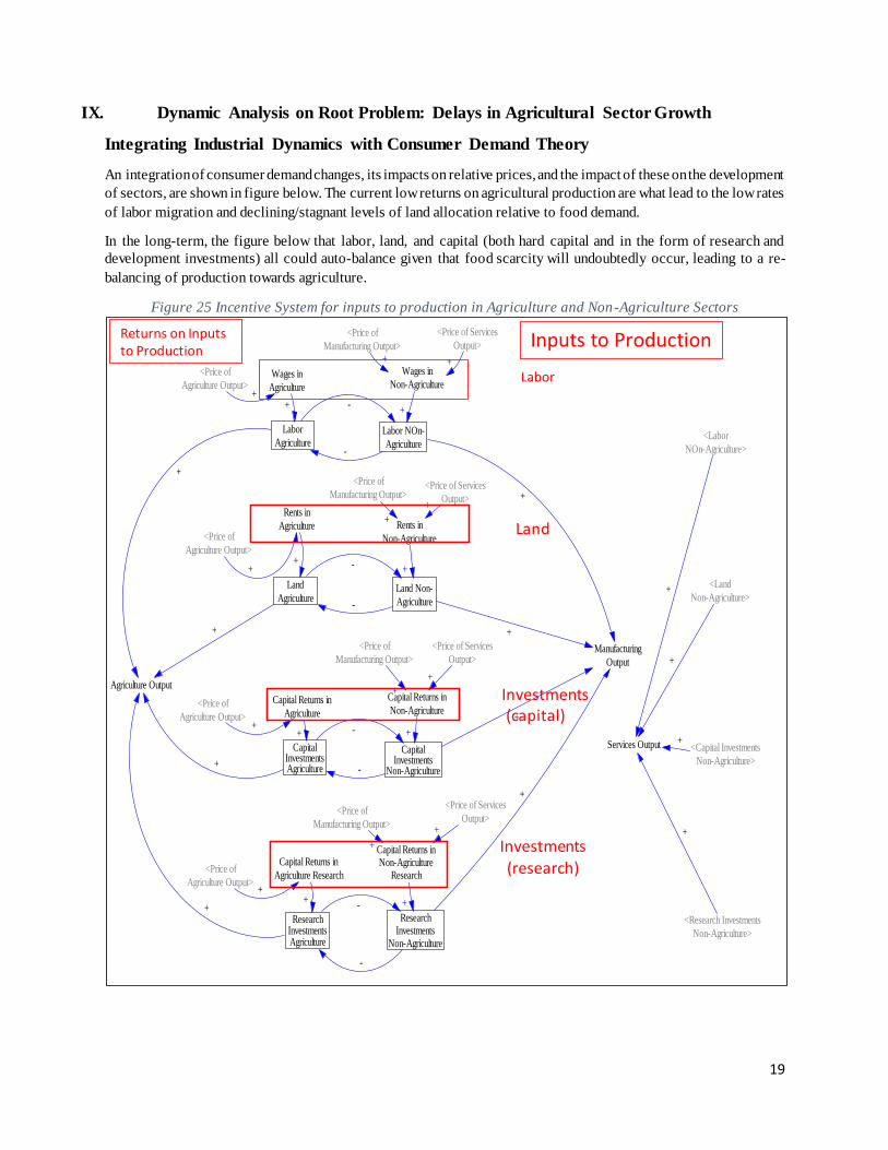
IX. Dynamic Analysis on Root Problem: Delays in Agricultural Sector Growth
Integrating Industrial Dynamics with Consumer Demand Theory
An integration of consumer demand changes, its impacts on relative prices, and the impact of these on the development
of sectors, are shown in figure below. The current low returns on agricultural production are what lead to the low rates
of labor migration and declining/stagnant levels of land allocation relative to food demand.
In the long-term, the figure below that labor, land, and capital (both hard capital and in the form of research and
development investments) all could auto-balance given that food scarcity will undoubtedly occur, leading to a re-
balancing of production towards agriculture.
Figure 25 Incentive System for inputs to production in Agriculture and Non-Agriculture Sectors
Labor
Agriculture
Land
Agriculture
CapitalInvestmentsAgriculture
ResearchInvestmentsAgriculture
Labor NOn-
Agriculture
Land Non-
Agriculture
CapitalInvestments
Non-Agriculture
ResearchInvestments
Non-Agriculture
-
-
-
-
-
-
-
-
Wages in
Agriculture
Rents in
Agriculture
Capital Returns in
Agriculture
Capital Returns in
Agriculture Research
+
+
+
+
Manufacturing
Output
Services Output
+
+
+
Agriculture Output
+
+
+
+
<Labor
NOn-Agriculture>
<Land
Non-Agriculture>
<Capital Investments
Non-Agriculture>
<Research Investments
Non-Agriculture>
+
+
+
+
+
<Price of
Agriculture Output>
<Price of
Agriculture Output>
<Price of
Agriculture Output>
<Price of
Agriculture Output>
+
+
+
+
<Price of
Manufacturing Output>
<Price of Services
Output>
<Price of
Manufacturing Output><Price of Services
Output>
Wages in
Non-Agriculture
Rents in
Non-Agriculture
Capital Returns in
Non-Agriculture
Capital Returns inNon-Agriculture
Research
<Price of
Manufacturing Output>
<Price of Services
Output>
<Price of
Manufacturing Output>
<Price of Services
Output>
+
+
+
+
+
+
+
+
+
+ +
+
Labor
Land
Investments
(capital)
Investments
(research)
Returns on Inputs to Production
Inputs to Production
20
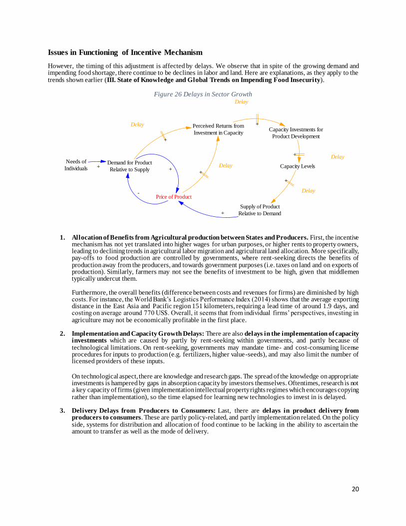
Issues in Functioning of Incentive Mechanism
However, the timing of this adjustment is affected by delays. We observe that in spite of the growing demand and impending food shortage, there continue to be declines in labor and land. Here are explanations, as they apply to the trends shown earlier (III. State of Knowledge and Global Trends on Impending Food Insecurity).
Figure 26 Delays in Sector Growth
1. Allocation of Benefits from Agricultural production between States and Producers. First, the incentive mechanism has not yet translated into higher wages for urban purposes, or higher rents to property owners, leading to declining trends in agricultural labor migration and agricultural land allocation. More specifically, pay-offs to food production are controlled by governments, where rent-seeking directs the benefits of production away from the producers, and towards government purposes (i.e. taxes on land and on exports of production). Similarly, farmers may not see the benefits of investment to be high, given that middlemen typically undercut them. Furthermore, the overall benefits (difference between costs and revenues for firms) are diminished by high costs. For instance, the World Bank’s Logistics Performance Index (2014) shows that the average exporting distance in the East Asia and Pacific region 151 kilometers, requiring a lead time of around 1.9 days, and costing on average around 770 US$. Overall, it seems that from individual firms’ perspectives, investing in agriculture may not be economically profitable in the first place.
2. Implementation and Capacity Growth Delays: There are also delays in the implementation of capacity
investments which are caused by partly by rent-seeking within governments, and partly because of technological limitations. On rent-seeking, governments may mandate time- and cost-consuming license procedures for inputs to production (e.g. fertilizers, higher value-seeds), and may also limit the number of licensed providers of these inputs.
On technological aspect, there are knowledge and research gaps. The spread of the knowledge on appropriate investments is hampered by gaps in absorption capacity by investors themselves. Oftentimes, research is not a key capacity of firms (given implementation intellectual property rights regimes which encourages copying rather than implementation), so the time elapsed for learning new technologies to invest in is delayed.
3. Delivery Delays from Producers to Consumers: Last, there are delays in product delivery from
producers to consumers. These are partly policy-related, and partly implementation related. On the policy side, systems for distribution and allocation of food continue to be lacking in the ability to ascertain the amount to transfer as well as the mode of delivery.
Demand for Product
Relative to Supply
Capacity Investments for
Product Development
Capacity Levels
Supply of Product
Relative to Demand
Price of Product
+
+
+
+
-
Needs of
Individuals +
Delay
Delay
Delay
Perceived Returns from
Investment in Capacity
+
+
Delay
+
Delay
21
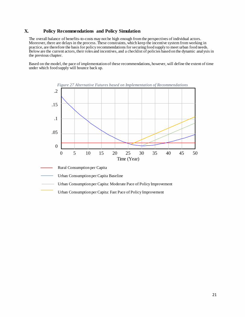
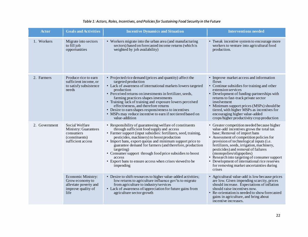
X. Policy Recommendations and Policy Simulation
The overall balance of benefits-to-costs may not be high enough from the perspectives of individual actors. Moreover, there are delays in the process. These constraints, which keep the incentive system from working in practice, are therefore the basis for policy recommendations for securing food supply to meet urban food needs. Below are the current actors, their roles and incentives, and a checklist of policies based on the dynamic analysis in the previous chapter. Based on the model, the pace of implementation of these recommendations, however, will define the extent of time under which food supply will bounce back up.
Figure 27 Alternative Futures based on Implementation of Recommendations
Rural Consumption per Capita
Urban Consumption per Capita Baseline
Urban Consumption per Capita: Moderate Pace of Policy Improvement
Urban Consumption per Capita: Fast Pace of Policy Improvement
Consumption per Urban and Rural Population
.2
.15
.1
.05
0
0 5 10 15 20 25 30 35 40 45 50
Time (Year)Agri Supply per Person in Urban Area after Sales : Urban 1 4 Yield Revised
Agri Supply Rural Area per person after Sales : Urban 1 4 Yield Revised
22
Actor Goals and Activities Incentive Dynamics and Situation Interventions needed
1. Workers Migrate into sectors to fill job opportunities
• Workers migrate into the urban area (and manufacturing sectors) based on forecasted income returns (which is weighted by job availability)
• Tweak incentive system to encourage more workers to venture into agricultural food production.
2. Farmers Produce rice to earn sufficient income, or to satisfy subsistence needs
• Projected rice demand (prices and quantity) affect the targeted production
• Lack of awareness of international markets lowers targeted production
• Perceived returns on investments in fertilizer, seeds, farming practices shapes investments
• Training lack of training and exposure lowers perceived effectiveness, and therefore returns
• Desire to earn shapes responsiveness to incentives • MSPs may reduce incentive to earn if not tiered based on
value-addition
• Improve market access and information flows
• Continue subsidies for training and other extension services
• Development of funding-partnerships with returns to fast-track private sector involvement
• Minimum support prices (MSPs) should be tiered, with higher MSPs as incentives for encouraging higher value-added crops/higher productivity crop production
2. Government Social Welfare Ministry: Guarantees consumers (constituents) sufficient access
• Responsibility of guaranteeing welfare of constituents through sufficient food supply and access
• Farmer support (input subsidies: fertilizers, seed, training, pesticides, machinery) to boost production
• Import bans, export quotas and minimum support price to guarantee demand for farmers (and therefore, production targeting)
• Consumer support through food price subsidies to boost access
• Export bans to ensure access when crises viewed to be impending
• Greater competition needed because higher value-add incentives grows the total tax base; Removal of import bans
• Assessment of competition policies for provision of technological inputs (i.e. fertilizers, seeds, irrigation, machinery, pesticides) and removal of failures (monopolies/oligopolies)
• Research into targeting of consumer support • Development of international rice reserves
for removing market uncertainties during crises
Economic Ministry: Grow economy to alleviate poverty and improve quality of life
• Desire to shift resources to higher value-added activities; low returns to agriculture influence gov’ts to migrate from agriculture to industry/services
• Lack of awareness of/appreciation for future gains from agriculture sector growth
• Agricultural value-add is low because prices are low. Given impending scarcity, prices should increase. Expectations of inflation should raise incentives now.
• Re-orientation is needed to show forecasted gains in agriculture, and bring about incentive increases.
Table 1: Actors, Roles, Incentives, and Policies for Sustaining Food Security in the Future
23
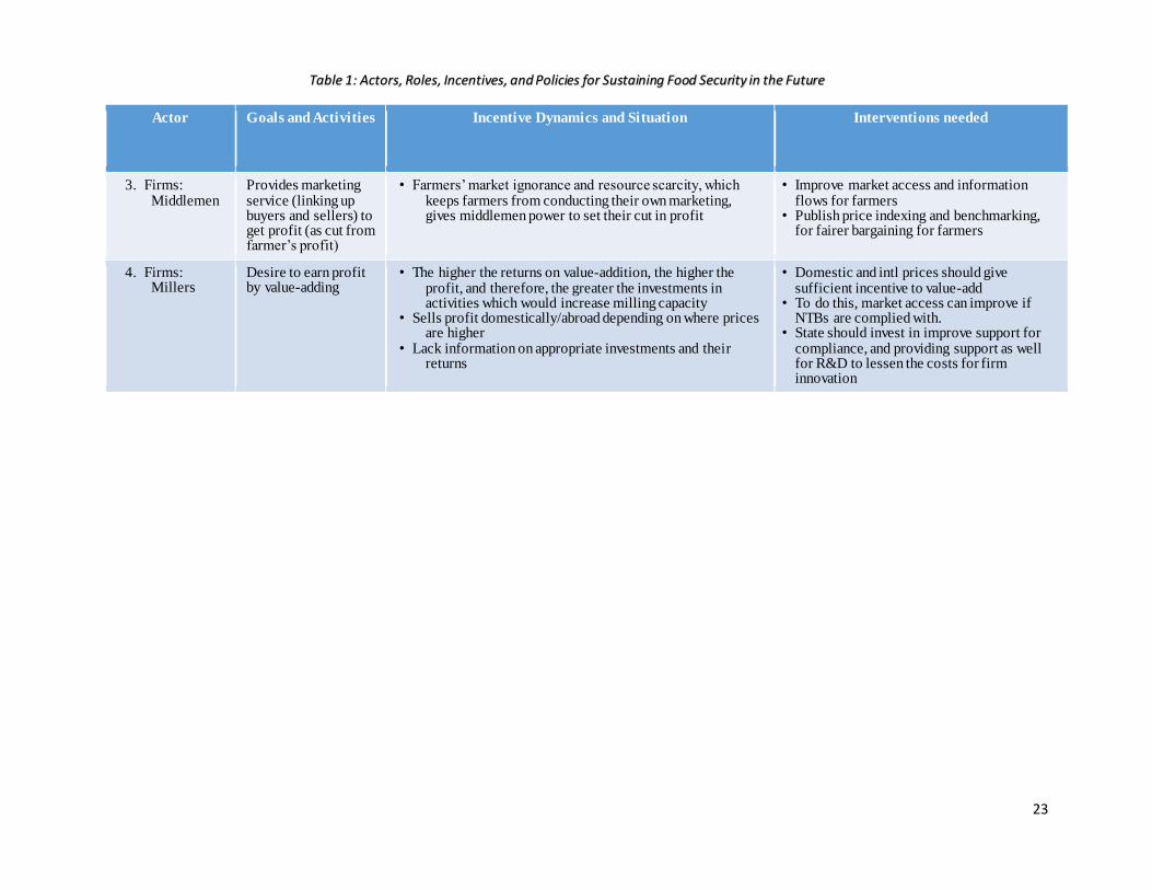
Actor Goals and Activities Incentive Dynamics and Situation Interventions needed
3. Firms: Middlemen
Provides marketing service (linking up buyers and sellers) to get profit (as cut from farmer’s profit)
• Farmers’ market ignorance and resource scarcity, which keeps farmers from conducting their own marketing, gives middlemen power to set their cut in profit
• Improve market access and information flows for farmers
• Publish price indexing and benchmarking, for fairer bargaining for farmers
4. Firms: Millers
Desire to earn profit by value-adding
• The higher the returns on value-addition, the higher the profit, and therefore, the greater the investments in activities which would increase milling capacity
• Sells profit domestically/abroad depending on where prices are higher
• Lack information on appropriate investments and their returns
• Domestic and intl prices should give sufficient incentive to value-add
• To do this, market access can improve if NTBs are complied with.
• State should invest in improve support for compliance, and providing support as well for R&D to lessen the costs for firm innovation
Table 1: Actors, Roles, Incentives, and Policies for Sustaining Food Security in the Future
24
XI. Conclusion
In this paper, we began with an assessment of global trends showing increasing global food insecurity ( as a comparison of food supply to demand). We then looked into the dynamics of how the current food insufficiency situation has developed, with the primary lenses of urban development and rural production dynamics. There was shown to be a lack of coordination between urban migration and rural production, leading to a falling per capita urban food consumption (as shown by model simulations). In looking into how better coordination can occur, we looked at the market price mechanism and its impacts on industrial and sector growth. Based on this, we found that there is also an alternative future that food allocation and prioritization by governments, firms, and consumers can bounce back up, with growing food scarcity. This happens once the threshold for food supply (relative to demand) is crossed. However, the combination of market failures shaping the allocation of resources, investment delays from poor spread of knowledge of appropriate investments, and the delays in product delivery from producers to consumers , are the key factors that need to be addressed. The more they are addressed, the better the capability of the market’s price mechanism to mobilize actors naturally. Policy recommendations showed three potential scenarios for the extent of time (in years) under which the urban food security situation will occur. The fact that the problem remains to be a persistent one shows that the feedback loops for addressing it are not yet triggered; as such, the price mechanism is not yet functioning properly. The set of policy recommendations, derived from the causal analysis, may be applied to systemically improve the dynamics shaping the future of food security globally and by extension, in urban areas.

25
XII. References
1. Forrester (1961). Industrial Dynamics
2. International Rice Research Institute (IRRI). Rice Almanac, 4 th Edition.
3. World Bank (2014). World Development Indicators (website).
4. United Nations Food and Agriculture Organization (2014). FAO Statistics (website).
5. World Bank (2014). Logistics Performance Index 2014.
26
P POPULA
TION 0
IM In-Migration 0OM
Out-Migration 0
B Births 0D Deaths 0
BN Births
Normal 0
++ +
DN Deaths
Normal 0+
OMN Out-Migration
Normal 0
IMN In-Migration
Normal 0
++ + +
AM Attractiveness
Multiplier 0 +
XIII. Appendix 1: Urban1 Model Assumptions of Louis Alfeld and Alan Graham
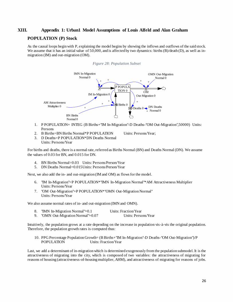
POPULATION (P) Stock
As the causal loops begin with P, explaining the model begins by showing the inflows and outflows of the said stock. We assume that it has an initial value of 50,000, and is affected by two dynamics: births (B)/death (D), as well as in-migration (IM) and out-migration (OM).
Figure 28: Population Subset
1. P POPULATION= INTEG (B Births+"IM In-Migration"-D Deaths-"OM Out-Migration",50000) Units: Persons
2. B Births=BN Births Normal*P POPULATION Units: Persons/Year;
3. D Deaths=P POPULATION*DN Deaths Normal Units: Persons/Year
For births and deaths, there is a normal rate, referred as Births Normal (BN) and Deaths Normal (DN). We assume
the values of 0.03 for BN, and 0.015 for DN.
4. BN Births Normal=0.03 Units: Persons/Person/Year 5. DN Deaths Normal=0.015 Units: Persons/Person/Year
Next, we also add the in- and out-migration (IM and OM) as flows for the model.
6. "IM In-Migration"=P POPULATION*"IMN In-Migration Normal"*AM Attractiveness Multiplier Units: Persons/Year
7. "OM Out-Migration"=P POPULATION*"OMN Out-Migration Normal" Units: Persons/Year
We also assume normal rates of in- and out-migration (IMN and OMN).
8. "IMN In-Migration Normal"=0.1 Units: Fraction/Year 9. "OMN Out-Migration Normal"=0.07 Units: Persons/Year
Intuitively, the population grows at a rate depending on the increase in population vis-à-vis the original population. Therefore, the population growth rates is computed thus:
10. PPG Percentage Population Growth= (B Births+"IM In-Migration"-D Deaths-"OM Out-Migration")/P POPULATION Units: Fraction/Year
Last, we add a determinant of in-migration which is determined exogenously from the population submodel. It is the attractiveness of migrating into the city, which is composed of two variables: the attractiveness of migrating for reasons of housing (attractiveness-of-housing multiplier, AHM), and attractiveness of migrating for reasons of jobs.
27
11. AM Attractiveness Multiplier="AHM Attractiveness-of-Housing-Multiplier"*"AJM Attractiveness-of-Jobs-Multiplier" Units: **undefined**
The AJM is affected by the labor-force-to-jobs ratio (LFJR) or the ratio of the number of units in the labor force over
the jobs available. LFJR affects AJM negatively since it represents unemployment whenever the ratio is in excess of 1, and as LJFR increases, the growing scarcity of jobs makes it less attractive to migrate for job reasons since this brings wages down (economic theory states that excess of jobs leads to an equilibrium wage rate which is less than if there were sufficient numbers of jobs).
12. "AJM Attractiveness-of-Jobs-Multiplier" = WITH LOOKUP (LFJR Labor Force to Job Ratio, ([(0,0)-
(2,2)],(0,2),(0.2,1.95),(0.4,1.8),(0.6,1.6),(0.8,1.35),(1,1),(1.2 ,0.5),(1.4,0.3),(1.6,0.2),(1.8,0.15),(2,0.1) )) Units: **undefined**
On the other hand, the AHM is affected by the households-to-houses ratio (HHR). HHR likewise affects AHM negatively since when HHR is greater than 1, there are more households than houses, leading to a housing shortage. Economic theory states that when there is a shortage, the equilibrium price for a good is higher than if there was no shortage. Therefore, higher prices for housing make it less attractive to migrate into the City.
13. "AHM Attractiveness-of-Housing-Multiplier" = WITH LOOKUP ("HHR Households-to-Houses Ratio",
([(0,0)-(2,2)],(0,1.4),(0.2,1.4),(0.4,1.35), (0.6,1.3),(0.8,1.15),(1,1),( 1.2,0.8),(1.4,0.65),(1.6,0.5),(1.8,0.45),(2,0.4) ))
Units: **undefined**
BUSINESS STRUCTURES (BS) Stock
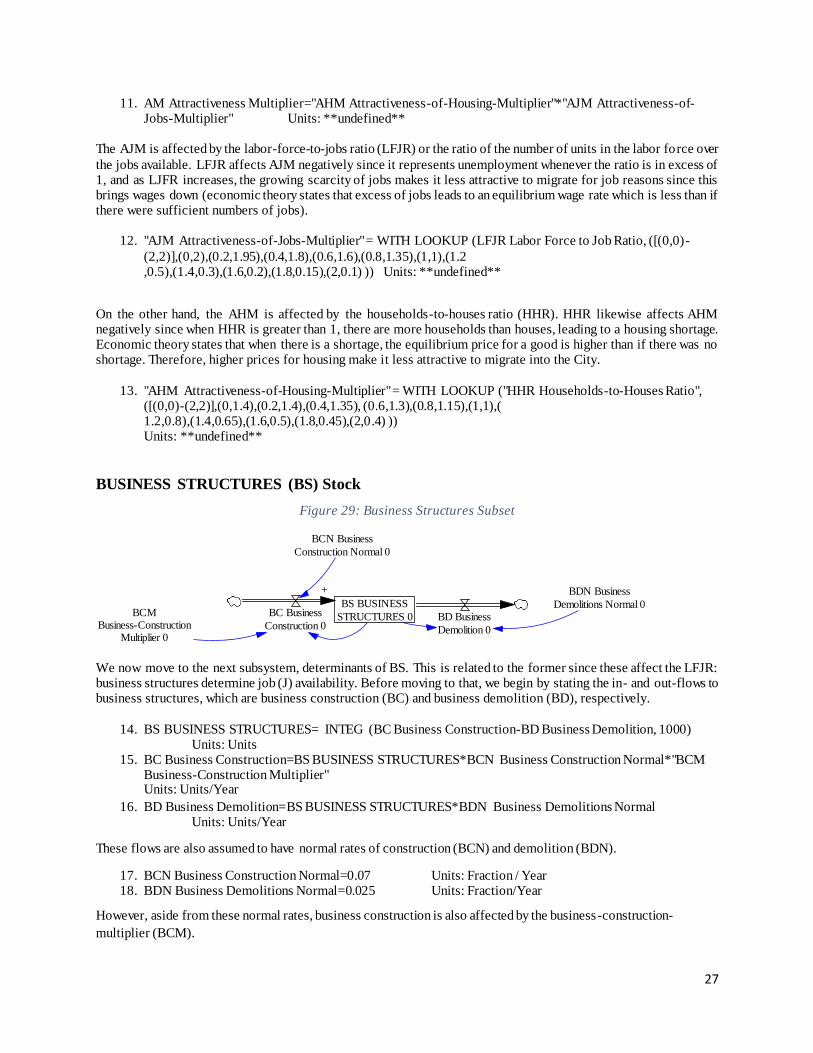
Figure 29: Business Structures Subset
We now move to the next subsystem, determinants of BS. This is related to the former since these affect the LFJR: business structures determine job (J) availability. Before moving to that, we begin by stating the in- and out-flows to business structures, which are business construction (BC) and business demolition (BD), respectively.
14. BS BUSINESS STRUCTURES= INTEG (BC Business Construction-BD Business Demolition, 1000) Units: Units
15. BC Business Construction=BS BUSINESS STRUCTURES*BCN Business Construction Normal*"BCM Business-Construction Multiplier"
Units: Units/Year
16. BD Business Demolition=BS BUSINESS STRUCTURES*BDN Business Demolitions Normal Units: Units/Year
These flows are also assumed to have normal rates of construction (BCN) and demolition (BDN).
17. BCN Business Construction Normal=0.07 Units: Fraction / Year 18. BDN Business Demolitions Normal=0.025 Units: Fraction/Year
However, aside from these normal rates, business construction is also affected by the business-construction-
multiplier (BCM).
BS BUSINESS
STRUCTURES 0BC Business
Construction 0BD Business
Demolition 0
BCN Business
Construction Normal 0
+
BCMBusiness-Construction
Multiplier 0
BDN Business
Demolitions Normal 0
28
19. "BCM Business-Construction Multiplier"="BLM Business-Land Multiplier"* "BLFM Business-Labor-Force Multiplier" Units: **undefined**
The rationale behind BCM is that apart from normal rates (explained by reasons exogenous to the model), BS cannot
grow if there is not sufficient demand for jobs (which make BS cost-effective), and if there is not sufficient space for
building. Therefore, determinants of BCM are the Business-Labor-Force Multiplier, which talks about the reaction
of business construction to the LFJR (in cases of job shortage, more buildings will be created due to increasing
demand for jobs; therefore, LFJR affects BLM positively), and the business-land-multiplier (BLM) which talks
about how business construction can be restricted by land scarcity. The land scarcity is measured by the land
fraction occupied (LFO), which affects the BLM negatively (since less land means less business structures can be
created).
20. "BLFM Business-Labor-Force Multiplier" = WITH LOOKUP (LFJR Labor Force to Job Ratio, ([(0,0)-(2,2)],(0,0.2),(0.2,0.25),(0.4,0.35),(0.6,0.5),(0.8,0.7), (1,1),( 1.2,1.35),(1.4,1.6),(1.6,1.8),(1.8,1.95),(2,2) ))
Units: **undefined**
21. "BLM Business-Land Multiplier" = WITH LOOKUP (LFO Land Fraction Occupied, ([(0,0)-(1,1.45)],(0,1),(0.1,1.15),(0.2,1.3),(0.3,1.4),(0.4,1.45), (0.5,1.4),(0.6,1.3),(0.7,0.9),(0.8,0.5),(0.9,0.25),(1,0)
)) Units: **undefined**
Interaction of BUSINESS STRUCTURES and POPULATION
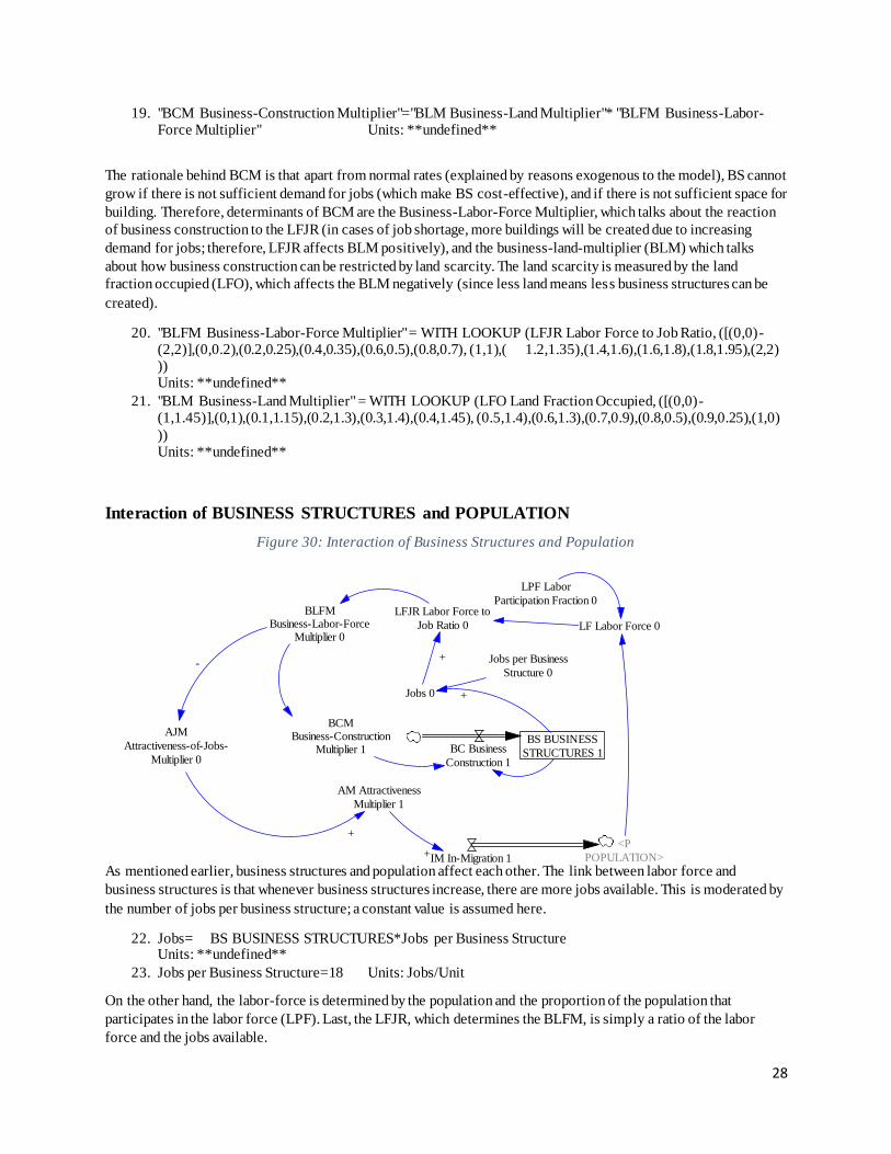
Figure 30: Interaction of Business Structures and Population
As mentioned earlier, business structures and population affect each other. The link between labor force and
business structures is that whenever business structures increase, there are more jobs available. This is moderated by
the number of jobs per business structure; a constant value is assumed here.
22. Jobs= BS BUSINESS STRUCTURES*Jobs per Business Structure Units: **undefined**
23. Jobs per Business Structure=18 Units: Jobs/Unit
On the other hand, the labor-force is determined by the population and the proportion of the population that
participates in the labor force (LPF). Last, the LFJR, which determines the BLFM, is simply a ratio of the labor
force and the jobs available.
Jobs 0
Jobs per Business
Structure 0
+
LFJR Labor Force to
Job Ratio 0
+
LF Labor Force 0
BLFMBusiness-Labor-Force
Multiplier 0
<P
POPULATION>
LPF Labor
Participation Fraction 0
IM In-Migration 1
AM Attractiveness
Multiplier 1
+
AJM
Attractiveness-of-Jobs-
Multiplier 0
+
-
BS BUSINESS
STRUCTURES 1BC Business
Construction 1
BCMBusiness-Construction
Multiplier 1
29
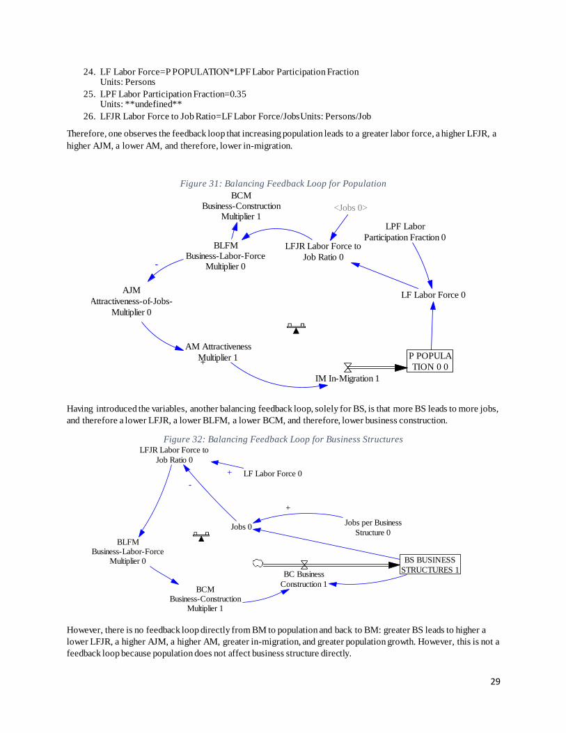
24. LF Labor Force=P POPULATION*LPF Labor Participation Fraction Units: Persons
25. LPF Labor Participation Fraction=0.35 Units: **undefined**
26. LFJR Labor Force to Job Ratio=LF Labor Force/JobsUnits: Persons/Job
Therefore, one observes the feedback loop that increasing population leads to a greater labor force, a higher LFJR, a
higher AJM, a lower AM, and therefore, lower in-migration.
Figure 31: Balancing Feedback Loop for Population
Having introduced the variables, another balancing feedback loop, solely for BS, is that more BS leads to more jobs,
and therefore a lower LFJR, a lower BLFM, a lower BCM, and therefore, lower business construction.
Figure 32: Balancing Feedback Loop for Business Structures
However, there is no feedback loop directly from BM to population and back to BM: greater BS leads to higher a
lower LFJR, a higher AJM, a higher AM, greater in-migration, and greater population growth. However, this is not a
feedback loop because population does not affect business structure directly.
LFJR Labor Force to
Job Ratio 0
LF Labor Force 0
BLFMBusiness-Labor-Force
Multiplier 0
LPF Labor
Participation Fraction 0
IM In-Migration 1
AM Attractiveness
Multiplier 1
+
AJM
Attractiveness-of-Jobs-
Multiplier 0
+
-
BCMBusiness-Construction
Multiplier 1
P POPULA
TION 0 0
<Jobs 0>
Jobs 0Jobs per Business
Structure 0
+
LFJR Labor Force to
Job Ratio 0
LF Labor Force 0
BLFMBusiness-Labor-Force
Multiplier 0
+
- BS BUSINESS
STRUCTURES 1BC Business
Construction 1BCM
Business-ConstructionMultiplier 1
-

30
HOUSING (H) Stock and Feedback Loops
The housing sector has construction (HC) and demolition (HD) as in- and out-flows.
27. H HOUSES= INTEG (HC Housing Construction-HD Housing Demolition, 14000) Units: Housing Units
28. HC Housing Construction=H HOUSES*HCM Housing Construction Normal*"HCM Housing-Construction Multiplier"
Units: Housing Units / Year
29. HD Housing Demolition=H HOUSES*HDN Housing Demolition Normal Units: Housing Units/Year
These likewise have their normal rates of construction (HCN) and demolition (HDN):
30. HCN Housing Construction Normal=0.07 Units: Housing Units / Year 31. HDN Housing Demolition Normal=0.015 Units: Fraction/Year
However, another variable that affects housing is the Housing-Construction Multiplier (HCM), which is affected by
the two multipliers: the first is the housing-land-multiplier (HLM) which responds to land availability indicated by
the LFO, and the second is the housing-availability multiplier (HLM) which responds market demand for housing as
reflected by the HHR.
32. "HCM Housing-Construction Multiplier"="HAM Housing-Availability Multiplier"*"HLM Housing-Land-
Multiplier" Units: **undefined** 33. "HLM Housing-Land-Multiplier" = WITH LOOKUP (LFO Land Fraction Occupied, ([(0,0)-
(1,1.5)],(0,0.4),(0.1,0.7),(0.2,1),(0.3,1.25),(0.4,1.45),(0.5,1.5 ),(0.6,1.5),(0.7,1.4),(0.8,1),(0.9,0.5),(1,0) )) Units: **undefined**
34. "HAM Housing-Availability Multiplier" = WITH LOOKUP ("HHR Households-to-Houses Ratio", ([(0,0.2)-(2,2)],(0,0.2),(0.2,0.25),(0.4,0.35), (0.6,0.5),(0.8,0.7),(1,1),(1.2,1.35),(1.4,1.6),(1.6,1.8),(1.8,1.95),(2,2) ))
Units: **undefined**
The number of houses affects the households-to-houses ratio (HHR), since more houses mean that this ratio
decreases. The number of households in one house is determined by the household size (HS), for which a constant
number is assumed, as well as the population size (P).
35. "HHR Households-to-Houses Ratio"=P POPULATION/(H HOUSES*HS Household Size) Units: Households / Housing Unit
36. HS Household Size=4 Units: Persons/Household
The housing subsystem is shown below:
31
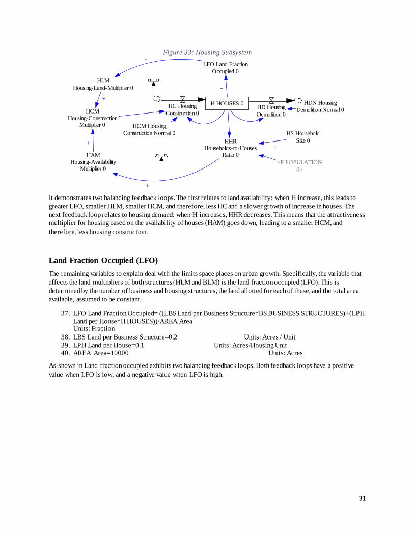
Figure 33: Housing Subsystem
It demonstrates two balancing feedback loops. The first relates to land availability: when H increase, this leads to
greater LFO, smaller HLM, smaller HCM, and therefore, less HC and a slower growth of increase in houses. The
next feedback loop relates to housing demand: when H increases, HHR decreases. This means that the attractiveness
multiplier for housing based on the availability of houses (HAM) goes down, leading to a smaller HCM, and
therefore, less housing construction.
Land Fraction Occupied (LFO)
The remaining variables to explain deal with the limits space places on urban growth. Specifically, the variable that
affects the land-multipliers of both structures (HLM and BLM) is the land fraction occupied (LFO). This is
determined by the number of business and housing structures, the land allotted for each of these, and the total area
available, assumed to be constant.
37. LFO Land Fraction Occupied= ((LBS Land per Business Structure*BS BUSINESS STRUCTURES)+(LPH
Land per House*H HOUSES))/AREA Area Units: Fraction
38. LBS Land per Business Structure=0.2 Units: Acres / Unit
39. LPH Land per House=0.1 Units: Acres/Housing Unit 40. AREA Area=10000 Units: Acres
As shown in Land fraction occupied exhibits two balancing feedback loops. Both feedback loops have a positive
value when LFO is low, and a negative value when LFO is high.
H HOUSES 0
LFO Land Fraction
Occupied 0
+
HC Housing
Construction 0HD Housing
Demolition 0
HCM Housing
Construction Normal 0
HCMHousing-Construction
Multiplier 0
HLM
Housing-Land-Multiplier 0
HDN Housing
Demolition Normal 0
-
+
HAMHousing-Availability
Multiplier 0
HHRHouseholds-to-Houses
Ratio 0
+
-
+
HS Household
Size 0-
<P POPULATION
0>
32
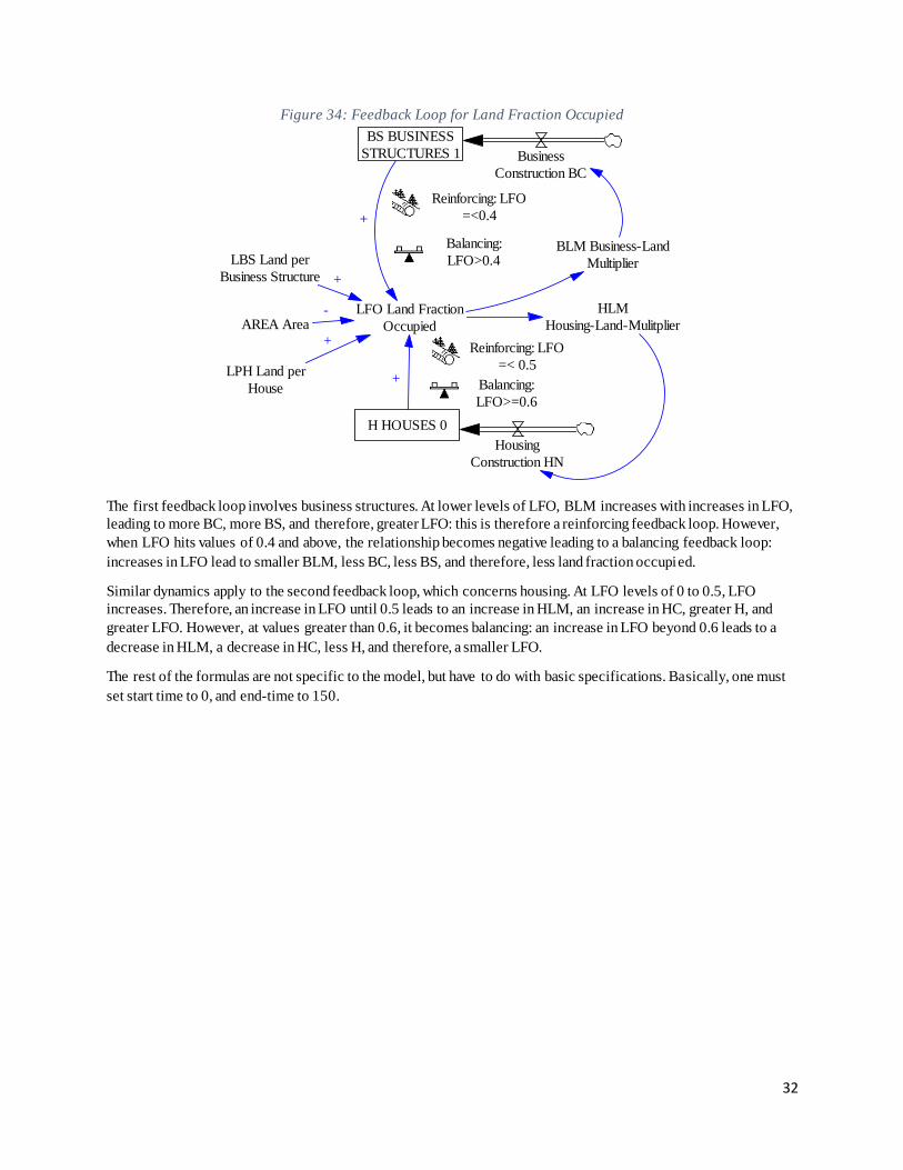
Figure 34: Feedback Loop for Land Fraction Occupied
The first feedback loop involves business structures. At lower levels of LFO, BLM increases with increases in LFO,
leading to more BC, more BS, and therefore, greater LFO: this is therefore a reinforcing feedback loop. However,
when LFO hits values of 0.4 and above, the relationship becomes negative leading to a balancing feedback loop:
increases in LFO lead to smaller BLM, less BC, less BS, and therefore, less land fraction occupied.
Similar dynamics apply to the second feedback loop, which concerns housing. At LFO levels of 0 to 0.5, LFO
increases. Therefore, an increase in LFO until 0.5 leads to an increase in HLM, an increase in HC, greater H, and
greater LFO. However, at values greater than 0.6, it becomes balancing: an increase in LFO beyond 0.6 leads to a
decrease in HLM, a decrease in HC, less H, and therefore, a smaller LFO.
The rest of the formulas are not specific to the model, but have to do with basic specifications. Basically, one must
set start time to 0, and end-time to 150.
LFO Land Fraction
Occupied
HLM
Housing-Land-Mulitplier
BLM Business-Land
MultiplierLBS Land per
Business Structure
AREA Area
LPH Land per
House
+
-
+
BS BUSINESS
STRUCTURES 1
+
H HOUSES 0
+
Business
Construction BC
Housing
Construction HN
Reinforcing: LFO
=<0.4
Reinforcing: LFO
=< 0.5
Balancing:
LFO>0.4
Balancing:
LFO>=0.6
33
XIV. TABLE OF FIGURES
FIGURE 1 GLOBAL CONSUMPTION TRENDSSOURCE: COPIED FROM RICE ALMANAC, 4TH EDITION
(IRRI, 2013) 4
FIGURE 2 FACTORS AFFECTING FOOD SUFFICIENCY 4
FIGURE 3 AREA HARVESTED AND AGRICULTURAL LANDSOURCE: FAO AND WORLD BANK 5
FIGURE 4 SHARES OF SECTORS IN EMPLOYMENT 5
FIGURE 5 POPULATION IN RURAL AREAS 5
FIGURE 6 GROSS VALUE ADDED PER WORKER, BY SECTOR 6
FIGURE 7 GROSS VALUE ADDED, AGRICULTURE ONLY 6
FIGURE 8 AGRICULTURAL INVESTMENTS BY TYPE OF CAPITAL SOURCE: FAO STATISTICS 6
FIGURE 9 GLOBAL YIELD GROWTH FOR RICE, ANNUAL AVERAGES SOURCE: FAO 7
FIGURE 10 IMPACT OF CLIMATE CHANGE ON RICE YIELDS 7
FIGURE 11 MAIN CAUSAL LOOPS IN URBAN1 MODEL 8
FIGURE 12: MAIN REFERENCE MODE IN URBAN1 MODEL 9
FIGURE 13 INTERACTIONS BETWEEN URBAN AND RURAL POPULATIONS 10
FIGURE 14 URBAN1 MODEL SIMULATION RESULTS 11
FIGURE 15 RURAL POPULATION SENSITIVITY TESTS 11
FIGURE 16 AGRICULTURAL PRODUCTION IN RURAL AREAS 12
FIGURE 17 ACTUAL CONSUMPTION PER RURAL POPULATION 12
FIGURE 18 URBAN AND RURAL POPULATION SHARES 13
FIGURE 19 AGRICULTURAL PRODUCTION 13
FIGURE 20 CONSUMPTION PER URBAN AND RURAL POPULATION 14
FIGURE 21 AGRICULTURAL STOCK AND DYNAMICS AFFECTING IT 15
FIGURE 22 DYNAMICS OF SECTOR GROWTH 16
FIGURE 23 DELAYS IN SECTOR GROWTH 17
FIGURE 24 CONSUMER UTILITY PER SECTOR OUTPUT AND AUTO-REBALANCING MECHANISM OF
PRICES 18
FIGURE 25 INCENTIVE SYSTEM FOR INPUTS TO PRODUCTION IN AGRICULTURE AND NON-
AGRICULTURE SECTORS 19
FIGURE 26 DELAYS IN SECTOR GROWTH 20
FIGURE 27 ALTERNATIVE FUTURES BASED ON IMPLEMENTATION OF RECOMMENDATIONS 21
FIGURE 28: POPULATION SUBSET 26
FIGURE 29: BUSINESS STRUCTURES SUBSET 27
FIGURE 30: INTERACTION OF BUSINESS STRUCTURES AND POPULATION 28
FIGURE 31: BALANCING FEEDBACK LOOP FOR POPULATION 29
FIGURE 32: BALANCING FEEDBACK LOOP FOR BUSINESS STRUCTURES 29
FIGURE 33: HOUSING SUBSYSTEM 31
FIGURE 34: FEEDBACK LOOP FOR LAND FRACTION OCCUPIED 32