Dynamic Slicing of Object-Oriented

andAspect-Oriented Softwares

Alina Mishra(Roll no.: 211CS3376)

Department of Computer Science and Engineering

National Institute of Technology, Rourkela

Odisha - 769 008, India

Dynamic Slicing of Object-Oriented

and

Aspect-oriented Softwares

Thesis submitted in partial fulfillment

of the requirements for the degree

of

Master of Technology

by

Alina MishraRoll no-211CS3376

under the guidance of

Prof. Durga Prasad Mohapatra

Department of Computer Science and Engineering

National Institute of Technology, Rourkela

Odisha,769 008, India

June 2013

Department of Computer Science and EngineeringNational Institute of Technology RourkelaRourkela-769 008, Odisha, India.

June 3, 2013

Certificate

This is to certify that the work in the thesis entitled “Dynamic Slicing of Object-

Oriented and Aspect-Oriented Softwares” by Alina Mishra is a record of an

original research work carried out under my supervision and guidance in partial fulfillment

of the requirements for the award of the degree of Master of Technology in Computer Science.

Neither this thesis nor any part of it has been submitted for any degree or academic award

elsewhere.

Prof. Durga Prasad Mohapatra

Associate Professor

Computer Science and Engineering, NIT Rourkela

Acknowledgement

“No one walks alone on the journey of life. just where do you start to thank those that

joined you, walked beside you, and helped you along the way.....”

Thank you God for showing me the path. . .

I owe deep gratitude to the ones who have contributed greatly in completion of this thesis.

Foremost, I would like to express my sincere gratitude to my advisor, Prof. Durga Prasad

Mohaptra for providing me with a platform to work on challenging areas of Program Slicing.

His profound insights and attention to details have been true inspirations to my research.

I am very much indebted to Prof. Santanu Kumar Rath, Prof. Ashok Kumar Turuk

and Prof. Banshidhar Majhi for their encouragement and insightful comments at different

stages of thesis that were indeed thought provoking.

Most importantly, none of this would have been possible without the love of Papa and

Maa. My family to whom this dissertation is dedicated to, has been a constant source of

love, concern, support and strength all these years. I would like to express my heartfelt

gratitude to them.

I would like to thank all my friends and lab-mates for their encouragement and under-

standing. Their help can never be penned with words.

Alina Mishra

Abstract

Program slicing is a program analysis technique that uses program statement dependence

information to identify parts of a program that influence or are influenced by an initial set

of program points of interest (called the slice criteria). Slicing is generally based on program

code. An alternative approach to compute the slice is from specifications developed using

formalism such as Unified Modeling Languages(UML). Moreover in component based soft-

ware development, only the specifications are available and the source code is proprietary.

UML is widely used for object-oriented modeling and design. In our research, we focus

on UML communication diagram to compute the dynamic slices because communication

diagrams model the dynamic behaviour. We first develop a suitable intermediate represen-

tation for communication diagram named as Communication Dependence Graph (CoDG).

Then, we propose two dynamic slicing algorithms. We have named the first algorithm edge-

marking dynamic slicing algorithm for communnication diagram (EMACD) and the second

node-marking dynamic slicing algorithm for communnication diagram (NMACD). To verify

the correctness and preciseness of our algorithms, we have implemented our algorithms and

also calculated the space and time complexity.

Aspect-oriented Programming (AOP) is a recent programming paradigm that focuses on

modular implementations of various crosscutting concerns. In our research, we proposed a

technique for dynamic slicing of aspect-oriented software based on the UML communica-

tion diagram. Next, we generate an intermediate representation from the communication

diagram which we named as Communication Aspect Dependency Graph (CADG). Then,

we proposed an edge marking dynamic slicing algorithm named as Aspect-Oriented Edge

Marking Algorithm (AOEM). The novelty in our approach is that we present the commu-

nication diagram for the aspect-oriented software. We have implemented the algorithm and

also found the space and time complexity of the algorithm.

Keywords: UML, Communication Diagram, Communication Dependence Graph (CoDG),

EMACD, NMACD,Communication Aspect Dependency Graph (CADG), AOEM.

Contents

1 Introduction 2

1.1 Categories of Program Slicing . . . . . . . . . . . . . . . . . . . . . . . . . . 4

1.1.1 Static slicing . . . . . . . . . . . . . . . . . . . . . . . . . . . . . . . 4

1.1.2 Dynamic slicing . . . . . . . . . . . . . . . . . . . . . . . . . . . . . . 5

1.1.3 Simultaneous dynamic slicing . . . . . . . . . . . . . . . . . . . . . . 6

1.1.4 Quasi-static slicing . . . . . . . . . . . . . . . . . . . . . . . . . . . . 7

1.1.5 Amorphous slicing . . . . . . . . . . . . . . . . . . . . . . . . . . . . 7

1.2 Motivation for Our Work . . . . . . . . . . . . . . . . . . . . . . . . . . . . . 7

1.3 Objectives of Our Work . . . . . . . . . . . . . . . . . . . . . . . . . . . . . 9

1.4 Organization of the Thesis . . . . . . . . . . . . . . . . . . . . . . . . . . . . 10

2 Background 11

2.1 Basic Concepts . . . . . . . . . . . . . . . . . . . . . . . . . . . . . . . . . . 11

2.2 Basic UML 2.0 concepts . . . . . . . . . . . . . . . . . . . . . . . . . . . . . 13

2.3 Aspect-oriented programming concepts . . . . . . . . . . . . . . . . . . . . . 16

2.4 Applications of Slicing . . . . . . . . . . . . . . . . . . . . . . . . . . . . . . 18

2.4.1 Program Differencing . . . . . . . . . . . . . . . . . . . . . . . . . . . 19

2.4.2 Regression Testing . . . . . . . . . . . . . . . . . . . . . . . . . . . . 19

2.4.3 Program Debugging . . . . . . . . . . . . . . . . . . . . . . . . . . . 20

2.4.4 Reverse Engineering . . . . . . . . . . . . . . . . . . . . . . . . . . . 20

2.4.5 Software Maintenance . . . . . . . . . . . . . . . . . . . . . . . . . . 20

3 Review of Related Work 21

3.1 Slicing of Procedural and Object-oriented Programs . . . . . . . . . . . . . . 21

3.2 Slicing of Object-oriented Architectural Models . . . . . . . . . . . . . . . . 23

3.3 Slicing of Aspect-oriented Softwares . . . . . . . . . . . . . . . . . . . . . . . 24

CONTENTS ii

4 Dynamic Slicing of Communication Diagram 26

4.1 Basic Concepts And Definition . . . . . . . . . . . . . . . . . . . . . . . . . . 27

4.2 Dynamic Slicing of UML Communication Diagram . . . . . . . . . . . . . . 28

4.2.1 Edge Marking Dynamic Slicing Algorithm for Communication Diagram 28

4.2.2 Communication Dependence Graph . . . . . . . . . . . . . . . . . . 31

4.2.3 Working of EMACD algorithm . . . . . . . . . . . . . . . . . . . . . 33

4.2.4 Correctness of EMACD Algorithm . . . . . . . . . . . . . . . . . . . 36

4.2.5 Complexity Analysis of EMACD Algorithm . . . . . . . . . . . . . . 36

4.2.6 Comparison with the related work . . . . . . . . . . . . . . . . . . . . 38

4.2.7 Node Marking Dynamic Slicing Algorithm for Communication Diagram 39

4.2.8 Working of NMACD algorithm . . . . . . . . . . . . . . . . . . . . . 40

4.2.9 Correctness of NMACD Algorithm . . . . . . . . . . . . . . . . . . . 43

4.2.10 Complexity Analysis of NMACD Algorithm . . . . . . . . . . . . . . 43

4.2.11 Comparison Between EMACD and NMACD . . . . . . . . . . . . . . 43

4.3 Implementation . . . . . . . . . . . . . . . . . . . . . . . . . . . . . . . . . . 44

4.3.1 Experimental Results . . . . . . . . . . . . . . . . . . . . . . . . . . . 45

5 Dynamic Slicing of Aspect-oriented UML Communication Diagram 47

5.1 Basic Concepts and Definition . . . . . . . . . . . . . . . . . . . . . . . . . . 48

5.2 Dynamic Slicing of Aspect-oriented UML Communication Diagram . . . . . 51

5.2.1 Aspect-Oriented Edge Marking Algorithm (AOEM) . . . . . . . . . 51

5.2.2 Communication Aspect Dependency Graph . . . . . . . . . . . . . . 53

5.2.3 Working of AOEM algorithm . . . . . . . . . . . . . . . . . . . . . . 55

5.2.4 Complexity Analysis of AOEM algorithm . . . . . . . . . . . . . . . . 58

5.2.5 Comparison with the related work . . . . . . . . . . . . . . . . . . . . 58

5.3 Implementation . . . . . . . . . . . . . . . . . . . . . . . . . . . . . . . . . . 59

5.3.1 Experimental Results . . . . . . . . . . . . . . . . . . . . . . . . . . . 60

6 Conclusions and Future Work 62

6.1 Contributions . . . . . . . . . . . . . . . . . . . . . . . . . . . . . . . . . . . 62

6.1.1 Dynamic Slicing of UML communication Diagram . . . . . . . . . . . 62

6.1.2 Dynamic Slicing of Aspect-oriented UML Communication Diagram . 63

List of Publications from the Thesis 64

BIBLIOGRAPHY 64

List of Figures

2.1 An Example Program . . . . . . . . . . . . . . . . . . . . . . . . . . . . . . . 12

2.2 Control Flow Graph for the example given in Fig.2.1 . . . . . . . . . . . . . 12

2.3 Classification of different types of UML diagrams . . . . . . . . . . . . . . . 14

2.4 An example of communication diagram showing Withdraw() usecase of ATM 15

2.5 An example of communication diagram showing IssueTicket()usecase of On-

line Railway Reservation System . . . . . . . . . . . . . . . . . . . . . . . . . 17

4.1 Communication Diagram for IssueBook usecase of Library Management System 29

4.2 Control Flow Graph of IssueBook example shown in Fig.4.1 . . . . . . . . . 30

4.3 Communication Dependence Graph of IssueBook example shown in Fig. 4.1 32

4.4 Updated CoDG of communication diagram in Fig. 4.1showing dynSlice(16)for

EMACD algorithm . . . . . . . . . . . . . . . . . . . . . . . . . . . . . . . . 35

4.5 Updated CoDG of communication diagram in Fig. 4.1 showing dynSlice(16)

for NMACD algorithm . . . . . . . . . . . . . . . . . . . . . . . . . . . . . . 42

4.6 Snapshots of GUI to give input to both EMACD and NMACD algorithm . 45

4.7 Screenshot of the EMACD algorithm showing dynSlice(16) . . . . . . . . . . 45

4.8 Screenshot of the NMACD algorithm showing dynSlice(16) . . . . . . . . . . 45

4.9 Comparison of Average run-time for EMACD and NMACD . . . . . . . . . . 46

5.1 Aspect-oriented communication diagram for IssueBook scenario of Library

Management System . . . . . . . . . . . . . . . . . . . . . . . . . . . . . . . 50

5.2 Control Flow Graph of IssueBook example shown in Fig.5.1 . . . . . . . . . 52

5.3 Communication Aspect Dependency Graph of IssueBook example shown in

Fig. 5.1 . . . . . . . . . . . . . . . . . . . . . . . . . . . . . . . . . . . . . . 54

5.4 Updated CADG of IssueBook example shown in Fig. 5.1 showing dynSlice(19)

for AOEM algorithm . . . . . . . . . . . . . . . . . . . . . . . . . . . . . . . 57

5.5 Snapshots of GUI to give input for AOEM algorithm . . . . . . . . . . . . . 60

LIST OF FIGURES iv

5.6 Snapshot of the AOEM algorithm showing dynSlice(19) . . . . . . . . . . . . 60

5.7 Average run-time of AOEM algorithm for different communication diagram . 61

List of Tables

4.1 Updated Dynamic Slice Of Each Node . . . . . . . . . . . . . . . . . . . . . 37

4.2 Average run time of EMACD and NMACD algorithm . . . . . . . . . . . . . 46

5.1 Average run time for AOEM algorithm . . . . . . . . . . . . . . . . . . . . . 61

Chapter 1

Introduction

Nearly every transactions carried out in today’s world make use of different types of software

solutions. These software solutions are becoming reasonably complex and their qualities

have been largely bounded by cost and time factors. It has been established that approx-

imately 60% of the software built at present goes unused due to their lack of ability to

meet the above cited constraints, which in turn results in enormous loss of money, time and

manpower. Therefore, software testing activities are extremely important for developing of

reliable software. Object-oriented procedure modularizes the software, but simultaneously,

it is extremely complex and difficult to test and debug for errors.

Program slicing is a reverse engineering technique that has been usually studied since it was

first proposed in 1979 [38]. It is a significant method which has many applications in the

field of software testing. Program slicing offers a innovative way to perform software mainte-

nance and software understanding. Program slicing is defined as a decomposition strategy

which removes program statements that are not applicable to a particular computation,

known as slicing criterion. The residual statements form an executable program called a

slice that outline a distinction of the original programs definition. It provides programmer

the statements that are only relevant to computation of a given function. Essentially, pro-

gram slicing is a technique for simplifying programs by giving emphasis on selected aspects

of semantics. It is also a method of program analysis used to extract a set of statements

from a program which is relevant for a particular computation.

Slicing of a program is done with respect to a slicing criterion . Usually, a slicing criterion

defined as a pair 〈S,V〉 , where S is the statement number and V defines the set of variables.

A slice of a given program P with respect to a given slicing criterion 〈S,V〉, is the set of all

the statements of the program P that might affect the slicing criterion for every possible

3

input to the program. Various assumptions of program slices have been proposed [5, 38].

Also, a number of methods have been proposed to compute the slices. The main motivation

for this large number of slicing techniques lies in the fact that different types of applications

need different properties of slices.

Program slicing technique has been widely studied and applied deeply into all the phases

of software engineering. In the requirement stage, we analyse the Software Requirement

Specification (SRS) document dynamically and problem is discovered as soon as possible.

In the design stage, slicing of architecture or UML models is used to create the module with

low coupling and high cohesion, hence reducing complexity of the software. In applications

like coding, testing, maintenance phase, program slicing techniques can be used to achieve

code optimization and localisation of error.

As defined by Weiser [38] a program slice S is a reduced, executable program obtained from

a program P by removing statements, in such a way that S replicate part of the behaviour

of P. Executable does not mean that the slice is only a closure of statements, but it also

can be compiled and run. The slicing technique initially proposed by Weiser [38–40] is

currently called as static backward slicing because the slices that are obtained do not de-

pend on the input values. It is considered as backward slicing because during computation

of slices, the flow of control is in backward direction of the program. A forward slice [35]

contains all statements depending on the slicing criterion, whereas backward slice contains

all statements that slicing criteria may depend on. Another definition of a slice is that it is a

subset of the statements and control predicates of the program which directly or indirectly

affect the values computed at the slicing criterion, but which do not essentially form an

executable program. Admirable surveys of program slicing are available in [5, 35,42]

The high-level design configuration of object-oriented software is defined by its architec-

ture. Architectural design models are more helpful as the size and complexity of software

increases. The significant uses of architectural design models are assessment, understanding

and testing a proposed solution [22]. Unified Modeling Language (UML) is most widely

used for construction of architectural models of complex and large software [22]. It offers

a broad collection of visual artifacts for modeling the various aspects of a system. As the

software size and complexity tends to increase, UML models also become more complex

which involves hundreds of objects and thousands of interactions among them. Hence, it

becomes very difficult to handle, analyze and comprehend these models. Since the infor-

mation regarding a system is scattered across a range of model views shown using various

diagrams, evaluating the UML models is a challenge. Analysing the effect of a modification

in one model on another model therefore becomes an imperative problem. For such vast

1.1 Categories of Program Slicing 4

architectures, it becomes tremendously demanding to analyse these models. Moreover, it

turns out to be difficult on one hand and equally advantageous on the other to discover the

consequence of a particular change to one model on other models.

With this motivation, different program slicing techniques are introduced to modularize

huge architectural modules into smaller and manageable modules. However, considering

the software architectures, a slicing technique should recognize different characteristics of

UML diagrams such as use cases, classes and relationships among them, and objects and

interactions between them, etc. In UML 2.0 models, interaction is represented using differ-

ent diagrams like communication diagram, sequence diagram, interaction overview diagram

and timing diagram. A communication diagram is comprised of objects and associations

which shows how the objects are communicating. One advantage of using communication

diagram is that it does not consider the timing aspect of the interaction, rather it focuses on

objects and the communication between them. Also, communication diagram is compact in

size compared to sequence diagram since timeline is not used in it. In a sequence diagram

whenever we need to add any object it is added to the right of the diagram. Hence, sequence

diagram sometimes becomes very unwieldy. Therefore, we have used the communication

diagram for analyzing the dynamic behavior of the system. To perform architectural slic-

ing, it is first required to transform architectural model into a appropriate intermediate

representation which represent various relationship that is present among different elements

within models. This intermediate representation is then evaluated by the slicing algorithms

to compute the slices.

1.1 Categories of Program Slicing

Several categories of program slicing are found in literature. Program slicing is mainly

classified into two categories, namely static slicing [40] and dynamic slicing [40]. Depending

upon the application, slicing can also be classified as forward slice or backward slice [14],

inter-procedural or intra-procedural slice [14]. Other categories of slicing includes quasi-

static slicing, amorphous slicing and simultaneous dynamic slicing.

1.1.1 Static slicing

As defined by Weiser, a program slice includes the parts or components of a program that

influence the values computed at some point of interest known as a slicing criterion [5].

1.1 Categories of Program Slicing 5

Usually, a slicing criterion comprises of a pair 〈S, V〉, where S is defined as the statement

number and V as a set of variables. Statistically obtainable information is utilised for slicing

thus this type of slicing is called as static slicing.

Example:

(1) DataInputStream di = new DataInputStream (System.in);

(2) var= Integer.parseInt(di.readLine());

(3) prod=1;

(4) sum=0;

(5) for(count=1; count<=var; count++) {(6) sum=sum+count;

(7) prod=prod*count; }(8) System.out.println(“The Sum is : ”+sum);

(9) System.out.println(“The Product is :” + prod);

Slice: with respect to the slicing criteria (8, sum).

(1) DataInputStream di = new DataInputStream(System.in);

(2) var= Integer.parseInt(di.readLine());

(4) sum=0;

(5) for(count=1; count<=var; count++) {(6) sum=sum+count; }(8) System.out.println(“The Sum is : ”+sum);

1.1.2 Dynamic slicing

In program slicing, the slicing criterion comprises of the variables that produce an unex-

pected result on some given input to the program [45]. But, a static slice may include

statements which have no influence on the values of the variables of interest for the partic-

ular execution. Dynamic slicing takes the input given to the program during its execution

and the slice contains only those statements that cause the failure while specific execution

of interest. Dynamic analysis is used by dynamic slicing to find all and only the statements

that have an effect on the variables of interest on particular execution trace [5]. The benefit

of dynamic slicing is run-time handling of pointer variables and arrays.

Dynamic slicing will take care of each element of an array independently, while static slicing

considers every definition or use of some array element as a definition or use of the complete

array [19]. In the same way, dynamic slicing differentiates the objects that are pointed to

by pointer variables in a program execution. A dynamic slicing criterion represents the in-

1.1 Categories of Program Slicing 6

put, and makes a distinction between dissimilar occurrences of a statement in an execution.

Slicing criteria is defined as a triplet (input, statement number, variable). The difference

between dynamic and static slicing is that dynamic slicing takes fixed input for a program,

while static slicing does not make postulations regarding the input [7].

Example:

(1) DataInputStream di = new DataInputStream (System.in);

(2) p= Integer.parseInt(di.readLine());

(3) i=1;

(4) while (i<=p) {(5) if (i mod 2==0) then

(6) a=17; else

(7) a=18;

(8) i=i+1; }(9) System.out.println(a);

Slice: slice with criterion (p = 2, 9, a)

(1) DataInputStream di = new DataInputStream (System.in);

(2) p= Integer.parseInt(di.readLine());

(3) i=1;

(4) while (i<=p) {(5) if (i mod 2==0) then

(6) a=17;

(8) i=i+1; }(9) System.out.println(a);

1.1.3 Simultaneous dynamic slicing

Hall [12] proposed a different approach to the definition of a slice regarding a set of executions

of the program. This innovative slicing method merges the use of a set of test cases with

program slicing [6]. This method is known as simultaneous dynamic program slicing as it

expands and at the same time applies to a set of test cases, the dynamic slicing technique

which generates executable slices that are accurate on only one input.

1.2 Motivation for Our Work 7

1.1.4 Quasi-static slicing

Quasi static slicing method was first introduced by Venkatesh [37]. It is an amalgam or

fusion of Static Slicing and Dynamic Slicing. Static slicing is observed during compile time,

without using information regarding the input variables of the program. Dynamic slicing

analyses the code by means of giving input to the program. It is created at run time

corresponding to a particular input. Also, there is a trade-off between dynamic and static

slicing methods. Static slicing requires more space and resources as well as performs all

feasible execution of the program but dynamic slicing requires less space and is specific to

a program execution. In addition, dynamic slices are smaller than static slice.

In case of quasi slicing the value of a few variables are fixed, while the value of other

variables vary. Slicing criteria consists of the set of variables of interest and initial conditions

and hence quasi slicing is called as Conditioned slicing. This technique is unsuccessful

to establish consistent treatment of static and dynamic slicing. In addition, there is no

algorithmic description for this technique.

1.1.5 Amorphous slicing

The slicing methods discussed formerly such as static and dynamic slicing, simultaneous

dynamic slicing and quasi static slicing etc. are syntax preserving, while amorphous slicing

is focused on preserving the semantics of the program. Syntax preserving slicing technique

is based on deleting statements from the program based on the slicing criterion and thus

the syntax of the program statements does not alter even after slicing is carried out. In case

of amorphous slicing [13], slice is obtained using some program transformation technique

that preserves the semantics of the program corresponding to the slicing criterion. The

slices formed are not as large as obtained through other slicing techniques. The slice is

significantly simplified form of the program based on the slicing criterion. The advantage

of amorphous slicing includes program comprehension, analysis and reuse.

1.2 Motivation for Our Work

A most important intend of all the slicing techniques is to recognize as small a slice cor-

responding to a slicing criterion as possible because smaller slices are more useful. To a

large extent of available literature on program slicing, it is observed that improving the

algorithms for slicing is done in terms of improving the efficiency of the slicing algorithm

1.2 Motivation for Our Work 8

and reducing the size of the slice.

Slicing is commonly based on program code. An alternative approach is to compute the

slice from specifications created with the help of formalism such as UML models. In this

approach, slices are computed during analysis or design stage itself, preferably at low-level

design stage. Also, in component based software development, only the component speci-

fications are available and the source code of components are proprietary. Computing the

slice from design specifications adds the benefit of permitting slices to be obtainable early in

the software development life cycle. It is therefore, enviable to compute slices from software

design document besides computing slices from the code.

UML is extensively used for modelling and design of object-oriented software. In recent

times, numerous techniques have been proposed to execute different UML models. Exe-

cutable UML models permit model specifications to be efficiently converted into code. In

addition to reducing effort in the coding stage, it too guarantees platform independence and

evade obsolescence. This is so because the code frequently needs to change while software

is ported to a new platform. Our computation of slice can also be employed on executable

UML models.

With this motivation, we give attention to UML communication diagrams for computation

of the slices. A major purpose of this technique is program debugging i.e. to search for the

errors during the execution of software. Also, these errors are usually dynamic (behavioural)

in nature. Customer comprehends software in terms of behaviour and not structure. There-

fore, we choose the communication diagram for our work.

AOP is an emerging implementation level method which allows isolating pieces of behaviour

into separate units called aspects. Much of the literature on slicing of AOP is based on code.

Till now no work is done to develop a formal design specification for AOP based software

and slicing of design models for the same. The main advantage of this technique is that

it clearly modularises the crosscutting services. It also gives the benefit of platform in-

dependence and obtaining the slice at an early stage. With this motivation, we focus on

developing a communication diagram for the Aspect-oriented software and also developing

an algorithm for slicing of it.

The above reasons motivate us to identify the major goals of our thesis and for developing

dynamic slicing algorithms for UML communication diagrams and aspect based communi-

cation diagram.

1.3 Objectives of Our Work 9

1.3 Objectives of Our Work

The foremost objective of our work is to develop dynamic slicing algorithms for object-

oriented and aspect-oriented software. Our key goals are:

• We wish to compute dynamic slices of UML communication diagram for object-

oriented software as fast as possible.

To achieve this, we plan to develop:

1. Suitable intermediate representations for UML communication diagram on which

the slicing algorithm can be applied.

2. Dynamic slicing algorithms for object-oriented software, using the proposed in-

termediate representation.

• Dynamic slicing of architectural models are valuable for debugging purposes and hence

competent computation of dynamic slices is extremely significant to interactively im-

pound bugs in an object-oriented program. Present techniques of dynamic slicing

experience the difficulty of huge space and run-time overheads. Our goal would, thus,

be to develop techniques that are more space and time efficient.

• Subsequently, we desire to expand this approach to compute dynamic slices of archi-

tectural models of aspect-oriented software. AOP helps to modularise the croscutting

concerns in a software. Also, it enables more code reuse and reduce the costs of feature

implementation. In this approach, slices are computed during analysis or design stage

itself, preferably during low-level design stage. We have considered aspect based UML

communication diagram to compute the slice.

To achieve this, we plan to develop:

1. Suitable aspect based communication diagram for representing the dynamic be-

haviour of aspect-oriented software.

2. Suitable intermediate representations for aspect based communication diagram

on which the slicing algorithm can be applied.

3. Dynamic slicing algorithms for slicing of aspect based communication diagrams,

using the proposed intermediate representation.

1.4 Organization of the Thesis 10

1.4 Organization of the Thesis

Our thesis is divided into chapters that are organized as follows:

Chapter 2 includes the background concepts used in the rest of the thesis. The chapter

contains some graph-theoretic concepts which will be used afterwards in our algorithms.

We illustrate some intermediate program representation concepts which are used in slicing

techniques. Then, we discuss some applications of dynamic slicing. In the end, we discuss

the concepts of aspect-oriented software and benefits of using AOP software.

Chapter 3 presents a concise review of the related work significant to our contribution.

We initially consider the work on dynamic slicing of architectural models representing object-

oriented software followed by description of the work on slicing of aspect-oriented softeware.

Chapter 4 deals with dynamic slicing of UML communication diagram for object-oriented

software. We discuss how to develop a suitable intermediate representation for communi-

cation diagrams which we named communication dependence graph. Next, we explain two

dynamic slicing algorithms i.e. edge marking and node marking dynamic slicing algorithm

for communication diagram with example. We have implemented and proved that this

algorithm computes correct dynamic slices.

Chapter 5 deals with dynamic slicing of aspect-based communication diagram for aspect-

oriented software. We discuss the process to develop an appropriate intermediate representa-

tion for communication diagrams which we named communication aspect dependency graph.

Next, we explain an edge marking dynamic slicing algorithm for aspect based communi-

cation diagram with example. We have also implemented and found the space and time

complexities for our proposed algorithm.

Chapter 6 concludes the thesis by giving a summary of our contributions. We also discuss

the achievable future extensions to our work.

Chapter 2

Background

Program slicing is very helpful in different applications like software testing, software mea-

surement, software maintenance, program parallelization, program debugging, etc. since a

slice is a supreme subset of the original program that guarantees to authentically demon-

strate the particular behaviour of the original program within the specified domain. Since

Weiser [38] initially proposed the notion of program slicing in 1979, different properties of

slicing have been proposed to compute more accurate slices as well as to employ slice in

different stages of SDLC (Software Development Life Cycle). This chapter deals with the

essential concepts, definition and terminologies related with the slicing of object-oriented

and aspect-oriented software at the design stage of the software development.

2.1 Basic Concepts

This section briefly describes some fundamental definitions and terminologies related with

the intermediate representation.

Definition 2.1 Directed Graph: A directed graph G is a pair (N,E) where N represents

a finite non-empty set of nodes, and E ⊆ N ×N represents a set of directed edges between

the nodes. Consider G = (N,E) be a directed graph. If (x, y) is an edge of G, then x is

called a predecessor of y and y is called a successor of x. The predecessors of a node adds

up to give its in-degree, and the successors of a node adds up to give its out-degree. In this

thesis, we use interchangeably the words graph and directed graph.

2.1 Basic Concepts 12

Figure 2.1: An Example Program

Start

1 2 3 4

5

67

8

9 Stop

Figure 2.2: Control Flow Graph for the example given in Fig.2.1

Definition 2.2 Flow Graph: A flow graph is a quadruple (N,E, Start, Stop) in which

(N,E) is a graph, Start ∈ N is a distinguished node of in-degree zero called the start node,

Stop ∈ N is a distinguished node of out-degree zero called the stop node, there exists a path

from Start to every other node in the graph, and there exists a path from every other node

in the graph to Stop.

Definition 2.3 Control Flow Graph: Let the set N represent the set of statements of a

program P . The control flow graph of the program P is the flow graphG= (N1, E, Start, Stop)

where N1 = N ∪ (Start, Stop). An edge (m,n) ∈ E indicates the possible flow of control

from the node m to the node n. Note that the subsistence of an edge (x, y) in the control

flow graph means that control must transfer from x to y during program execution. Fig.2.2

represents the CFG of the example program given in Fig.2.1. The CFG of a program P

form the branching structures of the program, and it can be build while parsing the source

2.2 Basic UML 2.0 concepts 13

code using algorithms that include linear time complexity in the size of the program.

2.2 Basic UML 2.0 concepts

Unified Modeling Language (UML) is defined as a graphical idiom for envisioning, identify-

ing, creating and documenting the artifacts of a software system.UML is a blueprint of the

actual system and helps in documentation of the system [4]. It makes any complex system

easily understandable by the disparate developers who are working on different platforms.

Another benefit is that UML model is not a system or platform specific. Modeling is an

indispensable part of huge software projects, which as well facilitates in the improvement of

medium and small projects. There are numerous explanations to use UML as a modeling

language:

• The amalgamation of terminology and the consistency of notation escort to a consid-

erable easing of communication in the software industry. It assists the swapping of

models among different departments or companies.

• UML is widely supported and is platform independent, hence assists developers work-

ing in different platforms.

• UML-based software offers easiness for comparison among different software systems

based on structure and behavior.

• Using UML helps new developers to understand the software more easily and also

lowers the development cost.

UML 2.x has 14 types of diagrams divided into two categories. Seven diagram types

represent structural information, and the other seven represents general types of behavior,

including four that represent different aspects of interactions.

1. Behavioural diagrams: Diagrams which characterize the behavioral features of a

software system. This category includes use case diagram, activity diagram and state-

machine diagram in addition to four interaction diagrams.

2. Interaction diagrams: Interaction diagrams are subset of behavioural diagrams

which emphasize interactions among objects. This category includes communication

diagram, interaction overview diagram, sequence diagram, and timing diagram.

2.2 Basic UML 2.0 concepts 14

3. Structured diagrams: These diagrams show the constituent of a specification that

does not depend upon time. This category includes class diagram, composite struc-

ture diagram, component diagram, deployment diagram, object diagram, and package

diagram.

These diagrams can be categorized hierarchically as shown in the Fig.2.3

Figure 2.3: Classification of different types of UML diagrams

In our research, we give attention to UML communication diagram for computing the

dynamic slice at the architectural level. UML communication diagrams are used to illus-

trate the flow of functionality during execution of a use case. A communication diagram is

comprised of objects and associations which shows how the objects are communicating [1].

One advantage of using communication diagram is that it does not consider the timing as-

pect of the interaction; rather it focuses on objects and the communication between them.

Also, communication diagram is compact in size compared to sequence diagram since time-

line is not used in it. In a sequence diagram, whenever we need to add any object it is

added to the right of the diagram. Hence, sequence diagram sometimes becomes very un-

wieldy. A communication diagram is a useful extension of the object diagram. Object

diagram gives the snapshot of a system at any point of time, but communication diagram

adds the dimension of time and gives the snapshot of the system at various points of time.

Therefore, we have used the communication diagram for analyzing the dynamic behavior of

2.2 Basic UML 2.0 concepts 15

the system. An example of UML 2.0 communication diagram is shown in Fig.2.4. In the

Figure 2.4: An example of communication diagram showing Withdraw() usecase of ATM

diagram, the rectangular box represents objects or lifeline in the communication diagram

arranged in a free form. Messages in the communication diagram are shown as a line with

sequence expression and an arrow above the line. The arrow specifies the direction of the

communication. A message can be an operation call or initiation of execution or a sending

or reception of a signal.

Based on the nature of action a message can be of several types like asynchronous call,

synchronous call, create, reply, delete. Synchronous call messages are represented by filled

arrow head. It symbolizes a function call, i.e. send message and defer execution while

waiting for a response. Asynchronous call is revealed with open arrow head. In case of

asynchronous call, a message is send and the next message is send without waiting for a

response. Create message is sent to a lifeline or object to create itself. Delete message is

sent to terminate another object or lifeline.

To represent extra information in the sequence diagram, “notes” are used. Notes are rep-

resented by symbol of dog-eared rectangle linked to the object lifeline through a dashed

2.3 Aspect-oriented programming concepts 16

line. Notes are basically used for representing additional information like pseudo code, post

condition, pre condition, text annotations, constraints etc.

2.3 Aspect-oriented programming concepts

Aspect-oriented programming (AOP): AOP is an emerging programming paradigm

that focuses on modular implementation of cross-cutting concerns [9] such as exception

handling, synchronization, security, data access, logging. This technique was first introduced

by Gregor Kiczales et al. [17]. Aspect-Oriented Programming provides specific language

mechanisms to explicitly capture the cross-cutting structure. Representation of such cross-

cutting concerns by use of standard language constructs give poorly structured code because

these concerns are tangled with the crucial functionality of the code. This increases the

complexity and creates difficulty in maintenance considerably.

AOP intends to resolve this difficulty by allowing the programmer to build up cross-cutting

concerns as complete stand-alone modules called aspects. The central idea behind AOP

is to build a program by unfolding each concern separately. Aspect-oriented programming

languages provide unique opportunities for program analysis schemes. For instance, to

implement program slicing on aspect oriented software, definite aspect-oriented features

such as join-point, advice, aspect, and introduction must be taken care of appropriately.

Even though these features add great strengths to model the cross-cutting concerns in an

aspect-oriented program, they also introduce difficulties to analyze the program.

Aspects: An aspect is an ordinary feature that’s usually scattered across methods, classes,

object hierarchies, or even whole object models. An aspect is a crosscutting type, defined

by aspect declarations. Aspects may have methods and fields just like any other class. They

may also contain pointcut, advice, and introduction (inter-type) declarations.

Advice: This is a method like construct that is required to define crosscutting behavior.

Advice is classified into three types in AspectJ: before, after, and around. On a defined

joinpoint after advice executes after the program proceeds with that joinpoint. Before the

program proceeds with that joinpoint before advice executes. Around advice executes when

the joinpoint is reached, and has a explicit control over the program whether or not the

program proceeds with that joinpoint.

Crosscutting Concerns: Crosscutting concerns put a negative impact on the quality of

the software developed which can be reduced to a great extent by using aspects [16]. Most

of the classes in object-oriented programming perform a single, specific function, but many

2.3 Aspect-oriented programming concepts 17

a times they share some secondary requirements with other classes. A concern is said to be

crosscutting concern if it satisfies the two characteristics- scattered and tangled. When the

design of a single requirement or functionality is inevitably scattered across several classes

and operations in the object-oriented design, then we say that the functionality is scattered.

When a single class or operation in the object-oriented paradigm encloses design details of

multiple requirements, then it is tangled.

Figure 2.5: An example of communication diagram showing IssueTicket()usecase of Online

Railway Reservation System

2.4 Applications of Slicing 18

Aspect-based Communication Diagram: UML communication diagram is used to

show the communications between different objects involved in a given problem scenario.

The ordering of the messages is shown by the help of numbering technique. In order to draw

the communication diagram, we identify the objects that are participating in the scenario.

Then all the objects are connected using a link. Through the link the messages are sent

between the objects to carry out the given scenario.

In our work, we have considered aspect-oriented based communication diagram to compute

the dynamic slice at the architectural level. As we know, aspects in AOP are similar

to classes in OOP; we have represented the objects of the aspects similar to OOP. In

the example of aspect-oriented (woven) communication diagram shown in Fig.2.5, we have

considered three base classes (Passenger, ServiceController and TrainDatabase), one Aspect

(AccessController), and one Around advice (login).

The aspect in the scenario has a vital impact on the security of the system as it allows

only the authenticated users for the enquiry process. The method p information() of base

class passenger act as joinpoint through pass pointcut designator. We have represented the

pointcut i.e. the first message in dotted line from base class to aspect. At this point of

time, the message is sent and the execution is temporarily stopped until acknowledgement

is received. After the passenger informations are validated the control moves back to the

suspended base class and the execution resumes for enquiring the train details.

2.4 Applications of Slicing

This section illustrates the utilization of program slicing techniques in different applica-

tions. The applications of program slicing techniques has now extended into a powerful

set of tools for use in such various applications as program understanding and verifica-

tion, automated computation of several software engineering metrics, software maintenance

and testing, reverse engineering, parallelization of sequential programs, functional cohe-

sion, software portability, compiler optimization, program integration, reusable component

generation, software quality assurance, etc [10, 35, 39, 42]. Program slicing is exceptionally

useful in abstracting the business rules from traditional systems. A complete study on the

applications of program slicing is made by Binkley and Gallagher [5] and Lucia [26].

2.4 Applications of Slicing 19

2.4.1 Program Differencing

Program differencing [25] is the task of analyzing an old and a new version of a program

in order to establish the set of program components of the new version so as to represent

semantic and syntactic changes. Such information is useful for the reason that only the

program components reflecting changed behavior need to be tested [3]. There are two

linked differencing problems:

1. Identify all the components of two programs which have dissimilar behaviour.

2. Fabricate a program that incarcerates the semantic differences among two programs.

For old and new programs, a clear-cut solution for the problem 1 is achieved by evaluating

the backward slices of the vertices in old and new ’s dependence graphs Gold and Gnew.

Here, the backward slice is computed regarding a given slicing criterion. Components whose

vertices in Gnew and Gold have isomorphic slices have the same behavior in old and new ;

therefore the set of vertices from Gnew for which there is no vertex in Gold with an isomorphic

slice approximates the set of components new with a change in behavior.

An explanation to the next differencing problem is achieved by taking the backward slice

with regard to the set of affected points (i.e., the vertices in Gnew with different behavior

than in Gold). For programs with method calls, two modifications are essential: First, inter-

procedural slicing techniques are required to be used to ensure that the resulting program

slice is executable. Second, this result is overly negative: Let a component c in method P be

invoked from two call-sites c1 and c2. If c is identified as an affected point by a forward slice

that enters P through c1 then we will include c1 but not c2 in the program that captures the

differences. However, the backward slice with respect to c would include both c1 and c2.

2.4.2 Regression Testing

Regression testing [11,44] is the method of testing changes to software in order to ascertain

that the older programming still works with the new changes. Any adverse behavior that

can result due to a small change in the program needs to be tested which might include

running a large number of test cases. Program slicing is very helpful to split tests cases

into those that require to be repeated, since they have been affected by a change, and those

which can be avoided, as their behaviour can be assured to be unaffected by the change.

2.4 Applications of Slicing 20

2.4.3 Program Debugging

Debugging becomes a complicated task when one comes across with a large program and

small solution concerning the location of a bug. The method to find a bug typically entails

running the program repeatedly, learning more and lessening down the search each time,

until the bug is finally located [26]. Program slicing was formerly proposed by examining

the operation naturally carried out by programmers while debugging a piece of code.

Even after several improvements to the fundamental slicing techniques, program debugging

remains a chief application area of slicing techniques. Program slicing is useful for debugging,

since it potentially allows one to overlook many statements in the process of localizing the

bug. If a program determines a flawed value for a variable a, then the statements in the

slice that includes the variable a have added to the result of that value, other statements

which are not present in the slice can be ignored.

2.4.4 Reverse Engineering

Reverse engineering addresses the problem of understanding the existing design of a pro-

gram and the method this design differs from the original design [27]. This includes abstract-

ing out of the source code the design decisions and motivation from the initial development

and understanding the algorithms chosen. Program slicing offers a tool set for this type of

re-abstraction. For example, a program can be demonstrated as a pattern of slices struc-

tured by the is-a-slice-of relation. Evaluating the original lattice and the lattice after (years

of) maintenance can lead an engineer towards places where reverse engineering should be

used. Since slices are not essentially adjoining blocks of code they are suitable to identify

differences in algorithms which may cover multiple blocks or procedures.

2.4.5 Software Maintenance

To preserve huge software system is a demanding task. Majority of the software system

splurge about 70% or more of their lifetime in the phase of software maintenance where

they are enhanced and enlarged. The most important problem in software maintenance is

to determine whether a change at one place in a program will affect the behaviour of other

parts of the program. It is a expensive procedure as each modification to a program must

take into account various composite dependence relationships in the existing software.

Chapter 3

Review of Related Work

This chapter provides an outline of the fundamental program slicing techniques and concise

history about their development. We give a short survey that reviews majority of the

existing slicing techniques including the static slicing, dynamic slicing, slicing of object-

oriented architectural models, and slicing of aspect-oriented software.

3.1 Slicing of Procedural and Object-oriented Programs

This section discusses the related work on static and dynamic slicing of the procedural and

object-oriented programs based on the source code. Program slicing, which was originally

established by Weiser in 1979 [38], is a decomposition method that remove from program

those statements significant to a particular computation. Weiser defined program slicing as

a type of executable backward static slicing. A backward slice contains all statements that

the computation at the slicing criteria may depend on, whereas a forward slice comprises all

statements depending on the slicing criterion. The intra-procedural static slicing algorithm

[39] used Control Flow Graph (CFG) as the intermediate representation of the program. In

Weiser’s algorithm [39,40], slices are designed from scratch i.e. information obtain through

any preceding calculation of slices are not considered. This is a foremost shortcoming of

their approach.

Ottenstein and Ottenstein [30] employ the Program Dependence Graph (PDG) as the in-

termediate representation for computing intra-procedural slices. Horowitz et al. [14] en-

hanced the PDG representation to the System Dependence Graph (SDG) for computing

inter-procedural static slicing. Since 1979, several alternatives of slicing, which are not

static, have been proposed.

3.1 Slicing of Procedural and Object-oriented Programs 22

Korel and Laski [18] extended Weiser’s CFG based static slicing algorithm and introduced

the notion of dynamic slicing. A dynamic slice is different from static slice in the fact that

dynamic slice is computed with regard to only one execution of the program. It does not

include the statements that have no significance with the slicing criteria for some particular

input. The dynamic slice computed by Korel and Laski may be imprecise, if a program

consists of loops, because in that case N may be unbounded where N is the number of

statements executed (length of execution) during run time of the program. This is a major

shortcoming of their approach.

Agrawal and Horgan [2] introduced the algorithm for computing dynamic slices of procedu-

ral programs using dependence graphs. They introduced the notion ofDynamic Dependence

Graph (DDG) to compute precise dynamic slices. The number of nodes in a DDG is same

as the number of statements executed, which may be unbounded for programs containing

loops. Then Agrawal and Horgan [2] tried to reduce the number of nodes by the concept of

Reducing Dynamic Dependence Graph (RDDG).

Mund et al. [29] enhanced their approach and proposed three intra-procedural dynamic

slicing algorithms. Two of the three proposed algorithms compute dynamic slices of struc-

tured program using PDG as an intermediate representation and to compute dynamic slice

of unstructured programs, they introduce the idea of Unstructured Program Dependence

Graph (UPDG) as the intermediate representation. Their algorithm is based on marking

and unmarking the dependence edges as and when the dependence arises and cease respec-

tively.Mund et al. [29] proposed a new algorithm for inter-procedural dynamic slicing of

structured programs.

When slicing object-oriented programs, representation of the programs is a major prob-

lem. Various object-oriented features such as classes, inheritance, and polymorphism need

to be taken care of while slicing of object-oriented programs. The presence of polymor-

phism and dynamic binding raise the difficulty in process of tracing dependencies in OOPs.

Larsen and Harrold [24] enhanced the SDG of Horwitz et al. [14] to compute slicing of

object-oriented programs. After developing the SDG, Larsen and Harrold used the two-

phase algorithm to compute the static slice of an object-oriented program.

Zhao [45] extended the DDG of Agrawal and Horgan [2], as dynamic object-oriented depen-

dence graph (DODG) to represent different types of dynamic dependencies among statement

instances for a particular execution of an object-oriented program. The DODG is based on

dynamic analysis of control flow and data flow of the program. The chief drawback of

this approach is that the number of nodes in a DODG is equal to the number of executed

3.2 Slicing of Object-oriented Architectural Models 23

statements, which may be unbounded for programs having many loops. Song et al. [33]

proposed a technique to compute forward dynamic slices of object-oriented programs by

the help of dynamic object relationship diagram (DORD). In this process, they computed

the dynamic slices for each statement immediately after the statement is executed. Xu et

al. [41] extended their earlier method to dynamically slice object-oriented programs. Their

method employs object program dependence graph (OPDG) and other static information

to reduce the information to be traced during execution. Based on this model, they have

proposed algorithms to dynamically slice methods, objects and classes.

Mohapatra et al. [28] extended Mund’s edge marking algorithm to compute dynamic slice of

object-oriented programs. They used an extended system dependence graph (ESDG) as the

intermediate program representation. Their dynamic slicing algorithm is based on mark-

ing and unmarking of the edges of ESDG as and when the dependencies arise and stop at

runtime. Their algorithm is named as Edge Marking Dynamic Slicing Algorithm (EMDS).

This algorithm does not require any new nodes to be created and added to the ESDG at

the runtime nor does it require any execution trace in a file.

3.2 Slicing of Object-oriented Architectural Models

This section briefly reviews the related work on slicing of object-oriented softwares models.

Zhao [45] examined a novel dependence analysis technique, called architecture dependence

analysis, to support software architecture development. Zhao extended his work and intro-

duced a static architecture slicing technique, which work by removing irrelevant components

and connectors, and assures that the behaviour of a sliced system remains unaltered.

Kim [36] proposed an architectural model slicing algorithm known as dynamic software

architecture slicing (DSAS) . Kim’s work is capable of generating a smaller number of

components and connectors in every slice as compared to [36]. This is mostly correct in

conditions where a large number of ports are present and their invocation can alter the

values of some variables, or the execution of some events.

Korel et al. [19] proposed a technique of slicing state-based models, like EFSMs (Ex-

tended Finite State Machines). They proposed two types of slicing - deterministic and

non-deterministic slicing. Their method also involves a slice reduction technique to reduce

the size of a resulting EFSM slice. Korel et al. [20] also present a tool which implements

their slicing technique for EFSM models.

Lallchandani et al. [22] proposed an algorithm for static slicing of UML diagrams. They

3.3 Slicing of Aspect-oriented Softwares 24

created a model dependency graph (MDG) by combining UML class diagram and UML

sequence diagram. For a given slicing criterion, their algorithm traverses the constructed

MDG to identify the relevant model elements. But our algorithms compute dynamic slices

as compared to their algorithms.

3.3 Slicing of Aspect-oriented Softwares

In this section, we discuss few related work on slicing of aspect-oriented softwares. Aspect-

oriented softwares differ from procedural or object-oriented based softwares in many ways.

For example, the concepts of advice, join points, aspects, and their associated constructs

shows some major differences. These aspect-oriented features may have an impact on the

computation of slices for aspect-oriented softwares and thus should be taken care of appro-

priately.

Zhao [46] was the first to develop the aspect-oriented system dependence graph (ASDG) to

represent aspect oriented programs. The ASDG is constructed by combining the SDG for

non-aspect code, the aspect dependence graph (ADG) for aspect code and some additional

dependence arcs used to connect the SDG and ADG. Then, Zhao used the two-phase slicing

algorithm proposed by Larsen and Harrold [24] to compute static slice of aspect-oriented

programs.

Mohapatra et al. [8] proposed a dynamic slicing algorithm for aspect-oriented programs, us-

ing a dependence-based representation called Dynamic Aspect-Oriented Dependence Graph

(DADG) as the intermediate program representation. They have used a trace file to store

the execution history of the program.

Mohapatra et al. [31] proposed a node marking technique for dynamic slicing algorithm for

aspect-oriented programs using an Extended Aspect-Oriented System Dependence Graph

(EASDG) as an intermediate program representation. Ishio et al. [15] proposed an appli-

cation of a call graph generation and program slicing to assist in debugging. A call graph

visualizes control dependence relations between objects and aspects and supports the de-

tection of an infinite loop.

Y.Zhuo et al. [43] extended previous dependence-based representations called system depen-

dence graphs (SDGs) to represent aspect-oriented programs and presented an SDG construc-

tion algorithm. After the construction, the result is the complete SDG. The SDGs capture

the additional structure present in many aspect-oriented features such as join points, advice,

introduction, aspects, and aspect inheritance, and various types of interactions between as-

3.3 Slicing of Aspect-oriented Softwares 25

pects and classes. They also correctly reflect the semantics of aspect-oriented concepts such

as advice precedence, introduction scope, and aspect weaving. SDGs therefore provide a

solid foundation for the further analysis of aspect-oriented programs.

Chapter 4

Dynamic Slicing of Communication

Diagram

There is an ever increasing importance being put on design models to support the evo-

lution of large software systems. Design models are being maintained and updated from

initial development as well as being reverse engineered to more accurately reflect the state

of evolving systems. Generally, program slicing is based on the source code for a software.

Alternatively, we can compute the slice from the design specification. Program slicing tech-

nique is used to debug any errors in the design document at an earlier stage of software

development. A major goal of any dynamic slicing technique is efficiency since the slicing

results may be used during interactive applications such as program debugging. With this

motivation, in this chapter, we propose new dynamic slicing algorithms for computing slices

of UML models for object-oriented softwares. An increasing amount of resources are being

spent in debugging, testing and maintaining these products. Slicing techniques promise to

come in handy at this point. We have considered the UML 2.x Communication Diagram

for analysing the dynamic behaviour of the system. For our research, we have taken the

example of Library Management System (LMS) and considered the IssueBook usecase. In

the first step, we have identified the objects involved in the IssueBook scenario. Next, we

have drawn the Communication Diagram for the scenario using the MagicDraw tool.

After obtaining the Communication Diagram, we identified the flow of control and derived

the Control Flow Graph(CFG). To draw the CFG, each message that is communicated

between the involved objects is considered as a node of the graph. An edge between two

nodes is drawn if there exists any dependencies between the flow of the messages. From

the CFG, we identified the dependencies between the nodes of the graph. Dependencies

4.1 Basic Concepts And Definition 27

are of two types: data dependency and control dependency. Then, we developed a new

intermediate representation from the CFG. This new representaion we named as Communi-

cation Dependency Graph (CoDG). Then we proposed two dynamic slicing algorithms called

as Edge Marking Dynamic Slicing Algorithm for Communication Diagram (EMACD) and

Node Marking Dynamic Slicing Algorithm for Communication Diagram(NMACD) . The

EMACD algorithm is based on the marking and unmarking of the edges of the CoDG as

the dependencies rises and ceases. The NMACD algorithm is based on the marking and

unmarking of the nodes of the CoDG as the dependencies rises and ceases. For each given

set of input our algorithm traverse the CoDG and finds the corressponding slice based on

the slicing criterion. We have analytically calculated the correctness and preciseness of the

algorithm. Also we have calculated the time complexity and space complexity of both the

algorithm.

4.1 Basic Concepts And Definition

To calculate a slice it is first required to transform a model into a suitable intermediate rep-

resentation. In this section, we present a few basic concepts, notations and terminologies

associated with the intermediate representation of dependence graph based slicing algo-

rithm. In our algorithm, we have named the intermediate representation as Communication

Dependence Graph (CoDG) which captures the notion of data dependency and control de-

pendency.

Definition1 RecentDef(var): For each variable var, RecentDef(var) represents the pointer

to the node (label number of the node) corresponding to the most recent definition of the

variable var.

Definition2 Communication Dependence Graph (CoDG): We define Communica-

tion Dependence Graph (CoDG) as a directed graph with (N,E), where N is a set of nodes

and E is a set of edges. CoDG shows the dependency of a given node on the others. Here

a node represents either a message or a note in the communication diagram and edges rep-

resent either control or data dependency among the messages.

Definition3 dynslice(m): For each node m of the CoDG CG ( message m of the commu-

nication diagram), dynslice(m) represents the dynamic slice with respect to the most recent

execution of the node m.

4.2 Dynamic Slicing of UML Communication Diagram 28

4.2 Dynamic Slicing of UML Communication Diagram

In this section, we present dynamic slicing algorithms of architectural models. In our ap-

proach, we have considered communication diagram to generate the dynamic slice. We

have used communication diagram to capture the dynamic interactions among objects. A

communication diagram comprises of objects and associations which shows how the objects

are communicating. One advantage of using communication diagram is that it does not

consider the timing aspect of the interaction, rather it focuses on objects and the com-

munication between them. Also, communication diagram is compact in size compared to

sequence diagram since timeline is not used in it. Also, in sequence diagram whenever we

need to add any object it is added to the right of the diagram. Hence, sequence diagram

sometime becomes very unwieldy. A communication diagram is a useful extension of the

object diagram. Object diagram gives the snapshot of a system at any point of time, but

communication diagram adds the dimension of time and gives the snapshot of the system

at various point of time. Therefore, we have used the communication diagram for analysing

the dynamic behaviour of the system.

4.2.1 Edge Marking Dynamic Slicing Algorithm for Communica-

tion Diagram

We now provide an overview of our EMACD algorithm. We first construct the CoDG from

the communication diagram as an intermediate representation. Consider the example of

communication diagram given in Fig.4.1. Its corresponding CFG is shown in Fig.4.2.

4.2 Dynamic Slicing of UML Communication Diagram 29

Fig

ure

4.1:

Com

munic

atio

nD

iagr

amfo

rIs

sueB

ook

use

case

ofL

ibra

ryM

anag

emen

tSyst

em

4.2 Dynamic Slicing of UML Communication Diagram 30

Sta

rt

12

34

56

7

89

10

11

12

13

14

15

16

17

18

19

20

21

22

23

24

25

26

Sto

p

Fig

ure

4.2:

Con

trol

Flo

wG

raph

ofIs

sueB

ook

exam

ple

show

nin

Fig

.4.1

4.2 Dynamic Slicing of UML Communication Diagram 31

4.2.2 Communication Dependence Graph

In this section, we define our CoDG representation of UML 2.0 Communication diagrams.

CoDG represents the dependency among the messages that are passed between various

objects in a given scenario. Two types of dependencies are considered in the CoDG- data

dependency and control dependency. These are represented by different types of edges in

the Communication Dependence Graph. CoDG captures only the dynamic dependencies

among objects in the system. Dynamic dependencies vary with time viz. data dependencies.

Data dependence edges of CoDG represent the flow of data among the messages that are

passed between objects in a communication diagram. In addition, it also shows the effect

of the calling messages on the return value of that call. Control dependence edges of CoDG

show flow of control in communication diagram. To draw CoDG, we follow the following

steps:

1. Draw the communication diagram for the given scenario in the system.

2. Construct the Control Flow Graph (CFG) from communication diagram by identifying

the various dependencies among the messages that are passed from one object to

another.

3. From the CFG, construct the CoDG by classifying the dependency as- data depen-

dence or control dependence edges.

An Example of CoDG

To explain the construction of CoDG, we have considered the IssueBook() scenario of Library

Management System(LMS) system. In the first step, we identify the objects involved in the

scenario and the communication among them. Then we used the MagicDraw tool to draw

the communication diagram as shown in Fig.4.1. From the communication diagram, the

CFG is drawn as shown in Fig.4.2. All the messages are represented by a node. The node

number is equal to the label of the messages in the communication diagram. The edges of

the graph represent the dependency among the nodes. From the CFG, we have classified

the edges that are control dependent and data dependent. The control dependent edges

are represented by solid edges and data dependent edges are represented by dashed edges.

After each execution of a message the graph is updated to find the recent dependencies. In

the graph, the previous execution dependencies are unmarked in order to get precise slices.

4.2 Dynamic Slicing of UML Communication Diagram 32

12

34

56

7

89

10

11

12

13

14

15

16

17

18

19

20

21

22

23

24

25

26

Fig

ure

4.3:

Com

munic

atio

nD

epen

den

ceG

raph

ofIs

sueB

ook

exam

ple

show

nin

Fig

.4.

1

4.2 Dynamic Slicing of UML Communication Diagram 33

The CoDG constructed from the CFG in Fig.4.2 is shown in Fig.4.3. In the figure

the solid line represent the control dependency and the dashed lines represent the data

dependency among the messages. This graph is traversed using EMACD algorithm to find

the corressponding slice.

Let the node n in CoDG corresponds to the message m in communication diagram Cd.

During execution of Cd, let dynSlice(m) denotes the dynamic slice with respect to the node

m. Let (m, u1), (m, u2),· · · ,(m, uk) be all the marked dependence edges of m in the updated

CoDG.

Then, dynSlice(m) = {u1, u2, · · · , uk} ∪ dynSlice(u1) ∪ dynSlice(u2) ∪ dynSlice(uk).

4.2.3 Working of EMACD algorithm

We illustrate the working of the algorithm with the help of an example. Consider the

communication diagram of LMS IssueBook function in Fig.4.1 and its CoDG shown in

Fig.4.3. During the initialization step, EMACD algorithm first unmark all the dependence

edges and set dynSlice(m) = φ, for every node of CoDG. Now, consider the input values

Mid = 433 (let it be a valid id), (t, a) = (available book), BookIssued=2, reserved=false

and Issuelimit = 5. For this input values, program will execute the statements 1, 2, 3, 4, 6,

7, 8, 11, 12, 14, 15, 16, 17, 21,22, 23, 24, 25, 26. Let us assume that a slicing command (16,

r) is given at message number 16. This command requires us to find the backward dynamic

slice for the variable r at node 16. According to the EMACD algorithm, the dynamic slice

at statement 16 is given by the expression dynSlice(16) = 15 ∪ dynSlice(15). By evaluating

the expression in a recursive manner, we can get the final dynamic slice at statement 16.

During run-time, the slice for each statement is computed, immediately after the execution

of the statement. The updated CoDG is shown in Fig.4.4. The required slice is shown by

shaded nodes.

4.2 Dynamic Slicing of UML Communication Diagram 34

Algorithm 1 Edge Marking Dynamic Slicing algorithm of Communication Diagram

(EMACD)

1: CoDG Construction

(a) CFG = constructCFG(CG) //Call a procedure for CFG construction

(b) CoDG = constructCoDG(CFG) //Call a procedure for CoDG construction

2: Initialisation: Before execution do the following:

(a) Unmark all the data and control dependence edges of CoDG.

(b) Mark every control dependence edge (y, x) for current execution of variable var.

(c) Set dynSlice(n)=φ for every node n of CoDG.

(d) Set RecentDef(var)=φ for each variable var of the communication diagram.

3: RunTime Updation: With the given set of input values we traverse the communication

diagram sequentially and after each message m of the communication diagram is processed

do the following steps:

(a) For every variable var used at n do the following:

1. Unmark the marked data dependence edge associated with the variable var

corressponding to previous execution of message m.

2. Mark the data dependence edge (n,u) where u = RecentDef(var)

(b) Let (n, u1),(n, u2),· · · ,(n, uk) be all the marked dependence edges of m in updated

CoDG.

(c) Update the dynSlice(n)={u1, u2,· · · , uk} ∪ dynSlice(u1) ∪ dynSlice(u2) ∪dynSlice(uk).

(d) If n is a Def(var) message, then update RecentDef(var)=n

(e) Exit if terminate message is encountered.

4.2 Dynamic Slicing of UML Communication Diagram 35

12

34

56

7

89

10

11

12

13

14

15

16

17

18

19

20

21

22

23

24

25

26

Fig

ure

4.4:

Up

dat

edC

oDG

ofco

mm

unic

atio

ndia

gram

inF

ig.

4.1s

how

ing

dynSlice

(16)

for

EM

AC

Dal

gori

thm

4.2 Dynamic Slicing of UML Communication Diagram 36

4.2.4 Correctness of EMACD Algorithm

In this section, we sketch the proof of correctness of our algorithm.

EMACD algorithm always finds a correct dynamic slice with respect to a given

slicing criterion.

Proof . The proof is given through mathematical induction. Let Cd be a communication

diagram for which we want to compute the dynamic slice using EMACD algorithm. For any

set of input values, the dynamic slice with respect to the first executed message is certainly

correct, according to the definition. Using this argument, we establish that the dynamic

slice with respect to the second executed statement is also correct. During the execution,

assume that the EMACD algorithm has produced correct dynamic slice prior to the present

execution of a node s. Let var be a variable used at s, and Dynamic Slice(s, var) be the

dynamic slice with respect to the slicing criterion (s, var) for the present execution of the

node s. Let the node d = RecentDef(var) is the reaching definition of the variable var for

the present execution of the node s. Note that the node d is executed prior to the current

execution of the node s and dynSlice(d) contains all those nodes which have affected the

current value of variable var used at s. Our EMACD algorithm has marked all the incoming

edges to d only from those nodes on which d is dependent. If a node has not affected the

variable var, then it will not be included in dynSlice(d). So, dynSlice(s) = {d1, d2,· · ·,dk} ∪ dynSlice(d1) ∪ dynSlice(d2) ∪· · · ∪ dynSlice(dk). Since dynSlice(d1), dynSlice(d2),

· · · , dynSlice(dk) are all precise, then dynSlice(s) computed by the algorithm must also be

precise. This establishes the correctness of the algorithm.

4.2.5 Complexity Analysis of EMACD Algorithm

Space Complexity

Let Cd be a communication diagram having m messages. Each message is represented by

a single vertex in CoDG. A graph with n number of nodes requires O(n2) space. Thus, the

space require for the CoDG is O(n2). We also need the following additional run-time space

to manipulate the CoDG.

1. To store the dynSlice(m) for each message of the communication diagram Cd, at

most O(n) space is necessary, because the maximum size of the slice is equivalent to

number of messages in the communication diagram. Therefore, for n messages, the

space requirement of dynSlice(m) becomes O(n2).

4.2 Dynamic Slicing of UML Communication Diagram 37

Table 4.1: Updated Dynamic Slice Of Each Node

NODE No. Resulting Dynamic Slice

dynSlice(1) 0

dynSlice(2) 2,1

dynSlice(3) 3,2,1

dynSlice(4) 4,3,2,1

dynSlice(5) 5,3,2,1

dynSlice(6) 6,4,3,2,1

dynSlice(7) 7,6,4,3,2,1

dynSlice(8) 8,7,6,4,3,2,1

dynSlice(9) 9,7,6,4,3,2,1

dynSlice(10) 10,9,7,6,4,3,2,1

dynSlice(11) 11,8,7,6,4,3,2,1

dynSlice(12) 12,11,8,7,6,4,3,2,1

dynSlice(13) 13,12,11,8,7,6,4,3,2,1

dynSlice(14) 14,12,11,8,7,6,4,3,2,1

dynSlice(15) 15,14,12,11,8,7,6,4,3,2,1

dynSlice(16) 16,15,14,12,11,8,7,6,4,3,2,1

dynSlice(17) 17,16,15,14,12,11,8,7,6,4,3,2,1

dynSlice(18) 18,16,15,14,12,11,8,7,6,4,3,2,1

dynSlice(19) 19,18,16,15,14,12,11,8,7,6,4,3,2,1

dynSlice(20) 20,19,18,16,15,14,12,11,8,7,6,4,3,2,1

dynSlice(21) 21,17,16,15,14,12,11,8,7,6,4,3,2,1

dynSlice(22) 22,21,17,16,15,14,12,11,8,7,6,4,3,2,1

dynSlice(23) 23,22,21,17,16,15,14,12,11,8,7,6,4,3,2,1

dynSlice(24) 24,23,22,21,17,16,15,14,12,11,8,7,6,4,3,2,1

dynSlice(25) 25,24,23,22,21,17,16,15,14,12,11,8,7,6,4,3,2,1

dynSlice(26) 26,25,24,23,22,21,17,16,15,14,12,11,8,7,6,4,3,2,1

4.2 Dynamic Slicing of UML Communication Diagram 38

2. Consider v number of variables are present in the communication diagram Cd. To

store the RecentDef(var) for each variable var of Cd, at most O(n) space is necessary.

Assuming that the number of variables exist is less than number of messages, EMACD

algorithm will require O(n2) space to store RecentDef(var) of all variables.

Therefore, the space complexity of the EMACD algorithm is O(n2), where n is the number

of messages in the communication diagram Cd.

Time Complexity

Let Cd be a communication diagram having n number of messages. The total time com-

plexity of EMACD algorithm is because of two components. The first one is result of the

execution time required for the run-time maintenance of CoDG. The second one is the time

required to calculate dynSlice(n). The time necessary to store the required information at

every node is O(n), where n is the number of messages in communication diagram. The

time needed to traverse the CoDG and reach the specified nodes is O(n2), where n is the

number of messages in communication diagram. So, run-time complexity of the EMACD

algorithm for computing the dynamic slice is O(n2S), where S is the length of the execution.

4.2.6 Comparison with the related work

Korel et al. [21] has proposed an algorithm for slicing state-based models. The architec-

tures used in their techniques do not differentiate between the structural and behavioral

aspects of a system. This does not permit the computed architectural slices to completely

uncover the dependencies existing among different model elements. They compute static

model slices of EFSM models and then apply a slice reduction step after the computation

of the slice. Our algorithm computes the slice for the behavioural aspects of the system.

The worst case time requirement and space complexity for the architecture slicing algo-

rithms reported by Zhao [46] is quadratic in the number of components, connectors and

the attachments. The DSAS algorithm of Kim et al. [36] needs O(N2) space in the worst

case and O(N) time to extract architecture slices, where N is the total number of event

occurrences. Note that N may be unbounded for large systems containing event cycles. Our

EMACD algorithm has the space complexity of O(n2) and a time complexity of O(n2S),

where n is the number of messages in the communication diagram and S is the length of

execution. Our EMACD algorithm requires no additional space overhead at run-time as no

new nodes are added during the process of slice computation. Samuel et al. [32] proposed

4.2 Dynamic Slicing of UML Communication Diagram 39

an algorithm to generate test case using slicing of sequence diagram. They create a message

dependence graph (MDG) from the sequence diagram and then applied edge marking dy-

namic slicing algorithm to compute the slice. They did not differentiate between the data

dependence edge and control dependence edges while constructing the MDG. Instead, they

used the concept of stable and unstable edges to compute the dynamic slices of a sequence

diagram. Their edge marking algorithm requires at most O(n2) space to store the MDG,

at most O(n2) space to store the dynamic slices of the executed nodes and at most O(n2)

space to store the all other information, where n is the number of messages in the sequence

diagram. So, the worst case time complexity of their algorithm for computing and updating

information corresponding to an execution of node is O(n2). Thus, worst case time com-

plexity of their algorithm for the whole execution of the MDG in an actual run is O(n2N),

where N is the length of execution. Our proposed algorithm requires at most O(n2) space

to store the CoDG, at most O(n2) space to store the dynamic slice of the executed nodes

and at most O(n) space to store the other information. The time spent for calculating and

updating the information corresponding to an execution of node u is O(kn), where k is the

number of variables used at node u. Thus the worst case time complexity of our algorithm

for the entire execution in an actual run is O(knN), where N is the length of the execution.

Lallchandani et al. [22] proposed an algorithm for static slicing of UML diagrams. They

create a model dependency graph (MDG) by combining UML class diagram and UML se-

quence diagram. For a given slicing criterion, their algorithm traverses the constructed

MDG to identify the relevant model elements. But our algorithms compute dynamic slices

as compared to their algorithms.

4.2.7 Node Marking Dynamic Slicing Algorithm for Communica-

tion Diagram

We now provide an overview of our NMACD algorithm. We first construct the CoDG from

the communication diagram as an intermediate representation. Consider the example of

communication diagram given in Fig.4.1 for the IssueBook usecase in LMS software. Its

corresponding CFG is shown in Fig.4.2. Let the node u in the CoDG corresponds to the

message m in the communication diagram Cd. During execution, let dynSlice(m) denote the

dynamic slice with respect to the variable x for the most recent execution of the message

corresponding to the node u. Let v1, v2· · · vk be all marked predecessor nodes of u in the

CoDG after execution of node u. Then, dynamic slice with respect to the node u is given by,

dynSlice(n)={v1, v2 · · · vk} ∪ dynSlice(v1) ∪ dynSlice(v2) ∪ dynSlice(vk). We now present

4.2 Dynamic Slicing of UML Communication Diagram 40

the steps of our NMACD algorithm for communication diagram.

The CoDG constructed from the CFG in Fig.4.2 is shown in Fig.4.3. In the figure the

dashed lines represent the data dependency and the solid lines represent the control depen-

dency among the messages. This graph is traversed using NMACD algorithm to find the

corressponding slice.

4.2.8 Working of NMACD algorithm

We illustrate the working of the algorithm with the help of an example. Consider a com-

munication diagram of LMS IssueBook function in Fig.4.1 and its CoDG shown in Fig.4.3.

During the initialization step, NMACD algorithm first unmark all the appropriate nodes

and set dynSlice(m) = φ, for every node of CoDG. Now consider the input values Mid = 433

(let it be a valid id), (t, a) = (available book), BookIssued=2, reserved=false and Issuelimit

= 5. For this input values, program will execute the statements 1, 2, 3, 4, 6, 7, 8, 11, 12, 14,

15, 16, 17, 21,22, 23, 24, 25, 26. Let us assume that a slicing command (16, r) is given at

message number 16. This command requires us to find the backward dynamic slice for the

variable r at node 16. According to the NMACD algorithm, the dynamic slice at statement

16 is given by the expression dynSlice(16) = 15 ∪ dynSlice(15). By evaluating the expression

in a recursive manner, we can get the final dynamic slice at statement 16. During run-time,

the slice for each statement is computed, immediately after the execution of the statement.

So, we are able to get the final dynamic slice at statement 16 by performing a table look

up on dynSlice(16). Fig.4.5 shows the updated CoDG of communication daigram in Fig.4.1

for dynSlice(16). The shaded nodes constitutes the required slice.

4.2 Dynamic Slicing of UML Communication Diagram 41

Algorithm 2 Node Marking Dynamic Slicing algorithm of Communication Diagram

(NMACD)

1: CoDG Construction

(a) First construct the Control Flow Graph of the communication diagram Cd.

(b) From CFG, construct the corresponding Communication Dependence Graph

(CoDG).

2: Initialisation: Before execution do the following:

(a) Unmark all the nodes of CoDG.

(b) Set dynSlice(n)=φ for every nodes n of CoDG.

(c) Set RecentDef(x)=φ for every variable x of the communication diagram.

3: RunTime Updation: With the given set of input values we traverse the communication

diagram sequentially and after each message m of the communication diagram is processed

do the following steps:

(a) Let (n,v1),(n,v2)· · · (n, vk) be all the marked successor nodes of n in CoDG,

then Update the dynSlice(n)={v1, v2 · · · vk} ∪ dynSlice(v1) ∪ dynSlice(v2) ∪dynSlice(vk).

(b) If n is a Def(x) message, then

(i) Unmark the node RecentDef(x).

(ii) Update RecentDef(x)=n.

(c) Mark the node n

(d) Exit when encounter the terminate message.

4.2 Dynamic Slicing of UML Communication Diagram 42

12

34

56

7

89

10

11

12

13

14

15

16

17

18

19

20

21

22

23

24

25

26

Fig

ure

4.5:

Up

dat

edC

oDG

ofco

mm

unic

atio

ndia

gram

inF

ig.

4.1

show

ing

dynSlice

(16)

for

NM

AC

Dal

gori

thm

4.2 Dynamic Slicing of UML Communication Diagram 43

4.2.9 Correctness of NMACD Algorithm

In this section, we sketch the proof of correctness of our Algorithm2.

NMACD algorithm always finds a correct dynamic slice with respect to a given

slicing criterion.

Proof . A formal proof of the theorom and correctness of the algorithm can be constructed

through mathematical induction by following an approach similar to the given in the proof

of Algorithm1.

4.2.10 Complexity Analysis of NMACD Algorithm

Space Complexity

Like EMACD algorithm, it can be shown that the space complexity of the NMACD algo-

rithm is O(n2), where n is the number of messages in the communication diagram.

Time Complexity

Let Cd be a communication daigram having m messages. The total time complexity of our

NMACD algorithm is due to two components. The first one is due to the execution time

requirement for the run-time maintenance of CoDG. The second one is due to the time

requirement to look up the data structure dynSlice(m) for extracting the dynamic slice,

once a slicing command is given. Like EMACD algorithm, it can be shown that, the run-

time complexity of the NMACD algorithm for computing the dynamic slice, for the entire

execution is O(n2S), where S is the length of execution of the communication diagram. Each

vertex of the CoDG is annotated with its most recent dynamic slice during execution. Thus,

slices can be extracted in constant time i.e., in O(1) time.

4.2.11 Comparison Between EMACD and NMACD

Both EMACD and NMACD algorithms use CoDG as the intermediate representation, and

compute the correct dynamic slice. The EMACD algorithm is based on marking and un-

marking the edges of CoDG as and when dependencies arise and cease at run-time whereas,

the NMACD algorithm is based on marking and unmarking the nodes of CoDG appro-

priately at run-time. For marking and unmarking the dependence edges of CoDG corre-

sponding to an execution of a message n, the EMACD algorithm needs O(n2) time in the

worst case. For marking and unmarking the appropriate nodes, the NMACD algorithm al-

4.3 Implementation 44

ways takes the constant time. Thus, NMACD algorithm is more efficient than the EMACD

algorithm.

4.3 Implementation

In this section, we briefly explain the implementation for our algorithms. The key stimulus

for implementing algorithms is to check the preciseness and the correctness of both the al-

gorithms. We have tested our algorithm through different slicing criterion. We have coded

our algorithm in Java. First we are generating the Control Flow Graph (CFG) of the com-

munication diagram. From CFG, we are developing the Communication Dependence Graph

(CoDG). We have taken a node in the CoDG for each message in the UML communication

diagram. These nodes are interconnected by the help of dependency edge.

The dependency edge represents two types of dependencies: data dependency and control

dependency. We are storing the whole information about the CoDG in a file. While storing

the different information about the CoDG, we store the data in structure data type. This

data structure contains various information about each node in the CoDG like control de-

pendency, data dependency, status- marked or unmarked. The communication dependency

graph is given as input to our algorithm dynamically. The GUI for taking the input of data

dependent edges, control dependent edges, number of variables used and node number at

which slice is to be found is shown in Fig.4.6a, Fig.4.6b, Fig.4.6c and Fig.4.6d respectively.

In addition to it, we are computing information related to each node and variable like:

1. The set def(var) and Use(var) for every variable var in the communication diagram.

2. For every variable var, pointer to the node corresponding to its most recent definition

at run-time, i.e. RecentDef(Var).

3. For every node n in the CoDG, the dynamic slice, dynSlice(n) corresponding to its

most recent definition.

Structure is used to store the sets def(Var), Use(Var), RecentDef(Var) and dynSlice(u).

The state of the variable is used in marking and unmarking the edges of CoDG after each

statement is executed. After constructing the CoDG statically, we invoke the algorithm

for execution. After execution of every message, the status field is marked and unmarked

reasonably, and dynamic slice is updated. The dynamic slice is stored in a table created

at the run-time. When the user inputs slicing criterion i.e. message number the algorithm

outputs the slice along with the computation time with respect to that slicing criterion.

4.3 Implementation 45

(a) Input for data

dependent edges

(b) Input for control de-

pendent edges

(c) Input for variables used in

the communiation diagram

(d) Input for node number at

which slice to be found

Figure 4.6: Snapshots of GUI to give input to both EMACD and NMACD algorithm

The snapshot of the dynamic slice obtained at node number 16 of EMACD algorithm and

NMACD algorithm is shown in Fig.4.7 and Fig.4.8 respectively.

Figure 4.7: Screenshot of the EMACD algorithm showing dynSlice(16)

Figure 4.8: Screenshot of the NMACD algorithm showing dynSlice(16)

4.3.1 Experimental Results

This section briefly discuss our experimental results with reference to the run-time require-

ment for EMACD algorithm and NMACD algorithm. Table 4.2 gives the summary for the

average run-time requirements of these algorithms for different communication diagram.

Fig.4.9 shows the graphical representation for the comparison of the average run-time re-

quirements of these algorithms. We have computed the average run-time requirements of

4.3 Implementation 46

Table 4.2: Average run time of EMACD and NMACD algorithm

Sl.No. No.of Messages Avg. run-time for EMACD (in msec) Avg. run-time for NMACD (in msec)

1 15 8.6284 7.8654

2 26 12.0235 11.0305

3 39 16.0087 15.0035

4 54 21.5658 20.2945

both the algorithms because we computed the dynamic slices at different messages of the

communication diagram. It can be observed from Table 4.2, that the run-time requirement

increases marginally with increse in program size. In addition to it, it can be observed that

the average run-time of NMACD algorithm is less as compared to EMACD algorithm. As

per the analysis presented in subsection 4.2.11, for marking and unmarking the nodes of the

CoDG during run-time NMACD algorithm takes constant time while EMACD algorithm

requires O(n2) time for marking and unmarking the edges of CoDG, where n represents the

order of number of messages in communication diagram. Therefore, the NMACD algorithm

is marginally more efficient than the EMACD algorithm.

Figure 4.9: Comparison of Average run-time for EMACD and NMACD

Chapter 5

Dynamic Slicing of Aspect-oriented

UML Communication Diagram

Aspect-oriented programming (AOP) is an emerging programming paradigm that focuses

on modular implementation of cross-cutting concerns such as exception handling, synchro-

nization, security, data access, logging. This technique was first introduced by Kiczales et al.

Representation of such cross-cutting concerns by use of standard language constructs gives

poorly structured code because these concerns are tangled with the crucial functionality of

the code. This considerably increases the complexity and creates difficulty in maintenance.

AOP intends to resolve this difficulty in maintenance by allowing the programmer to build

up cross-cutting concerns as complete stand-alone modules called aspects. The central idea

behind AOP is to build a program by unfolding each concern separately. Aspect-oriented

programming languages provide unique opportunities for program analysis schemes. For

instance, to implement program slicing on aspect-oriented software, definite aspect-oriented

features such as join-point, advice, aspect, introduction must be taken care of appropriately.

Even though these features adds great strength to model the cross-cutting concerns in an

aspect-oriented program, they also introduce difficulties to analyse the program.

Traditional programming paradigms like procedural and object-oriented (OO) techniques

can facilitate programmers in the mechanism of Separation of Concerns to some extents.

Taking the example of procedural programming languages (such as C and Pascal) grant sep-

aration of concerns into procedures whereas object-oriented programming languages (such

as Java and C++) allow software developers to separate the concerns into methods and

classes. However, AOP languages such as AspectJ, carry a step forward and help devel-

opers to separate crosscutting concerns which are scattered across different procedures (or

5.1 Basic Concepts and Definition 48

various classes) of a software into modular units called Aspects. One of the potentiality

of the aspect-oriented programming languages is aiding the defining, designing, specifying,

and constructing aspects and imposing a better coding style. However, few errors that are

generated by the untrained programmers or by the poor understanding of requirements dur-

ing development cannot be avoideded. Also, in AOP paradigm the behavior of the system

is changed due to weaving the aspects into the original programs.

In this chapter, we use a communication diagram to capture the dynamic interactions be-

tween objects of a system. A communication diagram is the combination of objects and

associations between them that corressponds to communication between objects. Here, we

have considered the aspect-oriented UML communication diagram for representing the sys-

tem dynamic properties. For a given problem scenario, we first draw the communication

diagram. Once the diagram is done,it is converted into an intermediate representation,

which we named Communication Aspect Dependency Graph (CADG). In the next step, the

CADG is traversed according to the algorithm proposed on the basis of marking and un-

marking of the dependence edges in the graph. The algorithm is named Aspect-Oriented

Edge Marking Algorithm (AOEM). The traversal of the graph is based on the slicing crite-

rion. As a result, we obtained the required slice from the architectural model at a higher

level of abstraction.

5.1 Basic Concepts and Definition

This section gives a brief overview about some basic definitions, notations and terminologies

related to the intermediate representation and the working of the algorithm.

UML Communication Diagram: UML communication diagram is used to show the

communication between the different objects involved in a given problem scenario. The

ordering of the messages is shown with the help of numbering technique. In order to draw

the communication diagram, we identify the objects that are participating in the scenario.

Then all objects are connected using a link. Through the link the messages are sent between

the objects to carry out the given scenario. In our work, we have considered aspect-oriented

based communication diagram to compute the dynamic slice at the architectural level. As we

know, aspects in AOP are similar to classes in OOP, we have represented the objects of the

aspects similar to OOP. In the example of aspect-oriented (woven) communication diagram

shown in Fig.5.1, we have considered five base classes (Member, LMS, MemberRecord,

Transaction and Book), one Aspect (AccessController), and one Around advice (Login).

5.1 Basic Concepts and Definition 49

The aspect in the scenario has a vital impact on the security of the system as it allows only

the authenticated users for the enquiry process. The method pass id() of base class Member

act as joinpoint through pointcut designator. We have represented the pointcut i.e. the

first message in dotted line from base class to aspect. At this point of time, the message

is sent and the execution is temporarily stopped until acknowledgement is received. After

the memberId (MId) is validated, control moves back to the suspended base class and the

execution resumes for enquiring the book details.

Communication Aspect Dependency Graph (CADG): We define Communication

Aspect Dependency Graph (CADG) as a directed graph with (N, E), where N is a set

of nodes and E is a set of edges. CADG demonstrates the dependency of a node under

consideration on the others. In this case, a node represents either a message or a note in

the communication diagram and edges represent either control or data dependency among

nodes. The CADG is used to represent the dynamic dependencies among the messages in

the aspect-oriented communication diagram for IssueBook usecase in Library Management

System. The communication diagram of IssueBook usecase as shown in Fig.5.1, is considered

to construct the CADG as shown in Fig.5.2.

RecentDef (x): For all variable x, RecentDef (x) gives the pointer to the node or label

number of the node equivalent to the latest definition of the variable under consideration.

Each time a variable in the message is redefined, the RecentDef(x) for the variable changes.

dynSlice(n): For every node n of the CADG i.e. message m of the communication diagram,

dynSlice(n) stores the dynamic slice with respect to the most recent execution of the node

n. This is calculated at the run-time of the algorithm. We define the dynamic slice dynSlice

as follows: dynSlice(n) = {v1, v2 · · · vk} ∪ dynSlice(v1)∪ dynSlice(v2) ∪ · · · ∪ dynSlice(vk).

5.1 Basic Concepts and Definition 50

Fig

ure

5.1:

Asp

ect-

orie

nte

dco

mm

unic

atio

ndia

gram

for

Issu

eBook

scen

ario

ofL

ibra

ryM

anag

emen

tSyst

em

5.2 Dynamic Slicing of Aspect-oriented UML Communication Diagram 51

5.2 Dynamic Slicing of Aspect-oriented UML Com-

munication Diagram

In this section, we present the dynamic slicing algorithm for aspect-oriented (woven) commu-

nication Diagram. The communication diagram is used to capture the dynamic properties

of the system. The communication diagram gives the snapshots of the system at various

point of time. The important benefit of using communication diagram is that it repre-

sent the interaction among the objects involved in a particular scenario. Also, the size of

communication diagram is small compared to other interaction diagrams such as sequence

diagram and interaction overview diagram. We proposed a dynamic slicing algorithm based

on marking and umarking of edges as the dependencies arises and ceases during run time.

The algorithm is named as Aspect-Oriented Edge Marking Algorithm (AOEM).

5.2.1 Aspect-Oriented Edge Marking Algorithm (AOEM)

We now provide an overview of our AOEM algorithm. We first construct the Communication

Aspect Dependency Graph (CADG) from the communication diagram as an intermediate

representation. Then we traverse the CADG by the AOEM algorithm to find the dynamic

slice of the aspect-oriented communication diagram. Consider the example of communica-

tion diagram given in Fig.5.1. Its corresponding CFG is shown in Fig.5.2.

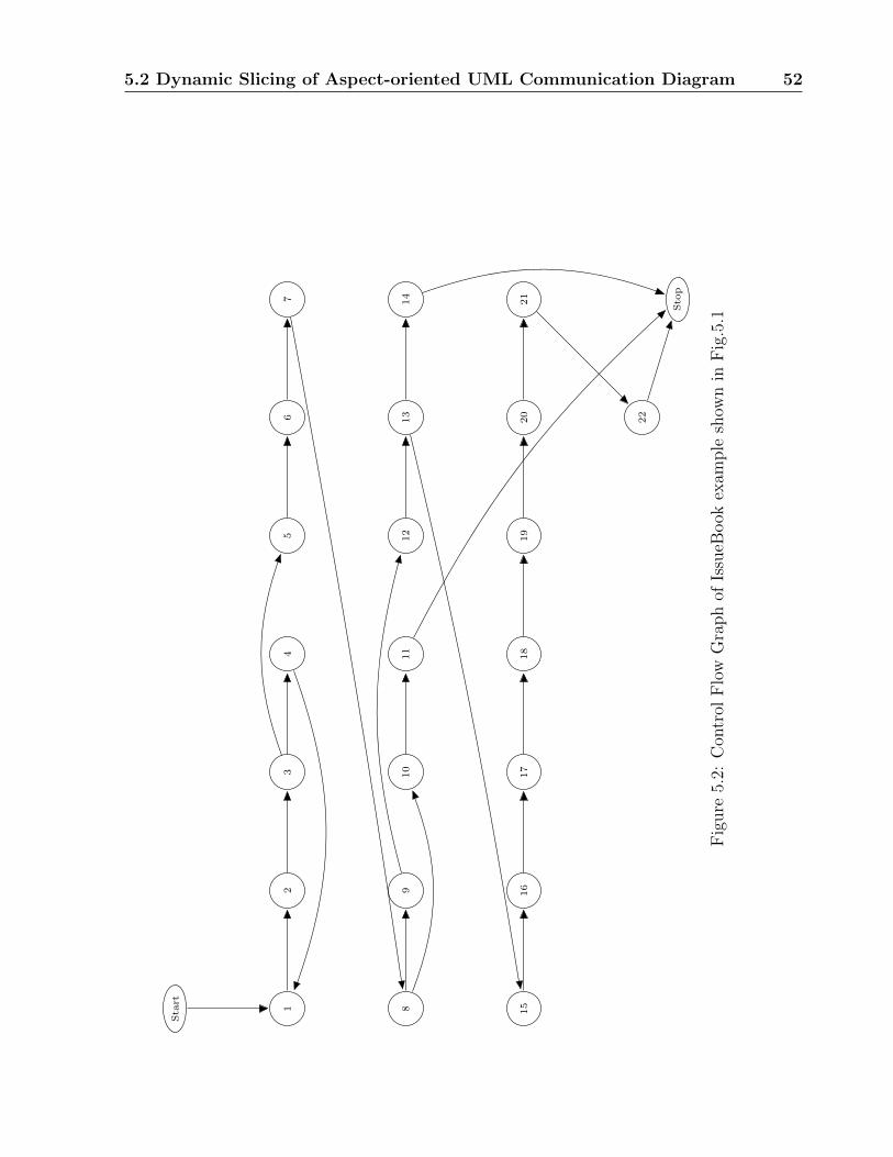
5.2 Dynamic Slicing of Aspect-oriented UML Communication Diagram 52

Sta

rt

12

34

56

7

89

10

11

12

13

14

15

16

17

18

19

20

21

22

Sto

p

Fig

ure

5.2:

Con

trol

Flo

wG

raph

ofIs

sueB

ook

exam

ple

show

nin

Fig

.5.1

5.2 Dynamic Slicing of Aspect-oriented UML Communication Diagram 53

5.2.2 Communication Aspect Dependency Graph

In this section, we present our CADG representation of UML 2.0 Communication diagrams

for aspect-oriented software. CADG demonstrates the dependency between the messages

that are passed linking various objects in a given problem scenario. Dependencies considered

in the CADG are classified into two different types namely data dependency edges and

control dependency edges. We have used different notations to represent the different types

of edges in the Communication Aspect Dependency Graph. CADG is confined to represent

only the dynamic dependencies existing among various objects concerned in the scenario.

Dynamic dependencies show a discrepancy with time (example data dependencies). The

flow of data among the messages that are passed between objects in the communication

diagram are represented by data dependence edges of CADG. Additionally, it shows the

effect of the calling messages on the return value of that call. Control dependence edges

of CADG represents flow of control in the communication diagram. We follow the steps

mentioned below to construct CADG from communication diagram:

1. Draw the communication diagram for the given scenario in the system.

2. Represent each message of the communication diagram as node in CADG and label

it with the message number.

3. Identify the different control dependencies and data dependencies existing between

the messages passed among the objects in the communication diagram and represent

them as edges in CADG.

An Example CADG

To explain the construction of CADG, we have considered the IssueBook() scenario of

Library Management System. In the first step, we identified the objects concerned with the

scenario and the communication among them. Then we draw the communication diagram

as shown in Fig.5.1. From the communication diagram, the CFG is drawn as shown in

Fig.5.2. From the CFG, the different dependencies are identified and shown in Fig.5.3.

Each message is represented by a node. The label of the messages in the communication

diagram is identical to the node number in CADG. The edges of the graph represent the

dependencies among the nodes. The control dependence edges are represented by solid

edges and data dependence edges are represented by dashed edges. After each execution of

a message the graph is updated to find the recent dependencies.

5.2 Dynamic Slicing of Aspect-oriented UML Communication Diagram 54

12

34

56

7

89

10

11

12

13

14

15

16

17

18

19

20

21

22

Fig

ure

5.3:

Com

munic

atio

nA

spec

tD

epen

den

cyG

raph

ofIs

sueB

ook

exam

ple

show

nin

Fig

.5.

1

5.2 Dynamic Slicing of Aspect-oriented UML Communication Diagram 55

5.2.3 Working of AOEM algorithm

We now demonstrate the working of AOEM algorithm with the help of our previously

discussed example. Consider the communication diagram of IssueBook scenario in Fig.5.1

and the corressponding CADG shown in Fig.5.3. While execution of the initialization step,

AOEM algorithm first unmarks all the dependence edges and set dynSlice(n) = φ, for every

node of CADG. Now consider the following set of values: MId = valid, v = 1, p = 1 and

l = 1. For these set of given values, the model will have the execution trace as 1, 2, 3, 5,

6, 7, 8, 9, 12, 13, 15, 16, 17,18, 19, 20, 21, 22. Let us assume that a slicing command (19,

bId) is given. This command requires us to find the backward dynamic slice for the bId

variable at node 19. According to the AOEM algorithm, the dynamic slice at statement 19

is given by the expression dynSlice(19) = 18 ∪ dynSlice(18). By evaluating the expression

in a recursive manner, we can get the final dynamic slice at statement 19. The shaded

vertices in Fig.5.4 represents the dynamic slices with respect to bId variable at node 19.

5.2 Dynamic Slicing of Aspect-oriented UML Communication Diagram 56

Algorithm 3 Aspect-Oriented Edge Marking Algorithm (AOEM)

1: CADG Construction

(a) CFG = constructCFG(CG) //Call a procedure for CFG construction

(b) CADG = constructCADG(CFG) //Call a procedure for CADG construction

2: Initialisation: Before execution do the following:

(a) Unmark all the data and control dependence edges of CoDG.

(b) Mark all control dependence edge (y,x) where x is not a loop control node.

(c) Set dynSlice(n)=φ for every node n of CADG.

(d) Set RecentDef(var)=φ for each variable var of the communication diagram.

3: RunTime Updation: With the given set of values, we traverse the communication

diagram sequentially and after each message m of the communication diagram is processed

do the following steps:

(a) For every variable var used at n do the following:

1. Unmark the marked data dependence edge associated with the variable var

corressponding to previous execution of message m.

2. Mark the data dependence edge (n, u) where u = RecentDef(var)

(b) Let (n, u1),(n, u2),· · · ,(n, uk) be all marked dependence edges in updated CoDG.

(c) Update dynSlice(n) = {u1, u2,· · · ,uk} ∪ dynSlice(u1) ∪ dynSlice(u2) ∪dynSlice(uk).

(d) If n is a Def(var) message, then update RecentDef(var)= n

(e) If n is a loop control node, then do -

1. Mark every control dependence edge (x, n), for which this execution of n

corressponds to entry of loop in CADG.

2. Unmark every incoming dependence edge (x, n), for which this execution of

n corressponds to exit of loop in CADG.

(f) Exit if terminate message is encountered.

5.2 Dynamic Slicing of Aspect-oriented UML Communication Diagram 57

12

34

56

7

89

10

11

12

13

14

15

16

17

18

19

20

21

22

Fig

ure

5.4:

Up

dat

edC

AD

Gof

Issu

eBook

exam

ple

show

nin

Fig

.5.

1sh

owin

gdynSlice

(19)

for

AO

EM

algo

rith

m

5.2 Dynamic Slicing of Aspect-oriented UML Communication Diagram 58

5.2.4 Complexity Analysis of AOEM algorithm

Space Complexity

Let Cd be a communication diagram having m messages. Each message is represented by a

single vertex in CADG. A graph with n number of nodes requires O(n2) space. Thus, the

space require for the CADG is O(n2). We also need the following additional run-time space

to manipulate the CADG.

1. To store the dynSlice(m) for each message of the communication diagram Cd, at

most O(n) space is necessary, because the maximum size of the slice is equivalent to

number of messages in the communication diagram. Therefore, for n messages, the

space requirement of dynSlice(m) becomes O(n2).

2. Consider v number of variables are present in the communication diagram Cd. To

store the RecentDef(var) for each variable var of Cd, at most O(n) space is necessary.

Assuming that the number of varaibles exist is less than number of messages, AOEM

algorithm will require O(n2) space to store RecentDef(var) of all variables.

Therefore, the space complexity of the AOEM algorithm is O(n2), where n is the number

of messages in the communication diagram Cd.

Time Complexity

Let Cd be a communication diagram having n number of messages. The total time com-

plexity of AOEM algorithm is because of two components. The first one is result of the

execution time required for the run-time maintenance of CADG. The second one is the time

required to calculate dynSlice(n). The time necessary to store the required information at

every node is O(n), where n is the number of messages in communication diagram. The

time needed to traverse the CADG and reach the specified nodes is O(n2), where n is the

number of messages in communication diagram. So, run-time complexity of the AOEM

algorithm for computing the dynamic slice is O(n2S), where S is the length of the execution.

5.2.5 Comparison with the related work

To the best of our knowledge no one has done slicing of aspect based UML communication

diagram. In the absence of any directly related work, we compare our work with the work

based on slicing of object-oriented UML models and code based slicing of aspect-oriented

5.3 Implementation 59

software. Korel et al. [21] proposed an algorithm for slicing of statebased models. The

architectures used in their procedures do not make a distinction between the structural and

behavioral aspects of a system. Also, it was designed for OOP. In our approach, we have

considered the dynamic nature of the aspect-oriented system.

Mohapatra et al. [8] proposed an algorithm called Trace Based Dynamic Slice TBDS

algorithm. This algorithm computes the dynamic slice from the code of aspect-oriented

programs using a dependence based graph called Dynamic Aspect-Oriented Dependence

Graph DADG. Our algorithm intends to find the dynamic slice from the design stage using

communication diagram at architectural level.

Zhao [46, 47] initially proposed a static slicing algorithm for AOP through aspect mining

technique. Then, it was extended by constructing Sequence Dependence Graph for aspect-

oriented programs. But this technique was unable to handle the pointcut. In our approach,

CADG is able to find the dynamic slice as well as considers the pointcut feature of aspect-

oriented programming.

Braak [34] extended the technique proposed by Zhao [46, 47] by including the Inter-type

declarations in the graph. Then the two phase algorithm proposed by Horwitz et al. [14]

was used to find the static slice of the aspect-oriented program. But our algorithm finds

the dynamic slice for aspect-oriented programs at the architectural level.

Lallchandani et al. [23] proposed an algorithm to find the dynamic slice combining class

diagram and sequence diagram. The representation is named as Model Dependency Graph

(MDG) for object-oriented programs. Whereas we have considered the communication

diagram for aspect-oriented programs.

5.3 Implementation

In this section, we discuss the implementation of our AOEM algorithm. The motivation for

our implementation is to validate the correctness and the preciseness of our algorithm. We

have tested our algorithm on different aspect-based communication diagram and different

slicing criterion. We have coded our algorithm in JAVA. First we are generating Commu-

nication Aspect Dependency Graph (CADG) from the communication diagram. We have

taken a node in the CADG for each message in communication diagram. These nodes are

connected with the help of dependency edge. The dependency edge represents two types

of dependencies: data dependency and control dependency. We are storing the whole in-

formation about the CADG in a file. While storing the different information about the

5.3 Implementation 60

(a) Input for data

dependent edges

(b) Input for control de-

pendent edges

(c) Input for node number at

which slice to be found

Figure 5.5: Snapshots of GUI to give input for AOEM algorithm

CADG, we store the data in structure data type. This data structure contains various

information about each node in the CADG like control dependency, data dependency, sta-

tus: marked or unmarked. We have also calculated various attribute of each variable like

def(var), use(var)and RecentDef(var). We have developed a dynamic GUI (Graphical User

interface) for providing the input to our algorithm. The GUI for taking the input of data

dependent edges, control dependent edges and node number at which slice is to be found is

shown in Fig.5.5a, Fig.5.5b and Fig.5.5c respectively.

The snapshot for dynSlice(19) is shown in Fig.5.6.

Figure 5.6: Snapshot of the AOEM algorithm showing dynSlice(19)

5.3.1 Experimental Results

In this section, we discuss our experimental results regarding the run-time requirement for

the AOEM algorithm. Table 5.1 summarizes the average run-time requirement of AOEM

5.3 Implementation 61

Table 5.1: Average run time for AOEM algorithm

Sl.No Number of messages Avg. run-time for AOEM algo.(in msec)

1 16 12.0045

2 22 14.0876

3 39 18.0004

4 48 20.2213

algorithm for different aspect-based communication diagram. for this, we have considered

four different scenarios and drawn the communication diagram for it. Then we applied our

AOEM algorithm at different node number for each communication diagram. Next, we

have computed the average run-time taken by our algorithm for each of the communication

diagram. The result shows the overall trend of the performance of our AOEM algorithm.

Fig.5.7 shows the graphical representation of average run-time of AOEM algorithm. It can

be observed from the figure that the run-time of the algorithm only increases marginally

with increase in number of messages in the communication diagram.

Figure 5.7: Average run-time of AOEM algorithm for different communication diagram

Chapter 6

Conclusions and Future Work

The major aim of our research was to develop efficient dynamic slicing algorithms for object-

oriented and aspect-oriented softwares. Below, we summarize the important contributions

of our work. At the end, some suggestions for future work are given.

6.1 Contributions

In this section, we summarize the important contributions of our work. There are two

important contributions, Dynamic Slicing of UML communication Diagram and Dynamic

Slicing of Aspect-oriented UML Communication Diagram.

6.1.1 Dynamic Slicing of UML communication Diagram

We first developed a communication diagram with the help of MagicDraw tool. In the next

step, we generated an intermediate representation for the communication diagram which

we named Communication Dependency Graph (CoDG). Then we proposed two dynamic

slicing algorithm called as Edge Marking Dynamic Slicing Algorithm for Communication

Diagram(EMACD)and Node Marking Dynamic Slicing Algorithm for Communication Di-

agram(NMACD). We have computed that the space complexity of both the algorithm is

O(n2), where n is the number of messages in the communication diagram. The time com-

plexity of both the algorithm is O(n2S), where S is the length of the execution. We have

also shown that our algorithm is more efficient than the exisitng algorithms. We have also

proved that our algorithm computes the correct dynamic slices. We have implemented both

the algorithm in Java to demonstrate their correctness.

6.1 Contributions 63

Future work

We now briefly outline the possible extensions to our work.

• Our work can be extended to compute the dynamic slices using other UML diagrams

like activity, class and statechart diagrams.

• The work can also be extended to compute dynamic slices by combining two diagrams

like activity diagrams and class diagrams, class diagrams and sequence diagrams.

6.1.2 Dynamic Slicing of Aspect-oriented UML Communication

Diagram

We have used UML 2.0 aspect-oriented based communication diagram to compute the dy-

namic slices. We have developed a Communication Aspect Dependence Graph (CADG)

as an intermediate representation. Then, we propose an algorithm Aspect-Oriented Edge

Marking Algorithm (AOEM). We have shown that the time complexity of our algorithm is

O(n2S), where S is the length of the execution. The space complexity of our algorithm is

O(n2), where n is the number of messages in the communication diagram. We have also

proved that our algorithm computes the correct dynamic slice. We have implemented the

algorithm to demonstrate their correctness.

Future Work

We briefly outline the following possible extensions to our work.

• Our current work can be extended to compute dynamic slices of other UML 2.0 dia-

grams like activity diagrams, state-chart diagrams, interaction overview diagrams.

• Computing dynamic slices of a combination of two or more UML 2.0 diagrams like

communication diagram and class diagram, communication diagram and activity di-

agram etc. is another direction for extension.

Dissemination of Work

Dynamic Slicing of Communication Diagram [Chapter #4]

1. Dynamic Slicing of UML Communication Diagram, In 3rd IEEE International Advance

Computing Conference , Pages- 1394 - 1399, February 2013.

2. A Node Marking Algorithm for Dynamic Slicing of UML Communication Diagrams, In Ac-

cepted for Publication International conference on Advanced Computing, Networking

and Informatics (ICACNI), Raipur, June 2013.

Dynamic Slicing of Aspect-oriented Communication Diagram [Chapter #5]

1. Dynamic Slicing of Aspect-oriented UML Communication Diagram, In 6th National

Workshop on Recent Trends in Software Testing (RTST), Published in International

Journal of Computer Science and Informatics, 3(2), pages- 58-63, May 2013

Bibliography

[1] A.Abdurazik and J.Offutt. Using uml collaboration diagrams for static checking and test gen-

eration. In Proceedings 3rd international conference on the UML’00, pages 383–395, October

2000.

[2] H. Agrawal and J. Horgan. Dynamic program slicing. In Proceedings of the ACM SIGPLAN’90

Conference on Programmimg Lanuages Design and Implementation, SIGPLAN Notices, Anal-

ysis and Verification, volume 25, pages 246–256, White Plains, NewYork, 1990.

[3] Taweesup Apiwattanapong, Alessandro Orso, and Mary Jean Harrold. Jdiff: A differencing

technique and tool for object-oriented programs. Automated Software Engineering, 14(1):3–

36, 2007.

[4] Jim Arlow and Ila Neustadt. UML 2 and the unified process: practical object-oriented analysis

and design. Addison-Wesley Professional, 2005.

[5] D. Binkley and K. B. Gallagher. Program Slicing, Advances in Computers, volume 43. Aca-

demic Press, San Diego, CA, 1996.

[6] Gerardo Canfora, Aniello Cimitile, and Andrea De Lucia. Conditioned program slicing. In-

formation and Software Technology, 40(11):595–607, 1998.

[7] Z. Chen and B. Xu. Slicing object-oriented Java programs. ACM SIGPLAN Notices, 36:33–40,

2001.

[8] R Kumar D. P. Mohapatra, M. Sahu and R Mall. Dynamic slicing of aspect-oriented programs.

Informatica, 32(3):261–274, 2008.

[9] Kiczales G. and Mezini M. Aspect-oriented programming and modular reasoning. In Pro-

ceedings of the 27th International Conference on Software Engineering, ICSE05, pages 49–58,

May 2005.

[10] K. Gallagher and J. Lyle. Using program slicing in software maintenance. IEEE Transactions

on Software Engineering, 17(8):751–761, 1991.

BIBLIOGRAPHY 66

[11] Rajiv Gupta, Mary Jean Harrold, and Mary Lou Soffa. An approach to regression testing

using slicing. In Proceedings on Software maintenance, pages 299–308. IEEE, 1992.

[12] R.J. Hall. Automatic extraction of executable program subsets by simultaneous program

slicing. Journal of Automated Software Engineering, 2(1):33–53, 1995.

[13] Mark Harman and Sebastian Danicic. Amorphous program slicing. In Proceedings Fifth

Iternational Workshop on Program Comprehension, pages 70–79. IEEE, 1997.

[14] S. Horwitz, T. Reps, and D. Binkley. Interprocedural slicing using dependence graphs. ACM

Transactions on Programming Languages and Systems, 12(1):26–61, 1990.

[15] Katsuro Inoue Ishio, Shinji Kusumoto. Debugging support for aspect-oriented program based

on program slicing and call graph. In Proceedings of the 20th IEEE International Conference

on Software Mai1ntenance (ICSM04), pages 178–187, September 2004.

[16] A Garciac J Hernndeza J M Conejero, E Figueiredob and E Juradoa. On the relationship

of concern metrics and requirements maintainability. Information and Software Technology,

54(2):212–238, 2012.

[17] Lamping J. Loingtier J. M. Lopes C. V. Maeda C. Kiczales G., Irwin J. and Mendhekar A.

Aspect-oriented programming. In Proceedings of the European Conference on Object-Oriented

Programming(ECOOP), June 1997.

[18] B. Korel and J. Laski. Dynamic program slicing. Information Processing Letters, 29(3):155–

163, 1988.

[19] B. Korel and J. Rilling. Dynamic program slicing methods. Information and Software Tech-

nology, 40:647–659, 1998.

[20] B. Korel and S. Yalamanchili. Forward derivation of dynamic slices. In Proceedings of the

International Symposium on Software Testingand Analysis, pages 66–79, 1994.

[21] Singh I. Tahat L. Korel, B. and B. Vaysburg. Slicing of statebased models. In Proceedings of

the International Conference on Software Maintenance, pages 34–43, 2003.

[22] J. T. Lallchandani and R. Mall. Slicing uml architectural models. SIGSOFT Softw. Eng.

Notes, 33(3):41–49, 2008.

[23] Jaiprakash T. Lallchandani and R. Mall. A dynamic slicing technique for uml architectural

models. IEEE Transactions on Software Engineering, 37(6), December 2011.

[24] L. D. Larson and M. J. Harrold. Slicing object-oriented software. In Proceedings of the 18th

International Conference on Software Engineering, German, March 1996.

BIBLIOGRAPHY 67

[25] Alex Loh and Miryung Kim. Lsdiff: a program differencing tool to identify systematic struc-

tural differences. In Proceedings of the 32nd ACM/IEEE International Conference on Software

Engineering-Volume 2, 2010.

[26] A. D. Lucia. Program slicing: Methods and applications. In Proceedings of IEEE International

Workshop on Source Code Analysis and Manipulation, pages 142–149, 2001.

[27] R. Mall. Fundamentals of Software Engineering. Prentice Hall, India, 2nd Edition, 2003.

[28] Durga Prasad Mohapatra, Rajib Mall, and Rajeev Kumar. An edge marking dynamic slicing

technique for object-oriented programs. In Proceedings of 28th IEEE Annual International

Computer Software and Applications Conference, IEEE CS Press, pages 60–65, September

2004.

[29] G. B. Mund, R. Mall, and S. Sarkar. Computation of intraprocedural dynamic program slices.

Information and Software Technology, 45:499–512, April 2003.

[30] K. Ottenstein and L. Ottenstein. The program dependence graph in software development

environment. In Proceedings of the ACM SIGSOFT/SIGPLAN Software Engineering Sym-

posium on Practical Software Develop Environments, SIGPLAN Notices, volume 19, pages

177–184, 1984.

[31] M. Sahu and D. P. Mohapatra. A node marking technique for dynamic slicing of aspect-

oriented programs. In Proceedings of the 10th International Conference on Information Tech-

nology (ICIT07), pages 155–160, 2007.

[32] Philip Samuel and Rajib Mall. A novel test case design technique using dynamic slicing of

uml sequence diagrams. e-Informatica: Software Engineering Journal, 2(1), 2008.

[33] Y. Song and D. Huynh. Forward Dynamic Object-Oriented Program Slicing, Application

Specific Systems and Software Engineering and Technology (ASSET’99). IEEE CS Press,

1999.

[34] Timon ter Braak. Extending program sliccing in aspect-oriented programming with inter-type

declarations. In Proceedings of 5th Twente Student Conference on IT,, June 2006.

[35] F. Tip. A survey of program slicing techniques. Journal of Programming Languages, 3(3):121–

189, 1995.

[36] L. Chung T.Kim, Y.-T. Song and D. T. Huynh. Software architecture analysis: a dynamic

slicing approach. In ACIS Int. J Comp. Inf. Sci., pages 91–103, March 2000.

BIBLIOGRAPHY 68

[37] Guda A Venkatesh. The semantic approach to program slicing. Proceedings of the ACM

SIGPLAN conference on Programming language design and implementation, 26(6):107–119,

1991.

[38] M. Weiser. Program Slices: Formal, Psychological, and Practical Investigations of an Au-

tomatic Program Abstraction Method. PhD thesis, University of Michigan, Ann Arbor, MI,

1979.

[39] M. Weiser. Programmers use slices when debugging. Communications of the ACM, 25(7):446–

452, 1982.

[40] M. Weiser. Program slicing. IEEE Transactions on Software Engineering, 10(4):352–357,

1984.

[41] B. Xu and Z. Chen. Dynamic slicing object-oriented programs for debugging. In SCAM,

pages 115–122, 2002.

[42] B. Xu, J. Qian, X. Zhang, Z. Wu, and L. Chen. A brief survey of program slicing. ACM

SIGSOFT Software Engineering Notes, 30(2):1–36, 2005.

[43] J. Wang Y. Chen Hongmin Lu Baowen Xu Y. Zhou, L. Wen. Drc: A dependence rela-tionships

based cohesion measure for classes. In Proceedings 10th Asia- Pacic Software Engineering

Conference (APSEC 2003), December 2003.

[44] Shin Yoo and Mark Harman. Regression testing minimization, selection and prioritization: a

survey. Software Testing, Verification and Reliability, 22(2):67–120, 2012.

[45] J. Zhao. Dynamic slicing of object-oriented programs. Technical report, Information Process-

ing Society of Japan, May 1998.

[46] J. Zhao. Slicing aspect-oriented software. In Proceedings of 10th International Workshop on

Program Comprehension, pages 251–260, June 2002.

[47] J. Zhao and M. Rinard. System dependence graph construction for aspect-oriented programs.

Technical report, Laboratory Of Computer Science, Massachusetts institute of Technology,

March 2003.