Embed Size (px)
Citation preview

Ghent UniversityFaculty of Engineering
Department of Civil Engineering (TW15)Laboratory of Soil Mechanics
Dynamic Soil Properties out of SCPT
and Bender Element Tests with
Emphasis on Material Damping
Lutz Karl
A thesis submitted in accordance with the requirements ofthe degree of Doctor of Philosophy in the Faculty of
Engineering, Department of Civil Engineering
Academic year 2004–2005


Supervisor: Prof. dr. ir. W. Haegeman
Laboratory of Soil MechanicsDepartment of Civil Engineering (TW15)Faculty of EngineeringGhent University
Technologiepark 9059052 Ghent (Zwijnaarde)Belgium
Tel. +36 9 264 57 23+36 9 264 57 17
Fax +36 9 264 57 49
http://terzaghi.ugent.be


Preface
I wish to thank all persons who have contributed to this thesis with theirwork, their ideas and helpful comments. First of all, I would like to thank mysupervisor Prof. Wim Haegeman for providing the testing equipment and forthe extensive assistance throughout this research.
I am also very grateful to Prof. Geert Degrande from the K.U. Leuven forhis numerous valuable suggestions and support.
Furthermore I wish to thank the co-workers of the STWW-project ”Trafficinduced vibrations in buildings” from the K.U. Leuven, especially Lincy Pyl,Dr. Janusz Kogut, Serge Jacobs and Kathleen Geraedts.
The help of Prof. Mia Loccufier, Peter Buffel, Wouter Ost and the staff ofthe Laboratory of Soil Mechanics in Ghent is very much acknowledged. Specialthanks deserves also Lou Areias for shearing his knowledge on the SCPT, forperforming of field tests and for the visual wave velocity interpretation at thesites in Retie, Waremme and Lincent.
The research presented in this thesis is embedded in the STWW-projectIWT000152 ”Traffic induced vibrations in buildings”. The financial support ofthe Ministry of the Flemish Community for this project is likewise gratefullyacknowledged.
Lutz KarlJanuary 2005
v


Contents
Preface v
Frequently used symbols and units xi
I Introduction and background 1
1 Introduction 3
1.1 Purpose and scope . . . . . . . . . . . . . . . . . . . . . . . . . 3
1.2 Outline of the thesis . . . . . . . . . . . . . . . . . . . . . . . . 4
2 Dynamic soil properties 7
2.1 Dynamic shear modulus . . . . . . . . . . . . . . . . . . . . . . 7
2.2 Attenuation parameters of soils . . . . . . . . . . . . . . . . . . 11
3 Methods to determine G and D 19
3.1 Laboratory tests . . . . . . . . . . . . . . . . . . . . . . . . . . 19
3.1.1 Piezoelectric bender and compression element tests . . . 21
3.1.2 Cyclic triaxial tests . . . . . . . . . . . . . . . . . . . . . 22
3.1.3 Cyclic simple shear tests . . . . . . . . . . . . . . . . . . 23
3.1.4 Cyclic torsional shear tests . . . . . . . . . . . . . . . . 23
3.1.5 Resonant column test . . . . . . . . . . . . . . . . . . . 23
3.1.6 Free torsion pendulum test . . . . . . . . . . . . . . . . 24
3.2 In situ tests . . . . . . . . . . . . . . . . . . . . . . . . . . . . . 28
3.2.1 Seismic reflection test . . . . . . . . . . . . . . . . . . . 28
3.2.2 Seismic refraction test . . . . . . . . . . . . . . . . . . . 29
3.2.3 Spectral analysis of surface waves (SASW) . . . . . . . 30
3.2.4 Seismic cross-hole test . . . . . . . . . . . . . . . . . . . 31
3.2.5 Seismic down-hole and up-hole test . . . . . . . . . . . . 32
3.2.6 Seismic cone penetration test . . . . . . . . . . . . . . . 33
3.2.7 Geotomography . . . . . . . . . . . . . . . . . . . . . . . 33
3.2.8 High-strain tests . . . . . . . . . . . . . . . . . . . . . . 34
vii

viii CONTENTS
II Characterization of the testing sites 35
4 Test site Retie 374.1 Introduction . . . . . . . . . . . . . . . . . . . . . . . . . . . . . 374.2 Borings and undisturbed sampling . . . . . . . . . . . . . . . . 384.3 Cone penetration test (CPT) . . . . . . . . . . . . . . . . . . . 414.4 Seismic cone penetration test (SCPT) . . . . . . . . . . . . . . 41
4.4.1 Test description . . . . . . . . . . . . . . . . . . . . . . . 414.4.2 Test results for the wave velocities . . . . . . . . . . . . 444.4.3 Test results for the damping ratio . . . . . . . . . . . . 45
4.5 Spectral analysis of surface waves (SASW) . . . . . . . . . . . . 474.5.1 Test description . . . . . . . . . . . . . . . . . . . . . . . 474.5.2 Test results . . . . . . . . . . . . . . . . . . . . . . . . . 48
4.6 Overview of the test results Retie . . . . . . . . . . . . . . . . . 49
5 Test site Lincent 535.1 Introduction . . . . . . . . . . . . . . . . . . . . . . . . . . . . . 535.2 Borings and undisturbed sampling . . . . . . . . . . . . . . . . 535.3 Cone penetration test (CPT) . . . . . . . . . . . . . . . . . . . 575.4 Seismic cone penetration test (SCPT) . . . . . . . . . . . . . . 60
5.4.1 Remarks on the testing Setup . . . . . . . . . . . . . . . 605.4.2 Test results for the wave velocity . . . . . . . . . . . . . 615.4.3 Test results for the damping ratio . . . . . . . . . . . . 62
5.5 Spectral analysis of surface waves (SASW) . . . . . . . . . . . . 625.5.1 Remarks on the testing setup and inversion assumptions 625.5.2 Test results . . . . . . . . . . . . . . . . . . . . . . . . . 63
5.6 Overview of the test results Lincent . . . . . . . . . . . . . . . 64
6 Test site Waremme 676.1 Introduction . . . . . . . . . . . . . . . . . . . . . . . . . . . . . 676.2 Borings and undisturbed sampling . . . . . . . . . . . . . . . . 676.3 In situ tests . . . . . . . . . . . . . . . . . . . . . . . . . . . . . 71
6.3.1 Cone penetration test (CPT) . . . . . . . . . . . . . . . 716.3.2 Seismic cone penetration test (SCPT) . . . . . . . . . . 726.3.3 Spectral analysis of surface waves (SASW) . . . . . . . 76
6.4 Laboratory tests to obtain Gmax and D . . . . . . . . . . . . . 776.4.1 Bender elements with time arrival interpretation . . . . 776.4.2 Free torsion pendulum test . . . . . . . . . . . . . . . . 796.4.3 Resonant column test . . . . . . . . . . . . . . . . . . . 80
6.5 Overview of the test results Waremme . . . . . . . . . . . . . . 81
7 Test site Sint-Katelijne-Waver 857.1 Introduction . . . . . . . . . . . . . . . . . . . . . . . . . . . . . 857.2 Borings and undisturbed sampling . . . . . . . . . . . . . . . . 857.3 In situ tests . . . . . . . . . . . . . . . . . . . . . . . . . . . . . 87
7.3.1 Marchetti dilatometer test (DMT) . . . . . . . . . . . . 87

CONTENTS ix
7.3.2 Cone penetration test (CPT) . . . . . . . . . . . . . . . 887.3.3 Seismic cone penetration test (SCPT) . . . . . . . . . . 887.3.4 Spectral analysis of surface waves (SASW) . . . . . . . 907.3.5 Seismic refraction test (SRT) . . . . . . . . . . . . . . . 90
7.4 Laboratory tests to obtain Gmax and D . . . . . . . . . . . . . 917.4.1 Bender elements with time arrival interpretation . . . . 917.4.2 Free torsion pendulum test . . . . . . . . . . . . . . . . 927.4.3 Resonant column test . . . . . . . . . . . . . . . . . . . 93
7.5 Overview of the test results St.-Katelijne-Waver . . . . . . . . . 94
8 Test site Ghent 978.1 Introduction . . . . . . . . . . . . . . . . . . . . . . . . . . . . . 978.2 Borings and sampling . . . . . . . . . . . . . . . . . . . . . . . 978.3 Cone penetration test (CPT) . . . . . . . . . . . . . . . . . . . 998.4 Seismic cone penetration test (SCPT) . . . . . . . . . . . . . . 99
8.4.1 Testing setup . . . . . . . . . . . . . . . . . . . . . . . . 998.4.2 Test results for the wave velocity . . . . . . . . . . . . . 1008.4.3 Test results for the damping ratio . . . . . . . . . . . . 100
8.5 Overview of the test results Ghent . . . . . . . . . . . . . . . . 101
III Studies on testing methods 105
9 SCPT based techniques 1079.1 Motivation and purpose . . . . . . . . . . . . . . . . . . . . . . 1079.2 Applied equipment and selection criteria . . . . . . . . . . . . . 108
9.2.1 Seismic source . . . . . . . . . . . . . . . . . . . . . . . 1089.2.2 Seismic cones . . . . . . . . . . . . . . . . . . . . . . . . 1119.2.3 Data acquisition system . . . . . . . . . . . . . . . . . . 117
9.3 Methods for the shear modulus . . . . . . . . . . . . . . . . . . 1199.3.1 Direct time methods . . . . . . . . . . . . . . . . . . . . 1219.3.2 Indirect time methods . . . . . . . . . . . . . . . . . . . 121
9.4 Methods to obtain the Damping Ratio . . . . . . . . . . . . . . 1259.4.1 Attenuation coefficient method . . . . . . . . . . . . . . 1259.4.2 Spectral ratio slope method . . . . . . . . . . . . . . . . 1289.4.3 Hysteresis stress-strain-curves . . . . . . . . . . . . . . . 131
9.5 Artificially generated signals . . . . . . . . . . . . . . . . . . . . 1429.5.1 Calculated velocities from the simulated signals . . . . . 1519.5.2 Calculated damping ratio . . . . . . . . . . . . . . . . . 1529.5.3 Conclusions for the analysis of real SCPT data . . . . . 156
9.6 Measurements performed at the test sites . . . . . . . . . . . . 1609.6.1 Campaign I (geophones) . . . . . . . . . . . . . . . . . . 1609.6.2 Campaign II (HAMLIN accelerometers) . . . . . . . . . 1609.6.3 Campaign III, Ghent (Bruel & Kjær accelerometers) . . 166
9.7 Summary and remaining problems . . . . . . . . . . . . . . . . 169

x CONTENTS
10 Bender element technique 17310.1 Motivation and purpose . . . . . . . . . . . . . . . . . . . . . . 17310.2 Description of the equipment . . . . . . . . . . . . . . . . . . . 174
10.2.1 Bender elements . . . . . . . . . . . . . . . . . . . . . . 17410.2.2 Signal generation and measurement apparatus . . . . . 176
10.3 Techniques to determine Gmax . . . . . . . . . . . . . . . . . . 17810.3.1 Wave travel distance . . . . . . . . . . . . . . . . . . . . 17810.3.2 Selection of the input-signal shape . . . . . . . . . . . . 17910.3.3 Methods for determining the travel time . . . . . . . . . 17910.3.4 Difficulties in the arrival time determination . . . . . . . 182
10.4 Methods to obtain the damping ratio . . . . . . . . . . . . . . . 18610.4.1 Resonant method . . . . . . . . . . . . . . . . . . . . . . 18610.4.2 Use of multiple shear wave arrivals . . . . . . . . . . . . 20410.4.3 Use of different travel paths . . . . . . . . . . . . . . . . 210
10.5 The resonant method . . . . . . . . . . . . . . . . . . . . . . . . 21310.5.1 Introduction . . . . . . . . . . . . . . . . . . . . . . . . 21310.5.2 Site in Waremme . . . . . . . . . . . . . . . . . . . . . . 21310.5.3 Site in Sint-Katelijne-Waver . . . . . . . . . . . . . . . . 215
10.6 Summary and remarks . . . . . . . . . . . . . . . . . . . . . . . 216
11 Conclusions and summary 235
IV Appendix 239
A Accuracy and costs of soil tests 241A.1 Laboratory tests . . . . . . . . . . . . . . . . . . . . . . . . . . 242A.2 Field tests . . . . . . . . . . . . . . . . . . . . . . . . . . . . . . 243A.3 Selection conclusions . . . . . . . . . . . . . . . . . . . . . . . . 244
Bibliography 249

Frequently used symbolsand units
The following table presents the most frequently used symbols and abbrevia-tions. The symbols are, in most cases, also defined when they are introducedin the text. Time histories are in general represented by small letters; theirfrequency domain representation by capital letters.
Symbols and units
A signal amplitude, amplitude spectrum; m, m/s, m/s2;area m2
a sample radius, distance; m;time history m, m/s, m/s2
c cohesion; damping coefficient; Pa; kg/s;wave velocity m/s
CA added mass coefficient −D damping ratio −, %d diameter, depth, distance mDs damping ratio of the s-wave −, %E elasticity modulus; energy Pa; JEmax, E0 dynamic elasticity modulus PaEI bending stiffness Nm2
e void ratio −f frequency Hzfcut cut-off frequency HzFe void ratio function −FFT Fast Fourier Transformation
as a synonym for a discreteFourier Transformation in general
G shear modulus PaGmax, G0 dynamic shear modulus PaH transfer function; height −; mh height mIFFT inverse transformation to the FFT
xi

xii FREQUENTLY USED SYMBOLS
I area moment of inertia; impedance m4; kg/(m2s)Ip plasticity index −, %J mass polar moment of inertia kg m2
K bulk modulus Pak stiffness; wavenumber; kg/s2; 1/m;
shear coefficient; permeability −; m/ski intrinsic permeability m2
l,L length mm mass kgma added mass per unit length kg/mOCR over consolidation ratio −p pseudo simultaneous signal m, m/s, m/s2
pa atmospheric pressure PaQ quality factor −qc cone resistance N/m2
R cross power spectrum; receiverr cross-correlated signal; receiver signal; s · m2; ...;
radius, distance mS spectrum of signal s; sources time history m, m/s, m/s2
s∗ mean absolute deviationT oscillation period st time su(t) displacement function mVp compression wave velocity m/sVs shear wave velocity m/sx, y, z coordinates in space my mode shape (displacement) mz derivative of the logarithmic s/m;
amplitude ratio; distance m
α attenuation coefficient 1/mβ porosity −γ shear strain; unit weight −, %; N/m3
δ logarithmic decrement −δn, δn+1 amplitudes of an oscillation m∆t time shift s∆x distance mη viscosity Pa · sλ wavelength mν ratio of poisson −ξ fraction of critical damping −, %ρ density kg/m3
σ normal stress Paσ′
0 mean effective stress Pa

FREQUENTLY USED SYMBOLS xiii
σ′
1,2,3 isotropic confining stress Paτ shear stress; time shift Pa; sφ phase shift; angle of internal friction −; o
ω circular frequency 1/sω0 circular frequency at resonance 1/s
Subscripts
B related to the bottom sensor of the seismic conek related to bulk compressionkin kinematicmax maximummin minimump related to p-wavespot potentialR related to a receiver signalr related to Rayleigh-wavess related to s-waves; related to a sender signalT related to the top sensor of the seismic cone
Superscripts
′ related to an effective value or an imaginary component∗ related to an complex value˙ 1st derivative after the time¨ 2nd derivative after the time
Other symbols
ˆ related to an amplitude of a parameter¯ related to a complex conjugate

xiv FREQUENTLY USED SYMBOLS

Part I
Introduction andbackground
1


Chapter 1
Introduction
1.1 Purpose and scope
The evaluation of a number of civil engineering problems involve the transmis-sion of waves through soil, such as seismic response under earthquake loading,foundation response under dynamic loading and vibrations in buildings, in-duced by various sources. Important sources are industrial activities (looms,printing presses), building activities (pile driving, installation of sheet piles anddemolition of buildings), rail and road traffic.
Mechanical waves can be divided in body and surface waves. Body wavescan exist in an ideal full space or they travel in a region that is not affectedby a free surface. P- (primary, compression, longitudinal) waves and s- (secon-dary, shear, transverse) waves are types of body waves. The particle motionof p-waves is in propagation direction; the particle motion of s-waves is per-pendicular to the direction of propagation. Surface waves may only exist atthe surface or the boundary, separating media of different properties. Rayleigh(vertically polarized) and Love (horizontally polarized) waves are examples ofsurface waves.
The prediction of elastic wave propagation from the source, through thesoil to the receiver can be performed by means of numerical models. Effects ofconstruction and renovation of traffic infrastructure or other vibration sourcescan already be evaluated in the phase of planning. Unreasonable nuisances toresidents or damage to buildings can be avoided by design of a proper vibrationisolation system. Experimental validation has shown that the estimated soilcharacteristics crucially affect the vibration prediction accuracy in the free fieldand in buildings.
The most important characteristic parameters are the velocity of s- and p-waves and the material damping ratios of these body waves. Material dampingin the soil represents energy dissipation caused by friction between solid partic-les in the skeleton and by the relative motion between the soil skeleton and thepore fluid. Material damping must be distinguished from geometrical or radial
3

4 CHAPTER 1. INTRODUCTION
damping. Since the velocity of p-waves is highly affected by the groundwatertable, the most efforts are spent to the determination of the s-wave velocity.S-waves are transmitted in saturated soils by the soil fabric only. The dynamicshear modulus, Gmax, can be calculated directly based on the s-wave velocity.
There are only a few techniques available to determine the damping ratio.Only laboratory tests, as resonant column and cyclic shear tests, but no fieldtesting methods, can be considered as established techniques.
This work focuses on the determination of the damping ratio of shear wavesby means of field and laboratory tests. Therefore extended interpretation tech-niques for the seismic cone penetration test (SCPT) and the bender elementtest (BE) are studied and evaluated.
The SCPT is an extension of the cone penetration test (CPT). The useof the CPT in the geotechnical engineering practice has increased sharply inrecent years. Therefore the CPT equipment is widely spread. Since most ofthis equipment is also used in a SCPT the economical barriers for the transferof technique to practice are low. The BE methods are in the focus of interestsbecause bender elements can be mounted in various laboratory testing devicesand are able to generate s-waves with very low strain amplitudes similar tothose found in situ.
The research is embedded in the project ”Traffic induced vibrations in buil-dings” initiated from the K.U. Leuven and Ghent University. Within the frame-work of this project soil parameters at different sites are determined for use asinput parameters in a numerical model to predict the wave propagation. Fivetest sites in Belgium are chosen for testing: Waremme, Lincent, Retie, Sint-Katelijne-Waver and Ghent. The SCPT and the BE test are a substantial partof this exploration to measure the shear wave velocity and the damping ratio.The extensive testing campaigns offered the unique opportunity to evaluateand improve the methods on different soil materials.
1.2 Outline of the thesis
An introduction in Chapter 2 is devoted to the fundamentals of the dynamicsoil properties: shear modulus and the attenuation parameters. This is followedby an overview of state of the art methods to determine the shear modulus andthe damping ratio in Chapter 3. Laboratory testing techniques and in situ testsare considered.
The Chapters 4 to 8 provide information on the testing sites in Retie, Lin-cent, Waremme, Sint-Katelijne-Waver and Ghent. Apart from a general de-scription of each site, the essential results of all performed tests are given,including free torsion pendulum and resonant column tests. The findings ofthe bender element resonant tests are the only exception. These are discussedin Chapter 10.
Readers primarily interested in the BE- and SCPT testing methods, whichare closer investigated in this work, may at first skip the five chapters on thetesting sites to come back later to certain results, if necessary.

1.2. OUTLINE OF THE THESIS 5
Chapter 9 is dedicated to the SCPT. The selected test equipment and de-veloped data acquisition tools are described. After a summary on methods todetermine the s-wave velocity, the chapter focuses on possibilities to measurethe damping ratio based on time recods gathered by a SCPT. The results ofan evaluation of the spectral ratio slope and the attenuation coefficient methodby means of a numerical simulation of the test are given. Finally the obtainedresults on the five testing sites are summarized.
Chapter 10 deals with the methods based on the bender element test. Pro-cedures to measure the arrival time of the s-wave are described at first. Thenmethods to determine attenuation parameters are given. A resonant method isapplied on samples from two of the testing sites and the results are discussed.
Chapter 11 concludes the main findings of the thesis and gives suggestionsfor further research.
The obtained insights in the accuracy of the testing techniques concerningthe G-modulus and the damping ratio are used to compare the methods underconsideration of their costs. The results of the comparison can be found in theappendix and can be considered as a conclusion of this work.

6 CHAPTER 1. INTRODUCTION

Chapter 2
Dynamic soil properties
2.1 Dynamic shear modulus
A harmonic loading of a soil element as depicted in Figure 2.1 leads to a stress-strain diagram as shown in Figure 2.2. It is a typical outcome of a cyclictorsion or a cyclic triaxial test. A hysteresis loop accrues for each period of theoscillation. The shear modulus is found as the slope of the line that connectsthe point of origin and the inversion point between loading and unloading. Thismodulus is also called secant modulus or equivalent modulus. It decreases withan increase of load and shear amplitude. Therefore the stress-strain relationshipis principally non-linear. A schematic sketch of the shear modulus in functionof the shear strain is given in Figure 2.3.
The first loading curve, sometimes called the backbone curve, connectsthe load inversion points of oscillation periods with different levels of shearstrain and has a hyperbolic shape. The slope in the origin point to this curvecorresponds to the dynamic shear modulus Gmax or G0. It is also called tangentmodulus. Gmax is the shear modulus in the low strain range, usually assumedat values below the linear elastic threshold strain of about γ = 5 · 10−3 %. Itis in general expected that Gmax does not change in the low-strain range.
Vibrations caused by seismic in situ tests, traffic, construction works, weakearthquakes or even blastings usually have shear strain amplitudes below5 · 10−3 %. This opens the opportunity to model the wave propagation with acomparatively simple linear elastic constitutive model with Gmax as its essentialparameter.
Gmax in Pa can be calculated as:
Gmax = ρ V 2s (2.1)
with the soil density (ρ) in kg/m3 and the shear wave velocity (Vs) in m/s.This essential relation is used to obtain Gmax by means of various seismicgeophysical tests providing values of Vs.
7

8 CHAPTER 2. DYNAMIC SOIL PROPERTIES
Figure 2.1: Cyclic loading: load his-tory.
Figure 2.2: Cyclic loading: hystere-sis loops.
Shear strain, γ
She
ar m
odul
us, G
Dam
ping
rat
io, D
G
D
Figure 2.3: Shear modulus and damping ratio in function of shear strain.

2.1. DYNAMIC SHEAR MODULUS 9
Laboratory tests have shown that soil stiffness is influenced mainly by cyclicstrain amplitude, void ratio, mean effective stress, plasticity index, overconsoli-dation ratio and number of loading cycles. The secant shear modulus decreaseswith increasing shear strain amplitude. Gmax is, according to the definition,strain independent. The parameters which can influence Gmax are summarizedin Table 2.1 taken from Dobry & Vucetic (1987). In function of the type of soilsome of these parameters might be irrelevant.
Increasing parameter Gmax
mean effective stress, σ′
0 increases with σ′
0
void ratio, e0 decreases with e0
geological age, tg increases with tgcementation, c increases with coverconsolidation ratio, OCR increases with OCRplasticity index, Ip increases with Ip if OCR > 1;
stays approximately constantif OCR = 1
Strain rate, γ no effect for non-plastic soils;increases with γ for the case ofplastic materials
number of loading cycles, N decreases after N cycles of largecyclic strain amplitudes,but recovers with time in clays;increases with N for sand
Table 2.1: Influence of different parameters on Gmax for normally to moderatelyoverconsolidated soils, Dobry & Vucetic (1987).
A large amount of laboratory test results, primarily from resonant columntests, are available in literature from different authors. They are the basis ofempirical correlation functions developed in the past. One of the most knownformulas can be found in Hardin & Black (1969) and can be applied for claysand sands. It considers Gmax as a function of void ratio (e0), mean effectivestress (σ′
0 = (σ′
1 + σ′
2 + σ′
3)/3), overconsolidation ratio (OCR) and plasticityindex (Ip):
Gmax = 625 Fe p1−na σ′ n
0 OCRk (2.2)
with the atmospheric pressure (pa ≈ 100kPa) in the same units as Gmax andσ′
0, an empirical exponent k related to the plasticity index Ip
k ≈I0.72p
50≤ 0.5 (2.3)
the void ratio function Fe, varying somewhat in different studies, and a stress

10 CHAPTER 2. DYNAMIC SOIL PROPERTIES
exponent n. Hardin & Black (1969) introduced originally
Fe = 0.51(2.973− e0)
2
1 + e0(2.4)
this has later been improved to cover a wider range of void ratios in Hardin(1978):
Fe =1
0.3 + 0.7e20(2.5)
Another expression for Fe is given by Jamiolkowski et al. (1991):
Fe =1
e1.30
(2.6)
The stress exponent is often taken as n=0.5 but can be calculated for indi-vidual soils from the results of laboratory tests at different effective confiningpressures.
Other empirical relationships are proposed for different soil types. Some ofthem can be found in Kramer (1996) together with correlation functions basedon parameters obtained by conventional in-situ tests as CPT (cone penetra-tion test), SPT (standard penetration test), DMT (dilatometer test) and PMT(pressuremeter test).
The shear modulus G at higher shear strain amplitudes can be obtained ifa hyperbolic non-linear constitutive model Duncan & Chang (1970) is used. Itshows the relation between G and Gmax:
G =Gmax
1 + γ/γr(2.7)
with
γr =τmax
Gmax(2.8)
τmax represents the maximum shear stress before failure occurs. γ is the shearstrain related to the calculated G. Details can be found for instance in Studer& Koller (1997).
Ishibashi & Zhang (1993) describe the modulus reduction G/Gmax with γas a function of mean effective stress and plasticity index only:
G
Gmax= K(γ, Ip) (σ′
0)m(γ,Ip)−m0 (2.9)
with
m(γ, Ip) −m0 = 0.272
[
1 . . .
. . .− tanh
ln
[
(
0.000556
γ
)0.4]]
e−0.0145 I1.3p (2.10)

2.2. ATTENUATION PARAMETERS OF SOILS 11
K(γ, Ip) = 0.5
[
1 . . .
. . .+ tanh
ln
[
(
0.000102 + n(Ip)
γ
)0.492]]
(2.11)
n(Ip) =
0.0 for Ip = 0(sandy soils)
3.37 · 10−6 I1.404p for 0 < Ip ≤ 15
(low plastic soils)7.0 · 10−7 I1.976
p for 15 < Ip ≤ 70(medium plastic soils)
2.7 · 10−5 I1.115p for Ip > 70
(high plastic soils)
(2.12)
This empirical formulation is based on a large amount of data and covers awide range of materials from gravelly soils to moderately overconsolidated clays.It will show its special usefulness in this research in relation with correlationfunctions for the damping ratio from the same authors.
2.2 Attenuation parameters of soils
Energy is dissipated in soils and structures by several mechanisms, includingfriction, heat generation and plastic yielding. For soils and structures the domi-nating mechanisms are not understood sufficiently to allow them to be explicitlymodeled. As a result, the effects of various loss mechanisms are usually lumpedtogether and represented by some convenient damping mechanism.
The most commonly used mechanism for representing energy dissipation isviscous damping. It can be illustrated by means of a viscous damped singledegree of freedom (SDOF) system as shown in Figure 2.4. This system issubjected to a harmonic displacement u(t) governed by
u(t) = u0 sinωt (2.13)
whereas ω is the excitation frequency. The reaction force F(t) is:
F (t) = k u(t) + c u(t) = k u0 sinωt+ c u0 ω cosωt (2.14)
The energy dissipated during the oscillation can be obtained using the re-lation du = u dt as:
ED =
∫
c udu =
∫
c u udt (2.15)

12 CHAPTER 2. DYNAMIC SOIL PROPERTIES
m
c
k
Q(t)
u(t)
F(t)
Figure 2.4: Damped SDOF system subjected to an external displacement u(t).
After introduction of integration limits the dissipated energy in one cycle ofoscillation ED, vis, agreeing with the area inside the hysteresis loop Aloop, vis,can be expressed as:
Aloop, vis=ED, vis =
∫ T
0
c u udt = πu20ωc (2.16)
T = 2π/ω is the period. At maximum displacement, the velocity is zero andthe strain energy ES stored in the spring of the SDOF is given by
AAOB=ES =1
2k u2
0 (2.17)
whereas AAOB represents the area between the points A, O, B in Figure 2.2.The ratio of dissipated energy and strain energy ED, vis/ES gives:
ED, vis
ES=
2π c ω
k(2.18)
and by using the relations for the natural frequency ω0 =√
k/m and the critical
damping cc = 2mω0 = 2√
k m:
ED, vis
ES= 4π
c
cc
ω
ω0= 4π ξ β (2.19)
The fraction of critical damping is abbreviated as c/cc = ξ and the frequencyratio as ω/ω0 = β. This leads to a formulation for the ratio of critical damping:
ξ =c
cc=
ED, vis
4π β ES=
Aloop, vis
4π β AAOB(2.20)
ξ is a constant for the viscous damped system. But the dissipated energy perloading cycle ED, vis is proportional to the loading frequency ω as can be seen inEquation (2.16). Since damping in soil is in general assumed to be frequencyindependent, that means ED, vis is not a function of frequency, the viscousdamped system has to be adapted to meet this requirement. The adaptedsystem is called a system with hysteretic or rate independent damping.

2.2. ATTENUATION PARAMETERS OF SOILS 13
The aim can be achieved by changing the frequency independent dampingcoefficient c to a coefficient ceq, called equivalent damping coefficient, which isinversely proportional to the loading frequency. ceq is defined as:
ceq =ηk
ω(2.21)
η is the loss factor and independent of frequency. The fraction of criticaldamping ξeq is then
ξeq =ceq
cc=
η k
2ω√mk
=η√k
2ω√m
=η
2β(2.22)
ξeq is a function of β and therefore also function of the loading frequency ω.The loss factor η can be expressed as energy ratio. The dissipated energy
of the hysteretic system can be given as
ED, hys = πu20 ω ceq (2.23)
If Equation (2.17) is used one can write in analogy to Equation (2.19)
ED, hys
ES= 4π
ceq
cc
ω
ω0(2.24)
and after introduction of Equation (2.21)
ED, hys
ES= 2π η (2.25)
This leads to a loss factor of
η =ED, hys
2π ES(2.26)
The afterwards used material damping ratio D can be derived from the lossfactor by
D =η
2(2.27)
Therefore Equation (2.26) can be expressed as
D =ED, hys
4π ES=Aloop, hys
4π AAOB(2.28)
Experiments show that some energy is dissipated even at very low strainlevels, so the damping ratio is never zero. Above the threshold strain, thewidth of the hysteresis loop increases with increasing cyclic strain amplitude,indicating an increasing damping ratio with increasing strain amplitude.
The concept of the equivalent damping coefficient ceq works well in thefrequency domain, but if the equation of motion should be used in the timedomain it cannot be applied.

14 CHAPTER 2. DYNAMIC SOIL PROPERTIES
In this case hysteretic damping can be approximated by an equivalent hys-teretic model. This is a purely viscous system with a constant c matched toa ceq at a certain frequency. Preferably the natural frequency of the systemis used (β = 1). In this way the amplification function of the viscous dampedsystem shows a reasonable agreement with the hysteretic system, at least inthe important range of the natural frequency.
Isotropic visco-hysteretic elastic material model The further treatmentof the wave attenuation needs a constitutive equation for a continuum. Basis isan isotropic visco-hysteretic elastic material model as described in Molenkamp& Smith (1980).
The relation between stress, strain and strain rate is given by
σij = 2Geij + 3Kεmδij + 2G′eij + 3K ′εmδij (2.29)
in which G is the shear modulus, K the bulk modulus, G′ the viscous shearmodulus, K′ the viscous bulk modulus, εm the isotropic strain component, eij
the deviatoric strain tensor component and δij the Kronecker delta.The equation can be divided into the isotropic stress component σm and
the deviatoric component sij
σij = sij + σm δij (2.30)
with
σm = 3Kεm + 3K ′εm (2.31)
and
sij = 2Geij + 2G′eij (2.32)
For cyclic deformations the Equations (2.31) and (2.32) can be written as
σm = 3K∗εm ei(ωt+φm) (2.33)
and
sij = 2G∗eij ei(ωt+ξij) (2.34)
in which φm is the phase of the isotropic stress components, ξij the tensor ofthe phase of the deviatoric stress component and ˆ indicates the amplitude ofa parameter. G∗ and K∗ incorporate moduli and viscous moduli in complexparameters
G∗ = G+ iωG′ (2.35)
and
K∗ = K + iωK ′ (2.36)

2.2. ATTENUATION PARAMETERS OF SOILS 15
A material is considered as hysteretic when the dissipated energy per cycleis independent of the frequency of loading, i.e. the damping ratio and the lossfactor are constant. Molenkamp & Smith (1980) express the dissipated energyper period and the average elastic energy for cyclic deviatoric and volume-tric deformations in the notation of the visco-elastic material model. If theseenergies are introduced in an equation for the damping ratio D, analogical toEquation (2.28), the following formulations are obtained
Ds =ωG′
2G(2.37)
for the shear deformation and
Dk =ωK ′
2K(2.38)
for dilatation.Since D should be frequency independent, G’ and K’ have to be inversely
proportional to ω. This concept is already used in connection with the in-troduction of the ceq in the SDOF system. G’ and K’ can be expressed byconverting of the Equations (2.37) and (2.38) as
G′ =2Ds G
ωK ′ =
2Dk K
ω
with leads introduced in the Equations (2.35) and (2.36) to the complex moduli
G∗ = G+ 2iDs G (2.39)
and
K∗ = K + 2iDk K (2.40)
It will be useful in the methods for determination the damping ratio ofshear waves by means of the SCPT to express Ds also in terms of a complexwavenumber k∗. According to the elastic-viscoelastic correspondence principlethe solution of a harmonic boundary value problem in linear viscoelasticitycan be obtained from the solution of the corresponding elastic boundary valueproblem. Using this principle and Equation (2.1) a complex value of the shearwave velocity V∗
s can be calculated by
V ∗
s =
√
G∗
ρ(2.41)
this is linked to the complex wave number by
k∗ =ω
V ∗
s
(2.42)

16 CHAPTER 2. DYNAMIC SOIL PROPERTIES
The Equations (2.35), (2.37), (2.41) and (2.42) conclude in an expressionfor k∗ = k + k′
Ds =k k′
k2 − k′2(2.43)
which can be simplified for a small attenuation (k′ << k) and writing the at-tenuation coefficient as α = k′ to
Ds =k′
k=α
k(2.44)
If α is isolated the in Section 9.4.1 needed relation
α = k Ds =ω Ds
Vs=
2π f Ds
Vs(2.45)
is obtained.Other measures of energy dissipation are the quality factor Q and the spe-
cific damping capacity ψ related to the damping ratio D and the loss factor ηby:
Q =1
2D, ψ = 2πD, η = 2D (2.46)
In infinite, isotropic visco-elastic materials the relationship between thedamping ratio for p-waves Dp, s-waves Ds and for bulk compression Dk isgiven by Fratta & Santamarina (1996) and Winkler & Nur (1979) based on ananalytical solution of the wave equation:
Dk (1 + ν) = 3Dp (1 − ν) − 2Ds (1 − 2ν) (2.47)
In most problems, it is assumed that there is no dissipation of energy in purecompressive or dilational processes and therefore Dk = 0. With this hypothesisUdıas (1999) obtains the following relation
Dp
Ds=Qs
Qp=
2
3
1 − 2ν
1 − ν(2.48)
with ν the ratio of Poisson.Under consideration of the dependence of p-wave velocity Vp and s-wave
velocity Vs
Vp
Vs=
√
2 · 1 − ν
1 − 2ν(2.49)
Equation (2.48) can also be written in terms of the wave velocities
Dp
Ds=Qs
Qp=
4
3
(
Vs
Vp
)2
(2.50)

2.2. ATTENUATION PARAMETERS OF SOILS 17
The increase of the damping ratio with the shear strain can be estimatedunder the same assumptions used for Equation (2.8):
D
Dmax=
γ/γr
1 + γ/γr(2.51)
This relationship is given schematically in Figure 2.3.The influence factors on the damping ratio for normally consolidated and
moderately overconsolidated soils are summarized in Table 2.2. Especiallythe dependence on the plasticity characteristics should be emphasized. Thedamping ratios of highly plastic soils are lower than those of low plasticity soilsat the same cyclic strain amplitude.
Increasing parameter Damping ratio, D
mean effective stress, σ′
0 decreases with σ′
0;effect decreases with increasing Ip
void ratio, e0 decreases with e0
geological age, tg decreases with tgcementation, c may decrease with coverconsolidation ratio, OCR not affectedplasticity index, Ip decreases with Ipcyclic strain, γ increases with γStrain rate, γ stays constant or
may increase with γnumber of loading cycles, N not significant for
moderate γ and N
Table 2.2: Influence of different parameters on D for normally to moderatelyoverconsolidated soils, Dobry & Vucetic (1987).
Ishibashi & Zhang (1993) developed a closed expression for the dampingratio based on the modulus reduction G/Gmax and the plasticity index. It isvalid for non-plastic to highly plastic soils if the degree of overconsolidationremains moderate.
D =0.333
(
1 + e−0.0145I1.3p
)
2
0.586
(
G
Gmax
)2
. . .
. . .− 1.547G
Gmax+ 1
(2.52)
If Equation (2.9) is used to calculate the modulus reduction, the damping ratiocan be described as a function of mean effective stress, shear strain amplitudeand plasticity index.

18 CHAPTER 2. DYNAMIC SOIL PROPERTIES

Chapter 3
Methods to determine Gand D
This chapter gives an overview of the standard soil tests for the determinationof the dynamic parameters with emphasis on the resonant column test and thefree torsion pendulum test since both tests are performed in this research toobtain reference values for Gmax and D on two of the testing sites (Waremmeand Sint-Katelijne-Waver).
It is useful to divide the testing procedures for dynamic soil parameters intests working under low strain conditions so the deformations can be assumedas elastic and tests under high strain conditions with non negligible plasticdeformations. Some of the high strain tests are able to observe the dynamicsoil behavior to the range of failure.
An overview of the relevant shear strain amplitudes in different engineeringapplications and test methods is given in Figure 3.1.
3.1 Laboratory tests
A limited number of laboratory tests are performed in the range of elasticdeformations. They include resonant column test, piezoelectric bender elementtest, piezoelectric compression element test and ultrasonic test. The free torsionpendulum test is also able to reach the range of elastic soil behavior. It can beseen as a special kind of resonant column test.
The cyclic direct or simple shear test, cyclic torsional shear test and cyclictriaxial test belong to the group of high strain tests. They are mainly developedto study the liquefaction behavior under earthquake loading.
The analysis of the test results of the three cyclic methods is based onthe interpretation of the measured stress-strain hysteresis loops as describedin Section 2.2. Whereas direct or simple shear and torsional shear tests give,due to the applied shear loading, a G-modulus and damping ratio, the most
19

20 CHAPTER 3. METHODS TO DETERMINE G AND D
10−3 10−2 10−1 1 1010−4
Shear Strain Amplitude γ [%]
Sor
t of P
robl
emLa
bora
tory
Tes
tsIn
situ
Tes
ts
seismic survey
strong earthquakes, farfield of explosions
machine foundations
v ibrations caused by traffic, blastings and weak earthquakes
nearfield of explosions
refraction and reflection seismic
dynamically loaded plates, shear tests
free oscillation tests, enforced oscillations
cross−hole, up−hole and down−hole seismic
shaking table
cyclic triaxial test
cyclic torsional shear tests (hollow−cylinder)
resonant column tests (hollow−cylinder)
resonant column tests (cylindrical specimen)
ultrasonic tests
10−3 10−2 10−1 1 1010−4
Figure 3.1: Overview of possible shear strain amplitudes, Studer & Koller(1997).

3.1. LABORATORY TESTS 21
common test, the cyclic triaxial test, at first provides values for the dynamicelasticity modulus and only indirectly the G-modulus.
Besides the direct testing of soil specimens, also small-scale physical modelscan be subjected to a cyclic loading. These tests are performed on shakingtables or, for models whose stress dependency has to match that of the full-scale problem, more commonly in centrifuges.
Figure 3.2: Cyclic simple shear testdevice from Airey & Wood (1987).
Figure 3.3: Cyclic triaxial test de-vice from Kramer (1996).
3.1.1 Piezoelectric bender and compression element tests
Transmitter and receiver elements can be placed at each end of a specimen ascan be seen in Figure 3.4. The elements are made of piezoelectric materialsexhibiting changes in dimensions when subjected to a voltage across their facesand producing a voltage across their faces when distorted. An electrical pulseapplied to the transmitter causes it to deform rapidly and produce a stresswave that travels through the specimen toward the receiver. When the stresswave reaches the receiver, it generates a voltage pulse that is measured. Thewave speed is calculated from the arrival time and the known distance betweentransmitter and receiver.
Dependent on the internal structure of the piezoelectric materials p- ors-waves can be generated and registered. Elements generating s-waves arecalled bender elements because of their shape of movement and penetrate afew millimeters into the sample. A schematic view of such an element is givenin Figure 3.5. Elements to generate p-waves are compression elements or ifthey are driven on very high frequencies, ultrasonic elements. Compressionelements usually do not penetrate into the specimen.
Instead of bender elements shear plates are also used, which transfer theremoving energy by friction without any penetration of the soil sample. Shearplates are more effective at high confining stresses and with very coarse soils(Brignoli et al. (1996)). However, they are bigger, require much larger drivingvoltages and at low confining stresses are less efficient than benders.
Lings & Greening (2001) explain how a modification to a standard elementdesign can result in a single hybrid element, termed a bender/extender, capable

22 CHAPTER 3. METHODS TO DETERMINE G AND D
Top cap(receiver)
Bottom cap(sender)
Benderelements Sample
Figure 3.4: Bender elements in-stalled in a triaxial cell.
Figure 3.5: Bender element, posi-tive voltage causes the element tobend one way, negative voltage cau-ses it to bend the other, Kramer(1996).
of transmitting and receiving both s- and p-waves. Such elements are alreadycommercially available.
The dynamic shear modulus Gmax and the dynamic elasticity modulus Emax
can be calculated out of the s- and p-wave velocity using Equation (2.1) and
Emax = V 2p ρ
(1 + ν)(1 − 2ν)
1 − ν(3.1)
with the p-wave velocity (Vp) and Poisson’s ratio (ν).
Because the specimens are not disturbed during the tests the piezoelectricelements are incorporated in various soil testing devices, such as conventionaltriaxial devices, oedometers and direct or simple shear devices.
A Chapter 10 is devoted to the bender element technique and more detailscan be found there.
3.1.2 Cyclic triaxial tests
The test device consists of the standard triaxial testing equipment extendedwith a cyclic axial loading unit. In some cases, the cell pressure is also app-lied cyclically. Isotropic or anisotropic initial stress conditions are possible. Asketch of the device in given in Figure 3.3. Bedding errors and system com-pliance effects generally limit the measurements to shear strains greater than10−2 %, although local strain devices can produce accurate measurements atstrain levels as small as 10−4 %.

3.1. LABORATORY TESTS 23
3.1.3 Cyclic simple shear tests
The cyclic simple shear test device, as shown in Figure 3.2 is most commonlyused for liquefaction testing. A short cylindrical specimen is restrained againstlateral expansion. By applying cyclic horizontal shear stresses to the top orbottom of the specimen, the test specimen is deformed in much the same wayas an element of soil subjected to vertically propagating s-waves. Simple sheardevices that control the vertical and horizontal stresses independently are ableto impose stresses other than those corresponding to K0 conditions.
3.1.4 Cyclic torsional shear tests
The cyclic torsional shear test works with a torsional loading of a cylindricalsoil specimen. The equipment looks like a conventional triaxial device exceptfor the added cyclic loading apparatus. Isotropic and anisotropic initial stressesare possible. The test is most commonly used to measure stiffness and dampingcharacteristics over a wide range of strain levels. Torsional testing of soil speci-mens produce shear strains that range from zero along the axis of the specimento a maximum value at the outer edge. To increase the radial uniformity ofshear strains, testing devices for hollow cylinder specimen are used.
3.1.5 Resonant column test
The resonant column test is a well-known technique to determine the dynamicshear modulus, dynamic elasticity modulus and damping ratio. In a triaxial cella soil sample is installed and excited torsionally or axially at its top end. Theexcitation is most commonly harmonic, in a range between 30 and 300 Hz, butalso random white noise (Cascante & Santamarina (1997)) or pulses (Nakagawaet al. (1996)) have been used. There are devices for cylindrical samples andfor hollow-cylindrical samples available, the latter minimize the variation ofshear strain amplitudes across the sample in the case of torsional excitation.With a built in accelerometer the acceleration at the top of the sample can bemeasured.
After the resonant column sample has been prepared and consolidated,cyclic loading is begun. The loading frequency starts from a low value, gra-dually increases until the response is locally maximized and the phase shiftbetween driving signal and measured acceleration signal is equal to π. Thelowest frequency with a local maximum in the response function is assigned tothe fundamental frequency of the sample. This frequency is a function of thesoil stiffness, the sample geometry and characteristics of the apparatus. Basedon the assumed system with a single degree of freedom as shown in Figure 3.6the relevant formulas for torsional and axial loading, taking into account theadditional mass of the top cap and the moving parts of the driving unit, aregiven in Equation (3.2) and Equation (3.3). They can be found for instance inStuder & Koller (1997).

24 CHAPTER 3. METHODS TO DETERMINE G AND D
Sample
Top cap and mov ing parts of the oscillator
h
J0, m0
J, m
Figure 3.6: SDOF system assumed for the behavior of sample and apparatus.
J
J0=ωn h
Vstan
ωn h
Vs(3.2)
m
m0=ωn h
Vltan
ωn h
Vl(3.3)
J, J0 are the mass polar moments of inertia of respectively the sample andthe top cap; m, m0 are the mass of respectively the sample and the top cap; his the sample height and ωn the circular frequency of the system at resonance.The G-modulus can be calculated out of Vs by means of Equation (2.1). Theconstrained elasticity modulus follows from the longitudinal wave velocity Vl:
E = ρ V 2l (3.4)
Alternatively to a harmonic sinusoidal excitation, the fundamental natural fre-quency can also be obtained by a single pulse excitation. The frequency of thedeveloping free oscillation corresponds to the natural frequency of the system.The damping ratio can be determined by the logarithmic decrement methodas shown in the description of the free torsion pendulum technique later.
The measured response curve, in the case of harmonic excitation, can beanalyzed using the half-power bandwidth method or the circle-fit method. Bothsystem identification techniques will be presented later on to obtain the dam-ping ratio by means of bender elements. Finally, if the applied dynamic forceis quantitatively known by a careful calibration of the apparatus, the amplifi-cation factor at resonance can be used to obtain the damping ratio as well.
The devices used in this research are of the Drnevich type using a Hardinoscillator to apply a torque to the top of the sample. A dynamic axial loadingis not possible in such a device. Both isotropic and anisotropic stress stagescan be imposed.
3.1.6 Free torsion pendulum test
The free torsion pendulum test, sometimes also called Zeevaert test after its in-ventor, is performed on a sample from the site in Waremme and Sint-Katelijne-Waver. A schematic sketch of the device at the soil mechanics laboratory atGhent University is given in Figure 3.9. For earlier publications on the devicecan be referred to Storrer et al. (1986) and Van Impe (1977).

3.1. LABORATORY TESTS 25
Confinement pressure
Sam
ple
Air
Water
CellOil
Hardin−oscillator
HangerDial gauge
Figure 3.7: Resonant column testdevice with Hardin oscillator of theDrnevich type.
Figure 3.8: Resonant column testdevice of the Stokoe type, Kramer(1996).
Counter weightsHorizontal arm
Contactless displacement sensorConfinement
pressure
Sam
ple
Air
Water
Sealing bus
Cell
Torsion shaft
Air pressure chamber
Figure 3.9: Test set-up of the free torsion pendulum test at Ghent University.

26 CHAPTER 3. METHODS TO DETERMINE G AND D
A soil sample with a diameter of 100 mm and a height of approximately200 mm, covered by a rubber membrane is installed under drained conditionsin a slightly adapted conventional triaxial cell. In this cell the soil sample,caught by an upper and a lower cap with lamellas, is subjected to a confiningwater pressure. The sample is allowed to consolidate freely under the app-lied hydrostatic pressure. Due to the lamellas, no slip between the caps andthe sample can occur when afterwards trough the upper cap a torsional mo-ment is applied on the sample. After consolidation, a heavy weight horizontalbeam is installed symmetrically on the axis of the sample. Due to the specialconstruction of the torsion shaft and also due to the special conceived uppercap, it remains possible, after a free consolidation, to connect the beam to thesoil sample without any slipping and to eliminate a preliminary distortion ofthe sample by the torsion shaft. The whole weight of the horizontal beam isbalanced through a thin steel wire, in order not to apply any supplementaryvertical load to the sample. For testing, the horizontal very stiff beam is givena small impulse by a lightweight hammer, allowing the system to vibrate freely.The damped oscillating vibration of the system is measured by a contactlessproximity transducer at one end of the beam. Typical amplitudes are less than2 mm. As an example a time record is given in Figure 3.10.
0 1 2 3 4 5−0.4
−0.2
0
0.2
0.4
Time [s]
Bea
m d
ispl
acem
ent [
mm
]
δn δ
n+1
Figure 3.10: Displacement record free torsion pendulum test.
In order to avoid an important damping caused by the apparatus itself,sealings on the basis of an air-pressure cushion are used and disturbances bythe measurement device are prevented by the contactless displacement sensor.Therefore it becomes possible to neglect the influences of the apparatus itselfon the measured damped oscillations of the soil sample.
Assuming elastic deformations of the soil sample during such damped freeoscillating vibration, the dynamic shear modulus G can be derived by meansof the following expression:
G = ωS2 · 2h · JS
πa4(3.5)

3.1. LABORATORY TESTS 27
In this equation ωS is the undamped circular frequency of the equipment inclu-ding the soil sample, h the height of the sample, a the radius of the soil sampleand JS the polar moment of inertia of all oscillating parts of the apparatus(Ja) and of the soil sample (Jp). In the framework of this research Ja has beencarefully recalculated using the mass and the dimensions of all oscillating parts,as shown in Figure 3.11. A value of Ja = 3.26158 kgm2 has been found for thedevice in Ghent. The undamped natural circular frequency ωS can be calcu-lated using the damped frequency ωD, obtained out of the measured vibrationperiod, and the fraction of critical damping ξ:
ωS =ωD
√
1 − ξ2(3.6)
ξ is calculated with the help of the logarithmic decrement method:
ξ =1
2πlog
δnδn+1
(3.7)
with δn and δn+1 successive amplitudes of the oscillation.ξ of the viscous system has to be related to the damping ratio D of the
hysteretic system. This can be done by comparing Equation (2.20) with Equa-tion (2.28) assuming ED, vis = ED, hys. It is obvious that for the resonance case,β = 1, the damping ratio D and the fraction of critical damping ξ are equal,that means:
D =η
2= ξ for β = 1 (3.8)
The level of shear strain can be estimated by:
γ =2
3
δn,n+1 · ar · h (3.9)
δn,n+1 is the mean oscillation amplitude between the two amplitudes δn andδn+1 used to calculate the damping ratio, r is the distance between the mea-suring point on the beam and the center of rotation. The factor 2/3 indicatesthat strain is calculated for a cylindrical face on 2/3 of the sample radius.
The initial shear strain applied in this test is, in dependence of the forceof the hammer blow, in general higher than 10−3 %. Typical values for smallhammer blows are 10−2 %. However, the amplitudes decrease after a coupleof free oscillations below the linear elastic limit. A MATLAB algoritmn wasdeveloped to pick all usable peaks of the recorded damped beam oscillation,instead of using only the first peaks. In this way the change of damping ratioand G-modulus could be computed during the whole decay process. Becausethe strain amplitude and frequency change from cycle to cycle, G-modulusand damping ratio can be plotted versus shear strain. The resulting curvesof several hammer blows, usually 20, are averaged to improve the accuracy ofthe obtained values. The G-modulus and the damping ratio could finally beobtained in a range between 10−4 % and 10−1 % of strain. Because of the

28 CHAPTER 3. METHODS TO DETERMINE G AND D
Sam
ple
h
d=2a
2·r
h ≈ 20 cm2a ≈ 10 cm2r = 99.7 cm
Horizontal arm
Jp
Ja JS=Jp+Ja
Figure 3.11: Oscillating parts of the apparatus included in the calculation ofthe polar moment of inertia JS.
increasing importance of noise in the measured signals at low amplitudes, thereliability of the test decreases in the neighbourhood of the lower border of theshear strain. The natural frequency of the sample-apparatus system is between3 and 6 Hz for the tested soils from the sites in Waremme and Sint-Katelijne-Waver.
3.2 In situ tests
The in situ tests can also be divided in tests belonging to the small-strainrange and others belonging to the high strain range. The various seismic tests,using an artificial vibration source and vibration sensors are classified into thefirst category. To the second category belong the conventional static tests likecone and standard penetration test, pressuremeter and dilatometer tests. Theyprovide an indirect way to obtain dynamic moduli by means of correlation func-tions. Dynamically loaded steel plates open the possibility to gather stiffnessinformation of the first decimeters close to the surface in the low- and in thehigh-strain range.
The seismic tests focus in general on the determination of the velocity ofp- and s-waves. If the generated wave is measured at several sensors also acalculation of the damping ratio is possible. Especially for the cross-hole testattempts are known from different authors.
3.2.1 Seismic reflection test
The seismic reflection test measures wave propagation velocities and thicknessof superficial layers. The method follows the principle of echo-sounding andradar. The test is performed by producing an impulsive disturbance at thesource, S, and measuring the arrival time at the receiver, R, located at a certaindistance from the source as shown in Figure 3.12. Dependent on the used source

3.2. IN SITU TESTS 29
the test can analyze p- and s-waves. However, because the generation of highenergy s-waves is difficult, the separation of the s-wave from the first arrivingp-waves might fail.
S R
2 ic
H
direct wave
x
I
v1
II
v2
Figure 3.12: Ray paths in the seismic reflection test.
Some of the wave energy will follow the direct path from source to receiver.Another part will travel downwards until it is reflected at the boundary of anunderlaying layer. The wave velocity of the superficial layer can be calculatedfrom the arrival time of the direct wave.
Because the angle of incidence at the layer interface has to be equal to thereflexion angle and using the wave velocity already known, the thickness of thesuperficial layer can be calculated.
If two or more receivers are used, a possible inclination of the layer interfacecan be theoretically estimated. However, the practical realization fails in themost cases. The properties of deeper layers may be evaluated using reflectionsfrom deeper interfaces.
The method is limited to situations where the arrival times of the directand the reflected wave are sufficiently different. This means for instance thatthe method is especially confident for deep layers and less for shallow layers. Ifused, also arrival times from waves reflected at several layer interfaces have tobe distinguishable.
Additional information on the reflection test can be found in Kramer (1996).
3.2.2 Seismic refraction test
The seismic refraction test involves the measurement of travel times of p- ors-waves from an impulse source to a linear array of receiver points along theground surface at different distances from the source. The distances betweenthe receivers are remarkable larger than chosen in the refection test. Therefraction tests uses only the arrival time of the first wave component regardless

30 CHAPTER 3. METHODS TO DETERMINE G AND D
of its travel path. Therefore problems to distinguish between wave componentscannot appear. Figure 3.13 shows the used ray paths in the seismic refractionmethod.
If it is assumed that the site consists of a two-layered elastic half-space onepart of the wave energy travels directly from the source to the receiver array,which can be used to calculate the wave speed of the superficial layer. Otherparts travel downward toward the boundary between layer 1 and layer 2. At theboundary, these rays are reflected and refracted. The direction of the refractedray is determined by Snell’s law given in Equation (3.10).
sin i1v1
=sin i2v2
(3.10)
At the critical angle ic, that means short before a total reflection appears,the refracted ray travels in layer two horizontally, parallel to the boundary.This ray will send continuously parts of its energy back to layer one. At thepassage of the layer boundary refraction reoccurs and a head wave travelingtowards the surface develops. The refraction angle in layer one is the sameas the critical angle of incidence ic. Because the wave velocity in layer two ishigher than in layer one the head wave arrives from a certain distance from thesource xc on the surface before the component taking the shorter direct paththrough layer one with the lower wave speed.
The wave velocity in layer two, v2, can be calculated based on the velocityin the superficial layer, v1, and the arrival time of the head wave at at leasttwo distances from the source or graphically from the slope in the time arrivaldiagram as seen in Figure 3.14. Because the length and the shape of the travelpath of the refracted wave is known if v1 and v2 are obtained, the thickness Hof the superficial layer might be calculated.
The method is also applicable for inclined layer interfaces and multi-layeredstratifications, if the wave propagation velocity increases with the layer depth.
Closer details for the practical application can be found in Kramer (1996)or in the geophysical literature for instance in Udıas (1999).
3.2.3 Spectral analysis of surface waves (SASW)
The SASW-technique uses the characteristics of Rayleigh waves to obtain thestratification of a site. Rayleigh waves travel, as surface waves, in the regionclose to the soil-air interface. Due to the fact that the penetration depthof the Rayleigh waves into the ground is approximately one wavelength, thethickness of the layer package influencing the speed of the wave changes withthe wavelength. This leads to a wave velocity that depends on the wavelengthrespectively the frequency. Such behavior is also called dispersion.
In most cases a drop weight or a hammer is used to generate Rayleigh waves.If a harmonic source is applied the technique is called continuous surface wavemethod (CSW). The wave arrival in at least two points at some distance fromthe source is recorded with geophones or accelerometers as shown in Figure 3.15.

3.2. IN SITU TESTS 31
S R
x
I
II
ic ic
v1 v1
v2>v1
direct wave
head waveH
Figure 3.13: Ray paths for the seismic re-fraction test.
t
x
1/v1
1/v2
xc
direct wave(refracted wav e)
head wave
Figure 3.14: Time arrivaldiagram as result of a seis-mic refraction test.
A cross power spectrum between the two signals is calculated. The unwrappedphase of this spectrum is used to calculate an experimental dispersion curve ofthe Rayleigh wave velocity.
S R1
d1
R2
d2
Figure 3.15: Typical configuration of source and receivers in a SASW test.
Identification of the thickness and shear wave velocity of subsurface layersinvolves the iterative matching of a theoretical dispersion curve to the expe-rimental dispersion curve. A solution for a series of uniform elastic layers ofinfinite horizontal extent is used to predict the theoretical dispersion curve.Initial estimates of the thickness and the shear wave velocity of each layer arethen adjusted in an inversion procedure until the values that produce the bestfit to the experimental dispersion curve are found.
More details can be obtained from Nazarian & Desai (1993) and Yuan & Na-zarian (1993). Lai (1998) and Lai et al. (2002) describe an advanced inversiontechnique to determine simultaneously s-wave velocity and attenuation.
3.2.4 Seismic cross-hole test
The seismic cross-hole test measures the p- and s-wave velocities betweenboreholes. At least two boreholes are necessary. The first for installing aseismic source. This might be a mechanical or an explosive source. If the focusis on the survey of the s-wave velocity the preference is on a mechanical sourceable to produce s-wave impulses with reversible polarity.

32 CHAPTER 3. METHODS TO DETERMINE G AND D
In the second hole a receiver is installed at the same depth as the source inthe first borehole. The measurement is triggered at the source and the arrivaltime of s- respectively p-wave is obtained by visual interpretation of the signalfrom the receiver borehole. By testing at various depths, a velocity profile canbe drawn. A sketch of the test set-up is given in Figure 3.16.
Because the trigger time measurement is potentially inaccurate it is de-sirable to use more than two boreholes, that means more than one receiverpoint. The wave velocity is then calculated from the difference in the arrivaltimes at the receiver holes. This has the additional advantage that instead ofa visual interpretation, cross correlation can be used. Typical distances bet-ween the boreholes are 5 to 12 m for layered soils and up to 30 m for nearlyhomogeneous sites.
Mok et al. (1988) describe the application of the attenuation coefficientmethod for the determination of the damping ratio based on a cross-hole test.
3.2.5 Seismic down-hole and up-hole test
The source in the down-hole test is located at the surface close to a boreholewith an installed receiver at a certain depth. The generated waves travels nearlyvertically from source to receiver. In the up-hole test the source is situated inthe borehole and the measurement is done at the surface. The set-up is shownin Figure 3.16.
The down-hole test is more commonly used than the up-hole test becauseit is more convenient to place and adjust a seismic source at the surface thanin a borehole.
The analysis of the arrival times is done as in the cross-hole test by visualinterpretation or if more than one receiver at different distances from the sourceare used also cross correlation can be applied.
S R1 R2 S
R
R
S
a) c)b)
Figure 3.16: a) Seismic cross-hole test, b) seismic up-hole test, c) seismic down-hole test.

3.2. IN SITU TESTS 33
3.2.6 Seismic cone penetration test
The seismic cone penetration test (SCPT) can be seen as a special version ofa down-hole test with the receivers (geophones or accelerometers) installed inthe tip of a cone pushed into the ground by a conventional cone penetrationequipment (CPT truck, Figures 3.17 and 3.18). Since no borehole is necessarythe test is much less expensive than a down-hole test.
Figure 3.17: SCPT in Ghent. Figure 3.18: SCPT in Retie withautomotive remote-controlled trackvehicle.
P- and s-wave sources are placed at the surface beside the penetration pointof the cone. The sources consist of steel beams or plates which are hit by ahammer horizontally (s-wave source) or vertically (p-wave source). The conewith the receivers is pushed stepwise into the ground. Usual intervals are 0.5or 1.0 m. At each step the source generates a seismic pulse recorded by thecone receivers. The determination of the p- or s-wave arrival can be performedvisually. If two receivers in a certain distance are installed in a cone (dual cone)the travel time between these receivers can be calculated by cross correlation.The travel time leads directly to the wave velocity using the direct wave travelpath from the source to the cone.
More details are discussed later when a method to obtain damping ratioout of SCPT data is presented in Chapter 9.
3.2.7 Geotomography
Tomography is a method to obtain a two-dimensional image of a site (Johnsonet al. (1978), Lytle (1978)). Using multiple receivers and sources, a large matrixof source-receiver travel times can be measured and compared with predicti-ons of a ray-tracing model. The number, position and inclination of materialboundaries are adjusted until the computed travel-time matrix matches theobserved matrix. The distribution of the elastic parameters can be obtainedeven for sites with difficult stratification.

34 CHAPTER 3. METHODS TO DETERMINE G AND D
3.2.8 High-strain tests
Various in-situ tests working in the high-strain range are in use. They providesoil stiffness parameters in this strain range either directly like for instancedilatometer test (DMT) and pressuremeter test (PMT) or by means of corre-lation like cone penetration test (CPT) and standard penetration test (SPT).Furthermore also correlations to the parameters in the low strain range aredeveloped.
The elasticity modulus of superficial layers can also be obtained by measu-ring the settlement of plates loaded statically or dynamically. Dependent onthe type of dynamic loading device the high strain range can be covered as wellas the low strain range. The falling weight device is an example in the lowstrain range. The ”water cannon” developed by the ETH in Zurich (Studer &Koller (1997)) works for instance in the high-strain range.
In the case of cohesive soils and rocks dynamic stiffness parameters areobtained by means of a free oscillation test of a laterally free part after releasingan applied lateral force. Dependent on the initial deformation the values arevalid for low- or high-strain conditions.

Part II
Characterization of thetesting sites
35


Chapter 4
Test site Retie
4.1 Introduction
The site is situated on a field next to the property of the architect P. Mer-tens, Molsebaan 43 in Retie and around the house of the architect itself. Thefollowing tests were performed or previous data were available on the site inRetie:
Date Available In Situ Tests Abbr. Depth[m]
01/04/1936 Boring, creamery St. Martin, 68.0Flemish Subsoil Database
01/08/1977 Boring, Lageweg 19, 186.0Flemish Subsoil Database
28/01/2000 3 CPT performed by CPT1 7.4Geologica NV, Bertem CPT2 3.2
CPT3 9.008/11/2000 Boring B1 18.0
3 SASW set-ups (two from KUL SASW KULand one from UGent, concluding SASW UGentin an inversion calculation fromKUL and one from UGent)
13/12/2000 2 SCPT with a single geophone SCPT1 10.8cone SCPT2 12.3
10/04/2001 2 SCPT with a single geophone SCPT3 12.5cone SCPT4 12.5
12/05/2003 1 SCPT with a dual accelerometer SCPT5 12.3cone
Table 4.1: Overview of the available in situ tests.
37

38 CHAPTER 4. TEST SITE RETIE
The position of each boring or penetration test can be found in Figure 4.1.A detailed description of the testing procedure of the SASW tests and theSCPT’s in combination with the visual interpretation of the recorded signalscan be found in the report Areias & Haegeman (2001). This report gives allnumerical values of wave velocities from SCPT1 to SCPT4 and the results ofinversion approaches with different numbers of layers on the SASW test of K.U.Leuven.
4.2 Borings and undisturbed sampling
A drilling was performed until a depth of 18 m. The soil consists of sand and finesand over the whole drilling. The top tertiary layer is sand from the formationof Mol. Data of deep drillings until 68 m in close proximity to the testing siteand even deeper borings from the region of Retie are available from the FlemishSubsoil Data Base. They confirm that the sand reaches from the surface to adepth of at least 186 m. The stratification found by the performed boring B1is given in Table 4.2. The soil description is not detailed enough to distinguishbetween the shallow layer of quaternary deposits and the deeper tertiary layers.The borderline is estimated at a depth of 5 m, considering the results of theCPT, the geological map and other drillings in the neighborhood. The profileof a drilling in Retie, Lageweg 19 is described in Table 4.3. It includes thegeological stratification of the tertiary deposits to a depth of 190 m. It can beused to estimate the soil structure at Molsebaan 43 for great depths.
From To Color Main Component Admixtures[m] [m]
0.00 0.50 dark brown topsoil -0.50 1.50 light brown sand silt1.50 2.50 beige sand -2.50 3.50 beige fine sand silt3.50 4.00 beige fine sand -4.00 5.00 beige fine sand gravel5.00 7.00 beige, green sand -7.00 9.00 beige, green fine sand silt9.00 14.00 beige, green sand silt
14.00 15.00 green sand -15.00 16.00 green sand silt16.00 17.00 green silt sand17.00 18.00 green sand -Lithographic Stratification: 0 to 5 m quaternary deposits, 5 to 18 m for-mation of Mol.
Table 4.2: Results of boring B1 at the Retie site.

4.2. BORINGS AND UNDISTURBED SAMPLING 39
Figure 4.1: Site location plan, Retie.

40 CHAPTER 4. TEST SITE RETIE
From To Color Main Admixtures[m] [m] Component
0.00 6.00 yellow fine sand quartz6.00 10.00 yellow fine sand partly lignite
10.00 34.00 white fine sand quartz, partly lignite34.00 38.00 green fine sand clay, partly much glauconite38.00 46.00 gray, white sand much clay, glauconite, partly
quartz46.00 58.00 gray, white unknown glauconite, partly clay58.00 174.00 gray, green fine sand glauconite
174.00 182.00 gray, green fine sand glauconite, lime182.00 186.00 black fine sand much glauconiteLithographic Stratification: 0 to 6 m quaternary deposits, 6 to 26 m for-mation of Mol, 26 to 46 m formation of Kasterlee, 46 to 102 m formationof Diest, 102 to 158 m member of Dessel (formation of Diest), 158 to 190 mformation of Berchem.
Table 4.3: Results of boring Lageweg 19.
However due to the non plastic behavior of the material, undisturbed samp-ling was impossible. As a consequence laboratory tests on undisturbed materialcould not be performed and the density of the material could not be obtained.
The physical characteristics of Mol sand have been widely studied throughformer static and dynamic tests at Ghent University and the Flemish Geotech-nical Institute. Some results are given in the following section.
Sand of Mol
The sand is geologically referred to a Tertiary-Pliocene deposit at Mol in thenorth-east of Belgium. Mol sands are nearly pure quartz sands. A typicalcomposition is 96 % of quartz mineral and 4 % of mica and traces of otherminerals. The physical characteristics and the curve of grain size distributionare given in Table 4.4, Table 4.5 and Figure 4.2. The data were collected byYoon (1991) and can be used as reference for Mol sand.
The majority of the grains of Mol sand falls in the fraction of fine sand.The given uniformity coefficient and the degree of curvature classify the sandas poorly graded (SP) following ASTM D-2487. The maximal and minimalpossible void ratio found by laboratory compaction experiments allows to cal-culate a range of the dry and saturated unit weight. The dry unit weight isbetween 13.55 and 16.39 kN/m3. The saturated value reaches from 18.25 to20.02 kN/m3 and can be taken as an assumption of the unit weight in situbelow the groundwater table. The density above the groundwater can not begiven because of the missing value of the saturation degree. But it has to besituated between the range for the dry and the saturated density.

4.3. CONE PENETRATION TEST (CPT) 41
0.0010.010.11 10
0
10
20
30
40
50
60
70
80
90
100
Grain size [mm]
Sie
ve r
esid
ue [%
]
Fraction V − Gravel IV − coarse to medium Sand III − fine Sand II − Silt I − Clay
2 0.2 0.06 0.002
Figure 4.2: Grain size distribution of Mol sand.
Fraction Grain diameter Classification Mass[mm] [%]
I+II <0.06 Clay to Silt 0.6III 0.06-0.2 fine Sand 63.4IV 0.2-2.0 medium to coarse Sand 36.0V >2.0 Gravel and Stones 0.0
Table 4.4: Grain distribution of Mol Sand.
4.3 Cone penetration test (CPT)
Three CPT’s have been performed by Geologica N.V. around the buildingno. 43. A 50 kN CPT mobile apparatus has been used. The device is notautomotive. It is maneuvered by hand and needs to be anchored in the soil inorder to archive the required reaction force for a CPT sounding.
The resulting profiles of the cone resistance qc for each single CPT and anaveraged profile are given in Figure 4.3. The cone resistance of the tests clearlyindicates a weaker layer at the depth of 4 to 5 m with a thickness of 0.5 and1 m. Such a soft layer is not seen in the profile of the drilling. Figure 4.4shows the undrained angle of internal friction φ calculated from the averagedcone resistance. The value is approximately 30 at depths below the weakintermediate layer and 34 above.
The groundwater table measured in the holes of the CPT’s is 1.15 m belowthe surface.
4.4 Seismic cone penetration test (SCPT)
4.4.1 Test description
SCPT1 to SCPT4 were performed using a 200 kN CPT truck fitted with ad-ditional tracks. The tracks can be lowered to support the conventional wheeldrive. Areas of difficult access can be reached by this means. For SCPT5 a200 kN automotive remote-controlled track vehicle was available that is trans-

42 CHAPTER 4. TEST SITE RETIE
Parameter Unit Value
Median grain size, d50 mm 0.195
Uniformity coefficient, d60
d10- 1.6
Degree of curvature, Cc = d302
d10·d60- 1.02
Specific gravity, Gs - 2.65Void ratio: maximum emax - 0.918
minimum emin - 0.585Dry unit weight: minimum γdmin kN/m3 13.553
maximum γdmax kN/m3 16.387Saturated unit weight: minimum γrmin kN/m3 18.25
maximum γrmax kN/m3 20.02
Table 4.5: Properties of Mol sand.
0 10 20
0
1
2
3
4
5
6
7
8
9
CPT 1
Dep
th [m
]
0 10 20
0
1
2
3
4
5
6
7
8
9
CPT 2
qc [MN/m²]
0 10 20
0
1
2
3
4
5
6
7
8
9
CPT 3
qc [MN/m²]
0 10 20
0
1
2
3
4
5
6
7
8
9
CPT 1−3
qc [MN/m²]q
c [MN/m²]
Mean qc
Range of standard deviation
Figure 4.3: Cone resistance qc single and mean profiles, Retie.
ported on the whole on top of a truck in the public road traffic. The CPTtruck and the track vehicle provide a sufficient dead load therefore anchoringin the ground is not necessary.
Test depths went to 12.5 m and were limited by the mechanical strength ofthe cone and the extension rods or by the resolution of the vibration sensors.The maximum safe load on the cone at penetration refusal is 100 kN.
A cone equipped with a triaxial geophone and a cross-section of 10 cm2 hasbeen applied in SCPT1 to SCPT4. A cone with two triaxial accelerometers

4.4. SEISMIC CONE PENETRATION TEST (SCPT) 43
10 15 20 25 30 35 40
0
1
2
3
4
5
6
7
8
9
CPT 1-3
φ [°]
Dep
th [
m]
Mean φRange of standard deviation
Figure 4.4: Undrained angle of internal friction φ calculated from qc, Retie.
mounted in a distance of about 1 m and a cross-section of 15 cm2 was used inSCPT5. The wave arrival time in test 1 to 4 was obtained by visual interpre-tation; in SCPT5 cross correlation in the time domain has been applied.
The seismic source for S- and P-waves consists of a loaded steel beam. Asystem of rollers between the beam and the coupling load was used in SCPT1,SCPT3 and SCPT5. It lowers the horizontal friction between beam and load,increasing the wave energy transfered to the ground. In SCPT2 a beam withsoil blades on its bottom side was in use to interlock the beam better with theground. Two kinds of hammers were applied to generate the wave pulse, aconventional sledgehammer and a mechanical swing hammer with adjustablefalling height.
The design and working principles of the source beam and the mechanicalswing hammer can be found in detail in Areias et al. (1999) and Areias et al.(2004).

44 CHAPTER 4. TEST SITE RETIE
4.4.2 Test results for the wave velocities
The results are presented in graphical form for shear wave velocity Vs and com-pression wave velocity Vp in the Figures 4.5 and 4.6. Vp values are availablefor SCPT1 and SCPT2 only. Both Vs and Vp generally show a trend of in-creasing velocity with depth. Because of less arbitrary of the cross correlationand the smaller scatter in the profile it can be assumed that SCPT5 gives themost reliable values. At larger depths the compression wave velocities comeclose to the velocity of compression waves in the present groundwater, about1450 m/s.
0 200 400 600
0
2
4
6
8
10
12
14
SCPT 1−4
S−wave velocity [m/s]
Dep
th [m
]
0 500 1000 1500 2000
0
2
4
6
8
10
12
14
SCPT 1−2
P−wave velocity [m/s]
Dep
th [m
]
No. 1No. 2
No. 1No. 2No. 3No. 4
Figure 4.5: S-wave and P-wave velocity, SCPT1-SCPT4, visual interpretation,Retie.
SCPT1 to SCPT4 belong to the first SCPT’s performed by Ghent Univer-sity. The adjustment of the seismic source was not always optimal. Becausewith SCPT5 a reliable profile is available a re-analysis of SCPT1 to SCPT4 withthe cross correlation technique is not considered and also not very promising.

4.4. SEISMIC CONE PENETRATION TEST (SCPT) 45
0 50 100 150 200 250 300 350 400 450 500
0
2
4
6
8
10
12
SCPT 5
S−wave velocity [m/s]
Dep
th [m
]
Mechanical HammerSledgehammer
Figure 4.6: SCPT5, S-wave velocity, cross correlation, Retie.
4.4.3 Test results for the damping ratio
The gathered time records of SCPT5 have been used for an analysis of thedamping ratio D of the shear wave component by means of the spectral ratioslope method. The technique is described in Section 9.4.2. The results of thedamping ratio given in Figure 4.7 show major variation. At a few depths evennegative values are found. It is not reasonable to fit a line to obtain a closedprofile. The shallow layer until about 6 m depth shows a mean damping ratioof 4 %, below this layer the value exceeds 10 % following the increasing trend ofthe shear wave velocity. Under the assumption that the reached shear strain isbelow 10−3 %, the values in comparison with values found in literature appearto be quite high. Figure 4.8 gives example results from laboratory tests onsands collected by Seed & Idriss (1970).
To provide alternative and perhaps more reliable values of the dampingratio the correlation function of Ishibashi & Zhang (1993) is applied (Equation(2.52)). The correlation function has been developed from a statistical analysisof results of a large number of laboratory tests, mostly resonant column tests,published in literature. It allows to estimate the damping ratio of a large rangeof soils, from sands to moderately over-consolidated clays. The mean effectivestress σ0, the plasticity index Ip and the shear strain γ are necessary inputvalues. A profile of the damping ratio for the site of Retie is calculated withthe assumption of the soil parameters in Table 4.6 and γ = 10−3 %.

46 CHAPTER 4. TEST SITE RETIE
0 10 20 30 40
0
2
4
6
8
10
12
Damping ratio [%]
Dep
th [m
]
0 1 2 3
0
2
4
6
8
10
12
Damping ratio [%]
Dep
th [m
]
Mechanical HammerSledgehammer
Figure 4.7: Values of damping ratio found from SCPT5 (left) and profile ob-tained by Ishibashi’s equation (right).
Figure 4.8: Damping ratio for sand, mean values and scattering range fromSeed & Idriss (1970).

4.5. SPECTRAL ANALYSIS OF SURFACE WAVES (SASW) 47
Unit Value
Unit weight: above groundwater level γ kN/m3 18.0below groundwater level γ ′ kN/m3 10.0
Angle of internalfriction φ′: 0 to 4 m depth 34.0
deeper than 4 m 30.0K0: 0 to 4 m depth - 0.441
deeper than 4 m - 0.500Plasticity index Ip: all depths - 0.0
Table 4.6: Input parameters for Ishibashi’s equation.
The by the buoyancy corrected unit weight of the saturated sand below thegroundwater table γ ′ is arbitrarily chosen at the upper end of the possible ragegiven in Table 4.5. The not fully saturated unit weight above the groundwateris chosen between the rages of dry and saturated unit weight. The internalfriction angle φ′ taken from the CPT’s is used to estimate a K0 value (ratiohorizontal to vertical stress). The latter is needed together with the verticalstress for the calculation of the horizontal stress. Both stresses lead to themean effective stress. It should be remarked that the parameters as used inthe Ishibashi equation should not be seen as a conclusion of the physical soilparameters. They are only one possible configuration out of the ranges givenearlier.
D decreases from 2.1 % close to the surface to 1.2 % at 20 m depth. Thecomplete profile can be found on the right side of Figure 4.7.
4.5 Spectral analysis of surface waves (SASW)
4.5.1 Test description
Setup 1 and setup 2
A drop weight device of the K.U. Leuven has been in use for setup 1, anotherfrom Ghent University has been used for setup 2 to generate surface waves.In both setups accelerometers were installed at fix distances from the sourceat 2, 4, 6, 8, 12, 16, 24, 32 and 48 m. Additionally two geophones have beenplaced at 12 and 30 m (subsetup a), 8 and 24 m (subsetup b) and 8 and 16 m(subsetup c). The data of the vibration signals have been acquired by K.U.Leuven for the accelerometers and by Ghent University for the geophones. Theobtained accelerometer signals from setup 1 and setup 2 have been analyzed byK.U. Leuven and for setup 1 the Rayleigh wave dispersion curve was calculatedand an inversion algorithm applied. The data from the geophones were not usedfor the analyses of setup 1 and 2.
Detailed information on both setups can be found in Pyl et al. (2000) whichis included in the report Areias & Haegeman (2001). The found shear wave

48 CHAPTER 4. TEST SITE RETIE
velocity profile is referred as SASW KUL in Figure 4.9.
Setup 3
Setup 3 has been performed approximately on the line of setup 2. Two geopho-nes were consecutively placed at spacings of 0.5, 1, 2, 4, 8 and 12 m. Elasticstress waves were generated by the impact of a hand-held hammer for the shor-ter distances and the drop weight of Ghent University for the greater distances.The wave source was placed on an equal distance from the first receiver as thecorresponding receiver spacing. The data were acquired by Ghent University,a dispersion curve was obtained and an inversion calculation was done. Theinversion led to the shear wave velocity profile shown in Figure 4.9 referred asSASW UGent.
0 100 200 300
0
1
2
3
4
5
6
SASW UGent
S−wave velocity [m/s]
Dep
th [m
]
0 100 200 300
0
1
2
3
4
5
6
SASW KUL
S−wave velocity [m/s]
Dep
th [m
]
Figure 4.9: SASW performed by Ghent University and K.U. Leuven, S-wavevelocity, Retie.
4.5.2 Test results
A model with 3 layers on a half-space has been used in the inversion calcu-lation of K.U. Leuven and Ghent University. The density ρ was chosen asρ = 2000 kg/m3. The coefficient of Poisson ν was assumed as ν = 0.48 fromK.U. Leuven and as ν = 0.30 from Ghent University. It should be noted thatthe inversion calculation is very less sensitive regarding the chosen density andthe Poisson ratio. Deviating assumptions as in this case have nearly no influ-ence on the results. A variation of the number of layers in the initial profile of

4.6. OVERVIEW OF THE TEST RESULTS RETIE 49
the inversion was done by K.U. Leuven. However the variation in the obtainedshear wave velocities was minor.
Even though the site has a homogeneous sand profile, the shear wave pro-files from K.U. Leuven and Ghent University show a weaker layer with lowerpropagation velocity. The profile from Ghent University has the soft layer bet-ween 1.2 and 2 m depth and the profile from K.U. Leuven at a depth betweenabout 0.46 and 0.77 m. The calculated velocity at depths below 3.70 m is with250 and 253 m/s for both tests similar.
4.6 Overview of the test results Retie
Figure 4.10 summarizes the geotechnical findings for the site in Retie. It givesa simplified profile of the performed drilling B1 and the shear wave velocity.The latter profile is based on the results of SCPT5 for depths below 1.50 m.The velocity of the shallow layer is taken from both SASW tests. The soft layerindicated by the CPT’s and SASW tests is because of its uncertain depth andthickness not reflected in the simplified shear wave velocity profile. Furthermoreit could not be confirmed by the boring and the SCPT’s. The averaged CPTprofiles for tip resistance qc and internal friction φ are repeated. Table 4.7 givesthe numerical values.

50 CHAPTER 4. TEST SITE RETIE
Figure 4.10: Summary of the test results at Retie site.

4.6. OVERVIEW OF THE TEST RESULTS RETIE 51
Averaged CPT-Profile Profile of SCPT5Depth qc φ Depth Vs[MH]
Vs[SH]Vs[MEAN]
[m] [MN/m2] [] [m] [m/s] [m/s] [m/s]0.20 0.60 26.70 1.34 232.53 225.53 229.030.40 1.53 29.96 1.86 236.93 230.33 233.630.60 2.90 31.57 2.38 213.81 228.68 221.240.80 3.47 31.55 2.89 201.65 218.30 209.971.00 5.70 33.37 3.41 200.16 206.83 203.491.20 8.07 34.83 3.93 211.03 210.14 210.581.40 9.33 34.97 4.44 243.12 226.73 234.921.60 10.60 35.31 4.96 240.19 222.77 231.481.80 10.63 34.90 5.48 223.52 212.77 218.152.00 10.77 34.64 5.99 216.02 226.58 221.302.20 10.00 33.95 6.51 256.70 260.62 258.662.40 10.50 33.92 7.03 304.54 282.66 293.602.60 10.07 33.37 7.54 344.96 331.56 338.262.80 9.50 32.65 8.06 356.10 318.50 337.303.00 11.00 33.53 8.58 362.70 311.04 336.873.20 10.50 33.03 9.09 360.40 362.95 361.683.40 9.60 32.27 9.61 339.19 333.69 336.443.60 10.10 32.33 10.12 314.46 324.38 319.423.80 7.15 29.13 10.64 378.21 329.72 353.964.00 4.80 27.23 11.16 302.68 388.34 345.514.20 5.20 27.53 11.67 353.76 389.94 371.854.40 3.75 24.804.60 3.00 22.324.80 3.20 20.23 SASW UGent5.00 9.60 30.58 Layer Thickness Vs
5.20 8.50 29.67 [m] [m/s]5.40 7.60 28.62 1 1.2 2205.60 9.65 30.09 2 0.3 805.80 9.75 29.98 3 0.5 1206.00 8.20 28.58 4 ∞ 2506.20 8.00 28.196.40 7.60 27.486.60 8.35 27.87 SASW KUL6.80 8.20 27.58 Layer Thickness Vs
7.00 9.90 29.00 [m] [m/s]7.20 11.35 29.68 1 0.46 1437.40 15.75 31.42 2 0.31 467.60 15.20 31.03 3 2.93 1597.80 15.50 31.02 4 ∞ 2538.00 11.00 28.808.20 11.20 28.778.40 11.00 28.488.60 12.00 28.958.80 13.50 29.63
Table 4.7: Numerical values of the averaged CPT, SCPT5 and SASW results.

52 CHAPTER 4. TEST SITE RETIE

Chapter 5
Test site Lincent
5.1 Introduction
The testing site is located on a field between the Rue de la Bruyere in Lincentand the high speed railway track Brussels-Cologne. A very elaborated soiltesting campaign is performed in preparation of the construction works to thenew build high speed track in 1993 and 1994. Information on the results of insitu and laboratory tests in close proximity to the testing site is provided byTucRail. They delivered conventional soil parameters of the site. SASW testsand SCPT’s are performed by the Ghent University and K.U. Leuven. Table5.1 gives an overview of all tests performed at this site.
A site plan is given in Figure 5.1. It shows the position of each in situtest. For the testing procedure of the SASW test and the visual interpretationof the SCPT can be referred to the report Areias & Haegeman (2001). Thereport gives the numerical values of wave velocities from SCPT1 to SCPT3.The SASW test of K.U. Leuven is described in Pyl & Degrande (2001a).
5.2 Borings and undisturbed sampling
The drilling with the closest proximity to the locations of the SCPT’s, SASWtests and train vibration measurements is boring B1108. It reaches a depth of15 m. A simplified description of the boring profile is given in Table 5.2.
A top layer with a thickness of 1.2 m is followed by a layer of fine sandreaching to a depth of 3.2 m. Between 3.2 and 7.5 m a sequence of very stifflayers of arenite embedded in clay has been found. Arenite is a sediment of theresidue of a sand stone transported from another place. The fixations betweenthe individual grains can reach from intact to very loose. None of the performedCPT’s or SCPT’s could pass this layer because the maximum pushing force wasreached.
Below the arenite layers is a layer of clay from 7.5 to 8.5 m depth, followedby fine sand from 8.5 to 10.0 m. Between 10 and 15 m thin layers of fine sand
53

54 CHAPTER 5. TEST SITE LINCENT
!"
#$$%&&'()*
Figure 5.1: Site location plan, Lincent.

5.2. BORINGS AND UNDISTURBED SAMPLING 55
Date Available In Situ Tests Abbr. Depth[m]
01/02/1939 Boring at the Rue de Liege inLincent, from the Flemish SubsoilData Base
34.0
24/06/1991 Boring at the corner BurgemeesterDumont Straat to Lijsemstraat inWaasmont, from the Flemish Sub-soil Data Base
74.0
18/08/1993 Boring No. 1108 provided by Tuc-Rail
B1108 15.0
06/07/1993 3 CPT No. 1107, 1108, 1109 CPT1107 4.0provided by TucRail CPT1108 5.5
CPT1109 7.209/04/2001 3 SCPT with a single geophone SCPT1 5.0
cone SCPT2 5.5SCPT3 7.5
01/06/2001 3 SASW set-ups SASW KUL1SASW KUL2SASW UGent
15/05/2003 2 SCPT with a dual accelerometer SCPT4 5.7cone SCPT5 7.2
Table 5.1: Overview of the available in situ tests.
and clay are found in a quick succession.The sediments in a depth from 1 to 13 m can be geologically assigned to the
tertiary formation of Hannut. The layer from 13 to 15 m refers to the tertiaryformation of Herrs.
Two other deeper borings found in the Flemish Subsoil Database are de-scribed in Table 5.3 and Table 5.4. The location of these borings is in thecenter of Maasmont and in the Rue de Liege in Lincent. Even so the layerdescriptions agree not always with the profile of boring B1108, they give anindication about the depth of the underlaying cretaceous formation consistingof porous chalk. The transition from the tertiary formations to the cretaceousformation is found at a depth of about 30 m in Lincent and at 60 m depth inWaasmont. A value in between can be assumed for the actual site close to therailway track.
Properties of the sampled material
Undisturbed soil samples are taken from the boring B1108 and classificationtests have been performed. Table 5.5 gives an overview of the results at threeselected sampling depths. Figure 5.2 shows the grain size distribution at thedifferent depths. The sample of depth 1 is taken from the silt layer close to the

56 CHAPTER 5. TEST SITE LINCENT
From To Color Main Admixtures[m] [m] Component
0.00 1.20 brown silt gravel1.20 2.00 gray, brown to olive-green fine sand clay, glauconite2.00 2.50 beige to gray beige fine sand clay, glauconite2.50 3.20 gray to dark gray fine sand silt, clay,
glauconite3.20 7.50 Sequence of:
a) dark gray to green arenite fine sand,glauconite
b) dark gray to green brown clay fine sand, silt,glauconite
7.50 8.00 dark gray, dark green clay silt8.00 8.50 gray green to dark green clay silt, glauconite8.50 10.00 gray, dark green fine sand glauconite
10.00 10.50 brown gray to dark green clay glauconite10.50 11.00 gray, dark green fine sand glauconite11.00 11.50 brown gray to dark green clay glauconite11.50 12.50 Sequence of:
a) dark brown to dark green clay silt, fine sand,glauconite
b) dark gray green to sand arenitebrown green
12.50 13.00 dark gray clay silt, fine sand13.00 15.00 Sequence of:
a) gray, dark gray clay fine sand,glauconite
b) dark gray to dark green fine sand glauconiteLithographic Stratification: 0 to 1 m quaternary deposits, 1 to 2.5 m mem-ber of Halen/Lincent (formation of Hannut), 2.5 to 13 m member of Wa-terschei (formation of Hannut), 13 to 15 m member of Gelinden/Orp (for-mation of Heers).
Table 5.2: Results of boring B1108 at the Lincent site.
surface. Sample 2 consists of the clay material in which the hard arenite layersare embedded. Sample 3 is finally taken from an arenite layer. The grain sizedistribution curve of sample 3 shows a significant amount of gravel.
The density is obtained for the clay sample only. The wet unit weight is15.9 kN/m3 and the dry unit weight is 11.1 kN/m3.

5.3. CONE PENETRATION TEST (CPT) 57
From To Color Main Admixtures[m] [m] Component
0.00 1.00 brown back filling -1.00 13.00 tawniness clay stones
13.00 45.00 gray clay petrified clay layers45.00 50.00 light gray silt -50.00 58.00 gray, green sand stones58.00 60.00 gray, green sand glauconite60.00 74.00 white porous chalk -Lithographic Stratification: 0 to 1 m quaternary deposits, 1 to 45 m forma-tion of Hannut and formation of Tienen, 45 to 50 m member of Gelinden(formation of Heers), member of Orp (formation of Heers), 60 to 74 mcretaceous formations.
Table 5.3: Results of the boring in Waasmont.
From To Color Main Admixtures[m] [m] Component
0.00 4.00 brown silt glauconite, clay, sand4.00 9.00 gray clay sand, glauconite9.00 17.00 gray silt -
17.00 21.00 gray silt sand, mica, sporadic glauconite21.00 31.00 gray silt much sand31.00 34.00 white chalk -Lithographic Stratification: 0 to 4 m quaternary deposits, 4 to 9 m memberof Lincent (formation of Hannut), 9 to 31 m member of Gelinden (formationof Heers), 31 to 34 m chalk (cretaceous formations).
Table 5.4: Results of the boring in Lincent, Rue de Liege.
Groundwater table
The borehole of drilling B1108 was converted to a monitoring station for thegroundwater table. Form August 1993 to July 1997 the water level is measured.It changes in a range between 6.0 m to 12.2 m below the surface, the meanvalue is 10.4 m.
5.3 Cone penetration test (CPT)
Data of three CPT soundings provided by TucRail in close proximity to thetesting field are taken into consideration. The profiles of the cone resistanceqc are given in Figure 5.3. The figure on the most right side shows the meanvalue of all three tests. CPT1108 is performed on the same location as boringB1108. Both other CPT’s are adjusted in height to the level of CPT1108 and

58 CHAPTER 5. TEST SITE LINCENT
Unit Sample 1 Sample 2 Sample 3Depth m 1.0-1.4 3.0-3.4 5.0-5.4Grain size distributionFrac- Graintion diameterI <0.002 mm
(clay) % 16 34 18II 0.002-0.06 mm
(silt) % 57 26 15III 0.06-0.2 mm
(fine sand) % 24 32 15IV 0.2-2.0 mm
(medium/coarse sand) % 3 8 13
V 2.0-20.0 mm(fine gravel) % 0 0 32
VI >20.0 mm(coarse gravel/stones) % 0 0 7
Specific gravity, GS - 2.633 2.594 2.514Water content, w % 12.87 42.99 24.50Void ratio, e - 1.2864Degree of Saturation, Sr % 86.7Unit weight, γ kN/m3 15.9Dry unit weight, γd kN/m3 11.1Saturated unit weight, γr kN/m3 16.7Liquid limit, wL % 31.6 71.1 59.0Plastic limit, wP % 21.7 39.8 38.3Plasticity index, IP % 9.9 31.3 20.7Classification CL OH GC
silty organic gravel-sand-clay clay clay mixture
Table 5.5: Properties of samples taken in Lincent.

5.3. CONE PENETRATION TEST (CPT) 59
0.0010.010.11 10
0
10
20
30
40
50
60
70
80
90
100
Grain size [mm]
Sie
ve r
esid
ue [%
]
V − fine Gravel IV − coarse to medium Sand III − fine Sand II − Silt I − Clay
2 0.2 0.06 0.002 20
VI
coar
se G
rave
l to
Sto
nes
Depth 3 (5.0−5.4 m)
Depth 2 (3.0−3.4 m)
Depth 1 (1.0−1.4 m)
Figure 5.2: Grain size distribution at the Lincent site.
0 50 100
0
1
2
3
4
5
6
7
CPT 1107
Dep
th [m
]
0 50 100
0
1
2
3
4
5
6
7
CPT 1108
qc [MN/m²]
0 50 100
0
1
2
3
4
5
6
7
CPT 1109
0 50 100
0
1
2
3
4
5
6
7
CPT 1107−1109
qc [MN/m²] q
c [MN/m²] q
c [MN/m²]
Mean qc
Range ofstandard deviation
Figure 5.3: Cone resistance qc single and mean profiles, Lincent.

60 CHAPTER 5. TEST SITE LINCENT
0 5 10 15 20 25 30 35 40 45
0
1
2
3
4
5
6
7
CPT 1107, 1108, 1109
Dep
th [m
]Mean φRange ofstandard deviation
φ [°]
Figure 5.4: Undrained angle of internal friction φ calculated from qc, Lincent.
B1108 so they can be directly compared.The penetration depth of the CPT’s is limited to a maximum of 6.5 m
because of the hard stratum of the arenite. The first appearance of the arenitein the boring profile at 3.2 m is confirmed by CPT1108 and CPT1109. InCPT1107, the farthest from B1108, it appears at a depth of about 4.4 m.
Figure 5.4 gives the profile of the correlated undrained angle of internalfriction φ.
5.4 Seismic cone penetration test (SCPT)
5.4.1 Remarks on the testing Setup
SCPT1 to SCPT3 are performed using the 200 kN CPT truck fitted withadditional tracks. SCPT4 and SCPT5 are done by the 200 kN automotiveremote-controlled track vehicle. The tests penetrate to depths between 5.0 and7.2 m and are limited again by the mechanical strength of the cone and theextension rods as soon as the hard arenite layer is reached.
The seismic single cone with the triaxial geophone array is used in SCPT1to SCPT3. The dual cone with two triaxial accelerometers in 1 m distanceis used for SCPT4 and SCPT5. The de-coupled seismic source provides the

5.4. SEISMIC CONE PENETRATION TEST (SCPT) 61
needed shear wave excitation in most cases. Only for SCPT2 the coupledseismic source is in use. Some closer details on cone and source can be foundin Section 4.4.1.
0 100 200 300 400 500
0
1
2
3
4
5
6
7
8
SCPT 1−3
S−wave velocity [m/s]
Dep
th [m
]
0 100 200 300 400
0
1
2
3
4
5
6
7
8
SCPT 4−5
S−wave velocity [m/s]
Dep
th [m
]
No. 4No. 5
No. 1No. 2No. 3
Figure 5.5: S-wave velocity from SCPT1-SCPT3 using visual interpretation(left) and SCPT4-SCPT5 using cross correlation (right), Lincent.
5.4.2 Test results for the wave velocity
Figure 5.5 presents the profiles of shear wave velocity from all performedSCPT’s. The plot on the left side shows the results of SCPT1 to SCPT3,analysed using the visual interpretation of the first shear wave arrival. Theright side gives the profiles of SCPT4 and SCPT5. These are calculated bymeans of cross correlation between the two simultaneously recorded signals ofthe dual cone in one of the horizontal axes. Each of the lines in the right figureis the average of the two independently obtained velocity profiles using a sled-gehammer on one side of the beam and the mechanical swing hammer on theother side. The results of the shear wave velocity show a very good agreementwith both types of hammers.
As already seen on the site of Retie, the profiles obtained by visual inter-pretation show a much higher scatter and variation than those obtained bythe cross correlation technique. Therefore also in this case it is assumed thatSCPT4 and SCPT5 deliver more reliable values on the soil profile than theother SCPT’s.
The curves of SCPT4 and SCPT5 show a quite linear increase of the shearwave velocity from about 160 m/s at 1 m depth to about 310 m/s at 6.5 m

62 CHAPTER 5. TEST SITE LINCENT
depth. A discontinuity at the interface to the arenite layer cannot be found.SCPT1 shows a significant increase of the velocity at about 4.5 m depth. InSCPT2 and SCPT3 a sudden change may be seen at a depth of 3.5 m but isdoubtful.
Vp values are not calculated accurately because of poor signal definitionand are therefore not presented here.
5.4.3 Test results for the damping ratio
0 1 2 3 4 5 6 7 8 9 10
0
1
2
3
4
5
6
7
8
SCPT 5
Damping Ratio [%]
Dep
th [m
]
Mechanical HammerSledgehammer
Figure 5.6: Values of damping ratio obtained from SCPT5, Lincent.
The signals recorded in the SCPT5 are analyzed to obtain the dampingratio. The spectral ratio slope method is used for this purpose. The resultsare presented in Figure 5.6. The values are in the range between 0 and 6 % atall depths. The large variation cannot be considered as really satisfying. Forcloser details it can be refered to Section 4.4.3 on the Retie site where a similarscatter is found.
5.5 Spectral analysis of surface waves (SASW)
5.5.1 Remarks on the testing setup and inversion assump-tions
SASW performed by K.U. Leuven - SASW KUL1/KUL2
Two setups are performed by K.U. Leuven. The first test uses the falling weightdevice of K.U. Leuven; the second test uses a falling weight of TNO with a 5times higher mass. The measurement line is chosen along the access road and

5.5. SPECTRAL ANALYSIS OF SURFACE WAVES (SASW) 63
the excitation weight is placed close to the rail track as shown in the site plan.In the first setup the accelerometers are installed at 3, 4, 6, 8, 12, 16, 24, 32and 48 m distance from the source; setup two uses accelerometers at distancesof 8, 12, 16, 20, 24, 32, 40, 48, 64, 80, 96, 128, 160 and 198 m.
Detailed information on the SASW tests of K.U. Leuven are given in Pyl &Degrande (2001a). Inversion approaches with different numbers of layers arecommented in this report. The final inversion calculation for the first setup usesa model with 4 layers on a halfspace; for setup two three layers on a halfspaceare used. The coefficient of Poisson ν = 0.33 and the density ρ = 1800 kg/m3
are kept constant in the inversion procedure.
SASW performed by Ghent University - SASW UGent
A SASW test is performed in the direct neighbourhood to the SASW measu-rement line of K.U. Leuven. The drop weight of the Ghent University and ahand-held hammer is used to generate the surface waves. The testing procedureis the same as at the Retie site.
The inversion calculation shows a profile of two layers on the halfspace.The density and Poisson’s ratio are chosen ρ = 2000 kg/m3 and ν = 0.3, re-spectively.
5.5.2 Test results
0 100 200 300 400
0
1
2
3
4
5
6
7
8
SASW UGent
S−wave velocity [m/s]
Dep
th [m
]
0 100 200 300 400
0
1
2
3
4
5
6
7
8
SASW KUL1/KUL2
S−wave velocity [m/s]
Dep
th [m
]
Setup 1 (KUL1)Setup 2 (KUL2)
Figure 5.7: SASW performed by Ghent University and K.U. Leuven, S-wavevelocity, Lincent.

64 CHAPTER 5. TEST SITE LINCENT
The shear wave velocity profiles are given in Figure 5.7. The left side showsthe profile obtained by the Ghent University and the right side the two profilesof K.U. Leuven.
The results of all inversion calculations show an increasing stiffness withdepth. At 3.0 respectively 3.5 m depth a stiffness increase is observed. This isprobably caused by the arenite layer.
5.6 Overview of the test results Lincent
Figure 5.8 summarizes the gathered geotechnical data for the site in Lincent.It gives a simplified profile of drilling B1108. The layers are labeled based onthere main components. Names in brackets give information on the componentsbesides this main component. They are partly questionable. Which means aclayey sand could also be a silty sand, a sandy clay, a silty clay.
The profile of the shear wave velocity is summarized out of the results ofSCPT4 and SCPT5 for depths below 1 m. It is assumed that both tests deliverthe most reliable values. They show a very uniform increase of the velocitywith depth. Furthermore the SASW profiles plot in the same range. The s-wave velocity of the very shallow layer is taken as a mean value from all threeperformed SASW tests.
Table 5.6 presents selected numerical values for CPT, SCPT and SASWtests.

5.6. OVERVIEW OF THE TEST RESULTS LINCENT 65
0.00
m
Fin
e S
and
Quaternary Deposits
Formation of Hannut (Tertiary Deposit)
Mea
nG
rou
nd
wat
er10
.40
m
140
160
310
0.00
m
0.70
Sim
plif
ied
Str
atif
icat
ion
o
f D
rilli
ng
B11
08A
vera
ged
CP
T-P
rofi
les
Sim
plif
ied
S-W
ave
Vel
oci
ty P
rofi
leT
ipR
esis
tan
ceIn
tern
alF
rict
ion
Vs
[m/s
]
Sit
e L
ince
nt
1.20
3.20
7.50
8.50
10.0
0
15.0
0Silt
Seq
uen
ce o
f A
ren
ite
/ Cla
y
Cla
y
Fin
e S
and
Seq
uen
ce o
fF
ine
San
d /
Cla
y 13.0
0
Formation of Heers (Tertiary Deposit)
020
4060
0 1 2 3 4 5 6 70
2040
1.70
7.20
020
040
0
2 765430 1
2 765430 1
Depth [m]
Depth [m]
Depth [m]
qc
[MN
/m²]
ph
i [°]
S-w
ave
velo
city
[m
/s]
1.00
Th
e s-
wav
e ve
loci
ty p
rofi
le s
tart
s fr
om
a d
epth
of
0.70
m w
ith
th
e su
rfac
e o
f th
e b
ori
ng
B11
08 a
s re
fere
nce
-lev
el.
Rem
ark:
(Su
rfac
e al
titu
de
of
the
test
ing
fie
ld)
(Cla
yey
San
d)
(San
dy
Cla
y to
Silt
y C
lay)
(Silt
y C
lay)
(Silt
y C
lay)
Figure 5.8: Summary of the test results at the Lincent site.

66 CHAPTER 5. TEST SITE LINCENT
Averaged CPT-Profile Profiles of SCPT’sDepth qc φ SCPT4 SCPT5
[m] [MN/m2] [] Depth Vs Vs
0.20 12.20 40.00 [m] [m/s] [m/s]0.40 9.75 40.00 0.83 421.31 173.210.60 9.37 37.80 1.34 174.63 166.650.80 6.50 34.10 1.86 166.23 190.101.00 9.03 34.67 2.38 176.08 203.971.20 10.90 34.97 2.89 216.80 201.141.40 8.33 34.40 3.41 223.96 221.101.60 4.17 29.47 3.93 231.00 251.711.80 1.37 20.80 4.44 231.92 274.002.00 2.53 23.53 4.96 253.00 279.622.20 13.53 30.93 5.48 - 272.432.40 14.37 32.37 5.99 - 280.412.60 1.30 17.13 6.51 - 324.832.80 2.33 20.873.00 3.83 24.10 SASW UGent3.20 40.77 36.07 Layer Thickness Vs
3.40 47.07 37.50 [m] [m/s]3.60 10.10 28.20 1 1.0 1103.80 6.27 23.70 2 2.5 1654.00 33.30 33.53 3 ∞ 3004.20 48.00 36.354.40 43.00 35.85 SASW KUL14.60 19.60 28.45 Layer Thickness Vs
4.80 8.50 28.10 [m] [m/s]5.00 42.80 35.00 1 0.19 1085.20 58.00 37.55 2 2.53 1585.40 15.10 31.05 3 0.22 1765.60 11.00 28.95 4 3.33 2485.80 8.15 26.15 5 ∞ 2496.00 23.95 29.206.20 44.15 32.50 SASW KUL26.40 52.50 35.75 Layer Thickness Vs
6.60 60.00 36.80 [m] [m/s]6.80 44.00 35.30 1 3.02 150
2 0.10 2803 0.56 2784 ∞ 282
Table 5.6: Numerical values of the averaged CPT, SCPT4, SCPT5 and SASWresults.

Chapter 6
Test site Waremme
6.1 Introduction
The site is situated in the garden of the house Rue de la Costale 55 in Waremme.The property borders directly on the high speed railway track Brussels-Cologne.Data from the elaborated soil testing campaign performed in preparation ofthe construction works to the new build high speed track in 1993 and 1994are provided by TucRail. They delivered conventional soil parameters of thesite. SASW tests, SCPT’s and a boring are performed by the Ghent Universityand K.U. Leuven. Undisturbed and also disturbed material obtained by theboring are tested by means of bender element, resonant column and free torsionpendulum test to determine Gmax and D. Table 6.1 gives an overview of allconsidered tests performed at this site. A site plan is given in Figure 6.1.
For the testing procedure of the SASW test and the visual interpretationof the SCPT can be referred to the report Areias & Haegeman (2001). Thereport gives the numerical values of wave velocities from SCPT1 and SCPT2.The SASW test of K.U. Leuven is described in Pyl & Degrande (2001b).
6.2 Borings and undisturbed sampling
The boring B1 is driven on the meadow on a direct line between the houseRue de la Costale 55 and the train track. The description of the boring profileis given in Table 6.2. It shows beneath a shallow top layer of 1 m thicknessconsisting of topsoil mixed with gravel a quite homogeneous layer of a clayeysilt. The color of the silt layer changes from rust brown over gray to black. Itis resting on a cretaceous formation of chalk. The transition zone consists of amixture of silt with field-stones and starts at about 12 m depth.
By means of the boring B3064 driven in 1993 on the other side of the traintrack and a boring, not closer described, available from the Flemish SubsoilDatabase, the first 7.5 m from the surface is assigned geologically to a qua-ternary deposit. The rest of the silt layer until the beginning of the chalk is
67

68 CHAPTER 6. TEST SITE WAREMME
Figure 6.1: Site location plan, Waremme.

6.2. BORINGS AND UNDISTURBED SAMPLING 69
Date Available In Situ Tests Abbr. Depth[m]
01/08/1936 Boring close to the station inWaremme, Flemish Subsoil DataBase
52.0
20/09/1993 Boring No. 3064 provided byTucRail
B3064 20.0
27/02/2001 Boring with discontinuous samp-ling
B1 12.5
18/08/1993 1 CPT No. 3063 provided byTucRail
CPT3063 12.0
19/08/1993 1 CPT No. 3064 provided byTucRail
CPT3064 12.2
31/05/2001 2 SASW set-ups K.U. Leuven SASW KUL1SASW KUL2
01/06/2001 2 SASW set-ups Ghent SASW UGent1University SASW UGent2
06/04/2001 2 SCPT with a single geophone SCPT1 12.5cone SCPT2 12.0
13/08/2002 1 SCPT with a dual accelerome-ter cone
SCPT3 11.4
13/08/2002 1 SCPT with a dual accelerome-ter cone
SCPT4 11.4
18/09/2002 1 SCPT with a dual accelerome-ter cone
SCPT5 11.4
Table 6.1: Overview of the available in situ tests.
considered as belonging to the tertiary formation of Heers (member of Orb).Boring B3064 described in Table 6.3 confirms the findings from boring B1.
It is driven until a depth of 20 m and shows that the chalk extends at least tothis depth. It is reasonably assumed that the surface at B1 and B3064 are onthe same level.
The boring provided by the Flemish Subsoil Database is located at thestation. This is situated in the center of Waremme in about 1.3 km distancefrom the testing field Rue de la Costale. Its data are given in Table 6.4. Itshows the extension of the cretaceous bedrock from 14 m to 52 m depth (finalboring depth). The found rock material changes between chalk, flint and tuff.
Properties of the sampled material
Classification tests have been performed on two samples of boring B3064. Bothbelong to the silt layer, one from a depth between 3.0 and 3.4 m, the other froma depth between 5.0 and 5.4 m. Figure 6.2 shows the grain size distribution ofthe two samples. A wet unit weight of 19.74 and 20.24 kN/m3 was determined;

70 CHAPTER 6. TEST SITE WAREMME
From To Color Main Component Admixtures[m] [m]
0.00 1.00 dark brown gravel -1.00 7.50 rust brown silt clay7.50 8.25 gray brown silt clay8.25 11.50 gray silt clay
11.50 12.00 gray silt field-stone12.00 12.50 black silt field-stone12.50 12.75 black field-stone chalkLithographic Stratification: 0 to 7.5 m quaternary deposits, 7.5 to 12.5 mmember of Orb (formation of Heers), 12.5 to 12.75 m chalk (cretaceousformation).
Table 6.2: Results of boring B1 at the Waremme site.
the dry unit weight is around 16.71 kN/m3. More details and the plasticityparameters are given in Table 6.5.
0.0010.010.11 10
0
10
20
30
40
50
60
70
80
90
100
Grain size [mm]
Sie
ve r
esid
ue [%
]
V − fine Gravel IV − coarse to medium Sand III − fine Sand II − Silt I − Clay
2 0.2 0.06 0.002 20
VI
coar
se G
rave
l to
Sto
nes
Depth 2 (5.0−5.4 m)
Depth 1 (3.0−3.4 m)
Figure 6.2: Grain size distribution at the Waremme site, B3064.
CU-triaxial tests are performed on the samples. An interpretation of theresults leads to mean values for the effective shear resistance parameters: φ′ =36o and c′ = 4 kPa.
The undisturbed material of boring B1 is used for bender element tests,resonant column and free torsion pendulum tests. The results are given later.
Groundwater table
The borehole of drilling B3064 was converted to a monitoring station for thegroundwater table. Form October 1993 to May 1994 the water level is mea-sured. It changes in a range between 3.28 m to 4.23 m below the surface, themean value is 3.7 m.
During the boring B1, directly in the garden of the property, the groundwa-ter table was found at a depth of 6.72 m. The latter value might be erroneousbecause only a single level determination was done.

6.3. IN SITU TESTS 71
From To Color Main Admixtures[m] [m] Component
0.00 1.40 brown silt fine sand, angularsmall stones
1.40 3.40 brown ocher silt fine sand3.40 4.50 brown, yellow ocher silt fine sand4.50 7.40 yellow ocher silt fine sand7.40 8.00 olive-green to silt fine sand
yellow ocher8.00 9.40 dark green, grayly, silt fine sand
partly yellow ocher9.40 11.40 dark green, grayly, silt clay, ferric oxide
rust brown11.40 12.50 dark gray, greenish silt sand, small
angular flintstones
12.50 14.00 dark green angular flint fine sandstones (1-3 cm)
14.00 15.50 light gray chalk sand, smallangular flintstones (2-5 cm)
15.50 16.00 whitish beige chalk sand16.00 19.50 light gray, beige chalk sand, small
angular flintstones (1-5 cm)
19.50 20.00 whitish beige chalk sandLithographic Stratification: 0 to 8.0 m quaternary deposits, 8.0 to 12.5 mformation of Heers, 12.5 to 20.00 m chalk (cretaceous formation).
Table 6.3: Results of boring B3064 at the Waremme site.
6.3 In situ tests
6.3.1 Cone penetration test (CPT)
Two CPT profiles provided by TucRail are taken into consideration. CPT3064was performed at the same place as B3064. CPT3063 was situated at about85 m distance from the test site in the direction of Brussels. The profiles of thecone resistance qc are given in the Figures 6.3 and 6.4. The average of bothis shown in Figure 6.5. CPT3063 is shifted about 1.5 m in depth to take thedifferent levels of the surface between both CPT’s into account so that theycan be directly compared.
The penetration depth of both tests is limited by the stiff transition layerbetween the clayey silt and the chalk bedrock at 12 respectively 13 m.

72 CHAPTER 6. TEST SITE WAREMME
From To Color Main Component Admixtures[m] [m]
0.00 3.00 brown silt topsoil3.00 10.00 brown silt lime
10.00 14.00 gray silt -14.00 18.00 gray flint chalk18.00 23.00 brown tuff -23.00 47.00 yellow chalk -47.00 52.00 gray tuff flintLithographic Stratification: 0 to 14.0 m quaternary deposits,14.0 to 52.0 m chalk (cretaceous formation).
Table 6.4: Results of a boring at the station in Waremme.
Figure 6.6 gives the profile of the correlated undrained angle of internalfriction φ.
6.3.2 Seismic cone penetration test (SCPT)
Remarks on the testing setup
The 200 kN CPT truck fitted with additional tracks is employed for SCPT1and SCPT2. The seismic single cone with the triaxial geophone array togetherwith the de-coupled seismic beam source is used for these tests. The beam isplaced under the end of the truck chassis.
SCPT3, SCPT4 and SCPT5 are performed by the 200 kN automotiveremote-controlled track vehicle and the seismic dual cone equipped with twotriaxial accelerometers. The de-coupling rolls for the source are not used. InSCPT3 the source beam is placed directly under the tracks of the CPT vehicle,approximately in the middle. Because by this means the vertical static loadingof the beam could not be adjusted to a reasonable level the obtained vibrationsignal strength was not optimum and the results have not been further ana-lyzed. In SCPT4 and SCPT5 the source beam is placed under the hydraulicsupporting legs of the vehicle leading to better results. Some closer details oncone and source can be found in Section 4.4.1.
The penetration depth of the SCPT’s is limited by the hard strata of chalkat depths between about 11 and 12 m.
Test results for the wave velocity
Figure 6.7 shows the results of SCPT1 and SCPT2, analysed using the visualinterpretation of the first shear wave arrival. Figure 6.8 gives the profiles ofSCPT4 and SCPT5. These are calculated by means of cross-correlation bet-ween the two simultaneously recorded signals of the dual cone in one of thehorizontal axes. Each of the lines of SCPT4 and SCPT5 is the average of the
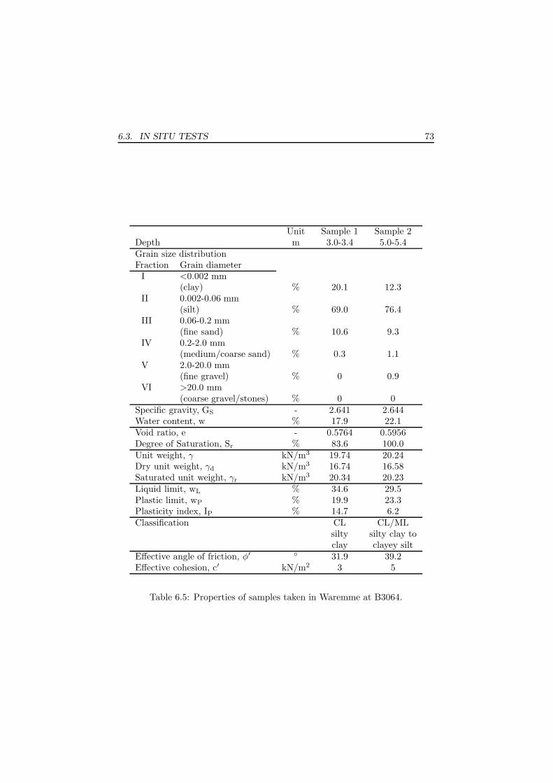
6.3. IN SITU TESTS 73
Unit Sample 1 Sample 2Depth m 3.0-3.4 5.0-5.4Grain size distributionFraction Grain diameter
I <0.002 mm(clay) % 20.1 12.3
II 0.002-0.06 mm(silt) % 69.0 76.4
III 0.06-0.2 mm(fine sand) % 10.6 9.3
IV 0.2-2.0 mm(medium/coarse sand) % 0.3 1.1
V 2.0-20.0 mm(fine gravel) % 0 0.9
VI >20.0 mm(coarse gravel/stones) % 0 0
Specific gravity, GS - 2.641 2.644Water content, w % 17.9 22.1Void ratio, e - 0.5764 0.5956Degree of Saturation, Sr % 83.6 100.0Unit weight, γ kN/m3 19.74 20.24Dry unit weight, γd kN/m3 16.74 16.58Saturated unit weight, γr kN/m3 20.34 20.23Liquid limit, wL % 34.6 29.5Plastic limit, wP % 19.9 23.3Plasticity index, IP % 14.7 6.2Classification CL CL/ML
silty silty clay toclay clayey silt
Effective angle of friction, φ′ 31.9 39.2Effective cohesion, c′ kN/m2 3 5
Table 6.5: Properties of samples taken in Waremme at B3064.

74 CHAPTER 6. TEST SITE WAREMME
0 10 20
0
2
4
6
8
10
12
14
qc [MN/m²]
Dep
th [m
]
Figure 6.3: CPT3064,cone resistance profileqc.
0 10 20
0
2
4
6
8
10
12
14
qc [MN/m²]
Dep
th [m
]
Figure 6.4: CPT3063,cone resistance profileqc.
0 10 20
0
2
4
6
8
10
12
14
qc [MN/m²]
Dep
th [m
]
Figure 6.5: CPT3064and 3063, mean qc.
two independently obtained velocity profiles using a sledgehammer on one sideof the beam and the mechanical swing hammer on the other side. The resultsof the shear wave velocity show a very good agreement with both types ofhammers.
The profiles obtained by visual interpretation show a higher scatter andvariation than those obtained by the cross correlation technique. Thereforealso in this case it is assumed that SCPT4 and SCPT5 deliver more reliablevalues than the other SCPT’s.
However, SCPT4 and SCPT5 differ in the shallow rage down to 3.5 m notinsignificantly. A local difference in the soil properties might be an explanationsince the tests have been performed at some distance from each other. Ingreater depths both tests agree very well.
If SCPT4 and SCPT5 are summarized a quite linear increase from 115 m/sat 1 m depth to 265 m/s at 11 m depth can be concluded.
Vp values are not calculated accurately because of poor signal definition.

6.3. IN SITU TESTS 75
0 10 20 30 40 50
0
2
4
6
8
10
12
14
φ [°]
Dep
th [m
]
Figure 6.6: Undrained angle of internal friction φ calculated from qc, Waremme.
0 200 400 600
0
2
4
6
8
10
12
14
S−wave velocity [m/s]
Dep
th [m
]
SCPT 1−2
No. 1No. 2
Figure 6.7: S-wave velocity fromSCPT1 - SCPT2 using visual inter-pretation, Waremme.
0 200 400 600
0
2
4
6
8
10
12
14
S−wave velocity [m/s]
Dep
th [m
]
SCPT 4−5
No. 4No. 5
Figure 6.8: S-wave velocity fromSCPT4 - SCPT5 using cross corre-lation, Waremme.

76 CHAPTER 6. TEST SITE WAREMME
0 2.5 5 7.5 10
0
2
4
6
8
10
12
14
Damping Ratio [%]
Dep
th [m
]
SCPT 5
Mechanical HammerSledgehammer
Figure 6.9: Values of damping ratio obtained from SCPT5, Waremme.
Test results for the damping ratio
The signals recorded in the SCPT5 are analyzed to obtain the damping ratio.The spectral ratio slope method is used for this purpose. The results arepresented in Figure 6.9. The determined values focus in the range between 0and 3 %. For closer details on the scattering it can be refered to Section 4.4.3on the Retie site where a similar scatter is found.
6.3.3 Spectral analysis of surface waves (SASW)
Remarks on the testing setup and inversion assumptions
Two measurement lines are tested once by the K.U. Leuven and another timeby the Ghent University. The first line is situated parallel to the building No.55 and is named setup 1. The other line is perpendicular to the rail way trackand named setup 2. Both lines are indicated in Figure 6.1.
SASW performed by K.U. Leuven (KUL) The falling weight device ofthe K.U. Leuven is used as source in these tests.
In the first setup the accelerometers are installed at 3, 4, 6, 8, 12, 24, 32and 48 m distance from the source; setup two uses accelerometers at distancesof 3, 4, 6, 8, 12, 16 and 24 m only, because the space in the direction of the railway track is limited.
Detailed information on the SASW tests of K.U. Leuven are given in Pyl& Degrande (2001b). The inversion is performed initially assuming a layer on

6.4. LABORATORY TESTS TO OBTAIN GMAX AND D 77
a halfspace. An extension to two layers on a halfspace changed nearly nothingon the determined s-wave profiles.
The coefficient of Poisson ν = 0.33, the density ρ = 1800 kg/m3 and thedamping ratio for p- and s-wave βs = βp = 0.5 % are kept constant in the in-version procedure.
SASW performed by Ghent University (UGent) The two SASW testsof Ghent University are performed on the same lines as the tests of K.U. Leuven.The drop weight of the Ghent University and a hand-held hammer is used togenerate the surface waves. The testing procedure is the same as at the Retiesite.
The inversion calculation delivered already sufficient result with the simu-lation of a halfspace only. The density and Poisson’s ratio are chosen withρ = 2000 kg/m3 and ν = 0.3, respectively.
Test results
The shear wave velocity profiles are given in Figure 6.10 for setup 1 and inFigure 6.11 for setup 2.
The results of nearly all inversion calculations show a constant stiffness withdepth. The SASW test of the K.U. Leuven suggests a change of s-wave velocityat a depth of 4.5 m in the case of setup 1.
6.4 Laboratory tests to obtain Gmax and dam-
ping ratio
6.4.1 Bender elements with time arrival interpretation
Two samples of boring B1 were installed in the triaxial bender element testdevice in a way that the s-wave velocity in the vertical direction can be deter-mined. Two other were installed turned by 90o. By this means the horizontals-wave velocity can be measured. The sample was consolidated under isotropicstress conditions. The s-wave velocity is measured at the end of the consolida-tion by a visual interpretation of the arrival signals. A back pressure of 100 kPawas used in al tests.
Table 6.6 summarizes the results and gives also calculated values of themaximum shear modulus Gmax. The necessary density are actual values at theend of the consolidation step. Figure 6.12 and Figure 6.13 show the results ingraphical form.
It is obvious that the differences in the results of horizontal and verticalpropagation are small if samples from a similar depth are compared. Thismeans that no significant structural anisotropy is found.
The development of Gmax during consolidation and further details can befound in the technical report Haegeman (2002).

78 CHAPTER 6. TEST SITE WAREMME
0 100 200 300
0
1
2
3
4
5
6
7
8
S−wave velocity [m/s]
Dep
th [m
]
Setup 1
UGentKUL
Figure 6.10: SASW results at setup1, parallel to the house, Waremme.
0 100 200 300
0
1
2
3
4
5
6
7
8
S−wave velocity [m/s]
Dep
th [m
]
Setup 2
UGentKUL
Figure 6.11: SASW results at se-tup 2, perpendicular to the rail waytrack, Waremme.
Sample / σ′
1,2,3 [kPa]Depth 25 50 100 200 400 600
B1/2 Vs [m/s] 120.1 143.2 182.5 221.6 279.4 -2.0-2.5 m Gmax [MPa] 26.7 40.9 66.9 99.4 159.6 -B1/10 Vs [m/s] - 168.2 198.2 239.8 294.3 315.6v
ert.
10.0-10.5 m Gmax [MPa] - 57.1 79.1 116.6 177.0 204.8
B1/3 Vs [m/s] 110.4 138.9 175.1 217.7 - -3.0-3.5 m Gmax [MPa] 27.3 43.8 70.6 111.0 - -B1/11 Vs [m/s] - 173.1 211.7 245.5 293.1 -h
oriz.
11.0-11.5 m Gmax [MPa] - 55.5 82.7 111.1 159.1 -
Table 6.6: Results of isotropic bender element tests with vertical and horizontalpropagation direction.

6.4. LABORATORY TESTS TO OBTAIN GMAX AND D 79
0 100 200 300 400 500 600 7000
50
100
150
200
250
300
350
400
σc [kPa]
Vs [m
/s]
B 1/2, verticalB 1/10, verticalB 1/3, horizontalB 1/11, horizontal
Figure 6.12: S-wave velocity by iso-tropic bender element tests withvertical and horizontal propagationdirection.
0 100 200 300 400 500 600 7000
50
100
150
200
250
σc [kPa]
Gm
ax [M
Pa]
B 1/2, verticalB 1/10, verticalB 1/3, horizontalB 1/11, horizontal
Figure 6.13: G0 by isotropic ben-der element tests with vertical andhorizontal propagation direction.
6.4.2 Free torsion pendulum test
A sample from the boring B1 from a depth of 12.0 to 12.5 m was tested inthe free torsion pendulum device of the Ghent University. The sample consistsmainly of silt and is taken from the transition area between the silt layer andthe chalk bedrock.
The dimensions of the sample were: 20 cm height, 10 cm diameter. Theisotropic stress stages have been chosen to 50, 100, 200 and 400 kPa. Themodulus at the reference shear strain of 10−5 is 35.1, 62.1, 100.6 and 152.9 MPaat 50, 100, 200 and 400 kPa confining stress respectively.
The obtained results of the 200 kPa consolidation stage show an exceptionalbehavior. The G-modulus increases extremely from γ = 10−5 in the direction ofthe lower shear strain. The damping ratio shows a peak at γ = 3 · 10−6. Eventhough the test was repeated several times with the same exceptional result,both phenomena are considered to be caused by the testing device. Thereforethe given values for the 200 kPa stage should be trusted only above a shearstrain of 10−5 for the G-modulus and above 10−4 for the damping ratio.
The damping ratio at a reference shear strain was found in the range of 1.0to 3.0 %, neglecting the 200 kPa stage. The smaller values correspond to thehigher confining stress stages and the larger ones to smaller stresses.
Shear modulus and damping ratio in function of the applied shear strain canbe found in Figure 6.14. The same parameters in dependence of the confiningstress at a shear strain of 10−5 are given in Figure 6.15.

80 CHAPTER 6. TEST SITE WAREMME
10-6
10-5
10-4
10-3
0
20
40
60
80
100
120
140
160
180
Shear Strain, γ [-]
G [M
Pa]
G-Modulus
10-6
10-5
10-4
10-3
0
0.05
0.1
0.15
Shear Strain, γ [-]
D [-
]
Damping Ratio
50 kPa100 kPa200 kPa400 kPa
50 kPa100 kPa200 kPa400 kPa
Figure 6.14: G-modulus and damping ratio versus applied shear strain obtainedby the Free Torsion Pendulum Test, sampling depth: 12.0 to 12.5 m, boringB1, Waremme.
6.4.3 Resonant column test
The tests were performed by the laboratory of the Norwegian GeotechnicalInstitute (NGI) in Oslo on two undisturbed samples from the site of Waremme.The sampling depth was 4.0-4.5 and 5.0-5.5 m. An isotropic confining stress of50, 100, 200 and 400 kPa was applied to the soil sample. Shear modulus anddamping ratio were measured during consolidation at a strain level of 10−5.The results at the end of consolidation, after about two days, are given inFigure 6.15.
The averaged values of the shear modulus for both samples increase withthe confining stress from 41.8 MPa at 50 kPa isotropic stress to 65.4 MPa at100 kPa, to 103.2 MPa at 200 kPa and finally to 154.6 MPa at 400 kPa.
The damping ratio is for all stress stages between 1.0 and 1.5 %. Thedamping ratio obtained by the free torsion pendulum test is in for the lowerstress stages higher than the results from the resonant column test. The shearmoduli agree very well with the findings from the free torsion pendulum test.

6.5. OVERVIEW OF THE TEST RESULTS WAREMME 81
0 100 200 300 4000
20
40
60
80
100
120
140
160
σc [kPa]
G [M
Pa]
G−Modulus
Resonant Column Test, 4.0−4.5 mResonant Column Test, 5.0−5.5 mFree Torsion Pendulumn Test, 12.0−12.5 m
0 100 200 300 4000
0.005
0.01
0.015
0.02
0.025
0.03
0.035
0.04
0.045
0.05
σc [kPa]
D [−
]
Dampig Ratio
Figure 6.15: G-Modulus and damping ratio versus isotropic confining stress,shear strain 10−5, boring B1, Waremme.
6.5 Overview of the test results Waremme
Figure 6.16 summarizes the gathered geotechnical data for the site in Waremme.It gives a simplified profile of drilling B1. The layers are labeled based on theirmain components.
The profile of the shear wave velocity is concluded out of the results ofSCPT4 and SCPT5 for depths deeper than 1 m. It is assumed that both testsdeliver the most reliable values. They show a uniform increase of the velocitywith depth, which is considered by the assumption of a linear increase from115 m/s at 1 m depth to 265 m/s at 11 m depth. Furthermore the resultsobtained by the SASW tests fall in the same range. The s-wave velocity ofthe very shallow layer is taken from the SASW tests on setup 1. Its value is155 m/s.
Table 6.7 presents selected values for qc and φ of the averaged CPT-profile;Table 6.8 gives the s-wave velocities determined by SCPT4, SCPT5 and thefour SASW tests.

82 CHAPTER 6. TEST SITE WAREMME
0.00
m Silt
Quaternary Deposits
Formation of Heers(Tertiary Deposit)
Gro
un
dw
ater
6.72
m
155
115
265
0.00
m
1.00
Sim
plif
ied
Str
atif
icat
ion
o
f D
rilli
ng
B1
Ave
rag
ed C
PT
-Pro
file
sS
imp
lifie
d S
-Wav
e V
elo
city
Pro
file
Tip
Res
ista
nce
Inte
rnal
Fri
ctio
nV
s [m
/s]
Sit
e W
arem
me
1.00
11.5
0
12.5
0
Gra
vel
Ch
alk
Silt
/Sto
ne
Mix
ture
12.5
0
11.0
0
Depth [m]
7.50
(Cla
yey
Silt
to
Silt
y C
lay)
12.7
5
Creataceousformation
020
040
0
0 2 4 6 8 10 12 14
S-w
ave
velo
city
[m
/s]
Depth [m]
05
1015
20
0 2 4 6 8
10 12 140
2040
141210
0 2 4 6 8Depth [m]
q
[MN
/m²]
cφ
[°]
Figure 6.16: Summary of the test results at Waremme.

6.5. OVERVIEW OF THE TEST RESULTS WAREMME 83
Averaged CPT-ProfileDepth qc φ Depth qc φ
[m] [MN/m2] [] [m] [MN/m2] []0.20 4.69 41.10 6.40 1.68 16.500.40 5.47 38.70 6.60 1.49 14.350.60 5.08 36.50 6.80 1.49 11.250.80 2.77 32.20 7.00 1.30 12.451.00 3.54 32.30 7.20 1.49 12.101.20 2.77 30.00 7.40 1.50 11.901.40 3.17 29.90 7.60 1.88 13.601.60 2.00 31.65 7.80 1.89 13.951.80 2.59 30.85 8.00 2.08 14.552.00 2.97 30.05 8.20 4.20 20.952.20 2.40 27.05 8.40 4.97 22.302.40 1.83 24.20 8.60 5.36 22.402.60 1.25 20.05 8.80 6.13 23.852.80 0.87 14.70 9.00 5.36 22.503.00 1.25 19.25 9.20 6.33 23.453.20 1.25 18.10 9.40 5.95 22.703.40 1.65 20.30 9.60 4.41 20.353.60 1.26 16.75 9.80 4.22 19.853.80 1.46 17.15 10.00 5.18 21.354.00 1.27 16.15 10.20 4.41 19.904.20 1.27 15.55 10.40 6.54 22.604.40 1.47 16.35 10.60 5.96 21.054.60 1.47 15.95 10.80 7.31 20.804.80 1.28 13.55 11.00 7.31 20.655.00 1.47 14.20 11.20 6.93 21.805.20 1.66 15.95 11.40 7.32 22.305.40 1.67 16.05 11.60 5.97 21.455.60 2.05 17.60 11.80 4.24 18.205.80 1.87 15.95 12.00 28.68 25.656.00 1.87 14.30 12.20 30.99 26.756.20 1.87 16.05
Table 6.7: Numerical values of the averaged CPT results.

84 CHAPTER 6. TEST SITE WAREMME
Profiles of SCPT’s SASW UGent Setup 1SCPT4 SCPT5 Layer Thickness Vs
Depth Vs Vs [m] [m/s][m] [m/s] [m/s] 1 > 7 1550.7 52.55 138.88
1.20 65.75 193.76 SASW UGent Setup 21.70 92.25 263.57 Layer Thickness Vs
2.20 116.95 200.76 [m] [m/s]2.70 117.45 154.75 1 > 7 1653.20 135.10 190.883.70 145.55 170.25 SASW KUL Setup 14.20 141.55 171.41 Layer Thickness Vs
4.70 145.15 176.11 [m] [m/s]5.20 158.95 183.72 1 4.46 1545.70 178.45 189.64 2 1.08 2156.20 186.55 198.07 3 ∞ 2166.70 191.75 199.987.20 193.60 199.84 SASW KUL Setup 27.70 204.80 201.18 Layer Thickness Vs
8.20 219.25 212.40 [m] [m/s]8.70 227.20 219.79 1 0.27 1459.20 251.90 244.33 2 0.70 1799.70 273.95 259.74 3 ∞ 179
10.20 264.20 267.7910.70 264.90 252.49
Table 6.8: Numerical values of SCPT4, SCPT5 and SASW results.

Chapter 7
Test siteSint-Katelijne-Waver
7.1 Introduction
The test location (I) is situated on a field on the property of the De NayerInstitute in Sint-Katlijne-Waver. Two borings were driven and two SCPT’swere performed. In the framework of a research project on Soil DisplacementScrew Piles a previous elaborate soil testing campaign has been performed ona research site at a distance of about 150 m. The surface of this site, lateron labelled as II, is about 2.3 m below the surface of site I. The tests havebeen performed at the end of the 1990th. They deliver beside conventional soilparameters also information on shear and compression wave velocity obtainedby SASW and seismic refraction tests. A detailed summary on this results canbe found in Menge (2001), but the most essential findings are also repeated inthe following. Table 7.1 gives an overview of the in situ tests which results areneeded later.
A sketch of the site is given in Figure 7.1. It shows the position of the insitu test on location I.
7.2 Borings and undisturbed sampling
The stratification of the site is quite simple. It consists of a disturbed top layerof clayed sand with stones and gravel, followed by a homogeneous layer of claywhich extends to great depths. The interface between the sand and the clay isfor testing site I at about 3 m depth and for site II at 0.7 m depth.
The clay belongs geologically to the tertiary formation of Boom, the sandof the top layer is a quaternary deposit.
85

86 CHAPTER 7. TEST SITE SINT-KATELIJNE-WAVER
Date Available In Situ Tests Site Abbr. Depth[m]
14/05/2003 Boring with discontinuous samp-ling
I B1I 11.0
14/05/2003 Boring with continuous sampling I B2I 11.013/05/2003 SCPT I SCPT1 12.914/05/2003 SCPT I SCPT2 12.9
Boring with undisturbed samp-ling
II B1II 14.0
30 CPT using an electrical cone II CPT-E 14.04 Marchetti dilatometer tests II DMT 13.05 SASW profiles II SASW1-53 measurement lines tested byseismic refraction test
II SRT
Table 7.1: Overview of the used in situ tests.
SCPT 2
B 2
SCPT 1
B 1
Parking Space
TreeTree Tree
7.20
14.0
04.
005.
003.
60
5.20
3.1012.10
1.60 1.80
Access Road
Building of the De Nayer Institute
Entrance
Tree
[m]
Figure 7.1: Site location plan, Sint-Katelijne-Waver, site I.
Groundwater table
The groundwater table is found at site I at depths between 0.5 and 1 m depth.If a horizontal groundwater table between site I and II is assumed the table atsite II can be estimated 2.8 to 3.3 m deep.

7.3. IN SITU TESTS 87
Properties of the sampled material
Important physical parameters of the Boom clay found in boring B1II are givenin the following. Laboratory tests to obtain Gmax and the damping ratio arediscussed in Section 7.4.
At site II samples are taken in the Boom clay at four depths, 4.5 to 4.9 m(sample a), 8.5 to 8.9 m (sample b), 10.5 to 10.9 m (sample c) and 13.5 to13.9 m (sample d). The density, the water content, the degree of saturationand the plasticity index are similar. Therefore Table 7.2 also summarizes themean values for all four samples. The range of the curves of the grain sizedistribution is given in Figure 7.2.
CU-triaxial tests are performed on samples from the four depths. A globalinterpretation of all results leads to the effective shear resistance parametersφ′ = 28o and c′ = 23 kPa.
Parameter Unit Sample Meana b c d Value
Dry unit weight, γd kN/m3 15.7 15.3 15.5 15.4 15.5Natural unit weight, γ kN/m3 19.7 19.3 19.5 19.4 19.5Water content, w: % 25.3 26.0 25.8 26.1 25.8Saturation degree, Sr: % (101.8) 99.2 (100.9) (101.0) 100.0Liquid limit, wL: % 72.2 65.1 75.9 71.8 71.6Plastic limit, wP: % 25.4 25.3 26.2 26.0 25.7Plasticity index, IP: % 46.8 39.9 49.7 45.8 45.6
Table 7.2: Properties of Boom clay.
0.0010.010.11 10
0
10
20
30
40
50
60
70
80
90
100
Grain size [mm]
Sie
ve r
esid
ue [%
]
V − fine Gravel IV − coarse to medium Sand III − fine Sand II − Silt I − Clay
2 0.2 0.06 0.002 20
VI
coar
se G
rave
l to
Sto
nes
Range of grain size distribution
Figure 7.2: Grain size distribution at Sint-Katelijne-Waver.
7.3 In situ tests
7.3.1 Marchetti dilatometer test (DMT)
Altogether four DMT’s were performed on site II. A profile of the overcon-solidation ratio OCR and another for the K0-value were correlated using the

88 CHAPTER 7. TEST SITE SINT-KATELIJNE-WAVER
0 20 40 60 80
0
2
4
6
8
10
12
14
Overconsolidation ratio
Dep
th [m
]
Figure 7.3: Overconsolidation ra-tio derived from dilatometer test re-sults at site II.
1 2 3 4
0
2
4
6
8
10
12
14
K0
Dep
th [m
]
Figure 7.4: K0-value derived fromdilatometer test results at site II.
horizontal stress index KD, obtained directly from the test. Both are shownin Figure 7.3 and Figure 7.4. Menge (2001) gives details on the correlationequation.
The OCR-value in the boom clay is in the range between 70 at shallowdepths and 15 at 14 m depth. K0 decreases in the same zone from 3 to 1.8.Because the top layer at site I is 2.3 m thicker than at site II it is not possibleto convert the values directly to site I. However, it can be assumed that site Iwould show similar results.
7.3.2 Cone penetration test (CPT)
CPT’s have been done during the research project on Soil Displacement ScrewPiles using electrical CPT-cones. The averaged profile of the tip resistance qc
of 6 of the CPT’s is drawn in Figure 7.5. A high reliability of the CPT resultsis concluded from the small range of standard deviation. Some discontinuitiesin the averaged profile can be explained by the presence of a few boulders atseveral depths. Also in this case the different thick top layers at site I and IIhave to be kept in mind if the profile should be used also for site I.
7.3.3 Seismic cone penetration test (SCPT)
Test setup
The two SCPT’s on site I are performed using the 200 kN automotive remote-controlled track vehicle. The cone was driven to a final depth of about 13 m in

7.3. IN SITU TESTS 89
0 1 2 3 4 5
0
2
4
6
8
10
12
14
qc [MN/m²]
Dep
th [m
]
Figure 7.5: Averaged cone resistance qc and range of standard deviation, site II.
0 100 200 300
0
1
2
3
4
5
6
7
8
9
S−wave velocity [m/s]
Dep
th [m
]
SCPT 1−2
No. 1No. 2
Figure 7.6: S-wave velocity usingcross correlation based on SCPT1and SCPT2.
0 2 4 6 8 10
0
1
2
3
4
5
6
7
8
9
Damping Ratio [%]
Dep
th [m
]
SCPT 2
Mechanical HammerSledgehammer
Figure 7.7: Values of damping ratioobtained from SCPT2.

90 CHAPTER 7. TEST SITE SINT-KATELIJNE-WAVER
both tests. Because of a bad signal quality leading to unreasonable fluctuationsin the results of the shear wave velocity the results are only shown to a depthof 7.5 and 8.5 m.
The dual cone with two triaxial accelerometers in 1 m distance is usedtogether with the de-coupled seismic source for SCPT1 and SCPT2. Somecloser details on cone and source can be found in Section 4.4.1.
Test results for the wave velocity
Figure 7.6 gives the profiles of the shear wave velocity obtained by the crosscorrelation technique. Each profile is the mean curve of a profile calculatedusing the sledgehammer and another one using the mechanical swing hammer.
At depths beneath about 4 m the profiles of SCPT1 and SCPT2 fall togetherand are in the range of 150 to 180 m/s. The shallow layer of clayed sand isindicated by higher velocities up to 200 and 250 m/s. The agreement betweenthe two tests is in this top layer not as perfect as in the deeper clay layer.
Test results for the damping ratio
The SCPT2 is analyzed to obtain the damping ratio using the spectral ratioslope method. The results are presented in Figure 7.7. The values are in therange between 0 and 5 % at all depths. The variation is qualitativelly similarto the other test sites. For closer details it can be refered to Section 4.4.3 onthe Retie site.
7.3.4 Spectral analysis of surface waves (SASW)
5 measurement lines were tested by the SASW method on site II. The resultingprofiles are presented in Figure 7.8, the numerical values are given in Table7.3. The inversion calculation was performed assuming three layers on thehalfspace, for SASW 2 and 5 four layers of the halfspace were preferred becausethe measured dispersion curve could be better approximated and because a fillmaterial was used at both measurement lines to replace the first 30 cm of thetop soil material. The very similar profiles from the five SASW tests show anincreasing stiffness with depth. Within the clay layer the shear wave velocityincreases from about 170 to 470 m/s. In comparison with the SCPT’s are thesenoticeable higher values.
7.3.5 Seismic refraction test (SRT)
3 measurement lines on site II are also tested by seismic refraction. Figure 7.9shows the obtained profiles. A s-wave velocity of VS = 145 m/s was found inthe top layer until a depth of 2 m. This corresponds to a G0 of 40 MPa. Thep-wave velocity gives values below 1000 m/s.
Table 7.4 gives the obtained velocity values for the clay layer beneath 2 mdepth. The s-wave velocity averages to about 350 m/s; the p-wave velocity

7.4. LABORATORY TESTS TO OBTAIN GMAX AND D 91
0 200 400 600 800
0
1
2
3
4
5
6
7
8
9
S−wave velocity [m/s]
Dep
th [m
]
No. 1No. 2No. 3No. 4No. 5
Figure 7.8: SASW tests performedat site II.
0 200 400 600 800
0
1
2
3
4
5
6
7
8
9
S−wave velocity [m/s]
Dep
th [m
]
Profile AProfile BProfile C
Figure 7.9: Seismic refraction testresults at site II.
No. 1 No. 2 No. 3 No. 4 No. 5Layer d Vs d Vs d Vs d Vs d Vs
[m] [m/s] [m] [m/s] [m] [m/s] [m] [m/s] [m] [m/s]
1 0.8 90 0.3 170 0.7 110 0.6 90 0.3 2002 1.0 180 0.5 100 1.1 170 1.2 170 0.5 1103 4.1 380 1.1 160 4.4 320 4.2 350 1.1 1604 ∞ 450 4.3 340 ∞ 470 ∞ 470 4.4 3005 ∞ 500 ∞ 700
Table 7.3: SASW Profiles, site II.
agrees with the propagation speed in water of about 1450 m/s or is even higher.Closer details on these seismic refraction tests can be found in Menge (2001).
However, the found s-wave velocity of the clay confirms the results of theSASW tests but is higher than the results from the SCPT’s.
7.4 Laboratory tests to obtain Gmax and dam-
ping ratio
7.4.1 Bender elements with time arrival interpretation
The undisturbed samples from site II were tested in a triaxial cell under iso-tropic confining stress. The results of the analysis of the arrival of the shear

92 CHAPTER 7. TEST SITE SINT-KATELIJNE-WAVER
Profile Vp Vs ν Edyn G0
[m/s] [m/s] [-] MPa MPa
A 1667 320 0.48 576 195B 1457 348 0.47 675 231C 1669 385 0.47 840 286
Table 7.4: Seismic refraction test results for the clay material beneath a depthof 2 m, site II.
0 100 200 300 400 500 6000
20
40
60
80
100
120
140
160
σc [kPa]
G0 [M
Pa]
Figure 7.10: Results of bender ele-ment tests, shear modulus G0 ver-sus isotropic consolidation stress σc,site II.
0 100 200 300 400 500 6000
50
100
150
200
250
300
σc [kPa]
VS [m
/s]
Figure 7.11: Results of bender ele-ment tests, s-wave velocity VS ver-sus isotropic consolidation stress σc,site II.
wave are drawn in Figure 7.10 and Figure 7.11. Both diagrams show the sameresults once in terms of shear modulus and the other in terms of shear wavevelocity. They can be linked if a density of 1988 kg/m3 is used.
7.4.2 Free torsion pendulum test
A sample taken from the boring segment between 4.0 and 4.5 m depth ofboring B2I was installed in the free torsion pendulum test device of the GhentUniversity. The dimensions of the sample were: 20 cm height, 10 cm diameter.The isotropic stress stages have been chosen to 50, 100, 200 and 400 kPa. Thedamping ratio at a reference shear strain of 10−5 was found in the range of 3.0 to4.0 %. The smaller values correspond as expected to the higher confining stressstages and the larger ones to smaller stresses. The modulus at the referenceshear strain is 35.0, 42.1, 53.4 and 69.2 MPa at 50, 100, 200 and 400 kPaconfining stress respectively.
Shear modulus and damping ratio in function of the applied shear strain canbe found in Figure 7.12. The same parameters in dependence of the confining

7.4. LABORATORY TESTS TO OBTAIN GMAX AND D 93
10−6
10−5
10−4
10−3
0
10
20
30
40
50
60
70
80
90
Strain [−]
G [M
Pa]
G−Modulus
10−6
10−5
10−4
10−3
0
0.01
0.02
0.03
0.04
0.05
0.06
0.07
0.08
Strain [−]
D [−
]
Damping Ratio
50 kPa100 kPa200 kPa400 kPa
50 kPa100 kPa200 kPa400 kPa
Figure 7.12: G-Modulus and damping ratio versus applied shear strain obtainedby the Free Torsion Pendulum Test, sampling depth: 4.0 to 4.5 m, site I.
stress at a shear strain of 10−5 are given in Figure 7.13. The found increaseof the damping ratio from a shear strain of 2 · 10−6 to lower strains is notexpected. It is assumed that this is caused by limitations in the test equipmentto measure very small movements of the excitation beam.
7.4.3 Resonant column test
A Boom clay sample has been sent to the private laboratory GEOLABO inFrance to perform a resonant column test. The isotropic stress stages havebeen again chosen to 50, 100, 200 and 400 kPa. Shear modulus and dampingratio were measured during consolidation at a strain level of 10−5. The valuesof the shear modulus increase with the confining stress from 27.9 MPa at 50 kPaisotropic stress to 32.3 MPa at 100 kPa, to 42.0 MPa at 200 kPa and finallyto 55.9 MPa at 400 kPa. The damping ratio is for all stress stage between 3.5and 4.0 %. Both can be seen in Figure 7.13.
The damping ratio agrees very well with the findings from the free torsionpendulum test. The shear modulus obtained by the free torsion pendulum testis in all cases 20 to 30 % higher than the results from the resonant column test.
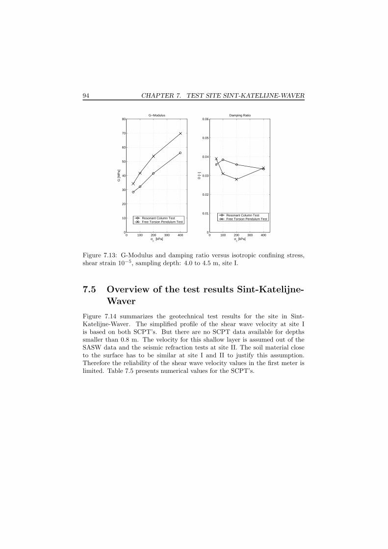
94 CHAPTER 7. TEST SITE SINT-KATELIJNE-WAVER
0 100 200 300 4000
10
20
30
40
50
60
70
80G−Modulus
σc [kPa]
G [M
Pa]
0 100 200 300 4000
0.01
0.02
0.03
0.04
0.05
0.06Damping Ratio
σc [kPa]
D [−
]
Resonant Column TestFree Torsion Pendulum TestResonant Column Test
Free Torsion Pendulum Test
Figure 7.13: G-Modulus and damping ratio versus isotropic confining stress,shear strain 10−5, sampling depth: 4.0 to 4.5 m, site I.
7.5 Overview of the test results Sint-Katelijne-
Waver
Figure 7.14 summarizes the geotechnical test results for the site in Sint-Katelijne-Waver. The simplified profile of the shear wave velocity at site Iis based on both SCPT’s. But there are no SCPT data available for depthssmaller than 0.8 m. The velocity for this shallow layer is assumed out of theSASW data and the seismic refraction tests at site II. The soil material closeto the surface has to be similar at site I and II to justify this assumption.Therefore the reliability of the shear wave velocity values in the first meter islimited. Table 7.5 presents numerical values for the SCPT’s.

7.5. OVERVIEW OF THE TEST RESULTS ST.-KATELIJNE-WAVER 95
0.00
m
Cla
yey
San
d
Quaternary Deposits
Formation of Boom
100
180
0.00
m
Sim
plif
ied
Str
atif
icat
ion
at
Sit
e I
Ave
rag
ed C
PT
-Pro
file
at S
ite
IIS
imp
lifie
d S
-Wav
e V
elo
city
Pro
file
at
Sit
e I
Vs
[m/s
]
Sit
e S
int-
Kat
elijn
e-W
aver
11.0
0
010
020
0
2 765430 1 Depth [m] S-w
ave
velo
city
[m
/s]
Cla
y
3.00
Gro
un
dw
ater
,m
ax. 2
.80
mm
in. 3
.30
m
0.00
m
0.70
m
14.0
0 m
16.3
0 m
2.30
m
3.00
m
Sim
plif
ied
Str
atif
icat
ion
at
Sit
e II
surf
ace
site
Isu
rfac
e si
te II
Ref
eren
ce le
vel:
Cla
yey
San
d
Cla
y
Depth [m] 8 12 1462 4 100
q
[MN
/m²]
01
32
45
c
300
8 9
210
150
210
0.80
3.00
8.50
Gro
un
dw
ater
as a
t si
te I
Formation of Boom Quaternary Deposits
Figure 7.14: Summary of the test results at Sint-Katelijne-Waver.

96 CHAPTER 7. TEST SITE SINT-KATELIJNE-WAVER
Profiles of SCPT’sSCPT1 SCPT2
Depth Vs Vs
[m] [m/s] [m/s]0.83 - 204.271.34 142.06 172.301.86 234.22 181.082.38 244.37 208.202.89 255.15 166.953.41 173.68 140.833.93 145.93 151.184.44 151.52 153.124.96 155.63 151.815.48 157.93 160.795.99 162.15 163.296.51 164.29 174.007.03 166.16 169.567.54 164.36 165.638.06 - 179.598.58 - 184.12
Table 7.5: Numerical values of Vs from SCPT1 and SCPT2.

Chapter 8
Test site Ghent
8.1 Introduction
The test location in Ghent is situated close to a storage and garage buildingof the Flemish Geotechnical Institute on the campus of the Ghent Universityin Zwijnaarde. A SCPT is performed on this site. Boring and CPT dataare additionally available. They have been gathered in preparation of theconstruction of the buildings of the geotechnical institute in the late 1960th.
A lay-out plan of the testing site is given in Figure 8.1 and the overview ofall used in situ test results can be found in Table 8.1.
Date Available In Situ Tests Abbr. Depth[m]
15/07/1968 Boring inside the ground-plan of themain building of the Flemish Geotech-nical Institute
B6 14.0
19/07/1968 Boring at the closest corner of the sto-rage and garage building to SCPT1
B21 5.0
19/07/1968 CPT at the place of boring B21 CPT21 14.7525/11/2003 SCPT with a dual cone equipped with
Bruel & Kjær accelerometersSCPT1 17.5
Table 8.1: Overview of the available in situ tests.
8.2 Borings and sampling
The boring B21 in close proximity to the performed SCPT reached only to adepth of 5 m. Therefore it is combined with the deeper, but also more far,boring B6. The stratification of the combined profile at the place of boring
97

98 CHAPTER 8. TEST SITE GHENT
SCPT 1
B 21
Parking Space
Storage and Garage Building
Flemish Geotechnical Institute / Ghent UniversityTechnologiepark 905, Zwijnaarde
Parking Space
B 6
CPT 21
Figure 8.1: Site location plan, Ghent.
B21 is given in Table 8.2 and in the site overview in Figure 8.5. Because of theextrapolation, the accuracy of the layer interface-levels at depths deeper than5 m might be rather low.
However, the site has a 0.75 m thick top layer of a silty sand followed byfine sand to a depth of about 8.25 m. The sand is mixed from this depth onwith an increasing amount of silt. The material is classified as silty sand tosandy silt.
All described soil layers are deposits originated in the Quaternary. The firsttertiary layer at the site is referred to the formation of Tilt. It is deeper thanthe final depth of the evaluated boring. Its presence is seen in boring profilesavailable in the Flemish Geotechnical Database on other locations inside theuniversity campus.
Groundwater table
The groundwater table is found at the boring B21 at 1.85 m depth.

8.3. CONE PENETRATION TEST (CPT) 99
From To Color Main Admixtures[m] [m] Component
0.0 0.75 dark brown fine sand silt0.75 8.25 gray, brown fine sand -8.25 10.80 gray fine sand silt
10.80 13.50 gray silt fine sandLithographic Stratification: 0 to 13.5 m quaternary deposits.
Table 8.2: Combined results of boring B21 and B6 for the location of B21.
8.3 Cone penetration test (CPT)
A CPT sounding has been performed at the place of boring B21 at one cornerof the garage. The profile of the tip resistance of the cone qc is given in Figure8.2.
0 2 4 6 8 10 12 14 16
0
2
4
6
8
10
12
14
16
qc [MN/m²]
Dep
th [m
]
Figure 8.2: Cone resistance qc, CPT21.
8.4 Seismic cone penetration test (SCPT)
8.4.1 Testing setup
The SCPT was performed using a 200 kN CPT-tuck without track support.Because of a very good signal quality the test was driven to a final depth ofabout 17.5 m.

100 CHAPTER 8. TEST SITE GHENT
The dual cone with two triaxial accelerometers from Bruel & Kjær (Section9.2.2), mounted in 1 m distance from each other, is used together with a de-coupled seismic source. Instead of the steel beam two square shaped woodenplates were applied. The horizontal hammer blows on the edge of the plateswere performed by the sledgehammer from both sides of the truck. The me-chanical swing hammer was not used at this site. Some closer details on coneand source can be found in Section 4.4.1.
8.4.2 Test results for the wave velocity
The shear wave velocity profiles obtained by cross correlation from both excita-tion directions are very consistently. They are given in Figure 8.3. A simplifiedprofile can be found in the summary in Figure 8.5.
8.4.3 Test results for the damping ratio
The data of the SCPT are analyzed to obtain the damping ratio using thespectral ratio slope method. The results are presented in Figure 8.4. Thevalues are mainly in the range between 0 and 10 % at all depths. The variationis qualitativelly similar to the other test sites. For closer details on the variationin the results can be refered to Section 4.4.3.
0 100 200 300 400
0
2
4
6
8
10
12
14
16
18
S−wave velocity [m/s]
Dep
th [m
]
SCPT 1
Left sideRight side
Figure 8.3: S-wave velocity fromSCPT using cross correlation, exci-tation from both sides of the truck.
0 10 20 30
0
2
4
6
8
10
12
14
16
18
Damping Ratio [%]
Dep
th [m
]
SCPT 1
Left sideRight side
Figure 8.4: Values of damping ra-tio obtained from SCPT, excitationfrom both sides of the truck.

8.5. OVERVIEW OF THE TEST RESULTS GHENT 101
8.5 Overview of the test results Ghent
Figure 8.5 summarizes the gathered geotechnical data for the site in Ghent.The simplified s-wave velocity profile is only derived from the SCPT in Figure8.3 because there are no other measurements of wave velocity performed at thissite. Table 8.3 presents numerical values for the SCPT.

102 CHAPTER 8. TEST SITE GHENT
0.00
m
Sim
plif
ied
Str
atif
icat
ion
at
Dri
llin
g B
21S
imp
lifie
d S
-Wav
e V
elo
city
Pro
file
fr
om
SC
PT
1
Sit
e G
hen
t, T
ech
no
log
iep
ark
905
0.75
Gro
un
dw
ater
1.85
m
Quaternary Deposits
8.25
10.8
0
13.5
0Fin
e S
and
(Silt
y S
and
)
(Silt
y S
and
)F
ine
San
d
(San
dy
Silt
)S
ilt
(San
d)
Fin
e S
and
141210Depth [m] 86420 16
q
[MN
/m²]
c
02
46
810
1214
16
Ave
rag
ed C
PT
-Pro
file
at
CP
T21
Depth [m]0 2 4 6 8 10 12 14 16 18
S-w
ave
velo
city
[m
/s]
100
020
030
040
0
280
180
160
Vs
[m/s
]
3.00
0.00
m
250
7.80
17.0
0
Figure 8.5: Summary of the test results at the site in Ghent.

8.5. OVERVIEW OF THE TEST RESULTS GHENT 103
Profiles of SCPT’sSCPT1
Depth Vs, Left Vs, Right
[m] [m/s] [m/s]1.34 228.02 170.231.86 198.58 192.482.38 179.91 173.012.89 156.71 164.083.41 172.16 176.043.93 182.39 181.694.44 203.71 195.254.96 214.44 220.845.48 231.68 227.225.99 242.09 260.006.51 269.30 272.487.03 265.46 286.807.54 287.33 284.058.06 261.24 261.198.58 251.82 258.829.09 247.12 250.819.61 238.09 245.00
10.13 246.17 242.8310.64 242.77 239.0111.16 248.12 249.5711.67 256.85 251.5012.19 228.94 238.7412.71 243.60 248.0213.22 257.02 256.1213.74 261.63 268.8914.26 259.69 279.1514.77 267.13 270.4115.29 256.53 260.2115.81 245.56 260.2516.32 252.19 264.3016.84 230.26 241.43
Table 8.3: Numerical values of Vs from SCPT1; excitation from the left andfrom the right side.

104 CHAPTER 8. TEST SITE GHENT

Part III
Studies on testing methods
105


Chapter 9
SCPT based techniques
9.1 Motivation and purpose
The seismic cone penetration test (SCPT) is developed from the cone penetra-tion test (CPT) using electrical cones. The capabilities of an electrical cone areextended by adding geophones or accelerometers to the usual transducers fortip resistance, sleeve friction and pore pressure. Also cones that are limited tothe vibration sensors are in use. These cones are called ”dummy cones”. Wavesgenerated at the surface travel to the cone pushed into the ground. The test issimilar to a down-hole test except for the borehole, necessary in the down-holetest to install seismic sensors. The main purpose of the method is to obtain thevelocity of shear and compression waves leading to values for Gmax and Emax.
Objectives and methodology
Aim of this part of the research is to obtain at first confidence in the deter-mination of wave velocity profiles. Afterwards the possibilities to use hiddeninformation in the time histories to calculate the damping ratio of the soilshould be investigated. The incorporation of the damping ratio measurementwould mean a significant improvement of the SCPT method. This is especiallytrue considering the fact that the few other approaches (e.g. SASW with ex-tended inversion, cross-hole test) to measure material damping in-situ are stillunder research and not state-of-the-art.
In order to achieve the aims the following topics are treated and describedin this chapter:
- Description of the test equipment
- Selection of suitable sensors for the installation in the seismic cone
- Summary of available direct and indirect time methods to measure wavevelocity, including example calculations
107

108 CHAPTER 9. SCPT BASED TECHNIQUES
- Theoretical background of three approaches to determine the dampingratio: Attenuation coefficient method, spectral ratio slope method andthe analysis of stress-strain curves
- Application of attenuation coefficient method and spectral ratio slopemethod on artificially generated time records to study the influence ofsignal windowing to the results
- Application of the spectral ratio slope method on all test sites (Retie,Lincent, Waremme, Sint-Katelijne-Waver, Ghent)
- Analysis of stress-strain curves based on data from a SCPT in Waremme
- Comparison of the results from the SCPT with resonant column and freetorsion pendulum tests on samples from Waremme and Sint-Katelijne-Waver concerning Vs and Ds
9.2 Applied equipment and selection criteria
An overview of a typical seismic cone set-up is given in Figure 9.1; the equip-ment described in detail in the following paragraphs is shown in Figure 9.2.
Beam
Static Load
Seismic Cone Penetrometer
Triaxial Accelerometers
Lateral Offset
Sledge−hammer
MechanicalHammer
LT
LB
tT
tB
Dep
th
Figure 9.1: Schematic sketch of a SCPT set-up using a dual cone.
9.2.1 Seismic source
The seismic source consists of a steel beam loaded by the weight of the CPTtruck and different types of hammers. A horizontal hammer blow at one endof the beam produces a shear wave dominated pulse and a vertical blow on topof the beam a compression wave dominated pulse.

9.2. APPLIED EQUIPMENT AND SELECTION CRITERIA 109
Ham
lin a
ccel
erom
eter
s or
geop
hone
s
Geo
phon
es
X2, Y2, Z2
X1, Y1, Z1
X1, Y1, Z1
6 channels
3 channels
Hammer and beam(shearwave source)
Termination box
Fugro signal conditioner module
PC with data−acquisition cardTrigger
channel
Brü
l & K
jaer
acc
eler
omet
ers
X2, Y2, Z2
X1, Y1, Z1
Dual seismic cone Single seismic cone
6 channels
ENDEVCO ICP source/amplifier
Figure 9.2: Functional overview of the seismic cone equipment.
Applied loadprovided by the CPT truck
Roller systemUpper bearing beams
Source beam Impact anvil
Applied loadprovided by the CPT truck
Impact anvil
Wooden beams
Applied loadprovided by the CPT truck
Source beam Impact anvil
a)
b)
c)
Figure 9.3: a) conventional coupled source, b) de-coupled source, c) de-coupledsource with a wooden plate as designed by Areias et al. (2004).

110 CHAPTER 9. SCPT BASED TECHNIQUES
The SCPT’s performed in the framework of this research use in most of thecases a source beam with a system of rollers on top, under the loading weight ofthe CPT truck. It is developed by Areias et al. (1999) and called a de-coupledsource. This increases the horizontal mobility of the beam resulting in a moreefficient transfer of the impact energy of the hammer to the actually generatedshear waves. Comparative studies between the de-coupled and the coupledsource without the roller system are found in Areias et al. (2004) showing thepositive effect of the rollers.
According to the same author there is an optimum vertical stress at theboundary between beam and soil. Consequently, it is always attempted toadjust the vertical force on the beam, applied by hydraulic cylinders, to itsoptimum value. This is checked by comparing time records of additional ham-mer blows performed in the beginning of each SCPT with the cone at a fixedshallow depth.
In the SCPT test on the university campus in Ghent two wooden plates aresuccessfully used instead of the steel beam. Their size suits more the demandsof an easy transport than the steel beam. Also in this case rollers under theloading piston are placed. Figure 9.3 shows principle sketches of the sourcebeams.
The impact energy is given by a sledge hammer or a mechanical swinghammer with an adjustable falling height. With the latter is aimed to generaterepeatable shear pulses of the same intensity. However, comparisons of repea-ted blows with the cone at a certain depth show that the assumption that themechanical swing hammer provides a repeatable source is questionable. Diffe-rences in the amplitudes and shapes of the generated shear pulse are observed,probably caused by a slight backwards movement of the hammer support andbeam from blow to blow. A fixing of the hammer frame with metal pins onthe ground could not improve the result. Furthermore it can be assumed thatthe load on the source beam changes with time due to a slowly sinking of theCPT truck additionally causing a changing shear amplitude.
The acceleration of the head of the mechanical swing hammer is measuredon the occasions of the SCPT5 in Retie and SCPT1 in Sint-Katelijne-Waver.A small shock accelerometer is installed on the backside of the hammer head.The weight of the whole moving arm of the hammer is approximately 25 kg.Because of the unknown weight distribution in the hammer arm, the impactforce was not calculated.
Four selected hammer impacts at the site in Retie are shown in Figure 9.4.Figure 9.5 provides the associated amplitude spectra. Even so the spectra arepartly different, it can be concluded that the main energy of the hammer impactis located between 200 and 600 Hz. It has to be remarked that the measuredtime histories characterize only the impact force applied to the source beam.The energy distribution of the dynamic force transfered to the ground mightbe different.
Another point concerns the measurement itself: the signal is sampled with2000 Hz, more than sufficient for the ground vibrations, but the frequency

9.2. APPLIED EQUIPMENT AND SELECTION CRITERIA 111
content of the impact pulse approaches the Nyquist frequency of 1000 Hz.Because there is no anti-aliasing filter applied to the hammer channel, it isnot completely impossible that existing signal parts at frequencies higher than1000 Hz are wrapped into the high frequency parts of the spectrum just below1000 Hz. However, this disturbance is probably limited to the higher frequencyrange.
0.48 0.5 0.52 0.54 0.56−8
−6
−4
−2
0
2
4
6
8x 10
4
Time [s]
Par
ticle
acc
eler
atio
n [m
/s²]
0.48 0.5 0.52 0.54 0.56−8
−6
−4
−2
0
2
4
6
8x 10
4
Time [s]
Par
ticle
acc
eler
atio
n [m
/s²]
0.48 0.5 0.52 0.54 0.56−8
−6
−4
−2
0
2
4
6
8x 10
4
Time [s]
Par
ticle
acc
eler
atio
n [m
/s²]
0.48 0.5 0.52 0.54 0.56−8
−6
−4
−2
0
2
4
6
8x 10
4
Time [s]
Par
ticle
acc
eler
atio
n [m
/s²]
No. 295 No. 309
No. 321 No. 325
Figure 9.4: Acceleration of the mechanical swing hammer during the SCPTNo. 5 in Retie, selected impacts.
9.2.2 Seismic cones
Two seismic cones are available at Ghent University manufactured by FugroEngineers, the Netherlands; one cone with a single triaxial array of geophonesand another cone with two triaxial arrays of accelerometers, installed 1 m or0.5 m distance from each other. The single cone is additionally equipped withtransducers for the tip resistance, sleeve friction and pore pressure. The dualcone is a dummy cone without conventional transducers. The cross-sectionaltip area of the single cone is 10 cm2 and of the dual cone 15 cm2. Sketchesof the dual cone with 1 m sensor distance and of the single cone are given in

112 CHAPTER 9. SCPT BASED TECHNIQUES
0 200 400 600 800 10000
10
20
30
40
50
60
70
80
90
100
Frequency [Hz]
Am
plitu
de S
pect
rum
[m/s
²]
No. 295
No. 309
No. 325
No. 321
Figure 9.5: Amplitude spectra of the selected hammer impacts from Figure9.4.
Figure 9.6.In the frame of this research both cones are used. The seismic sensors
in the dual cone are replaced two times in the run of the project. The firstchange replaced the originally installed geophones by VTI Hamlin accelerome-ters because of insufficient frequency response characteristics of the geophonesas described later on. These accelerometers where later replaced by accelero-meters from Bruel & Kjær to improve the signal-to-noise ratio leading to largertesting depths.
In the following the characteristics of the sensors used are described.
GeoSpace geophones
The triaxial array consists of three single geophones GSC-14-L3 produced byGeoSpace. The geophones are designed and built to maintain performancecharacteristics even after being subjected to high shock forces. The main spe-cifications of the sensors given by the manufacturer are:
• Natural frequency: 28 Hz ± 5 Hz
• Moving mass: 2.15 g
• Dimensions (diameter/height): 1.7 cm / 1.8 cm
• Open circuit damping: 18 %
• Intrinsic voltage sensitivity: 0.114 V/(cm/s), amplified by an internalamplifier to 27 V/(cm/s)
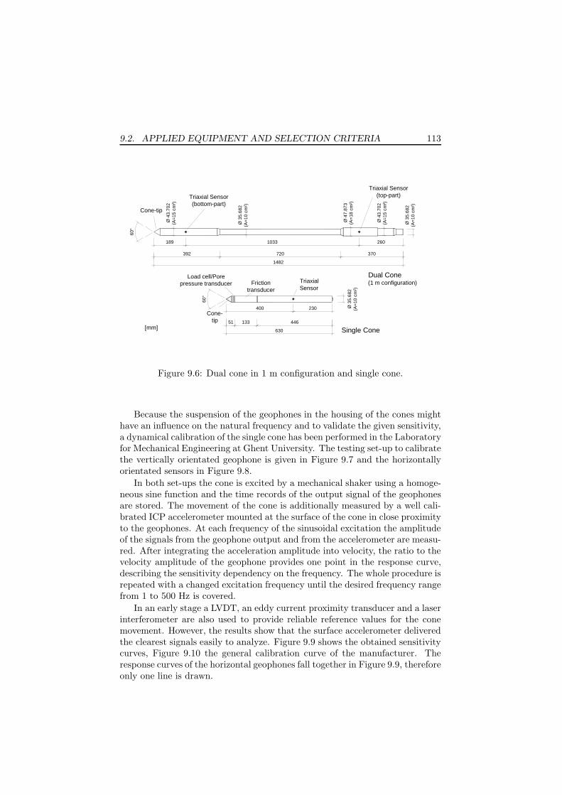
9.2. APPLIED EQUIPMENT AND SELECTION CRITERIA 113
189 1033 260
392 720 370
1482
60°
Ø 4
3.70
2( A
=15
cm
²)
Ø 3
5.68
2(A
=10
cm
²)
Ø 4
7.87
3(A
=18
cm
²)
400 230
51 133 446
630
60°
Cone-tip
Triaxial Sensor (bottom-part)
Triaxial Sensor (top-part)
Triaxial Sensor
Cone-tip
Load cell/Pore pressure transducer Friction
transducer
Dual Cone
Single Cone
Ø 3
5.6 8
2(A
=10
cm
²)
[mm]
Ø 3
5.68
2(A
=10
cm
²)
Ø 4
3.70
2(A
=1 5
cm
²)
(1 m configuration)
Figure 9.6: Dual cone in 1 m configuration and single cone.
Because the suspension of the geophones in the housing of the cones mighthave an influence on the natural frequency and to validate the given sensitivity,a dynamical calibration of the single cone has been performed in the Laboratoryfor Mechanical Engineering at Ghent University. The testing set-up to calibratethe vertically orientated geophone is given in Figure 9.7 and the horizontallyorientated sensors in Figure 9.8.
In both set-ups the cone is excited by a mechanical shaker using a homoge-neous sine function and the time records of the output signal of the geophonesare stored. The movement of the cone is additionally measured by a well cali-brated ICP accelerometer mounted at the surface of the cone in close proximityto the geophones. At each frequency of the sinusoidal excitation the amplitudeof the signals from the geophone output and from the accelerometer are measu-red. After integrating the acceleration amplitude into velocity, the ratio to thevelocity amplitude of the geophone provides one point in the response curve,describing the sensitivity dependency on the frequency. The whole procedure isrepeated with a changed excitation frequency until the desired frequency rangefrom 1 to 500 Hz is covered.
In an early stage a LVDT, an eddy current proximity transducer and a laserinterferometer are also used to provide reliable reference values for the conemovement. However, the results show that the surface accelerometer deliveredthe clearest signals easily to analyze. Figure 9.9 shows the obtained sensitivitycurves, Figure 9.10 the general calibration curve of the manufacturer. Theresponse curves of the horizontal geophones fall together in Figure 9.9, thereforeonly one line is drawn.

114 CHAPTER 9. SCPT BASED TECHNIQUES
Roller bearing
Triaxial geophone(inside)
Accelerometer
Shaker
Single Cone
Figure 9.7: Calibration ofthe single cone with instal-led geophones, vertical.
Roller bearing(rotation centre) Triaxial geophone (inside)
Accelerometer
Shaker
Single coneLeaf spring
Figure 9.8: Calibration of the single conewith installed geophones, horizontal.
It is not possible to compare the calibration curve given by the sensormanufacturer with the results of our calibration directly because the cone ma-nufacturer has added an amplifier to the signal flow. It is impossible to switchthis amplification off during the calibration.
The results of these tests are: a) the geophones in vertical and horizontaldirection have a similar response behavior, b) the sensitivity over the investiga-ted frequency range is not flat at any frequency, c) the natural frequency of thesensors is about 33 Hz. Therefore the measurement sensors are not qualified fortasks were an accurate amplitude is requested. Nevertheless they are sufficientfor analyses of time arrivals for wave velocity measurements.
VTI Hamlin accelerometers SCA 600
For afore mentioned reasons the geophones of the dual cone are in the frame-work of this research replaced by accelerometers of the type SCA600-C13H1Gfor the horizontal axes and by SCA600-C13V1G for the vertical axis.
The vertical Hamlin accelerometers of the dual cone are calibrated in themechanical engineering laboratory under similar testing conditions as the singlecone, using one reference accelerometer. The testing set-up for the horizontalaccelerometers is slightly modified to consider the two triaxial arrays. Thesketch of the set-up is given in Figure 9.11.

9.2. APPLIED EQUIPMENT AND SELECTION CRITERIA 115
0 50 100 150 200 250 300 350 400 450 5000
1
2
3
4
5
6
Frequency [Hz]
Sen
sitiv
ity [V
/ (m
m/s
)]
Vertical GeophoneHorizontal Geophones
Figure 9.9: Calibration curves of the seismic single cone equipped with geo-phones GeoSpace GSC-14-L3.
101
102
103
10−2
10−1
100
FREQUENCY [Hz]
OU
TP
UT
[V/(
IN/S
EC
)]
GeoSpaceGSC−14−L3
Figure 9.10: Calibration curve of the geophones GeoSpace GSC-14-L3 as pro-vided by the manufacturer.

116 CHAPTER 9. SCPT BASED TECHNIQUES
Roller bearing(rotation centre)
Triaxial accelerometer (inside)
Reference accelerometer
Shaker
Dual cone
Leaf spring
Reference accelerometer
Triaxial accelerometer (inside)
Figure 9.11: Calibration of the dual cone with installed Hamlin accelerometers,horizontal.
The main specifications of the Hamlin sensors are:
• Measuring range: ± 1.5 g
• Sensitivity: 1.116 V/g by own calibration, 1.333 V/g given by manufac-turer
• linearity: until 400 Hz ± 150 Hz flat response with a deviation smallerthan -3 dB
• Resolution (Residual noise): 0.9 - 4.5 mg (1 mg = 9.81 · 10−3m/s2)
The accelerometers have in principle a true DC response. That meansthe sensitivity should not drop down in the low frequency range. However,the conditioner equipment adds a bandpass filter with corner frequencies of 1and 350 Hz, that can partly explain the changing curve in the range belowapproximately 20 Hz as shown in Figure 9.12.
The sensitivity of the accelerometers is according to our own calibrationslightly lower than expected from the manufacturer specification. In the insitu tests the value of 1.116 V/g is always used.
Triaxial DeltaTron Bruel & Kjær accelerometers
The installed Hamlin accelerometers showed an unexpected high noise compo-nent forcing in almost all cases to stop SCPT testing at depths of about 10 mbecause of low signal-to-noise ratio, so the main wave pulse was not identifiableanymore.
Therefore it is decided to change the accelerometers once more. This timetriaxial accelerometers of the type Bruel & Kjær 4506 B 002 are installed.The sensors require a constant power supply compatible to the IsoTron or ICPspecifications. They have a noise level 30 to 150 times smaller than those ofthe Hamlin accelerometers.

9.2. APPLIED EQUIPMENT AND SELECTION CRITERIA 117
0 20 40 60 80 100 120 1400
0.2
0.4
0.6
0.8
1
1.2
1.4
Frequency [Hz]
Sen
sitiv
ity [V
/g]
chosen characteristic sensitivity: 1.116 V/g(exact at 23 and 50 Hz )
Figure 9.12: Calibration curves of the Hamlin accelerometers of type SCA600-C13H1G/C13V1G.
The main parameters of the Bruel & Kjær 4506 B 002 accelerometers are:
• Measuring range: ± 7 g
• Sensitivity: ≈ 1 V/g (exact values specified by the manufacturer separa-tely for each axis)
• Amplitude linearity (flat response with a deviation smaller than 10 %):
– Horizontal axes: 30 - 1600 Hz
– Vertical axis: 30 - 3500 Hz
• Resolution (Residual noise):
– Horizontal axes: 0.03 mg (1 mg = 9.81 · 10−3m/s2)
– Vertical axis: 0.06 mg
A calibration by means of the shaking apparatus is not performed anymore.Figure 9.13 gives the response curve provided by Bruel & Kjær.
9.2.3 Data acquisition system
A PC-based data acquisition system is used to record waveform signals fromthe SCPT. The set-up can be found in Figure 9.2.
For measurements with the dual cone, at least 6 channels are required. Thesignal conditioner module provides the power for the sensors inside the cone

118 CHAPTER 9. SCPT BASED TECHNIQUES
Figure 9.13: Typical frequency response of the Bruel & Kjær 4506 B 002.
and applies an analogue bandpass filter to the signals with the edge frequencies1 and 350 Hz (high-pass 1 Hz, 6 dB/oct; low-pass 350 Hz, 12 dB/oct). Thisconditioner module of the seismic cone is connected to the termination box ofthe data acquisition card inside the PC by conventional BNC-cables. The firstchannel is used to trigger the measurement. The hammer and the beam areconnected to this port. A voltage of 5 V is applied to the channel inside thetermination box. When hammer and beam get in contact, the two poles arebypassed over a resister and the voltage on the channel drops. This can beused to generate a software trigger in the acquisition program.
In the case that the Bruel & Kjær accelerometers are used the conditionerunit is to be replaced by an ICP or Isotron source. At the test site in Ghenta filter and amplifier system KEMO VBF35 provided by the K.U. Leuven isused. The lowpass cut-off frequency is set to 1000 Hz. Alternatively the 9channel source and amplifier of Ghent University ENDEVCO 2792B withoutfilter can be applied.
SCPT’s using the single cone are performed with a sampling frequency of4000 Hz; vibration events measured with the dual cone are sampled at 2000Hz. So the Nyquist frequency is 2000, respectively 1000 Hz, much higher thanthe 350 Hz cut-off frequency of the bandpass filter, or equal to the 1000 Hz cut-off frequency of the KEMO VBF35 system. Aliasing effects are consequentlyimpossible or in case of the KEMO amplifier sufficiently reduced. On the sitein Ghent at some depths measurements are repeated without analog low-passfilter. The time histories show a similar quality as those with filter except forsome additional noise.
Main specifications of the data acquisition card manufactured by MicrostarLaboratories are:
• Type: DAP 4000a/112, PCI bus
• Number of analog inputs: 16

9.3. METHODS FOR THE SHEAR MODULUS 119
• Possible input ranges: ± 2.5 V, ± 5 V, ± 10 V
• Maximum sampling frequency (all channels together): 800 kHz
• Analog/digital resolution: 14 bit
• Programmable gain rates: 1, 10, 100, 500
For this research a software tool for data acquisition is developed in thegraphical programming environment LabVIEW. The main features of this pro-gram are described below.
• possibility to handle 10 channels, 6 for the dual seismic cone, 3 for anadditional surface vibration measurement, 1 for a shock accelerometermounted at the impact hammer
• possibility to average different repetitions of an event at the time of mea-surement
• free choice of sampling rate, pre- and post-trigger time (limited by theacquisition card)
• measurement triggering by a contact signal or by exceeding an adjustablevoltage level on one of the channels
• possibility to apply a gain (1, 10, 100, 500) to each channel separately
• storage of the acquired data in an easy to read ASCII-file
• quick overview of the signals in time and frequency domain
• possibility to reject disturbed signals
• possibilities to store events manually, semi-automatically and automati-cally
• advanced capabilities of further automated analyses using the power ofthe LabVIEW environment
The program replaces the commercial software packet ProView from Nicoletand is already used during the calibration tests of the single and dual cone. Thiswork is done with the help of the Department of Electronics and InformationSystems of the Ghent University.
9.3 Methods to obtain the dynamic shear mo-
dulus
The shear modulus is obtained by determining the shear wave velocity Vs.Because the generated waves reach only very small strain levels below the

120 CHAPTER 9. SCPT BASED TECHNIQUES
elastic threshold strain the modulus calculated with Equation (2.1) can beassumed as Gmax or G0.
The elasticity modulus Emax or E0 can be calculated out of the compressionwave velocity Vp using Equation (9.1) for an infinite elastic medium.
Emax = V 2p ρ
(1 + ν)(1 − 2ν)
1 − ν(9.1)
Poisson’s ratio ν can be directly determined out of the ratio between Vp
and Vs in Equation (9.2).
ν =1
2
(
Vp
Vs
)2
− 2(
Vp
Vs
)2
− 1(9.2)
The wave velocity is calculated by comparing time records from differentdepths. If a single cone with a sensor array at a certain depth is used, theexcitation pulse can be only measured once. In this case the comparison isperformed with a time record obtained at another cone depth, associated withanother excitation pulse. The test depth interval in this research is approxi-mately 50 cm. Other authors prefer 100 cm because this value matches thestandard length of an extension rod of the SCPT.
If a dual cone is used for the test, as in nearly all cases in this project,the comparison can be done between the time records obtained from the twotriaxial arrays installed in the cone related to the same excitation pulse. Themost important advantages of a dual cone in comparison to a single-array coneare: a) measurements of arrival times are independent of trigger accuracy, b)measurements are not affected by the energy of the source and c) accuracy ofdepth measurement between tests is not critical to the overall accuracy of theresults.
It is assumed that the waves travel on the shortest way from the center ofthe source, in general for s-waves the middle of the used source beam or plate,to the sensors installed in the cone. Because the source beam is placed at ahorizontal distance usually longer than 1 m, from the cone rod, this geometricaloffset has to be taken into account.
The assumption that the origin of the generated wave is in the middle ofthe source beam might be questionable depending on the actual shape of theinterface between beam and ground surface. Another possible origin might bethe end of the beam on the side of the hammer strike. For a vertical hit on topof the beam to generate p-waves, the last assumption seems more reliable andis therefore chosen. However, one should bear in mind that the possible errorintroduced by a wrong selected origin, decreases with an increasing penetrationdepth of the cone.
The actual travel path can deviate from the direct line if the wave is re-fracted on layer interfaces. Based on Snell’s law as given in Equation (3.10)the bended travel path from source to receiver can be predicted. However,

9.3. METHODS FOR THE SHEAR MODULUS 121
Stewart (1992) has shown that the consideration of a bended path has nearlyno influence on the calculated wave velocity and is therefore not taken intoaccount.
The main focus to calculate the wave velocity is the determination of thetravel time between two measurement points. The methods to achieve this canbe divided into direct and indirect time methods.
The signals of the horizontal sensors in the direction of the hammer impact(y-axis) are used for the s-wave velocity determination. The vertical sensors(z-axis) are used for the p-wave velocity determination.
9.3.1 Direct time methods
Direct time methods are based on the visual interpretation of the time histories.Characteristic points in the signals are identified and their shifts in time withincreasing depth are used to calculate the wave velocity.
The most obvious way is to determine the time of the first arrival of the p-or s-wave, but also the first peak or the first trough might be used. Anotherpossibility is to draw two signals from hammer impacts from both sides of thesource beam on top of each other. The shear wave component of the two signalswill be polarized. This can be seen in the example time histories in Figure 9.14.Components not related to the generated s-wave will show the same polarity inboth signals. In this way the s-wave component can be identified more easily.The reference point in time is the first crossing point of the two signals closeto the time of first arrival. The method is therefore called cross-over method.
The direct time methods represent the most straightforward way to obtainthe wave velocity. However, there are cases where the identification of the cho-sen reference point is difficult and requires some experience from the operator.Beyond that is an automation of the first arrival or peak picking fault-prone.Therefore the application of the methods is in general time consuming.
9.3.2 Indirect time methods
The most popular indirect methods are the cross correlation method, still per-formed in the time domain, and the method based on the phase of the crosspower spectrum as a frequency domain technique.
It is found in this research that the cross correlation in the time domainworks most effectively and reliably. In addition it provides the opportunity forautomation. Therefore the applied technique is explained in more detail usingexample time histories.
Cross correlation method
The time shift, ∆t = τ , between the signals of the bottom and the top acce-lerometer in the cone, sB and sT, is obtained at the maximum of the cross

122 CHAPTER 9. SCPT BASED TECHNIQUES
0.5 0.52 0.54 0.56 0.58 0.6 0.62 0.64 0.66−0.4
−0.2
0
0.2
0.4Top element, y−direction, Depth: 12.19 m
Time [s]
Par
ticle
vel
ocity
[m/s
²]
0.5 0.52 0.54 0.56 0.58 0.6 0.62 0.64 0.66−0.4
−0.2
0
0.2
0.4Bottom element, y−direction, Depth: 13.22 m
Time [s]
Par
ticle
vel
ocity
[m/s
²]
Hammer blow leftHammer blow right
Hammer blow leftHammer blow right
Figure 9.14: Example time histories from the site in Ghent, cone tip at a fixeddepth, hammer blows from left and right.
correlation function, rBT:
rBT (τ) =
∫
∞
t=−∞
sB(t) sT (t+ τ) dt (9.3)
The difference in the travel path length divided by the time shift gives theshear wave velocity.
Because the sampling frequency is limited, the accuracy of the time shift∆t, obtained by the cross correlation is also limited. In most cases the samplingfrequency is set to 2000 Hz, corresponding to a sampling interval of 0.5 ms.The calculated time shifts are consequently multiples of 0.5 ms. This leads, inconsideration of the small travel path length between the two receivers of about1 m, to an insufficient accurate velocity calculation. The obvious solution forthis problem is to increase the sampling frequency. This is done in reality bychanging the settings of the analogue/digital converter in the data acquisitionunit or, more conveniently, by interpolating between the measured data points.The latter technique allows to increase the sampling frequency artificially tovirtually any value.

9.3. METHODS FOR THE SHEAR MODULUS 123
The interpolation is based on the sampling theorem of the digital signal pro-cessing. The theorem implies that a band limited signal is completely describedif it is sampled with at least the double of the maximum signal frequency. Thisis ensured by the selection of a sufficient high sampling frequency. Thereforeit is possible to reconstruct the signal between the sampling intervals unambi-guously. With other words, it is possible to interpolate. Kammeyer & Kroschel(1998) provide an equation for this interpolation for an arbitrary time t:
s(t) =
∞∑
k=−∞
s(k/fS) · sin[π(fS · t− k)]
π(fS · t− k)(9.4)
with the signal s(t) originally sampled as s(k/fS) at times k/fS. fS is the originalsampling frequency and k the sample index.
The signals are processed by another algorithm more straightforward toimplement. The source can be found in Weinstein & Clifford (1979) and isrealized in a MATLAB script. The main steps are the following:
1. expanding of the input data vector by inserting zeros between the originaldata values
2. design of a special symmetric FIR (finite impulse response) filter thatallows the original data to pass through unchanged and interpolates inbetween
3. application of the filter to the input data vector to produce the interpo-lated output vector
The time records obtained from SCPT’s are interpolated to a 50 timeshigher sampling rate. This means, for the case of fS = 2 kHz, an artificialsampling frequency of 100 kHz, corresponding to a sampling interval of 0.01 ms.This leads consequently to a finer time shift and also wave velocity resolution.
Figure 9.15 gives an example time history from the testing site in Ghent.The actual acquired data points are indicated as dots, the line in between isinterpolated and further on used for the cross correlation.
Figure 9.16 shows the cross correlation of the left side time records givenin Figure 9.14. The maximum of the curve appears at a ∆t of 4.23 ms. Thetravel-path difference is 1.0304 m, giving a s-wave velocity of 243.60 m/s.
Phase of the cross power spectrum
The phase of the cross power spectrum can be used to analyze the variation ofthe velocity with frequency. The technique is the basis of the SASW method.After the calculation of the discrete Fourier transformation of both signalssT(t) and sB(t) the cross power spectrum is obtained by Equation (9.7). SB(f)is the complex conjugate spectrum of the bottom signal. The discrete Fouriertransformation is abbreviated for simplicity as FFT (Fast Fourier Transfor-mation) even though the FFT is only a certain but most common numericalimplementation of the discrete Fourier transformation.

124 CHAPTER 9. SCPT BASED TECHNIQUES
0.54 0.55 0.56 0.57 0.58 0.59 0.6−0.4
−0.2
0
0.2
0.4Top element, y−direction, depth: 12.19 m
Time [s]
Par
ticle
acc
eler
atio
n [m
/s²]
Acquired data pointsInterpolated time history
Figure 9.15: Example of the signal interpolation on the measurement signal.
−0.1 −0.05 0 0.05 0.1 0.15
−4
−2
0
2
4
x 10−4
Time shift [s]
Cro
ss−
corr
elat
ion
[m²/
s³] ∆t = 4.23 ms
Figure 9.16: The cross correlation of the signals from Figure 9.14; picked ma-ximum at ∆t = 4.23 ms.

9.4. METHODS TO OBTAIN THE DAMPING RATIO 125
ST (f) = FFT (sT (t)) (9.5)
SB(f) = FFT (sB(t)) (9.6)
RTB = ST (f) · SB(f) (9.7)
The phase shift φ between the signals is calculated from RTB:
tan(φ) =Im(RTB)
Re(RTB)(9.8)
The phase shift is wrapped, that means the values are limited by −π and π.Before the time shift ∆t(f) between the two signal is calculated using Equation(9.9), it has to be unwrapped.
∆t(f) =φ(f)
2π f(9.9)
Finally the wave velocity V(t) is obtained in consideration of the travel pathdifference ∆x.
V (t) =∆x
∆t(f)(9.10)
Figure 9.17 shows the application on signals from the site in Ghent as usedin Figure 9.14. The velocity in the range of 50 to 150 Hz is nearly constant,confirming the assumption that the s-wave is not dispersive, and is in goodagreement with the result of the cross correlation in the time domain. Outsidethe frequency range of 50 to 150 Hz, the velocity fluctuates. This is in consi-deration of the frequency content of the signals also reasonable. Most of theenergy is concentrated in the range of 50 to 150 Hz. The calculation of thecoherence function would probably confirm this finding.
9.4 Methods to obtain the Damping Ratio
9.4.1 Attenuation coefficient method
This paragraph will introduce the equations describing body waves and discussfactors affecting the amplitude of these waves. This leads to a method toquantify the wave attenuation from seismic measurements.
First consider a simple sine wave with no attenuation traveling along astring with wavelength λ, velocity c and source amplitude A0. t marks thetime and x the distance of the current observation point from the source, then:
A++(x, t) = A0 sin2π
λ(x− ct) (9.11)

126 CHAPTER 9. SCPT BASED TECHNIQUES
0 50 100 150 200 250 3000
0.5
1
1.5
2
2.5x 10
−3 Amplitude spectra, y−direction
Am
plitu
de [m
/s²]
0 50 100 150 200 250 300−5
0
5
10Wrapped / unwrapped phase of the cross−power spectrum
Pha
se a
ngle
[rad
]
0 50 100 150 200 250 3000
100
200
300
400
500S−wave velocity
Frequency [Hz]
S−
wav
e ve
loci
ty [m
/s]
Unwrapped phaseWrapped phase
Top element, depth: 12.19 mBottom element, depth: 13.22 m
Result of time domain cross−correlation, Vs = 243.60 m/s
Figure 9.17: Analysis of the phase of the cross power spectrum; amplitudespectra of the signals, phase shift and resulting s-wave velocity; travel-pathdifference between the two signals is 1.0304 m.

9.4. METHODS TO OBTAIN THE DAMPING RATIO 127
By introducing the wave number k = 2π/λ and the angular frequencyω = 2π/T with T = λ/c where T is the period and neglecting any phase shiftthe following equation is obtained:
A++(x, t) = A0 sin(kx− ωt) (9.12)
or, in terms of the complex exponential:
A++(x, t) = A0ei(kx−ωt) (9.13)
For spherical waves in a homogeneous medium, neglecting near field terms, theamplitude decays inversely with the distance x:
A+(x, t) =A0
xei(kx−ωt) (9.14)
This attenuation is also called geometrical damping. Factors for other typesof waves can be found in Table 9.1.
Amplitude decay with distance xWave type Point source Line source
Body waves at depth x−1 x−1/2
Body waves at the surface x−2 x−1
Rayleigh waves x−1/2 x0
Table 9.1: Geometrical damping; the amplitude at a distance x from the sourceis proportional to the tabulated values (Studer & Koller (1997)).
In order to introduce material damping caused by a not perfectly elasticmedium, the wave number is allowed to be complex: k∗ = k + iα. Equation(9.14) becomes:
A+(x, t) =A0
xe−αx eik x e−iωt (9.15)
with α the frequency dependent attenuation coefficient. The real factor ofEquation (9.15) characterizes the spatial variation of amplitudes of the waveand is repeated here:
A(x) =A0
xe−αx (9.16)
If we consider signals measured at two distances x1 and x2 from the source,where x2 is greater than x1, then the ratio of the amplitudes is:
A2
A1=x1
x2e−α(x2−x1) (9.17)

128 CHAPTER 9. SCPT BASED TECHNIQUES
and after taking the natural logarithm:
ln
(
A2
A1
)
= ln
(
x1
x2
)
− α(x2 − x1) (9.18)
Equation (9.18) can be transformed to:
α =ln
(
A1
A2
x1
x2
)
x2 − x1(9.19)
which leads with Equation (2.45):
α =2π f D
c(9.20)
to the formulation of the damping ratio
D =c
2πf
ln(
A1
A2
x1
x2
)
x2 − x1(9.21)
If the dual cone is used and the technique is applied to s-waves with velocityVs, Equation (9.21) changes to:
Ds =Vs
2πf
ln(
AT
AB
xT
xB
)
xB − xT(9.22)
xT and xB represent the travel path length from the source to the top, respec-tively the bottom sensor array; AT is the amplitude of the frequency spectrumof the signal of the top sensor, AB is the corresponding amplitude of the bottomsensor.
The time records of a dual cone SCPT given in Figure 9.14 are used togive an example of the described theory. Figure 9.18 shows, based on Equa-tion (9.19), the calculated attenuation coefficient α versus the frequency. Thehighest signal energy is in the frequency range between 90 and 130 Hz. Thiscan be seen in Figure 9.17. The curve of α shows, neglecting some scatter, aquite linear slope at the discussed frequencies.
This slope appears in the diagram of the damping ratio Ds given in Figure9.19 as a region of an only slightly changing Ds. The mean value between 90and 130 Hz is in this case 2.7 %.
9.4.2 Spectral ratio slope method
The attenuation coefficient method can be adapted to make the results inde-pendent from the selection of a factor for the geometrical attenuation that doesnot depend on frequency.

9.4. METHODS TO OBTAIN THE DAMPING RATIO 129
0 50 100 150 200 250 300−0.5
−0.4
−0.3
−0.2
−0.1
0
0.1
0.2
0.3
0.4
0.5
Frequency [Hz]
Atte
nuat
ion
Coe
ffici
ent,
α [m
−1 ]
Figure 9.18: Attenuation coefficient for the example signals from Figure 9.14.
0 50 100 150 200 250 300−20
−15
−10
−5
0
5
10
15
20
Frequency [Hz]
Dam
ping
Rat
io, D
[%]
Mean value 90 − 130 Hz:D = 2.67 %
Figure 9.19: Damping ratio based on attenuation coefficient method, meanvalue for the range of highest signal energy.

130 CHAPTER 9. SCPT BASED TECHNIQUES
It can be assumed that the attenuation coefficient α depends linearly onthe frequency f for the frequency range of interest:
α = z f (9.23)
After introduction of Equation (9.23), Equation (9.18) is differentiated withrespect to f:
d ln(
A2
A1
)
df= −z(x2 − x1) (9.24)
It can be noted that the factor to correct the geometrical damping fromEquation (9.14) is eliminated by differentiating. Any geometric term affectingthe amplitude that does not depend on frequency will also be eliminated. Thiswill include the transmission and reflection corrections on layer interfaces if thevelocities are independent of frequency, which is the case if the frequency rangefor the analysis is properly selected. If x1 is held constant and x2 (or simplyx) is varied, differentiating with respect to x gives:
∂2 ln(
A2
A1
)
∂f ∂x= −z (9.25)
Techniques which are based on the Equations (9.24) and (9.25) are calledspectral ratio slope methods (SRS) and are described among others in Udıas(1999), Buttkus (1991), Kudo & Shima (1981) and Stewart (1992). z is linkedto the damping ratio D and the geophysical properties quality factor Q anddissipation factor Q−1:
D =1
2Q=Q−1
2=z c
2π(9.26)
D is generally assumed to be independent of the amplitude of the particlemotion at small strains and of the frequency. The latter means α is a linearfunction of frequency.
The determination of the damping ratio for the case of the dual cone anda s-wave follows from the Equations (9.25) and (9.26). The differentiation tothe length is simply replaced by the difference of the travel path length to thebottom and top accelerometer ∆x = xB − xT:
Ds =1
2Q=Q−1
2=Vs
2πz =
Vs
2π
d(
ln AT
AB
)
df ∆x(9.27)
where f is frequency, AT is the amplitude of the frequency spectrum of thesignal of the top sensor installed in the cone, AB is the corresponding spectrumof the bottom accelerometer, z is the slope of the logarithmic spectral ratiodivided by ∆x and Vs is the shear wave velocity.
Figure 9.20 shows the natural logarithm of the spectral ratio ln(AT/AB), asused in Equation (9.27), calculated based on the time histories of Figure 9.14.The slope of the line in the frequency range 90 to 130 Hz is equal to z ∆x andresults in a damping ratio Ds of 7.7 %.
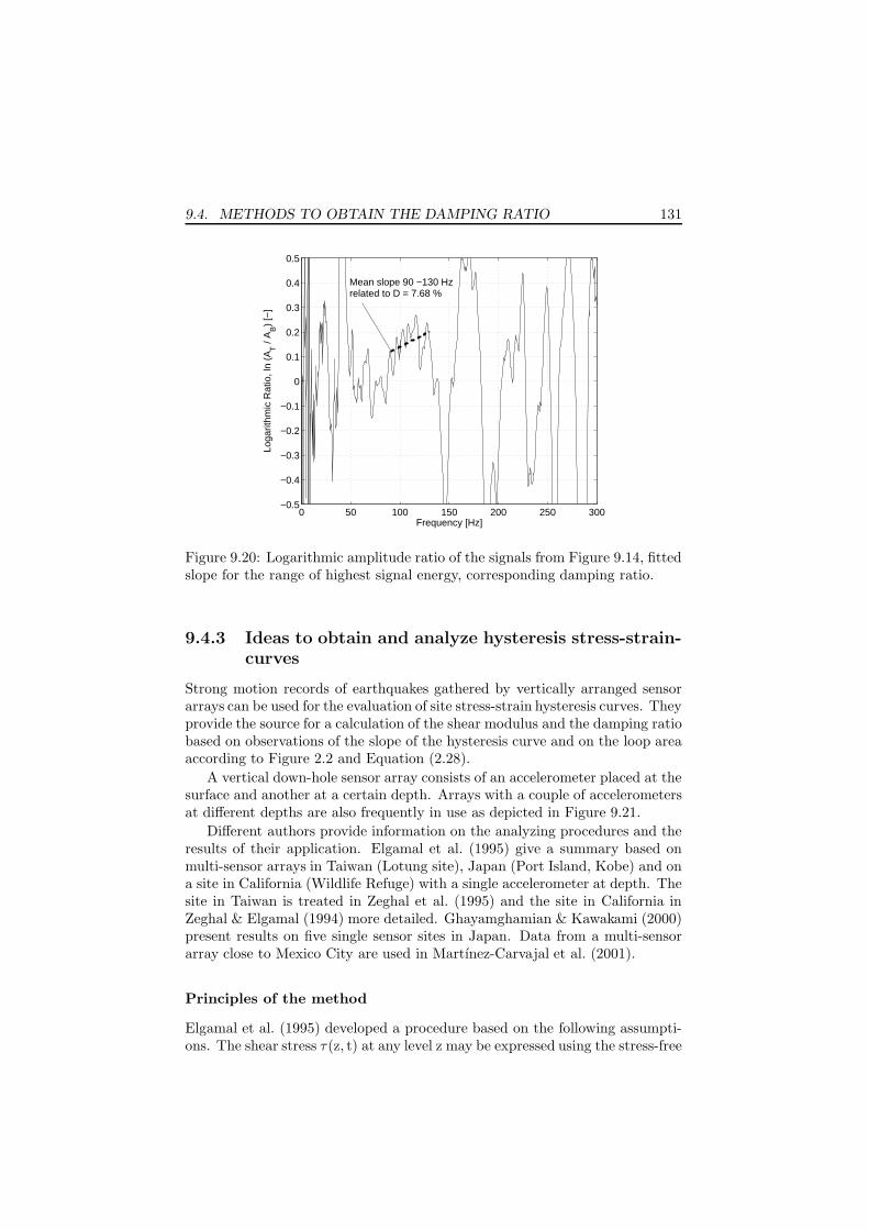
9.4. METHODS TO OBTAIN THE DAMPING RATIO 131
0 50 100 150 200 250 300−0.5
−0.4
−0.3
−0.2
−0.1
0
0.1
0.2
0.3
0.4
0.5
Frequency [Hz]
Loga
rithm
ic R
atio
, ln
(AT /
AB)
[−]
Mean slope 90 −130 Hz related to D = 7.68 %
Figure 9.20: Logarithmic amplitude ratio of the signals from Figure 9.14, fittedslope for the range of highest signal energy, corresponding damping ratio.
9.4.3 Ideas to obtain and analyze hysteresis stress-strain-curves
Strong motion records of earthquakes gathered by vertically arranged sensorarrays can be used for the evaluation of site stress-strain hysteresis curves. Theyprovide the source for a calculation of the shear modulus and the damping ratiobased on observations of the slope of the hysteresis curve and on the loop areaaccording to Figure 2.2 and Equation (2.28).
A vertical down-hole sensor array consists of an accelerometer placed at thesurface and another at a certain depth. Arrays with a couple of accelerometersat different depths are also frequently in use as depicted in Figure 9.21.
Different authors provide information on the analyzing procedures and theresults of their application. Elgamal et al. (1995) give a summary based onmulti-sensor arrays in Taiwan (Lotung site), Japan (Port Island, Kobe) and ona site in California (Wildlife Refuge) with a single accelerometer at depth. Thesite in Taiwan is treated in Zeghal et al. (1995) and the site in California inZeghal & Elgamal (1994) more detailed. Ghayamghamian & Kawakami (2000)present results on five single sensor sites in Japan. Data from a multi-sensorarray close to Mexico City are used in Martınez-Carvajal et al. (2001).
Principles of the method
Elgamal et al. (1995) developed a procedure based on the following assumpti-ons. The shear stress τ(z, t) at any level z may be expressed using the stress-free

132 CHAPTER 9. SCPT BASED TECHNIQUES
1
∆ z1
Free groundsurface
2
3
4
5
6
i−1
i
i+1
z
∆ z2
∆ z3
∆ z3
∆ z4
∆ zi−1
∆ zi
a1
a2
ai+1
ai
ai−1
a6
a5
a4
a3
Accelerometers
Figure 9.21: Multi-accelerometer array (Zeghal et al. (1995)).
surface boundary condition and a shear beam model as:
τ(z, t) =
∫ z
ζ=0
ρ u(ζ, t) dζ (9.28)
in which ρ is the mass density and u(ζ, t) is the lateral acceleration at level ζ.Because the acceleration is only known at the discrete points zi in depth whereaccelerometers are placed, an assumption for the intermediate sections has tobe made. The most simple way is to apply a linear interpolation. The shearstresses at levels zi and (zi−1 + zi)/2 reduce then to:
τi(t) = τi−1(t) + ρui−1 + ui
2∆zi−1 (9.29)
τi−1/2(t) = τi−1(t) + ρ3ui−1 + ui
8∆zi−1 (9.30)
i = 2, 3, . . .
in which subscripts i and (i-1/2) refer to levels zi (of the ith accelerometer)and (zi−1 + zi)/2 (halfway between accelerometers i and (i-1)) respectively,τi = τ(zi, t), ui = u(zi, t) and ∆zi is the distance between the accelerometers.
The corresponding shear strains at levels zi and (zi−1 + zi)/2 may be ex-pressed as:

9.4. METHODS TO OBTAIN THE DAMPING RATIO 133
γi(t) =1
∆zi−1 + ∆zi
(
(ui+1 − ui)∆zi−1
∆zi· · ·
. . . +(ui − ui−1)∆zi
∆zi−1
)
(9.31)
γi−1/2(t) =ui − ui−1
∆zi−1(9.32)
i = 2, 3, . . .
in which ui = u(zi, t) is the lateral displacement.
The displacement can be calculated through double integration of the re-corded acceleration history u(zi, t). It could be necessary to remove the baseline drifts caused by the integration. This can be done by removing of the verylow frequency parts by means of a high-pass filter or a detrend algorithm.
The result of the Equations (9.30) and (9.32) are time histories of shearstress and shear strain. If the shear stress is drawn against the shear strainthe typical hysteresis loops appear. Because the shape of the loops is straindependent it is useful to select cycles with similar maximum strain range forthe further analysis by using a rectangular window on the stress and strainhistories.
A disadvantage of the calculation of the shear stress history in multi-sensorarrays by means of Equation (9.30) is that the calculation for a certain depthneeds all previous stress histories at smaller depth. Possible errors will thereforebe cumulated from depth to depth.
The accuracy of the calculated shear stress and strain amplitudes is a func-tion of the distance between the recording points and the recorded accelerationwavelength. The discrete formulas can only capture waves below a certain fre-quency, determined by the distance between the recordings. From the samplingtheorem follows, in a complete analogue way to a discrete sampling in time,that the smallest possible wavelength λmin has to be at least the double ofthe distance ∆z between the sampling points. Ghayamghamian & Kawakami(2000) claim even a stricter rule, the highest frequency fmax should correspondto a wavelength λmin four times the distance ∆z between the recording points
λmin = 4 ∆z fmax =c
λmin(9.33)
in which c is the wave propagation velocity.
Based on this criterion stress and strain time histories have to be low-passfiltered to remove high frequency components. It has to be ensured that thefilter introduces no phase shift to the signals therefore FIR (finite impulseresponse) filters are preferred.
Typical upper edges of the passband for earthquakes and common transdu-cer spacings in seismic arrays are between 1.7 and 6 Hz.

134 CHAPTER 9. SCPT BASED TECHNIQUES
Transfer of the technique to the SCPT
The setup of the seismic cone penetration test has a lot of similarities to aseismic down-hole array to record strong motion earthquake events. However,there are a couple of differences which have to be taken into account before themethod can be used for SCPT’s. The main differences are:
1. There is usually no surface time record available in a normal SCPT.
2. The dual-cone provides only two simultaneously recorded time histories.
3. The generated waves by the SCPT source travel downwards whereas theearthquake waves travel upwards from the bedrock to the surface.
4. The typical frequencies of an earthquake signal are much lower than therange generated by the SCPT source.
5. The distances between the seismic transducers is in case of the dual-coneapproximately 1 m; the accelerometers in the earthquake arrays have amuch larger spacing.
The highest usable frequency for a SCPT can be calculated by Equation(9.33). Assuming a wave velocity c = Vs = 150 . . .350 m/s and ∆z = 1.033 mthe usable frequency range ends at fmax = 36.3 . . .84.7 Hz. Because the mostsignal energy can be found between about 50 and 150 Hz it is obvious that onlya part of the signal energy is actually in the usable range.
Because during the test the seismic cone is pushed into the ground, recor-ded signals at different depth are available. If the seismic source is sufficientlyrepeatable all signals can be collected and it can be assumed that they areidentically the same as if they would be measured simultaneously. Unfortuna-tely the used mechanical swing hammer cannot provide a highly reproduciblesource. A solution to overcome this problem could be to calculate the transferfunction between the signals obtained from both cone sensors. By means ofthese transfer functions it should be possible to recreate an array of signals withthe same properties as if they would have been recorded at the same excitationblow.
Figure 9.22 gives a schematic view of the transfer function technique. Atransfer function H1/2 between two signals a1 and a2 is the complex ratio oftheir spectra A1 and A2:
H1/2 =FFT (a2)
FFT (a1)=A2
A1(9.34)
Fourier transformation and inverse Fourier transformation are abbreviatedwith FFT and IFFT, respectively.

9.4. METHODS TO OBTAIN THE DAMPING RATIO 135
Fre
e gr
ound
surf
ace z
1.03
3
Pse
ud
o s
imu
ltan
eou
s si
gn
als
Sur
face
se
nsor
Dep
th−
Inde
x (m
)S
CP
T t
ime
reco
rds
of
con
secu
tive
mea
sure
men
t d
epth
s(d
ual
co
ne)
m=1 2 3 4 5
i−1 i
2,1
3,13/
2AA
H=
1,1a
2,1a
3,1a
3,2
4,24/
3AA
H=
3,2a
4,2a4,3a
5,3a4,3
5,35/
4AA
H=
1,2
−−
iia
iia
,2−1
,2
,2/
1−
−−−
=i
i
ii
ii
AAH
1,11
ap
=
2,12
ap
=
3,13
ap
=
()
()
4/3
3,1
4/3
34
HA
IFF
T
HP
IFF
Tp
⋅=
⋅=
()
()
5/4
4/3
3,1
5/4
45
HH
AIF
FT
HP
IFF
Tp
⋅⋅
=⋅
=
()
...1
/2
21
=⋅
=−
−−
−i
ii
iH
PIF
FT
p
()
()
()
∏=
−
−
−−
=
⋅⋅
⋅⋅
=⋅
=
i kk
k
ii
ii
ii
HA
IFF
T
HH
HA
IFF
T
HP
IFF
Tp
4/
13,1
/1
5/4
4/3
3,1
/1
1
...
()
()
mm
mn
mn
pF
FT
P
aF
FT
A
==,
,
n=1
23
i−2In
dex
SC
PT
−su
b−se
tup
(n)
Dua
l con
e se
nsor
s
1.03
3
1.03
3
1.03
3
[m]
Figure 9.22: Use of transfer functions (H) to generate pseudo simultaneoussignals.

136 CHAPTER 9. SCPT BASED TECHNIQUES
Application of the hysteresis technique to Waremme data
The described method is evaluated at the site in Waremme on data from thesledgehammer excitation of SCPT5. Additionally to the dual cone, an accele-rometer array consisting of one sensor for each coordinate axis is placed at thesurface in close proximity to the pushing rod of the cone. The transfer functiontechnique is used based on the recorded lateral signals in the direction of thehammer blow (y-axis). Figure 9.23 shows the applied algorithm.
The signals are first visually checked and averaged as in the spectral-ratioslope and the attenuation coefficient method. In the following step the matrix ofacceleration signals as obtained from one excitation hammer strike at all SCPTdepths simultaneously, is calculated by means of transfer functions. To obtainstable pseudo simultaneous signals it is necessary to eliminate all frequencycomponents below 10 Hz using a high-pass filter.
A low-pass filter with an edge frequency of 60 Hz is applied at the same timeas the 10 Hz high-pass filter. It is supposed to remove high frequency partsnot correctly captured by the sensor array because of the distances betweenthe accelerometers. Following the SCPT profile of the site in Waremme (e.g.Figure 6.8) the s-wave velocities are between 150 and 260 m/s. If a maximumfrequency of 60 Hz is present the smallest wavelengths are in the range of 2.5 to4.3 m. However, λmin for the accelerometer interval of 1 m is according to therule in Equation (9.33) 4 m. The low-pass filter edge frequency has to be setto 36.3 Hz to fulfill the rule. But in the frequency band below 36.3 Hz remainsonly a very few amount of signal energy. Therefore the edge frequency is setto 60 Hz to include more signal energy. This way seems acceptable becauseEquation (9.33) includes some kind of safety factor. λmin = 2 ∆z = 2 m onlyfollows from the sampling theorem directly, which is fulfilled.
Because only signal parts close to the mean shear wave pulse are qualified todraw meaningful stress-strain curves and to further improve the stability of thecalculated signals, the acceleration signals are windowed by means of a taperedwindow. The window is the same as shown in Figure 9.39 and described in9.5 with a length of 32.5 ms to both sides of the maximum of the accelerationsignal. The filtering and windowing is done before the transfer function processand is repeated once more afterwards.
In a next step the acceleration signals are integrated with depth, star-ting at the surface, and multiplied with the density. An averaged densityof ρ = 2040 kg/m3 is obtained by the performed laboratory tests on samplesfrom the site. Shear stress time histories are the result.
The shear strain histories need first the calculation of the displacementhistories by double integration of the acceleration signals. A filter with a passband between 10 and 60 Hz is applied after each integration step. In thisway signal drifts can be successfully removed. Figures 9.24 to 9.27 give theacceleration signals, the calculated displacement time histories, shear strainand shear stress histories drawn against the depth.
In the final step shear stress, τ , is plotted versus shear strain, γ. Completeloops are selected and G-modulus and damping ratio are calculated based on

9.4. METHODS TO OBTAIN THE DAMPING RATIO 137
Data Format Conversion from ASCII format of LabVIEW
ascii2mat.m
Generation of pseudo simultaneous signals
maketrans.m
Input data from LabVIEW data acquistition program
G and D for the selected loop
−consideration of sensor sensitiv ity and applied gain factors
Visual check of the time records andaveraging
−1 to 5 signals averaged under manual control
avershowex.mautoav erfiles.m
−band−pass filter with edge frequencies 10 and 60 Hz, tapered window (extended−cosine−window) +/− 32.5 ms arround the maximum−calculation of the transfer function between the cone sensor positions−repetition of filtering and windowing
Calculation of shear stress and shear strain time histories
lintrans.m
Drawing and evaluation of the s tres s −s train−hys teres is −loops
htrans.mhistloops.mellipse.m
−double integration of the acceleration records to displacement time histories, application of the bandpass filter after each integration step−differentiating of the surface sensor records to acceleration for the case that geophones are used−calculation of stress and strain time histories
−manual selection of certain loops−calculation of the related G−modulus and Damping ratio
Dat
a p
rep
arat
ion
as
for
spec
tral
rat
io s
lop
e a
nd
att
enu
atio
n c
oef
fici
ent
met
ho
d
Figure 9.23: Application of the hysteresis method to data from the Waremmesite, SCPT3.

138 CHAPTER 9. SCPT BASED TECHNIQUES
Figure 9.24: Normalized acceleration histories versus depth, Waremme,SCPT3.
Figure 9.25: Normalized displacement histories versus depth, Waremme,SCPT3.

9.4. METHODS TO OBTAIN THE DAMPING RATIO 139
Figure 9.26: Normalized shear strain histories versus depth, Waremme, SCPT3.
Figure 9.27: Normalized shear pstress histories versus depth, Waremme,SCPT3.

140 CHAPTER 9. SCPT BASED TECHNIQUES
the measurement of areas following Equation (2.28).
-2 -1 0 1 2
x 10-6
-150
-100
-50
0
50
100
150
Shear strain, γ [-]
She
ar s
tres
s, τ
[Pa]
Hysteresis-Loop I
Loop I t = 0.505 ... 0.524 s, G = 87.127 MPa V
s = 207 m/s (with ρ = 2040 kg/m³),
D = 25.75 %
Loop I
t = 0.524 s t = 0.505 s
Figure 9.28: Stress-strain hysteresiscurves related to the time-histories inFigure 9.30, loop I.
-2 -1 0 1 2
x 10-6
-150
-100
-50
0
50
100
150
Shear strain, γ [-]
She
ar s
tress
, τ [P
a]
Hysteresis-Loop II
Loop II t = 0.523 ... 0.544 s, G = 63.436 MPa V
s = 176 m/s (with ρ = 2040 kg/m³),
D = 27.57 %
Loop II
t = 0.544 s
t = 0.523 s
Figure 9.29: Stress-strain hysteresiscurves related to the time-histories inFigure 9.30, loop II.
Figure 9.28 and 9.29 give the stress-strain diagrams at a depth of 3.71 m.Two complete loops could be distinguished and are marked by thick lines inthe two figures. The found damping ratio is 25.7 to 27.6 % and unexpectedlyhigh. The calculated shear wave velocity is 176 to 207 m/s and in the range ofthe cross correlation measurement on the SCPT data.
Figure 9.30 shows the location of the loops in the form of strain and stressversus time.
Obstacles and difficulties in applying the technique
It is quite difficult to find usable loops for analysis. A majority of the stress-strain diagrams show also in the parts of the strongest signal energy comple-tely unshaped loops and even if acceptable portions are found the calculateddamping ratio is often above 100 %. Because of the questionable results thetechnique is not elaboratly tried at the other sites.
The difficulties related to this technique are probably caused by the ne-cessary quite strict filter and windowing regime. Critical error introducingsteps of the algorithm are listed in the following.
Transfer functions Preliminary trials to use the transfer function methodwithout any filtering and windowing led with increasing depth to dissatisfyingtime histories. They are dominated by noise and very low frequency com-ponents. From a certain depth on, the shear wave pulse is not distinguishableany more although the real measured time record at the corresponding depthis quite clear. Especially the windowing is virtually indispensable for the tech-nique.

9.4. METHODS TO OBTAIN THE DAMPING RATIO 141
0.45 0.475 0.5 0.525 0.55 0.575 0.6−2
−1
0
1
2x 10
−6 Shear strain
Time, t [s]
She
ar s
trai
n, γ
[−]
0.45 0.475 0.5 0.525 0.55 0.575 0.6−200
−100
0
100
200Shear stress
Time, t [s]
She
ar s
tres
s, τ
[Pa]
Loop I
Loop II
Loop I
Loop II
Figure 9.30: Shear strain and shear stress time histories at a depth of 3.71 mafter sledgehammer excitation, Waremme, SCPT3.
A comparison of the calculated time histories with the actually measuredones shows a small time shift. Explanation for this might be the multiplicationof small numerical errors in the transfer function from the surface over all conedepths to the depth of interest. Another reason is the fact that the distancebetween the cone sensors is actually 1.033 m but the cone has been pushed intothe ground in intervals of 0.5 m. That means the pseudo simultaneous signalsare calculated for a slightly longer travel path length, 3.3 cm per 1 m depth, asin reality. However, in the later SCPT’s the cone pushing interval was changedto 51.65 cm instead of 50 cm to compensate the deviation. Calculations of thetransfer function techniques on these tests still show some signal shift betweencalculated and measured signals at greater depths.
An improvement of the seismic source, so that it can be considered as fullyreproducible, could make the transfer function approach avoidable with positiveeffects on the results.
Acceleration integration The double integration of the pseudo simulta-neous acceleration time histories adds other difficulties to be handled. Aftereach integration step the signal has to be filtered to remove the appearing si-

142 CHAPTER 9. SCPT BASED TECHNIQUES
gnal drifts. In this case a rectangular high-pass filter (FIR) is used. This filterprovides a unit gain factor over the desired frequency pass band and introducesno phase shift in the filtering procedure. Also an IIR filter with smoother filterflanks designed after Ormsby (1961) is tried. Both filters are only efficient inremoving the disturbing signal drifts if all components below about 10 Hz aresignificantly reduced or removed. This means of course a loss of importantsignal information.
Stress-strain calculation The receiver spacing between the dual cone sen-sors is not optimum. A low-pass filter has to be applied to remove frequencycomponents above 60 Hz. Unfortunately, the main wave energy is with 50 to150 Hz in this frequency range.
9.5 SRS method and ACM on artificially gene-rated signals
Preliminary trials of the SRS method on SCPT data show a wide result scat-tering concerning the damping ratio. Because other in situ testing techniqueswere not available it was not clear if this variation is due to real changes in thesoil properties with depth or caused by the algorithm of analyzing.
Therefore the seismic cone test is simulated using the program SPECTRALproviding artificial input signals for the analyzing procedures.
The algorithm of analyzing applied on the measured signals at the testingsites is also used to analyze the simulated signals. Essentially three artificialsoil profiles as given in Figure 9.31 are evaluated, a half-space, a one layer anda two layer profile. Damping ratio, shear wave and compression wave velocityare kept constant within one layer.
The geometrical conditions for a typical SCPT are also used for the simula-ted tests as given in Figure 9.32. In particular a horizontal off-set of the sourceof one meter and a depth distance between the simulated signal records of 0.5m are chosen.
The excitation hammer blow is simulated by a point load on the surface.In the cases of profile a) and c) the direction of the force is once horizontaland once vertical. For profile b) only the horizontal excitation is used. Thebehavior of the excitation force follows a squared sine function and is given inFigure 9.33.
The calculation of the p-wave velocity is performed using the vertical par-ticle acceleration caused by the simulated vertical impact. The s-wave velocityis obtained based on the horizontal particle acceleration due to the horizontalimpact force.
The damping ratio is calculated for the shear wave only, therefore the ho-rizontal acceleration in connection with the horizontal impact is used.
The Figures 9.34, 9.35 and 9.36 show the time histories used for the s-wavevelocity and the damping ratio calculation. The direct s- and p-wave compo-
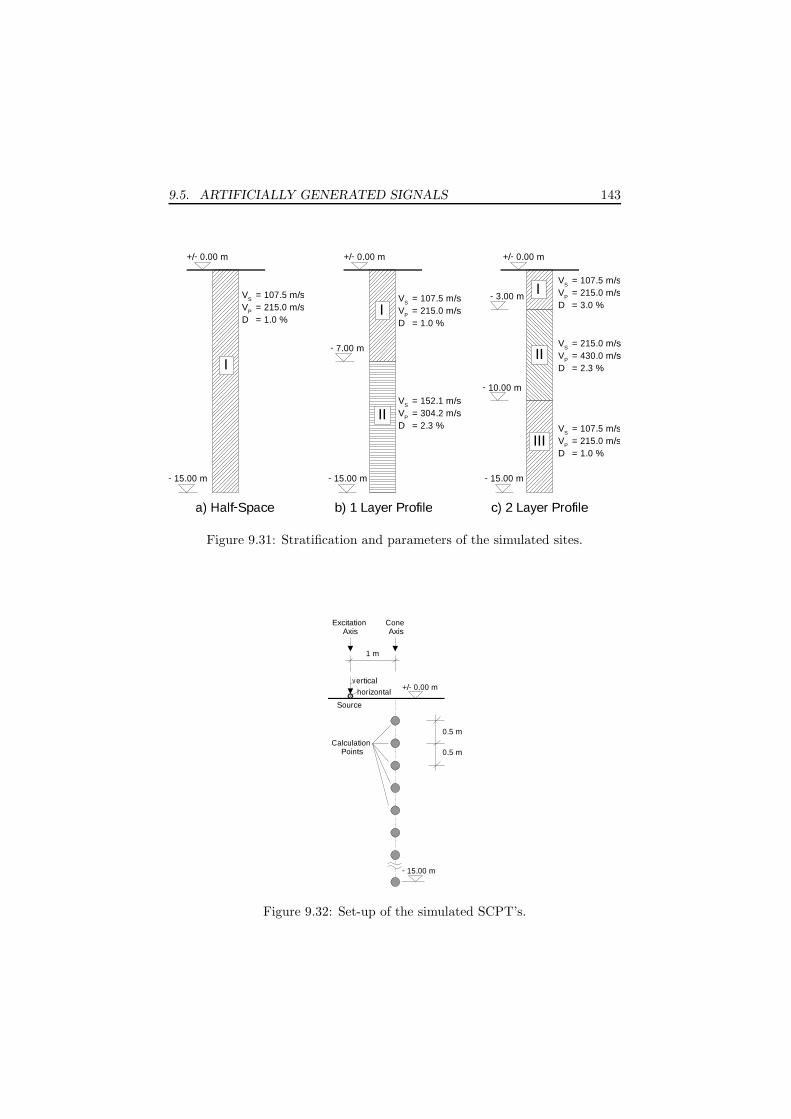
9.5. ARTIFICIALLY GENERATED SIGNALS 143
VS = 107.5 m/sVP = 215.0 m/sD = 1.0 %
a) Half−Space b) 1 Layer Profile c) 2 Layer Profile
VS = 107.5 m/sVP = 215.0 m/sD = 1.0 %
VS = 152.1 m/sVP = 304.2 m/sD = 2.3 %
VS = 107.5 m/sVP = 215.0 m/sD = 3.0 %
VS = 215.0 m/sVP = 430.0 m/sD = 2.3 %
VS = 107.5 m/sVP = 215.0 m/sD = 1.0 %
I
II
I
I
II
III
− 7.00 m
− 15.00 m
+/− 0.00 m +/− 0.00 m +/− 0.00 m
− 15.00 m − 15.00 m
− 3.00 m
− 10.00 m
Figure 9.31: Stratification and parameters of the simulated sites.
1 m
0.5 m
0.5 m
Excitation Axis
Cone Axis
Source
Calculation Points
+/− 0.00 m
− 15.00 m
v erticalhorizontal
Figure 9.32: Set-up of the simulated SCPT’s.

144 CHAPTER 9. SCPT BASED TECHNIQUES
10 15 20 25 30 35 40
0
0.2
0.4
0.6
0.8
1
t [ms]
0 200 400 600 800 1000 1200 1400 1600 1800 20000
0.2
0.4
0.6
0.8
1
Frequency Spectrum Source Function
f [Hz]
Time History Source Function
Nor
mal
ised
forc
e [−
] N
orm
alis
ed fo
rce
[−]
Figure 9.33: Time history and frequency content of the simulated normalizedimpact force.
nent is indicated. There is an unexpected component in profile b) between p-and s-wave arrival assumed to be caused by an internal calculation instabilityin the SPECTRAL program algorithm. Besides this, reflections on the layerinterfaces can be very well seen. Also nicely seen, at least in profile c), isthat the refraction of the s-wave component at a layer boundary generates anadditional wave component traveling with p-wave velocity.
The complex structure of the time records of the 2 layer profile c) emphasizesthe need to implement a possibility to select parts of the signals and not touse the whole signal for the velocity and damping analysis. It is expectedthat at least the common treatment of wave components of different speedwill cause significant errors in the calculation of the damping ratio as the wavevelocity is an essential part of the SRS method and the ACM. The wave velocitycalculation based on cross correlation should be not affected as long as theamplitudes of the component of interest are higher than the others.
The analysis of the simulated signals is performed through a couple of MAT-LAB script files. The algorithm is outlined in Figure 9.37. The SRS methodand the ACM are applied to signals from depths with one meter distance,meter-by-meter approach. The SRS method is additionally tried on two si-gnals from a depth of 5 and 12 m. The slope of the spectral logarithmic ratiois obtained by a linear curve fit in a frequency range of 300 Hz always cente-red at the frequency of the maximum spectral amplitude. The damping ratio

9.5. ARTIFICIALLY GENERATED SIGNALS 145
0 0.05 0.1 0.15 0.2
0
2
4
6
8
10
12
14
16
t [s]
Dep
th [m
]
a) Half−Space
S
Figure 9.34: Simulated time histories for profile a) Half-Space, horizontal exci-tation.

146 CHAPTER 9. SCPT BASED TECHNIQUES
0 0.05 0.1 0.15 0.2
0
2
4
6
8
10
12
14
16
t [s]
Dep
th [m
]
b) 1 Layer Profile
Laye
r I
Laye
r II
S
S P
P
Figure 9.35: Simulated time histories for profile b) one layer on a half-space,horizontal excitation.

9.5. ARTIFICIALLY GENERATED SIGNALS 147
0 0.02 0.04 0.06 0.08 0.1 0.12
0
2
4
6
8
10
12
14
16
t [s]
Dep
th [m
]
c) 2 Layer Profile
P S
P S
P S
Laye
r I
Laye
r II
Laye
r III
Figure 9.36: Simulated time histories for profile c) two layers on a half-space,horizontal excitation.

148 CHAPTER 9. SCPT BASED TECHNIQUES
determined by the ACM is an average value for the same frequency range. Tostudy the influence of the different length of a cutting window, different shapesof window functions and the meaning of additional noise to the results of thehalf-space of profile a), some parameters are changed which will be explainedfurther on.
Data Format Adaption from SPECTRAL format
makeSCPTfiles.m
Selection of signal parts(rectangular window)
srsdatanew.m
Signal adaption
AdaptFFT.m
−Length adjustment of the windowed signal part (E)−Adding of noise (N)−Applying of Hanning (H) or tapert (T) window
Input data from SPECTRAL program
Cros s −Correlation
autoSCPTFromWinSig.mautoSCPTFromWinSig3.m
Cros s −Correlation
autoSCPTFromWinSig2.m
Meter−by−meter approach Selected depth area
Vs vs. Depth
Spectral Ratio Slope Method (SRS)
dualmanu.m
Attenuation Coefficient Method (ACM)
dualmanu3.m
Spectral Ratio Slope Method (SRS)
dualmanu2.m
Vs for the selected depth area
D vs. Depth D vs. Depth D for the selected depth area
Figure 9.37: Flow chart for the calculations on the simulated SCPT’s.
Window-length
The signal from the half-space profile a) is analyzed using three different win-dow lengths. First the complete signal without window is used, secondly asignal of a length of the first 1.5 cycles of the s-wave component is used whichis virtually the whole s-wave component and finally a signal containing onlythe first cycle of the s-wave component is analyzed. Figure 9.38 illustrates the

9.5. ARTIFICIALLY GENERATED SIGNALS 149
shape of the signal after the window is applied. The windowing is done manu-ally by selecting the crossing points with the neutral position. In this way itcan happen that the two proceeded windowed signals have a slightly differentlength. To investigate influences of this fact all calculations are done additio-nally with signals of exactly the same length. For this case it is accepted thatone of the signals contains more than one respectively 1.5 cycles. Results ofexact equal signal length are indicated with ”E” in the summary Table 9.2.
1.5 Cycles
1 Cycle
Figure 9.38: Schematic view of the results after windowing of 1.5 cycles (1.5periods) and one cycle (1 period) of the signal.
Window-function
Hanning window Additionally to the simple rectangular shaped window, atapered window and a Hanning, also called Hann window, is applied. The shapeof the window function is given in Figure 9.39. The Hanning window followsa cosine function and is defined by Equation (9.35). n describes the length ofthe window in number of samples; k is the sample index. The Hanning windowis a common window type and for instance used by Kudo & Shima (1981) fordamping measurements on a down-hole setup with two boreholes.
w(k + 1) = 0.5
(
1 − cos
(
2πk
n− 1
))
, k = 0, . . . , n− 1 (9.35)
Tapered window The tapered window is a combination of Hanning windowand rectangular window. The abrupt jump from 0 to 1 of the rectangularwindow is changed by the gentle slope of the Hanning window. The intervalbetween 0 on 1 is chosen to 2 ms. The tapered window called extended-cosine-bell window is used by Mok et al. (1988) for the damping determination indown-hole tests.
Results based on the Hanning window and the tapered window are indicatedwith ”H” respectively with ”T” in the summary Table 9.2.
Benefits of windowing The reasons for applying a window to the signalare essentially the following.
Most obvious and already mentioned is the need to select a certain wavecomponent if other components with high amplitudes are present. The origin

150 CHAPTER 9. SCPT BASED TECHNIQUES
0 5 10 150
0.2
0.4
0.6
0.8
1
Time (ms)
Am
plitu
de
Time domain
0 0.2 0.4 0.6 0.8-100
-50
0
50
Frequency (kHz)
Mag
nitu
de (
dB)
Frequency domain
HanningTaperedRectangular
Figure 9.39: Hanning, tapered and rectangular window with a typical lengthof 1.5 cycles in time and frequency domain.
of these wave components could be a reflection or refraction at a layer interfaceor the surface, other wave sources in the neighborhood or simply different typesof wave propagation, like p- or s-waves.
A second reason to apply a window is the idea to eliminate portions in thesignal containing only noise. These are large parts of the signal before and afterthe actual vibration event. In this way the disturbing spectral parts, relatedto the noise in the amplitude spectrum, are reduced.
The third reason is related to the signal processing and the calculationof the FFT spectrum. This is also the reason why windowing is of such animportance in digital and analogue signal processing. If a periodic signal ofinfinite length has to be analyzed to obtain its frequency content it is obviousthat a part of the signal has to be selected. If this is done completely witharbitrary start and end points it is possible that at the borders of the selectionthe signal is not close to the zero line. Because the FFT algorithm assumesa periodic continuation of the signal after the cutting point, discontinuitiesin the signal progression occur. This again leads in the frequency spectrumto a ”leakage” of the peaks. That means parts of the energy of a frequencycomponent are not shown at the original frequency, they are included in thebroadened main peak and in ripples beside the main peak. This is the so calledGibb’s phenomenon. To prevent the spectral leakage, virtually two ways canbe gone: a) the signal is cut (rectangular shaped window) at points of thezero-crossing respectively parts where the signal is approximately zero or b) awindow function is applied which diminishes the signal amplitude towards theborders of the window. Method a) uses an effect called ”picket fence”, so theripple effects are essentially multiplied with zero. Method b) is more generalto use, however the signal is altered by the window function which can causeunpredictable effects.

9.5. ARTIFICIALLY GENERATED SIGNALS 151
One can imagine the application of a window on a signal in the frequencydomain by the convolution of the ideal spectrum of the infinite long signaland the spectrum of the window function. Further details can be found in theliterature on digital signal processing as for instance in Best (1991).
The signals of the vibrations caused by the SCPT are not periodic, theyare transient. That means for analysis of the full signal length, windowing isnot necessary or more exact the selection of another window type than therectangular shaped window needs not to be done. But if for the first tworeasons parts of the signals should be blind out, the influence of the Gibb’sphenomenon has to be considered. Therefore the signals are manually, withbest possible accuracy, cut at the zero-crossing points and additionally theeffects of a Hanning and a tapered window are studied.
Additional noise
Results marked with ”N” have been obtained based on signals where noise witha maximum amplitude of 10 % of the maximum peak particle acceleration ofthe signal was added.
9.5.1 Calculated velocities from the simulated signals
0 50 100 150 200 250 300
0
2.5
5
7.5
10
12.5
15
Wave velocity [m/s]
Dep
th [m
]
Simulated half−space
Vs
Vp
Figure 9.40: Calculated wave velocities, profile a), half-space.
Figures 9.40, 9.41 and 9.42 give s- and p-wave velocity as calculated by thecross correlation technique. The curves are virtually independent of the length

152 CHAPTER 9. SCPT BASED TECHNIQUES
0 50 100 150 200 250 300
0
2.5
5
7.5
10
12.5
15
Wave velocity [m/s]
Dep
th [m
]
Simulated 1 layer profile
Vs
Figure 9.41: Calculated s-wave ve-locity, profile b), one layer on a half-space.
0 100 200 300 400 500
0
2.5
5
7.5
10
12.5
15
Wave velocity [m/s]
Dep
th [m
]
Simulated 2 layer profile
Vs
Vp
Figure 9.42: Calculated wave velo-city, profile c), two layers on a half-space.
and shape of the applied window as long as the wave component of interesthas a higher amplitude than all others. The input velocities are nearly exactlyfound except for the shallow depths smaller than 2.5 m in case of the profilea). This is probably due to the fact that the difference in travel path lengthbetween two measurement points close to the surface is rather small, so smalldeviations in the time arrival determination have an unequal higher disturbinginfluence in the resulting velocity.
9.5.2 Calculated damping ratio
The input parameter for the damping ratio is Ds = Dp = 1% over the wholedepth of profile a). Table 9.2 and Figure 9.44 summarize the results concerningthe damping ratio for the half-space profile a). The Figures 9.45 to 9.51 showthe results for selected parameter configurations. Table 9.2 gives the value ofthe averaged damping ratio over all n obtained points of the profile between 5.5and 11.5 m, D, and as a measure for scattering, the mean absolute deviations∗D0
from the target value D0 = 1%. The latter is defined as:
s∗D0=
1
n
n∑
i=1
|Di −D0| . (9.36)

9.5. ARTIFICIALLY GENERATED SIGNALS 153
In the case where the signals at 5 and 12 m are compared the single calcu-lated value D is given. s∗D0
is then simply the deviation from the target inputvalue.
As an example Figure 9.43 shows for the calculation point at 10 m depth theinfluence of the length of the rectangular window to the shape of the amplitudespectra of the signals and the logarithmic ratio between both.
0 200 400 600 800 1000 1200 1400 1600 1800 20000
0.5
1
Spectrum at depth 10.5 m, AB
Nor
mal
ized
A
mpl
itude
[−]
0 200 400 600 800 1000 1200 1400 1600 1800 20000
0.5
1
Spectrum at depth 9.5 m, AT
Nor
mal
ized
A
mpl
itude
[−]
0 200 400 600 800 1000 1200 1400 1600 1800 20000
0.5
1
1.5Logarithmic Ratio, ln(A
T/A
B)
Frequency [Hz]
Loga
rithm
ic
Rat
io [−
]
Full signal (a)1.5 cycles (b)1 cycle (c)
Range of slope calculation,+/− 150 Hz from the peak−frequency
Figure 9.43: Influence of the length of a rectangular shaped window on theamplitude spectra and the logarithmic amplitude ratio, half-space profile a),calculation depth 10 m.
Evaluation of the results for the half-space
a) Full signal
The SRS method and ACM give for depths longer than about 2.5 m andthe rectangular window nearly perfect results. This can be seen in Figure9.45. The application of a window function is nearly meaningless becauseapplied over the full signal almost all significant parts of the signal stayvirtually unchanged. The reason for the deviation in the case of thecombination Hanning window and ACM, D ≈ 0.5% is not known.

154 CHAPTER 9. SCPT BASED TECHNIQUES
0.000 0.200 0.400 0.600 0.800 1.000
a
aH
aT
aN
b
bE
bH
bT
bEH
bET
bN
c
cE
cH
cT
cEH
cET
cN
Mean absolute deviation s* [%]
Selected-Depth, SRS
Metre-by-Metre, ACM
Metre-by-Metre, SRSFu
ll si
gn
al1.
5 cy
cles
1 cy
cle
Figure 9.44: Mean absolute deviation of the damping ratio profiles obtainedfrom the simulated SCPT’s.

9.5. ARTIFICIALLY GENERATED SIGNALS 155
Modified Parameters Metre-by-Metre Selected-DepthMethod Area Method
SRS ACM SRS
Win
dow
length
EqualW
indow
length
Hannin
gW
indow
Taper
edW
indow
Nois
e
Id-C
ode
D s∗D0
D s∗D0
D s∗D0
[%] [%] [%] [%] [%] [%]
a 1.003 0.009 0.975 0.025 1.002 0.002x aH 1.002 0.005 0.505 0.495 1.002 0.002
x aT 1.003 0.009 0.975 0.025 1.002 0.002
a)
Full
signal
x aN 1.025 0.225 0.968 0.111 1.063 0.063
b 1.137 0.147 1.895 0.945 1.029 0.029x bE 0.987 0.032 0.978 0.024 1.108 0.108
x bH 0.869 0.148 1.644 0.665 0.815 0.185x bT 1.360 0.398 1.842 0.888 1.089 0.089
x x bEH 0.682 0.318 1.037 0.044 0.718 0.282x x bET 0.910 0.092 0.983 0.022 1.174 0.174b
)1.5
cycl
es)
x bN 1.139 0.432 1.896 0.985 1.078 0.078
c 0.580 0.566 1.281 0.476 0.570 0.430x cE 0.469 0.645 1.173 0.179 0.774 0.226
x cH 0.360 0.640 0.993 0.581 0.480 0.520x cT 0.496 0.593 1.034 0.414 0.561 0.439
x x cEH 0.271 0.729 1.031 0.466 0.569 0.431x x cET 0.329 0.671 1.108 0.395 0.761 0.239
c)1
cycl
e
x cN 0.584 0.586 1.273 0.483 0.638 0.362
Table 9.2: Evaluation of modified window parameters.
b) 1.5 cycles
The SRS method provides for this shorter window length the best resultsif the rectangular shaped window is used. If care is taken for an exactequal window length in both signals the result can be improved slightly.The application of Hanning or tapered window is not able to better theaverage value nor the mean absolute deviation. The ACM delivers ingeneral more inaccurate results than the SRS method only in the case ofan exact equal window length the 1 % damping can be approximatellyfound. Figures 9.46 and Figure 9.47 deliver selected calculated dampingprofiles for 1.5 cycle window length.
c) 1 cycle
Finally for the shortest window, profiles can be found in Figure 9.48 and

156 CHAPTER 9. SCPT BASED TECHNIQUES
Figure 9.49. The SRS methods gives, independent from the window type,too low values for the damping ratio around 0.5 %. Better results comefrom ACM but also here the scatter is high as seen in the SRS technique.The closest proximity of the averaged damping ratio to the input dampingof 1 % is reached using an equal window length and a hanning window.
Evaluation of the results for the noise comparison
The introduced noise has some influence to the results. Example profiles com-paring the results from the rectangular window with different window lengthwith and without the additional 10 % noise are given in the Figures 9.50 and9.51. Differences are not really significiant.
Evaluation of the results for the profiles b) and c)
Figure 9.52 and 9.53 give the damping ratio profiles for the more complicatedsoil profiles b) and c) for the SRS technique and ACM in case of a rectangularwindow with and without equal length. Especially in profile c) in the range ofthe layer change the deviation from the input damping ratios and the scatterare high.
The direct traveling shear wave, indicated with ”S” in the Figures 9.35 and9.36, is separated by the window. The length of the window is set as large aspossible.
9.5.3 Conclusions for the analysis of real SCPT data
This parameter study has shown that overall the influence of the type of windowis rather small. It seems useful to choose an exact equal window length for bothsignals. However, the main conclusion is, that the length of the applied windowhas the most significant influence on the result and its scatter. As shorter thewindow is chosen as larger the deviation and as larger the scatter too.

9.5. ARTIFICIALLY GENERATED SIGNALS 157
−0.5 0 0.5 1 1.5 2 2.5 3
0
2.5
5
7.5
10
12.5
15
Damping ratio [%]
Dep
th [m
]
Simulated half−space, full signal
SRS aACM a
Figure 9.45: Damping ratio, profile a), based on the full signal.

158 CHAPTER 9. SCPT BASED TECHNIQUES
−0.5 0 0.5 1 1.5 2 2.5 3
0
2.5
5
7.5
10
12.5
15
Damping ratio [%]
Dep
th [m
]
Simulated half−space, 1.5 cycles, SRS
SRS bSRS bESRS bHSRS bT
Figure 9.46: Damping ratio, profilea), based on a windowed signal of 1.5cycle length, spectral ratio slope me-thod.
−0.5 0 0.5 1 1.5 2 2.5 3
0
2.5
5
7.5
10
12.5
15
Damping ratio [%]
Dep
th [m
]
Simulated half−space, 1.5 cycles, ACM
ACM bACM bEACM bHACM bT
Figure 9.47: Damping ratio, profilea), based on a windowed signal of 1.5cycle length, attenuation coefficientmethod.
−0.5 0 0.5 1 1.5 2 2.5 3
0
2.5
5
7.5
10
12.5
15
Damping ratio [%]
Dep
th [m
]
Simulated half−space, 1 cycle, SRS
SRS cSRS cESRS cHSRS cT
Figure 9.48: Damping ratio, profilea), based on a windowed signal of 1cycle length, spectral ratio slope me-thod.
−0.5 0 0.5 1 1.5 2 2.5 3
0
2.5
5
7.5
10
12.5
15
Damping ratio [%]
Dep
th [m
]
Simulated half−space, 1 cycle, ACM
ACM cACM cEACM cHACM cT
Figure 9.49: Damping ratio, profilea), based on a windowed signal of 1 cy-cle length, attenuation coefficient me-thod.

9.5. ARTIFICIALLY GENERATED SIGNALS 159
−0.5 0 0.5 1 1.5 2 2.5 3
0
2.5
5
7.5
10
12.5
15
Damping ratio [%]
Dep
th [m
]
Simulated half−space, noise, SRS
SRS aSRS aNSRS bSRS bNSRS cSRS cN
Figure 9.50: Damping ratio, profilea), noise influence, spectral ratio slopemethod.
−0.5 0 0.5 1 1.5 2 2.5 3
0
2.5
5
7.5
10
12.5
15
Damping ratio [%]
Dep
th [m
]
Simulated half−space, noise, ACM
ACM aACM aNACM bACM bNACM cACM cN
Figure 9.51: Damping ratio, profilea), noise influence, attenuation coef-ficient method.
−5 0 5 10 15
0
2.5
5
7.5
10
12.5
15
Damping ratio [%]
Dep
th [m
]
Simulated 1 layer profile
SRS SRS EACM ACM E
D = 1.0 %
D = 2.3 %
Figure 9.52: Damping ratio, profileb), selected results in comparison withthe input values.
−5 0 5 10 15
0
2.5
5
7.5
10
12.5
15
Damping ratio [%]
Dep
th [m
]
Simulated 2 layer profile
SRS SRS EACM ACM E
D = 3.0 %
D = 2.3 %
D = 1.0 %
Figure 9.53: Damping ratio, profilec), selected results in comparison withthe input values.
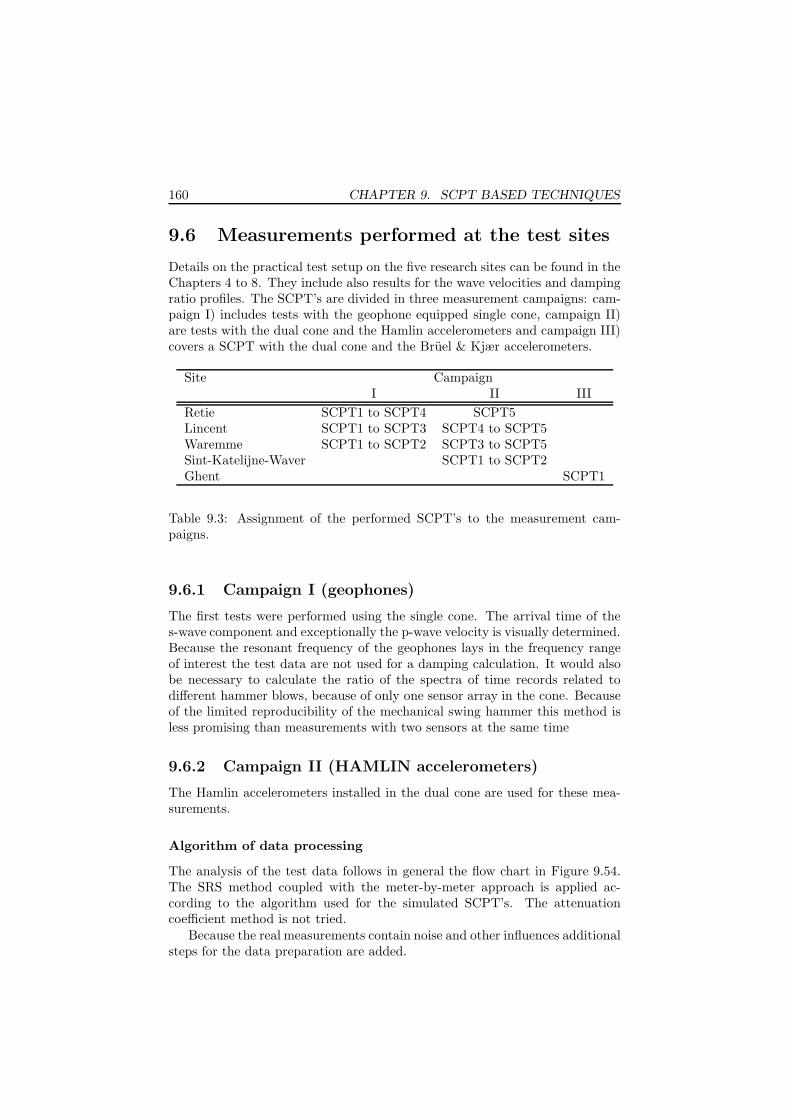
160 CHAPTER 9. SCPT BASED TECHNIQUES
9.6 Measurements performed at the test sites
Details on the practical test setup on the five research sites can be found in theChapters 4 to 8. They include also results for the wave velocities and dampingratio profiles. The SCPT’s are divided in three measurement campaigns: cam-paign I) includes tests with the geophone equipped single cone, campaign II)are tests with the dual cone and the Hamlin accelerometers and campaign III)covers a SCPT with the dual cone and the Bruel & Kjær accelerometers.
Site CampaignI II III
Retie SCPT1 to SCPT4 SCPT5Lincent SCPT1 to SCPT3 SCPT4 to SCPT5Waremme SCPT1 to SCPT2 SCPT3 to SCPT5Sint-Katelijne-Waver SCPT1 to SCPT2Ghent SCPT1
Table 9.3: Assignment of the performed SCPT’s to the measurement cam-paigns.
9.6.1 Campaign I (geophones)
The first tests were performed using the single cone. The arrival time of thes-wave component and exceptionally the p-wave velocity is visually determined.Because the resonant frequency of the geophones lays in the frequency rangeof interest the test data are not used for a damping calculation. It would alsobe necessary to calculate the ratio of the spectra of time records related todifferent hammer blows, because of only one sensor array in the cone. Becauseof the limited reproducibility of the mechanical swing hammer this method isless promising than measurements with two sensors at the same time
9.6.2 Campaign II (HAMLIN accelerometers)
The Hamlin accelerometers installed in the dual cone are used for these mea-surements.
Algorithm of data processing
The analysis of the test data follows in general the flow chart in Figure 9.54.The SRS method coupled with the meter-by-meter approach is applied ac-cording to the algorithm used for the simulated SCPT’s. The attenuationcoefficient method is not tried.
Because the real measurements contain noise and other influences additionalsteps for the data preparation are added.

9.6. MEASUREMENTS PERFORMED AT THE TEST SITES 161
Data Format Conversion from ASCII format of LabVIEW
ascii2mat.m
Windowing / Filtering
srsdatanew.m
Input data from LabVIEW data acquistition program
Cross−Correlation
autoSCPTFromWinSig.mautoSCPTFromWinSig3.m
Meter−by−meter approach
Vs vs. Depth
Spectral Ratio Slope Method (SRS)
dualmanu.m
D vs. Depth
−consideration of sensor sensitivity and applied gain factors
Visual check of the time records andaveraging
−1 to 5 signals averaged under manual control
avershowex.mautoaverfiles.m
−manual / semi−automatic signal−part−selection (rectangular window)−poss. low−pass filtering (200 Hz cut−off frequency)
Figure 9.54: Flow chart for the calculations on the data from the SCPT testingsites, SRS method.

162 CHAPTER 9. SCPT BASED TECHNIQUES
After the conversion of the ASCII data, gathered with the LabVIEW-program, taking into account the sensors sensitivity and possibly applied gainfactors by the conditioner equipment, all signals are visually checked. Usually5 repetition of excitation hammer blows at each cone depth are recorded. Thisopens the possibility to skip obviously disturbed hammer blows that have beenoverlooked during the measurement.
The remaining time records are averaged in the time domain to improvethe signal to noise ratio. A trial with averaging in the frequency domain led tovirtually the same averaged signals.
However, even after averaging of up to 5 signals the obtained time recordshave still remarkable noise components. Figure 9.57 shows an averaged timerecord from the site in Sint-Katelijne-Waver. Figure 9.55 shows the averagedsignals according to their depth.
0.45 0.5 0.55 0.6 0.65 0.7
0
2
4
6
8
10
12
14
16
18
t [s]
Dep
th [m
]
Figure 9.55: Sint-Katelijne-Waver,bottom element, y-axis, sledge ham-mer, SCPT2.
0.45 0.5 0.55 0.6 0.65 0.7
0
2
4
6
8
10
12
14
16
18
t [s]
Dep
th [m
]
Figure 9.56: Ghent, bottom element,y-axis, sledge hammer, SCPT1.
The high noise level suggests the application of a low-pass filter. In thisway it is more straightforward to find reasonable points for the beginning andthe end of the rectangular window. A corner frequency of 200 Hz is the bestcompromise between smoothing the signal and keeping its frequency content.The filtering is done before the signals are windowed.
Afterwards the main cycle, following the same definition given in Figure9.38 (1 cycle), of every signal is cut by a rectangular window.
Because most of the signal energy is situated in the frequency range between

9.6. MEASUREMENTS PERFORMED AT THE TEST SITES 163
0.55 0.555 0.56 0.565 0.57 0.575 0.58 0.585 0.59 0.595 0.6−0.1
−0.05
0
0.05
0.1Unfiltered, averaged signal
Time [s]
Par
ticle
acc
eler
atio
n [m
/s²]
0.55 0.555 0.56 0.565 0.57 0.575 0.58 0.585 0.59 0.595 0.6−0.1
−0.05
0
0.05
0.1200 Hz−low−pass filtered, averaged signal
Time [s]
Par
ticle
acc
eler
atio
n [m
/s²]
Figure 9.57: Example of averaged time histories from the top accelerometer,y-direction, Depth 11.67 m, Sint-Katelijne-Waver (SCPT2) before and afterfiltering.

164 CHAPTER 9. SCPT BASED TECHNIQUES
75 and 130 Hz, the slope of the logarithmic spectral ratio is obtained by fittinga straight line in this range.
The s-wave velocity calculated by the cross correlation technique is foundto be independent of the application of the low-pass filter. Also if the signal isnot windowed the velocity profile stays the same.
The results of s-wave velocity and damping ratio are given in the Figures9.58 to 9.65. The same results are already included in the previous chapterson the test sites Retie, Lincent, Waremme and Sint-Katelijne-Waver, Chapter4 to 7.
Retie The site in Retie is characterized by a sand profile. The soil changes atabout 5 to 6 m depth from a fine sand to the coarser sand of the formation ofMol. This boundary layer is confirmed by a change in the shear wave velocityfrom averaged 215 to 335 m/s.
The results of the damping ratio show major variation. The shallow layeruntil about 6 m depth has a mean damping ratio of 4 %, below this layer thevalue exceeds 10 %. This means the layer interface fine sand to sand is alsoidentifiable in the damping ratio measurements.
Although comparative damping values found in literature, based on labo-ratory tests and a shear strain of smaller than 10−3 %, differ a lot, a dampingratio of more than 10 % is not expected. Seed & Idriss (1970) designate a Dof 1 to 4 % as a resonable value for the low strain range in sands.
0 50 100 150 200 250 300 350 400
0
2
4
6
8
10
12
14
Retie
Dep
th [m
]
S−Wave Velocity [m/s]
Mechanical Hammer (SCPT)Sledge Hammer (SCPT)SASW
Figure 9.58: Shear wave velocity Vs,site in Retie, campaign II.
0 10 20 30 40
0
2
4
6
8
10
12
14
Retie
Damping Ratio [%]
Dep
th [m
]
Mechanical HammerSledge Hammer
Figure 9.59: Damping ratio Ds, sitein Retie, campaign II.

9.6. MEASUREMENTS PERFORMED AT THE TEST SITES 165
Lincent The site in Lincent shows a quite complicated stratification reachingfrom clay to fine sand. Extraordinary is the stiff layer between 3.2 and 7.5 mconsisting of the rock residual arenite embedded in clay. The shear wave pro-file shows a nearly uniform increase with depth. The stiff layer cannot berecognized.
The calculated damping ratio is spread between 0 and 6 % over the wholetesting depth. There is no specific trend with the depth observable.
0 50 100 150 200 250 300 350 400
0
1
2
3
4
5
6
7
8
Lincent
Mechanical Hammer (SCPT)Sledge Hammer (SCPT)SASW
Dep
th [m
]
S−Wave Velocity [m/s]
Figure 9.60: Shear wave velocity Vs,site in Lincent, campaign II.
0 2 4 6 8 10
0
1
2
3
4
5
6
7
8
Lincent
Damping Ratio [%]
Dep
th [m
]
Mechanical HammerSledge Hammer
Figure 9.61: Damping ratio Ds, sitein Lincent, campaign II.
Waremme The testing site in Waremme has a homogeneous layer of silton top of an underlaying bedrock of chalk. The shear wave velocity increasesmonotonously with the depth after some disturbances in the top 3 m.
The damping ratio is mostly between 0 and 3 %. These are values typicalfor a silt according to some authors, for instance Kudo & Shima (1981). Aslight increase of the damping ratio with depth can be recognized.
The indicated results of resonant column and free torsion pendulum tests atthe sampling depths, a reference shear strain of 10−5 and an isotropic confiningstress equal to the mean effective stress in situ, show a reasonable agreementwith the SCPT results. The SASW profile gives a slightly lower Vs-value thanthe SCPT.
Sint-Katelijne-Waver The site Sint-Katelijne-Waver consists of a clay layerbelow a shallow layer of clayey sand. The boundary between both is at about

166 CHAPTER 9. SCPT BASED TECHNIQUES
0 50 100 150 200 250 300 350
0
2
4
6
8
10
12
14
16
Waremme
S−Wave Velocity [m/s]
Dep
th [m
]
Mechanical Hammer (SCPT)Sledge Hammer (SCPT)SASWResonant Column TestFree Torsion Pendulum Test
Figure 9.62: Shear wave velocity Vs,site in Waremme, campaign II.
0 2 4 6 8 10
0
2
4
6
8
10
12
14
16
Waremme
Damping Ratio [%]
Dep
th [m
]
Mechanical HammerSledge HammerResonant Column TestFree Torsion Pendulum Test
Figure 9.63: Damping ratio Ds, sitein Waremme, campaign II.
3 m depth. It is clearly recognizable in the Vs profile by a sudden decrease inVs.
The damping ratio is in the top layer between 0 and 2 %. The deeper layerexceeds this range until approximately 5 %. A typical range for a clay is givenfor instance by Mok et al. (1988). This range is 4 to 7 % agreeing with theSCPT results.
A resonant column test and a free torsion pendulum test, performed onsamples from 4.0 to 4.5 m depth, show a good agreement to the Vs and the Dcalculated by the SCPT data.
9.6.3 Campaign III, Ghent (Bruel & Kjær accelerome-ters)
The SCPT on the campus of the Ghent University is done with the Bruel &Kjær accelerometers, providing a much higher resolution than the Hamlin sen-sors and so an improved signal-to-noise ratio. Figure 9.56 shows the normalizedtime records of the test in Ghent. The difference to the time histories obtainedwith the Hamlin sensors on the site in Sint-Katelijne-Waver given on the leftside is quite obvious. While the test in Sint-Katelijne-Waver had to be stoppedat a depth of 13 m because of a bad signal quality, the test in Ghent providesuntil the final depth of about 18 m signals with very small noise components.
Because of this good signal quality no low-pass filter has to be applied. Re-garding to the experiences with small window lengths on the simulated signals,

9.6. MEASUREMENTS PERFORMED AT THE TEST SITES 167
0 50 100 150 200 250 300
0
1
2
3
4
5
6
7
8
9
10
11
Sint Katelijne−Waver
Dep
th [m
]
S−Wave Velocity [m/s]
Mechanical Hammer (SCPT)Sledge Hammer (SCPT)Resonant Column TestFree Torsion Pendulum Test
Figure 9.64: Shear wave velocity Vs,site in Sint-Katelijne-Waver, cam-paign II.
0 2 4 6 8 10
0
1
2
3
4
5
6
7
8
9
10
11
Sint Katelijne−Waver
Damping Ratio [%]
Dep
th [m
]
Mechanical Hammer (SCPT)Sledge Hammer (SCPT)Resonant Column TestFree Torsion Pendulum Test
Figure 9.65: Damping ratio Ds, sitein Sint-Katelijne-Waver, campaignII.
different window lengths are tried. The procedure is the same as for campaignII given in Figure 9.54. The averaging of up to 5 signals is done in the same wayas in campaign II. The slope of the logarithmic spectral ratio is obtained byfitting a straight line in a range of 150 Hz on both sides of the amplitude peakof the frequency spectrum. This is the same range as used in the simulatedsignal analysis. Because the frequency of maximum energy is in general below150 Hz, the application of the rule leads practically to a range from 0 to about250 Hz.
The results of the s-wave velocity given in Figure 9.68 (identical with Figure8.3) are again independent from the applied window. The damping ratio inFigure 9.69 (identical with Figure 8.4) is calculated with the SRS methodwith meter-by-meter approach and no window is used, so averaged signals areanalyzed without further modifications on the full signals.
For comparative reasons the SRS method is also applied with rectangularwindowed signals of one cycle length and on the full signal. Additionally arectangular window is tried with 0 from the beginning of the time record to thefirst appearance of the shear wave component and 1 for the rest of the signal.This window aims to exclude components arriving before the shear wave. Suchfast components, possibly p-waves, with remarkable amplitudes are found atsome depths.
As an example Figure 9.67 shows the amplitude spectra used for the dam-

168 CHAPTER 9. SCPT BASED TECHNIQUES
ping calculation at the depth of 12.71 m. Figure 9.66 gives the resulting profilesof the damping ratio obtained after applying the three window lengths.
−10 0 10 20 30
0
2.5
5
7.5
10
12.5
15
17.5
20
22.5
Damping ratio [%]
Dep
th [m
]Ghent, SCPT 1
Full signal2nd part1 cycle
Figure 9.66: Influence of the length of the rectangular window to the dampingprofile on the Ghent site.
The profile based on the full signal agrees essentially with the profile basedon the second part of the signal, at least for greater depths. The profile of theone-cycle-window shows some deviation.
The site in Ghent, the only one covered by campaign III, has an extendedlayer of fine sand. From about 8 m depth to greater depths it changes stepwiseto a silt. The shear wave velocity increases with depth in the superficial finesand. In the underlaying slightly coarser material it is almost constantly 250m/s.
The damping ratio is again unexpectedly high. Even though the majority ofthe calculated values is below 10 % some of them fall also in the range between10 and 20 %. The damping ratio seems to be not depth dependent.
It is remarkable that the damping ratio at both sites dominated by sand,Retie and Ghent, has unexpected high values, not agreeing with values givenby other authors. However, the results at the sites characterized by silt andclay give reasonable result ranges.
Beside this it cannot be hidden that the result scattering is not satisfying.

9.7. SUMMARY AND REMAINING PROBLEMS 169
0 50 100 150 200 250 3000
0.5
1Spectrum at depth 13.22 m, A
B
Nor
mal
ized
Am
plitu
de [−
]
0 50 100 150 200 250 3000
0.5
1Spectrum at depth 12.19 m, A
T
Nor
mal
ized
Am
plitu
de [−
]
0 50 100 150 200 250 300−0.5
0
0.5
1Logarithmic Ratio, ln(A
T/A
B)
Frequency [Hz]
Loga
rithm
ic R
atio
[−]
Full signal2nd part1 cycle
Range of slope calculation, 0 until the peak−frequency + 150 Hz
Figure 9.67: Influence of the length of an applied rectangular shaped windowon the amplitude spectra and the logarithmic amplitude ratio, Ghent SCPT1,calculation depth 12.71 m.
9.7 Summary and remaining problems
The selection of a suitable sensor equipment is more complex than expected.A geophone shows to be not capable to measure vibration levels accurately be-cause of its frequency dependent response. The first accelerometer selected hasa resolution not sufficient to reach greater depths. This problem can be solvedby another change of the sensors. An accelerometer with a higher resolution isinstalled improving the signal quality significantly.
Amongst the studied methods to determine the s-wave arrival the crosscorrelation in the time domain is quite fast selected as the preferable method.In connection with an artificial increase of the sampling frequency accurate s-wave velocities can be calculated by a fast automated procedure. This is shownby SCPT’s on the five test sites.
Three methods are considered to calculate the damping ratio out of theSCPT time records. Two techniques are based on the ratio of spectral ampli-tudes of time records of the same vibration event gathered at different sourcedistances (attenuation coefficient method (ACM), spectral ratio slope method

170 CHAPTER 9. SCPT BASED TECHNIQUES
0 50 100 150 200 250 300 350 400
0
2
4
6
8
10
12
14
16
18
Ghent
Left sideRight side
Dep
th [m
]
S−Wave Velocity [m/s]
Figure 9.68: Shear wave velocity Vs,site in Ghent, campaign III.
0 5 10 15 20 25 30
0
2
4
6
8
10
12
14
16
18
Ghent
Damping Ratio [%]
Dep
th [m
]
Left sideRight side
Figure 9.69: Damping ratio Ds, sitein Ghent, campaign III.
(SRS method)). The third approach is based on the analysis of stress-straincurves derived by the recorded time histories assuming a shear beam model ofthe soil.
Artificially generated time records are generated for three fictive site stra-tifications. The procedures for the ACM and the SRS method are applied onthese simulated SCPT data. A variation of the used window length and typeto select the direct shear wave components indicates that the window lengthshould be chosen as long as possible. An influence of the type of windowfunction cannot be found.
The spectral ratio slope method is applied on the five test sites. Concerningthe damping ratio the results of the field tests show some scatter. This stillhas to be improved before the method can be used as a reasonable source fornumerical models to predict and evaluate vibrations. However, by taking inconsideration that there are nearly no other, at least no cost-equivalent, fieldtests available to determine the damping ratio, it seems desirable to developthis techniques further in the future.
A trail to calculate stress-strain hysteresis loops out of the signals from aSCPT from the site in Waremme shows limited success. Even though a numberof loops are well shaped, the obtained damping ratios are beyond the expectedrange. Reasons are assumed to be a to large receiver distance and the algorithmof data analysis, which needs double integration of the time records and addssmall errors caused by signal noise from the surface to the calculation depth.

9.7. SUMMARY AND REMAINING PROBLEMS 171
Caparison tests using the resonant column and the free torsion pendulumtests on samples from Waremme and Sint-Katelijne-Waver show a good agree-ment with the SCPT’s concerning the s-wave velocity. The range of dampingratios obtained by the SRS method matches with the results from the labora-tory tests.
An outline of the main findings and conclusions:
• Accelerometers have because of their flat response in the low frequencyrange in contrast to miniature geophones advantages if accurate vibrationmeasurements are needed. The finally installed Bruel & Kjær accelero-meters are highly suitable for this purpose.
• The averaging of time histories is an important tool to improve the signalto noise ratio.
• Vs can be accurately determined by the cross correlation technique.
• It is questionable if a mechanical swing hammer with an adjustable fal-ling height can be considered as a highly repeatable source. An increasingsettlement of the source beam during a SCPT changes the coupling stressbeam-soil and therewith the energy transfer characteristic from the ham-mer to the soil.
• An artificial increase of the sampling frequency to 100 kHz improvesthe Vs determination. By this way the minimum sampling frequencyof 20 kHz, requested by the guideline for SCPT of the ISSMGE TC 10(2004), can be fulfilled even if the physical sampling frequency is farbelow.
• The application of a window function to a time record should be restric-ted. The s-wave velocity determination on real measured signals neededno windowing in the case of the testing sites. The application of the SRSmethod to calculate the damping ratio needs a windowing but it shouldbe as long as possible. It is useful to choose exactly the same length forboth compared time histories.
• A window function other than the rectangular window brings no furtherimprovement.

172 CHAPTER 9. SCPT BASED TECHNIQUES

Chapter 10
Bender element technique
10.1 Motivation and purpose
To characterize soils dynamically, piezoceramic elements have been increasinglyused in the last 30 years. In an early stage piezoceramics were mainly used togenerate and receive compression waves. Since little information about the soilstructure can be obtained and the p-wave velocities are highly influenced by thepresence of pore fluid, the piezoceramics have been combined in different formsto generate and receive shear waves. Such combined forms of piezoceramics areknown as bender elements.
In most of the papers presented in literature bender elements are used tomeasure wave velocity in the time domain. In these methods a pulse is emittedby a bender element and the travel time is determined when the pulse arrivesat the second bender element, with the tip located at a known distance fromthe tip of the emitter.
The shear strain of a pulse generated by a bender element is less than10−3 %, falling in the elastic strain range of soil.
Objectives and methodology
The objectives of the part of the research devoted to the bender elements is atfirst to select a reliable method to measure the s-wave velocity. Based on that,procedures should be investigated to measure also the damping ratio by meansof bender elements. Such a possibility would be an important enhancement ofthe bender element technique.
In order to achieve the objectives the following topics are treated and des-cribed in this chapter:
- Description of bender elements and test equipment
- Summary of methods to determine the time of wave travel using timeand frequency domain techniques
173

174 CHAPTER 10. BENDER ELEMENT TECHNIQUE
- Discussion on problems which may affect the identification of the arrivaltime (p-wave, components, near field effects, inductive coupling betweensender and receiver element)
- Theoretical background of a modal test of a soil sample installed in atriaxial cell to determine the damping ratio (The test is later called benderelement resonant technique.)
- Analytical and numerical prediction of the natural frequencies of the soilsample
- Experimental and theoretical studies on the influence of the confiningmedium on the natural frequencies of the specimen
- Tests on undisturbed material from the sites in Waremme and Sint-Katelijne-Waver using the bender element resonant method
- Discussion of a method using the properties of waves reflected on the endcaps of the specimen to determine the damping ratio, including a test ona silt sample from Waremme
- Study of a method to eliminate the influence of the transfer characteristicof the bender elements enabling the application of the spectral ratio slopemethod on bender element time histories
10.2 Description of the equipment
10.2.1 Bender elements
Bender elements consist of two thin piezoceramic plates rigidly bonded to a cen-tral metallic plate. Two thin conductive layers, electrodes, are glued externallyto the bender.
The polarization of the ceramic material in each plate and the electricalconnections are such that when a driving voltage is applied to the element, oneplate elongates and the other shortens. The net result is a bending displace-ment. On the other hand, when an element is forced to bend, an electricalsignal can be measured through the wires leading to the element.
There are two possible versions, differing only in the electrical connectionof the two polarized plates: a series or a parallel connection (Figure 10.1). Asthe series version gives a higher output for a given distortion, it is better touse it as a receiver. The parallel version has an additional electrode betweenthe piezoceramic plates and is better used as transmitter because it gives thelargest distortion for a given input.
A transmitter and receiver element can be placed in various soil testingdevices, such as oedometer, simple shear test device or, as in this research, inthe bottom and top cap of a conventional triaxial device.
Although a combination of a parallel element as sender and a serial elementas receiver would improve the signal quality, in the frame of this research only

10.2. DESCRIPTION OF THE EQUIPMENT 175
a) b)
Figure 10.1: (a) Series and (b) parallel connected piezoceramic element (Dyvik& Madshus (1985)).
series connected elements are used. This gives the opportunity to change thepulse direction in the sample without the element configuration influencing thereceiving signal. It means the received signals should have the same shapeindependent of the sending direction.
The electromechanical properties of the series connected bender elementsare given in Table 10.1.
Material: Lead ZirconateTitanate (PZT-5HN)
Dimensions,length: 20 mmwidth: 10 mmthickness: 0.5 mmResonant frequency,unmounted: 610 Hzcapacitance: 6.5 nFMaximum drive voltages,low frequency: 50 Vat resonance: 15 Vused range 0.1 - 15 kHz: 20 VSample penetration,bottom cap: 1.6 mmtop cap: 2.4 mm
Table 10.1: Properties of the bender elements.

176 CHAPTER 10. BENDER ELEMENT TECHNIQUE
10.2.2 Signal generation and measurement apparatus
The equipment to perform pulse bender element tests is given in Figure 10.2.The setup for a test with a continuous excitation with a sample of a smallheight, as it has been used in the later explained resonant method, is depictedin Figure 10.3.
Top cap
Bottom cap
Benderelements Sample
Source Ch.1 Ch.2
Signal Analyzer
AmplifierIN OUT TRIGG.
Var.: trigger on sending signal
Var.: trigger on step pulse
Figure 10.2: Schematic test setup forthe pulse test with the two variationsof triggering.
Top cap
Bottom cap
Sample
Source Ch.1 Ch.2
Signal Analyzer
AmplifierIN OUT TRIGG.
Benderelements
Figure 10.3: Schematic test setup forthe resonant test.
Signal generation
A HP 3562A Dynamic Signal Analyzer provides a continuous sine output signal.The frequency can be step-less chosen between 0 and 100 kHz. Because theamplitude of the output is limited to 5 V, an additional power amplifier isnecessary.
Alternative signal generation Instead of the signal analyzer, not able togenerate a sine pulse directly, a sound card of a computer is also tried as signalsource with success. It provides a very cost-effective way to produce signals ofarbitrary characteristics, including sine pulses. The sound card is steered by aMATLAB script but also a control by LabVIEW can be implemented. Becausethe output amplitude of the sound card is also limited to about 5 V a subsequentamplification is unavoidable. However, to obtain the results presented in theframe of this research the sound card method is not used, it is stuck to thesignal analyzer as source.
Signal amplification
The driving signal is amplified by a specially developed power amplifier to anamplitude of 20 V (40 V peak-to-peak amplitude). The amplifier is also ableto cut single sine pulses from the continuous sine to provide a pulse source.Simultaneously to the sine pulse it also generates a function of rectangular

10.2. DESCRIPTION OF THE EQUIPMENT 177
shape with the same length as the circle duration of the sine pulse. This signalis intended to trigger the data acquisition, because it is supposed to be perfectlyin phase with the sine pulse. It is shown later that the analyzer for the dataacquisition also can directly trigger on the sine pulse making the trigger pulseunnecessary and eliminating the incorporation of triggering errors caused byobserved small deviations of the starting times of the rectangular trigger pulseand the sine pulse.
If a continuous signal with amplified amplitudes is desired the pulse cuttingfunction of the device can be switched off. The signal analyzer and the amplifierare shown in Figure 10.4.
Figure 10.4: Signal analyzer and source am-plifier.
Figure 10.5: Triaxial cell withsample.
Signal acquisition
The receiver signal is sampled by the same dynamic analyzer used already forthe generation of the continuous sine function. It is able to capture signals attwo channels. The first channel is in general connected in parallel to the signalthat is driving the sender element and is used to trigger the measurement.The second channel is connected to the output of the receiver element. If therectangular pulse of the amplifier is used as trigger signal, it is connected tothe first channel instead of the driving signal. The collected data is transferredto a computer by means of a floppy disk.
A function of the analyzer to average repetitions of the receiver signal isused to reduce the signal noise during pulse tests. Usually 20 single pulses areaveraged and summarized to one signal for the further interpretation.
To calculate a response function between the output and the input signalof the bender elements, the swept sine mode is used. If the dynamic analyzer

178 CHAPTER 10. BENDER ELEMENT TECHNIQUE
is set to this mode and a frequency span with a step width is given, the devicechanges the source frequency automatically, calculates the ratio between sourceand receiver amplitudes and draws the response curve. Such a test takes about1.5 minutes.
Triaxial cell
The test triaxial cell, subjecting the sample to an isotropic confining waterpressure, is shown in Figure 10.5. It is a conventional triaxial cell connected toa cell- and back-pressure supply panel and has a graduated burette to measurethe volume change. Bender elements are mounted at the center of the bottomand top cap.
A diagram of the bender element mounted in the base of the cell is presentedin Figure 10.6.
8 4
3
3 1
2
6
7
9
5
Figure 10.6: Bottom cap with bender element and compression wave element;1) compression wave transducer, 2) isolation support, 3) epoxy, 4) bender ele-ment (shear wave transducer), 5) latex, 6) wire leads, 7) bottom cap, 8) porousstone, 9) drainage.
The mass of a standard metal upper cap (about 600 g) is several times largerthan the mass of the soil specimen. Therefore it was necessary in application ofthe later described resonant method, to redesign the metal cap and to replaceit by a new one, made of plastic material with a total mass of about 51 g. Forthe test in resonant mode the plunger is disconnected from the top cap to allowits free movement in all directions.
It was very useful to connect the electrical ground of all components of themeasuring system to the metal parts of the cell housing.
10.3 Techniques to determine Gmax
10.3.1 Wave travel distance
The smallest distance between the bender elements is assumed to be the lengthof the wave travel path needed for the calculation of the wave velocity. This

10.3. TECHNIQUES TO DETERMINE GMAX 179
is the distance between the tip of the transmitter element and the tip of thereceiver element, also called the tip-to-tip distance. This assumption is basedon the work of Dyvik & Madshus (1985), confirmed by studies using differentelement penetration depths by Brignoli et al. (1996), for instance.
10.3.2 Selection of the input-signal shape
Although pulse tests with bender elements started with a step function, as seenin Dyvik & Madshus (1985), a sine pulse with a shape of a single sine cycleis now most commonly used. It opens the opportunity to study the influenceof the frequency on the signals. Occasionally also driving signals consistingof several sine cycles and deformed sine cycles, as suggested by Jovicic et al.(1996), are used to simplify the identification of the s-wave arrival. For specialsignal analyzes also continuous sine signals are applied.
10.3.3 Methods for determining the travel time
Figure 10.7 shows a typical receiver signal obtained from a bender test using asingle sine pulse of 4.5 kHz for the silt material of the testing site in Waremme.As it will be explained later the arrival time corresponds with the first inflexionat point D’. The example time record shows beside the first arrival also clearlya second and a third wave arrival. However, in the majority of bender elementmeasurements it is not possible to identify such multiple arrivals.
−0.5 0 0.5 1 1.5 2 2.5 3 3.5 4 4.5 5
−0.5
−0.25
0
0.25
0.5
Time [ms]
Out
put v
olta
ge [m
V]
−0.5 0 0.5 1 1.5 2 2.5 3 3.5 4 4.5 5
−20
−10
0
10
20In
put v
olta
ge [V
]
A
B B’
B’’
A’’
A’
A’’’
B’’’
C’
D’ D’’ D’’’
Near−Field Effect
Input Signal
O
Figure 10.7: Bender element record on silt from the Waremme site, depth:11.0 -11.5 m, 200 kPa isotropic effective stress, pulse frequency f = 4.5 kHz,Vs = 229 m/s, arrival time at point D’: 371 µs, travel path length 8.5 cm, inputand output signal.
In the following, methods for the determination of the travel time of theshear wave through the sample are summarized. Because the s-wave velocityis not changing with frequency, the simple visual interpretation of the receiversignal is still the most commonly used technique. Sanches-Salinero et al. (1986)developed an analytical solution for the time record at a monitoring pointthat would result from a transverse sine pulse of a point source within an

180 CHAPTER 10. BENDER ELEMENT TECHNIQUE
infinite isotropic medium. Jovicic et al. (1996) made finite element calculationsconfirming the analytical calculation. The essential findings are the definitionof a phenomenon called near field effect, explained in detailed later in thissection, which is the reason for a deflection, as labeled in Figure 10.7, direct infront of the arrival point. Viggiani & Atkinson (1995) and Jovicic et al. (1996)concluded from their laboratory work and from the numerical study that themost consistent results are obtained by assuming that the shear wave arrivalis marked by this first inflexion labeled as D’. Therefore in the framework ofthis research this point is chosen in all cases, if it is identifiable. Additionallythe frequency of the sine pulse is varied to check if the selected point is notmoving with frequency. So the test is repeated at 3, 6, 9 and 15 kHz sine pulsefrequency.
First direct arrival in the output signal
The travel time can be estimated as the time between the start of the inputvoltage pulse to the sending bender (point O) and the first deflection in theoutput signal from the receiver bender (between point C’ and D’). Dependingon the bender element signals, the identification of the first deflection pointcan be straightforward or difficult. The arrival point of the shear wave frontcan be masked by faster traveling p-wave components, the described near fieldphenomenon and by an inductive coupling between the sender and receiverchannels.
Travel time between characteristic points of input and output signals
The travel time of an impulse wave between two points in space may be takenas the time between characteristic points in the signals recorded at these twopoints. Two measured receiver signals are needed for this approach.
Because in the case of a bender element test only one actual receiver signalis available, it has to be assumed that the input signal to the transmittingelement has the same shape as a fictive receiver signal at the source. The inputsignal is then used as the first receiver signal.
This assumption is questionable because of two reasons. The first is the ca-pability of the bender elements to follow the driving signal. Studies of differentauthors as for instance by Jovicic et al. (1996), applying self-monitoring ele-ments, show that the ability of the bender elements to follow the driving signaldecreases in the very high frequency range. This is no problem for single andmultiple excitation sine pulses since the commonly used frequencies are belowthis range. But if rectangular step function are used, such high frequencies arereached.
The second problem is related to the transfer characteristic element soiland the attenuation in the soil itself. Even though the transfer characteristicmechanism is not well understood it can be seen from practical tests thatboth phenomena cause a change of the frequency content of the signal. Thecompared signals, i.e. driving signal and one receiver signal, show therefore

10.3. TECHNIQUES TO DETERMINE GMAX 181
a different shape also in the time domain. This again makes the picking ofcomparable points at the two signals often erroneous. The method is thereforenot used in this work.
It has to be remarked that this doubt is also valid for other methods com-paring a driving and a receiver signal, especially the cross correlation of thetwo signal types in the time domain.
The most commonly used characteristic points are the first peak (point Aand A’), first trough point (B and B’) or zero crossings of the input and outputsignals.
Travel time out of cross correlation of input and output signal
Another way for the determination of the travel time between sender and re-ceiver element is the calculation of the cross correlation between sender andreceiver signal. The equation for the cross correlation is given, analogue to thetechnique used in the SCPT, by:
rRS(τ) =
∫
∞
t=−∞
sR(t) sS(t+ τ) dt (10.1)
where sS is the sender signal, sR the receiver signal and t the time. rRS willreach a maximum value for the time shift τ that equals the travel time of theimpulse from source to the receiver.
If reflected or refracted waves are strong and the cross correlation fails, awindowing of the receiver signal can be useful.
Travel time out of the phase of the cross power spectrum of inputand output signal
Instead of the cross correlation in the time domain also cross correlation in thefrequency domain might be applied. This method leads, again very analogue tothe described technique for the SCPT, using the wrapped and unwrapped phaseof the cross-power spectrum to the wave velocity as function of the frequency.Because the shear wave velocity is in general not frequency dependent, thatmeans not dispersive, an average value of the velocity over the frequency rangewith a reasonable high signal energy, can be calculated. Viggiani & Atkinson(1995) describe the steps involved in this method and apply it to bender ele-ment tests. Their results show that the travel times calculated using the crosscorrelation and the cross-power-spectrum method are almost identical.
Travel time using multiple arrivals in the output signal
Output signals show in some cases a clear second arrival or even multiple ar-rivals of the input wave. The second arrival is the input wave after it reflectsfrom the receiver cap, travels back to the transmitter cap where it reflects againand then returns to the receiver cap a second time. Arrivals of a higher orderare caused by successive refections on receiver and top cap. Assuming plane

182 CHAPTER 10. BENDER ELEMENT TECHNIQUE
wave propagation, the time between the multiple arrivals in the output signalis equal to multiples of the double of the travel time from cap to cap.
The travel time may be determined using either characteristic peaks orthe cross correlation method. Possible characteristic points in the exampletime record are A’-A”-A”’, B’-B”-B”’ or D’-D”-D”’. The cross correlation ofthe output signal with itself, also called an auto-correlation, is in principlesufficient to determine the travel time. If the different arrivals are not verywell separated it is useful to create, by windowing, for each wave arrival adummy signal, where all parts outside the time window containing the arrival,are set to zero. The dummy signals are than cross-correlated which each other.Arulnathan et al. (1998) found this method helpful in their studies.
The advantage using multiple arrivals in opposite to the comparison ofsender and receiver signal is the avoidance of the assumption that the electricalinput signal is transfered perfectly into a mechanical oscillation of the bendertip. That means for instance that the method is also open for a step pulseexcitation.
However, multiple arrivals are not very often observed in the bender elementoutput signal. Therefore the field of application is quite restricted.
Travel time out of the phase shift of continuous cycled bender tests
To remove uncertainties in the identification of the travel time, recent innovati-ons have led to continuous wave cycles being used. The technique is describedby Blewett et al. (1999) and a FE interpretation is given in Hardy et al. (2003).
In this method a continuously cycled sine voltage is applied to the trans-mitter element at a low frequency. The output from the receiver is displayedtogether with the driving voltage. The frequency of the input voltage is in-creased until the input and the output signals come into phase. If the initialfrequency was low enough, under this conditions exactly one complete wave-length is created between the bender element tips. The frequency is againincreased until a couple of full wavelengths is obtained. Knowing the frequencyof the input voltage, the number of full wavelengths and the tip-to-tip distance,the shear wave velocity can be calculated. In the case that it is uncertain whe-ther input and output are fully in phase or not, the cross correlation can helpto determine the phase shift and to correct the result.
10.3.4 Difficulties in the arrival time determination
There are effects which make the identification of the s-wave arrival difficult, ifnot impossible. These are shortly described now. It is often possible to reducetheir influence by adapting the measurement configuration.
P-wave components
Bender elements generate besides the transversely polarized shear waves alsoa certain amount of compression waves, traveling with p-wave velocity. This
10.3. TECHNIQUES TO DETERMINE GMAX 183
velocity is faster than the s-wave and can reach, if the sample is fully satura-ted, the compression wave velocity of the pore water. Therefore these wavecomponents arrive before the s-wave and might overlap with the actual s-wavearrival.
Brignoli et al. (1996) show a collection of typical receiver signal shapes,including partly significant p-wave components. It is noticed that this kind ofdisturbances are more frequent in measurements with shear-plate transducersand rather seldom seen if bender elements are used.
Near field effects
This phenomenon was first treated by Sanches-Salinero et al. (1986) by means ofan analytical model. A transverse sine pulse of a point source within an infiniteisotropic elastic medium is modeled and the time record at a monitoring pointat some distance is calculated. It was found that the resulting wave consistsof three coupled wave components with different characteristics. All threecomponents represent transverse motion, but they propagate with differentvelocities; the first two (Γ1 and Γ2) with the velocity of a shear wave and thethird (Γ3) with the velocity of a compression wave. For the three componentsthe attenuation arising from the geometrical damping occurs at different rates,Γ2 and Γ3 attenuating an order of magnitude faster than the Γ1. Γ1 representsthe far field pure shear wave. Γ2 and Γ3 are the near field components, becausethey have only significant amplitudes in close proximity to the source.
The initial polarity of Γ3 is opposite to Γ2 and more important also toΓ1. This agrees very well with the observations in typical time records ofexperimental data as shown in Figure 10.7. The deflection caused by the nearfield component is always opposite to the first deflection of the s-wave. Thearrival of the near field component Γ3 is almost identical with the p-wavearrival. This is confirmed experimentally by Brignoli et al. (1996) for dryspecimens. In saturated soils the arrival of the near field component does,following Brignoli et al. (1996), not show a strong initial excursion from the zeroaxis so the arrival time cannot be clearly determined. Nevertheless, the nearfield component arrival gives much lower velocities than p-waves in the fluid-soil system, measured with compression transducers. Therefore it is assumedthat the near field component travels with the speed of the p-wave of the dryspecimen.
Even so the analytical solution is based on a single sine pulse the resultsare transferable to other excitation shapes such as step pulses.
Brignoli et al. (1996) conclude from the findings of Sanches-Salinero et al.(1986) that it is in general useless to reverse the electrical impulse to the trans-mitter element for the purpose of reversing only the shear wave arrival (Γ1)since also Γ2 and Γ3 reverse.
In order to separate the near field from the far field Sanches-Salinero et al.(1986) introduced the parameter Rd. The amplitude of the near field compo-nent in relation to those of the first s-wave arrival becomes less significant with

184 CHAPTER 10. BENDER ELEMENT TECHNIQUE
an increasing Rd. Rd is defined by:
Rd =d
λ=d f
Vs(10.2)
where d is the travel distance, λ is the wavelength and f is the frequency of theinput signal. Because of the increasing deviation of the frequency of the recei-ved s-wave arrival from the input pulse frequency with increasing frequency,Brignoli et al. (1996) use the frequency of the first sine cycle of the receiveds-wave arrival.
While Sanches-Salinero et al. (1986) suggested Rd ≥ 2, Brignoli et al. (1996)obtain results without near field component from Rd > 4 to 5 only. Viggiani &Atkinson (1995) specify that the near field effect may mask the arrival of thes-wave when Rd = 0.25 to 4. Arroyo (2001) calculates a lower limit for Rd of0.625, based on an allowed error in the Vs determination of less than 5 %. Theminimum frequency in function of the wave velocity and the Rd value for asample in a typical triaxial cell with 11.7 cm tip-to-tip distance can be selectedusing Figure 10.9. Figure 10.8 gives the same diagram for a sample with 2.6 cmheight, later used to obtaine the damping ratio.
0 100 200 300 400 500 6000
5
10
15
20
25
30R
d - Ratio for a sample with 26 mm tip to tip distance
Vs [m/s]
f mea
n [kH
z]
Rd = d / λ
Rd=1
Rd=0.25
Rd=2
Rd=3
Rd=4
5 6 7 10
Limits for the appearance of the near-field effect by Viggiani & Atkinson (1995)
Figure 10.8: Mean frequency of the received signal fmean in function of Vs. andRd for a sample with 26 mm distance between the bender tips.
If signal interpretation is difficult due to the near field phenomenon, anincrease of the excitation frequency will make the arrival point identificationeasier. A high excitation frequency has also the advantage that the received

10.3. TECHNIQUES TO DETERMINE GMAX 185
0 100 200 300 400 500 6000
5
10
15
20
25
30R
d - Ratio for a sample with 117 mm tip to tip distance
Vs [m/s]
f mea
n [kH
z]
Rd = d / λ
Rd=1
Rd=0.25
Rd=2
Rd=3
Rd=4
5
6
7 10
Limits for the appearance of the near-field effect by Viggiani & Atkinson (1995)
Figure 10.9: Diagram like Figure 10.8 for 117 mm tip-to-tip distance.
signal will be shorter in time. Therefore the maximum possible error by awrong identification of the arrival point is smaller.
Different authors give also an upper limit for Rd. This is not based on thenear field effect. It is simply due to the fact that bender elements become lesseffective at high frequencies. The driving voltage has to be increased with anincrease of the pulse frequency to obtain a similar movement. Furthermorethe elements cannot perfectly follow the input signal at high frequencies. Thisphenomenon is known as overshooting. Additionally, the deviation between thefrequency of the driving signal and the mean frequency of the actually generatedwaves becomes larger with higher frequencies. (The driving frequency is alwayshigher than the frequency of the transmitted wave.)
Inductive coupling
In some test set-ups it is observed that the output signal is superimposed witha signal of the same shape as the input signal and with no shift in time to theinput signal. This behavior is caused by capacitive coupling between input andoutput signal inside the measurement apparatus. The phenomenon is found atall kinds of shapes of the input signal. Especially the results from the set-upof Dyvik & Madshus (1985) with a step-pulse excitation show the effect quitesignificantly.
A careful grounding of all involved devices, including the housing of thetesting cell, can reduce the effect partly.

186 CHAPTER 10. BENDER ELEMENT TECHNIQUE
10.4 Methods to obtain the damping ratio
10.4.1 Resonant method
The work of Brocanelli & Rinaldi (1998) describes a method to measure thedamping ratio and shear wave velocity, using bender elements while workingin the frequency domain.
The idea of the method is to bring a short cylindrical soil sample in a shearmovement. For that reason the bottom bender element is excited with a steadysine signal of constant voltage and the amplitude is measured at the receiverelement. To make this value independent from the source amplitude it is nor-malized by this amplitude. This process is repeated at different frequenciesuntil the whole spectrum of sample response is defined. The damping ratio isestimated at the points of the curve around the natural frequency of the shearmode. For this purpose different techniques are available such as the half-powerbandwidth and the more general circle-fit method, the latter is also using thephase components of the resonant curves. Preliminary tests on a clay sampleshowed that it could be difficult to find the correct peak in the response spec-trum corresponding with the shear mode. So it is useful to have knowledge ofthe frequency range were this mode dominates.
The main tasks to apply this method are: a) finding a suitable way topinpoint the shear mode frequency and b) the calculation of the damping valuefrom the response spectrum at that frequency.
Natural frequency of the shear movement
Analytical formulations A cylindrical soil sample placed in the triaxialcell can be considered in a simplified assumption as a fixed-free beam with themass of the top cap attached at the free end. Brocanelli & Rinaldi (1998) haveshown by means of a finite element analysis of a 3 cm high sample that, witha relatively light mass at the top, the sample deforms in perfect shear in thefirst mode and with an increasing mass at the top, the shape of the deformedspecimen tends to be flexural. For a pure shear deformation an expressionfor the angular natural frequency of the first shear mode (ωs) can be derivedfrom the wave equation for a shear wave propagating in a rod and the forceequilibrium at the boundaries:
k mT
m=ωs L
Vstan
ωs L
Vs(10.3)
where m is the mass of the top cap, mT is the mass of the sample, L is thesample length, k is the shear factor and Vs is the shear wave velocity. The latteris connected to the shear modulus G and the unit mass ρ by the expressionalready mentioned:
Vs =
√
G
ρ(10.4)

10.4. METHODS TO OBTAIN THE DAMPING RATIO 187
A detailed formulation can be found for instance in Graff (1991) and Bro-canelli & Rinaldi (1998). For long samples or large masses of the top cap, thefirst resonant mode of the beam will be predominately of the bending. Forthe case of a pure bending deformation Cascante et al. (1998) obtained thefollowing equation from the Rayleigh approximation:
ω2f =
3EI
L3[
33140mT +m
[
1 + 3 hL + 9
4
(
hL
)2]] (10.5)
E is the modulus of elasticity, I the area moment of inertia and h the distancebetween the end of the sample and the centroid of the mass of the top cap.
The basic concept in the Rayleigh method is the principle of conservation ofenergy. To apply the Rayleigh procedure, it is necessary to assume the shape ofthe system in its fundamental mode of vibration. This assumption of a shapefunction effectively reduces the system to a SDOF system. Thus the frequencyof vibration can be found by equating the maximum strain energy developedduring the motion to the maximum kinetic energy. Detailed information con-cerning Rayleigh’s method can be found in Clough & Penzien (1993).
Because the real behavior of the sample is always influenced by shearingand bending it could be difficult to find criteria to decide what expression ismore suitable. Therefore the Rayleigh expression was extended by a term forthe horizontal shear displacement. This led to the following equation:
ω2 = 4260EI L2 + 5GA kη2
mT γ +m δ(10.6)
with
γ = 198L5 + 231L3η + 70Lη2
and
δ = 840L5 + 2520L4h+ 840L3η . . .
. . .+ 1260L2hη + 1890L3h2 + 210Lη2
The derivation of Equation (10.6) can be found at the end of this section.The actual shape of the mode is supposed as the superposition of a bendingand a shearing displacement. η depends on the ratio between these two parts.The unit of η is m2. A is the area of the cross section. The resonant frequencyω can be calculated at those η where ω becomes a minimum. This follows fromthe consideration that any shape other than the true vibration shape wouldrequire the action of additional external constraints to maintain equilibrium.These extra constrains would stiffen the system, adding to its potential strainenergy, and thus cause an increase in the computed frequency. Consequently,the true vibration shape will yield the lowest frequency obtainable by Rayleigh’s

188 CHAPTER 10. BENDER ELEMENT TECHNIQUE
method. The solution of the extreme value problem is possible but leads to avery large expression and is therefore not given here.
Another approach to calculate the natural frequency of the soil sample isto use the thick beam theory, the so-called Timoshenko beam theory. TheTimoshenko beam includes the bending effects, and shear and rotary inertiaeffects. A suitable solution of the system of differential equations of a cantileverbeam with a mass elastically mounted at the free end can be found in Rossit& Laura (2001). Simplified to the case of a rigid mounted mass, this solutionis given by the following determinant expression:
0 =
∣
∣
∣
∣
∣
∣
∣
∣
0 δL2 0 ε
L2
−(
δαL + αL
)
−Ω2mrηλε
βL − βL −Ω2mrηλ
sinαL cosαL sinhβL coshβL− δ
αL cosαL δαL sinαL ε
βL coshβL εβL sinhβL
∣
∣
∣
∣
∣
∣
∣
∣
(10.7)
with
mr =m
mTΩ2 =
ω2TL
3mT
EIη =
I
AL2λ =
2(1 + ν)
k
F = Ω2 Ω2η2λ− 1
L4H = (1 + λ)
Ω2η
L2
ε = Ω2ηλ+ β2L2 δ = Ω2ηλ− α2L2
α =
√
H +√H2 − 4F
2β =
√
−H +√H2 − 4F
2
The natural circular frequency ωT can be extracted from this expression.
L
m
mT, A, I , ν, k
Figure 10.10: Simplified system with parameters of Equation (10.7).
Derivation of Equation (10.6), Rayleigh’s method The mode shapefor the horizontal bending displacement yB of the specimen at elevation x isassumed to be a third-order polynomial, as shown in Figure 10.11:
yB(x) = a0 + a1x+ a2x2 + a3x
3 (10.8)

10.4. METHODS TO OBTAIN THE DAMPING RATIO 189
At the lower plate (corresponding to x = 0) the displacement and the tangentare y(0) = 0 and y’(0) = 0, respectively. Hence, a0 = 0 and a1 = 0. Neglec-ting the moment at the top end x = L, EI y′′(L) = 0. Then, Equation (10.8)becomes
yB(x) = αx2[3L− x] for x ≤ L (10.9)
where α is a constant given by α = a2/3L = −a3. The horizontal displacementof a rigid mass placed above the specimen is estimated from the horizontaldisplacement y(L) and the tangent y’(L) at the top of the specimen:
yB(x) = αL2[2L+ 3(x− L)] for x > L (10.10)
The mode shape for the shearing displacement yS is assumed to be linear. Thisis described by:
yS = βx for x ≤ L (10.11)
and
yS = βL for x > L (10.12)
The superposition of bending and shearing follows then with:
y(x) = αx2[3L− x] + βx for x ≤ L (10.13)
and
y(x) = αL2[2L+ 3(x− L)] + βL for x > L (10.14)
The maximum internal potential energy Epot is computed by taking into con-sideration the internal energy of the bending and shearing component of thedeformed specimen:
Epot =1
2EI
∫ L
0
(y′′)2dx+1
2GAk
∫ L
0
(y′)2dx (10.15)
Introducing Equation (10.13) in Equation (10.15) gives:
Epot = 6EIα2L3 . . .
. . .+GAk
(
12
5α2L5 + 2αL3β +
1
2β2L
)
(10.16)
The maximum kinetic energy Ekin is computed by presuming harmonic oscil-lation with frequency ω. The component for the specimen is
Ekin, mT=
1
2ρω2A
∫ L
0
y2dx (10.17)

190 CHAPTER 10. BENDER ELEMENT TECHNIQUE
or using Equation (10.13):
Ekin, mT= mT ω
2
(
33
70α2L6 +
11
20αβL4 +
1
6β2L2
)
(10.18)
The kinetic energy for a concentrated mass added at a distance h above thespecimen can be evaluated using Equation (10.14) at x = h + L:
Ekin, m =1
2m y2
h+L ω2 (10.19)
and
Ekin, m =1
2mω2(4α2L6 + 12α2L5h+ 4αβL4 . . .
. . .+ 6αβL3h+ 9α2L4h2 + β2L2) (10.20)
Finally, the circular resonant frequency for the flexural mode is computed byequating the maximum internal potential energy Epot and the maximum kineticenergy Ekin, mT + Ekin, m:
ω2 = 4260EI L2 + 5GA kη2
mT γ +m δ(10.21)
with
γ = 198L5 + 231L3η + 70Lη2
and
δ = 840L5 + 2520L4h+ 840L3η . . .
. . .+ 1260L2hη + 1890L3h2 + 210Lη2
At the same time α and β are replaced by η = β/α.
h
L
Top Cap
Sample
m
mT
m
mT
b)a)
E,G=∞
G=0
E,G=∞
E=0
x
Figure 10.11: Assumed mode shapes a) bending and b) shearing.

10.4. METHODS TO OBTAIN THE DAMPING RATIO 191
The soil sample as a cylindrical waveguide The term waveguide is usedto describe situations where a wave is propagated in structures, like rods, platesor geological strata, whose shape directs the motion along a favored dimensionof the structure, for instance the length of a rod or the plane of the strata.When this dimension is assumed to be infinite and the cross-section has a cy-lindrical symmetry the situation enables the mathematical analysis based onthe Pochhammer-Chree frequency equation originally published in Pochham-mer (1876) and later independently by Chree (1889). This leads to the clas-sification of waves in three families (torsion, longitudinal and flexural). Thesewaves show almost always dispersion, that means a dependence of the phasevelocity on frequency.
The equation is used mainly in techniques in the field of non-destructivetesting of pipes, cables and optical fibers. Publications on this topic focustherefore on frequencies in the sound and ultrasonic range.
The sample in the triaxial cell is cylindrical and therefore axial symmetricbut clearly not infinite long, especially if, as presented in the tests later, asample of only 3 cm height with a diameter of 5 cm is used. Another obstaclein applying the theory is, that the Pochhammer-Chree equation is a solutionfor the far-field, that means the calculated mode shapes claim to be valid forany section of the cylinder. This is not fitting with the reality if the excitationin the sample center is considered.
Nevertheless, this approach enables insight into more complicated modes ofwave propagation in cylinders than treated so far.
Arroyo (2001) is applying the waveguide approach to the situation of benderelement pulse tests with the objective to explain geometrical dispersion effectscausing difficulties in the identification of the arrival time.
Theoretical background and mode description Waves propagatingalong the waveguide in the positive z direction are assumed to be time harmonicand can be described by:
~u(r, θ, z, t) = ~u(r) ei n θ ei(ω t−k z) (10.22)
where ~u = ur ~er + uθ ~eθ + uz ~ez is the displacement vector in cylindrical coor-dinates r, θ, z and ω and k are the circular frequency and the wavenumber,respectively. The circumferential order n is an integer that describes the sym-metry of the waveform around the z-axis. The modes with n=0 (axisymmetric)can be decoupled in two families: torsional (T(0,m)), with azimuthal displace-ment only, and longitudinal (L(0,m)), with both axial and radial displacements.The modes without axial symmetry are called flexural (F(n,m), with n ≥ 1) andexhibit all three displacements coupled. The three mode families are shown inFigure 10.12.
The circumferential order n specifies for n > 0 the number of cycles aroundthe z axis. The index m is used to sort the modes for a given family, in ascendingphase speed. It gives the number of counterrotating sections along the radius.

192 CHAPTER 10. BENDER ELEMENT TECHNIQUE
uθ ur
uz
uθ
ur
Torsional Longitudinal Flexural
uz
Figure 10.12: Torsional, longitudinal and flexural modes in a cylindrical wave-guide (Seco et al. (2002)).
When the assumed waveform of Equation (10.22) is combined with theboundary conditions, that the surfaces are traction-free, we arrive at the fre-quency equation for the waveguide in the form of:
detDf (k, ω, n, b) = 0 (10.23)
where Df is a 6x6 matrix. The cylinder parameters are the outer radius b, thep-wave velocity in a rod c0 (c0 =
√
E/ρ) and the Poisson ratio ν. For givencylinder parameters and circumferential order n, the result is a relationshipbetween the frequency and the wavenumber, which can be solved to find afinite number of propagation modes, with real wavenumbers, and an infinitenumber of evanescent modes, which have complex wavenumbers and do notpropagate. This leads to the conclusion that all modes except the fundamentalmodes of each mode family are only present above a cut-off frequency, differentfor each mode.
Because the practical computation is done using a set of MATLAB scriptsdeveloped by Fernando Seco and because the Pochhammer-Chree approachplays only a secondary roll in this research, the reader is referred to Eringen& Suhubi (1975), Thurston (1992) and Thurston (1978) for closer details inthe mathematical theory. The latter article provides also some insights in theeffects appearing if the waveguide is not of infinite length.
Calculation of cut-off frequencies and dispersion curves for thesilt from the Waremme site A computation based on the properties ofthe tested reconstituted silt sample S1 from the Waremme site is done usinga set of MATLAB scripts (PCDISP) provided by Fernando Seco. Informa-tion on these tools can be found for instance in Seco et al. (2002). The in-put parameters for the program are a cylinder radius b = 2.5 cm, a densityρ = 1984 kg/m3, a rod p-wave velocity Vp = c0 = 348.4 m/s and a Poisson ra-tio ν = 0.29. The parameters correspond to a s-wave velocity measured in thespecimen of Vs = 216.9 m/s.

10.4. METHODS TO OBTAIN THE DAMPING RATIO 193
Objective in the calculation are the dispersion curves of the modes below10 kHz and the cut-off frequencies of every mode. Flexural modes are calculatedfor n = 1 and n = 2 only.
Figure 10.13 shows the obtained frequency dependent phase velocities ofevery identified mode and Table 10.2 gives the related cut-off frequencies.
ModesTorsional Longitudinal Transversal
Type fcut Type fcut Type fcut
[kHz] [kHz] [kHz]T(0,1) 0.0 L(0,1) 0.0 F(1,1) 0.0T(0,2) 7.0916 L(0,2) 5.2910 F(1,2) 2.5424
L(0,3) 5.3678 F(1,3) 3.8733L(0,4) 9.6875 F(1,4) 7.3620
F(1,5) 8.7852F(1,6) 9.7086F(2,1) 3.2417F(2,2) 4.2175F(2,3) 6.0311F(2,4) 9.2602
Table 10.2: Calculated cut-off frequencies, fcut, for the example silt materialS1.
Even so Figure 10.13 is quantitatively valid only for the used input values,the qualitative findings are valid also for other soil properties. Some essentialfindings are therefore pointed out in the following:
- The fundamental torsional mode T(0,1) is the only mode showing nodispersive behavior. It travels with the velocity of a shear wave in arod, equal to the shear wave velocity in an infinite medium. This is thetypical mode used in a resonant column device with torsional excitationand agrees with the elementary theory of torsional vibration in a rod.
- Higher torsional modes start asymptotic at a certain cut-off frequencyand at high frequencies they approach asymptotic the s-wave velocity.
- The basic longitudinal mode L(0,1) agrees at low frequencies with thevelocity of a compression wave (c0 = Vp(rod)) in the thin rod model.However, at high frequencies the velocity approaches the Rayleigh-wavevelocity Vr.
- Higher longitudinal rods have a cut-off frequency and approach at infinitehigh frequencies the s-wave velocity Vs.

194 CHAPTER 10. BENDER ELEMENT TECHNIQUE
01
23
45
67
89
100
100
200
300
400
500
600
700
800
900
1000
Fre
quen
cy [k
Hz]
Phase speed [m/s]
Dis
pers
ion
curv
es (
phas
e sp
eed)
T(0
,1)
T(0
,2)
L(0,
1)
L(0,
2)L(
0,3)
L
(0,4
)
F(1
,1)
F(1
,2)
F(1
,3)
F(1
,4)
F(2
,1)
F(2
,2)
F(2
,3)
F(2
,4)
F(1
,4)
Vp (
infin
ite m
ediu
m)
Vs (
infin
ite m
ediu
m/r
od)
c 0 =V
p (ro
d)
Vr (
half
spac
e)
Figure 10.13: Dispersion curves of an infinite cylinder with 5 cm diameterreconstituted silt from the Waremme site.

10.4. METHODS TO OBTAIN THE DAMPING RATIO 195
- F(1,1) is the fundamental flexural mode present at all frequencies. Itstarts with a velocity of zero and then increases asymptotic to theRayleigh-wave velocity at high frequencies. It can be shown (Eringen& Suhubi (1975)) that the dispersion curve is coincident with that pre-dicted by simpler theories of beam flexure. For the whole frequency rangethe Timoshenko theory for thick beams is applicable and for the low fre-quency range a Bernoulli-Euler beam is sufficiently exact.
- Higher flexural modes appear above their cut-off frequencies and approachthe s-wave velocity from above.
Conclusions for the further work Because above described modelsof the guided waves show deviations to the real conditions of the laboratorytest, particularly concerning the geometry of the excitation elements and theshortness of the sample, only incomplete information concerning the behaviorof the sample in the laboratory test is possible.
Longitudinal and torsional waves are most probably not excited becausethere shape is less akin to the load shape generated by the bender elements.This leaves only the flexural modes F(n,m) as candidates to describe the dy-namic behavior of the soil sample. If the excitation frequency stays below thecut-off frequency of the first higher flexural mode F(1,2) only the fundamentalmode F(1,1) is left.
Beside the numerical calculation, the cut off-frequency of mode F(1,2) canbe also approximated by this simple equation:
fcut, F (1,2) = 0.5681Vs
d(10.24)
where d is the cylinder diameter. This equation is based on Thurston (1992)providing also cut-off frequencies for even higher flexural modes, longitudinaland torsional modes.
The guided wave theory further confirms that the application of the givenEquation (10.7), based on the Timoshenko beam theory, is suitable to describethe dynamic behavior of the soil sample because the formulation agrees withthe fundamental flexural mode F(1,1).
Finite element model The given analytical expressions describe only thefirst flexural mode. Even though the kind of excitation suggests that this modeis dominating, a finite element model is used to study what other modes appearand especially to check how they interact with the flexural mode of interest.Furthermore the validity of the Rayleigh and the Timoshenko formulation canbe evaluated.
The system of the cylindrical sample and the top cap is modeled in the threedimensional space with the FE-program ABAQUS. All nodes in the bottom faceof the sample were fixed. The discretization of sample and cap is done by nearlycubic brick elements of about 4 mm length as shown in Figure 10.14. Linear

196 CHAPTER 10. BENDER ELEMENT TECHNIQUE
Figure 10.14: Discretization of sample andtop-cap.
x
yz
Figure 10.15: Axes orienta-tion.
elasticity is chosen for the behavior of the soil sample and the cap. The latteris modeled with the actual properties of the plastic material, i.e. a mass of 51g, an elasticity modulus of 3400 MPa, a height of 19 mm and a diameter of50 mm. The frequency extraction procedure of ABAQUS is used to calculatethe natural frequencies and mode shapes. This procedure uses the subspaceiteration eigenvalue extraction technique. The modeling of the bender elementsitself and the excitation is not necessary for this purpose.
The first five modes together with a verbal description are given in Table10.3. This table is valid for a tested reconstituted silt sample S1 at 100 kPaconfining pressure, as described in Section 10.5.2, and for the later definedadded mass coefficient CA = 0.
From the FEM-calculation it is seen that the lowest mode is indeed a flexuralmode dominated by shear deformation. The frequency of the second modeseems to be sufficiently higher so not interacting with the first mode.
Mode 1 Mode 2 Mode 3 Mode 4 Mode 5
875 Hz 1301 Hz 2171 Hz 2354 Hz 4251 Hzflexural torsional longitudinal flexural torsional,
2nd order
Table 10.3: Natural frequencies found by finite element calculation for sampleS1, 100 kPa and CA = 0.

10.4. METHODS TO OBTAIN THE DAMPING RATIO 197
Poisson’s ratio The shear wave velocity is determined by time arrivalmeasurements on the real sample so the shear modulus is known. However theanalytical expressions as well as the finite element model need the elasticitymodulus too. An experimental measurement using pulses of compression wa-ves was not done. Therefore, the elasticity modulus was calculated assuminga Poisson’s ratio of ν = 0.29. The finite element analysis is performed withdifferent ν values to evaluate the influence of ν on the natural frequencies. Thedifferences between the natural frequencies for the lowest mode, dominatedby shear deformation, were not crucial. Therefore an assumption of ν = 0.29seems to be acceptable and is used in all calculations.
Shear coefficient k A shear coefficient k is needed in the Equations(10.6) and (10.7). The coefficient is a dimensionless quantity, dependent onthe shape of the cross section and is introduced to account for the fact thatthe shear stress and shear strain are not uniformly distributed over the crosssection. According to the definition, k is the ratio of the average shear strain ona section to the shear strain at the centroid. The use of the shear stress insteadof the shear strain gives equivalent results. Besides the simple, Poisson’s ratioindependent assumption k = 0.9, Cowper (1966) gives the following expressionfor a circular cross section:
k =6(1 + ν)
7 + 6ν(10.25)
This gives for a Poisson’s ratio of ν = 0.29, k = 0.886.The k coefficient can be derived from the FE calculation too. Therefore
the shear stress distribution in steady state condition caused by the first modeis computed at 10 cross-sections of the sample-top-cap-model. The elasticproperties of the model are based on the properties of a reconstituted siltsample used in a preliminary test and is slightly different from those of sampleS1. The shear wave velocity is Vs = 224.5 m/s, the density ρ = 2051 kg/m3
and Poisson’s ratio ν = 0.29. The sample hight is exactly 30 mm.The system is loaded by a sinusoidal point force of 1 N with the frequency
of the first flexural mode in a node at 1.6 mm height from the bottom sideof the sample. This is the place of the bender element tip. The value of theexcitation force has no influence on the obtained k factor, because it is definedas a ratio between two values of shear stress or shear strain. The excitation isdone in direction of the y-axis of the system. A sketch of the coordinate axes inrelation to the sample dimensions can be seen in Figure 10.15. The Tables 10.5and 10.6 show the shear stress distribution at five selected cross-sections andthe shear stress along the x-axis of these sections. The shape of the distributionchanges quite obviously with the distance from the bottom of the sample.
The shear stress at each node in a cross section is taken and averaged underconsideration of its area of influence. This value is divided by the shear stressin the middle of the section and gives a k factor. All k factors are given in Table10.4. As already expected from the stress distribution diagrams the k value

198 CHAPTER 10. BENDER ELEMENT TECHNIQUE
decreases with the distance from a fixed bottom of the sample. The k valuesfor the different sections are again averaged taking into account its height ofinfluence, hinflu..
Section z hinflu. k[mm] [mm] [-]
1 0.40 0.40 1.04872 0.80 0.80 1.02543 1.60 2.43 0.95514 5.66 4.06 0.85525 9.72 4.06 0.78246 13.77 4.06 0.75567 17.83 4.06 0.76098 21.89 4.06 0.77819 25.94 4.06 0.764210 30.00 2.03 0.7412
Average: k = 0.8039
Table 10.4: k-factors on all computed cross-sections.
The final k factor calculated at the frequency of the 1st mode is k = 0.8039,somewhat less than Cowper’s shear coefficient. This seems reasonable sinceCowper points out that his values of k are most satisfactory for static and low-frequency deformations of beams and not for high-frequency vibrations as inour case.
Other authors, also summarized in Cowper’s paper, advocate that k shouldbe adjusted arbitrary to calculate the high-frequency spectrum of vibratingbeams and have successfully used lower values of k too. A deviation from theanalytical shear coefficient can also be expected from the fact that the assumedevenness of the cross section is not guaranteed and also the local influences ofthe boundary conditions at both ends of the sample cannot be negligible.
The estimation of the natural frequencies in the experimental part of thiswork is always done with the FEM-value k = 0.8039.
Influence of the confining water pressure on the natural frequency ofthe sample The water in the triaxial cell used to apply an isotropic stressto the sample, is considered as an incompressible and inviscid fluid. An openwater surface does not exist in the closed cell. In this case the influence of thefluid to the natural frequencies of a rigid cylinder, surrounded by the fluid, canbe taken into account by introducing an additional mass to the system. Thismass results from some of the fluids particles being permanently displaced bythe intruding body and can be quantified following Wilson (1984):
ma = CA ρF πd2
4(10.26)

10.4. METHODS TO OBTAIN THE DAMPING RATIO 199
Cross-section Center-line
−30 −20 −10 0 10 20 30−30
−20
−10
0
10
20
30
x [mm]
y [m
m]
Shear stress, section at z = 0 mm
100
100
150
150
150
150
200
200
200
250 250
Isolineslabelled in N/m²
→↑x
y
z = 0, k = 1.0487
−30 −20 −10 0 10 20 300
100
200
300
x [mm]
She
ar s
tres
s [N
/m²]
Shear stress, line at y = 0, z = 0 mm
−30 −20 −10 0 10 20 30−30
−20
−10
0
10
20
30
x [mm]
y [m
m]
Shear stress, section at z = 5.66 mm
90
90
90
90
90
90
100
100
100
100
110
110
110
110
110
110
120
120
120
120
120
120
120
130130
130
130130
130
140
140
140
140140
140
150
150
150
150150
150
160
160
160
160160
Isolineslabelled in N/m²
→↑x
y
z = 5.66 mm, k = 0.8552
−30 −20 −10 0 10 20 300
100
200
300
x [mm]
She
ar s
tres
s [N
/m²]
Shear stress, line at y = 0, z = 5.66 mm
−30 −20 −10 0 10 20 30−30
−20
−10
0
10
20
30
x [mm]
y [m
m]
Shear stress, section at z = 13.77 mm
40 40
60
60
80
80
80
80
100
100
100
100
120
120
120
120
140
140
140
140
140
160
160
160
160
Isolineslabelled in N/m²
→↑x
y
z = 13.77 mm, k = 0.7556
−30 −20 −10 0 10 20 300
100
200
300
x [mm]
She
ar s
tres
s [N
/m²]
Shear stress, line at y = 0, z = 13.77 mm
Table 10.5: Shear stress distribution over the sample cross-section and at thex-axis at z=0/5.66/13.77 mm, k-value for each height.

200 CHAPTER 10. BENDER ELEMENT TECHNIQUE
Cross-section Center-line
−30 −20 −10 0 10 20 30−30
−20
−10
0
10
20
30
x [mm]
y [m
m]
Shear stress, section at z = 21.89 mm
40
40
60
60
60
8080
8080
100
100
100
100
120
120
120
120
Isolineslabelled in N/m²
→↑x
y
z = 21.89 mm, k = 0.7781
−30 −20 −10 0 10 20 300
100
200
300
x [mm]
She
ar s
tres
s [N
/m²]
Shear stress, line at y = 0, z = 21.89 mm
−30 −20 −10 0 10 20 30−30
−20
−10
0
10
20
30
x [mm]
y [m
m]
Shear stress, section at z = 30 mm
20
20
40 40
60
60
60
60
80
80
80
80
100
100
100
100
120
120Isolineslabelled in N/m²
→↑x
y
z = 30.00 mm, k = 0.7412
−30 −20 −10 0 10 20 300
100
200
300
x [mm]
She
ar s
tres
s [N
/m²]
Shear stress, line at y = 0, z = 30 mm
Table 10.6: Shear stress distribution over the sample cross-section and at thex-axis at z=21.89/30.00 mm, k-value for each height.

10.4. METHODS TO OBTAIN THE DAMPING RATIO 201
ma denotes the added mass per unit length, CA is a non-dimensional addedmass coefficient, ρF is the fluid density and d the diameter of the cylinder. Itis observed that, as the cylinder length becomes much larger than its diameter,the value of CA approaches a theoretical limit of unity. For shorter cylindersdifferent authors give coefficients depending on the length to diameter ratiol/d. For instance Hafner (1977):
CA =1
1 + (d/l)2(10.27)
Equation (10.27) is given for the case of a moving cylinder with two free ends.Even though the considered system of sample and top cap is fixed at one sideit can be assumed that this equation gives a reasonable approximation. Thelength l is assumed to be the total length of sample and top cap.
So resonance frequency calculations, including the effects of the confiningwater, can be easily performed using a virtual mass composed of the actualbody mass and the above given added mass.
Viscous material damping
The basis for the analysis of the frequency response of the soil sample is theidentification of different modes of vibration at resonance. The damping ratioD is calculated at these points of the response spectrum in the neighbourhoodof a resonance peak.
Amplitude of the response spectrum The most common method of mea-suring damping uses the relative width of the response spectrum. Using thevariables indicated on the curve in Figure 10.16, the logarithmic decrement δand the damping ratio D, can be calculated from (Richart et al. (1970)):
δ =2πD√1 −D2
=π
2
f22 − f2
1
f2m
√
A2
A2max −A2
√1 − 2D2
1 −D2(10.28)
When D is small, the last term and (1 − D2)0.5 can be taken as equal to1.0. Further simplification is possible, if A is chosen equal to Amax/2
0.5:
D =f22 − f2
1
4f2m
(10.29)
The application of this expression is usually called the half-power bandwidthmethod.
Circle-fit method The circle-fit method, described in Ewins (1988) is ableto calculate the damping ratio with very few points around the resonance peakand the amplitude of the peak has only little influence on the result. This is anadvantage in cases were different modes have frequencies close to each other.

202 CHAPTER 10. BENDER ELEMENT TECHNIQUE
Figure 10.16: Resonant curve with variables for half-power bandwidth method.
The Nyquist plot of the response spectrum of a single degree of freedomsystem leads to a circle as shown in Figure 10.17. Even though the sample isnot such a system it behaves for selected frequency sections in the same way.The material damping can be calculated from points close to the maximumamplitude using the following expression:
D =ω2
2 − ω21
2ω0
[
ω2 tan α2
2 + ω1 tan α1
2
] (10.30)
with:
- ω0, angular frequency corresponding to the maximum sweep angular ve-locity;
- ω1, ω2, angular frequencies;
- α1, α2, angles at both sides of ω0.
A circle is fitted to the points of the response curve close to the resonantfrequency to find the center. Knowing this point makes it possible to determinethe necessary angles α.
Multi-degree of freedom methods The frequency response function froma linear system is defined as the ratio between the frequency domain represen-tations of the signal leaving the system Y(ω) and the input signal X(ω). Thefunction can be described further as a ratio of two polynomials, as shown inEquation (10.31).
H(ω) =Y (ω)
X(ω)=
∑mk=0 ak (iω)k
∑nk=0 bk (iω)k
(10.31)

10.4. METHODS TO OBTAIN THE DAMPING RATIO 203
Im
Re c
α1 α2
ω1
ω2 ω0
at Resonance
Figure 10.17: Nyquist plot used in the circle-fit-method.
b0 can be chosen as one without loss of generality. In a process of curvefitting the analytical form to the measurement data, the unknown coefficientsof both the numerator and denominator polynomials, ak(k = 0, . . . ,m) andbk(k = 1, . . . , n), can be obtained.
If the rational fraction form is transformed into the partial fraction formthe poles ω∞ and the roots ω0 can be determined. Equation (10.32) gives sucha partial fraction form.
H(ω) =am
bn
∏mk=1(iω − iω0,k)
∏nk=1(iω − iω∞,k)
=am
bn
im
in
∏mk=1(ω − ω0,k)
∏nk=1(ω − ω∞,k)
(10.32)
For a model with N-degrees-of-freedom the frequency response function con-tains N-pole pairs. The order of nominator, m, and denominator, n, polyno-mial has not to be different. Iglesias (2000) shows that both can be chosen asn = m = 2N. This leads to the following simplified equation:
H(ω) =a2N
b2N
2N∏
k=1
ω − ω0,k
ω − ω∞,k(10.33)
The eigenfrequencies fk and the damping ratio Dk can be calculated basedon the poles of the response function using these relations:
fk =|ω∞,k|
2 π(10.34)
Dk = −Re(ω∞,k)
|ω∞,k|(10.35)
The practical difficulties in applying this approach are essentially the calcu-lation of appropriate curve fitting parameters ak and bk. Fortunately the pro-blem is almost identical with the design of a digital infinite-impulse-response

204 CHAPTER 10. BENDER ELEMENT TECHNIQUE
filter (IIR-filter) based on a given filter frequency response function. The ob-tained parameters ak and bk are in this case called filter coefficients and couldbe directly used to filter a signal in the time domain. For the filter design awide number of software packages are available.
In this research a MATLAB script developed by Iglesias (2000) for theparameter estimation based on an article of Richardson & Formenti (1982) isused.
10.4.2 Use of multiple shear wave arrivals
It is possible to identify a second or higher order arrival in the time recordof a bender element pulse test under special circumstances. This is causedby a reflection of the generated waves on the receiver and the sender cap. Atime record with this characteristic has the advantage that the same wave trainis measured at several times with the same bender element. This overcomesthe problem that the transfer characteristic, particle movement in the soil toelectrical output voltage, is not quantitatively known. If the same element isused, amplitude comparisons of the different arrivals can be performed.
Based on this idea a typical time record showing multiple arrivals in aWaremme-site-silt-sample is analyzed using the spectral ratio slope method(SRS).
It has to be emphasized that multiple arrivals cannot often be identified inbender element time records. The tests on the Boom clay of Sint-Katelijne-Waver for instance show no distinguishable second arrival.
Time records with multi-arrival characteristic
Figure 10.18 shows time records obtained from a sample of the site in Waremmefrom a depth of 3.0 to 3.5 m (Sample: B1/3). Arrivals up to the third ordercan be distinguished. The consolidation is performed with a confining stress of200 kPa. Bender elements are mounted in the top and the bottom cap of thetriaxial cell. The top cap is connected to the loading piston of the cell. Thesample diameter is 50 mm, its height is L = 85 mm and Vs = 230m/s. Thebender elements are driven by sinusoidal pulses with frequencies of 3000, 4500and 6000 Hz.
Spectral amplitude ratio
The attenuation coefficient αS is calculated based on the ratio between thespectral amplitudes of signal sections (r1st, r2nd, r3rd) related to arrivals ofdifferent order.
This means for the first and the second arrival:
αS =1
2Lln
|FFT (r1st)||FFT (r2nd)|
(10.36)

10.4. METHODS TO OBTAIN THE DAMPING RATIO 205
−0.8 −0.5 0 0.5 1 1.5 2 2.5 3 3.5
x 10−3t in s
Pulse frequency: 3000 Hz
Pulse frequency: 4500 Hz
Pulse frequency: 6000 Hz
1st arrival 2nd arrival 3rd arrival
o
o
o
o
o
o
o
o
o
Figure 10.18: Time histories of BE measurements on the silt from Waremme,sample height: L = 8.5 cm, Vs = 230m/s, selected window ranges are indicated.
and for the first and the third arrival:
αS =1
4Lln
|FFT (r1st)||FFT (r3rd)|
(10.37)
A rectangular window is used to separate the arrivals. Its center is set tothe maximum signal peak related to the arrival. The length of the window isalways 586 µs.
The Figures 10.19 to 10.21 give the attenuation coefficient with frequencyfor the three excitation frequencies. Two curves are included in each figure.One is related to the wave travel from the first to the second arrival and theother to the interval between the first and the third arrival.
A slope z is fitted to the curves in a frequency range of 2000 Hz centeredat the mean dominant frequencies and the damping ratio Ds is calculated byEquation (9.26):
Ds =z · Vs
2π(10.38)
The results are summarized in Table 10.7. The calculated damping ratios arebetween 6.3 and 9.3 %.
Amplitude ratio at the frequencies with the highest energy
Because, in opposite to a SCPT, the frequency content of the BE-excitationcan be varied easily by changing the length, respectively the frequency, of the

206 CHAPTER 10. BENDER ELEMENT TECHNIQUE
0 1000 2000 3000 4000 5000 60000
2
4
6
8
10
Atte
nuat
ion
coef
ficie
nt [1
/m]
Frequency [Hz]
1st to 2nd arrival1st to 3rd arrival
z = 2.0041 ⋅ 10−3 s/m,D
S = 7.34 %
z = 2.0352 ⋅ 10−3 s/m,D
S = 7.45 %
Figure 10.19: Attenuation coefficient for a pulse of 3000 Hz.
0 2000 4000 6000 80000
2
4
6
8
10
Atte
nuat
ion
coef
ficie
nt [1
/m]
Frequency [Hz]
1st to 2nd arrival1st to 3rd arrival
z = 2.3415 ⋅ 10−3 s/m,D
S = 8.57 %
z = 1.7205 ⋅ 10−3 s/m,D
S = 6.30 %
Figure 10.20: Attenuation coefficient for a pulse of 4500 Hz.
0 2000 4000 6000 80000
5
10
15
20
Atte
nuat
ion
coef
ficie
nt [1
/m]
Frequency [Hz]
1st to 2nd arrival1st to 3rd arrival
z = 2.1814 ⋅ 10−3 s/m,D
S = 7.99 %
z = 2.5276 ⋅ 10−3 s/m,D
S = 9.25 %
Figure 10.21: Attenuation coefficient for a pulse of 6000 Hz.
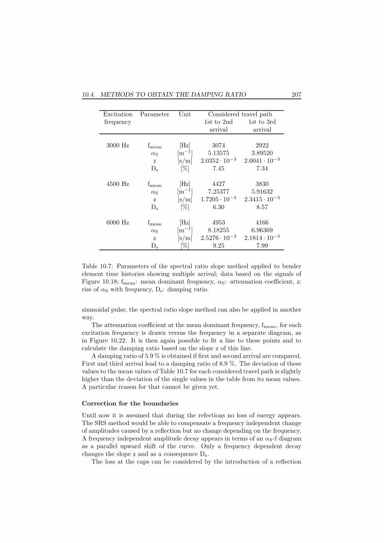
10.4. METHODS TO OBTAIN THE DAMPING RATIO 207
Excitation Parameter Unit Considered travel pathfrequency 1st to 2nd 1st to 3rd
arrival arrival
3000 Hz fmean [Hz] 3074 2922αS [m−1] 5.13575 3.89520z [s/m] 2.0352 · 10−3 2.0041 · 10−3
Ds [%] 7.45 7.34
4500 Hz fmean [Hz] 4427 3830αS [m−1] 7.25377 5.91632z [s/m] 1.7205 · 10−3 2.3415 · 10−3
Ds [%] 6.30 8.57
6000 Hz fmean [Hz] 4953 4166αS [m−1] 8.18255 6.96369z [s/m] 2.5276 · 10−3 2.1814 · 10−3
Ds [%] 9.25 7.99
Table 10.7: Parameters of the spectral ratio slope method applied to benderelement time histories showing multiple arrival; data based on the signals ofFigure 10.18; fmean: mean dominant frequency, αS: attenuation coefficient, z:rise of αS with frequency, Ds: damping ratio.
sinusoidal pulse, the spectral ratio slope method can also be applied in anotherway.
The attenuation coefficient at the mean dominant frequency, fmean, for eachexcitation frequency is drawn versus the frequency in a separate diagram, asin Figure 10.22. It is then again possible to fit a line to these points and tocalculate the damping ratio based on the slope z of this line.
A damping ratio of 5.9 % is obtained if first and second arrival are compared.First and third arrival lead to a damping ratio of 8.9 %. The deviation of thesevalues to the mean values of Table 10.7 for each considered travel path is slightlyhigher than the deviation of the single values in the table from its mean values.A particular reason for that cannot be given yet.
Correction for the boundaries
Until now it is assumed that during the refections no loss of energy appears.The SRS method would be able to compensate a frequency independent changeof amplitudes caused by a reflection but no change depending on the frequency.A frequency independent amplitude decay appears in terms of an αS-f diagramas a parallel upward shift of the curve. Only a frequency dependent decaychanges the slope z and as a consequence Ds.
The loss at the caps can be considered by the introduction of a reflection

208 CHAPTER 10. BENDER ELEMENT TECHNIQUE
2500 3000 3500 4000 4500 5000 55000
2
4
6
8
10
Atte
nuat
ion
coef
ficie
nt [1
/m]
Frequency [Hz]
1st to 2nd arrival1st to 3rd arrival
z = 2.4163 ⋅ 10−3 s/m,D
S = 8.85 %
z = 1.6108 ⋅ 10−3 s/m,D
S = 5.90 %
Figure 10.22: Attenuation coefficient at the mean dominant frequencies of thethree excitation pulses.
factor c(ω) in the Equations (10.36) and (10.37). This means for the first andthe second arrival:
αS =1
2Lln
∣
∣FFT (r1st) · c(ω)2∣
∣
|FFT (r2nd)|
=1
2Lln
|FFT (r1st)||FFT (r2nd)|
+1
2Lln
∣
∣c(ω)2∣
∣ (10.39)
and for the first and the third arrival:
αS =1
4Lln
∣
∣FFT (r1st) · c(ω)4∣
∣
|FFT (r3rd)|
=1
4Lln
|FFT (r1st)||FFT (r3rd)|
+1
4Lln
∣
∣c(ω)4∣
∣ (10.40)
The exponent of c(ω) indicates the number of reflections the signal has toundergo. Two reflections are considered for the travel path between 1st and2nd arrival and four reflections between 1st to 3rd arrival.
The simplest way to model the boundary effects is to assume at the interfacesoil to metal cap a two media boundary as shown in Figure 10.23. The factor ccan be expressed based on a constant cross section of both media. The equationfollows Clough & Penzien (1993) and Fratta & Santamarina (1996):
c =
ISample
ICap− 1
1 +ISample
ICap
(10.41)

10.4. METHODS TO OBTAIN THE DAMPING RATIO 209
Sample
Top/Bottom Cap
s1 s2 = IFFT(FFT(s1) · c(ω))
c1
Figure 10.23: Schematic view of wave refectionand refraction on top and bottom cap.
Sam
ple
Cap
Cap
LoadingPiston
Base Plate
Figure 10.24: Triaxialcell with installed sam-ple.
The impedances I can be calculated by the material density ρ and the shearwave velocity Vs:
I = ρ Vs (10.42)
According to the equation, the reflection factor c is not depending on fre-quency and therefore has no influence on the damping calculation using thespectral ratio slope technique. For the used testing device and the tested sam-ple |c| = 0.9586. This value is based on the material parameters in Table 10.8.
Parameter Unit Sample CapsDensity, ρ [kg/m3] 2342 8009S-wave velocity, Vs [m/s] 230 3180Impedance, I [kg/(m2s)] 5.3866 · 105 2.5470 · 107
Reflection coefficient, |c| [-] 0.9586
Table 10.8: Calculation of the reflection coefficient c for the case of the siltsample Waremme B1/3.
Fratta & Santamarina (1996) provide also an equation for a three mediaboundary. The base plate of the triaxial cell and the loading piston, as shown inin Figure 10.24, could be considered as the third medium. In this way the effectsof reflection and refraction on the interface cap to base plate respectively pistoncould be taken into account. However, there are some difficulties in determininga suitable impedance for the third medium. Fratta & Santamarina (1996)found, based on their sample and apparatus parameters, a reflection coefficientc(ω) depending on frequency in a range below 1000 Hz. At higher frequenciesc(ω) is nearly constant.

210 CHAPTER 10. BENDER ELEMENT TECHNIQUE
It is assumed that this frequency dependent component has only minoreffects on the damping ratio obtained by the spectral ratio slope method. Itcould cause a slight underestimation of the actual damping ratio.
10.4.3 Use of different travel paths
The direct application of the spectral ratio slope method or alternatively the at-tenuation coefficient method on the setup of two bender elements in a triaxialcell sample is not possible because there is no sufficient information on thetransfer characteristics soil - BE - output voltage, respectively driving voltage- BE - soil. This transfer characteristic might be expressed as a transfer func-tion κ(f), potentially highly frequency dependent. κ(f) incorporates effects ofdifferent resonance frequencies of the elements, different penetration depths ofthe elements and the coupling of the element tip and the specimen.
However, there is a theoretical approach to eliminate the influence of κ(f)if two measurements with opposite wave propagation directions are combined.The realization of this idea needs two receiver elements and two transmitterelements installed on one sample.
Ground level of the box
76
55
101077 354835
Figure 10.25: Frame with mounted sender (S1/S2) and receiver elements(R1/R2), unit: mm, Wang et al. (2004).
A preliminary test using this technique is published by Wang et al. (2004).The author uses a container of the dimensions 25 cm (H) x 50 cm (L) x 33.2cm (W) filled with sand. The bender elements are mounted on a frame, shownin Figure 10.25, and buried in the container. The damping ratio is calculatedby means of the spectral ratio method.
The background of the technique is described based on a setup of a triaxialcell with horizontally mounted elements. The Equation (9.19) for the atte-nuation coefficient α is adapted using the parameters defined in Figure 10.26.

10.4. METHODS TO OBTAIN THE DAMPING RATIO 211
Equation (9.19) is repeated here:
α(f) =ln
(
A1
A2· x1
x2
)
x2 − x1
The seismic pulse is transmitted from an element placed on the sample. Itis received simultaneously from two receiver elements on the other site of thesample (setup A). After that, a pulse is sent from the other transmitter and isreceived from both receiver elements (setup B).
BE
Setup A
z1A
Receiver 1
z2A
FFT(r1A) FFT(r1A)⋅κ1
FFT(r2A)⋅κ2
FFT(r2A)Receiver 2
Sender 1
Sender 2
Soil Specimen
Setup B
z2B
Receiver 1
z1B
FFT(r1B) FFT(r1B)⋅κ1
FFT(r2B)⋅κ2 FFT(r2B)
Receiver 2
Sender 1
Sender 2
Soil Specimen
BE BE
BE BE
BE
BE BE
Figure 10.26: Sketch of a sample with horizontal bender elements.
Four time records are obtained, r1A and r2A for setup A and r1B and r2B forsetup B. Their spectral amplitudes as a function of the frequency are indicatedas FFT(r...). z... gives the travel path length between sender and receiver forthe different combinations.
The attenuation coefficient for setup 1 can be expressed as:
α(f) =ln
(
FFT (r1A) κ1
FFT (r2A) κ2· z1A
z2A
)
z2A − z1A(10.43)
α(f) for setup 2 is:
α(f) =ln
(
FFT (r2B) κ2
FFT (r1B) κ1· z2B
z1B
)
z1B − z2B(10.44)
The Equations (10.43) and (10.44) can be transformed into:
α(f) (z2A − z1A) = ln
(
FFT (r1A)
FFT (r2A)
)
+ ln
(
κ1
κ2
)
+ ln
(
z1A
z2A
)
(10.45)
and
α(f) (z1B − z2B) = ln
(
FFT (r2B)
FFT (r1B)
)
+ ln
(
κ2
κ1
)
+ ln
(
z2B
z1B
)
(10.46)

212 CHAPTER 10. BENDER ELEMENT TECHNIQUE
If the sum of both equations is calculated the transfer functions κ1 and κ2
are eliminated and an expression for α(f) using the information of all four timerecords can be derived as:
α(f) =ln
(
FFT (r1A)FFT (r2A) ·
FFT (r2B)FFT (r1B) · z1A
z2A· z2B
z1B
)
z2A − z1A + z1B − z2B(10.47)
Equation (10.47) is independent of the unknown BE-transfer characteristicsand can be further developed to an expression according to the spectral ratioslope method, which is not done here. Wang et al. (2004) found for dry Ottawasand a damping ratio of 3.6 % if this method is applied, admittedly with anotherelement configuration. However, this value is quite high compared with othervalues given by the same authors based on resonant column tests.

10.5. THE RESONANT METHOD 213
10.5 Measurements of damping ratio on samp-les taken at the test sites based on the re-
sonant method
10.5.1 Introduction
The bender element test is performed on samples from the site in Waremmeand Sint-Katelijne-Waver. The specimens are subjected to different isotropicstress levels by an external water pressure. The back pressure applied to thesample is set to 100 kPa. The external isotropic pressure is therefore chosenalways 100 kPa above the value of the target effective stress. The absorption ofwater by the sample during consolidation is measured and taken into accountfor the calculation of the sample mass. The shear wave velocity is determinedby the analysis of the wave arrival at each stress level. The properties of thefree top cap are: height 19 mm, mass 50.74 g and diameter 50 mm.
The damping ratio is calculated based on half-power bandwidth and circle-fit method.
10.5.2 Site in Waremme
Altogether three samples taken from the drilling B1 in Waremme are tested.Specimen S1 is a reconstituted sample; S2 and S3 are undisturbed samples. Allsamples have a length of 29 to 30 mm. The 300 kPa consolidation stage of thesample S3 is repeated with air as confining medium to study its influence onthe response spectrum.
The Figures 10.27 to 10.29 present the measured response spectra, the Ta-bles 10.9 and 10.10 the predicted and measured natural frequencies includingthe physical parameters of the samples.
The theoretical estimation of the natural frequencies of the first mode isdone with an added mass coefficient of CA = 0.48, which corresponds to alength to diameter ratio of 0.96, and as well with no added mass (CA = 0) toallow comparisons. The coefficient is calculated by means of Equation (10.27).
As expected, the frequencies including the added mass component are lowerthan the values without the additional mass. For the same CA, the results fromthe Rayleigh expression show a good agreement with the FEM-values. Thefrequencies calculated by the Timoshenko equation are always higher.
The test results show that the natural frequencies and the shear wave ve-locities increase with an increasing cell pressure. The amplitude ratios of theobserved peaks decrease with increasing stress level.
The predicted frequencies are in all cases higher than the measured ones.The closest agreement to the experimental results is achieved at CA = 0.48 bythe Rayleigh equation and the FEM. A frequency comparison for the case ofsample S2 can be seen in Figure 10.30
The damping ratio versus effective confinement stress is shown in Figure10.31. D is in the range of 7.2 to 9.9 % for S1, between 4.7 and 7.3 % for S2

214 CHAPTER 10. BENDER ELEMENT TECHNIQUE
and between 2.3 and 7.8 % for S3. The deviation between the values from thehalf-power method and the circle-fit method are in nearly all cases less than1 %. A dependence of the damping ratio on the confining stress could be notnoticed in the stress range applied. The damping values are high in comparisonwith the resonant column and free torsion pendulm tests.
Example: half-power bandwidth and circle-fit method
Half-power and circle-fit method are used to obtain the damping ratio. TheFigures 10.32 shows an example of the half-power bandwidth technique appliedon the frequency response curve of the undisturbed silt sample S2 at 100 kPaconfining pressure. The calculation of the damping ratio D is based on Equation(10.29).
Figure 10.33 gives insides in the circle-fit technique based on the same re-sponse spectrum. The following algorithm is used:
• Drawing of the Nyquist plot from the experimental frequency responsecurve.
• Manual selection of some points of the response curve close to the reso-nance peak. These data points are indicated in the Nyquist plot of Figure10.33 as ”data points used for curve fitting”.
• Based on these selected points a circle is fitted.
• The center point of this circle is the origin of the angles α. The datapoint in the Nyquist plot with the largest distance to its adjoining pointsis the point of the natural frequency.
• Based of the selected range of data points for the curve fitting manycombinations of α- and ω-values are possible. They are all evaluated byEquation (10.30) and the damping ratio is obtained.
• All D-values are finally averaged and this average value provides the resultof the test.
Influence of the confining medium
For the evaluation of the influence of the water pressure to the response curvesin the experimental bender element test, the manner of applying the confiningstress is changed. The triaxial cell is connected to a source of controllable airpressure and the 300 kPa consolidation stage of sample S3 is repeated usingair pressure instead of the usual water pressure.
The response curve of this stage, given in Figure 10.34, has a similar shapeas this found using water pressure. The resonant peak of the first mode isshifted towards higher frequencies but not as much as predicted by analyticaland FEM calculations.

10.5. THE RESONANT METHOD 215
Comparison with other test methods
The Figures 10.35 and 10.36 summarize the results of the laboratory and insitu tests concerning Vs and D.
S-wave velocity The SCPT-profile is taken from SCPT5; the s-wave velocityof the shallow 7 m is 165 m/s based on the results of SASW UGent Setup 2.The results of the BE-time arrival method, the resonant column test and thefree torsion pendulum test are drawn according to the depth of sampling. Thegiven velocities of the BE-time arrival method are, because of a better accuracy,not taken from the short samples used for the BE-resonant method. Instead,the results shown in Figure 6.12 obtained from standard sized triaxial samplesare used. The isotropic stress related to each measured value is indicated at thedata point. The actual mean effective stress assumed at the sampling depth isgiven by an arrow enabling a raw ”graphical interpolation” between the datapoints. The tip of the arrow gives therefore the calculated s-wave velocity outof the laboratory tests at the sampling depth.
The effective stresses and the density of the silt increase with depth, accom-panied by an increase of the s-waves velocity. The results of the SCPT and thelaboratory tests confirm this increase in Vs. The s-wave velocity determinedby the in situ tests is higher than the results of the laboratory tests. This isvalid for the BE test, working under very low shear strain amplitudes, and alsofor the resonant column and free torsion pendulum test, operated at a shearstrain of 10−5. A possible reason for the difference of field and laboratory testscan be a loosening of the silt during the drilling and sampling process, leadingto a decrease in density. Another reason might be a lower shear strain in thefield tests.
Damping ratio The profile of the damping ratio in Figure 10.36 is arrangedin the same way as the Vs-profile. The damping ratio by the SCPT is basedon the spectral ratio slope method performed on the time records of SCPT5.The results of the BE-resonant method is the mean value of half-power andcircle-fit method of sample S2 calculated at each consolidation stage.
The values of the SCPT show major variation with the depth but their meanvalue falls in the same range than indicated by the resonant column and thefree torsion pendulum test. The damping ratio calculated by the BE-resonanttest is above the range of the SCPT results and the other laboratory tests. Apossible reason could be a frequency dependence of the damping ratio. Moreinformation on this topic is given in Section 10.6.
10.5.3 Site in Sint-Katelijne-Waver
Two Boom clay samples from the drilling B1I in Sint-Katelijne-Waver are testedby the bender element resonant technique. The length of sample C4 is about30 mm and sample C5 is 60 mm long. The additional sample C5 is selected toprove if the deviated equations for the resonance frequency can properly predict

216 CHAPTER 10. BENDER ELEMENT TECHNIQUE
the shift of the resonance frequency between samples of different lengths. Ifthis is the case, the association of the experimentally found natural frequencywith the modeled lowest vibration mode would be confirmed once more.
The isotropic confining stress is applied in stages of 50, 100, 200 and400 kPa. The results can be found in detail in the Tables 10.11 and 10.12;the response spectra are shown in Figure 10.37 and Figure 10.38. The addedmass coefficient is CA = 0.71 is case of sample C5, corresponding to a lengthto diameter ratio of 1.57.
The evaluation of the response function of sample C5 is not possible becauseof the relatively low natural frequency of the longer sample. It lays between 250to 400 Hz following the Rayleigh equation. However, there is no correspondingpeak in the response spectrum of Figure 10.38. It is assumed that the benderelements are not able to excite the sample sufficiently at such low frequencies.Therefore in the following only results of sample C4 are discussed.
The frequencies of resonance are in general below the values of the tests onthe silt material from Waremme agreeing with a lower s-wave velocity of theclay. The damping ratio calculated by the two analyzing methods are drawnversus confining stress in Figure 10.39. The ratio lays between 7.3 and 15.7 %.This is again higher than the values obtained by resonant column and freetorsion pendulum test and higher than the values found for the silt samples.
Comparison with other test methods
The profiles in the Figures 10.40 and 10.41 summarize the test results in thesame way as done for Waremme. The SCPT data are taken from SCPT2.
S-wave velocity The resonant column test indicates a slightly lower s-wavevelocity than the SCPT. The result of the free torsional pendulum test is almostidentical with the SCPT. The BE element test gives the highest velocities.Their differences from the other laboratory tests can be explained by a lowershear strain level during the BE tests.
Damping ratio An indication of the in situ mean effective stresses is for theD-profile not useful because the test data of the different confining stresses areto close to each other or because, in case of the BE-resonant method, D doesnot change monotonic with the confinement stress.
The result comparison for the damping ratio comes to the same conclusionsas at the site of Waremme. The BE-resonant results are the highest of alltest. The other laboratory tests values fall in the range of the scattered SCPTresults.
10.6 Summary and remarks
The determination of the s-wave velocity is performed by a visual picking ofthe first wave arrival. This technique has shown to be most straightforward

10.6. SUMMARY AND REMARKS 217
and flexible.
In the following methods to calculate the damping ratio are treated. Anapproach to analyze multiple refections by the spectral ratio slope method isapplied on a sample of the site in Waremme. Damping ratios calculated bythis technique for the silt material are in the same range as obtained by theBE resonant test.
A self correcting method is described to eliminate the influence of the trans-fer characteristic of the bender elements. This enables the application of thespectral ratio slope method.
The determination of the damping ratio focuses on the bender elementresonant method. At first the behavior of the sample-top-cap system is modeledanalytically, using the Timoshenko beam theory and Rayleigh’s approximation,and numerically, using the FE program ABAQUS. This provides informationon the natural frequency of the first flexural mode to be used in the modal test.The influence of the confinement medium water is considered by an added masscomponent and experimentally validated.
The first flexural mode is identified in experimental response curves bymeans of the natural frequency prediction. The response curves are analyzedusing circle-fit and half-power method to obtain the damping ratio. Undistur-bed samples from Waremme and Sint-Katelijne-Wave are tested.
Two basic problems appear looking at the test results. The first is thedeviation of the calculated and the measured resonant frequencies. The ass-umption of a beam with top-mass at its one end, even if shear effects are takeninto account, might be a relatively crude way to describe the very short, about3 cm long, sample and the top cap. The finite element model can partly over-come this geometrical problem, but also in this case, influences of the rubbermembrane and the not fully rigid mounting of the bottom cap are not takeninto account. Furthermore the consideration of the water in the cell by anadditional mass might not be sufficiently correct. If the viscosity of the wateris taken into account, a frictional (viscous) drag force, proportional to the ve-locity of the moving cylinder, has to be introduced (Wilson (1984)). The usedcoefficient CA for the added mass depends, besides the cylinder geometry, alsoon the Reynolds number and the cylinder roughness. A more detailed investi-gation could help to find a more exact theoretical solution. On the other handthe prediction of the natural frequency is only used to find the right resonantpeak among several, so the calculations are already sufficient for a successfulselection.
The second problem concerns the difference between the results of the BE-resonant test and the other laboratory tests. Possible explanations for thisphenomenon can be external factors as the supply cables to the top-cap, therubber membrane and the confining medium affecting slightly the oscillation.Another factor could be a possible frequency dependence of the damping ratio.
Remarks on the frequency dependence of the damping ratio A possi-ble reason of the high damping values obtained by the bender element resonant

218 CHAPTER 10. BENDER ELEMENT TECHNIQUE
technique might be the different range of working frequency of the tests. Cyclictests are usually performed at frequencies below 2 Hz; free torsion pendulumtest show commonly natural frequencies of sample and device below 10 Hz.Even resonant column tests devices reach, dependent on the sample geometryseldom resonance frequencies higher than 250 Hz, in the most cases much lower.In contrast to that, samples subjected to a BE-resonant test have natural fre-quencies, crucial for the damping determination, in the range between 400 to900 Hz.
A frequency dependence of the damping ratio could possibly explain thedeviation in the results. Unfortunately, this question is not completely solvedyet. Dobry & Vucetic (1987) write in their summary, given in table Table 2.2,on influence factors of the damping ratio, that with an increasing strain rate,i.e. frequency, the damping ratio ”stays or may increase”.
Mok et al. (1988) suggested based on the work of others that, for dryrocks and dry soils, D is independent of frequency. On the other hand, water-saturated rocks, sands and silts would show a definite dependency of D on fre-quency. For saturated clays the authors conclude a relatively small frequencydependency.
Several authors compare results from cyclic torsional shear tests and reso-nant column tests. Zavoral & Campanella (1994) are doing this for a marinesilt to clay deposit and found no frequency dependence. The cyclic torsionalapparatus was driven at frequencies between 0.01 and 1 Hz; the resonance wasreached in the range of 10 to 30 Hz. Bolton & Wilson (1989) come to the samefinding for a dry sand. The cyclic testing frequency was fixed at 0.001 Hz,the authors call it a pseudo-static test; the resonant conditions were obtainedbetween 45 and 95 Hz.
Lin et al. (1996), tested two types of sand at various frequencies in the rangefrom almost static to 20 Hz using again a cyclic torsional device. They foundan increase of damping ratio from 2.6 to 6.4 % for the first sand and between1.9 to 6.2 % for the other sand. These tests were performed at a shear strain of4 · 10−3 %. Remarkably no significant change in the G-modulus was observed.
A few in situ tests give also some indication of the influence of the frequencyon the damping ratio. Hall & Bodare (2000) describe a cross-hole test perfor-med in layers of mud and clay where the attenuation coefficient method is usedto analyze the attenuation. In the range between 20 and 30 Hz the dampingratio is found to be frequency independent. Mok et al. (1988) came to the sameresult for frequencies between 170 and 300 Hz and a site dominated by a clay.Kudo & Shima (1981) confirm an almost frequency independent behavior foran even larger range from 5 to 100 Hz based on a down-hole set-up in sand.
Mok et al. (1988) investigated the damping of p-waves in dry sand based ona miniaturized cross-hole set-up and the attenuation coefficient method. Theyfound in the range of 2200 to 3000 Hz an almost constant damping ratio.
A mathematical model including a frequency dependent damping can beobtained by Biot’s theory concerning the interaction of the pore water and thesoil fabric. If the soil is assumed to be a saturated two-phase medium the

10.6. SUMMARY AND REMARKS 219
damping ratio of the shear wave, following Biot’s theory, has to be frequencydependent. The damping ratio increases form the static case with the frequencyuntil a local maximum is reached after which the ratio decreases again. Figure10.42, taken from Stoll (1979), shows the logarithmic decrement as function offrequency according to Biot’s theory for the parameters given in Table 10.13.Beside self-explanatory values, a pore-size parameter (a) and a structure con-stant (c) are influencing the shape of the curves. The pore-size parameter(a) depends on the size and shape of the pores and can be estimated by themean grain diameter. However, the structure constant (c) is an experimentallydetermined parameter not easy to quantify.
Curve No. 1 shows the results of the calculation for a less permeable mate-rial. The logarithmic decrement stays constant in the whole observed frequencyrange and is equal to the decrement of the frame. All other parameter sets withhigher permeability lead to the described frequency dependent curves.
Further information on Biot’s theory can be found in the basic papers Biot(1956a) and Biot (1956b).
As a conclusion there is evidence that comparing free torsion pendulumtests, resonant column tests and BE tests on the level of damping ratio cangive different results due to frequency dependence of the ratio.

220 CHAPTER 10. BENDER ELEMENT TECHNIQUE
100 200 300 400 500 600 700 800 900 10000
0.2
0.4
0.6
0.8
1
x 10−5
Frequency [Hz]Am
plitu
de r
atio
rec
eive
r −
tran
smitt
er [−
]
582 Hz
708 Hz
807 Hz
100 kPa200 kPa300 kPa
Figure 10.27: Frequency response spectra for sample S1 (reconstituted silt).
100 200 300 400 500 600 700 800 900 10000
0.5
1
1.5
2x 10
−5
Frequency [Hz]
636 Hz
766 Hz
820 Hz
Am
plitu
de r
atio
rec
eive
r −
tran
smitt
er [−
]
100 kPa200 kPa300 kPa
Figure 10.28: Frequency response spectra for sample S2 (undisturbed silt).

10.6. SUMMARY AND REMARKS 221
100 200 300 400 500 600 700 800 900 10000
0.2
0.4
0.6
0.8
1
1.2x 10
−5
Frequency [Hz]Am
plitu
de r
atio
rec
eive
r −
tran
smitt
er [−
]
100 kPa200 kPa300 kPa
631 Hz
735 Hz
811 Hz
Figure 10.29: Frequency response spectra for sample S3 (undisturbed silt).
100 200 3000
200
400
600
800
1000
1200
Confinement stress [kPa]
Fre
quen
cy fl
exur
al m
ode
[Hz] Timoshenko Equation
Rayleigh Equation
FEMExperiment
Figure 10.30: Calculated and measured resonant frequencies for the first flexu-ral mode of sample S2, added mass effects are included (CA = 0.48).

222 CHAPTER 10. BENDER ELEMENT TECHNIQUE
0 100 200 300 400 5000
1
2
3
4
5
6
7
8
9
10
Stress, σ1, 2, 3
[kPa]
Dam
ping
rat
io, D
[%]
Free Torsion Pendulum (12.0−12.5 m)
Resonant Column (4.0−4.5 m)
Resonant Column (5.0−5.5 m)
S1
S1
S1
S2 S2
S2
S3
S3
S3
Half−Power MethodCircle−Fit Method
Sampling Depths: S1, S2 −> 4.0−4.5 m,S3 −> 5.0−5.5 m
Figure 10.31: Damping ratio’s obtained from the samples S1, S2 and S3 incomparison with resonant column test and free torsion pendulum test on othersamples of the same material (reference shear strain 10−3 %).
100 200 300 400 500 600 700 800 900 10000
0.5
1
1.5
2
2.5x 10
−5
Frequency [Hz]
Am
plitu
de r
atio
rec
eive
r −
tran
smitt
er [−
]
Amax
A = Amax
/ 20.5
f1 = 593 Hz
f2 = 672 Hz
fm
= 636 Hz
DHPM
=(f2−f
1) / (2 ⋅ f
m) = 6.2 %
Figure 10.32: Example of the half-power method to the frequency responsespectrum of sample S2 at 100 kPa isotropic stress.
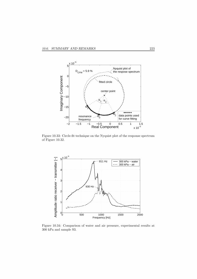
10.6. SUMMARY AND REMARKS 223
−2 −1.5 −1 −0.5 0 0.5 1 1.5
x 10−5
−20
−15
−10
−5
0
5x 10
−6
Real Component
Imag
inar
y C
ompo
nent
DCFM
= 5.9 %
center point
ω0
ω1
ω2
α1 α
2
fitted circle
Nyquist plot of the respose spectrum
resonance frequency
data points used for curve fitting
Figure 10.33: Circle-fit technique on the Nyquist plot of the response spectrumof Figure 10.32.
0 500 1000 1500 20000
1
2
3
4
5x 10
−6
Frequency [Hz]Am
plitu
de r
atio
rec
eive
r −
tran
smitt
er [−
]
930 Hz
811 Hz 300 kPa − water300 kPa − air
Figure 10.34: Comparison of water and air pressure, experimental results at300 kPa and sample S3.

224 CHAPTER 10. BENDER ELEMENT TECHNIQUE
0 50 100 150 200 250 300 350
0
2
4
6
8
10
12
14
Waremme
S−Wave Velocity [m/s]
Dep
th [m
]
Mechanical Hammer (SCPT)Sledge Hammer (SCPT)SASW
BE−Time arrival method
Resonant Column Test
BE−Time arrival method
Free Torsion Pendulum Test
25 k
Pa
50 k
Pa
100
kPa
200
Pa
400
kPa
50 k
Pa
100
kPa
200
kPa
400
kPa
50 k
Pa
100
kPa
200
kPa
400
kPa
600
kPa
50 k
Pa
100
kPa
200
kPa
33 kPa
62 kPa
77 kPa
126 kPa
141 kPa
actual mean effective stress at a certain depth
confining stress stages used in laboratory tests indicates the calculated velocity out of alaboratory test at sampling depth
Figure 10.35: Vs profile of the site in Waremme including the results of allperformed laboratory and in situ tests; the SCPT data are based on SCPT5;SASW results are based on SASW UGent setup 2.

10.6. SUMMARY AND REMARKS 225
0 2 4 6 8 10
0
2
4
6
8
10
12
14
Waremme
Damping Ratio [%]
Dep
th [m
]
Resonant Column Test
Free Torsion Pendulum Test
BE−resonant method
50 k
Pa
100
kPa
141 kPa
62 kPa 62 kPa
77 kPa
actual mean effective stress at a certain depth
confining stress stages used in laboratory tests indicates the calculated damping ratio out of a laboratory test at sampling depth
Mechanical HammerSledge Hammer
Figure 10.36: Ds profile of Waremme based on SCPT5 and including the otherlaboratory tests.

226 CHAPTER 10. BENDER ELEMENT TECHNIQUE
100 200 300 400 500 600 700 800 900 10000
1
2
3
4
5
6
7x 10
−6
Frequency [Hz]Am
plitu
de r
atio
rec
eive
r −
tran
smitt
er [−
]
397 Hz 460 Hz
609 Hz
735 Hz
50 kPa100 kPa200 kPa400 kPa
Figure 10.37: Frequency response spectra for sample C4 (undisturbed Boomclay).
100 200 300 400 500 600 700 800 900 10000
1
2
3
4
5
6x 10
−6
Frequency [Hz]Am
plitu
de r
atio
rec
eive
r −
tran
smitt
er [−
]
50 kPa100 kPa200 kPa400 kPa
Figure 10.38: Frequency response spectra for sample C5 (undisturbed Boomclay).
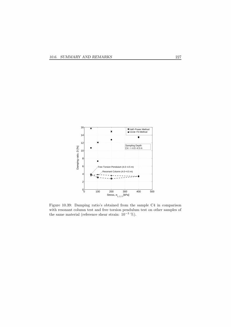
10.6. SUMMARY AND REMARKS 227
0 100 200 300 400 5000
2
4
6
8
10
12
14
16
Stress, σ1, 2, 3
[kPa]
Dam
ping
rat
io, D
[%]
Resonant Column (4.0−4.5 m)
Free Torsion Pendulum (4.0−4.5 m)
Half−Power MethodCircle−Fit Method
Sampling Depth: C4 −> 4.0−4.5 m
Figure 10.39: Damping ratio’s obtained from the sample C4 in comparisonwith resonant column test and free torsion pendulum test on other samples ofthe same material (reference shear strain: 10−3 %).

228 CHAPTER 10. BENDER ELEMENT TECHNIQUE
0 50 100 150 200 250 300
0
1
2
3
4
5
6
7
8
9
Sint−Katelijne−Waver
0 50 100 150 200 250 300
0
1
2
3
4
5
6
7
8
9
Dep
th [m
]
S−Wave Velocity [m/s]
actual mean effective stress at depth
confining stress stages used in laboratory tests indicates the calculated damping ratio out of a laboratory test at sampling depth
Resonant Column Test
Free Torsion Pendulum TestBE−resonant method
100
kPa
400
kPa
200
kPa
50 k
Pa
121 kPa
400
kPa
200
kPa
100
kPa
50 k
Pa
121 kPa
Mechanical Hammer (SCPT)Sledge Hammer (SCPT)
Figure 10.40: Vs profile of the site in Sint-Katelijne-Waver including the resultsof all performed laboratory and in situ tests; the SCPT data are based onSCPT 2.

10.6. SUMMARY AND REMARKS 229
0 5 10 15
0
1
2
3
4
5
6
7
8
9
Sint−Katelijne−Waver
Damping Ratio [%]
Dep
th [m
]
confining stress stages used in laboratory tests
50 k
Pa
100
kPa
200
kPa
400
kPa
BE−resonant method Resonant Column Test
Free Torsion Pendulum Test
50, 100, 200, 400 kPa
Mechanical HammerSledge Hammer
Figure 10.41: Ds profile of Sint-Katelijne-Waver based on SCPT2 and includingthe other laboratory tests.

230 CHAPTER 10. BENDER ELEMENT TECHNIQUE
Sample Description:Sample index S1 S2Site Waremme WaremmeDescription Silt SiltSampling reconst. sample undist. sampleDepth [m] 4.0-4.5 4.0-4.5
Initial test parameters:Length, L [mm] 29.0 29.5Diameters, d [mm] 50.0 50.0Distance BE tips [mm] 25.0 25.5Mass, mT [g] 101.53 119.49Unit mass, ρ [kg/m3] 1783.10 2062.90
Consolidation parameters:Effective stress, peff [kPa] 100 200 300 100 200 300Water absorption [g] 11.4 10.9 10.2 -3.2 -5.6 -7.0Effective mass, mT,eff [g] 113.0 112.5 111.8 116.3 113.9 112.5S-wave velocity, Vs [m/s] 216.9 224.5 246.3 197.7 246.1 271.3
Resonant frequencies:CA = 0
Rayleigh Eq., fRay [Hz] 888 918 1005 799 988 1084Timosh. Eq., fTBT [Hz] 962 995 1090 864 1070 1175FEM, fFEM [Hz] 875 904 989 787 972 1066
CA = 0 .48Rayleigh Eq., fRay [Hz] 773 799 875 696 860 943Timosh. Eq., fTBT [Hz] 843 871 954 757 937 1028FEM, fFEM [Hz] 763 788 862 686 847 929
Exp. result, fmeas [Hz] 582 708 807 636 766 820
Damping ratio:Half-Power, DHPM [%] 7.9 9.1 8.0 6.2 7.3 5.4Circle-fit, DCFM [%] 7.2 9.9 8.9 5.9 4.7 4.9
Table 10.9: Test data for sample S1 (reconstituted silt) and S2 (undisturbedsilt).

10.6. SUMMARY AND REMARKS 231
Sample Description:Sample index S3Site WaremmeDescription SiltSampling undist. sampleDepth [m] 5.0-5.5
Initial test parameters:Length, L [mm] 30.0Diameters, d [mm] 50.0Distance BE tips [mm] 26.0Mass, mT [g] 116.54Unit mass, ρ [kg/m3] 1978.44
Consolidation parameters:Effective stress, peff [kPa] 100 200 300 300
airWater absorption [g] 1.3 0.7 0.4 0.4Effective mass, mT,eff [g] 117.8 117.2 116.9 116.9S-wave velocity, Vs [m/s] 195.1 230.6 255.0 257.0
Resonant frequencies:CA = 0
Rayleigh Eq., fRay [Hz] 774 913 1009 1017Timosh. Eq., fTBT [Hz] 837 988 1092 1100
CA = 0 .48Rayleigh Eq., fRay [Hz] 674 796 879 886Timosh. Eq., fTBT [Hz] 766 904 999 1007
Exp. result, fmeas [Hz] 631 735 811 930
Damping ratio:Half-Power, DHPM [%] 7.8 6.8 (10.0) (17.5)Circle-fit, DCFM [%] 7.3 6.2 2.3 2.1
Table 10.10: Test data for sample S3 (undisturbed silt).

232 CHAPTER 10. BENDER ELEMENT TECHNIQUE
Sample Description:Sample index C4Site Sint-Katelijne-WaverDescription Boom-ClaySampling undist. sampleDepth [m] 4.0-4.5
Initial test parameters:Length, L [mm] 29.8Diameters, d [mm] 50.0Distance BE tips [mm] 25.8Mass, mT [g] 114.60Unit mass, ρ [kg/m3] 1961.86
Consolidation parameters:Effective stress, peff [kPa] 50 100 200 400Water absorption [g] 5.7 8.6 8.5 8.1Effective mass, mT,eff [g] 120.3 123.2 123.1 122.7S-wave velocity, Vs [m/s] 157.0 178.2 253.5 299.6
Resonant frequencies:CA = 0 .48Rayleigh Eq., fRay [Hz] 553 634 902 1064
Exp. result, fmeas [Hz] 397 460 609 735
Damping ratio:Half-Power, DHPM [%] 15.7 12.1 14.9 13.5Circle-fit, DCFM [%] 10.7 7.3 12.8 13.4
Table 10.11: Test data for sample C4 (undisturbed clay), 30 mm height.

10.6. SUMMARY AND REMARKS 233
Sample Description:Sample index C5Site Sint-Katelijne-WaverDescription Boom-ClaySampling undist. sampleDepth [m] 4.0-4.5
Initial test parameters:Length, L [mm] 59.5Diameters, d [mm] 50.0Distance BE tips [mm] 55.5Mass, mT [g] 221.62Unit mass, ρ [kg/m3] 1885.65
Consolidation parameters:Effective stress, peff [kPa] 50 100 200 400Water absorption [g] 8.1 7.3 5.5 2.8Effective mass, mT,eff [g] 229.7 228.9 227.1 224.4S-wave velocity, Vs [m/s] 175.4 205.9 232.9 290.0
Resonant frequencies:CA = 0 .71Rayleigh Eq., fRay [Hz] 255 299 337 418
Exp. result, fmeas [Hz] - - - -
Damping ratio:Half-Power, DHPM [%] - - - -Circle-fit, DCFM [%] - - - -
Table 10.12: Test data for sample C5 (undisturbed clay), 60 mm height.

234 CHAPTER 10. BENDER ELEMENT TECHNIQUE
Frequency [Hz]
L
og. D
ecre
men
t [−]
Curve No. 1
3
5
1 10 102 103 104
1
10−1
10−2
2
4
Figure 10.42: Logarithmic decrement in function of the frequency for s-wavesaccording to Biot’s theory, Stoll (1979).
Values for different curvesMaterial property Unit No. 1 No. 2 No. 3 No. 4 No. 5Mass density of grains, ρr kg/m3 2650Mass density of fluid, ρf kg/m3 1000Viscosity of fluid, η Pa s 0.001Shear modulus of frame, G MPa 56.7Structure constant, c - 1.25Intrinsic permeability, ki m2 2.5 1 1 2.3 5
·10−14·10−10
·10−11·10−11
·10−11
Permeability, k = ki · ρf g/η m/s 2.45 9.81 9.81 2.26 4.91with g = 9.81m/s2 ·10−7
·10−4·10−5
·10−4·10−4
Pore-size parameter, a m 3.8 3.9 1.2 1.9 2.8·10−6
·10−5·10−5
·10−5·10−5
Porosity, β - 0.49 0.36 0.36 0.36 0.36Log. decrement of framefor shearing motion, δ - 0.08 0.03 0.03 0.03 0.02Damping ratio, D = δ/(2π) % 1.27 0.48 0.48 0.48 0.32
Table 10.13: Material properties of the Biot theory example, Stoll (1979).

Chapter 11
Conclusions and summary
Main purpose of this research is to investigate to what extent the seismic conepenetration test (SCPT) and the bender element test (BE-test) primary deve-loped for the measurement of shear and compression wave velocities in soils canadditionally provide information on the material damping behavior of the soils.This chapter gives a summary of the research and points out main findings andconclusions.
Determination of wave velocities
At first, methods for the calculation of the wave velocities are studied and themost suitable techniques for both tests are selected. Because of its flexibilityand also considering the limited number of time histories to analyze, a visualinterpretation is chosen for the BE-test.
Under the conditions of a SCPT a visual arrival picking, cross correlationin the time domain and also a calculation of the cross power spectrum is con-sidered. The cross correlation in the time domain is preferred because it canbe automatically performed. This is necessary in view of the large amount oftime records during a SCPT. Furthermore it eliminates arbitrary influences bythe person performing the analysis regarding picking of the arrival time or theselection of a suitable frequency range.
The determination of the wave velocities provides for both types of testsreliable results and can be considered as sufficiently developed. This is provedon several test sites.
Determination of the damping ratio
Seismic cone penetration test After an extended selection process, a qua-lified sensor equipment for the damping measurements is found and installed ina seismic dual cone. The selected triaxial accelerometers meet the requirementsconcerning a small size, a flat frequency response, a high sensitivity and a highresolution.
235

236 CHAPTER 11. CONCLUSIONS AND SUMMARY
Two groups of approaches to calculate the damping ratio are investigated.The first methods are based on the spectral ratio of the amplitude spectraof two recorded signals. These are the attenuation coefficient method (ACM)and the spectral ratio slope method (SRS). The second group is studied to alower extend. It transfers a technology used for vertical seismic measurementarrays to record earthquakes to the SCPT. The time histories of the particleacceleration are converted using a shear beam model of the soil to stress-strainhysteresis curves. These are analyzed to obtain the damping ratio.
SRS method and ACM give a significant scatter of the damping ratio withdepth but also for the same depth, repetitions of the SCPT give results withsome deviation. It is conjectured that the scatter is caused by the pretreatmentof the measured signals before the spectral ratio is calculated. Pretreatmentmeans mainly the way of cutting the signal part of interest by the applicationof a window. This point is intensively studied by the variation of windowlength and type on measured and on simulated time histories. Especially byanalyzing the simulated signals it could be quite clearly shown that a tooshort cutting window is indeed the most dominating reason for the scattering,whereas the shape of the window function has very low influence. Unfortunatelythis finding cannot conclude in an improvement of the windowing techniquesince the separation of the main shear wave arrival, especially in signals showingreflected wave components and in noisy environments, is unavoidable and forcesoften to short windows.
The SRS method has the advantage in opposite to the ACM that it eli-minates the need of introducing of geometrical corrections and is therefore inprinciple preferable.
The technique based on the analyses of stress-strain time histories is appliedto data of one site. Even though a number of well shaped stress-strain loopscould be calculated the damping ratio (25 to 30 %) is quite far above theexpected range. Four main reasons can be identified: a) The receiver distanceof 1 m of the dual cone is to large to avoid spatial aliasing. b) The transferfunction approach, used to bypass the insufficent repeatability of the source,addes small errors caused by signal noise from the surface to the calculationdepth. c) The calculation of the shear stress time histories by an integrationwith depth starting at the stress-free surface collects likewise small signal errors.d) A double integration is needed for the shear strain calculation.
The reasons a) and b) can be eliminated when the receiver distance ischosen closer and a repeatable source is used. It is expected that in this waythe obtained damping ratio is lower and more credible.
Bender element test The most elaborated method studied is the benderelement resonant method. It is based on a modal test of a soil sample ina triaxial cell using BE’s for the excitation and the capturing of the responsemovement. Some modification on the standard triaxial equipment are necessaryto allow the upper BE cap a free oscillation.
The experimental natural frequencies of the sample have to be assigned to

237
certain mode shapes. Because the first flexural mode is used to obtain thedamping ratio, its frequency is predicted by means of two analytical formu-lations (Timoshenko beam theory, Rayleigh’s method) and a FE calculation(ABAQUS). The influence of the confining medium is taken into account bythe introduction of an added mass component. A reasonable approximation ofmeasured and predicted natural frequencies is obtained.
Results based on bender element resonant method are gathered on samplesof a silt (5 − 10 %) and a clay (10 − 16 %) material. These results are repeata-ble but higher than the results from resonant column and free torsion pendulumtests (1 − 4 %) performed for comparative purposes. There is some evidencethat this deviation is caused by the higher frequency used in the BE-test incomparison with the two other laboratory tests.
Another interpretation technique uses the property of shear wave pulses re-flected on the end caps of the triaxial device. The SRS method can be appliedbased on the spectral ratio between reflections of different order. Dampingratios calculated in this approach are between 7 and 9 % for the silt material.This is the same range as obtained by the BE resonant test. Unfortunately mul-tiple reflections could be not identified in samples of the clay material probablybecause of the higher attenuation in the clay.
A SRS based method to eliminate the influence of the transfer characteristicof the bender elements by means of a combined analysis of different travel pathsis discussed.
Practical relevance The SCPT and BE test methods for the determinationof the damping ratio need still a further refinement until they can be recommen-ded for the practical application. Especially the scattering seen in the ACMand SRS method should be reduced. However, by taking in consideration thatthere are nearly no other, at least no cost-equivalent, field tests available todetermine the damping ratio, it seems obvious to spend additional effort inthis technique.
Reasons for the high damping values of the BE-resonant method shouldalso be closer investigated.
Recommendations for further research
Seismic cone penetration test
• Application of the method to analyze stress-strain time histories on si-mulated SCPT data.
• Analysis of stress-strain time histories using shorter receiver distancesand a repeatable source.
• Further extensive SCPT testing may open the possibility for the develop-ment of correlations between damping and other cone measurements.

238 CHAPTER 11. CONCLUSIONS AND SUMMARY
• SASW tests with an advanced inversion algorithm to determine s-wavevelocity and damping ratio profiles simultaneously can provide an alter-native field test method. The technique is found in Lai (1998). Resultsof these SASW tests can be used to evaluate the profiles of the SCPT’s.
Bender elements
• The frequency dependency of the damping ratio can be investigated by aresonant column device with electronically adjustable working frequencyor cyclic triaxial tests.
• Application of the self correcting method of Wang et al. (2004) to elimi-nate the influence of the transfer characteristic of the bender elements onbender element configurations as described in Section 10.4.3.
• Replacement of the flexural excitation of the BE-resonant test by a tor-sional excitation. Nakagawa et al. (1996) give suggestions of a triaxialset-up using some bender elements radially orientated. Such a set-up canbe used to excite the first torsional shear mode of the sample. This is themode also used in standard resonant column devices. The mode has theadvantage, in opposite to the flexural mode, that it shows a pure sheardeformation and the kind of confinement medium has almost no influenceon the natural frequency.
• Efforts to use the Pochhammer-Chree approach for infinite long cylindersfor the calculation of natural frequencies of finite cylinders can possiblyimprove the natural frequency prediction.

Part IV
Appendix
239


Appendix A
Accuracy and costs of soiltests
This chapter provides some help in the selection of a suitable testing methodfor the s-wave velocity, respectively Gmax, and the damping ratio if a certainaccuracy is needed, taking into account the available financial and time budget.
It has to be emphasized that the testing methods related to the s-wavevelocity are of great variety and mostly well tried. Their application is relativelywidespread and some of them can be considered as standard methods.
This is in contrast to methods to determine the damping ratio. The selectionbandwidth of methods is limited. Furthermore a large number of techniques isonly poorly approved and has its use only in a research environment.
Table A.1 gives an overview of the common techniques indicating the shearstrain range of their applicability. In addition it gives relative ratings of theircosts, their accuracy and their currency of practical application. As a meanto compare the techniques the given classification of accuracy and costs arerelative values.
Some more details are provided in the following for the different groups oftests. All findings concerning the accuracy based on this research have to stayquite general and qualitative since either, as for the SCPT, no reference valuesof comparable tests are available or the data pool is too limited for statisticalanalyzes. Also the information on the costs has to stay qualitatively becauseits reliable quantification requires an elaborate market analysis which is notperformed.
However, in the frame of this research orders for resonant column tests areplaced with external laboratories. Additionally a few prices for other tests areavailable based on recent quotations of external companies and not at leastbased on the price list for tests performed by the Laboratory of Soil Mechanicsin Ghent. The individual test prices are summarized in Table A.2 together witha description of the testing conditions. They can provide an indication for thesituation on the local market but might not be complete and representative.
241

242 APPENDIX A. ACCURACY AND COSTS OF SOIL TESTS
A.1 Laboratory tests
Cyclic and resonant tests
Cyclic tests (cyclic triaxial, cyclic torsional shear and cyclic simple shear tests)and resonant tests (resonant column and free torsion pendulum test) are, ex-cept for the cyclic simple shear test, based on a triaxial apparatus extendedwith a loading facility to apply a dynamic loading. Cyclic tests are perfor-med commonly at frequencies around 1 Hz. Resonant column tests have toachieve the resonant frequency of the sample going up to a few hundred Hz.The resonant methods can work at lower shear strains than the cyclic tests.
If higher strain levels are needed a hollow-cylindrical specimen is used ins-tead of a cylindrical sample because it has a more uniform shear strain distri-bution over the cross-section.
Since the conditions in the triaxial stress cell are well controlled and thesetests are long time established the accuracy and the reproducibility of theresults is in general high. This is true for both G-modulus and damping ratio.Two resonant column tests performed on samples of comparable depths fromWaremme provided identical G and D values. The difference in the results ofthe free torsion pendulum test to the resonant column test can be consideredas small. The maximum deviation is found in one case to be 1.5 % dampingratio. The maximum deviation concerning the G-modulus is about 15 % at thesite in Waremme and up to 30 % at the site Sint-Katelijne-Waver. Both canbe tracked in the Figures 6.15 and 7.13.
However, if the in situ values should be approximated, the results dependalso on the success of the undisturbed sampling. Specimen of less cohesive soilslike sand or gravel can regularly not be taken in undisturbed conditions andhave to be reconstituted. It is often questionable if the results of a reconstitutedsample can be considered as representative for the in situ conditions especiallyin the small strain region.
The costs for laboratory testing include always the costs for the test itselfand also the costs for the drilling to sample the soil specimen.
In the frame of this research resonant column and free torsion pendulumtest are applied. It is found that the resonant column test provides the greaterreliability of both tests.
Bender element based tests
Time arrival method The bender element methods using the arrival time todetermine the s-wave velocity have the advantage that they can be incorporatedin a wide range of classical laboratory testing devices, in most cases triaxialtest devices, oedometers and simple shear apparatuses. Since the BE testing isconsidered as non-disturbing the basic purpose of the devices is not influenced.The combination of bender element tests to obtain the shear wave velocity andthe classical tests make the bender element technique very cost effective.
Despite of occasional problems concerning the identification of the arrival

A.2. FIELD TESTS 243
time, the method is able to provide results of high accuracy and reproducibility.Since the technique is in use for several years a lot of experience is availableand its application is widely spread.
The comparability to the resonant and the cyclic tests suffers sometimesunder the unknown level of shear strain reached. But it is assumed that theshear strain is always lower during a bender element test than in the otherlaboratory tests.
Damping ratio determination In comparison to the time arrival techni-ques, the determination of the damping ratio by the described resonant methodis not a commercial testing technique. It is only used in a research environment.
In the frame of this research the BE-resonant method and, to a smallerextend, also the multiple reflection approach is applied. Both techniques leadto significantly (1 to 10 %) higher damping ratios than the resonant techniques(resonant column and free torsion pendulum test). The results vary also withthe used analyzing technique, in case of the BE-resonant method, and the usedexcitation frequency, in case of the multiple reflection approach. This variationis in the range of +/– 0.25 to 2.5 % damping ratio. Based on these results theaccuracy of this techniques is considered as comparatively small.
The costs of the tests are similar to the time arrival method. It has to beensured only that the top cap of the triaxial apparatus is light in weight andcan move freely.
Ultrasonic tests / shaking table
These tests use ultrasonic acoustic waves to determine the p-wave velocity only.Since they are based on the same time arrival techniques as the bender elementtest, the accuracy of this method is considered as high. Application to obtainthe damping ratio of soil materials are not known.
Shaking table set-up’s are always very specifically orientated to a certainproblem. They are therefore rather expensive and the accuracy depends on thechosen configuration.
A.2 Field tests
The principal advantage of field tests is that they avoid the need to obtainundisturbed samples by drilling. This reduces on one side the testing costsand on the other side effects caused by sample disturbances. Furthermore fieldtests can be performed rapidly in comparison to laboratory tests where it needssome consolidation time to adjust the in situ stress conditions.
Surface methods
Surface techniques need no costly equipment to penetrate the ground and aretherefore the most inexpensive in situ testing techniques. Seismic reflectionand refraction tests but also the SASW tests belong to this group.

244 APPENDIX A. ACCURACY AND COSTS OF SOIL TESTS
The reflection and refraction test provide, dependent on the actual soil stra-tification, wave velocities of medium to high accuracy. Approaches to determinealso the damping ratio are not common.
The accuracy of the SASW technique depends on the complexity of the soillayering but can be considered as medium to high. Experiences concerning theaccuracy of the obtained damping ratio, if a combined Vs and D inversion isused, are very limited in literature, but promising.
Penetrating methods
The SCPT belongs to this group . Its price is situated between a purely surfacetechnique and a borehole method. The accuracy concerning the s-wave velocityhas shown to be very high coequal to a cross- or down-hole test.
However, the determination of the damping ratio by spectral ratio slopeor attenuation coefficient method is much less accurate and produces quitescattered profiles.
Borehole methods
These are the classical seismic methods to obtain Vs and Vp, the cross-, down-and up-hole methods. The determination of the wave arrival is no questionableissue anymore. Therefore the accuracy concerning the stiffness parameters ishigh.
The determination of the damping ratio is also based on spectral ratio slopeor attenuation coefficient method. Published results indicate a slightly betteraccuracy than found with SCPT. But also here the experiences are limited.
The borehole tests are quite expensive since the sender and / or the receiverare to be lowered in a cased borehole. In case of a cross-hole test at least twoholes are necessary, for a damping ratio determination even three holes areneeded.
A.3 Conclusions for the selection of a testingmethod
Concerning the determination of the shear wave velocity
• Expensive boreholes tests can be replaced by SCPT and SASW testswithout a loss of accuracy.
• If the testing costs are crucial, the SASW technique is suggested.
• The SCPT has its field of application at sites of a complex stratificationwhere the SASW inversion fails or the results are questionable.

A.3. SELECTION CONCLUSIONS 245
Concerning the determination of the damping ratio
• An exact and reliable determination of the damping ratio is best possiblewith the classical laboratory resonant test.
• Cyclic tests deliver also accurate results but the application concentrateson higher ranges of shear strain.
• In situ tests, especially the here considered SCPT, are less expensive, buttheir results are sometimes questionable. However, relative informationon the difference of the attenuation characteristics can be found.
• Tests using bender elements to obtain the damping ratio cannot yet besuggested as a reliable method, at least if they are not accompanied byother testing techniques.
• SASW tests with a combined Vs and D inversion might be an accuratesource in the future. Until now, there is not much experience available.

246 APPENDIX A. ACCURACY AND COSTS OF SOIL TESTSTest
ing
meth
od
Curr
ency
of
Applicability
at
Accura
cy
/R
eliability
Cost
s
dete
rmin
ati
on
of
small
larg
eG
/G
max/
GD
stra
ins
stra
ins
Vs
/V
pD
Laboratory
tests
Reso
nant
colu
mn
test
(cylinder
/hollow
-cylinder)
ff
g/g
l/m
++
++
++
++
+Fre
eto
rsio
npendulu
mte
sti
im
m+
++
++
+B
E-ti
me
arr
ivalm
eth
od
f-
g-
++
++
BE
-re
sonant
meth
od
rr
g-
++
+B
E-m
ult
iple
reflecti
on
appro
ach
rr
g-
++
++
+B
E-com
bin
ati
on
ofdiff
ere
nt
travelpath
sr
rg
-+
++
?+
Cyclic
tria
xia
lte
stf
fl
m+
++
++
++
++
Cyclic
sim
ple
shear
test
ii
lm
++
++
++
Cyclic
tors
ionalsh
ear
test
ff
gm
++
++
++
++
+U
ltra
sonic
test
s(o
nly
Vp)
i-
g-
++
+-
+Shakin
gta
ble
rr
-g
++
++
++
+In
situ
tests
SA
SW
-V
spro
file
f-
g-
++
-+
SA
SW
-com
bin
ed
invers
ion
for
Vs
and
Dpro
file
rr
g-
++
+(?
)+
SC
PT
-ti
me
arr
ival
f-
g-
++
+-
++
SC
PT
-sp
ectr
alra
tio
slope
/att
enuati
on
coeffi
cie
nt
meth
od
-r
g-
-+
++
SC
PT
-hyst
ere
sis
appro
ach
rr
g-
++
++
Dow
n-
and
up-h
ole
test
si
rg
-+
++
++
++
Cro
ss-h
ole
test
si
rg
-+
++
++
++
++
Reflecti
on-/
refr
acti
on
test
sf
-g
-+
+-
+Fre
eosc
illa
tion
test
s,enfo
rced
osc
illa
tions
rr
gm
++
++
+D
ynam
ically
loaded
pla
tes
f-
lg
+-
+In
situ
shear
test
sr
rl
g+
++
++
+G
eoto
mogra
phy
i-
g-
++
-+
+D
ilato
mete
rte
st(D
MT
)i
--
g+
+-
++
Pre
ssure
mete
rte
st(P
MT
)i
--
g+
+-
++
Sta
ndard
penetr
ati
on
test
(SP
T)
wit
hcorr
ela
tion
f-
-l
+-
++
Cone
penetr
ati
on
test
(CP
T)
wit
hcorr
ela
tion
f-
-l
+-
++
Legend:
Curr
ency:
f→
frequentl
y,i→
infr
equent,
r→
under
rese
arc
hcondit
ions
Shear
stra
inle
vel:
small
stra
in→
γ<
10−
3%
,la
rge
stra
in→
γ>
10−
3%
Applicability:
g→
good,m→
mediu
m,l→
less
,-→
not
suit
able
Accura
cy/C
ost
s:+→
low
,+
+→
mediu
m,+
++
→hig
h,+
++
+→
very
hig
h,-→
not
applicable
,?
→unknow
n
Table A.1: Comparison of the test methods for G (Gmax) and D.

A.3. SELECTION CONCLUSIONS 247
Testing method Labor- Conditions and remarks Costsatory∗ (excl.
VAT)
Laboratory testsResonant column test a) c one sample and four consolidation stages 2300 e
b) c same as a) 1850 e
Free torsion pendulumtest
n one sample and one consolidation stage 650 e
Bender element test a) n single test on one sample and one conso-lidation stage
250 e(pulse test)
b) n together with a conventional triaxial testto determine the shear parameters, inclu-ding: three samples with one consolida-tion stage each
680 e
Cyclic triaxial test a) n one sample, one consolidation stage, in-cluding on-specimen measurement of thesample dimensions and vertical arrival-time-BE-test, staggered increase of cyclicloading until sample failure
2100 e
b) c one sample, one consolidation stage, se-veral cyclic loading amplitudes
900 e
Field testsSCPT n profile to 12 m depth, seismic registrati-
ons every meter, s-wave profile; exclusivethe costs for the CPT-truck, transport tothe site and working hours of the techni-cian operating the CPT-truck
550 e
c CPT-truck and transport to a site inFlanders (price dependent on the site si-tuation)
100 to
250 e
c operating on the site by one person, priceper hour
60 e
Cross-hole test a) n profile to 12 m depth, seismic registra-tions every meter, application of a p-and a s-wave source, p- and s-wave velo-city determination, including one sourceborehole and two receiver holes
3000 e
b) c same as a) 6000 e
SASW test a) n one profile 200 eb) n one day of site work and one day of signal
processing and reporting1500 to1800 e
∗c→ commercial expert, n→ noncommercial institute (university, research institute)
Table A.2: Typical costs for laboratory and in situ tests.

248 APPENDIX A. ACCURACY AND COSTS OF SOIL TESTS

Bibliography
Airey, D. W. & Wood, D. M., 1987. An evaluation of direct simple shear testson clay. Geotechnique, 37(1):25–35.
Areias, L. & Haegeman, W., 2001. In Situ Tests Retie-Waremme-Lincent.Interim Report IV.1.16.3 (19/09/2001), Ghent University.
Areias, L., Van Impe, W. F. & Haegeman, W., 1999. Variation of shear waveenergy with coupling stress in the SCPT method. European Journal of En-
vironmental and Engineering Geophysics, 4:87–95.
Areias, L., Haegeman, W. & Van Impe, W. F., 2004. New de-coupled shearwave source for the SCPT test. In Proceedings of the 2nd International
Conference on Geotechnical Site Characterization, volume 1, pages 643–645.Porto.
Arroyo, M., 2001. Pulse tests in soil samples. Ph.D. thesis, University ofBristol.
Arulnathan, R., Ross, W. B. & Riemer, M. F., 1998. Analysis of BenderElement Tests. Geotechnical Testing Journal, 21(2):120–131.
Best, R., 1991. Digitale Meßwertverarbeitung. Oldenbourg, Munich, Vienna.
Biot, M., 1956a. Theory of propagation of elastic waves in a fluid saturatedporous solid. I. Low frequency range. Journal of the Acoustical Society of
America, 28(2):168–178.
Biot, M., 1956b. Theory of propagation of elastic waves in a fluid saturatedporous solid. II. High frequency range. Journal of the Acoustical Society of
America, 28(2):179–191.
Blewett, J., Blewett, I. J. & Woodward, P. K., 1999. Measurement of shear-wave velocity using phase-sensitive detection techniques. Canadian Geotech-
nical Journal, 36:934–939.
Bolton, M. D. & Wilson, M. R., 1989. An experimental and theoretical compari-son between static and dynamic torsional soil tests. Geotechnique, 39(4):585–599.
249

250 BIBLIOGRAPHY
Brignoli, E. G. M., Gotti, M. & Stokoe, K. H. II, 1996. Measurement ofshear waves in laboratory specimens by means of piezoelectric transducers.Geotechnical Testing Journal, 19(4):384–397.
Brocanelli, D. & Rinaldi, V., 1998. Measurement of low-strain material dam-ping and wave velocity with bender elements in the frequency domain. Ca-
nadian Geotechnical Journal, 35:1032–1040.
Buttkus, B., 1991. Spektralanalyse und Filtertheorie in der angewandten Geo-
physik. Springer, Berlin.
Cascante, G. & Santamarina, C., 1997. Low Strain Measurements Using Ran-dom Noise Excitation. Geotechnical Testing Journal, 20(1):29–39.
Cascante, G., Santamarina, C. & Yassir, N., 1998. Flexural excitation in astandard torsional-resonant column device. Canadian Geotechnical Journal,35:478–490.
Chree, C., 1889. The equations of an isotropic elastic solid in polar and cy-lindrical coordinates, their solutions and applications. Transactions of the
Cambridge Philosophical Society, 14:250.
Clough, R. W. & Penzien, J., 1993. Dynamics of structures. McGraw-Hill,New York, 2nd edition.
Cowper, G. R., 1966. The Shear Coefficient in Timoshenko´s Beam Theory.Journal of Applied Mechanics, pages 335–340.
Dobry, R. & Vucetic, M., 1987. Dynamic properties and seismic response ofsoft clay deposits. In International Symposium on Geotechnical Engineering
of Soft Soils, volume 2, pages 51–87. Mexico City.
Duncan, J. M. & Chang, C. Y., 1970. Nonlinear analysis of stress and strainin soils. Journal of the Soil Mechanics and Foundation Division, ASCE,96(SM5):1629–1653.
Dyvik, R. & Madshus, C., 1985. Lab Measurements of Gmax using BenderElements. In Advances in the Art of Testing Soils Under Cyclic Conditions,pages 186–196. ASCE, New York.
Elgamal, A.-W., Zeghal, M., Tang, H. T. & Stepp, J. C., 1995. Lotung Down-hole Array. I: Evaluation of Site Dynamic Properties. Journal of Geotechnical
Engineering, 121(4):350–362.
Eringen, A. C. & Suhubi, E. S., 1975. Elastodynamics, Linear Theory, volume 2.Academic Press, New York, San Francisco, London.
Ewins, D. J., 1988. Modal Testing: Theory and Practice. Research StudiesPress, Taunton.

BIBLIOGRAPHY 251
Fratta, D. & Santamarina, J. C., 1996. Wave Propagation in Soils: Multi-Mode,Wide-Band Testing in a Waveguide Device. Geotechnical Testing Journal,19(2):130–140.
Geologica N.V., 2000. Soil Expertise Retie Molsebaan 43. Technical ReportD23923, Geologica N.V., Tervuursesteenweg 200, 3060 Bertem, Belgium.
Ghayamghamian, M. R. & Kawakami, H., 2000. On-site nonlinear hysteresiscurves and dynamic soil properties. Journal of Geotechnical and Geoenvi-
ronmental Engineering, 126(6):543–555.
Graff, K. F., 1991. Wave Motion in elastic Solids. Dover Publications, NewYork.
Haegeman, W., 2002. Studie van de dynamische glijdingsmoduli via benderelementproeven op de testsite te Waremme. Technical Report IV.1.16.3,Ghent University.
Hafner, E., 1977. Untersuchung der hydrodynamischen Krafte auf Baukorper
im Tiefwasserbereich des Meeres. Institut fur Wasserbau der UniversitatStuttgart, Stuttgart.
Hall, L. & Bodare, A., 2000. Analyses of the cross-hole method for determiningshear wave velocities and damping ratios. Soil Dynamics and Earthquake
Engineering, 20:167–175.
Hardin, B. O., 1978. The Nature of the Stress-Strain Behavior for Soils. InEarthquake Engineering and Soil Dynamics, volume 1, pages 3–90. ASCE,New York.
Hardin, B. O. & Black, W. L., 1969. Vibration Modulus of Normally Consolida-ted Clay. Journal of the Soil Mechanics and Foundation Division, 95:1531–1537.
Hardy, S., Zdravkovic, L. & Potts, D. M., 2003. Numerical interpretation ofcontinuously cycled bender element tests. Department of Civil & Environ-mental Engineering, Imperial College, London.
Iglesias, A. M., 2000. Investigating Various Modal Analysis Extraction Tech-
niques to Estimate Damping Ratio. Master’s thesis, Virginia PolytechnicInstitute and State University, Blacksburg, Virginia.
Ishibashi, I. & Zhang, X., 1993. Unified dynamic shear moduli and dampingratios of sand and clay. Soils and Foundations, 33(1):182–191.
ISSMGE TC 10, 2004. Seismic Cone Downhole Procedure to Measure ShearWave Velocity - A Guidline (Draft Version 4). Meeting of TC 10 on occasionof ISC’2 in Porto.

252 BIBLIOGRAPHY
Jamiolkowski, M., Leroueil, S. & Lo Presti, D. C. F., 1991. Theme Lecture:Design Parameters from Theory to Practice. In Geo-Coast ’91, pages 1–41.Yokohama.
Johnson, S. A., Greenleaf, J. F., Ritman, E. L., Harris, L. D. & Rajagopolan,B., 1978. Three-dimensional analysis and display of rock and soil masses forsite characterization: potential contributions from medical imaging techni-ques. In Specialty Workshop on Site Characterization and Exploration, pages322–334. Northwestern University, Evanston, Illinois.
Jovicic, V., Coop, M. R. & Simic, M., 1996. Objective criteria for the determi-ning Gmax from bender element tests. Geotechnique, 46:357–362.
Kammeyer, K. D. & Kroschel, K., 1998. Digitale Signalverarbeitung, Filterung
und Spektralanalyse. Teubner, Stuttgart, 4th edition.
Karl, L. & Haegeman, W., 2004. In situ measurement of material dampingwith seismic cone penetration test. In Viana da Fonseca & Mayne, editors,Proceedings of the 2nd International Conference on Geotechnical Site Cha-
racterization, volume 2, pages 1655–1662. Porto.
Karl, L., Haegeman, W., Pyl, L. & Degrande, G., 2003. Measurement of mate-rial damping with bender elements in triaxial cell. In Proceedings of the Third
International Symposium on Deformation Characteristics of Geomaterials,
Vol. 1, pages 3–11. Lyon.
Kramer, S. L., 1996. Geotechnical earthquake engineering. Prentice Hall.
Kudo, K. & Shima, E., 1981. Attenuation of shear waves in soil. In M. Toksoz& D. Johnston, editors, Seismic Wave Attenuation, Geophysics reprint series
No. 2, pages 325–338. Society of Exploration Geophysicists.
Lai, C. G., 1998. Simultaneous inversion of Rayleigh phase velocity and atte-
nuation for near-surface site characterization. Ph.D. thesis, Georgia Instituteof Technology.
Lai, C. G., Rix, G. J., Foti, S. & Roma, V., 2002. Simultaneous measure-ment and inversion of surface wave dispersion and attenuation curves. Soil
Dynamics and Earthquake Engineering, 22:923–930.
Lin, M.-L., Huang, T.-H. & You, J.-C., 1996. The effects of frequency ondamping properties of sand. Soil Dynamics and Earthquake Engineering,15:269–278.
Lings, M. L. & Greening, P. D., 2001. A novel bender/extender element forsoil testing. Geotechnique, 51(8):713–717.
Lytle, R. J., 1978. Geophysical characterization using advanced data proces-sing. In Specialty Workshop on Site Characterization and Exploration, pages291–300. Northwestern University, Evanston, Illinois.

BIBLIOGRAPHY 253
Martınez-Carvajal, H., Taboada-Urtuzuastegui, V. M. & Romo, M. P., 2001.Analysis of some downhole acceleration records from ”CENTRAL DE AB-ASTO OFICINAS” site at Mexico City. In Fourth International Conference
on Resent Advances in Geotechnical Earthquake Engineering and Soil Dy-
namics and Symposium in Honor of Professor W.D. Liam Finn, pages 1–6,paper no. 9.10. San Diego.
Menge, P., 2001. Soil investigation results at Sint-Katelijne-Waver. In Holey-man, editor, Screw Piles - Installation and Design in Stiff Clay, pages 19–62.Swets & Zeitlinger.
Mok, Y. J., Sanchez-Salinero, I., Stokoe, K. H. II & Roesset, J. M., 1988.In situ damping measurement by crosshole seismic method. In Earthquake
Engineering and Soil Dynamics II. ASCE Spec. Conferences, volume No. 20,pages 305–320. ASCE, Park City, Utah.
Molenkamp, F. & Smith, I. M., 1980. Hysteretic and viscous material damping.International journal for numerical and analytical methods in geomechanics,4:293–311.
Nakagawa, K., Soga, K. & Mitchell, J. K., 1996. Pulse Transmission System forMeasuring Wave Propagation in Soils. Journal of Geotechnical Engineering,122(4):302–308.
Nazarian, S. & Desai, M. R., 1993. Automated Surface Wave Method: FieldTesting. Journal of Geotechnical Engineering, 119(7):1094–1111.
Ormsby, J. F. A., 1961. Design of numerical filters with applications tomissile data processing. Journal of the Association for Computing Machi-
nery, 8(3):440–466.
Pochhammer, L., 1876. Uber die Fortpflanzungsgeschwindigkeiten kleinerSchwingungen in einem unbegrenzten isotropen Kreiszylinder. Journal fur
die reine und angewandte Mathematik, 81:324–336.
Pyl, L. & Degrande, G., 2001a. Determination of the dynamic soil characte-ristics with the SASW method at a site in Lincent. Internal Report BWM-2001-02, K.U. Leuven.
Pyl, L. & Degrande, G., 2001b. Determination of the dynamic soil charac-teristics with the SASW method at a site in Waremme. Internal ReportBWM-2001-11, K.U. Leuven.
Pyl, L., Lombaert, G. & Degrande, G., 2000. Determination of the dynamicsoil characteristics with the SASW method at a site in Retie. Internal ReportBWM-2000-12, K.U. Leuven.
Richardson, M. H. & Formenti, D. L., 1982. Parameter Estimation from Fre-quency Response Measurements using Rational Fraction Polynomials. InInternational Modal Analysis Conference, pages 167–181.

254 BIBLIOGRAPHY
Richart, F. E., Hall, J. R. & Woods, R. D., 1970. Vibration of soils and
foundations. Prentice-Hall, Englewood Cliffs, N. J.
Rossit, C. A. & Laura, P. A. A., 2001. Transverse, normal modes of vibrationof a cantilever Timoshenko beam with a mass elastically mounted at the freeend. Journal of the Acoustical Society of America, 6(110):2837–2840.
Sanches-Salinero, I., Roesset, J. M. & Stokoe, K. H. II, 1986. Analytical studiesof body wave propagation and attenuation. Report GR 86-15, University ofTexas, Austin.
Seco, F., Martın, J. M., Jimenez, A., Pos, J. L., Calderon, L. & Ceres, R.,2002. PCDISP: A tool for the simulation of wave propagation in cylindricalwaveguides. In 9th International Congress on Sound and Vibration. Orlando,Florida.
Seed, H. B. & Idriss, I. M., 1970. Soil moduli and damping for dynamic responseanalysis. Report EERC 70-10, UCB.
Stewart, W. P., 1992. Insitu measurements of dynamic soil properties with
emphasis on damping. Ph.D. thesis, University of British Columbia, Depart-ment of Civil Engineering, Vancouver.
Stoll, R. D., 1979. Experimental studies of attenuation in sediments. Journal
of the Acoustical Society of America, 66(4):1152–1160.
Storrer, O., Van Den Broeck, M. & Van Impe, W. F., 1986. A numerical modelanalysing free torsion pendulum results. In 2nd International Symposium
on Numerical Models in Geomechanics, pages 265–273. Ghent University,Ghent.
Studer, J. A. & Koller, M. G., 1997. Bodendynamik; Grundlagen, Kennziffern,
Probleme. Springer, Berlin, 2 edition.
Thurston, R. N., 1978. Elastic waves in rods and clad rods. Journal of the
Acoustical Society of America, 64(1):1–37.
Thurston, R. N., 1992. Elastic Waves in Rods and optical Fibers. Journal of
Sound and Vibration, 159(3):441–467.
Udıas, A., 1999. Principles of Seismology. Cambridge University Press, Cam-bridge, 1 edition.
Van Impe, W., 1977. De vrije wringingsproef: een belangrijke bijdrage totde studie van het gedrag van funderingen onder invloed van grondtrillingen.Tijdschrift der Openbare Werken van Belgie, pages 1–18.
Viggiani, G. & Atkinson, J. H., 1995. Interpretation of Bender Element Tests.Geotechnique, 45(1):149–154.

BIBLIOGRAPHY 255
Wang, Y. H., Yan, W. M. & Lo, K. F., 2004. Laboratory and in-situ measu-rement of attenuation in soil. In Viana da Fonseca & Mayne, editors, 2nd
Conference on Geotechnical and Geophysical Site Characterization, volume 2,pages 1883–1889. Porto.
Weinstein & Clifford, 1979. Programs for Digital Signal Processing. IEEEPress, New York.
Wilson, J. F., 1984. Dynamics of offshore structures. John Wiley & Sons, NewYork.
Winkler, K. & Nur, A., 1979. Pore Fluids and Seismic Attenuation in Rocks.Geophysical Research Letters, 6(1):1–4.
Yoon, Y.-W., 1991. Static and dynamic behavior of crushable and non-crushable
sands. Ph.D. thesis, Ghent University, Laboratory of Soil Mechanics.
Yuan, D. & Nazarian, S., 1993. Automated Surface Wave Method: InversionTechnique. Journal of Geotechnical Engineering, 119(7):1112–1126.
Zavoral, D. Z. & Campanella, R. G., 1994. Frequency effects on dam-ping/modulus of cohesive soil. In R. J. Ebelhar, V. P. Drnevich & B. L.Kutter, editors, Dynamic Geotechnical Testing II, ASTM STP 1213, pages191–201. ASTM, Philadelphia.
Zeghal, M. & Elgamal, A.-W., 1994. Analysis of site liquefaction using earth-quake records. Journal of Geotechnical Engineering, 120(6):996–1017.
Zeghal, M., Elgamal, A.-W., Tang, H. T. & Stepp, J. C., 1995. Lotung Down-hole Array. II: Evaluation of Soil Nonlinear Properties. Journal of Geotech-
nical Engineering, 121(4):363–377.