Dynamic state estimation and prediction for real-timecontrol and operationNguyen, H.P.; Venayagamoorthy, G.K.; Kling, W.L.; Ribeiro, P.F.

Published in:Power Systems Conference 2013 (PS13), 12-15 March 2013, Clemson

Published: 01/01/2013

Document VersionPublisher’s PDF, also known as Version of Record (includes final page, issue and volume numbers)

Please check the document version of this publication:

• A submitted manuscript is the author's version of the article upon submission and before peer-review. There can be important differencesbetween the submitted version and the official published version of record. People interested in the research are advised to contact theauthor for the final version of the publication, or visit the DOI to the publisher's website.• The final author version and the galley proof are versions of the publication after peer review.• The final published version features the final layout of the paper including the volume, issue and page numbers.

Link to publication

General rightsCopyright and moral rights for the publications made accessible in the public portal are retained by the authors and/or other copyright ownersand it is a condition of accessing publications that users recognise and abide by the legal requirements associated with these rights.

• Users may download and print one copy of any publication from the public portal for the purpose of private study or research. • You may not further distribute the material or use it for any profit-making activity or commercial gain • You may freely distribute the URL identifying the publication in the public portal ?

Take down policyIf you believe that this document breaches copyright please contact us providing details, and we will remove access to the work immediatelyand investigate your claim.

Download date: 15. Jul. 2018

1

Abstract—Real-time control and operation are crucial to deal

with increasing complexity of modern power systems. To

effectively enable those functions, it is required a Dynamic State

Estimation (DSE) function to provide accurate network state

variables at the right moment and predict their trends ahead.

This paper addresses the important role of DSE over the

conventional static State Estimation in such new context of smart

grids. DSE approaches normally based on Extended Kalman

Filter (EKF) need to collect recursively time-historic data, to

update covariance vectors, and to treat heavy computation

matrices. Computation burden mitigates the state-of-the-art

utilizations of DSE in real large-scale networks although DSE

was introduced several decades ago. In this paper, an

improvement of DSE by using Unscented Kalman Filter (UKF) to

alleviate computation burden will be discussed. The UKF-based

approach avoids using linearization procedure thus outperforms

the EKF-based approach to cope with non-linear models.

Performance of the method is investigated with a simulation on a

18-bus test network. Preliminary results have been gained

through a case study that motivate further research on this

approach.

Index Terms-- State Estimation, Dynamic State Estimation,

Extended Kalman Filter, Unscented Kalman Filter, Renewable

Energy Sources.

I. INTRODUCTION

ONSIDERING massive integration of the variable and

unpredictable Renewable Energy Source (RES) and new

types of load consumptions, e.g. heat pumps, electric vehicles,

the electric power grid is becoming much more complex and

dynamic. Real-time control and operation are playing an

important role to reduce consequences of intermittency and

uncertainty in such new context of smart grids. These

functions require advanced techniques to not only estimate

system state variables but also predict their trends steps ahead

[1]. By improving the monitoring capability of the grid,

control action will be trigger in real-time thus improve system

reliability and stability.

Static State Estimation (SSE) provides a snapshot of power

system operating point reflected by state variables, e.g. bus

voltage magnitudes and phase angles, based on a set of

measurements, e.g. voltage magnitudes, power flows, and

P. H. Nguyen, W. L. Kling, and P. F. Ribeiro are with Eindhoven

University of Technology, the Netherlands (e-mail: p.nguyen.hong@tue.nl; w.l.kling@tue.nl; p.f.ribeiro@tue.nl).

G. K. Venayagamoorthy is with Clemson University, USA (e-mail:

gkumar@ieee.org).

power injections. SSE was first introduced by Schweppe and

Wildes based on Weighted Least Square (WLS) in 1970 [2].

In an effort to reduce computation burden, several hierarchical

estimation methods were then proposed and summarized in

[3]. Distributed approaches for SSE have gained also

significant interest to comply state variables from different

network areas on different voltage levels [4]. According to the

way of defining network areas, different distributed algorithms

for SSE were proposed. In [5], Ebrahimian and Baldick

introduced a robust algorithm based on linear augmented

Lagrangians for overlapping bus boundaries. Conejo et. al.

presented a straight forward and effective algorithm for

overlapping tie-line boundaries in [6]. By using Multi-Agent

System technology, Nordman and Lehtonen proposed a new

approach for distributed SSE in [7]. In our previous research

work, this idea was extended with completely decentralized

SSE method in [8]. Further information about static state

estimation can be referred from [9].

SSE has been utilized widely in the past due to its reliable

capability and reasonable accuracy for quasi static situation.

For online and real-time applications, SSE has to be repeated

in a small enough ∆t time step (sampling time), which leads to

undesirable property [10]. Actually, this kind of succession

static estimators, so-called tracking estimator algorithms, can

provide only information about static steady-state variables.

Nowadays with highly dynamic nature of smart grids, this

traditional approach might be an obstacle for advanced real-

time control functions desired for the complex and uncertain

electric power system.

Dynamic State Estimation (DSE) was also introduced early

in 1970 by Debs and Larson with a relative simplified model

for tracking state vectors in [10]. Leite da Silva et. al.

extended the approach with a focus on forecasting and

filtering the state vectors by using exponential smoothing and

least-square estimation [11]. Since then, DSE has been known

as an alternative state estimation approach that is able to

predict state vectors one time step ahead based on the priori

knowledge and be corrected with next measurement sets.

Depending on the techniques, estimated variables of DSE can

be either static state variable, e.g. bus voltage magnitudes and

phase angles, or dynamic state variables, e.g. speed variables

of generators.

In general, the DSE model is based on the Extended

Kalman Filtering (EKF) theory including three main steps of

parameter identification, state forecasting/prediction, and state

filtering/correction. However, EKF needs to collect

recursively time-historic data, to update covariance vectors

Dynamic state estimation and prediction for

real-time control and operation P. H. Nguyen, Member, IEEE, G. Kumar Venayagamoorthy, Senior Member, IEEE, W. L. Kling,

Member, IEEE, and P.F. Ribeiro, Fellow, IEEE

C

2

and to treat heavy computation matrices. These steps mitigate

the application of EKF in real large-scale power systems.

Recent applications of Unscented Transformation

techniques improve significantly the performance of Kalman

Filter based estimation for DSE. Valverde and Terzija have

shown the advantage of the Unscented Kalman filter (UKF)

over EKF and WLS methods [12]. In [13], the capability of

UKF for addressing dynamic variables, e.g. speed variables,

internal voltage value, etc. was presented a simplified

simulation including a small number of generators. Another

research focusing on the generator variables was introduced in

[14]. In all research works, UKF showed its advantage in

terms of robustness, speed of converge, and bad data

identification compared with the classical EKF-based method.

In this paper, a detailed model for DSE will be presented

including three main steps of parameter identification, state

prediction, and state correction. The paper will focus on

advanced utilization of UKF and adapt this advanced

technique in three mentioned steps. Combination of UKF with

neural network models will be discussed to improve the

performance of DSE in estimating and predicting system state.

II. DYNAMIC STATE ESTIMATION

A dynamic model that provides a more compete way of

monitoring system operating conditions than the static one,

can be represented by a process equation (1) and a

measurement equation (2) as follows:

1 ,k k kk x f x q (1)

( , )k k kk z h x r (2)

where k is the time sample; xk is the state vector; qk represents

modeling uncertainties, corresponding to a white Gaussian

noise with zero mean and covariance matrix Qk; zk is the

measurement vector; h is a set of nonlinear load-flow

functions for the current network configuration; rk is a

Gaussian error vector, with zero mean and diagonal

covariance matrix Rk.

In this state-space model, equation (1) can be interpreted as

the memory of the system state time evolution and equation

(2) is considered as its refreshment. Such memory will be

responsible for the forecasting capability of the model.

Depending on availability of measurements, the model can be

adequacy or parsimony.

The basic idea of state estimation function is to determine

the most likely system state vector x, including either static

steady-state variables or dynamic state variables:

, , , ,T

i i inject i i x θ V P ,

based on the quantities, that are measured and acquired by

remote terminal units (RTU), are presented as:

, , , ,T

flow flow inject inject z V P Q P Q .

While SSE based on WLS provides only a snapshot of the

current state vector, i.e. xk at a certain time k, DSE aims to

provide not only time-varying solutions but also predict the

future operating points of the system. The idea of one step

ahead prediction recently mentioned by Venayagamoorthy et.

al in [1] is crucial to enable real-time operation and control

functions. It is an overview about several previous works

using neural network models for dynamic state estimation of

generators, with a special focus on wind turbine. This paper

adopts and extends the idea to get early predictions for having

time to allocate optimally distributed resources.

A. EKF-based DSE

As the most popular approach to handle complexity of the

above model, the EKF-based method is to simplify equation

(1), with the assumption of the quasi steady-state behavior of

the system, as follows:

1k k k k k x F x g q (3)

where matrix Fk represents how fast the transition between

states are; vector gk is associated with the trend behavior of the

state trajectory.

DSE depends heavily on the forecasting technique adopted

[15]. Different forecasting techniques can be applied for the

estimation of Fk, gk, and Qk. Kalman filter in [16], exponential

smoothing in [11], and artificial neural networks (ANN) in

[17]–[18], have been successfully utilized under this context.

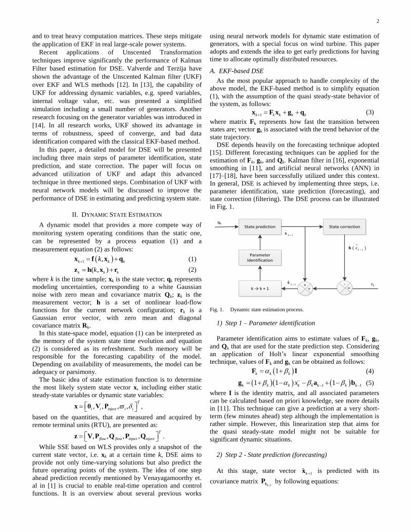
In general, DSE is achieved by implementing three steps, i.e.

parameter identification, state prediction (forecasting), and

state correction (filtering). The DSE process can be illustrated

in Fig. 1.

State prediction

Parameter Identification

State correctionqk

k → k + 1rk+

+-

+

1k x

1ˆ

k x

1kx

h

Fig. 1. Dynamic state estimation process.

1) Step 1 – Parameter identification

Parameter identification aims to estimate values of Fk, gk,

and Qk that are used for the state prediction step. Considering

an application of Holt’s linear exponential smoothing

technique, values of Fk and gk can be obtained as follows:

1k k k F I

(4)

1 11 1 1k k k k k k k kx

g a b (5)

where I is the identity matrix, and all associated parameters

can be calculated based on priori knowledge, see more details

in [11]. This technique can give a prediction at a very short-

term (few minutes ahead) step although the implementation is

rather simple. However, this linearization step that aims for

the quasi steady-state model might not be suitable for

significant dynamic situations.

2) Step 2 - State prediction (forecasting)

At this stage, state vector 1kx is predicted with its

covariance matrix 1kx

P by following equations:

3

1ˆ

k k k k x F x g (6)

1 ˆ .k k

T

k k k

x xP F P F Q

(7)

while ˆ kxP is the covariance matrix to estimate ˆ

kx at time k.

State prediction is an interesting area that the computational

intelligence (CI) can be exploited. ANN as a typical

application of CI has been extensively studied in [17]-[18].

The prediction model can be improved by integrating load

forecasting, that has been proposed as a concept of

forecasting-aided state estimation (FASE) in [15].

3) Step 3 - State correction (filtering)

By updating a new set of measurements 1kz , the predicted

state vector 1kx can be corrected (filtered) leading to a new

state vector 1

ˆkx with its error covariance

1ˆ kxP . An objective

function for correcting process, at time k + 1, is presented as

follows:

1 1T T

xx z x z x x x x x J h R h P

(8)

where the time index k+1 has been omitted for simplification;

and R is variance vector of the measurement errors.

Similar to WLS estimation for SSE, minimization of xJ

leads to an iterative solution, i.e. iterated extended Kalman

filter, as follows:

1 1 1 1 1ˆ .k k k k kx x x K z h (9)

The gain matrix 1kK is computed by following equation:

11 1 1

1

T T

k x

K H R H P H R (10)

where,

1k

x

x

hH : Jacobian matrix.

Respectively to 1

ˆkx , its error covariance matrix

1ˆ kxP is

computed as follows:

1

11 1

ˆ .k

T

x

x

P H R H P

(11)

B. UKF-based DSE

Basically, EKF is an extension of Kalman filtering through

a linearization procedure to solve nonlinear models. Though

this approach has been considered feasibly, it provides only an

approximation to optimal nonlinear estimation. It causes to

biased estimates and erroneous covariance [1]. Furthermore,

calculation of the Jacobian matrix Hk+1 for each time step

could also slow down the process of DSE.

UKF-based DSE is an improvement to cope with non-linear

nature of DSE. Based on the unscented transformation (UT)

theory, the approach propagates statistical distribution of the

state via non-linear equations to provide better results. Above

three main steps of DSEs will be adjusted according to UT

technique as follows:

1) Step 1 – Parameter identification (including sigma

points calculation)

Besides identifying Fk and gk, this stage includes also sigma

point calculation. From the current state vector ˆkx

and its

covariance ˆ kxP , UT propagate statistical distribution to form a

matrix Xk of 2N + 1 sigma vectors as follows:

ˆ ˆˆ ˆ

k kk k k kN N x x

X x x P x P (12)

where 2 N n is a scaling parameter with the

spreading constant ( 410 1 ) and the secondary scaling

(usually, 3 n ).

2) Step 2 - State prediction (forecasting)

From the sets of sigma points in (11), the prediction step in

(5) is adjusted as follows:

1

i i

k k k k X F X g (13)

2

1

0

Nm i

k i k

i

W

x X (14)

1

2

1 1

0

.k

NT

c i i

i k k i k k i k

i

W

xP X x X x Q

(15)

with weighting factors given by

0 ;mWN

2

0 1 ;cWN

1.

2

m c

k kW WN

3) Step 3 - State correction (filtering)

From predicted state vector 1kx and its covariance

1kM , a

new set of sigma points is generated as:

1 11 1 1 1

ˆk kk k k kN N

x x

X x x P x P (16)

to be propagated through the measurement-update equations:

1 1ˆ ˆi i

k k Y h X (17)

2

1 1

0

ˆˆN

m i

k i k

i

W

y Y (18)

1

2

ˆ 1 1

0

ˆ ˆˆ ˆk

N Tc i i

i k k i k k i k

i

W

yP Y y Y y R

(19)

1 1

2

ˆ 1 1

0

ˆ ˆk k

N Tc i i

i k k i k k i

i

W

x yP X x Y y

(20)

Then, the gain matrix 1kK

is calculated as:

1 1 1

1

ˆ ˆ1 k k kk

x y y

K P P

(21)

Correction of the state vector and its covariance are calculated

by following equations:

1 1 1 1ˆˆ ˆi

k k k k k i x x K Y y (22)

1 1 1ˆ 1 1.k k k

T

k k x x y

P P K P K

(23)

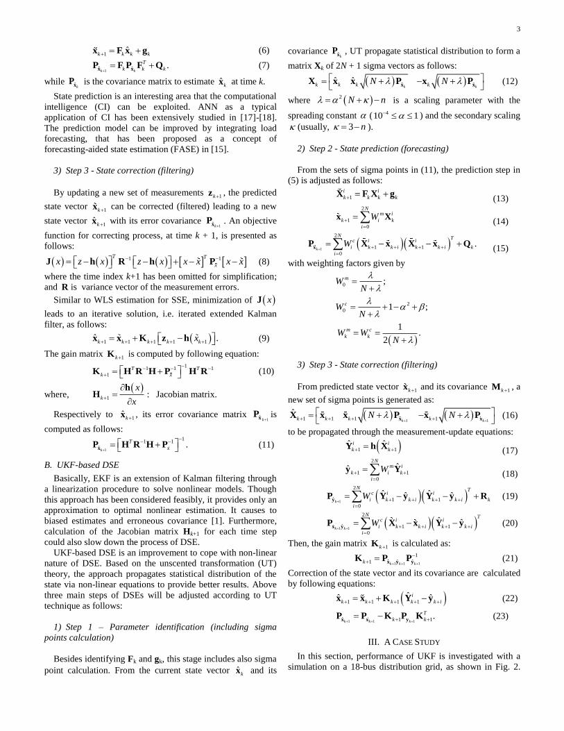
III. A CASE STUDY

In this section, performance of UKF is investigated with a

simulation on a 18-bus distribution grid, as shown in Fig. 2.

4

This test network is modified from the IEEE 34-bus test

network [19] with some simplifications as follows [20]:

Distributed loads will be approximately placed one-

third at the end of the line and two-thirds at one-

fourth of the way from the source end;

Only the main three phase sections are included, the

unbalance phase loads are summed up at the root;

Constant PQ loads are represented by dynamic load

models. Constant Z loads are represented by passive

resistors and inductors. Constant I loads are

neglected.

Fig. 2. Single-line diagram of the 18-bus test network modified from the

IEEE 34-bus network by representing shading areas as equivalent buses. Note

that placements of distributed loads will create additional buses in some line

sessions.

Network model is built in a real-time simulation on the

Real-Time Digital Simulation (RTDS) platform. To perform

the slow dynamics of the system, 50 time-sample intervals

with the time resolution of 0.08 sec. were obtained from the

RTDS platform. During the simulation time, there is a voltage

drop occurring at bus 800. To have realistic measurement data,

values of bus voltages, power flows, and power injections

from the simulation are interfered with random additive

Gaussian noise: 0;0.1%N .

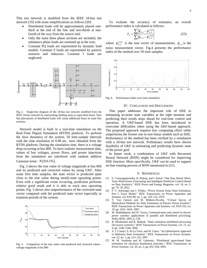
Fig. 3 shows the true value of voltage magnitude at bus 800

and its predicted and corrected values by using UKF. After

some first time samples, the state vector is predicted quite

close to the true value during steady-state operating points.

Even with a significant event occurring, prediction performs

relative good result and it is able to track new operating

points. Fig. 3 shows also outperformance of the corrected state

vector compared with the predicted state vector especially in

transient periods of the system.

Fig. 3. Comparison of the true value with predicted and corrected values -

voltage magnitude at bus 800.

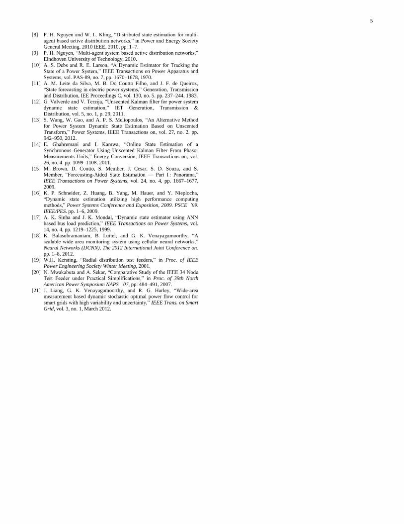
To evaluate the accuracy of estimator, an overall

performance index is calculated as follows: ,

1 1

,

1 1

ˆ i i true

k k

k i i true

k k

J

y y

y y (23)

where ,

1

i true

ky is the true vector of measurements; 1

i

ky is the

noisy measurement vector. Fig.4 presents the performance

index of the method over 50 time samples.

Fig. 4. Performance index over time simulation.

IV. CONCLUSION AND DISCUSSIONS

This paper addresses the important role of DSE in

estimating accurate state variables at the right moment and

predicting their trends steps ahead for real-time control and

operation. A UKF-based DSE has been introduced to

overcome difficulties when using the EKF-based approach.

The proposed approach requires less computing effort while

outperforms the former one in non-linear models such as DSE.

Performance of the method has been verified by a simulation

with a 18-bus test network. Preliminary results have shown

feasibility of UKF in estimating and predicting dynamic state

of the power grid.

In future work, a combination of UKF with Recurrent

Neural Network (RNN) might be considered for improving

DSE function. More specifically, UKF can be used to support

on-line training process of RNN mentioned in [21].

V. REFERENCES

[1] G. Venayagamoorthy, K. Rohrig, and I. Erlich, “One Step Ahead: Short-Term Wind Power Forecasting and Intelligent Predictive Control Based

on Data Analytics,” IEEE Power and Energy Magazine, vol. 10, no. 5,

pp. 70–78, 2012. [2] F. C. Schweppe and J. Wildes, “Power System Static-State Estimation,

Part I: Exact Model,” IEEE Transactions on Power Apparatus and

Systems, vol. PAS-89, no. 1, pp. 120–125, 1970. [3] T. Van Cutsem and M. Ribbens-Pavella, “Critical Survey of

Hierarchical Methods for State Estimation of Electric Power Systems,”

IEEE Transactions on Power Apparatus and Systems, vol. PAS-102, no. 10, pp. 3415–3424, 1983.

[4] M. Shahidehpour and W. Yaoyu, Communication and control in electric

power systems: applications of parallel and distributed processing. Wiley-IEEE, 2003, p. 534.

[5] R. Ebrahimian and R. Baldick, “State estimation distributed processing

[for power systems],” IEEE Transactions on Power Systems, vol. 15, no. 4, pp. 1240–1246, 2000.

[6] A. J. Conejo, S. de La Torre, and M. Canas, “An Optimization Approach

to Multiarea State Estimation,” IEEE Transactions on Power Systems,

vol. 22, no. 1, pp. 213–221, 2007.

[7] M. M. Nordman and M. Lehtonen, “Distributed agent-based State

estimation for electrical distribution networks,” IEEE Transactions on Power Systems, vol. 20, no. 2, pp. 652–658, 2005.

0 5 10 15 20 25 30 35 40 45 5022

24

26

28

30

V8

00

Time samples

True value

Corrected value

Predicted value

0 5 10 15 20 25 30 35 40 45 500

0.2

0.4

0.6

0.8

Perf

orm

ance index, J

Time samples

5

[8] P. H. Nguyen and W. L. Kling, “Distributed state estimation for multi-

agent based active distribution networks,” in Power and Energy Society General Meeting, 2010 IEEE, 2010, pp. 1–7.

[9] P. H. Nguyen, “Multi-agent system based active distribution networks,”

Eindhoven University of Technology, 2010. [10] A. S. Debs and R. E. Larson, “A Dynamic Estimator for Tracking the

State of a Power System,” IEEE Transactions on Power Apparatus and

Systems, vol. PAS-89, no. 7, pp. 1670–1678, 1970. [11] A. M. Leite da Silva, M. B. Do Coutto Filho, and J. F. de Queiroz,

“State forecasting in electric power systems,” Generation, Transmission

and Distribution, IEE Proceedings C, vol. 130, no. 5. pp. 237–244, 1983. [12] G. Valverde and V. Terzija, “Unscented Kalman filter for power system

dynamic state estimation,” IET Generation, Transmission &

Distribution, vol. 5, no. 1, p. 29, 2011. [13] S. Wang, W. Gao, and A. P. S. Meliopoulos, “An Alternative Method

for Power System Dynamic State Estimation Based on Unscented

Transform,” Power Systems, IEEE Transactions on, vol. 27, no. 2. pp. 942–950, 2012.

[14] E. Ghahremani and I. Kamwa, “Online State Estimation of a

Synchronous Generator Using Unscented Kalman Filter From Phasor

Measurements Units,” Energy Conversion, IEEE Transactions on, vol.

26, no. 4. pp. 1099–1108, 2011.

[15] M. Brown, D. Coutto, S. Member, J. Cesar, S. D. Souza, and S. Member, “Forecasting-Aided State Estimation — Part I : Panorama,”

IEEE Transactions on Power Systems, vol. 24, no. 4, pp. 1667–1677,

2009. [16] K. P. Schneider, Z. Huang, B. Yang, M. Hauer, and Y. Nieplocha,

“Dynamic state estimation utilizing high performance computing methods,” Power Systems Conference and Exposition, 2009. PSCE ’09.

IEEE/PES. pp. 1–6, 2009.

[17] A. K. Sinha and J. K. Mondal, “Dynamic state estimator using ANN based bus load prediction,” IEEE Transactions on Power Systems, vol.

14, no. 4, pp. 1219–1225, 1999.

[18] K. Balasubramaniam, B. Luitel, and G. K. Venayagamoorthy, “A scalable wide area monitoring system using cellular neural networks,”

Neural Networks (IJCNN), The 2012 International Joint Conference on.

pp. 1–8, 2012.

[19] W.H. Kersting, “Radial distribution test feeders,” in Proc. of IEEE

Power Engineering Society Winter Meeting, 2001.

[20] N. Mwakabuta and A. Sekar, “Comparative Study of the IEEE 34 Node Test Feeder under Practical Simplifications,” in Proc. of 39th North

American Power Symposium NAPS ’07, pp. 484–491, 2007.

[21] J. Liang, G. K. Venayagamoorthy, and R. G. Harley, “Wide-area measurement based dynamic stochastic optimal power flow control for

smart grids with high variability and uncertainty,” IEEE Trans. on Smart

Grid, vol. 3, no. 1, March 2012.