Embed Size (px)
Citation preview

Technical Report Documentation Page 1. Report No. FHWA/TX-06/0-4946-1
2. Government Accession No.
3. Recipient's Catalog No. 5. Report Date September 2005
4. Title and Subtitle
DYNAMIC TRAFFIC FLOW MODELING FOR INCIDENT DETECTION AND SHORT-TERM CONGESTION PREDICTION: YEAR 1 PROGRESS REPORT
6. Performing Organization Code
7. Author(s) Kevin Balke, Nadeem Chaudhary, Chi-Lueng Chu, Shamanth Kuchangi, Paul Nelson, Praprut Songchitruksa, Dvahg Swaroop, and Vipin Tyagi
8. Performing Organization Report No. Report 0-4946-1
10. Work Unit No. (TRAIS)
9. Performing Organization Name and Address Texas Transportation Institute The Texas A&M University System College Station, Texas 77843-3135
11. Contract or Grant No. Project 0-4946 13. Type of Report and Period Covered Technical Report: September 2004 – August 2005
12. Sponsoring Agency Name and Address Texas Department of Transportation Research and Technology Implementation Office P.O. Box 5080 Austin, Texas 78763-5080
14. Sponsoring Agency Code
15. Supplementary Notes Project performed in cooperation with the Texas Department of Transportation and the Federal Highway Administration. Project Title: Dynamic Traffic Flow Modeling for Incident Detection and Short-Term Congestion Prediction URL: http://tti.tamu.edu/documents/0-4946-1.pdf 16. Abstract The purpose of this report is to summarize the research activities that were performed during the first year of this research project. In conducting this research, the research team split into several independent groups, each focusing on different aspects of the problem. One group has been focused on using weather and traffic flow conditions as predictors of incident conditions. Their activities are summarized in Chapter II. Other groups have been focused on developing models for producing short-term forecasts of potential congestion, using current measured traffic conditions. The results of these activities are summarized in Chapter III. Finally, we are beginning the process of developing a prototype tool that operators can use in a control center to display forecasted conditions. The beginnings of a high-level, functional specification for the tool are provided in Chapter IV. 17. Key Words Incident Predictors, Traffic Modeling, Short-Term Congestion Prediction
18. Distribution Statement No restrictions. This document is available to the public through NTIS: National Technical Information Service Springfield, Virginia 22161 http://www.ntis.gov
19. Security Classif.(of this report) Unclassified
20. Security Classif.(of this page) Unclassified
21. No. of Pages 120
22. Price
Form DOT F 1700.7 (8-72) Reproduction of completed page authorized


DYNAMIC TRAFFIC FLOW MODELING FOR INCIDENT DETECTION AND SHORT-TERM CONGESTION PREDICTION:
YEAR 1 PROGRESS REPORT
by
Kevin Balke, Ph.D., P.E.
Center Director, TransLink® Texas Transportation Institute
Nadeem Chaudhary, Ph.D., P.E.
Senior Research Engineer Texas Transportation Institute
Chi-Lueng Chu
Graduate Student Worker Texas Transportation Institute
Shamanth Kuchangi
Graduate Research Assistant Department of Computer Science
Texas A&M University
Paul Nelson, Ph.D. Research Associate
Texas Engineering Experiment Station
Praprut Songchitruksa, Ph.D. Assistant Research Scientist
Texas Transportation Institute
Dvahg Swaroop, Ph.D. Associate Professor
Department of Mechanical Engineering Texas A&M University
Vipin Tyagi
Ph.D. Candidate Department of Mechanical Engineering
Texas A&M University
Report 0-4946-1 Project 0-4946
Project Title: Dynamic Traffic Flow Modeling for Incident Detection and Short-Term Congestion Prediction
Performed in cooperation with the Texas Department of Transportation
and the Federal Highway Administration
September 2005
TEXAS TRANSPORTATION INSTITUTE
The Texas A&M University System College Station, Texas 77843-3135


v
DISCLAIMER
This research was performed in cooperation with the Texas Department of Transportation
(TxDOT) and the Federal Highway Administration (FHWA). The contents of this report reflect
the views of the authors, who are responsible for the facts and the accuracy of the data presented
herein. The contents do not necessarily reflect the official view or policies of the FHWA or
TxDOT. This report does not constitute a standard, specification, or regulation.
This report is not intended for construction, bidding, or permit purposes. The engineer in
charge of the project was Kevin N. Balke, P.E. #66529.
The United States Government and the State of Texas do not endorse products or
manufacturers. Trade or manufacturers’ names appear herein solely because they are considered
essential to the object of this report.

vi
ACKNOWLEDGMENTS
This project was conducted in cooperation with TxDOT and FHWA. The researchers
acknowledge the efforts of the TxDOT Project Monitoring Committee:
• Charles Brindell, Traffic Management Section, Traffic Operations Division
• Henry Wickes, Traffic Management Section, Traffic Operations Division
• Ron Fuessel, Traffic Management Section, Traffic Operations Division
• Brian Burk, TxDOT Austin District
Al Kosik (Traffic Management Section, Traffic Operations Division) served as the program
coordinator (PC) for this project.
The researchers also express their appreciation to Brian Burk, Scott Cunningham, and
John Gold of TxDOT’s Austin District for their kind assistance in preparing the geometry data of
the freeway systems in Austin, Texas.
vii
TABLE OF CONTENTS
Page List of Figures............................................................................................................................... ix List of Tables ................................................................................................................................ xi Chapter I. Introduction................................................................................................................ 1
Project Objectives ....................................................................................................................... 1 Scope and Organization of Report.............................................................................................. 2
Chapter II. Modeling Incident Predictors and Conditions....................................................... 3 Identification of Candidate Incident Prediction Models............................................................. 3 Modeling Incident Predictors and Conditions ............................................................................ 4
Methodology........................................................................................................................... 6 Analysis of Weather Data ....................................................................................................... 9 Analysis of Loop Detector Data ........................................................................................... 17 Next Steps ............................................................................................................................. 26
Chapter III. Modeling Short-Term Traffic Congestion.......................................................... 29 Introduction............................................................................................................................... 29
Literature Review.................................................................................................................. 33 Prediction Strategies ............................................................................................................. 36
Data Issues ................................................................................................................................ 40 Background on Information Theory ..................................................................................... 40 Empirical Study .................................................................................................................... 41 Analysis of Entropy .............................................................................................................. 41 Analysis of Mutual Information............................................................................................ 42 Conclusions........................................................................................................................... 43
Automation of HCM Analysis Techniques for Freeway Operations........................................ 44 Overview of Chapter 22 Methodology ................................................................................. 45 Perspective on Chapter 22 Methodology and the KWM...................................................... 47 Status of Related Automation Efforts ................................................................................... 49 Requirements for Application to Predict Short-Term Congestion ....................................... 51
Input-Output Analysis of Cumulative Flows............................................................................ 54 Background........................................................................................................................... 54 Proposed Methodology ......................................................................................................... 57 Illustration Using Simulation................................................................................................ 62 Application of Proposed Methodology to Real Data............................................................ 65 Data Integrity ........................................................................................................................ 71 Summary ............................................................................................................................... 72 Other Work Underway.......................................................................................................... 73
Non-continuum Modeling of Traffic Movement...................................................................... 73 Traffic Movement Model...................................................................................................... 74 Traffic Data........................................................................................................................... 77 Free Regime: Discrete Traffic State Propagation ................................................................. 80 Regimes 1 and 2: Estimation of Traffic Parameters and Traffic State Prediction................ 84 Conclusion and Work in Progress......................................................................................... 91
viii
Chapter IV. High-Level Specifications for Prototype Tool .................................................... 93 Assumptions.............................................................................................................................. 93 Data ........................................................................................................................................... 94 Traffic Flow Model................................................................................................................... 94 Incident Precursors.................................................................................................................... 95 Incident Projections .................................................................................................................. 95 Preventive Measures ................................................................................................................. 95
References.................................................................................................................................... 97 Appendix: Software Tool Development .................................................................................. 101
Software Description .............................................................................................................. 101 Freeway System.................................................................................................................. 101 Input Data............................................................................................................................ 104
Current Status of 0-4946 Data Analyzer................................................................................. 106
ix
LIST OF FIGURES Page Figure 1. Sequence of Proposed Work Tasks. ............................................................................... 2 Figure 2. Modeling Methodology. ................................................................................................. 7 Figure 3. Map of Studied Locations. ........................................................................................... 11 Figure 4. Nest Structure for Studied Incident Types. .................................................................. 13 Figure 5. Model Goodness-of-Fit. ............................................................................................... 23 Figure 6. Predicted Likelihood of Collisions (US 183 @ Station ID 26).................................... 25 Figure 7. Predicted Likelihood of Collisions (Loop 1 @ Station ID 255). ................................. 26 Figure 8. Schematic of Hypothetical Example Freeway Section. ............................................... 29 Figure 9. An Example of Model Fitting to Time-Series Data. .................................................... 30 Figure 10. A Zoomed-In Portion of Previous Plot....................................................................... 31 Figure 11. Freeway Breakdown Phenomenon. ............................................................................ 34 Figure 12. Conceptual Framework for a Microsimulation-Based Prediction System. ................ 39 Figure 13. Space-Time Diagram of Densities for Test Scenario 2 of Nelson and Kumar (46)... 51 Figure 14. Input-Output Diagram. ............................................................................................... 55 Figure 15. Input-Output Diagram Using Moving Time Coordinates System. ............................ 56 Figure 16. Constant Vehicle Flow. .............................................................................................. 57 Figure 17. Increase Vehicle Flow. ............................................................................................... 58 Figure 18. Decrease Vehicle Flow............................................................................................... 58 Figure 19. Incident at Freeway Section without Spillback. ......................................................... 59 Figure 20. Incident at Freeway Section with Spillback. .............................................................. 60 Figure 21. Freeway Detector System........................................................................................... 60 Figure 22. Different Freeway Configurations.............................................................................. 61 Figure 23. Freeway System.......................................................................................................... 62 Figure 24. Scenario without Incident........................................................................................... 64 Figure 25. Scenario with Incident. ............................................................................................... 66 Figure 26. Delayed-Flow during the Beginning and Ending of the Incident............................... 67 Figure 27. Study Sites on US 183, Austin, Texas........................................................................ 68 Figure 28. Flow-in-Process and Delayed-Flow of Guadalupe-Lamar-Lazy Site. ....................... 70 Figure 29. Flow-in-Process and Delayed-Flow of Guadalupe-Lazy. .......................................... 70 Figure 30. Flow-in-Process and Delayed-Flow of Tweed-Pavilion Site. .................................... 71 Figure 31. Data on Carver Avenue and Chevy Chase Drive. ...................................................... 72 Figure 32. Schematic Showing Division of a Freeway into Sections.......................................... 75 Figure 33. Traffic Data for 05/17/2004 at a Location on US 183 NB (Station Number 13). ...... 78 Figure 34. Traffic Data for 05/16/2004 at a Location on US 183 NB (Station Number 13). ...... 79 Figure 35. Schematic of the Network under Consideration for Simulating the Free Flow on US
183 NB. ................................................................................................................................. 82 Figure 36. Plot of Number of Vehicles Passing per Minute at Source Station #23..................... 82 Figure 37. Plot of Number of Vehicles Passing per Minute at Station #25................................. 83 Figure 38. Plot of Number of Vehicles Passing per Minute at Station #29................................. 83 Figure 39. Plot of Number of Vehicles Passing per Minute at Station #33................................. 84 Figure 40. Estimated Aggregate Following Distance in a Section on US 183 NB on May 18,
2004....................................................................................................................................... 86

x
Figure 41. Estimated Number of Vehicles in a Section on US 183 NB on May 18, 2004.......... 87 Figure 42. Plot of Aggregate Traffic Speed in the Section for Thursday, April 15, 2004........... 90 Figure 43. Plot of Aggregate Traffic Speed in the Section for Friday, February 13, 2004. ........ 91 Figure 44. High-Level Schematic Function Diagram of On-Line System. ................................. 93 Figure A-1. Software Flow Chart. ............................................................................................. 102 Figure A-2. Freeway System. .................................................................................................... 102 Figure A-3. Snapshot of the Prototype Software. ...................................................................... 107

xi
LIST OF TABLES Page Table 1. Estimated Nested MNL Model for US 183. .................................................................. 14 Table 2. Estimated Non-nested MNL Model for Combined Data............................................... 15 Table 3. Estimated Binary Logit Model for Collision Incident. .................................................. 24 Table 4. Mean Entropy. ............................................................................................................... 42 Table 5. Results of Pair Wise t-tests of Variable X and Y............................................................ 42 Table 6. Mean Mutual Information between Variables X and Y.................................................. 43 Table 7. Mean Time-Shifted Mutual Information. ...................................................................... 43 Table 8. Arrival Rate Distribution. .............................................................................................. 63 Table 9. Cumulative Count for the Number of Vehicles during Free Regime for the Network 23-
25-29-33................................................................................................................................ 84 Table 10. Estimated Parameters for Regime 1 (a). ...................................................................... 88 Table 11. Estimated Parameters for Regime 1 (b). ...................................................................... 89 Table A-1. Data Definitions....................................................................................................... 103 Table A-2. Data Format of Freeway Configurations File.......................................................... 104


1
CHAPTER I. INTRODUCTION
PROJECT OBJECTIVES
The goal of this research project is to produce a tool that TxDOT can implement in the
freeway management centers that will allow them to use traffic detector information currently
being generated in their freeway management systems to make real-time, short-term predictions
of when and where incidents and congestion are likely to occur on the freeway network. The idea
is to combine roadway network modeling, traffic flow simulation, statistical regression and
prediction methodologies, and archived and real-time traffic sensor information to forecast when
and where: (a) traffic conditions will exist that are likely to produce an incident and (b) platoons
of traffic will merge together to create congestion on the freeway. To accomplish this goal, we
have identified four objectives as part of this research effort:
1. Develop a methodology for identifying and predicting when and where incidents are
likely to occur on the freeway system by comparing traffic detector data from around
known incident conditions.
2. Develop a model to predict traffic flow parameters 15 to 30 minutes into the future
based on current and historical traffic flow conditions.
3. Develop a prototype tool that can be implemented by TxDOT in their freeway
management centers that combines the ability to predict potential incident conditions
and short-term congestion.
4. Conduct a demonstration of the prototype tool.
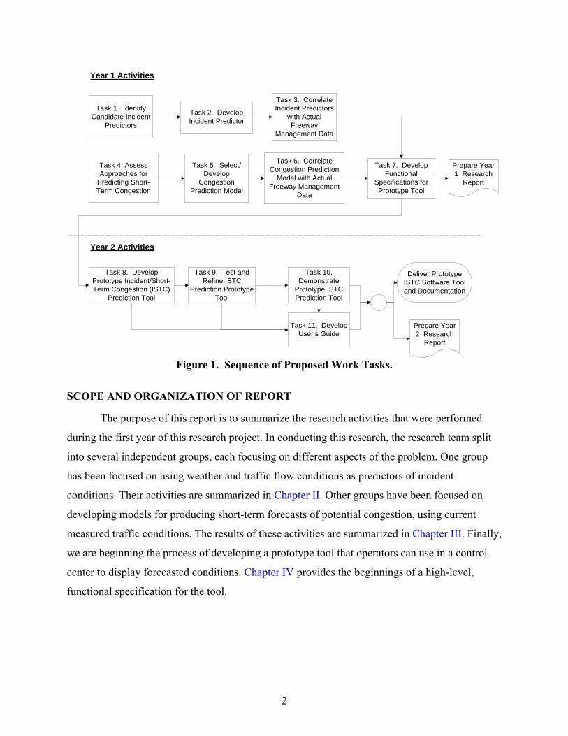
Figure 1 shows an overview of the two-year work plan that we have devised for
completing this research effort. The first year of the work plan focuses on developing models
needed for predicting incident potential and short-term congestion. A key task is to identify the
most suitable predictors for use in these models. The second year of the project will focus on
developing a prototype incident/short-term congestion (ISTC) prediction tool that TxDOT can
implement in their control centers.
2
Task 1. Identify Candidate Incident
Predictors
Task 3. Correlate Incident Predictors
with Actual Freeway
Management Data
Task 2. Develop Incident Predictor
Task 4 Assess Approaches for
Predicting Short-Term Congestion
Task 5. Select/Develop
Congestion Prediction Model
Task 6. Correlate Congestion Prediction
Model with Actual Freeway Management
Data
Task 8. Develop Prototype Incident/Short-Term Congestion (ISTC)
Prediction Tool
Task 9. Test and Refine ISTC
Prediction Prototype Tool
Task 10. Demonstrate
Prototype ISTC Prediction Tool
Task 11. Develop User’s Guide
Deliver Prototype ISTC Software Tool and Documentation
Prepare Year 1 Research
Report
Task 7. Develop Functional
Specifications for Prototype Tool
Prepare Year 2 Research
Report
Year 1 Activities
Year 2 Activities
Figure 1. Sequence of Proposed Work Tasks.
SCOPE AND ORGANIZATION OF REPORT
The purpose of this report is to summarize the research activities that were performed
during the first year of this research project. In conducting this research, the research team split
into several independent groups, each focusing on different aspects of the problem. One group
has been focused on using weather and traffic flow conditions as predictors of incident
conditions. Their activities are summarized in Chapter II. Other groups have been focused on
developing models for producing short-term forecasts of potential congestion, using current
measured traffic conditions. The results of these activities are summarized in Chapter III. Finally,
we are beginning the process of developing a prototype tool that operators can use in a control
center to display forecasted conditions. Chapter IV provides the beginnings of a high-level,
functional specification for the tool.

3
CHAPTER II. MODELING INCIDENT PREDICTORS AND CONDITIONS
IDENTIFICATION OF CANDIDATE INCIDENT PREDICTION MODELS
A precursor is a variable that is derived from traffic stream data whose variations can
indicate or point to a desirable pattern in traffic flow behavior. Recent research in incident
prediction has widely used the concept of precursors in its models for predictions. Several
researchers have worked with various precursors and tested the potential of those precursors for
incident prediction.
Traffic volume has traditionally been a precursor of interest to many researchers for
statistically relating to crash frequency. This precursor has been statistically quite significant, and
research using models with volume has shown to be capable of describing 60 percent of the
incidents (1). However, longer aggregation time involved in deducing traffic volumes has been a
restriction of using volume as a precursor in real-time prediction systems. Volume has been
predominantly useful in highway or intersection safety oriented studies.
Hourly flow, which is a shorter time aggregation of volume, is another precursor that has
been used by a couple of researchers to predict accident rate. The results of models involving
hourly flow have indicated some definitive correlation between hourly flow and accident rate, as
in the work of Hiselius (2) an increasing rate of accidents with hourly flow is indicated.
Segregating hourly flow rate by vehicle type, Hiselius also observed a constant increase in
accident rate with hourly flow in the case of cars, but a decreasing rate with hourly flow in the
case of trucks (2). Another study (3) also affirms that hourly flow provides a better
understanding of the interactions like incidents; however, there has not been elaborate work on
hourly flow as a precursor and a convenient prediction model for real-time applications.
Time headway has been tried as a casual precursor. Research shows that shorter
headways have been the reason for collisions (4). However, again, there has been no
convincingly explanatory model for use of this precursor in real-time incident prediction
systems.
Research has found that the coefficient of variation in speed (CVS) along the lane to be
sensitive in predicting accidents (5, 6, 7, 8, 9). Most of the models using CVS as a precursor
have found very satisfactory correlation with accidents. Abdel-Aty et al. (8) have documented
that their model’s crash prediction level was around 62 percent, and similarly convincing results
4
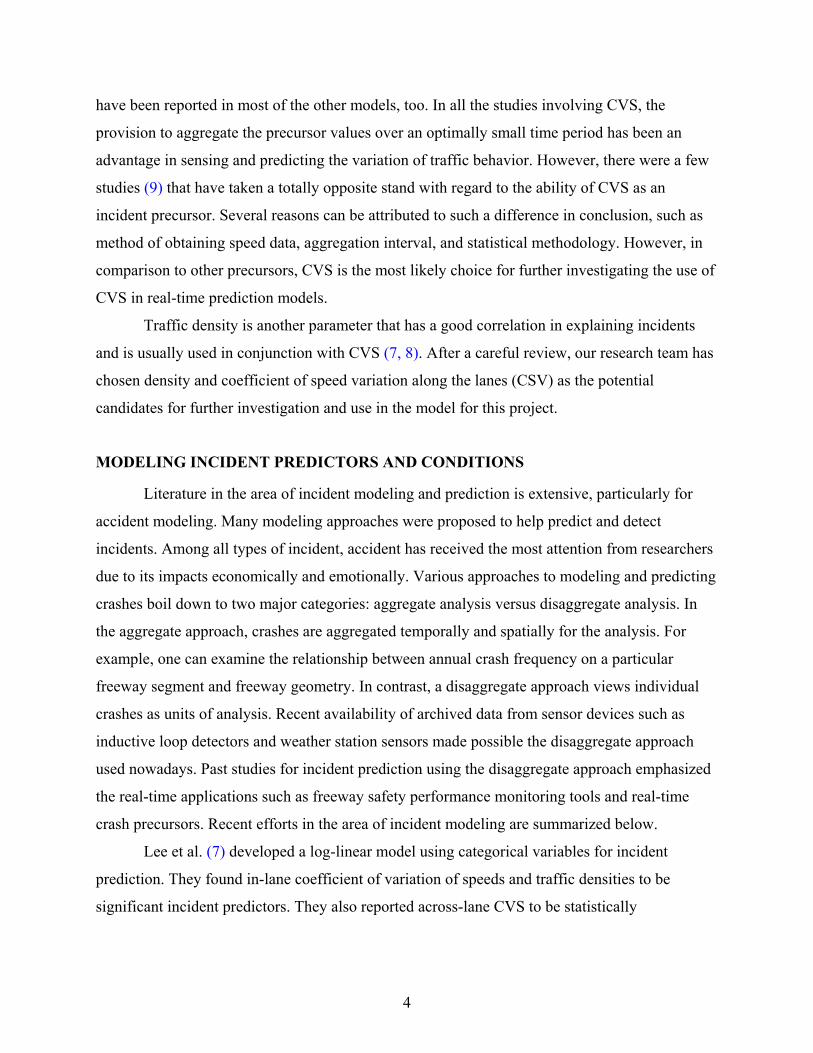
have been reported in most of the other models, too. In all the studies involving CVS, the
provision to aggregate the precursor values over an optimally small time period has been an
advantage in sensing and predicting the variation of traffic behavior. However, there were a few
studies (9) that have taken a totally opposite stand with regard to the ability of CVS as an
incident precursor. Several reasons can be attributed to such a difference in conclusion, such as
method of obtaining speed data, aggregation interval, and statistical methodology. However, in
comparison to other precursors, CVS is the most likely choice for further investigating the use of
CVS in real-time prediction models.
Traffic density is another parameter that has a good correlation in explaining incidents
and is usually used in conjunction with CVS (7, 8). After a careful review, our research team has
chosen density and coefficient of speed variation along the lanes (CSV) as the potential
candidates for further investigation and use in the model for this project.
MODELING INCIDENT PREDICTORS AND CONDITIONS
Literature in the area of incident modeling and prediction is extensive, particularly for
accident modeling. Many modeling approaches were proposed to help predict and detect
incidents. Among all types of incident, accident has received the most attention from researchers
due to its impacts economically and emotionally. Various approaches to modeling and predicting
crashes boil down to two major categories: aggregate analysis versus disaggregate analysis. In
the aggregate approach, crashes are aggregated temporally and spatially for the analysis. For
example, one can examine the relationship between annual crash frequency on a particular
freeway segment and freeway geometry. In contrast, a disaggregate approach views individual
crashes as units of analysis. Recent availability of archived data from sensor devices such as
inductive loop detectors and weather station sensors made possible the disaggregate approach
used nowadays. Past studies for incident prediction using the disaggregate approach emphasized
the real-time applications such as freeway safety performance monitoring tools and real-time
crash precursors. Recent efforts in the area of incident modeling are summarized below.
Lee et al. (7) developed a log-linear model using categorical variables for incident
prediction. They found in-lane coefficient of variation of speeds and traffic densities to be
significant incident predictors. They also reported across-lane CVS to be statistically

5
insignificant. Their research indicated that practitioners consider different sizes of moving
average window for different indicators.
Oh et al. (5) employed a nonparametric Bayesian classification method to predict real-
time accident likelihood using loop detector data. They tested mean and standard deviation of
flow, occupancy, and speed for the ability to predict crashes. A standard deviation of speed was
found to outperform other indicators as a real-time crash precursor. The proposed method,
however, may have limited potential for field implementation. First, only a single indicator was
used in the model, which makes it unlikely to capture a variety of traffic conditions leading to
crashes. Second, a selection of accident likelihood threshold is arbitrary. Third, the method is
still inefficient; in other words, it produces a significant rate of false alarm.
Golob and Recker (10) applied nonlinear canonical correlation with cluster analysis to
determine how any traffic flow condition on an urban freeway can be classified into mutually
exclusive clusters (regimes) that differ in terms of likelihood of crash by types. Although they
did not conduct a full-scale validation of their modeling approach, they did find that accurate
estimation of crash rates heavily depends on the quality of loop data.
Giuliano (11) studied the frequency, patterns, and duration of incidents on a high-volume
urban freeway. Models of incident duration were estimated using analysis of variance
(ANOVA) with natural logarithm of duration being a dependent variable. She found incident
duration to vary by incident type, lane closure, and time of day.
Madanat et al. (12) developed binary logit models for likelihood prediction of two types
of freeway incidents: accidents and overheating vehicles. They considered both loop and
environment data in their model development. They found peak period, temperature, rain, speed
variance, and merge section to be significant predictors of overheating incidents. For the crash
prediction model, only three variables were found to be statistically significant, which are rain,
merge section, and visibility.
Although researchers have conducted a number of studies in the area of incident
management in the past, relatively few have considered the use of both loop and environment
data for real-time incident prediction. Weather and environment data were analyzed in a fairly
aggregate picture, such as wet versus dry or daytime versus nighttime. Time-varying
environment-related variables such as visibility and precipitation are now obtainable from many
weather stations but are rarely addressed in the analysis. A methodology that utilizes these two

6
data sources for the incident prediction may lead to advancement in the capability to predict and
detect incidents. As such, there is a need to explore the feasibility of predicting incidents using
both real-time loop detectors and environment data. The researchers hope that this project will
shed light on critical conditions that may lead to incident occurrences. Successful results and
findings from this project would lead to a field implementation that aims to better the freeway
incident management system. This, in turn, would help increase freeway productivity and
freeway safety overall, which is the ultimate goal of this project.
We attempted to answer two important questions in this task:
• Given weather and loop detector data, how can we predict the likelihood of
incidents?
• Are certain types of incidents more likely to occur than others for a given set of data
conditions?
To answer these questions, we conducted this project as described in the following section.
Methodology
Freeway incidents can be classified into two categories for analytical purposes: in-lane
and non-in-lane incidents. In-lane incidents are those that cause disruption to mainline traffic
streams. They can vary significantly in levels of disruption. For example, multilane blocking
vehicle overturns are usually more disruptive than single-lane blocking rear-end crashes. Loop
data conditions prior to incidents may be used to predict these in-lane incidents. On the other
hand, non-in-lane incidents such as vehicle stalls or shoulder disablements are not easily
observed through the changes in loop data conditions. Therefore, weather and environment data
can play an important role in predicting these types of incidents.
The modeling methodology in this project is structured as shown in Figure 2. We first
analyzed the relationship between weather and environment data and incident types. Incident
types are difficult to predict using loop data because their impact may not be observable and
certain types of incident may have no impact at all. Environment data such as time of day and
lighting conditions can be very helpful in predicting the type of incident that is most likely to
occur under a certain set of conditions. As a following step, we examined the loop data for their
ability to predict and detect in-lane incidents. Only accidents were considered in this analysis,
while congestion and stall incidents were excluded. Congestion incidents were excluded at this

7
stage for two reasons: (a) their patterns of occurrences are fairly recurring, and (b) the occurrence
mechanism of accidents is quite different from congestions. Stall or disablement, although
frequent, is found to have negligible impact on the loop data. In the final step, based upon the
findings in both steps of the analyses, we will develop an incident prediction model integrating
weather, environment, and loop data conditions.
Figure 2. Modeling Methodology.

8
There are two types of outcomes in which we are interested: (a) likelihood of incident
occurrences and (b) likelihood of a particular incident type. Both types of outcome are discrete
and qualitative by nature; therefore, a typical linear regression approach would not be suitable in
this case. Discrete outcome modeling approaches are becoming more common as a convenient
statistical analysis tool to address problems of this nature. For example, researchers have used
binary probit models to examine the factors influencing rear-end versus side-swipe accidents and
single-vehicle versus multi-vehicle accidents (13). They also used ordered probit models to
describe the severity of accident injuries (13). The outcome of this class of models is a
probability associated with a set of explanatory variables, and this predicted probability in turn
determines the outcome.
In this project, logit models were selected for the analyses for the following reasons:
• Logit models have closed-form expressions.
• Logit and probit models give similar results (14). Therefore, the use of probit models
does not give any significant advantages over logit models.
• Logit models are computationally convenient for real-time implementation.
In this project, the binary logit model was used when two incident types are considered.
Multinomial logit (MNL) and nested MNL were considered in cases where there are more than
two incident types. The nested MNL model addresses the problem of independent of irrelevant
alternatives (IIA) by placing the outcomes that are expected to share common unobserved
disturbances in the same nest (15).
The standard multinomial logit formulation is of the form:
( ) [ ]( )
expexp
i inn
I InI
P i
∀
=∑
β Xβ X
. (1)
where,
Pn(i) = the probability of observation n having discrete outcome i,
Xin = a vector of measurable characteristics that determine the outcome for
observation n,
iβ = a vector of estimable parameters for discrete outcome i, and
I = all possible outcomes for observation n.

9
The binary logit model is a special case of multinomial logit model when only two
discrete outcomes are being considered.
The nested MNL model requires the assumption of generalized extreme value
distribution for disturbance terms. The nested MNL model can be expressed mathematically as:
( ) [ ][ ]
expexp
i in i inn
I In I InI
LSP i
LSφφ
∀
+=
+∑β Xβ X
, (2)
( ) |
|
exp|
expj i jn
nJ i Jn
J
P j i
∀
⎡ ⎤⎣ ⎦=⎡ ⎤⎣ ⎦∑β X
β X, and (3)
( )|ln expin J i JnJ
LS∀
⎡ ⎤= ⎢ ⎥⎣ ⎦∑ β X . (4)
where,
Pn(i) = the unconditional probability of observation n having discrete outcome i,
X = the vectors of observable characteristics that determine the likelihood of
discrete outcomes,
β = vectors of estimable parameters,
Pn(j|i) = the probability of observation n having discrete outcome j conditioned on
the outcome being in outcome category i,
J = the conditional set of outcomes,
LSin = the inclusive value (logsum), and
φ = an estimable parameter.
Analysis of Weather Data
Numerous studies in the past reported that there exists a statistically significant
relationship between weather conditions and traffic accidents. Madanat et al. (12) found
visibility, rain, and temperature as useful predictors for certain types of incidents. Khattak et al.
(13) examined differential impacts of adverse weather on crash types on limited-access
roadways. Binary probit models were estimated for single- versus two-vehicle crashes and for
rear-end versus side-swipe crashes. Injury severity was also analyzed using ordered probit

10
models. Shankar et al. (16) explored the effects of roadway geometrics, weather, and other
seasonal effects on accident frequencies using a negative binomial model. Several weather-
related factors such as maximum rainfall and number of rainy days were found to be significant.
In addition, interactions between weather and geometric variables also were found to be
important determinants of accident frequencies. Both studies by Khattak et al. (13) and Shankar
et al. (16) were aggregate analysis; therefore, loop detector data were not considered in the
studies. Brodsky and Hakkert (17) studied the risk of road accident in rainy weather. The results
indicated that the added risk of an injury accident in rainy conditions can be substantial.
Furthermore, the hazard could be even greater when a rain follows a dry spell.
However, past studies were primarily aggregate analyses. For example, the monthly
accident frequency and annual number of accidents were typically used as dependent variables.
A set of explanatory variables including the weather data was used to describe the variability in
the frequency and type of accidents. This traditional modeling approach was useful for
identifying factors contributing to frequency and various types of accidents for highway design
and planning purposes; however, it is of limited use for real-time prediction of incidents in
freeway operations. In addition, the weather stations in many metropolitan cities in the United
States are capable of reporting the weather conditions on an hourly basis. Therefore, the first task
is to examine the relationship between the incident types and environment variables.
We first examined the relationship between hourly weather records and types of incident.
Given that an incident has already taken place on a freeway, we need to determine what kind of
incident is most likely based on current weather and environment data. We begin with data
descriptions used in the study. Then, several logit models were estimated for each individual
roadway as well as combined data. Subsequently, results and findings from the analysis are
discussed.
Data
In the analysis of weather and environment data, we considered three freeway sections in
Austin, Texas (see Figure 3), which are (a) IH-35, (b) Loop 1, and (c) US 183.
We used incident logs and weather station data to create a data set for incident type
modeling. We obtained incident logs from 2002 to 2004 for the selected roadway sections.
Incident logs are recorded manually by freeway operators; therefore, human errors and
unreported incidents are not unexpected, particularly during the hours without monitoring. Each

11
incident log contains useful information about each incident occurrence. In general, each log will
approximately tell where, when, and what type of incident was happening. Note that there is a
lag time between actual incident occurrence and reported times. Literature indicated that this lag
time varies depending on type of incident. Major incidents such as multilane-blocking accidents
usually have a short lag time, while minor incidents such as shoulder disablements are likely to
have a long lag time. It is worth noting that incident logs of Austin freeways also contain a
number of “test” incidents. These incidents are logged by operators only for testing purpose and,
thus, must be removed prior to the analysis.
Figure 3. Map of Studied Locations.
Another source of data is weather stations. These climatological data are provided by the
National Climatic Data Center (NCDC), and they can be accessed online (18). There are three
weather stations in the vicinity of selected freeways: (a) Camp Mabry, (b) Austin-Bergstrom
International Airport, and (c) Georgetown Airport. We selected the Camp Mabry station as it is

12
situated relatively closer to the studied freeways than the other two stations. Weather records are
usually archived on an hourly basis. The data are archived at more frequent intervals (every 10 to
20 minutes) during special weather events such as heavy fog and thunderstorm. Hourly and
special report types are denoted in weather records as “AA” and “SP,” respectively.
Applications of weather forecast in freeway operations are not as extensive as in those of
air traffic control. Weather records are used in this project to represent weather conditions during
incident occurrences. Note that these weather stations may not exactly represent the true weather
conditions at considered freeway segments due to spatial weather irregularities. However, it
should give fairly accurate weather conditions during special weather events. Weather condition
data are typically qualitative, and some are ordinal. For example, a weather type “TS” would
represent moderate thunderstorm while TS+ and TS- indicate heavy and light thunderstorm,
respectively. The data are recorded in text format. In addition, there can be a combination of
weather types. For instance, if a thunderstorm and a haze are occurring at the same time, the
weather type record will be “TS HZ.” In order to perform the analysis, these text formats must be
recorded as dummy variables, and a combination of weather types must be split into a set of
single indicator variables.
Logged date and time of incident occurrences were matched with the nearest hourly
weather records. These two sources of data were combined into one single table for the analysis.
In addition, we obtained the daily sunrise and sunset times in 2004 to determine the lighting
condition at the time of incident occurrence. Since changes in these times are insignificant year
over year, we assumed the 2004 sunrise and sunset times to be representative of the other years
as well.
Model Development
Three major types of incidents reported in incident logs are: (a) congestion, (b) collision,
and (c) stall. A single-level MNL model was not suitable in this case since congestion incidents
tended to follow a regular pattern. Therefore, incident types are classified into two categories: (a)
recurring and (b) non-recurring. This classification scheme places collision and stall incidents in
the same branch. A nest structure as shown in Figure 4 was used for the estimation of nested
MNL models.

13
Figure 4. Nest Structure for Studied Incident Types.
First, we estimated the models separately for each of the studied freeways. Due to
inadequate sample size of congestion incidents on IH-35, we estimated a binary logit model for
differential impacts of weather and environment conditions on collision versus stall incidents.
For the other two roadways, nested MNL models were estimated using the proposed nest
structure in Figure 4. Finally, we combined the data from all the selected roadways to estimate an
overall nested MNL model. Estimation results are presented in the next section. The models were
estimated using an econometric analysis software package called LIMDEP.
Results
Estimation results from US 183 and combined data are presented in Table 1 and Table 2,
respectively. To interpret the results, a positive coefficient estimate indicates that the presence of
such a variable would increase the likelihood of a particular incident type. For the non-recurring
incident branch, a positive coefficient estimate increases the likelihood of a collision incident.
Similarly, a positive coefficient estimate in the recurring (congestion) branch signifies an
increase in the likelihood of congestion.

14
Table 1. Estimated Nested MNL Model for US 183.
Variable Estimated Coefficient t-ratio P-value
Estimated model for the nest alternative (collision vs. stall) Constant -0.2225 0.1018 0.0288 Nighttime indicator (1 if nighttime; 0 if otherwise) 0.8985 0.3816 0.0185 Poor visibility indicator (1 if visibility is 4 miles or less; 0 if
otherwise)
0.8973 0.3802 0.0183
Estimated model for the branch choice (recurring vs. non-recurring) Direction indicator (1 if northbound; 0 if southbound) -0.4818 0.2120 0.0231 Morning peak indicator (1 if time is from 7:15 AM to
9:15 AM; 0 if otherwise) 1.5587 0.2015 0.0000
Nighttime indicator (1 if nighttime; 0 if otherwise) 2.0333 0.3517 0.0000 Clear sky indicator (1 if the sky is clear below 12000 ft; 0 if
otherwise) 0.6616 0.1918 0.0006
Natural log of visibility -0.7540 0.1037 0.0000 Rain indicator (1 if there is a presence of rain; 0 if otherwise)
-1.3242 0.5778 0.0219
Inclusive value parameters Recurring nest (fixed at 1.0 because there is only one
alternative) … Fixed parameter …
Non-recurring nest
0.7109
Number of observations 702 Restricted log-likelihood -800.59 Log-likelihood at convergence -671.08
The confidence levels of each variable can be determined from the t-ratios or P-values.
The t-ratios are obtained by dividing estimated coefficients with respective standard errors. A
higher absolute value of t-ratios implies a higher confidence level. A P-value can be compared
directly to a specified significance level. For example, a P-value of 0.07 would be statistically
significant at 5 percent significance level but insignificant at 10 percent significance level.
Table 1 is an example of a nested MNL model estimated for an individual roadway. The
inclusive parameter estimate of a non-recurring nest substantially departs from 1.0, indicating
that a nested MNL model is a suitable choice.
As expected, congestion was more likely to occur during the morning peak and in the
southbound direction toward Austin. The increase in congestion likelihood is partly explained by
home-to-work trips in the morning in the southbound direction. Home-to-work trips are more
likely to occur over a short period of time in the morning, thus creating congestion. They are also
15
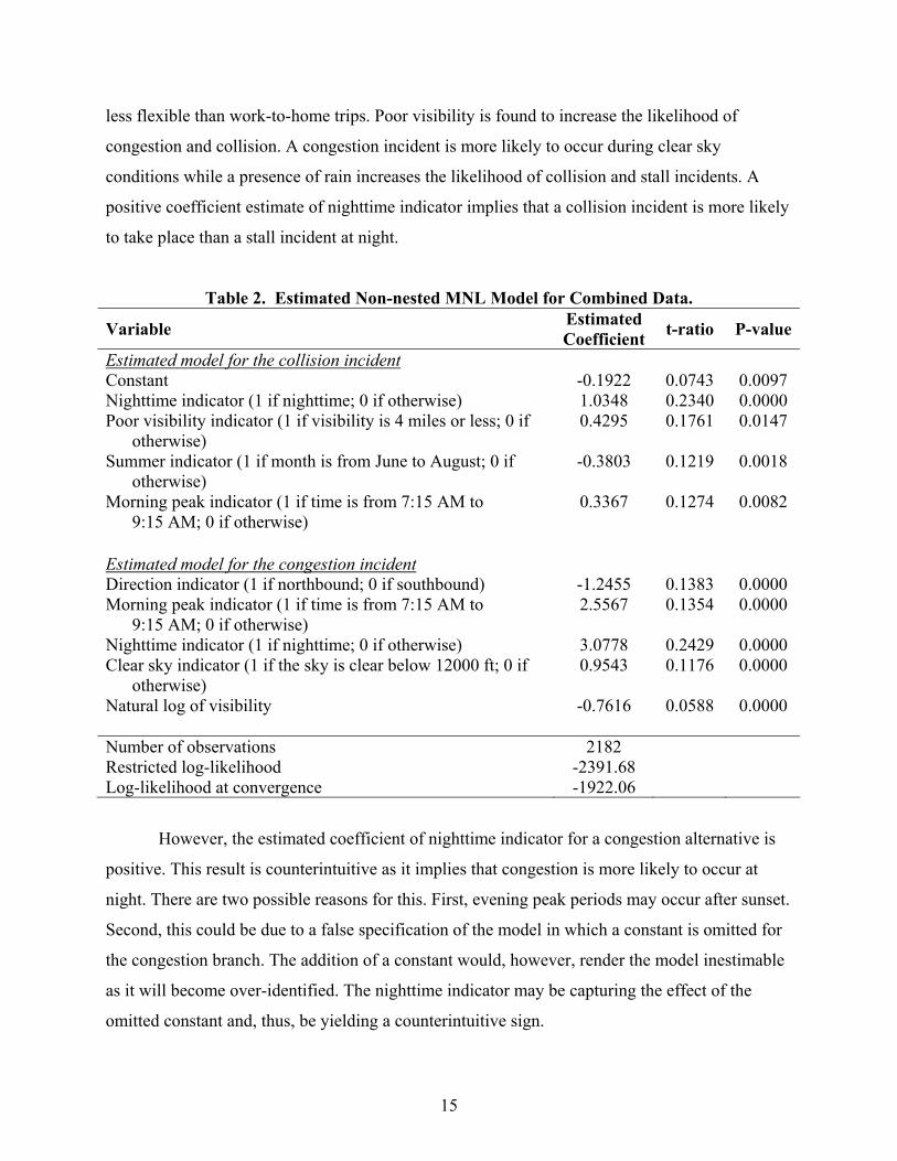
less flexible than work-to-home trips. Poor visibility is found to increase the likelihood of
congestion and collision. A congestion incident is more likely to occur during clear sky
conditions while a presence of rain increases the likelihood of collision and stall incidents. A
positive coefficient estimate of nighttime indicator implies that a collision incident is more likely
to take place than a stall incident at night.
Table 2. Estimated Non-nested MNL Model for Combined Data.
Variable Estimated Coefficient t-ratio P-value
Estimated model for the collision incident Constant -0.1922 0.0743 0.0097 Nighttime indicator (1 if nighttime; 0 if otherwise) 1.0348 0.2340 0.0000 Poor visibility indicator (1 if visibility is 4 miles or less; 0 if
otherwise) 0.4295 0.1761 0.0147
Summer indicator (1 if month is from June to August; 0 if otherwise)
-0.3803 0.1219 0.0018
Morning peak indicator (1 if time is from 7:15 AM to 9:15 AM; 0 if otherwise)
0.3367 0.1274 0.0082
Estimated model for the congestion incident Direction indicator (1 if northbound; 0 if southbound) -1.2455 0.1383 0.0000 Morning peak indicator (1 if time is from 7:15 AM to
9:15 AM; 0 if otherwise) 2.5567 0.1354 0.0000
Nighttime indicator (1 if nighttime; 0 if otherwise) 3.0778 0.2429 0.0000 Clear sky indicator (1 if the sky is clear below 12000 ft; 0 if
otherwise) 0.9543 0.1176 0.0000
Natural log of visibility
-0.7616 0.0588 0.0000
Number of observations 2182 Restricted log-likelihood -2391.68 Log-likelihood at convergence -1922.06
However, the estimated coefficient of nighttime indicator for a congestion alternative is
positive. This result is counterintuitive as it implies that congestion is more likely to occur at
night. There are two possible reasons for this. First, evening peak periods may occur after sunset.
Second, this could be due to a false specification of the model in which a constant is omitted for
the congestion branch. The addition of a constant would, however, render the model inestimable
as it will become over-identified. The nighttime indicator may be capturing the effect of the
omitted constant and, thus, be yielding a counterintuitive sign.

16
Congestion incidents on US 183 in 2004 were excluded from the modeling consideration
due to an excessive number of reported congestions, which is likely to be attributed to changes in
occupancy thresholds for congestion during the studied period. Estimation results are similar to
the model for Loop 1 (not shown here). The natural logarithm of visibility was found to be more
statistically significant than the original values. The log of visibility is used instead of the
original values in order to account for the scaling effect. For example, a one-mile decrease in
visibility from two to one is likely to have more significant impact on incident likelihood than a
decrease from nine to eight miles.
We combined data from all the selected freeways and then estimated the nested MNL
model for three types of incidents. The inclusive parameter value of the estimated model was
0.971, thus indicating that it can be reduced to a non-nested MNL model. Table 2 shows the
estimated non-nested MNL model using the combined data. Aggregating data can help mitigate
the bias caused by the overrepresentation of congestion or the under-representation of collision
in the sample. One concern regarding data aggregation is that each selected freeway must share
common characteristics that allow them to be aggregated. Observation showed that the estimated
models for each selected freeway did not give any contradictory results.
Table 2 shows that clear sky condition, morning peak, and southbound direction increase
the likelihood of congestion. A presence of rain was no longer statistically significant when
using combined data. A coefficient estimate of nighttime indicator is counterintuitive, which is
possibly due to an omitted constant as aforementioned. Similarly, we found that the natural
logarithm of visibility was a better variable than visibility itself. A decrease in log of visibility
tends to increase the probability of non-recurring incidents. In addition, we found nighttime and
visibility of four miles or lower to increase the likelihood of accident. A combination of both
nighttime and poor visibility also was found to give additional rise in the likelihood of collision
incident. Increase in stall likelihood during the summer season is probably explained by
overheating vehicles.
In the next section, loop detector data are evaluated to determine if and how they can be
used to predict freeway incidents. Loop detectors are installed extensively on Loop 1 and
US 183. Loop installation is somewhat limited on IH-35. Therefore, we performed an analysis of
loop detectors using only the data from Loop 1 and IH-35.

17
Analysis of Loop Detector Data
In Texas, loop detectors provide a stream of one-minute observations of volume, speed,
occupancy, and truck percent. These data are used in several applications such as congestion
detection, travel time estimation, etc. The majority of loop data applications are passive in that
the events must happen before actions will be taken. This analysis examines whether these data
carry useful information that would allow us to predict incidents. The ability to predict incidents
in advance would allow the traffic management center (TMC) operators to act proactively and
deploy necessary preventive measures to minimize the risk of incident occurrences. We used the
loop detector data to help predict incident versus non-incident likelihoods. This analysis requires
two groups of data: incident and non-incident conditions.
Data
The concept of incident prediction using loop detector data focuses on understanding the
relationship between disruptive traffic conditions and incident occurrences. Identifying incident
precursors that have a strong relationship with incidents is central to this analysis.
Only the collision incident variable is considered in this analysis for two reasons. First,
the majority of incidents that involve in-lane traffic disruptions are collision incidents. Stall
incidents usually cause only a slight disruption, if any, to traffic flows. Many stall incidents are
on roadway shoulders, which make it difficult to observe any impacts from loop data. Second,
lag time for accidents is likely to be short, thus avoiding the problem of identification of actual
incident occurrence time.
We used loop detector and collision data from Loop 1 and US 183 in 2003 and 2004 in
this analysis. IH-35 was excluded due to limited loop installations. Next, loop data must be
associated with each collision record. Since each collision record in incident logs contains date
and time of collision, direction of roadway, and description of nearby cross street, we used
direction of roadway and description of nearby cross street to locate the corresponding detector
identifications (IDs) and station ID from a loop detector inventory file. A program was coded to
perform this task. We then examined and edited manually the matched results since differences
in the spelling of cross street names in incident log and loop inventory files cannot be easily
accounted for in the programming. We excluded collision records that cannot be associated with
any loop detector data in the proximity from further analysis.

18
Once the detector IDs are determined, the loop detector data can be retrieved either by
lane or by station using recorded collision date and time. A selection of pre-accident duration for
the analysis of traffic dynamics requires careful consideration. Lag time, which is the time
between actual and reported accident occurrence, plays an important role in this consideration.
For example, if the average lag time is three minutes, this means that pre-accident duration must
be at least three minutes before the reported time. Since there is no comprehensive study
regarding the lag time, we consider an average lag time of five minutes as the absolute minimum
in this project. The pre-accident analysis of loop data was carried out at least five minutes prior
to the reported time.
Computed Measures
There is a large catalog of measures that can be computed from a stream of one-minute
observations of loop detectors. Studies by Lee et al. (6, 7) identified the average variation of
speed on each lane (CVS) and traffic density as potential crash precursors. Average variation of
speed difference across adjacent lanes was also tested but was insignificant. Oh et al. (5)
evaluated the five-minute average and standard deviation of flow, occupancy, and speed for their
performance as indicators of disruptive traffic dynamics. Standard deviation of speed was
selected as a single measure for real-time estimation of accident likelihood.
In this project, we tested average volume, average speed, average occupancy, and average
variation of speed (CVS) on each lane. The computation procedure requires a specification of
window size for moving averages. The computation is performed first for each individual lane
detector. Then, station averaging is applied to a set of detectors that belong to the same station. A
program was coded to perform this task. The program inputs require station ID, date, and size of
moving average window to calculate interested measures from the loop data.
Lane Data — For each individual lane detector, average volume, average speed, average
occupancy, and variation of in-lane speed were computed. Moving average window size can be
specified in the calculation. Three-, five-, and eight-minute moving averages were tested in this
analysis.

19
The average volume per minute is calculated as:
1
N
ii
N==∑
(5)
where,
iq = one-minute volume count of ith interval, and
N = number of one-minute intervals in a specified averaging window.
The average occupancy is calculated as:
1
N
ii
oo
N==∑
(6)
where,
io = one-minute average percent occupancy.
Also, it should be noted that occupancy is a proportional indicator of density.
The weighted average speed is calculated as:
1
1
N
i ii
N
ii
q vv
q
=
=
=∑
∑ (7)
where,
iv = one-minute weighted average speed of ith interval.
The weighted average speed has an advantage over the arithmetic mean in that zero-count
intervals are not used in the calculation, thus avoiding underestimation of mean values. The
weighted average speed better describes the true fluctuation of vehicles’ speed over time,
particularly during nighttime where there is a preponderance of zero-count intervals.
The coefficient of variation in speed is a measure of the fluctuation in traveling speed.
Past studies indicate that a breakdown in traffic flow will significantly increase the CVS and,
thus, the likelihood of accidents (6).
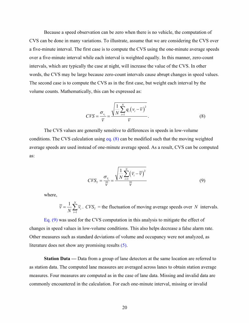
20
Because a speed observation can be zero when there is no vehicle, the computation of
CVS can be done in many variations. To illustrate, assume that we are considering the CVS over
a five-minute interval. The first case is to compute the CVS using the one-minute average speeds
over a five-minute interval while each interval is weighted equally. In this manner, zero-count
intervals, which are typically the case at night, will increase the value of the CVS. In other
words, the CVS may be large because zero-count intervals cause abrupt changes in speed values.
The second case is to compute the CVS as in the first case, but weight each interval by the
volume counts. Mathematically, this can be expressed as:
( )2
1
1
.i
N
i iv i
q v vNCVS
v vσ =
−= =
∑ (8)
The CVS values are generally sensitive to differences in speeds in low-volume
conditions. The CVS calculation using eq. (8) can be modified such that the moving weighted
average speeds are used instead of one-minute average speed. As a result, CVS can be computed
as:
( )2
1
1
i
N
iv i
v
v vNCVS
v vσ =
−= =
∑ (9)
where,
1
1 N
ii
v vN =
= ∑ . vCVS = the fluctuation of moving average speeds over N intervals.
Eq. (9) was used for the CVS computation in this analysis to mitigate the effect of
changes in speed values in low-volume conditions. This also helps decrease a false alarm rate.
Other measures such as standard deviations of volume and occupancy were not analyzed, as
literature does not show any promising results (5).
Station Data — Data from a group of lane detectors at the same location are referred to
as station data. The computed lane measures are averaged across lanes to obtain station average
measures. Four measures are computed as in the case of lane data. Missing and invalid data are
commonly encountered in the calculation. For each one-minute interval, missing or invalid

21
measures in each lane detector can either be omitted or specially treated. In this project, we treat
any intervals that have invalid computed lane measures as invalid intervals.
The average volume across lanes is defined by:
1
1 .s jj
q q=
= ∑l
l (10)
where,
l = the number of lanes at the station.
The average occupancy across lanes is defined by:
1
1 .s jj
o o=
= ∑l
l (11)
The average speed across lanes is defined by:
1
1 .s jj
v v=
= ∑l
l (12)
The average CVS across lanes is defined by:
1
1 .jj
CVS CVS=
= ∑l
l (13)
The station average measures were computed for every minute of valid lane detector data.
These data are further matched with both incident and non-incident conditions to produce a data
set for model development.
Model Development
Incident logs contain the information about the lanes affected by incidents. TxDOT lane
numbering is designated in an ascending order from median to shoulder. For example, #1, #2,
and #3 signify median, middle, and shoulder lanes, respectively. Since the excessive fluctuation
of individual lane measures tends to offset the benefits from microscopic loop data, the station
average data were instead examined in our analysis.
Estimation of real-time crash likelihoods using a binary logit model requires a sample of
two traffic conditions: incident and non-incident traffic conditions. The incidents are verified and
22
logged manually by TMC operators from 6:00 AM to 12:00 AM during weekdays and 12:00 AM
to 6:00 AM on Saturday. Incidents that occurred outside these hours were not recorded. Full-year
archived loop detector data at selected freeway segments were available for 2003 and 2004.
Therefore, we limited the study periods to only weekdays in 2003 and 2004 between 6:00 AM
and 12:00 AM (midnight).
In 2003, there were a total of 82 collisions reported on these two freeways. Only 54 out
of 82 collisions could be paired with the freeway loop detectors in the vicinity based on the cross
street descriptions in incident logs.
For non-incident traffic data, we randomly sampled the loop data from these two roadway
segments during incident-free traffic conditions. To do so, we first filtered the loop data for only
the days without any reported incidents. Because operators log incidents only when the TMC is
operating, we constrained the sampling periods to these hours only. A 2003 data set consisted of
44 collision records and 106 non-incident records. We applied a similar procedure to the 2004
data set. A final data set for model estimation consisted of 117 collision records and 342 non-
incident records from random sampling during non-incident days.
Binary logit models were estimated to predict the likelihood of accident. The developed
model aims to predict real-time accident likelihoods given an observation stream of loop detector
data. Explanatory variables tested in the model development include volume, occupancy, and
speed as well as computed values such as CVS.
To model the collision likelihood using loop data, we need to specify two parameters
properly: moving average window size and incident detection time. A large moving average
window size would help eliminate minor fluctuations in traffic dynamics, but it may obscure
discernible changes in traffic dynamics. A small moving average window size, on the contrary,
would be more sensitive to changes in traffic conditions while also subject to excessive false
alarms. How much in advance the model would be able to predict a collision depends on the
incident detection time used in the model development. If we analyze the traffic conditions
10 minutes prior to the accident reported time, this would imply that the estimated model will be
predicting the likelihood of collisions within the next 10 minutes. It is worth noting that
excessive incident detection time would make it difficult to observe any disruptive traffic
conditions that may lead to crashes. In the model calibration process, this would reduce the
model goodness-of-fit as well. Conversely, shorter incident detection time may increase the

23
likelihood of observing disruptive traffic conditions leading to crashes, while the ability to
predict the collision in advance would be limited to only the incident detection time used in the
calibration.
To optimize these two parameters, different moving average windows and incident
detection times were evaluated for their influence on the model goodness-of-fit. Average
occupancy and average CVS are found to be statistically significant consistently, amongst others.
As such, we retained these two variables for the evaluation of model goodness-of-fit for different
combinations of model parameters.
The evaluation result is presented graphically in Figure 5. A combination of incident
detection time of 15 minutes and 5-minute moving average was found to give the best model
goodness-of-fit. Therefore, this set of parameters is used and recommended for the selection of
the final model. Model Goodness-of-Fit
30.00
35.00
40.00
45.00
50.00
55.00
10 15 20 25 30 35
Detection Time (minutes)
Chi
-squ
are
stat
istic
s
3-min window5-min window8-min window
Figure 5. Model Goodness-of-Fit.
Results
Using 15-minute detection time and 5-minute moving average, the estimated binary logit
model before estimation corrections is presented in Table 3. By using loop data at 15 minutes

24
prior to the reported incident occurrence, the estimated model provides an advance warning in
terms of a likelihood of collision within the next 15 minutes.
Table 3. Estimated Binary Logit Model for Collision Incident.
Variable Estimated Coefficient t-ratio P-value
Constant -2.508 -9.150 0.0000 Average occupancy (%) 0.139 4.776 0.0000 Average CVS 14.251 3.703 0.0002 Number of observations 380 Restricted log-likelihood -212.58 Log-likelihood at convergence -186.68
Both coefficient estimates for average occupancy and average CVS are positive. This is
quite intuitive as it implies that abrupt increases in occupancy and CVS simultaneously will
significantly give rise to the likelihood of collision. During a low-volume condition, CVS in
general is relatively large. But, without a significant increase in occupancy, the likelihood of
collision will not be much affected. Similarly, a normal increase in traffic flow during the course
of the day would typically translate to an increase in average occupancy. However, average CVS
will usually stay approximately unchanged, thus leaving the likelihood of collision unaffected as
well.
Since the collision outcomes are overrepresented in the sample, an estimation correction
must be made. The correction is straightforward, providing that a full set of outcome-specific
constants is specified in the model. Under these conditions, standard logit model estimation
correctly estimates all parameters except for the outcome-specific constants. To correct the
constant estimates, each constant must have the following subtracted from it:
ln ,i
i
SFPF
⎛ ⎞⎜ ⎟⎝ ⎠
(14)
where,
SFi = the fraction of observations having outcome i in the sample, and
PFi = the fraction of observations having outcome i in the total population.

25
With estimation corrections, we adjusted the constants of each outcome. We assumed
that approximately 2 percent of the loop data were influenced by collision incidents. This will
give PF = 0.2 and SF = 117/459.
Model Test: Collision Incidents — Using the estimated binary logit model in Table 3
with adjusted constants, the minute-to-minute prediction of likelihood of collision can be
obtained. We tested the developed model to several sets of data with collision incidents. For
example, a five-day data set at station ID 26 of US 183 from October 10–14, 2004, was input
into the model. A collision incident was reported on October 12, 2004, at 1:06 PM. The predicted
likelihood of collision over the same five days is shown in Figure 6.
Time
Like
lihoo
d of
Col
lisio
n
12:00 12:00 12:00 12:00 12:00 12:00 12:00 12:00 12:00 12:00Oct 10 2004 Oct 11 2004 Oct 12 2004 Oct 13 2004 Oct 14 2004 Oct 15 2004
0.1
0.3
0.5
0.7
0.9
Figure 6. Predicted Likelihood of Collisions (US 183 @ Station ID 26).
All the test results are very encouraging as the model predicts high likelihoods of
collision quite accurately. A jump in likelihood later after crashes also implies a possibility of
secondary crashes. This could signal TMC operators to examine the warnings and deploy
necessary preventive measures in advance.

26
Model Test: Non-incident Conditions — The estimated model also was tested with
several data sets from non-incident days. For instance, we used five-day loop data without any
incidents reported from Loop 1 at station ID 255 from April 21–25, 2003. Predicted likelihoods
of collisions for the selected five days do not reveal any drastic increase in the likelihood of
collision (see Figure 7). The maximum predicted likelihood is less than 0.025. This result
indicates that the developed model is robust to minor fluctuations of the selected incident
precursors.
Time
Like
lihoo
d of
Col
lisio
n
12:00 12:00 12:00 12:00 12:00 12:00 12:00 12:00 12:00 12:00 12:00Apr 21 2003 Apr 22 2003 Apr 23 2003 Apr 24 2003 Apr 25 2003 Apr 26 2003
0.01
00.
015
0.02
00.
025
Figure 7. Predicted Likelihood of Collisions (Loop 1 @ Station ID 255).
From the model testing of non-incident conditions, we found that the test results are quite
satisfactory as they imply a low rate of false alarms. The estimation results indicate that
occupancy and average variation of speed are potential precursors of crashes. These findings are
also consistent with the previous studies by Lee et al. (7).
Next Steps
We conducted the analyses of weather, environment, and loop data to evaluate their
feasibility in predicting incident types and occurrences on freeways. First, nested and non-nested
multinomial logit models were estimated to study the impacts of weather and environment data
on incident types. Factors such as visibility, time of day, and lighting conditions were found to
be significant determinants of incident types studied: collision, congestion, and stall. Then, we
examined the loop data for their ability to predict an in-lane incident, which is a collision in this
case. Coefficient of variation in speed and average occupancy were found to be promising
precursors of freeway accidents. The five-minute moving average window was found to give the

27
best prediction results. The model was able to predict the likelihood of accident within the next
15 minutes based on a stream of loop detector data. Model testing with both incident and non-
incident conditions reveals that the method produces a low rate of false alarm and is capable of
predicting the likelihood of secondary crashes.
In the next step of this research, we are combining the findings and results from both
analyses to develop an integrated procedure for predicting incident occurrences and their type
utilizing weather, environment, and loop detector data. One possible approach is to use a series
of logit model predictions in the order of information available. For example, we can predict the
likelihood of incident versus no incident based on loop data and environment data. If the
predicted likelihood of incident is above the warning threshold, we can feed loop data and full-
information weather and environment data into a second set of models to predict the most likely
incident type. Common issues encountered with data sources such as erroneous and missing data
must be properly addressed in the next step. We expect that the proposed framework can be quite
effective yet efficient enough for real-time implementation. This next phase is expected to be
completed by the end of 2005, and the evaluation results may be available as early as the
beginning of 2006.

29
CHAPTER III. MODELING SHORT-TERM TRAFFIC CONGESTION
INTRODUCTION
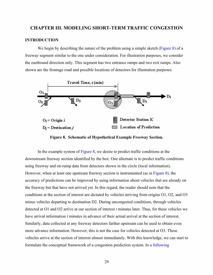
We begin by describing the nature of the problem using a simple sketch (Figure 8) of a
freeway segment similar to the one under consideration. For illustration purposes, we consider
the eastbound direction only. This segment has two entrance ramps and two exit ramps. Also
shown are the frontage road and possible locations of detectors for illustration purposes.
Figure 8. Schematic of Hypothetical Example Freeway Section.
In the example system of Figure 8, we desire to predict traffic conditions at the
downstream freeway section identified by the box. One alternate is to predict traffic conditions
using freeway and on-ramp data from detectors shown in the circle (local information).
However, when at least one upstream freeway section is instrumented (as in Figure 8), the
accuracy of predictions can be improved by using information about vehicles that are already on
the freeway but that have not arrived yet. In this regard, the reader should note that the
conditions at the section of interest are dictated by vehicles arriving from origins O1, O2, and O3
minus vehicles departing to destination D2. During uncongested conditions, through vehicles
detected at O1 and O2 arrive at our section of interest t minutes later. Thus, for these vehicles we
have arrival information t minutes in advance of their actual arrival at the section of interest.
Similarly, data collected at any freeway detectors farther upstream can be used to obtain even
more advance information. However, this is not the case for vehicles detected at O3. These
vehicles arrive at the section of interest almost immediately. With this knowledge, we can start to
formulate the conceptual framework of a congestion prediction system. In a following

30
subsection, we will describe some scenarios to introduce concepts related to prediction based on
local and advance information. The advantage of such an approach is that it provides redundancy
to handle cases where a subset of detectors fails. Before proceeding, however, we will define two
terms useful for the material presented in this section.
Let Tn be the current time at which a prediction needs to be made T (i.e., 5, 10, 15, or 30)
minutes after Tn. The value of T is known as the prediction horizon (PH). The usual approach is
to first fit a mathematical model to describe a time series and then to extrapolate (or interpolate)
to this model to produce a prediction into the selected time horizon. A variety of mathematical
forms are available, and the exact form selected depends on the characteristics (shape, trend,
cycles, etc.) of the given time series. Figure 9 and Figure 10 provide graphical illustration of the
model fitting process using a series of one-minute volume data for a freeway lane. These data
were collected from 4:00 to 6:00 PM.
4 PM to 6 PM Volumes for a Freeway Lane on US 183
0
5
10
15
20
25
0 20 40 60 80 100 120 140
One-Minute Counts3rd Degree PolynomialLinear10-Sample Moving AverageExponential
Figure 9. An Example of Model Fitting to Time-Series Data.
Tn
Prediction Horizon

31
4 PM to 6 PM Volumes for a Freeway Lane on US 183
9.5
10
10.5
11
11.5
12
12.5
13
13.5
0 20 40 60 80 100 120 140
One-Minute Counts3rd Degree PolynomialLinear10-Sample Moving AverageExponential
Figure 10. A Zoomed-In Portion of Previous Plot.
As can be seen from a visual inspection of the plot of one-minute volume counts in
Figure 10, there are significant variations in minute-to-minute values. These variations could be
the result of platooning of vehicles, which can be observed even during near-congested free-flow
conditions, or other factors. However, from a macroscopic perspective, the data series shows a
downward trend (decreasing volumes as time passes). This trend is consistent with the reduction
of traffic demand expected during this time (PM peak period) of the day.
Figure 10 shows a zoomed-in view of the four models (a third-degree polynomial, linear,
10-sample moving average, and exponential) fitted to the sample data for illustration purposes.
As shown in this figure, the moving average follows the behavior of actual data, but the
averaging dampens the effects of large variations in the original data. In this case, of downward
trend, exponential smoothing underestimates the behavior of counts as compared to the linear
model. Thus, exponential smoothing is not a good model for these data. The third-degree
polynomial model is similar to the linear model except that it also captures a flat trend in the
middle of the data series.
Once we select an appropriate subset of models for further evaluation, it can be used to
predict the value of the fitted variable at some time in the future. It should be noted that
prediction is nothing more than a projection of the model into a future time. The reader should
note that the four models illustrated in Figure 10 provide different projections (predictions). A
32
statistical analysis can be used to test the prediction accuracy by comparing predicted and
observed values. One commonly used method is to compare root mean square error (RMSE) for
each model and select the model with the least error (19). RMSE is calculated as follows
( )[ ] NvolumepredictedvolumemeasuredRMSE ∑ −= 2 (15)
where,
N = the number of observation points.
The ability of a prediction model to predict a certain distance into the future (the
prediction horizon) depends on the aggregation level of data used to develop the model. For
instance, if one-minute (five-minute) data are used, the model will have a one-minute (five-
minute) prediction horizon; however, the model can be used recursively to predict farther into
the future by using predicted values from the previous steps. Furthermore, a prediction method
can be formulated to make use of any available historical data. One such method would be to use
real-time data up to time Tn and historic data for time Tn+T to predict traffic conditions at time
Tn+T. The general form of such a prediction model for variable X might be as follows:
TTTTT NNN
XXX ++ −+= ˆ)1(' ββ (16)
where, =+
'TTN
X the predicted value at time Tn+T, =
NTX the model value at time Tn,
=+TTNX̂ the historical value at time Tn+T, and
=β a constant in the interval ]1,0[ .
The constant β specifies relative weight to be given to real-time and historic data. For
instance, a value of 0 for β requests the model to use historic data only, a value of 0.75 requests
the model to use both real-time and historic data but with three times more weight to real-time
data, and a value of 1 requests the model to ignore historic data. Furthermore, it is not difficult to
develop an adaptive scheme to select or set values of β in real time. One possible use of an
adaptive application of this parameter would be for providing fail-safety in case real-time data
for a detector are missing or deemed faulty according to certain tests.

33
Literature Review
Real-time assessment of freeway traffic conditions has been a subject of intense research
for several decades. However, most of this work has primarily focused on detection or
assessments rather than prediction of traffic conditions and incidents. The bulk of this work deals
with detection of freeway breakdown, incident detection, and estimation of travel times. Here it
is worth noting that accurate detection of traffic conditions is essential for providing good
predictions. Thus, findings of research related to the assessment of existing traffic conditions are
useful for this project as well. In the following paragraphs, we provide a summary of recent
findings relevant to this project.
The definition of freeway capacity has been debated for quite some time now and there
are disagreements between researchers about how to measure the capacity of a freeway section.
For instance, Zhang and Levinson (20) submit that Highway Capacity Manual (HCM) 2000
definitions of capacity are inadequate and that freeway capacity should only be measured at an
active bottleneck. Based on a study of 27 sites in Minnesota, they proposed a diagnostic tool to
identify congestion. Their method uses 30-second occupancy from a pair of upstream and
downstream detectors. This method uses data from individual lanes and consists of two stages
described below:
Step 1:
1. If minimum occupancy of all freeway detectors at a station is greater than
25 percent, the traffic at that station is in a congested state.
2. If the maximum occupancy of all freeway detectors at a station is less than
20 percent, the traffic at the station is in an uncongested state.
3. Otherwise, the traffic state at this station is in transition.
Step 2:
1. If the upstream station is congested and the downstream station is uncongested for
more than five minutes, a breakdown just occurred and the segment defined by
the two stations is an active bottleneck. The beginning interval of the five-minute
period is identified as the start of a queue discharge period.
2. After the beginning of a queue discharge period, if both stations are uncongested
for a period of five minutes, the bottleneck has recovered.

34
This research also shows that the activation of a bottleneck causes flow to drop by 2 to
11 percent. These results are similar to those published by Persaud et al. (21), who used data
from a freeway in Canada. Figure 11 illustrates the freeway breakdown phenomenon recently
observed by these researchers.
Figure 11. Freeway Breakdown Phenomenon.
The following points highlight the findings:
• As traffic flow increases, average speeds may decrease but generally remain near
free-flow speeds.
• For a short period just before breakdown, flow may be as high as 2600 vehicles per
hour (vph). This region is marked by a shaded box.
• At freeway breakdown, there is a drastic reduction in flow and speed. Vehicle speeds
may even reach zero just upstream of the bottleneck. A queue condition forms.
• As the queue of vehicles discharges from the bottleneck, speeds start to increase and
the freeway capacity stabilizes at the breakdown capacity level of 2100 to 2200 vph.

35
This two-capacity phenomenon often occurs at freeway entrance ramps where platoons of
vehicles trying to enter the congested freeway create a bottleneck. The result is a reduction in
service capacity. In addition, the shockwave created by a sudden drop in speed may travel for
many miles upstream causing unsafe conditions. Persaud et al. (21) also calibrated a logistics
model to estimate the probability of breakdown (PB) as a function of one-minute flows:
U
U
B eeP+
=1
(17)
where, U = a+b*(Flow), and
Flow = one-minute total volumes across all freeway lanes.
Their calibration of the model resulted in values of –11.8 and –0.003536 for the
parameters a and b, respectively.
The second thrust of research has been the development and study of automatic incident
detection. This research and development thrust has produced and compared the performance of
a wide array of methodologies (22, 23, 24). According to the first source (22), these
methodologies are based on several different technologies including: artificial intelligence, video
detection, catastrophe theory, statistical methods, and pattern recognition. Numerous models
have been developed within each category. The majority of these methods use speed, occupancy,
and flow information from inductive loop detectors. Furthermore, field experience shows that
these methods are still flawed because of low detection rates, false alarms, and undetected effects
due to inclement weather.
The third thrust of research deals with the estimation and prediction of travel times on
freeways. Chen et al. present a system that calculates and displays predicted travel times on
designated routes in California (25). Coifman proposes a method to estimate link travel times
based on point estimates (26). This approach is based on simplification of the flow-density
relationship proposed by Newell (27), and it has produced good estimates in the absence of
incidents. This theory is also the basis for one of the approaches used in this project, which we
describe later.

36
Prediction Strategies
Local Strategies
The local prediction strategy uses local information only. In the example of Figure 11,
prediction of traffic conditions (i.e., volume, occupancy, and/or speed) at the freeway section of
interest at a time T minutes from current time (Tn) will require T-horizon predictions of data from
detector stations 4 and 5 (shown inside the circle in Figure 8). These predictions could be done
for data from each detector (speed trap in this case), or for combined data for all lanes. The next
step would be to combine these individual predictions to predict traffic conditions at the section
of interest. How to combine the data to obtain predictions for the section of interest depends on
the time series itself (volume, occupancy, or speed). For instance, volume can be simply added;
however, elaborate schemes are needed to predict occupancy and speed. As an example,
downstream speed is a function of not only the speed time series at detector 4, but also volumes
measured at both detectors 4 and 5.
If an appropriate model is used, a local prediction strategy will generally work well under
free-flow conditions; however, the accuracy of predictions will not be good in the presence of
bottlenecks or incidents upstream or downstream of the detector stations. The reason is that such
situations can suddenly change the pattern of the time series, requiring additional information
that cannot be collected at the local level. One advantage of a local strategy is that it requires
little calibration. In other words, these strategies are less sensitive to detectors consistently
under- or overestimating the data.
System-Based Strategies
System-based strategies combine data from a group of adjacent detectors to predict traffic
conditions at a freeway section of interest. These methods can be analytical or simulation based.
In this section, we discuss these methods by providing examples of how local information can be
combined to develop a system-based strategy.
Analytical Strategies — The following two examples show how local information can
be combined to develop a system-based strategy using an analytical approach. The first example
is the free-flow case that occurs when T is equal to t (the free-flow travel time in Figure 8). In
this case, we can use actual data from detector stations (DSs) 1, 2, 3, and 5 collected until Tn.
Data collected from DSs 1 and 2, after appropriate adjustment for vehicles leaving the system at

37
DS 3, provide information about the vehicles that are already on the freeway and that are
expected to arrive at the section of interest t minutes from now. For traffic measured at DS 5,
however, a T-horizon prediction will need to be made using data collected until time now (Tn).
These two groups of sources can be combined now to predict traffic conditions at the section of
interest T minutes into the future. If the travel time is different (significantly smaller or larger)
from the prediction horizon, extrapolation or interpolation of mathematical model representing
the time series data from DS 1 and 2 will need to be made.
The second example occurs with freeway congestion at a specific location. If an incident
or bottleneck occurs just upstream of DS 4 and causes a queue condition, the arrival of vehicles
from DS 1 to DS 4 will be delayed. In such a case, the actual travel time between DS 1 and DS 4
will have to be estimated using data collected at DS 4 as well. The use of cumulative flows is one
such approach. It is based on the theory developed by Newell (27). The use of cumulative flows
is one of several approaches being investigated by the research team for this project. It compares
the expected traffic flow from DS 2 to actual traffic measured at DS 4 to determine the number
of vehicles accumulated (and consequently delay) in the section between the two detector
stations. Up to this point, the research team’s work has focused on the assessment of the current
conditions (that is, at time Tn) at various sections of the freeway. A more detailed description of
the cumulative flow methodology designed for this project and the initial test results are provided
in another section of this report.
Simulation Models — Computer models are frequently used to assess the conditions of
roadway facilities. These models can be categorized as macroscopic, mesoscopic, and
microscopic. Another way of categorizing such models is by using the functionality provided by
them. The two main categories are traffic flow and traffic assignment. In recent years, hybrid
traffic-assignment-flow models also have emerged.
Macroscopic models are based on simplified mathematical formulations that attempt to
describe the average behavior of a group of vehicles over specified time duration (i.e., 1, 5, or
10 minutes). Examples of these include speed-flow, speed-density, and flow-density models. The
speed prediction models being investigated by members of this research team also fall in this
category. The objective of these models is to estimate average vehicle speed in a freeway section
using speed and volume data from detector stations at the upstream and downstream ends of the
section. Macroscopic models are extremely efficient from a computational point of view.

38
Microscopic models are the most detailed in that they incorporate behavior (car
following, lane changing, merge, diverge, etc.) of individual vehicles in small time steps
(one second or even one-tenth of a second). Because of the level of detail simulated, these
models are also the most intense from a computational point of view.
Mesoscopic models fall somewhere between macroscopic and microscopic models,
depending on the detail simulated. Most models in this category deal with aggregate behavior of
a group of vehicles but perform simulation in small steps similar to the microscopic models.
Regardless of its type, a simulation model requires a given set of input data for all
sources and destinations for the system under investigation to assess the internal state of the
system corresponding to the provided data. Proper use of a simulation model requires
verification that the model is producing results that mimic field conditions. This verification
process is known as “calibration.”
If we were to simulate the conditions of the freeway in Figure 8 using one-hour data
collected until time Tn, we would need to provide one-hour volume data from detector stations 1,
2, and 5. We also would need information about where this traffic is going (i.e., proportions of
traffic from O1 exiting to destinations D1, D2, and D3). Some simulation models have the ability
to calculate this origin-destination (O-D) information using counts from entrance and exit
detectors using methods such as the gravity model, while others require the user to provide the
correct O-D matrix. It should be noted that O-D patterns change by time of day. We also will
need free-flow or desired speeds for each freeway section and detailed geometric information
required by the model. Assuming that we have accurate data, a one-hour simulation will assess
internal conditions (speeds, volumes, and occupancy) at any selected point on the freeway. Most
microscopic simulation models allow the user to create a data collection point, which can be used
to find out how well the model simulates observed conditions. For instance, a comparison of data
for a simulated detector at DS 4 with actual data collected at DS 4 (Figure 8) will provide the
user the ability to determine if the selected model needs calibration. Most simulation models
provide parameters that can be tweaked to produce simulation results to match real conditions.
Several simulation runs may be needed until the user is satisfied with the results of a simulation
model.
In the above example, using data until Tn will only tell about conditions until that time.
To use a simulation model for prediction requires that predicted data be used. In the case of our

39
example, we will have to perform local predictions of data collected from DSs 1, 2, 3, 5, 6, and 7
and use these predicted data to simulate future conditions. Figure 12 illustrates the conceptual
framework for a prediction system based on a simulation model.
Simulatation of data using Linear Prediction
9.5
10
10.5
11
11.5
12
12.5
13
13.5
0 20 40 60 80 100 120 140
Figure 12. Conceptual Framework for a Microsimulation-Based Prediction System.
As shown in Figure 12, two simulation threads will have to be run. One thread uses data
collected until Tn plus prediction until Tn+T to predict future conditions of the system. The
second thread is run at time Tn+T using actual data collected until this time. This latter run is
made to verify the accuracy of prediction and to use in real-time adaptive calibration of future
predictions. Although this framework is simple from a conceptual point of view, development of
a prediction system using existing simulation models is complicated because this method
requires changing input data in real time, a feature most existing simulation models do not
support. The following paragraph provides a description of some of the currently available
simulation models and their capabilities.
Microscopic traffic flow simulation models include CORSIM (28), VISSIM (29), and
PARAMICS (30). These models use static data and are incapable of accommodating any traffic
diversion due to traffic congestion and incidents. Traditional traffic assignment models, on the
other hand, are for planning purposes and do not provide detailed analysis of traffic flow.
Therefore, these models are not of use in this project. Recent years have seen the evolution of
Tn
Prediction for Tn+T
Tn+T
Thread 1 At Tn, simulate using real-time plus predicted data.
Thread 2 At Tn+T, simulate using real-time data.

40
hybrid models that combine the features of the above types of models. Examples of these models
include DYNASMART (31) and MITSIM (32). The strength of these two models is their ability
to change traffic assignments based on the behavior of simulated traffic. However, all five
models described above are designed for off-line use. As such, they require static input data that
cannot be combined with real-time data on the fly. Recent extension of DYNASMART to
DYNASMART-X fills this void. DYNASMART-X combines real-time data with static data to
make traffic assignments in real time. Projects are underway to field-test this tool.
DATA ISSUES
Currently, lane-by-lane volumes and occupancies, speed, and truck percentages are
collected for Austin freeways on a one-minute basis. A prediction system can be designed to use
lane-by-lane data or aggregate data for all lanes. However, it is worth investigating which subset
of these data is the most useful. This section is devoted to the analysis of information contained
in Austin data. Information theory was used for this purpose.
Background on Information Theory
Different variables such as traffic volume, occupancy, and speed/speed variation have
been used in different traffic and incident prediction models. However, it is often debated as to
which variable(s) is (are) better suited for this purpose. To gain a better understanding of the
usefulness of available data, we analyzed a subset of real data from Austin, Texas, using a
methodology based on information theory. This methodology, proposed by Foo et al. (33),
applies information theory to study the value of each variable.
In information theory, the value of a variable is measured by entropy and mutual
information contained in a set of variables. Entropy is a measure of the amount of uncertainty in
a random variable, and it is defined as:
( ) ( ) ( )xpxpXH
xlog∑−= , (18)
where, H(X) = the entropy of variable X, and
p(X) = the probability density of X.
Data with larger entropy values are more valuable than those with smaller values.

41
Mutual information between two variables, X and Y, measures how much information
variable X contains about Y. More formally, it is a measure of the reduction of uncertainty of Y
due to the knowledge of X and is defined as:
( ) ( ) ( )( ) ( )∑∑=
x y ypxpyxpyxpYXI ,log,, (19)
where, I(X,Y) = the mutual information between X and Y, and
p(X,Y) = the joint probability density of X and Y.
For example, assume that we have three variables, A, B, and X, and I(A,X) = 0.9 and
I(B,X) = 0.5. Then, we can claim that A tells more about X than B. Therefore, A is a better
predictor of X than B.
Empirical Study
To study the value of each variable, namely, volume, occupancy, and speed, we selected
the northbound section of US 183 from Carver Avenue to Fathom Circle in Austin, Texas. The
data used in this analysis were collected from 6:00 AM to 9:00 AM on February 4, 2002,
(Monday) through February 7, 2002 (Thursday).
Analysis of Entropy
We calculated entropy of volume, occupancy, and speed; and joint entropy of volume and
occupancy, volume and speed, and occupancy and speed for each detector in the study section.
Using 0.05 as the significant level, we performed pair wise t-tests between the entropies of two
variables, X and Y.
Define di = xi–yi as the difference between the i-th observation of x and the i-th
observation of y, and μD as the mean of d; then the hypothesis testing procedures is as follows:
H0: (null hypothesis): μD = 0.
H1: (alternate hypothesis): μD > 0.
Rejection Rule with 0.05 significant level (α = 0.05):
Reject H0 if t-Statistic > tα = 1.65.
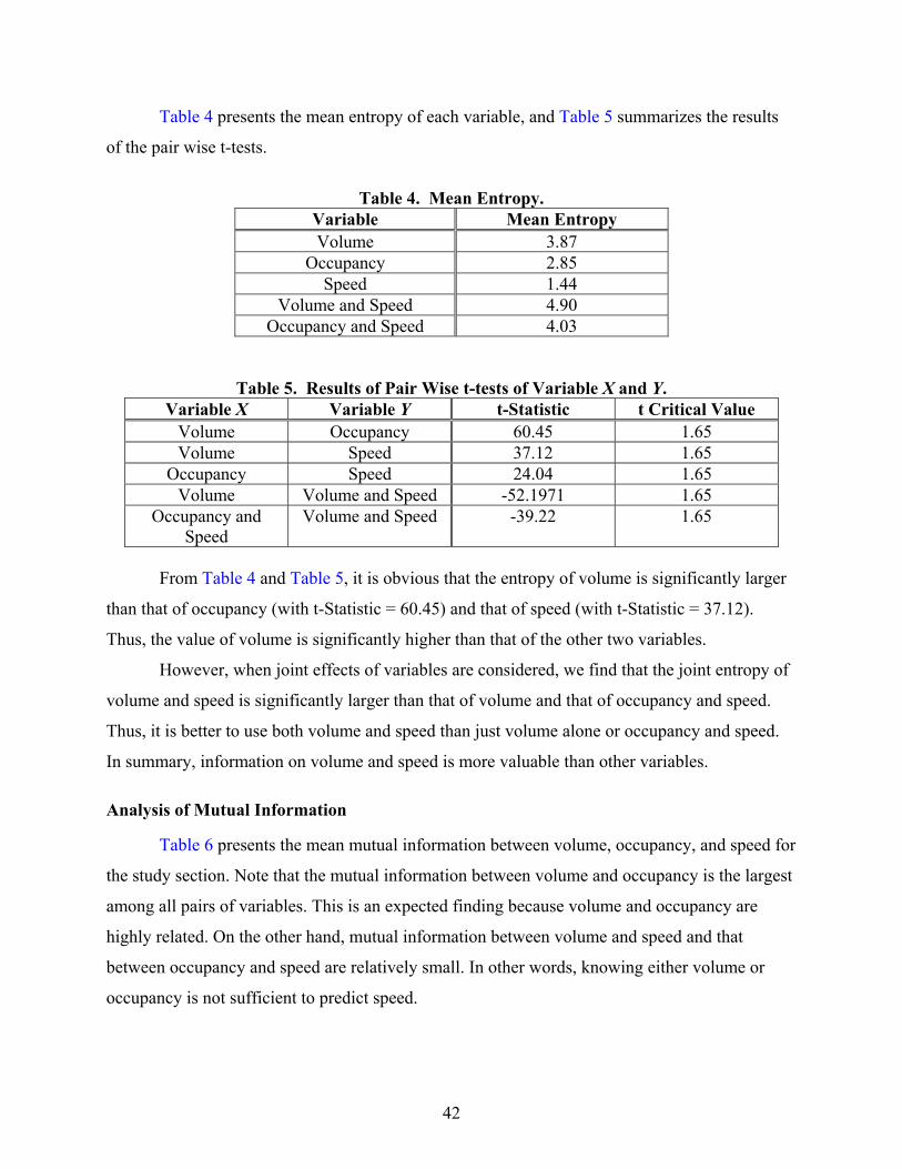
42
Table 4 presents the mean entropy of each variable, and Table 5 summarizes the results
of the pair wise t-tests.
Table 4. Mean Entropy.
Variable Mean Entropy Volume 3.87
Occupancy 2.85 Speed 1.44
Volume and Speed 4.90 Occupancy and Speed 4.03
Table 5. Results of Pair Wise t-tests of Variable X and Y. Variable X Variable Y t-Statistic t Critical Value
Volume Occupancy 60.45 1.65 Volume Speed 37.12 1.65
Occupancy Speed 24.04 1.65 Volume Volume and Speed -52.1971 1.65
Occupancy and Speed
Volume and Speed -39.22 1.65
From Table 4 and Table 5, it is obvious that the entropy of volume is significantly larger
than that of occupancy (with t-Statistic = 60.45) and that of speed (with t-Statistic = 37.12).
Thus, the value of volume is significantly higher than that of the other two variables.
However, when joint effects of variables are considered, we find that the joint entropy of
volume and speed is significantly larger than that of volume and that of occupancy and speed.
Thus, it is better to use both volume and speed than just volume alone or occupancy and speed.
In summary, information on volume and speed is more valuable than other variables.
Analysis of Mutual Information
Table 6 presents the mean mutual information between volume, occupancy, and speed for
the study section. Note that the mutual information between volume and occupancy is the largest
among all pairs of variables. This is an expected finding because volume and occupancy are
highly related. On the other hand, mutual information between volume and speed and that
between occupancy and speed are relatively small. In other words, knowing either volume or
occupancy is not sufficient to predict speed.

43
Table 6. Mean Mutual Information between Variables X and Y. Variable X Variable Y Mean Mutual Information
Volume Occupancy 1.844 Volume Speed 0.39
Occupancy Speed 0.27
As suggested by Foo et al. (33), we also can estimate the prediction power of each
variable by using time-shifted mutual information. For instance, time-shifted mutual information
of volume can be the mutual information between the volume for the past one minute and the
volume for the next one minute. Recall that mutual information between X and Y measures how
much information X contains about Y. Therefore, time-shifted mutual information of X measures
how much information X at the current time contains about X at a future time. Table 7
summarizes the results of the time-shifted mutual information calculated for each variable.
Table 7. Mean Time-Shifted Mutual Information.
Variable Mean Time-Shifted Mutual Information Volume 3.43
Occupancy 2.56 Speed 1.28
Note that volume has the largest time-shifted mutual information. By performing pair
wise t-tests, we confirmed that time-shifted mutual information of volume is significantly larger
than that of occupancy (with t-Statistic = 59.71) and that of speed (with t-Statistic = 37.33).
Therefore, we conclude that volume has better prediction power than the other two variables.
Conclusions
Based on the empirical study, we suggest using volume and speed as the key variables for
developing our prediction model. The reasons for this recommendation are summarized below.
First, volume and speed have the largest entropy among all the variables. Thus,
information on volume and speed has significantly higher value than other variables. Besides,
mutual information between volume and speed indicates that volume and speed are not strongly
dependent; neither are occupancy and speed. Since volume does not contain much information
about speed (and vice versa), we need information on both volume and speed. On the contrary,
mutual information between volume and occupancy is very large, and thus, volume may serve as
a proxy for occupancy (and vice versa). Since volume has larger entropy and larger time-shifted

44
mutual information than occupancy has, as well as the fact that the joint entropy of volume and
speed is larger than that of occupancy and speed, we conclude that volume is a better variable to
use than occupancy.
AUTOMATION OF HCM ANALYSIS TECHNIQUES FOR FREEWAY OPERATIONS
Under Task 4 of the project proposal (“Assess Approaches for Predicting Short-Term
Congestion”) one of the alternatives to be assessed was “automating the Highway Capacity
Manual (HCM) analysis techniques for analyzing freeway operations.” We carried out such an
assessment, specifically directed toward the technique described in Chapter 22 of HCM 2000
(34), “Freeway Facilities.” The results of that assessment are described below, following the next
paragraph, which is intended to provide an understanding of the context of Chapter 22 of the
HCM within the overall suite of HCM chapters devoted to various types of analyses related to
freeways.
Chapter 13 (“Freeway Concepts”) of HCM 2000 is an introduction to such basic concepts
as “capacity and quality of service for freeways.” In the introduction to this chapter it is further
stated that “this chapter can be used in conjunction with the methodologies of Chapter 22
(Freeway Facilities), Chapter 23 (Basic Freeway Segments), Chapter 24 (Freeway Weaving), and
Chapter 25 (Ramps and Ramp Junctions).” However, the basic methodologies of most of these
chapters are limited to the undersaturated case, presumably based upon considerations such as
“unlike free flow, queue discharge and congested flow have not been extensively studied…”
(HCM 2000, p. 13-5), and the statement (same page, in regard to an instance of a flow/speed
relationship representing three separate regimes: “undersaturated,” “queue discharge,” and
“oversaturated”) that “analysts are cautioned that although the relationship…may provide a
general predictive model for speed under queue discharge and oversaturated flows, it should be
considered conceptual at best.” However, as this task is prediction of congestion, and therefore
consideration of oversaturated flows is inherent within the task, any methodology applicable to
this task requires centrally consideration of oversaturated cases and the resulting congested flow.
With very much respect to the various authors of the cited chapters of HCM 2000, we
believe the inapplicability of the methodologies presented to oversaturated flows stems from the
very strong tradition of presenting in HCM 2000 only methodologies that are suitable for hand
implementation. The fact is that queue discharge and oversaturated flow are relatively well

45
understood theoretically, but any realistic procedure for their analysis is quite impractical to
implement manually. Among the chapters listed above only Chapter 22 breaks significantly with
the HCM tradition of providing analysis techniques only for the undersaturated case.
In regard to the procedures provided in Chapter 22, the following statement (p. 22-42) is
made: “The analyst could, given enough time, analyze a completely undersaturated time-space
domain manually, although this is highly unlikely. It is not expected that an analyst will ever
manually analyze a time-space domain that includes oversaturation. [Emphasis added.] For
heavily congested freeway facilities with interacting bottleneck queues, a simulation model
might be more applicable.” We believe these considerations suggest the Chapter 22 procedure is
particularly appropriate to be considered for the automation envisioned in the current project.
The principal reason that oversaturation is unlikely to be analyzed manually is the complexity of
the corresponding procedure of Chapter 22 of HCM 2000. The computational module provided
for oversaturated segments is described via a highly iterative 35-step four-page flowchart.
However, the basic technology for its implementation as a computer automation is well
developed.
Overview of Chapter 22 Methodology
The Chapter 22 methodology is based upon the kinematic-wave model (KWM), the
original “hydrodynamic model” of vehicular traffic flow. This model was discovered
independently by Lighthill and Whitham (35) and by Richards (36). The required inputs to any
application of the KWM are a (position-dependent) flow-density function (or any equivalent via
the fundamental relationship flow = speed*density), the time-dependency of the demand at all
entrances to the facility being modeled, the time-dependent capacity at all exits, the densities
throughout the facility at some “initial” time, and of course the facility geometry.
The Chapter 22 methodology uses in the undersaturated regime (i.e., densities below the
45 pc/mi/ln at which an assumed capacity flow is assumed to be reached for any given free-flow
speed) a certain (family of, depending upon various adjustment factors) flow-density function(s),
as described in Chapter 23 (Exhibit 23-3, p. 23-5, and eq. [23-4]). In the oversaturated regime it
uses a linear extrapolation from the capacity point to a jam density of 190 pc/mi/ln. The latter is
adapted from Newell (27).

46
A module is provided to estimate entrance and exit demands from 15-minute traffic
counts. (These demands need not be the observed flows because of possible effects of
congestion.) Alternately, estimated demands can be applied if desired (e.g., for purposes of
planning applications).
We recommend a simplified queuing analysis for purposes of providing the initial density
profile, termed “background density.” This is determined by first taking flows upstream of any
bottleneck equal to the sum of the total (net) initial upstream demand, and flows downstream of a
bottleneck equal to the capacity of that bottleneck. The background densities are then taken as
those densities corresponding to that flow as a free flow, i.e., the lower of the two densities that
correspond to that flow on the prevailing flow-density function. This procedure essentially
assumes that the facility is free of congestion at the initial time, which is one of the limitations of
the methodology. (See item iii below.)
Even given these quantities, analytic solutions are known only for very simple cases,
particularly very simple facility geometries. However, even these analytic solutions are quite
valuable for purposes of benchmarking computational solutions. Therefore, the Chapter 22
methodology ultimately invokes a computational procedure in which the conceptually
continuous time and space variables are replaced by discrete counterparts. The facility itself is
divided into “segments,” with two or more adjacent segments joined at “nodes.” Nodes may be
points at which merges or diverges occur, or they may be points of spatial inhomogeneity of the
roadway (e.g., a lane drop), or they may be inserted simply in order to accurately capture spatial
inhomogeneity of the traffic flow over a homogeneous section of freeway.
Time discretization is accomplished by introducing a time step. The objective of the
discrete computational process is to compute, at each time step, the flows at all nodes and the
mean densities within each segment. This computation is accomplished in order of increasing
time, and from upstream to downstream within each time step, beginning at entrant mainline
nodes. At each time step the flow at a given node is updated as the minimum of a number of
different potential flows, each of which takes into account one particular constraint on the flow at
that node, and is computable on the basis of densities and flows at either the preceding time step
or at the current time step but at upstream nodes or segments.
A number of limitations of the Chapter 22 methodology are expressly noted. Those that
seem most relevant to the objectives of TxDOT Project 0-4946 are:

47
i. “Multiple overlapping bottlenecks are an example” that “certain freeway traffic
conditions cannot easily be analyzed by the methodology” (p. 22-1).
ii. “The freeway facility methodology is limited to the extent that it can accommodate
demand in excess of capacity. The procedures address only local oversaturated flow
situations, not system-wide oversaturated flow conditions” (p. 22-1).
iii. “The completeness of the analysis will be limited if freeway segments in the first
time interval, the last time interval, and the first freeway segment do not all have
demand-to-capacity ratios less than 1.00” (p. 22-1).
iv. “The demand-capacity ratios should be less than 1.0 for all cells along the four
boundaries of the time-space domain. If they are not, further analysis may be flawed
and in some cases should not be undertaken” (p. 22-13).
Perspective on Chapter 22 Methodology and the KWM
The essential ingredients of the KWM are the equation of continuity (conservation of
vehicles), and a flow-density relationship, often termed a “fundamental diagram” (FD), or
“traffic stream model.” The conservation law is widely accepted, even though as it appears
within the KWM it incorporates the idea that the motion of discrete vehicles can be represented
in terms of quantities (densities and flows) that vary continuously with space and time. In fact,
Papageorgieu (37) has described the equation of conservation of vehicles as “the only accurate
physical law available for traffic flow.” However, researchers have raised serious doubts
regarding the validity of fundamental diagrams. This has contributed to doubts regarding the
validity of KWMs, although there also have been doubts raised from other considerations. These
two sources of doubt regarding the KWM are discussed respectively in the next two paragraphs.
The principal source of doubt about FDs arises simply from the fact that repeated
measurements (e.g., 38, 39) do not support them. Cassidy and Windover (40) have argued that
this could be attributable to the data analysis methodologies employed, particularly to the use of
variables (e.g., densities and flows) obtained by aggregating over fixed time intervals. It is
interesting that this state of uncertainty about the proper place of fundamental diagrams within
transportation science and engineering remains in considerable doubt more than 70 years after
they were initial proposed by Greenshields (41).

48
Doubts about the validity of the KWM also have been raised because of the use of
incorrect discrete computational approximations. The most common instance of an incorrect
computational approximation is, in the terminology of the Chapter 22 methodology, the
(intuitively appealing) approximation of the flow between adjacent segments during a time step
as the flow corresponding to the density in the upstream segment at the beginning of that time
step. For uncongested flows this approximation produces adequate approximations, given
suitable segment lengths and time steps. However, under congested conditions this approach can
considerably overestimate the flow from an uncongested upstream segment to a congested
downstream segment, as occurs in queue formation; likewise, it can considerably underestimate
the flow from a congested upstream segment to an uncongested downstream segment, as occurs
in queue discharge. See Ross (42, 43) and Newell (44) for an instance of incorrect inference
regarding the KWM that was drawn from this approach, and the related discussion.
These doubts regarding the KWM gave considerable encouragement to the development
of alternative models, including alternative hydrodynamic models, microscopic models, and
most recently the increasingly popular mesoscopic models. Nonetheless, the KWM has retained
considerable credibility among transportation engineers and scientists, as witnessed by its
incorporation in the HCM. We suspect the reasons behind this include the following:
• The KWM reproduces qualitatively many phenomena observed in traffic flow,
including queue formation (propagation of shock waves), queue discharge, queue
dissipation (e.g., from declining upstream demand), and even interaction of queues
although one of the quotations above suggests the Chapter 22 implementation of a
KWM solution has difficulty with such interactions.
• Under steady-state demands that lead to system-wide conditions of undersaturated
flow, the intuitive and familiar capacity analysis that underlies much of the HCM is
simply the steady-state form of the KWM. Note however that steady-state analyses
never are appropriate when oversaturation prevails because oversaturation by
definition is associated with growth of queues, and therefore time-varying behavior.
Nelson and Kumar (45) showed that for the Godunov computational approximation to the
KWM the appropriate boundary conditions consist of specification of the demand at entrant
boundaries during free flow immediately downstream of those boundaries, and of the supply at
exiting boundaries during conditions of congested flow immediately upstream of those

49
boundaries. Lebacque (46) has extended this result to the KWM itself. These theoretical results
raise some issues in regard to the treatment of boundary conditions within the Chapter 22
methodology. Specifically, within these specifications of boundary conditions there is no
suggestion of the requirement that the demand-capacity ratios be less than 1 that is highlighted in
the limitations iii and iv above. This naturally raises the question of the extent to which these
limitations on the demand-capacity ratio are absolutely required. We return further to this issue
in the discussion of boundary conditions with the following subsection “Requirements for
Application to Predict Short-Term Congestion.”
Similarly, there is no inherent restriction on the initial conditions for the KWM that
corresponds to the limitation that the demand-capacity ratios all be less than 1 at the initial and
terminal times. However, the simplified queuing analysis that is used to establish the initial
density profile certainly is most reasonable when there are no oversaturated flows at the initial
time. Further, the measures of effectiveness calculation that seems to be the principal objective
of the Chapter 22 methodology certainly is most reasonable when both the initial and the
terminal states have no oversaturated flows, even locally.
Finally, although we have described the Chapter 22 methodology above as based upon
computational solution of the KWM, we should clarify that it is not so described within the
chapter itself. Although it is reasonable to view the methodology in this manner, it also is
reasonable to view it as a modification of classical queuing analysis to incorporate the effects of
congestion, particularly the finite storage capacity of segments (i.e., the nonzero length of
vehicles). In effect any modification of queuing theory, in the context of traffic flow, to take into
account these factors also can be viewed as a computational approximation to the KWM.
Status of Related Automation Efforts
The history of traffic flow theory is replete with instances of incorrect methodologies
used for the computational solution of the KWM, but correct methods have been known and
employed for some time. P. Michalopoulos and J. P. Lebacque (references presently unavailable,
but work done circa 1984) seem to have been independently the first to apply correct
computational schemes to traffic flow. The Godunov method that seems to have first been so
employed by Lebacque has emerged as the method of popular choice, presumably in large part
because its essential ingredients have a reasonably natural interpretation within traffic flow

50
theory. This method has subsequently been rediscovered by others (47, 48) For completeness we
should mention that much of the natural interpretation of the Godunov method within its
application to traffic flow was developed initially in the latter work.
The French code STRADA (49), which employs the Godunov method, seems to be the
closest thing to a commercial application code that employs a computational solution (via the
Godunov method) to the KWM as its computational engine. This code is regarded by its authors
as a research code, but it seems to have been widely employed within France for purposes of
analysis of various kinds of traffic operations.
Results from computational solution of a KWM are most naturally presented as a space-
time diagram of density, speed, or flow. Figure 13, from Nelson and Kumar (45), is an
illustrative instance of such a presentation. Very briefly, the test scenario underlying this diagram
consists of a one-hour simulation of a 13-mile section of freeway, with a lane drop at five miles,
a second lane drop at nine miles, an initially uniform density corresponding to free flow below
the capacity of either of the two bottlenecks, and entrant demand undergoing several jump
increases during the simulation (cf. the density increases along the line distance = 0 that
corresponds to the entrant section). The demand jump at t = 0.1 hours generates a queue
discharge wave that ultimately activates the nine-mile bottleneck, at around t = 0.25 hours. A
shock subsequently propagates upstream and serves as the upstream boundary of a congested
region of enqueued flow at a density of about 190 vpm over the downstream portion of the two-
lane section between the five-mile and nine-mile stations. This shock grows in strength (i.e., the
queue grows faster) as it is joined by the queue-discharge waves from subsequent jumps in
entrant demand. The queue-discharge wave originating from the entrant demand jump at
t = 0.5 hours activates the five-mile bottleneck before the shock wave propagating upstream
reaches that bottleneck. The queue thus generated has a density of about 210 vpm over this three-
lane section of freeway, but that jumps to over 300 vpm when the shock propagating upstream
from the nine-mile station arrives. The arrival of this latter shock is an instance of “interacting
bottleneck queues,” and this diagram shows there is no inherent limitation that precludes such
interactions from being treated via an appropriate computational solution of the KWM.

51
Figure 13. Space-Time Diagram of Densities for Test Scenario 2 of Nelson and Kumar
(45).
Requirements for Application to Predict Short-Term Congestion
There are two significant research issues associated with implementation of a predictive
model based upon computational solution of the kinematic-wave model to provide a timely
prediction of development of congested flow. (Here “timely” means sufficiently far in advance
of the anticipated time of actual development to permit countermeasures to be taken to prevent
that development.) The first is a computational implementation issue, relating to precisely what
measurements should be used as input to that computation, that clearly is solvable, but that in its
implementation seems to involve issues not heretofore explored. The second issue is related to
how far in advance traffic flow can be predicted with sufficient precision to warrant
implementation of countermeasures. The latter is really the central research issue that underlies
the feasibility of implementing the potentially high-payoff techniques being explored in this
project.

52
Where to Make Measurements
This issue is best illustrated by means of a simple example. Suppose it is desired to
predict, using the kinematic-wave model and based upon measurements occurring at times prior
to t = T, the state of traffic flow over a section of roadway extending from position x = 0 to x = L,
and at a specified subsequent time T+ΔT. Exactly what measurements should be employed as the
required input data to permit the computational solution (of the KWM) necessary to provide this
prediction?
The classical mathematic view of this prediction problem is that we would need to know
the initial densities along the segment 0 ≤ x ≤ L at the “initial” time t = T, and the flows at the
boundaries x = 0,L between times t = T and t = T + ΔT. (More precisely, mathematically the flow
at the upstream boundary is only needed at times during which free flow prevails there, and the
flow at the downstream boundary is only required for periods during which congestion prevails
there. In practice both are available, subject to the considerations discussed following, which
raises an additional issue of how best to use the “excess” information to achieve more reliable
predictions.) However, this statement of the required boundary data requires use of
measurements after time t = T, which is contrary to the objective described in the preceding
paragraph. How do we modify the requirements on the boundary data to accomplish this
objective?
One possibility would be to use historical boundary data (e.g., from similar days of the
week, under similar weather conditions) to provide the required boundary data. This solution
clearly is feasible and probably should be used at least as a base case in any study of this issue.
However, it seems contrary to the implicit objective of basing predictions upon best available
current data, which is available up to time T.
An alternative approach to this problem is to trade spatial proximity of measurements in
order to employ measurements made at earlier times. More precisely, suppose in the above
highly idealized situation we elect to employ flow measurements made at upstream position
x = –a < 0 and downstream position x = L+b>L, with historical data employed only after time
t = T. Then the flow in the targeted section 0 ≤ x ≤ L is actually independent of the historical
data, provided the upstream measurement section is sufficiently far away from the entrant section
x = 0 (i.e., a> ΔT/vff, where vff is free-flow speed) and the downstream measurement section is
sufficiently far away from the exit section x = L (i.e., b > ΔT/wu, where wu is the maximum [in

53
absolute value] upstream wave speed [typically about 20 mph]). This observation permits
predictions that realistically depend only upon measurements taken far enough in advance to
permit countermeasures.
In more realistic situations (e.g., presence of on-ramps) it is unlikely that we will be able
to completely avoid use of historical data. However, it seems likely that considerations such as
that of the preceding paragraph can at least minimize the dependence upon historical data, which
is a desirable step.
The preceding discussion has focused upon boundary data, but some mention is
appropriate for the initial conditions (i.e., densities at time t = T). The obvious approach is to
estimate those conditions from the data available, at and immediately prior to that time, from
detectors located on the targeted section. This will be only an estimate (i.e., will contain errors),
principally because of the spatial sparseness of these detectors. This approach will contribute to
the unreliability of the predictions, which is the next topic of discussion.
Reliability of Predictions
At best the KWM, like any other macroscopic model, provides a mean value of the traffic
flow, where this mean is over some large set (“ensemble”) of potential realizations, all of which
are consistent with the measurements that necessarily must be employed. For small elapsed
prediction times (the “ΔT” of the preceding discussion) most of these realizations will lie close to
the predicted means, and therefore presumably the predictions will lie close to most instances of
reality. However, as time elapses the underlying statistical distribution will spread out (its
variance will increase), and the predictions made will be less and less accurate, for more and
more cases. The central question underlying this project is whether the time over which the
predictions remain reasonably reliable is larger than the minimum time required to implement
countermeasures.
It is appropriate to note that the question of reliability of short-term traffic predictions has
been addressed in the literature (50, 51). However, much of these prior discussions have been
directed toward predictions of travel time, for which persistence is reasonably reliable, and
therefore historical data provide a reasonable basis. By contrast, the objective of the present task
is precisely to predict the onset of congestion, which is to say occurrence of a lack of persistence,
which is a more difficult matter to achieve.

54
INPUT-OUTPUT ANALYSIS OF CUMULATIVE FLOWS
This document presents a simple methodology for evaluating the operating states of a
freeway using cumulative flow data from pairs of adjacent detectors along the freeway. The
methodology is based on the works by Newell (27) and Cassidy and Windover (40).
This document is organized as follows. First, we provide background on using
cumulative flow and moving time coordinates system. Next, we analyze the behavior of two
quantities—flow-in-process and delayed-flow—under different traffic conditions and propose a
methodology for identifying traffic flow states. Then, we provide a demonstration of the use of
this methodology using detector data obtained from computer simulation. Next, we apply the
proposed methodology to a subset of real data from Austin, Texas, and discuss data accuracy and
data integrity issues identified during this stage. Finally, we describe a software tool being
developed to automate the analysis of data.
Background
This section provides an overview of cumulative flow and moving time coordinates
(MTC) systems, which are the foundations of the proposed methodology described in the next
section. Readers interested in further details are referred to Newell (27) and Cassidy and
Windover (40).
Cumulative Flow
Cumulative flow is the measure of the total number of vehicles passing over a detector
from some referenced time (i.e., since 8:00 A.M.). Define:
A(x,t) = cumulative number of vehicles that have passed detector location x by time t,
xu = an upstream detector location,
xd = a downstream detector location, and
y = freeway section of interest bounded by xu and xd.
For any section y, we can construct an input-output diagram by drawing the cumulative
flow curves, A(xu, t) and A(xd, t), with respect to time as shown in Figure 14. This input-output
diagram is a very useful tool for analyzing the characteristics of freeway traffic flow in section y.
More specifically, the vertical distance between the two curves at some time tj is the total number
of vehicles in section y at that time. In this document, we define this quantity as flow-in-process

55
of section y. Furthermore, the horizontal distance between the curves at height j represents the
travel time of the jth vehicle from xu to xd.
Time
Cum
ulat
ive
Flow
Flow-in-Process
A(xu, t)
A(xd,t)
Travel Timej
tj Time
Cum
ulat
ive
Flow
Flow-in-Process
A(xu, t)
A(xd,t)
Travel Timej
tj
Figure 14. Input-Output Diagram.
Moving Time Coordinates System
Even though the input-output diagram provides us with information on flow-in-process
and travel time, additional information can be obtained by using an MTC system.
Define moving time, t'(x,t), as follows:
)(),(' xxvttxt d −+= (20)
where,
t = the actual data collection time (i.e., 8:00 AM, 8:01 AM, 8:02 AM, etc.) at xu,
and
v = the average free-flow travel time per unit distance (i.e., per foot, per meter,
etc.) from xu to xd.
We can now define new cumulative flow curves as follows:

56
))(',()',(' uduu xxvtxAtxA −−= (21) and
)',()',(' txAtxA dd = . (22)
This transformation is equivalent to shifting the upstream curve A(xu,t) (in Figure 14) to
the right by an amount equal to the free-flow travel time from xu to xd. In this MTC system, a
vehicle traveling at v takes zero time to travel from xu to xd in the absence of delay inside section
y. Figure 15 illustrates cumulative curves of Figure 14 in an MTC system. As shown in Figure
15, the vertical distance between the two curves at any time tj represents current delay to vehicles
in section y. In this document, we refer to this quantity as delayed flow.
Moving Time
Cum
ulat
ive
Flow
Delayed-Flow
A'(xu, t ')
A' (xd,t ')
tj Moving Time
Cum
ulat
ive
Flow
Delayed-Flow
A'(xu, t ')
A' (xd,t ')
tj
Figure 15. Input-Output Diagram Using Moving Time Coordinates System.

57
Proposed Methodology
Characteristics of Flow-in-Process and Delayed-Flow
In this section, we discuss characteristics of flow-in-process and delayed-flow under
different traffic conditions on a freeway section.
First, consider a perfect case where the following occurs:
• vehicles arrive uniformly at xu,
• vehicles arrive at a constant rate at xu, and
• vehicles travel from xu to xd at the average free-flow speed.
In this case, the two cumulative curves will be parallel (Figure 16a), and the upstream
cumulative curve will superimpose the downstream cumulative curve in the MTC system (Figure
16b). As a result, flow-in-process will be constant and delayed-flow will be zero.
Figure 16. Constant Vehicle Flow.
Suppose there is an increase in traffic flow at time t, while the travel time is not affected.
In this case, there will be more vehicles traveling in the section starting at time t. As a result,
there will be a jump in flow-in-process while delayed-flow will remain zero (Figure 17).
Similarly, if traffic flow decreases at time t without affecting travel time, there will be a decrease
in flow-in-process while delayed-flow will remain unchanged (Figure 18).
Time
0
A(xu, t)
A(xd,t)
Flow-In-Process
Time
0
A(xu, t)
A(xd,t)
Flow-In-Process
Moving Time
0
A'(xu, t ') = A' (xd,t ')
Delayed-Flow = 0
Moving Time
0
A'(xu, t ') = A' (xd,t ')
Delayed-Flow = 00
A'(xu, t ') = A' (xd,t ')
Delayed-Flow = 0

58
Figure 17. Increase Vehicle Flow.
Figure 18. Decrease Vehicle Flow.
Now, suppose that an incident occurs in the section at time t1' resulting in increased travel
time between the two detector locations. In the MTC system, this situation will cause the
cumulative flow from xd to be lower than that from xu, resulting in a positive delayed-flow. When
the incident clears at some time t2 ' > t1 ', the number of vehicles leaving the downstream detector
location will increase, resulting in a decrease in flow-in-process and delayed-flow. Examples of
the input-output diagrams and the corresponding flow-in-process and delayed-flow for the case
described above are illustrated in Figure 19.
If the shock wave resulting from the incident reaches xu, the operation of the adjacent
upstream freeway will be compromised. This spillback of congestion into the upstream freeway
section can be identified by doing a similar analysis for that section.
Moving Time
0
A'(xu, t ') = A' (xd,t ')
Delayed-Flow = 0
t ' Moving Time
0
A'(xu, t ') = A' (xd,t ')
Delayed-Flow = 0
t 'Time
A(xu, t)A(xd,t)
Flow-In-Process
t t '
0
Time
A(xu, t)A(xd,t)
Flow-In-Process
t t '
0
Moving Time0
A'(xu, t ') = A' (xd,t ')
Delayed-Flow = 0
t ' Moving Time0
A'(xu, t ') = A' (xd,t ')
Delayed-Flow = 0
t 'Time
A(xu, t)A(xd,t)
Flow-In-Process0
t t ' Time
A(xu, t)A(xd,t)
Flow-In-Process0
t t '

59
Figure 19. Incident at Freeway Section without Spillback.
Figure 20 illustrates the effects of spillback on the affected freeway sections. Figure 20a
presents the input-output diagrams for section yd (section where the incident occurs). Figure 20b
shows the input-output diagrams for the upstream section yu. In this example, the incident occurs
at t1', and the shock wave spills back to the upstream section yu at t1. The figure also shows that
the incident clears (that is, flow-in-process at section yd starts to decrease) at t2' while the effects
of the incident in the upstream section start to subside at t2 > t2'.
The reader should note that input-output diagrams of section yu (Figure 20b) are similar
to those in Figure 19, indicating the effect of the incident does not reach further into the upstream
section. Should the shock wave reach the upstream section of yu, Figure 20b will be similar to
Figure 20a.
Methodology
Based on the analysis in the previous section, we proposed evaluating the current
operating states of the freeway system by monitoring the flow-in-process and delayed-flow of
each adjacent pair of detectors along the freeway starting from the farthest downstream section
yn, back to the farthest upstream freeway y1 (Figure 21).
Time
A(xu, t)
A(xd,t)
Flow-In-Process
t1' t2'0
Time
A(xu, t)
A(xd,t)
Flow-In-Process
t1' t2'0
Moving Time0
A'(xu, t ')
A' (xd,t ')
Delayed-Flow
t1' t2'Moving Time0
A'(xu, t ')
A' (xd,t ')
Delayed-Flow
t1' t2'

60
Time
Time
A(xu, t)
A(xd,t)
Flow-In-Process
t1' t2't1 t2 Moving Time
A'(xu, t ') A' (xd,t ')
Delayed-Flow
00
t1' t2'
A(xuu, t)
A(xu,t)
Flow-In-Process
t1 t2 Moving Time
A'(xuu, t ')
A' (xu,t ')
Delayed-Flow
0
t1 t2
0
(a)Input-output diagrams for section yd.
(b) Input-output diagrams for upstream section yu.
Time
Time
A(xu, t)
A(xd,t)
Flow-In-Process
t1' t2't1 t2 Moving Time
A'(xu, t ') A' (xd,t ')
Delayed-Flow
00
t1' t2'
A(xuu, t)
A(xu,t)
Flow-In-Process
t1 t2 Moving Time
A'(xuu, t ')
A' (xu,t ')
Delayed-Flow
0
t1 t2
0
(a)Input-output diagrams for section yd.
(b) Input-output diagrams for upstream section yu. Figure 20. Incident at Freeway Section with Spillback.
y1
y2
Yn-2
Yn-1
yny1
y2
Yn-2
Yn-1
yn Figure 21. Freeway Detector System.
As discussed in the previous section, the flow-in-process and delayed-flow can identify
whenever there is a volume change on any freeway section. Therefore, these indicators can
identify start and end of peak flow periods as well as incidents. In addition, analysis of areas
under the elevated sections of a delayed-flow curve may quantify the amount of delay at each
freeway section. However, this issue needs further investigation. For instance, if an incident
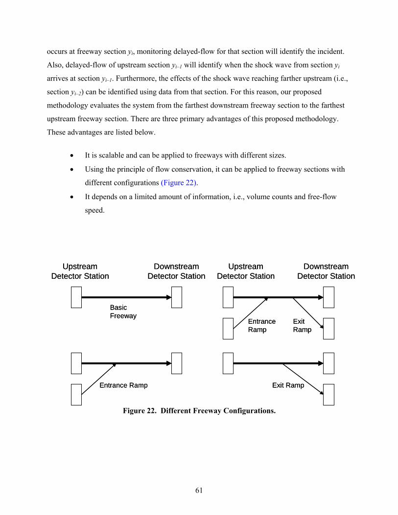
61
occurs at freeway section yi, monitoring delayed-flow for that section will identify the incident.
Also, delayed-flow of upstream section yi–1 will identify when the shock wave from section yi
arrives at section yi–1. Furthermore, the effects of the shock wave reaching farther upstream (i.e.,
section yi–2) can be identified using data from that section. For this reason, our proposed
methodology evaluates the system from the farthest downstream freeway section to the farthest
upstream freeway section. There are three primary advantages of this proposed methodology.
These advantages are listed below.
• It is scalable and can be applied to freeways with different sizes.
• Using the principle of flow conservation, it can be applied to freeway sections with
different configurations (Figure 22).
• It depends on a limited amount of information, i.e., volume counts and free-flow
speed.
Upstream Detector Station
Downstream Detector Station
Basic Freeway
Entrance Ramp Exit Ramp
EntranceRamp
ExitRamp
Upstream Detector Station
Downstream Detector Station
Upstream Detector Station
Downstream Detector Station
Basic Freeway
Entrance Ramp Exit Ramp
EntranceRamp
ExitRamp
Upstream Detector Station
Downstream Detector Station
Figure 22. Different Freeway Configurations.

62
Illustration Using Simulation
In this section, we illustrate the proposed methodology by applying it to count data
obtained from computer simulation using VISSIM 4.00 (52). The simulated system is a three-
lane freeway with four basic freeway sections in the study area (Figure 23). In addition, the
freeway speed was uniformly distributed in the range of 55 and75 vehicles per hour.
Detector x1
Detector x2
Detector x3
Detector x4
Detector x5
1900 feet
1900 feet
950 feet
950 feet Section y1
Section y2
Section y3
Section y4
Incident location
Detector x1
Detector x2
Detector x3
Detector x4
Detector x5
1900 feet
1900 feet
950 feet
950 feet Section y1
Section y2
Section y3
Section y4
Incident location
Figure 23. Freeway System.
We divided the simulation into three time periods. Table 8 provides the durations and
arrival rates for these periods. The reader should note that the arrival rate increases significantly
after the first 15 minutes of simulation. The period of high demand lasts for 30 minutes, at which
point the arrival rate drops to the initial rate. For the study described here, we conducted one
one-hour simulation without any incident and one one-hour simulation with a single 10-minute
incident, which started 1800 seconds into the simulation and blocked the middle lane only. As

63
illustrated in Figure 23, the incident occurred at section y3 immediately downstream of detector
station x3.
Table 8. Arrival Rate Distribution.
Figure 24 shows the flow-in-process and delayed-flow plots for the no-incident scenario.
Here, the curves of flow-in-process and delayed-flow with respect to time are not piecewise
linear as in the previous section. This difference is because vehicle arrivals are random as
opposed to the uniform arrivals assumed for previous illustrations. Furthermore, individual
vehicles travel at different speeds and not the average free-flow speed as assumed earlier. These
characteristics are similar to that observed in the real world. Nevertheless, the reader should note
that the curves of flow-in-process and delayed-flow can be approximated by piecewise linear
curves to produce curves similar to those presented in the previous section.
In Figure 24, the flow-in-process for each section increased sharply some time after
900 seconds of simulation and reduced sharply some time after 2700 seconds of simulation time.
In general, this result agrees with the arrival (demand) data presented in Table 8. The reader will
notice that the elevated portion of the flow-in-process curves do not start at 900 seconds but are
slightly shifted to the right. This shift is equal to the travel time from the vehicle entry point into
the system to the detector locations and shows when the increased traffic started impacting each
section. Also note that flow-in-process of sections y3 and y4 are larger than those of sections y1
and y2 during the period with increased traffic flow. In general, longer sections result in larger
flow-in-process, which is defined as vehicles traveling in the section at a particular time. Since
section y3 and y4 are longer than sections y1 and y2, it is expected that the flow-in-processes of
sections y3 and y4 are larger than those of sections y1 and y2. Despite a significant increase in
demand, however, delayed-flow remains approximately the same at all freeway sections during
the entire simulation period. This is because no disruptions occurred on any section.
From (seconds) To (seconds) Arrival Rate (vph) 0 900 4000
900 2700 7500 2700 3600 4000

64
0 900 1800 2700 3600Time
0 900 1800 2700 3600
Time
0 900 1800 2700 3600Time
0 900 1800 2700 3600
Time
0 900 1800 2700 3600Moving Time
0 900 1800 2700 3600
Moving Time
0 900 1800 2700 3600Moving Time
0 900 1800 2700 3600
Moving Time
Flow-In-Process Delayed-Flow
y4
y3
y2
y1
Section
0 900 1800 2700 3600Time
0 900 1800 2700 3600
Time
0 900 1800 2700 3600Time
0 900 1800 2700 3600
Time
0 900 1800 2700 3600Moving Time
0 900 1800 2700 3600
Moving Time
0 900 1800 2700 3600Moving Time
0 900 1800 2700 3600
Moving Time
Flow-In-Process Delayed-Flow
y4
y3
y2
y1
Section
0 900 1800 2700 3600Time
0 900 1800 2700 3600
Time
0 900 1800 2700 3600Time
0 900 1800 2700 3600
Time
0 900 1800 2700 3600Moving Time
0 900 1800 2700 3600
Moving Time
0 900 1800 2700 3600Moving Time
0 900 1800 2700 3600
Moving Time
Flow-In-Process Delayed-Flow
y4
y3
y2
y1
Section
Figure 24. Scenario without Incident.

65
Figure 25 presents the flow-in-process and delayed-flow plots for the scenario with
incident. Notice that the behaviors of flow-in-process and delayed-flow plots for each section are
similar to that in Figure 24 until 1800 seconds. In other words, these plots detect an increase in
traffic and no increase in delay. At around 1800 seconds, delayed-flow of section y3 increases
significantly, which indicates an incident. Later, delayed-flow and flow-in-process of upstream
sections, y2 and y1, also increase, while the delayed-flow of section y3 does not drop. It serves as
a signal that the shock wave created by the incident has reached the upstream sections.
More detailed information can be obtained by magnifying the scale of plots for sections
y1, y2, and y3 (Figure 26). Figure 26a shows how time lags in peaks of delayed-flow at adjacent
sections identify the progression of the shock wave. Note that delayed-flow of downstream
section y4 is not affected, while the flow-in-process decreases during the incident. This happens
because fewer vehicles enter section y4 during the incident.
Similarly, Figure 26b shows time lags between the times at which congestion starts to
clear at adjacent sections. Since the incident lasted for 600 seconds, we would expect that
delayed-flow for the section with incident quickly drops to the level prior to the incident. This is
the case for section y3 at time 2400 seconds. Delayed-flows of sections y1 and y2 do not drop to
the expected levels until several minutes after the incident cleared. This result is not surprising.
In this section, we presented the application of the proposed methodology by simulating a
basic freeway section. Additional research to verify the methodology via computer simulation
for other configurations of freeway sections (Figure 21) is currently underway. This ongoing
work includes simulations with different locations and durations of incidents. The results
obtained so far have produced similar results.
Application of Proposed Methodology to Real Data
This section documents the application of the proposed methodology to two sites along
northbound US 183 in Austin, Texas. The first site includes the detector stations located at
Guadalupe Street, Lamar Boulevard, and Lazy Lane, and the second site consists of detector
stations located at Tweed Court and Pavilion Boulevard. Data used here were collected by the
Texas Department of Transportation in 2002. The study sites are illustrated in Figure 27.
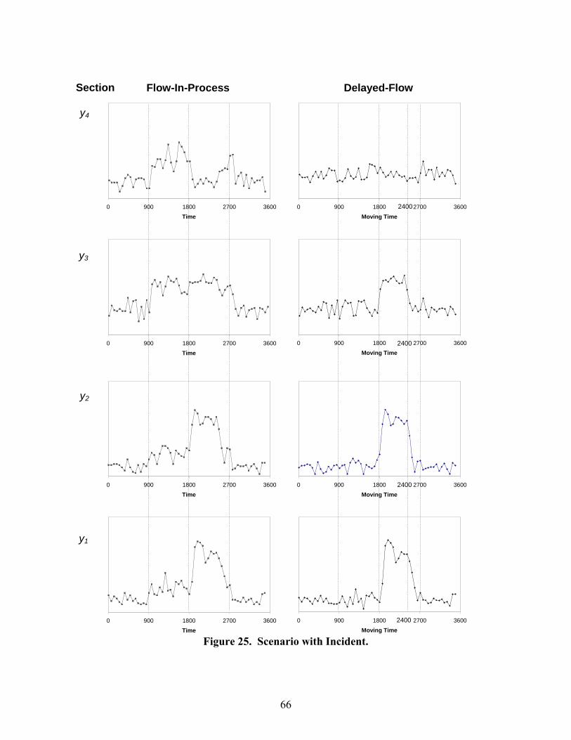
66
0 900 1800 2700 3600
Moving Time
0 900 1800 2700 3600
Moving Time
0 900 1800 2700 3600
Moving Time
0 900 1800 2700 3600
Time
0 900 1800 2700 3600
Time
0 900 1800 2700 3600
Time
0 900 1800 2700 3600
Time2400
2400
Flow-In-Process Delayed-Flow
y4
y3
y2
y1
Section
0 900 1800 2700 3600
Moving Time
2400
2400
Figure 25. Scenario with Incident.

67
1580 1640 1700 1760 1820 1880 1940 2000
Moving Time
1580 1640 1700 1760 1820 1880 1940 2000
Moving Time
1580 1640 1700 1760 1820 1880 1940 2000
Moving Time
2300 2360 2420 2480 2540 2600 2660 2720
Moving Time
2320 2380 2440 2500 2560 2620 2680
Moving Time
2320 2380 2440 2500 2560 2620 2680
Moving Time
(a) Incident occurrence (b) Incident termination
y3
y2
y1
1580 1640 1700 1760 1820 1880 1940 2000
Moving Time
1580 1640 1700 1760 1820 1880 1940 2000
Moving Time
1580 1640 1700 1760 1820 1880 1940 2000
Moving Time
2300 2360 2420 2480 2540 2600 2660 2720
Moving Time
2320 2380 2440 2500 2560 2620 2680
Moving Time
2320 2380 2440 2500 2560 2620 2680
Moving Time
(a) Incident occurrence (b) Incident termination
y3
y2
y1
Figure 26. Delayed-Flow during the Beginning and Ending of the Incident.

68
Lamar Boulevard
Lazy Lane
Guadalupe Street
Lamar Boulevard
Lazy Lane
Guadalupe Street
Tweed Court
Pavilion Boulevard
Tweed Court
Pavilion Boulevard
Figure 27. Study Sites on US 183, Austin, Texas.
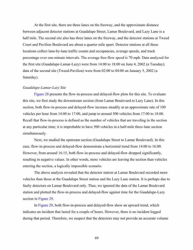
69
At the first site, there are three lanes on the freeway, and the approximate distance
between adjacent detector stations at Guadalupe Street, Lamar Boulevard, and Lazy Lane is a
half mile. The second site also has three lanes on the freeway, and the detector stations at Tweed
Court and Pavilion Boulevard are about a quarter mile apart. Detector stations at all these
locations collect lane-by-lane traffic counts and occupancies, average speeds, and truck
percentage over one-minute intervals. The average free-flow speed is 70 mph. Data analyzed for
the first site (Guadalupe-Lamar-Lazy) were from 14:00 to 18:00 on June 4, 2002 (a Tuesday);
data of the second site (Tweed-Pavilion) were from 02:00 to 04:00 on January 5, 2002 (a
Saturday).
Guadalupe-Lamar-Lazy Site
Figure 28 presents the flow-in-process and delayed-flow plots for this site. To evaluate
this site, we first study the downstream section (from Lamar Boulevard to Lazy Lane). In this
section, both flow-in-process and delayed-flow increase steadily at an approximate rate of 100
vehicles per hour from 14:00 to 17:00, and jump to around 500 vehicles from 17:00 to 18:00.
Recall that flow-in-process is defined as the number of vehicles that are traveling in the section
at any particular time; it is improbable to have 500 vehicles in a half-mile three-lane section
simultaneously.
Next, we studied the upstream section (Guadalupe Street to Lamar Boulevard). In this
case, flow-in-process and delayed-flow demonstrate a horizontal trend from 14:00 to 16:00.
However, from around 16:15, both flow-in-process and delayed-flow dropped significantly,
resulting in negative values. In other words, more vehicles are leaving the section than vehicles
entering the section, a logically impossible scenario.
The above analysis revealed that the detector station at Lamar Boulevard recorded more
vehicles than those at the Guadalupe Street station and the Lazy Lane station. It is perhaps due to
faulty detectors on Lamar Boulevard only. Thus, we ignored the data of the Lamar Boulevard
station and plotted the flow-in-process and delayed-flow against time for the Guadalupe-Lazy
section in Figure 29.
In Figure 29, both flow-in-process and delayed-flow show an upward trend, which
indicates an incident that lasted for a couple of hours. However, there is no incident logged
during that period. Therefore, we suspect that the detectors may not provide an accurate volume

70
count. To further investigate the issue, we applied the methodology to another site, Tweed-
Pavilion.
-250
-200
-150
-100
-50
0
50
100
150
14:0
014
:15
14:3
014
:45
15:0
015
:15
15:3
015
:45
16:0
016
:15
16:3
016
:45
17:0
017
:15
17:3
017
:45
18:0
0
Time
-250
-200
-150
-100
-50
0
50
100
14:0
014
:15
14:3
014
:45
15:0
015
:15
15:3
015
:45
16:0
016
:15
16:3
016
:45
17:0
017
:15
17:3
017
:45
18:0
0
Moving Time
Guadalupe-Lamar
0
100
200
300
400
500
600
14:0
014
:15
14:3
014
:45
15:0
015
:15
15:3
015
:45
16:0
016
:15
16:3
016
:45
17:0
017
:15
17:3
017
:45
18:0
0
Time
0
100
200
300
400
500
600
14:0
014
:15
14:3
014
:45
15:0
015
:15
15:3
015
:45
16:0
016
:15
16:3
016
:45
17:0
017
:15
17:3
017
:45
18:0
0
Moving Time
Lamar-Lazy
Flow-In-Process Delayed-Flow
-250
-200
-150
-100
-50
0
50
100
150
14:0
014
:15
14:3
014
:45
15:0
015
:15
15:3
015
:45
16:0
016
:15
16:3
016
:45
17:0
017
:15
17:3
017
:45
18:0
0
Time
-250
-200
-150
-100
-50
0
50
100
14:0
014
:15
14:3
014
:45
15:0
015
:15
15:3
015
:45
16:0
016
:15
16:3
016
:45
17:0
017
:15
17:3
017
:45
18:0
0
Moving Time
Guadalupe-Lamar
-250
-200
-150
-100
-50
0
50
100
150
14:0
014
:15
14:3
014
:45
15:0
015
:15
15:3
015
:45
16:0
016
:15
16:3
016
:45
17:0
017
:15
17:3
017
:45
18:0
0
Time
-250
-200
-150
-100
-50
0
50
100
14:0
014
:15
14:3
014
:45
15:0
015
:15
15:3
015
:45
16:0
016
:15
16:3
016
:45
17:0
017
:15
17:3
017
:45
18:0
0
Moving Time
Guadalupe-Lamar
0
100
200
300
400
500
600
14:0
014
:15
14:3
014
:45
15:0
015
:15
15:3
015
:45
16:0
016
:15
16:3
016
:45
17:0
017
:15
17:3
017
:45
18:0
0
Time
0
100
200
300
400
500
600
14:0
014
:15
14:3
014
:45
15:0
015
:15
15:3
015
:45
16:0
016
:15
16:3
016
:45
17:0
017
:15
17:3
017
:45
18:0
0
Moving Time
Lamar-Lazy
Flow-In-Process Delayed-Flow
Figure 28. Flow-in-Process and Delayed-Flow of Guadalupe-Lamar-Lazy Site.
0
50
100
150
200
250
300
350
14:0
014
:15
14:3
014
:45
15:0
015
:15
15:3
015
:45
16:0
016
:15
16:3
016
:45
17:0
017
:15
17:3
017
:45
18:0
0
Time
0
50
100
150
200
250
300
350
14:0
014
:15
14:3
014
:45
15:0
015
:15
15:3
015
:45
16:0
016
:15
16:3
016
:45
17:0
017
:15
17:3
017
:45
18:0
0
Moving Time
Guadalupe-Lazy
Flow-In-Process Delayed-Flow
0
50
100
150
200
250
300
350
14:0
014
:15
14:3
014
:45
15:0
015
:15
15:3
015
:45
16:0
016
:15
16:3
016
:45
17:0
017
:15
17:3
017
:45
18:0
0
Time
0
50
100
150
200
250
300
350
14:0
014
:15
14:3
014
:45
15:0
015
:15
15:3
015
:45
16:0
016
:15
16:3
016
:45
17:0
017
:15
17:3
017
:45
18:0
0
Moving Time
Guadalupe-Lazy
0
50
100
150
200
250
300
350
14:0
014
:15
14:3
014
:45
15:0
015
:15
15:3
015
:45
16:0
016
:15
16:3
016
:45
17:0
017
:15
17:3
017
:45
18:0
0
Time
0
50
100
150
200
250
300
350
14:0
014
:15
14:3
014
:45
15:0
015
:15
15:3
015
:45
16:0
016
:15
16:3
016
:45
17:0
017
:15
17:3
017
:45
18:0
0
Moving Time
Guadalupe-Lazy
Flow-In-Process Delayed-Flow
Figure 29. Flow-in-Process and Delayed-Flow of Guadalupe-Lazy.

71
Tweed-Pavilion Site
The section between detector stations located at Tweed Court and Pavilion Boulevard is a
basic freeway section (i.e., there are no ramps in this section). Figure 30 presents plots of flow-
in-process and delayed-flow for this site. Here, both flow-in-process and delayed-flow increase
with the passage of time. Note that data used here are from a non-peak period with volumes of
less than 1000 vehicles recorded at both locations during the two-hour period. In addition, logs
contained no record of an incident. These findings lead us to conclude that the volume counts are
inaccurate and that there are inconsistencies between detector stations. We also noticed such
inconsistencies by randomly inspecting data from other sections on US 183.
0
20
40
60
80
100
120
140
160
2:00
2:15
2:30
2:45
3:00
3:15
3:30
3:45
4:00
Time
Flow-In-Process Delayed-Flow
0
20
40
60
80
100
120
140
160
2:00
2:15
2:30
2:45
3:00
3:15
3:30
3:45
4:00
Moving Time
0
20
40
60
80
100
120
140
160
2:00
2:15
2:30
2:45
3:00
3:15
3:30
3:45
4:00
Time
Flow-In-Process Delayed-Flow
0
20
40
60
80
100
120
140
160
2:00
2:15
2:30
2:45
3:00
3:15
3:30
3:45
4:00
Moving Time
Figure 30. Flow-in-Process and Delayed-Flow of Tweed-Pavilion Site.
Data Integrity
In a previous section, we used computer simulation to demonstrate that flow-in-process
and delayed-flow can be useful in detecting different operating states along a freeway. However,
as demonstrated in the previous section, the proposed methodology fails when faulty data are
used. Application of the proposed methodology to a small subset of US 183 in Austin, Texas,
revealed inconsistencies in volume counts from adjacent detector locations. Further investigation
of Austin data revealed other inconsistencies such as very low freeway speeds (30 mph) during
low-volume early-morning periods.
Figure 31 illustrates partial data collected from Carver Avenue and Chevy Chase Drive
on US 183, where Carver Avenue is located immediately upstream of Chevy Chase Drive. Here,

72
the upstream location recorded no vehicles, while the downstream location recorded positive
volume count.
Also, the upstream entrance ramp reported “–1” for speed and truck percentage, which
indicates the detector is not functioning. However, volume and occupancies are “0” but not “–1.”
It is not clear how to interpret these data given that the speed and truck percentages are flagged
with negative values. We need further information to determine if part of the data should be
accepted as valid when some fields are flagged with values of “–1,” or if all data for that detector
should be considered invalid.
Upstream Freeway Station (Carver Avenue) Detector Vol Occ. Speed %Tr Detector Vol Occ. Speed %Tr Detector Vol Occ. Speed %Tr 2001011 0 0 0 0 2001012 0 0 0 0 2001013 0 0 0 0 2001011 0 0 0 0 2001012 0 0 0 0 2001013 0 0 0 0 2001011 0 0 0 0 2001012 0 0 0 0 2001013 0 0 0 0 2001011 0 0 0 0 2001012 0 0 0 0 2001013 0 0 0 0 2001011 0 0 0 0 2001012 0 0 0 0 2001013 0 0 0 0
Upstream Entrance Ramp Station (Carver Avenue) Detector Vol Occ. Speed %Tr 2001015 0 0 0 0 2001015 0 0 0 0 2001015 0 0 0 0 2001015 0 0 0 0 2001015 0 0 0 0
Downstream Freeway Station (Chevy Chase Drive)
Detector Vol Occ. Speed %Tr Detector Vol Occ. Speed %Tr Detector Vol Occ. Speed %Tr 2000511 0 0 0 0 2000512 6 2 47 0 2000513 0 0 0 0 2000511 0 0 0 0 2000512 1 0 49 0 2000513 0 0 0 0 2000511 1 0 49 0 2000512 1 0 49 0 2000513 0 0 0 0 2000511 0 0 0 0 2000512 2 1 43 50 2000513 0 0 0 0 2000511 0 0 0 0 2000512 0 0 0 0 2000513 0 0 0 0
Figure 31. Data on Carver Avenue and Chevy Chase Drive.
Summary
This paper presented a methodology for assessing the operating states of a freeway using
volume data from pairs of adjacent detectors along the freeway. The methodology compares the
differences in cumulative flows from two neighboring detector locations to identify volume
changes and incidents. The advantages of the methodology are its scalability, robustness in
modeling different freeway configurations, and the limited amount of information required.

73
To demonstrate the methodology, we created a four-section freeway in VISSIM. Using
the data generated by VISSIM, we demonstrated that the methodology successfully identifies
changes in volume and the occurrence of an incident and the effects of the resulting shock wave.
Although the proposed methodology is promising, it fails when faulty data are used. An
analysis of existing data collected from stations along US 183 revealed the presence of
inconsistent or faulty data in numerous cases. Some examples of such data are:
• inconsistent volume counts in that the total number of vehicles recorded at an
upstream station does not match with volumes recorded at an immediate downstream
location in a basic freeway segment,
• very low speeds during early morning hours with light traffic, and
• zero volumes for a significant period of time.
There is a need to investigate and correct the causes of these inconsistencies because
accurate data are needed to successfully achieve the objectives of this project.
Other Work Underway
As an ongoing subtask, researchers also are developing software for implementing
selected traffic assessment/prediction models for this project and to serve as a basis for the
prototype software to be developed during the second fiscal year.
As mentioned previously, we are developing additional simulation scenarios that will
allow us to verify the proposed methodology for different freeway-section configurations.
Furthermore, we plan to modify the proposed methodology to model freeway sections where the
location of the entrance/exit ramp detector is significantly different from the closest freeway
detector location.
NON-CONTINUUM MODELING OF TRAFFIC MOVEMENT
Traffic is modeled as a countable infinite collection of homogeneous interconnected
dynamical systems, with each vehicle being considered as a dynamical system of finite state
space dimension. Analogous to the limit of a sequence of numbers, we define a limit of the
collection of dynamical systems as a “representative” dynamical system of same state space
dimension as any other system (vehicle) in the collection. The choice of the limit of a collection
as an aggregate is motivated by the need to convert from a Lagrangian description (vehicle

74
following) to an Eulerian description (dynamics at a fixed point on the freeway) since traffic
operations are performed at fixed points on the freeway.
Traffic Movement Model
Since we consider each vehicle in the traffic as a dynamical system of fixed state space
dimension, it is appropriate to consider the potential measurable and/or inferable state variables
that can adequately describe the movement of traffic on the freeway. For this, we divide the
freeway into sections and index them in an increasing order as we traverse toward the upstream
sections. Thus if any section is indexed as i, the immediate upstream section is indexed as i+1.
We develop the traffic movement model for each individual section, and thus, we have a
representative vehicle for each section. Figure 32 shows a schematic for a typical division of a
freeway into sections and their numbering. The sections can have any number of entrance and
exit ramps.
Variables That Are Used to Describe the Traffic Movement
We use the number of vehicles in any section at any given time, aggregate following
distance, and the aggregated speed of traffic as the variables that can describe the traffic
dynamics in a section of a freeway. The aggregate following distance and number of vehicles are
considered as different state variables for the following reasons:
• We believe that the psychology/inconsistency of drivers can render aggregate
following distance and number of vehicles as independent variables.
• Should a traffic model of higher fidelity, involving distinct classes of vehicles, be
developed, there will be two variables representing the aggregated following
distance for each class of vehicle. Hence, to be consistent with possible future
refinements, it makes sense to consider the two as independent variables.
• Observations made from traffic data suggest the existence of different traffic regimes
(for example congested and uncongested), and thus, there is a switch in the driving
behavior of drivers. This switch potentially can be made on the basis of the number
of vehicles in a section as aggregated following distance is problematic, especially
with different classes of vehicles and driving behavior.

75
Figure 32. Schematic Showing Division of a Freeway into Sections.
It is reasonable to assume that vehicles on a freeway react to changes in the following
distance and the relative velocity to maintain a safe distance from their preceding vehicles on a
freeway. One may model the vehicle following behavior of a non-automated vehicle on the
freeway as:
( )ΔΔ= && ,,νfv (23)
where,
v& = the rate of change of vehicle speed with respect to time,
Δ = the following distance, and
Δ& = the rate of change with respect to time of the following distance of a vehicle
traveling on a freeway.
This model of vehicle following neglects variations in the driving behavior of a variety of
drivers; nevertheless, this is a reasonable model for the following reasons:
• We are interested in the aggregate behavior of vehicles on the freeways. Also,
observation of stable maximum throughput on a number of freeway sections

76
suggests that the aggregate behavior of vehicles is well defined, although the
behavior of individual vehicles may not be.
• The granularity of the model required dictates the heterogeneity of vehicle following
behavior to be considered at the microscopic level.
We also make an important assumption that the vehicle following behavior is either
string stable (in the case of current traffic) or can be engineered to be string stable (in the case of
automated traffic). This assumption enables us to approximate the vehicle following dynamics of
each of the vehicles in a section of a freeway with that of a “representative” vehicle. In physical
terms, it enables us to approximate the evolution of traffic speed from the dynamics of
representative vehicles in the traffic.
The Model
Let iN& denote the rate of change of number of vehicles with respect to time of the
number of vehicles in i section. Then iN& is computed using the balance of vehicles on the
freeway as follows:
iexi
enii nNNN &&&& ~+−= (24)
where,
eniN& = the rate of vehicles entering the section from its upstream section,
exiN& = the rate of vehicles exiting the given section into a downstream section (if
there is one), and
in&~ = the net inflow into the section from the ramps.
If there are l sections under consideration and they are indexed in an increasing
order from the downstream end to the upstream end, the following must be true to ensure
compatibility:
1...,,2,1,1 −==+ liNN eni
exi
&& (25)
The constitutive equation for exiN& is:
is
iiexi L
NvN
,
=& (26)

77
where,
isL , = the length of the ith section.
Putting everything together, the traffic movement model for the ith section of a
freeway is:
iexi
enii nNNN &&&& ~+−= (27)
( )
iis
icari N
LL &&
,
2Δ+
−=Δ (28)
( )iiivfv ΔΔ= && ,, (29)
is
iiexi L
NvN
,
=& (30)
exi
eni NN 1+=& (31)
Traffic Data
Typical traffic sensors like cameras and inductive traffic loop detectors are local in
nature, as they are installed at specific locations on a freeway. With a camera, one can obtain the
measurements of speed and following distance of a vehicle as it crosses a point on the highway
and the rate at which vehicles enter and exit a section of a freeway. The typical measurements
that one can obtain from a dual trap inductive loop detector are the speed of a vehicle as it
crosses a specific point and the number of vehicles passing through the point at regular intervals
of time.
US 183 Dual Loop Detector Data
For this project, we have utilized loop detector data from the US 183 freeway in Austin,
which were collected by the Texas Department of Transportation. The data were made available
by the TransLink® Laboratory at the Texas Transportation Institute. The measurements that are
available from the loop detector data on US 183 are:
• number of vehicles passing through the detector location,
• average speed of vehicles that pass through the detector location,
• occupancy, and
• percentage of trucks.

78
These data are aggregated into one-minute intervals. Upon careful observation of data for
working days on many freeway locations, we observe that the aggregate behavior of traffic does
show a stable maximum throughput. By stable maximum throughput, we mean that values close
to this maximum are observed on a number of days and in a repeatable manner.
Figure 33 shows typical aggregate speed, number of vehicles passing per minute, and the
occupancy (in percentage) at the detector station (number 13) at Lamar Boulevard North on
US 183 northbound (NB) in Austin. The same kinds of plots are observed at many different
locations for all the weekdays. Figure 34 shows the same data for a weekend (Sunday in this
figure) for the same location.
0 3 6 9 12 15 18 21 240
10
20
30
40
50
60
70
80
90
100
Time of the day (in hrs)
Agg
rega
te S
peed
, # o
f veh
icle
s, O
bser
ved
Occ
upan
cy
Station 13
Aggregate Speed (MPH)# of vehicles/minObserved Occupancy (%)
Figure 33. Traffic Data for 05/17/2004 at a Location on US 183 NB (Station Number 13).

79
0 3 6 9 12 15 18 21 240
10
20
30
40
50
60
70
80
90
Time of the day (in hrs)
Agg
rega
te S
peed
, # o
f veh
icle
s, O
bser
ved
Occ
upan
cy
Station 13
Aggregate Speed (MPH)# of vehicles/minObserved Occupancy (%)
Figure 34. Traffic Data for 05/16/2004 at a Location on US 183 NB (Station Number 13).
Upon observation of the traffic data for many days for the years 2002, 2003, and 2004 we
make the following deductions:
• Traffic movement is different for weekdays (working days) and weekends (including
holidays). This difference may be observed in terms of the number of vehicles
passing per minute and the occupancy levels.
• There seems to be different traffic movement regimes for traffic movement on
weekdays, i.e.:
• almost constant aggregate speed for almost the whole day besides the time
period from 4:30 PM to 7:00 PM; and
• a sharp drop in the speed around 4:30 PM to 7:00 PM, with an increase in the
number of vehicles passing per minute and the occupancy levels.
• There seems to be a threshold occupancy level for the sharp drop in the aggregate
speeds. This threshold occupancy level is location specific and varies from 15 to
25 percent.
• Periods of almost constant aggregate speed and of sharp speed drops suggest the
existence of different driving behaviors as a reaction to the number of vehicles that

80
are trying to use the same section of the freeway at the same time. Typically, for
weekdays, we can distinguish the traffic movement into the following regimes:
• Free Regime: observed during early morning hours and late night hours,
typically from 9:30 PM to 7:00 AM;
• Regime 1: observed from 7:00 AM to 4:30 PM and 7:00 PM to 9:30 PM; and
• Regime 2: observed from 4:30 PM to 7:00 PM.
By different traffic regimes, we mean that different vehicle following behaviors can be
hypothesized. During the Free Regime, high aggregate speeds and very few vehicles per minute
passing through a location are measured on the freeway. This can be deduced both from the
occupancy and number of vehicles per minute data. The vehicles being driven in this regime can
be thought of as being driven with their desired speeds without any interaction with the fellow
vehicles. During Regime 1 and Regime 2 there is an interaction between the vehicles as far
greater occupancy levels and the number of vehicles passing through per minute are observed.
These observations are repeatable for different working days and locations during the same time
durations.
Free Regime: Discrete Traffic State Propagation
During the Free Regime, there is no interaction between the vehicles, and the behavior of
all the vehicles is fairly random. All the vehicles can drive at their desired speeds. Thus, the idea
of a “representative” vehicle does not hold, and no specific vehicle following law can be
generalized to describe the driver behavior for the current traffic. In this research project we are
trying to model the current traffic, so we treat the movement of traffic in Free Regime as a case
of “discrete traffic state propagation.”
We develop a state propagation model to predict traffic state (number of vehicles) at a
fixed downstream location on a freeway. The predictions are made by using real-time dual trap
detector data on the number of vehicles passing through a fixed upstream location and their
average speeds. The modeling framework involves considering the freeway as being divided into
multiple links with the two detector stations making up the two ends of a link. Vehicles entering
and exiting through the ramps are also taken into account. The prediction of traffic state at a
downstream location is based on the information of traffic state at upstream locations on a
freeway. To predict the number of vehicles at a downstream end of a link, we use the real-time

81
average speed of the traffic and the number of vehicles exiting the upstream detector station. For
simulation studies, an upstream detector location is made the source, and then consecutive
estimates of the number of vehicles at each downstream detector locations are made for a
network of links. The number of vehicles moving toward the downstream end of a link is
computed using the estimate of the number of vehicles at the current end (upstream end) of the
link and the net vehicle inflow/outflow from the ramps. Following are the assumptions made
while modeling the Free Regime using discrete state propagation:
• We assumed a single lane straight freeway. This is done by aggregating the vehicles
on all the lanes of the freeway.
• We assumed zero initial conditions for the number of vehicles in a link. This is a
reasonable assumption because during the Free Regime times, there are not many
vehicles in any section at a given time.
• Vehicles while traversing a link maintain the speed at which they enter the link.
• Since the location of the entry and exit ramps is unknown, we assumed them to be
located very near the upstream detector station.
• Exiting vehicles exit the freeway without affecting the movement of traffic on the
freeway. Similarly, we assumed the entering vehicles to merge with the mainline
freeway traffic and attain the average freeway speed in the current link almost
instantaneously.
• The traffic data information from the ramps (both entry and exit) is used in real time.
This is done since no origin-destination information of the traffic on the freeway is
assumed.
Below we provide some results of the simulations done for a network of three
consecutive links, covering 1.76 miles (from Lazy Lane to Mopac South on US 183 northbound).
The extreme upstream detector is station number 23. The extreme downstream detector location
is station number 33. Thus, the network is station numbers: 23-25-29-33. The network under
consideration has two exit and one entry ramps.
Figure 35 shows the schematic of the network under consideration. Figure 36 shows the
number of vehicles passing per minute through the originating (“source”) station. Figure 37
through Figure 39 show the estimated and observed number of vehicles passing through stations
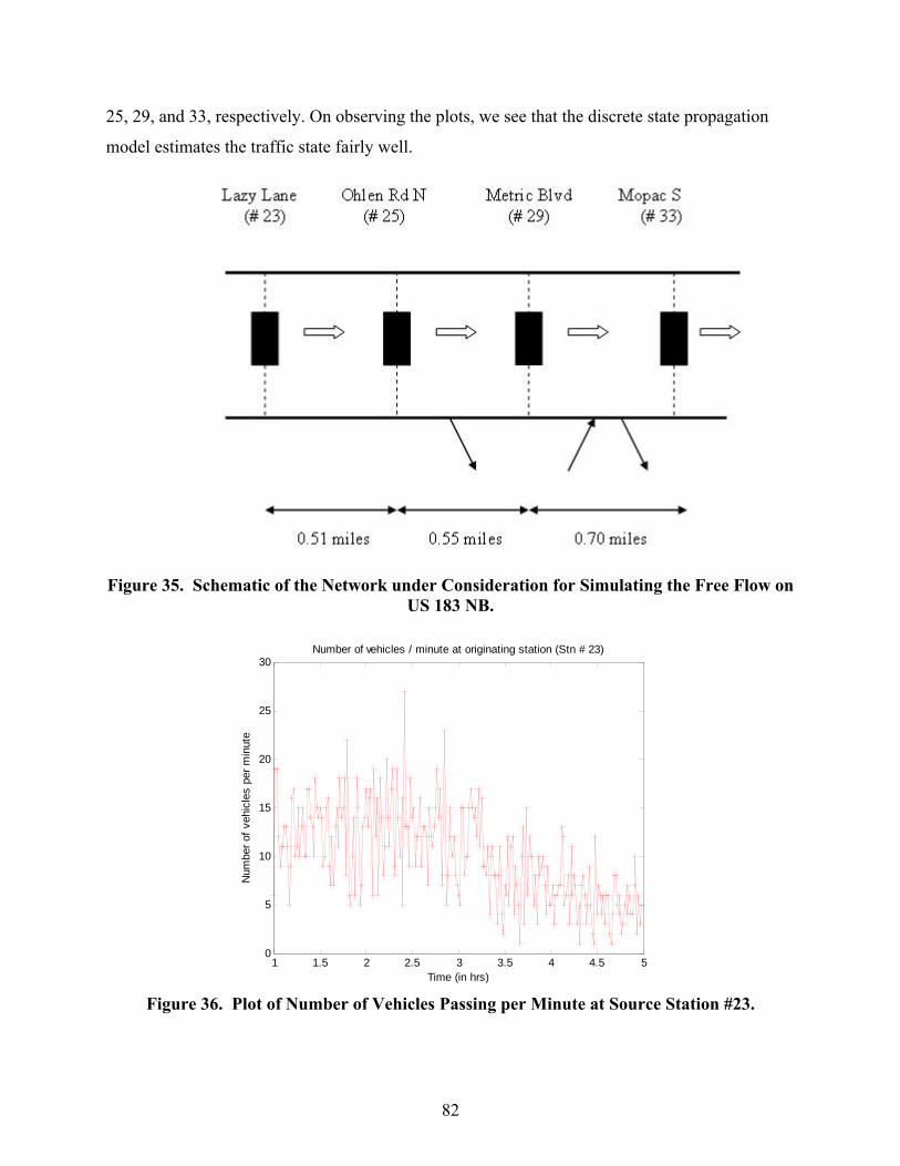
82
25, 29, and 33, respectively. On observing the plots, we see that the discrete state propagation
model estimates the traffic state fairly well.
Figure 35. Schematic of the Network under Consideration for Simulating the Free Flow on
US 183 NB.
1 1.5 2 2.5 3 3.5 4 4.5 50
5
10
15
20
25
30
Time (in hrs)
Num
ber o
f veh
icle
s pe
r min
ute
Number of vehicles / minute at originating station (Stn # 23)
Figure 36. Plot of Number of Vehicles Passing per Minute at Source Station #23.
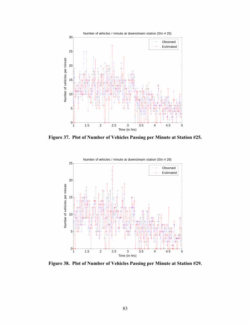
83
1 1.5 2 2.5 3 3.5 4 4.5 50
5
10
15
20
25
30
TIme (in hrs)
Num
ber o
f veh
icle
s pe
r min
ute
Number of vehicles / minute at downstream station (Stn # 25)
ObservedEstimated
Figure 37. Plot of Number of Vehicles Passing per Minute at Station #25.
1 1.5 2 2.5 3 3.5 4 4.5 50
5
10
15
20
25
Time (in hrs)
Num
ber o
f veh
icle
s pe
r min
ute
Number of vehicles / minute at downstream station (Stn # 29)
ObservedEstimated
Figure 38. Plot of Number of Vehicles Passing per Minute at Station #29.

84
1 1.5 2 2.5 3 3.5 4 4.5 50
2
4
6
8
10
12
14
16
18
Time (in hrs)
Num
ber o
f veh
icle
s pe
r min
ute
Number of vehicles / minute at downstream station (Stn # 33)
ObservedEstimated
Figure 39. Plot of Number of Vehicles Passing per Minute at Station #33.
Table 9 shows the cumulative number of vehicles data for a particular day, when the
simulations were carried out for a time duration during the Free Regime (1:00 AM to 5:00 AM).
The numbers of vehicles leaving and entering through the ramps also are included in the
simulations. From the results we observe that some vehicles are “lost” in the section. This can be
due to the fact that we do not know the initial conditions of the traffic state in the network. Also,
not knowing the exact location of the entry and exit ramps is a potential reason for the error in
predicting the traffic state.
Table 9. Cumulative Count for the Number of Vehicles during Free Regime for the
Network 23-25-29-33. Station Number Observed Predicted Error %
23 2400 NA NA 25 2417 2240 7.3231 29 1857 1799 3.1233 33 1430 1274 10.9091
Regimes 1 and 2: Estimation of Traffic Parameters and Traffic State Prediction
The traffic model that we developed is primarily based on the idea of representing the
aggregate behavior of traffic movement with a “representative” vehicle, the dynamics of which

85
are based on the interactions between the vehicles in the traffic. In this section we corroborate
the non-continuum traffic model with the real traffic data obtained from the Austin freeways.
Use of Historic Traffic Data to Identify the Structure of Vehicle Following for Regimes 1 and 2
From traffic loop detector data, repetitive patterns are observed in traffic throughput with
respect to the time of the day. The traffic data for the number of vehicles passing through a
location and their aggregate speeds are used to identify the structure of vehicle following for the
traffic movement in Regimes 1 and 2. The following state space model is constructed for
identification purposes:
⎥⎥⎦
⎤
⎢⎢⎣
⎡+
⎥⎥⎦
⎤
⎢⎢⎣
⎡−+=+ )(~)()(
)()()1(,
knL
kNkvkNhkNkN i
is
iieniii (32)
⎥⎥⎦
⎤
⎢⎢⎣
⎡+=+
is
iiexsumi
exsumi L
kNkvhkNkN
,,,
)()(~)()1( (33)
( )
⎥⎥⎦
⎤
⎢⎢⎣
⎡+
⎥⎥⎦
⎤
⎢⎢⎣
⎡−
⎥⎥⎦
⎤
⎢⎢⎣
⎡ Δ+−Δ=+Δ )(~)()(
)()(
)()1(,,
2
knL
kNkvkN
LkL
hkk iis
iieni
is
icarii (34)
where,
iN = the number of vehicles in the section,
sumiexN , = the cumulative number of vehicles exiting a section,
iΔ = the state vector of the aggregate following distance, and
h = the time step.
The system takes )~( iien nN + , the net inflow of vehicles into the section in each time step
as the input. The system output is taken to be sumiexN , , the cumulative number of vehicles exiting
the section. Thus, the model assumes that the rate of change of number of vehicles with respect
to time in a section is known. Since we do not know the initial conditions of the states iN ,
sumiexN , , and iΔ , we design a state estimator using the extended Kalman filtering technique.

86
Structure of Vehicle Following Dynamics for Traffic under Different Regimes
We apply the extended Kalman filtering methodology to identify the states in the state
space model described above. Use of the Gaussian white noise sequences in the state transition
equation helps to treat the aggregate following distance and the number of vehicles in the section
as different state variables. The aggregate speed data are used to estimate the states at each time
instant. The simulations for estimating the number of vehicles in the section and the aggregate
following distance for Regimes 1 and 2 are done for many weekdays. Figure 40 shows the
aggregate following distance, and Figure 41 shows the estimated number of vehicles in a section.
We conducted simulations for a section stretching from Lamar Boulevard North to Ohlen Road
North on US 183 northbound in Austin. The section length under consideration is 2.84 lane miles
(data for all the three lanes was aggregated). A fixed length of a vehicle is taken as 15 feet for the
purposes of these simulations.
Figure 40. Estimated Aggregate Following Distance in a Section on US 183 NB
on May 18, 2004.

87
Figure 41. Estimated Number of Vehicles in a Section on US 183 NB on May 18, 2004.
Upon careful observation of the plot of estimated aggregated following distance we can
distinguish two “sub-regimes” in Regime 1:
• varying aggregate following distance and
• almost constant aggregate following distance.
Also, we note that the following distance reacts quite sharply to the sharp drop and rise in
the aggregate speeds between 4:30 PM to 7:00 PM (Regime 2). We now give the following
structure to the vehicle following.
• Regime 1: Observed from 7:00 AM to 4:30 PM and 7:00 PM to 9:30 PM. We have
the following sub-regimes:
1. Regime 1 (a): Observed from 7:00 AM to 11:30 AM and 7:00 PM to 9:30 PM:
[ ]iwiiw
i vhh
v −Δ+Δ= (1 λ&& (35)
2. Regime 1 (b): Observed from 11:30 AM to 4:30 PM:
))(( ,211 car
i
isii L
NL
v −−Δ+Δ= λλ && (36)

88
• Regime 2: Observed from 4:30 PM to 7:00 PM. (Work is still under progress to
model this traffic regime.)
In traffic Regime 1 (a), it is hypothesized that the drivers tend to maintain a following
distance that varies with the speed of the vehicle. This hypothesis also substantiates the
observation that the drivers tend to accept smaller following distances while maintaining almost
constant speeds. This happens when there is an increase in the demand on utilization of the
freeway (more number of vehicles are driving). On the other hand, during Regime 1 (b), it is
hypothesized that the drivers tend to maintain a “constant” following distance. Work is still
under progress to model the vehicle following behavior for Regime 2.
In the above equations, the parametersλ , 1λ , and 2λ reflect the time constants associated
with driving in their respective traffic regimes. These along with wh are estimated from the traffic
data. The numerical values of parameters associated with this structure are specific to the
freeway section under consideration.
Estimating the Traffic Parameters Associated with Different Traffic Regimes
The values of estimated states, the aggregate following distance and the number of
vehicles in the section, and the aggregate speed data are used to estimate the parameters. The
principle of least squares is then applied to estimate the parameters. The estimated parameters
show consistent repetitive values for different working days. Table 10 gives the estimated values
of parameters for Regime 1 (a).
Table 10. Estimated Parameters for Regime 1 (a). Regime 1 (a)
Monday Tuesday Wednesday Thursday Friday λ hw λ hw λ hw λ hw λ hw
7.71E-4 0.0623 7.79E-4 0.0522 4.87E-4 0.1036 2.81E-4 0.1007 6.89E-4 0.0607 8.81E-4 0.0579 1.09E-3 0.0526 6.26E-4 0.0858 5.59E-3 0.0817 9.24E-4 0.0558 4.84E-4 0.0610 3.35E-4 0.0572 5.03E-4 0.1509 6.24E-4 0.1117 3.98E-4 0.0894 1.25E-4 0.0650 4.32E-4 0.0590 4.93E-4 0.0997 3.24E-4 0.0862 2.80E-4 0.0608 4.16E-4 0.0589 7.15E-4 0.0613 3.39E-4 0.0840 7.92E-4 0.0791 4.86E-4 0.0747

89
The units of λ and wh are minute-1 and minute, respectively. The parameters show
repetitive trends with respect to the day of the week. The time headway wh varies from about
three to nine seconds. For example, on Mondays the time headway is about three to four seconds.
These numbers are fairly reasonable for the current traffic. The small values of λ and typical
values of time headway and speed in the section suggest that drivers are ready to accept shorter
following distances so that they can drive with almost constant speeds and that the rate of change
of speed is more dependent on the relative speed.
Table 11 gives the estimated values of parameters for Regime 1 (b). From the values of
1λ and 2λ we deduce that the rate of change of aggregate speed for the section considered is
more dependent on the relative velocity.
Table 11. Estimated Parameters for Regime 1 (b). Regime 1 (b)
Monday Tuesday Wednesday Thursday Friday λ1 λ2 λ1 λ2 λ1 λ2 λ1 λ2 λ1 λ2
26.296 0.6611 40.508 -0.0357 19.969 0.1377 19.298 -0.0456 40.323 0.0182 21.758 0.0157 35.356 -0.0228 19.540 0.0342 19.167 -0.0258 37.487 1.0640 23.328 0.0454 33.811 -0.0301 19.940 0.0219 17.788 -0.0234 43.110 0.0905 26.539 0.1996 32.425 -0.0094 22.483 0.1452 18.032 -0.0101 43.229 0.1748 28.557 0.5011 31.643 -0.0193 20.254 0.1215 26.297 -0.1239 40.369 0.1328
Estimation of Traffic State in Real Time
After estimating the time constants associated with the different traffic regimes from
historical data, we use them to predict the traffic state. Extended Kalman filtering is again used
to estimate the states of traffic in real time, but now the state vector also includes the aggregate
speed of the traffic (speed of the “representative” vehicles for the particular section). The input to
the system is taken to be the net inflow of vehicles into the section )~( iien nN + . The output of the
system is again taken to be the cumulative number of vehicles exiting the section. To validate the
estimated states, we plotted the predicted aggregate speed against the observed aggregate speed
for the time duration on the particular day. The predictions made by this filtering technique are
one step predictions. Since the time step used is one minute (the traffic data are available in one-
minute intervals), the model is able to predict aggregate speeds one minute in advance.
Below we give a few results for the estimation of traffic state in real time. In the plots
below, the predicted speed is plotted against the observed traffic speed for traffic Regime 1 (b).

90
The results are for the same section for which the parameter results have been presented. The
values of traffic parameters (estimated from historic data) are used in real-time estimation of the
traffic state. We predicted the aggregate traffic speed on a one-minute basis. Figure 42 and
Figure 43 show the one step predicted aggregate traffic speed for congestion in Regime 2 for two
working days in the year 2004. It is important to note the scale used in the plots. The vertical
scale is about four miles per hour. From the plots, we can see that the model is able to predict the
aggregate traffic speed very well, and in this sense the estimation is fairly accurate.
Figure 42. Plot of Aggregate Traffic Speed in the Section for Thursday, April 15, 2004.

91
Figure 43. Plot of Aggregate Traffic Speed in the Section for Friday, February 13, 2004.
Conclusion and Work in Progress
The driving behavior for traffic in Regime 2 is yet to be modeled. Work also is underway
to increase the prediction window to be on the order of five to ten minutes, which can be more
beneficial in predicting both the recurring and non-recurring congestion. The switching of modes
of traffic regimes also warrants attention, so that control algorithms can be developed for
Advanced Traveler Management Systems and Advanced Traveler Information Systems
applications.


93
CHAPTER IV. HIGH-LEVEL SPECIFICATIONS FOR PROTOTYPE TOOL
Figure 44 shows a schematic functional diagram of the prototype tool. A more detailed
functional description of each of the components follows. This more detailed discussion falls
short of providing a detailed description of component (module) interfaces and associated
formats, but it does indicate where those details need subsequently to be defined in detail.
Figure 44. High-Level Schematic Function Diagram of On-Line System.
ASSUMPTIONS
The objective is to use the best available data, at some arbitrary time T, to predict the
probability of an incident, as a function of time and position, for a designated section of freeway
(“target section”), and over the “prediction interval” T to T+ΔT. The “prediction duration” ΔT
must be long enough to permit countermeasures to be undertaken, but sufficiently short that the
predictions will be reasonably accurate. Predictions will be updated at “updating horizons”
δt < ΔT .

94
DATA
The function of the data module is to provide appropriately formatted input data to the
traffic flow module. Input data required by the traffic flow model include suitable representations
of both observed data on the current day up to time T, and historical data, presumably in some
mean sense, with allowance for time of day, day of week, etc. Of course, historical data are
always available; however, the key hypothesis of the project is that use of current data as
available, rather than mean historical data, will permit a more precise projection of probability of
an incident. For implementation, detailed decisions regarding formatting of both historical data
and current data need to be undertaken. For the historical data, we need to develop
corresponding reference archives for designated target sections of freeway. The data module will
have access to both these historical reference archives and the current detector data, and on
demand from the traffic flow module will provide the appropriate data in a format to be
determined in detail.
TRAFFIC FLOW MODEL
The “traffic flow model” is the system module that will acquire the requisite data from
the data module, and produce therefrom a representation of the state of traffic flow over the
target section and the prediction interval that is native to the methodology of the particular traffic
flow model. Possible instances of a traffic flow model that are under consideration include:
• a traffic flow model based on the kinematic-wave model, in which case the output
would be some representation of the time and position variation of density (or flow
or speed) over the target section and the prediction interval;
• a traffic flow model based on vehicle car following dynamics; and
• any other current or future model (for example, DYNASMART or one of the other
currently available models).
This design permits the traffic flow model to be developed independently of the data
module, provided both respect the defined interface. The interface between traffic flow model
and incident precursor model will not be independent of the details of the traffic flow model, but
defining them as separate modules will permit their development in parallel and will permit
decoupled version development for these two modules. The driving force behind the design
decision not to “lock into” a single uniform interface between traffic flow models and incident

95
precursor modules is the desire to retain maximum flexibility and modularity regarding the
choice of traffic flow model, thereby providing the ability to adapt rapidly to developments in the
fast-paced field of computational simulation of traffic flow.
INCIDENT PRECURSORS
The function of the incident precursor module is to accept as input the traffic flow
representation native to a particular traffic flow model, for the designated target section of
freeway and over the prediction interval under consideration, and produce from that the time and
position dependency of the selected incident precursors (e.g., longitudinal speed variation and
density). Thus, the incident precursor module must be tailored to the particular traffic flow
model, but its output must conform to a uniform interface between incident precursor modules
and incident projection modules. Details of the incident-precursor/incident-projection interface
remain to be developed.
INCIDENT PROJECTIONS
The incident precursor module takes as its input the output of the incident precursor
module, which is to say a representation, in a format to be decided subsequently in detail, of the
time and position dependency of the selected incident precursors, over the designated target
section and prediction interval. As its output it produces a suitable representation of the predicted
frequency of incidents over the target section and prediction interval. Details of the format of
these incident projections remain to be determined, but a hard requirement is that this
representation be suited to an intuitive graphical representation for quick grasp by control center
operators.
PREVENTIVE MEASURES
The details of the preventive measures that might be undertaken are outside the scope of
the project itself. However, we do require some input from TxDOT on the possibilities because
the time scale required to implement preventive measures materially affects the required
prediction duration (i.e., ΔT in the preceding development).


97
REFERENCES
1. Gribe, P. (2003). “Accident Prediction Models for Urban Roads.” Accident Analysis and Prevention, Vol. 35, pp. 273-285.
2. Hiselius, L. W. (2004). “Estimating the Relationship between Accident Frequency and Homogeneous and Inhomogeneous Traffic Flows.” Accident Analysis and Prevention, Vol. 36, pp. 985-999.
3. Cedar, A., and M. Livneh (1982). “Relationships between Road Accidents and Hourly Traffic Flow—I.” Accident Analysis and Prevention, Vol. 14, pp.19-34.
4. Davis, G. A. (2005). “Collective Responsibility in Freeway Rear-End Collisions. An Application of Casual Models.” Presented at Transportation Research Board Annual Meeting, Washington, D.C.
5. Oh, J.-S., C. Oh, S. G. Ritchie, and M. Chang (2005). “Real-Time Estimation of Accident Likelihood for Safety Enhancement.” Journal of Transportation Engineering, ASCE, Vol. 131, No. 5, pp. 358-363.
6. Lee, C., F. Saccomanno, and B. Hellinga (2002). “Analysis of Crash Precursors on Instrumented Freeways.” Transportation Research Record 1784, TRB, National Research Council, Washington, D.C., pp. 1-8.
7. Lee, C., B. Hellinga, and F. Saccomanno (2003). “Real-Time Crash Prediction Model for Application to Crash Prevention in Freeway Traffic.” Transportation Research Record 1840, TRB, National Research Council, Washington, D.C., pp. 67-77.
8. Abdel-Aty, M., A. Pande, N. Uddin, H. Al-Deek, and E. Radwan (2004). Linking Crash Patterns to ITS -Related Archived Data. Final Report, University of Central Florida, Orlando.
9. Kockelman, K. M., and J. Ma (2004). „Freeway Speeds and Speed Variations Preceding Crashes, within and across Lanes.” Presented at ITS America 2004, 14th Annual Meeting and Exposition, San Antonio, Texas.
10. Golob, T. F., and W. W. Recker (2004). “A Method for Relating Type of Crash to Traffic Flow Characteristics on Urban Freeways.” Transportation Research, Part A, Vol. 38, No. 1, Elsevier, pp. 53-80.
11. Guiliano, G. (1989). “Incident Characteristics, Frequency, and Duration on a High Volume Urban Freeway.” Transportation Research, Part A, Vol. 23, No. 5, pp. 387-396.
12. Madanat, S., P. Liu, H. Pan, and H. Teng (1997). “Freeway Incident Likelihood Prediction and Response Decision-Making.” In Joint Highway Research Project Report FHWA/IN/JHRP-96/6, Project No. HPR-2090, Purdue University, West Lafayette, Indiana.
13. Khattak, A. J., P. Kantor, and F. M. Council (1998). “Role of Adverse Weather in Key Crash Types on Limited-Access Roadways: Implications for Advanced Weather Systems.” Transportation Research Record 1621, TRB, National Research Council, Washington, D.C., pp. 10-19.
14. Greene, W. H. (2002). Econometric Analysis. 5th Ed., Prentice Hall, Pearson Education, Inc., Upper Saddle River, New Jersey.
15. Washington, S., M. Karlaftis, and F. Mannering (2003). Statistical and Econometric Methods for Transportation Data Analysis. CRC Press, Boca Raton, Florida.

98
16. Shankar, V., F. Mannering, and W. Barfield (1995). “Effect of Roadway Geometrics and Environmental Factors on Rural Freeway Accident Frequencies.” Accident Analysis and Prevention, Vol. 27, No. 3, pp. 371-389.
17. Brodsky, H., and A. S. Hakkert (1988). “Risk of a Road Accident in Rainy Weather.” Accident Analysis and Prevention, Vol. 20, No. 3, pp. 161-176.
18. http://cdo.ncdc.noaa.gov/ulcd/ULCD, accessed August 25, 2005. 19. Chandrasekaran, P. (1998). Prediction of Traffic Flow for Real-Time Control. Master’s
Thesis, Texas A&M University, College Station, Texas. 20. Zhang, L., and D. Levinson (January 2004). Some Properties of Flows at Freeway
Bottlenecks. Transportation Research Board Annual Meeting CD-ROM, Washington, D.C.
21. Persaud, B., S. Yagar, D. Tsui, and H. Look. Study of Breakdown-Related Capacity for a Freeway with Ramp Metering. http://www.civil.ryerson.ca/staff_fac/publications/persaud/bdowntrb012revnov.htm, accessed August 25, 2005.
22. http://www.trafficlab.utah.edu/research/projects/current/acrobat/IncidentDet.pdf, accessed August 25, 2005.
23. Koppelman, F. S., and W. Lin (August 1996). Development of an Expressway Incident Detection Algorithm for the ADVANCE Area Based on the California Algorithm Set. Path Project Report TRF-ID-311/312, The Transportation Center, Northwestern University, Evanston, Illinois.
24. Browne, R., S. Foo, S. Huynh, B. Abdulhai, and F. Hall (January 2005). “AID CAAT: The Automatic Incident Detection Algorithm Comparison and Analysis Tool.” Transportation Research Board Annual Meeting CD-ROM, Washington, D.C.
25. Chen, C., A. Skabardonis, and P. Varaiya (January 2004). “A System for Displaying Travel Times on Changeable Message Signs.” Transportation Research Board Annual Meeting CD-ROM, Washington, D.C.
26. Coifman, B. (2002). “Estimating Travel Times and Vehicle Trajectories on Freeways using Dual Loop Detectors.” Transportation Research, Part A, Vol. 36, No. 4, pp. 351-364.
27. Newell, G. (1993). “A Simplified Theory of Kinematic Waves in Highway Traffic, Part II: Queuing at Freeway Bottlenecks.” Transportation Research, Part B, Vol. 27, pp.289-303.
28. CORSIM, Version 1.03, User’s Manual (Apr 1997). Kaman Science Corporation, Colorado Springs, Colorado.
29. Parker, M. (2002). “Zooming In on Traffic Microsimulation.” Traffic Technology International, Dorking, Surrey, United Kingdom.
30. Smith, M., S. Druitt, G. Cameron, and D. McArthur (July 1994). PARAMICS Final Report. Report No. EPCC-PARAMICS-FINAL, University of Edinburgh, Parallel Computing Center, Scotland.
31. Mahmassani, H., and K. Abdelghany (2003). “DYNASMART-IP: Dynamic Traffic Assignment Meso-simulator for Intermodal Networks.” In Advanced Modeling for Transit Operations and Service Planning, pp. 201-229, Elsevier Science Publishers, Amsterdam, Netherlands.

99
32. Ben-Akiva, M., D. Cueno, M. Hasan, M. Jha, and Q. Yang (2003). “Evaluation of Freeway Control Using Microscopic Simulation Laboratory.” Transportation Research, Part C: Emerging Technologies, Vol. 11, No. 1, pp. 29-50.
33. Foo, S., B. Abdulhai, and M. Elbagoury (January 2005). “Information Theoretic Analysis of Loop Detector Data.” Transportation Research Board Annual Meeting CD-ROM, Washington, D.C.
34. Highway Capacity Manual 2000. Transportation Research Board, National Research Council, Washington, D.C.
35. Lighthill, M. J., and G. B. Whitham (1955). “On Kinematic Waves II—A Theory of Traffic Flow on Long Crowded Roads.” In Proceedings Royal Society, London, Vol. A229, pp. 317-345.
36. Richards, P. I. (1955). “Shockwaves on the Highway.” Operations Research, Vol. 4, pp. 42-51.
37. Papageorgieu, M. (1998). “Some Remarks on Macroscopic Traffic Flow Modeling.” Transportation Research A 32, pp. 323-329.
38. Drake, J., J. Schofer, and A. May. (1967). A Statistical Analysis of Speed Density Hypotheses. Highway Research Record 154, pp. 53-87.
39. Koshi, M., M. Iwasaki, and I. Okhura (1983). “Some Findings and an Overview on Vehicular Flow Characteristics.” In Proceedings of the Eighth International Symposium on Transportation Traffic Theory, V. F. Hurdle et al., eds., University of Toronto Press, Toronto, pp. 403-426.
40. Cassidy, M. J., and J. R. Windover (1995). “Methodology for Assessing Dynamics of Freeway Traffic Flow.” Transportation Research Record 1484, TRB, National Research Council, Washington, D.C., pp. 73-79.
41. Greenshields, B. N. (1934). “A Study of Traffic Capacity.” In Proceedings of the 14th Annual Meeting of the Highway Research Board, Highway Research Board, Washington, D.C., pp. 448-474.
42. Ross, P. (1988). “Traffic Dynamics.” Transportation Research B 22, pp. 421-435. 43. Ross, P. (1989). “Response to Newell.” Transportation Research B, 23B, pp. 390-391. 44. Newell, G. F. (1989). “Comments on Traffic Dynamics.” Transportation Research B,
23B, pp. 386-389. 45. Nelson, P., and N. Kumar (2004). “Point Constrictions, Interface and Boundary
Conditions for the Kinematic-Wave Model.” Proceedings TRB 2004 (published in CD format), Washington, D.C.
46. Lebacque, J. P. (to appear). “Intersection Modeling, Application to Macroscopic Network Traffic Flow Models and Traffic Management. In Proceedings of the Workshop on Traffic and Granular Flow 2003.
47. Bui, D. D., P. Nelson, and S. L. Narasimhan (1992). Computational Realizations of the Entropy Condition in Modeling Congested Traffic Flow. Texas Transportation Institute, College Station, Texas.
48. Daganzo, C. F. (1994). “The Cell Transmission Model: A Dynamic Representation of Highway Traffic Consistent with the Hydrodynamic Theory.” Transportation Research B, Vol. 28, pp. 269-287.
49. Buisson, C. (1997). “Découpage objets de Strada.” Internal report Licit, Entre-Inrets, France.

100
50. Head, K. L. (1994). “Event-Based Short-Term Traffic Flow Prediction Model.” Transportation Research Record 1510, TRB, National Research Council, Washington D.C, pp. 45-52.
51. Yang, F., Z. Lin, H.X. Liu, and B. Ran (2004). “Online Recursive Algorithm for Short-Term Traffic Prediction.” Transportation Research Record 1879, TRB, National Research Council, Washington D.C, pp. 1-9.
52. VISSIM 4.00 User Manual (2004). PTV, Stumpfstraβe 1, D-76131 Karlsruhe, Germany.

101
APPENDIX: SOFTWARE TOOL DEVELOPMENT
The primary objective of this project is to develop freeway traffic assessment and
prediction models and a prototype software implementation of selected models. To provide for
efficient testing and development of these models, researchers are developing a software
package. The objective is to produce an off-line research tool that would provide a basis for the
prototype software to be delivered to TxDOT at the end of this project. To fulfill the above
requirements, the following functionality, graphically shown in Figure A-1, is needed:
1. Read a freeway configuration file and create the precedence relationships for all
detectors in the freeway system.
2. Mimic real-time operation by reading data of the entire freeway system in one-
minute steps.
3. After reading new data at each one-minute step:
a. Invoke selected traffic assessment/prediction models, and
b. Display/output key indicators/measurements regarding the status (locations of
congestion and incidents, travel times, etc.) of the freeway.
SOFTWARE DESCRIPTION
Freeway System
In this software (currently named 0-4946 Data Analyzer), a freeway system is modeled
using four basic objects: system, station, detector, and record. The “system” is composed of
“stations,” which in turn contain “detectors” at the same location. A “record” contains minute-
by-minute volume, occupancy, speed, and truck percentage data for each detector. Figure A-2
illustrates these relationships.

102
Figure A-1. Software Flow Chart.
Figure A-2. Freeway System.
The freeway system shown in Figure A-2 has eight detectors and four stations. Station I
has detectors 1, 2, and 3; station II has detector 4; station III has detectors 5, 6, and 7; and station
IV has detector 8. Table A-1 presents the data definitions.
Station
Detector
1
2
3
4
5
6
7
8
I
II
III
IV
Traffic Assessment/
Prediction Models
Read Freeway Configurations
Begin
Read One-minute
Detectors Data
Output Indicators/
Measurements
Update Database
Historical Data

103
Table A-1. Data Definitions.
System Data Name Description System Name Freeway name. Direction Traffic flow direction. Station Vector List of all the stations in the system. Time Stamp Time stamp of the last data record read. Record Interval Interval between each data record.
Station Data Name Description Station ID Unique station identification number. Station Name Name of the cross street identifying the station. X-Coordinate Y-Coordinate
Station’s geographic coordinates (for distance calculation).
Link Speed Free-flow speed of the section from current station to the next downstream station on the freeway.
Detectors Vector Detectors associated with the station. Upstream Station Vector Set of immediate upstream stations. Downstream Station Vector Set of immediate downstream stations.
Detector Data Name Description Detector ID Unique detector identification number. Record Vector Minute-by-minute data records.
Record Data Name Description Time Stamp Time stamp of the record. Volume One-minute volume. Occupancy Occupancy, 0–100%. Speed Average speed, mph. Truck Percentage Average truck percentage, 0–100%.

104
Input Data
The software requires two data input sources, namely freeway configurations and
detectors data. All data input files are in comma-separated format.
Freeway Configurations File
The freeway configurations file contains the information necessary to define the freeway
system. The data format is shown in Table A-2.
Table A-2. Data Format of Freeway Configurations File.
Line 1 Data Name Description System Name Name of the freeway. Direction Traffic bound. Record Interval Interval between each data record, in seconds.
Line 2+ Data Name Description Station ID Unique station identification number.
Station Type
Station Type: FWY (freeway station), ENT (entrance ramp station), EXT (exit ramp station), and SER (service road station).
Station Name Name of the cross street that identifies the station. Link Information Identifier Value: “L.” Latitude X-coordinate of the station. Longitude Y-coordinate of the station. Link Speed Free-flow speed, in mph. Detector Identifier Value: “D.” Detector IDs Set of detector IDs that belong to the station. Downstream Station Identifier Value: “S.” Downstream Station IDs Set of immediate downstream station IDs.
As shown in Table A-2, the first line of the file contains general information about the
freeway, i.e., system name, freeway direction, and record interval that is the time between
successive data collection points. Currently, this value is 60 seconds.
Each following line (lines 2 through n) defines a station. Each of these lines has three
elements: link information identifier, detector identifier, and downstream station identifier. Since
the number of detectors and number of downstream stations vary, identifiers are also used to
mark the beginning and ending of the corresponding data.

105
For program development, Traffic Detector Mapbook: Traffic Operations Detector
Locations in Austin, Texas prepared by the Texas Transportation Institute was used to derive
information on station ID, detector type, cross street name, and detector ID, and to define the
precedence relationships of the stations on the freeway. TxDOT’s Austin District provided the
information on estimated free-flow speed of each freeway system and latitude and longitude for
each detector using State Plane Central Zone (4203), NAD83 datum, high accuracy regional
network (HARN) grid coordinates. Latitude and longitude of each detector provide the x- and y-
coordinates of each station. If a station has more than one detector, we use the coordinates for the
detector in the rightmost lane as an approximation.
Detector Data
Historic detector data files used were provided by TxDOT. Each data file contains one-
hour data for all detectors for which data are being collected. Files are named following a
specific naming convention that contains the freeway name, year, month, date, and time of the
data collected. For example, the following file contains detector data for US 183 for the “0900”
hour (09:00–09:59) on January 2, 2004:
US 0183 SCU 20040102 0900.DET
Freeway Date Time Extension
In each file, the first line contains data that defines the number of the detector for which
data are being collected, detector IDs, and the station name and has the following format:
nnn,xxxxx,yyyyyyyyyyyyyyyyyyyyyyyyyyyyyy, xxxxx,yyyyyyyyyyyyyyyyyyyyyyyyyyyyyy, ……
where:
nnn = number of detectors for which data are being collected,
xxxxx = detector ID, and
yyyyyyyyyyyyyyyyyyyyyyyyyyyyyy = station name string.

106
The next 60 lines provide minute-by-minute volume, occupancy, speed, and truck
percentage data for each detector and have the following format:
hhmmss,xxxxx,vvv,ooo,sss,ttt,xxxxx,vvv,ooo,sss,ttt,…
where,
hhmmss = time stamp (hh = hour, mm = minute, ss = second) of the data
recorded,
xxxxx = detector ID,
vvv = one-minute volume,
ooo = occupancy, 0–100%,
sss = average speed, mph, and
ttt = average truck percentage, 0–100%.
CURRENT STATUS OF 0-4946 DATA ANALYZER
Currently, the software has the capabilities of creating the precedence relationships of all
the stations on a freeway system by reading a freeway configuration file and mimicking real-time
operation by reading minute-by-minute data for the entire freeway system. Researchers have
started using the software for calculating entropy and mutual information of volume, occupancy,
and speed to gain understanding of these variables. Also, the software is able to calculate and
output cumulative volume counts of all or selected detectors for analysis. A snapshot of the
software is shown in Figure A-3.
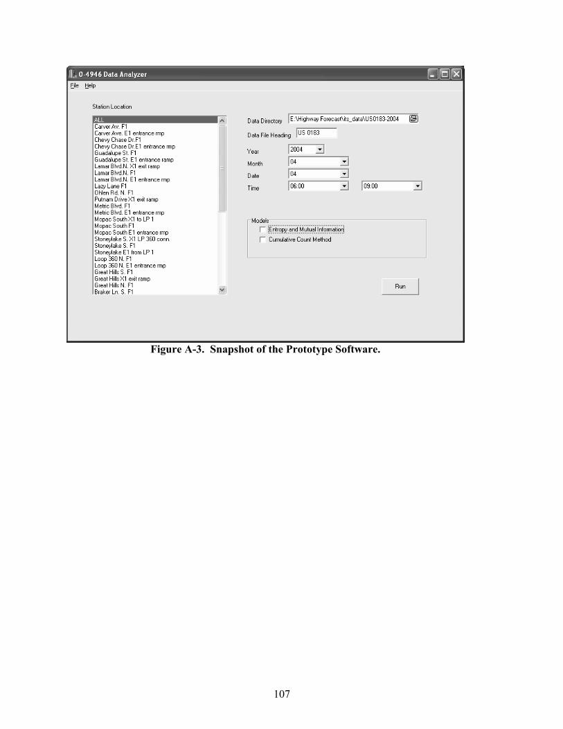
107
Figure A-3. Snapshot of the Prototype Software.