Dynamical correlation functions of the mesoscopic pairing model

Alexandre Faribault,1 Pasquale Calabrese,2 and Jean-Sébastien Caux3

1Physics Department, ASC and CeNS, Ludwig-Maximilians-Universität, 80333 München, Germany2Dipartimento di Fisica dell’Università di Pisa and INFN, 56127 Pisa, Italy

3Institute for Theoretical Physics, Universiteit van Amsterdam, 1018 XE Amsterdam, The Netherlands�Received 2 March 2010; revised manuscript received 12 April 2010; published 7 May 2010�

We study the dynamical correlation functions of the Richardson pairing model �also known as the reduced-or discrete-state Bardeen, Cooper, Schrieffer model� in the canonical ensemble. We use the algebraic BetheAnsatz formalism, which gives exact expressions for the form factors of the most important observables. Bysumming these form factors over a relevant set of states, we obtain very precise estimates of the correlationfunctions, as confirmed by global sum rules �saturation above 99% in all cases considered�. Unlike the case ofmany other Bethe Ansatz solvable theories, simple two-particle states are sufficient to achieve such saturations,even in the thermodynamic limit. We provide explicit results at half filling and discuss their finite-size scalingbehavior.

DOI: 10.1103/PhysRevB.81.174507 PACS number�s�: 74.20.�z, 02.30.Ik, 71.10.Li

I. INTRODUCTION

Possibly the most remarkable incipient property asso-ciated to a fermionic gas is its instability to the pairingphenomenon. Under an arbitrarily weak attractive force,which can originate in such a simple process as coup-ling to phonons, the gas will develop an instability towardthe formation of Cooper pairs, this process forming thebasis of the Bardeen, Cooper, Schrieffer �BCS� theory ofsuperconductivity,1 with further remarkable consequencessuch as the Meissner and Josephson effects. Within BCStheory, single-particle excitations are suppressed by the su-perconducting gap, which is obtained from the solution of avariational ansatz for the wave function defined in the grand-canonical ensemble �electron number is by construction notconserved anymore� and in the thermodynamic limit �since acontinuous energy band is assumed�.

While these mean-field approaches successfully describethe experimental features of the traditional bulk supercon-ductors, recent experiments have also considered metallicnanograins2,3 in which the level spacing is finite and of thesame order as the superconducting gap, and in which someCoulomb-blockade effects could occur in view of the finitecharging energy of the grain. These studies open the door tomany interesting further questions not answerable withinBCS theory, and require mesoscopic effects to be encom-passed back into the model. One way to approach this prob-lem is to use the so-called reduced BCS model, defined bythe Hamiltonian

HBCS = ��=1

�=+,−

N��

2c��

† c�� − g ��,�=1

N

c�+† c�−

† c�−c�+, �1�

which was introduced by Richardson in the early 1960s inthe context of nuclear physics.4 The model describes�pseudo� spin-1/2 fermions �electrons, nucleons, etc.� in ashell of doubly degenerate single-particle energy levels withenergies �� /2, �=1, . . . ,N. c�,� are the fermionic annihila-tion operators, �=+,− labels the degenerate time-reversedstates �i.e., spin or isospin� and g denotes the effective pair-

ing coupling constant. Despite its simplified character �theinteraction couples all levels uniformly�, the model doeshave a number of advantages as compared to BCS theory.First of all, it can be solved within the canonical ensemble�fixed number of electrons�, a situation which is relevant forisolated nanograins. Second, and rather remarkably for anexactly solvable model, it remains solvable for an arbitrarychoice of parameters and can thus provide quantitative pre-dictions for various situations obtained by considering vari-ous choices of the set of energy levels �� �both their numberand their individual value�, coupling g, and filling. Besidesmesoscopic superconductivity, this model and its solutionalso find applications in other fields �see the reviews in Refs.5 and 6 for some applications outside of condensed-matterphysics�.

The nature of the electronic states in a metallic nanograincan conceivably be probed in a number of different experi-ments. Electronic transport through such a grain could bestudied by attaching either metallic or superconducting leads.The observable I-V characteristics or Josephson currentswould be theoretically obtainable from correlation functionswithin the grain. Such correlations, however, are not easilyobtainable from the basic exact solution of the model, whichfocuses on wave functions but does not allow to make directcontact with the dynamics of observables. The history of thestudy of correlations in the Richardson model is, however,already rather rich. Richardson himself in 1965 �Ref. 7� de-rived a first exact expression for static correlation functions.In a significant development, Amico and Osterloh8 proposeda new method to write down such correlations explicitly butwith results limited to system sizes of up to 16 particles. Amajor simplification was then proposed by Zhou et al.:9,10

using the algebraic Bethe Ansatz �ABA� and the Slavnovformula for scalar products of states,11 they managed to ob-tain the static correlation functions as sums over Np

2 determi-nants of Np�Np matrices. These expressions have been fur-ther simplified by us in a previous publication, where theywere evaluated numerically for a particular choice of theenergy levels �� �Ref. 12� allowing to describe the crossoverfrom mesoscopic to macroscopic physics, going beyond pre-

PHYSICAL REVIEW B 81, 174507 �2010�

1098-0121/2010/81�17�/174507�19� ©2010 The American Physical Society174507-1

vious results limited to fewer particles.8,13 We mention that adifferent approach, valid in the case of highly degenerate ��,is also available.14

Despite all these developments, up to now none of theseapproaches has been adapted and used to calculate dynamicalcorrelation functions, important to quantify the response of aphysical system to any realistic experimental probe. In thispaper we use a method that mixes integrability and numericsand is similar to that used by some of us to study the dy-namical correlation functions15 and entanglement entropy16

in spin chains, as well as dynamical correlations in Bosegases.17 In short, the ABACUS method18 consists in using theexact knowledge of the form factors of physical observablesas determinants of matrices whose entries are the unknownRichardson rapidities. For any given state, these rapiditiesare calculated by solving the Richardson equations. The cor-responding form factors are then evaluated. Finally we needto sum over all these contributions, but this can be done bysearching for the states in the Hilbert space that contributemore significantly to the correlation function. This is done byoptimizing properly the scanning of the Hilbert space18 andthe accuracy of the result is kept under control by checkingthe values of the sum rules. However, we will see that for theRichardson model, this scanning is particularly easy sincethe two-particle states dominate the sum even when increas-ing the number of particles �in strong contrast with whathappens for other models15,17�. This property is clearly con-nected with the mean-field character of the model in the ther-modynamic limit and the subsequent suppression of quantumfluctuations. However at finite �sufficiently low� number ofparticles the effect of quantum fluctuations can be revealedby small, but maybe measurable, multiparticle channels. Wemention that another variation on the ABACUS logic has re-cently been used for the calculation of out-of-equilibriumobservables in the pairing model subjected to a quantumquench, but in that case the class of excitations contributingwas much wider.19,20

The paper is organized as follows. In Sec. II we discussthe model and its general properties. In Sec. III we recall thealgebraic Bethe Ansatz approach to the model and we pro-ceed to some simplifications of the determinant expressions.In Sec. IV we introduce the sum rules for the consideredcorrelation functions and we present the selection rules forthe form factors that will help in the numerical computationby reducing the number of intermediate states we have tosum over. In Sec. V all the correlation functions are explic-itly calculated at half filling. We report our main conclusionsand discuss open problems for future investigation in Sec.VI. Appendix A reports the technical details on how to solvethe Richardson equations for any excited state while Appen-dix B looks at the details of the strong-coupling expansion ofa studied correlation function in order to explain its scalingbehavior.

II. MODEL

As it is written in Eq. �1�, singly as well as doubly occu-pied levels are allowed. The interaction, however, couplesonly doubly occupied levels among themselves, and due to

the so-called blocking effect,3,4 unpaired particles completelydecouple from the dynamics and behave as if they were free.We will denote the total number of fermions as Nf and thetotal number of pairs as Np. Due to level blocking, we willthus only consider Nf =2Np paired particles in N unblockedlevels, keeping in mind that we could reintroduce blockedlevels later if needed in the actual phenomenology desired.In terms of pair annihilation and creation operators

b� = c�−c�+, b�† = c�+

† c�−† , �2�

the Hamiltonian is

H = ��=1

N

��b�†b� − g �

�,�=1

N

b�†b�, �3�

and n�=2b�†b� is the number of particles in level �.

The pair creation and annihilation operators satisfy thecommutation relations

�b�,b�†� = ����1 − 2b�

†b��, �b�,b�� = �b�† ,b�

†� = 0. �4�

The term 2b�†b� in the first commutator makes the model

different from free bosons and therefore nontrivial.Using the pseudospin realization of electron pairs

S�z =b�

†b�−1 /2, S�− =b�, and S�

+ =b�† , the BCS Hamiltonian

becomes �up to a constant�

H = ��=1

N

��S�z − g �

�,�=1

N

S�+S�

− . �5�

The operators S��,z obey the standard su�2� spin algebra and

so Hamiltonian �5� describes a spin-1/2 magnet with long-range interaction for the XY components in a site-dependentlongitudinal magnetic field ��. Such a magnetic Hamiltonianis known in the literature as a Gaudin magnet.21 An impor-tant relation is

S��S�

= S�2 − �S�

z �2 � S�z . �6�

A. Grand-canonical BCS wave function

In the grand-canonical �GC� ensemble the ground-statewave function is the BCS �Ref. 1� variational ansatz

�GS� = ��

�u� + ei�v�b�†��0�, u�

2 + v�2 = 1, �7�

where the variational parameters u� and v� are real and � isa phase which, it turns out, must be � independent. �GS� isnot an eigenstate of the particle number operator Nf and the

average condition Nf�= Nf determines the GC chemical po-tential. Likewise, the commonly used definition

�GC = 2g��

b�� = 2g��

u�v�ei� �8�

for the superconducting gap makes sense only in a GC en-semble, since b�� is zero when evaluated at fixed particlenumber. The variational parameters are obtained as

FARIBAULT, CALABRESE, AND CAUX PHYSICAL REVIEW B 81, 174507 �2010�

174507-2

v�2 =

1

21 −�� − �

���� − ��2 + ��GC�2� , �9�

where � is the GC chemical potential.

B. Canonical description and Richardson solution

The exact solution �i.e., the full set of eigenstates andeigenvalues� of Hamiltonian �1� in the canonical ensemblewas derived by Richardson.4 The model can be encompassedinto the framework on integrable models22 and is tractable bymeans of algebraic methods.9,10,23,24 We review here only themain points of this solution.

In the ABA, eigenstates are constructed by applying rais-ing operators on a so-called reference state �pseudovacuum�.We here choose the pseudovacuum �in the pseudospin repre-sentation� to be fully polarized along the −z axis

S�z �0� = −

1

2�0�, ∀ � . �10�

In the pair representation, this state thus corresponds to theFock vacuum. Eigenstates with Np pairs are then character-ized by Np spectral parameters �rapidities� wj, and take theform of Bethe wave functions

� wj�� = �k=1

Np

C�wk��0� . �11�

The operators C, together with operators A, B, and D definedas

A�wk� =− 1

g+ �

�=1

NS�

z

wk − ��

, B�wk� = ��=1

NS�

−

wk − ��

,

C�wk� = ��=1

NS�

+

wk − ��

, D�wk� =1

g− �

�=1

NS�

z

wk − ��

�12�

obey the Gaudin algebra, which is the quasiclassical limit ofthe quadratic Yang-Baxter algebra associated to the gl�2� in-variant R matrix �we refer the readers to Ref. 10 for details�.

The wave functions �Eq. �11�� are eigenstates of the trans-fer matrix, and thus of Hamiltonian �1�, when the parameterswj satisfy the Richardson equations

−1

g= �

�=1

N1

wj − ��

− �k�j

Np 2

wj − wkj = 1, . . . ,Np. �13�

Throughout the paper we will refer with Latin indices to therapidities and with greek ones to the energy levels. The totalenergy of a Bethe state is, up to a constant,

E w� = �j

wj . �14�

For a given N and Np the number of solutions of the Rich-ardson equations is � N

Np�, and coincides with the dimension of

the Hilbert space of Np pairs distributed into N different lev-els, i.e., the solutions to the Richardson equations give all theeigenstates of the model.

Note that one could also use the pseudovacuum to be thestate fully polarized along the z axis �instead of −z�. Thisleads to slight differences in the expressions, which one canresolve by comparing Refs. 9 and 10.

III. CORRELATION FUNCTIONS AND ALGEBRAICBETHE ANSATZ

We are interested in the dynamical correlation functionsof the form

GO���t� =

GS�O�†�t�O��0��GS�GS�GS�

, �15�

at fixed number of pairs Np. Here O� stands for a “local”operator in the Heisenberg picture �i.e., depending on asingle energy level ��. We consider O� equal to S�

z or S��.

By inserting the complete set of states � w�� with w� a setof Mw rapidities solution to the Richardson equations, andusing the time evolution of the eigenstate, we can rewrite thedynamical correlation function as the sum

GO���t� = �

w�

w��O��GS�� w��O��GS�ei wt

GS�GS� w�� w��, �16�

where form factors and norms are obtainable by algebraicBethe Ansatz9,10 and will be discussed in the next section.The frequency w is just w=Ew−EGS−��Mw−Np�, wherethe energies E� and EGS are given in Eq. �14�. � is thechemical potential �needed only for S�� and Mw is the num-ber of rapidities of the state � w��. More easily, we can write w=Ew−E0,w, where E0,w is the lowest energy state with thesame number of rapidities as � w��. Notice that for Sz corre-lation function, we only need states with Mw=Np, and so thechemical-potential term is absent while for S+S−�, we needonly states with Np−1 rapidities.

The most relevant physical observables are clearly globalones, when the sum over the internal energy levels is per-formed. We will consider diagonal and global correlationfunctions, whose static counterparts for S� are the diagonal25

and off-diagonal order parameters. We consider in the fol-lowing the three global correlators:

Gzzd �t� = �

�=1

N GS�S�z �t�S�

z �0��GS�GS�GS�

, �17�

G+−d �t� = �

�=1

N GS�S�+�t�S�

−�0��GS�GS�GS�

, �18�

G+−od �t� = �

�,�=1

N GS�S�+�t�S�

−�0��GS�GS�GS�

. �19�

We will mainly study them in frequency space, since theirstructure is less complicated, and we will only plot a fewexamples in real time.

We stress that while the level-resolved correlators dependstrongly on the choice of the energy levels ��, for the globalones it is expected that most of the qualitative features and

DYNAMICAL CORRELATION FUNCTIONS OF THE… PHYSICAL REVIEW B 81, 174507 �2010�

174507-3

several quantitative ones are not affected by the choice of themodel. Thus our results, even if obtained for a specificchoice of ��, should display the main features of the dynami-cal correlation functions for a wide variety of Richardsonmodels.

Algebraic Bethe Ansatz and form factors

The previous exact expression �Eq. �11�� gives one anextremely compact parametrization of the system’s eigen-states. Only Np complex parameters �rapidities� are neededdespite the factorially large Hilbert space. As stated in thecurrent section, it is also possible to find compact expres-sions for the scalar products and form factors �matrix ele-ments of operators� needed to evaluate Eq. �16�. They aregiven by determinants of Np by Np square matrices which arealso easily computable despite the large dimension of theHilbert space.

We can find eigenstates one by one by finding given so-lutions to the Np Richardson equations shown in Eq. �13��see Appendix A�. The contribution to the correlation func-tions coming from each of these eigenstates is then obtainedthrough simple determinants. We can therefore compute thesum in Eq. �16�, one eigenstate at a time. Provided a fairlysmall subset of the full Hilbert space heavily dominates thissum �as will be discussed in section and further proven nu-merically�, it is possible to approach the exact correlation bysumming a limited number of easily computable contribu-tions.

The starting point to calculate correlation functions withthe algebraic Bethe Ansatz is having a representation for thescalar products of two generic states defined by Np rapidities�Np Cooper pairs�

w�� v�� = 0��b=1

Np

B�wb��a=1

Np

C�va��0� , �20�

when at least one set of parameters �e.g., wb but not va� is asolution to the Richardson equations. Following standard no-tations, C is the conjugate of the operator B. Such a repre-sentation exists, and is known as the Slavnov formula,11

which for the case at hand specifically reads9

w�� v�� =

�a�b

Np

�vb − wa�

�b�a

�wb − wa��a�b

�vb − va�� detNp

J� va�, wb�� ,

�21�

where the matrix elements of J are given by

Jab =vb − wb

va − wb��

�=1

N1

�va − ����wb − ���

− 2�c�a

Np 1

�va − vc��wb − vc�� �22�

from which the norms of states simply follow from v→w as� v��2=detNp

G with a Gaudin matrix

Gab = ���=1

N1

�va − ���2 − 2�c�a

Np 1

�va − vc�2 a = b ,

2

�va − vb�2 a � b ,� �23�

recovering Richardson’s old result.7

The key point is that any form factor of a local spin op-erator between two Bethe eigenstates can be represented viaEq. �12� as a scalar product with one set, e.g., v� not satis-fying the Bethe equations, for which Slavnov’s formula isapplicable. This has been explicitly worked out in Ref. 9. For w�, v� containing, respectively, Np+1 and Np elements, thenonzero form factors are

w��S�−� v�� = v��S�

+� w��

=

�b=1

Np+1

�wb − ���

�a=1

Np

�va − ���

detNp+1 T��, w�, v��

�b�a

�wb − wa��b�a

�vb − va�

�24�

and, for both w� and v� containing Np rapidities

�w��S�z ��v�� = �

a=1

Np �wa − ����va − ���

�

detNp�1

2Tz��w�,�v�� − Q��,�w�,�v���

�b�a

�wb − wa��b�a

�vb − va�,

�25�

with the matrix elements of T given by �b�Np+1�

Tab��� = �c�a

Np+1

�wc − vb����=1

N1

�vb − ����wa − ���

− 2�c�a

1

�vb − wc��wa − wc�� ,

TaNp+1��� =1

�wa − ���2 , Qab��� =

�c�b

�vc − vb�

�wa − ���2 .

Above, Tz is the Np�Np matrix obtained from T by deletingthe last row and column and replacing Np+1 by Np in thematrix elements. Here it is assumed that both va� and wb�are solutions to Richardson’s Bethe equations. However, theresults are still valid for S�

� if only wb� satisfy the Betheequations.

When approaching a bifurcation point �see Appendix A�in the solutions of the Richardson equations, some individualterms in the sum defining the matrix elements of T tend todiverge �because wb→�� for some b and ��. Those diver-gences cancel out when the sum is taken, but they can stilllead to large numerical inaccuracies. By using the Richard-

FARIBAULT, CALABRESE, AND CAUX PHYSICAL REVIEW B 81, 174507 �2010�

174507-4

son equations, it is possible to eliminate such potentiallyproblematic terms and rewrite the matrix T as

Tab =

2�c�a

Np

�wc − vb�

wa − vb�

c�b

1

�vb − vc�− �

c�a

1

�vb − wc�� ,

�26�

where potentially diverging terms have been removed. Westress once again that such a formula holds only if both wa�and va� are solutions to the Richardson equations with thesame g. This expression has been obtained before in Ref. 19.

IV. SUM RULES AND SELECTION RULES

The standard way to assess the accuracy of a numericalcalculation in which we discard part of the states consists inusing sum rules, e.g., summing of all the contributions inde-pendently of the energy of the intermediate state. When sum-ming over all states, we always get static quantities, and, inthe present case, they can be obtained by very simple con-siderations.

For Gzzd we have the sum rule

��=1

N

� v�

� v��S�z �GS��2

GS�GS� v�� v��= �

�=1

N GS��S�z �2�GS�

GS�GS�= �Sz�2� =

N

4.

�27�

Only the � NNp

� states with the same number of rapidities as theground state contribute to this correlation function. Insteadfor G+−

d we have

��=1

N GS�S�+S�

−�GS�GS�GS�

=N

2+ Sz� =

N

2, �28�

as easily shown by using Eq. �6�. Here, only the � NNp−1 � states

with one less rapidity than the ground state contribute to thiscorrelation and to the similar one containing off-diagonalterms G+−

od . In this last case we have

��,�=1

N GS�S�+S�

−�GS�GS�GS�

� �od, �29�

that is the off-diagonal order parameter, which can be ob-tained by the solution of the Richardson equations for theground state and using the Hellmann-Feynman theorem.12

We will see in the following that the two-particle stateswill give most of the contribution to the correlation func-tions, always saturating the sum rules to more than 99%accuracy. We show in the following sections that some se-lection rules imply that only two-particle states have nonzerocontribution to the correlation functions for g=0 and for g→�. Although at intermediate couplings this set of statesdoes not give 100% saturation of the sum rules, these twolimits clearly give insight as to why they remain extremelydominant in every regime.

A. Weak-coupling regime

In the noninteracting g=0 limit, the fixed Np eigenstatesare quite naturally described by placing the Np Cooper pairs�flipped pseudospins� in any of the � N

Np� possible sets of Np

energy levels picked from the N available ones. This trans-lates into a representation in terms of rapidities given bysetting the Np rapidities to be strictly equal to the energies ��

of the Np levels occupied by a pair. Since

limu→��

C�u� = limu→��

Si+

u − ��

, �30�

the states built in such way will have diverging norms andform factors, but it remains possible to describe the limitcorrectly because in the ratio of form factors and norm thetwo divergences cancel. Since any of these states is an eigen-vector of every S�

z operators, at g=0 the only contributions tothe Sz correlations come from the ground state to ground-state form factor GS�S�

z �GS�. In a perturbative expansion26

in g, it is easy to see that at first order, the corrections to theground state comes only from states � w�= ��1�

. . .��Np� �� dif-

fering from it by at most one rapidity �in the g→0 limit�.They constitute the full set of two-particle states, obtained bycreating a “hole” and a “particle,” i.e., moving a single Coo-per pair �rapidity� in the ground state to any of the availableunoccupied states.

At g=0, the v��S�−�GS� form factors are nonzero

whenever � v�= ��1. . .��Np−1

�� is obtained by removing a

single rapidity from the Np pairs ground state �GS= w1=�1 , . . . ,wNp

=�Np��. These states can also all be thought of as

two-particle states in the Np−1 pairs sector, since they canall be generated by moving a single rapidity in the Np−1ground state.

In the specific case of half filling �Np=N /2�, treating ev-ery two-particle excitation means that only N2 /4 states areneeded, out of the full � N

N/2 �-dimensional Hilbert space. Quitenaturally, when a nonzero coupling is included these statesmight not be sufficient anymore, but as will be shown in thenext two sections, for g→�, only this set of states is onceagain needed to compute every nonzero form factor of localspin operators.

B. Strong-coupling (g\�) regime

Yuzbashyan et al.27,28 showed that the solutions to theRichardson equations are such that in the g→� limit, a num-ber Nr of the rapidities will diverge as wi�Cig+O�g0�. Thecoefficients Ci are given by the Nr roots of the appropriateLaguerre polynomial27

LNr

−1−N−2�Nr−Np��Ci� = 0. �31�

In the infinitely large-coupling limit, the impact of the di-verging rapidities is well defined. In fact, limu→� C�u����S�

+ =Stot+ is the total spin raising operator. In this

limit, the coupling term g���S�+S�

− =gStot+ Stot

− completelydominates the Hamiltonian and so its eigenstates becomeeigenstates of the Stot

2 operator too. Through simple energeticconsideration,27,29 one can then easily show that the number

DYNAMICAL CORRELATION FUNCTIONS OF THE… PHYSICAL REVIEW B 81, 174507 �2010�

174507-5

of diverging rapidities is related to the eigenvalue J�J+1� ofStot

2 by the relation

Nr = J + Np −N

2. �32�

A state defined by Np rapidities, of which Nr are infinite,therefore belongs to a subspace of the total Fock space de-fined by eigenvalues of Stot

z and Stot2 given by quantum num-

bers m=−N /2+Np and J=Nr−Np+N /2. This allows us toderive explicit strong-coupling selection rules for the variousform factors used in this work.

Since a given eigenstate, in this limit, is built out of alinear superposition of the various spin states with fixed Jand m, it can be decomposed onto the joint eigenbasis of spin� combined with the various multiplets emerging from theaddition of the remaining N−1 spins 1

2 .For a given �fixed degeneracy index k� N−1 spins multi-

plet with magnitude J�, one can write the highest weightstate as

�k,J = J� +1

2,m = J� +

1

2� = �↑�� � �k,J�,m� = J�� .

�33�

The n times repeated action of Stot− =S�

− +SN−1− on this state

will generate the eigenstates

�k,J� +1

2,m� +

1

2− n� = C1

n�↑�� � �k,J�,J� − n� + C2n�↓��

� �k,J�,J� − n + 1� ,

where we do not need to explicitly specify the Clebsh-Gordan coefficients. Combining this multiplet with a spin 1

2also gives rise to a second set of states given by J=J�−1 /2and the corresponding allowed values of m� −J ,−J+1, . . . ,J−1,J�. These states are easily constructed by mak-ing them orthogonal to the previously found ones, i.e.,

�k,J� −1

2,m� +

1

2− n� = − C2

n�↑�� � �k,J�,J� − n� + C1n�↓��

� �k,J�,J� − n + 1� . �34�

Any general state with fixed J and m can therefore havecontributions coming from J+1 /2 or J−1 /2 multiplets of theN−1 excluded spins, i.e.,

�k

Ak�k,J,m� = �k�B1

k�↑�� � �k,J −1

2,m −

1

2� + B2

k�↓��

� �k,J −1

2,m +

1

2� + B3

k�↑�� � �k,J +1

2,m

−1

2� + B4

k�↓�� � �k,J +1

2,m +

1

2�� . �35�

Given this form, it is trivial to see that the application of S�z

or S�− on any of these states will result in

S�z �

k

Ak�k,J,m� � �kB1

k�↑�� � �k,J −1

2,m −

1

2� − B2

k�↓��

� �k,J −1

2,m +

1

2� + B3

k�↑�� � �k,J

+1

2,m −

1

2� − B4

k�↓�� � �k,J +1

2,m

+1

2�� ,

S�−�

k

Ak�k,J,m� � �kB1

k�↓�� � �k,J −1

2,m −

1

2� + B3

k�↓��

� �k,J +1

2,m −

1

2�� .

Consequently, the form factors for S�z

��k�

Ak�� k�,J�,m���S�

z ��k

Ak�k,J,m�� , �36�

can exclusively be nonzero if J�� J−1,J ,J+1� and m�=m.Similarly, the S�

− form factor

��k�

Ak�� k�,J�,m���S�

−��k

Ak�k,J,m�� , �37�

is nonzero only if J�� J−1,J ,J+1� and m�=m−1.Since, as we pointed out earlier, the value of J is related to

the number of diverging rapidities, these selection rulestranslate into selection rules for the total number of rapiditiesand the number of diverging rapidities.

The S�z form factor is nonzero for m�=m and therefore for

a total number of rapidities in the intermediate states �Np��given Np�=Np. Using this fact, the selection rule on J� andEq. �32�, we easily find that the only contributions comefrom states with Nr�= Nr−1,Nr ,Nr+1�.

Similarly, for S�−, we find that Np�=Np−1 and the number

of diverging rapidities must be given by Nr�= Nr ,Nr−1,Nr−2�. For the specific case of ground state �Nr=Np divergingrapidities� expectation values, nonzero contributions to S�

z

correlations are found exclusively for intermediate stateswith either Np or Np−1 diverging rapidities since Nr�=Np+1�Np is impossible. Identically, for S�

−, the only possiblecases are given by an intermediate state with Np−1 or Np−2 diverging rapidities.

Finally, for the S�z form factors involving only the ground

state, one can use the fact that

limg→�

�GS� = limg→�

�j=1

NpC�v j��0� � �Stot+ �Np�0� = �↑��

� � i1,. . .,�Np−1�

� N−1

Np−1�

� ↑�1. . . ↑�Np−1

�� + �↓��

� � �1,. . .,�Np

�

�N−1

Np�

� ↑�1. . . ↑�Np

�� , �38�

FARIBAULT, CALABRESE, AND CAUX PHYSICAL REVIEW B 81, 174507 �2010�

174507-6

where � �1,. . .,�M�� ↑�1. . .↑�M

�� is simply the sum over all pos-sible states containing M up spins picked out of the N−1levels which exclude level �. The action of S�

z on this state istrivially given by multiplying by 1/2 while adding a minussign to the second sum, which in the end allows us to simplyprove that

limg→�

GS�S�z �GS� �

1

2� N − 1

Np − 1� − �N − 1

Np��

=1

2

�N − 1�!�N − Np − 1�!�Np − 1�! 2Np − N

�N − Np�Np� .

�39�

One immediately sees that the half-filling 2Np=N casehas the peculiar feature of having these “ground state toground state” form factors go down to zero in the strong-limit coupling.

C. Correspondence between g=0 and g\� eigenstates

1. General algorithm

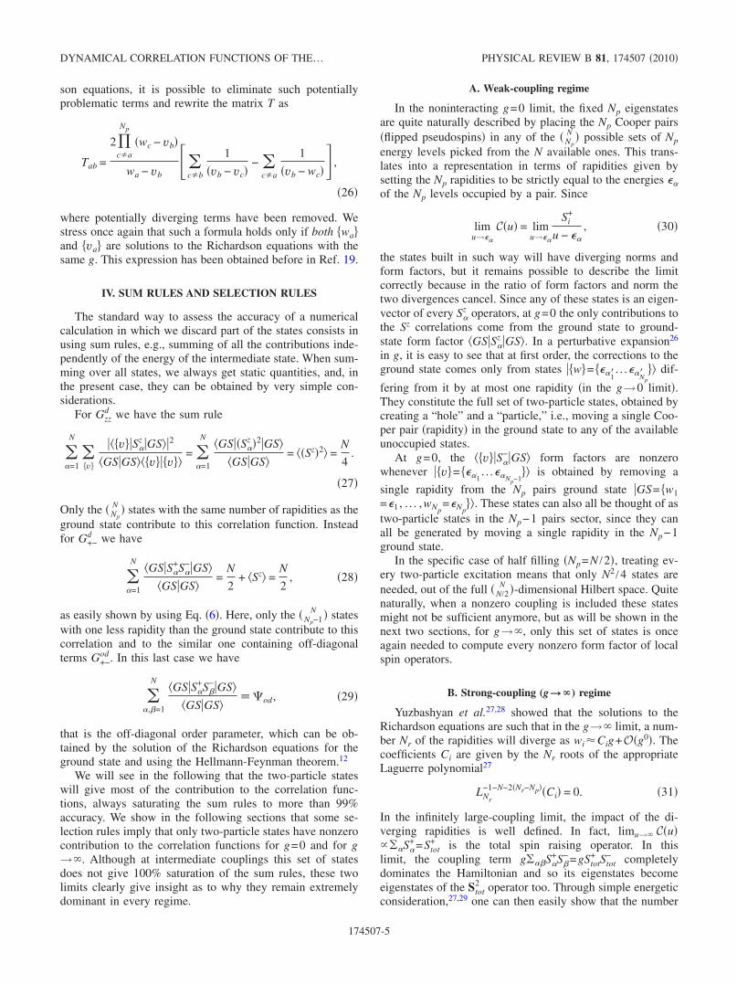
An algorithm relating the g=0 structure of a state to thenumber of diverging rapidities it will have at g→� wasalready proposed in Refs. 30 and 31. It necessitates theevaluation of various quantities for every possible partitionsof the N levels into three disjoint contiguous sets of levels.An equivalent result can be obtained through the simple fol-lowing algorithm, which was discussed before in Ref. 20.

By splitting any g=0 configuration of rapidities intoblocks of contiguous occupied and empty states, one cansimply obtain the number of diverging roots. Figure 1 showssome examples of this construction. Every circle represents asingle-energy level and the blackened ones are occupied by aCooper pair at g=0.

We then label the various blocks according to the follow-ing prescription. The highest block of rapidities is labeled byindex i=1 and contains P1 rapidities. The block of unoccu-pied states right below it will be also labeled by i=1 andcontains H1 empty levels. We continue this labeling by de-

fining P2�H2� as the number of rapidities �unoccupied states�in the next block until every single one of the Nb blocks hasbeen labeled. In the event that the lowest block �i=Nb� is ablock of rapidities, as is the case in the middle example inFig. 1, we set HNb

=0.The number of diverging rapidities is then simply given

by

Nr = �PNb+ ANb−1 − min�PNb

+ ANb−1,HNb�� �40�

with the Ai terms defined recursively as

Ai = �Pi + Ai−1 − min�Pi + Ai−1,Hi�� �41�

with A0=0.This can be thought of as a “dynamical” process which is

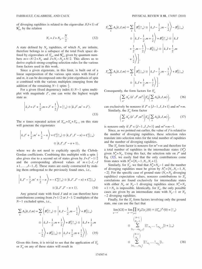
best understood by looking at the g evolution of the rapidi-ties as shown in Fig. 2 for the three states in Fig. 1.

FIG. 1. Construction of the contiguous blocks necessary to es-tablish the g=0, g→� correspondence.

FIG. 2. �Color online� Evolution of the rapidities �real part�from 0 to large g for the states presented in Fig. 1.

DYNAMICAL CORRELATION FUNCTIONS OF THE… PHYSICAL REVIEW B 81, 174507 �2010�

174507-7

As g rises, each rapidity has a tendency to go down to-ward −�. Any block of Hi unoccupied states stops up to Hirapidities from doing so by keeping them finite. If Pi rapidi-ties are going down and they meet a block of Hi unoccupiedstates every rapidity will be kept finite if Hi� Pi �Ai=0rapidities will go through�. On the other hand, whenever Hi� Pi, only Hi rapidities can be kept finite and the remainingAi= Pi−Hi will keep going down toward −�. Starting fromthe highest block of rapidities �of size P1� we therefore haveA1= P1−min�P1 ,H1� which go through the H1 empty statesbelow. These will be added to the following block of P2rapidities giving P2+A1 rapidities which then meet a blockof H2 unoccupied states. A2= �P2+A1�−min�P2+A1 ,H2� willgo through and continue their descent. Keeping this analysisgoing until we reach the last blocks gives out the result givenabove.

2. Application to ground states and single excitation states

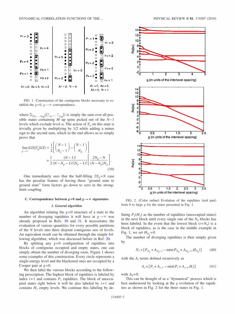
At g=0, for any of the canonical ground states containingNp rapidities in the Np lowest energy levels, we have a singleblock of unoccupied N−Np levels and a single block of Npoccupied levels �see the left group in Fig. 3�. Since no unoc-cupied levels are below this Np-rapidities block, they wouldall diverge in the g→� limit.

Focusing on the states built out of a single excitationabove this ground state, we find three distinct cases.When one moves the top rapidity �from level Np� to a higherlevel �say, level ��Np�, the resulting block structure is�P1=1��H1=�−Np��P2=Np−1� �see middle group in Fig. 3�which leads in the strong-coupling limit to the single P1rapidity being kept finite while the remaining Np−1 will di-verge. In the second scenario, if one promotes any of therapidities at level ��Np �excluding the topmost one� to thelevel Np+1 the resulting structure is �P1=Np−�+1��H1=1��P2=�−1� �see the right group in Fig. 3�. Once again,this leads to one of the P1 rapidities staying finite due to theunoccupied block H1=1 while the other Np−1 rapidities willdiverge.

The last possible case is a single excitation obtained bymoving a rapidity from level ��Np into an empty level ��Np+1. Doing this gives the following block structure �P1=1��H1=�−Np−1��P2=Np−���H2=1��P3=�−1�. In theend the P1 rapidity will stay finite because of H1, and one ofthe P2 rapidities will remain finite as well, leading to a totalof two finite rapidities.

From very simple combinatorics we therefore find that wecan build N−1 single finite rapidity states �at g→�� by de-

forming g=0 two-particle states. Moreover, at g→� for agiven number of rapidities, the total number of states withJ=Np−1 �single finite rapidity� is given by the total numberof solutions to the single Bethe equation �i=1

N 1�−�i

=0.32 Thisequation also has N−1 distinct solutions and therefore everystate with a single finite rapidity at strong coupling stemsfrom one of the two-particle states at g=0. This was pointedout before in Refs. 30 and 31.

From the previous sections we concluded that for the S�z

form factors one can get contributions coming from the Nprapidities states with either Np or Np−1 of them diverging.The first case we now know corresponds to the ground state.Since we also showed that every state with one finite rapidityis generated by singly excited states, it becomes clear that thetwo-particle states do give out every nonzero contributions inthe g→� limit. For S�

− we showed that only the Np−1ground state �all rapidities divergent� or the Np−1 states withNp−2 diverging rapidities contribute. Once again this meansthat the intermediate sum can be limited to the Np−1 groundstate and single excitation �two-particle� states. One shouldalso notice that, in this limit, any single excitation statewhich leads to two finite rapidities will not contribute al-though at weaker coupling they could.

Since the complete set of two particle states �plus theground state� saturates the sum rules in both g→0 and g→� limits, it is reasonable to assume that they will also belargely dominant in the crossover regime. This fact will beexplicitly proven numerically since even for the smallest sys-tems, this subset represents, for any g, more than 99% of theweight.

V. DYNAMICAL CORRELATION FUNCTIONS

We have presented all the ingredients to calculate the dy-namical correlation functions: we need to solve the Richard-son equations for each state � w��, calculate its energy Ew,use the rapidities defining the solution to compute the deter-minant and calculate the form factors. However, while theformulas we obtained for the correlation functions are com-pletely general and are valid for any choice of the Hamil-tonian parameters �� and g, to obtain a physical result westill have to perform the sum over the states and this cannotbe done analytically. Thus we need to make a choice of themodel to study. As we already mentioned, we only considerthe most-studied case in the condensed-matter literature,which consists of N equidistant levels at half filling, i.e.,N=2Np. We define the levels as

�� = � with � = 1 . . . N , �42�

i.e., we measure the energy scale in terms of the interlevelspacing and we fix the Debye frequency �the largest energylevel� to N.

A. Diagonal Sz correlator

We start our analysis with the diagonal Sz correlator that,in frequency space, reads

FIG. 3. A ground state and the corresponding set of states whichgive a single finite rapidity at g→�.

FARIBAULT, CALABRESE, AND CAUX PHYSICAL REVIEW B 81, 174507 �2010�

174507-8

Gzzd � � = �

n=1

N

� v�

� v��Snz �GS��2

GS�GS� v�� v���� − Ev + EGS� �43�

with � v�� having N /2 rapidities. In particles language this isa density-density correlator. At any finite N, this is a sum of� peaks each at the energy of the excited state � v��, and eachweighted with the corresponding form factor.

In the thermodynamic limit where N→� while the inter-level spacing d→0 �keeping a finite bandwidth for thesingle-particle excitations�, we can think of any g�0 as be-ing already the strong-coupling case, i.e., the BCS mean-field treatment becomes exact. In such a case correlationfunctions should be described by the g→� limit where onlythe single finite rapidity band would contribute. However, weare interested here in mesoscopic effects at finite N, that areencoded in the quantization of the energy levels and in thepotential presence of nontrivial contribution from other ex-cited states.

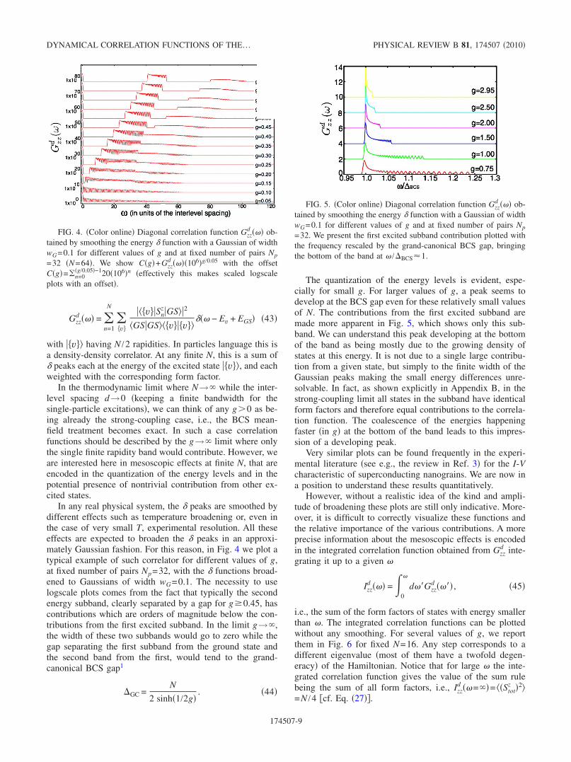
In any real physical system, the � peaks are smoothed bydifferent effects such as temperature broadening or, even inthe case of very small T, experimental resolution. All theseeffects are expected to broaden the � peaks in an approxi-mately Gaussian fashion. For this reason, in Fig. 4 we plot atypical example of such correlator for different values of g,at fixed number of pairs Np=32, with the � functions broad-ened to Gaussians of width wG=0.1. The necessity to uselogscale plots comes from the fact that typically the secondenergy subband, clearly separated by a gap for g�0.45, hascontributions which are orders of magnitude below the con-tributions from the first excited subband. In the limit g→�,the width of these two subbands would go to zero while thegap separating the first subband from the ground state andthe second band from the first, would tend to the grand-canonical BCS gap1

�GC =N

2 sinh�1/2g�. �44�

The quantization of the energy levels is evident, espe-cially for small g. For larger values of g, a peak seems todevelop at the BCS gap even for these relatively small valuesof N. The contributions from the first excited subband aremade more apparent in Fig. 5, which shows only this sub-band. We can understand this peak developing at the bottomof the band as being mostly due to the growing density ofstates at this energy. It is not due to a single large contribu-tion from a given state, but simply to the finite width of theGaussian peaks making the small energy differences unre-solvable. In fact, as shown explicitly in Appendix B, in thestrong-coupling limit all states in the subband have identicalform factors and therefore equal contributions to the correla-tion function. The coalescence of the energies happeningfaster �in g� at the bottom of the band leads to this impres-sion of a developing peak.

Very similar plots can be found frequently in the experi-mental literature �see e.g., the review in Ref. 3� for the I-Vcharacteristic of superconducting nanograins. We are now ina position to understand these results quantitatively.

However, without a realistic idea of the kind and ampli-tude of broadening these plots are still only indicative. More-over, it is difficult to correctly visualize these functions andthe relative importance of the various contributions. A moreprecise information about the mesoscopic effects is encodedin the integrated correlation function obtained from Gzz

d inte-grating it up to a given

Izzd � � = �

0

d �Gzzd � �� , �45�

i.e., the sum of the form factors of states with energy smallerthan . The integrated correlation functions can be plottedwithout any smoothing. For several values of g, we reportthem in Fig. 6 for fixed N=16. Any step corresponds to adifferent eigenvalue �most of them have a twofold degen-eracy� of the Hamiltonian. Notice that for large the inte-grated correlation function gives the value of the sum rulebeing the sum of all form factors, i.e., Izz

d � =��= �Stotz �2�

=N /4 �cf. Eq. �27��.

FIG. 4. �Color online� Diagonal correlation function Gzzd � � ob-

tained by smoothing the energy � function with a Gaussian of widthwG=0.1 for different values of g and at fixed number of pairs Np

=32 �N=64�. We show C�g�+Gzzd � ��106�g/0.05 with the offset

C�g�=�n=0�g/0.05�−120�106�n �effectively this makes scaled logscale

plots with an offset�.

FIG. 5. �Color online� Diagonal correlation function Gzzd � � ob-

tained by smoothing the energy � function with a Gaussian of widthwG=0.1 for different values of g and at fixed number of pairs Np

=32. We present the first excited subband contribution plotted withthe frequency rescaled by the grand-canonical BCS gap, bringingthe bottom of the band at /�BCS�1.

DYNAMICAL CORRELATION FUNCTIONS OF THE… PHYSICAL REVIEW B 81, 174507 �2010�

174507-9

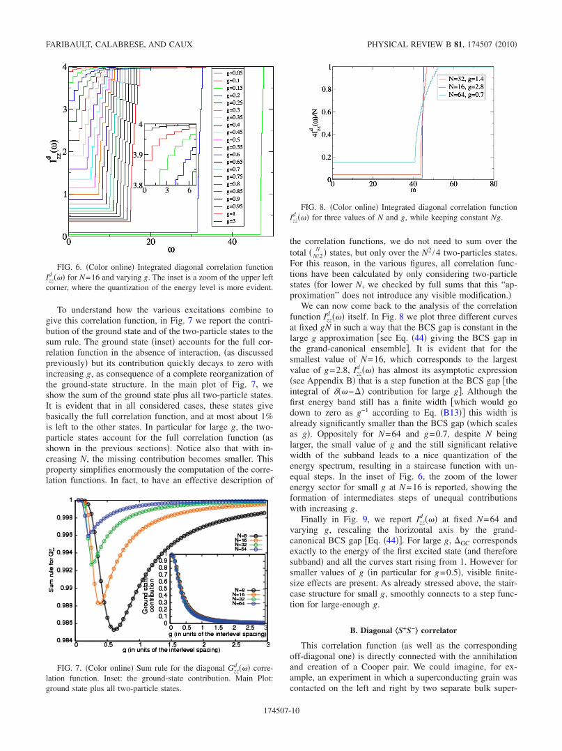
To understand how the various excitations combine togive this correlation function, in Fig. 7 we report the contri-bution of the ground state and of the two-particle states to thesum rule. The ground state �inset� accounts for the full cor-relation function in the absence of interaction, �as discussedpreviously� but its contribution quickly decays to zero withincreasing g, as consequence of a complete reorganization ofthe ground-state structure. In the main plot of Fig. 7, weshow the sum of the ground state plus all two-particle states.It is evident that in all considered cases, these states givebasically the full correlation function, and at most about 1%is left to the other states. In particular for large g, the two-particle states account for the full correlation function �asshown in the previous sections�. Notice also that with in-creasing N, the missing contribution becomes smaller. Thisproperty simplifies enormously the computation of the corre-lation functions. In fact, to have an effective description of

the correlation functions, we do not need to sum over thetotal � N

N/2 � states, but only over the N2 /4 two-particles states.For this reason, in the various figures, all correlation func-tions have been calculated by only considering two-particlestates �for lower N, we checked by full sums that this “ap-proximation” does not introduce any visible modification.�

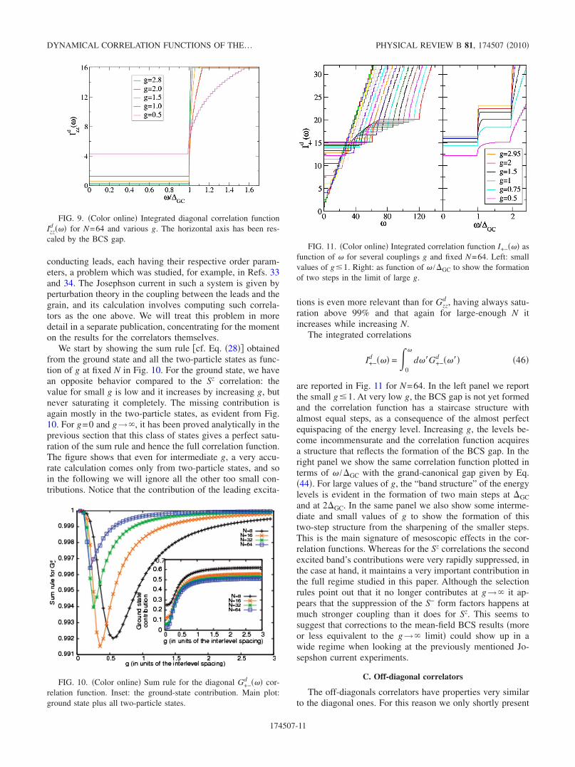
We can now come back to the analysis of the correlationfunction Izz

d � � itself. In Fig. 8 we plot three different curvesat fixed gN in such a way that the BCS gap is constant in thelarge g approximation �see Eq. �44� giving the BCS gap inthe grand-canonical ensemble�. It is evident that for thesmallest value of N=16, which corresponds to the largestvalue of g=2.8, Izz

d � � has almost its asymptotic expression�see Appendix B� that is a step function at the BCS gap �theintegral of �� −�� contribution for large g�. Although thefirst energy band still has a finite width �which would godown to zero as g−1 according to Eq. �B13�� this width isalready significantly smaller than the BCS gap �which scalesas g�. Oppositely for N=64 and g=0.7, despite N beinglarger, the small value of g and the still significant relativewidth of the subband leads to a nice quantization of theenergy spectrum, resulting in a staircase function with un-equal steps. In the inset of Fig. 6, the zoom of the lowerenergy sector for small g at N=16 is reported, showing theformation of intermediates steps of unequal contributionswith increasing g.

Finally in Fig. 9, we report Izzd � � at fixed N=64 and

varying g, rescaling the horizontal axis by the grand-canonical BCS gap �Eq. �44��. For large g, �GC correspondsexactly to the energy of the first excited state �and thereforesubband� and all the curves start rising from 1. However forsmaller values of g �in particular for g=0.5�, visible finite-size effects are present. As already stressed above, the stair-case structure for small g, smoothly connects to a step func-tion for large-enough g.

B. Diagonal ŠS+S−‹ correlator

This correlation function �as well as the correspondingoff-diagonal one� is directly connected with the annihilationand creation of a Cooper pair. We could imagine, for ex-ample, an experiment in which a superconducting grain wascontacted on the left and right by two separate bulk super-

FIG. 6. �Color online� Integrated diagonal correlation functionIzzd � � for N=16 and varying g. The inset is a zoom of the upper left

corner, where the quantization of the energy level is more evident.

FIG. 7. �Color online� Sum rule for the diagonal Gzzd � � corre-

lation function. Inset: the ground-state contribution. Main Plot:ground state plus all two-particle states.

FIG. 8. �Color online� Integrated diagonal correlation functionIzzd � � for three values of N and g, while keeping constant Ng.

FARIBAULT, CALABRESE, AND CAUX PHYSICAL REVIEW B 81, 174507 �2010�

174507-10

conducting leads, each having their respective order param-eters, a problem which was studied, for example, in Refs. 33and 34. The Josephson current in such a system is given byperturbation theory in the coupling between the leads and thegrain, and its calculation involves computing such correla-tors as the one above. We will treat this problem in moredetail in a separate publication, concentrating for the momenton the results for the correlators themselves.

We start by showing the sum rule �cf. Eq. �28�� obtainedfrom the ground state and all the two-particle states as func-tion of g at fixed N in Fig. 10. For the ground state, we havean opposite behavior compared to the Sz correlation: thevalue for small g is low and it increases by increasing g, butnever saturating it completely. The missing contribution isagain mostly in the two-particle states, as evident from Fig.10. For g=0 and g→�, it has been proved analytically in theprevious section that this class of states gives a perfect satu-ration of the sum rule and hence the full correlation function.The figure shows that even for intermediate g, a very accu-rate calculation comes only from two-particle states, and soin the following we will ignore all the other too small con-tributions. Notice that the contribution of the leading excita-

tions is even more relevant than for Gzzd , having always satu-

ration above 99% and that again for large-enough N itincreases while increasing N.

The integrated correlations

I+−d � � = �

0

d �G+−d � �� �46�

are reported in Fig. 11 for N=64. In the left panel we reportthe small g�1. At very low g, the BCS gap is not yet formedand the correlation function has a staircase structure withalmost equal steps, as a consequence of the almost perfectequispacing of the energy level. Increasing g, the levels be-come incommensurate and the correlation function acquiresa structure that reflects the formation of the BCS gap. In theright panel we show the same correlation function plotted interms of /�GC with the grand-canonical gap given by Eq.�44�. For large values of g, the “band structure” of the energylevels is evident in the formation of two main steps at �GCand at 2�GC. In the same panel we also show some interme-diate and small values of g to show the formation of thistwo-step structure from the sharpening of the smaller steps.This is the main signature of mesoscopic effects in the cor-relation functions. Whereas for the Sz correlations the secondexcited band’s contributions were very rapidly suppressed, inthe case at hand, it maintains a very important contribution inthe full regime studied in this paper. Although the selectionrules point out that it no longer contributes at g→� it ap-pears that the suppression of the S− form factors happens atmuch stronger coupling than it does for Sz. This seems tosuggest that corrections to the mean-field BCS results �moreor less equivalent to the g→� limit� could show up in awide regime when looking at the previously mentioned Jo-sepshon current experiments.

C. Off-diagonal correlators

The off-diagonals correlators have properties very similarto the diagonal ones. For this reason we only shortly present

FIG. 9. �Color online� Integrated diagonal correlation functionIzzd � � for N=64 and various g. The horizontal axis has been res-

caled by the BCS gap.

FIG. 10. �Color online� Sum rule for the diagonal G+−d � � cor-

relation function. Inset: the ground-state contribution. Main plot:ground state plus all two-particle states.

FIG. 11. �Color online� Integrated correlation function I+−� � asfunction of for several couplings g and fixed N=64. Left: smallvalues of g�1. Right: as function of /�GC to show the formationof two steps in the limit of large g.

DYNAMICAL CORRELATION FUNCTIONS OF THE… PHYSICAL REVIEW B 81, 174507 �2010�

174507-11

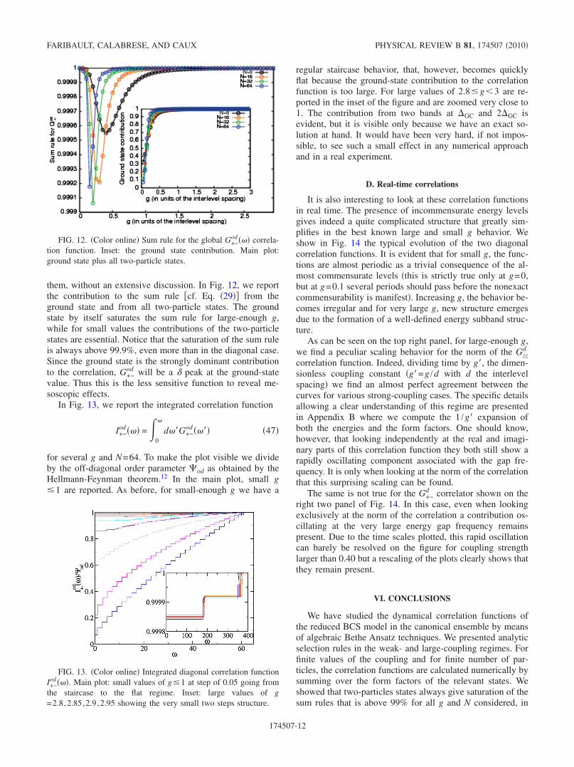
them, without an extensive discussion. In Fig. 12, we reportthe contribution to the sum rule �cf. Eq. �29�� from theground state and from all two-particle states. The groundstate by itself saturates the sum rule for large-enough g,while for small values the contributions of the two-particlestates are essential. Notice that the saturation of the sum ruleis always above 99.9%, even more than in the diagonal case.Since the ground state is the strongly dominant contributionto the correlation, G+−

od will be a � peak at the ground-statevalue. Thus this is the less sensitive function to reveal me-soscopic effects.

In Fig. 13, we report the integrated correlation function

I+−od � � = �

0

d �G+−od � �� �47�

for several g and N=64. To make the plot visible we divideby the off-diagonal order parameter �od as obtained by theHellmann-Feynman theorem.12 In the main plot, small g�1 are reported. As before, for small-enough g we have a

regular staircase behavior, that, however, becomes quicklyflat because the ground-state contribution to the correlationfunction is too large. For large values of 2.8�g�3 are re-ported in the inset of the figure and are zoomed very close to1. The contribution from two bands at �GC and 2�GC isevident, but it is visible only because we have an exact so-lution at hand. It would have been very hard, if not impos-sible, to see such a small effect in any numerical approachand in a real experiment.

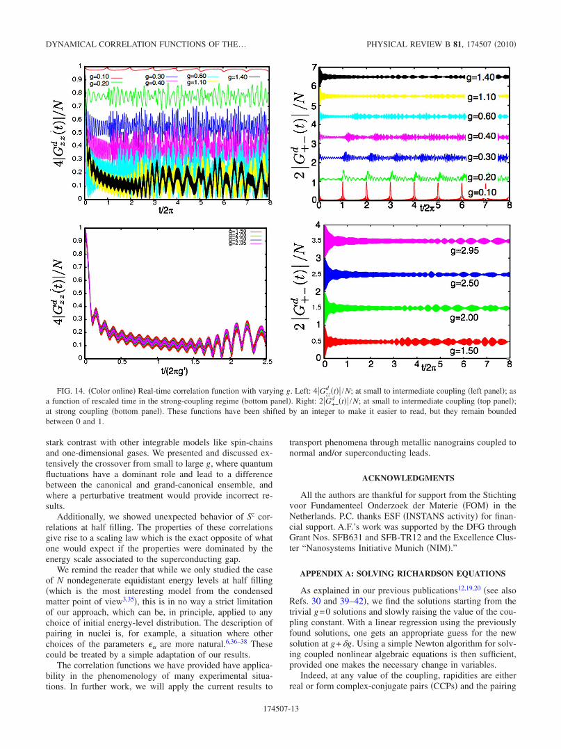
D. Real-time correlations

It is also interesting to look at these correlation functionsin real time. The presence of incommensurate energy levelsgives indeed a quite complicated structure that greatly sim-plifies in the best known large and small g behavior. Weshow in Fig. 14 the typical evolution of the two diagonalcorrelation functions. It is evident that for small g, the func-tions are almost periodic as a trivial consequence of the al-most commensurate levels �this is strictly true only at g=0,but at g=0.1 several periods should pass before the nonexactcommensurability is manifest�. Increasing g, the behavior be-comes irregular and for very large g, new structure emergesdue to the formation of a well-defined energy subband struc-ture.

As can be seen on the top right panel, for large-enough g,we find a peculiar scaling behavior for the norm of the Gzz

d

correlation function. Indeed, dividing time by g�, the dimen-sionless coupling constant �g�=g /d with d the interlevelspacing� we find an almost perfect agreement between thecurves for various strong-coupling cases. The specific detailsallowing a clear understanding of this regime are presentedin Appendix B where we compute the 1 /g� expansion ofboth the energies and the form factors. One should know,however, that looking independently at the real and imagi-nary parts of this correlation function they both still show arapidly oscillating component associated with the gap fre-quency. It is only when looking at the norm of the correlationthat this surprising scaling can be found.

The same is not true for the G+−d correlator shown on the

right two panel of Fig. 14. In this case, even when lookingexclusively at the norm of the correlation a contribution os-cillating at the very large energy gap frequency remainspresent. Due to the time scales plotted, this rapid oscillationcan barely be resolved on the figure for coupling strengthlarger than 0.40 but a rescaling of the plots clearly shows thatthey remain present.

VI. CONCLUSIONS

We have studied the dynamical correlation functions ofthe reduced BCS model in the canonical ensemble by meansof algebraic Bethe Ansatz techniques. We presented analyticselection rules in the weak- and large-coupling regimes. Forfinite values of the coupling and for finite number of par-ticles, the correlation functions are calculated numerically bysumming over the form factors of the relevant states. Weshowed that two-particles states always give saturation of thesum rules that is above 99% for all g and N considered, in

FIG. 12. �Color online� Sum rule for the global G+−od � � correla-

tion function. Inset: the ground state contribution. Main plot:ground state plus all two-particle states.

FIG. 13. �Color online� Integrated diagonal correlation functionI+−od � �. Main plot: small values of g�1 at step of 0.05 going from

the staircase to the flat regime. Inset: large values of g=2.8,2.85,2.9,2.95 showing the very small two steps structure.

FARIBAULT, CALABRESE, AND CAUX PHYSICAL REVIEW B 81, 174507 �2010�

174507-12

stark contrast with other integrable models like spin-chainsand one-dimensional gases. We presented and discussed ex-tensively the crossover from small to large g, where quantumfluctuations have a dominant role and lead to a differencebetween the canonical and grand-canonical ensemble, andwhere a perturbative treatment would provide incorrect re-sults.

Additionally, we showed unexpected behavior of Sz cor-relations at half filling. The properties of these correlationsgive rise to a scaling law which is the exact opposite of whatone would expect if the properties were dominated by theenergy scale associated to the superconducting gap.

We remind the reader that while we only studied the caseof N nondegenerate equidistant energy levels at half filling�which is the most interesting model from the condensedmatter point of view3,35�, this is in no way a strict limitationof our approach, which can be, in principle, applied to anychoice of initial energy-level distribution. The description ofpairing in nuclei is, for example, a situation where otherchoices of the parameters �� are more natural.6,36–38 Thesecould be treated by a simple adaptation of our results.

The correlation functions we have provided have applica-bility in the phenomenology of many experimental situa-tions. In further work, we will apply the current results to

transport phenomena through metallic nanograins coupled tonormal and/or superconducting leads.

ACKNOWLEDGMENTS

All the authors are thankful for support from the Stichtingvoor Fundamenteel Onderzoek der Materie �FOM� in theNetherlands. P.C. thanks ESF �INSTANS activity� for finan-cial support. A.F.’s work was supported by the DFG throughGrant Nos. SFB631 and SFB-TR12 and the Excellence Clus-ter “Nanosystems Initiative Munich �NIM�.”

APPENDIX A: SOLVING RICHARDSON EQUATIONS

As explained in our previous publications12,19,20 �see alsoRefs. 30 and 39–42�, we find the solutions starting from thetrivial g=0 solutions and slowly raising the value of the cou-pling constant. With a linear regression using the previouslyfound solutions, one gets an appropriate guess for the newsolution at g+�g. Using a simple Newton algorithm for solv-ing coupled nonlinear algebraic equations is then sufficient,provided one makes the necessary change in variables.

Indeed, at any value of the coupling, rapidities are eitherreal or form complex-conjugate pairs �CCPs� and the pairing

FIG. 14. �Color online� Real-time correlation function with varying g. Left: 4�Gzzd �t�� /N; at small to intermediate coupling �left panel�; as

a function of rescaled time in the strong-coupling regime �bottom panel�. Right: 2�G+−d �t�� /N; at small to intermediate coupling �top panel�;

at strong coupling �bottom panel�. These functions have been shifted by an integer to make it easier to read, but they remain boundedbetween 0 and 1.

DYNAMICAL CORRELATION FUNCTIONS OF THE… PHYSICAL REVIEW B 81, 174507 �2010�

174507-13

of two rapidities only occurs at bifurcation points g� at whichthey are both exactly worth �c, i.e., one of the single-particleenergy levels. It is also possible, as g is increased, that twopaired rapidities split apart becoming both real again. At acritical g� where a pair splits or forms, the derivatives

dwi

dg arenot defined making the computation of the necessary Jaco-bian impossible. This problem is easily circumvented by, inthe vicinity of critical point at which wi=wj =�c, making thefollowing change in variables:

�+ = wi + wj ,

�− = �wi − wj�2. �A1�

On both sides of g�, those are two real variables and theyhave well-defined derivatives even at the bifurcation point.The fact that g is slowly increased allows us to figure outbeforehand whether given rapidities are about to form �orbreak� complex-conjugate pairs. Naturally, it makes the nu-merical procedure more tedious than it would be if one wasable to guess correctly the structure at the precise value of gin which we are interested. However the lack of known ana-lytical results about the solutions to these precise Bethe

equations forces us to use this scanning procedure. Fortu-nately, for the dynamical correlations we only need a veryrestricted set of states in order to get a very accurate descrip-tion. Since single solutions are addressed one by one inde-pendently of the dimension of the full Hilbert space, theproblem remains numerically tractable for fairly large systemsizes which matrix diagonalization could not tackle.

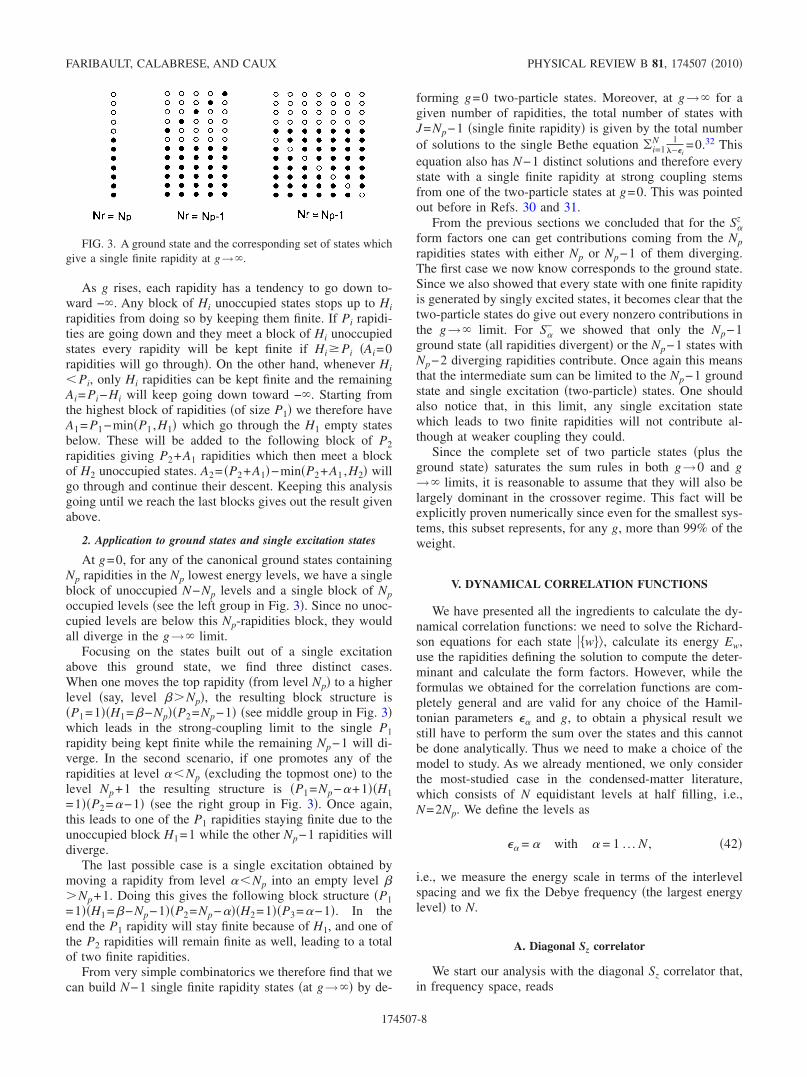
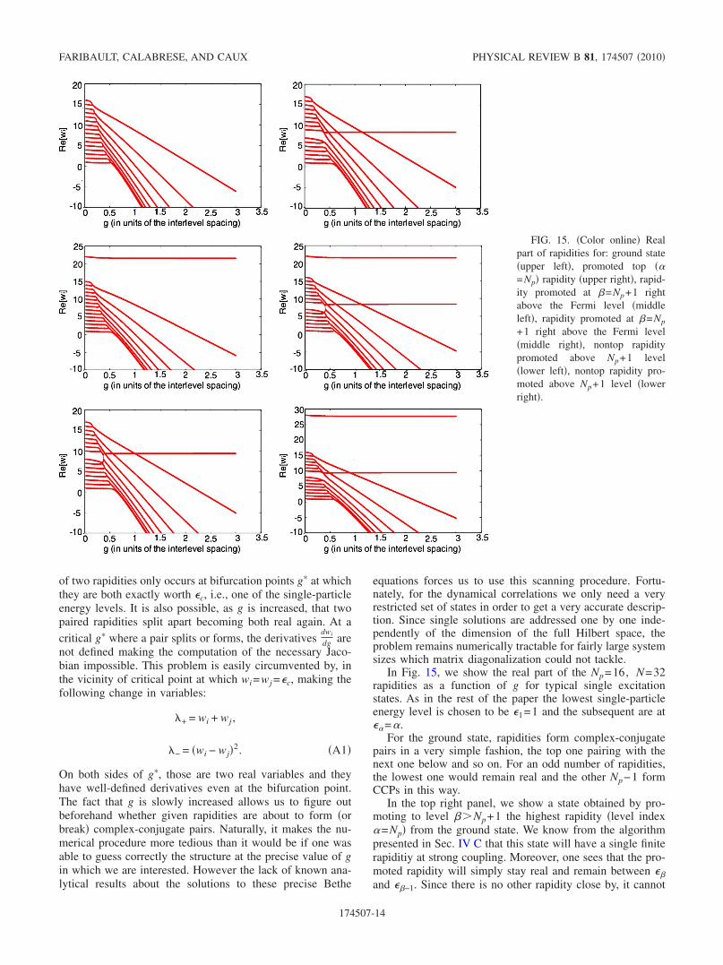
In Fig. 15, we show the real part of the Np=16, N=32rapidities as a function of g for typical single excitationstates. As in the rest of the paper the lowest single-particleenergy level is chosen to be �1=1 and the subsequent are at��=�.

For the ground state, rapidities form complex-conjugatepairs in a very simple fashion, the top one pairing with thenext one below and so on. For an odd number of rapidities,the lowest one would remain real and the other Np−1 formCCPs in this way.

In the top right panel, we show a state obtained by pro-moting to level ��Np+1 the highest rapidity �level index�=Np� from the ground state. We know from the algorithmpresented in Sec. IV C that this state will have a single finiterapiditiy at strong coupling. Moreover, one sees that the pro-moted rapidity will simply stay real and remain between ��

and ��−1. Since there is no other rapidity close by, it cannot

FIG. 15. �Color online� Realpart of rapidities for: ground state�upper left�, promoted top ��=Np� rapidity �upper right�, rapid-ity promoted at �=Np+1 rightabove the Fermi level �middleleft�, rapidity promoted at �=Np

+1 right above the Fermi level�middle right�, nontop rapiditypromoted above Np+1 level�lower left�, nontop rapidity pro-moted above Np+1 level �lowerright�.

FARIBAULT, CALABRESE, AND CAUX PHYSICAL REVIEW B 81, 174507 �2010�

174507-14

form a pair to go through the energy level ��−1. Indeed, thestructure of the Richardson equations prevents a single rapid-ity to be equal to an energy level �c since the diverging term

1wi−�c

has to be cancelled by a diverging term −2wi−wj

. The re-maining rapidities will simply form CCPs as they would fora Np−1 pairs ground state.

The two figures in the middle are built by promoting arapidity with index ��Np to level �=Np+1. In both cases,we find only a single finite rapidity at strong coupling but westill have two different scenarios. The top contiguous blockhas an even �odd� number of rapidity on the left �right�panel. For an odd number of rapidities in the top block, thelowest one from that block will simply stay real and between��+1 and ��. In the even case, the lowest two rapidities fromthe top block will actually form a pair at the energy level�+1, then split apart into two real rapidities at level �. Thissplitting will make one rapidity be above �� where it willstay until g→� while the other one goes below �� and willlater form a pair with the top rapidity from the block under-neath.

Finally, the lowest panels which lead to two finite rapidi-ties at strong coupling behave in a similar way for the lowestNp−1 rapidities, whereas the promoted one stays finite in thesame way it did in the top right panel. At g→� the state withone single finite rapidity in between ��−1 and ��, for Np���N is the deformed version of the g=0 state built byexciting the ground state’s top rapidity wi=�Np

to level ��.On the other hand if the finite rapidity is between 1���Np and �+1 the state is the deformed version of g=0 stateobtained by promoting the ground state’s rapidity wi=�� tolevel �Np+1. The approximative location �between given en-ergy states� of these strong-coupling finite rapidities was al-ready know and used in32 to compute nonequilibrium dy-namics in the related central-spin model. However we hereshow how they each correspond to a known g=0 state de-formed by interactions.

APPENDIX B: STRONG COUPLING SCALING

Hand-waving arguments tend to lead to the idea that theexcitation gap should be the dominant energy scale in thissystem at least for strong coupling where one expects theBCS description to be more or less adequate. We wouldtherefore expect correlations in time to show strong oscilla-tions at a frequency given by the gap �i.e., �g in the strong-coupling limit�. Surprisingly, the SzSz correlations shown inFig. 14 actually show the exact opposite behavior. The mag-nitude of correlations do show scalable behavior but theyhappened to be slowed down by an increasing g and there-fore an increasing gap.

This appendix aims at understanding this peculiar scalingproperty. In order to do so, we can rely on the strong-coupling expansion of the Richardson equations. The follow-ing analysis will give us “semianalytical” �i.e., getting thenumerical values still needs numerical work� expressions forboth the energies and the form factors needed to understandthis correlator.

We assume a convergent expansion exists around the g→� point for the values of the rapidities themselves �Fig. 15

shows this assumption to be correct at strong-enough g�.Keeping only the first relevant corrections, we can writedown, for the three types of states we are interested in: �1�the ground state

wj = CjNpg + Aj + Bj

1

g∀ j = 1 . . . Np, �B1�

�2� the single finite rapidity states

��k = �k� + �k

1

g

wjk = Cj

Np−1g + Ajk + Bj

k1

g� ∀ j = 1 . . . Np − 1, �B2�

and �3� states with two finite rapidities

��1,k = �1,k

� + �1,k1

g

�2,k = �2,k� + �2,k

1

g

wjk = Cj

Np−2g + Aj�k + Bj�

k1

g

� ∀ j = 1 . . . Np − 2.

�B3�

In the last two cases we have, respectively, either N−1 or�Np�2−NpN−N−1 possible values of k each associated witha different possible solution of the Richardson equations �dif-ferent possible values of the � rapidities which remain fi-nite�. In all three cases, Eq. �31� gives the values of the Cconstants which define the diverging rapidities in the g→�limit which are therefore independent of the choice of finiterapidities values for any given k. One should understand thatg here is considered to be the dimensionless quantity g

d , dbeing the interlevel spacing.

1. Energies

The respective energies of these states, obtained by sum-ming the Np rapidities are therefore simply given by

EGS = �j=1

Np

CjNp�g + �

j=1

Np

Aj� + �j=1

Np

Bj�1

g, �B4�

Ek = �j=1

Np−1

CjNp−1�g + �k

� + �j=1

Np−1

Ajk� + �k + �

j=1

Np−1

Bjk�1

g,

�B5�

E�1,k,�2,k= �

j=1

Np−2

CjNp−2�g + �1,k

� + �2,k� + �

j=1

Np−2

Aj�k�

+ �1,k + �2,k + �j=1

Np−2

Bj�k�1

g. �B6�

The expansion of the Richardson equations around thestrong-coupling solutions with a single finite rapidity givesus

DYNAMICAL CORRELATION FUNCTIONS OF THE… PHYSICAL REVIEW B 81, 174507 �2010�

174507-15

− j

g= �

�=1

N1

1 −��

j

− 2 �j��j

Np−1 j

j − j�− 2

1

1 −�k

j

, �B7�

− CjNp−1 − Aj

k1

g� �N − 2� − 2 �

j��j

Np−1Cj

Np−1

CjNp−1 − Cj�

Np−1

+ ���=1

N

��� − 2�k�� 1

CjNp−1g

�+ 2 �

j��j

Np−1 �Cj�Np−1Aj

k − Aj�k Cj

Np−1�

�CjNp−1 − Cj�

Np−1�2

1

g. �B8�

Which, order by order gives

− CjNp−1 = �N − 2� − 2 �

j��j

Np−1Cj

Np−1

CjNp−1 − Cj�

Np−1 , �B9�

− Ajk = ��

�=1

N

��� − 2�k�� 1

CjNp−1

+ 2 �j��j

Np−1 �Cj�Np−1Aj

k − Aj�k Cj

Np−1�

�CjNp−1 − Cj�

Np−1�2. �B10�

These equations are defined for any of the Np−1 values ofindex j. Summing up the Np−1 �Eq. �B9�� �divided byCj

Np−1�, we find

− �Np − 1� = �N − 2��j

1

CjNp−1 , �B11�

while summing up the Eq. �B10� gives us

− �j

Ajk = ��

�=1

N

��� − 2�k���

j

1

CjNp−1 ,

�j

Ajk = ��

�=1

N

��� − 2�k�� �Np − 1�

�N − 2�. �B12�

Using this last expression, the energies of every single finiterapidity state can be written including the lowest correctionin 1

g as

Ek = �j=1

Np−1

CjNp−1�g + ��k

��N − 2Np

N − 2+ �

j=1

Np−1

�Bjk�

1

g+ O� 1

g2� .

�B13�

This shows that the half-filled case leads to the completeenergy collapse of the first excited band as proven before inRef. 27, i.e., lim

g→�

Ek−Ek�=0. The zero bandwidth obtained in

this specific case will be shown to be one of the centralelements in the scaling properties of the Sz operators dynami-cal correlations.

2. Eigenstates

In order to establish a similar expansion for the statesthemselves, one can simply use their representation as a Be-the state �Eq. �11�� and expand the C operators used to con-struct them. Keeping terms up to order 1

g for both divergent�w=Cg+A+ B

g � and finite ��=��+ �g � rapidities we have

C�w� � ��=1

NS�

+

w − ��

=1

Cg��=1

N

S�+1 +

�� − A

C

1

g�

=1

CgStot

+ −1

g

A

CStot

+ +1

g

1

C ��=1

N

��S�+� ,

C��� � ��=1

N

S�+ 1

�� − ��

−1

g

�

��� − ���2� . �B14�

By getting rid of the 1Cg prefactors which, for physical quan-

tities, will always be cancelled by equivalent factors in thenorms, we can therefore write

�GS� � �GSNp� +1

g��=1

N

G�S�+�GSNp−1� , �B15�

��k� � ��=1

N

F�k S�

+�GSNp−1� +1

g�

�,�=1

N

G�,�k S�

+S�+�GSNp−2� ,

�B16�

��1,k,�2,k� � ��,�=1

N

F�,�k S�

+S�+�GSNp−2�

+1

g�

�,�,�=1

N

G�,�,�k S�

+S�+S�

+�GSNp−3� , �B17�

where the states �GSM���Stot+ �M�0�. The following set of

definitions was also used:

G� ��j=1

Np Aj

CjNp� + �

j=1

Np 1

CjNp���,

F�k �

1

�k� − ��

,

G�,�k � − �

j�=1

Np−1 Aj�k

Cj�Np−1� 1

�k� − ��

−�k

��k� − ���2

+ �j�=1

Np−11

Cj�Np−1� ��

��k� − ���2 ,

F�,�k �

1

�1,k� − ��

1

�2,k� − ��

,

FARIBAULT, CALABRESE, AND CAUX PHYSICAL REVIEW B 81, 174507 �2010�

174507-16

G�,�,�k � −

�2,k

��2,k� − ���2

1

�1,k� − ��

−�1,k

��1,k� − ���2

1

�2,k� − ��

− �j�=1

Np−2 Aj�k

Cj�Np−2� 1

�1,k� − ��

1

�2,k� − ��

+ �j�=1

Np−21

Cj�Np−2� ��

��1,k� − �����2,k

� − ���. �B18�

3. Form factors

At g→� it is straightforward to compute value of thevarious forms factors. For the ground state it was done pre-

viously �Eq. �39��. Although the first-order correction canalso be obtained in a similar fashion, we will not explicitlyneed the coefficients of the expansion and therefore simplywrite

GS�S�z �GS� �

1

2� N − 1

Np − 1� − �N − 1

Np�� +

1

gA�

�B19�

with A� an unspecified �although obtainable� constant.Identically, for single finite rapidity states we can write

GS�S�z ��k�g→� = �

�

F�k GSNp�S�

z S�+�GSNp−1�

= ����

F�k GSNp��1

2�↑�,↑�� � �

�1,. . .�Np−2�

� N−2

Np−2�

� ↑�1. . . ↑�Np−2

�� −1

2�↑�,↓�� � �

�1,. . .�Np−1�

� N−2

Np−1�

� ↑�1. . . ↑�Np−1

���+ F�

k 1

2GSNp���↑�� � �

�1,. . .�Np−1�

� N−1

Np−1�

� ↑�1. . . ↑�Np−1

��� =1

2 ����

F�k� N − 2

Np − 2� − � N − 2

Np − 1�� +

1

2F�

k� N − 1

Np − 1�

=1

2��

F�k� N − 2

Np − 2� − � N − 2

Np − 1�� +

1

2F�

k� N − 1

Np − 1� − � N − 2

Np − 2� + � N − 2

Np − 1�� . �B20�

The orthogonality of these states with the ground state also allows us to write

GS��k�g→� = ��

F�k GSNp���↑�� � �

�1,. . .,�Np−1�

� N−1

Np−1�

� ↑�1. . . ↑�Np−1

��� = � N − 1

Np − 1��

�

F�k� = 0, �B21�

and therefore, adding the next order term through an un-specified constant

GS�S�z ��k� �

F�k

2� N − 1

Np − 1� − � N − 2

Np − 2� + � N − 2

Np − 1�� +

B�k

g

= F�k �N − 2�!

�Np − 1�!�N − Np − 1�!+

B�k

g. �B22�

It was also proven in Sec. IV B that at g→� we haveGS�Sn

z ��1,k ,�2,k�g→�=0 and we therefore have

GS�S�z ��1,k,�2,k� �

C�k

g. �B23�

Finally one can similarly compute the squared norms of theground state and the single rapidity states.

GS�GS�g→� = � N

Np� , �B24�

�k��k�g→� = ��,�

F�k �F�

k ��GSNp−1�S�−S�

+�GSNp−1�

= ����

F�k �F�

k ��� N − 2

Np − 2� + �

�

�F�k �2� N − 1

Np − 1�

= ��,�

F�k �F�

k ��� N − 2

Np − 2� + �

�

�F�k �2� N − 1

Np − 1�

− � N − 2

Np − 2��

= 0 + ��

�F�k �2

�N − 2�!�Np − 1�!�N − Np − 1�!

. �B25�

DYNAMICAL CORRELATION FUNCTIONS OF THE… PHYSICAL REVIEW B 81, 174507 �2010�

174507-17

Specializing to the half-filled case, we find

��=1

N �GS�S�z �GS��2

GS�GS�GS�GS��

A

g2 , �B26�

��=1

N �GS�S�z ��k��2

GS�GS��k��k�� � N

4�N − 1�� + ��=1

N2 Re�F�

k B�k �

g��

�F�k �2

�N/2�!�N/2�!�N�!

+B

g2 , �B27�

��=1

N �GS�S�z ��1,k,�2,k��2

GS�GS��1,k,�2,k��1,k,�2,k��

C

g2 . �B28�

At order 0 in 1g we therefore find that the only N−1 nonzero contributions coming from the form factors �the ones involving

the single finite rapidity states� are actually all equal. At the next leading order the only contributions also come from the samereduced set of states.

Using Eq. �43� we can write the correlation function by summing over the N−1 possible values of �k. At order 1g , we have

Gzzd � � � �

k=1

N−1

�� − Ek + EGS��� N

4�N − 1�� + �n=1

N2 Re�Fn

kBnk�

g�i

�Fik�2

�N/2�!�N/2�!�N�! � , �B29�

whose Fourier transform gives us

Gzzd �t� � �

k=1

N−1

e−i�Ek−EGS�t�� N

4�N − 1�� + ��=1

N2 Re�F�

k B�k �

g��

�F�k �2

�N/2�!�N/2�!�N�! � . �B30�

Looking exclusively at the magnitude of the correlations and therefore at phase-independent properties of this correlator wehave

�Gzzd �t��2 � �

k,k�=1

N−1

e−i�Ek−Ek��t�� N

4�N − 1��2

+ � ��N/2�!�2

2�N − 1��N − 1�!�Re�

�=1

N

�F�k B�

k + F�k�B�

k��

g��

�F�k �2 � . �B31�

Since Eq. �B13� tells us that

Ek − Ek� ��k,k�

g, �B32�

we can write

�Gzzd �t��2 � �

k,k�=1

N−1

e−i�k,k��t/g��� N

4�N − 1��2

+ � ��N/2�!�2

2�N − 1��N − 1�!�Re�

n=1

N

�FnkBn

k + Fnk�Bn

k��

g�i

�Fik�2 � . �B33�

This shows that at strong-enough coupling the dominantterm

� N

4�N − 1��2

�k,k�=1

N−1

e−i�k,k��t/g� �B34�

is purely a function of tg . This fact is only true at half filling

where the ground-state average of any S�z is zero. Moreover,

half filling also allows fulfillment of the second necessarycondition, the vanishing of width of the first excited band.The first effect makes the energy scale associated to the BCSgap irrelevant since only the first band of excited states iscontributing to the correlations. The vanishing width of this

FARIBAULT, CALABRESE, AND CAUX PHYSICAL REVIEW B 81, 174507 �2010�

174507-18

band is then responsible for the “inverted scaling” by makingthe relevant energy differences smaller as g increases.

This very peculiar half-filling scaling property makes itpossible to slow down specific dynamical processes in thissystem by making the interaction stronger. Since they areonly related to the spectrum and the condition GS�S�

z �GS�=0, this scaling law would hold at half filling for any pos-sible correlations of S�

z operators; be they local, global, in-tralevel or interlevel correlations. The magnitude of any one

of the possible correlations would still follow a similarlyscalable time evolution.

Although clearly valid in the strong g limit where 1g �1,

we also find through the numerical work carried out in thispaper that this scaling behavior extends to a very broad rangeof coupling constants. For g�1.5d with d the interlevelspacing, we find that 1

g corrections are already strongly sup-pressed and the scaling behavior is therefore already appar-ent.

1 J. Bardeen, L. N. Cooper, and J. R. Schrieffer, Phys. Rev. 106,162 �1957�; 108, 1175 �1957�.

2 D. C. Ralph, C. T. Black, and M. Tinkham, Phys. Rev. Lett. 74,3241 �1995�; C. T. Black, D. C. Ralph, and M. Tinkham, ibid.76, 688 �1996�; D. C. Ralph, C. T. Black, and M. Tinkham, ibid.78, 4087 �1997�.

3 J. von Delft and D. C. Ralph, Phys. Rep. 345, 61 �2001�.4 R. W. Richardson, Phys. Lett. 3, 277 �1963�; 5, 82 �1963�; R. W.

Richardson and N. Sherman, Nucl. Phys. 52, 221 �1964�; 52,253 �1964�.

5 J. Dukelsky, S. Pittel, and G. Sierra, Rev. Mod. Phys. 76, 643�2004�.

6 D. J. Dean and M. Hjorth-Jensen, Rev. Mod. Phys. 75, 607�2003�.

7 R. W. Richardson, J. Math. Phys. 6, 1034 �1965�.8 L. Amico and A. Osterloh, Phys. Rev. Lett. 88, 127003 �2002�.9 H.-Q. Zhou, J. Links, R. H. McKenzie, and M. D. Gould, Phys.

Rev. B 65, 060502�R� �2002�.10 J. Links, H.-Q. Zhou, R. H. McKenzie, and M. D. Gould, J.

Phys. A 36, R63 �2003�.11 N. A. Slavnov, Teor. Mat. Fiz. 79, 232 �1989�.12 A. Faribault, P. Calabrese, and J.-S. Caux, Phys. Rev. B 77,

064503 �2008�.13 A. Mastellone, G. Falci, and R. Fazio, Phys. Rev. Lett. 80, 4542

�1998�.14 S. Staudenmayer, W. Belzig, and C. Bruder, Phys. Rev. A 77,

013612 �2008�.15 J.-S. Caux and J. M. Maillet, Phys. Rev. Lett. 95, 077201

�2005�; J.-S. Caux, R. Hagemans, and J. M. Maillet, J. Stat.Mech.: Theory Exp. 2005, P09003.

16 V. Alba, M. Fagotti, and P. Calabrese, J. Stat. Mech.: TheoryExp. 2009, P10020.

17 J.-S. Caux and P. Calabrese, Phys. Rev. A 74, 031605�R� �2006�;J.-S. Caux, P. Calabrese, and N. A. Slavnov, J. Stat. Mech.:Theory Exp. 2007, P01008.

18 J.-S. Caux, J. Math. Phys. 50, 095214 �2009�.19 A. Faribault, P. Calabrese, and J.-S. Caux, J. Stat. Mech.: Theory

Exp. 2009, P03018.20 A. Faribault, P. Calabrese, and J.-S. Caux, J. Math. Phys. 50,

095212 �2009�.21 M. Gaudin, Modèles Exactement Résolus �Les Éditions de Phy-

sique, Les Ulis, France, 1995�.22 M. C. Cambiaggio, A. M. F. Rivas, and M. Saraceno, Nucl.

Phys. A 624, 157 �1997�.23 L. Amico, G. Falci, and R. Fazio, J. Phys. A 34, 6425 �2001�.24 J. von Delft and R. Poghossian, Phys. Rev. B 66, 134502 �2002�.25 J. von Delft, A. D. Zaikin, D. S. Golubev, and W. Tichy, Phys.

Rev. Lett. 77, 3189 �1996�.26 M. Schechter, Y. Imry, Y. Levinson, and J. von Delft, Phys. Rev.

B 63, 214518 �2001�.27 E. A. Yuzbashyan, A. A. Baytin, and B. L. Altshuler, Phys. Rev.

B 68, 214509 �2003�.28 E. A. Yuzbashyan, A. A. Baytin, and B. L. Altshuler, Phys. Rev.

B 71, 094505 �2005�.29 I. Snyman and H. B. Geyer, Phys. Rev. B 73, 144516 �2006�.30 J. M. Román, G. Sierra, and J. Dukelsky, Nucl. Phys. B 634,

483 �2002�.31 J. M. Román, G. Sierra, and J. Dukelsky, Phys. Rev. B 67,

064510 �2003�.32 M. Bortz and J. Stolze, Phys. Rev. B 76, 014304 �2007�.33 K. A. Matveev, M. Gisselfält, L. I. Glazman, M. Jonson, and R.

I. Shekhter, Phys. Rev. Lett. 70, 2940 �1993�.34 Y. Tanuma, Y. Tanaka, and K. Kusakabe, Physica E 40, 257

�2007�.35 J. Dukelsky and G. Sierra, Phys. Rev. Lett. 83, 172 �1999�; G.

Sierra, J. Dukelsky, G. G. Dussel, J. von Delft, and F. Braun,Phys. Rev. B 61, R11890 �2000�.

36 A. Belic, D. J. Dean, and M. Hjorth-Jensen, Nucl. Phys. A 731,381 �2004�.

37 V. Zelevinsky and A. Volya, Nucl. Phys. A 752, 325 �2005�.38 T. Sumaryada and A. Volya, Phys. Rev. C 76, 024319 �2007�.39 R. W. Richardson, Phys. Rev. 141, 949 �1966�.40 M. Sambataro, Phys. Rev. C 75, 054314 �2007�.41 S. Rombouts, D. Van Neck, and J. Dukelsky, Phys. Rev. C 69,

061303�R� �2004�.42 F. Domínguez, C. Esebbag, and J. Dukelsky, J. Phys. A 39,

11349 �2006�.

DYNAMICAL CORRELATION FUNCTIONS OF THE… PHYSICAL REVIEW B 81, 174507 �2010�

174507-19