Embed Size (px)
Citation preview
Dynamical modelling, analysisand optimization of a floater
blanket for the Ocean Grazer.
Clemente Pinol, Sılvia
First supervisor: Bayu Jayawardhana
Second supervisor: Antonis I. Vakis
Master’s Thesis
Industrial Engineering
2014/2015
Abstract
The Ocean Grazer is a novel ocean energy collection and storage device, designedto extract and store multiple forms of ocean energy.
This work aims to study and model the interaction between sea waves andthe Ocean Grazer as well as to propose a model for its floater blanket. In thisline, simulations are performed to gain an insight into the dynamical behaviourof the whole system and to find out the configuration of the controllable variablethat enables to harvest the maximum amount of energy.
Contents
1 Introduction 31.1 Renewable Energy . . . . . . . . . . . . . . . . . . . . . . . . . . 31.2 Ocean energy . . . . . . . . . . . . . . . . . . . . . . . . . . . . . 51.3 Wave Energy Converters . . . . . . . . . . . . . . . . . . . . . . . 71.4 Ocean Grazer . . . . . . . . . . . . . . . . . . . . . . . . . . . . . 101.5 Goals of this thesis . . . . . . . . . . . . . . . . . . . . . . . . . . 13
2 Theoretical background 142.1 Water waves . . . . . . . . . . . . . . . . . . . . . . . . . . . . . . 14
2.1.1 Potential flow . . . . . . . . . . . . . . . . . . . . . . . . . 152.1.2 Linear waves . . . . . . . . . . . . . . . . . . . . . . . . . 182.1.3 Real waves . . . . . . . . . . . . . . . . . . . . . . . . . . 19
2.2 Wave loading . . . . . . . . . . . . . . . . . . . . . . . . . . . . . 212.2.1 Hydrostatic forces . . . . . . . . . . . . . . . . . . . . . . 212.2.2 Hydrodynamic forces . . . . . . . . . . . . . . . . . . . . . 222.2.3 Hydrodynamic coefficients . . . . . . . . . . . . . . . . . . 25
2.3 Wave energy . . . . . . . . . . . . . . . . . . . . . . . . . . . . . 29
3 Modelling 323.1 Description of the system . . . . . . . . . . . . . . . . . . . . . . 32
3.1.1 Buoy . . . . . . . . . . . . . . . . . . . . . . . . . . . . . . 343.1.2 Rod . . . . . . . . . . . . . . . . . . . . . . . . . . . . . . 343.1.3 Cylinder . . . . . . . . . . . . . . . . . . . . . . . . . . . . 343.1.4 Pistons . . . . . . . . . . . . . . . . . . . . . . . . . . . . 343.1.5 Reservoirs . . . . . . . . . . . . . . . . . . . . . . . . . . . 35
3.2 Models considered . . . . . . . . . . . . . . . . . . . . . . . . . . 373.2.1 Forces and loads . . . . . . . . . . . . . . . . . . . . . . . 373.2.2 System of equations . . . . . . . . . . . . . . . . . . . . . 46
4 Results and discussion 514.1 Simulation parameters and assumptions . . . . . . . . . . . . . . 514.2 Simulation I: A single pump . . . . . . . . . . . . . . . . . . . . . 53
4.2.1 Initial conditions . . . . . . . . . . . . . . . . . . . . . . . 534.2.2 Time histories: Displacements, pressure, forces and powers 54
1
CONTENTS
4.3 Simulation II: Multi-pump . . . . . . . . . . . . . . . . . . . . . . 624.3.1 Initial conditions . . . . . . . . . . . . . . . . . . . . . . . 634.3.2 Time histories: Displacements, pressure, forces and powers 64
4.4 Optimization . . . . . . . . . . . . . . . . . . . . . . . . . . . . . 72
5 Conclusions and Future work 74
A Matlab code 76A.1 Code simulation I and II . . . . . . . . . . . . . . . . . . . . . . . 76A.2 Code exhaustive search . . . . . . . . . . . . . . . . . . . . . . . 82
2
Chapter 1
Introduction
1.1 Renewable Energy
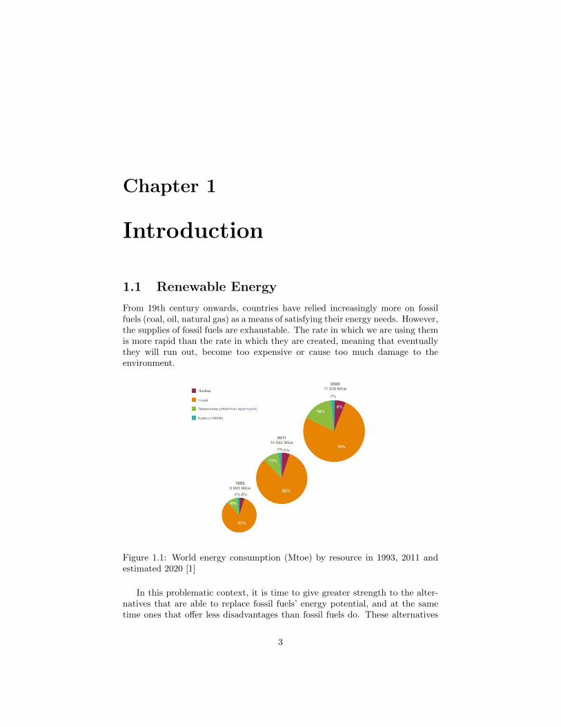
From 19th century onwards, countries have relied increasingly more on fossilfuels (coal, oil, natural gas) as a means of satisfying their energy needs. However,the supplies of fossil fuels are exhaustable. The rate in which we are using themis more rapid than the rate in which they are created, meaning that eventuallythey will run out, become too expensive or cause too much damage to theenvironment.
Figure 1.1: World energy consumption (Mtoe) by resource in 1993, 2011 andestimated 2020 [1]
In this problematic context, it is time to give greater strength to the alter-natives that are able to replace fossil fuels’ energy potential, and at the sametime ones that offer less disadvantages than fossil fuels do. These alternatives
3
1.1. RENEWABLE ENERGY
focus on the use and exploitation of renewable energy resources. Figure 1.1shows the evolution of the energy consumption by resource, it can be seen thatalthough in the last 10 years fossil fuels are the most consumed, the forecast forthe close future already considers that they will begin to decrease and renewableresources will grow.
The term “renewable” in terms of supplies means that something can bereplenished. Therefore, renewable energy uses sources that are continually re-plenished by nature (the sun, the wind, water, the Earth’s heat or plants). Dif-ferent technologies can be used to turn these fuels into usable forms of energy,not only electricity but also heat, chemicals or mechanical power.
Using renewable energy is not only beneficial because of its limitless suppliesbut also because it is less harmful for the environment. Renewable energytechnologies are commonly related to terms like “clean” or “green” because theyproduce fewer pollutants, whereas burning fossil fuels sends greenhouse gasesinto the atmosphere, trapping the sun’s heat and contributing to global warmingas well as releasing pollutants into the air, soil and water, then damaging theenvironment and humans themselves.
Most renewable energy can come either directly or indirectly from the sun.Solar energy can be used directly for heating, for generating electricity and fora variety of commercial and industrials uses.
The sun’s heat also drives the winds, whose energy can be harvested withwind turbines. Following this, the winds and the sun’s heat cause water toevaporate. When this water vapour turns into rain or snow and flows downhillinto rivers or streams, its energy can be captured using hydroelectric power.Along with the rain and snow, the sun also causes plants to grow. The organicmatter that makes up those plants is known as biomass. Biomass can be usedto produce electricity, transportation fuels, or chemicals. The use of biomassfor any of these purposes is called bioenergy.
But not all renewable energy resources come from the sun. Geothermalenergy exploits the Earth’s internal heat for a variety of uses, including electricpower production, and the heating and cooling of buildings. The energy of theocean’s tides come from the gravitational pull of the moon and the sun upon theEarth. In addition to tidal energy, there’s the energy of the ocean’s waves, whichare driven by both the tides and the winds. The sun also warms the surface ofthe ocean more than the ocean’s depths do so, creating a temperature differencethat can be used as an energy source. In summary, what is known as “oceanenergy” comes from a number of sources that are to be explained.
4
1.2. OCEAN ENERGY
1.2 Ocean energy
Oceans, covering over 70% of the Earth’s surface [2], are indeed an enormoussource of renewable energy. In 1799, oceans were first recognized as an energyresource as the first patent for harnessing ocean’s wave energy was proposed byMonsieur Girard [3].
Despite this early development, high costs of construction, deployment andmaintenance meant that the development of ocean technology staggered untilthe 1960s. Recently and because of the oil shortage crisis in 1973, the interest inrenewable energy grew and thus ocean energy was reconsidered as an alternativeenergy resource. Research and development of the ocean energy technologystarted again in the 1990s and it is still in its early developmental stages.
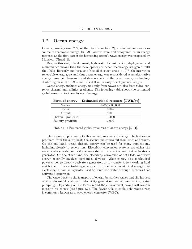
Ocean energy includes energy not only from waves but also from tides, cur-rents, thermal and salinity gradients. The following table shows the estimatedglobal resource for these forms of energy.
Form of energy Estimated global resource [TWh/yr]
Waves 8.000 - 80.000Tides 300+
Currents 800+Thermal gradients 10.000Salinity gradients 2.000
Table 1.1: Estimated global resources of ocean energy [3] [4].
The ocean can produce both thermal and mechanical energy. The first one isproduced from the sun’s heat; the second one comes out from tides and waves.On the one hand, ocean thermal energy can be used for many applications,including electricity generation. Electricity conversion systems use either thewarm surface water or boil the seawater to turn a turbine that activates agenerator. On the other hand, the electricity conversion of both tidal and waveenergy generally involves mechanical devices. Wave energy uses mechanicalpower either to directly activate a generator, or to transfer it to a working fluidwhich then drives a turbine/generator. In order to convert tidal energy intoelectricity, a dam is typically used to force the water through turbines thatactivate a generator.
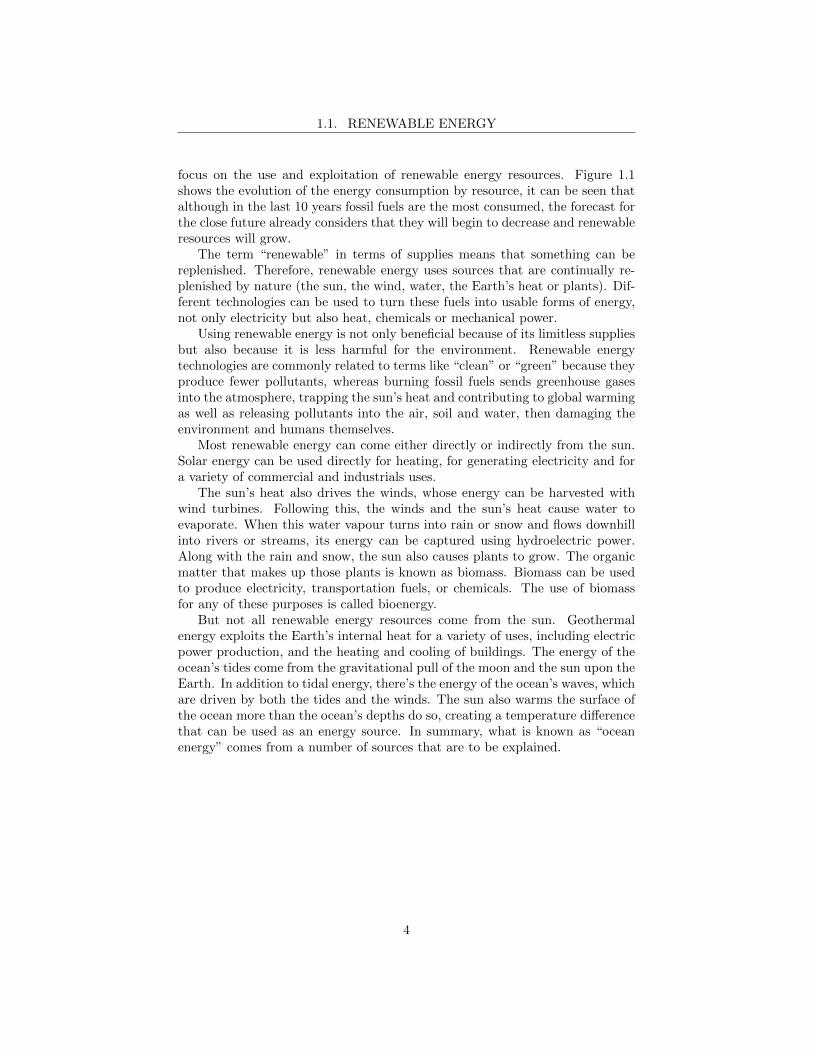
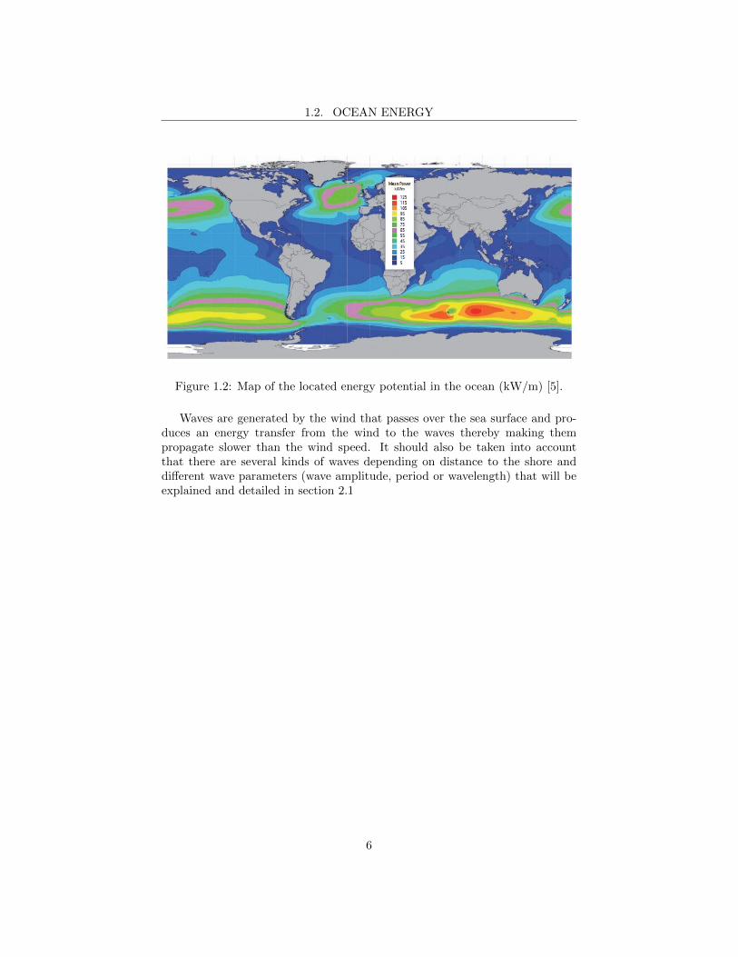
The wave power is the transport of energy by surface waves and the harvestof it to do useful work (e.g. electricity generation, water desalination, waterpumping). Depending on the location and the environment, waves will containmore or less energy (see figure 1.2). The device able to exploit the wave poweris commonly known as a wave energy converter (WEC).
5
1.2. OCEAN ENERGY
Figure 1.2: Map of the located energy potential in the ocean (kW/m) [5].
Waves are generated by the wind that passes over the sea surface and pro-duces an energy transfer from the wind to the waves thereby making thempropagate slower than the wind speed. It should also be taken into accountthat there are several kinds of waves depending on distance to the shore anddifferent wave parameters (wave amplitude, period or wavelength) that will beexplained and detailed in section 2.1
6
1.3. WAVE ENERGY CONVERTERS
1.3 Wave Energy Converters
Despite the fact that the field regarding ocean energy technologies is not yetdeeply developed, many studies and work are currently being done in differentuniversities and research institutions all over the world. The interest in renew-able energies (due to mainly oil crises and environmental problems) as well asthe ocean power potential are making the investments and research in waveenergy converters increase.
Wave energy converters can be classified depending on different criteria suchas their location in the ocean, their dimensions, their principle of operation ortheir energy capture system.
Looking into ocean characteristics, we will find that depending on the loca-tion and sea depth, waves will be different. So, in order to harvest the maximumamount of energy of these distinct waves, there will exist specific kinds of WECsthat will interact with them. These devices can be classified according to dif-ferent criteria listed above.
Installation site
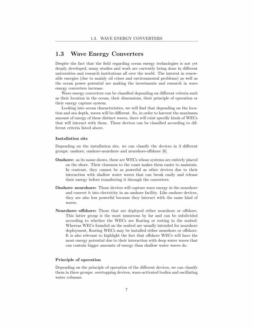
Depending on the installation site, we can classify the devices in 3 differentgroups: onshore, onshore-nearshore and nearshore-offshore [6].
Onshore: as its name shows, these are WECs whose systems are entirely placedon the shore. Their closeness to the coast makes them easier to maintain.In contrast, they cannot be as powerful as other devices due to theirinteraction with shallow water waves that can break easily and releasetheir energy before transferring it through the converters.
Onshore–nearshore: Those devices will capture wave energy in the nearshoreand convert it into electricity in an onshore facility. Like onshore devices,they are also less powerful because they interact with the same kind ofwaves.
Nearshore–offshore: Those that are deployed either nearshore or offshore.This latter group is the most numerous by far and can be subdividedaccording to whether the WECs are floating or resting in the seabed.Whereas WECs founded on the seabed are usually intended for nearshoredeployment, floating WECs may be installed either nearshore or offshore.It is also relevant to highlight the fact that offshore WECs will have themost energy potential due to their interaction with deep water waves thatcan contain bigger amounts of energy than shallow water waves do.
Principle of operation
Depending on the principle of operation of the different devices, we can classifythem in three groups: overtopping devices, wave-activated bodies and oscillatingwater columns.
7
1.3. WAVE ENERGY CONVERTERS
Figure 1.3: Distance criteria for shore areas [7].
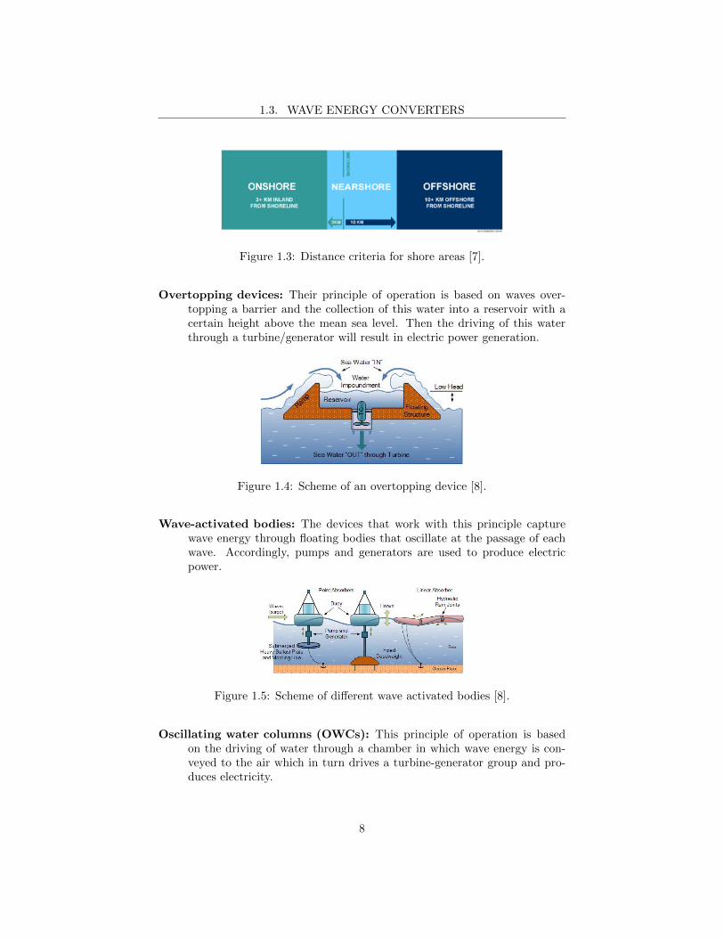
Overtopping devices: Their principle of operation is based on waves over-topping a barrier and the collection of this water into a reservoir with acertain height above the mean sea level. Then the driving of this waterthrough a turbine/generator will result in electric power generation.
Figure 1.4: Scheme of an overtopping device [8].
Wave-activated bodies: The devices that work with this principle capturewave energy through floating bodies that oscillate at the passage of eachwave. Accordingly, pumps and generators are used to produce electricpower.
Figure 1.5: Scheme of different wave activated bodies [8].
Oscillating water columns (OWCs): This principle of operation is basedon the driving of water through a chamber in which wave energy is con-veyed to the air which in turn drives a turbine-generator group and pro-duces electricity.
8
1.3. WAVE ENERGY CONVERTERS
Figure 1.6: Scheme of an oscillating water column device [8].
Energy capture system
Two categories can be distinguished in this classification. The first one includesWECs that use turbine-generator groups to obtain electricity. This category isby far the most numerous.
The second category includes devices that use wave energy to move a mech-anism and then transform this motion into electricity without any intermediatefluid.
Dimensions and direction of elongation
In this classification, three different kinds of WECs can be found depending ontheir size and their relative position to the waves [4].
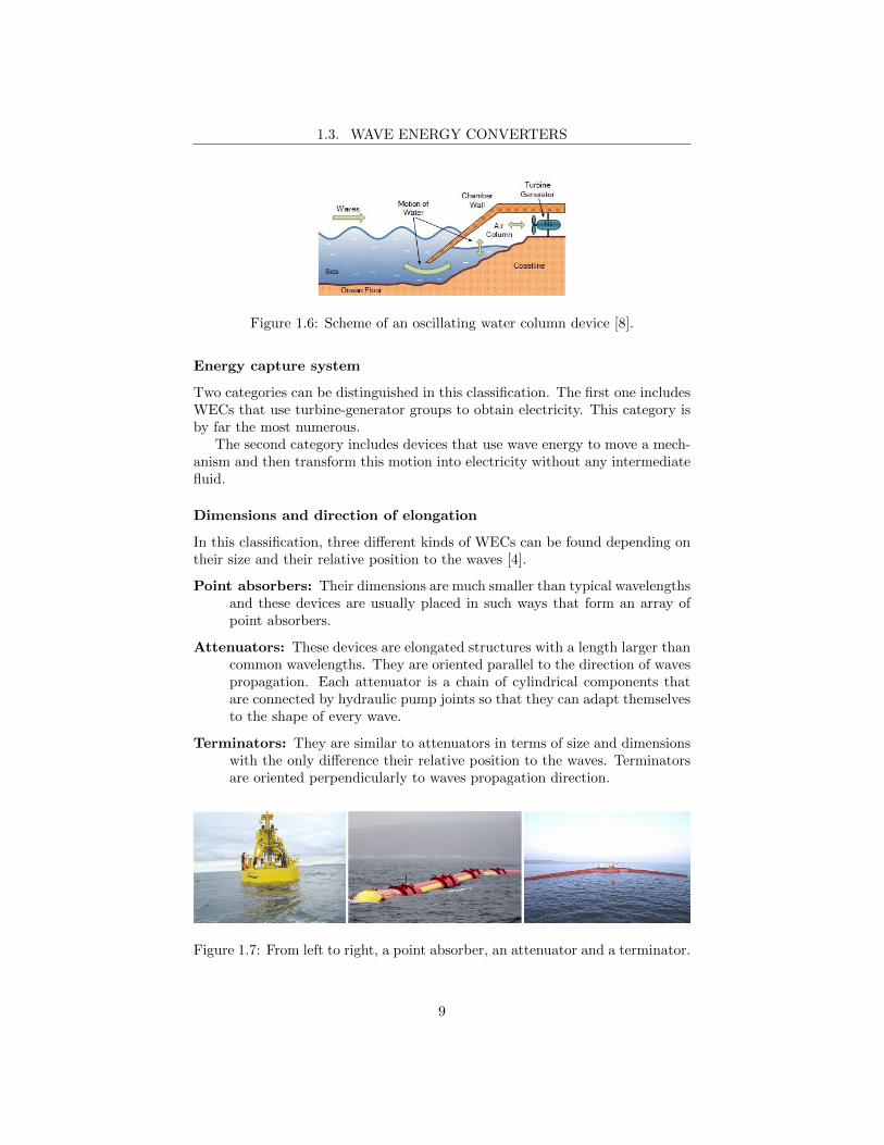
Point absorbers: Their dimensions are much smaller than typical wavelengthsand these devices are usually placed in such ways that form an array ofpoint absorbers.
Attenuators: These devices are elongated structures with a length larger thancommon wavelengths. They are oriented parallel to the direction of wavespropagation. Each attenuator is a chain of cylindrical components thatare connected by hydraulic pump joints so that they can adapt themselvesto the shape of every wave.
Terminators: They are similar to attenuators in terms of size and dimensionswith the only difference their relative position to the waves. Terminatorsare oriented perpendicularly to waves propagation direction.
Figure 1.7: From left to right, a point absorber, an attenuator and a terminator.
9
1.4. OCEAN GRAZER
1.4 Ocean Grazer
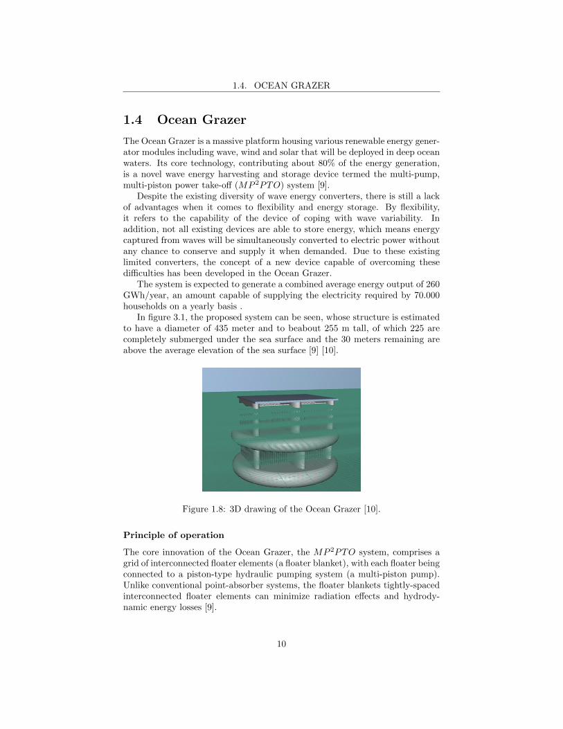
The Ocean Grazer is a massive platform housing various renewable energy gener-ator modules including wave, wind and solar that will be deployed in deep oceanwaters. Its core technology, contributing about 80% of the energy generation,is a novel wave energy harvesting and storage device termed the multi-pump,multi-piston power take-off (MP 2PTO) system [9].
Despite the existing diversity of wave energy converters, there is still a lackof advantages when it comes to flexibility and energy storage. By flexibility,it refers to the capability of the device of coping with wave variability. Inaddition, not all existing devices are able to store energy, which means energycaptured from waves will be simultaneously converted to electric power withoutany chance to conserve and supply it when demanded. Due to these existinglimited converters, the concept of a new device capable of overcoming thesedifficulties has been developed in the Ocean Grazer.
The system is expected to generate a combined average energy output of 260GWh/year, an amount capable of supplying the electricity required by 70.000households on a yearly basis .
In figure 3.1, the proposed system can be seen, whose structure is estimatedto have a diameter of 435 meter and to beabout 255 m tall, of which 225 arecompletely submerged under the sea surface and the 30 meters remaining areabove the average elevation of the sea surface [9] [10].
Figure 1.8: 3D drawing of the Ocean Grazer [10].
Principle of operation
The core innovation of the Ocean Grazer, the MP 2PTO system, comprises agrid of interconnected floater elements (a floater blanket), with each floater beingconnected to a piston-type hydraulic pumping system (a multi-piston pump).Unlike conventional point-absorber systems, the floater blankets tightly-spacedinterconnected floater elements can minimize radiation effects and hydrody-namic energy losses [9].
10
1.4. OCEAN GRAZER
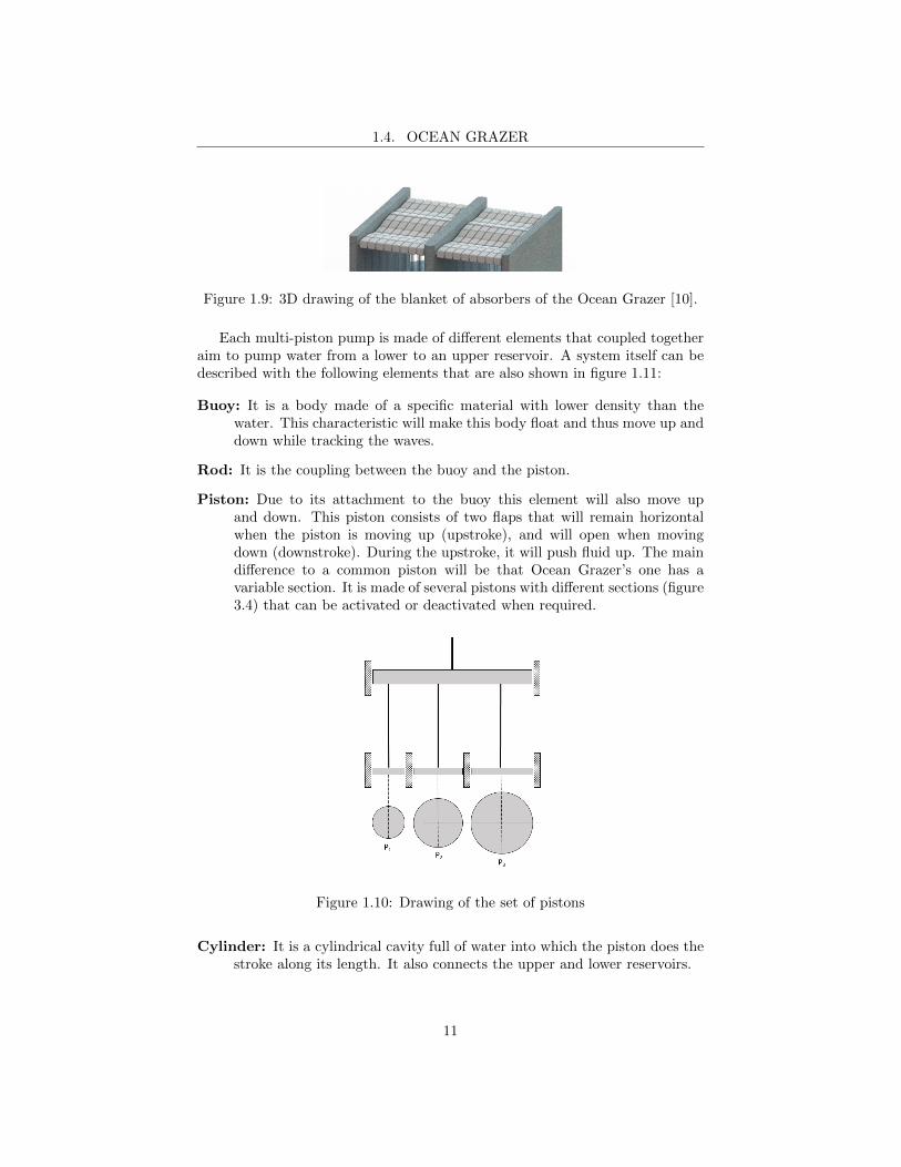
Figure 1.9: 3D drawing of the blanket of absorbers of the Ocean Grazer [10].
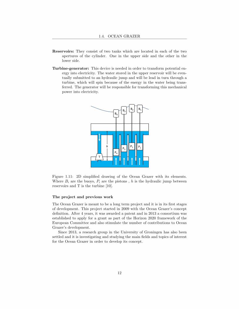
Each multi-piston pump is made of different elements that coupled togetheraim to pump water from a lower to an upper reservoir. A system itself can bedescribed with the following elements that are also shown in figure 1.11:
Buoy: It is a body made of a specific material with lower density than thewater. This characteristic will make this body float and thus move up anddown while tracking the waves.
Rod: It is the coupling between the buoy and the piston.
Piston: Due to its attachment to the buoy this element will also move upand down. This piston consists of two flaps that will remain horizontalwhen the piston is moving up (upstroke), and will open when movingdown (downstroke). During the upstroke, it will push fluid up. The maindifference to a common piston will be that Ocean Grazer’s one has avariable section. It is made of several pistons with different sections (figure3.4) that can be activated or deactivated when required.
Figure 1.10: Drawing of the set of pistons
Cylinder: It is a cylindrical cavity full of water into which the piston does thestroke along its length. It also connects the upper and lower reservoirs.
11
1.4. OCEAN GRAZER
Reservoirs: They consist of two tanks which are located in each of the twoapertures of the cylinder. One in the upper side and the other in thelower side.
Turbine-generator: This device is needed in order to transform potential en-ergy into electricity. The water stored in the upper reservoir will be even-tually submitted to an hydraulic jump and will be lead in turn through aturbine, which will spin because of the energy in the water being trans-ferred. The generator will be responsible for transforming this mechanicalpower into electricity.
Figure 1.11: 2D simplified drawing of the Ocean Grazer with its elements.Where Bi are the buoys, Pi are the pistons , h is the hydraulic jump betweenreservoirs and T is the turbine [10].
The project and previous work
The Ocean Grazer is meant to be a long term project and it is in its first stagesof development. This project started in 2009 with the Ocean Grazer’s conceptdefinition. After 4 years, it was awarded a patent and in 2013 a consortium wasestablished to apply for a grant as part of the Horizon 2020 framework of theEuropean Committee and also stimulate the number of contributions to OceanGrazer’s development.
Since 2013, a research group in the University of Groningen has also beensettled and it is investigating and studying the main fields and topics of interestfor the Ocean Grazer in order to develop its concept.
12
1.5. GOALS OF THIS THESIS
1.5 Goals of this thesis
The development of the Ocean Grazer project is still in its first stages. Despitethe fact that many studies have already been carried out by its research group,there are a lot of topics that have still to be approached. The first projectsfocused on (1) studying the behaviour of a single system [11] [12], (2) perform-ing control strategies in order to maximize the energy harvested [13] and (3)modelling the behaviour of a single element of the system as the piston, the rod,the check-valves. In addition, a prototype of a single-piston pump was designedand built in order to test the principle of operation of a single system.
This work is the first approach to the blanket concept of the Ocean Grazer.It aims to study this new WEC from the view of multiple systems and not froma single one. That means some new factors (forces, criteria, theories) will haveto be taken into consideration and they will probably have a direct effect on theinteraction between buoys and a random wave.
This project intends to offer a mathematical model capable of simulatinga system of multiple pumps in order to calculate the energy that can be har-vested and also perform control strategies that will optimize this total amountof energy. Therefore, the main goals of this thesis can be summarized in:
1. Studying and analysing hydrodynamical theories that can be applied to theOcean Grazer.
2. Reaching a dynamical model that describes the behaviour of multiple sys-tems and the effects of their interactions.
3. Performing simulations and analysing the behaviour of the whole system:displacements, velocities, forces and energies involved.
4. Optimizing the energy harvested by the whole system using a control vari-able.
13
Chapter 2
Theoretical background
2.1 Water waves
Sea waves are the main source of energy for the Ocean Grazer (see section 1.4).This is the reason why it is extremely necessary to understand the behaviourof waves and their variability. When designing devices that will interact withwaves, it is also important to take into consideration parameters that will influ-ence the calculation of stresses and energies.
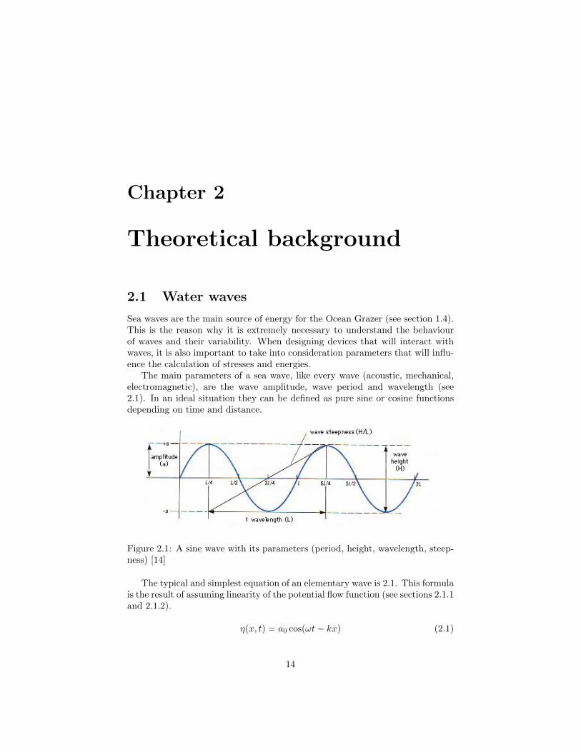
The main parameters of a sea wave, like every wave (acoustic, mechanical,electromagnetic), are the wave amplitude, wave period and wavelength (see2.1). In an ideal situation they can be defined as pure sine or cosine functionsdepending on time and distance.
Figure 2.1: A sine wave with its parameters (period, height, wavelength, steep-ness) [14]
The typical and simplest equation of an elementary wave is 2.1. This formulais the result of assuming linearity of the potential flow function (see sections 2.1.1and 2.1.2).
η(x, t) = a0 cos(ωt− kx) (2.1)
14
2.1. WATER WAVES
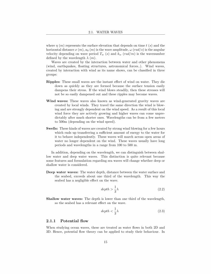
where η (m) represents the surface elevation that depends on time t (s) and thehorizontal distance x (m), a0 (m) is the wave amplitude, ω (rad/s) is the angularvelocity depending on wave period Tw (s) and kw (rad/m) is the wavenumberdefined by the wavelength λ (m).
Waves are created by the interaction between water and other phenomena(wind, earthquakes, floating structures, astronomical forces..). Wind waves,created by interaction with wind as its name shows, can be classified in threegroups:
Ripples: These small waves are the instant effect of wind on water. They diedown as quickly as they are formed because the surface tension easilydampens their stress. If the wind blows steadily, then these stresses willnot be so easily dampened out and these ripples may become waves.
Wind waves: These waves also known as wind-generated gravity waves arecreated by local winds. They travel the same direction the wind is blow-ing and are strongly dependent on the wind speed. As a result of this localwind force they are actively growing and higher waves can come unpre-dictably after much shorter ones. Wavelengths can be from a few metersto 500m (depending on the wind speed).
Swells: These kinds of waves are created by strong wind blowing for a few hourswhich ends up transferring a sufficient amount of energy to the water forit to behave independently. These waves will march across open areas ofwater no longer dependent on the wind. These waves usually have longperiods and wavelengths in a range from 100 to 500 m.
In addition, depending on the wavelength, we can distinguish between shal-low water and deep water waves. This distinction is quite relevant becausesome features and formulation regarding sea waves will change whether deep orshallow water is considered.
Deep water waves: The water depth, distance between the water surface andthe seabed, exceeds about one third of the wavelength. This way theseabed has a negligible effect on the wave.
depth >1
3λ (2.2)
Shallow water waves: The depth is lower than one third of the wavelength,so the seabed has a relevant effect on the wave.
depth <1
3λ (2.3)
2.1.1 Potential flow
When studying ocean waves, these are treated as water flows in both 2D and3D. Hence, potential flow theory can be applied to study their behaviour. In
15
2.1. WATER WAVES
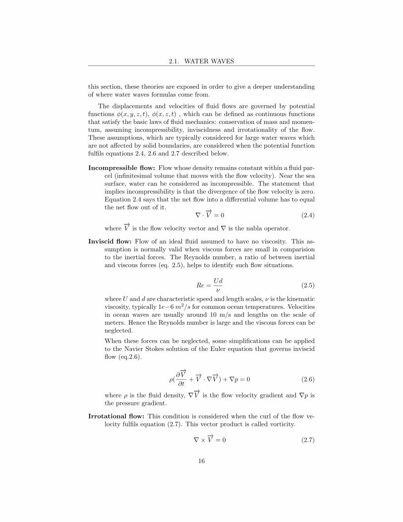
this section, these theories are exposed in order to give a deeper understandingof where water waves formulas come from.
The displacements and velocities of fluid flows are governed by potentialfunctions φ(x, y, z, t), φ(x, z, t) , which can be defined as continuous functionsthat satisfy the basic laws of fluid mechanics: conservation of mass and momen-tum, assuming incompressibility, inviscidness and irrotationality of the flow.These assumptions, which are typically considered for large water waves whichare not affected by solid boundaries, are considered when the potential functionfulfils equations 2.4, 2.6 and 2.7 described below.
Incompressible flow: Flow whose density remains constant within a fluid par-cel (infinitesimal volume that moves with the flow velocity). Near the seasurface, water can be considered as incompressible. The statement thatimplies incompressibility is that the divergence of the flow velocity is zero.Equation 2.4 says that the net flow into a differential volume has to equalthe net flow out of it.
∇ ·−→V = 0 (2.4)
where−→V is the flow velocity vector and ∇ is the nabla operator.
Inviscid flow: Flow of an ideal fluid assumed to have no viscosity. This as-sumption is normally valid when viscous forces are small in comparisionto the inertial forces. The Reynolds number, a ratio of between inertialand viscous forces (eq. 2.5), helps to identify such flow situations.
Re =Ud
ν(2.5)
where U and d are characteristic speed and length scales, ν is the kinematicviscosity, typically 1e−6 m2/s for common ocean temperatures. Velocitiesin ocean waves are usually around 10 m/s and lengths on the scale ofmeters. Hence the Reynolds number is large and the viscous forces can beneglected.
When these forces can be neglected, some simplifications can be appliedto the Navier Stokes solution of the Euler equation that governs inviscidflow (eq.2.6).
ρ(∂−→V
∂t+−→V · ∇
−→V ) +∇p = 0 (2.6)
where ρ is the fluid density, ∇−→V is the flow velocity gradient and ∇p is
the pressure gradient.
Irrotational flow: This condition is considered when the curl of the flow ve-locity fulfils equation (2.7). This vector product is called vorticity.
∇×−→V = 0 (2.7)
16
2.1. WATER WAVES
In the case of water waves, this condition can be applied to large ones dueto the fact that an spherical particle will have no rotation except throughshear forces [15].
However, we have to take into account that near solid boundaries (e.g. afloater), irrotational as well as inviscid flow may not be valid assumptions. Dueto wall roughness, small flow structures with turbulence are created near thebody. This effect can be accounted through considering drag forces in the bal-ance of forces acting on a body.
Velocity potential
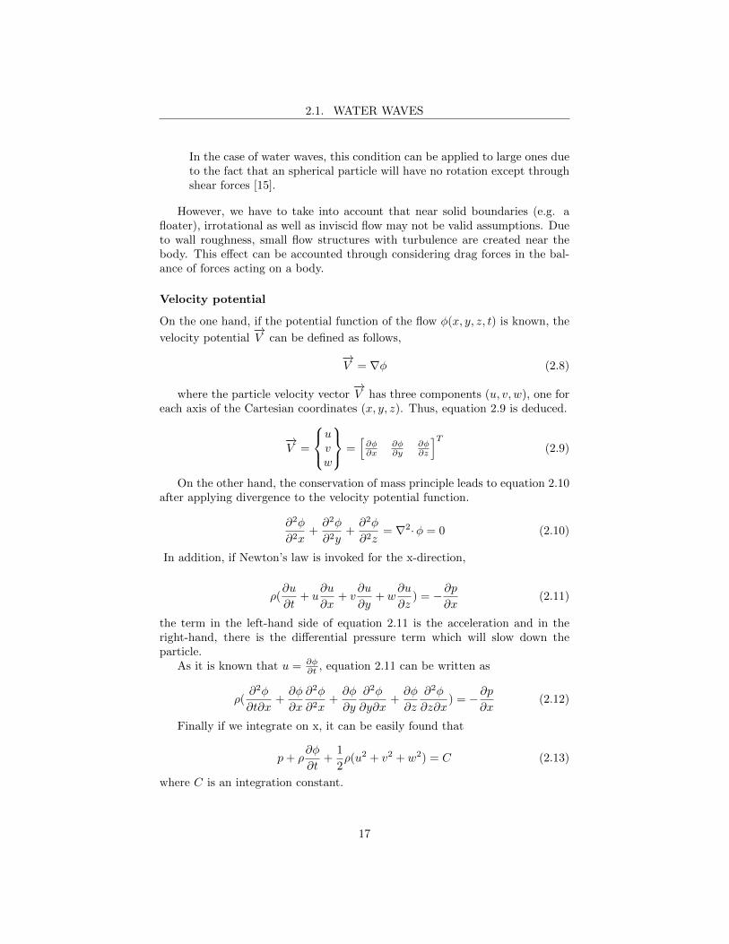
On the one hand, if the potential function of the flow φ(x, y, z, t) is known, the
velocity potential−→V can be defined as follows,
−→V = ∇φ (2.8)
where the particle velocity vector−→V has three components (u, v, w), one for
each axis of the Cartesian coordinates (x, y, z). Thus, equation 2.9 is deduced.
−→V =
uvw
=[∂φ∂x
∂φ∂y
∂φ∂z
]T(2.9)
On the other hand, the conservation of mass principle leads to equation 2.10after applying divergence to the velocity potential function.
∂2φ
∂2x+∂2φ
∂2y+∂2φ
∂2z= ∇2·φ = 0 (2.10)
In addition, if Newton’s law is invoked for the x-direction,
ρ(∂u
∂t+ u
∂u
∂x+ v
∂u
∂y+ w
∂u
∂z) = −∂p
∂x(2.11)
the term in the left-hand side of equation 2.11 is the acceleration and in theright-hand, there is the differential pressure term which will slow down theparticle.
As it is known that u = ∂φ∂t , equation 2.11 can be written as
ρ(∂2φ
∂t∂x+∂φ
∂x
∂2φ
∂2x+∂φ
∂y
∂2φ
∂y∂x+∂φ
∂z
∂2φ
∂z∂x) = −∂p
∂x(2.12)
Finally if we integrate on x, it can be easily found that
p+ ρ∂φ
∂t+
1
2ρ(u2 + v2 + w2) = C (2.13)
where C is an integration constant.
17
2.1. WATER WAVES
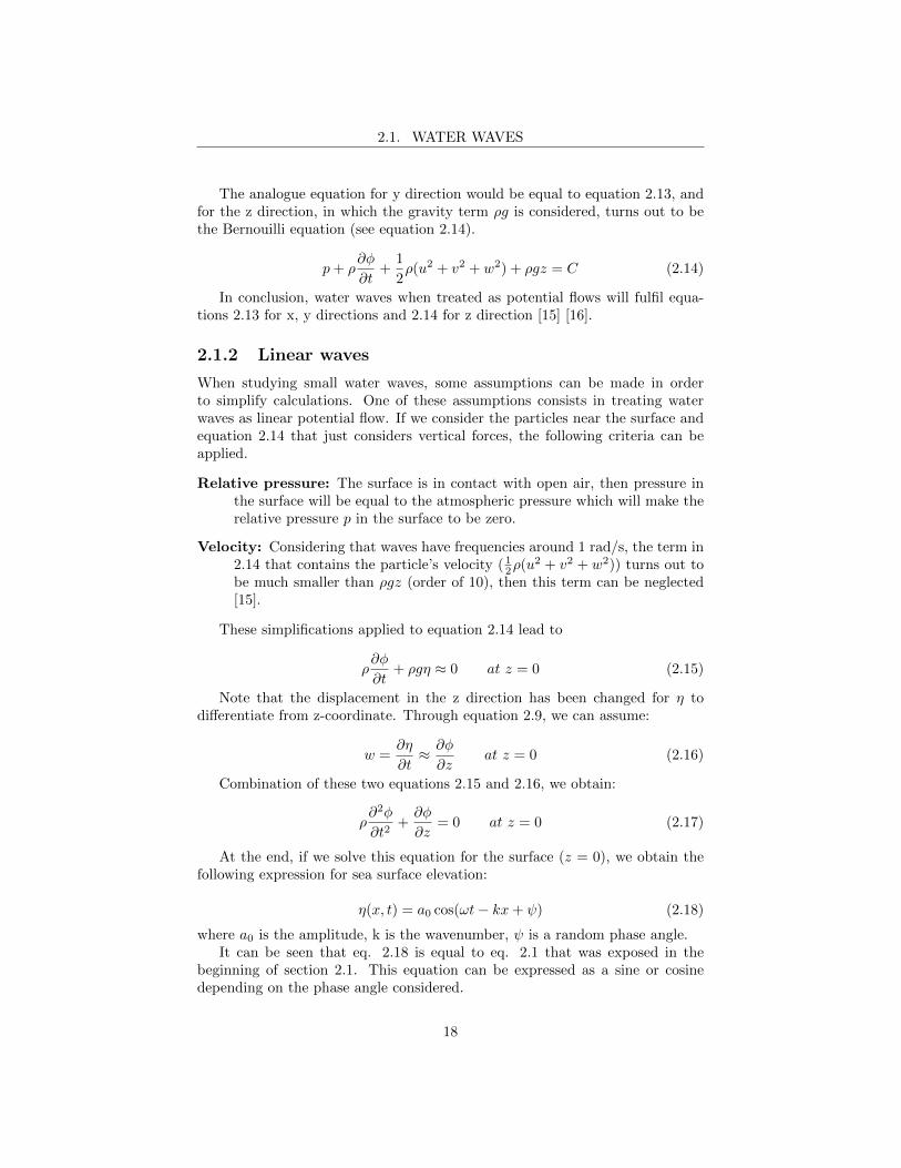
The analogue equation for y direction would be equal to equation 2.13, andfor the z direction, in which the gravity term ρg is considered, turns out to bethe Bernouilli equation (see equation 2.14).
p+ ρ∂φ
∂t+
1
2ρ(u2 + v2 + w2) + ρgz = C (2.14)
In conclusion, water waves when treated as potential flows will fulfil equa-tions 2.13 for x, y directions and 2.14 for z direction [15] [16].
2.1.2 Linear waves
When studying small water waves, some assumptions can be made in orderto simplify calculations. One of these assumptions consists in treating waterwaves as linear potential flow. If we consider the particles near the surface andequation 2.14 that just considers vertical forces, the following criteria can beapplied.
Relative pressure: The surface is in contact with open air, then pressure inthe surface will be equal to the atmospheric pressure which will make therelative pressure p in the surface to be zero.
Velocity: Considering that waves have frequencies around 1 rad/s, the term in2.14 that contains the particle’s velocity (1
2ρ(u2 + v2 + w2)) turns out tobe much smaller than ρgz (order of 10), then this term can be neglected[15].
These simplifications applied to equation 2.14 lead to
ρ∂φ
∂t+ ρgη ≈ 0 at z = 0 (2.15)
Note that the displacement in the z direction has been changed for η todifferentiate from z-coordinate. Through equation 2.9, we can assume:
w =∂η
∂t≈ ∂φ
∂zat z = 0 (2.16)
Combination of these two equations 2.15 and 2.16, we obtain:
ρ∂2φ
∂t2+∂φ
∂z= 0 at z = 0 (2.17)
At the end, if we solve this equation for the surface (z = 0), we obtain thefollowing expression for sea surface elevation:
η(x, t) = a0 cos(ωt− kx+ ψ) (2.18)
where a0 is the amplitude, k is the wavenumber, ψ is a random phase angle.It can be seen that eq. 2.18 is equal to eq. 2.1 that was exposed in the
beginning of section 2.1. This equation can be expressed as a sine or cosinedepending on the phase angle considered.
18
2.1. WATER WAVES
If the following expressions for the phase velocity (2.19) and the dispersionrelation (2.20) are considered, one can express the candidate potential functionas in eq. 2.21.
c =ω
k(2.19)
ω =2φ
Tw=
√kg tanh(kH) (2.20)
φ(x, z, t) = −a0ωk
cosh(k(z +H))
sinh(kH)sin(ωt− kx+ ψ) (2.21)
where c is the phase velocity, ω the angular frequency, k the wave-number, a0 isthe wave amplitude, λ the wavelength, Tw the wave period and H is the depth.
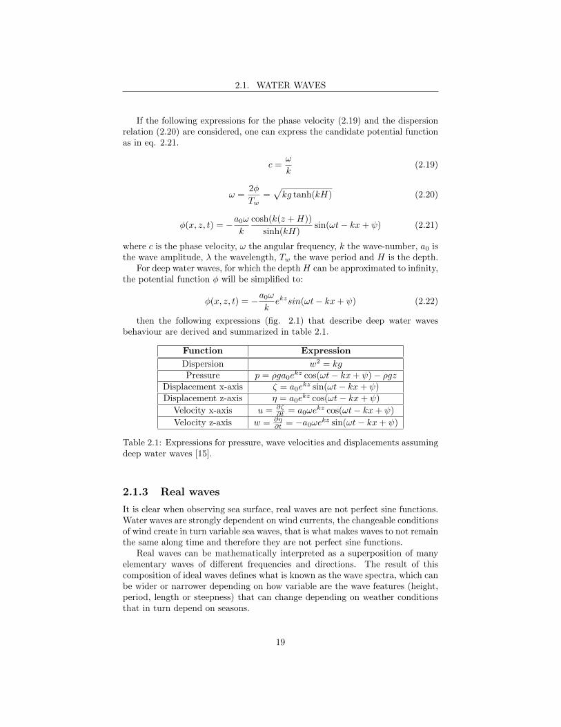
For deep water waves, for which the depth H can be approximated to infinity,the potential function φ will be simplified to:
φ(x, z, t) = −a0ωkekzsin(ωt− kx+ ψ) (2.22)
then the following expressions (fig. 2.1) that describe deep water wavesbehaviour are derived and summarized in table 2.1.
Function Expression
Dispersion w2 = kgPressure p = ρga0e
kz cos(ωt− kx+ ψ)− ρgzDisplacement x-axis ζ = a0e
kz sin(ωt− kx+ ψ)Displacement z-axis η = a0e
kz cos(ωt− kx+ ψ)
Velocity x-axis u = ∂ζ∂t = a0ωe
kz cos(ωt− kx+ ψ)
Velocity z-axis w = ∂η∂t = −a0ωekz sin(ωt− kx+ ψ)
Table 2.1: Expressions for pressure, wave velocities and displacements assumingdeep water waves [15].
2.1.3 Real waves
It is clear when observing sea surface, real waves are not perfect sine functions.Water waves are strongly dependent on wind currents, the changeable conditionsof wind create in turn variable sea waves, that is what makes waves to not remainthe same along time and therefore they are not perfect sine functions.
Real waves can be mathematically interpreted as a superposition of manyelementary waves of different frequencies and directions. The result of thiscomposition of ideal waves defines what is known as the wave spectra, which canbe wider or narrower depending on how variable are the wave features (height,period, length or steepness) that can change depending on weather conditionsthat in turn depend on seasons.
19
2.1. WATER WAVES
With non-deterministic processes, waves heights are supposed to follow theRayleigh distribution if Gaussian process can be assumed [17]. One of thisprocesses can consist in recording the wave height in a specific location alongtime. It is clear that as longer periods of time recording, more accurate will bethe approximations derived from the data. Hence, the probability of occurrenceof a concrete wave height is defined as:
p(Hw) =H
4m0exp(− H2
8m0) (2.23)
where H is the wave height and m0 is defined as the variance of the surfaceelevation. The standard deviation can be estimated once the mean wave heightis known. The mean wave height can be estimated using the data recorded andcalculating either the height average H (2.24) or the significant wave heightHm0 (2.25).
m0 =H2
2π(2.24)
m0 =H2m0
16(2.25)
By definition Hm0is the mean wave height of the highest one-third of waves
recorded but an easier way to calculate it is the approximation to the half ofthe maximum wave height [18].
There exist different forms of modelling the spectra of ocean waves. Exam-ples of standard forms are JONSWAP, Pierson-Moskowitz, Ochi and Bretschnei-der which are used according to application. Current work in the Ocean GrazerGroup focuses in modelling real waves using wave spectra provided by JON-SWAP method. Ocean wave spectra, in most of the cases, follows the Rayleighdistribution. However, some exceptions have been observed when it comes aboutextreme events like intense storms. Hence, the Weillbull distribution can affordwider range of variation and allows to describe such processes [15].
20
2.2. WAVE LOADING
2.2 Wave loading
The interaction of waves and floating bodies results in different forces and loadsapplied on the body’s surface. There exists mathematical models that allowus to know the behaviour of both stationary and moving bodies submerged inwater.
In this section, the different forces and loads that typically act on a floatingbody are described in order to determine later which of them can be applicableor relevant to Ocean Grazer models.
The study of these forces will be extremely relevant in this work, becauseof the necessity of knowing how the wave is modified after trespassing one rowof the blanket. Key aspects for the modelling of these forces will be the char-acteristics of incoming waves, the movement of the floating structure and itsgeometry.
When studying floating devices, it is necessary to consider the forces betweenthe fluid (sea water) and the device not only in a static situation (stationary)but also in the dynamic one. Thus, we can differentiate between hydrostaticand hydrodynamic forces.
2.2.1 Hydrostatic forces
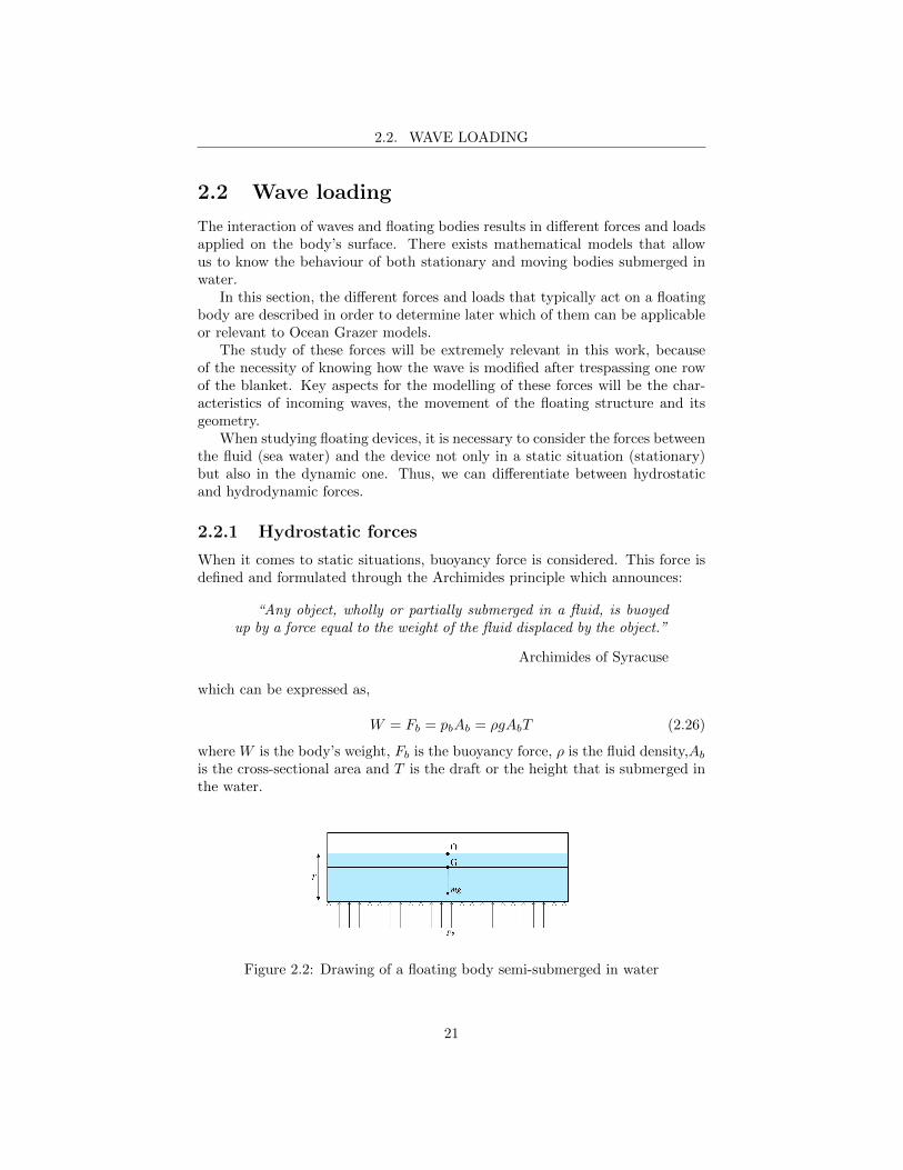
When it comes to static situations, buoyancy force is considered. This force isdefined and formulated through the Archimides principle which announces:
“Any object, wholly or partially submerged in a fluid, is buoyedup by a force equal to the weight of the fluid displaced by the object.”
Archimides of Syracuse
which can be expressed as,
W = Fb = pbAb = ρgAbT (2.26)
where W is the body’s weight, Fb is the buoyancy force, ρ is the fluid density,Abis the cross-sectional area and T is the draft or the height that is submerged inthe water.
Figure 2.2: Drawing of a floating body semi-submerged in water
21
2.2. WAVE LOADING
But this situation is only possible if the body is static in still water. Whenthere are disturbances to this equilibrium situation, e.g waves or externals forceapplied on the body, then other forces play a role and we cannot consider onlybuoyancy any more. Actually when considering dynamic situations only distur-bances to equilibrium are usually considered, then body’s weight and buoyancyforce don’t need to be considered[19].
2.2.2 Hydrodynamic forces
When considering the motion of the fluid surface, other forces such excitation,radiation, diffraction or drag, should be taken into account. These forces willdepend mainly on the kind of wave and its characteristics and also on the sizeand geometry of the floating body.
When classifying them, we can differentiate between two types of hydrody-namic forces: viscous and inertial [20]
Viscous forces
These forces are produced by the drag created by bodys motion and they dependon different parameters such as the Reynolds number, the Keulegan-Carpenternumber or the roughness. Two types of drag (form drag and friction drag) canbe distinguished.
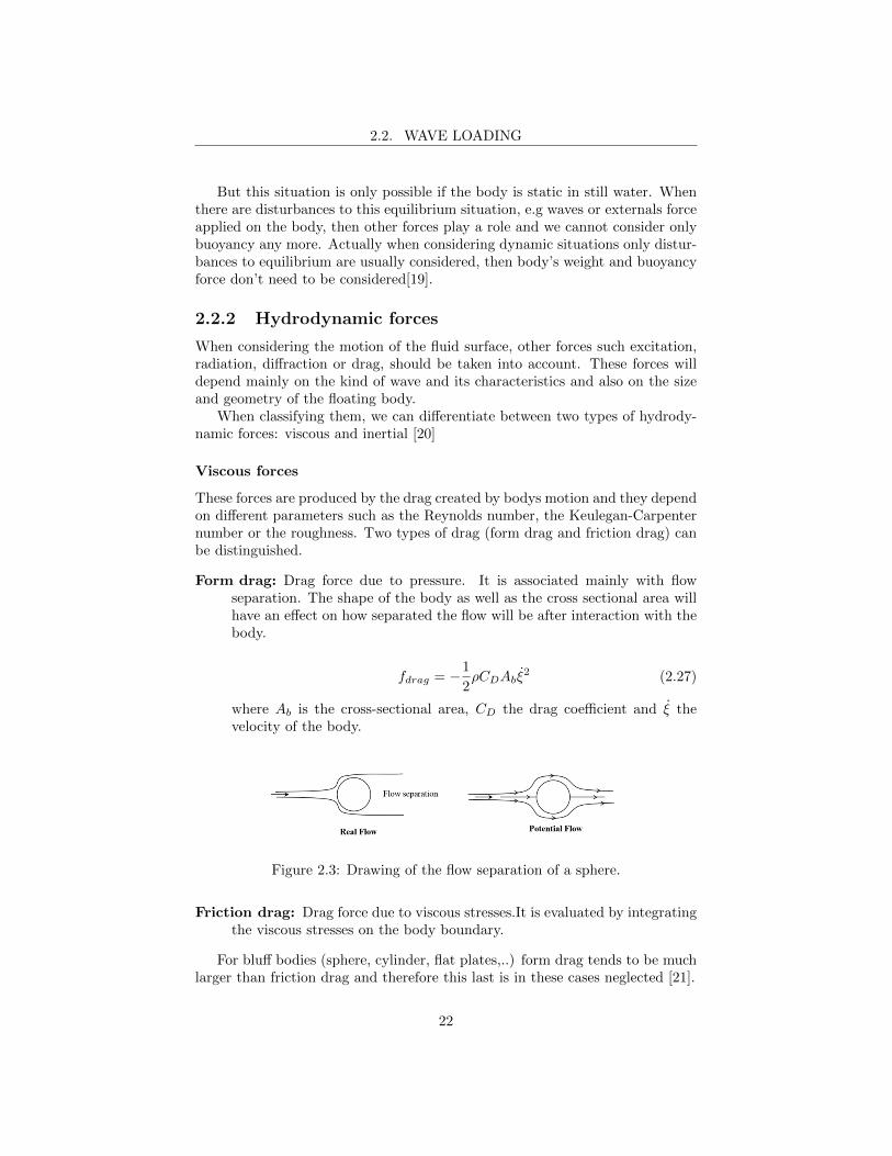
Form drag: Drag force due to pressure. It is associated mainly with flowseparation. The shape of the body as well as the cross sectional area willhave an effect on how separated the flow will be after interaction with thebody.
fdrag = −1
2ρCDAbξ
2 (2.27)
where Ab is the cross-sectional area, CD the drag coefficient and ξ thevelocity of the body.
Figure 2.3: Drawing of the flow separation of a sphere.
Friction drag: Drag force due to viscous stresses.It is evaluated by integratingthe viscous stresses on the body boundary.
For bluff bodies (sphere, cylinder, flat plates,..) form drag tends to be muchlarger than friction drag and therefore this last is in these cases neglected [21].
22
2.2. WAVE LOADING
Inertial forces
These forces (Froude-Krylov, diffraction and radiation force) arise from potentialflow theory (see section 2.1.1). When a wave with its own period, amplitudeand wave-length meets up a body, the wave potential created by this interactioncan be understood as the sum of an incident wave potential, a diffracted and aradiated wave potential.
φ = φI + φD + φR (2.28)
Incident wave field φI : The incident wave is the wave that reaches the bodybut without considering its presence (ghost body). When L (body’s char-acteristic dimension) is much smaller than the wavelength (λ), the incidentwave field is not significantly modified by the presence of the body, there-fore radiation and diffraction terms can be ignored.
Diffracted wave field φD : It is created due to the presence of a fixed body.The flow is deflected of its course by the presence of an obstacle assumingthat the body is stationary. It is considered when L is not much smallerthan λ, that means the wave field near body will be affected even if bodyis stationary.
∂φD∂n
= −∂φI∂n
on S (2.29)
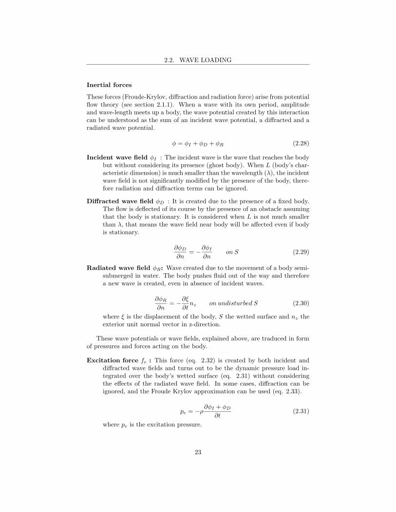
Radiated wave field φR: Wave created due to the movement of a body semi-submerged in water. The body pushes fluid out of the way and thereforea new wave is created, even in absence of incident waves.
∂φR∂n
= −∂ξ∂tnz on undisturbed S (2.30)
where ξ is the displacement of the body, S the wetted surface and nz theexterior unit normal vector in z-direction.
These wave potentials or wave fields, explained above, are traduced in formof pressures and forces acting on the body.
Excitation force fe : This force (eq. 2.32) is created by both incident anddiffracted wave fields and turns out to be the dynamic pressure load in-tegrated over the body’s wetted surface (eq. 2.31) without consideringthe effects of the radiated wave field. In some cases, diffraction can beignored, and the Froude Krylov approximation can be used (eq. 2.33).
pe = −ρ∂φI + φD∂t
(2.31)
where pe is the excitation pressure.
23
2.2. WAVE LOADING
fe = −∫S
nzpedS (2.32)
fe = FFK = −∫S
nzpIdS (2.33)
where pI is the pressure created by the incident wave field only.
Radiation force φr : This wave-making force created derived from the radi-ated wave field will depend on the velocity of the body.
pr = −ρ∂φR∂t
(2.34)
fr = −∫S
nzprdS (2.35)
Thus, the motion of a floating body, without taking into account forcesinvolved in the power take-off, can be described with equation 2.36,
mξ + Cξ = fe + fr + fdrag (2.36)
where m is the mass of the floating body, C the restoring buoyancy termand ξ, ξ are acceleration and displacement of the body respectively.
In this section, special attention is given to radiation forces and its wavemak-ing effect. It is of special interest to know how this effect can be mathematicallymodelled when considering systems of more than one floating body.
When considering the formulation of this force (fr), two different terms canbe differentiated,
fr = −maξ −Bw(ξ − e−kwT vw) (2.37)
where ξ and ξ are the acceleration and the velocity of the body respectively,e−kwT vwis the wave velocity on the bottom surface on the body, ma is the added-mass(defined by its coefficient Ca) and Bw is the wave-radiation damping coefficient.
Added mass term (maξ): This term considers the mass of fluid in the sur-roundings that is being accelerated by the body’s motion.
Radiation damping term (Bw(ξ − e−kwT vw)): This one accounts for the en-ergy that is being transferred to the fluid by body’s velocity.
J.Falnes [22] explains that when considering more than one oscillating body,the radiated wave created by one has an effect not only over the body itself butalso over other bodies in surroundings due to the fact that the new radiatedwave propagates away from the body that has created it and eventually will acton other bodies as a force.
Therefore, this radiation force between bodies can be modelled with a damperbetween them. Thus, the radiation force acting on body “1” that considers theeffect of body“2” and vice versa can be written as follows [23] [24],
24
2.2. WAVE LOADING
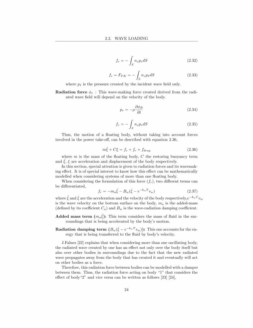
fr,1 = ma11 ξ1 +ma21 ξn−Bw,11(ξ1− e−kwT vw1)−Bw,21(ξ2− e−kwT vw2) (2.38)
fr,2 = ma22 ξ2 +ma12 ξ1−Bw,22(ξn− e−kwT vwn)−Bw,12(ξ1− e−kwT vw1) (2.39)
where maij and Bwij are the added-mass and wave-radiation damping coeffi-cient respectively that are also known as hydrodynamic coefficients and dependon the geometry of the body as well as on the wave period. Note that coefficientsBw,11 and Bw,22 cannot be negative and it can be proved that Ca,12 = Ca,21and Bw,12 = Bw,21 [24].
2.2.3 Hydrodynamic coefficients
By hydrodynamic coefficients, we understand parameters that depend on thedynamic interaction between a fluid and a solid boundary. These coefficientsneed to be considered for formulating the hydrodynamic forces.
In this case, there is a drag coefficient CD when considering viscous forces,the wave-radiation damping coefficient Bw and the added-mass coefficient Cathat are needed for formulating radiation forces.
There are several options that are valid to determine such coefficients. Forsimple geometries (sphere, vertical plane, horizontal walls, cylinders), there areanalytical methods that can be used to determine these coefficients. For arbi-trary geometries, several degrees of freedom and bodies, there exist commercialcodes based on Boundary-Element-Method like WAMIT® or ANSYS® Aqwa�).
Drag coefficient CD
The drag coefficient can be estimated with analytical methods. These methodsrequire the calculation of independent variables that represent the flow condi-tion. For unsteady flow, Reynolds number (eq. 2.40) can be used but if oscil-lating flow is considered, it is preferable to use the Keulegan-Carpenter number(eq. 2.41).
Re =uaD
ν(2.40)
KC =uaTwD
(2.41)
where ua is the flow velocity amplitude, D the characteristic dimension of thebody, ν is the kinematic viscosity and Tw the wave period.
For deep water, the Keulegan-Carpenter number can be expressed as,
KC = 2πa0D
(2.42)
where a0 is the wave amplitude.
25
2.2. WAVE LOADING
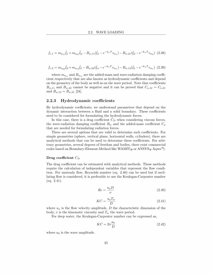
If we also know the roughness of body’s walls (ε/D), typical values for thedrag coefficient (CD) can be found graphically.
Figure 2.4: CD as function of KC for cylinders in waves Re > 5 · 10−5 [25]
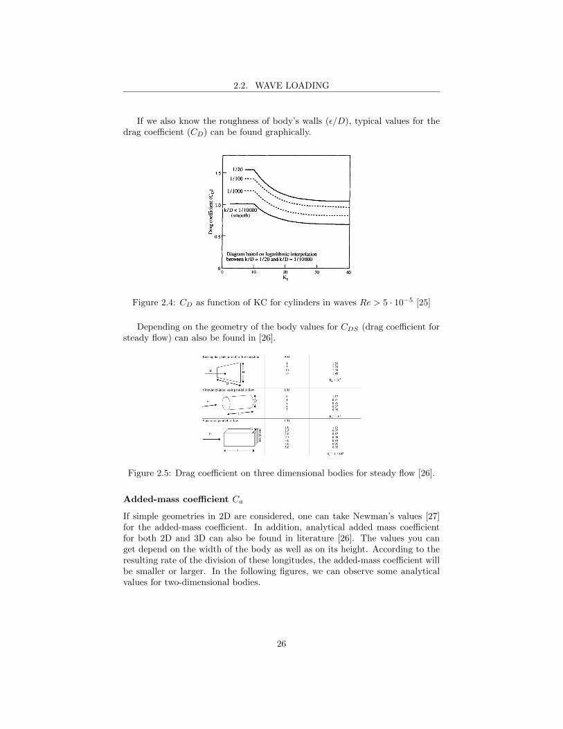
Depending on the geometry of the body values for CDS (drag coefficient forsteady flow) can also be found in [26].
Figure 2.5: Drag coefficient on three dimensional bodies for steady flow [26].
Added-mass coefficient Ca
If simple geometries in 2D are considered, one can take Newman’s values [27]for the added-mass coefficient. In addition, analytical added mass coefficientfor both 2D and 3D can also be found in literature [26]. The values you canget depend on the width of the body as well as on its height. According to theresulting rate of the division of these longitudes, the added-mass coefficient willbe smaller or larger. In the following figures, we can observe some analyticalvalues for two-dimensional bodies.
26
2.2. WAVE LOADING
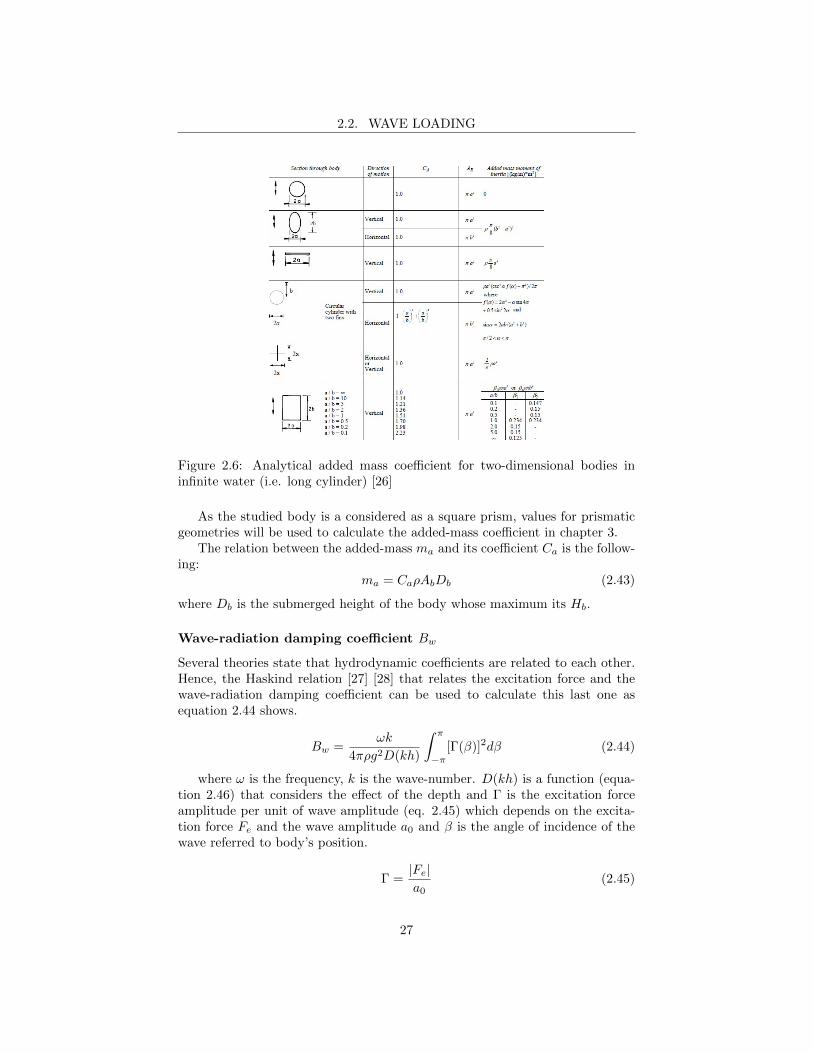
Figure 2.6: Analytical added mass coefficient for two-dimensional bodies ininfinite water (i.e. long cylinder) [26]
As the studied body is a considered as a square prism, values for prismaticgeometries will be used to calculate the added-mass coefficient in chapter 3.
The relation between the added-mass ma and its coefficient Ca is the follow-ing:
ma = CaρAbDb (2.43)
where Db is the submerged height of the body whose maximum its Hb.
Wave-radiation damping coefficient Bw
Several theories state that hydrodynamic coefficients are related to each other.Hence, the Haskind relation [27] [28] that relates the excitation force and thewave-radiation damping coefficient can be used to calculate this last one asequation 2.44 shows.
Bw =ωk
4πρg2D(kh)
∫ π
−π[Γ(β)]2dβ (2.44)
where ω is the frequency, k is the wave-number. D(kh) is a function (equa-tion 2.46) that considers the effect of the depth and Γ is the excitation forceamplitude per unit of wave amplitude (eq. 2.45) which depends on the excita-tion force Fe and the wave amplitude a0 and β is the angle of incidence of thewave referred to body’s position.
Γ =|Fe|a0
(2.45)
27
2.2. WAVE LOADING
D(kh) = (1 +2kh
sinh 2kh) tanh kh (2.46)
where h is the depth and k the wave-number. When considering deep-water,this function becomes 1:
D(kh) = 1 h −→∞ (2.47)
Therefore, if we also consider the dispersion relation (see figure 2.1), theHaskind Relation for deep water can be written as follows,
Bw =ω3
4πρg3
∫ π
−π[Γ(β)]2dβ h −→∞ (2.48)
If the body is axysimmetric, Γ does not depend on angle β, independently ofthe wave’s direction, it will always find the same geometry of the body. Then,formulas 2.44 and 2.48 can be simplified as follows,
Bw =ωkΓ2
2ρg2D(kh)(2.49)
and assuming deep water,
Bw =ω3Γ2
2ρg3h −→∞ (2.50)
In 2D and assuming deep water conditions, the radiation damping coefficientcan be expressed as in equation 2.51 [29].
Bw =ωΓ2
ρg2h −→∞ (2.51)
Note that Γ is defined as in equation 2.45 and will be specifically detailed forthe studied case in the next chapters (see equation 3.4).
28
2.3. WAVE ENERGY
2.3 Wave energy
If wave energy converters exist, that is because ocean waves contain energy thatcan be efficiently extracted. However, the calculation of energy in waves is nottrivial. The fact that the behaviour of real waves is difficult to predict and theydon’t have constant features (frequency, amplitude...) along time, make thiscalculation difficult. Although there exist formulas that estimate wave powerand energy [30], they are for a determined wave height and period (see eq. 2.52).Then, if the period and amplitude of the wave are known for an instant of time,the energy can be calculated as follows,
Jwave = ρgH2m0
16(2.52)
where Jwave is the energy per unit of sea surface and Hm0 is the significantwave height (see section 2.1.3). If we know that the relation between the signif-icant wave height (Hm0) and a sinusoidal wave height (H) is Hm0 =
√2H then
equation 2.52 can be also expressed as,
Jwave = ρgH2
8(2.53)
In addition if we consider that the energy in waves is transported with a velocityequal to group velocity cg),
cg =λ
2Tw=gTw4π
(2.54)
thus, equation 2.55 per unit width for wave energy is derived.
Ewave =1
32πρg2H2T 2
w (2.55)
where Ewave is the wave energy per unit of width.Now, the wave power can be expressed (eq.2.56) as it is clear that Ewave =
PwaveTw where Pwave represents the wave power per unit of width.
Pwave =1
32πρg2H2Tw (2.56)
Regarding energy, it is important to account for not only the energy con-tained in waves but also the energy that is being extracted from them. Thislast one will depend on the device that is being deployed with such aim. In thecase of WEC’s based on oscillating bodies, the power extracted depend on thehydrodynamic forces acting on the body as well as on the forces from the powertake-off.
Not all the power contained in a wave can be taken out by a single body.Thus, the instantaneous absorbed power (eq. 2.57) by the body and the poweroutput (eq. 2.58) can be considered and calculated.
Pabs(t) = (fe(t) + fr(t)− ρgAbξ)ξ (2.57)
29
2.3. WAVE ENERGY
PPTO(t) = (Bξ +Kξ)ξ (2.58)
It is important to mention that the calculation of efficiencies of the waveabsorption process should be avoided, especially when dealing with small devices[24]. Instead of considering an efficiency, the absorption width (eq. 2.59) has tobe considered.
L =PabsPwave
(2.59)
where L is the mentioned capture width which can be larger than the physicaldimension. Note that Pwave is the power per unit of width and Pabs the powerabsorbed, therefore L is not dimensionless.
Given equation 2.59, the maximum capture width is defined as
Lmax =PmaxPwave
(2.60)
where Pmax is the power absorbed when the velocity of the body is in phasewith the excitation force [23] [24].
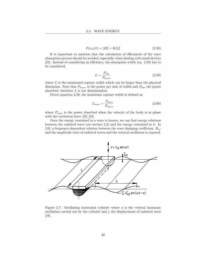
Once the energy contained in a wave is known, we can find energy relationsbetween the radiated wave (see section 2.2) and the energy contained in it. In[19], a frequency-dependent relation between the wave damping coefficient, Bw,and the amplitude ratio of radiated waves and the vertical oscillation is exposed.
Figure 2.7: Oscillating horizontal cylinder where z is the vertical harmonicoscillation carried out by the cylinder and ζ the displacement of radiated wave[19].
30
2.3. WAVE ENERGY
Through the statement that the energy provided by the hydrodynamic damp-ing force (Bwz) is equal to the energy dissipated by the radiated waves, thefollowing relation is found:
1
2Bwω
2z2a =ρg2ζ2aL
2ω(2.61)
and the amplitude of the radiated wave can be expressed as follows,
ζa =
√Bwω3z2aρg2L
(2.62)
31
Chapter 3
Modelling
In order to provide a model for the blanket, it is necessary to describe the waveenergy converter itself. In the first part of this chapter (section 3.1), the OceanGrazer system, its principle of operation and its components are described andexplained accurately. In the second part (section 3.2), the different forces andinfluential variables are estimated in order to be included in the model that willallow to perform simulations and calculate state variable for the blanket.
3.1 Description of the system
The Ocean Grazer is a novel wave energy harvesting and storage device termedthe multi-pump, multi-piston power take-off MP 2PTO system. Through themovement of a floater blanket of buoys that track the waves, pistons with vari-able section attached to the buoys by a rod move upwards and downwardspumping water in its turn from a lower to an upper reservoir.
Each multi-piston pump is powered by one floater element to internally dis-place trough a piston a column of working fluid between a lower and an upperreservoir, creating hydraulic head (see fig. 3.3). Each floater element withinthe floater blanket can therefore gradually extract the energy from an incomingwave, so that all of the waves original energy will have been extracted by thetime it exits the Ocean Grazer structure. The working fluid (conditioned water)pumped and stored in the upper reservoir will be eventually lead through anhydraulic jump and a turbine, converting potential energy in mechanical energy,then a generator will produce electricity out of the mechanical energy.
32
3.1. DESCRIPTION OF THE SYSTEM
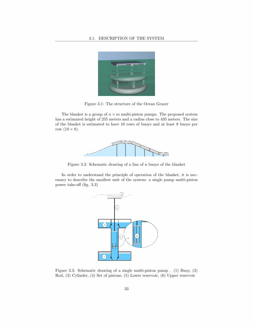
Figure 3.1: The structure of the Ocean Grazer
The blanket is a group of n×m multi-piston pumps. The proposed systemhas a estimated height of 255 meters and a radius close to 435 meters. The sizeof the blanket is estimated to have 10 rows of buoys and at least 8 buoys perrow (10× 8).
Figure 3.2: Schematic drawing of a line of n buoys of the blanket
In order to understand the principle of operation of the blanket, it is nec-essary to describe the smallest unit of the system: a single pump multi-pistonpower take-off (fig. 3.3)
Figure 3.3: Schematic drawing of a single multi-piston pump . (1) Buoy, (2)Rod, (3) Cylinder, (4) Set of pistons, (5) Lower reservoir, (6) Upper reservoir
33
3.1. DESCRIPTION OF THE SYSTEM
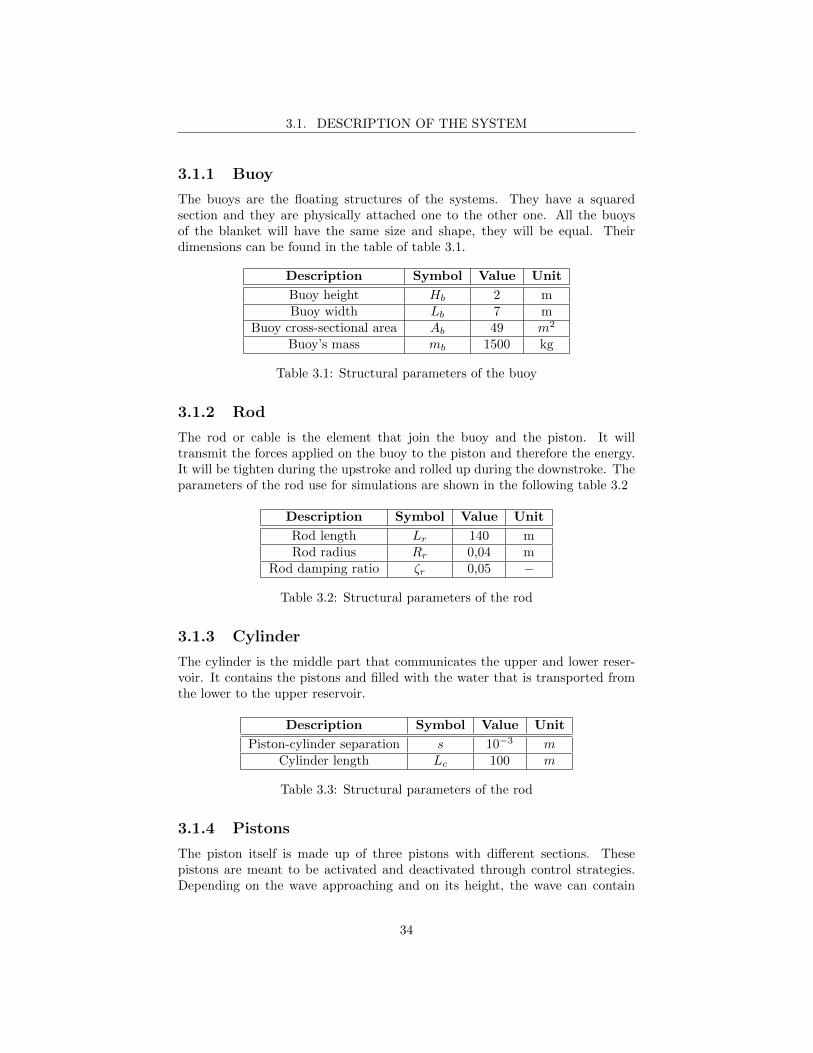
3.1.1 Buoy
The buoys are the floating structures of the systems. They have a squaredsection and they are physically attached one to the other one. All the buoysof the blanket will have the same size and shape, they will be equal. Theirdimensions can be found in the table of table 3.1.
Description Symbol Value Unit
Buoy height Hb 2 mBuoy width Lb 7 m
Buoy cross-sectional area Ab 49 m2
Buoy’s mass mb 1500 kg
Table 3.1: Structural parameters of the buoy
3.1.2 Rod
The rod or cable is the element that join the buoy and the piston. It willtransmit the forces applied on the buoy to the piston and therefore the energy.It will be tighten during the upstroke and rolled up during the downstroke. Theparameters of the rod use for simulations are shown in the following table 3.2
Description Symbol Value Unit
Rod length Lr 140 mRod radius Rr 0,04 m
Rod damping ratio ζr 0,05 −
Table 3.2: Structural parameters of the rod
3.1.3 Cylinder
The cylinder is the middle part that communicates the upper and lower reser-voir. It contains the pistons and filled with the water that is transported fromthe lower to the upper reservoir.
Description Symbol Value Unit
Piston-cylinder separation s 10−3 mCylinder length Lc 100 m
Table 3.3: Structural parameters of the rod
3.1.4 Pistons
The piston itself is made up of three pistons with different sections. Thesepistons are meant to be activated and deactivated through control strategies.Depending on the wave approaching and on its height, the wave can contain
34
3.1. DESCRIPTION OF THE SYSTEM
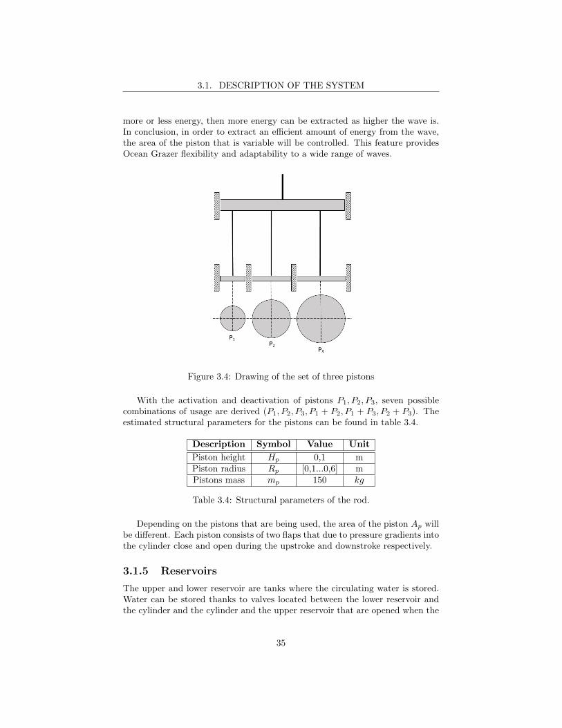
more or less energy, then more energy can be extracted as higher the wave is.In conclusion, in order to extract an efficient amount of energy from the wave,the area of the piston that is variable will be controlled. This feature providesOcean Grazer flexibility and adaptability to a wide range of waves.
Figure 3.4: Drawing of the set of three pistons
With the activation and deactivation of pistons P1, P2, P3, seven possiblecombinations of usage are derived (P1, P2, P3, P1 + P2, P1 + P3, P2 + P3). Theestimated structural parameters for the pistons can be found in table 3.4.
Description Symbol Value Unit
Piston height Hp 0,1 mPiston radius Rp [0,1...0,6] mPistons mass mp 150 kg
Table 3.4: Structural parameters of the rod.
Depending on the pistons that are being used, the area of the piston Ap willbe different. Each piston consists of two flaps that due to pressure gradients intothe cylinder close and open during the upstroke and downstroke respectively.
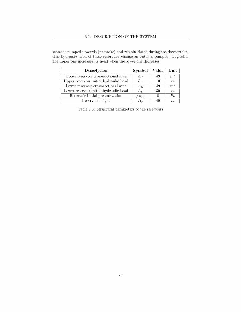
3.1.5 Reservoirs
The upper and lower reservoir are tanks where the circulating water is stored.Water can be stored thanks to valves located between the lower reservoir andthe cylinder and the cylinder and the upper reservoir that are opened when the
35
3.1. DESCRIPTION OF THE SYSTEM
water is pumped upwards (upstroke) and remain closed during the downstroke.The hydraulic head of these reservoirs change as water is pumped. Logically,the upper one increases its head when the lower one decreases.
Description Symbol Value Unit
Upper reservoir cross-sectional area AU 49 m2
Upper reservoir initial hydraulic head LU 10 mLower reservoir cross-sectional area AL 49 m2
Lower reservoir initial hydraulic head LL 30 mReservoir initial pressurization pH,L 0 Pa
Reservoir height Hr 40 m
Table 3.5: Structural parameters of the reservoirs
36
3.2. MODELS CONSIDERED
3.2 Models considered
In this section, two models applicable to Ocean grazer’s blanket are proposedtaking into consideration the theoretical background exposed in previous chap-ters (see chapter 2) and the conditions and requirements of the system itself.
In the first part, the different forces and its characteristic coefficients aredefined and estimated. In the second part, the systems of equations for thedifferent models are shown.
3.2.1 Forces and loads
When modelling a wave energy converter several kinds of loads have to betaken into consideration. On the one hand, there are the above mentionedhydrodynamic forces, which define the interactions between the wave and thesubmerged bodies, in this case the buoys, and at the end of the day have a biginfluence on the energy that is being transferred from the wave to the device. Onthe other hand, we have the forces that define the power take-off and describehow the energy is transferred inside the device. These forces will be modelledthrough a spring and damper between the buoys and the pistons.
When it comes to decide which hydrodynamics loads should be consideredin the studied case, the size of the buoy relative to the wave can help assumingwhich forces will have a bigger influence. These assumptions depend on if abody is considered either a small or a large volume object and indeed if thelocation leads to consider deep or shallow water waves.
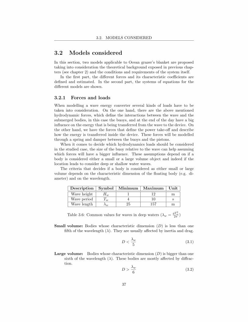
The criteria that decides if a body is considered as either small or largevolume depends on the characteristic dimension of the floating body (e.g. di-ameter) and on the wavelength.
Description Symbol Minimum Maximum Unit
Wave height Hw 1 12 mWave period Tw 4 10 sWave length λw 25 157 m
Table 3.6: Common values for waves in deep waters (λw =gT 2
w
2π )
Small volume: Bodies whose characteristic dimension (D) is less than onefifth of the wavelength (λ). They are usually affected by inertia and drag.
D <λw5
(3.1)
Large volume: Bodies whose characteristic dimension (D) is bigger than onesixth of the wavelength (λ). These bodies are mostly affected by diffrac-tion.
D >λw6
(3.2)
37
3.2. MODELS CONSIDERED
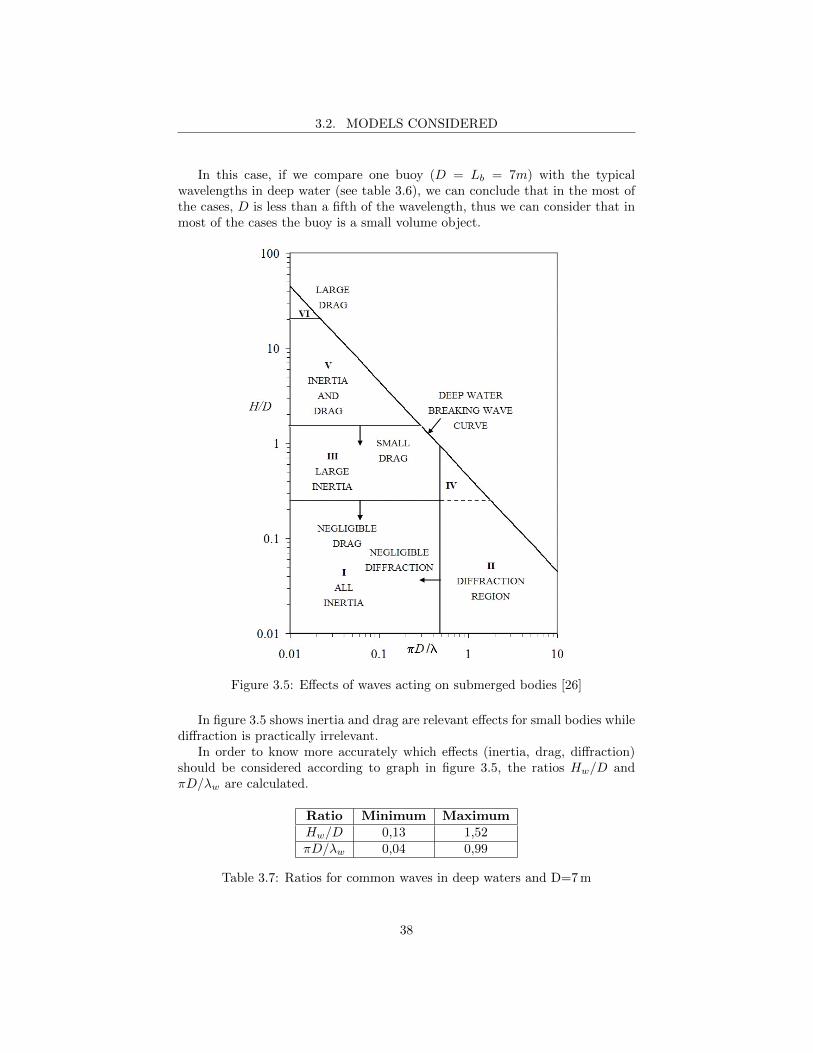
In this case, if we compare one buoy (D = Lb = 7m) with the typicalwavelengths in deep water (see table 3.6), we can conclude that in the most ofthe cases, D is less than a fifth of the wavelength, thus we can consider that inmost of the cases the buoy is a small volume object.
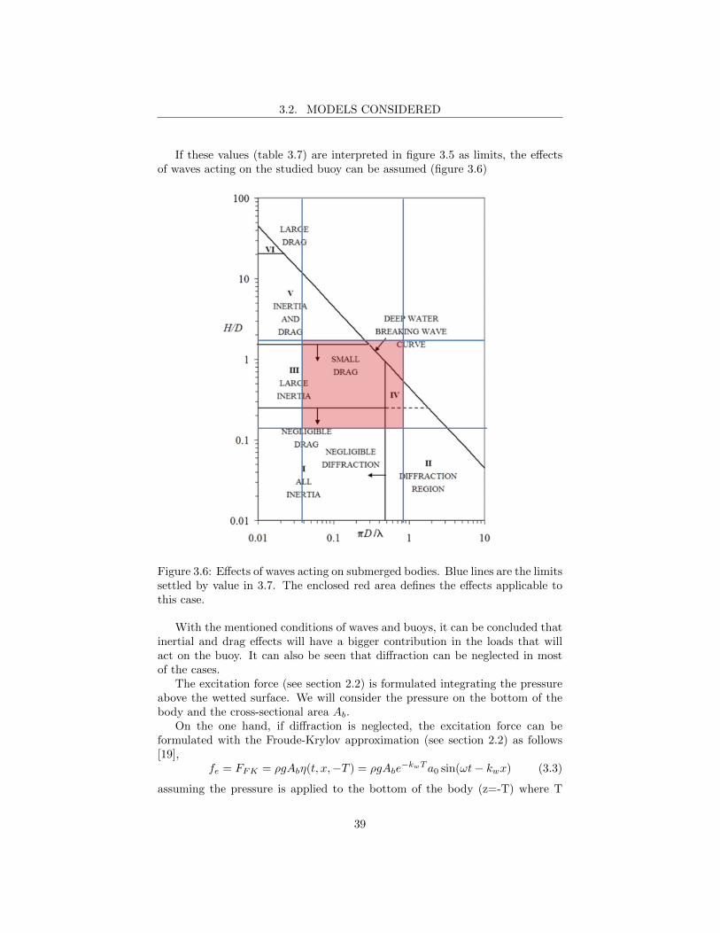
Figure 3.5: Effects of waves acting on submerged bodies [26]
In figure 3.5 shows inertia and drag are relevant effects for small bodies whilediffraction is practically irrelevant.
In order to know more accurately which effects (inertia, drag, diffraction)should be considered according to graph in figure 3.5, the ratios Hw/D andπD/λw are calculated.
Ratio Minimum MaximumHw/D 0,13 1,52πD/λw 0,04 0,99
Table 3.7: Ratios for common waves in deep waters and D=7 m
38
3.2. MODELS CONSIDERED
If these values (table 3.7) are interpreted in figure 3.5 as limits, the effectsof waves acting on the studied buoy can be assumed (figure 3.6)
Figure 3.6: Effects of waves acting on submerged bodies. Blue lines are the limitssettled by value in 3.7. The enclosed red area defines the effects applicable tothis case.
With the mentioned conditions of waves and buoys, it can be concluded thatinertial and drag effects will have a bigger contribution in the loads that willact on the buoy. It can also be seen that diffraction can be neglected in mostof the cases.
The excitation force (see section 2.2) is formulated integrating the pressureabove the wetted surface. We will consider the pressure on the bottom of thebody and the cross-sectional area Ab.
On the one hand, if diffraction is neglected, the excitation force can beformulated with the Froude-Krylov approximation (see section 2.2) as follows[19],
fe = FFK = ρgAbη(t, x,−T ) = ρgAbe−kwTa0 sin(ωt− kwx) (3.3)
assuming the pressure is applied to the bottom of the body (z=-T) where T
39
3.2. MODELS CONSIDERED
is the initial draft. The excitation force will depend on the wave-number kw,the wave frequency ω, time t and horizontal coordinate x. Note if the radiationforce is formulated as −Bw ξ, then excitation force can consider also dampingeffects (Bwe
−kwT vw).Once, the excitation force is defined, the excitation force amplitude per unit
of wave amplitude Γ can be given 2.45
Γ =|fe|a0
= ρgAbe−kwT (3.4)
which depends on the wave-number kw, and therefore on the wave-period Tw orwave frequency ω.
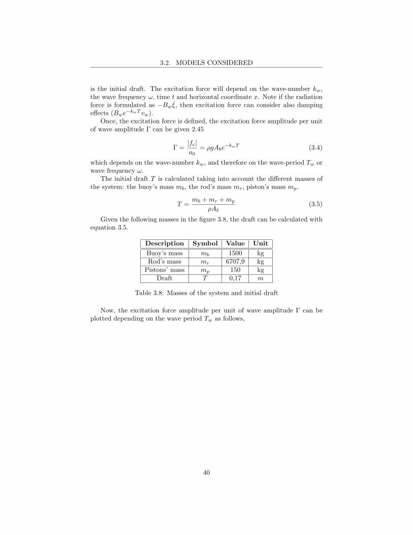
The initial draft T is calculated taking into account the different masses ofthe system: the buoy’s mass mb, the rod’s mass mr, piston’s mass mp.
T =mb +mr +mp
ρAb(3.5)
Given the following masses in the figure 3.8, the draft can be calculated withequation 3.5.
Description Symbol Value Unit
Buoy’s mass mb 1500 kgRod’s mass mr 6707,9 kg
Pistons’ mass mp 150 kgDraft T 0,17 m
Table 3.8: Masses of the system and initial draft
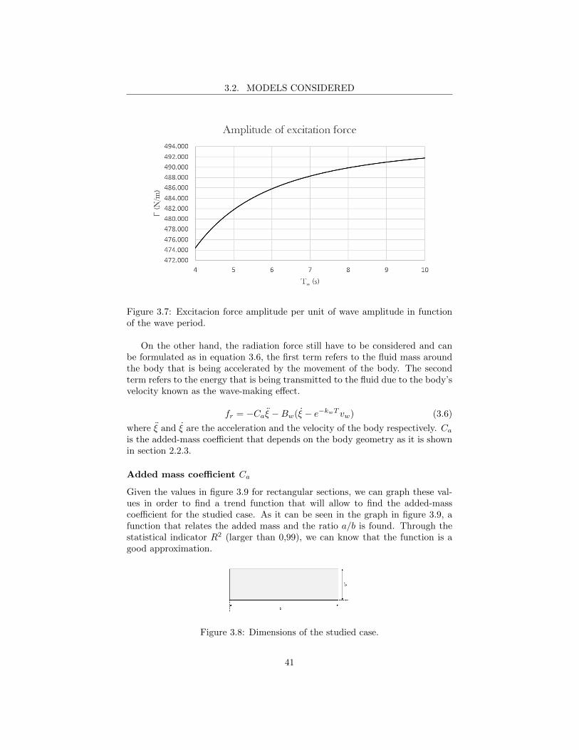
Now, the excitation force amplitude per unit of wave amplitude Γ can beplotted depending on the wave period Tw as follows,
40
3.2. MODELS CONSIDERED
Figure 3.7: Excitacion force amplitude per unit of wave amplitude in functionof the wave period.
On the other hand, the radiation force still have to be considered and canbe formulated as in equation 3.6, the first term refers to the fluid mass aroundthe body that is being accelerated by the movement of the body. The secondterm refers to the energy that is being transmitted to the fluid due to the body’svelocity known as the wave-making effect.
fr = −Caξ −Bw(ξ − e−kwT vw) (3.6)
where ξ and ξ are the acceleration and the velocity of the body respectively. Cais the added-mass coefficient that depends on the body geometry as it is shownin section 2.2.3.
Added mass coefficient Ca
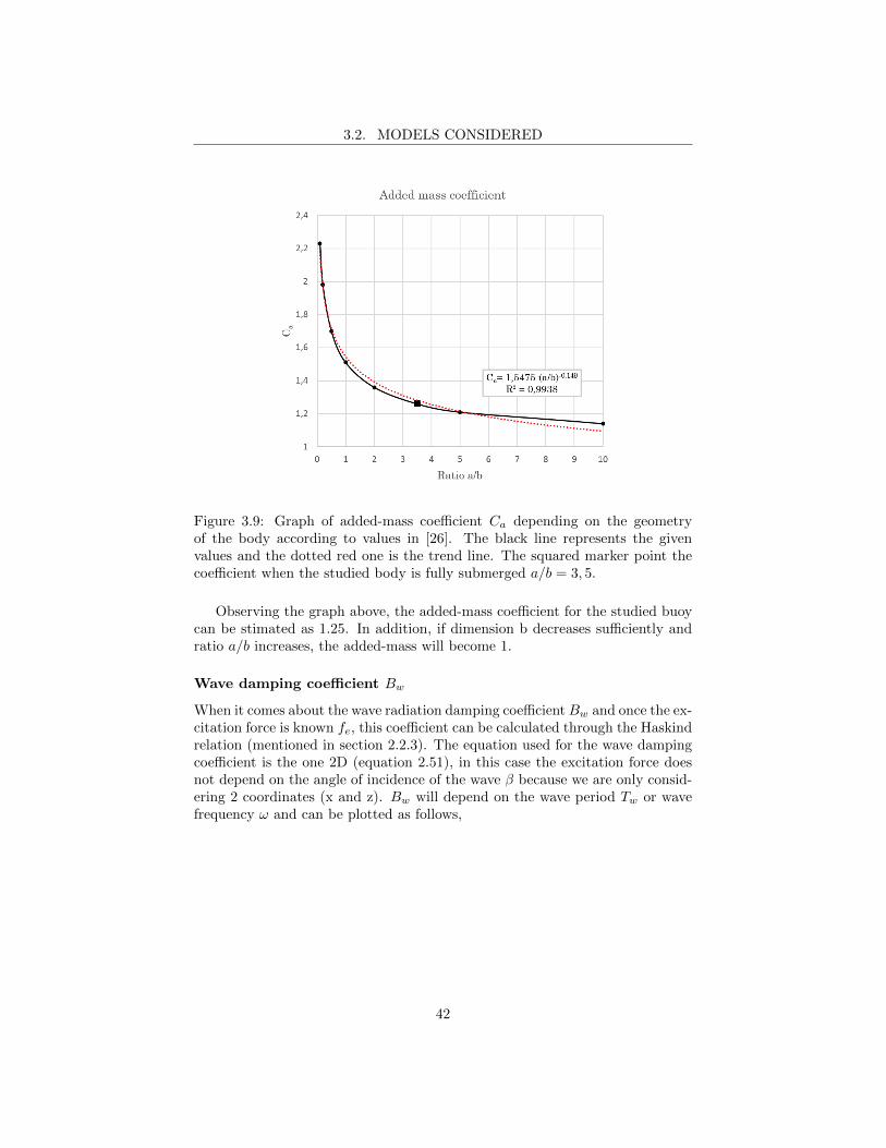
Given the values in figure 3.9 for rectangular sections, we can graph these val-ues in order to find a trend function that will allow to find the added-masscoefficient for the studied case. As it can be seen in the graph in figure 3.9, afunction that relates the added mass and the ratio a/b is found. Through thestatistical indicator R2 (larger than 0,99), we can know that the function is agood approximation.
Figure 3.8: Dimensions of the studied case.
41
3.2. MODELS CONSIDERED
Figure 3.9: Graph of added-mass coefficient Ca depending on the geometryof the body according to values in [26]. The black line represents the givenvalues and the dotted red one is the trend line. The squared marker point thecoefficient when the studied body is fully submerged a/b = 3, 5.
Observing the graph above, the added-mass coefficient for the studied buoycan be stimated as 1.25. In addition, if dimension b decreases sufficiently andratio a/b increases, the added-mass will become 1.
Wave damping coefficient Bw
When it comes about the wave radiation damping coefficientBw and once the ex-citation force is known fe, this coefficient can be calculated through the Haskindrelation (mentioned in section 2.2.3). The equation used for the wave dampingcoefficient is the one 2D (equation 2.51), in this case the excitation force doesnot depend on the angle of incidence of the wave β because we are only consid-ering 2 coordinates (x and z). Bw will depend on the wave period Tw or wavefrequency ω and can be plotted as follows,
42
3.2. MODELS CONSIDERED
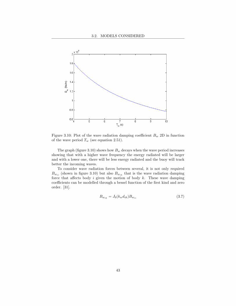
Figure 3.10: Plot of the wave radiation damping coefficient Bw 2D in functionof the wave period Tw (see equation 2.51).
The graph (figure 3.10) shows how Bw decays when the wave period increasesshowing that with a higher wave frequency the energy radiated will be largerand with a lower one, there will be less energy radiated and the buoy will trackbetter the incoming waves.
To consider wave radiation forces between several, it is not only requiredBwii
(shown in figure 3.10) but also Bwikthat is the wave radiation damping
force that affects body i given the motion of body k. These wave dampingcoefficients can be modelled through a bessel function of the first kind and zeroorder. [31].
Bwik= J0(kwdik)Bwii (3.7)
43
3.2. MODELS CONSIDERED
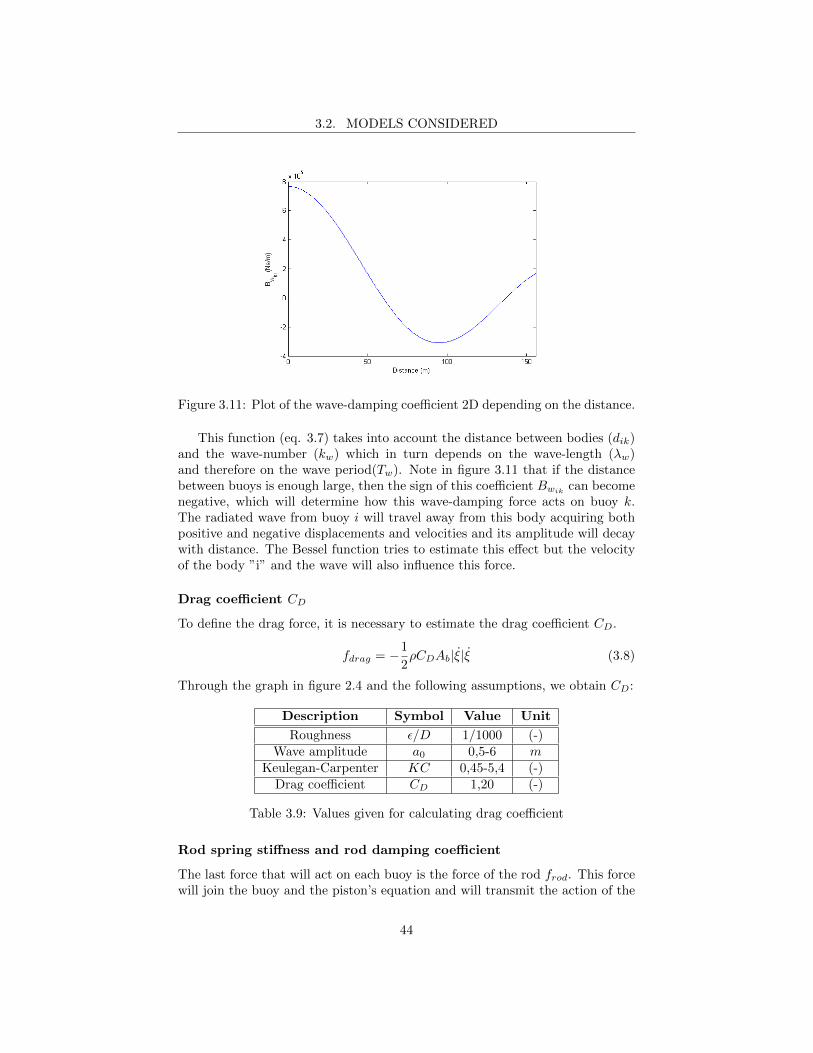
Figure 3.11: Plot of the wave-damping coefficient 2D depending on the distance.
This function (eq. 3.7) takes into account the distance between bodies (dik)and the wave-number (kw) which in turn depends on the wave-length (λw)and therefore on the wave period(Tw). Note in figure 3.11 that if the distancebetween buoys is enough large, then the sign of this coefficient Bwik
can becomenegative, which will determine how this wave-damping force acts on buoy k.The radiated wave from buoy i will travel away from this body acquiring bothpositive and negative displacements and velocities and its amplitude will decaywith distance. The Bessel function tries to estimate this effect but the velocityof the body ”i” and the wave will also influence this force.
Drag coefficient CD
To define the drag force, it is necessary to estimate the drag coefficient CD.
fdrag = −1
2ρCDAb|ξ|ξ (3.8)
Through the graph in figure 2.4 and the following assumptions, we obtain CD:
Description Symbol Value Unit
Roughness ε/D 1/1000 (-)Wave amplitude a0 0,5-6 m
Keulegan-Carpenter KC 0,45-5,4 (-)Drag coefficient CD 1,20 (-)
Table 3.9: Values given for calculating drag coefficient
Rod spring stiffness and rod damping coefficient
The last force that will act on each buoy is the force of the rod frod. This forcewill join the buoy and the piston’s equation and will transmit the action of the
44
3.2. MODELS CONSIDERED
wave on the buoy through the piston and hence, the power. It will be modelledwith a spring and a damper between the buoy and the piston.
frod = C(ξ − zp) +K(ξ − zp − Lr) (3.9)
where C is the rod damping coefficient, K is the rod spring stiffness, zp is thepiston’s velocity, zp is the piston’s displacement and Lr is the rod’s length.
The values considered for the damping coefficient C and the spring stiffnessK are the following:
Description Symbol Value Unit
Damping coefficient C 9, 651 · 103 Ns/mSpring stiffness K 6, 209 · 106 N/m
Table 3.10: Damping and spring stiffness coefficients for the force of rod accord-ing to [11],[12].
45
3.2. MODELS CONSIDERED
3.2.2 System of equations
The model that will be proposed for the blanket considers existing models fora single piston pump [11] [12] [13]. In this section, a model for a single-pistonpump is introduced, then two possible models considering multiple pumps aredescribed to be later simulated.
A single piston pump
The model of a single piston pump consists of several equations. The first onewill consider the forces acting on the buoy, while the second one will take intoaccount the forces acting on the piston.
If in equilibrium, the forces that are taken into account are the buoyancyforce and the weight, in dynamic situations we only consider disturbances toequilibrium, so instead of considering buoyancy and the body’s weight, therestoring buoyancy force fhs will be considered [24] [19]. This force fhs ismodelled like a spring whose stiffness is the term ρgAb.
fhs = ρswgAbξ (3.10)
Hence and given also the forces described in the previous section 3.2.1, thebuoy’s equation can be written as follows:
mbξ + fhs = fe + fr + fdrag − frod (3.11)
Introducing the forces of equations 3.6, 3.9 and 3.10 into the above equation3.11 yields:
mbξ+ρswgAbξ = fe−maξ−Bw(ξ−e−kwT vw)+fdrag−C(ξ−zp)−K(ξ−zp−Lr)(3.12)
that can be gathered as follows:
(mb+ma)ξ = −(K+ρswgAb)ξ−(Bw+C)ξ+Kzp+Czp+Bwe−kwT vw+KLr+fe+fdrag
(3.13)depending on variables ξ, ξ, ξ, zp, zp that are the displacement, velocity, acceler-ation of the buoy and displacement and velocity of the piston respectively. T isthe initial draft or the initial submerged height which is calculated as follows:
T =mb +mr +mp
ρAb(3.14)
For the piston, two equations are defined to differentiate between the up-stroke and the downstroke. The difference is mainly the mass of the fluid.During the upstroke, the piston has to hold the weight of the fluid column thatis being carried upwards while valves are opened. During the downstroke, thevalves are closed and the piston goes down following the movement of the buoy.
During the upstroke:
46
3.2. MODELS CONSIDERED
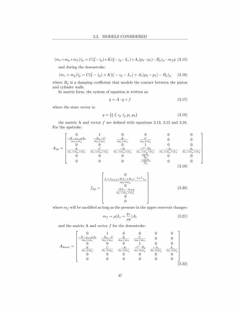
(mr+mp+mf )zp = C(ξ−zp)+K(ξ−zp−Lr)+Ac(p4−p1)−Bpzp−mfg (3.15)
and during the downstroke:
(mr +mp)zp = C(ξ − zp) +K(ξ − zp − Lr) +Ac(p4 − p1)−Bpzp (3.16)
where Bp is a damping coefficient that models the contact between the pistonand cylinder walls.
In matrix form, the system of equation is written as:
q = A · q + f (3.17)
where the state vector is:
q = {ξ ξ zp zp p1 p4} (3.18)
the matrix A and vector f are defined with equations 3.13, 3.15 and 3.16.For the upstroke:
Aup =
0 1 0 0 0 0−K−ρswgAb
mb+ma
−Bw−Cmb+ma
Kmb+ma
Cmb+ma
0 0
0 0 0 1 0 0K
mr+mp+mf
Cmr+mp+mf
−Kmr+mp+mf
−C−Bp
mr+mp+mf
−Ac
mr+mp+mf
Ac
mr+mp+mf
0 0 0 ρgAc
AU0 0
0 0 0 −ρgAc
AL0 0
(3.19)
fup =
0fe+fdrag+KLr+Bwe
−kwT vwmb+ma
0−KLr−mfgmr+mp+mf
00
(3.20)
where mf will be modified as long as the pressure in the upper reservoir changes:
mf = ρ(Lc +p1ρg
)Ac (3.21)
and the matrix A and vector f for the downstroke:
Adown =
0 1 0 0 0 0−K−ρswgAb
mb+ma
−Bw−Cmb+ma
Kmb+ma
Cmb+ma
0 0
0 0 0 1 0 0K
mr+mp
Cmr+mp
−Kmr+mp
−C−Bp
mr+mp
−Ac
mr+mp
Ac
mr+mp
0 0 0 0 0 00 0 0 0 0 0
(3.22)
47
3.2. MODELS CONSIDERED
fdown =
0fe+fdrag+KLr+Bwe
−kwT vwmb+ma
0−KLr
mr+mp
00
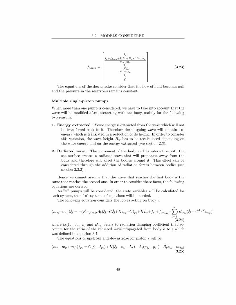
(3.23)
The equations of the downstroke consider that the flow of fluid becomes nulland the pressure in the reservoirs remains constant.
Multiple single-piston pumps
When more than one pump is considered, we have to take into account that thewave will be modified after interacting with one buoy, mainly for the followingtwo reasons:
1. Energy extracted : Some energy is extracted from the wave which will notbe transferred back to it. Therefore the outgoing wave will contain lessenergy which is translated in a reduction of its height. In order to considerthis variation, the wave height Hw has to be recalculated depending onthe wave energy and on the energy extracted (see section 2.3).
2. Radiated wave : The movement of the body and its interaction with thesea surface creates a radiated wave that will propagate away from thebody and therefore will affect the bodies around it. This effect can beconsidered through the addition of radiation forces between bodies (seesection 2.2.2).
Hence we cannot assume that the wave that reaches the first buoy is thesame that reaches the second one. In order to consider these facts, the followingequations are derived.
As ”n” pumps will be considered, the state variables will be calculated foreach system, then ”n” systems of equations will be needed.
The following equation considers the forces acting on buoy i:
(mbi+mai)ξi = −(K+ρswgAb)ξi−Cξi+Kzpi+Czpi+KLr+fei+fdragi−n∑k=1
(Bwki(ξk−e−kwT vwk
)
(3.24)where kε[1, .., i, .., n] and Bwki
refers to radiation damping coefficient that ac-counts for the ratio of the radiated wave propagated from body k to i whichwas defined in equation 3.7.
The equations of upstroke and downstroke for piston i will be
(mr+mp+mfi)zpi = C(ξi− zpi)+K(ξi−zpi−Lr)+Ac(p4i−p1i)−Bpzpi−mfig(3.25)
48
3.2. MODELS CONSIDERED
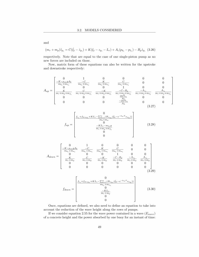
and
(mr +mp)zpi = C(ξi − zpi) +K(ξi − zpi − Lr) +Ac(p4i − p1i)−Bpzpi (3.26)
respectively. Note that are equal to the case of one single-piston pump as nonew forces are included on those.
Now, matrix form of these equations can also be written for the upstrokeand downstroke respectively:
Aup =
0 1 0 0 0 0−K−ρswgAb
mbi+mai
−Cmbi
+mai
Kmbi
+mai
Cmbi
+mai0 0
0 0 0 1 0 0K
mr+mp+mfi
Cmr+mp+mfi
−Kmr+mp+mfi
−C−Bp
mr+mp+mfi
−Aci
mr+mp+mfi
Aci
mr+mp+mfi
0 0 0ρgAci
AU0 0
0 0 0−ρgAci
AL0 0
(3.27)
fup =
0fei+fdragi
+KLr−∑n
k=1(Bwki(ξk−e−kwT vwk
))
mb+ma
0−KLr−mfi
g
mr+mp+mfi
00
(3.28)
Adown =
0 1 0 0 0 0−K−ρswgAb
mbi+mai
−Cmbi
+mai
Kmbi
+mai
Cmbi
+mai0 0
0 0 0 1 0 0K
mr+mp
Cmr+mp
−Kmr+mp
−C−Bp
mr+mp
−Aci
mr+mp
Aci
mr+mp
0 0 0 0 0 00 0 0 0 0 0
(3.29)
fdown =
0fei+fdragi
+KLr−∑n
k=1(Bwki(ξk−e−kwT vwk
))
mbi+mai
0−KLr
mr+mp
00
(3.30)
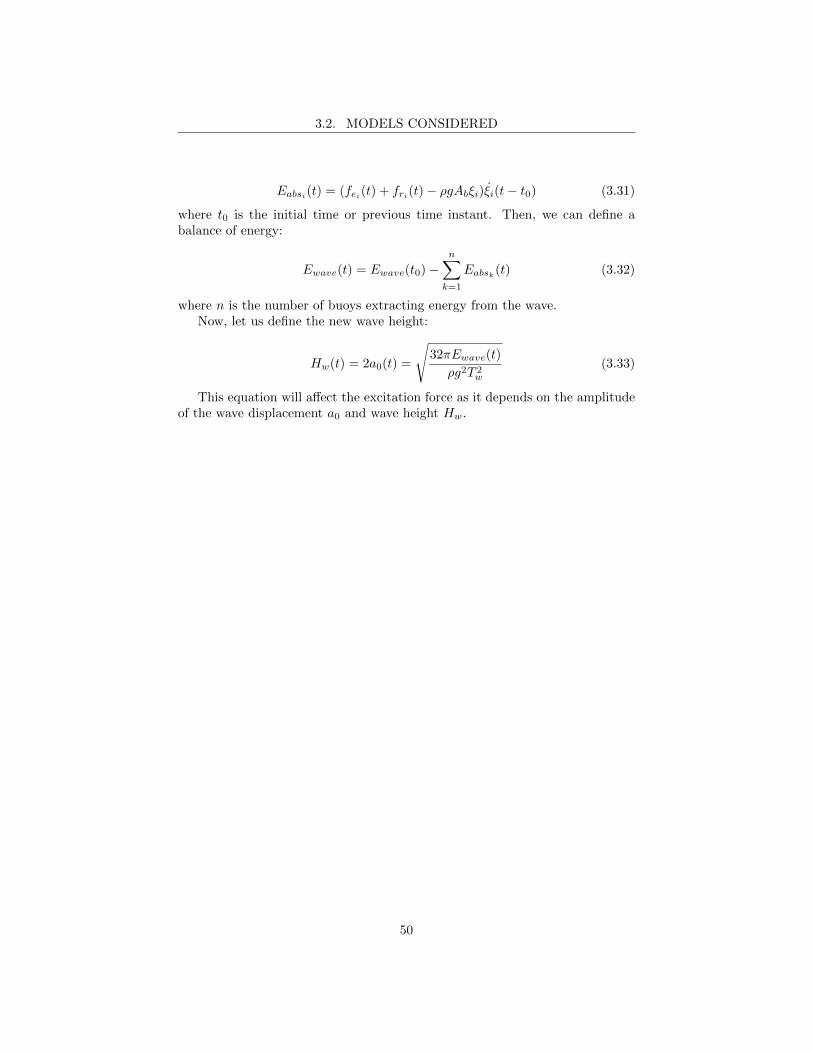
Once, equations are defined, we also need to define an equation to take intoaccount the reduction of the wave height along the rows of pumps.
If we consider equation 2.55 for the wave power contained in a wave (Ewave)of a concrete height and the power absorbed by one buoy for an instant of time:
49
3.2. MODELS CONSIDERED
Eabsi(t) = (fei(t) + fri(t)− ρgAbξi)ξi(t− t0) (3.31)
where t0 is the initial time or previous time instant. Then, we can define abalance of energy:
Ewave(t) = Ewave(t0)−n∑k=1
Eabsk(t) (3.32)
where n is the number of buoys extracting energy from the wave.Now, let us define the new wave height:
Hw(t) = 2a0(t) =
√32πEwave(t)
ρg2T 2w
(3.33)
This equation will affect the excitation force as it depends on the amplitudeof the wave displacement a0 and wave height Hw.
50
Chapter 4
Results and discussion
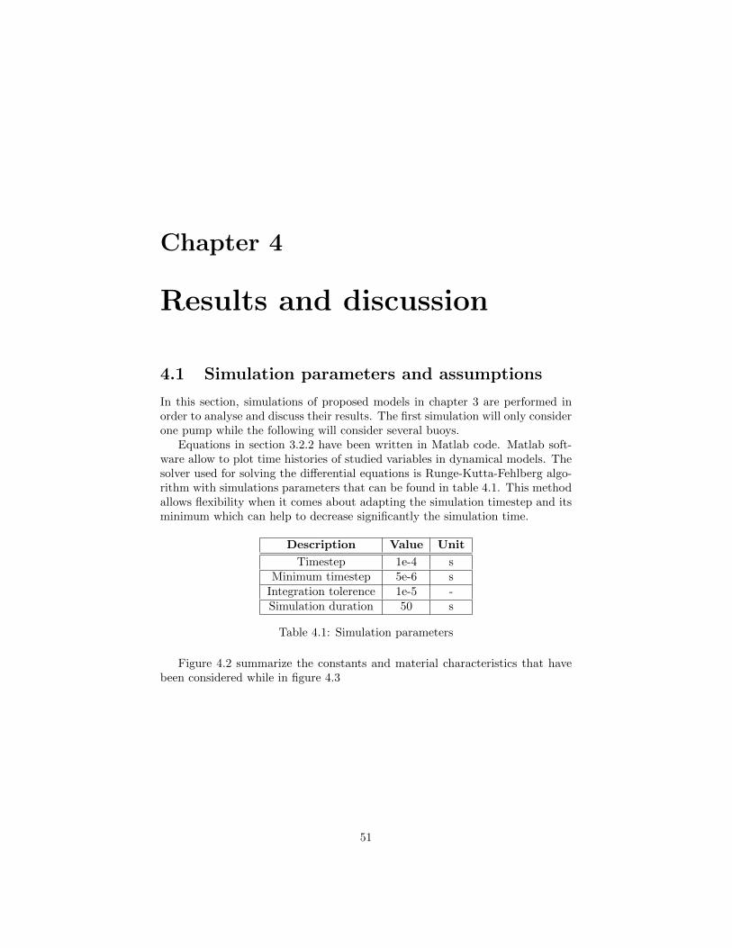
4.1 Simulation parameters and assumptions
In this section, simulations of proposed models in chapter 3 are performed inorder to analyse and discuss their results. The first simulation will only considerone pump while the following will consider several buoys.
Equations in section 3.2.2 have been written in Matlab code. Matlab soft-ware allow to plot time histories of studied variables in dynamical models. Thesolver used for solving the differential equations is Runge-Kutta-Fehlberg algo-rithm with simulations parameters that can be found in table 4.1. This methodallows flexibility when it comes about adapting the simulation timestep and itsminimum which can help to decrease significantly the simulation time.
Description Value Unit
Timestep 1e-4 sMinimum timestep 5e-6 s
Integration tolerence 1e-5 -Simulation duration 50 s
Table 4.1: Simulation parameters
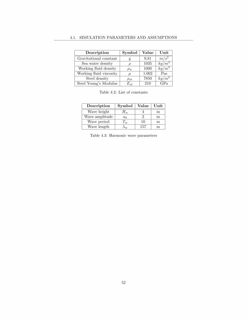
Figure 4.2 summarize the constants and material characteristics that havebeen considered while in figure 4.3
51
4.1. SIMULATION PARAMETERS AND ASSUMPTIONS
Description Symbol Value Unit
Gravitational constant g 9.81 m/s2
Sea water density ρ 1035 kg/m3
Working fluid density ρw 1000 kg/m3
Working fluid viscosity µ 1.002 PasSteel density ρst 7850 kg/m3
Steel Young’s Modulus Est 210 GPa
Table 4.2: List of constants
Description Symbol Value Unit
Wave height Hw 4 mWave amplitude a0 2 m
Wave period Tw 10 mWave length λw 157 m
Table 4.3: Harmonic wave parameters
52
4.2. SIMULATION I: A SINGLE PUMP
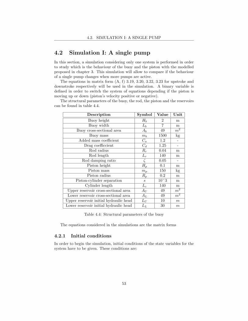
4.2 Simulation I: A single pump
In this section, a simulation considering only one system is performed in orderto study which is the behaviour of the buoy and the piston with the modelledproposed in chapter 3. This simulation will allow to compare if the behaviourof a single pump changes when more pumps are active.
The equations in matrix form (A, f) 3.19, 3.20, 3.22, 3.23 for upstroke anddownstroke respectively will be used in the simulation. A binary variable isdefined in order to switch the system of equations depending if the piston ismoving up or down (piston’s velocity positive or negative).
The structural parameters of the buoy, the rod, the piston and the reservoirscan be found in table 4.4.
Description Symbol Value Unit
Buoy height Hb 2 mBuoy width Lb 7 m
Buoy cross-sectional area Ab 49 m2
Buoy mass mb 1500 kgAdded mass coefficient Ca 1.2 -
Drag coefficcient Cd 1.25 -Rod radius Rr 0.04 mRod length Lr 140 m
Rod damping ratio ζ 0.05 -Piston height Hp 0.1 mPiston mass mp 150 kgPiston radius Rp 0.2 m
Piston-cylinder separation s 10−3 mCylinder length Lc 140 m
Upper reservoir cross-sectional area AU 49 m2
Lower reservoir cross-sectional area AL 49 m2
Upper reservoir initial hydraulic head LU 10 mLower reservoir initial hydraulic head LL 30 m
Table 4.4: Structural parameters of the buoy
The equations considered in the simulations are the matrix forms
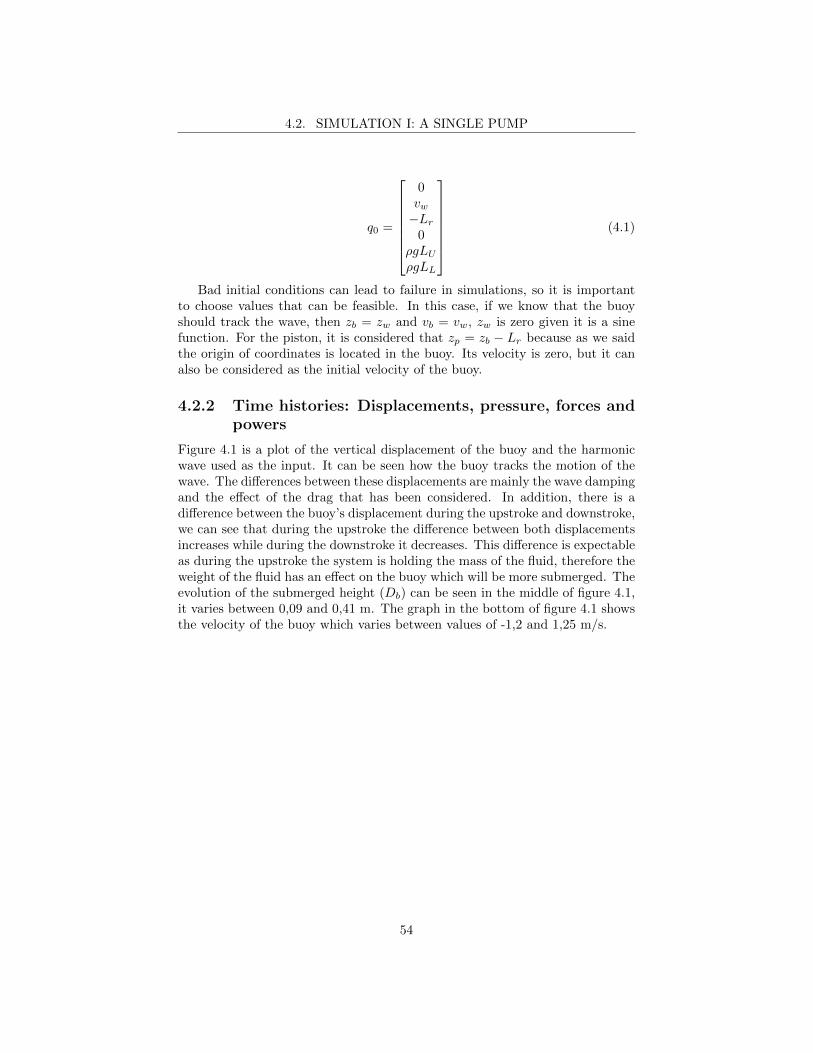
4.2.1 Initial conditions
In order to begin the simulation, initial conditions of the state variables for thesystem have to be given. These conditions are:
53
4.2. SIMULATION I: A SINGLE PUMP
q0 =
0vw−Lr
0ρgLUρgLL
(4.1)
Bad initial conditions can lead to failure in simulations, so it is importantto choose values that can be feasible. In this case, if we know that the buoyshould track the wave, then zb = zw and vb = vw, zw is zero given it is a sinefunction. For the piston, it is considered that zp = zb − Lr because as we saidthe origin of coordinates is located in the buoy. Its velocity is zero, but it canalso be considered as the initial velocity of the buoy.
4.2.2 Time histories: Displacements, pressure, forces andpowers
Figure 4.1 is a plot of the vertical displacement of the buoy and the harmonicwave used as the input. It can be seen how the buoy tracks the motion of thewave. The differences between these displacements are mainly the wave dampingand the effect of the drag that has been considered. In addition, there is adifference between the buoy’s displacement during the upstroke and downstroke,we can see that during the upstroke the difference between both displacementsincreases while during the downstroke it decreases. This difference is expectableas during the upstroke the system is holding the mass of the fluid, therefore theweight of the fluid has an effect on the buoy which will be more submerged. Theevolution of the submerged height (Db) can be seen in the middle of figure 4.1,it varies between 0,09 and 0,41 m. The graph in the bottom of figure 4.1 showsthe velocity of the buoy which varies between values of -1,2 and 1,25 m/s.
54
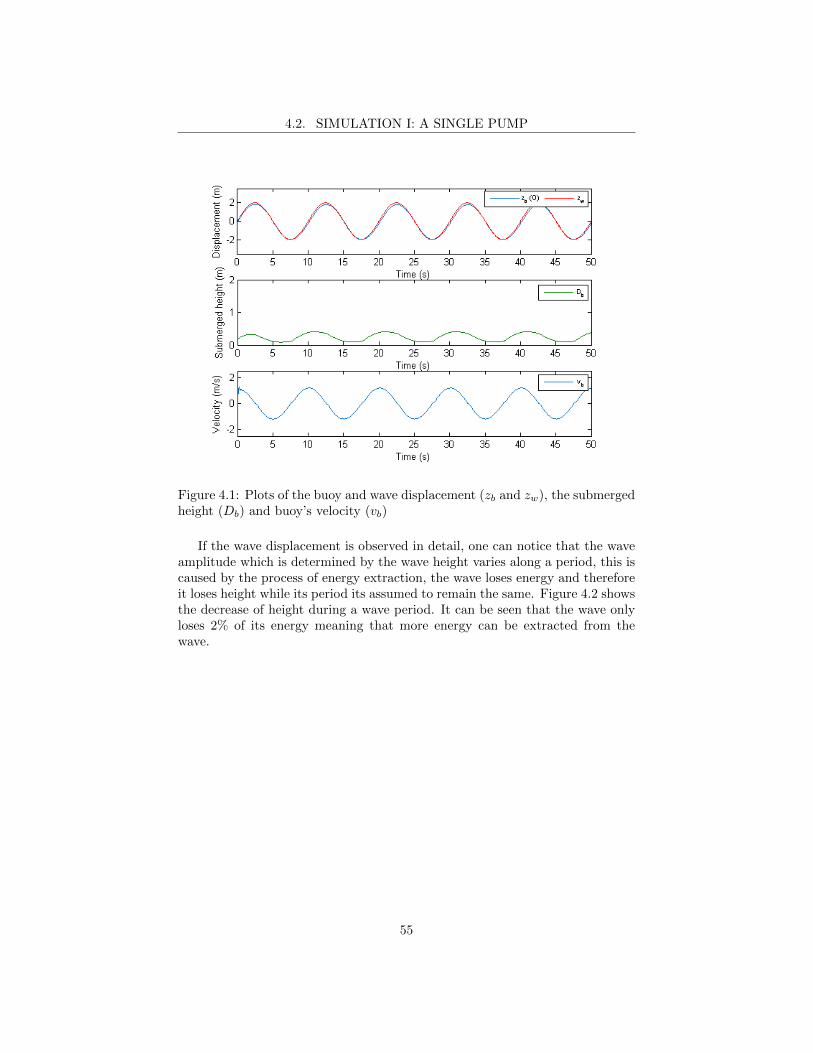
4.2. SIMULATION I: A SINGLE PUMP
Figure 4.1: Plots of the buoy and wave displacement (zb and zw), the submergedheight (Db) and buoy’s velocity (vb)
If the wave displacement is observed in detail, one can notice that the waveamplitude which is determined by the wave height varies along a period, this iscaused by the process of energy extraction, the wave loses energy and thereforeit loses height while its period its assumed to remain the same. Figure 4.2 showsthe decrease of height during a wave period. It can be seen that the wave onlyloses 2% of its energy meaning that more energy can be extracted from thewave.
55
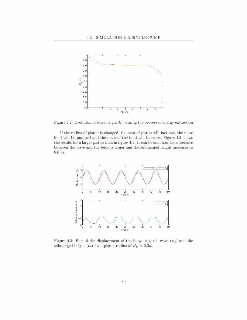
4.2. SIMULATION I: A SINGLE PUMP
Figure 4.2: Evolution of wave height Hw during the process of energy extraction
If the radius of piston is changed, the area of piston will increase, the morefluid will be pumped and the mass of the fluid will increase. Figure 4.3 showsthe results for a larger piston than in figure 4.1. It can be seen how the differencebetween the wave and the buoy is larger and the submerged height increases to0,6 m.
Figure 4.3: Plot of the displacement of the buoy (zb), the wave (zw) and thesubmerged height (m) for a piston radius of RP = 0.3m
56
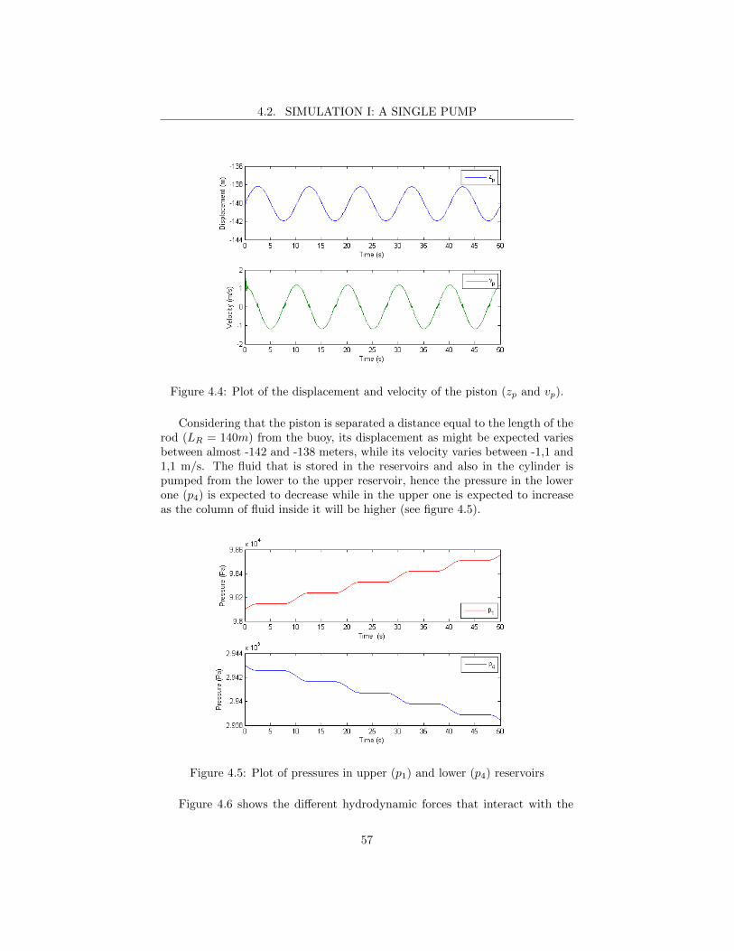
4.2. SIMULATION I: A SINGLE PUMP
Figure 4.4: Plot of the displacement and velocity of the piston (zp and vp).
Considering that the piston is separated a distance equal to the length of therod (LR = 140m) from the buoy, its displacement as might be expected variesbetween almost -142 and -138 meters, while its velocity varies between -1,1 and1,1 m/s. The fluid that is stored in the reservoirs and also in the cylinder ispumped from the lower to the upper reservoir, hence the pressure in the lowerone (p4) is expected to decrease while in the upper one is expected to increaseas the column of fluid inside it will be higher (see figure 4.5).
Figure 4.5: Plot of pressures in upper (p1) and lower (p4) reservoirs
Figure 4.6 shows the different hydrodynamic forces that interact with the
57
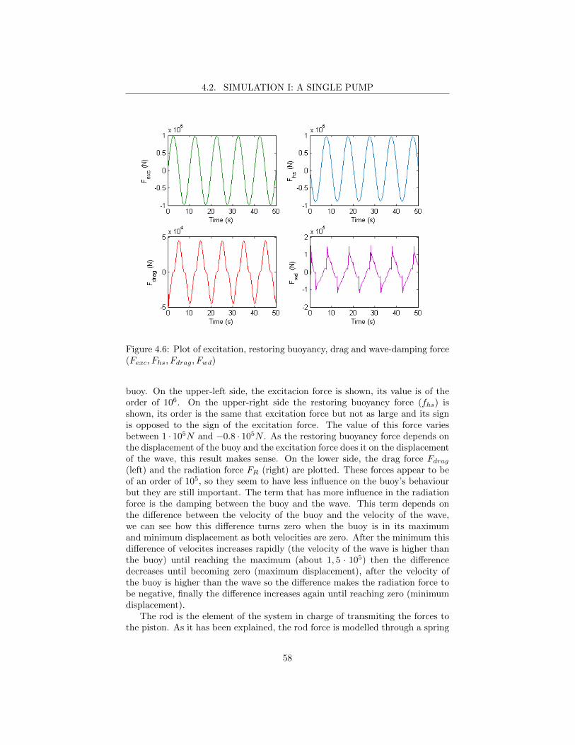
4.2. SIMULATION I: A SINGLE PUMP
Figure 4.6: Plot of excitation, restoring buoyancy, drag and wave-damping force(Fexc, Fhs, Fdrag, Fwd)
buoy. On the upper-left side, the excitacion force is shown, its value is of theorder of 106. On the upper-right side the restoring buoyancy force (fhs) isshown, its order is the same that excitation force but not as large and its signis opposed to the sign of the excitation force. The value of this force variesbetween 1 · 105N and −0.8 · 105N . As the restoring buoyancy force depends onthe displacement of the buoy and the excitation force does it on the displacementof the wave, this result makes sense. On the lower side, the drag force Fdrag(left) and the radiation force FR (right) are plotted. These forces appear to beof an order of 105, so they seem to have less influence on the buoy’s behaviourbut they are still important. The term that has more influence in the radiationforce is the damping between the buoy and the wave. This term depends onthe difference between the velocity of the buoy and the velocity of the wave,we can see how this difference turns zero when the buoy is in its maximumand minimum displacement as both velocities are zero. After the minimum thisdifference of velocites increases rapidly (the velocity of the wave is higher thanthe buoy) until reaching the maximum (about 1, 5 · 105) then the differencedecreases until becoming zero (maximum displacement), after the velocity ofthe buoy is higher than the wave so the difference makes the radiation force tobe negative, finally the difference increases again until reaching zero (minimumdisplacement).
The rod is the element of the system in charge of transmiting the forces tothe piston. As it has been explained, the rod force is modelled through a spring
58
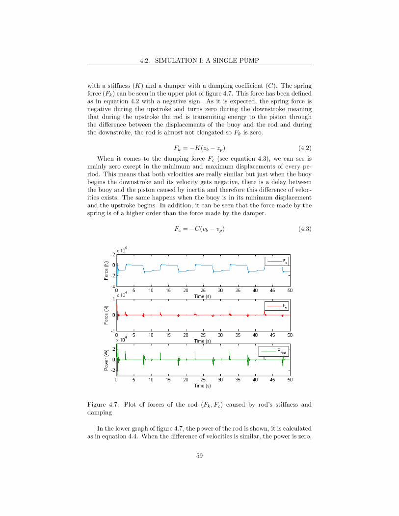
4.2. SIMULATION I: A SINGLE PUMP
with a stiffness (K) and a damper with a damping coefficient (C). The springforce (Fk) can be seen in the upper plot of figure 4.7. This force has been definedas in equation 4.2 with a negative sign. As it is expected, the spring force isnegative during the upstroke and turns zero during the downstroke meaningthat during the upstroke the rod is transmiting energy to the piston throughthe difference between the displacements of the buoy and the rod and duringthe downstroke, the rod is almost not elongated so Fk is zero.
Fk = −K(zb − zp) (4.2)
When it comes to the damping force Fc (see equation 4.3), we can see ismainly zero except in the minimum and maximum displacements of every pe-riod. This means that both velocities are really similar but just when the buoybegins the downstroke and its velocity gets negative, there is a delay betweenthe buoy and the piston caused by inertia and therefore this difference of veloc-ities exists. The same happens when the buoy is in its minimum displacementand the upstroke begins. In addition, it can be seen that the force made by thespring is of a higher order than the force made by the damper.
Fc = −C(vb − vp) (4.3)
Figure 4.7: Plot of forces of the rod (Fk, Fc) caused by rod’s stiffness anddamping
In the lower graph of figure 4.7, the power of the rod is shown, it is calculatedas in equation 4.4. When the difference of velocities is similar, the power is zero,
59
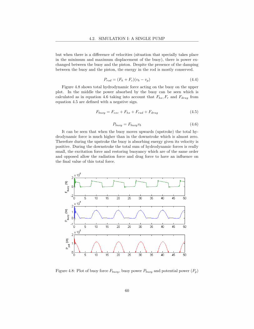
4.2. SIMULATION I: A SINGLE PUMP
but when there is a difference of velocities (situation that specially takes placein the minimum and maximum displacement of the buoy), there is power ex-changed between the buoy and the piston. Despite the presence of the dampingbetween the buoy and the piston, the energy in the rod is mostly conserved.
Prod = (Fk + Fc)(vb − vp) (4.4)
Figure 4.8 shows total hydrodynamic force acting on the buoy on the upperplot. In the middle the power absorbed by the buoy can be seen which iscalculated as in equation 4.6 taking into account that Fhs, Fr and Fdrag fromequation 4.5 are defined with a negative sign.
Fbuoy = Fexc + Fhs + Frad + Fdrag (4.5)
Pbuoy = Fbuoyvb (4.6)
It can be seen that when the buoy moves upwards (upstroke) the total hy-drodynamic force is much higher than in the downstroke which is almost zero.Therefore during the upstroke the buoy is absorbing energy given its velocity ispositive. During the downstroke the total sum of hydrodynamic forces is reallysmall, the excitation force and restoring buoyancy which are of the same orderand opposed allow the radiation force and drag force to have an influence onthe final value of this total force.
Figure 4.8: Plot of buoy force Fbuoy, buoy power Pbuoy and potential power (Pp)
60
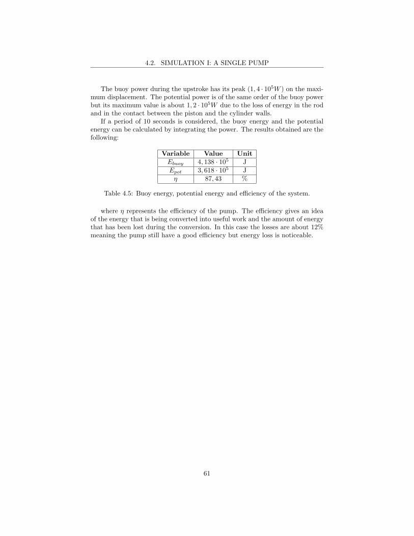
4.2. SIMULATION I: A SINGLE PUMP
The buoy power during the upstroke has its peak (1, 4 · 105W ) on the maxi-mum displacement. The potential power is of the same order of the buoy powerbut its maximum value is about 1, 2 · 105W due to the loss of energy in the rodand in the contact between the piston and the cylinder walls.
If a period of 10 seconds is considered, the buoy energy and the potentialenergy can be calculated by integrating the power. The results obtained are thefollowing:
Variable Value UnitEbuoy 4, 138 · 105 JEpot 3, 618 · 105 Jη 87, 43 %
Table 4.5: Buoy energy, potential energy and efficiency of the system.
where η represents the efficiency of the pump. The efficiency gives an ideaof the energy that is being converted into useful work and the amount of energythat has been lost during the conversion. In this case the losses are about 12%meaning the pump still have a good efficiency but energy loss is noticeable.
61
4.3. SIMULATION II: MULTI-PUMP
4.3 Simulation II: Multi-pump
In this section, a system of pumps is simulated with the model explained insection 3.2. In this simulation, the interaction between five pumps (each onewith its buoy, rod and piston) is studied and analysed. The algorithm developedin Matlab code allows to calculate several buoys or just one taking into accountthat as more pumps have to be calculated, the simulation time will increasereasonably. In addition, some assumptions have been made in order to makethese calculations:
� In reality, buoys are physically attached meaning that there exist hingeforces between them. In the simulation these forces are not considered asonly interactions with waves are studied and buoys are treated as lumpedmasses. The buoys are considered to be separated a concrete distance(pitch).
� The pumps are considered to be identical. They are using the same pistonand cylinder characteristics, their buoys are the same. Only the location(x coordinate) is different and therefore the wave input will be differentas it depends on distance.
� As the wave energy is calculated for a single wave of a specific wave heightand period, the input waves in the simulation are considered as singleand not as a group. Therefore, the pumps are extracting energy from aconcrete wave in every instant that does not have to be the same.
� Values for the characteristics of materials and fluids as well as coefficientshave been calculated through estimations as it has been explained in chap-ter 3.
62

4.3. SIMULATION II: MULTI-PUMP
Description Symbol Value Unit
Number of pumps B 5 -Pump i [1...5] -
Buoy height Hbi 2 mBuoy width Lbi 7 m
Buoy cross-sectional area Abi 49 m2
Buoy mass mbi 1500 kgDistance between buoys pitch 1 mAdded mass coefficient Cai 1.2 -
Drag coefficcient Cdi 1.25 -Rod radius Rri 0.04 mRod length Lri 140 m
Rod damping ratio ζi 0.05 -Piston height Hpi 0.1 mPiston mass mpi 150 kgPiston radius Rpi 0.2 m
Piston-cylinder separation si 10−3 mCylinder length Lci 140 m
Upper reservoir cross-sectional area AUi 49 m2
Lower reservoir cross-sectional area ALi49 m2
Upper reservoir initial hydraulic head LU 10 mLower reservoir initial hydraulic head LL 30 m
Table 4.6: Structural parameters of the buoys
The equations used for this second simulation are the ones in the matrixform (3.27, 3.28, 3.29 and 3.30) that define the behaviour of the system for bothupstroke and downstroke. The strategy followed to solve equations during thesimulation time (50 s) is that the state variables of all buoys are solved for everytimestep. This way the effect through time of radiation forces between buoys isconsidered.
4.3.1 Initial conditions
The initial conditions considered for all the pumps are the same as one pump butconsidering that variables may be different as it happens with wave displacementand velocity.
q0i =
zwi
vwi
zwi− Lri0
ρgLUi
ρgLLi
(4.7)
63
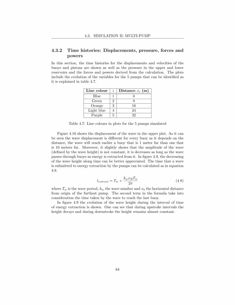
4.3. SIMULATION II: MULTI-PUMP
4.3.2 Time histories: Displacements, pressure, forces andpowers
In this section, the time histories for the displacements and velocities of thebuoys and pistons are shown as well as the pressure in the upper and lowerreservoirs and the forces and powers derived from the calculation. The plotsinclude the evolution of the variables for the 5 pumps that can be identified asit is explained in table 4.7.
Line colour i Distance xi (m)
Blue 1 0Green 2 8Orange 3 16
Light blue 4 24Purple 5 32
Table 4.7: Line colours in plots for the 5 pumps simulated
Figure 4.10 shows the displacement of the wave in the upper plot. As it canbe seen the wave displacement is different for every buoy as it depends on thedistance, the wave will reach earlier a buoy that is 1 meter far than one thatis 10 meters far. Moreover, it slightly shows that the amplitude of the wave(defined by the wave height) is not constant, it is decreases as long as the wavepasses through buoys as energy is extracted from it. In figure 4.9, the decreasingof the wave height along time can be better appreciated. The time that a waveis submitted to energy extraction by the pumps can be calculated as in equation4.8.
textract = Tw +kwxBTw
2π(4.8)
where Tw is the wave period, kw the wave number and xb the horizontal distancefrom origin of the furthest pump. The second term in the formula take intoconsideration the time taken by the wave to reach the last buoy.
In figure 4.9 the evolution of the wave height during the interval of timeof energy extraction is shown. One can see that during upstroke intervals theheight decays and during downstroke the height remains almost constant.
64
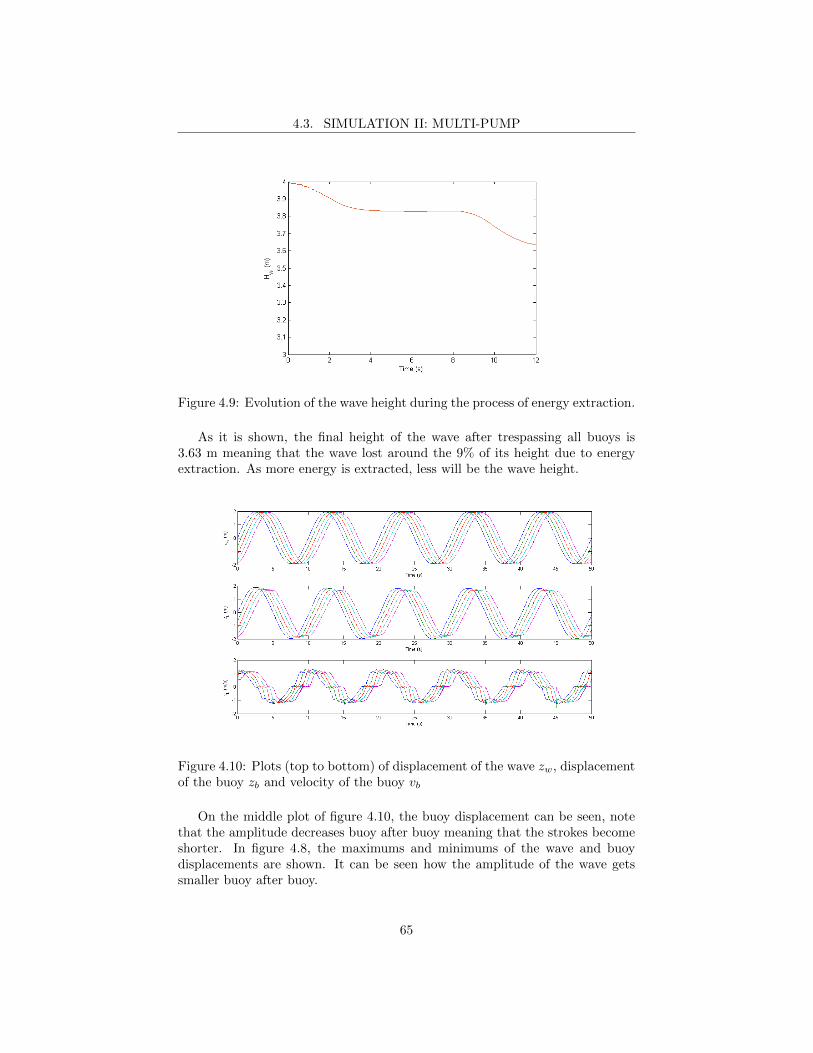
4.3. SIMULATION II: MULTI-PUMP
Figure 4.9: Evolution of the wave height during the process of energy extraction.
As it is shown, the final height of the wave after trespassing all buoys is3.63 m meaning that the wave lost around the 9% of its height due to energyextraction. As more energy is extracted, less will be the wave height.
Figure 4.10: Plots (top to bottom) of displacement of the wave zw, displacementof the buoy zb and velocity of the buoy vb
On the middle plot of figure 4.10, the buoy displacement can be seen, notethat the amplitude decreases buoy after buoy meaning that the strokes becomeshorter. In figure 4.8, the maximums and minimums of the wave and buoydisplacements are shown. It can be seen how the amplitude of the wave getssmaller buoy after buoy.
65
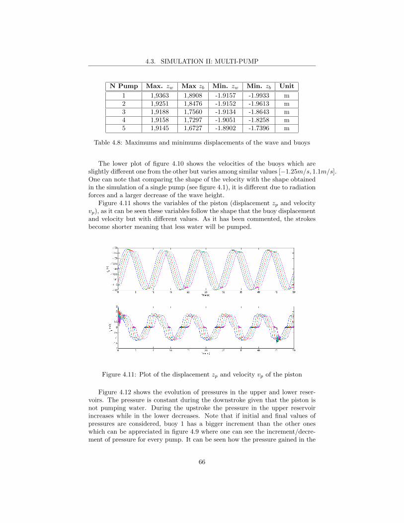
4.3. SIMULATION II: MULTI-PUMP
N Pump Max. zw Max zb Min. zw Min. zb Unit
1 1,9363 1,8908 -1.9157 -1.9933 m2 1,9251 1,8476 -1.9152 -1.9613 m3 1,9188 1,7560 -1.9134 -1.8643 m4 1,9158 1,7297 -1.9051 -1.8258 m5 1,9145 1,6727 -1.8902 -1.7396 m
Table 4.8: Maximums and minimums displacements of the wave and buoys
The lower plot of figure 4.10 shows the velocities of the buoys which areslightly different one from the other but varies among similar values [−1.25m/s, 1.1m/s].One can note that comparing the shape of the velocity with the shape obtainedin the simulation of a single pump (see figure 4.1), it is different due to radiationforces and a larger decrease of the wave height.
Figure 4.11 shows the variables of the piston (displacement zp and velocityvp), as it can be seen these variables follow the shape that the buoy displacementand velocity but with different values. As it has been commented, the strokesbecome shorter meaning that less water will be pumped.
Figure 4.11: Plot of the displacement zp and velocity vp of the piston
Figure 4.12 shows the evolution of pressures in the upper and lower reser-voirs. The pressure is constant during the downstroke given that the piston isnot pumping water. During the upstroke the pressure in the upper reservoirincreases while in the lower decreases. Note that if initial and final values ofpressures are considered, buoy 1 has a bigger increment than the other oneswhich can be appreciated in figure 4.9 where one can see the increment/decre-ment of pressure for every pump. It can be seen how the pressure gained in the
66
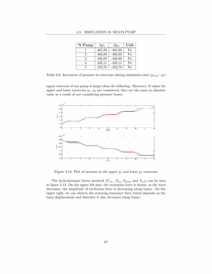
4.3. SIMULATION II: MULTI-PUMP
N Pump ∆p1 ∆p4 Unit
1 465,99 -465,99 Pa2 460,89 -460,89 Pa3 436,69 -436,69 Pa4 432,11 -432,11 Pa5 422,78 -422,78 Pa
Table 4.9: Increment of pressure in reservoirs during simulation time (pend−pi)
upper reservoir of one pump is larger than the following. Moreover, if values forupper and lower reservoirs p1, p4 are considered, they are the same in absolutevalue as a result of not considering pressure losses.
Figure 4.12: Plot of pressure in the upper p1 and lower p4 reservoirs
The hydrodynamic forces involved (Fexc, Fhs, Fdrag and Fwd) can be seenin figure 4.13. On the upper left plot, the excitation force is shown, as the wavedecreases, the amplitude of excitation force is decreasing along buoys. On theupper right, we can observe the restoring buoyancy force which depends on thebuoy displacement and therefore it also decreases along buoys.
67
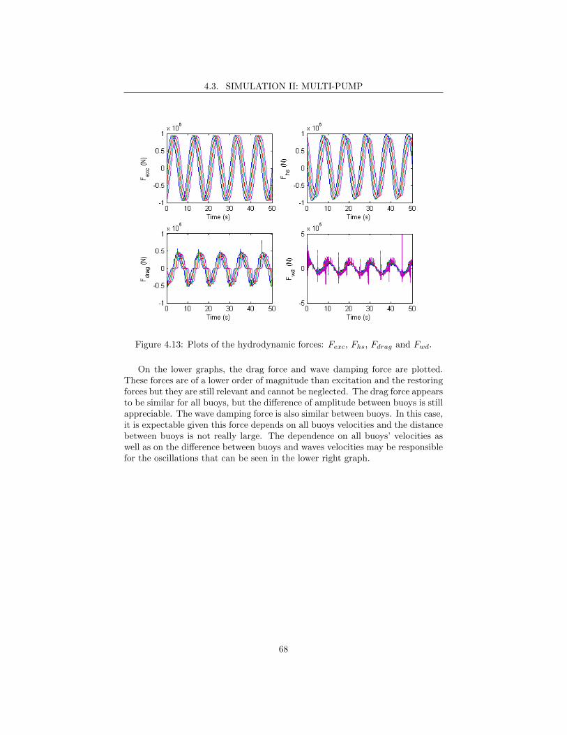
4.3. SIMULATION II: MULTI-PUMP
Figure 4.13: Plots of the hydrodynamic forces: Fexc, Fhs, Fdrag and Fwd.
On the lower graphs, the drag force and wave damping force are plotted.These forces are of a lower order of magnitude than excitation and the restoringforces but they are still relevant and cannot be neglected. The drag force appearsto be similar for all buoys, but the difference of amplitude between buoys is stillappreciable. The wave damping force is also similar between buoys. In this case,it is expectable given this force depends on all buoys velocities and the distancebetween buoys is not really large. The dependence on all buoys’ velocities aswell as on the difference between buoys and waves velocities may be responsiblefor the oscillations that can be seen in the lower right graph.
68
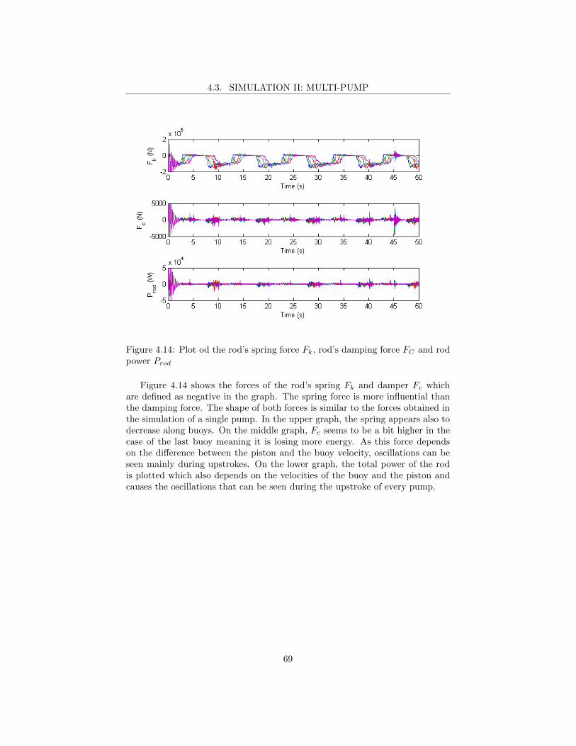
4.3. SIMULATION II: MULTI-PUMP
Figure 4.14: Plot od the rod’s spring force Fk, rod’s damping force FC and rodpower Prod
Figure 4.14 shows the forces of the rod’s spring Fk and damper Fc whichare defined as negative in the graph. The spring force is more influential thanthe damping force. The shape of both forces is similar to the forces obtained inthe simulation of a single pump. In the upper graph, the spring appears also todecrease along buoys. On the middle graph, Fc seems to be a bit higher in thecase of the last buoy meaning it is losing more energy. As this force dependson the difference between the piston and the buoy velocity, oscillations can beseen mainly during upstrokes. On the lower graph, the total power of the rodis plotted which also depends on the velocities of the buoy and the piston andcauses the oscillations that can be seen during the upstroke of every pump.
69
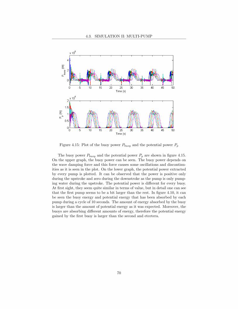
4.3. SIMULATION II: MULTI-PUMP
Figure 4.15: Plot of the buoy power Pbuoy and the potential power Pp
The buoy power Pbuoy and the potential power Pp are shown in figure 4.15.On the upper graph, the buoy power can be seen. The buoy power depends onthe wave damping force and this force causes some oscillations and discontinu-ities as it is seen in the plot. On the lower graph, the potential power extractedby every pump is plotted. It can be observed that the power is positive onlyduring the upstroke and zero during the downstroke as the pump is only pump-ing water during the upstroke. The potential power is different for every buoy.At first sight, they seem quite similar in terms of value, but in detail one can seethat the first pump seems to be a bit larger than the rest. In figure 4.10, it canbe seen the buoy energy and potential energy that has been absorbed by eachpump during a cycle of 10 seconds. The amount of energy absorbed by the buoyis larger than the amount of potential energy as it was expected. Moreover, thebuoys are absorbing different amounts of energy, therefore the potential energygained by the first buoy is larger than the second and etcetera.
70
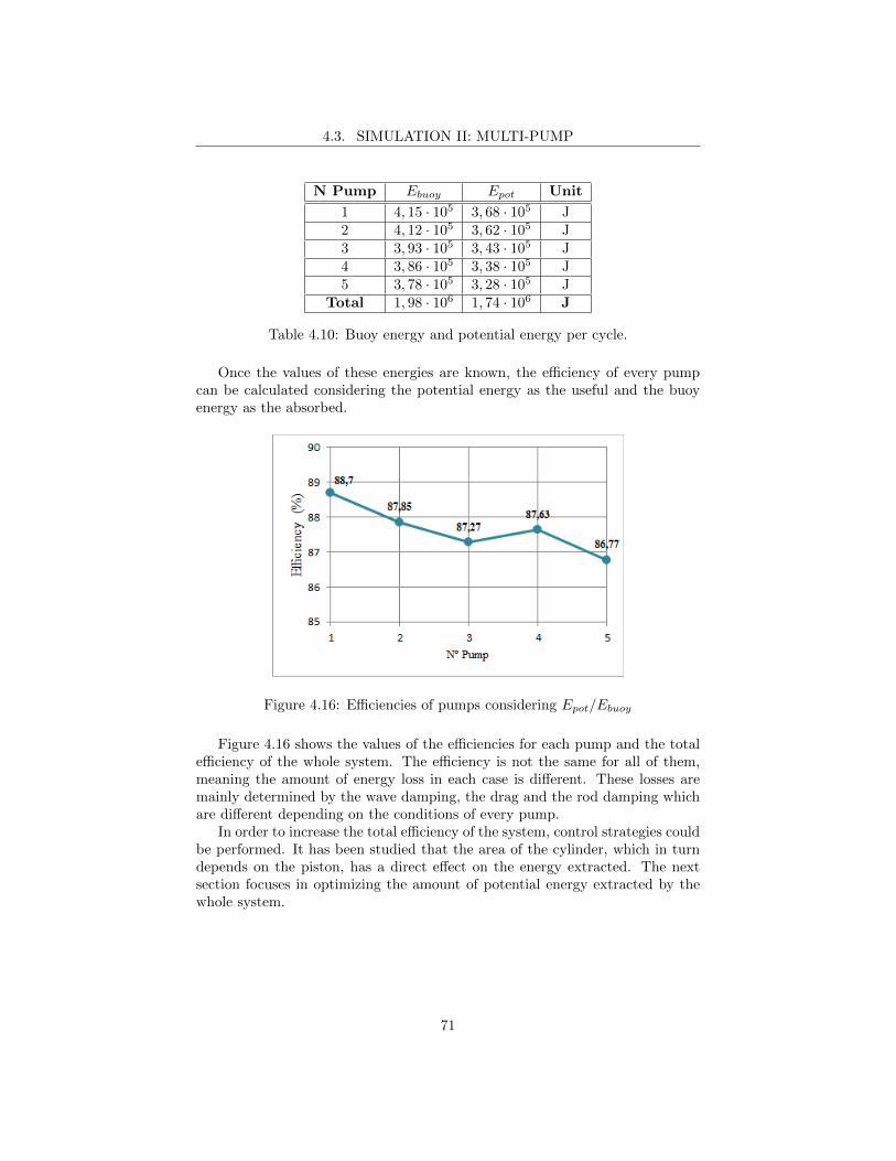
4.3. SIMULATION II: MULTI-PUMP
N Pump Ebuoy Epot Unit
1 4, 15 · 105 3, 68 · 105 J2 4, 12 · 105 3, 62 · 105 J3 3, 93 · 105 3, 43 · 105 J4 3, 86 · 105 3, 38 · 105 J5 3, 78 · 105 3, 28 · 105 J
Total 1, 98 · 106 1, 74 · 106 J
Table 4.10: Buoy energy and potential energy per cycle.
Once the values of these energies are known, the efficiency of every pumpcan be calculated considering the potential energy as the useful and the buoyenergy as the absorbed.
Figure 4.16: Efficiencies of pumps considering Epot/Ebuoy
Figure 4.16 shows the values of the efficiencies for each pump and the totalefficiency of the whole system. The efficiency is not the same for all of them,meaning the amount of energy loss in each case is different. These losses aremainly determined by the wave damping, the drag and the rod damping whichare different depending on the conditions of every pump.
In order to increase the total efficiency of the system, control strategies couldbe performed. It has been studied that the area of the cylinder, which in turndepends on the piston, has a direct effect on the energy extracted. The nextsection focuses in optimizing the amount of potential energy extracted by thewhole system.
71
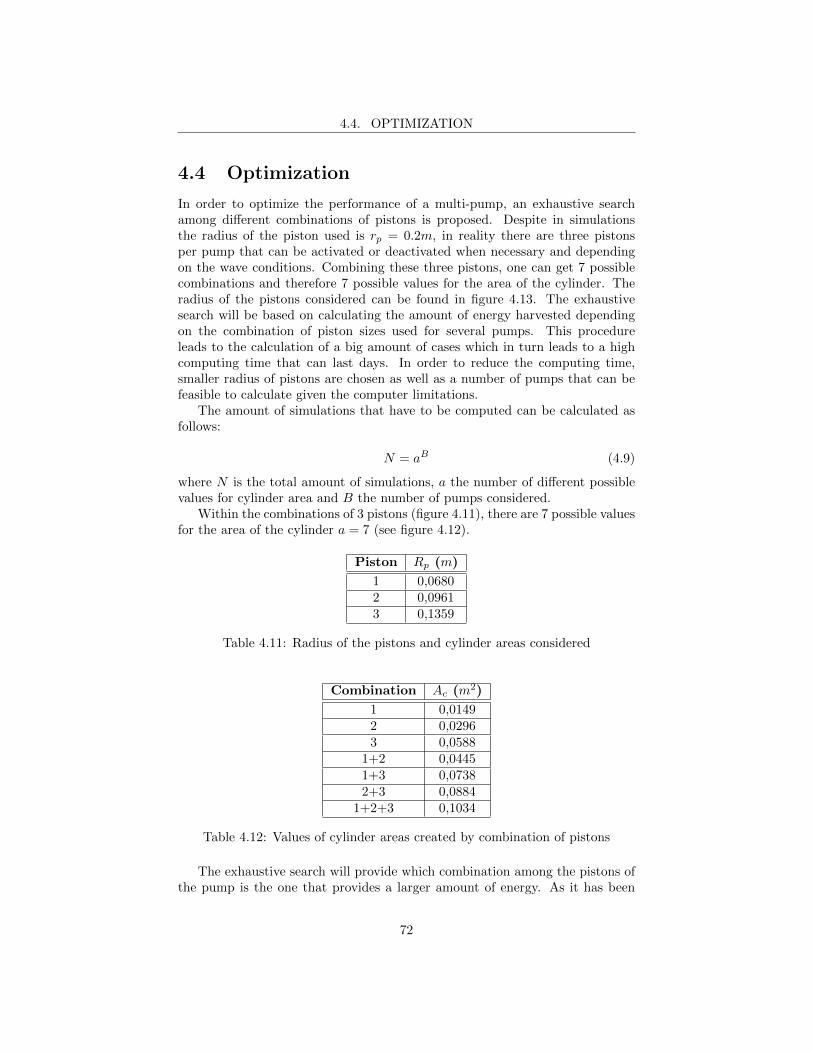
4.4. OPTIMIZATION
4.4 Optimization
In order to optimize the performance of a multi-pump, an exhaustive searchamong different combinations of pistons is proposed. Despite in simulationsthe radius of the piston used is rp = 0.2m, in reality there are three pistonsper pump that can be activated or deactivated when necessary and dependingon the wave conditions. Combining these three pistons, one can get 7 possiblecombinations and therefore 7 possible values for the area of the cylinder. Theradius of the pistons considered can be found in figure 4.13. The exhaustivesearch will be based on calculating the amount of energy harvested dependingon the combination of piston sizes used for several pumps. This procedureleads to the calculation of a big amount of cases which in turn leads to a highcomputing time that can last days. In order to reduce the computing time,smaller radius of pistons are chosen as well as a number of pumps that can befeasible to calculate given the computer limitations.
The amount of simulations that have to be computed can be calculated asfollows:
N = aB (4.9)
where N is the total amount of simulations, a the number of different possiblevalues for cylinder area and B the number of pumps considered.
Within the combinations of 3 pistons (figure 4.11), there are 7 possible valuesfor the area of the cylinder a = 7 (see figure 4.12).
Piston Rp (m)
1 0,06802 0,09613 0,1359
Table 4.11: Radius of the pistons and cylinder areas considered
Combination Ac (m2)
1 0,01492 0,02963 0,0588
1+2 0,04451+3 0,07382+3 0,0884
1+2+3 0,1034
Table 4.12: Values of cylinder areas created by combination of pistons
The exhaustive search will provide which combination among the pistons ofthe pump is the one that provides a larger amount of energy. As it has been
72
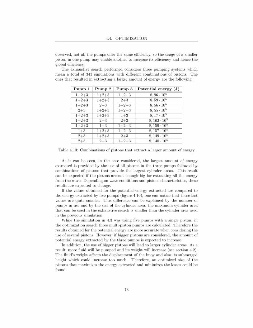
4.4. OPTIMIZATION
observed, not all the pumps offer the same efficiency, so the usage of a smallerpiston in one pump may enable another to increase its efficiency and hence theglobal efficiency.
The exhaustive search performed considers three pumping systems whichmean a total of 343 simulations with different combinations of pistons. Theones that resulted in extracting a larger amount of energy are the following:
Pump 1 Pump 2 Pump 3 Potential energy (J)
1+2+3 1+2+3 1+2+3 8, 96 · 105
1+2+3 1+2+3 2+3 8, 59 · 105
1+2+3 2+3 1+2+3 8, 56 · 105
2+3 1+2+3 1+2+3 8, 55 · 105
1+2+3 1+2+3 1+3 8, 17 · 105
1+2+3 2+3 2+3 8, 162 · 105
1+2+3 1+3 1+2+3 8, 159 · 105
1+3 1+2+3 1+2+3 8, 157 · 105
2+3 1+2+3 2+3 8, 149 · 105
2+3 2+3 1+2+3 8, 140 · 105
Table 4.13: Combinations of pistons that extract a larger amount of energy
As it can be seen, in the case considered, the largest amount of energyextracted is provided by the use of all pistons in the three pumps followed bycombinations of pistons that provide the largest cylinder areas. This resultcan be expected if the pistons are not enough big for extracting all the energyfrom the wave. Depending on wave conditions and pistons characteristics, theseresults are expected to change.
If the values obtained for the potential energy extracted are compared tothe energy extracted by five pumps (figure 4.10), one can notice that these lastvalues are quite smaller. This difference can be explained by the number ofpumps in use and by the size of the cylinder area, the maximum cylinder areathat can be used in the exhaustive search is smaller than the cylinder area usedin the previous simulation.
While the simulation in 4.3 was using five pumps with a single piston, inthe optimization search three multi-piston pumps are calculated. Therefore theresults obtained for the potential energy are more accurate when considering theuse of several pistons. However, if bigger pistons are considered, the amount ofpotential energy extracted by the three pumps is expected to increase.
In addition, the use of bigger pistons will lead to larger cylinder areas. As aresult, more fluid will be pumped and its weight will increase (see section 4.2).The fluid’s weight affects the displacement of the buoy and also its submergedheight which could increase too much. Therefore, an optimized size of thepistons that maximizes the energy extracted and minimizes the losses could befound.
73
Chapter 5
Conclusions and Futurework
After taking into consideration the theoretical background about hydrodynam-ics, mechanics and control that is applicable to wave energy converters, a firstmathematical model that describes the behaviour of multiple pumps and theirinteraction with waves has been reached. It has been proved that sea waves areaffected by the interaction with floating bodies and therefore not all the pumpscan extract the same amount of energy from waves. It can also be concludedthat all pumping systems are influenced by the others and a multi-pump waveenergy converter allows to harvest a larger amount of energy than a single onedoes, increasing hence the efficiency of the whole system. Therefore, the conceptof a multi-pump wave energy converter is feasible and full of sense. Moreover,an optimal configuration of the pistons of three pumps has been found, provingthat the cylinder area and the pistons affect the energy harvested not only bya single pump but also by multiple pumps.
Despite the fact that this work has contributed to prove the principle ofoperation of the Ocean Grazer, future work has to be done in this line in orderto reach a model that can fit more accurately the real system. Work in differentfields can be done for contributing in the development of the Ocean Grazer.Some examples derived from this work are proposed:
� Hydrodynamic coefficients: Despite the fact that hydrodynamics havebeen estimated through theoretical formulation, simulations with softwarebased on the boundary-element method can be performed in order todetermine more accurately excitation forces on the buoy as well as theadded mass and the wave damping coefficient. This method allows toconsider arbitrary geometries, several degrees of freedom and bodies. Sothe results obtained from it should provide results that approach betterthe reality. Commercial codes with this method are WAMIT�, AnsysAqua�and Aquaplus�.
74
� Optimization of the buoy’s design: Hydrodynamic coefficient andforces depend on the buoy geometry, then an optimum design of the buoycan be found in order to minimize losses and maximize the absorption ofenergy by the buoy.
� The joint between buoys: The present work has not considered thecontact between buoys which is important. This joint and the forces in-volved have to be defined and modelled in order to include it in multi-pumpmodels and study its behaviour.
� A prototype of the blanket: A prototype of the blanket should bedesigned and built in order to make a proof of concept and compare theresults between theoretical models and the prototype.
� Deeper insight on the pumping system: In order to provide realismto the system, the different parts of this system should be analysed andmodelled in detail taking into consideration materials, dimensions andfunctions.
� Determining the number of pumping systems: In this work, aconcrete number of pumps have been considered. Future work could focuson determining which is the feasible number of pump that optimizes theenergy harvested.
� Developing a multi-pump model considering 3D: At the end, amathematical model that considers the three dimensions and the six modesof motions will have to be developed with the aim of simulating the wholebehaviour of the Ocean Grazer.
Some of these examples could be done right after this work while others arelong-term projects that can take years of research. The Ocean Grazer teamworks simultaneously in many projects with a continuous feedback betweenthem in order to achieve better results and contribute every day with the OceanGrazer project.
75

Appendix A
Matlab code
A.1 Code simulation I and II
Find below the matlab code used for simulations I and II. The variable ”numberof buoys B” can be changed to consider more pumpin systems.
% Detailed explanation goes here
% List of variablesclear all
global B w kw z0i rho R0 g Ab Ca Hb Cd mb T rhow Lc Lr ...AU AL K C mr mp Bp pi Lb
% Simulation parameterstimestep = 1e−4; % Initial time step size (s)dtmin = 1e−6; % Minimum step size (s)endtime = 40; % Simulation duration (s)inttol = 1e−5; % Integration tolerance (−)
% Constantspi=3.14;g=9.81;
% Blanket sizeB=3; % Total number of buoys
% Buoy parametersAb=49; % Buoy's cross−sectional area (mˆ2)Hb=2; % Buoy's height (m)Lb=7; % Buoy's width/length (Beam) (m)mb=1500; % Buoy's mass (kg)Ca=1.2; % Added−mass coefficientCd=1.25;
% Wave parametersz0i=2; % Initial Wave Height (m)T=10; % Wave period (s)
76

A.1. CODE SIMULATION I AND II
w=2*pi/T; % Wave angular−frequency (rad/s)rho=1030; % Sea water density (kg/mˆ3)lambda=g*Tˆ2/(2*pi); % Wave−length (m)kw=2*pi/lambda; % Wave number (rad/m)h=500000000000; % Depth (m)nw=endtime/T; % number of waves simulated
% Buoy's coordinatesx0=0; % Offset x axispitch=1; % space between buoysd=7+pitch; % Horizontal/vertical distance between buoys
% Set coordinatesi=1;while i ≤B+1
x(i)=x0+d*(i−1); %Buoy x−coordinatei=i+1;
end
%Rod's parametersLr=140; % Rod's length (m)Rr=0.04; % Rod radius (m)ESt=210e9; % Steel Young's modulus (Pa)K=(pi*Rrˆ2*ESt)/Lr; % Rod's stifness (N/m)Xi=0.05; % Rod damping ratio (−)C=2*Xi*(mb*K)ˆ0.5; % Damping coefficient buoy/piston (Ns/m)rhost=7850; % Steel density (kg/m3)mr =rhost*(pi*Rrˆ2)*Lr; % Rod's mass (kg)
%PistonRp(1,1)=0.3; % Piston radius (m)Rp(2,1)=0.3;Rp(3,1)=0.3;mp=150; % Piston's mass (kg)sp=1e−3; % Piston−cylinder separation (m)Hp=0.1; % Piston height (m)mu=1.002; % Free water viscosity (Pas)Bp=2*pi*Rp*Hp*mu/sp;
%CylinderLc=100; % Cylinder length (m)rhow=1000; % Water density (kg/mˆ3)Rc=Rp+sp*ones(B,1);buoy=1;while buoy≤B
Ac(buoy)=pi*Rc(buoy)ˆ2;buoy=buoy+1;
end
%ReservoirsAU=49; % Area upper reservoir (mˆ2)AL=49; % Area lower reservoir (mˆ2)LU=10; % Upper reservoir inital hydraulic head (m)LL=30; % Lower reservoir inital hydraulic head (m)
77

A.1. CODE SIMULATION I AND II
% Calculate blanket
%Create matrices and vectorsq = zeros(6,B); % State vectorf = zeros(6,1); % Forcing vectorA = zeros(6,6); % Composite matrixt = zeros(5e5,1); % Timenumerror = t; % Integration errortstep = t; % Integration time step
%Initial conditionsi=1;time=0;t(i)=time;buoy=1;Ew=rho*(gˆ2)*((z0iˆ2)*(Tˆ2)*(Ab)ˆ0.5)/(8*pi)*ones(5e5,nw);while buoy≤B
wave(buoy)=1;z0(i,wave(buoy))=z0i;zw(i,buoy)=z0(i,wave(buoy))*sin(−kw*x(buoy)+w*t(i));vw(i,buoy)=z0(i,wave(buoy))*w*cos(−kw*x(buoy)+w*t(i));aw(i,buoy)=−z0(i,wave(buoy))*wˆ2*sin(−kw*x(buoy)+w*t(i));tb(buoy)=abs(kw*x(buoy)*T/(2*pi)); %Time to reach next buoym1(i,buoy)= mb;m2(i,buoy)= mr+mp;mf(i,buoy)=0;Ti=(mb+mr+mp)/(Ab*rho);Db(i,buoy)=Ti;ma(i,buoy)=Ca*rho*Ab*Db(i,buoy);Fexc(i,buoy)=rho*Ab*g*exp(−kw*Ti)*zw(i,buoy);R0=(w*(rho*Ab*g*exp(−kw*Ti))ˆ2)/(2*rho*gˆ2);R(i,buoy)=R0;z(i,buoy)=zw(i,buoy);v(i,buoy)=0;zp(i,buoy)=z(i,buoy)−Lr;vp(i,buoy)=0;p1(i,buoy)=rhow*g*LU;p4(i,buoy)=rhow*g*LL;a(i,buoy)=0;Fwdamp(i,buoy)=−R(i,buoy)*(v(i,buoy)−exp(−kw*Ti)*vw(i,buoy));Fdrag(i,buoy)=0;Ppto(i,buoy)=0;Pp(i,buoy)=0;Pbuoy(i,buoy)=0;Ebuoy(i,buoy)=0;Ep(i,buoy)=0;active(buoy)=0;
if vp(i,buoy)>0;SWITCH(buoy)=1;
elseSWITCH(buoy)=0;
endbuoy=buoy+1;
78

A.1. CODE SIMULATION I AND II
end
%Assign initial conditions to state vectorq(1,:)=z(i,:); % Assign z to vector q(1)q(2,:)=zp(i,:);q(3,:)=v(i,:); % Assign v to vector q(3)q(4,:)=vp(i,:);q(5,:)=p1(i,:);q(6,:)=p4(i,:);
% Iterate over timewhile time < endtime−timestep
buoy=1;while buoy≤B
%−−−−−−−−−−−−−−−−−−−−−−−−−−−−−−−−−−−−−−−−−−−−−−−−−−−−−−−−−−−−−−−−−−−−−−% Equivalent mass−spring−damping matrix and forcing function%−−−−−−−−−−−−−−−−−−−−−−−−−−−−−−−−−−−−−−−−−−−−−−−−−−−−−−−−−−−−−−−−−−−−−−
% Assemble forcing function
f(3,1)=(K*Lr+Fexc(i,buoy)+Fwdamp(i,buoy)+Fdrag(i,buoy))/m1(i,buoy);f(4,1)=((−K*Lr)−SWITCH(buoy)*g*mf(i,buoy))/m2(i,buoy);
% Assemble composite mass−damping−stiffness matrixA(1,3)=1;A(2,4)=1;A(3,1)=−(rho*g*Ab+K)/(m1(i,buoy));A(3,2)=K/(m1(i,buoy));A(3,3)=−(C)/(m1(i,buoy));A(3,4)=C/(m1(i,buoy));A(4,1)=K/(m2(i,buoy));A(4,2)=−K/m2(i,buoy);A(4,3)=C/m2(i,buoy);A(4,4)=−(C+Bp(buoy))/m2(i,buoy);A(4,5)=−Ac(buoy)*SWITCH(buoy)/m2(i,buoy);A(4,6)=Ac(buoy)*SWITCH(buoy)/m2(i,buoy);A(5,4)=SWITCH(buoy)*rhow*g*Ac(buoy)/AU;A(6,4)=−SWITCH(buoy)*rhow*g*Ac(buoy)/AL;
%−−−−−−−−−−−−−−−−−−−−−−−−−−−−−−−−−−−−−−−−−−−−−−−−−−−−−−−−−−−−−−−−−−−−−−% Runge−Kutta solver%−−−−−−−−−−−−−−−−−−−−−−−−−−−−−−−−−−−−−−−−−−−−−−−−−−−−−−−−−−−−−−−−−−−−−−
% Solve system: d/dt<q≥[A]<q>+<f>% Runge−Kutta−Fehlberg (RKF) methodk1 = timestep*(A*q(:,buoy)+f);temp = q(:,buoy)+(1/4)*k1;k2 = timestep*(A*temp+f);temp = q(:,buoy)+(3/32)*k1+(9/32)*k2;k3 = timestep*(A*temp+f);temp = q(:,buoy)+(1932/2197)*k1−(7200/2197)*k2+(7296/2197)*k3;k4 = timestep*(A*temp+f);temp = q(:,buoy)+(439/216)*k1−8*k2+(3680/513)*k3−(845/4104)*k4;k5 = timestep*(A*temp+f);temp = q(:,buoy)−(8/27)*k1+2*k2−(3544/2565)*k3+...
(1859/4104)*k4−(11/40)*k5;
79
A.1. CODE SIMULATION I AND II
k6 = timestep*(A*temp+f);
% RK4 solutionqRK4 = q(:,buoy)+(25/216)*k1+(1408/2565)*k3+...
(2197/4101)*k4−(1/5)*k5;
% RKF solutionq(:,buoy) = q(:,buoy)+(16/135)*k1+(6656/12825)*k3+...
(28561/56430)*k4−(9/50)*k5+(2/55)*k6;
% Local (discretization) error estimatenumerror(i) = sum(abs(q(:,buoy)−qRK4));
% Extract kinematicsz(i+1,buoy) =q(1,buoy);zp(i+1,buoy) =q(2,buoy);v(i+1,buoy) =q(3,buoy);vp(i+1,buoy) =q(4,buoy);p1(i+1,buoy) =q(5,buoy);p4(i+1,buoy) =q(6,buoy);
buoy=buoy+1;end
% Calculate new timesteptimestep = 0.9*timestep*inttol/numerror(i);
if timestep < dtmin, timestep = dtmin; endtstep(i) = timestep;
% Increment iteration indexi = i+1;
% Increment timetime = time+timestep;t(i) = time;
%Calculate wave energy and new height.buoy=1;while buoy≤B
if time≥tb(buoy)active(buoy)=1;
elseactive(buoy)=0;
endwave(buoy)=ceil((time−kw*x(buoy)*T/(2*pi))/T)*active(buoy)+(1−active(buoy));Ebuoy(i,buoy)=Pbuoy(i−1,buoy)*(t(i)−t(i−1))*active(buoy);
if buoy==1Ew(i,wave(buoy))=Ew(i−1,wave(buoy))−Ebuoy(i,buoy);
elseif wave(buoy)==wave(buoy−1)
Ew(i,wave(buoy))=Ew(i,wave(buoy))−Ebuoy(i,buoy);else
Ew(i,wave(buoy))=Ew(i−1,wave(buoy))−Ebuoy(i,buoy);end
end
80

A.1. CODE SIMULATION I AND II
z0(i,wave(buoy))=(8*pi*Ew(i,wave(buoy))/(rho*(gˆ2)*...(Tˆ2)*((Ab)ˆ0.5)))ˆ0.5;
buoy=buoy+1;end
%Calculate values for next timestepbuoy=1;while buoy≤B
% Calculate new wave amplitudezw(i,buoy)=z0(i,wave(buoy))*sin(−kw*x(buoy)+w*t(i));vw(i,buoy)=z0(i,wave(buoy))*w*cos(−kw*x(buoy)+w*t(i));aw(i,buoy)=−z0(i,wave(buoy))*(wˆ2)*sin(−kw*x(buoy)+w*t(i));Db(i,buoy)=zw(i,buoy)−z(i,buoy)+Ti;
if (Db(i,buoy)≤0) %non submergedma(i,buoy)=0;R(i,buoy)=R0;
elseif (Db(i,buoy)>0) && (Db(i,buoy)≤Hb) %partially submergedma(i,buoy)=Ca*rho*Ab*Db(i,buoy);R(i,buoy)=R0;
else %fully submergedma(i,buoy)=Ca*rho*g*Ab*Hb;R(i,buoy)=0;
endm1(i,buoy)=ma(i,buoy)+mb;mf(i,buoy)=rhow*(Lc+p1(i,buoy)/(rhow*g))*Ac(buoy);mup=mf(i,buoy)+mr+mp;mdown=mr+mp;
if vp(i,buoy)>0m2(i,buoy)=mup;SWITCH(buoy)=1;
elseif vp(i,buoy)≤0m2(i,buoy)=mdown;SWITCH(buoy)=0;
end
buoy=buoy+1;end
%Calculate forces, powers & energiesbuoy=1;while buoy≤B
buoy2=1;Fwdamp(i,buoy)=0;while buoy2≤BFwdamp(i,buoy)=Fwdamp(i,buoy)−besselj(0,kw*abs(x(buoy)−...
x(buoy2)))*R(i,buoy2)*(v(i,buoy2)−exp(−kw*Ti)*vw(i,buoy2));buoy2=buoy2+1;endFexc(i,buoy)=rho*g*Ab*exp(−kw*Ti)*zw(i,buoy);Fdrag(i,buoy)=−0.5*Cd*Ab*rho*abs(v(i,buoy))*v(i,buoy);Fhs(i,buoy)=−rho*g*Ab*z(i,buoy);Fkrod(i,buoy)=−K*(z(i,buoy)−zp(i,buoy)−Lr);
81

A.2. CODE EXHAUSTIVE SEARCH
Fcrod(i,buoy)=−C*(v(i,buoy)−vp(i,buoy));Fpto(i,buoy)=Fkrod(i,buoy)+Fcrod(i,buoy);Q(i,buoy)=Ac(buoy)*vp(i,buoy)*SWITCH(buoy);Pbuoy(i,buoy)=((Fexc(i,buoy)+Fwdamp(i,buoy)+Fhs(i,buoy)+...
Fdrag(i,buoy))*v(i,buoy))*active(buoy);Ppto(i,buoy)=(Fkrod(i,buoy)+Fcrod(i,buoy))*(v(i,buoy)−vp(i,buoy));Pp(i,buoy)=rhow*g*(Lc+(p1(i,buoy)−p4(i,buoy))/(rhow*g))*Q(i,buoy);Ep(i,buoy)=rhow*g*(Lc+(p1(i−1,buoy)−p4(i−1,buoy))/(rhow*g))...
*Q(i−1,buoy)*(t(i)−t(i−1));buoy=buoy+1;
end
end
t(length(z)+1:end)=[];k=3;in=find(t≥20,1,'first');out=find(t≥30,1,'first');Eptot=Ep(in:out,:);Eptot=sum(Eptot);Eptot=sum(Eptot);
A.2 Code exhaustive search
Find below, the code used for the exhaustive search. Note that the ”potentialenergy”function uses the same code of section A.1 but variables Rp and Ac are definedas the variables of the function.
clear allsp=1e−3;Rp1=0.068; % Piston's radius (m)Rp2=0.0961;Rp3=0.1359;Ac1=pi*(Rp1+sp)ˆ2; % Piston area (mˆ2)Ac2=pi*(Rp2+sp)ˆ2;Ac3=pi*(Rp3+sp)ˆ2;
Piston=zeros(7,2);Piston(1,:)=[Ac1 Rp1];Piston(2,:)=[Ac2 Rp2];Piston(3,:)=[Ac3 Rp3];Piston(4,:)=[Ac1+Ac2 Rp1+Rp2];Piston(5,:)=[Ac1+Ac3 Rp1+Rp3];Piston(6,:)=[Ac2+Ac3 Rp2+Rp3];Piston(7,:)=[Ac1+Ac2+Ac3 Rp1+Rp2+Rp3];
k=1;for i1=1:7
for i2=1:7for i3=1:7
Area(k,:)=[Piston(i1,1) Piston(i2,1) Piston(i3,1)] ;Rpist(k,:)=[Piston(i1,2) Piston(i2,2) Piston(i3,2)];Energy(k,:)=potentialenergy(Area(k,:),Rpist(k,:));
82

A.2. CODE EXHAUSTIVE SEARCH
k=k+1;end
endend
83
Bibliography
[1] World Energy Council. World energy resources, survey 2013. Technicalreport, World Energy Council.
[2] U.S. National Renewable Energy Laboratory. Ocean energy technologyoverview. Technical report, U.S. Department of Energy, 2009.
[3] AEA Energy and Environment. Review and analysis of ocean energy sys-tems development and supporting policies. Technical report, SustainableEnergy Ireland (SEI), 2006.
[4] Se Joon Lim. Wave energy converters. Stanford University, 2013.http://large.stanford.edu/courses/2013/ph240/lim2/.
[5] A. Lewis. S. Estefen. J. Huckerby. W. Musial. T. Pontes. J. Torres-Martinez.Ocean energy. In IPCC Special Report on Renewable Energy Sources andClimate Change Mitigation. Technical report, Cambridge University Press.
[6] M. Alvarez G. Iglesias and P. Garca. Wave Energy Converters. Technicalreport, University of Santiago de Compostela, 2001.
[7] Wind sector. Wind farm classes: Offshore, nearshore, onshore. Website:http://windsector.tumblr.com.
[8] Alternative energy tutorials. Wave energy devices. Website:http://www.alternative-energy-tutorials.com.
[9] Ocean Grazer Group. The Ocean Grazer: A novel ocean energy collectionand storage device. Website: http://www.oceangrazer.com/.
[10] Harmen Meijer. Simulating a piston-type hydraulic pump for the OceanGrazer. Master’s thesis, University of Groningen, 2014.
[11] Josep Martı Saumell. Dynamical modelling, analysis and control design ofa distributed sea wave energy storage system. Master’s thesis, Universityof Groningen, 2013.
[12] Antonis I. Vakis. Tribological model of a single-piston pump for a novelwave energy converter. Technical report, University of Groningen, 2013.
84
BIBLIOGRAPHY
[13] Bruno Galvan Garcıa. Nonlinear control design for wave energy converter.Master’s thesis, University of Groningen, 2014.
[14] Motion in the sea waves. Website: http://www.marine.tmd.go.th/.
[15] Franz S. Hover and Michael S. Triantafyllou. Water waves. Center forOcean Engineering, MIT, 2009.
[16] A.H. Techet. Potential flow theory. Online resource: MIT 2.016 Hydrody-namics, 2005.
[17] Michel K. Ochi. Ocean Waves: The Stochastic Approach. Cambridge OceanTechnologies series 6, 2005.
[18] Leo H. Holthuijsen. Waves in Oceanic and Coastal Waters. CambridgeUniversity Press, 2007.
[19] J. M. J. Journe and W. W. Massie. Offshore Hydromechanics. TU Delft,2001.
[20] Department of Ocean Engineering. MIT. Lecture 13.021 Marine hydrody-namics. Online resource, 2014.
[21] MIT. Chapter 4. real fluid effects. Online resource: MIT course MarineHydrodynamics, 2005.
[22] J. Falnes. Surface wave interactions with systems of oscillating bodies andpressure distributions. Applied Ocean Research, 7(4):225 – 234, 1985.
[23] J. Falnes. Ocean waves and oscillating systems. Cambridge UniversityPress, 2002.
[24] Antonio F.O. Falc ao. Modelling of wave energy conversion. Online re-source: Slides, 2014.
[25] Geir Moe Ove T. Gudmestad. Hydrodynamic coefficients for calculation ofhydrodynamic loads on offshore truss structures. Marine Structures, 1996.
[26] DNV. Modelling and Analysis of Marine Operations. Det Norske VeritasAS, February 2014.
[27] John N. Newman. Marine Hydrodynamics. MIT Press, 1977.
[28] O. M. Faltinsen. Sea loads on ships and offshore structures. CambridgeUniversity Press, 1990.
[29] Paul D. Sclavounos. Ocean wave interaction with ships and offshore energysystems. chapter 10: Added-mass, damping coefficients and exciting forces.Lecture notes MIT 2.24, 2002. http://ocw.mit.edu/courses.
[30] J. Falnes. A review of wave-energy extraction. Marine Structures, 20:186– 199, 2007.
85

BIBLIOGRAPHY
[31] J. Falnes. Radiation impedance matrix and optimum power absorption forinteracting oscillators in surface waves. Applied Ocean Research, 2(2):75–80, 1980.
86