P . I . C . M . – 2018Rio de Janeiro, Vol. 1 (523–550)

DYNAMICAL, SYMPLECTIC AND STOCHASTICPERSPECTIVES ON GRADIENT-BASED OPTIMIZATION

M I. J

AbstractOur topic is the relationship between dynamical systems and optimization. This

is a venerable, vast area in mathematics, counting among its many historical threadsthe study of gradient flow and the variational perspective on mechanics. We aim tobuild some new connections in this general area, studying aspects of gradient-basedoptimization from a continuous-time, variational point of view. We go beyond clas-sical gradient flow to focus on second-order dynamics, aiming to show the relevanceof such dynamics to optimization algorithms that not only converge, but convergequickly.

Although our focus is theoretical, it is important to motivate the work by consideringthe applied context from which it has emerged. Modern statistical data analysis ofteninvolves very large data sets and very large parameter spaces, so that computationalefficiency is of paramount importance in practical applications. In such settings, thenotion of efficiency is more stringent than that of classical computational complexitytheory, where the distinction between polynomial complexity and exponential complex-ity has been a useful focus. In large-scale data analysis, algorithms need to be not merelypolynomial, but linear, or nearly linear, in relevant problem parameters. Optimizationtheory has provided both practical and theoretical support for this endeavor. It has sup-plied computationally-efficient algorithms, as well as analysis tools that allow rates ofconvergence to be determined as explicit functions of problem parameters. The dictumof efficiency has led to a focus on algorithms that are based principally on gradients ofobjective functions, or on estimates of gradients, given that Hessians incur quadratic orcubic complexity in the dimension of the configuration space Bottou [2010] and Nes-terov [2012a].

More broadly, the blending of inferential and computational ideas is one of the ma-jor intellectual trends of the current century—one currently referred to by terms suchas “data science” and “machine learning.” It is a trend that inspires the search for newmathematical concepts that allow computational and inferential desiderata to be stud-ied jointly. For example, one would like to impose runtime budgets on data-analysisalgorithms as a function of statistical quantities such as risk, the number of data pointsand the model complexity, while also taking into account computational resource con-straints such as number of processors, the communication bandwidth and the degreeof asynchrony. Fundamental understanding of such tradeoffs seems likely to emergeMSC2010: primary 65K10; secondary 90C25, 90C26, 37M15, 37J05, 49M99.

523

524 MICHAEL I. JORDAN

through the development of lower bounds—by establishing notions of “best” one canstrip away inessentials and reveal essential relationships. Here too optimization theoryhas been important. In a seminal line of research beginning in the 1970’s, Nemirovskii,Nesterov and others developed a complexity theory of optimization, establishing lowerbounds on rates of convergence and discovering algorithms that achieve those lowerbounds Nemirovskii and Yudin [1983] and Nesterov [1998]. Moreover, the model ofcomplexity was a relative one—an “oracle” is specified and algorithms can only useinformation that is available to the oracle. For example, it is possible to consider ora-cles that have access only to function values and gradients. Thus the dictum of practicalcomputational efficiency can be imposed in a natural way in the theory.

Our focus is the class of optimization algorithms known as “accelerated algorithms”Nesterov [1998]. These algorithms often attain the oracle lower-bound rates, althoughit is something of a mystery why they do so. We will argue that some of mystery isdue to the historical focus in optimization on discrete-time algorithms and analyses. Inoptimization, the distinction between “continuous optimization” and “discrete optimiza-tion” refers to the configuration (“spatial”) variables. By way of contrast, our discussionwill focus on continuous time. In continuous time we can give acceleration a mathemat-ical meaning as a differential concept, as a change of speed along a curve. And we canpose the question of “what is the fastest rate?” as a problem in variational analysis; inessence treating the problem of finding the “optimal way to optimize” for a given oracleitself as a formal problem of optimization. Such a variational perspective also has theadvantage of being generative—we can derive algorithms that achieve fast rates ratherthan requiring an analysis to establish a fast rate for a specific algorithm that is derivedin an adhoc manner.

Working in continuous time forces us to face the problem of discretizing a continuous-time dynamical system, so as to derive an algorithm that can be implemented on a dig-ital computer. Interestingly, we will find that symplectic integrators, which are widelyused for integrating dynamics obtained from variational or Hamiltonian perspectives,are relevant in the optimization setting. Symplectic integration preserves the continu-ous symmetries of the underlying dynamical system, and this stabilizes the dynamics,allowing step sizes to be larger. Thus algorithms obtained from symplectic integrationcan move more quickly through a configuration space; this gives a geometric meaningto “acceleration.”

It is also of interest to consider continuous-time stochastic dynamics that are in somesense “accelerated.” The simplest form of gradient-based stochastic differential equa-tion is the Langevin diffusion. The particular variant that has been studied in the litera-ture is an overdamped diffusion that is an analog of gradient descent. We will see thatby considering instead an underdamped Langevin diffusion, we will obtain a methodthat is more akin to accelerated gradient descent, and which in fact provably yields afaster rate than the overdamped diffusion.

The presentation here is based on joint work with co-authors Andre Wibisono, AshiaWilson, Michael Betancourt, Chi Jin, Praneeth Netrapalli, Rong Ge, Sham Kakade, Ni-ladri Chatterji and Xiang Cheng, as well as other co-authors who will be acknowledgedin specific sections.

DYNAMICAL, SYMPLECTIC AND STOCHASTIC OPTIMIZATION 525

1 Lagrangian and Hamiltonian Formulations of AcceleratedGradient Descent

Given a continuously differentiable function f on an open Euclidean domain X, andgiven an initial point x0 2 X, gradient descent is defined as the following discretedynamical system:

(1) xk+1 = xk � �rf (xk);

where � > 0 is a step size parameter.When f is convex, it is known that gradient descent converges to the global optimum

x?, assumed unique for simplicity, at a rate of O(1/k) Nesterov [ibid.]. This meansthat after k iterations, the function value f (xk) is guaranteed to be within a constanttimes 1/k of the optimum value f ? = f (x?). This is a worst-case rate, meaningthat gradient descent converges as least as fast as O(1/k) across the function class ofconvex functions. The constant hidden in the O(�) notation is an explicit function of acomplexity measure such as a Lipschitz constant for the gradient.

In the 1980’s, a complexity theory of optimization was developed in which ratessuch as O(1/k) could be compared to lower bounds for particular problem classes Ne-mirovskii and Yudin [1983]. For example, an oracle model appropriate for gradient-based optimization might consider all algorithms that have access to sequences of gradi-ents of a function, and whose iterates must lie in the linear span of the current gradientand all previous gradients. This model encompasses, for example, gradient descent, butother algorithms are allowed as well. Nemirovskii and Yudin [ibid.] were able to prove,by construction of a worst-case function, that no algorithm in this class can convergeat a rate faster than O(1/k2). This lower bound is better than gradient descent, and itholds open the promise that some gradient-based algorithm can beat gradient descentacross the family of convex functions. That promise was realized by Nesterov [1983],who presented the following algorithm, known as accelerated gradient descent:

yk+1 = xk � �rf (xk)

xk+1 = (1 + �k)yk+1 � �kyk ;(2)

and proved that the algorithm converges at rate O(1/k2) for convex functions f . Here�k is an explicit function of the other problem parameters. We see that the accelerationinvolves two successive gradients, and the resulting dynamics are richer than those ofgradient descent. In particular, accelerated gradient descent is not a descent algorithm—the function values can oscillate.

Nesterov’s basic algorithm can be presented in other ways; in particular, we will alsouse a three-sequence version:

xk = yk + �kvk

yk+1 = xk � �rf (xk)

vk+1 = yk+1 � yk :(3)

We note in passing that in both this version and the two-sequence version, the parameter�k is time-varying for some problem formulations and constant for others.

526 MICHAEL I. JORDAN

After Nesterov’s seminal paper in 1983, the subsequent three decades have seen thedevelopment of a variety of accelerated algorithms in a wide variety of other problemsettings. These include mirror descent, composite objective functions, non-Euclideangeometries, stochastic variants and higher-order gradient descent. Rates of convergencehave been obtained for these algorithms, and these rates often achieve oracle lowerbounds. Overall, acceleration has been one of the most productive ideas in modernoptimization theory. See Nesterov [1998] for a basic introduction, and Bubeck, Y. T.Lee, and M. Singh [2015] and Allen-Zhu and Orecchia [2014] for examples of recentprogress.

And yet the basic acceleration phenomenon has remained somewhat of a mystery. Itsderivation and its analysis are often obtained only after lengthy algebraic manipulations,with clever but somewhat opaque upper bounds needed at critical junctures.

In Wibisono, A. C. Wilson, and Jordan [2016], we argue that this mystery is due inpart to the discrete-time formalism that is generally used to derive and study gradient-based optimization algorithms. Indeed, the notion of “acceleration” seems ill-defined ina discrete-time framework; what does it mean to move more quickly along a sequenceof discrete points? Such a notion seems to require an embedding in an underlying flowof time, such that acceleration can be viewed as a diffeomorphism. Moreover, if ac-celerated optimization algorithms are in some sense optimal, there must be somethingspecial about the curve that they follow in the configuration space, not merely the speedat which they move. Such a separate characterization of curve and speed also seem torequire continuous time.

Wibisono, A. C. Wilson, and Jordan [ibid.] address these issues via a variationalframework that aims to capture the phenomenon of acceleration in some generality.We review this framework in the remainder of this section, discussing the Lagrangianformulation that captures acceleration in continuous time, showing how this formula-tion gives rise to a family of differential equations whose convergence rates are thecontinuous-time counterpart of the discrete-time oracle rates. We highlight the problemof the numerical integration of these differential equations, setting up the symplecticintegration approach that we discuss in Section 2.

We consider the general non-Euclidean setting in which the spaceX is endowed witha distance-generating function h : X! R that is convex and essentially smooth (i.e., his continuously differentiable in X, and krh(x)k� ! 1 as kxk ! 1). The functionh can be used to define a measure of distance in X via its Bregman divergence:

Dh(y; x) = h(y) � h(x) � hrh(x); y � xi:(4)

The Euclidean setting is obtained when h(x) = 12kxk2.

We use the Bregman divergence to construct a Bregman kinetic energy for a dynam-ical system. We do this by taking the Bregman divergence between a point x and itstranslation in the direction of the velocity v by a time-varying magnitude, e�˛t :

K(x; v; t) := Dh(x+ e�˛t v; x):(5)

Using the definition in Eq. (4), we see that this kinetic energy can be interpreted ascomparison between the amount that h changes under a finite translation, h(x+e�˛t v)�h(x), versus an infinitesimal translation, e�˛t hrh(x); vi.

DYNAMICAL, SYMPLECTIC AND STOCHASTIC OPTIMIZATION 527

We now define a time-dependent potential energy, U (x):

U (x; t) := eˇt f (x);(6)

and we subtract the potential energy from the kinetic energy to obtain the BregmanLagrangian:

L(x; v; t) =:= e˛t+ t (K(x; v; t) � U (x; t))

= e˛t+ t (Dh(x+ e�˛t v; x) � eˇt f (x)):(7)

In this equation, the time-dependent factors ˛t ; ˇt and t are algorithmic degrees of free-dom that allow the Bregman–Lagrangian framework to encompass a range of differentalgorithms.

Although ˛t ; ˇt and t can be set independently in principle, we define a set of idealscaling conditions that reduce these three degrees of freedom to a single functional de-gree of freedom:

˙t � e˛t

t = e˛t :(8)

Wibisono, A. C. Wilson, and Jordan [ibid.] show that these conditions are needed toobtain differential equations whose rates of convergence are the optimal rates; see The-orem 1 below.

Given the Bregman Lagrangian, we use standard calculus of variations to obtain adifferential equation whose solution is the path that optimizes the time-integrated Breg-man Lagrangian. In particular, we form the Euler–Lagrange equations:

d

dt

�@L

@v(xt ; xt ; t)

��

@L

@x(xt ; xt ; t) = 0;(9)

a computation which is easily done based on Eq. (7). Using the ideal scaling conditionsin Eq. (8), the result simplifies to the following master differential equation:

xt + (e˛t � ˙ t )xt + e2˛t+ˇt

hr

2h(xt + e�˛t xt )i�1

rf (xt ) = 0:(10)

We see that the equation is second order and non-homogeneous. Moreover, the gradientrf (xt ) appears as a force, modified by geometric terms associated with the Bregmandistance-generating function h. As we will discuss below, this equation is a generalform of Nesterov acceleration in continuous time.

It is straightforward to obtain a convergence rate for the master differential equation.We define the following Lyapunov function:

Et = Dh (x?; xt + e�˛t xt ) + eˇt (f (xt ) � f ?)):(11)

Taking a first derivative with respect to time, and asking that this derivative be lessthan or equal to zero, we immediately obtain a convergence rate, as documented in thefollowing theorem, whose proof can be found in Wibisono, A. C. Wilson, and Jordan[ibid.].

528 MICHAEL I. JORDAN

Theorem 1. If the ideal scaling in Eq. (8) holds, then solutions to the Euler–Lagrangeequation Eq. (10) satisfy

f (xt ) � f ?� O(e�ˇt ):

For further explorations of Lyapunov-based analysis of accelerated gradient methods,see A. C. Wilson, Recht, and Jordan [2016].

Wibisono, A. C. Wilson, and Jordan [2016] studied a subfamily of Bregman La-grangians with the following choice of parameters, indexed by a parameter p > 0:

˛t = logp � log t

ˇt = p log t + logC

t = p log t;(12)

whereC > 0 is a constant. This choice of parameters satisfies the ideal scaling conditionin Eq. (8). The Euler–Lagrange equation, Eq. (10), reduces in this case to:

xt +p + 1

txt + Cp2tp�2

�r

2h

�xt +

t

pxt

���1

rf (xt ) = 0;(13)

and, by Theorem 1, it has an O(1/tp) rate of convergence.The case p = 2 of the Eq. (13) is the continuous-time limit of Nesterov’s accelerated

mirror descent Krichene, Bayen, and Bartlett [2015], the case p = 3 is the continuous-time limit of Nesterov’s accelerated cubic-regularized Newton’s method Nesterov andPolyak [2006]. In the Euclidean case, when the Hessian r2h is the identity matrix, werecover the following differential equation:

xt +3

txt + rf (xt ) = 0;(14)

which was first derived by Su, Boyd, and Candes [2016] as the continuous-time limitof the basic Nesterov accelerated gradient descent algorithm in Eq. (2).

The Bregman Lagrangian has several mathematical properties that give significantinsight into aspects of the acceleration phenomenon. For example, the Bregman La-grangian is closed under time dilation. This means that if we take an Euler–Lagrangecurve of a Bregman Lagrangian and reparameterize time so that we travel the curve ata different speed, then the resulting curve is also the Euler–Lagrange curve of anotherBregman Lagrangian, with appropriately modified parameters. Thus, the entire familyof accelerated methods correspond to a single curve in spacetime and can be obtainedby speeding up (or slowing down) any single curve. As suggested earlier, the BregmanLagrangian framework permits us to separate out the consideration of the optimal curvefrom optimal speed of movement along that curve.

Finally, we turn to a core problem—how to discretize the master differential equationso that it can be solved numerically on a digital computer. Wibisono, A. C. Wilson, andJordan [2016] showed that naïve discretizations can fail to yield stable discrete-timedynamical systems, or fail to preserve the fast oracle rates of the underlying continuoussystem. Motivated by the three-sequence form of Nesterov acceleration (see Eq. (3)),

DYNAMICAL, SYMPLECTIC AND STOCHASTIC OPTIMIZATION 529

they derived the following algorithm, in the case of the logarithmic parameterizationshown in Eq. (12):

xk+1 =p

k + pzk +

k

k + pyk

yk = argminy2X

�fp�1(y; xk) +

N

�p pjjy � xkjj

p

�zk = argmin

z2X

�C p k(p�1)

hrf (yk); zi+1

�pDh(z; zk�1)

�:(15)

Here fp�1(y; xk) is the order-p Taylor expansion of the objective function around xk

andN andC are scaling coefficients and � is a step size. AlthoughWibisono, A. C.Wil-son, and Jordan [ibid.] were able to prove that this discretization is stable and achievesthe oracle rate ofO(1/kp), the discretization is heuristic and does not flow natural fromthe dynamical-systems framework. In the next section, we revisit the discretization is-sue from the point of view of symplectic integration.

2 A Symplectic Perspective on Acceleration

Symplectic integration is a general for the discretization of differential equations thatpreserves various of the continuous symmetries of the dynamical systemHairer, Lubich,and G [2006]. In the case of differential equations obtained from mechanics, these sym-metries include physically-meaningful first integrals such as energy and momentum.Symplectic integrators exactly conserve these quantities even if the dynamical flow isonly approximated. In addition to the appeal of this result from the point of view ofphysical conservation laws, the preservation of continuous symmetries means that sym-plectic integrators tend to be more stable than other integration schemes, such that itis possible to use larger step sizes in the discrete-time system. It is this latter fact thatsuggests a role for symplectic integrators in the integration of the differential equationsassociated with accelerated optimization methods. This idea has been pursued in recentwork by Betancourt, Jordan, and A. Wilson [2018], whose results we review in thissection.

While symplectic integrators can be obtained from a Lagrangian framework, theyare most naturally obtained from a Hamiltonian framework. We thus begin by trans-forming the Bregman Lagrangian into a Bregman Hamiltonian. This is readily done viaa Legendre transform, as detailed in Wibisono, A. C. Wilson, and Jordan [2016] andBetancourt, Jordan, and A. Wilson [2018]. The resulting Hamiltonian is as follows:

H (x; r; t) = e˛(t)+ (t)

�Dh�(e� (t)r+

@h

@x(r);

@h

@x(x)) + eˇ(t)f (x)

�;(16)

whereDh�(r; s) = h�(r) � h�(s) �

@h�

@r(s) � (r � s);

and where h� is the Fenchel conjugate:

h�(r) =v2T X

sup (hr; vi � h(v)) :

530 MICHAEL I. JORDAN

10-8

10-4

100

104

1 10 100 1000 10000

Hamiltonian

Nesterov

n-2.95

f(x)

Iterations

p = 2, N = 2, C = 0.0625, ε = 0.1

(a)

10-8

10-4

100

104

1 10 100 1000 10000

Hamiltonian

Nesterov

f(x)

Iterations

p = 2, N = 2, C = 0.0625, ε = 0.25

(b)

Figure 1: (a) When appropriately tuned, both the leapfrog integrator and thethree-sequence Nesterov algorithm simulate the same latent Bregman dynamicsand hence achieve similar convergence rates, here approximately O(k�2:95). (b)Given a larger step size, the symplectic integrator remains stable and thus con-verges more quickly, whereas the three-sequence Nesterov algorithm becomesunstable.

DYNAMICAL, SYMPLECTIC AND STOCHASTIC OPTIMIZATION 531

Given the Bregman Hamiltonian in Eq. (16), Betancourt, Jordan, and A. Wilson[2018] follow a standard sequence of steps to obtain a symplectic integrator. First, theBregman Hamiltonian is time-varying, and it is thus lifted into a time-invariant Hamil-tonian on an augmented configuration space that includes time as an explicit variableand includes a conjugate energy variable in the phase space. Second, the Hamiltonianis split into a set of component Hamiltonians, each of which can be solved analytically(or nearly so via simple numerical methods). Third, the component dynamics are com-posed symmetrically to form the full dynamics. In particular, Betancourt, Jordan, andA. Wilson [ibid.] illustrate how to form a symmetric leapfrog integrator (a particularkind of symplectic integrator) for the Bregman Hamiltonian. They prove that the errorbetween this integrator and the true dynamics is of order O(�2), where � is the step sizein the discretization.

Betancourt, Jordan, andA.Wilson [ibid.] also present empirical results for a quadraticobjective function, f (x) = h�1x; xi, on a 50-dimensional Euclidean space, where

Σij = �ji�j j;

and � = 0:9. This experiment was carried out in the setting of Eq. (12), for variouschoices of p, C and N . Representative results are shown in Figure 1(a), which com-pare the leapfrog integrator with the three-sequence version of Nesterov accelerationfrom Eq. (15). Here we see that both approaches yield stable, oscillatory dynamicswhose asymptotic convergence rate is approximately O(k�2:95). Moreover, as shownin Figure 1(b), the symplectic integrator remains stable when a larger step size is chosen,whereas the three-sequence Nesterov algorithm becomes unstable.

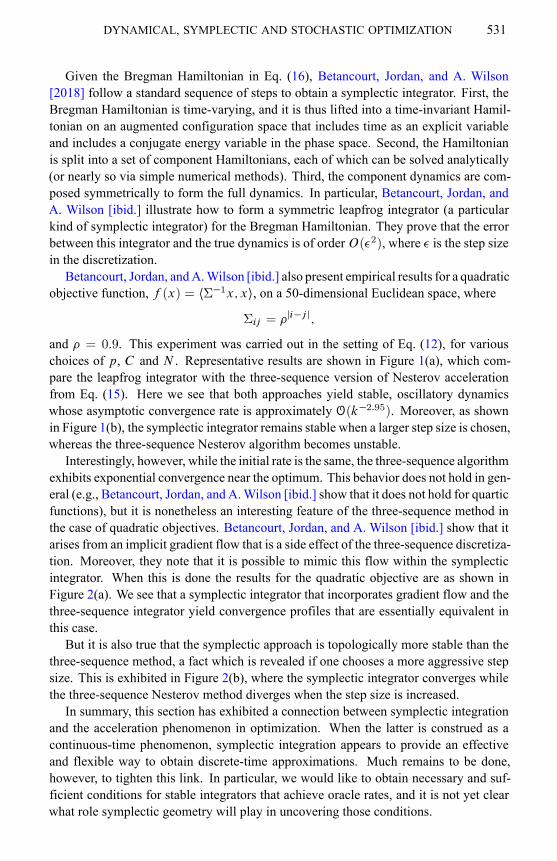
Interestingly, however, while the initial rate is the same, the three-sequence algorithmexhibits exponential convergence near the optimum. This behavior does not hold in gen-eral (e.g., Betancourt, Jordan, and A.Wilson [ibid.] show that it does not hold for quarticfunctions), but it is nonetheless an interesting feature of the three-sequence method inthe case of quadratic objectives. Betancourt, Jordan, and A. Wilson [ibid.] show that itarises from an implicit gradient flow that is a side effect of the three-sequence discretiza-tion. Moreover, they note that it is possible to mimic this flow within the symplecticintegrator. When this is done the results for the quadratic objective are as shown inFigure 2(a). We see that a symplectic integrator that incorporates gradient flow and thethree-sequence integrator yield convergence profiles that are essentially equivalent inthis case.

But it is also true that the symplectic approach is topologically more stable than thethree-sequence method, a fact which is revealed if one chooses a more aggressive stepsize. This is exhibited in Figure 2(b), where the symplectic integrator converges whilethe three-sequence Nesterov method diverges when the step size is increased.

In summary, this section has exhibited a connection between symplectic integrationand the acceleration phenomenon in optimization. When the latter is construed as acontinuous-time phenomenon, symplectic integration appears to provide an effectiveand flexible way to obtain discrete-time approximations. Much remains to be done,however, to tighten this link. In particular, we would like to obtain necessary and suf-ficient conditions for stable integrators that achieve oracle rates, and it is not yet clearwhat role symplectic geometry will play in uncovering those conditions.

532 MICHAEL I. JORDAN

10-8

10-4

100

104

1 10 100 1000 10000

Nesterov

Symplectic

f(x)

Iterations

p = 2, N = 2, C = 0.0625, ε = 0.1

(a)

10-8

10-4

100

104

1 10 100 1000 10000

NesterovSymplectic

f(x)

Iterations

p = 2, N = 2, C = 0.0625, ε = 0.25

(b)

Figure 2: (a) By incorporating gradient flow into the leapfrog integration of theBregmanHamiltonian dynamics we recover the same asymptotic exponential con-vergence near the minimum of the objective exhibited by the dynamical Nesterovalgorithm. (b) These modified Hamiltonian dynamics remain stable even as weincrease the step size, allowing for more efficient computation and the advanta-geous asymptotic behavior.

DYNAMICAL, SYMPLECTIC AND STOCHASTIC OPTIMIZATION 533

3 Acceleration and the Escape from Saddle Points in NonconvexOptimization

In this section we turn to nonconvex optimization. Although the general nonconvexsetting harbors many intractable problems about which little can be said regarding com-putational or statistical efficiency, it turns out that for a wide range of problems in statis-tical learning, there is sufficient mathematical structure present in the nonconvex settingthat useful mathematical results can be obtained. Indeed, in many cases the ideas andalgorithms from convex optimization—suitably modified—can be carried over to thenonconvex setting. In particular, for gradient-based optimization, the same algorithmsthat perform well in the convex setting also tend to yield favorable performance in thenonconvex setting. In this sense, convex optimization has served as a laboratory fornonconvex optimization, in addition to having many natural applications of its own.

A useful first foothold on nonconvex optimization is obtained by considering the cri-terion of first-order stationarity. Given a differentiable function f : X! R, on somewell-behaved Euclidean domain X of dimension d , we define first-order stationarypoints to be those points x 2 X where the gradient vanishes: krf (x)k = 0. Althoughfirst-order stationary points can in general be associated with many kinds of topologicalsingularity, for many statistical learning problems it suffices to consider the categoriza-tion into points that are global minima, local minima, local maxima and saddle points.Of these, localmaxima are rarely viewed as problematic—simplemodifications of gradi-ent descent, such as stochastic perturbation, can suffice to ensure that algorithms do notget stuck at local maxima. Local minima have long been viewed as the core concern innonconvex optimization for statistical learning problems. Recent work has shown, how-ever, that in a wide range of nonconvex statistical learning problems, local minima areprovably absent, or, in empirical studies, evenwhen local minima are present they do notappear to be discovered by gradient-based algorithms. Such results have been obtainedfor smooth semidefinite programs Boumal, Voroninski, and A. Bandeira [2016], matrixcompletion Ge, J. D. Lee, and Ma [2016], synchronization and MaxCut A. S. Bandeira,Boumal, and Voroninski [2016] andMei, Misiakiewicz, Montanari, and Oliveira [2017],multi-layer neural networks Choromanska, Henaff, Mathieu, Arous, and LeCun [2014]and Kawaguchi [2016], matrix sensing Bhojanapalli, Neyshabur, and Srebro [2016] androbust principal components analysis Ge, Jin, and Y. Zheng [2017].

As for global minima, while they are unambiguously the desirable end states foroptimization algorithms, when there are multiple global minima it will generally benecessary to impose additional criteria (e.g., statistical) to single out preferable globalminima, and to ask that an optimization algorithm respect this preference. We will notdiscuss these additional criteria here.

It remains to consider saddle points. Naively one might view these as akin to localmaxima, in the sense that it is plausible that a simple perturbation could suffice for agradient-based algorithm to roll down a direction of negative curvature. Such an argu-ment has support from a recent theoretical result: J. D. Lee, Simchowitz, Jordan, andRecht [2016] have shown that under regularity conditions gradient descent will con-verge asymptotically and almost surely to a (local) minimum and thus avoid saddle

534 MICHAEL I. JORDAN

points. In particular, a gradient-based algorithm that is initialized at a random point inX will avoid any and all saddle points in the asymptotic limit. While this result helps toemphasize the strength of gradient descent, it is of limited practical in that it is asymp-totic (providing no rate of convergence); moreover, critically, it does not provide anyinsight into the rate of escape of saddle points as a function of dimension. While undersuitable regularity all directions are escape directions for local maxima, it could be thatonly one direction is an escape direction for a saddle point. The computational burdenof finding that direction could be significant; perhaps exponential in dimension. Giventhat modern statistical learning problems can involve many hundreds of thousands ormillions of dimensions, such a burden would be fatal.

We thus focus our discussion on saddle points. To tie the discussion here to thediscussion of the previous section, we take a dynamical systems perspective and studythe extent to which acceleration (second-order dynamics) is able to improve the rateof escape of saddle points in gradient-based optimization. Intuitively, there is a narrowregion around a saddle point in which the flow is principally directed towards the saddlepoint, and it seems plausible that an accelerated algorithm is able to bypass such a regionmore effectively than a non-accelerated algorithm. Whether this is actually true has beenan open question in the literature.

To understand how dynamics and geometry interact in the neighborhood of saddlepoints, it is necessary to go beyond first-order stationarity, which lumps saddle pointstogether with local minima, and to impose a condition that excludes saddle points. Wedefine a second-order stationary point to be a point x 2 X such that krf (x)k = 0

and �min(r2f (x)) � 0. This definition includes local minima, but it also allows

degenerate saddle points, in which the smallest eigenvalue of the Hessian is zero, andso we also define a strict saddle point to be a point x 2 X for which �min(r

2f (x)) < 0.These two definitions jointly allow us to separate local minima from most saddle points.In particular, if all saddle points are strict, then an algorithm that converges to a second-order stationary point necessarily converges to a local minimum. (See Ge, Huang, Jin,and Yuan [2015] for further discussion.)

It turns out that these requirements are reasonable in practical applications. Indeed,it it has been shown theoretically that all saddle points are strict in many of the non-convex problems mentioned earlier, including tensor decomposition, phase retrieval,dictionary learning and matrix completion Ge, Huang, Jin, and Yuan [2015], J. Sun,Qu, and J. Wright [2016b,a], Bhojanapalli, Neyshabur, and Srebro [2016], and Ge, J. D.Lee, andMa [2016] Coupled with the fact (mentioned above) that there is a single globalminimum in such problems, we see that an algorithm that converges to a second-orderstationary point will actually converge to a global minimum.

To obtain rates of convergence, we need to weaken the definitions of stationarity toallow an algorithm to arrive in a ball of size � > 0 around a stationary point, for varying�. We define an �-first-order stationary point as a point x 2 X such that krf (x)k � �.Similarly we define an �-second-order stationary point as a point x 2 X for which�min(r

2f (x)) � �p��, where � is the Hessian Lipschitz constant. (We have fol-lowed Nesterov and Polyak [2006] in using a parameterization for the Hessian that isrelative to size of the gradient.)

DYNAMICAL, SYMPLECTIC AND STOCHASTIC OPTIMIZATION 535

Finally, we need to impose smoothness conditions on f that are commensurate withthe goal of finding second-order stationary points. In particular, we require both thegradient and the Hessian to be Lipschitz:

krf (x1) � rf (x2)k � `kx1 � x2k(17)

kr2f (x1) � r2f (x2)k � �kx1 � x2k;(18)

for constants 0 < `; � <1, and for all x1; x2 2 X.Before turning to algorithmic issues, let us calibrate our expectations regarding achiev-

able rates of convergence by considering the simpler problem of finding an �-first-orderstationary point, under a Lipschitz condition solely on the gradient. Nesterov [1998] hasshown that if gradient descent is run with fixed learning rate � = 1

`, and the termination

condition is krf (x)k � �, then the output will be an �-first-order stationary point, andthe algorithm will terminate within the following number of iterations:

O

�`(f (x0) � f ?)

�2

�;

where x0 is the point at which the algorithm is initialized. While the rate here is lessfavorable than in the case of smooth convex functions—where it is O(�)1—the rateretains the essential feature from the convex setting that it is independent of dimension.Recall, however, that saddle points are �-first-order stationary points, and thus this resultdescribes (inter alia) the rate of approach to a saddle point. The question that we nowturn to is the characterization of the rate of escape from a saddle point, where we expectthat dimensionality will rear its head.

Turning to algorithmic considerations, we first note that—in contradistinction to theconvex case—pure gradient descent will not suffice for convergence to a local minimum.Indeed, in the presence of saddle points, the rate of convergence of gradient descent candepend exponentially on dimensionDu, Jin, J. Lee, Jordan, Poczos, andA. Singh [2018].Thus we need to move beyond gradient descent to have a hope of efficient escape fromsaddle points. We could avail ourselves of Hessians, in which case it would be relativelyeasy to identify directions of escape (as eigenvectors of the Hessian), but as discussedearlier we wish to avoid the use of Hessians on computational grounds. Instead, wefocus on gradient descent that is augmented with a stochastic perturbation. Ge, Huang,Jin, and Yuan [2015] and Jin, Ge, Netrapalli, Kakade, and Jordan [2017], studied suchan augmentation in which a homogeneous stochastic perturbation (uniform noise in aball) is added sporadically to the current iterate. Specifically, noise is added when: (1)the norm of the gradient at the current iterate is small, and (2) the most recent suchperturbation is at least T steps in the past, where T is an algorithmic hyperparameter.We refer to this algorithm as “perturbed gradient descent” (PGD); see Algorithm 1.

We can now state a theorem, proved in Jin, Ge, Netrapalli, Kakade, and Jordan [ibid.],that provides a convergence rate for PGD. Note that PGD has various algorithm hyper-parameters, including r (the size of the ball from which the perturbation is drawn), T

1In Section 1 we expressed rates in terms of the achieved � after a given number of iterations; here we usethe inverse function, expressing the number of iterations in terms of the accuracy. Expressed in the formerway, the rate here is O(1/

pk).

536 MICHAEL I. JORDAN

Algorithm 1 Perturbed Gradient Descent (PGD)for k = 0; 1; : : : ; doif krf (xk)k < g and no perturbation in last T steps thenxk xk + �k �k ∼ Unif (B0(r))

xk+1 = xk � �rf (xk)

(the minimum number of time steps between perturbations), � (the step size), and g (thebound on the norm of the gradient that triggers a perturbation). As shown in Jin, Ge,Netrapalli, Kakade, and Jordan [2017], all of these hyperparameters can be specified asexplicit functions of the Lipschitz constants ` and �. The only remaining hyperparame-ters are a constant quantifying the probability statement in the theorem, and a universalscaling constant.

Theorem 2 (Theorem). Assume that the function f is `-smooth and �-Hessian Lip-schitz. Then, with high probability, an iterate xk of PGD (Algorithm 1) will be an�-second order stationary point after the following number of iterations k:

O

�`(f (x0) � f ?)

�2log4

�d

�2

��:

We see that the first factor is exactly the same as for �-first-order stationary pointswith pure gradient descent. The penalty incurred by incorporating the perturbation—and thereby avoiding saddle points—is quite modest—it is only polylogarithmic in thedimension d .

With this convergence result as background, we turn to the main question of thissection: Does acceleration aid in the escape from saddle points? In particular, can weimprove on the rate in Theorem 2 by incorporating acceleration into the perturbed gradi-ent descent algorithm? We will see that the answer is “yes”; moreover, we will see thata continuous-time dynamical-systems perspective will play a key role in establishingthe result.

A major challenge in analyzing accelerated algorithms is that the objective functiondoes not decrease monotonically as is the case for gradient descent. In the convex case,we met this challenge by exploiting the Lagrangian/Hamiltonian formulation to designa Lyapunov function; see Eq. (11). These Lyapunov functions, however, involve theglobal minimum x?, which is unknown to the algorithm. This is not problematic in theconvex setting, as terms involving x? can be bounded using convexity; in the nonconvexsetting, however, it is fatal.

To overcome this problem in the nonconvex setting, Jin, Netrapalli, and Jordan [2017]developed a Hamiltonian that is appropriate for the analysis of nonconvex problems.Specializing to Euclidean geometry, the function takes the following form:

(19) Et :=1

2�kvtk

2 + f (xt );

a sum of kinetic energy and potential energy terms. Let us consider using this Hamilto-nian to analyze the following second-order differential equation:

(20) x+ � x+ rf (x) = 0:

DYNAMICAL, SYMPLECTIC AND STOCHASTIC OPTIMIZATION 537

Algorithm 2 Perturbed Accelerated Gradient Descent (PAGD)1: v0 = 0

2: for k = 0; 1; : : : ; do3: if krf (xk)k � � and no perturbation in last T steps then4: xk xk + �k �k ∼ Unif (B0(r))

)Perturbation

5: yk = xk + �kvk

6: xk+1 = yk � �rf (yk)

9=; AGD7: vk+1 = xk+1 � xk

8: if f (xk) � f (yk) + hrf (yk); xk � yki � 2kxk � ykk

2 then9: (xk+1; vk+1) = Negative-Curvature-Exploitation(xk ; vk)

) Negative curvatureexploitation

Integrating both sides, we obtain:

(21) f (x(t2)) +1

2x(t2)2 = f (x(t1)) +

1

2x(t1)2 � �

Z t2

t1

x(t)2dt:

The integral shows that the Hamiltonian decreases monotonically with time t , and thedecrease is given by the dissipation term �

R t2t1x(t)2dt . Note that Eq. (21) holds regard-

less of the convexity of f (�).Although the Hamiltonian decreases monotonically in continuous time, Jin, Netra-

palli, and Jordan [ibid.] show that this is not the case in discrete time (in the nonconvexsetting). Thus, once again, the complexity associated with acceleration manifests itselfprincipally in the transition to discrete time. Jin, Netrapalli, and Jordan [ibid.] were ableto resolve this problem by isolating a condition under which the change of the Hamil-tonian is indeterminate (it may decrease or increase), and show that under the comple-ment of this condition, the Hamiltonian necessarily decreases. Roughly speaking, thecondition arises when the function is “too nonconvex.” Moreover, this condition canbe assayed algorithmically, and the algorithm can be modified to ensure decrease of theHamiltonian when the condition arises.

The overall algorithm, PerturbedAcceleratedGradient Descent (PAGD), is presentedinAlgorithm 2. Steps 3 and 4 are identical to the PGD algorithm. Steps 5, 6 and 7 replacegradient descent in the latter algorithm with accelerated gradient descent (cf. Eq. (3)).Step 8 measures the “amount of nonconvexity,” and if it is too large, makes a call toa function called “Negative-Curvature-Exploitation.” This function does one of twothings: (1) if the momentum is large, it zeros out the momentum; (2) if the momentumis small, it conducts a local line search along the direction of the momentum. Jin, Ne-trapalli, and Jordan [ibid.] prove that this overall algorithm yields monotone decreasein the Hamiltonian. Moreover, they use this result to prove the following theorem re-garding the convergence rate of PAGD. (As in the case of PGD, we are not specifyingthe settings of the various algorithm hyperparameters; we refer to Jin, Netrapalli, andJordan [ibid.] for these settings. We note, however, that all hyperparameters are func-tions of the Lipschitz constants ` and �, with the exception of a constant quantifying theprobability statement in the theorem, and a universal scaling constant.)

538 MICHAEL I. JORDAN

Figure 3: Perturbation ball in three dimensions and “thin pancake” stuck region.

Theorem 3. Assume that the function f is `-smooth and �-Hessian Lipschitz. Then,with high probability, at least one of iterates, xk , of PAGD (Algorithm 2) will be an�-second order stationary point after the following number of iterations:

O

`1/2�1/4(f (x0) � f �)

�7/4log6

�d

�

�!:

Comparing this result to Theorem 2, we see that the rate has improved from 1/�2 to1/�7/4. Thus we see that acceleration provably improves upon gradient descent in thenonconvex setting—acceleration hastens the escape from saddle points. We also seethat, once again, there is a mild—polylogarithmic—dependence on the dimension d .

The core of the proofs of Theorems 2 and 3 revolves around the study of the localgeometry around saddlepoints and its interaction with gradient-descent dynamics. Asdepicted in Figures 3 and 4, there is a slab-like region in the neighborhood of a saddlepoint in which gradient descent will be “stuck”—taking an exponential amount of timeto escape. This region is not flat, but instead varies due to the variation of the Hessianin this neighborhood. The Lipschitz assumption gives us control over this variation.To analyze the width of the stuck region, and thus its volume as a fraction of the per-turbation ball, Jin, Netrapalli, and Jordan [2017] study the rate of escape of a pair ofgradient-descent (or accelerated-gradient-descent) sequences that start on the sides of

DYNAMICAL, SYMPLECTIC AND STOCHASTIC OPTIMIZATION 539

w

Figure 4: Gradient flow and “narrow band” stuck region in two dimensions.

the stuck region. These initial points are a distance r apart along the direction givenby the minimum eigenvector of the Hessian, r2f (x), at the saddle point. The criticalvalue r for which at least one of the two sequences escapes the stuck region quicklycan be computed, and this provides an estimate of the volume of the stuck region. Theoverall result is that this volume is small compared to that of the perturbation ball, andthus the perturbation is highly likely to cause the optimization algorithm to leave thestuck region (and not return).

4 Underdamped Langevin Diffusion

Our focus thus far has been on dynamical systems which are deterministic, with stochas-ticity introduced in a limited way—as a perturbation that ensures fast escape from asaddle point. The particular perturbation that we have analyzed—a uniform perturba-tion in a ball—is sufficient for fast escape, but it is not necessary. Given the success ofthis simple choice, however, we are motivated to study more thoroughgoing stochasticapproaches to our problem. We may wish to investigate, for example, whether a lesshomogeneous perturbation might suffice. Also, recalling the statistical learning settingthat motivates us, even if the optimization problem is formulated as a deterministic one,the underlying data that parameterize this problem are best viewed as random, suchthat algorithm tractories become stochastic processes, and algorithm outputs becomerandom variables. Thus, taking a stochastic-process point of view opens the door toconnecting algorithmic results to inferential results.

We thus turn to a discussion of stochastic dynamics. Given our continuous-timefocus, these stochastic dynamics will be expressed as stochastic differential equations.Moreover, we will again be interested in second-order (“momentum”) dynamics, and

540 MICHAEL I. JORDAN

will investigate the extent to which such dynamics can yield improvements over first-order dynamics.

The classical connection between gradient descent and stochastic differential equa-tions is embodied in the overdamped Langevin diffusion:

dxt = �rf (xt )dt +p2dBt ;

where xt 2 Rd andBt is d -dimensional standard Brownianmotion. Undermild regular-ity conditions, it is known that the invariant distribution of this continuous-time processis proportional to p?(x) / exp(−(f (x))). Thus samples from p?(x) can be obtainedby solving the diffusion numerically. Such a numerical solution is generally referred toas “Langevin Markov chain Monte Carlo” or “Langevin MCMC.”

Asymptotic guarantees for overdamped Langevin MCMC were established inGelfand and Mitter [1991]. The first explicit proof of non-asymptotic convergence ofoverdamped Langevin MCMC for log-smooth and strongly log-concave distributionswas given by Dalalyan [2017], who showed that discrete, overdamped Langevin dif-fusion achieves � error, in total variation distance, in O(d/�2) steps. Following this,Durmus and Moulines [2016] proved that the same algorithm achieves � error, in 2-Wasserstein distance, in O(d/�2) steps.2

Our second-order perspective motivates us to consider underdamped Langevin diffu-sion:

dvt = � vt dt � urf (xt )dt +p2 udBt

dxt = vt dt;(23)

where u and are parameters. It can be shown that the invariant distribution of thiscontinuous-time process is proportional to exp(−(f (x)+kvk22/2u)). Thus the marginaldistribution of x is proportional to exp(−f (x)) and samples from p?(x) / exp(�f (x))can be obtained by solving the underdamped Langevin diffusion numerically and ignor-ing the momentum component.

Underdamped Langevin diffusion is interesting because it is analogous to acceler-ated gradient descent; both are second-order dynamical systems. Moreover, it containsa Hamiltonian component, and its discretization can be viewed as a form of Hamilto-nian MCMC. Hamiltonian MCMC has been empirically observed to converge faster tothe invariant distribution compared to standard Langevin MCMC Betancourt, Byrne,Livingstone, and Girolami [2017].

In recent work, Cheng, Chatterji, Bartlett, and Jordan [2017] have analyzed un-derdamped Langevin diffusion. They have shown that—in the same setting analyzedby Durmus and Moulines [2016] for overdamped Langevin diffusion—that the under-damped algorithm achieves a convergence rate of O(

pd/�) in 2-Wasserstein distance.

2 Recall that the Wasserstein distance, W2(�; �), between probability measures � and � is defined asfollows:

W2(�; �) :=

inf

�2Γ(�;�)

Zkx � yk22d�(x; y)

!1/2

;(22)

where � ranges over the set of transference plans Γ(�; �).

DYNAMICAL, SYMPLECTIC AND STOCHASTIC OPTIMIZATION 541

This is a significant improvement over the O(d/�2) rate of overdamped Langevin dif-fusion, both in terms of the accuracy parameter � and the dimension d .

5 Discussion

The general topic of gradient-based optimization, and its application to large-scale sta-tistical inference problems, is currently very active. Let us highlight one particular setof questions that appear likely to attract ongoing attention in coming years. Note thatoptimization methods are used classically in the statistical setting to solve point estima-tion problems, where the core problem is to output a single point in the configurationspace that has desirable statistical properties. But the broader problem is to provide inaddition an indication of the uncertainty associated with that output, in the form of somesummary of a probability distribution. Optimization ideas can be relevant here as well,by considering a configuration space that is a space of probability distributions. Relat-edly, one can ask to converge not to a single point, but to a distribution over points. TheHamiltonian approach naturally yields oscillatory solutions, and, as we have seen, somework is required to obtain algorithms that converge to a point. This suggests that theHamiltonian approachmay in fact be easier to employ in the setting of distributional con-vergence than in the point estimation setting, and thereby provide an algorithmic bridgebetween point estimation and broader inference problems. Indeed, in Bayesian infer-ence, Hamiltonian formulations (and symplectic integration, in the form of leapfrog in-tegrators) have been successfully employed in the setting of Markov chain Monte Carloalgorithms, where the momentum component of the Hamiltonian (empirically) providesfaster mixing. Deeper connections between acceleration and computationally-efficientinference are clearly worth pursuing.

References

Alekh Agarwal, Sahand Negahban, and Martin J Wainwright (2010). “Fast global con-vergence rates of gradient methods for high-dimensional statistical recovery”. In: Ad-vances in Neural Information Processing Systems (NIPS), pp. 37–45.

Naman Agarwal, Zeyuan Allen-Zhu, Brian Bullins, Elad Hazan, and TengyuMa (2017).“Finding approximate local minima faster than gradient descent”. In: Proceedings ofthe 49th Annual ACMSIGACT Symposium on Theory of Computing. ACM, pp. 1195–1199. MR: 3678262.

Zeyuan Allen-Zhu and Elad Hazan (2016). “Variance reduction for faster non-convexoptimization”. In: International Conference on Machine Learning (ICML), pp. 699–707.

Zeyuan Allen-Zhu and Lorenzo Orecchia (2014). “Linear coupling: An ultimate unifi-cation of gradient and mirror descent”. arXiv: 1407.1537. MR: 3754927 (cit. onp. 526).

Animashree Anandkumar, Rong Ge, Daniel Hsu, Sham M. Kakade, and Matus Telgar-sky (2014). “Tensor Decompositions for Learning Latent Variable Models”. Journalof Machine Learning Research 15, pp. 2773–2832. MR: 3270750.

542 MICHAEL I. JORDAN

Sanjeev Arora, Rong Ge, Ankur Moitra, and Sushant Sachdeva (2012). “Provable ICAwith unknown Gaussian noise, with implications for Gaussian mixtures and autoen-coders”. In: Advances in Neural Information Processing Systems (NIPS), pp. 2375–2383.

Kazuoki Azuma (1967). “Weighted sums of certain dependent random variables”. To-hoku Mathematical Journal, Second Series 19.3, pp. 357–367. MR: 0221571.

Pierre Baldi and Kurt Hornik (1989). “Neural networks and principal component analy-sis: Learning from examples without local minima”. Neural networks 2.1, pp. 53–58.MR: 0936601.

Afonso S Bandeira, Nicolas Boumal, and Vladislav Voroninski (2016). “On the low-rank approach for semidefinite programs arising in synchronization and communitydetection”. In:Conference on Computational Learning Theory (COLT), pp. 361–382(cit. on p. 533).

Amir Beck and Marc Teboulle (2009). “A fast iterative shrinkage-thresholding algo-rithm for linear inverse problems”. SIAM Journal on Imaging Sciences 2.1, pp. 183–202. MR: 2486527.

Yoshua Bengio (2009). “Learning deep architectures for AI”. Foundations and trends®in Machine Learning 2.1, pp. 1–127. MR: 3617773.

Michael Betancourt, Simon Byrne, Sam Livingstone, and Mark Girolami (2017). “Thegeometric foundations of Hamiltonian Monte Carlo”. Bernoulli 23, pp. 2257–2298.MR: 3648031 (cit. on p. 540).

Michael Betancourt, Michael I Jordan, and Ashia Wilson (2018). “On symplectic opti-mization”. arXiv: 1802.03653 (cit. on pp. 529, 531).

Srinadh Bhojanapalli, Behnam Neyshabur, and Nati Srebro (2016). “Global optimalityof local search for low rank matrix recovery”. In: Advances in Neural InformationProcessing Systems (NIPS), pp. 3873–3881 (cit. on pp. 533, 534).

Léon Bottou (2010). “Large-scale machine learning with stochastic gradient descent”.In: Proceedings of COMPSTAT’2010. Springer, pp. 177–186. MR: 3362066 (cit. onp. 523).

Nicolas Boumal, Vlad Voroninski, and Afonso Bandeira (2016). “The non-convexBurer-Monteiro approach works on smooth semidefinite programs”. In: Advancesin Neural Information Processing Systems (NIPS), pp. 2757–2765 (cit. on p. 533).

Stephen Boyd and Lieven Vandenberghe (2004). Convex optimization. Cambridge uni-versity press. MR: 2061575.

Alan J Bray and David S Dean (2007). “Statistics of critical points of gaussian fields onlarge-dimensional spaces”. Physical review letters 98.15, p. 150201. MR: 2346609.

Sébastien Bubeck et al. (2015). “Convex optimization: Algorithms and complexity”.Foundations and Trends® in Machine Learning 8.3-4, pp. 231–357.

Sébastien Bubeck, Yin Tat Lee, and Mohit Singh (2015). “A geometric alternative toNesterov’s accelerated gradient descent”. arXiv: 1506.08187 (cit. on p. 526).

Emmanuel J Candes, Xiaodong Li, and Mahdi Soltanolkotabi (2015). “Phase retrievalvia Wirtinger flow: Theory and algorithms”. IEEE Transactions on Information The-ory 61.4, pp. 1985–2007. MR: 3332993.

DYNAMICAL, SYMPLECTIC AND STOCHASTIC OPTIMIZATION 543

Emmanuel J Candes and Yaniv Plan (2011). “Tight oracle inequalities for low-rank ma-trix recovery from a minimal number of noisy random measurements”. IEEE Trans-actions on Information Theory 57.4, pp. 2342–2359. MR: 2809094.

J-F Cardoso (1989). “Source separation using higher order moments”. In: Acoustics,Speech, and Signal Processing. IEEE, pp. 2109–2112.

Yair Carmon and John C Duchi (2016). “Gradient Descent Efficiently Finds the Cubic-Regularized Non-Convex Newton Step”. arXiv: 1612.00547.

Yair Carmon, John C Duchi, Oliver Hinder, and Aaron Sidford (2016). “AcceleratedMethods for Non-Convex Optimization”. arXiv: 1611.00756. MR: 3814027.

Yair Carmon, Oliver Hinder, John C Duchi, and Aaron Sidford (2017). “Convex untilProven Guilty: Dimension-Free Acceleration of Gradient Descent on Non-ConvexFunctions”. arXiv: 1705.02766.

Coralia Cartis, Nicholas Gould, and Ph L Toint (2010). “On the complexity of steepestdescent, Newton’s and regularized Newton’s methods for nonconvex unconstrainedoptimization problems”. Siam journal on optimization 20.6, pp. 2833–2852. MR:2721157.

Louis Augustin Cauchy (1847). “Méthode générale pour la résolution des systémesd’équations simultanees”. C. R. Acad. Sci. Paris.

Xiang Cheng, Niladri Chatterji, Peter Bartlett, and Michael I Jordan (2017). “Under-damped Langevin MCMC: A non-asymptotic analysis”. arXiv: 1707.03663 (cit. onp. 540).

Anna Choromanska, Mikael Henaff, Michael Mathieu, Gérard Ben Arous, and YannLeCun (2014). “The Loss Surface of Multilayer Networks”. arXiv:1412.0233 (cit.on p. 533).

P. Comon (2002). “Tensor decompositions”.Mathematics in Signal Processing V, pp. 1–24. MR: 1931400.

Pierre Comon, Xavier Luciani, and André LF De Almeida (2009). “Tensor decompo-sitions, alternating least squares and other tales”. Journal of Chemometrics 23.7-8,pp. 393–405.

Frank E Curtis, Daniel P Robinson, and Mohammadreza Samadi (2014). “A trust re-gion algorithm with a worst-case iteration complexity of O(��3/2) for nonconvexoptimization”.Mathematical Programming, pp. 1–32. MR: 3612930.

Arnak S Dalalyan (2017). “Theoretical guarantees for approximate sampling fromsmooth and log-concave densities”. Journal of the Royal Statistical Society: SeriesB 79, pp. 651–67. MR: 3641401 (cit. on p. 540).

Yann N Dauphin, Razvan Pascanu, Caglar Gulcehre, Kyunghyun Cho, Surya Ganguli,and Yoshua Bengio (2014). “Identifying and attacking the saddle point problem inhigh-dimensional non-convex optimization”. In: Advances in Neural InformationProcessing Systems (NIPS), pp. 2933–2941.

Simon Du, Chi Jin, Jason Lee, Michael I Jordan, Barnabas Poczos, and Aarti Singh(2018). “Gradient descent can take exponential time to escape saddle points”. In:Advances in Neural Information Processing Systems (NIPS) 30 (cit. on p. 535).

Alain Durmus and Eric Moulines (2016). “Sampling from strongly log-concave dis-tributions with the Unadjusted Langevin Algorithm”. arXiv: 1605.01559 (cit. onp. 540).

544 MICHAEL I. JORDAN

Alan Frieze, Mark Jerrum, and Ravi Kannan (1996). “Learning linear transforma-tions”. In: 2013 IEEE 54th Annual Symposium on Foundations of Computer Science,pp. 359–359. MR: 1450634.

Yan V Fyodorov and Ian Williams (2007). “Replica symmetry breaking condition ex-posed by random matrix calculation of landscape complexity”. Journal of StatisticalPhysics 129.5-6, pp. 1081–1116. MR: 2363390.

Rong Ge, Furong Huang, Chi Jin, and Yang Yuan (2015). “Escaping From SaddlePoints—Online Stochastic Gradient for Tensor Decomposition”. In: Conference onComputational Learning Theory (COLT) (cit. on pp. 534, 535).

Rong Ge, Chi Jin, and Yi Zheng (2017). “No Spurious Local Minima in NonconvexLow Rank Problems: A Unified Geometric Analysis”. arXiv: 1704.00708 (cit. onp. 533).

Rong Ge, Jason D Lee, and Tengyu Ma (2016). “Matrix completion has no spuriouslocal minimum”. In: Advances in Neural Information Processing Systems (NIPS),pp. 2973–2981 (cit. on pp. 533, 534).

Saul B Gelfand and S Mitter (1991). “Recursive stochastic algorithms for global opti-mization in Rd ”. SIAM Journal on Control and Optimization 29, pp. 999–1018. MR:1110084 (cit. on p. 540).

Saeed Ghadimi and Guanghui Lan (2016). “Accelerated gradient methods for noncon-vex nonlinear and stochastic programming”. Mathematical Programming 156.1-2,pp. 59–99. MR: 3459195.

E Hairer, C Lubich, andWanner G (2006).Geometric Numerical Integration: Structure-Preserving Algorithms for Ordinary Differential Equations. New York: Springer.MR: 2221614 (cit. on p. 529).

Morgan A Hanson (1999). “Invexity and the Kuhn–Tucker theorem”. Journal of math-ematical analysis and applications 236.2, pp. 594–604. MR: 1704601.

Radoslav Harman and Vladimır Lacko (2010). “On decompositional algorithms for uni-form sampling from n-spheres and n-balls”. Journal of Multivariate Analysis 101.10,pp. 2297–2304. MR: 2719863.

Richard A Harshman (1970). “Foundations of the PARAFAC procedure: Models andconditions for an “explanatory”multi-modal factor analysis”.UCLAWorking Papersin Phonetics 16.1, p. 84.

Daniel Hsu and ShamMKakade (2013). “Learning mixtures of spherical gaussians: mo-ment methods and spectral decompositions”. In: Proceedings of the 4th conferenceon Innovations in Theoretical Computer Science. ACM, pp. 11–20. MR: 3385380.

Furong Huang, UN Niranjan, Mohammad Umar Hakeem, and Animashree Anandku-mar (2013). “Fast Detection of Overlapping Communities via Online Tensor Meth-ods”. arXiv:1309.0787.

AapoHyvarinen (1999). “Fast ICA for noisy data usingGaussianmoments”. In:Circuitsand Systems. Vol. 5, pp. 57–61.

Aapo Hyvärinen, Juha Karhunen, and Erkki Oja (2004). Independent component anal-ysis. Vol. 46. John Wiley & Sons.

DYNAMICAL, SYMPLECTIC AND STOCHASTIC OPTIMIZATION 545

Masato Inoue, Hyeyoung Park, and Masato Okada (2003). “On-Line Learning Theoryof Soft Committee Machines with Correlated Hidden Units–Steepest Gradient De-scent and Natural Gradient Descent–”. Journal of the Physical Society of Japan 72.4,pp. 805–810.

Prateek Jain, Chi Jin, Sham M Kakade, and Praneeth Netrapalli (2015). “Computingmatrix squareroot via non convex local search”. arXiv: 1507.05854.

Prateek Jain, Sham M Kakade, Rahul Kidambi, Praneeth Netrapalli, and Aaron Sid-ford (2017). “Accelerating Stochastic Gradient Descent”. arXiv: 1704.08227. MR:3827111.

Prateek Jain, Praneeth Netrapalli, and Sujay Sanghavi (2013). “Low-rank matrix com-pletion using alternating minimization”. In: Proceedings of the Forty-Fifth annualACM symposium on Theory of Computing, pp. 665–674. MR: 3210828.

Chi Jin, Rong Ge, Praneeth Netrapalli, Sham M Kakade, and Michael I Jordan (2017).“How to escape saddle points efficiently”. In: International Conference on MachineLearning (ICML) (cit. on pp. 535, 536).

Chi Jin, Praneeth Netrapalli, and Michael I Jordan (2017). “Accelerated gradient de-scent escapes saddle points faster than gradient descent”. arXiv: 1711.10456 (cit.on pp. 536–538).

David S Johnson, Christos H Papadimitriou, andMihalis Yannakakis (1988). “How easyis local search?” Journal of computer and system sciences 37.1, pp. 79–100. MR:0973658.

HamedKarimi, Julie Nutini, andMark Schmidt (2016). “Linear convergence of gradientand proximal-gradient methods under the Polyak-Lojasiewicz condition”. In: JointEuropean Conference onMachine Learning and Knowledge Discovery in Databases.Springer, pp. 795–811.

Kenji Kawaguchi (2016). “Deep learning without poor local minima”. In: Advances InNeural Information Processing Systems (NIPS), pp. 586–594 (cit. on p. 533).

Krzysztof C Kiwiel (2001). “Convergence and efficiency of subgradient methodsfor quasiconvex minimization”. Mathematical programming 90.1, pp. 1–25. MR:1819784.

Tamara G Kolda (2001). “Orthogonal tensor decompositions”. SIAM Journal on MatrixAnalysis and Applications 23.1, pp. 243–255. MR: 1856608.

Walid Krichene, Alexandre Bayen, and Peter Bartlett (2015). “Accelerated mirror de-scent in continuous and discrete time”. In: Advances in Neural Information Process-ing Systems (NIPS) 27 (cit. on p. 528).

JasonDLee,Max Simchowitz,Michael I Jordan, and Benjamin Recht (2016). “Gradientdescent only converges to minimizers”. In: Conference on Computational LearningTheory (COLT), pp. 1246–1257 (cit. on p. 533).

Yin Tat Lee and Aaron Sidford (2013). “Efficient accelerated coordinate descent meth-ods and faster algorithms for solving linear systems”. In: Foundations of ComputerScience (FOCS). IEEE, pp. 147–156. MR: 3246216.

Kfir Y Levy (2016). “The Power of Normalization: Faster Evasion of Saddle Points”.arXiv: 1611.04831.

Huan Li and Zhouchen Lin (2017). “Provable Accelerated Gradient Method for Non-convex Low Rank Optimization”. arXiv: 1702.04959.

546 MICHAEL I. JORDAN

Olvi L Mangasarian (1965). “Pseudo-convex functions”. Journal of the Society for In-dustrial & Applied Mathematics, Series A: Control 3.2, pp. 281–290. MR: 0191659.

Song Mei, Theodor Misiakiewicz, Andrea Montanari, and Roberto I Oliveira (2017).“Solving SDPs for synchronization and MaxCut problems via the Grothendieck in-equality”. In: Conference on Computational Learning Theory (COLT), pp. 1476–1515 (cit. on p. 533).

Ion Necoara, Yurii Nesterov, and Francois Glineur (2015). “Linear convergence of firstorder methods for non-strongly convex optimization”. arXiv: 1504.06298.

Arkadii Nemirovskii and David Yudin (1983). Problem Complexity and Method Effi-ciency in Optimization. New York: John Wiley. MR: 0702836 (cit. on pp. 524, 525).

Yurii Nesterov (1983). “A method of solving a convex programming problem with con-vergence rate O(1/k2)”. Soviet Mathematics Doklady 27, pp. 372–376 (cit. on p. 525).

– (1998). Introductory Lectures on Convex Programming. New York: Springer. MR:2142598 (cit. on pp. 524–526, 535).

– (2004). Introductory Lectures on Convex Optimization. Vol. 87. Springer Science &Business Media. MR: 2142598.

– (2008). “Accelerating the cubic regularization of Newton’s method on convex prob-lems”. Mathematical Programming 112.1, pp. 159–181. MR: 2327005.

– (2012a). “Efficiency of coordinate descent methods on huge-scale optimization prob-lems”. SIAM Journal of Optimization 22, pp. 341–362. MR: 2968857 (cit. on p. 523).

– (2012b). “Efficiency of coordinate descent methods on huge-scale optimization prob-lems”. SIAM Journal on Optimization 22.2, pp. 341–362. MR: 2968857.

Yurii Nesterov and Boris T Polyak (2006). “Cubic regularization of Newton methodand its global performance”. Mathematical Programming 108.1, pp. 177–205. MR:2229459 (cit. on pp. 528, 534).

Praneeth Netrapalli, Prateek Jain, and Sujay Sanghavi (2013). “Phase retrieval usingalternating minimization”. In: Advances in Neural Information Processing Systems(NIPS), pp. 2796–2804. MR: 3385838.

Michael O’Neill and Stephen JWright (2017). “Behavior of Accelerated Gradient Meth-ods Near Critical Points of Nonconvex Problems”. arXiv: 1706.07993.

Bruno A Olshausen and David J Field (1997). “Sparse coding with an overcompletebasis set: A strategy employed by V1?” Vision research 37.23, pp. 3311–3325.

Panos M Pardalos (1993). Complexity in numerical optimization. World Scientific. MR:1358836.

Dohyung Park, Anastasios Kyrillidis, Constantine Caramanis, and Sujay Sanghavi(2017). “Non-square matrix sensing without spurious local minima via the Burer-Monteiro approach”. In: International Conference on Artificial Intelligence andStatistics (AISTATS), pp. 65–74.

Boris T Polyak (1963). “Gradient methods for the minimisation of functionals”. USSRComputational Mathematics and Mathematical Physics 3.4, pp. 864–878. MR:0158568.

Alexander Rakhlin, Ohad Shamir, and Karthik Sridharan (2012). “Making Gradient De-scent Optimal for Strongly Convex Stochastic Optimization”. In: ICML, pp. 449–456.

DYNAMICAL, SYMPLECTIC AND STOCHASTIC OPTIMIZATION 547

Magnus Rattray, David Saad, and Shun-ichi Amari (1998). “Natural gradient descentfor on-line learning”. Physical review letters 81.24, p. 5461.

Sashank J Reddi, Ahmed Hefny, Suvrit Sra, Barnabas Poczos, and Alex Smola (2016).“Stochastic variance reduction for nonconvex optimization”. In: International Con-ference on Machine Learning (ICML), pp. 314–323.

Clément W Royer and Stephen J Wright (2017). “Complexity analysis of second-orderline-search algorithms for smooth nonconvex optimization”. arXiv: 1706.03131.MR: 3799071.

David E Rumelhart, Geoffrey E Hinton, and Ronald J Williams (1988). “Learning rep-resentations by back-propagating errors”. Cognitive modeling 5.

David Saad and Sara A Solla (1995). “On-line learning in soft committee machines”.Physical Review E 52.4, p. 4225.

Andrew M Saxe, James L McClelland, and Surya Ganguli (2013). “Exact solutions tothe nonlinear dynamics of learning in deep linear neural networks”. arXiv:1312.6120.

Shai Shalev-Shwartz, Ohad Shamir, Karthik Sridharan, and Nathan Srebro (2009).“Stochastic convex optimization”. In: Conference on Computational Learning The-ory (COLT).

Shai Shalev-Shwartz and Tong Zhang (2014). “Accelerated proximal stochastic dualcoordinate ascent for regularized loss minimization”. In: International Conferenceon Machine Learning (ICML), pp. 64–72. MR: 3033340.

Weijie Su, Stephen Boyd, and Emmanuel J Candes (2016). “A differential equation formodeling Nesterov’s accelerated gradient method: theory and insights”. Journal ofMachine Learning Research 17.153, pp. 1–43. MR: 3555044 (cit. on p. 528).

Ju Sun, Qing Qu, and John Wright (2016a). “A geometric analysis of phase retrieval”.In: IEEE International Symposium on Information Theory (ISIT). IEEE, pp. 2379–2383 (cit. on p. 534).

– (2016b). “Complete dictionary recovery over the sphere I: Overview and the geo-metric picture”. IEEE Transactions on Information Theory 63, pp. 853–884. MR:3604646 (cit. on p. 534).

Ruoyu Sun and Zhi-Quan Luo (2016). “Guaranteed matrix completion via non-convexfactorization”. IEEE Transactions on Information Theory 62.11, pp. 6535–6579.MR:3565131.

A. Wibisono, Ashia C Wilson, and Michael I Jordan (2016). “A variational perspectiveon accelerated methods in optimization”. Proceedings of the National Academy ofSciences 133, E7351–E7358. MR: 3582442 (cit. on pp. 526–529).

Ashia C Wilson, Benjamin Recht, and Michael I Jordan (2016). “A Lyapunov analysisof momentum methods in optimization”. arXiv: 1611.02635 (cit. on p. 528).

Stephen J Wright and Jorge Nocedal (1999). Numerical optimization. Vol. 2. SpringerNew York. MR: 1713114.

Qinqing Zheng and John Lafferty (2016). “Convergence Analysis for Rectangular Ma-trix Completion Using Burer-Monteiro Factorization and Gradient Descent”. arXiv:1605.07051.

J. Y. Zou, D. Hsu, D. C. Parkes, and R. P. Adams (2013). “Contrastive Learning UsingSpectral Methods”. In: Advances in Neural Information Processing Systems (NIPS),pp. 2238–2246.

548 MICHAEL I. JORDAN

Received 2017-12-01.

M I. Jjordan@cs.berkeley.edujordan@stat.berkeley.eduU C , B