Embed Size (px)
Citation preview

Dynamical systems and ecological modeling
Matt Guay
Maryland Mathematical Modeling Contest
October 9th, 2014
Maryland Mathematical Modeling Contest Dynamics and parameter estimation

Ecological dynamics
Interactions of organisms in natural environments - prettycomplicated.
To understand some facet of an ecosystem, we can usemathematical models.
Objective: A good model is simple (abstracts away irrelevantdetail) but not too simple (captures phenomena of interest).
First step: Know what you want to model, and what youdon’t!
Maryland Mathematical Modeling Contest Dynamics and parameter estimation

Predators and prey
Start simple! Build the simplest possible model beforeworrying about elaborations.
For us: One predator species, one prey.
We’ll investigate two possible models:
Ordinary differential equation model: Track only populationsizes that evolve according to an ODE.
Discrete dynamic model: Explicitly simulate a number oforganisms moving, predating, reproducting, etc.
Both can be understood as types of dynamical systems.
Maryland Mathematical Modeling Contest Dynamics and parameter estimation

Dynamical systems
For our purposes, a state space X is a finite collection of statevariables x = (xi)
Mi=1, each taking values in a (discrete or
continuous) domain S (i.e. X = SM ).
Dynamical systems are functions on a state space whichchange with time t ∈ T . The time domain T may becontinuous (T = R) or discrete (T = N).
A dynamical system on this state space evolves according toan evolution function Φ : X × T → X obeying certainproperties. See e.g. Wikipedia for the full definition.
Important specific examples include autonomous ODEs,autonomous difference equations, and cellular automata.
Maryland Mathematical Modeling Contest Dynamics and parameter estimation

Ordinary differential equations
Continuous-time, continuous-space dynamical systems form asubset of ordinary differential equations. In this case,X = RM , T = R, and the state variables evolve as a functionx(t) in RM satisfying the ODE
x = F (x)
x(0) = x0
for a continuous (or better) function F and initial state x0.
This ODE is autonomous since F does not depend on t.
Maryland Mathematical Modeling Contest Dynamics and parameter estimation
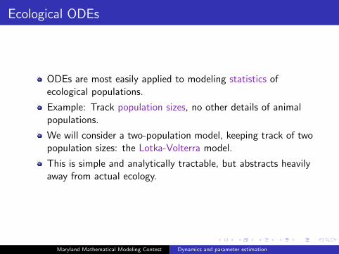
Ecological ODEs
ODEs are most easily applied to modeling statistics ofecological populations.
Example: Track population sizes, no other details of animalpopulations.
We will consider a two-population model, keeping track of twopopulation sizes: the Lotka-Volterra model.
This is simple and analytically tractable, but abstracts heavilyaway from actual ecology.
Maryland Mathematical Modeling Contest Dynamics and parameter estimation

Lotka-Volterra history
First developed by Vito Volterra ca. 1926 to explain thevariances in fish catches in the Adriatic Sea.
Four important model assumptions:
The prey population grows exponentially in the absence ofpredation.The predator population decreases exponentially in the absenceof prey.Predators reduce prey population growth rate, proportional toboth the predator and prey populations.Prey increases the predator population growth rate,proportional to both the predator and prey populations.
Maryland Mathematical Modeling Contest Dynamics and parameter estimation

Lotka-Volterra equation
Two state variables (x, y) ∈ R2. Prey population is x,Predator population is y.
Four parameters: α - prey growth rate. β - prey predationeffect. γ - predator population decay rate. δ - predatorpredation effect.
Lotka-Volterra equation (LVE): Given initial x0 and y0, x(t)and y(t) satisfy
dx
dt= αx− βxy
dy
dt= δxy − γy.
Maryland Mathematical Modeling Contest Dynamics and parameter estimation

Lotka-Volterra equation
One can use the various tools of dynamical systems theory toanalyze the behavior of x(t) and y(t). Spoiler: They oscillate,or y(t)→ 0 and x(t) grows unboundedly, or both populationsgo to 0.
More important for mathematical modeling is the ability tonumerically solve the equations. LVE generalizations canremain numerically solvable even when not analyticallytractable (more effects, more species, etc.).
Maryland Mathematical Modeling Contest Dynamics and parameter estimation

Solving LVE numerically
Numerical ODE solvers are a fantastically useful set of toolsavailable for most programming languages.
For an arbitrary ODE, numerical simulation may be extremelydifficult. There is tons of literature on the ways to efficientlynumerically solve different classes of ODEs.
For the M3C/MCM, knowing how to use these tools is crucialto building an ODE model.
Model example: Solving LVE using ode45 and MATLAB.
Maryland Mathematical Modeling Contest Dynamics and parameter estimation

And now for a
- MATLAB break -
Maryland Mathematical Modeling Contest Dynamics and parameter estimation

ODE model weaknesses
List some!
Maryland Mathematical Modeling Contest Dynamics and parameter estimation

Discrete modeling approaches
We can revisit the way we model predator-prey interactions,and simulate the organisms instead of tracking populationstatistics.
ODE models look at dynamics in a low-dimensional statespace (in the LVE case, R×R)
Idea: Let the state space correspond to a high-dimensionalphysical space (sorta).
States are discrete objects in physical space (sorta).
Discrete time corresponding to iterative state updates.
Simplest approach here: cellular automata (CA).
Maryland Mathematical Modeling Contest Dynamics and parameter estimation

Cellular automata
Underlying state space X is a grid of M spatial “cells”x = {xi}Mi=1 (though other spatial graphs work, too).
The possible states are a small, finite set S, e.g. S = {0, 1},S = {red, blue, green}, S = {fox, rabbit}.Time variable t ∈ T = N.
State evolution can be defined by a discrete differenceequation, but it is often useful to use a transition map instead.
Maryland Mathematical Modeling Contest Dynamics and parameter estimation

Cellular automata
Transition maps: in general,
x(t+ 1) = F (x(t)),
where the transition map F is a function (deterministic CA)or a stochastic process (stochastic CA) taking values in S.
Commonly, xi(t+ 1) depends only on xi(t) and xj(t) for xj ina neighborhood N(xi) of xi.
Figure: Two common neighborhoods; (a) Von Neumann and (b) Moore.
Maryland Mathematical Modeling Contest Dynamics and parameter estimation

A predator-prey CA model
Assumptions:
1. Two “animals”: fox (predator) and rabbit (prey).
2. Foxes can move, die, eat, and reproduce with someprobabilities.
3. Rabbits can move, die, and reproduce with some probabilities.
Setup:
State space is an N ×N grid.
States are empty (E), fox, (F ), rabbit (R).
The transition map is stochastic and best describedalgorithmically, using Moore neighborhoods.
Maryland Mathematical Modeling Contest Dynamics and parameter estimation
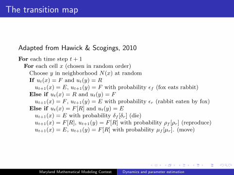
The transition map
Adapted from Hawick & Scogings, 2010
For each time step t+ 1For each cell x (chosen in random order)Choose y in neighborhood N(x) at randomIf ut(x) = F and ut(y) = Rut+1(x) = E, ut+1(y) = F with probability εf (fox eats rabbit)
Else if ut(x) = R and ut(y) = Fut+1(x) = F , ut+1(y) = E with probability εr (rabbit eaten by fox)
Else if ut(x) = F [R] and ut(y) = Eut+1(x) = E with probability δf [δr] (die)ut+1(x) = F [R], ut+1(y) = F [R] with probability ρf [ρr] (reproduce)ut+1(x) = E, ut+1(y) = F [R] with probability µf [µr]. (move)
Maryland Mathematical Modeling Contest Dynamics and parameter estimation

A predator-prey CA model
Things to note
The mathematical formalism is instructive in general, but analgorithmic description is more useful for most models.
Lots of parameters! εf , εr for eating, δf , δr for dying, ρf , ρrfor reproduction, µf , µr for moving.
Parameter values dictate system dynamics. Extinction of oneor both species, or cyclic population growth and decline (a laLotka-Volterra) are all possible.
Maryland Mathematical Modeling Contest Dynamics and parameter estimation

(Start simulation now)
Maryland Mathematical Modeling Contest Dynamics and parameter estimation

Model strengths and weaknesses
Strengths:
Captures more aspects of population dynamics thanLotka-Volterra.
CA’s allow simple, well-chosen rules to generate complexbehaviors.
Easy to program.
Large numbers of parameters mean behavior can be tailoredto known data.
Easy to modify for better model fidelity.
Maryland Mathematical Modeling Contest Dynamics and parameter estimation

Model strengths and weaknesses
Weaknesses:
Still fails to capture many aspects of predator-prey dynamics.
High-dimensional state spaces mean analytic results aredifficult to produce.
Simulation via cellular automata is usually inductive ratherthan deductive.
May be computationally intractable for large domains.
Maryland Mathematical Modeling Contest Dynamics and parameter estimation

Elaborations on this model
Instead of a grid, consider an automaton on a general graph,for better spatial fidelity.
Create a more complicated food web by adding additionalpossible CA states.
Investigate agent-based models instead of CA models.
Rules can be made to vary in space and/or time.
Maryland Mathematical Modeling Contest Dynamics and parameter estimation

And now...
Contest Tips 1
Maryland Mathematical Modeling Contest Dynamics and parameter estimation

Contest necessities
Everyone should have a computer to work on.
Look for a (reasonably) comfortable working space ahead oftime.
Software to write up your solution (LaTeX)
A programming language at least one (preferably two)teammates can use.
Be able to learn, quickly!
Maryland Mathematical Modeling Contest Dynamics and parameter estimation

Suggested timeline
Before contest begins: Coordinate! Know where you’llmeet, exchange email addresses and phone numbers. Knowwhen teammates won’t be available
Friday: Problem is put online at 5PM. Time for research. Doas much background research on the problem as you can.Start outlining at least two possible modeling approaches.
Saturday: Keep doing background research. Choose amodeling approach, start programming an implementation.Start writing. Suggested: 2 working on the model, 1 writing.
Sunday: Both implementation and writing should be in fullswing. By Sunday night, 2 people should be writing. Don’t goto sleep.
Monday: Solution is due at 10AM sharp. Plan to finish by9AM.
Maryland Mathematical Modeling Contest Dynamics and parameter estimation

Solution paper structure
Abstract
Title page, table of contents
Problem description
Model description (including proposed solution)
Model assumptions
Results
Model strengths and weaknesses
Conclusion
Code appendix
Works cited
Maryland Mathematical Modeling Contest Dynamics and parameter estimation

Finding and using documents
Obvious starting places: Google, Google Scholar. Researchpapers > random websites.
http://www.lib.umd.edu/ may have access to papers youcan’t get on Google Scholar.
Investigate references in papers you’ve already found.
Google Scholar also lets you see who has cited a given paper(super helpful).
Keep a running bibliography, even of papers you aren’t sureyou’ll use. You can trim it at the end.
Maryland Mathematical Modeling Contest Dynamics and parameter estimation

Finding and using software
You’ll likely need new software, or software libraries during thecompetition.
Use existing code when possible. Don’t write your own unlessyou have to!
Finding and using new software/code means knowing how tosearch effectively.
Look for documentation or help pages.
Maryland Mathematical Modeling Contest Dynamics and parameter estimation

![MATH 614, Spring 2016 [3mm] Dynamical Systems …Dynamical Systems and Chaos Lecture 1: Examples of dynamical systems. A discrete dynamical system is simply a transformation f : X](https://img.pdfslide.net/doc/110x75/5fc3a613bb041d25ed5cc331/math-614-spring-2016-3mm-dynamical-systems-dynamical-systems-and-chaos-lecture.jpg)


![OutcomeandComplicationsofCombinedPhacoemulsification ...combinedphacoemulsification[17,18].Combinedsurgery helpsminimizingtheeconomiccost[11].Asalast,butnot least advantage, combined](https://img.pdfslide.net/doc/110x75/610121f62de6813fce181dac/outcomeandcomplicationsofcombinedphacoemulsification-combinedphacoemulsiication1718combinedsurgery.jpg)