Dynamic Pricing with an Unknown Demand Model:

Asymptotically Optimal Semi-myopic Policies

N. Bora Keskin∗

University of Chicago

Assaf Zeevi†

Columbia University

This version: January 31, 2014

Abstract

We consider a monopolist who sells a set of products over a time horizon of T periods. The

seller initially does not know the parameters of the products’ linear demand curve, but can

estimate them based on demand observations. We first assume that the seller knows nothing

about the parameters of the demand curve, and then consider the case where the seller knows

the expected demand under an incumbent price. It is shown that the smallest achievable revenue

loss in T periods, relative to a clairvoyant who knows the underlying demand model, is of order√T in the former case and of order logT in the latter case. To derive pricing policies that

are practically implementable, we take as our point of departure the widely used policy called

greedy iterated least squares (ILS), which combines sequential estimation and myopic price

optimization. It is known that the greedy ILS policy itself suffers from incomplete learning,

but we show that certain variants of greedy ILS achieve the minimum asymptotic loss rate. To

highlight the essential features of well-performing pricing policies, we derive sufficient conditions

for asymptotic optimality.

Keywords: Revenue management, pricing, sequential estimation, exploration-exploitation.

1 Introduction

Pricing decisions often involve a trade-off between learning about customer behavior to increase

long-term revenues, and earning short-term revenues. In this paper we examine that trade-off.

Overview of the problem. In our learning-and-earning problem there is a seller that can

adjust the price of its product over time. Customer demand for the seller’s product is determined

by the price, according to an underlying parametric demand model. The seller is initially uncertain

about the parameters of the demand model but can use price as a learning tool, estimating the

∗Booth School of Business, e-mail: bora.keskin@chicagobooth.edu†Graduate School of Business, e-mail: assaf@gsb.columbia.edu

1

model parameters based on the empirical market response to successive prices. This is a dynamic

pricing problem with demand model uncertainty.

A particular example that motivates our study is the pricing of financial services, such as con-

sumer and auto loans. As noted by Phillips (2005, pp. 266-267), sellers of consumer lending

products are typically capable of quoting a different interest rate to each customer who requests a

loan. This transaction structure, which Phillips calls customized pricing, creates a price experimen-

tation opportunity for the seller. At the same time, price experimentation does not seem to be very

common in practice (Phillips 2010); for many consumer lending products, a bank will very often

keep the interest rate that it charges fixed, over extended periods of time. It then knows with high

confidence the average market response to that one price, referred to hereafter as the incumbent

price, but may be uncertain about market response to alternative prices. In this paper we study

several closely related models of dynamic pricing with demand model uncertainty, both with and

without prior knowledge of market response to an incumbent price. The models employed are

somewhat stylized, intended to provide fundamental insight while lacking the fine structure needed

in real-world applications.

Another feature of consumer lending that influences our problem formulation is high transaction

volume: a commercial bank typically encounters hundreds of lending opportunities per day. In our

model the horizon length T can be thought of as a proxy for the number of potential sales, and

“demand” can be thought of as the portion of these that are successfully captured. To assess the

quality of any pricing policy, we focus on the asymptotic growth of regret : the expected loss of

revenue relative to a clairvoyant who knows the underlying demand model, as the horizon length

T becomes large. When we speak later of asymptotically optimal policies, this will mean policies

that achieve a minimal growth rate of regret.

Focus on semi-myopic policies. According to a report by the Boston Consulting Group,

myopic pricing policies are common practice in many industries, and pricing executives usually

do not engage in price experimentation or other forms of active learning (Morel, Stalk, Stanger

and Wetenhall 2003). A conventional procedure is to simply combine greedy price optimization

with sequential estimation as follows: whenever a seller needs to adjust its price, the first step

is to estimate the parameters of a demand model, and then the seller charges whatever price

maximizes expected profit, assuming that the unknown model parameters are equal to the most

recent estimates. As will be explained later, this approach leads to poor profit performance due

to incomplete learning : because there is no explicit effort to create price dispersion, there is no

guarantee that parameter estimates will converge to the true values. To provide practical insight,

we use the myopic approach as a starting point, modifying it to guard against poor performance. It

will be shown that the resulting semi-myopic policies are asymptotically optimal in a well defined

mathematical sense.

2

Related literature. The trade-off between exploration (learning) and exploitation (earning)

has long been a focus of attention in statistics, engineering, and economics. There has been recent

interest in this topic in the operations research and management science (OR/MS) realm, especially

in the field of dynamic pricing and revenue management. Economists were the first to formulate

a learn-and-earn problem in a pricing context, but recent OR/MS work has a somewhat different

flavor, emphasizing development of practical policies whose performance is provably good although

not necessarily optimal.

Harrison, Keskin and Zeevi (2012) analyze the performance of myopic pricing and some of its

variants in a stylized Bayesian setting where one of two possible demand models is known to be

true. Under mild assumptions that ensure the existence of just one “uninformative” price (that is,

just one price that fails to distinguish between the two demand hypotheses), they show that the

myopic price sequence converges either to the uninformative price or else to the true optimal price,

each with positive probability. Having thus established that myopic pricing may lead to incomplete

learning, they go on to prove positive results about variants of myopic pricing that avoid use of

the uninformative price. Harrison et al. (2012) also discuss in detail how recent OR/MS papers

on learning-and-earning relate to the antecedent economics literature, and we refer to their paper

for a more complete list of references. Two other closely related papers on dynamic pricing with

demand model uncertainty are due to Broder and Rusmevichientong (2012) and den Boer and

Zwart (2013). Broder and Rusmevichientong (2012) consider a general parametric demand model

to evaluate the performance of maximum-likelihood-based policies, and concentrate on the idea of

combining the myopic approach with explicit price experimentation. Dividing the sales horizon

into cycles of increasing length, they design a policy that applies fixed experimental prices at the

beginning of each cycle, and charges the myopic maximum-likelihood-based price during the rest

of the same cycle. They show that their policy is asymptotically optimal. The framework of den

Boer and Zwart (2013) involves a demand model with two unknown parameters. Using a myopic

maximum-likelihood-based policy as a starting point, den Boer and Zwart design a variant of the

myopic policy, namely the controlled variance pricing policy, by creating taboo intervals around

uninformative prices, and derive a theoretical bound on the performance of this variant. In a

more recent study that has been conducted in parallel to our work, den Boer (2013) extends the

controlled variance pricing policy of den Boer and Zwart (2013) to the case of multiple products

with a generalized linear demand curve. A common theme in these papers is that they all consider

some particular parametric family of pricing policies to find a good balance between learning and

earning. In contrast, we provide in this paper general sufficient conditions that achieve the same

goal, which sheds further light on the role and impact of price experimentation.

There are two other noteworthy differences between our work and that of Broder and Rus-

mevichientong (2012). First, like den Boer and Zwart (2013), Broder and Rusmevichientong study

the pricing of a single product, whereas we extend our analysis to the case of many products with

3

substitutable demand. As will be explained in detail later, learning and earning in higher dimen-

sions requires extra care. Broder and Rusmevichientong (2012) also derive logarithmically growing

regret bounds in a particular variant of their original problem, which they call the “well-separated”

case. At least superficially, this might seem similar to our analysis of the incumbent-price problem,

but that appearance is somewhat deceptive: at least in our view, the incumbent-price formulation

is better motivated from a practical standpoint than the well-separated problem, and while the

performance bounds alluded to above are of similar nature, the analysis is distinctly different in

the two settings.

There are also OR/MS studies that take on different approaches to dynamic pricing to learn

and earn. Kleinberg and Leighton (2003) employ a multi-armed bandit approach in a dynamic

pricing context by allowing the seller to use only a discrete grid of prices within the continuum of

feasible prices. They show that certain methods in multi-armed bandit literature work well for a

carefully chosen price grid. A key feature of this study is that the seller needs to know the time

horizon before the problem starts, so that he will be able to choose a sufficiently fine grid of prices.

Carvalho and Puterman (2005) consider dynamic pricing problem with a binomial-logistic demand

curve, and analyze the performance of several pricing policies. They conduct a simulation study

to demonstrate that one-step lookahead policies could perform significantly better than myopic

policies.

The particular myopic policy we examine in this paper is greedy iterative least squares (ILS),

which combines the myopic approach mentioned above with sequential estimation based on ordinary

least squares regression. Greedy ILS was first formulated by Anderson and Taylor (1976) in a

problem motivated by medical applications. Based on simulation results, Anderson and Taylor

argued that the plain version of greedy ILS could be used in regulation problems, such as stabilizing

the response of patients to the dosage level of a given drug (see Lai and Robbins 1979, Section 1 for

further details about this medical motivation). There are a few studies that demonstrate that the

parameter estimates of greedy ILS are consistent when either charging any feasible price provides

information about the unknown response curve, or greedy ILS charges only the prices that provide

information (cf., e.g., Taylor 1974, Broder and Rusmevichientong 2012). However, as shown by Lai

and Robbins (1982), the parameter estimates computed under greedy ILS may not be consistent,

and the resulting controls may be sub-optimal. Because of this negative result, there is a clear need

to “tweak” the plain version of greedy ILS in order to generate well-performing policies.

Main contributions and organization of the paper. Our study makes four main contri-

butions to the literature on learning-and-earning. First, our formulation of the incumbent-price

problem, where the seller starts out knowing one point on its demand curve, is both novel and

widely applicable, at least as an approximation. As will be shown later, our conclusions for the

incumbent-price problem differ sharply from those for the conventional problem. Second, unlike

4

previous studies on this subject, our paper provides general sufficient conditions for asymptotic

optimality of semi-myopic policies, providing general guidelines for implementing price experimen-

tation strategies. Said optimality conditions are obtained using analytical tools that apply broadly

to problems of dynamic pricing with model uncertainty. Our third contribution is the development

of these tools by (i) using the concept of Fisher information to find natural and intuitive lower

bounds on regret, and (ii) using martingale theory to control pricing errors, and construct semi-

myopic policies whose order of regret matches these lower bounds. Finally, our analysis covers the

pricing of multiple products with substitutable demand, which, as will be seen in what follows, is

not a straightforward extension of single-product pricing. In essence, learning in a high dimen-

sional price space requires sufficient “variation” in the directions of successive price vectors, and

the necessity of spanning the price space brings forth the idea of orthogonal pricing.

Our paper is organized as follows. In Section 2 we formulate our problem. In Section 3 we analyze

single-product pricing by first constructing a lower bound on the revenue loss of any given policy,

and then providing a set of sufficient conditions for asymptotic optimality. To facilitate practical

implementation of our results, we also give some examples of policies that meet these asymptotic

optimality conditions. Toward the end of Section 3, we analyze the incumbent-price problem

explained above, and finish that section by comparing the results obtained in the conventional

setting with the ones obtained in the incumbent-price setting. In Section 4 the single-product

results are generalized to a multi-product setting. Section 5 summarizes the main contributions of

this paper. The proofs of formal results are postponed to the appendices.

2 Problem Formulation

Basic model elements. Consider a firm, hereafter called the seller, that sells n distinct products

over a time horizon of T periods. In each period t = 1, 2, . . . the seller must choose an n× 1 price

vector pt = (p1t, . . . , pnt) from a given feasible set [ℓ, u]n ⊆ Rn, where 0 ≤ ℓ < u < ∞, after which

the seller observes the demand Dit for each product i in period t. (In practice, different products

may have different price intervals, and it is straightforward to generalize the following analysis to

the case where the feasible set of prices is an arbitrary but fixed rectangle in Rn.) In this paper

we focus on linear demand models, which elucidate the key features of the problem by making our

analysis more transparent (see Section 5 for further discussion of the linear demand assumption).

Suppose that Dit is given by

Dit = αi + βi · pt + ǫit for i = 1, . . . , n and t = 1, 2, . . .

where αi ∈ R, βi = (βi1, . . . , βin) ∈ Rn are the demand model parameters, which are initially

unknown to the seller, ǫit are unobservable demand shocks, and x · y =∑n

i=1 xiyi denotes the inner

product of vectors x and y. We assume that {ǫit}i=1,...,n, t=1,...,T are independent and identically

5

distributed random variables with mean zero and variance σ2, and that there exists a positive

constant z0 such that E[ezǫit] <∞ for all |z| ≤ z0. (An important example is where ǫitiid∼ N (0, σ2);

in treating this case, it is more realistic to consider small values of σ so that the probability of

observing a negative demand is negligible.) To simplify notation, we let θ := (α1, β1, . . . , αn, βn) ∈Rn2+n be the vector of demand model parameters for all products, and express the demand vector

Dt = (D1t, . . . ,Dnt) ∈ Rn in terms of θ as follows:

Dt = a+Bpt + ǫt for t = 1, 2, . . . (2.1)

where ǫt := (ǫ1t, . . . , ǫnt) ∈ Rn, a := (α1, . . . , αn) ∈ R

n, and B is an n × n matrix whose ith row is

βTi , that is,

B =

β11 β12 · · · β1n

β21 β22 · · · β2n...

.... . .

...

βn1 βn2 · · · βnn

.

Because prices can always be expressed as increments above marginal production cost, we assume

without loss of generality that the marginal cost of production is zero, and use the terms “profit”

and “revenue” interchangeably. The seller’s expected single-period revenue function is

rθ(p) := p · (a+Bp) for θ ∈ Rn2+n and p ∈ [ℓ, u]n. (2.2)

Let ϕ(θ) be the price that maximizes the expected single-period revenue function rθ(·), i.e.,

ϕ(θ) := argmax{rθ(p) : p ∈ [ℓ, u]n}. (2.3)

Before selling starts, nature draws the value of θ from a compact rectangle Θ ⊆ Rn2+n. We assume

that the optimal price corresponding to each θ ∈ Θ is an interior point of the feasible set [ℓ, u]n,

implying that B is negative definite. (If B were not negative definite, then there would exist a

non-zero vector z such that zTBz ≥ 0, and we would get a corner solution by changing the price

in the direction of z.) Therefore, the first-order condition for optimality is

η(θ, p) := a +(B +BT

)p = 0, (2.4)

from which we deduce that ϕ(θ) = −(B + BT

)−1a ∈ (ℓ, u)n. If the seller has only one product

(that is, n = 1), then the revenue-maximizing price simply becomes ϕ((α, β)

)= −α/(2β).

Because Θ is a compact set and B is negative definite, we have the following: for all θ ∈ Θ the

eigenvalues of the matrix B are in the interval [bmin, bmax], where −∞ < bmin < bmax < 0. In the

single-product case, this fact implies that the slope parameter β is contained in [bmin, bmax].

Pricing policies, induced probabilities, and performance metric. Denote by Ht the

vectorized history of demands and prices observed through the end of period t. That is, Ht :=

6

(D1, p1, . . . ,Dt, pt). We define a policy as a sequence of functions π = (π1, π2, . . .), where πt+1 is

a measurable mapping from R2nt into [ℓ, u]n for all t = 1, 2, . . . , and π1 is a constant function.

The argument of the pricing function πt+1 is Ht. The seller exercises a policy π to construct a

nonanticipating price sequence p = (p1, p2, . . .), charging price vector pt in period t. This definition

of a pricing policy implies that each pt is adapted to Ht−1 = (D1, p1, . . . ,Dt−1, pt−1).

Any pricing policy induces a family of probability measures on the sample space of demand

sequences D = (D1,D2, . . .). Given the parameter vector θ = (α1, β1, . . . , αn, βn) and a policy π,

let Pπθ be a probability measure satisfying

Pπθ (D1 ∈ dξ1, . . . ,DT ∈ dξT ) =

T∏

t=1

n∏

i=1

Pǫ(αi + βi · pt + ǫit ∈ dξit) for ξ1, . . . , ξT ∈ Rn, (2.5)

where Pǫ(·) is the probability measure of random variables ǫit, and p = (p1, p2, . . .) is the price

sequence formed under policy π and demand realizations D1,D2, . . . In our context, Pπθ (A) is the

probability of an event A given that the parameter vector is θ and the seller uses policy π. Thus,

pt = πt(Ht−1) almost surely under Pπθ , which implies that pt is completely characterized by π, θ,

and Ht−1. Accordingly the expected T -period revenue of the seller is

Rπθ (T ) = Eπθ

{ T∑

t=1

rθ(pt)}, (2.6)

where Eπθ is the expectation operator associated with the probability measure Pπθ . The performance

metric we will use throughout this study is the T -period regret, defined as

∆πθ (T ) = Tr∗θ −Rπθ (T ) for θ ∈ Θ and T = 1, 2, . . . (2.7)

where r∗θ := rθ(ϕ(θ)

)is the optimal expected single-period revenue. While deriving our lower

bounds on best achievable performance, we will also make use of the worst-case regret, which is

given by

∆π(T ) = sup{∆πθ (T ) : θ ∈ Θ

}for T = 1, 2, . . . (2.8)

The regret of a policy can be interpreted as the expected revenue loss relative to a clairvoyant

policy that knows the value of θ in period 0; smaller values of regret are more desirable for the

seller.

Greedy iterated least squares (ILS). Given the history of demands and prices through the

end of period t, the least squares estimator of θ is given by

θt = argminθ

{SSEt(θ)}, (2.9)

where SSEt(θ) =∑t

s=1

∑ni=1(Dis −αi − βi · ps)2 for θ = (α1, β1, . . . , αn, βn). Using the first-order

optimality conditions of the least squares problem (2.9), the estimator θt can be expressed explicitly

7

as θt = (α1t, β1t, . . . , αnt, βnt) where

[αit

βit

]=

[t

∑ts=1 p

Ts∑t

s=1 ps∑t

s=1 pspTs

]−1 [ ∑ts=1Dis∑ts=1Disps

]

for i = 1, . . . , n. Combining the preceding least squares formula with the demand equation (2.1),

one has the following:

[αit − αi

βit − βi

]= J −1

t Mit for all i = 1, . . . , n and t = n+ 1, n + 2, . . . , (2.10)

where Jt is the empirical Fisher information given by

Jt =

[t

∑ts=1 p

Ts∑t

s=1 ps∑t

s=1 pspTs

]

=t∑

s=1

([1ps

]·[

1ps

]T), (2.11)

andMit is the (n+1)×1 vector, Mit :=∑t

s=1

(ǫis[

1ps

]). With a single product, the estimation error

expressed in (2.10) reduces to θt − θ = J −1t Mt, where Jt =

∑ts=1

[1 psps p2s

]and Mt =

∑ts=1

[ ǫsǫsps

].

Because θ lies in the compact rectangle Θ, the accuracy of the unconstrained least squares

estimate θt can be improved by projecting it into the rectangle Θ. We denote by ϑt the truncated

estimate that satisfies ϑt := argminϑ∈Θ{‖ϑ − θt‖}, where by assumption the corresponding price

vector ϕ(ϑt) is an interior point of the feasible set [ℓ, u]n. We call the policy that charges price

pt = ϕ(ϑt−1) in period t = 1, 2, . . . the greedy iterated least squares (ILS) policy. Because greedy

ILS cannot estimate anything without data, we fix n + 1 non-random and linearly independent

vectors for p1, p2, . . . , pn+1, and (whenever necessary) ϑ0, ϑ1, . . . , ϑn can be found accordingly.

In the following section we will focus on the case n = 1, and explain in Section 4 how the

single-product analysis extends to the case of multiple products with substitutable demand.

3 Analysis of the Single-Product Setting

To introduce our main ideas in a simple setting we assume throughout this section that the seller

has a single product to sell (that is, n = 1), and consequently drop the product index i from the

demand parameters αi and βi.

3.1 A Lower Bound on Regret

We use the case where ǫtiid∼ N (0, σ2) to derive a lower bound on regret. In fact, our analysis for

all lower bounds on regret is valid for a broader exponential family of distributions whose densities

8

have the following parametric form: fǫ(ξ |σ) = c(σ) exp(h(ξ) +

∑kj=1wj(σ)tj(ξ)

)for ξ ∈ R, where

h(·) and tj(·) are differentiable functions. This family includes a wide range of distributions such

as Gaussian, log-normal, exponential, and Laplace distributions. The last paragraph of Section

A.1 explains how our proof of the lower bound with Gaussian noise can be extended to the more

general setting.

All the information that a pricing policy can use is that contained in the history vector Ht, which

can be quantified as follows. Given θ = (α, β), the density of Ht is

gt(Ht, θ) =

t∏

s=1

1

σφ

(Ds − α− βps

σ

), (3.1)

where φ(·) denotes the standard Gaussian density. Thus, Ht has the following Fisher information

matrix:

Iπt (θ) := Eπθ

{[∂ log gt(Ht, θ)

∂θ

]T ∂ log gt(Ht, θ)

∂θ

}=

1

σ2Eπθ [Jt] . (3.2)

To obtain a lower bound on regret, the following lemma is key.

Lemma 1 (lower bound on cumulative pricing error) There exist finite positive constants

c0 and c1 such that

supθ∈Θ{∑T

t=2 Eπθ

(pt − ϕ(θ)

)2} ≥T∑

t=2

c0

c1 + supθ∈Θ{C(θ)Eπθ [Jt−1] C(θ)T

} , (3.3)

where C(·) is a 1× 2 matrix function on Θ such that C(θ) = [−ϕ(θ) 1].

Lemma 1, whose proof relies on a multivariate version of the van Trees inequality (cf. Gill and

Levit 1995, p. 64), expresses the manner in which the growth rate of regret depends on accumulated

information. If the denominator on the right side of inequality (3.3) converges to a constant, then

information acquisition stops prematurely (incomplete learning), and hence regret would grow

linearly over time. Thus, one would expect a “good” policy to make supθ∈Θ{C(θ)Eπθ [Jt−1] C(θ)T

}

diverge to infinity for any given non-zero 1×2 matrix function C(·). If this quantity grows linearly,

then we would arrive at a logarithmically growing lower bound on regret. However, if we specify

the function C(·) as in Lemma 1, we realize that a logarithmic lower bound is in fact loose.

For C(θ) = [−ϕ(θ) 1], the quantity in the supremum on the right hand side of (3.3) becomes∑t

s=1 Eπθ

(ps − ϕ(θ)

)2, which is almost identical to the quantity in the supremum on the left hand

side. Viewing these quantities as a time-indexed sequence of real numbers, we then deduce that

each term supθ∈Θ{∑T

t=1 Eπθ

(pt − ϕ(θ)

)2}is at least of order

√T , which leads to the following

conclusion.

Theorem 1 (lower bound on regret) There exists a finite positive constant c such that ∆π(T ) ≥c√T for any pricing policy π and time horizon T ≥ 3.

9

Remark The constant c in the above theorem, and all the constants that will appear in the

following theorems are spelled out explicitly in the appendices. See Section 3.5 for a discussion of

how these constants depend on characteristics of the demand shocks.

According to Theorem 1, the T -period regret of any given policy must be at least of order√T . A

policy π for which the growth rate of regret does not exceed order√T (up to logarithmic terms) will

be called asymptotically optimal. In the next subsection we explain how greedy ILS fails to achieve

this benchmark while certain variants of greedy ILS do achieve it. With slight abuse of terminology,

the minimum asymptotic growth rate for regret will also be referred to as the minimum asymptotic

loss rate.

Besbes and Zeevi (2011) and Broder and Rusmevichientong (2012) provide lower bounds on

regret that grow proportional to√T in similar dynamic pricing contexts with demand model

uncertainty. The argument used in those papers relies on the Kullback-Leibler divergence, and

deals with uncertainty in a single model parameter. Our proof of Theorem 1 employs an entirely

different argument that uses the van Trees inequality and the concept of Fisher information, and

we derive lower bounds for parameter uncertainty in two and higher dimensions.

3.2 Sufficient Conditions for Asymptotic Optimality

We now derive a set of conditions which assure that the regret of a policy is asymptotically optimal.

Our starting point is the greedy ILS policy, which is commonly used in practice. As explained in

Section 2, the operating principles of greedy ILS are (i) estimating at the beginning of each time

period the unknown model parameters via ordinary least squares regression, and (ii) charging in

that period the “greedy” or “myopic” price that would be appropriate if the most recent least

squares estimates were precisely correct. Although the iterative use of this estimate-and-then-

optimize method seems reasonable, it does not take into account the fact that the myopic price

optimization routine will be repeated in the future. There is a threat that the greedy price will not

generate enough information, causing the seller to stop learning prematurely. Thus, greedy ILS

estimates may get stuck at parameter values that are not the true ones. This phenomenon, which

is called incomplete learning, was first analyzed by Lai and Robbins (1982) in a sequential decision

problem motivated by medical treatments. Recently, den Boer and Zwart (2013) showed that the

same result holds in a dynamic pricing context like ours. An important consequence of incomplete

learning is that the seller forfeits a constant fraction of expected revenues in each period, causing

regret to grow linearly over time.

In modifying greedy ILS, our main concern is to make sure that information is gathered at an

adequate rate. One measure of information is the minimum eigenvalue of the empirical information

matrix Jt, denoted by µmin(t). Although it is possible to use µmin(t) as the sole information metric

in the remainder of our analysis, we choose to employ a more practical information metric, which is

10

closely related to µmin(t). The information metric we will use is the sum of squared price deviations,

which is expressed as

Jt =

t∑

s=1

(ps − pt)2 ,

where pt = t−1∑t

s=1 ps. The following lemma relates µmin(t) to Jt. (For this lemma, readers are

reminded that ℓ and u are a given lower bound and a given upper bound, respectively, on prices.)

Lemma 2 (minimum eigenvalue of Fisher information) Let µmin(t) be the smallest eigen-

value of Jt. Then µmin(t) ≥ γJt, where γ = 2/(1 + 2u− ℓ)2.

An immediate implication of the above result is that one can control the rate of information

acquisition by controlling the process {Jt}. We use this observation to show that the least squares

estimation errors decrease exponentially as a function of Jt.

Lemma 3 (exponential decay of estimation errors) There exist finite positive constants ρ

and k such that, under any pricing policy π,

Pπθ

{‖θt − θ‖ > δ, Jt ≥ m

}≤ kt exp

(− ρ(δ ∧ δ2)m

), (3.4)

for all δ,m > 0 and all t ≥ 2.

Lemma 3 shows that, by imposing carefully designed time-dependent constraints on the growth

of the process Jt, the seller can directly control how fast estimation errors converge to zero. This

leads to the following recipe for asymptotic optimality.

Theorem 2 (sufficient conditions for asymptotic optimality) Assume that θ ∈ Θ. Let κ0,

κ1 be finite positive constants, and let π be a pricing policy that satisfies

(i) Jt ≥ κ0√t

(ii)∑t

s=0

(ϕ(ϑs)− ps+1

)2 ≤ κ1√t

almost surely for all t. Then there exist a finite positive constant C such that ∆πθ (T ) ≤ C

√T log T

for all T ≥ 3.

A simple verbal paraphrase of the preceding theorem is the following: a policy will perform well if

it (i) accumulates information at an adequate rate, and (ii) does not deviate “too much” from greedy

pricing. The conditions laid out in this theorem describe the (asymptotically) optimal balance

between learning and earning. Condition (i) takes care of learning by forcing the information

metric Jt to grow at an adequate rate, whereas condition (ii) limits the deviations from the greedy

ILS price, making sure that enough emphasis is given to earning. Failure to satisfy either one of

11

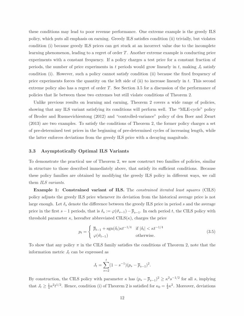
these conditions may lead to poor revenue performance. One extreme example is the greedy ILS

policy, which puts all emphasis on earning. Greedy ILS satisfies condition (ii) trivially, but violates

condition (i) because greedy ILS prices can get stuck at an incorrect value due to the incomplete

learning phenomenon, leading to a regret of order T . Another extreme example is conducting price

experiments with a constant frequency. If a policy charges a test price for a constant fraction of

periods, the number of price experiments in t periods would grow linearly in t, making Jt satisfy

condition (i). However, such a policy cannot satisfy condition (ii) because the fixed frequency of

price experiments forces the quantity on the left side of (ii) to increase linearly in t. This second

extreme policy also has a regret of order T . See Section 3.5 for a discussion of the performance of

policies that lie between these two extremes but still violate conditions of Theorem 2.

Unlike previous results on learning and earning, Theorem 2 covers a wide range of policies,

showing that any ILS variant satisfying its conditions will perform well. The “MLE-cycle” policy

of Broder and Rusmevichientong (2012) and “controlled-variance” policy of den Boer and Zwart

(2013) are two examples. To satisfy the conditions of Theorem 2, the former policy charges a set

of pre-determined test prices in the beginning of pre-determined cycles of increasing length, while

the latter enforces deviations from the greedy ILS price with a decaying magnitude.

3.3 Asymptotically Optimal ILS Variants

To demonstrate the practical use of Theorem 2, we now construct two families of policies, similar

in structure to those described immediately above, that satisfy its sufficient conditions. Because

these policy families are obtained by modifying the greedy ILS policy in different ways, we call

them ILS variants.

Example 1: Constrained variant of ILS. The constrained iterated least squares (CILS)

policy adjusts the greedy ILS price whenever its deviation from the historical average price is not

large enough. Let δs denote the difference between the greedy ILS price in period s and the average

price in the first s− 1 periods, that is δs := ϕ(ϑs−1)− ps−1. In each period t, the CILS policy with

threshold parameter κ, hereafter abbreviated CILS(κ), charges the price

pt =

{pt−1 + sgn(δt)κt

−1/4 if |δt| < κt−1/4

ϕ(ϑt−1) otherwise.(3.5)

To show that any policy π in the CILS family satisfies the conditions of Theorem 2, note that the

information metric Jt can be expressed as

Jt =

t∑

s=2

(1− s−1)(ps − ps−1)2.

By construction, the CILS policy with parameter κ has (ps − ps−1)2 ≥ κ2s−1/2 for all s, implying

that Jt ≥ 14κ

2t1/2. Hence, condition (i) of Theorem 2 is satisfied for κ0 =14κ

2. Moreover, deviations

12

from the greedy ILS price have the following deterministic upper bound: |ϕ(ϑs−1)− ps| ≤ κs−1/4.

Thus, condition (ii) is satisfied with κ1 = 2κ2. As a result, any policy in the CILS family achieves

the performance guarantee in Theorem 2. Of course, one can tune the policy parameter κ to

further improve the performance. As explained in the proof of Theorem 2, the constant in front

of the√T log T term in the upper bound is C1 = 4|bmin|(8K0ρ

−1κ−2 + κ2), where K0 = (1 +

5k)maxj=1,2

{maxθ{(∂ϕ(θ)/∂θj)2}

}, so the policy parameter that minimizes the upper bound is

κ∗ = (8K0/ρ)1/4.

The controlled-variance policy of den Boer and Zwart (2013) is an example that belongs to the

CILS family, and the performance guarantee that den Boer and Zwart prove for regret under their

policy is O(√T log T ).

Example 2: ILS with deterministic testing. Our second modification of greedy ILS, called

ILS with deterministic testing (ILS-d), conducts price experiments to gather information. To specify

the experimental prices and the periods at which experiments will take place, we let p1, p2 be two

distinct prices in [ℓ, u], and T1,t, T2,t be two sequences of sets satisfying the following conditions:

for each i and t, suppose that Ti,t ⊆ Ti,t+1, and T1,t, T2,t are disjoint subsets of {1, 2, . . . , t}, eachcontaining ⌊κ

√t⌋ distinct elements. In period t, an ILS-d policy with threshold parameter κ and

experimental prices p1 and p2, abbreviated ILS-d(κ, p1, p2), charges the price

pt =

p1 if t ∈ T1,tp2 if t ∈ T2,tϕ(ϑt−1) otherwise.

(3.6)

An ILS-d policy with parameters κ, p1, p2 conducts ⌊κ√t⌋ experiments in the first t periods,

which implies that Jt =∑t

s=1(ps − pt)2 ≥ ∑

s∈T1,t∪T2,t (ps − pt)2 ≥ 1

4(p1 − p2)2⌊κ

√t⌋ for all t.

Moreover, because ILS-d(κ, p1, p2) deviates from the greedy ILS price in at most κ√t periods, we

have∑t

s=0

(ϕ(ϑs)− ps+1

)2 ≤ κ(u− ℓ)2√t for all t. Thus, ILS-d(κ, p1, p2) satisfies the conditions of

Theorem 2 with κ0 =14 (κ−1)(p1− p2)2 and κ1 = κ(u−ℓ)2. As argued in our previous example, one

can tune ILS-d by minimizing the upper bound in Theorem 2 with respect to the policy parameters.

The MLE-cycle policy of Broder and Rusmevichientong (2012) is closely related to the ILS-d

family of policies. However the plain version of MLE-cycle does not update estimates at every

period, meaning that strictly speaking it is not an ILS-d policy. In their numerical experiments,

Broder and Rusmevichientong define and simulate refined versions of MLE-cycle that are indeed

members of the ILS-d family.

Remark Because the greedy ILS policy projects unconstrained least squares estimates θt onto

Θ, the ILS variants described above use the knowledge of Θ. Replacing the projected least squares

estimates ϑt with θt in the definition of greedy ILS, we can employ the exact arguments in the proof

of Theorem 2 to obtain similar asymptotically optimal ILS variants that do not use the knowledge

of Θ.

13

3.4 An Alternative Formulation: Incumbent-Price Problem

In this subsection we consider a modification of the learn-and-earn problem where the seller is

effectively uncertain about just one demand parameter. Specifically, we assume that the seller

knows the expected demand under a particular price p to be a particular quantity D. Thus the

demand parameters α and β are known to be related by the equation

D = α+ βp. (3.7)

where D and p are given constants. Because the market response to price p is already known, one

has to choose a price different from p to acquire further information about the demand model. In

that sense, p is the unique uninformative price within the feasible price domain [ℓ, u].

This model variant is of obvious theoretical interest, and it also approximates a situation that

is common in practice, where a seller has been charging a single price p for a long time and has

observed the corresponding average demand to be D. With that situation in mind, we call p the

incumbent price, and D the incumbent demand. Of course, a seller will never know the expected

demand under an incumbent price exactly, but if the incumbent price has been in effect long enough,

residual uncertainty about the corresponding expected demand will be negligible compared with

uncertainty about the sensitivity of demand to deviations from the incumbent price.

Both Taylor (1974) and Broder and Rusmevichientong (2012) have studied dynamic pricing

models with linear demand and just one unknown parameter, but those studies both considered

the artificial situation where the intercept α is known exactly. That is, earlier studies with a single

unknown demand parameter have assumed that the seller knows exactly the market response to

a price of zero. In addition to its unreality, that scenario does not confront the seller with an

interesting or difficult trade-off, because the only uninformative price is zero, and a price of zero

is not attractive to a profit-maximizing seller in any case. For example, when α is known exactly

there is no threat of incomplete learning under greedy ILS, because greedy prices are always strictly

positive. The incumbent-price model that we consider is more realistic and much more interesting

mathematically.

To avoid a borderline case where the seller must stop learning in order to price optimally, we

assume that the incumbent price does not exactly equal the optimal price induced by nature’s

choice of θ; that is, p 6= ϕ(θ), although p and ϕ(θ) can be arbitrarily close to each other. For

notational simplicity, in this subsection we re-express the seller’s decision in period t as a deviation

from the incumbent price (rather than the new price itself), and denote it by xt = pt − p. As a

result, the demand equation (2.1) becomes

Dt = D + βxt + ǫt for t = 1, 2, . . . (3.8)

One can take the view that the only uncertain demand parameter is β, since (3.7) defines α in

terms of β. In the remainder of this subsection we will assume without loss of generality that the

14

parameter vector θ consists only of the slope parameter β, whose value is drawn in period 0 from

the compact interval B := [bmin, bmax]. Therefore we can redefine the single-period revenue function

as follows:

rβ(x) := (p + x)(D + βx) for β ∈ R and p+ x ∈ [ℓ, u]. (3.9)

The price deviation that maximizes rβ(·) can then be calculated as

ψ(β) := argmax{rβ(x) : p+ x ∈ [ℓ, u]}, (3.10)

implying by (3.7) that p + ψ(β) = ϕ((α, β)

). With these new constructs, we can update the

definitions of expected T -period revenue Rπβ(T ) and T -period regret ∆πβ(T ) by just replacing θ, pt,

and ϕ(·) with β, xt, and ψ(·) in equations (2.6) and (2.7). Because we assume that the optimal

price and the incumbent price do not coincide, the worst-case regret becomes

∆π(T ) = sup{∆πβ(T ) : bmin ≤ β ≤ bmax, ψ(β) 6= 0

}for T = 1, 2, . . . (3.11)

To construct a lower bound on regret, we consider the case where ǫtiid∼ N (0, σ2), and quantify

the information contained in the sales data observed through the end of period t. The density of

the history vector Ht in the incumbent-price setting is

gt(Ht, β) =

t∏

s=1

1

σφ

(Ds − D − βxs

σ

). (3.12)

Therefore the Fisher information matrix of Ht is

Iπt (β) := Eπβ

{[∂ log gt(Ht, β)

∂β

]2}=

1

σ2Eπβ[Jt], (3.13)

where Jt :=∑t

s=1 x2s. Because Fisher information is a scalar rather than a matrix in this setting,

we will use Jt as the only information metric throughout this subsection. The needed analog of

Lemma 1 in our incumbent-price setting is the following result.

Lemma 4 (lower bound on cumulative pricing error) Assume that the incumbent-price re-

lation (3.7) holds. Then, there exist finite positive constants c0 and c1 such that

supβ∈B, ψ(β)6=0

{∑Tt=2 E

πβ

(xt − ψ(β)

)2} ≥T∑

t=2

c0

c1 + supβ∈B{Eπβ[Jt−1] }. (3.14)

Like Lemma 1, the preceding lower bound indicates that the growth rate of regret is determined

by accumulated information. However, in contrast to the original problem, the incumbent-price

problem allows the seller to accumulate information “for free” as long as it does not charge the

incumbent price, which is the unique uninformative action in this setting. As a result, our informa-

tion metric can increase linearly without forcing regret to increase linearly. Using this observation

and plugging into (3.14), we have a logarithmically growing lower bound on regret. The following

corollary of Lemma 4 spells this out mathematically.

15

Theorem 3 (lower bound on regret) Assume that the incumbent-price relation (3.7) holds.

Then there exists a finite positive constant c such that ∆π(T ) ≥ c log T for any pricing policy π and

time horizon T ≥ 3.

Remark A similar logarithmic lower bound is obtained by Broder and Rusmevichientong (2012,

Theorem 4.5 on p. 21) in a dynamic pricing problem with a binary-valued market response.

However, their model is one in which no uninformative action exists, and hence incomplete learning

is impossible. Both our result and theirs are proved using the van Trees inequality, following

Goldenshluger and Zeevi (2009). The essential added feature of our problem formulation is the

existence of a strictly positive uninformative price (the incumbent price), which creates a risk of

incomplete learning, making the seller’s problem strictly more difficult.

Theorem 3 implies that the minimum asymptotic loss rate for the incumbent-price problem is

log T . Accordingly, any policy π that satisfies ∆π(T ) = O(log T ) is considered to be asymptotical

optimal in the incumbent-price setting.

To show that the logarithmic lower bound in Theorem 3 is in fact achievable, we start as before

with the greedy ILS policy. The basic principles of greedy ILS stay essentially the same under

assumption (3.7). At the end of each period t, greedy ILS calculates the least squares estimator

βt, which can be explicitly expressed as

βt =

∑ts=1(Ds − D)xs∑t

s=1 x2s

. (3.15)

By the demand equation (3.8), this implies that

βt − β =Mt

Jt(3.16)

for all t = 1, 2, . . ., where Mt :=∑t

s=1 ǫsxs. It is known that β lies in the interval [bmin, bmax], so

we assume that the estimates are projected into this interval. That is, the greedy ILS policy uses

the truncated estimate bt = bmin ∨ (βt ∧ bmax), where ∨ and ∧ denote the maximum and minimum

respectively. The corresponding price p + ψ(bt) = p/2 − D/(2bt) is by assumption an interior

point of the feasible price interval [ℓ, u]. Thus the greedy ILS policy in the incumbent-price setting

charges price pt = p + ψ(bt−1

)in period t = 1, 2, . . . To generate an initial data point, we fix the

first greedy ILS price deterministically and b0 can be found accordingly.

Having explained how greedy ILS operates in the incumbent-price setting, we now determine

sufficient conditions for asymptotic optimality. The next lemma, which is an analog of Lemma 3,

characterizes the relationship between the estimation errors and accumulated information.

Lemma 5 (exponential decay of estimation errors) Assume that the incumbent-price relation

(3.7) holds. Then there exists a finite positive constant ρ such that, under any pricing policy π,

Pπβ

{|βt − β| > δ, Jt ≥ m

}≤ 2 exp

(− ρ(δ ∧ δ2)m

)(3.17)

16

for all δ,m > 0 and all t ≥ 2.

The probability bounds in the preceding lemma and its earlier counterpart, Lemma 3, are slightly

different. The bound in Lemma 3, which is derived for the two-dimensional estimator θt, has

a polynomial term kt in front of the exponential term, whereas in Lemma 5 the corresponding

polynomial term, which simply equals 2, has a lower degree because the latter lemma is derived in

a one-dimensional parameter space (see the proofs in Appendix A for further details). Apart from

polynomial terms, Lemma 5 appears to be identical to Lemma 3, but there is actually a fundamental

difference between them, arising from the definitions of the information metrics Jt and Jt. Once the

seller’s prices get close to the optimal price in the incumbent-price setting, we know that the price

deviations xt will approach the optimal price deviation ψ(β), making the information metric Jt

grow linearly. However, when we relax the incumbent-price assumption there is no such guarantee.

In our original setting, a linearly growing Jt means that the seller’s price pt eventually deviates from

the average price pt−1 by a constant, making the seller’s regret grow linearly even though the true

demand parameters are estimated efficiently (i.e., with exponential bounds on probability of error).

Because of this distinction, Lemma 5 leads to the following asymptotic optimality conditions.

Theorem 4 (sufficient conditions for asymptotic optimality) Assume that the incumbent-

price relation (3.7) holds, that β ∈ [bmin, bmax], and that ψ(β) 6= 0. There exist finite positive

constants κ0, κ1, and C such that if π is a pricing policy that satisfies

(i) Jt ≥ κ0 log t

(ii)∑t

s=0

(ψ(bs)− xs+1

)2 ≤ κ1 log t

almost surely for all t, then ∆πβ(T ) ≤ C log T for all T ≥ 3.

By modifying in the obvious way the definitions of CILS and ILS-d policies (Section 3.3) readers can

easily construct concrete examples of families of asymptotically optimal policies for the incumbent-

price problem. For example, let us re-define CILS(κ) as the policy that charges the price pt =

p + λtδt + sgn(δt)κt−1/2 in period t, where δt = ψ(bt−1) is the price deviation of greedy ILS, and

λt = max{0, 1 − κt−1/2/|ψ(bt−1)|} ∈ [0, 1]. To demonstrate the benefit of applying conditions (i)

and (ii) of Theorem 4, we display in Figure 1 the simulated performance of greedy ILS and CILS

in an incumbent-price problem. As we can clearly observe, the regret of greedy ILS grows linearly

over time, whereas the regret of CILS grows logarithmically, in accordance with the performance

guarantee in Theorem 4.

3.5 Qualitative Insights

Information envelopes. Compared to the sufficient conditions enunciated in Theorem 2 for our

original problem, those given in Theorem 4 put less emphasis on learning and more emphasis on

17

T

∆π(T )

CILS

greedy ILS

×1050 2 4 6 8 10

500

1000

1500

Figure 1: Performance of greedy ILS and CILS in the incumbent-price setting. The upper

and lower curves display the T -period regret ∆π(T ) of greedy ILS and CILS(κ = 0.1) respectively,

where the problem parameters are α = 1.1, β = −0.5, p = 1, D = 0.6, σ = 0.1, and [ℓ, u] = [0.75, 2].

For each policy the initial price is p + x1 = u = 2. Linearly growing regret of greedy ILS suggests

that this policy does not satisfy the sufficient conditions for asymptotic optimality given in Theorem

4.

earning, and that re-balancing assures that the O(log T ) bound on asymptotic regret (Theorem 3)

is achieved. The contrast between this O(log T ) bound and the O(√T log T ) bound in Theorem 2

helps us quantify the value of knowing expected demand at the incumbent price (that is, the value

of knowing one point on the linear demand curve).

The first sufficient condition in both Theorem 2 and Theorem 4 describes what might be called

an information envelope. If accumulated information, as measured by the metric Jt or Jt, is kept

above the envelope, learning is “fast enough” to ensure asymptotic optimality. However, that must

be accomplished without too much deviation from greedy pricing, a requirement that is expressed

by the second sufficient condition in Theorems 2 and 4.

To demonstrate the practical necessity of our sufficient conditions, we simulate the performance

of several pricing policies that violate those conditions. We have shown in Section 3.3 that the

CILS policy with threshold parameter κ = 2λ1/2 guarantees that Jt stays above the envelope λt1/2.

18

Viewing this original version of CILS as the CILS with information envelope Λ(t) = λt1/2, we can

extend the definition of the CILS family to accommodate different information envelopes simply

by adjusting equation (3.5). Given 0 < γ < 1, if we replace the t−1/4 terms with t−γ/2 in (3.5),

we obtain the CILS with information envelope Λ(t) = λt1−γ . Figure 2 shows that policies from

the broader CILS family perform poorly, i.e., with loss rate exceeding O(√T ), if their information

envelopes grow more quickly or more slowly than the asymptotically optimal information envelope

Λ(t) = λt1/2.

√T

∆π(T )

Λ1(t) = λt1/2

Λ2(t) = λt1/4

Λ3(t) = λt3/4

Λ4(t) = λ log t

0 50 100 150 200 250 300 350

10

20

30

40

50

60

70

80

90

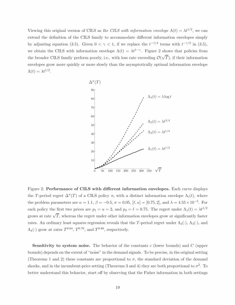
Figure 2: Performance of CILS with different information envelopes. Each curve displays

the T -period regret ∆π(T ) of a CILS policy πi with a distinct information envelope Λi(t), where

the problem parameters are α = 1.1, β = −0.5, σ = 0.05, [ℓ, u] = [0.75, 2], and λ = 4.55×10−5. For

each policy the first two prices are p1 = u = 2, and p2 = ℓ = 0.75. The regret under Λ1(t) = λt1/2

grows at rate√T , whereas the regret under other information envelopes grow at significantly faster

rates. An ordinary least squares regression reveals that the T -period regret under Λ2(·), Λ3(·), andΛ4(·) grow at rates T 0.64, T 0.70, and T 0.80, respectively.

Sensitivity to system noise. The behavior of the constants c (lower bounds) and C (upper

bounds) depends on the extent of “noise” in the demand signals. To be precise, in the original setting

(Theorems 1 and 2) these constants are proportional to σ, the standard deviation of the demand

shocks, and in the incumbent-price setting (Theorems 3 and 4) they are both proportional to σ2. To

better understand this behavior, start off by observing that the Fisher information in both settings

19

is inversely proportional to σ2. At first glance, this suggests that the magnitude of the regret would

be proportional to σ2 in both cases. However, this intuition is only correct in the incumbent-price

setting, because the information metric Jt =∑t

s=1(ps − p)2 will grow linearly over time (with high

probability), implying that the logarithmic information envelope constraint in Theorem 4(i) would

be eventually non-binding. As a consequence, with high probability Jt will be eventually of order

σ2t. In contrast, in the original setting the information metric Jt =∑t

s=1(ps−pt)2 cannot increase

linearly if the price process pt is convergent. Consequently, if σ increases, say, the information

envelope should scale up in proportion to σ so that sample paths of Jt would increase at least at

the same rate as σ. In that case, the cumulative squared deviations from the greedy price would not

increase faster than σ, implying by Theorem 2 that the seller’s regret would scale up by order σ. (If

the information envelope is inflated at a higher rate, e.g., proportional to σ2, then the cumulative

squared deviations from the greedy price increase at the same rate as the information envelope,

leading to a regret of order σ2, which is strictly worse if σ > 1.) Due to the above logic, the seller’s

revenue performance is less sensitive to noise in the original setting than in the incumbent-price

setting.

4 Extension to Multiple Products with Substitutable Demand

In this section we extend our single-product results to the case of multiple products with sub-

stitutable demand. With a single product, the only critical issue was the rate of information

acquisition. However, when there are two or more products the direction of information acquisition

also becomes relevant. If all of the price deviation vectors pt − pt−1 point in a particular direction,

then the seller would be able to learn only a relation among the demand model parameters, rather

than learning the value of every parameter. Thus a successful multi-product pricing policy needs

to make sure that information is collected not only at the right rate but also evenly in all directions

of the price deviation space. To collect information in such a way, we will force each set of n con-

secutive price deviation vectors to be an orthogonal basis for Rn. This idea of orthogonal pricing,

which will be explained in further detail below, is the most prominent feature of our approach to

multi-product pricing.

4.1 Generalization of Main Ideas

To extend the analysis in Section 3.1 to multiple dimensions, we begin by deriving a lower bound on

regret. Consider the case where ǫitiid∼ N (0, σ2). Given the parameter vector θ = (α1, β1, . . . , αn, βn),

the history Ht has the following density:

gt(Ht, θ) =

t∏

s=1

n∏

i=1

1

σφ

(Dis − αi − βi · ps

σ

). (4.1)

20

Therefore, letting ⊗ denote the Kronecker product of matrices, we get by elementary algebra that

the Fisher information contained in Ht is

Iπt (θ) := Eπθ

{[∂ log gt(Ht, θ)

∂θ

]T ∂ log gt(Ht, θ)

∂θ

}

=1

σ4Eπθ

{[ t∑

s=1

ǫs ⊗[

1ps

]]T t∑

s=1

ǫs ⊗[

1ps

]}

=1

σ2Eπθ [In ⊗ Jt], (4.2)

where the last equation follows because the ǫit are independent and Eπθ [ǫ

2it] = σ2. The following

result is the analog of Lemma 1 in the multi-product setting.

Lemma 6 (lower bound on cumulative pricing error) There exist finite positive constants

c0 and c1 such that

supθ∈Θ{∑T

t=2 Eπθ

∥∥pt − ϕ(θ)∥∥2} ≥

T∑

t=2

c0

c1 + supθ∈Θ{tr

(C(θ)Eπθ [Jt−1]C(θ)T

)} , (4.3)

where C(·) is an n × (n + 1) matrix function on Θ such that C(θ) = [−ϕ(θ) In], and tr(·) is the

matrix trace operator.

Using Lemma 6, we can generalize Theorem 1 to the case of multiple products.

Theorem 5 (lower bound on regret) There exists a finite positive constant c such that ∆π(T ) ≥c√T for any pricing policy π and time horizon T ≥ 3.

Remark The constant c in the preceding theorem is directly proportional to |bmax|, where bmax < 0

is the upper bound on the eigenvalues of the demand parameter matrix B. Note that, in the single-

product case, bmax is simply the largest value that the slope parameter β can take. In general,

the constants in the lower bounds (cf. Theorems 1, 3, 5, and 7) are proportional to |bmax|, andthe constants in the upper bounds (cf. Theorems 2, 4, 6, and 8) are proportional to |bmin|, wherebmin < 0 is the lower bound on the eigenvalues of B. This relationship demonstrates that the seller’s

regret would decrease as the expected demand function becomes more “unresponsive” to changes

in price.

To derive sufficient conditions of asymptotic optimality in the multivariate setting, we will first

focus on policies that satisfy an orthogonal pricing condition, and then generalize the definition of

our information metric. A pricing policy π is said to be an orthogonal pricing policy if for each

τ = 1, 2, . . . there exist Xτ ∈ Rn and vτ > 0 such that

Vτ :={v−1τ

(ps − ps−1 −Xτ

): s = n(τ − 1) + 1, . . . , n(τ − 1) + n

}(4.4)

21

forms an orthonormal basis of Rn, and e · Xτ = n−1/2vτ‖Xτ‖ for all e ∈ Vτ . That is, for any

given block of n periods, there is an orthonormal basis embedded within the price deviation vectors

ps − ps−1. Here, Xτ can be interpreted as the “nominal” price deviation in periods n(τ − 1) +

1, . . . , n(τ−1)+n. In most instances, it would be sufficient to simply take Xτ equal to an n-vector

of zeros, and let each price deviation vector ps − ps−1 be orthogonal to the previous n − 1 price

deviation vectors, but we adopt the slightly more general definition in (4.4) to allow for a wider

family of policies (see, e.g., the example at the end of this subsection). When n = 1, we let Xτ = 0,

and note that all pricing policies are orthogonal.

To characterize the rate of information acquisition for orthogonal pricing policies, we generalize

the mathematical expression for sum of squared price deviations Jt, which was frequently used in

Section 3. In the single-product setting where prices are scalars, the information metric we used

was

Jt =

t∑

s=1

(ps − pt)2 =

t∑

s=2

(1− s−1)(ps − ps−1)2 for t = 1, 2, . . .

Our information metric for the multi-product setting adds squared lengths of price deviation vectors

over blocks of n periods. To be precise, we extend the above definition by letting

Jt = n−1

n⌊t/n⌋∑

s=2

(1− s−1)∥∥ps − ps−1 −X⌈s/n⌉

∥∥2

= n−1

⌊t/n⌋∑

τ=1

n∑

i=1

(1− 1

n(τ−1)+i

)v2τ for t = 1, 2, . . .

Note that the former definition of Jt is a special case of the latter when n = 1, in which case we

assume Xτ = 0 for all τ .

Using the definition of orthogonal pricing policy and our new information metric, we derive the

following multivariate counterpart of Lemma 2.

Lemma 7 (minimum eigenvalue of Fisher information) Let µmin(t) be the smallest eigen-

value of In ⊗ Jt. Under any orthogonal pricing policy one has µmin(t) ≥ γJt, where γ =

1/(1 + 2u− ℓ)2.

In the following result, we extend Lemma 3 to include orthogonal pricing policies in the multi-

product setting.

Lemma 8 (exponential decay of estimation errors) There exist finite positive constants ρ

and k such that, under any orthogonal pricing policy π,

Pπθ

{‖θt − θ‖ > δ, Jt ≥ m

}≤ ktn

2+n−1 exp(− ρ(δ ∧ δ2)m

)(4.5)

for all δ,m > 0 and all t ≥ 2.

22

The polynomial term ktn2+n−1 in the preceding probability bound reflects the effect of having a

higher dimensional parameter space, thereby generalizing the polynomial term kt in Lemma 3,

which is derived assuming n = 1. In the last result of this subsection, we generalize Theorem 2 to

the case of multiple products.

Theorem 6 (sufficient conditions for asymptotic optimality) Assume that θ ∈ Θ. Let κ0,

κ1 be finite positive constants, and π be an orthogonal pricing policy satisfying

(i) Jt ≥ κ0√t

(ii)∑t

s=0

∥∥ϕ(ϑ⌊s/n⌋

)− ps+1

∥∥2 ≤ κ1√t

almost surely for all t. Then there exists a finite positive constant C such that ∆πθ (T ) ≤ C

√T log T

for all T ≥ 3.

It is possible to express condition (i) of Theorem 6 in terms of the minimum eigenvalue of the

empirical Fisher information matrix, µmin(t), simply by replacing Jt with µmin(t). The definition

of orthogonal pricing policy and the generalization of our information metric Jt offers a practical

and fairly general way of controlling µmin(t) to accumulate information at the desired rate, which

is of order√t in our setting. Naturally, one might use alternative rates for different purposes. For

instance, Lai and Wei (1982) derive conditions on µmin(t) to obtain almost sure bounds on least

squares errors in various settings, and in a recent study, den Boer (2013) extends some of these

ideas to a dynamic pricing setting, arriving at an O(√T log T ) upper bound on the regret of a

policy based on maximum quasi-likelihood estimation.

Example: Multivariate CILS. To generalize the CILS policy family to the multi-product

case, let us first re-express in a more compact form the pricing rule of CILS in the single-product

case, which is given in (3.5): in period t, CILS(κ) charges the price pt = pt−1+λtδt+sgn(δt)κt−1/4,

where δt = ϕ(ϑt−1)−pt−1 and λt = max{0, 1−κt−1/4/|δt|} ∈ [0, 1]. The general version of CILS(κ)

has a similar functional form. For each τ = 1, 2, . . . and i = 1, . . . , n, the multivariate constrained

iterated least squares (MCILS) policy with threshold parameter κ, abbreviated MCILSn(κ), uses

the following price vector in period t = n(τ − 1) + i:

pn(τ−1)+i = pn(τ−1)+i−1 + λτ δτ + κτ−1/4eiτ (4.6)

where δτ = ϕ(ϑn(τ−1)

)− pn(τ−1), λτ = max{0, 1 − κτ−1/4/‖δτ‖} ∈ [0, 1], and {eiτ : i = 1, . . . , n}

is the orthonormal basis of Rn satisfying n−1/2∑n

i=1 eiτ = δτ/‖δτ‖. Note that, if n = 1, the only

possible choice for e1t is sgn(δt), implying that MCILS1(κ) coincides with CILS(κ).

To see that any MCILS policy satisfies the conditions of Theorem 6, we first note that MCILSn(κ)

is an orthogonal policy, because if we let Xτ = λτδτ and vτ = κτ−1/4 for all τ the set of vectors

in (4.4) satisfies the orthogonal pricing condition. Moreover, under MCILSn(κ), we have Jt ≥

23

12n

−1κ2∑⌊t/n⌋

τ=1 τ−1/2 ≥ 14n

−1κ2t1/2, which satisfies condition (i) with κ0 = 14n

−1κ2. Finally, for all

τ and i, we have∥∥ϕ(ϑn(τ−1)

)−pn(τ−1)+i

∥∥ ≤ κτ−1/4+maxi{pn(τ−1)+i−pn(τ−1)} ≤ (κ+u−ℓ)τ−1/4; so

condition (ii) is satisfied with κ1 = 2(κ+u− ℓ)2. As a result, MCILSn(κ) achieves the performance

guarantee in Theorem 6. To illustrate this fact, we display in Figure 3 the simulated performance

of an MCILS policy in a particular numerical example.

T

∆π(T )

MCILS

greedy ILS

0 2500 5000 7500 10000

50

100

150

200

250

Figure 3: Performance of greedy ILS and multivariate CILS. The upper and lower curves

depict the T -period regret ∆π(T ) of greedy ILS and MCILS2(κ = 0.25) respectively, where the

problem parameters are α1 = 1.1, α2 = 0.7, β1 = (−0.5, 0.05), β2 = (0.05,−0.3), σ = 0.1,

and [ℓ, u] = [0.75, 2]. For each policy the first three price vectors are p1 = (ℓ, ℓ) = (0.75, 0.75),

p2 = (u, u) = (2, 2), and p3 = (u, ℓ) = (2, 0.75). The regret of greedy ILS grows linearly over time,

whereas the regret of MCILS2(0.25) grows at rate√T .

In summary, MCILS policy family combines the orthogonal pricing condition with the rate at

which CILS accumulates information. Using the same reasoning, it is straightforward to generalize

the ILS-d policy family to the multi-product setting.

24

4.2 Incumbent-Price Problem with Multiple Products

To provide a complete picture, we now extend the incumbent-price analysis in Section 3.4 to the

case of two or more products. Our formulation of the incumbent-price problem remains essentially

the same, except prices are n× 1 vectors rather than scalars. So assumption (3.7) is replaced with

D = a+Bp , (4.7)

where a and B are the parameters of the demand model (2.1). Assuming the seller knows that

(4.7) holds with certainty, the seller’s demand model becomes

Dt = D +Bxt + ǫt for t = 1, 2, . . . (4.8)

where xt = pt− p. Because the above demand model can be fully specified by learning the value of

B, we treat B as the matrix containing all demand parameters. To be precise, we assume that the

demand parameter vector is b := vec(BT) = (β1, . . . , βn) ∈ Rn2

, and that nature selects the value of

b from a compact rectangle B ⊆ Rn2

in period 0. Using the multivariate analogs of the single-period

revenue function rβ(·) and the optimal price deviation function ψ(·), which were originally expressed

in equations (3.9) and (3.10), we let ∆πb (T ) denote the T -period regret under policy π and parameter

vector b. Consequently the worst-case regret is ∆π(T ) := sup{∆πb (T ) : b ∈ B, ψ(b) 6= 0n}.

As before, we consider the case where ǫitiid∼ N (0, σ2). Conditional on b = (β1, . . . , βn), the

density of Ht in the multivariate incumbent-price setting is

gt(Ht, b) =t∏

s=1

n∏

i=1

1

σφ

(Dis − Di − βi · xs

σ

). (4.9)

Therefore, the Fisher information for Ht is

Iπt (b) := Eπb

{[∂ log gt(Ht, b)

∂b

]T ∂ log gt(Ht, b)

∂b

}=

1

σ2Eπb [In ⊗ Jt] , (4.10)

where Jt :=∑t

s=1 xsxTs . As in the case of our previous lower bounds on pricing errors, we use the

multivariate version of the van Trees inequality to get the following lemma.

Lemma 9 (lower bound on cumulative pricing error) Assume that the incumbent-price re-

lation (4.7) holds. Then there exist finite positive constants c0 and c1 such that

supb∈B, ψ(b)6=0n

{∑Tt=2 E

πb

∥∥xt − ψ(b)∥∥2} ≥

T∑

t=2

c0

c1 + supb∈B{1Tn Eπb [Jt−1] 1n

} , (4.11)

where 1n is an n× 1 vector of ones.

By virtue of Lemma 9, we arrive at our final lower bound on regret.

25

Theorem 7 (lower bound on regret) Assume that the incumbent-price relation (4.7) holds.

Then there exists a finite positive constant c such that ∆π(T ) ≥ c log T for any pricing policy π and

time horizon T ≥ 3.

To achieve the minimum asymptotic loss rate given above, we first state an orthogonal pricing

condition for the multivariate incumbent-price problem: a policy π is an orthogonal pricing policy

in the incumbent-price setting if for each τ = 1, 2, . . . there exist Xτ ∈ Rn and vτ > 0 such that

Vτ :={v−1τ

(xs−Xτ

): s = n(τ − 1)+ 1, . . . , n(τ − 1) +n

}forms an orthonormal basis of Rn, and

e ·Xτ = n−1/2vτ‖Xτ‖ for all e ∈ Vτ . We also generalize the definition of the information metric Jt

as

Jt = n−1

n⌊t/n⌋∑

s=1

∥∥xs −X⌈s/n⌉∥∥2 =

⌊t/n⌋∑

τ=1

v2τ for t = 1, 2, . . .

Having updated our orthogonality condition and information metric, we first show that one can

control the minimum eigenvalue of the empirical Fisher information matrix.

Lemma 10 (minimum eigenvalue of Fisher information) Assume that the incumbent-price

relation (4.7) holds, and let µmin(t) be the smallest eigenvalue of In⊗Jt. Then under any orthogonal

pricing policy one has µmin(t) ≥ Jt.

Remark In the single-product case, µmin(t) simply equals Jt, implying that the bound stated in

Lemma 10 is tight.

Letting bt be the least squares estimate of b in period t, we generalize Lemma 5 as follows.

Lemma 11 (exponential decay of estimation errors) Assume that the incumbent-price re-

lation (4.7) holds. There exist finite positive constants ρ and k such that, under any orthogonal

pricing policy π,

Pπb

{‖bt − b‖ > δ, Jt ≥ m

}≤ ktn

2−1 exp(− ρ(δ ∧ δ2)m

)(4.12)

for all δ,m > 0 and all t ≥ 2.

Finally, denoting by bt the projection of bt onto B, we use the preceding lemma to generate the

last set of sufficient conditions for asymptotic optimality.

Theorem 8 (sufficient conditions for asymptotic optimality) Assume that the incumbent-

price relation (4.7) holds, that b ∈ B, and that ψ(b) 6= 0n. There exist finite positive constants κ0,

κ1, and C such that if π is an orthogonal pricing policy satisfying

(i) Jt ≥ κ0 log t

(ii)∑t

s=0

∥∥ψ(b⌊s/n⌋

)− xs+1

∥∥2 ≤ κ1 log t

almost surely for all t, then ∆πb (T ) ≤ C log T for all T ≥ 3.

26

5 Concluding Remarks

On the linear demand assumption. Linear demand models are commonly used in economic

theory, and also in revenue management practice, but they are obviously restrictive. To justify

our assumption of linear demand in the learning-and-earning problem, one possible argument is

that (a) any demand function can be closely approximated by a linear function if the range of

permissible prices is sufficiently narrow, and (b) narrow price ranges are often enforced in dynamic

pricing contexts, because the seller, not wishing to provoke a competitive response, considers only

“tactical” deviations from an incumbent price.

Alternatively, one may argue that essentially the same analysis applies with a generalized linear

model (GLM) q = F (L(p)), where q is the vector of expected demands in response to price vector p,

L is a linear function, and F is a general “link function.” If the link function is known but the coef-

ficients of L are not known, then the problem of dynamic pricing under the GLM essentially maps

to the problem treated here: one can make use of generalized least squares estimation in place of

the simple least squares estimates used in the present paper. den Boer and Zwart (2013) adopt this

framework in their study of constrained variance pricing. The GLM framework adds a substantial

layer of technical detail, so we have focused on the simpler class of linear models, striving to achieve

a more transparent analysis. One can consider extensions to more general parametric families, using

the method of maximum likelihood to make inferences about model parameters. Because maximum

likelihood estimators ultimately are expressed as averages of suitable score functions, one can use

martingale methods and associated large deviation inequalities in that context, as we have done in

the linear context, but the analysis is more technical and cumbersome; see Besbes and Zeevi (2009)

for an indication of the tools involved. Finally, recent work of Besbes and Zeevi (2013) indicates

that in certain circumstances a misspecification that stems from assuming linear demand, while the

true demand model has different functional form, may not be as detrimental as one would expect.

Discussion of main contributions. The main contributions of this paper are (a) the formu-

lation of the incumbent-price problem, which applies to a substantial number of cases in pricing

practice, (b) the generality of the price experimentation solutions offered, (c) the development of

a unifying theme to analyze dynamic pricing problems with demand model uncertainty, and (d)

the extension of single-product pricing analysis to the case of multiple products with substitutable

demand.

With regard to (a), the main insight we derive is the sharp contrast between the results obtained

in the incumbent-price setting, and the original setting. All of the regret bounds we derive in the

incumbent-price setting are of order log T , whereas the regret bounds in the original setting are

of order√T or higher. This difference shows that knowing average demand under the incumbent

price has significant value, and our asymptotic optimality conditions in Theorems 4 and 8 provide

practical guidelines on how best to use this incumbent-price information.

27

With regard to (b), a prominent feature of our analysis is that we do not focus on a particular

parametric family of pricing policies. Instead, we derive general sufficient conditions for asymptotic

optimality (cf. Theorems 2, 4, 6, and 8), and show by example that these conditions are necessary in

practice. In Section 3.3, we provide a few ideas about how to construct pricing policies that satisfy

the asymptotic optimality conditions, but the general nature of our results allows practitioners to

design price experimentation policies that best fit their particular business setting.

With regard to (c), we employ a systematic mode of analysis for eliciting lower and upper bounds

on the performance of pricing policies. The lower bounds are obtained via the van Trees inequality,

which is a generalized version of the Cramer-Rao bound, and our upper bounds are obtained via

an exponential martingale argument. We predict that this unifying approach will find more use in

the broader context of revenue management and pricing, particularly in the analysis of problems

that involve model uncertainty.

The results in this paper introduce asymptotic optimality to multi-product pricing with demand

model uncertainty. Our analysis shows that learning and earning in higher dimensions is not a

straightforward repetition of learning and earning in one dimension. To be precise, when there is

more than one pricing decision, information should be collected by spanning the entire action space

so that the seller would learn the values of all demand parameters, instead of the value of a linear

combination of them. The orthogonal pricing condition, which is described in detail in Section 4,

is an intuitive and easily implementable way to ensure that information is accumulated evenly in

all directions. We believe that the extension to multiple products with substitutable demand is

an important feature that distinguishes our work from other recent studies in the dynamic pricing

literature.

Appendix A: Proofs of the Results in Section 3

A.1 A Lower Bound on Regret

Proof of Lemma 1. Let λ be an absolutely continuous density on Θ, taking positive values on the

interior of Θ and zero on its boundary (cf. Goldenshluger and Zeevi 2009, p. 1632 for a standard

choice of λ). Then, the multivariate van Trees inequality (cf. Gill and Levit 1995) implies that

Eλ

{Eπθ

(pt − ϕ(θ)

)2} ≥

(Eλ

[C(θ) (∂ϕ/∂θ)T

])2

Eλ

[C(θ)Iπt−1(θ)C(θ)T

]+ I(λ)

, (A.1)

where I(λ) is the Fisher information for the density λ, and Eλ(·) is the expectation operator

with respect to λ. Note that for all θ = (α, β) ∈ Θ we have C(θ) (∂ϕ/∂θ)T = −ϕ(θ)/(2β), andIπt−1(θ) = σ−2

Eπθ [Jt−1]. Using these identities and adding up inequality (A.1) over t = 2, . . . , T ,

28

we obtainT∑

t=2

Eλ

{Eπθ

(pt − ϕ(θ)

)2} ≥T∑

t=2

(Eλ[ϕ(θ)/(2β)]

)2

σ−2Eλ

[C(θ)Eπθ [Jt−1] C(θ)T

]+ I(λ)

.

Because Eλ(·) is a monotone operator,

supθ∈Θ{∑T

t=2 Eπθ

(pt − ϕ(θ)

)2} ≥T∑

t=2

infθ∈Θ{(ϕ(θ)/(2β)

)2}

σ−2 supθ∈Θ{C(θ)Eπθ [Jt−1] C(θ)T

}+ I(λ)

.

In the preceding inequality, note that infθ∈Θ{(ϕ(θ)/(2β)

)2} ≥ ℓ2/(4b2min) because 0 < ℓ ≤ ϕ(θ),

and bmin ≤ β < 0. So we let c0 = σ2ℓ2/(4b2min), c1 = σ2I(λ), and arrive at the desired result.

Proof of Theorem 1. Due to the fact that C(θ) = [−ϕ(θ) 1], we have C(θ)Eπθ [Jt−1]C(θ)T =∑t−1

s=1 Eπθ

(ps − ϕ(θ)

)2. Thus, inequality (3.3) of Lemma 1 is equivalent to the following:

supθ∈Θ{∑T

t=2 Eπθ

(pt − ϕ(θ)

)2} ≥T∑

t=2

c0

c1 + supθ∈Θ{∑t−1

s=1 Eπθ

(ps − ϕ(θ)

)2} . (A.2)

Recalling the definition of the worst-case regret (2.8), we also get

∆π(T ) = supθ∈Θ

{ T∑

t=1

Eπθ

[r∗θ − rθ(pt)

]}

= supθ∈Θ

{ T∑

t=1

Eπθ

[ϕ(θ)

(α+ βϕ(θ)

)− pt(α+ βpt)

]}

= supθ∈Θ

{− β

T∑

t=1

Eπθ

(pt − ϕ(θ)

)2}

≥ |bmax| supθ∈Θ

{ T∑

t=2

Eπθ

(pt − ϕ(θ)

)2},

because β is contained in [bmin, bmax]. Therefore, inequality (A.2) implies that

∆π(T ) ≥ b2max

T∑

t=2

c0|bmax|c1 +∆π(t− 1)

. (A.3)

Let K1 = b2maxc0, and K2 = |bmax|c1. Because ∆π(t) is non-decreasing in t, the preceding inequality

implies that

∆π(T ) ≥ K1(T − 1)

K2 +∆π(T )≥ K1T

2K3∆π(T ),

for all T ≥ 2, where K3 := K2/∆π(1) + 1 ≤ 4K2/(u − ℓ)2 + 1. Thus, ∆π(T ) ≥ c

√T , where

c =√K1/(2K3).

As mentioned earlier, the above proof holds for a broader exponential family of distributions

whose densities have the form fǫ(ξ |σ) = c(σ) exp(h(ξ) +

∑kj=1wj(σ)tj(ξ)

)for ξ ∈ R, where h(·)

29

and tj(·) are differentiable functions. To see this generalization, first note that the proofs of Lemma

1 and its subsequent counterparts (Lemmas 4, 6, and 9) rely on Fisher information matrices that

are computed by using the density of Gaussian distribution with zero mean and σ2 variance. As a

matter of fact, we can obtain an almost identical Fisher information matrix as long as noise terms

have a density of “similar shape.” To be precise, if we assume that the distribution of the ǫt belongs

to the exponential family mentioned above, the density of history vector Ht would be

gt(Ht, θ) =

t∏

s=1

fǫ(Ds − α− βps |σ),

which implies that the Fisher information matrix of Ht is

Iπt (θ) := Eπθ

{[∂ log gt(Ht, θ)

∂θ

]T ∂ log gt(Ht, θ)

∂θ

}= k(σ)Eπθ [Jt] ,

where k(σ) = E[(h′(ǫt)+

∑kj=1wj(σ)t

′j(ǫt))

2]. Replacing equation (3.2) with the preceding identity,

we carry out the rest of our argument exactly the same way.

A.2 Sufficient Conditions for Asymptotic Optimality

Proof of Lemma 2. Take an arbitrary unit vector y = (y1, y2) ∈ R2. Note that

yTJty =

t∑

s=1

(y1 + y2ps)2 =

t∑

s=1

(y1 + y2pt)2 + y22

t∑

s=1

(ps − pt)2.

The first term on the right side above equals (y1 + y2pt)2t. Moreover, the second term can be

expressed as y22∑t

s=1(ps − pt)2 = y22Jt. Because Jt ≤ (u− ℓ)2t, we get by elementary algebra that

yTJty ≥ γJt, where γ = 2/(1 + 2u− ℓ)2. Recalling that the unit vector y was selected arbitrarily,

we conclude by the Rayleigh-Ritz theorem that µmin(t) ≥ γJt.

Proof of Lemma 3. We will complete the proof in four steps.

Step 1: Derive an upper bound on the exponential moments of the error terms. Because the ǫt

have a light-tailed distribution with mean zero and variance σ2, there exists z0 > 0 such that

Eπθ [exp(zǫt)] = 1+ z Eπθ [ǫt]+

∞∑

k=2

zkEπθ [ǫkt ]

k!= 1+

1

2ν(z)σ2z2 for all z satisfying |z| ≤ z0, (A.4)

where ν(z) :=∑∞

k=2

(2zk−2

Eπθ [ǫ

kt ])/(k!σ2) <∞. Thus,

Eπθ [exp(zǫt)] ≤ exp

(12ν(z)σ2z2

)

≤ exp(12ν∗σ2z2

)for all z satisfying |z| ≤ z0 , (A.5)

30

where ν∗ = max|z|≤z0{ν(z)}. Note that, if the ǫt have a Gaussian distribution, then the preceding

inequalities hold with equality and ν(z) = ν∗ = 1 for all z ∈ R.

Step 2: Define a family of supermartingales {Zys }. We know by the least squares equation (2.10)

that θt − θ = J−1t Mt. Let y = (y1, y2) be a 2 × 1 vector with ‖y‖ = δ, and define the process

{Zys , s = 1, 2, . . .} such that Zy0 = 1 and

Zys := exp{ 1

ζ∗σ2

(y · Ms −

1

2yTJsy

)}for all s = 1, 2, . . . , (A.6)

where ζ∗ = (1∨δ)(ν∗∨(z∗/z0)

), and z∗ = max‖y‖≤1, p∈[ℓ,u]{|y1+y2p|/σ2}. Note that Zys is integrable

for all s. Letting Fs := σ(D1, . . . ,Ds), we get by the tower property that

Eπθ [Z

ys |Fs−1] = exp

{ 1

ζ∗σ2

(y ·Ms−1 −

1

2yTJsy

)}Eπθ

[exp

{ 1

ζ∗σ2y · (Ms −Ms−1)

}∣∣∣Fs−1

].

Because Ms − Ms−1 = (ǫs, ǫsps) and |y1 + y2ps|/(ζ∗σ2) ≤ z0|y1 + y2ps|/(δz∗σ2) ≤ z0 for all

ps ∈ [ℓ, u], inequality (A.5) implies that the conditional expectation on the right side immediately

above satisfies

Eπθ

[exp

{ 1

ζ∗σ2y · (Ms −Ms−1)

} ∣∣∣Fs−1

]≤ exp

{ 1

2ζ∗σ2yT[

1 psps p2s

]y}.

Combining the preceding identity and inequality, we deduce that

Eπθ [Z

ys |Fs−1] ≤ exp

{ 1

ζ∗σ2

(y · Ms−1 −

1

2yTJs−1y

)}= Zys−1.

So (Zys ,Fs) is a supermartingale for any given y ∈ R2 with ‖y‖ = δ.

Step 3: Construct a stochastic process {Zs} that characterizes the probability bound. Let ws =

δJ −1s Ms/‖J −1

s Ms‖, and define the stochastic process {Zs, s = 1, 2, . . .} such that Zs = Zwss for

all s. Fix m > 0, let ξ be an arbitrary positive real number, and A := {‖Mt‖ ≤ ξt} ∈ Ft. Then,

we deduce the following by the union bound:

Pπθ

(‖θt − θ‖ > δ, Jt ≥ m

)= P

πθ

(‖J −1

t Mt‖ > δ, Jt ≥ m)

≤ Pπθ

(‖J −1

t Mt‖ > δ, Jt ≥ m, A)

+ Pπθ

(Jt ≥ m, Ac

). (A.7)

To derive an upper bound the first probability on the right hand side above, note that

Pπθ

(‖J −1

t Mt‖ > δ, Jt ≥ m, A)

≤ Pπθ

(wt · Mt ≥ wT

t Jtwt, Jt ≥ m, A)

(A.8)

because ‖J−1t Mt‖ > δ implies wt · Mt ≥ wT

t Jtwt for the above choice of wt. Combined with the

definition of the process {Zs}, this implies that

Pπθ

(‖J −1

t Mt‖ > δ, Jt ≥ m, A)

≤ Pπθ

(Zt ≥ exp

{wTt Jtwt2ζ∗σ2

}, Jt ≥ m, A

).

31

Because µmin(t) is the smallest eigenvalue of Jt, and ‖wt‖ = δ, we deduce by the Rayleigh-Ritz

theorem that wTt Jtwt ≥ δ2µmin(t), and in conjunction with Lemma 2 we get

Pπθ

(‖J −1

t Mt‖ > δ, Jt ≥ m, A)

≤ Pπθ

(Zt ≥ exp

{γ δ2m2ζ∗σ2

}, A).

Step 4: Prove Zt is bounded above by a supermartingale with very high probability. Noting that

the function L(y) := y ·Mt− 12y

TJty is concave, we deduce that L(w)−L(y) ≤ (w− y) ·∇L(y) =

(w−y) ·(Mt−Jty) ≤ ‖w−y‖ ‖Mt‖+(1+u2)‖w−y‖2t. Thus, on the event A = {‖Mt‖ ≤ ξt}, wehave Zyt ≥ e−(ξ+1+u2)/(ζ∗σ2)Zt for all y within the (1/t)-neighborhood of wt. Let S = {y1, y2, . . . , yS}be a set of S = ⌈πδt⌉ distinct points that are evenly spaced on the circle {y ∈ R

2 : ‖y‖ = δ}.Therefore, at time s = t, ws has to be in the (1/t)-neighborhood of some y ∈ S, implying

Zyt ≥ e−(ξ+1+u2)/(ζ∗σ2)Zt for some y ∈ S. Thus, we have

Pπθ

(‖J −1

t Mt‖ > δ, Jt ≥ m, A)

≤ Pπθ

(Zt ≥ exp

{γ δ2m2ζ∗σ2

}, A)

≤ Pπθ

(Zyt ≥ K1 exp(ρ0δ

2m) for some y ∈ S, A)

where K1 = e−(ξ+1+u2)/(ζ∗σ2) and ρ0 = γ/(2ζ∗σ2). Then, by the union bound, we have

Pπθ

(‖J −1

t Mt‖ > δ, Jt ≥ m, A)

≤∑

yj∈SPπθ

(Zyjt ≥ K1 exp(ρ0δ

2m), A).

By Markov’s inequality and the fact that Zyjt is a supermartingale with Z

yj0 = 1 for all yj ∈ S, each

term inside the preceding sum satisfies Pπθ(Zyjt ≥ K1 exp(ρ0δ

2m), A)≤ 1

K1exp(−ρ0δ2m). Because

there are S = ⌈πδt⌉ points in S, the preceding inequality implies the following upper bound on the

first term on the right hand side of (A.7):

Pπθ

(‖J −1

t Mt‖ > δ, Jt ≥ m, A)

≤ 1+K2tK1

exp(−ρ0δ2m) ,

where K2 = (1∨δ)π. Using a simplified version of the above exponential supermartingale argument

(see, for instance, the proof of Lemma 5) and the fact that Jt ≤ (u−ℓ)2t for all t, it is straightforwardto show that

Pπθ

(Jt ≥ m, Ac

)= P

πθ

(Jt ≥ m, ‖Mt‖ > ξt

)

≤ Pπθ

(Jt ≥ m,

∣∣∣t∑

s=1

ǫs

∣∣∣ > ξt√2

)+ P

πθ

(Jt ≥ m,

∣∣∣t∑

s=1

ǫsps

∣∣∣ > ξt√2

)

≤ 2 exp

(− ξ2m

4ζ∗σ2(u− ℓ)2

)+ 2exp

(− ξ2m

4ζ∗σ2(u− ℓ)2u2

). (A.9)

Choosing ξ = 2(1 ∨ δ)σ(u − ℓ)(ζ∗(1 + u2)ρ0

)1/2 ≥ 2δσ(u − ℓ)(ζ∗(1 + u2)ρ0

)1/2, we have P

πθ

(Jt ≥

m, Ac)≤ 4 exp(−ρ0δ2m). Having found upper bounds on both terms on the right hand side of

32

(A.7), we let ρ = (1 ∨ δ)ρ0 = 12γσ

−2(ν∗ ∨ (z∗/z0)

)−1and k = 4 + (1 + K2)/K1 to conclude the

proof.

Proof of Theorem 2. First, note that the revenue loss of a policy comes from either least squares

estimation errors, or perturbations from the greedy ILS price. More formally, conditioned on the

parameter vector θ and policy π, we have the following upper bound on the expected value of

squared pricing error in period t+ 1:

Eπθ

(ϕ(θ)− pt+1

)2 ≤ 2Eπθ(ϕ(θ)− ϕ(ϑt)

)2+ 2Eπθ

(ϕ(ϑt)− pt+1

)2, (A.10)

where ϑt is the truncated least squares estimate calculated at the end of period t. Consider the

first term on the right side of inequality (A.10). By the mean value theorem, we have |ϕ(θ) −ϕ(ϑt)| ≤

√2K0 ‖θ−ϑt‖ where K0 = maxj=1,2

{maxθ{(∂ϕ(θ)/∂θj)2}

}. Therefore, by monotonicity

of expectation we have

Eπθ

(ϕ(θ)− ϕ(ϑt)

)2 ≤ 2K0 Eπθ

∥∥θ − ϑt∥∥2

(a)

≤ 2K0 Eπθ

∥∥θ − θt∥∥2

(b)= 2K0

∫ ∞

0Pπθ

(∥∥θ − θt∥∥2 > x, Jt ≥ κ0

√t)dx

≤ 4K0 log t

ρκ0√t

+ 2K0

∫ ∞

2 log t

ρκ0√

t

Pπθ

(∥∥θ − θt∥∥2 > x, Jt ≥ κ0

√t)dx

(c)

≤ 4K0 log t

ρκ0√t

+ 2K0

∫ ∞

2 log t

ρκ0√

t

kt exp(− ρ(

√x ∧ x)κ0

√t)dx

=4K0 log t

ρκ0√t

+ 2K0

∫ 1

2 log t

ρκ0√

t

k exp(− 1

2ρxκ0

√t)dx+ 2K0

∫ ∞

1k exp

(− 1

2ρ√xκ0

√t)dx

≤ 4K0

ρκ0√t

(log t+

k

t+

4k

t

)≤ 4K0(1 + 5k) log t

ρκ0√t

for all t ≥ N , where: (a) follows since ‖θ − ϑt‖ ≤ ‖θ − θt‖, (b) follows by condition (i), (c) follows

by Lemma 3, and N is the smallest natural number such that kN exp(−12ρκ0

√N) ≤ 1. Thus,

inequality (A.10) becomes

Eπθ

(ϕ(θ)− pt+1

)2 ≤ 4K0 log t/(ρκ0√t) + 2Eπθ

(ϕ(ϑt)− pt+1

)2for all t ≥ N, (A.11)

where K0 = (1 + 5k)K0. Summing over t = N, . . . , T − 1 we obtain

T−1∑

t=N

Eπθ

(ϕ(θ)− pt+1

)2 ≤ 8K0

ρκ0

√T log T + 2

T−1∑

t=N

Eπθ

(ϕ(ϑt)− pt+1

)2.

33

By condition (ii), we have an upper bound also on the second term on the right side, implying that

T−1∑

t=N

Eπθ

(ϕ(θ)− pt+1

)2 ≤ 8K0

ρκ0

√T log T + 2κ1

√T ≤

(8K0

ρκ0+ 2κ1

)√T log T.

Because β is contained in the interval [bmin, bmax], we have

∆π(T ) = supθ∈Θ

{− β

T−1∑

t=0

Eπθ

(ϕ(θ)− pt+1

)2}

≤ |bmin| supθ∈Θ

T−1∑

t=0

Eπθ

(ϕ(θ)− pt+1

)2.

Thus we deduce that ∆π(T ) ≤ C0 + C1

√T log T , where C0 = |bmin|(u − ℓ)2N , and C1 =

|bmin|(8K0ρ−1κ−1

0 + 2κ1). Choosing C = max{C0, C1} concludes the proof.

Remark Assuming that we put equal emphasis on learning and earning (i.e., κ0 = κ1), we can

minimize the constant C1 by choosing κ0 = κ1 = (4K0/ρ)1/2. With that choice, we have C1 =

8|bmin|(K0/ρ)1/2.

A.3 An Alternative Formulation: Incumbent-Price Problem

Proof of Lemma 4. Let λ be an absolutely continuous density on B = [bmin, bmax], taking positive

values on (bmin, bmax) and zero on the extreme points {bmin, bmax}. By the van Trees inequality (Gill

and Levit 1995), we have

Eλ

{Eπβ

(xt − ψ(β)

)2} ≥(Eλ[ψ

′(β)])2

Eλ[Iπt−1(β)] + I(λ), (A.12)

where I(λ) is the Fisher information for the density λ, and Eλ(·) is the expectation operator with

respect to λ. Using the fact that Iπt−1(β) = σ−2Eπβ[Jt−1], and adding up inequality (A.12) over

t = 2, . . . , T , we get

T∑

t=2

Eλ

{Eπβ

(xt − ψ(β)

)2} ≥T∑

t=2

(Eλ[ψ

′(β)])2

σ−2Eλ

[Eπβ[Jt−1]

]+ I(λ)

.

Monotonicity of Eλ(·) further implies that

supβ∈B, ψ(β)6=0

{∑Tt=2 E

πβ

(xt − ψ(β)

)2} ≥T∑

t=2

infβ∈B{(ψ′(β)

)2}

σ−2 supβ∈B{Eπβ[Jt−1]

}+ I(λ)

.

Letting c0 = σ2 infβ∈B{(ψ′(β)

)2}= σ2D2/(4b4min), c1 = σ2 I(λ), we obtain inequality (3.14).

Proof of Theorem 3. Note that Js ≤ (u− ℓ)2s for all s. Thus, Lemma 4 implies that

supβ∈B, ψ(β)6=0

{∑Tt=2 E

πβ

(xt − ψ(β)

)2} ≥T∑

t=2

c0c1 + (u− ℓ)2(t− 1)

.

34

Because β is contained in [bmin, bmax], the preceding inequality further implies that

∆π(T ) = supβ∈B, ψ(β)6=0

{− β

T∑

t=1

Eπβ

(xt − ψ(β)

)2}

≥ |bmax| supβ∈B, ψ(β)6=0

T∑

t=2

c0c1 + (u− ℓ)2(t− 1)

.

To simplify notation, we let K1 = |bmax|c0/(u − ℓ)2, K2 = c1/(u− ℓ)2, and deduce that

∆π(T ) ≥ K1

T−1∑

t=1

1

K2 + t≥ c

T−1∑

t=1

1

t,

where c = K1/(1 +K2). Thus, ∆π(T ) ≥ c log T for all T ≥ 2.

Proof of Lemma 5. As in the proof of Lemma 3, we will first find an exponential supermartingale,

and then apply Markov’s inequality to get the desired bound. Recall that we have by (A.5)

Eπβ[exp(zǫt)] ≤ exp(12ν

∗σ2z2) for all z satisfying |z| ≤ z0, where ν∗ = max|z|≤z0{ν(z)}, and ν(z) =∑∞

k=2

(2zk−2

Eπβ[ǫ

kt ])/(k!σ2). By the least squares equation (3.15) we also have βt−β =Mt/Jt. Let

y ∈ R, and define the process {Zys , s = 1, 2, . . .} such that Zy0 = 1 and

Zys := exp{ 1

ζ∗σ2

(yMs −

1

2y2Js

)}for all s = 1, 2, . . . , (A.13)

where ζ∗ = (1∨ δ)(ν∗ ∨ (z∗/z0)

), and z∗ = max|y|≤1, p+x∈[ℓ,u]{|yx|/σ2}. The tower property implies

that

Eπβ[Z

ys |Fs−1] = exp

{ 1

ζ∗σ2

(yMs−1 −

1

2y2Js

)}Eπβ

[exp

(yxsǫsζ∗σ2

)∣∣Fs−1

],

where Fs = σ(D1, . . . ,Ds). Using inequality (A.5) and noting that |yxs|/(ζ∗σ2) ≤ z0|yxs|/(δz∗σ2) ≤z0 for all p + xs ∈ [ℓ, u], we compute the following upper bound on the conditional expectation

on the right hand side above: Eπβ[exp

(yxsǫs/(ζ

∗σ2))|Fs−1] ≤ exp

(y2x2s/(2ζ

∗σ2)), so (Zys ,Fs) is a

supermartingale for all y ∈ R. Now choose y = δ, fix m > 0, and note that

Pπβ{βt − β > δ, Jt ≥ m} = P

πβ{Mt > δJt, Jt ≥ m}

= Pπβ{yMt > y2Jt, Jt ≥ m} .

By definition of the process Zyt , this implies that

Pπβ{βt − β > δ, Jt ≥ m} = P

πβ

{Zyt ≥ exp

( δ2Jt2ζ∗σ2

), Jt ≥ m

}

≤ Pπβ

{Zyt ≥ exp

( δ2m

2ζ∗σ2

)}.

35

Using Markov’s inequality, and the fact that Zyt is a martingale with Zy0 = 1, we obtain the following

exponential bound:

Pπβ{βt − β > δ, Jt ≥ m} ≤ exp

(− δ2m

2ζ∗σ2

).

Repeating the above argument for y = −δ, we derive the same exponential bound on Pπβ{βt − β <

−δ, Jt ≥ m}. Finally, we let ρ = (1 ∨ δ)/(2ζ∗σ2) = 12γσ

−2(ν∗ ∨ (z∗/z0)

)−1, and arrive at the

desired result.

Proof of Theorem 4. We begin with decomposing the revenue loss in period t+ 1. Note that

Eπβ

(ψ(β) − xt+1

)2 ≤ 2Eπβ(ψ(β)− ψ(bt)

)2+ 2Eπβ

(ψ(bt)− xt+1

)2, (A.14)

where bt is the truncated least squares estimate calculated at the end of period t. To find an upper

bound on the first term on the right side of the preceding inequality, we define the sequence of

events {A1, A2, . . .} such that

At =

t−1⋂

s=⌊ t−12

⌋

{(ψ(β)− ψ(bs)

)2 ≤(ψ(β)

)2

12

}for all t = 1, 2, . . . (A.15)

By the triangle inequality, we have

(ψ(β)

)2 ≤ 3(ψ(β)− ψ(bs)

)2+ 3

(ψ(bs)− xs+1

)2+ 3x2s+1

for all s between ⌊(t− 1)/2⌋ and t− 1. Thus one has (almost surely) the following on At:

Jt ≥t−1∑

s=⌊ t−12

⌋

x2s+1

≥t−1∑

s=⌊ t−12

⌋

(ψ(β)

)2

3−

t−1∑

s=⌊ t−12

⌋

(ψ(β) − ψ(bs)

)2 −t−1∑

s=⌊ t−12

⌋

(ψ(bs)− xs+1

)2. (A.16)

Note that the first sum on the right side of inequality (A.16) is greater than(ψ(β)

)2(t−1)/6, while

the second sum is less than(ψ(β)

)2(t − 1)/24 by definition of the event At. Moreover, the third

sum is less than κ1 log(t−1) by condition (ii) in the hypothesis. Combining all these facts, we have

Jt ≥((

ψ(β))2

8− κ1 log(t− 1)

t− 1

)(t− 1) on At.

Since the sequence s−1 log s converges to zero as s tends to ∞, there exists a natural number N0(β)

such that for all t ≥ N0(β) we have Jt ≥(ψ(β)

)2(t− 1)/16 on the event At.

Having shown that Jt grows linearly on At, we now turn our attention to prove that each At is

a very likely event. The union bound implies

Pπβ(A

ct) ≤

t−1∑

s=⌊(t−1)/2⌋Pπβ

{(ψ(β)− ψ(bs)

)2>

(ψ(β)

)2

12

}.

36

By the mean value theorem, we deduce that |ψ(β) − ψ(bs)| ≤ √K0 |β − bs| , where K0 =

maxβ∈[bmin,bmax]

(ψ′(β)

)2= D2/(4b4max). Thus, the preceding inequality leads to

Pπβ(A

ct) ≤

t−1∑

s=⌊(t−1)/2⌋Pπβ

{√K0 |β − bs| >

|ψ(β)|√12

}.

Invoking condition (i) in the hypothesis, we further get

Pπβ(A

ct) ≤

t−1∑

s=⌊(t−1)/2⌋Pπβ

{|β − bs| >

|ψ(β)|√12K0

, Js ≥ κ0 log s

}

(a)

≤t−1∑

s=⌊(t−1)/2⌋Pπβ

{|β − βs| >

|ψ(β)|√12K0

, Js ≥ κ0 log s

}

(b)

≤t−1∑

s=⌊(t−1)/2⌋2 exp

(−ρκ0

( |ψ(β)|√12K0

∧(ψ(β)

)2

12K0

)log s

)≤

t−1∑

s=⌊(t−1)/2⌋s−q

where: (a) follows since |β− βs| ≥ |β−bs|; (b) follows by Lemma 5; and q := 112ρκ0

{ |ψ(β)|√K0

∧ (ψ(β))2

K0

}.

Choosing κ0 greater than 36ρ−1{ |ψ(β)|√

K0∧ (ψ(β))2

K0

}−1, we ensure that q ≥ 3. Thus, for all t ≥ 5, we

have

Pπβ(A

ct) ≤

∞∑

s=⌊ t−12

⌋

s−3 ≤∫ ∞

⌊ t−12

⌋(s− 1)−3ds ≤ 2(t− 4)−2,

hence∑∞

t=5 Pπβ(A

ct) ≤ π2/3. Recalling inequality (A.14), we can now bound the first term on the

right side as follows. Let N(β) = max{N0(β), 5}. Then for any time period t ≥ N(β), we have by

virtue of the mean value theorem that

Eπβ

(ψ(β) − ψ(bt)

)2= E

πβ

[(ψ(β) − ψ(bt)

)2; At

]+ E

πβ

[(ψ(β) − ψ(bt)

)2; Act

]

≤ K0 Eπβ[(β − bt)

2;At] + Eπβ

[(ψ(β)− ψ(bt)

)2; Act

]. (A.17)

Since |β − βt| ≥ |β − bt|, the first term on the right side of inequality (A.17) is bounded above by

K0 Eπβ[(β − βt)

2;At]. By the least squares equation (3.16), this further implies that

K0 Eπβ[(β − bt)

2;At] ≤ K0 Eπβ

[M2t

J2t

; At

]

≤ 256K0(ψ(β)

)4(t− 1)2

Eπβ[M

2t ; At] (A.18)

since for all t ≥ N(β) we have Jt ≥(ψ(β)

)2(t− 1)/16 on the event At. Noting that Eπβ[M

2t ; At] ≤

Eπβ[M

2t ] = σ2 Eπβ[Jt] ≤ σ2(u− ℓ)2t, we get

K0 Eπβ[(β − bt)

2;At] ≤K1

t,

37

for all t ≥ N(β), where K1 = 512K0σ2(u − ℓ)2

(ψ(β)

)−4. Having found an upper bound on the

first term on the right side of inequality (A.17), we also notice that the second term is smaller than

4(u − ℓ)2 Pπβ(Act), because both the optimal price p + ψ(β) and the greedy ILS price p + ψ(bt) are

contained in [ℓ, u]. So, letting K2 = 4(u− ℓ)2, we deduce by inequality (A.17) that

Eπβ

(ψ(β) − ψ(bt)

)2 ≤ K1 t−1 + K2 P

πβ(A

ct). (A.19)

Thus, inequality (A.14) becomes

Eπβ

(ψ(β) − xt+1

)2 ≤ 2K1 t−1 + 2K2 P

πβ(A

ct) + 2Eπβ

(ψ(bt)− xt+1

)2.

Letting T ≥ N(β), and adding the preceding inequality over t = N(β), . . . , T , one obtains

T∑

t=N(β)

Eπβ

(ψ(β) − xt+1

)2 ≤ 2K1 log T + 2K2π2/3 + 2

T∑

t=N(β)

Eπβ

(ψ(bt)− xt+1

)2.

By condition (ii) in the hypothesis, the third term on the right hand side is bounded from above by

κ1 log T , so we deduce that ∆πβ(T ) ≤ C0 + C1 log T , with C0 = 4|bmin|

((u − ℓ)2N(β) + K2π

2/6)

and C1 = |bmin|(2K1 + κ1). To complete the proof, let C = max{C0, C1}.

Appendix B: Proofs of the Results in Section 4

B.1 Generalization of Main Ideas

Proof of Lemma 6. In what follows, we will extend the proof of Lemma 1 to higher dimensions.

As before, we choose λ to be an absolutely continuous density on Θ, taking positive values on the

interior of Θ and zero on its boundary. Let C(·) be n × (n2 + n) matrix function on Θ such that

C(θ) = 1Tn ⊗ C(θ), where 1n is an n× 1 vector of ones. That is, C(θ) = [C1(θ) · · · Cn(θ)], where

Ci(θ) := C(θ) =

−ϕ1(θ) 1 0 · · · 0

−ϕ2(θ) 0 1 · · · 0

......

.... . .

...

−ϕn(θ) 0 0 · · · 1

for i = 1, . . . , n and all θ ∈ Θ.

Invoking the multivariate van Trees inequality (Gill and Levit 1995), we obtain

Eλ

{Eπθ

∥∥pt − ϕ(θ)∥∥2} ≥

(Eλ

[tr

{C(θ) (∂ϕ/∂θ)T

} ])2

Eλ

[tr

{C(θ)Iπt−1(θ) C(θ)T

} ]+ I(λ)

, (B.1)

where I(λ) is the Fisher information for the density λ, and Eλ(·) is the expectation operator with

respect to λ. We begin by computing tr

{C(θ) (∂ϕ/∂θ)T

}, which appears in the numerator on

38

the right side. Applying the implicit function theorem on the first-order condition of optimality

expressed in (2.4), we deduce that

∂ϕ

∂θ= −

(∂η

∂p

)−1∂η

∂θ= −

(B +BT

)−1 ∂η

∂θ.

Because B +BT is symmetric and negative definite, it has a symmetric inverse. So, we get

tr

{C(θ)

(∂ϕ

∂θ

)T}= −tr

{C(θ)

(∂η

∂θ

)T(B +BT

)−1}.

Note that for matrices A, B, C, D of such size that one can form the matrix products AC and

BD, one has (A ⊗ B)(C ⊗ D) = AC ⊗ BD. Using this result, which will hereafter be called the

mixed product property, and the fact that

(∂η∂θ

)T

=

0 0 · · · 0

ϕ1(θ) 0 · · · 0

0 ϕ1(θ) · · · 0

......

. . ....

0 0 · · · ϕ1(θ)

......

......

0 0 · · · 0

ϕn(θ) 0 · · · 0

0 ϕn(θ) · · · 0...

.... . .

...

0 0 · · · ϕn(θ)

+

1 0 · · · 0

ϕ1(θ) 0 · · · 0

ϕ2(θ) 0 · · · 0

......

. . ....

ϕn(θ) 0 · · · 0

......

......

0 0 · · · 1

0 0 · · · ϕ1(θ)

0 0 · · · ϕ2(θ)...

.... . .

...

0 0 · · · ϕn(θ)

= ϕ(θ)⊗[0n

In

]+ In ⊗

[1

ϕ(θ)

],

we further deduce that C(θ) (∂η/∂θ)T =(1Tn ϕ(θ)

)⊗ In + 1Tn ⊗ 0n = In

∑ni=1 ϕi(θ), which in turn

implies that

tr

{C(θ)

(∂ϕ

∂θ

)T}= tr

{(−B −BT

)−1} n∑

i=1

ϕi(θ). (B.2)

Because the eigenvalues of the matrix B are in the interval [bmin, bmax], we obtain the following by

elementary algebra:

tr

{(−B −BT

)−1}

≥ n2

tr

{−B −BT

} ≥ n

2|bmin|.

Combined with equation (B.2) and the fact that ϕi(θ) ≥ ℓ > 0 for all i, the preceding inequal-

ity implies that tr

{C(θ) (∂ϕ/∂θ)T

}≥ n2ℓ/(2|bmin|). Now, we turn our attention to computing

39

tr

{C(θ)Iπt−1(θ) C(θ)T

}, which is in the denominator on the right side of (B.1). By the mixed

product property, we have

C(θ)Iπt−1(θ) C(θ)T =1

σ2Eπθ

{1TnIn1n ⊗ [−ϕ(θ) In] Jt−1 [−ϕ(θ) In]

T}

=n

σ2

t−1∑

s=1

Eπθ

(ps − ϕ(θ)

)(ps − ϕ(θ)

)T.

Thus, tr{C(θ)Iπt−1(θ) C(θ)T

}= nσ−2

∑t−1s=1 E

πθ

∥∥ps − ϕ(θ)∥∥2 = nσ−2

tr

{C(θ)Eπθ [Jt−1]C(θ)T

}. By

this identity and the fact that tr{C(θ) (∂ϕ/∂θ)T

}≥ n2ℓ/(2|bmin|), inequality (B.1) becomes

Eλ

{Eπθ

∥∥pt − ϕ(θ)∥∥2} ≥ c0

c1 + Eλ

[tr

{C(θ)Eπθ [Jt−1]C(θ)T

} ] ,

where c0 = n3σ2ℓ2/(4b2min) and c1 = σ2I(λ)/n. Summing over 2, . . . , T , and using the monotonicity

of Eλ(·) completes the proof.

Proof of Theorem 5. Note that tr{C(θ)Eπθ [Jt−1]C(θ)T

}=∑t−1

s=1 Eπθ

∥∥ps−ϕ(θ)∥∥2, implying that

inequality (4.3) of Lemma 6 can also be expressed as

supθ∈Θ{∑T

t=2 Eπθ

∥∥pt − ϕ(θ)∥∥2} ≥

T∑

t=2

c0

c1 + supθ∈Θ{∑t−1

s=1 Eπθ

∥∥ps − ϕ(θ)∥∥2} . (B.3)

Now, because the eigenvalues of the B are contained in [bmin, bmax], we have by the definition of

the worst-case regret (2.8),

∆π(T ) = supθ∈Θ

{ T∑

t=1

Eπθ

[r∗θ − rθ(pt)

]}

= supθ∈Θ

{ T∑

t=1

Eπθ

[ϕ(θ) ·

(a+Bϕ(θ)

)− pt · (a+Bpt)

]}

= supθ∈Θ

{−

T∑

t=1

Eπθ

(pt − ϕ(θ)

)TB(pt − ϕ(θ)

)}

≥ |bmax| supθ∈Θ

{ T∑

t=2

Eπθ

∥∥pt − ϕ(θ)∥∥2}.

Combining the preceding inequality with (B.3), we obtain

∆π(T ) ≥ b2max

T∑

t=2

c0∆π(t− 1) + |bmax|c1

. (B.4)

Note that the inequality immediately above is identical to inequality (A.3) in the proof of Theorem

1. To complete the proof, we apply exactly the same argument that follows (A.3).

40

Proof of Lemma 7. First, note that µmin(t) is also the smallest eigenvalue of Jt because the

unique eigenvalue of In is 1. Let y be an arbitrary unit vector in Rn+1, and y∗ be the n× 1 vector

consisting of the last n components of y, that is, y∗ = (y2, . . . , yn+1). Then,

yTJty =

t∑

s=1

(y1 + y∗ · ps)2 =

t∑

s=1

(y1 + y∗ · pt)2 +t∑

s=1

(y∗ · (ps − pt)

)2.

As in the proof of Lemma 2, we would like to find a lower bound on yTJty to invoke the Rayleigh-

Ritz theorem. Note that the first term on the right side above is (y1 + y∗ · pt)2t, whereas the

second term equals∑t

s=1

(y∗ · (ps − pt)

)2= yT∗ Jty∗ , where Jt :=

∑ts=1(ps − pt)(ps − pt)

T =∑t

s=2(1− s−1)(ps − ps−1)(ps − ps−1)T. Therefore, we have

yTJty = (y1 + y∗ · pt)2t +

t∑

s=2

(1− s−1)(y∗ · xs)2

where xs = ps − ps−1 for all s. By the orthogonal pricing condition, we know that for each

τ = 1, 2, . . . there exists Xτ ∈ Rn and vτ > 0 such that Vτ =

{v−1τ

(δs − Xτ

): s = n(τ − 1) +

1, . . . , n(τ − 1) + n}is an orthonormal basis of Rn. Thus the sum on the right hand side above

can also be expressed as

t∑

s=2

(1− s−1)(y∗ · xs)2 =t∑

s=2

(1− s−1)(y∗ ·X⌈s/n⌉ + y∗ · (xs −X⌈s/n⌉)

)2

≥ 1

2

⌊t/n⌋∑

τ=1

n∑

i=1

(y∗ ·Xτ + y∗ · (xn(τ−1)+i −Xτ )

)2.

Letting eiτ = v−1τ

(xn(τ−1)+i −Xτ

), yiτ = y∗ · eiτ , and recalling that eiτ ·Xτ = n−1/2vτ‖Xτ‖ for all

i = 1, . . . , n, we deduce by the preceding inequality that

t∑

s=2

(1− s−1)(y∗ · xs)2 ≥ 1

2

⌊t/n⌋∑

τ=1

n∑

i=1

(n−1/2‖Xτ‖

n∑

j=1

yjτ + vτ yiτ

)2

=1

2

⌊t/n⌋∑

τ=1

n∑

i=1

(n−1‖Xτ‖2

( n∑

j=1

yjτ

)2+ 2n−1/2‖Xτ‖

( n∑

j=1

yjτ

)vτ yiτ + v2τ y

2iτ

)

≥ 1

2

⌊t/n⌋∑

τ=1

v2τ

n∑

i=1

y 2iτ .

Because ‖y∗‖2 =∑n

i=1 y2iτ , and ‖xn(τ−1)+i −Xτ‖ = vτ for all i = 1, . . . , n, we deduce that

t∑

s=2

(1− s−1)(y∗ · xs)2 ≥ 1

2‖y∗‖2

⌊t/n⌋∑

τ=1

v2τ .

41

Using the definition of the information metric Jt, we have yTJty ≥ (y1 + y∗ · pt)2t + 12‖y∗‖2Jt.

Finally, we note that Jt ≤ (u − ℓ)2t, and deduce by elementary algebra that yTJty ≥ γJt, where

γ = 1/(1 + 2u − ℓ)2. Because y was selected arbitrarily, the Rayleigh-Ritz theorem implies that

µmin(t) ≥ γJt.

Proof of Lemma 8. To get the desired result, we will extend the proof of Lemma 3 to higher

dimensions. By (A.5), we have Eπθ [exp(zǫit)] ≤ exp(12ν

∗σ2z2) for all z satisfying |z| ≤ z0, where

ν∗ = max|z|≤z0{ν(z)}, and ν(z) =∑∞

k=2

(2zk−2

Eπθ [ǫ

kit])/(k!σ2). Note that the least squares equation

(2.10) implies that θt−θ = (In⊗J−1t )Mt, whereMt is the (n

2+n)×1 vectorMt = (M1t, . . . ,Mnt).

Select y to be an (n2 + n)× 1 vector with ‖y‖ = δ. Define the process {Zys , s = 1, 2, . . .} such that

Zy0 = 1 and

Zys := exp

{ 1

ζ∗σ2

(y ·Ms −

1

2yT(In ⊗ Js)y

)}for all s = 1, 2, . . . , (B.5)

where ζ∗ = (1 ∨ δ)(ν∗ ∨ (z∗/z0)

), and z∗ = maxy∈Rn+1, ‖y‖≤1, p∈[ℓ,u]n

{|y ·

[1p

]|/σ2

}. To show that

Zys is a supermartingale, we let Fs := σ(D1, . . . ,Ds), and note that

Eπθ [Zy

s |Fs−1] = exp{ 1

ζ∗σ2

(y ·Ms−1−

1

2yT(In⊗Js)y

)}Eπθ

[exp

{ 1

ζ∗σ2y · (Ms−Ms−1)

}∣∣∣Fs−1

].

Letting yi =(y(n+1)(i−1)+1, . . . , y(n+1)(i−1)+n+1

)∈ R

n+1, the conditional expectation on the right

hand side of the preceding inequality can be bounded as

Eπθ

[exp

{ 1

ζ∗σ2y · (Ms −Ms−1)

}∣∣∣Fs−1

] (a)

≤n∏

i=1

Eπθ

[exp

{ 1

ζ∗σ2(yi ·[

1ps

])ǫis

}∣∣∣Fs−1

]

(b)

≤n∏

i=1

exp{ 1

2ζ∗σ2(yi ·[

1ps

])2}

(c)

≤ exp{ 1

2ζ∗σ2yT(In ⊗

[1ps

])(In ⊗

[1ps

]T)y}, (B.6)

where: (a) follows by the independence of the ǫit, and the fact that y·(Ms−Ms−1) = y·(ǫs⊗

[1ps

])=

∑ni=1

(yi ·

[1ps

])ǫis; (b) follows by inequality (A.5), and the fact that

∣∣yi ·[

1ps

]∣∣/(ζ∗σ2) ≤ z0∣∣yi ·

[1ps

]∣∣/(δz∗σ2) ≤ z0 for all i = 1, . . . , n, and ps ∈ [ℓ, u]n; and (c) follows because∑n

i=1

(yi ·[

1ps

])2=

yT(In ⊗

[1ps

])(In ⊗

[1ps

]T)y. Using the mixed product property, we also get

(In ⊗

[1ps

])(In ⊗

[1ps

]T)

= In ⊗([

1ps

]·[

1ps

]T).

As a result, Eπθ [Zys |Fs−1] ≤ Zy

s−1, and hence Zys is a supermartingale. For the rest of this proof, we

choose ws = δ(In ⊗ J−1s )Ms/‖(In ⊗ J−1

s )Ms‖, and define the stochastic process {Zs} such that

Zs = Zwss for all s. Fixing m > 0, and defining the event A := {‖Mt‖ ≤ ξt} ∈ Ft for ξ > 0, we

obtain the following by the argument we used to derive inequality (A.7):

Pπθ

(‖θt − θ‖ > δ, Jt ≥ m

)≤ P

πθ

(‖(In ⊗ J−1

t )Mt‖ > δ, Jt ≥ m, A)

+ Pπθ

(Jt ≥ m, Ac

). (B.7)

42

As argued in the proof of Lemma 3, we use the definition of Zt and the Rayleigh-Ritz theorem to

get the following upper bound on the first probability on the right hand side of (B.7):

Pπθ

(‖(In ⊗ J−1

t )Mt‖ > δ, Jt ≥ m, A)

≤ Pπθ

(Zt ≥ exp

{µmin(t)δ2

2ζ∗σ2

}, Jt ≥ m, A

),

where µmin(t) is the smallest eigenvalue of empirical Fisher information matrix In ⊗ Jt. Recallingthat the pricing policy π is orthogonal, we apply Lemma 7 in the preceding inequality, and obtain

Pπθ

(‖(In ⊗ J −1

t )Mt‖ > δ, Jt ≥ m, A)

≤ Pπθ

(Zt ≥ exp

{γ δ2m2ζ∗σ2

}, Jt ≥ m, A

).

Using the concavity of the function L(y) := y · Mt − 12y

T(In ⊗ Jt)y as in the proof of Lemma 3,

we further deduce that the following is true on the event A: Zyt ≥ e−(ξ+n+n2u2)/(ζ∗σ2)Zt for all

y in the (1/t)-neighborhood of wt. Fixing a set S of ⌈πδt⌉n2+n−1 distinct points on the sphere

{y ∈ Rn2+n : ‖y‖ = δ}, we make sure that Zy

t ≥ e−(ξ+n+n2u2)/(ζ∗σ2)Zt for some y ∈ S. Thus we

have

Pπθ

(‖(In ⊗J −1

t )Mt‖ > δ, Jt ≥ m, A)

≤ Pπθ

(Zyt ≥ K1 exp(ρ0 δ

2m) for some y ∈ S),

where K1 = e−(ξ+n+n2u2)/(ζ∗σ2) and ρ0 = γ/(2ζ∗σ2). Using the union bound on the right hand side

of preceding inequality, we deduce that

Pπθ

(‖(In ⊗ J−1

t )Mt‖ > δ, Jt ≥ m, A)

≤∑

yj∈SPπθ

(Z yjt ≥ K1 exp(ρ δ

2m)).

Applying Markov’s inequality on each term in the preceding sum, and noting that Eπθ [Zyjt ] ≤ Z yj

0 =

1 for all yj ∈ S, we get

Pπθ

(‖(In ⊗ J−1

t )Mt‖ > δ, Jt ≥ m, A)≤ 1+K2tn

2+n−1

K1exp(−ρ0 δ2m) ,

where K2 =(π(1 ∨ δ)

)n2+n−1. Moreover, by the argument used to obtain inequality (A.9), we

further get

Pπθ

(Jt ≥ m, Ac

)= P

πθ

(Jt ≥ m, ‖Mt‖ > ξt

)

≤n∑

i=1

Pπθ

(Jt ≥ m,

∣∣∣t∑

s=1

ǫis

∣∣∣ > ξt√n2 + n

)+

n∑

i,j=1

Pπθ

(Jt ≥ m,

∣∣∣t∑

s=1

ǫispjs

∣∣∣ > ξt√n2 + n

)

≤ 2n exp

(− ξ2m

2(n2 + n)ζ∗σ2(u− ℓ)2

)+ 2n2 exp

(− ξ2m

2(n2 + n)ζ∗σ2(u− ℓ)2u2

).

Finally, we choose ξ = (1∨δ)σ(u−ℓ)(2ζ∗(n2+n)(1+u2)ρ0

)1/2 ≥ δσ(u−ℓ)(2ζ∗(n2+n)(1+u2)ρ0

)1/2

to obtain Pπθ

(Jt ≥ m, Ac

)≤ 2(n2 + n) exp(−ρ0 δ2m). Now, we can construct the desired upper

43

bound on the right hand side of (B.7) by letting ρ = (1 ∨ δ)ρ0 = 12γσ

−2(ν∗ ∨ (z∗/z0)

)−1and

k = 2(n2 + n) + (1 +K2)/K1.

Proof of Theorem 6. This proof is almost identical to the proof of Theorem 2. Replacing the

absolute value in that proof with Euclidean norm, and using exactly the same arguments, we arrive

at the following analog of inequality (A.11):

Eπθ

∥∥ϕ(θ)− pt+1

∥∥2 ≤ 2K0(n3 + n2)(n2 − n+ 1) log t

ρκ0√t

+ 2Eπθ∥∥ϕ(ϑ⌊t/n⌋)− pt+1

∥∥2 for all t ≥ N0 ,

(B.8)

where N0 is the smallest natural number satisfying kNn2−n+10 exp(−1

2ρκ0√N0) ≤ 1, and K0 =

(1 + 5k)maxi, j, θ{(∂ϕi(θ)/∂θj)

2}. We let N = max{N0, n+ 1}, sum the preceding inequality over

t = N, . . . , T − 1, and invoke condition (ii) to get

T−1∑

t=N

Eπθ

∥∥ϕ(θ)− pt+1

∥∥2 ≤ 8K0n5

ρκ0

√T log T + 2κ1

√T ≤

(8K0n

5

ρκ0+ 2κ1

)√T log T.

Recalling that the eigenvalues of the matrix B are in the interval [bmin, bmax], we get

∆π(T ) = supθ∈Θ

{−T−1∑

t=0

Eπθ

(ϕ(θ)− pt+1

)TB(ϕ(θ)− pt+1

)}

≤ |bmin| supθ∈Θ

T−1∑

t=0

Eπθ

∥∥ϕ(θ)− pt+1

∥∥2 .

Thus we have ∆π(T ) ≤ C0+C1

√T log T , where C0 = n |bmin| (u−ℓ)2N and C1 = |bmin|

(8K0n

5ρ−1κ−10 +

2κ1). We conclude the proof by choosing C = max{C0, C1}.

Remark As argued in the remark following the proof of Theorem 2, we can minimize C1 with

respect to κ0 and κ1 under the assumption that equal emphasis will be given to learning and

earning. The optimal choice is κ0 = κ1 = (4K0n5/ρ)1/2, and the corresponding minimal value is

C1 = 8|bmin|(K0n

5/ρ)1/2

.

B.2 Incumbent-Price Problem with Multiple Products

Proof of Lemma 9. As in the proofs of our previous information-based inequalities, we will first

invoke the van Trees inequality (Gill and Levit 1995). Choose λ to be an absolutely continuous

density on B, taking positive values on the interior of B and zero on its boundary. Let C(b) =

(B + BT)e1bT for all b ∈ B, where b = vec(BT) = (β1, . . . , βn), and e1 is the first unit vector in

the standard basis of Rn. Then, the multivariate van Trees inequality (Gill and Levit 1995) implies

that

Eλ

{Eπb

∥∥xt − ψ(b)∥∥2} ≥

(Eλ

[tr

{C(b) (∂ψ/∂b)T

} ])2

Eλ

[tr

{C(b) Iπt−1(b) C(b)T

} ]+ I(λ)

, (B.9)

44

where I(λ) is the Fisher information for the density λ, Eλ(·) is the expectation operator with respect

to λ, and Eπb (·) is the expectation operator given that parameter vector is b and the seller uses policy

π. To obtain a lower bound on the right side of (B.9), we compute tr

{C(b) (∂ψ/∂b)T

}as follows.

Invoking the implicit function theorem on the first-order optimality condition η(b, x) := D +

BTp+ (B +BT)x = 0, we get

∂ψ

∂b= −

(∂η∂x

)−1∂η

∂b= −

(B +BT

)−1 ∂η

∂b.

Therefore, we have tr

{C(b) (∂ψ/∂b)T

}= −tr

{C(b) (∂η/∂b)T(B + BT)−1

}because B + BT has a

symmetric inverse. Moreover, using the fact that (∂η/∂b)T =(p + ψ(b)

)T ⊗ In + In ⊗ ψ(b),

we deduce that C(b) (∂η/∂b)T = (B + BT) e1[η(b, ψ(b)

)− D

]T. By the first-order condition of

optimality, we know that η(b, ψ(b)

)= 0, which implies that C(b) (∂η/∂θ)T = −(B + BT) e1D

T.

So, we get

tr

{C(b)

(∂ψ∂b

)T}

= tr

{(B +BT) e1D

T(B +BT)−1}.

Since the trace of a matrix is similarity-invariant, we conclude that tr

{C(b) (∂ψ/∂b)T

}= tr

{e1D

T}=

D1. Hence, the numerator on the right side of inequality (B.9) equals D21 > 0. To find a finite

upper bound on the denominator, we note that

tr

{C(b) Iπt−1(b) C(b)T

}=

1

σ2tr

{Eπb

[(B +BT)e1b

T(In ⊗ Jt−1)beT

1 (B +BT)]}

=1

σ2Eπb

[bT(In ⊗ Jt−1)b

]tr

{(B +BT)e1e

T

1 (B +BT)},

because bT(In ⊗ Jt−1)b is a scalar. Moreover, we get by elementary algebra that tr

{(B +

BT)e1eT1 (B+BT)

}=∑n

i=1(β1i+βi1)2. Since B is a compact set, there exists a finite positive con-

stant βmax such that |βij | ≤ βmax for all i and j. This fact implies that tr

{(B+BT)e1e

T1 (B+BT)

}≤

4nβ2max. Another consequence of the same fact is that bT(In ⊗ Jt−1)b =∑t−1

s=1

∑ni=1 E

πb (β

T

i xs)2 ≤

β2max

∑t−1s=1

∑ni=1 E

πb (1

Tnxs)

2 = nβ2max1Tn Jt−11n. As a result, we have

tr

{C(b) Iπt−1(b) C(b)T

}≤ 4n2β4max

σ2Eπb

[1TnJt−11n

].

Thus inequality (B.9) implies that

Eλ

{Eπb

∥∥xt − ψ(θ)∥∥2} ≥ c0

c1 + Eλ

[Eπb

[1TnJt−11n

]} ] ,

where c0 = (σ2D21)/(4n

2β4max) and c1 =(σ2I(λ)

)/(4n2β4max). We conclude the proof by summing

up the preceding inequality over 2, . . . , T , and using the monotonicity of Eλ.

Proof of Theorem 7. In what follows, we will essentially repeat the proof of Theorem 3 with

slight modification. Using Lemma 4, we deduce that

supb∈B, ψ(b)6=0n

{∑Tt=2 E

πb

∥∥xt − ψ(b)∥∥2} ≥

T∑

t=2

c0c1 + n2(u− ℓ)2(t− 1)

,

45

because 1Tn Js1n ≤ n2(u− ℓ)2s for all s. Moreover, recalling the fact that the eigenvalues of B are

in [bmin, bmax], we further get

∆π(T ) = supb∈B, ψ(b)6=0n

{−

T∑

t=1

Eπb

(xt − ψ(b)

)TB(xt − ψ(b)

)}

≥ |bmax| supb∈B, ψ(b)6=0n

T∑

t=2

c0c1 + n2(u− ℓ)2(t− 1)

.

Letting K1 = |bmax|c0/(n(u− ℓ)

)2, K2 = c1/

(n(u− ℓ)

)2, we obtain

∆π(T ) ≥ K1

T−1∑

t=1

1

K2 + t≥ c

T−1∑

t=1

1

t≥ c log T ,

where c = K1/(1 +K2). This concludes the proof.

Proof of Lemma 10. Because the unique eigenvalue of In is 1, µmin(t) is also the smallest

eigenvalue of Jt. Take an arbitrary unit vector y ∈ Rn. Then,

yTJty =

t∑

s=1

(y · xs)2.

The orthogonal pricing condition implies that for each τ = 1, 2, . . . there exist Xτ ∈ Rn and vτ > 0

such that Vτ :={v−1τ

(xs −Xτ

): s = n(τ − 1) + 1, . . . , n(τ − 1) + n

}forms an orthonormal basis

of Rn, and e ·Xτ = n−1/2vτ‖Xτ‖ for all e ∈ Vτ . Thus,

t∑

s=1

(y · xs)2 =

t∑

s=1

(y ·X⌈s/n⌉ + y · (xs −X⌈s/n⌉)

)2

=

⌊t/n⌋∑

τ=1

n∑

i=1

(y ·Xτ + y · (xn(τ−1)+i −Xτ )

)2.

Let eiτ = v−1τ

(xn(τ−1)+i−Xτ

), and yiτ = y ·eiτ . Because eiτ ·Xτ = n−1/2vτ‖Xτ‖ for all i = 1, . . . , n,

the preceding inequality implies

t∑

s=1

(y · xs)2 =

⌊t/n⌋∑

τ=1

n∑

i=1

(n−1/2‖Xτ‖

n∑

j=1

yjτ + vτyiτ

)2

=

⌊t/n⌋∑

τ=1

n∑

i=1

(n−1‖Xτ‖2

( n∑

j=1

yjτ

)2+ 2n−1/2‖Xτ‖

( n∑

j=1

yjτ

)vτyiτ + v2τy

2iτ

)

=

⌊t/n⌋∑

τ=1

v2τ

n∑

i=1

y2iτ = ‖y‖2⌊t/n⌋∑

τ=1

v2τ .

46

Combining the preceding inequality with the definition of Jt and the fact that ‖y‖ = 1, we deduce

that yTJty ≥ Jt. Recalling that the unit vector y was selected arbitrarily, we conclude by the

Rayleigh-Ritz theorem that µmin(t) ≥ Jt. This concludes the proof.

Proof of Lemma 11. Our approach in this proof is similar to that in the proofs of Lemmas 3, 5,

and 8. We will first construct an exponential supermartingale, and then use Markov’s inequality

to characterize the estimation errors. Note the following for the least squares estimate bt:

bt − b = (In ⊗ J −1t )Mt , (B.10)

where Mt is the n2 × 1 vector Mt :=∑t

s=1 ǫs ⊗ xs. Given an n2 × 1 vector y with ‖y‖ = δ, let

{Zys , s = 1, 2, . . .} be a stochastic process such that Zy

0 = 1 and

Zys := exp

{ 1

ζ∗σ2

(y · Ms −

1

2yT(In ⊗ Js)y

)}for all s = 1, 2, . . . , (B.11)

where ζ∗ = (1 ∨ δ)(ν∗ ∨ (z∗/z0)

), z∗ = maxy∈Rn, ‖y‖≤1, p+x∈[ℓ,u]n

{|y · x|/σ2

}, ν∗ = max|z|≤z0{ν(z)},

and ν(z) =∑∞

k=2

(2zk−2

Eπb [ǫ

kit])/(k!σ2). Denoting Fs := σ(D1, . . . ,Ds), we deduce by tower prop-

erty the following:

Eπb [Zy

s |Fs−1] = exp{ 1

ζ∗σ2

(y · Ms−1−

1

2yT(In⊗Js)y

)}Eπb

[exp

{ 1

ζ∗σ2y · (Ms−Ms−1)

}∣∣∣Fs−1

],

where Eπb (·) is the expectation operator given that parameter vector is b and the seller uses policy

π. Let yi =(yn(i−1)+1, . . . , yn(i−1)+n

)∈ R

n. Using inequality (A.5), the independence of the ǫit,

and the fact that |yi · xs|/(ζ∗σ2) ≤ z0|yi · xs|/(δz∗σ2) ≤ z0 for all i = 1, . . . , n, and p + xs ∈ [ℓ, u]n

as in the argument used to derive inequality (B.6), we compute an upper bound on the conditional

expectation Eπb [exp{ 1

ζ∗σ2 y · (Ms − Ms−1)}|Fs−1], and get

Eπb [Zy

s |Fs−1] ≤ exp{ 1

ζ∗σ2

(y · Ms−1 −

1

2yT(In ⊗ Js−1)y

)}= Zy

s−1 ,

because (In⊗xs)(In⊗xTs ) = In⊗xsxTs by virtue of the mixed product property. Having shown that

(Zys ,Fs) is a supermartingale, we define the stochastic process {Zs} satisfying Zs = Zws

s , where

ws = δ(In ⊗ J−1s )Ms/‖(In ⊗ J−1

s )Ms‖. Letting A := {‖Mt‖ ≤ ξt}, and recalling the argument

we employed for deriving inequalities (A.7) and (B.7), we get

Pπb

(‖bt − b‖ > δ, Jt ≥ m

)≤ P

πb

(‖(In ⊗ J−1

t )Mt‖ > δ, Jt ≥ m, A)

+ Pπb

(Jt ≥ m, Ac

), (B.12)

where Pπb (·) is the probability measure given that parameter vector is b and the seller uses policy

π. Using the definition of Zt, the Rayleigh-Ritz theorem, and Lemma 10, we deduce that

Pπb

(‖(In ⊗ J −1

t )Mt‖ > δ, Jt ≥ m, A)

≤ Pπb

(Zt ≥ exp

{γ δ2m2ζ∗σ2

}, Jt ≥ m, A

).

47

As argued in the proof of Lemma 8, we fix a set S of ⌈πδt⌉n2−1 distinct points on the sphere

{y ∈ Rn2

: ‖y‖ = δ} to make sure that Zyt ≥ e−(ξ+n2(u−ℓ)2)/(ζ∗σ2)Zt for some y ∈ S, and obtain the

following by the union bound:

Pπb

(‖(In ⊗ J−1

t )Mt‖ > δ, Jt ≥ m, A)

≤∑

yj∈SPπb

(Z yjt ≥ K1 exp(ρ0δ

2m)).

where K1 = e−(ξ+n2(u−ℓ)2)/(ζ∗σ2) and ρ0 = γ/(2ζ∗σ2). By Markov’s inequality, and the fact that

Eπb [Z

yjt ] ≤ Z yj

0 = 1 for all yj ∈ S, this further implies

Pπb

(‖(In ⊗ J−1

t )Mt‖ > δ, Jt ≥ m, A)≤ 1+K2tn

2−1

K1exp(−ρ0δ2m) ,

where K2 =(π(1∨ δ)

)n2−1. So, we have found an upper bound on the first term on the right hand

side of (B.12). To bound the second term, let ξ = (1∨δ)σ(u−ℓ)2n(2ζ∗ρ0)1/2 ≥ δσ(u−ℓ)2n(2ζ∗ρ0)1/2,and get P

πb

(Jt ≥ m, Ac

)≤ 2n2 exp(−ρ0 δ2m) as argued in the proof of Lemma 8. Choosing

ρ = (1 ∨ δ)ρ0 = 12γσ

−2(ν∗ ∨ (z∗/z0)

)−1and k = 2n2 + (1 +K2)/K1 concludes the proof.

Proof of Theorem 8. This proof is a generalization of the proof of Theorem 4 to the case of

multiple dimensions. Recalling that the two sources of revenue loss of an ILS variant are estimation

errors and perturbations from the greedy ILS price, the conditional expectation of the squared

pricing errors can be bounded from above as follows:

Eπb

∥∥ψ(b)− xt+1

∥∥2 ≤ 2Eπb∥∥ψ(b)− ψ(bt)

∥∥2 + 2Eπb∥∥ψ(bt)− xt+1

∥∥2 , (B.13)

where bt denotes the truncated least squares estimate in period t, and Eπb (·) is the expectation

operator given that parameter vector is b and the seller uses policy π. To analyze the first term on

the right-hand side of this inequality, we define the sequence of events {At} such that

At =

⌊ t−nn

⌋⋂

τ=⌊ t−n2n

⌋

n⋂

i=1

{∥∥ψ(b)− ψ(bnτ+i)∥∥2 ≤ ‖ψ(b)‖2

12

}for all t ≥ n, (B.14)

where n is the number of products. We know by the triangle inequality that

‖xnτ+i‖2 ≥ ‖ψ(b)‖23

− ‖ψ(b)− ψ(bnτ+i)‖2 − ‖ψ(bnτ+i)− xnτ+i+1‖2

for all τ and i. By the definition of At, we further deduce that the following holds on At:

‖xnτ+i‖2 ≥‖ψ(b)‖2

3− ‖ψ(b)‖2

12− ‖ψ(bnτ+i)− xnτ+i+1‖2

=‖ψ(b)‖2

4− ‖ψ(bnτ+i)− xnτ+i+1‖2

≥ ‖ψ(b)‖24

−n∑

i=1

‖ψ(bnτ+i)− xnτ+i+1‖2

48

for τ = ⌊(t− n)/(2n)⌋, . . . , ⌊(t− n)/n⌋ and i = 1, . . . , n. Combining the preceding inequality with

the definition of Jt, which is given in (4.12), we further get

Jt ≥⌊ t−n

n⌋∑

τ=⌊ t−n2n

⌋

min1≤i≤n

{‖xnτ+i‖2}

≥⌊ t−n

n⌋∑

τ=⌊ t−n2n

⌋

‖ψ(b)‖24

−⌊ t−n

n⌋∑

τ=⌊ t−n2n

⌋

n∑

i=1

‖ψ(bnτ+i)− xnτ+i+1‖2

≥⌊ t−n

n⌋∑

τ=⌊ t−n2n

⌋

‖ψ(b)‖24

−t∑

s=0

∥∥ψ(bs)− xs+1

∥∥2. (B.15)

Using condition (ii) in the hypothesis, we can bound the second sum on the right side of (B.15),

and conclude that

Jt ≥(‖ψ(b)‖2

8n− κ1 log t

t− n

)(t− n) on At ,

where t ≥ n. The sequence (s − n)−1 log s converges to zero as s tends to ∞. So, we know that

there is a natural number N0(b) large enough that for all t ≥ N0(b) we have Jt ≥ ‖ψ(b)‖2(t−n)/16on At, implying that the growth rate of Jt is linear on At. To show that the events At occur

“frequently,” we will construct an upper bound on Pπb (A

ct) as in the proof of Theorem 4. First,

Pπb (A

ct) ≤

⌊ t−nn

⌋∑

τ=⌊ t−n2n

⌋

n∑

i=1

Pπb

{∥∥ψ(b)− ψ(bnτ+i)∥∥2 > ‖ψ(b)‖2

12

},

where Pπb (·) is the probability measure given that parameter vector is b and the seller uses policy

π. Since n⌊(t− n)/(2n)⌋+ 1 ≥ ⌊(t− n)/(2n)⌋ , and n⌊(t− n)/n⌋+ n ≤ t for all t, the preceding

inequality leads to

Pπb (A

ct) ≤

t∑

s=⌊ t−n

2n⌋

Pπb

{∥∥ψ(b)− ψ(bs)∥∥2 > ‖ψ(b)‖2

12

}.

As in the proof of Theorem 4, we use the mean value theorem to obtain

Pπb (A

ct) ≤

t∑

s=⌊ t−n

2n⌋

Pπb

{√n3K0

∥∥b− bs∥∥ > ‖ψ(b)‖√

12

},

where K0 = maxi, j, b{(∂ψi(b)/∂bj)

2}. Invoking condition (i) in the hypothesis, and recalling the

fact that∥∥b− bs

∥∥ ≥∥∥b− bs

∥∥, we get

Pπb (A

ct) ≤

t∑

s=⌊ t−n2n

⌋

Pπb

{∥∥b− bs∥∥ > ‖ψ(b)‖√

12n3K0

, Js ≥ κ0 log s

}.

49

By Lemma 11, this implies that

Pπb (A

ct) ≤

t∑

s=⌊ t−n2n

⌋

ksn2−1 exp

(−ρκ0

( ‖ψ(b)‖√12n3K0

∧ ‖ψ(b)‖212n3K0

)log s

)≤

t∑

s=⌊ t−n2n

⌋

ks−q ,

where q := 112n3 ρκ0

{‖ψ(b)‖√K0

∧ ‖ψ(b)‖2K0

}− n2 + 1. As in the univariate case, we pick κ0 greater than

12(n5 + 2n3)ρ−1{‖ψ(b)‖√

K0∧ ‖ψ(b)‖2

K0

}−1to ensure that q ≥ 3, and consequently get

∑∞t=5n P

πb (A

ct) ≤

kπ2/3.

Finally we turn our attention to our initial upper bound on squared pricing errors, which is

displayed in (B.13). Letting N(b) = max{N0(b), 5n}, we deduce by the multivariate mean value

theorem that for all t ≥ N(b) we have

Eπb

∥∥ψ(b)− ψ(bt)∥∥2 = E

πb

[∥∥ψ(b) − ψ(bt)∥∥2;At

]+ E

πb

[∥∥ψ(b) − ψ(bt)∥∥2;Act

]

≤ n3K0 Eπb

[‖b− bt‖2;At

]+ E

πb

[∥∥ψ(b) − ψ(bt)∥∥2;Act

]. (B.16)

Because ‖b− bt‖ ≥ ‖b− bt‖, the first term on the right side of inequality (B.16) is bounded above

by K0 Eπb

[‖b− bt‖2;At

]. By the least squares equation (B.10), this further implies that

n3K0 Eπb

[‖b− bt‖2;At

]≤ n3K0 E

πb

[∥∥(In ⊗ J−1t )Mt

∥∥2; At]

≤ 256n3K0

‖ψ(b)‖4(t− n)2Eπb [‖Mt‖2; At]

because for all t ≥ N(b) we have µmin(t) ≥ Jt ≥ ‖ψ(b)‖2(t − n)/16 on At, where µmin(t) is

the smallest eigenvalue of In ⊗ J −1t . Since E

πb [‖Mt‖2; At] ≤ E

πb [‖Mt‖2] = nσ2 Eπb [ tr(Jt) ] ≤

n2σ2(u− ℓ)2t, we further have

n3K0 Eπb

[‖b− bt‖2;At

]≤ K1

t,

for all t ≥ N(b), where K1 = 512n5K0σ2(u − ℓ)2‖ψ(b)‖−4. Note also that the second term on the

right side of inequality (B.16) is smaller than 4n(u− ℓ)2 Pπθ (Act), because p+ψ(b) and p+ψ(bt) are

in [ℓ, u]n. Therefore, inequality (B.16) implies that

Eπb

∥∥ψ(b)− ψ(bt)∥∥2 ≤ K1 t

−1 + K2 Pπb (A

ct),

where K2 = 4n(u− ℓ)2. Note that the preceding inequality is almost identical to inequality (A.19)

in the proof of Theorem 4. Applying the final set of arguments in that proof, i.e., summing

the preceding inequality over t = N(b), . . . , T , and invoking condition (ii) in the hypothesis, we

conclude that ∆πb (T ) ≤ C0 + C1 log T , where C0 = 4|bmin|

((u− ℓ)2N(b) + K2kπ

2/6)

and C1 =

|bmin|(2K1 + κ1). Letting C = max{C0, C1} concludes the proof.

50

References

Anderson, T. W. and Taylor, J. (1976), ‘Some Experimental Results on the Statistical Properties

of Least Squares Estimates in Control Problems’, Econometrica 44(6), 1289–1302.

Besbes, O. and Zeevi, A. (2009), ‘Dynamic Pricing Without Knowing the Demand Function: Risk

Bounds and Near-Optimal Algorithms’, Operations Research 57(6), 1407–1420.

Besbes, O. and Zeevi, A. (2011), ‘On the Minimax Complexity of Pricing in a Changing Environ-

ment’, Operations Research 59(1), 66–79.

Besbes, O. and Zeevi, A. (2013), ‘On the Surprising Sufficiency of Linear Models for Dynamic

Pricing with Demand Learning’. Working paper, Columbia University, New York, NY.

Broder, J. and Rusmevichientong, P. (2012), ‘Dynamic Pricing under a General Parametric Choice

Model’, Operations Research 60(4), 965–980.

Carvalho, A. and Puterman, M. (2005), ‘Learning and Pricing in an Internet Environment with

Binomial Demands’, Journal of Revenue and Pricing Management 3(4), 320–336.

den Boer, A. (2013), ‘Dynamic Pricing with Multiple Products and Partially Specified Demand

Distribution’. Forthcoming in Mathematics of Operations Research.

den Boer, A. and Zwart, B. (2013), ‘Simultaneously Learning and Optimizing using Controlled

Variance Pricing’. Forthcoming in Management Science.

Gill, R. and Levit, B. (1995), ‘Applications of the van Trees Inequality: A Bayesian Cramer-Rao

Bound’, ISI and Bernoulli Society for Mathematical Statistics and Probability 1(1/2), 59–79.

Goldenshluger, A. and Zeevi, A. (2009), ‘Woodroofe’s One-armed Bandit Problem Revisited’, An-

nals of Applied Probability 19(4), 1603–1633.

Harrison, J., Keskin, N. and Zeevi, A. (2012), ‘Bayesian Dynamic Pricing Policies: Learning and

Earning Under a Binary Prior Distribution’, Management Science 58(3), 570–586.

Kleinberg, R. and Leighton, T. (2003), ‘The Value of Knowing a Demand Curve: Bounds on

Regret for Online Posted-Price Auctions’, Proceedings of the 44th Annual IEEE Symposium

on Foundations of Computer Science pp. 594–605.

Lai, T. and Robbins, H. (1979), ‘Adaptive Design and Stochastic Approximation’, Annals of Statis-

tics 7(6), 1196–1221.

Lai, T. and Robbins, H. (1982), ‘Iterated Least Squares in Multiperiod Control’, Advances in

Applied Mathematics 3(1), 50–73.

51

Lai, T. and Wei, C. (1982), ‘Least Squares Estimates in Stochastic Regression Models with Applica-

tions to Identification and Control of Dynamic Systems’, The Annals of Statistics 10(1), 154–

166.

Morel, P., Stalk, G., Stanger, P. and Wetenhall, P. (2003), ‘Pricing Myopia’. The Boston Consulting

Group Perspectives.

Phillips, R. (2005), Pricing and Revenue Optimization, Stanford University Press, Stanford, CA.

Phillips, R. (2010). Private communication.

Taylor, J. (1974), ‘Asymptotic Properties of Multiperiod Control Rules in the Linear Regression

Model’, International Economic Review 15(2), 472–484.

52