Dynamics and control for multi-agent networked …...Analogies with theparticle method(P. A. Raviart, J. Comp. Math., 1986) which refers to numerical schemes for time-dependent problems

DYNAMICS AND CONTROL FORMULTI-AGENT NETWORKEDSYSTEMSA FINITE DIFFERENCE APPROACH

Umberto Biccari

DeustoTech, Universidad de Deusto, Bilbao, SpainJoint work with Dongnam Ko and Enrique Zuazua

Universidad de Cantabria, Santander, April 3rd 2019

Mat. Models Methods Appl. Sci., to appear

INTRODUCTION

IntroductionTwo limit models

Controllability of linear model

Collective behavior models

• They describe the dynamics of a system of interacting individuals.

• They are applied in a large spectrum of subjects such as synchronizationof coupled oscillators, random networks, multi-area power grid, opinionpropagation,...

Fitz-Hugh-Nagumo oscillators

[Davison et al., Allerton 2016] Yeast’s protein interactions

[Jeong et al., Nature, 2001]

European natural gas pipeline

network [www.offiziere.ch]

2 / 38



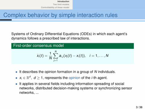
Complex behavior by simple interaction rules

Systems of Ordinary Differential Equations (ODEs) in which each agent’sdynamics follows a prescribed law of interactions.

First-order consensus model

xi (t) =1N

N∑j=1

ai,j (xj (t)− xi (t)), i = 1, . . . ,N

• It describes the opinion formation in a group of N individuals.

• xi ∈ Rd , d ≥ 1, represents the opinion of the i-th agent.

• It applies in several fields including information spreading of socialnetworks, distributed decision-making systems or synchronizing sensornetworks, ...

3 / 38



Linear versus Nonlinear

Linear networked multi-agent models1: ai,j are the elements of theadjacency matrix of a graph with nodes xi

ai,j > 0, if i 6= j and xi is connected to xj

ai,j = 0, otherwise.

Nonlinear alignment models2:

ai,j := a(|xj − xi |), where a : R+ → R+,

a ≥ 0 is the influence function. The connectivity depends on the contrast ofopinions between individuals.

1 Olfati-Saber, Fax, and Murray, IEEE Proc., 20072 Motsch and Tadmor, SIAM Rev., 2014

4 / 38



Controllability

Linear finite-dimensional system{x = Ax + Bu, t ∈ [0,T ]

x(0) = x0

x ∈ RN , u ∈ RM M ≤ N, A ∈ RN×N , x ∈ RN×M

Exact controllability at time T > 0.Given any initial datum and final target x0, xT ∈ RN there exists u : [0,T ]→ RM suchthat the corresponding solution x satisfies x(T ) = 0.

Null controllability at time T > 0.Given any initial datum x0 ∈ RN there exists u : [0,T ]→ RM such that thecorresponding solution x satisfies x(T ) = 0.

Approximate controllability at time T > 0.Given any ε > 0 and any initial datum and final target x0, xT ∈ RN there existsu : [0,T ]→ RM such that the corresponding solution x satisfies ‖x(T )− xT ‖RN ≤ ε.

Stabilization.Given any initial datum x0 ∈ RN there exists u : [0,T ]→ RM such that thecorresponding solution x has uniform exponential decay: |x(t)| ≤ ce−ωt |x0|.

5 / 38



Consensus

Depending on the nature of the interactions, the system may converge to aparticular configuration, called consensus which is characterized by theproperty x1 = x2 = . . . = xN := x∞.

• ••• ••• ••••••

•

•

xi (t)

x∞

Caponigro, Carrillo, Fornasier, Piccoli, Tadmor,Trélat,...

Convergence to consensus happens naturally whenever the system is suffi-ciently close to this configuration.

6 / 38



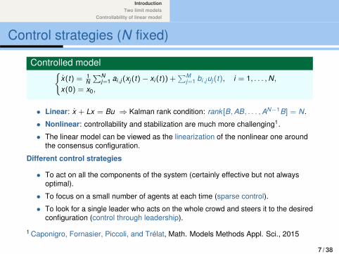
Control strategies (N fixed)

Controlled model{x(t) = 1

N∑N

j=1 ai,j (xj (t)− xi (t)) +∑M

j=1 bi,j uj (t), i = 1, . . . ,N,x(0) = x0,

• Linear: x + Lx = Bu ⇒ Kalman rank condition: rank [B,AB, . . . ,AN−1B] = N.

• Nonlinear: controllability and stabilization are much more challenging1.

• The linear model can be viewed as the linearization of the nonlinear one aroundthe consensus configuration.

Different control strategies

• To act on all the components of the system (certainly effective but not alwaysoptimal).

• To focus on a small number of agents at each time (sparse control).

• To look for a single leader who acts on the whole crowd and steers it to the desiredconfiguration (control through leadership).

1 Caponigro, Fornasier, Piccoli, and Trélat, Math. Models Methods Appl. Sci., 2015

7 / 38

TWO LIMIT MODELS



Mean-field limit equations

When the number of agents N tends to infinity, the ODE consensus model is replacedwith a suitable PDE.

Nonlinear alignment models:

xi =1N

N∑j=1

a(|xj − xi |)(xj − xi ), i = 1, . . . ,N, a : R+ → R+.

Classical mean-field theory suggests to consider the N-particle distribution function

µN = µN(x , t) :=1N

N∑i=1

δxi (t).

and to look for the equation it satisfies as N → +∞.

Particle methodAnalogies with the particle method (P. A. Raviart, J. Comp. Math., 1986) which refersto numerical schemes for time-dependent problems in PDE where, for each time t , theexact solution is approximated by a linear combination of Dirac measures.

9 / 38



The limit µ = limN→+∞ µN solves the non-local transport equation 1,2

∂tµ = ∂x

(µ(x , t)

∫Rd

a(|y − x |)(x − y)µ(y , t) dy).

The convolution kernel describes the mixing of opinions due to the interactionsamong the agents during the time evolution of the dynamics.

The system of ODEs describing the agents dynamics defines thecharacteristics of the underlying transport equation. The coupling of the agentsdynamics introduces the non-local effects on transport.

1 Ha and Tadmor, Kinetic Relat. Methods, 20082 Motsch and Tadmor, SIAM Rev., 2014

10 / 38



Mean-field limit for linear models?

• The mean-field equation involves the density µ, which does not containthe full information of the state since it does not keep track of theidentities of agents (label i).

Linear networked model with three agents

x + Lx = 0 and L =

1 −1 0−1 2 −10 −1 1

.

Two different initial datax1(0) = (−1, 0, 1) (left)and x2(0) = (−2, 3,−1)(right) whose dynamics aredifferent though they havethe same distribution µ3.

11 / 38



Graph limit method

• Based on the theory of graph limits.• Considers the phase-value function xN(s, t) defined as

xN(s, t) =N∑

i=1

xi (t)χIi (s, t), s ∈ (0, 1), t > 0,N⋃

i=1

Ii = [0, 1].

An opinion datum for N = 20 and its function z20 on [0, 1]

12 / 38



Formal procedure

Let (xNi )N

i=1 be the solution of the following consensus model

xNi =

1N

N∑j=1

aNi,jψ(xN

j − xNi ),

where aNi,j are constant and ψ represents nonlinearity.

The graph limit theory says that if

W N(s, s∗) =N∑

i,j=1

aNi,jχ[ i

N ,(i+1)

N

)(s)χ[ jN ,

(j+1)N

)(s∗)

is uniformly bounded and converges to W , then the phase-value functionxN(s, t) converges to the solution of the non-local diffusive equation

∂tx(s, t) =

∫ 1

0W (s, s∗)ψ(x(s∗, t)− x(s, t))ds∗1 .

1 Medvedev, SIAM J. Math. Anal., 201413 / 38



Example of the graph limit

Model with a periodic dense network

x + Lr x = 0, Lr =1N

(li,j )Ni,j=1, r ∈ (0, 1/2]

li,j =

`, if i = j−1, if j − i ∈ [−`, `] \ {0} (mod N)

0, otherwise

` = [rN], the closest integer to rN.

This leads to the non-local diffusion equation with

W (θ, θ∗) = χ[−2πr,2πr ](θ∗ − θ), θ, θ∗ ∈ S1.

14 / 38



Non-local diffusion equation

∂tx(θ, t) =

∫S1

W (θ∗, θ)(x(θ∗, t)− x(θ, t)) dθ∗

W (θ, θ∗) = χ[−2πr,2πr ](θ∗ − θ), θ∗, θ ∈ S1.

•∫S1 W (θ∗, θ)(x(θ∗, t)− x(θ, t)) dθ∗ = 0 for weak interactions r → 0,

leading to the trivial dynamics:

∂tx(s, t) ≡ 0.

• A non trivial limit dynamics requires a large number of interactions amongthe agents

(# of nonzero aij ) ∼ N2 as N → +∞.

15 / 38



Nonlinear subordination

• Finite ODE collective dynamics:

xi =1N

N∑j=1

a(|xj − xi |)(xj − xi ).

• Graph limit model:

xt (s, t) =∫ 1

0a(|x(s∗, t)− x(s, t)|)(x(s∗, t)− x(s, t))ds∗.

• Mean-field limit model:

µt (x , t) +∇x (V [µ]µ) = 0, where V [µ] :=

∫X

a(x∗ − x)µ(x∗, t)dx∗.

Subordination transformationFrom non-local "parabolic" to non-local "hyperbolic":µ(x , t) =

∫S δ(x − x(s, t))ds.

Similar to the link between kinetic equations and conservation laws.

P.-L. Lions, B. Perthame and E. Tadmor, J. Amer. Math. Soc., 1994.16 / 38

CONTROLLABILITY OF LINEARMODEL



Consider the control problem associated to the linear consensus model

x + Lx = Bu.

One looks for u = u(t) so to steer the system into the consensus at time T :

x(T ) = (x , . . . , x)T .

Different types of control actions

On one single agent or a few ones:

B = (1, 0, . . . , 0)T or B = (0, . . . , 0, Ik , 0, . . . , 0)T ,

for k × k identity matrix Ik .

For finite-dimensional linear systems, the Kalman rank condition provides anecessary and sufficient condition

rank[B, LB, . . . , LN−1B] = N.

18 / 38



Challenge

Analyze the behavior as N → +∞.

We discuss four examples of linear networked consensus models, inspired inprevious knowledge on:

• 1− d heat equations.

• 2− d heat equations.

• Non-local diffusive equations.

• Fractional heat equations.

Rough answer

Control properties ARE NOT UNIFORM as N → +∞. The goal shouldrather be getting sharp estimates on how these properties diverge with N.

19 / 38



A model with sparse graph

Sparse graph

ai,j = 1 if j = i ± 1, ai,j = 0 otherwise.

Each agent i communicates with its neighbors, i − 1 and i + 1.

x1x2.........

xN

+

1 −1 0 . . . . . . 0−1 2 −1 . . . . . . 0...

. . ....

.... . .

...0 . . . . . . −1 2 −10 . . . . . . . . . −1 1

︸︷︷︸

L

x1x2.........

xN

=

00.........0

.

20 / 38



Link with semi-discrete PDEsRescaled version of the finite difference semi-discretization of the one-dimensionalheat equation with homogeneous Neumann boundary conditions on [0, 1].

x1x2.........

xN

+ N2

1 −1 0 . . . . . . 0−1 2 −1 . . . . . . 0...

. . ....

.... . .

...0 . . . . . . −1 2 −10 . . . . . . . . . −1 1

︸︷︷︸

D

x1x2.........

xN

=

00.........0

.

Our system corresponds to the finite-difference discretization of

ut − N−2uxx = 0, t ∈ [0,T ]

or, alternatively, to the finite-difference discretization of

ut − uxx = 0, t ∈ [0,T/N2].

21 / 38



Control cost

Applying known results of semi-discretized heat equations we deduce that thecost of controlling the sparse network of N agents to consensus in finite time Tis of the order of

C ∼ exp(cN2/T ).

Control of sparse networked system

• If T ∼ N2, ‖uN(t)‖L2(0,T ) ≤ C.

• If T is independent of N, then ‖uN(t)‖L2(0,T ) ∼ C1 exp(C2N2).

The 1− d sparse network exhibits a slow diffusion rate. Controlling the systemthrough the action on a % of individuals of the network requires a time of theorder of T ∼ N2 or controls of exponential size, so to steer the system toconsensus.

22 / 38



Spectral analysis

The control properties of an infinite-dimensional symmetric system rely heavilyon these two properties of its spectrum {λk}k ≥1:

• λk+1 − λk ≥ γ > 0, for all k ≥ 1.

•∑

k≥1 λ−1k < +∞.

These conditions are satisfied uniformly in N by the eigenvalues of thesemi-discrete heat equation, which essentially behave like those of the actualheat equation (λk ∼ k2), but not by the ones of the consensus model

Link with Müntz theoremWe are considering dynamical systems generated by real exponentialexp(−λk t) that, under the change of variables z = exp(t) take the poly-nomial form zλk .

23 / 38



2D sparse networked model

Similar results can be achieved for more general networks related to the finite-differencesemi-discretization of the heat equation in R2.

Model on a 2D graph

xi,j (t) =N∑

k,l=1

a(i,j),(k,l)(xk,l (t)− xi,j (t)), i, j = 1, . . . ,N,

a(i,j),(k,l) = 1, if (k , l) = (i ± 1, j) or (i, j ± 1)

a(i,j),(k,l) = 0, otherwise.

24 / 38



This model corresponds to the control problem on the semi-discretizedtwo-dimensional heat equation with scaling N−2:

x + N−2Qx = Bu

B = [I, 0, . . . , 0]T .

Analogously to the one-dimensional case, we have a control cost exponentiallylarge in N.

Control of the 2D sparse networked system

The control cost behaves C ∼ exp(N2/T ) as in the one-dimensional case.

25 / 38



Example of the graph limit

For examples with dense interactions, we may scale the model with a periodicdense network presented before:

Model with a periodic dense network

x + Lr x = 0, Lr =1N

(li,j )Ni,j=1, r ∈ (0, 1/2]

li,j =

2, if i = j−1/`, if j − i ∈ [−`, `] \ {0} (modN)

0, otherwise

` = [rN], the closest integer to rN.

This leads to the non-local diffusion equation with

W (θ, θ∗) =1

2πrχ[−2πr,2πr ](θ∗ − θ), θ, θ∗ ∈ S1.

26 / 38



We may expect that a dense graph with many interactions among the agentsimproves the control properties. Spectral analysis shows that this is not thecase.

The eigenvalues λ`k and eigenvectors ψ`k can be calculated explicitly since thematrix Lr is Toeplitz:

Spectrum

λ`k =4`

∑j=1

sin2(

kπjN

),

ψ`k =

(sin

(2kπj

N

)+ cos

(2kπj

N

))N

j=1, k = 1, . . . ,N.

Also for this model we have a bad spectral behavior from the controllabilitypoint of view.

27 / 38



The case r = 1/N

• For r = 1/N, corresponding to ` = 1, we can quantify explicitly thespectral properties.

• Notice that, in this case, the graph is not really dense, since each agent iscommunicating only with the left and right neighbors.

λ1k = 4 sin2

(kπN

), k = 1, . . . ,N

λ1N−k = λ1

k .

We have eigenvalues with multiplicity 2.This is consequence of the periodicity ofthe network.

Distribution of the eigenvaluesfor r = 1/N ⇒ ` = 1.

28 / 38



• This case corresponds to a rescaledsemi-discrete heat equation with periodicboundary conditions.

• It is enough to take

B = (1, 0, . . . , 0, 1)T

that is, controlling only two agents (blackbox in the figure).

Then, as for our first example, the controllability cost is of the order of

C ∼ exp(N2/T ).

• When the time of control is T ∼ N2, controllability to consensus isachievable with a control of size uniformly bounded on N.

• When we need a control time T independent of N , it requires controlsexponentially large.

29 / 38



The case r = 1/2

• Also for r = 1/2, corresponding to ` = N/2, we can easily analyze thespectrum.

• In this case, all the agents are in communication with each other.

λNk = 2, k = 1, . . . ,N − 1, λN

N = 0.

We have eigenvalues with multiplicity N − 1.

Eigenvalues (left) and spectral gap (right) for r = 1/2⇒ ` = N/2.

30 / 38



The intermediate cases

• For r ∈ (1/N, 1/2), it is difficult to study the spectral properties analytically.

λ`k =1`

[2`+ 1− csc

(kπN

)sin

(kπ(2`+ 1)

N

)], k = 1, . . . ,N

Eigenvalues (left) and spectral gap (right) with N = 45 and various r .

• Simulations show that the spectral properties deteriorate as r increases.• We have many repeated eigenvalues, but it is not easy to explicitly track their

distribution.

31 / 38



Conclusions

Our analysis shows that dense graphs have worse controllabilityproperties than the sparse ones (first example).

• ` = 1: with B = (1,0, . . . ,0,1)T we recover the samecontrollability time and cost as our first example.

• ` > 2: the controllability properties of the system deteriorate as rincreases.. Our previous discussion suggests that we may recover better

controllability properties by increasing the number of controlledagents

B = [I`, 0, . . . , 0, I`]T .

WORK IN PROGRESS

32 / 38



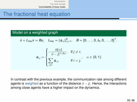
The fractional heat equation

Model on a weighted graph

x + Lfracx = Bu, Lfrac = (ai,j )Ni,j=1, B = [0, . . . , 0, IN , 0, . . . , 0]T .

ai,j =

− c(α)

|i − j|1+2α , if j 6= i,∑j 6=i

ai,j , if i = j., α ∈ (0, 1)

In contrast with the previous example, the communication rate among differentagents is weighted as a function of the distance |i − j|. Hence, the interactionsamong close agents have a higher impact on the dynamics.

33 / 38



Lfrac describes a dense network inspired on the fractional Laplacian.

Dfrac := N2αLfrac

is the finite difference discretization of the fractional Laplace operator.

Fractional Laplacian

(−d2x )αu(x) := cαP.V .

∫R

u(x)− u(y)

|x − y |1+2α dy .

x + Dfracx = Bu

is the semi-discretized control problem for the fractional heat equation

∂tu + (−d2x )αu = fχω, t ≥ 0.

It corresponds the graph limit non-local diffusive model with

W (x , y) = |x − y |−1−2α,

34 / 38



The fractional heat equation is null-controllable in time T > 0⇔ α > 1/2.3,4

The eigenvalues of Dfrac behave as λDk ∼ k2α, k ≥ 1.

Spectral behavior

α ≤ 1/2⇒N∑

k=1

(λD

k

)−1≥ N, α > 1/2⇒

N∑k=1

(λD

k

)−1≤ C < +∞

infk=1,...,N−1

(λD

k+1 − λDk

)=

λD

N − λDN−1 = O(N2α−1), α < 1/2

λD2 − λD

1 = O(1), α ≥ 1/2.

For α ≤ 1/2, the control cost is not bounded in N. In particular, for α < 1/2 itblows-up exponentially as exp(N1−2α).3Micu and Zuazua SIAM J. Cont. Optim., 20064Biccari and Hernández-Santamaría, IMA J. Math. Control. Inf., 2018

35 / 38



What about x + Lfracx = Bu?

• This time, even in the case α > 1/2, the controllability properties are notuniform in N due to the scaling of the matrix Lfrac .

• The eigenvalues of Lfrac behave as

λLk = N−2αλD

k ∼(

kN

)2α

.

Consequently, the spectral gap is very small even for α > 1/2.

• The two systems are equivalent up to time-scaling t 7→ N−2αt :

x + Dfracx = 0, t ∈ [0,T/N2α].

Hence, the cost of controlling x + Lfracx = Bu is of the order ofexp(CN2α/T ).

36 / 38



Conclusions

• We considered finite-dimensional collective behavior models and wediscussed their infinite-agents limits.

• The nature of the interactions among the individuals determines the limitapproach one should use. Networked systems require the employment ofa graph limit, while for aligned ones it is possible to rely on the classicalmean-field theory.

• These two limit approaches lead to substantially different kinds ofequations, a diffusion and a transport one, respectively. We showed thatthe diffusion equation is subordinated to the transport one through anaveraging process.

• We analyzed controllability properties of linear networked models bylinking them to the finite difference semi-discretization of heat-likeequations.

• This allows to get to some conclusions learning from the existing theoryof control of parabolic PDEs and their numerical counterparts, and to getsome estimates on the cost of controlling systems as N → +∞.

37 / 38



THANK YOU FOR YOUR ATTENTION!

This project has received funding from the European Research Coun-cil (ERC) under the European Union’s Horizon 2020 research andinnovation program (grant agreement No 694126-DYCON).

38 / 38

Documents

Dynamics and control for multi-agent networked …...Analogies with theparticle method(P. A. Raviart, J. Comp. Math., 1986) which refers to numerical schemes for time-dependent problems