Embed Size (px)
Citation preview
Dynamics and Control in Natural and Engineered
Multi-Agent Systems
Benjamin Nabet
A Dissertation
Presented to the Faculty
of Princeton University
in Candidacy for the Degree
of Doctor of Philosophy
Recommended for Acceptance
by the Department of
Mechanical and Aerospace Engineering
November, 2009

c© Copyright 2009 by Benjamin Nabet.
All rights reserved.
Abstract
Today there is a rapidly expanding and vibrant community of scientists interested in the
phenomenon of collective behavior. Collective behavior holds clues to the evolution of social
dynamics in animal or human groups, and also for the development of novel technological
solutions, from autonomous swarms of exploratory robots to smart grids that reliably dis-
tribute electricity to consumers in a dynamic fashion. In this dissertation we study the
dynamics and control of multi-agent systems in both the engineered and the natural set-
ting.
Focusing first on the engineered setting, we derive provable, distributed control laws for
stabilizing and changing the shape of a formation of vehicles in the plane using dynamic
models of tensegrity structures. Tensegrity models define the desired, controlled, multi-
vehicle system dynamics, in which each node of the tensegrity structure maps to a vehicle
and each interconnecting strut or cable in the structure maps to a virtual interconnection
between vehicles. Our method provides provably well-behaved changes of formation shape
over a prescribed time interval. A designed path in shape space is mapped to a path in the
parametrized space of tensegrity structures, and the vehicle formation tracks this path with
forces derived from the time-varying tensegrity model.
Turning our attention to the natural setting, we then present and study Lagrangian
models to investigate the mechanisms of decision-making and leadership in animal groups.
We study the motion dynamics of a population that includes “informed” individuals with
conflicting preferences and “uninformed” individuals without preferences. This work is the
result of an interaction between complex discrete-time models developed by biologists that
iii

produce highly suggestive simulations, and continuous-time models that, though simpler and
less suggestive, allow for a thorough investigation of the dynamics in a general context with
a complete exploration of parameter space, thus allowing us to uncover unifying principles
of motion.
iv

Acknowledgements
First, I would like to thank my advisor Professor Naomi Leonard for giving me the oppor-
tunity to work with her, and for her constant support and inspiration. I am particularly
grateful for her openness to new ideas and her encouragement to define my own research
topics.
I would like to thank the principal readers of this dissertation, Professor Simon Levin
and Professor Jeremy Kasdin. Their comments and feedback improved this dissertation
immeasurably. My examiners Professor Philip Holmes and Professor Iain Couzin deserve
many thanks for their time and interest.
Princeton is a unique academic institution where I had the privilege to meet and work
with many great scholars. I thank Professor Simon Levin and Professor Philip Holmes
for serving on my thesis committee and taking much of their precious time to discuss my
research and provide me with their guidance. I am deeply grateful to Professor Iain Couzin
and the members of his research group for their collaboration. The research presented
here on collective behavior in animal groups would not have been possible without their
contributions and insights. I would also like to acknowledge all my instructors at Princeton
University for sharing their knowledge and passion. Thanks also to the many administrators
who have helped me navigate my time in Princeton. I am especially grateful to Jessica
O’Leary who is a source of constant support for all of us MAE graduate students, and who
always has a nice word to say.
Apart from the academics, I also found in Princeton many friends. I want to thank
particularly Laurent Pueyo for being no less than the best office mate one could possibly
v

imagine. Un grand merci to my dear friend Arthur Denner, it is a privilege to have you as
a friend along with my other “Princeton uncle”. I cannot thank you enough for going over
every line of this dissertation; your facility with language and your generosity in sharing it
with me not only improved the work at hand but also gave me skills that I will carry with
me wherever I go.
I cannot thank my family enough; I know it was hard for them to see me leave for the
other side of the Atlantic, but they nevertheless gave me their support. Papa et Maman, I
would never be writing these lines without your love and encouragement, I hope to always
be a source of joy and satisfaction for you. I thank my older brother and sister Olivier
and Estelle and their families. I also thank my wife’s parents Herbert and Ann Berezin for
thinking of me as one of their own children.
Finally my last words go to my dear wife Shani, I cannot thank you enough for always
being there and riding the ups and downs of the life of a graduate student always with a
smile and comforting words. For a long time I wondered what led me to Princeton and not
anywhere else in the world, but then I met you and it was all clear.
vi
Contents
Abstract iii
Acknowledgements v
Contents vii
1 Introduction 1
1.1 Motivation and Problem Statement . . . . . . . . . . . . . . . . . . . . . . . 1
1.2 Survey of Related Work . . . . . . . . . . . . . . . . . . . . . . . . . . . . . 3
1.2.1 Aggregation and Decision-making in Animal Groups . . . . . . . . . 3
1.2.2 Coordination under Decentralized Control in Groups of Robots . . . 7
1.3 Thesis Overview . . . . . . . . . . . . . . . . . . . . . . . . . . . . . . . . . 12
2 Shape Control and Tensegrity Structures 16
2.1 Background on Tensegrity Structures . . . . . . . . . . . . . . . . . . . . . . 17
2.1.1 Origins of Tensegrities . . . . . . . . . . . . . . . . . . . . . . . . . . 17
2.1.2 Analysis and Design Methods for Tensegrity Structures. . . . . . . . 19
2.2 Tensegrity Structures and the Shape Control Problem . . . . . . . . . . . . 22
2.3 Mathematical Models for the Dynamics of a Tensegrity . . . . . . . . . . . 24
2.3.1 Connelly’s Model . . . . . . . . . . . . . . . . . . . . . . . . . . . . . 25
2.3.2 Augmented Model . . . . . . . . . . . . . . . . . . . . . . . . . . . . 27
2.4 Stabilization for a Desired Group Geometry . . . . . . . . . . . . . . . . . . 28
vii
2.4.1 Smooth Parameterization of the Model . . . . . . . . . . . . . . . . . 29
2.4.2 Stability Analysis . . . . . . . . . . . . . . . . . . . . . . . . . . . . . 33
2.5 Examples and Simulations . . . . . . . . . . . . . . . . . . . . . . . . . . . . 35
2.5.1 Snelson’s X Tensegrity Framework . . . . . . . . . . . . . . . . . . . 35
2.5.2 A Five Vehicle Network Example . . . . . . . . . . . . . . . . . . . . 37
3 Group Reconfiguration and Tensegrity Structure 44
3.1 Control Law for Shape Reconfiguration . . . . . . . . . . . . . . . . . . . . 45
3.1.1 Path Design in Shape Space . . . . . . . . . . . . . . . . . . . . . . . 45
3.1.2 Parameterized Control Law . . . . . . . . . . . . . . . . . . . . . . . 48
3.2 Boundedness and Convergence . . . . . . . . . . . . . . . . . . . . . . . . . 50
3.3 Examples and Simulations . . . . . . . . . . . . . . . . . . . . . . . . . . . . 52
4 Collective Decision Making: Discrete Time Models 61
4.1 Discrete-time Model from Couzin et al. [19] . . . . . . . . . . . . . . . . . . 62
4.1.1 The Model . . . . . . . . . . . . . . . . . . . . . . . . . . . . . . . . 62
4.1.2 Summary of the Results in Couzin et al. [19] . . . . . . . . . . . . . 66
4.2 Influence of Naive Individuals in the Direction Model . . . . . . . . . . . . . 67
4.3 Influence of Naive Individuals in the Target Model . . . . . . . . . . . . . . 77
5 Collective Decision Making: A Simple Analytical Model 83
5.1 Model and Reduction . . . . . . . . . . . . . . . . . . . . . . . . . . . . . . 83
5.1.1 Particle Model . . . . . . . . . . . . . . . . . . . . . . . . . . . . . . 85
5.1.2 Time Scale Reduction . . . . . . . . . . . . . . . . . . . . . . . . . . 87
5.2 Phase Space Dynamics of the Reduced Model . . . . . . . . . . . . . . . . . 94
5.2.1 Equilibria of the Reduced System (5.20) . . . . . . . . . . . . . . . . 94
5.2.2 Bifurcations in the Reduced Model (5.20) . . . . . . . . . . . . . . . 102
5.3 Extensions and Robustness of the Model . . . . . . . . . . . . . . . . . . . . 117
5.3.1 Uneven Informed Subgroups . . . . . . . . . . . . . . . . . . . . . . . 118
5.3.2 Heterogeneous Subgroups . . . . . . . . . . . . . . . . . . . . . . . . 118
viii
5.3.3 Forgetting Factor Feedback . . . . . . . . . . . . . . . . . . . . . . . 126
6 Collective Decision Making: Analytical Model with Time-Varying Con-
necting Topology 130
6.1 Model and Invariant Manifolds . . . . . . . . . . . . . . . . . . . . . . . . . 131
6.1.1 Particle Model . . . . . . . . . . . . . . . . . . . . . . . . . . . . . . 131
6.1.2 Invariant Manifolds in the Model . . . . . . . . . . . . . . . . . . . . 133
6.2 Attractiveness of the Invariant Manifolds: Results and Interpretation . . . . 139
6.3 Attractiveness and Phase Space Dynamics of the Reduced Models . . . . . 143
6.3.1 Invariant manifolds M1 and M2, (A12, A13, A23) = (1, 0, 1) or (1, 1, 0) 143
6.3.2 Invariant Manifold M3, (A12, A13, A23) = (0, 0, 0) . . . . . . . . . . . 145
6.3.3 Invariant Manifolds M4 and M5, (A12, A13, A23) = (0, 1, 0) or (0, 0, 1) 146
6.3.4 Invariant Manifold M6, (A12, A13, A23) = (1, 0, 0) . . . . . . . . . . . 148
6.3.5 Invariant Manifold M7, (A12, A13, A23) = (0, 1, 1) . . . . . . . . . . . 150
6.3.6 Invariant Manifold M8, (A12, A13, A23) = (1, 1, 1) . . . . . . . . . . . 152
6.4 Summary and Forgetting Factor Feedback Extension . . . . . . . . . . . . . 158
6.4.1 Summary . . . . . . . . . . . . . . . . . . . . . . . . . . . . . . . . . 158
6.4.2 Forgetting Factor Feedback . . . . . . . . . . . . . . . . . . . . . . . 160
7 Conclusions and Future Directions 174
7.1 Summary . . . . . . . . . . . . . . . . . . . . . . . . . . . . . . . . . . . . . 174
7.2 Future Lines of Research . . . . . . . . . . . . . . . . . . . . . . . . . . . . . 177
A Technical Proofs for Chapter 5 180
B Technical Proofs for Chapter 6 183
References 188
ix
Chapter 1
Introduction
1.1 Motivation and Problem Statement
Collective behavior in the human, animal or engineered setting is a fascinating phenomenon.
Whether it is behavioral economists trying to understand the decision-making process of
market participants and its influence on market prices and returns, or biologists wondering
how schooling fishes, flocking birds or swarming ants make rapid collective decisions on
where to move or what task to perform in often variable and dangerous environments, or
engineers trying to design collaborating teams of robots by emulating mechanisms observed
in nature, the attention of many scientists has been captivated by the subject of collective
behavior.
Today we are far from the “thought transference” abilities hypothesized by Selous in
which a connectivity of individual minds is required to explain how tens of thousands of
starlings come together to roost [106]. It is now accepted that individuals in animal groups
make their movement decisions on the basis of local cues from both the environment and
near neighbors [18], and that through its interactions with other individuals in the group,
each individual gains access to information beyond its own cognitive abilities. The transfer
of information in this way between group members creates collective behaviors that give
the impression to a field observer that there exists a “collective mind” within the group
1
2
[17]. That is, through their simple interactions, individuals in a group collectively perform
tasks without the need for a centralized control or global blueprint, as though endowed with
a collective mind. This capability holds the solution to the decentralized control problem
that engineers designing collaborating teams of mobile robots are to solve. The mechanisms
through which the capabilities of a group of individuals become greater than the sum of
the capabilities of its individual members provides a compelling model for the design of
collaborating teams of mobile robots.
Cooperative teams of mobile robots have been deployed on land, sea and air to perform
various tasks including searching and sampling both for commercial and for military appli-
cations. Recent efforts in cooperative control of groups of robots have focused on emulating
collective behaviors observed in animal groups. This new multi-disciplinary effort has been
beneficial to biologists and engineers alike. Mathematical techniques commonly used in the
engineered setting help reveal fundamental mechanisms of collective behavior in the natural
setting, and the mechanisms of animal collective behavior, once deciphered, provide new
inspiration for design in engineering.
In this dissertation we study the dynamics and control of both engineered and natural
systems. We first derive provable, decentralized control laws for stabilizing and smoothly
changing the shape of a group of vehicles in the plane. Tensegrity structures are used
to model the controlled multi-vehicle system dynamics, with each node in the tensegrity
corresponding to a vehicle and each connecting element of the tensegrity corresponding to
a virtual interconnection between a pair of vehicles. Then, turning our attention to the
biological setting, we present and study models to investigate the mechanisms of decision-
making and leadership in animal groups. We study the motion dynamics of a population
that includes two subgroups that are “informed” such that individuals in each subgroup
have a preferred direction and one subgroup that is “uninformed” such that individuals
in this subgroup do not have a preferred direction of motion. This work is the results of
an interaction between two types of models: complex discrete time models developed by
biologists that produce highly suggestive simulations, and continuous time models that,

3
though simple and less suggestive, make it possible to explore the dynamics in a more
general context, thus allowing us to uncover unifying principles of motion.
1.2 Survey of Related Work
The literature on topics related to this dissertation is vast, and the survey of related work
that we present is therefore necessarily incomplete. Although in this dissertation the first
chapters focus on multi-agent systems in the engineered setting while later chapters focus
on multi-agent systems in the natural setting, we present our survey of related work in the
opposite order. We first summarize research in modeling of aggregation and decision making
in animal groups. We then summarize related research in coordinated control of robotic
teams. This order is chosen as the research on multi-agent systems in the natural setting
has tended to precede and inspire the research on multi-agent systems in the engineered
setting.
1.2.1 Aggregation and Decision-making in Animal Groups
Aggregation Modeling: Most animal species live in groups, in the sense defined by
Wilson as “any set of organisms, belonging to the same species, that remains together for a
period of time, interacting with one another to a distinctly greater degree than with other
conspecifics” [81]. The reasons why species have evolved to this social tendency have been
extensively studied and are well understood. They include an increased chance of surviving
predation, enhanced foraging, conservation of heat and such social benefits as finding a mate.
See Chapter 2 in [57] for a full review of the benefits of group formation. The mechanisms
of aggregation and cohesiveness of aggregated groups, however, are not as well understood.
The modeling and analysis of these phenomena continue to generate considerable interest in
the ethology community with many problems remaining open. Self organization theory has
gone a long way in explaining the emergence of group behavior, suggesting that complex
large-scale behaviors are the result of simple interactions among individuals in the group
[43, 10]. Deriving the precise mechanism by which simple interactions produce complex
4
behaviors has proven difficult. One of the difficulties stems from the fact that patterns
which are posited to emerge from individual behavior are observable only at the level of
the population [42]. The observation that the same individual interaction may translate
into different group behaviors under the influence of different environments complicates the
problem, posing another challenge to uncovering aggregation mechanisms [30].
The dynamics of aggregation in animal groups that have been studied in the ethology
literature have been described mainly with two types of models: Eulerian and Lagrangian.
Eulerian models, also known as continuum models, describe a group using a continuous
density measure. They characterize the behavior of the group by describing the dynamics
of group properties such as population density or group size. The dynamics of the group
properties are usually modeled with a set of partial differential equations. Abstracting to
group properties has been a very appealing approach, given the availability of sophisticated
mathematical tools to analyze such systems. Gueron and Levin modelled the dynamics of
large wildebeest herds using an Eulerian approach [41]. Their model revealed a plausible
mechanism for self organization that spontaneously produces front patterns. Front patterns
predicted by this model were validated with aerial photos. The Eulerian approach has also
been very successful in describing the mechanism of aggregation for dense species such as
bacteria or for some insect swarms [37].
The Eulerian approach has its limitations however. It has not proven particularly well
suited for modeling aggregation of groups of moderate to low density including some schools
of fish and flocks of bird. Also, since in continuum models individual animals are not
represented, their social interactions cannot be implemented directly. Many continuum
models therefore describe social behavior using a heuristic interpretation of individual-
based models or of data collected in observations; the partial differential equations for the
group property of interest are formulated so as to include relevant diffusion, convection,
and interaction terms. Aiming to avoid building a model based on heuristic interpretation,
Grunbaum derived the formulation of a continuum model explicitly from a Lagrangian-
type model [38]. This allowed him to directly implement relevant interactions between
5
individuals in the group.
Lagrangian models describe the group as a collection of discrete individuals interacting
with each other and determine the trajectories of individual animals. The rules governing
the group’s movements are often described with a set of discrete time or continuous time
ordinary differential equations incorporating physical laws (e.g., Newton’s second law) and
social rules (attraction, repulsion and tendency to align). Okubo, in paralleling Newtonian
dynamics to diffusion processes in ecological systems, revealed the tendency of individuals
to be both attracted to and align with others, but he did not discuss the tendency to move
away from individuals that are too close [84]. Aoki’s pioneering simulation study of schools
of fish proved the relevance of all three aforementioned social rules suggesting that the
main tendencies that individual fish adopt are attraction to and alignment with neighbors
and repulsion to individuals presenting a risk of collision [3]. While a clear advantage of
the Lagrangian approach is that it allows for implementation of specific behavioral rules,
limited computing power for many years made it impossible to study those models to
their full potential. Simulations of these models could only be performed on groups of
few individuals and for short periods of time. With the advent of ever more powerful
computers it is now possible to perform simulations on large numbers of individuals and
for significant amount of time. Accordingly, Lagrangian models are now capturing more
attention [130, 19].
Another advantage of the Lagrangian approach is that the simulated behavior can be
visualized and in this way compared with the observed behavior of the natural systems they
represent. Grunbaum et al. developed motion analysis hardware and software to precisely
track in three dimensions the positions of fishes in small schools of four or eight fishes
[39]. The authors used this framework to calibrate the parameters of the alignment force
and attraction/repulsion force of their theoretical model [20]. More recently Bellerini et al.
performed a large-scale observational study of flocks of starlings, reconstructing groups of up
to three thousand birds [4]. The results of their field study supported the notion, assumed
in most theoretical models, of a zone of repulsion around each individual. However, their
6
study suggested that interactions between individuals depend on “topological” distances
(how many “birds away”) rather than on metric distances as many models assume.
Information and Decision Making: Although animal groups are known to utilize social
information [57], little is known about the mechanisms underlying decision-making and
information transfer in groups, this despite the growing interest in collective phenomena in
biology, engineering and psychology. Currently, research is being done to understand how
animals use the behavior of other group members to make accurate decisions.
It has been shown that some animals species migrating in groups (especially birds), are
born with genetic information of migratory directions [44]. In a classic field experiment,
Perdeck displaced juvenile and adult starlings 800km in an airplane flight [92, 23]. It was
shown that the juvenile starlings continued to migrate in the same direction that they had
flown prior to displacement, whereas the adults compensated for the displacement by taking
a different direction. However this type of genetic information of migratory direction has
not been found in many species. Another type of elaborate mechanism used by individuals
to make decisions is the famous waggle-dance that honeybees have been observed to use in
recruiting members to visit food sources [66]. However such elaborate mechanisms are not
observed in most groups of fish or birds [57]. For many species, it has been shown that only
a few individuals with pertinent information, such as the knowledge of a migration route,
of a source of food or of the efficient behavior to adopt, are necessary to successfully guide
the group. Further, in many species, it is not possible to identify which individuals have
information and whether it is reliable or not. In a controlled experiment, Reebs trained
golden shiners to expect food at a given time and given location in the tank and showed
that when introduced to a shoal of untrained golden shiners, the trained shiners were able
to direct the shoal to the food source [96] without causing it to split. With a different
controlled experiment involving guppy shoal, Swaney et al. showed further that familiar
and well trained demonstrators were more efficient than unfamiliar and poorly trained
demonstrator in guiding the shoal to a food source [119].
Animal groups may be constituted with informed individuals with conflicting informa-
7
tion. Convergence to a common decision such as direction of travel or other activity is
described with the notion of consensus. In a recent paper, Couzin et al. revealed plausible
mechanisms for decision making and leadership by using a discrete simulation of particles
moving in the plane [19]. In this simulation, each particle represents an individual animal
and the motion of each individual is influenced by the state of its neighbors (e.g., relative
position and relative heading). Within this group, there are two subgroups of informed
individuals and one subgroup of naive individuals; each subgroup of informed individuals
has a preferred direction of motion that it can use along with the information on its neigh-
bors to make decisions. It is shown that information can be transferred within groups even
when there is no signaling, no identification of the informed individuals, and no evaluation
of others’ information. It was also observed that with two informed subgroups of equal
population, the direction of group motion depends on the degree to which the preferred
directions differ. For small disagreement, the group follows the average preferred direction
of all informed individuals, while for large disagreement the group selects one of the two
preferred directions. This model is more thoroughly studied in Chapter 4. Recent research
has also suggested that quorum response may be a particular mechanism for such decision
making. A quorum like behavior means that the probability of an individual performing
a certain action increases dramatically when seeing a threshold number of other individ-
uals performing this action. It has been shown to be relevant to decision-making in fish
[132, 118], honeybees [104], ants [94] or cockroaches [2].
1.2.2 Coordination under Decentralized Control in Groups of Robots
The apparent effortlessness with which coordination under decentralized control emerges in
natural systems, as reported in the previous section, has motivated engineers to seek to emu-
late such systems for the design of collaborative teams of robots. Two key parameters govern
the possibility of achieving coordination under decentralized control in engineered multi-
agent systems: sensing and inter-vehicle communication. Unlike their biological couterparts
which can use their senses, refined through evolution, to take cues from the environement
8
and neighbors, robots have more limited sensing and communication technologies at their
disposal. Our survey provides an overview of existing research on two types of coordina-
tion under decentralized control: first on consensus and synchronization, then on formation
control.
Consensus and synchronization: Interest in the phenomenon of consensus and syn-
chronization appeared in the computer science community during the 1980s. Bertsekas
and Tsitsiklis designed models of distributed asynchronous computation in order to create
efficient methods for parallel computating, strategies of distributed optimization, and dis-
tributed signal processing [128, 5, 127]. An important building block of all these methods is
the “agreement algorithm” in which agents (e.g. signal processing units, computation units)
reach consensus on a common value through each agent forming convex combinations of
its current value and those of its neighbors. Reynolds in his 1987 seminal paper used such
an “agreement algorithm” to propose a simple model of flocking, his motivation being to
create computer animations realistically representing the motion of a flock of birds [97].
In the 1990s Viscek et al. demonstrated the relevance of Reynolds’ work to particle
physics by proposing a Lagrangian, discrete-time linear model to investigate the emergence
of self-ordered motion in multi-particle systems with biologically motivated interactions
[129]. In the Viscek model individuals traveling at constant speed head in the average
direction of motion of their neighbors. The model presented in this now classic paper, which
is actually a special case of the flocking model developed by Reynolds [97], catalyzed research
efforts in the physics community around the topic of consensus dynamics. Toner and Tu
developed an Eulerian model of flocking dynamics describing a large class of microscopic
rules, including the ones utilized in the Viscek paper [125, 126]. Other studies of collective
motion of self-propelled particles that are related to the Viscek model include [36, 35].
Savkin later implemented the Viscek model on groups of autonomous robots [102].
The behavior predicted by the Viscek model was explained theoretically by Jadbabaie
et al. who treated it as a switched linear system and applied tools from algebraic graph
theory and matrix analysis [48]. They were able to prove for a coordinated group of agents
9
behaving according to the “nearest neighbor” rules of the Viscek model, convergence to
a common direction of travel under constraints on the switching times. Their worked
sparked tremendous interest in the control theory community. Recognizing the relevance
of graph theory, Olfati-Saber and Murray used “balanced graphs” to address the average-
consensus problem [87] and produced an algorithm that is valid for multi-agent networks
with fixed or switching topologies, with or without time-delays. Moreau extended the results
in [48] and presented sufficient conditions on the communication topology that guarantee
consensus, deriving them by supplementing the tools from graph theory with tools from
systems-theory [74]. Moreau studied both discrete-time and continuous-time consensus
models and presented sufficient conditions under which the equilibrium corresponding to
all individual agents’ converging to a common state value is uniformly exponentially stable.
Moreau showed that the common value to which the agents converge depends on the initial
condition. A key, non-intuitive result that Moreau demonstrated was that a more complete
communication topology does not necessarily translate into a faster convergence and in some
extreme cases may even cause loss of convergence. However, when the common state space
shared by the agents is non-Euclidean and/or the dynamics of the agents are nonlinear,
the results in Moreau [74] are only local. Scardovi et al. generalized Moreau’s result to
nonlinear dynamics on non-Euclidean space [103]. They studied the behavior of a network
of N agents that each evolves on the circle S1, also known as the problem of consensus on
the N -torus, and proposed an algorithm that achieves synchronization or balancing under
mild connectedness assumptions on the communication graph. The convergence results
proven in [103] are global.
The problem of consensus on the N -torus has been studied by many scientists in various
contexts including biology [135], chemistry [59] and neuroscience [113] to understand and
model periodic phenomena. The formulation of the problem of consensus on the N -torus
used in many of these works was first presented by Kuramoto in his 1984 study of “chem-
ical oscillations” [60]. The Kuramoto model describes the evolution in time of a group of
coupled-phase oscillators with global interactions. Many variations of the Kuramoto model
10
have been studied. See [115, 1] for reviews of these variations. The Kuramoto model has
recently played a critical role in our context of collective motion. Justh and Krishnaprasad
developed a motion model in which vehicles travel at constant speed and are controlled by
steering their direction of travel [49, 50]. This framework was successfully used by Sepulchre
et al. to stabilize circular and parallel collective motion [108]. Extensions of these results
assuming only limited communications between the steered particles were presented by the
same authors in [107]. In the formulation of the steering control laws used in [108, 107] the
coupling between particles is based on the Kuramoto model. In Chapters 5 and 6 of this
dissertation, the particle models used to study leadership and decision-making are similar
to the cooperative models used in [49, 50, 108, 107] with coupling between agents based on
the Kuramoto model.
Formation Control: Also within the domain of decentralized control is the problem
of formation control which is central to Chapters 2 and 3 of this dissertation. In the
context of formation control, vehicle interactions are driven by the task they are required
to perform. For example, for the design of mobile sensors carrying out collective sampling
or searching tasks, the configuration of the group can be critical. Controlling the geometry
and resolution of the vehicle formation, also referred to collectively as the “shape” of the
formation, offers important advantages to performance and efficiency of data gathering
and processing. Depending on the field being surveyed, smaller or larger formations might
be more efficient and certain shapes of the group might be preferable for estimating field
parameters such as gradients or higher-order derivatives from noisy measurements made by
the mobile sensors. Ogren et al. presented a stable control strategy for groups of vehicles to
move and reconfigure cooperatively to perform gradient climbing missions [83]. In this work
optimal shapes were designed to minimize error. Zhang and Leonard, taking the results
from Ogren et al. a step further, presented an algorithm for level set tracking where the
shape of the group was dynamically controlled so as to minimize the least mean square error
in gradient estimates of a scalar field [139, 140]. Shape control can be significant in other
vehicle network tasks as well, for example, when vehicles need to coordinate their activity
11
in order to escort, carry or otherwise interact with objects in their environment.
The earliest work on formation control, which can be dated back at least to the 1960’s,
involved one dimensional strings of inter-connected vehicles. Motivated by the development
of a high speed ground transport system, Levine and Athans presented an optimal linear
feedback control law regulating the position and velocity of a densely packed string of high
speed vehicles [65]. Other related work on the control of strings of vehicles includes [91, 70].
A method particularly relevant to the work presented in Chapters 2 and 3 that has
proven successful in designing distributed control laws of multi-vehicle formations has in-
volved the use of artificial potential functions [98, 85]. Initially, potentials were used solely
to prevent collisions in the vehicle network. Wang used repulsive potential functions to re-
duce the possibility of collisions with other robots and obstacles but in this work, potentials
were not used to achieve a desired formation [131]. In a related work, Khosla and Volpe
used potentials to design the workspace of a manipulator; regions in the workspace to be
avoided by the manipulator were modelled by repulsive potentials (energy peaks), and the
regions into which the manipulator is to move were modelled by an attractive potential
(energy valleys) [56].
Research on multi-robot path coordination using artificial potentials appeared later with
Warren [133]. In this work, the planning of multi-robot paths is performed by mapping the
real space of the robots into a configuration-space-time, with appropriate potential fields
applied throughout in order to influence the paths of the robots. Leonard and Fiorelli
presented a different framework for coordinated and distributed control of a multi-vehicle
system using artificial potentials [63]. They supplemented the artificial potentials by intro-
ducing “virtual leaders” which are moving reference points to which vehicles respond much
as they respond to other neighbors. These virtual leaders are used in the methodology to
eliminate undesirable equilibria created by the artificial potentials and to manipulate the
group behavior (e.g., translation and rotation of the formation). In this dissertation we
map the vehicle formation to a virtual tensegrity structure and design the potentials in this
structure in order to drive the shape of the formation.
12
Research on formation control has also drawn inspiration and tools from graph theory,
which, as we have already discussed, has proven useful in the context of consensus and
synchronization. Tabuada et al. modelled formations using formation graphs, i.e., graphs
whose nodes represent the individual vehicle kinematics and whose edges represent the inter-
vehicle constraints to be satisfied [120]. Fax and Murray described the interactions between
vehicles using results on graph Laplacians [27]. They derived a Nyquist-like stability crite-
rion for vehicle formation from the eigenvalues of the Laplacian matrix. Olfati-Saber and
Murray utilized the notion of graph rigidity to study and manipulate (i.e., join or split)
multi-vehicle formations [86]. Also inspired by the notion of graph rigidity, Eren et al.
presented a systematic method of maintaining rigidity for a vehicle formation when a ve-
hicle is lost [26]. Their method descibes how to minimally rearrange the connectivity of
the formation while maintaining rigidity. Tensegrity structures studied in Chapter 2 can be
treated as undirected graphs, and the stress matrix defined in equation (2.3) can be viewed
as a weighted pseudo Laplacian.
1.3 Thesis Overview
Motivated by the resurgence of interest in group motion by engineers as well as biologists,
this dissertation offers contributions to the analysis of control and dynamics of multi-agent
systems in the engineered and natural settings. The dissertation is divided in two parts. In
Chapters 2 and 3 we focus on the engineering setting and develop a mathematical framework
to generate control laws that stabilize any desired group shape in the plane and allow for
continuous reconfiguration of the group shape. In Chapters 4 through 6 where we focus
on the natural setting, we develop and analyze mathematical models for leadership and
decision making in the context of animal group motion. Some of the developments of this
dissertation have been previously published or submitted for publication in archival journals.
See [78, 80, 72]. Conference papers in which earlier versions of the results appeared include
[77, 79]. Results presented in Chapters 4 and 6 have not yet appeared elsewhere.
In Chapter 2 we design control laws that drive vehicle formations into shapes with
13
forces that can be represented as those internal to tensegrity structures. We first give a
brief history of the field of tensegrities and present existing methods for designing tensegrity
structures. We then motivate the use of tensegrity structures for solving the problem of
formation control. We go on to present two possible models for the forces of a tensegrity
structure: Connelly’s model [12] and an augmented version of it that we construct. For
each model, the relationship between the parameters of the model and the equilibrium
structure is formulated. We then present a smooth method for choosing the parameters
of the augmented model in a way that makes an arbitrary shape stable. Stability of the
desired shape is proven using the linearization of the controlled system. We illustrate the
results with examples of the computation of the parameters and a discussion on the number
of links between the nodes of a tensegrity that are necessary to realize a desired shape.
In Chapter 3 we again use the map between vehicles in a formation and nodes in a
tensegrity structure to derive a control law for vehicles in a formation that enables a well-
behaved reconfiguration between arbitrary planar shapes. The new control law, designed
to make nodes follow a smooth path in the space of stable tensegrities, is defined as a
smooth parameterization by time of the control law for stabilization of planar shapes that
is presented in Chapter 2. Tools from the nonlinear systems theory literature are utilized
to prove that the trajectory of the formation, in shape space, is close to the prescribed path
and that it converges to the desired final shape. We then present numerical simulations of
the time-varying control law and discuss its performance.
In Chapter 4 we investigate mechanisms of leadership and decision making in animal
groups such as schools of fish or flocks of birds through the simulation and analysis of a
discrete-time individual-based (i.e. Lagrangian) model developed by Couzin et al. in [19].
We consider a heterogeneous group of both informed individuals with conflicting preferences
and uninformed individuals, i.e, individuals without preferences. We consider two variations
of the discrete-time model presented in [19], one where the informed individuals have a fixed
preferred direction of travel and another where the preference is a destination, referred to as
a target. For each variation of this model we investigate the role of uninformed individuals
14
in the decision-making process highlighting both the drawbacks and the benefits of having
uninformed individuals in the group.
In Chapter 5, we analyze a continuous-time model of a multi-agent system. This model
is motivated by the simulation study in [19] also treated in Chapter 4, on the dynamics
of leadership and decision making in animal group motion. In this model, each individual
moves at constant speed in the plane and adjusts its heading in response to relative headings
of others in the population. The population includes three subgroups - two “informed”
subgroups in which individuals have a preferred direction of motion and one “uninformed”
subgroup in which individuals do not have a preferred direction of motion. We present
the model first in its general form and prove that it can be reduced to a three-dimensional
system using a time-scale reduction argument. We then study the full phase space dynamics
of the reduced model in a particular case, computing equilibria and proving stability and
bifurcations. We conclude the chapter with an investigation of several extensions of the
model to test its robustness through numerical simulations.
In Chapter 6, we derive and study the dynamics of a low-dimensional, deterministic,
coordinated control system. This model, motivated by the observed deviations between the
qualitative behavior of the discrete-time model presented in [19] and that of the continuous-
time model presented in Chapter 5, relaxes two of that model’s simplifying assumptions.
We present the model first in its general form and prove that it can be reduced to a three-
dimensional system using a time-scale reduction argument. However, unlike the model
presented in Chapter 5 which has only one invariant manifold the model presented in this
chapter has several, each characterized by a set of interaction gains between the different
subgroups. For each invariant manifold, we determine whether they are attractive or not
and for the manifolds that are attractive, we also describe the stable and unstable equilibria
of the corresponding reduced model and interpret the stable motions in the context of
animal group motion. We conclude the chapter by an extension of the model investigated
numerically to test its robustness.
We conclude in Chapter 7 with a summary of the contributions of this dissertation and

15
suggest possible future lines of research motivated by the presented work.

Chapter 2
Shape Control and Tensegrity
Structures
The tasks a mobile sensor network may need to perform include gradient climbing [83,
9], boundary tracking [139, 140] and surveillance [136]. For a network carrying out such
sampling or searching tasks, efficient feedback and coordinated control over the formation
of the sensors is critical. Depending on the field that is being surveyed, as well as the task
that is being performed, certain shapes and sizes of the group are preferable. For a mobile
sensor network moving through a time-varying environment, an ideal coordinated control
design should enable the network to reconfigure itself in response to real time measurements.
We seek in this chapter to present a method to systematically design control laws which
use dynamic models of tensegrity structures to stabilize any desired planar shape, shape
referring, in our case, to the scale and geometry of the group, i.e. the way the individual
vehicles are arranged relative to one another rather than where the group is or how it is
oriented. This work has appeared in [77, 78].
16
17
2.1 Background on Tensegrity Structures
2.1.1 Origins of Tensegrities
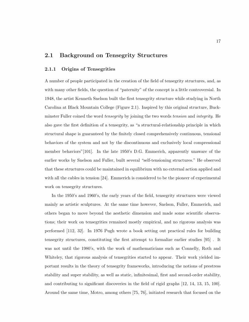
A number of people participated in the creation of the field of tensegrity structures, and, as
with many other fields, the question of “paternity” of the concept is a little controversial. In
1948, the artist Kenneth Snelson built the first tensegrity structure while studying in North
Carolina at Black Mountain College (Figure 2.1). Inspired by this original structure, Buck-
minster Fuller coined the word tensegrity by joining the two words tension and integrity. He
also gave the first definition of a tensegrity, as “a structural-relationship principle in which
structural shape is guaranteed by the finitely closed comprehensively continuous, tensional
behaviors of the system and not by the discontinuous and exclusively local compressional
member behaviors”[101]. In the late 1950’s D.G. Emmerich, apparently unaware of the
earlier works by Snelson and Fuller, built several “self-tensioning structures.” He observed
that these structures could be maintained in equilibrium with no external action applied and
with all the cables in tension [24]. Emmerich is considered to be the pioneer of experimental
work on tensegrity structures.
In the 1950’s and 1960’s, the early years of the field, tensegrity structures were viewed
mainly as artistic sculptures. At the same time however, Snelson, Fuller, Emmerich, and
others began to move beyond the aesthetic dimension and made some scientific observa-
tions; their work on tensegrities remained mostly empirical, and no rigorous analysis was
performed [112, 32]. In 1976 Pugh wrote a book setting out practical rules for building
tensegrity structures, constituting the first attempt to formalize earlier studies [95] . It
was not until the 1980’s, with the work of mathematicians such as Connelly, Roth and
Whiteley, that rigorous analysis of tensegrities started to appear. Their work yielded im-
portant results in the theory of tensegrity frameworks, introducing the notions of prestress
stability and super stability, as well as static, infinitesimal, first and second-order stability,
and contributing to significant discoveries in the field of rigid graphs [12, 14, 13, 15, 100].
Around the same time, Motro, among others [75, 76], initiated research that focused on the

18
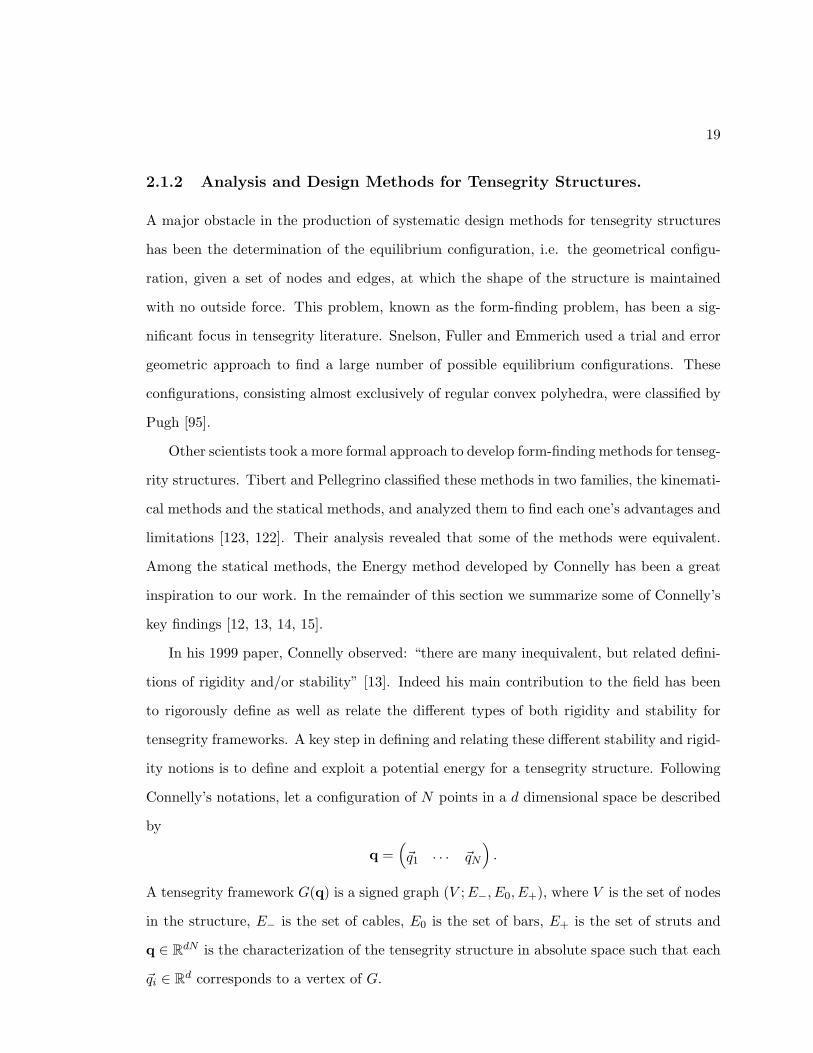
Figure 2.1: The plywood X-Piece built by Kenneth Snelson in 1948. It is considered to bethe first prestressed tensegrity ever built.
dynamics of tensegrity structures. They were able to determine the dynamic characteristics
of a tensegrity prototype by applying a harmonic excitation on one node and measuring the
dynamic response of the other nodes. Mathematicians such as Oppenheim and Williams
took the study of these dynamics further. They proved closed-form analytical solutions for
the vibrations and damping of simple tensegrity structures [134, 88]. During the 1990’s
these structures caught the attention of the control theory community, among them Skel-
ton and Sultan, who went on to develop the concept of controllable tensegrity structures
[111, 117, 116]. Inspired by this concept of controllable structures, civil and aerospace en-
gineers began, in more recent years, to use tensegrity structures for the construction of
deployable domes, bridges, space constructions, and morphing wings, drawn by the aes-
thetic appeal of these constructions as well as by their structural properties [73, 122, 33].
In biology, some scholars argue that tensegrity is a fundamental element of the building
architecture of life [137, 47].
19
2.1.2 Analysis and Design Methods for Tensegrity Structures.
A major obstacle in the production of systematic design methods for tensegrity structures
has been the determination of the equilibrium configuration, i.e. the geometrical configu-
ration, given a set of nodes and edges, at which the shape of the structure is maintained
with no outside force. This problem, known as the form-finding problem, has been a sig-
nificant focus in tensegrity literature. Snelson, Fuller and Emmerich used a trial and error
geometric approach to find a large number of possible equilibrium configurations. These
configurations, consisting almost exclusively of regular convex polyhedra, were classified by
Pugh [95].
Other scientists took a more formal approach to develop form-finding methods for tenseg-
rity structures. Tibert and Pellegrino classified these methods in two families, the kinemati-
cal methods and the statical methods, and analyzed them to find each one’s advantages and
limitations [123, 122]. Their analysis revealed that some of the methods were equivalent.
Among the statical methods, the Energy method developed by Connelly has been a great
inspiration to our work. In the remainder of this section we summarize some of Connelly’s
key findings [12, 13, 14, 15].
In his 1999 paper, Connelly observed: “there are many inequivalent, but related defini-
tions of rigidity and/or stability” [13]. Indeed his main contribution to the field has been
to rigorously define as well as relate the different types of both rigidity and stability for
tensegrity frameworks. A key step in defining and relating these different stability and rigid-
ity notions is to define and exploit a potential energy for a tensegrity structure. Following
Connelly’s notations, let a configuration of N points in a d dimensional space be described
by
q =(~q1 · · · ~qN
).
A tensegrity framework G(q) is a signed graph (V ;E−, E0, E+), where V is the set of nodes
in the structure, E− is the set of cables, E0 is the set of bars, E+ is the set of struts and
q ∈ RdN is the characterization of the tensegrity structure in absolute space such that each
~qi ∈ Rd corresponds to a vertex of G.
20
Tensegrities with the same shape and edges should be viewed as identical. Shape refers
to the way the nodes are arranged relative to one another regardless of where the structure
is or how it is oriented. Thus, a given shape can be associated with an equivalence class
containing an infinite number of absolute position vectors. As we defined in [78], let ~qc =
(1/N)N∑i=1
~qi be the center of mass of the tensegrity. For two configurations q1 ∈ RdN and
q2 ∈ RdN , we define the equivalence relation R as
q1Rq2 ⇐⇒∃(R,~t) ∈ SE(d) and
q2 = (q1 after rigid rotation about ~q1c by R and translation by ~t).
An element of SE(d) is a rigid motion and so any two configurations in the same equivalence
class R have the same shape. We can therefore identify a given shape with the equivalence
class [qe] = q ∈ RdN | qeRq, where qe is a representative configuration with the given
shape. The class [qe] can be identified with SE(d). We note that the ordering of the nodes
in the placement matters to classify shapes since two configurations q1 and q2 representing
the same geometric shape but with nodes permuted will not be in the same equivalence
class.
The edges in E− correspond to cables, the edges in E0 to bars, and the edges in E+ to
struts. Cables are always in tension, struts are always in compression, and bars can bear
both tension and compression. In addition, physical constraints are assumed on the edges:
cables cannot increase in length, struts cannot decrease in length, and bars cannot change
length. For each 1 ≤ i ≤ N and 1 ≤ j ≤ N , we define ωij to be the stress of the edge ij
linking node i and j. This parameter is assumed to be symmetric i.e., ωij = ωji, and in
the case that node i and j are not connected, we have ωij = 0. This collection of stresses
is denoted as one vector ω ∈ RN(N−1)
2 ; in the case that ω has all components non-zero, the
connection topology of the graph is complete. A stress ω on a tensegrity framework is a
proper self stress if the following three conditions are satisfied [15]:
1. ωij ≥ 0 for cables i.e. ij ∈ E−
2. ωij ≤ 0 for struts i.e. ij ∈ E+
21
3.N∑j=1
ωij(qj − qi) = 0 ∀i ∈ 1, · · · , N.
A tensegrity is said to be prestress stable if it has a strict proper self stress (i.e., a
proper self stress with all inequalities strict) such that a certain energy function has a local
minimum at the given configuration [15]. Connelly defines a potential energy and states
sufficient conditions on the defined potential for prestress stability [12]. Given a stress ω,
we have
V (q) =12
N∑i=1
N∑j=i+1
ωij‖~qj − ~qi‖2 (2.1)
where ~qi ∈ Rd is the position vector of node i, x = (x1, . . . , xN )T , y = (y1, . . . , yN )T ,
z = (z1, . . . , zN )T and q =
x
y
z
. (From now on we write∑i<j
to representN∑i=1
N∑j=i+1
.) From
the Energy Principle, if such a potential has a local minimum at qe which is isolated up to
rigid transformation, then the tensegrity framework G(qe) is prestress stable [12, 13].
In order to make the search for critical points of the potential V (q) more systematic
[77, 78], the potential (2.1) is rewritten as the following quadratic form:
V (q) =12qT (Ω⊗ I3)q, (2.2)
where I3 is the 3 × 3 identity matrix, Ω ⊗ I3 is the 3N × 3N block diagonal matrixΩ 0 0
0 Ω 0
0 0 Ω
and the elements of Ω are given by
Ωij =
N∑j=1
ωij if i = j
−ωij if i 6= j.
(2.3)
This matrix Ω introduced by Connelly in [12] is called the stress matrix. The stress matrix
is an N ×N symmetric matrix, and the N -dimensional vector 1 =(
1 · · · 1)T
is in the
kernel of Ω . As mentioned earlier, a sufficient condition for the tensegrity framework to be
prestress stable in a configuration qe is that the quadratic form V (q) have a local minimum
22
at qe. The positive definiteness of V (q) is directly related to that of Ω, but we cannot
expect strict positive definiteness as we already noted that 1 ∈ ker(Ω). In addition, the
necessary condition that ω be a proper self stress can be rewritten as
(Ω⊗ I3)qe = 0. (2.4)
This means that the kernel of Ω should be at least d+ 1 dimensional to make qe a prestress
stable configuration.
Connelly defined a stronger type of prestress stability called super stability which re-
quires prestress stability with the additional condition that Ω be positive semidefinite with
maximal rank, i.e. rank(Ω) = N − d− 1. Hence, to design a super stable tensegrity frame-
work, one must find a set of stresses such that Ω ≥ 0 and dim(ker(Ω)) = d+1. Connelly was
able with this characterization to create and analyze super stable tensegrity frameworks in
the shape of any strictly convex polygons. We will use this characterization in Section 2.3
and adapt them to our setting and motivating application.
2.2 Tensegrity Structures and the Shape Control Problem
Our goal to design control laws that drive vehicle formation into shapes with forces that can
be represented as those internal to tensegrity structures is motivated by the already existing
use of tensegrity structures as controllable structures [111, 116, 117]. Skelton and his col-
laborators who developed the concept of controllable tensegrity structures [111] promoted
them as a “new class of smart structures.” They argued that tensegrity structures present
promising opportunities for control design, with the edges “simultaneously perform-[ing]
the functions of strength, sensing, actuating and feedback control.” In addition, tensegrity
structures are deployable as Tibert has shown [122], meaning that they are capable of large
displacements, making them attractive for modeling a reconfigurable mobile sensor network.
These large displacements, as Skelton argued, can be achieved, moreover, with little change
in the potential energy of the structure [110]. This observation from Skelton and his collab-
orators is justified by the fact that shape changes of tensegrity structures are achieved by
23
changing the equilibrium of the structure, thus removing the need of control energy to hold
the new shape against the previous equilibrium. It suggests that a reconfigurable mobile
sensor network controlled with forces that can be represented as those internal to a tenseg-
rity structures would be energy efficient. It was further shown that the prestress nature of
tensegrity structures is critical in maintaining the shape in the presence of external forces
[109].
We define a one-to-one mapping between the mobile sensor network and a tensegrity
structure as follows [77, 78]: each node of the tensegrity structure is identified with one
vehicle of the network and the edges of the structure correspond to communications and
directions of forces between the vehicles. If an edge is a cable, the force is attractive; if the
edge is a strut, the force is repulsive. The magnitude of the forces depends on the tensegrity
structure parameters as well as the relative distance between the vehicles associated with
the edge. This mapping implies that each vehicle is modeled as a point mass with double
integrator dynamics. The point-mass model may appear somewhat simplistic as it seems to
ignore the challenges of controlling the detailed dynamics of each of the individual vehicles.
However, in practical experiments such as AOSN (Autonomous Ocean Sampling Network),
involving design and implementation of coordinated control for a network of autonomous
underwater vehicles deployed in the ocean, decoupling the design of the coordinating control
strategy from the lower-level, individual-based trajectory tracking control has proven to be
possible and also critical [29]. We thus focus our efforts on the coordinated trajectory design
problem of a group of point masses with double-integrator dynamics.
As we described in the previous section, the form-finding problem has been a major focus
of the tensegrity literature. In order to solve our shape control problem, we essentially have
to solve a “reverse engineering” problem, i.e., determine a set of edges and a model for the
forces that realizes any desired shape. Connelly has proven a conjecture that provides a
means to systematically design stable planar tensegrities in the shape of any strictly convex
polygon [12]. Connelly’s result is valid however only if physical constraints on the edges of
the tensegrity framework are assumed. In our virtual setting, these constraints associated
24
with physical struts and cables have to be relaxed. The restrictions that cables do not
increase in length and struts do not decrease in length, cannot be imposed as constraints
on the distances between pairs of vehicles that are not physically connected. For the same
reason, it is not possible for us to use bars in the tensegrity framework we design. As we will
show, this requires us to modify Connelly’s model by augmenting it. The augmented model
is used to stabilize tensegrities of any arbitrary planar shape and is not limited to strictly
convex polygons. However, in comparison to Connelly’s results, our systematic method
produces a tensegrity framework with often a greater number of edges required. The issue
of the number of edges required to realize a given shape is further discussed in Section 2.5.
2.3 Mathematical Models for the Dynamics of a Tensegrity
In this section we describe two possible models for the forces of a tensegrity structure in
the plane, Connelly’s and our augmented version of it. For each of these models we deter-
mine the equations of motion and the potential of the structure as well as the equilibrium
condition, i.e., the relationship between the choice of cables, struts and parameters for the
corresponding model and its equilibria. We described this first in [77, 78]. In Connelly’s
model, presented in Section 2.1.2, the edges are modeled as linear springs with zero rest
length. Cables have a positive spring constant while struts have a negative one [12, 14].
Hence, as we noted in Section 2.1.2, shape control cannot be achieved with this model
in the constraint free approach we are considering. In the absence of the cable and strut
constraints, Connelly’s model does not yield an isolated equilibrium but a continuum of
equilibria, allowing for arbitrary stretching and shrinking of a tensegrity in the plane. To
isolate planar tensegrities without assuming any constraints on the distances between the
agents, it is necessary to modify the model. We propose a second model built as an aug-
mented version of Connelly’s model. In this model the edges are modeled as springs with
finite, nonzero rest length. Cables are always longer than their rest length, i.e., in tension;
struts are always shorter than their rest length, i.e., in compression.
25
2.3.1 Connelly’s Model
This model for the forces of a tensegrity is derived from Connelly’s potential energy defined
in Section 2.1.2 specialized in the plane. The force ~fi→j ∈ R2 applied to node j as a result
of the presence of node i is derived from the defined potential (2.2) and is given by
~fi→j = ωij(~qi − ~qj) = −~fj→i. (2.5)
Using the force model (2.5), we derive the equations of motion for each node of the tensegrity.
We introduce in the system a linear damping of the form −ν~qn, where ν > 0 is the damping
coefficient. The equations of motion for the nodes of the tensegrity structure in a Cartesian
planar reference frame are computed from Hamilton’s equations as
xi = pxi
yi = pyi
pxi = −νpxi −∂V
∂xi
pyi = −νpyi −∂V
∂yi
∀i ∈ 1, ..., N, (2.6)
where V (q) = qT (Ω ⊗ I2)q and, where (pxi , pyi ) are the momenta of the ith unit mass
particle, respectively, in the x- and the y-directions. From now on the following notations
will be used: q = (x,y) ∈ Q = (R2)N is an element in the configuration space and
z = (q,p) = (x,y,px,py) ∈ T ∗Q = (R4)N is an element in the cotangent bundle, where
px = (px1 , ..., pxN ) and py = (py1, ..., p
yN ).
Our goal is to solve for and stabilize the tensegrity structure such that a desired shape
[qe] is a stable equilibrium of the system. This requires solving for the stresses ωij . In the
case where ωij = 0 is computed for some ij, it is interpreted that nodes i and j are not
connected. ze is an equilibrium of (2.6) if and only if px = py = 0 and qe = (xe,ye) is a
critical point of the potential V (q). Since the potential V (q) only depends on the relative
positions of nodes, then qe is an equilibrium shape of (2.6) if and only if every q ∈ [qe] is
an equilibrium shape of (2.6). Let [ze] = ([qe],0,0), it follows that ze is an equilibrium of
(2.6) if and only if every ze ∈ [ze] is an equilibrium of (2.6).
26
Using the expression of the potential from (2.2) we derive a simple relationship between
the choice of stresses ωij and the equilibria of the model. The critical points of (2.2) and
hence the equilibrium shapes of (2.6) are given by
qT (Ω⊗ I2) = 0. (2.7)
Since the stress matrix is symmetric, a placement qe = (xe,ye) is a critical point of the
potential V (q) if and only if xe and ye are in the kernel of Ω. We note that, assuming
ωij ≥ 0 for cables and ωij ≤ 0 for struts, (2.7) fulfills the last condition to make ω a proper
self stress. Recall that 1 is in the kernel of Ω. Assuming that the nodes are not all in a line,
xe,ye and 1 are linearly independent. We can conclude that with this model a combination
of cables and struts can generate an equilibrium shape if and only if rank(Ω) ≤ N − 3. We
assume from now on that N ≥ 4. By choosing the stresses of the edges of the structure so
that rank(Ω) = N − 3, the kernel of the stress matrix Ω is exactly three dimensional, and
we can prescribe the shape of the equilibrium. We note that choosing the parameters ωij
such that Ω ≥ 0 makes [qe] a super stable tensegrity structure.
However, in our constraint free approach, this model does not prescribe the size of the
equilibrium configuration. Indeed if ker(Ω) = spanxe,ye,1 then [qe] = [(αxe, βye)] is also
an equilibrium shape ∀α, β ∈ R. For real tensegrities this is not a problem because the cable
and strut constraints are incompatible with the shapes [qe] = [(αxe, βye)] for (α, β) 6= (1, 1).
In the virtual setting, however, where the same constraints cannot be imposed, we get a
continuum of equilibria, which is not desirable. For example, if the prescribed shape for the
tensegrity is a square, it will be the case that not only all squares but also all rectangles
will be equilibria.
In order to use tensegrity structures in our virtual setting, we need to modify this model
to isolate the equilibrium. In the next section we exploit the simple equation (2.7), derived
using the linear model (2.5), that determines the geometry of the tensegrity as a function
of the parameters ωij . We propose an augmented model for the forces along edges that
isolates a shape, fixing both geometry and size.
27
2.3.2 Augmented Model
Modeling the edges as springs with zero rest length yielded, in the absence of physical
constraints on the edges, a continuum of equilibria for the system (2.6), fixing only the
geometry of the structure but not its size. To isolate the equilibrium of the size of the desired
shape, we augment Connelly’s model and make the edges linear springs with finite, nonzero
rest length. In this augmented model, cables are always longer than their rest length, i.e.,
in tension, and struts are always shorter than their rest length i.e. in compression. For two
nodes i, j we define
~fi→j = αijωijrij − lijrij
(~qi − ~qj) = −~fj→i. (2.8)
Here rij = ‖~qi − ~qj‖ is the relative distance between nodes i and j, lij is the rest length of
the spring that models the edge ij, ωij is the spring constant/stress from model (2.5), and
αij is a scalar parameter that fixes the spring constant of model (2.8) for the edge ij. With
these forces, the potential of a tensegrity framework is given by
V (q) =12
∑i<j
αijωij(rij − lij)2. (2.9)
With the same damping used in (2.6), the equations of motion are
xi = pxi
yi = pyi
pxi = −νpxi −N∑j=1
ωij(xi − xj)
pyi = −νpyi −N∑j=1
ωij(yi − yj)
∀i ∈ 1, ..., N, (2.10)
where ωij is given by
ωij(x,y) = αijωij(1− lijrij
). (2.11)
Our goal again is to solve for and stabilize the tensegrity structure such that [qe] is an
equilibrium shape of the system (2.10), i.e., to find the relationship between the choice
of parameters αij , lij and ωij and the equilibrium shapes of the system (2.10). As in the
28
previous model, since V (q) only depends on the relative position of nodes, then qe is an
equilibrium shape of (2.10) if and only if every q ∈ [qe] is an equilibrium shape of (2.10).
We likewise define [ze] = ([qe],0,0). Then ze is an equilibrium of (2.10) if and only if every
z ∈ [ze] is an equilibrium of (2.10). As for model (2.6), ze is an equilibrium of (2.10) if and
only if px = py = 0 and qe = (xe,ye) is a critical point of the potential V (q). The critical
points of V (q) are given by
N∑j=1
αijωij(~qj − ~qi)(1− lijrij
) = 0, i = 1, . . . , N. (2.12)
From (2.12), an analogue of the stress matrix Ω is constructed. The new stress matrix is
not a constant matrix and depends on the relative distances between pairs of nodes. The
entries of the new stress matrix are given by
Ωij(x,y) =
N∑j=1
ωij(x,y) if i = j
−ωij(x,y) if i 6= j
where ωij , the stress of the edge ij (now state dependent), is defined by (2.11). The vector
1 is also in the kernel of Ω, ∀ (x,y) ∈ R2N .
This new state dependent stress matrix is now used to characterize the equilibria of
(2.10). To make a shape [qe] a critical point of the potential, we need to pick (if possible)
the parameters αij , lij and ωij so that for all q = (x,y) ∈ [qe],
Ω(x,y)x = 0
Ω(x,y)y = 0.(2.13)
We show in the next section that it is possible to choose the parameters αij , lij and ωij such
that equation (2.13) is solved and that [ze] = ([qe],0,0) is an isolated exponentially stable
equilibrium set of (2.10).
2.4 Stabilization for a Desired Group Geometry
Our goal is to solve for and stabilize the tensegrity structure so that [ze] = ([qe],0,0) is
a stable equilibrium set of (2.10) making [qe] a stable shape of the tensegrity framework.
29
This requires us to find the parameters αij , lij and ωij that solve (2.13). We present in
this section a systematic method to choose the parameters αij , lij and ωij to solve (2.13).
Further, we prove that this choice of parameters makes [ze] = ([qe],0,0) an isolated locally
exponentially stable equilibrium set of (2.10). These developments have been described in
[77, 78].
2.4.1 Smooth Parameterization of the Model
For any desired group shape [qe], we explain how to choose the parameters αij , lij and ωij
to make [qe] an isolated equilibrium shape of the system. As a first step we choose the
parameters αij and lij for all i, j so that Ω(xe,ye) = Ω. In order to make ωij(xe,ye) = ωij ,
we choose αij , lij such that αij(1− lijreij
) = 1. This last equation is solved by picking
αij =π
arctanωij
lij = reij
(1− 1
πarctanωij
).
(2.14)
In the case where edge ij is a strut, then ωij < 0, and equation (2.14) makes αij < 0 and
lij > reij . This is consistent with the assumption that a strut is modeled as a linear spring,
with a positive spring constant αijωij > 0, shorter than its rest length. In the case that
edge ij is a cable, then ωij > 0, and equation (2.14) makes αij > 0 and lij < reij . This is
consistent with the assumption that a cable is modeled as a linear spring, with a positive
spring constant αijωij > 0, longer than its rest length. The choice of lij and αij is not
unique, but rather was chosen to make the vector field (2.10) a C∞ map of ωij and reij .
This result is critical in the next chapter to prove that the time varying control law that
changes the shape of the formation from any initial shape to any final desired shape is well
behaved.
We now show that the parameters ωij can be found independently of parameters αij
and lij , such that ker(Ω) = spanxe,ye,1 and the nonzero eigenvalues of Ω are all strictly
positive. This makes the equilibrium shape [qe] = (xe,ye) an isolated minimum of the
potential V (q), i.e., our choices ensure that we have the right combination of struts and
30
cables to make [qe] a stable equilibrium shape. The stress matrix Ω is symmetric; hence it
has only real eigenvalues and can be diagonalized using an orthonormal basis. As mentioned
previously, assuming that all the nodes are not in a line, then xe,ye and 1 are linearly
independent. We complete these three vectors with N − 3 others and obtain a basis of RN .
Then applying the Gram-Schmidt procedure to those vectors yields an orthonormal basis
(v1, . . . ,vN ) for RN that satisfies
spanv1,v2,v3 = spanxe,ye,1.
We now define the N × N diagonal matrix D with diagonal elements (0, 0, 0, d4, . . . , dN ),
where di > 0 ∀i, and the orthonormal N×N matrix Λ =(v1 · · · vN
). The matrix com-
puted as ΛDΛT , is symmetric positive semi-definite with its kernel equal to spanxe,ye,1.Setting Ω = ΛDΛT determines values of stresses ωij that make the desired shape [qe] a
tensegrity structure. The choice of eigenvalues D and eigenvectors Λ for the stress matrix
is not unique. In Section 2.5.2 we investigate, through an example, how the choice of D and
Λ influences the resulting interconnection topology that is needed to achieve the desired
shape.
We now prove that this choice of parameters makes [ze] an isolated equilibrium set of
(2.10).
Theorem 2.4.1 Choosing the parameters αij , lij and ωij to solve (2.13) makes [ze] =
([qe],0,0) an isolated equilibrium set of (2.10).
Proof: In order to prove this result, we show that [qe] is an isolated critical point of V (q)
by proving that the second variation of V (q), evaluated at [qe] is a positive definite matrix
except in the symmetry directions SE(2). As we pointed out earlier, the potential V (q)
only depends on the relative distances between nodes. This implies that V (q) and also
the Lagrangian of the system are invariant under the action of the Lie group SE(2) on the
configuration space Q. With these symmetries, critical points of V (q) are only isolated
modulo SE(2) transformation making δ2V (qe) not definite in these directions. The matrix
31
δ2V (qe) is given by
δ2V (qe) =
Ω + Lωx(qe) Lωxy(qe)
Lωxy(qe) Ω + Lωy(qe)
(2.15)
where Ω is the stress matrix derived in equation (2.3) and the ijth element of each bloc
matrix is
Lωx(i, j) =
−αijωij (xi−xj)2lij
r3ij
if i 6= j
N∑j=1,j 6=i
αijωij(xi−xj)2lij
r3ij
if i = j
Lωy(i, j) =
−αijωij (yi−yj)2lij
r3ij
if i 6= j
N∑j=1,j 6=i
αijωij(yi−yj)2lij
r3ij
if i = j
and
Lωxy(i, j) =
−αijωij (xi−xj)(yi−yj)lij
r3ij
if i 6= j
N∑j=1,j 6=i
αijωij(xi−xj)(yi−yj)lij
r3ij
if i = j.
Lemma 2.4.2 δ2V (qe) is a positive semi-definite matrix.
Proof: We write δ2V (qe) as
δ2V (qe) = M1 +M2 =
Ω 0N
0N Ω
+
Lωx Lωxy
Lωxy Lωy
.
Recall that Ω is designed to be positive semi-definite, hence M1 ≥ 0. We then show that
M2 is positive semi-definite. By direct computation,
(qTx qTy
) Lωx Lωxy
Lωxy Lωy
qx
qy
= qTxLωxqx + qTy Lωyqy + 2qTxLωxyqy, (2.16)
where qx = (qx1 · · · qxN )T ∈ RN , and qy = (qy1 · · · qyN )T ∈ RN . Each term of the sum can
32
be rewritten as
qTxLωxqx =N∑i=1
N∑j=1,j 6=i
qxiαijωij(xi − xj)2lij
r3ij
(qxi − qxj )
=∑i<j
αijωij(xi − xj)2lijr3ij
(qxi − qxj )2,
qTy Lωyqy =N∑i=1
N∑j=1,j 6=i
qyiαijωij(yi − yj)2lij
r3ij
(qyi − qyj )
=∑i<j
αijωij(yi − yj)2lijr3ij
(qyi − qyj )2,
qTxLωxyqy =N∑i=1
N∑j=1,j 6=i
qxiαijωij(xi − xj)(yi − yj)lij
r3ij
(qyi − qyj )
=∑i<j
αijωij(xi − xj)(yi − yj)lijr3ij
(qyi − qyj )(qxi − qxj ).
(2.16) can now be factored as
qTxLωxqx+qTy Lωyqy+2qTxLωxyqy =∑i<j
αijωijlijr3ij
((yi−yj)(qyi−qyj )+(xi−xj)(qxi−qxj )
)2 ≥ 0.
(2.17)
Equation (2.17) concludes the proof that M2 ≥ 0, and hence δ2V (qe) ≥ 0
Lemma 2.4.3 The kernel of δ2V (qe) is equal to
span
1
0
,
0
1
,
−ye
xe
.
Proof: We write again δ2V (qe) as
δ2V (qe) = M1 +M2 =
Ω 0N
0N Ω
+
Lωx Lωxy
Lωxy Lωy
.
By Lemma 2.4.2, M1 and M2 are symmetric, positive semi-definite matrices, hence
q ∈ ker(δ2V (qe))⇐⇒ q ∈ ker(M1) and q ∈ ker(M2). (2.18)
By design, ker(M1) = spanw1,w2,w3; by direct computation, we check spanw1,w2,w3 ∈ker(M2). Using (2.18), we conclude that the kernel of δ2V (qe) is exactly spanned by
w1,w2,w3.
33
We can now conclude the proof of the theorem by combining these two lemmas. By
Lemma 2.4.3, the three linearly independent eigenvectors for the three zero eigenvalues
are
1
0
,
0
1
,
−ye
xe
. These vectors correspond respectively to symmetries
of translation along the x-axis and the y-axis and of rotation about the origin. In addi-
tion, Lemma 2.4.2 guarantees that all other eigenvalues of δ2V (qe) are strictly positive.
Combining Lemma 2.4.2 and Lemma 2.4.3 concludes the proof of the theorem.
2.4.2 Stability Analysis
We now present the proof of the local exponential stability for the isolated equilibrium set
[ze] using the linearization of (2.10).
Theorem 2.4.4 [ze] = ([qe],0,0) is a locally exponentially stable equilibrium set of (2.10).
Proof: We prove local exponential stability for the isolated equilibrium set [ze] using the
linearization of (2.10). The Jacobian of (2.10) evaluated at ze = (xe,ye,0,0) is given by
Dg(ze) =
02n I2n
−δ2V (qe) −νI2n
. (2.19)
We show that this matrix is negative semi-definite and that the three zero eigenvalues
correspond to the symmetry directions SE(2). The linearization Dg(ze) can be written as
Dg(ze) =
1ν δ
2V (qe) I2n
−δ2V (qe) −νI2n
+
− 1ν δ
2V (qe) 02n
02n 02n
= B1 +B2.
By Lemma 2.4.2, B2 is negative semi definite. To show that B1 is also negative semi definite,
we proceed to two changes of basis represented by the following two invertible matrices:
P1 =
1ν I2n
1ν I2n
02n I2n
P2 =
02n I2n
I2n1ν δ
2V (qe)(
1ν δ
2V (qe)− νI2n
)−1
.
34
The representation of B1 in the new basis is computed as
P−12 P−1
1 B1P1P2 =
1ν δ
2V (qe)− νI2n 02n
02n 02n
.
This matrix is negative semi definite ∀ν > √λmax(δ2V (qe)), where λmax(δ2V (qe)
)is the
largest eigenvalue of δ2V (qe). We now show by direct computation that the zero eigenvalues
correspond to the SE(2) symmetries.
02n I2n
−δ2V (qe) −νI2n
x
y
px
py
=
0
0
0
0
if and only if
px
py
−δ2V (qe)
x
y
− νI2n
px
py
=
0
0
0
0
if and only if
x
y
px
py
∈ span
1
0
0
0
,
0
1
0
0
,
−ye
xe
0
0
.
These three vectors correspond respectively to symmetries of translation along the x-axis
and the y-axis and of rotation about the origin.
Local asymptotic stability can also be proven using the total energy of the system as a
Lyapunov function. In the next chapter we utilize the exponential stability result for the
equilibrium set [ze] = ([qe],0,0) to construct a well behaved time-dependent control law
that enables the tensegrity to reconfigure itself between arbitrary planar shapes.
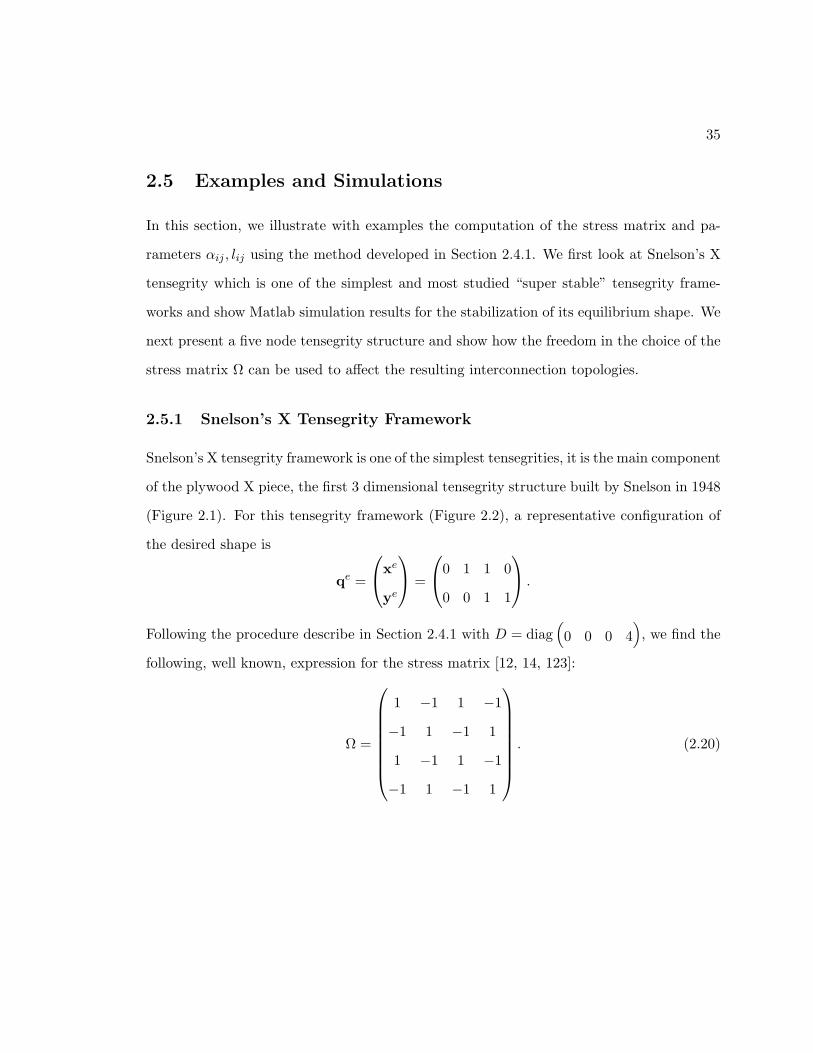
35
2.5 Examples and Simulations
In this section, we illustrate with examples the computation of the stress matrix and pa-
rameters αij , lij using the method developed in Section 2.4.1. We first look at Snelson’s X
tensegrity which is one of the simplest and most studied “super stable” tensegrity frame-
works and show Matlab simulation results for the stabilization of its equilibrium shape. We
next present a five node tensegrity structure and show how the freedom in the choice of the
stress matrix Ω can be used to affect the resulting interconnection topologies.
2.5.1 Snelson’s X Tensegrity Framework
Snelson’s X tensegrity framework is one of the simplest tensegrities, it is the main component
of the plywood X piece, the first 3 dimensional tensegrity structure built by Snelson in 1948
(Figure 2.1). For this tensegrity framework (Figure 2.2), a representative configuration of
the desired shape is
qe =
xe
ye
=
0 1 1 0
0 0 1 1
.
Following the procedure describe in Section 2.4.1 with D = diag(
0 0 0 4)
, we find the
following, well known, expression for the stress matrix [12, 14, 123]:
Ω =
1 −1 1 −1
−1 1 −1 1
1 −1 1 −1
−1 1 −1 1
. (2.20)
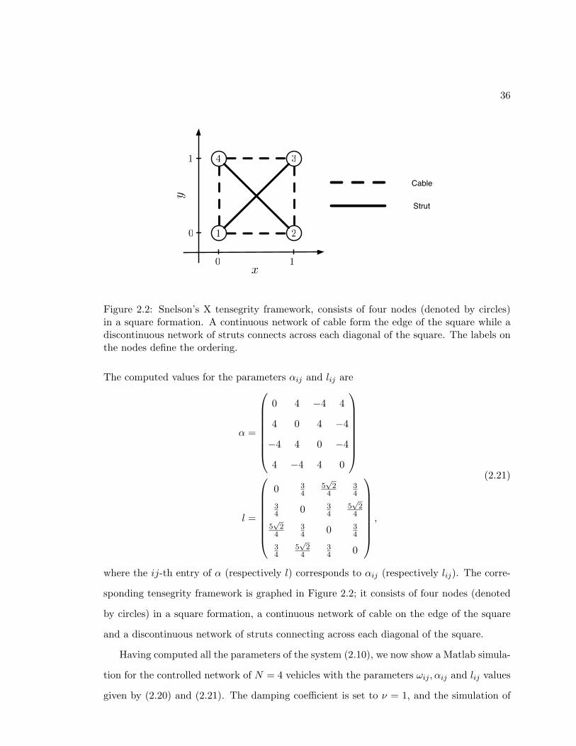
36
1
34
20
0
1
1
y
x
Cable
Strut
Figure 2.2: Snelson’s X tensegrity framework, consists of four nodes (denoted by circles)in a square formation. A continuous network of cable form the edge of the square while adiscontinuous network of struts connects across each diagonal of the square. The labels onthe nodes define the ordering.
The computed values for the parameters αij and lij are
α =
0 4 −4 4
4 0 4 −4
−4 4 0 −4
4 −4 4 0
l =
0 34
5√
24
34
34 0 3
45√
24
5√
24
34 0 3
4
34
5√
24
34 0
,
(2.21)
where the ij-th entry of α (respectively l) corresponds to αij (respectively lij). The corre-
sponding tensegrity framework is graphed in Figure 2.2; it consists of four nodes (denoted
by circles) in a square formation, a continuous network of cable on the edge of the square
and a discontinuous network of struts connecting across each diagonal of the square.
Having computed all the parameters of the system (2.10), we now show a Matlab simula-
tion for the controlled network of N = 4 vehicles with the parameters ωij , αij and lij values
given by (2.20) and (2.21). The damping coefficient is set to ν = 1, and the simulation of
37
the system is run from t = 0s to t = 20s. The initial conditions are given by
x1(0) x2(0) x3(0) x4(0)
y1(0) y2(0) y3(0) y4(0)
x1(0) x2(0) x3(0) x4(0)
y1(0) y2(0) y3(0) y4(0)
=
−1 2 0 −2
−1 1 2 1
1 −2 3 0
12 0 2 −1
,
where xi, yi have units of m and xi, yi have units of m/s. Figure 2.3 shows plots of the
positions for each of the four networked vehicles and Figure 2.4 shows plots of the velocities
for each of the four networked vehicles, after some oscillations, convergence to a fixed shape
is obvious. In Figure 2.5 snapshots of the tensegrity network are plotted at t = 0s, 0.25s, 2s
and at t = 20. The prescribed shape [qe] is indeed reached by the vehicle network but the
structure is both translated and rotated from qe. This is due to the initial conditions and
the changing linear and angular momentum of the system. It highlights the fact that we are
only controlling the shape of the formation but not its position or orientation in absolute
space.
2.5.2 A Five Vehicle Network Example
We now illustrate with a five node tensegrity network example the effect of the choices of
eigenvalues D and eigenvector Λ of the stress matrix Ω on the resulting interconnection
topology of the tensegrity realizing the desired shape. This study is reported in [77, 78]. It
is known that stable tensegrity structures with N nodes require at least 2N − 2 edges [14].
Connelly has proven a result that provides a means to systematically design stable planar
tensegrities in the shape of any strictly convex polygon [12]. His method is designed to yield
tensegrity structures with minimal number of edges. Our method allows us to generate
tensegrity structures of any shape, convex or non-convex, but often yields interconnection
topologies with number of edges greater than the proven lower bound. However, as we
illustrate, it is possible in our method to use the freedom of choice in the eigenvalues and
eigenvectors of the stress matrix to reduce the number of edges.
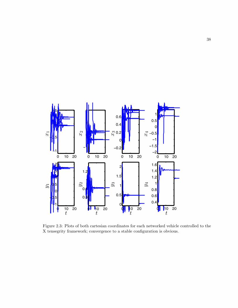
38
0 10 20
!1
!0.5
0
0.5
t
x1(
t)
0 10 20
!1
!0.5
0
0.5
1
1.5
2
t
y1(
t)
0 10 20
!1
0
1
2
t
x2(
t)
0 10 20
0.6
0.8
1
1.2
t
y2(
t)
0 10 20
!0.2
0
0.2
0.4
0.6
t
x3(
t)
0 10 20
0
0.5
1
1.5
2
t
y3(
t)
0 10 20
!2
!1.5
!1
!0.5
0
0.5
1
t
x4(
t)
0 10 20
0.4
0.6
0.8
1
1.2
1.4
1.6
t
y4(
t)0 10 20
!1
!0.5
0
0.5
t
x1(
t)
0 10 20
!1
!0.5
0
0.5
1
1.5
2
t
y1(
t)
0 10 20
!1
0
1
2
t
x2(
t)
0 10 20
0.6
0.8
1
1.2
t
y2(
t)
0 10 20
!0.2
0
0.2
0.4
0.6
t
x3(
t)
0 10 20
0
0.5
1
1.5
2
t
y3(
t)
0 10 20
!2
!1.5
!1
!0.5
0
0.5
1
t
x4(
t)
0 10 20
0.4
0.6
0.8
1
1.2
1.4
1.6
t
y4(
t)
0 10 20
!1
!0.5
0
0.5
t
x1(
t)
0 10 20
!1
!0.5
0
0.5
1
1.5
2
t
y1(
t)
0 10 20
!1
0
1
2
t
x2(
t)
0 10 20
0.6
0.8
1
1.2
t
y2(
t)
0 10 20
!0.2
0
0.2
0.4
0.6
t
x3(
t)
0 10 20
0
0.5
1
1.5
2
t
y3(
t)
0 10 20
!2
!1.5
!1
!0.5
0
0.5
1
t
x4(
t)
0 10 20
0.4
0.6
0.8
1
1.2
1.4
1.6
t
y4(
t)
0 10 20
!1
!0.5
0
0.5
t
x1(
t)
0 10 20
!1
!0.5
0
0.5
1
1.5
2
t
y1(
t)
0 10 20
!1
0
1
2
t
x2(
t)
0 10 20
0.6
0.8
1
1.2
t
y2(
t)
0 10 20
!0.2
0
0.2
0.4
0.6
t
x3(
t)
0 10 20
0
0.5
1
1.5
2
t
y3(
t)
0 10 20
!2
!1.5
!1
!0.5
0
0.5
1
t
x4(
t)
0 10 20
0.4
0.6
0.8
1
1.2
1.4
1.6
t
y4(
t)0 10 20
!1
!0.5
0
0.5
t
x1(
t)
0 10 20
!1
!0.5
0
0.5
1
1.5
2
t
y1(
t)
0 10 20
!1
0
1
2
t
x2(
t)
0 10 20
0.6
0.8
1
1.2
t
y2(
t)
0 10 20
!0.2
0
0.2
0.4
0.6
t
x3(
t)
0 10 20
0
0.5
1
1.5
2
t
y3(
t)
0 10 20
!2
!1.5
!1
!0.5
0
0.5
1
tx4(
t)
0 10 20
0.4
0.6
0.8
1
1.2
1.4
1.6
t
y4(
t)0 10 20
!1
!0.5
0
0.5
t
x1(
t)
0 10 20
!1
!0.5
0
0.5
1
1.5
2
t
y1(
t)
0 10 20
!1
0
1
2
t
x2(
t)
0 10 20
0.6
0.8
1
1.2
t
y2(
t)
0 10 20
!0.2
0
0.2
0.4
0.6
t
x3(
t)
0 10 20
0
0.5
1
1.5
2
t
y3(
t)
0 10 20
!2
!1.5
!1
!0.5
0
0.5
1
t
x4(
t)
0 10 20
0.4
0.6
0.8
1
1.2
1.4
1.6
t
y4(
t)0 10 20
!1
!0.5
0
0.5
t
x1(
t)
0 10 20
!1
!0.5
0
0.5
1
1.5
2
t
y1(
t)
0 10 20
!1
0
1
2
t
x2(
t)
0 10 20
0.6
0.8
1
1.2
t
y2(
t)
0 10 20
!0.2
0
0.2
0.4
0.6
t
x3(
t)
0 10 20
0
0.5
1
1.5
2
t
y3(
t)
0 10 20
!2
!1.5
!1
!0.5
0
0.5
1
t
x4(
t)
0 10 20
0.4
0.6
0.8
1
1.2
1.4
1.6
t
y4(
t)0 10 20
!1
!0.5
0
0.5
t
x1(
t)
0 10 20
!1
!0.5
0
0.5
1
1.5
2
t
y1(
t)
0 10 20
!1
0
1
2
t
x2(
t)
0 10 20
0.6
0.8
1
1.2
t
y2(
t)
0 10 20
!0.2
0
0.2
0.4
0.6
t
x3(
t)
0 10 20
0
0.5
1
1.5
2
t
y3(
t)
0 10 20
!2
!1.5
!1
!0.5
0
0.5
1
t
x4(
t)
0 10 20
0.4
0.6
0.8
1
1.2
1.4
1.6
t
y4(
t)
x1
y 1
t t t t
x2
y 2 y 3x
3
x4
y 4
Figure 2.3: Plots of both cartesian coordinates for each networked vehicle controlled to theX tensegrity framework; convergence to a stable configuration is obvious.
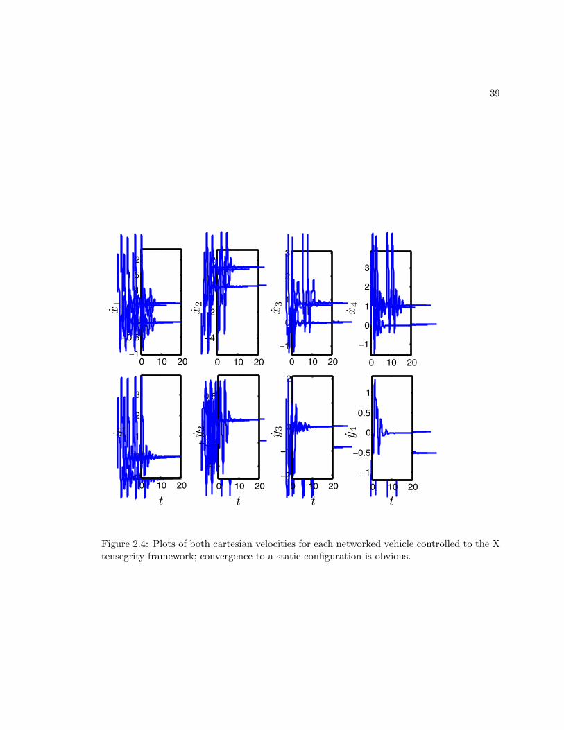
39
t t t t
0 10 20!1
!0.5
0
0.5
1
1.5
2
t
x1(
t)
0 10 20!1
0
1
2
3
t
y1(
t)
0 10 20
!4
!2
0
2
t
x2(
t)
0 10 20
!1
!0.5
0
0.5
t
y2(
t)
0 10 20
!1
0
1
2
3
t
x3(
t)
0 10 20
!2
!1
0
1
2
t
y3(
t)
0 10 20
!1
0
1
2
3
tx4(
t)
0 10 20
!1
!0.5
0
0.5
1
t
y4(
t)0 10 20
!1
!0.5
0
0.5
1
1.5
2
t
x1(
t)
0 10 20!1
0
1
2
3
t
y1(
t)
0 10 20
!4
!2
0
2
t
x2(
t)
0 10 20
!1
!0.5
0
0.5
t
y2(
t)
0 10 20
!1
0
1
2
3
t
x3(
t)
0 10 20
!2
!1
0
1
2
t
y3(
t)
0 10 20
!1
0
1
2
3
tx4(
t)
0 10 20
!1
!0.5
0
0.5
1
t
y4(
t)0 10 20
!1
!0.5
0
0.5
1
1.5
2
t
x1(
t)
0 10 20!1
0
1
2
3
t
y1(
t)
0 10 20
!4
!2
0
2
t
x2(
t)
0 10 20
!1
!0.5
0
0.5
t
y2(
t)
0 10 20
!1
0
1
2
3
t
x3(
t)
0 10 20
!2
!1
0
1
2
t
y3(
t)
0 10 20
!1
0
1
2
3
t
x4(
t)
0 10 20
!1
!0.5
0
0.5
1
t
y4(
t)0 10 20
!1
!0.5
0
0.5
1
1.5
2
t
x1(
t)
0 10 20!1
0
1
2
3
t
y1(
t)
0 10 20
!4
!2
0
2
t
x2(
t)
0 10 20
!1
!0.5
0
0.5
t
y2(
t)
0 10 20
!1
0
1
2
3
t
x3(
t)
0 10 20
!2
!1
0
1
2
t
y3(
t)
0 10 20
!1
0
1
2
3
t
x4(
t)
0 10 20
!1
!0.5
0
0.5
1
t
y4(
t)0 10 20
!1
!0.5
0
0.5
1
1.5
2
t
x1(
t)
0 10 20!1
0
1
2
3
t
y1(
t)
0 10 20
!4
!2
0
2
t
x2(
t)
0 10 20
!1
!0.5
0
0.5
t
y2(
t)
0 10 20
!1
0
1
2
3
t
x3(
t)
0 10 20
!2
!1
0
1
2
t
y3(
t)
0 10 20
!1
0
1
2
3
t
x4(
t)
0 10 20
!1
!0.5
0
0.5
1
t
y4(
t)
0 10 20!1
!0.5
0
0.5
1
1.5
2
t
x1(
t)
0 10 20!1
0
1
2
3
t
y1(
t)
0 10 20
!4
!2
0
2
t
x2(
t)
0 10 20
!1
!0.5
0
0.5
t
y2(
t)
0 10 20
!1
0
1
2
3
t
x3(
t)
0 10 20
!2
!1
0
1
2
t
y3(
t)
0 10 20
!1
0
1
2
3
tx4(
t)
0 10 20
!1
!0.5
0
0.5
1
t
y4(
t)0 10 20
!1
!0.5
0
0.5
1
1.5
2
t
x1(
t)
0 10 20!1
0
1
2
3
t
y1(
t)
0 10 20
!4
!2
0
2
t
x2(
t)
0 10 20
!1
!0.5
0
0.5
t
y2(
t)
0 10 20
!1
0
1
2
3
t
x3(
t)
0 10 20
!2
!1
0
1
2
t
y3(
t)
0 10 20
!1
0
1
2
3
tx4(
t)
0 10 20
!1
!0.5
0
0.5
1
t
y4(
t)0 10 20
!1
!0.5
0
0.5
1
1.5
2
t
x1(
t)
0 10 20!1
0
1
2
3
t
y1(
t)
0 10 20
!4
!2
0
2
t
x2(
t)
0 10 20
!1
!0.5
0
0.5
t
y2(
t)
0 10 20
!1
0
1
2
3
t
x3(
t)
0 10 20
!2
!1
0
1
2
t
y3(
t)
0 10 20
!1
0
1
2
3
tx4(
t)
0 10 20
!1
!0.5
0
0.5
1
t
y4(
t)
x1
x2
x3
x4
y 4y 3y 2y 1
Figure 2.4: Plots of both cartesian velocities for each networked vehicle controlled to the Xtensegrity framework; convergence to a static configuration is obvious.
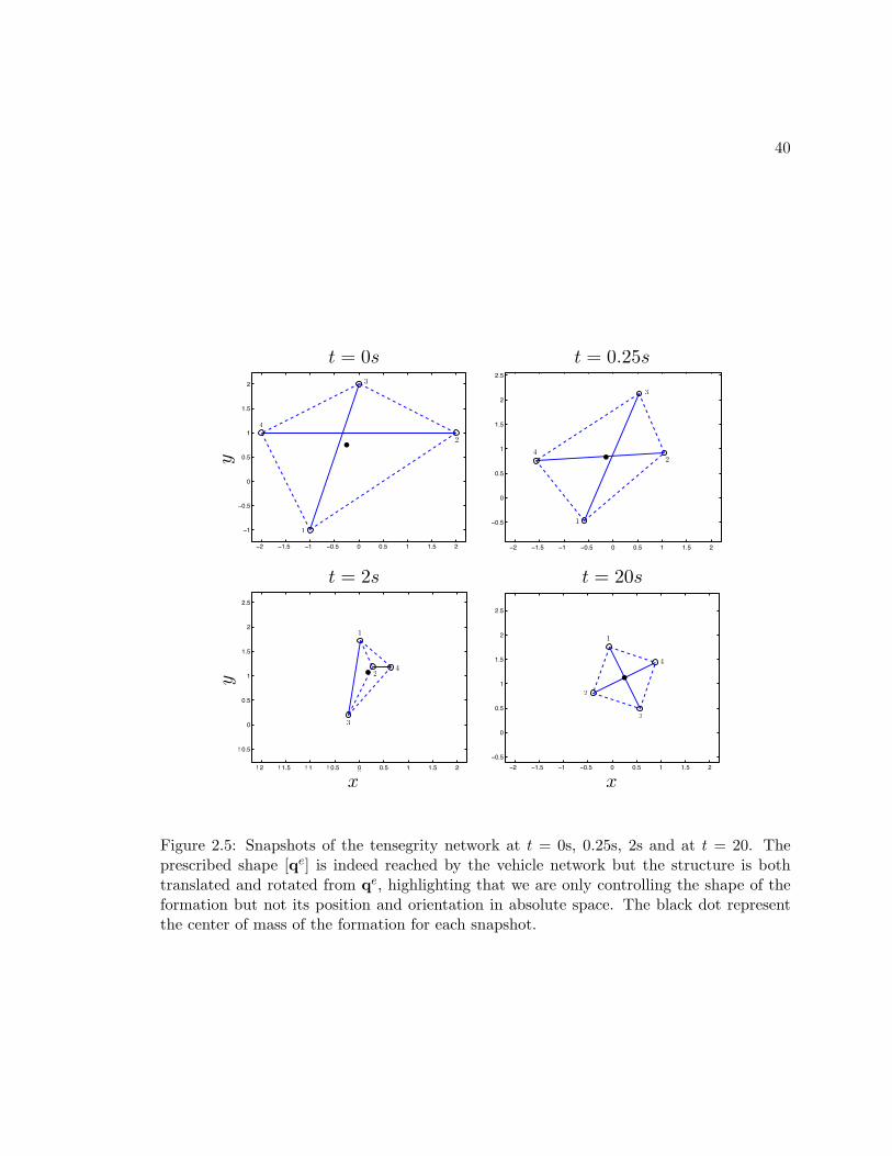
40
!! !"#$ !" !%#$ % %#$ " "#$ !
!"
!%#$
%
%#$
"
"#$
!
x
y
!! !"#$ !" !%#$ % %#$ " "#$ !
!%#$
%
%#$
"
"#$
!
!#$
x
y
! ! ! "#$ ! " ! %#$ % %#$ " "#$ !
! %#$
%
%#$
"
"#$
!
!#$
x
y
!! !"#$ !" !%#$ % %#$ " "#$ !
!%#$
%
%#$
"
"#$
!
!#$
x
y
t = 0s t = 0.25s
t = 2s t = 20s
x x
yy
Figure 2.5: Snapshots of the tensegrity network at t = 0s, 0.25s, 2s and at t = 20. Theprescribed shape [qe] is indeed reached by the vehicle network but the structure is bothtranslated and rotated from qe, highlighting that we are only controlling the shape of theformation but not its position and orientation in absolute space. The black dot representthe center of mass of the formation for each snapshot.
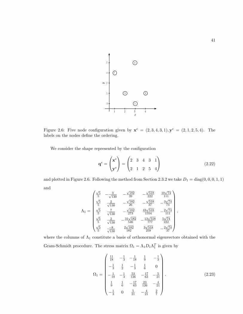
41
1 3
4
21
1
y
x
2
3
4
5
432
5
Figure 2.6: Five node configuration given by xe = (2, 3, 4, 3, 1),ye = (2, 1, 2, 5, 4). Thelabels on the nodes define the ordering.
We consider the shape represented by the configuration
qe =
xe
ye
=
2 3 4 3 1
2 1 2 5 4
(2.22)
and plotted in Figure 2.6. Following the method from Section 2.3.2 we takeD1 = diag(0, 0, 0, 1, 1)
and
Λ1 =
√5
5 − 3√130
−√
18239 −
√518
22210√
74111
√5
52√130
−√
18226 −
√51837 −3
√74
74√
55
7√130
−√
182273
43√
5181554 −2
√74
111√
55
2√130
−31√
182546 −13
√518
7775√
74222
√5
5−8√130
2√
182182
3√
518259 −2
√74
37
,
where the columns of Λ1 constitute a basis of orthonormal eigenvectors obtained with the
Gram-Schmidt procedure. The stress matrix Ω1 = Λ1D1ΛT1 is given by
Ω1 =
1118 −1
3 − 118
19 −1
3
−13
12 −1
316 0
− 118 −1
353126 −17
63 − 521
19
16 −17
6323126 − 4
21
−13 0 5
21 − 421
27
. (2.23)
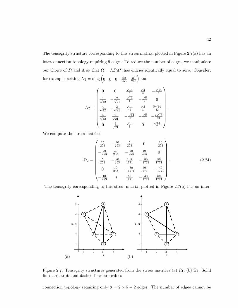
42
The tensegrity structure corresponding to this stress matrix, plotted in Figure 2.7(a) has an
interconnection topology requiring 9 edges. To reduce the number of edges, we manipulate
our choice of D and Λ so that Ω = ΛDΛT has entries identically equal to zero. Consider,
for example, setting D2 = diag(
0 0 0 60253
30253
)and
Λ2 =
0 0√
146
√2
3 −√
146
1√42− 2√
21
√147 −
√2
2 0
4√42− 2√
21
√14
42
√2
35√
1442
5√42
2√21
−√
1421 −
√2
6 −2√
1421
0 3√21
√147 0
√147
.
We compute the stress matrix:
Ω2 =
25253 − 20
2535
253 0 − 10253
− 20253
30253 − 20
25310253 0
5253 − 20
2531351771 − 80
177150
1771
0 10253 − 80
177150
1771 − 401771
− 10253 0 50
1771 − 401771
601771
. (2.24)
The tensegrity corresponding to this stress matrix, plotted in Figure 2.7(b) has an inter-
(a)
1 3
4
21
1
y
x
2
3
4
5
432
5
(b)
1 3
4
21
1
y
x
2
3
4
5
432
5
Figure 2.7: Tensegrity structures generated from the stress matrices (a) Ω1, (b) Ω2. Solidlines are struts and dashed lines are cables
connection topology requiring only 8 = 2 × 5 − 2 edges. The number of edges cannot be
43
reduced further since we have reached the lower bound proven in [14]. We note that not
only the number of edges required is different between the tensegrities realized by Ω1 and
Ω2 but also the nature of the edges. While both tensegrities have a continuous network of
cables around, the tensegrity realized by Ω1 has inside a discontinuous network of cables and
strut and the tensegrity realized by Ω2 has inside a discontinuous network of only struts.
Tensegrities with a continuous network of cables around and a discontinuous network of
struts is a common outcome of the method designed by Connelly in [14].
As the number of nodes increases, it becomes harder to systematically find a combination
of eigenvalues and eigenvectors that yields a tensegrity with the minimum number of edges.
However, as the above example illustrates, it may be possible to manipulate the choices of
D and Λ to reduce the number of connections in a tensegrity derived using our method.
Our approach has significant advantages because it is systematic and smooth. We exploit
these features in the next chapter, where we define a smooth parameterization (by time)
of the control law (2.10), creating a systematic framework for smooth reconfiguration of
tensegrity structures between arbitrary planar shapes.
Chapter 3
Group Reconfiguration and
Tensegrity Structure
In the previous chapter, we created a framework to stabilize arbitrary planar formations by
mapping vehicles of a network to nodes of a tensegrity structure and controlling the vehicles
with the forces induced by the tensegrity’s edges, modeled by (2.8). In this chapter, we take
this result a step further and present a new control law for the nodes that enables a well-
behaved reconfiguration between arbitrary planar shapes. The control law is designed to
make the nodes follow a smooth path, in shape space, of stable tensegrities. This new control
law is defined as a smooth parameterization over time of the control law for stabilization
of planar tensegrities presented in the previous chapter, given by (2.10). In Section 3.1
we present the construction of the parameterized control law. In Section 3.2 we study
the resulting controlled time-varying dynamical system and prove that the system is well
behaved, i.e., that the trajectory stays close, in shape space, to the prescribed path and
that it converges to the final shape. In Section 3.3 we present a numerical example of the
implementation of the control law and discuss its performance. This work has appeared in
[78].
44
45
3.1 Control Law for Shape Reconfiguration
Using the same notations as in Chapter 2, we define a desired starting shape [qe0] and a
desired ending shape [qef ], each with the same number of nodes. Our goal is to design a
control law that smoothly takes the structure from the shape [qe0] to the shape [qef ] over a
given time interval. The proposed control law is constructed in two steps. First, we design
in shape space a smooth path [qe](t) such that [qe](0) = [qe0] and [qe](τ) = [qef ], where
τ is a parameter to be chosen that determines the speed of the reconfiguration. Second
we develop a method to deduce the variations of parameters αij(t), lij(t) and ωij(t) that
are necessary to make the tensegrity follow the planned path [qe](t) in shape space. The
smooth evolution of the parameters defines a smoothly time-varying control law.
3.1.1 Path Design in Shape Space
In this section, we design a smooth path of tensegrity shapes such that, given any initial
and final shapes [qe0] and [qef ], [qe](0) = [qe0] and [qe](τ) = [qef ]. To do so, we first need
to pair each node of the initial shape with a node of the final shape and thus determine
which place each node will take in the final shape. The pairing of nodes between the
initial shape and final shape is not unique. For our motivating application, that of a vehicle
network, depending on the environment in which the network operates and the optimization
objectives of the reconfiguration, one pairing may be preferable over another. The path we
design here in order to define the control law is the simplest possible. We assume that
the vehicles are moving free of any external force from the environment and that there
are no obstacles. Further, with an eye toward preventing collisions between vehicles and
minimizing the energy input to vehicles, we set the following two conditions: first, the
planned trajectories of two distinct nodes must not intersect and second, the planned total
distance travelled by all the nodes should be minimized. Meeting these two conditions in the
planned trajectories, however, does not guarantee that in an actual vehicle network there
will be no collisions between the vehicles and that the total consumption of energy by all
the vehicles through the reconfiguration will be minimized. As we observe in the simulation
46
presented in Section 2.5, the linear and angular momenta of the controlled system for
stabilization of a given shape (2.10) are not conserved, and for this reason, the center of
mass and the orientation of the vehicle network may change during the reconfiguration.
These deviations in absolute space from the planned path may cause the chosen pairing to
exceed the minimum energy consumption and/or may create situations in which collisions
between vehicles occur. However, simulations like the one presented in Section 3.3 suggest
good performance for a “slow enough” reconfiguration (i.e., one with a “large enough” τ)
using the control law designed in this section.
In the simple path we propose, each vehicle travels on a straight line [78]. The advantage
of using the straight line solution is that choosing the pairing with minimal total distance
covered by the vehicles automatically guarantees that no crossing will occur between the
planned trajectories. However, in the case of a perturbed environment or with obstacles in
the field, tracking such a path is almost always not optimal or not feasible. For example, in
the context of underwater vehicles operating in the ocean, as considered in [64], the vehicles
may be subject to currents. If the current acts in the opposite direction of the trajectory
of one vehicle, this vehicle could be significantly slowed down and/or may be unable to
track the prescribed (straight-line) trajectory; under either circumstance the reconfiguration
would be compromised. In the context of a unsteady field, Inanc et al. developed a method
to choose an optimal path using Lagrangian Coherent Structures [46]. In the context of a
field with obstacles, Erdmann and Lozano-Perez proposed a solution to choose an optimal
path in two steps [25]. First, paths that avoid collisions with static obstacles are planned
for each robot, then the speed of each robot is adjusted to prevent collisions between the
vehicles. Although we focus on straight line paths here, our approach can be adapted to
accommodate other kinds of planned paths.
To plan a path, we select representative configurations q0 ∈ [qe0] and qf ∈ [qef ] in such
a way as to minimize
d0→f =N∑i=1
‖~q0i − ~qfi‖. (3.1)
This is done by computing d0→f for all possible node pairings and shape orientations (with
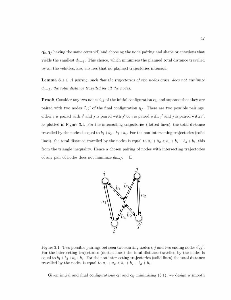
47
q0,qf having the same centroid) and choosing the node pairing and shape orientations that
yields the smallest d0→f . This choice, which minimizes the planned total distance travelled
by all the vehicles, also ensures that no planned trajectories intersect.
Lemma 3.1.1 A pairing, such that the trajectories of two nodes cross, does not minimize
d0→f , the total distance travelled by all the nodes.
Proof: Consider any two nodes i, j of the initial configuration q0 and suppose that they are
paired with two nodes i′, j′ of the final configuration qf . There are two possible pairings:
either i is paired with i′ and j is paired with j′ or i is paired with j′ and j is paired with i′,
as plotted in Figure 3.1. For the intersecting trajectories (dotted lines), the total distance
travelled by the nodes is equal to b1 +b2 +b3 +b4. For the non-intersecting trajectories (solid
lines), the total distance travelled by the nodes is equal to a1 + a2 < b1 + b2 + b3 + b4, this
from the triangle inequality. Hence a chosen pairing of nodes with intersecting trajectories
of any pair of nodes does not minimize d0→f .
Figure 3.1: Two possible pairings between two starting nodes i, j and two ending nodes i′, j′.For the intersecting trajectories (dotted lines) the total distance travelled by the nodes isequal to b1 +b2 +b3 +b4. For the non-intersecting trajectories (solid lines) the total distancetravelled by the nodes is equal to a1 + a2 < b1 + b2 + b3 + b4.
Given initial and final configurations q0 and qf minimizing (3.1), we design a smooth
48
path of tensegrities qe(t) = (xe(t),ye(t)) using the following linear interpolation [78]:
qe(t) =t
τqf +
(1− t
τ
)q0, t ∈ [0, τ ]
qe(t) = qf , t > τ.
(3.2)
The parameter τ has units of time and allows for tuning of the tensegrity’s reconfiguration
speed. The greater τ is, the slower the tensegrity reconfigures itself.
The linear interpolation given by (3.2), defines a smooth path of shapes between two
arbitrary shapes [qe0] and [qef ]. We now use our map from shapes to tensegrities to define
a control law that will track this or any other planned smooth path. The design of the
reconfiguration using a path of stable tensegrities is motivated by the robustness properties
of stable tensegrity structures mentioned in the previous chapter and explained in [109].
3.1.2 Parameterized Control Law
In this section we define a smooth parameterization (over time) of the dynamics of a tenseg-
rity structure (2.10) such that the tensegrity follows a smooth path in shape space [qe](t),
for example the straight-line path given by (3.2). This control law was presented earlier in
[78]. The control law we present does not require a straight-line path, but only a smooth
path [qe](t) such that [qe](0) = [qe0] and [qe](τ) = [qef ]. The simulations presented in Sec-
tion 3.3 use the path given by (3.2) to illustrate the method. The parameterization of the
controlled system (2.10) which we now consider is given by
xi = pxi
yi = pyi
pxi = −νpxi −N∑j=1
αij(t)ωij(t)(
1− lij(t)rij(t)
)(xi − xj)
pyi = −νpyi −N∑j=1
αij(t)ωij(t)(
1− lij(t)rij(t)
)(yi − yj),
i = 1, . . . , N, (3.3)
where the parameters αij(t), lij(t) and ωij(t) are to be chosen so that at each time t, [ze](t) =
([qe](t),0,0) is an exponentially stable equilibrium set of (3.3). This choice of parameters
49
thus creates a manifold of stable tensegrities along the path [qe](t). As a first step to making
the solution of the controlled system follow the path [qe](t), we define the appropriate
variation of the parameters αij(t), lij(t) and ωij(t) so that at each instant t, [qe](t) is an
exponentially stable equilibrium shape of the controlled system (3.3). Given that the system
(3.3) is nonlinear with time-varying inputs, we use results from Lawrence and Rugh [62] to
show that the non-autonomous system (3.3) is well behaved. By well behaved, we mean that
the quantity ‖[q](t)− [qe](t)‖ is bounded during the trajectory and that [q](t) converges to
the final shape [qef ] as t→∞. To ensure that at each instant t, [qe](t) is an exponentially
stable shape of (3.3), we follow a procedure similar to the one developed in Section 2.4.1.
We choose the parameters αij(t), lij(t) and ωij(t) so thatΩ(t,xe(t),ye(t)) 0
0 Ω(t,xe(t),ye(t))
xe(t)
ye(t)
= 0, t ∈ [0, τ ]
Ω(t,xe(τ),ye(τ)) 0
0 Ω(t,xe(τ),ye(τ))
xe(τ)
ye(τ)
= 0, t > τ,
(3.4)
where the explicit dependence of Ω in t comes from its dependence on the parameters
αij(t), lij(t) and ωij(t). As with equation (2.13) in Section 2.4.1, equation (3.4) is solved in
two steps. First we choose the parameters αij(t), lij(t) for all i, j so that Ω(t,xe(t),ye(t)) =
Ω(t). This last equation is solved by choosing
αij(t) =π
arctan (ωij(t))
lij(t) = reij(t)(
1− 1π
arctan (ωij(t))),
(3.5)
where reij(t) = ‖~qei (t) − ~qej (t)‖ is the relative distance between node i and node j at time t
along the planned path in shape space [qe](t). The parameters ωij(t) are then computed as
in Section 2.4.1 using the identity
Ω(t) = Λ(t)DΛ(t)T , (3.6)
where D = diag(
0 0 0 d4 · · · dN
), di > 0, i = 4, . . . , N and the columns of Λ(t)
constitute a basis of orthonormal eigenvectors obtained by the Gram-Schmidt procedure
50
on the N linearly independent vectors xe(t),ye(t),1,w4(t), · · · ,wN (t). This choice makes
[qe](t) a parameterized (over t) family of exponentially stable equilibrium shapes for the
system (3.3). We now use results from Lawrence and Rugh [62] to show that the nonlinear
system with time-varying control inputs (3.3) is well behaved as defined above.
3.2 Boundedness and Convergence
In this section we prove that with the parameters αij(t), lij(t) and ωij(t) solving (3.5) and
(3.6), the controlled system (3.3) is well behaved. In other words we prove that under the
time-varying controlled system (3.3), the reconfiguring tensegrity remains close, in shape
space, to the prescribed shape path [qe](t) (i.e., ‖[q](t)− [qe](t)‖ bounded) and that it con-
verges to the final prescribed shape [qef ] (i.e., [q](t)→ [qef ] as t→∞). These developments
have been described in [78]. We prove these results for the time-varying controlled system
(3.3) by using the main theorem in Lawrence and Rugh [62] for nonlinear systems with
slowly varying inputs. The argument of the proof of this theorem is that solutions of a
nonlinear system with a manifold of exponentially stable equilibria parameterized by con-
stant inputs remains close to the manifold if the initial condition is “close” to that manifold
and the inputs “slowly” vary. Similar results have been proven in [51, 53], although the
assumptions on the vector field are not exactly identical and the methods used to prove the
respective theorems differ. Kelemen [51] investigated stability of the manifold using the lin-
earization of the system and the Gronwall-Bellman inequality, while Khalil and Kokotovic
[53] used a Lyapunov function type approach to prove their stability result. The stability
theorem we are using from Lawrence and Rugh [62] is also proven with a Lyapunov function
type approach. Borrowing the notations from [62], the following setting is considered: a
system described by
z(t) = f(z(t),u(t)), z(0) = z0, t ≥ 0, (3.7)
where z(t) ∈ R4N is the state vector, u(t) = (αij(t), lij(t), ωij(t), reij(t)) is the time-varying
input vector, and f is the vector field given by (3.3). For such system, Lawrence and Rugh
proved the following result [62]:
51
Theorem 3.2.1 Suppose the system (3.7) satisfies
H1 f : R4N × Rm 7→ R4N is twice differentiable,
H2 there is a bounded, open set Γ ⊂ Rm and a continuously differentiable function z :
Γ 7→ R4N such that for each constant input value u ∈ Γ, f(z(u),u) = 0,
H3 there is a λ > 0 such that for each u ∈ Γ, the eigenvalues of (∂f/∂z)(z(u),u) have
real parts no greater than −λ.
Then there is a ρ∗ > 0 such that given any ρ ∈ [0, ρ∗] and T > 0, there exist δ1(ρ), δ2(ρ, T ) >
0 for which the following property holds. If a continuously differentiable input u(t) satisfies
u(t) ∈ Γ, t ≥ t0,
‖z0 − z(u(t0))‖ < δ1
and1T
∫ t+T
t‖u(σ)‖dσ < δ2, t ≥ t0,
then the corresponding solution of (3.7) satisfies
‖z(t)− z(u(t))‖ < ρ, t ≥ t0.
To apply Theorem 3.2.1 to our system, we first show that all three conditions H1-H3 are
satisfied.
We prove that the vector field (3.3) satisfies H1 using the smoothness of f(z(.),u(.))
as a function of Ω(.) and re(.) as noted in Section 2.4.1 and showing that Ω(t) and re(t)
are smooth functions of t. Assuming [qe](t) is a smooth path of tensegrities in shape space
between the starting and ending shapes [qe0] and [qef ] (e.g., the path [qe](t) given by the
linear interpolation (3.2)), re(t) is a smooth function of t. The time-varying stress matrix
Ω(t) is computed as
Ω(t) = Λ(t)DΛ(t)T ,
where D is a constant diagonal matrix and the columns of Λ(t) constitute an orthonormal
basis of RN obtained through a Gram-Schmidt procedure on the N linearly independent
52
vectors xe(t),ye(t),1,w4(t), · · · ,wN (t). The vectors obtained from a Gram-Schmidt proce-
dure consist of linear combinations of the original set of linearly independent vectors; hence
Λ(t) and consequently Ω(t) are smooth functions of t. In Section 2.4.1 we noted that the
choice for the parameters αij and lij given by
αij =π
arctanωij
lij = reij
(1− 1
πarctanωij
)is such that the vector field (2.10) is a smooth map of ωij and reij . This shows that the
vector field f(z(.),u(.)) is a smooth function of Ω(t) and re(t), concluding the proof that
the system (3.3) satisfies H1 being C∞ and hence C2 differentiable in t,Ω(t) and re(t).
Using the results from Section 2.4.2, we now prove that (3.3) satisfies both H2 and
H3. From Theorems 2.4.1 and 2.4.4 we know that choosing the parameters αij , lij and ωij
satisfying (2.13) makes [ze] an isolated exponentially stable equilibrium set of (2.10). Hence
choosing αij(t), lij(t) and ωij(t) satisfying (3.4) for every t makes [ze](t) a parameterized
(by Ω(t) and re(t)) exponentially stable equilibrium set of (3.3), concluding the proof that
(3.3) satisfies both H2 and H3.
Theorem 3.2.1 guarantees that if we start “close enough” to the shape [qei ] (i.e., ‖[z0]−[ze0]‖ < δ1) and the reconfiguration is not “too fast” (i.e τ is large enough such that
1T
∫ t+Tt ‖u(σ)‖dσ < δ2), then the solution of (3.3) satisfies ‖[z](t) − [ze](t)‖ < ρ. This
proves that the reconfiguration is well behaved with ‖[q](t)− [qe](t)‖ bounded and [z](t)→
[zef ] =
[qef ]
0
as t → ∞. We next explore the performance of this control law with a
simulated example.
3.3 Examples and Simulations
In this section we present simulation results for the reconfiguration control law given by
(3.3). With an example involving six nodes, we investigate the effect of the choice of τ on the
“shape error” and on the total distance travelled by the vehicles through the reconfiguration.
53
Shape error e(t) is measured as
e(t) =
√√√√ N∑i=1
(diG(t)− deiG(t))2, (3.8)
where diG(t) is the observed distance between the ith node and the center of mass of the
tensegrity at time t and deiG(t) is the planned distance between the ith node and the center
of mass of the tensegrity at time t.
Looking at snapshots of the reconfiguration for different times allows us to interpret
the physical meaning of shape error. We consider as an example the reconfiguration of a
six-vehicle formation from initial shape [qe0] to final shape [qef ], represented respectively by
the configurations q0,qf , given by
q0 =
−1 1 2 1 −1 −2
−2 −2 0 2 2 0
qf =
−2 2 0 12 0 −1
2
−32 −3
2 −12
12
52
12
,
where the coordinates are expressed in meters. Figure 3.2 shows the planned initial shape,
final shape and planned intermediary shapes as prescribed by (3.2) for t = τ3 and t = 2τ
3 .
We note that the final shape is non-convex. In the context of a mobile sensor network, this
reconfiguration corresponds to having the network that is sampling the environment shift
from lower resolution in a larger space to higher resolution in a smaller space.
Figure 3.3 shows the evolution of the mean total distance travelled by the six nodes
calculated over four thousand runs as a function of τ , for values of τ between .1s and 16s
with increment of .1s. Each run has an initial condition randomly picked from a normal
distribution with mean [ze0] =
[qe0]
0
and variance 0.1. For increasing τ in the range from
0 to 3s, the total distance decreases dramatically from about 30m to about 12m. For τ > 3s,
as τ increases, the total distance converges to an asymptote. This is lower bounded by the
total distance travelled in the linear designed path given by (3.2), represented in Figure
3.3 by the solid white line. The planned distance for this path is calculated as 8.58m.
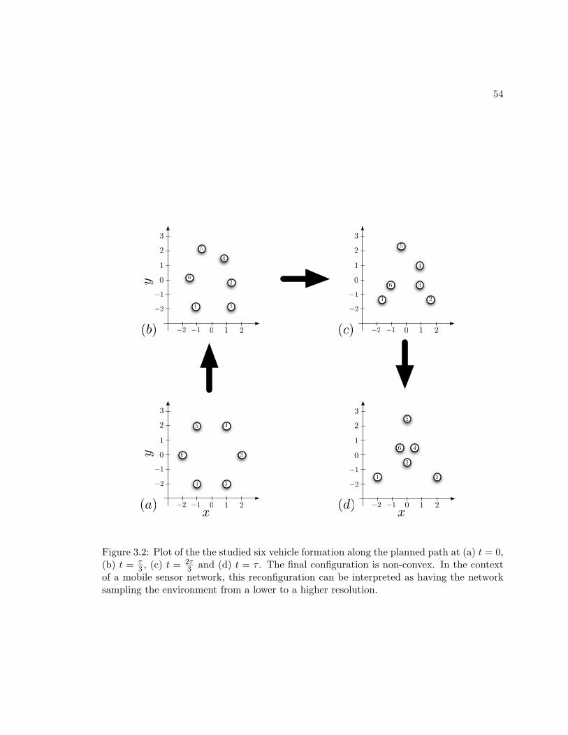
54
−2 −1 0 1 2
3
−2
−1
0
1
2
1 2
3
45
6
−2 −1 0 1 2
3
−2
−1
0
1
2
1 2
3
45
6
−2 −1 0 1 2
3
−2
−1
0
1
2
1 2
3
4
6
5
−2 −1 0 1 2
3
−2
−1
0
1
25
6 4
3
21
x x
yy
(a)
(b) (c)
(d)
Figure 3.2: Plot of the the studied six vehicle formation along the planned path at (a) t = 0,(b) t = τ
3 , (c) t = 2τ3 and (d) t = τ . The final configuration is non-convex. In the context
of a mobile sensor network, this reconfiguration can be interpreted as having the networksampling the environment from a lower to a higher resolution.
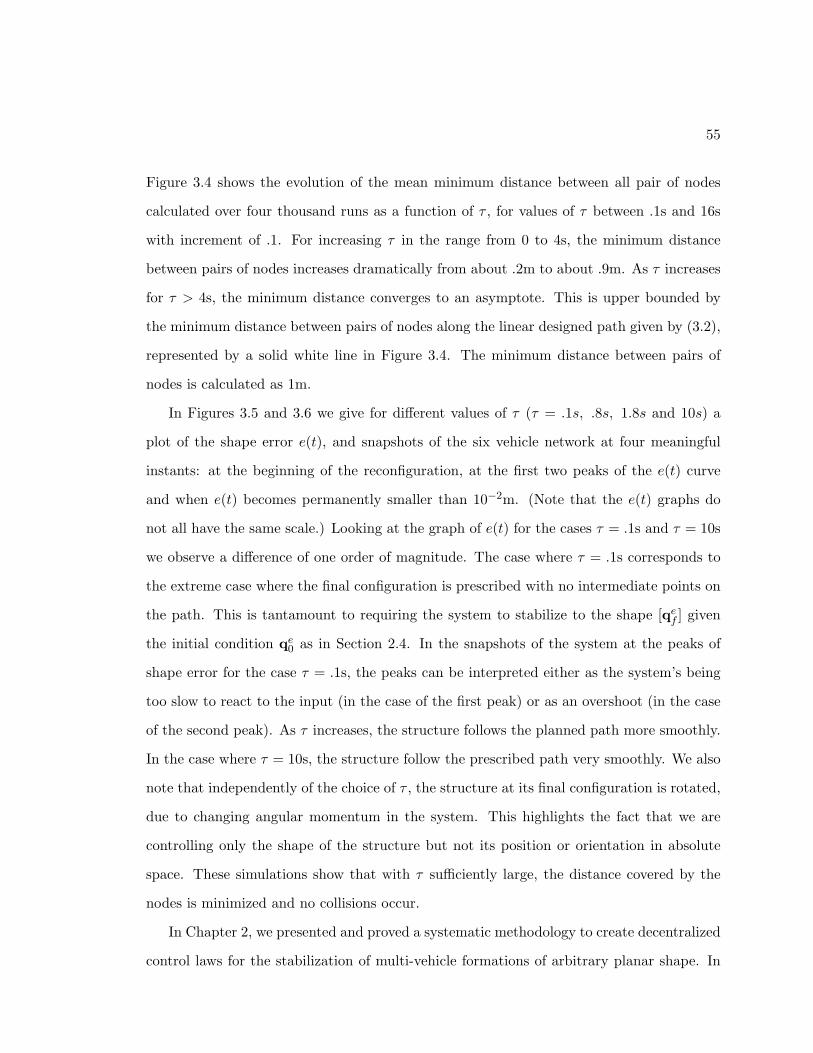
55
Figure 3.4 shows the evolution of the mean minimum distance between all pair of nodes
calculated over four thousand runs as a function of τ , for values of τ between .1s and 16s
with increment of .1. For increasing τ in the range from 0 to 4s, the minimum distance
between pairs of nodes increases dramatically from about .2m to about .9m. As τ increases
for τ > 4s, the minimum distance converges to an asymptote. This is upper bounded by
the minimum distance between pairs of nodes along the linear designed path given by (3.2),
represented by a solid white line in Figure 3.4. The minimum distance between pairs of
nodes is calculated as 1m.
In Figures 3.5 and 3.6 we give for different values of τ (τ = .1s, .8s, 1.8s and 10s) a
plot of the shape error e(t), and snapshots of the six vehicle network at four meaningful
instants: at the beginning of the reconfiguration, at the first two peaks of the e(t) curve
and when e(t) becomes permanently smaller than 10−2m. (Note that the e(t) graphs do
not all have the same scale.) Looking at the graph of e(t) for the cases τ = .1s and τ = 10s
we observe a difference of one order of magnitude. The case where τ = .1s corresponds to
the extreme case where the final configuration is prescribed with no intermediate points on
the path. This is tantamount to requiring the system to stabilize to the shape [qef ] given
the initial condition qe0 as in Section 2.4. In the snapshots of the system at the peaks of
shape error for the case τ = .1s, the peaks can be interpreted either as the system’s being
too slow to react to the input (in the case of the first peak) or as an overshoot (in the case
of the second peak). As τ increases, the structure follows the planned path more smoothly.
In the case where τ = 10s, the structure follow the prescribed path very smoothly. We also
note that independently of the choice of τ , the structure at its final configuration is rotated,
due to changing angular momentum in the system. This highlights the fact that we are
controlling only the shape of the structure but not its position or orientation in absolute
space. These simulations show that with τ sufficiently large, the distance covered by the
nodes is minimized and no collisions occur.
In Chapter 2, we presented and proved a systematic methodology to create decentralized
control laws for the stabilization of multi-vehicle formations of arbitrary planar shape. In
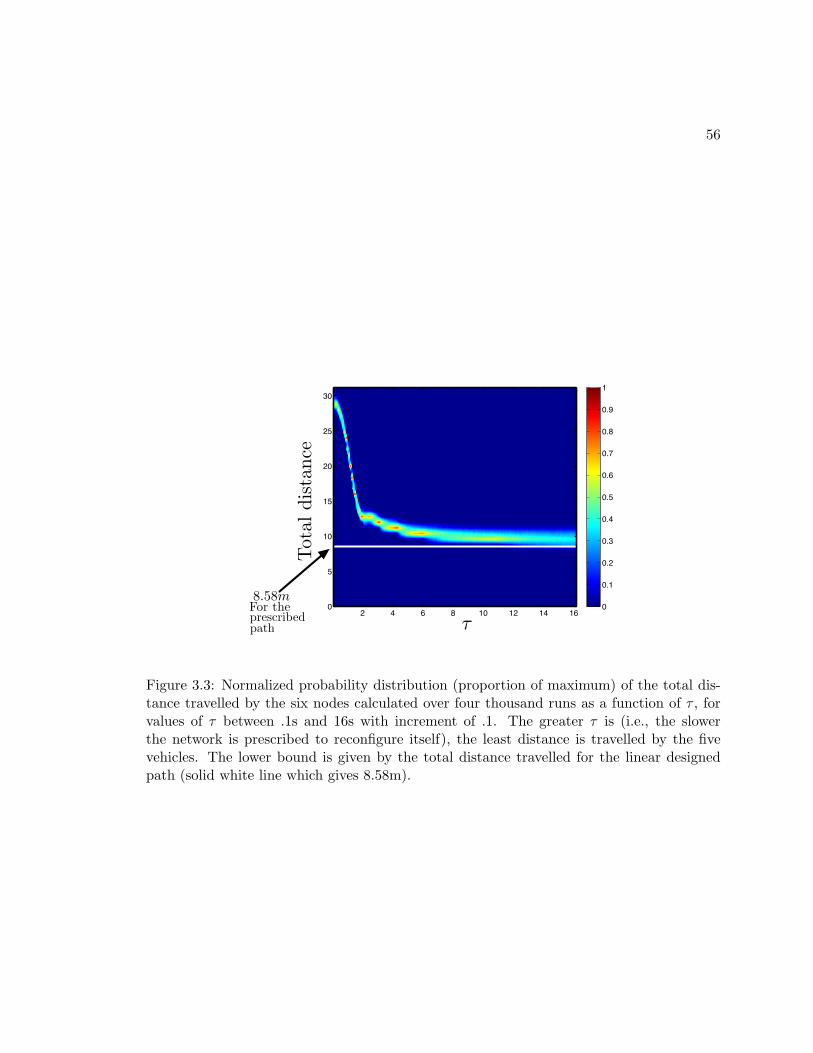
56
8.58m
2 4 6 8 10 12 14 160
5
10
15
20
25
30
0
0.1
0.2
0.3
0.4
0.5
0.6
0.7
0.8
0.9
1
Figure 3.3: Normalized probability distribution (proportion of maximum) of the total dis-tance travelled by the six nodes calculated over four thousand runs as a function of τ , forvalues of τ between .1s and 16s with increment of .1. The greater τ is (i.e., the slowerthe network is prescribed to reconfigure itself), the least distance is travelled by the fivevehicles. The lower bound is given by the total distance travelled for the linear designedpath (solid white line which gives 8.58m).
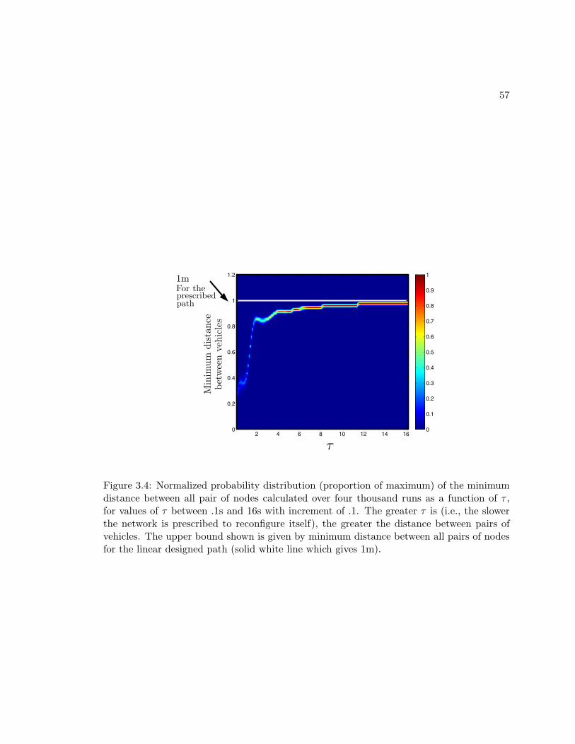
57
2 4 6 8 10 12 14 160
0.2
0.4
0.6
0.8
1
1.2
0
0.1
0.2
0.3
0.4
0.5
0.6
0.7
0.8
0.9
1
Min
imum
dist
ance
betw
een
vehi
cles
1m
Figure 3.4: Normalized probability distribution (proportion of maximum) of the minimumdistance between all pair of nodes calculated over four thousand runs as a function of τ ,for values of τ between .1s and 16s with increment of .1. The greater τ is (i.e., the slowerthe network is prescribed to reconfigure itself), the greater the distance between pairs ofvehicles. The upper bound shown is given by minimum distance between all pairs of nodesfor the linear designed path (solid white line which gives 1m).
58
0 1 2 3 4 5 6 7 8 9 100
0.5
1
1.5
2
2.5
3
τ =0.1 total distance=29.5621
τ = .1τ = .8τ = 1.8τ = 10
!! !" # " ! $!!%&
!!
!"%&
!"
!#%&
#
#%&
"
"%&
!
!%&
$
!! !" # " ! $!!%&
!!
!"%&
!"
!#%&
#
#%&
"
"%&
!
!%&
$
!! !" # " ! $!!%&
!!
!"%&
!"
!#%&
#
#%&
"
"%&
!
!%&
$
!! !" # " ! $!!%&
!!
!"%&
!"
!#%&
#
#%&
"
"%&
!
!%&
$
!! !" # " ! $!!%&
!!
!"%&
!"
!#%&
#
#%&
"
"%&
!
!%&
$
!! !" # " ! $!!%&
!!
!"%&
!"
!#%&
#
#%&
"
"%&
!
!%&
$
!! !" # " ! $!!%&
!!
!"%&
!"
!#%&
#
#%&
"
"%&
!
!%&
$
!! !" # " ! $!!%&
!!
!"%&
!"
!#%&
#
#%&
"
"%&
!
!%&
$e(t)
τ = .1st = 0s t = .11s t = 1.2s t = 9.4s
t = 0.5s t = 1.5s t = 9.45s
x
y
t
Total Distance=29.6m
Total Distance=25.5m
y
x x x
t = 0s
(a)
(b)
τ = .8s
0 1 2 3 4 5 6 7 8 9 100
0.2
0.4
0.6
0.8
1
1.2
1.4
τ =0.8 total distance=25.5321
τ = .8τ = 1.8τ = 10
t
e(t)
!! !" # " ! $!!%&
!!
!"%&
!"
!#%&
#
#%&
"
"%&
!
!%&
$
!! !" # " ! $!!%&
!!
!"%&
!"
!#%&
#
#%&
"
"%&
!
!%&
$
yy
x x x x
!! !" # " ! $!!%&
!!
!"%&
!"
!#%&
#
#%&
"
"%&
!
!%&
$
!! !" # " ! $!!%&
!!
!"%&
!"
!#%&
#
#%&
"
"%&
!
!%&
$
!! !" # " ! $!!%&
!!
!"%&
!"
!#%&
#
#%&
"
"%&
!
!%&
$
!! !" # " ! $!!%&
!!
!"%&
!"
!#%&
#
#%&
"
"%&
!
!%&
$
!! !" # " ! $!!%&
!!
!"%&
!"
!#%&
#
#%&
"
"%&
!
!%&
$
!! !" # " ! $!!%&
!!
!"%&
!"
!#%&
#
#%&
"
"%&
!
!%&
$
(c)
(d)
Figure 3.5: For τ = 0.1s, .8s, shape error is plotted as a function of time. (a)-(c) givesnapshots of the six vehicle network along the prescribed path qe(t) respectively for τ =0.1s, .8s. (b)-(d) give snapshots of the actual six vehicle network at the beginning of thereconfiguration, at the first two peak of the e(t) curve and when the shape error becomespermanently smaller than 10−2m respectively for τ = 0.1s, .8s.
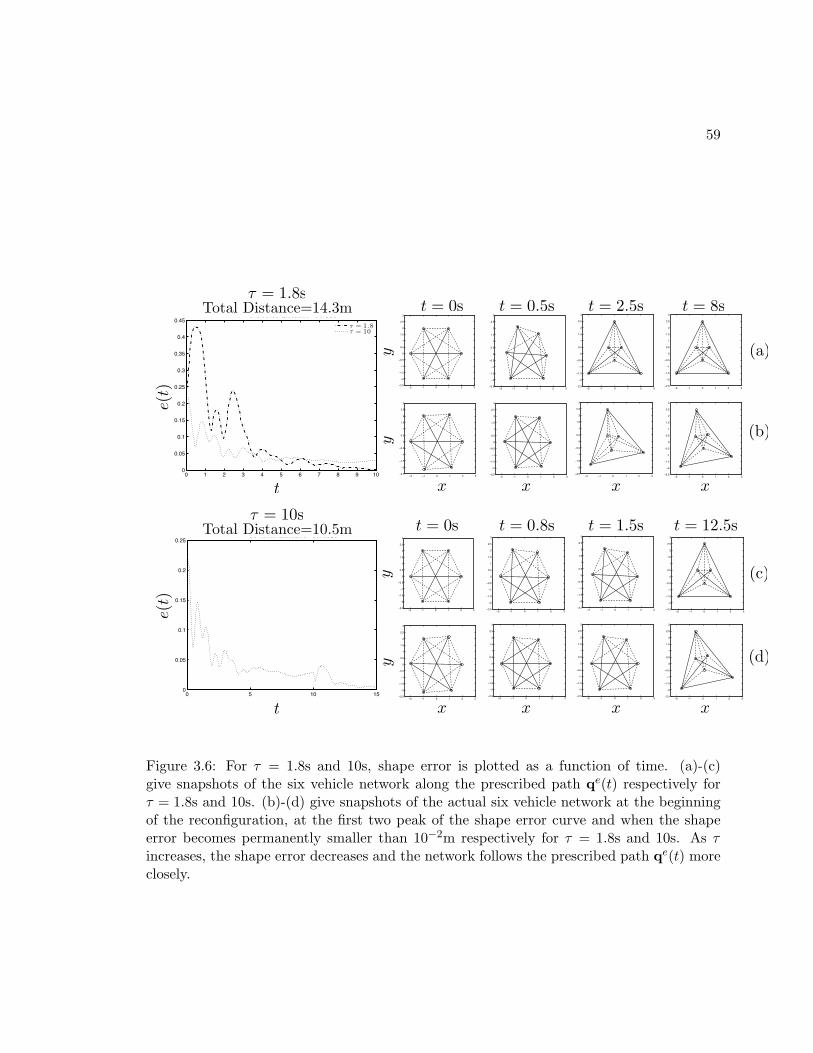
59
!! !" # " ! $!!%&
!!
!"%&
!"
!#%&
#
#%&
"
"%&
!
!%&
$
!! !" # " ! $!!%&
!!
!"%&
!"
!#%&
#
#%&
"
"%&
!
!%&
$e(t)
t = 0s
t = 1.5s
x
y
t
y
x x x
t = 0s
(a)
(b)
t
e(t)
!! !" # " ! $!!%&
!!
!"%&
!"
!#%&
#
#%&
"
"%&
!
!%&
$
!! !" # " ! $!!%&
!!
!"%&
!"
!#%&
#
#%&
"
"%&
!
!%&
$
yy
x x x x
(c)
(d)
τ = 1.8sTotal Distance=14.3m
0 1 2 3 4 5 6 7 8 9 100
0.05
0.1
0.15
0.2
0.25
0.3
0.35
0.4
0.45
τ =1.8 total distance=14.336
τ = 1.8τ = 10
Total Distance=10.5mτ = 10s
0 5 10 150
0.05
0.1
0.15
0.2
0.25
τ =10 total distance=10.4625
t = 0.5s t = 2.5s t = 8s
t = 0.8s t = 12.5s
!! !" # " ! $!!%&
!!
!"%&
!"
!#%&
#
#%&
"
"%&
!
!%&
$
!! !" # " ! $!!%&
!!
!"%&
!"
!#%&
#
#%&
"
"%&
!
!%&
$
!! !" # " ! $!!%&
!!
!"%&
!"
!#%&
#
#%&
"
"%&
!
!%&
$
!! !" # " ! $!!%&
!!
!"%&
!"
!#%&
#
#%&
"
"%&
!
!%&
$
!! !" # " ! $!!%&
!!
!"%&
!"
!#%&
#
#%&
"
"%&
!
!%&
$
!! !" # " ! $!!%&
!!
!"%&
!"
!#%&
#
#%&
"
"%&
!
!%&
$
!! !" # " ! $!!%&
!!
!"%&
!"
!#%&
#
#%&
"
"%&
!
!%&
$
!! !" # " ! $!!%&
!!
!"%&
!"
!#%&
#
#%&
"
"%&
!
!%&
$
!! !" # " ! $!!%&
!!
!"%&
!"
!#%&
#
#%&
"
"%&
!
!%&
$
!! !" # " ! $!!%&
!!
!"%&
!"
!#%&
#
#%&
"
"%&
!
!%&
$
!! !" # " ! $!!%&
!!
!"%&
!"
!#%&
#
#%&
"
"%&
!
!%&
$
!! !" # " ! $!!%&
!!
!"%&
!"
!#%&
#
#%&
"
"%&
!
!%&
$
Figure 3.6: For τ = 1.8s and 10s, shape error is plotted as a function of time. (a)-(c)give snapshots of the six vehicle network along the prescribed path qe(t) respectively forτ = 1.8s and 10s. (b)-(d) give snapshots of the actual six vehicle network at the beginningof the reconfiguration, at the first two peak of the shape error curve and when the shapeerror becomes permanently smaller than 10−2m respectively for τ = 1.8s and 10s. As τincreases, the shape error decreases and the network follows the prescribed path qe(t) moreclosely.

60
this chapter we extended the proven framework to control changes of formation shape over
a given time interval. In the subsequent chapters of this dissertation we will turn our
attention to the dynamics of decision making in groups. The problem of interest is the
following: given a group of individuals, by which mechanisms if any can they agree on
a direction of travel even when some individuals have conflicting preferences. We look
at this problem in a natural setting and build and/or study models with the motivation
of understanding the key mechanisms. The goal is to set the foundation for a mutually
beneficial interaction between biology and engineering such that analysis tools derived to
study collective robotic behavior are used to test plausible mechanisms of decision making in
animal groups, and, in return, the understanding of such phenomenon provides inspiration
for new control strategies for engineered cooperative multi-agent systems.
Chapter 4
Collective Decision Making:
Discrete Time Models
In the remaining chapters of this dissertation, we turn our attention to group dynamics in the
context of natural systems. We investigate mechanisms of leadership and decision making in
animal groups such as schools of fish or flocks of birds through the simulation and analysis of
discrete- and continuous-time individual-based (i.e. Lagrangian) models. More specifically
we consider a heterogeneous group of both informed individuals with conflicting preferences
and uninformed individuals, i.e, individuals without preferences. We assume that there
is no explicit signaling and that group members cannot recognize which individuals are
informed and how accurate the information is. This conservative assumption makes this
research relevant to species where it is not reasonable to assume sophisticated cognitive
abilities. For example groups of migrating fish, birds or insects can be so crowded as to
limit significantly the range over which neighbors can be detected, making the hypothesis
of sophisticated communication abilities unlikely.
For such a collective, we address the following leadership and consensus decision-making
problems: how can information be transferred and how can a consensus be reached in the
group? This research has been conducted with both complex stochastic discrete times mod-
els and simplified deterministic continuous-time models. The former gives highly suggestive
61
62
simulations, whereas the latter allows a deeper investigation of the microscopic reasons for
the macroscopic behaviors observed and a more complete exploration of parameter space.
In this chapter we present a discrete-time model developed by Couzin et al. in [19] and
present a new investigation of this model focusing on the role of uninformed individuals in
the decision-making process within a heterogeneous group. We highlight both the draw-
backs and the benefits of having uninformed individuals in the group. In Section 4.1 we
present two variations of the discrete-time model used in [19]. In one variation, the informed
individuals have a fixed preferred direction of travel; in the other variation, the preference
is a destination, referred to as a target. We then summarize the results in Couzin et al. [19].
In Section 4.2 we investigate the influence of the uninformed individuals in the model with
preferred direction. In Section 4.3 we investigate the influence of uninformed individuals in
the model with targets.
4.1 Discrete-time Model from Couzin et al. [19]
4.1.1 The Model
The discrete-time model from [19] considers a group of N individuals, each modeled as a
particle moving in the plane at constant speed si, i = 1, . . . , N . At time t, each individual
is characterized by a position vector ci(t) and a velocity vector vi(t). The velocity vi(t)
is applied to the i-th particle between time t − ∆t and time t. At each time step, the
individuals in the group update their direction of travel depending on social interactions
with local neighbors and, when applicable, on a preferred direction of travel. The population
is divided into three subgroups, two informed and one uninformed. Let Ni, i = 1, 2, 3 be,
respectively, the set of indices in 1, · · · , N corresponding to individuals in the first and
second informed subgroups and in the uninformed subgroup. Each individual in the first
and second subgroups has a preferred direction of travel (where the preference represents,
for example, knowledge of the direction to a food source or of a migration route) and
can use that preference along with information it has on its neighbors to make decisions.
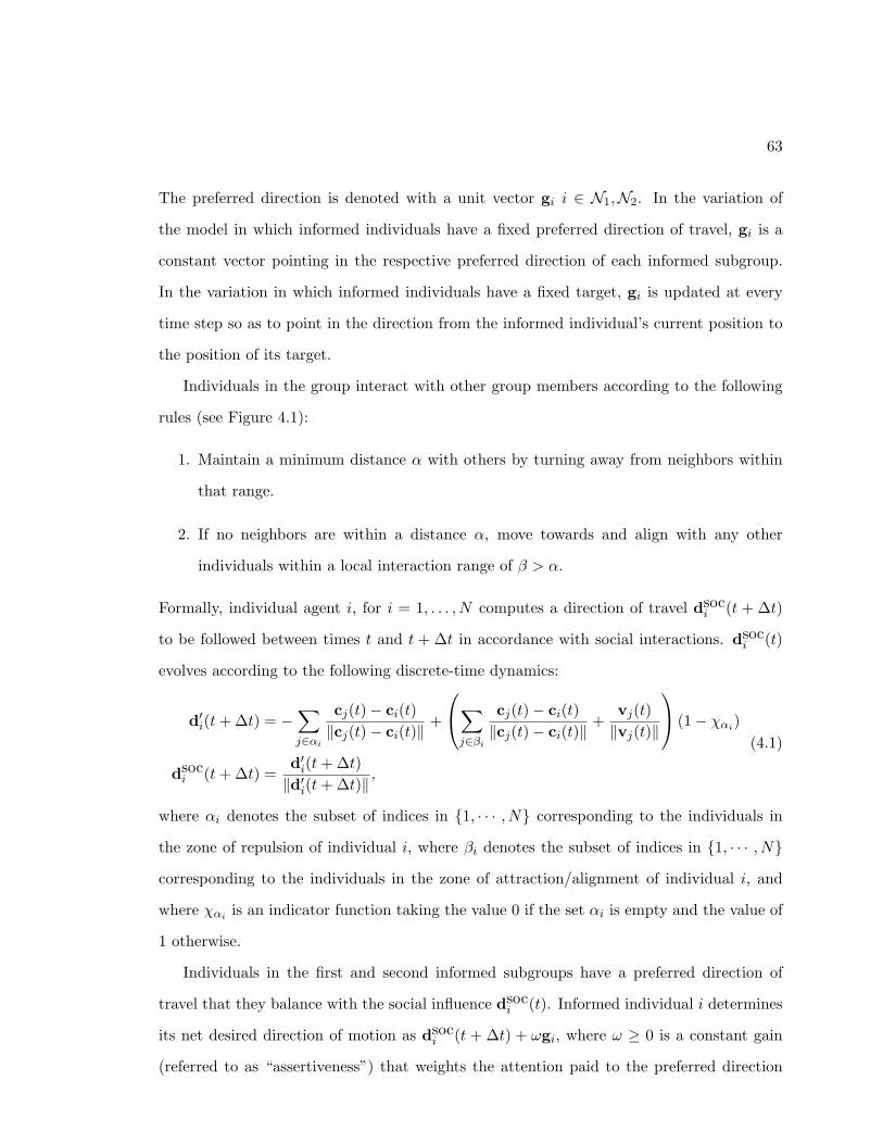
63
The preferred direction is denoted with a unit vector gi i ∈ N1,N2. In the variation of
the model in which informed individuals have a fixed preferred direction of travel, gi is a
constant vector pointing in the respective preferred direction of each informed subgroup.
In the variation in which informed individuals have a fixed target, gi is updated at every
time step so as to point in the direction from the informed individual’s current position to
the position of its target.
Individuals in the group interact with other group members according to the following
rules (see Figure 4.1):
1. Maintain a minimum distance α with others by turning away from neighbors within
that range.
2. If no neighbors are within a distance α, move towards and align with any other
individuals within a local interaction range of β > α.
Formally, individual agent i, for i = 1, . . . , N computes a direction of travel dsoci (t + ∆t)
to be followed between times t and t + ∆t in accordance with social interactions. dsoci (t)
evolves according to the following discrete-time dynamics:
d′i(t+ ∆t) = −∑j∈αi
cj(t)− ci(t)‖cj(t)− ci(t)‖ +
∑j∈βi
cj(t)− ci(t)‖cj(t)− ci(t)‖ +
vj(t)‖vj(t)‖
(1− χαi)
dsoci (t+ ∆t) =
d′i(t+ ∆t)‖d′i(t+ ∆t)‖ ,
(4.1)
where αi denotes the subset of indices in 1, · · · , N corresponding to the individuals in
the zone of repulsion of individual i, where βi denotes the subset of indices in 1, · · · , Ncorresponding to the individuals in the zone of attraction/alignment of individual i, and
where χαi is an indicator function taking the value 0 if the set αi is empty and the value of
1 otherwise.
Individuals in the first and second informed subgroups have a preferred direction of
travel that they balance with the social influence dsoci (t). Informed individual i determines
its net desired direction of motion as dsoci (t + ∆t) + ωgi, where ω ≥ 0 is a constant gain
(referred to as “assertiveness”) that weights the attention paid to the preferred direction
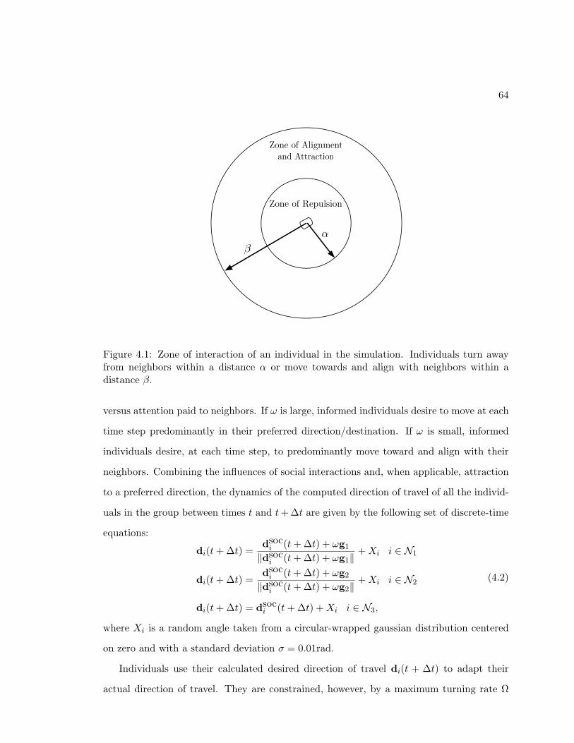
64
Figure 4.1: Zone of interaction of an individual in the simulation. Individuals turn awayfrom neighbors within a distance α or move towards and align with neighbors within adistance β.
versus attention paid to neighbors. If ω is large, informed individuals desire to move at each
time step predominantly in their preferred direction/destination. If ω is small, informed
individuals desire, at each time step, to predominantly move toward and align with their
neighbors. Combining the influences of social interactions and, when applicable, attraction
to a preferred direction, the dynamics of the computed direction of travel of all the individ-
uals in the group between times t and t+ ∆t are given by the following set of discrete-time
equations:
di(t+ ∆t) =dsoci (t+ ∆t) + ωg1
‖dsoci (t+ ∆t) + ωg1‖ +Xi i ∈ N1
di(t+ ∆t) =dsoci (t+ ∆t) + ωg2
‖dsoci (t+ ∆t) + ωg2‖ +Xi i ∈ N2
di(t+ ∆t) = dsoci (t+ ∆t) +Xi i ∈ N3,
(4.2)
where Xi is a random angle taken from a circular-wrapped gaussian distribution centered
on zero and with a standard deviation σ = 0.01rad.
Individuals use their calculated desired direction of travel di(t + ∆t) to adapt their
actual direction of travel. They are constrained, however, by a maximum turning rate Ω
65
such that the maximum change in direction of travel between t and t+ ∆t is Ω∆t. For an
individual moving at a speed of si, if the angle between the velocity vector vi(t) at time t
and the calculated direction of travel di(t+ ∆t) between time t and time t+ ∆t is smaller
than Ω∆t, then vi(t + ∆t) is equal to sidi(t + ∆t); otherwise vi(t + ∆t) is equal to vi(t)
rotated by Ω∆t towards di(t + ∆t). The discrete-time dynamics of the individuals in the
group can then be written as
vi(t+ ∆t) =
sidi(t+ ∆t) if |mod(θd − θv, 2π)− π| ≤ Ω∆t
vi(t)R (sgn(mod(θd − θv, 2π)− π)Ω∆t) otherwise,
ci(t+ ∆t) = ci(t) + vi(t+ ∆t)∆t,(4.3)
where θv (respectively θd) is the oriented principal value of the angle between vi(t) and the
rightward unit vector i.e., the angle θv between vi(t) and the rightward unit vector such
that θv ∈ [−π, π) (respectively between di(t+∆t) and a rightward unit vector), the function
mod(x, 2π) is defined as x− 2πn with n = floor( x2π ), the function sgn is defined as
sgn(x) =
1 if x > 0
−1 if x < 0
0 if x = 0,
and R(θ) is the 2× 2 rotation matrix given by
R(θ) =
cos θ − sin θ
sin θ cos θ
.
In some of the simulations presented in [19], a “forgetting factor” feedback was intro-
duced by making the weight ω of the attraction to the preferred direction state dependent.
More specifically, if at a given time step, informed individuals find themselves moving in
a “similar” direction to their preferred direction (within ± 20 deg), the weight ω is in-
creased by ωinc up to a maximum value ωmax; otherwise it is decreased by ωdec up to 0.
In the simulations presented in this chapter, no “forgetting factor” feedback is considered.
However, similar feedback terms are considered in the extensions for the analytical models
presented in Chapters 5 and 6.
66
4.1.2 Summary of the Results in Couzin et al. [19]
Using the model described above considering informed individuals with fixed preferred di-
rections, Couzin et al. addressed the following two questions: how can information be
transferred within a group without signaling or individual recognition and how can consen-
sus decisions be made by groups containing individuals with conflicting preferences. They
demonstrated plausible mechanisms for information to flow within a group, assuming lim-
ited cognitive abilities for the group members. This work also revealed that leadership can
emerge from the differences in preference of members when individuals, informed or unin-
formed, respond spontaneously to those individuals that have information although without
necessarily recognizing them as such.
The first question was investigated by considering a group with one informed subgroup
and one uninformed subgroup. The authors showed that for a given group size, the accuracy
of group motion increases asymptotically as the proportion of informed individuals increases,
accuracy being measured as the normalized angular deviation of group direction around the
preferred direction g. They noticed furthermore that the larger the group, the smaller the
proportion of informed individuals needed to be to achieve any given level of accuracy.
These simulations also showed that higher values of ω yield greater accuracy but at the cost
of increasing the probability of group fragmentation.
The second question was investigated by considering a group containing two informed
subgroups with conflicting preferences and one uninformed subgroup. Simulations showed
that with two informed subgroups of equal population, the direction of group motion de-
pends on the degree to which the preferred directions differ. For disagreements below a
certain threshold, the group follows the average preferred direction of all informed indi-
viduals, while for disagreements greater than the threshold, the group selects with equal
probability one of the two preferred directions. When introducing the “forgetting factor”
feedback described above, the same transition from averaging the preferred directions to
collectively selecting one preferred direction occurs, although the threshold is smaller. One
remarkable feature of these simulations is that the informed individuals are not aware of
67
how many individuals share their preferred direction and whether or not they are in the
majority. Moreover, when one informed subgroup has a population greater than the other,
even if only by one extra individual, the group is nevertheless able to sense this. For dis-
agreements greater than the threshold, the group selects with almost probability one the
preferred direction of the informed subgroup in the majority rather than randomly selecting
either of the preferred directions.
This model produces highly suggestive simulation results but contains many degrees
of freedom. In order to isolate biologically plausible mechanisms for the decision-making
behavior observed in [19] when there are two informed subgroups with conflicting informa-
tion, we proposed and analyzed in [80] a continuous-time model making several simplifying
assumptions. First, rather than considering interaction zones as in (4.1), we assumed an
all-to-all communication topology, meaning that every individual senses every other indi-
vidual in the group and adjusts its own direction of travel accordingly. Second, we removed
the “forgetting factor” feedback term considered in some simulations in [19] by not allowing
informed individuals to update the strength of their attraction to their preferred direction.
Finally we ignored the presence of uninformed individuals. This model and its analysis are
presented in detail in Chapter 5 of this dissertation. Notably, the continuous-time model
produced some but not all of the behaviors observed in [19], suggesting that some of the
simplifying assumptions made may be responsible for the collective behavior observed in
[19]. Driven by the analysis of the continuous-time model, we reexamine, in the remain-
der of this chapter, the simulation from [19], focusing on the subtle and nontrivial role of
uninformed individuals in achieving consensus decisions. We first explore the role of naive
individuals in the case where informed individuals have a fixed preferred direction of travel.
We then consider the case where informed individuals have a fixed target.
4.2 Influence of Naive Individuals in the Direction Model
In the context of animal foraging or migration, it has been shown that in many cases only a
few individuals have pertinent information of where to travel [96, 119, 31, 105]. Simulations
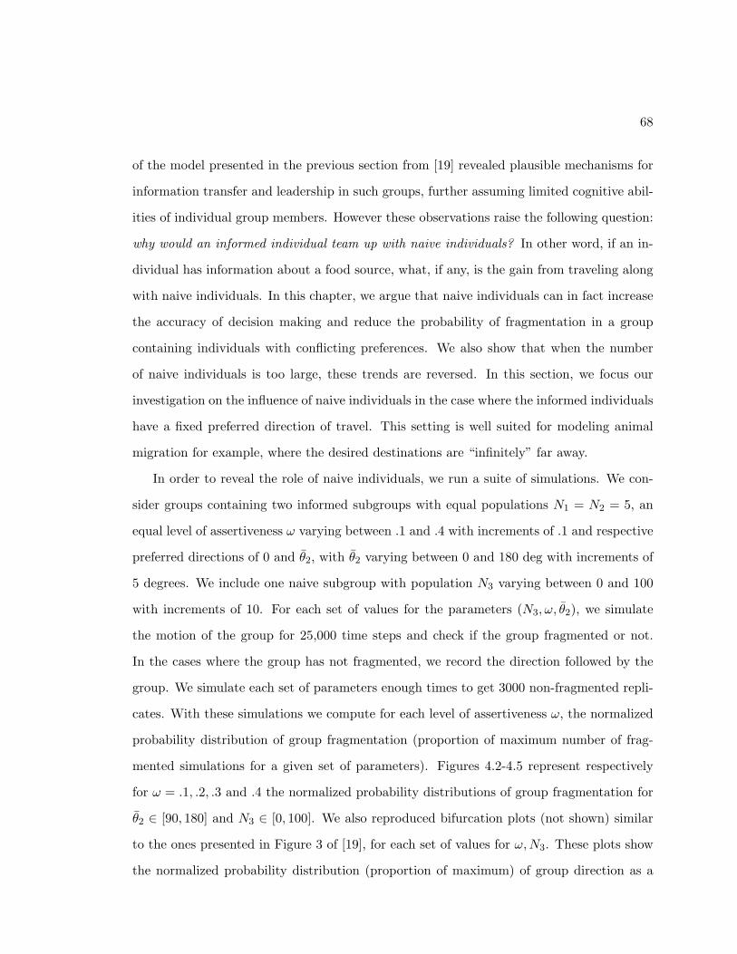
68
of the model presented in the previous section from [19] revealed plausible mechanisms for
information transfer and leadership in such groups, further assuming limited cognitive abil-
ities of individual group members. However these observations raise the following question:
why would an informed individual team up with naive individuals? In other word, if an in-
dividual has information about a food source, what, if any, is the gain from traveling along
with naive individuals. In this chapter, we argue that naive individuals can in fact increase
the accuracy of decision making and reduce the probability of fragmentation in a group
containing individuals with conflicting preferences. We also show that when the number
of naive individuals is too large, these trends are reversed. In this section, we focus our
investigation on the influence of naive individuals in the case where the informed individuals
have a fixed preferred direction of travel. This setting is well suited for modeling animal
migration for example, where the desired destinations are “infinitely” far away.
In order to reveal the role of naive individuals, we run a suite of simulations. We con-
sider groups containing two informed subgroups with equal populations N1 = N2 = 5, an
equal level of assertiveness ω varying between .1 and .4 with increments of .1 and respective
preferred directions of 0 and θ2, with θ2 varying between 0 and 180 deg with increments of
5 degrees. We include one naive subgroup with population N3 varying between 0 and 100
with increments of 10. For each set of values for the parameters (N3, ω, θ2), we simulate
the motion of the group for 25,000 time steps and check if the group fragmented or not.
In the cases where the group has not fragmented, we record the direction followed by the
group. We simulate each set of parameters enough times to get 3000 non-fragmented repli-
cates. With these simulations we compute for each level of assertiveness ω, the normalized
probability distribution of group fragmentation (proportion of maximum number of frag-
mented simulations for a given set of parameters). Figures 4.2-4.5 represent respectively
for ω = .1, .2, .3 and .4 the normalized probability distributions of group fragmentation for
θ2 ∈ [90, 180] and N3 ∈ [0, 100]. We also reproduced bifurcation plots (not shown) similar
to the ones presented in Figure 3 of [19], for each set of values for ω,N3. These plots show
the normalized probability distribution (proportion of maximum) of group direction as a
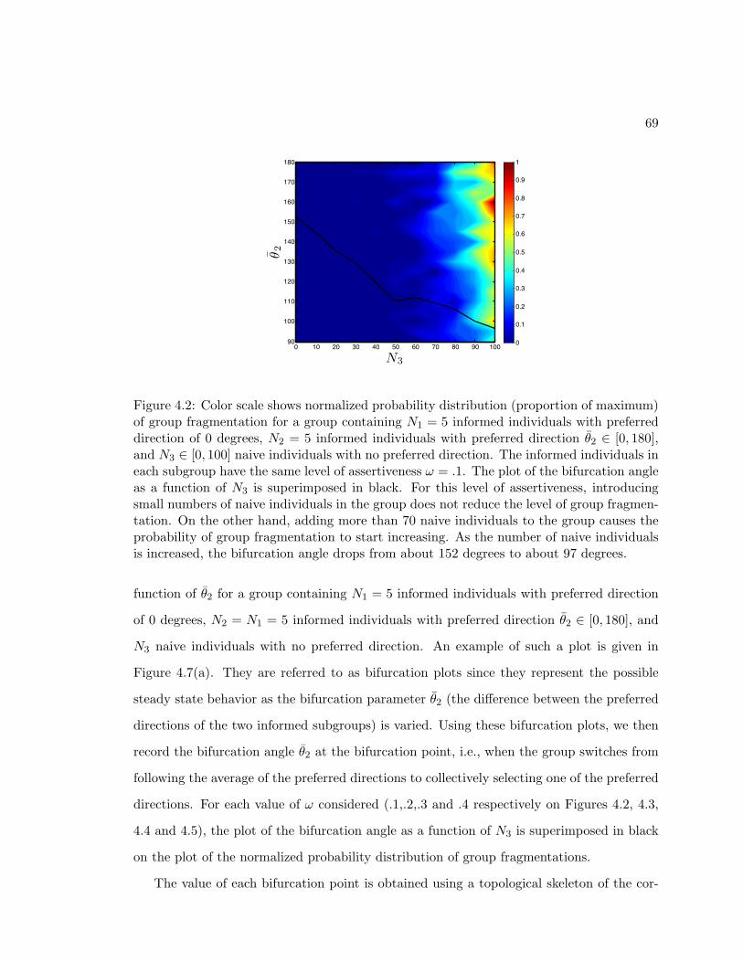
69
N3
θ2
0 10 20 30 40 50 60 70 80 90 10090
100
110
120
130
140
150
160
170
180
0
0.1
0.2
0.3
0.4
0.5
0.6
0.7
0.8
0.9
1
Figure 4.2: Color scale shows normalized probability distribution (proportion of maximum)of group fragmentation for a group containing N1 = 5 informed individuals with preferreddirection of 0 degrees, N2 = 5 informed individuals with preferred direction θ2 ∈ [0, 180],and N3 ∈ [0, 100] naive individuals with no preferred direction. The informed individuals ineach subgroup have the same level of assertiveness ω = .1. The plot of the bifurcation angleas a function of N3 is superimposed in black. For this level of assertiveness, introducingsmall numbers of naive individuals in the group does not reduce the level of group fragmen-tation. On the other hand, adding more than 70 naive individuals to the group causes theprobability of group fragmentation to start increasing. As the number of naive individualsis increased, the bifurcation angle drops from about 152 degrees to about 97 degrees.
function of θ2 for a group containing N1 = 5 informed individuals with preferred direction
of 0 degrees, N2 = N1 = 5 informed individuals with preferred direction θ2 ∈ [0, 180], and
N3 naive individuals with no preferred direction. An example of such a plot is given in
Figure 4.7(a). They are referred to as bifurcation plots since they represent the possible
steady state behavior as the bifurcation parameter θ2 (the difference between the preferred
directions of the two informed subgroups) is varied. Using these bifurcation plots, we then
record the bifurcation angle θ2 at the bifurcation point, i.e., when the group switches from
following the average of the preferred directions to collectively selecting one of the preferred
directions. For each value of ω considered (.1,.2,.3 and .4 respectively on Figures 4.2, 4.3,
4.4 and 4.5), the plot of the bifurcation angle as a function of N3 is superimposed in black
on the plot of the normalized probability distribution of group fragmentations.
The value of each bifurcation point is obtained using a topological skeleton of the cor-
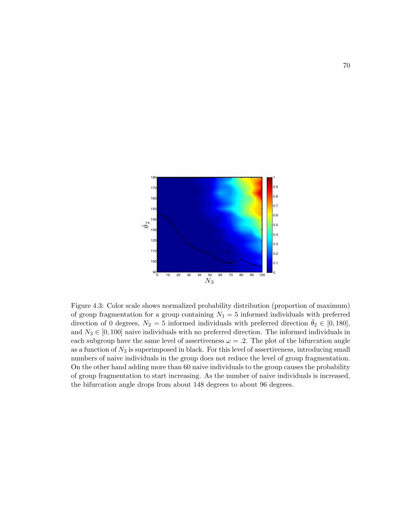
70
N3
θ2
0 10 20 30 40 50 60 70 80 90 10090
100
110
120
130
140
150
160
170
180
0
0.1
0.2
0.3
0.4
0.5
0.6
0.7
0.8
0.9
1
Figure 4.3: Color scale shows normalized probability distribution (proportion of maximum)of group fragmentation for a group containing N1 = 5 informed individuals with preferreddirection of 0 degrees, N2 = 5 informed individuals with preferred direction θ2 ∈ [0, 180],and N3 ∈ [0, 100] naive individuals with no preferred direction. The informed individuals ineach subgroup have the same level of assertiveness ω = .2. The plot of the bifurcation angleas a function ofN3 is superimposed in black. For this level of assertiveness, introducing smallnumbers of naive individuals in the group does not reduce the level of group fragmentation.On the other hand adding more than 60 naive individuals to the group causes the probabilityof group fragmentation to start increasing. As the number of naive individuals is increased,the bifurcation angle drops from about 148 degrees to about 96 degrees.
71
N3
θ2
0 10 20 30 40 50 60 70 80 90 10090
100
110
120
130
140
150
160
170
180
0
0.1
0.2
0.3
0.4
0.5
0.6
0.7
0.8
0.9
1
Figure 4.4: Color scale shows normalized probability distribution (proportion of maximum)of group fragmentation for a group containing N1 = 5 informed individuals with preferreddirection of 0 degrees, N2 = N1 = 5 informed individuals with preferred direction θ2 ∈[0, 180], and N3 ∈ [0, 100] naive individuals with no preferred direction. The informedindividuals in each subgroup have the same level of assertiveness ω = .3. The plot of thebifurcation angle as a function of N3 is superimposed in black. For this level of assertiveness,introducing naive individuals to the group initially reduces the level of group fragmentation(N3 ∈ [0, 40]). However adding more than 40 naive individuals to the group causes theprobability of group fragmentation to start increasing. As the number of naive individualsis increased, the bifurcation angle drops from about 127 degrees to about 95 degrees.
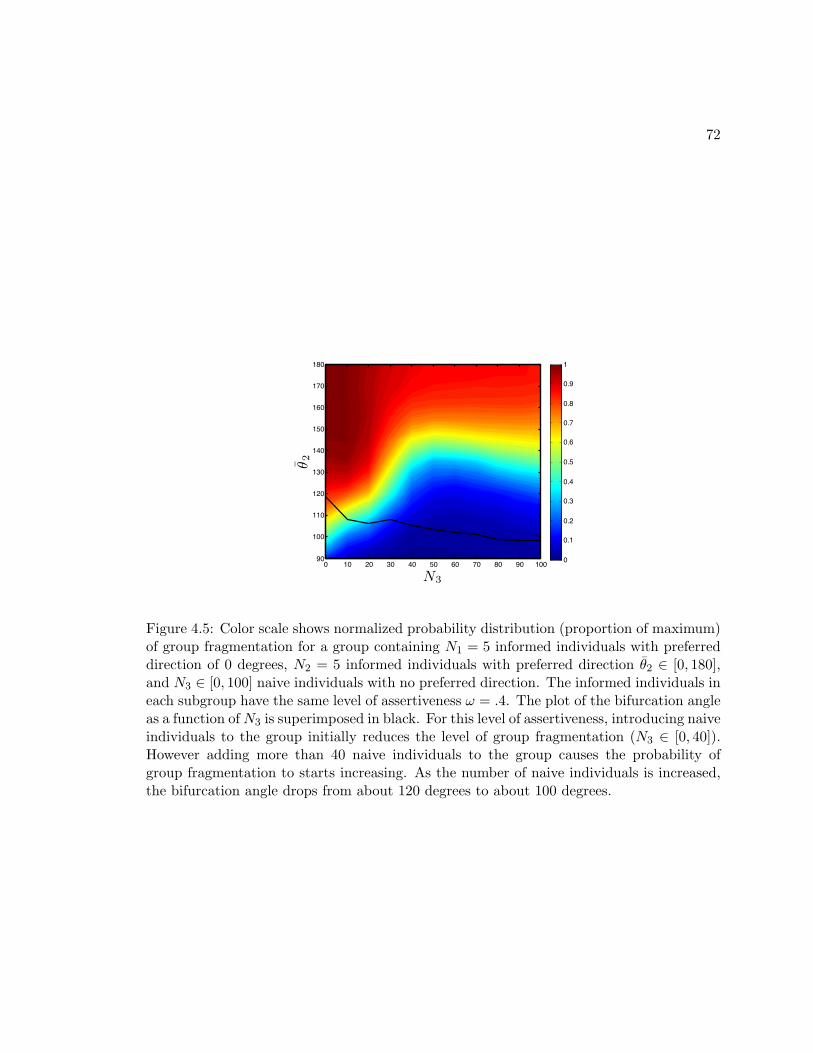
72
N3
θ2
0 10 20 30 40 50 60 70 80 90 10090
100
110
120
130
140
150
160
170
180
0
0.1
0.2
0.3
0.4
0.5
0.6
0.7
0.8
0.9
1
Figure 4.5: Color scale shows normalized probability distribution (proportion of maximum)of group fragmentation for a group containing N1 = 5 informed individuals with preferreddirection of 0 degrees, N2 = 5 informed individuals with preferred direction θ2 ∈ [0, 180],and N3 ∈ [0, 100] naive individuals with no preferred direction. The informed individuals ineach subgroup have the same level of assertiveness ω = .4. The plot of the bifurcation angleas a function ofN3 is superimposed in black. For this level of assertiveness, introducing naiveindividuals to the group initially reduces the level of group fragmentation (N3 ∈ [0, 40]).However adding more than 40 naive individuals to the group causes the probability ofgroup fragmentation to starts increasing. As the number of naive individuals is increased,the bifurcation angle drops from about 120 degrees to about 100 degrees.
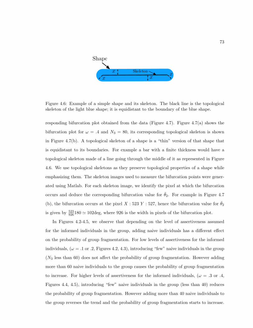
73
Figure 4.6: Example of a simple shape and its skeleton. The black line is the topologicalskeleton of the light blue shape; it is equidistant to the boundary of the blue shape.
responding bifurcation plot obtained from the data (Figure 4.7). Figure 4.7(a) shows the
bifurcation plot for ω = .4 and N3 = 80, its corresponding topological skeleton is shown
in Figure 4.7(b). A topological skeleton of a shape is a “thin” version of that shape that
is equidistant to its boundaries. For example a bar with a finite thickness would have a
topological skeleton made of a line going through the middle of it as represented in Figure
4.6. We use topological skeletons as they preserve topological properties of a shape while
emphasizing them. The skeleton images used to measure the bifurcation points were gener-
ated using Matlab. For each skeleton image, we identify the pixel at which the bifurcation
occurs and deduce the corresponding bifurcation value for θ2. For example in Figure 4.7
(b), the bifurcation occurs at the pixel X : 523 Y : 527, hence the bifurcation value for θ2
is given by 523926180 ' 102deg, where 926 is the width in pixels of the bifurcation plot.
In Figures 4.2-4.5, we observe that depending on the level of assertiveness assumed
for the informed individuals in the group, adding naive individuals has a different effect
on the probability of group fragmentation. For low levels of assertiveness for the informed
individuals, (ω = .1 or .2, Figures 4.2, 4.3), introducing “few” naive individuals in the group
(N3 less than 60) does not affect the probability of group fragmentation. However adding
more than 60 naive individuals to the group causes the probability of group fragmentation
to increase. For higher levels of assertiveness for the informed individuals, (ω = .3 or .4,
Figures 4.4, 4.5), introducing “few” naive individuals in the group (less than 40) reduces
the probability of group fragmentation. However adding more than 40 naive individuals to
the group reverses the trend and the probability of group fragmentation starts to increase.
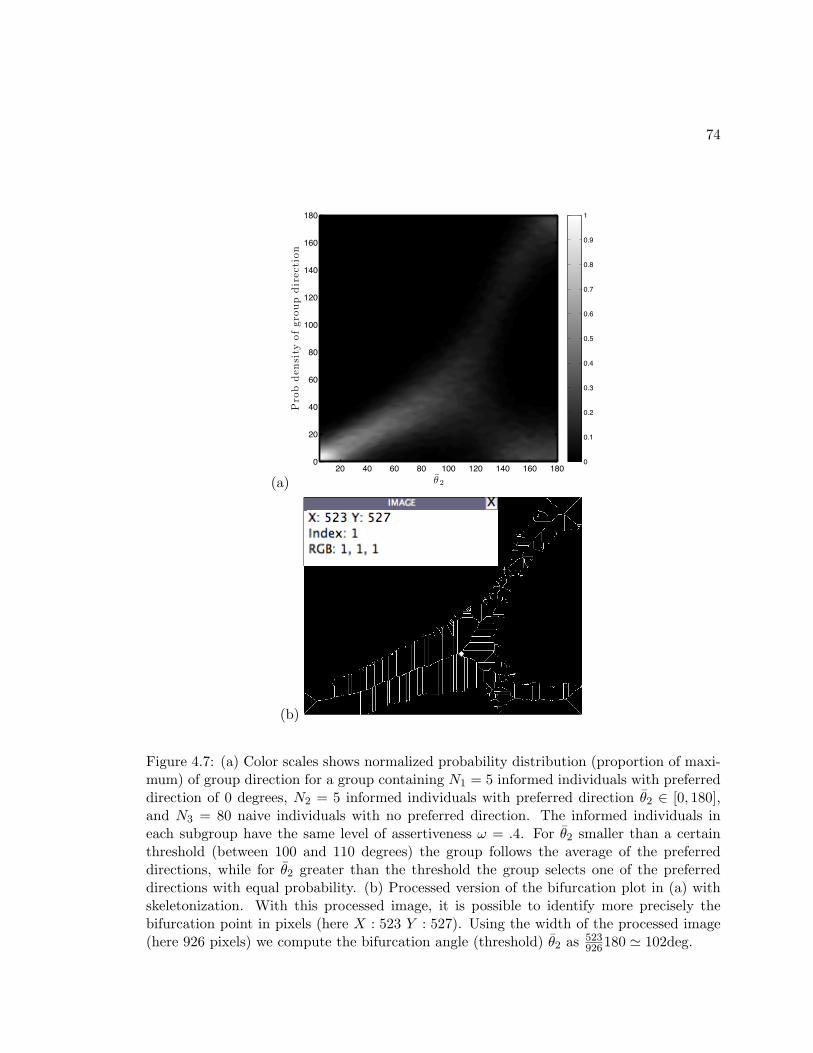
74
(a) θ2
Pro
bden
sity
ofgr
oup
dir
ecti
on
20 40 60 80 100 120 140 160 1800
20
40
60
80
100
120
140
160
180
0
0.1
0.2
0.3
0.4
0.5
0.6
0.7
0.8
0.9
1
(b)
Figure 4.7: (a) Color scales shows normalized probability distribution (proportion of maxi-mum) of group direction for a group containing N1 = 5 informed individuals with preferreddirection of 0 degrees, N2 = 5 informed individuals with preferred direction θ2 ∈ [0, 180],and N3 = 80 naive individuals with no preferred direction. The informed individuals ineach subgroup have the same level of assertiveness ω = .4. For θ2 smaller than a certainthreshold (between 100 and 110 degrees) the group follows the average of the preferreddirections, while for θ2 greater than the threshold the group selects one of the preferreddirections with equal probability. (b) Processed version of the bifurcation plot in (a) withskeletonization. With this processed image, it is possible to identify more precisely thebifurcation point in pixels (here X : 523 Y : 527). Using the width of the processed image(here 926 pixels) we compute the bifurcation angle (threshold) θ2 as 523
926180 ' 102deg.
75
This suggests that for groups with fairly assertive informed individuals with conflicting
preferences, naive individuals can help the group remain cohesive. When there are very
large numbers of naive individuals, they can increase the probability of group fragmentation.
For all levels of assertiveness, we observe (Figures 4.2-4.5) that the bifurcation angle is
a decreasing function of the number of naive individuals N3, i.e., adding naive individuals
moves the bifurcation point to the left. This means that the more naive individuals that join
the group, the smaller the disagreement between the informed individuals needs to be to
have the group switch from following the average of the preferred directions to collectively
selecting one of the preferred directions. In other words, having naive individuals in a group
increases the sensitivity of decision making in a group containing informed individuals with
conflicting preferences. This trend is observed for all levels of assertiveness for the informed
individuals but is more dramatic for lower levels of assertiveness. For ω = .1 the bifurcation
angle dropped from about 152 deg to about 97 deg while for ω = .4 the bifurcation angle
only dropped from about 120 deg to about 100 deg. This suggests that informed individuals
that are less confident derive a greater benefit from associating and sharing their information
with naive individuals than more confident informed individuals do.
The simulations presented in this section suggest two things. First naive individuals, in
some circumstances, can help keep a group cohesive but, when in too great numbers, cause
the group to fragment. Second, adding naive individuals to a group increases the sensitivity
of decision making by increasing the size of the region of parameter space in which the
group selects one of the preferred directions rather than follow the average of the preferred
directions. In order to show that improving the sensitivity of decision making also improves
its accuracy, we turn our attention from the the case where the informed individuals have
a preferred direction to the case where they have a fixed target.
These two cases are in fact intimately related. As we explained in Section 4.1, informed
individuals having a fixed target is equivalent to their having a changing preferred direction
pointing towards the target. As shown in Figure 4.8, depending on the location of the
agents relative to the targets, the difference of preferred direction between the two informed
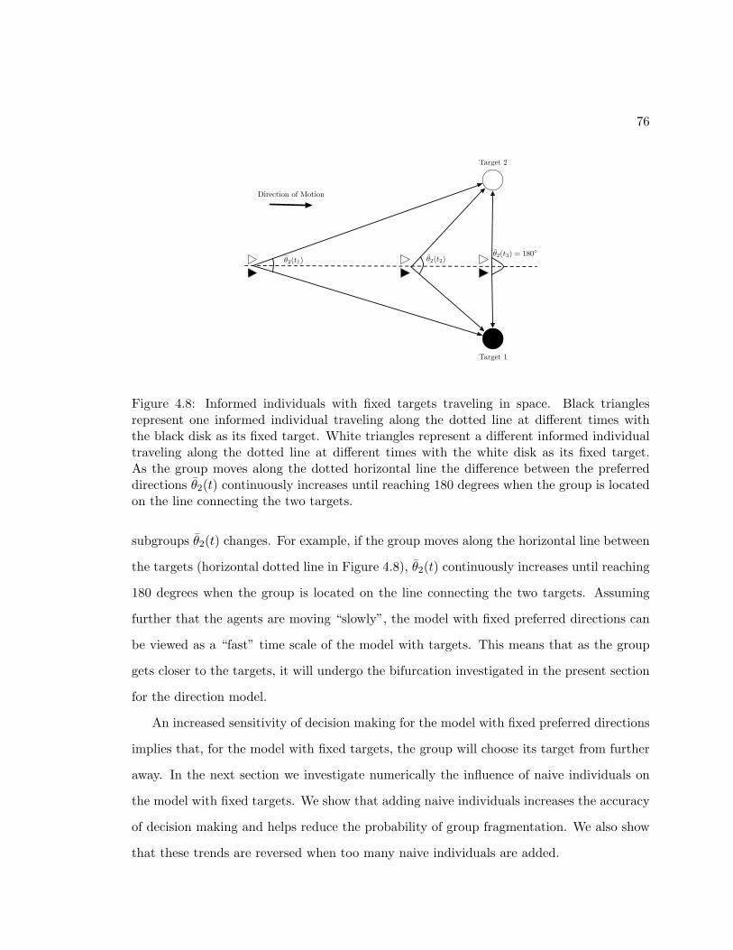
76
Direction of Motion
Target 1
Target 2
θ2(t1) θ2(t2)θ2(t3) = 180
Figure 4.8: Informed individuals with fixed targets traveling in space. Black trianglesrepresent one informed individual traveling along the dotted line at different times withthe black disk as its fixed target. White triangles represent a different informed individualtraveling along the dotted line at different times with the white disk as its fixed target.As the group moves along the dotted horizontal line the difference between the preferreddirections θ2(t) continuously increases until reaching 180 degrees when the group is locatedon the line connecting the two targets.
subgroups θ2(t) changes. For example, if the group moves along the horizontal line between
the targets (horizontal dotted line in Figure 4.8), θ2(t) continuously increases until reaching
180 degrees when the group is located on the line connecting the two targets. Assuming
further that the agents are moving “slowly”, the model with fixed preferred directions can
be viewed as a “fast” time scale of the model with targets. This means that as the group
gets closer to the targets, it will undergo the bifurcation investigated in the present section
for the direction model.
An increased sensitivity of decision making for the model with fixed preferred directions
implies that, for the model with fixed targets, the group will choose its target from further
away. In the next section we investigate numerically the influence of naive individuals on
the model with fixed targets. We show that adding naive individuals increases the accuracy
of decision making and helps reduce the probability of group fragmentation. We also show
that these trends are reversed when too many naive individuals are added.
77
4.3 Influence of Naive Individuals in the Target Model
We now focus our investigation on the influence of naive individuals in the case where the
informed individuals have a fixed target. This setting is well suited for modeling animal
foraging, for example, where desired destinations are a finite distance away. In order to
reveal the role of the naive individuals, we run a suite of simulations. We consider groups
containing two informed subgroups of unequal numbers with N1 = 6 and N2 = 5 but with
equal levels of assertiveness ω varying from .1 to .4 by increments of .1, along with one
naive subgroup with population N3 varying between 0 and 100 by increments of 5. For such
a group, reaching the target of the first informed subgroup constitutes the more accurate
decision. For all simulations, the group starts randomly distributed (according to a uni-
form distribution) in a disk centered at the point (0, 0) in the plane with a radius of 12
√N ;
the individuals in the first subgroup have a fixed target located at (2300,−1000), and the
individuals in the second informed subgroup have a fixed target located at (2300, 1000).
The targets are chosen such that the difference in preferred direction between two informed
informed individuals located at the point (0, 0), at the beginning of the simulation is ap-
proximately 47 degrees. Given the restriction on the initial conditions given above, this
choice guarantees that the group will go through the bifurcation that we described in the
previous section (i.e., when the difference in preferred direction is 100-150 degrees depend-
ing on the parameter values). For each set of values of the parameters (N3, ω), we simulate
the motion of the group for 100,000 time steps and check whether it reached a target or not
and record which target was reached. We simulate each set of parameters enough times to
get 1,000 replicates where the group reaches a target. With these simulations we compute,
for all levels of assertiveness ω ∈ [.1, .4] and for all values of N3 ∈ [0, 100], the probability of
group fragmentation, the probability of the group’s reaching the target of the first informed
subgroup (referred to as the “majority target”), and the probability, given that the group
has not fragmented, of the group’s reaching the target of the second informed subgroup
(referred to as the “minority target”). Figures 4.9-4.11 represent for ω = .1, .2, .3 and .4 the
evolution, as a function of N3, of the probability of group fragmentation, the probability of
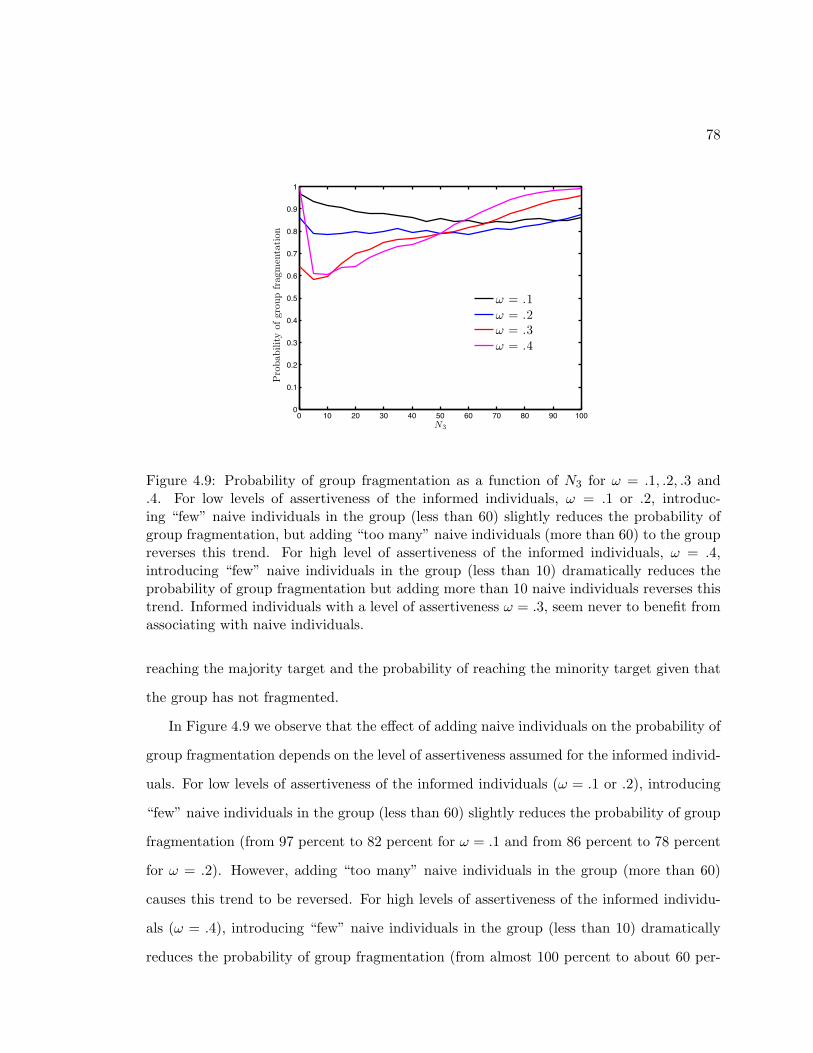
78
0 10 20 30 40 50 60 70 80 90 1000
0.1
0.2
0.3
0.4
0.5
0.6
0.7
0.8
0.9
1
N30 0.2 0.4 0.6 0.8 10
0.1
0.2
0.3
0.4
0.5
0.6
0.7
0.8
0.9
1
N3
ω = .1ω = .2ω = .3ω = .4
Pro
babi
lity
ofgr
oup
frag
men
tati
on
Figure 4.9: Probability of group fragmentation as a function of N3 for ω = .1, .2, .3 and.4. For low levels of assertiveness of the informed individuals, ω = .1 or .2, introduc-ing “few” naive individuals in the group (less than 60) slightly reduces the probability ofgroup fragmentation, but adding “too many” naive individuals (more than 60) to the groupreverses this trend. For high level of assertiveness of the informed individuals, ω = .4,introducing “few” naive individuals in the group (less than 10) dramatically reduces theprobability of group fragmentation but adding more than 10 naive individuals reverses thistrend. Informed individuals with a level of assertiveness ω = .3, seem never to benefit fromassociating with naive individuals.
reaching the majority target and the probability of reaching the minority target given that
the group has not fragmented.
In Figure 4.9 we observe that the effect of adding naive individuals on the probability of
group fragmentation depends on the level of assertiveness assumed for the informed individ-
uals. For low levels of assertiveness of the informed individuals (ω = .1 or .2), introducing
“few” naive individuals in the group (less than 60) slightly reduces the probability of group
fragmentation (from 97 percent to 82 percent for ω = .1 and from 86 percent to 78 percent
for ω = .2). However, adding “too many” naive individuals in the group (more than 60)
causes this trend to be reversed. For high levels of assertiveness of the informed individu-
als (ω = .4), introducing “few” naive individuals in the group (less than 10) dramatically
reduces the probability of group fragmentation (from almost 100 percent to about 60 per-
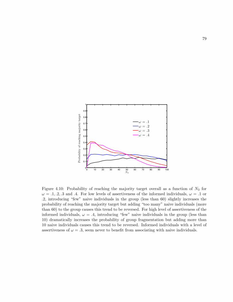
79
0 10 20 30 40 50 60 70 80 90 1000
0.1
0.2
0.3
0.4
0.5
0.6
0.7
0.8
0.9
1
N3
Pro
babi
lity
ofre
achi
ngm
ajor
ity
targ
et
0 0.2 0.4 0.6 0.8 10
0.1
0.2
0.3
0.4
0.5
0.6
0.7
0.8
0.9
1
N3
ω = .1ω = .2ω = .3ω = .4
Figure 4.10: Probability of reaching the majority target overall as a function of N3 forω = .1, .2, .3 and .4. For low levels of assertiveness of the informed individuals, ω = .1 or.2, introducing “few” naive individuals in the group (less than 60) slightly increases theprobability of reaching the majority target but adding “too many” naive individuals (morethan 60) to the group causes this trend to be reversed. For high level of assertiveness of theinformed individuals, ω = .4, introducing “few” naive individuals in the group (less than10) dramatically increases the probability of group fragmentation but adding more than10 naive individuals causes this trend to be reversed. Informed individuals with a level ofassertiveness of ω = .3, seem never to benefit from associating with naive individuals.
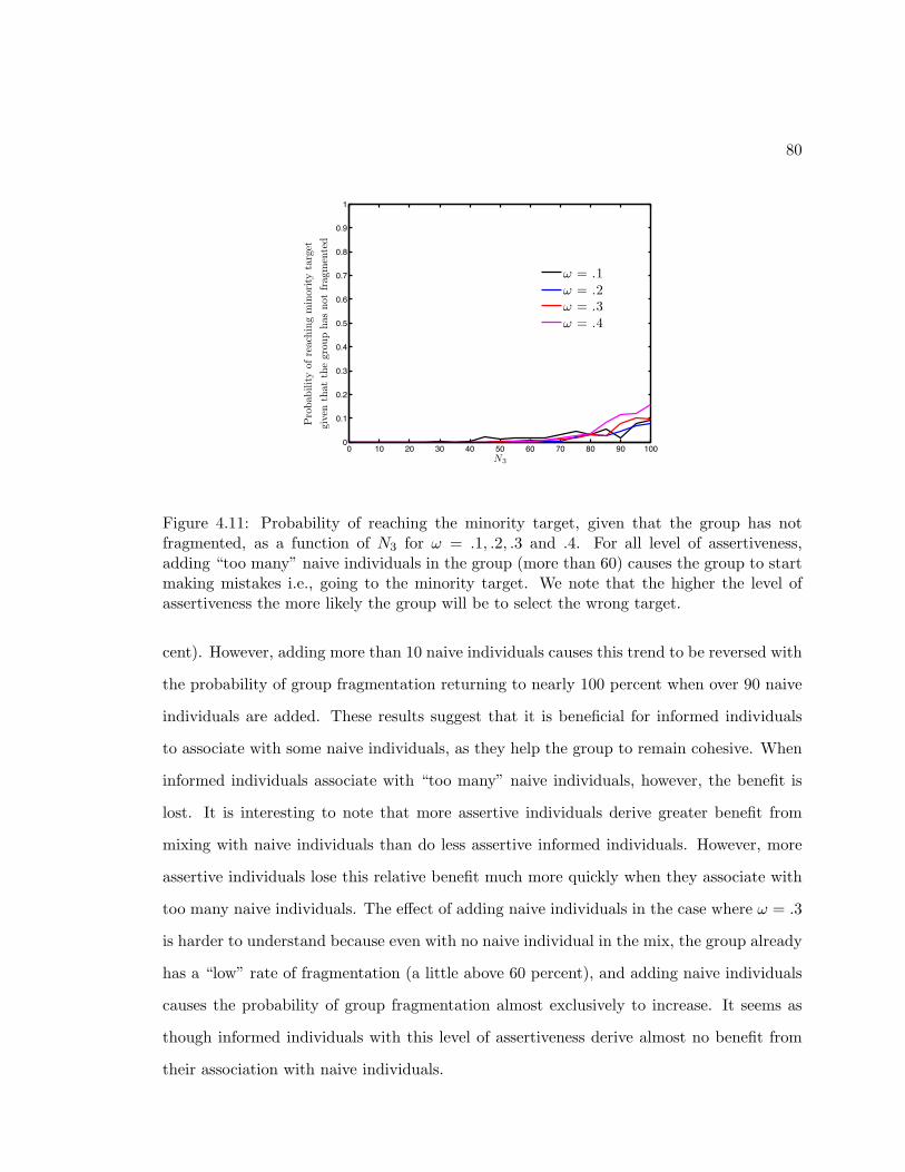
80
Pro
babi
lity
ofre
achi
ngm
inor
ity
targ
etgi
ven
that
the
grou
pha
sno
tfr
agm
ente
d
0 10 20 30 40 50 60 70 80 90 1000
0.1
0.2
0.3
0.4
0.5
0.6
0.7
0.8
0.9
1
N3
0 0.2 0.4 0.6 0.8 10
0.1
0.2
0.3
0.4
0.5
0.6
0.7
0.8
0.9
1
N3
ω = .1ω = .2ω = .3ω = .4
Figure 4.11: Probability of reaching the minority target, given that the group has notfragmented, as a function of N3 for ω = .1, .2, .3 and .4. For all level of assertiveness,adding “too many” naive individuals in the group (more than 60) causes the group to startmaking mistakes i.e., going to the minority target. We note that the higher the level ofassertiveness the more likely the group will be to select the wrong target.
cent). However, adding more than 10 naive individuals causes this trend to be reversed with
the probability of group fragmentation returning to nearly 100 percent when over 90 naive
individuals are added. These results suggest that it is beneficial for informed individuals
to associate with some naive individuals, as they help the group to remain cohesive. When
informed individuals associate with “too many” naive individuals, however, the benefit is
lost. It is interesting to note that more assertive individuals derive greater benefit from
mixing with naive individuals than do less assertive informed individuals. However, more
assertive individuals lose this relative benefit much more quickly when they associate with
too many naive individuals. The effect of adding naive individuals in the case where ω = .3
is harder to understand because even with no naive individual in the mix, the group already
has a “low” rate of fragmentation (a little above 60 percent), and adding naive individuals
causes the probability of group fragmentation almost exclusively to increase. It seems as
though informed individuals with this level of assertiveness derive almost no benefit from
their association with naive individuals.
81
In Figure 4.10 we observe that the variations of the probability of group fragmenta-
tion described in the previous paragraph translates into variations of the probability of the
group’s reaching the majority target. For “low” levels of assertiveness (ω = .1 or .2), intro-
ducing “few” naive individuals in the group (less than 60) slightly increases the probability
of reaching the majority target (from 4 percent to 16 percent for ω = .1 and from 14 per-
cent to 22 percent for ω = .2). This trend is reversed, however, when “too many” naive
individuals (more than 60) are added to the group. For high levels of assertiveness of the
informed individuals (ω = .4), introducing “few” naive individuals in the group (less than
10) dramatically increases the probability of reaching the majority target (from almost 0
percent to about 40 percent). However adding more than 10 naive individuals causes this
trend to be reversed, with the probability of reaching the majority target decreasing again
to nearly 0 percent when more than 90 naive individuals are added. These observations
further support the idea that informed individuals benefit from associating with some naive
individuals, since it increases the accuracy of decision making, but that associating with too
many naive individuals diminishes this benefit. The plot for ω = .3 also suggests that by this
measure some informed individuals derive no benefit in associating with naive individuals.
In Figure 4.11 we observe that for all levels of assertiveness, adding “too many” naive
individuals in the group (more than 60) causes the group to start making mistakes, i.e.,
going to the minority target. We note moreover that the higher the level of assertiveness the
more likely the group will be to select the wrong target. With one hundred naive individuals
in the group, if the informed individuals have a low level of assertiveness (ω = .1), then
the group will choose the “wrong” target about 8 percent of the time, whereas if the level
of assertiveness of the informed individuals is high (ω = .4), then the group will choose
the “wrong” target as often as 18 percent of the time. This trend is consistent with our
earlier observation that more assertive informed individuals are more strongly penalized by
associating with “too many” naive individuals.
Our numerical investigation of the subtle role of naive individuals in the decision-making
process within a heterogeneous group using the discrete-time model developed by Couzin
82
et al. [19] has highlighted possible drawbacks and benefits for informed individuals in asso-
ciating with naive individuals. In both settings, with informed individuals having a fixed
preferred direction and informed individuals having a fixed target, simulations suggest that
informed individuals benefit from associating with some naive individuals, as they help the
group remain cohesive and increase the sensitivity and accuracy of the decision making.
When informed individuals associate with too many naive individuals, however, the bene-
fits vanish. In these simulations, we also encountered phenomena that are hard to explain.
For informed individuals with a certain level of assertiveness, there seemed to be no benefit
in associating with naive individuals, only drawbacks. This observation highlights the point
made at the beginning of this chapter: although the discrete-time model produces highly
suggestive simulations, it is sometime hard to understand in detail the microscopic reasons
for the macroscopic behavior observed. In the next two chapters of this dissertation, we turn
our attention to simplified deterministic continuous-time models which allow for a deeper
investigation of the behavior produced and a more complete exploration of parameter space.
Chapter 5
Collective Decision Making: A
Simple Analytical Model
In this chapter, we derive and study the dynamics of a low-dimensional, deterministic,
coordinated control system designed as an interacting approximation of the individual-based
model investigated in Chapter 4. In Section 5.1, we present the model and its reduction using
a time-scale separation argument. In Section 5.2 we study the full phase-space dynamics
of the reduced model by computing equilibria and proving stability and bifurcations. In
Section 5.3 we consider several extensions of the model to test its robustness. The material
in this chapter has previously appeared in [79, 80]. The same model with certain kinds of
heterogeneity was studied with an equation-free approach in [72].
5.1 Model and Reduction
The continuous-time model we present here is an interactive partner to the discrete-time
model described in Chapter 4. The discrete-time model, first presented by Couzin et al. in
[19], contains many degrees of freedom and produces highly suggestive simulation results.
It is difficult, however, to use this model to prove particular mechanisms, define unifying
principles, and explore all possible behaviors. The continuous-time model that we propose
83
84
and study here in a particular case is represented by a set of ordinary differential equations.
A clear advantage of using ordinary differential equations is that it makes available to us
sophisticated tools from the nonlinear dynamical system literature. It is then possible to
study the global phase-space for the proposed simple model by computing equilibria and
proving stability and bifurcations.
In order to formulate our continuous-time model, we make several simplifying assump-
tions from the model presented in [19] and in Chapter 4. First, our model describes the
dynamics of the heading angles for all individuals in the population independent of their
positions. Second, an all-to-all communication topology is assumed, meaning that every
individual senses every other individuals in the population, so as to be able to adjust its
own steering rate. Third, we remove the “forgetting factor” feedback term by not allowing
informed individuals to update the strength of their attraction to their preferred direc-
tion. Finally, for the purpose of the global phase-space analysis, we ignore the presence of
naive individuals (i.e. individuals without a preferred direction of travel) when describing
the phase-space dynamics of the reduced model. These simplifications from the original
discrete-time model yield a model that produces qualitative behaviors some of which, but
not all, are observed in [19]. The observed deviations then draw our attention to a small
number of assumptions that are potentially responsible for the behavior in [19]. Our explo-
ration of the role of the naive individuals in the decision-making process, for example, as
presented in Chapter 4, was motivated by the deviation between [80] and the result pub-
lished in [19]. It is in this sense that we describe the continuous-time model presented here
as an interacting partner to the discrete-time model of [19] and Chapter 4. In Chapter 6,
we derive and analyze a similar model but relax the all-to-all coupling assumption and con-
sider the presence of naive individuals. This model produces qualitative behaviors closer,
although not identical, to the ones observed in [19] and in Chapter 4.
85
5.1.1 Particle Model
In this model, we consider a population of N interacting individuals, each described as a
unit mass Newtonian particle moving in the plane at constant speed and controlled by its
steering rate. The steering rate evolves though time under the influence of inter-particle
measurements and, when applicable, information represented by a preferred direction of
travel. Preferred directions of travel can, for example, represent knowledge of a migration
route or of the direction to a known good source of food or resource. The model assumes
an all-to-all communication topology in the group. In the natural setting, this all-to-all
coupling assumption may be reasonably well justified for tightly clustered groups. For
large swarms of insects or for microscopic organisms, however, this assumption is no longer
realistic. It is for this reason that, in the next chapter, we relax this assumption and consider
a model where the strength of the coupling between individuals is time-varying, yielding
non-complete communication topologies.
The population is divided into three subgroups: two subgroups of informed individuals
with N1 and N2 agents, respectively, and one subgroup of naive (uninformed) individuals
with N3 agents such that N1 + N2 + N3 = N . We define N1 and N2, respectively as the
subsets of indices in 1, . . . , N corresponding to individuals in the informed subgroups 1
and 2, and N3 as the remaining subset of indices corresponding to the naive individuals.
The cardinality of each subset Nk is Nk, k = 1, 2, 3. Agents in the informed subgroup i
have a preferred direction of travel θi, for i = 1, 2.
We denote as θj the instantaneous heading direction of individual j, where θj is allowed
to take any value in the circle S1. Let ~rj ∈ R2 be the position in the plane of the jth
individual moving at constant speed V0, then the instantaneous velocity vector ~Vj = d~rjdt is
given by
~Vj = (V0 cos θj , V0 sin θj) , j = 1, . . . , N.
The model we define consists of a set of differential equations describing the dynamics of
these instantaneous heading directions θj . The dynamics are modeled with steering terms
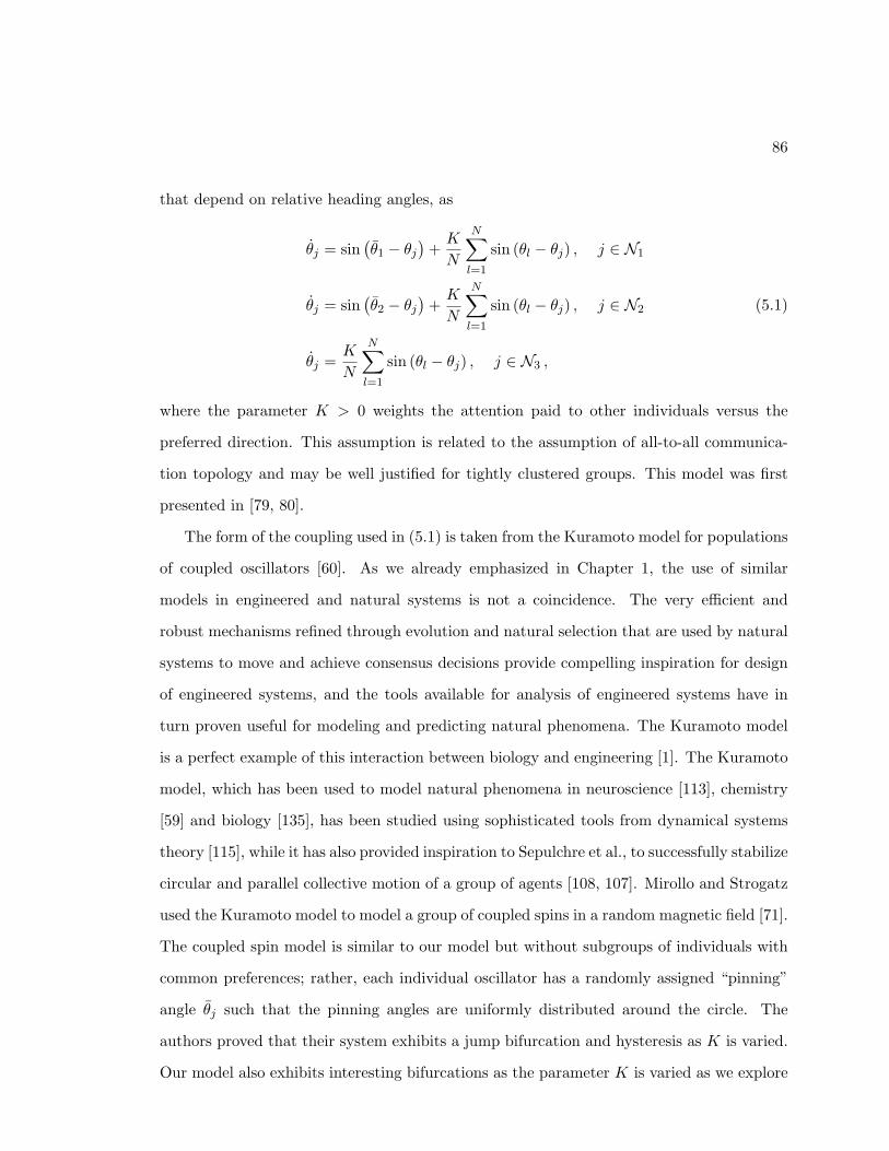
86
that depend on relative heading angles, as
θj = sin(θ1 − θj
)+K
N
N∑l=1
sin (θl − θj) , j ∈ N1
θj = sin(θ2 − θj
)+K
N
N∑l=1
sin (θl − θj) , j ∈ N2
θj =K
N
N∑l=1
sin (θl − θj) , j ∈ N3 ,
(5.1)
where the parameter K > 0 weights the attention paid to other individuals versus the
preferred direction. This assumption is related to the assumption of all-to-all communica-
tion topology and may be well justified for tightly clustered groups. This model was first
presented in [79, 80].
The form of the coupling used in (5.1) is taken from the Kuramoto model for populations
of coupled oscillators [60]. As we already emphasized in Chapter 1, the use of similar
models in engineered and natural systems is not a coincidence. The very efficient and
robust mechanisms refined through evolution and natural selection that are used by natural
systems to move and achieve consensus decisions provide compelling inspiration for design
of engineered systems, and the tools available for analysis of engineered systems have in
turn proven useful for modeling and predicting natural phenomena. The Kuramoto model
is a perfect example of this interaction between biology and engineering [1]. The Kuramoto
model, which has been used to model natural phenomena in neuroscience [113], chemistry
[59] and biology [135], has been studied using sophisticated tools from dynamical systems
theory [115], while it has also provided inspiration to Sepulchre et al., to successfully stabilize
circular and parallel collective motion of a group of agents [108, 107]. Mirollo and Strogatz
used the Kuramoto model to model a group of coupled spins in a random magnetic field [71].
The coupled spin model is similar to our model but without subgroups of individuals with
common preferences; rather, each individual oscillator has a randomly assigned “pinning”
angle θj such that the pinning angles are uniformly distributed around the circle. The
authors proved that their system exhibits a jump bifurcation and hysteresis as K is varied.
Our model also exhibits interesting bifurcations as the parameter K is varied as we explore
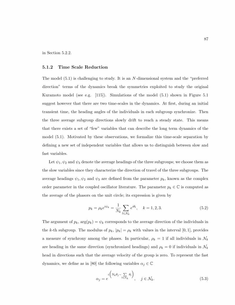
87
in Section 5.2.2.
5.1.2 Time Scale Reduction
The model (5.1) is challenging to study. It is an N -dimensional system and the “preferred
direction” terms of the dynamics break the symmetries exploited to study the original
Kuramoto model (see e.g. [115]). Simulations of the model (5.1) shown in Figure 5.1
suggest however that there are two time-scales in the dynamics. At first, during an initial
transient time, the heading angles of the individuals in each subgroup synchronize. Then
the three average subgroup directions slowly drift to reach a steady state. This means
that there exists a set of “few” variables that can describe the long term dynamics of the
model (5.1). Motivated by these observations, we formalize this time-scale separation by
defining a new set of independent variables that allows us to distinguish between slow and
fast variables.
Let ψ1, ψ2 and ψ3 denote the average headings of the three subgroups; we choose them as
the slow variables since they characterize the direction of travel of the three subgroups. The
average headings ψ1, ψ2 and ψ3 are defined from the parameter pk, known as the complex
order parameter in the coupled oscillator literature. The parameter pk ∈ C is computed as
the average of the phasors on the unit circle; its expression is given by
pk = ρkeiψk =
1Nk
∑l∈Nk
eiθl , k = 1, 2, 3. (5.2)
The argument of pk, arg(pk) = ψk corresponds to the average direction of the individuals in
the k-th subgroup. The modulus of pk, |pk| = ρk with values in the interval [0, 1], provides
a measure of synchrony among the phases. In particular, ρk = 1 if all individuals in Nkare heading in the same direction (synchronized headings) and ρk = 0 if individuals in Nkhead in directions such that the average velocity of the group is zero. To represent the fast
dynamics, we define as in [80] the following variables αj ∈ C
αj = ei
(Nkθj−
Pl∈Nk
θl
), j ∈ Nk. (5.3)
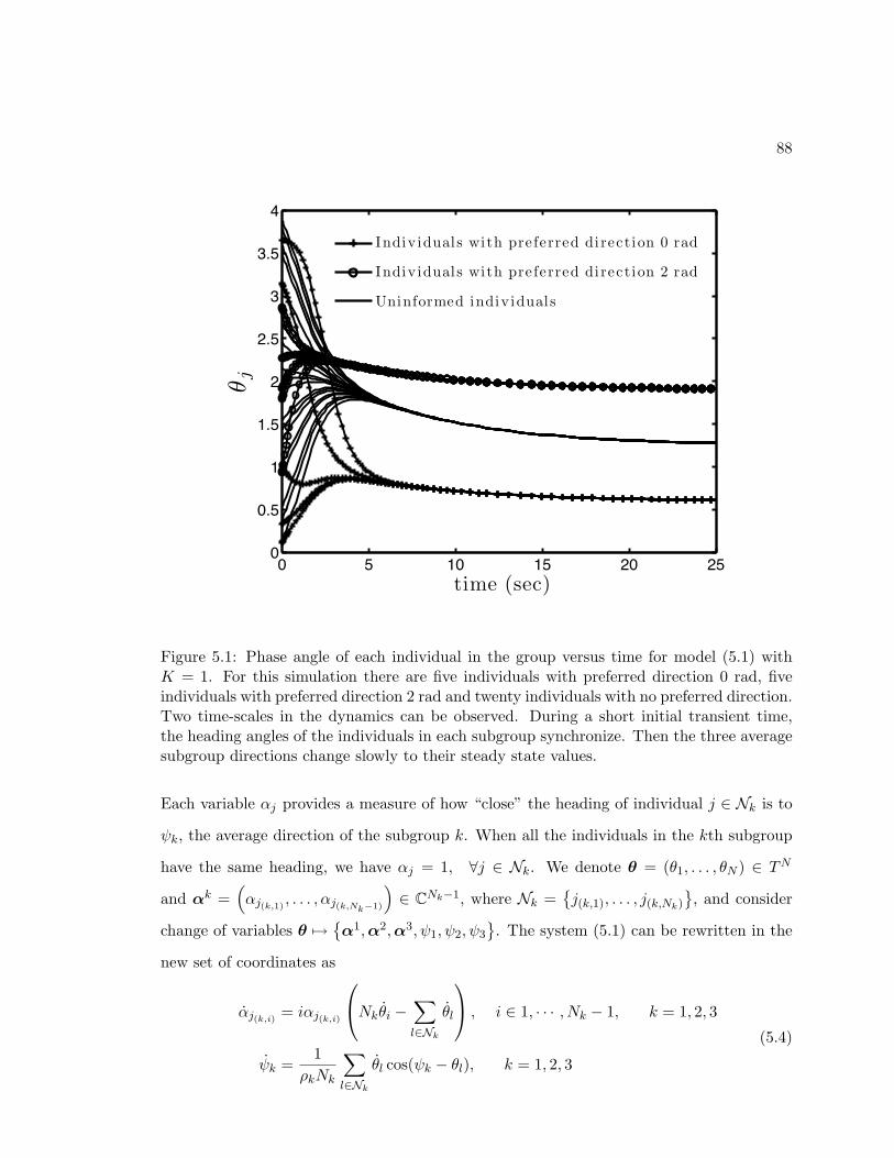
88
0 5 10 15 20 250
0.5
1
1.5
2
2.5
3
3.5
4
time (sec)
θj
Indiv idual s with preferred direction 0 rad
Individual s with preferred direction 2 rad
Uninformed individual s
Figure 5.1: Phase angle of each individual in the group versus time for model (5.1) withK = 1. For this simulation there are five individuals with preferred direction 0 rad, fiveindividuals with preferred direction 2 rad and twenty individuals with no preferred direction.Two time-scales in the dynamics can be observed. During a short initial transient time,the heading angles of the individuals in each subgroup synchronize. Then the three averagesubgroup directions change slowly to their steady state values.
Each variable αj provides a measure of how “close” the heading of individual j ∈ Nk is to
ψk, the average direction of the subgroup k. When all the individuals in the kth subgroup
have the same heading, we have αj = 1, ∀j ∈ Nk. We denote θ = (θ1, . . . , θN ) ∈ TN
and αk =(αj(k,1)
, . . . , αj(k,Nk−1)
)∈ CNk−1, where Nk =
j(k,1), . . . , j(k,Nk)
, and consider
change of variables θ 7→ α1,α2,α3, ψ1, ψ2, ψ3
. The system (5.1) can be rewritten in the
new set of coordinates as
αj(k,i) = iαj(k,i)
Nkθi −∑l∈Nk
θl
, i ∈ 1, · · · , Nk − 1, k = 1, 2, 3
ψk =1
ρkNk
∑l∈Nk
θl cos(ψk − θl), k = 1, 2, 3
(5.4)
89
Following the calculations in [115, 80], we rewrite the coupled multi-agent system dynamics
(5.4) as
αj = iN1αj
( (sin(θ1 − θj
)− ρ1 sin(θ1 − ψ1
))+KN1
Nρ1 sin (ψ1 − θj)
+∑k=2,3
KNk
Nρk (sin (ψk − θj)− ρ1 sin (ψk − ψ1))
), j ∈ N1, j 6= j(1,N1)
αj = iN2αj
( (sin(θ2 − θj
)− ρ2 sin(θ2 − ψ2
))+KN2
Nρ2 sin (ψ2 − θj)
+∑k=1,3
KNk
Nρk (sin (ψk − θj)− ρ2 sin (ψk − ψ2))
), j ∈ N2, j 6= j(2,N2)
αj = iN1αj
(KN3
Nρ3 sin (ψ3 − θj)
+∑k=2,3
KNk
Nρk (sin (ψk − θj)− ρ3 sin (ψk − ψ3))
), j ∈ N3, j 6= j(3,N3)
ψ1 =1ρ1
∑j∈N1
(1N1
sin(θ1 − θj
)+K
N
(3∑
k=1
Nk
N1ρk sin (ψk − θj)
))cos (ψ1 − θj)
ψ2 =1ρ2
∑j∈N2
(1N2
sin(θ2 − θj
)+K
N
(3∑
k=1
Nk
N2ρk sin (ψk − θj)
))cos (ψ2 − θj)
ψ3 =1ρ3
∑j∈N3
(K
N
(3∑
k=1
Nk
N3ρk sin (ψk − θj)
))cos (ψ3 − θj)
(5.5)
for ρk 6= 0, k = 1, 2, 3.
The solution αj = 1 for j ∈ Nk, k = 1, 2, 3, (or equivalently θj = ψk, j ∈ Nk, k = 1, 2, 3,)
is an isolated solution of αj = 0, j ∈ Nk, j 6= j(k,Nk) k = 1, 2, 3. For this solution ρk = 1,
k = 1, 2, 3. In other words, θj = ψk, j ∈ Nk, k = 1, 2, 3 is an invariant manifold of the system
(5.5); we call this manifold M. Physically this means that if we start with all individuals
synchronized within their respective subgroup (i.e., θj = ψk, j ∈ Nk, k = 1, 2, 3), they will
remain so for all time.
Lemma 5.1.1 The change of variables θ 7→ (α1, ψ1,α2, ψ2,α
3, ψ3) is well defined near the
invariant manifold M.
Proof: We write (α1, ψ1,α2, ψ2,α
3, ψ3) = F (θ) and prove that F is locally invertible near
90
M. On M, we have
∂αj(k,l)∂θm
∣∣∣∣M
=
−i if m ∈ Nk, m 6= j(k,l)
(Nk − 1)i if m = j(k,l)
0 otherwise
∂ψk∂θm
∣∣∣∣M
=
1Nk
if m ∈ Nk0 otherwise.
(5.6)
Using (5.6), the Jacobian of F evaluated on M can be written as
dF
dθ
∣∣∣∣M
= diag(Ak),
where
Ak =
(Nk − 1)i −i · · · · · · −i−i . . . . . . −i ......
. . . . . . . . ....
−i · · · −i (Nk − 1)i −i1Nk
· · · · · · · · · 1Nk
∈ RNk×Nk , k = 1, 2, 3.
Each Ak is invertible with
A−1k =
− iNk
0 · · · 0 1
0. . . . . .
......
.... . . . . . 0
...
0 · · · 0 − iNk
...
iNk
· · · · · · iNk
1
∈ RNk×Nk , (5.7)
hence dFdθ
∣∣M is also invertible. This concludes the proof that F : θ 7→ (α1, ψ1,α
2, ψ2,α3, ψ3)
is locally invertible in a neighborhood of M. Hence the change of variables from θ 7→(α1, ψ1,α
2, ψ2,α3, ψ3) is well defined near M.
In order to prove the time-scale reduction, we rewrite the model (5.5) in the form of
a singular perturbation model, decomposing it into a boundary layer (fast) model and a
reduced (slow) model. We suppose K ≥ N >> 1 and let ε = 1/K. We assume further that
N1 and N2 are such that 1/N1, 1/N2, N1/N , N2/N are not as small as ε. For example, if
91
K = N = 100, N1 = N2 = 10, N3 = 80, then ε = 0.01 but 1/N1 = 1/N2 = N1/N = N2/N =
0.1 =√ε. Given these assumptions the coupled multi-agent system dynamics (5.5) become
εαj = iN1αj
(ε(sin(θ1 − θj
)− ρ1 sin(θ1 − ψ1
))+N1
Nρ1 sin (ψ1 − θj)
+∑k=2,3
Nk
Nρk (sin (ψk − θj)− ρ1 sin (ψk − ψ1))
)(5.8)
=: g1j
(α1,α2,α3, ψ1, ψ2, ψ3, ε
), j ∈ N1, j 6= j(1,N1)
εαj = iN2αj
(ε(sin(θ2 − θj
)− ρ2 sin(θ2 − ψ2
))+N2
Nρ2 sin (ψ2 − θj)
+∑k=1,3
Nk
Nρk (sin (ψk − θj)− ρ2 sin (ψk − ψ2))
)(5.9)
=: g2j
(α1,α2,α3, ψ1, ψ2, ψ3, ε
), j ∈ N2, j 6= j(2,N2)
εαj = iN1αj
(N3
Nρ3 sin (ψ3 − θj)
+∑k=2,3
Nk
Nρk (sin (ψk − θj)− ρ3 sin (ψk − ψ3))
)(5.10)
=: g3j
(α1,α2,α3, ψ1, ψ2, ψ3, ε
), j ∈ N3, j 6= j(3,N3)
ψ1 =1ρ1
∑j∈N1
(1N1
sin(θ1 − θj
)+K
N
3∑k=1
Nk
N1ρk sin (ψk − θj)
)cos (ψ1 − θj) (5.11)
=: f1
(α1,α2,α3, ψ1, ψ2, ψ3, ε
)ψ2 =
1ρ2
∑j∈N2
(1N2
sin(θ2 − θj
)+K
N
3∑k=1
Nk
N2ρk sin (ψk − θj)
)cos (ψ2 − θj) (5.12)
=: f2
(α1,α2,α3, ψ1, ψ2, ψ3, ε
)ψ3 =
1ρ3
∑j∈N3
(K
N
(3∑
k=1
Nk
N3ρk sin (ψk − θj)
))cos (ψ3 − θj) (5.13)
=: f3
(α1,α2,α3, ψ1, ψ2, ψ3, ε
)for ρk 6= 0, k = 1, 2, 3.
With ε << 1, the model (5.8)-(5.13) is in the form of a singular perturbation model
(as described in [54]). The N − 3 dimensional boundary layer (fast) model is represented
by (5.8)-(5.10) and the 3 dimensional reduced (slow) model is represented by (5.11)-(5.13).
The reduced dynamics on the invariant manifold M are then given by
ψk = fk(α1 = 1,α2 = 1,α3 = 1, ψ1, ψ2, ψ3, 0
), k = 1, 2, 3,
92
where 1 = (1, . . . , 1), which can be written as
ψ1 = sin(θ1 − ψ1
)+K
NN2 sin (ψ2 − ψ1) +
K
NN3 sin (ψ3 − ψ1)
ψ2 = sin(θ2 − ψ2
)+K
NN1 sin (ψ1 − ψ2) +
K
NN3 sin (ψ3 − ψ2)
ψ3 =K
NN1 sin (ψ1 − ψ3) +
K
NN2 sin (ψ2 − ψ3) .
(5.14)
Theorem 5.1.2 Assuming N1 = N2 and N3 = 0, the invariant manifold M is attractive.
Given the attractiveness of the invariant manifold, singular perturbation theory (see e.g.
[54]) then guarantees that solutions to the unreduced dynamics stay close to solutions of
the reduced system.
Proof of Theorem 5.1.2: Assuming N1 = N2 and N3 = 0, we show that the invariant
manifoldM is attractive by proving that it is a locally exponentially stable manifold of the
boundary layer dynamics
dαjdt
= gj(α1,α2, ψ1, ψ2, 0), j ∈ Nk, j 6= j(k,Nk), k = 1, 2, (5.15)
uniformly in ψ1, ψ2.
The boundary layer dynamics can be written as
αj = iN1αj
(−N1
Nρ1 sin(ψ1 − θj) +
N2
Nρ2
(sin(ψ2 − θj)− ρ1 sin(ψ2 − ψ1)
)+N3
Nρ3
(sin(ψ3 − θj)− ρ1 sin(ψ3 − ψ1)
)), j ∈ N1, j 6= j(1,N1)
αj = iN2αj
(−N2
Nρ2 sin(ψ2 − θj) +
N1
Nρ1
(sin(ψ1 − θj)− ρ2 sin(ψ1 − ψ2)
)+N3
Nρ3
(sin(ψ3 − θj)− ρ2 sin(ψ3 − ψ2)
)), j ∈ N2, j 6= j(2,N2).
The linearization of the boundary layer model is given by
∂αj∂αm
∣∣∣∣M
=− iNk
N
∂θj∂αm
∣∣∣∣M
(Nk +
∑l 6=k
Nl cos(ψl − ψk))
+∂ρk∂αm
∣∣∣∣M
∑l 6=k
Nl sin(ψl − ψk) ,
j ∈ Nk, j 6= j(k,Nk), k = 1, 2, 3, m ∈ 1, . . . , N \ j(1,N1), j(2,N2).(5.16)
93
Using equation (5.7), the values for ∂θj∂αm
∣∣∣M
can be read as
∂θj∂αm
∣∣∣∣M
=
−iNk
if m = j,
0 otherwise.(5.17)
Taking partial derivatives with respect to αm of equation (5.2) yields
∂ρk∂αm
eiψk + ρki∂ψk∂αm
eiψk =i
Nk
∑j∈Nk
∂θj∂αm
eiθj . (5.18)
Evaluating (5.18) on M and using equation (5.7) gives
∂ρk∂αm
∣∣∣∣M
=i
Nk
∑j
∂θj∂αm
∣∣∣∣M
= 0. (5.19)
Plugging equation (5.17) and (5.19) into (5.16), the Jacobian can be rewritten as a diagonal
matrix J with
Jjj = − 1N
(Nk +
∑l 6=k
Nl cos(ψl − ψk)), j ∈ Nk, j 6= j(k,Nk), k = 1, 2.
When N1 = N2 the eigenvalues of J are strictly negative, thus concluding the proof that
M is a locally exponentially stable manifold of (5.15) uniformly in ψ1, ψ2. Hence M, the
invariant manifold of (5.1) defined by θj = ψk, j ∈ Nk, k = 1, 2, is attractive.
The solution of the boundary layer (fast) dynamics corresponds to synchronization of
all particle headings in subgroup k to a common heading ψk, for k = 1, 2, 3. These common
headings then follow the reduced (slow) model (5.14). This reduced model is one in which
all the agents in each subgroup (informed subgroups 1 and 2 and naive subgroup 3) behave
as a single entity and the inter-subgroup coupling term is weighted by the corresponding
subgroup population size as well as the bifurcation parameter K. This grouping of identical
individuals is consistent with the spatial clustering observed in the simulations from [19].
In the next section, we present a full phase-space dynamics analysis of the reduced model
(5.14) assuming N1 = N2 and N3 = 0, and in so doing show the different stable and
unstable motions, and investigate bifurcations in the K, θ2 parameters. Extension to the
cases N1 6= N2 and N3 6= 0 will be considered numerically in Section 5.3. The extension to
the case N3 6= 0 is developed more formally in Chapter 6.
94
5.2 Phase Space Dynamics of the Reduced Model
In the case N1 = N2 and N3 = 0, the system (5.14) becomes
ψ1 = sin(θ1 − ψ1
)+K
2sin (ψ2 − ψ1)
ψ2 = sin(θ2 − ψ2
)+K
2sin (ψ1 − ψ2) .
(5.20)
Without loss of generality we set θ1 = 0 and consider the two bifurcation parameters, K ≥ 0
and θ2 ∈ (0, π]. The case θ2 = 0, which corresponds to having all informed individuals
identical, is ignored. In this case there is no disagreement, and it can be shown that the
groups travel in the direction θ1 = θ2 = 0.
We note that in the studied special case (i.e., N1 = N2 and N3 = 0), the reduced model
is a gradient system. The dynamics are gradient such that
ψk = − ∂V∂ψk
,
where V is given by
V (ψ1, ψ2) = − cos(θ1 − ψ1)− cos(θ2 − ψ2
)− K
2cos (ψ2 − ψ1) .
Thus, LaSalle’s Invariance Principle guarantees that all solutions converge to the set of
critical points of V (ψ1, ψ2) and that there are no periodic solutions.
5.2.1 Equilibria of the Reduced System (5.20)
We compute the equilibria of the system (5.20) but note that, except for specific values
of the parameters K, θ2, we cannot find closed form expressions for all of them. For each
equilibrium we nevertheless describe how its value and stability changes as the bifurcation
parameters K and θ2 vary. We call an equilibrium synchronized if ψ1 = ψ2 mod 2π and
anti-synchronized if ψ1 − ψ2 = π mod 2π. The equilibria are given by
− sinψ1 +K
2sin (ψ2 − ψ1) = 0
sin(θ2 − ψ2
)+K
2sin (ψ1 − ψ2) = 0.
95
There are two sets of solutions, the first set given by
ψ1 = π − θ2 + ψ2
sin(ψ2 − θ2
)=K
2sin θ2, (5.21)
and the second set given by
ψ1 = θ2 − ψ2 (5.22)
sin(θ2 − ψ2
)=K
2sin(2ψ2 − θ2
). (5.23)
In the first set of solutions, equation (5.21) has two solutions: ψ2 = θ2 +arcsin(K2 sin θ2
)and ψ2 = θ2 + π− arcsin
(K2 sin θ2
). These two solutions exist if and only if |K2 sin θ2| ≤ 1.
Lemma 5.2.1 If |K2 sin θ2| < 1, then the two equilibria ψS1 = (ψ1, ψ2)S1 and ψS2 =
(ψ1, ψ2)S2 satisfying (5.21) and given by
ψS1 =(π + arcsin
(K
2sin θ2
), θ2 + arcsin
(K
2sin θ2
)), (5.24)
ψS2 =(− arcsin
(K
2sin θ2
), π + θ2 − arcsin
(K
2sin θ2
)), (5.25)
are saddle points ∀K > 0 and ∀θ2 ∈ [0, π]. If K2 sin θ2 = 1, then ψS1 = ψS2. In this case, if
also K > 0 and θ2 ∈(0, π2
) ∪ (π2 , π), then ψS1 = ψS2 is unstable with one zero eigenvalue
and one positive real eigenvalue. If θ2 = π2 (and K = 2), then both eigenvalues are zero.
Proof: The proof of Lemma 5.2.1 can be found in Appendix A.
Figure 5.2 shows the equilibrium ψS1 for K = 1, 2, 4 and θ2 = 0.1, π2 , π. For this
equilibrium, the relative heading of the two informed subgroups is constant, and equal to
θ2 − π. As θ2 goes from 0 to π, the equilibrium goes from being anti-synchronized, with
each subgroup traveling opposite to its preferred direction, to being synchronized in the
preferred direction of the second informed subgroup.
Figure 5.3 shows the equilibrium ψS2 for K = 1, 2, 4 and θ2 = .1, π2 , π. For this equilib-
rium, the relative heading of the two informed subgroups is constant, and equal to θ2+π. As
θ2 goes from 0 to π, the equilibrium goes from being anti-synchronized, with each subgroup
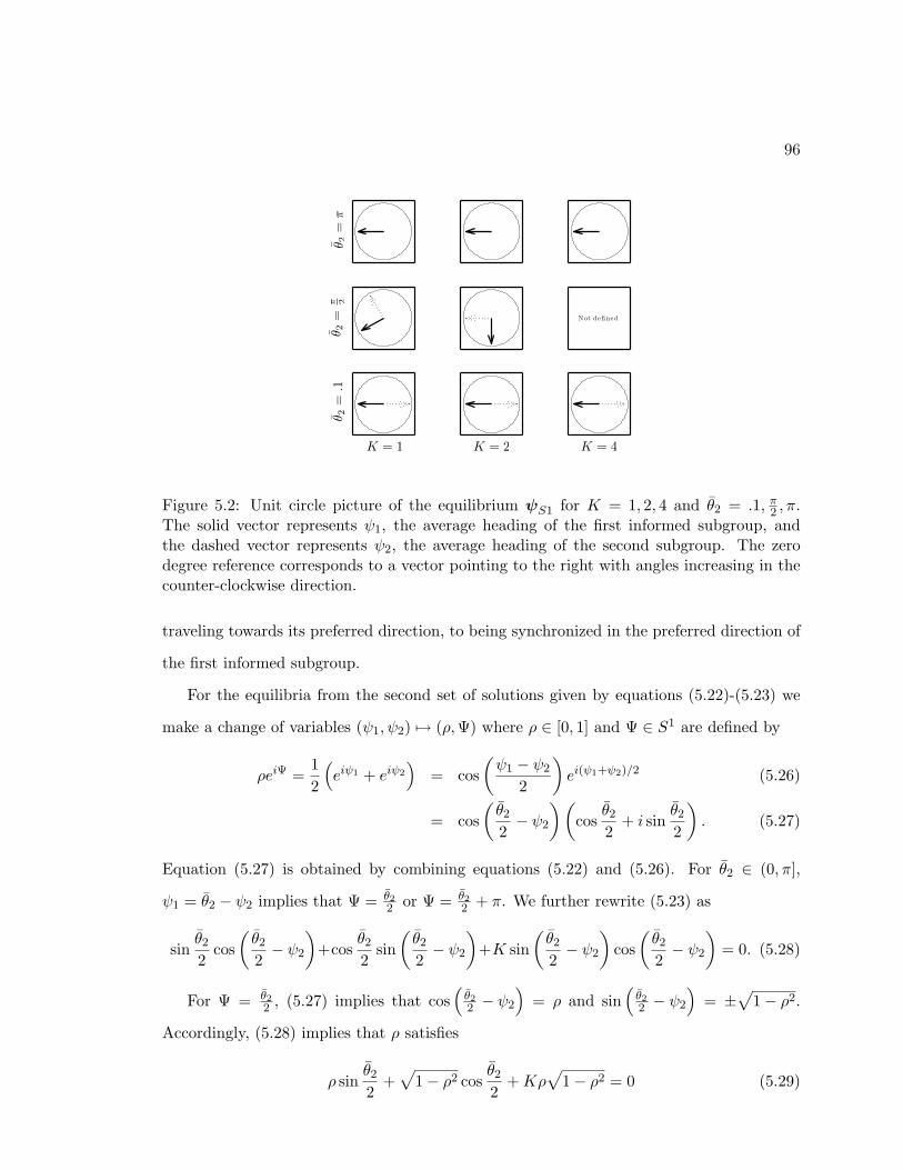
96
K = 1 K = 4
θ 2=
.1θ 2
=π 2
K = 2
θ 2=π
Not defined
Figure 5.2: Unit circle picture of the equilibrium ψS1 for K = 1, 2, 4 and θ2 = .1, π2 , π.The solid vector represents ψ1, the average heading of the first informed subgroup, andthe dashed vector represents ψ2, the average heading of the second subgroup. The zerodegree reference corresponds to a vector pointing to the right with angles increasing in thecounter-clockwise direction.
traveling towards its preferred direction, to being synchronized in the preferred direction of
the first informed subgroup.
For the equilibria from the second set of solutions given by equations (5.22)-(5.23) we
make a change of variables (ψ1, ψ2) 7→ (ρ,Ψ) where ρ ∈ [0, 1] and Ψ ∈ S1 are defined by
ρeiΨ =12
(eiψ1 + eiψ2
)= cos
(ψ1 − ψ2
2
)ei(ψ1+ψ2)/2 (5.26)
= cos(θ2
2− ψ2
)(cos
θ2
2+ i sin
θ2
2
). (5.27)
Equation (5.27) is obtained by combining equations (5.22) and (5.26). For θ2 ∈ (0, π],
ψ1 = θ2 − ψ2 implies that Ψ = θ22 or Ψ = θ2
2 + π. We further rewrite (5.23) as
sinθ2
2cos(θ2
2− ψ2
)+cos
θ2
2sin(θ2
2− ψ2
)+K sin
(θ2
2− ψ2
)cos(θ2
2− ψ2
)= 0. (5.28)
For Ψ = θ22 , (5.27) implies that cos
(θ22 − ψ2
)= ρ and sin
(θ22 − ψ2
)= ±
√1− ρ2.
Accordingly, (5.28) implies that ρ satisfies
ρ sinθ2
2+√
1− ρ2 cosθ2
2+Kρ
√1− ρ2 = 0 (5.29)
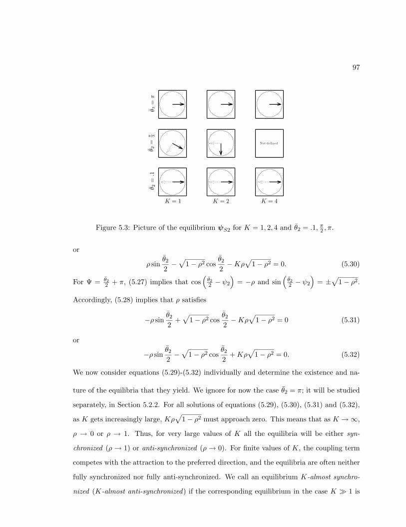
97
K = 1 K = 4
θ 2=
.1θ 2
=π 2
K = 2
θ 2=π
Not defined
Figure 5.3: Picture of the equilibrium ψS2 for K = 1, 2, 4 and θ2 = .1, π2 , π.
or
ρ sinθ2
2−√
1− ρ2 cosθ2
2−Kρ
√1− ρ2 = 0. (5.30)
For Ψ = θ22 + π, (5.27) implies that cos
(θ22 − ψ2
)= −ρ and sin
(θ22 − ψ2
)= ±
√1− ρ2.
Accordingly, (5.28) implies that ρ satisfies
−ρ sinθ2
2+√
1− ρ2 cosθ2
2−Kρ
√1− ρ2 = 0 (5.31)
or
−ρ sinθ2
2−√
1− ρ2 cosθ2
2+Kρ
√1− ρ2 = 0. (5.32)
We now consider equations (5.29)-(5.32) individually and determine the existence and na-
ture of the equilibria that they yield. We ignore for now the case θ2 = π; it will be studied
separately, in Section 5.2.2. For all solutions of equations (5.29), (5.30), (5.31) and (5.32),
as K gets increasingly large, Kρ√
1− ρ2 must approach zero. This means that as K →∞,
ρ → 0 or ρ → 1. Thus, for very large values of K all the equilibria will be either syn-
chronized (ρ → 1) or anti-synchronized (ρ → 0). For finite values of K, the coupling term
competes with the attraction to the preferred direction, and the equilibria are often neither
fully synchronized nor fully anti-synchronized. We call an equilibrium K-almost synchro-
nized (K-almost anti-synchronized) if the corresponding equilibrium in the case K 1 is
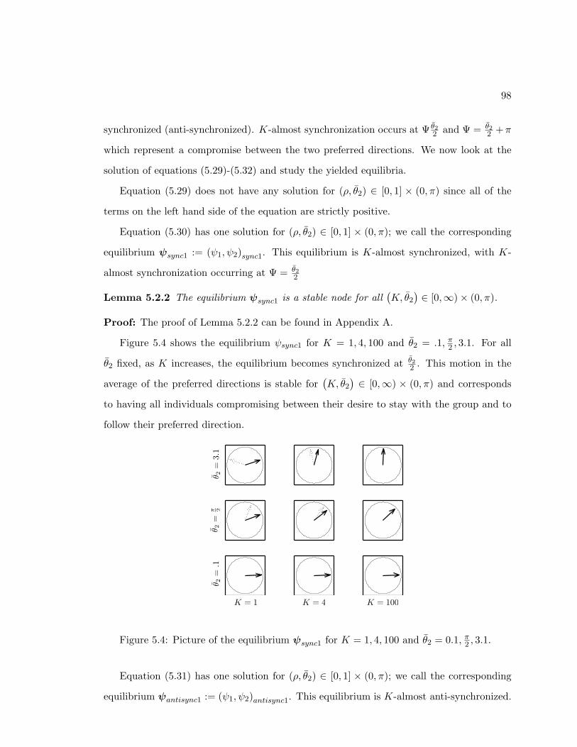
98
synchronized (anti-synchronized). K-almost synchronization occurs at Ψ θ22 and Ψ = θ2
2 +π
which represent a compromise between the two preferred directions. We now look at the
solution of equations (5.29)-(5.32) and study the yielded equilibria.
Equation (5.29) does not have any solution for (ρ, θ2) ∈ [0, 1] × (0, π) since all of the
terms on the left hand side of the equation are strictly positive.
Equation (5.30) has one solution for (ρ, θ2) ∈ [0, 1] × (0, π); we call the corresponding
equilibrium ψsync1 := (ψ1, ψ2)sync1. This equilibrium is K-almost synchronized, with K-
almost synchronization occurring at Ψ = θ22
Lemma 5.2.2 The equilibrium ψsync1 is a stable node for all(K, θ2
) ∈ [0,∞)× (0, π).
Proof: The proof of Lemma 5.2.2 can be found in Appendix A.
Figure 5.4 shows the equilibrium ψsync1 for K = 1, 4, 100 and θ2 = .1, π2 , 3.1. For all
θ2 fixed, as K increases, the equilibrium becomes synchronized at θ22 . This motion in the
average of the preferred directions is stable for(K, θ2
) ∈ [0,∞) × (0, π) and corresponds
to having all individuals compromising between their desire to stay with the group and to
follow their preferred direction.
K = 1 K = 4
θ 2=
.1θ 2
=π 2
θ 2=
3.1
K = 100
Figure 5.4: Picture of the equilibrium ψsync1 for K = 1, 4, 100 and θ2 = 0.1, π2 , 3.1.
Equation (5.31) has one solution for (ρ, θ2) ∈ [0, 1] × (0, π); we call the corresponding
equilibrium ψantisync1 := (ψ1, ψ2)antisync1. This equilibrium is K-almost anti-synchronized.
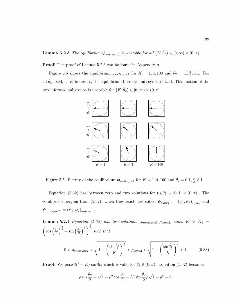
99
Lemma 5.2.3 The equilibrium ψantisync1 is unstable for all(K, θ2
) ∈ [0,∞)× (0, π).
Proof: The proof of Lemma 5.2.3 can be found in Appendix A.
Figure 5.5 shows the equilibrium ψantisync1 for K = 1, 4, 100 and θ2 = .1, π2 , 3.1. For
all θ2 fixed, as K increases, the equilibrium becomes anti-synchronized. This motion of the
two informed subgroups is unstable for(K, θ2
) ∈ [0,∞)× (0, π).
K = 1 K = 4
θ 2=
.1θ 2
=π 2
θ 2=
3.1
K = 100K = 1 K = 2 K = 4
θ 2=
.1θ 2
=π 2
θ 2=
3.1
Figure 5.5: Picture of the equilibrium ψantisync1 for K = 1, 4, 100 and θ2 = 0.1, π2 , 3.1.
Equation (5.32) has between zero and two solutions for (ρ, θ) ∈ [0, 1] × (0, π). The
equilibria emerging from (5.32), when they exist, are called ψsync2 := (ψ1, ψ2)sync2 and
ψantisync2 := (ψ1, ψ2)antisync2.
Lemma 5.2.4 Equation (5.32) has two solutions (ρantisync2, ρsync2) when K > K1 =(cos(θ22
) 23 + sin
(θ22
) 23
) 32
such that
0 < ρantisync2 <
√√√√1−(
sin θ22
K
) 23
< ρsync2 <
√√√√1−(
sin θ22
K
)2
< 1. (5.33)
Proof: We pose K ′ = K/ sin θ22 , which is valid for θ2 ∈ (0, π). Equation (5.32) becomes
ρ sinθ2
2+√
1− ρ2 cosθ2
2−K ′ sin θ2
2ρ√
1− ρ2 = 0,
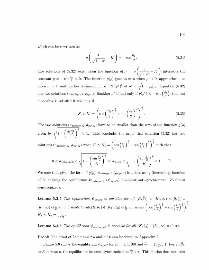
100
which can be rewritten as
ρ
(1√
1− ρ2−K ′
)= − cot
θ2
2. (5.34)
The solutions of (5.32) exist when the function g(ρ) = ρ
(1√
1−ρ2−K ′
)intersects the
constant y = − cot θ22 < 0. The function g(ρ) goes to zero when ρ → 0, approaches +∞when ρ → 1, and reaches its minimum of −K ′(ρ∗)3 at ρ∗ =
√1− 1
K′2/3. Equation (5.32)
has two solutions (ρantisync2, ρsync2) flanking ρ∗ if and only if g(ρ∗) < − cot(θ22
); this last
inequality is satisfied if and only if
K > K1 =
(cos(θ2
2
) 23
+ sin(θ2
2
) 23
) 32
. (5.35)
The two solutions (ρantisync2, ρsync2) have to be smaller than the zero of the function g(ρ)
given by
√1−
(sin
θ22
K
)2
< 1. This concludes the proof that equation (5.32) has two
solutions (ρantisync2, ρsync2) when K > K1 =(
cos(θ22
) 23 + sin
(θ22
) 23
) 32
such that
0 < ρantisync2 <
√√√√1−(
sin θ22
K
) 23
< ρsync2 <
√√√√1−(
sin θ22
K
)2
< 1.
We note that given the form of g(ρ), ρantisync2 (ρsync2) is a decreasing (increasing) function
of K, making the equilibrium ψantisync2 (ψsync2) K-almost anti-synchronized (K-almost
synchronized).
Lemma 5.2.5 The equilibrium ψsync2 is unstable for all (K, θ2) ∈ [K1,∞) × (0, π2 ) ∪
[K0,∞)×(π2 , π) and stable for all (K, θ2) ∈ [K1,K0)×(π2 , π), where(
cos(θ22
) 23 + sin
(θ22
) 23
) 32
=
K1 < K0 = 2sin θ2
.
Lemma 5.2.6 The equilibrium ψantisync2 is unstable for all (K, θ2) ∈ [K1,∞)× (0, π).
Proof: The proof of Lemmas 5.2.5 and 5.2.6 can be found in Appendix A.
Figure 5.6 shows the equilibrium ψsync2 for K = 1, 4, 100 and θ2 = .1, π2 , 3.1. For all θ2,
as K increases, the equilibrium becomes synchronized at θ22 +π. This motion does not exist
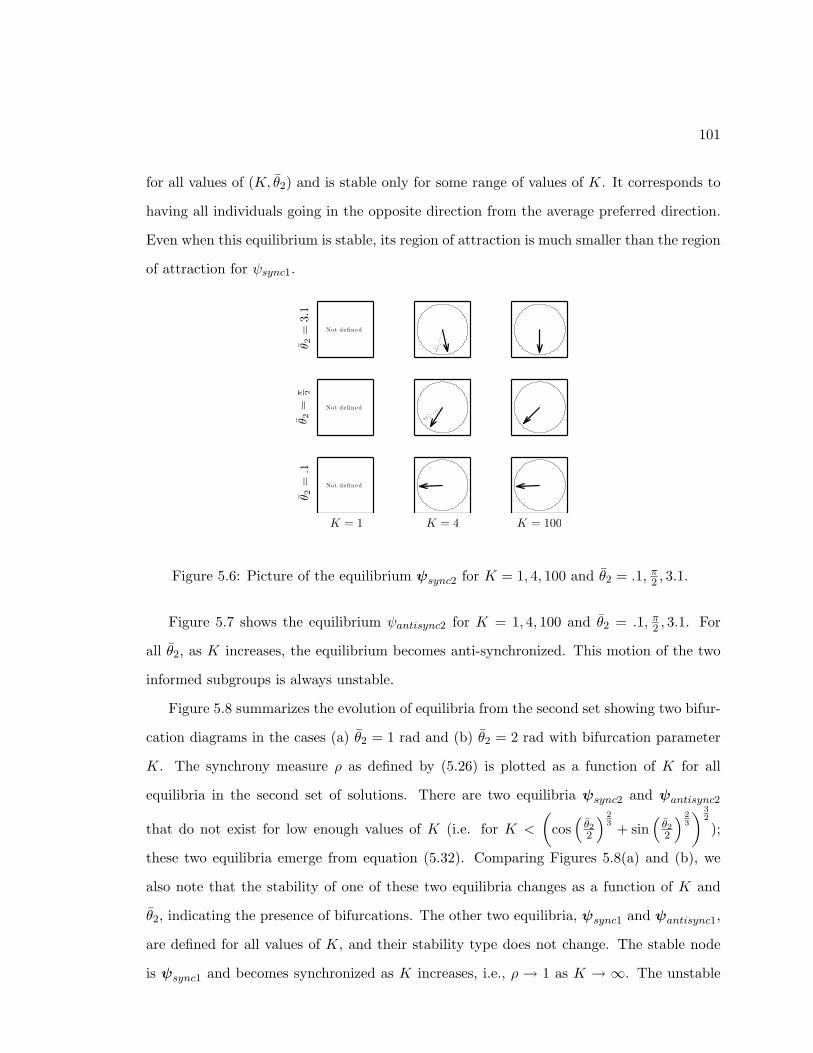
101
for all values of (K, θ2) and is stable only for some range of values of K. It corresponds to
having all individuals going in the opposite direction from the average preferred direction.
Even when this equilibrium is stable, its region of attraction is much smaller than the region
of attraction for ψsync1.
K = 1 K = 4
θ 2=
.1θ 2
=π 2
θ 2=
3.1
K = 100
Not defined
Not defined
Not defined
Figure 5.6: Picture of the equilibrium ψsync2 for K = 1, 4, 100 and θ2 = .1, π2 , 3.1.
Figure 5.7 shows the equilibrium ψantisync2 for K = 1, 4, 100 and θ2 = .1, π2 , 3.1. For
all θ2, as K increases, the equilibrium becomes anti-synchronized. This motion of the two
informed subgroups is always unstable.
Figure 5.8 summarizes the evolution of equilibria from the second set showing two bifur-
cation diagrams in the cases (a) θ2 = 1 rad and (b) θ2 = 2 rad with bifurcation parameter
K. The synchrony measure ρ as defined by (5.26) is plotted as a function of K for all
equilibria in the second set of solutions. There are two equilibria ψsync2 and ψantisync2
that do not exist for low enough values of K (i.e. for K <
(cos(θ22
) 23 + sin
(θ22
) 23
) 32
);
these two equilibria emerge from equation (5.32). Comparing Figures 5.8(a) and (b), we
also note that the stability of one of these two equilibria changes as a function of K and
θ2, indicating the presence of bifurcations. The other two equilibria, ψsync1 and ψantisync1,
are defined for all values of K, and their stability type does not change. The stable node
is ψsync1 and becomes synchronized as K increases, i.e., ρ → 1 as K → ∞. The unstable
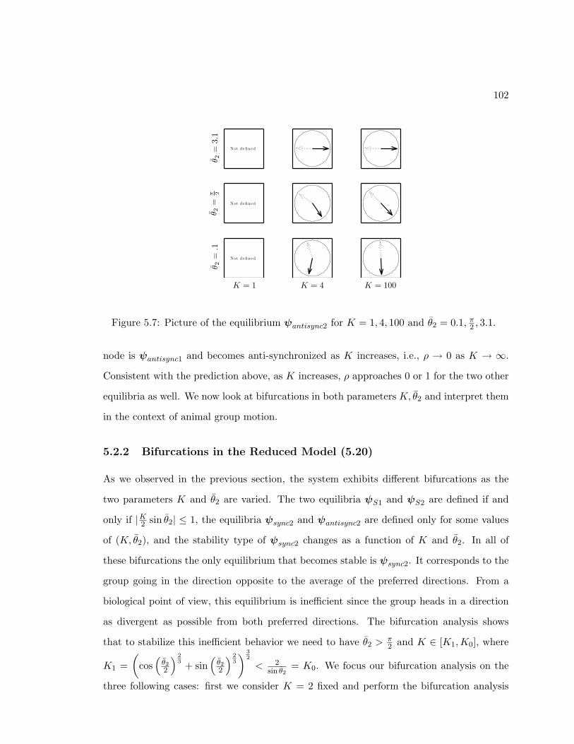
102
K = 1 K = 4
θ 2=
.1θ 2
=π 2
θ 2=
3.1
K = 100K = 1 K = 2 K = 4
θ 2=
.1θ 2
=π 2
θ 2=
3.1
Not defined
Not defined
Not defined
Figure 5.7: Picture of the equilibrium ψantisync2 for K = 1, 4, 100 and θ2 = 0.1, π2 , 3.1.
node is ψantisync1 and becomes anti-synchronized as K increases, i.e., ρ → 0 as K → ∞.
Consistent with the prediction above, as K increases, ρ approaches 0 or 1 for the two other
equilibria as well. We now look at bifurcations in both parameters K, θ2 and interpret them
in the context of animal group motion.
5.2.2 Bifurcations in the Reduced Model (5.20)
As we observed in the previous section, the system exhibits different bifurcations as the
two parameters K and θ2 are varied. The two equilibria ψS1 and ψS2 are defined if and
only if |K2 sin θ2| ≤ 1, the equilibria ψsync2 and ψantisync2 are defined only for some values
of (K, θ2), and the stability type of ψsync2 changes as a function of K and θ2. In all of
these bifurcations the only equilibrium that becomes stable is ψsync2. It corresponds to the
group going in the direction opposite to the average of the preferred directions. From a
biological point of view, this equilibrium is inefficient since the group heads in a direction
as divergent as possible from both preferred directions. The bifurcation analysis shows
that to stabilize this inefficient behavior we need to have θ2 >π2 and K ∈ [K1,K0], where
K1 =(
cos(θ22
) 23 + sin
(θ22
) 23
) 32
< 2sin θ2
= K0. We focus our bifurcation analysis on the
three following cases: first we consider K = 2 fixed and perform the bifurcation analysis
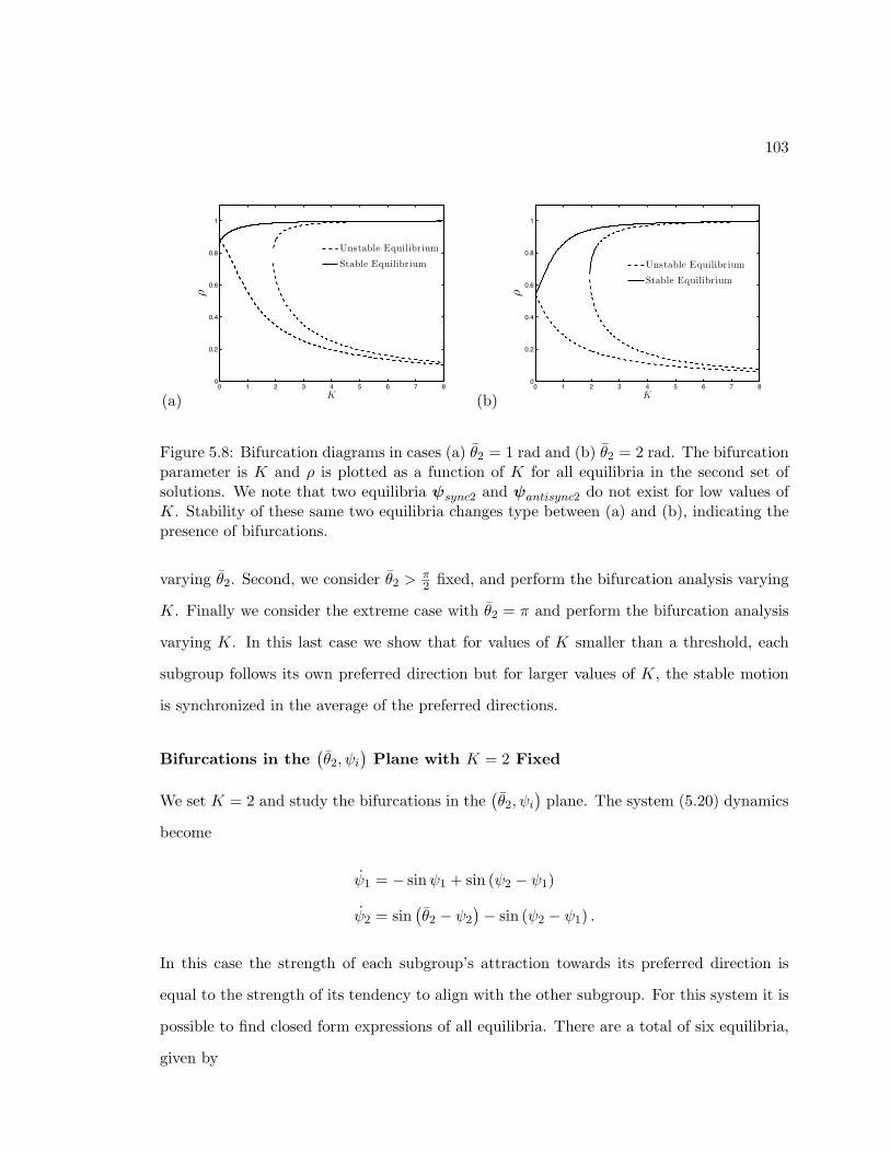
103
(a)0 1 2 3 4 5 6 7 8
0
0.2
0.4
0.6
0.8
1
K
ρ
Unstable Equilibrium
Stable Equilibrium
(b)0 1 2 3 4 5 6 7 8
0
0.2
0.4
0.6
0.8
1
K
ρ
Unstable Equilibrium
Stable Equilibrium
Figure 5.8: Bifurcation diagrams in cases (a) θ2 = 1 rad and (b) θ2 = 2 rad. The bifurcationparameter is K and ρ is plotted as a function of K for all equilibria in the second set ofsolutions. We note that two equilibria ψsync2 and ψantisync2 do not exist for low values ofK. Stability of these same two equilibria changes type between (a) and (b), indicating thepresence of bifurcations.
varying θ2. Second, we consider θ2 >π2 fixed, and perform the bifurcation analysis varying
K. Finally we consider the extreme case with θ2 = π and perform the bifurcation analysis
varying K. In this last case we show that for values of K smaller than a threshold, each
subgroup follows its own preferred direction but for larger values of K, the stable motion
is synchronized in the average of the preferred directions.
Bifurcations in the(θ2, ψi
)Plane with K = 2 Fixed
We set K = 2 and study the bifurcations in the(θ2, ψi
)plane. The system (5.20) dynamics
become
ψ1 = − sinψ1 + sin (ψ2 − ψ1)
ψ2 = sin(θ2 − ψ2
)− sin (ψ2 − ψ1) .
In this case the strength of each subgroup’s attraction towards its preferred direction is
equal to the strength of its tendency to align with the other subgroup. For this system it is
possible to find closed form expressions of all equilibria. There are a total of six equilibria,
given by
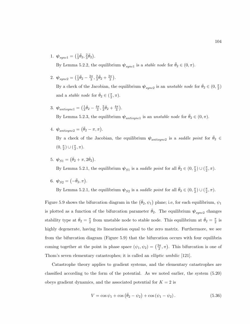
104
1. ψsync1 =(
13 θ2,
23 θ2
).
By Lemma 5.2.2, the equilibrium ψsync1 is a stable node for θ2 ∈ (0, π).
2. ψsync2 =(
13 θ2 − 2π
3 ,23 θ2 + 2π
3
).
By a check of the Jacobian, the equilibrium ψsync2 is an unstable node for θ2 ∈ (0, π2 )
and a stable node for θ2 ∈ (π2 , π).
3. ψantisync1 =(
13 θ2 − 4π
3 ,23 θ2 + 4π
3
).
By Lemma 5.2.3, the equilibrium ψantisync1 is an unstable node for θ2 ∈ (0, π).
4. ψantisync2 =(θ2 − π, π
).
By a check of the Jacobian, the equilibrium ψantisync2 is a saddle point for θ2 ∈(0, π2 ) ∪ (π2 , π).
5. ψS1 =(θ2 + π, 2θ2
).
By Lemma 5.2.1, the equilibrium ψS1 is a saddle point for all θ2 ∈ (0, π2 ) ∪ (π2 , π).
6. ψS2 =(−θ2, π
).
By Lemma 5.2.1, the equilibrium ψS2 is a saddle point for all θ2 ∈ (0, π2 ) ∪ (π2 , π).
Figure 5.9 shows the bifurcation diagram in the(θ2, ψ1
)plane; i.e, for each equilibrium, ψ1
is plotted as a function of the bifurcation parameter θ2. The equilibrium ψsync2 changes
stability type at θ2 = π2 from unstable node to stable node. This equilibrium at θ2 = π
2 is
highly degenerate, having its linearization equal to the zero matrix. Furthermore, we see
from the bifurcation diagram (Figure 5.9) that the bifurcation occurs with four equilibria
coming together at the point in phase space (ψ1, ψ2) =(
3π2 , π
). This bifurcation is one of
Thom’s seven elementary catastrophes; it is called an elliptic umbilic [121].
Catastrophe theory applies to gradient systems, and the elementary catastrophes are
classified according to the form of the potential. As we noted earlier, the system (5.20)
obeys gradient dynamics, and the associated potential for K = 2 is
V = cosψ1 + cos(θ2 − ψ2
)+ cos (ψ1 − ψ2) . (5.36)
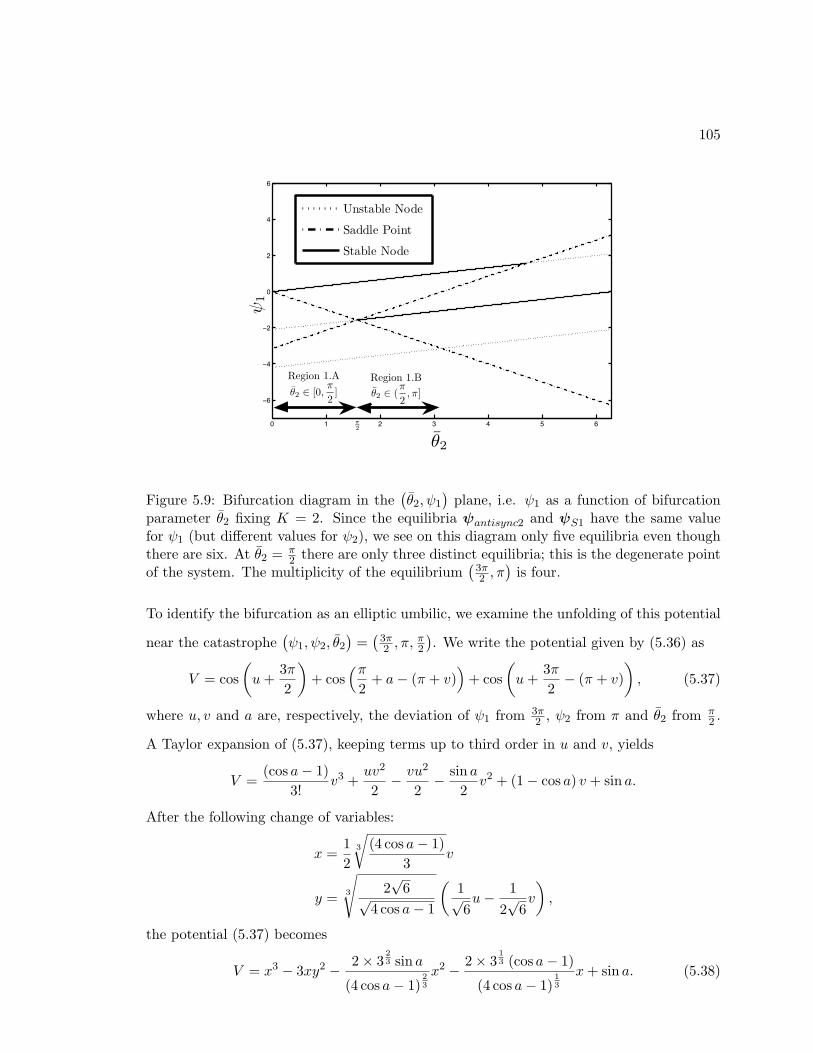
105
! " # $ % & '
!'
!%
!#
!
#
%
'
π2
Unstable Node
Saddle Point
Stable Node
Region 1.Bθ2 ∈ (
π
2, π]
Region 1.A
θ2 ∈ [0,π
2]
θ2
ψ1
Figure 5.9: Bifurcation diagram in the(θ2, ψ1
)plane, i.e. ψ1 as a function of bifurcation
parameter θ2 fixing K = 2. Since the equilibria ψantisync2 and ψS1 have the same valuefor ψ1 (but different values for ψ2), we see on this diagram only five equilibria even thoughthere are six. At θ2 = π
2 there are only three distinct equilibria; this is the degenerate pointof the system. The multiplicity of the equilibrium
(3π2 , π
)is four.
To identify the bifurcation as an elliptic umbilic, we examine the unfolding of this potential
near the catastrophe(ψ1, ψ2, θ2
)=(
3π2 , π,
π2
). We write the potential given by (5.36) as
V = cos(u+
3π2
)+ cos
(π2
+ a− (π + v))
+ cos(u+
3π2− (π + v)
), (5.37)
where u, v and a are, respectively, the deviation of ψ1 from 3π2 , ψ2 from π and θ2 from π
2 .
A Taylor expansion of (5.37), keeping terms up to third order in u and v, yields
V =(cos a− 1)
3!v3 +
uv2
2− vu2
2− sin a
2v2 + (1− cos a) v + sin a.
After the following change of variables:
x =12
3
√(4 cos a− 1)
3v
y = 3
√2√
6√4 cos a− 1
(1√6u− 1
2√
6v
),
the potential (5.37) becomes
V = x3 − 3xy2 − 2× 323 sin a
(4 cos a− 1)23
x2 − 2× 313 (cos a− 1)
(4 cos a− 1)13
x+ sin a. (5.38)
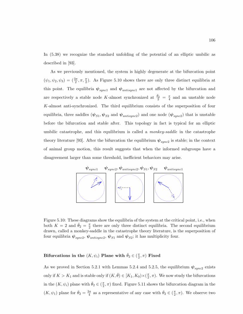
106
In (5.38) we recognize the standard unfolding of the potential of an elliptic umbilic as
described in [93].
As we previously mentioned, the system is highly degenerate at the bifurcation point
(ψ1, ψ2, ψ3) = (3π2 , π,
π2 ). As Figure 5.10 shows there are only three distinct equilibria at
this point. The equilibria ψsync1 and ψantisync1 are not affected by the bifurcation and
are respectively a stable node K-almost synchronized at θ22 = π
4 and an unstable node
K-almost anti-synchronized. The third equilibrium consists of the superposition of four
equilibria, three saddles (ψS1,ψS2 and ψantisync2) and one node (ψsync2) that is unstable
before the bifurcation and stable after. This topology in fact is typical for an elliptic
umbilic catastrophe, and this equilibrium is called a monkey-saddle in the catastrophe
theory literature [93]. After the bifurcation the equilibrium ψsync2 is stable; in the context
of animal group motion, this result suggests that when the informed subgroups have a
disagreement larger than some threshold, inefficient behaviors may arise.
ψantisync1ψsync1 ψsync2, ψantisync2,ψS1, ψS2
Figure 5.10: These diagrams show the equilibria of the system at the critical point, i.e., whenboth K = 2 and θ2 = π
2 there are only three distinct equilibria. The second equilibriumdrawn, called a monkey-saddle in the catastrophe theory literature, is the superposition offour equilibria ψsync2, ψantisync2, ψS1 and ψS2; it has multiplicity four.
Bifurcations in the (K,ψi) Plane with θ2 ∈ (π2 , π) Fixed
As we proved in Section 5.2.1 with Lemmas 5.2.4 and 5.2.5, the equilibrium ψsync2 exists
only ifK > K1 and is stable only if (K, θ) ∈ [K1,K0)×(π2 , π). We now study the bifurcations
in the (K,ψi) plane with θ2 ∈ (π2 , π) fixed. Figure 5.11 shows the bifurcation diagram in the
(K,ψ1) plane for θ2 = 3π4 as a representative of any case with θ2 ∈ (π2 , π). We observe two
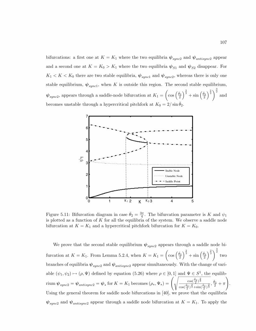
107
bifurcations: a first one at K = K1 where the two equilibria ψsync2 and ψantisync2 appear
and a second one at K = K0 > K1 where the two equilibria ψS1 and ψS2 disappear. For
K1 < K < K0 there are two stable equilibria, ψsync1 and ψsync2, whereas there is only one
stable equilibrium, ψsync1, when K is outside this region. The second stable equilibrium,
ψsync2, appears through a saddle-node bifurcation at K1 =(
cos(θ22
) 23 + sin
(θ22
) 23
) 32
and
becomes unstable through a hypercritical pitchfork at K0 = 2/ sin θ2.
0 1 2 3 4 50
1
2
3
4
5
6
7
Stable Node
Unstable Node
Saddle Point
K
1
K 0K 1
Figure 5.11: Bifurcation diagram in case θ2 = 3π4 . The bifurcation parameter is K and ψ1
is plotted as a function of K for all the equilibria of the system. We observe a saddle nodebifurcation at K = K1 and a hypercritical pitchfork bifurcation for K = K0.
We prove that the second stable equilibrium ψsync2 appears through a saddle node bi-
furcation at K = K1. From Lemma 5.2.4, when K = K1 =(
cos(θ22
) 23 + sin
(θ22
) 23
) 32
two
branches of equilibria ψsync2 and ψantisync2 appear simultaneously. With the change of vari-
able (ψ1, ψ2) 7→ (ρ,Ψ) defined by equation (5.26) where ρ ∈ [0, 1] and Ψ ∈ S1, the equilib-
riumψsync2 = ψantisync2 = ψ∗ forK = K1 becomes (ρ∗,Ψ∗) =
(√cos(
θ22
)23
cos(θ22
)23 +sin(
θ22
)23, θ22 + π
).
Using the general theorem for saddle node bifurcations in [40], we prove that the equilibria
ψsync2 and ψantisync2 appear through a saddle node bifurcation at K = K1. To apply the
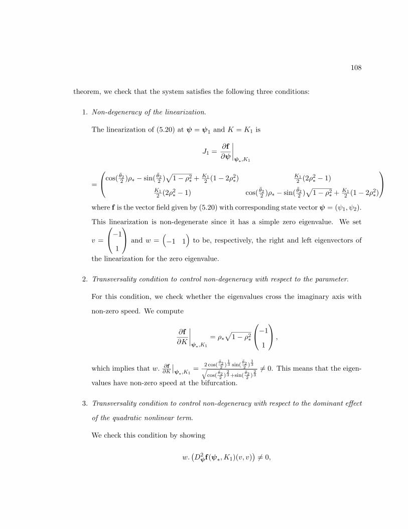
108
theorem, we check that the system satisfies the following three conditions:
1. Non-degeneracy of the linearization.
The linearization of (5.20) at ψ = ψ1 and K = K1 is
J1 =∂f∂ψ
∣∣∣∣ψ∗,K1
=
cos( θ22 )ρ∗ − sin( θ22 )√
1− ρ2∗ + K1
2 (1− 2ρ2∗)
K12 (2ρ2
∗ − 1)
K12 (2ρ2
∗ − 1) cos( θ22 )ρ∗ − sin( θ22 )√
1− ρ2∗ + K1
2 (1− 2ρ2∗)
where f is the vector field given by (5.20) with corresponding state vector ψ = (ψ1, ψ2).
This linearization is non-degenerate since it has a simple zero eigenvalue. We set
v =
−1
1
and w =(−1 1
)to be, respectively, the right and left eigenvectors of
the linearization for the zero eigenvalue.
2. Transversality condition to control non-degeneracy with respect to the parameter.
For this condition, we check whether the eigenvalues cross the imaginary axis with
non-zero speed. We compute
∂f∂K
∣∣∣∣ψ∗,K1
= ρ∗√
1− ρ2∗
−1
1
,
which implies that w. ∂f∂K
∣∣ψ∗,K1
= 2 cos(θ22
)13 sin(
θ22
)13q
cos(θ22
)23 +sin(
θ22
)23
6= 0. This means that the eigen-
values have non-zero speed at the bifurcation.
3. Transversality condition to control non-degeneracy with respect to the dominant effect
of the quadratic nonlinear term.
We check this condition by showing
w.(D2ψf(ψ∗,K1)(v, v)
) 6= 0,
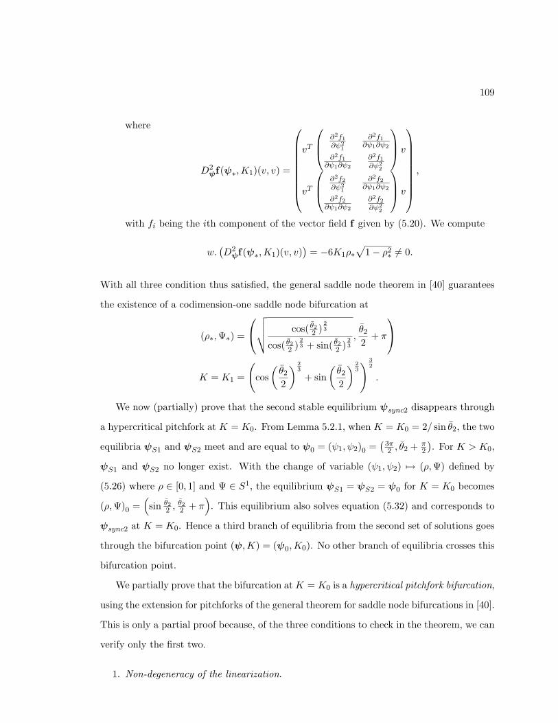
109
where
D2ψf(ψ∗,K1)(v, v) =
vT
∂2f1
∂ψ21
∂2f1
∂ψ1∂ψ2
∂2f1
∂ψ1∂ψ2
∂2f1
∂ψ22
v
vT
∂2f2
∂ψ21
∂2f2
∂ψ1∂ψ2
∂2f2
∂ψ1∂ψ2
∂2f2
∂ψ22
v
,
with fi being the ith component of the vector field f given by (5.20). We compute
w.(D2ψf(ψ∗,K1)(v, v)
)= −6K1ρ∗
√1− ρ2
∗ 6= 0.
With all three condition thus satisfied, the general saddle node theorem in [40] guarantees
the existence of a codimension-one saddle node bifurcation at
(ρ∗,Ψ∗) =
√√√√ cos( θ22 )
23
cos( θ22 )23 + sin( θ22 )
23
,θ2
2+ π
K = K1 =
(cos(θ2
2
) 23
+ sin(θ2
2
) 23
) 32
.
We now (partially) prove that the second stable equilibrium ψsync2 disappears through
a hypercritical pitchfork at K = K0. From Lemma 5.2.1, when K = K0 = 2/ sin θ2, the two
equilibria ψS1 and ψS2 meet and are equal to ψ0 = (ψ1, ψ2)0 =(
3π2 , θ2 + π
2
). For K > K0,
ψS1 and ψS2 no longer exist. With the change of variable (ψ1, ψ2) 7→ (ρ,Ψ) defined by
(5.26) where ρ ∈ [0, 1] and Ψ ∈ S1, the equilibrium ψS1 = ψS2 = ψ0 for K = K0 becomes
(ρ,Ψ)0 =(
sin θ22 ,
θ22 + π
). This equilibrium also solves equation (5.32) and corresponds to
ψsync2 at K = K0. Hence a third branch of equilibria from the second set of solutions goes
through the bifurcation point (ψ,K) = (ψ0,K0). No other branch of equilibria crosses this
bifurcation point.
We partially prove that the bifurcation at K = K0 is a hypercritical pitchfork bifurcation,
using the extension for pitchforks of the general theorem for saddle node bifurcations in [40].
This is only a partial proof because, of the three conditions to check in the theorem, we can
verify only the first two.
1. Non-degeneracy of the linearization.
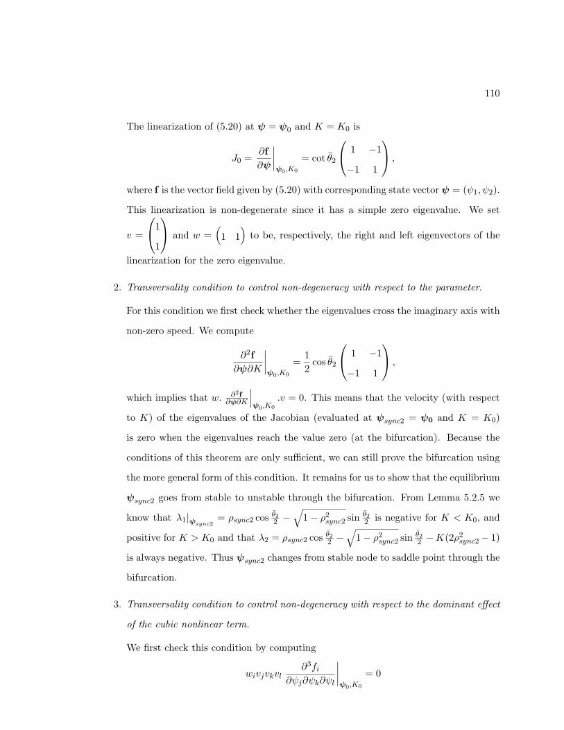
110
The linearization of (5.20) at ψ = ψ0 and K = K0 is
J0 =∂f∂ψ
∣∣∣∣ψ0,K0
= cot θ2
1 −1
−1 1
,
where f is the vector field given by (5.20) with corresponding state vector ψ = (ψ1, ψ2).
This linearization is non-degenerate since it has a simple zero eigenvalue. We set
v =
1
1
and w =(
1 1)
to be, respectively, the right and left eigenvectors of the
linearization for the zero eigenvalue.
2. Transversality condition to control non-degeneracy with respect to the parameter.
For this condition we first check whether the eigenvalues cross the imaginary axis with
non-zero speed. We compute
∂2f∂ψ∂K
∣∣∣∣ψ0,K0
=12
cos θ2
1 −1
−1 1
,
which implies that w. ∂2f∂ψ∂K
∣∣∣ψ0,K0
.v = 0. This means that the velocity (with respect
to K) of the eigenvalues of the Jacobian (evaluated at ψsync2 = ψ0 and K = K0)
is zero when the eigenvalues reach the value zero (at the bifurcation). Because the
conditions of this theorem are only sufficient, we can still prove the bifurcation using
the more general form of this condition. It remains for us to show that the equilibrium
ψsync2 goes from stable to unstable through the bifurcation. From Lemma 5.2.5 we
know that λ1|ψsync2 = ρsync2 cos θ22 −√
1− ρ2sync2 sin θ2
2 is negative for K < K0, and
positive for K > K0 and that λ2 = ρsync2 cos θ22 −√
1− ρ2sync2 sin θ2
2 −K(2ρ2sync2 − 1)
is always negative. Thus ψsync2 changes from stable node to saddle point through the
bifurcation.
3. Transversality condition to control non-degeneracy with respect to the dominant effect
of the cubic nonlinear term.
We first check this condition by computing
wivjvkvl∂3fi
∂ψj∂ψk∂ψl
∣∣∣∣ψ0,K0
= 0
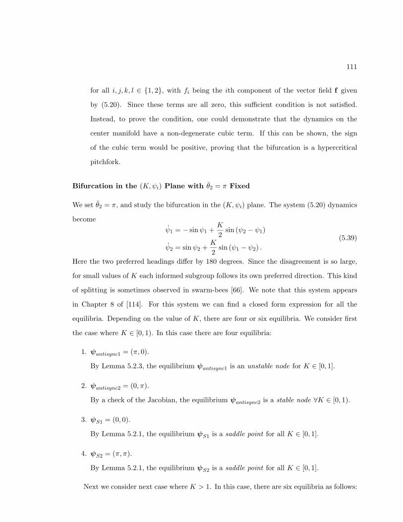
111
for all i, j, k, l ∈ 1, 2, with fi being the ith component of the vector field f given
by (5.20). Since these terms are all zero, this sufficient condition is not satisfied.
Instead, to prove the condition, one could demonstrate that the dynamics on the
center manifold have a non-degenerate cubic term. If this can be shown, the sign
of the cubic term would be positive, proving that the bifurcation is a hypercritical
pitchfork.
Bifurcation in the (K,ψi) Plane with θ2 = π Fixed
We set θ2 = π, and study the bifurcation in the (K,ψi) plane. The system (5.20) dynamics
becomeψ1 = − sinψ1 +
K
2sin (ψ2 − ψ1)
ψ2 = sinψ2 +K
2sin (ψ1 − ψ2) .
(5.39)
Here the two preferred headings differ by 180 degrees. Since the disagreement is so large,
for small values of K each informed subgroup follows its own preferred direction. This kind
of splitting is sometimes observed in swarm-bees [66]. We note that this system appears
in Chapter 8 of [114]. For this system we can find a closed form expression for all the
equilibria. Depending on the value of K, there are four or six equilibria. We consider first
the case where K ∈ [0, 1). In this case there are four equilibria:
1. ψantisync1 = (π, 0).
By Lemma 5.2.3, the equilibrium ψantisync1 is an unstable node for K ∈ [0, 1].
2. ψantisync2 = (0, π).
By a check of the Jacobian, the equilibrium ψantisync2 is a stable node ∀K ∈ [0, 1).
3. ψS1 = (0, 0).
By Lemma 5.2.1, the equilibrium ψS1 is a saddle point for all K ∈ [0, 1].
4. ψS2 = (π, π).
By Lemma 5.2.1, the equilibrium ψS2 is a saddle point for all K ∈ [0, 1].
Next we consider next case where K > 1. In this case, there are six equilibria as follows:
112
1. ψsync1 =(π − arccos
(− 1K
), arccos
(− 1K
)).
By Lemma 5.2.2, the equilibrium ψsync1 is a stable node for K > 1.
2. ψsync2 =(π + arccos
(− 1K
),− arccos
(− 1K
)).
By a check of the Jacobian, the equilibrium ψsync2 is a stable node ∀K > 1.
3. ψantisync1 = (π, 0).
By Lemma 5.2.3, the equilibrium ψantisync1 is an unstable node for K ≥ 1.
4. ψantisync2 = (0, π).
By a check of the Jacobian, the equilibrium ψantisync2 is a saddle point ∀K > 1.
5. ψS1 = (0, 0).
By Lemma 5.2.1, the equilibrium ψS1 is a saddle point for all K ≥ 1.
6. ψS2 = (π, π).
By Lemma 5.2.1, the equilibrium ψS2 is a saddle point for all K ≥ 1.
Figure 5.12 shows the bifurcation diagram in the (K,ψ1) plane; for each equilibrium, ψ1
is plotted as a function of the bifurcation parameter K. Before the bifurcation, i.e., K < 1,
the only stable equilibrium is ψantisync2 = (0, π). This corresponds to the case where each
informed subgroup follows its own preferred direction; there is no compromise between the
individuals, and the group splits. When K < 1 the strength of the coupling force relative to
the strength of the attraction to the preferred direction is too weak to influence the stable
steady state of the system. The motion of the group is the same as if there were no coupling
between the two informed subgroups. For K > 1, there are two stable equilibria, ψsync1
and ψsync2. These correspond, respectively, to the motion in the directions Ψ = θ22 = π
2 and
Ψ = θ22 + π = 3π
2 . As we increase the bifurcation parameter K, the two directions ψ1 and
ψ2 become synchronized. θ2 = π is the only case where we have two stable equilibria for
large value of K. At K = 1, the equilibrium ψantisync2 changes stability type from being a
stable node to being a saddle through a supercritical pitchfork bifurcation. We prove this,
by using the extension for pitchforks of the general theorem for saddle node bifurcations in
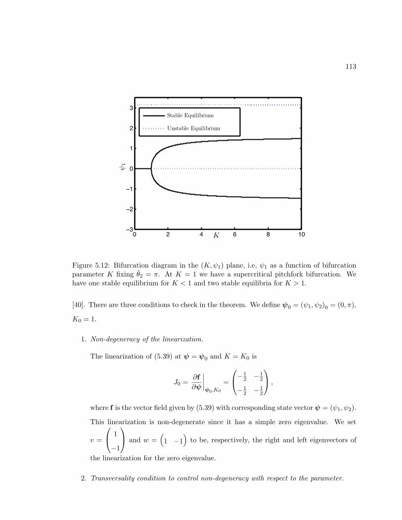
113
! " # $ % &!!'
!"
!&
!
&
"
'
K
ψ1
Stable Equilibrium
Unstable Equilibrium
Figure 5.12: Bifurcation diagram in the (K,ψ1) plane, i.e, ψ1 as a function of bifurcationparameter K fixing θ2 = π. At K = 1 we have a supercritical pitchfork bifurcation. Wehave one stable equilibrium for K < 1 and two stable equilibria for K > 1.
[40]. There are three conditions to check in the theorem. We define ψ0 = (ψ1, ψ2)0 = (0, π),
K0 = 1.
1. Non-degeneracy of the linearization.
The linearization of (5.39) at ψ = ψ0 and K = K0 is
J0 =∂f∂ψ
∣∣∣∣ψ0,K0
=
−12 −1
2
−12 −1
2
,
where f is the vector field given by (5.39) with corresponding state vector ψ = (ψ1, ψ2).
This linearization is non-degenerate since it has a simple zero eigenvalue. We set
v =
1
−1
and w =(
1 −1)
to be, respectively, the right and left eigenvectors of
the linearization for the zero eigenvalue.
2. Transversality condition to control non-degeneracy with respect to the parameter.
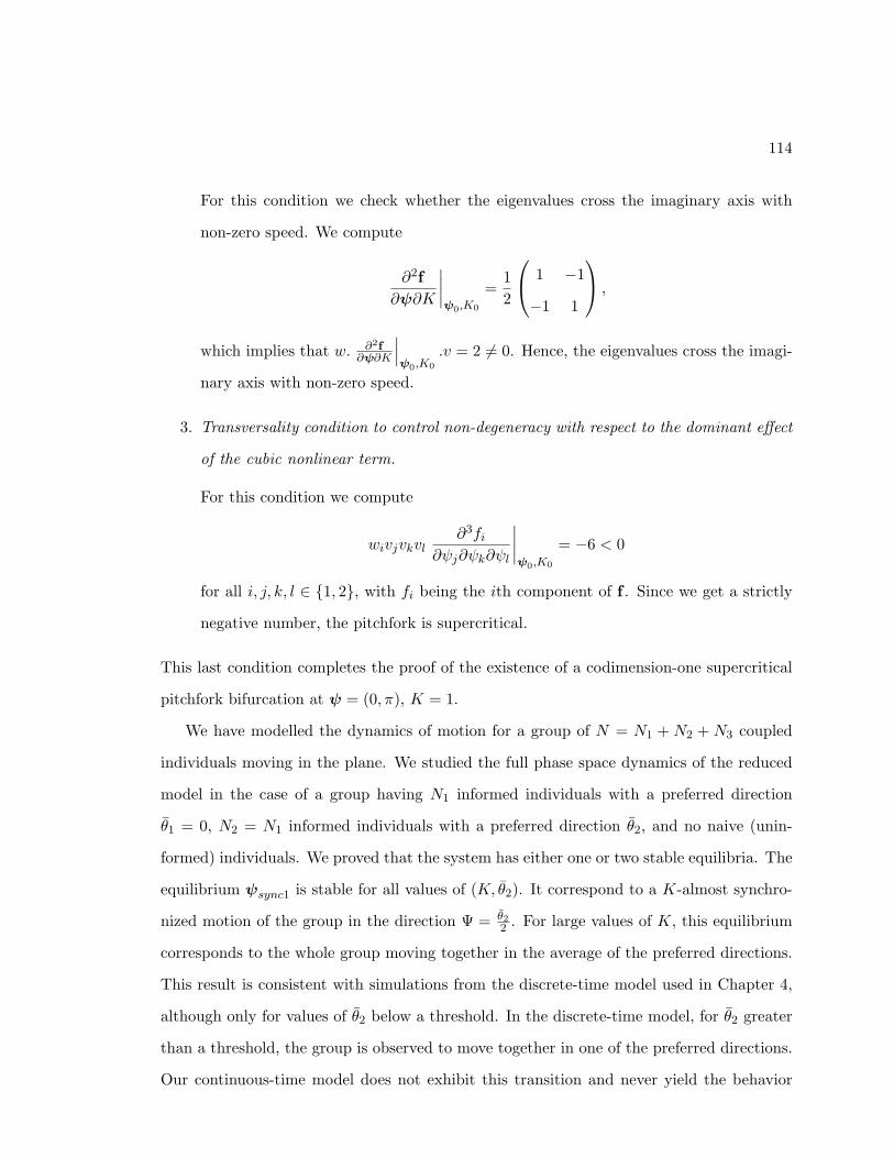
114
For this condition we check whether the eigenvalues cross the imaginary axis with
non-zero speed. We compute
∂2f∂ψ∂K
∣∣∣∣ψ0,K0
=12
1 −1
−1 1
,
which implies that w. ∂2f∂ψ∂K
∣∣∣ψ0,K0
.v = 2 6= 0. Hence, the eigenvalues cross the imagi-
nary axis with non-zero speed.
3. Transversality condition to control non-degeneracy with respect to the dominant effect
of the cubic nonlinear term.
For this condition we compute
wivjvkvl∂3fi
∂ψj∂ψk∂ψl
∣∣∣∣ψ0,K0
= −6 < 0
for all i, j, k, l ∈ 1, 2, with fi being the ith component of f . Since we get a strictly
negative number, the pitchfork is supercritical.
This last condition completes the proof of the existence of a codimension-one supercritical
pitchfork bifurcation at ψ = (0, π), K = 1.
We have modelled the dynamics of motion for a group of N = N1 + N2 + N3 coupled
individuals moving in the plane. We studied the full phase space dynamics of the reduced
model in the case of a group having N1 informed individuals with a preferred direction
θ1 = 0, N2 = N1 informed individuals with a preferred direction θ2, and no naive (unin-
formed) individuals. We proved that the system has either one or two stable equilibria. The
equilibrium ψsync1 is stable for all values of (K, θ2). It correspond to a K-almost synchro-
nized motion of the group in the direction Ψ = θ22 . For large values of K, this equilibrium
corresponds to the whole group moving together in the average of the preferred directions.
This result is consistent with simulations from the discrete-time model used in Chapter 4,
although only for values of θ2 below a threshold. In the discrete-time model, for θ2 greater
than a threshold, the group is observed to move together in one of the preferred directions.
Our continuous-time model does not exhibit this transition and never yield the behavior
115
where the group collectively selects one of the two preferred directions. Furthermore, for
(K, θ2) ∈ (K1,K0) × [π2 , π) the equilibrium ψsync2 is stable. It corresponds to a K-almost
synchronized motion of the group in the direction Ψ = θ22 + π. For large values of K,
this equilibrium corresponds to the whole group moving together in a direction opposite
to the average of the preferred directions. The region of attraction of this equilibrium is
relatively small, which can explain why this behavior was not observed in the simulation of
the discrete-time model.
Figure 5.13 shows the phase portrait for the subgroup heading directions ψ1 and ψ2 for
two values of θ2 and three values of K. The vertical (and likewise horizontal) edges are
identified since the phase space is the torus. Some of the stable and unstable manifolds
are plotted as solid lines and the vector field is plotted as arrows so that the flow can
be readily observed. For example, as described above, in the right, middle plot, these
manifolds illustrate the region of attraction for the second stable equilibrium ψsync2. The
middle plots together show before (left) and after (right) the elliptic umbilic catastrophe.
The three panels in the left column, corresponding to θ2 = π4 , show equilibria with K = 1
for the top plot, K = 2.5 for the middle plot, and K = 4 for the bottom plot. For example,
the single stable equilibrium can be observed to be near the point ψ1 = ψ2 = π8 , i.e., the
K-almost synchronized equilibrium ψsync1 at θ22 = π
8 . Likewise, the three panels in the
right column, corresponding to θ2 = 3π4 , show equilibria that can also be observed in the
bifurcation plot of Figure 5.11 at K = 1 for the top plot, K = 2.5 for the middle plot, and
K = 4 for the bottom plot.
We illustrate in Figure 5.14 the dynamics near one of the instabilities with a simulation in
the caseN1 = N2 = 5. Snapshots of the positions and heading directions of all 10 individuals
are shown at three different times in the three left column plots. The corresponding heading
directions of all 10 individuals are plotted on the unit circle together with the preferred
heading directions in the right column plots. The initial condition, shown in Figures 5.14(a)
and (b) is close to the saddle point ψsync2 shown in the bottom right plot of Figure 5.13,
i.e., the individuals are heading in the opposite direction of the compromise of the preferred
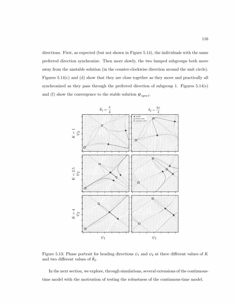
116
directions. First, as expected (but not shown in Figure 5.14), the individuals with the same
preferred direction synchronize. Then more slowly, the two lumped subgroups both move
away from the unstable solution (in the counter-clockwise direction around the unit circle).
Figures 5.14(c) and (d) show that they are close together as they move and practically all
synchronized as they pass through the preferred direction of subgroup 1. Figures 5.14(e)
and (f) show the convergence to the stable solution ψsync1.
0 1 2 3 4 5 60
1
2
3
4
5
6
0 1 2 3 4 5 60
1
2
3
4
5
6
0 1 2 3 4 5 60
1
2
3
4
5
6
0 1 2 3 4 5 60
1
2
3
4
5
6
0 1 2 3 4 5 60
1
2
3
4
5
6
0 1 2 3 4 5 60
1
2
3
4
5
6
!"# $ $"% $"& $"' $"# % %"% %"& %"'
!!"'
!!"&
!!"%
!
!"%
!"&
!"'
!"#
$
$"%
(
(
S ad d l eS t ab l e n od eU n s t ab l e n od e
Figure 5.13: Phase portrait for heading directions ψ1 and ψ2 at three different values of Kand two different values of θ2.
In the next section, we explore, through simulations, several extensions of the continuous-
time model with the motivation of testing the robustness of the continuous-time model.
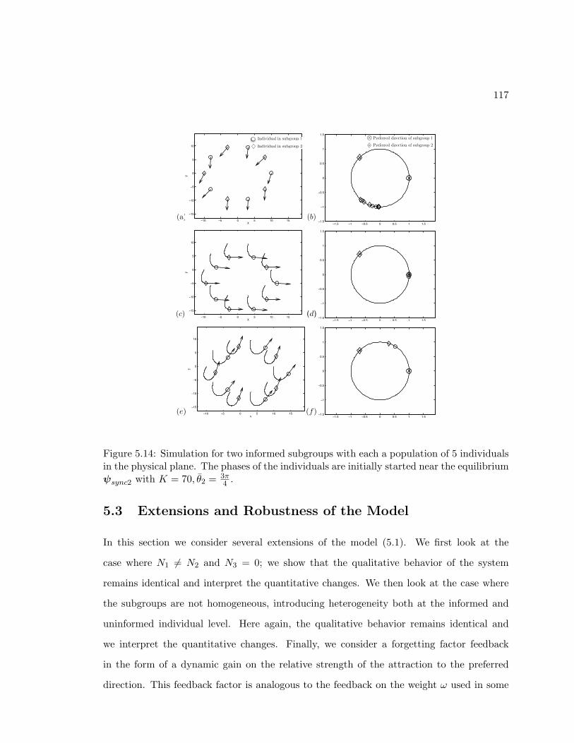
117
!!" !# " # !" !#
!!#
!!"
!#
"
#
!"
x
y
!!" !# " # !" !#
!!#
!!"
!#
"
#
!"
x
y
−10 −5 0 5 10 15
−15
−10
−5
0
5
10
x
y
!
×
!!"# !! !$"# $ $"# ! !"#!!"#
!!
!$"#
$
$"#
!
!"#
T i m e = 0s
!
×
!!"# !! !$"# $ $"# ! !"#!!"#
!!
!$"#
$
$"#
!
!"#
T i m e = 11 . 7313s
!!"# !! !$"# $ $"# ! !"#!!"#
!!
!$"#
$
$"#
!
!"#
T i m e = 19 . 1592s
Figure 5.14: Simulation for two informed subgroups with each a population of 5 individualsin the physical plane. The phases of the individuals are initially started near the equilibriumψsync2 with K = 70, θ2 = 3π
4 .
5.3 Extensions and Robustness of the Model
In this section we consider several extensions of the model (5.1). We first look at the
case where N1 6= N2 and N3 = 0; we show that the qualitative behavior of the system
remains identical and interpret the quantitative changes. We then look at the case where
the subgroups are not homogeneous, introducing heterogeneity both at the informed and
uninformed individual level. Here again, the qualitative behavior remains identical and
we interpret the quantitative changes. Finally, we consider a forgetting factor feedback
in the form of a dynamic gain on the relative strength of the attraction to the preferred
direction. This feedback factor is analogous to the feedback on the weight ω used in some
118
simulations in [19] which reinforces or diminishes the gain ω if informed individuals find
themselves moving towards or away from their preferred direction. In this case, we show
that consensus is always achieved, the group traveling either in the average of the preferred
directions or in one of the two preferred directions. In this case the continuous-time model
reproduces the discrete-time model results.
5.3.1 Uneven Informed Subgroups
The first extension we consider is the case where the two informed subgroups do not have
identical populations (N1 6= N2). In this case, the time-scale separation of the model (5.1)
still holds and the reduced dynamics (5.14) become
ψ1 = − sin (ψ1) +KN2
Nsin (ψ2 − ψ1)
ψ2 = sin(θ2 − ψ2
)+KN1
Nsin (ψ1 − ψ2) .
(5.40)
For this system, the nature of the persistent stable motion remains unchanged. That is,
there is still one persistent stable equilibrium (corresponding to ψsync1 in the case N1 =
N2) where for large values of K the two informed subgroups are synchronized. However,
synchronization no longer occurs at Ψ = θ22 , the average of the preferred directions. Instead,
synchronization occurs at a weighted average of the two preferred directions, 0 and θ2. If
N1 > N2, the value of Ψ for the persistent stable equilibrium is “closer” to 0 than to θ2;
if N2 > N1, the value of Ψ for the persistent stable equilibrium is “closer” to θ2 than to
0. Figure 5.15 shows the evolution of Ψ for the persistent stable equilibrium ψsync1 with
N2 = 10 fixed and N1 increasing such that the ratio N1N2
increases from 110 to 10. The value
of Ψ for the persistent stable equilibrium (corresponding to ψsync1 in the N1 = N2 case),
goes from being asymptotically close to θ2 = 2 rad to asymptotically approaching 0.
5.3.2 Heterogeneous Subgroups
The continuous-time model (5.1) that we studied in this chapter assumes some homogene-
ity in the group; specifically individuals in the same subgroup are assumed to be strictly
identical although have heterogeneous initial conditions. Here we consider extensions of
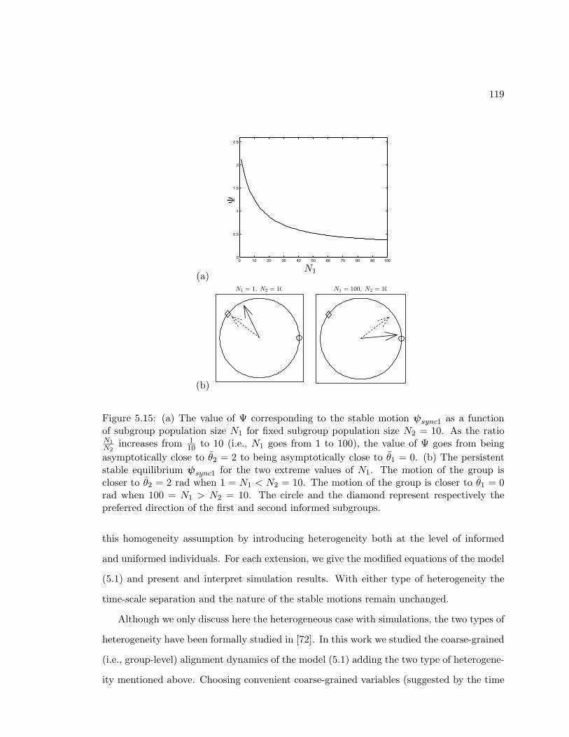
119
(a)
0 10 20 30 40 50 60 70 80 90 1000
0.5
1
1.5
2
2.5
N1
Ψ
(b)
N1 = 100, N2 = 10N1 = 1, N2 = 10
Figure 5.15: (a) The value of Ψ corresponding to the stable motion ψsync1 as a functionof subgroup population size N1 for fixed subgroup population size N2 = 10. As the ratioN1N2
increases from 110 to 10 (i.e., N1 goes from 1 to 100), the value of Ψ goes from being
asymptotically close to θ2 = 2 to being asymptotically close to θ1 = 0. (b) The persistentstable equilibrium ψsync1 for the two extreme values of N1. The motion of the group iscloser to θ2 = 2 rad when 1 = N1 < N2 = 10. The motion of the group is closer to θ1 = 0rad when 100 = N1 > N2 = 10. The circle and the diamond represent respectively thepreferred direction of the first and second informed subgroups.
this homogeneity assumption by introducing heterogeneity both at the level of informed
and uniformed individuals. For each extension, we give the modified equations of the model
(5.1) and present and interpret simulation results. With either type of heterogeneity the
time-scale separation and the nature of the stable motions remain unchanged.
Although we only discuss here the heterogeneous case with simulations, the two types of
heterogeneity have been formally studied in [72]. In this work we studied the coarse-grained
(i.e., group-level) alignment dynamics of the model (5.1) adding the two type of heterogene-
ity mentioned above. Choosing convenient coarse-grained variables (suggested by the time
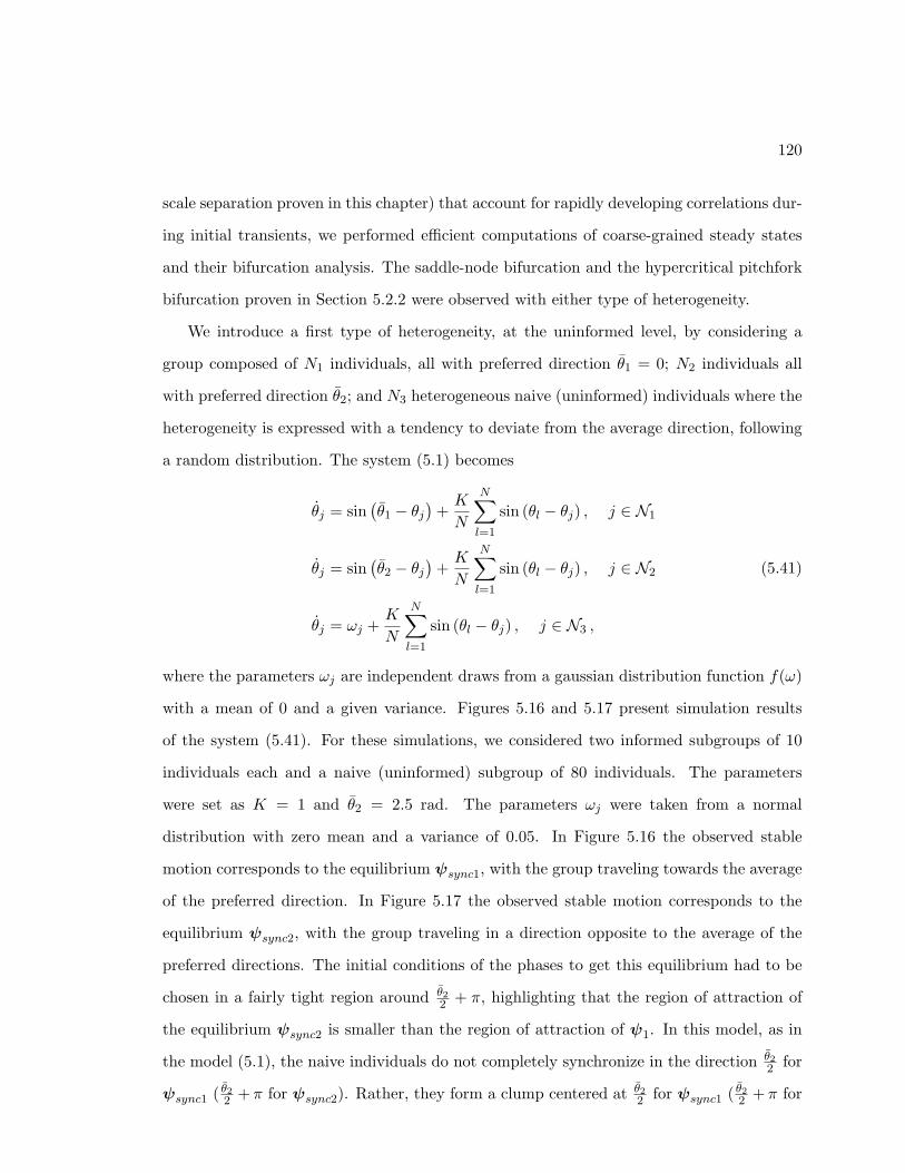
120
scale separation proven in this chapter) that account for rapidly developing correlations dur-
ing initial transients, we performed efficient computations of coarse-grained steady states
and their bifurcation analysis. The saddle-node bifurcation and the hypercritical pitchfork
bifurcation proven in Section 5.2.2 were observed with either type of heterogeneity.
We introduce a first type of heterogeneity, at the uninformed level, by considering a
group composed of N1 individuals, all with preferred direction θ1 = 0; N2 individuals all
with preferred direction θ2; and N3 heterogeneous naive (uninformed) individuals where the
heterogeneity is expressed with a tendency to deviate from the average direction, following
a random distribution. The system (5.1) becomes
θj = sin(θ1 − θj
)+K
N
N∑l=1
sin (θl − θj) , j ∈ N1
θj = sin(θ2 − θj
)+K
N
N∑l=1
sin (θl − θj) , j ∈ N2
θj = ωj +K
N
N∑l=1
sin (θl − θj) , j ∈ N3 ,
(5.41)
where the parameters ωj are independent draws from a gaussian distribution function f(ω)
with a mean of 0 and a given variance. Figures 5.16 and 5.17 present simulation results
of the system (5.41). For these simulations, we considered two informed subgroups of 10
individuals each and a naive (uninformed) subgroup of 80 individuals. The parameters
were set as K = 1 and θ2 = 2.5 rad. The parameters ωj were taken from a normal
distribution with zero mean and a variance of 0.05. In Figure 5.16 the observed stable
motion corresponds to the equilibrium ψsync1, with the group traveling towards the average
of the preferred direction. In Figure 5.17 the observed stable motion corresponds to the
equilibrium ψsync2, with the group traveling in a direction opposite to the average of the
preferred directions. The initial conditions of the phases to get this equilibrium had to be
chosen in a fairly tight region around θ22 + π, highlighting that the region of attraction of
the equilibrium ψsync2 is smaller than the region of attraction of ψ1. In this model, as in
the model (5.1), the naive individuals do not completely synchronize in the direction θ22 for
ψsync1 ( θ22 + π for ψsync2). Rather, they form a clump centered at θ22 for ψsync1 ( θ22 + π for
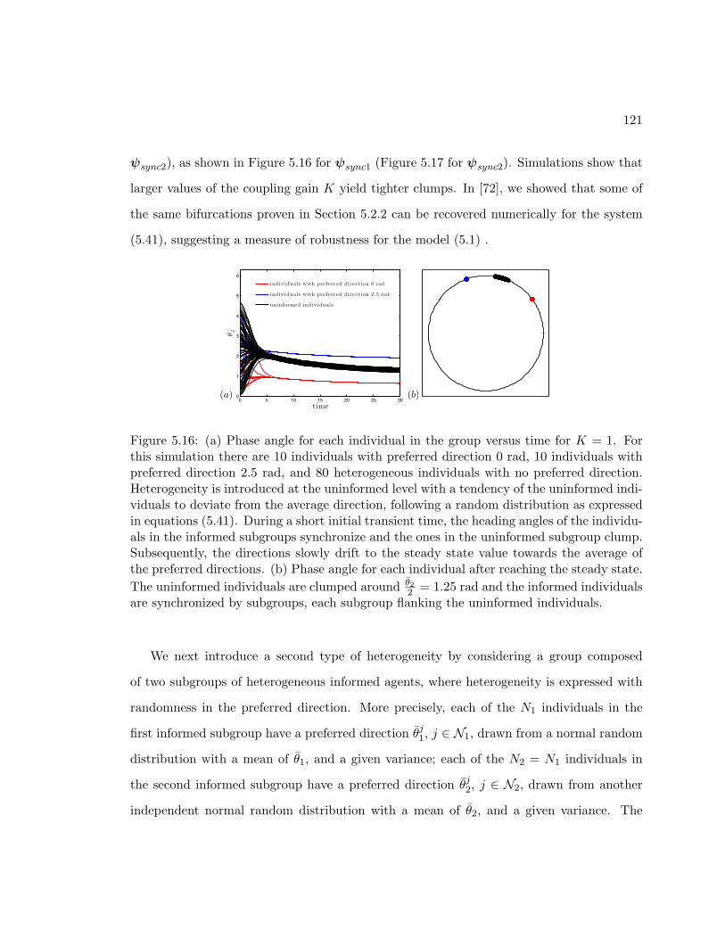
121
ψsync2), as shown in Figure 5.16 for ψsync1 (Figure 5.17 for ψsync2). Simulations show that
larger values of the coupling gain K yield tighter clumps. In [72], we showed that some of
the same bifurcations proven in Section 5.2.2 can be recovered numerically for the system
(5.41), suggesting a measure of robustness for the model (5.1) .
0 5 10 15 20 25 300
1
2
3
4
5
6
time
θj
0 10 20 30 40 50 600
1
2
3
4
5
6
time (sec)
θj
indiv idual s with preferred direction 0 rad
individual s with preferred direction 2.5 rad
uninformed individual s
(a) (b)
Figure 5.16: (a) Phase angle for each individual in the group versus time for K = 1. Forthis simulation there are 10 individuals with preferred direction 0 rad, 10 individuals withpreferred direction 2.5 rad, and 80 heterogeneous individuals with no preferred direction.Heterogeneity is introduced at the uninformed level with a tendency of the uninformed indi-viduals to deviate from the average direction, following a random distribution as expressedin equations (5.41). During a short initial transient time, the heading angles of the individu-als in the informed subgroups synchronize and the ones in the uninformed subgroup clump.Subsequently, the directions slowly drift to the steady state value towards the average ofthe preferred directions. (b) Phase angle for each individual after reaching the steady state.The uninformed individuals are clumped around θ2
2 = 1.25 rad and the informed individualsare synchronized by subgroups, each subgroup flanking the uninformed individuals.
We next introduce a second type of heterogeneity by considering a group composed
of two subgroups of heterogeneous informed agents, where heterogeneity is expressed with
randomness in the preferred direction. More precisely, each of the N1 individuals in the
first informed subgroup have a preferred direction θj1, j ∈ N1, drawn from a normal random
distribution with a mean of θ1, and a given variance; each of the N2 = N1 individuals in
the second informed subgroup have a preferred direction θj2, j ∈ N2, drawn from another
independent normal random distribution with a mean of θ2, and a given variance. The
122
0 5 10 15 20 25 300
1
2
3
4
5
6
time
θj
0 0.1 0.2 0.3 0.4 0.5 0.6 0.7 0.8 0.9 10
0.1
0.2
0.3
0.4
0.5
0.6
0.7
0.8
0.9
1
individuals with preferred direction θ1˜N (0, 0.1)
individuals with preferred direction θ2˜N (2.5, 0.1)
uninformed individuals
(b)(a)
Figure 5.17: (a) Phase angle for each individual in the group versus time for K = 1. Forthis simulation there are 10 individuals with preferred direction 0 rad, 10 individuals withpreferred direction 2.5 rad, and 80 heterogeneous individuals with no preferred direction.Heterogeneity is introduced at the uninformed level with a tendency of the uninformed indi-viduals to deviate from the average direction, following a random distribution as expressedin equations (5.41). During a short initial transient time, the heading angles of the indi-viduals in the informed subgroups synchronize and the ones in the uninformed subgroupclump. Subsequently, the directions slowly drift to the steady state value in a directionopposite to the average of the preferred directions. (b) Phase angle for each individual afterreaching the steady state. The uninformed individuals are clumped around θ2
2 + π = 4.39rad, and the informed individuals are synchronized by subgroups, each subgroup flankingthe uninformed individuals.
123
group also has N3 identical naive (uninformed) individuals. The system (5.1) becomes
θj = sin(θj1 − θj
)+K
N
N∑l=1
sin (θl − θj) , j ∈ N1
θj = sin(θj2 − θj
)+K
N
N∑l=1
sin (θl − θj) , j ∈ N2
θj =K
N
N∑l=1
sin (θl − θj) , j ∈ N3 ,
(5.42)
Figures 5.18 and 5.19 present simulation results of the system (5.42). For the simulations,
we considered two equal informed population of 10 individuals and a naive (uninformed)
population of 80 individuals. The parameters θj1 are taken from a normal distribution with
a mean of 0 and a variance of 0.1, the parameters θj2 are taken from a normal distribution
with a mean of 2.5 and a variance of 0.1, and the parameter K is set to 1. In Figure 5.18,
the observed stable motion corresponds to the equilibrium ψsync1, with the group traveling
toward the average of the preferred direction. In Figure 5.19 the observed stable motion
corresponds to the equilibrium ψsync2, with the group traveling in a direction opposite
to the average of the preferred directions. The initial conditions of the phases to get this
equilibrium also had to be chosen in a fairly tight region around θ22 +π, highlighting that the
region of attraction of the equilibrium ψsync2 is smaller than the region of attraction of ψ1.
For this model, as in model (5.1), the informed subgroups do not completely synchronize.
Rather, they form clumps distributed around a given equilibrium value. Simulations show
that larger values of the coupling gain K yield tighter clumps. In [72], we showed that some
of the same bifurcations proven in Section 5.2.2 can be recovered numerically for the system
(5.41), suggesting a measure of robustness for the model (5.1) .
For each of the three extensions we considered, simulation results suggest that the time-
scale separation, the nature of the stable motion, and some of the bifurcations proven in
Section 5.2.2 are preserved, implying some level of robustness of the model (5.1). However,
unlike the discrete-time model studied in Chapter 4 and in [19], neither the continuous-time
model (5.1) nor its extensions exhibit full synchronization of the group unless the coupling
gain K is very large (which is equivalent to the weight ω of the preferred direction in (4.2)
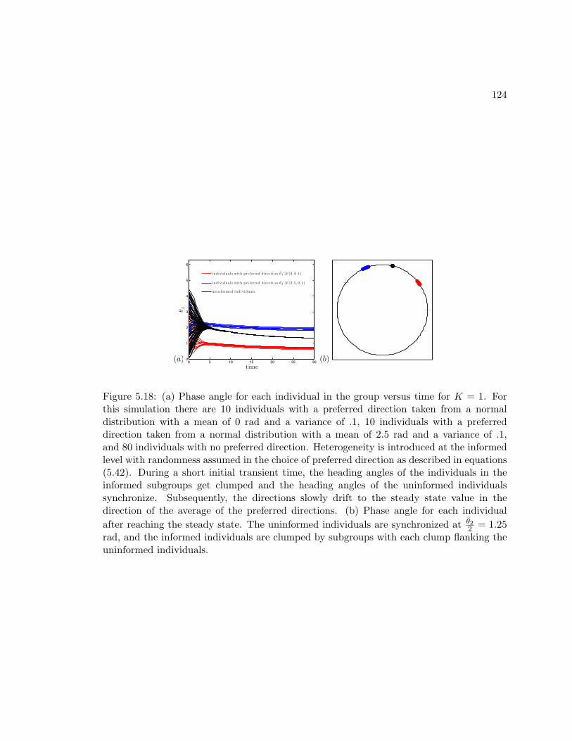
124
0 5 10 15 20 25 300
1
2
3
4
5
6
time
θj
0 0.1 0.2 0.3 0.4 0.5 0.6 0.7 0.8 0.9 10
0.1
0.2
0.3
0.4
0.5
0.6
0.7
0.8
0.9
1
individuals with preferred direction θ1˜N (0, 0.1)
individuals with preferred direction θ2˜N (2.5, 0.1)
uninformed individuals
(a) (b)
Figure 5.18: (a) Phase angle for each individual in the group versus time for K = 1. Forthis simulation there are 10 individuals with a preferred direction taken from a normaldistribution with a mean of 0 rad and a variance of .1, 10 individuals with a preferreddirection taken from a normal distribution with a mean of 2.5 rad and a variance of .1,and 80 individuals with no preferred direction. Heterogeneity is introduced at the informedlevel with randomness assumed in the choice of preferred direction as described in equations(5.42). During a short initial transient time, the heading angles of the individuals in theinformed subgroups get clumped and the heading angles of the uninformed individualssynchronize. Subsequently, the directions slowly drift to the steady state value in thedirection of the average of the preferred directions. (b) Phase angle for each individualafter reaching the steady state. The uninformed individuals are synchronized at θ2
2 = 1.25rad, and the informed individuals are clumped by subgroups with each clump flanking theuninformed individuals.
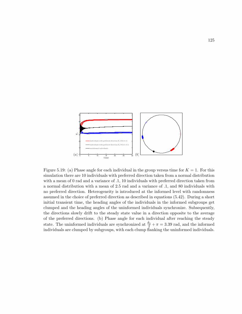
125
0 5 10 15 20 25 300
1
2
3
4
5
6
time
θj
0 0.1 0.2 0.3 0.4 0.5 0.6 0.7 0.8 0.9 10
0.1
0.2
0.3
0.4
0.5
0.6
0.7
0.8
0.9
1
individuals with preferred direction θ1˜N (0, 0.1)
individuals with preferred direction θ2˜N (2.5, 0.1)
uninformed individuals
(b)(a)
Figure 5.19: (a) Phase angle for each individual in the group versus time for K = 1. For thissimulation there are 10 individuals with preferred direction taken from a normal distributionwith a mean of 0 rad and a variance of .1, 10 individuals with preferred direction taken froma normal distribution with a mean of 2.5 rad and a variance of .1, and 80 individuals withno preferred direction. Heterogeneity is introduced at the informed level with randomnessassumed in the choice of preferred direction as described in equations (5.42). During a shortinitial transient time, the heading angles of the individuals in the informed subgroups getclumped and the heading angles of the uninformed individuals synchronize. Subsequently,the directions slowly drift to the steady state value in a direction opposite to the averageof the preferred directions. (b) Phase angle for each individual after reaching the steadystate. The uninformed individuals are synchronized at θ2
2 + π = 3.39 rad, and the informedindividuals are clumped by subgroups, with each clump flanking the uninformed individuals.
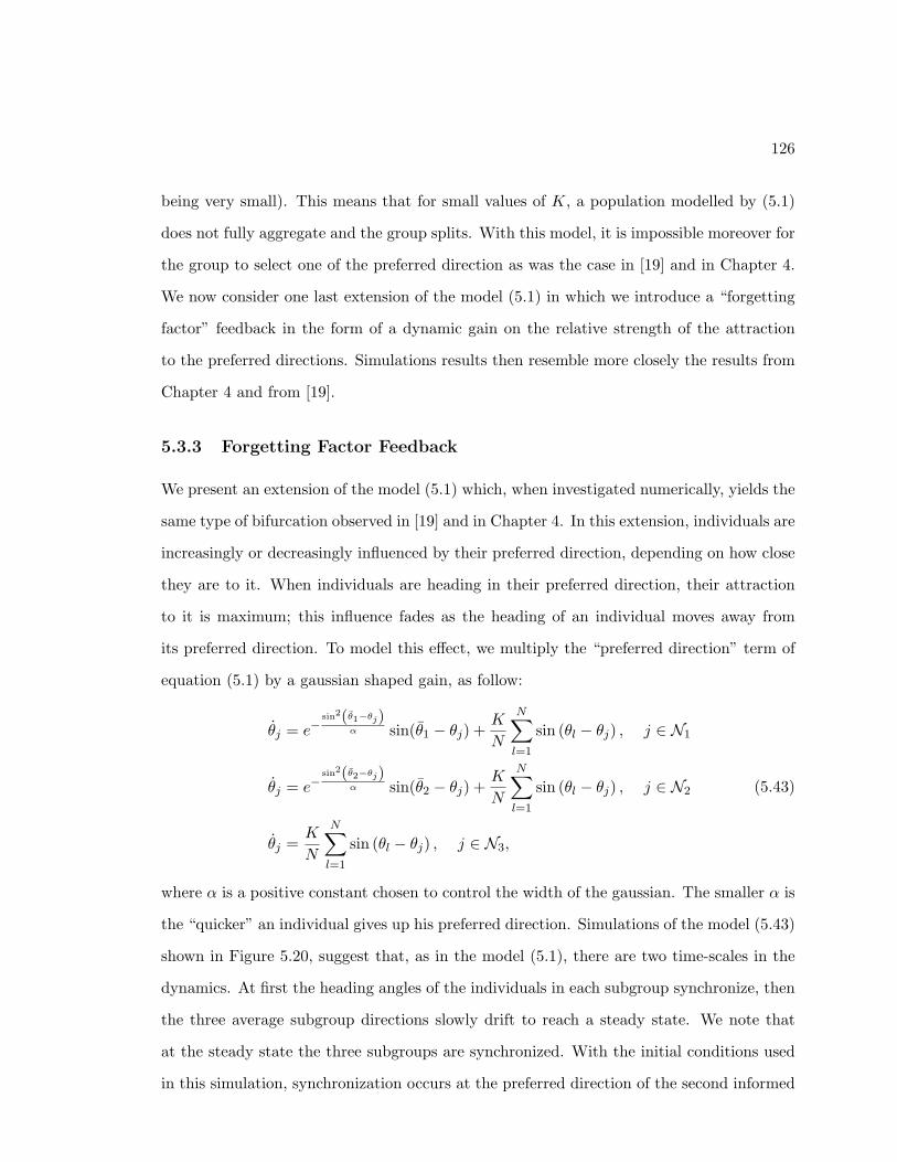
126
being very small). This means that for small values of K, a population modelled by (5.1)
does not fully aggregate and the group splits. With this model, it is impossible moreover for
the group to select one of the preferred direction as was the case in [19] and in Chapter 4.
We now consider one last extension of the model (5.1) in which we introduce a “forgetting
factor” feedback in the form of a dynamic gain on the relative strength of the attraction
to the preferred directions. Simulations results then resemble more closely the results from
Chapter 4 and from [19].
5.3.3 Forgetting Factor Feedback
We present an extension of the model (5.1) which, when investigated numerically, yields the
same type of bifurcation observed in [19] and in Chapter 4. In this extension, individuals are
increasingly or decreasingly influenced by their preferred direction, depending on how close
they are to it. When individuals are heading in their preferred direction, their attraction
to it is maximum; this influence fades as the heading of an individual moves away from
its preferred direction. To model this effect, we multiply the “preferred direction” term of
equation (5.1) by a gaussian shaped gain, as follow:
θj = e−sin2(θ1−θj)
α sin(θ1 − θj) +K
N
N∑l=1
sin (θl − θj) , j ∈ N1
θj = e−sin2(θ2−θj)
α sin(θ2 − θj) +K
N
N∑l=1
sin (θl − θj) , j ∈ N2
θj =K
N
N∑l=1
sin (θl − θj) , j ∈ N3,
(5.43)
where α is a positive constant chosen to control the width of the gaussian. The smaller α is
the “quicker” an individual gives up his preferred direction. Simulations of the model (5.43)
shown in Figure 5.20, suggest that, as in the model (5.1), there are two time-scales in the
dynamics. At first the heading angles of the individuals in each subgroup synchronize, then
the three average subgroup directions slowly drift to reach a steady state. We note that
at the steady state the three subgroups are synchronized. With the initial conditions used
in this simulation, synchronization occurs at the preferred direction of the second informed
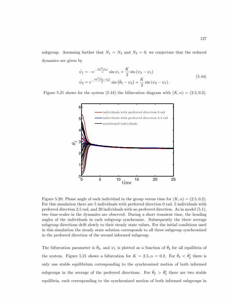
127
subgroup. Assuming further that N1 = N2 and N3 = 0, we conjecture that the reduced
dynamics are given by
ψ1 = −e− sin2(ψ1)α sinψ1 +
K
2sin (ψ2 − ψ1)
ψ2 = e−sin2(θ2−ψ2)
α sin(θ2 − ψ2
)+K
2sin (ψ2 − ψ1) .
(5.44)
Figure 5.21 shows for the system (5.44) the bifurcation diagram with (K,α) = (2.5, 0.2).
0 5 10 15 20 250
1
2
3
4
5
6
0 5 10 15 20 250
0.5
1
1.5
2
2.5
3
3.5
4
4.5
5
time
θj
0 10 20 30 40 50 600
1
2
3
4
5
6
time (sec)
θj
indiv idual s with preferred direction 0 rad
individual s with preferred direction 2.5 rad
uninformed individual s
Figure 5.20: Phase angle of each individual in the group versus time for (K,α) = (2.5, 0.2).For this simulation there are 5 individuals with preferred direction 0 rad, 5 individuals withpreferred direction 2.5 rad, and 20 individuals with no preferred direction. As in model (5.1),two time-scales in the dynamics are observed. During a short transient time, the headingangles of the individuals in each subgroup synchronize. Subsequently the three averagesubgroup directions drift slowly to their steady state values. For the initial conditions usedin this simulation the steady state solution corresponds to all three subgroup synchronizedin the preferred direction of the second informed subgroup.
The bifurcation parameter is θ2, and ψ1 is plotted as a function of θ2 for all equilibria of
the system. Figure 5.21 shows a bifurcation for K = 2.5, α = 0.2. For θ2 < θ∗2 there is
only one stable equilibrium corresponding to the synchronized motion of both informed
subgroups in the average of the preferred directions. For θ2 > θ∗2 there are two stable
equilibria, each corresponding to the synchronized motion of both informed subgroups in
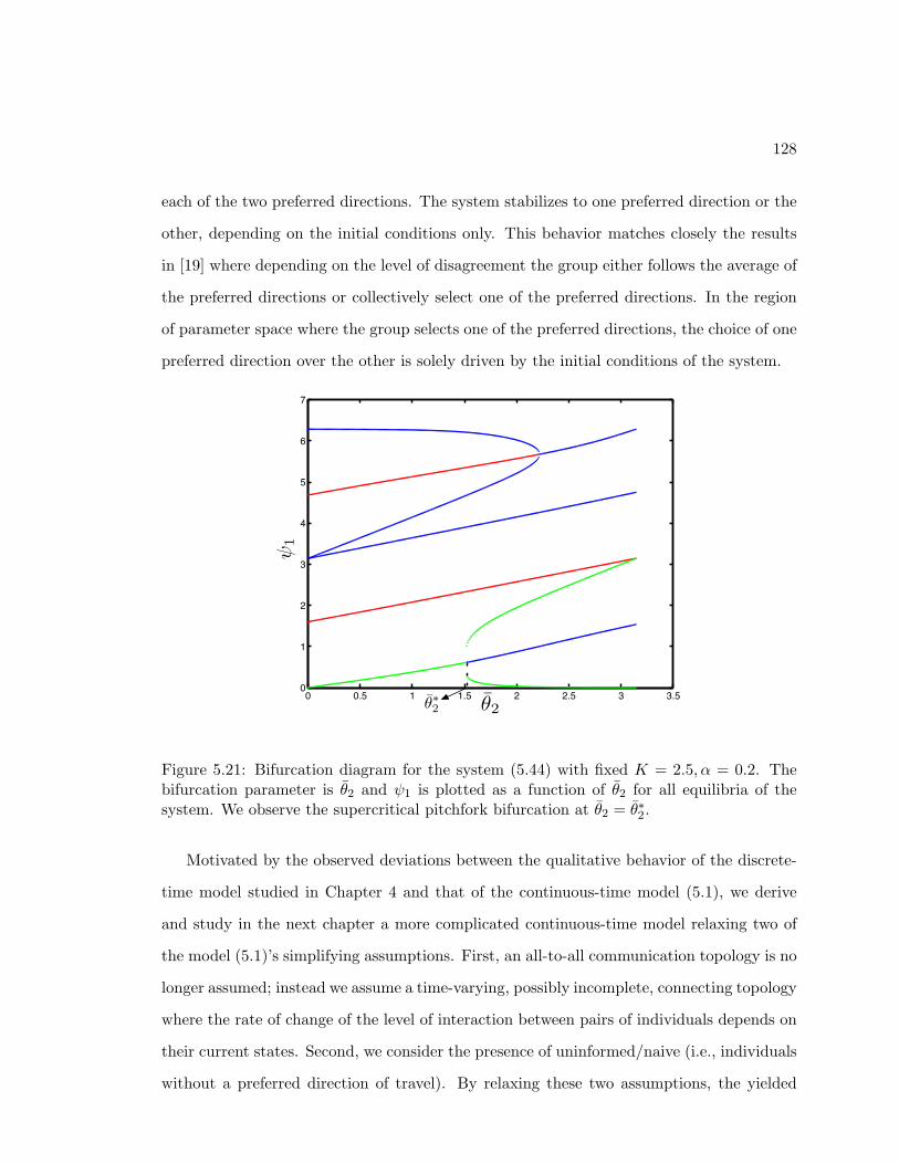
128
each of the two preferred directions. The system stabilizes to one preferred direction or the
other, depending on the initial conditions only. This behavior matches closely the results
in [19] where depending on the level of disagreement the group either follows the average of
the preferred directions or collectively select one of the preferred directions. In the region
of parameter space where the group selects one of the preferred directions, the choice of one
preferred direction over the other is solely driven by the initial conditions of the system.
0 0.5 1 1.5 2 2.5 3 3.50
1
2
3
4
5
6
7
b i f u r c a t i o n d i a g r a m K = 2 . 5 = 0 . 2
1
Figure 5.21: Bifurcation diagram for the system (5.44) with fixed K = 2.5, α = 0.2. Thebifurcation parameter is θ2 and ψ1 is plotted as a function of θ2 for all equilibria of thesystem. We observe the supercritical pitchfork bifurcation at θ2 = θ∗2.
Motivated by the observed deviations between the qualitative behavior of the discrete-
time model studied in Chapter 4 and that of the continuous-time model (5.1), we derive
and study in the next chapter a more complicated continuous-time model relaxing two of
the model (5.1)’s simplifying assumptions. First, an all-to-all communication topology is no
longer assumed; instead we assume a time-varying, possibly incomplete, connecting topology
where the rate of change of the level of interaction between pairs of individuals depends on
their current states. Second, we consider the presence of uninformed/naive (i.e., individuals
without a preferred direction of travel). By relaxing these two assumptions, the yielded

129
model produces qualitative behaviors closer, though not identical, to the ones observed
in [19] and in Chapter 4. The observed resulting deviations draw our attention to the
importance of a remaining simplifying assumption, namely, that our model describes the
dynamics of the heading angles for all individuals in the population independent of their
positions.
Chapter 6
Collective Decision Making:
Analytical Model with
Time-Varying Connecting
Topology
In this chapter, we derive and study the dynamics of a low-dimensional, deterministic,
coordinated control system. This model, a more complex version of the model presented
and studied in Chapter 5, relaxes two of that model’s simplifying assumptions. In Section
6.1 we present the model and identify invariant manifolds. In Section 6.2 we summarize
the conditions for each manifold to be attractive and describe the stable motions on these
invariant manifolds in the context of animal group motion. In Section 6.3 we study the at-
tractiveness of the identified invariant manifolds and the full phase-space reduced dynamics
on the attractive invariant manifolds. In Section 6.4 we consider an extension of the model
to test its robustness.
130
131
6.1 Model and Invariant Manifolds
The continuous-time model we present here is motivated by the observed deviations between
the realistic qualitative behavior of the discrete-time model studied in Chapter 4 and that
of the continuous-time model presented in Chapter 5. In order to formulate this new
continuous-time model, we relax two simplifying assumptions made in the model presented
in Chapter 5. First, an all-to-all communication topology is no longer assumed; instead we
assume a time-varying, possibly incomplete, connecting topology where the rate of change of
the level of interaction between pairs of individuals depends on their current states. Second,
whereas in the analyses of the previous model we ignored the presence of uninformed/naive
individuals (i.e., individuals without a preferred direction of travel), here we consider their
presence. With these two assumptions relaxed, the yielded model produces qualitative
behaviors that are closer, though not identical, to the ones observed in [19] and in Chapter
4. The observed resulting deviations draw our attention to the importance of a remaining
simplifying assumption, namely, that we are considering only the dynamics of the phases
and not the complete spatial dynamics of the individuals in the group.
6.1.1 Particle Model
Following the notation used in Chapter 5, we consider a population of N interacting indi-
viduals, each described as a unit mass Newtonian particle moving in the plane at constant
speed and controlled by its steering rate. The steering rate evolves through time under the
influence of inter-particle measurements and, where applicable, information represented by
a preferred direction of travel. Unlike in the model presented in the previous chapter, in this
model we do not assume a fixed all-to-all communication topology in the group. Rather, we
consider a time-varying, possibly incomplete, undirected communication topology in which
the rate of change of the level of interaction between individuals depends on their current
states. We denote as alj(t), l ∈ 1, . . . , N, j ∈ 1, . . . , N, the coupling gain quantifying
the level of interaction between agent l and agent j, where alj(t) = ajl(t) is allowed to take
any value between 0 and 1. In the case where alj = 0, agents l and j are not interacting.
132
In the case where alj = 1, the interaction between agents l and j is maximum.
The model we define consists of a set of differential equations describing the dynamics
of the instantaneous heading directions θj and interaction gains alj . The dynamics for the
heading angles are modeled with steering terms that depend on relative heading angles, as
in the previous chapter; the dynamics of the interaction gains are modelled with a saturated
integrator dynamics written as
θj = sin(θ1 − θj
)+K1
N
N∑l=1
ajl sin (θl − θj) , j ∈ N1
θj = sin(θ2 − θj
)+K1
N
N∑l=1
ajl sin (θl − θj) , j ∈ N2
θj =K1
N
N∑l=1
ajl sin (θl − θj) , j ∈ N3
ηlj = K2(ρlj − r), l ∈ 1, . . . , N, j ∈ l + 1, . . . , N
alj =1
1 + e−ηlj, l ∈ 1, . . . , N, j ∈ l + 1, . . . , N,
(6.1)
where ηlj = ηjl ∈ R is an integrated variable, ρlj = | eiθl+eiθj2 | gives a measure of the level
of synchrony between agents l and j, the parameter K1 > 0 weights the attention paid to
other individuals versus the preferred direction, the parameter K2 > 0 quantifies the speed
at which the interaction gains evolve, and r ∈ [0, 1] is a fixed threshold. If ρlj > r, i.e.,
synchrony is above the threshold, then ηlj increases and alj eventually converges to 1, the
maximum interaction strength. If ρlj < r, i.e., synchrony is below the threshold, then ηlj
decreases and alj eventually converges to 0, no interconnection. The use of such dynamics for
the interaction gains allows us to include the effect of memory on the interactions between
individuals. This formulation is similar to the drift diffusion dynamics used to model “two-
alternative forced choice tasks” in psychological studies such as [7]. The dynamics of alj
can be written in a simpler form, substituting the dynamics of ηlj , as
alj = K2(1− alj)alj(ρlj − r), l ∈ 1, . . . , N, j ∈ l + 1, . . . , N. (6.2)
We will use this formulation in the remainder of the analysis.
133
6.1.2 Invariant Manifolds in the Model
Like the model (5.1) discussed in the previous chapter, the (N+ N(N−1)2 )-dimensional model
(6.1) is challenging to study. Simulations of the model (6.1) shown in Figures 6.1 suggest,
however, that we can reduce the complexity of the system using time scale arguments, as
we did in the previous chapter. During an initial transient time, the heading angles of
the individuals in each subgroup synchronize and the interaction gains between subgroups
converge to a fixed value (zero or one). Then, the three average subgroup directions slowly
drift to reach a steady state. This means that, as was true for the model presented in the
previous chapter, the long-term dynamics of the model (6.1) can be described by ψ1, ψ2
and ψ3, which are the average heading directions of the three subgroups. However, unlike
the model (5.1) which has only one invariant manifold the system (6.1) has several, each
characterized by a set of interaction gains between the different subgroups. Figures 6.2
- 6.5 present simulations illustrating six different invariant manifolds (each corresponding
to a different interconnection topology between the subgroups) to which the system can
converge during the fast time scale. We note that for these simulations, the gain K2 used is
smaller than the one used in Figure 6.1. Even without a sharp distinction of the two time
scales, the nature of the long term behavior is preserved.
In Figure 6.2 all three simulations presented have the same parameter values K1 =
2, K2 = 5, N1 = N2 = 10, N3 = 30, r = .8, θ1 = 0 rad, θ2 = 3 rad but each has a different
initial conditions. The first simulation is shown in panels (a), (b), (c), the second in panels
(d), (e), (f) and the third in panels (g), (h), (i). In the first simulation, all interaction
gains converge to 1. At the steady state, each informed subgroup compromises between its
preferred direction and the average of the two preferred directions, while the uninformed
subgroup travels in a direction corresponding to the average of the preferred directions.
In the second simulation, the interaction gains between individuals in the first informed
subgroup and individuals in the uninformed subgroup converge to 1, the interaction gains
between individuals in the second informed subgroup and individuals in the other two
subgroups (the uninformed subgroup and the first informed subgroup) converge to zero.
134
At the steady state, the first informed subgroup travels in its preferred direction along
with the uninformed subgroup, while the second informed subgroup, disconnected from
the two other subgroups, travels in its preferred direction. In the third simulation, the
scenario is symmetrical to the previous one: the second informed subgroup travels in its
preferred direction along with the uninformed subgroup, while the first informed subgroup,
disconnected from the two other subgroups, travels in its preferred direction.
In Figure 6.3 the values of the parameters K1, K2, r and θ1 are identical to the ones
used in Figure 6.2, but the preferred direction of the second subgroup is set to θ2 = .5 rad. In
this simulation, the interaction gains between individuals in the first informed subgroup and
individuals in the second informed subgroup converge to 1 and the interaction gains between
individuals in the uninformed subgroup and individuals in the other two subgroups (the first
and second informed subgroups) converge to zero. At the steady state, the two informed
subgroups compromise between their preferred directions and the average of the preferred
directions, while the uninformed subgroup, disconnected from the two other subgroups,
travels in its initial heading.
In Figure 6.4 the values of the parameter K1, K2 are identical to the ones in Figures 6.2
and 6.3. The threshold r is set to .95 and the preferred directions of the first and second
informed subgroups are set to θ1 = 1 rad and θ2 = 3.1 rad, respectively. In this simulation,
all interaction gains between individuals in different subgroups converge to zero. At the
steady state, there are no interactions between subgroups, each informed subgroup travels
in its preferred direction and the uninformed subgroup travels in its initial direction.
In Figure 6.5 the values of the parameters are chosen as K1 = 2, K2 = 7, N1 = N2 =
10, N3 = 30, r = .85, θ1 = π4 rad and θ2 = 5π
4 rad. In this simulation, the interaction
gains between individuals in the first informed subgroup and individuals in the second
subgroup converge to zero and the interaction gains between individuals in the uninformed
subgroup and individuals in both of the informed subgroups converge to 1. At the steady
state, each of the two informed subgroups, although not directly connected to the other,
compromises between its preferred direction and the average of the two preferred directions;
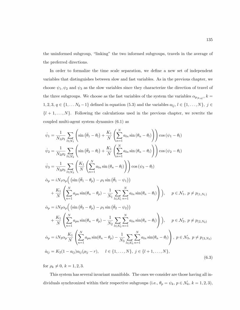
135
the uninformed subgroup, “linking” the two informed subgroups, travels in the average of
the preferred directions.
In order to formalize the time scale separation, we define a new set of independent
variables that distinguishes between slow and fast variables. As in the previous chapter, we
choose ψ1, ψ2 and ψ3 as the slow variables since they characterize the direction of travel of
the three subgroups. We choose as the fast variables of the system the variables αp(k,q), k =
1, 2, 3, q ∈ 1, . . . Nk−1 defined in equation (5.3) and the variables alj , l ∈ 1, . . . , N, j ∈l + 1, . . . , N. Following the calculations used in the previous chapter, we rewrite the
coupled multi-agent system dynamics (6.1) as
ψ1 =1
N1ρ1
∑l∈N1
(sin(θ1 − θl
)+K1
N
(N∑n=1
aln sin (θn − θl)))
cos (ψ1 − θl)
ψ2 =1
N2ρ2
∑l∈N2
(sin(θ2 − θl
)+K1
N
(N∑n=1
aln sin (θn − θl)))
cos (ψ2 − θl)
ψ3 =1
N3ρ3
∑l∈N3
(K1
N
(N∑n=1
aln sin (θn − θl)))
cos (ψ3 − θl)
αp = iN1αp
( (sin(θ1 − θp
)− ρ1 sin(θ1 − ψ1
))+K1
N
N∑n=1
apn sin(θn − θp)− 1N1
∑l∈N1
N∑n=1
aln sin(θn − θl)), p ∈ N1, p 6= p(1,N1)
αp = iN2αp
( (sin(θ2 − θp
)− ρ1 sin(θ2 − ψ2
))+K1
N
N∑n=1
apn sin(θn − θp)− 1N2
∑l∈N2
N∑n=1
aln sin(θn − θl)), p ∈ N2, p 6= p(2,N2)
αp = iN3αpK1
N
N∑n=1
apn sin(θn − θp)− 1N3
∑l∈N3
N∑n=1
aln sin(θn − θl) , p ∈ N3, p 6= p(3,N3)
alj = K2(1− alj)alj(ρlj − r), l ∈ 1, . . . , N, j ∈ l + 1, . . . , N,(6.3)
for ρk 6= 0, k = 1, 2, 3.
This system has several invariant manifolds. The ones we consider are those having all in-
dividuals synchronized within their respective subgroups (i.e., θp = ψk, p ∈ Nk, k = 1, 2, 3),
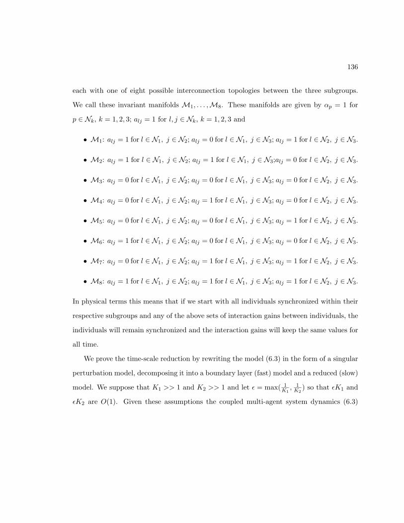
136
each with one of eight possible interconnection topologies between the three subgroups.
We call these invariant manifolds M1, . . . ,M8. These manifolds are given by αp = 1 for
p ∈ Nk, k = 1, 2, 3; alj = 1 for l, j ∈ Nk, k = 1, 2, 3 and
• M1: alj = 1 for l ∈ N1, j ∈ N2; alj = 0 for l ∈ N1, j ∈ N3; alj = 1 for l ∈ N2, j ∈ N3.
• M2: alj = 1 for l ∈ N1, j ∈ N2; alj = 1 for l ∈ N1, j ∈ N3;alj = 0 for l ∈ N2, j ∈ N3.
• M3: alj = 0 for l ∈ N1, j ∈ N2; alj = 0 for l ∈ N1, j ∈ N3; alj = 0 for l ∈ N2, j ∈ N3.
• M4: alj = 0 for l ∈ N1, j ∈ N2; alj = 1 for l ∈ N1, j ∈ N3; alj = 0 for l ∈ N2, j ∈ N3.
• M5: alj = 0 for l ∈ N1, j ∈ N2; alj = 0 for l ∈ N1, j ∈ N3; alj = 1 for l ∈ N2, j ∈ N3.
• M6: alj = 1 for l ∈ N1, j ∈ N2; alj = 0 for l ∈ N1, j ∈ N3; alj = 0 for l ∈ N2, j ∈ N3.
• M7: alj = 0 for l ∈ N1, j ∈ N2; alj = 1 for l ∈ N1, j ∈ N3; alj = 1 for l ∈ N2, j ∈ N3.
• M8: alj = 1 for l ∈ N1, j ∈ N2; alj = 1 for l ∈ N1, j ∈ N3; alj = 1 for l ∈ N2, j ∈ N3.
In physical terms this means that if we start with all individuals synchronized within their
respective subgroups and any of the above sets of interaction gains between individuals, the
individuals will remain synchronized and the interaction gains will keep the same values for
all time.
We prove the time-scale reduction by rewriting the model (6.3) in the form of a singular
perturbation model, decomposing it into a boundary layer (fast) model and a reduced (slow)
model. We suppose that K1 >> 1 and K2 >> 1 and let ε = max( 1K1, 1K2
) so that εK1 and
εK2 are O(1). Given these assumptions the coupled multi-agent system dynamics (6.3)
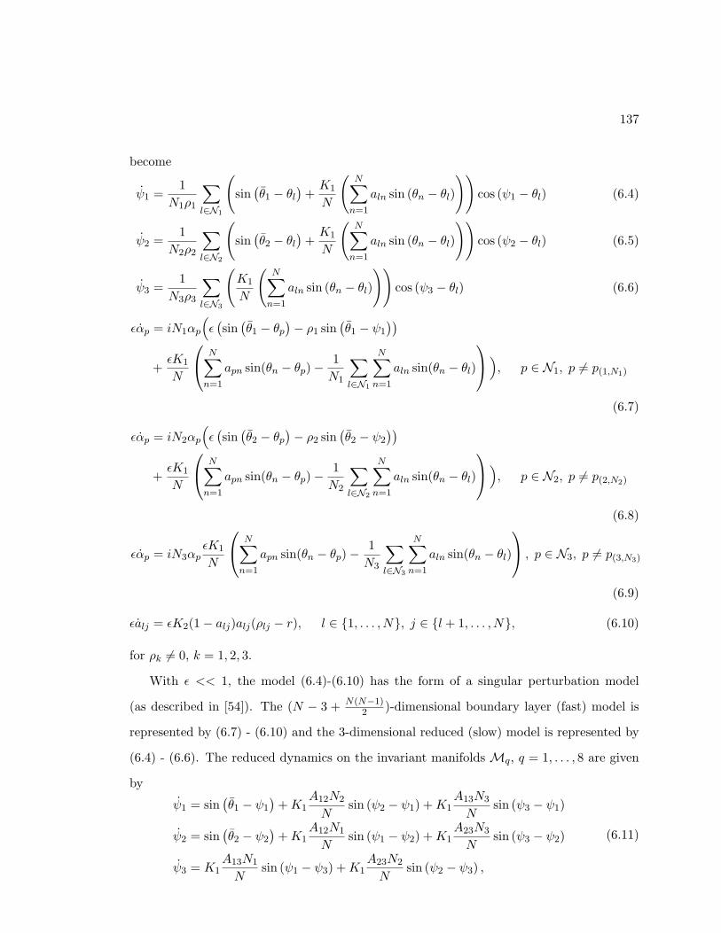
137
become
ψ1 =1
N1ρ1
∑l∈N1
(sin(θ1 − θl
)+K1
N
(N∑n=1
aln sin (θn − θl)))
cos (ψ1 − θl) (6.4)
ψ2 =1
N2ρ2
∑l∈N2
(sin(θ2 − θl
)+K1
N
(N∑n=1
aln sin (θn − θl)))
cos (ψ2 − θl) (6.5)
ψ3 =1
N3ρ3
∑l∈N3
(K1
N
(N∑n=1
aln sin (θn − θl)))
cos (ψ3 − θl) (6.6)
εαp = iN1αp
(ε(sin(θ1 − θp
)− ρ1 sin(θ1 − ψ1
))+εK1
N
N∑n=1
apn sin(θn − θp)− 1N1
∑l∈N1
N∑n=1
aln sin(θn − θl)), p ∈ N1, p 6= p(1,N1)
(6.7)
εαp = iN2αp
(ε(sin(θ2 − θp
)− ρ2 sin(θ2 − ψ2
))+εK1
N
N∑n=1
apn sin(θn − θp)− 1N2
∑l∈N2
N∑n=1
aln sin(θn − θl)), p ∈ N2, p 6= p(2,N2)
(6.8)
εαp = iN3αpεK1
N
N∑n=1
apn sin(θn − θp)− 1N3
∑l∈N3
N∑n=1
aln sin(θn − θl) , p ∈ N3, p 6= p(3,N3)
(6.9)
εalj = εK2(1− alj)alj(ρlj − r), l ∈ 1, . . . , N, j ∈ l + 1, . . . , N, (6.10)
for ρk 6= 0, k = 1, 2, 3.
With ε << 1, the model (6.4)-(6.10) has the form of a singular perturbation model
(as described in [54]). The (N − 3 + N(N−1)2 )-dimensional boundary layer (fast) model is
represented by (6.7) - (6.10) and the 3-dimensional reduced (slow) model is represented by
(6.4) - (6.6). The reduced dynamics on the invariant manifolds Mq, q = 1, . . . , 8 are given
by
ψ1 = sin(θ1 − ψ1
)+K1
A12N2
Nsin (ψ2 − ψ1) +K1
A13N3
Nsin (ψ3 − ψ1)
ψ2 = sin(θ2 − ψ2
)+K1
A12N1
Nsin (ψ1 − ψ2) +K1
A23N3
Nsin (ψ3 − ψ2)
ψ3 = K1A13N1
Nsin (ψ1 − ψ3) +K1
A23N2
Nsin (ψ2 − ψ3) ,
(6.11)
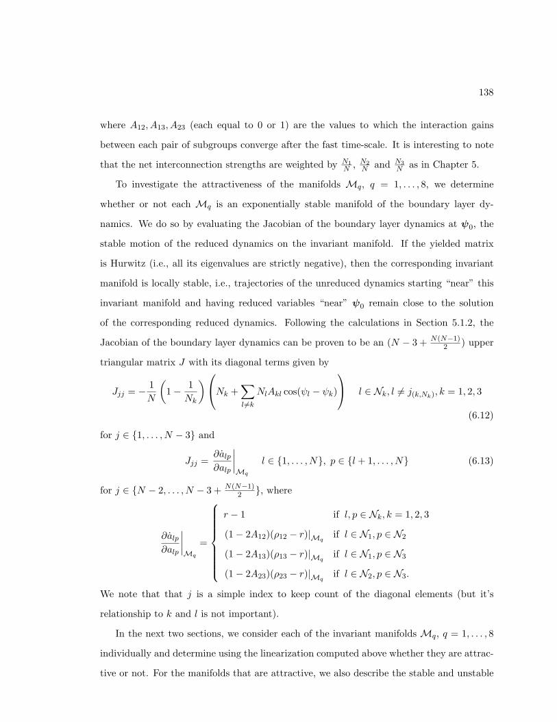
138
where A12, A13, A23 (each equal to 0 or 1) are the values to which the interaction gains
between each pair of subgroups converge after the fast time-scale. It is interesting to note
that the net interconnection strengths are weighted by N1N , N2
N and N3N as in Chapter 5.
To investigate the attractiveness of the manifolds Mq, q = 1, . . . , 8, we determine
whether or not each Mq is an exponentially stable manifold of the boundary layer dy-
namics. We do so by evaluating the Jacobian of the boundary layer dynamics at ψ0, the
stable motion of the reduced dynamics on the invariant manifold. If the yielded matrix
is Hurwitz (i.e., all its eigenvalues are strictly negative), then the corresponding invariant
manifold is locally stable, i.e., trajectories of the unreduced dynamics starting “near” this
invariant manifold and having reduced variables “near” ψ0 remain close to the solution
of the corresponding reduced dynamics. Following the calculations in Section 5.1.2, the
Jacobian of the boundary layer dynamics can be proven to be an (N − 3 + N(N−1)2 ) upper
triangular matrix J with its diagonal terms given by
Jjj = − 1N
(1− 1
Nk
)Nk +∑l 6=k
NlAkl cos(ψl − ψk) l ∈ Nk, l 6= j(k,Nk), k = 1, 2, 3
(6.12)
for j ∈ 1, . . . , N − 3 and
Jjj =∂alp∂alp
∣∣∣∣Mq
l ∈ 1, . . . , N, p ∈ l + 1, . . . , N (6.13)
for j ∈ N − 2, . . . , N − 3 + N(N−1)2 , where
∂alp∂alp
∣∣∣∣Mq
=
r − 1 if l, p ∈ Nk, k = 1, 2, 3
(1− 2A12)(ρ12 − r)|Mqif l ∈ N1, p ∈ N2
(1− 2A13)(ρ13 − r)|Mqif l ∈ N1, p ∈ N3
(1− 2A23)(ρ23 − r)|Mqif l ∈ N2, p ∈ N3.
We note that that j is a simple index to keep count of the diagonal elements (but it’s
relationship to k and l is not important).
In the next two sections, we consider each of the invariant manifolds Mq, q = 1, . . . , 8
individually and determine using the linearization computed above whether they are attrac-
tive or not. For the manifolds that are attractive, we also describe the stable and unstable
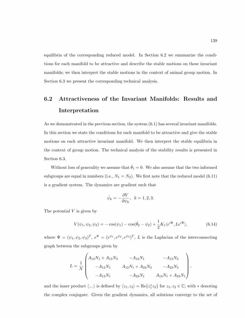
139
equilibria of the corresponding reduced model. In Section 6.2 we summarize the condi-
tions for each manifold to be attractive and describe the stable motions on these invariant
manifolds; we then interpret the stable motions in the context of animal group motion. In
Section 6.3 we present the corresponding technical analysis.
6.2 Attractiveness of the Invariant Manifolds: Results and
Interpretation
As we demonstrated in the previous section, the system (6.1) has several invariant manifolds.
In this section we state the conditions for each manifold to be attractive and give the stable
motions on each attractive invariant manifold. We then interpret the stable equilibria in
the context of group motion. The technical analysis of the stability results is presented in
Section 6.3.
Without loss of generality we assume that θ1 = 0. We also assume that the two informed
subgroups are equal in numbers (i.e., N1 = N2). We first note that the reduced model (6.11)
is a gradient system. The dynamics are gradient such that
ψk = − ∂V∂ψk
, k = 1, 2, 3.
The potential V is given by
V (ψ1, ψ2, ψ3) = − cos(ψ1)− cos(θ2 − ψ2) +12K1〈eiΨ, LeiΨ〉, (6.14)
where Ψ = (ψ1, ψ2, ψ3)T , eΨ = (eψ1 , eψ2 , eψ3)T , L is the Laplacian of the interconnecting
graph between the subgroups given by
L =1N
A12N1 +A13N3 −A12N1 −A13N3
−A12N1 A12N1 +A23N3 −A23N3
−A13N1 −A23N1 A13N1 +A23N1
,
and the inner product 〈., .〉 is defined by 〈z1, z2〉 = Rez∗1z2 for z1, z2 ∈ C, with ∗ denoting
the complex conjugate. Given the gradient dynamics, all solutions converge to the set of
140
critical points of V (ψ1, ψ2, ψ3) and there are no periodic solutions. The form of the potential
V given by (6.14) has been previously used in [103, 107].
Out of the eight manifolds M1, . . . ,M8, two are never attractive and the six others
may be attractive given some assumptions on the parameters of the model. The first two
invariant manifoldsM1 andM2 are always unstable. The dynamics on these two manifolds,
where (A12, A13, A23) = (1, 0, 1) and (A12, A13, A23) = (1, 1, 0) respectively, are symmetric;
in each case the uninformed subgroup is connected to only one informed subgroup and the
two informed subgroups are connected to each other.
The invariant manifold M3 is attractive if and only if r, θ2 and ψ3(0) are chosen such
that ∣∣∣1 + eiθ2∣∣∣− 2r < 0∣∣∣1 + eiψ3(0)∣∣∣− 2r < 0∣∣∣eiψ3(0) + eiθ2∣∣∣− 2r < 0.
(6.15)
On this invariant manifold, the stable equilibrium is ψM3,1 = (0, θ2, ψ3(0)). In this case,
the directions in which the subgroups are heading are “different enough” that they do
not “see” each other (i.e., ρij − r < 0 for all i 6= j ∈ 1, 2, 3). At the steady state, each
informed subgroup follows its preferred direction while the uninformed subgroup follows its
initial heading. At this equilibrium, there is no information transfer between the different
subgroups.
The invariant manifolds M4 and M5 are attractive if and only if the parameters r and
θ2 are chosen such that ∣∣∣1 + eiθ2∣∣∣− 2r < 0. (6.16)
The dynamics on these manifolds, where (A12, A13, A23) = (0, 1, 0) and (A12, A13, A23) =
(0, 0, 1), respectively, are symmetric; in each case the uninformed subgroup is connected
to only one informed subgroup and the two informed subgroups are disconnected from
each other. The stable equilibrium on each invariant manifold is ψM4,1 = (0, θ2, 0) and
ψM5,1 = (0, θ2, θ2), respectively. The directions in which the two informed subgroups are
heading are “different enough” that they do not “see” each other (i.e., ρ12 − r < 0). Each
141
informed subgroup travels in its preferred direction; the uninformed subgroup follows either
the first informed subgroup on M4 and the second informed subgroup, on M5.
On the invariant manifold M6 the dynamics of the two informed subgroups are inter-
connected but decoupled from the dynamics of the uninformed subgroup. The two informed
subgroups behave according to the model (5.20) studied in Section 5.2, and the uninformed
subgroup travels in its original heading (i.e., ψ3(t) = ψ3(0) for t > 0). We can hence write
an equilibrium of the system (6.22) as (ψ, ψ3(0)), where ψ is an equilibrium of the system
(5.20) with the gain K in (5.20) defined as K1 = KN2N1
. From the analysis in Section 5.2 we
know that, depending on the values of the parameters θ2 and K1, the reduced model (6.11)
can have up to two stable motions ψM6,1 = (ψsync1, ψ3(0)) and ψM6,2 = (ψsync2, ψ3(0)).
The manifoldM6 is attractive near the equilibrium ψM6,1 if r, θ2 and ψ3(0) are chosen
such that
2r −∣∣∣1 + eiθ2
∣∣∣ < 0∣∣∣1 + eiψ3(0)∣∣∣− 2r < 0∣∣∣eiθ2 + eiψ3(0)∣∣∣− 2r < 0.
If, on the other hand, r, θ2 and ψ3(0) are chosen such that
r −√
1− α2 < 0∣∣∣∣eiψ3(0) − ei“θ22
+arcsinα”∣∣∣∣− 2r < 0∣∣∣∣iei“ θ22 +arccosα
”+ eiψ3(0)
∣∣∣∣− 2r < 0,
where α =(N sin
θ22
2N1K1
) 13
, then M6 is attractive near the equilibrium ψM6,2. In physical
terms, the conditions mean that the preferred directions of the informed subgroups are
“close enough” to allow these two subgroups to “see” each other and that the heading in
which the uninformed subgroup initially travels is “different enough” from both preferred
directions that this subgroup does not “see” the other two. “Different” and “close enough”
are quantified with the threshold r. The two sets of conditions are similar except for the
142
fact that the uninformed subgroup has to initially head in a direction almost opposite to
the average of the two preferred directions for the first set of conditions and in a direction
close to the average of the two preferred directions for the second set of conditions.
For the stable motion ψM6,1, each informed subgroup compromises between its preferred
direction and the average of the two preferred directions, while the uninformed subgroup
travels in a direction “different enough” from that of either informed subgroup. For the
stable motion ψM6,2, the headings of two informed subgroups flank the heading opposite
the average of the preferred directions, while the uninformed subgroup travels in a direction
“different enough” from that of either informed subgroup.
The invariant manifoldM7 is attractive if and only if the parameters r and θ2 are chosen
such that1√
1 + ν2< r <
√12
+1
2√
1 + ν2,
where ν = N sinθ22
N3K1+N cosθ22
. On this manifold, the uninformed subgroup is connected to
both informed subgroups but the two informed subgroups are not connected to each other.
The equilibrium ψM7,6 =(θ22 + arctan ν, θ22 − arctan ν, θ22
)is the only stable one on this
manifold. In the motion corresponding to this equilibrium, the direction of the uninformed
subgroup is the average of the preferred directions of the two informed subgroups; the
direction of two informed subgroups flank it. The headings of the two informed subgroups
are “different enough” so that they do not “see” each other (i.e., ρ12−r < 0). However, they
are not “too different” i.e., each informed subgroup is connected to the uninformed subgroup
which travels in a direction corresponding to the average of their preferred directions.
On the invariant manifold M8, the group is connected with an all-to-all connecting
topology and the analysis from Section 5.2 can be adapted to compute the equilibria of
the reduced dynamics on M8 and evaluate their stability. Depending on the values of
the parameters θ2 and K1, the reduced model (6.11) can have up to two stable motions,
ψM8,8 and ψM8,11. In the first, the informed subgroups compromise between their preferred
direction and the average of the two preferred directions while the uninformed subgroup
travels in the average of the preferred directions. The second is symmetrical to the first:
143
the informed subgroups compromise between their preferred direction and the opposite of
the average of the two preferred directions while the uninformed subgroup travels in a
direction opposite to the average of the preferred directions. These results are similar to
the ones proven in Section 5.2. There is however a critical difference due to the presence
of uninformed individuals in the group. In the case where the number of uninformed
individuals exceeds a threshold given by N3 > 2N1
(1−
(2N1K1
N sinθ22
) 23
) 32
, the symmetric
equilibrium with the group traveling towards the opposite of the average of the preferred
directions no longer exists. This observation is consistent with the analysis from Chapter
4. The manifold M8 is attractive near the equilibrium ψM8,8 if the parameters r, θ2 are
chosen such that
2r − |1 + eiθ2 | < 0.
In physical terms the condition means that the preferred directions of the informed sub-
groups are close enough to allow individuals traveling in such directions to “see” each other.
The stability of the equilibrium ψM8,11 is not proven in Section 6.3 so we are unable to
give conditions for the attractiveness of the manifold M8 near that equilibrium.
6.3 Attractiveness and Phase Space Dynamics of the Re-
duced Models
As we discussed in Section 6.1, the system (6.1) has several invariant manifolds, some of
which are attractive under certain conditions on the parameters of the system. In this
section we present the technical proof for the attractiveness of each invariant manifold. In
the case where a manifold is shown to be attractive, we describe the stable and unstable
equilibria of the reduced model.
6.3.1 Invariant manifolds M1 and M2, (A12, A13, A23) = (1, 0, 1) or (1, 1, 0)
The cases where (A12, A13, A23) = (1, 0, 1) and (A12, A13, A23) = (1, 1, 0) are symmetric,
each corresponding to the uninformed subgroup being connected to only one informed sub-
144
group and the two informed subgroups being connected to each other. Given this symmetry
we investigate the stability of the manifold for (A12, A13, A23) = (1, 0, 1) as a representative
of both cases. In the case where (A12, A13, A23) = (1, 0, 1), the system (6.11) becomes
ψ1 = − sin (ψ1) +N1
NK1 sin (ψ2 − ψ1)
ψ2 = sin(θ2 − ψ2
)+N1
NK1 sin (ψ1 − ψ2) +
N3
NK1 sin (ψ3 − ψ2)
ψ3 =N3
NK1 sin (ψ2 − ψ3)
. (6.17)
The equilibria of this system have to lie on one of the ψ3-null-clines. The ψ3-null-clines
are given by ψ3 = ψ2 and ψ3 = ψ2 + π. We show that on either null-cline the invariant
manifold M1 cannot be attractive. The diagonal terms of the Jacobian of the boundary
layer dynamics J (6.12), (6.13) evaluated on the invariant manifold M1 are given by
Jjj =
− 1N
(1− 1
N1
)(N1 +N1 cos(ψ2 − ψ1)) j ∈ N1, j 6= j(1,N1)
− 1N
(1− 1
N1
)(N1 +N1 cos(ψ1 − ψ2) +N3) j ∈ N2, j 6= j(2,N2)
− 1N
(1− 1
N3
)(N1 +N3) j ∈ N3, j 6= j(3,N3)
for j ∈ 1, . . . , N − 3 and
Jjj =∂alp∂alp
∣∣∣∣M1
l ∈ 1, . . . , N, p ∈ l + 1, N,
for j ∈ N − 2, . . . , N − 3 + N(N−1)2 where
∂alj∂alj
∣∣∣∣M1
=
r − 1 if l, j ∈ Nk, k = 1, 2, 3
−(ρ12 − r) if l ∈ N1, j ∈ N2
(ρ13 − r) if l ∈ N1, j ∈ N3
−(ρ23 − r) if l ∈ N2, j ∈ N3.
On the ψ3-null-cline given by ψ3 = ψ2, ρ12 = ρ13; hence it is not possible to have both
−(ρ12 − r) < 0 and (ρ13 − r) < 0. On the ψ3-null-cline given by ψ3 = ψ2 + π, ρ23 = 0,
implying that −(ρ23 − r) = r > 0. These invariant manifolds are thus unstable for all
r ∈ [0, 1], θ2 ∈ [0, π].
145
6.3.2 Invariant Manifold M3, (A12, A13, A23) = (0, 0, 0)
In the case where (A12, A13, A23) = (0, 0, 0), the system (6.11) becomes
ψ1 = − sin (ψ1)
ψ2 = sin(θ2 − ψ2
)ψ3 = 0
. (6.18)
We compute the equilibria of the system (6.18) and determine the stability of each. We note
that there are no dynamics for ψ3; therefore, ψ3(t) = ψ3(0) for all t > 0. The dynamics of
ψ1 and ψ2 are decoupled and it is possible to find closed form expressions for all equilibria.
Stability of each equilibrium is determined from the eigenvalues of the Jacobian. There are
a total of four equilibria, given by
1. ψM3,1 = (0, θ2, ψ3(0)), stable for θ2 ∈ [0, π].
2. ψM3,2 = (0, θ2 + π, ψ3(0)), unstable for θ2 ∈ [0, π].
3. ψM3,3 = (π, θ2, ψ3(0)), unstable for θ2 ∈ [0, π].
4. ψM3,4 = (π, θ2 + π, ψ3(0)), unstable for θ2 ∈ [0, π].
The only stable equilibrium being ψM3,1 = (0, θ2, ψ3(0)), we now determine the range
of parameter values for θ2 and r for which the invariant manifold M3 is attractive. The
Jacobian of the boundary layer dynamics J given by equation (6.12), (6.13) evaluated on
the invariant manifold M3 at the stable equilibrium ψM3,1 = (0, θ2, ψ3(0)) is given by
Jjj = −Nk
N
(1− 1
Nk
)j ∈ Nk, j 6= j(k,Nk), k = 1, 2, 3
for j ∈ 1, . . . , N − 3 and
Jjj =∂alp∂alp
∣∣∣∣M3,ψM3,1
l ∈ 1, . . . , N, p ∈ l + 1, N,
146
for j ∈ N − 2, . . . , N − 3 + N(N−1)2 where
∂alj∂alj
∣∣∣∣M3,ψM3,1
=
r − 1 if l, j ∈ Nk, k = 1, 2, 3
(ρ12 − r)|ψM3,1if l ∈ N1, j ∈ N2
(ρ13 − r)|ψM3,1if l ∈ N1, j ∈ N3
(ρ23 − r)|ψM3,1if l ∈ N2, j ∈ N3.
Substituting in for ρ12, ρ13, and ρ23, the invariant manifold M3 is attractive if and only if
r, θ2 and ψ3(0) are chosen such that ∣∣∣1 + eiθ2∣∣∣− 2r < 0∣∣∣1 + eiψ3(0)∣∣∣− 2r < 0∣∣∣eiψ3(0) + eiθ2∣∣∣− 2r < 0.
(6.19)
Physically the conditions mean that the preferred directions of the informed subgroups are
“different enough” from each other and that the uninformed subgroup initially travels at a
heading “different enough” from both preferred directions. “Different enough” is quantified
with the threshold r.
6.3.3 Invariant Manifolds M4 and M5, (A12, A13, A23) = (0, 1, 0) or (0, 0, 1)
The cases where (A12, A13, A23) = (0, 1, 0) and (A12, A13, A23) = (0, 0, 1) are symmetri-
cal, each corresponding to the uninformed subgroup being connected to only one informed
subgroup and the two informed subgroups being disconnected. Given this symmetry, we
compute the equilibria and investigate stability only for (A12, A13, A23) = (0, 1, 0) as rep-
resentative of both cases. In the case where (A12, A13, A23) = (0, 1, 0), the system (6.11)
becomesψ1 = − sin (ψ1) +K1
N3
Nsin (ψ3 − ψ1)
ψ2 = sin(θ2 − ψ2
)ψ3 = K1
N1
Nsin (ψ1 − ψ3) .
(6.20)
We compute the equilibria of the system (6.20) and determine the stability of each. It is
possible to find closed form expressions for all equilibria. The stability of each equilibrium
147
is determined from the eigenvalues of the Jacobian. There are a total of eight equilibria
given by
1. ψM4,1 = (0, θ2, 0), stable for θ2 ∈ [0, π],K1 > 0.
2. ψM4,2 = (0, θ2, π), unstable for θ2 ∈ [0, π],K1 > 0.
3. ψM4,3 = (0, θ2 + π, 0), unstable for θ2 ∈ [0, π],K1 > 0.
4. ψM4,4 = (0, θ2 + π, π), unstable for θ2 ∈ [0, π],K1 > 0.
5. ψM4,5 = (π, θ2, π), unstable for θ2 ∈ [0, π],K1 > 0.
6. ψM4,6 = (π, θ2, 0), unstable for θ2 ∈ [0, π],K1 > 0.
7. ψM4,7 = (π, θ2 + π, π), unstable for θ2 ∈ [0, π],K1 > 0.
8. ψM4,8 = (π, θ2 + π, 0), unstable for θ2 ∈ [0, π],K1 > 0.
The only stable equilibrium being ψM4,1 = (0, θ2, 0), we now determine the range of param-
eter values for θ2 and r for which the invariant manifold M4 is attractive. The diagonal
terms of the Jacobian of the boundary layer dynamics J (6.12) evaluated on the invariant
manifold M4 at the stable equilibrium ψM4,1 is given by
Jjj =
− 1N
(1− 1
N1
)(N1 +N3) j ∈ N1, j 6= j(1,N1)
−N1N
(1− 1
N1
)j ∈ N2, j 6= j(2,N2)
− 1N
(1− 1
N3
)(N1 +N3) j ∈ N3, j 6= j(3,N3)
for j ∈ 1, . . . , N − 3 and
Jjj =∂alj∂alj
∣∣∣∣M4,ψM4,1
l ∈ 1, . . . , N, p ∈ l + 1, N,
for j ∈ N − 2, . . . , N − 3 + N(N−1)2 where
∂alj∂alj
∣∣∣∣M4,ψM4,1
=
r − 1 if l, j ∈ Nk, k = 1, 2, 3
(ρ12 − r)|ψM4,1if l ∈ N1, j ∈ N2
− (ρ13 − r)|ψM4,1if l ∈ N1, j ∈ N3
(ρ23 − r)|ψM4,1if l ∈ N2, j ∈ N3.
148
The invariant manifold M4 is attractive if and only if r and θ2 are chosen such that∣∣∣1 + eiθ2∣∣∣− 2r < 0. (6.21)
This means physically that the preferred directions of the informed subgroups are “different
enough”, given the threshold r.
6.3.4 Invariant Manifold M6, (A12, A13, A23) = (1, 0, 0)
In the case where (A12, A13, A23) = (1, 0, 0), the system (6.11) becomes
ψ1 = − sin (ψ1) +K1N1
Nsin (ψ2 − ψ1)
ψ2 = sin(θ2 − ψ2
)+K1N1
Nsin (ψ1 − ψ2)
ψ3 = 0.
(6.22)
In this case the two informed subgroups behave according to the model (5.20) studied in
Section 5.2, and the naive group travels in its original heading (i.e., ψ3(t) = ψ3(0) for
t > 0). The dynamics of the two informed subgroups are decoupled from the dynamics
of the uninformed subgroup. We can hence write an equilibrium of the system (6.22) as
(ψ, ψ3(0)), where ψ is an equilibrium of the system (5.20) with the K in (5.20) defined
by K1 = KN2N1
. From the analysis in Section 5.2 we know that, depending on the values of
the parameters θ2 and K1, the reduced model (6.11) can have up to two stable motions:
ψM6,1 = (ψsync1, ψ3(0)) and ψM6,2 = (ψsync2, ψ3(0)). From Lemmas 5.2.2 and 5.2.5,
using the re-parameterization defined above, the equilibrium ψM6,1 is stable for all θ2 ∈[0, π], K1 > 0 whereas the equilibrium ψM6,2 is stable if and only if θ2 ∈ [π2 , π] and
K1 ∈[
2NN1
(cos(θ22
) 23 + sin
(θ22
) 23
) 32
, 4NN1 sin θ2
].
We now determine the ranges of parameter values for θ2 and r for which the invariant
manifold M6 is stable near ψM6,1 and ψM6,2. The diagonal terms of the Jacobian of the
boundary layer dynamics J evaluated on M6 at ψM6,1 are given by
Jjj =
− 1N
(1− 1
N1
)(N1 +N1 cos(ψ2 − ψ1))|ψM6,1
j ∈ N1, j 6= j(1,N1)
− 1N
(1− 1
N1
)(N1 +N1 cos(ψ1 − ψ2))|ψM6,1
j ∈ N2, j 6= j(2,N2)
−N3N
(1− 1
N3
)j ∈ N3, j 6= j(3,N3)
(6.23)
149
for j ∈ 1, . . . , N − 3 and
Jjj =∂alj∂alj
∣∣∣∣M6,ψM6,1
l ∈ 1, . . . , N, p ∈ l + 1, N, (6.24)
for j ∈ N − 2, . . . , N − 3 + N(N−1)2 where
∂alj∂alj
∣∣∣∣M6,ψM6,1
=
r − 1 if l, j ∈ Nk, k = 1, 2, 3
− (ρ12 − r)|ψM6,1if l ∈ N1, j ∈ N2
(ρ13 − r)|ψM6,1if l ∈ N1, j ∈ N3
(ρ23 − r)|ψM6,1if l ∈ N2, j ∈ N3.
The Jacobian of the boundary layer dynamics on the manifold M6, at the equilibrium
ψM6,1 is Hurwitz if and only if all the terms given by equation (6.23), (6.24) are strictly
negative. From the analysis in Section 5.2.1 we know that for the equilibrium ψM6,1, the
principle value of the heading of the first and second informed subgroups are between 0 and
θ22 and between θ2
2 and θ2 respectively. Using these bounds for the heading of the informed
subgroups we obtain the following set of sufficient conditions to guarantee the attractiveness
of M6 near ψM6,1:
2r −∣∣∣1 + eiθ2
∣∣∣ < 0∣∣∣1 + eiψ3(0)∣∣∣− 2r < 0∣∣∣eiθ2 + eiψ3(0)∣∣∣− 2r < 0.
In physical terms the conditions mean that the preferred directions of the informed sub-
groups are “close enough” and that the uninformed subgroup initially travels at a heading
“different enough” from both preferred directions. “Different” and “close enough” are quan-
tified with the threshold r.
For the attractiveness of M6 near ψM6,2 it is also possible to give sufficient conditions
that guarantee it. From Lemma 5.2.4, we have√1− α2 < ρsync2 < 1,
where α2 =(N sin
θ22
2N1K1
) 23
. This means that the headings of the first and second informed
subgroups are between θ22 +π and θ2
2 +π+arcsinα and between θ2+π2 +arccosα and θ2
2 +π,
150
respectively. Using these bounds for the headings of the informed subgroups we obtain the
following set of sufficient conditions to guarantee the attractiveness of M6 near ψM6,2:
r −√
1− α2 < 0∣∣∣∣eiψ3(0) − ei“θ22
+arcsinα”∣∣∣∣− 2r < 0∣∣∣∣iei“ θ2+π
2+arccosα
”+ eiψ3(0)
∣∣∣∣− 2r < 0.
The uninformed subgroup is heading in a different enough direction from both informed
subgroups that informed individuals and uninformed individuals do not “see” each other
(i.e., ρ13 − r < 0 and ρ23 − r < 0).
6.3.5 Invariant Manifold M7, (A12, A13, A23) = (0, 1, 1)
In the case where (A12, A13, A23) = (0, 1, 1), the system (6.11) becomes
ψ1 = − sin (ψ1) +K1N3
Nsin (ψ3 − ψ1)
ψ2 = sin(θ2 − ψ2
)+K1N3
Nsin (ψ3 − ψ2)
ψ3 =K1N1
Nsin (ψ1 − ψ3) +
K1N1
Nsin (ψ2 − ψ3)
. (6.25)
We compute the equilibria of the system (6.11) and determine the stability of each equilibria.
It is possible for this system to find closed form expressions for all equilibria. The stability
of each equilibrium is determined using the Routh stability criterion. There are a total of
six equilibria given by
1. ψM7,1 =(π + arcsin γ, θ2 + arcsin γ, π+θ2
2 + arcsin γ)
, where γ = N3K1N cos θ22 . This
equilibrium is unstable for θ2 ∈ [0, π], K1 >NN3
.
2. ψM7,2 =(− arcsin γ, π + θ2 − arcsin γ, π+θ2
2 − arcsin γ)
, unstable for θ2 ∈ [0, π], K1 >
0.
3. ψM7,3 =(π+θ2
2 , θ2−π2 , θ22 + arccos(− NK1N3
cos θ22))
, unstable for θ2 ∈ [0, π], K1 > 0.
4. ψM7,4 =(π+θ2
2 , θ2−π2 , θ22 − arccos(− NK1N3
cos θ22))
, unstable for θ2 ∈ [0, π], K1 > 0.

151
5. ψM7,5 =(θ22 + π + arctan ν, θ22 + π − arctan ν, θ22
), where ν = N sin
θ22
N3K1+N cosθ22
. This
equilibrium is unstable for θ2 ∈ [0, π], K1 >NN3
.
6. ψM7,6 =(θ22 + arctan ν, θ22 − arctan ν, θ22
), stable for θ2 ∈ [0, π], K1 >
NN3
.
We now determine the ranges of parameter values for θ2 and r for which the invariant
manifold M7 is stable near ψM7,6. The diagonal terms of the Jacobian of the boundary
layer dynamics J evaluated on M7 at ψM7,6 are given by
Jjj =
− 1N
(1− 1
N1
)(N1 +N3 cos(ψ3 − ψ1))|ψM7,6
j ∈ N1, j 6= j(1,N1)
− 1N
(1− 1
N1
)(N1 +N3 cos(ψ3 − ψ2))|ψM7,6
j ∈ N2, j 6= j(2,N2)
− 1N
(1− 1
N3
)(N3 +N1 cos(ψ1 − ψ3) +N1 cos(ψ2 − ψ3))|ψM7,6
j ∈ N3, j 6= j(3,N3)
for j ∈ 1, . . . , N − 3 and
Jjj =∂alj∂alj
∣∣∣∣M7,ψM7,6
l ∈ 1, . . . , N, p ∈ l + 1, N,
for j ∈ N − 2, . . . , N − 3 + N(N−1)2 where
∂alj∂alj
∣∣∣∣M7,ψM7,6
=
r − 1 if l, j ∈ Nk, k = 1, 2, 3
(ρ12 − r)|ψM7,6if l ∈ N1, j ∈ N2
− (ρ13 − r)|ψM7,6if l ∈ N1, j ∈ N3
− (ρ23 − r)|ψM7,6if l ∈ N2, j ∈ N3.
Using the expressions of the phases ψ1, ψ2 and ψ3 at the equilibrium ψM7,6 we obtain the
following necessary and sufficient condition for the invariant manifold M7 to be attractive
near ψM7,6:
1√1 + ν2
< r <
√12
+1
2√
1 + ν2. (6.26)
In this case, the uninformed subgroup is heading in a “close enough” direction from both
informed subgroup that informed individuals and uninformed individuals “see” each other.
The two informed subgroups, however, are heading in “different enough” directions that
they do not “see” each other, although they are indirectly interacting with each other
through the uninformed subgroup.
152
6.3.6 Invariant Manifold M8, (A12, A13, A23) = (1, 1, 1)
In the case where (A12, A13, A23) = (1, 1, 1), the system (6.11) becomes
ψ1 = − sin (ψ1) +K1N1
Nsin (ψ2 − ψ1) +
K1N3
Nsin (ψ3 − ψ1)
ψ2 = sin(θ2 − ψ2
)+K1N1
Nsin (ψ1 − ψ2) +
K1N3
Nsin (ψ3 − ψ2)
ψ3 =K1N1
Nsin (ψ1 − ψ3) +
K1N1
Nsin (ψ2 − ψ3)
. (6.27)
We compute the equilibria of the system (6.27) but note that, except for specific values of
the parameters K1, θ2, we cannot find closed form expressions for all of them. For each
equilibrium we nevertheless describe how its value and stability changes as the bifurcation
parameters K, θ2 vary. The equilibria are given by
− sin (ψ1) +K1N1
Nsin (ψ2 − ψ1) +
K1N3
Nsin (ψ3 − ψ1) = 0
sin(θ2 − ψ2
)+K1N1
Nsin (ψ1 − ψ2) +
K1N3
Nsin (ψ3 − ψ2) = 0
K1N1
Nsin (ψ1 − ψ3) +
K1N1
Nsin (ψ2 − ψ3) = 0.
There are three sets of solutions, the first set given by
ψ1 =θ2 − π
2
ψ2 =θ2 + π
2
cos(ψ3 − θ2
2
)= − N
K1N3cos
θ2
2, (6.28)
the second set given by
ψ1 = π − θ2 + ψ2 (6.29)
sin(ψ2 − θ2
)=K1N1
Nsin θ2 +
K1N3
Ncos
θ2
2(6.30)
ψ3 =ψ1 + ψ2
2, (6.31)
153
and the third set given by
ψ1 = θ2 − ψ2 (6.32)
sin(θ2 − ψ2
)+K1N1
Nsin(θ2 − 2ψ2
)=K1N3
Nsin(θ2
2− ψ2
)(6.33)
ψ3 =ψ1 + ψ2
2. (6.34)
In the first set of solutions, we can find a closed form expression of each equilibrium.
Equation (6.28) has two solutions ψ3 = θ22 + π ± arccos
(N
K1N3cos θ22
). These two solutions
exist if and only if∣∣∣ NK1N3
cos θ22∣∣∣ ≤ 1.
Lemma 6.3.1 If∣∣∣ NK1N3
cos θ22∣∣∣ ≤ 1, then the two equilibria ψM8,1 and ψM8,2 satisfying
(6.28) and given by
ψM8,1 =(θ2 − π
2,θ2 + π
2,θ2
2+ π + arccos
(N
K1N3cos
θ2
2
))(6.35)
ψM8,2 =(θ2 − π
2,θ2 + π
2,θ2
2+ π − arccos
(N
K1N3cos
θ2
2
)), (6.36)
are unstable ∀K1 > min(N sinθ22
N1, NN3
√1+cos θ2
2 ).
Proof: The proof of Lemma 6.3.1 can be found in Appendix B.
In the second set of solutions, it is also possible to find a closed form expression for each
equilibrium. Equation (6.30) has two solutions ψ2 = θ2 +arcsin(K1N1N sin θ2 + K1N3
N cos θ22)
or ψ2 = θ2 +π−arcsin(K1N1N sin θ2 + K1N3
N cos θ22)
yielding a total of four equilibria. These
four equilibria exist if and only if∣∣∣K1N1
N sin θ2 + K1N3N cos θ22
∣∣∣ ≤ 1. For each value of θ2,
there is a range of values for K1 for which these equilibria exist. As θ2 approaches π the
range of values of K1 for which these equilibria exist becomes larger. We consider here the
case where these equilibria do not exist i.e., K1 >N
N1 sin θ2+N3 cosθ22
. We note that for the
simulation presented in Figure 6.2, the choice of parameters we made satisfy the conditions
for these equilibria to exist, but with the chosen initial conditions, the system does not
converge to any of these four equilibria.
154
For the equilibria in the third set of solutions given by (6.32) - (6.34) we make the same
change of variables as in Chapter 5, equation (5.26), (ψ1, ψ2) 7→(ρ, Ψ
)where ρ ∈ [0, 1] and
Ψ ∈ S1 are defined by
ρeiΨ =12
(eiψ1 + eiψ2
)= cos
(ψ1 − ψ2
2
)ei(ψ1+ψ2)/2 (6.37)
= cos(θ2
2− ψ2
)(cos
θ2
2+ i sin
θ2
2
). (6.38)
Equation (6.38) is obtained by using equation (6.32) in (6.37). For θ2 ∈ (0, π], ψ1 = θ2−ψ2
implies that Ψ = θ22 or Ψ = θ2
2 + π. An equilibrium of the system (6.27) can hence be
written as (ρ, ψ, ψ∗3), where ψ∗3 is the solution obtained from equation (6.34). We further
rewrite (6.33) as(sin
θ2
2+
2K1N1
Nsin(θ2
2− ψ2
))cos(θ2
2− ψ2
)+(
cosθ2
2+K1N3
N
)sin(θ2
2− ψ2
)= 0.
(6.39)
For Ψ = θ22 , (6.38) implies that cos
(θ22 − ψ2
)= ρ and sin
(θ22 − ψ2
)= ±
√1− ρ2.
Accordingly, (6.39) implies that ρ satisfies
ρ sinθ2
2+√
1− ρ2
(cos
θ2
2+K1N3
N
)+
2K1N1
Nρ√
1− ρ2 = 0 (6.40)
or
ρ sinθ2
2−√
1− ρ2
(cos
θ2
2+K1N3
N
)− 2K1N1
Nρ√
1− ρ2 = 0. (6.41)
For Ψ = θ22 + π, (6.38) implies that cos
(θ22 − ψ2
)= −ρ and sin
(θ22 − ψ2
)= ±
√1− ρ2.
Accordingly, (6.39) implies that ρ satisfies
−ρ sinθ2
2+√
1− ρ2
(cos
θ2
2+K1N3
N
)− 2K1N1
Nρ√
1− ρ2 = 0 (6.42)
or
−ρ sinθ2
2−√
1− ρ2
(cos
θ2
2+K1N3
N
)+
2K1N1
Nρ√
1− ρ2 = 0. (6.43)
We now consider equations (6.40)-(6.43) individually and determine the existence and na-
ture of the equilibria that they yield.
155
Equation (6.40) does not have any solution for (ρ, θ2) ∈ [0, 1] × (0, π) since all of the
terms on the left hand side of the equation are strictly positive.
Equation (6.41) has one solution for (ρ, θ2) ∈ [0, 1]× (0, π); we call this solution ρsync1.
It yields two equilibria ψM8,7 = (ρsync1, θ22 ,θ22 ) and ψM8,8 = (ρsync1, θ22 ,
θ22 + π). For large
values of K1 in both equilibria, the two informed subgroups become synchronized, with
synchronization occurring at Ψ = θ22 . The uninformed subgroup is heading in the average
of the preferred directions θ22 for the equilibrium ψM8,7 and in an opposite direction for
ψM8,8.
Lemma 6.3.2 The equilibrium ψM8,7 is stable for all(K, θ2
) ∈ [0,∞)× (0, π).
Proof: The proof of Lemma 6.3.2 can be found in Appendix B.
Lemma 6.3.3 The equilibrium ψM8,8 is unstable for all(K, θ2
) ∈ [0,∞)× (0, π).
Proof: The proof of Lemma 6.3.3 can be found in Appendix B.
Equation (6.42) has one solution for (ρ, θ2) ∈ [0, 1]×(0, π); we call this solution ρantisync1.
It yields two equilibria ψM8,9 = (ρantisync1, θ22 ,θ22 ) and ψM8,10 = (ρantisync1, θ22 ,
θ22 +π). For
large values of K1 in both equilibria, the two informed subgroups become anti-synchronized.
The uninformed subgroup is heading in the average of the preferred directions θ22 for the
equilibrium ψM8,9 and in an opposite direction for ψM8,10.
Lemma 6.3.4 The equilibria ψM8,9 and ψM8,10 are unstable for all(K, θ2
) ∈ [0,∞) ×(0, π).
Proof: The proof of Lemma 6.3.4 can be found in Appendix B.
Equation (6.43) has between zero and two solutions for (ρ, θ2) ∈ [0, 1] × (0, π). The
two solutions, when they exist, are called ρsync2 and ρantisync2. They yield four equilibria
ψM8,11 = (ρsync2, θ22 ,θ22 ), ψM8,12 = (ρsync2, θ22 ,
θ22 +π), ψM8,13 = (ρantisync2, θ22 +π, θ22 ) and
ψM8,14 = (ρantisync2, θ22 +π, θ22 +π). For large values of K1 in the two equilibria ψM8,11 and
ψM8,12, the two informed subgroups become synchronized, with synchronization occurring
at Ψ = θ22 + π. The uninformed subgroup is heading in the average of the preferred
156
directions θ22 for the equilibrium ψM8,11 and in an opposite direction for ψM8,12. For the
two equilibria ψM8,13 and ψM8,14, the two informed subgroups become anti-synchronized.
The uninformed subgroup is heading in the average of the preferred directions θ22 for the
equilibrium ψM8,13 and in an opposite direction for ψM8,14.
Lemma 6.3.5 Equation (6.43) has two solutions when (2N1K1)23 −(N sin θ2
2 )23 > (N3K1−
N cos θ22 )23 . If N3 > 2N1
(1−
(2N1K1
N sinθ22
) 23
) 32
, then equation (6.43) has no solutions ∀
K1, N1, θ2 ∈ [0,∞)2 × (0, π].
Proof: Let K ′ = 2N1K1
N sinθ22
which is well defined for θ2 ∈ (0, π]. Equation (6.43) can be
rewritten as
ρ(1√
1− ρ2−K ′) +
N3
2N1K ′ = − cot
θ2
2. (6.44)
The solutions of (6.43) exist when the function h(ρ) = ρ( 1√1−ρ2
−K ′) + N32N1
K ′ intersects
the constant y = − cot θ22 < 0. The function h(ρ) goes to N3K′
2N1when ρ 7→ 0, approaches
+∞ when ρ 7→ 1, and reaches its minimum of −K ′(ρ∗)3 + N3K′
2N1at ρ∗ =
√1− 1
K′2/3.
Equation (6.43) has two solutions (ρ1, ρ2) flanking ρ∗ if and only if h(ρ∗) < − cot θ22 ; this
last inequality is satisfied if and only if
(2N1K1)23 − (N sin
θ2
2)
23 > (N3K1 −N cos
θ2
2)
23 . (6.45)
If N3 > 2N1
(1−
(2N1K1
N sinθ22
) 23
) 32
, then h(ρ) > 0 ∀ρ ∈ [0, 1] and equation (6.43) has no
solution ∀ K1, N1, θ2 ∈ [0,∞)2 × (0, π].
We do not prove here the stability of these equilibria but given the analyses from Chapter
5, it is natural to conjecture that the equilibria ψM8,12, ψM8,13 and ψM8,14 are always
unstable and that for large enough values of θ2 there exists a range of values for K1 such
that the equilibrium ψM8,11 is stable.
We now determine the ranges of parameter values for θ2 and r for which the invariant
manifoldM8 is attractive near ψM8,7. The diagonal terms of the Jacobian of the boundary
157
layer dynamics J evaluated on M8 at ψM8,7 are given by
Jjj =
− 1N
(1− 1
N1
)(N1 +N1 cos(ψ2 − ψ1) +N3 cos(ψ3 − ψ1))|ψM8,7
j ∈ N1, j 6= j(1,N1)
− 1N
(1− 1
N1
)(N1 +N1 cos(ψ1 − ψ2) +N3 cos(ψ3 − ψ2))|ψM8,7
j ∈ N2, j 6= j(2,N2)
− 1N
(1− 1
N3
)(N3 +N1 cos(ψ1 − ψ3) +N1 cos(ψ2 − ψ3))|ψM8,7
j ∈ N3, j 6= j(3,N3)
for j ∈ 1, . . . , N − 3 and
Jjj =∂alj∂alj
∣∣∣∣M8,ψM8,7
l ∈ 1, . . . , N, p ∈ l + 1, N,
for j ∈ N − 2, . . . , N − 3 + N(N−1)2 where
∂alj∂alj
∣∣∣∣M8,ψM8,7
=
r − 1 if l, j ∈ Nk, k = 1, 2, 3
− (ρ12 − r)|ψM8,7if l ∈ N1, j ∈ N2
− (ρ13 − r)|ψM8,7if l ∈ N1, j ∈ N3
− (ρ23 − r)|ψM8,7if l ∈ N2, j ∈ N3.
From the analysis in Section 5.2, we know that for the equilibrium ψM7,6, the principal
values of the headings of the first and second informed subgroups are respectively, between
0 and θ22 and between θ2
2 and θ2. Given these bounds, the worst case scenario to satisfy the
stability criterium is when ψ1 = 0 and ψ2 = θ2, yielding the following sufficient condition
to guarantee the attractiveness of M8 near ψM8,7:
2r −∣∣∣1 + eiθ2
∣∣∣ < 0.
In physical terms, the condition means that the preferred directions of the two informed
subgroups are “close enough” given the threshold r that the interaction gain between two
individuals, one heading in the preferred direction of the first informed subgroup and the
other heading in the preferred direction of the second informed subgroup, would increase
given the dynamics (6.2).
158
6.4 Summary and Forgetting Factor Feedback Extension
6.4.1 Summary
In this chapter we have extended the model (5.1) of the dynamics of motion for a group
of N = N1 + N2 + N3 coupled individuals moving in the plane by relaxing the all-to-
all coupling assumption made in Chapter 5 and including uninformed individuals in the
analysis. We described eight invariant manifolds of the system and determined which ones
could be attractive and which ones could not. For each attractive manifold, we described
the stable and unstable equilibria of the corresponding reduced model and interpreted the
stable equilibria in the context of animal group motion. We proved that relaxing the all-to-
all connecting topology assumption yields a much richer behavior. Depending on the values
of the parameters θ2, r and K1, eight different group motions can occur.
We first observed an equilibrium similar to the persistent stable motion ψsync1 observed
in Chapter 5 where the two informed subgroups compromise between their preferred di-
rection and the average of the preferred direction. We proved in this present chapter that
the equilibrium ψM8,7 is stable for all values of the parameters K1, θ2. This equilibrium
is a K1-almost synchronized motion of the group in the direction θ22 . For moderate val-
ues of K1, the two informed subgroups compromise between their preferred direction and
the average of the preferred directions while the uninformed subgroup travels in a direc-
tion corresponding to the average of the preferred directions. For large values of K1, this
equilibrium corresponds to the whole group moving together in the average of the preferred
directions. We also showed that similar motion could be obtained in the invariant manifolds
M6 and M7. On the invariant manifold M6, the two informed subgroups behave exactly
according to the model (5.1) studied in Section 5.2. In this case, the two informed subgroups
compromise between their preferred direction and the average of the preferred directions
while the uninformed subgroup travels in its original heading. On the invariant manifold
M7, the two informed subgroups also compromise between their preferred direction and the
average of the preferred directions and the uninformed subgroup travels in the average of
159
the preferred directions. In this case, however, the two informed subgroups are not directly
connected to each other (i.e., A12 = 0); rather they are connected indirectly through their
mutual connection to the uninformed subgroup.
In contrast to the model (5.1), where informed individuals always compromise on their
preferred directions, we showed that with the model (6.1) it is possible to have informed
individuals travel exactly in their preferred direction. We observed this for three invariant
manifolds,M3,M4 andM5. In each case, the two informed subgroups become disconnected
from each other and follow their respective preferred directions. On the manifold M3 the
stable motion corresponds to each informed subgroup traveling in its preferred direction
and the uninformed subgroup traveling in its initial heading. For the manifolds M4 and
M5, each informed subgroup travels in its preferred direction with the uninformed subgroup
following the first informed subgroup for M4 and the second informed subgroup for M5.
We also noted that when the number of uninformed individuals in the group exceeds
a certain threshold, the inefficient motion ψM8,11, where the group heads in a direction
as divergent as possible from both preferred directions, disappears. This observation is
consistent with the analysis from Chapter 4, where using the discrete-time model from
[19], we argued that under certain circumstances, informed individuals derive a benefit in
associating with uninformed individuals.
However, as with the continuous-time model presented in the previous chapter, the
continuous-time model presented here does not reproduce the behavior we observed both in
[19] and in Chapter 4, where the group collectively selects one of the preferred directions.
As we explained above, informed individuals can follow their preferred direction only if they
are not connected to individuals of the other informed subgroup (i.e., A12 = 0). Moreover,
full synchronization of the group cannot occur unless the coupling gain K1 is very large.
This means that, for relatively small weight on the coupling in the model, the individuals
in the population do not fully aggregate and the group splits - although in some cases we
showed that the uninformed individuals do become synchronized with one or the other of
the informed subgroups. This deviation indirectly reveals the importance of a remaining
160
simplifying assumption, namely, that we consider only the dynamics of the phases and not
the complete spatial dynamics of the individuals in the group. For the simulations used
in [19] and in Chapter 4, we observed that in the case where the group collectively selects
one of the preferred directions, the leading informed subgroup travels in front, followed
by the uninformed subgroups, followed in turn by the other informed subgroup. With the
uninformed subgroup in between the two informed subgroups, the distance between the
informed individuals of the two subgroups could in some circumstances be large enough
that they would not interact with each other although travel in the same direction. As
we have mentioned earlier, our phase model requires that individuals traveling in the same
direction be connected.
With a model that only considers the phase dynamics, however, it is still possible to
reproduce the same behavior by introducing a forgetting factor feedback in the form of a
dynamic gain on the relative strength of the attraction to the preferred direction. This
feedback is analogous to the feedback on the weight ω in [19], which reinforces (diminishes)
the gain if individuals find themselves moving towards (away from) their preferred direction.
In the next section we present an extension of the model (6.1) where we implement such a
forgetting factor feedback.
6.4.2 Forgetting Factor Feedback
We now study an extension of the model (6.1), by considering a forgetting factor feedback
in the form of a dynamic gain on the relative strength of the attraction to the preferred
direction. Informed individuals are more or less influenced by their preferred directions
depending on how close they are to it. When informed individuals are heading in a direction
close to their preferred direction, their attraction to it increases; this influence fades as the
heading of an individual strays from its preferred direction. To add this effect, we multiply
the “preferred direction” term of equation (6.1) by a coupling gain ajθk , quantifying the
level of interaction between an informed agent j and its preferred direction θk, j ∈ Nk.The coupling gain ajθk is allowed to take any value between 0 and 1. In the case where
161
ajθk = 0, the informed agent j is not influenced by its preferred direction. In the case
where ajθk = 1, the attention paid by agent j to its preferred direction is maximum. We
show through simulations that, with this feedback, the group can achieve consensus with
the group heading either in one of the preferred directions or else in a direction close to the
average of the preferred directions. We will later explain what we mean by “close to the
average of the preferred directions”.
This forgetting factor feedback is different from the static feedback considered in Section
5.3 in that it includes a memory effect. If an informed individual is traveling close to its
preferred direction for a significant amount of time but subsequently finds itself traveling in
a different direction, its attraction to the preferred direction will start decreasing but will
not vanish immediately. The attraction of informed individuals to their preferred directions
depends not only on their current direction of travel but also on their direction of travel in
the “recent” past, recent being quantified by the speed of the dynamics for the gain ajθk
relative to the speed of the dynamic of the phase angle θj .
The dynamics of the interaction gains between the informed individuals and their pre-
ferred directions are modelled here with a saturated integrator dynamics identical to those
used previously in this chapter to model the interactions between individuals. The dynamics
of these interaction gains can be written as
ηjθk = K2(ρjθk − r), j ∈ Nk, k = 1, 2
ajθk =1
1 + e−ηjθk
, j ∈ Nk, k = 1, 2,(6.46)
where ηjθk ∈ R is an integrated variable, ρjθk = | eiθj+eiθk2 | gives a measure of the level of
synchrony between agent j and its preferred direction θk, the parameter K2 > 0 quantifies
the speed at which the interaction gains evolve, and r ∈ [0, 1] is a threshold. If ρjθk > r,
then ηjθk increases and ajθk eventually converges to 1; if ρjθk < r, then ηjθk decreases
and ajθk eventually converges to 0. As we explained above, the use of such dynamics
for the interaction gains allows us to include the effect of memory on the interactions
between informed individuals and their preferred directions. As for the interaction between
individuals, the dynamics of ajθk can be written in a simpler form, using the dynamics of
162
ηjθk , as
ajθk = K2(1− ajθk)ajθk(ρjθk − r), j ∈ Nk.
We use this formulation in the remainder of the analysis. The modified model for the
dynamics of the group can now be written as
θj = ajθ1 sin(θ1 − θj
)+K1
N
N∑l=1
ajl sin (θl − θj) , j ∈ N1
θj = ajθ2 sin(θ2 − θj
)+K1
N
N∑l=1
ajl sin (θl − θj) , j ∈ N2
θj =K1
N
N∑l=1
ajl sin (θl − θj) , j ∈ N3
alj = K2(1− alj)alj(ρlj − r), l ∈ 1, . . . , N, j ∈ l + 1, . . . , N
ajθk = K2(1− ajθk)ajθk(ρjθk − r), j ∈ Nk.
(6.47)
Simulations of the model (6.47) shown in Figures 6.6 suggest that the time-scale sepa-
ration observed in model (6.1) still occurs. At first the heading angles of the individuals in
each subgroup synchronize, then the three average subgroup directions slowly drift to reach
their steady state. We note that, for the case plotted, all three subgroups are synchronized
at the steady state. This model is similar to the model (6.1). The similarity makes it easy,
given the knowledge on the invariant manifolds of (6.1), to identify the invariant manifolds
of (6.47). The invariant manifolds of the model (6.47) are each characterized by a set of
interaction gains between the different subgroups, as was the case with the model (6.1); here
the invariant manifolds are also characterized by the set of interaction gains between the
informed subgroups and their respective preferred directions. Consequently, each invariant
manifold of the model (6.1) yields four invariant manifolds of the model (6.47): one in which
each informed subgroup is connected to its preferred direction, one in which no informed
subgroup is connected to its preferred directions and two in which one informed subgroup
is connected to its preferred direction and the other is not. Although a rigorous analysis of
the attractiveness of each of these thirty-two invariant manifolds and the stability analysis
of the equilibria on each of these invariant manifolds could be carried out, as was done in
163
Section 6.3 for the model (6.1), we limit ourselves here to presenting qualitative observations
on some interesting behaviors obtained with this model.
Figures 6.7 - 6.9 present simulations illustrating three different invariant manifolds each
exhibiting a biologically-relevant behavior. The simulations presented in Figures 6.7 and
6.8 were carried out with the following parameter values : K1 = 2, K2 = 7, N1 = N2 =
10, N3 = 30, r = .8, θ1 = 1 rad and θ2 = 3 rad. In these cases, the preferred directions are
different enough that two individuals each traveling in a different one of the two preferred
directions would not “see” each other and their coupling gain would decrease until reaching
zero. With the initial conditions used in the simulation presented in Figure 6.7, the inter-
action gains between every pair of individuals converge to 1; the interaction gains between
individuals in the first informed subgroup and their common preferred direction converge
to 1 while the interaction gains between individuals in the second informed subgroup and
their common preferred direction converge to 0. At the steady state, the group achieves
consensus with all three subgroups synchronized, traveling in the preferred direction of the
first informed subgroup. With the initial conditions used in Figure 6.8, we obtain a symmet-
rical scenario in which the group achieves consensus with all three subgroups synchronized,
traveling in the preferred direction of the second informed subgroup.
The simulation presented in Figure 6.9 was carried out with the following parameter
values: K1 = 5, K2 = 7, N1 = N2 = 10, N3 = 30, r = .9, θ1 = 0 rad and θ2 = π
rad. Compared to the simulations from Figures 6.7 and 6.8, the difference between the
preferred directions is greater and r is greater as well, meaning that individuals need to
be closer to each other to have increasing interaction gains and informed individuals need
to travel in a direction closer to their preferred direction to remain under its influence. In
this case, the initial conditions are such that the interaction gains between every pair of
individuals also converge to 1; however unlike in the other simulations, here the interaction
gain between each informed individual and its preferred directions converges to 0. On the
164
reduced manifold, the system becomes
ψ1 =K1N1
Nsin (ψ2 − ψ1) +
K1N3
Nsin (ψ3 − ψ1)
ψ2 =K1N1
Nsin (ψ1 − ψ2) +
K1N3
Nsin (ψ3 − ψ2)
ψ3 =K1N1
Nsin (ψ1 − ψ3) +
K1N1
Nsin (ψ2 − ψ3)
. (6.48)
We recognize here a variation of the Kuramoto model for coupled oscillator dynamics [60]
with zero natural frequency and non-identical coupling gains; the steady state solution is
thus one in which the three subgroups synchronize, traveling in the average of the initial
headings. In the simulation presented in Figure 6.9, it appears that the steady state value is
very close to the average of the preferred directions. This observation is not specific to the
initial conditions used here. Rather in the range of initial conditions in which this manifold
is attractive, the steady state value is near the average of the preferred directions. This
owes to the fact that the steady state value has to be “away” from both preferred direction
(otherwise the interaction gain between one informed subgroup and its preferred direction
would start increasing again and we would get one of the two solutions illustrated in Figures
6.7 and 6.8). We note however that, with the appropriate initial conditions, it is possible to
obtain a symmetric steady state solution with the group heading near the opposite of the
average of the preferred directions. This solution is interesting because the group acts as if
it is averaging the preferred directions, but when it is doing so, no individual is influenced
by its preferred direction.
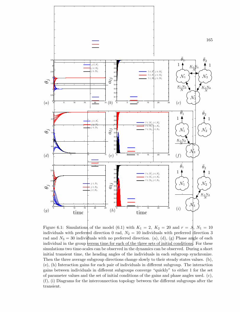
165
K1N1N
1 1
K1N3N
K1N3N
1 1
K1N3N
1 1
K1N3N
(i)
alj
0 5 10 15 20 250
0.5
1
1.5
2
2.5
3
3.5
(a)
0 0.1 0.2 0.3 0.4 0.5 0.6 0.7 0.8 0.9 10
0.1
0.2
0.3
0.4
0.5
0.6
0.7
0.8
0.9
1
l ∈ N1 j ∈ N2
l ∈ N1 j ∈ N3
l ∈ N2 j ∈ N3
0 0.1 0.2 0.3 0.4 0.5 0.6 0.7 0.8 0.9 10
0.1
0.2
0.3
0.4
0.5
0.6
0.7
0.8
0.9
1
j ∈ N1
j ∈ N2
j ∈ N3
0 5 10 15 20 250
0.1
0.2
0.3
0.4
0.5
0.6
0.7
0.8
0.9
1
0 0.1 0.2 0.3 0.4 0.5 0.6 0.7 0.8 0.9 10
0.1
0.2
0.3
0.4
0.5
0.6
0.7
0.8
0.9
1
l ∈ N1 j ∈ N2
l ∈ N1 j ∈ N3
l ∈ N2 j ∈ N3
0 0.1 0.2 0.3 0.4 0.5 0.6 0.7 0.8 0.9 10
0.1
0.2
0.3
0.4
0.5
0.6
0.7
0.8
0.9
1
j ∈ N1
j ∈ N2
j ∈ N3(b)
0 5 10 150
0.5
1
1.5
2
2.5
3
(d)
0 0.1 0.2 0.3 0.4 0.5 0.6 0.7 0.8 0.9 10
0.1
0.2
0.3
0.4
0.5
0.6
0.7
0.8
0.9
1
l ∈ N1 j ∈ N2
l ∈ N1 j ∈ N3
l ∈ N2 j ∈ N3
0 0.1 0.2 0.3 0.4 0.5 0.6 0.7 0.8 0.9 10
0.1
0.2
0.3
0.4
0.5
0.6
0.7
0.8
0.9
1
j ∈ N1
j ∈ N2
j ∈ N3
0 5 10 15 20 250
0.1
0.2
0.3
0.4
0.5
0.6
0.7
0.8
0.9
1
0 0.1 0.2 0.3 0.4 0.5 0.6 0.7 0.8 0.9 10
0.1
0.2
0.3
0.4
0.5
0.6
0.7
0.8
0.9
1
l ∈ N1 j ∈ N2
l ∈ N1 j ∈ N3
l ∈ N2 j ∈ N3
0 0.1 0.2 0.3 0.4 0.5 0.6 0.7 0.8 0.9 10
0.1
0.2
0.3
0.4
0.5
0.6
0.7
0.8
0.9
1
j ∈ N1
j ∈ N2
j ∈ N3(e)
(c)
(f)
0 5 10 15 20 250
0.5
1
1.5
2
2.5
3
3.5
4
time(g)0 0.1 0.2 0.3 0.4 0.5 0.6 0.7 0.8 0.9 1
0
0.1
0.2
0.3
0.4
0.5
0.6
0.7
0.8
0.9
1
l ∈ N1 j ∈ N2
l ∈ N1 j ∈ N3
l ∈ N2 j ∈ N3
0 0.1 0.2 0.3 0.4 0.5 0.6 0.7 0.8 0.9 10
0.1
0.2
0.3
0.4
0.5
0.6
0.7
0.8
0.9
1
j ∈ N1
j ∈ N2
j ∈ N3
0 5 10 15 20 250
0.1
0.2
0.3
0.4
0.5
0.6
0.7
0.8
0.9
1
time(h)
0 0.1 0.2 0.3 0.4 0.5 0.6 0.7 0.8 0.9 10
0.1
0.2
0.3
0.4
0.5
0.6
0.7
0.8
0.9
1
l ∈ N1 j ∈ N2
l ∈ N1 j ∈ N3
l ∈ N2 j ∈ N3
0 0.1 0.2 0.3 0.4 0.5 0.6 0.7 0.8 0.9 10
0.1
0.2
0.3
0.4
0.5
0.6
0.7
0.8
0.9
1
j ∈ N1
j ∈ N2
j ∈ N3
Figure 6.1: Simulations of the model (6.1) with K1 = 2, K2 = 20 and r = .8, N1 = 10individuals with preferred direction 0 rad, N2 = 10 individuals with preferred direction 3rad and N3 = 30 individuals with no preferred direction. (a), (d), (g) Phase angle of eachindividual in the group versus time for each of the three sets of initial conditions. For thesesimulations two time-scales can be observed in the dynamics can be observed. During a shortinitial transient time, the heading angles of the individuals in each subgroup synchronize.Then the three average subgroup directions change slowly to their steady states values. (b),(e), (h) Interaction gains for each pair of individuals in different subgroup. The interactiongains between individuals in different subgroups converge “quickly” to either 1 for the setof parameter values and the set of initial conditions of the gains and phase angles used. (c),(f), (i) Diagrams for the interconnection topology between the different subgroups after thetransient.
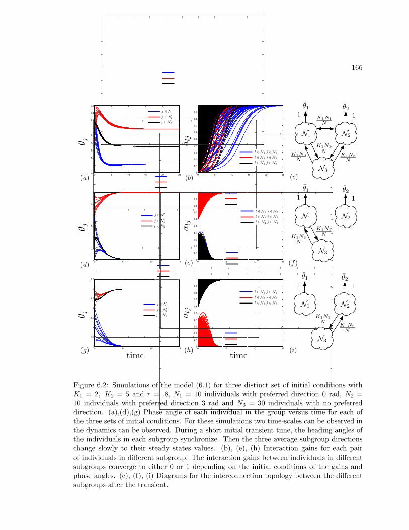
166
0 5 10 15 20 250.8
1
1.2
1.4
1.6
1.8
2
2.2
2.4
2.6
0 5 10 150
0.5
1
1.5
2
2.5
3
0 5 10 150
0.5
1
1.5
2
2.5
3
3.5
0 5 10 15 20 250
0.1
0.2
0.3
0.4
0.5
0.6
0.7
0.8
0.9
1
0 5 10 150
0.1
0.2
0.3
0.4
0.5
0.6
0.7
0.8
0.9
1
0 5 10 150
0.1
0.2
0.3
0.4
0.5
0.6
0.7
0.8
0.9
1
K1N1N
1 1
K1N3N
K1N3N
(a) (b) (c)
(d) (e) (f)
(g) (h) (i)timetime
θ jθ j
θ j
alj
alj
alj
0 0.1 0.2 0.3 0.4 0.5 0.6 0.7 0.8 0.9 10
0.1
0.2
0.3
0.4
0.5
0.6
0.7
0.8
0.9
1
l ∈ N1 j ∈ N2
l ∈ N1 j ∈ N3
l ∈ N2 j ∈ N3
0 0.1 0.2 0.3 0.4 0.5 0.6 0.7 0.8 0.9 10
0.1
0.2
0.3
0.4
0.5
0.6
0.7
0.8
0.9
1
j ∈ N1
j ∈ N2
j ∈ N3
0 0.1 0.2 0.3 0.4 0.5 0.6 0.7 0.8 0.9 10
0.1
0.2
0.3
0.4
0.5
0.6
0.7
0.8
0.9
1
l ∈ N1 j ∈ N2
l ∈ N1 j ∈ N3
l ∈ N2 j ∈ N3
0 0.1 0.2 0.3 0.4 0.5 0.6 0.7 0.8 0.9 10
0.1
0.2
0.3
0.4
0.5
0.6
0.7
0.8
0.9
1
j ∈ N1
j ∈ N2
j ∈ N3
0 0.1 0.2 0.3 0.4 0.5 0.6 0.7 0.8 0.9 10
0.1
0.2
0.3
0.4
0.5
0.6
0.7
0.8
0.9
1
l ∈ N1 j ∈ N2
l ∈ N1 j ∈ N3
l ∈ N2 j ∈ N3
0 0.1 0.2 0.3 0.4 0.5 0.6 0.7 0.8 0.9 10
0.1
0.2
0.3
0.4
0.5
0.6
0.7
0.8
0.9
1
j ∈ N1
j ∈ N2
j ∈ N3
0 0.1 0.2 0.3 0.4 0.5 0.6 0.7 0.8 0.9 10
0.1
0.2
0.3
0.4
0.5
0.6
0.7
0.8
0.9
1
l ∈ N1 j ∈ N2
l ∈ N1 j ∈ N3
l ∈ N2 j ∈ N3
0 0.1 0.2 0.3 0.4 0.5 0.6 0.7 0.8 0.9 10
0.1
0.2
0.3
0.4
0.5
0.6
0.7
0.8
0.9
1
j ∈ N1
j ∈ N2
j ∈ N3
0 0.1 0.2 0.3 0.4 0.5 0.6 0.7 0.8 0.9 10
0.1
0.2
0.3
0.4
0.5
0.6
0.7
0.8
0.9
1
l ∈ N1 j ∈ N2
l ∈ N1 j ∈ N3
l ∈ N2 j ∈ N3
0 0.1 0.2 0.3 0.4 0.5 0.6 0.7 0.8 0.9 10
0.1
0.2
0.3
0.4
0.5
0.6
0.7
0.8
0.9
1
j ∈ N1
j ∈ N2
j ∈ N3
0 0.1 0.2 0.3 0.4 0.5 0.6 0.7 0.8 0.9 10
0.1
0.2
0.3
0.4
0.5
0.6
0.7
0.8
0.9
1
l ∈ N1 j ∈ N2
l ∈ N1 j ∈ N3
l ∈ N2 j ∈ N3
0 0.1 0.2 0.3 0.4 0.5 0.6 0.7 0.8 0.9 10
0.1
0.2
0.3
0.4
0.5
0.6
0.7
0.8
0.9
1
j ∈ N1
j ∈ N2
j ∈ N3
K1N1N
1 1
K1N3N
K1N1N
1 1
K1N3N
K1N1N
Figure 6.2: Simulations of the model (6.1) for three distinct set of initial conditions withK1 = 2, K2 = 5 and r = .8, N1 = 10 individuals with preferred direction 0 rad, N2 =10 individuals with preferred direction 3 rad and N3 = 30 individuals with no preferreddirection. (a),(d),(g) Phase angle of each individual in the group versus time for each ofthe three sets of initial conditions. For these simulations two time-scales can be observed inthe dynamics can be observed. During a short initial transient time, the heading angles ofthe individuals in each subgroup synchronize. Then the three average subgroup directionschange slowly to their steady states values. (b), (e), (h) Interaction gains for each pairof individuals in different subgroup. The interaction gains between individuals in differentsubgroups converge to either 0 or 1 depending on the initial conditions of the gains andphase angles. (c), (f), (i) Diagrams for the interconnection topology between the differentsubgroups after the transient.
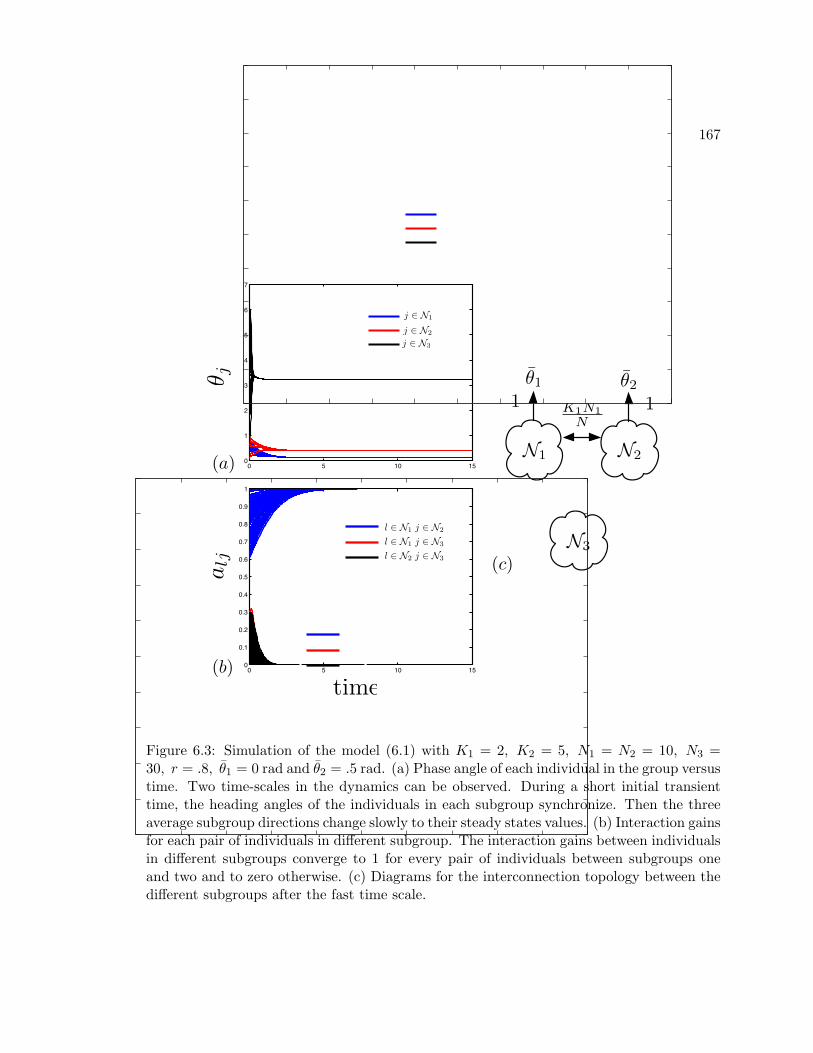
167
0 5 10 150
1
2
3
4
5
6
7
0 5 10 150
0.1
0.2
0.3
0.4
0.5
0.6
0.7
0.8
0.9
1
K1N1N
1 1
(c)
(b)
(a)
θ ja
lj
0 0.1 0.2 0.3 0.4 0.5 0.6 0.7 0.8 0.9 10
0.1
0.2
0.3
0.4
0.5
0.6
0.7
0.8
0.9
1
l ∈ N1 j ∈ N2
l ∈ N1 j ∈ N3
l ∈ N2 j ∈ N3
0 0.1 0.2 0.3 0.4 0.5 0.6 0.7 0.8 0.9 10
0.1
0.2
0.3
0.4
0.5
0.6
0.7
0.8
0.9
1
j ∈ N1
j ∈ N2
j ∈ N3
0 0.1 0.2 0.3 0.4 0.5 0.6 0.7 0.8 0.9 10
0.1
0.2
0.3
0.4
0.5
0.6
0.7
0.8
0.9
1
l ∈ N1 j ∈ N2
l ∈ N1 j ∈ N3
l ∈ N2 j ∈ N3
0 0.1 0.2 0.3 0.4 0.5 0.6 0.7 0.8 0.9 10
0.1
0.2
0.3
0.4
0.5
0.6
0.7
0.8
0.9
1
j ∈ N1
j ∈ N2
j ∈ N3
time
Figure 6.3: Simulation of the model (6.1) with K1 = 2, K2 = 5, N1 = N2 = 10, N3 =30, r = .8, θ1 = 0 rad and θ2 = .5 rad. (a) Phase angle of each individual in the group versustime. Two time-scales in the dynamics can be observed. During a short initial transienttime, the heading angles of the individuals in each subgroup synchronize. Then the threeaverage subgroup directions change slowly to their steady states values. (b) Interaction gainsfor each pair of individuals in different subgroup. The interaction gains between individualsin different subgroups converge to 1 for every pair of individuals between subgroups oneand two and to zero otherwise. (c) Diagrams for the interconnection topology between thedifferent subgroups after the fast time scale.
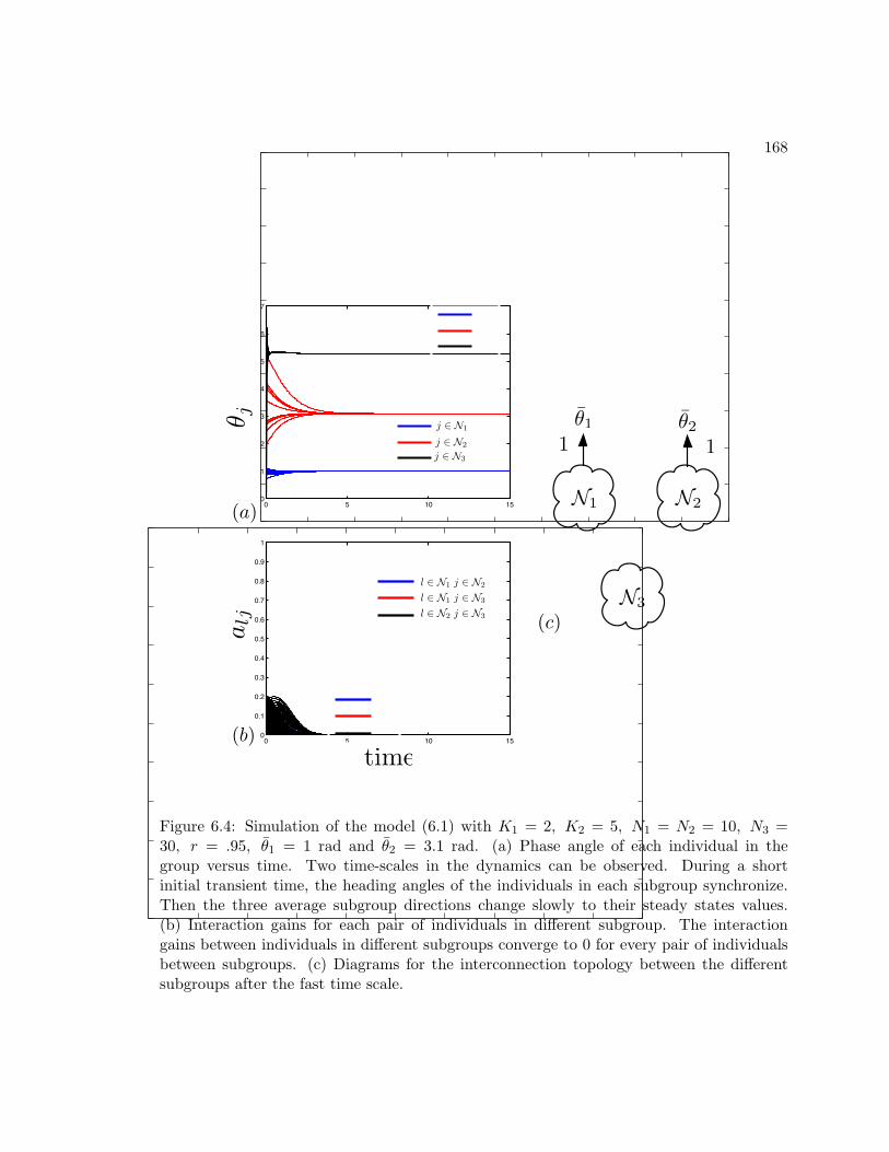
168
0 5 10 150
1
2
3
4
5
6
7
0 5 10 150
0.1
0.2
0.3
0.4
0.5
0.6
0.7
0.8
0.9
1
1 1
(c)
(b)
(a)
θ ja
lj
0 0.1 0.2 0.3 0.4 0.5 0.6 0.7 0.8 0.9 10
0.1
0.2
0.3
0.4
0.5
0.6
0.7
0.8
0.9
1
l ∈ N1 j ∈ N2
l ∈ N1 j ∈ N3
l ∈ N2 j ∈ N3
0 0.1 0.2 0.3 0.4 0.5 0.6 0.7 0.8 0.9 10
0.1
0.2
0.3
0.4
0.5
0.6
0.7
0.8
0.9
1
j ∈ N1
j ∈ N2
j ∈ N3
0 0.1 0.2 0.3 0.4 0.5 0.6 0.7 0.8 0.9 10
0.1
0.2
0.3
0.4
0.5
0.6
0.7
0.8
0.9
1
l ∈ N1 j ∈ N2
l ∈ N1 j ∈ N3
l ∈ N2 j ∈ N3
0 0.1 0.2 0.3 0.4 0.5 0.6 0.7 0.8 0.9 10
0.1
0.2
0.3
0.4
0.5
0.6
0.7
0.8
0.9
1
j ∈ N1
j ∈ N2
j ∈ N3
time
Figure 6.4: Simulation of the model (6.1) with K1 = 2, K2 = 5, N1 = N2 = 10, N3 =30, r = .95, θ1 = 1 rad and θ2 = 3.1 rad. (a) Phase angle of each individual in thegroup versus time. Two time-scales in the dynamics can be observed. During a shortinitial transient time, the heading angles of the individuals in each subgroup synchronize.Then the three average subgroup directions change slowly to their steady states values.(b) Interaction gains for each pair of individuals in different subgroup. The interactiongains between individuals in different subgroups converge to 0 for every pair of individualsbetween subgroups. (c) Diagrams for the interconnection topology between the differentsubgroups after the fast time scale.
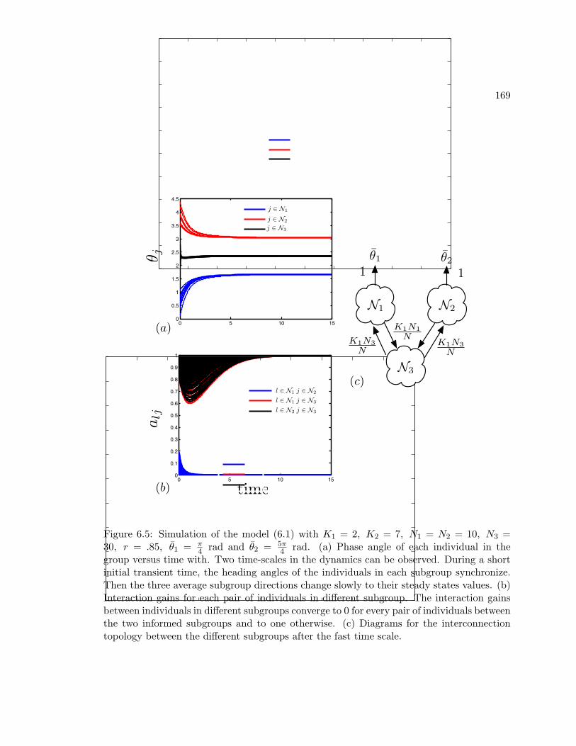
169
(c)
θ j
0 5 10 150
0.5
1
1.5
2
2.5
3
3.5
4
4.5
0 5 10 150
0.1
0.2
0.3
0.4
0.5
0.6
0.7
0.8
0.9
1
alj
(b)
(a)
time
0 0.1 0.2 0.3 0.4 0.5 0.6 0.7 0.8 0.9 10
0.1
0.2
0.3
0.4
0.5
0.6
0.7
0.8
0.9
1
l ∈ N1 j ∈ N2
l ∈ N1 j ∈ N3
l ∈ N2 j ∈ N3
0 0.1 0.2 0.3 0.4 0.5 0.6 0.7 0.8 0.9 10
0.1
0.2
0.3
0.4
0.5
0.6
0.7
0.8
0.9
1
j ∈ N1
j ∈ N2
j ∈ N3
0 0.1 0.2 0.3 0.4 0.5 0.6 0.7 0.8 0.9 10
0.1
0.2
0.3
0.4
0.5
0.6
0.7
0.8
0.9
1
l ∈ N1 j ∈ N2
l ∈ N1 j ∈ N3
l ∈ N2 j ∈ N3
0 0.1 0.2 0.3 0.4 0.5 0.6 0.7 0.8 0.9 10
0.1
0.2
0.3
0.4
0.5
0.6
0.7
0.8
0.9
1
j ∈ N1
j ∈ N2
j ∈ N3
θ j
1 1
K1N3N
K1N3N
K1N1N
Figure 6.5: Simulation of the model (6.1) with K1 = 2, K2 = 7, N1 = N2 = 10, N3 =30, r = .85, θ1 = π
4 rad and θ2 = 5π4 rad. (a) Phase angle of each individual in the
group versus time with. Two time-scales in the dynamics can be observed. During a shortinitial transient time, the heading angles of the individuals in each subgroup synchronize.Then the three average subgroup directions change slowly to their steady states values. (b)Interaction gains for each pair of individuals in different subgroup. The interaction gainsbetween individuals in different subgroups converge to 0 for every pair of individuals betweenthe two informed subgroups and to one otherwise. (c) Diagrams for the interconnectiontopology between the different subgroups after the fast time scale.
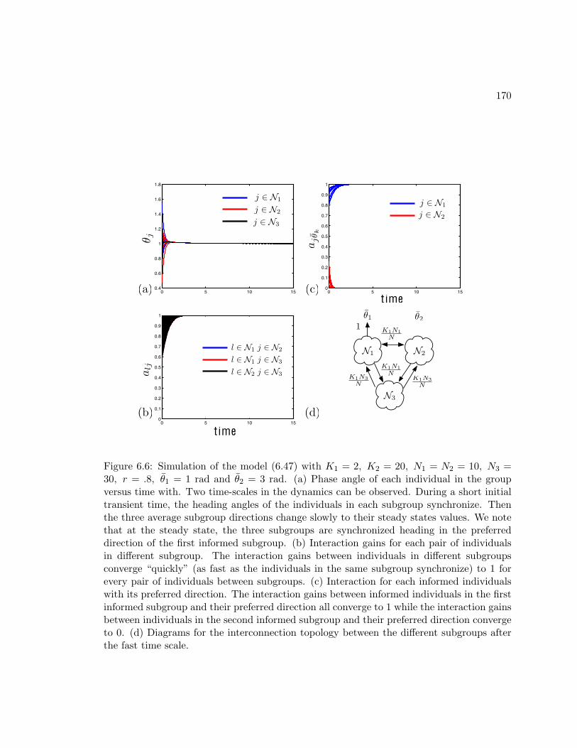
170
K1N1N
1
K1N3N
K1N3N
K1N1N
0 5 10 150
0.1
0.2
0.3
0.4
0.5
0.6
0.7
0.8
0.9
1
0 5 10 150.4
0.6
0.8
1
1.2
1.4
1.6
1.8
0 0.1 0.2 0.3 0.4 0.5 0.6 0.7 0.8 0.9 10
0.1
0.2
0.3
0.4
0.5
0.6
0.7
0.8
0.9
1
j ∈ N1
j ∈ N2
j ∈ N3
0 0.1 0.2 0.3 0.4 0.5 0.6 0.7 0.8 0.9 10
0.1
0.2
0.3
0.4
0.5
0.6
0.7
0.8
0.9
1
j ∈ N1
j ∈ N2
t ime
0 5 10 150
0.1
0.2
0.3
0.4
0.5
0.6
0.7
0.8
0.9
1
t ime
0 0.1 0.2 0.3 0.4 0.5 0.6 0.7 0.8 0.9 10
0.1
0.2
0.3
0.4
0.5
0.6
0.7
0.8
0.9
1
l ∈ N1 j ∈ N2
l ∈ N1 j ∈ N3
l ∈ N2 j ∈ N3
Figure 6.6: Simulation of the model (6.47) with K1 = 2, K2 = 20, N1 = N2 = 10, N3 =30, r = .8, θ1 = 1 rad and θ2 = 3 rad. (a) Phase angle of each individual in the groupversus time with. Two time-scales in the dynamics can be observed. During a short initialtransient time, the heading angles of the individuals in each subgroup synchronize. Thenthe three average subgroup directions change slowly to their steady states values. We notethat at the steady state, the three subgroups are synchronized heading in the preferreddirection of the first informed subgroup. (b) Interaction gains for each pair of individualsin different subgroup. The interaction gains between individuals in different subgroupsconverge “quickly” (as fast as the individuals in the same subgroup synchronize) to 1 forevery pair of individuals between subgroups. (c) Interaction for each informed individualswith its preferred direction. The interaction gains between informed individuals in the firstinformed subgroup and their preferred direction all converge to 1 while the interaction gainsbetween individuals in the second informed subgroup and their preferred direction convergeto 0. (d) Diagrams for the interconnection topology between the different subgroups afterthe fast time scale.
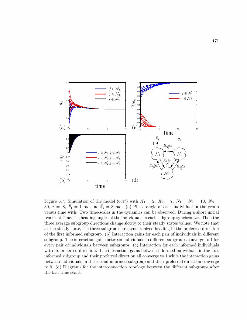
171
0 5 10 150
0.5
1
1.5
2
2.5
0 5 10 150
0.1
0.2
0.3
0.4
0.5
0.6
0.7
0.8
0.9
1
0 5 10 150
0.1
0.2
0.3
0.4
0.5
0.6
0.7
0.8
0.9
1
K1N1N
1
K1N3N
K1N3N
K1N1N
0 0.1 0.2 0.3 0.4 0.5 0.6 0.7 0.8 0.9 10
0.1
0.2
0.3
0.4
0.5
0.6
0.7
0.8
0.9
1
j ∈ N1
j ∈ N2
j ∈ N3
0 0.1 0.2 0.3 0.4 0.5 0.6 0.7 0.8 0.9 10
0.1
0.2
0.3
0.4
0.5
0.6
0.7
0.8
0.9
1
l ∈ N1 j ∈ N2
l ∈ N1 j ∈ N3
l ∈ N2 j ∈ N30 0.1 0.2 0.3 0.4 0.5 0.6 0.7 0.8 0.9 10
0.1
0.2
0.3
0.4
0.5
0.6
0.7
0.8
0.9
1
j ∈ N1
j ∈ N2
t ime
t ime
Figure 6.7: Simulation of the model (6.47) with K1 = 2, K2 = 7, N1 = N2 = 10, N3 =30, r = .8, θ1 = 1 rad and θ2 = 3 rad. (a) Phase angle of each individual in the groupversus time with. Two time-scales in the dynamics can be observed. During a short initialtransient time, the heading angles of the individuals in each subgroup synchronize. Then thethree average subgroup directions change slowly to their steady states values. We note thatat the steady state, the three subgroups are synchronized heading in the preferred directionof the first informed subgroup. (b) Interaction gains for each pair of individuals in differentsubgroup. The interaction gains between individuals in different subgroups converge to 1 forevery pair of individuals between subgroups. (c) Interaction for each informed individualswith its preferred direction. The interaction gains between informed individuals in the firstinformed subgroup and their preferred direction all converge to 1 while the interaction gainsbetween individuals in the second informed subgroup and their preferred direction convergeto 0. (d) Diagrams for the interconnection topology between the different subgroups afterthe fast time scale.
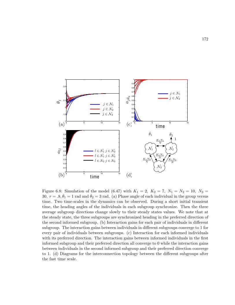
172
0 5 10 151
1.5
2
2.5
3
3.5
4
0 5 10 150
0.1
0.2
0.3
0.4
0.5
0.6
0.7
0.8
0.9
1
0 5 10 150
0.1
0.2
0.3
0.4
0.5
0.6
0.7
0.8
0.9
1
K1N1N
1
K1N3N
K1N3N
K1N1N
0 0.1 0.2 0.3 0.4 0.5 0.6 0.7 0.8 0.9 10
0.1
0.2
0.3
0.4
0.5
0.6
0.7
0.8
0.9
1
j ∈ N1
j ∈ N2
j ∈ N3
0 0.1 0.2 0.3 0.4 0.5 0.6 0.7 0.8 0.9 10
0.1
0.2
0.3
0.4
0.5
0.6
0.7
0.8
0.9
1
l ∈ N1 j ∈ N2
l ∈ N1 j ∈ N3
l ∈ N2 j ∈ N30 0.1 0.2 0.3 0.4 0.5 0.6 0.7 0.8 0.9 1
0
0.1
0.2
0.3
0.4
0.5
0.6
0.7
0.8
0.9
1
j ∈ N1
j ∈ N2
t ime
t ime
Figure 6.8: Simulation of the model (6.47) with K1 = 2, K2 = 7, N1 = N2 = 10, N3 =30, r = .8, θ1 = 1 rad and θ2 = 3 rad. (a) Phase angle of each individual in the group versustime. Two time-scales in the dynamics can be observed. During a short initial transienttime, the heading angles of the individuals in each subgroup synchronize. Then the threeaverage subgroup directions change slowly to their steady states values. We note that atthe steady state, the three subgroups are synchronized heading in the preferred direction ofthe second informed subgroup. (b) Interaction gains for each pair of individuals in differentsubgroup. The interaction gains between individuals in different subgroups converge to 1 forevery pair of individuals between subgroups. (c) Interaction for each informed individualswith its preferred direction. The interaction gains between informed individuals in the firstinformed subgroup and their preferred direction all converge to 0 while the interaction gainsbetween individuals in the second informed subgroup and their preferred direction convergeto 1. (d) Diagrams for the interconnection topology between the different subgroups afterthe fast time scale.
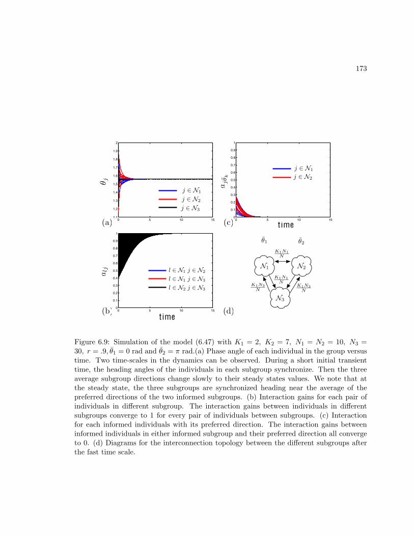
173
0 5 10 151.1
1.2
1.3
1.4
1.5
1.6
1.7
1.8
1.9
2
0 5 10 150
0.1
0.2
0.3
0.4
0.5
0.6
0.7
0.8
0.9
1
0 5 10 150
0.1
0.2
0.3
0.4
0.5
0.6
0.7
0.8
0.9
1
K1N1N
K1N3N
K1N3N
K1N1N
0 0.1 0.2 0.3 0.4 0.5 0.6 0.7 0.8 0.9 10
0.1
0.2
0.3
0.4
0.5
0.6
0.7
0.8
0.9
1
j ∈ N1
j ∈ N2
j ∈ N3
0 0.1 0.2 0.3 0.4 0.5 0.6 0.7 0.8 0.9 10
0.1
0.2
0.3
0.4
0.5
0.6
0.7
0.8
0.9
1
l ∈ N1 j ∈ N2
l ∈ N1 j ∈ N3
l ∈ N2 j ∈ N30 0.1 0.2 0.3 0.4 0.5 0.6 0.7 0.8 0.9 1
0
0.1
0.2
0.3
0.4
0.5
0.6
0.7
0.8
0.9
1
j ∈ N1
j ∈ N2
t ime
t ime
Figure 6.9: Simulation of the model (6.47) with K1 = 2, K2 = 7, N1 = N2 = 10, N3 =30, r = .9, θ1 = 0 rad and θ2 = π rad.(a) Phase angle of each individual in the group versustime. Two time-scales in the dynamics can be observed. During a short initial transienttime, the heading angles of the individuals in each subgroup synchronize. Then the threeaverage subgroup directions change slowly to their steady states values. We note that atthe steady state, the three subgroups are synchronized heading near the average of thepreferred directions of the two informed subgroups. (b) Interaction gains for each pair ofindividuals in different subgroup. The interaction gains between individuals in differentsubgroups converge to 1 for every pair of individuals between subgroups. (c) Interactionfor each informed individuals with its preferred direction. The interaction gains betweeninformed individuals in either informed subgroup and their preferred direction all convergeto 0. (d) Diagrams for the interconnection topology between the different subgroups afterthe fast time scale.
Chapter 7
Conclusions and Future Directions
In this dissertation we present a study of the dynamics and control of multi-agent systems
in both the engineered and the natural setting. Focusing first on the engineered setting, in
Chapters 2 and 3, we derive provable, distributed control laws for stabilizing and changing
the shape of vehicle formations in the plane using dynamic models of tensegrity structures.
In Chapters 4, 5 and 6, where we turn our attention to the natural setting, we present and
study Lagrangian models to investigate the mechanisms of decision-making and leadership
in animal groups. This chapter gives a brief summary of the approaches, results and conclu-
sions presented in this dissertation and suggests possible future lines of research motivated
by the presented work.
7.1 Summary
In Chapter 2 we design a control law that drives vehicle formations into arbitrary shapes
with forces that can be represented as those internal to tensegrity structures. Tensegrity
structures offer important advantages that we seek to translate to vehicle formations, includ-
ing the ability to maintain shape even in the presence of external forces. It is such dynamics
properties of tensegrity structures that led us to choose the tensegrity-based approach as
an alternative to approaches based on artificial potentials and edge design. The control law
is designed by defining a smooth map that takes any arbitrary planar shape and provides a
174
175
planar tensegrity with that shape. We prove stability of the desired shape for the dynamics
of the vehicle network that is represented as a tensegrity by using the linearization of the
yielded dynamical system. We illustrate the method with examples, one of which we use
to investigate how freedom in the choice of the parameter of the control law can be used
to affect the resulting interconnection topology of the vehicle network. The smoothness of
the mapping between shapes and tensegrities with respect to the shape parameters allows
us to extend the method to the transient problem of moving smoothly from one shape to
another, while maintaining stability along the way.
This transient problem is worked out formally in Chapter 3, where we use the smooth
map between vehicles in a formation and nodes in a tensegrity structure to derive a control
law that realizes well-behaved reconfiguration between arbitrary shapes. This control law
makes the nodes follow a smooth path in the space of stable tensegrities by smoothly
varying the parameters of the control law presented in Chapter 2 for stabilization of planar
shapes. Results from the nonlinear systems theory literature are utilized to derive sufficient
conditions that guarantee that the trajectory of the formation, in shape space, is close to
the prescribed path and that it converges to the desired final shape. Numerical simulations
are presented to illustrate the method. These illustrations hint at certain good performance
features of the method – specifically, the vehicles do not collide with each other and the
distance covered by all the vehicles is minimized during the reconfiguration.
In Chapter 4 we turn our attention to the natural setting and build on the decision-
making model of Couzin et al. [19]. We summarize the results from [19] and then focus
our attention on the role of naive individuals in the decision-making process. We show that
naive individuals help accelerate the process of consensus, unless they are too numerous. In
the case that they are too numerous, we show that this “overwhelming” number of naive
individuals causes the group to fragment and/or slows down the consensus process. Our
analysis, built primarily on simulations, reveals that the model from Couzin et al., although
very suggestive, is too complex to be analyzed mathematically. For this reason, proving
specific decision-making mechanisms requires the design of simplified, lower-dimensional

176
models such as the continuous-time models presented in Chapters 5 and 6.
In Chapter 5 we present and analyze a model for the dynamics of leadership and decision-
making in animal group motion. The model takes the general form of the Kuramoto model
of coupled oscillators with individual preferences; where such preference exist, they are as-
sociated with a fixed heading angle. The model is simplified through a time-scale reduction
argument to a three-dimensional gradient system of which we study the full phase space
dynamics by computing equilibria and proving stability and bifurcations. This model dif-
fers from the complex model proposed by Couzin et al. in that it makes several simplifying
assumptions, the most important of which are that we assume an all-to-all inter-connecting
topology in the group and ignore for the purpose of the analysis the presence of naive indi-
viduals in the group. Despite these assumptions, the yielded model captures some important
behaviors exhibited in the model presented in Chapter 4, among them that informed indi-
viduals tend to compromise toward the average of their preferred directions. This model
does not however exhibit full synchronization (i.e., consensus) unless the coupling gain K
between individuals is very large, meaning that for small values of K, the group does not
fully aggregate and in fact splits. These deviations between the model in Chapter 4 and
the model in Chapter 5 motivate the model presented and analyzed in Chapter 6.
In Chapter 6, we derive and study a similar model to the one given in Chapter 5 but
relax the two critical simplifying assumption stated above. First we do not assume an all-to-
all fixed communication topology but consider instead a time-varying, possibly incomplete,
connecting topology. Second, whereas in Chapter 5 we ignore the presence of naive indi-
viduals, in Chapter 6 their influence is considered. With those assumptions relaxed, the
model yields a much richer behavior with many invariant manifolds; we investigate the at-
tractiveness of eight of these invariant manifolds and study the reduced dynamics on the
attractive ones. In contrast to the model from Chapter 5, in which informed individuals
always compromise on their preferred directions, we show that with this model it is possible
to have informed individuals travel exactly in their preferred direction, but only when the
two informed subgroups do not interact with each other. We concluded the chapter with an
177
interesting extension in which we add a forgetting factor feedback in the form of a dynamic
gain on the strength of the attraction that informed individuals feel toward their preferred
direction. This extended model is highly suggestive in that it reproduces all the behavior
observed with the discrete-time model proposed by Couzin et al.
The work presented in this dissertation may be extended in several directions that
may make it possible to better understand how collective behavior emerges in the natural
setting and to develop more efficient control strategies for groups of robots emulating natural
systems. We list some possible future lines of research motivated by the presented work.
7.2 Future Lines of Research
Modeling collective behavior in animal groups As we noted, with both of the pro-
posed continuous time models from Chapters 5 and 6, the behavior observed both in [19]
and in Chapter 4, where the group collectively selects one of the preferred directions, cannot
be reproduced unless a forgetting feedback factor is introduced. Moreover, full synchroniza-
tion of the group cannot occur unless the coupling gain K1 is very large. This persistent
deviation indirectly reveals the importance of a remaining simplifying assumption, namely,
that we consider only the dynamics of the phases and not the complete spatial dynamics of
the individuals in the group. The lack of explicit consideration of spatial effects is rather
critical. For the simulations presented in [19] and in Chapter 4, in the case where the group
collectively selects one of the preferred direction, the three subgroups are consistently or-
dered with the “leading” informed subgroup in the front, the naive individuals just behind,
and the other subgroup far to the rear. The spacing between the two informed subgroups
created by the intervening presence of naive individuals is critical in that it allows the two
informed subgroups to travel in the same direction without directly interacting with each
other. This collective decision outcome cannot be reproduced by the phase models proposed
in Chapters 5 and 6 (or any other phase model), as interactions between two individuals
are solely determined by whether they are traveling in a similar direction or not. In order
to reproduce the collective decision-making outcome observed in [19], a challenging (and

178
necessary) next step for the models proposed in Chapters 5 and 6 would be to define a
framework in which the spatial dynamics could be layered on top of the phase dynamics
proposed here. This layering of phase and spatial dynamics is not a new idea: Justh and
Krishnaprasad developed a motion model in which vehicles travel at constant speed and are
controlled by steering their direction of travel [49, 50]. This framework was successfully used
by Sepulchre et al. to stabilize circular and parallel collective motion [108]. The challenge
in applying such a framework to model animal group motion would be to incorporate a way
for individuals/vehicles to have preferences as some do in our models.
Control of a group of robots The work presented in Chapters 2 and 3 in which we
designed control laws to stabilize arbitrary shapes and reconfigure a vehicle network between
arbitrary shapes can be extended in several ways. We suggest three of them here. First, as
we have noted in the examples from Chapter 2, given an arbitrary shape, our mapping often
yields a tensegrity structure in which the number of interconnections exceeds the proven
lower limit. We showed by means of an example how to manipulate our method so as to
reduce the number of interconnections; future work should examine the possibility of making
such a modification systematic. Second, the stability results proven in both Chapters 2 and
3 are local; it is of interest to consider proving more global results and exploring the global
phase space in view of better leveraging tensegrity structure dynamics. Pais et al. proved
global results for one-dimensional tensegrity structures and used the results to prove global
stability of planar and three-dimensional structures made up of a set of orthogonal one-
dimensional tensegrity structures [89]. Future work extending the method of the present
dissertation to three dimensions would provide a compelling alternative for controlling the
shape of three-dimensional formations. Finally we have argued using simulations that the
control law we have designed for the reconfiguration shows good performance in that vehicles
do not collide and the distance covered by all the vehicles is minimized. It would be necessary
before implementing our control into any physical system to investigate this issue more
rigorously. As our method and simulations imply, the rate of change of the parameters
(characterized by τ in our work) plays a crucial role in the robustness issue. As τ gets

179
larger (i.e., as the network is required to reconfigure at a slower pace), the network remains
closer to the prescribed trajectory. Given a path such as the one presented in Chapter 3
where trajectories of distinct vehicles do not collide and where the distance covered by the
vehicles is minimized, our control law has good performance. One should realize however
that enforcing the restriction of having no intersections in the planned trajectories of the
vehicles is more conservative than necessary. It would be sufficient to show that through
the path of the reconfiguration no two vehicles are required to be “too close” to each other
at any given time; two distinct vehicles could pass through the same location provided they
do so at different times.
Appendix A
Technical Proofs for Chapter 5
Proof of lemma 5.2.1: The linearization of (5.20) at each of the two equilibria ψS1 or
ψS2 gives the same symmetric Jacobian with eigenvalues λ1, λ2 ∈ R satisfying
λ1λ2 =K2
4sin2 θ2 − 1 < 0 for
∣∣∣∣K2 sin θ2
∣∣∣∣ < 1.
For θ2 ∈ [0, π] the eigenvalues are of opposite sign. This implies that ψS1 and ψS2 are
saddle points ∀K > 0 and ∀θ2 ∈ [0, π] if K2 sin θ2 < 1. In the case |K2 sin θ2| = 1, ψS1 =
ψS2 =(
3π2 ,
π2 + θ2
)and the eigenvalues are λ1 = 0 and λ2 = K cos θ2 > 0. Therefore for
θ2 ∈(0, π2
) ∪ (π2 , π), the equilibria ψS1 = ψS2 =(
3π2 ,
π2 + θ2
)are unstable with one zero
eigenvalue and one strictly positive eigenvalue. In case θ2 = π/2 and K = 2, λ1 = λ2 = 0.
Proof of lemma 5.2.2: Using cos(θ22 − ψ2
)= ρ and sin
(θ22 − ψ2
)= −
√1− ρ2, the
Jacobian at the equilibrium is computed; it is symmetric and the corresponding eigenvalues
are
λ1,2 = −(ρ cos
θ2
2+√
1− ρ2 sinθ2
2+K
2(2ρ2 − 1
))± K
2(2ρ2 − 1
).
We find using (5.30) for all(K, θ2
) ∈ [0,∞)× [0, π) that
−√
1− ρ2 sinθ2
2−K (2ρ2 − 1
)= −1
ρ
(1− ρ2
)cos
θ2
2−Kρ2 < 0. (A.1)
Thus, for all(K, θ2
) ∈ [0,∞) × [0, π), using (A.1) both eigenvalues are real and negative.
Hence ψsync1 is a stable node for all(K, θ2
) ∈ [0,∞)× [0, π).
180
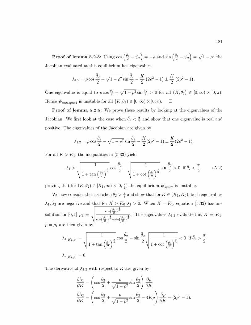
181
Proof of lemma 5.2.3: Using cos(θ22 − ψ2
)= −ρ and sin
(θ22 − ψ2
)=√
1− ρ2 the
Jacobian evaluated at this equilibrium has eigenvalues
λ1,2 = ρ cosθ2
2+√
1− ρ2 sinθ2
2− K
2(2ρ2 − 1
)± K
2(2ρ2 − 1
).
One eigenvalue is equal to ρ cos θ22 +√
1− ρ2 sin θ22 > 0 for all
(K, θ2
) ∈ [0,∞) × [0, π).
Hence ψantisync1 is unstable for all(K, θ2
) ∈ [0,∞)× [0, π).
Proof of lemma 5.2.5: We prove these results by looking at the eigenvalues of the
Jacobian. We first look at the case when θ2 <π2 and show that one eigenvalue is real and
positive. The eigenvalues of the Jacobian are given by
λ1,2 = ρ cosθ2
2−√
1− ρ2 sinθ2
2− K
2(2ρ2 − 1)± K
2(2ρ2 − 1).
For all K > K1, the inequalities in (5.33) yield
λ1 >
√√√√ 1
1 + tan(θ22
) 23
cosθ2
2−√√√√ 1
1 + cot(θ22
) 23
sinθ2
2> 0 if θ2 <
π
2, (A.2)
proving that for (K, θ2) ∈ [K1,∞)× [0, π2 ) the equilibrium ψsync2 is unstable.
We now consider the case when θ2 >π2 and show that for K ∈ (K1,K0), both eigenvalues
λ1, λ2 are negative and that for K > K0 λ1 > 0. When K = K1, equation (5.32) has one
solution in [0, 1] ρ1 =
√√√√ cos“θ22
” 23
cos“θ22
” 23
+sin“θ22
” 23
. The eigenvalues λ1,2 evaluated at K = K1,
ρ = ρ1 are then given by
λ1|K1,ρ1=√√√√ 1
1 + tan(θ22
) 23
cosθ2
2− sin
θ2
2
√√√√ 1
1 + cot(θ22
) 23
< 0 if θ2 >π
2
λ2|K1,ρ1= 0.
The derivative of λ1,2 with respect to K are given by
∂λ1
∂K=
(cos
θ2
2+
ρ√1− ρ2
sinθ2
2
)∂ρ
∂K
∂λ2
∂K=
(cos
θ2
2+
ρ√1− ρ2
sinθ2
2− 4Kρ
)∂ρ
∂K− (2ρ2 − 1).
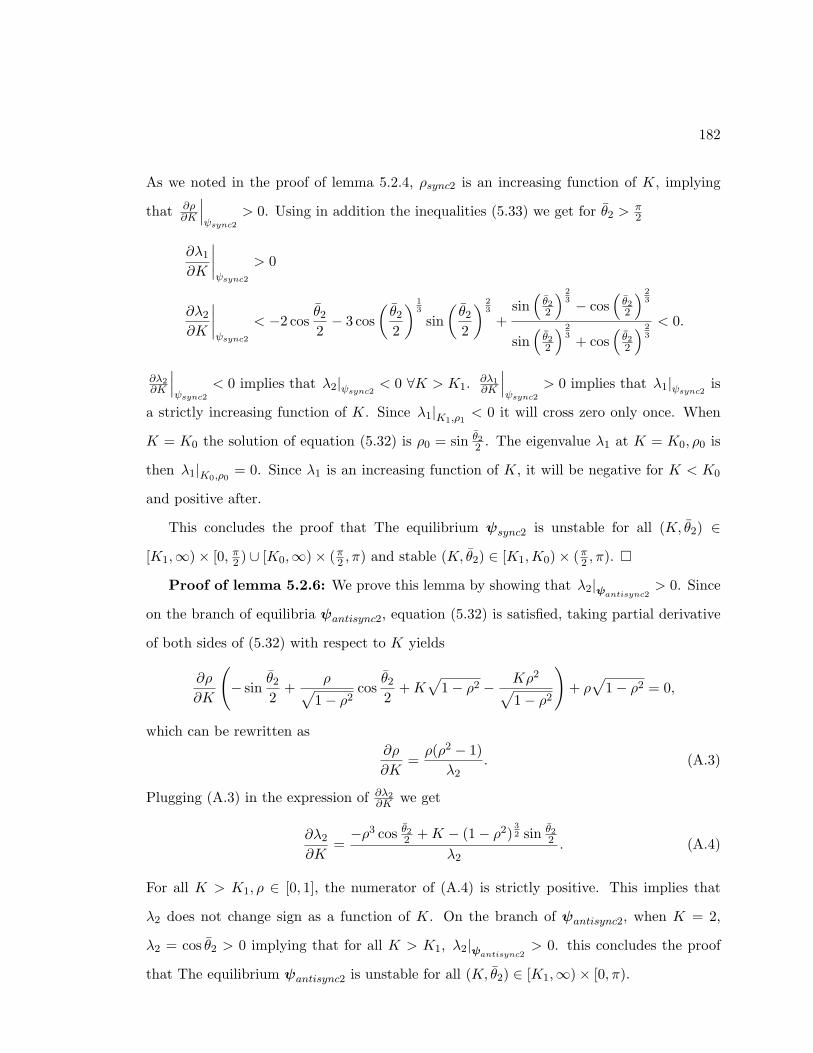
182
As we noted in the proof of lemma 5.2.4, ρsync2 is an increasing function of K, implying
that ∂ρ∂K
∣∣∣ψsync2
> 0. Using in addition the inequalities (5.33) we get for θ2 >π2
∂λ1
∂K
∣∣∣∣ψsync2
> 0
∂λ2
∂K
∣∣∣∣ψsync2
< −2 cosθ2
2− 3 cos
(θ2
2
) 13
sin(θ2
2
) 23
+sin(θ22
) 23 − cos
(θ22
) 23
sin(θ22
) 23 + cos
(θ22
) 23
< 0.
∂λ2∂K
∣∣∣ψsync2
< 0 implies that λ2|ψsync2 < 0 ∀K > K1. ∂λ1∂K
∣∣∣ψsync2
> 0 implies that λ1|ψsync2 is
a strictly increasing function of K. Since λ1|K1,ρ1< 0 it will cross zero only once. When
K = K0 the solution of equation (5.32) is ρ0 = sin θ22 . The eigenvalue λ1 at K = K0, ρ0 is
then λ1|K0,ρ0= 0. Since λ1 is an increasing function of K, it will be negative for K < K0
and positive after.
This concludes the proof that The equilibrium ψsync2 is unstable for all (K, θ2) ∈[K1,∞)× [0, π2 ) ∪ [K0,∞)× (π2 , π) and stable (K, θ2) ∈ [K1,K0)× (π2 , π).
Proof of lemma 5.2.6: We prove this lemma by showing that λ2|ψantisync2 > 0. Since
on the branch of equilibria ψantisync2, equation (5.32) is satisfied, taking partial derivative
of both sides of (5.32) with respect to K yields
∂ρ
∂K
(− sin
θ2
2+
ρ√1− ρ2
cosθ2
2+K
√1− ρ2 − Kρ2√
1− ρ2
)+ ρ√
1− ρ2 = 0,
which can be rewritten as∂ρ
∂K=ρ(ρ2 − 1)
λ2. (A.3)
Plugging (A.3) in the expression of ∂λ2∂K we get
∂λ2
∂K=−ρ3 cos θ22 +K − (1− ρ2)
32 sin θ2
2
λ2. (A.4)
For all K > K1, ρ ∈ [0, 1], the numerator of (A.4) is strictly positive. This implies that
λ2 does not change sign as a function of K. On the branch of ψantisync2, when K = 2,
λ2 = cos θ2 > 0 implying that for all K > K1, λ2|ψantisync2 > 0. this concludes the proof
that The equilibrium ψantisync2 is unstable for all (K, θ2) ∈ [K1,∞)× [0, π).
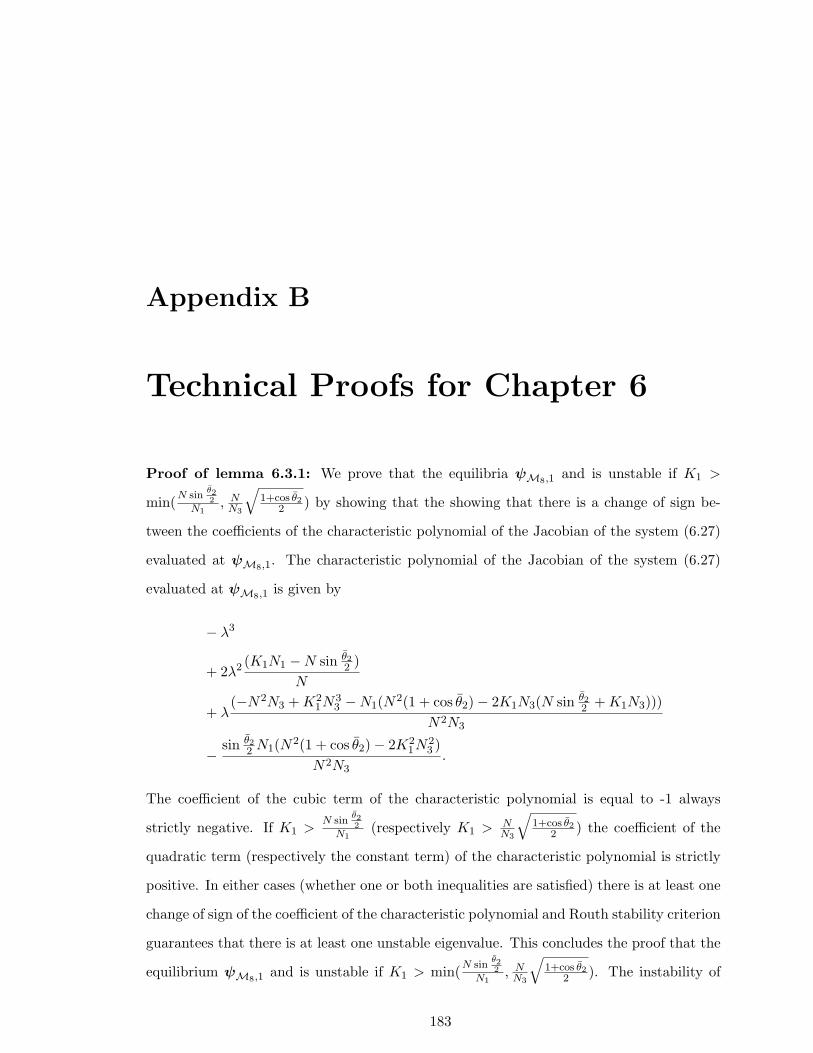
Appendix B
Technical Proofs for Chapter 6
Proof of lemma 6.3.1: We prove that the equilibria ψM8,1 and is unstable if K1 >
min(N sinθ22
N1, NN3
√1+cos θ2
2 ) by showing that the showing that there is a change of sign be-
tween the coefficients of the characteristic polynomial of the Jacobian of the system (6.27)
evaluated at ψM8,1. The characteristic polynomial of the Jacobian of the system (6.27)
evaluated at ψM8,1 is given by
− λ3
+ 2λ2 (K1N1 −N sin θ22 )
N
+ λ(−N2N3 +K2
1N33 −N1(N2(1 + cos θ2)− 2K1N3(N sin θ2
2 +K1N3)))N2N3
− sin θ22 N1(N2(1 + cos θ2)− 2K2
1N23 )
N2N3.
The coefficient of the cubic term of the characteristic polynomial is equal to -1 always
strictly negative. If K1 >N sin
θ22
N1(respectively K1 >
NN3
√1+cos θ2
2 ) the coefficient of the
quadratic term (respectively the constant term) of the characteristic polynomial is strictly
positive. In either cases (whether one or both inequalities are satisfied) there is at least one
change of sign of the coefficient of the characteristic polynomial and Routh stability criterion
guarantees that there is at least one unstable eigenvalue. This concludes the proof that the
equilibrium ψM8,1 and is unstable if K1 > min(N sinθ22
N1, NN3
√1+cos θ2
2 ). The instability of
183
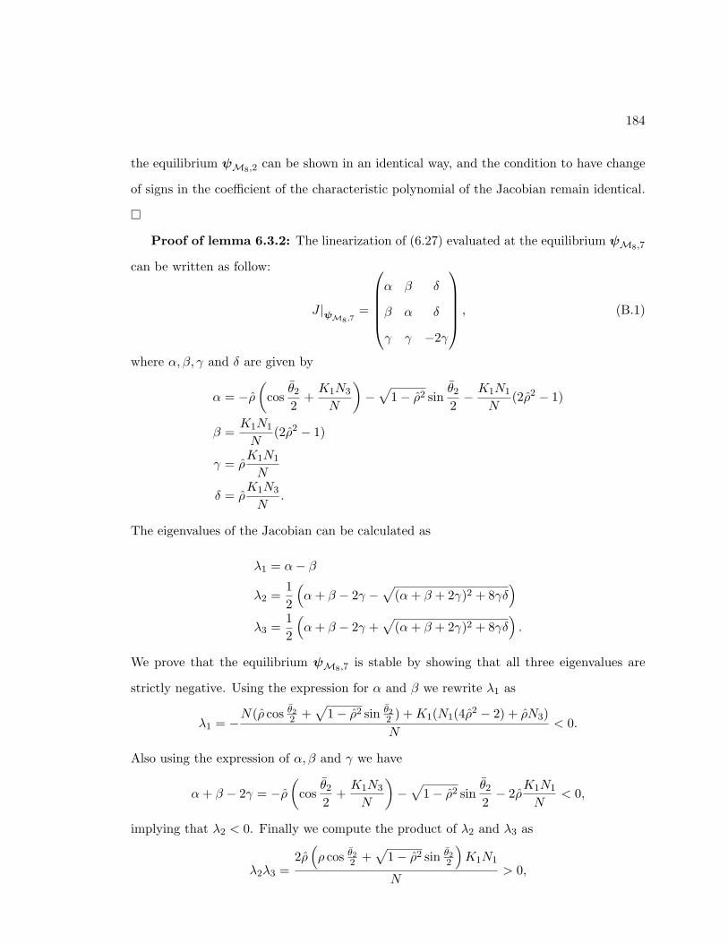
184
the equilibrium ψM8,2 can be shown in an identical way, and the condition to have change
of signs in the coefficient of the characteristic polynomial of the Jacobian remain identical.
Proof of lemma 6.3.2: The linearization of (6.27) evaluated at the equilibrium ψM8,7
can be written as follow:
J |ψM8,7=
α β δ
β α δ
γ γ −2γ
, (B.1)
where α, β, γ and δ are given by
α = −ρ(
cosθ2
2+K1N3
N
)−√
1− ρ2 sinθ2
2− K1N1
N(2ρ2 − 1)
β =K1N1
N(2ρ2 − 1)
γ = ρK1N1
N
δ = ρK1N3
N.
The eigenvalues of the Jacobian can be calculated as
λ1 = α− β
λ2 =12
(α+ β − 2γ −
√(α+ β + 2γ)2 + 8γδ
)λ3 =
12
(α+ β − 2γ +
√(α+ β + 2γ)2 + 8γδ
).
We prove that the equilibrium ψM8,7 is stable by showing that all three eigenvalues are
strictly negative. Using the expression for α and β we rewrite λ1 as
λ1 = −N(ρ cos θ22 +√
1− ρ2 sin θ22 ) +K1(N1(4ρ2 − 2) + ρN3)N
< 0.
Also using the expression of α, β and γ we have
α+ β − 2γ = −ρ(
cosθ2
2+K1N3
N
)−√
1− ρ2 sinθ2
2− 2ρ
K1N1
N< 0,
implying that λ2 < 0. Finally we compute the product of λ2 and λ3 as
λ2λ3 =2ρ(ρ cos θ22 +
√1− ρ2 sin θ2
2
)K1N1
N> 0,
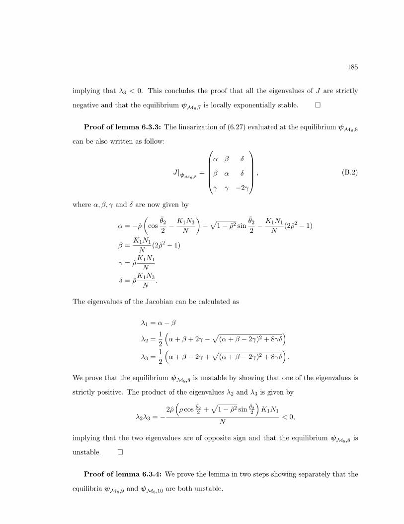
185
implying that λ3 < 0. This concludes the proof that all the eigenvalues of J are strictly
negative and that the equilibrium ψM8,7 is locally exponentially stable.
Proof of lemma 6.3.3: The linearization of (6.27) evaluated at the equilibrium ψM8,8
can be also written as follow:
J |ψM8,8=
α β δ
β α δ
γ γ −2γ
, (B.2)
where α, β, γ and δ are now given by
α = −ρ(
cosθ2
2− K1N3
N
)−√
1− ρ2 sinθ2
2− K1N1
N(2ρ2 − 1)
β =K1N1
N(2ρ2 − 1)
γ = ρK1N1
N
δ = ρK1N3
N.
The eigenvalues of the Jacobian can be calculated as
λ1 = α− β
λ2 =12
(α+ β + 2γ −
√(α+ β − 2γ)2 + 8γδ
)λ3 =
12
(α+ β − 2γ +
√(α+ β − 2γ)2 + 8γδ
).
We prove that the equilibrium ψM8,8 is unstable by showing that one of the eigenvalues is
strictly positive. The product of the eigenvalues λ2 and λ3 is given by
λ2λ3 = −2ρ(ρ cos θ22 +
√1− ρ2 sin θ2
2
)K1N1
N< 0,
implying that the two eigenvalues are of opposite sign and that the equilibrium ψM8,8 is
unstable.
Proof of lemma 6.3.4: We prove the lemma in two steps showing separately that the
equilibria ψM8,9 and ψM8,10 are both unstable.
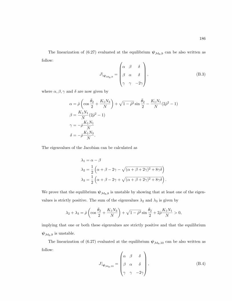
186
The linearization of (6.27) evaluated at the equilibrium ψM8,9 can be also written as
follow:
J |ψM8,9=
α β δ
β α δ
γ γ −2γ
, (B.3)
where α, β, γ and δ are now given by
α = ρ
(cos
θ2
2+K1N3
N
)+√
1− ρ2 sinθ2
2− K1N1
N(2ρ2 − 1)
β =K1N1
N(2ρ2 − 1)
γ = −ρK1N1
N
δ = −ρK1N3
N.
The eigenvalues of the Jacobian can be calculated as
λ1 = α− β
λ2 =12
(α+ β − 2γ −
√(α+ β + 2γ)2 + 8γδ
)λ3 =
12
(α+ β − 2γ +
√(α+ β + 2γ)2 + 8γδ
).
We prove that the equilibrium ψM8,8 is unstable by showing that at least one of the eigen-
values is strictly positive. The sum of the eigenvalues λ2 and λ3 is given by
λ2 + λ3 = ρ
(cos
θ2
2+K1N3
N
)+√
1− ρ2 sinθ2
2+ 2ρ
K1N1
N> 0,
implying that one or both these eigenvalues are strictly positive and that the equilibrium
ψM8,9 is unstable.
The linearization of (6.27) evaluated at the equilibrium ψM8,10 can be also written as
follow:
J |ψM8,10=
α β δ
β α δ
γ γ −2γ
, (B.4)
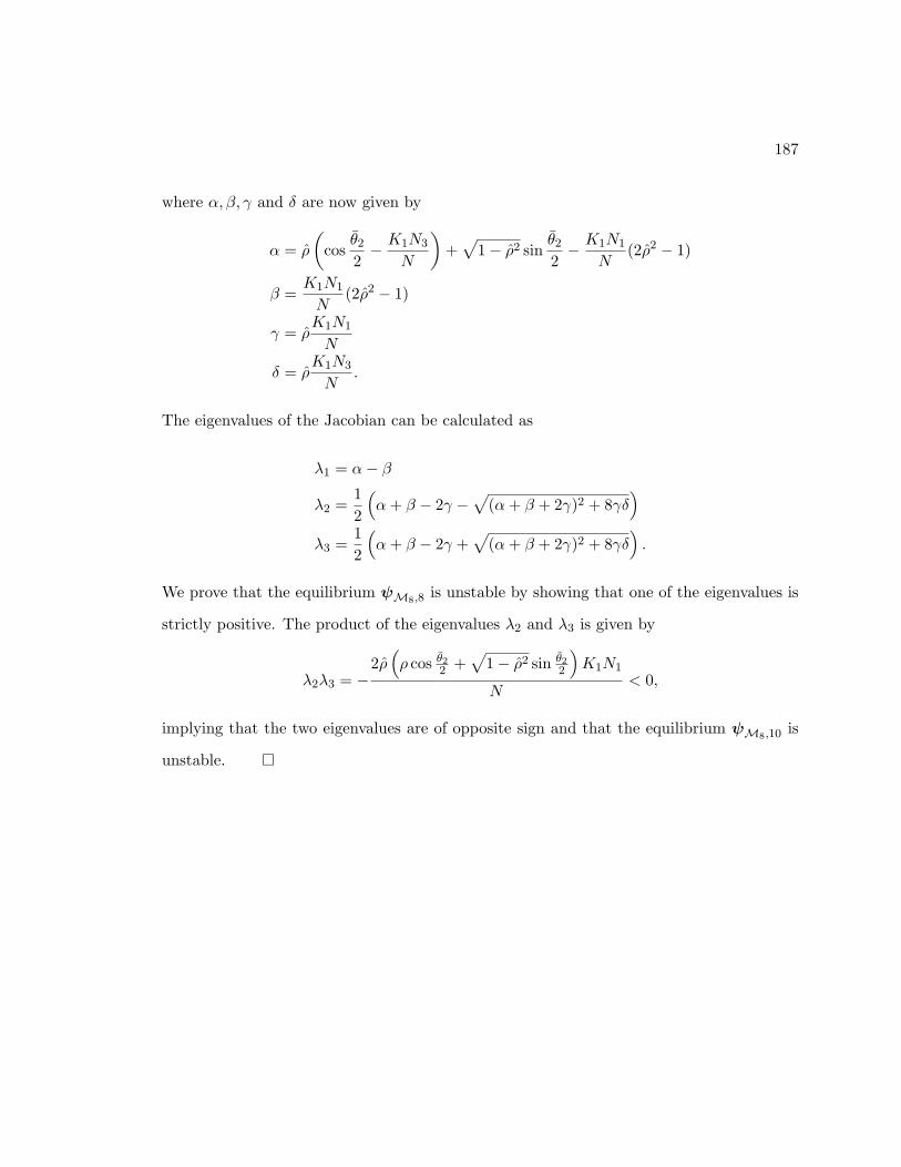
187
where α, β, γ and δ are now given by
α = ρ
(cos
θ2
2− K1N3
N
)+√
1− ρ2 sinθ2
2− K1N1
N(2ρ2 − 1)
β =K1N1
N(2ρ2 − 1)
γ = ρK1N1
N
δ = ρK1N3
N.
The eigenvalues of the Jacobian can be calculated as
λ1 = α− β
λ2 =12
(α+ β − 2γ −
√(α+ β + 2γ)2 + 8γδ
)λ3 =
12
(α+ β − 2γ +
√(α+ β + 2γ)2 + 8γδ
).
We prove that the equilibrium ψM8,8 is unstable by showing that one of the eigenvalues is
strictly positive. The product of the eigenvalues λ2 and λ3 is given by
λ2λ3 = −2ρ(ρ cos θ22 +
√1− ρ2 sin θ2
2
)K1N1
N< 0,
implying that the two eigenvalues are of opposite sign and that the equilibrium ψM8,10 is
unstable.
References
[1] J. Acebrons, L. Bonilla, and R. Spigler. The Kuramoto model: A simple paradigm
for synchronization phenomena. Reviews of Modern Physics, 77:137–185, 2005.
[2] J. Ame, J. Halloy, C. Rivault, C. Detrain, and J. Deneubourg. Collegial decision
making based on social amplification leads to optimal group formation. Proceedings
of the National Academy of Science, 103:5835–5840, 2006.
[3] I. Aoki. An analysis on the schooling mechanism in fish. Bull. Japanese Society
Scientific Fisheries, 48:1081–1088, 1982.
[4] M. Ballerini, N. Cabibbo, R. Candelelier, A. Cavagna, E. Cisbani, I. Giardina,
V. Lecomte, A. Orlandi, G. Parisi, A. Procaccini, M. Viale, and V. Zdravkovic. Inter-
action ruling animal collective behaviour depends on topological rather than metric
distance: Evidence from a field study. Proceedings of the National Academy of Science,
105:1232–1237, 2008.
[5] D. Bertsekas and J. Tsitsiklis. Parallel and Distributed Computation:Numerical Meth-
ods. Prentice-Hall, 1989.
[6] E. Biyik and M. Arcak. Area aggregation and time scale modeling for sparse nonlinear
networks. Proceedings of the 45th IEEE Conference on Decision and Control, pages
4046–4051, 2006.
188

189
[7] R. Bogacz, E. Brown, J. Moehlis, P. Holmes, and J. D. Cohen. The physics of optimal
decision making: A formal analysis of models of performance in two-alternative forced
choice tasks. Psychological Review, 113:700–765, 2006.
[8] B. Bollobas. Graph Theory: An Introductory Course. Springer-Verlag, New York,
1979.
[9] E. Burian, D. Yoerger, A. Bradley, and H. Singh. Gradient search with autonomous
underwater vehicle using scalar measurments. Proc. IEEE OES AUV Conf, 1996.
[10] S. Camazine, J. Deneubourg, N. Franks, J. Sneyd, G. Theraulaz, and E. Bonabeau.
Self-Organization in Biological Systems. Princeton University Press, Princeton, 2001.
[11] J. Cardy and S. Ostlund. Random symmetry-breaking fields and the xy model. Phys.
Rev. B, 25:6899–6909, 1982.
[12] R. Connelly. Rigidity and energy. Invent. Math., 66:11–33, 1982.
[13] R. Connelly. Tensegrity structures: why are they stable? Rigidity theory and appli-
cations., pages 47–543, 1999.
[14] R. Connelly. Generic global rigidity. Discrete Comput. Geom., 33:549–563, 2005.
[15] R. Connelly and W. Whiteley. Second-order rigidity and prestress stability for tenseg-
rity frameworks. SIAM J., 9, No. 3:453–491, 1996.
[16] J. Cortes, S. Martınez, T. Karatas, and F. Bullo. Coverage control for mobile sensing
networks. IEEE Trans. on Robotics and Automation, 20:243255, 2004.
[17] I. Couzin. Collective minds. Nature, 445:715, 2007.
[18] I. Couzin. Collective cognition in animal groups. Trends in Cognitive Sciences, 13,
No 1:36–43, 2009.
[19] I. Couzin, J. Krause, N. Franks, and S. Levin. Effective leadership and decision
making in animal groups on the move. Nature, 434:513–516, 2005.
190
[20] I. D. Couzin and J. Krause. Self-organization and collective behaviour in vertebrates.
Marine Ecology Progress Series, 273:239–249, 2004.
[21] J. Deneubourg and S. Goss. Collective patterns and decision-making. Ethology, Ecol-
ogy, and Evolution, 4:295–311, 1989.
[22] J. Deneubourg and S. Goss. Collective patterns and decision-making. Ethology Ecology
and Evolution, 1:295–311, 1989.
[23] S. Emlen. Modelling social animal aggregation, pages 129–219. Avian Biology, Vol. 5,
Ed. D.S. Farner and J.R. King and K.C. Parkes. Academic Press, 1975.
[24] D. Emmerich. Self-tensioning spherical structures: Single and double layer spheroids.
International Journal of Space Structures, 5, No. 3:353–374, 1990.
[25] M. Erdmann and T. Lozano-Perez. On multiple moving objects. Algorithmica, 2:477–
521, 1987.
[26] T. Eren, P. Belhumeur, and A. Morse. Closing ranks in vehicle formations based on
rigidity. In Decision and Control, 2002, Proceedings of the 41st IEEE Conference on,
volume 3, pages 2959–2964, 2002.
[27] J. Fax and R. Murray. Graph laplacians and stabilization of vehicle formations. In
Proc. 15th IFAC World Congress, volume 3, pages 283–288, 2002.
[28] J. Fax and R. Murray. Information flow and cooperative control of vehicle formations.
IEEE Trans. on Automatic Control, 49:1465–1476, 2004.
[29] E. Fiorelli, N. Leonard, P. Bhatta, D. Paley, R. Bachmayer, and D. Fratantoni. Multi-
AUV control and adaptive sampling in Monterey Bay. IEEE Journal of Oceanic
Engineering, 31(4):935–948, 2006.
[30] G. Flierl, D. Grunbaum, S. Levin, and D. Olson. From individuals to aggregations:
the interplay between behavior and physics. J. Theor. Biol, 196:397–454, 1999.
191
[31] N. R. Franks, S. C. Pratt, E. B. Mallon, N. F. Britton, and D. J. T. Sumpter. Infor-
mation flow, opinion polling and collective intelligence in house-hunting social insects.
Philosophical Transactions: Biological Sciences, 357(1427), 2002.
[32] R. B. Fuller. Tensile-integrity structures, US Patent 3,063,521, 1962.
[33] H. Furuya. Concept of deployable tensegrity structures in space application. Inter-
national Journal of Space Structures, 2:143–151, 1992.
[34] V. Gazi and K. Passino. Stability analysis of social foraging swarms: combined effects
of attractant/repellent profiles. Proceedings of the 41st IEEE Conference on Decision
and Control, 3:2848–2853 vol.3, 2002.
[35] G.Gregoire and H. Chate. Onset of collective and cohesive motion. Phys. Rev. Lett.,
92(2):025702, 2004.
[36] G.Gregoire, H. Chate, and Y. Tu. Moving and staying together without a leader.
Physica D, 181:157–170, 2003.
[37] D. Grunbam and A. Okubo. Modelling social animal aggregation, pages 296–325.
Frontiers in Mathematical Biology Ed. S. Levin. Springer, 1994.
[38] D. Grunbaum. Translating stochastic density-dependent individual behavior with
sensory constraints to an Eulerian model of animal swarming. Journal of Mathematical
Biology, 33:139–161, 1994.
[39] D. Grunbaum, S. Viscido, and J. Parrish. Extracting interactive control algorithms
from group dynamics of schooling fish. In V. Kumar, N. Leonard, and A. Morse,
editors, Proceeding, Block Island Workshop on Cooperative Control. Springer-Verlag,
2005.
[40] J. Guckenheimer and P. Holmes. Nonlinear Oscillations, Dynamical Systems, and
Bifurcations of Vector Fields. Springer-Verlag, New York, 1983.
192
[41] S. Gueron and S. Levin. Self-organization of front patterns in large wildebeest herds.
J. Theor. Biol, 165:541–552, 1993.
[42] S. Gueron, S. Levin, and D. Rubenstein. The dynamics of herds: From individuals to
aggregations. J. theor. Biol, 182:85–98, 1996.
[43] W. Hamilton. Geometry for the selfish herd. J. Theoretical Biology, 31:295–311, 1971.
[44] A. Helbig. Genetic basis of inheritance and evolutionary changes of migratory direc-
tions in palearctic warblers (aves: Sylviidae). The Journal of Experimental Biology,
199:49–55, 1996.
[45] R. Horn and C. Johnson. Matrix Analysis. Cambridge University Press, Cambridge,
1985.
[46] T. Inanc, S. Shadden, and J. Marsden. Optimal trajectory generation in ocean flows.
In Proc. American Control Conference, 2005.
[47] D. Ingber. Cellular tensegrity: defining new rules of biological design that govern the
cytoskeleton. Journal of Cell Science, 104:613–627, 1993.
[48] A. Jadbabaie, J. Lin, and A. Morse. Coordination of groups of mobile autonomous
agents using nearest neighbor rules. IEEE Trans. Aut. Control,, 48:988–1001, 2003.
[49] E. Justh and P. Krishnaprasad. Equilibria and steering laws for planar formations.
Systems and Control Letters, 52:25–38, 2004.
[50] E. Justh and P. S. Krishnaprasad. A simple control law for UAV formation flying.
Technical report, University of Maryland, 2002. Institute for Systems Research.
[51] M. Kelemen. A stability property. IEEE Trans. on Automatic Control, 31, No. 8,
1986.
[52] H. Khalil and P. Kokotovic. On stability properties of nonlinear systems with slowly
varying inputs. IEEE Transactions on Automatic Control, 35, No. 7:860–864, 1990.
193
[53] H. Khalil and P. Kokotovic. On stability properties of nonlinear systems with slowly
varying inputs. IEEE Trans. on Automatic Control, 36, No. 2, 1991.
[54] H. K. Khalil. Nonlinear Systems 3rd ed. Prentice Hall, 2002.
[55] O. Khatib. Real-time obstacle avoidance for manipulators and mobile robots. Int. J.
Rob. Res., 5(1):90–98, 1986.
[56] P. Khosla and R. Volpe. Superquadric artificial potentials for obstacle avoidance
and approach. Proceedings., 1988 IEEE International Conference on Robotics and
Automation, pages 1778–1784 vol.3, 1988.
[57] J. Krause and G. D. Ruxton. Living in Groups. Oxford Univ. Press, Oxford, 2002.
[58] L. C. V. Kumar and F. M. Campos. A paradigm for dynamic coordination of multiple
robots. Autonomous Robots, 17:721, 2004.
[59] Y. Kuramoto. Self-entrainment of a population of coupled non-linear oscillators.
In Proc. Int. Symp. Mathematical Problems in Theoretical Physics, pages 420–422,
Kyoto, Japan, 1975.
[60] Y. Kuramoto. Chemical oscillations, waves, and turbulence. Springer-Verlag, 1984.
[61] G. Laman. On graphs and rigidity of plane skeletal structures. Journal of Engineering
Mathematics, 4, No. 4, 1970.
[62] D. Lawrence and W. Rugh. On a stability theorem for nonlinear systems with slowly
varying inputs. IEEE Transactions on Automatic Control, 36, No. 2:229, 1991.
[63] N. Leonard and E. Fiorelli. Virtual leaders, artificial potentials and coordinated
control of groups. Proceedings of the 40th IEEE Conference on Decision and Control,
3:2968–2973, 2001.
[64] N. E. Leonard, D. Paley, F. Lekien, R. Sepulchre, D. Fratantoni, and R. Davis. Col-
lective motion, sensor networks and ocean sampling. Proceedings of the IEEE, 95, No.
1:48–74, 2007.
194
[65] W. Levine and M. Athans. On the optimal error regulation of a string of moving
vehicles. IEEE Trans. Automatic Control, 11, No. 3:355–361, 1966.
[66] M. Lindauer. Communication in swarm-bees searching for a new home. Nature,
179:63–67, 1957.
[67] M. Lindhe. A flocking and obstacle avoidance algorithm for mobile robots. Master’s
thesis, Royal Institute of Technology, Stockhom, Sweden, 2004.
[68] J. Marsden. Lectures on Mechanics. Cambridge University Press, 1992.
[69] J. Marsden and T. Ratiu. Introduction to Mechanics and Symmetry 2nd ed. Springer-
Verlag, 1999.
[70] S. Melzer and B. Kuo. A closed-form solution for the optimal error regulation of a
string of moving vehicles. IEEE Trans. Automatic Control, 16:50–51, 1971.
[71] R. E. Mirollo and S. H. Strogatz. Jump bifurcation and hysteresis in an infinite-
dimensional dynamical system of coupled spins. SIAM J. Appl. Math., 50(1):108–124,
1990.
[72] S. Moon, B. Nabet, N. Leonard, S. Levin, and I. Kevrekidis. Heterogeneous animal
group models and their group-level alignment dynamics; an equation-free approach.
Journal of Theoretical Biology, 246:100–112, 2007.
[73] K. Moored and H. Smith. The analysis of tensegrity structures for the design of
morphing wing. Transactions of the ASME, 74:668–676, 2007.
[74] L. Moreau. Stability of multiagent systems with time-dependent communication links.
IEEE Transaction on Automatic Control, 50, No. 2, 2005.
[75] R. Motro. Forms and forces in tensegrity systems. Third International Conference on
Space Structures, pages 180–185, 1984.
195
[76] R. Motro, S. Najari, and P. Jouanna. Static and dynamic analysis of tensegrity
systems. In Proc. ASCE Int. Symp. Shells and Spatial Structures, Computational
Aspects, pages 270–279, New York, 1986. Springer.
[77] B. Nabet and N. Leonard. Shape control of a multi-agent system using tensegrity
structures. In Proceedings of the 3rd IFAC Workshop on Lagrangian and Hamiltonian
Methods for Nonlinear Control, Nagoya, Japan, 2006.
[78] B. Nabet and N. Leonard. Tensegrity models and shape control of vehicle formations,
2009. http//arxiv.org/abs/0902.3710v1.
[79] B. Nabet, N. Leonard, I. Couzin, and S. Levin. Leadership in animal group mo-
tion: A bifurcation analysis. In Proceedings of the 17th International Symposium on
Mathematical Theory of Networks and Systems, Kyoto, Japan, 2006.
[80] B. Nabet, N. Leonard, I. Couzin, and S. Levin. Dynamics of decision-making in animal
group motion. Journal of Nonlinear Science, 19, No 4:399–435, 2009.
[81] O.E.Wilson. Sociobiology, The New Synthesis. Harvard University Press, Cambridge,
1975.
[82] P. Ogren, M. Egerstedt, and X. Hu. A control lyapunov function approach to multi-
agent coordination. Proceedings of the 40th IEEE Conference on Decision and Control,
2:1150–1155 vol.2, 2001.
[83] P. Ogren, E. Fiorelli, and N. Leonard. Cooperative control of mobile sensor networks:
Adaptive gradient climbing in a distributed environment. IEEE Trans. on Automatic
Control, 49, No. 8:1292–1302, 2004.
[84] A. Okubo. Diffusion and Ecological Problems: Mathematical Models, volume 10 of
Lecture Notes in Biomathematics. Springer-Verlag, New York, 1980.
196
[85] R. Olfati-Saber and R. Murray. Distributed cooperative control of multiple vehicle
formations using structural potential functions. In Proceedings of The 15th IFAC
World Congress , Barcelona, Spain, 2002.
[86] R. Olfati-Saber and R. Murray. Graph rigidity and distributed formation stabilization
of multi-vehicle systems. In Proceedings of the 41st Conference on Decision and
Control, 2002.
[87] R. Olfati-Saber and R. Murray. Consensus problems in networks of agents with
switching topology and time-delays. IEEE Trans. on Automatic Control, 49(9):1520–
1533, 2004.
[88] I. Oppenheim and W. Williams. Vibration and damping in tensegrity structures.
ASCE Journal of Aerospace Engineering, 14:8591, 2001.
[89] D. Pais, M. Cao, and N. Leonard. Formation shape and orientation control using
projected collinear tensegrity structures. In American Control Conference, St. Louis,
MO, 2009.
[90] D. Paley, F. Zhang, and N. Leonard. Cooperative control for ocean sampling: The
glider coordinated control system. IEEE Trans. on Control Systems Technology, 16,
No. 4:735–744, 2008.
[91] J. Pearson. On controlling a string of moving vehicles. IEEE Trans. Automatic
Control, 12:328–329, 1967.
[92] A. Perdeck. Two types of orientation in migrating starlings. Ardea, 46:1–37, 1958.
[93] T. Poston and I. Stewart. Catastrophe Theory and its Applications. Pitman, London,
1978.
[94] S. Pratt, E. Mallon, D. Sumpter, and N. Frank. Quorum sensing, recruitment, and
collective decision-making during colony emigration by the ant leptothorax albipennis.
Behavioral Ecology and Sociobiology, 52:117–127, 2002.
197
[95] A. Pugh. An Introduction to Tensegrity. University of California Press, Berkeley, CA,
1976.
[96] S. Reebs. Can a minority of informed leaders determine the foraging movements of a
fish shoal? Animal Behaviour, 59:403–409, 2000.
[97] C. Reynolds. Flocks, herds, and schools: A distributed behavioral model. Computer
Graphics, 21, No 4:25–34, 1987.
[98] E. Rimon and D. Koditschek. Exact robot navigation using artifical potential func-
tions. IEEE Trans. on Robotic and Automations, pages 501–518, 1992.
[99] G. Roberts. Why vigilance declines as group size increases. Animal Behavior, 51,
1996.
[100] B. Roth and W. Whiteley. Tensegrity frameworks. Trans. American Math. Soc, 265,
No 2.:419–446, 1981.
[101] S. Sadao. Fuller on tensegrity. International Journal of Space Structures, 11, 1996.
[102] A. Savkin. Coordinated collective motion of groups of autonomous mobile robots:
Analysis of Viscek’s model. IEEE Trans. on Automatic Control, 49, No. 6:981–983,
2004.
[103] L. Scardovi, A. Sarlette, and R. Sepulchre. Synchronization and balancing on the
N-torus. Systems and Control Letters, 56(5):335 – 341, 2007.
[104] T. Seeley and P. Visscher. Quorum sensing during nest-site selection by honeybee
swarms. Behavioral Ecology and Sociobiology, 56:594–601, 2004.
[105] T. D. Seeley. Honeybee ecology: a study of adaptation in social life. Princeton Uni-
versity Press, 1985.
[106] E. Selous. Thought Transference (or What?) in Birds. Constable and Company Ltd,
London, 1931.
198
[107] R. Sepulchre, D. Paley, and N. Leonard. Stabilization of planar collective motion with
limited communication. IEEE Trans. Aut. Control, 53, No. 3:706–719, 2008.
[108] R. Sepulchre, D. Paley, and N. E. Leonard. Stabilization of planar collective motion:
All-to-all communication. IEEE Transactions on Automatic Control, 52, No.5:811–
824, 2007.
[109] R. Skelton and M. de Oliveira. Tensegrity Systems. Springer, 2009.
[110] R. Skelton, J. Helton, R. Adhikari, J. Pinaud, and W. Chan. An introduction to
the mechanics of tensegrity structures. The Mechanical Systems Design Handbook:
Modeling, Measurement, and Control CRC Press, 2001.
[111] R. Skelton and C. Sultan. Controllable tensegrity, a new class of smart structures. In
Proc. SPIE 4th Symposium on Smart Structures and Materials, pages 166–177, 1997.
[112] K. Snelson. Continuous tension, discontinuous compression structures. U.S. Patent
3,169,611,, 1965.
[113] H. Sompolinsky, D. Golomb, and D. Kleinfeld. Global processing of visual stimuli
in a neural network of coupled oscillators. Proceedings of the National Academy of
Science USA, 87:7200–7204, 1990.
[114] S. Strogatz. Nonlinear Dynamics and Chaos. Perseus, 1994.
[115] S. H. Strogatz. From Kuramoto to Crawford: Exploring the onset of synchronization
in populations of coupled oscillators. Physica D, 143:1–20, 2000.
[116] C. Sultan. Modeling, design and control of tensegrity structures with applications.
PhD thesis, Purdue University, School of Aeronautics and Astronautics, 1999.
[117] C. Sultan and R. Skelton. Integrated design of controllable tensegrity structures. In
Proc. ASME Int. Mechanical Engineering Congress and Exposition, volume 54, pages
27–37, 1997.
199
[118] D. Sumpter, J. Krause, I. D. Couzin, and A. Ward. Consensus decision making by
fish. Current Biology, 18:1773–1777, 2008.
[119] W. Swaney, J. Kendal, H. Capon, C. Brown, and K. Laland. Familiarity facilitates
social learning of foraging behavour in the guppy. Animal Behaviour, 62:591–598,
2001.
[120] P. Tabuada, G. Pappas, and P. Lima. Feasible formations of multi-agent systems. In
Proceedings of the American Control Conference, volume 1, pages 56–61, 2001.
[121] R. Thom. Structural Stability and Morphogenesis. Benjamin, New York, 1972.
[122] A. Tibert. Deployable Tensegrity Structures for Space Applications. PhD thesis, Royal
Institute of Technology, Sweden, Department of Mechanics, 2002.
[123] A. Tibert and S. Pellegrino. Review of form-finding methods for tensegrity structures.
deployable structures lab, university of cambridge. International Journal of Space
Structures, 18, No. 4:209–223, 2003.
[124] N. Tinbergen. On aims and methods of ethology. Zeitschrift fur Tierpsychologie, 20,
1986.
[125] J. Toner and Y. Tu. Long-range order in a two-dimensional dynamical xy model: How
birds fly together. Phys. Rev. Lett., 75(23):4326–4329, 1995.
[126] J. Toner and Y. Tu. Flocks, herds, and schools: A quantitative theory of flocking.
Phys. Rev. Lett., 58(4):4828–4858, 1998.
[127] J. Tsitsiklis. Problems in decentralized decision making and computation. PhD thesis,
MIT, Department of Electrical Engineering, Cambridge, MA, 1984.
[128] J. Tsitsiklis and D. Bertsekas. Distributed asynchronous deterministic and stochastic
gradient optimization algorithms. IEEE Trans. Autom. Control, AC-31, No 9:803–
812, 1986.
200
[129] T. Viscek, A. Czirok, E. Ben-Jacob, I. Cohen, O. Shochet, and A. Tenenbaum.
Novel type of phase transition in a system of self-driven particles. Phys. Rev. Lett.,
75(6):1226–1229, 1995.
[130] S. Viscido, J. Parrish, and D. Grunbaum. Individual behavior and emergent properties
of fish schools: a comparison between observation and theory. Advances in the Study
of Behavior, 32:1–75, 2003.
[131] P. Wang. Interaction dynamics of multiple mobile robots with simple navigation
strategies. Journal of Robotic Systems, 7:77–101, 1989.
[132] A. Ward, D. Sumpter, I. D. Couzin, P. Hart, and J. Krause. Quorum decision-making
facilitates information transfer in fish shoals. Proceedings of the National Academy of
Science, 105, No.19:6948–6953, 2008.
[133] C. Warren. Multiple robot path coordination using artificial potential fields. Pro-
ceedings of the IEEE International Conference on Robotics and Automation, pages
500–505 vol.1, 1990.
[134] W. Williams. A primer on the mechanics of tensegrity structures. Technical report,
Carnegie Mellon University, 2003. Center for Nonlinear Analysis.
[135] A. Winfree. Biological rhythms and the behavior of populations of coupled oscillators.
Journal of Theoretical Biology, 16(1):15–42, 1967.
[136] R. Wood, S. Avadhanula, E. Stelz, M. Seeman, J. Entwistle, A. Bachrach, G. Barrows,
S. Sanders, and R. Fearing. Enabling technologies and subsystem integration for an
autonomous palm-sized glider. IEEE Robotics and Automation Magazine, 14, No.
2:82–91, 2007.
[137] G. Zanotti and C. Guerra. Is tensegrity a unifying concept of protein folds? FEBS
Letters, 534:7–10, 2003.
201
[138] F. Zhang, M. Goldgeier, and P. S. Krishnaprasad. Control of small formations us-
ing shape coordinates. Proc. 2003 IEEE International Conference on Robotics and
Automation, pages 2510–2515, 2003.
[139] F. Zhang and N. Leonard. Generating contour plots using multiple sensor platforms.
Proc. of 2005 IEEE Symposium on Swarm Intelligence, pages 309–314, 2005.
[140] F. Zhang and N. Leonard. Cooperative control and filtering for cooperative explo-
ration. IEEE Transactions on Automatic Control, 2008. to appear.