Dynamics and time series: theory and applicationshomepage.sns.it/marmi/lezioni/Lecture_6_2010.pdf · Dynamics and time series: theory and applications Stefano Marmi Scuola Normale

Dynamics and time series:

theory and applications

Stefano Marmi

Scuola Normale Superiore

Lecture 6, Jan 28, 2010

Il corso si propone di fornire un’introduzione allo studio delle applicazioni dei sistemi dinamici allo studio delle serie

temporali e al loro impiego nella modellizzazione matematica, con una enfasi particolare sull’analisi delle serie

storiche economiche e finanziarie. Gli argomenti e i problemi trattati includeranno (si veda la pagina web del docente

http://homepage.sns.it/marmi/ ):

Introduzione ai sistemi dinamici e alle serie temporali. Stati stazionari, moti periodici e quasi periodici. Ergodicità,

distribuzione uniforme delle orbite. Tempi di ritorno, diseguaglianza di Kac. Mescolamento. Entropia di Shannon.

Entropia di Kolmogorov-Sinai. Esponenti di Lyapunov. Entropia ed elementi di teoria dell’informazione. Catene di

Markov. Scommesse, giorchi probabilistici, gestione del rischio e criterio di Kelly.

Introduzione ai mercati finanziari: azioni, obbligazioni, indici. Passeggiate aleatorie, moto browniano geometrico.

Stazionarietà delle serie temporali finanziarie. Correlazione e autocorrelazione. Modelli auto regressivi. Volatilità,

eteroschedasticità ARCH e GARCH. L’ipotesi dei mercati efficienti. Arbitraggio. Teoria del portafoglio e il Capital

Asset Pricing Model.

Modalità dell'esame: Prova orale e seminari

Sistemi dinamici e teoria dell’informazione:

Benjamin Weiss: ―Single Orbit Dynamics‖, AMS 2000

Thomas Cover, Joy Thomas ―Elements of Information Theory‖ 2nd edition, Wiley 2006

Serie temporali:

Holger Kantz and Thomas Schreiber: Nonlinear Time Series Analysis, Cambridge University Press 2004

Michael Small: Applied Nonlinear Time Series Analysis. Applications in Physics, Physiology and Finance, World

Scientific 2005

Modelli matematici in finanza e analisi delle serie storiche:

M. Yor (Editor): Aspects of Mathematical Finance, Springer 2008

John Campbell, Andrew Lo and Craig MacKinlay: The Econometrics of Financial Markets, Princeton University

Press, 1997

Thomas Bjork: Arbitrage Theory in Continuous Time (Oxford Finance)

Stephen Taylor: "Modelling Financial Time Series" World Scientific 2008

Keith Cuthbertson, Dirk Nitzsche "Quantitative Financial Economics" John Wiley and Sons (2004)

Jan 28, 2010S. Marmi - Dynamics and time series -Lecture 6:Financial time series: stylized

facts and models2

http://homepage.sns.it/marmi/

• Lecture 1: An introduction to dynamical systems and to time series. (Today, 2 pm - 4 pm Aula Dini)

• Lecture 2: Ergodicity. Uniform distribution of orbits. Return times. Kac inequality Mixing (Thu Jan 14,

2 pm - 4 pm Aula Fermi) by Giulio Tiozzo

• Lecture 3: Kolmogorov-Sinai entropy. Randomness and deterministic chaos. (Wen Jan 20, 2 pm - 4 pm

Aula Bianchi) by Giulio Tiozzo

• Lecture 4: Introduction to financial markets and to financial time series (Thu Jan 21,

2 pm - 4 pm Aula Bianchi Lettere)

• Lecture 5: Central limit theorems (Wen Jan 27, 2 pm - 4 pm Bianchi) by Giulio Tiozzo

• Lecture 6: Financial time series: stylized facts and models (Thu Jan 28, 2 pm - 4 pm Bianchi)

• No lectures on Wen Feb 3 and Thu Feb 4

• Lectures 7 and 8 (including a seminar by F. Lillo) Wen Feb 10 and Thu Feb 11

• Lecture 9 on Wen Feb 17 No lecture on Thu Feb 18

• Lectures 10 and 11 (including a seminar by A. Carollo) Wen Feb 24 and Thu Feb 25

• Lectures 12 and 13 Wen Mar 3 and Thu Mar 4


facts and models3

• Seminar I: TBA (Fabrizio Lillo, Palermo, Thu Feb11)

• Seminar II: TBA (Angelo Carollo, Palermo, Thu Feb 25)

• Seminar III: TBA (Massimiliano Marcellino, European University Institute, Thu Mar

18)

• Challenges and experiments:

0. blog?

1. statistical arbitrage in sports betting: collecting time series, etc..

2. nonstationarity and volatility of financial series


facts and models4

Today’s bibliography:

R. Cont ―Empirical properties of asset returns: stylized

facts and statistical issues‖ Quantitative Finance 1 (2001)

223–236http://www.proba.jussieu.fr/pageperso/ramacont/papers/empirical.pdf

S.J. Taylor ―Asset Price Dynamics, Volatility, and

Prediction‖ Princeton University Press (2005). Chapters

2, 3 and 4

Steven Skiena CSE691 Computational Finance class at

Stony Brook: http://www.cs.sunysb.edu/~skiena/691/

Jan 28, 2010 5S. Marmi - Dynamics and time series -Lecture 6:Financial time series: stylized

facts and models

http://www.proba.jussieu.fr/pageperso/ramacont/papers/empirical.pdf

Reminder on the fundamentals of

investing• Investment returns are strongly related to their risk level

• Usually and loosely risk is quantified using volatility (standard deviation)

• Government (U.S., European, etc) bills /bonds (short/long term bonds 1month-1year / 2-30 years ).

Bonds are also issued by companies to finance their operations

• T.I.P. : inflation indexed bonds which guarantee a positive real return

• Stocks: risky but higher returns. Each share represents a given fraction of the ownership of the company.

• Certain stocks pay dividends, cash payments reflecting profits returned to shareholders. Other stocks

reinvest all returns back into the business.

• Exchanges: places where buyers/sellers trade securities (stocks, bonds, options, futures, commodities).

They provide liquidity, i.e.ability to buy and sell securities quickly, inexpensively, and at fair market value.

• Commodities are types of goods which can be defined so that they are largely indistinguishable in terms

of quality (e.g. orange juice, gold, cotton, pork bellies). Commodities markets exist to trade such products,

from before they are produced to the moment of shipping. The existence of agricultural futures gives

suppliers and consumers ways to protect themselves from unexpected changes in prices.

•Currency Markets: The largest financial markets by volume trade different types of currency, such as

dollars, Euros, and Yen.

•The spot price gives the cost of buying a good now, while futures permit one to buy the right to buy or sell

goods at fixed prices at some future date.


facts and models

Daily returns of General Motors

(1950-2008)


facts and models

Volatility clustering

Time series plots of returns display an important feature that is usually called volatility clustering. This empirical phenomenon was first observed by Mandelbrot (1963), who said of prices that ―large changes tend to be followed by large changes—of either sign—and small changes tend to be followed by small changes.‖Volatility clustering describes the general tendency for markets to have some periods of high volatility and other periods of low volatility. High volatility produces more dispersion in returns than low volatility, so that returns are more spread out when volatility is higher. A high volatility cluster will contain several large positive returns and several large negative returns, but there will be few, if any, large returns in a low volatility cluster.


facts and models

Daily returns of GM after normalization by

short-term (25 days) volatility


facts and models

Arbitrage

Arbitrage is a trading strategy which takes advantage of two or

more securities being inconsistently priced relative to each other.

In financial and economics theory arbitrage is the practice of

taking advantage of a price differential between two or

more markets or assets: striking a combination of matching deals

that capitalize upon the imbalance, the profit being the difference

between the prices. When used by academics, an arbitrage is a

transaction that involves no negative cash flow at any

probabilistic or temporal state and a positive cash flow in at least

one state; in simple terms, a risk-free profit.

Advanced arbitrage techniques involve sophisticated

mathematical analysis and rapid trading.


facts and models

Stock ReturnsLet pt be a representative price for a stock in period t (finaltransaction price or final quotation during the period). Assume that the buyer pays the seller immediately for stock bought . Let dt be the present value of dividends, per share, distributed to those people who own stock during period t . On almost all days there are no dividend payments → dt = 0. Sometimes dividend payments are simply ignored, so then dt = 0 for all days t .Three price change quantities appear in empirical research:r∗t = pt + dt − pt-1

r′t = (pt + dt − pt-1)/ pt-1, simple net return (arithmetic)rt = log(pt + dt ) − log pt-1. log returns (geometric)The return measures rt and r′t are very similar numbers, since1 + r′t = exp(rt) = 1 + rt + ½ rt

2 + …and very rarely are daily returns outside the range from −10% to 10%. It is common to assume that single-period geometric returns follow a normal distribution.


facts and models

The appropriate frequency of observations in a price series depends on the data available and the questions that interest a researcher. The time interval between prices ought to be sufficient to ensure that trade occurs in most intervals and it ispreferable that the volume of trade is substantial. Very often, selecting daily prices will be both appropriate and convenient.

The additional information increases the power of hypothesis tests, it improves volatility estimates, and it is essential for evaluations of trading rules. The number of observations in a time series of daily prices should be sufficient to permit powerful tests and accurate estimation of model parameters. Experience shows that at least four years of daily prices (more than 1000 observations) are often required to obtain interesting results; however, eight or more years of prices (more than 2000 observations) should be analyzed whenever possible.


facts and models

Statistical analysis of a time series:

moments of the probability distribution


facts and models

Taylor, Asset

Price Dynamics,

Volatility and

Prediction, P.U.P.

(2005)


facts and models

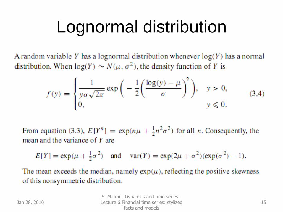
Lognormal distribution


facts and models

Higher moments: simmetry of the

distribution and fat tails

• Skewness: measures simmetry of the data about the mean (third moment)

• Kurtosis: peakedness of the distributionrelative to the normal distribution (hence the -3 term)

• Leptokurtic distribution (fat tailed): haspositive kurtosis


facts and models

Correlation between two data series

ψ,υ random variables with expectations μ(ψ ) and μ(υ)

σ(ψ) 2 =[ (μ(ψ2 )- μ(ψ)2 ] variance

The correlation coefficient of ψ,υ is

ρ(ψ,υ)=covariance(ψ,υ) / (σ(ψ) σ(υ))

= μ [(ψ- μ(ψ))(υ- μ (υ))] / (σ(ψ) σ(υ))

= μ [ψ υ - μ(ψ)μ (υ)] / (σ(ψ) σ(υ))

The correlation coefficient varies between -1 and 1 and equals 0 forindependent variables but this is only a necessary condition (e.g. υuniform on [-1,1] has zero correlation with its square)


facts and models

Sample correlation coefficient between

two finite series of data


facts and models

Autocorrelation function


facts and models

Stationarity• Stationarity: all parameters of the data series statistical distribution must be

time-independent

• Weak-stationarity: we only require that the first two moments (mean and variance) are constant

• Parameters can for example be moments of the probability distribution, but also coefficients in differential equations or autoregressive processes.


facts and models

Tests of stationarity

• Moving window analysis: Divide a long time series in

shorter windows and analyze these short windows

separately.

• For example split the series into two parts, compute

mean and variance and compare (remember that the

standard error will be σ/√N)


facts and models

Taylor, Asset Price Dynamics, Volatility and Prediction, P.U.P. (2005)


facts and models

Gaussian process

A process is called Gaussian if the multivariate distribution of

the consecutive variables (Xt+1,Xt+2,...,Xt+k) is multivariate

normal for all integers t and k. A stationary Gaussian process is

always strictly stationary, because then the first- and second-

order moments completely determine the multivariate

distributions.


facts and models

Why white noise?

Autocovariances

Autocorrelation of a stationary process (the variance is constant) ρ0 = 1, ρτ = ρ-τ

Spectral density function

The integral of s(ω) from 0 to 2π equals λ0. High values of s(ω) might indicate cyclical behavior with the period of one cycle equal to 2π/ω time units. For a white noise the spectral density function is the same constant for all frequencies ω


facts and models

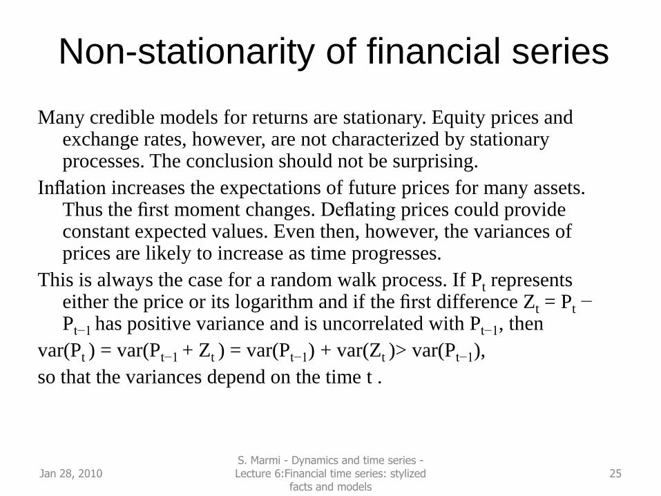
Non-stationarity of financial series

Many credible models for returns are stationary. Equity prices and exchange rates, however, are not characterized by stationary processes. The conclusion should not be surprising.

Inflation increases the expectations of future prices for many assets. Thus the first moment changes. Deflating prices could provide constant expected values. Even then, however, the variances of prices are likely to increase as time progresses.

This is always the case for a random walk process. If Pt represents either the price or its logarithm and if the first difference Zt = Pt − Pt−1 has positive variance and is uncorrelated with Pt−1, then

var(Pt ) = var(Pt−1 + Zt ) = var(Pt−1) + var(Zt )> var(Pt−1),

so that the variances depend on the time t .


facts and models

Uncorrelated processes

The simplest possible autocorrelation occurs when a process is a

collection of uncorrelated random variables so ρ0 = 1, ρτ = 0

for all τ>0

For an uncorrelated process the optimal forecast of the variable is

simply the unconditional mean.

Uncorrelated processes are often used to model asset returns

because they have some empirical support and they are

coherent with the efficient markets hypothesis


facts and models



facts and models

Statistical distribution of returns

In real world data analysis, not

only are the true mean and

standard deviations unknown

but the type of distribution that

generated the observed returns

(if any) is also unknown.

A simple test for normality is

orovided by the studentized

range SR: given a random

variable xi one defines

SR= (max xi – min xi)/σ

It depends heavily on the

extreme observations


facts and models

Stylized facts (R. Cont, Quantitative Finance (2001))

1. Absence of autocorrelations: (linear) autocorrelations of asset returns

are often insignificant, except for very small intraday time scales (≈ 20

minutes) for which microstructure effects come into play.

2. Heavy tails: the (unconditional) distribution of returns seems to

display a power-law or Pareto-like tail, with a tail index which is finite,

higher than two and less than five for most data sets studied. In

particular this excludes stable laws with infinite variance and the

normal distribution. However the precise form of the tails is difficult to

determine.

3. Gain/loss asymmetry: one observes large drawdowns in stock prices

and stock index values but not equally large upward movements


facts and models

Autocorreletion of daily returns and of their absolute values. The black

line is the best power law fit of the absolute values autocorrelations

y = 0.3697x-0.225

R² = 0.935

-0.1

-0.05

0

0.05

0.1

0.15

0.2

0.25

0.3

0.35

0.4

0 10 20 30 40 50 60 70 80 90 100

Index: DJIA (1885-2008)


facts and models

DJIA: daily

return at day i

vs. return at

day i-1, 5000

days

(approximately

1988-2008)

-0.1

-0.08

-0.06

-0.04

-0.02

0

0.02

0.04

0.06

0.08

0.1

-0.1 -0.08 -0.06 -0.04 -0.02 0 0.02 0.04 0.06 0.08 0.1

Serie1


facts and models

Distribution of returns of DJIA stocks: from

“Foundations of Finance”, Fama (1976)


facts and models


facts and models

4. Aggregational Gaussianity: as one increases the time scale Δt over which returns are calculated, their distribution looks more and more like a normal distribution. In particular, the shape of the distribution is not the same at different time scales.5. Intermittency: returns display, at any time scale, a high degree of variability. This is quantified by the presence of irregular bursts in time series of awide variety of volatility estimators.6. Volatility clustering: different measures of volatility display a positive autocorrelation over several days, which quantifies the fact that high-volatility events tend to cluster in time.7. Conditional heavy tails: even after correcting returns for volatility clustering (e.g. via GARCH-type models), the residual time series still exhibit heavy tails. However, the tails are less heavy than in the unconditional distribution of returns.



facts and models

8. Slow decay of autocorrelation in absolute returns: the

autocorrelation function of absolute returns decays slowly as a

function of the time lag, roughly as a power law with an exponent

β ∈ [0.2, 0.4]. This is sometimes interpreted as a sign of long-

range dependence.

9. Leverage effect: most measures of volatility of an asset are

negatively correlated with the returns of that asset.

10. Volume/volatility correlation: trading volume is correlated

with all measures of volatility.

11. Asymmetry in time scales: coarse-grained measures of

volatility predict fine-scale volatility better than the other way

round.



facts and models

0

20

40

60

80

100

120

140

160

1/3/

1951

1/3/

1953

1/3/

1955

1/3/

1957

1/3/

1959

1/3/

1961

1/3/

1963

1/3/

1965

1/3/

1967

1/3/

1969

1/3/

1971

1/3/

1973

1/3/

1975

1/3/

1977

1/3/

1979

1/3/

1981

1/3/

1983

1/3/

1985

1/3/

1987

1/3/

1989

1/3/

1991

1/3/

1993

1/3/

1995

1/3/

1997

1/3/

1999

1/3/

2001

1/3/

2003

1/3/

2005

1/3/

2007

numero giorni >1%

numero giorni <-1%

S&P500 scala logaritmica

Volatility clustering and leverage effect


facts and models

An autoregressive conditional heteroscedasticity (ARCH, Engle

(1982)) model considers the variance of the current error term to be a

function of the variances of the previous time period's error terms.

ARCH relates the error variance to the square of a previous period's

error. It is employed commonly in modeling financial time series that

exhibit time-varying volatility clustering, i.e. periods of swings

followed by periods of relative calm.


facts and models



facts and models



facts and models


facts and models40

Randomness and the physical law• It may well be that the universe itself is completely deterministic (though

this depends on what the ―true‖ laws of physics are, and also to some extent on certain ontological assumptions about reality), in which case randomness is simply a mathematical concept, modeled using such abstract mathematical objects as probability spaces. Nevertheless, the concept of pseudorandomness- objects which ―behave‖ randomly in various statistical senses - still makes sense in a purely deterministic setting. A

typical example are the digits of π=3.1415926535897932385…this is a deterministic sequence of digits, but is widely believed to behave pseudorandomly in various precise senses (e.g. each digit should asymptotically appear 10% of the time). If a deterministic system exhibits a sufficient amount of pseudorandomness, then random mathematical models (e.g. statistical mechanics) can yield accurate predictions of reality, even if the underlying physics of that reality has no randomness in it.

http://terrytao.wordpress.com/2007/04/05/simons-lecture-i-structure-and-randomness-in-fourier-analysis-and-number-theory/


facts and models

http://terrytao.wordpress.com/2007/04/05

Distribution

of daily

returns, Dow

Jones 1928-

20070

100

200

300

400

500

600

700

-0.0

5

-0.0

46

5

-0.0

43

-0.0

39

5

-0.0

36

-0.0

32

5

-0.0

29

-0.0

25

5

-0.0

22

-0.0

18

5

-0.0

15

-0.0

11

5

-0.0

08

-0.0

04

5

-0.0

01

0.0

02

5

0.0

06

0.0

09

5

0.0

13

0.0

16

5

0.0

2

0.0

23

5

0.0

27

0.0

30

5

0.0

34

0.0

37

5

0.0

41

0.0

44

5

0.0

48

Fre

qu

enza

Classe

Distribution of daily returns , DJIA

Frequenza

Geometric daily return at time t = (Price of index at time t / Price of index at

time t-1)-1Here the index is the Dow

Jones Industrial Average, t isinteger and counts only

open market daysThe value of the index is at

the closeJan 28, 2010S. Marmi - Dynamics and time series -Lecture 6:Financial time series: stylized

facts and models42

Una passeggiata aleatoria?

• In un famosissimo articolo Paul Samuelson (―Proof that

Properly Anticipated Prices Fluctuate Randomly‖, Industrial

Management Review, 6:2, 41-49 (1965)) diede una

dimostrazione matematica di questo fatto. Tutti gli argomenti

rigorosi devono fondarsi su assiomi e definizioni e su

impiegare una logica impeccabile, che certamente approssima

ma non incarna l’esperienza quotidiana dei mercati. Scrive lo

stesso Samuelson nelle conclusioni dell’articolo: ―Non si

dovrebbero dedurre troppe conseguenze dal teorema che ho

appena dimostrato. In particolare non ne segue che i mercati

competitivi reali funzionino bene.‖


facts and models43

The normal distribution


facts and models44

Do daily returns follow a

normal distribution?

Mean 00204

Median 00411Moda 0Standard deviation 0.011355

Varianza campionaria 00129Kurtosis 26.84192

Asymmetry -0.67021Intervallo 0.399044Minimum -0.25632Maximum 0.142729Sum 4.058169Number ofobservations 19848

ClassObservedFrequency

TheoreticalFrequency

x< -0.05 67 0.093902

-0.05<x<-0.045 19 0.567355

-0.045<x<-0.04 41 3.207188--0.04<x<0.035 51 14.9652

-0.035<x<-0.03 78 57.64526

-0.03<x<-0.025 117 183.3153

-0.025<x<-0.02 247 481.2993

-0.02<x<-0.015 484 1043.367-0.015<x<-0.01 1111 1867.6

-0.01<x<-05 2433 2760.391-0.05<x<0 4879 3369.05

0<x<05 5119 3395.46805<x<0.01 2881 2825.84

01<x<0.015 1219 1941.987

0.015<x<0.02 539 1102.011

0.02<x<0.025 241 516.3589

0.025<x<0.03 105 199.76740.03<x<0.035 77 63.8089

0.035<x<0.04 43 16.82651

0.04<x<0.045 27 3.662964

0.045<x<0.05 20 0.658208

x> 0.05 50 0.110887


facts and models45

Theoretical and observed frequency of

outliers in the history of 15 stockmarkets

Estrada, Javier: Black Swans and Market Timing: How Not to Generate Alpha. Available at SSRN: http://ssrn.com/abstract=1032962


facts and models46

Documents

Dynamics and time series: theory and applicationshomepage.sns.it/marmi/lezioni/Lecture_6_2010.pdf · Dynamics and time series: theory and applications Stefano Marmi Scuola Normale