PHYSICS OF FLUIDS 25, 073301 (2013)

Dynamics of cavitation clouds within a high-intensityfocused ultrasonic beam

Yuan Lu,1 Joseph Katz,1,a) and Andrea Prosperetti1,2

1Department of Mechanical Engineering, Johns Hopkins University, Baltimore,Maryland 21218, USA2Faculty of Science and Technology, Impact Institute and J. M. Burgers Center for FluidDynamics, University of Twente, 7500 AE Enschede, The Netherlands

(Received 11 June 2012; accepted 21 May 2013; published online 17 July 2013)

In this experimental study, we generate a 500 kHz high-intensity focused ultrasonicbeam, with pressure amplitude in the focal zone of up to 1.9 MPa, in initially qui-escent water. The resulting pressure field and behavior of the cavitation bubbles aremeasured using high-speed digital in-line holography. Variations in the water densityand refractive index are used for determining the spatial distribution of the acous-tic pressure nonintrusively. Several cavitation phenomena occur within the acousticpartially standing wave caused by the reflection of sound from the walls of the testchamber. At all sound levels, bubbly layers form in the periphery of the focal zonein the pressure nodes of the partial standing wave. At high sound levels, clouds ofvapor microbubbles are generated and migrate in the direction of the acoustic beam.Both the cloud size and velocity vary periodically, with the diameter peaking at thepressure nodes and velocity at the antinodes. A simple model involving linearizedbubble dynamics, Bjerknes forces, sound attenuation by the cloud, added mass, anddrag is used to predict the periodic velocity of the bubble cloud, as well as qualita-tively explain the causes for the variations in the cloud size. The analysis shows thatthe primary Bjerknes force and drag dominate the cloud motion, and suggests thatthe secondary Bjerknes force causes the oscillations in the cloud size. C© 2013 AIPPublishing LLC. [http://dx.doi.org/10.1063/1.4812279]

I. INTRODUCTION

High-intensity focused ultrasound (HIFU), along with the associated cavitation, is used in avariety of fields. In medicine, research on, and applications of, HIFU have been expanding rapidly.Novel approaches to extracorporeal lithotripsy rely on HIFU rather than on shock waves, as the moretraditional ones.1–7 HIFU is also studied for use in conjunction with shock-wave lithotripsy in orderto further reduce the fragments produced by that process.8 These and related application fall underthe broader category of histotripsy, in which acoustic cavitation is used for the precise mechanicalfractionation of tissues, e.g., in cancer therapy.9, 10 Some of these applications involve frequenciesin the range of 0.5–10 MHz, intensities in excess of 103 W/cm2, and exposure durations of 1–30 s.11

Many of these applications as well as others, including HIFU-induced cavitation for localized drugdelivery, are reviewed by Coussios and Roy.12 HIFU is also useful in many other applications suchas sonochemistry, in which acoustic cavitation initiates and enhances chemical reactions (see, e.g.,Refs. 13 and 14), acoustic cleaning and particle removal (see, e.g., Refs. 15 and 16), water treatment(see, e.g., Ref. 17), and many others.

When bubbles are in a non-uniform acoustic field, the spatial pressure gradient coupled withvolumetric pulsations produce a net force, which is termed the primary Bjerknes force.18 Thisacoustically generated force affects the bubble trajectories along with other hydrodynamic forces

a)Author to whom correspondence should be addressed. Electronic mail: katz@jhu.edu.

1070-6631/2013/25(7)/073301/17/$30.00 C©2013 AIP Publishing LLC25, 073301-1

073301-2 Lu, Katz, and Prosperetti Phys. Fluids 25, 073301 (2013)

such as added mass, drag, etc.19, 20 During acoustic cavitation, clouds of bubbles often form, eitherdirectly or through fission of collapsing bubbles,21 further complicating the understanding andmodeling of the dynamics involved. Relative to the single bubble cases, studies focusing on themotion of cavitation clouds in HIFU fields are relatively limited. Willard22 employed an intense,2.5 MHz, focused acoustic beam, with pressure amplitude of up to 7 MPa, to study the resultingcavitation. He observed generation of plume-like bubble clouds moving at velocity of up to 10m/s in both aerated and degassed water. The author suggested that the beam generated high-speedacoustic streaming in the liquid, which carried the clouds. He did not measure the liquid speeddirectly, but inferred it from the motion of microbubbles around the clouds. The measured velocitydid not exceed 2 m/s, implying that other mechanisms must be involved in accelerating the clouds.Wu et al.23 irradiated a cylindrical reactor with a 27.3 kHz, low level (maximum sound pressure of100 kPa) unfocused ultrasonic beam, and observed that cavitation clouds could be generated indegassed water. The clouds traveled in the sound propagation direction toward the water-air interfaceat a velocity of up to 1 m/s.

The presence of neighboring boundaries with the associated reflected waves further complicatesthe dynamics of bubble clouds. Maxwell et al.24 examined the formation of a cavitation cloudcaused by 5–20, 1 MHz, high-amplitude cycles of ultrasound. Recording high-speed images at ratesextending to 107 frames/s, they observed that clouds were initiated from a single cavitation bubblethat formed during the initial cycles of the pulse, and then grew along the acoustic axis, in a directionopposite to the propagation direction. Finally, Arora et al.,25 who are referred to later in this paper,investigated cavitation caused by a single HIFU cycle, and demonstrated the increase in extent andlongevity of a cavitation cloud caused by artificially seeding the flow with microbubbles.

In the present study, we generate a HIFU beam in an otherwise quiescent water container withpressure amplitude of up to 1.9 MPa, and use high-speed digital in-line holography to measurethe size, spatial distribution, and velocity of the bubbles. Furthermore, holography enables us torecord the spatial variations of the water refractive index, thus demonstrating a novel experimentaltechnique to visualize and quantify the acoustic field in the test chamber. The phenomena we describeare complex. In order to better understand them, we develop a model involving Bjerknes forces andattenuation of the sound field by the cloud. This model is able to predict the magnitude and spatialvariations in cloud velocity reasonably well.

II. EXPERIMENTAL SETUP AND PROCEDURES

A. Facility and instrumentation

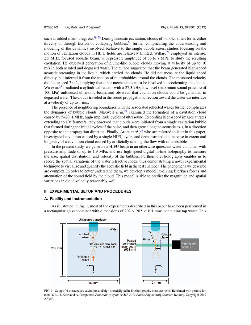
As illustrated in Fig. 1, most of the experiments described in this paper have been performed ina rectangular glass container with dimensions of 202 × 202 × 101 mm3 containing tap water. This

FIG. 1. Setups for the acoustic cavitation and high-speed digital in-line holography measurements. Reprinted with permissionfrom Y. Lu, J. Katz, and A. Prosperetti, Proceedings of the ASME 2012 Fluids Engineering Summer Meeting. Copyright 2012ASME.

073301-3 Lu, Katz, and Prosperetti Phys. Fluids 25, 073301 (2013)

chamber is open to the air on the top, and the water is initially quiescent. With a free interface, thewater is most likely saturated with non-condensable gases. Furthermore, the tap water is not filteredand, consequently, most likely contains abundant cavitation nuclei. Indeed, the images describedlater revealed occasional presence of some <10 μm particles in the sample volume. The HIFUtransducer, manufactured by Sonic Concepts, is positioned at the center of the top of the tank,with its radiating surface immersed in the water. This custom designed transducer operates at afixed frequency f = 500 kHz, and has a maximum input power Pin = 400 W. The correspondingwavelength λ, for a sound speed c0 of 1500 m/s in water at 20 ◦C, is 3 mm. The transducer has aconcave radiating surface with diameter drs of 33 mm, which focuses the ultrasonic beam to a zonelocated 64 mm away from its surface. The focal zone is an approximately cylindrical volume with adiameter df = 5.8 mm and a length of 42 mm, as provided by the manufacturer and confirmed by ourmeasurements (see below). The 500 kHz sinusoidal signal is generated using a function generator(Agilent Technologies, model No. 33220A). The signal is amplified by a 200 W RF power amplifier(Electronics & Innovation model No. 1020L), and monitored using a power meter (Sonic Concepts,model No. 22A). The signal is fed into a matching network, also manufactured by Sonic Concepts,and then into the transducer. At high power levels, the temperatures of the transducer itself and ofthe liquid in the focal zone increase rapidly. To prevent damage to the transducer and generationof thermally induced Rayleigh–Benard convection in the liquid, the transducer was operated in apulsed mode, each pulse lasting less than 2 s. The interval between two subsequent pulses wasseveral minutes and long enough to allow the liquid to return to the quiescent condition. Everyfew pulses, the bubbles accumulating on the transducer’s surface are removed to eliminate possibleadverse effects on the ultrasonic waves.

A substantial fraction of the data acquisition about the bubble cloud characteristics as wellas the sound field involves application of digital holography. Unlike conventional photography, ahologram is a record of the interference of the coherent light scattered from objects with a referencebeam. Consequently, it not only contains information on light intensity propagating from illuminatedobjects, but also the phase of this light field.27 Numerical reconstruction of the holograms at varyingdepths brings the objects, such as particles, bubbles, etc., into focus, enabling us to measure their size,shape, and spatial distribution.28–33 For the present application, we employ digital in-line holographyusing the optical setup illustrated in Fig. 1. Due to the rapid motion of the bubble clouds (velocities ofthe order of m/s), the light source is a Q-switched pulsed 523 nm (green) laser (CrystaLaser), whichgenerates up to 0.1 mJ/pulse, each with a duration of 10–20 ns, at a rate of up to 20 kHz. The laserbeam is collimated and illuminates the volume of interest, mostly in the focal zone of the ultrasonicbeam. The holograms are recorded using a high-speed CMOS camera (Photron FASTCAM-UltimaAPX), which can record 2000 f/s at full resolution of 1024 × 1024 pixels and up to 30 000 f/s ata resolution of 256 × 128 pixels. The magnification varies from 1:1, for which the resolution is17 μm/pixel, to 5:1, for which the resolution is 3.4 μm/pixel. Numerical reconstruction is performedusing in-house developed software.27 In addition to digital holography, we have also recorded imagesof the bubble fields using white light for illumination. The optical setup is identical to that shownin Fig. 1, except that the laser beam is replaced with a continuous incandescent light source. In thiscase, the exposure time can be controlled by the camera, but we have used full exposure times forimages shown in this paper, i.e., ∼33 μs at 30 000 f/s, and ∼166 μs at 6000 f/s.

B. Visualization and measurement of the HIFU pressure field

This section describes the method used to visualize the pressure field and to quantitativelycharacterize the pressure in the focal zone of the ultrasonic beam. The pressure wave in the focalzone is nearly one-dimensional and can be expressed as

p(x, t) = p0 + p′(x, t), (1)

where p0 and p′ are the undisturbed and acoustic pressures, respectively. The acoustic pressure canbe modeled as the sum of incident p′

in and reflected p′re waves

p′(x, t) = p′in(x, t) + p′

re(x, t) = pf sin(kx − ωt) + CR pf sin(kx + ωt + ς ). (2)

073301-4 Lu, Katz, and Prosperetti Phys. Fluids 25, 073301 (2013)

FIG. 2. Visualization and quantification of the focal zone of the ultrasonic wave; pf = 1.44 MPa. (a) A sample hologramshowing the instantaneous acoustic wave. The bright bands correspond to high pressure. (b) The distribution of the rmsgray levels, showing the partial standing wave structure. Reprinted with permission from Y. Lu, J. Katz, and A. Prosperetti,Proceedings of the ASME 2012 Fluids Engineering Summer Meeting. Copyright 2012 ASME.

Here k = 2π /λ is the wave number, ω = 2π f is the angular frequency, pf is the amplitude of theincident wave, and ς is a phase lag. To account for the attenuation of the reflected wave and thedefocusing of the reflected wave, we multiply its amplitude by a reflection coefficient CR, 0 < CR <

1. The magnitude of pf can be estimated from the input power and the efficiency (η = 0.85) of theHIFU system, as provided by the manufacturer. The resulting acoustic intensity at the transducer’sradiating surface is Irs = ηPin/(πdrs

2 / 4), and the acoustic pressure on the surface is prs = (2IrsZ)1/2,where Z is the acoustic impedance of water. The manufacturer specifies that the intensity gain inthe focal zone is g = 2.51, and the incident pressure amplitude in the focal zone is therefore pf

= gprs. For example, at Pin = 5 W, pf = 306 kPa, while at Pin = 110 W, pf = 1.44 MPa, and atPin = 200 W, pf = 1.94 MPa.

One can also estimate the amplitude of the acoustic field from the changes to the water density.The substantial pressure fluctuations in the focal zone cause detectable variations in the densityand the refractive index n of the water. When an initially collimated light beam passes throughthe spatially varying refractive index field, the beam alters its direction of propagation. Due to thisangular deviation of the laser beam, the holograms formed on the focus plane of the imaging lens,placed at a distance H from the center of the acoustic focal zone, contain non-uniform shadowgraphicpatterns. A sample hologram showing the instantaneous (averaged over the duration of the laser pulseof 10–20 ns) light intensity distribution for Pin = 110 W is presented in Fig. 2(a). The spatial intensityvariations of the light field are related to the Laplacian of the refractive index on a plane normal tothe light axis34

I ′z=H

I0

�= Iz=H − I0

I0= −H

∫ df/2

−d f/2(∇⊥2n)dz, (3)

where I0 is the undisturbed intensity and I is the intensity recorded at a distance z from the center ofthe acoustic beam (see Fig. 1). Assuming that the liquid density and refractive index vary mainly inthe acoustic propagation direction, ∇⊥2n is reduced to d2n/dx2 and

∫ df/2−df/2 (∇⊥2n)dz = (d2n/dx2)df .

Using a first order approximation for n = n(ρ), d2n/dx2 = (dn/dρ)(d2ρ/dx2). The quantity dn/dρ isa constant that can be determined from the Lorenz-Lorentz relation:34

n2 − 1

n2 + 2

1

ρ= C, (4)

073301-5 Lu, Katz, and Prosperetti Phys. Fluids 25, 073301 (2013)

where C is a constant that depends on the wavelength of the laser, properties of the liquid, temperature,and pressure. For a 523 nm laser wavelength at 20 ◦C and atmospheric pressure, C = 2.1 × 10−4

m3/kg.35 Finally, using a first order approximation, p′ = ρ ′c02, the acoustic pressure can be expressed

in terms of the light intensity

p′(x, t) = c2

(dn/dρ)k2df H

I ′(x, t)

I0. (5)

In the present experimental configuration, therefore, the acoustic pressure is proportional to the lightintensity passing through the focal zone, and can be estimated from the distribution of light intensity(gray level) in the holograms. The bright bands indicate locally high pressure (p′ > 0) since the lightconverges, and thus brighter (I′ > 0) in regions of high refractive index [see Fig. 2(a)].

In a partially standing wave, there are no true pressure nodes since there are no points wherethe rms pressure prms is zero. However, for convenience, we still choose to call the regions withminimum prms as “nodes” and those with maximum prms as “antinodes.” For the acoustic pressurefield defined in Eq. (2), prms = pf{0.5[1 + CR

2 − 2CR cos(2kx + ς )]}1/2. The reflection coefficientcan be obtained from CR = (prms

max − prmsmin) / (prms

max + prmsmin), taking advantage of aliasing

(variations in phase of instantaneous frames) caused by the mismatch between the acoustic frequencyand sampling rate. Using Eq. (5), prms can be replaced with the rms gray level (Irms) for each pixel,i.e.,

CR = I rmsmax − I rms

min

I rmsmax + I rms

min. (6)

The distribution of Irms for Pin = 110 W is shown in Fig. 2(b), for which I rmsmax = 21.7, I rms

min

= 13.1, based on averaging along the central line of several antinodes and nodes, and thus CR =0.25.

Using CR, Irms, and df provided by the manufacturer, as well as Eq. (5), the estimated amplitudeof the incident ultrasonic wave is pf = 1.32 MPa. This result differs by about 10% from the previouslymentioned amplitude calculated from information provided by the manufacturer (pf = 1.44 MPa).Figure 2(b) also confirms that the width of the focal zone is consistent with the information providedby the manufacturer (df = 5.8 mm). The distribution the rms levels indicates that 2.9 mm from thecenter of the focal zone, the rms level is 6 dB below the peak level.

III. RESULTS

A. Annular bubble structures in the periphery of the focal zone

This paper deals primarily with cavitation in the focal zone of the transducer, the topic covered inSec. III B. However, as background, it is of interest to summarize briefly the behavior of bubbles in thevicinity of, but outside, the focal zone as well. After being generated, bubbles subjected to acousticexcitation falling below the cavitation level are expected to grow by rectified diffusion.36 Such gasbubbles cannot survive in the focal zone, where the acoustic pressure is too high.37 Consequently,the phenomena described in this section occur outside of the focal zone at all transducer soundlevels. Two sample images recorded at low sound levels, using white light, are presented in Fig. 3.Figure 3(a) is a vertical plane view showing that the bubbles accumulate in layers separated by λ/2under the action of the primary Bjerknes forces. Figure 3(b) is a top (y-z) view showing that thebubbles are concentrated in circular ring surrounding, but clearly outside, the focal zone. This imagewas recorded in a smaller chamber during early experiments, in which the transducer was installedat the bottom of the facility, allowing observations from the top. The same phenomena occurred inthe chamber illustrated in Fig. 1.

The resonant radius of gas bubbles at the transducer’s frequency and atmospheric pressure isabout 5.9 μm. This radius is smaller than that of the bubbles in Fig. 3(a) implying, on the basis oflinear theory of the primary Bjerknes force, that the bubbles in this image are attracted to the nodesof the partial standing wave.18 Furthermore, the secondary Bjerknes forces among these bubbles areattractive.38 Therefore, adjacent bubbles tend to move toward each other, coalesce, and form biggerbubbles. These processes are evident in the high-speed movies, and the larger bubbles in Fig. 3(a),

073301-6 Lu, Katz, and Prosperetti Phys. Fluids 25, 073301 (2013)

FIG. 3. (a) Annular bubble layers in the pressure nodes at low sound intensity (pf = 306 kPa) recorded using white lightillumination.26 (b) A top-view of an early test chamber showing that the bubbles accumulate in the periphery of the focalzone (denoted with dashed circle). Reprinted with permission from Y. Lu, J. Katz, and A. Prosperetti, Proceedings of theASME 2012 Fluids Engineering Summer Meeting. Copyright 2012 ASME.

which vary in size between 100 and 250 μm, are the result of the coalescence of several small ones.The secondary Bjerknes force also causes bubbles smaller than about 20 μm to rapidly jitter andorbit around bigger ones. When the sound is turned off, all the bubbles rise toward the free surfacedue to buoyancy.

B. Cloud cavitation

At high sound levels (pf ≥ 1.2 MPa), cavitation inception occurs near the axis of the acousticbeam, predominantly within, but also upstream of, the focal zone. The resulting bubble clouds, whichare described below, travel at velocities of up to 4 m/s in the direction of the incident ultrasonicwave. This velocity is several orders of magnitude larger than the acoustically induced streaming,which was measured by tracking seeded micro-particles in the same facility, as well as by ParticleImage Velocimetry (PIV) in the previously mentioned small chamber, which could be pressurizedto prevent cavitation. These PIV measurements involved illumination of a non-cavitating focal zonewith a pulsed Nd:YAG laser sheet, and seeding of the flow with 11 μm hollow glass spheres witha specific gravity of 1.1. The results, obtained using standard data analysis procedures,39 revealedthat acoustic streaming generated velocities ranging between 2 and 8 mm/s (not shown), orders ofmagnitude smaller than the cavitation bubble cloud velocity. We do not show these PIV results sincethey are not relevant to the phenomena described below.

Two examples of superpositions of high-speed images demonstrating the initial formation andmigration of clouds for two sound levels are presented in Fig. 4. These images were recorded at30 000 f/s, at a resolution of 256 × 128 pixel, using white light illumination, and frames weresuper-imposed without any additional processing, enhancement, or relative translation (except fortrimming their sides). In each original frame, the cloud appears once, and the superposition shows thelocation and changes in size of the same cloud as it progresses along the direction of the ultrasonicbeam. The top cavitation “blob” in each image shows how the cavitation appears in the first framein which it becomes visible. Once cavitation inception occurs, the cavitation persists, namely, thecloud does not disappear for periods that vary between hundreds to thousands of acoustic cycles. InFigs. 4(a) and 4(c) we omit some of the frames (but not the first one) to make the ones displayedclearer, whereas the corresponding Figs. 4(b) and 4(d) contain all the frames with cavitation until thecavitation cloud leaves the field of view. In the following description, we separate the discussion onthe appearance of cavitation at moderate pressures, of which Figs. 4(a) and 4(b) are representatives,and at high pressures, of which Figs. 4(c) and 4(d) are representative.

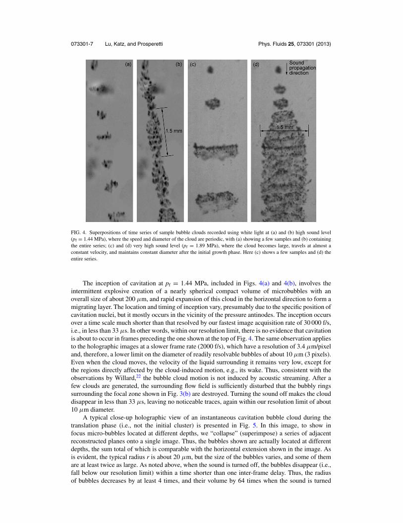
073301-7 Lu, Katz, and Prosperetti Phys. Fluids 25, 073301 (2013)

FIG. 4. Superpositions of time series of sample bubble clouds recorded using white light at (a) and (b) high sound level(pf = 1.44 MPa), where the speed and diameter of the cloud are periodic, with (a) showing a few samples and (b) containingthe entire series; (c) and (d) very high sound level (pf = 1.89 MPa), where the cloud becomes large, travels at almost aconstant velocity, and maintains constant diameter after the initial growth phase. Here (c) shows a few samples and (d) theentire series.

The inception of cavitation at pf = 1.44 MPa, included in Figs. 4(a) and 4(b), involves theintermittent explosive creation of a nearly spherical compact volume of microbubbles with anoverall size of about 200 μm, and rapid expansion of this cloud in the horizontal direction to form amigrating layer. The location and timing of inception vary, presumably due to the specific position ofcavitation nuclei, but it mostly occurs in the vicinity of the pressure antinodes. The inception occursover a time scale much shorter than that resolved by our fastest image acquisition rate of 30 000 f/s,i.e., in less than 33 μs. In other words, within our resolution limit, there is no evidence that cavitationis about to occur in frames preceding the one shown at the top of Fig. 4. The same observation appliesto the holographic images at a slower frame rate (2000 f/s), which have a resolution of 3.4 μm/pixeland, therefore, a lower limit on the diameter of readily resolvable bubbles of about 10 μm (3 pixels).Even when the cloud moves, the velocity of the liquid surrounding it remains very low, except forthe regions directly affected by the cloud-induced motion, e.g., its wake. Thus, consistent with theobservations by Willard,22 the bubble cloud motion is not induced by acoustic streaming. After afew clouds are generated, the surrounding flow field is sufficiently disturbed that the bubbly ringssurrounding the focal zone shown in Fig. 3(b) are destroyed. Turning the sound off makes the clouddisappear in less than 33 μs, leaving no noticeable traces, again within our resolution limit of about10 μm diameter.

A typical close-up holographic view of an instantaneous cavitation bubble cloud during thetranslation phase (i.e., not the initial cluster) is presented in Fig. 5. In this image, to show infocus micro-bubbles located at different depths, we “collapse” (superimpose) a series of adjacentreconstructed planes onto a single image. Thus, the bubbles shown are actually located at differentdepths, the sum total of which is comparable with the horizontal extension shown in the image. Asis evident, the typical radius r is about 20 μm, but the size of the bubbles varies, and some of themare at least twice as large. As noted above, when the sound is turned off, the bubbles disappear (i.e.,fall below our resolution limit) within a time shorter than one inter-frame delay. Thus, the radiusof bubbles decreases by at least 4 times, and their volume by 64 times when the sound is turned

073301-8 Lu, Katz, and Prosperetti Phys. Fluids 25, 073301 (2013)

FIG. 5. A close-up view of the inner structure of a bubble cloud; pf = 1.44 MPa. This picture is generated by collapsing aseries of reconstructed holograms from different depths onto a single plane.

off. It may therefore be estimated that the volume fraction of non-condensable gas in the bubblesduring the acoustic radiation is less than 1/64 (∼2%). This estimate neglects the mass diffusion ofnon-condensable gas out of the bubble between exposures, whose dissolution would take a longertime. This observation confirms that the bubbles in the cloud contain very little non-condensablegas. These bubbles, therefore, contain mostly water vapor. Consequently, in Secs. IV and V, inwhich we develop a model for the behavior of the cloud, we assume that the bubbles within thecavitation cloud contain only vapor. However, these bubbles do not collapse/disappear completelyduring the compression phase as long as the sound is turned on, presumably since the short durationof compression (2 μs) prevents them from condensing completely, allowing them to actually growin subsequent cycles. In contrast, the bubbles within the rings surrounding the acoustic focal zone(Sec. III A), which grow by rectified diffusion, contain mostly non-condensable gas. Accordingly,they do not disappear when the sound is turned off and rise by buoyancy.

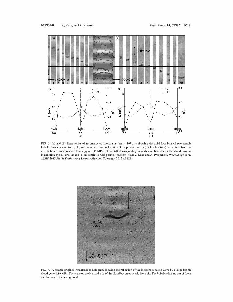
In general, the cloud size increases with acoustic pressure and its dynamics are found to becorrelated with its diameter and location relative to the sound field. When pf < 1.68 MPa, thecharacteristic diameter of the cloud is smaller than λ/3. In this case, the cloud periodically expandswhile decelerating and contracts while accelerating. These size variations are evident in Figs. 4(a)and 4(b). Quantitative examples of the changes in velocity and cloud size during the translation phaseare provided in Fig. 6. Figures 6(a) and 6(b) present two series of reconstructed holographic imagesof clouds, highlighting the changes in their size and location relative to the nodes and antinodes ofthe acoustic field. Here, the progression of the two clouds is presented in separate frames showing thelocation and timing of each image. Both clouds slow down and increase in size near the nodes of thepartial standing wave, as well as accelerate and shrink in the vicinity of the antinodes. Correspondinginformation on the cloud velocity and diameter is provided in Figs. 6(c) and 6(d). On the other hand,once formed, the thickness of the clouds fluctuates, but does not show a clear correlation with thestructure of the partial standing wave. Increasing the magnification of the holograms enables us toresolve the spatial distribution of bubbles within the cloud, as illustrated before in Fig. 5.

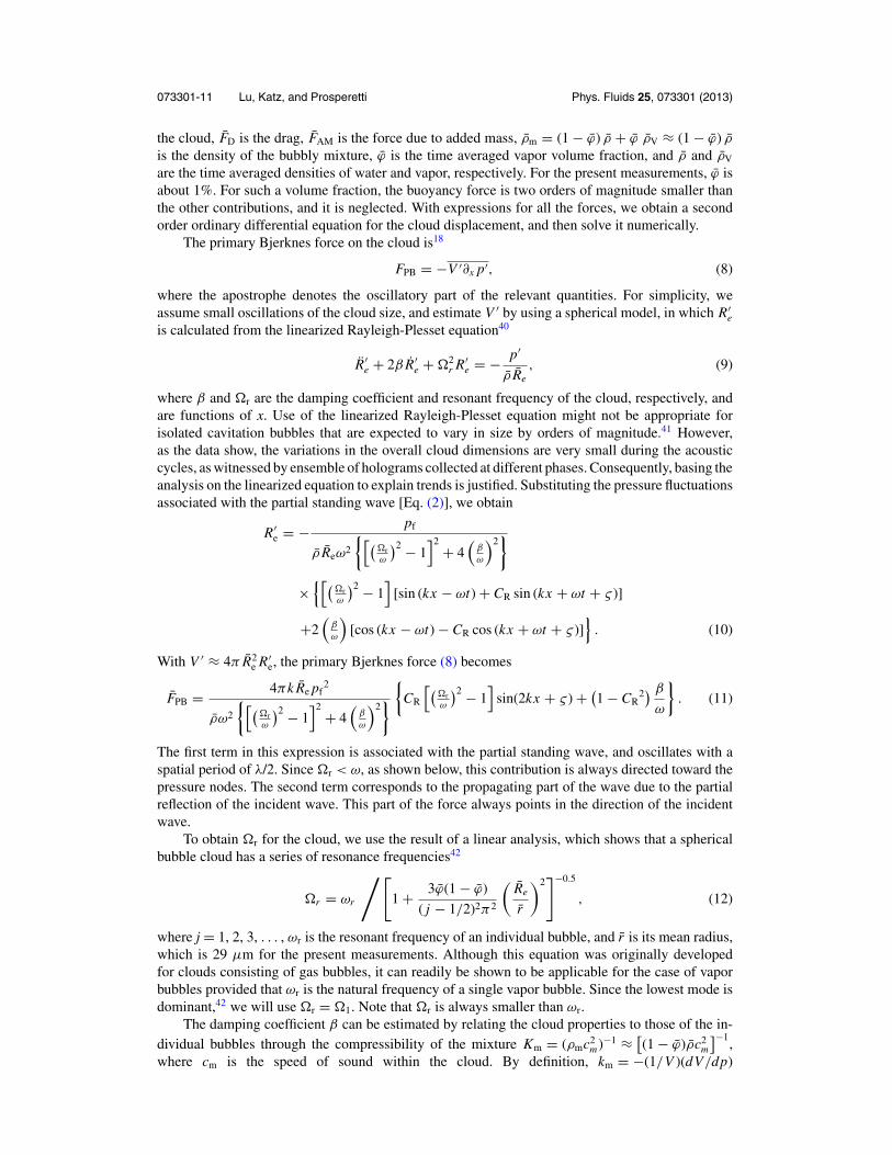
For pf ≥ 1.68 MPa, e.g., pf = 1.89 MPa, cavitation inception still appears as a ∼200 μm clusterof bubbles, as the top images in Figs. 4(c) and 4(d) demonstrate. Subsequently, the diameter ofsome of the clouds becomes comparable and even larger than λ/2, and they appear as flat disks withvarying thickness. In this case, after the initial growth phase, once the cloud reaches its maximumsize, its speed and diameter do not change significantly. The unreconstructed (i.e., original) hologramin Fig. 7 is an extreme example of a flattened thin layer of cavitation bubbles at high sound levels,

073301-9 Lu, Katz, and Prosperetti Phys. Fluids 25, 073301 (2013)

FIG. 6. (a) and (b) Time series of reconstructed holograms (�t = 167 μs) showing the axial locations of two samplebubble clouds in a motion cycle, and the corresponding location of the pressure nodes (thick solid-lines) determined from thedistribution of rms pressure levels; pf = 1.44 MPa. (c) and (d) Corresponding velocity and diameter vs. the cloud locationin a motion cycle. Parts (a) and (c) are reprinted with permission from Y. Lu, J. Katz, and A. Prosperetti, Proceedings of theASME 2012 Fluids Engineering Summer Meeting. Copyright 2012 ASME.

FIG. 7. A sample original instantaneous hologram showing the reflection of the incident acoustic wave by a large bubblecloud; pf = 1.89 MPa. The wave on the leeward side of the cloud becomes nearly invisible. The bubbles that are out of focuscan be seen in the background.

073301-10 Lu, Katz, and Prosperetti Phys. Fluids 25, 073301 (2013)

with a diameter as large as λ. We present an original hologram to show the cloud shape as wellas the signature of the acoustic field. Here, the amplitude of the acoustic wave on the “leeward”side of the cloud is much weaker than that on its “windward” side. This observation indicates thatthere is little transmission of sound through the cloud. Furthermore, the amplitude of the wave onthe acoustic windward side appears to be higher than that in the surrounding fluid, suggesting apartial reflection of the sound wave, which constructively interferes with the incident wave. Thesetrends imply that the weakening of the sound transmission eliminates the partial standing wave,and with it, the periodic variations in the cloud size and velocity. To confirm this statement, wecovered the bottom of the test chamber with fiber bristles in order to attenuate the sound reflection.Indeed, irrespective of the incident sound level, the periodic variations in the cloud velocity and sizedisappeared, supporting our hypothesis that both of them are caused by the partial standing wave.In Secs. IV and V, we develop a model that explains the periodic behavior of the bubble clouds.

Several comments should be made before concluding this observation section: First, like mostcavitation phenomena, the onset of cavitation depends on the presence of cavitation nuclei. Wedid not measure the nuclei concentration, but since our experiments were performed using tapwater saturated with non-condensable gases, this water was most likely rich with nucleation sites.However, one should keep in mind that the “strength” of the water increases with frequency, andonly micron size bubbles would become active at a frequency of 500 kHz. This fact may explainthe intermittent occurrence of cavitation inception in our experiments in spite of the high pressurepeaks. Second, phenomena relevant to the present findings were reported by Arora et al.25 Theyinvestigated cavitation caused by a single pulse involving ∼10 MPa tension for ∼2 μs, with andwithout artificial seeding of nuclei—phospholipid shelled, 2.5 μm diameter bubbles, and in waterdegassed to 30% of the saturation level. The amplitude of the present pressure pulses was 5–7 timessmaller, but the cycle duration was comparable. They also showed that cavitation was confined to thefocal zone of the acoustic beam irrespective of the nuclei concentration. Without artificial seeding,few traces of their bubble cloud remained after 165 μs, and they disappeared completely after265 μs. This rapid cloud disappearance was consistent, at least to within an order of magnitude,with the present observations, in which the cloud disappeared after 33 μs, presumably due to themarked differences in amplitude. To achieve cavitation that persisted for longer periods, Arora et al.had to introduce the abovementioned artificial nuclei. Their measurements confirmed that the spatialextent within the focal zone, concentration, and “longevity” (duration of time that they existed afterthe shock) of the cavitation increased substantially upon introduction nuclei.

IV. A MODEL FOR THE AXIAL MOTION OF THE BUBBLE CLOUD

The cloud appears as a pancake-like mixture of bubbles and water, with volume of V = π R2S,where R and S are its radius and thickness, respectively. However, some of its features are moreeasily estimated by approximating it as a sphere with an equivalent radius of Re = (3S / 4R)1/3R.The velocity of the cloud is three orders of magnitude lower than the speed of sound in water,i.e., the associated time scales are very different. Consequently, it is reasonable to perform ananalysis of the cloud dynamics, averaging over many acoustic cycles, but allowing time and cloudproperties to vary on the time scale of cloud translation. The motion of the cloud is assumed to beone-dimensional, along the direction of sound propagation. In addition, we assume that the cloudcontains uniformly distributed bubbles that are much smaller than the cloud size, and consequently,we treat it as a homogeneous medium. Internal interactions among the bubbles, e.g., by secondaryBjerknes forces, are also neglected. Gravity is neglected, consistent with its small magnitude relativeto the acoustic pressure gradients. Subject to these assumptions, an equation of motion for the cloudcan be formulated by combining the forces associated with its translation, namely added mass anddrag, with the acoustic forces, i.e., the primary Bjerknes force and the force resulting from loss ofmomentum of the acoustic beam due to attenuation

FPB + FAtt + FD + FAM = ρmV x, (7)

where the overbar denotes time averaging, dots denote time derivatives with respect to the cloudtime scale, FPB is the primary Bjerknes force, FAtt is the propulsive force due to sound attenuation in

073301-11 Lu, Katz, and Prosperetti Phys. Fluids 25, 073301 (2013)

the cloud, FD is the drag, FAM is the force due to added mass, ρm = (1 − ϕ) ρ + ϕ ρV ≈ (1 − ϕ) ρ

is the density of the bubbly mixture, ϕ is the time averaged vapor volume fraction, and ρ and ρV

are the time averaged densities of water and vapor, respectively. For the present measurements, ϕ isabout 1%. For such a volume fraction, the buoyancy force is two orders of magnitude smaller thanthe other contributions, and it is neglected. With expressions for all the forces, we obtain a secondorder ordinary differential equation for the cloud displacement, and then solve it numerically.

The primary Bjerknes force on the cloud is18

FPB = −V ′∂x p′, (8)

where the apostrophe denotes the oscillatory part of the relevant quantities. For simplicity, weassume small oscillations of the cloud size, and estimate V ′ by using a spherical model, in which R′

eis calculated from the linearized Rayleigh-Plesset equation40

R′e + 2β R′

e + �2r R′

e = − p′

ρ Re, (9)

where β and �r are the damping coefficient and resonant frequency of the cloud, respectively, andare functions of x. Use of the linearized Rayleigh-Plesset equation might not be appropriate forisolated cavitation bubbles that are expected to vary in size by orders of magnitude.41 However,as the data show, the variations in the overall cloud dimensions are very small during the acousticcycles, as witnessed by ensemble of holograms collected at different phases. Consequently, basing theanalysis on the linearized equation to explain trends is justified. Substituting the pressure fluctuationsassociated with the partial standing wave [Eq. (2)], we obtain

R′e = − pf

ρ Reω2

{[(�rω

)2 − 1]2

+ 4(

β

ω

)2}

×{[(

�rω

)2 − 1]

[sin (kx − ωt) + CR sin (kx + ωt + ς )]

+2(

β

ω

)[cos (kx − ωt) − CR cos (kx + ωt + ς)]

}. (10)

With V ′ ≈ 4π R2e R′

e, the primary Bjerknes force (8) becomes

FPB = 4πk Re pf2

ρω2

{[(�rω

)2 − 1]2

+ 4(

β

ω

)2} {CR

[(�rω

)2 − 1]

sin(2kx + ς ) + (1 − CR2) β

ω

}. (11)

The first term in this expression is associated with the partial standing wave, and oscillates with aspatial period of λ/2. Since �r < ω, as shown below, this contribution is always directed toward thepressure nodes. The second term corresponds to the propagating part of the wave due to the partialreflection of the incident wave. This part of the force always points in the direction of the incidentwave.

To obtain �r for the cloud, we use the result of a linear analysis, which shows that a sphericalbubble cloud has a series of resonance frequencies42

�r = ωr

/[1 + 3ϕ(1 − ϕ)

( j − 1/2)2π2

(Re

r

)2]−0.5

, (12)

where j = 1, 2, 3, . . . , ωr is the resonant frequency of an individual bubble, and r is its mean radius,which is 29 μm for the present measurements. Although this equation was originally developedfor clouds consisting of gas bubbles, it can readily be shown to be applicable for the case of vaporbubbles provided that ωr is the natural frequency of a single vapor bubble. Since the lowest mode isdominant,42 we will use �r = �1. Note that �r is always smaller than ωr.

The damping coefficient β can be estimated by relating the cloud properties to those of the in-dividual bubbles through the compressibility of the mixture Km = (ρmc2

m)−1 ≈ [(1 − ϕ)ρc2m

]−1,

where cm is the speed of sound within the cloud. By definition, km = −(1/V )(dV/dp)

073301-12 Lu, Katz, and Prosperetti Phys. Fluids 25, 073301 (2013)

= −(3/Re)(d R′e/dp′), and d R′

e/dp′ can be obtained from the solution to Eq. (9), R′e =

−p′ /{ρ Reω2[(

�rω

)2 − 1 + i2( β

ω)]}

, where i = √−1. By taking the real part [denoted with R{}]

of d R′e/dp′, we have

Km = − 3

Re{

d R′e

dp′

}=

3[(

�rω

)2 − 1]

ρ Re2ω2

{[(�rω

)2 − 1]2

+ 4(

β

ω

)2} . (13)

The complex sound speed in a bubbly mixture containing either gas or vapor bubbles is given by43

1

c2m

= 1

c20

+ 3ϕ

r2ω2[(

ωrω

)2 − 1 + i2( bω

)] , (14)

where b is the damping coefficient of an individual bubble. Since (1 − ϕ)ρKm ≈ {1/c2m

},

β = ω

2

⎧⎪⎪⎨⎪⎪⎩

3 (1 − ϕ)(

rRe

)2

(rωc0

)2 /[(�rω

)2 − 1]

+ 3ϕ

/([(ωrω

)2 − 1]2

+ 4(

bω

)2) −[(

�rω

)2 − 1]2

⎫⎪⎪⎬⎪⎪⎭

1/2

.

(15)The expressions of ωr and b of a linearly oscillating vapor bubble are provided in Ref. 44:

ωr =[

1

ρr2

(3 {K } − B� {K }

|K |2 − 2σ

r

)]1/2

(16)

and

b = 3

2ωρr2

� {K } + B {K }|K |2 , (17)

where�{} denotes the imaginary part, σ is the surface tension, and K is the complex compressibilityof a vapor bubble

K = 1

γ pb

+3cs

L

(γ − 1

γ

Ts

pb− dTs

dp

)⎡⎣ Dv

iωr2−√

Dv

iωr2coth

⎛⎝√

iωr2

Dv

⎞⎠⎤⎦

− i3κw

ρvLωr2

⎛⎝1 +

√iωr2

Dw

⎞⎠ dTs

dp, (18)

B = 2κw

ρvL Dw

dTs

dp

2Dw

ωr2

(p0 − pV + 2σ

r

)⎡⎣1 − 3G

⎛⎝√

ωr2

2Dw

⎞⎠⎤⎦ , (19)

and

G(w) = w4∫ ∞

0

exp [−(1 + i)s]

(w + s)5ds. (20)

In the above expressions, γ is the ratio of the specific heats, cs is the specific heat of the vapor alongthe saturation line, L is the latent heat, Ts is the mean temperature at the vapor-water interface, pb

is the mean pressure in the bubble, dTs/dp ≈ Ts / (LρV ), DV and DW are the thermal diffusivityof vapor and water, respectively, κW is the thermal conductivity of water, and �p is the differencebetween the liquid static pressure and the saturation pressure. For the current case, 2DW / (ωr )2

= 2.2 × 10−4, which is much smaller than unity. As a result, B is negligible and the calculation can

073301-13 Lu, Katz, and Prosperetti Phys. Fluids 25, 073301 (2013)

be greatly simplified.44, 45 Using the current parameters, ωr = 0.12ω and b = 0.072 ω, and as a result,�r [Eq. (12)] is at least an order of magnitude smaller than ω. All the terms needed for calculatingβ [Eq. (15)] and FPB [Eq. (11)] are now available.

Next, we estimate the propulsive force due to sound attenuation in the cloud, FAtt. Attenuationof sound in bubble clouds has been investigated extensively.43, 46 Such attenuation causes streamwisegradients in the associated normal Reynolds stress and, consequently, a streamwise force, much likein acoustic streaming.47, 48 For a bubbly cloud, the magnitude of this force is

FAtt = π R2ρ�u′2. (21)

Here u′ is the acoustically induced liquid velocity and � denotes the difference across the cloud. Fora linear acoustic wave, the velocity fluctuation on the acoustic windward side of the cloud is u′

wind= [p′

in − p′re exp (−αS)

]/ (ρc0), and on the leeward side is u′

lee = [p′in exp (−αS) − p′

re

]/ (ρc0),

where α is the attenuation coefficient across the cloud. In this estimate, we assume that the cloud issmall enough that the local sound diffraction by it does not affect the overall strength of the reflectedwave. Substituting Eq. (2) for the pressure, and time averaging, we obtain

FAtt =(

1 − e−2α S) (

1 − C2R

)p2

f π R2

2ρc20

. (22)

The attenuation coefficient is calculated from the complex sound speed in a bubbly mixture29

α = −ω�{

1

cm

}. (23)

Using Eq. (14), and the present conditions, we obtain α = 8.47 × 103 1/m and exp ( − αS) = 0.034for a characteristic cloud thickness of 200 μm, so that the wave is substantially attenuated acrossthe cloud.

The drag force on the cloud is

FD = − 12 CDρπ R2 x2, (24)

where CD is the drag coefficient. For a wide range of Reynolds numbers, the drag coefficient of acircular disk is essentially unity.49 Finally, we estimate the force due to the added mass by simplyassuming that the cloud is a sphere with an equivalent radius, i.e.,

FAM = −madd x = − 23 ρπ R3

e x . (25)

Use of an added mass for a thin disk with the same radius R, which would over-estimate theadded mass, would about double this force.50 Using the derived expressions for the forces, and achange of variables to X = x + ς

2k in order to eliminate the irrelevant phase lag ς , we obtain thefollowing nonlinear second order differential equation:

X = − CD

2 (1.5 − ϕ) SX2

+ 4kp2f Re

(1.5 − ϕ) ρ2ω2 R2 S

CR

[(�rω

)2 − 1]

sin X + (1 − C2R

)β /ω{[(

�rω

)2 − 1]2

+ 4(

β

ω

)2}

+(

1 − e−2α S) (

1 − C2R

)p2

f

2 (1.5 − ϕ) ρ2c20 S

. (26)

To estimate the cloud motion, we use the experimental observation that R(X ) os-cillates nearly harmonically in space and, as a result, we estimate it as R(X )= 0.5

[(Rmax − Rmin

)cos 2k X + (Rmax + Rmin

)]. Based on the average dimensions of 30 clouds,

we use Rmax = 350 μm and Rmin = 100 μm as the characteristic maximum and minimum radius,respectively. The thickness does not show a clear correlation with the partial standing wave, and

073301-14 Lu, Katz, and Prosperetti Phys. Fluids 25, 073301 (2013)

FIG. 8. (a) A comparison between the measured and predicted [Eq. (26)] bubble cloud velocity. The error bars indicate thestandard deviation of the measured values. (b) The predicted total force and its components; pf = 1.44 MPa.

seems to fluctuate about some mean value. For the calculation, we use the average thickness ofthe 30 clouds, S = 200 μm. With the initial conditions X (0) = λ/4, X (0) = 0, since cavitationinception typically occurs in the pressure antinodes, Eq. (26) is solved using the MATLAB solver“ode45.” Figure 8(a) shows the “steady-state” solution for pf = 1.44 MPa, and compares it to themeasured cloud velocity averaged over 30 clouds. The model reproduces the correct magnitudeof cloud velocity, but there is a phase difference. In the case of a big cloud (R = 1.5 mm, pf

= 1.89MPa), for which CR = 0, the model predicts a constant steady-state velocity of 1.36 m/s (afterthe initial acceleration), which is 12% lower than the averaged observed value (1.54 m/s).

Figure 8(b) shows the variations of calculated forces normalized using the predicted meanvelocity and characteristic mean radius. In the vicinity of the nodes the total force is negative,and thus decelerating the cloud there. The primary Bjerknes force and the drag contribute to thisdeceleration, while the attenuation force and added mass are positive. Although the latter are small,without the attenuation and added mass, the cloud would not have enough inertia to escape from thenodes, and would be trapped there. Near the antinodes, the primary Bjerknes force propels the cloud.Before concluding this section, it should be noted that we have performed the previous analysisalso for a cylindrical cloud with the measured radius and height. It adds extra complexity to theexpressions involved, but does not alter the predicted trends so significantly to warrant presentationof both results.

V. MECHANISMS AFFECTING THE BUBBLE CLOUD SIZE

In Sec. IV, the measured variations in cloud size were used as an input. In this section, wediscuss possible mechanisms affecting the periodic contraction and expansion of the smaller clouds.In general, one would expect that once cavitation inception occurs, persistent exposure to theacoustic field would increase the cavitation activity, as the bubbles collapse and fragment, thusincreasing the nuclei population. In contrast, the observed spatial extent of the cloud remains confinedand, furthermore, it shrinks near the pressure antinodes, where the pressure fluctuations peak. Apossible mechanism for these trends involves interactions among bubbles, such as the secondaryBjerknes force,38 namely, the force on a bubble resulting from the pressure field generated by volumeoscillations of all the other bubbles in a cloud.

It is well known that the secondary Bjerknes force between two equal bubbles, according tolinear theory, is attractive both when the bubbles are driven above and below the resonance frequency.The theory gives this force in the form38

FSB = − ρ

4π l2v′

1v′2, (27)

where v′1 and v′

2 are the oscillating bubble volumes, and l is the distance between them. To estimatethis force, we assume that the two bubbles have the same equilibrium radius, which is larger than the

073301-15 Lu, Katz, and Prosperetti Phys. Fluids 25, 073301 (2013)

resonant size, and that they are subjected to the pressure expressed in Eq. (2). Solving the linearizedRayleigh-Plesset equation40 for each bubble to estimate the volume oscillations gives

FSB = − 2π r2 p2f

ρω2l2

([(ωrω

)2 − 1]2

+ 4(

bω

)2)(−2CR cos X + CR

2 + 1). (28)

As is evident, FSB is negative, i.e., it is an attractive force.26 However, its magnitude peaks at theantinodes, where the pressure oscillation peaks, and is minimal at the nodes. Thus, the bubbleswithin the cloud are more likely to form dense clusters in the vicinity of the antinodes. The mag-nitude of the secondary Bjerknes force can be of the same order as the primary Bjerknes force,especially when many bubbles are involved. Thus, the influence of FSB is not negligible, and itsvariations along the path of the cloud could cause the changes to the cloud volume observed duringthe experiments.

VI. SUMMARY AND CONCLUSIONS

In this study, we have used high-speed digital in-line holography along with white light imagingto observe and measure cavitation phenomena within a high intensity focused ultrasonic beam in oth-erwise quiescent water. The amplitude of pressure oscillations is sufficiently high to cause changes tothe water density and, consequently, to its refractive index. These changes are recorded in hologramsand used to estimate the amplitude of pressure oscillations. The partially attenuated wave reflectedby the container walls interferes with the primary wave giving rise to a partial standing wave, inwhich the pressure field consists of both traveling and standing components with clearly definedpressure nodal and antinodal regions. Clouds of cavitation bubbles typically appear first near theantinodes, and then travel at speeds of several m/s in the same direction as the primary sound wave,consistent with prior observations.22, 23 The typical cloud size is a fraction of a millimeter, muchsmaller than the ultrasonic beam size, and it contains hundreds of microbubbles with typical radiusof 20 μm. Since the bubbles disappear in less than our fastest frame rate of 33 μs, we conclude thatthey contain mostly vapor. Therefore, the diffusion of non-condensable gases dissolved in the liquiddoes not play a significant role. The size and speed of the smaller clouds vary periodically, with thespeed peaking at the nodes, and the size at the antinodes. When the cloud becomes large enoughto block a significant fraction of the acoustic beam, these variations disappear. Under such condi-tions, after an initial growth, the cloud size and 1–2 m/s migration velocity remain approximatelyconstant.

The cloud motion cannot be a result of acoustic streaming since it moves at speeds that are muchhigher than that of the liquid surrounding the cloud. To explain the observed phenomena, we haveused an approximate model that accounts for the primary Bjerknes force, sound attenuation, addedmass, and drag. The volumetric oscillations of the cloud, required to calculate the primary Bjerknesforce, as well as the sound attenuation through the cloud, have been estimated using linearizedtheories. With the cloud size as an input, the model predicts fairly well the velocity magnitude andits variations along the partial standing wave. The dominant forces in the cloud dynamics are theprimary Bjerknes force and the drag force. The model also predicts the cloud motion when the soundattenuation is high enough to eliminate the reflected wave.

The oscillations in cloud size, which peaks in the nodal regions, cannot be caused by spatialvariations in cavitation, since the pressure oscillations peak at the antinodes. To explain them, atleast qualitatively, we have considered the effect of the secondary Bjerknes force, which involves theinteraction among bubbles. The force calculated using linear bubble dynamics indicates attractionamong the bubbles, which increases with the magnitude of pressure oscillations and can be of thesame order as the primary Bjerknes force. This attraction would reduce the cloud size around theantinodes to a greater extent than in the vicinity of the nodes, possibly explaining the observedtrends.

073301-16 Lu, Katz, and Prosperetti Phys. Fluids 25, 073301 (2013)

ACKNOWLEDGMENTS

The authors would also like to thank Yuri Ronzhes for his contributions to the construction ofthe experimental setups.

1 L. A. Crum, “Cavitation microjets as a contributory mechanism for renal calculi disintegration in ESWL,” J. Urol. 140(6),1587–1590 (1988).

2 J. J. Rassweiler, T. Knoll, K. U. Kohrmann, J. A. McAteer, J. E. Lingeman, R. O. Cleveland, M. R. Bailey, and C. Chaussy,“Shock wave technology and application: An update,” Eur. Urol. 59(5), 784–796 (2011).

3 J. Krimmel and T. Colonius, “Numerical simulation of shock wave generation and focusing in shock wave lithotripsy,”J. Acoust. Soc. Am. 123(5), 3367–3367 (2008).

4 Y. Matsumoto, J. S. Allen, S. Yoshizawa, T. Ikeda, and Y. Kaneko, “Medical ultrasound with microbubbles,” Exp. Therm.Fluid Sci. 29(3), 255–265 (2005).

5 O. A. Sapozhnikov, A. D. Maxwell, B. MacConaghy, and M. R. Bailey, “A mechanistic analysis of stone fracture inlithotripsy,” J. Acoust. Soc. Am. 121(2), 1190–1202 (2007).

6 T. Ikeda, S. Yoshizawa, M. Tosaki, J. S. Allen, S. Takagi, N. Ohta, T. Kitamura, and Y. Matsumoto, “Cloud cavitationcontrol for lithotripsy using high intensity focused ultrasound,” Ultrasound Med. Biol. 32(9), 1383–1397 (2006).

7 S. Yoshizawa, T. Ikeda, A. Ito, R. Ota, S. Takagi, and Y. Matsumoto, “High intensity focused ultrasound lithotripsy withcavitating microbubbles,” Med. Biol. Eng. Comput. 47(8), 851–860 (2009).

8 A. P. Duryea, A. D. Maxwell, W. W. Roberts, Z. Xu, T. L. Hall, and C. A. Cain, “In vitro comminution of model renalcalculi using histotripsy,” IEEE Trans. Ultrason. Ferroelectr. Freq. Control 58(5), 971–980 (2011).

9 C. C. Coussios, C. H. Farny, G. Ter Haar, and R. A. Roy, “Role of acoustic cavitation in the delivery and monitoring ofcancer treatment by high-intensity focused ultrasound (HIFU),” Int. J. Hyperthermia 23(2), 105–120 (2007).

10 J. Xu, T. A. Bigelow, and G. M. Riesberg, “Impact of preconditioning pulse on lesion formation during high-intensityfocused ultrasound histotripsy,” Ultrasound Med. Biol. 38(11), 1918–1929 (2012).

11 K. D. Evans, B. Weiss, and M. Knopp, “High-intensity focused ultrasound (HIFU) for specific therapeutic treatments: Aliterature review,” J. Diagn. Med. Sonography 23(6), 319–327 (2007).

12 C. C. Coussios and R. A. Roy, “Applications of acoustics and cavitation to noninvasive therapy and drug delivery,” Annu.Rev. Fluid Mech. 40, 395–420 (2008).

13 K. S. Suslick, “Sonochemistry,” Science 247(4949), 1439–1445 (1990).14 K. S. Suslick, Y. Didenko, M. M. Fang, T. Hyeon, K. J. Kolbeck, W. B. McNamara, M. M. Mdleleni, and M. Wong,

“Acoustic cavitation and its chemical consequences,” Philos. Trans. R. Soc. London, Ser. A 357(1751), 335–353(1999).

15 M. Hauptmann, F. Frederickx, H. Struyf, P. Mertens, M. Heyns, S. De Gendt, C. Glorieux, and S. Brems, “Enhancement ofcavitation activity and particle removal with pulsed high frequency ultrasound and supersaturation,” Ultrason. Sonochem.20(1), 69–76 (2013).

16 P. A. Deymier, J. O. Vasseur, A. Khelif, B. Djafari-Rouhani, L. Dobrzynski, and S. Raghavan, “Streaming and removalforces due to second-order sound field during megasonic cleaning of silicon wafers,” J. Appl. Phys. 88(11), 6821–6835(2000).

17 Z. Eren, “Ultrasound as a basic and auxiliary process for dye remediation: A review,” J. Environ. Manage. 104, 127–141(2012).

18 T. G. Leighton, A. J. Walton, and M. J. W. Pickworth, “Primary Bjerknes forces,” Eur. J. Phys. 11, 47–50 (1990).19 J. Rensen, D. Bosman, J. Magnaudet, C. D. Ohl, A. Prosperetti, R. Togel, M. Versluis, and D. Lohse, “Spiraling bubbles:

How acoustic and hydrodynamic forces compete,” Phys. Rev. Lett. 86(21), 4819–4822 (2001).20 A. A. Doinikov, “Translational motion of a spherical bubble in an acoustic standing wave of high intensity,” Phys. Fluids

14(4), 1420–1425 (2002).21 C. E. Brennen, “Fission of collapsing cavitation bubbles,” J. Fluid Mech. 472, 153–166 (2002).22 G. W. Willard, “Ultrasonically induced cavitation in water—A step-by-step process,” J. Acoust. Soc. Am. 25(4), 669–686

(1953).23 C. Wu, N. Nakagawa, and Y. Sekiguchi, “Observation of multibubble phenomena in an ultrasonic reactor,” Exp. Therm.

Fluid Sci. 31(8), 1083–1089 (2007).24 A. D. Maxwell, T. Y. Wang, C. A. Cain, J. B. Fowlkes, O. A. Sapozhnikov, M. R. Bailey, and Z. Xu, “Cavitation clouds

created by shock scattering from bubbles during histotripsy,” J. Acoust. Soc. Am. 130(4), 1888–1898 (2011).25 M. Arora, C. D. Ohl, and D. Lohse, “Effect of nuclei concentration on cavitation cluster dynamics,” J. Acoust. Soc. Am.

121(6), 3432–3436 (2007).26 Y. Lu, J. Katz, and A. Prosperetti, “Generation and transport of bubbles in intense ultrasonic fields,” in Proceedings of the

ASME 2012 Fluids Engineering Summer Meeting, Rio Grande, Puerto Rico, 8–12 July 2012 (ASME, 2012), Paper No.FEDSM2012-72286.

27 J. Katz and J. Sheng, “Applications of holography in fluid mechanics and particle dynamics,” Annu. Rev. Fluid Mech. 42,531–555 (2010).

28 J. H. Milgram and W. C. Li, “Computational reconstruction of images from holograms,” Appl. Opt. 41(5), 853–864 (2002).29 J. Sheng, E. Malkiel, and J. Katz, “Digital holographic microscope for measuring three-dimensional particle distributions

and motions,” Appl. Opt. 45(16), 3893–3901 (2006).30 Y. Lu, B. Gopalan, E. Celik, J. Katz, and D. M. Van Wie, “Stretching of turbulent eddies generates cavitation near a

stagnation point,” Phys. Fluids 22(4), 041702 (2010).31 F. Dubois, L. Joannes, and J. C. Legros, “Improved three-dimensional imaging with a digital holography microscope with

a source of partial spatial coherence,” Appl. Opt. 38(34), 7085–7094 (1999).

073301-17 Lu, Katz, and Prosperetti Phys. Fluids 25, 073301 (2013)

32 U. Schnars and W. Juptner, “Direct recording of holograms by a CCD target and numerical reconstruction,” Appl. Opt.33(2), 179–181 (1994).

33 W. B. Xu, M. H. Jericho, I. A. Meinertzhagen, and H. J. Kreuzer, “Digital in-line holography for biological applications,”Proc. Natl. Acad. Sci. U.S.A. 98(20), 11301–11305 (2001).

34 R. J. Goldstein, Fluid Mechanics Measurements (Taylor & Francis, Philadelphia, 1996).35 I. Thormahlen, J. Straub, and U. Grigull, “Refractive-index of water and its dependence on wavelength, temperature, and

density,” J. Phys. Chem. Ref. Data 14(4), 933–946 (1985).36 C. E. Brennen, Fundamentals of Multiphase Flow (Cambridge University Press, New York, 2005).37 M. P. Brenner, S. Hilgenfeldt, and D. Lohse, “Single-bubble sonoluminescence,” Rev. Mod. Phys. 74(2), 425–484 (2002).38 L. A. Crum, “Bjerknes forces on bubbles in a stationary sound field,” J. Acoust. Soc. Am. 57(6), 1363–1370 (1975).39 J. R. Hong, J. Katz, and M. P. Schultz, “Near-wall turbulence statistics and flow structures over three-dimensional roughness

in a turbulent channel flow,” J. Fluid Mech. 667, 1–37 (2011).40 M. S. Plesset and A. Prosperetti, “Bubble dynamics and cavitation,” Annu. Rev. Fluid Mech. 9, 145–185 (1977).41 W. Kreider, L. A. Crum, M. R. Bailey, and O. A. Sapozhnikov, “A reduced-order, single-bubble cavitation model with

applications to therapeutic ultrasound,” J. Acoust. Soc. Am. 130(5), 3511–3530 (2011).42 L. Dagostino and C. E. Brennen, “Linearized dynamics of spherical bubble clouds,” J. Fluid Mech. 199, 155–176 (1989).43 K. W. Commander and A. Prosperetti, “Linear pressure waves in bubbly liquids—Comparison between theory and

experiments,” J. Acoust. Soc. Am. 85(2), 732–746 (1989).44 Y. Hao and A. Prosperetti, “The dynamics of vapor bubbles in acoustic pressure fields,” Phys. Fluids 11(8), 2008–2019

(1999).45 V. N. Alekseev, “Steady-state behavior of a vapor bubble in an ultrasonic-field,” Sov. Phys. Acoust. 21(4), 311–313 (1975).46 L. Dagostino and C. E. Brennen, “Acoustical absorption and scattering cross-sections of spherical bubble clouds,”

J. Acoust. Soc. Am. 84(6), 2126–2134 (1988).47 J. Lighthill, Waves in Fluids (Cambridge University Press, Cambridge, UK, 1978).48 J. Lighthill, “Acoustic streaming,” J. Sound Vib. 61(3), 391–418 (1978).49 F. W. Roos and W. W. Willmarth, “Some experimental results on sphere and disk drag,” AIAA J. 9(2), 285–291 (1971).50 H. Lamb, Hydrodynamics (Dover Publications, New York, NY, 1945).