Dynamics of ferrofluidic flow in the Taylor-Couette …chaos1.la.asu.edu/~yclai/papers/SREP_2017_ADL.pdf · Dynamics of ferrofluidic flow in the Taylor-Couette system with a small

1Scientific RepoRts | 7:40012 | DOI: 10.1038/srep40012

www.nature.com/scientificreports

Dynamics of ferrofluidic flow in the Taylor-Couette system with a small aspect ratioSebastian Altmeyer1, Younghae Do

2 & Ying-Cheng Lai3

We investigate fundamental nonlinear dynamics of ferrofluidic Taylor-Couette flow - flow confined be-tween two concentric independently rotating cylinders - consider small aspect ratio by solving the ferro-hydrodynamical equations, carrying out systematic bifurcation analysis. Without magnetic field, we find steady flow patterns, previously observed with a simple fluid, such as those containing normal one-

or two vortex cells, as well as anomalous one-cell and twin-cell flow states. However, when a symmetry-breaking transverse magnetic field is present, all flow states exhibit stimulated, finite two-fold mode. Various bifurcations between steady and unsteady states can occur, corresponding to the transitions between the two-cell and one-cell states. While unsteady, axially oscillating flow states can arise, we also detect the emergence of new unsteady flow states. In particular, we uncover two new states: one contains only the azimuthally oscillating solution in the configuration of the twin-cell flow state, and an-other a rotating flow state. Topologically, these flow states are a limit cycle and a quasiperiodic solution on a two-torus, respectively. Emergence of new flow states in addition to observed ones with classical fluid, indicates that richer but potentially more controllable dynamics in ferrofluidic flows, as such flow states depend on the external magnetic field.

The flow between two concentric differentially rotating cylinders, the Taylor-Couette system (TCS), has played a central role in understanding the various hydrodynamic stabilities1,2 TCS has been a paradigm to investigate many fundamental nonlinear dynamical phenomena in fluid flows. The simplicity of the geometry of the system allows for well-controlled experimental studies. The vast literature in this area has been built on the TCS with a simple fluid. (For convenience, in this paper we call TCS with a simple fluid the ‘classical TCS’). Recently there has been an increasing amount of interest in the flow dynamics of the TCS with a complex fluid3–9. A representative type of complex fluids is ferrofluids10, which are manufactured fluids consisting of dispersion of magnetized nanoparticles in a liquid carrier. A ferrofluid can be stabilized against agglomeration through the addition of a surfactant monolayer onto the particles. In the absence of any magnetic field, the nanoparticles are randomly orientated so that the fluid has zero net magnetization. In this case, the nanoparticles alter little the viscosity and the density of the fluid. Thus, in the absence of any external field a ferrofluid behaves as a simple (classical) fluid. However, when a magnetic field of sufficient strength is applied, the hydrodynamical properties of the fluid, such as the viscosity, can be changed dramatically11,12 and the dynamics can be drastically altered. Studies indi-cated that, under a symmetry-breaking transverse magnetic field, all flow states in the TCS become intrinsically three-dimensional3,5,7. As such, a magnetic field can have a significant influence on the hydrodynamical stability and the underlying symmetries of the flow states through, e.g., certain induced azimuthal modes7. Aside this a change in the magnetic field strength can also induce turbulence8. Ferrofluidic flows have wide applications, ranging from gaining insights into the fundamentals of geophysical flows through laboratory experiments13,14 to the development of microfluidic devices and computer hard drives. For example, a recent study demonstrated that ferrofluidic flows in the TCS can reverse their directions of rotation spontaneously9, which has implications to the phenomenon of geomagnetic reversal14–21.

Our study of the ferrofluidic flow states in the TCS with a small aspect ratio was motivated by the following considerations. Previous numerical and experimental works demonstrated that the effects of end walls are not negligible22–25 even in the large aspect ratio TCS. The walls can thus have a significant effect on the flow dynamics.

1Institute of cience an ec no o ustria I ustria 3400 osterneu ur ustria. 2Department of at ematics enter for on inear D namics un poo ationa ni ersit Dae u 41 epu ic of

orea. 3 c oo of ectrica omputer an ner n ineerin ri ona tate ni ersit empe ri ona 8 287 . orrespon ence an re uests for materia s s ou e a resse to .D. emai : o nu.ac. r

ecei e : 13 une 201

accepte : 30 o em er 201

Pu is e : 0 anuar 2017

OPEN

www.nature.com/scientificreports/


For the classical TCS or for TCS with a ferrofluid but without any magnetic field, for small aspect ratio (e.g., Γ ≈ 1) the flow dynamics is dominated by the competition between normal and anomalous flow states, leading to rich dynamical behaviors26–30. Here the term “normal” (“anomalous”) is referred to as a flow state with vortex cells that give an inward (outward) flow near each lid in the radial direction. For systems of a small height different flows patterns with one (one-cell flow state) or two (two-cell flow state) Taylor vortex cells were detected31,32. A plausible mechanism for the emergence of the flow states is that the vortex cells, independent of the normal or anomalous nature of the flow, divide the flow in the axial direction. In addition, flows with two identical cells, the so called “twin-cell” flows, were observed33, in which the two vortex cells divide the flow in the radial instead of the common axial direction. That is, both cells touch the top and the bottom lids. While most flow states are steady, an unsteady and axially oscillatory flow state was also experimentally detected34 and numerically demon-strated33. An alternative type of unsteady flow states with more complex dynamics35 was observed in the TCS with an extraordinarily small aspect ratio (e.g., Γ = 0.5), where the flow can change among two, three, and four cells in a radially separating configuration over one period. To summarize briefly, existing works on the classical TCS demonstrated that complex oscillatory flow patterns can arise when the aspect ratio of the system is reduced. An open issue is what types of dynamical behaviors can arise in the flow patterns in the ferrofluidic TCS, subject to a magnetic field.

In this paper, we report the results from a systematic computational study of the ferrofluidic flow dynamics in the TCS with a small aspect ratio, i.e., on the order of unity, which we choose as a bifurcation parameter (The radius ratio of the cylinders [inner cylinder radius/outer cylinder radius] is fixed to 0.5). Another bifurcation parameter is the Reynolds number (Re2 = ω2r2d/ν see Methods) of the outer cylinder. Specifically, we set the rotation speed of the inner cylinder so as to fix its Reynolds number at Re1 = 250, and vary the rotation speed of the outer cylinder. Both end walls confining the TCS are stationary. To distinguish from the dynamics of a simple fluid, we apply a symmetry breaking, transverse magnetic field. The main results can be stated as follows. We find that all flow states exhibit a general feature: they contain a stimulated two-cell mode5,25,36. As the aspect ratio is changed, various bifurcations between steady and unsteady flow states can occur, corresponding to the transi-tions between the two-cell and one-cell states. While unsteady, axially oscillating flow states similar to those in a simple fluid can occur, novel unsteady flow states that are not found in the classical TCS can arise. In particular, we uncover two new states: one that contains only the azimuthally oscillating solution in the configuration of the twin-cell flow state, and another a rotating flow state, which correspond topologically to limit cycle and quasipe-riodic solution on a two-torus, respectively. Due to the sequence of bifurcations following a symmetry breaking bifurcation, the one-cell and twin-cell flow states are symmetrically related. We also uncover various regions of bistability with the coexistence of one- and two-cell flow states. The emergence of the novel flow states in addition to those occurring typically in the classical TCS suggests that the ferrofluidic TCS can exhibit richer dynamics that are potentially more controllable due to their dependence on an additional experimentally adjustable param-eter: the magnetic field strength.

ResultsNomenclature. We focus on the flow states in the small aspect-ratio TCS. A common feature shared by all flow states is that the axisymmetric Fourier mode associated with the azimuthal wavenumber m = 0 (see Methods) is dominant so that the flow states correspond to toroidally closed solutions. Note that ferrofluidic flows dominated by an azimuthally modulated m = 0 mode differ from the classical wavy vortex flow solutions in the absence of any magnetic field37–41, which are time-periodic, rotating states that do not propagate axially. In the presence of a transverse magnetic field, all the flow states are fundamentally three dimensional with a stimulated m = 2 mode, leading to steady (non-rotating) wavy vortex flows3,5,7. Rotating flows with a finite m = 1 mode can also arise, so do unsteady (oscillatory) flow solutions. A key indicator differentiating various flow states is the number of vortex cells present in the annulus, i.e., in the (r, z) plane. To take into account all the differences, we use the notation Con# m

spec defined in Table 1 to distinguish the different flow patterns. For example, the notion ‑N2 2

z osci stands for an unsteady, axially oscillating [z-osci] two-cell2 flow state in the normal configuration [N] with a stimulated m = 2 mode2. It is worth mentioning that all calculated wavy flows are stable. However, for the

# nCo mspec

Indicator Description Elements# number of vortex cells 1, 2

Con configuration

N (normal),A (anomalous),

T (twin-cell)M (modulated rotating wave),

spec specification

z-osci (axially oscillating),θ-osci (azimuthally oscillating),

rot (rotating)c (compressed)

* (symmetry related)m stimulated modes 1, 2

Table 1. Flow state nomenclature and abbreviations.



parameter regimes considered the Taylor-vortex flow (TVF) solutions are unstable. The magnetic field strength can be characterized by the Niklas parameter (see Methods). In the present work we consider a transverse field with fixed parameter sx = 0.6. The velocity and vorticity fields are u = (u, v, w) and ∇ × u = (ξ, η, ζ), respectively.

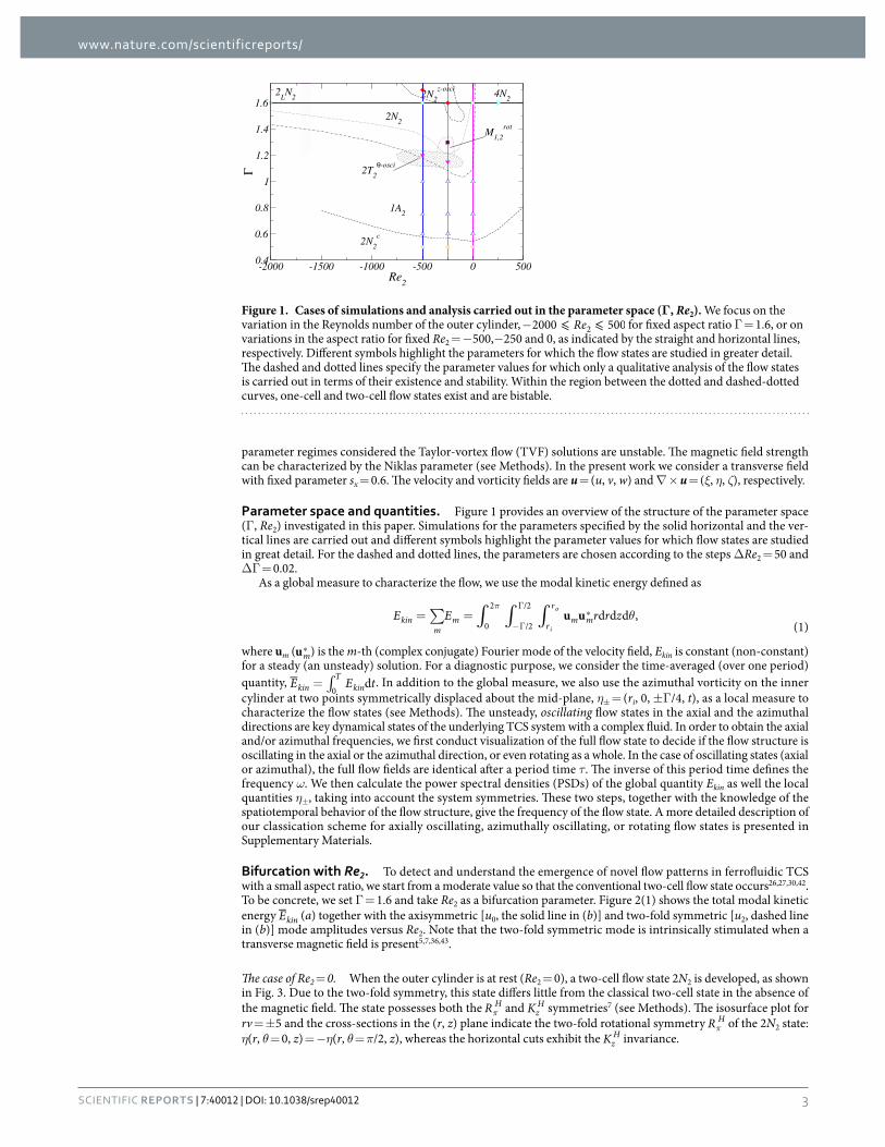
Parameter space and quantities. Figure 1 provides an overview of the structure of the parameter space (Γ , Re2) investigated in this paper. Simulations for the parameters specified by the solid horizontal and the ver-tical lines are carried out and different symbols highlight the parameter values for which flow states are studied in great detail. For the dashed and dotted lines, the parameters are chosen according to the steps ∆ Re2 = 50 and ∆ Γ = 0.02.

As a global measure to characterize the flow, we use the modal kinetic energy defined as

∫ ∫ ∫∑ θ= =π

−Γ

Γ ⁎E E r r zu u d d d ,(1)kin

mm r

rm m0

2

/2

/2

i

o

where um ( ⁎um) is the m-th (complex conjugate) Fourier mode of the velocity field, Ekin is constant (non-constant) for a steady (an unsteady) solution. For a diagnostic purpose, we consider the time-averaged (over one period) quantity, ∫=E E tdkin

Tkin0

. In addition to the global measure, we also use the azimuthal vorticity on the inner cylinder at two points symmetrically displaced about the mid-plane, η± = (ri, 0, ± Γ /4, t), as a local measure to characterize the flow states (see Methods). The unsteady, oscillating flow states in the axial and the azimuthal directions are key dynamical states of the underlying TCS system with a complex fluid. In order to obtain the axial and/or azimuthal frequencies, we first conduct visualization of the full flow state to decide if the flow structure is oscillating in the axial or the azimuthal direction, or even rotating as a whole. In the case of oscillating states (axial or azimuthal), the full flow fields are identical after a period time τ. The inverse of this period time defines the frequency ω. We then calculate the power spectral densities (PSDs) of the global quantity Ekin as well the local quantities η±, taking into account the system symmetries. These two steps, together with the knowledge of the spatiotemporal behavior of the flow structure, give the frequency of the flow state. A more detailed description of our classication scheme for axially oscillating, azimuthally oscillating, or rotating flow states is presented in Supplementary Materials.

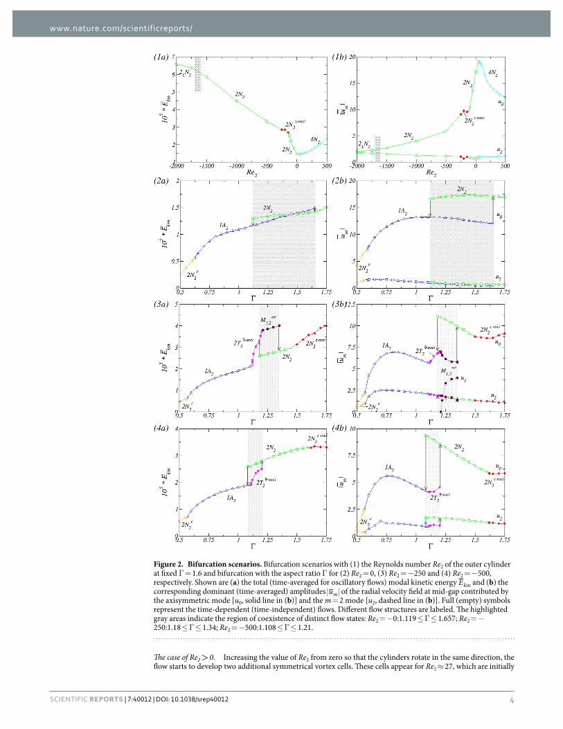
Bifurcation with Re2. To detect and understand the emergence of novel flow patterns in ferrofluidic TCS with a small aspect ratio, we start from a moderate value so that the conventional two-cell flow state occurs26,27,30,42. To be concrete, we set Γ = 1.6 and take Re2 as a bifurcation parameter. Figure 2(1) shows the total modal kinetic energy Ekin (a) together with the axisymmetric [u0, the solid line in (b)] and two-fold symmetric [u2, dashed line in (b)] mode amplitudes versus Re2. Note that the two-fold symmetric mode is intrinsically stimulated when a transverse magnetic field is present5,7,36,43.

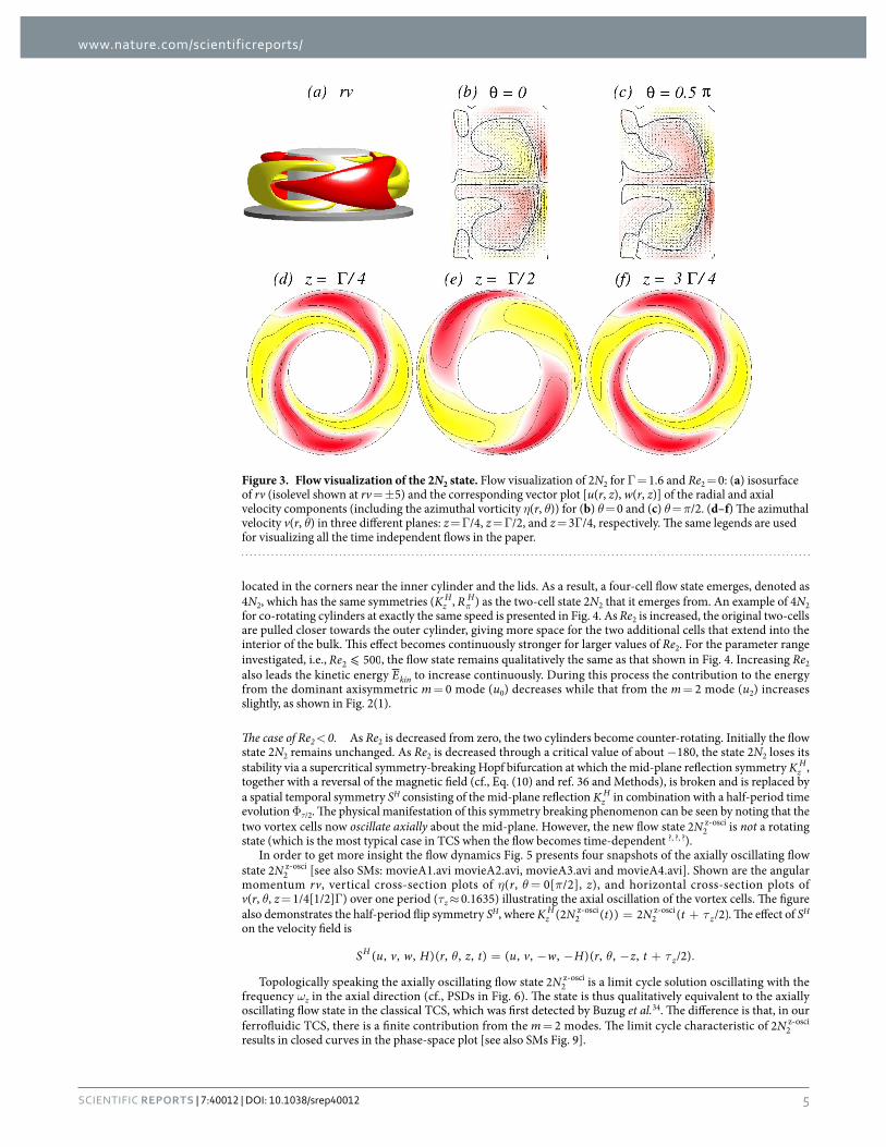
The case of Re2 = 0. When the outer cylinder is at rest (Re2 = 0), a two-cell flow state 2N2 is developed, as shown in Fig. 3. Due to the two-fold symmetry, this state differs little from the classical two-cell state in the absence of the magnetic field. The state possesses both the πR H and Kz

H symmetries7 (see Methods). The isosurface plot for rv = ± 5 and the cross-sections in the (r, z) plane indicate the two-fold rotational symmetry πR H of the 2N2 state: η(r, θ = 0, z) = − η(r, θ = π/2, z), whereas the horizontal cuts exhibit the Kz

H invariance.

-2000 -1500 -1000 -500 0 500Re2

0.4

0.6

0.8

1

1.2

1.4

1.6

Γ

2N2z-osci2LN2

2N2c

1A2

2N2

4N2

2T2θ-osci

M1,2rot

Figure 1. Cases of simulations and analysis carried out in the parameter space (Γ, Re2). We focus on the variation in the Reynolds number of the outer cylinder, − ⩽ ⩽Re2000 5002 for fixed aspect ratio Γ = 1.6, or on variations in the aspect ratio for fixed Re2 = − 500,− 250 and 0, as indicated by the straight and horizontal lines, respectively. Different symbols highlight the parameters for which the flow states are studied in greater detail. The dashed and dotted lines specify the parameter values for which only a qualitative analysis of the flow states is carried out in terms of their existence and stability. Within the region between the dotted and dashed-dotted curves, one-cell and two-cell flow states exist and are bistable.



The case of Re2 > 0. Increasing the value of Re2 from zero so that the cylinders rotate in the same direction, the flow starts to develop two additional symmetrical vortex cells. These cells appear for Re2 ≈ 27, which are initially

Figure 2. Bifurcation scenarios. Bifurcation scenarios with (1) the Reynolds number Re2 of the outer cylinder at fixed Γ = 1.6 and bifurcation with the aspect ratio Γ for (2) Re2 = 0, (3) Re2 = − 250 and (4) Re2 = − 500, respectively. Shown are (a) the total (time-averaged for oscillatory flows) modal kinetic energy Ekin and (b) the corresponding dominant (time-averaged) amplitudes um of the radial velocity field at mid-gap contributed by the axisymmetric mode [u0, solid line in (b)] and the m = 2 mode [u2, dashed line in (b)]. Full (empty) symbols represent the time-dependent (time-independent) flows. Different flow structures are labeled. The highlighted gray areas indicate the region of coexistence of distinct flow states: Re2 = − 0:1.119 ≤ Γ ≤ 1.657; Re2 = − 250:1.18 ≤ Γ ≤ 1.34; Re2 = − 500:1.108 ≤ Γ ≤ 1.21.



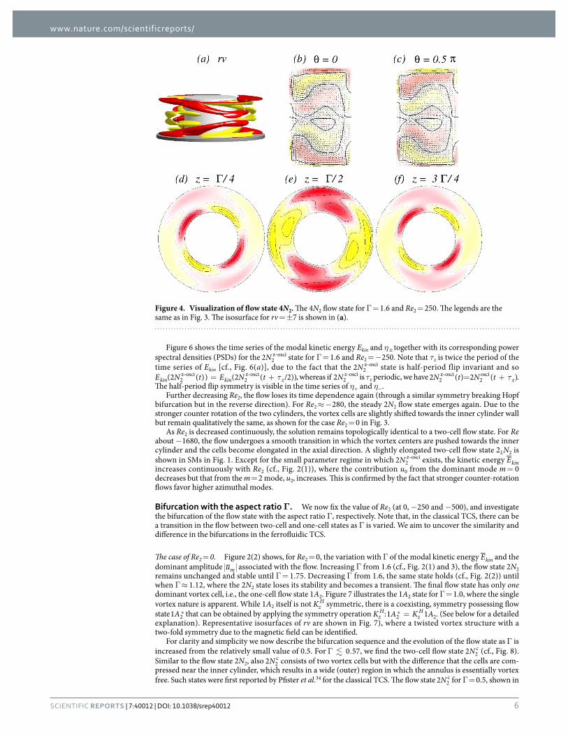
located in the corners near the inner cylinder and the lids. As a result, a four-cell flow state emerges, denoted as 4N2, which has the same symmetries (Kz

H, πR H) as the two-cell state 2N2 that it emerges from. An example of 4N2 for co-rotating cylinders at exactly the same speed is presented in Fig. 4. As Re2 is increased, the original two-cells are pulled closer towards the outer cylinder, giving more space for the two additional cells that extend into the interior of the bulk. This effect becomes continuously stronger for larger values of Re2. For the parameter range investigated, i.e., ⩽Re 5002 , the flow state remains qualitatively the same as that shown in Fig. 4. Increasing Re2 also leads the kinetic energy Ekin to increase continuously. During this process the contribution to the energy from the dominant axisymmetric m = 0 mode (u0) decreases while that from the m = 2 mode (u2) increases slightly, as shown in Fig. 2(1).

The case of Re2 < 0. As Re2 is decreased from zero, the two cylinders become counter-rotating. Initially the flow state 2N2 remains unchanged. As Re2 is decreased through a critical value of about − 180, the state 2N2 loses its stability via a supercritical symmetry-breaking Hopf bifurcation at which the mid-plane reflection symmetry Kz

H, together with a reversal of the magnetic field (cf., Eq. (10) and ref. 36 and Methods), is broken and is replaced by a spatial temporal symmetry SH consisting of the mid-plane reflection Kz

H in combination with a half-period time evolution Φ τ/2. The physical manifestation of this symmetry breaking phenomenon can be seen by noting that the two vortex cells now oscillate axially about the mid-plane. However, the new flow state ‑N2 2

z osci is not a rotating state (which is the most typical case in TCS when the flow becomes time-dependent ?, ?, ?).

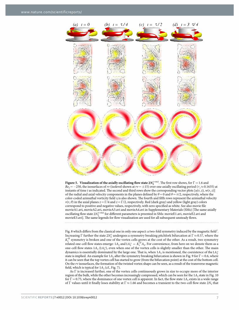
In order to get more insight the flow dynamics Fig. 5 presents four snapshots of the axially oscillating flow state ‑N2 2

z osci [see also SMs: movieA1.avi movieA2.avi, movieA3.avi and movieA4.avi]. Shown are the angular momentum rv, vertical cross-section plots of η(r, θ = 0[π/2], z), and horizontal cross-section plots of v(r, θ, z = 1/4[1/2]Γ ) over one period (τz ≈ 0.1635) illustrating the axial oscillation of the vortex cells. The figure also demonstrates the half-period flip symmetry SH, where τ= +‑ ‑K N t N t(2 ( )) 2 ( /2)z

Hz2

z osci2z osci . The effect of SH

on the velocity field is

θ θ τ= − − − + .S u v w H r z t u v w H r z t( , , , )( , , , ) ( , , , )( , , , /2)Hz

Topologically speaking the axially oscillating flow state ‑N2 2z osci is a limit cycle solution oscillating with the

frequency ωz in the axial direction (cf., PSDs in Fig. 6). The state is thus qualitatively equivalent to the axially oscillating flow state in the classical TCS, which was first detected by Buzug et al.34. The difference is that, in our ferrofluidic TCS, there is a finite contribution from the m = 2 modes. The limit cycle characteristic of ‑N2 2

z osci results in closed curves in the phase-space plot [see also SMs Fig. 9].

Figure 3. Flow visualization of the 2N2 state. Flow visualization of 2N2 for Γ = 1.6 and Re2 = 0: (a) isosurface of rv (isolevel shown at rv = ± 5) and the corresponding vector plot [u(r, z), w(r, z)] of the radial and axial velocity components (including the azimuthal vorticity η(r, θ)) for (b) θ = 0 and (c) θ = π/2. (d–f) The azimuthal velocity v(r, θ) in three different planes: z = Γ /4, z = Γ /2, and z = 3Γ /4, respectively. The same legends are used for visualizing all the time independent flows in the paper.



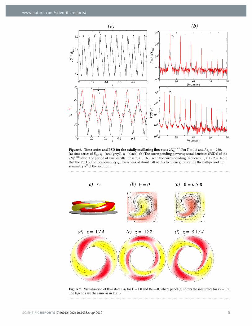
Figure 6 shows the time series of the modal kinetic energy Ekin and η ± together with its corresponding power spectral densities (PSDs) for the ‑N2 2

z osci state for Γ = 1.6 and Re2 = − 250. Note that τz is twice the period of the time series of Ekin [cf., Fig. 6(a)], due to the fact that the ‑N2 2

z osci state is half-period flip invariant and so τ= +‑ ‑E N t E N t(2 ( )) (2 ( /2))kin kin z2

z osci2z osci , whereas if ‑N2 2

z osci is τz periodic, we have τ= +‑N t N t2 ( ) 2 ( )z2z osci

2osci .

The half-period flip symmetry is visible in the time series of η+ and η−.Further decreasing Re2, the flow loses its time dependence again (through a similar symmetry breaking Hopf

bifurcation but in the reverse direction). For Re2 ≈ − 280, the steady 2N2 flow state emerges again. Due to the stronger counter rotation of the two cylinders, the vortex cells are slightly shifted towards the inner cylinder wall but remain qualitatively the same, as shown for the case Re2 = 0 in Fig. 3.

As Re2 is decreased continuously, the solution remains topologically identical to a two-cell flow state. For Re about − 1680, the flow undergoes a smooth transition in which the vortex centers are pushed towards the inner cylinder and the cells become elongated in the axial direction. A slightly elongated two-cell flow state 2LN2 is shown in SMs in Fig. 1. Except for the small parameter regime in which ‑N2 2

z osci exists, the kinetic energy Ekin increases continuously with Re2 (cf., Fig. 2(1)), where the contribution u0 from the dominant mode m = 0 decreases but that from the m = 2 mode, u2, increases. This is confirmed by the fact that stronger counter-rotation flows favor higher azimuthal modes.

Bifurcation with the aspect ratio Γ. We now fix the value of Re2 (at 0, − 250 and − 500), and investigate the bifurcation of the flow state with the aspect ratio Γ , respectively. Note that, in the classical TCS, there can be a transition in the flow between two-cell and one-cell states as Γ is varied. We aim to uncover the similarity and difference in the bifurcations in the ferrofluidic TCS.

The case of Re2 = 0. Figure 2(2) shows, for Re2 = 0, the variation with Γ of the modal kinetic energy Ekin and the dominant amplitude um associated with the flow. Increasing Γ from 1.6 (cf., Fig. 2(1) and 3), the flow state 2N2 remains unchanged and stable until Γ = 1.75. Decreasing Γ from 1.6, the same state holds (cf., Fig. 2(2)) until when Γ ≈ 1.12, where the 2N2 state loses its stability and becomes a transient. The final flow state has only one dominant vortex cell, i.e., the one-cell flow state 1A2. Figure 7 illustrates the 1A2 state for Γ = 1.0, where the single vortex nature is apparent. While 1A2 itself is not Kz

H symmetric, there is a coexisting, symmetry possessing flow state ⁎A1 2 that can be obtained by applying the symmetry operation Kz

H: =⁎A K A1 1zH

2 2. (See below for a detailed explanation). Representative isosurfaces of rv are shown in Fig. 7), where a twisted vortex structure with a two-fold symmetry due to the magnetic field can be identified.

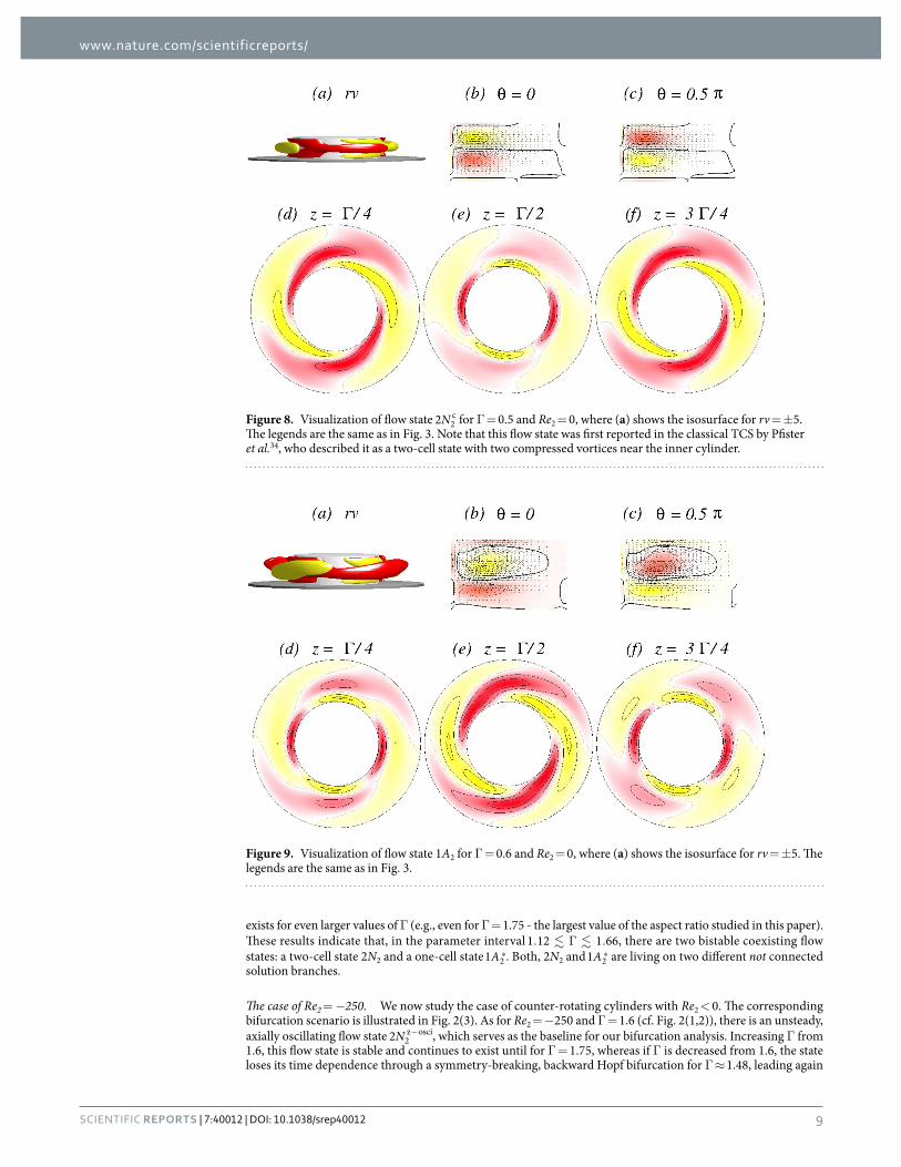
For clarity and simplicity we now describe the bifurcation sequence and the evolution of the flow state as Γ is increased from the relatively small value of 0.5. For 1Γ .0 57, we find the two-cell flow state N2 2

c (cf., Fig. 8). Similar to the flow state 2N2, also N2 2

c consists of two vortex cells but with the difference that the cells are com-pressed near the inner cylinder, which results in a wide (outer) region in which the annulus is essentially vortex free. Such states were first reported by Pfister et al.34 for the classical TCS. The flow state N2 2

c for Γ = 0.5, shown in

Figure 4. Visualization of flow state 4N2. The 4N2 flow state for Γ = 1.6 and Re2 = 250. The legends are the same as in Fig. 3. The isosurface for rv = ± 7 is shown in (a).



Fig. 8 which differs from the classical one in only one aspect: a two-fold symmetry induced by the magnetic field7. Increasing Γ further the state N2 2

c undergoes a symmetry breaking pitchfork bifurcation at Γ ≈ 0.57, where the Kz

H symmetry is broken and one of the vortex cells grows at the cost of the other. As a result, two symmetry related one-cell flow states emerge: 1A2 and =⁎A K A1 z

H2 2. For convenience, from here on we denote them as a

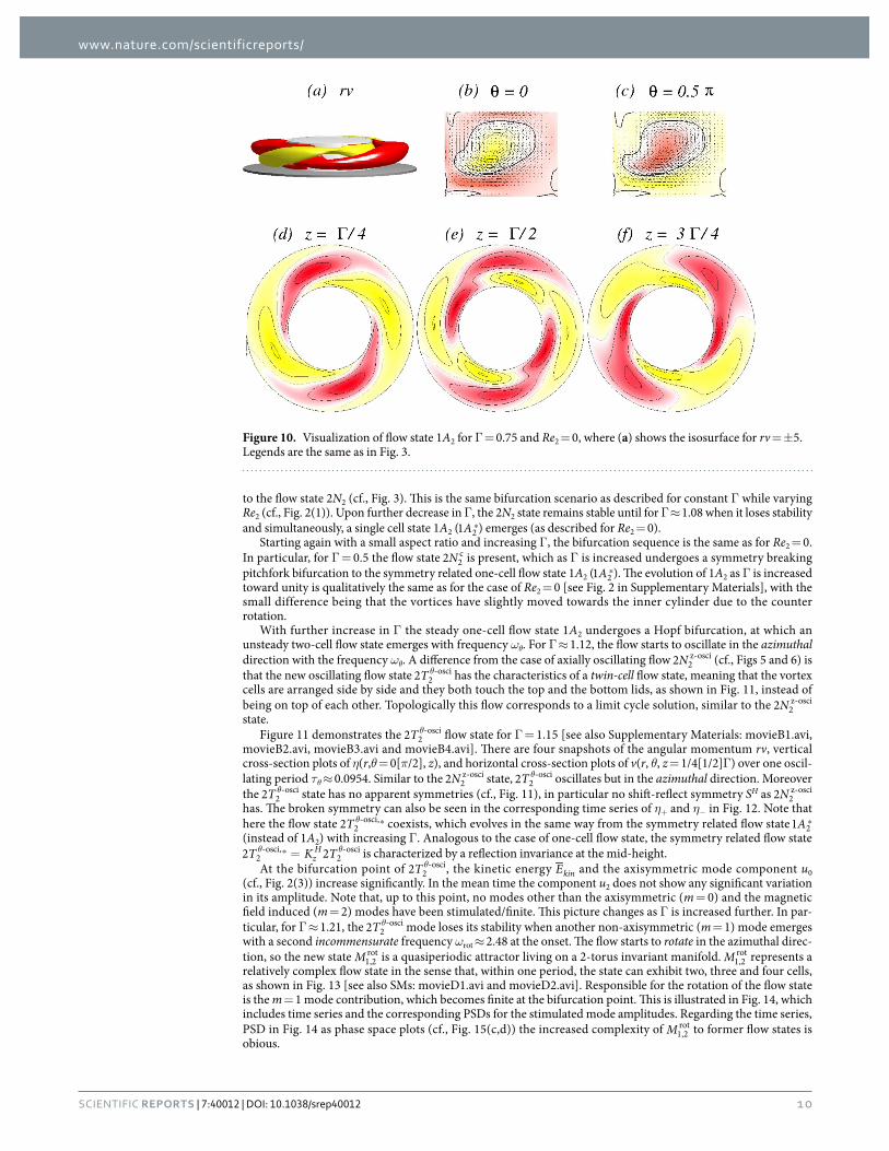
one-cell flow states 1A2 ( ⁎A1 2 ), even when one of the vortex cells is slightly smaller than the other. The main dynamics is essentially dominated by the large one. That is, when 1A2 is mentioned, the coexistence of the ⁎A1 2 state is implied. An example for 1A2 after the symmetry breaking bifurcation is shown in Fig. 9 for Γ = 0.6, where it can be seen that the top vortex cell has started to grow (from the bifurcation point) at the cost of the bottom cell. On the rv isosurfaces, the formation of the twisted vortex shape can be seen, as a result of the transverse magnetic field, which is typical for 1A2 (cf., Fig. 7).

As Γ is increased further, one of the vortex cells continuously grows in size to occupy more of the interior region of the bulk, while the other becomes increasingly compressed, which can be seen for the 1A2 state in Fig. 10 for Γ = 0.75, where the dominance of one vortex cell is apparent. In fact, the flow state 1A2 exists in a wide range of Γ values until it finally loses stability at Γ ≈ 1.66 and becomes a transient to the two-cell flow state 2N2 that

Figure 5. Visualization of the axially oscillating flow state ‑N2 z2

osci. The first row shows, for Γ = 1.6 and Re2 = − 250, the isosurfaces of rv (isolevel shown at rv = ± 15) over one axially oscillating period (τz ≈ 0.1635) at instants of time t as indicated. The second and third rows show the corresponding vector plots [u(r, z), w(r, z)] of the radial and axial velocity components in the planes defined by θ = 0 and θ = π/2, respectively, where the color-coded azimuthal vorticity field η is also shown. The fourth and fifth rows represent the azimuthal velocity v(r, θ) in the axial planes z = Γ /4 and z = Γ /2, respectively. Red (dark gray) and yellow (light gray) colors correspond to positive and negative values, respectively, with zero specified as white. See also movie file movieA1.avi, movieA2.avi, movieA3.avi and movieA4.avi in Supplementary Materials (SMs) [The same axially oscillating flow state ‑N2 2

z osci for different parameters is preented in SMs: movieE1.avi, movieE2.avi and movieE3.avi]. The same legends for flow visualization are used for all subsequent unsteady flows.



Figure 6. Time series and PSD for the axially oscillating flow state ‑N2 z2

osci. For Γ = 1.6 and Re2 = − 250, (a) time series of Ekin, η+ [red (gray)], η− (black). (b) The corresponding power spectral densities (PSDs) of the

‑N2 2z osci state. The period of axial oscillation is τz ≈ 0.1635 with the corresponding frequency ωz ≈ 12.232. Note

that the PSD of the local quantity η− has a peak at about half of this frequency, indicating the half-period flip symmetry SH of the solution.

Figure 7. Visualization of flow state 1A2 for Γ = 1.0 and Re2 = 0, where panel (a) shows the isosurface for rv = ± 7. The legends are the same as in Fig. 3.



exists for even larger values of Γ (e.g., even for Γ = 1.75 - the largest value of the aspect ratio studied in this paper). These results indicate that, in the parameter interval 1 1. Γ .1 12 1 66, there are two bistable coexisting flow states: a two-cell state 2N2 and a one-cell state ⁎A1 2 . Both, 2N2 and ⁎A1 2 are living on two different not connected solution branches.

The case of Re2 = −250. We now study the case of counter-rotating cylinders with Re2 < 0. The corresponding bifurcation scenario is illustrated in Fig. 2(3). As for Re2 = − 250 and Γ = 1.6 (cf. Fig. 2(1,2)), there is an unsteady, axially oscillating flow state −N2 2

z osci, which serves as the baseline for our bifurcation analysis. Increasing Γ from 1.6, this flow state is stable and continues to exist until for Γ = 1.75, whereas if Γ is decreased from 1.6, the state loses its time dependence through a symmetry-breaking, backward Hopf bifurcation for Γ ≈ 1.48, leading again

Figure 9. Visualization of flow state 1A2 for Γ = 0.6 and Re2 = 0, where (a) shows the isosurface for rv = ± 5. The legends are the same as in Fig. 3.

Figure 8. Visualization of flow state N2 2c for Γ = 0.5 and Re2 = 0, where (a) shows the isosurface for rv = ± 5.

The legends are the same as in Fig. 3. Note that this flow state was first reported in the classical TCS by Pfister et al.34, who described it as a two-cell state with two compressed vortices near the inner cylinder.


1 0Scientific RepoRts | 7:40012 | DOI: 10.1038/srep40012

to the flow state 2N2 (cf., Fig. 3). This is the same bifurcation scenario as described for constant Γ while varying Re2 (cf., Fig. 2(1)). Upon further decrease in Γ , the 2N2 state remains stable until for Γ ≈ 1.08 when it loses stability and simultaneously, a single cell state 1A2 ( ⁎A1 2 ) emerges (as described for Re2 = 0).

Starting again with a small aspect ratio and increasing Γ , the bifurcation sequence is the same as for Re2 = 0. In particular, for Γ = 0.5 the flow state N2 2

c is present, which as Γ is increased undergoes a symmetry breaking pitchfork bifurcation to the symmetry related one-cell flow state 1A2 ( ⁎A1 2 ). The evolution of 1A2 as Γ is increased toward unity is qualitatively the same as for the case of Re2 = 0 [see Fig. 2 in Supplementary Materials], with the small difference being that the vortices have slightly moved towards the inner cylinder due to the counter rotation.

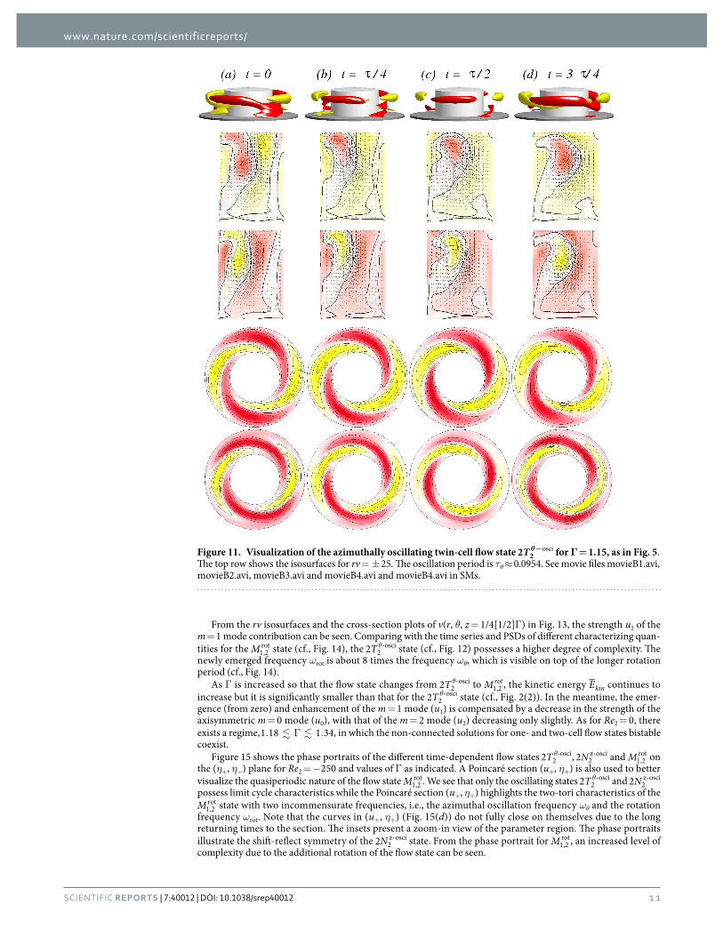
With further increase in Γ the steady one-cell flow state 1A2 undergoes a Hopf bifurcation, at which an unsteady two-cell flow state emerges with frequency ωθ. For Γ ≈ 1.12, the flow starts to oscillate in the azimuthal direction with the frequency ωθ. A difference from the case of axially oscillating flow ‑N2 2

z osci (cf., Figs 5 and 6) is that the new oscillating flow state θ‑T2 2

osci has the characteristics of a twin-cell flow state, meaning that the vortex cells are arranged side by side and they both touch the top and the bottom lids, as shown in Fig. 11, instead of being on top of each other. Topologically this flow corresponds to a limit cycle solution, similar to the ‑N2 2

z osci state.

Figure 11 demonstrates the θ‑T2 2osci flow state for Γ = 1.15 [see also Supplementary Materials: movieB1.avi,

movieB2.avi, movieB3.avi and movieB4.avi]. There are four snapshots of the angular momentum rv, vertical cross-section plots of η(r,θ = 0[π/2], z), and horizontal cross-section plots of v(r, θ, z = 1/4[1/2]Γ ) over one oscil-lating period τθ ≈ 0.0954. Similar to the ‑N2 2

z osci state, θ‑T2 2osci oscillates but in the azimuthal direction. Moreover

the θ‑T2 2osci state has no apparent symmetries (cf., Fig. 11), in particular no shift-reflect symmetry SH as ‑N2 2

z osci has. The broken symmetry can also be seen in the corresponding time series of η+ and η− in Fig. 12. Note that here the flow state θ‑ ⁎T2 2

osci, coexists, which evolves in the same way from the symmetry related flow state ⁎A1 2 (instead of 1A2) with increasing Γ . Analogous to the case of one-cell flow state, the symmetry related flow state

=θ θ‑ ⁎ ‑T K T2 2zH

2osci,

2osci is characterized by a reflection invariance at the mid-height.

At the bifurcation point of θ‑T2 2osci, the kinetic energy Ekin and the axisymmetric mode component u0

(cf., Fig. 2(3)) increase significantly. In the mean time the component u2 does not show any significant variation in its amplitude. Note that, up to this point, no modes other than the axisymmetric (m = 0) and the magnetic field induced (m = 2) modes have been stimulated/finite. This picture changes as Γ is increased further. In par-ticular, for Γ ≈ 1.21, the θ‑T2 2

osci mode loses its stability when another non-axisymmetric (m = 1) mode emerges with a second incommensurate frequency ωrot ≈ 2.48 at the onset. The flow starts to rotate in the azimuthal direc-tion, so the new state M1,2

rot is a quasiperiodic attractor living on a 2-torus invariant manifold. M1,2rot represents a

relatively complex flow state in the sense that, within one period, the state can exhibit two, three and four cells, as shown in Fig. 13 [see also SMs: movieD1.avi and movieD2.avi]. Responsible for the rotation of the flow state is the m = 1 mode contribution, which becomes finite at the bifurcation point. This is illustrated in Fig. 14, which includes time series and the corresponding PSDs for the stimulated mode amplitudes. Regarding the time series, PSD in Fig. 14 as phase space plots (cf., Fig. 15(c,d)) the increased complexity of M1,2

rot to former flow states is obious.

Figure 10. Visualization of flow state 1A2 for Γ = 0.75 and Re2 = 0, where (a) shows the isosurface for rv = ± 5. Legends are the same as in Fig. 3.



From the rv isosurfaces and the cross-section plots of v(r, θ, z = 1/4[1/2]Γ ) in Fig. 13, the strength u1 of the m = 1 mode contribution can be seen. Comparing with the time series and PSDs of different characterizing quan-tities for the M1,2

rot state (cf., Fig. 14), the θ‑T2 2osci state (cf., Fig. 12) possesses a higher degree of complexity. The

newly emerged frequency ωrot is about 8 times the frequency ωθ, which is visible on top of the longer rotation period (cf., Fig. 14).

As Γ is increased so that the flow state changes from θ‑T2 2osci to M rot

1,2 , the kinetic energy Ekin continues to increase but it is significantly smaller than that for the θ‑T2 2

osci state (cf., Fig. 2(2)). In the meantime, the emer-gence (from zero) and enhancement of the m = 1 mode (u1) is compensated by a decrease in the strength of the axisymmetric m = 0 mode (u0), with that of the m = 2 mode (u2) decreasing only slightly. As for Re2 = 0, there exists a regime, 1 1. Γ .1 18 1 34, in which the non-connected solutions for one- and two-cell flow states bistable coexist.

Figure 15 shows the phase portraits of the different time-dependent flow states θ‑T2 2osci, ‑N2 2

z osci and M1,2rot on

the (η+, η−) plane for Re2 = − 250 and values of Γ as indicated. A Poincaré section (u+, η+) is also used to better visualize the quasiperiodic nature of the flow state M1,2

rot. We see that only the oscillating states θ‑T2 2osci and ‑N2 2

z osci possess limit cycle characteristics while the Poincaré section (u+, η+) highlights the two-tori characteristics of the M1,2

rot state with two incommensurate frequencies, i.e., the azimuthal oscillation frequency ωθ and the rotation frequency ωrot. Note that the curves in (u+, η+) (Fig. 15(d)) do not fully close on themselves due to the long returning times to the section. The insets present a zoom-in view of the parameter region. The phase portraits illustrate the shift-reflect symmetry of the ‑N2 2

z osci state. From the phase portrait for M1,2rot, an increased level of

complexity due to the additional rotation of the flow state can be seen.

Figure 11. Visualization of the azimuthally oscillating twin-cell flow state θ−T2 2osci for Γ = 1.15, as in Fig. 5.

The top row shows the isosurfaces for rv = ± 25. The oscillation period is τθ ≈ 0.0954. See movie files movieB1.avi, movieB2.avi, movieB3.avi and movieB4.avi and movieB4.avi in SMs.



The case of Re2 = −500. We now study the case of strongly counter rotating cylinders: Re2 = − 500. The bifurca-tion diagram with Γ is shown in Fig. 2(4). For Γ = 1.6 we find the flow state 2N2 (Fig. 2(1)) Increasing Γ , the state loses its stability at Γ ≈ 1.62 through a symmetry breaking Hopf bifurcation and the resulting state is again the unsteady, axially oscillating flow state ‑N2 2

z osci (cf., Figs 5 and 6), which remains stable until Γ ≈ 1.75.We find that the oscillation amplitude is much smaller than that for the ‑N2 2

z osci state at Re2 = − 250 (cf. Fig. 5). As Γ is decreased, the state remains stable until for Γ ≈ 1.18 when it loses stability, at which the one-cell flow state 1A2 ( ⁎A1 2 ) emerges, similar to the cases of Re2 = 0 and Re2 = − 250. In the opposite direction, i.e., starting from the steady flow state N2 2

c for Γ = 0.5 and increasing Γ , the state loses its stability at Γ ≈ 0.59 through the same symme-try breaking pitchfork bifurcation as for the cases of Re2 = 0 and Re2 = − 250. Due to the stronger counter rotation, two additional vortex cells start to develop near the outer cylinders for the flow state N2 2

c. The symmetry related one-cell flow state 1A2 or ⁎A1 2 appears as the size of one of the vortex cells increases or shrinks, respectively. Upon further increase in Γ , the flow state 1A2 remains stable with slight but continuous change in the position of the vortex cell. The larger vortex cell moves towards the inner cylinder, while the second vortex cell grows and moves radially outward towards the outer cylinder. In principle this is the same evolution as for the case of Re2 = − 250, with the only difference being that, due to the stronger counter rotation (Re2 = − 500), the vortex cells and in particular their centers are slightly shifted and located closer towards the inner cylinder.

For Γ ≈ 1.08, the flow becomes time dependent, and the azimuthally oscillating twin-cell flow state θ‑T2 2osci

emerges. The dynamics is almost the same as seen in Figs 11 and 12 for slightly smaller Γ = 1.15 and Re2 = − 250. With a further increase in Γ , this state loses its stability at Γ ≈ 1.35 and becomes a transient to the flow state 2N2. For Re2 = − 500, there then exists again a regime, 1 1. Γ .1 18 1 34, in which the one-cell and two-cell flow states bistable coexist. Differing from the case of Re1 = − 250, there is absence of more complex (e.g., quasiperiodic solution) flow state for Re2 = − 500. The phase portraits for the azimuthally and axially oscillating flow states

‑N2 2z osci and θ‑T2 2

osci is similar to these solutions at Re2 = − 250.A focus of our present study is axially or azimuthally oscillating flow states. It should be noted, however, that

flow states of combined axial and azimuthal oscillations can occur in the parameter regime of larger aspect ratio and very large values of the Reynolds number. A more detailed discussion about the behaviors of the angular momentum and torque can be found in Supplementary Materials.

Discussion and Summary of Main FindingsAs a fundamental paradigm of fluid dynamics, the TCS has been extensively investigated computationally and experimentally. In spite of the long history of the TCS and the vast literature on the subject, the dynamics of

0 0.25 0.5 0.75 1t

1.8

2

2.2

2.4

105 *

Eki

n

τθ

0 20 40 60 80frequency

10-8

10-4

100

104

PSD

of E

kin

ωθ

0 0.25 0.5 0.75 1t

-60

-50

-40

-30

-20

-10

η −η +

τθ


10-6

10-3

100

PSD

of η

−

ωθ

(a) (b)

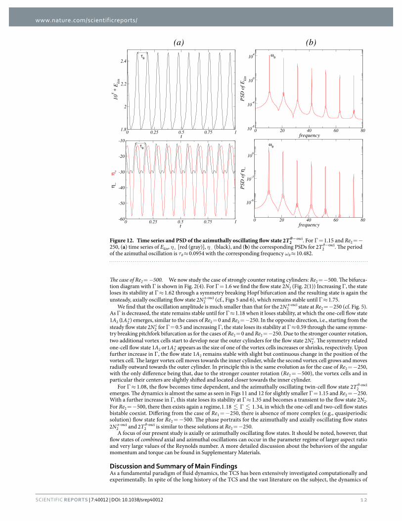
Figure 12. Time series and PSD of the azimuthally oscillating flow state θ−T2 2osci. For Γ = 1.15 and Re2 = −

250, (a) time series of Ekin, η+ [red (gray)], η− (black), and (b) the corresponding PSDs for θ−T2 2osci. The period

of the azimuthal oscillation is τθ ≈ 0.0954 with the corresponding frequency ωθ ≈ 10.482.



TCS with a complex fluid subject to a symmetry breaking magnetic field have begun to be investigated relatively recently. In fact, a gap existed in our knowledge about the nonlinear dynamics of such systems with a small aspect ratio. The present work is aimed to fill this gap.

Through systematic and extensive simulations of the ferrohydrodynamical equations, a generalization of the classic Navier-Stokes equation into ferrofluidic systems subject to a magnetic field, we unveil the emergence and evolution of distinct dynamical flow states. As the Reynolds number of the outer cylinder and/or the aspect ratio is changed, symmetry-breaking pitchfork and Hopf bifurcations can occur, leading to transitions among various flow states, e.g., the two-cell and one-cell states. The presence of the transverse magnetic field stipulates that all flow states must inherently be three-dimensional5,7,43.

The detailed emergence, dynamical evolution, and transitions among the various flow states can be summa-rized, as follows. We first identify a fundamental building block that plays a dominant role in the formation of various flow structures: the order-two azimuthal m = 2 mode. For small aspect ratio (e.g., Γ ≈ 0.5), the two-cell state N2 2

c dominates which, due to its two-fold flow symmetry, differs little from the one in the classical TCS34. Depending on the rotational speed and the direction of the outer cylinder the vortex cells within the N2 2

c state can move closer towards the inner cylinder. The flow is steady and exhibits a more complex set of symmetries associ-ated with the magnetic field, namely, a combination of the two-fold symmetry and the reflection symmetry about the mid-plane under reversal of the field direction. As Γ is increased, this flow state undergoes a symmetry break-ing bifurcation at which one vortex cell starts to grow while the other begins to shrink, eventually generating two symmetry related one-cell flow states: 1A2 and =⁎A K A1 1z

H2 2. When the outer cylinder is at rest (i.e., Re2 = 0), the

state 1A2 loses stability and eventually becomes a transient to the steady, axially symmetric two-cell flow state 2N2. For counter-rotating cylinders (i.e., Re2 < 0), we find a transition to the same flow state 2N2 at a larger value of Γ .

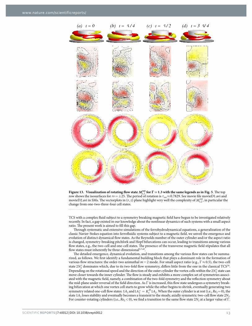
Figure 13. Visualization of rotating flow state M ,rot1 2 for Γ = 1.3 with the same legends as in Fig. 5. The top

row shows the isosurfaces for rv = ± 25. The period of rotation is τrot ≈ 0.7829. See movie file movieD1.avi and movieD2.avi in SMs. The vectorplots in (r, z) plane highlight very well the complexity of M1,2

rot, in particular the change from one-two-three-four cell states.



However, prior to this transition a distinct bifurcation sequence leading to new unsteady flow states occurs. In fact, as Γ is increased, the one-cell flow state 1A2 becomes modulated in that the smaller vortex cell grows along the inner cylinder while the other vortex cell is pulled outward. Eventually the steady flow state 1A2 undergoes a Hopf bifurcation to a periodic, azimuthally oscillating flow state θ‑T2 2

osci in the twin-cell configuration (side-by-side arrangement) where both vortex cells touch the top and bottom lids, which topologically corre-sponds to a limit cycle. During the dynamical evolution, there are two symmetry related flow states: θ‑T2 2

osci and =θ θ‑ ⁎ ‑T K T2 2z

H2

osci,2

osci. Increasing Γ further, we find two possible bifurcation scenarios. First, θ‑T2 2osci loses its

stability and becomes a transient to the steady flow state 2N2. Second, θ‑T2 2osci becomes unstable, leading to an

unsteady quasiperiodic flow state M1,2rot. The quasiperiodic state has finite contribution from the m = 1 mode and

rotates in the azimuthal direction. As a result, one of the two frequencies, ωθ, corresponds to the frequency of the underlying θ‑T2 2

osci mode from which it bifurcates, and the second frequency ωrot comes from the rotation of the m = 1 mode, a flow state with a helical shape (cf., Fig. 13). For larger values of Γ , the unsteady flow state M1,2

rot eventually loses its stability and becomes transient towards the steady state 2N2.

A similar scenario occurs when the aspect ratio is varied in the opposite direction, i.e., from large to small values. At a certain point the steady two-cell flow state 2N2 loses its stability and is replaced by one of the

0 0.5 1 1.5 2t

2

3

4

5

6

7

8

105 *

Eki

n

τrot


10-8

10-6

10-4

10-2

100

PSD

of E

kin

ωrot

0 0.5 1 1.5 2t

-400

-200

0

200

400

η −η +

τrot


10-6

10-4

10-2

100

102

PSD

of η

−

ωrot

0 0.5 1 1.5 2t

0

2

4

6

8

|um

|

u0

u2

u1


10-8

10-6

10-4

10-2

100

PSD

of |

u 0|

(a) (b)

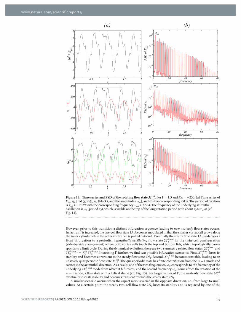
Figure 14. Time series and PSD of the rotating flow state M ,rot1 2 . For Γ = 1.3 and Re2 = − 250, (a) Time series of

Ekin, η+ [red (gray)], η− (black), and the amplitudes |um|, and (b) the corresponding PSDs. The period of rotation is τrot ≈ 0.7829 with the corresponding frequency ωrot ≈ 2.554. The frequency of the underlying azimuthal oscillation is ωθ (period τθ), which is visible on the top of the long rotation period with about τθ ≈ τrot/8 (cf. Fig. 13).



symmetry related steady one-cell flow states, 1A2 or ⁎A1 2 . Depending on the parameters there is a relatively large regime in which the both not-connected solutions, two-cell and one-cell flow states bistable coexist. It is worth mentioning that our computations never reveal any signature of the transition from the steady two-cell flow state 2N2 to any of the unsteady one-cell flow states (i.e., θ‑T2 2

osci or M1,2rot). The reduction in the vortex cells (from two

to one) appears to happen only between the steady flow states.In addition to these unsteady flow states, we detect another unsteady flow state, the axially oscillating flow

state ‑N2 2z osci that is known for the classical TCS34. The state ‑N2 2

z osci emerges at a large value of Γ or through var-iation of the rotation speed of the outer cylinder through a symmetry breaking Hopf bifurcation out of the flow state 2N2. Similar to θ‑T2 2

osci, the flow state ‑N2 2z osci is a limit cycle solution which is half-period flip invariant

under the symmetry operation SH.To summarize the complicated bifurcation/transition scenarios in the ferrofluidic TCS with a small aspect

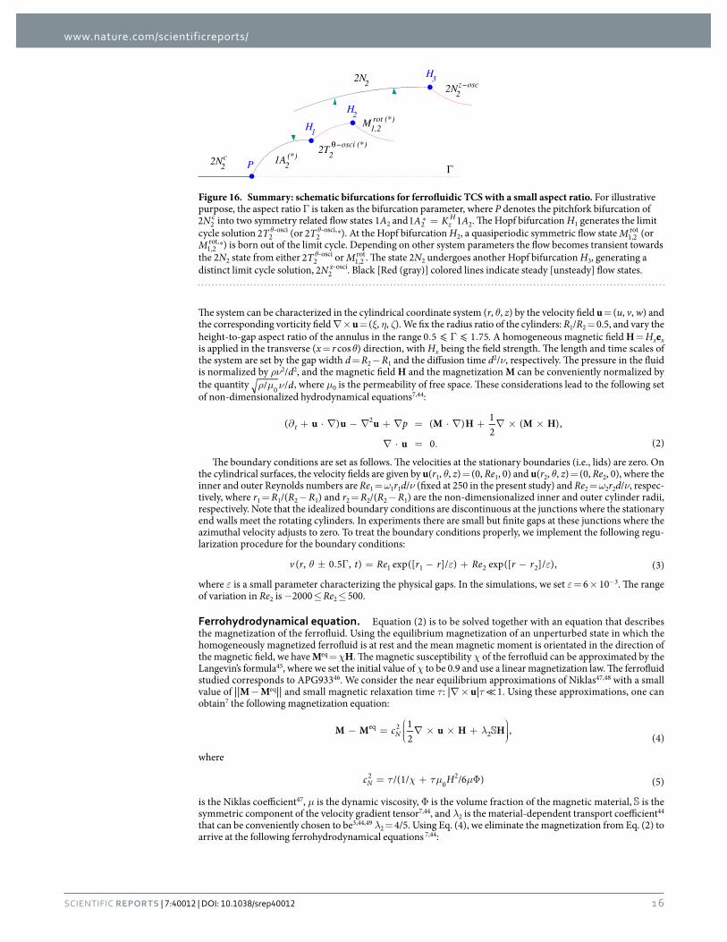
ratio in a transparent way, we produce a schematic bifurcation diagram with the aspect ratio Γ being the bifurca-tion parameter, as shown in Fig. 16. The symmetry breaking associated with each bifurcation point can be described succinctly, as follows. At the pitchfork bifurcation point P, the two-cell flow state N2 2

c, which is invari-ant under the symmetries πR H and Kz

H, loses stability, giving rise to the one-cell flow state 1A2. In fact, breaking the Kz

H symmetry results in two symmetry related flow states 1A2 and =⁎A K A1 1zH

2 2. The state 1A2 loses stability through the Hopf bifurcation H1 at which a limit cycle state θ‑T2 2

osci (or θ‑ ⁎T2 2osci, ) is born. Finally a second fre-

quency appears through another Hopf bifurcation H2, leading to a two-frequency quasiperiodic solution M1,2rot

(or ⁎M1,2rot, ).

MethodsSystem setting and the Navier-Stokes equation. We consider a standard TCS consisting of two con-centric, independently rotating cylinders. Within the gap between the two cylinders there is an incompressible, isothermal, homogeneous, mono-dispersed ferrofluid of kinematic viscosity ν and density ρ. The inner and outer cylinders have radius R1 and R2, and they rotate with the angular velocity ω1 and ω2, respectively. The boundary conditions at the cylinder surfaces are of the non-slip type, and the end walls enclosing the annulus are stationary.

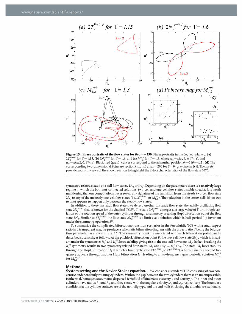
Figure 15. Phase portraits of the flow states for Re2 = −250. Phase portraits in the (η+, η−) plane of (a) θ‑T2 2

osci for Γ = 1.15, (b) ‑N2 2z osci for Γ = 1.6, and (c) M1,2

rot for Γ = 1.3, where η± = η(ri, θ, ± Γ /4, t), and u+ = u(d/2, 0, Γ /4, t). Black [red (gray)] curves correspond to the azimuthal position θ = 0 [θ = π/2]. (d) The corresponding two-dimensional Poincaré section (u+, η+) at η− = 200 for θ = 0 (gray line in (c)). The insets provide zoom-in views of the shown section to highlight the 2-tori characteristics of the flow state M1,2

rot.



The system can be characterized in the cylindrical coordinate system (r, θ, z) by the velocity field u = (u, v, w) and the corresponding vorticity field ∇ × u = (ξ, η, ζ). We fix the radius ratio of the cylinders: R1/R2 = 0.5, and vary the height-to-gap aspect ratio of the annulus in the range . Γ .⩽ ⩽0 5 1 75. A homogeneous magnetic field H = Hxex is applied in the transverse (x = r cos θ) direction, with Hx being the field strength. The length and time scales of the system are set by the gap width d = R2 − R1 and the diffusion time d2/ν, respectively. The pressure in the fluid is normalized by ρν2/d2, and the magnetic field H and the magnetization M can be conveniently normalized by the quantity ρ µ ν d/ /0 , where µ0 is the permeability of free space. These considerations lead to the following set of non-dimensionalized hydrodynamical equations7,44:

∂ + ⋅ ∇ − ∇ + ∇ = ⋅ ∇ + ∇ × ×

∇ ⋅ = .

pu u u M H M H

u

( ) ( ) 12

( ),

0 (2)t

2

The boundary conditions are set as follows. The velocities at the stationary boundaries (i.e., lids) are zero. On the cylindrical surfaces, the velocity fields are given by u(r1, θ, z) = (0, Re1, 0) and u(r2, θ, z) = (0, Re2, 0), where the inner and outer Reynolds numbers are Re1 = ω1r1d/ν (fixed at 250 in the present study) and Re2 = ω2r2d/ν, respec-tively, where r1 = R1/(R2 − R1) and r2 = R2/(R2 − R1) are the non-dimensionalized inner and outer cylinder radii, respectively. Note that the idealized boundary conditions are discontinuous at the junctions where the stationary end walls meet the rotating cylinders. In experiments there are small but finite gaps at these junctions where the azimuthal velocity adjusts to zero. To treat the boundary conditions properly, we implement the following regu-larization procedure for the boundary conditions:

θ ε ε± . Γ = − + −v r t Re r r Re r r( , 0 5 , ) exp([ ]/ ) exp([ ]/ ), (3)1 1 2 2

where ε is a small parameter characterizing the physical gaps. In the simulations, we set ε = 6 × 10−3. The range of variation in Re2 is − 2000 ≤ Re2 ≤ 500.

Ferrohydrodynamical equation. Equation (2) is to be solved together with an equation that describes the magnetization of the ferrofluid. Using the equilibrium magnetization of an unperturbed state in which the homogeneously magnetized ferrofluid is at rest and the mean magnetic moment is orientated in the direction of the magnetic field, we have Meq = χH. The magnetic susceptibility χ of the ferrofluid can be approximated by the Langevin’s formula45, where we set the initial value of χ to be 0.9 and use a linear magnetization law. The ferrofluid studied corresponds to APG93346. We consider the near equilibrium approximations of Niklas47,48 with a small value of ||M − Meq|| and small magnetic relaxation time τ: |∇ × u|τ ≪ 1. Using these approximations, one can obtain7 the following magnetization equation:

λ− = ⎛⎝⎜⎜ ∇ × × + ⎞

⎠⎟⎟⎟cM M u H H1

2,

(4)Neq 2

2

where

τ χ τµ µ= + Φc H/(1/ /6 ) (5)N2

02

is the Niklas coefficient47, µ is the dynamic viscosity, Φ is the volume fraction of the magnetic material, is the symmetric component of the velocity gradient tensor7,44, and λ2 is the material-dependent transport coefficient44 that can be conveniently chosen to be3,44,49 λ2 = 4/5. Using Eq. (4), we eliminate the magnetization from Eq. (2) to arrive at the following ferrohydrodynamical equations 7,44:

2N2c

H1

H2

H32N2 2N2z−osc

1A2(*) 2

−osci (*)θ2T

M1,2rot (*)

P Γ

Figure 16. Summary: schematic bifurcations for ferrofluidic TCS with a small aspect ratio. For illustrative purpose, the aspect ratio Γ is taken as the bifurcation parameter, where P denotes the pitchfork bifurcation of N2 2

c into two symmetry related flow states 1A2 and =⁎A K A1 1zH

2 2. The Hopf bifurcation H1 generates the limit cycle solution θ‑T2 2

osci (or θ‑ ⁎T2 2osci, ). At the Hopf bifurcation H2, a quasiperiodic symmetric flow state M1,2

rot (or ⁎M1,2

rot, ) is born out of the limit cycle. Depending on other system parameters the flow becomes transient towards the 2N2 state from either θ‑T2 2

osci or M1,2rot. The state 2N2 undergoes another Hopf bifurcation H3, generating a

distinct limit cycle solution, ‑N2 2z osci. Black [Red (gray)] colored lines indicate steady [unsteady] flow states.



∂ + ⋅ ∇ − ∇ + ∇ = −⎡

⎣⎢⎢∇ ⋅ ⎛⎝⎜⎜ +

⎞⎠⎟⎟⎟ + × ∇ × ⎛

⎝⎜⎜ +

⎞⎠⎟⎟⎟⎤

⎦⎥⎥

p su u u H F H H F H( )2

45

45

,(6)t M

x22

where F = (∇ × u/2) × H, pM is the dynamic pressure incorporating all magnetic terms that can be expressed as gradients, and sx is the Niklas parameter [Eq. (8)]. To the leading order, the internal magnetic field in the ferro-fluid can be approximated by the externally imposed field36, which is reasonable for obtaining the dynamical solutions of the magnetically driven fluid motion. Equation (6) can then be simplified as

∂ + ⋅ ∇ − ∇ + ∇ = ∇ − ∇ ⋅ −

× ⎡⎣⎢⎢∇ × ∇ × × − × ∇ + ∇

× ⎤⎦⎥⎥⎫⎬⎪⎪⎭⎪⎪.

{p su u u u H H

u H H u

H

( ) 45

[ ( )]

12

( ) ( ) 45

( )(7)

t M x2 2 2

2

This way, the effect of the magnetic field and the magnetic properties of the ferrofluid on the velocity field can be characterized by a single parameter, the magnetic field or the Niklas parameter47:

χχ χ η

=++ −

.s H c2(2 )(2 ) (8)x

x N22 2 2

Numerical method. The ferrohydrodynamical equations of motion Eq. (6) can be solved3,7,36 by combining a standard, second-order finite-difference scheme in (r, z) with a Fourier spectral decomposition in θ and (explicit) time splitting. The variables can be expressed as

∑θ = θ

=−f r z t f r z t e( , , , ) ( , , ) ,

(9)m m

m

mim

max

max

where f denotes one of the variables {u, v, w, p}. For the parameter regimes considered, the choice =m 10max provides adequate accuracy. We use a uniform grid with spacing δr = δz = 0.02 and time steps δt < 1/3800.

Symmetries. In a classical TCS or a ferrofluidic TCS without any external magnetic field where the fluid is confined by end walls, the system is invariant with respect to arbitrary rotations about the axis and the reflections about axial mid-height. For a ferrofluid under a transverse magnetic field, these symmetries are broken and the flow is inherently three-dimensional for any non-zero values of the parameters Re1, Re2 and sx, due to the rotation of the cylinders5,7,36,43. With at least one cylinder rotating, the inclusion of the magnetic terms in the ferrohydro-dynamic equation results in a downward directed force on the side where the field enters the system (θ = 0), and an upward directed force on the opposite side (θ = π) where the field exits the annulus. The resulting flow states can possess more complicated symmetries, such as the reflection Kz

H about the annulus mid-height plane along with an inversion of the magnetic field direction. There can also be a rotational invariance αR H for discrete angle α = π in combination with the reversal of the magnetic field, where the angle π specifies the direction of the mag-netic field when entering the annulus. Thus the symmetries associated with the velocity field are

θ θ πθ θ

= − +

= − − − .πR u v w H r z t u v w H r z t

K u v w H r z t u v w H r z t( , , , )( , , , ) ( , , , )( , , , ),( , , , )( , , , ) ( , , , )( , , , ) (10)

H

zH

For a periodic solution (with period τ), the flow field is also invariant under the discrete time translation

θ θ τΦ = + .τ u v w H r z t u v w H r z t( , , , )( , , , ) ( , , , )( , , , )

Further details of the magnetic field induced two-fold symmetry can be found in ref. 7.

References1. Taylor, G. I. Stability of a viscous liquid contained between two rotating cylinders. Philos. Trans. R. Soc. London A 223, 289 (1923).2. Chossat, P. & Iooss, G. The Couette-Taylor Problem (Springer, Berlin, 1994).3. Altmeyer, S., Hoffmann, C., Leschhorn, A. & Lücke, M. Influence of homogeneous magnetic fields on the flow of a ferrofluid in the

taylor-couette system. Phys. Rev. E 82, 016321 (2010).4. Reindl, M. & Odenbach, S. Influence of a homogeneous axial magnetic field on Taylor-Couette flow of ferrofluids with low particle-

particle interaction. Expts. Fluids 50, 375–384 (2011).5. Reindl, M. & Odenbach, S. Effect of axial and transverse magnetic fields on the flow behavior of ferrofluids featuring different levels

of interparticle interaction. Phys. Fluids 23, 093102 (2011).6. Altmeyer, S. Untersuchungen von komplexen Wirbelströmungen mit newtonschem Fluid und Ferrofluiden im Taylor-Couette System.

Doktorarbeit, Universität des Saarlandes, Saarbrücken (2011). Unveröffentlicht.7. Altmeyer, S., Lopez, J. & Do, Y. Effect of elongational flow on ferrofuids under a magnetic field. Phys. Rev. E 88, 013003 (2013).8. Altmeyer, S., Do, Y.-H. & Lai, Y.-C. Transition to turbulence in taylor-couette ferrofluidic flow. Sci. Rep. 5, 10781 (2015).9. Altmeyer, S., Do, Y.-H. & Lai, Y.-C. Magnetic field induced flow reversal in a ferrofluidic taylor-couette system. Sci. Rep. 5, 18589

(2015).10. Rosensweig, R. E. Ferrohydrodynamics (Cambridge University Press, Cambridge, 1985).11. McTague, J. P. Magnetoviscosity of magnetic colloids. J. Chem. Phys. 51, 133 (1969).



12. Shliomis, M. I. Effective viscosity of magnetic suspensions. Sov. Phys. JETP 34, 1291 (1972).13. Hart, J. E. A magnetic fluid laboratory model of the global buoyancy and wind-driven ocean circulation: Analysis. Dyn. Atmos.

Oceans 41, 121–138 (2006).14. Hart, J. E. & Kittelman, S. A magnetic fluid laboratory model of the global buoyancy and wind-driven ocean circulation:

Experiments. Dyn. Atmos. Oceans 41, 139–147 (2006).15. Glatzmaier, G. A. & Roberts, P. H. A three dimensional self-consistent computer simulation of a geomagnetic field reversal. Nature

377, 203–209 (1995).16. Glatzmaier, G. A. & Roberts, P. H. A three-dimensional convective dynamo solution with rotating and finitely conducting inner core

and mantle. Phys. Earth Planet. Inter. 91, 63–75 (1995).17. Glatzmaier, G. A. & Roberts, P. H. Rotation and magnetism of earth’s inner core. Science 274, 1887–1891 (1996).18. Glatzmaier, G. A., Coe, R. S., Hongre, L. & Roberts, P. H. The role of the earth’s mantle in controlling the frequency of geomagnetic

reversals. Nature 401, 885–890 (1999).19. Glatzmaier, G. A. & Roberts, P. H. Geodynamo theory and simulations. Rev. Mod. Phys. 72, 1081–1123 (2000).20. Hart, J. E. Ferromagnetic rotating Couette flow: The role of magnetic viscosity. J. Fluid Mech. 453, 21–38 (2002).21. Berhanu1, M. et al. Magnetic field reversals in an experimental turbulent dynamo. Europhys. Lett. 77, 59001 (2007).22. Benjamin, T. Bifurcation phenomena in steady flows of a viscous fluid. i. theory. Philo. Trans. Roy. Soc. A 1–26 (1978).23. Benjamin, T. Bifurcation phenomena in steady flows of a viscous fluid. ii. experiments. Philo. Trans. Roy. Soc. A 27–43 (1978).24. Cliffe, K. A., Kobine, J. J. & Mullin, T. The role of anomalous modes in Taylor-Couette flow. Philo. Trans. Roy. Soc. A 439, 341–357

(1992).25. Altmeyer, S. et al. End wall effects on the transitions between taylor vortices and spiral vortices. Phys. Rev. E 81, 066313 (2010).26. Benjamin, B. & Mullin, T. Anomalous modes in taylor-couette experiments. Proc. R. Soc. London Ser. A 377, 221 (1981).27. Lücke, M., Mihelcic, M., Wingerath, K. & Pfister, G. Flow in a small annulus between concentric cylinders. J. Fluid Mech. 140,

343–353 (1984).28. Pfister, G., Schmidt, H., Cliffe, K. A. & Mullin, T. Bifurcation phenomena in taylor-couette flow in a very short annulus. J. Fluid

Mech. 191, 1–18 (1988).29. Pfister, G., Schulz, A. & B., L. Eur. J. Mech. B 10(2), 247 (1991).30. Pfister, G., Buzug, T. & Enge, N. Characterization of experimental time series from taylor-couette flow. Physica D 58, 441–454

(1992).31. Cliffe, K. A. Numerical calculations of two-cell and single-cell taylor flows. J. Fluid Mech. 135, 219–233 (1983).32. Schulz, A., Pfister, G. & Tavener, S. J. The effect of outer cylinder rotation on taylor-Couette flow at small aspect. Phys. Fluids 15, 417

(1991).33. Nakamura, I. & Toya, Y. Acta Mech. 117, 33 (1996).34. Buzug, T., von Stamm, J. & Pfister, G. Characterization of experimental time series from taylor-couette flow. Physica A 191, 559

(1992).35. Furukawa, H., Watanabe, T., Toya, Y. & I., N. Flow pattern exchange in the taylor-couette system with a very small aspect ratio. Phys.

Rev. E 65, 036306 (1992).36. Altmeyer, S., Lopez, J. & Do, Y. Influence of an inhomogeneous internal magnetic field on the flow dynamics of ferrofluid between

differentially rotating cylinders. Phys. Rev. E 85, 066314 (2012).37. Golubitsky, M., Stewart, I. & Schaeffer, D. Singularities and Groups in Bifurcation Theory II (Springer, New York, 1988).38. Golubitsky, M. & Langford, W. F. Pattern formation and bistability in flow between counterrotating cylinders. Physica D 32, 362–392

(1988).39. Wereley, S. T. & Lueptow, R. M. Spatio-temporal character of non-wavy and wavy taylor-couette flow. J. Fluid Mech. 364, 59–80

(1998).40. Hoffmann, C., Altmeyer, S., Pinter, A. & Lücke, M. Transitions between taylor vortices and spirals via wavy taylor vortices and wavy

spirals. New J. Phys. 11, 053002 (2009).41. Martinand, D., Serre, E. & Lueptow, R. Mechanisms for the transition to waviness for taylor vortices. Phys. Fluids 26, 094102 (2014).42. Altmeyer, S., Do, Y., Marquez, F. & Lopez, J. M. Symmetry-breaking hopf bifurcations to 1-, 2-, and 3-tori in small-aspect-ratio

counterrotating taylor-couette flow. Phys. Rev. E 86 (2012).43. Altmeyer, S., Hoffmann, C., M., A. L. & Lücke Influence of homogeneous magnetic fields on the flow of a ferrofluid in the taylor-

couette system. Phys. Rev. E 82, 016321 (2010).44. Müller, H. W. & Liu, M. Structure of ferrofluid dynamics. Phys. Rev. E 64, 061405 (2001).45. Langevin, P. Magnétisme et théorie des électrons. Annales de Chemie et de Physique 5, 70–127 (1905).46. Embs, J., Müller, H. W., Wagner, C., Knorr, K. & Lücke, M. Measuring the rotational viscosity of ferrofluids without shear flow. Phys.

Rev. E 61, R2196–R2199 (2000).47. Niklas, M. Influence of magnetic fields on Taylor vortex formation in magnetic fluids. Z. Phys. B 68, 493 (1987).48. Niklas, M., Müller-Krumbhaar, H. & Lücke, M. Taylor–vortex flow of ferrofluids in the presence of general magnetic fields. J. Magn.

Magn. Mater. 81, 29 (1989).49. Odenbach, S. & Müller, H. W. Stationary off-equilibrium magnetization in ferrofluids under rotational and elongational flow. Phys.

Rev. Lett. 89, 037202 (2002).

AcknowledgementsY.D. was supported by the National Research Foundation of Korea(NRF) grant funded by the Korea government(MSIP) (No. 2016R1A2B4011009). Y.C.L. was supported by AFOSR under Grant No. FA9550-15-1-0151. Y.C.L. would also like to acknowledge support from the Vannevar Bush Faculty Fellowship program sponsored by the Basic Research Office of the Assistant Secretary of Defense for Research and Engineering and funded by the Office of Naval Research through Grant No. N00014-16-1-2828.

Author ContributionsS.A. devised the research project and performed numerical simulations. S.A., Y.D. and Y.C.L. analyzed the results and wrote the paper.

Additional InformationSupplementary information accompanies this paper at http://www.nature.com/srepCompeting financial interests: The authors declare no competing financial interests.How to cite this article: Altmeyer, S. et al. Dynamics of ferrofluidic flow in the Taylor-Couette system with a small aspect ratio. Sci. Rep. 7, 40012; doi: 10.1038/srep40012 (2017).



Publisher's note: Springer Nature remains neutral with regard to jurisdictional claims in published maps and institutional affiliations.

This work is licensed under a Creative Commons Attribution 4.0 International License. The images or other third party material in this article are included in the article’s Creative Commons license,

unless indicated otherwise in the credit line; if the material is not included under the Creative Commons license, users will need to obtain permission from the license holder to reproduce the material. To view a copy of this license, visit http://creativecommons.org/licenses/by/4.0/ © The Author(s) 2017

Supplementary Material to

“Dynamics of ferrofluidic flow in the Taylor-Couette system with a small aspect ratio”

Sebastian Altmeyer,1, ⇤ Younghae Do,2, † and Ying-Cheng Lai31

Institute of Science and Technology Austria (IST Austria), 3400 Klosterneuburg, Austria

2

Department of Mathematics, KNU-Center for Nonlinear Dynamics,

Kyungpook National University, Daegu, 41566, Republic of Korea

3

School of Electrical, Computer and Energy Engineering,

Arizona State University, Tempe, Arizona, 85287, USA

(Dated: October 29, 2016)

Herewith we provide additional material, figures and movies as well as more detailed discussions for the further interestedreader.

Additional figures in SM

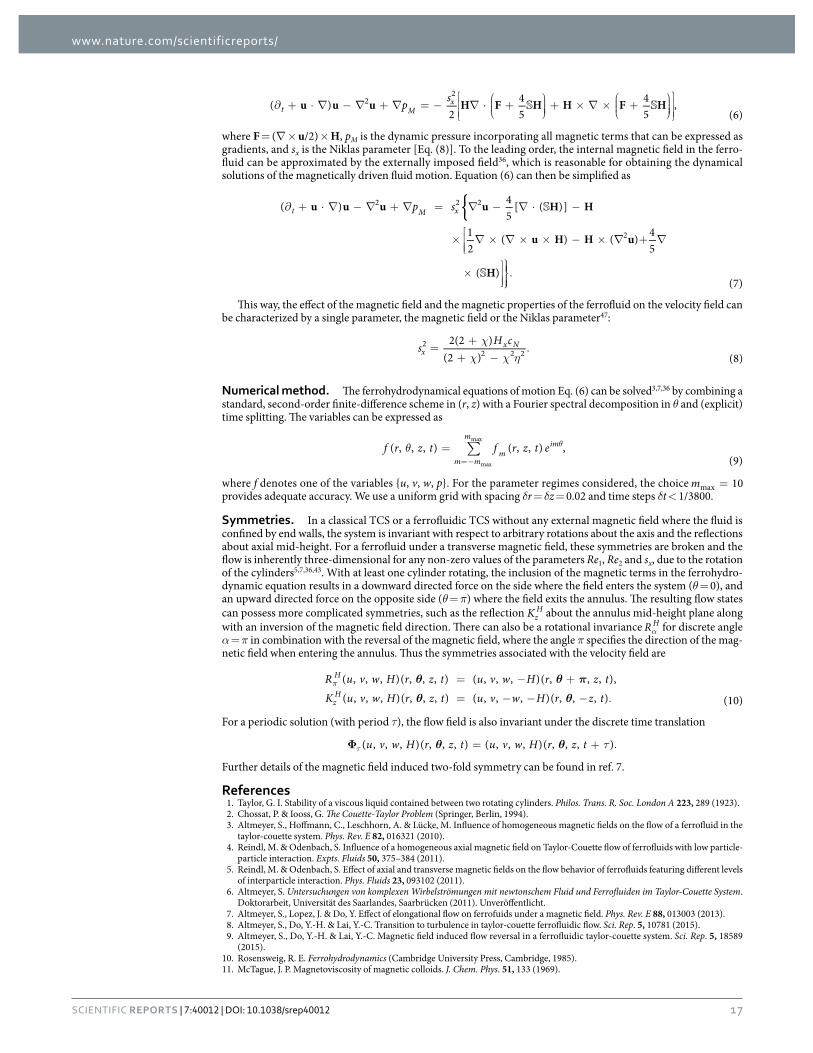
Flow structures Figure 1 presents a slightly elongated two-cell flow state 2L

N2. This flow state is found to exist only atstrong counterrotation (Re . �1680) and differs from 2N2 in that way that the vortex centers are pushed towards the innercylinder and the cells become elongated in the axial direction.

Figure 2 shows visualization of the flow pattern for � = 1.0, Re2 = �250 indicates a modulation in the flow structure of1A2. The one-cell flow state remains but a minor, second vortex cell starts to grow in the axial direction near the inner cylinderas the large vortex cell (top in Fig. 2) is pulled outwards due to the counter rotation.

A typical flow state 2N2 is presented in Fig. 3 for parameters at � = 1.6 and Re2 = �250. Compared to other presented 2N2

states for Re = 0 (see Fig. 3 in main paper) or Re = �250 (see Fig. 2) the vortex centers are shifted closer toward the innercylinder due to the strong counter rotation.

The figures 4 and 5 present either snapshots and time series of the 2N z-osci2 state for parameters at � = 1.7 and Re2 = �500

(see Figs. 5 and 6 in main paper).Figure 6 presents the flow state 1A2 at � = 1.0 and Re2 = �250. Increasing � this flow remains first stable with slight but

continuous change in the position of the vortex cell. The larger vortex cell moves towards the inner cylinder, while the secondvortex cell grows and moves radially outward towards the outer cylinder. In principle this is the same evolution as for the caseof Re2 = �250, with the only difference being that, due to the stronger counter rotation (Re2 = �500), the vortex cells and inparticular their centers are slightly shifted and located closer towards the inner cylinder.

The Figs. 7 and 8 present snapshots, time series and PSD for the azimuthally oscillating twin-cell flow state 2T ✓-osci2 at

� = 1.2, Re2 = �500.

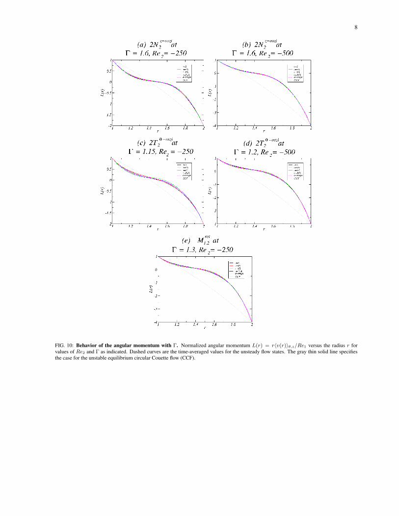
Behaviors of the angular momentum and torque To further characterize the flow states, we examine the behaviors of theangular momentum and torque. Figure 10 shows the mean (axially and azimuthally averaged) angular momentum L(r) =rhv(r)i

✓,z

/Re1, normalized by the inner Reynolds number Re1, versus the radius r for different values of the aspect ratio�. For unsteady flow states, the time-averaged values over one period are shown, where the gray thin solid line indicates thebehavior for the unstable equilibrium circular Couette flow (CCF) for comparison. For all the flow states, the angular momentumis transported outwards from the inner cylinder, which is typical for the TCS.

When the outer cylinder is at rest, the L(r) curves have a large slope near the inner cylinder wall. For the 2N c

2 state thecurve is convex. The largest slope of L(r) at the inner boundary corresponds to the smallest value of �. After the bifurcationleading to the emergence of the one-cell flow state 1A2, the L(r) curves start to form a plateau region about the center of thebulk, which becomes more pronounced as � is increased, as shown in Fig. 10(a). The fact that for the flow state 2N2 the curveL(r) has a local maximum in the outer bulk region at r ⇡ 0.72d indicates strongly oscillatory dynamics in the outer region. ForRe2 < 0 all L(r) curves have a similar shape with increased slope near the boundaries and reduced slope in the interior. Dueto the stronger torque the steepest part of L(r) now occurs at the outer boundary. Increasing � the slopes of L(r) near the innerand outer boundaries decrease. For Re = �250, changes in the shape of the L(r) curves are relatively moderate, where thelargest change occurs at r ⇡ 0.35d and r ⇡ 0.85d while close to the central region (r ⇡ 0.6d), there is little change in L(r)(pinned). For the two-cell flow states 2N2 and 2N z-osci

2 , the central region is flattened. For Re = �500 the variations of the flowstates in the outer half of the bulk are the strongest. Increasing � results in a decrease in the slope of L(r), minimizing the size

2

FIG. 1: Visualization of the flow state 2LN2. Flow visualization of 2LN2 for � = 1.6, Re2 = �2000: (a) isosurface of rv (isolevel shownat rv = ±7) and the corresponding vector plot [u(r, z), w(r, z)] of the radial and axial velocity components (including the azimuthal vorticity⌘(r, ✓)) for (b) ✓ = 0 and (c) ✓ = ⇡/2. (d-f) The azimuthal velocity v(r, ✓) in three different planes: z = �/4, z = �/2, and z = 3�/4,respectively. The same legends are used for visualizing all the time independent flows in the paper.

of the interior plateau region. Similar to the case of Re = �250, the central parts of the curve L(r) for the two-cell flow stateslie below the ones for the one-cell states.

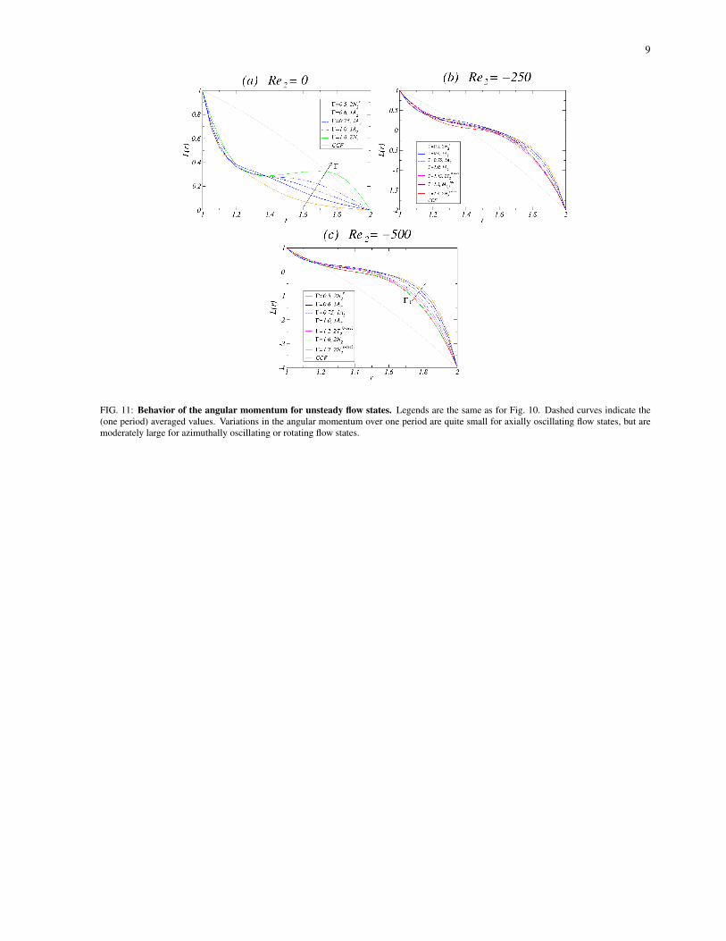
After the averaged quantities we will now look at the variations within the time-dependent solutions. Therefore Fig. 11 showsthe variation in the angular momentum L(r) over one period for different unsteady state flows. We see that variations of L(r)for the axially oscillating flow state 2N z-osci

2 are quite small. Moderate changes over one period are visible only in the inner halfof the bulk for Re2 = �250, as shown in Fig. 11(a). For Re2 = �500 the variations are insignificant, as shown in Fig. 11(b).However, for the azimuthally oscillating flow states 2T ✓-osci

2 , the variations in L(r) over one period are moderate (larger thanthose for axial oscillations) with stronger (weaker) amplitude for Re2 = �250 (Re2 = �500). Over one period the slope ofL(r) in the interior region changes significantly. Modulation also takes place near the center of the bulk, as shown in Fig. 11(c).For the rotating flow state M rot

1,2, the main changes in L(r) occurs in the outer bulk region, as shown in Fig. 11(e), accountingfor the dynamics associated with the m = 1 mode.

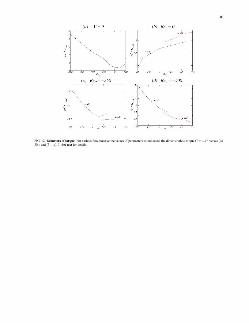
Last we will investigate on the behaviors of the dimensionless torque G = ⌫J! with Re2 and � (Fig. 12). The torqueis calculated based on the fact that, for a flow between infinite cylinders the transverse current of the azimuthal motion, i.e.,J! = r3[hu!i

A,t

� ⌫h@r

!iA,t

] [1], where h...iA

⌘R

rd✓dz

2⇡rl , is a conserved quantity [1]. Thus, the dimensionless torque is thesame at the inner and outer cylinders. For the two-cell and four-cell flow states for � = 1.6 (Fig. 11), the torque G is minimalfor Re2 = 0 and increases monotonically as the value of Re2 is increased in either direction. Note that we do not distinguishthe various flow states in detail but only focus on the one-cell and two-cell flow states. For Re = 0 (Re = �500), the torque Gmonotonically increases (decreases) as � is increased, regardless of the nature of the flow state (e.g., one-cell, two-cell, steady,or unsteady). For Re = �250 the torque for the one-cell flow states initially decreases with �, reaches a minimum and increasesafterwards. However for the two-cell flow states, G increases monotonically with �.

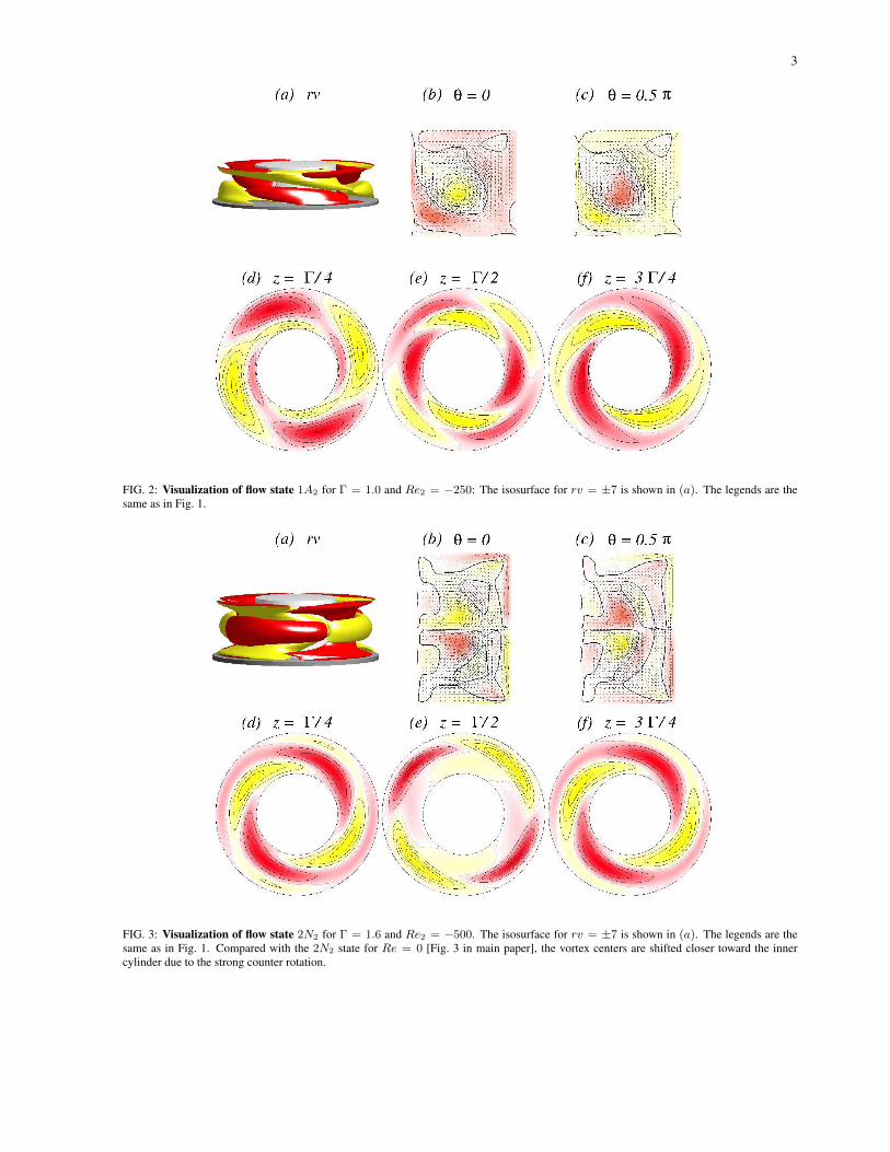
3

FIG. 2: Visualization of flow state 1A2 for � = 1.0 and Re2 = �250: The isosurface for rv = ±7 is shown in (a). The legends are thesame as in Fig. 1.

FIG. 3: Visualization of flow state 2N2 for � = 1.6 and Re2 = �500. The isosurface for rv = ±7 is shown in (a). The legends are thesame as in Fig. 1. Compared with the 2N2 state for Re = 0 [Fig. 3 in main paper], the vortex centers are shifted closer toward the innercylinder due to the strong counter rotation.

4

FIG. 4: Visualization of the axially oscillating two-cell flow state 2N z-osci

2 . The first row shows, for � = 1.7 and Re2 = �500, theisosurfaces of rv (isolevel shown at rv = ±15) over one axially oscillating period (⌧z ⇡ 0.157, and corresponding frequency !✓ ⇡ 12.682)at instants of time t as indicated. The second and third rows show the corresponding vector plots [u(r, z), w(r, z)] of the radial and axialvelocity components in the planes defined by ✓ = 0 and ✓ = ⇡/2, respectively, where the color-coded azimuthal vorticity field ⌘ is alsoshown. The fourth and fifth rows represent the azimuthal velocity v(r, ✓) in the axial planes z = �/4 and z = �/2, respectively. Red (darkgray) and yellow (light gray) colors correspond to positive and negative values, respectively, with zero specified as white. See also movie filemovieA1.avi in Supplementary Materials (SMs). The same legends for flow visualization are used for all subsequent unsteady flows. Seemovie files movieE1.avi, movieE2.avi and movieE3.avi in Supplementary Materials. Comparing with the 2N z-osci

2 state [Fig. 5 in main paper],the oscillation amplitude is smaller.

5

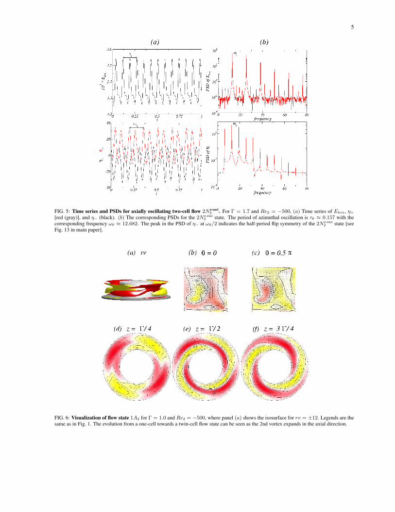
FIG. 5: Time series and PSDs for axially oscillating two-cell flow 2N z-osci

2 . For � = 1.7 and Re2 = �500, (a) Time series of Ekin, ⌘+[red (gray)], and ⌘� (black). (b) The corresponding PSDs for the 2N z-osci

2 state. The period of azimuthal oscillation is ⌧✓ ⇡ 0.157 with thecorresponding frequency !✓ ⇡ 12.682. The peak in the PSD of ⌘� at !✓/2 indicates the half-period flip symmetry of the 2N z-osci

2 state [seeFig. 13 in main paper].

FIG. 6: Visualization of flow state 1A2 for � = 1.0 and Re2 = �500, where panel (a) shows the isosurface for rv = ±12. Legends are thesame as in Fig. 1. The evolution from a one-cell towards a twin-cell flow state can be seen as the 2nd vortex expands in the axial direction.

6

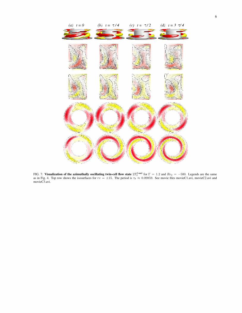
FIG. 7: Visualization of the azimuthally oscillating twin-cell flow state 2T ✓-osci

2 for � = 1.2 and Re2 = �500. Legends are the sameas in Fig. 4. Top row shows the isosurfaces for rv = ±15. The period is ⌧✓ ⇡ 0.09859. See movie files movieC1.avi, movieC2.avi andmovieC3.avi.

7

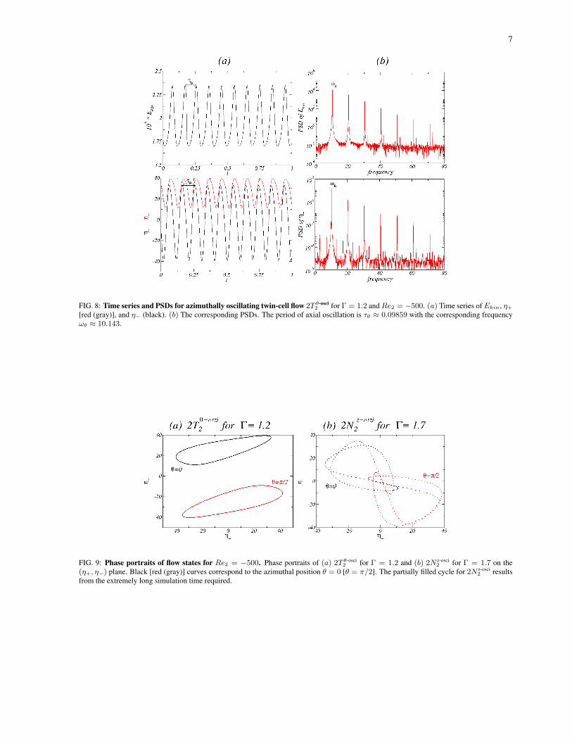
FIG. 8: Time series and PSDs for azimuthally oscillating twin-cell flow 2T ✓-osci

2 for � = 1.2 and Re2 = �500. (a) Time series of Ekin, ⌘+[red (gray)], and ⌘� (black). (b) The corresponding PSDs. The period of axial oscillation is ⌧✓ ⇡ 0.09859 with the corresponding frequency!✓ ⇡ 10.143.

FIG. 9: Phase portraits of flow states for Re2 = �500. Phase portraits of (a) 2T ✓-osci2 for � = 1.2 and (b) 2N z-osci

2 for � = 1.7 on the(⌘+, ⌘�) plane. Black [red (gray)] curves correspond to the azimuthal position ✓ = 0 [✓ = ⇡/2]. The partially filled cycle for 2N z-osci

2 resultsfrom the extremely long simulation time required.

8

FIG. 10: Behavior of the angular momentum with �. Normalized angular momentum L(r) = rhv(r)i✓,z/Re1 versus the radius r forvalues of Re2 and � as indicated. Dashed curves are the time-averaged values for the unsteady flow states. The gray thin solid line specifiesthe case for the unstable equilibrium circular Couette flow (CCF).

9

FIG. 11: Behavior of the angular momentum for unsteady flow states. Legends are the same as for Fig. 10. Dashed curves indicate the(one period) averaged values. Variations in the angular momentum over one period are quite small for axially oscillating flow states, but aremoderately large for azimuthally oscillating or rotating flow states.

10

FIG. 12: Behaviors of torque. For various flow states at the values of parameters as indicated, the dimensionless torque G = ⌫J! versus (a)Re2 and (b� d) �. See text for details.

11

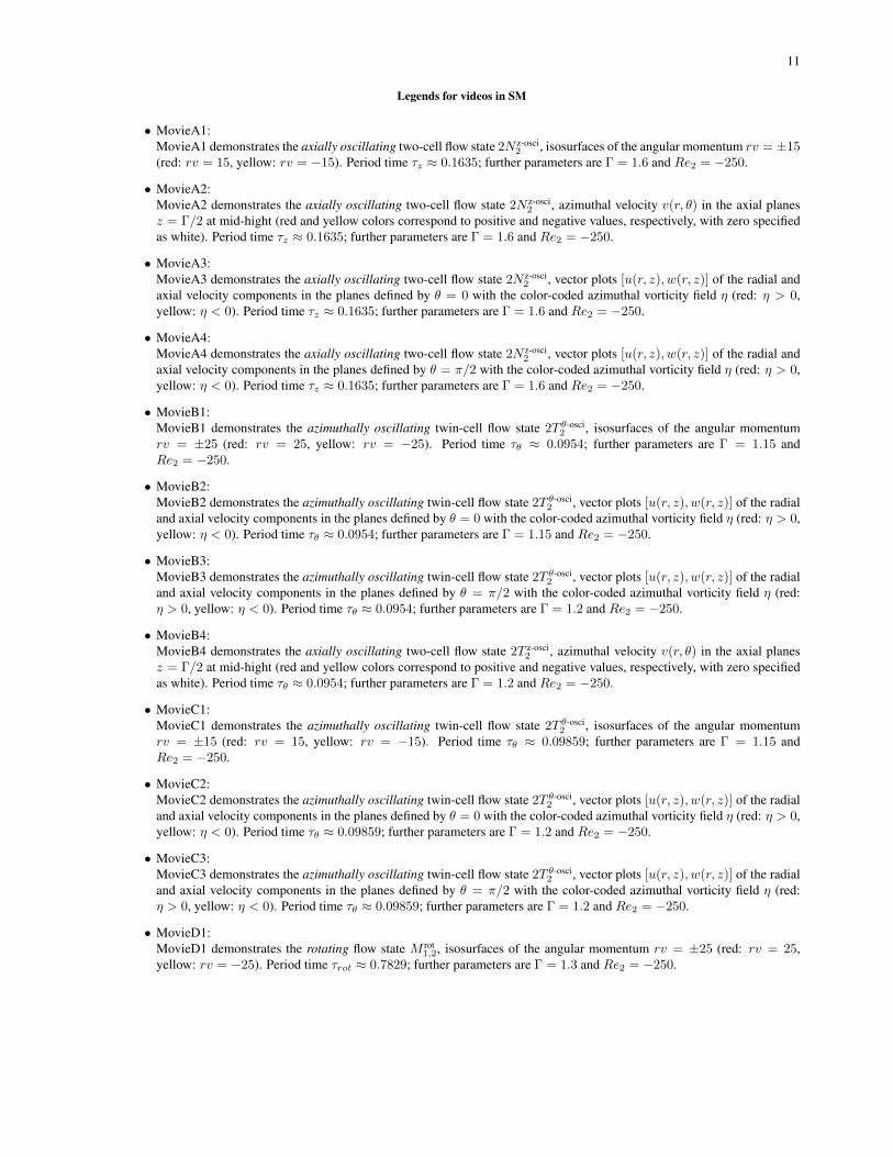
Legends for videos in SM

• MovieA1:MovieA1 demonstrates the axially oscillating two-cell flow state 2N z-osci

2 , isosurfaces of the angular momentum rv = ±15(red: rv = 15, yellow: rv = �15). Period time ⌧

z

⇡ 0.1635; further parameters are � = 1.6 and Re2 = �250.


2 , azimuthal velocity v(r, ✓) in the axial planesz = �/2 at mid-hight (red and yellow colors correspond to positive and negative values, respectively, with zero specifiedas white). Period time ⌧

z



2 , vector plots [u(r, z), w(r, z)] of the radial andaxial velocity components in the planes defined by ✓ = 0 with the color-coded azimuthal vorticity field ⌘ (red: ⌘ > 0,yellow: ⌘ < 0). Period time ⌧

z



2 , vector plots [u(r, z), w(r, z)] of the radial andaxial velocity components in the planes defined by ✓ = ⇡/2 with the color-coded azimuthal vorticity field ⌘ (red: ⌘ > 0,yellow: ⌘ < 0). Period time ⌧

z


• MovieB1:MovieB1 demonstrates the azimuthally oscillating twin-cell flow state 2T ✓-osci

2 , isosurfaces of the angular momentumrv = ±25 (red: rv = 25, yellow: rv = �25). Period time ⌧

✓

⇡ 0.0954; further parameters are � = 1.15 andRe2 = �250.


2 , vector plots [u(r, z), w(r, z)] of the radialand axial velocity components in the planes defined by ✓ = 0 with the color-coded azimuthal vorticity field ⌘ (red: ⌘ > 0,yellow: ⌘ < 0). Period time ⌧

✓



2 , vector plots [u(r, z), w(r, z)] of the radialand axial velocity components in the planes defined by ✓ = ⇡/2 with the color-coded azimuthal vorticity field ⌘ (red:⌘ > 0, yellow: ⌘ < 0). Period time ⌧

✓


• MovieB4:MovieB4 demonstrates the axially oscillating two-cell flow state 2T z-osci

2 , azimuthal velocity v(r, ✓) in the axial planesz = �/2 at mid-hight (red and yellow colors correspond to positive and negative values, respectively, with zero specifiedas white). Period time ⌧

✓


• MovieC1:MovieC1 demonstrates the azimuthally oscillating twin-cell flow state 2T ✓-osci


✓

⇡ 0.09859; further parameters are � = 1.15 andRe2 = �250.



✓




✓


• MovieD1:MovieD1 demonstrates the rotating flow state M rot

1,2, isosurfaces of the angular momentum rv = ±25 (red: rv = 25,yellow: rv = �25). Period time ⌧

rot


12

• MovieD2:MovieD2 demonstrates the rotating flow state M rot

1,2,, azimuthal velocity v(r, ✓) in the axial planes z = �/2 at mid-hight(red and yellow colors correspond to positive and negative values, respectively, with zero specified as white). Period time⌧rot


• MovieE1:MovieE1 demonstrates the azimuthally oscillating twin-cell flow state 2T z-osci


z




z




z


⇤ Electronic address: [email protected]† Electronic address: [email protected]

[1] Eckhardt, B. & Grossmann, S. & Lohse, D. Torque scaling in turbulent Taylor-Couette flow between independently rotating cylinders. J.

Fluid Mech. 581, 221–250 (2007).

Documents

Dynamics of ferrofluidic flow in the Taylor-Couette …chaos1.la.asu.edu/~yclai/papers/SREP_2017_ADL.pdf · Dynamics of ferrofluidic flow in the Taylor-Couette system with a small