Embed Size (px)
Citation preview
Dynamics of Ice Sheets and Glaciers
Ralf Greve
Institute of Low Temperature Science
Hokkaido University
Lecture Notes
Sapporo 2004/2005

Literature
Ice dynamics
Paterson, W. S. B. 1994. The Physics of Glaciers. Pergamon Press, Oxford etc., 3rd
edition.
Van der Veen, C. J. 1999. Fundamentals of Glacier Dynamics. A. A. Balkema, Rot-
terdam.
Hutter, K. 1983. Theoretical Glaciology: Material Science of Ice and the Mechanics of
Glaciers and Ice Sheets. D. Reidel Publishing Company, Dordrecht etc.
Zotikov, I. A. 1986. The Thermophysics of Glaciers. D. Reidel Publishing Company,
Dordrecht etc.
Greve, R. 2000. Large-scale glaciation on Earth and on Mars. Habilitation thesis,
Department of Mechanics, Darmstadt University of Technology (available online
at http://hgxpro1.lowtem.hokudai.ac.jp/∼greve/papers/2000/Greve00c.pdf).
Continuum mechanics, mathematics
Hutter, K. and K. Johnk. 2004. Continuum Methods of Physical Modeling. Springer-
Verlag, Berlin etc.
Greve, R. 2003. Kontinuumsmechanik. Eine Einfuhrung fur Ingenieure und Physiker.
Springer-Verlag, Berlin etc.
Liu, I-S. 2002. Continuum Mechanics. Springer-Verlag, Berlin etc.
Heinbockel, J. H. 1996. Introduction to tensor calculus and continuum mechanics. De-
partment of Mathematics and Statistics, Old Dominion University, Norfolk, Vir-
ginia (free, available online at http://www.math.odu.edu/∼jhh/counter2.html).
i
Bronshtein, I. N., K. A. Semendyayev, G. Musiol and H. Muehlig. 2004. Handbook of
Mathematics. Springer-Verlag, Berlin etc., 4th edition.
Any textbook on elementary calculus and linear algebra of the distinguished reader’s
preference...
ii
Contents
1 Vectors, tensors and their representation 1
1.1 Definition of a vector, basic properties . . . . . . . . . . . . . . . . . . 1
1.2 Representation of vectors as number triples . . . . . . . . . . . . . . . . 3
1.3 Tensors . . . . . . . . . . . . . . . . . . . . . . . . . . . . . . . . . . . 5
2 Elements of continuum mechanics 7
2.1 Bodies and configurations . . . . . . . . . . . . . . . . . . . . . . . . . 7
2.2 Kinematics . . . . . . . . . . . . . . . . . . . . . . . . . . . . . . . . . 8
2.2.1 Deformation gradient, stretch tensors . . . . . . . . . . . . . . . 8
2.2.2 Velocity, acceleration, velocity gradient . . . . . . . . . . . . . . 11
2.3 Balance equations . . . . . . . . . . . . . . . . . . . . . . . . . . . . . . 15
2.3.1 Reynolds’ transport theorem . . . . . . . . . . . . . . . . . . . . 15
2.3.2 General balance equation . . . . . . . . . . . . . . . . . . . . . . 17
2.3.3 General jump condition . . . . . . . . . . . . . . . . . . . . . . 18
2.3.4 Mass balance . . . . . . . . . . . . . . . . . . . . . . . . . . . . 20
2.3.5 Momentum balance . . . . . . . . . . . . . . . . . . . . . . . . . 21
2.3.6 Balance of angular momentum . . . . . . . . . . . . . . . . . . . 24
2.3.7 Energy balance . . . . . . . . . . . . . . . . . . . . . . . . . . . 26
2.4 Constitutive equations . . . . . . . . . . . . . . . . . . . . . . . . . . . 29
2.4.1 Simple bodies with fading memory . . . . . . . . . . . . . . . . 29
2.4.2 Linear-elastic solid . . . . . . . . . . . . . . . . . . . . . . . . . 30
2.4.3 Newtonian fluid . . . . . . . . . . . . . . . . . . . . . . . . . . . 32
3 Large-scale dynamics of ice sheets 35
3.1 Constitutive equations for polycrystalline ice . . . . . . . . . . . . . . . 35
3.1.1 Microstructure of ice . . . . . . . . . . . . . . . . . . . . . . . . 35
3.1.2 Creep of polycrystalline ice . . . . . . . . . . . . . . . . . . . . . 36
iii
Contents
3.1.3 Flow relation . . . . . . . . . . . . . . . . . . . . . . . . . . . . 37
3.1.4 Heat flux and internal energy . . . . . . . . . . . . . . . . . . . 41
3.2 Full Stokes flow problem . . . . . . . . . . . . . . . . . . . . . . . . . . 42
3.2.1 Field equations . . . . . . . . . . . . . . . . . . . . . . . . . . . 42
3.2.2 Boundary conditions . . . . . . . . . . . . . . . . . . . . . . . . 45
3.2.3 Ice-thickness equation . . . . . . . . . . . . . . . . . . . . . . . 50
3.3 Hydrostatic approximation . . . . . . . . . . . . . . . . . . . . . . . . . 51
3.4 Shallow-ice approximation . . . . . . . . . . . . . . . . . . . . . . . . . 53
3.5 Vialov profile . . . . . . . . . . . . . . . . . . . . . . . . . . . . . . . . 60
4 Large-scale dynamics of ice shelves 65
4.1 Full Stokes flow problem, hydrostatic approximation . . . . . . . . . . . 65
4.2 Shallow-shelf approximation . . . . . . . . . . . . . . . . . . . . . . . . 68
5 Dynamics of glacier flow 75
6 Glacial isostasy 77
6.1 General remarks . . . . . . . . . . . . . . . . . . . . . . . . . . . . . . . 77
6.2 Structure of the Earth . . . . . . . . . . . . . . . . . . . . . . . . . . . 79
6.3 Simple isostasy models . . . . . . . . . . . . . . . . . . . . . . . . . . . 80
6.3.1 LLRA model . . . . . . . . . . . . . . . . . . . . . . . . . . . . 80
6.3.2 ELRA model . . . . . . . . . . . . . . . . . . . . . . . . . . . . 81
6.3.3 LLDA model . . . . . . . . . . . . . . . . . . . . . . . . . . . . 83
6.3.4 ELDA model . . . . . . . . . . . . . . . . . . . . . . . . . . . . 86
6.3.5 Performance of the simple models . . . . . . . . . . . . . . . . . 86
iv
1 Vectors, tensors and their
representation
1.1 Definition of a vector, basic properties
In mathematics, a vector is defined as an element of a vector space, and a vector space
is a commutative (Abelian) group with a scalar multiplication. This is an abstract
definition which has many possible realizations (numbers, functions, geometric objects
and so on). For our purposes, it is sufficient to consider one of them, namely the
geometric object of an arrow in the three-dimensional, Euklidian, physical space E .
Therefore, in our sense a vector a ∈ E is an arrow which is characterized by a length
and a direction. Physical quantities which can be described by such vectors are, for
instance, velocity, acceleration, momentum and force. By contrast, scalars are simple
numbers and characterize physical quantities without a direction, like mass, density,
temperature etc.
We will usually denote vectors by bold-face symbols like a, b, c... The sum
s = a + b (1.1)
of two vectors is then obtained by the parallelogram construction, and the scalar mul-
tiplication
p = λa, λ ∈ R (1.2)
(R denotes the set of real numbers) follows from multiplying the length of a by λ
(Fig. 1.1).
The length of the vector a is written as |a| (absolute value, norm), and its direction
can be characterized by the unit vector (length equal to one) ea = a/|a|. Further, the
dot product (inner product)
δ = a · b (1.3)
of two vectors is equal to the scalar given by |a| |b| cos ϕ (where ϕ is the angle between
1
1 Vectors, tensors and their representation
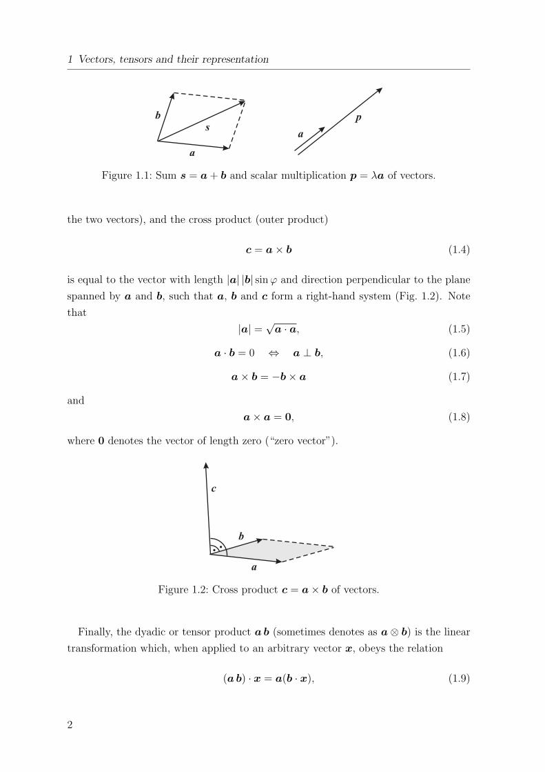
Figure 1.1: Sum s = a + b and scalar multiplication p = λa of vectors.
the two vectors), and the cross product (outer product)
c = a× b (1.4)
is equal to the vector with length |a| |b| sin ϕ and direction perpendicular to the plane
spanned by a and b, such that a, b and c form a right-hand system (Fig. 1.2). Note
that
|a| = √a · a, (1.5)
a · b = 0 ⇔ a ⊥ b, (1.6)
a× b = −b× a (1.7)
and
a× a = 0, (1.8)
where 0 denotes the vector of length zero (“zero vector”).
Figure 1.2: Cross product c = a× b of vectors.
Finally, the dyadic or tensor product ab (sometimes denotes as a⊗ b) is the linear
transformation which, when applied to an arbitrary vector x, obeys the relation
(ab) · x = a(b · x), (1.9)
2
1.2 Representation of vectors as number triples
where (b ·x) means the dot product (1.3). In other words, the transformation ab maps
the vector x onto the vector which has the direction of a and (b · x) times the length
of a.
1.2 Representation of vectors as number triples
Let eii=1,2,3 be a set of unit vectors which are perpendicular to each other and form
a right-hand system. In other words,
ei · ej = δij, (1.10)
where δij is the Kronecker symbol defined as
δij =
1, for i = j,
0, for i 6= j,(1.11)
and
ei × ej = ek, (i, j, k) ∈ (1, 2, 3), (2, 3, 1), (3, 1, 2). (1.12)
We will refer to such a set ei as an orthonormal basis (also Cartesian basis). An
arbitrary vector a can then uniquely be written as
a = a1e1 + a2e2 + a3e3 =3∑
i=1
aiei, (1.13)
where the ai are real numbers. With Einstein’s summation convention, which says that
double indices (here i) automatically imply summation, this can be written in compact
form as
a = aiei. (1.14)
Since the coefficients ai are unique for a given basis ei, it is possible to represent the
vector a by these coefficients. It is usual to arrange them in a column (number triple)
and write
aei =
a1
a2
a3
, (1.15)
which is to say, the vector a is represented by the components ai with respect to the ba-
sis ei. Of course, when a different orthonormal basis e?i is used, the representation
3
1 Vectors, tensors and their representation
of the vector a will change:
a = a?i e
?i , (1.16)
or
ae?i =
a?1
a?2
a?3
. (1.17)
Note that the vector a is still the same object (arrow in space), whereas its compo-
nents have changed. It is therefore of great importance to distinguish between vectors
themselves and their representation as number triples. Mixing up these two different
things is a notorious source of confusion. Only when a single basis ei is defined from
the outset, and all vectors are expressed in this basis, it is allowed to write sloppily
a =
a1
a2
a3
, (1.18)
but this requires a good deal of care.
In components with respect to a given basis ei, the dot product (1.3) can be
evaluated as
a · b = aibi, (1.19)
and the ith component of the cross product (1.4) is
(a× b)i = εijk ajbk (1.20)
(summation over j and k). In the latter expression, εijk is called the Levi-Civita symbol,
defined as
εijk =
1, for (i, j, k) ∈ (1, 2, 3), (2, 3, 1), (3, 1, 2),−1, for (i, j, k) ∈ (1, 3, 2), (3, 2, 1), (2, 1, 3),
0, otherwise (two or three indices equal).
(1.21)
The dyadic product defined in (1.9) is expressed as
ab = (aiei) (bjej) = aibj ei ej, (1.22)
(summation over i and j), where ei ej is the dyadic product of the respective basis
vectors.
4
1.3 Tensors
1.3 Tensors
A tensor A of rank two (often simply called a tensor) is defined as a linear transfor-
mation which maps vectors onto vectors:
y = A · x. (1.23)
We have already encountered special tensors of rank two, namely the dyadic products
between two vectors introduced in (1.9). Their expression with respect to an orthonor-
mal basis ei was given by (1.22), and similarly a general tensor of rank two can be
written as
A = Aij ei ej. (1.24)
Evidently, the tensor A is represented by the components Aij, and in analogy to (1.15)
this can be noted as
Aei =
A11 A12 A13
A21 A22 A23
A31 A32 A33
, (1.25)
where the components have been arranged into a quadratic matrix. Again, if a different
basis e?i is used, the representation will change,
Ae?i =
A?11 A?
12 A?13
A?21 A?
22 A?23
A?31 A?
32 A?33
, (1.26)
so that tensors and matrices must be distinguished in the same way as vectors and
number triples.
With the expression (1.24), the transformation (1.23) reads
y = (Aij ei ej) · (xk ek) = Aijxk ei (ej · ek) = Aijxk ei δjk = Aijxj ei, (1.27)
or
yi = Aijxj. (1.28)
Evidently, this is nothing else but the matrix-column product
y1
y2
y3
=
A11 A12 A13
A21 A22 A23
A31 A32 A33
·
x1
x2
x3
(1.29)
5
1 Vectors, tensors and their representation
expressed in (Cartesian) index notation. Index notation is a very efficient method of
carrying out computations in vector/tensor algebra and analysis [see also the expres-
sions (1.19) and (1.20) for the dot product and the cross product, respectively], and
we will use it frequently.
An important example for a tensor of rank two is the unity tensor 1, which provides
the identical transformation x = 1 · x. Its components in any orthonormal basis eiare given by the Kronecker symbol δij, that is,
1 = δij ei ej, (1.30)
so that its matrix representation is given by the unity matrix,
1ei =
1 0 0
0 1 0
0 0 1
. (1.31)
Evidently, when expressed in components, a tensor of rank two is a quantity with
two indices [see (1.24)]. As we have seen in Sect. 1.2, the expression of a vector in
components leads to a quantity with one index (for instance, ai), and of course a scalar
quantity does not have any indices at all. Therefore, vectors and scalars are also refered
to as tensors of rank one and zero, respectively.
As a generalisation of (1.23), tensors A[r] of rank r > 2 can now be defined inductively
as linear transformations which map vectors x onto tensors Y [r−1] of rank r − 1,
Y [r−1] = A[r] · x. (1.32)
Such tensors can be written in components as
A[r] = Ai1i2...ir ei1 ei2 . . . eir (1.33)
(summation over the r indices i1, i2, ..., ir). As an example, the Levi-Civita symbol
(1.21) can be interpreted as the components of a third-rank tensor ε[3],
ε[3] = εijk ei ej ek, (1.34)
which is known as the epsilon or permutation tensor. Tensors of rank four play a role
in the theory of elasticity.
6
2 Elements of continuum mechanics
2.1 Bodies and configurations
Continuum mechanics is concerned with the motion and deformation of continuous
bodies (for instance, a glacier). A body consists of an infinite number of material
elements, called particles. For any time t, each particle is identified by a position
vector x (relative to a prescribed origin O) in the physical space E , and the continuous
set of position vectors for all particles of the body is called a configuration κ of the
body. If t is the actual time, the corresponding configuration is called the present
configuration κt. In addition, we define a reference configuration κr which refers to a
fixed (or initial) time t0. Position vectors in the reference configuration will be written
in capitals like X; they can be used for identifying the individual particles of the body
independent of the actual time. Note that different sets of basis vectors (EAA=1,2,3,
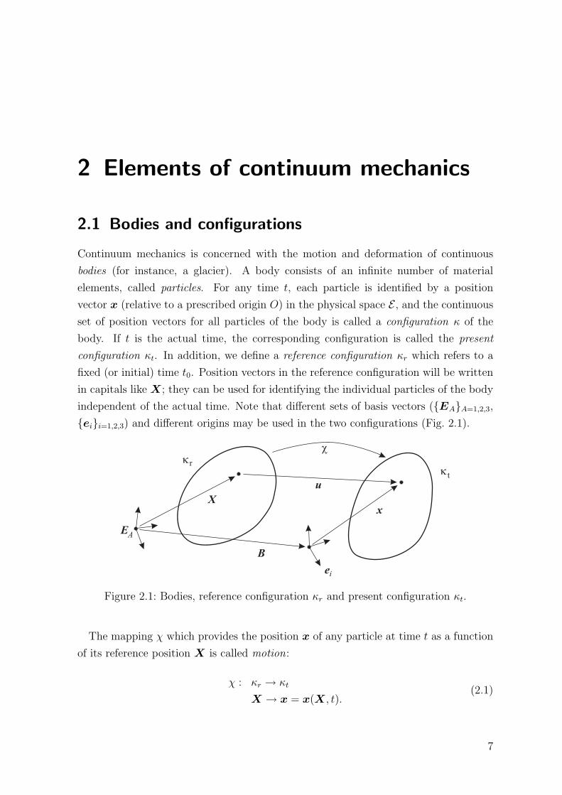
eii=1,2,3) and different origins may be used in the two configurations (Fig. 2.1).
Figure 2.1: Bodies, reference configuration κr and present configuration κt.
The mapping χ which provides the position x of any particle at time t as a function
of its reference position X is called motion:
χ : κr → κt
X → x = x(X, t).(2.1)
7
2 Elements of continuum mechanics
It is assumed that the motion x(X, t) is continuously differentiable in the entire body
(with the possible exception of singular lines or surfaces), so that the inverse mapping
χ−1 exists:
χ−1 : κt → κr
x → X = X(x, t).(2.2)
The displacement is defined as the connecting vector between a given particle in the
reference and present configuration. If the connecting vector between the two origins
of the basis systems is denoted by B, then
u = x−X + B (2.3)
holds. The above relationships are illustrated in Fig. 2.1.
Of course, in a deformable body the displacement at time t will in general be different
for the different particles, so that it can be written as the vector field u = u(X, t).
However, this is not the only possibility. Equation (2.2) shows that X can be expressed
in terms of x and t, so that we can also assume the displacement field as a function of
x and t, that is, u = u(x, t). These two possibilities hold also for other field quantities
ψ (density, temperature, velocity etc.), and we call ψ(X, t) the Lagrangian or material
description, whereas ψ(x, t) is refered to as the Eulerian or spatial description. Most
frequently, for solid bodies the Lagrangian description is used, whereas the Eulerian
description is more appropriate for problems of fluid dynamics (like glacier flow).
2.2 Kinematics
2.2.1 Deformation gradient, stretch tensors
The deformation gradient F is defined as the material gradient (gradient with respect
to X) of the motion (2.1),
F = Grad x(X, t), (2.4)
or in components
FiA =∂xi(X, t)
∂XA
= xi,A, (2.5)
where F = FiA ei EA, the operator Grad (·) is the material gradient, and the notation
(·),A means the partial derivative ∂(·)/∂XA. It is a tensor of rank two. Note that
small indices refer to the present configuration and capital indices to the reference
configuration.
8
2.2 Kinematics
According to the definition (2.4), the deformation gradient F can be interpreted as
the functional matrix of the motion function (2.1). It transforms line elements from
the reference configuration (dX) to the present configuration (dx),
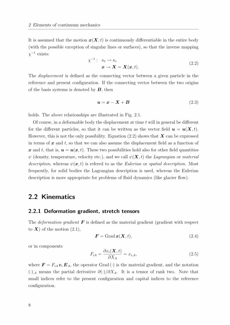
dx = F · dX, or dxi = FiA dXA, (2.6)
which is illustrated in Fig. 2.2.
Figure 2.2: Deformation gradient: Transformation between line and volume elementsin the reference and present configuration.
The determinant of the deformation gradient, called the Jacobian, is given as
J = det F , or J =1
6εABCεijkFiAFjBFkC ; (2.7)
in the component form on the right the Levi-Civita symbol, which was defined in (1.21),
appears. Since we have demanded that the motion function is invertible, J must be
different from zero, and the inverse deformation gradient F−1 exists. Further, real
motions cannot invert the orientation, so that
J > 0 (2.8)
must hold. The Jacobian determines the local volume change due to the motion,
dv = J dV, (2.9)
where dV is the volume element in the reference configuration which may be spanned
by three line elements dX(1), dX(2), dX(3), and dv is the volume element in the present
configuration spanned by dx(1), dx(2), dx(3) (Fig. 2.2).
The theorem of polar decomposition tells us that, like any tensor with positive deter-
9
2 Elements of continuum mechanics
minant, the deformation gradient F can be uniquely decomposed according to
F = R ·U = V ·R, (2.10)
where R is a proper orthogonal tensor (R ·RT = RT ·R = 1 and det R = +1), and the
tensors U und V are symmetric (U = UT, V = V T) and positive definite (∀x 6= 0:
x ·U ·x > 0, x ·V ·x > 0). The tensors U and V are called the right and left stretch
tensor, respectively, and R is the rotation tensor.
The polar decomposition of F can be obtained as follows. With (2.10) we compute
F T · F = UT ·RT ·R ·U = U · 1 ·U ⇒ U 2 = F T · F (2.11)
and
F · F T = V ·R ·RT · V T = V · 1 · V ⇒ V 2 = F · F T, (2.12)
which provides the stretch tensors U and V . The rotation tensor R follows then from
(2.10) as
R = F ·U−1, or R = V −1 · F . (2.13)
Note that (2.10) also implies the relation
V = R ·U ·RT, (2.14)
which means that the two stretch tensors are connected by a similarity transformation.
The polar decomposition of the deformation gradient F allows the interpretation of
an arbitrary deformation as a sequence of a local rigid-body rotation followed by a
stretching, or vice versa. With (2.6) we can write
dx = R ·U · dX = V ·R · dX. (2.15)
Since U is symmetric, there exists a special set of orthonormal basis vectors ei, called
the principal axes, for which the matrix U ei is diagonal, that is,
U ei = diag(λ1, λ2, λ3) =
λ1 0 0
0 λ2 0
0 0 λ3
. (2.16)
The λi, i = 1 . . . 3, are the eigenvalues of U , and due to the positive definiteness they
are all positive. This holds also for V , and because of the similarity transformation
10
2.2 Kinematics
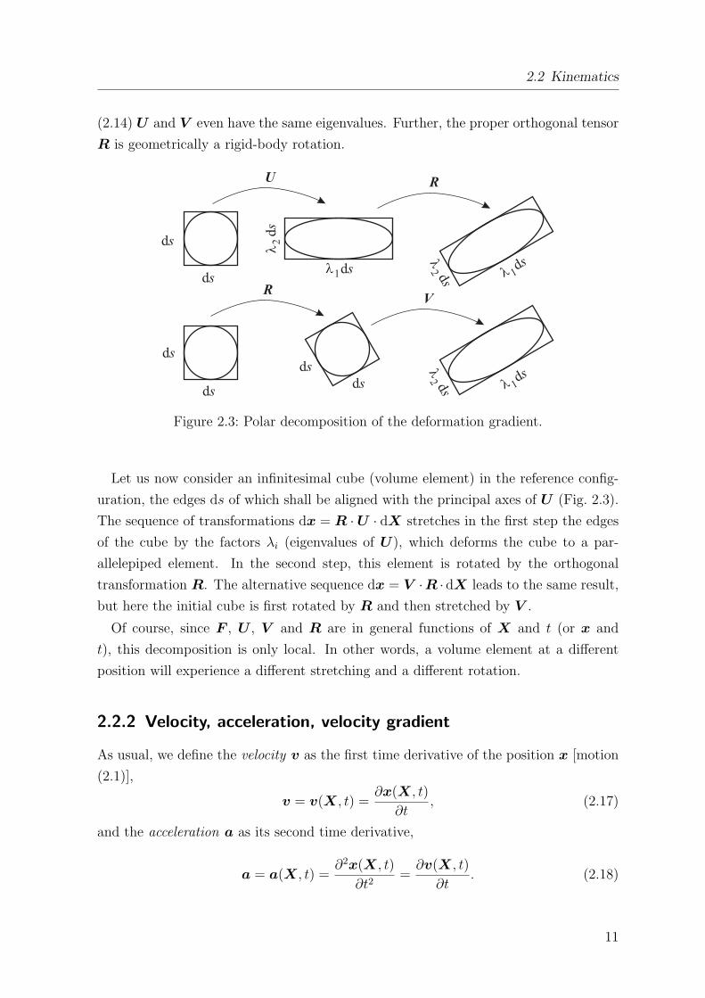
(2.14) U and V even have the same eigenvalues. Further, the proper orthogonal tensor
R is geometrically a rigid-body rotation.
Figure 2.3: Polar decomposition of the deformation gradient.
Let us now consider an infinitesimal cube (volume element) in the reference config-
uration, the edges ds of which shall be aligned with the principal axes of U (Fig. 2.3).
The sequence of transformations dx = R ·U · dX stretches in the first step the edges
of the cube by the factors λi (eigenvalues of U ), which deforms the cube to a par-
allelepiped element. In the second step, this element is rotated by the orthogonal
transformation R. The alternative sequence dx = V ·R ·dX leads to the same result,
but here the initial cube is first rotated by R and then stretched by V .
Of course, since F , U , V and R are in general functions of X and t (or x and
t), this decomposition is only local. In other words, a volume element at a different
position will experience a different stretching and a different rotation.
2.2.2 Velocity, acceleration, velocity gradient
As usual, we define the velocity v as the first time derivative of the position x [motion
(2.1)],
v = v(X, t) =∂x(X, t)
∂t, (2.17)
and the acceleration a as its second time derivative,
a = a(X, t) =∂2x(X, t)
∂t2=
∂v(X, t)
∂t. (2.18)
11
2 Elements of continuum mechanics
Evidently, this yields the velocity and acceleration fields in Lagrangian description. By
inserting the inverse motion (2.2) one can readily obtain the corresponding Eulerian
descriptions v(x, t) and a(x, t).
The time derivatives in (2.17) and (2.18) are taken for fixed material position vectors
X. We will call this the material time derivative, denoted briefly by the operators
d(•)/dt or (•)·. Therefore, for any field quantity ψ,
ψ =dψ
dt=
∂ψ(X, t)
∂t. (2.19)
For example, (2.17) and (2.18) read
v = x =dx
dt, a = x =
d2x
dt2= v =
dv
dt. (2.20)
By contrast, the operator ∂(•)/dt shall denote the local time derivative for fixed spatial
position vector x,∂ψ
∂t=
∂ψ(x, t)
∂t. (2.21)
With the chain rule, the relation between material and local time derivative follows as
dψ
dt=
d
dtψ(x(X, t), t)
=∂ψ(x, t)
∂t+ grad ψ(x, t) · dx(X, t)
dt
=∂ψ
∂t+ (grad ψ) · v, (2.22)
where the operator grad (·) is the spatial gradient, the components of which are the
partial derivatives (·),i = ∂(·)/∂xi. One says that the material time derivative dψ/dt
is composed by a local part ∂ψ/dt and an advective part (grad ψ) · v.
Relation (2.22) is equally valid if ψ is a vector or tensor field. Therefore, for the
acceleration expressed by (2.20)2,
a =∂v
∂t+ (grad v) · v. (2.23)
The tensor quantity
L = grad v =∂vi
∂xj
ei ej = vi,j ei ej (2.24)
which appears in (2.23) is called the velocity gradient. It is related to the material time
12

2.2 Kinematics
derivative of the deformation gradient as follows:
FiA =∂2xi(X, t)
∂t ∂XA
=∂vi(X, t)
∂XA
=∂vi(x, t)
∂xj
∂xj(X, t)
∂XA
=∂vi(x, t)
∂xj
FjA
⇒ F = L · F , or L = F · F−1. (2.25)
Without a formal proof (which is a bit tedious) we note for the material time derivative
of the Jacobian
J = J div v = J tr L (2.26)
(div v = vi,i = Lii = tr L, where the operator tr means the trace of a tensor). In words,
the divergence of the velocity field determines local volume changes [see also Eq. (2.9)],
which is a very intuitive result.
Like any arbitrary tensor, the velocity gradient can be additively decomposed into a
symmetric and an antisymmetric part:
L = D + W , (2.27)
withD = 1
2(L + LT) (“strain-rate tensor”),
W = 12(L−LT) (“spin tensor”).
(2.28)
Evidently, D = DT (symmetry) and W = −W T (antisymmetry) are fulfilled.
In order to give an interpretation of the elements of the matrix of the strain-rate
tensor D (with respect to a given orthonormal basis ei), we now compute the material
time derivative of line elements dx in the present configuration:
(dx)· = F · dX = L · F · dX = L · dx (2.29)
[where Eqs. (2.6), (2.25) and (dX)· = 0 were used]. For the scalar product between
two line elements dx(1) and dx(2), this yields
(dx(1) · dx(2))· = (dx(1))· · dx(2) + dx(1) · (dx(2))·
= (L · dx(1)) · dx(2) + dx(1) · (L · dx(2))
= dx(1) ·LT · dx(2) + dx(1) ·L · dx(2)
= 2 dx(1) ·D · dx(2). (2.30)
13
2 Elements of continuum mechanics
Let us assume
dx(1) = n(1)ds(1),
dx(2) = n(2)ds(2),n(1) · n(2) = cos((π/2)− γ) = sin γ, (2.31)
where n(1), n(2) are unit vectors, and γ is the deviation of the angle between n(1) and
n(2) from a right angle. Equation (2.30) then reads
(sin γ ds(1)ds(2))· = 2ds(1)ds(2) n(1) ·D · n(2)
⇒ γ cos γ + sin γ
((ds(1))·ds(1)
+(ds(2))·ds(2)
)= 2n(1) ·D · n(2). (2.32)
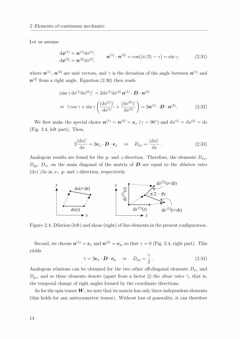
We first make the special choice n(1) = n(2) = ex (γ = 90) and ds(1) = ds(2) = ds
(Fig. 2.4, left part). Then,
2(ds)·ds
= 2ex ·D · ex ⇒ Dxx =(ds)·ds
. (2.33)
Analogous results are found for the y- and z-direction. Therefore, the elements Dxx,
Dyy, Dzz on the main diagonal of the matrix of D are equal to the dilation rates
(ds)·/ds in x-, y- and z-direction, respectively.
Figure 2.4: Dilation (left) and shear (right) of line elements in the present configuration.
Second, we choose n(1) = ex and n(2) = ey, so that γ = 0 (Fig. 2.4, right part). This
yields
γ = 2ex ·D · ey ⇒ Dxy =γ
2. (2.34)
Analogous relations can be obtained for the two other off-diagonal elements Dxz and
Dyz, and so these elements denote (apart from a factor 2) the shear rates γ, that is,
the temporal change of right angles formed by the coordinate directions.
As for the spin tensor W , we note that its matrix has only three independent elements
(this holds for any antisymmetric tensor). Without loss of generality, it can therefore
14
2.3 Balance equations
be written as
W =
0 −w3 w2
w3 0 −w1
−w2 w1 0
(2.35)
[see also Eq. (1.18) and the discussion there]. The wi arranged in the above form are
the components of the dual vector
w = dual W =
w1
w2
w3
, (2.36)
with which the linear transformation W · a (arbitrary vector a) can be expressed as a
cross product,
W · a = w × a. (2.37)
Thus, Eq. (2.29) yields
(dx)· = D · dx + w × dx. (2.38)
The first summand on the right-hand side describes the strain (deformation) part of
the motion, the second summand the local rigid-body rotation with angular velocity
w. This justifies the names “strain-rate tensor” and “spin tensor” for D and W ,
respectively.
2.3 Balance equations
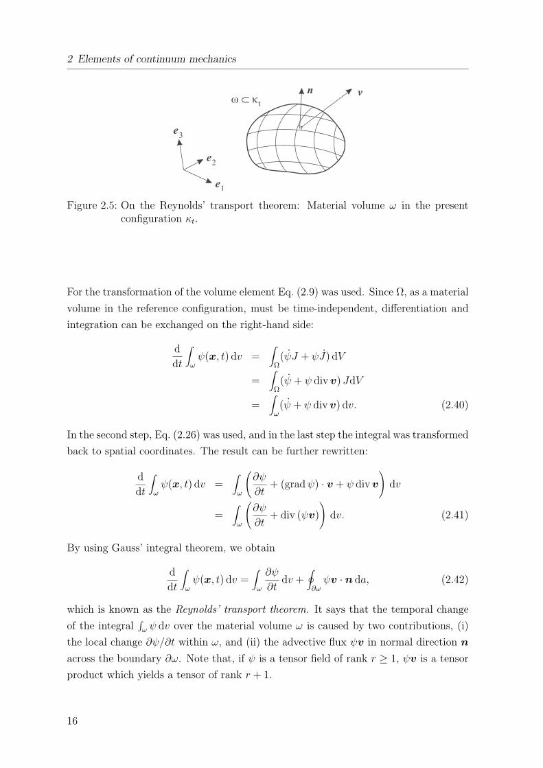
2.3.1 Reynolds’ transport theorem
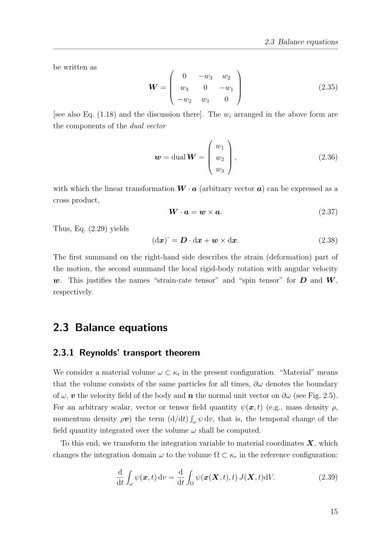
We consider a material volume ω ⊂ κt in the present configuration. “Material” means
that the volume consists of the same particles for all times, ∂ω denotes the boundary
of ω, v the velocity field of the body and n the normal unit vector on ∂ω (see Fig. 2.5).
For an arbitrary scalar, vector or tensor field quantity ψ(x, t) (e.g., mass density ρ,
momentum density ρv) the term (d/dt)∫ω ψ dv, that is, the temporal change of the
field quantity integrated over the volume ω shall be computed.
To this end, we transform the integration variable to material coordinates X, which
changes the integration domain ω to the volume Ω ⊂ κr in the reference configuration:
d
dt
∫
ωψ(x, t) dv =
d
dt
∫
Ωψ(x(X, t), t) J(X, t)dV. (2.39)
15
2 Elements of continuum mechanics
e1
e2
e3
n
w kÌt
v
Figure 2.5: On the Reynolds’ transport theorem: Material volume ω in the presentconfiguration κt.
For the transformation of the volume element Eq. (2.9) was used. Since Ω, as a material
volume in the reference configuration, must be time-independent, differentiation and
integration can be exchanged on the right-hand side:
d
dt
∫
ωψ(x, t) dv =
∫
Ω(ψJ + ψJ) dV
=∫
Ω(ψ + ψ div v) JdV
=∫
ω(ψ + ψ div v) dv. (2.40)
In the second step, Eq. (2.26) was used, and in the last step the integral was transformed
back to spatial coordinates. The result can be further rewritten:
d
dt
∫
ωψ(x, t) dv =
∫
ω
(∂ψ
∂t+ (grad ψ) · v + ψ div v
)dv
=∫
ω
(∂ψ
∂t+ div (ψv)
)dv. (2.41)
By using Gauss’ integral theorem, we obtain
d
dt
∫
ωψ(x, t) dv =
∫
ω
∂ψ
∂tdv +
∮
∂ωψv · n da, (2.42)
which is known as the Reynolds’ transport theorem. It says that the temporal change
of the integral∫ω ψ dv over the material volume ω is caused by two contributions, (i)
the local change ∂ψ/∂t within ω, and (ii) the advective flux ψv in normal direction n
across the boundary ∂ω. Note that, if ψ is a tensor field of rank r ≥ 1, ψv is a tensor
product which yields a tensor of rank r + 1.
16
2.3 Balance equations
2.3.2 General balance equation
Let G(ω, t) be an arbitrary physical quantity of the entire material volume ω (e.g., its
mass, momentum or internal energy). We assume that the change of G with time may
be due to three different processes, namely
• the flux F(∂ω, t) of G across the boundary ∂ω,
• the production P(ω, t) of G within the volume ω,
• the supply S(ω, t) of G within the volume ω.
Therefore, we can balance dG/dt as follows:
d
dtG(ω, t) = −F(∂ω, t) + P(ω, t) + S(ω, t), (2.43)
where positive fluxes have been defined as outflows of the volume, so that the flux
term has a negative sign. Conserved quantities shall be characterised by a vanishing
production.
In order to reformulate this statement, we assume that G, P and S can be expressed
as volume integrals of corresponding densities g, p and s (additivity),
G(ω, t) =∫ω g(x, t) dv, g : density of the quantity G,
P(ω, t) =∫ω p(x, t) dv, p : production density of G,
S(ω, t) =∫ω s(x, t) dv, s : supply density of G,
(2.44)
and that F can be obtained as the surface integral of a flux density φ,
F(∂ω, t) =∮
∂ωφ(x, t) · n da, (2.45)
where da is the scalar surface element. Note that, if G is a tensor quantity of rank
r ≥ 0 (scalar, vector etc.), then the rank of g, p and s is also equal to r, whereas the
rank of φ is r + 1.
Inserting the expressions (2.44) and (2.45) in Eq. (2.43) yields the general balance
equation in integral form,
d
dt
∫
ωg(x, t) dv = −
∮
∂ωφ(x, t) · n da +
∫
ωp(x, t) dv +
∫
ωs(x, t) dv. (2.46)
Provided that all fields in this equation are continuously differentiable, this equation
can be localized as follows. We apply the Reynolds’ transport theorem (2.42) to the
17
2 Elements of continuum mechanics
left-hand side (with ψ = g), transform all surface integrals to volume integrals with
Gauss’ integral theorem and assemble all terms on the left-hand side:
∫
ω
(∂g
∂t+ div (gv) + div φ− p− s
)dv = 0. (2.47)
This relation must hold for any arbitrary material volume ω, which is only possible, if
the integrand itself vanishes. Thus,
∂g
∂t= −div (φ + gv) + p + s, (2.48)
which is the general balance equation in local form. It balances the local change of the
density g with the production and supply densities and the negative divergence of two
flux terms, the actual flux density φ and the advective (or convective) flux density gv.
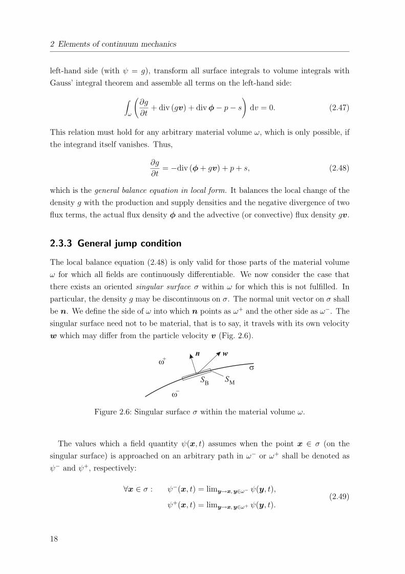
2.3.3 General jump condition
The local balance equation (2.48) is only valid for those parts of the material volume
ω for which all fields are continuously differentiable. We now consider the case that
there exists an oriented singular surface σ within ω for which this is not fulfilled. In
particular, the density g may be discontinuous on σ. The normal unit vector on σ shall
be n. We define the side of ω into which n points as ω+ and the other side as ω−. The
singular surface need not to be material, that is to say, it travels with its own velocity
w which may differ from the particle velocity v (Fig. 2.6).
Figure 2.6: Singular surface σ within the material volume ω.
The values which a field quantity ψ(x, t) assumes when the point x ∈ σ (on the
singular surface) is approached on an arbitrary path in ω− or ω+ shall be denoted as
ψ− and ψ+, respectively:
∀x ∈ σ : ψ−(x, t) = limy→x, y∈ω− ψ(y, t),
ψ+(x, t) = limy→x, y∈ω+ ψ(y, t).(2.49)
18
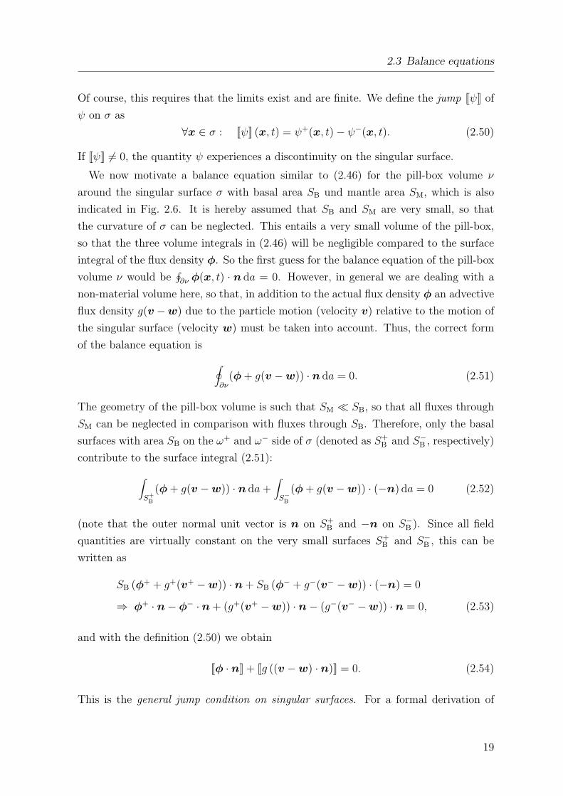
2.3 Balance equations
Of course, this requires that the limits exist and are finite. We define the jump [[ψ]] of
ψ on σ as
∀x ∈ σ : [[ψ]] (x, t) = ψ+(x, t)− ψ−(x, t). (2.50)
If [[ψ]] 6= 0, the quantity ψ experiences a discontinuity on the singular surface.
We now motivate a balance equation similar to (2.46) for the pill-box volume ν
around the singular surface σ with basal area SB und mantle area SM, which is also
indicated in Fig. 2.6. It is hereby assumed that SB and SM are very small, so that
the curvature of σ can be neglected. This entails a very small volume of the pill-box,
so that the three volume integrals in (2.46) will be negligible compared to the surface
integral of the flux density φ. So the first guess for the balance equation of the pill-box
volume ν would be∮∂ν φ(x, t) · n da = 0. However, in general we are dealing with a
non-material volume here, so that, in addition to the actual flux density φ an advective
flux density g(v −w) due to the particle motion (velocity v) relative to the motion of
the singular surface (velocity w) must be taken into account. Thus, the correct form
of the balance equation is
∮
∂ν(φ + g(v −w)) · n da = 0. (2.51)
The geometry of the pill-box volume is such that SM ¿ SB, so that all fluxes through
SM can be neglected in comparison with fluxes through SB. Therefore, only the basal
surfaces with area SB on the ω+ and ω− side of σ (denoted as S+B and S−B , respectively)
contribute to the surface integral (2.51):
∫
S+B
(φ + g(v −w)) · n da +∫
S−B(φ + g(v −w)) · (−n) da = 0 (2.52)
(note that the outer normal unit vector is n on S+B and −n on S−B ). Since all field
quantities are virtually constant on the very small surfaces S+B and S−B , this can be
written as
SB (φ+ + g+(v+ −w)) · n + SB (φ− + g−(v− −w)) · (−n) = 0
⇒ φ+ · n− φ− · n + (g+(v+ −w)) · n− (g−(v− −w)) · n = 0, (2.53)
and with the definition (2.50) we obtain
[[φ · n]] + [[g ((v −w) · n)]] = 0. (2.54)
This is the general jump condition on singular surfaces. For a formal derivation of
19
2 Elements of continuum mechanics
this jump condition it is refered to the textbooks on continuum mechanics given in the
literature list.
2.3.4 Mass balance
If the physical quantity G is identified with the total mass M of the material volume
ω, it is clear that dM/dt = 0, because the mass of a material volume cannot change
(as long as no relativistic velocities are involved). With the (mass) density ρ this can
be expressed asd
dt
∫
ωρ dv = 0. (2.55)
By comparison with the general balance equation (2.46) we find immediately
g = ρ, φ = 0, p = 0, s = 0. (2.56)
With these densities, the local balance equation (2.48) reads
∂ρ
∂t+ div (ρv) = 0. (2.57)
This is the mass balance, also known as continuity equation. An equivalent form can
be derived by differentiating the product,
∂ρ
∂t+ (grad ρ) · v + ρ div v = 0
⇒ ρ + ρ div v = 0. (2.58)
An important special case is that of a density-preserving material (also refered to as
incompressible, which is less precise, though), defined by a constant density, that is,
ρ = const or ρ = 0. For this case, (2.58) simplifies to
div v = 0, (2.59)
which is the mass balance or continuity equation for density-preserving materials. Ev-
idently, the corresponding velocity field is source-free (solenoidal).
By inserting the densities (2.56) in the general jump condition (2.54), we obtain the
mass jump condition on singular surfaces as
[[ρ ((v −w) · n)]] = 0. (2.60)
20
2.3 Balance equations
It simply states that the mass inflow at one side of the singular surface must equal the
mass outflow at the other side.
Let us come back to the general balance equation (2.48) and write the density g as
g = ρgs, (2.61)
where gs denotes the physical quantity under consideration per mass unit (which, of
course, only makes sense if the quantity is not the mass itself). This yields
∂(ρgs)
∂t+ div (φ + ρgsv) = p + s
⇒ ρ∂gs
∂t+ gs
∂ρ
∂t+ div φ + gs div (ρv) + (grad gs) · ρv = p + s
⇒ ρ
∂gs
∂t+ (grad gs) · v
+ gs
∂ρ
∂t+ div (ρv)
= −div φ + p + s. (2.62)
The first term in curly brackets is the material time derivative of g [see (2.22)], the
second term vanishes because of the mass balance (2.57). It remains
ρdgs
dt= −div φ + p + s (2.63)
as an alternative representation of the general balance equation, which can be used for
any quantity except mass.
2.3.5 Momentum balance
Let us now identify the physical quantity G with the total momentum P (vector!) of the
material volume ω. Since momentum is equal to mass times velocity, the momentum
density can be expressed as mass density times velocity,
g = ρv, (2.64)
and the total momentum P is equal to∫ω ρv dv. Following Newton’s Second Law, its
temporal change dP /dt must be given by the sum of all forces, F , which act on the
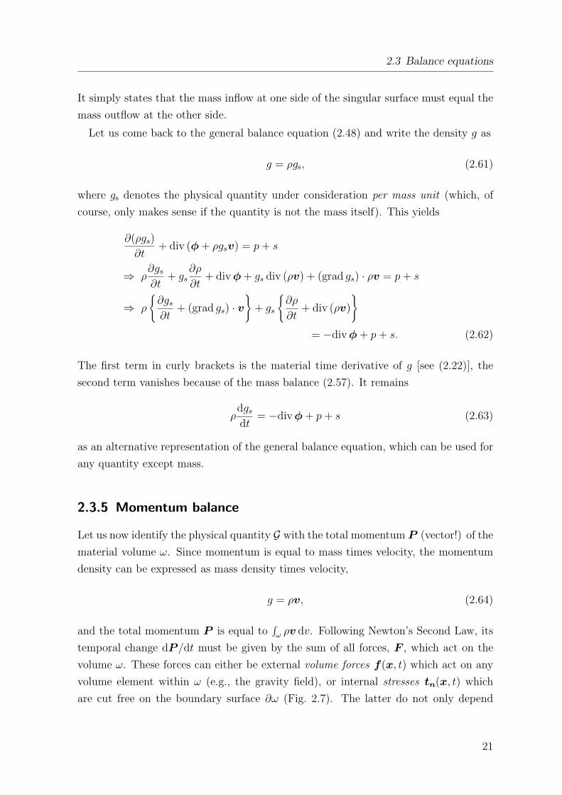
volume ω. These forces can either be external volume forces f(x, t) which act on any
volume element within ω (e.g., the gravity field), or internal stresses tn(x, t) which
are cut free on the boundary surface ∂ω (Fig. 2.7). The latter do not only depend
21
2 Elements of continuum mechanics
on position x and time t, but also on the orientation of the surface, expressed by the
normal unit vector n.
Figure 2.7: Volume forces f and surface forces tn which act on a material volume ω inthe present configuration κt.
The total force acting on the material volume ω is therefore
F =∮
∂ωtn(x, t) da +
∫
ωf(x, t) dv, (2.65)
and Newton’s Second Law reads
d
dt
∫
ωρ(x, t)v(x, t) dv =
∮
∂ωtn(x, t) da +
∫
ωf(x, t) dv. (2.66)
Except for the surface integral (flux term), this has the form of the general balance
equation (2.46). By comparing the flux terms, we infer that the stress vector tn must
be a linear function of n, that is,
tn(x, t) = t(x, t) · n, (2.67)
where t(x, t) is a tensor field of rank two which is called the Cauchy stress tensor. Now
we can identify
g = ρv, φ = −t, p = 0, s = f (2.68)
(the volume force is interpreted as a supply and not a production term because it is
assumed to have an external source), and from (2.48) we obtain the local form of the
momentum balance as∂(ρv)
∂t+ div (ρv v) = div t + f . (2.69)
22
2.3 Balance equations
With the specific momentum (momentum per mass unit)
gs =g
ρ= v (2.70)
and the representation (2.63) of the general balance equation, an equivalent form of
the momentum balance is
ρdv
dt= div t + f . (2.71)
Note that if the momentum balance is formulated in a non-inertial system (for instance,
the rotating Earth), the volume force f contains contributions from inertial forces
(centrifugal force, Coriolis force etc.).
The momentum jump condition on singular surfaces is readily obtained from (2.54)
and (2.68),
[[t · n]]− [[ρv ((v −w) · n)]] = 0. (2.72)
It relates the jump of the stress vector (t ·n) to the jump of the advective momentum
flux across the interface. In case of a material singular surface (v+ ·n = v− ·n = w ·n)
the stress vector is continuous,
[[t · n]] = 0. (2.73)
t yy
t zy
t zz
t xz
t yz
t xx
t yx
t zx
t zx
t yx
t xx
t yz
t xz
t zy
t yy
t xy
t zz
t xy
ex
ey
ez
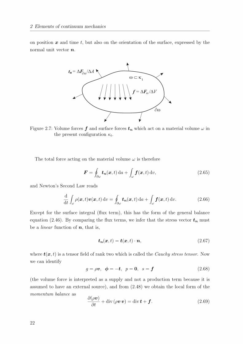
Figure 2.8: Components of the Cauchy stress tensor.
With respect to a given orthonormal basis ei, the matrix of the Cauchy stress
23
2 Elements of continuum mechanics
tensor t defined by (2.67) is
t =
txx txy txz
tyx tyy tyz
tzx tzy tzz
. (2.74)
The elements of this matrix can be interpreted as follows. For a cut along the xy plane,
that is, with normal unit vector n = ±ez (the sign depends on the orientation of the
plane), the stress vector
t±ez = ±t · ez = ±
txz
tyz
tzz
(2.75)
is obtained. Evidently, the diagonal element tzz is perpendicular to the cut plane,
whereas the off-diagonal elements txz and tyz are parallel to the plane. The same result
is found for cuts along the xz and yz planes. Therefore, the three diagonal elements
(txx, tyy, tzz) are refered to as normal stresses, and the six off-diagonal elements (txy,
tyx, txz, tzx, tyz, tzy) are called shear stresses. The meaning of these components is
illustrated in Fig. 2.8.
2.3.6 Balance of angular momentum
In point mechanics, the angular momentum L of a mass point is given by L = x× P
(cross product of position vector and momentum), and the torque M is defined as
M = x × F (cross product of position vector and force acting on the mass point).
In view of the momentum densities (2.68) for the continuous body, this motivates the
following identifications for the densities of angular momentum:
g = x× ρv, φ = −x× t, p = 0, s = x× f . (2.76)
Inserting this in (2.48) yields the balance of angular momentum,
∂(x× ρv)
∂t+ div [(x× ρv) v] = div (x× t) + x× f , (2.77)
or in index notation
∂
∂t(ρ εijkxjvk) + (ρ εijkxjvkvl),l = (εijkxjtkl),l + εijkxjfk. (2.78)
24
2.3 Balance equations
With the momentum balance (2.69), this can be drastically simplified. We compute
x× (2.69) in index notation,
∂
∂t(ρvk) + (ρvkvl),l = tkl,l + fk | · εijkxj
⇒ ∂
∂t(ρ εijkxjvk) + xj(ρ εijkvkvl),l = xj(εijktkl),l + εijkxjfk
⇒ ∂
∂t(ρ εijkxjvk) + (ρ εijkxjvkvl),l − ρ εijkvkvlxj,l
= (εijkxjtkl),l − εijktklxj,l + εijkxjfk, (2.79)
and subtract this from the balance of angular momentum (2.78), which leaves
ρ εijkvkvlδjl = εijktklδjl
⇒ ρ εijkvkvj = εijktkj
⇒ 12(ρ εijkvkvj + ρ εikjvjvk) = 1
2(εijktkj + εikjtjk)
⇒ ρ εijk(vkvj − vjvk) = εijk(tkj − tjk)
⇒ εijk(tkj − tjk) = 0. (2.80)
Evaluation of this result for i = 1 yields
ε123(t32 − t23) + ε132(t23 − t32) = 0
⇒ (tzy − tyz)− (tyz − tzy) = 0 ⇒ tyz = tzy. (2.81)
Similarly, for i = 2 and 3 one finds txz = tzx and txy = tyx, respectively. The balance
of angular momentum thus reduces to the statement that the Cauchy stress tensor is
symmetric,
t = tT, or tij = tji. (2.82)
By contrast, an independent jump condition of angular momentum does not exist; it
is fully equivalent to the momentum jump condition (2.72).
25
2 Elements of continuum mechanics
2.3.7 Energy balance
Balance of kinetic energy
We now compute the dot product of the momentum balance (2.71) and the velocity v
in index notation:
ρvkdvk
dt= tkl,lvk + fkvk
⇒ ρd
dt
(vkvk
2
)= (tklvk),l − tklvk,l + fkvk
= (t · v)l,l − (t ·L)ll + fkvk
⇒ ρd
dt
(v2
2
)= div (t · v)− tr (t ·L) + f · v (2.83)
[in the step from line 2 to 3 the symmetry of t, Eq. (2.82), has been used, and in the last
line we have introduced the speed v = |v|, which is the absolute value of the velocity].
For the second summand on the right-hand side, tr (t ·L), we apply the decomposition
(2.27) of L, the symmetry of t and the antisymmetry of W ,
tr (t ·L) = tr (t ·D) + tr (t ·W )
= tr (t ·D) + tijWji
= tr (t ·D) + 12(tijWji + tjiWij)
= tr (t ·D) + 12(tijWji − tijWji) = tr (t ·D), (2.84)
so that
ρd
dt
(v2
2
)= div (t · v)− tr (t ·D) + f · v. (2.85)
Since the kinetic energy of a mass m is given by mv2/2, the term v2/2 denotes the
specific kinetic energy (per unit mass) of a continuous body. Comparison of the above
result with the general balance equation (2.63) shows that it can be interpreted as the
balance of kinetic energy, where
g = ρv2/2 (kinetic energy density),
gs = v2/2 (specific kinetic energy),
φ = −t · v (power of stresses),
p = −tr (t ·D) (−p: dissipation power),
s = f · v (power of volume forces).
(2.86)
26
2.3 Balance equations
The attribution of the dissipation power as a production term and the power of volume
forces as a supply term was done because the former is only due to intrinsic quantities,
whereas in the latter the volume force occurs which has an external source. Thus, in
contrast to mass, momentum and angular momentum, the kinetic energy has a non-zero
production density, which means that it is not a conserved quantity.
Energy balance, balance of internal energy
The balance of kinetic energy, Eq. (2.85), is not an independent statement, but a
mere consequence of the momentum balance (2.71). However, classical mechanics and
thermodynamics tells us that the kinetic energy is only one part of the total energy of a
system (here: continuous body), and that the total energy is a conserved quantity (no
production). In order to formulate the (total) energy balance, we thus extend (2.86)
by introducing an internal energy, a heat flux and a radiation power and setting the
production to zero:
g = ρ(u + v2/2) (u: specific internal energy),
gs = u + v2/2,
φ = q − t · v (q: heat flux),
p = 0,
s = ρr + f · v (r: specific radiation power).
(2.87)
By inserting these densities in (2.48), the energy balance
∂
∂t
[ρ(u +
v2
2
)]+ div
[ρ(u +
v2
2
)v
]
= −div q + div (t · v) + ρr + f · v (2.88)
is obtained, which is also known as the First Law of Thermodynamics. An alternative
form follows from (2.63),
ρd
dt
(u +
v2
2
)= −div q + div (t · v) + ρr + f · v. (2.89)
27
2 Elements of continuum mechanics
This can be simplified further:
ρdu
dt+ ρvk
dvk
dt= −qk,k + (tklvk),l + ρr + fkvk
= −qk,k + tkl,lvk + tklvk,l + ρr + fkvk
⇒ ρdu
dt+ vk
ρdvk
dt− tkl,l − fk
= −qk,k + tlkLkl + ρr. (2.90)
The term in curly brackets vanishes identically because of the momentum balance
(2.71), and the term tlkLkl = tr (t·L) can again be replaced by tr (t·D) [see Eq. (2.84)],
so that we obtain
ρdu
dt= −div q + tr (t ·D) + ρr. (2.91)
Evidently, this is the balance of internal energy in the form (2.63), with the correspond-
ing densities
g = ρu,
gs = u (specific internal energy),
φ = q (heat flux),
p = tr (t ·D) (dissipation power),
s = ρr (r: specific radiation power).
(2.92)
In contrast to the total energy, the internal energy is not a conserved quantity. Its
production density is equal to the dissipation power, which already appeared in the
balance of kinetic energy (2.85) with a negative sign. The name “dissipation power” re-
sults from the fact that it annihilates kinetic energy and changes it into internal energy.
In other words, macroscopic mechanical energy is transformed into heat (microscopic,
unordered motion). Therefore, the dissipation power can also be interpreted as heat
production due to internal friction.
From (2.54) and (2.87) we obtain the energy jump condition
[[q · n]]− [[v · t · n]] +
[[ρ(u +
v2
2
)((v −w) · n)
]]= 0. (2.93)
In case of a material singular surface (v+ · n = v− · n = w · n) the third summand
vanishes, and because of the continuity of the stress vector t · n [Eq. (2.73)] it can be
28
2.4 Constitutive equations
factored out in the second summand:
[[q · n]]− [[v]] · t · n = 0
⇒ [[q · n]]− [[v⊥]] · t · n−[[v‖
]]· t · n = 0
⇒ [[q · n]]−[[v‖
]]· t · n = 0 (2.94)
[where v = v⊥ + v‖, with the normal component v⊥ = (v · n)n and the tangential
component v‖ = v−(v ·n)n; the jump of v⊥ vanishes because of v+ ·n = v− ·n]. Only
under the additional assumption of no-slip conditions, that is,[[v‖
]]= 0, the normal
component of the heat flux (q · n) becomes continuous.
2.4 Constitutive equations
2.4.1 Simple bodies with fading memory
The balance equations of mass, momentum and internal energy derived in Sect. 2.3
read
dρ
dt= −ρ div v, (2.95)
ρdv
dt= div t + f , (2.96)
ρdu
dt= −div q + tr (t ·D) + ρr (2.97)
[see Eqs. (2.58), (2.71) and (2.91); the balance of angular momentum is implicitly
included in the symmetry of t]. They constitute evolution equations for the unknown
fields ρ, v and u; however, on the right-hand sides the fields t and q are also unknown.
The supply terms f and r are assumed to be prescribed as external forcings. Therefore,
in components we have 1 + 3 + 1 = 5 equations (the momentum balance is a vector
equation!) for the 1 + 3 + 6 + 1 + 3 = 14 unknown fields ρ, v, t (symmetric tensor!),
u and q, and the system is highly under-determined. Therefore, additional closure
relations between the field quantities are required. These closure relations describe
the specific behaviour of the different materials (whereas the balance equations are
universally valid), and they are called constitutive equations or material equations.
The general theory of constitutive equations is a long story and beyond the scope
of this text. For a comprehensive treatment the reader may see the textbooks on
29
2 Elements of continuum mechanics
continuum mechanics given in the literature list. Here, we confine ourselves to a simple
class of materials, the so-called simple bodies with fading memory. This will be sufficient
for our purpose of describing ice-dynamic processes.
A simple body with fading memory is defined as a material whose constitutive equa-
tions are functions of the form
t = t (F , F , T, T , grad T ),
q = q (F , F , T, T , grad T ),
u = u (F , F , T, T , grad T )
(2.98)
(sometimes also higher-order time derivatives of the deformation gradient F are consid-
ered), where the temperature T (x, t) has been introduced as an additional scalar field
quantity. Hence, the Cauchy stress tensor t, the heat flux q and the specific internal
energy u are understood as the dependent material quantities, and the material shows
neither non-local nor memory effects. Note that due to Eq. (2.25) the dependency on
F can also be expressed as a dependency on the velocity gradient L. In the follow-
ing, we will discuss two examples of simple bodies with fading memory relevant for ice
dynamics, namely the linear-elastic solid (Hookean body) and the Newtonian fluid.
2.4.2 Linear-elastic solid
An elastic body is defined as a material for which the stress tensor depends on the
deformation gradient only:
t = t(F ). (2.99)
In particular, this excludes any temperature dependencies, so that the problem is purely
mechanical, and the energy balance (2.97) need not be taken into account.
For many practical applications, it is sufficient to assume small deformations, that
is, F ≈ 1. If we use the same origins (B = 0) and bases (ei = δiAEA) for the reference
and the present configuration (see Fig. 2.1), then the displacements u = x −X will
be small, that is, x ≈ X. The reference configuration and the present configuration
virtually fall together. It is then no longer necessary to distinguish between material
and spatial derivatives (∂/∂xi ≈ ∂/∂XA for i = A). For this situation, the displacement
gradient H is defined as
H = Grad u = F − 1, (2.100)
30
2.4 Constitutive equations
and the infinitesimal strain tensor ε is the symmetric part of it,
ε = 12(H + HT), or εij = 1
2(ui,j + uj,i). (2.101)
The constitutive equation of the isotropic, linear-elastic solid for small deformations,
also known as Hookean body, is now
t = (λ tr ε)1 + 2µ ε. (2.102)
This material equation is called Hooke’s law, and the two coefficients λ, µ are the Lame
parameters.
For the Hookean body, the mass balance (2.95) can be integrated directly. With
Eq. (2.26) and F ≈ 1 ⇒ J ≈ 1, we calculate
ρ + ρ div v = 0
⇒ ρ
ρ+
J
J= 0 ⇒ dρ
ρ+
dJ
J= 0
∣∣∣∣∫ t
t0
⇒ lnρ
ρ0
+ ln J = 0 ⇒ ρ
ρ0
J = 1 ⇒ ρ =ρ0
J≈ ρ0, (2.103)
where t0 is the initial time which defines the reference configuration, and ρ0 is the
constant density in the reference configuration.
We now insert Hooke’s law (2.102) in the momentum balance (2.96). For the diver-
gence of the stress tensor we find
(div t)i = tij,j = (λ εkk δij + 2µ εij),j
= (λuk,kδij),j + µui,jj + µuj,ij
= λuk,kjδij + µui,jj + µuj,ji
= (λ + µ) uk,ki + µui,jj
⇒ div t = (λ + µ) grad div u + µ∇2u, (2.104)
where the Laplace operator ∇2 is defined as ∇2 = div grad . With this, Eq. (2.103) and
v = x = (u + X)· = u we obtain
ρ0d2u
dt2= (λ + µ) grad div u + µ∇2u + f . (2.105)
This is the equation of motion for the Hookean body, and it is known as the Navier
equation. It consists of three component equations for the three unknown displacement
31
2 Elements of continuum mechanics
components ux, uy und uz, so that indeed a closed system is at hand.
2.4.3 Newtonian fluid
Compressible Newtonian fluid
A material is called viscous if the material function (2.98)1 for the stress tensor t
contains an explicit dependency on F or L. The most important realisation of a
viscous material is the Newtonian fluid (also called linear-viscous fluid), which can
either be compressible or density-preserving (incompressible). For the compressible
case, t depends linearly on the strain-rate tensor D (symmetric part of L) and the
density ρ by the following material function,
t = −p(ρ)1 + (λ(ρ) tr D)1 + 2η(ρ) D, (2.106)
where p is the pressure, and λ and η are the coefficients of viscosity. The parameters
η and κ = λ + 2η/3 are also known as the shear viscosity and the bulk viscosity,
respectively.
Except for the pressure term, the material function (2.106) corresponds largely to the
Hooke’s law (2.102), and by a computation similar to (2.104) we find for the divergence
of the stress tensor
div t = −grad p + (λ + η) grad div v + η∇2v. (2.107)
With this result, the momentum balance (2.96) yields the equation of motion
ρdv
dt= −grad p + (λ + η) grad div v + η∇2v + f , (2.108)
which is the Navier-Stokes equation for the case of a compressible Newtonian fluid. Note
the formal similarity to the Navier equation (2.105) for the Hookean body. Together
with the mass balance (2.95), we now have four component equations for the four
unknown field components vx, vy, vz and ρ, which is again a closed system.
Density-preserving (incompressible) Newtonian fluid
For the density-preserving (incompressible) Newtonian fluid, ρ = const holds, so that
the mass balance reduces to
div v = 0 (2.109)
32
2.4 Constitutive equations
[see Eq. (2.59)]. It is then convenient to split up the stress tensor according to
t = −p1 + tD, (2.110)
where
p = −1
3tr t (2.111)
denotes the pressure, and tD is the traceless stress deviator (tr tD = 0). Now the
material function (2.98)1 only determines the stress deviator tD and reads
tD = 2η D, (2.112)
where the coefficient η is again the shear viscosity (or simply the viscosity).
In order to derive the equation of motion for the density-preserving case, we compute
the divergence of the stress tensor with the decomposition (2.110), the material function
(2.112) and the mass balance (2.109):
div t = −grad p + div tD, (2.113)
where
(div tD)i = 2η Dij,j = η (vi,jj + vj,ij) = η (vi,jj + vj,ji)
= η [vi,jj + (div v),i] = η vi,jj = η (∇2v)i. (2.114)
Insertion of these results in the momentum balance (2.96) yields the Navier-Stokes
equation for the density-preserving Newtonian fluid,
ρdv
dt= −grad p + η∇2v + f . (2.115)
Note that here the pressure p appears as a free field, so that we have the four component
equations (2.109) and (2.115) for the four unknown field components vx, vy, vz and p.
If the viscosity η is temperature-dependent, then a thermo-mechanically coupled prob-
lem is at hand, for which the energy balance (2.97) must be solved in addition. This
requires to specify the material functions (2.98)2 and (2.98)3 for the heat flux and the
internal energy, respectively. Insertion in the energy balance yields the missing evolu-
tion equation for the temperature. For instance, if the heat flow is given by Fourier’s
law of heat conduction,
q = −κ grad T (2.116)
33
2 Elements of continuum mechanics
(κ: heat conductivity), and the internal energy is proportional to the temperature,
u = cT (2.117)
(c: specific heat), then the energy balance (2.97) results in
ρcdT
dt= κ div grad T + tr [(−p1 + 2ηD) ·D] + ρr
= κ∇2T − p tr D + 2η tr D2 + ρr
⇒ ρcdT
dt= κ∇2T + 2η tr D2 + ρr (2.118)
(note that tr D = div v = 0). Now we have the five equations (2.109), (2.115) and
(2.118) which govern the evolution of the five fields vx, vy, vz, p and T .
34
3 Large-scale dynamics of ice sheets
3.1 Constitutive equations for polycrystalline ice
3.1.1 Microstructure of ice
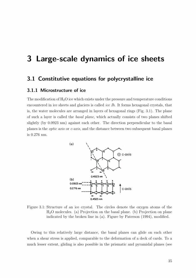
The modification of H2O ice which exists under the pressure and temperature conditions
encountered in ice sheets and glaciers is called ice Ih. It forms hexagonal crystals, that
is, the water molecules are arranged in layers of hexagonal rings (Fig. 3.1). The plane
of such a layer is called the basal plane, which actually consists of two planes shifted
slightly (by 0.0923 nm) against each other. The direction perpendicular to the basal
planes is the optic axis or c-axis, and the distance between two subsequent basal planes
is 0.276 nm.
Figure 3.1: Structure of an ice crystal. The circles denote the oxygen atoms of theH2O molecules. (a) Projection on the basal plane. (b) Projection on planeindicated by the broken line in (a). Figure by Paterson (1994), modified.
Owing to this relatively large distance, the basal planes can glide on each other
when a shear stress is applied, comparable to the deformation of a deck of cards. To a
much lesser extent, gliding is also possible in the prismatic and pyramidal planes (see
35
3 Large-scale dynamics of ice sheets
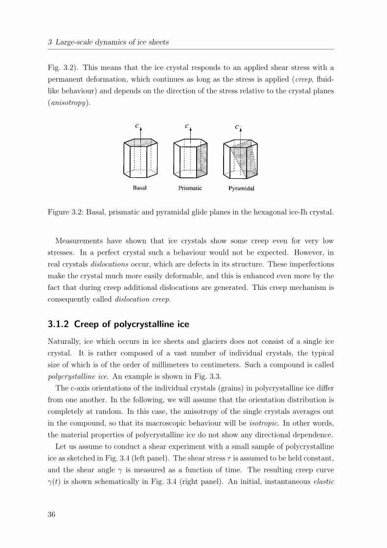
Fig. 3.2). This means that the ice crystal responds to an applied shear stress with a
permanent deformation, which continues as long as the stress is applied (creep, fluid-
like behaviour) and depends on the direction of the stress relative to the crystal planes
(anisotropy).
Figure 3.2: Basal, prismatic and pyramidal glide planes in the hexagonal ice-Ih crystal.
Measurements have shown that ice crystals show some creep even for very low
stresses. In a perfect crystal such a behaviour would not be expected. However, in
real crystals dislocations occur, which are defects in its structure. These imperfections
make the crystal much more easily deformable, and this is enhanced even more by the
fact that during creep additional dislocations are generated. This creep mechanism is
consequently called dislocation creep.
3.1.2 Creep of polycrystalline ice
Naturally, ice which occurs in ice sheets and glaciers does not consist of a single ice
crystal. It is rather composed of a vast number of individual crystals, the typical
size of which is of the order of millimeters to centimeters. Such a compound is called
polycrystalline ice. An example is shown in Fig. 3.3.
The c-axis orientations of the individual crystals (grains) in polycrystalline ice differ
from one another. In the following, we will assume that the orientation distribution is
completely at random. In this case, the anisotropy of the single crystals averages out
in the compound, so that its macroscopic behaviour will be isotropic. In other words,
the material properties of polycrystalline ice do not show any directional dependence.
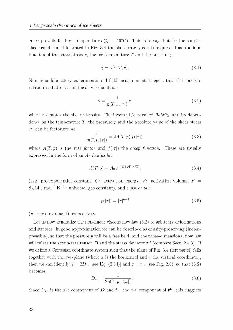
Let us assume to conduct a shear experiment with a small sample of polycrystalline
ice as sketched in Fig. 3.4 (left panel). The shear stress τ is assumed to be held constant,
and the shear angle γ is measured as a function of time. The resulting creep curve
γ(t) is shown schematically in Fig. 3.4 (right panel). An initial, instantaneous elastic
36
3.1 Constitutive equations for polycrystalline ice
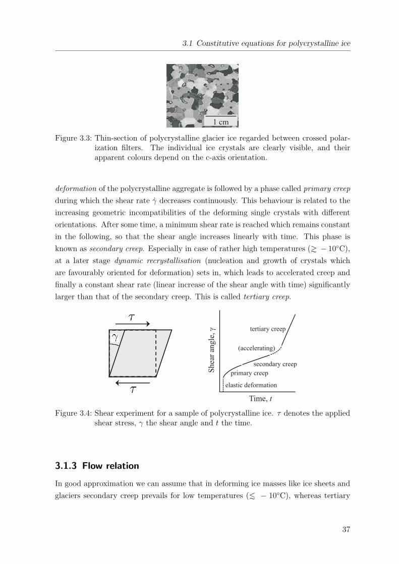
Figure 3.3: Thin-section of polycrystalline glacier ice regarded between crossed polar-ization filters. The individual ice crystals are clearly visible, and theirapparent colours depend on the c-axis orientation.
deformation of the polycrystalline aggregate is followed by a phase called primary creep
during which the shear rate γ decreases continuously. This behaviour is related to the
increasing geometric incompatibilities of the deforming single crystals with different
orientations. After some time, a minimum shear rate is reached which remains constant
in the following, so that the shear angle increases linearly with time. This phase is
known as secondary creep. Especially in case of rather high temperatures (? − 10C),
at a later stage dynamic recrystallisation (nucleation and growth of crystals which
are favourably oriented for deformation) sets in, which leads to accelerated creep and
finally a constant shear rate (linear increase of the shear angle with time) significantly
larger than that of the secondary creep. This is called tertiary creep.
Figure 3.4: Shear experiment for a sample of polycrystalline ice. τ denotes the appliedshear stress, γ the shear angle and t the time.
3.1.3 Flow relation
In good approximation we can assume that in deforming ice masses like ice sheets and
glaciers secondary creep prevails for low temperatures (> − 10C), whereas tertiary
37
3 Large-scale dynamics of ice sheets
creep prevails for high temperatures (? − 10C). This is to say that for the simple-
shear conditions illustrated in Fig. 3.4 the shear rate γ can be expressed as a unique
function of the shear stress τ , the ice temperature T and the pressure p,
γ = γ(τ, T, p). (3.1)
Numerous laboratory experiments and field measurements suggest that the concrete
relation is that of a non-linear viscous fluid,
γ =1
η(T, p, |τ |) τ, (3.2)
where η denotes the shear viscosity. The inverse 1/η is called fluidity, and its depen-
dence on the temperature T , the pressure p and the absolute value of the shear stress
|τ | can be factorized as1
η(T, p, |τ |) = 2A(T, p) f(|τ |), (3.3)
where A(T, p) is the rate factor and f(|τ |) the creep function. These are usually
expressed in the form of an Arrhenius law
A(T, p) = A0 e−(Q+pV )/RT , (3.4)
(A0: pre-exponential constant, Q: activation energy, V : activation volume, R =
8.314 J mol−1 K−1 : universal gas constant), and a power law,
f(|τ |) = |τ |n−1 (3.5)
(n: stress exponent), respectively.
Let us now generalize the non-linear viscous flow law (3.2) to arbitrary deformations
and stresses. In good approximation ice can be described as density-preserving (incom-
pressible), so that the pressure p will be a free field, and the three-dimensional flow law
will relate the strain-rate tensor D and the stress deviator tD (compare Sect. 2.4.3). If
we define a Cartesian coordinate system such that the plane of Fig. 3.4 (left panel) falls
together with the x-z-plane (where x is the horizontal and z the vertical coordinate),
then we can identify γ = 2Dxz [see Eq. (2.34)] and τ = txz (see Fig. 2.8), so that (3.2)
becomes
Dxz =1
2η(T, p, |txz|) txz. (3.6)
Since Dxz is the x-z component of D and txz the x-z component of tD, this suggests
38
3.1 Constitutive equations for polycrystalline ice
that the general flow law reads
D =1
2η(T, p, σ)tD. (3.7)
The only non-straightforward point is the question how the |txz| in Eq. (3.6) translates
to the newly introduced scalar σ (effective stress). As a relation between two tensors,
Eq. (3.7) must be independent of any particular basis (coordinate system). Therefore,
the effective stress σ cannot be equal to a single element like |txz|, but it must be a
scalar invariant of tD. A second-rank tensor in three-dimensional space has only three
independent invariants, which are in case of tD
ItD = tr tD = 0,
IItD = 12[tr (tD)2 − (tr tD)2] = 1
2tr (tD)2
= 12[(tDxx)
2 + (tDyy)2 + (tDzz)
2] + t2xy + t2xz + t2yz,
IIItD = det tD
(3.8)
(note that tij = tDij for i 6= j). If we choose
σ =√
IItD =√
12tr (tD)2 , (3.9)
then we have found an invariant quantity which simplifies to |txz| for the simple-shear
conditions of (3.6). It is therefore reasonable to assume that (3.9) is the correct ex-
pression for the effective stress in the flow law (3.7). Measurements have validated this
reasoning.
As for the fluidity 1/η in Eq. (3.7), we can directly infer its functional dependence
on T , p and σ from Eqs. (3.3), (3.4) and (3.5):
1
η(T, p, σ)= 2A(T, p) f(σ) (3.10)
[rate factor A(T, p), creep function f(σ)], with the Arrhenius law
A(T, p) = A0 e−(Q+pV )/RT (3.11)
and the power law
f(σ) = σn−1. (3.12)
The optimum value for the stress exponent n has been a matter of continuous debate,
39
3 Large-scale dynamics of ice sheets
but most frequently n = 3 is used.
The melting temperature of ice, Tm, is pressure-dependent. For low pressures (p >100 kPa), Tm = T0 = 273.15 K, and for pressures which occur typically in ice sheets
and glaciers (p > 50 MPa) the linear relation
Tm = T0 − β p (3.13)
holds. For pure ice, the Clausius-Clapeyron constant β has the value β = 7.42 ×10⁻⁸ K Pa−1, but under real conditions the value for air-saturated ice, β = 9.8 ×10⁻⁸ K Pa−1, is preferable. Under hydrostatic conditions, this leads to a melting-point
lowering of 0.87 K per kilometer of ice thickness. With (3.13), the homologous temper-
ature (temperature relative to pressure melting) is defined as
T ′ = T − Tm + T0 = T + β p, (3.14)
so that the pressure melting point always corresponds to T ′ = T0 = 273.15 K (or 0C).
Measurements have shown that the pressure dependence in the Arrhenius law (3.11) is
accounted for satisfactorily if the absolute temperature is replaced by the homologous
temperature, that is
A(T, p) = A(T ′) = A0 e−Q/RT ′ . (3.15)
Recommended values for the pre-exponential constant and the activation energy are
A0 = 3.985 × 10⁻¹³ s−1 Pa−3, Q = 60 kJ mol−1 for T ′ ≤ 263.15 K, and A0 = 1.916 ×10³ s−1 Pa−3, Q = 139 kJ mol−1 for T ′ ≥ 263.15 K. The larger activation energy for
warmer conditions is due to tertiary creep, and the two values of the pre-exponential
constant yield A(T ′ = 263.15 K) = 4.9 × 10⁻²⁵ s−1 Pa−3 for both regimes, so that the
function is continuous.
Equation (3.7) together with (3.10), (3.12) and (3.15) reads
D = A(T ′) σn−1 tD, (3.16)
which is called Nye’s generalization of Glen’s flow law, or Glen’s flow law for short. In
order to derive its inverse form, we define the effective strain rate
d =√
12tr D2 , (3.17)
[square root of the second invariant of the strain-rate tensor, compare to (3.9)], for
40
3.1 Constitutive equations for polycrystalline ice
which we obtain by inserting (3.16)
d = A(T ′) σn−1 σ = A(T ′) σn ⇔ σ = A(T ′)−1/n d1/n. (3.18)
Solving (3.16) for tD and using (3.18) yields
tD = A(T ′)−1 σ−(n−1)D
= A(T ′)−1 A(T ′)(n−1)/n d−(n−1)/nD
= A(T ′)−1/n d−(1−1/n)D
⇒ tD = B(T ′) d−(1−1/n)D, (3.19)
where the associated rate factor B(T ′) = A(T ′)−1/n has been introduced. We may
write this with the shear viscosity η as
tD = 2η(T ′, d) D (3.20)
[see (3.7)], where
η(T ′, d) =1
2B(T ′) d−(1−1/n). (3.21)
Evidently, the flow law for polycrystalline ice in the form of (3.7) or (3.20) is very similar
to that of the density-preserving Newtonian fluid which was discussed in Sect. 2.4.3
[see Eq. (2.112)]. The difference is that here we deal with a non-linear flow law, in
that the viscosity depends on the effective stress or the effective strain rate.
3.1.4 Heat flux and internal energy
The heat flux q in polycrystalline ice can be described well by Fourier’s law of heat
conduction [see (2.116)],
q = −κ(T ) grad T, (3.22)
with the temperature-dependent heat conductivity
κ(T ) = 9.828 e−0.0057 T [K] W m−1K−1. (3.23)
For T = T0 = 273.15 K this yields a value of 2.07 W m−1K−1, and it increases with
decreasing temperature. The caloric equation of state (constitutive equation for the
41
3 Large-scale dynamics of ice sheets
internal energy) is given by
u =
T∫
T0
c(T ) dT , (3.24)
which is a generalization of Eq. (2.117) with the temperature-dependent specific heat
c(T ) = (146.3 + 7.253 T [K]) J kg−1K−1. (3.25)
According to this formula, at T = T0 = 273.15 K one obtains 2127.5 J kg−1K−1. Con-
trary to the heat conductivity, the specific heat evidently decreases with decreasing
temperature.
3.2 Full Stokes flow problem
3.2.1 Field equations
With the constitutive equations given above, we are now able to formulate the mechan-
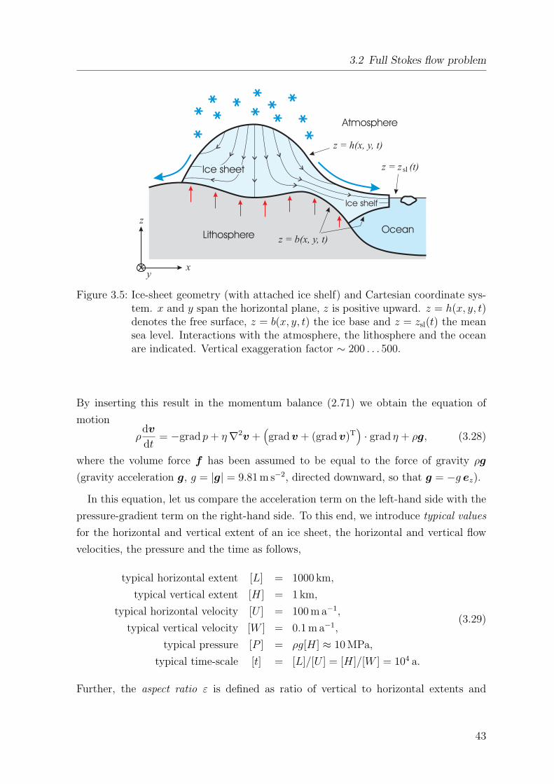
ical and thermodynamical field equations for the flow of ice in an ice sheet. Figure 3.5
shows the typical geometry (cross section) of a grounded ice sheet with attached float-
ing ice shelf (the latter will be treated in Chap. 4), as well as its interactions with the
atmosphere (snowfall, melting), the lithosphere (geothermal heat flux, isostasy) and
the ocean (melting, calving). Also, a Cartesian coordinate system is introduced, where
x and y lie in the horizontal plane, and z is positive upward. These coordinates are
naturally associated with the set of basis vectors ex, ey, ez. The free surface (ice-
atmosphere interface) is given by the function z = h(x, y, t), the ice base (ice-lithosphere
interface) by z = b(x, y, t).
Since we have assumed ice to be a density-preserving material, the mass balance
(2.59) applies,
div v = 0. (3.26)
The flow law in the form (3.20) yields for the divergence of the stress deviator [note
that, contrary to (2.114), η is not constant]
(div tD)i = 2(η Dij),j = 2η Dij,j + 2Dij η,j
= η (vi,jj + vj,ij) + (vi,j + vj,i) η,j
= η [(∇2v)i + (div v),i] +[(
grad v + (grad v)T)· grad η
]i
= η (∇2v)i +[(
grad v + (grad v)T)· grad η
]i. (3.27)
42
3.2 Full Stokes flow problem
Figure 3.5: Ice-sheet geometry (with attached ice shelf) and Cartesian coordinate sys-tem. x and y span the horizontal plane, z is positive upward. z = h(x, y, t)denotes the free surface, z = b(x, y, t) the ice base and z = zsl(t) the meansea level. Interactions with the atmosphere, the lithosphere and the oceanare indicated. Vertical exaggeration factor ∼ 200 . . . 500.
By inserting this result in the momentum balance (2.71) we obtain the equation of
motion
ρdv
dt= −grad p + η∇2v +
(grad v + (grad v)T
)· grad η + ρg, (3.28)
where the volume force f has been assumed to be equal to the force of gravity ρg
(gravity acceleration g, g = |g| = 9.81 m s−2, directed downward, so that g = −g ez).
In this equation, let us compare the acceleration term on the left-hand side with the
pressure-gradient term on the right-hand side. To this end, we introduce typical values
for the horizontal and vertical extent of an ice sheet, the horizontal and vertical flow
velocities, the pressure and the time as follows,
typical horizontal extent [L] = 1000 km,
typical vertical extent [H] = 1 km,
typical horizontal velocity [U ] = 100 m a−1,
typical vertical velocity [W ] = 0.1 m a−1,
typical pressure [P ] = ρg[H] ≈ 10 MPa,
typical time-scale [t] = [L]/[U ] = [H]/[W ] = 104 a.
(3.29)
Further, the aspect ratio ε is defined as ratio of vertical to horizontal extents and
43
3 Large-scale dynamics of ice sheets
velocities, respectively:
ε =[H]
[L]=
[W ]
[U ]= 10−3. (3.30)
For the horizontal direction, the ratio of acceleration and pressure gradient, called the
Froude number Fr, is then
Fr =ρ[U ]/[t]
[P ]/[L]=
ρ[U ]2/[L]
ρg[H]/[L]=
[U ]2
g[H]≈ 10−15 (3.31)
(note that 1 a = 31556926 s ≈√
1015 s), and for the vertical direction we obtain the
ratioρ[W ]/[t]
[P ]/[H]=
ρ[W ]2/[H]
ρg[H]/[H]=
[W ]2
g[H]= ε2Fr ≈ 10−21. (3.32)
Consequently, for the flow of ice sheets the acceleration term in the equation of motion
is completely negligible, and so (3.28) can be simplified to
−grad p + η∇2v +(grad v + (grad v)T
)· grad η + ρg = 0. (3.33)
This type of flow is called Stokes flow.
Since the equation of motion (3.33) contains the temperature-dependent viscosity, a
thermo-mechanically coupled problem is at hand, and its complete formulation requires
an evolution equation for the temperature field. As it was demonstrated in Sect. 2.4.3,
this equation can be derived by inserting the constitutive equations for the stress de-
viator (3.20), the heat flux (3.22) and the internal energy (3.24) in the internal-energy
balance (2.91). We obtain
du
dt= c
dT
dt, div q = −div (κ grad T ) (3.34)
and
tr (t ·D) = tr [(−p1 + 2ηD) ·D] = 2η tr D2 = 4η d2 (3.35)
[see (3.17)]. Further, except for the very uppermost few centimeters of ice exposed to
sunlight, the radiation r is negligible in an ice sheet, so that we obtain the temperature
evolution equation
ρcdT
dt= div (κ grad T ) + 4η d2. (3.36)
Since the ice temperature must not exceed the pressure melting point, the solution of
(3.36) is subject to the secondary condition T ≤ Tm. With the continuity equation
(3.26), the equation of motion (3.33) and the temperature evolution equation (3.36)
44
3.2 Full Stokes flow problem
we have found a closed system of five equations for the five unknown fields vx, vy, vz,
p and T of the thermo-mechanical Stokes flow problem.
3.2.2 Boundary conditions
In order to provide a solvable problem, the above system of equations needs to be
completed by appropriate boundary conditions at the free surface and the ice base (see
Fig. 3.5). The possible presence of attached ice shelves will be ignored for now.
Free surface
Like any boundary, the free surface of an ice sheet can be regarded as a singular surface
in the sense of Sect. 2.3.3. If we denote it in implicit form by the equation
Fs(x, t) = z − h(x, y, t) = 0, (3.37)
then it can be interpreted as zero-equipotential surface of the function Fs(x, t), and
the normal unit vector is the normalized gradient
n =grad Fs
|grad Fs| =1
Ns
−∂h
∂x
−∂h
∂y
1
, (3.38)
which points into the atmosphere (Fig. 3.6). Note that the abbreviation Ns stands for
the gradient norm,
Ns = |grad Fs| =(
1 +(∂h
∂x
)2+
(∂h
∂y
)2)1/2
. (3.39)
As a direct consequence of Eq. (3.37), the time derivative of Fs following the motion
of the free surface with velocity w must vanish,
dwFs
dt=
∂Fs
∂t+ (grad Fs) ·w = 0 (3.40)
[compare Eq. (2.22)]. Let v be the ice surface velocity, then we can introduce the ice
volume flux through the free surface,
a⊥s = (w − v) · n, (3.41)
45
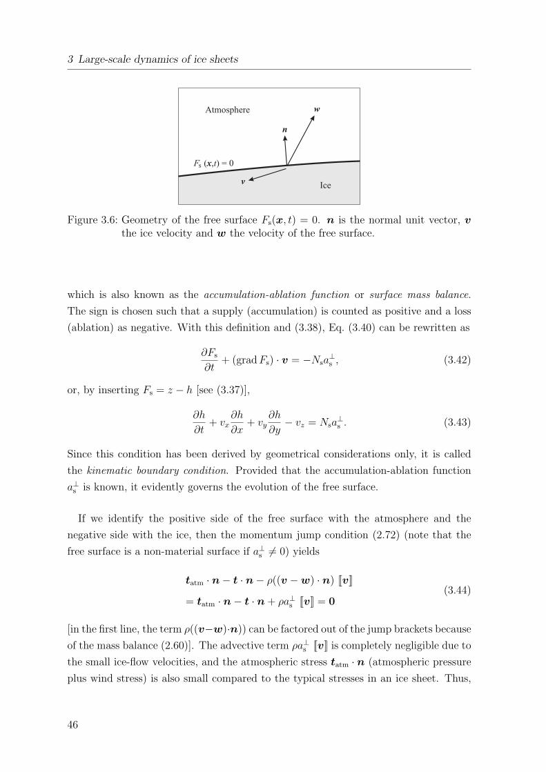
3 Large-scale dynamics of ice sheets
Figure 3.6: Geometry of the free surface Fs(x, t) = 0. n is the normal unit vector, vthe ice velocity and w the velocity of the free surface.
which is also known as the accumulation-ablation function or surface mass balance.
The sign is chosen such that a supply (accumulation) is counted as positive and a loss
(ablation) as negative. With this definition and (3.38), Eq. (3.40) can be rewritten as
∂Fs
∂t+ (grad Fs) · v = −Nsa
⊥s , (3.42)
or, by inserting Fs = z − h [see (3.37)],
∂h
∂t+ vx
∂h
∂x+ vy
∂h
∂y− vz = Nsa
⊥s . (3.43)
Since this condition has been derived by geometrical considerations only, it is called
the kinematic boundary condition. Provided that the accumulation-ablation function
a⊥s is known, it evidently governs the evolution of the free surface.
If we identify the positive side of the free surface with the atmosphere and the
negative side with the ice, then the momentum jump condition (2.72) (note that the
free surface is a non-material surface if a⊥s 6= 0) yields
tatm · n− t · n− ρ((v −w) · n) [[v]]
= tatm · n− t · n + ρa⊥s [[v]] = 0(3.44)
[in the first line, the term ρ((v−w)·n)) can be factored out of the jump brackets because
of the mass balance (2.60)]. The advective term ρa⊥s [[v]] is completely negligible due to
the small ice-flow velocities, and the atmospheric stress tatm · n (atmospheric pressure
plus wind stress) is also small compared to the typical stresses in an ice sheet. Thus,
46
3.2 Full Stokes flow problem
we can neglect both terms, and obtain the stress-free condition
t · n = 0. (3.45)
This is the dynamic boundary condition (that is, related to stresses) for the free surface.
For the temperature evolution equation (3.36), it is further required to provide a
thermodynamic boundary condition. This can simply be done by prescribing the surface
temperature Ts,
T = Ts. (3.46)
Measurements have shown that Ts can be well approximated by the mean-annual sur-
face air temperature, as long as the latter is ≤ 0C.
Ice base
Similar to the free surface, a kinematic boundary condition for the ice base can be
derived. Let
Fb(x, t) = b(x, y, t)− z = 0 (3.47)
be its implicit representation, then the normal unit vector is
n =grad Fb
|grad Fb| =1
Nb
∂b
∂x
∂b
∂y
−1
, (3.48)
which points into the bedrock (Fig. 3.7). The abbreviation Nb denotes the gradient
norm,
Nb = |grad Fb| =(
1 +( ∂b
∂x
)2+
(∂b
∂y
)2)1/2
. (3.49)
Analogous to Eq. (3.40), the time derivative of Fb following the motion of the ice
base vanishes,dwFb
dt=
∂Fb
∂t+ (grad Fb) ·w = 0, (3.50)
where w is the velocity of the ice base. With the ice volume flux through the base,
a⊥b = (v −w) · n, (3.51)
where the sign has been chosen such that a mass loss due to basal melting (and subse-
47
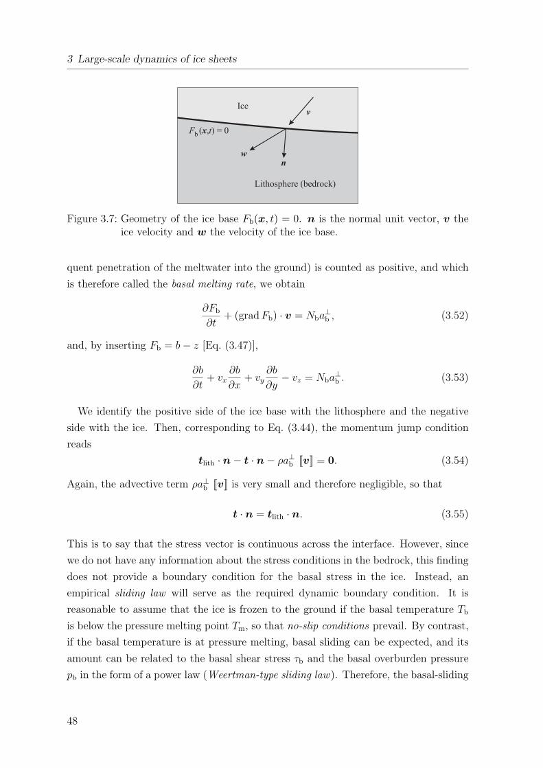
3 Large-scale dynamics of ice sheets
Figure 3.7: Geometry of the ice base Fb(x, t) = 0. n is the normal unit vector, v theice velocity and w the velocity of the ice base.
quent penetration of the meltwater into the ground) is counted as positive, and which
is therefore called the basal melting rate, we obtain
∂Fb
∂t+ (grad Fb) · v = Nba
⊥b , (3.52)
and, by inserting Fb = b− z [Eq. (3.47)],
∂b
∂t+ vx
∂b
∂x+ vy
∂b
∂y− vz = Nba
⊥b . (3.53)
We identify the positive side of the ice base with the lithosphere and the negative
side with the ice. Then, corresponding to Eq. (3.44), the momentum jump condition
reads
tlith · n− t · n− ρa⊥b [[v]] = 0. (3.54)
Again, the advective term ρa⊥b [[v]] is very small and therefore negligible, so that
t · n = tlith · n. (3.55)
This is to say that the stress vector is continuous across the interface. However, since
we do not have any information about the stress conditions in the bedrock, this finding
does not provide a boundary condition for the basal stress in the ice. Instead, an
empirical sliding law will serve as the required dynamic boundary condition. It is
reasonable to assume that the ice is frozen to the ground if the basal temperature Tb
is below the pressure melting point Tm, so that no-slip conditions prevail. By contrast,
if the basal temperature is at pressure melting, basal sliding can be expected, and its
amount can be related to the basal shear stress τb and the basal overburden pressure
pb in the form of a power law (Weertman-type sliding law). Therefore, the basal-sliding
48
3.2 Full Stokes flow problem
velocity vb can be expressed as
vb =
0, if Tb < Tm,
Cbτ pb
pqb
nτ , if Tb = Tm,(3.56)
where nτ denotes the direction of the basal shear stress τb in the tangential plane to
the ice base (nτ ⊥ n), and p and q are the basal-sliding exponents. Like for the stress
exponent n in the creep function (3.12) of Glen’s flow law, the best choice for their
values are a matter of debate, but commonly used values are (p, q) = (3, 1) or (3, 2) for
sliding on hard rock, and (p, q) = (1, 0) for sliding on soft, deformable sediment.
As for the thermodynamic boundary condition, sufficient information on the spatio-
temporal distribution of the basal temperature is not at hand, so that it cannot be
prescribed directly. Instead, we will have to formulate the energy jump condition
(2.93) for the ice base. We obtain
qlith · n− q · n− [[v]] · t · n + ρ((v −w) · n)
[[u +
v2
2
]]= 0. (3.57)
Note that the term ρ((v−w) ·n)) has been factored out of the jump brackets because
of the mass balance (2.60), and the stress vector t · n has been factored out due to
(3.55). The term −qlith ·n can be identified with the geothermal heat flux q⊥geo, that is,
the heat flow which enters the ice body from below due to the warmer Earth’s interior.
Further, we insert Eqs. (3.22) and (3.51), and neglect the very small kinetic energy
v2/2 in comparison with the internal energy u, so that
κ (grad T · n)− q⊥geo − [[v]] · t · n + ρa⊥b [[u]] = 0. (3.58)
Two cases are to be distinguished. For a cold base, that is, a basal temperature below
the pressure melting point, there cannot be any basal melting (a⊥b = 0), and no-slip
conditions prevail [see (3.56)1], so that [[v]] = 0. Thus, Eq. (3.58) simplifies to
κ (grad T · n) = q⊥geo, (3.59)
which is a Neumann-type boundary condition for the basal temperature. By contrast,
in case of a temperate base (basal temperature at the pressure melting point), the basal
49

3 Large-scale dynamics of ice sheets
temperature itself is known, namely
T = Tm (3.60)
(Dirichlet-type condition). As a consequence, the energy jump condition (3.58) is no
longer needed as boundary condition for the temperature field, but it can be used to
compute the unknown basal melting rate a⊥b . Since there will be meltwater on the
positive (lithosphere) side and ice on the negative (ice) side of the base, the jump of
the internal energy [[u]] is equal to the latent heat L of ice melt, that is, [[u]] = L.
Further, the velocity jump is given by the sliding velocity (3.56)2, so that [[v]] = −vb.
With these settings, the energy jump condition (3.58), solved for a⊥b , yields
a⊥b =q⊥geo − κ (grad T · n)− vb · t · n
ρL. (3.61)
Evidently, the situation is different from that of the free surface, in that the accumulation-
ablation function a⊥s must be prescribed as climatic input (along with the surface tem-
perature Ts), whereas the basal melting rate a⊥b can be computed. Instead, at the ice
base the geothermal heat flux q⊥geo must be prescribed as input quantity.
3.2.3 Ice-thickness equation
By combining the continuity equation (3.26) with the kinematic boundary condi-
tions (3.43) and (3.53), we can now derive an evolution equation for the ice thickness
H(x, y, t) = h(x, y, t)− b(x, y, t). To this end, we write (3.26) in components,
∂vx
∂x+
∂vy
∂y+
∂vz
∂z= 0, (3.62)
and integrate it from the ice base to the free surface:
h∫
b
∂vx
∂xdz +
h∫
b
∂vy
∂ydz +
h∫
b
∂vz
∂zdz = 0. (3.63)
The first two terms can be modified by using the Leibniz’ rule,
∂
∂x
h∫
b
vx dz =
h∫
b
∂vx
∂xdz + vx|z=h
∂h
∂x− vx|z=b
∂b
∂x(3.64)
50
3.3 Hydrostatic approximation
(and accordingly for the y-derivative), and the third term is simply
h∫
b
∂vz
∂zdz = vz|z=h − vz|z=b, (3.65)
so that
∂
∂x
h∫
b
vx dz +∂
∂y
h∫
b
vy dz
−vx|z=h∂h
∂x− vy|z=h
∂h
∂y+ vz|z=h + vx|z=b
∂b
∂x+ vy|z=b
∂b
∂y− vz|z=b = 0. (3.66)
With the kinematic conditions (3.43) and (3.53), this yields
∂
∂x
h∫
b
vx dz +∂
∂y
h∫
b
vy dz +∂h
∂t−Nsa
⊥s −
∂b
∂t+ Nba
⊥b = 0. (3.67)
By introducing the volume flux Q as the vertically integrated horizontal velocity, that
is,
Q =
Qx
Qy
=
∫ h
bvx dz
∫ h
bvy dz
, (3.68)
rearranging (3.67) and introducing the ice thickness H = h− b, we obtain
∂H
∂t= −div Q + Nsa
⊥s −Nba
⊥b (3.69)
(note that div Q = ∂Qx/∂x + ∂Qy/∂y). This result is known as the ice-thickness
equation. It is the central evolution equation in ice-sheet dynamics.
3.3 Hydrostatic approximation
In order to derive a simplified, approximated system of equations for the large-scale
dynamics of ice sheets, we go back to the momentum balance (2.71), and write it in
components. By neglecting again the acceleration terms [see (3.31), (3.32)] and setting
51
3 Large-scale dynamics of ice sheets
f = ρg = −ρg ez, we obtain
∂txx
∂x+
∂txy
∂y+
∂txz
∂z= 0,
∂txy
∂x+
∂tyy
∂y+
∂tyz
∂z= 0,
∂txz
∂x+
∂tyz
∂y+
∂tzz
∂z= ρg.
(3.70)
In all parts of an ice sheet, the shear stresses txz and tyz (> 100 kPa) are small compared
to the vertical normal stress tzz, which is approximately equal to the pressure p, so
that [tzz] ≈ [P ] = ρg[H] ≈ 10 MPa [see (3.29)]. Consequently, the vertical momentum
balance (3.70)3 can be reduced to a balance between the vertical gradient of tzz and
the gravity force,∂tzz
∂z= ρg. (3.71)
The same approximation in the vertical component of the stress-free condition at the
free surface (3.45) yields
tzz|z=h = 0, (3.72)
so that Eq. (3.71) can readily be integrated:
tzz = −ρg(h− z). (3.73)
Evidently, the vertical normal stress tzz is hydrostatic. With this result, the pressure
p reads
p = p− tDxx − tDyy − tDzz = −tDxx − tDyy − tzz
= ρg(h− z)− tDxx − tDyy. (3.74)
Thus, the horizontal normal stresses txx, tyy can be expressed as
txx = −p + tDxx = 2tDxx + tDyy − ρg(h− z),
tyy = −p + tDyy = 2tDyy + tDxx − ρg(h− z).(3.75)
Inserting this in the horizontal (x, y) components of the momentum balance (3.70)1,2
yields
2∂tDxx
∂x+
∂tDyy
∂x+
∂txy
∂y+
∂txz
∂z= ρg
∂h
∂x,
2∂tDyy
∂y+
∂tDxx
∂y+
∂txy
∂x+
∂tyz
∂z= ρg
∂h
∂y,
(3.76)
52
3.4 Shallow-ice approximation
and, by application of the flow law (3.20),
4∂
∂x
(η∂vx
∂x
)+ 2
∂
∂x
(η∂vy
∂y
)+
∂
∂y
(η(
∂vx
∂y+
∂vy
∂x))
+∂
∂z
(η(
∂vx
∂z+
∂vz
∂x))
= ρg∂h
∂x,
4∂
∂y
(η∂vy
∂y
)+ 2
∂
∂y
(η∂vx
∂x
)+
∂
∂x
(η(
∂vx
∂y+
∂vy
∂x))
+∂
∂z
(η(
∂vy
∂z+
∂vz
∂y))
= ρg∂h
∂y.
(3.77)
Equations (3.77) together with the continuity equation (3.26), which reads in compo-
nent form∂vx
∂x+
∂vy
∂y+
∂vz
∂z= 0, (3.78)
and the temperature evolution equation (3.36), which is
ρc(∂T
∂t+ vx
∂T
∂x+ vy
∂T
∂y+ vz
∂T
∂z
)
=∂
∂x
(κ∂T
∂x
)+
∂
∂y
(κ∂T
∂y
)+
∂
∂z
(κ∂T
∂z
)+ 4η d2, (3.79)
are four equations for the four unknown fields vx, vy, vz and T . This set of field equa-
tions is called the hydrostatic approximation. Compared to the full Stokes flow problem
formulated in Sect. 3.2.1, the pressure has been eliminated, which is a substantial sim-
plification of the problem. The field equations are completed by the kinematic bound-
ary condition (3.43), the stress-free condition (3.45) and the temperature condition
(3.46) at the free surface, the kinematic condition (3.53), the sliding law (3.56) and the
thermodynamic conditions (3.59), (3.60), (3.61) at the ice base and the ice-thickness
equation (3.69).
3.4 Shallow-ice approximation
Everywhere in an ice sheet except for the immediate vicinity (some 10 km horizontal
distance) of ice domes (local maxima of the surface elevation h) and ice margins,
the flow regime is essentially simple, bed-parallel shear, and the slopes of the free
surface and the ice base are small (Fig. 3.8). Under these circumstances, the relevant
components of the stress deviator tD are the shear stresses in the horizontal plane, txz
and tyz, which are supported by the basal drag. The normal stress deviators tDxx, tDyy
53
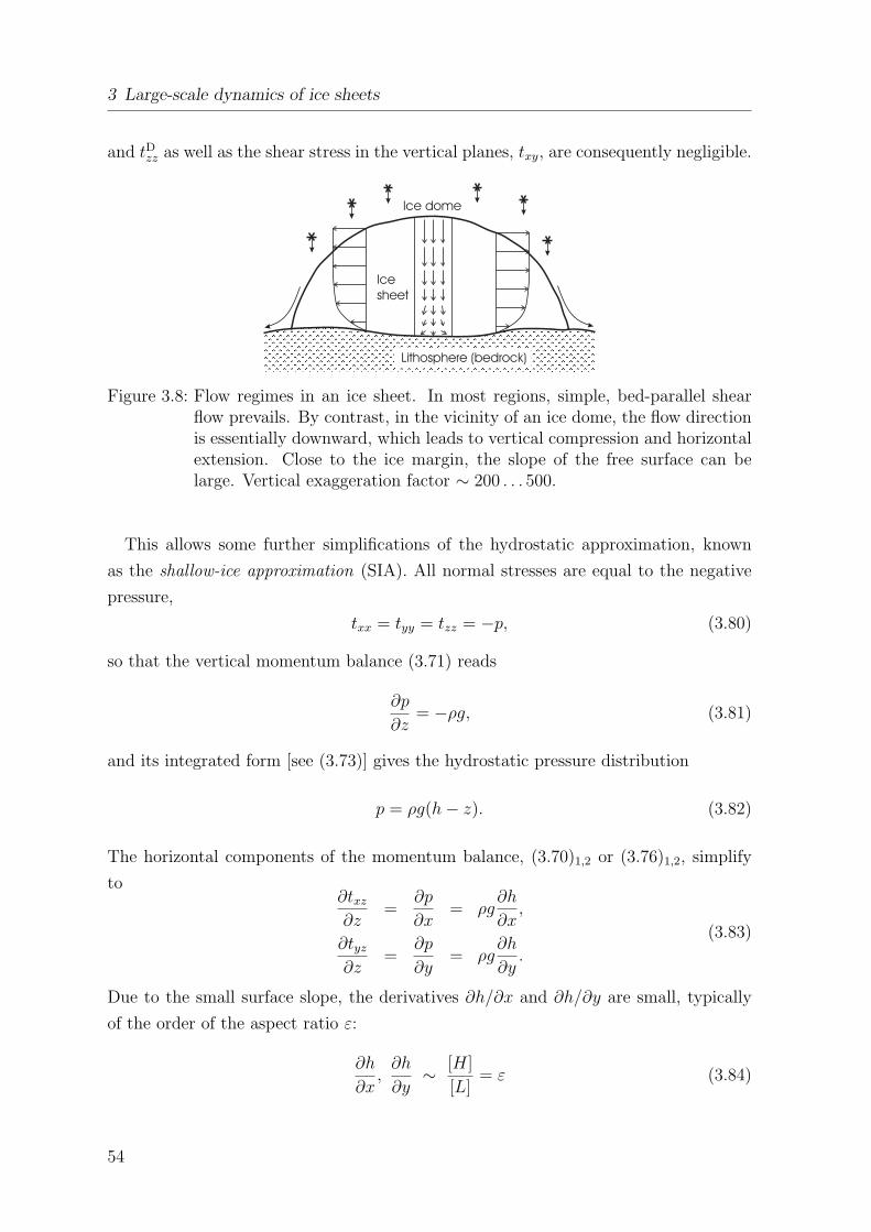
3 Large-scale dynamics of ice sheets
and tDzz as well as the shear stress in the vertical planes, txy, are consequently negligible.
Figure 3.8: Flow regimes in an ice sheet. In most regions, simple, bed-parallel shearflow prevails. By contrast, in the vicinity of an ice dome, the flow directionis essentially downward, which leads to vertical compression and horizontalextension. Close to the ice margin, the slope of the free surface can belarge. Vertical exaggeration factor ∼ 200 . . . 500.
This allows some further simplifications of the hydrostatic approximation, known
as the shallow-ice approximation (SIA). All normal stresses are equal to the negative
pressure,
txx = tyy = tzz = −p, (3.80)
so that the vertical momentum balance (3.71) reads
∂p
∂z= −ρg, (3.81)
and its integrated form [see (3.73)] gives the hydrostatic pressure distribution
p = ρg(h− z). (3.82)
The horizontal components of the momentum balance, (3.70)1,2 or (3.76)1,2, simplify
to∂txz
∂z=
∂p
∂x= ρg
∂h
∂x,
∂tyz
∂z=
∂p
∂y= ρg
∂h
∂y.
(3.83)
Due to the small surface slope, the derivatives ∂h/∂x and ∂h/∂y are small, typically
of the order of the aspect ratio ε:
∂h
∂x,
∂h
∂y∼ [H]
[L]= ε (3.84)
54
3.4 Shallow-ice approximation
[see Eqs. (3.29) and (3.30)]. Thus, the normal unit vector of the free surface (3.38) is
approximately vertical,
n =
0
0
1
= ez, (3.85)
and the stress-free condition (3.45) reduces to
p|z=h = 0, txz|z=h = 0, tyz|z=h = 0. (3.86)
With this finding, Eq. (3.83), the right-hand side of which does not depend on z, can
readily be integrated and yields
txz = −ρg(h− z)∂h
∂x,
tyz = −ρg(h− z)∂h
∂y.
(3.87)
Equations (3.82) and (3.87) tell us that in the SIA the stress field, the non-negligible
components of which are only p, txz and tyz, is fully determined if the geometry of the
ice sheet is known. The effective stress σ [see (3.8)2 and (3.9)] is then
σ =√
t2xz + t2yz = ρg(h− z)
((∂h
∂x
)2+
(∂h
∂y
)2)1/2
= ρg(h− z) |grad h|. (3.88)
These results can be inserted in the x-z and y-z components of Glen’s flow law in the
form (3.16):
1
2
(∂vx
∂z+
∂vz
∂x
)= A(T ′) σn−1 txz = −A(T ′) [ρg(h− z)]n|grad h|n−1∂h
∂x,
1
2
(∂vy
∂z+
∂vz
∂y
)= A(T ′) σn−1 tyz = −A(T ′) [ρg(h− z)]n|grad h|n−1∂h
∂y.
(3.89)
With the typical values (3.29) and the aspect ratio (3.30), we find for the velocity
derivatives on the left-hand side
∂vz
∂x
/∂vx
∂z,
∂vz
∂y
/∂vy
∂z∼ [W ]
[L]
/ [U ]
[H]=
[W ]
[U ]
[H]
[L]= ε2 ∼ 10−6, (3.90)
55
3 Large-scale dynamics of ice sheets
so that the horizontal derivatives of the vertical velocity are negligible. This yields
∂vx
∂z= −2A(T ′) [ρg(h− z)]n|grad h|n−1∂h
∂x,
∂vy
∂z= −2A(T ′) [ρg(h− z)]n|grad h|n−1∂h
∂y,
(3.91)
which can be integrated from the ice base z = b to an arbitrary position z in the ice
sheet in order to compute the horizontal velocities,
vx = vbx − 2(ρg)n|grad h|n−1∂h
∂x
∫ z
bA(T ′) (h− z)n dz,
vy = vby − 2(ρg)n|grad h|n−1∂h
∂y
∫ z
bA(T ′) (h− z)n dz,
(3.92)
where vbx and vby are the respective velocities at the ice base. Since the bed slopes are
of the same order of magnitude as the surface slopes [see (3.84)],
∂b
∂x,
∂b
∂y∼ [H]
[L]= ε, (3.93)
and the normal unit vector of the ice base (3.48) is approximately vertical,
n =
0
0
−1
= −ez, (3.94)
the tangential plane to the ice base is approximately equal to the horizontal plane.
Therefore, vbx and vby are the two components of the basal-sliding velocity vb given
by the sliding law (3.56). With
τb =
∣∣∣∣∣∣
txz|z=b
tyz|z=b
∣∣∣∣∣∣=
√t2xz|z=b + t2yz|z=b = ρgH |grad h|, (3.95)
pb = ρgH (3.96)
and
nτ =1
τb
txz|z=b
tyz|z=b
= − 1
|grad h|
∂h
∂x
∂h
∂y
, (3.97)
56
3.4 Shallow-ice approximation
we obtain
vbx =
0, if Tb < Tm,
−Cb(ρgH)p−q|grad h|p−1∂h
∂x, if Tb = Tm,
vby =
0, if Tb < Tm,
−Cb(ρgH)p−q|grad h|p−1∂h
∂y, if Tb = Tm.
(3.98)
By introducing the horizontal velocity vector
vh =
vx
vy
(3.99)
and the scalar function
C =
2(ρg)n|grad h|n−1∫ z
bA(T ′) (h− z)n dz, if Tb < Tm,
Cb(ρgH)p−q|grad h|p−1
+2(ρg)n|grad h|n−1∫ z
bA(T ′) (h− z)n dz, if Tb = Tm,
(3.100)
we can express the horizontal velocity (3.92) as
vx
vy
= −C
∂h
∂x
∂h
∂y
, or vh = −C grad h. (3.101)
This is to say that, in the shallow-ice approximation, the direction of the horizontal
velocity is anti-parallel to the gradient of the free surface. In other words, the ice flows
always down the steepest surface slope, irrespective of the bedrock topography (see
Fig. 3.9). This holds for any particle of the ice sheet, even the near-basal ice. However,
note that this result is only valid as long as the bed slopes are sufficiently small, as
described by Eq. (3.93).
The vertical velocity can now be computed by integrating the continuity equation
(3.78) from z = b to z,
vz = vz|z=b −∫ z
b
(∂vx
∂x+
∂vy
∂y
)dz. (3.102)
57
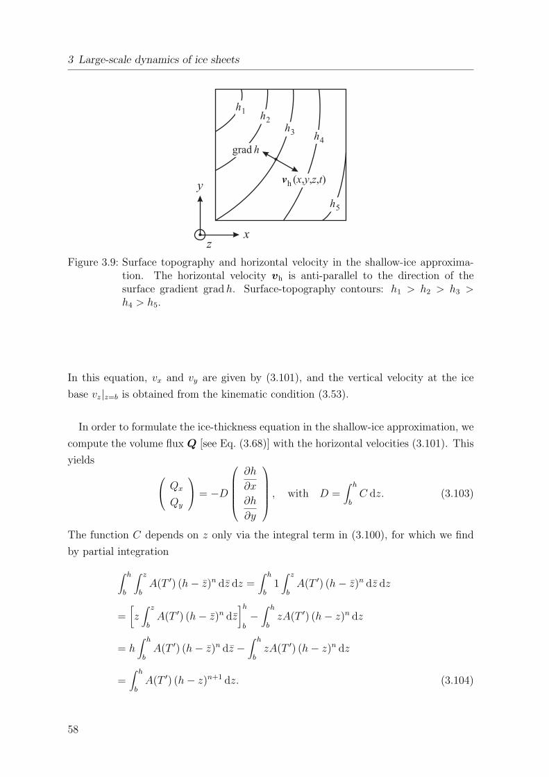
3 Large-scale dynamics of ice sheets
Figure 3.9: Surface topography and horizontal velocity in the shallow-ice approxima-tion. The horizontal velocity vh is anti-parallel to the direction of thesurface gradient grad h. Surface-topography contours: h1 > h2 > h3 >h4 > h5.
In this equation, vx and vy are given by (3.101), and the vertical velocity at the ice
base vz|z=b is obtained from the kinematic condition (3.53).
In order to formulate the ice-thickness equation in the shallow-ice approximation, we
compute the volume flux Q [see Eq. (3.68)] with the horizontal velocities (3.101). This
yields
Qx
Qy
= −D
∂h
∂x
∂h
∂y
, with D =∫ h
bC dz. (3.103)
The function C depends on z only via the integral term in (3.100), for which we find
by partial integration
∫ h
b
∫ z
bA(T ′) (h− z)n dz dz =
∫ h
b1
∫ z
bA(T ′) (h− z)n dz dz
=[z
∫ z
bA(T ′) (h− z)n dz
]h
b−
∫ h
bzA(T ′) (h− z)n dz
= h∫ h
bA(T ′) (h− z)n dz −
∫ h
bzA(T ′) (h− z)n dz
=∫ h
bA(T ′) (h− z)n+1 dz. (3.104)
58
3.4 Shallow-ice approximation
Thus, the function D is
D =
2(ρg)n|grad h|n−1∫ h
bA(T ′) (h− z)n+1 dz, if Tb < Tm,
CbH(ρgH)p−q|grad h|p−1
+ 2(ρg)n|grad h|n−1∫ h
bA(T ′) (h− z)n+1 dz, if Tb = Tm.
(3.105)
By inserting the volume flux (3.103) with the function (3.105) in the ice-thickness
equation (3.69) and using Ns ≈ 1, Nb ≈ 1 [due to (3.84) and (3.93)], we obtain
∂H
∂t=
∂
∂x
(D
∂h
∂x
)+
∂
∂y
(D
∂h
∂y
)+ a⊥s − a⊥b , (3.106)
or, alternatively, expressed as an evolution equation for the surface topography h,
∂h
∂t=
∂
∂x
(D
∂h
∂x
)+
∂
∂y
(D
∂h
∂y
)+ a⊥s − a⊥b +
∂b
∂t. (3.107)
Mathematically, this is a non-linear diffusion equation (the function D depends itself
on h) with additional source terms. As it was described at the end of Sect. 3.2.2, the
accumulation-ablation function a⊥s is a climatic input quantity, and the basal melt-
ing rate a⊥b is determined by Eq. (3.61). The unknown variation ∂b/∂t of the ice-
base/bedrock topography can be obtained from a model of glacial isostasy, which will
be treated later (see Chap. 6).
As for the temperature evolution equation (3.79), we complement the typical values
(3.29) by the typical temperature variation
[∆T ] = 20 K. (3.108)
Then, we find for the ratio of horizontal and vertical heat conduction
∂
∂x
(κ∂T
∂x
)/ ∂
∂z
(κ∂T
∂z
),
∂
∂y
(κ∂T
∂y
)/ ∂
∂z
(κ∂T
∂z
)
∼ κ[∆T ]
[L]2
/κ
[∆T ]
[H]2=
[H]2
[L]2= ε2 ∼ 10−6, (3.109)
so that horizontal heat conduction is negligible. Further, in the dissipation term we
express the effective strain rate d by the effective stress σ by using (3.18)1. This yields
ρc(∂T
∂t+ vx
∂T
∂x+ vy
∂T
∂y+ vz
∂T
∂z
)=
∂
∂z
(κ∂T
∂z
)+ 4η A2(T ′) σ2n, (3.110)
59
3 Large-scale dynamics of ice sheets
and, by inserting (3.10) and (3.12), we obtain
ρc(∂T
∂t+ vx
∂T
∂x+ vy
∂T
∂y+ vz
∂T
∂z
)=
∂
∂z
(κ∂T
∂z
)+ 2A(T ′) σn+1, (3.111)
where σ is given by Eq. (3.88). The boundary conditions for this equation are the
prescribed surface temperature (3.46), the temperature gradient (3.59) for a cold base
and the melting temperature (3.60) for a temperate base.
The shallow-ice approximation simplifies the problem of large-scale ice-sheet flow
drastically. The stress field is given by the simple, analytic expressions (3.82), (3.87)
and (3.88), and the velocity field depends only on the local ice-sheet geometry and
temperature via (3.101) and (3.102), whereas in the full Stokes flow problem and the
hydrostatic approximation systems of non-linear differential equations [Eqs. (3.33) and
(3.77), respectively] must be solved. The remaining “hard work” is the solution of the
surface evolution equation (3.107) and of the temperature evolution equation (3.111).
3.5 Vialov profile
For very simple, idealized cases, the equations of the shallow-ice approximation derived
above can be solved analytically. Let us consider the following situation:
• Two-dimensional problem in the x-z plane. (This can be interpreted as a flowline
model with neglegted lateral effects.)
• Ice-sheet extent between x = −L and x = L, symmetric around the ice dome at
x = 0.
• Steady-state conditions: ∂(·)/∂t = 0 for all field quantities.
• Flat, rigid bed: b(x, y, t) = 0, ∂b/∂t = 0.
• Constant surface accumulation a⊥s within −L < x < L.
• No basal melting (a⊥b = 0), no basal sliding (Cb = 0).
• Constant rate factor: A(T ′) = A = const.
The last assumption decouples the mechanical from the thermodynamical problem,
and therefore we do not have to deal with the temperature evolution equation (3.111).
The ice-surface equation (3.107) reads
d
dx
(D
dh
dx
)= −a⊥s , (3.112)
60
3.5 Vialov profile
where, according to Eq. (3.105),
D = 2A(ρg)n
∣∣∣∣∣dh
dx
∣∣∣∣∣n−1 ∫ h
b(h− z)n+1 dz
= 2A(ρg)n
∣∣∣∣∣dh
dx
∣∣∣∣∣n−1 [
−(h− z)n+2
n + 2
]h
b
=2A(ρg)n
n + 2hn+2
∣∣∣∣∣dh
dx
∣∣∣∣∣n−1
. (3.113)
By integrating (3.112) with respect to x, we obtain
2A(ρg)n
n + 2hn+2
∣∣∣∣∣dh
dx
∣∣∣∣∣n−1
dh
dx= −a⊥s x + c, (3.114)
where c is an integration constant. Due to the symmetry of the problem with respect
to x = 0, the left-hand side is an odd function of x. Therefore, this must also hold for
the right-hand side, so that c = 0. We introduce the abbreviation
A0 =2A(ρg)n
n + 2(3.115)
and note (3.114) for the domain 0 < x < L, where h decreases monotonically from
h(x=0) = h0 to h(x=L) = 0, so that ∂h/∂x < 0:
A0 hn+2
∣∣∣∣∣dh
dx
∣∣∣∣∣n−1
dh
dx= −a⊥s x ⇔ h(n+2)/n dh
dx= −
(a⊥sA0
x
)1/n
. (3.116)
This can be integrated by separating the variables:
h(n+2)/n dh = −(
a⊥sA0
x
)1/n
dx
⇒ n
2n + 2h(2n+2)/n = − n
n + 1
(a⊥sA0
)1/n
x(n+1)/n + d
⇒ h(2n+2)/n = −2
(a⊥sA0
)1/n
x(n+1)/n + d. (3.117)
The integration constant d is obtained by using the boundary condition at the margin,
h(x=L) = 0,
d = 2
(a⊥sA0
)1/n
L(n+1)/n, (3.118)
61
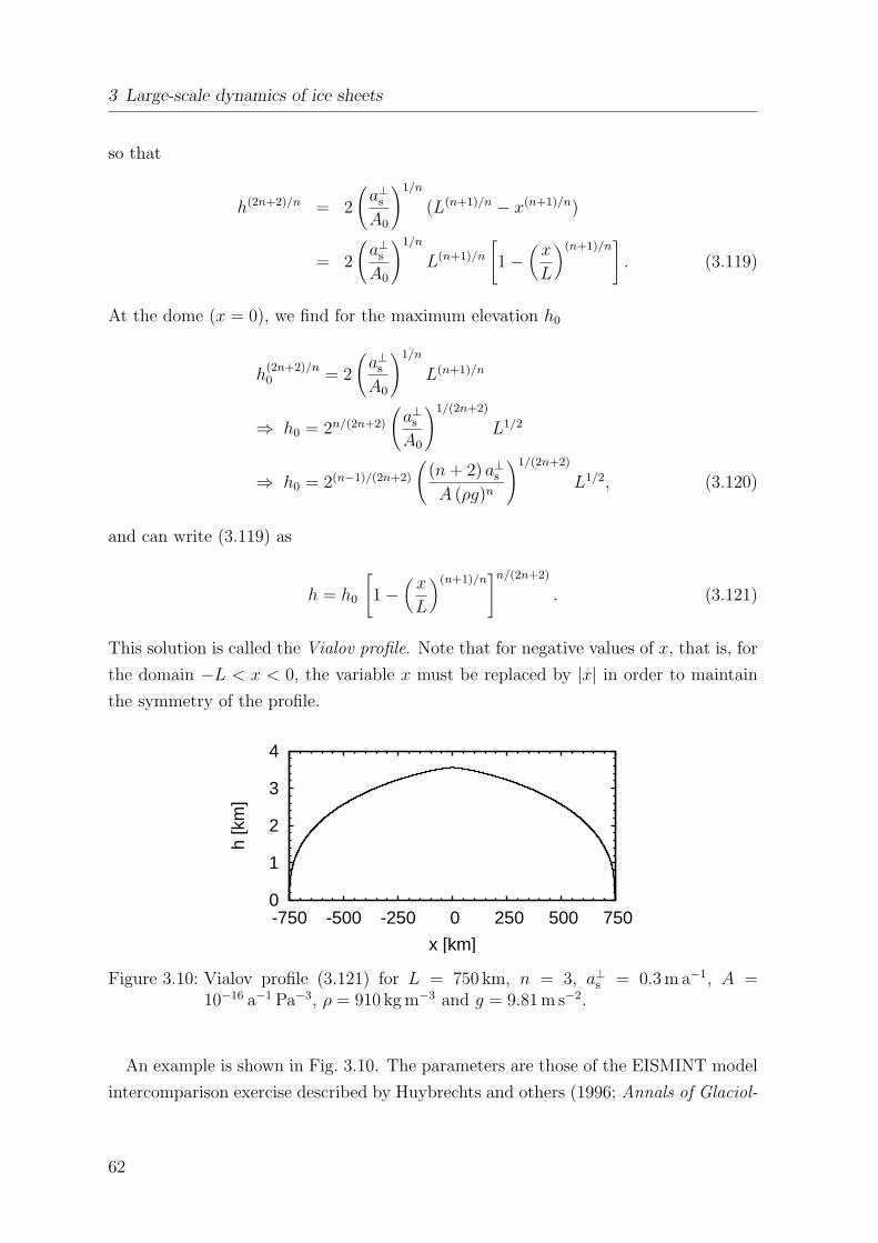
3 Large-scale dynamics of ice sheets
so that
h(2n+2)/n = 2
(a⊥sA0
)1/n
(L(n+1)/n − x(n+1)/n)
= 2
(a⊥sA0
)1/n
L(n+1)/n
[1−
(x
L
)(n+1)/n]. (3.119)
At the dome (x = 0), we find for the maximum elevation h0
h(2n+2)/n0 = 2
(a⊥sA0
)1/n
L(n+1)/n
⇒ h0 = 2n/(2n+2)
(a⊥sA0
)1/(2n+2)
L1/2
⇒ h0 = 2(n−1)/(2n+2)
((n + 2) a⊥sA (ρg)n
)1/(2n+2)
L1/2, (3.120)
and can write (3.119) as
h = h0
[1−
(x
L
)(n+1)/n]n/(2n+2)
. (3.121)
This solution is called the Vialov profile. Note that for negative values of x, that is, for
the domain −L < x < 0, the variable x must be replaced by |x| in order to maintain
the symmetry of the profile.
0
1
2
3
4
-750 -500 -250 0 250 500 750
h [k
m]
x [km]
Figure 3.10: Vialov profile (3.121) for L = 750 km, n = 3, a⊥s = 0.3 m a−1, A =10−16 a−1 Pa−3, ρ = 910 kg m−3 and g = 9.81 m s−2.
An example is shown in Fig. 3.10. The parameters are those of the EISMINT model
intercomparison exercise described by Huybrechts and others (1996; Annals of Glaciol-
62
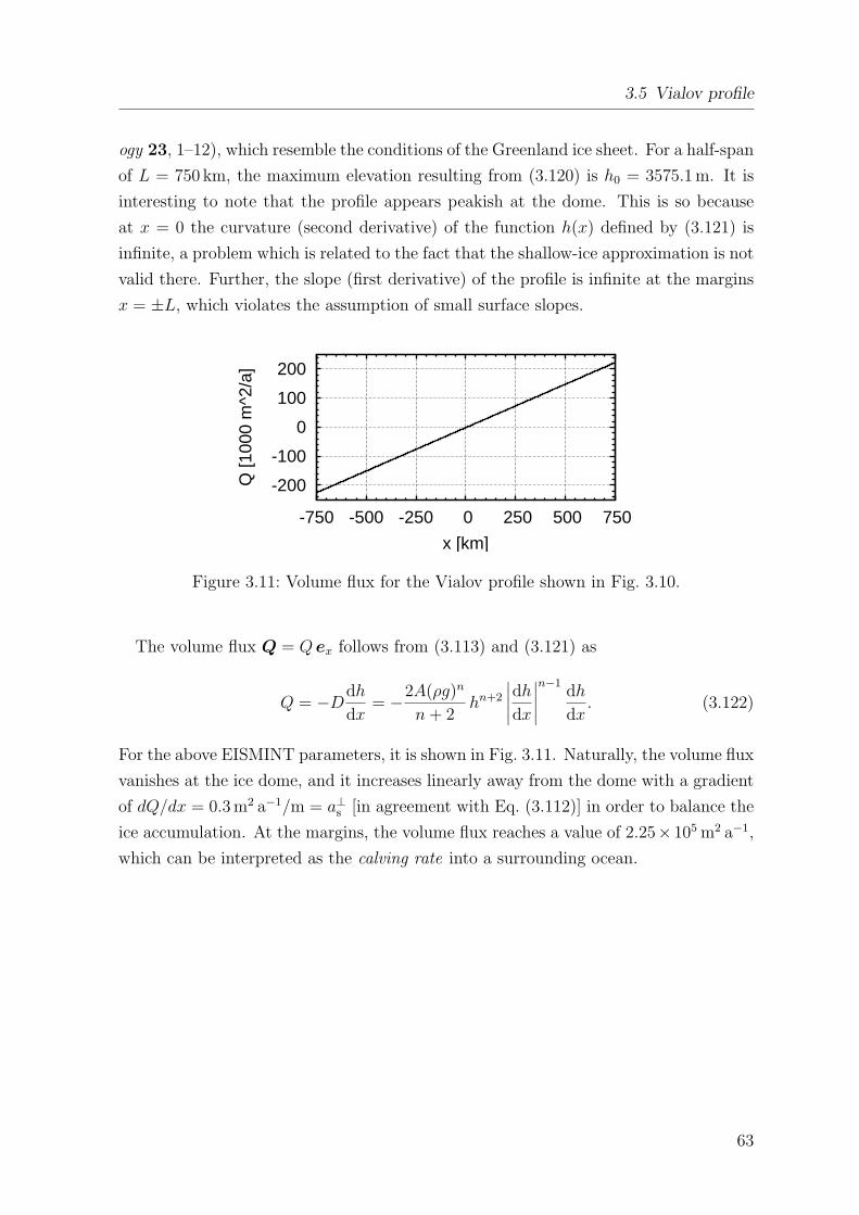
3.5 Vialov profile
ogy 23, 1–12), which resemble the conditions of the Greenland ice sheet. For a half-span
of L = 750 km, the maximum elevation resulting from (3.120) is h0 = 3575.1 m. It is
interesting to note that the profile appears peakish at the dome. This is so because
at x = 0 the curvature (second derivative) of the function h(x) defined by (3.121) is
infinite, a problem which is related to the fact that the shallow-ice approximation is not
valid there. Further, the slope (first derivative) of the profile is infinite at the margins
x = ±L, which violates the assumption of small surface slopes.
-200
-100
0
100
200
-750 -500 -250 0 250 500 750
Q [1
000
m^2
/a]
x [km]
Figure 3.11: Volume flux for the Vialov profile shown in Fig. 3.10.
The volume flux Q = Q ex follows from (3.113) and (3.121) as
Q = −Ddh
dx= −2A(ρg)n
n + 2hn+2
∣∣∣∣∣dh
dx
∣∣∣∣∣n−1
dh
dx. (3.122)
For the above EISMINT parameters, it is shown in Fig. 3.11. Naturally, the volume flux
vanishes at the ice dome, and it increases linearly away from the dome with a gradient
of dQ/dx = 0.3 m2 a−1/m = a⊥s [in agreement with Eq. (3.112)] in order to balance the
ice accumulation. At the margins, the volume flux reaches a value of 2.25×10⁵ m2 a−1,
which can be interpreted as the calving rate into a surrounding ocean.
63
3 Large-scale dynamics of ice sheets
64
4 Large-scale dynamics of ice shelves
4.1 Full Stokes flow problem, hydrostatic approximation
Ice shelves are floating ice masses, which are connected to and nourished by a grounded
ice sheet (see Fig. 3.5). Large ice shelves typically exist in large embayments of an ice
sheet, like the three major ice shelves of Antarctica (Ross ice shelf, Filchner-Rønne ice
shelf, Amery ice shelf). Smaller ice shelves can also be unbounded.
Ice shelves are smaller and thinner than ice sheets, and on average the ice flow is
distinctly faster. Suitable typical values are
typical horizontal extent [L] = 500 km,
typical vertical extent [H] = 500 m,
typical horizontal velocity [U ] = 1000 m a−1,
typical vertical velocity [W ] = 1 m a−1,
typical pressure [P ] = ρg[H] ≈ 5 MPa,
typical time-scale [t] = [L]/[U ] = [H]/[W ] = 500 a,
typical temperature variation [∆T ] = 20 K.
(4.1)
[compare Eqs. (3.29) and (3.108) for ice sheets]. Note the resulting time-scale [t], which
is twenty times smaller than that of ice sheets. The scales (4.1) give an aspect ratio of
ε =[H]
[L]=
[W ]
[U ]= 10−3 (4.2)
and a Froude number of
Fr =[U ]2
g[H]≈ 2× 10⁻¹³. (4.3)
Evidently, the aspect ratio is the same as for ice sheets, whereas the Froude number
is larger by a factor 200, but still extremely small. As a consequence, the flow of ice
shelves is governed by Stokes flow, too, and the equation of motion (3.33) remains
valid. Also, the mass balance (3.26), the temperature evolution equation (3.36), the
kinematic boundary condition (3.43), the stress-free condition (3.45) and the temper-
65
4 Large-scale dynamics of ice shelves
ature boundary condition (3.46) for the free surface hold without any changes.
The situation is different at the ice base, which is now an interface between ice and
sea water. First of all, melting and freezing processes can occur, so that the quantity
a⊥b defined in (3.51) can have either sign and must be interpreted as a basal melting-
freezing rate. It is positive for melting and negative for freezing. Apart from this
extended interpretation of a⊥b , the kinematic boundary condition (3.53) remains valid.
Consequently, the ice-thickness equation (3.69), which has been derived by using the
mass balance and the kinematic conditions at the free surface and the ice base, holds
as well.
Analogous to Eq. (3.54), the momentum jump condition is
tsea · n− t · n− ρa⊥b [[v]] = 0, (4.4)
where the lithospheric stress tlith has been replaced by the stress at the sea side of the
interface, tsea. Whereas the lithospheric stress under an ice sheet is unknown, the stress
conditions in the sea can be described by a hydrostatic pressure psea plus a shear stress
τ sea induced by the circulating sea water. The former corresponds to the weight of the
water column from the water surface (mean sea level z = zsl) to the ice base (z = b),
so that
tsea · n = −psea n + τ sea = −ρswg(zsl − b) n + τ sea, (4.5)
where ρsw is the density of sea water. Further, the advective term ρa⊥b [[v]] is negligible.
Therefore, we obtain the stress condition
t · n = −ρswg(zsl − b) n + τ sea. (4.6)
This relation serves as dynamic boundary condition at the base of an ice shelf. Thus,
the additional formulation of an empirical sliding law like (3.56) is not required.
The temperature of the ice at the ice base is equal to the temperature of the sea
water immediately below,
T = Tsea, (4.7)
which will be at the freezing point under the prevailing pressure and salinity conditions
(typically around −2C). The situation is therefore comparable to that of a temperate
base of an ice sheet [see Eq. (3.60)]. In addition to (4.7), we can formulate an energy
jump condition similar to (3.58),
κ (grad T · n)− q⊥sea − [[v]] · t · n + ρa⊥b [[u]] = 0, (4.8)
66
4.1 Full Stokes flow problem, hydrostatic approximation
where q⊥sea is the heat flux entering the ice body from the sea water below. For the
third term of (4.8), we find with (4.6)
[[v]] · t · n = −ρswg(zsl − b) [[v · n]] + [[v]] · τ sea. (4.9)
Using the general mass jump condition (2.60) and the definition (3.51) of a⊥b yields
ρsw(vsea −w) · n = ρ(v −w) · n = ρa⊥b
⇒ (vsea −w) · n =ρ
ρsw
a⊥b , (v −w) · n = a⊥b , (4.10)
so that the jump of the normal velocity in (4.9) is
[[v · n]] = (vsea −w) · n− (v −w) · n =ρ− ρsw
ρsw
a⊥b . (4.11)
Further, we define the frictional dissipation of the boundary-layer current below the
ice shelf as
δsea = [[v]] · τ sea, (4.12)
so that (4.9) becomes
[[v]] · t · n = (ρsw − ρ)g(zsl − b) a⊥b + δsea. (4.13)
As for the fourth term of (4.8), we state that, like for an ice sheet with a temperate
base, the jump of the internal energy is equal to the latent heat of ice melt ([[u]] = L).
By inserting this and (4.13) in (4.8), we obtain
κ (grad T · n)− (ρsw − ρ)g(zsl − b) a⊥b + ρLa⊥b = q⊥sea + δsea (4.14)
as energy jump condition at the ice-shelf base. Since the basal temperature is al-
ready determined by (4.7), Eq. (4.14) is not required as boundary condition for the
temperature field. However, provided that q⊥sea and δsea are known (for instance, from
measurements), it determines the basal melting-freezing rate a⊥b . Alternatively, if a⊥bis known, Eq. (4.14) can be used to compute the total heat input q⊥sea + δsea from the
sea water below the ice shelf.
The hydrostatic approximation works the same way as for ice sheets. By neglecting
the shear stresses txz and tyz in the vertical momentum balance, one finds the hydro-
static distribution (3.73) for the vertical normal stress tzz. This leads to the expressions
67
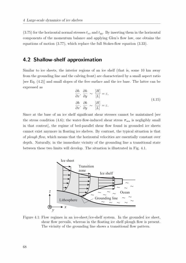
4 Large-scale dynamics of ice shelves
(3.75) for the horizontal normal stresses txx and tyy. By inserting them in the horizontal
components of the momentum balance and applying Glen’s flow law, one obtains the
equations of motion (3.77), which replace the full Stokes-flow equation (3.33).
4.2 Shallow-shelf approximation
Similar to ice sheets, the interior regions of an ice shelf (that is, some 10 km away
from the grounding line and the calving front) are characterized by a small aspect ratio
[see Eq. (4.2)] and small slopes of the free surface and the ice base. The latter can be
expressed as∂h
∂x,
∂h
∂y∼ [H]
[L]= ε,
∂b
∂x,
∂b
∂y∼ [H]
[L]= ε.
(4.15)
Since at the base of an ice shelf significant shear stresses cannot be maintained [see
the stress condition (4.6); the water-flow-induced shear stress τ sea is negligibly small
in that context], the regime of bed-parallel shear flow found in grounded ice sheets
cannot exist anymore in floating ice shelves. By contrast, the typical situation is that
of plough flow, which means that the horizontal velocities are essentially constant over
depth. Naturally, in the immediate vicinity of the grounding line a transitional state
between these two limits will develop. The situation is illustrated in Fig. 4.1.
Figure 4.1: Flow regimes in an ice-sheet/ice-shelf system. In the grounded ice sheet,shear flow prevails, whereas in the floating ice shelf plough flow is present.The vicinity of the grounding line shows a transitional flow pattern.
68
4.2 Shallow-shelf approximation
These considerations will now be used for deriving a further simplification of the hy-
drostatic approximation which is called the shallow-shelf approximation (SSA). Math-
ematically, the regime of plough flow can be defined by
∂vx
∂z≈ 0,
∂vy
∂z≈ 0. (4.16)
In other words, the horizontal velocities only depend on the horizontal coordinates and
the time,
vx = vx(x, y, t), vy = vy(x, y, t). (4.17)
We go back to the horizontal components of the momentum balance of the hydrostatic
approximation in the form (3.76). In order to make use of the fact that the shear
stresses vanish at the surface and at the base, these equations are now integrated over
depth:
2∫ h
b
∂tDxx
∂xdz +
∫ h
b
∂tDyy
∂xdz +
∫ h
b
∂txy
∂ydz +
∫ h
b
∂txz
∂zdz = ρgH
∂h
∂x,
2∫ h
b
∂tDyy
∂ydz +
∫ h
b
∂tDxx
∂ydz +
∫ h
b
∂txy
∂xdz +
∫ h
b
∂tyz
∂zdz = ρgH
∂h
∂y.
(4.18)
The first three integrals of each equation can be modified by using the Leibniz’ rule
(see also Sect. 3.2.3), whereas the last one simply gives the difference of txz or tyz at
the surface and at the base. One obtains
2∂
∂x
∫ h
btDxx dz − 2tDxx|z=h
∂h
∂x+ 2tDxx|z=b
∂b
∂x
+∂
∂x
∫ h
btDyy dz − tDyy|z=h
∂h
∂x+ tDyy|z=b
∂b
∂x
+∂
∂y
∫ h
btxy dz − txy|z=h
∂h
∂y+ txy|z=b
∂b
∂y+ txz|z=h − txz|z=b = ρgH
∂h
∂x,
2∂
∂y
∫ h
btDyy dz − 2tDyy|z=h
∂h
∂y+ 2tDyy|z=b
∂b
∂y
+∂
∂y
∫ h
btDxx dz − tDxx|z=h
∂h
∂y+ tDxx|z=b
∂b
∂y
+∂
∂x
∫ h
btxy dz − txy|z=h
∂h
∂x+ txy|z=b
∂b
∂x+ tyz|z=h − tyz|z=b = ρgH
∂h
∂y.
(4.19)
69
4 Large-scale dynamics of ice shelves
By introducing the membrane stresses N as the vertically integrated deviatoric stresses,
N =
h∫
b
tD dz, or Nij =
h∫
b
tDij dz, (4.20)
and rearranging terms, this yields
2∂Nxx
∂x+
∂Nyy
∂x+
∂Nxy
∂y
−2tDxx|z=h∂h
∂x− tDyy|z=h
∂h
∂x− txy|z=h
∂h
∂y+ txz|z=h
+2tDxx|z=b∂b
∂x+ tDyy|z=b
∂b
∂x+ txy|z=b
∂b
∂y− txz|z=b = ρgH
∂h
∂x,
2∂Nyy
∂y+
∂Nxx
∂y+
∂Nxy
∂x
−2tDyy|z=h∂h
∂y− tDxx|z=h
∂h
∂y− txy|z=h
∂h
∂x+ tyz|z=h
+2tDyy|z=b∂b
∂y+ tDxx|z=b
∂b
∂y+ txy|z=b
∂b
∂x− tyz|z=b = ρgH
∂h
∂y.
(4.21)
In order to further simplify this system, the stress conditions at the surface (3.45)
and at the base (4.6) must be considered. With the normal unit vector (3.38), the
condition (3.45) reads in components
1
Ns
(−txx|z=h
∂h
∂x− txy|z=h
∂h
∂y+ txz|z=h
)= 0,
1
Ns
(−tyy|z=h
∂h
∂y− txy|z=h
∂h
∂x+ tyz|z=h
)= 0,
1
Ns
(−txz|z=h
∂h
∂x− tyz|z=h
∂h
∂y+ tzz|z=h
)= 0.
(4.22)
In the last component, the shear stresses are negligible compared to the vertical normal
stress, so that it simplifies to
tzz|z=h = 0, (4.23)
in agreement with the hydrostatic distribution (3.73). In the first two components, we
replace the normal stresses txx and tyy by using the expressions (3.75) evaluated for
70
4.2 Shallow-shelf approximation
z = h,
−2tDxx|z=h∂h
∂x− tDyy|z=h
∂h
∂x− txy|z=h
∂h
∂y+ txz|z=h = 0.
−2tDyy|z=h∂h
∂y− tDxx|z=h
∂h
∂y− txy|z=h
∂h
∂x+ tyz|z=h = 0.
(4.24)
As a consequence, the second and fifth lines of the vertically integrated momentum
balance (4.21) vanish.
At the ice base, the component form of the stress condition (4.6) becomes with the
normal unit vector (3.48) and neglected shear stress τ sea
1
Nb
(txx|z=b
∂b
∂x+ txy|z=b
∂b
∂y− txz|z=b
)= −ρswg
Nb
(zsl − b)∂b
∂x,
1
Nb
(tyy|z=b
∂b
∂y+ txy|z=b
∂b
∂x− tyz|z=b
)= −ρswg
Nb
(zsl − b)∂b
∂y,
1
Nb
(txz|z=b
∂b
∂x+ tyz|z=b
∂b
∂y− tzz|z=b
)=
ρswg
Nb
(zsl − b).
(4.25)
Again, in the last component the shear stresses can be neglected compared to the
vertical normal stress, which yields
tzz|z=b = −ρswg(zsl − b). (4.26)
However, we can also obtain the value of tzz|z=b by evaluating the hydrostatic distri-
bution (3.73) for z = b,
tzz|z=b = −ρgH. (4.27)
Equating (4.26) and (4.27) relates the ice thickness H to the water column zsl − b,
ρH = ρsw(zsl − b). (4.28)
This result is called floating condition. By replacing b = h −H, it can be rearranged
into a relation for the freeboard h− zsl (part of the ice shelf above the water level),
ρH = ρsw(zsl − h + H) ⇒ h− zsl = H − ρ
ρsw
H =ρsw − ρ
ρsw
H. (4.29)
With the values ρ = 910 kg m−3 and ρsw = 1028 kg m−3, the freeboard is approximately
equal to 11.5% of the ice-shelf thickness, so that the remaining 88.5% will be below the
water level.
In the first two components of (4.25), we replace again txx and tyy by using (3.75),
71
4 Large-scale dynamics of ice shelves
now evaluated for z = b,
2tDxx|z=b∂b
∂x+ tDyy|z=b
∂b
∂x− ρgH
∂b
∂x+ txy|z=b
∂b
∂y− txz|z=b
= −ρswg(zsl − b)∂b
∂x,
2tyy|z=b∂b
∂y+ txx|z=b
∂b
∂y− ρgH
∂b
∂y+ txy|z=b
∂b
∂x− tyz|z=b
= −ρswg(zsl − b)∂b
∂y,
(4.30)
and because of the floating condition (4.28), this simplifies to
2tDxx|z=b∂b
∂x+ tDyy|z=b
∂b
∂x+ txy|z=b
∂b
∂y− txz|z=b = 0,
2tyy|z=b∂b
∂y+ txx|z=b
∂b
∂y+ txy|z=b
∂b
∂x− tyz|z=b = 0.
(4.31)
Therefore, the terms in the third and sixth lines of (4.21) to the left of the equals signs
vanish as well.
Application of the conditions (4.24) and (4.31) in the vertically integrated momentum
balance (4.21) provides
2∂Nxx
∂x+
∂Nyy
∂x+
∂Nxy
∂y= ρgH
∂h
∂x,
2∂Nyy
∂y+
∂Nxx
∂y+
∂Nxy
∂x= ρgH
∂h
∂y,
(4.32)
where h and H are related by the floating condition in the form (4.29). By vertically
integrating the flow law (3.20), one obtains
Nxx = 2η Dxx = 2η∂vx
∂x,
Nyy = 2η Dyy = 2η∂vy
∂y,
Nxy = 2η Dxy = η
(∂vx
∂y+
∂vy
∂x
),
(4.33)
where the independence of vx and vy on z, Eq. (4.17), and the definition of the mem-
72

4.2 Shallow-shelf approximation
brane stresses, Eq. (4.20), have been used, and the depth-integrated viscosity
η =
h∫
b
η dz (4.34)
has been introduced. Inserting of (4.33) in (4.32) finally yields
4∂
∂x
(η∂vx
∂x
)+ 2
∂
∂x
(η∂vy
∂y
)+
∂
∂y
(η(∂vx
∂y+
∂vy
∂x
))= ρgH
∂h
∂x,
4∂
∂y
(η∂vy
∂y
)+ 2
∂
∂y
(η∂vx
∂x
)+
∂
∂x
(η(∂vx
∂y+
∂vy
∂x
))= ρgH
∂h
∂y,
(4.35)
which is a non-linear elliptical boundary-value problem for the horizontal velocities vx
and vy. It must be complemented by boundary conditions along the margin of the ice
shelf, which are usually a prescribed inflow vgl at the grounding line and a hydrostatic
pressure distribution of the sea water at the calving front. This is illustrated in Fig. 4.2.
Figure 4.2: Ice-shelf geometry in the horizontal map plane. The horizontal velocityfield vh is a solution of the elliptical boundary-value problem (4.35). Theboundary values are defined by the prescribed inflow velocity at the ground-ing line, vgl, and the hydrostatic pressure of the sea water at the calvingfront.
The system of model equations in the shallow-shelf approximation is completed by
the vertically integrated mass balance [see Eq. (3.102)]
vz = vz|z=b −∫ z
b
(∂vx
∂x+
∂vy
∂y
)dz
73
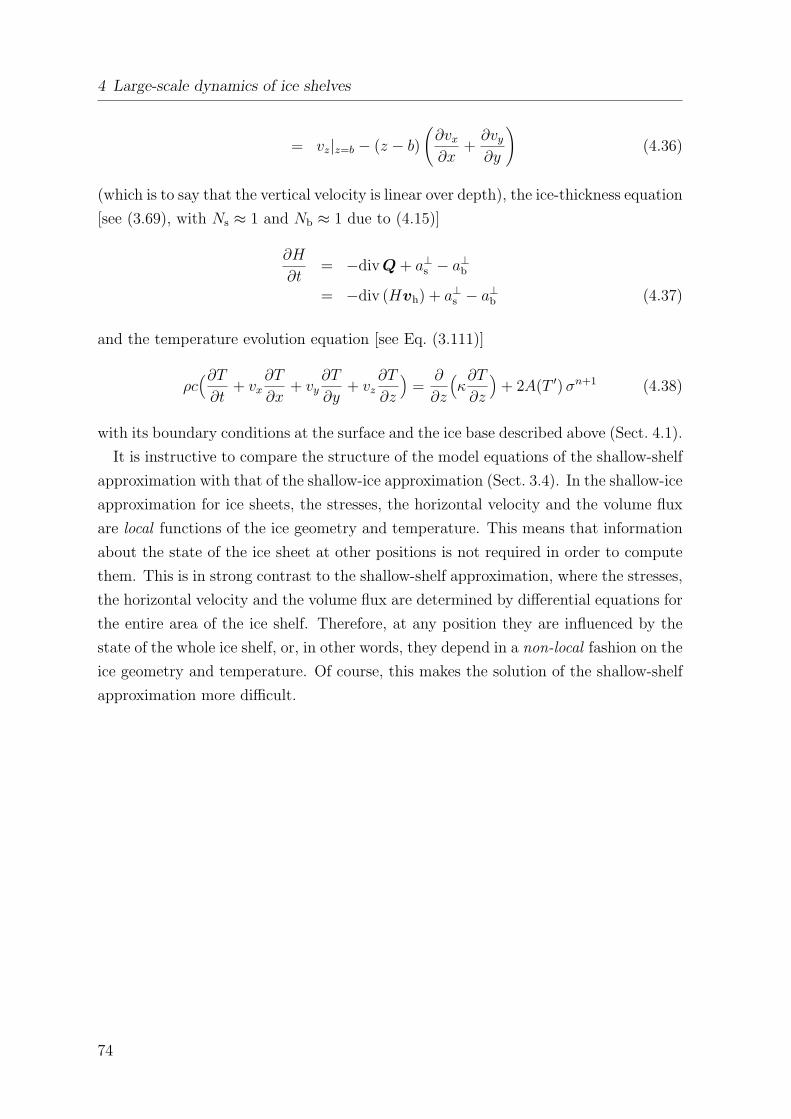
4 Large-scale dynamics of ice shelves
= vz|z=b − (z − b)
(∂vx
∂x+
∂vy
∂y
)(4.36)
(which is to say that the vertical velocity is linear over depth), the ice-thickness equation
[see (3.69), with Ns ≈ 1 and Nb ≈ 1 due to (4.15)]
∂H
∂t= −div Q + a⊥s − a⊥b
= −div (Hvh) + a⊥s − a⊥b (4.37)
and the temperature evolution equation [see Eq. (3.111)]
ρc(∂T
∂t+ vx
∂T
∂x+ vy
∂T
∂y+ vz
∂T
∂z
)=
∂
∂z
(κ∂T
∂z
)+ 2A(T ′) σn+1 (4.38)
with its boundary conditions at the surface and the ice base described above (Sect. 4.1).
It is instructive to compare the structure of the model equations of the shallow-shelf
approximation with that of the shallow-ice approximation (Sect. 3.4). In the shallow-ice
approximation for ice sheets, the stresses, the horizontal velocity and the volume flux
are local functions of the ice geometry and temperature. This means that information
about the state of the ice sheet at other positions is not required in order to compute
them. This is in strong contrast to the shallow-shelf approximation, where the stresses,
the horizontal velocity and the volume flux are determined by differential equations for
the entire area of the ice shelf. Therefore, at any position they are influenced by the
state of the whole ice shelf, or, in other words, they depend in a non-local fashion on the
ice geometry and temperature. Of course, this makes the solution of the shallow-shelf
approximation more difficult.
74
5 Dynamics of glacier flow
5.1 Scaling and hierarchy of approximations
The size of land ice masses spans several orders of magnitude, from large ice sheets
of a few thousand kilometers in diameter down to small glaciers of a few hundreds of
meters length. Consequently, the scaling given for ice sheets in Sect. 3 [Eqs. (3.29),
(3.108)] is not valid for smaller ice caps and glaciers, and needs to be modified.
However, in any case the Froude number Fr is small compared to unity, and therefore
the full Stokes flow problem formulated in Sect. 3.2 is applicable to land ice masses
of all shapes and sizes. On the other hand, the applicability of the approximations
defined in Sects. 3.3 and 3.4 is limited by the size of the ice masses. While the
hydrostatic approximation still provides reasonable accuracy for most problems of
glacier flow, the shallow-ice approximation is valid for the large-scale description of
ice sheets and large ice caps only.
In the following, due to shortage of time, we will only consider the “parallel-sided
slab” as a simple, analytically solvable problem.
5.2 Parallel-sided slab
Depending on the exact geometry, the central part of a small valley glacier can
sometimes be coarsely approximated as a parallel-sided slab on an inclined bed,
similar to the problem of a gravity-driven thin-film flow. This is sketched in Fig. 5.1.
In order to formulate the ice-flow problem for the parallel-sided slab as full Stokes
flow, let us make the following assumptions:
• Plane-strain approximation: purely two-dimensional problem in the vertical
x-z plane, no dependencies on the transverse coordinate y.
• Constant thickness H and inclination angle α.
• Uniformity in the downslope (x) direction: ∂(·)/∂x = 0 for all field quantities.
75
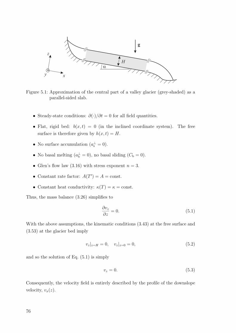
Figure 5.1: Approximation of the central part of a valley glacier (grey-shaded) as aparallel-sided slab.
• Steady-state conditions: ∂(·)/∂t = 0 for all field quantities.
• Flat, rigid bed: b(x, t) = 0 (in the inclined coordinate system). The free
surface is therefore given by h(x, t) = H.
• No surface accumulation (a⊥s = 0).
• No basal melting (a⊥b = 0), no basal sliding (Cb = 0).
• Glen’s flow law (3.16) with stress exponent n = 3.
• Constant rate factor: A(T ′) = A = const.
• Constant heat conductivity: κ(T ) = κ = const.
Thus, the mass balance (3.26) simplifies to
∂vz
∂z= 0. (5.1)
With the above assumptions, the kinematic conditions (3.43) at the free surface and
(3.53) at the glacier bed imply
vz|z=H = 0, vz|z=0 = 0, (5.2)
and so the solution of Eq. (5.1) is simply
vz = 0. (5.3)
Consequently, the velocity field is entirely described by the profile of the downslope
velocity, vx(z).
76
With the evident decomposition g = g sin α ex − g cos α ez, the x-component of
the Stokes equation (3.33) reads
−∂p
∂x+ η
(∂2vx
∂x2+
∂2vx
∂y2+
∂2vx
∂z2
)
+ 2∂vx
∂x
∂η
∂x+
(∂vx
∂y+
∂vy
∂x
)∂η
∂y+
(∂vx
∂z+
∂vz
∂x
)∂η
∂z
+ ρg sin α = 0, (5.4)
which simplifies to
η∂2vx
∂z2+
∂vx
∂z
∂η
∂z+ ρg sin α = 0
⇒ ∂
∂z
(η∂vx
∂z
)+ ρg sin α = 0. (5.5)
The first integral of this equation is
η∂vx
∂z= C1 − ρgz sin α, (5.6)
where C1 is an integration constant. Due to Glen’s flow law in the form (3.20), the
left-hand side is equal to the shear stress txz,
txz = η∂vx
∂z= C1 − ρgz sin α, (5.7)
which vanishes at the free surface (z = H) due to the stress-free boundary condition
(3.45). Hence, the integration constant can be determined,
txz|z=H = C1 − ρgH sin α = 0 ⇒ C1 = ρgH sin α, (5.8)
and we obtain the linear shear-stress profile
txz = η∂vx
∂z= ρg(H − z) sin α. (5.9)
In order to carry out the second integration, we insert the explicit form of the
viscosity which results from Eq. (3.21),
η =1
2B d−(1−1/n), where B = A−1/n and d =
1
2
∂vx
∂z. (5.10)
i
This yields
1
2A−1/n
(1
2
∂vx
∂z
)−(1−1/n)∂vx
∂z= ρg(H − z) sin α
⇒ A−1/n
(1
2
∂vx
∂z
)1/n
= ρg(H − z) sin α
⇒ ∂vx
∂z= 2A(ρg sin α)n(H − z)n
⇒ vx = −2A(ρg sin α)n
n + 1(H − z)n+1 + C2. (5.11)
The integration constant C2 results from the no-slip condition vx|z=0 = 0 (no basal
sliding),
vx|z=0 = −2A(ρg sin α)n
n + 1Hn+1 + C2 = 0
⇒ C2 =2A(ρg sin α)n
n + 1Hn+1. (5.12)
Therefore, we obtain the velocity profile
vx =2A(ρg sin α)n
n + 1
[Hn+1 − (H − z)n+1
], (5.13)
which is a quartic function of z for the stress exponent n = 3.
Analogous to Eq. (5.4), the z-component of the Stokes equation (3.33) is
−∂p
∂z+ η
(∂2vz
∂x2+
∂2vz
∂y2+
∂2vz
∂z2
)
+ 2∂vz
∂z
∂η
∂z+
(∂vx
∂z+
∂vz
∂x
)∂η
∂x+
(∂vy
∂z+
∂vz
∂y
)∂η
∂y
− ρg cos α = 0, (5.14)
and it simplifies for the parallel-sided-slab problem to
∂p
∂z= −ρg cos α. (5.15)
The integral of this equation is
p = C3 − ρgz cos α. (5.16)
Owing to the stress-free boundary condition at the free surface (3.45), the pressure
ii
vanishes there, which yields the integration constant C3,
p|z=H = C3 − ρgH cos α = 0 ⇒ C3 = ρgH cos α. (5.17)
Thus, we obtain the hydrostatic pressure profile
p = ρg(H − z) cos α. (5.18)
It is interesting to note that the results for the pressure, Eq. (5.18), and the shear
stress, Eq. (5.9), are not affected by the nonlinear flow law; the density-preserving
Newtonian fluid (see Sect. 2.4.3) provides the same results. The nonlinearity of the
Glen’s flow law affects only the velocity profile, which is quartic here [Eq. (5.13)],
but parabolic for the Newtonian fluid (stress exponent n = 1).
It is also possible to compute the temperature profile analytically. The tempera-
ture equation (3.36) reads
ρc
(∂T
∂t+ vx
∂T
∂x+ vy
∂T
∂y+ vz
∂T
∂z
)
=∂
∂x
(κ∂T
∂x
)+
∂
∂y
(κ∂T
∂y
)+
∂
∂z
(κ∂T
∂z
)+ 4ηd2, (5.19)
which simplifies to∂
∂z
(κ∂T
∂z
)= −4ηd2. (5.20)
By using Eq. (5.10), the right-hand side can be rewritten as follows,
∂
∂z
(κ∂T
∂z
)= −4× 1
2A−1/n
(1
2
∂vx
∂z
)−(1−1/n)
×(
1
2
∂vx
∂z
)2
= −(2A)−1/n
(∂vx
∂z
)1+1/n
. (5.21)
We substitute the term ∂vx/∂z with the result (5.13),
∂
∂z
(κ∂T
∂z
)= −(2A)−1/n [2A(ρg sin α)n(H − z)n]1+1/n .
= −2A(ρg sin α)n+1(H − z)n+1. (5.22)
iii
The first integral of this equation is
κ∂T
∂z=
2A(ρg sin α)n+1
n + 2(H − z)n+2 + C4. (5.23)
By assuming that the basal temperature does not reach the pressure melting point,
the integration constant can be obtained from the basal boundary condition (3.59),
−κ∂T
∂z
∣∣∣∣∣z=0
= q⊥geo
⇒ −2A(ρg sin α)n+1
n + 2Hn+2 − C4 = q⊥geo
⇒ C4 = −q⊥geo −2A(ρg sin α)n+1
n + 2Hn+2, (5.24)
so that
κ∂T
∂z= −q⊥geo −
2A(ρg sin α)n+1
n + 2
[Hn+2 − (H − z)n+2
]. (5.25)
Further integration yields
T = −q⊥geo
κz − 2A(ρg sin α)n+1
κ(n + 2)
[Hn+2z +
(H − z)n+3
n + 3
]+ C5. (5.26)
With the surface boundary condition (3.46), the integration constant can be com-
puted,
T |z=H = Ts
⇒ −q⊥geo
κH − 2A(ρg sin α)n+1
κ(n + 2)Hn+3 + C5 = Ts
⇒ C5 = Ts +q⊥geo
κH +
2A(ρg sin α)n+1
κ(n + 2)Hn+3, (5.27)
and we obtain for the temperature profile the relation
T = Ts +q⊥geo
κ(H − z)
+2AHn+3(ρg sin α)n+1
κ(n + 2)
[1− z
H− 1
n + 3
(H − z
H
)n+3]. (5.28)
The first line describes a linear profile due to heat conduction only, and the nonlinear
modification in the second line is due to the dissipation term 4ηd2 in the temperature
equation (5.20).
iv
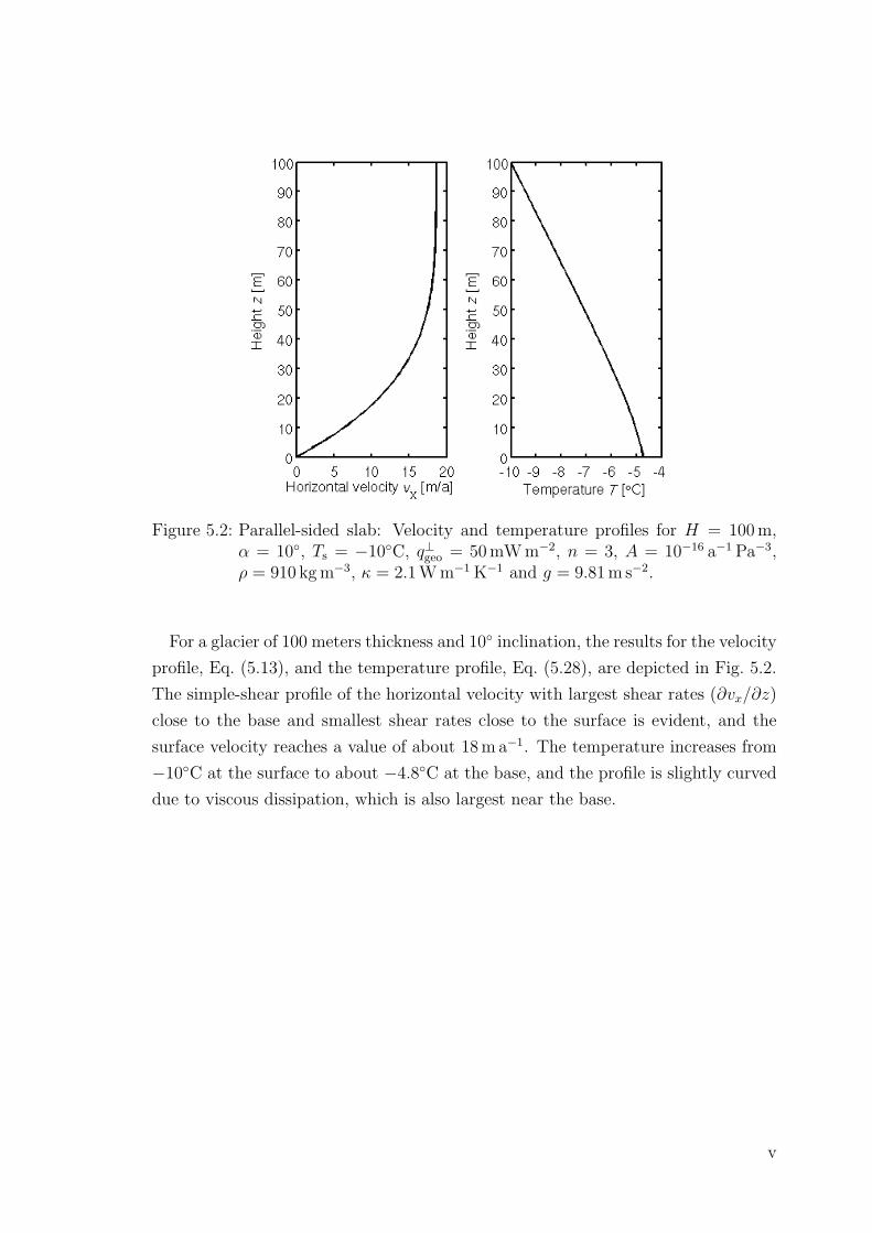
Figure 5.2: Parallel-sided slab: Velocity and temperature profiles for H = 100 m,α = 10, Ts = −10C, q⊥geo = 50 mW m−2, n = 3, A = 10−16 a−1 Pa−3,ρ = 910 kg m−3, κ = 2.1 W m−1 K−1 and g = 9.81 m s−2.
For a glacier of 100 meters thickness and 10 inclination, the results for the velocity
profile, Eq. (5.13), and the temperature profile, Eq. (5.28), are depicted in Fig. 5.2.
The simple-shear profile of the horizontal velocity with largest shear rates (∂vx/∂z)
close to the base and smallest shear rates close to the surface is evident, and the
surface velocity reaches a value of about 18 m a−1. The temperature increases from
−10C at the surface to about −4.8C at the base, and the profile is slightly curved
due to viscous dissipation, which is also largest near the base.
v
vi
6 Glacial isostasy
6.1 General remarks
The ice sheets on Earth have undergone very large changes over the glacial-interglacial
cycles in the past. Today, ice sheets of significant size occur only in Antarctica and
Greenland, whereas during the Last Glacial Maximum (LGM) 21000 years before
present, extended ice sheets covered also large parts of North America, North Europe,
the European Alps, Siberia and perhaps Tibet. These ice sheets, with typical thick-
nesses of some kilometers, impose therefore large, time-dependent loads on the crust of
the Earth, to which the body of the Earth as a visco-elastic, multi-layer system reacts
with a delayed, essentially vertical displacement.
At present, this effect is most conspicuous in Scandinavia and North America, where
a land uplift of the order of millimeters per year can be detected as a consequence of
the unloading from the glacial ice sheets. Fig. 6.1 displays the measured postglacial
fennoscandian land uplift, and it becomes evident that the pattern reflects the topogra-
phy of the fennoscandian glaciation at the LGM, with maximum values of > 8 mm a−1
in the northern Gulf of Bothnia.
The first known documentation of postglacial land uplift in Scandinavia dates back
to the year 1491, when the inhabitants of the Swedish town of Osthammar located
at the southern Gulf of Bothnia reported that their town can no longer be reached by
fishing-boats due to a growth of the land at the sea [for the historical outline given here
cf. Ekman (1991; Terra Nova 3, 358–365), and references therein]. First attempts from
the 18th century to explain this phenomenon blamed a decrease of the sea level for the
water retreat. So Hiarne proposed in 1706 that the water of the Baltic Sea runs off into
the deeper Atlantic, and Swedenborg claimed in 1719 that a gradual deceleration of the
rotation of the Earth leads to a general lowering of the sea level in higher latitudes. In
1743, Celsius calculated the water decrease by reconstructing the sea level over more
than 100 years for a seal rock at the coast of the small island Iggon, and published the
value 13 mm a−1, which is, according to modern knowledge, about 60% too large, yet
of the right order of magnitude. The remarkable explanation Celsius had in mind is
77
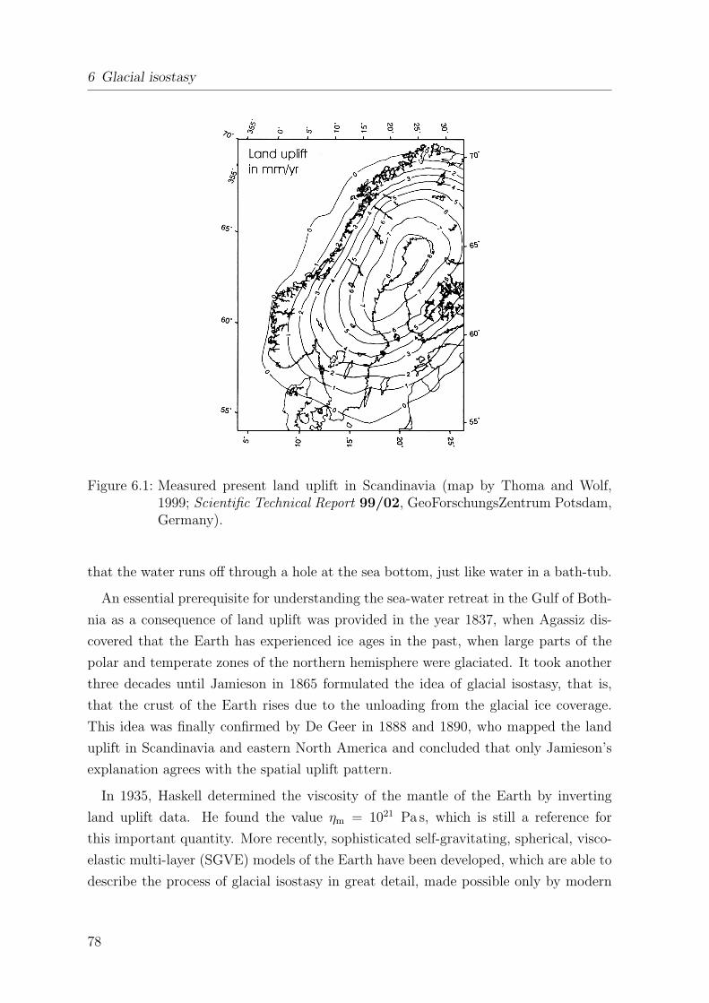
6 Glacial isostasy
Figure 6.1: Measured present land uplift in Scandinavia (map by Thoma and Wolf,1999; Scientific Technical Report 99/02, GeoForschungsZentrum Potsdam,Germany).
that the water runs off through a hole at the sea bottom, just like water in a bath-tub.
An essential prerequisite for understanding the sea-water retreat in the Gulf of Both-
nia as a consequence of land uplift was provided in the year 1837, when Agassiz dis-
covered that the Earth has experienced ice ages in the past, when large parts of the
polar and temperate zones of the northern hemisphere were glaciated. It took another
three decades until Jamieson in 1865 formulated the idea of glacial isostasy, that is,
that the crust of the Earth rises due to the unloading from the glacial ice coverage.
This idea was finally confirmed by De Geer in 1888 and 1890, who mapped the land
uplift in Scandinavia and eastern North America and concluded that only Jamieson’s
explanation agrees with the spatial uplift pattern.
In 1935, Haskell determined the viscosity of the mantle of the Earth by inverting
land uplift data. He found the value ηm = 1021 Pa s, which is still a reference for
this important quantity. More recently, sophisticated self-gravitating, spherical, visco-
elastic multi-layer (SGVE) models of the Earth have been developed, which are able to
describe the process of glacial isostasy in great detail, made possible only by modern
78
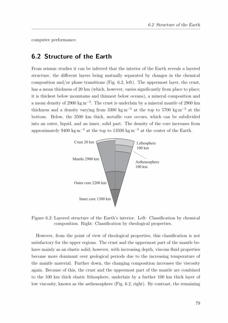
6.2 Structure of the Earth
computer performance.
6.2 Structure of the Earth
From seismic studies it can be inferred that the interior of the Earth reveals a layered
structure, the different layers being mutually separated by changes in the chemical
composition and/or phase transitions (Fig. 6.2, left). The uppermost layer, the crust,
has a mean thickness of 20 km (which, however, varies significantly from place to place;
it is thickest below mountains and thinnest below oceans), a mineral composition and
a mean density of 2900 kg m−3. The crust is underlain by a mineral mantle of 2900 km
thickness and a density varying from 3300 kg m−3 at the top to 5700 kg m−3 at the
bottom. Below, the 3500 km thick, metallic core occurs, which can be subdivided
into an outer, liquid, and an inner, solid part. The density of the core increases from
approximately 9400 kg m−3 at the top to 13500 kg m−3 at the center of the Earth.
Figure 6.2: Layered structure of the Earth’s interior. Left: Classification by chemicalcomposition. Right: Classification by rheological properties.
However, from the point of view of rheological properties, this classification is not
satisfactory for the upper regions. The crust and the uppermost part of the mantle be-
have mainly as an elastic solid; however, with increasing depth, viscous fluid properties
become more dominant over geological periods due to the increasing temperature of
the mantle material. Further down, the changing composition increases the viscosity
again. Because of this, the crust and the uppermost part of the mantle are combined
to the 100 km thick elastic lithosphere, underlain by a further 100 km thick layer of
low viscosity, known as the asthenosphere (Fig. 6.2, right). By contrast, the remaining
79
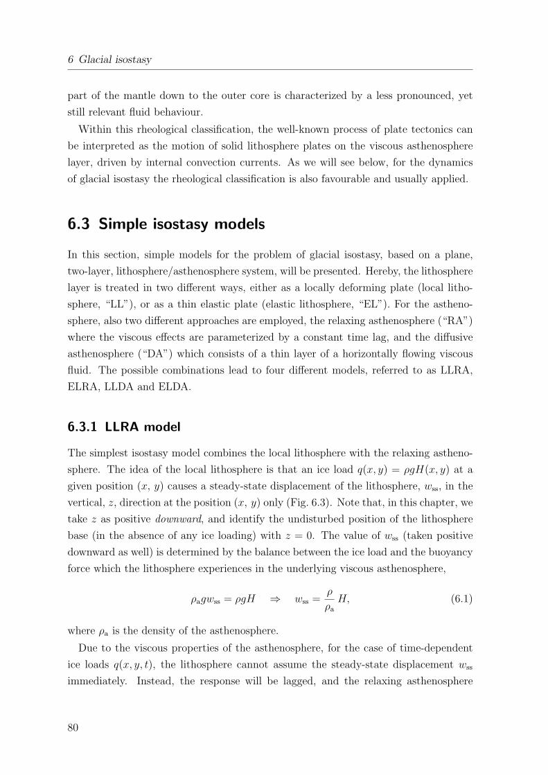
6 Glacial isostasy
part of the mantle down to the outer core is characterized by a less pronounced, yet
still relevant fluid behaviour.
Within this rheological classification, the well-known process of plate tectonics can
be interpreted as the motion of solid lithosphere plates on the viscous asthenosphere
layer, driven by internal convection currents. As we will see below, for the dynamics
of glacial isostasy the rheological classification is also favourable and usually applied.
6.3 Simple isostasy models
In this section, simple models for the problem of glacial isostasy, based on a plane,
two-layer, lithosphere/asthenosphere system, will be presented. Hereby, the lithosphere
layer is treated in two different ways, either as a locally deforming plate (local litho-
sphere, “LL”), or as a thin elastic plate (elastic lithosphere, “EL”). For the astheno-
sphere, also two different approaches are employed, the relaxing asthenosphere (“RA”)
where the viscous effects are parameterized by a constant time lag, and the diffusive
asthenosphere (“DA”) which consists of a thin layer of a horizontally flowing viscous
fluid. The possible combinations lead to four different models, referred to as LLRA,
ELRA, LLDA and ELDA.
6.3.1 LLRA model
The simplest isostasy model combines the local lithosphere with the relaxing astheno-
sphere. The idea of the local lithosphere is that an ice load q(x, y) = ρgH(x, y) at a
given position (x, y) causes a steady-state displacement of the lithosphere, wss, in the
vertical, z, direction at the position (x, y) only (Fig. 6.3). Note that, in this chapter, we
take z as positive downward, and identify the undisturbed position of the lithosphere
base (in the absence of any ice loading) with z = 0. The value of wss (taken positive
downward as well) is determined by the balance between the ice load and the buoyancy
force which the lithosphere experiences in the underlying viscous asthenosphere,
ρagwss = ρgH ⇒ wss =ρ
ρa
H, (6.1)
where ρa is the density of the asthenosphere.
Due to the viscous properties of the asthenosphere, for the case of time-dependent
ice loads q(x, y, t), the lithosphere cannot assume the steady-state displacement wss
immediately. Instead, the response will be lagged, and the relaxing asthenosphere
80
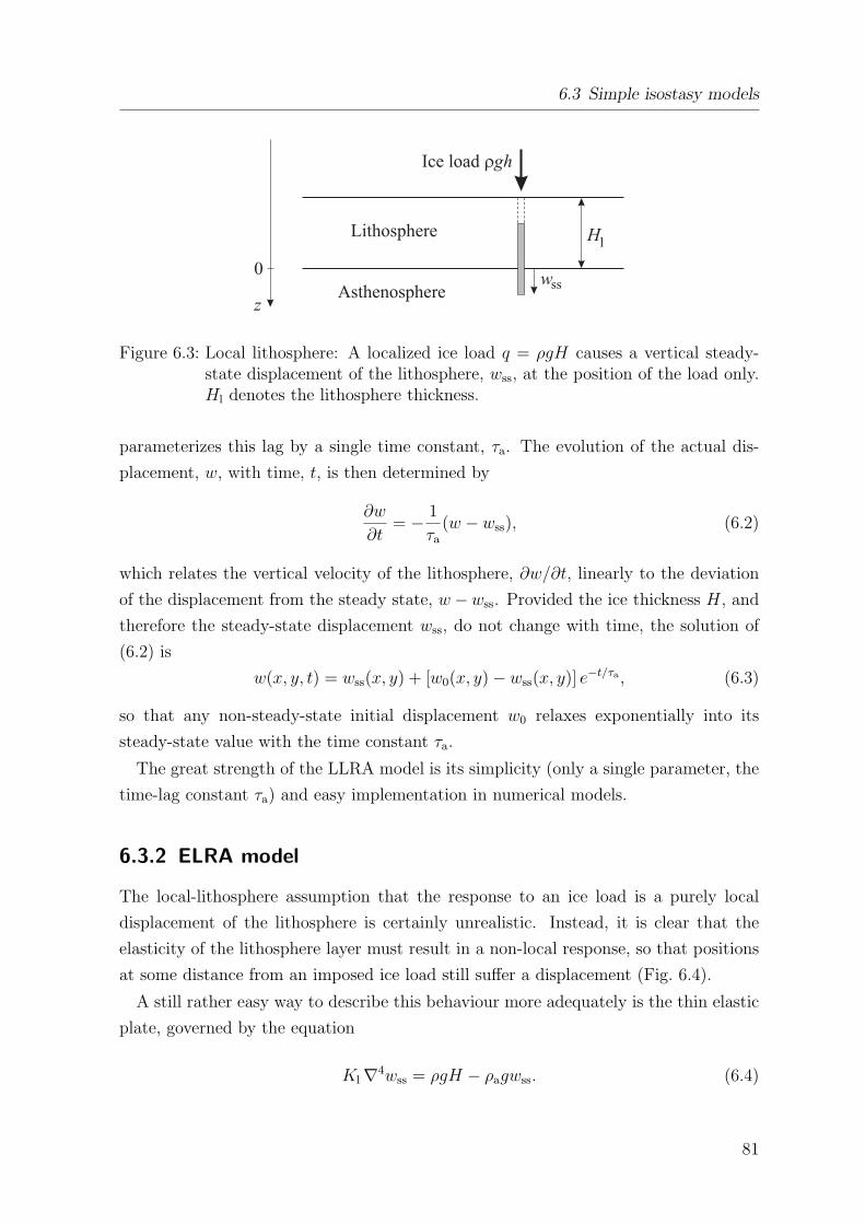
6.3 Simple isostasy models
Figure 6.3: Local lithosphere: A localized ice load q = ρgH causes a vertical steady-state displacement of the lithosphere, wss, at the position of the load only.Hl denotes the lithosphere thickness.
parameterizes this lag by a single time constant, τa. The evolution of the actual dis-
placement, w, with time, t, is then determined by
∂w
∂t= − 1
τa
(w − wss), (6.2)
which relates the vertical velocity of the lithosphere, ∂w/∂t, linearly to the deviation
of the displacement from the steady state, w−wss. Provided the ice thickness H, and
therefore the steady-state displacement wss, do not change with time, the solution of
(6.2) is
w(x, y, t) = wss(x, y) + [w0(x, y)− wss(x, y)] e−t/τa , (6.3)
so that any non-steady-state initial displacement w0 relaxes exponentially into its
steady-state value with the time constant τa.
The great strength of the LLRA model is its simplicity (only a single parameter, the
time-lag constant τa) and easy implementation in numerical models.
6.3.2 ELRA model
The local-lithosphere assumption that the response to an ice load is a purely local
displacement of the lithosphere is certainly unrealistic. Instead, it is clear that the
elasticity of the lithosphere layer must result in a non-local response, so that positions
at some distance from an imposed ice load still suffer a displacement (Fig. 6.4).
A still rather easy way to describe this behaviour more adequately is the thin elastic
plate, governed by the equation
Kl∇4wss = ρgH − ρagwss. (6.4)
81
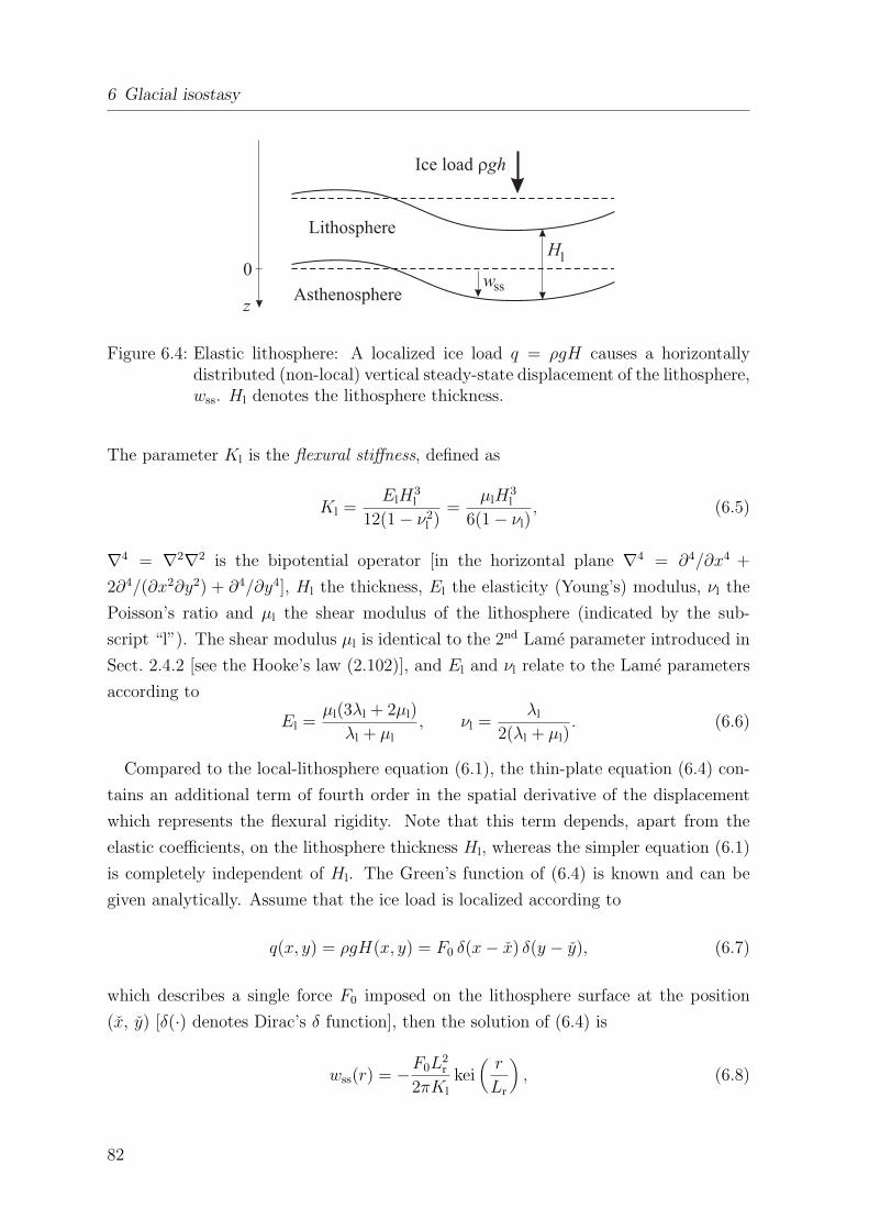
6 Glacial isostasy
Figure 6.4: Elastic lithosphere: A localized ice load q = ρgH causes a horizontallydistributed (non-local) vertical steady-state displacement of the lithosphere,wss. Hl denotes the lithosphere thickness.
The parameter Kl is the flexural stiffness, defined as
Kl =ElH
3l
12(1− ν2l )
=µlH
3l
6(1− νl), (6.5)
∇4 = ∇2∇2 is the bipotential operator [in the horizontal plane ∇4 = ∂4/∂x4 +
2∂4/(∂x2∂y2) + ∂4/∂y4], Hl the thickness, El the elasticity (Young’s) modulus, νl the
Poisson’s ratio and µl the shear modulus of the lithosphere (indicated by the sub-
script “l”). The shear modulus µl is identical to the 2nd Lame parameter introduced in
Sect. 2.4.2 [see the Hooke’s law (2.102)], and El and νl relate to the Lame parameters
according to
El =µl(3λl + 2µl)
λl + µl
, νl =λl
2(λl + µl). (6.6)
Compared to the local-lithosphere equation (6.1), the thin-plate equation (6.4) con-
tains an additional term of fourth order in the spatial derivative of the displacement
which represents the flexural rigidity. Note that this term depends, apart from the
elastic coefficients, on the lithosphere thickness Hl, whereas the simpler equation (6.1)
is completely independent of Hl. The Green’s function of (6.4) is known and can be
given analytically. Assume that the ice load is localized according to
q(x, y) = ρgH(x, y) = F0 δ(x− x) δ(y − y), (6.7)
which describes a single force F0 imposed on the lithosphere surface at the position
(x, y) [δ(·) denotes Dirac’s δ function], then the solution of (6.4) is
wss(r) = −F0L2r
2πKl
kei(
r
Lr
), (6.8)
82
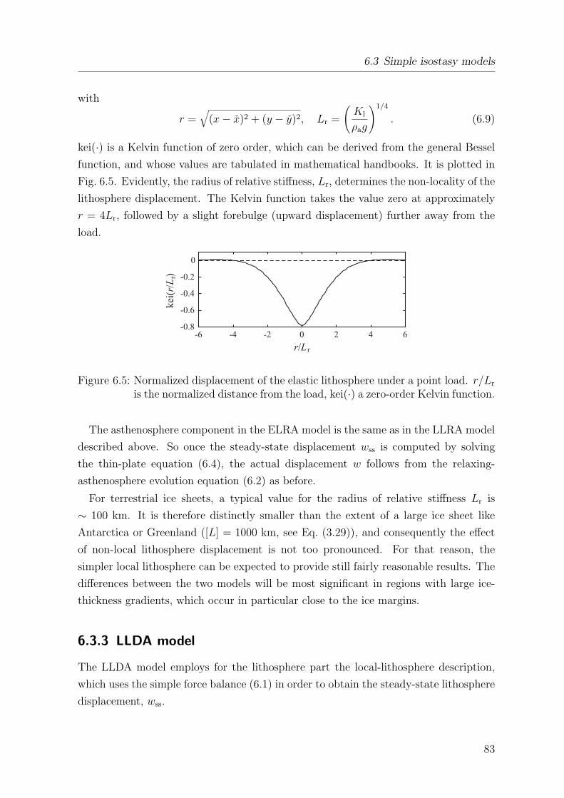
6.3 Simple isostasy models
with
r =√
(x− x)2 + (y − y)2, Lr =
(Kl
ρag
)1/4
. (6.9)
kei(·) is a Kelvin function of zero order, which can be derived from the general Bessel
function, and whose values are tabulated in mathematical handbooks. It is plotted in
Fig. 6.5. Evidently, the radius of relative stiffness, Lr, determines the non-locality of the
lithosphere displacement. The Kelvin function takes the value zero at approximately
r = 4Lr, followed by a slight forebulge (upward displacement) further away from the
load.
Figure 6.5: Normalized displacement of the elastic lithosphere under a point load. r/Lr
is the normalized distance from the load, kei(·) a zero-order Kelvin function.
The asthenosphere component in the ELRA model is the same as in the LLRA model
described above. So once the steady-state displacement wss is computed by solving
the thin-plate equation (6.4), the actual displacement w follows from the relaxing-
asthenosphere evolution equation (6.2) as before.
For terrestrial ice sheets, a typical value for the radius of relative stiffness Lr is
∼ 100 km. It is therefore distinctly smaller than the extent of a large ice sheet like
Antarctica or Greenland ([L] = 1000 km, see Eq. (3.29)), and consequently the effect
of non-local lithosphere displacement is not too pronounced. For that reason, the
simpler local lithosphere can be expected to provide still fairly reasonable results. The
differences between the two models will be most significant in regions with large ice-
thickness gradients, which occur in particular close to the ice margins.
6.3.3 LLDA model
The LLDA model employs for the lithosphere part the local-lithosphere description,
which uses the simple force balance (6.1) in order to obtain the steady-state lithosphere
displacement, wss.
83
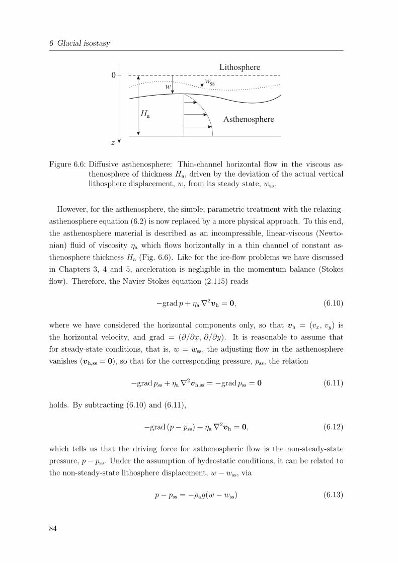
6 Glacial isostasy
Figure 6.6: Diffusive asthenosphere: Thin-channel horizontal flow in the viscous as-thenosphere of thickness Ha, driven by the deviation of the actual verticallithosphere displacement, w, from its steady state, wss.
However, for the asthenosphere, the simple, parametric treatment with the relaxing-
asthenosphere equation (6.2) is now replaced by a more physical approach. To this end,
the asthenosphere material is described as an incompressible, linear-viscous (Newto-
nian) fluid of viscosity ηa which flows horizontally in a thin channel of constant as-
thenosphere thickness Ha (Fig. 6.6). Like for the ice-flow problems we have discussed
in Chapters 3, 4 and 5, acceleration is negligible in the momentum balance (Stokes
flow). Therefore, the Navier-Stokes equation (2.115) reads
−grad p + ηa∇2vh = 0, (6.10)
where we have considered the horizontal components only, so that vh = (vx, vy) is
the horizontal velocity, and grad = (∂/∂x, ∂/∂y). It is reasonable to assume that
for steady-state conditions, that is, w = wss, the adjusting flow in the asthenosphere
vanishes (vh,ss = 0), so that for the corresponding pressure, pss, the relation
−grad pss + ηa∇2vh,ss = −grad pss = 0 (6.11)
holds. By subtracting (6.10) and (6.11),
−grad (p− pss) + ηa∇2vh = 0, (6.12)
which tells us that the driving force for asthenospheric flow is the non-steady-state
pressure, p− pss. Under the assumption of hydrostatic conditions, it can be related to
the non-steady-state lithosphere displacement, w − wss, via
p− pss = −ρag(w − wss) (6.13)
84
6.3 Simple isostasy models
(the minus sign is due to the fact that the displacements are counted positive down-
ward). Inserting this result in (6.12) and assuming that velocity changes occur mainly
in the vertical direction, that is
∂vh
∂x,
∂vh
∂y¿ ∂vh
∂z,
∂2vh
∂x2,
∂2vh
∂y2¿ ∂2vh
∂z2, (6.14)
yields∂2vh
∂z2= −ρag
ηa
grad (w − wss). (6.15)
Since the right-hand side is independent of z, this can easily be integrated. We neglect
the lithosphere displacements compared to the asthenosphere thickness,
w, wss ¿ Ha, (6.16)
so that the top of the asthenosphere is always approximately at z = 0 and the bottom
at z = Ha. Further, we assume rather arbitrarily that the velocity vanishes at the top
of the asthenosphere, and that the shear stress (and therefore the vertical derivative of
the velocity) vanishes at the bottom:
vh|z=0 = 0,∂vh
∂z
∣∣∣z=Ha
= 0. (6.17)
With these boundary conditions, double integration of (6.15) yields the parabolic ve-
locity field
vh = −ρag
2ηa
(z2 − 2Haz) grad (w − wss), (6.18)
the shape of which is indicated in Fig. 6.6.
By integrating the mass balance div v = 0 vertically from z = 0 to z = Ha, one finds
in analogy to the derivation of the ice-thickness equation (3.69)
∂Ha
∂t= −div
Ha∫
0
vh dz (6.19)
(note that any mass exchange at the top and the bottom has been neglected). If we
further assume that the bottom of the asthenosphere is rigid, then ∂Ha/∂t = −∂w/∂t,
so that∂w
∂t= div
∫ Ha
0vh dz. (6.20)
85
6 Glacial isostasy
Inserting the velocity profile (6.18) in this relation yields
∂w
∂t= −ρag
2ηa
div grad (w − wss)∫ Ha
0(z2 − 2Haz) dz
= −ρag
2ηa
∇2(w − wss)
[z3
3− 2Ha
z2
2
]Ha
0
=ρagH3
a
3ηa
∇2(w − wss), (6.21)
and, by introducing the diffusivity
Da =ρagH3
a
3ηa
, (6.22)
one finally obtains the diffusive thin-channel equation
∂w
∂t= Da∇2(w − wss). (6.23)
With the scale [L] for the horizontal extent of the ice load [see Eq. (3.29)], the associated
time scale for the diffusive asthenosphere motion is
τa =[L]2
Da
=3ηa
ρagH3a
[L]2. (6.24)
Note that here τa is proportional to the square of the extent of the ice load, whereas it
is a constant parameter in the relaxing-asthenosphere approach.
6.3.4 ELDA model
Finally, the ELDA model combines the elastic lithosphere and the diffusive astheno-
sphere. Therefore, the steady-state lithosphere displacement is computed by solving
the elastic thin-plate equation (6.4), and the actual displacement follows then from the
diffusive thin-channel equation (6.23).
6.3.5 Performance of the simple models
From the above discussions it should be expected that the ELDA model is the preferable
one of the four different models, simply because it is the least conceptual, yet the
most physical description of the relevant processes. Surprisingly, though, comparisons
with the more elaborate SGVE models mentioned in Sect. 6.1 have shown that, if
86
6.3 Simple isostasy models
lithosphere-displacement results of the latter are taken as a reference, the performance
of the simple models decreases in the order ELRA > LLRA > ELDA > LLDA.
This is to say that the elastic-lithosphere approach is superior to the local-lithosphere
approach as expected, but the relaxing asthenosphere performs better than the diffusive
asthenosphere. A likely explanation for this counterintuitive finding is that the motion
of the mantle induced by the varying ice load reaches far deeper than only to the
bottom of the asthenosphere, so that the thin-channel assumption of the diffusive-
asthenosphere approach is not adequate.
Consequently, as long as the high accuracy of a SGVE model is dispensable (for
instance, in a typical ice-sheet-modelling application), use of the ELRA model is
favourable. The even simpler LLRA model is still a reasonable, computationally faster
alternative (at the cost of some artificial fine structure in the computed uplift pat-
terns), whereas the models with the diffusive-asthenosphere parameterization, LLDA
and ELDA, should be discarded.
87
6 Glacial isostasy
88


![Glaciers I: Intro, Geology and Mass Balance · 2010-05-15 · Glaciers I: Intro, Geology and Mass Balance I. Why study glaciers? ... Extensive ice sheets [PPT] Alpine glaciers in](https://img.pdfslide.net/doc/110x75/5e6a67bcff4e7a35026bc1f6/glaciers-i-intro-geology-and-mass-balance-2010-05-15-glaciers-i-intro-geology.jpg)