Dynamics of International Financial Networks with Risk

Dynamics of International Financial Networks with Risk Management

Anna Nagurney and Jose Cruz

Department of Finance and Operations Management

Isenberg School of Management

University of Massachusetts

Amherst, Massachusetts 01003

July 2003; revised January 2004

Appears in Quantitative Finance 4 (2004), 279-291.

Abstract

In this paper, we develop an international financial network model in which the sources

of funds and the intermediaries are multicriteria decision-makers and are concerned with

both net revenue maximization and risk minimization. The model allows for both physical

as well as electronic transactions and considers three tiers of decision-makers who may be

located in distinct countries and may conduct their transactions in different currencies. We

describe the behavior of the various decision-makers, along with their optimality conditions,

and derive the variational inequality formulation of the governing equilibrium conditions.

We then propose a dynamic adjustment process which yields the evolution of the financial

flows and prices and demonstrate that it can be formulated as a projected dynamical system.

We also provide qualitative properties including stability analysis results. Finally, we discuss

a discrete-time algorithm which can be applied to track the dynamic trajectories and yields

the equilibrium financial flows and prices. We illustrate both the modeling framework as

well as the computational procedure with several numerical international financial network

examples.

1

1. Introduction

The new global financial marketplace is characterized by a wide spectrum of choices

available for financial transactions internationally plus a large number of decision-makers in-

volved, be they sources of financial funds, intermediaries, and/or, ultimately, the consumers

of the various financial products. In addition, new currencies have been introduced, such

as the euro, along with new financial products in different currencies and countries. More-

over, the landscape of financial decision-making has been transformed through advances in

telecommunications and, in particular, the Internet, providing business, brokerages, and con-

sumers with new modes of transaction, new types of products and services, as well as new

distribution channels.

Indeed, the growth of technology has allowed consumers and business to explore and

conduct their financial transactions not only within the perimeters of national boundaries

but outside them as well. At the same time that finance has become increasingly globalized,

partially due to the increasing role of electronic finance, decision-makers are being faced with

a growing importance of addressing risk due to heightened uncertainties. Such complex re-

alities raise major challenges and opportunities for financial quantitative modeling, analysis,

and computation.

In this paper, we consider financial networks and we develop an international financial

network model which includes intermediaries and also allows for the decision-makers to

transact either physically or electronically. The framework that we propose predicts the

equilibrium financial flows between tiers of the international financial network as well as the

equilibrium prices associated with the different tiers. In addition, it describes the evolution

of the financial flows and prices over time. The methodologies utilized in this paper include

finite-dimensional variational inequality theory (cf. Nagurney (1999) and the references

therein) as well as projected dynamical systems theory (Nagurney and Zhang (1996a) and

Nagurney and Siokos (1997)).

The model that we develop here, both in the static and dynamic versions, is sufficiently

general to be able to handle as many countries, sources of funds, currencies, and financial

products as mandated by the particular application. Although the topic of electronic fi-

nance, in general, has received much attention lately (cf. McAndrews and Stefanidis (2000),

2

Claessens, Glaessner, and Klingebiel (2000, 2001), Fan, Staeelert, and Whinston (2000),

Economides (2001), Allen, Hawkins, and Sato (2001), Sato and Hawkins (2001), Banks

(2001), Claessens, et al. (2003), and the references therein), there has been very little work

in the modeling, analysis, and solution of such problems, except for that of Nagurney and

Ke (2003) who focused, however, on single country modeling and Nagurney and Cruz (2002,

2003), who considered only static formulations.

Indeed, recently, financial networks have been utilized to develop general models with mul-

tiple tiers of decision-makers, including intermediaries, by Nagurney and Ke (2001, 2003) and

Nagurney and Cruz (2002, 2003). These models differ from the financial network models

described in Nagurney and Siokos (1997) in that the behavior of the individual decision-

makers associated with the distinct tiers of the network is explicitly captured and modeled.

Moreover, unlike the framework considered in Thore (1980), more general, including nonlin-

ear and asymmetric functions can be handled. However, the above-noted models of financial

networks with intermediaries have focused exclusively on optimization/equilibrium formula-

tions using finite-dimensional variational inequality formulations (see also Nagurney (1999)).

Here, in contrast, we turn to extending the above frameworks to incorporate dynamics.

In particular, in this paper, we not only extend the international financial network models

of Nagurney and Cruz (2002, 2003) to incorporate multicriteria decision-making explicitly

for the purpose of risk management, but we also introduce dynamics. The theory utilized

is the theory of projected dynamical systems (cf. Nagurney and Zhang (1996a) and the ref-

erences therein) which allows for the formulation and qualitative analysis of the interaction

of decision-makers whose decisions are subject to constraints. Projected dynamical systems

have been used to-date to formulate the dynamics of a variety of problems including those

arising in oligopolies, spatial price problems, traffic network problems, and financial net-

works (but without intermediation) (cf., respectively, Nagurney, Dupuis, and Zhang (1994),

Nagurney and Zhang (1996b), Nagurney and Zhang (1997), and Dong, Zhang, and Nagur-

ney (1996)). It is applied here for the first time in multitiered, multicriteria international

financial network problems with intermediation (as well as with electronic transactions and

risk management).

This paper is organized as follows. In Section 2, we develop the international financial

3

network model with multicriteria decision-makers. We describe the various decision-makers

and their behavior, and construct the equilibrium conditions, along with the variational

inequality formulation.

In Section 3, we propose a dynamic adjustment process by which the financial flows and

prices evolve and prove that the set of stationary points of the projected dynamical system

coincides with the set of solutions of the variational inequality. We then, in Section 4, obtain

qualitative properties of both the equilibrium pattern as well as the dynamic trajectories.

In Section 5, we present the algorithm, which is a discrete-time algorithm, and which

provides a time discretization of the dynamic trajectories. The algorithm is then applied in

Section 6 to compute the financial flows and prices in several international financial network

examples. We conclude the paper with a summary and a discussion in Section 7.

4

2. The International Financial Network Model with Risk Management

In this Section, we develop the international financial network model with three tiers of

decision-makers, which allows for both physical and electronic transactions. The multicriteria

decision-makers are the sources of funds as well as the intermediaries both of whom are

concerned with net revenue maximization and risk minimization. In this Section, we describe

the static version of the model, which is then extended to its dynamic counterpart in Section

3. The set of equilibrium points of the former are, subsequently, shown to coincide with the

set of stationary points of the latter.

The model consists of L countries, with a typical country denoted by l or l; I “source”

agents in each country with sources of funds, with a typical source agent denoted by i, and

J financial intermediaries with a typical financial intermediary denoted by j. Examples of

source agents are households and businesses, whereas examples of financial intermediaries

include banks, insurance companies, investment companies, brokers, including electronic

brokers, etc. Intermediaries in our framework need not be country-specific but, rather, may

be virtual.

We assume that each source agent can transact directly electronically with the consumers

through the Internet and can also conduct his financial transactions with the intermediaries

either physically or electronically in different currencies. There are H currencies in the

international economy, with a typical currency being denoted by h. Also, we assume that

there are K financial products which can be in distinct currencies and in different countries

with a typical financial product (and associated with a demand market) being denoted by k.

Hence, the financial intermediaries in the model, in addition to transacting with the source

agents, also determine how to allocate the incoming financial resources among distinct uses,

which are represented by the demand markets with a demand market corresponding to, for

example, the market for real estate loans, household loans, or business loans, etc., which, as

mentioned, can be associated with a distinct country and a distinct currency combination.

We let m refer to a mode of transaction with m = 1 denoting a physical transaction and

m = 2 denoting an electronic transaction via the Internet.

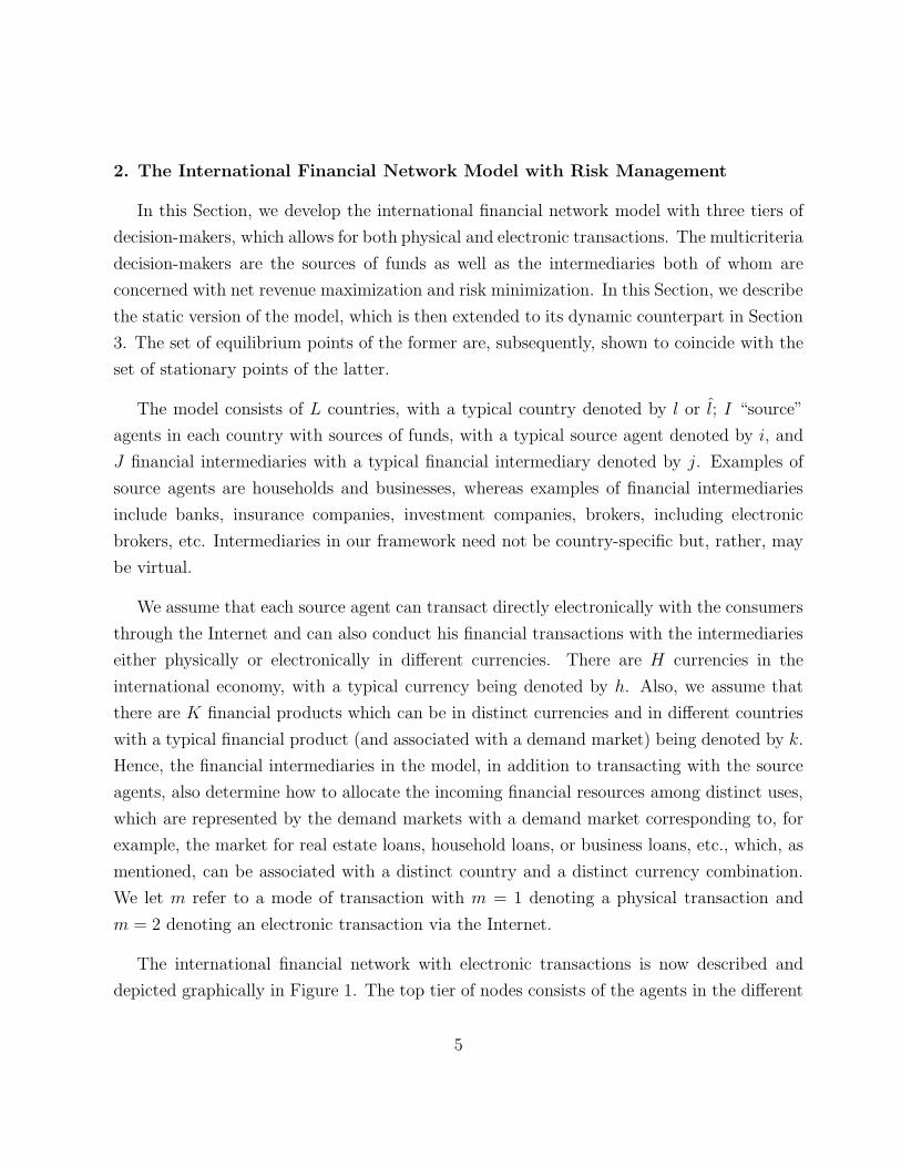
The international financial network with electronic transactions is now described and

depicted graphically in Figure 1. The top tier of nodes consists of the agents in the different

5

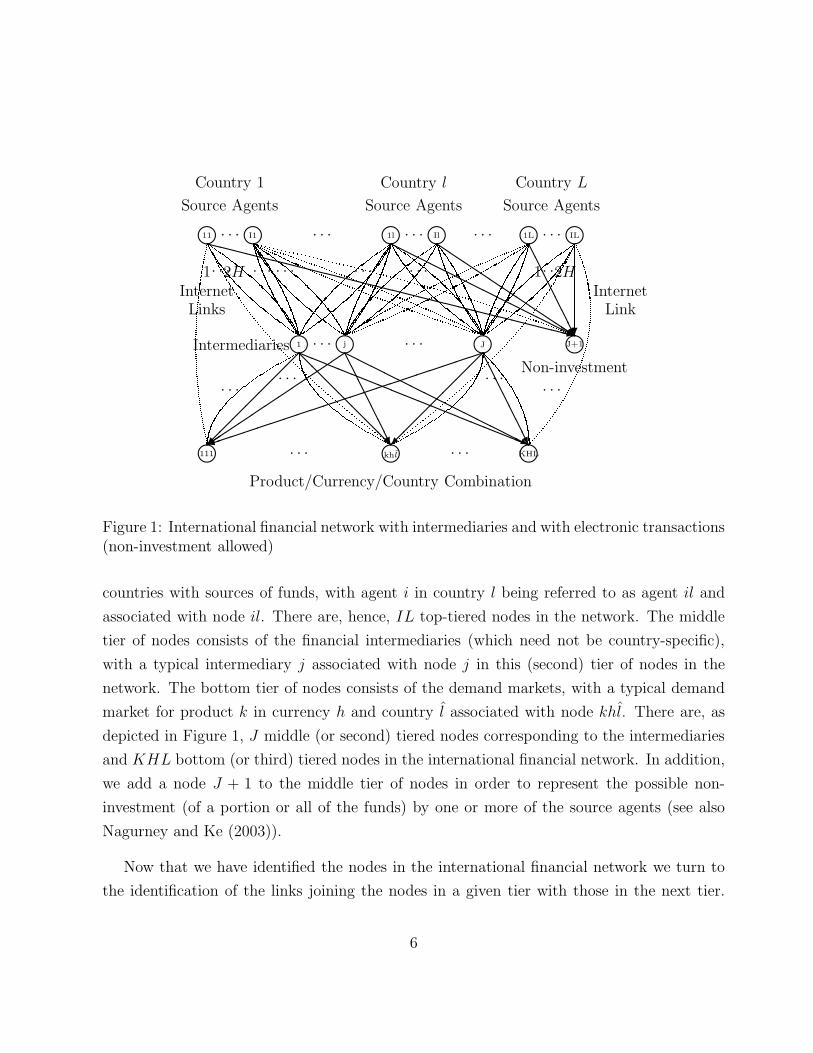
l l l l1 · · · j · · · J J+1

l l l111 · · · khl · · · KHL

l l l l l l11

InternetLinks

· · · I1 · · · 1l · · · Il · · · 1L · · · IL

InternetLink

?

AAAAAAAU

QQ

QQ

QQ

QQ

QQQs

HHHHHHHHHHHHHHj

XXXXXXXXXXXXXXXXXXXXXXXXXXXXz

AAAAAAAU

��

��

��

�

��)

HHHHHHHHHHHHHHj

AAAAAAAU

��

��

��

��

��+

aaaaaaaaaaaaaaaaaa

@@

@@

@@

@R

��

��

��

�

Product/Currency/Country Combination

Source Agents Source Agents Source Agents

Country 1 Country l Country L

1· · ·2H · · · · · · · · · · · · 1· · ·2H

Non-investment

Intermediaries

· · · · · ·· · · · · ·

Figure 1: International financial network with intermediaries and with electronic transactions(non-investment allowed)

countries with sources of funds, with agent i in country l being referred to as agent il and

associated with node il. There are, hence, IL top-tiered nodes in the network. The middle

tier of nodes consists of the financial intermediaries (which need not be country-specific),

with a typical intermediary j associated with node j in this (second) tier of nodes in the

network. The bottom tier of nodes consists of the demand markets, with a typical demand

market for product k in currency h and country l associated with node khl. There are, as

depicted in Figure 1, J middle (or second) tiered nodes corresponding to the intermediaries

and KHL bottom (or third) tiered nodes in the international financial network. In addition,

we add a node J + 1 to the middle tier of nodes in order to represent the possible non-

investment (of a portion or all of the funds) by one or more of the source agents (see also

Nagurney and Ke (2003)).

Now that we have identified the nodes in the international financial network we turn to

the identification of the links joining the nodes in a given tier with those in the next tier.

6

We also associate the financial flows with the appropriate links. We assume that each agent

i in country l has an amount of funds Sil available in the base currency. Since there are

assumed to be H currencies and 2 modes of transaction (physical or electronic), there are

2H links joining each top tier node il with each middle tier node j; j = 1, . . . , J , with the

first H links representing physical transactions between a source and intermediary, and with

the corresponding flow on such a link given, respectively, by xiljh1, and the subsequent H

links representing electronic transactions with the corresponding flow given, respectively, by

xiljh2. Hence, xil

jh1 denotes the nonnegative amount invested (across all financial instruments)

by source agent i in country l in currency h transacted through intermediary j using the

physical mode whereas xiljh2 denotes the analogue but for an electronic transaction. We

group the financial flows for all source agents/intermediaries/modes into the column vector

x1 ∈ R2ILJH+ . In addition, a source agent i in country l may transact directly with the

consumers at demand market k in currency h and country l via an Internet link. The

nonnegative flow on such a link joining node il with node khl is denoted by xilkhl

. We group

all such financial flows, in turn, into the column vector x2 ∈ RILKHL+ . Also, we let xil

denote the (2JH + KHL)-dimensional column vector associated with source agent il with

components:{xiljhm, xil

khl; j = 1, . . . , J ; h = 1, . . . , H; m = 1, 2; k = 1, . . . , K; l = 1, . . . , L}.

Furthermore, we construct a link from each top tiered node to the second tiered node J + 1

and associate a flow sil on such a link emanating from node il to represent the possible

nonnegative amount not invested by agent i in country l.

Each intermediary node j; j = 1, . . . , J , may transact with a demand market via a

physical link, and/or electronically via an Internet link. Hence, from each intermediary node

j, we construct two links to each node khl, with the first such link denoting a physical

transaction and the second such link – an electronic transaction. The corresponding flow, in

turn, which is nonnegative, is denoted by yj

khlm; m = 1, 2, and corresponds to the amount

of the financial product k in currency h and country l transacted from intermediary j via

mode m. We group the financial flows between node j and the bottom tier nodes into the

column vector yj ∈ R2KHL+ . All such financial flows for all the intermediaries are then further

grouped into the column vector y ∈ R2JKHL+ .

The notation for the prices is now given. There will be prices associated with each of the

tiers of nodes in the international financial network. The prices are assumed to be in the

7

base currency. Let ρil1jhm denote a price (in the base currency) associated with the financial

instrument in currency h transacted via mode m as quoted by intermediary j to agent il

and group the top tier prices into the column vector ρ1 ∈ R2ILJH+ . In addition, let ρil

1khl

denote a price, also in the base currency, associated with the financial instrument as quoted

by demand market khl to agent il and group these top tier prices into the column vector

ρ12 ∈ RILKHL+ . Let ρj

2khlm, in turn, denote the price associated with intermediary j for

product k in currency h and country l transacted via mode m and group all such prices into

the column vector ρ2 ∈ R2JKHL+ . Also, let ρ3khl denote the price of the financial product k in

currency h and in country l, and defined in the base currency, and group all such prices into

the column vector ρ3 ∈ RKHL+ . Finally, let eh denote the rate of appreciation of currency

h against the base currency, which can be interpreted as the rate of return earned due to

exchange rate fluctuations (see Nagurney and Siokos (1997)). These “exchange” rates are

grouped into the column vector e ∈ RH+ .

We now turn to describing the behavior of the various decision-makers represented by

the three tiers of nodes in Figure 1. We first focus on the top-tier decision-makers. We then

turn to the intermediaries and, subsequently, to the consumers at the demand markets.

The Behavior of the Agents with Sources of Funds and their Optimality Condi-

tions

We denote the transaction cost associated with source agent il transacting with intermediary

j in currency h via mode m by ciljhm (and measured in the base currency) and assume that:

ciljhm = cil

jhm(xiljhm), ∀i, l, j, h, m, (1a)

that is, the cost associated with source agent i in country l transacting with intermediary

j in currency h depends on the volume of the transaction. We denote the transaction cost

associated with source agent il transacting with demand market k in country l in currency

h via the Internet link by cilkhl

(and also measured in the base currency) and assume that:

cilkhl

= cilkhl

(xilkhl

), ∀i, l, k, h, l, (1b)

that is, the cost associated with source agent i in country l transacting with the consumers

for financial product k in currency h and country l. The transaction cost functions are

8

assumed to be convex and continuously differentiable and depend on the volume of flow of

the transaction.

The total transaction costs incurred by source agent il are equal to the sum of all of

his transaction costs associated with dealing with the distinct intermediaries and demand

markets in the different currencies. His revenue, in turn, is equal to the sum of the price

(rate of return plus the rate of appreciation) that the agent can obtain times the total

quantity obtained/purchased. Let now ρil∗1jhm denote the actual price charged agent il for

the instrument in currency h by intermediary j by transacting via mode m and let ρil∗1khl

, in

turn, denote the actual price associated with source agent il transacting electronically with

demand market khl. Similarly, let e∗h denote the actual rate of appreciation in currency h.

We later discuss how such prices are recovered.

We assume that each source agent seeks to maximize his net return with the net revenue

maximization criterion for source agent il being given by:

MaximizeJ∑

j=1

H∑

h=1

2∑

m=1

(ρil∗1jhm + e∗h)x

iljhm +

K∑

k=1

H∑

h=1

L∑

l=1

(ρil∗1khl + e∗h)x

ilkhl

−J∑

j=1

H∑

h=1

2∑

m=1

ciljhm(xil

jhm) −K∑

k=1

H∑

h=1

L∑

l=1

cilkhl

(xilkhl

). (2)

Note that the first two terms in (2) reflect the revenue whereas the last two terms represent

the costs.

In addition to the criterion of net revenue maximization, we also assume that each source

of funds is concerned with risk minimization. Here, for the sake of generality, we assume, as

given, a risk function for source agent il and denoted by ril, such that

ril = ril(xil), ∀i, l, (3)

where ril is assumed to be strictly convex and continuously differentiable. Note that the

risk function in (3) is dependent both on the financial transactions conducted physically

as well as electronically. Clearly, a possible risk function could be constructed as follows.

Assume a variance-covariance matrix Qil associated with agent il, which is of dimension

(2JH + KHL) × (2JH + KHL), symmetric, and positive definite. Then a possible risk

9

function for source agent i in country l would be given by:

ril(xil) = xilT Qilxil, ∀i, l. (4)

In such a case, one assumes that each source agent’s uncertainty, or assessment of risk,

is based on a variance-covariance matrix representing the source agent’s assessment of the

standard deviation of the prices of the financial instruments in the distinct currencies (see

also Markowitz (1952, 1959)).

Hence, the second criterion of source agent il corresponding to risk minimization can be

expressed as:

Minimize ril(xil). (5)

We are now ready to construct the multicriteria decision-making problem for a source

agent in a particular country.

The Multicriteria Decision-Making Problem for a Source Agent in a Particular

Country

Each source agent il associates a nonnegative weight αil with the risk minimization criterion

(5), with the weight associated with the net revenue maximization criterion (2) serving as the

numeraire and being set equal to 1. Thus, we can construct a value function for each source

agent (cf. Fishburn (1970), Chankong and Haimes (1983), Yu (1985), Keeney and Raiffa

(1993)) using a constant additive weight value function. Consequently, the multicriteria

decision-making problem for source agent il (for which the constraints are also included)

with the multicriteria objective function denoted by U il can be transformed into:

Maximize U il(xil) =J∑

j=1

H∑

h=1

2∑

m=1


iljhm +

K∑

k=1

H∑

h=1

L∑

l=1

(ρil∗1khl

+ e∗h)xilkhl

−J∑

j=1

H∑

h=1

2∑

m=1

ciljhm(xil

jhm) −K∑

k=1

H∑

h=1

L∑

l=1

cilkhl

(xilkhl

) − αilril(xil), (6)

subject to:J∑

j=1

H∑

h=1

2∑

m=1

xiljhm +

K∑

k=1

H∑

h=1

L∑

l=1

xilkhl

≤ Sil, (7)

10

and the nonnegativity assumption:

xiljhm ≥ 0, xil

khl≥ 0, ∀j, h, m, k, l, (8)

that is, according to (7), the allocations of source agent il’s funds among those available

from the different intermediaries in distinct currencies and transacted electronically with the

consumers at the demand markets cannot exceed his holdings. The first two terms in the

objective function (6) denote the revenue whereas the third and fourth terms denote the

transaction costs and the last term denotes the weighted risk. Note also that the objective

function given in (6) is strictly concave in the xil variables. Constraint (7) allows a source

agent not to invest a portion (or all) of his funds, with the “slack,” that is, the funds not

invested by agent i in country l being given by sil.

Optimality Conditions for All Source Agents

The optimality conditions of all source agents i; i = 1, . . . , I; in all countries: l; l = 1, . . . , L

(see also Bazaraa, Sherali, and Shetty (1993), Bertsekas and Tsitsiklis (1992), Nagurney

and Cruz (2002)), under the above stated assumptions on the underlying functions, can be

expressed as: determine (x1∗, x2∗) ∈ K1, satisfying

I∑

i=1

L∑

l=1

J∑

j=1

H∑

h=1

2∑

m=1

[αil ∂ril(xil∗)

∂xiljhm

+∂cil

jhm(xil∗jhm)

∂xiljhm

− ρil∗1jhm − e∗h

]×

[xil

jhm − xil∗jhm

]

+I∑

i=1

L∑

l=1

J∑

j=1

H∑

h=1

L∑

l=1


∂xilkhl

+∂cil

khl(xil∗

khl)

∂xilkhl

− ρil∗1khl

− e∗h

]×

[xil

khl− xil∗

khl

]≥ 0,

∀(x1, x2) ∈ K1, (9)

where K1 ≡ {(x1, x2)|(x1, x2) ∈ RIL(2JH+KHL)+ and satisfies (7), ∀i, l}.

The Behavior of the Intermediaries and their Optimality Conditions

The intermediaries (cf. Figure 1), in turn, are involved in transactions both with the source

agents in the different countries, as well as with the users of the funds, that is, with the

ultimate consumers associated with the markets for the distinct types of loans/products in

different currencies and countries and represented by the bottom tier of nodes of the network.

11

Thus, an intermediary conducts transactions via a physical link, and/or electronically via

an Internet link both with the source agents as well as with the consumers at the demand

markets.

An intermediary j is faced with what we term a handling/conversion cost, which may

include, for example, the cost of converting the incoming financial flows into the financial

loans/products associated with the demand markets. We denote such a cost faced by interme-

diary j by cj and, in the simplest case, cj would be a function of∑I

i=1

∑Ll=1

∑Hh=1

∑2m=1 xil

jhm,

that is, the holding/conversion cost of an intermediary is a function of how much he has

obtained in the different currencies from the various source agents in the different countries.

For the sake of generality, however, we allow the function to depend also on the amounts

held by other intermediaries and, therefore, we may write:

cj = cj(x1), ∀j. (10)

The intermediaries also have associated transaction costs in regards to transacting with

the source agents, which can depend on the type of currency as well as the source agent.

We denote the transaction cost associated with intermediary j transacting with agent il

associated with currency h via mode m by ciljhm and we assume that it is of the form

ciljhm = cil

jhm(xiljhm), ∀i, l, j, h, m, (11)

that is, such a transaction cost is allowed to depend on the amount allocated by the particular

agent in a currency and transacted with the particular intermediary via the particular mode.

In addition, we assume that an intermediary j also incurs a transaction cost cj

khlmassociated

with transacting with demand market khl, where

cj

khlm= cj

khlm(yj

khlm), ∀j, k, h, l, m. (12)

Hence, the transaction costs given in (12) can vary according to the intermediary/product/

currency/country combination and are a function of the volume of the product transacted.

We assume that the cost functions (10) – (12) are convex and continuously differentiable

and that the costs are measured in the base currency.

12

The actual price charged for the financial product k associated with intermediary j trans-

acting with the consumers in currency h via mode m and country l is denoted by ρj∗2khlm

, for

intermediary j. Later, we discuss how such prices are arrived at.

We assume that each intermediary seeks to maximize his net revenue with the net revenue

criterion for intermediary j being given by:

MaximizeK∑

k=1

H∑

h=1

L∑

l=1

2∑

m=1

(ρj∗2khlm

+ e∗h)yj

khlm− cj(x

1) −I∑

i=1

L∑

l=1

H∑

h=1

2∑

m=1

ciljhm(xil

jhm)

−K∑

k=1

H∑

h=1

L∑

l=1

2∑

m=1

cj

khlm(yj

khlm) −

I∑

i=1

L∑

l=1

H∑

h=1

2∑

m=1


iljhm. (13)

The first term in (13) represents the revenue of intermediary j; the subsequent three terms

correspond to the costs with the fifth term denoting the payments to the source agents for

the funds.

We assume that the intermediaries are also concerned with risk minimization and that

they have risk associated both with transacting with the various source agents in the different

countries and with the consumers for the products in the different currencies and countries.

The risk can also depend on the mode of transaction. Hence, we assume for each intermediary

j a risk function rj, which is strictly convex in its variables and continuously differentiable,

and of the form:

rj = rj(x1, y), ∀j. (14)

For example, the risk for intermediary j could be represented by a variance-covariance

matrix denoted by Qj with this matrix being positive definite and of dimensions (2IL +

2KHL) × (2IL + 2KHL) for each intermediary j. Such a matrix would reflect the risk

associated with transacting with the various source agents in the different countries and

with the consumers at the demand markets for the products in different currencies and in

different countries. If we let xj, without any loss in generality, denote the 2ILH-dimensional

column vector with the ilhm-th component given by xiljhm. Indeed, then a possible risk

function for intermediary j could be represented by the function:

rj(x1, y) =

[xj

yj

]T

Qj

[xj

yj

]. (15)

13

Note that, for the sake of modeling generality and flexibility, we allow the risk function

for an intermediary to depend not only on the financial flows flowing “into” and “out of”

that intermediary but on the other financial flows as well. The risk function given by (15)

is actually a special case of the one in (14) in that it depends only on the financial volumes

that the particular intermediary actually deals with.

The Multicriteria Decision-Making Problem for an Intermediary

We assume that each intermediary j associates a weight of 1 with his net revenue criterion

and a weight of βj with his risk level, with this term being nonnegative. Therefore, akin to

the mechanism used for each source agent, we have that the multicriteria decision-making

problem for each intermediary can be transformed directly into the optimization problem,

with the multicriteria objective function denoted by U j, and the decision-maker also faced

with constraints. Hence, we may write:

Maximize U j(xj, yj) =

K∑

k=1

H∑

h=1

L∑

l=1

2∑

m=1

(ρj∗2khlm

+ e∗h)yj

khlm− cj(x

1)−I∑

i=1

L∑

l=1

H∑

h=1

2∑

m=1

ciljhm(xil

jhm)

−K∑

k=1

H∑

h=1

L∑

l=1

2∑

m=1

cj

khlm(yj

khlm) −

I∑

i=1

L∑

l=1

H∑

h=1

2∑

m=1


iljhm − βjrj(x1, y) (16)

subject to:K∑

k=1

H∑

h=1

L∑

l=1

2∑

m=1

yj

khlm≤

I∑

i=1

L∑

l=1

H∑

h=1

2∑

m=1

xiljhm (17)

and the nonnegativity constraints:

xiljhm ≥ 0, yj

khlm≥ 0, ∀i, l, h, l, m. (18)

The multicriteria objective function (16) expresses that the difference between the rev-

enues (given by the first term) minus the handling cost, the two sets of transaction costs, and

the payout to the source agents (given by the subsequent four terms, respectively) should be

maximized, whereas the weighted risk (see the last term in (16)) should be minimized. The

objective function in (16) is concave in its variables under the above imposed assumptions.

Here we assume that the financial intermediaries can compete, with the governing opti-

mality/equilibrium concept underlying noncooperative behavior being that of Nash (1950,

14

1951), which states that each decision-maker (intermediary) will determine his optimal

strategies, given the optimal ones of his competitors. The optimality conditions for all

financial intermediaries simultaneously, under the above stated assumptions, can be com-

pactly expressed as (cf. Gabay and Moulin (1980), Dafermos and Nagurney (1987), and

Nagurney and Ke (2001, 2003)): determine (x1∗, y∗, γ∗) ∈ R2ILJH+2JKHL+J+ , such that

J∑

j=1

I∑

i=1

L∑

l=

H∑

h=1

2∑

m=1

[βj ∂rj(x1∗, y∗)

∂xiljhm

+∂cj(x

1∗)

∂xiljhm

+ ρil∗1jhm + e∗h +

∂ciljhm(xil∗

jhm)

∂xiljhm

− γ∗j

]×

[xil

jhm − xil∗jhm

]

+J∑

j=1

K∑

k=1

H∑

h=1

L∑

l=1

2∑

m=1

βj ∂rj(x1∗, y∗)

∂yj

khlm

+∂cj

khl(yj∗khlm

)

∂yj

khlm

− ρj∗2khlm

− e∗h + γ∗j

×

[yj

khlm− yj∗

khlm

]

+J∑

j=1

I∑

i=1

L∑

l=1

H∑

h=1

2∑

m=1

xil∗jhm −

K∑

k=1

H∑

h=1

L∑

l=1

2∑

m=1

yj∗khlm

×

[γj − γ∗

j

]≥ 0,

∀(x1, y, γ) ∈ R2ILJH+2JKHL+J+ , (19)

where γj is the Lagrange multiplier associated with constraint (17) (see Bazaraa, Sherali,

and Shetty (1993)), and γ is the J-dimensional column vector of Lagrange multiplers of all

the intermediaries with γ∗ denoting the vector of optimal multipliers.

The Consumers at the Demand Markets and the Equilibrium Conditions

We now describe the consumers located at the demand markets. The consumers take into

account in making their consumption decisions not only the price charged for the financial

product by the agents with source of funds and intermediaries but also their transaction

costs associated with obtaining the product.

Let cj

khlmdenote the transaction cost associated with obtaining product k in currency

h in country l via mode m from intermediary j and recall that yj

khlmis the amount of the

financial product k in currency h flowing between intermediary j and consumers in country

l via mode m. We assume that the transaction cost is measured in the base currency, is

continuous, and of the general form:

cj

khlm= cj

khlm(y), ∀j, k, h, l, m. (20a)

15

Furthermore, let cilkhl

denote the transaction cost associated with obtaining the financial

product k in currency h in country l electronically from source agent il, where we assume

that the transaction cost is continuous and of the general form:

cilkhl

= cilkhl

(x2), ∀i, l, k, h, l. (20b)

Hence, the transaction cost associated with transacting directly with source agents is of

a form of the same level of generality as the transaction costs associated with transacting

with the financial intermediaries.

Denote the demand for product k in currency h in country l by dkhl and assume, as given,

the continuous demand functions:

dkhl = dkhl(ρ3), ∀k, h, l. (21)

Thus, according to (21), the demand of consumers for the financial product in a currency

and country depends, in general, not only on the price of the product at that demand market

(and currency and country) but also on the prices of the other products at the other demand

markets (and in other countries and currencies). Consequently, consumers at a demand

market, in a sense, also compete with consumers at other demand markets.

The consumers take the price charged by the intermediary, which was denoted by ρj∗2khlm

for intermediary j, product k, currency h, and country l via mode m, the price charged by

source agent il, which was denoted by ρil∗1khl

, and the rate of appreciation in the currency, plus

the transaction costs, in making their consumption decisions. The equilibrium conditions for

the consumers at demand market khl, thus, take the form: for all intermediaries: j = 1, . . . , J

and all mode m; m = 1, 2:

ρj∗2khlm

+ e∗h + cj

khlm(y∗)

{= ρ∗

3khl, if yj∗

khlm> 0

≥ ρ∗3khl

, if yj∗khlm

= 0,(22)

and for all source agents il; i = 1, . . . , I and l = 1, . . . , L:

ρil∗1khl

+ e∗h + cilkhl

(x2∗)

{= ρ∗

3khl, if xil∗

khl> 0

≥ ρ∗3khl

, if xil∗khl

= 0,(23)

16

In addition, we must have that

dkhl(ρ∗3)

=J∑

j=1

2∑

m=1

yj∗khlm

+I∑

i=1

L∑

l=1

xil∗khl

, if ρ∗3khl

> 0

≤J∑

j=1

2∑

m=1

yj∗khlm

+I∑

i=1

L∑

l=1

xil∗khl

, if ρ∗3khl

= 0.

(24)

Conditions (22) state that consumers at demand market khl will purchase the product

from intermediary j, if the price charged by the intermediary for the product and the appreci-

ation rate for the currency plus the transaction cost (from the perspective of the consumer)

does not exceed the price that the consumers are willing to pay for the product in that

currency and country, i.e., ρ∗3khl

. Note that, according to (22), if the transaction costs are

identically equal to zero, then the price faced by the consumers for a given product is the

price charged by the intermediary for the particular product and currency in the country

plus the rate of appreciation in the currency. Conditions (23) state the analogue, but for the

case of electronic transactions with the source agents.

Condition (24), on the other hand, states that, if the price the consumers are willing to

pay for the financial product at a demand market is positive, then the quantity of at the

demand market is precisely equal to the demand.

In equilibrium, conditions (22), (23), and (24) will have to hold for all demand markets

and these, in turn, can be expressed also as an inequality analogous to those in (9) and (19)

and given by: determine (x2∗, y∗, ρ∗3) ∈ R

(IL+2J+1)KHL+ , such that

J∑

j=1

K∑

k=1

H∑

h=1

L∑

l=1

2∑

m=1

[ρj∗

2khlm+ e∗h + cj

khlm(y∗) − ρ∗

3khl

]×

[yj

khlm− yj∗

khlm

]

+I∑

i=1

L∑

l=1

K∑

k=1

H∑

h=1

L∑

l=1

[ρil∗

1khl+ e∗h + cil

khl(x2∗) − ρ∗

3khl

]×

[xil

khl− xil∗

khl

]

+K∑

k=1

H∑

h=1

L∑

l=1

J∑

j=1

2∑

m=1

yj∗khlm

+I∑

i=1

L∑

l=1

xil∗khl

− dkhl(ρ∗3)

×

[ρ3khl − ρ∗

3khl

]≥ 0,

∀(x2, y, ρ3) ∈ R(IL+2J+1)KHL+ . (25)

17

The Equilibrium Conditions for the International Financial Network with Mul-

ticriteria Decision-Makers

In equilibrium, the financial flows that the source agents in different countries transact with

the intermediaries must coincide with those that the intermediaries actually accept from

them. In addition, the amounts of the financial products that are obtained by the consumers

in the different countries and currencies must be equal to the amounts that both the source

agents and the intermediaries actually provide. Hence, although there may be competition

between decision-makers at the same level of tier of nodes of the financial network there must

be, in a sense, cooperation between decision-makers associated with pairs of nodes (through

positive flows on the links joining them). Thus, in equilibrium, the prices and financial flows

must satisfy the sum of the optimality conditions (9) and (19) and the equilibrium conditions

(25). We make these relationships rigorous through the subsequent definition and variational

inequality derivation below.

Definition 1: International Financial Network Equilibrium with Multicriteria

Decision-Makers

The equilibrium state of the international financial network with multicriteria decision-

makers and with electronic transactions is one where the financial flows between the tiers

of the network coincide and the financial flows and prices satisfy the sum of conditions (9),

(19), and (25).

The equilibrium state is equivalent to the following:

Theorem 1: Variational Inequality Formulation

The equilibrium conditions governing the international financial network with multicriteria

decision-makers and with electronic transactions according to Definition 1 are equivalent

to the solution of the variational inequality given by: determine (x1∗, x2∗, y∗, γ∗, ρ∗3) ∈K,

satisfying:

I∑

i=1

L∑

l=1

J∑

j=1

H∑

h=1

2∑

m=1


∂xiljhm

+∂cil

jhm(xil∗jhm)

∂xiljhm

+ βj ∂rj(x1∗, y∗)

∂xiljhm

+∂cj(x

1∗)

∂xiljhm

+∂cil

jhm(xil∗jhm)

∂xiljhm

− γ∗j

]

18

×[xil

jhm − xil∗jhm

]+

I∑

i=1

L∑

l=1

J∑

j=1

H∑

h=1

L∑

l=1


∂xilkhl

+∂cil

khl(xil∗

khl)

∂xilkhl

+ cilkhl

(x2∗) − ρ∗3khl

]×

[xil

khl− xil∗

khl

]

+J∑

j=1

K∑

k=1

H∑

h=1

L∑

l=1

2∑

m=1

βj ∂rj(x1∗, y∗)

∂yj

khlm

+∂cj

khlm(yj∗khlm

)

∂yj

khlm

+ cj

khlm(y∗) − ρ∗

3khl+ γ∗

j

×

[yj

khlm− yj∗

khlm

]

+J∑

j=1

I∑

i=1

L∑

l=1

H∑

h=1

2∑

m=1

xil∗jhm −

K∑

k=1

H∑

h=1

L∑

l=1

2∑

m=1

yj∗khlm

×

[γj − γ∗

j

]

+K∑

k=1

H∑

h=1

L∑

l=1

J∑

j=1

2∑

m=1

yj∗khlm

+I∑

i=1

L∑

l=1

xil∗khl

− dkhl(ρ∗3)

×

[ρ3khl − ρ∗

3khl

]≥ 0,

∀(x1, x2, y, γ, ρ3) ∈ K, (26)

where K ≡ {K1 × K2}, and K2 ≡ {(y, γ, ρ3)|(y, γ, ρ3) ∈ R2JKHL+J+KHL+ }.

Proof: Summation of inequalities (9), (19), and (25), yields, after algebraic simplification,

the variational inequality (26). 2

We now put variational inequality (26) into standard form which will be utilized in the

subsequent sections. For additional background on variational inequalities and their appli-

cations, see the book by Nagurney (1999). In particular, we have that variational inequality

(26) can be expressed as:

〈F (X∗), X − X∗〉 ≥ 0, ∀X ∈ K, (27)

where X ≡ (x1, x2, y, γ, ρ3) and F (X) ≡ (Filjhm, Filkhl, Fjkhlm, Fj, Fkhl) with indices: i =

1, . . . , I; l = 1, . . . , L; j = 1, . . . , J ; h = 1, . . . , H; m = 1, 2, and the specific components of F

given by the functional terms preceding the multiplication signs in (26), respectively. The

term 〈·, ·〉 denotes the inner product in N -dimensional Euclidean space.

We now describe how to recover the prices associated with the first two tiers of nodes in

the international financial network. Clearly, the components of the vector ρ∗3 are obtained

directly from the solution of variational inequality (26) as will be demonstrated explicitly

through several numerical examples in Section 6. In order to recover the second tier prices

associated with the intermediaries and the exchange rates one can (after solving variational

inequality (26) for the particular numerical problem) either (cf. (22)) set ρj∗2khlm

+ e∗h =

19

ρ∗3khl

− ckhl(y∗), for any j, k, h, l, m such that yj∗

khlm> 0, or (cf. (19)) for any yj∗

khlm> 0, set

ρj∗2khlm

+ e∗h = βj ∂rj(x1∗,y∗)

∂yj

khlm

+∂cj

khlm(yj∗

khlm)

∂yj

khlm

− γ∗j .

Similarly, from (19) we can infer that the top tier prices comprising the vector ρ∗1 can be

recovered (once the variational inequality (26) is solved with particular data) thus: for any

i, l, j, h, m, such that xil∗jhm > 0, set ρil∗

1jhm + e∗h=γ∗j − βj ∂rj(x1∗,y∗)

∂xiljhm

− ∂cj(x1∗)

∂xiljhm

− ∂ciljhm(xil∗

jhm)

∂xiljhm

.

In addition, in order to recover the first tier prices associated with the demand market

and the exchange rates one can (after solving variational inequality (26) for the particular

numerical problem) either (cf. (23)) set ρil∗1khl

+ e∗h = ρ∗3khl

− cilkhl

(x2∗), for any i, l, k, h, l such

that xil∗khl

> 0, or (cf. (9)) for any xil∗khl

> 0, set ρil∗1khl

+ e∗h = αil ∂ril(xil∗)

∂xilkhl

+∂cil

khl(xil∗

khl)

∂xilkhl

Note that in the absence of electronic transactions and with the weights associated with

risk all being equal to 1 the above model collapses to the model developed by Nagurney and

Cruz (2002).

20

3. The Dynamic Adjustment Process

In this Section, we propose a dynamic adjustment process which describes the disequi-

librium dynamics as the various international financial network decision-makers adjust their

financial flows between the tiers and the prices associated with the different tiers adjust as

well. Importantly, the set of stationary points of the projected dynamical system which

formulates the dynamic adjustment process will coincide with the set of solutions to the

variational inequality problem (26).

We begin by describing the dynamics underlying the prices of the financial products at

the various demand markets. We then proceed upward through the international financial

network (cf. Figure 1) to propose the dynamics of the financial flows and that of the prices

associated with the second tier of nodes.

Demand Market Price Dynamics

We assume that the rate of change of the price ρ3khl, denoted by ρ3khl, is equal to the difference

between the demand for the financial product at the demand market and the amount of the

product actually available at that particular market. Hence, if the demand for the product

at the demand market at an instant in time exceeds the amount available from the various

intermediaries and source agents, then the price will increase; if the amount available exceeds

the demand at the price, then the price will decrease. Moreover, it is guaranteed that the

prices do not become negative. Thus, the dynamics of the price ρ3khl for each k, h, l can be

expressed as:

ρ3khl =

{dkhl(ρ3) −

∑Jj=1

∑2m=1 yj

khlm− ∑I

i=1

∑Ll=1 xil

khl, if ρ3khl > 0

max{0, dkhl(ρ3) −∑J

j=1

∑2m=1 yj

khlm− ∑I

i=1

∑Ll=1 xil

khl}, if ρ3khl = 0.

(28)

The Dynamics of the Financial Products between the Intermediaries and the

Demand Markets

The rate of change of the financial flow yj

khlm, in turn, and denoted by yj

khlm, is assumed to

be equal to the difference between the price the consumers are willing to pay for the financial

product at the demand market minus the price charged and the various transaction costs

and the weighted marginal risk associated with the transaction. Here we also guarantee that

21

the financial flows do not become negative. Hence, we may write: for every j, k, h, l, m:

yj

khlm=

ρ3khl −∂cj

khlm(yj

khlm)

∂yj

khlm

− cj

khlm(y) − βj ∂rj(x1,y)

∂ykhlm

− γj, if yj

khlm> 0

max{0, ρ3khl −∂cj

khlm(yj

khlm)

∂yj

khlm

− cj

khlm(y) − βj ∂rj(x1,y)

∂yj

khlm

− γj}, if yj

khlm= 0.

(29)

Hence, according, to (29), if the price that the consumers are willing to pay for the product

(in the currency and country) exceeds the price that the intermediary charges and the various

transaction costs and weighted marginal risk, then the volume of flow of the product to that

demand market will increase; otherwise, it will decrease (or remain unchanged).

The Dynamics of the Prices at the Intermediaries

The prices at the intermediaries, whether they are physical or virtual, must reflect supply

and demand conditions as well. In particular, we let γj denote the rate of change in the

market clearing price associated with intermediary j and we propose the following dynamic

adjustment for every intermediary j:

γj =

{ ∑Kk=1

∑Hh=1

∑Ll=1

∑2m=1 yj

khlm− ∑I

i=1

∑Ll=1

∑Hh=1

∑2m=1 xil

jhm, if γj > 0

max{0, ∑Kk=1

∑Hh=1

∑Ll=1

∑2m=1 yj

khlm− ∑I

i=1

∑Ll=1

∑Hh=1

∑2m=1 xil

jhm}, if γj = 0.

(30)

Hence, if the financial flows into an intermediary exceed the amount demanded at the

demand markets from the intermediary, then the market-clearing price at that intermediary

will decrease; if, on the other hand, the volume of financial flows into an intermediary is

less than that demanded by the consumers at the demand markets (and handled by the

intermediary), then the market-clearing at that intermediary price will increase.

The Dynamics of the Financial Flows from the Source Agents

Note that, unlike the financial flows (as well as the prices associated with the distinct nodal

tiers of the network) between the intermediaries and the demand markets, the financial flows

from the source agents are subject not only to nonnegativity constraints but also to budget

constraints (cf. (7)). Hence, in order to guarantee that these constraints are not violated we

need to introduce some additional machinery based on projected dynamical systems theory

22

in order to describe the dynamics of these financial flows (see also, e.g., Nagurney and Zhang

(1996a) and Nagurney, Cruz, and Matsypura (2003)).

In particular, we denote the rate of change of the vector of financial flows from source

agent il by xil and noting that the best realizable direction for the financial flows from source

agent il must include the constraints, we have that:

xil = ΠKil(xil,−F il), (31)

where ΠK is defined as:

ΠK(x, v) = limδ→0

PK(x + δv) − x

δ, (32)

and PK is the norm projection defined by

PK(x) = argminx′∈K‖x′ − x‖. (33)

The feasible set Kil is defined as: Kil ≡ {xil|xil ∈ R2JH+KHL+ and satisfies (7)}, and F il is the

vector (see following (27)) with components: Filjhm, Filkhl and with indices: j = 1, . . . , J ;

h = 1, . . . , H; m = 1, 2, and k = 1, . . . , K. Hence, expression (31) reflects that the financial

flow on a link emanating from a source agent will increase if the price (be it the market-

clearing price associated with an intermediary or a demand market price) exceeds the various

costs and weighted marginal risk; it will decrease if the latter exceeds the former.

The Projected Dynamical System

Consider now a dynamical system in which the demand market prices evolve according to

(28); the financial flows between intermediaries and the demand markets evolve according to

(29); the prices at the intermediaries evolve according to (30), and the financial flows from

the source agents evolve according to (31) for all source agents il. Let X and F (X) be as

defined following (27) and recall the feasible set K. Then the dynamic model described by

(28)–(31) can be rewritten as a projected dynamical system (Nagurney and Zhang (1996a))

defined by the following initial value problem:

X = ΠK(X,−F (X)), X(0) = X0, (34)

where ΠK is the projection operator of −F (X) onto K at X (cf. (32)) and

X0 = (x10, x20, y0, γ0, ρ03) is the initial point corresponding to the initial financial flow and

price pattern.

23

The trajectory of (34) describes the dynamic evolution of and the dynamic interactions

among the international financial flows and prices. The dynamical system (34) is non-

classical since it has a discontinuous right-hand side due to the projection operation. Such

dynamical systems were introduced by Dupuis and Nagurney (1993) and have been used to

study a plethora of dynamic models in economic, finance, and transportation (see Nagur-

ney and Zhang (1996a)). In addition, the projected dynamical systems methodology has

been used to-date to formulate dynamical supply chain network models, with and without

electronic commerce (see, e.g., Nagurney and Dong (2002), Nagurney, Cruz, and Matsypura

(2003), and the references therein).

Here we apply the methodology, for the first time, to international financial network mod-

elling, analysis, and computation in the case of intermediation, electronic transactions, and

multicriteria decision-making. The following result is immediate from Dupuis and Nagurney

(1993).

Theorem 2: Set of Stationary Points Coincides with Set of Equilibrium Points

The set of stationary points of the projected dynamical system (34) coincides with the set

of solutions of the variational inequality problem (27) and, thus, with the set of equilibrium

points as defined in Definition 1.

With Theorem 2, we see that the dynamical system proposed in this Section, provides

the disequilibrium dynamics prior to the steady or equilibrium state of the international

financial network. Hence, once, a stationary point of the projected dynamical system is

reached, that is, when X = 0 in (34), that point (consisting of financial flows and prices)

also satisfies variational inequality (27); equivalently, (26), and is, therefore, an international

financial network equilibrium according to Definition 1.

The above described dynamics are very reasonable from an economic perspective and also

illuminate that there must be cooperation between tiers of decision-makers although there

may be competition within a tier.

24

4. Qualitative Properties

In this Section, we provide some qualitative properties of the solution to variational

inequality (26). In particular, we derive existence and uniqueness results. We also investigate

properties of the function F (cf. (27)) that enters the variational inequality of interest here.

Finally, we establish that the trajectories of the projected dynamical system (34) are well-

defined under reasonable assumptions.

Since the feasible set is not compact we cannot derive existence simply from the assump-

tion of continuity of the functions. Nevertheless, we can impose a rather weak condition to

guarantee existence of a solution pattern. Let

Kb ≡ {(x1, x2, y, γ, ρ3)|0 ≤ x1 ≤ b1; 0 ≤ x2 ≤ b1; 0 ≤ y ≤ b3; 0 ≤ γ ≤ b4; 0 ≤ ρ3 ≤ b5}, (35)

where b = (b1, b2, b3, b4, b5) ≥ 0 and x1 ≤ b1; x2 ≤ b2; y ≤ b3; γ ≤ b4;ρ3 ≤ b5 means that

xiljhm ≤ b1;x

ilkhl

≤ b2; yj

khlm≤ b3; γj ≤ b4; and ρ3khl ≤ b5 for all i, l, j, k, h, l, m. Then Kb

is a bounded closed convex subset of R2ILJH+ILKHL+2JKHL+J+KHL. Thus, the following

variational inequality

〈F (Xb), X − Xb〉 ≥ 0, ∀Xb ∈ Kb, (36)

admits at least one solution Xb ∈ Kb, from the standard theory of variational inequalities,

since Kb is compact and F is continuous. Following Kinderlehrer and Stampacchia (1980)

(see also Theorem 1.5 in Nagurney (1999)), we then have:

Theorem 3

Variational inequality (27) admits a solution if and only if there exists a b > 0, such that

variational inequality (36) admits a solution in Kb with

x1b < b1, x2b < b2, yb < b3, γb < b4, ρb3 < b5. (37)

25

Theorem 4: Existence of a Solution

Suppose that there exist positive constants M , N , R, with R > 0, such that:

αil ∂ril(xil)

∂xiljhm

+∂cil

jhm(xiljhm)

∂xiljhm

+ βj ∂rj(x1, y)

∂xiljhm

+∂cj(x)

∂xiljhm

+∂cil

jhm(xiljhm)

∂xiljhm

≥ M,

∀x1 with xiljhm ≥ N, ∀i, l, j, h, m, (38)

αil ∂ril(xil)

∂xilkhl

+∂cil

khl(xil

khl)

∂xilkhl

+ cilkhl

(x2) ≥ M, ∀x2 with xilkhl

≥ N, ∀i, l, j, h, l, (39)

βj ∂rj(x1, y)

∂yj

khlm

+∂cj

khl(yj

khlm)

∂yj

khlm

+ cj

khlm(y) ≥ M, ∀y with yj

khlm≥ N, ∀j, k, h, l, m, (40)

dkhl(ρ∗3) ≤ N, ∀ρ3 with ρ3khl > R, ∀k, h, l. (41)

Then variational inequality (26); equivalently, variational inequality (27), admits at least one

solution.

Proof: Follows using analogous arguments as the proof of existence for Proposition 1 in

Nagurney and Zhao (1993) (see also the existence proof in Nagurney and Ke (2001)). 2

Assumptions (38), (39), and (40) are reasonable from an economics perspective, since

when the financial flow between a source agent and intermediary or demand market or

between an intermediary and demand market is large, we can expect the corresponding sum

of the associated marginal risks and marginal costs of transaction and handling to exceed

a positive lower bound. Moreover (cf. (41)), in the case where the demand price of the

financial product in a currency and country as perceived by consumers at a demand market

is high, we can expect that the demand for the financial product at the demand market to

not exceed a positive bound.

We now establish additional qualitative properties both of the function F that enters the

variational inequality problem (cf. (27)), as well as uniqueness of the equilibrium pattern.

Since the proofs of Theorems 5 and 6 below are similar to the analogous proofs in Nagurney

and Ke (2001) they are omitted here. Additional background on the properties established

below can be found in the books by Nagurney and Siokos (1997) and Nagurney (1999).

26

Theorem 5: Monotonicity

Suppose that the risk function ril; i = 1, . . . , I; l = 1, . . . , L, and rj; j = 1, . . . , J , are strictly

convex and that the ciljhm, cil

khl, cj, cil

jhm, and cj

khlmfunctions are convex; the cj

khlmand cil

khl

functions are monotone increasing, and the dkhl functions are monotone decreasing functions,

for all i, l, j, h, k, l, m. Then the vector function F that enters the variational inequality (27)

is monotone, that is,

〈F (X ′) − F (X ′′), X ′ − X ′′〉 ≥ 0, ∀X ′, X ′′ ∈ K. (42)

Monotonicity plays a role in the qualitative analysis of variational inequality problems

similar to that played by convexity in the context of optimization problems. Under slightly

stronger conditions than thos applied in Theorem 5, we now state the following result.

Theorem 6: Strict Monotonicity

Assume all the conditions of Theorem 5. In addition, suppose that one of the families of

convex functions ciljhm; i = 1, ..., I; l = 1, . . . , L; j = 1, ..., J ; h = 1, . . . , H; m = 1, 2; cil

khl;

i = 1, ..., I; l = 1, . . . , L; k = 1, ..., K; h = 1, . . . , H; l = 1, . . . , L; cj; j = 1, ..., J ; ciljhm;

i = 1, . . . , I; l = 1, . . . , L; j = 1, . . . , J ; h = 1, . . . , H; m = 1, 2, and cj

khl; j = 1, . . . , J ;

k = 1, . . . , K; h = 1, . . . , H, and l = 1, . . . , L, is a family of strictly convex functions.

Suppose also that cj

khl; j = 1, ..., J ; k = 1, ..., K; h = 1, . . . , H; l = 1, . . . , L; cil

khl; i = 1, ..., I;

l = 1, . . . , L; k = 1, ..., K; h = 1, . . . , H; l = 1, . . . , L and -dkhl; k = 1, ..., K; h = 1, . . . , H;

l = 1, . . . , L, are strictly monotone. Then, the vector function F that enters the variational

inequality (27) is strictly monotone, with respect to (x1, x2, y, ρ3), that is, for any two X ′, X ′′

with (x1′ , x2′ , y′, ρ′

3) 6= (x1′′ , x2′′ , y′′, ρ3

′′):

〈F (X ′) − F (X ′′), X ′ − X ′′〉 > 0. (43)

27

Theorem 7: Uniqueness

Assuming the conditions of Theorem 6, there must be a unique international financial flow

pattern (x1∗, x2∗, y∗), and a unique demand price vector ρ∗3 satisfying the equilibrium condi-

tions of the international financial network. In other words, if the variational inequality (27)

admits a solution, then that is the only solution in (x1, x2, y, ρ3).

Proof: Under the strict monotonicity result of Theorem 6, uniqueness follows from the

standard variational inequality theory (cf. Kinderlehrer and Stampacchia (1980)) 2

Theorem 7: Lipschitz Continuity

The function that enters the variational inequality problem (27) is Lipschitz continuous, that

is,

‖F (X ′) − F (X ′′)‖ ≤ L‖X ′ − X ′′‖, ∀X ′, X ′′ ∈ K, where L > 0, (44)

under the following conditions:

(i). the ril, rj, ciljhm, cil

khl, cj, cil

jhm, cj

khlmfunctions have bounded second-order derivatives,

∀i, l, j, h, k, l, m;

(ii). the cjkhl, cil

khl, and dkhl functions have bounded first-order derivatives ∀i, l, j, k, h, l.

Proof: The result is direct by applying a mid-value theorem from calculus to the vector

function F that enters the variational inequality problem (27). 2

It is worth noting that the risk functions of the form (4) and (15) have bounded second-

order derivatives.

Theorem 8: Existence of a Unique Trajectory

Assume the conditions of Theorem 7. Then, for any X ∈ K, there exists a unique solution

X0(t) to the initial value problem (34).

Proof: See Dupuis and Nagurney (1993) and Nagurney and Zhang (1996a). 2

28

Note that unlike Theorems 3 and 4, this theorem is concerned with the existence of a

unique dynamic trajectory and not the existence and uniqueness of an equilibrium pattern.

We now, for completeness, provide a stability result(cf. Zhang and Nagurney (1995)). First,

we recall the following:

Definition 2: Stability of a Systems

The system defined in (34) is stable if, for every X0 and every equilibrium point X∗, the

Euclidean distance ‖X∗ − X0(t)‖ is a monotone nonincreasing function of time t.

We now provide a stability result.

Theorem 9: Stability of the International Financial Network

Assume the conditions of Theorem 5. Then the dynamical system (34) underlying the inter-

national financial network is stable.

Proof: Under the assumptions of Theorem 5, F (X) is monotone, and, hence, the conclusion

follows directly from Theorem 4.1 of Zhang and Nagurney (1995). 2

In the next Section, we propose the Euler method, which is a discrete-time algorithm

and serves to approximate the dynamic trajectories of (34) and also yields the equilibrium

international financial flow and price pattern.

29

5. The Discrete-Time Algorithm

In this Section, we consider the computation of solutions to variational inequality (26)

(or (27)); equivalently, the stationary points of (34). The algorithm that we propose is the

Euler-type method, which is induced by the general iterative scheme of Dupuis and Nagurney

(1993). The realization of the Euler method in the context of our model (for further details

in the application of other financial network problems, see also Nagurney and Siokos (1997))

is as follows, where T denotes an iteration counter:

The Euler Method

Step 0: Initialization

Set (x10, x20, y0, γ0, ρ03) ∈ K. Let T = 1 and set the sequence {aT } so that

∑∞T =1 aT , aT > 0,

aT → 0, as T → ∞ (such a sequence is required for convergence of the algorithm).

Step 1: Computation

Compute (x1T , x2T , yT , γT , ρT3 ) ∈ K by solving the variational inequality subproblem:

I∑

i=1

L∑

l=1

J∑

j=1

H∑

h=1

2∑

m=1

[xilT

jhm + aT (αil ∂ril(xilT −1)

∂xiljhm

+ βj ∂rj(x1T −1, yT −1)

∂xiljhm

+∂cil

jhm(xilT −1jhm )

∂xiljhm

+∂cj(x

1T −1)

∂xiljhm

+∂cil

jhm(xilT −1jhm )

∂xiljhm

− γT −1j ) − xilT −1

jhm

]×

[xil

jhm − xilTjhm

]

+I∑

i=1

L∑

l=1

J∑

j=1

H∑

h=1

L∑

l=1

xilT

khl+ aT (αil ∂ril(xilT −1)

∂xilkhl

+∂cil

khl(xilT −1

khl)

∂xilkhl

+cilkhl

(x2T −1) − ρT −13khl

) − xilT −1khl

]×

[xil

khl− xilT

khl

]

+J∑

j=1

K∑

k=1

H∑

h=1

L∑

l=1

2∑

m=1

yjT

khlm+ aT (βj ∂rj(x1T −1, yT −1)

∂yj

khlm

+∂cj

khlm(yjT −1

khlm)

∂yj

khlm

+cj

khlm(yT −1) − ρT −1

3khl+ γT −1

j ) − yjT −1

khlm

]×

[yj

khlm− yjT

khlm

]

+J∑

j=1

γT

j + aT (2∑

m=1

I∑

i=1

L∑

l=1

H∑

h=1

xilT −1jhm −

K∑

k=1

H∑

h=1

L∑

l=1

yjT −1

khlm

) − γT −1

j

×

[γj − γT

j

]

30

+K∑

k=1

H∑

h=1

L∑

l=1

ρT

3khl+ aT (

J∑

j=1

2∑

m=1

yjT −1

khlm+

I∑

i=1

L∑

l=1

xilT −1

khl− dkhl(ρ

T −13 )) − ρT −1

3khl

×

[ρ3khl − ρT

3khl

]≥ 0,

∀(x1, x2, y, γ, ρ3) ∈ K. (45)

Step 2: Convergence Verification

If |xilTjhm−xilT −1

jhm | ≤ ε,|xilTkhl

−xilT −1khl

| ≤ ε, |yjTkhlm

−yjT −1

khlm| ≤ ε, |γT

j −γT −1j | ≤ ε, |ρT

3khl−ρT −1

3khl| ≤ ε,

for all i = 1, · · · , I; l = 1, . . . , L; l; l = 1, . . . , L; m = 1, 2; j = 1, · · · , J ; h = 1, . . . , H;

k = 1, · · · , K, with ε > 0, a pre-specified tolerance, then stop; otherwise, set T := T + 1,

and go to Step 1.

Variational inequality subproblems (45) can be solved explicitly and in closed form since

the induced subproblems are actually quadratic programming problems and the feasible set

is a Cartesian product consisting of the the product of K1 and K2. The former has a sim-

ple network structure, whereas the latter consists of the cross product of the nonnegative

orthants: R2ILJH+ , RJ

+, and RKHL+ , and corresponding to the variables y, γ, and ρ3, respec-

tively. In fact, the subproblems in (45) corresponding to the x variables can be solved using

exact equilibration (cf. Dafermos and Sparrow (1969) and Nagurney (1999)), whereas the

remainder of the variables in (45) can be obtained by explicit formulae.

We now, for completeness, and also to illustrate the simplicity of the proposed compu-

tational procedure in the context of the international financial network model, state the

explicit formulae for the computation of the yT , the γT , and the ρT3 (cf. (45)).

Computation of the Financial Products from the Intermediaries

In particular, compute, at iteration T , the yjTkhlm

s, according to:

yjTkhlm

= max{0, yjT −1

khlm−aT (βj ∂rj(x1T −1, yT −1)

∂yj

khlm

+∂cj

khlm(yjT −1

khlm)

∂yj

khlm

+cj

khlm(yT −1)−ρT −1

3khl+γT −1

j )},

∀j, k, h, l, m. (46)

31

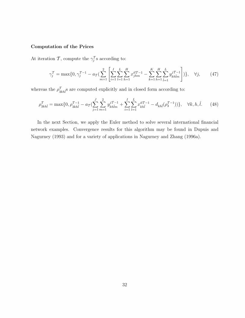
Computation of the Prices

At iteration T , compute the γTj s according to:

γTj = max{0, γT −1

j − aT (2∑

m=1

I∑

i=1

L∑

l=1

H∑

h=1

xilT −1jhm −

K∑

k=1

H∑

h=1

L∑

l=1

yjT −1

khlm

)}, ∀j, (47)

whereas the ρT3khl

s are computed explicitly and in closed form according to:

ρT3khl

= max{0, ρT −1

3khl− aT (

J∑

j=1

2∑

m=1

yjT −1

khlm+

I∑

i=1

L∑

l=1

xilT −1

khl− dkhl(ρ

T −13 ))}, ∀k, h, l. (48)

In the next Section, we apply the Euler method to solve several international financial

network examples. Convergence results for this algorithm may be found in Dupuis and

Nagurney (1993) and for a variety of applications in Nagurney and Zhang (1996a).

32

6. Numerical Examples

In this Section, we apply the Euler method to several international financial network ex-

amples. The Euler method was implemented in FORTRAN and the computer system used

was a Sun system located at the University of Massachusetts at Amherst. For the solution

of the induced network subproblems in the (x1, x2) variables we utilized the exact equili-

bration algorithm (see Dafermos and Sparrow (1969), Nagurney (1999), and the references

therein). The other variables were determined explicitly and in closed form as described in

the preceding section.

The convergence criterion used was that the absolute value of the flows and prices between

two successive iterations differed by no more than 10−4. The sequence {aT } used for all the

examples was: 1, 12, 1

2, 1

3, 1

3, 1

3, . . . in the algorithm.

We assumed in all the examples that the risk functions were of the form (4) and (15), that

is, that risk was represented through variance-covariance matrices for both the source agents

in the countries and for the intermediaries. We initialized the Euler method as follows: We

set xiljh1 = Sil

JHfor each source agent i and country l and for all j and h. All the other

variables were initialized to zero.

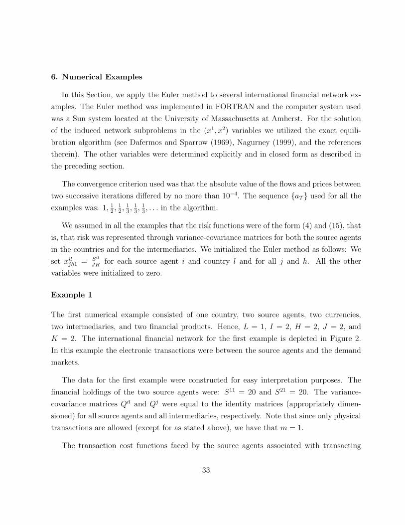
Example 1

The first numerical example consisted of one country, two source agents, two currencies,

two intermediaries, and two financial products. Hence, L = 1, I = 2, H = 2, J = 2, and

K = 2. The international financial network for the first example is depicted in Figure 2.

In this example the electronic transactions were between the source agents and the demand

markets.

The data for the first example were constructed for easy interpretation purposes. The

financial holdings of the two source agents were: S11 = 20 and S21 = 20. The variance-

covariance matrices Qil and Qj were equal to the identity matrices (appropriately dimen-

sioned) for all source agents and all intermediaries, respectively. Note that since only physical

transactions are allowed (except for as stated above), we have that m = 1.

The transaction cost functions faced by the source agents associated with transacting

33

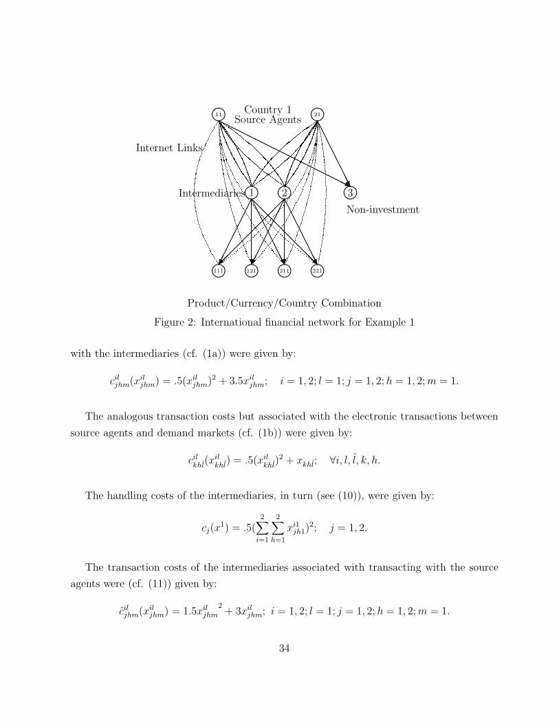
m m m1 2 3

Non-investment

Intermediaries

m m m m111 121 211 221

m m11

Internet Links

21


HHHHHHHHHHHHHHHj

AAAAAAAAU

AAAAAAAAU?

��

��

��

��

��

��

��

��

@@

@@

@@

@@R

AAAAAAAAU?

��

��

��

��

Source AgentsCountry 1

Figure 2: International financial network for Example 1

with the intermediaries (cf. (1a)) were given by:

ciljhm(xil

jhm) = .5(xiljhm)2 + 3.5xil

jhm; i = 1, 2; l = 1; j = 1, 2; h = 1, 2; m = 1.

The analogous transaction costs but associated with the electronic transactions between

source agents and demand markets (cf. (1b)) were given by:

cilkhl

(xilkhl

) = .5(xilkhl

)2 + xkhl; ∀i, l, l, k, h.

The handling costs of the intermediaries, in turn (see (10)), were given by:

cj(x1) = .5(

2∑

i=1

2∑

h=1

xi1jh1)

2; j = 1, 2.

The transaction costs of the intermediaries associated with transacting with the source

agents were (cf. (11)) given by:

ciljhm(xil

jhm) = 1.5xiljhm

2+ 3xil

jhm; i = 1, 2; l = 1; j = 1, 2; h = 1, 2; m = 1.

34

The transaction costs, in turn, associated with the electronic transactions at the demand

markets (from the perspective of the consumers (cf. (20b)) were given by:

cilkhl

(x2) = .1xilkhl

+ 1, ∀i, l, l, k, h.

The demand functions at the demand markets (refer to (3)) were:

d111(ρ3) = −2ρ3111 − 1.5ρ3121 + 1000, d121(ρ3) = −2ρ3121 − 1.5ρ3111 + 1000,

d211(ρ3) = −2ρ3211 − 1.5ρ3221 + 1000, d221(ρ3) = −2ρ3221 − 1.5ρ3211 + 1000.

and the transaction costs between the intermediaries and the consumers at the demand

markets (see (20a)) were given by:

cj

khlm(y) = yj

khlm+ 5; k = 1, 2; h = 1, 2; l = 1; m = 1.

In Example 1 all of the weights associated with the risk functions, that is, the αil and

the βj were set equal to 1 for all i, l, and j. This means that the source agents as well as

the intermediaries weight the criterion of risk minimization equally to that of net revenue

maximization.

The Euler method converged in 1,087 iterations and yielded the following equilibrium

financial flow pattern:

x1∗ := x11∗111 = x11∗

121 = x11∗211 = x11∗

221 = x21111∗ = x22∗

211 = x21∗211 = x21∗

221 = .372;

x2∗ := x11∗111 = x11∗

121 = x11∗211 = x11∗

221 = x21∗111 = x21∗

121 = x21∗211 = x21∗

221 = 4.627;

y∗ := y1∗1111 = y1∗

1211 = y1∗2111 = y1∗

2211 = y2∗1111 = y2∗

1211 = y2∗2111 = y2∗

2211 = .372.

Both source agents allocated the entirety of their funds to the instrument in the two

currencies; thus, there was no non-investment.

The vector γ∗ had components: γ∗1 = γ∗

2 = 276.742, and the computed demand prices at

the demand markets were: ρ∗3111 = ρ∗

3121 = ρ∗3211 = ρ∗

3221 = 282.858.

35

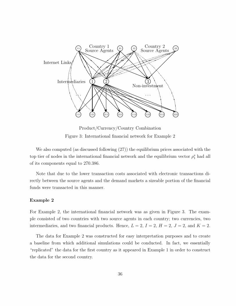
m m m1 2 3Non-investment

Intermediaries

m m m m m m m m111 121 211 221 112 122 212 222


m m m m11

Internet Links

21 12 22

aaaaaaaaaaaaaaaaaaa

@@

@@

@@

@@R

AAAAAAAAU

��

��

��

��

aaaaaaaaaaaaaaaaaaa

HHHHHHHHHHHHHHHj

QQ

QQ

QQ

QQ

QQQs

@@

@@

@@

@@R

AAAAAAAAU?

��

��

��

��

��

��

��

��

PPPPPPPPPPPPPPPPPPPPPPq

aaaaaaaaaaaaaaaaaaa

HHHHHHHHHHHHHHHj

QQ

QQ

QQ

QQ

QQQs

@@

@@

@@

@@R

AAAAAAAAU?

��

��

��

��



· · · · · ·

Figure 3: International financial network for Example 2

We also computed (as discussed following (27)) the equilibrium prices associated with the

top tier of nodes in the international financial network and the equilibrium vector ρ∗1 had all

of its components equal to 270.386.

Note that due to the lower transaction costs associated with electronic transactions di-

rectly between the source agents and the demand markets a sizeable portion of the financial

funds were transacted in this manner.

Example 2

For Example 2, the international financial network was as given in Figure 3. The exam-

ple consisted of two countries with two source agents in each country; two currencies, two

intermediaries, and two financial products. Hence, L = 2, I = 2, H = 2, J = 2, and K = 2.

The data for Example 2 was constructed for easy interpretation purposes and to create

a baseline from which additional simulations could be conducted. In fact, we essentially

“replicated” the data for the first country as it appeared in Example 1 in order to construct

the data for the second country.

36

Specifically, the financial holdings of the source agents were: S11 = 20, S21 = 20, S12 = 20,

and S22 = 20. The variance-covariance matrices Qil and Qj were equal to the identity ma-

trices (appropriately dimensioned) for all source agents in each country and for all interme-

diaries, respectively.

The transaction cost functions faced by the source agents associated with transacting

with the intermediaries were given by:

ciljhm(xil

jhm) = .5(xiljhm)2 + 3.5xil

jhm; i = 1, 2; l = 1, 2; j = 1, 2; h = 1, 2; m = 1.

The handling costs of the intermediaries (since the number of intermediaries is still equal

to two) remained as in Example 1, that is, they were given by:

cj(x1) = .5(

2∑

i=1

2∑

h=1

xi1jh1)

2; j = 1, 2.

The transaction costs of the intermediaries associated with transacting with the source

agents in the two countries were given by:

ciljhm(xil

jhm) = 1.5(xiljhm)2 + 3xil

jhm; i = 1, 2; l = 1, 2; j = 1, 2; h = 1, 2; m = 1.

The demand functions at the demand markets were:

d111(ρ3) = −2ρ3111 − 1.5ρ3121 + 1000, d121(ρ3) = −2ρ3121 − 1.5ρ3111 + 1000,

d211(ρ3) = −2ρ3211 − 1.5ρ3221 + 1000, d221(ρ3) = −2ρ3221 − 1.5ρ3211 + 1000,

d112(ρ3) = −2ρ3112 − 1.5ρ3122 + 1000, d122(ρ3) = −2ρ3122 − 1.5ρ3112 + 1000,

d212(ρ3) = −2ρ3212 − 1.5ρ3222 + 1000, d222(ρ3) = −2ρ3222 − 1.5ρ3212 + 1000,

and the transaction costs between the intermediaries and the consumers at the demand

markets were given by:

cj

khl(y) = yj

khl+ 5; j = 1, 2; k = 1, 2; h = 1, 2; l = 1, 2; m = 1.

The data for the electronic links were as in Example 1 and were replicated for the other

source agents.

37

The variance-covariance matrices were redimensioned and were equal to the identity ma-

trices. The weights associated with the risk functions were set equal to 1 for all the source

agents and intermediaries.

The Euler method converged in 1,826 iterations and yielded the following equilibrium

international financial flow pattern: only the electronic links had positive flows with all

other flows being identically equal to 0.000. In particular, the financial holdings of the

source agents in the different countries were equally allocated via electronic transactions

directly to the demand markets with xil∗khl

= 2.5000 for all i, l, k, h, l.

The vector γ∗ had components: γ∗1 = γ∗

2 = 279.6194, and the computed demand prices

at the demand markets were: ρ∗3khl

= 282.8578, ∀k, h, l. In this example, all the financial

transactions were conducted electronically.

These examples, although stylized, have been presented to show both the model and the

computational procedure. Obviously, different input data and dimensions of the problems

solved will affect the equilibrium financial flow and price patterns. One now has a powerful

tool with which to explore the effects of perturbations to the data as well as the effects of

changes in the number of source agents, countries, currencies, and/or products, as well as

the effects of the introduction of electronic transactions.

Note that the reason the Euler method requires many iterations for convergence is that

it also provides a time discretization of the financial flow and price trajectories.

38

7. Summary and Conclusions

In this paper, we developed a framework for the modeling, analysis, and computation of

solutions to international financial problems with intermediaries with multicriteria decision-

makers in the presence of electronic transactions. We proposed an international financial

network model consisting of three tiers of decision-makers: the source agents, the financial

intermediaries, and the consumers associated with the demand markets for distinct financial

products in distinct currencies and countries. We modeled the behavior of the decision-

makers, with the first two tiers being concerned both with net revenue maximization and

with risk minimization (with appropriate weights assigned to the latter), derived the opti-

mality conditions as well as the governing equilibrium conditions which reflect the (possible)

competition among decision-makers at the same tier of nodes but cooperation between tiers

of nodes. The framework allows for the handling of as many countries, as many source agents

in each country, as many currencies in which the financial products can be obtained, and

as many financial intermediaries, as mandated by the specific application. The formulation

of the equilibrium conditions was shown to be equivalent to a finite-dimensional variational

inequality problem.

We then proposed a dynamic adjustment process which provides the disequilibrium dy-

namics of the international financial flows and prices and formulated it as a projected dy-

namical system. We further demonstrated that the set of stationary points of the projected

dynamical system coincides with the set of solutions of the variational inequality formulation

of the international financial network equilibrium.

We provided a variety of qualitative properties of the equilibrium financial flow and price

pattern, and also established, under reasonable conditions, the stability of the international

financial network.

Finally, we proposed a time-discretization of the continuous time dynamic adjustment

process in the form of an Euler-type method which allows for closed form expressions of the

prices and certain financial flows at each time period. The Euler method was then applied

to solve international financial network examples.

This framework generalizes the recent work of Nagurney and Ke (2003) to the interna-

39

tional arena and that of Nagurney and Cruz (2002) to include dynamics and multicriteria

decision-making.

Acknowledgments

This research was supported, in part, by NSF Grant No.: IIS-0002647 and, in part, by an

AT&T Industrial Ecology Fellowship. This support is gratefully acknowledged.

The authors are indebted to the anonymous reviewers for their assistance.

References

Allen, H., Hawkins, J. and Sato, S. (2001), “Electronic Trading and its Implications for

Financial Systems,” Bank of International Settlements Papers No. 7, November, Bern,

Switzerland.

Banks, E. (2001), E-Finance: The Electronic Revolution, John Wiley & Sons, New York.

Bazaraa, M. S., Sherali, H. D. and Shetty, C. M. (1993), Nonlinear Programming: Theory

and Algorithms, John Wiley & Sons, New York.

Bertsekas, D. P. and Tsitsiklis, J. N. (1989), Parallel and Distributed Computation - Numer-

ical Methods, Prentice Hall, Englewood Cliffs, New Jersey.

Chankong, V. and Haimes, Y. Y. (1983), Multiobjective Decision Making: Theory and

Methodology , North-Holland, New York.

Claessens, S., Glaessner, T. and Klingebiel, D. (2000), “Electronic Finance: Reshaping the

Financial Landscape Around the World,” Financial Sector Discussion Paper No. 4, The

World Bank, Washington, DC.

Claessens, S., Glaessner, T. and Klingebiel, D. (2001), “E-Finance in Emerging Markets:

Is Leapfrogging Possible?” Financial Sector Discussion Paper No. 7, The World Bank,

Washington, DC.

Claessens, S., Dobos, G., Klingebiel, D. and Laeven, L. (2003), “The Growing Importance

40

of Networks in Finance and Their Effects on Competition,” in Innovations in Financial and

Economic Networks, A. Nagurney, editor, Edward Elgar Publishers, Cheltenham, England,

in press.

Dafermos, S. and Nagurney, A. (1987), “Oligopolistic and Competitive Behavior of Spatially

Separated Markets,” Regional Science and Urban Economics 17, 245-254.

Dafermos, S. and Sparrow, F. T. (1969), “The Traffic Assignment Problem for a General

Network,” Journal of Research of the National Bureau of Standards 73B, 91-118.

Dong, J., Zhang, D. and Nagurney, A. (1996), “A Projected Dynamical Systems Model of

General Financial Equilibrium with Stability Analysis,” Mathematical and Computer Mod-

elling 24, 35-44.

Dupuis, P. and Nagurney, A. (1993), “Dynamical Systmes and Variational Inequalities,”

Annals of Operations Research 44, 9-42.

Economides, N. (2001), “The Impact of the Internet on Financial Markets,” Journal of

Financial Transformation 1, 8-13.

Fan, M., Staellert, J. and Whinston, A. B. (2000), “The Internet and the Future of Financial

Markets,” Communications of the ACM 43, 83-88.

Fishburn, P. C. (1970), Utility Theory for Decision Making , John Wiley & Sons, New York.

Gabay, D. and Moulin, H. (1980), “On the Uniqueness and Stability of Nash Equilibria in

Noncooperative Games,” in Applied Stochastic Control of Econometrics and Management

Science, pp. 271-294, A. Bensoussan, P. Kleindorfer, and C. S. Tapiero, editors, North-

Holland, Amsterdam, The Netherlands.

Keeney, R. L. and Raiffa, H. (1993), Decisions with Multiple Objectives: Preferences and

Value Tradeoffs, Cambridge University Press, Cambridge, England.

Kinderlehrer, D. and Stampacchia, G. (1980), An Introduction to Variational Inequalities

and Their Application, Academic Press, New York.

41

Markowitz, H. M. (1952), “Portfolio Selection,” The Jounral of Finance 7, 77-91.

Markowitz, H. M. (1959), Portfolio Selection: Efficient Diversification of Investments, John

Wiley & Sons, Inc., New York.

McAndrews, J. and Stefanidis, C. (2000), “The Emergence of Electronic Communications

Networks in US Equity Markets,” Current Issues in Economics and Finance 6, 1-6, Federal

Reserve Bank of New York.

Nagurney, A. (1999), Network Economics: A Variational Inequality Approach, second and

revised edition, Kluwer Academic Publishers, Dordrecht, The Netherlands.

Nagurney, A. and Cruz, J. (2002), “International Financial Networks with Intermediation:

Modeling, Analysis, and Computations,” to appear in Computational Management Science.

Nagurney, A. and Cruz, J. (2003), “International Financial Networks with Electronic Trans-

actions,” in Innovations in Financial and Economic Networks, A. Nagurney, editor, Edward

Elgar Publishers, Cheltenham, England, pp. 135-167.

Nagurney, A., Cruz, J. and Matsypura, D. (2003), “Dynamics of Global Supply Chain Su-

pernetworks,” Mathematical and Computer Modelling 37, 963-983.

Nagurney, A. and Dong, J. (2002), Supernetworks: Decision-Making for the Information

Age, Edward Elgar Publishers, Cheltenham, England.

Nagurney, A., Dupuis, P. and Zhang, D. (1994), “A Dynamical Systems Approach for Net-

work Oligopolies and Varuational Inequalities,” Annals of Regional Science 28, 263-293.

Nagurney, A. and Ke, K. (2001), “Financial Networks with Intermediation,” Quantitative

Finance 1, 441-451.

Nagurney, A. and Ke, K. (2003), “Financial Networks with Electronic Transactions: Mod-

eling, Analysis, and Computations,” Quantitative Finance 3, 71-87.

Nagurney, A. and Siokos, S. (1997), Financial Networks: Statics and Dynamics, Springer-

Verlag, Heidelberg, Germany.

42

Nagurney, A. and Zhang, D. (1996a) Projected Dynamical Systems and Variational Inequal-

ities with Applications, Kluwer Academic Publishers, Dordrecht, The Netherlands.

Nagurney, A., and Zhang, D. (1996b), “Stability of Spatial Price Equilibrium Modeled as a

Projected Dynamical System,” Journal of Economic Dynamics and Control 20, 43-63.

Nagurney, A. and Zhang, D. (1997), “Formulation, Stability, and Computation of Traffic

Network Equilibria as Projected Dynamical Systems,” Journal of Optimization Theory and

its Applications 93, 417-444.

Nagurney, A. and Zhao, L. (1993), “Networks and Variational Inequalities in the Formu-

lation and Computation of Market Disequilibria: The Case of Direct Demand Functions,”

Transportation Science 27, 4-15.

Nash, J. F. (1950), “Equilibrium Points in N-Person Games,” in Proceedings of the National

Academy of Sciences, USA 36, 48-49.

Nash, J. F. (1951), “Noncooperative Games,” Annals of Mathematics 54, 286-298.

Sato, S. and Hawkins, J. (2001), “Electronic Finance: An Overview of the Issues,” Bank of

International Settlements Paper No. 7, November, Bern, Switzerland.

Thore, S. (1980), Programming the Network of Financial Intermediation, Universitetsforslaget,

Oslo, Norway.

Yu, P. L. (1985), Multiple-Criteria Decision-Making – Concepts, Techniques, and Extensions,

Plenum Press, New York.

Zhang, D. and Nagurney, A. (1995), “On the Stability of Projected Dynamical Systems,”

Journal of Optimization Theory and its Applications 85, 97-124.

43

Documents

Dynamics of International Financial Networks with Risk