Dynamics of laser ablation at the early stage during and ...laser.itp.ac.ru/publications/JPCS_774_1_012101.pdfDynamicsoflaserablationat theearly stageduring andafter ultrashortpulse

This content has been downloaded from IOPscience. Please scroll down to see the full text.

Download details:

IP Address: 95.28.0.115

This content was downloaded on 28/11/2016 at 09:13

Please note that terms and conditions apply.

You may also be interested in:

Adiabatic approximations for electrons interacting with ultrashort high-frequency laser pulses

Koudai Toyota, Ulf Saalmann and Jan M Rost

Blistering of film from substrate after action of ultrashort laser pulse

N A Inogamov, V V Zhakhovsky, V A Khokhlov et al.

Simulation of femtosecond pulsed laser ablation of metals

R V Davydov and V I Antonov

Photoionization of Rydberg States by Ultrashort Wavelet Pulses

S Yu Svita and V A Astapenko

Optical emission spectroscopy of plasma produced by laser ablation of iron sulfide

S Karatodorov, V Mihailov, T Kenek et al.

Fabrication of a microlens array in BK7 through laser ablation and thermal treatment techniques

M Blanco, D Nieto and M T Flores-Arias

Double ionization of molecule H2 in intense ultrashort laser fields

Thu-Thuy Le and Ngoc-Ty Nguyen

Dynamics of laser ablation at the early stage during and after ultrashort pulse

View the table of contents for this issue, or go to the journal homepage for more

2016 J. Phys.: Conf. Ser. 774 012101

(http://iopscience.iop.org/1742-6596/774/1/012101)

Home Search Collections Journals About Contact us My IOPscience

http://iopscience.iop.org/page/terms

http://iopscience.iop.org/article/10.1088/1742-6596/635/9/092116







http://iopscience.iop.org/1742-6596/774/1

http://iopscience.iop.org/1742-6596

http://iopscience.iop.org/

http://iopscience.iop.org/search

http://iopscience.iop.org/collections

http://iopscience.iop.org/journals

http://iopscience.iop.org/page/aboutioppublishing

http://iopscience.iop.org/contact

http://iopscience.iop.org/myiopscience

Dynamics of laser ablation at the early stage during

and after ultrashort pulse

D K Ilnitsky1,2, V A Khokhlov2, V V Zhakhovsky1,2, Yu V Petrov2,

K P Migdal1,2 and N A Inogamov1,2

1 Dukhov Research Institute of Automatics (VNIIA), Sushchevskaya 22, Moscow 127055,Russia2 Landau Institute for Theoretical Physics of the Russian Academy of Scienses, AkademikaSemenova 1a, Chernogolovka, Moscow Region 142432, Russia

E-mail: [email protected]

Abstract. Study of material flow in two-temperature states is needed for a fundamentalunderstanding the physics of femtosecond laser ablation. To explore phenomena at a very earlystage of laser action on a metallic target our in-house two-temperature hydrodynamics code isused here. The early stage covers duration of laser pulse with next first few picoseconds. Wedraw attention to the difference in behavior at this stage between the cases: (i) of an ultrathinfilm (thickness of order of skin depth dskin or less), (ii) thin films (thickness of a film is 4–7 ofdskin for gold), and (iii) bulk targets (more than 10dskin for gold). We demonstrate that thesedifferences follow from a competition among conductive cooling of laser excited electrons in askin layer, electron-ion coupling, and hydrodynamics of unloading caused by excess of pressureof excited free electrons. Conductive cooling of the skin needs a heat sink, which is performedby the cold material outside the skin. Such sink is unavailable in the ultrathin films.

1. Introduction

Studies of femtosecond laser ablation are important because, first, these lasers are relativelycheap and now are wide spread, and, second, there are many scientific and industrial applicationswhere they are used. There are a number of important studies devoted to this theme. Thesepapers treat or self-reflection at rather high intensities [1–3], or reflection of a probe pulse inpump-probe experiments [3–5], or consider hydrodynamics of shock waves generated by a laserpulse [6–9], or study thermomechanical ablation [10,11]. For bulk targets, this type of ablationstarts late in time, definitely later than the few first picoseconds. Thermomechanical ablationbegins from nucleation of voids at significant depth ∼ dT under a vacuum boundary. This factrelates to the case of a bulk target when thickness of a target df is large df ≫ dT . The scale dTis thickness of a heat affected zone. It is created during the two-temperature (2T) stage whenelectron heat conduction has enhanced values [12]. There is supersonic expansion of heat froma skin layer to the bulk of a target at the 2T stage. The rate of expansion of heat inside metal isdefined by electron Fermi velocities. Acoustic time scale ts = dT /cs gives duration of the timeinterval between arrival of a pump pulse and nucleation.

Below we consider a gold film on a glass substrate. Thickness of a film analyzed in our paperis df = 100 nm. Thickness of a heat affected zone in bulk gold is dT = 150 − 200 nm [13]. Our

XXXI International Conference on Equations of State for Matter (ELBRUS2016) IOP PublishingJournal of Physics: Conference Series 774 (2016) 012101 doi:10.1088/1742-6596/774/1/012101

Content from this work may be used under the terms of the Creative Commons Attribution 3.0 licence. Any further distributionof this work must maintain attribution to the author(s) and the title of the work, journal citation and DOI.

Published under licence by IOP Publishing Ltd 1

film is thinner df < dT than thickness of a heat affected zone. Thus, a film is heated fast and athermal energy distribution is approximately homogeneous across a film.

Thermomechanical ablation of a homogeneously heated freestanding film is studied well[10, 14, 15]. Slightly above the ablation threshold the film disrupts in its middle plane to twohalves. The case with a thin gold film df < dT on a glass substrate has been considered inpapers [16, 17]. This case is important for our work. It was shown [16, 17], that the situationwith a gold film on a glass is similar to the case of a freestanding film, because acoustic impedanceof glass is 6-7 times smaller than acoustic impedance of gold. Presence of glass does situationwith a homogeneously heated film slightly asymmetric relative to the middle plane of a film.

Let us say few words about thermomechanical ablation. Unloading into vacuum of aninfinitely large homogeneously pressurized semi-space proceeds with limited velocities, flow isself-similar, and there is a fan of the straight characteristics outgoing from the spatiotemporalpoint x = 0, t = 0; here we neglect very small duration of a pump pulse, thus the instant t = 0corresponds to arrival of a pump to a surface. The flow with a fan is called a centered rarefactionwave. This is a solution of equations of hydrodynamics corresponding to the decay of jump ofparameters (e.g., pressure) between two homogeneous semi-spaces. In this flow the decelerationsof material particles and tensile stresses are absent: there are only accelerations of Lagrangianparticles up to limiting velocity. The particles achieved this velocity form a plateau [18, 19].Pressure at plateau equals to pressure of vacuum.

But if the pressurized region is limited in its thickness then deceleration and tensile stressappear. The spatial limitation of a pressurized layer is in a form of finite depth dT of a heataffected and therefore pressurized surface layer of a semi-space or in a form of a thin film df < dT .Some interval of time after excitation by a pump is necessary to achieve a maximum absolutevalue of a tensile stress. This temporal interval is ∼ dT /c for a bulk target and ∼ df/c for athin film; here c is speed of sound. At the thermomechanical ablation threshold, the maximumtensile stress overcomes the material strength, thus nucleation begins. Merging of nuclei causesspallation [10,11,20] called thermomechanical ablation inside laser community.

Depth where the nucleation starts is of the order of dT or df for bulk and film targetsrespectively. This depth defines thickness of a spallation plate. Near ablation threshold thisthickness is 70–100 nm for a bulk gold [21] and 40–50 nm for a 100 nm film [17]. Below we showthat a much thinner spallation plate also exists.

This is the main idea of the paper. In the classical picture of thermomechanical ablationthe spallation follows from a spatial inhomogeneity dT or df of a pressurized layer. Contrary tothis particular spatial source of spallation, the temporal factor causes ablation in our new, “non-classical” way to spallation. This second type, “non-classical” electron pressure driven, timedependent ablation is thermomechanical one, as the first type is. It appears thanks to forceaction of electron pressure increased as a result of heating of electrons [22, 23]. The dynamiceffect of electron pressure sharply, during the ultrashort pulse, accelerates the vacuum boundaryto finite expansion velocity.

Ablation thresholds for the first and the second type break off are different. It is plausiblethat the second one is lower. Two ablation thresholds corresponding to early and late timeablations were described in papers [24–26]. These works are based on molecular dynamics (MD)simulation combined with the two-temperature (2T) model which includes not only 2T thermalterms (as in [11]) but also dynamic influence of the excited electrons. The two 2T thermal termsare connected with electron heat conduction and with electron-ion energy exchange, while thedynamic influence according to [24–26] has two factors.

One of these factors is the change of pressure as a result of excitation of electrons at fixedvolume. The second factor is the additional change of pressure due to pressure of free electrons.A bulk target has been considered in papers [24–26]. Below we will concentrate on the secondtype break off for the 100 nm film. It takes place rather early in time, therefore the mechanical


2

conditions at the opposite side of a film (the rear-side boundary) are not significant (are glass orvacuum placed there); the frontal and the rear-side boundaries do not have time to communicatethrough sound (but they communicate through supersonic 2T electron thermal heat transferusually called ballistic transport). The sense of the second type is connected with fast dropdown of electron internal energy in a skin-layer. This drop is possible thanks to powerfulelectron conduction if there is a cold volume contacting with a skin. The electron subsystem ofcold volume plays a role of a bulk cooler accepting energy flowing from a skin. Thermal energyflows very fast (faster than speed of sound [12]) along electron subsystem during 2T stage.Therefore the thermal contact between a film thinner than dT and support becomes importantif the support is made from highly conductive material, e.g., crystalline silicon. In our case thesupporting substrate is a glass. It is weakly heat conducting. Thus we put the condition ofthermal insulation at the rear-side.

The paper is constructed as the following sequence of the connected parts. First of all insection 2 “Thermal fluxes” we pay attention to the interplay of thermal powers and fluxes duringthe first picoseconds. After that in section 3 “Two-temperature flow” we consider particular 2T-HD simulations to understand the electron fluxes and the electron temperature dependencieson space and time near the vacuum surface. We are interested to consider a layer which will becovered by a hydrodynamic rarefaction wave during the first picoseconds.

There is significant deceleration of the vacuum boundary during the first picoseconds forthe weak electron-ion energy exchange rates. The deceleration is caused by the conductioncooling of electron subsystem of a skin layer and the corresponding drop of electron pressuresupporting expansion. The deceleration appears under action of negative total pressure insidethe rarefaction wave. Stretching of matter results in break off above the certain limit ofabsolute value of negative pressure. Dynamics of expansion in the spatially isothermal electrontemperature surrounding with decreasing in time electron temperature Te(t) is considered insections 4 “Second type break off” and 5 “Conductive decrease of pressure and appearance oftensile stress”.

Problem concerning strength of two-temperature (2T) matter is considered in sections 6“Two-temperature nucleation in stretched metal” and 7 “Two-temperature strength of gold”.Finally comparing the strength versus values of negative pressures we conclude that spalling ofextremely thin 7–10 nm spallation plate is possible.

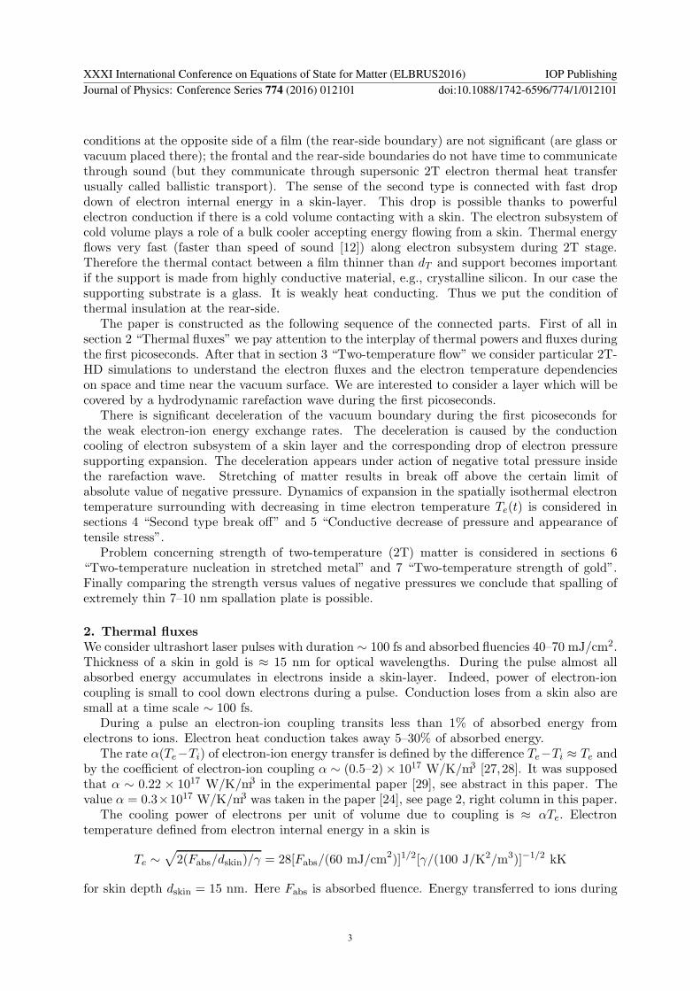
2. Thermal fluxes

We consider ultrashort laser pulses with duration ∼ 100 fs and absorbed fluencies 40–70 mJ/cm2.Thickness of a skin in gold is ≈ 15 nm for optical wavelengths. During the pulse almost allabsorbed energy accumulates in electrons inside a skin-layer. Indeed, power of electron-ioncoupling is small to cool down electrons during a pulse. Conduction loses from a skin also aresmall at a time scale ∼ 100 fs.

During a pulse an electron-ion coupling transits less than 1% of absorbed energy fromelectrons to ions. Electron heat conduction takes away 5–30% of absorbed energy.

The rate α(Te−Ti) of electron-ion energy transfer is defined by the difference Te−Ti ≈ Te andby the coefficient of electron-ion coupling α ∼ (0.5–2)× 1017 W/K/m3 [27,28]. It was supposedthat α ∼ 0.22 × 1017 W/K/m3 in the experimental paper [29], see abstract in this paper. Thevalue α = 0.3×1017 W/K/m3 was taken in the paper [24], see page 2, right column in this paper.

The cooling power of electrons per unit of volume due to coupling is ≈ αTe. Electrontemperature defined from electron internal energy in a skin is

Te ∼√

2(Fabs/dskin)/γ = 28[Fabs/(60 mJ/cm2)]1/2[γ/(100 J/K2/m3)]−1/2 kK

for skin depth dskin = 15 nm. Here Fabs is absorbed fluence. Energy transferred to ions during


3

0 40 80distance from initial vacuum boundary (nm)

0

4

8

elec

tron

the

rmal

flu

x (G

W/c

m2 )

t = 0.1 ps

t = 1 ps

t = 2 ps

t = 3 ps

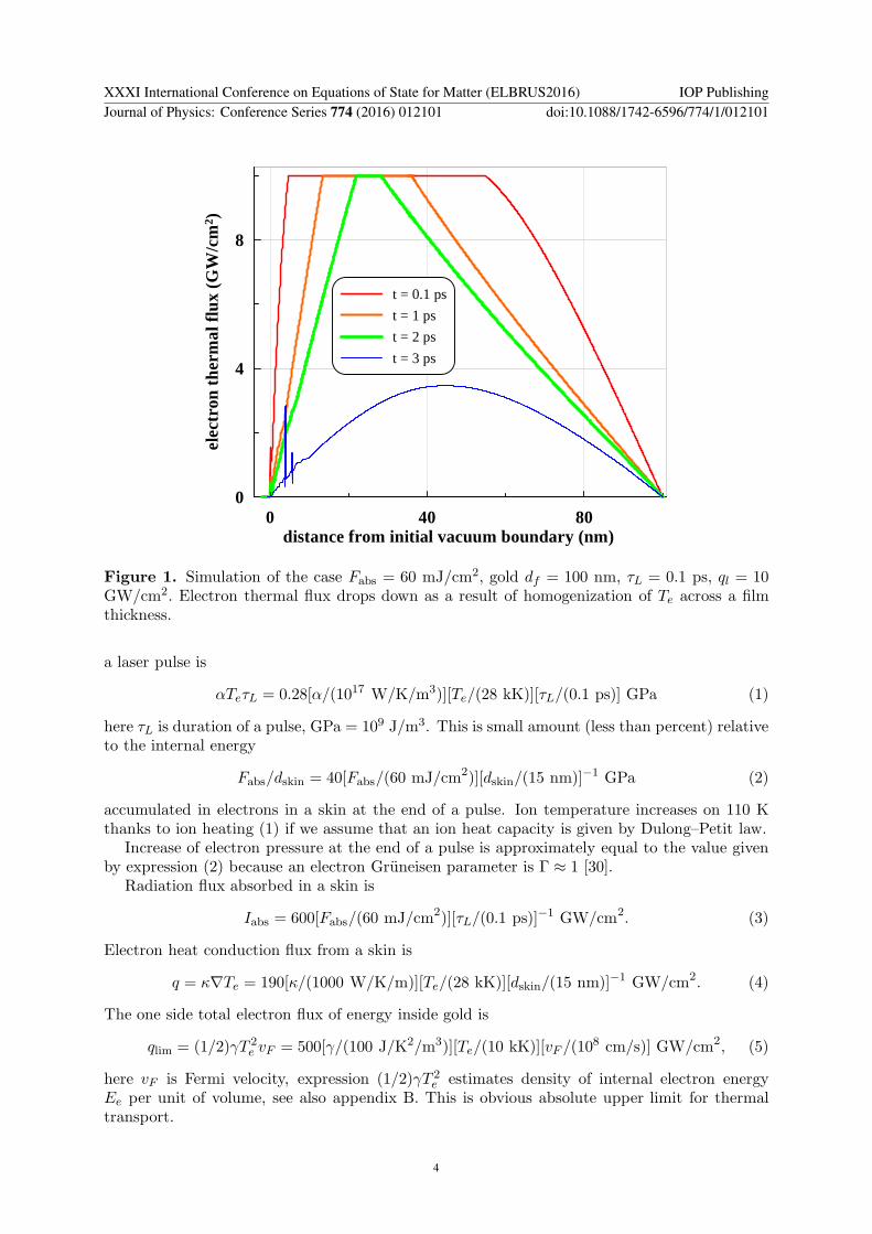
Figure 1. Simulation of the case Fabs = 60 mJ/cm2, gold df = 100 nm, τL = 0.1 ps, ql = 10GW/cm2. Electron thermal flux drops down as a result of homogenization of Te across a filmthickness.

a laser pulse is

αTeτL = 0.28[α/(1017 W/K/m3)][Te/(28 kK)][τL/(0.1 ps)] GPa (1)

here τL is duration of a pulse, GPa = 109 J/m3. This is small amount (less than percent) relativeto the internal energy

Fabs/dskin = 40[Fabs/(60 mJ/cm2)][dskin/(15 nm)]−1 GPa (2)

accumulated in electrons in a skin at the end of a pulse. Ion temperature increases on 110 Kthanks to ion heating (1) if we assume that an ion heat capacity is given by Dulong–Petit law.

Increase of electron pressure at the end of a pulse is approximately equal to the value givenby expression (2) because an electron Gruneisen parameter is Γ ≈ 1 [30].

Radiation flux absorbed in a skin is

Iabs = 600[Fabs/(60 mJ/cm2)][τL/(0.1 ps)]−1 GW/cm2. (3)

Electron heat conduction flux from a skin is

q = κ∇Te = 190[κ/(1000 W/K/m)][Te/(28 kK)][dskin/(15 nm)]−1 GW/cm2. (4)

The one side total electron flux of energy inside gold is

qlim = (1/2)γT 2e vF = 500[γ/(100 J/K2/m3)][Te/(10 kK)][vF /(10

8 cm/s)] GW/cm2, (5)

here vF is Fermi velocity, expression (1/2)γT 2e estimates density of internal electron energy

Ee per unit of volume, see also appendix B. This is obvious absolute upper limit for thermaltransport.


4

0 200 400distance from initial boundary (nm)

0

20

40

60el

ectr

on h

eat

flux

(G

W/c

m2 )

Influence of flux limitt = 0.1 ps

ql = 10 GW/cm2, Fabs = 60 mJ/cm2,

df = 100 nm, Kα = 6, τL = 0.1 ps

unlimited q, Fabs = 100 mJ/cm2,

bulk target, Kα = 4, τL = 0.1 ps

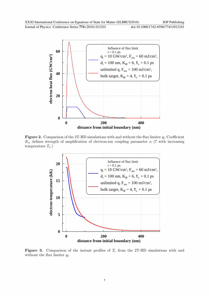
Figure 2. Comparison of the 2T-HD simulations with and without the flux limiter ql. CoefficientKα defines strength of amplification of electron-ion coupling parameter α (7 with increasingtemperature Te.)


0

5

10

15

20

elec

tron

tem

pera

ture

(kK

)

Influence of flux limitt = 0.1 ps

ql = 10 GW/cm2, Fabs = 60 mJ/cm2,

df = 100 nm, Kα = 6, τL = 0.1 ps

unlimited q, Fabs = 100 mJ/cm2,

bulk target, Kα = 4, τL = 0.1 ps

Figure 3. Comparison of the instant profiles of Te from the 2T-HD simulations with andwithout the flux limiter ql.


5

0 50 100 150 200distance from initial boundary (nm)

0

5

10

15

20

elec

tron

hea

t fl

ux (

GW

/cm

2 )

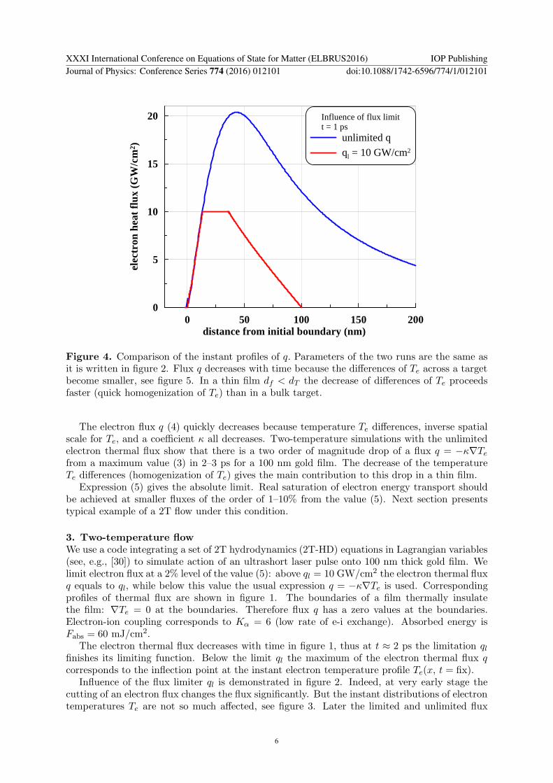
Influence of flux limitt = 1 ps

unlimited q

ql = 10 GW/cm2

Figure 4. Comparison of the instant profiles of q. Parameters of the two runs are the same asit is written in figure 2. Flux q decreases with time because the differences of Te across a targetbecome smaller, see figure 5. In a thin film df < dT the decrease of differences of Te proceedsfaster (quick homogenization of Te) than in a bulk target.

The electron flux q (4) quickly decreases because temperature Te differences, inverse spatialscale for Te, and a coefficient κ all decreases. Two-temperature simulations with the unlimitedelectron thermal flux show that there is a two order of magnitude drop of a flux q = −κ∇Te

from a maximum value (3) in 2–3 ps for a 100 nm gold film. The decrease of the temperatureTe differences (homogenization of Te) gives the main contribution to this drop in a thin film.

Expression (5) gives the absolute limit. Real saturation of electron energy transport shouldbe achieved at smaller fluxes of the order of 1–10% from the value (5). Next section presentstypical example of a 2T flow under this condition.

3. Two-temperature flow

We use a code integrating a set of 2T hydrodynamics (2T-HD) equations in Lagrangian variables(see, e.g., [30]) to simulate action of an ultrashort laser pulse onto 100 nm thick gold film. Welimit electron flux at a 2% level of the value (5): above ql = 10 GW/cm2 the electron thermal fluxq equals to ql, while below this value the usual expression q = −κ∇Te is used. Correspondingprofiles of thermal flux are shown in figure 1. The boundaries of a film thermally insulatethe film: ∇Te = 0 at the boundaries. Therefore flux q has a zero values at the boundaries.Electron-ion coupling corresponds to Kα = 6 (low rate of e-i exchange). Absorbed energy isFabs = 60 mJ/cm2.

The electron thermal flux decreases with time in figure 1, thus at t ≈ 2 ps the limitation qlfinishes its limiting function. Below the limit ql the maximum of the electron thermal flux qcorresponds to the inflection point at the instant electron temperature profile Te(x, t = fix).

Influence of the flux limiter ql is demonstrated in figure 2. Indeed, at very early stage thecutting of an electron flux changes the flux significantly. But the instant distributions of electrontemperatures Te are not so much affected, see figure 3. Later the limited and unlimited flux


6


0

2

4

6

8

elec

tron

hea

t fl

ux (

GW

/cm

2 )


unlimited q

ql = 10 GW/cm2

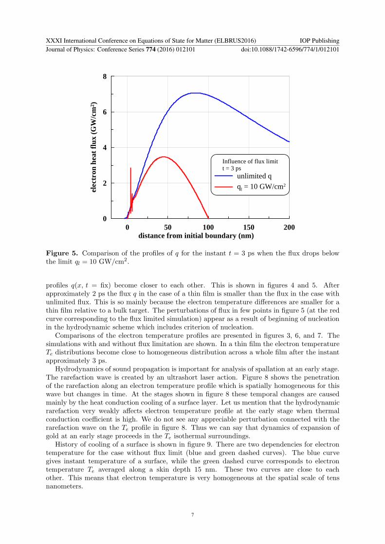
Figure 5. Comparison of the profiles of q for the instant t = 3 ps when the flux drops belowthe limit ql = 10 GW/cm2.

profiles q(x, t = fix) become closer to each other. This is shown in figures 4 and 5. Afterapproximately 2 ps the flux q in the case of a thin film is smaller than the flux in the case withunlimited flux. This is so mainly because the electron temperature differences are smaller for athin film relative to a bulk target. The perturbations of flux in few points in figure 5 (at the redcurve corresponding to the flux limited simulation) appear as a result of beginning of nucleationin the hydrodynamic scheme which includes criterion of nucleation.

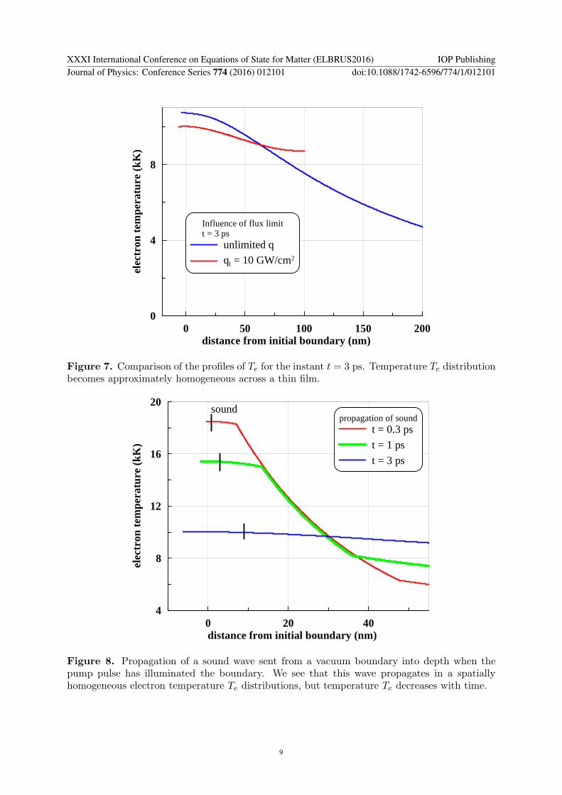
Comparisons of the electron temperature profiles are presented in figures 3, 6, and 7. Thesimulations with and without flux limitation are shown. In a thin film the electron temperatureTe distributions become close to homogeneous distribution across a whole film after the instantapproximately 3 ps.

Hydrodynamics of sound propagation is important for analysis of spallation at an early stage.The rarefaction wave is created by an ultrashort laser action. Figure 8 shows the penetrationof the rarefaction along an electron temperature profile which is spatially homogeneous for thiswave but changes in time. At the stages shown in figure 8 these temporal changes are causedmainly by the heat conduction cooling of a surface layer. Let us mention that the hydrodynamicrarefaction very weakly affects electron temperature profile at the early stage when thermalconduction coefficient is high. We do not see any appreciable perturbation connected with therarefaction wave on the Te profile in figure 8. Thus we can say that dynamics of expansion ofgold at an early stage proceeds in the Te isothermal surroundings.

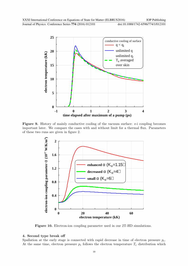
History of cooling of a surface is shown in figure 9. There are two dependencies for electrontemperature for the case without flux limit (blue and green dashed curves). The blue curvegives instant temperature of a surface, while the green dashed curve corresponds to electrontemperature Te averaged along a skin depth 15 nm. These two curves are close to eachother. This means that electron temperature is very homogeneous at the spatial scale of tensnanometers.


7


0

4

8

12

16

elec

tron

tem

pera

ture

(kK

)Influence of flux limitt = 1 ps

unlimited q

ql = 10 GW/cm2

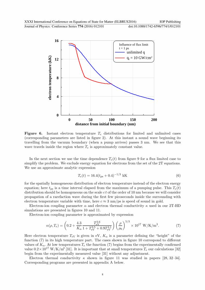
Figure 6. Instant electron temperature Te distributions for limited and unlimited cases(corresponding parameters are listed in figure 2). At this instant a sound wave beginning itstravelling from the vacuum boundary (when a pump arrives) passes 3 nm. We see that thiswave travels inside the region where Te is approximately constant value.

In the next section we use the time dependence Te(t) from figure 9 for a flux limited case tosimplify the problem. We exclude energy equation for electrons from the set of the 2T equations.We use an approximate analytic expression

Te(t) = 16.4(tps + 0.4)−1/3 kK (6)

for the spatially homogeneous distribution of electron temperature instead of the electron energyequation; here tps is a time interval elapsed from the maximum of a pumping pulse. This Te(t)distribution should be homogeneous on the scale c t of the order of 10 nm because we will considerpropagation of a rarefaction wave during the first few picoseconds inside the surrounding withelectron temperature variable with time, here c ≈ 3 nm/ps is speed of sound in gold.

Electron-ion coupling parameter α and electron thermal conductivity κ used in our 2T-HDsimulations are presented in figures 10 and 11.

Electron-ion coupling parameter is approximated by expression

α(ρ, Te) =

(

0.2 +4.3

Kα

T 3.6eV

1 + T 3.5eV + 0.9T 4.1

eV

)(

ρ

ρ0

)5/3

× 1017 W/K/m3. (7)

Here electron temperature TeV is given in eV, Kα is a parameter defining the “height” of thefunction (7) in its high temperature part. The cases shown in figure 10 correspond to differentvalues of Kα. At low temperatures Te the function (7) begins from the experimentally confirmedvalue 0.2×1017 W/K/m3 [31]. It is important that at small temperatures Te our calculations [32]begin from the experimentally measured value [31] without any adjustment.

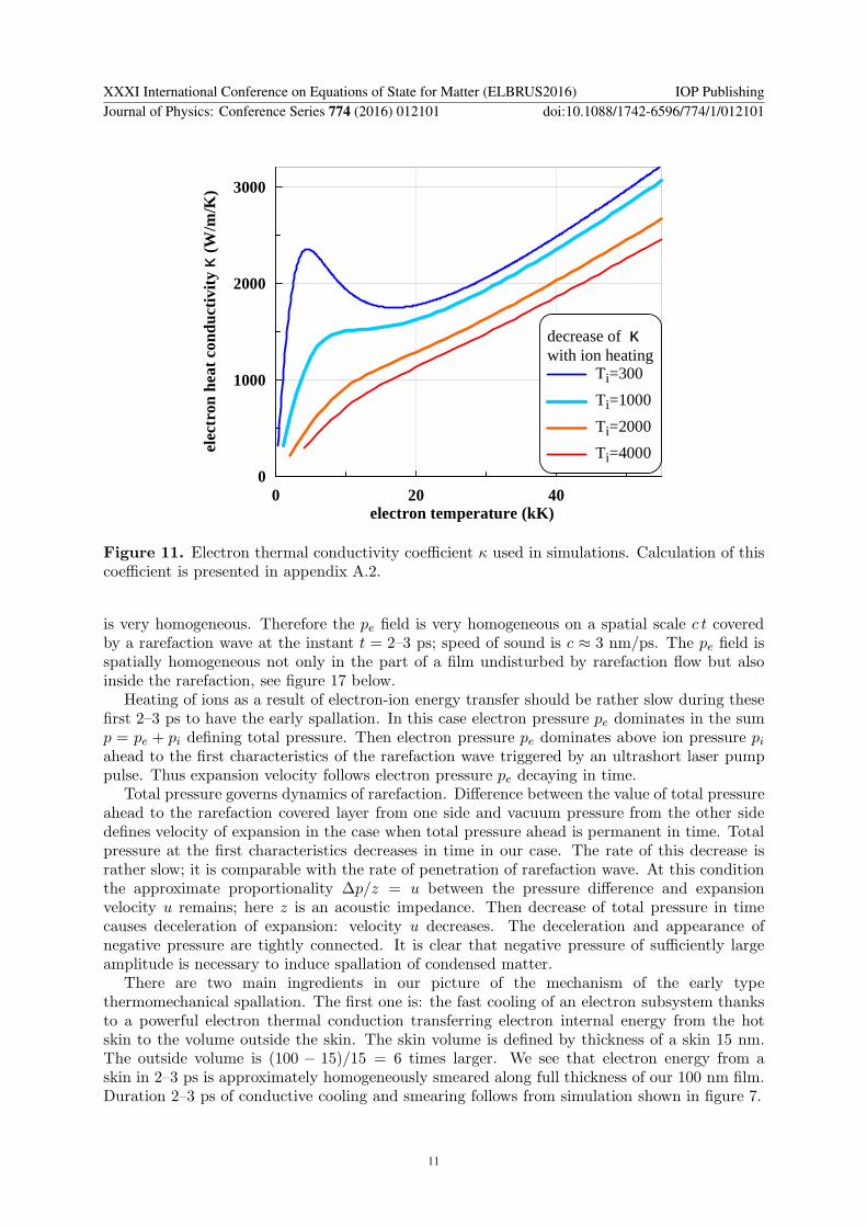
Electron thermal conductivity κ shown in figure 11 was studied in papers [28, 32–34].Corresponding programs are presented in appendix A below.


8


0

4

8

elec

tron

tem

pera

ture

(kK

)


unlimited q

ql = 10 GW/cm2

Figure 7. Comparison of the profiles of Te for the instant t = 3 ps. Temperature Te distributionbecomes approximately homogeneous across a thin film.


4

8

12

16

20

elec

tron

tem

pera

ture

(kK

)

propagation of soundt = 0.3 ps

t = 1 ps

t = 3 ps

sound

Figure 8. Propagation of a sound wave sent from a vacuum boundary into depth when thepump pulse has illuminated the boundary. We see that this wave propagates in a spatiallyhomogeneous electron temperature Te distributions, but temperature Te decreases with time.


9

-1 0 1 2 3 4time elapsed after maximum of a pump (ps)

0

5

10

15

20

25

elec

tron

tem

pera

ture

(kK

)conductive cooling of surface

q < ql

unlimited q

unlimited q,Te averagedover skin

Figure 9. History of mainly conductive cooling of the vacuum surface: e-i coupling becomesimportant later. We compare the cases with and without limit for a thermal flux. Parametersof these two runs are given in figure 2.

0 20 40 60electron temperature (kK)

0

0.4

0.8

1.2

1.6

2

elec

tron

-ion

cou

plin

g pa

ram

eter

α (

1017

W/K

/m3 )

enhanced α (Κα=1.15)

decreased α (Κα=4)

small α (Κα=6)

Figure 10. Electron-ion coupling parameter used in our 2T-HD simulations.

4. Second type break off

Spallation at the early stage is connected with rapid decrease in time of electron pressure pe.At the same time, electron pressure pe follows the electron temperature Te distribution which


10

0 20 40electron temperature (kK)

0

1000

2000

3000el

ectr

on h

eat

cond

ucti

vity

κ (

W/m

/K)

decrease of κwith ion heating

Ti=300

Ti=1000

Ti=2000

Ti=4000

Figure 11. Electron thermal conductivity coefficient κ used in simulations. Calculation of thiscoefficient is presented in appendix A.2.

is very homogeneous. Therefore the pe field is very homogeneous on a spatial scale c t coveredby a rarefaction wave at the instant t = 2–3 ps; speed of sound is c ≈ 3 nm/ps. The pe field isspatially homogeneous not only in the part of a film undisturbed by rarefaction flow but alsoinside the rarefaction, see figure 17 below.

Heating of ions as a result of electron-ion energy transfer should be rather slow during thesefirst 2–3 ps to have the early spallation. In this case electron pressure pe dominates in the sump = pe + pi defining total pressure. Then electron pressure pe dominates above ion pressure piahead to the first characteristics of the rarefaction wave triggered by an ultrashort laser pumppulse. Thus expansion velocity follows electron pressure pe decaying in time.

Total pressure governs dynamics of rarefaction. Difference between the value of total pressureahead to the rarefaction covered layer from one side and vacuum pressure from the other sidedefines velocity of expansion in the case when total pressure ahead is permanent in time. Totalpressure at the first characteristics decreases in time in our case. The rate of this decrease israther slow; it is comparable with the rate of penetration of rarefaction wave. At this conditionthe approximate proportionality ∆p/z = u between the pressure difference and expansionvelocity u remains; here z is an acoustic impedance. Then decrease of total pressure in timecauses deceleration of expansion: velocity u decreases. The deceleration and appearance ofnegative pressure are tightly connected. It is clear that negative pressure of sufficiently largeamplitude is necessary to induce spallation of condensed matter.

There are two main ingredients in our picture of the mechanism of the early typethermomechanical spallation. The first one is: the fast cooling of an electron subsystem thanksto a powerful electron thermal conduction transferring electron internal energy from the hotskin to the volume outside the skin. The skin volume is defined by thickness of a skin 15 nm.The outside volume is (100 − 15)/15 = 6 times larger. We see that electron energy from askin in 2–3 ps is approximately homogeneously smeared along full thickness of our 100 nm film.Duration 2–3 ps of conductive cooling and smearing follows from simulation shown in figure 7.


11

0 1 2 3distance from initial boundary (nm)

-5

0

5

10

15

20

25

tota

l pre

ssur

e (G

Pa)

t = 0.3 ps

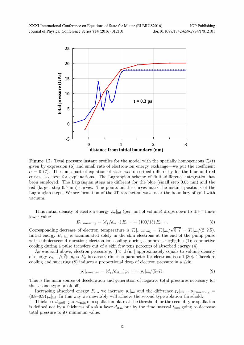
Figure 12. Total pressure instant profiles for the model with the spatially homogeneous Te(t)given by expression (6) and small rate of electron-ion energy exchange—we put the coefficientα = 0 (7). The ionic part of equation of state was described differently for the blue and redcurves, see text for explanations. The Lagrangian scheme of finite-difference integration hasbeen employed. The Lagrangian steps are different for the blue (small step 0.05 nm) and thered (larger step 0.5 nm) curves. The points on the curves mark the instant positions of theLagrangian steps. We see formation of the 2T rarefaction wave near the boundary of gold withvacuum.

Thus initial density of electron energy Ee|ini (per unit of volume) drops down to the 7 timeslower value

Ee|smearing = (df/dskin)Ee|ini = (100/15)Ee |ini. (8)

Corresponding decrease of electron temperature is Te|smearing = Te|ini/√5–7 = Te|ini/(2–2.5).

Initial energy Ee|ini is accumulated solely in the skin electrons at the end of the pump pulsewith subpicosecond duration; electron-ion cooling during a pump is negligible (1); conductivecooling during a pulse transfers out of a skin few tens percents of absorbed energy (4).

As was said above, electron pressure pe [Pa=J/m3] approximately equals to volume densityof energy Ee [J/m3]: pe ≈ Ee because Gruneisen parameter for electrons is ≈ 1 [30]. Thereforecooling and smearing (8) induces a proportional drop of electron pressure in a skin:

pe|smearing = (df/dskin) pe|ini = pe|ini/(5–7). (9)

This is the main source of deceleration and generation of negative total pressures necessary forthe second type break off.

Increasing absorbed energy Fabs we increase pe|ini and the difference pe|ini − pe|smearing =(0.8–0.9) pe|ini. In this way we inevitably will achieve the second type ablation threshold.

Thickness dspall−2 ≈ c tmin of a spallation plate at the threshold for the second type spallationis defined not by a thickness of a skin layer dskin but by the time interval tmin going to decreasetotal pressure to its minimum value.


12

-2 0 2 4distance from initial boundary (nm)

-10

-5

0

5

10

15

tota

l pre

ssur

e (G

Pa)

t = 1 ps

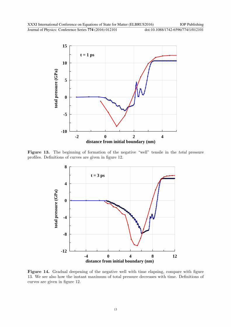
Figure 13. The beginning of formation of the negative “well” tensile in the total pressureprofiles. Definitions of curves are given in figure 12.

-4 0 4 8 12distance from initial boundary (nm)

-12

-8

-4

0

4

8

tota

l pre

ssur

e (G

Pa)

t = 3 ps

Figure 14. Gradual deepening of the negative well with time elapsing, compare with figure13. We see also how the instant maximum of total pressure decreases with time. Definitions ofcurves are given in figure 12.


13

-10 0 10 20distance from initial boundary (nm)

-12

-8

-4

0

4

8

tota

l pre

ssur

e (G

Pa)

t = 5 ps

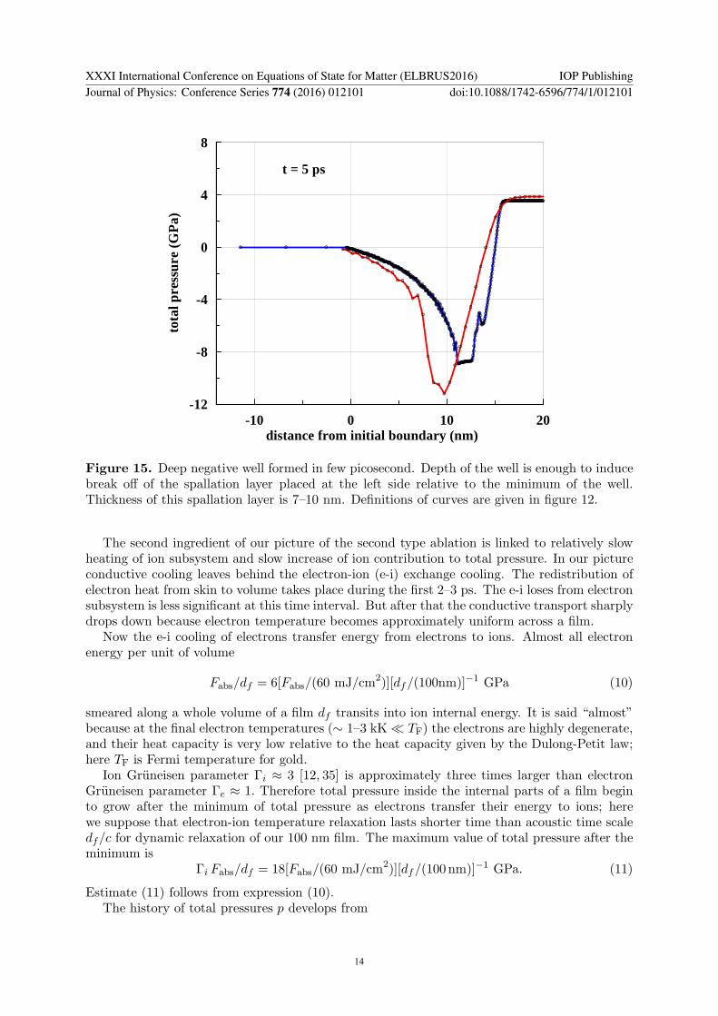
Figure 15. Deep negative well formed in few picosecond. Depth of the well is enough to inducebreak off of the spallation layer placed at the left side relative to the minimum of the well.Thickness of this spallation layer is 7–10 nm. Definitions of curves are given in figure 12.

The second ingredient of our picture of the second type ablation is linked to relatively slowheating of ion subsystem and slow increase of ion contribution to total pressure. In our pictureconductive cooling leaves behind the electron-ion (e-i) exchange cooling. The redistribution ofelectron heat from skin to volume takes place during the first 2–3 ps. The e-i loses from electronsubsystem is less significant at this time interval. But after that the conductive transport sharplydrops down because electron temperature becomes approximately uniform across a film.

Now the e-i cooling of electrons transfer energy from electrons to ions. Almost all electronenergy per unit of volume

Fabs/df = 6[Fabs/(60 mJ/cm2)][df/(100nm)]−1 GPa (10)

smeared along a whole volume of a film df transits into ion internal energy. It is said “almost”because at the final electron temperatures (∼ 1–3 kK ≪ TF) the electrons are highly degenerate,and their heat capacity is very low relative to the heat capacity given by the Dulong-Petit law;here TF is Fermi temperature for gold.

Ion Gruneisen parameter Γi ≈ 3 [12, 35] is approximately three times larger than electronGruneisen parameter Γe ≈ 1. Therefore total pressure inside the internal parts of a film beginto grow after the minimum of total pressure as electrons transfer their energy to ions; herewe suppose that electron-ion temperature relaxation lasts shorter time than acoustic time scaledf/c for dynamic relaxation of our 100 nm film. The maximum value of total pressure after theminimum is

Γi Fabs/df = 18[Fabs/(60 mJ/cm2)][df/(100 nm)]−1 GPa. (11)

Estimate (11) follows from expression (10).The history of total pressures p develops from


14

0 1 2 3 4 5time elapsed after maximum of pump (ps)

-10

0

10

20to

tal p

ress

ure

(GP

a)

0

4

8

12

inst

ant

posi

tion

of

min

imum

(nm

)

maximum total pressure

minimum total pressure

position of minimum

s

tm1

tm2

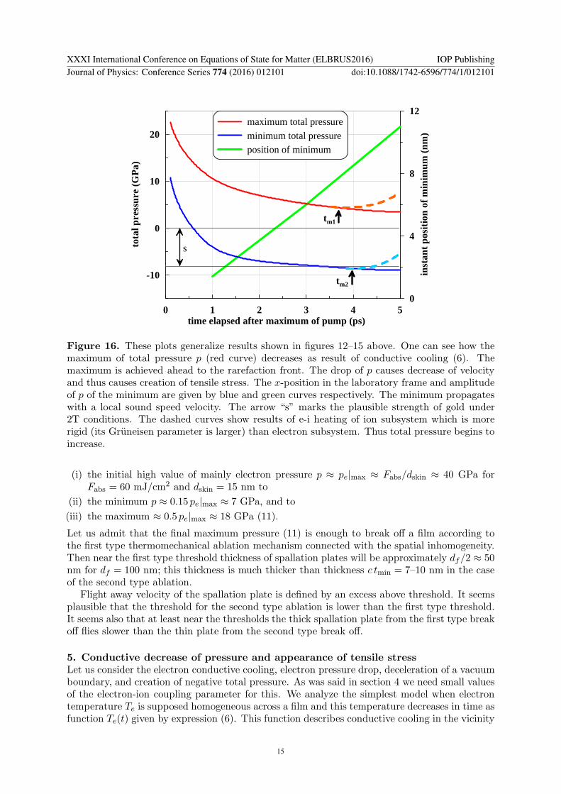
Figure 16. These plots generalize results shown in figures 12–15 above. One can see how themaximum of total pressure p (red curve) decreases as result of conductive cooling (6). Themaximum is achieved ahead to the rarefaction front. The drop of p causes decrease of velocityand thus causes creation of tensile stress. The x-position in the laboratory frame and amplitudeof p of the minimum are given by blue and green curves respectively. The minimum propagateswith a local sound speed velocity. The arrow “s” marks the plausible strength of gold under2T conditions. The dashed curves show results of e-i heating of ion subsystem which is morerigid (its Gruneisen parameter is larger) than electron subsystem. Thus total pressure begins toincrease.

(i) the initial high value of mainly electron pressure p ≈ pe|max ≈ Fabs/dskin ≈ 40 GPa forFabs = 60 mJ/cm2 and dskin = 15 nm to

(ii) the minimum p ≈ 0.15 pe|max ≈ 7 GPa, and to

(iii) the maximum ≈ 0.5 pe|max ≈ 18 GPa (11).

Let us admit that the final maximum pressure (11) is enough to break off a film according tothe first type thermomechanical ablation mechanism connected with the spatial inhomogeneity.Then near the first type threshold thickness of spallation plates will be approximately df/2 ≈ 50nm for df = 100 nm; this thickness is much thicker than thickness c tmin = 7–10 nm in the caseof the second type ablation.

Flight away velocity of the spallation plate is defined by an excess above threshold. It seemsplausible that the threshold for the second type ablation is lower than the first type threshold.It seems also that at least near the thresholds the thick spallation plate from the first type breakoff flies slower than the thin plate from the second type break off.

5. Conductive decrease of pressure and appearance of tensile stress

Let us consider the electron conductive cooling, electron pressure drop, deceleration of a vacuumboundary, and creation of negative total pressure. As was said in section 4 we need small valuesof the electron-ion coupling parameter for this. We analyze the simplest model when electrontemperature Te is supposed homogeneous across a film and this temperature decreases in time asfunction Te(t) given by expression (6). This function describes conductive cooling in the vicinity


15

-4 0 4 8 12distance from initial boundary (nm)

-20

-15

-10

-5

0

5

10

ion

& e

lect

ron

pres

sure

s (G

Pa)

t = 3 psPi, W-R

Pi, M-G

Pe, M-G

Pe, W-R

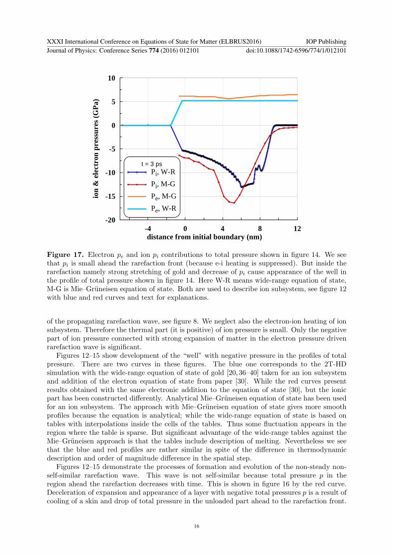
Figure 17. Electron pe and ion pi contributions to total pressure shown in figure 14. We seethat pi is small ahead the rarefaction front (because e-i heating is suppressed). But inside therarefaction namely strong stretching of gold and decrease of pi cause appearance of the well inthe profile of total pressure shown in figure 14. Here W-R means wide-range equation of state,M-G is Mie–Gruneisen equation of state. Both are used to describe ion subsystem, see figure 12with blue and red curves and text for explanations.

of the propagating rarefaction wave, see figure 8. We neglect also the electron-ion heating of ionsubsystem. Therefore the thermal part (it is positive) of ion pressure is small. Only the negativepart of ion pressure connected with strong expansion of matter in the electron pressure drivenrarefaction wave is significant.

Figures 12–15 show development of the “well” with negative pressure in the profiles of totalpressure. There are two curves in these figures. The blue one corresponds to the 2T-HDsimulation with the wide-range equation of state of gold [20,36–40] taken for an ion subsystemand addition of the electron equation of state from paper [30]. While the red curves presentresults obtained with the same electronic addition to the equation of state [30], but the ionicpart has been constructed differently. Analytical Mie–Gruneisen equation of state has been usedfor an ion subsystem. The approach with Mie–Gruneisen equation of state gives more smoothprofiles because the equation is analytical; while the wide-range equation of state is based ontables with interpolations inside the cells of the tables. Thus some fluctuation appears in theregion where the table is sparse. But significant advantage of the wide-range tables against theMie–Gruneisen approach is that the tables include description of melting. Nevertheless we seethat the blue and red profiles are rather similar in spite of the difference in thermodynamicdescription and order of magnitude difference in the spatial step.

Figures 12–15 demonstrate the processes of formation and evolution of the non-steady non-self-similar rarefaction wave. This wave is not self-similar because total pressure p in theregion ahead the rarefaction decreases with time. This is shown in figure 16 by the red curve.Deceleration of expansion and appearance of a layer with negative total pressures p is a result ofcooling of a skin and drop of total pressure in the unloaded part ahead to the rarefaction front.


16

0.8 1.2 1.6 2expansion ratio V/V0

-20

0

20

40

tota

l pre

ssur

e p

( ρ,

Te

, Ti =

0)

(G

Pa)

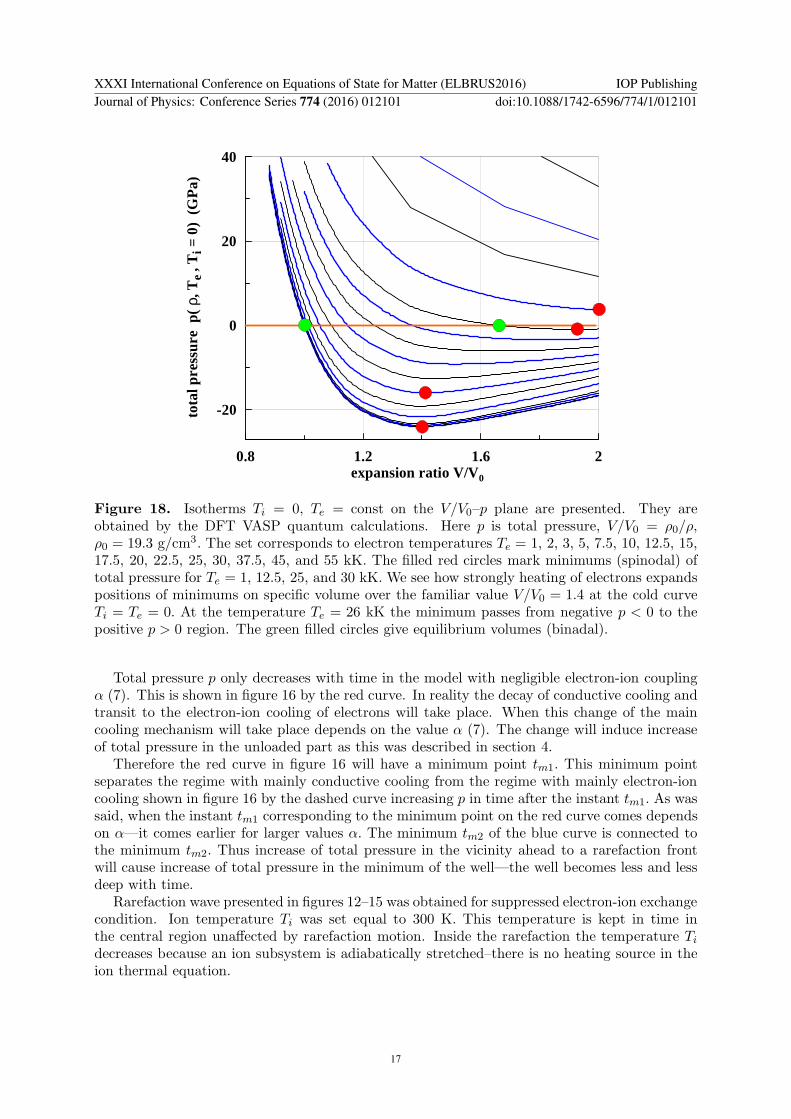
Figure 18. Isotherms Ti = 0, Te = const on the V/V0–p plane are presented. They areobtained by the DFT VASP quantum calculations. Here p is total pressure, V/V0 = ρ0/ρ,ρ0 = 19.3 g/cm3. The set corresponds to electron temperatures Te = 1, 2, 3, 5, 7.5, 10, 12.5, 15,17.5, 20, 22.5, 25, 30, 37.5, 45, and 55 kK. The filled red circles mark minimums (spinodal) oftotal pressure for Te = 1, 12.5, 25, and 30 kK. We see how strongly heating of electrons expandspositions of minimums on specific volume over the familiar value V/V0 = 1.4 at the cold curveTi = Te = 0. At the temperature Te = 26 kK the minimum passes from negative p < 0 to thepositive p > 0 region. The green filled circles give equilibrium volumes (binadal).

Total pressure p only decreases with time in the model with negligible electron-ion couplingα (7). This is shown in figure 16 by the red curve. In reality the decay of conductive cooling andtransit to the electron-ion cooling of electrons will take place. When this change of the maincooling mechanism will take place depends on the value α (7). The change will induce increaseof total pressure in the unloaded part as this was described in section 4.

Therefore the red curve in figure 16 will have a minimum point tm1. This minimum pointseparates the regime with mainly conductive cooling from the regime with mainly electron-ioncooling shown in figure 16 by the dashed curve increasing p in time after the instant tm1. As wassaid, when the instant tm1 corresponding to the minimum point on the red curve comes dependson α—it comes earlier for larger values α. The minimum tm2 of the blue curve is connected tothe minimum tm2. Thus increase of total pressure in the vicinity ahead to a rarefaction frontwill cause increase of total pressure in the minimum of the well—the well becomes less and lessdeep with time.

Rarefaction wave presented in figures 12–15 was obtained for suppressed electron-ion exchangecondition. Ion temperature Ti was set equal to 300 K. This temperature is kept in time inthe central region unaffected by rarefaction motion. Inside the rarefaction the temperature Ti

decreases because an ion subsystem is adiabatically stretched–there is no heating source in theion thermal equation.


17

1 2 3 4expansion ratio V/V0

-20

-10

0

10

tota

l pre

ssur

e p

( ρ,

Te

, Ti =

0)

(G

Pa)

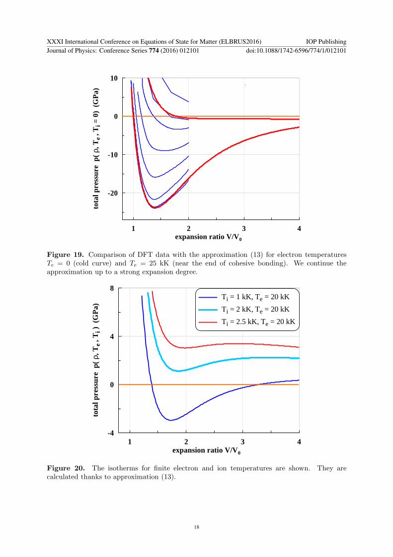
Figure 19. Comparison of DFT data with the approximation (13) for electron temperaturesTe = 0 (cold curve) and Te = 25 kK (near the end of cohesive bonding). We continue theapproximation up to a strong expansion degree.

1 2 3 4expansion ratio V/V0

-4

0

4

8

tota

l pre

ssur

e p

( ρ,

Te

, Ti )

(G

Pa)

Ti = 1 kK, Te = 20 kK

Ti = 2 kK, Te = 20 kK

Ti = 2.5 kK, Te = 20 kK

Figure 20. The isotherms for finite electron and ion temperatures are shown. They arecalculated thanks to approximation (13).


18

4 8 12 16 20density (g/cc)

0

1

2

3

4

5

ion

tem

pera

ture

(kK

)1T binodal, W-R EoS

1T binodal, DFT

2T binodal, Te = 10 kK



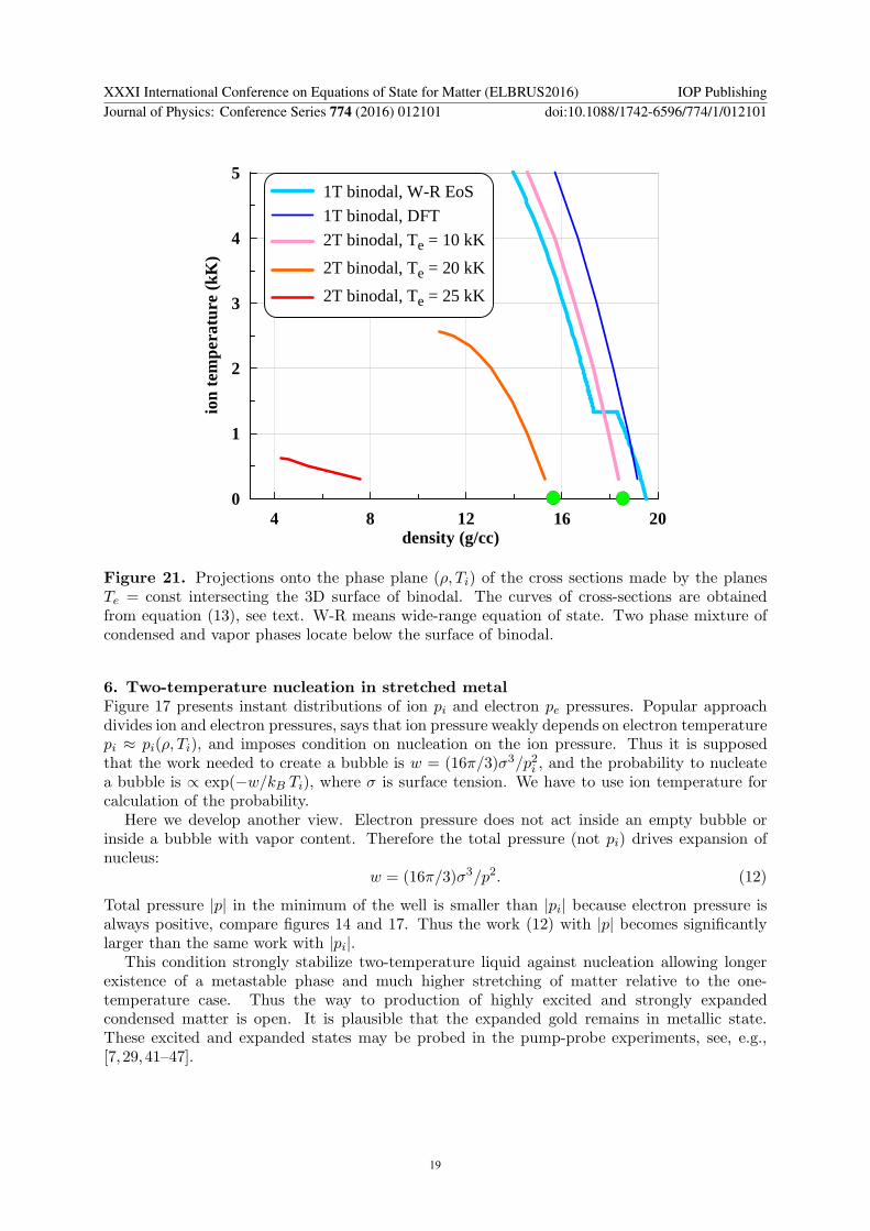
Figure 21. Projections onto the phase plane (ρ, Ti) of the cross sections made by the planesTe = const intersecting the 3D surface of binodal. The curves of cross-sections are obtainedfrom equation (13), see text. W-R means wide-range equation of state. Two phase mixture ofcondensed and vapor phases locate below the surface of binodal.

6. Two-temperature nucleation in stretched metal

Figure 17 presents instant distributions of ion pi and electron pe pressures. Popular approachdivides ion and electron pressures, says that ion pressure weakly depends on electron temperaturepi ≈ pi(ρ, Ti), and imposes condition on nucleation on the ion pressure. Thus it is supposedthat the work needed to create a bubble is w = (16π/3)σ3/p2i , and the probability to nucleatea bubble is ∝ exp(−w/kB Ti), where σ is surface tension. We have to use ion temperature forcalculation of the probability.

Here we develop another view. Electron pressure does not act inside an empty bubble orinside a bubble with vapor content. Therefore the total pressure (not pi) drives expansion ofnucleus:

w = (16π/3)σ3/p2. (12)

Total pressure |p| in the minimum of the well is smaller than |pi| because electron pressure isalways positive, compare figures 14 and 17. Thus the work (12) with |p| becomes significantlylarger than the same work with |pi|.

This condition strongly stabilize two-temperature liquid against nucleation allowing longerexistence of a metastable phase and much higher stretching of matter relative to the one-temperature case. Thus the way to production of highly excited and strongly expandedcondensed matter is open. It is plausible that the expanded gold remains in metallic state.These excited and expanded states may be probed in the pump-probe experiments, see, e.g.,[7, 29,41–47].


19

0 5 10 15 20 25electron temperature (kK)

-25

-20

-15

-10

-5

0

tota

l pre

ssur

e (G

Pa)

Ti = 0.3 kK

Ti = 1 kK

Ti = 2 kK

Ti = 3 kK

Ti = 4 kK

Ti = 5 kK

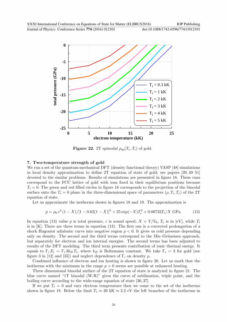
Figure 22. 2T spinodal psp(Te, Ti) of gold.

7. Two-temperature strength of gold

We run a set of the quantum-mechanical DFT (density functional theory) VASP [48] simulationsin local density approximation to define 2T equation of state of gold; see papers [39, 49–51]devoted to the similar problems. Results of simulations are presented in figure 18. These runscorrespond to the FCC lattice of gold with ions fixed in their equilibrium positions becauseTi = 0. The green and red filled circles in figure 18 corresponds to the projection of the binodalsurface onto the Ti = 0 plane in the three-dimensional space of parameters (ρ, Ti, Te) of the 2Tequation of state.

Let us approximate the isotherms shown in figures 18 and 19. The approximation is

p = ρ0 c2 (1−X)/[1 − 0.62(1 −X)]5 + 25 exp(−X)T 2

e + 0.00732Ti/X GPa. (13)

In equation (13) value p is total pressure, c is sound speed, X = V/V0, Te is in [eV], while Ti

is in [K]. There are three terms in equation (13). The first one is a corrected prolongation of ashock Hugoniot adiabatic curve into negative region p < 0. It gives us cold pressure dependingonly on density. The second and the third terms correspond to the Mie–Gruneisen approach,but separately for electron and ion internal energies. The second terms has been adjusted toresults of the DFT modeling. The third term presents contribution of ionic thermal energy. Itequals to ΓiEi = Γi 3kB Ti, where kB is Boltzmann constant. We take Γi = 3 for gold (seefigure 3 in [12] and [35]) and neglect dependence of Γi on density ρ.

Combined influence of electron and ion heating is shown in figure 20. Let us mark that theisotherms with the minimum in the range p > 0 seems are possible at enhanced heating.

Three dimensional binodal surface of the 2T equation of state is analyzed in figure 21. Theblue curve named “1T binodal (W-R)” gives the curve of sublimation, triple point, and theboiling curve according to the wide-range equation of state [36,37].

If we put Ti = 0 and vary electron temperature then we come to the set of the isothermsshown in figure 18. Below the limit Te ≈ 26 kK ≈ 2.2 eV the left branches of the isotherms in


20

figure 18 have intersection with the zero level of total pressure p = 0. These intersections aremarked by the green filled circles in figure 18. Increase of electron temperature Te increaseselectron pressure pe. This pressure expands gold. Thus density of the equilibrium state dropsand the green circle on the axis V ∝ 1/ρ in figure 18 moves to the right side.

The same green circles are shown in figure 21. They move in the direction of decrease ofdensity as electron temperature Te rises. As we increase temperature Te, the green circles infigure 21 shifts to the left side along the axis Ti = 0, and the area under binodal becomessmaller and smaller. Finally at temperature Te ≈ 26 kK ≈ 2.2 eV the binodal disappears. It isinteresting to follow this process in figures 18 and 21 simultaneously.

We use equation (13) to plot 2T binodals in figures 18 and 21. We fix temperatures Te andTi and find root ρ = ρ(Te, Ti) of equation p(ρ, Te, Ti) = 0 (13). This root gives us the 3D binodalsurface over the plane (Ti, Te).

In the 1T case Te = Ti = T the root ρ = ρ(T, T ) of equation p(ρ, T, T ) = 0 (13) gives us the1T binodal shown in figure 21 (deep blue curve). It goes close to the wide-range 1T binodal(blue curve with a step of the triple point). But DFT of crystal used in our DFT runs does notallow considering the case of fluid. Thus our DFT binodal does not have a step.

The ultimate strength of gold is defined by pressure at the 2T spinodal. We use equation(13) to obtain spinodal psp(Te, Ti). Derivative dp/dV of expression (13) has been calculated. Wefix temperatures Te, Ti and find root ρsp(Te, Ti) of equation dp/dV = 0. After that we calculatepressure at the spinodal surface

psp(ρsp(Te, Ti), Te, Ti).

The results are shown in figure 22.Tensile pressures achieved in simulations shown in figures 12-15 are near the spinodal

presented in figure 22 for typical temperatures Te = 10–15 kK, Ti = 1–3 kK. Thus ablationof a thin spallation plate through the second break off mechanism is possible. As a result thespallation plate 7–10 nm thick appears.

The maximum of a tensile stress in our 2T hydrodynamics simulations is achieved at theinstants t∗ = 2–3 ps at the depth c t∗ ≈ 7–10 nm. This maximum triggers nucleation or acousticinstability. This depth defines thickness of a spallation plate. Similar thicknesses were obtainedin paper [24]. We can not compare the instants when maximum tensile stress is achieved in [24]with our results because the profiles of total pressures at the first picoseconds are not givenin [24]. Visible gap between the spallation plate and the rest of a target appears between 10 and20 ps, see figure 2(a) in [24]. This time interval is significantly delayed relative to our nucleationinstants t∗. This may be explained by slow expansion of the banks of the developing gap.

8. Conclusion

We analyze above the new aspects of thermomechanical ablation by an ultrashort laser pulse.The most important problem solved in paper concerns the early stage of ablation. Usually peopleconsider thermomechanical ablation caused by deceleration related to spatial inhomogeneity.This is inhomogeneity or of a heat affected zone dT in a bulk target, or thickness of a film df incase of a thin film when df < dT . The scale dT is ∼ 100–200 nm for gold.

In our paper the alternative case is studied. In this case not a spatial inhomogeneity isa reason of deceleration, appearance of tensile stress, and nucleation. The reason is the fastdecrease of total pressure at the first 2–3 ps (section 4).

We link the decrease of total pressure in time with fast conductive cooling of a skin layerstrongly heated by absorption of a laser pulse. The decrease of total pressure (as a result ofcooling of electrons at relatively more slow heating of ions) lasts during very short time interval2–3 ps. After that total pressure begins to grow during the next finite time interval due to ionheating. It should be explained that we speak here about total pressure in a region close to thehead of the propagating rarefaction wave but outside rarefaction flow.


21

In this connection we have studied thermal problem at the early stage. Electron heat fluxesare estimated (sections 2 and 3). It is significant (for conductive cooling of a skin) how thickis a thin film df < dT relative to thickness of a skin layer (dskin ≈ 15 nm for optical lasers andgold). Indeed, the rest of a film (which remains cold during the subsecond laser pulse) serves asa cooling capacity taking heat from a skin. If a film is df ∼ dskin then the fast cooling (thanksto quick transfer of a heat into capacity) is absent. Thus the alternative mechanism of break offbecomes impossible.

In the alternative case, thickness of spallation plate is small. It is equal to 7–10 nm. Whilein the case of usual thermomechanical ablation, at the threshold, it is approximately a half ofthickness of a film. It is 40–50 nm for our film 100 nm thick.

We develop the models for 2T equation of state, thermal conductivity, and electron-ioncoupling. From equation of state the spinodal and strength of the 2T system is calculated(section 7).

We calculate expansion at the early stage and find that negative pressures appearing thanksto fast cooling have enough amplitude (section 5) to break off thin (7–10 nm) spallation layer(section 5).

Acknowledgments

Authors of the paper acknowledge support from the Russian Science Foundation project No. 14-19-01599.

Appendix A. Calculation of two-temperature electron thermal conductivity

Here we present two programs developed for calculation of coefficient of 2T heat conduction.They use the package of symbolic computations “Wolfram Mathematica”. Figure 11 is obtainedusing the second program. The first program gives slightly smaller values of coefficient κ. Thisis the programs for gold (Au). The program for calculation of coefficient κ for aluminum wasdeveloped in [52].

Appendix A.1. The first program “2T conduction”

(*Electron heat conductivity of gold*)

(*Approximations:

1. Two-parabolical DoS (electron density of states) with energies

and electron numbers

as functions of Te and V

2. Drude-approximation for the frequency of electron-ion collision:

nu_ei=e^2*n_s*rho_e/m_s, here n_s, m_s - concentration of s-electrons,

mass of one s-electron, rho_e - electrical resistivity

3. rho_e at T~Tmelting - fitting of experimental data, rho_e at T>>T_melting -

Mott‘s limit, rho_e as function of volume - rho_e (V)~V^(2G-1/3),

G - Gruneisen parameter


22

4. We use rho_e (V)~V^(2G-1/3) for solid AND liquid gold,

although in the latter case it may be wrong*)

(*Part I *)

(*Parameters of two-parabolical model*)

Z=11; (*total number of valence electrons*)

nat=6.022*19.28/196.97; (*atomic concentration*)

na=nat*0.148*0.1; (*atom. concentr. in a.u.*)

a1v[v_]=8.370116055555545 +0.7592750000000095*v;

(* v = V/Vo *)

b1v[v_]=-0.07772823222222186+0.14376283333333298*v;

c1v[v_]=0.002928826666666666;

f[te_,v_]=a1v[v]+b1v[v]*(te/11605)+c1v[v]*(te/11605)^2;

zd[te_,v_]=f[te,v];

(* d-electron number as a function of volume and electron temperature*)

zs[te_,v_]=Z-f[te,v];

(* s-electron number as a function of volume and electron temperature*)

e1a[v_]=5.561611190476584 +1.088018939393126*v-4.577624458874042*v^2;

e1b[v_]=-0.1255257317697-0.068264699156441

*Sin[30.86751811350718*v-23.774835712];

e1c[v_]=41.134008963928 -126.487749601735 v+129.28817149158718 v^2

-43.947589435989 v^3;

e1[te_,v_]=e1a[v]+e1b[v]*(te/11605)+e1c[v]*(te/11605)^2;

e2a[v_]=25.177545055555527 -17.103274999999968*v;

e2b[v_]=3.3169602455555496 -3.7120671666666607*v;

e2c[v_]=-1.964970711111108+1.955094999999997*v;

e2d[v_]=0.2921434513388884 -0.29283181916666623*v;

e2[te_,v_]=e2a[v]+e2b[v]*(te/11605)+e2c[v]*(te/11605)^2+e2d[v]*(te/11605)^3;


23

es[v_]=5.8-5.15*v;

eF[v_]=24.8-16*v;

ES[v_]=eF[v]-es[v]; (*s-electron minimum energy as a function of volume*);

E1[te_,v_]=ES[v]+(es[v]-e1[te,v]);

(*d-electron minimum energy as a function of volume

and electron temperature*);

E2[te_,v_]=ES[v]+(es[v]-e2[te,v]);

(*d-electron maximum energy as a function of volume

and electron temperature*);

ms[te_,v_]=27.211*(3*Pi*Pi*na*zs[te,v])^(2/3)/(2*ES[v]) ;

(*effective mass of s-electron*) ;

md[te_,v_]=27.211*(3*Pi*Pi*na*zd[te,v])^(2/3)/(2*(E1[te,v]-E2[te,v]))

(*effective mass of d-electron*)

(*Part II *)

(*Fittings of experimental data for electrical resistivity of gold*)

(*Experimental data used here was obtained by R.A. Matula

(J. Chem.Ref. Data, V. 8, P .1147, 1979, doi:10.1063/1.555614*)

rhoesol[ti_]=0.000068837*ti+2.3187200000000002*10^(-8)*ti^2

(*electrical conductivity of solid gold as function of temperature

(ion temperature)*)

rhoeliq[ti_]=0.308244+0.000157144‘*(ti-1337)

(*electical conductivity of liquid gold - this is approximation at temperatures

slightly above melting temperature at zero pressure*)

rholowT[ti_,v_]=If[ti<Tm[v],rhoesol[ti],rhoeliq[ti]] (*general formula*)

Grun[v_]=2.95*v^1.229 (*Gruneisen as function of volume*)

rlowT[v_,ti_]=rholowT[ti,v]*v^(2*Grun[v]-1/3)*(zs[1000,1]/zs[1000,v])^(2/3)

(*electrical conductivity at T <<T_Fermi as function of volume


24

and (ion) temperature*)

rMott=0.8

rhighT[v_]=rMott*v^(1/3)*(zs[55000,1]/zs[55000,v])^(2/3)

(*Mott limit dependence from volume*)

rTi[v_,ti_]=((rlowT[v,ti])^(-4)+(rhighT[v])^(-4))^(-0.25)

(*mathching of both fittings for electrical resistivity*)

(*Part III*)

(*Frequency of Drude collisions by Drude formula*)

(*constants and table data*)

hbar=1.054*10^(-27);

z2=(4.807*10^(-10))^2;

natsq3=(6.022*19.28*10^23/196.97)^(1/3);

L=4;

zz=zs[55000,1]

const=(3*Pi^2*L/zz^2)^(1/3)

rmaxCGSE=hbar/z2/natsq3*const

rmaxSI=0.2*rmaxCGSE*9*10^9*10^6*z2*natsq3^3

*rmaxCGSE/ms[1000,1]/(9.11*10^(-27))

nu0=6.425119880161749*10^14

constnu=nu0/rmaxSI

(*effective frequency of electron-ion collisions in accordance

with Drude formula*)

nuei[v_,ti_,te_]=

z2*natsq3^3*(1/v)*zs[te,v]*rTi[v,ti]*10^(-6)/ms[te,v]/(9.11*10^(-28)*9*10^9)

(*Part IV*)

(*gold two-temperature thermodynamics*)

(*volume and electron temperature dependent DoS*)

gs[e_,te_,v_]=1.5*zs[te,v]/v/(Abs[ES[v]])^(3./2.)*Sqrt[e+Abs[ES[v]]];

(*mean square of electron velocity*)


25

vs2[v_,te_]=

(2*Abs[ES[v]]+3*(te/11605))/ms[te,v]*(1.6022*10^(-19)/(0.911*10^(-30)));

(*fitting for electron chemical potential as function of electron temperature,

the dependence from volume are omitted*)

mu[te_]=

27.211*5*10^(-10)*te^2/(1+4*10^(-9)*te^2)-5*10^(-10)*te^2*Exp[-te/11000];

(*electron internal energy*)

uvs[te_,v_]=

NIntegrate[gs[e,te,v]*e/(1+Exp[(e-mu[te])*11605/te]) ,

{e,-Abs[ES[v]],50}]*(nat*1.6022*10^(-19)*10^29)

(*10^6 (CGSe to SI)/10^5( J/m^3/K)*)

(*electron specific heat*)

cvs[te_,v_]=D[uvs[te,v],te]/116050

(*gives a number of the electrons with energies below Fermi energy*)

NIntegrate[gs[e,1000,1],{e,-Abs[ES[1]],0}]

(*simple fit for electron specific heat*)

Cvss[v_,te_]=rc1[v]*te+rc2[v]*te^2+rc3[v]*te^3

(*Part V*)

(*construction of final expression*)

(*thermal resistivity due to electron-ion collisions*)

Sei[te_,ti_,vv_]=3*10^4*nuei[vv,ti,te]/((Cvss[vv,te]*10^5)*vs2[vv,te])

(*melting curve due to Lindemann law*)

Tm[v_]=1337*v^(2/3)*Exp[5.9/1.229*(1-v^(1.229))]

(*electron-electron contribution in heat conductivity

at equilibrium density*)

kee1[te_]=0.041*te+2.5*10^9/te^1.5

(*volume factor multiplied on previous expression; x = V/Vo *)

volkee[x_]=If[x>1,x^1.4,If[x<1,x^2.4,1]]

(*electron-electron contribution as a function

of electron temperature and density*)

kee[te_,x_]=kee1[te]*volkee[x]

(*parts of new formula of electron-phonon contribution

in electron heat conductivity of solid gold*)


26

(*the fittings introduced hereafter were obtained using Sei *)

P1[x_]=19800*x^1.77

Q1[x_]=4

L1[x_]=3.6*x^2.95

M1[x_]=3500*(1+1/(1+12*(x-1)^2))

N1[x_]=40000/x-28500

B1[te_,x_]=L1[x]/(1+((te-M1[x])/N1[x])^2)+Q1[x]*Tanh[te/P1[x]]

alpha[x_]=0.82*x^5.3

(*electron-ion contribution in heat conductivity of solid gold*)

keisol[te_,ti_,x_]=alpha[x]*te*(1000/ti)^2/(1+B1[te,x]*(1000/ti))

(*electon heat conductivity of solid gold*)

ksol[te_,ti_,x_]=1/(1/keisol[te,ti,x]+1/kee[te,x])

(*parts of new formula for electron-ion contribution

in electron heat conductivity of liquid gold*)

s[x_]=0.0363*Exp[0.4125*x]

t[x_]=0.7465*x-0.6244

z[x_]=8*10^(-4)/x/(1+0.4/x)

(*electron-ion contribution in heat conductivity of liquid gold*)

keiliq[te_,ti_,x_]=(s[x]+t[x]*Exp[-z[x]*ti])*te

(*electron heat conductivity of liquid gold*)

kliq[te_,ti_,x_]=1/(1/keiliq[te,ti,x]+1/kee[te,x])

(*full electron heat conductivity*)

k[te_,ti_,x_]=If[ti>Tm[x],kliq[te,ti,x],ksol[te,ti,x]]

(*Part VI*)

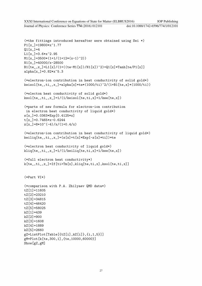
(*comparison with P.A. Zhilyaev QMD data*)

tZ[1]=11605

tZ[2]=23210

tZ[3]=34815

tZ[4]=46420

tZ[5]=58025

kZ[1]=439

kZ[2]=900

kZ[3]=1608

kZ[4]=1889

kZ[5]=2660

gZ=ListPlot[Table[{tZ[i],kZ[i]},{i,1,5}]]

gM=Plot[k[te,300,1],{te,10000,60000}]

Show[gZ,gM]


27

Appendix A.2. The second program “2T conduction”

(*the coefficients used here are taken from the work in

J.Phys.Conf.Ser. V.653, 012087 (Elbrus 2015)*)

t[r_,te_]=6*(te/11605)/(9.2*(r/19.5));

a=3.92; b=1.95; al=2*a+1; be=a+1; cab=(a-b)/(b+1);

yprime[r_]=((1+cab)*(r/19.3)^(al))/(1+cab*(r/19.3)^(be)) ;

cv[r_,te_]=131*t[r,te]*(1+3.07*t[r,te]*t[r,te])/(1+1.08*t[r,te]^2.07);

Trt=293; (*room temperature*)

xrt=19.28/19.5;

trt=Trt*6/(9.2*11605*(xrt^(2/3)));

(*electron-ion contribution in heat conductivity of solid gold*)

ksei[r_,te_,ti_]=

318*(r/19.3)*(yprime[r]/yprime[19.5])*Trt/ti*cv[r,te]/cv[19.5,298]

k0[r_,te_]=cv[r,te]

tl[ti_]=(ti-1337)/1000

xl[ti_]=0.887179-0.0328321*tl[ti]-0.0030982*(tl[ti]^2)-0.000164884*(tl[ti]^3)

tm=1337.0

xlm=xl[tm]

rl[ti_]=148.5+119.3*15.337*(ti/1000)/(14+ti/1000)

gam=2.

(*electron-ion contribution in heat conductivity of liquid gold*)

klei[r_,te_,ti_]=k0[r,te]*(3254/rl[ti])*((r/19.5)/xl[tm])

*(((r/19.5)/xl[ti])^gam)

(*electron-electron contribution in heat conductivity*)

keem[r_,te_]=

9.294*10^(-4)*t[r,te]/(1+0.03*Sqrt[t[r,te]]-0.2688*t[r,te]+

+0.9722*t[r,te]^2)*(r/19.5)^(-4./3.)

recks[r_,te_,ti_]=keem[r,te]+1/ksei[r,te,ti]

reckl[r_,te_,ti_]=keem[r,te]+1/klei[r,te,ti]


28

(*electron heat conductivity of solid (1) and liquid (2) gold *)

(*here "r" is density in g/cm^3 *)

ks[r_,te_,ti_]=1/recks[r,te,ti] (*1*)

kl[r_,te_,ti_]=1/reckl[r,te,ti] (*2*)

Appendix B. Limit of electron thermal transport

Heat flux jq can be expressed in terms of the entropy flux js:

jq = Tejs.

Taking into account thatTedS = dE − µdN,

where S is the entropy, N is the number of particles, one connects the heat flux with the energyflux jE and particle flux jN :

jq = Te js = jE − µ jN .

Here µ is a cheimical potential, close to the Fermi energy at not too high electron temperatures.Then integrating over all electrons within the conduction band with the energy of electron withthe wave vector ~k equal to ε(~k) and velocity v(~k), we obtain

jq =

∫

2d3k

(2π)3(ε(~k)− µ)v(~k)f(~k).

Here f(~k) is the electron partition function. Then in the case of not too high temperatures,

when ε(~k)− µ ≃ kBTe (only electrons within the energy interval ∼ kBTe are excited with theirnumber ∼ n kB Te/µ), the maximum possible heat flux can be estimated as

jq ≃ (kB Te) (n kB Te/µ) vF ≃ (n εF) (kB Te/µ)2 vF,

where vF being the Fermi velocity.

References[1] Milchberg H M, Freeman R R, Davey S C and More R M 1988 Phys. Rev. Lett. 61 2364–2367[2] Ng A, Celliers P, Forsman A, More R M, Lee Y T, Perrot F, Dharma-Wardana M W C and Rinker G A

1994 Phys. Rev. Lett. 72 3351–3354[3] Komarov P S, Ashitkov S I, Ovchinnikov A V, Sitnikov D S, Veysman M E, Levashov P R, Povarnitsyn M E,

Agranat M B, Andreev N E, Khishchenko K V and Fortov V E 2009 J. Phys. A: Math. Theor. 42 214057[4] Veysman M E, Agranat M B, Andreev N E, Ashitkov S I, Fortov V E, Khishchenko K V, Kostenko O F,

Levashov P R, Ovchinnikov A V and Sitnikov D S 2008 J. Phys. B: At. Mol. Opt. Phys. 41 125704[5] Agranat M B, Andreev N E, Ashitkov S I, Veysman M E, Levashov P R, Ovchinnikov A V, Sitnikov D S,

Fortov V E and Khishchenko K V 2007 JETP Lett. 85 271–276[6] Zhakhovskii V V and Inogamov N A 2010 JETP Lett. 92 521–526[7] Ashitkov S I, Agranat M B, Kanel’ G I, Komarov P S and Fortov V E 2010 JETP Lett. 92 516–520[8] Inogamov N, Zhakhovsky V V, Khokhlov V A and Shepelev V V 2011 JETP Lett. 93 226–232[9] Krasyuk I K, Pashinin P P, Semenov A Y, Khishchenko K V and Fortov V E 2016 Laser Phys. 26 094001

[10] Anisimov S I, Zhakhovskii V V, Inogamov N A, Nishihara K, Oparin A M and Petrov Yu V 2003 JETP Lett.

77 606–610[11] Ivanov D S and Zhigilei L V 2003 Phys. Rev. B 68 064114[12] Inogamov N A, Zhakhovskii V V, Ashitkov S I, Khokhlov V A, Shepelev V V, Komarov P S, Ovchinnikov

A V, Sitnikov D S, Petrov Yu V, Agranat M B, Anisimov S I and Fortov V E 2011 Contrib. Plasma Phys.

51 367–374[13] Demaske B J, Zhakhovsky V V, Inogamov N A and Oleynik I I 2010 Phys. Rev. B 82 064113[14] Zhakhovskii V V, Nishihara K, Anisimov S I and Inogamov N A 2000 JETP Lett. 71 167–172


29

[15] Upadhyay A K, Inogamov N A, Rethfeld B and Urbassek H 2008 Phys. Rev. B 78 045437[16] Inogamov N A, Zhakhovskii V V and Khokhlov V A 2015 J. Exp. Theor. Phys. 120 15–48[17] Inogamov N A, Zhakhovsky V V, Hasegawa N, Nishikino M, Yamagiwa M, Ishino M, Agranat M B, Ashitkov

S I, Faenov A Ya, Khokhlov V A, Ilnitsky D K, Pikuz T A, Takayoshi S, Tomita T and Kawachi T 2015Appl. Phys. B 119 413–419

[18] Inogamov N A, Anisimov S I and Retfeld B 1999 J. Exp. Theor. Phys. 88 1143–1150[19] Anisimov S I, Inogamov N A, Oparin A M, Rethfeld B, Yabe T, Ogawa M and Fortov V E 1999 Appl. Phys.

A 69 617–620[20] Povarnitsyn M E, Itina T E, Sentis M, Khishchenko K V and Levashov P R 2007 Phys. Rev. B 75 235414[21] Inogamov N A, Zhakhovskii V V, Ashitkov S I, Petrov Yu V, Agranat M B, Anisimov S I, Nishihara K and

Fortov V E 2008 J. Exp. Theor. Phys. 107 1–19[22] Inogamov N A, Zhakhovsky V V, Khokhlov V A, Demaske B J, Khishchenko K V and Oleynik I I 2014 J.

Phys.: Conf. Ser. 500 192023[23] Ilnitsky D K, Khokhlov V A, Inogamov N A, Zhakhovsky V V, Petrov Yu V, Khishchenko K V, Migdal K P

and Anisimov S I 2014 J. Phys.: Conf. Ser. 500 032021[24] Starikov S V and Pisarev V V 2015 J. Appl. Phys. 117 135901[25] Starikov S V, Faenov A Y, Pikuz T A, Skobelev I Y, Fortov V E, Tamotsu S, Ishino M, Tanaka M, Hasegawa

N, Nishikino M, Kaihori T, Imazono T, Kando M and Kawachi T 2014 Appl. Phys. B 116 1005–1016[26] Norman G, Starikov S, Stegailov V, Fortov V, Skobelev I, Pikuz T, Faenov A, Tamotsu S, Kato Y, Ishino

M, Tanaka M, Hasegawa N, Nishikino M, Ohba T, Kaihori T, Ochi Y, Imazono T, Fukuda Y, Kando Mand Kawachi T 2012 J. Appl. Phys. 112 013104

[27] Lin Z, Zhigilei L V and Celli V 2008 Phys. Rev. B 77 075133[28] Petrov Yu V, Inogamov N A and Migdal K P 2013 JETP Lett. 97 20–27[29] Chen Z, Holst B, Kirkwood S E, Sametoglu V, Reid M, Tsui Y Y, Recoules V and Ng A 2013 Phys. Rev.

Lett. 110 135001[30] Petrov Yu V, Migdal K P, Inogamov N A and Zhakhovsky V V 2015 Applied Physics B 119 401–411[31] Hohlfeld J, Wellershoff S S, Guedde J, Conrad U, Jaehnke V and Matthias E 2000 Chem. Phys. 251 237–258[32] Migdal K P, Il’nitsky D K, Petrov Yu V and Inogamov N A 2015 J. Phys.: Conf. Ser. 653 012086[33] Petrov Yu V, Inogamov N A, Anisimov S I, Migdal K P, Khokhlov V A and Khishchenko K V 2015 J. Phys.:

Conf. Ser. 653 012087[34] Petrov Yu V, Inogamov N A and Migdal K P 2015 PIERS Proceedings pp 2431–2435[35] Graf M J, Greeff C W and Boettger J C 2004 AIP Conf. Proc. 706 65–68[36] Khishchenko K V 2008 J. Phys.: Conf. Ser. 98 032023[37] Khishchenko K V 2008 J. Phys.: Conf. Ser. 121 022025[38] Levashov P R and Khishchenko K V 2007 AIP Conf. Proc. 955 59–62[39] Inogamov N A, Petrov Yu V, Zhakhovsky V V, Khokhlov V A, Demaske B J, Ashitkov S I, Khishchenko

K V, Migdal K P, Agranat M B, Anisimov S I, Fortov V E and Oleynik I I 2012 AIP Conf. Proc. 1464

593–608[40] Inogamov N A, Khokhlov V A, Zhakhovsky V V, Petrov Yu V, Khishchenko K V and Anisimov S I 2015

PIERS Proceedings pp 2422–2426[41] Widmann K, Ao T, Foord M E, Price D F, Ellis A D, Springer P T and Ng A 2004 Phys. Rev. Lett. 92

125002[42] Ao T, Ping Y, Widmann K, Price D F, Lee E, Tam H, Springer P T and Ng A 2006 Phys. Rev. Lett. 96

055001[43] Ping Y, Hanson D, Koslow I, Ogitsu T, Prendergast D, Schwegler E, Collins G and Ng A 2006 Phys. Rev.

Lett. 96 255003[44] Ping Y, Hanson D, Koslow I, Ogitsu T, Prendergast D, Schwegler E, Collins G and Ng A 2008 Phys. Plasmas

15 056303[45] Chen Z, Sametoglu V, Tsui Y Y, Ao T and Ng A 2012 Phys. Rev. Lett. 108 165001[46] Fourment C, Deneuville F, Descamps D, Dorchies F, Petit S and Peyrusse O 2014 Phys. Rev. B 89 161110(R)[47] Ashitkov S I, Komarov P S, Struleva E V, Agranat M B and Kanel G I 2015 JETP Lett. 101 276–281[48] Kresse G and Furthmuller J 1996 Comput. Mater. Sci. 6 15[49] Levashov P R, Sin’ko G V, Smirnov N A, Minakov D V, Shemyakin O P and Khishchenko K V 2010 J.

Phys.: Condens. Matter 22 505501[50] Sin’ko G V, Smirnov N A, Ovechkin A A, Levashov P R and Khishchenko K V 2013 High Energy Density

Phys. 9 309–314[51] Minakov D V, Levashov P R, Khishchenko K V and Fortov V E 2014 J. Appl. Phys. 115 223512[52] Inogamov N A and Petrov Yu V 2010 J. Exp. Theor. Phys. 110 446–468


30

Documents

Dynamics of laser ablation at the early stage during and ...laser.itp.ac.ru/publications/JPCS_774_1_012101.pdfDynamicsoflaserablationat theearly stageduring andafter ultrashortpulse