Embed Size (px)
Citation preview

HAL Id: tel-01148696https://tel.archives-ouvertes.fr/tel-01148696
Submitted on 5 May 2015
HAL is a multi-disciplinary open accessarchive for the deposit and dissemination of sci-entific research documents, whether they are pub-lished or not. The documents may come fromteaching and research institutions in France orabroad, or from public or private research centers.
L’archive ouverte pluridisciplinaire HAL, estdestinée au dépôt et à la diffusion de documentsscientifiques de niveau recherche, publiés ou non,émanant des établissements d’enseignement et derecherche français ou étrangers, des laboratoirespublics ou privés.
Dynamics of long range interacting systems beyond theVlasov limit
Jules Morand
To cite this version:Jules Morand. Dynamics of long range interacting systems beyond the Vlasov limit. High EnergyPhysics - Theory [hep-th]. Université Pierre et Marie Curie - Paris VI, 2014. English. �NNT :2014PA066624�. �tel-01148696�
Université Pierre et Marie Curie
Thèse de Doctorat
pour obtenir le grade de
docteur ès sciences
Spécialité : Physique statistique - Systèmes complexes
préparée auLaboratoire de Physique Nucléaire et Hautes Énergies
dans le cadre de l’École Doctorale ED 389
présentée et soutenue publiquementpar
Jules Morand
le 2 décembre 2014
Titre:Dynamics of long range interacting systems
beyond the Vlasov limit.
—
Dynamique des systèmes à longue portée
au delà de la limite de Vlasov.
Directeur de thèse: Michael Joyce
JuryM. Angel ALASTUEY, ExaminateurM. Julien BARRÉ, RapporteurM. Michael JOYCE, Directeur de thèse
Mme. Régine PERZYNSKI, ExaminatriceM. Stefano RUFFO, RapporteurM. Emmanuel TRIZAC, ExaminateurM. Pascal VIOT, Invité


Contents
Contents . . . . . . . . . . . . . . . . . . . . . . . . . . . . . . . . . . . . . iii
Introduction 1
1 Introduction to long-range interacting systems 31 Thermodynamics and dynamics . . . . . . . . . . . . . . . . . . . . . 3
1.1 Definition . . . . . . . . . . . . . . . . . . . . . . . . . . . . . 31.2 The distinctive thermodynamics of long-range systems . . . . 41.3 Dynamics of long-range systems . . . . . . . . . . . . . . . . . 91.4 Long-range systems with stochastic perturbations . . . . . . . 16
2 Self-gravitating systems . . . . . . . . . . . . . . . . . . . . . . . . . 172.1 3d self-gravity . . . . . . . . . . . . . . . . . . . . . . . . . . . 172.2 1d self-gravity . . . . . . . . . . . . . . . . . . . . . . . . . . . 20
2 Finite N corrections to Vlasov dynamics 251 A Vlasov-like equation for the coarse-grained phase space density . . 272 Statistical evaluation of the finite N fluctuating terms . . . . . . . . . 30
2.1 Mean and variance of ⇠v
. . . . . . . . . . . . . . . . . . . . . 312.2 Mean and variance of ⇠
F
. . . . . . . . . . . . . . . . . . . . . 313 Parametric dependence of the fluctuations . . . . . . . . . . . . . . . 35
3.1 Mean field Vlasov limit . . . . . . . . . . . . . . . . . . . . . . 353.2 Velocity fluctuations . . . . . . . . . . . . . . . . . . . . . . . 363.3 Force fluctuations . . . . . . . . . . . . . . . . . . . . . . . . . 36
4 Force fluctuations about the Vlasov limit: dependence on " . . . . . . 384.1 Case � < d
2
. . . . . . . . . . . . . . . . . . . . . . . . . . . . 384.2 Case d
2
< � < d+ 1
2
. . . . . . . . . . . . . . . . . . . . . . . . 394.3 Case d+ 1
2
< � . . . . . . . . . . . . . . . . . . . . . . . . . . 405 Exact one dimensional calculation and numerical results . . . . . . . 406 Discussion and conclusions . . . . . . . . . . . . . . . . . . . . . . . . 457 Appendix 1: Alternative derivation of h⇠2
F
i . . . . . . . . . . . . . . 48
3 Long-range systems with weak dissipation 511 Introduction . . . . . . . . . . . . . . . . . . . . . . . . . . . . . . . . 512 Mean field limit for long-range systems with dissipation . . . . . . . . 52
2.1 Dissipation through viscous damping . . . . . . . . . . . . . . 522.2 Dissipation by inelastic collisions. . . . . . . . . . . . . . . . . 54
3 Scaling quasi-stationary states . . . . . . . . . . . . . . . . . . . . . . 574 Numerical study: 1d self-gravitating system . . . . . . . . . . . . . . 62
4.1 SGS– 1d self-gravity (without dissipation) . . . . . . . . . . . 63
iii

CONTENTS
4.2 VDM – 1d self-gravity with viscous damping force . . . . . . . 654.3 ICM – 1d self-gravity with inelastic collisions . . . . . . . . . 674.4 Initial conditions for numerical simulation . . . . . . . . . . . 68
5 Simulation results for 1d self-gravity . . . . . . . . . . . . . . . . . . 735.1 Macroscopic observables . . . . . . . . . . . . . . . . . . . . . 735.2 SGS (without dissipation) . . . . . . . . . . . . . . . . . . . . 745.3 VDM: SGS with viscous damping . . . . . . . . . . . . . . . . 805.4 ICM: SGS with dissipation through inelastic collisions . . . . . 83
6 Conclusion . . . . . . . . . . . . . . . . . . . . . . . . . . . . . . . . . 92
4 Long-range systems with internal local perturbations 951 Introduction . . . . . . . . . . . . . . . . . . . . . . . . . . . . . . . . 952 The stochastic collision model (SCM) . . . . . . . . . . . . . . . . . . 97
2.1 Microscopic description of the stochastic collisions . . . . . . . 972.2 Kinetic equation . . . . . . . . . . . . . . . . . . . . . . . . . 982.3 Kramers Moyal expansion of the collision operator . . . . . . . 992.4 Moments of the collision operator . . . . . . . . . . . . . . . . 1002.5 Temporal evolution of moments . . . . . . . . . . . . . . . . . 1012.6 Instability of thermal equilibrium . . . . . . . . . . . . . . . . 1022.7 Evolution of energy . . . . . . . . . . . . . . . . . . . . . . . . 1032.8 Numerical results for the granular gas . . . . . . . . . . . . . . 1062.9 Numerical results for 1d self-gravitating gas . . . . . . . . . . 1102.10 Conclusion on SCM . . . . . . . . . . . . . . . . . . . . . . . . 117
3 The BSR model . . . . . . . . . . . . . . . . . . . . . . . . . . . . . 1183.1 BRS collisions . . . . . . . . . . . . . . . . . . . . . . . . . . . 1183.2 Numerical results for BRS model without gravity . . . . . . . 1203.3 Numerical results: BRS with gravity . . . . . . . . . . . . . . 1243.4 Conclusion on BRS collisions. . . . . . . . . . . . . . . . . . . 132
4 Conclusion . . . . . . . . . . . . . . . . . . . . . . . . . . . . . . . . . 132
Bibliography 135
iv
Introduction
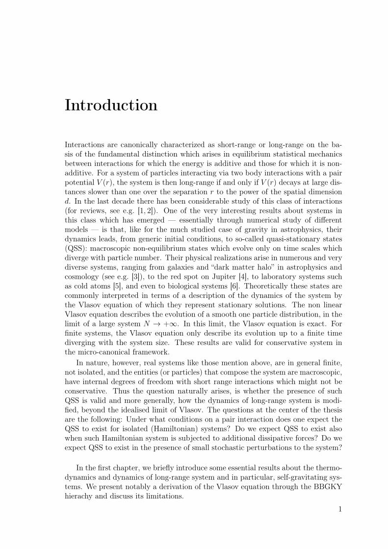
Interactions are canonically characterized as short-range or long-range on the ba-sis of the fundamental distinction which arises in equilibrium statistical mechanicsbetween interactions for which the energy is additive and those for which it is non-additive. For a system of particles interacting via two body interactions with a pairpotential V (r), the system is then long-range if and only if V (r) decays at large dis-tances slower than one over the separation r to the power of the spatial dimensiond. In the last decade there has been considerable study of this class of interactions(for reviews, see e.g. [1, 2]). One of the very interesting results about systems inthis class which has emerged — essentially through numerical study of differentmodels — is that, like for the much studied case of gravity in astrophysics, theirdynamics leads, from generic initial conditions, to so-called quasi-stationary states(QSS): macroscopic non-equilibrium states which evolve only on time scales whichdiverge with particle number. Their physical realizations arise in numerous and verydiverse systems, ranging from galaxies and “dark matter halo” in astrophysics andcosmology (see e.g. [3]), to the red spot on Jupiter [4], to laboratory systems suchas cold atoms [5], and even to biological systems [6]. Theoretically these states arecommonly interpreted in terms of a description of the dynamics of the system bythe Vlasov equation of which they represent stationary solutions. The non linearVlasov equation describes the evolution of a smooth one particle distribution, in thelimit of a large system N ! +1. In this limit, the Vlasov equation is exact. Forfinite systems, the Vlasov equation only describe its evolution up to a finite timediverging with the system size. These results are valid for conservative system inthe micro-canonical framework.
In nature, however, real systems like those mention above, are in general finite,not isolated, and the entities (or particles) that compose the system are macroscopic,have internal degrees of freedom with short range interactions which might not beconservative. Thus the question naturally arises, is whether the presence of suchQSS is valid and more generally, how the dynamics of long-range system is modi-fied, beyond the idealised limit of Vlasov. The questions at the center of the thesisare the following: Under what conditions on a pair interaction does one expect theQSS to exist for isolated (Hamiltonian) systems? Do we expect QSS to exist alsowhen such Hamiltonian system is subjected to additional dissipative forces? Do weexpect QSS to exist in the presence of small stochastic perturbations to the system?
In the first chapter, we briefly introduce some essential results about the thermo-dynamics and dynamics of long-range system and in particular, self-gravitating sys-tems. We present notably a derivation of the Vlasov equation through the BBGKYhierachy and discuss its limitations.
1

INTRODUCTION
In a second chapter, we explore the conditions on a pair interaction for the va-lidity of the Vlasov equation to describe the dynamics of an interacting N particlesystem in the large N limit. Using a coarse-graining in phase space of the exactKlimontovich equation for the N particle system, we evaluate, neglecting correla-tions of density fluctuations, the scalings with N of the terms describing the correc-tions to the Vlasov equation for the coarse-grained one particle phase space density.Considering a generic interaction with radial pair force F (r), with F (r) ⇠ 1/r� atlarge scales, and regulated to a bounded behaviour below a “softening” scale ", wefind that there is an essential qualitative difference between the cases � < d and� > d, i.e., depending on the the integrability at large distances of the pair force. Inthe former case, the corrections to the Vlasov dynamics for a given coarse-grainedscale are essentially insensitive to the softening parameter ", while for � > d theamplitude of these terms is directly regulated by ", and thus by the small scaleproperties of the interaction. This corresponds to a simple physical criterion for abasic distinction between long-range (� d) and short range (� > d) interactions,different to the canonical one (� d + 1 or � > d + 1 ) based on thermodynamicanalysis. This alternative classification, based on purely dynamical considerations,is relevant notably to understanding the conditions for the existence of so-calledquasi-stationary states in long-range interacting systems. This chapter follows veryclosely the content of an article submitted to Physical Review E [7].
In a third chapter, which is an extended report on the study of which the high-light results were published in Physical Review Letters [8], we consider long-rangeinteracting systems subjected to additional dissipative forces. Using an appropriatemean-field kinetic description, we show that models with dissipation due to a vis-cous damping or due to inelastic collisions admit “scaling quasi-stationary states”,i.e., states which are quasi-stationary in rescaled variables. A numerical study of onedimensional self-gravitating systems confirms both the relevance of these solutions,and gives indications of their regime of validity in line with theoretical predictions.We underline that the velocity distributions never show any tendency to evolvetowards a Maxwell-Boltzmann form.
In the last chapter, which is a report on work in progress (and not yet published),we study two different toy models to explore how different kinds of stochastic per-turbation affect the dynamics of long-range interaction system, and, in particular,the QSSs which are characteristic of them. In the models used, both extensions ofthe model with inelastic collision of the previous chapter, the perturbation is asso-ciated with the collision events, which can lead to gain or a loss of kinetic energy.For a first model, the collision are built such that on average over the realizations,the total energy in conserved, and in a second model, they are such that the systemrelax to a state where the loss and the gain of energy balance. For both modelsthe perturbation drives the system to evolve, through a family of QSS, into a non-equilibrium stationary state. This final stationary distribution, which is itself also astable QSS, does not depend on the initial conditions but does depend strongly onthe microscopic detail of the perturbation.
Thus our conclusion is that QSS appear to be a very robust feature of long-range systems, and their existence or occurrence is not conditioned in general onthe idealization that the system is isolated.
2

Chapter 1
Introduction to long-range
interacting systems
1 Thermodynamics and dynamics
1.1 Definition
A long-range interacting system is usually defined as collection of entities (particles,spins, vortices,..) interacting with a pair potential which is not integrable at r !+1. As we explain below, these systems have the property of non additivity andthis property has strong consequences on the equilibrium statistical mechanics ofthe system.
To be a little more precise, and explain the origin of this definition let us estimate,in d dimensions, the potential energy ep of a particle placed at the center of sphereof radius R enclosing a volume V = ⌦dR
d where other particles are homogeneouslydistributed (where ⌦d is the appropriate constant for the dimension d). We considerthat particles interact with a power low central potential defined as
�(r) =g
|r|↵ , (1.1)
where g is the coupling constant of the model and ↵ the exponent characterizingthe interaction. We use a cut-off ", to regulate the possible short-scale divergence of� (for ↵ > 0) i.e. we do not consider the contributions to ep from particles locatedwithin a sphere of small radius " around the particle considered. We will returnbelow to this point to discuss further the role and necessity for this cut-off. In thecontinuous limit, the individual potential energy is expressed as:
ep =
Z R
"
ddrn0
g
r↵=
0
J⌦d
Z R
"
drr1��=
n0
g⌦d
d� ↵(Rd�↵ � "d�↵
) , if ↵ 6= d
where n0
=
NV
is the particle density. The following distinction then follows.
• For ↵ > d, the potential is integrable: the energy per particle remains finite ifwe take R ! +1 at fixed n
0
(i.e. the usual thermodynamic limit). In thislimit, the contribution to ep due to far away particles is negligible comparedto that due to the ones close to it. Further, the total energy, E =
RVddrn
0
ep,
3
CHAPTER 1. INTRODUCTION TO LONG-RANGE INTERACTING SYSTEMS
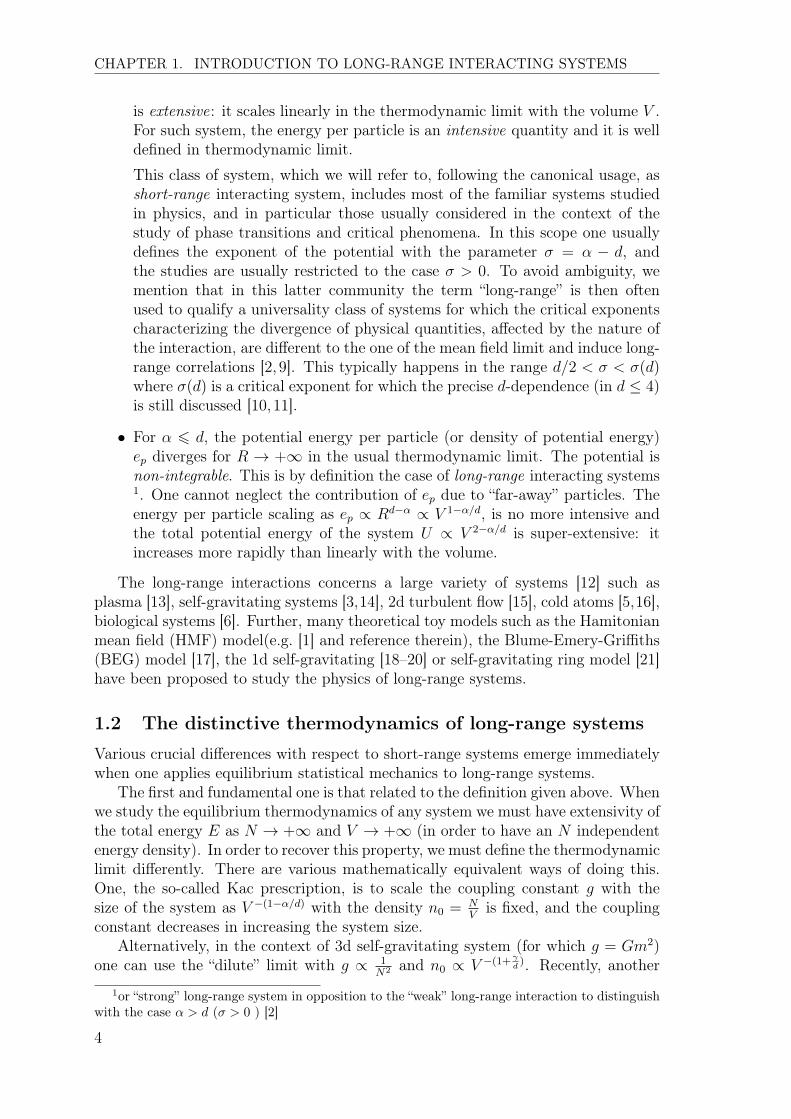
is extensive: it scales linearly in the thermodynamic limit with the volume V .For such system, the energy per particle is an intensive quantity and it is welldefined in thermodynamic limit.This class of system, which we will refer to, following the canonical usage, asshort-range interacting system, includes most of the familiar systems studiedin physics, and in particular those usually considered in the context of thestudy of phase transitions and critical phenomena. In this scope one usuallydefines the exponent of the potential with the parameter � = ↵ � d, andthe studies are usually restricted to the case � > 0. To avoid ambiguity, wemention that in this latter community the term “long-range” is then oftenused to qualify a universality class of systems for which the critical exponentscharacterizing the divergence of physical quantities, affected by the nature ofthe interaction, are different to the one of the mean field limit and induce long-range correlations [2, 9]. This typically happens in the range d/2 < � < �(d)where �(d) is a critical exponent for which the precise d-dependence (in d 4)is still discussed [10,11].
• For ↵ 6 d, the potential energy per particle (or density of potential energy)ep diverges for R ! +1 in the usual thermodynamic limit. The potential isnon-integrable. This is by definition the case of long-range interacting systems1. One cannot neglect the contribution of ep due to “far-away” particles. Theenergy per particle scaling as ep / Rd�↵ / V 1�↵/d, is no more intensive andthe total potential energy of the system U / V 2�↵/d is super-extensive: itincreases more rapidly than linearly with the volume.
The long-range interactions concerns a large variety of systems [12] such asplasma [13], self-gravitating systems [3,14], 2d turbulent flow [15], cold atoms [5,16],biological systems [6]. Further, many theoretical toy models such as the Hamitonianmean field (HMF) model(e.g. [1] and reference therein), the Blume-Emery-Griffiths(BEG) model [17], the 1d self-gravitating [18–20] or self-gravitating ring model [21]have been proposed to study the physics of long-range systems.
1.2 The distinctive thermodynamics of long-range systems
Various crucial differences with respect to short-range systems emerge immediatelywhen one applies equilibrium statistical mechanics to long-range systems.
The first and fundamental one is that related to the definition given above. Whenwe study the equilibrium thermodynamics of any system we must have extensivity ofthe total energy E as N ! +1 and V ! +1 (in order to have an N independentenergy density). In order to recover this property, we must define the thermodynamiclimit differently. There are various mathematically equivalent ways of doing this.One, the so-called Kac prescription, is to scale the coupling constant g with thesize of the system as V �(1�↵/d) with the density n
0
=
NV
is fixed, and the couplingconstant decreases in increasing the system size.
Alternatively, in the context of 3d self-gravitating system (for which g = Gm2)one can use the “dilute” limit with g / 1
N2 and n0
/ V �(1+
�
d
). Recently, another1or “strong” long-range system in opposition to the “weak” long-range interaction to distinguish
with the case ↵ > d (� > 0 ) [2]
4
CHAPTER 1. INTRODUCTION TO LONG-RANGE INTERACTING SYSTEMS
scaling limit have been proposed in [22], the author propose a scaling limit for aself-gravitating system of hard spheres keeping constant the packing fraction.
Such a procedure restores the extensivity of the system; but nevertheless it re-mains non-additive i.e. the interaction energy of any part of the system with thewhole is not negligible with respect to the internal energy of the given part. Wedetail further in the next section this point and discuss its particular consequenceon the thermodynamics of long-range interacting systems.
A second issue which present itself immediately in analysing the equilibrium ther-modynamics of long-range systems is one which occurs for any attractive power lawpotential 1/r↵ with ↵ > 0. An interesting example, of this class of system includes,3d self-gravitating system whose thermodynamics is discussed further below. Justas for short-range systems whose exponents are also positive, such systems requirea regularisation at short distances to avoid collapse. Indeed if only two particles getcloser and closer one another, these two can make the potential energy of the entiresystem diverges to �1. The total energy being conserved, the kinetic energy of thesystem increases and the number of accessible states diverges in the velocity space.As a consequence, the micro-canonical partition function:
⌦(E) /Z
ddNxddNx�(E �H({xN ,vN})), (1.2)
which enumerates the number of microscopic states at a fixed energy E, diverges ifand only if N � 3 [23]. Moreover, the Boltzmann entropy
S(E) = kBln(⌦(E)) (1.3)
increases without bound as well; and without entropy maxima an equilibrium statecannot exist.
Therefore the introduction of a short-scale regulator is needed to bound belowthe potential energy. For spin systems defined on a lattice like the BEG models,this divergence is naturally regulated. For particle system, one may also considerfermions and made use of the Pauli exclusion principle as it a been done for a self-gravitating system [24], or again hard core particle as in [22]. In general, an ad-hoccut-off is added to bound the potential. We will discuss in chapter 2, how the largescale dynamics of a long-range system is affected by the choice of the small scaleregularisation.
Finally, just as for systems, the number of accessible states (Eq. (1.2)) will alsodiverge if the system is not confined, unless the pair potential is attractive enoughto “self-confine” the particles (as is the case, as we will see, for example for 1d self-gravitational system). Thus, one has often to impose periodic boundary condition,or confine the system in a box.
Non-additivity
The central difficulty, as we have underlined, characteristic of any long-range system,arises from the non-integrable nature of the long-range potential at large distance.If the Kac prescription restore the extensivity of the long-range interacting system
5

CHAPTER 1. INTRODUCTION TO LONG-RANGE INTERACTING SYSTEMS
Figure 1.1: Schematic picture of a system partitioned into two parts, in red is theboundary between the two subsystems.
and makes possible the existence of a thermodynamic limit, such system, however,remains non-additive. Let us consider first a short-range system, and partition thesystem in two subsystems 1 and 2 (as in Fig. 1.1) of respective energies E
1
andE
2
. The total energy of the system is given by E = E1
+ E2
+ E12
where E12
isthe energy of interaction between the two subsystems. For a short-range system, aparticle, situated close to the boundary between the two subsystems, interacts onlywith particles close to the other side of the boundary, while the interactions withthe particle in the bulk of the other subsystem are negligible. Therefore, the energyof interaction E
12
is proportional to the surface of contact between the two volumes.Then, in thermodynamic limit E
12
becomes negligible with respect to E1
and E2
and in this limit E = E1
+ E2
: the system is additive.On the contrary for a long-range system, any particle in one of the two subsystem
interacts with every single particles of the other subsystem. The energy of interactionE
12
is no longer negligible at the thermodynamic limit and E 6= E1
+ E2
.
Ensemble inequivalence
An important result of the statistical mechanics built for short-range systems is theequivalence of statistical ensemble which means that mean quantities converge to thesame value in the thermodynamic limit. Indeed this result allows one, for example,to study the phase diagram of a system in the ensemble of its choice. Short-rangeinteracting systems are usually study in the canonical ensemble, because calculationsare easier than in the micro-canonical ensemble. The latter is essential, however,at a fundamental level to construct the canonical ensemble [1, 12, 25]. We nowbriefly recall the latter to highlight how the distinction on the basis of additivity isimportant between short-range and long-range interacting systems.
One considers an isolated system with energy E and divides it into two parts:a “small” part of energy E
1
that will be the system we want to study the statisticsand a “large” part of energy E
2
� E1
playing the role of the thermal bath. Theprobability that the system 1 has an energy E
1
, for an additive system is given by
p(E1
) =
1
⌦(E)
Z�(E
1
+ E2
� E)⌦
2
(E2
)dE2
(1.4)
=
⌦
2
(E � E1
)
⌦(E)
(1.5)
6
CHAPTER 1. INTRODUCTION TO LONG-RANGE INTERACTING SYSTEMS
where ⌦2
is the micro-canonical partition function of the subsystem defined similarlythan ⌦ in Eq. (1.2). Then, using the expression of the micro-canonical entropy(Eq. (1.3)), and Taylor expanding with E >> E
1
, we have:
p(E1
) =
1
⌦(E)
e1
k
B
S(E�E1) (1.6)
=
1
⌦(E)
e1
k
B
S(E)+
1k
B
E1@S
@E
|E
+o(E21) (1.7)
' 1
Ze��E1 , (1.8)
with Z the partition function and where we have define the inverse temperature ofthe bath:
� =
1
kB
@S
@E
����E
. (1.9)
We thus recover the canonical distribution for the system 1. We clearly see(Eq. (1.4)) that the property of additivity is crucial to build the canonical ensemble.For a short-range system, of course, this construction become strictly valid at thethermodynamic limit. For a long-range system, this construction is not mathemat-ically valid even at the thermodynamic limit. Hence non additive systems, and inparticular long-range one, are expect to have a very particular behaviour when theyare in contact with a thermal reservoir. The micro-canonical ensemble is clearlywell defined and the only issue is how to take the limit N ! +1. There is noformal barrier to calculate, for long-range system, in the canonical ensemble, butits physical meaning must be scrutinized carefully. For many long-range model, thecalculation have been done in both ensembles, defining formally the free energy2
and the canonical partition function.For some long-range systems, it turns out that the equilibrium results in both
ensembles are actually equivalent. This is, for example, the case of the 1d self-gravitating system [20, 26, 27], or of the HMF model [1]. For these two models,the thermal equilibrium can be work out in both ensembles and the equilibriumstatistical mechanics is well defined. Moreover the dynamical studies have shownthat the two long-range models effectively relax to the predicted equilibria whichhas, in particular, a Gaussian velocity distribution [1, 28].
However for other long-range systems, like in 3d self-gravity [27, 29] or for BEGmodel [17], the calculation shows that the ensembles are not equivalent: the equilib-rium solution found in maximising the entropy in the micro-canonical ensemble, orin minimizing the free energy in the canonical ensemble, are different in a substantialregion of the space of the parameters.
Non concave entropy and negative specific heat
It has been understood and shown rigorously [17,30] that the fundamental explana-tion of the non-equivalence of ensemble is the presence of a non-concave region inthe entropy-energy curve in the micro-canonical ensemble.
2We note that the Kac prescription (or other equivalent) to make the energy extensive is im-portant to define the free energy F = E � TS. Indeed as the entropy S / N , one needs E / N sothat both term defining F have the same scaling with N .
7
CHAPTER 1. INTRODUCTION TO LONG-RANGE INTERACTING SYSTEMS
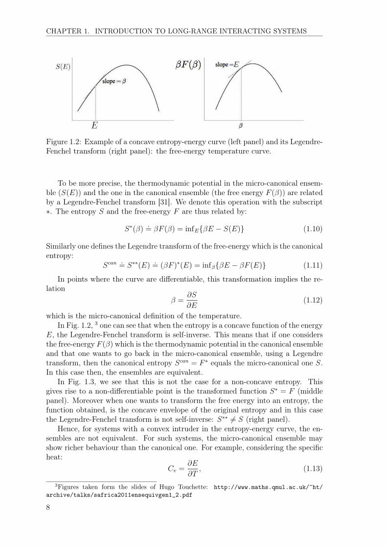
Figure 1.2: Example of a concave entropy-energy curve (left panel) and its Legendre-Fenchel transform (right panel): the free-energy temperature curve.
To be more precise, the thermodynamic potential in the micro-canonical ensem-ble (S(E)) and the one in the canonical ensemble (the free energy F (�)) are relatedby a Legendre-Fenchel transform [31]. We denote this operation with the subscript⇤. The entropy S and the free-energy F are thus related by:
S⇤(�)
.= �F (�) = infE{�E � S(E)} (1.10)
Similarly one defines the Legendre transform of the free-energy which is the canonicalentropy:
Scan .= S⇤⇤
(E)
.= (�F )
⇤(E) = inf�{�E � �F (E)} (1.11)
In points where the curve are differentiable, this transformation implies the re-lation
� =
@S
@E(1.12)
which is the micro-canonical definition of the temperature.In Fig. 1.2, 3 one can see that when the entropy is a concave function of the energy
E, the Legendre-Fenchel transform is self-inverse. This means that if one considersthe free-energy F (�) which is the thermodynamic potential in the canonical ensembleand that one wants to go back in the micro-canonical ensemble, using a Legendretransform, then the canonical entropy Scan
= F ⇤ equals the micro-canonical one S.In this case then, the ensembles are equivalent.
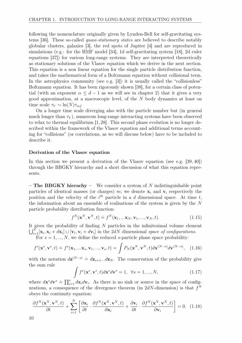
In Fig. 1.3, we see that this is not the case for a non-concave entropy. Thisgives rise to a non-differentiable point is the transformed function S⇤
= F (middlepanel). Moreover when one wants to transform the free energy into an entropy, thefunction obtained, is the concave envelope of the original entropy and in this casethe Legendre-Fenchel transform is not self-inverse: S⇤⇤ 6= S (right panel).
Hence, for systems with a convex intruder in the entropy-energy curve, the en-sembles are not equivalent. For such systems, the micro-canonical ensemble mayshow richer behaviour than the canonical one. For example, considering the specificheat:
Cv =@E
@T, (1.13)
3Figures taken form the slides of Hugo Touchette: http://www.maths.qmul.ac.uk/~ht/archive/talks/safrica2011ensequivgen1_2.pdf
8

CHAPTER 1. INTRODUCTION TO LONG-RANGE INTERACTING SYSTEMS
Figure 1.3: Sketch of a non concave entropy S verus the energy E (left panel), itsLegendre transform S⇤
(�) = F (�)(middle panel), and the Legendre-Fenchel trans-form of the free-energy (full line, right panel) F ⇤
(E) = S⇤⇤(E) 6= S(E).
related to the entropy by the relation
@2S
@E2
= � 1
T 2
1
Cv
. (1.14)
In the region where the curve S(E) is convex, the second derivative is positive,and then Cv < 0. A counter intuitive consequence is that when ones increase theenergy of the system, it may cool down. Moreover non-concave entropy is related toa rich variety of phenomena such as the appearance of first-order phase transitionsas well as metastable states in the canonical ensemble [32] and also the possibilityof ergodicity breaking [33]. In [32] the authors propose a complete classification ofmicro-canonical phase transitions in long-range interacting, their link to canonicalones, and of the possible situations of ensemble non-equivalence.
The results from equilibrium statistical mechanics aim to predict the final macro-scopic state of the system. However, to determine if the system does effectively relaxto such states, the dynamics of the system has to be studied.
1.3 Dynamics of long-range systems
Qualitative description
In a long-range interacting, the contribution to the force acting on a given particlecannot be approximated by that due to particles in its neighbourhood. The re-sultant strong coupling of numerous degrees of freedom allows important collectiveeffects in the many body dynamics. The detailed motion of every single particle is,in practice, inaccessible except by numerical simulation, and what we attempt todescribe analytically are the behaviours of macroscopic quantities such as the oneparticle phase space density.
Studies of the dynamics of long-range interacting system (e.g. [34, 35] or for re-view [1]) – both numerical and theoretical – have lead to the conclusion that it ischaracterized broadly by two distinct regimes: starting from a generic initial condi-tion, a long-range system of many bodies evolves first, on a time scale (⌧mf or ⌧dyn)characterizing the evolution under the mean field, towards a macroscopically station-ary state which does not coincide with the equilibria derived from the equilibriumthermodynamics. This early time process is often referred to as “violent relaxation”
9
CHAPTER 1. INTRODUCTION TO LONG-RANGE INTERACTING SYSTEMS
following the nomenclature originally given by Lynden-Bell for self-gravitating sys-tems [36]. These so-called quasi-stationary states are believed to describe notablyglobular clusters, galaxies [3], the red spots of Jupiter [4] and are reproduced insimulations (e.g.: for the HMF model [34], 1d self-gravitating system [18], 2d eulerequations [37]) for various long-range systems. They are interpreted theoreticallyas stationary solutions of the Vlasov equation which we derive in the next section.This equation is a non linear equation for the single particle distribution function,and takes the mathematical form of a Boltzmann equation without collisional term.In the astrophysics community (see e.g. [3]) it is usually called the “collisionless”Boltzmann equation. It has been rigorously shown [38], for a certain class of poten-tial (with an exponent ↵ d � 1 as we will see in chapter 2) that it gives a verygood approximation, at a macroscopic level, of the N body dynamics at least ontime scale ⌧V ⇠ ln(N)⌧mf
On a longer time scale diverging also with the particle number but (in generalmuch longer than ⌧V ), numerous long-range interacting systems have been observedto relax to thermal equilibrium [1,28]. This second phase evolution is no longer de-scribed within the framework of the Vlasov equation and additional terms account-ing for “collisions” (or correlations, as we will discuss below) have to be included todescribe it.
Derivation of the Vlasov equation
In this section we present a derivation of the Vlasov equation (see e.g. [39, 40])through the BBGKY hierarchy and a short discussion of what this equation repre-sents.
– The BBGKY hierachy – We consider a system of N indistinguishable pointparticles of identical masses (or charges) m; we denote xi and vi respectively theposition and the velocity of the ith particle in a d dimensional space. At time t,the information about an ensemble of realisations of the system is given by the Nparticle probability distribution function:
fN(x
N ,vN , t).= fN
(x
1
, ...xN ,v1
, ...,vN , t). (1.15)
It gives the probability of finding N particles in the infinitesimal volume elementSNi=1
[xi,xi + dxi] [ [vi,vi + dvi] in the 2dN dimensional space of configurations.For s = 1, ..., N , we define the reduced s-particle phase space probability:
f s(x
s,vs, t).= f s
(x
1
, ...xs,v1
, ...,vs, t) =
ZPN(x
N ,vN , t)dx(N�s)dv(N�s), (1.16)
with the notation dz(N�s) .= dzs+1
...dzN . The conservation of the probability givethe sum rule Z
f s(x
s,vs, t)dxsdvs= 1, 8s = 1, ..., N, (1.17)
where dxsdvs .=
Qsi=1
dxidvi. As there is no sink or source in the space of config-urations, a consequence of the divergence theorem (in 2dN -dimension) is that fN
obeys the continuity equation:
@fN(x
N ,vN , t)
@t+
NX
i=1
@xi
@t· @f
N(x
N ,vN , t)
@xi
+
@vi
@t· @f
N(x
N ,vN , t)
@vi
�= 0. (1.18)
10

CHAPTER 1. INTRODUCTION TO LONG-RANGE INTERACTING SYSTEMS
where · denotes the scalar product and we use the notation @@z
⌘ rz
for the gradient.Now if the N particles interact via a pair potential �(|x� y|), the Hamiltonian
of this system is given by:
H =
1
2
mNX
i=1
v
2
i +
NX
i=0
X
j>i
�(|xi � xj|). (1.19)
and we implicitly assume a regularization at r ! 0, if needed (we will come back tothis crucial point). For a Hamiltonian system, the equations of motion are:
@xi
@t=
@H
@mvi
= vi (1.20)
@vi
@t= �@H
@xi
= �NX
i 6=j
@�(|xi � xj|)@xi
.
Inserting then in Eq. (1.18), we obtain the Liouville equation:
@fN(x
N ,vN , t)
@t+
NX
i=1
vi · @f
N(x
N ,vN , t)
@xi
(1.21)
�X
j 6=i
@�(|xi � xj|)@xi
· @fN(x
N ,vN , t)
@vi
#= 0
Integrating Eq. (1.21) over velocities and position of N � s particle we obtain theso called Bogoliubov-Born-Green-Kiriwood-Yvon (BBGKY) hierarchy and assumingthat fN ! 0 when |vi|, |xi| ! +1, we have 8s = 1...N :
@f s
@t+
sX
i=1
vi · @fs
@xi
�sX
i 6=j
@�(|xi � xj|)@xi
· @fs
@vi
(1.22)
= (N � s)
sX
i=1
Zdxs+1
dvs+1
@�(xi � xs+1
)
@xi
· @fs+1
@vi
,
where the factor (N � s) comes from integrals over (assumed) indistinguishableparticles. One sees that each equation for f s is coupled to the next one for f s+1.This set of equations contain exactly the same information as the Liouville equationEq. (1.21).
– The Vlasov equation – It takes the from of a closed equation for the equationfor the single particle phase space density f 1
(x
1
,v1
). In order to obtain it, one needsto close the BBGKY hierarchy at the level of f 1 with assumptions that we discusshere.
11
CHAPTER 1. INTRODUCTION TO LONG-RANGE INTERACTING SYSTEMS
The first equation of the BBGKY hierachy (Eq. (1.22)) is:
@f 1
(x
1
,v1
, t)
@t+ v
1
· @f1
(x
1
,v1
, t)
@x1
(1.23)
� (N � 1)
Z@�(|x
1
� x
2
|)@x
1
· @f2
(x
1
,x2
,v1
,v2
, t)
@v1
dx2
dv2
= 0.
Now let us decompose the two-body distribution function:
f 2
(x
1
,x2
,v1
,v2
, t) = f 1
(x
1
,v1
, t)f 1
(x
2
,v2
, t) + g(x1
,x2
,v1
,v2
, t), (1.24)
where g is the connected or irreducible, two-point correlation function. To close thehierarchy i.e. to obtain an equation for the single particle distribution function f 1
only, we simply assume that g(x1
,x2
,v1
,v2
, t) = 0. In other words, we assume thatthe pair correlation and higher order correlations are negligible, or suppose whatBoltzmann called molecular chaos in the context of a dilute gas. If we supposethe initial condition, indeed, satisfies, fN
(x
1
,x2
,v1
,v2
, 0) =QN
i=1
f 1
(xi,vi, 0), onemay ask until which time t this assumption is a realistic description of the system.This property for a N body system to remains uncorrelated during its dynamicalevolution is called propagation of chaos. With this assumption, and in the limit oflarge N , the last term can be rewritten:
(N � 1)
@
@v1
Z@�
@x1
f 2
(x
1
,x2
,v1
,v2
, t)dx2
dv2
' @f 1
@v1
· @¯�[f 1
](x
1
, t)
@x1
, (1.25)
where the mean field potential ¯� is:
�[f 1
](x
1
, t) = (N � 1)
Z�(|x
1
� x
2
|)f 1
(x
2
,v2
, t)dx2
dv2
. (1.26)
Let us now take the limit N ! +1 at fixed f1
(x, v) (i.e. increasing the particledensity f = Nf 1 in phase space). We can obtain consistently an N independent limitif we take (N � 1)� ⇠ Cst, in other words, rescale the coupling of the interaction by1
N. This correspond to the Kac prescription, discussed earlier, in which the coupling
is scaled in order to obtain an extensive energy4. Indeed E ⇠ N2� ⇠ N when� ⇠ 1
N. We obtain then the Vlasov equation in its dimensionless form:
@f 1
(x,v, t)
@t+ v · @f
1
(x,v, t)
@x� @ ¯�[f 1
](x, t)
@x· @f
1
(x,v, t)
@v= 0, (1.27)
with the mean field potential:
�[f 1
](x, t) =
Z�(|x� x
0|)f 1
(x
0,v0, t)dx0dv0. (1.28)
For this equation, we recall that f 1 represents the single particle probability distri-bution normalised to unity.
4Here we assumed the system size is fixed, then this scaling is proportional to V as consideredabove.
12
CHAPTER 1. INTRODUCTION TO LONG-RANGE INTERACTING SYSTEMS
One may alternatively rewrite the equation in terms of the mass density in thephase space f(x,v, t) = Mf 1
(x,v, t). In the limit of large N with a potential scalingas � ⇠ 1
Nand the mass m ⇠ 1
N, such that the total mass M = mN remains fixed,
we obtain the (dimensional) Vlasov equation:
@f
@t+ v · @f
@x� @�[f ]
@x· @f@v
= 0, (1.29)
with the mean field potential:
�[f ](x) =1
M
Z�(|x� x
0|)f(x0,v0, t)dx0dv0. (1.30)
In this last expression Eq. (1.29), we see that the Vlasov equation is a continuousdescription of the particle dynamics in the limit of an infinite number of infinitelylight particles. The mean field limit can thus be described as a fluid limit. It canbe shown that the Vlasov dynamics has an infinite number of conserved quantitiescalled Casimir invariants:
C[f ] =
ZH(f(x,v, t))dxdv, (1.31)
where H is any function. The Vlasov equation admits an infinite number of sta-tionary solutions [1,41]. The continuous dynamics described by the Vlasov equationis a major subject of research in itself and also addressed in various different fields(astrophysics, plasma physics,..). Indeed, it is a complex non-linear equation and itsresolution, just as the N body dynamics, is very costly numerically (and even moreso because it is an equation for the 2d dimensional phase space).
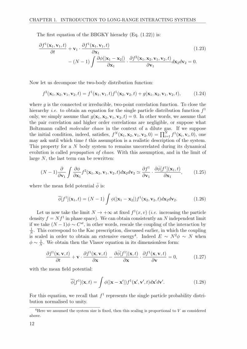
This standard derivation, just given, of the Vlasov equation is not completelysatisfactory: indeed, it remains quite unclear in what circumstances the essentialapproximation made of neglecting correlation will apply to a system in the classof Hamiltonian systems. It is known that for hard-core or short-range potential(e.g. van der Waals), the system is not well described by the Vlasov equation butinstead by the Boltzmann equation with a collision term accounting for short-rangecorrelations. Looking more carefully at the derivation, we have implicitly supposed,for example in Eq. (1.23), that integrals are not divergent. Also, for a system forwhich a short-scale regulation of the pair force is needed, the present derivationdoes not allows one to understand the effects of this regularization. We have simplystated that if we make certain approximations we obtain this equation, but have notjustified the approximation with any rigour.
One of the aims of the chapter 2 of the thesis is precisely to improve our under-standing of the range of application of the Vlasov equation.
Violent relaxation: the establishment of QSS
As we have stated, studies of long-range systems show that they evolve genericallythrough a phase of violent relaxation and organise in a QSS. Both this dynamicalevolution and the QSSs are believed to be described by the Vlasov equation andthe QSSs are stationary states of the latter5. As noted above, there are an infinite
5This statement “seems”,a priori, paradoxical because the macroscopic evolution described isirreversible, and one can easily check that the Vlasov equation is time reversible. The Vlasov
13
CHAPTER 1. INTRODUCTION TO LONG-RANGE INTERACTING SYSTEMS
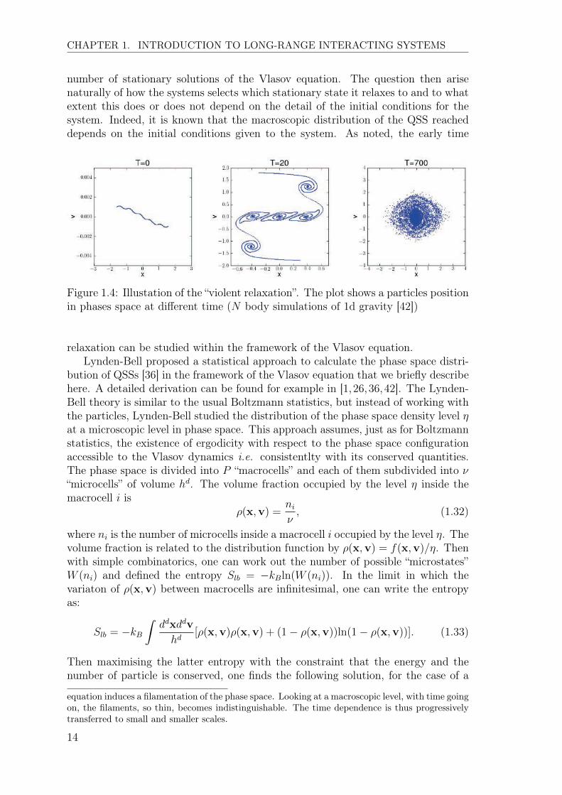
number of stationary solutions of the Vlasov equation. The question then arisenaturally of how the systems selects which stationary state it relaxes to and to whatextent this does or does not depend on the detail of the initial conditions for thesystem. Indeed, it is known that the macroscopic distribution of the QSS reacheddepends on the initial conditions given to the system. As noted, the early time
Figure 1.4: Illustation of the “violent relaxation”. The plot shows a particles positionin phases space at different time (N body simulations of 1d gravity [42])
relaxation can be studied within the framework of the Vlasov equation.Lynden-Bell proposed a statistical approach to calculate the phase space distri-
bution of QSSs [36] in the framework of the Vlasov equation that we briefly describehere. A detailed derivation can be found for example in [1,26,36,42]. The Lynden-Bell theory is similar to the usual Boltzmann statistics, but instead of working withthe particles, Lynden-Bell studied the distribution of the phase space density level ⌘at a microscopic level in phase space. This approach assumes, just as for Boltzmannstatistics, the existence of ergodicity with respect to the phase space configurationaccessible to the Vlasov dynamics i.e. consistentlty with its conserved quantities.The phase space is divided into P “macrocells” and each of them subdivided into ⌫“microcells” of volume hd. The volume fraction occupied by the level ⌘ inside themacrocell i is
⇢(x,v) =ni
⌫, (1.32)
where ni is the number of microcells inside a macrocell i occupied by the level ⌘. Thevolume fraction is related to the distribution function by ⇢(x,v) = f(x,v)/⌘. Thenwith simple combinatorics, one can work out the number of possible “microstates”W (ni) and defined the entropy Slb = �kBln(W (ni)). In the limit in which thevariaton of ⇢(x,v) between macrocells are infinitesimal, one can write the entropyas:
Slb = �kB
Zddxddv
hd[⇢(x,v)⇢(x,v) + (1� ⇢(x,v))ln(1� ⇢(x,v))]. (1.33)
Then maximising the latter entropy with the constraint that the energy and thenumber of particle is conserved, one finds the following solution, for the case of a
equation induces a filamentation of the phase space. Looking at a macroscopic level, with time goingon, the filaments, so thin, becomes indistinguishable. The time dependence is thus progressivelytransferred to small and smaller scales.
14
CHAPTER 1. INTRODUCTION TO LONG-RANGE INTERACTING SYSTEMS
single of a single level of density:
flb(x,v) =⌘
1 + e�(e(x,v)�µ), (1.34)
where e(x,v) =
1
2
mv
2
+ m¯�(x) is the single particle energy, and � and µ arethe Lagrange multipliers related to the two constraints (interpreted as the “inversetemperature” and “the chemical potential”).
It has been found through numerical studies that the LB theory can provide avery accurate description of the relaxed QSS, in certain parts of the initial conditionspace of specific models: in the HMF [43], and in model with 2d vortices [44].However more generally it is clear that the Lynden-Bell theory is inadequate, inparticular for system starting from state very far from a QSS. This have been shownfor the 1d self-gravitating system [18,42] and for the HMF [45]. In 3d gravity notably,an ubiquitous property of QSS is to have non-isotropic velocity distribution and evennon isotropic spatial distribution arising from spherically symmetric initial conditionand such state are not predicted by the theory of Lynden-Bell.
The main reason why the theory does not work for any initial condition is thatit supposes a mixing and ergodicity in the phase space, and these two requirementsare in general not verified by long-range systems. Other approaches to predict theproperty of QSS have been explored notably by [42]. The model constructed by theauthors, have given, in various cases (HMF, 1d self-gravity and others), frameworkto understand well these states based on an analysis of the dynamics of the phase ofviolent relaxation. In summary, during violent relaxation, the mean field potentialis characterised by quasi-periodic oscillations. These breathing modes have beennotably shown within the framework of kinetic equation (beyond Vlasov), in thecontext of cold-atoms [5]. It is possible, therefore, for some particles to enter inresonance with the oscillations and gain large amounts of energy at the expenseof the collective motion. This process is known as Landau damping. The Landaudamping diminishes the amplitude of the oscillations and leads to the formation ofa halo of highly energetic particles which surround the high density core [19]. Thephenomenon of Landau damping, first described heuristically by Landau [46] in thecontext of plasma physics has been recently formulated rigorously in the famouswork of Villani and Mouhot [47,48] in particular limits.
Evolution of QSS: beyond Vlasov equation
The state attained by a long-range system is a quasi -stationary state because, fora large but finite N particle system, a second relaxation occurs, on a much longertime scale ⌧R eventually bringing the system toward the thermal equilibrium (if welldefined). The time scale, in general also diverges with N and its precise dependencevaries with the model.
For 3d self-gravitating systems, Chandrasekahar [49] estimated the time scale forthermal relaxation to be ⌧R ⇠ N/ln(N)⌧dyn. His calculation, based on an estimationof the number of “collisions” a test particle has in the time it crosses the system(⇠ ⌧dyn). This estimate of the relaxation rate due to two-body collisions (for 3dgravity) has been generalised to a broad class of pair interactions in dimensionsd � 2 in [50]. The latter calculation also shows that the main contribution to this
15
CHAPTER 1. INTRODUCTION TO LONG-RANGE INTERACTING SYSTEMS
rate for a long-range system is due to small angle deflections (or “soft” collisions)rather than due to “hard” collisions giving large deflections.
While the mean field dominates the trajectories of particles, many small deflec-tions lead eventually to significant deviations from the collective dynamics. Thephysics of such“collisions” is not included into the Vlasov equation describing onlythe collective effects, and additional term can be derived to account for them.
One common approach is to add Fokker-Plank to the Vlasov equation [3, 14].To compute the diffusion coefficient, the microscopic detail of the mechanism ofcollision is needed with all the associated hypotheses underlying the calculation ofChandrasekar. This have been done notably in the context of 2d gravity in [51].
The Lennard-Balescu equation, coming from plasma physics, is another attemptto build such terms from a consistent derivation. To obtain it, one has to close theBBGKY hierarchy at the level of the two body correlation function f 2. In order to doso, one usually expands the pair density function as f 2
(z1
, z2
) = f(z1
)f(z2
)+g(z1
, z2
)
as discussed above (we use the simpler notation zi = (xi,vi) and f = f 1), and f 3 as
f 3
(z1
, z2
, z3
) = f(z1
)f(z2
)f(z3
) + f(z1
)g(z2
, z3
) (1.35)+ f(z
2
)g(z1
, z3
) + f(z3
)g(z1
, z3
) + h(z1
, z2
, z3
).
with h the connected three-point correlation function.Then assuming that h ⇠ 0 for large N , one obtains two coupled equation, closed
in f and g. Then solving formally the equation for g, it is possible to obtain, for anhomogeneous state (which is relevant in plasma physics but not for self-gravitatingsystem), an expression for the additional term of the Vlasov equation in f whichtake into account the finite N effects. The additional term take finally the formof Fokker-Planck terms with a diffusion coefficient which is a functional of f . Inpractice to solve this equation is difficult and it remains unclear whether it correctlydescribe the evolution of relaxation of the system.
1.4 Long-range systems with stochastic perturbations
The Vlasov equation applies to strictly conservative systems in a micro-canonicalframework, and the question inevitably arises of the robustness of QSSs, which arestationary solution of this equation, beyond this idealized limit.
In [52] the authors consider a long-range interacting system driven by exter-nal stochastic forces acting collectively on all the particles constituting the system.Given a long-range Hamiltonian H (Eq. (1.19)), they consider the following equationof motion:
qi =@H
@piand pi = �@H
@qi� ↵pi +
p↵⇠(qi, t), (1.36)
where ⇠(q, t) is a statistically homogeneous Gaussian stochastic force field ( or“noise”) with a zero mean and without temporal correlation i.e
h⇠(q, t)i = 0 and h⇠(qi, t)⇠(qj, t)i = C(|qi � qj|)�(t� t0), (1.37)
where ↵ controls the strength of the force and C is the (isotropic) correlation func-tion.
16

CHAPTER 1. INTRODUCTION TO LONG-RANGE INTERACTING SYSTEMS
Starting from a generalised Liouville equation for the N -particle distributionfunction fN (Eq. (1.15)), they derive a kinetic theory starting from a generalizedBBGKY hierarchy which takes the stochastic perturbation into account. Becausethe stochastic force is correlated in space it induces correlations on the system and,to treat this at a non-trivial level, the kinetic theory has to take into account theconnected pair correlation g between particle in the derivation the kinetic equation.To obtain Lennard-Balescu equation, their generalised BBGKY hierarchy is closed atthe level of g by neglecting the connected three-point and higher order correlationfunctions. They obtain thus a set of 2 equations, with both finite N effects andthe stochastic effect. Considering the limit N � 1 and N↵ � 1, in which thecharacteristic time ⌧stoch =
1
↵⌧dyn of the external perturbation is much shorter that
the one of the finite N effects ⌧fN ⇠ N⌧dyn, the author then treat the limit ↵ ⌧ 1.The authors able to show, in particular, that detail balance is respected (and thesystem evolved to a Gaussian velocity distribution) if and only if the noise is whitei.e. uncorrelated in space. In presence of correlated noise, the author shows that thesystem relaxes toward a non-equilibrium stationary state (NESS). The numericalsimulations of the HMF model reported in these article give not only very goodagreement with the kinetic theory developed for homogeneous state but also, forsome particular value of the parameter of the perturbation, the system exhibits avery interesting bistable behaviour: the system switches abruptly and intermittentlybetween a homogeneous and an inhomogeneous state.
In [53, 54] the authors consider a perturbation of the long-range dynamics witha diffusion process à la Langevin in order to attempt an operative description of acanonical ensemble for long-range interacting. There studies correspond to the onein [52] but for an uncorrelated noise. The author report also, in particular, that thesystem relaxes to non-equilibrium stationary state that are QSS.
In an other study [55] the HMF model is perturbed with a energy conserv-ing three-particle collision dynamics. At a given frequency, the velocities of threeparticles, chosen randomly within the whole system, are exchanged by a periodicpermutation. The authors showed in this case the QSSs are “destroyed” by thestochastic dynamics, and that the perturbation makes the system relax faster thethermal equilibrium.
In the spirit of these studies, in the chapter 3 and chapter 4 we consider long-range systems subjected to various kinds of perturbations, different to those de-scribed above.
2 Self-gravitating systems
2.1 3d self-gravity
The gravitational N body problem is evidently the most notable example of a long-range interacting system. The problem can be relevant at different scales in astro-physics and in cosmology, e.g. planetary system, stars a globular cluster, stars ingalaxies, galaxies in galaxy cluster. Considering such a system in an infinite space(or with periodic boundary conditions) is also a pertinent model in the context ofthe problem of non-linear structure formations in cosmology.
17

CHAPTER 1. INTRODUCTION TO LONG-RANGE INTERACTING SYSTEMS
Results from equilibrium statistical mechanics
The study of the thermodynamics of three dimensional self-gravitating systems isa specific example in which the small scale regulation of the divergence mentionedabove is relevant. One also has to enclose the system of N particles of massesm in a spherical box of radius R. Then, in the mean field limit N ! +1 with�ER/GM2
= Cst where M is the mass of the whole system and E the energy orN ! +1 with �GMm/R = Cst with � = (kBT )
�1 the inverse temperature), itis possible to determine the phase diagram in the canonical and micro-canonicalensemble. A result it is important to underline is that the phase diagram obtaineddepends on the small scales cut-off introduced to regularise the potential at r = 0
[56]. More precisely it depends not only on the nature of this cut-off (one can usea softened potential [57] or consider fermionic particles [24]) but also on its value.Without regularisation, nevertheless the problem can be solved formally using themean field limit [14] as there are, for example, local maxima of entropy which arewell defined independently of the cut-off. A famous result of the calculation isthat we obtain a caloric curve spiralling around a point. It presents then a nonconcave region and the ensembles are not equivalent in general. With a short-scaleregularisation, this is also true and lead to a very rich thermodynamics [56] [24].
When the energy in the micro-canonical ensemble or the temperature in thecanonical ensemble drops below a certain critical value Ec or Tc, respectively, thecorresponding thermodynamic potentials undergo a discontinuous jump [14, 56]. Ifno short-range cut-off is introduced, the discontinuous jump is infinite and the en-tropy and free energy diverge, and then no extrema can be found. This makes allnormal (non-singular) states of the self-attractive system metastable with respectto such a collapse; the collapse energy Ec is in fact an energy below which themetastable states cease to exist [57]. Above this energy, isothermal sphere typesolutions [14] exist. If, on the other hand, a short-range cutoff is introduced, theentropy and free energy jumps are finite. In this case, as a result of the collapse,the system goes into a non-singular state with a dense core and a sparse halo. Theprecise nature of the state depends on the details of the short-range behaviour ofthe potential [24]. There is an energy Ept for which both core-halo and isother-mal systems have the same entropy; above this energy the collapsed state becomesmetastable and at some higher energy it ceases to exist. It is possible to regard theenergy Ept as that where a true (first order) phase transition occurs. The value ofEpt, and in general the form of the entropy-energy curve, is highly sensitive to thedetails of the short-range cutoff [58].
These results thus shows a rich variety of equilibrium states. However both as-trophysical observation and numerical simulations show that, as we have discussedabove, a self-gravitating system is rapidly trapped into a QSS (in astrophysics lit-erature they more usually referred to as “collisionless equilibria”). While numericalsimulations show that the these states evolve on time scales in very good agreementwith the predictions of Chandrasekhar described above [59–61], whether the equi-libria derived from the mean field limit of equilibrium thermodynamics are actuallyever attained by such system remains, to our knowledge, an unanswered question.
18

CHAPTER 1. INTRODUCTION TO LONG-RANGE INTERACTING SYSTEMS
The Virial theorem and virialization.
As explained above a system starting from a phase space distribution which is nota time independent solution of the Vlasov equation undergoes a rapid evolutiontoward a Vlasov stable state (QSS).
One of the most noteworthy properties of such state is that they are so-calledvirial equilibria. This results is based on the “virial theorem” which we briefly discussnow for the self-gravitating case (but which can be generalised for any potential).We consider a system of self-gravitating particles in 3d interacting only through anexact �1/r potential. We introduce the inertia tensor [3]:
Iµ⌫ =
NX
i=1
mxi,µxi,⌫ , (1.38)
where xi,µ is the µth component of the ith particle. The second time derivative ofthis quantity is:
¨I = mNX
i=1
(xi,µxi,⌫ + xi,µxi,⌫ + 2xi,µxi,⌫) . (1.39)
Inserting the equations of motion of the particles in the last expression, one easilyobtains
¨I = 2m
NX
i=1
vi,µvi,µ �Gm2
NX
i=1
(xi,µ � xi,µ)(xj,⌫ � xi,⌫)
|xi � xj|3 . (1.40)
Taking the trace of the last expression one recognises that the first term on the righthand side is four times the kinetic energy and the second twice the potential energy.One thus obtains the Lagrange identity:
1
2
¨I = 2K + U (1.41)
If now we assume that the system is, at a macroscopic level, in a stationary state,one obtains:
2K + U = 0 (1.42)
Thus, up to fluctuations due to finite particle number, we expect any such systemto obey the relation (1.42). It can alternatively be directly derived from the Vlasovequation assuming only stationarity of f . We will illustrate this below for the caseof a 1d self-gravitating system. It is straightforward also to generalise this result toany potential 1/r↵ and to a system confined in a box, associated with a pressure:
2K + ↵U = 3PV 8↵ 6= 0 (1.43)
where P is the pressure and V the volume of the system.For a system in thermal equilibrium at temperature T , K =
3
2
NkBT , or moregenerally one can defined a kinetic temperature in this way (by 3
2
NkBT = hv2i)Then, if the pressure term can be neglected (e.g. in any QSS of an unbound self-gravitating system), we have, for the gravitational case: 2K + U = 0, thus E =
K + U = K =
3
2
NkBT , implying dEdT
= �kB3
2
N . But dEdT
is just, for a system inthermal equilibrium, its specific heat, and here we see it can be negative as mentioned
19

CHAPTER 1. INTRODUCTION TO LONG-RANGE INTERACTING SYSTEMS
above. Thus when a self-gravitating system loses energy it heats up. By losing heat,the system grows hotter and continues to radiate energy. This is the mechanism thatprevails in the internal region of stars [24]. For instance, at a stage where no morenuclear fuel is available, the core contracts and becomes hotter, giving its energy tothe outer part which expands and becomes colder.
2.2 1d self-gravity
We introduce here briefly the 1d self-gravitating system, which is a paradigmaticmodel for long-range interacting systems. Besides the fact that it provides a naturalcase to study as a toy model for 3d gravity, this 1d model has the very nice featurethat the particles trajectories can be analytically integrated between crossing whichmeans that they can be simulated “exactly” as describe in detail in chapter 3.
Definition of the model
We consider a system of N particles of identical masses m = 1 moving in 1d andinteracting through the gravitational pair interaction � which obey the 1d Poissonequation:
@2x�(x) = 2g�(x), (1.44)with g the coupling constant. The model can be also seen as infinite self-gravitatingsheets in three dimensions of surface mass density ⌃, which lead to the identificationhas g = 2⇡G⌃ with G the (3d) gravitational constant.
Then, in a system of N such particles, the force exerted on a particle i by all theother is:
Fi = gNX
j 6=i
sgn(xj � xi) , (1.45)
which can be written asFi = g [N>(xi)�N<(xi)] (1.46)
where N> ( N<) the number of particle on the left (right) of the particle i. Thusthe force is constant other than when particles cross.
We note further that compared to 3d gravity, 1d gravity differs notably in that (1)the force (and potential) is regular at r = 0 and thus no short-scale regularization isrequired and (2) the potential diverges at large separation and is therefore a confiningpotential. No box is therefore necessary to treat the equilibrium thermodynamics.
Virial theorem
In this section we derive the virial theorem for 1d gravity starting from the Vlasovequation. Integrating the 1d Vlasov equation over v, and using the assumptionf(x, v, t) ! 0 for v, x ! ±1, one obtains the continuity equation:
@⇢(x, t)
@t+
@ (⇢(x, t)v(x, t))
@x= 0. (1.47)
Now, if we multiply the Vlasov-Poisson equation by x and v and integrate withrespect the two variables over the whole space we obtain
Zxv@f
@tdxdv +
Zxv2
@f
@xdxdv �
Zxv@�
@x
@f
@vdxdv = 0 . (1.48)
20

CHAPTER 1. INTRODUCTION TO LONG-RANGE INTERACTING SYSTEMS
Considering first the integration over v, and integrating by parts the last term, thislast equation is rewritten:
Zx@ (⇢(x, t)v(x, t))
@tdx+
Zx@(⇢(x, t)v2(x, t))
@xdx+
Zx⇢(x, t)
@�
@xdx = 0. (1.49)
Integrating by parts and using the continuity equation (1.47), the first term gives:
� 1
2
d
dt
Zx2
@⇢(x, t)v(x, t)
@x=
1
2
d2
dt2
Zx2⇢(x, t) =
1
2
d2I(t)
dt2. (1.50)
with I the moment of inertia. The second term isZ
x@(⇢(x, t)v2(x, t))
@xdx = �
Z⇢(x, t)v2(x, t) = �2K(t). (1.51)
Finally, the third term equals may be written asZ
x⇢(x, t)@ ¯�(x)
@xdx =
1
M
Z Z⇢(x, t)gm
x(x� x0)
|x� x0| ⇢(x0, t)dxdx0. (1.52)
Noting that the symmetric part, by exchange x $ x0, of =
x(x�x0)
|x�x0| is Sym =
1
2
|x�x0| and as ⇢(x, t)⇢(x0, t) is symmetric under this exchange, only the symmetricpart survives in the integral and the third term equals the mean field potentialenergy:
1
2M
Z Z⇢(x0, t)gm|x� x0|⇢(x, t)dx0dx = U(t). (1.53)
Collecting all terms one obtains the Lagrange indentity
1
2
d2I
dt2= 2K(t)� U(t). (1.54)
Hence for stationary states of the Vlasov equation, i.e. for QSS, we obtain the virialtheorem for 1d gravity: 2K = U . In this case a virialised state verify E = 3K =
3
2
U = Cste. Further we note the specific heat is always positive, and indeed, it turnsout that as we saw, the thermodynamic ensembles are equivalent.
Thermodynamics
As we have noted, this model does not present the small scale divergence problem;moreover, as we noted, it is not necessary to enclose the system in a box. Theequilibrium thermodynamics has been completely solve by Rybicki in 1971 [20] andreproduced in greater detail in [26]. Remarkably, the calculation give an exactexpression, even for a finite N , of the equilibrium solution in both the canonical andmicro-canonical ensemble. The Hamiltonian of the system is
H(x,v) = K(v) + U(x) =
NX
i
1
2
mv2i +gm2
2
NX
j=1
NX
k 6=j
|xj � xk|; (1.55)
21
CHAPTER 1. INTRODUCTION TO LONG-RANGE INTERACTING SYSTEMS
where x = x1
, ...xN and v = v1
, ..., vN . In this calculation, we start from thedefinition of the equilibrium distribution in the canonical ensemble
fc(x, v) = (zN !)
�1
Z ZdxNdvN�(x)�(v)e��H(v,x) 1
N
NX
i=1
�(x� xi)�(v � vi) , (1.56)
where �(x)�(v) is the constraint on the center of mass to remains fixed at the ori-gin, and z the corresponding partition function. The factor N ! arises because weassumed indistinguishable particles. With this assumption the distribution function1
N
PNi=1
�(x�xi)�(v� vi) can be replaced by �(p� pN)�(x�xN) under the integral.Hence, an important consequence, is that the equilibrium solution is separable:
fc(x, v) = ⇢c(x)⇥c(v), (1.57)
with⇢c(x) = (QN !)
�1
Zddx�(x)e��U(x)�(x� xN), (1.58)
and⇥c(v) = (R)
�1
Zddv�(v)e��K(v)�(v � vN), (1.59)
where Q and R are the corresponding partition functions which normalise the twodistributions with the relation z = QR. And then by direct calculation, usingFourier transform and complex analysis one can show that
⇥c(v) =
s�N
2⇡m(N � 1)
eB�mv
2
2(N�1) , (1.60)
and
⇢c(x) = N�gm2
NX
j=1
ANj e
�N�gm2j|x|, (1.61)
withAN
j =
j(�1)
j+1
[(N � 1)!]
2
(N � 1� j)!(N � 1 + j)!. (1.62)
The calculation of the equilibrium solution in the micro-canonical ensembleis then obtained performing an inverse Laplace transform of the canonical solu-tions [20]. Then taking the limit N ! +1 at fixed mass M and energy E using thecharacteristic momentum and length scale: �2
=
4m2E3M
and ⇤ =
4E3gM2 , one obtains:
feq(x, v) =1
2
p⇡
1
�⇤sech
2
⇣x
⇤
⌘e(�
v
�
)
2
(1.63)
Dynamics
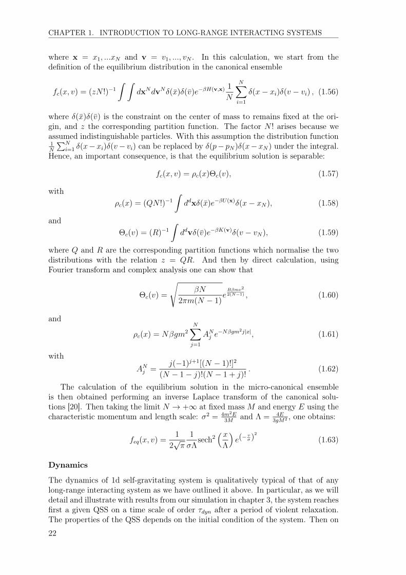
The dynamics of 1d self-gravitating system is qualitatively typical of that of anylong-range interacting system as we have outlined it above. In particular, as we willdetail and illustrate with results from our simulation in chapter 3, the system reachesfirst a given QSS on a time scale of order ⌧dyn after a period of violent relaxation.The properties of the QSS depends on the initial condition of the system. Then on
22

CHAPTER 1. INTRODUCTION TO LONG-RANGE INTERACTING SYSTEMS
much longer times scales, proportional to N in units of ⌧dyn, these QSS relax to thethermal equilibrium (given by Eq. (1.63) above). One notable feature is that thisrelaxation is very slow, in the sense that ⌧relax ' zN⌧dyn where z is a numerical factorof order 102�10
3 which depends on the QSS [28]. The calculation of Chandrasekharfor 3d is not generalizable to this case as there are no real collisions in 1d becauseparticles just cross on another and indeed the mechanism for this relaxation tothermal equilibrium remains an open problem for this system.
23

CHAPTER 1. INTRODUCTION TO LONG-RANGE INTERACTING SYSTEMS
24
Chapter 2
Finite N corrections to Vlasov
dynamics
We saw in the previous chapter that one of the most interesting feature of thedynamics of a long-range interacting system it that they are trapped into QSS.A basic question is whether the appearance of these out of equilibrium stationarystates — and more generally the validity of the Vlasov equation to describe thesystem’s dynamics — applies to the same class of long-range interactions as definedby equilibrium statistical mechanics, or only to a sub-class of them, or indeed to alarger class of interactions. In short, in what class of systems can we expect to seethese quasi-stationary states? Are they typical of long-range interactions as definedcanonically? Or are they characteristic of a different class?
To answer these questions requires establishing the conditions of validity of theVlasov equation, and specifically how such conditions depend on the two-body in-teraction. In the literature there are, on the one hand, some rigourous mathematicalresults establishing sufficient conditions for the existence of the Vlasov limit. It hasbeen proven notably [38, 62, 63] that the Vlasov equation is valid on times scales oforder ⇠ logN times the dynamical time, for strictly bound pair potentials decayingat large separations r slower than r�(d�2). On the other hand, both results of numer-ical study and various theoretical approaches, based on different approximations orassumptions, suggest that much weaker conditions are sufficient, and the timescalesfor the validity of the Vlasov equation can be much longer. In the much studied caseof gravity, notably, a treatment originally introduced by Chandrasekhar, [49] andsubsequently refined by other authors (see e.g. [35,59,64,65] in which non-Vlasov ef-fects are assumed to be dominated by incoherent two body interactions gives a timescale ⇠ N/logN times the dynamical time for the validity of the Vlasov equation, atleast close to stationary solutions representing quasi-stationary states, and this inabsence of a regularisation of the singularity in the two-body potential. Theoreticalapproaches in the physics literature derive the Vlasov equation and kinetic equa-tions describing corrections to it (for a review see [1,66]) either within the frameworkof the BBGKY hierarchy [40], as we saw in the previous chapter, or starting fromthe exact Klimontovich equation for the N body system [67, 68]. These approachesare both widely argued (e.g. see e.g. [1, 2, 66, 69, 70], to lead generally to lifetimesof quasi-stationary states of order ⇠ N times the dynamical time for any softenedpair potential , except in the special case of spatially homogeneous quasi-stationarystates one dimension.
25

CHAPTER 2. FINITE N CORRECTIONS TO VLASOV DYNAMICS
In this chapter, we address the question of the validity of Vlasov dynamics usingan approach starting from the exact Klimontovich equation. Instead of considering,as is often done (see e.g. [1,2,69] , an average over an ensemble of initial conditionsto define a smooth one particle phase density, we follow an approach (described e.g.in [71]) in which such a smoothed density is obtained by performing a coarse-grainingin phase space. This approach gives the Vlasov equation for the coarse-grained phasespace density when certain terms are discarded. We study how the latter “non-Vlasov” terms depend on the particle number N , on the scales introduced by thecoarse-graining. In particular we develop this study analyzing the dependence on thelarge and small distance behavior of the two body potential. Our analysis leading tothe scaling behaviours of these terms is based only one very simple — but physicallyreasonable — hypothesis that we can neglect all correlations in the (microscopic) Nbody configurations other than those coming from the mean (coarse-grained) phasespace density.
The main physical result we highlight is that, under this simple hypothesis, thecoarse-grained dynamics of an interacting N -particle system shows a very differentdependence on the pair interaction at small scale depending on how fast the interac-tion decays at large distances: for interactions of which the pair force is integrable atlarge scales the coarse-grained N body dynamics is highly sensitive to how the poten-tial is softened at much smaller scales, while for pair forces which are non-integrablethe opposite is true. Correspondingly, while the Vlasov limit may be obtained forany pair interaction which is softened suitably at small scales, the conditions onthe short-scale behaviour of the interaction are very different depending on whetherits large scale behaviour is in one of of these two classes. This result provides amore rigorous basis for a “dynamical classification" of interactions as long-range orshort-range, which has been introduced on the basis of simple considerations of theprobability distribution of the force on a random particle in a uniform particle dis-tribution in [72], and found also in [50] to coincide with a classification based onthe dependence on softening of collisional time scales using a generalisation of theanalysis of Chandrasekhar for the case of gravity.
The chapter is organized as follows. In the next section we derive the equationfor the coarse-grained phase space density and write in a simple form the non-Vlasov terms our subsequent analysis focusses on. In section 2 we first explain ourcentral hypothesis concerning the N -body dynamics, and then apply it to evalu-ate the statistical properties of the non-Vlasov terms. In the following section wethen determine the scaling behaviours of these expressions, i.e., how they dependparametrically on the relevant parameters introduced, and in particular on the twoparameters characterising the two body interaction — its large scale decay and thescale at which it is softened. In section 4 we use these expressions to identify thedominant contributions to the non-Vlasov terms, which turn out to differ dependingon how rapidly the interaction decays at large scales. In the following section wepresent more complete exact results for the one dimensional case and the comparisonwith a simple numerical simulation. We then summarize our results and conclusions,discussing in particular the central assumptions and the dependence of our findingson them.
26
CHAPTER 2. FINITE N CORRECTIONS TO VLASOV DYNAMICS
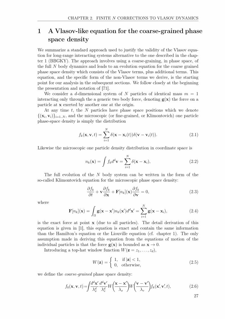
1 A Vlasov-like equation for the coarse-grained phase
space density
We summarize a standard approach used to justify the validity of the Vlasov equa-tion for long-range interacting systems alternative to the one described in the chap-ter 1 (BBGKY). The approach involves using a coarse-graining, in phase space, ofthe full N body dynamics and leads to an evolution equation for the coarse grainedphase space density which consists of the Vlasov terms, plus additional terms. Thisequation, and the specific form of the non-Vlasov terms we derive, is the startingpoint for our analysis in the subsequent sections. We follow closely at the beginningthe presentation and notation of [71].
We consider a d-dimensional system of N particles of identical mass m = 1
interacting only through the a generic two body force, denoting g(x) the force on aparticle at x exerted by another one at the origin.
At any time t, the N particles have phase space positions which we denote{(xi,vi)}i=1..N , and the microscopic (or fine-grained, or Klimontovich) one particlephase-space density is simply the distribution
fk(x,v, t) =NX
i=1
�(x� xi(t))�(v � vi(t)). (2.1)
Likewise the microscopic one particle density distribution in coordinate space is
nk(x) =
Zfkd
dv =
NX
i=1
�(x� xi), (2.2)
The full evolution of the N body system can be written in the form of theso-called Klimontovich equation for the microscopic phase space density:
@fk@t
+ v
@fk@x
+ F[nk](x)@fk@v
= 0, (2.3)
where
F[nk](x) =
Z
⌦
g(x� x
0)nk(x
0)ddx0
=
NX
i=1
g(x� xi), (2.4)
is the exact force at point x (due to all particles). The detail derivation of thisequation is given in [1], this equation is exact and contain the same informationthan the Hamilton’s equation or the Liouville equation (cf. chapter 1). The onlyassumption made in deriving this equation from the equations of motion of theindividual particles is that the force g(x) is bounded as x ! 0.
Introducing a top-hat window function W (z = z1
, . . . , zd),
W (z) =
⇢1, if |z| < 1,0, otherwise,
(2.5)
we define the coarse-grained phase space density:
f0
(x,v, t)=
Zddx0
�dx
ddv0
�dvW
✓x� x
0
�x
◆W
✓v � v
0
�v
◆fk(x
0,v0, t), (2.6)
27
CHAPTER 2. FINITE N CORRECTIONS TO VLASOV DYNAMICS
where �x and �v are the characteristic sizes of the coarse-graining cell in positionand, respectively, velocity space. We will denote by C(x,v) the coarse graining cellcentred at (x,v), which thus has a phase space volume �dx �dv, and
Nc(x,v, t) =⇡d
(�(d/2 + 1))
2
�dx�dvf0(x,v, t), (2.7)
is the number of particles in C(x,v). We suppose that the coarse graining cell isalways much smaller (in both real and velocity space) than the characteristic size ofthe system, but sufficiently large to contain a large number of particles, i.e., �x ⌧ Lx
and �v ⌧ Lv where Lx and Lv the characteristic size of the system in coordinateand velocity space respectively, and
1 ⌧ Nc(x,v, t) ⌧ N . (2.8)
Likewise we define the coarse-grained spatial density as
n0
(x, t) =
Zddvf
0
(x,v, t) =
Zddx0
�xW
✓x� x
0
�dx
◆nk(x
0). (2.9)
To obtain a Vlasov-like equation we integrate Eq. (2.3) over the coarse-graining cellover x and v. We obtain, for the first term;
Z Zddx0ddv0@fk
@tW
✓x
0 � x
�x
◆W
✓v
0 � v
�v
◆=
@f0
(x,v, t)
@t. (2.10)
For the second term using the Einstein summation convention for repeated index,for j = 1 . . . d, we have:Z Z
ddx0ddv0
�dx�dv
v0j.@fk@x0
j
W
✓x
0 � x
�x
◆W
✓v
0 � v
�v
◆(2.11)
=
Z Zddx0ddv0
�dx�dv
vj.@fk@x0
j
W
✓x
0 � x
�x
◆W
✓v
0 � v
�v
◆
+
Z Zddx0ddv0
�dx�dv
(v0j � vj).@fk@x0
j
W
✓x
0 � x
�x
◆W
✓v
0 � v
�v
◆
=�Z Z
ddx0ddv0
�dx�dv
fkvj.@
@x0j
W
✓x
0 � x
�x
◆W
✓v
0 � v
�v
◆
�Z Z
ddx0ddv0
�dx�dv
fk(v0j � vj).
@
@x0j
W
✓x
0 � x
�x
◆W
✓v
0 � v
�v
◆.
To obtain the last equality we have used an integration by parts, in which the termhfkW
⇣x
0�x
�x
⌘W
⇣v
0�v
�v
⌘i+1
�1vanishes. Then noting that
@
@x0j
W
✓x
0 � x
�x
◆= � @
@xj
W
✓x
0 � x
�x
◆, (2.12)
28

CHAPTER 2. FINITE N CORRECTIONS TO VLASOV DYNAMICS
the derivatives @@x
i
can be taken out of the integrals and we obtain for the secondterm
vj.@f
0
@xj
+
@
@xj
ZZ
C(x,v)
ddx0ddv0
�dx�dv
(v0j � vj)fk=v
@f
@x+
@
@x
2
4 1
Nc(x,v, t)
X
i2C(x,v)
vi(t)� v
3
5 .
(2.13)Then following the same procedure, adding F
0
(x, t)�F
0
(x, t) under the integraland again integrating by parts the third term gives:
F
0
(x) · @f0@v
+
@
@v
2
4 1
Nc(x,v, t)
X
i2C(x,v)
Fi(t)� F
0
(x, t)
3
5 . (2.14)
Collecting all expressions derived above, we obtain the following equation:
@f0
@t+ v · @f0
@x+ F
0
(x) · @f0@v
=� @
@x[f
0
⇠v
]� @
@v[f
0
⇠F
] , (2.15)
whereF
0
(x, t) =
Z
⌦
g(x� x
0)n
0
(x
0, t)ddx0 , (2.16)
is the force at the point x due to the coarse-grained distribution (which we willidentify as the mean-field force). Furthermore
⇠v
(x,v, t) =
2
4 1
Nc(x,v, t)
X
i2C(x,v)
vi(t)
3
5� v , (2.17)
where vi is the velocity of particle i, and
⇠F
(x,v, t) =
2
4 1
Nc(x,v, t)
X
i2C(x,v)
Fi(t)
3
5� F
0
(x, t) , (2.18)
where Fi is the exact force acting on the particle i, i.e., Fi = F(xi, t) where wesimplify the above notation:
F(x, t).= F[nk](x) =
Z
⌦
g(x� x
0)nk(x
0, t)ddx0 . (2.19)
Thus ⇠v
is the “velocity fluctuation” in the cell (x,v) around the coarse-grainedvelocity v, i.e., difference between the arithmetic mean of particles velocities inthe cell (i.e. the velocity of the center of mass) and the velocity at the centre ofthe coarse-graining cell, and ⇠
F
(x,v, t) is the “force fluctuation” around the coarse-grained force, i.e. the difference between the arithmetic mean of the exact forcesacting on each particle in the cell (equal to the force on the centre of mass of theparticles in the cell) and the force at the centre of the cell due to the coarse-grainedparticle distribution.
If the right hand side of Eq. (2.15) is set equal to zero, we recover, given Eq.(2.16), the Vlasov equation for the coarse-grained phase space density f
0
(x,v, t).
29
CHAPTER 2. FINITE N CORRECTIONS TO VLASOV DYNAMICS
Establishing the validity of the Vlasov equation in an appropriate limit thus requiresshowing that the terms on the right-hand side may indeed be taken to zero in thislimit. For a real system, for which N is finite and the typical number of particles ina coarse-graining cell is finite, Eq. (2.15) is not closed for the coarse-grained phasespace density, but rather coupled to the fine-grained density through the terms onthe right-hand side. If it is possible to define the Vlasov limit for the system, theseterms will represent at any finite (but large) N , small perturbations to the pureVlasov evolution of the coarse-grained distribution associated with the “graininess”of the system which, under suitable hypothesis, are responsible for the relaxation ofthe system to the thermodynamic equilibrium. In the rest of this article we focus onthese terms, and establish their scaling with N (or, equivalently, as a function of thecharacteristic scales of the coarse-graining cell), given certain simplifying hypotheses.
2 Statistical evaluation of the finite N fluctuating
terms
We now focus on the two terms on the right-hand side of Eq. (2.15). Their di-rect evaluation is clearly impossible as in principle it requires knowledge of the fullfine-grained phase space density. We can, however, determine how they scale asa function of relevant parameters by using a statistical approach: given a coarse-grained distribution f
0
(x,v) we can consider in each cell of the single particle phasespace, the fine-grained distribution to be characterized by an ensemble of realizationsof particle distributions having f
0
(x,v) as constant mean density. If we know thestatistical properties of this ensemble, we can then, in principle, calculate those ofthe fluctuating terms on the right-hand side of Eq. (2.15). In particular, we can thenconsider how the amplitudes of these statistical quantities depend on the relevantparameters.
We make here the most simple possible hypothesis about this ensemble for thefine-grained phase space density: we suppose that it corresponds to the ensemble ofrealisations of an inhomogeneous Poissonian point process with mean density givenby the coarse-grained phase space density f
0
(x,v). In other words we assume thatthe particles are randomly distributed, without any correlation, inside each coarse-grained cell, with a mean density which varies from cell to cell following f
0
(x,v). Thedensity-density correlations are thus fully described by the one point distributionf0
(x,v), and all other correlations, of the fluctuations around this mean density, areneglected. Physically this means we retain the “pure” finite N (discreteness) effectsarising from the fluctuations of the mean density, but neglect the correlation of thesefluctuations. Alternatively one can consider that we proceed by assuming completeignorance of the distribution of particles below the coarse-graining scale, other thanthe information furnished about it by the coarse-grained density itself. This allowsus to close, at least in a statistical formulation, Eq. (2.15) for f
0
(x,v). Indeed thishypothesis is arguably the most natural one to make in seeking to obtain a criterionfor the validity of the Vlasov equation which is based only on the coarse grainingdensity f
0
(x,v) and the properties of the pair interaction itself.Formally we can state our assumption to be that the relevant terms can be
evaluated by considering an ensemble realisations of a point process with the N
30
CHAPTER 2. FINITE N CORRECTIONS TO VLASOV DYNAMICS
particle probability distribution in phase space given by (see, e.g., [73])
PN(x1
,v1
; ..;xN ,vN) =
NY
i=1
f0
(xi,vi)
N, (2.20)
assuming the coarse-grained phase space density f0
(x,v) to be a smooth function.In practice it is convenient to perform the calculation with finite coarse-grained cellsin which f
0
(x,v) is fixed, and the particles are then distributed randomly in eachcoarse-grained cell.
2.1 Mean and variance of ⇠v
We first evaluate the mean and variance of ⇠v, as defined by Eq. (2.17) above,assuming now the defined properties of the ensemble of realisations. Given thatthe latter assigns randomly the velocities of the particles in the coarse-grained cell,which is centred at (x,v), we evidently have
*1
Nc(x,v, t)
X
i2C(x,v)
vi(t)
+= v , (2.21)
where h...i denotes the ensemble average. Therefore we have, as would be expected,
h⇠v
i = 0 . (2.22)
Calculating the variance of ⇠v
gives straightforwardly that
⌦⇠2v
↵=
1
Nc(x,v)
d
12
�2v, (2.23)
where we can take Nc = f0
(x,v)�dx�dv to be the average number of particles in the
cell, given that Nc = hNci + �Nc where by hypothesis �Nc ⇠ pNc ⌧ Nc
1. Giventhat Nc(x,v) is large, and vi are considered independent and identically distributedvariables, ⇠
v
is thus simply a Gaussian random variable with mean zero and variancegiven by Eq. (2.23).
2.2 Mean and variance of ⇠F
Let us evaluate now the first two moments of ⇠F
. To evaluate these quantities inthe ensemble defined above, it is useful first to note that
¯
F(x,v, t).=
1
Nc(x,v, t)
X
i2C(x,v)
Fi(t) (2.24)
=
1
Nc
NcX
i=1
N�NcX
I=1
g(xi � yI)
1In a uniform Poisson process with mean density n0, the PDF P (N,V ) of the number of particlesN in a volume V is P (N,V ) = (n0V )Ne
�n0V/N ! (see, e.g., [73])
31

CHAPTER 2. FINITE N CORRECTIONS TO VLASOV DYNAMICS
where the i runs over the Nc particles inside the coarse-graining cell C(x,v), andthe index I over the other N �Nc particles outside the cell. This is the case becausewe assume g(�x) = �g(x) (making the sum over all the mutual forces of thepairs of particles in the cell C(x,v) vanishes). As the individual pair forces dependonly on the spatial positions of particles, we need only specify, to calculate theensemble average of powers of the force, the probability distribution for the spatialpositions of these points. Given the writing of the force in (2.24), in which thesum is performed separately over the particles inside and outside the coarse-grainedcell C(x,v) considered, it is convenient to write the ensemble average in a similarform. As noted above we can take Nc to be fixed and equal to its average value,n0
(x)�dx, up to negligible corrections of order 1/pNc. We can then write the N
particle probability distribution as
P 0N(x1
, ..xNc
;y
1
, ..yN�Nc
) =
NcY
i=1
p(xi)
N�NcY
I=1
p(yI), (2.25)
where p(x) is the one-point probability distribution function of the spatial positionof a particle given the condition that it is contained in the cell, and p(y) is the one-point probability distribution of the spatial position of a particle given the conditionthat it is outside the cell. Given that the Nc particles are randomly distributed insidethe cell, we have simply
p(xi) =
⇢��dx , xi 2 C(x,v)
0, otherwise.(2.26)
We define further S(x), the support of W (x/�x), i.e., the “stripe” in phase space withthe same spatial coordinates as the phase space cell C(x,v) (see Fig. 2.1). Assumingthe number of particles in the cell Nc to be small compared to the total number ofparticles N , p(y) can be approximated everywhere simply by is the unconditionalone point PDF for the spatial distribution obtained by integrating (2.20) over allbut one space coordinate, i.e.,
p(y) =n0
(y)
N. (2.27)
Mean of ⇠F
Using (2.25) to calculate the ensemble average of the exact force exerted by allparticles on those in a coarse-grained cell, we have
⌦¯
F(x,v, t)↵= (N �Nc)
Z
⌦
ddx0Z
⌦
ddy0p(x0)p(y0
)g(x
0 � y
0)
=
Z
S(x)
ddx0
�dx
Z
⌦
ddy0n0
(y
0)g(x
0 � y
0)
=
Z
S(x)
ddx0
�dxF
0
(x
0), (2.28)
where we have approximated N�Nc
Nby 1. Thus
h⇠F
(x,v, t)i =Z
S(x)
ddx0
�dx[F
0
(x
0)� F
0
(x)] . (2.29)
32
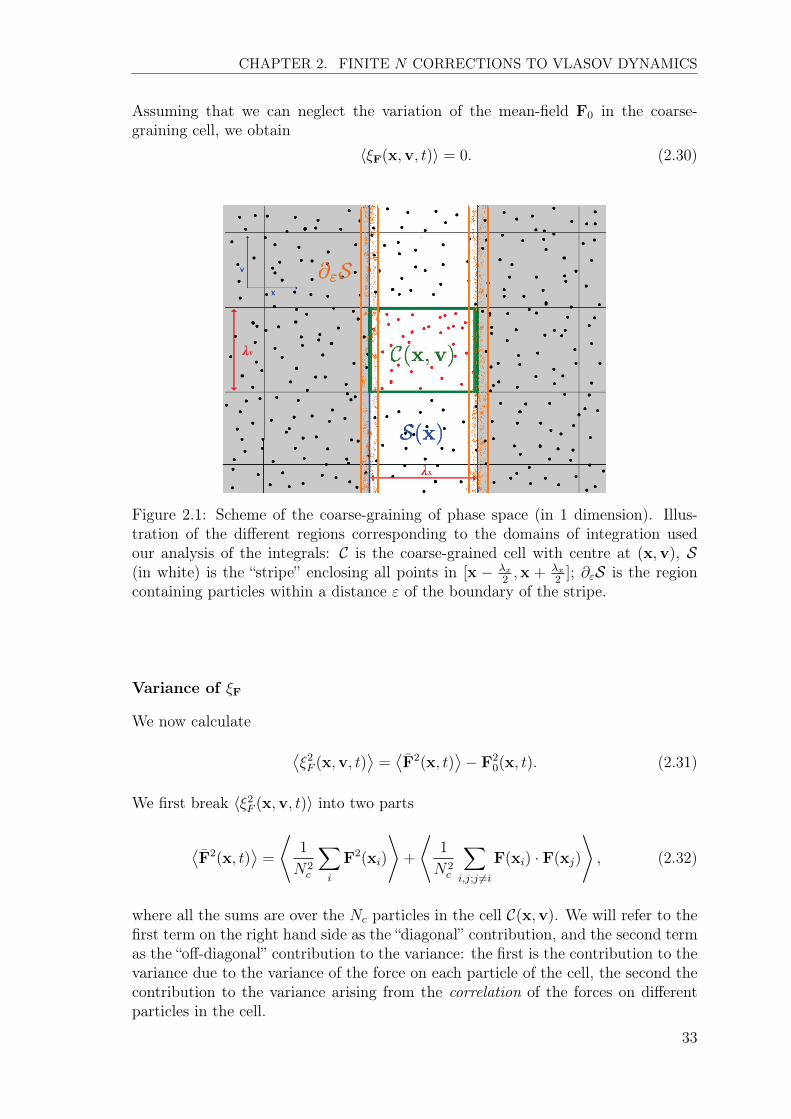
CHAPTER 2. FINITE N CORRECTIONS TO VLASOV DYNAMICS
Assuming that we can neglect the variation of the mean-field F
0
in the coarse-graining cell, we obtain
h⇠F
(x,v, t)i = 0. (2.30)
Figure 2.1: Scheme of the coarse-graining of phase space (in 1 dimension). Illus-tration of the different regions corresponding to the domains of integration usedour analysis of the integrals: C is the coarse-grained cell with centre at (x,v), S(in white) is the “stripe” enclosing all points in [x � �
x
2
,x +
�x
2
]; @"S is the regioncontaining particles within a distance " of the boundary of the stripe.
Variance of ⇠F
We now calculate
⌦⇠2F (x,v, t)
↵=
⌦¯
F
2
(x, t)↵� F
2
0
(x, t). (2.31)
We first break h⇠2F (x,v, t)i into two parts
⌦¯
F
2
(x, t)↵=
*1
N2
c
X
i
F
2
(xi)
++
*1
N2
c
X
i,j;j 6=i
F(xi) · F(xj)
+, (2.32)
where all the sums are over the Nc particles in the cell C(x,v). We will refer to thefirst term on the right hand side as the “diagonal” contribution, and the second termas the “off-diagonal” contribution to the variance: the first is the contribution to thevariance due to the variance of the force on each particle of the cell, the second thecontribution to the variance arising from the correlation of the forces on differentparticles in the cell.
33

CHAPTER 2. FINITE N CORRECTIONS TO VLASOV DYNAMICS
Further we can use Eq. (2.24) to split each term into two terms
⌦¯
F
2
(x, t)↵=
*1
N2
c
NcX
i
N�NcX
I
g
2
(xi � xI)
+
+
*1
N2
c
NcX
i
N�NcX
I,J ;I 6=J
g(xi � xI) · g(xi � xJ)
+
+
*1
N2
c
NcX
i,j;i 6=j
N�NcX
I
g(xi � xI) · g(xj � xI)
+
+
*1
N2
c
NcX
i,j;i 6=j
N�NcX
I,J ;I 6=J
g(xi � xI) · g(xj � xJ)
+,
where i, j again denote sums over the Nc particles inside the coarse-grained cell andI, J over the remaining N � Nc ⇠ N particles . Performing the ensemble averageby integrating over the PDF (2.25), the result can be conveniently divided in twoparts. The first and third terms give
1
Nc
Z
⌦
ddx0
�dxn0
(x
0)
Z
S(x)ddy g
2
(y
0 � x
0), (2.33)
and ✓1� 1
Nc(x,v)
◆Z
⌦
ddx0
�dxn0
(x
0)
Z
S(x)ddy0
g(y
0 � x
0)
�2
, (2.34)
respectively. Both the second and fourth terms can be expressed purely in terms ofthe mean-field, as
1
Nc
✓1� 1
N
◆Z
S(x)
ddx0
�dxF
2
0
(x
0), (2.35)
and ✓1� 1
Nc
◆✓1� 1
N
◆Z
S(x)
ddx1
�dx
Z
S(x)
ddx2
�dxF
0
(x
1
) · F0
(x
2
) (2.36)
respectively.Assuming that we can neglect the variation of the mean-field F
0
in the coarse-graining cell, we can perform the integrals in the last two expressions, and thenobtain
⌦⇠2F (x,v)
↵=
1
Nc(x,v)
Z
⌦
ddx0n0
(x
0)
Z
S(x)ddy0��d
x g
2
(y
0 � x
0)
+ (1� 1
Nc(x,v))
Z
⌦
ddx0n0
(x
0)
Z
S(x)ddy0��d
x g(y
0 � x
0)
�2
� 1
NF
2
0
(x). (2.37)
Our analysis below will focus essentially on the first two terms in this expressionas they are those which describe the contribution to the fluctuating terms whichare potentially sensitive to the small scale properties of the pair force g(x). We
34
CHAPTER 2. FINITE N CORRECTIONS TO VLASOV DYNAMICS
note that the first term comes from the “diagonal” part of the variance, and morespecifically it represents the contribution to the variance arising from the force on asingle particle in the cell due to a particle outside the cell: we will thus refer to it asthe two body contribution. The second integral in (2.37), on the other hand, arisesfrom the “off-diagonal” part of the variance, and more specifically it represents thecontribution to the variance of the force on the cell due to the correlation of theforce exerted on two particles inside the cell exerted by a particle outside the thecell: we will refer to it therefore as the three body contribution.
3 Parametric dependence of the fluctuations
We now analyse the expressions we have obtained, focussing on how their valuedepends parametrically on the relevant parameters we have introduced, notably thenumber of particles in the system (N), its size (Lx, Lv), the number of particles inthe coarse-graining cells (Nc) and the coarse-graining scales (�x, �v). Further wewill take the pair force to be given by g(x) = g|x|��
ˆ
x for � < 0, and by
g(x) = g
⇢ |x|��ˆ
x, |x| � ""��
ˆ
x, |x| < ", (2.38)
for � > 0, where g is the coupling constant (and g < 0 for the case of an attractiveinteraction). We will focus then on how the amplitude of the fluctuations of theforce depend also on the exponent � and the characteristic length " at which theforce is regularized at small scales. Indeed it is evident that we must introducesuch a regularization of the pair force, as without it the integrals in (2.37) can beill-defined.
3.1 Mean field Vlasov limit
The mean-field Vlasov limit is formulated by taking N ! 1 at fixed system size, andscaling g / N�1 so that the mean field F
0
remains fixed. Applying this procedure tothe expressions we have obtained for h⇠2
F
i and h⇠2v
i, both indeed converge to zero, forany non-zero ". In order to obtain these expressions we have, as noted, assumed alsothat the mean-field does not vary on the scale of the coarse-graining cell. Assumingthat the characteristic scale of variation of the coarse-grained phase space density,and mean field, is the system size Lx, for a finite coarse-graining cell we expectcorrections to our expressions due to the variation of these quantities on the scale�x which are suppressed at least by �x/Lx relative to those we have calculated. Thecoarse-grained phase space density f
0
(x,v, t) thus indeed obeys the Vlasov equationin the usual formulation of this limit, when the size of the coarse-graining cell istaken to be negligible with respect to the system size.
We now study more closely the approach to the Vlasov limit as characterized bythe scaling behaviour of the corrections to it. We assume that these are given bythose of the statistical quantities we have calculated, i.e. we take
|⇠v
| ⇠p
h⇠2v
i , |⇠F
| ⇠q
h⇠2F
i. (2.39)
35

CHAPTER 2. FINITE N CORRECTIONS TO VLASOV DYNAMICS
3.2 Velocity fluctuations
Given the result (2.23) and that Nc ⇠ NLd
x
Ld
v
�dx�dv we infer
|⇠v
| ⇠ 1pN
✓Lx
�x
◆d/2✓Lv
�v
◆d/2
�v. (2.40)
There is evidently no dependence on the pair force in this term. As already notedwe can recover the Vlasov limit by taking N ! 1. Further we can see that thisresult remains valid for arbitrarily small (but non-zero) values of the ratio �
x
Lx
sothat variation of coarse-grained quantities on the coarse-grained scale can indeed beneglected.
3.3 Force fluctuations
The scaling of the last term on the right-hand side (2.37) is already explicited,representing simply a fluctuation of the force about the mean field of order 1/
pN
times the mean field itself. In order to determine the dependences of the first twoterms we need to analyse carefully that of the integrals. To do so we divide thedomains of integration in the double integral into appropriate subdomains, isolatingthe region which may depends on the lower cut-off " in the pair force.
2 body contribution
We consider first the diagonal two body contribution, writing the double integral as
Z
⌦/S/@"
Sddx0
+
Z
@"
Sddx0
+
Z
S/@"
Sddx0
�⌦
✓n0
(x
0)
Z
B(x0,")
ddy0��dx g
2
(y
0 � x
0) (2.41)
+n0
(x
0)
Z
S(x,�)/B(x0,")
ddy��dx g
2
(y
0 � x
0)
◆,
where in this context ⌦ indicates the integration operation on the terms in paren-thesis, and as illustrated for the one dimensional case in Fig. 2.1, the integral overx
0, over the whole of space (⌦) has been divided into three parts:
• @"S: the set of points which are within a distance " of the boundary of thestripe S. The volume of this region is of order "�d�1
x .
• S/@"S: the set of points belonging to S but not belonging to @"S. For "⌧ �x,its volume is of order �dx.
• ⌦/S/@"S: the rest of space.
and the integral over y
0, over the stripe S has been divided into two parts:
• B(x
0, "): the set of points in S which are a distance of less than " from thepoint x
0. This region has a volume of order "d.
• S/B(x
0, "): the rest of S; for "⌧ �x, its volume is of order �dx.
36

CHAPTER 2. FINITE N CORRECTIONS TO VLASOV DYNAMICS
We consider now one by one the terms in the integral written as in (2.41). Thefirst term in the integration over x
0 excludes the region where the pair force is "-dependent, and is over a volume of order Ld
x. Hence if we suppose n0
⇠ const, itgives a contribution which scales as
⇠ n0
Ld�2�x . (2.42)
For the second region of integration over x
0, of volume of order "�d�1
x , the regionB(x0, ") of the integration over y
0 gives a contribution of order "�2� over a volumeof order "d, and thus
⇠ n0
("�d�1
x )"d��dx "�2� . (2.43)
In the region S(x)/B(x0, ") on the other hand, of volume of order �dx, we have
⇠ n0
("�d�1
x )��2�x . (2.44)
In the third region of integration over x
0, of volume of order �dx, we obtain again acontribution of order "�2� in the volume B(x0, "), and thus
⇠ n0
"d�2� , (2.45)
while the second term region of the y
0 integration gives
⇠ n0
�d�2�x . (2.46)
3 body contribution
Proceeding in the same manner, we write the 3-body contribution to the varianceof the force as
Z
⌦/S/@"
Sddx0
+
Z
@"
Sddx0
+
Z
S/@"
Sddx0
�⌦
✓n0
(x
0)
Z
B(x0,")
ddy0��dx g(y
0 � x
0) (2.47)
+n0
(x
0)
Z
S(x,�)/B(x0,")
ddy��dx g(y
0 � x
0)
◆2
.
The first term in the integration over x0 gives then a contribution
⇠ n0
Ld�2�x .
Compared to the 2-body integral, the analysis of the remaining parts is essentiallythe same, except for one important difference: as the integration over y0 is over thevector pair force, the integral over y0 is zero when integrated in a sphere around x
0;in particular the integration over B(x0, ") vanishes when B(x0, ") is fully containedin S. This is the case for the integration region S/@"S, which therefore does notdepend on " and simply gives a contribution of order
⇠ n0
�d�2�x . (2.48)
For the second integration region in the integral over x
0, the volume ⇠ "�d�1
x ,B(x0, ") is not fully contained in S and we have therefore a contribution from this
37
CHAPTER 2. FINITE N CORRECTIONS TO VLASOV DYNAMICS
part of the integration over y
0 of order "d��dx "��, while the second part, which
does not depend on ", gives a contribution of order ���x . Taking the square and
multiplying by the volume of @"S, we obtain three terms:
⇠ n0
"�d�1
x "2d��2dx "�2� , (2.49)
from the square of the first term,
⇠ n0
"�d�1
x "d��dx "�����
x , (2.50)
from the cross term, and⇠ n
0
"�d�1
x ��2�x , (2.51)
from the square of the second term.
4 Force fluctuations about the Vlasov limit: depen-
dence on "
Gathering together the expressions derived above, we obtain, keeping only the lead-ing divergence in " in each of the 2-body and 3-body contributions,
⌦⇠2F (x,v)
↵=
g2
Nc
�C
⌦
n0
Ld�2�x + CS n0
�d�2�x + C@S n0
"d�2��
(2.52)
+ g2(1� 1
Nc
)
�C 0
⌦
n0
Ld�2�x + C 0
S n0
�d�2�x + C 0
@S n0
"2d+1�2���(d+1)
x
�
� 1
N|F[n
0
](x)|2,
where all C⇤and C 0⇤ are constants (Note that we have not included (2.50) because
when it diverges, for � > d+1, the term retained is indeed more rapidly divergent.)Depending on the values of � and d different terms dominate. We consider each
case.
4.1 Case � < d
2
For this case, there are no divergences as "! 0, and for "⌧ �x ⌧ Lx, the dominantterm from the two integrals is
g2n0
Ld�2�x ⇠ 1
n0
Lx
g2n2
0
L2
x ⇠ 1
N|F
0
|2, (2.53)
and therefore we infer the scaling of the total force fluctuation is
|⇠F
| ⇠ 1pN|F
0
|. (2.54)
As noted above we therefore obtain in this case the Vlasov limit taking N ! 1with g ⇠ 1/N . Further we conclude that, at finite N , the fluctuations around themean-field force are dominated by contributions coming from fluctuations of thedensity at the scale of the system size, which dominate those coming both from thescale �x of the coarse-graining cell and those from the scale " at which the pair forceis regularized.
38

CHAPTER 2. FINITE N CORRECTIONS TO VLASOV DYNAMICS
4.2 Case
d
2 < � < d+ 12
In this range of �, there is a divergence at " ! 0 in the contribution coming fromthe 2-body term, while the 3-body term remains finite. Keeping only the dominantcontributions to the two integrals when "⌧ �x ⌧ Lx, we obtain
h⇠2F
(x)i ⇠ C"g2n
0
(x)
Nc(x,v)"d�2�
+ C 0�g
2n0
(x)�d�2�x , (2.55)
where C" and C 0� are constants.
Given the divergence in " we see explicitly that in this case the Vlasov limit isobtained taking N ! 1 with g ⇠ N�1 at finite non-zero ", while the limit does notexist in the absence of this small scale regularisation of the pair force.
Using Nc(x,v) / f0
(x,v)�dx�dv, we can write the dominant fluctuations as
h⇠2F
(x)i ⇠ g2n0
(x)
�dx
✓C"
"d�2�
f0
(x,v)�dv+ C 0
��2d�2�x
◆. (2.56)
This expression allows us to conclude, as anticipated, that there is a crucial differencebetween the following sub-cases: i) the range of � in which the first term dominates,and ii) the range in which the second term dominates:
For d2
< � < d:
In this case the exponent of �x in the second term inside the brackets in (2.56)is positive, and therefore when we increase �x at fixed " (and fixed �v), this termdominates over the first one. More specifically when �x � "(f
0
(x,v)�dv"d)
� 12d�2� this
term dominates, andh⇠2F i ⇠ g2n
0
(x)�d�2�x (2.57)
Thus, even though the amplitude of the fluctuations depends on ", and diverges as" ! 0, for a sufficiently large coarse-graining cell, fluctuations become in practiceeffectively insensitive to the value of ", for a wide range of values which is suchthat the larger is �x the smaller is the lower limit on ", with the latter vanishing as�x ! 1. Note that since
⇠F
⇠ 1pn0
(x)�dx
✓�xLx
◆d��
|F0
(x)| ⇠ 1pN
✓�xLx
◆d/2��
|F0
|, (2.58)
we can also neglect the final term in (2.37).
For d < � < d+ 1
2
:
In this range, it is instead the exponent of �x in the second term inside the bracketsin (2.56) which is now negative, and as a consequence it is now the first term whichdominates when we make the coarse-graining scale �x large. We have, therefore
h⇠2F
i ⇠ g2n0
f0
�dx�dv
"d�2� . (2.59)
Further as this can be rewritten as
|⇠F
| ⇠ 1pNNc
✓"
Lx
◆d/2��
|F0
|. (2.60)
39
CHAPTER 2. FINITE N CORRECTIONS TO VLASOV DYNAMICS
It follows that for sufficiently small " this is the dominant contribution to the fluc-tuations. In this range therefore the leading contribution to the force fluctuationsis directly dependent on ".
4.3 Case d+ 12 < �
In this case both the integrals giving the 2-body and 3-body contributions are di-vergent at small ", but the dominant divergence comes from the latter giving
h⇠2F (x)i ⇠ g2n0
(x)
"2d+1�2�
�d+1
x
. (2.61)
This case is therefore like the previous case (d < � < d + 1
2
): the dominant contri-bution to the fluctuations is divergent as "! 0.
5 Exact one dimensional calculation and numerical
results
For a one dimensional system, d = 1, it is possible to perform explicitly the integralsin (2.37) to obtain exactly the expression of the force fluctuations. In order toillustrate our main result above, we can compare the expressions we obtain, andin particular their leading scaling behaviours, with what is obtained directly bymeasuring the force fluctuations in cells on realisations of a homogeneous Poissonparticle distribution. As we are interested primarily in the " dependence of thesefluctuations we consider solely the contribution to them from the part of the integralwhich is potentially sensitive to them. We can therefore write
h⇠2F
(x)iS =
n0
Nc
Z �
x
2
��
x
2
dx0Z �
x
2
��
x
2
dy0��1
x g2(y0 � x0)
+n0
(1� 1
Nc
)
Z �
x
2
��
x
2
dx0
"Z �
x
2
��
x
2
dy0��1
x g(y0 � x0)
#2
,
where we use the subscript in h⇠2F
(x)iS to indicate that this is the contribution tothe force variance sourced by particles in the phase space “stripe” S, and
g(x) = g
(x
|x|�+1 , |x| � "x|x|"
�� |x| < ".(2.62)
40

CHAPTER 2. FINITE N CORRECTIONS TO VLASOV DYNAMICS
Integrating we obtain
h⇠2F
(x)iS = g21
Nc
n0
(x)
�x
1
1� �"2�2� � 4
1� 2��x"
1�2�+
1
(1� 2�)(1� �)�2�2�x
�
(2.63)
+g2(1� 1
Nc
)
n0
(x)
�2x
2�(1 + 2�)
2(1� �)(3� 2�)"3�2�
� 4�
(1� �)2(2� �)"1��
(�2��x � (�x � ")2��
)
� 4
(1� �)(2� �)(3� �)"��
(�3��x � (�x � ")3��
)
+
4
(1� �)(2� �)"1��
(�x � ")2��
� 4
(1� �)2
✓�x2
◆2�2�✓
�x2
� "
◆1X
n=0
(� � 1)n
1 + 2n
1
n!
✓1� 2
"
�x
◆2n
+
2
(1� �)2(3� 2�)�3�2�x
�,
where (x)n is the Pochhammer symbol, (x)n =
�(x+n)�(x)
= x(x+ 1)...(x+ n� 1).Expanding this expression in the limit "/� ! 0, and keeping only the leading
"-dependent terms, we obtain:
h⇠2F
(x)iS = g2n0
(x)
Nc
� 4
1� 2�"1�2�
+
1
(1� 2�)(1� �)�1�2�x
�(2.64)
+g2n0
(x)(1� 1
Nc
)
2�(1 + 2�)
2(1� �)(3� 2�)��2
x "3�2�
+
4
(1� �)2��1��x "2��
+ C�1�2�x
�,
where C is a constant depending on �. Comparing this expression with (2.52) whichwe obtained for the d-dimensional case, we note that we indeed have agreement whenwe take d = 1. The term of order "2�� corresponds to the term of order "d+1�� in(2.50) which we did not include in (2.52) because it is never the leading divergence.
We now compare these analytical expressions with those obtained from a directnumerical estimation of the same quantity in a Poissonian realisation of a particlesystem. To do so we have distributed N = 72900 particles randomly in a “phasespace box” (cf. illustration in Fig. 2.1) of side 27�v (in velocity) and 9�x (inposition). Thus there are 243 cells, containing, on average, 300 particles. We thencalculate the exact force on each particle in the system due to all particles in thestripe to which it belongs, i.e., F(xi) =
Pj2S g(xi � xj). For each cell we then
average this quantity to get ¯
F =
1
Nc
Pi2C F[nk](xi), and we finally estimate the
variance of this quantity over the 243 cells.Shown in Fig. 2.2 are the results of these numerical simulations compared with
the theoretical results, Eq. (2.63), for a range of values of " and different values of�. The agreement is excellent in all cases.
41
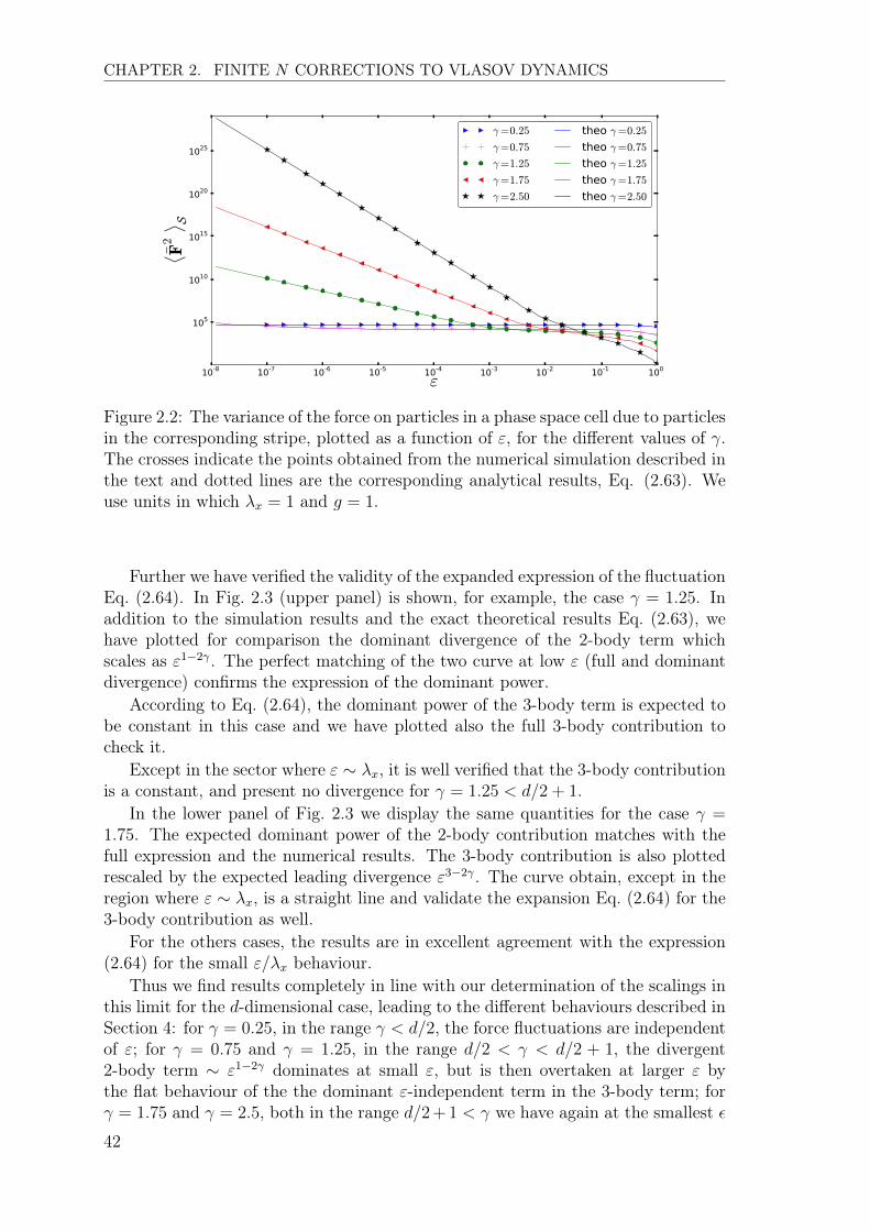
CHAPTER 2. FINITE N CORRECTIONS TO VLASOV DYNAMICS
Figure 2.2: The variance of the force on particles in a phase space cell due to particlesin the corresponding stripe, plotted as a function of ", for the different values of �.The crosses indicate the points obtained from the numerical simulation described inthe text and dotted lines are the corresponding analytical results, Eq. (2.63). Weuse units in which �x = 1 and g = 1.
Further we have verified the validity of the expanded expression of the fluctuationEq. (2.64). In Fig. 2.3 (upper panel) is shown, for example, the case � = 1.25. Inaddition to the simulation results and the exact theoretical results Eq. (2.63), wehave plotted for comparison the dominant divergence of the 2-body term whichscales as "1�2� . The perfect matching of the two curve at low " (full and dominantdivergence) confirms the expression of the dominant power.
According to Eq. (2.64), the dominant power of the 3-body term is expected tobe constant in this case and we have plotted also the full 3-body contribution tocheck it.
Except in the sector where " ⇠ �x, it is well verified that the 3-body contributionis a constant, and present no divergence for � = 1.25 < d/2 + 1.
In the lower panel of Fig. 2.3 we display the same quantities for the case � =
1.75. The expected dominant power of the 2-body contribution matches with thefull expression and the numerical results. The 3-body contribution is also plottedrescaled by the expected leading divergence "3�2� . The curve obtain, except in theregion where " ⇠ �x, is a straight line and validate the expansion Eq. (2.64) for the3-body contribution as well.
For the others cases, the results are in excellent agreement with the expression(2.64) for the small "/�x behaviour.
Thus we find results completely in line with our determination of the scalings inthis limit for the d-dimensional case, leading to the different behaviours described inSection 4: for � = 0.25, in the range � < d/2, the force fluctuations are independentof "; for � = 0.75 and � = 1.25, in the range d/2 < � < d/2 + 1, the divergent2-body term ⇠ "1�2� dominates at small ", but is then overtaken at larger " bythe flat behaviour of the the dominant "-independent term in the 3-body term; for� = 1.75 and � = 2.5, both in the range d/2+1 < � we have again at the smallest ✏
42

CHAPTER 2. FINITE N CORRECTIONS TO VLASOV DYNAMICS
Figure 2.3: The variance of the force on particles in a phase space cell due to particlesin the corresponding stripe, versus ", for � = 1.25 (upper panel) and � = 1.75 (lowerpanel). The full expression is compare (see text) with the leading "-divergence ofthe 3 and 2 body contribution Eq. (2.64). The units are such that �x = 1 and g = 1.
43
CHAPTER 2. FINITE N CORRECTIONS TO VLASOV DYNAMICS
the behaviour ⇠ "1�2� from the 2-body term, but at larger ✏ instead the dominantbehaviour "-dependent term ⇠ "3�2� from the 3-body term.
44
CHAPTER 2. FINITE N CORRECTIONS TO VLASOV DYNAMICS
6 Discussion and conclusions
Let us now discuss further the physical significance of these results, and in particularhow they justify the basic qualitative distinction between interactions as we haveanticipated in the introduction. We have considered a generic N -particle system withHamiltonian dynamics described by a two body interaction with a pair force ⇠ 1/r�
and regularized below a scale " to a constant value. Introducing a coarse-graining inphase space, one obtains an equation for the coarse-grained phase space density withterms corresponding to the Vlasov equation, in addition to “non-Vlasov” terms whichare functionals of the microscopic phase density. We then made the hypothesis thatthe typical amplitude of these terms can be estimated by assuming this microscopicphase space density to be given by a realisation of an inhomogeneous Poissonianpoint process, in which the mean density is specified by the coarse-grained phasespace density but the density fluctuations are uncorrelated. In other words weneglect all contributions due to correlation of density fluctuations with respect tothe ones due to the simple products of mean densities. Doing so we have determinedthe scalings of these latter terms as a function of the different scales in the problem,of � and of the spatial dimension d. If the assumed hypothesis is valid (for large N),a limit in which the Vlasov equation applies is simply any one in which the derivednon-Vlasov terms go to zero while the Vlasov terms tend to fixed finite values.
Our results show firstly that, for any interaction in the class we have considered,such a limit exists and can be defined in different ways: notably, by taking N toinfinity at fixed values of the other scales, and in particular at fixed smoothing; or,alternatively, by taking the limit in which the coarse-graining scale, while alwaysremaining small compared to the system size, is taken arbitrarily large comparedto the other scales, and in particular the smoothing scale ". However, when thislimit is taken, there is a important difference between the case in which � > d or� < d: for the former case the dominant correction term to the Vlasov limit is alwaysstrongly dependent on ", while in the latter case the dominant term, at fixed �x, isindependent of " in a wide range whose lower limit vanishes as �x diverges. Thisdifferent leading dependence on " corresponds to fluctuations which are sourced byquite different contributions in the two cases: for � > d, the dominant fluctuation inthe force on a coarse-graining cell comes from the contributions coming from forceson individual particles due to single particles which are “closeby”, i.e., within a radius": for � < d, on the other hand, the dominant fluctuation comes from the coherenteffect on two different particles in the cell coming from a single particle which is“far-away”, i.e. at a distance of order the size of the coarse-graining cell, or, even for� < d/2, of order the size of the system. Given that these amplitudes are those of theterms describing the corrections to the Vlasov evolution due to the large, but finite,number of particles in a real system, this means that the dynamics of the particlesystem at a coarse-grained scale in the two cases is dominated by completely differentcontributions: by the particle distribution at the smallest scales when � > d, and bythe particle distribution at the coarse-graining scale or larger when � < d. Thus inthe latter case we can decouple the dynamics at the coarse-graining scale from thatat smaller scales (the interparticle distance, the scale of particle size), while for � > dwe cannot do so. Or, in the language of renormalisation theory, the former admit akind of universality in which the coarse-grained dynamics is insensitive to the formof the interaction below this scale, while the latter do not. This is a basic qualitative
45
CHAPTER 2. FINITE N CORRECTIONS TO VLASOV DYNAMICS
distinction between the dynamics in these two cases, which corresponds naturallyto what one call “short-range” or “long-range”. In order to distinguish it from thecanonical distinction based on thermodynamical considerations, following [72], wecan refer to � > d as dynamically short-range, and � < d as dynamically long-range2
For what concerns quasi-stationary states the implications of this result andrelevance of the classification are simple: for all cases one would expect that suchstates may exist (since the Vlasov limit exists) but the conditions for their existence,which requires that the time scales of their persistence be long compared to thesystem dynamical time, will be very different. For � > d, their lifetime, which wouldbe expected to be directly related to the amplitude of the non-Vlasov term, can belong only if the smoothing scale in the force is sufficiently large; in the case � < d,their lifetime will be expected to be independent of ". We note that this is preciselyin line with results of analytical calculations based on the Chandrasekhar approachto estimation of the relaxation rate, and the results of numerical simulations ofsystems of this kind reported in [50].
These results are all, as we have emphasized, built on our central hypothesis thatcorrelation of density fluctuations, associated with the finite particle number, maybe neglected. To formulate it we must define a smooth mean phase space densityby introducing a coarse-graining scale, which is assumed to be a “mesoscopic scale”:arbitrarily small compared to the system size, and yet large enough so that thephase space cell contains many particles. Our central hypothesis is not one of whichwe can prove the validity, but it is a consistent, simple and physically reasonable,analogous to that of “molecular chaos” in the derivation of the Boltzmann equation.It is also in line with the fact that when Vlasov approximation is valid, the systemdynamics is defined in terms only of the mean density and fluctuations due to higherorder density correlations are considered subdominant. We note above all that itleads to conclusions and behaviours which are very reasonable physically, even inthe cases we have not focussed on but to which our analysis can be applied. Forexample, if we consider a hard repulsive core interaction without a smoothing, i.e.let " ! 0 for � large, we infer that the force fluctuation on a coarse-grained celldiverges and that there is thus no Vlasov limit. Indeed in this case an appropriatetwo body collision operator is required to take into account the effects of interactionsbetween particles.
Finally we note that the ensemble we have assumed to describe the fine-grainedphase space density is a realisation of a Poisson process with mean density given bythe coarse-grained space. This implies that we include (Poissonian) fluctuations ofparticle number at all scales: indeed these (finite particle number) fluctuations arethe source of the fluctuation terms in the dynamical equations which we have anal-ysed. One could consider that it might be more appropriate physically to take, inestimating the fluctuations induced at a given coarse-grained density, the ensemblein which the particle number is constrained to be fixed in all coarse-graining cells. Inother words we could average, given a coarse-grained phase space density, only over
2Or, alternatively, if one adopts the terminology advocated by [2], in which the thermodynamicdistinction is made between “strongly long-range” and “weakly long-range”, our classification couldbe described as a distinction between “dynamically strongly long-range” and “dynamically weaklylong-range” interactions.
46

CHAPTER 2. FINITE N CORRECTIONS TO VLASOV DYNAMICS
the configurations in which the particles, of fixed number in each cell, are distributedrandomly within the cells. It is straightforward to verify, with the appropriate mod-ification of the average, that doing so can only change our results for what concernsthe large scale contributions to the force fluctuations: the diverging behaviours atsmall scales we have focussed on arise from the fact that there is a finite probabilityfor a particle to be arbitrarily close to another one, and the local value of the den-sity will at most modify the amplitude but not the parametric dependence of thisterm. On the other hand, our determinations of the parametric dependence of thecontributions to the force fluctuations from the bulk will be expected to depend onhow the particle fluctuations at larger scales are constrained3.
In future work we plan to explore the possibility of developing the approach usedin this article to understand and describe further the effect of the “non-Vlasov" —collisional — terms on the evolution of a finite N system, i.e., to use it to developa kinetic equation for the N particle system, alternative to those developed in theliterature (see, e.g., [66, 69] for a discussion and references). We would to clarify inparticular the relation between this approach and that of Chandrasekhar which, aswe have noted, when extended to a generic interaction has been shown [50] to givevery consistent conclusions about the sensitivity of collisional relaxation of quasi-stationary states to the small scale regularisation. Likewise it would be interesting totry to test directly in numerical simulations for the validity of our central hypothesisabout correlations, and also characterize using analytical methods the robustness ofour central conclusions to the existence of different weak correlations of the densityfluctuations.
3A simple example is the case of one dimensional gravity, i.e., � = 0 in d = 1. In this casePoissonian force fluctuations indeed diverge with system size [74] precisely as derived here. Onthe other hand, because the force is independent of distance, the force fluctuation in a cell comingfrom particles in other cells vanishes if the number of particles in these cells does not fluctuate.
47
CHAPTER 2. FINITE N CORRECTIONS TO VLASOV DYNAMICS
7 Appendix 1: Alternative derivation of h⇠2F
iWe present in this appendix an alternative (but equivalent) calculation of the meanand variance of ⇠
F
. We recall it’s definition:
⇠F
(x,v, t) = ¯
F(x,v, t)� F
0
(x, t), (2.65)
where we have defined:
¯
F(x,v, t) =X
i2C(x,v)
Z
⌦
g(xi � x
0)nk(x
0)ddx0. (2.66)
To evaluate the moments, it is useful first to introduce nC(x,v) the microscopic densityof particle restricted to the cell C(x,v):
nC(x,v)(y0) =
NcX
i2C(x,v)
�(y0 � yi), (2.67)
where yi are the position of the particle inside the cell. We introduce also therestricted Klimontovich density nk/Cwhich does not include particle inside the cellsuch that:
nk(x0) = nC(x,v)(x
0) + nk/C(x
0). (2.68)
Then we express ¯
F as:
¯
F(x,v) =1
Nc
Z
⌦
ddx0Z
⌦
ddy0nk/C(x0)nC(x,v)(y
0)g(x
0 � y
0), (2.69)
where the integral over nC(x0)nC(y
0) vanishes because of the symmetry of the two
body force g(�x) = �g(x).Inside the cell we distribute the particle with an homogeneous Poisson process.
Out side the cell, by integration of the phase space probability (2.20) over thevelocities v
1
, ...vN , this is given by
P(x
1
,x2
..,xN) =
NY
i=1
p(xi) (2.70)
wherep(xi) =
⇢��dx , xi 2 C(x,v)
n0(xi
)
N�Nc
, otherwise.(2.71)
In other words, we assume the Nc particles in the cell to be distributed randomlyin the cell, and the remaining N � Nc particles to be distributed according to theinhomogeneous Poisson process with mean density n
0
(x). Using the latter, thefollows that ⌦
nk/C(x)↵= n
0
(x). (2.72)
Further we compute with, Eq. (2.25) the mean of nC(x,v)
⌦nC(x,v)(y)
↵=
Nc(x,v)
�x. (2.73)
48
CHAPTER 2. FINITE N CORRECTIONS TO VLASOV DYNAMICS
Moreover to compute the variance of F, it is useful to compute the correlationfunctions. Outside the cell we have, by definition of an inhomogeneous Poissonprocess:
⌦nk/C(x
0)nk/C(x
00)
↵= n
0
(x
0)�(x0 � x
00) + (1� 1
N �Nc
)n0
(x
0)n
0
(x
00). (2.74)
Inside the cell the correlation are zero as well, thus for any y
0,y00 2 C(x,v) we have:
hnC(y0)nC(y
00)i = Nc
�dx�(y0 � y
00) +
Nc(Nc � 1)
�2dx, (2.75)
where the (x,v) dependence of Nc is implicit. Finally, we have assume no correlationbetween particles inside and outside the cell, and then:
⌦nk/C(x
0)nC(x,v)(y
0)
↵=
⌦nk/C(x
0)
↵ ⌦nC(x,v)(y
0)
↵. (2.76)
Mean of ⇠F
Using the expression Eq. 2.69 and the mean of the densities computed above weobtain:
h¯F(x)i =Z
S(x,�x
)
ddy��dx
Z
⌦
ddx0n0
(x
0)g(y
0 � x
0)
=
Z
S(x,�x
)
ddy��dx F
0
(y
0), (2.77)
where S = S(x,�x) stands for an integration inside the ball centered in x of radius�x in real space, as represented in Fig. 2.1. Then the mean of the force fluctuation⇠F
givesh⇠
F
(x,v, t)i =Z
S(x,�x
)
ddy��dx F
0
(y
0)� F
0
(x, t). (2.78)
The first term represents the mean value of the mean field force F
0
over the coarse-gaining cell. Though, the mean field is defined at a coarse-grained level, then underthe scale �x, we do not make any other assumption in neglecting its fluctuation.Thus We obtain :
h⇠F
(x,v, t)i = 0. (2.79)
Variance of ⇠F
The mean field being constant over realisations we have:
h⇠2F (x,v, t)i = h¯F2
(x, t)i � F
2
0
(x, t). (2.80)
Using the expression (2.69), we express the variance of ¯
F as:
⌦¯
F
2
(x,v)↵=
1
N2
c (x,v)
Z Z Z Z ⌦nk/C(x
0)nk/C(x
00)
↵ hnC(y0)nC(y
00)i
g(y
0 � x
0)g(y
00 � x
00)ddx0ddx00ddy0ddy00.
(2.81)
49
CHAPTER 2. FINITE N CORRECTIONS TO VLASOV DYNAMICS
Using this last equation as well as the correlation function of the density eq. (2.75)and eq. (2.74), we get four terms. Two of these terms can be written as a function ofthe mean-field force squared and we obtain the following expression for the varianceof the force noise:
h⇠2F (x,v)i =1
Nc(x,v)
Z
⌦
ddx0n0
(x
0)
Z
S(x,�)ddy��d
g
2
(y
0 � x
0)
+ (1� 1
Nc(x,v))
Z
⌦
ddx0n0
(x
0)
Z
S(x,�)ddy0��d
g(y
0 � x
0)
�2
� 1
N �Nc
F
2
0
(x).
(2.82)
Approximating N �Nc ⇠ N , we obtain the same result than Eq. (2.37).
50
Chapter 3
Long-range systems with weak
dissipation
1 Introduction
We previously discussed, as a function of the range of the pair force, the validity ofthe Vlasov equation to describe the dynamics of a N body system, and the possiblepresence of QSS. These results apply a priori for a strictly Hamiltonian systemand one may wonder what happens to such states when the system is subjected tonon-Hamiltonian perturbations. In this chapter, we address the general issue of therobustness of QSS in presence of dissipation. We consider a long-range interactingsystem with two different classes of dissipative forces: on the one hand, a viscousdamping force, which we will refer to as the viscous damping model (VDM); on theother hand, instantaneous inelastic, but momentum conserving, collisions, which wewill refer to as the inelastic collisional model (ICM).
For the two classes of model we derive a kinetic equation in the weak dissipativelimit taking these effects into account. The precise meaning of weak here and thederivation are detailed in section 2. In the next section, the kinetic approach for thetwo class of models shows that a long-range interacting system with dissipation mayadmit scaling solutions. These solutions describe the evolution of the system througha sequence of QSS, remaining virialised at all time. In spite of the shrinking of thesystem due to the dissipation, when the system follows such scaling quasi-stationarystates the phase space distribution remains fixed up to a rescaling.
To check these theoretical predictions, numerical simulations of a 1d self-gravitatingsystem have been performed. The latter is simulated first in the presence of a fluiddamping force, and is thus an example of the VDM class of systems. Then, a secondnumerical investigation of the 1d self-gravitating system is considered with particlesundergoing inelastic collisions in order to also test the predictions with an exampleof ICM. The simulation method used is detailed in section 4.
In section 5, the numerical results are presented. In order to illustrate and tocomplete the description of the dynamics of long-range interacting system systemsgiven in the chapter 1, we first reproduce some known results for a 1d self-gravitatingsystem without dissipation. Then the simulations with the two types of dissipationare presented and discussed in the context of the kinetic theory developed.
51

CHAPTER 3. LONG-RANGE SYSTEMS WITH WEAK DISSIPATION
2 Mean field limit for long-range systems with dis-
sipation
In this section, for the two class of models studied, we derive, via a BBGKY hierarchygeneralised to non-Hamiltonian systems, a kinetic equation describing the evolutionof the one particle phase space distribution, in the mean field limit. It takes the formof a Vlasov equation with an additional term describing the non-conservative effectsof the given model. For the VDM, this first derivation is valid in any dimension.For the ICM, for simplicity, the derivation of kinetic equation is presented in 1d.Subsequently, we will restrict ourselves, for both models, to the 1d case.
We consider the case of N particles of identical mass m interacting through thelong-range power law potential
�(|r|) = � g
n|r|n , n < d, (3.1)
where g > 0 is the coupling constant. We consider attractive forces for simplicity.For n < d, we will consider below the large N mean field limit and thus implicitlywe assume as seen in the previous chapter that the singularity in the potential atr = 0 is regulated. However for n < d� 1, even the leading correction to the Vlasovequation are expected to be insensitive to the value of such a cut-off (if it is “soft”).
2.1 Dissipation through viscous damping
In addition to the long-range potential, we consider the general viscous dampingforce:
Fvd = �⌘m|v|↵ˆv , (3.2)where ↵ and ⌘ are constants and ˆ
v =
v
|v| is the unit vector parallel to the particlevelocity. Without dissipative effects, the one particle distribution function in phasespace f is governed, in the mean field limit, by the Vlasov equation. We saw, inchapter 1, that the Vlasov equation may be derived starting from the N particleprobability distribution function fN
(x
N ,vN , t) through the BBGKY hierarchy. Wecome back to this point in order to express the term corresponding to a generalviscous damping force in the kinetic equation. To do so we generalise the BBGKYhierarchy derivation. Here we start also from the continuity equation in the Nparticle phase space:
@fN(x
N ,vN , t)
@t+
NX
i=1
@xi
@t· @f
N(x
N ,vN , t)
@xi
+
@vi
@t· @f
N(x
N ,vN , t)
@vi
�= 0. (3.3)
For the VDM, the non-Hamiltonian equations of motion, are given by:
mai = Fi + Fvd = �mX
i 6=j
ri�(xi � xj)� ⌘mv
↵i ˆvi. (3.4)
Using Newton’s second law in the continuity equation Eq. (3.3) we obtain the fol-lowing generalised Liouville equation:
@fN
@t+
NX
i=1
(vi · @f
N
@xi
�X
j 6=i
ri�(xi � xj) · @fN
@vi
)= ⌘
NX
i=1
@
@vi
|vi|↵ ˆvifN . (3.5)
52
CHAPTER 3. LONG-RANGE SYSTEMS WITH WEAK DISSIPATION
Integrating over N �1 coordinates, and assuming fN(x
N ,vN , t) =PN
i=1
f 1
(xi,vi, t)in the mean field limit, the left-hand side of the equation gives the three usual termsof Vlasov equation. Performing this integration on the right-hand side of Eq. (3.5),we have
⌘NX
i=1
Zdx
1
..dxN�1
Zdv
1
..dvN�1
@
@vi
|vi|↵ ˆvifN= ⌘
@
@v|v|↵ˆvf 1
(x
1
,v1
, t). (3.6)
For a long-range system with viscous damping, in the mean field limit, the evolutionof the one particle distribution is therefore described by a modified Vlasov equationwith an operator JV DM [f ] accounting for the viscous damping:
@f
@t+ v.
@f
@x+ F[f ](x).
@f
@v= JV DM [f ]=⌘
@
@v.|v|↵ˆvf(x,v, t), (3.7)
whereF[f ](x) = �r�(x) (3.8)
is the mean field force with
�(x) =1
M
Z�(|x� x
0|)f(x0,v0, t)dx0dv, (3.9)
the mean field potential.
Cosmological motivations
We mention first one motivation for this model is given in the context of non linearstructure formation in cosmology. In this context, we can often make the approx-imation that particles, whether stars, galaxies or “dark matter” particles, interactonly through Newtonian gravity. Indeed, we suppose that other fundamental forcesare not relevant at the scale of a star cluster, a galaxy or galaxy cluster. The equa-tions of motion for a finite system of N self-gravitating particles in an expandinguniverse, with identical masses m are:
d2xi
dt2+ 2H
dxi
dt= �Gm
a3
NX
i 6=j
sgn(xi � xj)
|xi � xj|d�2
, (3.10)
where xi are the positions of the particles in “co-moving” coordinates, t the “cosmictime”. a is the scale factor, G the gravitational constant and H = a/a the Hubbleconstant.
Changing the time coordinate dt = a3/2d⌧ , equation (3.10) becomes
d2xi
d⌧ 2= ��(⌧)dxi
d⌧+ Fi with Fi = �Gm
NX
i 6=j
sgn(xi � xj)
|xi � xj|�(n+1)
, (3.11)
where �(⌧) depends on the scale factor a. Thus in these coordinates the expansionof the universe is expressed by a term equivalent to a fluid damping force in aneuclidean space. Further for the reference Einstein De Sitter model with a / t2/3
one has � = Cst.
53
CHAPTER 3. LONG-RANGE SYSTEMS WITH WEAK DISSIPATION
2.2 Dissipation by inelastic collisions.
We consider now a 1d long-range system undergoing momentum conserving, dissipa-tive collisions. We describe first the microscopic rules by which the velocities changefor two particle collisions. To describe the effects of many dissipative collisions onthe dynamics, we introduce the pseudo-Liouville operator, used in the literature ongranular systems, which models the irreversible evolution of the system. Then wederive a kinetic equation for the evolution of the one particle density, in both themean field (N ! +1) and the quasi-elastic limit (cR ! 1). We show that theselimits can be taken consistently.
Collision rule
We consider an inelastic collision of a pair of particles 1, 2 of the same mass m. Theparticle are ordered with positions x
1
< x2
. The coefficient of restitution cR, theratio of relative velocity before and after the collision, is canonically defined by therelation:
(v⇤2
� v⇤1
) = �cR(v2 � v1
), (3.12)
where v⇤ denotes the post-collisional velocities and where cR is constant. Using theconservation of the total momentum, one deduces the following 1d collision rule:
v⇤1
=v2
+
1� cR2
(v1
� v2
) (3.13)
v⇤2
=v1
� 1� cR2
(v1
� v2
).
For cR = 1, the Eq. (3.13) results in simple exchange of the particle’s velocities: thecollision is elastic; while, for an inelastic collisions 0 cR < 1. The last relationmay be inverted and written in terms of pre-collisional velocities v⇤⇤:
v⇤⇤1
=v2
+
1� c�1
R
2
(v1
� v2
) (3.14)
v⇤⇤2
=v1
� 1� c�1
R
2
(v1
� v2
).
An inelastic collision, thus results in a loss of energy per collision:
�K12
=
1
2
m(v⇤21
+ v⇤22
� v21
� v22
) = �m1� c2R
4
(v1
� v2
)
2. (3.15)
Pseudo-Liouville equation
To derive a kinetic term for non-Hamiltonian hard-core collisions we use the col-lisional operator introduced by Ernst in [75] for elastic collisions and extended totreat inelastic collision in the literature on granular systems [76–78]. Because of thedissipative nature of the collisions, the dynamics is irreversible, and the operatoris not self-adjoint. One may then construct two binary collision operators, one forforward time evolution T
+
and its adjoint for backward evolution: T+
= T� 6= T+
.We construct T
+
as follows.First, we define the two operators that change velocities according to the collision
rules (3.13). Let O(vi, vj) be an observable depending on the two velocities vi, vj54
CHAPTER 3. LONG-RANGE SYSTEMS WITH WEAK DISSIPATION
involved in the collision. We define the operators b
⇤ and b
⇤⇤ through the followingrelations:
b
⇤O(vi, vj) = O(v⇤i , v⇤j ) , (3.16)
i.e. b
⇤ changes the pre-collisional velocities into post-collisional velocities, and
b
⇤⇤O(vi, vj) = O(v⇤⇤i , v⇤⇤j ) , (3.17)
which performs the reverse operation and accounts for the backward evolution.Second, we consider here point particles (for 1d system, the particle size is irrele-
vant and can be set to 0), with hard core potential. The latter acts only when parti-cles are in contact and thus the spatial dependence of the operator is T
+
/ �(xi�xj).Moreover, we consider the change of the observable during an interval [t, t+ �t] in-cluding the collision event. Then T
+
/ b
⇤ � Id where Id is the operator identity.Finally, the binary collision operator is defined as:
T (ij)+
= |vi � vj|�(xi � xj)(b⇤ � Id), (3.18)
where the factor |vi � vj| is a flux term accounting for collisions to occurred onlyfor approaching particles [77]. The time evolution operator, which is the adjoint ofT (i,j)+
:
T (ij)
+
= T (ij)� = |vi � vj|�(xi � xj)(
1
c2Rb
⇤⇤ � Id). (3.19)
The probability that three particles collide at the same instant is assumed tobe zero. Then, one can write the pseudo-Liouville equation, with a right hand sideaccounting for all possible binary collisions:
(
@
@t+ L(N)
0
)f (N)
(xN , vN , t) =X
i<j
T (i,j)
+
f (N)
(xN , vN , t), (3.20)
where L(N)
0
=
PNi Li
0
=
PNi vi.
@@r
i
+ ai.@
@vi
.
Kinetic equation
We now integrate Eq. (3.20) over (N � 1) coordinates to obtain the first equa-tion of the BBGKY hierachy. Then assuming molecular chaos (Stosszahl ansatz)f 2
(x1
, x2
, v1
, v2
, t) = f(x1
, v1
, t)f(x2
, v2
, t), and integrating the right hand side ofEq. (3.20), we obtain the operator JICM [f ] that accounts for the dissipative colli-sions. With the same assumption, the left hand side gives the three terms of theVlasov equation. Then, in the mean field limit, the kinetic equation for ICM is givenby:
@f
@t+ v
@f
@x+ F [f ](x, t)
@f
@v= JICM [f ] , (3.21)
where F [f ](x, t) is the mean field force, as defined previously, and,
JICM [f ] =N
M
Zdv
1
dx1
T (1,2)
+
f(x1
, v1
, t)f(x2
, v2
, t) , (3.22)
55

CHAPTER 3. LONG-RANGE SYSTEMS WITH WEAK DISSIPATION
or in its explicit form:
JICM [f ](x, v, t) =N
M
Zdv
1
|v � v1
|f(x, v⇤⇤, t)f(x, v⇤⇤
1
, t)
c2R� f(x, v, t)f(x, v
1
, t)
�,
(3.23)
where the factor 1/M comes from the normalisation of f here taken to beZ
f(x, v, t)dxdv = M . (3.24)
We note that, for both sides of the equation, the derivation requires the molecularchaos assumption: the correlation between particles is neglected. This approxima-tion is valid at low density, where all collisions are supposed to be independentevents. In other words, before each collision, the particles has no memory of thepast collisions.
Weak dissipative limit.
So far, it has not been established that the collisional operator goes to a finite valuewhen N ! +1. More specifically we need to determine a scaling of this term sothat the energy dissipation per unit time is independent of N .
The mean field limit taken to obtain the Vlasov equation is defined by takingN ! +1 with m / 1/N and g / 1/N (so that the mean number density n
0
⇠ Nbut the mass density ⇢
0
= Cst). This limit fixed the mean field time scale:
⌧mf =
1pgn
0
. (3.25)
It is the characteristic time scale for the mean field dynamic, and in particular forthe establishment of a QSS. During this time scale, a particle typically “crosses” thesystem 1 and the number of collision undergoes by the system is then / N2.
Then using Eq. (3.15), during ⌧mf the dissipation of energy �E / 1�c2R
4
N2. Inorder to take the limit N ! +1 and cR ! 1 such that this amount remains fixed,we define
� =
(1� cR(N))N
2
(3.26)
to be the order parameter for this kind of dissipation, and take both limit keepingthis parameter constant.
This limit corresponds, to the quasi-elastic ((1 � cR) ⇠ 1
N! 0) limit usually
taken in the literature of granular gas [79, 80]. We will refer to it here as the weakdissipation limit.
In this limit where q =
1�cR
2
⇠ 1
N⌧ 1 we can perform a Kramers-Moyal expan-
sion of the collisional term [80]. To do so we split the integral in Eq. (3.23) into again term Gq depending on q and a loss term L.
JICM = Gq(x, v, t)� L(x, v, t). (3.27)1For a system with elastic collisions, as noted in chapter 1, particles just exchange their velocities
during collisions. One can then imagine a equivalent system of “ghost” particles, passing throughone another. In this point of view, the force acting a ghost particle in discontinuous at each crossingand during ⌧mf a particle undergoes a number of collision / N .
56

CHAPTER 3. LONG-RANGE SYSTEMS WITH WEAK DISSIPATION
The loss term is the rate at which particles leave the phase space element dxdvaround (x, v):
L(x, v, t) =N
M
Zdv0|v0 � v|f(x, v0, t)f(x, v, t) , (3.28)
and the gain term Gq, the rate at which dvdx is populated by the collisions, may beexpressed with a Dirac distribution imposing the constraint on the two pre-collisionalvelocities v0 and v00 to change according to the rules (3.14) such that one of the twopost-collisional velocities is v:
G� =
N
M
Z Zdv0dv00|v0 � v00|f(x, v0, t)f(x, v00, t)�(v � qv0 � (1� q)v00). (3.29)
Then, taking q ⌧ 1 we expand the Dirac distribution to second order in q:
�(v � qv0 � (1� q)v00) = �(v � v00 + q(v00 � v0)) (3.30)
= �(v � v00) + q(v00 � v0)�0(v00 � v0) +1
2
q2(v00 � v0)�00(v00 � v0),
where �0, �00 are the successive the distributional derivatives of the Dirac distribution,defined by their action on the test function '.
Zdx�0(x)'(x) = �
Zdx�(x)'0
(x). (3.31)
Using the expanded form of � and the last equation in the Eq. (3.29), at the sameorder of approximation q ⇠ 1
Nthan for the Vlasov equation, we obtain for Gq:
Gq =N
M
f(x, v, t)
Z|v0 � v|f(v0)dv0 + 1� cR
2
@
@v
Z|v0 � v|(v0 � v)f(v)f(v0)dv0
�.
(3.32)Gathering up Eqs. (3.28) and (3.32) we obtain, in the weak dissipative limit, theapproximate form of the collision operator which we will use in what follows:
JICM [f ] =�
M
@
@v
Za1
(x, v, t)f(x, v, t) , (3.33)
where a1
=
Rdv0(v0 � v)|v0 � v|f(x, v0, t).
3 Scaling quasi-stationary states
For both classes of dissipation considered, we have now derived, from continuityequations in the N body phase space and shown that their evolution, is, in a welldefined mean field limit, an additional term, denoted J [f ], on the right-hand side ofthe Vlasov equation:
@f(x, v, t)
@t+ v.
@f(x, v, t)
@x+ F [f ](x).
@f(x, v, t)
@v= J [f ] , (3.34)
where F [f ](x) = gM
Rdx0dv0sgn(x0 � x)|x0 � x|�(n+1). For the case of the VDM, in
1d, this operator is:JV DM [f ] = ⌘
@
@v(v↵f(x, v, t)) , (3.35)
57
CHAPTER 3. LONG-RANGE SYSTEMS WITH WEAK DISSIPATION
while for the ICM, it is expressed, in the quasi-elastic limit, as:
JICM [f ] =�
Nm
@
@v
f(x, v, t)
Zdv0(v0 � v)|v0 � v|f(x0, v0, t)
�. (3.36)
We now look for scaling solutions to this equation using the following ansatz:
fscal(x, v, t) =M
x(t)v(t)˜f
✓x
x(t),
v
v(t)
◆, (3.37)
where ˜f is a dimensionless function. In what follows, all dimensionless quantitieswill be written with a tilde over their symbols. Inserting the ansatz in Eq. (3.34),obtain:
� M
x(t)v(t)
"1
x(t)
dx(t)
dt˜f(y, z) +
1
v(t)
dv(t)
dt˜f(y, z)� 1
x(t)
dx(t)
dty@ ˜f(y, z)
@y(3.38)
� 1
v(t)
dv(t)
dtz@ ˜f(y, z)
@z
#+
1
x2
(t)z@ ˜f(y, z)
@z+
gM ˜F [
˜f ](y)
v2(t)x(n+2)
(t)
@ ˜f(y, z)
@z= J [fscal] ,
where y and z rescaled variables (y =
xx(t)
, z =
vv(t)
), and
˜F [
˜f ](y) =
Zsgn(y � y0)|y � y0|�(n+1)
˜f(y0, z)dy0dz , (3.39)
is the dimensionless mean-field force. Further, we have for the VDM:
JV DM [fscal] = M⌘v↵�2
(t)
x(t)
@(z↵ ˜f(y, z))
@z, (3.40)
and for the ICM:
JICM [fscal] = M�
x2
(t)
@(a1
(y, z) ˜f(y, z))
@z, (3.41)
wherea1
(y, z) =
Z(z � z0)|z � z0| ˜f(y, z0)dz0 . (3.42)
The existence of a scaling solution imposes to choose x and v such that eachterm of Eq. (3.38) has the same time dependence, implying the following set ofproportionality relations:
dx(t)
dt
1
x(t)/ dv(t)
dt
1
v(t)/ 1
x2
(t)/ 1
v2(t)xn+2
(t)/
(⌘v↵�1
(t), forVDM
� v(t)x(t)
, for ICM .(3.43)
Using the third relation, coming from the two last terms of the right hand side ofEq. (3.38) we have that:
v2xn= cste . (3.44)
This means that the viral ratio
R = �2K
nU/ v2(t)xn
(t) , (3.45)
58
CHAPTER 3. LONG-RANGE SYSTEMS WITH WEAK DISSIPATION
must be constant. The time derivative of Eq. (3.44) implies also the first relation ofEq. (3.43).
We now assume further that the system is in a QSS in the limit that the dissi-pation is absent. With this assumption, and with Eq. (3.44), we have that
z@ ˜f(y, z)
@y+
gM
v2xn¯A(y)
@ ˜f(y, z)
@z= 0 . (3.46)
i.e., the last two terms on the right hand side of Eq. (3.38) cancel. This also impliesthat the virial ratio R is unity. Physically this means we assume that all time de-pendence of the evolution arises solely from the dissipation. This corresponds to anadiabatic limit of weak dissipation in which the time scale on which the dissipationcauses macroscopic evolution is arbitrarily long compared to the time scale associ-ated with the mean-field dynamics. In other words, the system has always the timeto virialize i.e. to redistribute a part of the loss of kinetic energy in a proportionalloss of potential energy. The scaling solution thus excludes all non-trivial time de-pendence due to the mean-field dynamics beyond its effect in virializing the system,and in particular does not describe the phase of violent relaxation to virial equilib-rium. We will evaluate further below the validity of this crucial approximation.
Using Eq. (3.46) the constraints on x and v reduce now to the simple one:
dv(t)
dt
1
v(t)/
(⌘v↵�1, forVDM
� vx, for ICM
(3.47)
andv2 / x�n. (3.48)
Now, using this two last relation of proportionality it follows that the only re-quirement on the scaling solution is
dv(t)
dt
1
v(t)= �A
0
⌘v�(t), (3.49)
with� = ↵� 1, (3.50)
for the VDM, and
dv(t)
dt
1
v(t)= �A
1
�v(t)x(t)�1
= �A1
�v�, (3.51)
with� = (n+ 2)/n, (3.52)
for the ICM, where A0
and A1
are dimensionless positive constants. Integratingthese equations, we obtain
v(t) = v0
8<
:
⇣1 + sgn(�) t
tc
⌘� 1�
� 6= 0
e�t
t
c � = 0
, (3.53)
59

CHAPTER 3. LONG-RANGE SYSTEMS WITH WEAK DISSIPATION
where tc is a characteristic time scale and v0
is an arbitrary constant. The solutionsfor x(t) follow from Eq. (3.44).
x(t) = x0
8<
:
⇣1 + sgn(�) t
tc
⌘n
�
� 6= 0
ent
t
c � = 0.(3.54)
Further, one can deduce the energy decay law of the system. Using the virial theorem2K + nU = 0, the total energy E may be expressed as:
E = (1� 2
n)K. (3.55)
Finally the energy evolves as
E(t) = E0
8<
:
⇣1 + sgn(�) t
tc
⌘� 2�
� 6= 0
e�2tt
c � = 0.(3.56)
For attractive pair potentials with n < 0, which is the class of long-range potentialswe are considering here (in d = 1), the scaling solution therefore describes, when� < 0, a system which undergoes a collapse in the finite time tc. This feature ofthe dynamics is similar to the one of a dissipative granular system with a zero pairpotential between collisions. Let us recall that, for such a system, the energy decaylaw is given by the so-called Haff’s law [81] which describe also a collapse in a finitetime.
For � = 0, the system undergoes a monotonic contraction characterized by thetime tc, but never collapses. For the ICM, this is the case for a system interactingby a pair potential with exponent n = �2 (a harmonic potential). For the VDM,this corresponds to a linear fluid damping for which ↵ = 1.
We now return to the essential approximation we have made in deriving thescaling solution. This corresponds to assuming that ⌧diss � ⌧mf , where ⌧diss and ⌧mf
are the characteristic times for, respectively, the dissipation of the system energyE and the mean-field (Vlasov) dynamics (where ⌧mf has been defined above inEq. (3.25)). We now work out how ⌧diss evolves with time in the scaling solution.
To do so, coming back to Eq. (3.34), we derive an expression for tc startingfrom the arbitrary time t = 0. With the assumption, on the time scale ⌧diss, onecan ignore the two last terms of the right hand side of modified Vlasov equationEq. (3.34). This means that we neglect the rapid exchange between the potentialand the kinetic energy of the long-range system, and so K / U / E / Cst. Thenmultiplying the right-hand side of the Vlasov equation by v2 and integrating overposition and velocity coordinates, the only remaining term gives:
Z Z@f(x, v, t)
@tv2dxdv = 2
dK(t)
dt. (3.57)
with K the kinetic energy of the system. Further, multiplying by v2 and integratingover position and velocity the left hand side for the two models, we obtain, for theVDM,
dK
dt= �⌘
2
Z|v|↵+1f(x, v, t)dvdx; (3.58)
60
CHAPTER 3. LONG-RANGE SYSTEMS WITH WEAK DISSIPATION
and for the ICM, remarking the non symmetric part of the function (v, v0) =
v(v � v0) under the exchange v $ v0 vanishes, we obtain:
dK
dt= ��
4
Z Z|v � v0|3f(x, v, t)f(x, v0, t)dvdv0dx. (3.59)
Substituting the scaling solution, in the two last equations, we obtain, for the VDM,
IKdv2(t)
dt= �⌘|v(t)|�+2IV DM ; (3.60)
and for the ICM, with the use of relation Eq. (3.44), we get
IKdv2(t)
dt= �� 1
2
|v(t)|3x(t)
IICM = �� 12
|v(t)|�+2IICM , (3.61)
where IK =
Rz2 ˜fdydz, IV DM =
Rz↵+1
˜fdydz, and IICM =
R R |z�z0| ˜f ˜fdydzdz0 aredimensionless finite integrals depending on ˜f . Finally, remarking that
dv2
dt
����t=0
/ � 1
tcv2(0), (3.62)
is it easy to work out that, for the two models we respectively obtain the scaling oftc:
tc / 1
⌘
v2(0)
|v(0)|�+2
, (3.63)
where ⌘ is replaced by � for the ICM.For both cases, tc diverges as the inverse of the strength of the dissipation as
one would expect. tc represents the time scale for dissipation starting from the(arbitrary) time t = 0. In the scaling solution, the characteristic time for thedissipation starting from an arbitrary time t thus scales as
⌧diss(t) / v��(t) (3.64)
For a typical system size x(t), the mean field acceleration scales as x�(n+1), and ⌧mf ,the typical time for a particle to cross the system scales as;
⌧mf / xn+22 . (3.65)
With the use of Eq. (3.44), it follows that
⌧diss/⌧mf / v[��+n+2n
] (3.66)
Therefore if � > �c =
n+2
nthe ratio of these timescales increases as a function of
time. In other words, if � > �c, the scaling solution drives the system to a regimein which the approximation underlying it becomes arbitrarily well satisfied: theseparation of time scale ⌧diss � ⌧mf becomes more and more accurate. In this case,then, we might expect that the scaling solution may be an attractor of the dynamics,while for � < �c, the opposite is the case and the scaling solution might describea transient behavior. The case � = �c, which corresponds precisely to the ICM, isthe marginal one. In this case, the ratio ⌧diss/⌧mf remains constant in the scalingsolution, and one might thus expect this solution to be a transient which persistson a time scale dependent on this ratio.
61
CHAPTER 3. LONG-RANGE SYSTEMS WITH WEAK DISSIPATION
4 Numerical study: 1d self-gravitating system
To illustrate and check the theoretical results, and in particular the relevance ofthe scaling QSS solutions we have derived from the different kinetic equations, weperformed numerical simulations on a reference long-range interacting system toymodel: the 1d self-gravitating system. In this model, as discussed in chapter 1,the force is constant between particle collisions and the N equations of motion canbe integrated exactly. Then, to simulate the system an event driven algorithm canbe implemented. No discretization of the equations of motion is necessary and thedynamics is exact, in the sense that the code is only limited by the round-off of thecomputer [82]. Moreover, this 1d model exhibits many dynamical features similarto 3d self-gravitating systems.
In this section, we present the numerical method used to implement the simula-tion of three 1d self-gravitating system:
• the model without dissipation, which we refer to as SGS. We use this modelas a test of our numerical simulation by comparing with known results.
• the SGS with an additional linear fluid damping force which is an example ofthe VDM, corresponding to the case ↵ = 1 and � > �c.
• the SGS with inelastic collisions. This is an example of the ICM with � =
�c = �1 (n = �1).
All three models are simulated numerically with an event driven method. In thealgorithm, the time evolution consists in elementary steps of the dynamics : Thealgorithm can be divided into steps:
1. computation of the next collision times of each pair of particles;
2. determination of the pair with the shortest time to its next collision;
3. update of the colliding particles positions and velocities forward up to the nextcollision time;
4. change of particle’s velocities following collision rules.
Steps 1 and 3 require the equations of motion to be integrated. For step 2, we usea basic sorting algorithm. The object “particle” has several attributes: the position,the velocity, the next collision time tcol and the time up to which its position isupdated. Indeed, in order to reduce the time of the simulation we do not moveall the particles at each step, but only the two particles involved in the collision,and then also the two next neighbouring particles in order to compute the threenew collision times [83]. Thus, at a given step, all particles are not at the samephysical time. Then, in order to extract observables at a given physical time t, weupdate all the particles up to this time. At step 4, the appropriate collision rule isimplemented (elastic for SGS and VDM, inelastic for ICM). To simulate all threemodels the code used is based on an existing code (adapted where appropriate)written by F. Sicard to simulate in particular cosmological toy models of this kind.This code uses periodic boundary conditions rather than open boundary conditionappropriate for our model. However we will show below that in the limit that the
62
CHAPTER 3. LONG-RANGE SYSTEMS WITH WEAK DISSIPATION
ratio of the size of the system compared to the size of the periodic box goes tozero, the force in the periodic system converges to the expression of the force fora isolated system. If this ratio is sufficiently small, the force is an arbitrary goodapproximation to the one of the our model.
Finally, in the last subsection we present the different distributions we usedas initial conditions for our simulation, and explain how we generate them. Thefollowing section will be devoted to our numerical results.
4.1 SGS– 1d self-gravity (without dissipation)
Equation of motion of an isolated SGS
We recall the equation of motion of the 1d SGS model (discussed also in chapter 1).We consider a finite system of N identical self-gravitating particles with masses setequal to 1 for convenience. The force acting on particle i is given by:
FN(xi) = gNX
j=1
sgn(xj � xi) = g[N>(xi)�N<(xi)], (3.67)
where N>(xi) (and N<(xi) ) is the number of particles on the right (the left) of xi.Between two collisions, the force on each particle is thus constant. The equations ofmotion of the system are therefore:
d2xi
dt2= g[N>(xi)�N<(xi)]. (3.68)
Then between two collisions the motion can be integrated trivially and an eventdriven dynamics can be implemented. This simulation method has been used byother studies (e.g. [26, 82]). As mentioned and detailed further below, we used aslightly different simulation method with periodic boundary conditions.
Time unit of the simulationIn order to estimate the characteristic time of the dynamics and choose an appro-
priate time unit in the simulation, one considers the following situation. At t = 0, weimagine the N particles distributed on a regular lattice between x = 0 and x = L
0
with lattice spacing L0N
= n�1
0
. The equations of motion are:
xj = �gNX
i 6=j
sgn(xi � xj) = g(2j �N). (3.69)
Integrating these equations from t = 0 (xi(t = 0) = (
1
2
+ i)n�1
0
) and solving for thetime ⌧cm at which all particles reach the center of mass L
0
/2, we obtain ⌧cm =
1pgn0
.For convenience, following the choice of [18], we define the unit of time for our thesimulations as twice this time:
⌧dyn =
2qg NL0
. (3.70)
We shall see in section 5 that ⌧dyn is the characteristic period of oscillation of thevirial ratio: it is roughly the time scale in which the system converts potentialenergy into kinetic energy and inversely. It is also called the mean field time andthe notation ⌧mf may also be used.
63

CHAPTER 3. LONG-RANGE SYSTEMS WITH WEAK DISSIPATION
Equation of motions for a periodic system
To simulate the dynamics, as noted we used a code designed to simulate a 1d SGSwhich is infinite and periodic. We used this code because it allows one to studyin an analogous manner to cosmological simulation of the universe (in 3d), initialconditions in which matter is distributed almost uniformly throughout space (usinge.g. small displacement from a regular lattice [84,85]). In practice we do not reportresults for this case here.
The definition of the force Eq. (3.67) is for a system containing a finite numberof particles, but it is ill defined for an infinite periodic system. The code used isbased on the following regularisation of the expression (3.67):
F1(xi) = lim
µ!0
X
j 6=i
e�µ|xi
�xj
|sgn(xi � xj). (3.71)
For an infinite periodic distribution with N points in each cell, it can be shown [84,86]that this expression can be written as:
F1(ui) = 2gnL(ui � hui) , (3.72)
where nL.=
NL
is the number density in the box, and ui are the positions of the par-ticles ordered from i = 1, .., N in [0, L] relative to a regular lattice i.e. ui = xi � siwhere si = (i � 1
2
)n�1
L ; and hui = 1
N
Pi ui is the average particle displacement. In
practice, and in what follows, we take hui = 0 or equivalently we set the center ofmass of the system to be at the center of the box.
Substituting ui = xi � si in the expression of the regularised force given byEq. (3.72) and then noting that N<(xi) = i� 1 and N>(xi) = N � i, the force maybe expressed as [87]:
F1(xi) = g[N>(xi)�N<(xi)]� 2gnL(xi � hxi)), (3.73)
where hxi is the center of mass of the system. The first term of Eq. (3.73) is ⇠ gNwhile the second is ⇠ gnLL0
= g↵N with L0
= ↵L the size of the system and ↵ theratio between the system size and the size of the prediodic box. Thus, if ↵ ⌧ 1,the second term (“background” term 2) is negligible and converges to the expression(3.67).
Integration of the equations of motion.
From Eq. (3.72) we see that each particle is simply evolving is an inverted harmonicpotential centred on its lattice site. The equations of motion, valid between twocollisions, becomes:
d2ui
dt2� 1
⌧ 2Lui = 0, (3.74)
2Originally, in the case of a infinite 3d system, the analogous force was regularised by subtractingthe contribution due to the mean density (the background) in a ad hoc manner (Jean’s swindle).The derivation of the force from the expression (3.73) shows that it is a mathematically well definedregularization.
64

CHAPTER 3. LONG-RANGE SYSTEMS WITH WEAK DISSIPATION
with⌧L =
1p2gnL
. (3.75)
In simulations, calculations are done in the dimensionless time ta =
t⌧L
. Betweentwo collisions, integrating Eq. (3.74) between an initial time t = t0a and ta, we thenupdate the position and the velocity of particles using:
u(ta) = u(ta) cosh(ta � t0a) + v(t0a) sinh(ta � t0a) (3.76)x(ta) = si + ui(ta)
v(ta) = v(t0a) cosh(ta � t0a) + u(ts0
) sinh(ta � t0a). (3.77)
Next collision timeAfter each collisions between two particles, we need to compute the next collision
time of each pairs of particles (i, i + 1). Starting from an arbitrary time t0a, thecondition xi(tcol) = xi+1
(tcol) leads to the following polynomial in X = etcol
(�u+�v)X2
+ 2n�1
L X +�u��v (3.78)
where �u = ui+1
(t0a)�ui(t0
a) and �v = vi+1
(t0a)� vi(t0
a). From the positive roots wededuce the next collision time. If their is no positive root, the next collision time isset to infinity.
4.2 VDM – 1d self-gravity with viscous damping force
Equation of motions for periodic system
To simulate this model, we again use a code built to simulate an infinite periodicsystem. As for SGS, the code reproduces our model in the limit that the size of thesystem is negligible compare to the size of the periodic box. Like the code describedabove, this code was designed to simulate a toy model for cosmological structureformation, but now including an additional term to mimic the effect of universe inexpansion (see section 2.1) which, in appropriate variables, is just a fluid dampingterm.
The equations of motion in this case are derived starting from [87]:
d2xi
dt2+ 2H
dxi
dt= � g
a3lim
µ!0
X
j 6=i
e�µ|xi
�xj
|sgn(xi � xj) (3.79)
which is simply the 1d analogy of the equation of motion of 3d cosmological sim-ulation where H =
aa
is the “Hubble constant” function, and a(t) the scale factor.Again, using displacements from a regular lattice: ui = xi�(
1
2
+i)n�1
L . The equationof motion may be written as:
d2ui
dt2+ 2H
dui
dt=
1
a32gn
0
(ui � hui) (3.80)
with hui = 0 in practice in the simulation code.
65
CHAPTER 3. LONG-RANGE SYSTEMS WITH WEAK DISSIPATION
Taking a(t) = (t/t0
)
2/3 with t0
=
1p3gn
L
an arbitrary time as in the reference“Einstein De Sitter” cosmology [85,87]), we substitute a in Eq. (3.80) and express itusing the time variable te = t/t
0
, we obtain:
d2ui
dt2e+
4
3te
dui
dte=
2
3t2eui (3.81)
Making the change of time variable
t
⌧L=
r2
3
ln(te) (3.82)
where ⌧L given in Eq. (3.75), we obtain:
d2ui
dt2+
1
⌧Lp6
dui
dt� 1
⌧ 2Lui = 0 . (3.83)
We recognise the two terms of Eq. (3.74) describing an Hamiltonian SGS, withan additional term that account for the damping. We now suppose the system isconfine in a region L
0
= ↵L in the center of the box and express Eq. (3.83) with thedimensionless time variable
˜t =t
⌧dyn=
1
2
p2↵
t
⌧L, (3.84)
where ⌧dyn is the time unit associated with the finite isolated system. and goingback to xi = si + ui coordinates; the last equation can be written:
d2xi
d˜t2+ �↵
dxi
d˜t= g[N>(xi)�N<(xi)]� 2gN↵xi, (3.85)
where�↵ = 2
p↵/3 = ⌘⌧dyn (3.86)
is the coefficient of dissipation in units of ⌧�1
dyn. Again we see explicitly that in thelimit ↵ ⌧ 1, the background term is negligible and the equation used in the codeapproximates arbitrary well the one of a finite system with fluid damping. We notealso that as the dissipation leads to a system contraction, this approximation turnsout to be more and more accurate with time. Moreover, in these units, the equationsare independent of n
0
=
NL0
. Therefore with this method one can tune the parameter↵ =
nL
n0and allows the experiment of different viscous coefficient �↵.
Integration of the equations of motion.
Then, between two collisions, it is simple to integrate Eq. (3.81). Then, in VDMsimulations, particles are moved forward up to the next collision time using thefollowing expressions:
ui(te) = ui(t0
e)
"3
5
✓tet0e
◆2/3
+
2
5
✓tet0e
◆�1
#+ t0evi(t
0
e)3
5
"✓tet0e
◆2/3
�✓tet0e
◆�1
#(3.87)
xi(te) = si + ui(te)
vi(te) =dui
dte
with t0e, this initial time (or last collision time) in unit of t0
66
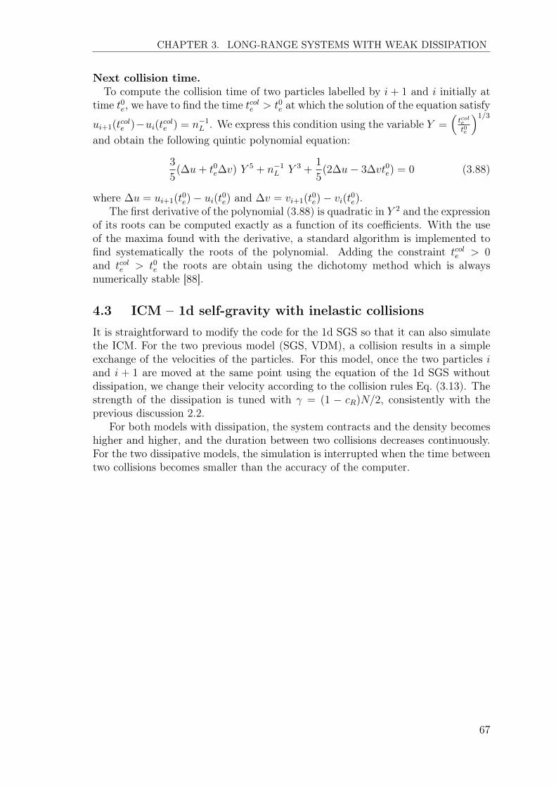
CHAPTER 3. LONG-RANGE SYSTEMS WITH WEAK DISSIPATION
Next collision time.To compute the collision time of two particles labelled by i + 1 and i initially at
time t0e, we have to find the time tcole > t0e at which the solution of the equation satisfy
ui+1
(tcole )�ui(tcole ) = n�1
L . We express this condition using the variable Y =
⇣tcole
t0e
⌘1/3
and obtain the following quintic polynomial equation:
3
5
(�u+ t0e�v) Y 5
+ n�1
L Y 3
+
1
5
(2�u� 3�vt0e) = 0 (3.88)
where �u = ui+1
(t0e)� ui(t0
e) and �v = vi+1
(t0e)� vi(t0
e).The first derivative of the polynomial (3.88) is quadratic in Y 2 and the expression
of its roots can be computed exactly as a function of its coefficients. With the useof the maxima found with the derivative, a standard algorithm is implemented tofind systematically the roots of the polynomial. Adding the constraint tcole > 0
and tcole > t0e the roots are obtain using the dichotomy method which is alwaysnumerically stable [88].
4.3 ICM – 1d self-gravity with inelastic collisions
It is straightforward to modify the code for the 1d SGS so that it can also simulatethe ICM. For the two previous model (SGS, VDM), a collision results in a simpleexchange of the velocities of the particles. For this model, once the two particles iand i + 1 are moved at the same point using the equation of the 1d SGS withoutdissipation, we change their velocity according to the collision rules Eq. (3.13). Thestrength of the dissipation is tuned with � = (1 � cR)N/2, consistently with theprevious discussion 2.2.
For both models with dissipation, the system contracts and the density becomeshigher and higher, and the duration between two collisions decreases continuously.For the two dissipative models, the simulation is interrupted when the time betweentwo collisions becomes smaller than the accuracy of the computer.
67

CHAPTER 3. LONG-RANGE SYSTEMS WITH WEAK DISSIPATION
4.4 Initial conditions for numerical simulation
For the SGS, the system relaxes, in few times of ⌧dyn, to a QSS. The nature of theQSS, i.e. its distribution function, depends on the nature probability distributionwe use to generate initial conditions. In presence of dissipation, we expect thesystem to proceed in the same way through this phase of its evolution because ofthe separation of time scales. As our purpose is to examine the robustness suchQSS, it is important to have a variety QSS, and thus variety of initial conditions.
We present, here, the three different initial conditions we have employed: the“rectangular water-bag” initial condition with different initial virial ratio, the micro-canonical equilibrium, and another water-bag configuration called “Fermi degener-ate”.
- 1 - Rectangular water-bag distribution
A water-bag distribution is one which is single valued and non-zero only in a compactregion of phase space. The rectangular water-bag initial condition in which thisregion is rectangular has been used to study the Vlasov dynamics [18, 26, 42]. It issimple, and macroscopic quantities can be easily computed.
To start from a rectangular water-bag distribution, we choose randomly anduniformly the (phase space) coordinates of N particles in the rectangular domainD = [�L
0
/2, L0
/2] ⇥ [�V0
/2, V0
/2]. The one particle probability distribution func-tion is then:
P1
(xi, vi) =
⇢1
L0V0, if (x, v) 2 D,
0, otherwise.(3.89)
The normalization is such that the integral of PN(x1
, v1
, ..., xN , vN) = ⇧Ni=1
P1
(xi, vi)over the 2N coordinates of phase space is unity.
Using this probability distribution function we can compute the mean initialkinetic energy over the realisations of the process,
hK0
i =Z L0/2
�L0/2
Z V0/2
�V0/2
1
2
mNX
i=1
v2iPN(vi)dNvi =
1
8
NmV 2
0
3
, (3.90)
and the mean initial potential energy 3
hU0
i =Z L0/2
�L0/2
Z V0/2
�V0/2
U(xi)P({xi})dNxidNvi (3.93)
3For the force given in Eq. (3.73) (with periodic boundary condition), the expression for thepotential energy in coordinates where the centre of mass is zero is:
U(xi,t) = g
X
i,j2S
X
i6=j
|xi � xj |� g↵n0x2i (3.91)
and the mean initial potential energy is:
hU0i = gL0N
2 �N
6� 2g↵L0
N
2
6. (3.92)
Given that the size if the box is always much larger than the size of the system, the backgroundterm is negligible (↵ ⌧ 1)
68
CHAPTER 3. LONG-RANGE SYSTEMS WITH WEAK DISSIPATION
Figure 3.1: Two examples of rectangular water-bag distributions, left panel for R0
=
0.01 and right panel for R0
= 1 both with 1024 particles. The units are such thatthe mean density n
0
= 1 and ⌧dyn = 1.
We have:
R0
=
2hK0
ihU
0
i =
V 2
0
2g(N � 1)L0
(3.94)
R0
is thus directly related to the aspect ratio of the rectangular water-bag. Theinitial energy E
0
is completely determined by R0
.In the following results we use mainly two values of the initial virial ratio:
• R0
= 1 for which 2K0
⇠ U0
: "hot" initial state.
• R0
= 0.01 for which K0
⌧ U0
: "cold" initial state.
We do not consider the initial conditions where R0
> 1 as there are known to relaxinto similar QSS as for R
0
< 1 [26].
- 2 - Equilibrium state
As we have discussed in chapter 1, in 1d, the thermal equilibrium of an open self-gravitating system is well defined. Further the micro-canonical and the canonicalensemble are equivalent. Maximising this in canonical or micro-canonical ensemble,one can compute the exact thermal equilibrium solution of the system in the mean-field limit [20,26](chapter 1):
feq(x, v) =1
2
p⇡
1
�⇤sech
2
⇣x
⇤
⌘exp
✓�⇣ v�
⌘2
◆, (3.95)
with the two characteristic scales depending on the total energy of the system E:
�2
=
4E
3mN, ⇤ =
4E
3g(mN)
2
. (3.96)
69
CHAPTER 3. LONG-RANGE SYSTEMS WITH WEAK DISSIPATION
For this solution of the Vlasov equation, the distribution of positions and velocitiesare separable and using the dimensionless variable ⇠ = x/� and ⌘ = v/�, we choosethe N particle initial positions randomly with the probability distribution function
g(⇠) =1
2
sech
2
(⇠) = ⇤⇢eq(x); (3.97)
and the velocities randomly following the distribution4:
h(⌘) =1p⇡exp
��⌘2� = �✓eq(v). (3.101)
It has been demonstrated [28] that the thermal equilibrium is the only separablestationary solution of Vlasov equation. Moreover simulation have shown that finiteN system relax toward this equilibrium on a time scale ⇠ N⌧dyn( [28] and referencetherein.
- 3 - Fermi degenerate water-bag distribution
A consequence of Jean’s Theorem [3], in 1d, is that any distribution which is only afunction of
e(x, v) =1
2
mv2 +m¯�(x) , (3.102)
the individual energy of a particle, is a stationary solution of the Vlasov equation. In1966, Hohl and Feix derived a non-equilibrium stationary solution of the 1d Vlasovequation [89]. The authors seek for a water-bag distribution of this kind. Theysought a solution in which f is taken to be constant in the area A of phase spacesuch that e(x, v) < emax, where emax is a maximum particle energy, and zero outside,i.e.:
f(x, v) ⌘ ˜f(e) =
⇢f0
, if 0 < e emax,0, if e > emax
. (3.103)
It is then possible to derive an expression for the curve bounding A: definingv+
(x) > 0 and v�(x) = �v+
(x) < 0 to be the contour of the water-bag, symmetric
4The random generator of the computer gives a random number rect[0,1] between 0 and 1 withuniform probability. In order to generate the spatial distribution we use the inverse transformmethod (e.g. [88]). For this we use the anti-derivative of g of Eq. (3.97) which is G(⇠) = 1
2 tanh (⇠).Then compute it inverse:
G
�1(⇠) =1
2ln
✓1 + ⇠
1� ⇠
◆. (3.98)
Then the distribution g(⇠) in position is generated by transforming rect[0,1] with G
�1:
⇠ =1
2ln
✓1+rect[0,1]1� rect[0,1]
◆(3.99)
For the Gaussian velocity distribution h(⌘), we make use of the Box Muller method [88] andgenerate with the following expression:
⌘ =1p⇡
q� ln(rect[0,1]) sin(2⇡rect[0,1]) (3.100)
70
CHAPTER 3. LONG-RANGE SYSTEMS WITH WEAK DISSIPATION
Figure 3.2: Phase space realisation for 1024 particles of the micro-canonical equilib-rium.
with respect to the x axes. Then the water-bag distribution solution of the stationaryVlasov equation may be written as:
˜f(x, v) = f0
⇥(v � v+
(x))⇥(v � v�(x)), (3.104)
with ⇥(x) the step function (heavy-side). Then, inserting in the stationary Vlasovequation we obtain:
✓v@
@x+ F
@
@v
◆f0
⇥(v � v+
(x))⇥(v � v�(x)) = 0 (3.105)
with F the mean field force. Using the derivative of the distribution ⇥, the latterequation is equivalent to:
�(v � v+
)
✓v@v
+
@x+ F
◆� �(v � v�)
✓v@v�@x
+ F
◆= 0 (3.106)
Then, integrating over v and using v�(x) = �v+
(x) we obtain:
v±@v±@x
� F = 0 (3.107)
Further, F is given by the Poisson equation:
� @F
@x= 2g⇢(x) = 4gm
Z v+(x)
0
˜f(x, v)dv = 4gmf0
v+
(3.108)
Inserting in Eq. (3.107), one gets the following differential equation for the contour:
@2v+
@x2
+
1
v+
✓@v
+
@x
◆2
� 4gf0
= 0 (3.109)
71
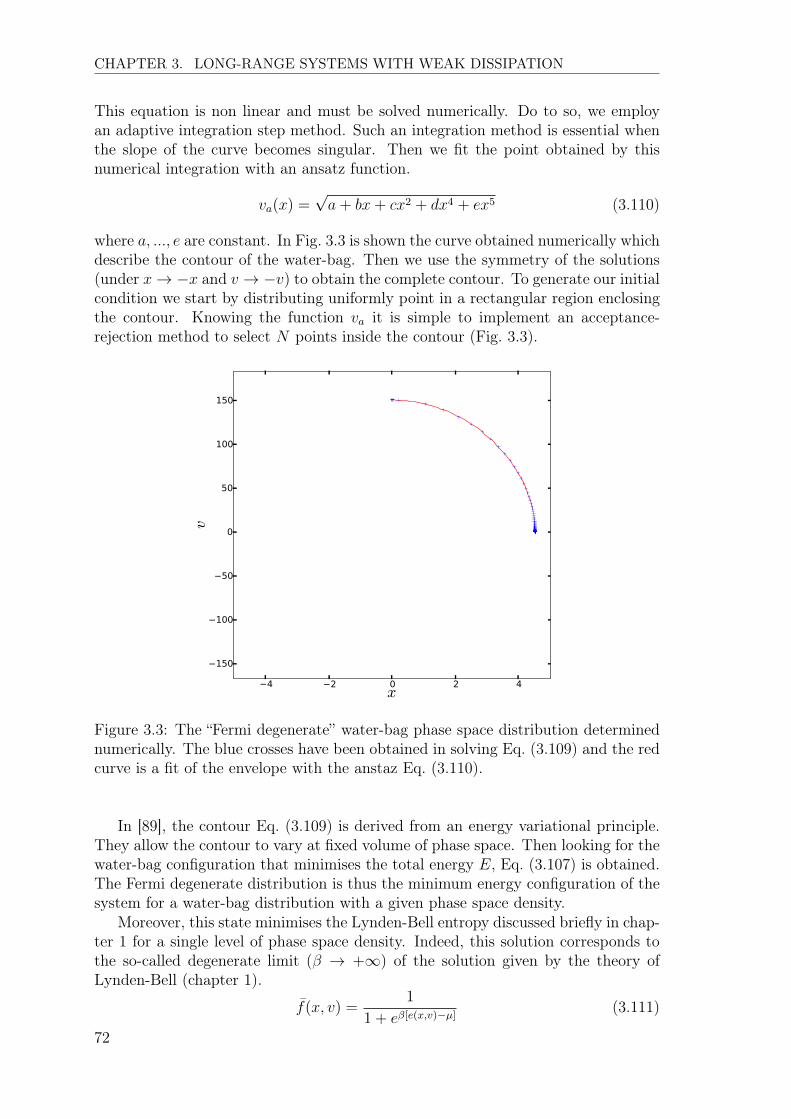
CHAPTER 3. LONG-RANGE SYSTEMS WITH WEAK DISSIPATION
This equation is non linear and must be solved numerically. Do to so, we employan adaptive integration step method. Such an integration method is essential whenthe slope of the curve becomes singular. Then we fit the point obtained by thisnumerical integration with an ansatz function.
va(x) =pa+ bx+ cx2
+ dx4
+ ex5 (3.110)
where a, ..., e are constant. In Fig. 3.3 is shown the curve obtained numerically whichdescribe the contour of the water-bag. Then we use the symmetry of the solutions(under x ! �x and v ! �v) to obtain the complete contour. To generate our initialcondition we start by distributing uniformly point in a rectangular region enclosingthe contour. Knowing the function va it is simple to implement an acceptance-rejection method to select N points inside the contour (Fig. 3.3).
Figure 3.3: The “Fermi degenerate” water-bag phase space distribution determinednumerically. The blue crosses have been obtained in solving Eq. (3.109) and the redcurve is a fit of the envelope with the anstaz Eq. (3.110).
In [89], the contour Eq. (3.109) is derived from an energy variational principle.They allow the contour to vary at fixed volume of phase space. Then looking for thewater-bag configuration that minimises the total energy E, Eq. (3.107) is obtained.The Fermi degenerate distribution is thus the minimum energy configuration of thesystem for a water-bag distribution with a given phase space density.
Moreover, this state minimises the Lynden-Bell entropy discussed briefly in chap-ter 1 for a single level of phase space density. Indeed, this solution corresponds tothe so-called degenerate limit (� ! +1) of the solution given by the theory ofLynden-Bell (chapter 1).
¯f(x, v) =1
1 + e�[e(x,v)�µ](3.111)
72
CHAPTER 3. LONG-RANGE SYSTEMS WITH WEAK DISSIPATION
with µ = emax is the analogous of the Fermi energy in a fermionic gas. This iswhy this state is called “Fermi degenerate”. Because of the property of stationarityans stability, we found interesting to use this particular distribution as an initialcondition of our simulations.
5 Simulation results for 1d self-gravity
We now present our numerical results. First, we reconsider the case of an isolatedsystem and check that we reproduce results obtained in other studies. Indeed thedynamics of a finite 1d SGS has been the subject of numerous studies [19,28,89,90].In particular, it is important to verify that the numerical method used simulatesaccurately a finite system despite the presence of the background term. We will seethat the simulations indeed reproduce the known results on violent relaxation towardQSS and on the thermal relaxation. Moreover, increasing the temporal resolutionof observables we were able to exhibit the presence of "breathing modes" in the 1dSGS model. These modes have been analytically studied for SGS [91] and for otherlong-range interacting models in [5, 92].
Second, we present the results of the VDM. We show that the decay law (Eq. (3.53))fits perfectly the theoretical prediction from the kinetic equation. Moreover for thedifferent initial conditions we show that the scaling QSS are a very good descriptionof the dynamics.
Finally, numerical results of the ICM are displayed. For this model, the predic-tion of a system collapse in a finite time fits with the simulation data. However, forinitial conditions with R
0
⌧ 1, we observe significant deviations from the scalingsolution at longer times. These deviations do not correspond to any tendency of thesystem to approach its thermal equilibrium, but on the contrary takes the systemfurther from this latter state.
5.1 Macroscopic observables
We monitor the kinetic energy and the potential energy which is computed withEq. (3.91). In addition, two macroscopic “order parameters” are convenient to studythe dynamics.
The first one is the virial ratio already introduced above and defined by
R(t) =2K(t)
U(t), (3.112)
where K and U are respectively the kinetic energy and the potential energy. Astationary solution of the Vlasov equation implies the virial ratio to be strictly 1.Thus in a mean field (N = 1) description of the system, this ratio being unity is anecessary condition to be in a QSS. For our finite N system, we say the system is“virialised” when R is unity (up to small finite N fluctuations).
The second observable is the separability ratio
�11
(t) =h|x(t)v(t)|i
h|x(t)|ih|v(t)|i � 1 (3.113)
73
CHAPTER 3. LONG-RANGE SYSTEMS WITH WEAK DISSIPATION
where h.i is an arithmetic mean over the N particles. This ratio is zero if and onlyif the system is in thermal equilibrium [26].
Since �11
is defined as a ratio if the moments of the position and velocity distri-bution, in a QSS this ratio has a constant value.
Finally, we study also the spatial and velocity distributions. The histogramsdisplay below will represents the averaged statistic over many realisations of thedynamics to reduce finite-size effects.
5.2 SGS (without dissipation)
As described in previous studies and discussed in chapter 1, the dynamics of 1dSGS is described by a two stages of evolution during each of which the shape ofthe distribution function changes significantly. We describe first the results of thesimulation for the shorter time (“collisionless”, or “violent” ) relaxation. We thenillustrate the long time relaxation toward the thermal equilibrium.
Violent relaxation to QSS
Fig. 3.4 illustrates the complex dynamics of violent relaxation. Each panel showsthe particle positions in phase space, at a given time. In each case the 100 realisa-tions of the system are over-plotted. As time progresses the phase space structure“winds up” into a filamentary structure. As the dynamics goes on, the filamentsstretch spiralling around the center and finally mix and become indistinguishable(last 2 panels). At a macroscopic level, the phase space distribution does not evolvesignificantly any more: the QSS is attained.
We now analyse the evolution of the macroscopic quantities introduced aboveduring this early stage relaxation. In Fig. 3.5 the virial ratio is displayed as a functionof time up to 150⌧dyn. For both initial conditions, in ⇠ 10⌧dyn, the parameter relaxesto the value 1 with fluctuations smaller than 10
�2. A blow-up of the oscillationsis presented below for both cases. In the left panels we zoom in on the first fewdynamical times; and in the right panels on later times once it has virialised. Forboth case, when the system is relaxing (left panels), the smallest period of oscillationsis apparently exactly ⌧dyn independently of the initial condition and of the numberof particles.
Moreover for the hot initial condition the virial ratio oscillates manifesting beatlike structure, suggesting the existence of two slightly different frequencies. One ofthe two frequencies is clearly the inverse of the time units: ⌧�1
dyn =
pgn
0
/2. Indeedwe note that these features are not present for the cold case while the oscillationsof period of ⌧dyn are still present. After the system has virialised (right panels),the oscillations are still present with a period of order ⌧dyn, increasing the numberof particles does not appears to quench the fluctuations. Moreover, the results,averaged over 100 realisations of the initial distribution, explore largely the statisticof the initial rectangular portion of phase space. Thus it seems that these oscillationsare representative of the (coarse grained) Vlasov dynamics.
Such “breathing modes” have been studied and seen in various kinds of simula-tions [5] and they have been analytically studied for self-gravitating system in [91].These modes generate an oscillating potential with which some particles resonate.
74

CHAPTER 3. LONG-RANGE SYSTEMS WITH WEAK DISSIPATION
Figure 3.4: Phase space position 100 realisations of a 1024 particles system areplotted on top of each other for the times t/⌧dyn = 0, 3.5, 10.5, 21.2, 31.8, 70, forthe rectangular water-bag initial condition with R
0
= 0.01
As discussed in chapter 1, in the core-halo theory for violent relaxation [42], this pro-cess is proposed to be the analogous to a Landau damping mechanism, responsiblefor the formation of the “halo” in the distribution displayed below.
In Fig. 3.6 is presented a plot of �11
for the first 100 dynamical times startingfrom many different initial conditions. After ⇠ 10 � 20⌧dyn, the parameter relaxesto a stationary value which depends on the initial condition considered. The valuesare consistent with the ones obtained in [18,26] for the rectangular water-bag case.For the water-bag initial states, which are not stationary solutions of the Vlasovequation, the relaxation of this parameter and of the virial ratio, clearly indicatethe establishment of QSS. Also one remarks that as R
0
! 0 the stationary value
75
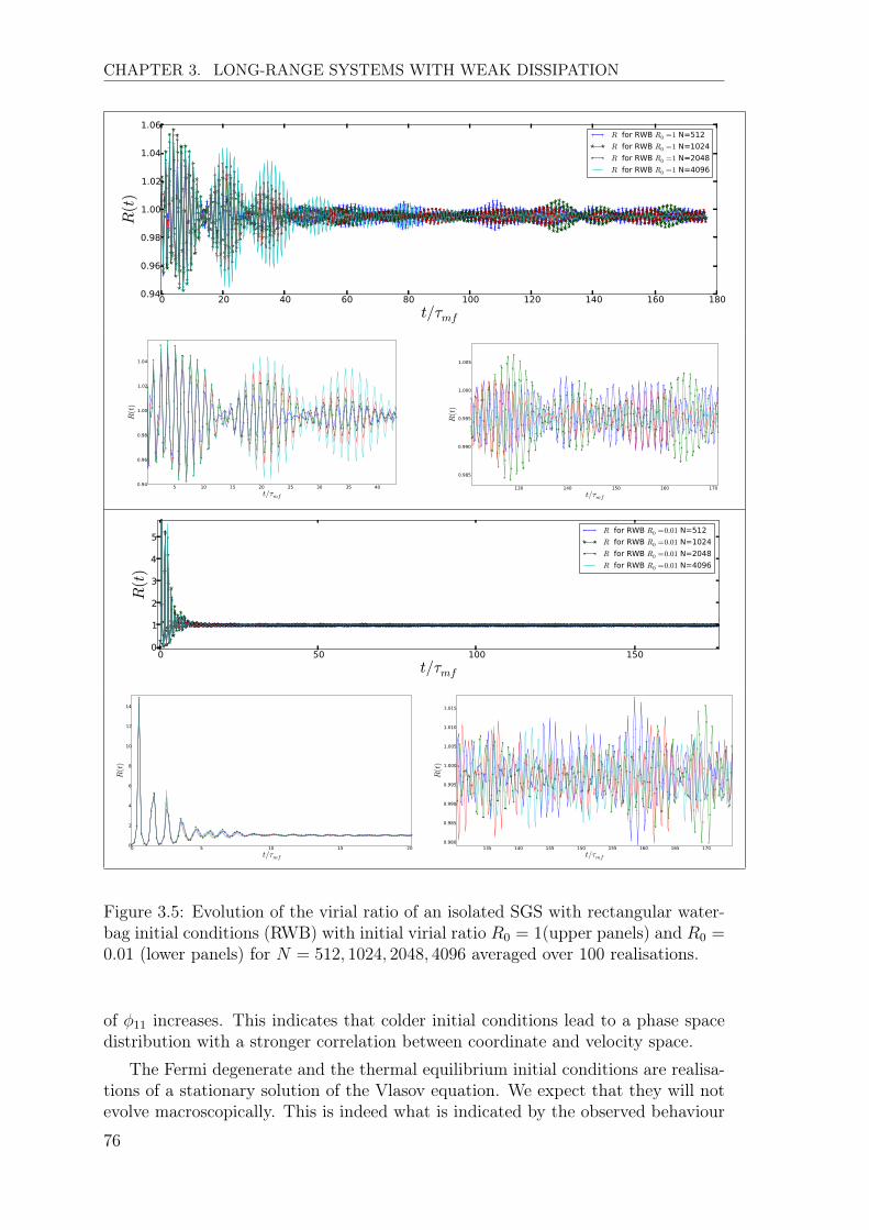
CHAPTER 3. LONG-RANGE SYSTEMS WITH WEAK DISSIPATION
Figure 3.5: Evolution of the virial ratio of an isolated SGS with rectangular water-bag initial conditions (RWB) with initial virial ratio R
0
= 1(upper panels) and R0
=
0.01 (lower panels) for N = 512, 1024, 2048, 4096 averaged over 100 realisations.
of �11
increases. This indicates that colder initial conditions lead to a phase spacedistribution with a stronger correlation between coordinate and velocity space.
The Fermi degenerate and the thermal equilibrium initial conditions are realisa-tions of a stationary solution of the Vlasov equation. We expect that they will notevolve macroscopically. This is indeed what is indicated by the observed behaviour
76
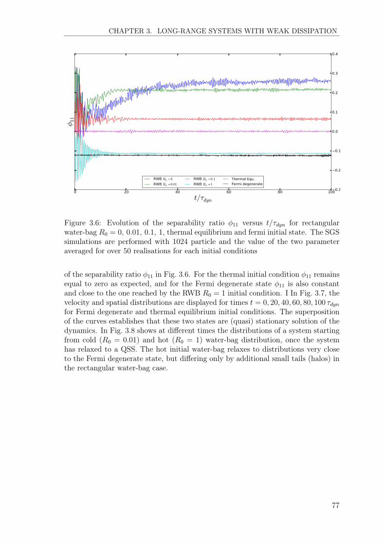
CHAPTER 3. LONG-RANGE SYSTEMS WITH WEAK DISSIPATION
Figure 3.6: Evolution of the separability ratio �11
versus t/⌧dyn for rectangularwater-bag R
0
= 0, 0.01, 0.1, 1, thermal equilibrium and fermi initial state. The SGSsimulations are performed with 1024 particle and the value of the two parameteraveraged for over 50 realisations for each initial conditions
of the separability ratio �11
in Fig. 3.6. For the thermal initial condition �11
remainsequal to zero as expected, and for the Fermi degenerate state �
11
is also constantand close to the one reached by the RWB R
0
= 1 initial condition. I In Fig. 3.7, thevelocity and spatial distributions are displayed for times t = 0, 20, 40, 60, 80, 100 ⌧dynfor Fermi degenerate and thermal equilibrium initial conditions. The superpositionof the curves establishes that these two states are (quasi) stationary solution of thedynamics. In Fig. 3.8 shows at different times the distributions of a system startingfrom cold (R
0
= 0.01) and hot (R0
= 1) water-bag distribution, once the systemhas relaxed to a QSS. The hot initial water-bag relaxes to distributions very closeto the Fermi degenerate state, but differing only by additional small tails (halos) inthe rectangular water-bag case.
77
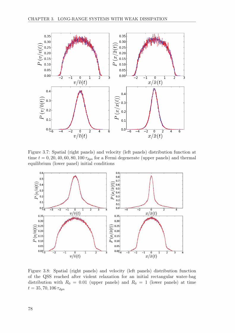
CHAPTER 3. LONG-RANGE SYSTEMS WITH WEAK DISSIPATION
Figure 3.7: Spatial (right panels) and velocity (left panels) distribution function attime t = 0, 20, 40, 60, 80, 100 ⌧dyn for a Fermi degenerate (upper panels) and thermalequilibrium (lower panel) initial conditions
Figure 3.8: Spatial (right panels) and velocity (left panels) distribution functionof the QSS reached after violent relaxation for an initial rectangular water-bagdistribution with R
0
= 0.01 (upper panels) and R0
= 1 (lower panels) at timet = 35, 70, 106 ⌧dyn
78

CHAPTER 3. LONG-RANGE SYSTEMS WITH WEAK DISSIPATION
Relaxation to equilibrium
We briefly present results on much longer time evolution of this system. We canobserve, as in other studies, a relaxation to thermal equilibrium. The physicalprocess involving this relaxation acts on much longer time scale which recently havebeen shown to be of order of to ⇠ zN⌧dyn where z is a numerical factor of order10
2 � 10
3 [28,93,94]. The relaxation time has been shown to be strongly dependenton the initial virial ratio R
0
[28].In Fig. 3.9 is shown an average over 50 realisations of a simulation of 128 particles
starting from a cold intial state run for 5.105⌧dyn. The relaxation takes place on thesame time scale for order 105⌧dyn, in good agreement with the results of [28] obtainedusing a different code.
Figure 3.9: Thermal relaxation of a system of 128 particles (50 realisations). Theenergy and the virial ratio R and the separability ratio �
11
, versus t/⌧dyn for rect-angular water-bag R
0
= 0.01.
79
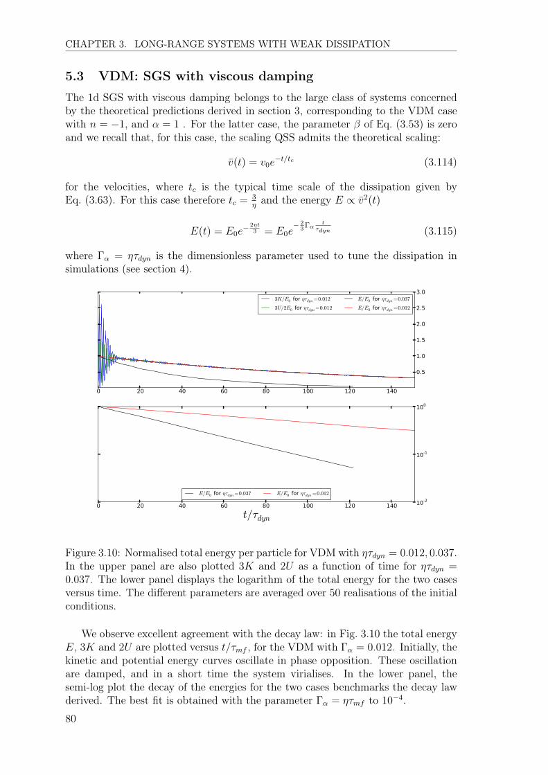
CHAPTER 3. LONG-RANGE SYSTEMS WITH WEAK DISSIPATION
5.3 VDM: SGS with viscous damping
The 1d SGS with viscous damping belongs to the large class of systems concernedby the theoretical predictions derived in section 3, corresponding to the VDM casewith n = �1, and ↵ = 1 . For the latter case, the parameter � of Eq. (3.53) is zeroand we recall that, for this case, the scaling QSS admits the theoretical scaling:
v(t) = v0
e�t/tc (3.114)
for the velocities, where tc is the typical time scale of the dissipation given byEq. (3.63). For this case therefore tc =
3
⌘and the energy E / v2(t)
E(t) = E0
e�2⌘t3
= E0
e� 2
3�↵
t
⌧
dyn (3.115)
where �↵ = ⌘⌧dyn is the dimensionless parameter used to tune the dissipation insimulations (see section 4).
Figure 3.10: Normalised total energy per particle for VDM with ⌘⌧dyn = 0.012, 0.037.In the upper panel are also plotted 3K and 2U as a function of time for ⌘⌧dyn =
0.037. The lower panel displays the logarithm of the total energy for the two casesversus time. The different parameters are averaged over 50 realisations of the initialconditions.
We observe excellent agreement with the decay law: in Fig. 3.10 the total energyE, 3K and 2U are plotted versus t/⌧mf , for the VDM with �↵ = 0.012. Initially, thekinetic and potential energy curves oscillate in phase opposition. These oscillationare damped, and in a short time the system virialises. In the lower panel, thesemi-log plot the decay of the energies for the two cases benchmarks the decay lawderived. The best fit is obtained with the parameter �↵ = ⌘⌧mf to 10
�4.
80
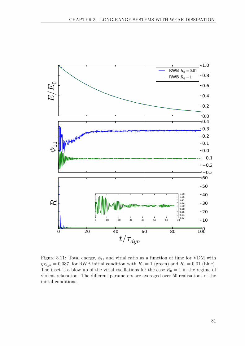
CHAPTER 3. LONG-RANGE SYSTEMS WITH WEAK DISSIPATION
Figure 3.11: Total energy, �11
and virial ratio as a function of time for VDM with⌘⌧dyn = 0.037, for RWB initial condition with R
0
= 1 (green) and R0
= 0.01 (blue).The inset is a blow up of the virial oscillations for the case R
0
= 1 in the regime ofviolent relaxation. The different parameters are averaged over 50 realisations of theinitial conditions.
81
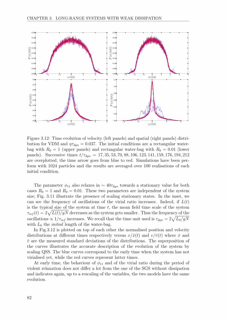
CHAPTER 3. LONG-RANGE SYSTEMS WITH WEAK DISSIPATION
Figure 3.12: Time evolution of velocity (left panels) and spatial (right panels) distri-bution for VDM and ⌘⌧dyn = 0.037. The initial conditions are a rectangular water-bag with R
0
= 1 (upper panels) and rectangular water-bag with R0
= 0.01 (lowerpanels). Successive times t/⌧dyn = 17, 35, 53, 70, 88, 106, 123, 141, 159, 176, 194, 212are overplotted, the time arrow goes from blue to red. Simulations have been per-form with 1024 particles and the results are averaged over 100 realisations of eachinitial condition.
The parameter �11
also relaxes in ⇠ 40⌧dyn towards a stationary value for bothcases R
0
= 1 and R0
= 0.01. These two parameters are independent of the systemsize; Fig. 3.11 illustrate the presence of scaling stationary states. In the inset, wecan see the frequency of oscillations of the virial ratio increases. Indeed, if L(t)is the typical size of the system at time t, the mean field time scale of the system⌧mf (t) = 2
pL(t)/gN decreases as the system gets smaller. Thus the frequency of the
oscillations / 1/⌧mf increases. We recall that the time unit used is ⌧dyn = 2
pL0
/gNwith L
0
the initial length of the water-bag.In Fig.3.12 is plotted on top of each other the normalised position and velocity
distributions at different times respectively versus x/x(t) and v/v(t) where x andv are the measured standard deviations of the distributions. The superposition ofthe curves illustrates the accurate description of the evolution of the system byscaling QSS. The blue curves correspond to the early time when the system has notvirialised yet, while the red curves represent latter times.
At early time, the behaviour of �11
and of the virial ratio during the period ofviolent relaxation does not differ a lot from the one of the SGS without dissipationand indicates again, up to a rescaling of the variables, the two models have the sameevolution.
82

CHAPTER 3. LONG-RANGE SYSTEMS WITH WEAK DISSIPATION
5.4 ICM: SGS with dissipation through inelastic collisions
According to the discussion after Eq. (3.66), this is a limit case. Indeed this modelis a particular case of the ICM class, with � = �c = 1, corresponding to the ratiobetween the two time scales ⌧diss and ⌧dyn which remains constant in the scalingQSS. Thus as we have discussed, for this case the scaling solution may be expectedto represent well the behaviour of the system for a transient period.
Rectangular water-bag initial conditions
Figure 3.13: Evolution of the phase space distribution of ICM with N� = 0.01starting from a rectangular initial condition with R
0
= 1. The 100 realisations ofthe initial condition are plotted on the top of each others.
The four first panels of Fig. 3.13 show the early time evolution of the system(t = 0, 7, 14, 28 ⌧dyn ). It appears to be just like the period of violent relaxation for aHamiltonian long-range interacting system, and as we see below, during this period,
83
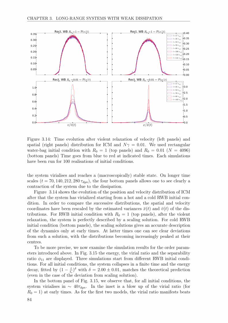
CHAPTER 3. LONG-RANGE SYSTEMS WITH WEAK DISSIPATION
Figure 3.14: Time evolution after violent relaxation of velocity (left panels) andspatial (right panels) distribution for ICM and N� = 0.01. We used rectangularwater-bag initial condition with R
0
= 1 (top panels) and R0
= 0.01 (N = 4096)(bottom panels) Time goes from blue to red at indicated times. Each simulationshave been run for 100 realisations of initial conditions.
the system virialises and reaches a (macroscopically) stable state. On longer timescales (t = 70, 140, 212, 280 ⌧dyn), the four bottom panels allows one to see clearly acontraction of the system due to the dissipation.
Figure 3.14 shows the evolution of the position and velocity distribution of ICMafter that the system has virialized starting from a hot and a cold RWB initial con-dition. In order to compare the successive distributions, the spatial and velocitycoordinates have been rescaled by the estimated variances x(t) and v(t) of the dis-tributions. For RWB initial condition with R
0
= 1 (top panels), after the violentrelaxation, the system is perfectly described by a scaling solution. For cold RWBinitial condition (bottom panels), the scaling solutions gives an accurate descriptionof the dynamics only at early times. At latter times one can see clear deviationsfrom such a solution, with the distributions becoming increasingly peaked at theircentres.
To be more precise, we now examine the simulation results for the order param-eters introduced above. In Fig. 3.15 the energy, the virial ratio and the separabilityratio �
11
are displayed. Three simulations start from different RWB initial condi-tions. For all initial conditions, the system collapses in a finite time and the energydecay, fitted by (1 � t
tc
)
� with � = 2.00 ± 0.01, matches the theoretical prediction(even in the case of the deviation from scaling solution).
In the bottom panel of Fig. 3.15, we observe that, for all initial conditions, thesystem virialises in ⇠ 40⌧dyn. In the inset is a blow up of the virial ratio (forR
0
= 1) at early times. As for the first two models, the virial ratio manifests beats
84
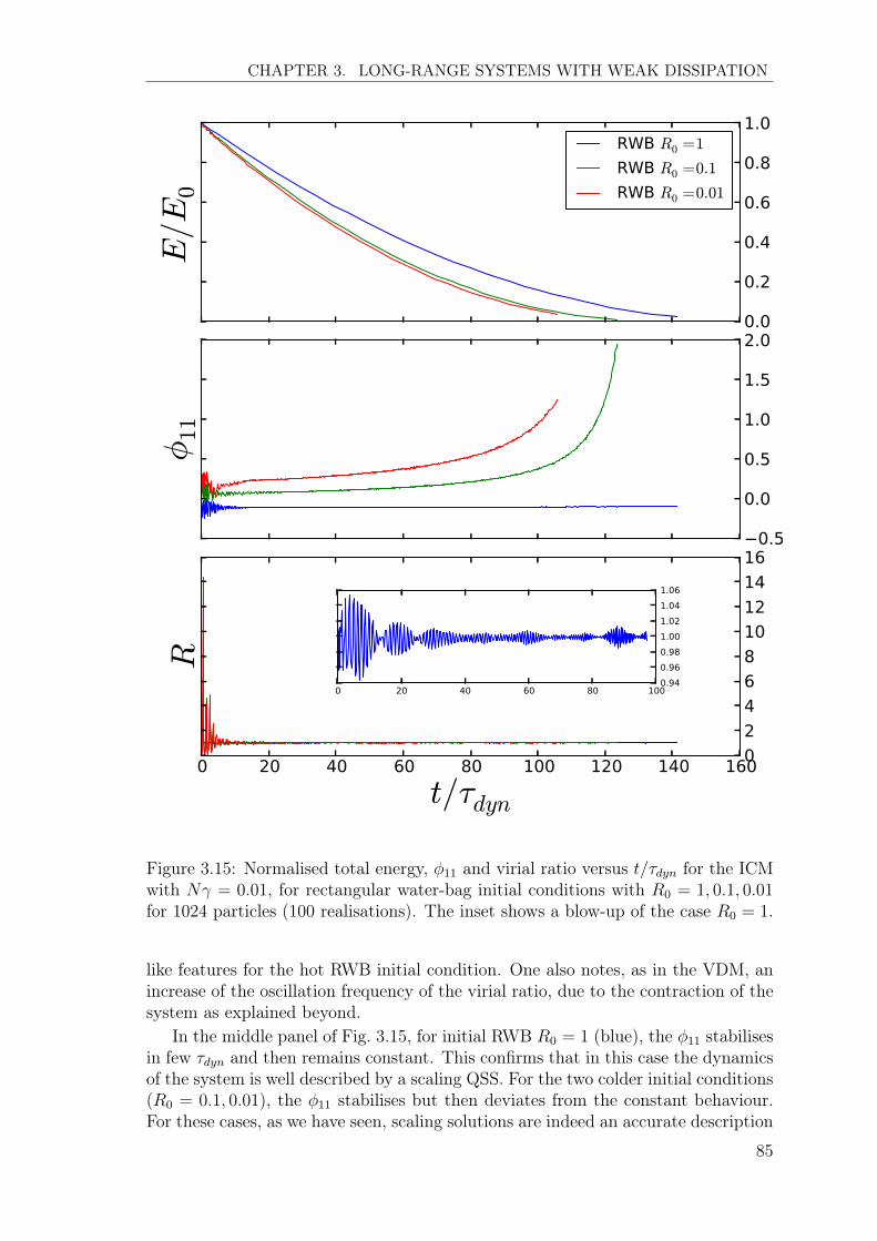
CHAPTER 3. LONG-RANGE SYSTEMS WITH WEAK DISSIPATION
Figure 3.15: Normalised total energy, �11
and virial ratio versus t/⌧dyn for the ICMwith N� = 0.01, for rectangular water-bag initial conditions with R
0
= 1, 0.1, 0.01for 1024 particles (100 realisations). The inset shows a blow-up of the case R
0
= 1.
like features for the hot RWB initial condition. One also notes, as in the VDM, anincrease of the oscillation frequency of the virial ratio, due to the contraction of thesystem as explained beyond.
In the middle panel of Fig. 3.15, for initial RWB R0
= 1 (blue), the �11
stabilisesin few ⌧dyn and then remains constant. This confirms that in this case the dynamicsof the system is well described by a scaling QSS. For the two colder initial conditions(R
0
= 0.1, 0.01), the �11
stabilises but then deviates from the constant behaviour.For these cases, as we have seen, scaling solutions are indeed an accurate description
85

CHAPTER 3. LONG-RANGE SYSTEMS WITH WEAK DISSIPATION
of the system only for a transient period and this is also reflected in the behaviourof �
11
.
Figure 3.16: For the ICM, reduced total energy E(t)/E(0) versus �t/⌧dyn, for theindicated values of � and R
0
= 0.01. The inset shows a zoom on the shorter timeevolution.
In Fig. 3.16 we plotted the energy decay curves for different values of � as afunction of the rescaled time �t/⌧dyn. With this change of variables the curves su-perpose and, as expected by the theoretical treatment (cf. Eq. (3.63)), the collapsetime scales as tc ⇠ ��1 just as the time scale ⌧diss associated with the dissipation.We also note that the collapse time tc depends slightly on the initial conditions(Fig. 3.15). The inset of Fig. 3.16 shows small deviations from the scaling behaviourat short times, associated with the virial oscillations during the initial violent relax-ation.
The bottom panel of Fig. 3.17, shows a semi-log plot of �11
as a function of t,for � = 0.01, 0.005, 0.001. We see that the early time relaxation is not affected bythe variation of the strength of the perturbation up to ⇠ 10⌧dyn. Indeed choosing �sufficiently small, the two time scales of the system are well separated (⌧dyn ⌧ ⌧diss).Thus the effect of the dissipation happens on longer time scale, as expected.
The upper panel of Fig. 3.17 shows the evolution of �11
for the ICM startingfrom R
0
= 0.01, R0
= 0.1 and R0
= 1, and each for the three different values of�. As well as the energy, the evolution of �
11
, for all initial conditions, collapsesusing the rescaled time �t/⌧dyn. This seems to indicate that the dependence of thedynamics on � might be scaled out using this time coordinates.
86
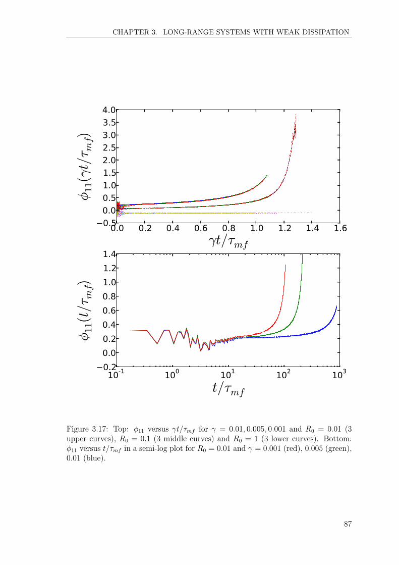
CHAPTER 3. LONG-RANGE SYSTEMS WITH WEAK DISSIPATION
Figure 3.17: Top: �11
versus �t/⌧mf for � = 0.01, 0.005, 0.001 and R0
= 0.01 (3upper curves), R
0
= 0.1 (3 middle curves) and R0
= 1 (3 lower curves). Bottom:�11
versus t/⌧mf in a semi-log plot for R0
= 0.01 and � = 0.001 (red), 0.005 (green),0.01 (blue).
87
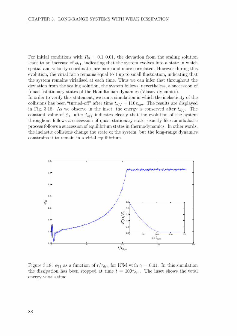
CHAPTER 3. LONG-RANGE SYSTEMS WITH WEAK DISSIPATION
For initial conditions with R0
= 0.1, 0.01, the deviation from the scaling solutionleads to an increase of �
11
, indicating that the system evolves into a state in whichspatial and velocity coordinates are more and more correlated. However during thisevolution, the virial ratio remains equal to 1 up to small fluctuation, indicating thatthe system remains virialised at each time. Thus we can infer that throughout thedeviation from the scaling solution, the system follows, nevertheless, a succession of(quasi-)stationary states of the Hamiltonian dynamics (Vlasov dynamics).In order to verify this statement, we run a simulation in which the inelasticity of thecollisions has been “turned-off” after time toff = 110⌧dyn. The results are displayedin Fig. 3.18. As we observe in the inset, the energy is conserved after toff . Theconstant value of �
11
after toff indicates clearly that the evolution of the systemthroughout follows a succession of quasi-stationary state, exactly like an adiabaticprocess follows a succession of equilibrium states in thermodynamics. In other words,the inelastic collisions change the state of the system, but the long-range dynamicsconstrains it to remain in a virial equilibrium.
Figure 3.18: �11
as a function of t/⌧dyn for ICM with � = 0.01. In this simulationthe dissipation has been stopped at time t = 100⌧dyn. The inset shows the totalenergy versus time
88

CHAPTER 3. LONG-RANGE SYSTEMS WITH WEAK DISSIPATION
Vlasov stable initial conditions.
Figure 3.19: Time evolution after violent relaxation of velocity (left panels) andspatial (right panels) distribution for ICM and N� = 0.01. We used fermi degenerate(N = 1290) and thermal equilibrium (N = 1024) initial conditions. Time goes fromblue to red. Each simulations have been run for 100 realisations of initial conditions.
To explore further the domain of validity of the scaling-QSS as a function of theinitial condition taken in this limit case of the theory, we run simulations with ther-mal equilibrium and Fermi degenerate initial condidtions (see sec. 4.4). Contraryto rectangular water-bag, these states are, by construction, stationary solutions ofthe Vlasov equation (Vlasov stable).
In Fig. 3.19, the top panels show the evolution of the spatial and velocity dis-tributions starting from a Fermi degenerate initial condition as a function of therescaled variables x/x(t) and v/v(t). We observe that for this case also the scal-ing solution appears to be a accurate description of the dynamics. In the bottompanels, the same quantities are plotted for a simulation starting from the thermalequilibrium. In this case also, we observe clear deviation from the scaling dynamicsat later times. For the two cases the evolution of the energy of the system is thesame as for RWB initial condition and we do not display it here.
In Fig. 3.20 we show the evolution of the virial ratio and the separability ratio �11
of a simulation starting from the Fermi degenerate state. For comparison, we alsodisplay these quantities starting from an initial rectangular water-bag with R
0
= 1.In the inset we can verify that the system is indeed already virialised when startingfrom this initial condition. Further for this case �
11
remains constant throughoutthe evolution, confirming that, for this initial condition also, the systems dynamicsis well described by the scaling QSS.
89
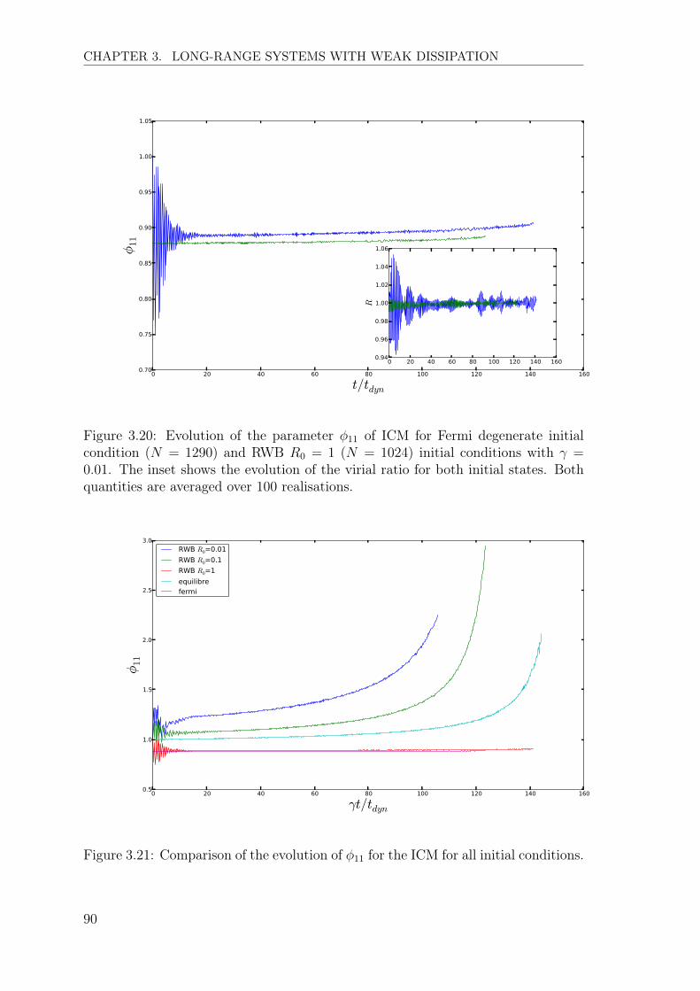
CHAPTER 3. LONG-RANGE SYSTEMS WITH WEAK DISSIPATION
Figure 3.20: Evolution of the parameter �11
of ICM for Fermi degenerate initialcondition (N = 1290) and RWB R
0
= 1 (N = 1024) initial conditions with � =
0.01. The inset shows the evolution of the virial ratio for both initial states. Bothquantities are averaged over 100 realisations.
Figure 3.21: Comparison of the evolution of �11
for the ICM for all initial conditions.
90

CHAPTER 3. LONG-RANGE SYSTEMS WITH WEAK DISSIPATION
In Fig. 3.21 is shown the evolution of �11
for all the different initial conditionswe have used. We observe that for the thermal equilibrium initial condition, thescaling QSS gives an accurate description of the system evolution at early time. Atlater times, for this case, the deviation from the scaling dynamics measured by �
11
is comparable to the one starting from cold RWB initial conditions. It is a strikingfeature of our results that the system, when its shows deviation from scaling QSS,does not show any tendency to evolve toward the thermal equilibrium (or a scalingversion of this state), but on the contrary evolves away from this state towards morecorrelated states. To better understand this feature is one of the motivations of thenext chapter.
91
CHAPTER 3. LONG-RANGE SYSTEMS WITH WEAK DISSIPATION
6 Conclusion
In this chapter we have studied the effect of various kinds of dissipation on the dy-namics of long-range interacting systems. For a Hamiltonian system, in the meanfield limit, the dynamics is described by the Vlasov equation. This non linear equa-tion for the phase space density admits an infinite number of stationary solutions.The stationary solutions of the Vlasov description are quasi-stationary states of thelong-range particles dynamics.
For a 1d long-range interacting system, we showed that the QSS are robust to alarge class of dissipative effects including fluid damping and, to lesser extent, inelasticcollisions. This robustness has been characterized theoretically by the existence ofscaling solutions of the appropriately modified Vlasov equation. This equation,derived under mean field and molecular chaos assumptions, has the same structureas the Vlasov equation with additional terms accounting for the dissipation. Theexistence of scaling solutions was derived under the assumption of separation ofthe two central characteristic time scales of the system: ⌧diss, the time scale ofthe dissipation and ⌧dyn, the time scale of the mean field dynamics. Under thisassumption, the system dissipates energy sufficiently slowly that the system alwaysremains very close to a QSS. After the initial phase of violent relaxation lastingabout 40⌧dyn, in which the QSS is established, the system undergoes a contractionon the longer time scale ⌧diss � ⌧dyn. Under a well defined rescaling of the positionand the velocity variables, the system keeps the same QSS distribution throughoutthe contraction.
The existence of scaling QSS has been confirmed by simulation of the N bodylong-range dynamics for two models of dissipation in the case of 1d gravity. Fora fluid dissipative model, where the dissipation takes place homogeneously in thesystem, scaling QSS are found to be a very good description of the dynamics forany initial condition. However for a model with inelastic collisions, the dissipationdepends on the frequency of collisions and thus on the density of the system. In thiscase, for inhomogeneous QSS, the dissipation is more important in the denser regionof the system. In coordinates following the contraction of the system, this implies aneffective energy transfer in the system, a change of phase space distribution and thesystem leave the scaling solutions on time scale of order of ⌧diss. We have shown thatthis evolution drives the system towards more correlated states between position andvelocity distributions, and thus further away from the thermal equilibrium.
Furthermore, we have shown the perturbed system remains at all times virialised.Thus, by switching the dissipation off once the system has left the scaling solution,we have shown that the system stays in the more correlated state indicating thatthis increase of the correlation induced by inelastic collision is indeed an adiabaticevolution through quasi stationary states of the isolated system. Hence, this colli-sional perturbation of the dynamics leads to a whole range of stationary solution ofthe dynamics of the unperturbed system.
The inelastic collisions added to the 1d system induces local contractions ofthe phase space volume occupied by the system and makes it collapse. Moreover,following this collapse in dimensionless variables, the inelastic collision induces localchange of velocity distribution, while a 1d elastic collisions does not change it. Forthe quasi-elastic limit of the model, each collision induces an infinitesimal and localchange in the velocity distribution. Even if this change is purely deterministic
92
CHAPTER 3. LONG-RANGE SYSTEMS WITH WEAK DISSIPATION
microscopically, on a coarse-grained level one would expect to be able to treat itas a stochastic process. However, the contraction of the system due to the energydissipation makes it very difficult to explore further the evolution away from thescaling QSS, and in particular whether the perturbation drives it to a new stationarystate at some time.
In the next chapter, we pursue the question raised by this interesting evolutiontoward more correlated QSS. To do so we introduce a similar class of perturbationarising from collisions in a long-range system, but such that the energy is conservedon average.
93

CHAPTER 3. LONG-RANGE SYSTEMS WITH WEAK DISSIPATION
94

Chapter 4
Long-range systems with internal
local perturbations
1 Introduction
In the previous chapter we have studied the effects of dissipation on a long-rangesystem and, in particular, on QSSs which are one of their most striking feature. Inthe limit of the separation of the relevant time scales, a kinetic equation, derivedfor a large class of one dimensional long-range models, enabled the prediction of theexistence of “scaling QSS”. Evolving in such a solution the systems keeps the samephase space distribution up to a rescaling, and thus the dissipation has a somewhattrivial effect on the QSS which would appear in the isolated system. Simulations ofa 1d self-gravitating system with different sorts of dissipation have largely confirmedthat such states do indeed describe well the evolution of these systems starting froma range of different initial conditions.
However, in one of the two models (the ICM), we have clearly seen evolution de-viating from scaling QSS, and interestingly, as we have noted, this evolution bringsthe system toward more correlated states rather than toward thermal equilibrium.Indeed, on the basis of work in the literature [95,96] (see chapter 1) we might haveanticipated that the “internal” stochasticity of the model might lead to a relaxationto thermal equilibrium. To further our study of this observation – and, more gener-ally, to explore how different kinds of perturbation affect the dynamics of long-rangesystems and, in particular, their QSS– we study in this chapter two different toymodels.
The first model is a variant of the ICM in which particles undergo not just in-elastic, but also super-elastic collisions (i.e. in which there is a net gain rather thana loss of energy). As we will detail, this is a generalisation of a granular modelstudied in literature [97]. In contrast with the ICM, the model has a dynamicswhich is explicitly stochastic: we chose randomly whether the collision is inelasticof super-elastic. Further we choose, essentially for simplicity, to conserve the energyon average (over the realisations). Indeed, in the ICM, as dissipation leads to acontinuous contraction of the system, it becomes difficult numerically to follow theevolution of the system on a long time scale.This model can be considered as a simple toy model for real long-range interacting
95

CHAPTER 4. LONG-RANGE SYSTEMS WITH INTERNAL LOCALPERTURBATIONS
systems in which there are additional short-range interactions which come into playwhen particles are close to one another– and which lead to energy loss or gain to otherdegrees of freedom (e.g. through radiation or to internal degrees of freedom). Super-elastic collisions can model thermally activated nanoclusters [98, 99] and have alsobeen reported for large-scale magnetized plasmoid in the heliosphere [100]. Granu-lar models incorporating a random coefficient of restitution have been used in [97]to study the effect of energy injection of a vibrated 2d granular gas. In the lat-ter study, more generally, different distributions of the values of the coefficient ofrestitution are considered. Further we note that such model could be considered tostudy the effects of errors introduced in the numerical integration of a long-rangesystem. For example in 3d self-gravitating system the velocity change of particleswhen they pass very close to one another, in a“hard” two body collision, is knownto be associated often with non-physical energy change due to poor integration ofthe trajectories [101,102].
The second model we consider is based on another granular model [103]. It isanother variant of the ICM in which energy is injected by collisions with an addi-tional constant velocity “kick”. Again we consider a one dimensional self-gravitatingsystem subjected to such collisions. In this case the system is expected to be ableto attain a stationary state in which the energy is constant. This model in contrastwith the first one is deterministic like the ICM.
We describe both models as a long-range systems subjected to “internal” and“local” perturbation: internal in the sense that the perturbation is associated withparticular events in the system i.e. interaction between elements internal to thesystem (rather than with external agents); and local because the perturbation islocalised in space and depends only on the state at this point of the system (and noton the state of the whole system). As we will discuss in our conclusion, we believethat this locality is central to the very different behaviour we observe compared tothe model of [55] showing relaxation to thermal equilibrium.
The chapter is organised as follows. In the next section we consider the firstmodel described above. We derive for it, under the assumption that the total en-ergy is conserved, a modified Vlasov equation which accounts for the effect of thestochastic collisions in the quasi-elastic (perturbative) limit. We use it to show inparticular that the thermal equilibrium of the 1d self-gravitating system is unstablewhen the perturbation is present. We then study the evolution of the energy of asingle realisation, and show, using heuristic arguments, that, at any finite time, theenergy variance, goes to zero as N does to infinity. This result means that the as-sumption of the energy conservation is indeed valid in the mean field - quasi-elasticlimit. Numerical results for the model are then presented, first for the model in theabsence of gravity and then with gravity
In the following section we investigate the second model through an essentiallynumerical study. In the case of the one dimensional granular gas (i.e. withoutgravity) we show that the system relaxes toward a bimodal velocity distribution.Further, the simulations reveal hydrodynamical modes that have been seen for thismodel in higher dimensions [103]. For the self-gravitating model we find that thesystem reach a steady state, independent of the initial conditions which evolves at
96
CHAPTER 4. LONG-RANGE SYSTEMS WITH INTERNAL LOCALPERTURBATIONS
longer time to state which is highly ordered microscopically.
2 The stochastic collision model (SCM)
After giving the microscopic definition of the collisions in the model, we develop akinetic theory to describe its macroscopic evolution. We show that, in the quasi-elastic limit, the collisional operator added to the Vlasov equation can be written in aFokker Planck form. This kinetic equation allows us to determine the large N scalingof the parameter characterising the perturbation in order to obtain a consistent meanfield - quasi-elastic limit. An analysis of the moments of the collisional term is thenpresented. This permits us to write a dynamical equation for the moments of thephase space density function. From these equations, we deduce, in particular, theinstability of the thermal equilibrium distribution. Finally, by an analysis of therandom process undergone by the energy of a single realisation, we establish thevalidity of the assumption we made to build the kinetic equation. These results aregeneral and valid for the model both with and without long-range interactions. In asecond part of this section numerical results for the model with and without gravityare presented and discussed.
2.1 Microscopic description of the stochastic collisions
The stochastic collision model (SCM) is defined as follows. Denoting vij the relativevelocity of particles i and j with velocities vi and vj prior to the collision, the post-collisional velocities v⇤i and v⇤j are given by:
v⇤i =vj +1� ↵
2
vij (4.1)
v⇤j =vi � 1� ↵
2
vij,
where the coefficient of restitution ↵ is chosen randomly with equal probability fromthe two values cR and cR related by
cR =
q2� c2R . (4.2)
This relation ensures that the magnitude of the energy change, for a given relativevelocity at collision, is the same in all collisions. The sign of the energy change isdetermined by whether we choose cR or cR:
• For an inelastic collision we use the usual restitution coefficient 0 cR < 1,such that the energy change after collision is
�Kinel = �m1� c2R
4
(vij)2 0, (4.3)
• For a collision involving a gain of energy, so called super-elastic collision, wedefine, as a function of cR, the corresponding super-elastic coefficient of resti-tution cR =
p2� c2R such that the energy change after collision is
�Ksuperel = ��Kinel � 0 . (4.4)
97
CHAPTER 4. LONG-RANGE SYSTEMS WITH INTERNAL LOCALPERTURBATIONS
With this definition, 1 < cR p2, and the quasi-elastic limit is such that both cR
and cR go to unity.We note that for this model the Jacobian of the transformation of the phase
space volume element is the random variable ↵ and takes a value either less thanor greater than unity, i.e. for a collision between two particles 1 and 2, the mea-sure of the phase space dx
1
dx2
...dxNdv⇤1
dv⇤2
..dvN = ↵dx1
dx2
...dxNdv1dv2..dvN , iscorrespondingly either smaller or greater than before the collision1.
2.2 Kinetic equation
In the previous chapter, the modified Vlasov equation for a model with inelasticcollisions was derived from a generalised Liouville equation. We have truncated theBBGKY hierachy, neglecting the two point correlation function and obtained themodified Vlasov equation:
@tf(x, v, t) + v.@xf(x, v, t)� @x ¯�[f ](x, t).@vf(x, v, t) = J�[f, f ](x, v, t) . (4.5)
where the collision term J�[f, f ](x, v, t) is the rate of change of the phase spacedensity resulting from the collision rules. We saw in chapter 3 that it can be splitinto a gain and a loss term:
J�[f, f ](x, v, t) = G�(x, v, t)� L(x, v, t) . (4.6)
The loss term measures the decrease of the population of particles inside a volumedxdv in the phase space around point (x, v) during the time interval dt:
L(x, v, t) =N
Mf(x, v, t)
Zdv0|v0 � v|f(x, v0, t) . (4.7)
and the gain term i.e. the increase of the population in an infinitesimal volumeduring dt is:
G�(x, v, t) =N
M
Z Zdv0dv00|v0 � v00|f(x, v0, t)f(x, v00, t)�(v � �v0 � (1� �)v00) .
We define for convenience2
� =
(1� cR)
2
. (4.8)
Given that (1� �)� = (1� c2R)/4, the corresponding � for a super-elastic collision,is a solution of the equation (4.4)
�Ksuperel(�) = ��Kinel(�) () (1� �)� = �(1� �)� . (4.9)
and therefore:
� =
1
2
�r(1� �)� +
1
4
. (4.10)
1In the view where the phase space of the non-Hamiltonian system is a manifold with a constantprobability measure as proposed in [104], the manifold is locally dilated or contracted in a randommanner at each collision.
2N.B.: The definition of � in this chapter is different the one in the previous chapter, where weused the notation q for this expression.
98

CHAPTER 4. LONG-RANGE SYSTEMS WITH INTERNAL LOCALPERTURBATIONS
Subsequently, we define the collisional operator for super-elastic collisions as:
J� [f, f ](x, v, t) = G�(x, v, t)� L[f, f ](x, v, t) . (4.11)
We have derived a collisional operator for the two kinds of collisions the particlesare subjected to. In the microscopic dynamics, collisions happen at discrete timeintervals and instantaneously. The equation (4.5), for the ICM, implicitly involvesa coarse-graining in time on a time interval dt in which many collisions occur in aphase space element. This means in particular (as we will verify below) that wehave implicitly assumed energy conservation. This assumption is valid exactly inthe model only if we consider an average over realisations. We will see below that italso be taken to be valid for a single realisation in the quasi-elastic limit of interestto us. With these assumptions which will be discussed further in section 2.7, thekinetic equation for the SCM is written:
@tf(x, v, t) + v.@xf(x, v, t)� @x�[f ](x, t).@vf(x, v, t) = JSCM [f, f ](x, v, t) (4.12).=
1
2
(J�(x, v, t) + J�(x, v, t)) .
2.3 Kramers Moyal expansion of the collision operator
We derive now the expression for the collisional operator in the quasi-elastic limitusing a Kramers Moyal expansion of this operator. We take the limit of small � andexpand the two gain rates G⇤ to second order respectively in � and �. Doing so, weobtain:
G� =
N
M
f(x, v, t)
Z|v0 � v|f(v0)dv0 + �@v
Z|v0 � v|(v0 � v)f(v)f(v0)dv0 (4.13)
+
1
2
�2@2v
Z|v0 � v|(v0 � v)2f(v)f(v0)dv0
�,
(4.14)
and the same expression for G� but with � instead of � . With the use of Eq. (4.9),one has the following relation:
� + � = �2 + �2 = �2 + o(�2) . (4.15)
Gathering terms, and using the last relation, we find that in the quasi-elasticlimit, the collisional operator takes a Fokker Planck form:
JSCM [f ] =�2N
M
�@v(f(x, v, t)a[f ](x, v, t)) + 1
2
@2v(f(x, v, t)D[f ](x, v, t))
�, (4.16)
with an acceleration and diffusion coefficient which are functions of the distributionfunction:
a[f ](x, v, t) =
Z|v0 � v|(v0 � v)f(x, v0, t)dv0 ; (4.17)
andD[f ](x, v, t) =
Z|v0 � v|(v0 � v)2f(x, v0, t)dv0 . (4.18)
99
CHAPTER 4. LONG-RANGE SYSTEMS WITH INTERNAL LOCALPERTURBATIONS
Large N scaling of �
Following the same reasoning as for the treatment of the ICM in the previous chapter,we consider how the parameter must be scaled in the N ! +1 mean field limit inwhich the Vlasov equation describes the evolution of the phase space density due tothe long-range interaction. For the ICM, we saw that taking the limit 1� cR ⌧ 1,the Kramers Moyal expansion gives a term proportional to (1�c
R
)N2
= �ICM . FromEq. (4.16) we see that, for the SCM, we need to take �2N ⇠ Cst as N ! +1 sothat the collision term does not diverge in the large N limit. We thus introduce arescaled parameter
�SCM =
(1� cR)pN
2
. (4.19)
In our numerical simulation with gravity we will keep this parameter fixed as wevary N .
2.4 Moments of the collision operator
We consider the following moments of the full collisional integralZ
vnJSCM [f, f ]dvdx =
Zdvdx vn
1
2
[J�(x, v, t) + J�(x, v, t)] . (4.20)
We first consider the first term on the right hand side of the equation, and usingthe definition of the collisional operator we obtain:
Zvn1
J�[f, f ](x, v1, t)dxdv1 =1
m
ZZvn1
|v1
� v2
|f(x, v⇤⇤
1
, t)f(x, v⇤⇤2
, t)
c2R(4.21)
�f(x, v1
, t)f(x, v2
, t)] dxdv2
dv1
,
where v⇤⇤i,j = vi,j ± �(vi � vj) are the pre-collisional velocities. Splitting the lastintegral, changing the velocity coordinates of the first term with the post-collisionalvelocities v⇤i,j = vi,j ± (1� cR)/2(vi � vj) and regrouping terms we obtain:
ZvnJ�[f, f ]dvdx =
Z Z((v⇤
1
)
n � vn1
)|v1
� v2
|f(x, v1
, t)f(x, v2
, t)dv1
dv2
. (4.22)
Now we define
�n(v1, v2) = (v⇤1
)
n � vn1
= (�v1
� (1� �)v2
)
n � vn1
. (4.23)
The rest of the integrand, |v1
� v2
|f(x, v1
, t)f(x, v2
, t), is symmetric under the ex-change v
1
$ v2
. Thus the nth moment integrals (4.22) reduce toZ
vnJ�[f, f ]dvdx =
Z Z�
Sn(v1, v2)|v1 � v
2
|f(x, v1
, t)f(x, v2
, t)dv1
dv2
, (4.24)
where �Sn is the symmetric part of �n under the exchange v
1
$ v2
defined by,
�
Sn(v1, v2) =
1
2
(�n(v1, v2) + �n(v2, v1)). (4.25)
100

CHAPTER 4. LONG-RANGE SYSTEMS WITH INTERNAL LOCALPERTURBATIONS
It is easy to compute the following expressions:
�
S0
= 0, (4.26)�
S1
= �(v1
+ v2
), (4.27)�
S2
= ��(1� �)(v1
� v2
)
2, (4.28)�
S4
= �2(1� �)2(v1
� v2
)
4 � 2�(1� �)(v1
� v2
)
2
(v21
+ v22
+ v1
v2
). (4.29)
Inserting these results in (4.24), we can deduce the following expression for themoments of the collisional term:
ZvJ�[f, f ]dvdx = 0, (4.30)
which is an expression of the conservation of momentum in collisions, further,Z
v2J�[f, f ]dvdx = ��(1� �)N
M
Z|v
1
� v2
|3f(x, v1
, t)f(x, v2
, t)dxdv1
dv2
, (4.31)
andZ
v4J�[f, f ]dvdx = �2(1� �)2N
M
Z(v
1
� v2
)
4|v1
� v2
|f(x, v1
, t)(x, v2
, t)dxdv1
dv2
,
(4.32)
� 2�(1� �)
Z(v
1
� v2
)
2
(v21
+ v22
+ v1
v2
)|v1
� v2
|f(x, v1
, t)f(x, v2
, t)dxdv1
dv2
.
The equivalent expressions for the operator J� are easily deduced. Then using therelation �(1� �) = ��(1� �), we find:
Zv2JSCM [f, f ]dxdv = 0, (4.33)
which is simply the expression of energy conservation. For the fourth moment wehave:
Zv4JSCM [f, f ]dxdv =
�2(1� �)2N
2M
Z|v
1
� v2
|5f(x, v1
, t)f(x, v2
, t) . (4.34)
2.5 Temporal evolution of moments
We have now the expression of different moments of the collision operator. We nowintegrate the Vlasov equation over vn to get the time evolution of these moments.The first term on left hand side of Eq. (4.12) gives:
Z Zvn@f(x, v, t)
@tdxdv =
dhvnidt
. (4.35)
In the case without gravity the mean field term in a Vlasov equation vanishes and theterm proportional to @xf vanishes if we assume the system to be spatially uniform. Inthe gravitating case we can, following the same reasoning as in the previous chapter,assume that these two terms also do not contribute in the limit of weak perturbation
101
CHAPTER 4. LONG-RANGE SYSTEMS WITH INTERNAL LOCALPERTURBATIONS
i.e. in the limit in which the time scale ⌧SCM ⇠ 1
�2N⌧dyn is long compared to the
mean field time scale ⌧dyn, so that the system always remains very close to virialized.Using results of the last section, we then obtain:
dhv2idt
= 0, (4.36)
i.e. then the kinetic (and also total) energy is conserved. We also have,
dhv4idt
=
�2(1� �)2N
2M
Z|v
1
� v2
|5f(x, v1
, t)f(x, v2
, t)dxdv1
dv2
. (4.37)
The right hand side of Eq. (4.37) is positive definite and thus it predicts that hv4iincreases monotonically in time. We infer that if the system reaches a stationarystate hv4i must diverge in this case. Indeed we have implicitly assumed, in ourderivation, that the integral on the right-hand side of Eq. (4.37) is finite and thusEq. (4.37) can be used only if the velocity distribution decreases faster than v�6.
2.6 Instability of thermal equilibrium
In this section we apply Eq. (4.37) to the particular case where the initial distributionis the thermal equilibrium. This shows the important result that the equilibrium ofthe isolated system is not one for our perturbed system. More specifically it givesus a prediction which we will be able to compare to the results from simulation.Inserting the expression of the thermal equilibrium, given in chapter 1, for 1d self-gravitating system, on the right hand side of Eq. (4.37),
dhv4idt
=
�2(1� �)2N
2M
Z|v
1
� v2
|5feq(x, v1, t)feq(x, v2, t)dv1dv2 (4.38)
=
�2(1� �)2N
2M
Z⇢2eq(x)dx
Z|v
1
� v2
|5 e(
v
21+v
22
�
2 )
�2⇡dv
1
dv2
=
�2(1� �)2N
2M
8
p2p⇡�5
Z⇢2eq(x)dx ,
where Z⇢2eq(x)dx =
1
4⇤
2
Zsech
4
(
x
⇤
)dx =
1
3⇤
. (4.39)
On the other hand, for the granular case, if we consider a uniform spatial distributionwith a Gaussian velocity distribution the calculation give the same result but forthe spatial distribution:
Z⇢2eq(x)dx =
Z+L0/2
�L0/2
1
L2
0
dx =
1
L0
. (4.40)
We introduce the standard 4
th moment or kurtosis of the velocity distribution:
�2
=
hv4ihv2i2 (4.41)
102
CHAPTER 4. LONG-RANGE SYSTEMS WITH INTERNAL LOCALPERTURBATIONS
because we set v = hvi = 0 without loss of generality. This parameter, used inthe simulations below, give a measure of the deviation from a Gaussian velocitydistribution for which �
2
= 3.For sufficiently short times we can deduce from Eq.(4.36) that hv2i(t) = Cst .
= �2,then integrating Eq. (4.38) from 0 to t we predict the early evolution of �
2
for thisperturbation starting from equilibrium solution:
�2
(t) =hv4ihv2i2 = 3 + t⇥ �2(1� �)2N
2M
8
p2p⇡�5
Z⇢2eq(x)dx (4.42)
This last equation Eq. (4.42)should be a good approximation up to a finite timewhen the distribution deviates from the thermal equilibrium significantly.
2.7 Evolution of energy
In order to build the kinetic theory, we have assumed implicitly that, at each timeinterval dt, the kinetic energy gain and lost by the system cancels i.e. the energyis conserved exactly. Such a conservation of energy is only, evidently, valid in theensemble average over all realisations of the stochastic dynamics while the energy ina given realisation does vary. However we show here that the variance, in the largeN mean field - quasi-elastic limit, at any fixed time, goes to zero. Thus, in this limitwe can expect the kinetic theory to be valid for a single realisation.
We label, the successive collisions, k = 1...kt, with kt the number of collisions upto a time t. Defining � =
1�c2R
4
= (1� �)�, the kth collision (at time tk) induces themicroscopic energy change:
�Ek = ⌘k�(�vk)2 (4.43)
where ⌘k = ±1 are uncorrelated random variables and �vk = vij = vi � vj where iand j the two particles involved in the collision k. In this model the energy thusperforms a random walk with varying step-lengths.
We now assume that (i) successive steps are uncorrelated i.e. h�vk�v0ki = �k,k0for any two collisions k and k0 ; and (ii) the velocities of colliding particles areuncorrelated, and more specifically that: h�v2ki = 2hv2i(tk). With these assumptionwe have a relation between the mean squared relative velocity and the kinetic energy(and total) energy of the system:
h�v2ki = 4
K(tk)
N= a
E(tk)
N; (4.44)
where a is a numerical factor depending on the model considered:
• For a granular system, the total energy equals the kinetic energy and a = 4
• For a long-range system with a pair potential ⇠ 1/rn, we assume the systemremains virialised, and a =
4nn+2
With these assumptions we have simply:
�Ek = ⌘ka�
NEk , (4.45)
103
CHAPTER 4. LONG-RANGE SYSTEMS WITH INTERNAL LOCALPERTURBATIONS
for the kth collision, where Ek is the energy of the system at the time of the collision.It follows therefore that up to collision kt:
Ekt
= E0
kt
�1Y
k=0
(1 + ⌘ka�
N) . (4.46)
Taking the averaged over the ensemble of realisations (with ⌘k = ±1 and uncor-related) we obtain: h(1 + ⌘ka�/N) >= 1 and
D�1 + ⌘k
a�N
�2
E= (1 + a2�2/N2
) Thus,averaging Eq. (4.46) we get,
hEkt
i = E0
, (4.47)
i.e the averaged energy is indeed conserved and
hE2
kt
i =✓1 +
a2�2
N2
◆kt
E2
0
. (4.48)
Considering now the quasi-elastic limit of the previous section �2
= �2(1 � �)2 '�2 = �
SCM
N, and thus a2�2
N2 =
a2�SCM
N3 . Then, in the large N limit, expanding Eq. (4.48)in a2�2
SCM
N3 ⌧ 1, we have:
hE2
kt
i = ekt
log
✓1+
a
2�
SCM
N
3
◆
' ekta
2�
2SCM
N
3 . (4.49)
Considering now a time scale on which energy perturbation (as measure by thevariance) is small i.e.
kta2�SCM
N3
⌧ 1. (4.50)
On such a time scale we can now estimate kt the number of collisions, in the approx-imation that the macroscopic evolution is unchanged by the perturbation: for thecase without gravity we have kt / N⌧granu (since ⌧granu is the typical time betweencollisions), while for the case with gravity kt / N2⌧dyn (since ⌧dyn is the typical timefor a particle to cross the system). Thus for the first cases we need that t such that
a2�2SCM
N2
t
⌧granu⌧ 1 , (4.51)
for the energy to be conserved and for the case with gravity we need:
a2�2SCM
N
t
⌧dyn⌧ 1 . (4.52)
Thus in the large N limit, the variance of the energy can indeed always be takento be arbitrary small and the kinetic theory developed should hold even for a singlerealisation (and not just for the ensemble average).
Correspondingly, for a large but finite number of particles N , or equivalentlyat small but fixed �, the assumption of energy conservation in a realisation is areasonable approximation up to a finite time tN , which scales as tN ⇠ N2⌧granu fora self-gravitating system and as tN ⇠ N⌧dyn for a granular system.
Moreover, the variance is expected to grow linearly with time at short times afterwhich it should grow exponentially. Therefore to run to longer time in the mean
104
CHAPTER 4. LONG-RANGE SYSTEMS WITH INTERNAL LOCALPERTURBATIONS
field limit (the limit of the kinetic theory) of the model, one needs to increase thesystem size.
In conclusion, the kinetic theory developed, and its results, are expected to hold,at least up to a finite time t growing with the particle number and this justifynumerical simulation which we present the results in the following section. Finally,from Eq. (4.46), we can also deduce the full energy distribution. Considering thelogarithm this equation is:
ln(Ekt
) = ln(E0
) +
kt
�1X
j=1
ln(1 + a⌘k), (4.53)
i.e. the process is a biased random walk of step ln(1± a�). In the large N limit, wecan neglect the small bias; indeed as � ⇠ 1/N , we have ln(1 ± a�) ⇠ ±a�. Then,in the large N limit, in the logarithm of the energy, the dynamics in energy spaceis a simple random walk. Therefore, the distribution P(E
0
|E, kt) of the energy atcollision kt, starting form energy E
0
, is log-normal:
P(E0
|E, kt) =E
0
Ep4⇡Dkt
e� ln2(E/E0)
4Dk
t , (4.54)
where the coefficient of diffusion is, for �⌧ 1,
D =
a2�2
2
. (4.55)
105
CHAPTER 4. LONG-RANGE SYSTEMS WITH INTERNAL LOCALPERTURBATIONS
2.8 Numerical results for the granular gas
In this section we present out numerical results of SCM for the case where theparticles do not interact other than at collisions. This is the 1d case of a modelstudied in [97]. We consider this model first to check that we can reproduce previousresults, and also to probe the correctness of the kinetic theory in this case.
Method of simulation and units
We simulate the SCM without gravity with an event-driven dynamics in preciselythe way described in the previous chapter for the ICM. The system is thus confinedin a box of size L
0
with elastic boundaries conditions.We choose to work in units of m = 1, L
0
= N and ⌧granu =
1
n�10 v0
= 1 where v0
(equals thus unity) is the initial kinetic temperature.In the code, we use the following definition of the perturbation parameter:
� =
(1� cR)
2
. (4.56)
(i.e. we do not make use of �SCM introduced above for the moment.)We also measure the kurtosis of the velocity distribution �
2
in Eq. (4.41). Weshall also estimate the variance of the (kinetic) energy calculated as follows:
hK2ic = 1
R� 1
RX
r=1
(Kr � hKi)2, (4.57)
with Kr is the energy of the realisation r, R the realisations number and hKi =
1
R
PRr=1
Kr the mean energy, in order to compare with of the theoretical variance,Eq. (4.48).
Numerical results
In the first panel of Fig. 4.1, we display the time evolution of the energy (averagedover realisations) of the SCM without gravity with � = 0.01 for N = 1024, 8196. Themean energy is conserved to a good approximation up to a time which increases asN grows. The second panel of Fig. 4.1, shows the evolution of the estimated variancehK2ic.We clearly see that as N increases, the variance decreases and that the linearbehaviour predicted in section 2.7 is well verified at early time. For longer times,larger fluctuations for both quantities appears. Fluctuation comes from the largedeviation of a single realisation and one would need an average over more realisationsto recover the average behaviour. In the third panel of Fig. 4.1, the kurtosis �
2
ofthe velocity distribution is plotted as a function of t/⌧granu. The straight line (inblack) is a plot of the equation (4.42) with the parameter value of the simulation.The kurtosis starts from 3 (corresponding to the initial Gaussian distribution) asexpected.
The fluctuations around the averaged curve becomes significant after t ' 1000⌧granu.As expected the Eq. (4.42) describes well the deviation from the Gaussian distribu-tion up to a finite time. These results indicate that the large N limit in which thekinetic theory was derived is an accurate description of the system at early time, fora large enough number of realisations.
106

CHAPTER 4. LONG-RANGE SYSTEMS WITH INTERNAL LOCALPERTURBATIONS
Figure 4.1: Evolution of the energy per particle average over 100 realisations, itestimated variance hK2ic, and the kurtosis �
2
, SCM without gravity with � = 0.01,for N = 1024, 8196 and with an initial homogeneuous state with Gaussian velocitydistribution.
Fig. 4.2 shows the evolution of the kurtosis �2
, on a longer time scale than forthe previous figure, for different values of � versus the rescaled time t�2/⌧granu.The superposition of the curves indicate, that the time evolution of the system isrescaled by �2 in agreement with Eq. (4.37). At early times, the linear behaviour ofEq. (4.42) is verified, while at longer times �
2
apparently reaches a � independent“plateau” plus residual large fluctuations. The left hand side of Eq. (4.37) beingpositive, one would expect, a monotonic growth of the kurtosis.
Fig. 4.3 shows the evolution of the velocity distribution of the granular gas for
107
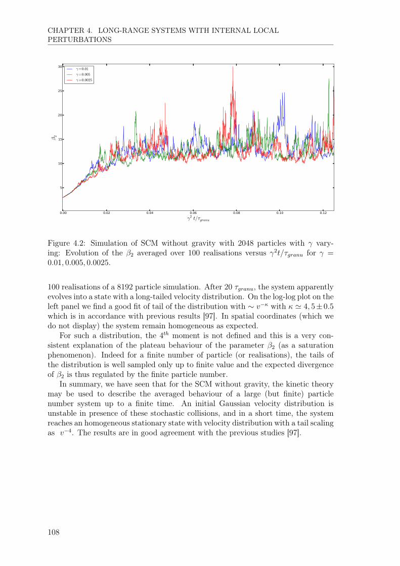
CHAPTER 4. LONG-RANGE SYSTEMS WITH INTERNAL LOCALPERTURBATIONS
Figure 4.2: Simulation of SCM without gravity with 2048 particles with � vary-ing: Evolution of the �
2
averaged over 100 realisations versus �2t/⌧granu for � =
0.01, 0.005, 0.0025.
100 realisations of a 8192 particle simulation. After 20 ⌧granu, the system apparentlyevolves into a state with a long-tailed velocity distribution. On the log-log plot on theleft panel we find a good fit of tail of the distribution with ⇠ v� with ' 4, 5±0.5which is in accordance with previous results [97]. In spatial coordinates (which wedo not display) the system remain homogeneous as expected.
For such a distribution, the 4
th moment is not defined and this is a very con-sistent explanation of the plateau behaviour of the parameter �
2
(as a saturationphenomenon). Indeed for a finite number of particle (or realisations), the tails ofthe distribution is well sampled only up to finite value and the expected divergenceof �
2
is thus regulated by the finite particle number.In summary, we have seen that for the SCM without gravity, the kinetic theory
may be used to describe the averaged behaviour of a large (but finite) particlenumber system up to a finite time. An initial Gaussian velocity distribution isunstable in presence of these stochastic collisions, and in a short time, the systemreaches an homogeneous stationary state with velocity distribution with a tail scalingas v�4. The results are in good agreement with the previous studies [97].
108
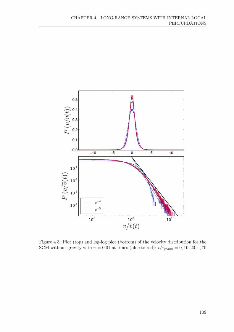
CHAPTER 4. LONG-RANGE SYSTEMS WITH INTERNAL LOCALPERTURBATIONS
Figure 4.3: Plot (top) and log-log plot (bottom) of the velocity distribution for theSCM without gravity with � = 0.01 at times (blue to red): t/⌧granu = 0, 10, 20, .., 70
109

CHAPTER 4. LONG-RANGE SYSTEMS WITH INTERNAL LOCALPERTURBATIONS
2.9 Numerical results for 1d self-gravitating gas
Method of simulation and units
In order to simulate the SCM with gravity, we modify the code implemented forICM by adding super-elastic collisions of Eq. (4.1). At each collision, with a randomgenerator, the code chooses, with equal probability, if the collision is super-elastic orinelastic. We recall that this code used is valid to simulate a finite self-gravitatingsystem only if particles remains confined in a small region compared to the size ofthe box. We choose units with m = 1 and the initial spatial density n
0
= 1. Itis appropriate to adopt the same time unit as the SGS model of the last chapter:⌧dyn =
2pgn0
.As discussed in section 2.3 we characterize the collisions by �SCM :
�SCM =
(1� cR)pN
2
. (4.58)
To probe the macroscopic evolution, we measure the parameter �11
and the virialratio defined in chapter 3, and make also use of the kurtosis of the velocity distri-bution �
2
in Eq. (4.41). For the each quantity Q (Q = E,�11
, R, ..) we define theestimated standard deviation:
phQ2i =
vuut 1
R� 1
RX
r=1
(Qr � hQi)2 (4.59)
with Qr the value of the quantity for the realisation r, R the number of numericalrealisations and hQi the mean quantity. We use this standard error to check whetherthe mean over the finite number of realisations can be taken to be representative ofthe true mean.
Validity of the mean field description
The two upper panels of Fig. 4.4 show, for the SCM with �SCM = 0.03, the temporalevolution of the energy, both for 5 individual realisations (in colour) and its averageover 300 realisations (in black), for N = 128 (top panel) and 512 (lower panel). Wesee that for the former case the average is close to constant only at earlier times butnot at longer times; while for the case N = 512, the conservation is within about10% over the whole time range.
The behaviour of the standard deviation, shown in the third panel, estimatedfrom 300 realisations for each of N = 128, 256, 512, shows that the behaviour offluctuation of the estimated mean is indeed just a reflection of the root of the variancewhich grows with time more or less monotonically. These behaviours are in line withour expectation following the discussion is section 2.7, and we note that the standarddeviation of the energy appears (qualitatively) to grow in proportion to
pt, which
is consistent with the expression of the variance Eq. (4.48). We see clearly that, atfixed t, as N ! +1 we do indeed expect the energy to be conserved exactly aspredicted.
110

CHAPTER 4. LONG-RANGE SYSTEMS WITH INTERNAL LOCALPERTURBATIONS
Figure 4.4: Two top panels: Normalised total energy versus t/⌧dyn for 5 differentrealisations (in color), the black line represents the mean over the 300 realisationsof the process, for N = 128 (Top) and N = 512 (Middle). In the bottom panel thetime evolution of the standard error for N = 128, 256, 512 particles (�SCM = 0.03).
111

CHAPTER 4. LONG-RANGE SYSTEMS WITH INTERNAL LOCALPERTURBATIONS
Figure 4.5: Top panels: Virial ratio as a function of time of a single realisation (incyan), and for its mean over the 300 realisations (in black), for N = 512. Bottompanel: the evolution of the standard deviation over realisations for N = 128, 256, 512particles (�SCM = 0.03).
Fig. 4.5 shows, for the same model as in the previous figure, the evolution of thevirial ratio as a function of time. The upper panel shows its value for an individualrealisation (in color) and the averaged over 300 realisations for N = 512. Thelower panel shows the standard deviation of R, for N = 128 to 512. Clearly thefluctuations of the virial ratio are below 1 (corresponding to a system which isvirialised) and these fluctuations decrease in value and in amplitude as N increases.Thus as N ! +1, in the quasi-elastic limit, the system remains always exactlyvirialised and this is a strong indication that it evolves through a family of QSS.
Fig. 4.6 shows the evolution of the separability ratio �11
. The upper panel showsit for two realisations and for the average over 300 realisations. �
11
evolves on thesame time scale as the variance of R, and reaches (as the variance of R) a well definedaveraged “plateau” at longer times. The fluctuation from realisation to realisationof �
11
are very large and their standard deviation is shown in the lower panel forN = 128 to 512. At earlier times it appears that the standard deviation decreases asN increases but at longer times it appears to be independent of N . This means thatthe system reaches a stationary virialised state but it is not clear that it convergesto a well defined single value of �
11
as N ! +1. This is further shown in Fig. 4.7which shows for the same time axes, the evolution of both �
11
(top) and �2
(bottom)for different N . In the lower panel is also plotted the theoretical prediction from the
112
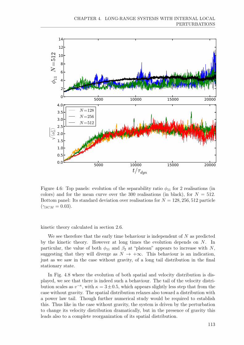
CHAPTER 4. LONG-RANGE SYSTEMS WITH INTERNAL LOCALPERTURBATIONS
Figure 4.6: Top panels: evolution of the separability ratio �11
for 2 realisations (incolors) and for the mean curve over the 300 realisations (in black), for N = 512.Bottom panel: Its standard deviation over realisations for N = 128, 256, 512 particle(�SCM = 0.03).
kinetic theory calculated in section 2.6.
We see therefore that the early time behaviour is independent of N as predictedby the kinetic theory. However at long times the evolution depends on N . Inparticular, the value of both �
11
and �2
at “plateau” appears to increase with N ,suggesting that they will diverge as N ! +1. This behaviour is an indication,just as we saw in the case without gravity, of a long tail distribution in the finalstationary state.
In Fig. 4.8 where the evolution of both spatial and velocity distribution is dis-played, we see that there is indeed such a behaviour. The tail of the velocity distri-bution scales as v�, with = 3±0.5, which appears slightly less step that from thecase without gravity. The spatial distribution relaxes also toward a distribution witha power law tail. Though further numerical study would be required to establishthis. Thus like in the case without gravity, the system is driven by the perturbationto change its velocity distribution dramatically, but in the presence of gravity thisleads also to a complete reorganization of its spatial distribution.
113
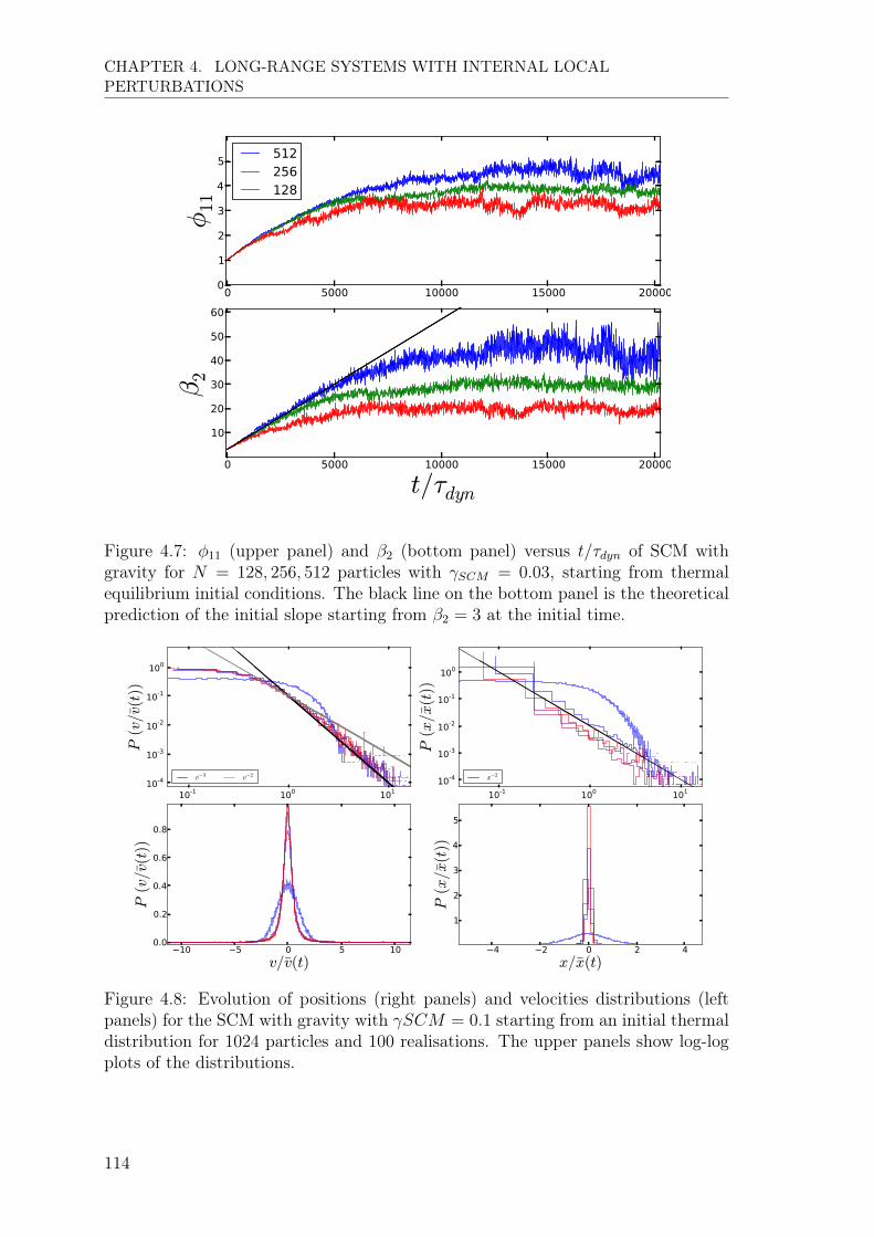
CHAPTER 4. LONG-RANGE SYSTEMS WITH INTERNAL LOCALPERTURBATIONS
Figure 4.7: �11
(upper panel) and �2
(bottom panel) versus t/⌧dyn of SCM withgravity for N = 128, 256, 512 particles with �SCM = 0.03, starting from thermalequilibrium initial conditions. The black line on the bottom panel is the theoreticalprediction of the initial slope starting from �
2
= 3 at the initial time.
Figure 4.8: Evolution of positions (right panels) and velocities distributions (leftpanels) for the SCM with gravity with �SCM = 0.1 starting from an initial thermaldistribution for 1024 particles and 100 realisations. The upper panels show log-logplots of the distributions.
114
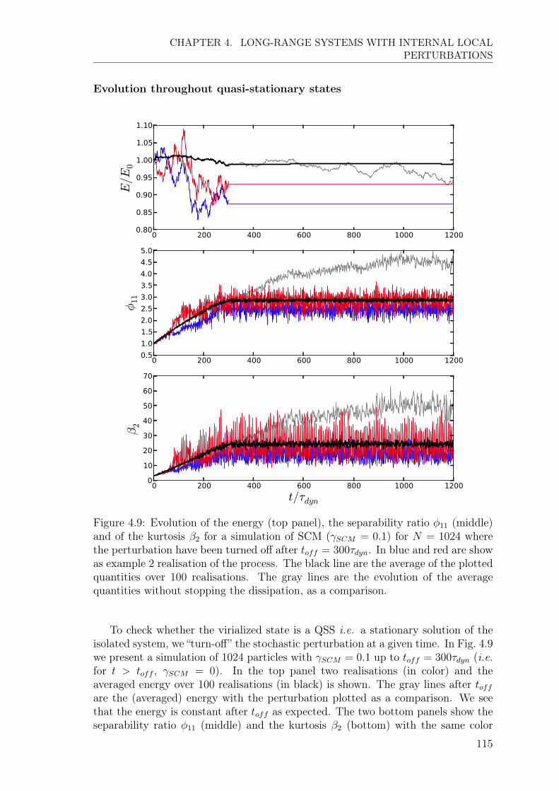
CHAPTER 4. LONG-RANGE SYSTEMS WITH INTERNAL LOCALPERTURBATIONS
Evolution throughout quasi-stationary states
Figure 4.9: Evolution of the energy (top panel), the separability ratio �11
(middle)and of the kurtosis �
2
for a simulation of SCM (�SCM = 0.1) for N = 1024 wherethe perturbation have been turned off after toff = 300⌧dyn. In blue and red are showas example 2 realisation of the process. The black line are the average of the plottedquantities over 100 realisations. The gray lines are the evolution of the averagequantities without stopping the dissipation, as a comparison.
To check whether the virialized state is a QSS i.e. a stationary solution of theisolated system, we “turn-off” the stochastic perturbation at a given time. In Fig. 4.9we present a simulation of 1024 particles with �SCM = 0.1 up to toff = 300⌧dyn (i.e.for t > toff , �SCM = 0). In the top panel two realisations (in color) and theaveraged energy over 100 realisations (in black) is shown. The gray lines after toffare the (averaged) energy with the perturbation plotted as a comparison. We seethat the energy is constant after toff as expected. The two bottom panels show theseparability ratio �
11
(middle) and the kurtosis �2
(bottom) with the same color
115
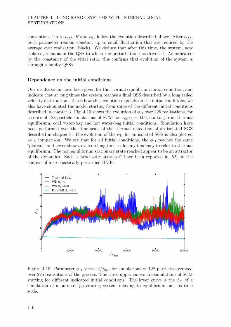
CHAPTER 4. LONG-RANGE SYSTEMS WITH INTERNAL LOCALPERTURBATIONS
convention. Up to toff , R and �11
follow the evolution described above. After toff ,both parameter remain constant up to small fluctuation that are reduced by theaverage over realisation (black). We deduce that after this time, the system, nowisolated, remains in the QSS to which the perturbation has driven it. As indicatedby the constancy of the virial ratio, this confirms that evolution of the system isthrough a family QSSs.
Dependence on the initial conditions
Our results so far have been given for the thermal equilibrium initial condition, andindicate that at long times the system reaches a final QSS described by a long tailedvelocity distribution. To see how this evolution depends on the initial conditions, wealso have simulated the model starting from some of the different initial conditionsdescribed in chapter 3. Fig. 4.10 shows the evolution of �
11
over 225 realisations, fora series of 128 particle simulations of SCM for �SCM = 0.02, starting from thermalequilibrium, cold water-bag and hot water-bag initial conditions. Simulation havebeen performed over the time scale of the thermal relaxation of an isolated SGSdescribed in chapter 3. The evolution of the �
11
for an isolated SGS is also plottedas a comparison. We see that for all initial conditions, the �
11
reaches the same“plateau” and never shows, even on long time scale, any tendency to relax to thermalequilibrium. The non equilibrium stationary state reached appear to be an attractorof the dynamics. Such a “stochastic attractor” have been reported in [52], in thecontext of a stochastically perturbed HMF.
Figure 4.10: Parameter �11
versus t/⌧dyn for simulations of 128 particles averagedover 225 realisations of the process. The three upper curves are simulations of SCMstarting for different indicated initial conditions. The lower curve is the �
11
of asimulation of a pure self-gravitating system relaxing to equilibrium on this timescale.
116

CHAPTER 4. LONG-RANGE SYSTEMS WITH INTERNAL LOCALPERTURBATIONS
2.10 Conclusion on SCM
Our numerical study of the SCM with and without gravity shows an early timebehaviour in good agreement with the kinetic theory developed to describe it. Inthe presence of gravity, in the mean-field and quasi-elastic limit, the system, startingfrom any initial condition, evolves on a N independent time scale through a familyof virialized state, each of which is a QSS of the unperturbed long-range system,until it reaches an apparently unique virialized state. This state is not the thermalequilibrium of the isolated model, and indeed is typically “further away” (in terms ofcorrelations measured by �
11
) from the thermal equilibrium. Therefore we observedcompelling evidence for the establishment of a “universal” non-equilibrium stationarystate in this model. Despite the stochasticity of the dynamics, there is no tendencyof the system to relax toward equilibrium. This clearly contrasts with the resultsobtained with a toy model in [95] constructed to test for the robustness of QSS tostochastic perturbations.
117

CHAPTER 4. LONG-RANGE SYSTEMS WITH INTERNAL LOCALPERTURBATIONS
3 The BSR model
To go further in our study of the effect of “internal” perturbations on the dynamicsof long-range systems, and in particular on their QSS, we have considered a sec-ond model introduced by Brito, Rosso & Soto [103] and also studied by Brey etal. [105, 106] in the context of granular gas. In this case, particles undergo dissi-pative collisions and an energy influx, is necessary to maintain a steady state. Inexperiments of agitated granular particle this energy can be provided mechanically:the particles are distributed between two horizontal plates, and the bottom plate bya permanent shaking transfers the kinetic energy to the particles by collisions withthe plate [107–109]. In this quasi-two dimensional geometry, the vertical vibrationsare much faster that the time scale of the horizontal dynamic system and the energyprovided vertically is transmitted horizontally to the system through collisions. TheBRS model differs from the SCM in the way the injection of energy compensatingthe energy lost by inelastic collisions is modelled. Instead of super-elastic collisions,a fixed velocity “kick” is given to the colliding particles.
Compared to the SCM of the previous section, this model differs in several re-spects: Firstly, the energy is not conserved (even on average), but the system canattain a steady state of fixed macroscopic energy. Secondly, the long tails of thestationary state observed in the SCM are expected to be suppressed, because, aswe will see in the collision rules, inelastic collisions dominate for high relative ve-locities. Thirdly, the model has, like the ICM, a strictly deterministic dynamics. Itthus allows us to probe whether the explicit stochasticity of the SCM is really anessential feature for its qualitative behaviour, and notably the apparent existence ofa universal non-equilibrium stationary state.
We first define the model and discuss some of its particular features. We thenperform a numerical study, first considering the model without gravity (which hasnot been studied, in one dimension, in references [103,105]). We then study the fullmodel with (1d) gravity. The results we report are a preliminary analysis of themodel and we will discuss briefly, in our conclusions, how this analysis should becompleted in future work.
3.1 BRS collisions
Let 1 and 2 be two particles of the system (such that x1
< x2
) which collide withrelative velocity v
12
= v1
�v2
> 0. The post-collisional velocities v⇤1
and v⇤2
are givenby the following momentum conserving rules:
v⇤1
=v2
+ �v12
�� (4.60)v⇤2
=v1
� �v12
+�
with � =
1�cR
2
, cR the coefficient of restitution, and � > 0 the constant velocity“kick”. This is the one dimensional version of the rules in [103]. We note that in [105]the same collision rules are considered, except that the sign of � is negative. In thiscase a particle gains velocity in the direction of the other colliding particle afterthe collision, which tends to increase the probability of re-collision phenomenon andleads rapidly to numerical difficulties. Thus we limit ourselves the original collisionrules in [103].
118
CHAPTER 4. LONG-RANGE SYSTEMS WITH INTERNAL LOCALPERTURBATIONS
Depending on the initial relative velocity of the two colliding particles, the ab-solute value of relative velocity between particles can increase or decrease. Indeedthe kinetic energy change in a collision is:
�KBRS =
1
4
m((v⇤21
+ v⇤22
)� (v21
+ v22
)) = m[�
2
+�cRv12 � 1� c2R4
v212
] (4.61)
The unique solution for colliding particles (with v12
> 0) of the equation �KBRS = 0
is:v012
=
2�
1� cR=
�
�(4.62)
Thus for 0 < v12
< �
�, �KBRS > 0 the kinetic energy gain is positive, while for a
relative velocity such that v12
> �
�the system loses energy. Note in particular that
particles with velocity close to zero gain a velocity ±�.
Stationarity
It is important to remark that the velocity kick � does not depend on the pre-collisional velocity. Thus for a BRS collision the transformation of the phase spacevolume is just obtained from the inelastic part:
dv⇤1
dv⇤2
= cRdv1dv2 (4.63)
Each collision thus give a contraction of the occupied phase space region, andthrough the evolution the support of the probability distribution function is thusnecessary reduced. In other words the relevant measure dv
1
...dvN to describe thevelocity space becomes arbitrary small with time, and selects more and more limitedvalues of particle velocities. T his contracting measure is a property of this non-Hamiltonian system, just as it is of the ICM [104]. However while the ICM leads toa cooling which asymptotically brings the system to a zero energy state in which allparticles are at rest, we expect the BRS model to lead to a stationary state at fixednon zero energy. (Indeed a stationary state with zero energy cannot exist becausethere is always then a net energy injection). Thus we conclude that if the BRS canreach a stationary state it must have a distribution with support of zero measure inthe phase space of dimension 2dN .
From the collision rule (4.60), it is evident that the evolution may in fact leadto the “selection” of very particular values of the velocity and give a stationarydistribution of zero measure: we have seen that if the relative velocity at collisionv12
has the value �
�, the collision is elastic and thus the particles simply “exchange
velocities” and the velocity distribution does not evolve i.e.
v⇤1
= v2
v⇤2
= v1
. (4.64)
These considerations are valid for both the gravitational and granular case (withoutgravity).
Now, in the case without gravity velocities change only at collision when theycollide. Therefore if we have a distribution with v
12
= ±�
�for all pairs of particles,
the distribution is macroscopically stationary. This will be true if we have any two
119
CHAPTER 4. LONG-RANGE SYSTEMS WITH INTERNAL LOCALPERTURBATIONS
velocities, v and v + �
�, and further since the collision with the walls are elastic we
must have v1
= �v2
. Thus we infer
v1
= ±�2�
v2
= ⌥�2�
. (4.65)
We thus might expect that the system may relax, starting for a generic initial con-dition with no net velocity drift, to a uniform spatial distribution and a velocitydistribution of the form:
gst(v) =1
2
(�(v � vst) + �(v + vst)). (4.66)
However it is clear that the velocity distribution will not evolve more genericallyif there are only particles with the two velocities ± �
2�, irrespectively of the spatial
distribution.In such states and specifically for the velocity distribution given by Eq. (4.66)
we have:Kst =
1
2
mh⌃Ni=1
v2i i =N�2
8�2. (4.67)
Thus the kinetic temperature of such a stationary state (or possible oscillatingstate in the configuration space with the same stationary velocity distribution) isexpected to be proportional to �
2
�2 . It is interesting to compare this with the pre-dicted kinetic energy derived for the 2d case. In [103] the stationary temperature isderived using hydrodynamic approached, and in [105] in any dimension by a kineticapproach with the use of modified collisional operator. For a Gaussian distribution,this temperature is:
TGs =
mc2R⇡
4(1� c2R)2
"1 +
s
1 +
4(1� c2R)
⇡c2R
#�
2. (4.68)
The later results does not a priori apply to the one dimensional case of the numericalsimulation of the next section. Indeed, in [105] we remark that the coefficients of theSonine expansion used to derived the results diverge for d = 1, indicating that theGaussian approximation is very bad in one dimension. However for cR ! 1 the latterexpression give the same scaling ( TG
s ⇠ �
2
�2 ) in the parameter which characterizethe perturbation represented by the BRS collisions.
3.2 Numerical results for BRS model without gravity
Method and units
We present now the results of our numerical simulations of this model. The simu-lation method only requires a simple modification compared to the previous model,adapting the collision rule according to Eq. (4.60). The particles are placed againin a box of size L = N with elastic walls. We restrict the investigation to thequasi-elastic limit � ⌧ 0 which is the relevant limit in the gravitational case, inwhich we wish to treat BRS collisions as a perturbation. We start from a spatiallyhomogeneous distribution, and the velocities are distributed following a Gaussian.We work again in units with the particles masses m = 1, their number densityn0
= 1; the variance of the initial Gaussian velocity distribution v0
= 1 and thus⌧granu =
1
n�10 v0
= 1.
120
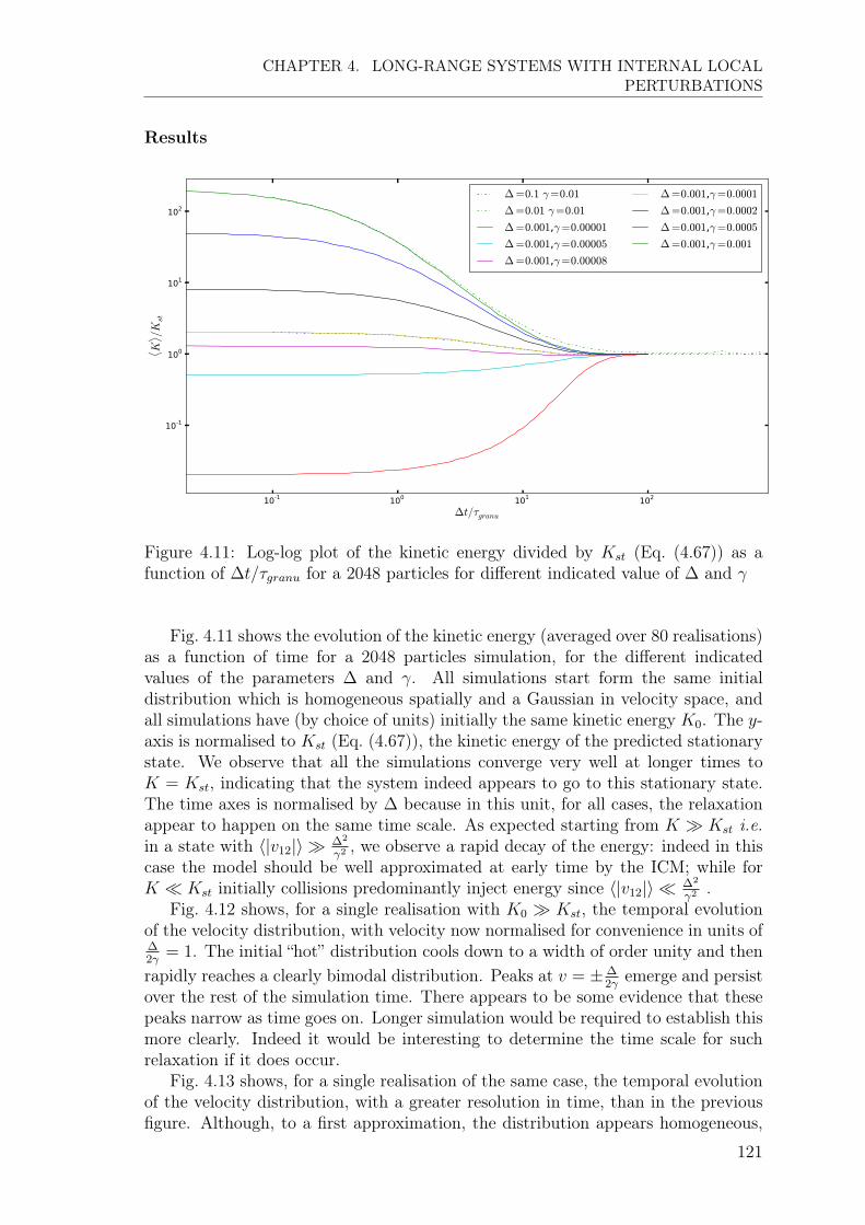
CHAPTER 4. LONG-RANGE SYSTEMS WITH INTERNAL LOCALPERTURBATIONS
Results
Figure 4.11: Log-log plot of the kinetic energy divided by Kst (Eq. (4.67)) as afunction of �t/⌧granu for a 2048 particles for different indicated value of � and �
Fig. 4.11 shows the evolution of the kinetic energy (averaged over 80 realisations)as a function of time for a 2048 particles simulation, for the different indicatedvalues of the parameters � and �. All simulations start form the same initialdistribution which is homogeneous spatially and a Gaussian in velocity space, andall simulations have (by choice of units) initially the same kinetic energy K
0
. The y-axis is normalised to Kst (Eq. (4.67)), the kinetic energy of the predicted stationarystate. We observe that all the simulations converge very well at longer times toK = Kst, indicating that the system indeed appears to go to this stationary state.The time axes is normalised by � because in this unit, for all cases, the relaxationappear to happen on the same time scale. As expected starting from K � Kst i.e.in a state with h|v
12
|i � �
2
�2 , we observe a rapid decay of the energy: indeed in thiscase the model should be well approximated at early time by the ICM; while forK ⌧ Kst initially collisions predominantly inject energy since h|v
12
|i ⌧ �
2
�2 .Fig. 4.12 shows, for a single realisation with K
0
� Kst, the temporal evolutionof the velocity distribution, with velocity now normalised for convenience in units of�
2�= 1. The initial “hot” distribution cools down to a width of order unity and then
rapidly reaches a clearly bimodal distribution. Peaks at v = ± �
2�emerge and persist
over the rest of the simulation time. There appears to be some evidence that thesepeaks narrow as time goes on. Longer simulation would be required to establish thismore clearly. Indeed it would be interesting to determine the time scale for suchrelaxation if it does occur.
Fig. 4.13 shows, for a single realisation of the same case, the temporal evolutionof the velocity distribution, with a greater resolution in time, than in the previousfigure. Although, to a first approximation, the distribution appears homogeneous,
121

CHAPTER 4. LONG-RANGE SYSTEMS WITH INTERNAL LOCALPERTURBATIONS
Figure 4.12: Distribution of the velocity v�/2�
for one realisation of 1d granular sys-tem with BRS collisions. The snapshots are taken at time t = 0, 5, 10, 15, ...100⌧granu.The simulation is for N = 2048 particles with � = 0.01 and � = 0.01
it is evident that there are coherent time dependent fluctuations at large spatialscales. These appear to be the one dimensional equivalent of the hydrodynamicmodes observed in the 2d version of this model in [103,105].
In summary, in the 1d BRS model without gravity we observe that arbitraryinitial states are driven efficiently to a state which has a very stable energy ⇠ �
2
�2
and with an almost stationary bimodal velocity distribution (probably converging tothe exactly bimodal distribution of Eq. (4.66) ) and with persistent hydrodynamicmodes about an average (in time) uniform spatial distribution.
122
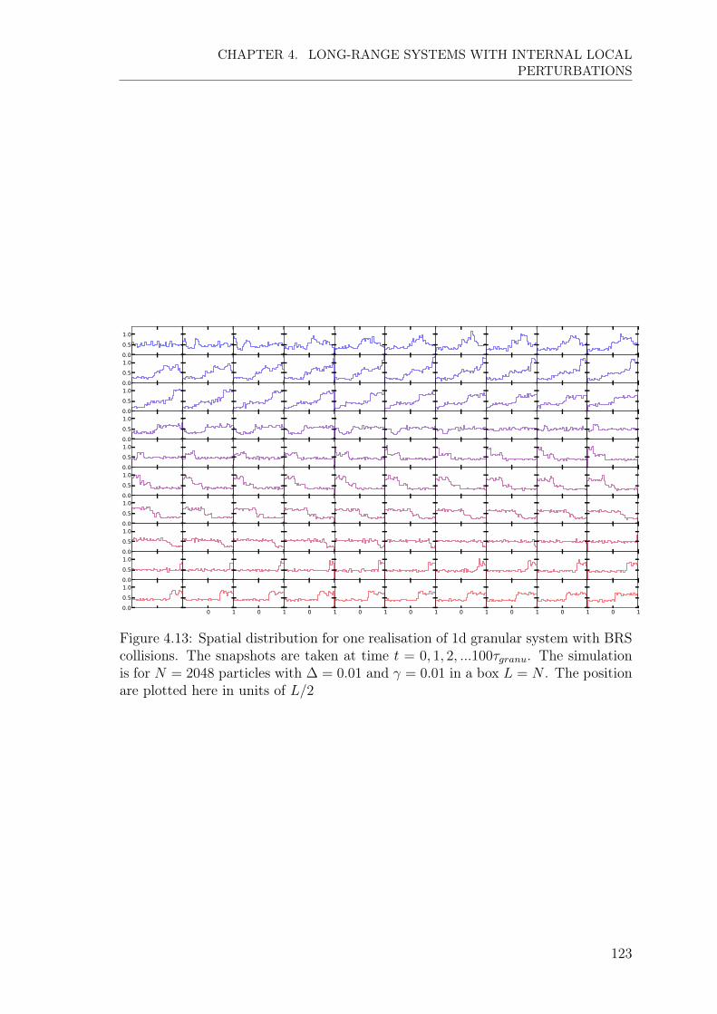
CHAPTER 4. LONG-RANGE SYSTEMS WITH INTERNAL LOCALPERTURBATIONS
Figure 4.13: Spatial distribution for one realisation of 1d granular system with BRScollisions. The snapshots are taken at time t = 0, 1, 2, ...100⌧granu. The simulationis for N = 2048 particles with � = 0.01 and � = 0.01 in a box L = N . The positionare plotted here in units of L/2
123

CHAPTER 4. LONG-RANGE SYSTEMS WITH INTERNAL LOCALPERTURBATIONS
3.3 Numerical results: BRS with gravity
Method and units
We now consider how the dynamics of a 1d self-gravitating system is modified byBRS collisions. To simulate this system we again use the code with a periodic box(see chapter 3), simply modifying appropriately the collision rules.
We work in units with particle masses m = 1, the initial density n0
=
L0N
= 1
where L0
is the initial region of the phase space (we also choose in this case L0
⌧ L,L the size of the periodic box, which is the requirement for the accuracy of theregularized gravity code) and time is measured again in units of
⌧dyn =
2pgn
0
= 1 (4.69)
just as for SGS and ICM (chapter 3). As for the ICM, we expect ⌧dyn to be thecharacteristic mean field time only at early time: as the system evolves away fromits initial states its density can change greatly and thus the characteristic time ofthe mean field dynamics.
Preliminary results
In Fig. 4.14 is shown the average over 20 realisations of the energy, the virial ratio R,and the parameters �
11
and �2
as a function of time for 128 particles with � = 10
�2
and � = 10
�4. The blue curves are the results for “cold” water-bag initial distribution(R
0
= 0.01) and the green are for a “hot” water-bag initial condition with R0
= 1 (for details see chapter 3).
In the first panel, the temporal evolution of the total energy is shown in a semi-log plot. For both simulations the energy relaxes toward the same stationary valuefor both initial conditions in approximately 150⌧dyn. In the second panel we seethat the system virialises in only ⇠ 10 � 20 ⌧dyn and then remains very close to avirialised state.
Just as for the ICM, the inset is a blow up of the initial virial oscillations forthe “hot” initial conditions. As might be anticipated, these oscillations have char-acteristic period decreasing in time. Indeed, as the energy decreases, the density nincreases. and the period of the mean field oscillation 2p
gn(t)thus decreases.
The third panel and the fourth panel show the evolution, respectively, of theseparability ratio �
11
and the kurtosis of the velocity distribution �2
. Both simu-lations show, up to ⇠ 100⌧dyn, a behaviour very close to that observed in the ICMfor the same initial condition. After a first phase of (violent, in the case R
0
= 0.01)relaxation, lasting ⇠ 10 � 20 ⌧dyn, both quantities settle to non-zero values, whichare very close to a constant in the case R
0
= 1 but slowly increase in the caseR
0
= 0.01. Indeed given that the starting energy E0
is much greater than ⇠ �
2
�2 ,the model is very well approximated initially by the ICM: then when the energyreaches a value close to �
2
�2 the behaviour of �11
and �2
rapidly changes as the sys-tem is rapidly (in ⇠ 10 � 20 ⌧dyn) apparently driven into a stationary state. Afterthis second relaxation all parameters are stable and their oscillation are remarkablysmall (even for only one realisation), indicating that the system has reached a welldefined stationary state, independent of the initial condition.
124
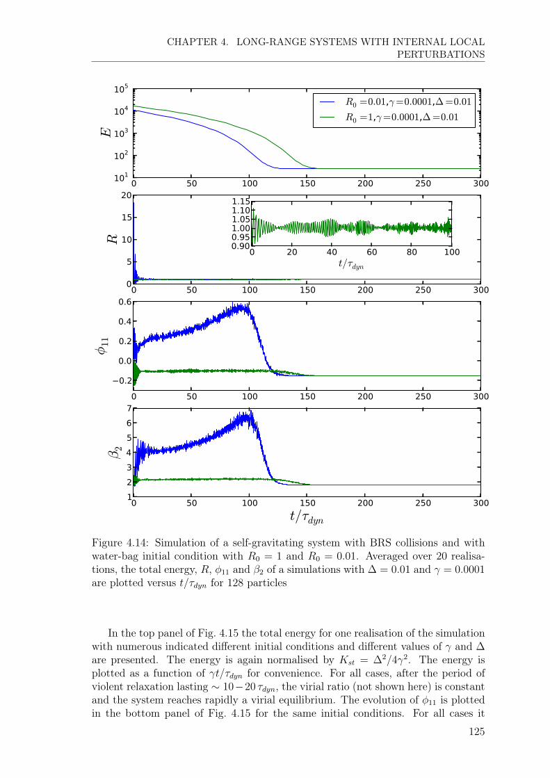
CHAPTER 4. LONG-RANGE SYSTEMS WITH INTERNAL LOCALPERTURBATIONS
Figure 4.14: Simulation of a self-gravitating system with BRS collisions and withwater-bag initial condition with R
0
= 1 and R0
= 0.01. Averaged over 20 realisa-tions, the total energy, R, �
11
and �2
of a simulations with � = 0.01 and � = 0.0001are plotted versus t/⌧dyn for 128 particles
In the top panel of Fig. 4.15 the total energy for one realisation of the simulationwith numerous indicated different initial conditions and different values of � and �are presented. The energy is again normalised by Kst = �
2/4�2. The energy isplotted as a function of �t/⌧dyn for convenience. For all cases, after the period ofviolent relaxation lasting ⇠ 10�20 ⌧dyn, the virial ratio (not shown here) is constantand the system reaches rapidly a virial equilibrium. The evolution of �
11
is plottedin the bottom panel of Fig. 4.15 for the same initial conditions. For all cases it
125
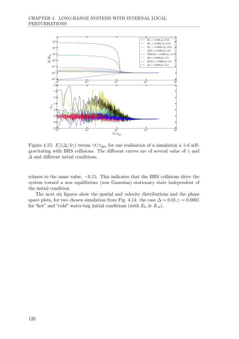
CHAPTER 4. LONG-RANGE SYSTEMS WITH INTERNAL LOCALPERTURBATIONS
Figure 4.15: E/(�/4�) versus �t/⌧dyn for one realisation of a simulation a 1-d self-gravitating with BRS collisions. The different curves are of several value of � and� and different initial conditions.
relaxes to the same value, �0.15. This indicates that the BRS collisions drive thesystem toward a non equilibrium (non Gaussian) stationary state independent ofthe initial condition.
The next six figures show the spatial and velocity distributions and the phasespace plots, for two chosen simulation from Fig. 4.14: the case � = 0.01,� = 0.0001for “hot” and “cold” water-bag initial conditions (with E
0
� Kst).
126
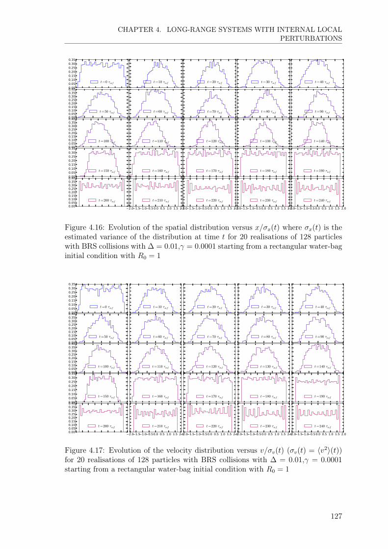
CHAPTER 4. LONG-RANGE SYSTEMS WITH INTERNAL LOCALPERTURBATIONS
Figure 4.16: Evolution of the spatial distribution versus x/�x(t) where �x(t) is theestimated variance of the distribution at time t for 20 realisations of 128 particleswith BRS collisions with � = 0.01,� = 0.0001 starting from a rectangular water-baginitial condition with R
0
= 1
Figure 4.17: Evolution of the velocity distribution versus v/�v(t) (�v(t) = hv2i(t))for 20 realisations of 128 particles with BRS collisions with � = 0.01,� = 0.0001starting from a rectangular water-bag initial condition with R
0
= 1
127

CHAPTER 4. LONG-RANGE SYSTEMS WITH INTERNAL LOCALPERTURBATIONS
Figure 4.18: Time evolution of the normalised spatial distribution for 20 realisationsof 128 particles with BRS collisions with � = 0.01,� = 0.0001 starting from arectangular water-bag initial condition with R
0
= 0.01
Figure 4.19: Time evolution of the normalised velocity distribution for 20 realisationsof 128 particles with BRS collision with � = 0.01,� = 0.0001 starting from arectangular water-bag initial condition with R
0
= 0.01
128
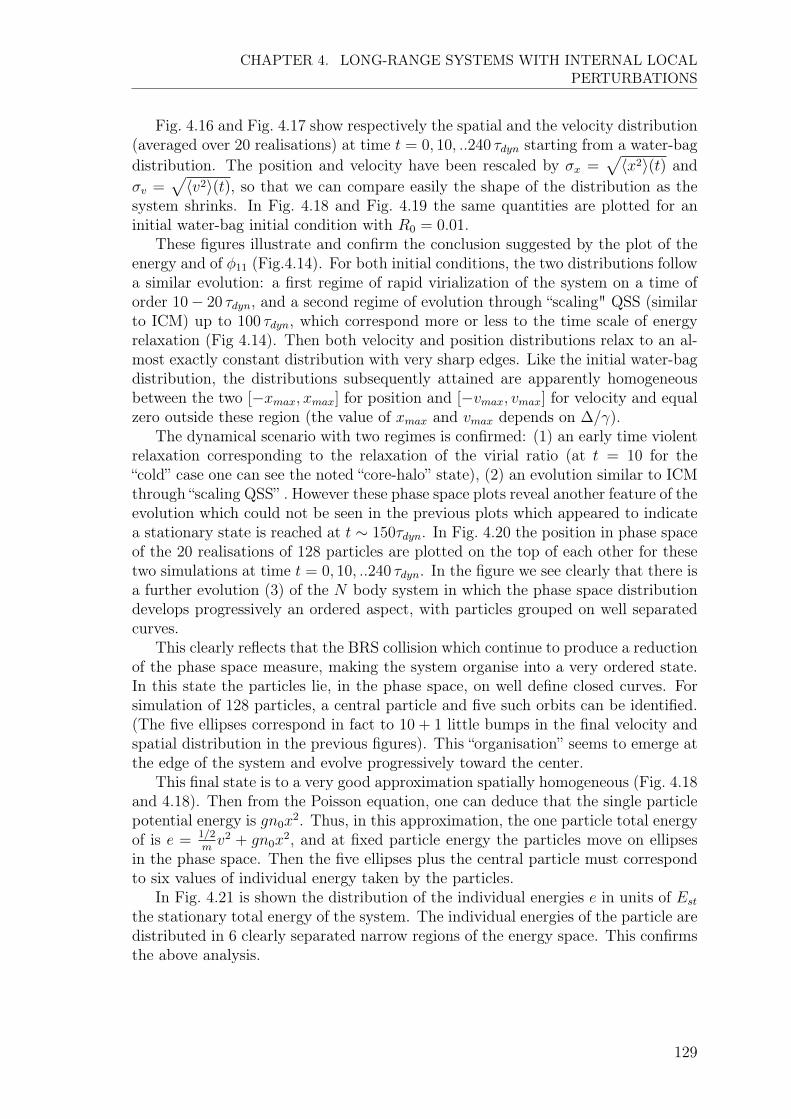
CHAPTER 4. LONG-RANGE SYSTEMS WITH INTERNAL LOCALPERTURBATIONS
Fig. 4.16 and Fig. 4.17 show respectively the spatial and the velocity distribution(averaged over 20 realisations) at time t = 0, 10, ..240 ⌧dyn starting from a water-bagdistribution. The position and velocity have been rescaled by �x =
phx2i(t) and�v =
phv2i(t), so that we can compare easily the shape of the distribution as thesystem shrinks. In Fig. 4.18 and Fig. 4.19 the same quantities are plotted for aninitial water-bag initial condition with R
0
= 0.01.These figures illustrate and confirm the conclusion suggested by the plot of the
energy and of �11
(Fig.4.14). For both initial conditions, the two distributions followa similar evolution: a first regime of rapid virialization of the system on a time oforder 10� 20 ⌧dyn, and a second regime of evolution through “scaling" QSS (similarto ICM) up to 100 ⌧dyn, which correspond more or less to the time scale of energyrelaxation (Fig 4.14). Then both velocity and position distributions relax to an al-most exactly constant distribution with very sharp edges. Like the initial water-bagdistribution, the distributions subsequently attained are apparently homogeneousbetween the two [�xmax, xmax] for position and [�vmax, vmax] for velocity and equalzero outside these region (the value of xmax and vmax depends on �/�).
The dynamical scenario with two regimes is confirmed: (1) an early time violentrelaxation corresponding to the relaxation of the virial ratio (at t = 10 for the“cold” case one can see the noted “core-halo” state), (2) an evolution similar to ICMthrough “scaling QSS” . However these phase space plots reveal another feature of theevolution which could not be seen in the previous plots which appeared to indicatea stationary state is reached at t ⇠ 150⌧dyn. In Fig. 4.20 the position in phase spaceof the 20 realisations of 128 particles are plotted on the top of each other for thesetwo simulations at time t = 0, 10, ..240 ⌧dyn. In the figure we see clearly that there isa further evolution (3) of the N body system in which the phase space distributiondevelops progressively an ordered aspect, with particles grouped on well separatedcurves.
This clearly reflects that the BRS collision which continue to produce a reductionof the phase space measure, making the system organise into a very ordered state.In this state the particles lie, in the phase space, on well define closed curves. Forsimulation of 128 particles, a central particle and five such orbits can be identified.(The five ellipses correspond in fact to 10 + 1 little bumps in the final velocity andspatial distribution in the previous figures). This “organisation” seems to emerge atthe edge of the system and evolve progressively toward the center.
This final state is to a very good approximation spatially homogeneous (Fig. 4.18and 4.18). Then from the Poisson equation, one can deduce that the single particlepotential energy is gn
0
x2. Thus, in this approximation, the one particle total energyof is e =
1/2mv2 + gn
0
x2, and at fixed particle energy the particles move on ellipsesin the phase space. Then the five ellipses plus the central particle must correspondto six values of individual energy taken by the particles.
In Fig. 4.21 is shown the distribution of the individual energies e in units of Est
the stationary total energy of the system. The individual energies of the particle aredistributed in 6 clearly separated narrow regions of the energy space. This confirmsthe above analysis.
129

CHAPTER 4. LONG-RANGE SYSTEMS WITH INTERNAL LOCALPERTURBATIONS
Figure 4.20: Evolution of the particle position in phase space, for a simulationwith 128 particles starting from rectangular water-bag with R
0
= 0.01 (the 25 toppanels) and R
0
= 1 (bottom panels). On the top of each other the position of theparticles of the 20 realisations of the self-gravitating -BRS dynamic are plotted attime t = 0, 10.., 240 ⌧dyn. The parameters for BRS collisions are � = 0.0001 and� = 0.01.
130
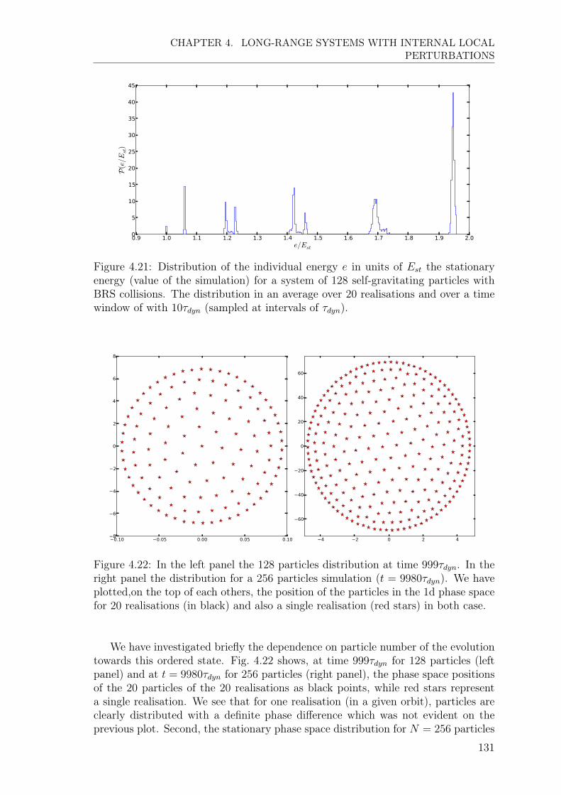
CHAPTER 4. LONG-RANGE SYSTEMS WITH INTERNAL LOCALPERTURBATIONS
Figure 4.21: Distribution of the individual energy e in units of Est the stationaryenergy (value of the simulation) for a system of 128 self-gravitating particles withBRS collisions. The distribution in an average over 20 realisations and over a timewindow of with 10⌧dyn (sampled at intervals of ⌧dyn).
Figure 4.22: In the left panel the 128 particles distribution at time 999⌧dyn. In theright panel the distribution for a 256 particles simulation (t = 9980⌧dyn). We haveplotted,on the top of each others, the position of the particles in the 1d phase spacefor 20 realisations (in black) and also a single realisation (red stars) in both case.
We have investigated briefly the dependence on particle number of the evolutiontowards this ordered state. Fig. 4.22 shows, at time 999⌧dyn for 128 particles (leftpanel) and at t = 9980⌧dyn for 256 particles (right panel), the phase space positionsof the 20 particles of the 20 realisations as black points, while red stars representa single realisation. We see that for one realisation (in a given orbit), particles areclearly distributed with a definite phase difference which was not evident on theprevious plot. Second, the stationary phase space distribution for N = 256 particles
131
CHAPTER 4. LONG-RANGE SYSTEMS WITH INTERNAL LOCALPERTURBATIONS
(right panel) presents 8 ellipses (and no particle in the center) which are thus moredensely packed than in the 128 particle case. Therefore, this attractor state (whichdoes not depend on initial conditions) depends evidently on the number of particle.Thus unlike the first two phases of relaxation, we clearly cannot expect to describeusing the mean field description of this ordered state and the relaxation to it. (Webelieve the latter should describe however very well the first two stages.) Further,the time scale of the relaxation to this state increases with the number of particles(the time of relaxation changes approximatively by an order of magnitude when weincrease the number of particle by 2). Indeed, looking carefully the 256 particle caseone sees small “defects” in the order of the one particle distribution, and also thatthe most central circles are not very well defined, indicating that the state is still“organising” at the time shown.
Finally, we have “turned-off” the perturbation once the system is in this state(at t = 1000⌧dyn) for a 128 particle simulation. We observed the system remainsin this particular ordered state and found that it is stable at least up to 1000⌧dyn.Thus, the state appears to be a stationary solution of the (Hamiltonian) N -bodydynamics with elastic collisions.
3.4 Conclusion on BRS collisions.
The local and internal perturbation represented by BRS collisions appear to lead toa universal non-equilibrium stationary state. As in the SCM this states is very farfrom the thermal equilibrium of the 1d isolated self-gravitating system, but is verydifferent to those observed in the SCM. For the granular system (without gravity),this state presents a bimodal velocity distribution that we were able to predict, andthe spatial distribution showing hydrodynamic modes. The characterisation of themodes and a broader study of all the limits (in particular the limit cR ! 1) of thissystem would be an interesting development to complete the study. For the self-gravitating case, we find that the system reaches a steady state, again independentof the initial conditions. Once the system reaches the energy balance, particlesorganise precisely to a very stable, and ordered state. In this state particles lie onwell defined, apparently elliptic, orbits in the phase space corresponding to differentparticle energy level. These results should be completed by further numerical andanalytical study in order to establish that the two first stages of evolution can bedescribed by a large N mean field limit. For the third phase, the relaxation tothe final microscopically ordered phase occurs on a time scale dependent on N andalso the properties of this “ordered” state could perhaps be understood analytically,maybe through some minimization procedures.
4 Conclusion
In this chapter, we have investigated the effects on the dynamics of long-range inter-acting systems of a certain class of “local internal” perturbations through the studyof two one dimensional toy models. More specifically in both case we consider twoperturbations of the dynamics inspired by granular studies, considering momentumconserving but non-Hamiltonian collisions.
132
CHAPTER 4. LONG-RANGE SYSTEMS WITH INTERNAL LOCALPERTURBATIONS
We considered firstly the SCM, a non deterministic extension of the ICM, inwhich each collision is randomly inelastic or super-elastic. The collision rules arebuilt such that on average, over the realisations of the stochastic process, the totalenergy remains fixed. In a second model, the BRS, the system is perturbed withinelastic collisions and driven by a constant energy input at each collision. Thecollisions, deterministic in this case, bring the system into a steady state where thegain and the loss of energy is balanced.
Both internal perturbation act microscopically and locally but completely mod-ify the global organisation of the system: they push the long-range system far fromits initial QSS. In that sense the QSSs are not robust to such perturbations. How-ever, the evolution, in both cases, happens through a succession of virialised states,stationary solutions of the Vlasov equation. For both perturbations, the collisions,described by a non Hamiltonian term local in space and a functional of the velocitydistribution added to the Vlasov equation, drive the system to a non-equilibriumstationary state (NESS). The stationary distribution does not depend on the initialconditions but depend strongly on the microscopic details of the perturbation. Inboth case we have checked that the NESS is a QSS i.e. it is a stationary solution ofthe unperturbed dynamics.
It is interesting to compare the latter results with the existing one in the liter-ature. In [95] the stochastic force added to the long-range system which acts in anon-local manner on the system. Indeed the three particles of which the velocitiesare permuted, are chosen from the whole system. This process increases the mixingin velocity space, in a way which tends to destroy its space dependence and it drivesthe system to the thermal equilibrium. For the self-gravitating case, it has been ver-ified that such a non-local perturbation indeed makes the system relax efficiently tothe thermal equilibrium3. In the models presented above (BRS,ICM,SCM), the per-turbation, as we have underlined, has the property of being local, i.e the change inthe velocity distribution depends only of the region of the system where the collisionhappens. It may be that such property is important for the stochastic perturbationto drive the system toward a NESS rather than thermal equilibrium.
Our study is complementary to that of reference [52]. As discussed in chapter 1,the authors add an external stochastic force (noise) acting also globally on thesystem. We can consider collisions as internal stochastic forces simply acting atthe collision point, and what differs from [52], is that the force is coupled to thestate of the system: this is appropriate to model the effects, for example, of othersshort-range interaction at play in the system. However, we found a similar featureof the dynamics as in the study [52] which is that the system indeed genericallyrelaxes to a “stochastic attractor” independent of the initial conditions.
The latter results and the present study lead us to postulate that the relaxationtoward thermal equilibrium is probably the exception for such perturb long-rangesystems and attained in very special circumstances. Conversely, QSSs with theirnon-trivial organisation in phase space appear to be a robust feature even whenthese systems are perturbed.
3Internship report of T. Epalle, 2013, under supervision of M. Joyce and D. Benhaiem
133
CHAPTER 4. LONG-RANGE SYSTEMS WITH INTERNAL LOCALPERTURBATIONS
134

Bibliography
[1] A. Campa, T. Dauxois, and S. Ruffo, Phys. Rep. 480, 57 (2009).
[2] F. Bouchet, S. Gupta, and D. Mukamel, Physica A 389, 4389 (2010).
[3] J. Binney and S. Tremaine, Galactic Dynamics, 2 ed. (Princeton UniversityPress, 2008).
[4] F. Bouchet and J. Sommeria, J. Fluid Mech. 464, 165 (2002).
[5] A. Olivetti, J. Barré, B. Marcos, F. Bouchet, and R. Kaiser, Phys. Rev. Lett.103, 224301 (2009).
[6] J. Sopik, C. Sire, and P.-H. Chavanis, Phys. Rev. E 72, 26105 (2005).
[7] A. Gabrielli, M. Joyce, and J. Morand, arXiv Prepr. (2014), 1408.0999.
[8] M. Joyce, J. Morand, F. Sicard, and P. Viot, Phys. Rev. Lett. 112, 070602(2014).
[9] J. Sak, Phys. Rev. B 8 (1973).
[10] T. Blanchard, M. Picco, and M. A. Rajabpour, EPL (Europhysics Lett. 101,2 (2012).
[11] I. Balog, G. Tarjus, and M. Tissier, arXiv Prepr. , 1 (2014), 1407.4891.
[12] T. Dauxois, S. Ruffo, E. Arimondo, and M. Wilkens, Dynamics and Thermo-dynamics of Systems with Long-Range Interactions, Lecture Notes in PhysicsVol. 602 (Berlin Springer Verlag, 2002).
[13] A. A. Vlasov, Sov. Phys. Uspekhi 10, 721 (1968).
[14] T. Padmanabhan, Phys. Rep. 188, 285 (1990).
[15] F. Bouchet and M. Corvellec, J. Stat. Mech. Theory Exp. 2010, P08021(2010).
[16] M. Chalony, J. Barré, B. Marcos, A. Olivetti, and D. Wilkowski, Phys. Rev.A 87, 13401 (2013), 1202.1258.
[17] J. Barré, D. Mukamel, and S. Ruffo, Phys. Rev. Lett. 87 (2001), 0102036.
[18] M. Joyce and T. Worrakitpoonpon, Phys. Rev. E 84, 11139 (2011).
135
BIBLIOGRAPHY
[19] T. N. Teles, Y. Levin, and R. Pakter, Mon. Not. R. Astron. Soc 417, L21(2011).
[20] G. G. B. Rybicki, Astrophys. Space Sci. 14, 56 (1971).
[21] Y. Sota, O. Iguchi, M. Morikawa, T. Tatekawa, and K.-i. Maeda, Phys. Rev.E 64 (2001), 0009412.
[22] M. Champion, A. Alastuey, T. Dauxois, and S. Ruffo, arXiv Prepr. (2012),1210.5592.
[23] M.-L. Chabanol, F. Corson, and Y. Pomeau, EPL (Europhysics Lett. 50, 148(2000).
[24] P.-H. Chavanis, Int. J. Mod. Phys. B 20, 3113 (2006).
[25] E. Brunet, L. Foret, and J. Beugnon, Cours de Physique Statistique, 2013.
[26] T. Worrakitpoonpon, Relaxation of isolated self-gravitating systems in oneand three dimensions, PhD thesis, Université Pierre et Marie Curie, 2011.
[27] C. Sire and P.-H. Chavanis, Phys. Rev. E 66, 046133 (2002).
[28] M. Joyce and T. Worrakitpoonpon, J. Stat. Mech. 2010, P10012 (2010).
[29] P.-H. Chavanis, Int. J. Mod. Phys. B 20, 3113 (2006).
[30] H. Touchette, Europhys. Lett. 96, 50010 (2011).
[31] H. Touchette, Legendre-Fenchel transforms in a nutshell, 2005.
[32] F. Bouchet and J. Barré, J. Stat. Phys. 118, 1073 (2005).
[33] D. Mukamel, S. Ruffo, and N. Schreiber, Phys. Rev. Lett. 95, 240604 (2005).
[34] Y. Y. Yamaguchi, J. Barré, F. Bouchet, T. Dauxois, and S. Ruffo, Physica A337, 36 (2004).
[35] P.-H. Chavanis, J. Stat. Mech. Theory Exp. 2010, P05019 (2010).
[36] D. Lynden-Bell, Mon. Not. R. Astron. Soc 136, 101 (1967).
[37] F. Bouchet and A. Venaille, Phys. Rep. 515, 227 (2012).
[38] W. Braun and K. Hepp, Commun. Math. Phys. 113, 101 (1977).
[39] P.-H. Chavanis, Physica A 387, 787 (2008).
[40] R. Balescu, Equilibrium and Non-Equilibrium Statistical MechanicsWiley-Interscience publication (John Wiley & Sons, 1975).
[41] P.-H. Chavanis and F. Bouchet, A&A 430, 771 (2005).
[42] Y. Levin, R. Pakter, F. B. Rizzato, T. N. Teles, and F. P. Benetti, Phys. Rep.535, 1 (2013).
136

BIBLIOGRAPHY
[43] A. Antoniazzi et al., Phys. Rev. E 75, 11112 (2007).
[44] P.-H. Chavanis, J. Sommeria, and R. Robert, Astrophys. J. 471, 385 (1996).
[45] R. Pakter and Y. Levin, Phys. Rev. Lett. 106, 200603 (2011).
[46] L. D. Landau and E. M. Lifshitz, Physical kinetics, Course of theoreticalPhysics Vol. 10 (Robert Maxwell, M.C., 1981).
[47] C. Mouhot and C. Villani, J. Math. Phys. 51, 015204 (2010).
[48] C. Mouhot and C. Villani, Acta Math. 207, 29 (2011).
[49] S. Chandrasekhar, Astrophys. Journal. 97, 255 (1943).
[50] A. Gabrielli, M. Joyce, and B. Marcos, Phys. Rev. Lett. 105, 210602 (2010).
[51] B. Marcos, Phys. Rev. E 88 (2013).
[52] C. Nardini, S. Gupta, S. Ruffo, T. Dauxois, and F. Bouchet, J. Stat. Mech.Theory Exp. 2012, P12010 (2012).
[53] F. Baldovin and E. Orlandini, Int. J. Mod. Phys. B 21, 4000 (2007).
[54] P.-H. Chavanis, F. Baldovin, and E. Orlandini, Phys. Rev. E 83, 40101 (2011).
[55] S. Gupta and D. Mukamel, J. Stat. Mech. 2010, P08026 (2010).
[56] I. Ispolatov and E. Cohen, Phys. Rev. Lett. 87, 210601 (2001).
[57] I. Ispolatov and E. Cohen, Phys. Rev. E 64, 056103 (2001).
[58] P.-H. Chavanis and I. Ispolatov, Phys. Rev. E 66, 036109 (2002).
[59] R. T. Farouki and E. E. Salpeter, Astrophys. J. 427, 676 (1994).
[60] J. Diemand, B. Moore, J. Stadel, and S. Kazantzidis, Mon. Not. R. Astron.Soc. 348, 977 (2004).
[61] C. Theis, Astron. Astrophys. 1189, 1180 (1998).
[62] H. Spohn, Large scale dynamics of interacting particles (Springer, 1991).
[63] M. Hauray and P.-E. Jabin, Arch. Ration. Mech. Anal. 183, 489 (2007).
[64] M. Henon, Ann. d’Astrophysique 21, 186 (1958).
[65] R. T. Farouki and E. E. Salpeter, Astrophys. J. 253, 512 (1982).
[66] P.-H. Chavanis, Eur. Phys. J. Plus 128, 106 (2013).
[67] Y. L. Klimontovich and D. Terhaar, The Statistical Theory of Non-equilibriumProcesses in Plasma˜International series of monographs in natural philosophy(M.I.T. Press, 1967).
[68] D. R. Nicholson, Laser Part. Beams 2, 127 (1983).
137
BIBLIOGRAPHY
[69] P.-H. Chavanis, Eur. Phys. J. Plus 127, 19 (2012).
[70] T. R. Filho, M. Amato, and A. Figueiredo, Phys. Rev. E 89, 1 (2012),arXiv:1203.0082v1.
[71] A. Dominguez and T. Buchert, A&A 460, 443 (2005).
[72] A. Gabrielli, M. Joyce, B. Marcos, and F. Sicard, J. Stat. Phys. 141, 970(2010).
[73] A. Gabrielli, T. Baertschiger, M. Joyce, B. Marcos, and F. S. Labini, Phys.Rev. E 74, 21110 (2006).
[74] A. Gabrielli and M. Joyce, Phys. Rev. E 81, 21102 (2010).
[75] M. Ernst, J. R. Dorfman, W. R. Hoegy, and J. M. J. van Leeuwen, Physica45, 127 (1969).
[76] A. Zippelius, Phys. A Stat. Mech. its Appl. 369, 143 (2006).
[77] T. van Noije, M. Ernst, and R. Brito, Physica A 251, 266 (1998).
[78] J. Talbot, R. D. Wildman, and P. Viot, Phys. Rev. Lett. 107, 138001 (2011).
[79] S. Aumaître, A. Alastuey, and S. Fauve, Eur. Phys. J. B 54, 263 (2006).
[80] S. McNamara and W. R. Young, Phys. Fluids A 5, 34 (1993).
[81] P. K. Haff, J. Fluid Mech. 134, 401 (1983).
[82] A. E. Schulz, W. Dehnen, G. Jungman, and S. Tremaine, Mon. Not. R. Astron.Soc. 431, 49 (2012).
[83] A. Noullez, D. Fanelli, and E. Aurell, J Comput Phys 186, 697 (2003).
[84] A. Gabrielli, M. Joyce, and F. Sicard, Phys. Rev. E 80, 041108 (2009).
[85] F. Sicard, Out-of-equilibrium dynamics in infinite one-dimensional self-gravitating systems, PhD thesis, Université Pierre et Marie Curie, 2010.
[86] B. N. Miller and J.-L. Rouet, Phys. Rev. E 82 (2010).
[87] D. Benhaiem, M. Joyce, and F. Sicard, Mon. Not. R. Astron. Soc 429, 3423(2013).
[88] P. Viot, Numerical Simulation in Statistical Physics Lecture, 2014.
[89] F. Hohl and M. R. Feix, Astrophys. J. 147, 1164 (1967).
[90] B. N. Miller and J.-L. Rouet, J. Stat. Mech. Theory Exp. 2010, P12028(2010).
[91] S. Mathur, Mon. Not. R. Astron. Soc. 243, 529 (1990).
138

BIBLIOGRAPHY
[92] A. Olivetti, Des systèmes à longue portée aux atomes froids, PhD thesis,Université de Nice-Sophia Antipolis, 2011.
[93] K. R. Yawn and B. N. Miller, Phys. Rev. E 68, 56120 (2003).
[94] T. Tsuchiya, N. Gouda, and T. Konishi, Phys. Rev. E 53, 1 (1995).
[95] S. Gupta and D. Mukamel, Phys. Rev. Lett. 105, 40602 (2010).
[96] F. Baldovin, P.-H. Chavanis, and E. Orlandini, Phys. Rev. E 79, 011102(2009).
[97] A. Barrat, E. Trizac, and J. Fuchs, Eur. Phys. J. E 170, 161 (2001).
[98] K. Saitoh, A. Bodrova, H. Hayakawa, and N. Brilliantov, Phys. Rev. Lett.105 (2010).
[99] H. Kuninaka and H. Hayakawa, Prog. Theor. Phys. Suppl. 178, 157 (2009).
[100] C. Shen et al., Nat. Phys. 8, 923 (2012).
[101] A. Knebe, A. V. Kravtsov, S. Gottlöber, and A. A. Klypin, Mon. Not. R.Astron. Soc. 317, 630 (2000).
[102] M. Joyce and F. S. Labini, Mon. Not. R. Astron. Soc. 429, 1088 (2012).
[103] R. Brito, D. Risso, and R. Soto, Phys. Rev. E 87, 022209 (2013).
[104] M. E. Tuckerman, C. J. Mundy, and G. J. Martyna, Eur. Lett. 45, 149 (1999).
[105] J. J. Brey, M. I. García de Soria, P. Maynar, and V. Buzón, Phys. Rev. E 88,062205 (2013).
[106] J. J. Brey, P. Maynar, M. I. García de Soria, and V. Buzón, Phys. Rev. E 89,052209 (2014).
[107] J. Olafsen and J. Urbach, Phys. Rev. Lett. 95, 098002 (2005).
[108] N. Rivas et al., Phys. Rev. Lett. 106, 088001 (2011).
[109] B. Néel, I. Rondini, A. Turzillo, and R. Soto, Prepr. arXiv (2014), 1401.1839v2.
139

BIBLIOGRAPHY
140