‘

Dynamics of pearling instability in polymersomes: the role of shear membrane

viscosity and spontaneous curvature

J. Lyu,1, 2 K. Xie,1, 3 R. Chachanidze,2 A. Kahli,4 G. Boedec,4, a) and M.

Leonetti4, 2, 5, b)

1)Aix Marseille Univ, Centrale Marseille, CNRS, M2P2, Marseille,

France2)Univ. Grenoble Alpes, CNRS, LRP, Grenoble, France3)Univ. Bordeaux, CNRS, LOMA, Bordeaux, France4)Aix Marseille Univ, Centrale Marseille, CNRS, IRPHE, Marseille,

France5)Aix Marseille Univ, CNRS, CINaM, Marseille, France

(Dated: 15 October 2021)

1

arX

iv:2

110.

0702

6v1

[co

nd-m

at.s

oft]

13

Oct

202

1

The stability of copolymer tethers is investigated theoretically. Self-assembly of diblock

or triblock copolymers can lead to tubular polymersomes which are known experimentally

to undergo shape instability under thermal, chemical and tension stresses. It leads to a

periodic modulation of the radius which evolves to assembly-line pearls connected by tiny

tethers. We study the contributions of shear surface viscosity and spontaneous curvature

and their interplay to understand the pearling instability. The performed linear analysis

of stability of this cylinder-to-pearls transition shows that such systems are unstable if the

membrane tension is larger than a finite critical value contrary to the Rayleigh-Plateau in-

stability, an already known or if the spontaneous curvature is in a specific range which

depends on membrane tension. For the case of spontaneous curvature-induced shape insta-

bility, two dynamical modes are identified. The first one is analog to the tension-induced

instability with a marginal mode. Its wavenumber associated to the most unstable mode

decreases continuously to zero as membrane viscosity increases. The unexpected second

one has a finite range of unstable wavenumbers. The wavenumber of the most unstable

mode tends to a constant as membrane viscosity increases. In this mode, its growth rate

becomes independent of the bulk viscosity in the limit of high membrane viscosity and

behaves as a pure viscous surface.

a)boedec@irphe.univ-mrs.frb)fanleo42@gmail.com

2

I. INTRODUCTION

Polymersomes are drops bounded by a copolymer membrane1. They result from the self-

assembly of diblock copolymers in a structure already encountered when phospholipids self-

organize in a lipid bilayer. Copolymers are versatile associating biocompatibility and biodegrad-

ability to a wide chemical diversity2,3. Cross-linking between diblock copolymers confers an

increasing rigidity4. Under UV illumination, polymersomes with asymmetrical bilayers made of

a copolymer with a rod-like conformation can exhibit bursting induced by curling5. The self-

assembly of triblock copolymers in a single monolayer provides an one more tool to design con-

tainers reserved to drug delivery for example. Polymersomes are promising vehicles in biomedical

applications6.

Polymersomes have analog properties to lipid vesicles. Basically, at the thermodynamical equi-

librium, their shapes are governed by bending energy and the two constraints on the inner volume

and on the surface area which are both constant because of the impermeability and the incom-

pressibility of the membrane contrary to a droplet. Polymersomes like vesicles exhibit an extended

zoology of shapes1,7–9. Notably, polymersomes and vesicles can have a cylindrical shape with an

aspect ratio up to 100. Their diameters vary from several micrometers10,11 to several tenths of

nanometers12,13. Speaking more generally on lipids and copolymers, these tubes can result from

various physical origins: a spontaneous curvature, the fabrication leading to a cylinder-like steady

state which corresponds to a local minimum of energy13, the pulling by a local force from a mother

vesicle14–18 or the emergence of tubes from vesicles due to an external flow19,20, an electric field11

or an osmotic for examples. Sedimentation of vesicles21–23 is a typical example of flow-induced

deformations, from quasi-sperical shapes to very thin tubes varying the Bond number24,25. The

process is analog in withdrawal configuration26. Tubulation can also result from encapsulating

biopolymers and osmotic deflation27 and from a mixing of membrane lipids28 for example.

The polymersome tubes can evolve to a modulated (or corrugated) shape under stretching14

or after a thermal quench10 resulting in a pattern reminiscent from the viscous Rayleigh-Plateau

instability29 and the pearling instability along lipid tubes induced by an optical tweezer30, an elec-

tric field11, a magnetic field31, the gravity field24 or by interactions with anchored amphiphilic

polymers32 or nanoparticles33. Note that pearling is also observed in biological cells under ac-

tive processes34 but also when cortical actin network is lacking35. It is possible to distinguish

the pearling instability in two sub-classes: tension-induced pearling and spontaneous curvature-

3

induced pearling. Anyway, the pattern along polymersomes emerges on a very slow characteristic

time compared to experiments on lipid tethers. The viscous dissipation in the membrane is ex-

pected to play a role.

At a dynamical point of view, the membranes of polymersomes are characterized by their flu-

idity. More generally, fluid interfaces are characterized by several viscosities depending on their

assembly structure: dilational and shear surface viscosities and intermonolayer friction. As self-

organized copolymer membranes are incompressible, the dilational surface viscosity is not rele-

vant in our case. A membrane made of triblock copolymers is a monolayer and hasn’t any contact

friction contrary to the case of a bilayer of diblock copolymers, the most standard case. However,

it is generally assumed that the intermonolayer friction plays a role in thin structures less than one

micrometer in lipid membranes36,37. Finally, for the stability study of copolymer tubes larger than

several hundreds of nanometers, it is reasonable to consider an incompressible membrane with

only the shear surface viscosity at least in a first approach.

Contrary to lipid membranes, copolymer ones present a very high shear resistance. Their

surface (or membrane) viscosity µs is approximately three orders of magnitude larger than lipid

one38,39. In their seminal work, considering the motion of a protein, P. G. Saffman and M. Delbruck

introduced a characteristic length Lsd = µs/(ηi + ηo) where ηi,o are respectively the bulk viscosi-

ties of inner and outer fluids40,41. The ratio Lsd/R where R is the characteristic length of the

system gives an order of magnitude of the dissipation inside the membrane versus the bulk one. It

is called the shear Boussinesq number. If Lsd/R << 1, the effect of membrane shear is negligible.

First, consider a fluid lipid bilayer embedded in water: Lsd ≈ 0.9 µm in the disordered state and

Lo ≈ 7.8 µm in the ordered state deduced from the pattern of membrane flow of a vesicle adhered

on a substrate37. For a mixing of DOPC, DPPC and cholesterol and varying the temperature, the

range of Lsd varies from 0.2 µm to 100 µm, values obtained by the measurement of the diffusion

of lipid domains42,43. The membrane viscosity of Red Blood Cells is larger in the range 2 − 9

10−7 Pa.m.s which corresponds to a Saffman-Delbruck length about 30 µm44–46. In outer air cells,

Lsd exceeds 1 mm47. For a polymersome made of PEO-PBd copolymer, µs ≈ 4 10−6 Pa.s.m

what means Lsd ≈ 1− 2 mm, a value determined by falling-ball viscosimetry and pulling a tether

by optical tweezers38,39. All these experimental examples indicate that the contribution of shear

membrane viscosity is expected to play a major role in the dynamics of polymersomes. A typical

example is the transition between tank-treading and tumbling motion of a polymersome in a shear

flow. The shear membrane viscosity should promote tumbling compared to tank-treading motion.

4

Surface viscosities play also a role in the shape and dynamics of surfactant-laden droplets48,49,

capsules50,51 and elastic tubes52,53.

In the present work, we study the stability of an initial cylindrical polymersome under an ex-

ternal forcing such as an applied surface mechanical tension or the appearance of a spontaneous

curvature. The latter could be due to a change of copolymer conformation under illumination the

former to an external force for example. A linear stability analysis is performed taking into account

the shear membrane dissipation, a salient feature of polymersomes. In the following, the second

part presents the modeling (bulk and boundary equations) used to describe the physical quantities

such as pressure, flow velocity, tension and membrane velocity. Especially, the mechanical equi-

librium at the membrane is detailed with each membrane force such as bending, tension and in

particular the viscous force due to shear membrane viscosity. To be useful in any applications,

the general expression of the viscous force is provided with the tools of differential geometry, the

essential elements being recalled in appendix. The force is fully derived in the linear regime with

the unexpected normal component. In the third part, the basic state is recalled. In the fourth part,

all the equations are linearized and solved to study the behavior of perturbations of wavenumbers

k = 2π/λ where λ is the wavelength. In the fifth part, the dispersion relation s = s(k) is deter-

mined, 1 / |s| being the growing characteristic time of the perturbation k if s is positive (unstable

mode) or the damping time if s is negative (stable mode).

II. MODELING

A. Problem

The model system is an infinite cylinder of an initial radius R bounded by a membrane made

of copolymers and embedded in an infinite bath. The inner and outer incompressible fluids are

newtonian of viscosities ηi and ηo respectively. The aim of this study is to consider the stability of

the membrane shape r = R under a perturbation of the shape δR(z, t) where z is the coordinate

along the cylinder axis and t the time. This response is made quantitative by a linear analysis of

stability of the system which provides the dispersion relation s = s(k) where s is the growth rate

and k the wavenumber characterizing the space modulation of shape perturbation along the axis

of the cylinder. If the perturbation δR(z, t) increases (s > 0) with time, the shape is unstable and

stable in the contrary case (s < 0).

5

Various kinds of systems will be studied. In the case of two fluids on both sides of the mem-

brane, the system is a polymersome with a membrane made of a monolayer of triblock copolymers

or a bilayer of diblock copolymers. In the case of only one outer fluid, the system is a micelle with

a membrane made of copolymers. The common characteristic of these systems is the high mem-

brane viscosity compared to the lipidic one. The following results are established for the first case

and extended to the second one.

In such a geometry, a point xxx in the space is well defined by its cylindrical coordinates:

xxx = r(θ, z)ererer + z ezezez (1)

where (ererer; eθeθeθ; ezezez) are the the unit vectors of the cylindrical basis. The aim of this study is to

consider the stability of the membrane shape r = R under an axisymmetrical perturbation of the

shape δR(z, t). A point xxxm at the interface is localized by:

xmxmxm = (R + δR(z, t))ererer + z ezezez (2)

Bulk equations

Considering typical parameter values, the density ρ = 103 kg.m−3 and the viscosity η = 1

mPa.s of water, a tether radius R ≈ 1µm and a typical velocity U ≈ 1µm.s−1, inertial effects

are negligible as the Reynolds number Re = URρ/η ≈ 10−6. Thus, the pressure and the velocity

field satisfy the Stokes equation:

−∇∇∇pi,o + ηi,o ∆VVV i,o = 000 (3)

and the incompressibility equation:

∇∇∇. VVV i,o = 0 (4)

The pressure is an harmonic function. Indeed, the combination of the two previous equations (Eqs.

3,4) leads to:

∆ pi,o = 0 (5)

Boundary conditions

The membrane made of copolymers is impermeable to the passage of solvent, small molecules

and ions on the time scale of experiments. It involves that the normal component of bulk velocities

is continuous:

VVV m =∂xmxmxm∂t

(6)

6

VVV m.nnn = VVV i.nnn = VVV o.nnn (7)

where xmxmxm is a point of the membrane and nnn the outer vector normal to the membrane. If a mem-

brane made of a single monolayer of copolymers is considered, the continuity of tangent veloc-

ities is necessarily satisfied. More generally, as explained in the introduction, a first reasonable

approach of tubular polymersomes with a radius larger than several hundreds of nanometers is to

consider the continuity of tangent velocity :

VVV m.ttt = VVV i.ttt = VVV o.ttt (8)

where ttt refers to the tangent vectors to the membrane. If we consider a system made of a diblock

copolymer bilayer, the characteristic time of flip-flop between the two monolayers is very large

compared to the time of the experimental process. It is already the case for lipids which are much

smaller molecules. Moreover, the compressibility coefficient of a copolymer monolayer is very

high, larger than for lipids. The condition of surface incompressibility is satisfied:

∇s∇s∇s.VVVi = ∇s∇s∇s.VVV

o = 0 (9)

where∇s∇s∇s is the surface gradient. Finally the membrane under flow is at the mechanical equilib-

rium:

(¯σσσo − ¯σσσi)nnn + fffm = 000 (10)

where ¯σσσ = −p111 + 2η ¯DDD is the newtonian stress tensor and fffm is the mechanical membrane force

per unit area. η is the bulk viscosity and ¯DDD = (1/2) (∇V∇V∇V + ∇TV∇TV∇TV ) the strain rate tensor. Eq. 10

provides the normal and tangent mechanical equilibriums.

B. The membrane force

The membrane viscous force

The studied system concerns a surface that models a membrane of several nanometers of thick-

ness. At a general point of view, a local parametrization (s1; s2) is necessary to describe the

variations of geometrical and physical quantities along the surface. The contravariant local basis

(ttt1; ttt2; nnn) permit to separate the membrane velocity in its tangent and normal parts:

VVV m = V β tttβ + Vnnnn (11)

7

where the notation of Einstein is used and V β is the contravariant coordinate. The general viscous

interfacial force can be derived from the Scriven stress tensor54. Here, we consider a viscous

membrane with a shear resistance and without any dilatational viscosity as the membrane is a

bidimensional incompressible fluid. The expression of the force per unit area fff v is more intricate

than bending and tension forces55:

fff v = µs (∇2V β +KV β − 2Vn∇βH) tttβ

+2(Hgαβ −Kαβ)∇αVn tttβ

+ 2µs

(Kαβ∇αV β − Vn(4H2 −K)

)nnn (12)

where H is the mean curvature, K the gaussian curvature, gαβ the metric tensor in the covariant

basis and Kαβ the contravariant curvature tensor. All these quantities are defined in the appendix

with some additional elements of differential geometry to explain in details how to the derive some

expressions obtained in the following parts.

The tension and bending force

The response of a copolymer membrane to a constraint is governed first by the bending energy

well described by the Helfrich energy, used extensively in the literature :

Fκ =κ

2

∫Sm

[2H(xxxm)−H0

]2dS (13)

where κ is the bending modulus of the order of twenty thermal energy kBT of the membrane, H0

its spontaneous curvature characteristic of the system and H the mean curvature.

Fγ =

∫Sm

γ(xxxm)dS (14)

where γ is the membrane tension associated with the 2D incompressibility of membrane flow.

γ is an unknown quantity equivalent to a bidimensionnal pressure associated to the constraint of

incompressibility (eq. 9). Thus there is no reason to have a constant tension in an unstationnary

physical configuration. The forces per unit area are:

fffκ = − δFκδxxxm

= −κ(2∆sH + 4H(H2 −K))nnn

−2κH0Knnn + κH20Hnnn (15)

fffγ = − δFγδxxxm

= ∇∇∇sγ + 2γHnnn (16)

8

The minus sign in eq. 15 comes from our convention: the radius of curvature of a sphere is

negative. Note that the last term of bending force can be recast in the tension force setting γ =

γ − (1/2)κH20 . The total membrane force fffm appearing in the mechanical equilibrium (eq. 10)

satisfies:

fffm = fffκ + fffγ + fff v (17)

III. THE BASIC STATE

In the basic state, the shape is a cylinder of radius R under tension γ0. All the quantities are

named by a superscript (0) which means order zero to contrast with perturbations which are of the

order one. There is no fluid flow:

VVV (i,o),(0) = 000 (18)

The external pressure po,(0) is set to zero while the internal pressure pi,(0) is given by the normal

component of the mechanical equilibrium with the effective membrane tension γ0:

pi,(0) = p0 =γ0

R− κ

2R3+κH2

0

R=

γ0

R− κ

2R3(19)

γ0 = γ0 +1

2κH2

0 (20)

Other quantities of the order zero come from differential geometry and are essential to calculate

the viscous membrane force fff v. They are provided in the appendix unless :

H(0) = − 1

2R; K(0) = 0 (21)

ttt(0)θ = Reθeθeθ ; ttt(0)

z = ezezez ; nnn(0) = ererer (22)

IV. LINEAR ANALYSIS OF STABILITY

A. Notation

The perturbation of membrane shape δR(z, t) is expanded on normal modes of wavenumber k:

δR =∑k

δRk =∑k

Rk est+ jkz + cc (23)

9

with | Rk |<< R, j2 = −1. Rk is the amplitude of the perturbation of mode k. ccmeans complex

conjugate. All the physical quantities are developed in the same way:

δA =∑k

δAk + cc =∑k

A(i,o)k (r) est+ jkz + cc (24)

where δA are the pressure δp(i,o), the radial δV (i,o)r or longitudinal δV (i,o)

z velocities in the inner

and outer volumes. The amplitude is a function of the radial coordinate r.

B. Membrane incompressibility and viscous force

Associating the bulk incompressibility of fluids (eq. 4) to the membrane incompressibility (eq.

9) permit to simplify the second constraint to:

(nnn. ¯DDD.nnn

)xxxm

= 0 (25)

Using eq. 22, the linearization leads to ererer.δδδ ¯DDD.ererer = 0 and becomes in cylindrical coordinates:(∂δV

(i,o)r

∂r

)r=R

= 0 (26)

In the basic state, velocity is zero (eq. 18): V β,(0) = V(0)n = 0. Thus only the terms of the

membrane viscous force (eq. 12) with non zero geometrical factors in the basic state are relevant.

With all the results of the appendix C, the linearized membrane viscous force is derived:

fff v = µs

(∂2δV(i,o)z

∂z2− 1

R

∂δV(i,o)r

∂z

)r=R

ezezez

− 2µsR2

(δV (i,o)r )r=R ererer (27)

The perturbed force has still a normal component, a property of a bidimensionnal flow on a curved

surface.

C. Hydrodynamics

The pressure is an harmonic function. In the cylindrical geometry, Using the condition of

existence at the center of the cylinder r = 0 and when r tends to infinity, we derive:

δpi,(1)k = pik I0(kr) est+ jkz (28)

10

δpo,(1)k = pokK0(kr) est+ jkz (29)

where I0 and K0 are modified Bessel functions of first and second kind of order 0. The fluid

velocities are calculated from Stokes equation (Eq. 3):

δV ir,k =

(uikI1(kr) +

pik2ηi

rI0(kr))est+ jkz (30)

δV iz,k =

(vikI0(kr) +

jpik2ηi

rI1(kr))est+ jkz (31)

δV or,k =

(uokK1(kr) +

pok2ηo

rK0(kr))est+ jkz (32)

δV oz,k =

(vokK0(kr) − jpok

2ηorK1(kr)

)est+ jkz (33)

where I1 and K1 are modified Bessel functions of first and second kind of order 1.

The fluid is incompressible (Eq. 4) leading to two relations between inner and outer coeffi-

cients:

pik + ηik(uik + jvik) = 0 (34)

pok + ηok(−uok + jvok) = 0 (35)

D. Boundary conditions at membrane

The tangent and normal velocities are continuous at the membrane (eqs. 7, 8):

vikI0 +jpik2ηi

RI1 = vokK0 −jpok2ηo

RK1 (36)

uikI1 +pik2ηi

RI0 = uokK1 +pok2ηo

RK0 (37)

where the argument of Bessel functions is kR.

The new equation 26 dealing with the membrane incompressibility allows to calculate simply

two new relations:

uik =pikR

2ηi

I0 + kRI1

I1 − kRI0

(38)

uok =pokR

2ηo

K0 − kRK1

kRK0 + K1

(39)

where the relations I ′0 = I1, K ′0 = −K1, (xI1)′ = xI0 and (xK1)′ = −xK0 are used. Solving

all the equations 34-39 permit to establish the relation between inner and outer perturbations of

pressures:

pok = pikηoηi

kRK0 +K1

I1 − kRI0

2I0I1 + kR(I21 − I2

0 )

2K0K1 + kR(K20 −K2

1)(40)

11

Note that here the ratio of viscosities appears.

All the relations between the coefficients are valid whatever the forces involved in the mechan-

ical equilibrium. The tangent one permit to determine the variation of the mechanical tension

γ = γ0 + δγ:

∂δγ

∂z+ ηo

(∂δV oz

∂r+∂δV o

r

∂z

)− ηi

(∂δV iz

∂r+∂δV i

r

∂z

)+µs

(∂2δV(i,o)z

∂z2− 1

R

∂δV(i,o)r

∂z

)= 0 (41)

with the equation applied at r = R. To understand the different contributions to the tension, we

first investigate the case µs = 0:

γµs=0k =

pokkK1 +

pikkI1 − pokR

(K0 +K1

K0 − kRK1

kRK0 +K1

)+pikR

(I0 + I1

I0 + kRI1

I1 − kRI0

)(42)

The third and fourth terms cancel without contrast of viscosity between inside and outside (see

40). In the case µs 6= 0, the mechanical tension is:

γk = γµs=0k +

µsηipki

2I0I1 + kR(I21 − I2

0 )

I1 − kRI0

(43)

Consider now the normal mechanical equilibrium taking anti account the membrane incompress-

ibility constraint (eq. 26):

δpi − δpo − δγ

R− 2µsR2

δV ir

= κ(2∂2δH

∂z2+

3

R2δH +

2

RδK)

+2κH0δK − 2γ0δH (44)

where δH = H −H(0) = H + 1/2R and δK = K −K(0) = K. Their expressions are provided

in the appendix D as a function of δR and its derivatives. This equation has been separated in two

members, the right member which depend on δH and δK and thus on δR and the left member

with terms of pressure, membrane viscous force and tension which depend on the coefficients

p(i,o)k after little algebra. The right member will provide the criteria of instability while the left one

contributes to the dynamics, the characteristic time of growing perturbation. Eq. 44 provides the

relation between the amplitudes of pressure pik and and shape perturbation R(1)k .

12

V. RESULTS AND DISCUSSION

A. dispersion relation in the general case

To obtain the characteristic time of growth or relaxation of a shape perturbation δR, the conti-

nuity of the normal membrane velocity satisfies with eqs:

∂δRk

∂t= sδRk = δV

(i,o)r,k (45)

leading to the following relation between the amplitudes :

sR(1)k = uikI1 +

pik2ηi

RI0 (46)

Using , the dispersion relation s = s(k) is provided by the following general equation what is the

original analytical result of this paper:

s(k) = − κ

2R3

Q(k)

(1 + k2R2)D(k)(47)

Q(k) = kR (R4k4 + bR2k2 + c) (48)

D(k) =µsR

kR

1 + k2R2+ ηi

I21

2I0I1 + kR(I21 − I2

0 )

+ ηoK2

1

2K0K1 + kR(K20 −K2

1)(49)

associated with the following definitions of the constants:

b =γ0R

2

κ− 1

2+ 2H0R

=γ0R

2

κ− 1

2+ 2H0R +

1

2H2

0R2 (50)

c =3

2− γ0R

2

κ

=3

2− γ0R

2

κ− 1

2H2

0R2 (51)

The polynome P (k) can be determined by the minimization of the energy of a modulated

lipidic tube and has been performed by several authors56,57. The product (1 + k2R2)D(k) is often

called the dynamical factor which characterizes how fast the perturbation is damped or amplified.

It takes into account the hydrodynamic dissipation in the outer and inner bulk and also here, the

hydrodynamic dissipation along the membrane. Sometimes, it was proposed that this term is the

13

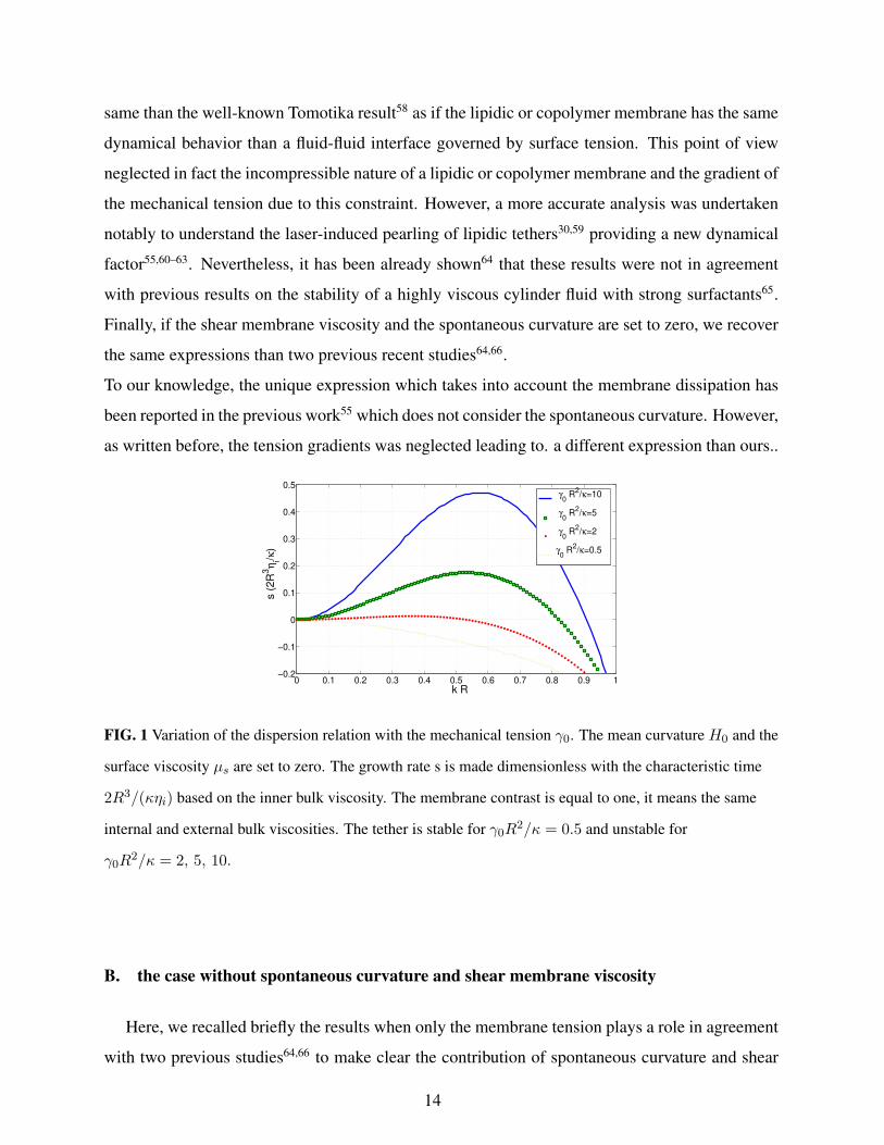
same than the well-known Tomotika result58 as if the lipidic or copolymer membrane has the same

dynamical behavior than a fluid-fluid interface governed by surface tension. This point of view

neglected in fact the incompressible nature of a lipidic or copolymer membrane and the gradient of

the mechanical tension due to this constraint. However, a more accurate analysis was undertaken

notably to understand the laser-induced pearling of lipidic tethers30,59 providing a new dynamical

factor55,60–63. Nevertheless, it has been already shown64 that these results were not in agreement

with previous results on the stability of a highly viscous cylinder fluid with strong surfactants65.

Finally, if the shear membrane viscosity and the spontaneous curvature are set to zero, we recover

the same expressions than two previous recent studies64,66.

To our knowledge, the unique expression which takes into account the membrane dissipation has

been reported in the previous work55 which does not consider the spontaneous curvature. However,

as written before, the tension gradients was neglected leading to. a different expression than ours..

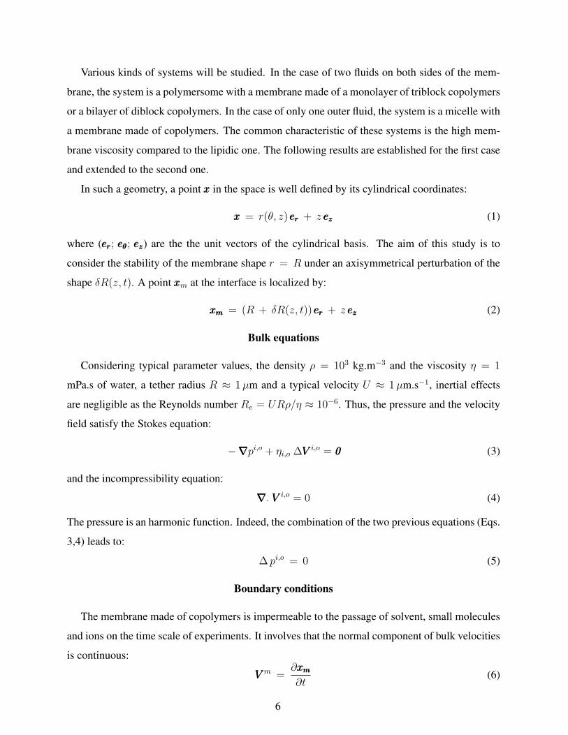
0 0.1 0.2 0.3 0.4 0.5 0.6 0.7 0.8 0.9 1−0.2

−0.1

0

0.1

0.2

0.3

0.4

0.5

k R

s (

2R

3η

i/κ)

γ0 R

2/κ=10

γ0 R

2/κ=5

γ0 R

2/κ=2

γ0 R

2/κ=0.5

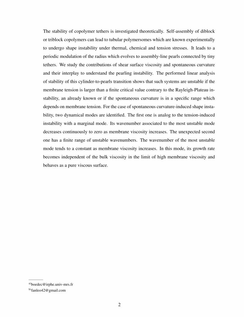
FIG. 1 Variation of the dispersion relation with the mechanical tension γ0. The mean curvature H0 and the

surface viscosity µs are set to zero. The growth rate s is made dimensionless with the characteristic time

2R3/(κηi) based on the inner bulk viscosity. The membrane contrast is equal to one, it means the same

internal and external bulk viscosities. The tether is stable for γ0R2/κ = 0.5 and unstable for

γ0R2/κ = 2, 5, 10.

B. the case without spontaneous curvature and shear membrane viscosity

Here, we recalled briefly the results when only the membrane tension plays a role in agreement

with two previous studies64,66 to make clear the contribution of spontaneous curvature and shear

14

membrane viscosity in the following. Thus, we set: H0 = 0 and µs = 0.

If we only keep the pressure and the membrane terms that do not depend on space, the pressure

perturbation can be written using the normal equilibrium (eq. 44) and appendix D:

δpi − δpo ≈ δR

R2

( 3κ

2R2− γ0

)(52)

Where the radius is increased (decreased) by the perturbation δR, the pressure diminishes (raises)

if the membrane tension γ0 exceeds a critical value γc, a function of the bending elastic modulus

and the radius: γ0 > γc with γc = 3κ/2R2. This corresponds to b > 0 and c < 0. In this

case, a longitudinal flow amplifies the initial perturbation: the membrane tube is unstable. This

result is known and has also been derived by energetic analysis. It highlights the contribution of

bending energy. Indeed, for a fluid-fluid interface, the critical surface tension of the Rayleigh-

Plateau instability is zero and not a finite value as here. At equilibrium, the membrane tension

is γ = κ/2R2 obtained by the minimization of the Helfrich and tension energies for a cylinder.

It means that an external force must be applied to reach the threshold γc with a laser, an electric

field, a flow such as in elongationnal configuration or sedimentation. If a force f pulls the tether

at each tip, the critical force fc is given by: fc = (γc + κ2R2 )2πR = (8/3)πRγc, an expression

different from 2πRγc given for a fluid-fluid interface which still underlines the role of bending

energy. Another characteristic of this instability is that all the wavenumbers in the range [0; k0] are

unstable as their growth rate s(k) is positive (see figure 1):

k0 =1

R

(1

4− γ0R

2

2κ+

1

4

(4(γ0R

2

κ)2 + 12

γ0R2

κ− 23

)1/2)1/2

(53)

One of the unstable modes grows faster and is called the most unstable wavenumber km that

increases with the dimensionless membrane tension γ0R2/κ and with the ratio of viscosities ηi/ηo.

With the same viscosities inside and outside ηi = ηo, km ≈ 0.56/R what corresponds to a

growth rate sm = s(km) ≈ 0.24κ/ηR3. The characteristic time is given by the competition

between bending resistance and viscous stress. Consider the following parameter to have an order

of magnitude: a radius R = 1µm, a lipidic bending modulus κ = 20kBT and the water viscosity

η = 1 m.Pa.s: the wavelength λm = km/2π ≈ 11µm and 1/sm ≈ 50 ms. Relevant values of

the difference of viscosities between inside and outside and membrane tension leads to a 10 %

variation of km. A complete analysis of variations of km and sm with the membrane tension and

the bulk viscosities can be found in our previous study64.

15

C. the case with spontaneous curvature and without shear membrane viscosity

0 0.2 0.4 0.6 0.8 1 1.2−0,02

0

0,02

0,04

k R

s (

2R

3/η

iκ)/

(H0R

)2

H0R=10

H0R=20

H0R=50

H0R=100

H0R=1000

H0R=−1000

H0R=−100

H0R=−50

H0R=−20

H0R=−10

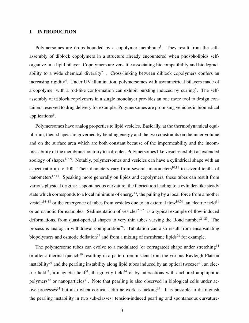
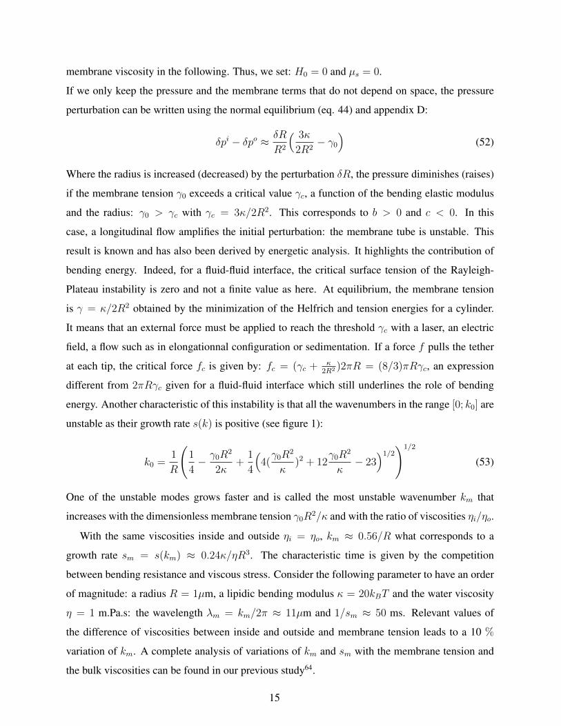
FIG. 2 Variation of the dispersion relation with the spontaneous curvature H0 in the regime of high H0.

The mechanical tension γ0 and the membrane viscosity µs are set to zero, The dispersion relation s(k)

tends to the curve s(k) ≈ ηiκH20/(2R) in the limit of high spontaneous curvature. The wavenumber which

cancels the growth rate is 1/R and the wavenumber km of maximal growth rate is approximately 0.61/R

for large H0. These expressions can provide good orders of magnitude in a large range of H0 in a first

approximation.

We recall the convention on the sign of H0: the curvature of a sphere and by extension of a

cylinder is negative. It comes from a preliminary choice using differential geometry to describe

more easily the variations of the geometrical properties along the surface. To come back to the

other convention (a positive curvature for a sphere or a cylinder), H0 has to be replaced by −H0.

Then, the only difference is the constant b which becomes b = γ0R2

κ− 1

2− 2H0R.

The spontaneous curvature H0 appears either in the effective membrane tension γ0 or by the

variation of the gaussian curvature (see eq. 10) which provides a linear variation of the coefficient

b with H0. This linear term disappears if the membrane is flat (see eq. 97) highlighting the

difference with previous studies67. Investigating the signs of b and c makes clear that at large

spontaneous curvature, the coefficients are dominated by the square of H0 while for weak values,

the linear term is essential. For the sake of simplicity, we only investigate the limits of zero tension

γ0 = 0 (figures 2 and 3) and zero effective tension γ0 = 0 (figure 4). This choice has a degree of

which provide a clear picture of the contribution of spontaneous curvature.

16

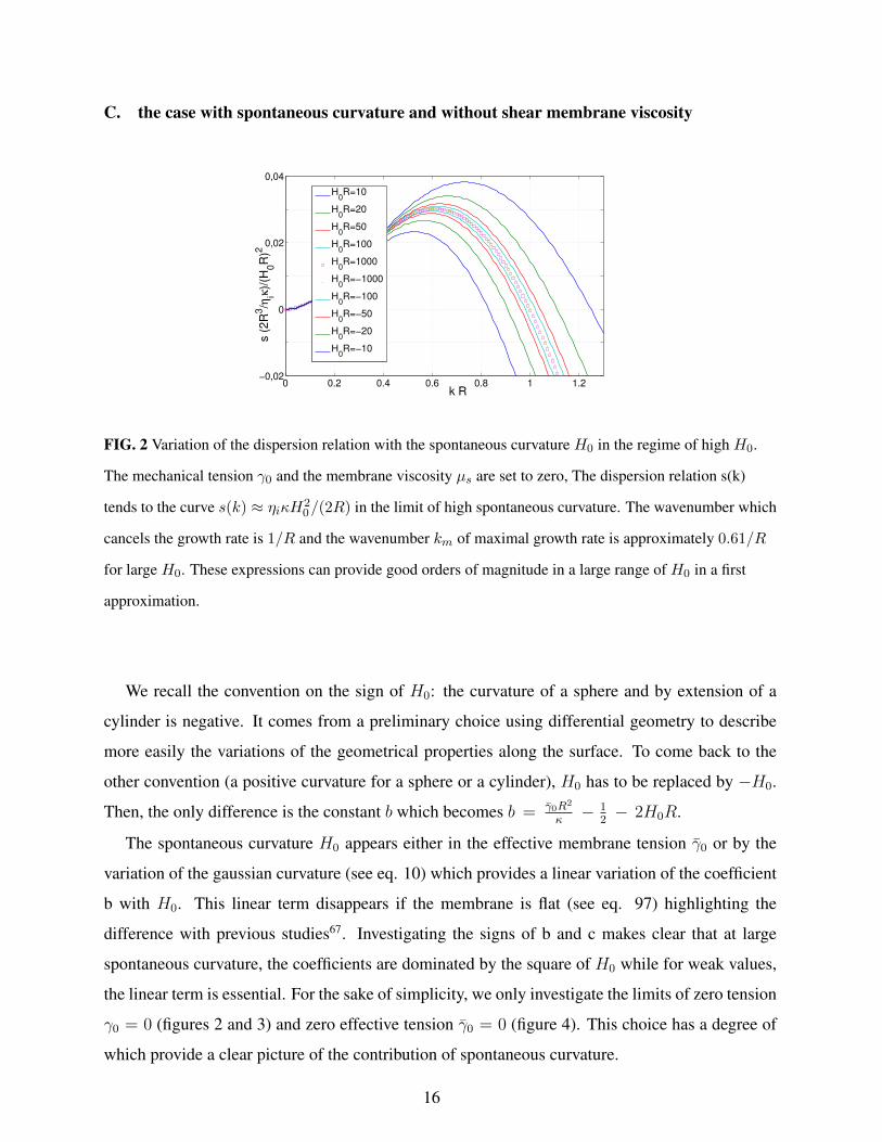
0 0.2 0.4 0.6 0.8 1 1.2 1.4 1.6−0.2

−0.1

0

0.1

0.2

0.3

k R

s (

2R

3η

i/κ)

H0R = −1.6

H0R = −1.3

H0R = −1

H0R = −0.5

H0R = 1

H0R = 1.6

FIG. 3 Variation of the dispersion relation with the spontaneous curvature H0 in the regime of moderate

H0 range. The mechanical tension γ0 and the membrane viscosity µs are set to zero, the internal and

external bulk viscosities are equal. Note that with our convention, the curvature of a sphere is negative, a

classic way in modeling of vesicles under flow. The tether is unstable for H0 = −1.6/R, −1.3/R and

stable for H0 = −0.5/R, 1/R, 1.6/R. The transition is at H0 = −1/R. The negative and positive values

of H0 have been chosen such that (1/2)H20R

2 < 3/2, the threshold of the instability driven by the

mechanical tension.

In the case without mechanical tension (γ0 = 0), the limits of high (figure 2) and small to

moderate (figure 3) spontaneous curvature present a different relation of dispersion, i.e the vari-

ation of the growth rate s of a perturbation in respect of its wavenumber k. Indeed, in the limit

of large values of the spontaneous curvature, the cylinder membrane is always unstable due to

the effective membrane tension γ0 = κH20/2 >> 3/2 explaining shape instability (b > 0 and

c < 0): see figure 2. As expected, the dispersion relation is analog to the tension-induced pearling

instability which is recalled in the section V B. The marginal mode is the zero wavenumber (figure

2). In the case of small to moderate spontaneous curvature (figure 3), the tether becomes unsta-

ble above the threshold HOc = −1/R corresponding to the marginal mode kc = 1/R. A finite

range of wavenumbers [k1; k2] with k1 > 0 is unstable contrary to tension-induced pearling. For

H0R = −1.8, the most unstable mode kc = 2π/λc leading to a wavelength λc ≈ 5.38R. Here,

the term 2κH0δK ≈ 2κH0k2δR/R of the normal mechanical equilibrium eq. 44 varies linearly

with H0 and governs the amplified perturbation. A necessary condition is a negative spontaneous

curvature: H0 < 0 corresponding to the same sign of the tether’s curvature. This is strikingly dif-

17

ferent from the effective tension-induced instability where H0 and −H0 play the same role. Thus,

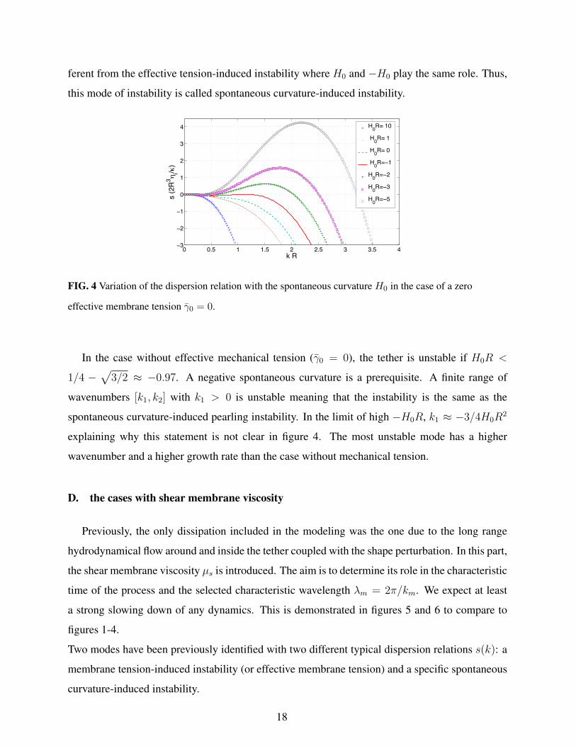
this mode of instability is called spontaneous curvature-induced instability.

0 0.5 1 1.5 2 2.5 3 3.5 4−3

−2

−1

0

1

2

3

4

k R

s (2

R3 η

i/κ)

H0R= 10

H0R= 1

H0R= 0

H0R=−1

H0R=−2

H0R=−3

H0R=−5

FIG. 4 Variation of the dispersion relation with the spontaneous curvature H0 in the case of a zero

effective membrane tension γ0 = 0.

In the case without effective mechanical tension (γ0 = 0), the tether is unstable if H0R <

1/4 −√

3/2 ≈ −0.97. A negative spontaneous curvature is a prerequisite. A finite range of

wavenumbers [k1, k2] with k1 > 0 is unstable meaning that the instability is the same as the

spontaneous curvature-induced pearling instability. In the limit of high −H0R, k1 ≈ −3/4H0R2

explaining why this statement is not clear in figure 4. The most unstable mode has a higher

wavenumber and a higher growth rate than the case without mechanical tension.

D. the cases with shear membrane viscosity

Previously, the only dissipation included in the modeling was the one due to the long range

hydrodynamical flow around and inside the tether coupled with the shape perturbation. In this part,

the shear membrane viscosity µs is introduced. The aim is to determine its role in the characteristic

time of the process and the selected characteristic wavelength λm = 2π/km. We expect at least

a strong slowing down of any dynamics. This is demonstrated in figures 5 and 6 to compare to

figures 1-4.

Two modes have been previously identified with two different typical dispersion relations s(k): a

membrane tension-induced instability (or effective membrane tension) and a specific spontaneous

curvature-induced instability.

18

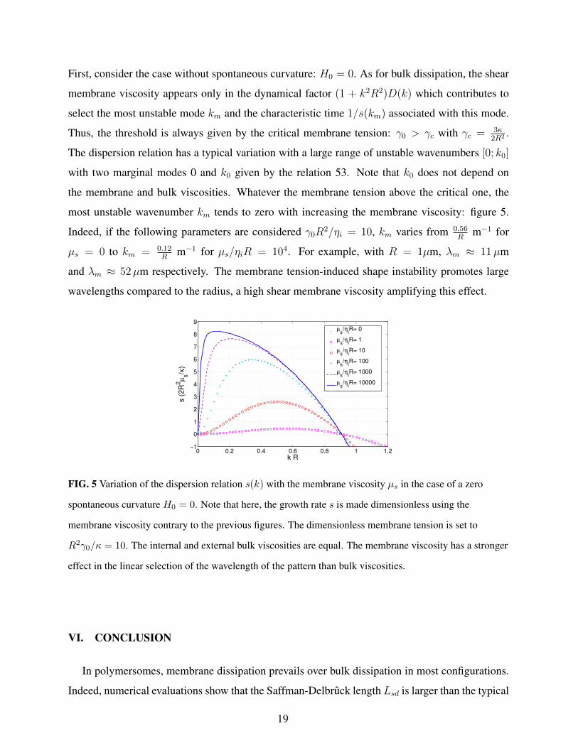
First, consider the case without spontaneous curvature: H0 = 0. As for bulk dissipation, the shear

membrane viscosity appears only in the dynamical factor (1 + k2R2)D(k) which contributes to

select the most unstable mode km and the characteristic time 1/s(km) associated with this mode.

Thus, the threshold is always given by the critical membrane tension: γ0 > γc with γc = 3κ2R2 .

The dispersion relation has a typical variation with a large range of unstable wavenumbers [0; k0]

with two marginal modes 0 and k0 given by the relation 53. Note that k0 does not depend on

the membrane and bulk viscosities. Whatever the membrane tension above the critical one, the

most unstable wavenumber km tends to zero with increasing the membrane viscosity: figure 5.

Indeed, if the following parameters are considered γ0R2/ηi = 10, km varies from 0.56

Rm−1 for

µs = 0 to km = 0.12R

m−1 for µs/ηiR = 104. For example, with R = 1µm, λm ≈ 11µm

and λm ≈ 52µm respectively. The membrane tension-induced shape instability promotes large

wavelengths compared to the radius, a high shear membrane viscosity amplifying this effect.

0 0.2 0.4 0.6 0.8 1 1.2−1

0

1

2

3

4

5

6

7

8

9

k R

s (

2R

2µ

s/κ

)

µs/η

iR= 0

µs/η

iR= 1

µs/η

iR= 10

µs/η

iR= 100

µs/η

iR= 1000

µs/η

iR= 10000

FIG. 5 Variation of the dispersion relation s(k) with the membrane viscosity µs in the case of a zero

spontaneous curvature H0 = 0. Note that here, the growth rate s is made dimensionless using the

membrane viscosity contrary to the previous figures. The dimensionless membrane tension is set to

R2γ0/κ = 10. The internal and external bulk viscosities are equal. The membrane viscosity has a stronger

effect in the linear selection of the wavelength of the pattern than bulk viscosities.

VI. CONCLUSION

In polymersomes, membrane dissipation prevails over bulk dissipation in most configurations.

Indeed, numerical evaluations show that the Saffman-Delbruck length Lsd is larger than the typical

19

0 0.5 1 1.5

−0.4

−0.2

0

0.2

0.4

0.6

k R

s (

2R

2µ

s/κ

)

µs/Rη

i= 1

µs/Rη

i= 10

µs/Rη

i= 100

µs/Rη

i= 250

µs/Rη

i= 1000

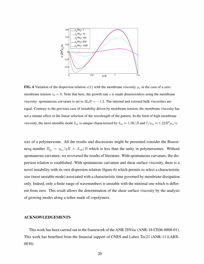
FIG. 6 Variation of the dispersion relation s(k) with the membrane viscosity µs in the case of a zero

membrane tension γ0 = 0. Note that here, the growth rate s is made dimensionless using the membrane

viscosity. spontaneous curvature is set to H0R = −1.3. The internal and external bulk viscosities are

equal. Contrary to the previous case of instability driven by membrane tension, the membrane viscosity has

not a minute effect in the linear selection of the wavelength of the pattern. In the limit of high membrane

viscosity, the most unstable mode km is unique characterized by km ≈ 1.06/R and 1/sm ≈ 1.22R2µs/κ.

size of a polymersome. All the results and discussions might be presented consider the Boussi-

nesq number Bqs = ηss/ηR = Lsd/R which is less than the unity in polymersomes. Without

spontaneous curvature, we revovered the results of literature. With spontaneous curvature, the dis-

persion relation is established. With spontaneous curvature and shear surface viscosity, there is a

novel instability with its own dispersion relation (figure 6) which permits to select a characteristic

size (most unstable mode) associated with a characteristic time governed by membrane dissipation

only. Indeed, only a finite range of wavenumbers is unstable with the minimal one which is differ-

ent from zero. This result allows the determination of the shear surface viscosity by the analysis

of growing modes along a tether made of copolymers.

ACKNOWLEDGEMENTS

This work has been carried out in the framework of the ANR 2DVisc (ANR-18-CE06-0008-01).

This work has benefited from the financial support of CNES and Labex Tec21 (ANR-11-LABX-

0030).

20

APPENDIX A - SOME ELEMENTS OF DIFFERENTIAL GEOMETRY

Here, we recall some elements of differential geometry which are necessary to calculate the

tension force, the bending force and especially the viscous membrane force (see Eq. 12) which is

a complex function of geometrical quantities and membrane velocity. A point of the membrane is

localized by a parametrization (s1; s2):

xxxm = xxxm(s1, s2) (54)

The tangent vectors to the surface at xxxm are defined by:

tttβ =∂xxxm∂sβ

(55)

The normal unit vector at the same point is determined as usual:

nnn =ttt1 ∧ ttt2|| ttt1 ∧ ttt2 ||

(56)

The contravariant basis (ttt1 ; ttt2 ; nnn) permit to define all the physical quantities at the surface. In-

deed, the velocity is given by its contravariant coordinate and the normal one: see eq. 11. A dual

basis called covariant (ttt1 ; ttt2 ; nnn) can be defined as:

tttβ.tttα = δαβ (57)

where δατ is the Kronecker symbol. The metric (g) and curvature (K) tensors are given by:

gαβ = tttα.tttβ ; gαβ = tttα.tttβ (58)

Kαβ = −tttα.∂nnn

∂sβ(59)

gαβ gβτ = δατ ; g = det(gαβ) (60)

The two metric tensors are useful to go down and up an index of tensors: gαβAβ = Aα and

gαβAβ = Aα. To calculate the membrane viscous force, it is necessary to calculate gατKτβ =

Kαβ and gβτKα

τ = Kαβ .

The two invariants of the curvature tensor are the mean curvature H and the gaussian curvature

K:

H =1

2Kαα =

1

2gαβKβα (61)

K = det(Kαβ) (62)

21

Differential operators are necessary to calculate the gradient of the mechanical tension in fffγ

and the Laplace-Beltrami of the mean curvature of the bending force fffκ:

∇∇∇sf =( ∂f∂sα

)tttα (63)

∆sf =1√g

∂

∂sβ

(√g gβα

∂f

∂sα

)(64)

APPENDIX B - AXISYMMETRICAL EXPRESSIONS IN THE PARAMETRIZATION

(θ, z)

As explained in the section II A, the characteristics of the studied system are well described by

a local basis based on the parametrization (θ, z). As we consider axisymmetrical deformations,

the shape of the membrane is only a function of z:

xxxm = f(z, t)ererer + z ezezez (65)

Thus, the contravariant basis (tttθ; tttz; nnn) satisfies using eq. 65:

tttθ =∂xxxm∂θ

= f eθeθeθ (66)

tttz =∂xxxm∂z

= f ′ererer + ezezez (67)

nnn =tttθ ∧ tttz|| tttθ ∧ tttz ||

=ererer − f ′ ezezez√

1 + f ′2(68)

where f ′ = (∂f/∂z). The metric tensor in the covariant and contravariant basis are deduced:

gθθ = f 2 (69)

gθz = gzθ = 0 (70)

gzz = 1 + f ′2 (71)

gθθ =1

f 2(72)

gθz = gzθ = 0 (73)

gzz =1

1 + f ′2(74)

The curvature tensor Kαβ is:

Kθθ = − f√1 + f ′2

(75)

Kθz = Kzθ = 0 (76)

Kzz =f ′′√

1 + f ′2(77)

22

Some intermediates are necessary:

Kθθ = − 1

f√

1 + f ′2(78)

Kzθ = Kθ

z = 0 (79)

Kzz =

f ′′

(1 + f ′2)3/2(80)

Thus, the mean H and gaussian K curvatures are determined:

2H =f ′′

(1 + f ′2)3/2− 1

f√

1 + f ′2(81)

K = − f ′′

f(1 + f ′2)(82)

To determine the membrane viscous force, the tensor Kαβ is necessary:

Kθθ = − 1

f 3√

1 + f ′2(83)

Kθz = Kzθ = 0 (84)

Kzz =f ′′

(1 + f ′2)5/2(85)

APPENDIX C - BASIC STATE

The previous quantities are calculated in the resting state, a cylinder of radius f(z, t) = R:

ttt(0)θ = Reθeθeθ ; ttt(0)

z = ezezez ; nnn(0) = ererer (86)

H(0) = − 1

2R; K(0) = 0 ; g(0) = R2 (87)

g(0)θθ = R2 ; g

(0)θz = g

(0)zθ = 0 ; g(0)

zz = 1 (88)

gθθ,(0) =1

R2; gθz,(0) = gzθ,(0) = 0 ; gzz,(0) = 1 (89)

K(0)θθ = −R ; K

(0)θz = K

(0)zθ = 0 ; K(0)

zz = 0 (90)

Kθ,(0)θ = − 1

R; K

z,(0)θ = Kθ,(0)

z = 0 ; Kz,(0)z = 0 (91)

Kθθ,(0) = − 1

R3;Kθz,(0) = Kzθ,(0) = 0; Kzz,(0) = 0 (92)

23

APPENDIX D - PERTURBATIONS

Only the geometrical quantities which are necessary to the calculation of the linearized state

are provided. The shape perturbation is a modulated cylinder of radius f(z, t) = R + δR(z, t)

with the condition || δR ||<< R:

tθtθtθ = tθtθtθ(0) + δReθeθeθ (93)

tztztz = tztztz(0) + δR′ ererer (94)

nnn = nnn(0) − δR′ ezezez (95)

δH = H −H(0) =1

2(δR′′ +

δR

R2) (96)

δK = K −K(0) = K = −δR′′

R(97)

∆sδH = ∆sH =∂2δH

∂z2=

1

2(δR′′′′ +

δR′′

R2) (98)

∇∇∇sδγ = ∇∇∇sγ =(∂δγ∂z

)ezezez (99)

REFERENCES

1B. M. Disher, Y. Y. Won, D. S. Ege, J. C. M. Lee, F. S. Bates, D. E. Disher, and D. A. Ham-

mer, “Polymersomes: tough vesicles made from diblock copolymers,” Science 284, 1143–1146

(1999).2G. Y. Liu, C. J. Chen, and J. Ji, “Biocompatible and biodegradable polymersomes as delivery

vehicles in biomedical applications,” Soft Matter 8, 8811–8821 (2012).3M. Dionzou, A. Morere, C. Roux, B. Lonetti, J.-D. Marty, C. Mingotaud, P. Joseph,

D. Goudouneche, B. Payre, M. Leonetti, and A.-F. Mingotaud, “Comparison of methods for

the fabrication and the characterization of polymer self-assemblies: what are the important pa-

rameters?” Soft Matter 12, 2166–2176 (2016).4G. P. Robbins, D. Lee, J. S. Katz, P. R. Frail, M. J. Therien, J. C. Crocker, and D. A. Hammer,

“Effects of membrane rheology on leuko-polymersome adhesion to inflammatory ligands,” Soft

Matter 7, 769–779 (2011).5E. Mabrouk, D. Cuvelier, F. Brochard-Wyart, P. Nassoy, and M. H. Li, “Bursting of sensitive

polymersomes induced by curling,” PNAS 106, 7294–7298 (2009).6D. E. Disher and F. Ahmed, “Polymersomes,” Ann. rev. biomed. Eng. 8, 323–341 (2006).

24

7U. Seifert, “Configurations of fluid membranes and vesicles,” Adv. Phys. 46, 13–137 (1997).8M. Yanagisawa, M. Imai, and T. Taniguchi, “Shape deformation of ternary vesicles coupled with

phase separation,” Phys. Rev. Lett. 100, 148102 (2008).9X. Li, “Shape transformations of bilayer vesicles from amphiphilic block copolymers: a dissipa-

tive particle dynamics simulation study,” Soft Matter 9, 11663–11670 (2013).10A. A. Reinecke and H. G. Dobereiner, “Slow relaxation dynamics of tubular polymersomes after

thermal quench,” Langmuir 19, 605–608 (2003).11K. P. Sinha, S. Gadkari, and R. M. Thaokar, “Electric field induced pearling instability in cylin-

drical vesicles,” Soft Matter 9, 7274–7293 (2013).12I. W. Hamley, “Nanoshells and nanotubes from block copolymers,” Soft Matter 1, 36–43 (2005).13L. Wang, H. Huang, and T. He, “Rayleigh instability induced cylinder-to-sphere transition in

block copolymer micelles: Direct visualization of the kinetic pathway,” ACS Macro Letters 3,

433–438 (2014).14J. E. Reiner, J. M. Wells, R. B. Kishore, C. Pfefferkorn, and K. Helmerson, “Stable and robust

polymer nanotubes stretched from polymersomes,” PNAS 103, 1173–1177 (2006).15A.-S. Smith, E. Sackmann, and U. Seifert, “Pulling tethers from adhered vesicles,” Physical

Review Letters 92, 208101 (2004).16M. Karlsson, K. Sott, A.-S. Cans, A. Karlsson, R. Karlsson, and O. Orwar, “Micropipet-assisted

formation of microscopic networks of unilamellar lipid bilayer nanotubes and containers,” Lang-

muir 17, 6754–6758 (2001).17T. R. Powers, G. Huber, and R. E. Goldstein, “Fluid-membrane tethers: Minimal surfaces and

elastic boundary layers,” Physical Review E 78, 041901 (2002).18I. Dereryi, F. Julicher, and J. Prost, “Formation and interaction of membrane tubes,” Physical

Review Letters 88, 238101 (2002).19S. Dittrich, Petra, M. Heule, P. Renaud, and A. Manz, “On-chip extrusion of lipid vesicles and

tubes through microsized aperture,” Lab on a Chip 6, 488–493 (2006).20V. Kantsler, E. Segre, and V. Steinberg, “Critical dynamics of vesicle stretching transition in

elongational flow,” Phys. Rev. Lett. 101, 048101 (2008).21G. Boedec, M. Leonetti, and M. Jaeger, “3d vesicle dynamics simulations with a linearly trian-

gulated surface,” J. Comp. Phys. 230, 1020–1034 (2011).22G. Boedec, M. Jaeger, and M. Leonetti, “Settling of a vesicle in the limit of quasispherical

shapes,” J. Fluid Mech. 690, 227–261 (2012).

25

23I. Rey Suarez, C. Leidy, G. Teliez, G. Gay, and A. Gonzalez-Mancera, “Slow sedimentation and

deformability of charged lipid vesicles,” Plos ONE 8, e68309 (2013).24Z. H. Huang, M. Abkarian, and A. Viallat, “Sedimentation of vesicles: from pear-like shapes to

micro tether extrusion,” New J. Phys. 13, 035026 (2011).25G. Boedec, M. Jaeger, and M. Leonetti, “Sedimentation-induced tether on a settling vesicle,”

Phys. Rev. E 88, 010702 (2013).26S. Chatkaew, M. Georgelin, M. Jaeger, and M. Leonetti, “Dynamics of vesicle unbinding under

axisymmetric flow,” Phys. Rev. Lett. 103, 248103 (2009).27T. Okano, K. Inoue, K. Koseki, and H. Suzuki, “Deformation modes of giant unilamellar vesicles

encapsulating biopolymers,” ACS Synth. Biol. 7, 739–747 (2018).28T. Bhatia, J. Agudo-Canalejo, R. Dimova, and R. Lipowsky, “Membrane nanotubes increase the

robustness of giant vesicles,” ACS Nano 12, 4478–4485 (2018).29S. Tomotika, “On the instability of a cylindrical thread of a viscous liquid surrounded by an-

other viscous fluid,” Proceedings of the Royal Society of London. Series A - Mathematical and

Physical Sciences 150, 322–337 (1935).30R. Bar-Ziv and E. Moses, “Instability and ”pearling” states produced in tubular membranes by

competition of curvature and tension,” Phys. Rev. Lett. 73, 1392–1395 (1994).31C. Menager, M. Meyer, V. Cabuil, A. Cebers, J.-C. Bacri, and R. Perzynski, “Magnetic phos-

pholipid tubes connected to magnetoliposomes: Pearling instability induced by a magnetic field,”

The European Physical Journal E 7, 325–337 (2002).32I. Tsafrir, D. Sagi, T. Arzi, M.-A. Guedeau-Boudeville, V. Frette, D. Kandel, and J. Stavans,

“Pearling instabilities of membrane tubes with anchored polymers,” Phys. Rev. Lett. 86, 1138–

1141 (2001).33Y. Yu and S. Granick, “Pearling of lipid vesicles induced by nanoparticles,” Journal of American

Chemical Society 131, 14158–14159 (2009).34U. Jelercic and N. S. Gov, “Pearling instability of membrane tubes driven by curved proteins and

actin polymerization,” Physical Biology 12, 066022 (2015).35D. Heinrich, M. Ecke, M. Jasmin, U. Engel, and G. Gerisch, “Reversible membrane pearling in

live cells upon destruction of the actin cortex,” Biophysical journal 106, 1079–1091 (2014).36U. Seifert and S. A. Langer, “Viscous modes of fluid bilayer membranes,” Europhysics Letters

23, 71–76 (1993).

26

37A. R. Honerkamp-Smith, F. G. Woodhouse, V. Kanstler, and R. E. Goldstein, “Membrane vis-

cosity determined from shear-driven flow in giant vesicles,” Phys. Rev. Lett. 111, 038103 (2013).38R. Dimova, U. Seifert, B. Pouligny, S. Forster, and H. G. Dobereiner, “Hyperviscous diblock

copolymerr vesicles,” Eur. Phys. J. E 7, 241–250 (2002).39J. F. Le Meins, O. Sandre, and S. Lecommandoux, “Recent trends in the tuning of polymer-

somes’ membrane properties,” Eur. Phys. J. E 34, 1–17 (2011).40P. G. Saffman and M. Delbrick, “Brownian motion in biological membranes,” PNAS 72, 3111–

3113 (1975).41P. G. Saffman, “Brownian motion in thin sheets of viscous fluid,” J. Fluid Mech. 73, 593–602

(1976).42P. Cicuta, S. L. Keller, and S. L. Veatch, “Diffusion of liquid domains in lipid bilayer mem-

branes,” J. Phys. Chem. B 111, 3328–3331 (2007).43E. P. Petrov and P. Schwile, “Translational diffusion in lipid membranes beyond the saffman-

delbruck approximation,” Biophys. J. 94, L41–L43 (2008).44G. B. Nash and H. J. Meiselman, “Red cell and ghost viscoelasticity. effects of hemoglobin

concentration and in vivo aging.” Biophys. J. 43, 63–73 (1983).45R. M. Hochmuth, P. R. Worthy, and E. A. Evans, “Red cell extensional recovery and the deter-

mination of membrane viscosity,” Biophysical Journal 26, 101–114 (1979).46R. Tran-Son-Tay, S. P. Sutera, and P. R. Rao, “Determination of red blood cell membrane vis-

cosity from rheoscopic observations of tank-treading motion.” Biophys. J. 46, 65–72 (1984).47Z. Li, B. Anvari, M. Takashima, P. Brecht, J. H. Torres, and W. E. Brownell, “Membrane

tether formation from outer hair cells with optical tweezers,” Biophysical Journal 82, 1386–1395

(2002).48Z. Y. Luo, X. L. Shang, and B. F. Bai, “Influence of pressure-dependent surface viscosity on

dynamics of surfactant-laden drops in shear flow,” J. Fluid Mech. 858, 91–121 (2019).49J. Gounley, G. Boedec, M. Jaeger, and M. Leonetti, “Influence of surface viscosity on droplets

in shear flow,” J. Fluid Mech. 791, 464–494 (2016).50P. Bagchi and R. M. Kalluri, “Dynamics of nonspherical capsules in shear flow,” Phys. Rev. E

79, 031915 (2009).51C. de Loubens, J. Deschamps, F. Edwards-Levy, and M. Leonetti, “Tank-treading of microcap-

sules in shear flow,” J. Fluid Mech. 789, 750–767 (2016).

27

52C. Bacher, K. Graessel, and S. Gekle, “Rayleigh–plateau instability of anisotropic interfaces.

part 2. limited instability of elastic interfaces,” J. Fluid Mech. 910, A47 (2021).53S. Mora, T. Phou, J.-M. Fromental, L. M. Pismen, and Y. Pomeau, “Capillarity driven instability

of a soft solid,” Phys. rev. lett. 105, 214301 (2010).54L. Scriven, “Dynamics of a fluid interface equation of motion for newtonian surface fluids,”

Chem. Eng. Sci. 12, 98–108 (1960).55T. R. Powers, “Dynamics of filaments and membranes in a viscous fluid,” Rev. Mod. Phys. 82,

1607–1631 (2010).56R. Granek and Z. Olami, “Dynamics of rayleigh-like instability induced by laser tweezers in

tubular vesicles of self-assembled membranes,” J. Phys. II France 5, 1349–1370 (1995).57S. Chaıeb and S. Rica, “Spontaneous curvature-induced pearling instability,” Phys. Rev. E 58,

7733–7737 (1998).58R. Granek, “Spontaneous curvature-induced rayleigh-like instability in swollen cylindrical mi-

celles,” Langmuir 12, 5022–5027 (1996).59R. Bar-Ziv, E. Moses, and P. Nelson, “Dynamic excitations in membranes induced by optical

tweezers,” Biophysical Journal 75, 294 – 320 (1998).60P. Nelson, T. Powers, and U. Seifert, “Dynamical theory of the pearling instability in cylindrical

vesicles,” Phys. Rev. Lett. 74, 3384–3387 (1995).61K. Gurin, V. Lebedev, and A. Muratov, “Dynamic instability of a membrane tube,” JETP 83,

321–326 (1996).62R. E. Goldstein, P. Nelson, T. Powers, and U. Seifert, “Front propagation in the pearling insta-

bility of tubular vesicles,” J. Phys II France 6, 767–796 (1996).63T. R. Powers and R. E. Goldstein, “Pearling and pinching: Propagation of rayleigh instabilities,”

Phys. Rev. Lett. , 2555–2558 (1997).64G. Boedec, M. Jaeger, and M. Leonetti, “Pearling instability of a cylindrical vesicle,” Journal of

Fluid Mechanics 743, 262–279 (2014).65M.-L. E. Timmermans and J. R. Lister, “The effect of surfactant on the stability of a liquid

thread,” Journal of Fluid Mechanics 459, 289–306 (2002).66V. Narsimhan, A. P. Spann, and E. S. G. Shaqfeh, “The mechanism of shape instability for a

vesicle in extensional flow,” Journal of Fluid Mechanics 750, 144–190 (2014).67Z. Shi and T. Baumgart, “Dynamics and instabilities of lipid bilayer membrane shapes,” Ad-

vances in Colloid and Interface Science 208, 76–88 (2014).

28