SciPost Physics Submission

Dynamics of the order-parameter statistics in the long-range Isingmodel

Nishan Ranabhat1,2?, Mario Collura1

1 SISSA - International School for Advanced Studies, via Bonomea 265, 34136 Trieste, Italy2 The Abdus Salam International Centre for Theoretical Physics, Strada Costiera 11, 34151

Trieste, Italy? nranabha@sissa.it

October 27, 2021

Abstract

We study the relaxation of the local ferromagnetic order in the transverse field quantum Isingchain with power-law decaying interactions ∼ 1/rα. We prepare the system in the GHZ stateand study the time evolution of the probability distribution function (PDF) of the order-parameter within a block of ` when quenching the transverse field. The model is knownto support long-range order at finite temperature for α ≤ 2.0 [1–3]. In this regime, quasi-localized topological magnetic defects are expected to strongly affect the equilibration of thefull probability distribution. We highlight different dynamical regimes where gaussificationmechanism may be slowed down by confinement and eventually breaks. We further studythe PDF dynamics induced by changing the effective dimensionality of the system; we mimicthis by quenching the range of the interactions. As a matter of fact, the behavior of thesystem crucially depends on the value of α governing the unitary evolution.

Contents

1 Introduction 2

2 Model and methods 32.1 Hamiltonian of Long-range transverse field Ising model 32.2 Full counting statistics 32.3 Quench Protocol and numerical details 4

3 Results 53.1 Quench along transverse field 53.2 Quench of the interaction range 12

4 Conclusion and Outlook 13

A Long range Ising Hamiltonian as an MPO 14

B Convergence with bond dimension 14

References 17

1

arX

iv:2

110.

1377

0v1

[co

nd-m

at.s

tr-e

l] 2

6 O

ct 2

021

SciPost Physics Submission

1 Introduction

Advances in the field of synthetic quantum matter in laboratory has allowed us to gain deeperinsights into the static and dynamic properties of isolated many body quantum systems [3–10].One of the primary objective of these experiments is to calculate the full quantum mechanicalprobability distribution of certain observables as it holds the full information about the quantumfluctuation in the system. In parallel, several analytical and numerical studies have been carriedout to study the full probability distribution of the system’s order parameter both in equilibriumand out of equilibrium regime [11–19]. In this work we study the dynamics of order parameterstatistics, encoded in its probability distribution, of the long-range Ising model following a globalquantum quench [20]. Similar studies have been carried out for systems with short range inter-action [11–13, 15], where the main objective is to see if and how the initial order in the systemmelts after quantum quench. Long-range Ising model is more interesting as it exhibits short-rangeIsing and mean-field universality class [3] connected by an intermediate region where the criticalexponents vary monotonically [21]. Quenches in the mean-field regime reveals information onthe dynamics of systems with dimension higher than one.

We perform two different kind of quenches; the first kind is along the transverse field at con-stant value of interaction range. Here we initialize our system deep in the ferromagnetic region,which is characterized by double peak probability distribution function (PDF) of our local orderparameter. Locality is a crucial concept to ensure the relaxation of the order parameter at latetime [22]. The system is then suddenly quenched along the transverse field and evolved with thenew Hamiltonian. We are interested in how the initial ferromagnetic order melts after a quan-tum quench and specially if the PDF attains a Gaussian shape around zero in the maximum timelimit and system size that we can effectively simulate. The second kind of quench is performedalong the direction of the interaction range, keeping constant the transverse field. We performquenches in both directions: initializing the system as fully connected and quenching to a shortrange Hamiltonian, and vice versa. We investigate how the system retains memory of the initialferromagnetic order after the quench, and whether quenches performed in opposite directions arequalitatively equivalent.

Specifically, the manuscript is organized as follows:

• In Sec. 2 we introduce the model, the parameters involved, and the equilibrium phasediagram. We define the local order parameter and introduce the full counting statistics.We define the cumulant generating function and its relation to the probability distributionfunction (PDF) and outline the steps to compute each of these in a spin model. We definethe general quench protocol and explain in detail the algorithms used.

• Sec. 3 is devoted to the results. We present the results for the dynamics of order param-eter statistics for quenches along the transverse field, at different values of the interactionrange. We show that there is a region in the parameter space where the the system nevershows Gaussification, independently of the simulation time and the system size. On the con-trary, outside this region the Gaussification of the PDF strongly depends on the simulationparameters. We also present the results for the dynamics of the order parameter statistics

2

SciPost Physics Submission

for quenches along the interaction range at different values of transverse field. Here weshow that the dynamics is strongly dependent on the post quench parameters and that thequenches performed in the opposite direction yields qualitatively different behaviour.

• In Sec. 4 we draw our conclusion, also mentioning further possible lines of investigationand eventually connecting this study to finite temperature analysis.

2 Model and methods

2.1 Hamiltonian of Long-range transverse field Ising model

We study the long range transverse field Ising model. A spin model like this can be experimentallyrealized with systems of trapped ions [3, 23, 24] where the interaction is mediated by collectivevibrations. The Hamiltonian is

H(α, h/J) = −1

K(α)

N∑

i< j

J|i − j|α

S xi S x

j − hN∑

i=1

Szi (1)

where Sai , a = x , y, z are the spin 1/2 matrices on the i th lattice site. The spin-spin interaction

is long ranged and is decaying as the inverse power of the distance between two spins. Thisinteraction is tuned by the interaction range α. The Kac normalization is defined as

K(α) = 1N − 1

N∑

i< j

J|i − j|α

=1

N − 1

N∑

n=1

N − nnα

(2)

and ensures the intensive scaling of the energy density for α < 1, which otherwise blows up sincethe spin-spin interaction series becomes hyper-harmonic in the thermodynamic limit.

At the two extremities of the exponent αwe have two familiar models: (i) at α=∞ the modelreduces to the well-celebrated nearest-neighbor Ising model with transverse field, which can besolved analytically in terms of free fermions [25]; this model undergoes an equilibrium quantumphase transition from ferromagnetic to paramagnetic phase at hc/J = 0.5. (ii) At α = 0.0 wherethe model becomes a fully connected, and it is also known as Lipkin, Meshkov, and Glick (LMG)model [26–28]; here the zero-temperature ferromagnetic and paramagnetic phases are separatedby a critical point at hc/J = 1. In thermodynamic limit, the quantum phase-transition point iskept unchanged for all 0≤ α≤ 1.

However, it is sufficient to have α < 2.0 to observe a persisting ferromagnetic long-range or-der at low but finite temperature for |h| smaller than a critical value. In this regime, the systemmanifests a plethora of exotic phenomena such as non-linear light-cone propagation of correla-tions [29–31], dynamical phase transitions [32–35], quasi-localization of topological defects [36],and time-crystalline behavior [37]. Recently, pre-thermal stabilization of time-crystalline behaviorhas been also established for α > 2.0 [38]. Some of these phenomena have been investigated ina range of experiments with trapped ions [39–43].

2.2 Full counting statistics

The full information on how the order melts after a quench is provided by the time evolution ofthe full probability distribution function (PDF) of the order parameter. Our order parameter is the

3

SciPost Physics Submission

longitudinal magnetization defined in a subsystem of length l

M(l) =l∑

i=1

S xi (3)

Observables that are defined over a fixed subsystem relax locally in space unlike the globalobservables [22] and also have thermodynamic behavior in l unlike localized observables. There-fore observables of this kind are suitable choice to study the relaxation dynamics after a globalquantum quench. The probability that the observable defined in equation (3) will take a value min a certain state |Φ⟩ is

Pl(m) = ⟨Φ|δ(M(l)−m)|Φ⟩=∫ ∞

−∞

dθ2π

e−iθm ⟨Φ|eiθM(l)|Φ⟩ (4)

where Gl(θ ) = ⟨Φ|eiθM(l)|Φ⟩ is the generating function of the moments of Pl(m), and satisfy thefollowing properties: Gl(0) = 1, Gl(−θ ) = Gl(θ )∗, Gl(θ + 2π) = (−1)l Gl(θ ). The first twoproperties are trivial. The last one can be easily verified by exploiting the following identities

eiθM(l) =l∏

j=1

eiθSxj , eiθSx

j = cos�

θ

2

�

+ i sin�

θ

2

�

σxj (5)

thus implying

ei(θ+2π)M(l) =l∏

j=1

�

− cos�

θ

2

�

− i sin�

θ

2

�

σxj

�

= (−1)l eiθM(l). (6)

Thanks to this periodicity, we can restrict the range of θ in equation (4) in the interval−π ≤ θ < π. Finally, since m can take either integer or half integer values depending uponwhether l is even or odd, we can rewrite the PDF as

Pl(m) =

¨∑

r∈Z Gl(r)δ(m− r) if l is even,∑

r∈Z Gl(r +12)δ(m− r − 1

2) if l is odd,(7)

where

Gl(r) =

∫ π

−π

dθ2π

e−irθGl(θ ). (8)

The computational bottleneck of calculating the PDF is the generating function Gl(θ ) afterwhich Pl(m) is obtained by a simple Fourier transformation.

2.3 Quench Protocol and numerical details

The general quench protocol reads as follow (hereafter J = 1): (i) At t = 0 the system is ini-tialized in the ground state |ψi⟩ of a certain point in the equilibrium phase space denoted by apair of parameters (αi , hi). (ii) The system is then suddenly quenched to a different point in theparameter space, (α f , h f ), and it is evolved unitarily with the Hamiltonian H(α f , h f ), accordinglyto |ψt⟩= e−i tH(α f ,h f ) |ψi⟩ .

In order to accomplish the task we have used matrix product state (MPS) based Density MatrixRenormalization Group (DMRG) algorithm [44–46], and we have initialized the system in the

4

SciPost Physics Submission

ground state of the Hamiltonian H(αi , hi). For all cases considered, we have taken the MPS bonddimension χ = 100, which turns out to be largely sufficient to get a representation of the exactground state with sufficient precision (see Appendix B ). Notice that, in the case of quenchesstarting from hi = 0 [cf. Sec. 3.1], the initial state admits an exact MPS representation with χ = 2.

Thereafter, for the unitary time evolution we use the Time Dependent Variational Principle(TDVP) algorithm [47,48], with second-order integration scheme, to solve the local forward andbackward Schrodinger’s equations. In our numerical simulations we used a single-site TDVP recipeand we kept fixed the initial MPS bond dimension; we fixed the Trotter time-step to d t = 0.05.

We simulated the dynamics of systems with size L = 200, and we measured our observablefor different subsystems l; nevertheless, the majority of the results we presented correspond tothe subsystem of size l = 100. Lets mention that the bottleneck of the simulation is the localeigensolver in DMRG sweep, and the local exponential solver in TDVP sweep for which we haveused Lanczos algorithm [49] with full re-orthogonalization [50]. With the MPS representation ofthe state |Φ⟩, the generating function Gl(θ ) can be measured by sandwiching the product operatoreiθM(l) and exploiting usual tensor-network techniques. We have chosen the subsystem of size lto be at the center of the full system to avoid any boundary effects that might come into play.Finally, the discrete Fourier transform is used to compute P(m, l), using equation (7) with therange θ ∈ [π,π] and discretization step dθ = 0.01.

3 Results

We investigate the dynamics of the subsystem magnetization PDF after a quantum quench. Weconsider two different classes of quantum quenches.

• We initialize the system at hi = 0 and quench the transverse field to finite h f for a givenvalue of interaction range.

• We initialize the system at α = 0 (fully connected) and quench the interaction range toα = 10 (short range Ising) while fixing the transverse field. We also perform a similarquench in opposite direction.

3.1 Quench along transverse field

Here we study the time evolution of the full PDF of the subsystem magnetization Ml(t) aftera quantum quench along the direction of transverse field h. We will keep our quench entirelywithin the ferromagnetic region of the ground state equilibrium phase diagram [3]. We prepareour system in the ground state of the Hamiltonian (1) with h= 0, which is the Z2 symmetric GHZstate [51,52]

|ψi⟩=1p

2(|→, ...→,→,→ ...,→⟩+ |←, ...←,←,← ...,←⟩). (9)

This state is characterised by a two-peak PDF, Pl(m) =12(δm,l/2 + δm,−l/2), thus exhibiting

long-range ferromagnetic order. We suddenly quench the system to a final hamiltonian H(h f )with0< h f < hc(α), where hc(α) is the equilibrium ferromagnetic to paramagnetic transition point atthe givenα. We then evolve the PDF of the subsystem magnetization with post quench hamiltonianin real time with TDVP. The late-time behaviour of the PDF is observed to be strongly dependent

5

SciPost Physics Submission

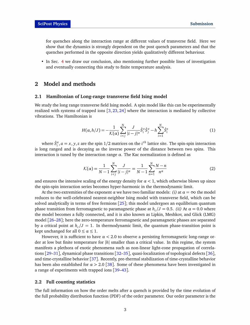
on the post quench parameters and the subsystem size l. In figure 1 we show this dependencewith few representative quenches. In the first row we see that the dynamics is qualitatively thesame for α ∈ {0.0,1.0} and h f = 0.30. In both cases we see that the system strongly retains theinitial long range ferromagnetic order throughout the time evolution. Furthermore we observe apeculiar oscillation in PDF with a return frequency along the time axis. This behavior completelychanges for α = 2.5 where the initial ferromagnetic order starts to melts at later time signifyinga completely different dynamics. This change in behavior is better captured in figure 2. In thesecond row we observe a different quench dynamics for the same values of α, and a larger valueof the post-quench transverse field h f = 0.50. Here, as expected, the initial ferromagnetic orderquickly melts since the larger transverse field works against it. However, depending on the strengthof interaction range, the time evolution of the PDF undergoes a qualitative change in its late timedynamical behavior. For α = {0.0,1.0} the dynamics of the PDF is characterised by periodicre-bouncing of probability streams which lead to a broad and flat distribution; for α = 2.5 thisbehavior completely changes with PDF smoothly melting and eventually attaining a Gaussianshape centered around zero.

Gaussification of the PDF is an important behavior because it signifies the complete meltingof the long range ferromagnetic order into a paramagnetic one. We expect Gaussification whenthe linear dimension of the subsystem exceeds the correlation length of the steady state i.e. l > ξ.The goodness of Gaussification is measured qualitatively by comparing the PDF with the Gaussianapproximation obtained with the first two moments

Pl(µ, t) =1

p

2πσ2(t)exp

�

−(µ− m(t))2

2σ2(t)

�

(10)

where m(t) = ⟨ψt |M(l) |ψt⟩ andσ(t) = ⟨ψt | (M(l)−m(t))2 |ψt⟩ are the first two moments of

Figure 1: PDF dynamics of subsystem magnetization after a quantum quench for l = 100,α ∈ {0.0, 1.0,2.5} and h f ∈ {0.30,0.50} (in first and second rows respectively).

6

SciPost Physics Submission

our order parameter. Quantitatively the goodness of Gaussification can be measured by defininga metric Distance to Gaussian (DG) as

DG =√

√

∑

m

[P(m)− PG(m)]2 (11)

where P(m) is the PDF calculated numerically and PG(m) is the corresponding Gaussian PDFapproximated using 10. DG is the measure of how close (or far) is the PDF from the Gaussianshape, DG = 0 implies a perfect Gaussian shape. This measure is used in [9] under the nameDistance to Thermalization (DT). DG might not be a proper metric for cases in which the systemdoes not relax to a steady state in the given time frame and shows oscillations, in such cases weintroduce the time averaged DG as

DGavg =1

T − To

∫ T

To

DG(d t)d t (12)

where To is chosen to avoid the initial sharp drop in DG [cf. Fig. 4].

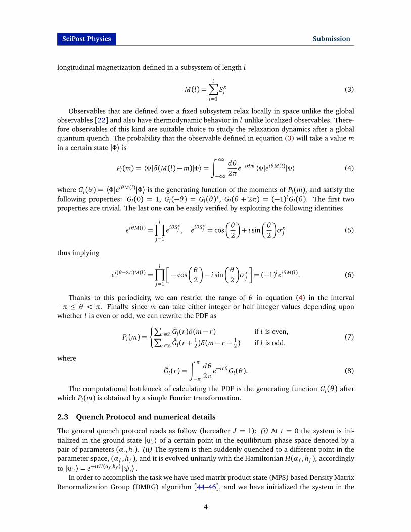
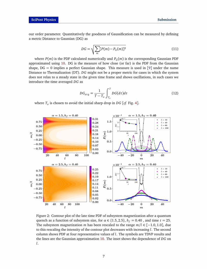
Figure 2: Contour plot of the late time PDF of subsystem magnetization after a quantumquench as a function of subsystem size, for α ∈ {1.5, 2.5}, h f = 0.40 , and time t = 25.The subsystem magnetization m has been rescaled to the range m/l ∈ [−1.0, 1.0], dueto this rescaling the intensity of the contour plot decreases with increasing l. The secondcolumn shows PDF at four representative values of l. The symbols are TDVP results andthe lines are the Gaussian approximation 10. The inset shows the dependence of DG onl.

7

SciPost Physics Submission

In figure 2 we plot the dependence of late time PDF of order parameter on subsystem sizel for two representative values of interaction range above and below α = 2.0 and h f ≤ 0.50.We observe two characteristically different behavior of PDF in these two regimes. For α = 1.5the PDF remains double peaked for all values of l and further, the two branches of PDF divergeswith increasing l suggesting that in thermodynamic limit the initial memory of long range order isstrongly retained. Forα= 2.5 the PDF is double peaked for smaller l, becomes flat for intermediatel and eventually becomes Gaussian for large l, suggesting that in thermodynamic limit the initialmemory of long range order completely melts. These two characteristically different behavior ofPDF above and below α= 2.0 is the basis of dynamical quantum phase transition based on orderparameter (DQPT-OP) as proposed in [32] according to which for h f ≤ 0.50, α = 2.0 marks thetransition line between dynamical ferromagnet and dynamical paramagnet.

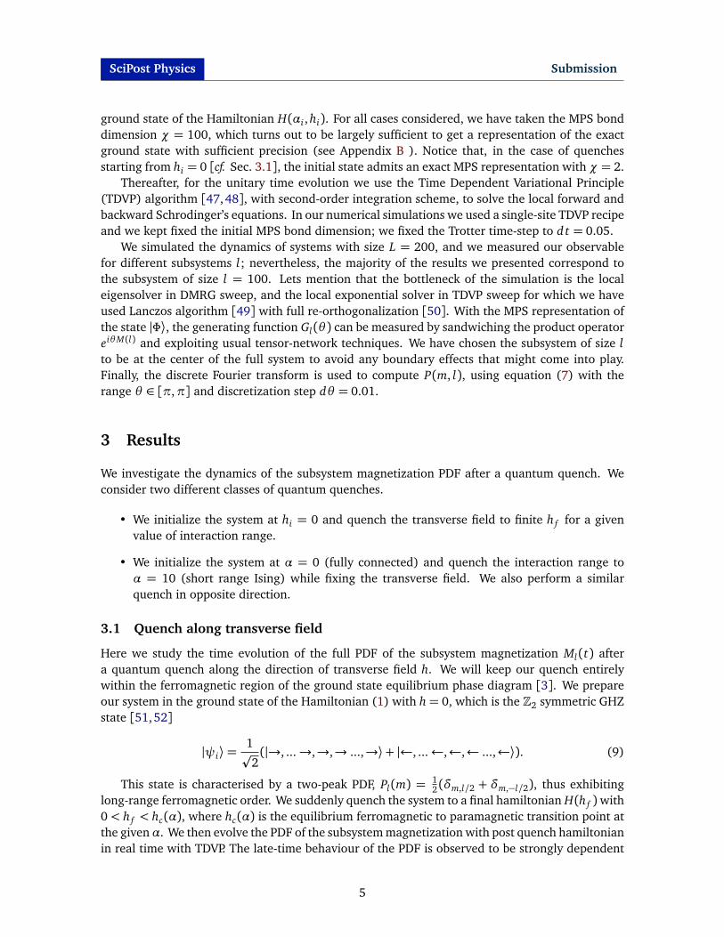
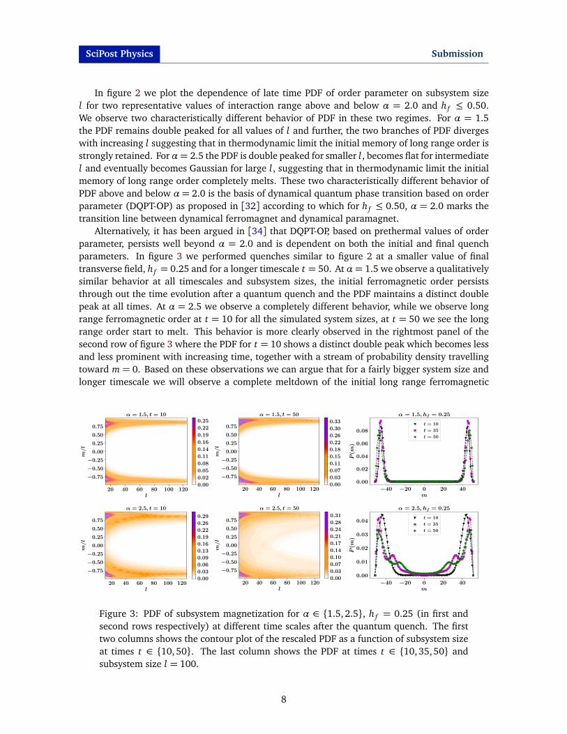
Alternatively, it has been argued in [34] that DQPT-OP, based on prethermal values of orderparameter, persists well beyond α = 2.0 and is dependent on both the initial and final quenchparameters. In figure 3 we performed quenches similar to figure 2 at a smaller value of finaltransverse field, h f = 0.25 and for a longer timescale t = 50. At α= 1.5 we observe a qualitativelysimilar behavior at all timescales and subsystem sizes, the initial ferromagnetic order persiststhrough out the time evolution after a quantum quench and the PDF maintains a distinct doublepeak at all times. At α = 2.5 we observe a completely different behavior, while we observe longrange ferromagnetic order at t = 10 for all the simulated system sizes, at t = 50 we see the longrange order start to melt. This behavior is more clearly observed in the rightmost panel of thesecond row of figure 3 where the PDF for t = 10 shows a distinct double peak which becomes lessand less prominent with increasing time, together with a stream of probability density travellingtoward m = 0. Based on these observations we can argue that for a fairly bigger system size andlonger timescale we will observe a complete meltdown of the initial long range ferromagnetic

Figure 3: PDF of subsystem magnetization for α ∈ {1.5, 2.5}, h f = 0.25 (in first andsecond rows respectively) at different time scales after the quantum quench. The firsttwo columns shows the contour plot of the rescaled PDF as a function of subsystem sizeat times t ∈ {10, 50}. The last column shows the PDF at times t ∈ {10,35, 50} andsubsystem size l = 100.

8

SciPost Physics Submission

order and most possibly Gaussification of the PDF in this regime. This translates to the lack ofDQPT-OP beyond α= 2.0.

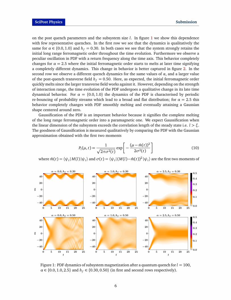
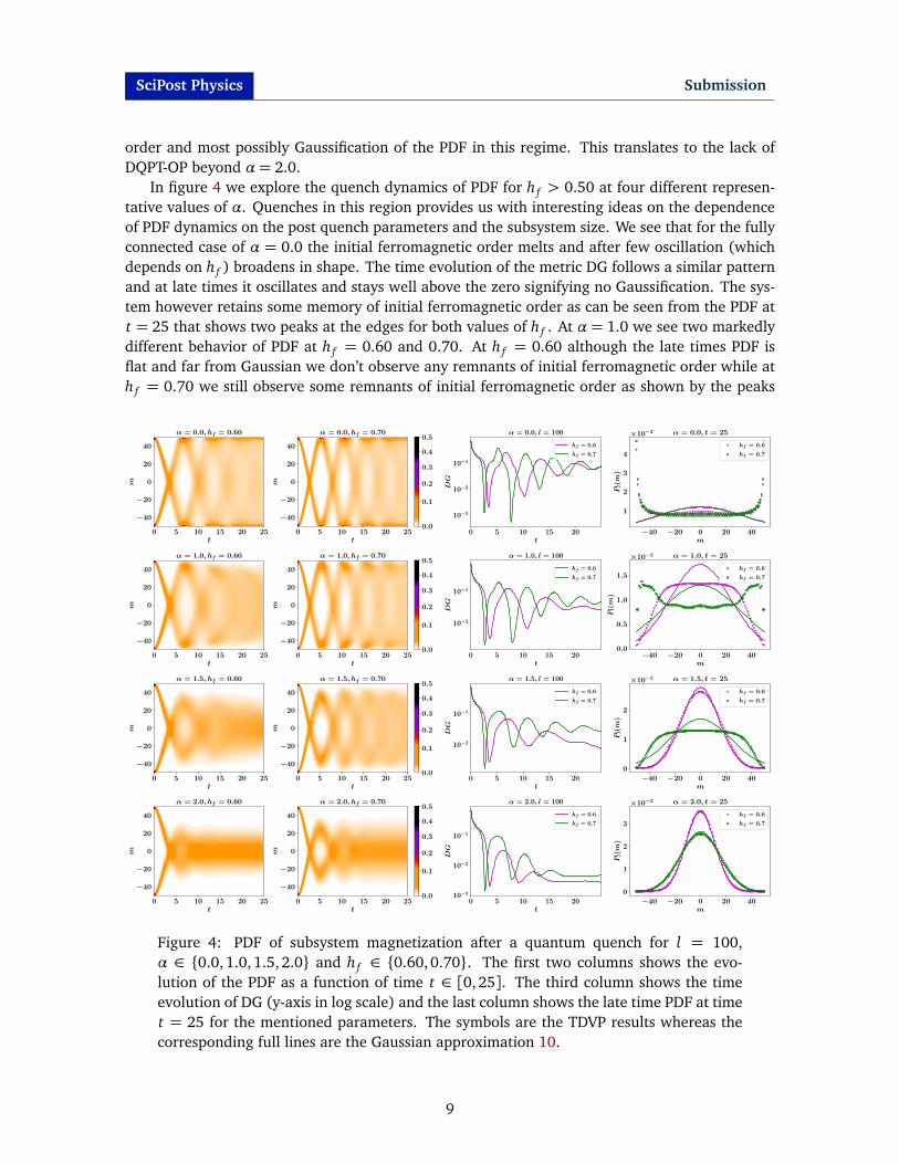
In figure 4 we explore the quench dynamics of PDF for h f > 0.50 at four different represen-tative values of α. Quenches in this region provides us with interesting ideas on the dependenceof PDF dynamics on the post quench parameters and the subsystem size. We see that for the fullyconnected case of α = 0.0 the initial ferromagnetic order melts and after few oscillation (whichdepends on h f ) broadens in shape. The time evolution of the metric DG follows a similar patternand at late times it oscillates and stays well above the zero signifying no Gaussification. The sys-tem however retains some memory of initial ferromagnetic order as can be seen from the PDF att = 25 that shows two peaks at the edges for both values of h f . At α = 1.0 we see two markedlydifferent behavior of PDF at h f = 0.60 and 0.70. At h f = 0.60 although the late times PDF isflat and far from Gaussian we don’t observe any remnants of initial ferromagnetic order while ath f = 0.70 we still observe some remnants of initial ferromagnetic order as shown by the peaks

Figure 4: PDF of subsystem magnetization after a quantum quench for l = 100,α ∈ {0.0,1.0, 1.5,2.0} and h f ∈ {0.60,0.70}. The first two columns shows the evo-lution of the PDF as a function of time t ∈ [0, 25]. The third column shows the timeevolution of DG (y-axis in log scale) and the last column shows the late time PDF at timet = 25 for the mentioned parameters. The symbols are the TDVP results whereas thecorresponding full lines are the Gaussian approximation 10.

9

SciPost Physics Submission

at the edges of late time PDF. These two different behaviors shows the strong dependence of dy-namics of PDF after quantum quench on the depth of the quench. As the depth of the quench isincreased more energy is injected into the system due to which the system takes longer time torelax to a steady state after quench and consequently we observe more oscillations in the evolu-tion of PDF. At α = 1.5 we observe Gaussification of PDF at late times for h f = 0.60, howeveron increasing the quench depth to h f = 0.70 the PDF becomes a flat distribution for the samesimulation time. In this case the time evolution of the metric DG provides a clearer picture as forh f = 0.60 DG starts to relax to zero whereas for h f = 0.7 it oscillates and stays well above zero.Further increasing the interaction range to α= 2.0 we observe clear Gaussification at both valuesof h f . The time evolution of DG also shows that the system relaxes to a stationary state faster andto a lower value for h f = 0.60 than h f = 0.70.

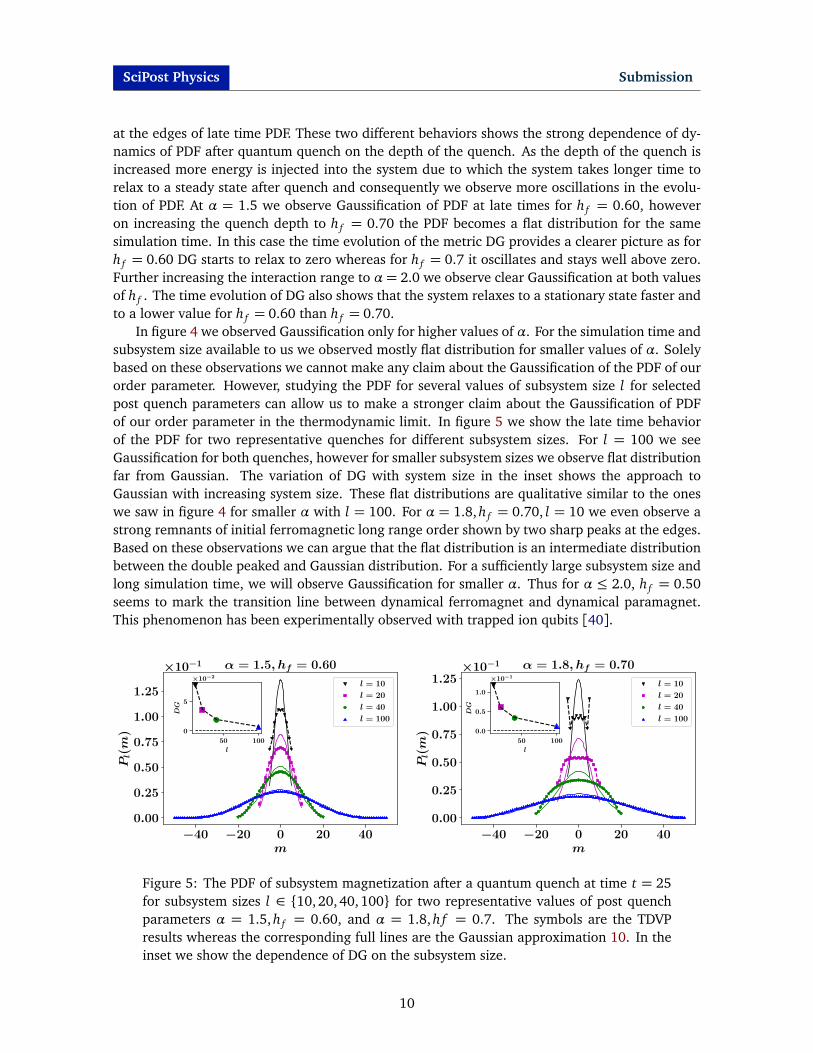
In figure 4 we observed Gaussification only for higher values of α. For the simulation time andsubsystem size available to us we observed mostly flat distribution for smaller values of α. Solelybased on these observations we cannot make any claim about the Gaussification of the PDF of ourorder parameter. However, studying the PDF for several values of subsystem size l for selectedpost quench parameters can allow us to make a stronger claim about the Gaussification of PDFof our order parameter in the thermodynamic limit. In figure 5 we show the late time behaviorof the PDF for two representative quenches for different subsystem sizes. For l = 100 we seeGaussification for both quenches, however for smaller subsystem sizes we observe flat distributionfar from Gaussian. The variation of DG with system size in the inset shows the approach toGaussian with increasing system size. These flat distributions are qualitative similar to the oneswe saw in figure 4 for smaller α with l = 100. For α = 1.8, h f = 0.70, l = 10 we even observe astrong remnants of initial ferromagnetic long range order shown by two sharp peaks at the edges.Based on these observations we can argue that the flat distribution is an intermediate distributionbetween the double peaked and Gaussian distribution. For a sufficiently large subsystem size andlong simulation time, we will observe Gaussification for smaller α. Thus for α ≤ 2.0, h f = 0.50seems to mark the transition line between dynamical ferromagnet and dynamical paramagnet.This phenomenon has been experimentally observed with trapped ion qubits [40].

Figure 5: The PDF of subsystem magnetization after a quantum quench at time t = 25for subsystem sizes l ∈ {10,20, 40,100} for two representative values of post quenchparameters α = 1.5, h f = 0.60, and α = 1.8, hf = 0.7. The symbols are the TDVPresults whereas the corresponding full lines are the Gaussian approximation 10. In theinset we show the dependence of DG on the subsystem size.

10

SciPost Physics Submission

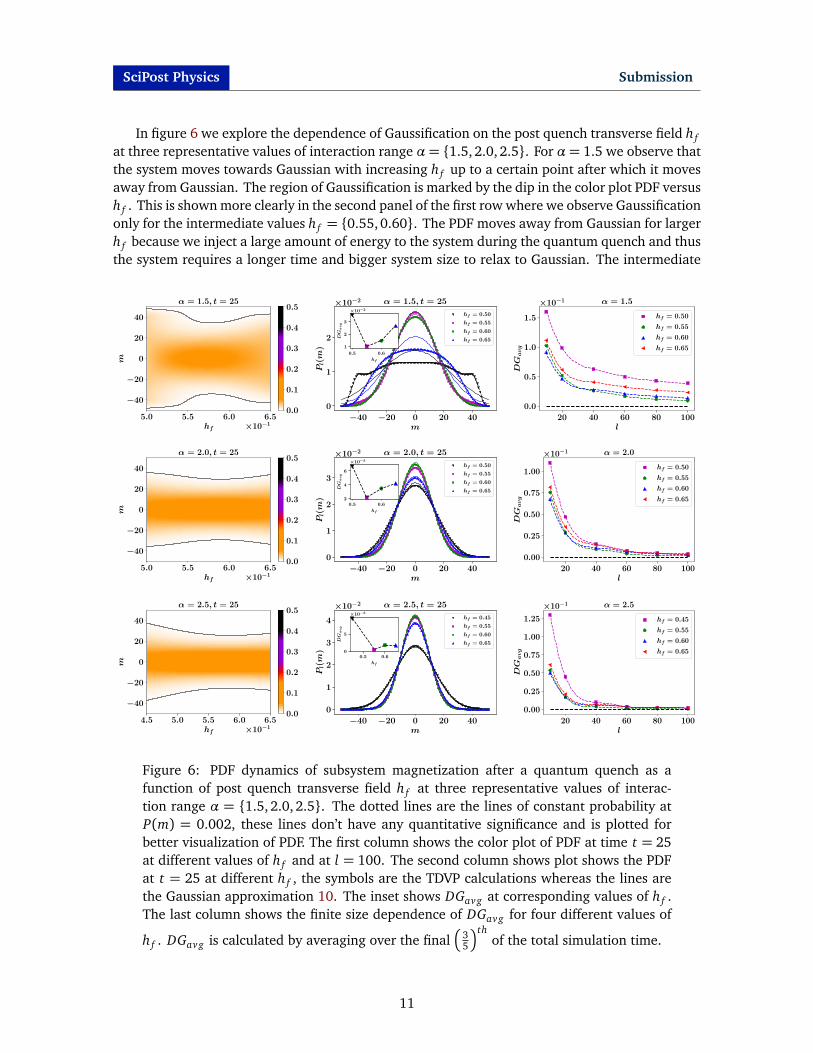
In figure 6 we explore the dependence of Gaussification on the post quench transverse field h fat three representative values of interaction range α= {1.5, 2.0,2.5}. For α= 1.5 we observe thatthe system moves towards Gaussian with increasing h f up to a certain point after which it movesaway from Gaussian. The region of Gaussification is marked by the dip in the color plot PDF versush f . This is shown more clearly in the second panel of the first row where we observe Gaussificationonly for the intermediate values h f = {0.55,0.60}. The PDF moves away from Gaussian for largerh f because we inject a large amount of energy to the system during the quantum quench and thusthe system requires a longer time and bigger system size to relax to Gaussian. The intermediate

Figure 6: PDF dynamics of subsystem magnetization after a quantum quench as afunction of post quench transverse field h f at three representative values of interac-tion range α = {1.5,2.0, 2.5}. The dotted lines are the lines of constant probability atP(m) = 0.002, these lines don’t have any quantitative significance and is plotted forbetter visualization of PDF. The first column shows the color plot of PDF at time t = 25at different values of h f and at l = 100. The second column shows plot shows the PDFat t = 25 at different h f , the symbols are the TDVP calculations whereas the lines arethe Gaussian approximation 10. The inset shows DGavg at corresponding values of h f .The last column shows the finite size dependence of DGavg for four different values of

h f . DGavg is calculated by averaging over the final�

35

�thof the total simulation time.

11

SciPost Physics Submission

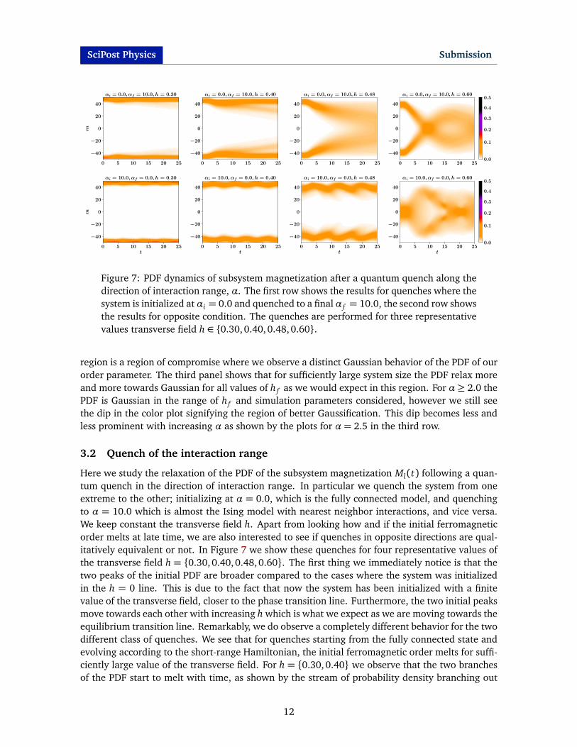
Figure 7: PDF dynamics of subsystem magnetization after a quantum quench along thedirection of interaction range, α. The first row shows the results for quenches where thesystem is initialized at αi = 0.0 and quenched to a final α f = 10.0, the second row showsthe results for opposite condition. The quenches are performed for three representativevalues transverse field h ∈ {0.30,0.40, 0.48,0.60}.

region is a region of compromise where we observe a distinct Gaussian behavior of the PDF of ourorder parameter. The third panel shows that for sufficiently large system size the PDF relax moreand more towards Gaussian for all values of h f as we would expect in this region. For α≥ 2.0 thePDF is Gaussian in the range of h f and simulation parameters considered, however we still seethe dip in the color plot signifying the region of better Gaussification. This dip becomes less andless prominent with increasing α as shown by the plots for α= 2.5 in the third row.

3.2 Quench of the interaction range

Here we study the relaxation of the PDF of the subsystem magnetization Ml(t) following a quan-tum quench in the direction of interaction range. In particular we quench the system from oneextreme to the other; initializing at α = 0.0, which is the fully connected model, and quenchingto α = 10.0 which is almost the Ising model with nearest neighbor interactions, and vice versa.We keep constant the transverse field h. Apart from looking how and if the initial ferromagneticorder melts at late time, we are also interested to see if quenches in opposite directions are qual-itatively equivalent or not. In Figure 7 we show these quenches for four representative values ofthe transverse field h = {0.30, 0.40,0.48, 0.60}. The first thing we immediately notice is that thetwo peaks of the initial PDF are broader compared to the cases where the system was initializedin the h = 0 line. This is due to the fact that now the system has been initialized with a finitevalue of the transverse field, closer to the phase transition line. Furthermore, the two initial peaksmove towards each other with increasing h which is what we expect as we are moving towards theequilibrium transition line. Remarkably, we do observe a completely different behavior for the twodifferent class of quenches. We see that for quenches starting from the fully connected state andevolving according to the short-range Hamiltonian, the initial ferromagnetic order melts for suffi-ciently large value of the transverse field. For h = {0.30,0.40} we observe that the two branchesof the PDF start to melt with time, as shown by the stream of probability density branching out

12

SciPost Physics Submission

from the main PDF peak, although the initial ferromagnetic order effectively remains throughoutthe evolution. For h= 0.48 we observe the complete meltdown of the initial ferromagnetic orderwith some hints of Gaussification at late times. On the other hand, for quenches starting fromthe ground state of the short-range Hamiltonian and evolving according to the fully connectedHamiltonian, we observe strong remnants of the initial ferromagnetic order throughout the evo-lution with no sign of meltdown. We see that although the PDF becomes more oscillatory withincreasing h there is no change in the intensity of the PDF branches. The last column shows theresult for similar quenches but at h = 0.6, these quenches are different from others in the sensethat the point α= 10.0, h= 0.6 lies in the paramagnetic regime of the equilibrium phase diagram.For quench from α = 0.0 to α = 10.0 we observe that the initial ferromagnetic order melts fasterthan before now that the system is quenched to a point in paramagnetic regime in equilibriumphase diagram. The quench in opposite direction is initialized at a paramagnetic point so the PDFbegins as a Gaussian which relaxes quickly. Interestingly, in intermediate times we observe anappearance of double peak PDF signifying long range ferromagnetic order. This long range orderis short lived and melts quickly. However, the fate of the PDF in a long time limit is not very clear.

The two cases of α considered here are two extremes of the long-range Ising model. Whenα= 10.0 the system is close to well known transverse field Ising model. This model does not showany long-range order at finite temperature, thus it is not surprising to observe a melting of theinitial ferromagnetic order after the quench; indeed, the protocol injects a finite amount of energyto the system, simulating a finite temperature environment. So while we quench the system fromone point in ferromagnetic region to another point in ferromagnetic region in an equilibrium phasediagram, the system actually relax to a paramagnetic point in a finite temperature phase diagram.On the other hand, the fully connected Ising model supports long-range ferromagnetic order evenat finite temperature [1, 2, 53] which is presumably the reason why we observe strong remnantsof the initial ferromagnetic order at late time.

4 Conclusion and Outlook

We studied the dynamics of the PDF of the subsystem magnetization in the long-range Ising modelafter a quantum quench. We constrained most of our quenches in the ferromagnetic region of theequilibrium phase diagram as we expect non-trivial dynamics in this region. We studied quenchesalong the transverse field and interaction range. We found that the dynamics of the order param-eter depends very much on the post quench parameters. Based on these observations we showedthat for quenches in the region between the lines α = 2.0 and h f = 0.50, starting from Z2 sym-metric GHZ state, the initial ferromagnetic long-range order persists throughout time evolution.Outside this region we observed that the initial ferromagnetic order eventually melts. In the regionabove h f = 0.50 we observed Gaussification of the order parameter PDF for increasing value ofα. Gaussification of the order parameter PDF in this region is dependent on the size of the subsys-tem (and eventually the size of the system we can simulate) and the total simulation time whichgreatly constrained our numerical work. However, with a finite size analysis for some represen-tative quenches, we can safely claim that for sufficiently large system size and longer simulationtime we do expect Gaussification of the order parameter PDF for all α, provided a sufficiently largevalue of the final transverse field.

For quenches along the interaction range, we found qualitatively different dynamics of theorder parameter PDF, depending on the direction of the quench. While for quenches starting

13

SciPost Physics Submission

form the fully connected state and evolving with short-range Hamiltonians we saw an effectivemelting of the initial ferromagnetic order, we observed a complete persistence of the initial orderfor quenches in the opposite direction.

Attaining Gaussification of subsystem magnetization PDF for quenches from one point in theferromagnetic region of the equilibrium phase diagram to another point within the ferromagneticregion is a non trivial phenomenon, suggesting that the system relaxes to a paramagnetic pointin the dynamical phase diagram. These results open up the possibility to further study the ther-malization dynamics in the long-range Ising model. In fact, the non-equilibrium results could becompared with a finite temperature analysis of the model, by observing if the late-time subsys-tem magnetization after the quench converges to the thermal expectation value correspondingto the effective temperature fixed by the strength of the quench [22]. So far, mainly short rangemodels have been investigated in this perspective [12, 15]; for long-range models a clear path-way is to combine the present analysis with matrix product density operator(MPDO) [54] basedTDVP, modified to generate finite temperature states starting from the infinite temperature densitymatrix [55,56].

A Long range Ising Hamiltonian as an MPO

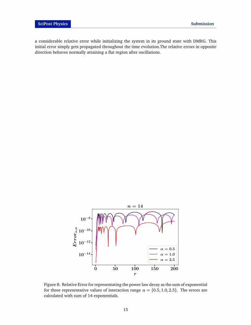
It is straightforward to represent a long range Hamiltonian with exponentially decaying interactionas an MPO [46]. Representing a long range Hamiltonian with power law decay requires firstrepresenting the power law decay as the sum of exponential [57] and then representating theHamiltonian as an MPO [58]. The goodness of this representation depends on how precisely dowe represent the power law decaying function as the sum of exponentials which is quantified bya metric Errorα,n

Errorα,n =

�

�

�

�

�

1rα−

n∑

i=1

x iλri

�

�

�

�

�

(13)

where the number of exponentials in the sum n determines the precision of fitting. We observethat with n= 14 the relative error is 10−7 or smaller [cf. Fig. 8].

B Convergence with bond dimension

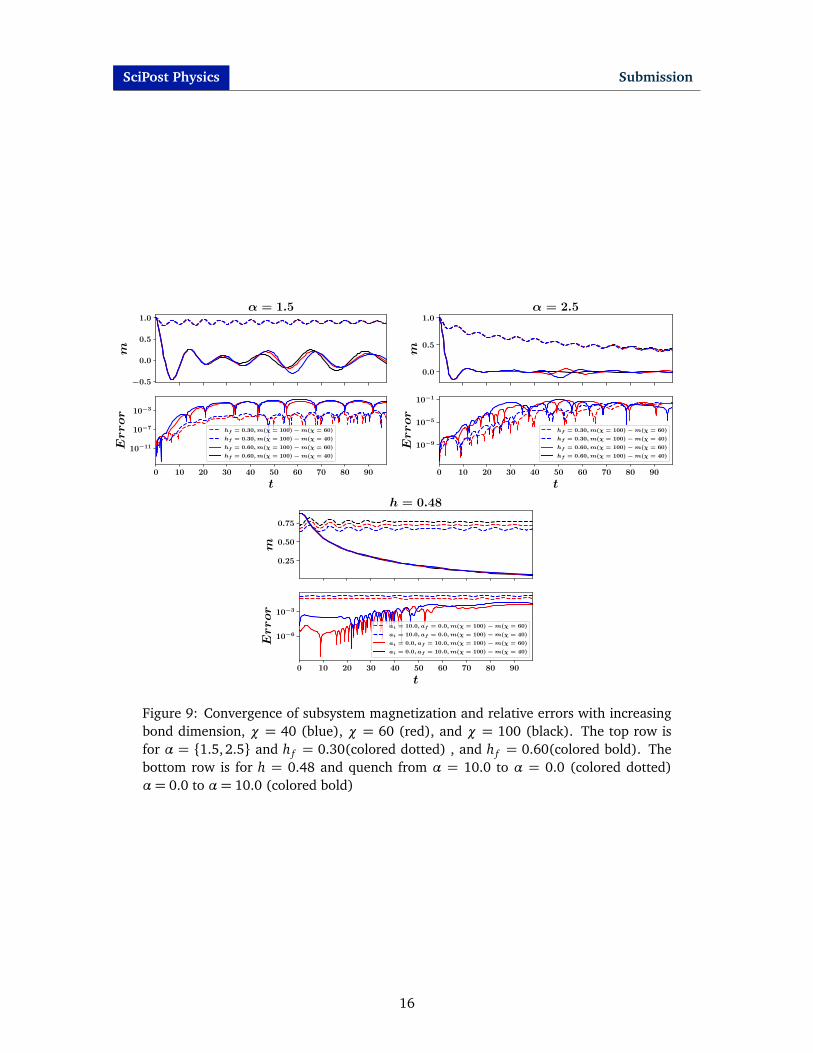
To ensure the data generated by the simulations are correct we need to check the convergenceof the errors with increasing bond dimension. In TDVP the bond dimension is responsible forprojection error [59], which is a primary source of error. To check that the errors converge withincreasing bond dimension we compare the time evolution of subsystem magnetization and rel-ative errors for some representative cases of quantum quenches for χ = {40,60, 100} in figure9. Quenches along the transverse field show similar behavior, the relative error converges andbecomes flat in a long time limit for all values of post quench parameter. Furthermore, for timesup to 25, which is the maximum time reached for most of the results in the main text, the relativeerrors are smaller than 10−3. Relative errors behave strangely for the quenches in the direction ofinteraction range. The relative errors for quench from α = 10.0 to α = 0.0 remains flat throughthe time evolution, maintaining a constant shift from one other. This is because the point α= 10.0and h = 0.48 is very close to the critical line of the equilibrium phase diagram and we generate

14

SciPost Physics Submission

a considerable relative error while initializing the system in its ground state with DMRG. Thisinitial error simply gets propagated throughout the time evolution.The relative errors in oppositedirection behaves normally attaining a flat region after oscillations.

0 50 100 150 200r

10−14

10−12

10−10

10−8

Errorα,n

n = 14

α = 0.5

α = 1.0

α = 2.5

Figure 8: Relative Error for representating the power law decay as the sum of exponentialfor three representative values of interaction range α = {0.5, 1.0,2.5}. The errors arecalculated with sum of 14 exponentials.

15

SciPost Physics Submission

Figure 9: Convergence of subsystem magnetization and relative errors with increasingbond dimension, χ = 40 (blue), χ = 60 (red), and χ = 100 (black). The top row isfor α = {1.5,2.5} and h f = 0.30(colored dotted) , and h f = 0.60(colored bold). Thebottom row is for h = 0.48 and quench from α = 10.0 to α = 0.0 (colored dotted)α= 0.0 to α= 10.0 (colored bold)

16

SciPost Physics Submission

References

[1] F. J. Dyson, Existence of a phase-transition in a one-dimensional ising ferromagnet, Communi-cations in Mathematical Physics 12, 91 (1969), doi:https://doi.org/10.1007/BF01645907.

[2] A. Dutta and J. K. Bhattacharjee, Phase transitions in the quantum ising androtor models with a long-range interaction, Phys. Rev. B 64, 184106 (2001),doi:10.1103/PhysRevB.64.184106.

[3] M. Knap, A. Kantian, T. Giamarchi, I. Bloch, M. D. Lukin and E. Demler, Probing real-spaceand time-resolved correlation functions with many-body ramsey interferometry, Phys. Rev. Lett.111, 147205 (2013), doi:10.1103/PhysRevLett.111.147205.

[4] J. Bohnet, B. Sawyer, J. Britton, M. Wall, A. Rey, M. Foss-Feig and J. Bollinger, Quantumspin dynamics and entanglement generation with hundreds of trapped ions, Science 352, 1297(2016), doi:10.1126/science.aad9958.

[5] F. Meinert, M. J. Mark, E. Kirilov, K. Lauber, P. Weinmann, A. J. Daley and H.-C. Nägerl,Quantum quench in an atomic one-dimensional ising chain, Phys. Rev. Lett. 111, 053003(2013), doi:10.1103/PhysRevLett.111.053003.

[6] C. Gross and I. Bloch, Quantum simulations with ultracold atoms in optical lattices, Science357, 995 (2017), doi:10.1126/science.aal3837.

[7] T. Langen, R. Geiger and J. Schmiedmayer, Ultracold atoms out of equilibrium, Annual Reviewof Condensed Matter Physics 6(1), 201 (2015), doi:10.1146/annurev-conmatphys-031214-014548.

[8] T. Kinoshita, T. Wenger and D. Weiss, A quantum newton’s cradle, Nature 440, 900 (206),doi:https://doi.org/10.1038/nature04693.

[9] Y. Tang, W. Kao, K.-Y. Li, S. Seo, K. Mallayya, M. Rigol, S. Gopalakrishnan and B. L. Lev,Thermalization near integrability in a dipolar quantum newton’s cradle, Phys. Rev. X 8, 021030(2018), doi:10.1103/PhysRevX.8.021030.

[10] R. Islam, E. Edwards, K. Kim, S. Korenblit, C. Noh, H. Carmichael, G.-D. Lin, L.-M.Duan, C.-C. Joseph Wang, J. Freericks and C. Monroe, Onset of a quantum phasetransition with a trapped ion quantum simulator, Nature Communications 2 (2011),doi:https://doi.org/10.1038/ncomms1374.

[11] S. Groha, F. H. L. Essler and P. Calabrese, Full counting statistics in the transverse field isingchain, SciPost Phys. 4, 43 (2018), doi:10.21468/SciPostPhys.4.6.043.

[12] M. Collura and F. H. L. Essler, How order melts after quantum quenches, Phys. Rev. B 101,041110 (2020), doi:10.1103/PhysRevB.101.041110.

[13] M. Collura, Relaxation of the order-parameter statistics in the ising quantum chain, SciPostPhys. 7, 72 (2019), doi:10.21468/SciPostPhys.7.6.072.

[14] M. Collura, F. H. L. Essler and S. Groha, Full counting statistics in the spin-1/2 heisenbergXXZ chain, Journal of Physics A: Mathematical and Theoretical 50(41), 414002 (2017),doi:10.1088/1751-8121/aa87dd.

17

SciPost Physics Submission

[15] R. J. V. Tortora, P. Calabrese and M. Collura, Relaxation of the order-parameter statis-tics and dynamical confinement, EPL (Europhysics Letters) 132(5), 50001 (2020),doi:http://dx.doi.org/10.1209/0295-5075/132/50001.

[16] R. W. Cherng and E. Demler, Quantum noise analysis of spin systems realized with cold atoms,New Journal of Physics 9(1), 7 (2007), doi:10.1088/1367-2630/9/1/007.

[17] A. Lamacraft and P. Fendley, Order parameter statistics in the critical quantum ising chain,Phys. Rev. Lett. 100, 165706 (2008), doi:10.1103/PhysRevLett.100.165706.

[18] D. A. Ivanov and A. G. Abanov, Characterizing correlations with full counting statis-tics: Classical ising and quantum x y spin chains, Phys. Rev. E 87, 022114 (2013),doi:10.1103/PhysRevE.87.022114.

[19] J.-M. Stéphan and F. Pollmann, Full counting statistics in the haldane-shastry chain, Phys.Rev. B 95, 035119 (2017), doi:10.1103/PhysRevB.95.035119.

[20] P. Calabrese and J. Cardy, Quantum quenches in extended systems, Journal of Statisti-cal Mechanics: Theory and Experiment 2007(06), P06008 (2007), doi:10.1088/1742-5468/2007/06/P06008.

[21] Z. Zhu, G. Sun, W.-L. You and D.-N. Shi, Fidelity and criticality of a quantum ising chain withlong-range interactions, Phys. Rev. A 98, 023607 (2018), doi:10.1103/PhysRevA.98.023607.

[22] F. H. L. Essler and M. Fagotti, Quench dynamics and relaxation in isolated integrable quantumspin chains, Journal of Statistical Mechanics: Theory and Experiment 2016(6), 064002(2016), doi:10.1088/1742-5468/2016/06/064002.

[23] D. Porras and J. I. Cirac, Effective quantum spin systems with trapped ions, Phys. Rev. Lett.92, 207901 (2004), doi:10.1103/PhysRevLett.92.207901.

[24] X.-L. Deng, D. Porras and J. I. Cirac, Effective spin quantum phases in systems of trapped ions,Phys. Rev. A 72, 063407 (2005), doi:10.1103/PhysRevA.72.063407.

[25] E. Lieb, T. Schultz and D. Mattis, Two soluble models of an antiferromagnetic chain, Annalsof Physics 16(3), 407 (1961), doi:https://doi.org/10.1016/0003-4916(61)90115-4.

[26] H. Lipkin, N. Meshkov and A. Glick, Validity of many-body approximation methods for asolvable model: (i). exact solutions and perturbation theory, Nuclear Physics 62(2), 188(1965), doi:https://doi.org/10.1016/0029-5582(65)90862-X.

[27] N. Meshkov, A. Glick and H. Lipkin, Validity of many-body approximation methods fora solvable model: (ii). linearization procedures, Nuclear Physics 62(2), 199 (1965),doi:https://doi.org/10.1016/0029-5582(65)90864-3.

[28] A. Glick, H. Lipkin and N. Meshkov, Validity of many-body approximation methodsfor a solvable model: (iii). diagram summations, Nuclear Physics 62(2), 211 (1965),doi:https://doi.org/10.1016/0029-5582(65)90864-3.

[29] P. Hauke and L. Tagliacozzo, Spread of correlations in long-range interacting quantum systems,Phys. Rev. Lett. 111, 207202 (2013), doi:10.1103/PhysRevLett.111.207202.

18

SciPost Physics Submission

[30] M. Foss-Feig, Z.-X. Gong, C. W. Clark and A. V. Gorshkov, Nearly linear light conesin long-range interacting quantum systems, Phys. Rev. Lett. 114, 157201 (2015),doi:10.1103/PhysRevLett.114.157201.

[31] A. S. Buyskikh, M. Fagotti, J. Schachenmayer, F. Essler and A. J. Daley, Entanglement growthand correlation spreading with variable-range interactions in spin and fermionic tunneling mod-els, Phys. Rev. A 93, 053620 (2016), doi:10.1103/PhysRevA.93.053620.

[32] B. Žunkovic, M. Heyl, M. Knap and A. Silva, Dynamical quantum phase transitions in spinchains with long-range interactions: Merging different concepts of nonequilibrium criticality,Phys. Rev. Lett. 120, 130601 (2018), doi:10.1103/PhysRevLett.120.130601.

[33] G. Piccitto, B. Žunkovic and A. Silva, Dynamical phase diagram of a quan-tum ising chain with long-range interactions, Phys. Rev. B 100, 180402 (2019),doi:10.1103/PhysRevB.100.180402.

[34] J. C. Halimeh, V. Zauner-Stauber, I. P. McCulloch, I. de Vega, U. Schollwöck and M. Kastner,Prethermalization and persistent order in the absence of a thermal phase transition, Phys. Rev.B 95, 024302 (2017), doi:10.1103/PhysRevB.95.024302.

[35] J. C. Halimeh and V. Zauner-Stauber, Dynamical phase diagram of quantum spin chains withlong-range interactions, Phys. Rev. B 96, 134427 (2017), doi:10.1103/PhysRevB.96.134427.

[36] A. Lerose, B. Žunkovic, A. Silva and A. Gambassi, Quasilocalized excitations induced by long-range interactions in translationally invariant quantum spin chains, Phys. Rev. B 99, 121112(2019), doi:10.1103/PhysRevB.99.121112.

[37] D. V. Else, B. Bauer and C. Nayak, Prethermal phases of matter protected by time-translationsymmetry, Phys. Rev. X 7, 011026 (2017), doi:10.1103/PhysRevX.7.011026.

[38] A. Kyprianidis, F. Machado, W. Morong, P. Becker, K. Collins, D. ELSE, L. Feng, P. Hess,C. Nayak, G. Pagano, N. Yao and C. Monroe, Observation of a prethermal discrete time crystal,Science 372, 1192 (2021), doi:10.1126/science.abg8102.

[39] K. Giergiel, T. Tran, A. Zaheer, A. Singh, A. Sidorov, K. Sacha and P. Hannaford, Creat-ing big time crystals with ultracold atoms, New Journal of Physics 22(8), 085004 (2020),doi:10.1088/1367-2630/aba3e6.

[40] J. Zhang, G. Pagano, P. W. Hess, A. Kyprianidis, P. Becker, H. Kaplan, A. V. Gorshkov, Z.-X.Gong and C. Monroe, Observation of a many-body dynamical phase transition with a 53-qubitquantum simulator, Nature 551, 601 (2017), doi:https://doi.org/10.1038/nature24654.

[41] P. Jurcevic, H. Shen, P. Hauke, C. Maier, T. Brydges, C. Hempel, B. P. Lanyon,M. Heyl, R. Blatt and C. F. Roos, Direct observation of dynamical quantum phasetransitions in an interacting many-body system, Phys. Rev. Lett. 119, 080501 (2017),doi:10.1103/PhysRevLett.119.080501.

[42] P. Jurcevic, B. P. Lanyon, P. Hauke, C. Hempel, P. Zoller, R. Blatt and C. F. Roos, Quasiparticleengineering and entanglement propagation in a quantum many-body system, Nature 511, 202(2014), doi:https://doi.org/10.1038/nature13461.

19

SciPost Physics Submission

[43] P. Richerme, Z.-X. Gong, A. Lee, C. Senko, J. Smith, M. Foss-Feig, S. Michalakis, A. V. Gorshkovand C. Monroe, Non-local propagation of correlations in quantum systems with long-rangeinteractions, Nature 511, 198 (2014), doi:https://doi.org/10.1038/nature13450.

[44] S. R. White, Density matrix formulation for quantum renormalization groups, Phys. Rev. Lett.69, 2863 (1992), doi:10.1103/PhysRevLett.69.2863.

[45] S. R. White, Density-matrix algorithms for quantum renormalization groups, Phys. Rev. B 48,10345 (1993), doi:10.1103/PhysRevB.48.10345.

[46] U. Schollwöck, The density-matrix renormalization group in the age of matrix product states,Annals of Physics 326(1), 96 (2011), doi:10.1016/j.aop.2010.09.012, January 2011 SpecialIssue.

[47] J. Haegeman, J. I. Cirac, T. J. Osborne, I. Pižorn, H. Verschelde and F. Verstraete, Time-dependent variational principle for quantum lattices, Phys. Rev. Lett. 107, 070601 (2011),doi:10.1103/PhysRevLett.107.070601.

[48] J. Haegeman, C. Lubich, I. Oseledets, B. Vandereycken and F. Verstraete, Unifying timeevolution and optimization with matrix product states, Phys. Rev. B 94, 165116 (2016),doi:10.1103/PhysRevB.94.165116.

[49] C. Lanczos, An iteration method for the solution of the eigenvalue i problem. of linear differentialand integral operators, Journal of Research of the National Bureau of Standards 45, 255(1950), doi:10.6028/jres.045.026.

[50] H. D. Simon, Analysis of the symmetric lanczos algorithm with reorthogonalization methods,Linear Algebra and its Applications 61, 101 (1984), doi:https://doi.org/10.1016/0024-3795(84)90025-9.

[51] D. M. Greenberger, M. A. Horne and A. Zeilinger, Going Beyond Bell’s Theorem, pp. 69–72,Springer Netherlands, Dordrecht, doi:10.1007/978-94-017-0849-4 (1989).

[52] D. Bouwmeester, J.-W. Pan, M. Daniell, H. Weinfurter and A. Zeilinger, Observation ofthree-photon greenberger-horne-zeilinger entanglement, Phys. Rev. Lett. 82, 1345 (1999),doi:10.1103/PhysRevLett.82.1345.

[53] E. Gonzalez-Lazo, M. Heyl, M. Dalmonte and A. Angelone, Finite-temperature crit-ical behavior of long-range quantum Ising models, SciPost Phys. 11, 76 (2021),doi:10.21468/SciPostPhys.11.4.076.

[54] F. Verstraete, J. J. García-Ripoll and J. I. Cirac, Matrix product density operators: Simu-lation of finite-temperature and dissipative systems, Phys. Rev. Lett. 93, 207204 (2004),doi:10.1103/PhysRevLett.93.207204.

[55] A. H. Werner, D. Jaschke, P. Silvi, M. Kliesch, T. Calarco, J. Eisert and S. Montangero, Positivetensor network approach for simulating open quantum many-body systems, Phys. Rev. Lett.116, 237201 (2016), doi:10.1103/PhysRevLett.116.237201.

[56] D. Jaschke, S. Montangero and L. D. Carr, One-dimensional many-body entangled open quan-tum systems with tensor network methods, Quantum Science and Technology 4(1), 013001(2018), doi:10.1088/2058-9565/aae724.

20

SciPost Physics Submission

[57] B. Pirvu, V. Murg, J. Cirac and F. Verstraete, Matrix product operator representations, NewJournal of Physics 12(2), 025012 (2010), doi:10.1088/1367-2630/12/2/025012.

[58] G. M. Crosswhite, A. C. Doherty and G. Vidal, Applying matrix product opera-tors to model systems with long-range interactions, Phys. Rev. B 78, 035116 (2008),doi:10.1103/PhysRevB.78.035116.

[59] S. Paeckel, T. Köhler, A. Swoboda, S. R. Manmana, U. Schollwöck and C. Hubig, Time-evolution methods for matrix-product states, Annals of Physics 411, 167998 (2019),doi:10.1016/j.aop.2019.167998.

21