Dynamics of Wall-Bounded Turbulence - UPM

6

Dynamics of Wall-Bounded TurbulenceJavier Jimenez and Genta Kawahara

6.1 Introduction

This chapter deals with the dynamics of wall-bounded turbulent flows, with

a decided emphasis on the results of numerical simulations. As we will see,

part of the reason for that emphasis is that much of the recent work on

dynamics has been computational, but also that the companion chapter by

Marusic and Adrian (2012) in this volume reviews the results of experiments

over the same period.

The first direct numerical simulations (DNS) of wall-bounded turbulence

(Kim et al., 1987) began to appear soon after computers became powerful

enough to allow the simulation of turbulence in general (Siggia, 1981; Ro-

gallo, 1981). Large-eddy simulations (LES) of wall-bounded flows had been

published before (Deardorff, 1970; Moin and Kim, 1982) but, after DNS

became current, they were de-emphasized as means of clarifying the flow

physics, in part because doubts emerged about the effect of the poorly re-

solved near-wall region on the rest of the flow. Some of the work summarized

below has eased those misgivings, and there are probably few reasons to dis-

trust the information provided by LES on the largest flow structures, but

any review of the physical results of numerics in the recent past necessarily

has to deal mostly with DNS. Only atmospheric scientists, for whom the

prospect of direct simulation remains remote, have continued to use LES

to study the mechanics of the atmospheric surface layer (see, for example,

Deardorff, 1973; Siebesma et al., 2003). A summary of the early years of

numerical turbulence research can be found in Rogallo and Moin (1984) and

Moin and Mahesh (1998). Here, we review the advances that have taken

place in its application to wall-bounded flows since the first of those two

papers, and, in particular, what we have learned during that time about

221

jimenez

Typewritten Text

In "Ten Chapters in Turbulence" (P.A. Davidson, Y. Kaneda & K. R. Sreenivasan, eds) Cambridge U. Press (2013) pp. 221-268

jimenez

Typewritten Text

jimenez

Typewritten Text

jimenez

Typewritten Text

jimenez

Typewritten Text

jimenez

Typewritten Text

jimenez

Typewritten Text

jimenez

Typewritten Text

222 Jimenez & Kawahara

the physics of the flow. The interactions with experimental results will be

discussed where appropriate.

First of all, it is important to emphasize that numerical simulations and

experiments are different, although related, approximations to reality, and

that they should not be expected to agree exactly with each other. For

example, computing a channel in a doubly periodic domain is an approx-

imation, in the same way as an experimental channel with a finite aspect

ratio. In both cases, the parameters have to be chosen so that the resulting

system approaches ‘closely enough’ the ideal channel of real interest, which

is infinitely long and wide. Simulations only need to reproduce experiments,

and vice versa, in the sense that they are both intended to approximate the

same real object, and neither of the two is automatically to be preferred to

the other.

Luckily, the strengths and weaknesses of the two techniques tend to be

complementary. Simulations give precise answers to precisely posed and con-

trolled problems, with precisely known initial and boundary conditions. No

simulation can be run without fully stipulating all those factors, and the only

limitation to our knowledge in that respect is how many data we choose to

store. The situation is typically different in experiments, for which there are

often unknown factors that are difficult to document, such as inflow condi-

tions and wind tunnel imperfections. Those imperfections are different from

the ones in numerics, but they are in no sense more ‘natural’. For exam-

ple, it is tempting to consider that the random perturbations in the free

stream of a wind tunnel are a ‘more natural’ trigger for transition than the

deterministic perturbations typically introduced in simulations, but there is

nothing random about the natural world, and the perturbations present in

different experiments are as different from each other, and as different from

the ones presumably present in our intended applications, as any determin-

istic perturbation imposed in a simulation. In most cases, randomness is not

a virtue, but a measure of our ignorance.

Another difference that is often mentioned is that experiments are imper-

fect measurements of a ‘true’ system, while simulations are perfect measure-

ments of something that is at best only an approximation. Both things are

true, but only in the weak sense that it is not completely clear whether the

Navier–Stokes equations represent fluid flow, or whether they have continu-

ous unique solutions. The first concern is probably not worse than worrying

about whether the air in a wind tunnel is a perfect gas, but the second is

slightly more substantive. Numerical methods typically assume some conti-

nuity in the solutions that they represent, in which case their error bounds

are extremely well understood and kept under tight control in most simu-

6: Dynamics of Wall-Bounded Turbulence 223

lations. The error associated with the numerical approximation is usually

negligible compared with the statistical uncertainty. On the other hand,

most simulation codes are designed to be ‘robust’, and to behave gracefully

when an unexpected discontinuity is found. For that reason, they would

probably miss a hypothetical isolated finite-time singularity weak enough to

have only a local effect. Note that if those singular, or perhaps exceptionally

sharp, events were anything but rare, they would be caught and avoided by

most numerical techniques, and that identifying rare events experimentally

is also hard; but it is probably true that experiments have a better chance

of doing so than simulations.

Another important difference between simulations and experiments is that

the latter are typically cheaper to run, at least once the initial investment

is discounted, and that it is easier to rerun an experiment than to repeat a

large DNS. As a consequence, experiments can scan a wider class of flows for

a given effort, and they remain the method of choice when the behaviour of

some simple quantity is required over a wide range of parameters. They are

also able to collect more cheaply long statistical series, although, for reasons

unclear to the present authors, it is often true that experimental data are

noisier than numerical ones.

A characteristic of simulations is that everything is measured, and that

everything can be stored and reprocessed in the future. Recent experimental

techniques, such as PIV, approach the full-field capability of simulations

(see the chapter by Marusic and Adrian in this volume), but the ability of

DNS to create time-resolved three-dimensional fields of the three velocity

components, gradients, and pressure, is still unmatched. That is an obvious

advantage of simulations, but it is also responsible for their higher cost. It

is no cheaper to compute the mean velocity profile of a boundary layer than

to compute the whole flow field, but it is infinitely cheaper experimentally.

That is one of the reasons why experiments, at least apparently, cover a wider

range of Reynolds numbers than simulations. It is relatively easy to create

a high-Reynolds-number flow in the laboratory, even if it is hard to measure

it in detail beyond low order magnitudes such as the mean velocity, or some

fluctuation intensities. Simulations, on the other hand, need to compute

everything to estimate even those quantities, and the cost of increasing the

Reynolds number has to be paid ‘in full’.

Even so, the Reynolds numbers of simulations have increased steadily in

the past quarter century, and it is important to realize that this process is not

open-ended. The goal of turbulence theory, and of the supporting simulations

and experiments, should not be to reach ever increasing Reynolds numbers,

but to describe turbulence well enough to be able to make useful predictions


under any circumstance. It has been understood since Kolmogorov (1941)

that the key complication of turbulence is its multiscale character, and it is

probably true that, if we could compile a detailed data base of the space-

time evolution of enough flows with a reasonably wide range of scales, such

a data base would contain all the information required to formulate a theory

of turbulence. Of course, such a data set would not be a theory, but it is

doubtful whether further increasing the Reynolds number of the simulations,

or of the experiments, would provide much additional help in formulating

one (Jimenez, 2012).

It is difficult to say a-priori when that stage will be reached, but a rough es-

timation is possible. The large, energy-containing, structures of wall-bounded

flows are of the order of the boundary layer thickness δ (which we will also

use for the channel half-width or for the pipe radius), and the smallest near-

wall viscous structures have sizes of the order of 100ν/uτ , where ν is the

fluid viscosity, and uτ = τ1/2w is the friction velocity, defined in term of the

wall shear stress τw. Variables scaled with uτ and ν are said to be in wall

units, and will be denoted by a ‘+’ superscript. Note that, since we restrict

ourselves in this chapter to incompressible flows, we will always assume the

fluid density to be ρ = 1, and drop it from our equations. Capitals are

used for instantaneous values, lower-case symbols for fluctuations with re-

spect to the mean, and primes for the root-mean-squared intensities of those

fluctuations. The average ⟨·⟩ is conceptually defined over many equivalent

independent experiments, unless otherwise noted. We denote by x, y and z

the streamwise, wall-normal and spanwise coordinates, respectively, and the

corresponding velocity components by U , V and W . With this notation, the

ratio between the largest and smallest scales in the flow is δ+/100, where

δ+ = uτδ/ν is the friction Reynolds number.

The channel simulations of Kim et al. (1987) had δ+ = 180, and therefore

had essentially no scale range, but the more recent numerical channels by del

Alamo et al. (2004), Abe et al. (2004) or Hoyas and Jimenez (2006), and the

boundary layers by Lee and Sung (2007, 2011), Simens et al. (2009), Wu and

Moin (2010), Schlatter et al. (2009); Schlatter and Orlu (2010), and Sillero

et al. (2010), with δ+ ≈ 1000− 2000, are comparable to most well-resolved

experiments, and have a full decade of scale disparity. It will be shown in

§6.4 that those simulations are already providing a lot of information on the

multiscale dynamics of wall-bounded flows. Moreover, because the Reynolds

numbers of simulations and experiments are beginning to be comparable,

it is now possible to validate, for example, the structural models derived


from experimental observations (e.g. Adrian, 2007) with the time-resolved

three-dimensional flow fields of simulations, and vice versa.

It is probably true that a further factor of 5–10 in δ+, which would give

us a range of scales close to 100, would provide us with all the information

required to understand many of the dynamical aspects of wall-bounded tur-

bulence. Using the usual estimate of δ+3for the cost of simulations, and

the present rate of increase in computer speed of 103 per decade, it should

be possible to compile such a data base within the next decade (Jimenez,

2003).

This brings us to discuss the question of structure versus statistics, which

has been a recurrent theme in turbulence theory from its beginning. Thus,

while Richardson (1920) framed the multiscale nature of turbulence in terms

of ‘little and big whorls’, the older decomposition paper of Reynolds (1894)

had centred solely on the statistics of the fluctuations, and proved to be

more fruitful for the practical problem of turbulence modelling. Even the

classical paper of Kolmogorov (1941), which is usually credited with intro-

ducing the concept of a turbulent cascade, is a statistical description of the

fluctuation intensity versus scale, and it was only the slightly less famous

companion paper by Obukhov (1941) that put the cascade concept in terms

of interactions among eddies. It can be argued that it was not until the vi-

sualizations of large coherent structures in free-shear layers by Brown and

Roshko (1974), and of sublayer streaks in boundary layers by Kline et al.

(1967), that the structural view of turbulence gained modern, although still

far from universal, acceptance.

This is not the place to discuss the relative merits of the two points of

view, which, in any case, should be judged in relation to each particular

application, but simulations have come down decisively on the side of struc-

ture. This is in part because, as we have seen, simulations are an expensive

way of compiling statistics, in the same way that experiments are not very

good at extracting structure, but it also points to one of the characteristic

advantages of numerics, which is their ability to simulate unphysical systems.

Structural models often take a deterministic view of the flow, and deal

with how its different parts interact with each other. Some of the most pow-

erful tools for analysing interactions in physics have long been conceptual

experiments, which often involve systems that cannot be physically realized,

such as, for example, point masses. In simple dynamical situations, the out-

come of such experiments can often be guessed correctly, and used to judge

the soundness of a particular model, but in complex phenomena, such as tur-

bulence, the guessing almost always has to be substituted by the numerical

simulation of the modified system. We will see in §6.3 examples of how the


dynamics of near-wall turbulence was clarified in part through experiments

of this kind, in which some of the inherent limitations of numerics, such as

spatial periodicity, were put to good use in isolating what was essential, and

what accidental. Similar techniques have been used for isotropic turbulent

flows, which are outside the scope of the present article, but some examples

can be found in Kida (1985) or She (1993).

It should be noted that conceptual experiments are not completely beyond

the reach of the laboratory. For example, rough walls can be used as con-

ceptual tests for the importance of near-wall processes in wall turbulence,

since roughness destroys the detailed interactions that dominate the flow

over smooth walls (Flores and Jimenez, 2006). In the same way, the use by

Bradshaw (1967) of adverse pressure gradients to explore the importance

of ‘inactive’ modes in boundary layers, remains one of the most beautiful

examples of the experimental use of those techniques. However, the freedom

afforded by numerical simulations to create artificial systems is difficult to

match experimentally.

There are finally two approaches to the study of turbulence in which simu-

lation techniques are predominant. The first one is the study of equilibrium,

or otherwise simple, solutions of the Navier–Stokes equations that may be

important in turbulent flows. It is generally understood that turbulence is

chaotic, and it would be a surprise if a steady structure, or even a steady

wave, were to be found in a natural turbulent flow. But it is also a common

experience that such flows contain ‘coherent’ structures with long lifetimes.

Examples range from the already cited large-scale coherent eddies of jets

and shear layers, or from the sublayer streaks in wall-bounded turbulence,

to the small-scale long-lived vortices in the dissipative range of many turbu-

lent flows (Vincent and Meneguzzi, 1991; Jimenez et al., 1993). Not only are

those structures believed to contribute substantially to the overall statistical

properties of their respective flows but, once they are properly understood,

they point to efficient control strategies (Ho and Huerre, 1984).

The prevalence of such structures raises the question of whether they can

be identified with underlying solutions of the equations of motion, which

are almost certain to be unstable, and therefore experimentally unobserv-

able, but which can be extracted numerically as properties of the averaged

velocity profile of the flow under study. For wall-bounded turbulence, the

first solutions of this kind were obtained by Nagata (1990), and many more

have been found since then. They are not only conceptually important, but

their signature can be identified in full-scale turbulence (Jimenez et al.,

2005). Moreover, not only the equilibrium structures, but their connections

in phase space have been examined more recently, and appear to be related


to the temporal modulation of the near-wall velocity fluctuations (Halcrow

et al., 2009). This approach is reviewed in §6.5.The last interesting result of numerical experiments is the study of the

possible relation between linear dynamics and the large-scale structures of

turbulent flows. Turbulence is nonlinear, but a consideration of the time

scales of the different processes shows that the dominant effect in the creation

of the largest scales of shear flows is the energy transfer from the mean shear

to the fluctuations, which is a linear process. It was understood from the

beginning that the coherent eddies of free-shear layers were reflections of

the Kelvin-Helmholtz instability of the mean velocity profile (Brown and

Roshko, 1974; Gaster et al., 1985), but it was thought for a long time that

wall-bounded flows, whose mean velocity profiles are linearly stable, could

not be explained in the same way. That changed when it was realized in

the early 1990’s that even stable linear perturbations can grow substantially

by extracting energy from the mean flow, and that it is possible to relate

such ‘transient’ growth to the observed coherent structures in wall-bounded

turbulence (Butler and Farrell, 1993; del Alamo and Jimenez, 2006). Space

considerations prevent us from discussing that question here in detail, but

occasional references to it will be made where appropriate.

6.2 The classical theory of wall-bounded turbulence

Wall-bounded turbulence includes pipes, channels and boundary layers. We

will restrict ourselves to cases with little or no longitudinal pressure gradi-

ents, since otherwise the flow tends to relaminarize or to separate. In the

first case it stops being turbulent, and in the second one it loses many of its

wall-bounded characteristics, and tends to resemble free-shear flows. Wall-

bounded turbulence is of huge technological importance. About half of the

energy spent worldwide in moving fluids along pipes and canals, or vehicles

through air or water, is dissipated by turbulence in the immediate vicinity

of walls. Turbulence was first studied scientifically in attached wall-bounded

flows (Hagen, 1839; Darcy, 1854), but those flows have remained to this day

worse understood than their homogeneous or free-shear counterparts. That

is in part because what is sought in both cases is different. In the classi-

cal conceptual model for isotropic turbulence, energy resides in the largest

eddies, and cannot be dissipated until it is transferred by a self-similar cas-

cade of ‘inertial’ eddies to the smaller scales of the order of the Kolmogorov

viscous length η, where viscosity can act (Richardson, 1920; Kolmogorov,

1941). The resulting energy spectrum, although now recognized as only an

approximation, describes well the experimental observations, not only for


101

103

105

λ/η

kE(k

)Energy

Dissipation

(a)

y+

λx+ 10

210

310

4

102

103

(b)

Figure 6.1 Spectral energy density, kE(k). (a) In isotropic turbulence, as a function

of the isotropic wavelength λ = 2π/k. (b) In a numerical turbulent channel with half-

width δ+ = 2003 (Hoyas and Jimenez, 2006), plotted as a function of the streamwise

wavelength λx, and of the wall distance y. The shaded contours are the density of the

kinetic energy of the velocity fluctuations, kxEuu(kx). The lines are the spectral density

of the surrogate dissipation, νkxEωω(kx), where ω are the vorticity fluctuations. At each

y the lowest contour is 0.86 times the local maximum. The horizontal lines are y+ = 80

and y/δ = 0.2, and represent conventional limits for the logarithmic layer. The diagonal

through the energy spectrum is λx = 5y; the one through the dissipation spectrum is

40η. The arrows indicate the implied cascades.

isotropic turbulence, but also for small-scale turbulence in general. A sketch

can be found in Figure 6.1(a).

However, isotropic theory gives no indication of how energy is fed into the

turbulent cascade. In shear flows, the energy source is the gradient of the

mean velocity, and the mechanism is the interaction between that gradient

and the average momentum fluxes carried by the velocity fluctuations (Ten-

nekes and Lumley, 1972). We have already mentioned that, in free-shear

flows such as jets or mixing layers, this leads to large-scale instabilities of

the mean velocity profile (Brown and Roshko, 1974), with sizes of the or-

der of the flow thickness. The resulting ‘integral’ eddies contain most of the

energy, and the subsequent transfer to the smaller scales is thought to be

essentially similar to the isotropic case.

In contrast, wall-bounded flows force us to face squarely the role of in-

homogeneity. That can be seen in Figure 6.1(b), in which each horizontal

section is the equivalent to the spectra in Figure 6.1(a) for a given wall

distance. The energy is again at large scales, while the dissipative eddies

are smaller, but the sizes of the energy-containing eddies change with the

distance to the wall, and so does the range of scales over which the en-

ergy has to cascade. It turns out that, except very near or very far from

the wall, where there are small imbalances between the production and the


dissipation of turbulent kinetic energy, most of the energy generated at a

given distance from the wall is dissipated locally (Hoyas and Jimenez, 2008),

but the eddy sizes containing most of the energy at one wall distance are

in the midst of the inertial cascade when they are observed farther away.

The Reynolds number, defined as the scale disparity between energy and

dissipation at some given location, also changes with wall distance, and the

main emphasis in wall turbulence is not on the local inertial energy cascade,

but on the interplay between different scales at different distances from the

wall.

Models for wall-bounded turbulence also have to deal with spatial fluxes

that are absent from the homogeneous case. The most important one is that

of momentum. Consider a turbulent channel, driven by a pressure gradi-

ent between infinite parallel planes, and decompose the flow quantities into

mean values and fluctuations with respect to those means. Using stream-

wise and spanwise homogeneity, and assuming that the averaged velocities

are stationary, the mean streamwise momentum equation is

∂x⟨P ⟩ = −∂y⟨uv⟩+ ν∂yy⟨U⟩, (6.1)

Streamwise momentum is fed across the channel by the mean pressure gra-

dient, ∂x⟨P ⟩, which acts over the whole cross section, and is removed by

viscous friction at the wall, to where it is carried by the averaged momen-

tum flux of the fluctuations −⟨uv⟩. This tangential Reynolds stress resides

in eddies of roughly the same scales as the energy, and it is clear from Fig-

ure 6.1(b) that the sizes of the stress-carrying eddies change as a function

of the wall distance by as much as the scale of the energy across the inertial

cascade. This implies that momentum is transferred in wall-bounded tur-

bulence by an extra spatial cascade. Momentum transport is present in all

shear flows, but the multiscale spatial cascade is characteristic of very inho-

mogeneous situations, such as wall turbulence, and complicates the problem

considerably.

The wall-normal variation of the range of scales across the energy cascade

divides the flow into several distinct regions. Wall-bounded turbulence over

smooth walls can be described by two sets of scaling parameters (Tennekes

and Lumley, 1972). Viscosity is important near the wall, and length and

velocity in that region scale in wall units. There is no scale disparity in

this region, as seen in Figure 6.1(b). Most large eddies are excluded by

the presence of the impermeable wall, and the energy and dissipation are at

similar sizes. If y is the distance to the wall, y+ is a Reynolds number for the

size of the structures, and it is never large within this layer, which is typically

defined at most as y+ . 150 (Osterlund et al., 2000). It is conventionally


divided into a viscous sublayer, y+ . 10, where viscosity is dominant, and

a ‘buffer’ layer in which both viscosity and inertial effects have to be taken

into account.

The velocities also scale with uτ away from the wall, because the momen-

tum equation 6.1 requires that the Reynolds stress, −⟨uv⟩, can only change

slowly with y to compensate for the pressure gradient. This uniform velocity

scale is the extra constraint introduced in wall-bounded flows by the mo-

mentum transfer. The length scale in the region far from the wall is the

flow thickness δ, but, between the inner and the outer regions, there is an

intermediate layer where the only available length scale is the distance y to

the wall .

Both the constant velocity scale across the intermediate region, and the

absence of a length scale other than y, are only approximations. It will be

seen below that large-scale eddies of size O(δ) penetrate to the wall, and

that the velocity does not scale strictly with uτ even in the viscous sublayer.

On the other hand, Figure 6.1(b) shows that, for y/δ . 0.2, the length

scale of the energy-containing eddies is approximately proportional to y,

and, if both approximations are accepted, it follows from relatively general

arguments that the mean velocity in this ‘logarithmic’ layer is (Townsend,

1976)

⟨U⟩+ = κ−1 log y+ +A. (6.2)

This form agrees well with experimental evidence, with an approximately

universal Karman constant, κ ≈ 0.4, but the intercept A depends on the

details of the near-wall region, because 6.2 does not extend to the wall.

For smooth walls, A ≈ 5. In spite of its simplicity and good experimen-

tal agreement, the theoretical argument leading to 6.2 has been challenged

(Barenblatt et al., 2000) and extended (Afzal and Yajnik, 1973). For ex-

ample, it is theoretically possible to include a coordinate offset inside the

logarithm in 6.2, which is expected to scale roughly in wall units (Wosnik

et al., 2000; Oberlack, 2001; Spalart et al., 2008). Since that question is es-

sentially unrelated to the simulation results, it will not be pursued here, but

a short critical discussion, including a reanalysis of the DNS results, can be

found in Jimenez and Moser (2007).

The viscous, buffer, and logarithmic layers are the most characteristic

features of wall-bounded flows, and constitute the main difference between

them and other types of turbulence. Even if they are geometrically thin with

respect to the layer as a whole, they are extremely important. We saw in the

introduction that the ratio between the inner and the outer length scales is

10−2δ+, where the friction Reynolds number δ+ ranges from 200 for barely


turbulent flows, to 106 for large water pipes. In the latter, the near-wall layer

is only about 10−4 times the pipe radius, but it follows from 6.2 that, even in

that case, 35% of the velocity drop takes place below y+ = 50. Because there

is relatively little energy transfer among layers, except in the viscous and

buffer regions, those percentages also apply to where the energy is dissipated.

Turbulence is characterized by the expulsion towards the small scales of the

energy dissipation, away from the large energy-containing eddies. In the limit

of infinite Reynolds number, this is believed to lead to non-differentiable

velocity fields. In wall-bounded flows that separation occurs not only in the

scale space for the velocity fluctuations, but also in the shape of the mean

velocity profile for the momentum transfer. The singularities are expelled

both from the large scales, and from the centre of the flow towards the

logarithmic and viscous layers near the walls.

The near-wall viscous layer is relatively easy to simulate numerically be-

cause the local Reynolds numbers are low, and difficult to study experimen-

tally because it is usually very thin in laboratory flows. Its modern study

began experimentally in the 1970’s (Kline et al., 1967; Morrison et al., 1971),

but it got its strongest impulse with the advent of high-quality direct nu-

merical simulations in the late 1980’s and in the 1990’s (Kim et al., 1987).

We will see in the next section that it is one of the turbulent systems about

which most is known.

Most of the velocity difference that does not reside in the near-wall vis-

cous region is concentrated just above it, in the logarithmic layer, which is

also unique to wall turbulence. It follows from 6.2 that the velocity differ-

ence above the logarithmic layer is about 20% of the total when δ+ = 200,

and that it decreases logarithmically as the Reynolds number increases. In

the limit of very large Reynolds numbers, all the velocity drop is in the

logarithmic layer.

The logarithmic layer is intrinsically a high-Reynolds number phenomenon.

Its existence requires at least that its upper limit should be above the lower

one, so that 0.2δ+ & 150, and δ+ & 750. The local Reynolds numbers y+

of the eddies are also never too low. The logarithmic layer has been stud-

ied experimentally for a long time, but numerical simulations with even an

incipient logarithmic region have only recently become available. It is worse

understood than the viscous layers, and will be reviewed in §6.4.

6.3 The dynamics of the near-wall region

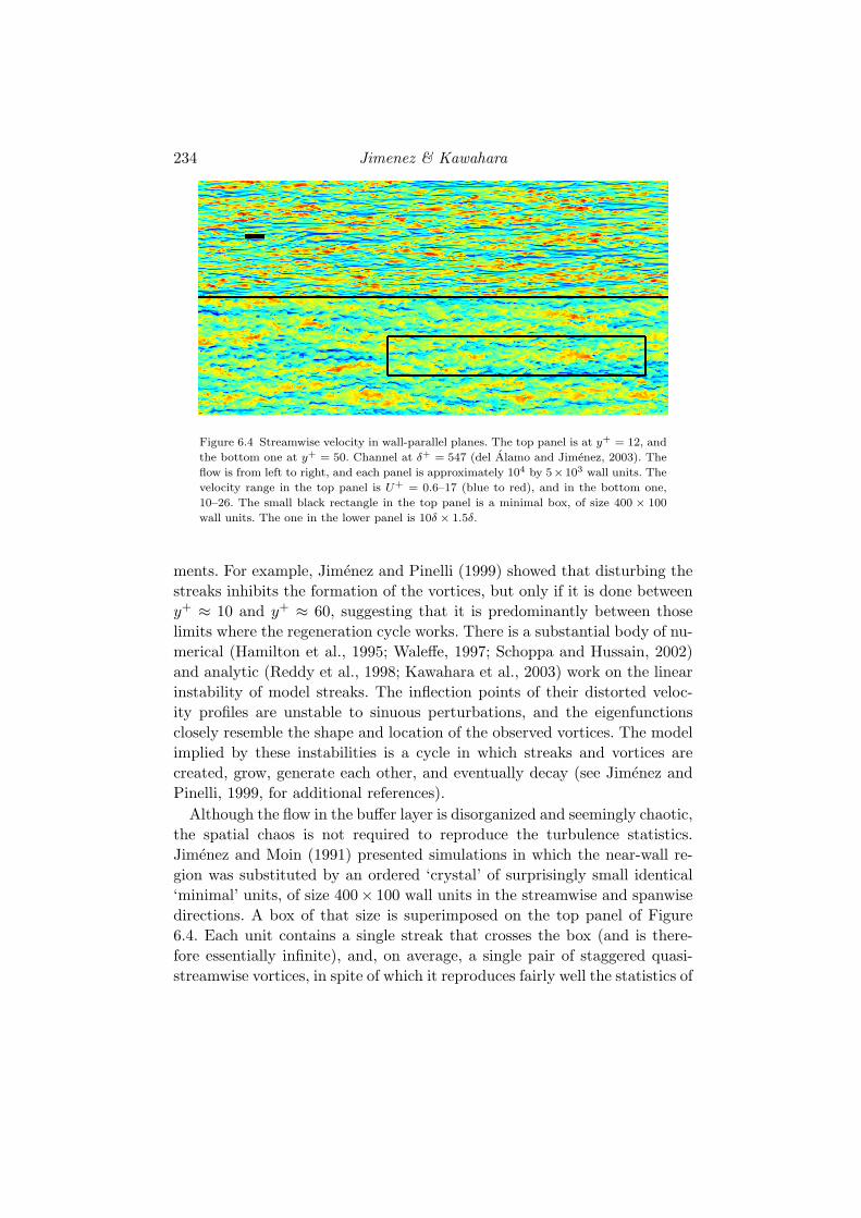
The region below y+ ≈ 100 is dominated by coherent streaks of the stream-

wise velocity and by quasi-streamwise vortices. The former are an irregular


102

103

104

102

103

λx+

λ z+

(a)

102

103

104

102

103

λx+

λ z+

(b)

Figure 6.2 Two-dimensional spectral energy density kxkzE(kx, kz) in the near-wall re-

gion (y+ = 15), in terms of the streamwise and spanwise wavelengths. Numerical chan-

nels, , δ+ = 547 (del Alamo and Jimenez, 2003); , 934 (del Alamo et al.,

2004); , 2003 (Hoyas and Jimenez, 2006). Spectra are normalized in wall units,

and the two contours for each spectrum are 0.125 and 0.625 times the maximum of the

spectrum for the highest Reynolds number. The heavy straight line is λz = 0.15λx, and

the heavy dots are λx = 10δ for the three cases. The dashed rectangle is the spectral

region used in Figure 6.3(a) to isolate the near-wall structures. (a) Kinetic energy. (b)

Enstrophy, |ω|2.

array of long (x+ ≈ 103–104) sinuous alternating streamwise jets superim-

posed on the mean shear, with an average spanwise separation of the order

of z+ ≈ 100. The quasi-streamwise vortices are slightly tilted away from the

wall, and stay in the near-wall region only for x+ ≈ 100 (Moin and Moser,

1989). Several vortices are associated with each streak (Jimenez et al., 2004),

with a longitudinal spacing of the order of x+ ≈ 300.

The streaks and the vortices are easily separated in the two-dimensional

spectral densities in Figure 6.2, which are taken at the kinetic energy peak

near y+ = 15. The streaks are represented by the spectra of the kinetic

energy in Figure 6.2(a), which are dominated by the streamwise velocity.

The vortices are represented by the enstrophy spectra in Figure 6.2(b), which

are very similar to those of the wall-normal velocity at this distance to the

wall. The three spectra in each figure correspond to turbulent channels at

different Reynolds numbers, and differ from one another almost exclusively

in the long and wide structures in the upper-right corner of the kinetic

energy spectra, with sizes of the order of λx × λz = 10δ × 1.5δ. A rectangle

with these dimensions has been added to Figure 6.4, where the large-scale

modulation of the flow can be easily seen.

In this section, we deal mostly with the rotational structures in the spec-

tral region in which λ+x . 104 and λ+z . 600. Figure 6.3(a) shows that, when

the statistics are computed within that window, they are essentially indepen-


0 50 1000

2

4

6

u′2 /u

τ2

y+

(a)

0 15 30

1

2

3

y+

u’+

v’+

(b)

Figure 6.3 Profiles of the velocity fluctuations. (a) Squared intensities of the streamwise

velocity. Simple lines are computed within the spectral window λ+x × λ+z = 104 × 600;

those with symbols are outside that window. Lines and conditions as in Figure 6.2. (b)

Root-mean-squared intensities. Simple lines are a full channel with δ+ = 180 (Kim et al.,

1987); △ , a minimal channel with δ+ = 180 (Jimenez and Moin, 1991); ◦ , a

permanent-wave autonomous solution (Jimenez and Simens, 2001). , streamwise

velocity; , wall-normal velocity.

dent of the Reynolds number, especially below y+ ≈ 100. The larger-scale

structures outside the window become stronger as the Reynolds number in-

creases, and contain no enstrophy or tangential Reynolds stresses at this

wall distance. They extend into the logarithmic layer, where they are both

rotational and carry stresses (Hoyas and Jimenez, 2006), and correspond to

the ‘inactive eddies’ of Townsend (1961). They will be discussed in §6.4. Inthis part of the flow, they are responsible for the growth of the turbulent

energy with the Reynolds number (deGraaff and Eaton, 2000).

Note that, even within the rotational region, the longer end of the spec-

trum is also wider. It was shown by Jimenez et al. (2004) that this is mostly

due to meandering of the structures, and that even the longest near-wall

low-velocity streaks are seldom wider than ∆z+ = 50. We will see below

that this is also the order of magnitude of the height of those streaks, which

are therefore roughly equilateral wavy cylinders. Meandering, as well as a

certain amount of branching, is easily seen in the top panel of Figure 6.4

and in Figure 6.6(e), and has been documented in the logarithmic layer by

Hutchins and Marusic (2007).

Soon after they were discovered by Kline et al. (1967), it was proposed

that the streaks and the vortices were involved in a regeneration cycle in

which the vortices are the results of an instability of the streaks (Swearin-

gen and Blackwelder, 1987), while the streaks are caused by the advection

of the mean velocity gradient by the vortices (Bakewell and Lumley, 1967).

Both processes have been documented and sharpened by numerical experi-


Figure 6.4 Streamwise velocity in wall-parallel planes. The top panel is at y+ = 12, and

the bottom one at y+ = 50. Channel at δ+ = 547 (del Alamo and Jimenez, 2003). The

flow is from left to right, and each panel is approximately 104 by 5×103 wall units. The

velocity range in the top panel is U+ = 0.6–17 (blue to red), and in the bottom one,

10–26. The small black rectangle in the top panel is a minimal box, of size 400 × 100

wall units. The one in the lower panel is 10δ × 1.5δ.

ments. For example, Jimenez and Pinelli (1999) showed that disturbing the

streaks inhibits the formation of the vortices, but only if it is done between

y+ ≈ 10 and y+ ≈ 60, suggesting that it is predominantly between those

limits where the regeneration cycle works. There is a substantial body of nu-

merical (Hamilton et al., 1995; Waleffe, 1997; Schoppa and Hussain, 2002)

and analytic (Reddy et al., 1998; Kawahara et al., 2003) work on the linear

instability of model streaks. The inflection points of their distorted veloc-

ity profiles are unstable to sinuous perturbations, and the eigenfunctions

closely resemble the shape and location of the observed vortices. The model

implied by these instabilities is a cycle in which streaks and vortices are

created, grow, generate each other, and eventually decay (see Jimenez and

Pinelli, 1999, for additional references).

Although the flow in the buffer layer is disorganized and seemingly chaotic,

the spatial chaos is not required to reproduce the turbulence statistics.

Jimenez and Moin (1991) presented simulations in which the near-wall re-

gion was substituted by an ordered ‘crystal’ of surprisingly small identical

‘minimal’ units, of size 400× 100 wall units in the streamwise and spanwise

directions. A box of that size is superimposed on the top panel of Figure

6.4. Each unit contains a single streak that crosses the box (and is there-

fore essentially infinite), and, on average, a single pair of staggered quasi-

streamwise vortices, in spite of which it reproduces fairly well the statistics of


0 200 400 600

0.8

1

1.2

t+

∂ yU+ w

(a)

(b)

Figure 6.5 Evolution of a minimal Poiseuille flow during a bursting event. L+x × δ+ ×

L+z = 460× 180× 125. (a) Evolution of the mean velocity gradient at the wall. The dots

correspond to the snapshots on the right. (b) The top frames are isosurfaces U+ = 8,

coloured by the distance to the wall, up to y+ = 30 (blue to red). The bottom ones are

ω+x = 0.2 (purple), and −0.2 (cyan). The flow is from bottom-left to top-right, and time

marches towards the right. The top of the boxes is y+ = 60, and the axes move with

velocity U+a = 7.6.

the full flow (Figure 6.3b). Moreover, it was shown by Jimenez and Pinelli

(1999), that the dynamics of the layer below y+ ≈ 60 is autonomous, in

the sense that the streaks and the vortices continue regenerating themselves

even when the flow above them is artificially removed, and that those local

interactions still result in approximately correct statistics.

Even further removed from the real flow are the three-dimensional nonlin-

ear equilibrium solutions of the Navier–Stokes equations discussed in §6.5,which were first obtained numerically at about the same time as the minimal

units just mentioned. Their fluctuation intensity profiles, included in Figure

6.3(b), are also strongly reminiscent of experimental turbulence.

On the other hand, although its statistics are well approximated by those

steady solutions, the real flow is not steady. The time evolution of the near-

wall structures is most easily studied in minimal boxes, because each of them

contains only a few structures whose evolution can be traced by integral

measures over the whole box. All those measures ‘burst’ quasi-periodically

on times of the order of T+ = Tu2τ/ν ≈ 400 (Jimenez and Moin, 1991;

Hamilton et al., 1995; Jimenez et al., 2005). An example is given in Figure

6.5, which depicts the rising phase of a burst. The streak becomes wavy,

friction increases sharply, and the streamwise vorticity grows. It is harder

to follow the time evolution of individual structures in real flows, but when

their statistics are compiled over randomly chosen sub-boxes of ‘minimal’

size, their distributions agree well with those of the temporal variability of

the minimal flows (Jimenez et al., 2005), suggesting that full flows also burst.


The period given above is longer than the survival time of individual vortices,

which decay viscously with a characteristic time T+ ≈ 60 if their production

is artificially inhibited by damping the streaks (Jimenez and Pinelli, 1999).

A similar time scale, T+ ≈ 50, can be extracted from the space-time spectra

of the wall-normal velocity in natural flows (del Alamo et al., 2006). The

discrepancy between the vortex lifetimes and the bursting period suggests

that the regeneration cycle consists of a relatively quiescent phase followed

by shorter eruptions. Jimenez et al. (2005) analysed several minimal flows,

and concluded that the bursting phase takes about one-third of the cycle,

or T+ ≈ 100, half of which is taken by the growth of the instability, and the

other half by its decay.

It is likely that the quasi-periodic bursting of the minimal boxes is an

artefact of the spatial periodicity, and that the streaks in the real flow move

away from the location where they are created before bursting again. In a

minimal periodic flow, the spatial periodicity brings the streak back into the

simulation box but, in a real one, bursts would be more or less independent

of each other. All that probably remains is the average time elapsed from

the moment in which a burst creates a vortex and begins to form a streak,

until the streak becomes unstable and erupts into a new burst. That time

is presumably related to the growth rate of the instabilities of the streak

itself, which is proportional to its internal velocity gradient, of the order

of uτ/∆z. The implied growth times, T+ = O(∆z+), are about a hundred

wall units, compatible with the bursting times mentioned above. Note that

the approximate agreement of those orders of magnitude is unlikely to be

a coincidence, and should rather be seen as determining the size of the

streaks. Schoppa and Hussain (2002) noted that the streaks found in real

flows are typically stable, or at most marginally unstable, and the likeliest

interpretation of that observation is that the streaks grow until they become

unstable, after which they burst, and are quickly destroyed. On the other

hand, the viscous decay time of the streak is T+ = O(∆z+2) = O(3000),

much longer than the bursting period, suggesting again that the length of

the streaks is determined by their instabilities, rather than by their viscous

decay.

The streaks are wakes created in the mean velocity profile as the vortices

are advected and sheared. For example, Jimenez et al. (2004) studied the re-

lation between streaks and vortices using as surrogates connected regions in

which u or v were more than one standard deviation away from their means

in planes parallel to the wall. Two such objects were considered related if

their rectangular bounding boxes intersected. Figure 6.6(a) shows the prob-

ability density functions (PDFs) of the position of the v > v′ ejections with


0 300 6000

0.5

1u

Lu

vxv

x+v

p.d

.f.

(a)

0 20 40 600

200

400

y+

L

+ x

(b)

0 2000 400010

−6

10−4

10−2

L+x

(c)

0 2000 4000

10−5

10−4

10−3

L+x

(d)

(e)

Figure 6.6 Numerical channels as in Figure 6.2. (a) Compensated PDF, Lup(xv|Lu), of

the positions of the front ends of the bounding boxes of v > v′ ejections with respect

to the front-end of the low-velocity streaks they intersect, for several bands of streak

lengths, limited by L+u = 50, 100, 200, 400, 700, 1100. Channel with δ+ = 2003 and y+ =

13. Longer PDFs correspond to longer streaks. (b) Average lengths of the bounding boxes

of strong velocity fluctuations, as functions of y. Lines with open symbols are |u| ≥ u′.

, Low-velocity; , high-velocity. Lines with closed symbols are |v| ≥ v′. ◦,δ+ = 934; △, 2003. (c) PDFs of the lengths of the velocity perturbations. Lines as in

(b), but ◦, y+ = 13; △, y+ = 50. δ+ = 2003. (d) PDFs of the lengths of the u–boxes,

restricted to the band 13 ≤ y+ ≤ 50. Lines as in (b), but ▽, δ+ = 547; ◦, 934; △, 2003.

The heavy chaindotted lines are exponentials with L+c = 350 and 103. (e) Long sublayer

streak, defined as a connected region in the plane y+ = 13 for which u < −u′, in a

channel at δ+ = 2003. The tick marks in the streamwise (x) axis are 1000 wall units

apart.

respect to the head of the streak to which they are related, as functions of

the streak length. The ejections are uniformly distributed along the streaks,

except at the streak head, which is always more likely to have an ejection.

If, in this wake model, we assume an advection velocity U+ad ≈ 8 near the

wall (Kim and Hussain, 1993), the vortices would create streaks of length


L+x ≈ 800 before decaying, which is consistent with the spectral maximum in

Figure 6.2(a). Moreover, the ratio (one to three) between the active lifetimes

of the bursts and the full regeneration period suggests that there should be

a similar ratio between active and total lengths along the streaks, which is

also roughly correct. The mean length of the vortices, as measured by the

regions of high wall-normal velocity in the buffer layer, is approximately 80

wall units (Figure 6.6b), while we have already seen that their mean spacing

along the streaks is of the order of λ+x = 300.

Figure 6.6(b) shows that the character of the streaks changes around

y+ ≈ 30–40, which is also where viscosity stops being an important dynam-

ical factor for the energy-containing eddies (Jimenez et al., 2004). Figure

6.6(c) shows the PDFs of the lengths of the streaks (u) and vortices (v)

in two planes at different distances from the wall. In the viscous region,

y+ = 12, the average length of low-speed streaks, L+x ≈ 500, is about twice

that of the high-speed ones, but they shorten away from the wall, and set-

tle to L+x ≈ 250 beyond y+ = 50. Above that height, the lengths of the

two types of streaks are essentially the same and, at least at the Reynolds

number of Figure 6.6(c), the longest streaks are the low-velocity ones in

the viscous layer. The simplest explanation is that the high-velocity regions

have a higher velocity gradient at the wall, and, being associated with down-

washes, are not as tall as the low-velocity ones. The viscous dissipation is

proportional to the square of the velocity derivatives, and, at y+ ≈ 10, it

is predominantly due to the wall-normal gradients. Thus, although there is

very little asymmetry between the streaks of both signs regarding the wall-

parallel velocity gradients , the dissipation due to the wall-normal ones is

much higher in the thinner fast streaks than in the taller low-speed ones.

That asymmetry weakens as the effect of viscosity decreases away from the

wall, and the two velocity signs then behave similarly. The disappearance

of the long streaks above the viscous region can also be seen in the spec-

tral densities shown in Figure 6.8(a), in the next section, which correspond

to the logarithmic layer, but which includes the kinetic-energy spectrum at

y+ = 15, for comparison. Even at the relatively high Reynolds number of

this figure, which would tend to reinforce the larger structures of the outer

region, the energy in λ+x × λ+z ≈ 104 × 100 has disappeared at y+ = 100,

and the remaining long structures seem to belong to the logarithmic-layer

family. The same distinction is clear in Figure 6.4. The streaks in the upper

panel, at y+ = 12, are mostly absent from the lower one, at y+ = 50, and

the longest structures at the higher level are wider and more disorganized.

On the other hand, the positive and negative v-structures, corresponding to


the vortices, have lengths similar to each other, and both grow longer away

from the wall.

The viscous low-velocity streaks are not only long in the mean, but the

PDF of their lengths has a very long superexponential tail, which can only

be explained by the interaction of several bursts. A plausible model for

that interaction is suggested by Figure 6.6(d). It was shown by del Alamo

et al. (2006) that the largest vortical structures at each wall distance are

objects that remain attached to the wall even when they extend far into the

flow (Townsend, 1961), and that they are associated with long low-velocity

features. Consequently, part of the reason why the PDFs in Figure 6.6(c) are

long is that they include the roots of taller objects that do not really belong

to their wall distance. In an attempt to separate those roots from the PDFs

of objects which are local to the viscous region, we display in Figure 6.6(d)

the difference between the histograms at the planes y+ = 12 and y+ = 50.

The long low-speed streaks of the viscous layer still appear, but their PDF is

now a fairly good exponential, with a characteristic length L+c ≈ 1000, which

is the same for the three Reynolds numbers in the figure. The distributions of

the high-velocity streaks are also exponential, but with a shorter length scale,

L+c ≈ 250. Exponential probability distributions suggest a Poisson process

(Feller, 1971), which can be incorporated into several plausible models for

the viscous region.

The simplest one is that streaks grow by the aggregation of smaller units.

Consider elementary streaks created by individual bursts with average length

L0, and assume that each such unit has a probability q < 1 of connecting

with another one, either by chance, or by creating a new burst in its wake.

The probability of a composite streak of n ≥ 1 units is p(n) = (1− q)qn−1,

which can be written it terms of the streak length, L = nL0, as p(L) ∼exp(−L/Lc) for L ≥ L0, where Lc = −L0/ log(q). The two factors entering

Lc can be separated if we take into account that the PDF peaks at L = L0,

in which case the best fit to Figure 6.6(d) is approximately L+0 ≈ 500 and

q ≈ 0.6. Those are sensible numbers, given the previous discussion on the

effects of a single burst, and they are given some credence by the appearance

of the long streaks, such as the one in Figure 6.6(e), but they should be used

with care because the subtraction method used to generate Figure 6.6(d) is

hard to justify for the very short events near the mode of the PDF. For

example, note that the shortest streaks around L0 become more frequent as

the Reynolds number increases, causing a systematic lowering of the offset

of the exponential tails. Moreover, an equally valid model would be that

streaks tend to form infinitely long networks, but are cut randomly by some

external influence, presumably from the logarithmic or outer layers. The


0 50 1000

1

2

3

y+

u’+, v

’+

(a)

0 50 1000

1

2

3

y+

u’+, v

’+

(b)

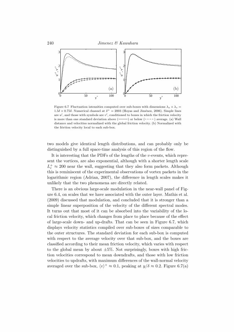
Figure 6.7 Fluctuation intensities computed over sub-boxes with dimensions λx × λz =

1.5δ × 0.75δ. Numerical channel at δ+ = 2003 (Hoyas and Jimenez, 2006). Simple lines

are u′, and those with symbols are v′, conditioned to boxes in which the friction velocity

is more than one standard deviation above ( ) or below ( ) average. (a) Wall

distance and velocities normalized with the global friction velocity. (b) Normalized with

the friction velocity local to each sub-box.

two models give identical length distributions, and can probably only be

distinguished by a full space-time analysis of this region of the flow.

It is interesting that the PDFs of the lengths of the v-events, which repre-

sent the vortices, are also exponential, although with a shorter length scale

L+c ≈ 200 near the wall, suggesting that they also form packets. Although

this is reminiscent of the experimental observations of vortex packets in the

logarithmic region (Adrian, 2007), the difference in length scales makes it

unlikely that the two phenomena are directly related.

There is an obvious large-scale modulation in the near-wall panel of Fig-

ure 6.4, on scales that we have associated with the outer layer. Mathis et al.

(2009) discussed that modulation, and concluded that it is stronger than a

simple linear superposition of the velocity of the different spectral modes.

It turns out that most of it can be absorbed into the variability of the lo-

cal friction velocity, which changes from place to place because of the effect

of large-scale down- and up-drafts. That can be seen in Figure 6.7, which

displays velocity statistics compiled over sub-boxes of sizes comparable to

the outer structures. The standard deviation for each sub-box is computed

with respect to the average velocity over that sub-box, and the boxes are

classified according to their mean friction velocity, which varies with respect

to the global mean by about ±5%. Not surprisingly, boxes with high fric-

tion velocities correspond to mean downdrafts, and those with low friction

velocities to updrafts, with maximum differences of the wall-normal velocity

averaged over the sub-box, ⟨v⟩+ ≈ 0.1, peaking at y/δ ≈ 0.2. Figure 6.7(a)


compares statistics over boxes whose friction velocities are more than one

standard deviation above or below the global mean. The former are more

intense than the latter, but most of the difference can be compensated by

normalizing both the velocities and the wall distance with the local mean

friction velocity averaged over the box, as in Figure 6.7(b). That makes

sense, because the boxes, which at the Reynolds number of the simulation

are 3000× 1500 wall units long and wide, are much larger than the elemen-

tary structures of the viscous layer, which therefore ‘live’ in an environment

defined by the mean box properties (Jimenez, 2012).

In summary, our best understanding of the viscous and buffer layers is, at

present, that the peak of the energy spectrum, at λ+x ×λ+z = 1000×100, is as-

sociated with structures that can be approximated by the steady travelling-

wave solutions of the Navier-Stokes equations discussed in §6.5, but which

in reality undergo strong quasi-periodic bursting. The bursts create vortices

whose wakes are elemental streaks with lengths of the order of 1000 wall

units, and which aggregate into the longer observed composite objects, ei-

ther by chance or by generating new bursts in their tails. Those structures

are restricted to y+ . 50, which is the only part of the flow in which high-

and low-velocity streaks are substantially different from each other. They

give way above that level to more symmetric velocity fluctuations, in which

viscosity is not the determining factor.

6.4 The logarithmic and outer layers

Immediately above the viscous region we find the logarithmic and outer

layers. They are expensive to compute, and the first simulations with even

an incipient logarithmic region have only recently began to appear. For

example, the logarithmic layer in the numerical channel in Figure 6.1(b) is

defined as the range, y+ = 80 to 400, in which the wavelength of the spectral

energy peak grows linearly with y, and only spans a factor of five. Even

so, those simulations, as well as the simultaneous advances in experimental

methods reviewed by Marusic and Adrian (2012) in this volume, have greatly

improved our knowledge of the kinematics of the outer-layer structures, and

are beginning to give some indications about their dynamics.

Before considering those results, it should be stressed that structural

models mean something different for the outer and buffer layers. Near the

wall, the local Reynolds numbers are low, and the structures are smooth,

and it is possible to speak of ‘objects’, and to write equations for them.

Both things are harder above the buffer layer. The integral scales are O(y),

the velocity fluctuations are O(uτ ), and the turbulent Reynolds number is


102

103

104

102

103

104

λ+x

λ+ z

(a)

100

101

102

100

101

λx/y

λ z/y

(b)

Figure 6.8 (a) Spectral densities of the kinetic energy in the logarithmic region of a

numerical channel at δ+ = 2003, versus wavelengths scaled in wall units. Isolines are

0.125 times the maximum of each spectrum. , y+ = 15; , 100; ,

200; , 300. (b) Two-dimensional spectral densities of u (without symbols) and v

(with symbols), versus wavelengths scaled with the wall distance. Lines as in (a). The

dashed rectangle is (λx, λz) = (6, 3)y. Isolines are 0.3 and 0.6 times the maximum of

each spectrum.

Re = O(uτy/ν ≡ y+). The definition of the outer layers, y+ ≫ 1, implies

that most of their structures have large internal Reynolds numbers, and are

themselves turbulent. The energy-containing eddies have cascades connect-

ing them to the dissipative scales, and algebraic spectra that correspond to

non-smooth geometries. They are ‘eddies’, rather than ‘vortices’, because

turbulent vorticity is always at the viscous Kolmogorov length scale, sep-

arated from the energy-containing scales by a ratio Re3/4. Some examples

are given in Figure 6.9. We can only expect dynamical descriptions of those

structures in a statistical sense, perhaps coupled to stochastic models for

the turbulent cascade ‘underneath’.

Perhaps the first new information provided by the numerics about the log-

arithmic layer was spectral, although some of the early analyses of large-eddy

simulations of channels contributed significantly to the understanding of the

bursting event (Kim, 1985). Very large scales had been found experimentally

in the outer layers of turbulent wall flows (Jimenez, 1998; Kim and Adrian,

1999), but DNS provided the first data about their two-dimensional spectra,

and about their wall-normal correlations (del Alamo and Jimenez, 2003; del

Alamo et al., 2004). Figure 6.8(a) shows that the spectral densities of the

kinetic energy in the logarithmic region have elongated shapes along lines

λ2z ∼ yλx, which del Alamo and Jimenez (2003) interpreted as the signature

of statistically conical structures similar to the ‘attached’ eddies proposed

by Townsend (1976). Note that this description only holds above y+ ≈ 100.


As mentioned in the previous section, the buffer-layer spectrum in Figure

6.8(a) is dominated by streaks with λ+z ≈ 100, but they have essentially

disappeared at y+ = 100. The vorticity is isotropic above that height, with

the three components centred around 40 Kolmogorov viscous units (Fig-

ure 6.1b), but the large-scale velocities are very anisotropic, with the long

structures mostly associated with the streamwise component (Figure 6.8b).

Figures 6.8(a) and 6.8(b) show that the cores of the velocity spectra scale

relatively well with the wall distance, although, as in all turbulent flows,

their short wavelengths scale with the Kolmogorov viscous length, and the

long- and wide-wavelength limits of the streamwise velocity scale with the

channel height. The velocities below λ+x ≈ 500 are essentially isotropic (not

shown), with similar intensities for the three components. Note that the

scaling with y of the wavelengths in Figure 6.8(b) can be read as meaning

that the structures that reach from the wall to height y are not much longer

than 6y in the logarithmic layer. Longer structures are also taller. We will

see later that the dashed rectangle in Figure 6.8(b) represents the minimal

box that can sustain turbulence up to a given y, presumably because it is

able to contain at least one complete structure with that height.

Indeed, when three-dimensional flow fields eventually became available

from simulations, it was found that there is a self-similar hierarchy of com-

pact ejections extending from the buffer layer into the outer flow, within

which the coarse-grained dissipation is more intense than elsewhere (del

Alamo et al., 2006). An example is shown in Figure 6.9(a). They correspond

to the ejections represented by the v-spectra in Figure 6.8(b), and, when

the flow is conditionally averaged around them, as in Figure 6.9(b), they are

associated with extremely long, conical, low-velocity regions whose intersec-

tion with a fixed y is a parabola that explains the quadratic behaviour of

the spectrum of u. These are probably the same objects variously described

as VLSM or “superstructures” in the paper by Marusic and Adrian (2012)

in this volume, and are not just statistical constructs. Individual cones are

observed as low-momentum ‘ramps’ in streamwise sections of instantaneous

flow fields (Meinhart and Adrian, 1995), and two examples can be seen in

the instantaneous streamwise velocity isosurface in Figure 6.9(c). As in the

buffer layer, the longest low-velocity structures at each height appear to be

composite objects, formed by the concatenation of smaller subunits of di-

mensions of the order of the v-ejections mentioned above (Figure 6.9d). We

have seen that their near-wall footprints are seen in the spectra of the buffer

layer as the ‘tails’ in Figure 6.2(a).

When the cones reach heights of the order of the flow thickness, they

stop growing, and become long cylindrical ‘streaks’, similar to those of the


(b)

(a)

(c)

(d)

Figure 6.9 (a) The coloured object is a cluster of connected vortices in a δ+ = 550

channel (del Alamo and Jimenez, 2003), from red near the wall, to yellow near y = δ.

Grey objects are unconnected vortices. (b) Averaged velocity field conditioned to a

vortex cluster. The black mesh is an isosurface of the PDF of the vortex positions.

The blue volume surrounding the cluster is the isosurface u+ = 0.3, and the red one

downstream is the isosurface u+ = −0.1. The vector plots represent (v, w) in the planes

rx/yc = 10, 20 (from del Alamo et al., 2006). (c) Isosurface of the streamwise fluctuation

velocity, u+ = −2, in a computational channel with δ+ = 550. The flow is from left to

right, in a partial domain (15.5×5.5) δ in the streamwise and spanwise directions. Colours

are distance from the wall, from blue at the wall, to red at the central plane. Figures (a)

and (c), courtesy of O. Flores. (d) Long logarithmic-layer streak, defined as a connected

region in the plane y+ = 200 for which u < −u′, in a channel at δ+ = 2003. The tick

marks in the streamwise (x) axis are 1000 wall units apart, and the red box is (6, 3)y.

sublayer, but with spanwise scales of about 1–2δ. They are fully turbu-

lent objects, and neither simulations nor experiments have provided hard


101

102

103

10

20

y+

⟨U⟩+

(a)

0 500 1000 15000

200

400

L+z

y+ dev

(b)

Figure 6.10 (a) Mean profiles of small-box simulations, compared with a full-box one.

δ+ ≈ 1800. , L+x × L+

z = 440 × 110; , 1350 × 670; , 2900 × 1450;

, full. (b) Height of the logarithmic profile in small-box simulations, as a function

of the spanwise box dimension. The open circles are the cases in (a). The two symbols

at L+z ≈ 100 have δ+ = 180 and 1800. The triangles are as in (a), but with shorter or

longer boxes, 770× 1440 and 2700× 680. The dashed line is ydev = 0.3Lz .

estimates of their maximum length, although the longest available spectra

suggests lengths of about 25δ (Jimenez and Hoyas, 2008). The wall-normal

dimension of these ‘global modes’ is of the order of the flow thickness, and

they extend from the central plane to the wall (del Alamo and Jimenez,

2003; del Alamo et al., 2004). The probability density functions of the ve-

locity strongly suggest that these large scales account for the variation of the

turbulence intensities with the Reynolds number, both near and far from the

wall (Jimenez and Hoyas, 2008), both of which disappear when wavelengths

longer than about 6δ are filtered from the flow field (Jimenez, 2007).

It is interesting that the logarithmic layer can also be simulated in rel-

atively small numerical boxes, periodic in the two wall-parallel directions

(Flores and Jimenez, 2010). Those boxes are not minimal in the sense of

those discussed in §6.3 for the buffer layer. When the simulation box is

made smaller, turbulence does not decay, but becomes restricted to a thin-

ner layer near the wall. In that sense, the minimal boxes of Jimenez and

Moin (1991) are the innermost members of a hierarchy in which progres-

sively smaller wall-attached structures are isolated in progressively smaller

numerical boxes. The especial feature of the minimal boxes of the buffer

layer is that they cannot be restricted any further, while larger boxes iso-

late more complicated structures, fully multiscale, that reach from the wall

farther into the core flow.

That can be seen in Figure 6.10(a), which compares the mean velocity

profiles of three numerical channels with different periodic box sizes to the

profile of a full channel, all at the same nominal Reynolds number. The


(a)

(b)

Figure 6.11 (a) Temporal evolution of the Reynolds stress, −⟨uv⟩ for a small-box sim-

ulation, δ+ = 1800, L+x = 2900, L+

z = 1450. In the top panel, ⟨uv⟩, is averaged over

each wall-parallel plane; in the central one, it is averaged only over events for which

(u < 0, v > 0), and in the bottom one, for (u > 0, v < 0). The heavy dashed lines are

dy/dt = ±uτ . (b) Time evolution of the U+ = 15 isosurface during the burst marked

by the two vertical lines in the middle panel of (a). Colours are distance from the wall,

with a maximum (red) y/δ ≈ 0.4. The flow is from bottom-left to top-right, and time

increases towards the right (from Flores and Jimenez, 2010).

smallest box corresponds to the minimal dimensions in §6.3, and its pro-

file diverges just above the buffer layer. The other two, with larger boxes,

reproduce well the logarithmic profile over taller regions. If we arbitrarily

define the limit of healthy turbulence as the point where the mean profiles

begin to diverge from that of a full-sized flow, it turns out to be roughly

proportional to the box size. The critical dimension appears to be the span-

wise periodicity, ydev ≈ 0.3Lz, as seen in Figure 6.10(b), which includes the

three cases in Figure 6.10(a), plus other combinations in which one of the

box dimensions was doubled or halved independently of the other one. This

result agrees with the early experiments of Toh and Itano (2005), who were

able to simulate a healthy logarithmic profile in a numerical channel with

a fairly wide box, but whose streamwise dimension was of the order of the

buffer-layer minimal boxes (L+z = 380 ≈ δ+).

As in the case of the buffer layer, small-box simulations can be used to

study the dynamics of the elementary energy-containing structures of the


logarithmic layer. They also contain a single large-scale streamwise-velocity

streak, and they also burst intermittently. An example is given in Figure

6.11(a), which displays the time evolution of the Reynolds stress, −⟨uv⟩,averaged over wall-parallel planes, as a function of the wall distance. The

top panel of the Figure reveals that the stress-producing events are tem-

porally intermittent. The averaging can be separated into points in which

the velocity perturbations are in the different quadrants of the (u, v) plane.

The two lower panels of Figure 6.11(a) display the time history of the av-

erage stress for points in the two main stress-producing quadrants. It is not

surprising that ejections, (u < 0, v > 0), move away from the wall, while

sweeps, (u > 0, v < 0), move towards it, but it is interesting that the verti-

cal velocities are similar in both cases (of the order of uτ ), and remarkably

uniform over the region depicted, suggesting that the two events are parts

of some common larger structure.

The evolution of the velocity field during the burst is shown in Figure

6.11(b), and looks remarkably similar to the events in the buffer layer. The

single streak in the simulation box becomes increasingly wavy, and is even-

tually destroyed by the instability, but it should be emphasized that, in spite

of the obvious similarities between Figures 6.11(b) and 6.5(b), the boxes in

Figure 6.11(b) are about fifteen times wider than those in the buffer layer,

and that the streak is now a fully turbulent multiscale object. The bursting

period can be estimated from the temporal evolution of different integrated

quantities, and depends on the distance to the wall (uτT ≈ 6y), rather than

on the size of box. Wider boxes simply continue the linear trend farther from

the wall. As in the buffer layer, we know less about the temporal evolution

of the structures in full-size flows, but the temporal variability of the statis-

tics of the minimal boxes is essentially identical to the variability among

randomly chosen sub-boxes of the same size in full channels, suggesting that

the processes are similar in the full and restricted systems (for details, see

Flores and Jimenez, 2010).

On the other hand, it is also unlikely in this case that the minimal boxes

represent the complete behaviour of real flows. In a hypothetical cycle in

which the instabilities of the large-scale low-velocity cones create the inter-

mittent ejections associated with the vortex tangles, which in turn create

new streaks, the minimal boxes can probably only represent correctly the

part connected with a single instability event. For example, the formation

of the composite streak in Figure 6.9(d) clearly requires more space than

the minimal dimensions, and the processes responsible for the concatena-

tion of these subunits into larger wholes, especially regarding their apparent

alignment into streamwise streaks, are not understood.


This qualitative model does not include interactions among different wall

distances. Each streak instability creates an ejection of comparable size,

which in turn recreates a commensurate streak. The fact that small boxes

sustain healthy turbulence up to a certain wall distance without the corre-

sponding larger scales suggests that the overlying structures are unnecessary

for the smaller ones. Numerical experiments in which the viscous wall cycle

is artificially removed, but whose outer-flow ejections and streaks remain

essentially identical to those above smooth walls (Flores and Jimenez, 2006;

Flores et al., 2007), suggest that the small-scale structures below a given

ejection are also essentially accidental. Experimentally, this is equivalent to

the classical observation that the outer parts of turbulent boundary layers

are independent of wall roughness (Townsend, 1976; Jimenez, 2004). Note,

however, that this independence among scales cannot be complete, because

the central constraint of wall-bounded turbulence is that the mean momen-

tum transfer has to be balanced among the different wall distances. That

is what fixes the relative intensity of the momentum-carrying structures of

different sizes.

It is not difficult to construct conceptual feed-back models in which locally

weak structures, with too little Reynolds stress, result in the local accelera-

tion of the mean velocity profile, which in turn leads to local enhancements

of the velocity gradient and to the strengthening of the local fluctuations.

But one should beware of two-scale models of turbulence, which in this case

would be one scale of fluctuations and the mean flow. Everything that we

know about turbulence points to its multiscale character, without privileged

spectral gaps. It is more likely that any interaction leading to the adjust-

ment of the intensities of the structures at different wall distances takes

place between structures of roughly similar sizes, without necessarily pass-

ing through the mean flow. Elucidating such a mechanism will require either

fairly large Reynolds numbers, or clever postprocessing techniques.

The models outlined in this section have been mostly derived from compu-

tational experiments. The experimental observations of the past decade have

suggested a different scenario in which the basic object is a hairpin vortex

growing from the wall, whose induced velocity creates the low momentum

ramps mentioned above (Adrian et al., 2000). The hairpins regenerate each

other, creating packets that are responsible for the long observed streaks

(Christensen and Adrian, 2001).

Some of the differences between the two models are probably notational.

For example, individual hairpins can be made to correspond to the instabil-

ities of the shear layers around the streaks, especially if hairpins are allowed

to be irregular or incomplete. The formation of vortex packets would corre-


spond to the lengthening of the streaks in the wake of the bursts. Similarly,

the respective emphases on vortices and on larger eddies might be influ-

enced by the relatively coarse resolution of most experiments, which are

unable to resolve individual vortices. Relying on conditional averages, as in

Figure 6.9(b), or on limited statistics based on selected ‘recognizable’ ob-

jects, might give an impression of symmetry that does not apply to more

typical individual structures. But it is harder to reconcile the respective

treatments of the importance of the wall. The ‘numerical’ model emphasizes

the effect of the local velocity shear, while the ‘experimental’ one appears

to require the formation of hairpins at, or near, the buffer region. We have

argued above that the evidence supports the former, but the experimental

observations are also plausible. The theoretical results are ambiguous. The

original simulations supporting the growth of hairpin packets were carried

out by Zhou et al. (1999) on a laminar flow with a mean turbulent velocity

profile, using molecular viscosity. They show hairpins growing away from the

wall. But Flores and Jimenez (2005) have argued that large structures feel

the effect of small-scale turbulent dissipation, and should be studied using

some kind of subgrid eddy viscosity. When that is done, vorticity rises very

little before it is dissipated.

Only recently has it become possible to compile flow animations fully

resolved in both space and time (Lozano-Duran and Jimenez, 2010), and

their analysis has only just began. The resolution of the controversy about

the flow of causality in the logarithmic layer will have to wait for those

results.

6.5 Coherent structures and dynamical systems

We have seen in the previous sections several instances in which the be-

haviour of the flow can be qualitatively explained in terms of determin-

istic interactions among structures. In fact, although apparently infinite-

dimensional, the turbulent motion of a viscous fluid in a finite domain, gov-

erned by the Navier–Stokes equations, i.e., by partial differential evolution

equations is a finite-dimensional dynamical system. Physically, the reason is

that small-scale motions are smoothed by viscosity.

There is a mathematical proof of the existence of approximate inertial

manifolds for the Navier–Stokes equations and this proof leads to an ap-

proximate relation between the dominant modes and the higher-order ones

that can be truncated (Foias et al., 2001). Within such a manifold, the

Navier–Stokes equations can be approximated by a finite-dimensional sys-

tem of ordinary differential evolution equations. For example, Keefe et al.


(1992) demonstrated numerically that a spatially periodic turbulent chan-

nel flow with δ+ = 80, simulated with a spatial resolution of 16 × 33 × 16,

was really confined to a finite-dimensional strange attractor whose Kaplan–

Yorke dimension was estimated to be 780, about 10% of the total number of

numerical degrees of freedom. That measure of the dimension of the attrac-

tor is based on the Lyapunov exponents of the system, and approximately

measures the dimension of the subspace whose volume neither increases nor

decreases during the evolution of the flow (Frederickson et al., 1983).

Dynamical-system theory tells us that coherent structures in turbulent

flows may be thought of as low-dimensional invariant sets in phase space,

in the neighbourhood of which the system spends a substantial fraction of

time, as suggested in Jimenez (1987). Spatio-temporally organized structures

appear when a turbulent state approaches such an invariant set. Possible in-

variant solutions are simple saddles in phase space, such as steady travelling

waves, or orbits that are periodic in time in some moving frame of refer-

ence. It is known that the statistical properties of chaotic low-dimensional

dynamical systems can be estimated from the coherent states represented

by unstable periodic orbits (Cvitanovic, 1987; Artuso et al., 1990a,b; Chris-

tiansen et al., 1997). In this section, we will restrict ourselves to such rel-

atively simple solutions, even if coherent structures can also correspond to

more complex sets in much lower dimensional systems, such as the strange

attractors of some highly reduced dynamical systems obtained from the

Navier–Stokes equations by proper orthogonal decomposition (see Holmes

et al., 1996).

The computation of such solutions in ideal, infinitely large, plane chan-

nels, or in experimental rectangular ducts with inflow and outflow boundary

conditions, is at the moment beyond our computational capabilities, but we

have argued above that the purpose of theory is not necessarily to repro-

duce experiments, but to give information on how the cases of interest could

eventually be predicted. Numerical simulations in doubly periodic domains

are known to reproduce well the statistics of experiments, and we have seen

that even the minimal flow units invented by Jimenez and Moin (1991) for

plane Poiseuille turbulence, and later applied by Hamilton et al. (1995) to

plane Couette turbulence, represent well at least part of the buffer layer.

Such reduced systems are small enough for their coherent structures to be

described in terms of a simple invariant solutions, and we will see below that

several have been found for doubly- or singly-periodic ‘minimal’ domains in

plane Couette, Poiseuille, Hagen–Poiseuille, and square-duct flows.

The first solutions of this kind were obtained by Nagata (1990) in plane

Couette flow. That flow is stable to infinitesimal disturbances at all Reynolds


numbers, so that nonlinear solutions cannot simply be found by continuation

from the laminar state. Nagata (1990) found his solution by first imposing

a spanwise rotation on the system, which led to a sequential series of bi-

furcations of two- and three-dimensional steady solutions from the laminar

state. He then extended one of those three-dimensional nonlinear solutions

to the non-rotating case. Clever and Busse (1992) obtained the same three-

dimensional solution by initially imposing a temperature difference between

the two horizontal walls of a Couette flow, and the same solution was again

found by Waleffe (1998, 2003) who, based on the physical insight previ-

ously gained by Hamilton et al. (1995) into the self-sustaining process of

turbulent coherent structures, initiated his continuation from an artificial

flow with streamwise-independent longitudinal vortices induced by an im-

posed body force. The three-dimensional equilibrium solution found by those

three groups arises from a saddle-node bifurcation at a finite value of the

Reynolds number, above which it splits into two solution branches. As we

will see later, the solutions of the upper branch contain a wavy low-velocity

streak and a pair of staggered counter-rotating streamwise vortices, and are

remarkably similar to the coherent structures of the turbulent buffer layer.

The solutions in the lower branch are closer to the laminar state. Other equi-

librium solutions have been found more recently for Couette flow by Nagata

(1997); Schmiegel (1999); Gibson et al. (2008, 2009); Itano and Generalis

(2009). They are not necessarily related to the one originally identified by

Nagata (1990), but they have been used to discuss coherent structures and

the subcritical transition to turbulence.

In contrast to plane Couette flow, laminar plane Poiseuille flow in a chan-

nel is unstable to infinitesimal disturbances beyond a certain Reynolds num-

ber, from where a two-dimensional equilibrium travelling-wave solution bi-

furcates subcritically. A three-dimensional solution originating from the two-

dimensional wave was found by Ehrenstein and Koch (1991), while Waleffe

(1998, 2001, 2003) and Itano and Toh (2001) found families of three-dimen-

sional steady travelling waves that are not known to be connected to the

laminar state. In Waleffe (1998, 2001, 2003), he used the artificial-force ap-

proach to construct nonlinear steady travelling waves with a reflectional

symmetry with respect to the channel central plane, which also contain

streaks and vortices. His Poiseuille solution can be continuously connected

to the Nagata (1990) solution for plane Couette flow (Waleffe, 2003). Itano

and Toh (2001) solution also includes streaks and vortices, but they are

localized near one of the two walls. A three-dimensional steady travelling

with a very similar structure was found by Jimenez and Simens (2001) in a

so-called ‘autonomous’ flow that is confined to the vicinity of one wall under


the action of a damping filter (Jimenez and Pinelli, 1999). That is the case

used in Figure 6.3(b) to compare the fluctuation profiles of simple solutions

with those of real turbulence.

The laminar Hagen–Poiseuille flow in a circular pipe is also linearly sta-

ble at all Reynolds numbers, but Faisst and Eckhardt (2003) and Wedin and

Kerswell (2004) have recently discovered three-dimensional steady travelling-

wave solutions by using the self-sustaining approach proposed by Waleffe

(1998, 2003). Both groups obtain the same solution, which possesses discrete

rotational symmetry with respect to the pipe axis, with wavy low-velocity

streaks flanked by staggered streamwise vortices. The solution with three-

fold rotational symmetry arises from a saddle-node bifurcation at the lowest

Reynolds number, although it was later found that travelling waves without

any discrete rotational symmetry exist at much lower Reynolds numbers

(Pringle and Kerswell, 2007).

As in circular pipes, the laminar flow in a square duct is linearly stable,

and no travelling-wave solutions were known until three three-dimensional

steady travelling waves were found using the artificial-force approach or

internal heating. The two found by Wedin et al. (2009) and Okino et al.

(2010) have low- or high-velocity streaks and streamwise vortices on only

two opposite walls, while the other two walls of the duct are empty. The

one found by Uhlmann et al. (2010), on the other hand, has streaks and

vortices on the four walls, so that its streamwise-averaged cross-flow velocity

exhibits an eight-vortex pattern closely resembling the mean secondary flow

of experimental turbulent ducts (Figure 6.12). This correspondence gives

some support to the numerical evidence that the mean secondary motion

of low-Reynolds-number square-ducts is a direct consequence of coherent

structures (Pinelli et al., 2010).

We already mentioned in §6.3 and §6.4 that turbulent flow is really un-

steady, even in small boxes, and that something like a bursting cycle is

necessary for regenerating the fluctuations. However, even if we have just

seen that three-dimensional equilibrium solutions reproducing buffer-layer

coherent structures are available for a variety of wall-bounded flows, only a

few periodic solutions have recently been discovered.

In plane Couette flow, Clever and Busse (1997) analysed the linear sta-

bility of Nagata (1990) three-dimensional steady solution, and identified a

Hopf bifurcation from where a temporally-periodic three-dimensional nonlin-

ear solution arises. They continued that solution within its stable parameter

range by forward time integration, but found that its properties did not dif-

fer too much from those of the steady solution due to the small amplitude

of the oscillations. Using an iterative method to minimize the recurrence


x/δ

z/δ

y/δ

(a)

z/δ

y/δ

(b)

z/δ

y/δ

(c)

Figure 6.12 Shape of the eight-vortex steady upper-branch travelling wave in a duct,

at bulk Reynolds number Re = Ubδ/ν = 1404, and streamwise wavelength Lx/δ = 2π

(Uhlmann et al., 2010). (a, b) The green sheet near the wall is an isosurface of the

streamwise velocity, 0.55 times its maximum. The blue and red tubular structures are

the streamwise vorticity, ±0.65 times its maximum (ω+x = ±0.0655). Figure (a) only

shows surfaces to one side of a duct diagonal. (c) The contour lines are isolines of

the streamwise-averaged streamwise velocity, (0.25, 0.5, 0.75 times its maximum). The

arrows are the streamwise-averaged secondary velocity.

error, Kawahara and Kida (2001) found a more unsteady three-dimensional

unstable periodic solution for plane Couette flow, which reproduces much

better the full regeneration cycle of near-wall coherent structures, i.e., the

formation and development of low-velocity streaks by decaying streamwise

vortices, the bending of the streaks followed by the regeneration of the vor-

tices, the breakdown of the streaks, and the rapid development of the vor-

tices. They also obtained a gentler periodic solution that represents a weak

spanwise standing-wave motion of the low-velocity streak.

More recently Viswanath (2007) has developed a new method based on

Newton–Krylov iteration and on a locally-constrained optimal hook step,

and applied it to the computation of periodic solutions in Couette flow.

His method is matrix-free, and drastically reduces the computational time

and memory required for the Newton iteration. Using it, he obtained five


new three-dimensional periodic solutions that demonstrate the breakup and

reorganization of near-wall coherent structures.

In plane Poiseuille flow, Toh and Itano (2003) identified a three-dimension-

al periodic-like solution that could originate from a heteroclinic connection

between two equivalent Itano and Toh (2001) stready travelling waves that

differ from each other by a spanwise shift of half a wavelength. Their so-

lution is reminiscent of the heteroclinic cycle identified in a highly reduced

dynamical-system approximation to near-wall turbulence by Aubry et al.

(1988), who also observed a connection between two fixed points differing

by a similar spanwise shift.

More recently, Duguet et al. (2008) found a three-dimensional periodic so-

lution in Hagen–Poiseuille flow that bifurcates from the Pringle and Kerswell

(2007) travelling wave without any discrete rotational symmetry.

Most of the unstable periodic orbits have been found for wall bounded

shear flows, but there are a few exceptions. One is the periodic solution

found by van Veen et al. (2006) in a Kida–Pelz highly-symmetric flow in

a triply periodic domain (Kida, 1985), which reproduces the universal Kol-

mogorov (1941) energy spectrum with the right energy dissipation rate, even

though its Reynolds number is too low to identify any real inertial range.

Another periodic solution was obtained in the GOY (Gledzer–Ohkitani–

Yamada) shell model by Kato and Yamada (2003), who observed that the

solution not only exhibits the Kolmogorov inertial-range energy spectrum,

but also intermittency.

It is curious that averaging along a single unstable periodic orbit of rela-

tively short period, such as in these solutions or in those mentioned above

for plane Couette flow (Kawahara and Kida, 2001; Viswanath, 2007), repro-

duces so well typical properties of turbulence, such as the energy spectra and

the r.m.s. velocity profiles, which are long-time averages along true turbulent

orbits. A possible interpretation has recently been proposed by Saiki and Ya-

mada (2009, 2010), who showed that periodic orbits are really special. If one

evaluates the statistical mean and variance of the time averages of dynami-

cal variables along distinct periodic orbits with similar periods, the mean is

nearly the same as that along chaotic segments with corresponding lengths,

but the variance is significantly smaller than along the chaotic segments.

This observation suggests that short periodic orbits might be better repre-

sentations of the statistical behaviour of turbulent systems than comparable

segments of their true temporal evolution in the sense that the statistical

values along periodic orbits are confined to a narrower range around the

exact one.

We now discuss the possible relevance of these simple invariant solutions


to wall-bounded turbulence. All the solutions just described are unstable at

the Reynolds numbers at which turbulence is observed, but the dimensions

of their unstable manifolds in phase space are typically low (Waleffe, 2001;

Kawahara, 2005; Wang et al., 2007; Kerswell and Tutty, 2007; Viswanath,

2009). Therefore, although we should not expect to observe them as such in

real turbulence, a generic turbulent solution could approach them and spend

a substantial fraction of its lifetime in their neighbourhood. In a nonlinear

dynamical system the transverse intersections of the stable and unstable

manifolds of the same or different periodic orbits lead to homoclinic or hete-

roclinic orbits, and to the appearance of chaotic behaviour through Smale’s

horseshoe (Guckenheimer and Holmes, 1986). Therefore, the tangle of sta-

ble and unstable manifolds of the above simple invariant solutions could

represent turbulence dynamics, while the simple solutions themselves would

represent coherent structures.

To ascertain whether that is really the case for near-wall turbulence,

Jimenez et al. (2005) collected the simple solutions available at the time for

Poiseuille and Couette flows, some of which we have seen to have velocity

fluctuation profiles strongly reminiscent of real turbulence. The characteris-

tics of those profiles are summarized in Figure 6.13, which has been adapted

from that paper by adding some of the solutions that have been found since

then. Each solution is represented by a single point whose coordinates are

the maximum values, u′max and v′max, of its intensity profiles. Most solutions

fall into one of two classes: a ‘vortex-dominated’ (upper) family, character-

ized by smaller u′max and larger v′max, and a ‘streak-dominated’ (lower) one,

characterized by larger u′max and smaller v′max. As in §6.3 we take the stream-

wise and wall-normal velocity fluctuations as respectively representing the

intensities of the streamwise velocity streaks and of the quasi-streamwise

vortices.

In the upper-left corner of Figure 6.13 we find the vortex-dominated solu-

tions, and in the lower-right corner the streak-dominated ones. The former

are represented by Kawahara and Kida (2001) dynamic periodic solution, by

Nagata (1990) upper-branch steady solutions, and by Jimenez and Simens

(2001) autonomous travelling waves. The temporal averages of Viswanath

(2007) periodic solutions in plane Couette flow are also part of this family.

These are the solutions closer to real turbulence, and the full channel of Kim

et al. (1987) is included in the figure as comparison.

The streak-dominated family includes Kawahara and Kida (2001) gentle

periodic orbit, Nagata (1990) lower-branch steady solutions. the permanent

wave obtained by Itano and Toh (2001) in Poiseuille flow, and the hetero-

clinic connection identified by Toh and Itano (2003). The figure includes the


2 4 60

0.5

1

max+

v’m

ax

+

u’

Figure 6.13 Classification into upper and lower families of the simple solutions, in terms

of their maximum streamwise and wall-normal r.m.s. velocities, u′max and v′max. Solid

symbols are classified as upper-branch, and open ones as lower-branch. The solid large

and small loops represent the dynamic (L+x × L+

z × δ+ = 190 × 130 × 34) and the

gentle (L+x × L+

z × δ+ = 154 × 105 × 28) periodic solutions at Re = 400 in Kawahara

and Kida (2001). △, Nagata (1990) steady solution for several values of the spanwise

wavelength at Re = 400 and Lx/δ = 2π (upper branch, L+z × δ+ = 76− 132× 35; lower

branch, L+z × δ+ = 53− 92× 24− 25). �, autonomous solutions in Jimenez and Simens

(2001) (L+x × L+

z × δ+1 = 151 − 189 × 180 × 38 − 46, where δ1 is the filter height). •,Waleffe (2003) upper-branch solution for Q/ν = 1303, where Q is the volume flux per

unit span. L+x ×L+

z × δ+ = 387× 149× 123; ◦, Waleffe (2003) lower-branch solution for

Q/ν = 1390, L+x × L+

z × δ+ = 379 × 146 × 121; �, Itano and Toh (2001) asymmetric

wave for Q/ν = 4000, Lx/δ = π and Lz/δ = 0.4π. The dotted loop is the periodic-like

solution of Toh and Itano (2003). H, temporal averages of Viswanath (2007) periodic

solutions (cases P2 − P6 in his table 1) for Re = 400 and Lx/δ × Lz/δ = 1.75π × 1.2π

in plane Couette flow. �, upper branch of Uhlmann et al. (2010) eight-vortex travelling-

wave solution in square duct flow (Re = 1371, Lx/δ = 2π). We have also shown the

turbulent state computed by Kim et al. (1987) (L+x ×L+

z × δ+ = 2300× 1150× 180) by

the symbol ‘+’ for comparison.

two permanent waves by Waleffe (2003) for Poiseuille flow, which were clas-

sified as lower- or upper-branch in the original reference, but which appear

here to be too close to the turning point to differ too much from each other.

The upper-branch of Uhlmann et al. (2010) eight-vortex travelling wave

in a square duct is also included, and is relatively close to the upper-family

solutions mentioned above, in spite of its significantly different boundary

conditions, but the corresponding lower-branch solution has a weaker u′max

than the upper-branch one, and is thus quite different from the lower-family

solutions discussed here.

Besides those statistical differences, the spatial structures of the upper

and lower families are also quite different. The two flow fields in Figure 6.14

correspond to the upper and lower Nagata (1990) solutions at comparable

Reynolds numbers and dimensions. They differ mainly in the location of the


y

z

(a)

y

z

(b)

Figure 6.14 Projection of the streamwise vorticity, ωx, and velocity fields in the cross-

plane (z, y), for (a) the upper-branch (L+z = 99), and (b) lower-branch (L+

z = 67)

solutions of Nagata (1990). Re = 400, Lx/δ×Lz/δ = 2π×0.9π. The thick solid lines are

different sections of the surface u = 0, i.e, the critical layer. Arrows are the cross-plane

velocities at x = 0, defined so that the first streamwise harmonic of u is proportional to

cos(2πx/Lx). The arrows are uniformly scaled in wall units, and the longest arrows in

(a) are roughly 1.9uτ . The dark- and light-gray objects are isosurfaces ω+x = ±0.155.

streamwise vorticity, which is concentrated in the form of sheets on a critical

layer in the case of the lower-branch solution, but which has two concen-

trated tubular vortices in each flank of the streak in the case of the upper

one. The spatial structure of the upper solution reproduces well the near-

wall coherent structures, with a pair of counter-rotating staggered stream-

wise vortices flanking a wavy low-velocity streak (see §6.3). The streamwise

vortical structures are responsible for the larger v′max in the upper family,

but note that there is no one-to-one correspondence between the strength of

the vortices and that of the streak. The latter is a consequence of the action

of the vortices over a period of time, and this time scale is as important in

determining the streak intensity as the vortex strength. There is little doubt

that, in the absence of viscosity or of other limiting factor, a long perma-

nent vortex would eventually pump the mean velocity profile into uniform

streamwise regions in which the streamwise velocity would be that of one

or the other wall. Viscosity or instabilities limit that distortion, and the

simplest explanation of the weaker streaks, and smaller u′max, of the upper-

branch solutions is that the flank vortices shorten the effective time scale of

the pumping by providing an effective eddy viscosity that homogenizes the

streamwise-velocity profile.

The lower solution family is probably not directly related to turbulence,

and it is now believed to play an important role in the subcritical transition

to turbulence (Kerswell, 2005; Eckhardt et al., 2007). At Reynolds numbers

low enough for laminar flow to be stable, there is a boundary in phase space


c /cf fl

δLz

+

λz

+=100

20 30 40 500

1002001

2

3

4

+

Figure 6.15 Friction coefficient, normalized by a corresponding laminar value, cf/cfl, of

Nagata (1990) solution for plane Couette flow as a function of the spanwise wavelength

L+z , and of the friction Reynolds number δ+. Streamwise wavelength Lx/δ = 2π

that separates the basins of attraction of the turbulent and laminar states.

Some of the lower-family solutions for plane Poiseuille and Couette flow

have only one unstable direction in phase space, so that those invariant sets

and their stable manifolds form the laminar-to-turbulent separatrix (Itano

and Toh, 2001; Waleffe, 2003; Kawahara, 2005; Wang et al., 2007; Schneider

et al., 2008).

Figure 6.15 shows the friction coefficient of Nagata (1990) solutions nor-

malized with that of the laminar state, for a fixed value of the streamwise

wavelength Lx/δ = 2π, as a function of the spanwise wavelength and of

the friction Reynolds number. Both the upper and the lower branches of

the solution have higher friction coefficients than the laminar state. The

range of spanwise wavelengths for which the solutions exist is always around

L+z = 100, which is close to the observed mean separation of buffer-layer

streaks, and the range itself, L+z ≈ 50− 150, is in good agreement with the

range of streak spacings found in experimental turbulent boundary layers

by Smith and Metzler (1983), λ+z ≈ 50 − 200. The same range of spanwise

wavelengths is also found in Kawahara and Kida (2001) stronger periodic

solution in plane Couette flow (Kawahara, 2009), and is around the width

of the narrowest minimal flow unit for sustained turbulence (Jimenez and

Moin, 1991). Although its relation with the above nonlinear states is un-

clear, linear analysis of the system around the state point corresponding to

the averaged turbulent flow demonstrates that a three-dimensional infinites-

imal perturbation with L+z ≈ 100, also representing streaks and streamwise

vortices, leads to optimal transient growth (del Alamo and Jimenez, 2006).

In pipe flow, on the other hand, Kerswell and Tutty (2007) performed a

detailed analysis of the correlations between the velocity fields of a turbulent


state and those of Wedin and Kerswell (2004) travelling waves with discrete

rotational symmetry, and showed that turbulence only visits the close vicin-

ity of the travelling waves in phase space for 10% of the time, suggesting

that there should be other objects, such as periodic orbits, which turbulence

approaches more frequently. More recently, Willis and Kerswell (2008) ex-

amined the relation of known travelling-wave solutions with flow states in

a long pipe, and suggested that both the lower and upper branches of their

solutions sit in an intermediate region of phase space, between laminar and

turbulent states, rather than being embedded within the turbulent attractor

itself.

We close this section by briefly discussing possible future areas of research

in the nascent field of the possible relation between the coherent structures

of turbulence and dynamical systems. Although it has turned out that the

structures, the dynamics, and the statistics of buffer-layer coherent struc-

tures are tantalizingly close to those of some nonlinear equilibria, or to the

finite-amplitude oscillations represented by known simple invariant sets in

phase space, the dynamical interpretation of the large-amplitude intermit-

tent events observed in the near-wall region remains unclear. One possibil-

ity is that those violent events correspond in phase space to the unstable

or stable manifolds of the simple invariant solutions just described, or to

their connections. Halcrow et al. (2009) have quantitatively identified hete-

roclinic connections between known equilibrium solutions of plane Couette

flow, and van Veen et al. (2011) recently developed a numerical method for

computing two-dimensional unstable manifolds in large systems, which they

used to significantly extend the unstable manifold of Kawahara and Kida

(2001) gentle periodic orbit in plane Couette flow and then to find homo-

clinic orbits from/to that periodic orbit (van Veen and Kawahara, 2011).

These studies are the first steps in the exploration of global phase-space

structures in near-wall turbulence.

Another possible research direction relates to the large-scale flow struc-

tures of transitional and turbulent wall flows, such as turbulent spots (Dau-

chot and Daviaud, 1995), oblique stripes (Prigent et al., 2002), puffs (Wyg-

nanski and Champagne, 1973) and large-scale streaks (see §6.4). Most of

the available invariant solutions have been obtained in more or less mini-

mal flow units that cannot accommodate those large-scale structures. Spa-

tially localized invariant solutions (including chaotic edge states) in a larger

periodic box would be useful for the characterization of transitional large-

scale structures (Cherhabili and Ehrenstein, 1997; Ehrenstein et al., 2008;

Schneider et al., 2010; Duguet et al., 2009; Willis and Kerswell, 2009; Melli-

bovsky et al., 2009). We also saw in §6.4 that Flores and Jimenez (2010) have


found quasi-periodic bursts in the logarithmic region of fully turbulent chan-

nel flow, strongly reminiscent of the regeneration cycle in the buffer layer,

suggesting that the large-scale dynamics in the logarithmic layer might be

related to invariant solutions in larger periodic domains.

6.6 Conclusions

In summary, our knowledge of wall-bounded turbulence has advanced a lot

in the last thirty years, and we have argued that this has been due, in large

part, to the availability of reasonably affordable direct numerical simula-

tions. Although we have shown several instances of how that has happened

in detail, it may be appropriate to summarize here the nature of the changes

that simulations have brought to the study of turbulence.

Every science passes through several stages in its development. The most

primitive one is characterized by the scarcity of suitable data, which leads to

the appearance of theories attempting to explain the few data available, but

whose further predictions cannot be easily tested. Planetary science was a

typical example until the advent of space exploration, and turbulence spent

much of the XXth century in this stage. Fluid flow is difficult to measure

and to visualize, and the available data were relatively few and incomplete.

It was possible to propose almost any theory about turbulence structure and

dynamics, with relatively few constraints from observations.

The situation began to change in the 1950’s with the advent of hot wires,

which gave the first glimpses of the structure of the turbulent eddies, and

it became a flood with direct numerical simulations. In the same way that

it became impossible to speak about canals in Mars after the first space

probes, the data generated by DNS, and to a lesser but important extent by

experimental visualisations and PIV, have produced much tighter limits for

our theories.

It is probably true that the data required to test almost any theory about

the dynamics of canonical turbulent flows already exist in some numerical

data base, or that, if it were known which data are missing, they could

probably be easily computed in a relatively short time.

What this new development denies us is the freedom to speculate. Al-

most anything that can be proposed can be tested, and the nature of the

turbulence problem is quickly changing from one of accumulating new data

to one of interpreting existing ones. It is not necessarily a simpler problem,

but it is different from much of what we have been doing up to now. The

consequences for turbulence theory can only be guessed at this moment.


Acknowledgments The preparation of this article has been supported in

part by the Spanish CICYT, under grant TRA2009-11498, by the Euro-

pean Research Council Advanced Grant ERC-2010.AdG-20100224, and a

Grant-in-Aid for Scientific Research (B) from the Japanese Society for the

Promotion of Science. The authors cordially thank D. Viswanath and M.

Uhlmann for the original data of periodic solutions in Couette flow, and

of travelling waves in a square-duct, and O. Flores for Figures 6.9(a) and

6.9(c).

References

Abe, H., Kawamura, H., and Matsuo, Y. 2004. Surface heat-flux fluctuations in aturbulent channel flow up to Reτ = 1020 with Pr = 0.025 and 0.71. Int. J.Heat Fluid Flow, 25, 404–419.

Adrian, R. J. 2007. Hairpin vortex organization in wall turbulence. Phys. Fluids.,19, 041301.

Adrian, R. J., Meinhart, C. D., and Tomkins, C. D. 2000. Vortex organization inthe outer region of the turbulent boundary layer. J. Fluid Mech., 422, 1–54.

Afzal, N., and Yajnik, K. 1973. Analysis of turbulent pipe and channel flows atmoderately large Reynolds number. J. Fluid Mech., 61, 23–31.

Artuso, R., Aurell, E., and Cvitanovic, P. 1990a. Recycling of strange sets: I. Cycleexpansions. Nonlinearity, 3, 325–359.

Artuso, R., Aurell, E., and Cvitanovic, P. 1990b. Recycling of strange sets: II.Applications. Nonlinearity, 3, 361–386.

Aubry, N., Holmes, P., Lumley, J. L., and Stone, E. 1988. The dynamics of coherentstructures in the wall region of a turbulent boundary layer. J. Fluid Mech.,192, 115–173.

Bakewell, H. P., and Lumley, J. L. 1967. Viscous sublayer and adjacent wall regionin turbulent pipe flow. Phys. Fluids, 10, 1880–1889.

Barenblatt, G. I., Chorin, A. J., and Prostokishin, V. M. 2000. Self-similar inter-mediate structures in turbulent boundary layers at large Reynolds numbers.J. Fluid Mech., 410, 263–283.

Bradshaw, P. 1967. Inactive motions and pressure fluctuations in turbulent bound-ary layers. J. Fluid Mech., 30, 241–258.

Brown, G. L., and Roshko, A. 1974. On the density effects and large structure inturbulent mixing layers. J. Fluid Mech., 64, 775–816.

Butler, K. M., and Farrell, B. F. 1993. Optimal perturbations and streak spacingin wall-bounded shear flow. Phys. Fluids A, 5, 774–777.

Cherhabili, A., and Ehrenstein, U. 1997. Finite-amplitude equilibrium states inplane Couette flow. J. Fluid Mech., 342, 159–177.

Christensen, K. T., and Adrian, R. J. 2001. Statistical evidence of hairpin vortexpackets in wall turbulence. J. Fluid Mech., 431, 433–443.

Christiansen, F., Cvitanovic, P., and Putkaradze, V. 1997. Spatiotemporal chaosin terms of unstable recurrent patterns. Nonlinearity, 10, 55–70.


Clever, R. M., and Busse, F. H. 1992. Three-dimensional convection in a horizontalfluid layer subjected to a constant shear. J. Fluid Mech., 234, 511–527.

Clever, R. M., and Busse, F. H. 1997. Tertiary and quaternary solutions for planeCouette flow. J. Fluid Mech., 344, 137–153.

Cvitanovic. 1987. Invariant measurement of strange sets in terms of cycles. Phys.Rev. Lett., 61, 2729–2732.

Darcy, H. 1854. Recherches experimentales relatives au mouvement de l’eau dansles tuyeaux. Mem. Savants Etrang. Acad. Sci. Paris, 17, 1–268.

Dauchot, O., and Daviaud, F. 1995. Finite amplitude perturbation and spots growthmechanism in plane Couette flow. Phys. Fluids, 7, 335–343.

Deardorff, J. W. 1970. A numerical study of three-dimensional turbulent channelflow at large Reynolds number. J. Fluid Mech., 41, 453–480.

Deardorff, J. W. 1973. The use of subgrid transport equations in a three-dimensionalmodel of atmospheric turbulence. J. Fluid Eng., 95, 429–438.

deGraaff, D. B., and Eaton, J. K. 2000. Reynolds number scaling of the flat-plateturbulent boundary layer. J. Fluid Mech., 422, 319–346.

del Alamo, J. C., and Jimenez, J. 2003. Spectra of very large anisotropic scales inturbulent channels. Phys. Fluids, 15, L41–L44.

del Alamo, J. C., and Jimenez, J. 2006. Linear energy amplification in turbulentchannels. J. Fluid Mech., 559, 205–213.

del Alamo, J. C., Jimenez, J., Zandonade, P., and Moser, R. D. 2004. Scaling ofthe energy spectra of turbulent channels. J. Fluid Mech., 500, 135–144.

del Alamo, J. C., Jimenez, J., Zandonade, P., and Moser, R. D. 2006. Self-similarvortex clusters in the logarithmic region. J. Fluid Mech., 561, 329–358.

Duguet, Y., Pringle, C. C., and Kerswell, R. R. 2008. Relative periodic orbits intransitional pipe flow. Phys. Fluids, 20, 114102.

Duguet, Y., Schlatter, P., and Henningson, D. S. 2009. Localized edge states inplane Couette flow. Phys. Fluids, 21, 111701.

Eckhardt, B., Scheider, T. M., Hof., B., and Westerweel, J. 2007. Turbulence tran-sition in pipe flow. Ann. Rev. Fluid Mech., 39, 447–468.

Ehrenstein, U., and Koch, W. 1991. Three-dimensional wavelike equilibrium statesin plane Poiseuille flow. J. Fluid Mech., 228, 111–148.

Ehrenstein, U., Nagata, M., and Rincon, F. 2008. Two-dimensional nonlinear planePoiseuille–Couette flow homotopy revisited. Phys. Fluids, 20, 064103.

Faisst, H., and Eckhardt, B. 2003. Traveling waves in pipe flow. Phys. Rev. Lett.,91, 224502.

Feller, W. 1971. An Introduction to Probability theory and its Applications. thirdedn. Vol. 1. Wiley. pg. 446–448.

Flores, O., and Jimenez, J. 2005. Linear dynamics of turbulent structures in thelog layer. Pages LR–1 of: Proc. Div. Fluid Dyn. Am. Phys. Soc.

Flores, O., and Jimenez, J. 2006. Effect of wall-boundary disturbances on turbulentchannel flows. J. Fluid Mech., 566, 357–376.

Flores, O., and Jimenez, J. 2010. Hierarchy of minimal flow units in the logarithmiclayer. Phys. Fluids, 22, 071704.


Flores, O., Jimenez, J., and del Alamo, J. C. 2007. Vorticity organization in theouter layer of turbulent channels with disturbed walls. J. Fluid Mech., 591,145–154.

Foias, C., Manley, O., Rosa, R., and Temam, R. 2001. Navier–Stokes Equationsand Turbulence. Cambridge University Press.

Frederickson, P., Kaplan, J. L., Yorke, E. D., and Yorke, J. A. 1983. The Lyapunovdimension of strange attractors. J. Diffl. Equat., 49, 185–207.

Gaster, M., Kit, E., and Wygnanski, I. 1985. Large-scale structures in a forcedturbulent mixing layer. J. Fluid Mech., 150, 23–39.

Gibson, J. F., Halcrow, J., and Cvitanovic, P. 2008. Visualizing the geometry ofstate space in plane Couette flow. J. Fluid Mech., 611, 107–130.

Gibson, J. F., Halcrow, J., and Cvitanovic, P. 2009. Equilibrium and travelling-wavesolutions of plane Couette flow. J. Fluid Mech., 638, 243–266.

Guckenheimer, J., and Holmes, P. 1986. Nonlinear Oscillations, Dynamical Sys-tems, and Bifurcations of Vector Fields, 2nd ed. Springer Verlag.

Hagen, G. H. L. 1839. Uber den Bewegung des Wassers in engen cylindrischenRohren. Poggendorfs Ann. Physik Chemie, 46, 423–442.

Halcrow, J., Gibson, J. F., and Cvitanovic, P. 2009. Heteroclinic connections inplane Couette flow. J. Fluid Mech., 621, 365–376.

Hamilton, J. M., Kim, J., and Waleffe, F. 1995. Regeneration mechanisms of near-wall turbulence structures. J. Fluid Mech., 287, 317–348.

Ho, C. H., and Huerre, P. 1984. Perturbed free shear layers. Ann. Rev. Fluid Mech.,16, 365–424.

Holmes, P., Lumley, J. L., and Berkooz, G. 1996. Turbulence, Coherent Structures,Dynamical Systems and Symmetry, 1st ed. Cambridge University Press.

Hoyas, S., and Jimenez, J. 2006. Scaling of the velocity fluctuations in turbulentchannels up to Reτ = 2003. Phys. Fluids, 18, 011702.

Hoyas, S., and Jimenez, J. 2008. Reynolds number effects on the Reynolds-stressbudgets in turbulent channels. Phys. Fluids, 20, 101511.

Hutchins, N., and Marusic, I. 2007. Evidence of very long meandering featuresin the logarithmic region of turbulent boundary layers. J. Fluid Mech., 579,467–477.

Itano, T., and Generalis, S. C. 2009. Hairpin vortex solution in planar Couetteflow: A tapestry of knotted vortices. Phys. Rev. Lett., 102, 114501.

Itano, T., and Toh, S. 2001. The dynamics of bursting process in wall turbulence.J. Phys. Soc. Jpn., 70, 703–716.

Jimenez, J. 1987. Coherent structures and dynamical systems. Pages 323–324 of:Proc. CTR Summer Program 1987. Stanford University.

Jimenez, J. 1998. The largest scales of turbulence. Pages 137–154 of: CTR Ann.Res. Briefs. Stanford University.

Jimenez, J. 2003. Computing high-Reynolds number flows: Will simulations eversubstitute experiments? J. of Turbulence, 22.

Jimenez, J. 2004. Turbulent flows over rough walls. Ann. Rev. Fluid Mech., 36,173–196.

Jimenez, J. 2007. Recent developments in wall-bounded turbulence. Rev. R. Acad.Cien. Serie A, Mat., 101, 187–203.


Jimenez, J. 2012. Cascades in wall-bounded turbulence. Ann. Rev. Fluid Mech.,44, 27–45.

Jimenez, J., and Hoyas, S. 2008. Turbulent fluctuations above the buffer layer ofwall-bounded flows. J. Fluid Mech., 611, 215–236.

Jimenez, J., and Moin, P. 1991. The minimal flow unit in near-wall turbulence. J.Fluid Mech., 225, 221–240.

Jimenez, J., and Moser, R. D. 2007. What are we learning from simulating wallturbulence? Phil. Trans. Roy. Soc. A, 365, 715–732.

Jimenez, J., and Pinelli, A. 1999. The autonomous cycle of near wall turbulence.J. Fluid Mech., 389, 335–359.

Jimenez, J., and Simens, M. P. 2001. Low-dimensional dynamics in a turbulentwall flow. J. Fluid Mech., 435, 81–91.

Jimenez, J., Wray, A. A., Saffman, P. G., and Rogallo, R. S. 1993. The structureof intense vorticity in isotropic turbulence. J. Fluid Mech., 255, 65–90.

Jimenez, J., del Alamo, J. C., and Flores, O. 2004. The large-scale dynamics ofnear-wall turbulence. J. Fluid Mech., 505, 179–199.

Jimenez, J., Kawahara, G., Simens, M. P., Nagata, M., and Shiba, M. 2005. Char-acterization of near-wall turbulence in terms of equilibrium and ‘bursting’solutions. Phys. Fluids, 17, 015105.

Kato, S., and Yamada, M. 2003. Unstable periodic solutions embedded in a shellmodel turbulence. Phys. Rev. E, 68, 025302(R).

Kawahara, G. 2005. Laminarization of minimal plane Couette flow: Going beyondthe basin of attraction of turbulence. Phys. Fluids, 17, 041702.

Kawahara, G. 2009. Theoretical interpretation of coherent structures in near-wallturbulence. Fluid Dynamics Research, 41, 064001.

Kawahara, G., and Kida, S. 2001. Periodic motion embedded in plane Couetteturbulence: regeneration cycle and burst. J. Fluid Mech., 449, 291–300.

Kawahara, G., Jimenez, J., Uhlmann, M., and Pinelli, A. 2003. Linear instabilityof a corrugated vortex sheet – a model for streak instability. J. Fluid Mech.,483, 315–342.

Keefe, L., Moin, P., and Kim, J. 1992. The dimension of attractors underlyingperiodic turbulent Poiseuille flow. J. Fluid Mech., 242, 1–29.

Kerswell, R. R. 2005. Recent progress in understanding the transition to turbulencein a pipe. Nonlinearity, 18, R17–R44.

Kerswell, R. R., and Tutty, O. R. 2007. Recurrence of travelling waves in transitionalpipe flow. J. Fluid Mech., 584, 69–102.

Kida, S. 1985. Three-dimensional periodic flows with high-symmetry. J. Phys. Soc.Japan, 54, 3132–2136.

Kim, J. 1985. Turbulence structures associated with the bursting event. Phys.Fluids, 28, 52–58.

Kim, J., and Hussain, F. 1993. Propagation velocity of perturbations in channelflow. Phys. Fluids A, 5, 695–706.

Kim, J., Moin, P., and Moser, R. D. 1987. Turbulence statistics in fully developedchannel flow at low Reynolds number. J. Fluid Mech., 177, 133–166.

Kim, K.C., and Adrian, R. J. 1999. Very large-scale motion in the outer layer.Phys. Fluids, 11, 417–422.


Kline, S. J., Reynolds, W. C., Schraub, F. A., and Runstadler, P. W. 1967. Structureof turbulent boundary layers. J. Fluid Mech., 30, 741–773.

Kolmogorov, A. N. 1941. The local structure of turbulence in incompressible viscousfluids a very large Reynolds numbers. Dokl. Akad. Nauk. SSSR, 30, 301–305.Reprinted in Proc. Roy. Soc. London. A 434, 9–13 (1991).

Lee, S-H., and Sung, H. J. 2007. Direct numerical simulation of the turbulentboundary layer over a rod-roughened wall. J. Fluid Mech., 584, 125–146.

Lee, S-H., and Sung, H. J. 2011. Very-large-scale motions in a turbulent boundarylayer. J. Fluid Mech., 673, 80–120.

Lozano-Duran, A., and Jimenez, J. 2010. Time-resolved evolution of the wall-bounded vorticity cascade. Pages EB–3 of: Proc. Div. Fluid Dyn. Am. Phys.Soc.

Marusic, I., and Adrian, R. J. 2012. The eddies and scales of wall-turbulence. Thisvolume.

Mathis, R., Hutchins, N., and Marusic, I. 2009. Large-scale amplitude modulationof the small-scale structures in turbulent boundary layers. J. Fluid Mech.,628, 311–337.

Meinhart, C. D., and Adrian, R. J. 1995. On the existence of uniform momentumzones in a turbulent boundary layer. Phys. Fluids, 7, 694–696.

Mellibovsky, F., Meseguer, A., Schneider, T. M., and Eckhardt, B. 2009. Transitionin localized pipe flow turbulence. Phys. Rev. Lett., 103, 054502.

Moin, P., and Kim, J. 1982. Numerical investigation of turbulent channel flow. J.Fluid Mech., 118, 341–377.

Moin, P., and Mahesh, K. 1998. Direct numerical simulation: A tool in turbulenceresearch. Ann. Rev. Fluid Mech., 30, 539–578.

Moin, P., and Moser, R. D. 1989. Characteristic-eddy decomposition of turbulencein a channel. J. Fluid Mech., 200, 471–509.

Morrison, W. R. B., Bullock, K. J., and Kronauer, R. E. 1971. Experimentalevidence of waves in the sublayer. J. Fluid Mech., 47, 639–656.

Nagata, M. 1990. Three-dimensional finite-amplitude solutions in plane Couetteflow: Bifurcation from infinity. J. Fluid Mech., 217, 519–527.

Nagata, M. 1997. Three-dimensional traveling-wave solutions in plane Couette flow.Phys. Rev. E, 55, 2023–2025.

Oberlack, M. 2001. A unified approach for symmetries in plane parallel turbulentshear flows. J. Fluid Mech., 427, 299–328.

Obukhov, A. M. 1941. On the distribution of energy in the spectrum of turbulentflow. Dokl. Akad. Nauk. SSSR, 32, 22–24.

Okino, S., Nagata, M., Wedin, H., and Bottaro, A. 2010. A new nonlinear vortexstate in square-duct flow. J. Fluid Mech., 657, 413–429.

Osterlund, J. M., Johansson, A. V., Nagib, H. M., and Hites, M. 2000. A note onthe overlap region in turbulent boundary layers. Phys. Fluids, 12, 1–4.

Pinelli, A., Uhlmann, M., Sekimoto, A., and Kawahara, G. 2010. Reynolds numberdependence of mean flow structure in square duct turbulence. J. Fluid Mech.,644, 107–122.


Prigent, A., Gregorie, G., Chate, H., Dauchot, O., and van Saarloos, W. 2002.Large-scale finite-wavelength modulation within turbulent shear flows. Phys.Rev. Lett., 89, 014501.

Pringle, C. C., and Kerswell, R. R. 2007. Asymmetric, helical, and mirror-symmetrictraveling waves in pipe flow. Phys. Rev. Lett., 99, 074502.

Reddy, S. C., Schmid, P. J., Baggett, J. S., and Henningson, D. S. 1998. On stabilityof streamwise streaks and transition thresholds in plane channel flows. J. FluidMech., 365, 269–303.

Reynolds, O. 1894. On the dynamical theory of incompressible viscous fluids andthe determination of the criterion. Phil. Trans. Roy. Soc. London, 186, 123–164. Papers, ii, 535.

Richardson, L. F. 1920. The supply of energy from and to atmospheric eddies.Proc. Roy. Soc. A, 97, 354–373.

Rogallo, R. S. 1981. Numerical experiments in homogeneous turbulence. Tech.Memo 81315. NASA.

Rogallo, R. S., and Moin, P. 1984. Numerical simulations of turbulent flows. Ann.Rev. Fluid Mech., 16, 99–137.

Saiki, Y., and Yamada, M. 2009. Time-averaged properties of unstable periodicorbits and chaotic orbits in ordinary differential equation systems. Phys. Rev.E, 79, 015201(R).

Saiki, Y., and Yamada, M. 2010. Unstable periodic orbits embedded in a continuoustime dynamical system – time averaged properties. RIMS Kokyuroku, 1713,111–123.

Schlatter, P., and Orlu, R. 2010. Assessment of direct numerical simulation data ofturbulent boundary layers. J. Fluid Mech., 659, 116–126.

Schlatter, P., Orlu, R., Li, Q., Fransson, J.H.M., Johansson, A.V., Alfredsson, P. H.,and Henningson, D. S. 2009. Turbulent boundary layers up to Reθ = 2500through simulation and experiments. Phys. Fluids, 21, 05702.

Schmiegel, A. 1999. Transition to turbulence in linearly stable shear flows. Ph.D.thesis, Faculty of Physics, Philipps-Universitat Marburg.

Schneider, T. M., Gibson, J. F., Lagha, M., De Lillo, F., and Eckhardt, B. 2008.Laminar-turbulent boundary in plane Couette flow. Phys. Rev. E, 78, 037301.

Schneider, T. M., Gibson, J. F., and Burke, J. 2010. Snakes and ladders: localizedsolutions of plane Couette flow. Phys. Rev. Lett., 104, 104501.

Schoppa, W., and Hussain, F. 2002. Coherent structure generation in near-wallturbulence. J. Fluid Mech., 453, 57–108.

She, Z.-S. 1993. Constrained Euler system for Navier–Stokes turbulence. Phys.Rev. Lett., 70, 1255–1258.

Siebesma, A. P., Bretherton, C. S., Brown, A., A.Chlond, Cuxart, J., Duynkerke,P. G., Jiang, H. L., Khairoutdinov, M., Lewellen, D., Moeng, C. H., Sanchez,E., Stevens, B., and Stevens, D. E. 2003. A large eddy simulation intercom-parison study of shallow cumulus convection. J. Atmos. Sci., 60, 1201–1219.

Siggia, E. D. 1981. Numerical study of small scale intermittency in three-dimensional turbulence. J. Fluid Mech., 107, 375–406.


Sillero, J. A., Borrell, G., Gungor, A. G., Jimenez, J., Moser, R.D., and Oliver,T. A. 2010. Direct simulation of the zero-pressure-gradient boundary layer upto Reθ = 6000. Pages EB–4 of: Proc. Div. Fluid Dyn. Am. Phys. Soc.

Simens, M.P., Jimenez, J., Hoyas, S., and Mizuno, Y. 2009. A high-resolution codefor turbulent boundary layers. J. Comput. Phys., 228, 4218–4231.

Smith, C. R., and Metzler, S. P. 1983. The characteristics of low speed streaksin the near wall region of a turbulent boundary layer. J. Fluid Mech., 129,27–54.

Spalart, P. R., Coleman, G. N., and Johnstone, R. 2008. Direct numerical simulationof the Ekman layer: A step in Reynolds number, and cautious support for alog law with a shifted origin. Phys. Fluids, 20, 101507.

Swearingen, J. D., and Blackwelder, R. F. 1987. The growth and breakdown ofstreamwise vortices in the presence of a wall. J. Fluid Mech., 182, 255–290.

Tennekes, H., and Lumley, J. L. 1972. A First Course in Turbulence. MIT Press.Toh, S., and Itano, T. 2003. A periodic-like solution in channel flow. J. Fluid Mech.,

481, 67–76.Toh, S., and Itano, T. 2005. Interaction between a large-scale structure and near-

wall structures in channel flow. J. Fluid Mech., 524, 249–262.Townsend, A. A. 1961. Equilibrium layers and wall turbulence. J. Fluid Mech., 11,

97–120.Townsend, A. A. 1976. The Structure of Turbulent Shear Flow, 2nd ed. Cambridge

University Press.Uhlmann, M., Kawahara, G., and Pinelli, A. 2010. Traveling-waves consistent with

turbulence-driven secondary flow in a square duct. Phys. Fluid, 22, 084102.van Veen, L., and Kawahara, G. 2011. Homoclinic tangle on the edge of shear

turbulence. Phys. Rev. Lett., 107, 114501.van Veen, L., Kawahara, G., and Matsumura, A. 2011. On matrix-free computation

of 2D unstable manifolds. SIAM J. Sci. Comp., 33, 25–44.van Veen, L., Kida, S., and Kawahara, G. 2006. Periodic motion representing

isotropic turbulence. Fluid Dynamics Research, 38, 19–46.Vincent, A., and Meneguzzi, M. 1991. The spatial structure and statistical proper-

ties of homogeneous turbulence. J. Fluid Mech, 225, 1–25.Viswanath, D. 2007. Recurrent motions within plane Couette turbulence. J. Fluid

Mech., 580, 339–358.Viswanath, D. 2009. The critical layer in pipe flow at high Reynolds number. Phil.

Trans. Roy. Soc. A, 367, 561–576.Waleffe, F. 1997. On a self-sustaining process in shear flows. Phys. Fluids, 9,

883–900.Waleffe, F. 1998. Three-dimensional coherent states in plane shear flows. Phys.

Rev. Lett., 81, 4140–4143.Waleffe, F. 2001. Exact coherent structures in channel flow. J. Fluid Mech., 435,

93–102.Waleffe, F. 2003. Homotopy of exact coherent structures in plane shear flows. Phys.

Fluids, 15, 1517–1534.Wang, J., Gibson, J., and Waleffe, F. 2007. Lower branch coherent states in shear

flows: Transition and control. Phys. Rev. Lett., 98, 204501.


Wedin, H., and Kerswell, R. R. 2004. Exact coherent structures in pipe flow:travelling wave solutions. J. Fluid Mech., 508, 333–371.

Wedin, H., Bottaro, A., and Nagata, M. 2009. Three-dimensional traveling wavesin a square duct. Phys. Rev. E, 79, 065305(R).

Willis, A. P., and Kerswell, R. R. 2008. Coherent structures in localized and globalpipe turbulence. Phys. Rev. Lett., 100, 124501.

Willis, A. P., and Kerswell, R. R. 2009. Turbulent dynamics of pipe flow capturedin a reduced model: puff relaminarization and localized ‘edge’ states. J. FluidMech., 619, 213–233.

Wosnik, M., Castillo, L., and George, W. K. 2000. A theory for turbulent pipe andchannel flows. J. Fluid Mech., 421, 115–145.

Wu, X., and Moin, P. 2010. Transitional and turbulent boundary layer with heattransfer. Phys. Fluids., 22, 085105.

Wygnanski, I. J., and Champagne, F. H. 1973. On transition in a pipe. Part 1. Theorigin of puffs and slugs and the flow in a turbulent slug. J. Fluid Mech., 59,281–335.

Zhou, J., Adrian, R. J., S., Balachandar, and Kendall, T. M. 1999. Mechanismsfor generating coherent packets of hairpin vortices in channel flow. J. FluidMech., 387, 353–396.

Documents

Dynamics of Wall-Bounded Turbulence - UPM