Embed Size (px)
Citation preview

Dynamics Solver
December 10, 2000
Juan M. AguirregabiriaDepartment of Theoretical Physics
The University of the Basque CountryP.O. Box 644, 48080 Bilbao (Spain)
eman ta zabal zazu Tel:Fax:E-mail:WWW:
+34 94 601 25 93+34 94 464 85 [email protected]://tp.lc.ehu.es/jma.html

2 Tutorial
Copyright 1992-1998 Juan M. AguirregabiriaAll rights reserved.
HP LaserJet, HP Deskjet and HPGL are registered trademarks of Hewlett-Packard Corp. Microsoft is aregistered trademark of Microsoft Corporation. Windows is a trademark of Microsoft Corporation.Postscript is a registered trademark of Adobe Systems, Inc. Mathematica is a trademark of WolframResearch, Inc. All other brand names and product names used in the help and documentation files aretrademarks, registered trademarks or trade names of their respective holders.
License
Dynamics Solver is FreeWare; there is no charge for using it and it may be distributed freely so long asthe files are kept together and unaltered. You may neither sell nor profit from distribution of DynamicsSolver in any way without the written permission of the author.
Disclaimer
In no event will the Author be liable to users for any damages, including but not limited to any lost profits,lost savings or other incidental or consequential damages arising out of the use or the inability to use thisprogram, even if the Author has been advised of the possibility of such damages, or for any claim by otherparty.

3
To the memory of my father

4 Tutorial
Acknowledgments
This version of Dynamics Solver has benefited greatly from critical comments made by friends fromEuskal Herriko Unibertsitatea, Université Pierre et Marie Curie, and Universitat de Barcelona. For thishelp, the author is very grateful to Lluís Bel, Aníbal Hernández, Alfred Molina and Martín Rivas.
5
Introduction
Program Description
Dynamics Solver is intended to solve initial and boundary-value problems for continuous and discretedynamical systems:
• single ordinary differential equations of arbitrary order,
• systems of any number of first-order ordinary differential equations,
• a rather large class of functional-differential equations and systems,
• iterated maps and recurrences in arbitrary dimensions,
• any problem that can be written in one of the aforementioned forms.
No programming is necessary: everything can be entered in user-friendly dialog boxes and complexgraphics (and numerical) results can be easily and quickly obtained. The program has a powerful built-in compiler that automatically translates a large class of mathematical expressions written in a standardformat into an internal code that can be executed very fast.
Apart from the dynamical system solution, one can compute any quantity involving the solution and itsderivatives (for one or more values of the independent variables), the problem parameters and the initialconditions. For example, it is possible to draw phase-space portraits (including an optional directionfield), Poincaré maps, Liapunov exponents, cobweb diagrams, histograms and bifurcation diagrams.The results can be projected (in perspective or not) along any direction and particular subspaces of thephase space (or the space of initial conditions) may be analyzed easily.
Very different kinds of results may be obtained in different graphics and text formats displayed in oneor more windows. They can be sent to any Windows compatible printer or plotter and advanced outputformats are available, including Encapsulated Postscript and user-defined formats. The results can beeasily collected in a file in order to process them by means of other programs, such as Mathematica. It isalso possible to generate animated output.
There are many programs to draw geometrical figures, but most of them are not appropriate to draw thefigures that physicists often need when preparing lectures or research papers. One would not want to haveto learn to use a very complex CAD program only to draw some figures in a collection of exercises.Simpler programs exist, but they are not able to draw mathematically defined curves (say a semi-cubicparabola) or to place elements at arbitrary points (often they can only be placed at some grid points), or toinclude data points. Dynamics Solver can be used to draw segments, arcs of circles and ellipses, arrows,arbitrary parametric curves in two and three dimensions, a large class of fractals, and points and lines fromexternal data files (which can be generated by Dynamics Solver itself or any other program). The maingoal is to have completely correct figures (not only artistic approximations) in a device-independentformat that can be translated to standard formats (HPGL or Postscript, for instance) that, in turn, can beeasily combined with output files from powerful text processors and formatters (we have TeX in mind, ofcourse).
Each problem can be saved to and retrieved from a disk file. This “problem file“ can also be edited andused as a template for related problems. One can extend the program by providing more integrationmethods or additional mathematical functions.
A complete, context-sensitive, cross-referenced help system is available and each error message anddialog box has a help button that can be used to get the corresponding information. Furthermore, theprogram is highly configurable to better suit your needs and tastes.
Who May Use Dynamics Solver
Dynamics Solver is both a powerful professional tool to be used by physicists, mathematicians andengineers in their everyday work, and also a pedagogical tool to help learning and teaching aboutdifferential equations, continuous and discrete nonlinear dynamical systems, deterministic chaos, etc.

6 Tutorial
Topics that were traditionally omitted in introductory courses because of their mathematical complexitycan now be analyzed easily. Even when exact solutions are known, it is often given by means of complexmathematical expressions that are not easily understood without explanatory graphics. Students can gain amore intuitive comprehension of many problems by analyzing them in a numerical laboratory, andDynamics Solver is flexible enough to be an effective numerical laboratory in which many problems fromphysics and engineering can be easily tested. Note also that many examples discussed in books oncomputational physics and in papers published in journals like American Journal of Physics, EuropeanJournal of Physics, etc. can be analyzed, without programming, by means of Dynamics Solver. Forinstance, when teaching differential equations you can use Dynamics Solver in many different ways.Plenty of useful examples can be found in the excellent textbook of Borelli [1991], which can also be usedto teach a full laboratory course on differential equations.
Program Versions
There are two versions of Dynamics Solver:
• a 16-bit edition which will run under Windows 3.1 (or compatible environments, includingWindows for Workgroups 3.1+, Windows 95, Windows 98 and Windows NT 3.5 for Intelprocessors). Though it may run under Windows 3.1, it includes many interface enhancements ofWindows 95/98/NT4, such as tabbed dialogs, toolbars, tooltips, status bar, spin controls andpopup menus invoked with the right mouse button.
• a 32-bit edition which will run only under Windows 95, Windows 98 and Windows NT 4.0 andtakes advantage of the enhanced possibilities of this environment, such as:
• long file names,• use of the registry instead of .INI files,• bigger integers for repeated integration,• problem files automatically added to the Documents entry of the Start menu,• context help for dialog controls,• creation of new problem files from the New menu entry that opens when right-clicking in an
Explorer or My PC folder (or even on the Desktop),• any problem that was open when the system is shut down will be reopened in the next
Windows session,• more memory,• QuickView compatibility,
and more...

7
Table of ContentsINTRODUCTION TO DYNAMICS SOLVER.........................................................................................................11
Tutorial ...................................................................................................................................................11Starting Dynamics Solver....................................................................................................................................11Exiting Dynamics Solver.....................................................................................................................................12Getting Help........................................................................................................................................................12Using Problem Files............................................................................................................................................13A Simple Dynamical System...............................................................................................................................13Graphics Output..................................................................................................................................................15Solving the Dynamical System............................................................................................................................16Output Ranges.....................................................................................................................................................17Numerical Output................................................................................................................................................18Output Quantities................................................................................................................................................19Example Files......................................................................................................................................................20Systems of Equations..........................................................................................................................................20Projections...........................................................................................................................................................21Poincaré Sections................................................................................................................................................22Constrained Initial Conditions and Boundary Conditions...................................................................................22Numerical Simulation..........................................................................................................................................24Functional-Differential Equations and Text Output............................................................................................25Numerical Quadrature.........................................................................................................................................26Discrete Dynamical Systems...............................................................................................................................27Function Graphs and Parametric Curves.............................................................................................................28Drawing with Dynamics Solver...........................................................................................................................30Decorative Examples...........................................................................................................................................31High-Resolution Drawings..................................................................................................................................32Extending Dynamics Solver................................................................................................................................33
MANUAL ......................................................................................................................................................34Running Dynamics Solver.......................................................................................................................34
Starting Dynamics Solver....................................................................................................................................34Previous instances...............................................................................................................................................35Command line options.........................................................................................................................................35
Dynamical Systems.................................................................................................................................37Single Equations and First-Order Systems..........................................................................................................37Higher Order Systems.........................................................................................................................................38Equations Not Written in Normal Form..............................................................................................................38Functional-Differential Equations.......................................................................................................................39Discontinuities in Functional-Differential Equations..........................................................................................40Integro-Differential Equations and Definite Integrals.........................................................................................41Discrete Dynamical Systems: Iterated Maps and Recurrences............................................................................41Problem Parameters.............................................................................................................................................42Complex Numbers...............................................................................................................................................42Entering the Dynamical System into Dynamics Solver.......................................................................................43Dealing with Discontinuities...............................................................................................................................44
Initial Values...........................................................................................................................................45Initial Conditions for Ordinary Differential Equations........................................................................................45Constrained Initial Conditions............................................................................................................................46Initial Conditions for Functional-Differential Equations.....................................................................................47Initial Conditions for Discrete Dynamical Systems.............................................................................................47Entering Initial Values........................................................................................................................................48Entering Initial Values on the Screen..................................................................................................................48Solutions Arriving to a Predefined Point.............................................................................................................48Multiple Sets of Initial Conditions......................................................................................................................48Entering Initial Functions and Constrained Initial Conditions............................................................................49Reading Initial Conditions from Data Files.........................................................................................................49
Boundary Conditions..............................................................................................................................51Boundary Conditions for Ordinary Differential Equations..................................................................................51Defining Boundary Conditions............................................................................................................................53Solving Boundary-Value Problems.....................................................................................................................54
Solution Options.....................................................................................................................................55Solution Range....................................................................................................................................................55Selecting the Integration Range...........................................................................................................................55Selecting When to Have Output..........................................................................................................................56Forcing the Program to Wait...............................................................................................................................56

8 Tutorial
Storing the Solution in Memory..........................................................................................................................57Integration Step and Integration Error.................................................................................................................57Selecting the Integration Method.........................................................................................................................57Selecting the Integration Step..............................................................................................................................62
Output Parameters................................................................................................................................. 63Graphics Output...................................................................................................................................................63Output Ranges.....................................................................................................................................................64Screen and Solution Attributes............................................................................................................................65Plotting Functions and Curves.............................................................................................................................65Saving and Loading Graphics and Text Screens..................................................................................................66Text Output..........................................................................................................................................................66Numerical Output................................................................................................................................................67Sending the Results to an External File...............................................................................................................67Reading Values from the Keyboard or External Files..........................................................................................68Reading Dynamics Solver’s Output in Mathematica...........................................................................................68Reading Dynamics Solver’s Output in GNUplot.................................................................................................69Format String.......................................................................................................................................................69
Interactive Solution................................................................................................................................71Selecting Initial Conditions on the Screen...........................................................................................................71Starting, Stopping and Resuming the Solution....................................................................................................71Selecting the Solution Direction..........................................................................................................................72Erasing and Refreshing Windows........................................................................................................................72Zooming a Graphics Window..............................................................................................................................72
Advanced Procedures............................................................................................................................74Repeated Integration/Iteration.............................................................................................................................74Drawing Phase Portraits.......................................................................................................................................75Using Projections.................................................................................................................................................75Drawing the Direction Field................................................................................................................................77Using Poincaré Sections......................................................................................................................................77Computing Periods..............................................................................................................................................79Drawing Bifurcation Diagrams............................................................................................................................80Computing Liapunov Exponents.........................................................................................................................81Computing Histograms........................................................................................................................................81Drawing Cobwebs................................................................................................................................................81Some Examples....................................................................................................................................................82
Using Graphics Elements.......................................................................................................................84Graphics Elements...............................................................................................................................................85
Printing..................................................................................................................................................96Printing Text........................................................................................................................................................96Fast Graphics Printing.........................................................................................................................................96Preparing Printing................................................................................................................................................96PostScript Printing...............................................................................................................................................97Plotter Output......................................................................................................................................................97
REFERENCE INFORMATION..........................................................................................................................99Menu commands.................................................................................................................................... 99
File.......................................................................................................................................................................99Edit ....................................................................................................................................................................100Output................................................................................................................................................................103Window.............................................................................................................................................................105Go......................................................................................................................................................................107Draw..................................................................................................................................................................107Zoom, step and order.........................................................................................................................................109Action ................................................................................................................................................................110Configuration.....................................................................................................................................................113Help...................................................................................................................................................................114
Dialog Boxes........................................................................................................................................116Dynamical System Type....................................................................................................................................117Advanced settings..............................................................................................................................................117Definitions.........................................................................................................................................................117Parameters..........................................................................................................................................................118Equations...........................................................................................................................................................118Initial values......................................................................................................................................................119Boundary conditions..........................................................................................................................................119Iteration Range...................................................................................................................................................119Range.................................................................................................................................................................120
9
Numerical Method.............................................................................................................................................121Graphics Output................................................................................................................................................121Graphics Output for Maps................................................................................................................................. 122Format...............................................................................................................................................................122Cursor................................................................................................................................................................123Colors................................................................................................................................................................123View Point for Projections................................................................................................................................124Plotter................................................................................................................................................................124Text Output.......................................................................................................................................................125Text Output for Maps........................................................................................................................................125Numerical Output in Status Line.......................................................................................................................126Compiler Error..................................................................................................................................................126Mode................................................................................................................................................................. 126Print...................................................................................................................................................................127Graphics Element..............................................................................................................................................128New Graphics Element......................................................................................................................................129Preferences........................................................................................................................................................129Boxes................................................................................................................................................................. 130Graphics............................................................................................................................................................130Other..................................................................................................................................................................131Customize Toolbars and Popup Menu..............................................................................................................132External Libraries..............................................................................................................................................132Escape Sequences..............................................................................................................................................132Initial Values browser.......................................................................................................................................133Parameter browser.............................................................................................................................................133About Dynamics Solver.....................................................................................................................................134Dynamics Solver is already running Dialog Box..............................................................................................134Input File Dialog Box........................................................................................................................................134Output File Dialog Box.....................................................................................................................................134Input Value Dialog Box....................................................................................................................................135Save points in memory to external file..............................................................................................................135Tip of the Day Dialog Box................................................................................................................................135Color Common Dialog Box...............................................................................................................................136Open/Save Common Dialog Box......................................................................................................................136Print Common Dialog Box................................................................................................................................136Printer Setup Common Dialog Box...................................................................................................................136Find Common Dialog Box................................................................................................................................136Replace Common Dialog Box...........................................................................................................................136
Keyboard..............................................................................................................................................137Menu Entries.....................................................................................................................................................137Cursor Movement Keys.....................................................................................................................................138Dialog Box Keys...............................................................................................................................................138Editing Keys......................................................................................................................................................139Help Keys..........................................................................................................................................................139Menu Keys........................................................................................................................................................139System Keys......................................................................................................................................................139Text Selection Keys...........................................................................................................................................140Window Keys....................................................................................................................................................140
Edit Windows........................................................................................................................................141Edit all Settings in a Text Window....................................................................................................................142Edit Project Notes.............................................................................................................................................142
Mathematical Expressions....................................................................................................................143Numbers............................................................................................................................................................143Mathematical Operators....................................................................................................................................143Comparison Operators.......................................................................................................................................144Logical Operators..............................................................................................................................................144Conditional Operator.........................................................................................................................................144Operator Precedence..........................................................................................................................................144Parentheses........................................................................................................................................................145Identifiers..........................................................................................................................................................145Variables for Graphics Elements.......................................................................................................................145Independent Variable........................................................................................................................................145Dependent Variables.........................................................................................................................................145Interpolated Solution.........................................................................................................................................145Initial Values.....................................................................................................................................................146

10 Tutorial
User-defined Parameters....................................................................................................................................146Predefined Constants.........................................................................................................................................147One-Variable Functions.....................................................................................................................................147Two-Variable Functions....................................................................................................................................148Skip function......................................................................................................................................................150Input File...........................................................................................................................................................150Output File.........................................................................................................................................................150Three-Variable Functions..................................................................................................................................151Graphics Functions............................................................................................................................................151Other Functions.................................................................................................................................................152Mathematical Extensions...................................................................................................................................153Compiler Description.........................................................................................................................................153Examples............................................................................................................................................................154
APPENDICES..............................................................................................................................................156Customization......................................................................................................................................156
Writing External Integration Codes...................................................................................................................157Adding Mathematical Functions and Constants................................................................................................157Editing Fonts.....................................................................................................................................................157
Problem Files.......................................................................................................................................158Example Files....................................................................................................................................................158
Technical Information..........................................................................................................................163Dynamics Solver files...........................................................................................................................164Warning and Error Messages..............................................................................................................166Hints.....................................................................................................................................................175Frequently Asked Questions.................................................................................................................177Utilities.................................................................................................................................................178
ClipData.............................................................................................................................................................178CompEPS..........................................................................................................................................................178
Bugs, Suggestions and Fixed Versions................................................................................................. 179Bibliography........................................................................................................................................180
Dynamical Systems............................................................................................................................................180Nonlinear Systems and Chaos............................................................................................................................180Numerical Calculus............................................................................................................................................180

Starting Dynamics Solver 11
Introduction to Dynamics Solver
Tutorial
This section shows briefly some of the most basic possibilities of Dynamics Solver. The user is referred tothe rest of the manual and help file to find both a complete description of each feature and a systematicdiscussion of the way in which a problem can be set up and input into Dynamics Solver. You may want toread this section from the program help system: you will be able to load the examples by clicking with themouse in their name.
Starting Dynamics Solver
To start Dynamics Solver select it from the Start/Programs/Dynamics Solver menu (under Windows 3.1,double click with the left mouse button on the Dynamics Solver icon in the Dynamics Solver group ofProgram Manager). Dynamics Solver will start after a short initialization and you will see a windowdisplaying a tip. Use the mouse to click the Close button and the main window that lies behind will bevisible.
If there is another instance of Dynamics Solver running when the program is started directly with noproblem file appended after its file specification, or when the same problem file is being analyzed byanother copy of the program, the following dialog will open:

12 Tutorial
You can select there one of the problem files which are already open or start a new copy of the program. Itis also possible to cancel the operation. To start always a new copy of the program you may disable theCheck previous instances entry of the Preferences/Other dialog box which opens when using theConfiguration/Preferences menu.
Exiting Dynamics Solver
To exit Dynamics Solver, use the following procedure:
1. If the program is solving a problem, stop the solution by pressing Esc (or use the Go/Stop!
menu or the corresponding toolbar button1).
2. Press Alt+F4 (or use the File/Quit menu). If the current problem file has been changed youwill get a warning and the opportunity to save the changes (see also Saving and Loading aProblem).
Getting Help
You can get help at any time by using the Help/Index menu entry or the F1 key. The Table of Contentshelp topic will be displayed and from there you can go anywhere in the help system. (Consult yourWindows manual or the Help on Help topic.)
It is also possible to have context sensitive help:
• While browsing through a menu press F1 and the corresponding help topic will be displayed.
• From any dialog box press the Help button to get the corresponding help topic.
• Press Shift+F1 . The mouse pointer will change and you can put it over a toolbar button or screenpiece. Click the left button and the corresponding help topic will be shown. Use Esc to abandon theoperation.
• In the 32-bit edition, dialog boxes have the familiar ? button that allows getting the help topiccorresponding to (most) dialog controls. It is also possible to right click the mouse to get the What’s
1 Every menu entry has a button that can be displayed in a toolbar and added to a popup menu that openswhen pressing the right mouse button. The toolbars and buttons which will be displayed and the contentsof the popup menu are controlled from the Toolbar and popup menu entry of the Configuration menu.

Using Problem Files 13
that menu from which the help topic is accessed. If there is no help for a control, try getting the helpcorreponding to its title or caption.
Using Problem Files
One of the most interesting features of Dynamics Solver is its ability to save a problem to the disk. Youcan retrieve it at any time to repeat or extend the analysis you have made so far. These files, calledproblem files in the manual and help file, can also be used as the starting point for a similar problem or toview and modify the problem as a whole. Over a hundred examples are included on the distribution disksin the form of problem files. Most probably they have been copied to your hard disk by the Setup (orINSTALL ) program.
1. To save the current problem press F2 or use the File/Save menu entry (or the corresponding
toolbar button).
2. To save the current problem under a different name use the File/Save as menu entry (or the
corresponding toolbar button).
In the second case, or if the problem has not been saved before, you will be prompted, in one of thestandard dialog boxes which are often displayed by Windows programs, for a file name. Unless you givean explicit extension (which could be a single period), Dynamics Solver will add the default .DSextension. If there is already a file with the same name, a warning will be issued and you will have anotheropportunity before overwriting it.
A problem file can be loaded from the disk in different ways. If Dynamics Solver is already running, youcan change the problem under study by using one of the following methods:
1. Press the F3 key or use the File/Open menu entry or the corresponding toolbar button. Youwill then be prompted, in one of the standard dialog boxes that are often displayed by Windowsprograms, for a file name. Unless you give an explicit extension (which could be a single period),Dynamics Solver will add the default .DS extension.
2. Pick a name from the list of the four most recently used problem files, which is displayed at theend of the File menu. This is a convenient way to resume the analysis of a problem.
3. Drag the problem file from File Manager and drop it over Dynamics Solver.
To start a new copy of Dynamics Solver with a problem file (you can run simultaneously as many copiesas you want as long as Window has enough resources):
4. Start (double click on) the Program Manager icon representing to the problem file.
5. Start (double click on) the File Manager entry corresponding to the problem file.
6. From any program or utility that lets you run Windows applications and documents (such as theFile/Execute menu entries in File Manager and Program Manager) you can simply enter asprogram to be run the complete file specification for the problem file. (You could append that filespecification after the one corresponding to the executable program, DSOLVER.EXE; but this isnot really necessary if the problem file has the default .DS extension, because Windows alreadyknows it has to use Dynamics Solver to run files with that extension.)
A Simple Dynamical System
Our first example will be the well-known damped pendulum:
d x
dt
dx
dtx
2
2 0+ + =γ sin .
To analyze this equation by means of Dynamics Solver, it must be solved for the highest order derivative:
14 Tutorial
d x
dt
dx
dtx
2
2 = − −γ sin .
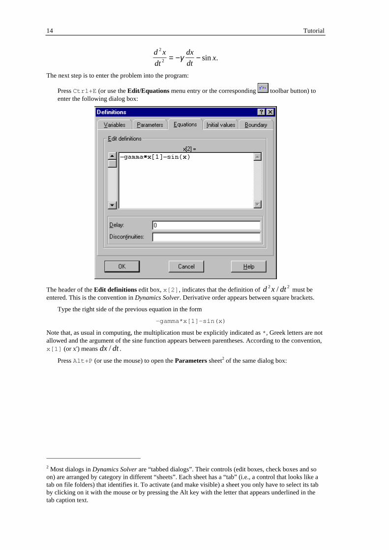
The next step is to enter the problem into the program:
Press Ctrl+E (or use the Edit/Equations menu entry or the corresponding toolbar button) toenter the following dialog box:
The header of the Edit definitions edit box, x[2] , indicates that the definition of d x dt2 2/ must beentered. This is the convention in Dynamics Solver. Derivative order appears between square brackets.
Type the right side of the previous equation in the form
-gamma*x[1]-sin(x)
Note that, as usual in computing, the multiplication must be explicitly indicated as * , Greek letters are notallowed and the argument of the sine function appears between parentheses. According to the convention,x[1] (or x') means dx dt/ .
Press Alt+P (or use the mouse) to open the Parameters sheet2 of the same dialog box:
2 Most dialogs in Dynamics Solver are “tabbed dialogs”. Their controls (edit boxes, check boxes and soon) are arranged by category in different “sheets”. Each sheet has a “tab” (i.e., a control that looks like atab on file folders) that identifies it. To activate (and make visible) a sheet you only have to select its tabby clicking on it with the mouse or by pressing the Alt key with the letter that appears underlined in thetab caption text.

Graphics Output 15
Type the name, gamma, and value, say 0, for the only parameter.
Press Enter or use the OK button to accept the definitions. The dialog box will close.
Graphics Output
The best Dynamics Solver feature is the ability to show the results of integration in graphics format. Totake advantage of this possibility, one or more graphics windows must be created.
Press Ctrl+G (or use the Output/New graph window menu entry or the corresponding toolbarbutton) to create a new graphics window. The Expressions sheet of the Graphics Output dialog boxwill open:

16 Tutorial
You can change many settings there, but press Enter or use the OK button to accept the default values.The dialog box will close.
Solving the Dynamical System
When a graphics window is active, you will see a flashing cross inside a circle in the center of thewindow. This is a cursor, the coordinates of which are displayed between parentheses in the middle panelof the status line3, and represent the initial values for the dependent variable, x , and its first derivative,x[1] . Because so far you have not chosen the initial conditions, they have the default null value.
Press the Left arrow. The cursor will move to a new point whose coordinates (-0.01,0) are updated inthe middle panel of the status line indicating that the initial value for x has changed from 0 to -0.01.
To change the initial condition for x[1] from 0 to 0.01, press the Up arrow. Hold down the Shiftkey and press again the Up key: the value for x[1] changes now faster!
Repeat the previous commands to select (-0.5,0.3) as initial conditions.
(You can also use the mouse pointer to select initial conditions. Locate the mouse pointer at thedesired point —the coordinates of the mouse pointer are permanently displayed in the right panel ofthe status line— and then double click on the left mouse button.)
To start the actual integration of the equation, press Enter (or use the Go/Start menu entry or the
corresponding toolbar button).
The solution appears as a curve in the (x,dx/dt) space, the so-called phase space. Since we are integratingthe undamped harmonic oscillator, the solution is periodic and appears on the screen as a clockwise curvethat repeats over itself.
Press Esc (or use the Go/Stop menu entry or the corresponding toolbar button) to stop theintegration.
3 The status line is the last line in the main window. It is used to display:
1. In the left panel: numerical results, information and help lines, or the kind of graphics elementbeing edited.
2. In the middle panel: the coordinates of the cursor indicating the initial condition (or the anglevalues of some graphics elements).
3. In the right panel: the coordinates of the mouse pointer.

Output Ranges 17
Output Ranges
Press Ctrl+F (or use the Output/Graphics format menu entry or the corresponding toolbarbutton) to open again the Expressions sheet of the Graphics Output dialog box:
Change the Min. x , Max. x, Min. y and Max. y entries and press Enter to select as new window thesquare -4< x, dx/dt <4.
Press Del (or use the Window/Erase window menu entry or the corresponding toolbar button)to erase the screen, where the old curve is still being displayed.
Use the mouse (and the arrow keys, if necessary) to select the initial condition (3,0) and then pressEnter to start the integration. The curve is no longer an ellipse, because now the pendulum startsfrom rest near its top position and the oscillation is harmonic only for small amplitudes.
To see how the curve repeats itself, press Del to erase the screen while the integration is still beingperformed. The closed solution will be drawn again.
Press Esc to stop the integration.
Try different initial conditions by moving the cursor (other ways of entering initial conditions andchoosing the window will be discussed later on) and using Enter and Esc .
You can also try different values of the parameter gamma.

18 Tutorial
Press Ctrl+A (or use the Edit/Parameters menu entry or the corresponding toolbar button) toopen again the Parameters dialog sheet:
By changing the values for gamma and repeating the integration (it will be useful to clear the screen fromtime to time as described before), you can see how the shape of the solution curve depends on gamma.For 0 < gamma < 1, we obtain the damped harmonic oscillator that spirals toward the center. For gamma> 1 one gets the overdamped cases.
If you want to save this first problem, use F2 as described in Saving and Loading a Problem.
Numerical Output
Now suppose you want numerical information about the solution while it is being drawn on the screen.
Press Ctrl+S (or use the Output/Status line menu entry or the corresponding toolbar button)to open the Numerical Output in Status Line dialog box:
Change the default value of Frequency from 0 (which means no numerical output) to 100, to indicatethat you want a numerical value every 100 points drawn on the screen. (Do not forget to press Enterto accept the new value.)
Press Enter to repeat the integration.

Output Quantities 19
Now, while the solution is being computed and displayed, you can see in the left panel of the status linethe changing numerical values of t and x. Numerical output is not restricted to the values of theindependent variable and the dependent variable: it is possible to have numerical information on anydesired expression, such as the energy of the system, for instance. Also, you can send numerical results toits own text window, to the printer or to an external file (to be processed by Dynamics Solver or otherprograms).
Output Quantities
You might prefer the values of t and x displayed in graphical format, rather than having them in numericalform; that is, a (t,x) plot of the solution instead of the default drawing of the (x,dx/dt) phase space. Youcan, in fact, plot in each axis any expression made up of the solution (even at different values of time), itsderivatives, and the parameters and initial conditions of the problem. (The full flexibility of the integratedexpression compiler will be described later.)
Press Ctrl+F (or use the Output/Graphics format menu entry or the corresponding toolbarbutton) to open again the Expressions sheet of the Graphics Output dialog box:
Change the Horizontal axis and Vertical axis entries to read t and x , respectively.
Change also the range displayed in the horizontal axis (which will now display the ever-increasingpositive value of t ) by setting Min. x to 0 and Max. x to 50 to display the range 0 < t < 50. Set alsoMin. y to -4 and Max. y to 4 to display the range -4 < x < 4.
Press Enter to close the dialog box.
Press Del (or use the Window/Erase window menu entry or the corresponding toolbar button)to erase the screen, where the old curve is still being displayed.
Press Enter to repeat the integration. When the solution runs off the screen, stop it with Esc .
You will see x displayed against t: it is clearly different from the familiar sinusoid.

20 Tutorial
Depending of the initial values you selected the last time, you may have noticed that the solution did notstart at the position of the flashing cursor, which may be located outside the screen. This is not a bug inthe program, but it is due to the fact that you have changed the meaning of the axes used to display results.When used to input initial conditions, the cursor position still refers to the default x and x[1] . It will bedescribed later how to choose which variable, derivative, or parameter will have its initial value selectedon each axis by the cursor.
Example Files
In the previous sections you have seen how directly a problem can be entered and solved in DynamicsSolver. It has also been shown that several settings (output window, expressions in axes, initial conditions,parameter values, numerical results, etc.) can be easily changed. But there are many other possibilities inthe program. In order to get an overview of some of the more important ones, you will take advantage ofthe File/Open menu. Problem files will be used in the remaining of this tutorial to see what can be done inDynamics Solver. The remaining sections in the manual (or the Dynamics Solver help) will show youhow to do it.
To avoid typing definitions and setting options, you will load problem files from the EXAMPLES directoryin your Dynamics Solver directory. When each example is needed, use the procedure explained in Savingand Loading a Problem.
Keep in mind that these examples could also be quickly entered by hand and the problem easily saved tothe disk.
Systems of Equations
Dynamics Solver can solve not only a single equation, but also a system of equations. For instance,suppose you want to analyze the famous Lorenz equations:
( )dx
dty x
dy
dtrx y xz
dz
dtbz xy
= −
= − −
= − +
σ ,
,
.
Load LORENZ.DS in the EXAMPLES\CHAOS directory. If you are curious about how the problemhas been entered into Dynamics Solver, you can examine the entries discussed in previous sections.
You already know how to start solving the problem, after having changed the initial conditions ifnecessary, by using Enter .
You will see different projections of a beautiful orbit that stays forever in a well-defined region, but neverrepeats itself. Recall that you can erase the current window at any moment without interrupting the

Projections 21
integration by pressing Del . To erase all the windows, press Ctrl+Del or use the Window/Erase all
menu entry or the corresponding toolbar button)
The orbit wanders around a complicated object (a so-called strange attractor) in the three-dimensionalphase space, but you only see its projections on the different coordinate planes and one of the windowsshows a projection along a view line.
Projections
To get a better idea of the shape of a three-dimensional orbit, you can use the projections on the threecoordinate planes, (x,y), (y,z) and (x,z), as shown in three of the windows inEXAMPLES\ODES\TORUS.DS:
In Dynamics Solver you can also project the solution (in perspective or not) along an arbitrary direction,as shown in another window of the same problem.
From the previous figure it is rather clear that the orbit lies on a surface that has the form of a bagel (amathematical torus).
Another example of the same projection techniques is shown in EXAMPLES\CHAOS\LORENZ.DS.

22 Tutorial
Poincaré Sections
You can also see in the figure
that the section of the torus is not circular. Moreover, you can directly see this section in the windowentitled Poincaré section where the (x,z) coordinates of the points of intersection of the orbit withthe y = 0 plane are displayed.
Since successive solution points lying in this Poincaré section are located far away from each other, theywill look odd if joined by a segment.
This intersection of the orbit with a plane is a very specific Poincaré section, but Dynamics Solver is ableto compute rather general Poincaré sections. More interesting examples are computed in other problemfiles. For instance, one can see how works the “stretch-and-fold” mechanism in the strange attractor ofDuffing equation (see EXAMPLES\ODES\DUFFING2.DS)
Furthermore, the same basic mechanism used by Dynamics Solver to draw Poincaré sections can be usedto compute the periods of closed orbits and other quantities, as explained later.
Constrained Initial Conditions and Boundary Conditions
Projections and Poincaré sections are useful to obtain two-dimensional information from higher-dimensional systems. There is still another way to lower the dimension. In a Poincaré section one choosesfrom all the solutions only those points that satisfy a given condition. It is also possible to choose all the

Constrained Initial Conditions and Boundary Conditions 23
points, but only from those solutions that satisfy a certain condition. In Dynamics Solver, this can be doneby imposing a set of conditions on the initial values of the problem. This allows analyzing subspaces ofthe full phase space of the problem.
For example, consider the Hénon-Heiles system, i.e., the Hamiltonian system corresponding to thepotential
( )V x y x y x y y( , ) .= + + −1
2
1
32 2 2 3
The energy is a conserved quantity. If you are interested only in those solutions corresponding to a givenvalue of the energy, you can choose at will the initial values for x, y and dy/dt, for instance, and then usethe energy value and its definition to select dx/dt. You can easily instruct Dynamics Solver to do thatautomatically. The solutions corresponding to a certain energy value span the so-called “energy surface,”which has three dimensions. One can then take a Poincaré section of this energy surface by selecting, forinstance, the points at which x = 0. This will give a two-dimensional plot that can be obtained by using theexample in EXAMPLES\CHAOS\HENONHEI.DS.
In the left panel of the status line you can see the values of time t and energy E. Since the last quantityshould be conserved, you can check if it really remains unchanged; this gives you a measure of theintegration quality.
If you now disable the numerical output (by using Output/Status line and setting the Frequency entry tozero), set the energy value to E = 0.125 (by using Edit/Parameters), and select different initialconditions, you can obtain the following classical plot:
As will be explained in other sections, constrained initial conditions are useful not only to analyze energysurfaces and more general subspaces of the phase space of a problem, but also to solve in DynamicsSolver complex problems that do not appear in one of the simple forms discussed so far. Note also that,though only a single Poincaré condition can be imposed in Dynamics Solver, you can impose oneadditional condition for each initial value. These conditions need not be constants of motion of theproblem. It is also possible to use constrained conditions that are not solved for the initial values.
Finally, Dynamics Solver may handle a very general class of boundary conditions. Run the example inEXAMPLES\QUANTUM\HARMONIC.DS to obtain numerically the well-known energy spectrum andwave functions of the quantum harmonic oscillator:

24 Tutorial
Numerical Simulation
Dynamics Solver is a good tool for numerical simulation of complex systems. For instance, by sendingmultiple output to a single window you may see how evolve three stars under their mutual gravitationalattraction. A classical examples is solved in EXAMPLES\MECH\BURREAU.DS:
You may also see in real time how chaotic scattering happens in EXAMPLES\CAHOS\DISKSCAT.DS:

Functional-Differential Equations and Text Output 25
Functional-Differential Equations and Text Output
Dynamics Solver can also solve many functional-differential equations. For instance, some arguments canbe taken at different values of the independent variable. Consider the following delay-differential equationas an example:
x t x t x ta•
= + − +( ) ( ) ( ) .12
The only non-simultaneous element of this equation is the second term on the right side. It corresponds toa retarded value, t-1, of the independent variable. In consequence, in this problem the delay is constantand equal to 1. If you load EXAMPLES\DELAY\DELAY1.DS, you will see solutions corresponding todifferent nonlinear initial conditions in the form:
x t x v t t t( ) ( ), .= + + − ≤ ≤0 02 1 0for
In the left window the solution is displayed in graphics format while the right window is used to display,in text format, a more complex quantity: the second derivative of the solution divided by the parameter a.On the order hand, you may be surprised that the solution plot does not start at the point where the cursorwas located. This is because the solutions of delay-differential equations have a discontinuity in the firstderivative of the solution at the point where the first step starts (t=0 in this example). As will be explainedelsewhere, Dynamics Solver can deal with these discontinuities. In the example just loaded, this has been

26 Tutorial
accomplished simply by selecting 1 in the Delay entry, after using Ctrl+E (or the Edit/Equations menu
entry or the corresponding toolbar button) to enter the following dialog box:
Numerical Quadrature
Dynamics Solver is able to compute numerically an integral in the form:
=I f t dta
b
( ) .∫ In the example in EXAMPLES\NUMERIC\ELLIPTIC.DS , you can see the Legendre elliptic integral offirst kind
∫−
u
vm
dvmu
0 2sin1=)|F(
compared with the value returned by the built-in function EllipticF . The result appears in numericalform in a text window:
F( 0,0.35) = 0 (= 0 ) F( 0.1,0.35) = 0.100058308406611 (= 0.100058308406611) F( 0.2,0.35) = 0.200465856018663 (= 0.200465856018663) F( 0.3,0.35) = 0.301568679040681 (= 0.301568679040681) F( 0.4,0.35) = 0.403705717550479 (= 0.403705717550479) F( 0.5,0.35) = 0.507203524076695 (= 0.507203524076695) F( 0.6,0.35) = 0.612368848706666 (= 0.612368848706666) F( 0.7,0.35) = 0.719478402127162 (= 0.719478402127164) F( 0.8,0.35) = 0.828765240551856 (= 0.828765240551861) F( 0.9,0.35) = 0.94040157950294 (= 0.940401579502963) F( 1,0.35) = 1.0544785484357 (= 1.0544785484357 ) F( 1.1,0.35) = 1.17098453149242 (= 1.17098453149242 ) F( 1.2,0.35) = 1.28978524551951 (= 1.28978524551951 ) F( 1.3,0.35) = 1.41061024239575 (= 1.41061024239575 ) F( 1.4,0.35) = 1.53305137237861 (= 1.53305137237861 ) F( 1.5,0.35) = 1.65657797218095 (= 1.65657797218095 )
Discrete Dynamical Systems 27
F( 1.5708,0.35) = 1.74435059748001 (= 1.74435059697121 )
Discrete Dynamical Systems
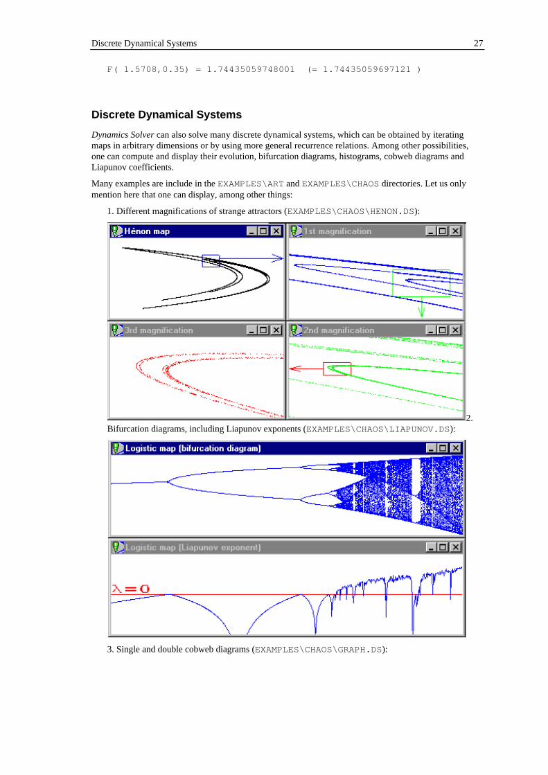
Dynamics Solver can also solve many discrete dynamical systems, which can be obtained by iteratingmaps in arbitrary dimensions or by using more general recurrence relations. Among other possibilities,one can compute and display their evolution, bifurcation diagrams, histograms, cobweb diagrams andLiapunov coefficients.
Many examples are include in the EXAMPLES\ART and EXAMPLES\CHAOS directories. Let us onlymention here that one can display, among other things:
1. Different magnifications of strange attractors (EXAMPLES\CHAOS\HENON.DS):
2.Bifurcation diagrams, including Liapunov exponents (EXAMPLES\CHAOS\LIAPUNOV.DS):
3. Single and double cobweb diagrams (EXAMPLES\CHAOS\GRAPH.DS):

28 Tutorial
4.More sophisticated graphics, as the “devil's staircase” displayed below(EXAMPLES\CHAOS\DEVIL.DS):
Function Graphs and Parametric Curves
You can also use Dynamics Solver to plot the graph of a function by solving a trivial differential equation,such as dy/dx = 0, and inserting the function definition in the Horizontal axis and Vertical axis entries.For instance, in EXAMPLES\DRAWING\GAMMA.DS the graph of the Euler Γ function is drawn:

Function Graphs and Parametric Curves 29
Parametric curves in the plane are also readily obtained in a similar way. For instance,EXAMPLES\DRAWING\LISSAJOU.DS lets you draw the Lissajous curves defined as:
x at b
y ct d
= += +
cos( ),
cos( ).
In this example you can select c and d with the cursor and a and b by using the Parameters dialog sheet
(which can be obtained by pressing Ctrl+A , the Edit/Parameters menu entry or the corresponding toolbar button)).
It is also possible to draw projections of three-dimensional curves. You can see Lissajous figures in threedimensions by loading EXAMPLES\DRAWING\LISSAJO3.DS.
A better way to plot functions and to draw curves (and other graphics elements) is described in the nextsection of this tutorial: Drawing with Dynamics Solver.

30 Tutorial
Drawing with Dynamics Solver
Dynamics Solver can be used to draw rather complex figures including segments, circles, ellipses,parametric curves in two and three dimensions, text strings (with Latin, Greek and Cyrillic letters),arrowheads, points and lines from external data files and a large class of fractal curves. This ability is veryuseful to add lettering and other informative elements to a problem solution (as illustrated in differentexample problem files)
or when preparing drawings for courseware material and research papers:
Several interesting examples are included in the EXAMPLES\DRAWING and EXAMPLES\FRACTALdirectories. Let us mention here another (better) way to draw Lissajous figures

Decorative Examples 31
and a typical fractal curve:
Decorative Examples
Dynamics Solver can also be used to get some artistic (!?) drawings as in many examples included in theEXAMPLES\ART and EXAMPLES\CHAOS directories. Let us only mention the following problem files:

32 Tutorial
1. EXAMPLES\CHAOS\HENONMAP.DS:
2. EXAMPLES\ART\COS1.DS:
High-Resolution Drawings
So that the user can see exactly what the screen looks like, the figures in this tutorial are direct screendumps, and they have in consequence a rather low resolution. Needless to say, graphics screens can beprinted, in different resolutions, by using standard Windows procedures.
On the other hand, Dynamics Solver can produce very high quality drawings (including lettering) by usingthe highest resolution available in your printer or plotter. You may also export graphics (and text) instandard formats (bitmaps, metafiles, Encapsulated Postscript, etc.) to be used by external wordprocessors or text formatters (like TEX and LATEX).
This rather complex topic is described in detail in the Printing section.

Extending Dynamics Solver 33
Extending Dynamics Solver
Dynamics Solver has very powerful built-in features, but they can be extended in different ways to dealwith very complex problems:
• New integration methods may be written in any programming language and used from DynamicsSolver. Examples in C, Pascal and FORTRAN are provided.
• Special functions (as well as very complex expressions that would be evaluated too slowly by theintegrated compiler) may be written in any programming language and used from Dynamics Solver.Examples in C, Pascal and FORTRAN are provided.

34 Running Dynamics Solver
Manual
Running Dynamics Solver
This chapter describes the different ways to start the program and the problem files.
Starting Dynamics Solver
One usually starts Dynamics Solver by choosing its icon from the Start/Programs/Dynamics Solver menu(or, under Windows 3.1+, by double clicking with the left mouse button on the Dynamics Solver icon inthe Dynamics Solver group of Program Manager). Dynamics Solver will start after a short initializationand you will see the tip window (if it is not disabled) over the main window:
You can also start Dynamics Solver (or, directly, a problem file4) by means of any of the usual proceduresto start Windows applications and documents:
1. Icons in Program Manager groups (or My PC folders).
2. Entries in File Manager, Start menu or Explorer.
3. The Start/Execute menu or the File/Execute command in Program Manager or File Manager..
4. One of the many applications that let you run Windows programs and documents (even from DOSboxes).
4 A “problem file” is an ASCII file containing the data for a problem (differential system, discretedynamical system or set of drawings) that can be analyzed by means of Dynamics Solver. Its defaultextension is .DS .

Previous instances 35
5. Under Windows 95/98/NT4, the program may be started from the command line in a DOS box. Aproblem file may be directly opened by using the start command.
Previous instances
If there is another instance of Dynamics Solver running when the program is started directly with noproblem file appended after its file specification, or when the same problem file is being analyzed byanother copy of the program, the following dialog will open:
You can select there one of the problem files which are already open or start a new copy of the program. Itis also possible to cancel the operation. To start always a new copy of the program you may disable theCheck previous instances entry of the Preferences/Other dialog box which opens when using theConfiguration/Preferences menu.
Command line options
In most cases the command line used to run the program by any method includes only its filespecification:[path]dsolver[.exe](c:\dsolver\dsolver.exe , for instance).The program path is optional if the program is in the current directory or in the PATH. Under Windows95/98/NT4, if the program is correctly installed, it is also optional in all cases but running it from a DOSbox, in which casestart dsolver[.exe]will be enough.
To start a problem file directly the syntax is:[path]dsolver[.exe] problemwhere problem is the complete file specification of the problem file.In many cases (short cuts in My PC, the Start menu or Explorer, Program Manager icons, the Executeentry of Explorer, Program Manager, or many other programs) the program specification is optional andit may be replaced by start in a DOS box under Windows 95/98/NT4.
When a problem file is opened you may change the corresponding definition in any way and Enter oruse the Go/Start menu to start solving it. If you want the problem to be automatically solved after it isloaded, use one of the following command lines:[path]dsolver[.exe] /r problem[path]dsolver[.exe] /x problem

36 Running Dynamics Solver
The difference lies in the fact that in the latter case (using /x) the program will exit when the solutionends, unless an errors happens. In the event of an error you will have an opportunity to see it and theprogram must be closed manually, as when /r is used. To be useful, when using /x you should probablymake the program send some output to external files (see Output and output files).
To print a problem file, you may select the corresponding entry in the menu that opens when right clickingon the problem file icon in My PC or Explorer, or in the File menu of Program Manager. To print thesame problem in the default printer you may also execute the program followed by /p and the problemfile name, in the form:[path]dsolver[.exe] /p problem
Under Windows 95/98/NT4 you may drag the problem and drop it over any installed printer or, if you arean advanced user, execute the following equivalent command line:[path]dsolver[.exe] /pt problem device driver outputwhere device is the printer name (say, HP Deskjet), driver the printer driver (for instance, HPDSKJET)and output the output port (LPT1: , FILE: , etc.)

Single Equations and First-Order Systems 37
Dynamical Systems
This chapter first describes the types of dynamical systems that can be analyzed with Dynamics Solver andthen discuss how to write them into the appropriate mathematical form. Finally we describe the way toenter these dynamical systems into the program.
Single Equations and First-Order Systems
Apart form other classes of dynamical systems that will be described later, Dynamics Solver may handledirectly, with no previous modification, with the following types of ordinary differential equations:
1. A single first-order equation written in the normal form
dy
dxf x y= ( , ), (1)
as, for instance, the disintegration law:
.Ndt
dN −= (2)
Note that in Equation (1) the unknown is y while x is the independent variable, but in (2) the dependentvariable is N and t is the independent variable.
2. A single equation of arbitrary order solved for the highest-order derivative:
d x
dtf t x
dx
dt
d x
dt
n
n
n
n=
−
−, , ,..., .1
1 (3)
A well-known example is given by the equation of motion of the simple pendulum:
.0sin2
2
=++ θθγθl
g
dt
d
dt
d(4)
3. A system of n first-order equations written in normal form:
( )
( )
( )
dx
dtf t x x
dx
dtf t x x
dx
dtf t x x
n
n
nn n
11 1
22 1
1
=
=
=
, ,..., ,
, ,..., ,
...
, ,..., .
(5)
In the previous chapter, for instance, we saw the Lorenz equations:
( )dx
dty x
dy
dtrx y xz
dz
dtbz xy
= −
= − −
= − +
σ ,
,
.
(6)
Of course, it is not claimed that all the equations or systems of the previous types can be solved byDynamics Solver, but only that they have the right form to be directly handled by the program. To have areasonably good numerical solution, the functions appearing in their definition must be “well behaved,”

38 Dynamical Systems
and there is no easy way to know if this is true or not for a given problem. (The interested user may referto a textbook on numerical analysis; see the Bibliography .) Fortunately, many interesting problemsarising in practice (in physics, mathematics and engineering) can be successfully analyzed by usingDynamics Solver.
Higher Order Systems
To handle systems of equations of order higher than first order, you can always rewrite them in the formof a first-order system by introducing additional variables. The idea is to treat each derivative but the lastas a new variable. The procedure, which is fully described in any textbook on differential equations, canbe easily understood in an example. Let us consider the equations of motion of a point particle of mass mmoving in the gravitational field of another mass M held at rest at the origin of coordinates. Newtonequations of this Kepler problem are
md
dtG
mM
r r
2
2 2
r r= − . (7)
As a consequence of the angular momentum conservation, you can always choose the coordinate system insuch a way that the motion is confined to the (x,y) plane. The nontrivial components of (7) are, then, twosecond-order equations:
( )
( )
d x
dt
GMx
x y
d y
dt
GMy
x y
2
2 2 2 3 2
2
2 2 2 3 2
= −+
= −+
/
/
,
.
(8)
To write this system in a form Dynamics Solver can understand, the first-order derivatives (i.e., thevelocity components) must be considered as new variables. If one uses the names u = dx/dt and v = dy/dt,system (8) can be written in the form of a system of four first-order equations:
( )
( )
dx
dtu
dy
dtv
du
dt
GMx
x y
dv
dt
GMy
x y
=
=
= −+
= −+
,
,
,
.
/
/
2 2 3 2
2 2 3 2
(9)
In a similar way, you can always lower the order of equations by introducing new dependent variables andthe corresponding new equations.
Equations Not Written in Normal Form
Dynamics Solver understand only equations written in “normal form,” that is, solved for the highest-orderderivative. When this is not true the system must rewritten. For example, let us assume that we do notknow the elementary exact solution of the Friedmann equation for for the radius R of a closed universe:

Functional-Differential Equations 39
dR
dt R
= −
21
1 (10)
Dynamics Solver understand only equations written in “normal form,” that is, solved for the highest orderderivative. When this is not true the system must rewritten. For example, let us assume that we do notknow the elementary exact solution of the Friedmann equation for for the radius R of a closed universe:
One can split Equation (10) in two equations of first order:
dR
dt R= −1
1 (11)
and
dR
dt R= − −1
1 (12)
The square root appearing in the right side of both equations will lead to numerical difficulties. If in thenumerical integration and due to accumulated numerical errors the argument of the square root becomes avery tiny but negative number, which would raise an error. Moreover, the solution of (11) corresponds toan ever-increasing universe radius while in (12) the solution is always decreasing. However, the physicalsolution switches from one equation to the other: it starts with a null radius R (the “big bang”) andincreases according to Equation (11) until R = 1, when both sides of Equation (11) vanish and the solutionalso satisfies (12) and will start decreasing until R = 0 (the “big crunch”).
In this particular case, all these problems can be solved with a bit of ingenuity by using the Backwardfunction, as shown in FRW1.DS. It is enough to integrate forward according the Equation (12) andbackward using Equation (11).
There is also another possibility: by taking the derivative of (10) you obtain:
d R
dt R
2
2 2
1
2= − (13)
which appears in normal form and can be used both for forward and backward integration, as inFRW2.DS.
Note, however, that although derivatives can be used in many cases to write the problem in normal form,the new equation or system is not equivalent to the original one. It has all the solutions of the latter and, ingeneral, a lot more. In principle, the solutions of the original problem can always be selected by choosingthose initial conditions that satisfy it (it will be shown in the next chapter that this can be easily done inDynamics Solver). Nevertheless, in some cases the unavoidable numerical errors will give a numericalsolution that is only a reasonable approximation to a solution of the derived system and does not satisfythe original equations. If this happens (and Dynamics Solver can be used to know if it actually happens),you cannot use this method of taking derivatives.
Functional-Differential Equations
Among the most original features of Dynamics Solver we may mention its ability to solve a large class offunctional-differential equations. For instance, it can deal with differential-difference equations that can bewritten in normal form with right sides containing previous values of the variables. For instance, the Ikedaequation
( )dx
dtt x t A B x t r( ) ( ) cos ( ) ,= − + + −2 1 2 (14)
has a single constant delay r, while the following retarded modification (with two constant delays) of theclassical model of Kermack-McKendrick for epidemic propagation:

40 Dynamical Systems
dx
dtt x t y t y t
dy
dtt x t y t y t
dz
dtt y t y t
( ) ( ) ( ) ( ),
( ) ( ) ( ) ( ),
( ) ( ) ( ).
= − − + −
= − −
= − −
1 10
1
10
(15)
The delay may be variable, as in
( ).)()(2
2
txtdt
dxat
dt
xd −−= (16)
The only condition equations must satisfy is that all the arguments appearing on the right sides must haveknown values when they are evaluated. This is possible if they have been computed previously or if theyare specified as part of the initial conditions of the problem, as discussed in the next chapter.
In some complex cases the already mentioned tricks of introducing new variables and taking derivatives ofthe equations can help to put the equations in the correct form. For instance, let us consider two electronsthat are held at rest at positions -x(0) and x(0) and then released when t = 0. If the radiation reaction isneglected, the classical relativistic equation of motion of each electron is given, in appropriatedimensionless variables, by
( )x t
x t
x t x t r
x t r
x t r
••
••
•=−
+ −− −
+ −( )
( )
( ) ( )
( )
( ),
/
11
1
2 3 2
2 (17)
where the delay r is given by the condition
( ) + ( - ) = x t x t r r . (18)
Since the delay is in fact an unknown, instead or the functional equation (18), it is better to use thedifferential equation one obtains by taking the derivative of (18). The final system now read
( )( )
( )( )
( )( )
x t v t
v tv t
x t x t r t
v t r t
v t r t
r tv t v t r t
v t r t
•
•
•
=
=−
+ −− −+ −
=+ −
+ −
( ) ( ),
( )( )
( ) ( ( ))
( )
( ),
( )( ) ( )
( ).
/1 1
1
1
2 3 2
2 (19)
with the initial constraint
r(0)=2x(0). (20)
Among the retarded arguments there can appear not only the solution but also some of its derivatives, aswill be shown below.
Discontinuities in Functional-Differential Equations
The actual integration of delay-differential equations is performed in steps of length equal to the delay.This “method of steps” is able to solve a large class of functional-differential equations. Note that the steplength will not be constant if the delay changes. An unavoidable characteristic of this method is that thesolutions, in general, have discontinuities in their derivatives at the points separating contiguous steps.(This problem is discussed in the textbooks cited in the Bibliography .) In order to improve the quality of
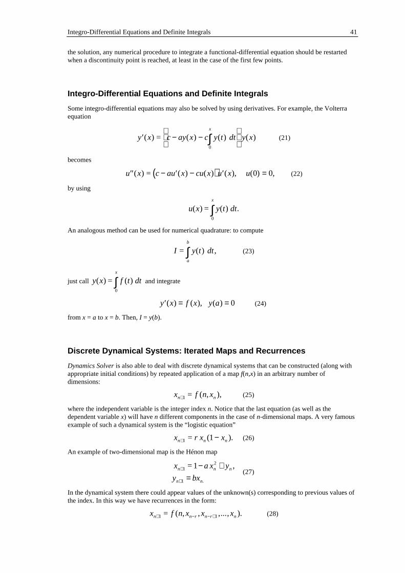
Integro-Differential Equations and Definite Integrals 41
the solution, any numerical procedure to integrate a functional-differential equation should be restartedwhen a discontinuity point is reached, at least in the case of the first few points.
Integro-Differential Equations and Definite Integrals
Some integro-differential equations may also be solved by using derivatives. For example, the Volterraequation
( ) =′ − −
∫y x c ay x c y t dt y x
x
( ) ( ) ( )0
(21)
becomes
( ) ( ) =′′ − ′ − ′ =u x c au x cu x u x u( ) ( ) ( ), ( ) ,0 0 (22)
by using
( ) =u x y t dtx
( ) .0∫
An analogous method can be used for numerical quadrature: to compute
=I y t dta
b
( ) ,∫ (23)
just call ( ) =y x f t dtx
( )0∫ and integrate
′ = =y x f x y a( ) ( ), ( ) 0 (24)
from x = a to x = b. Then, I = y(b).
Discrete Dynamical Systems: Iterated Maps and Recurrences
Dynamics Solver is also able to deal with discrete dynamical systems that can be constructed (along withappropriate initial conditions) by repeated application of a map f(n,x) in an arbitrary number ofdimensions:
= ( ,x f n xn n+1 ), (25)
where the independent variable is the integer index n. Notice that the last equation (as well as thedependent variable x) will have n different components in the case of n-dimensional maps. A very famousexample of such a dynamical system is the “logistic equation”
=x r x xn n n+ −1 1( ). (26)
An example of two-dimensional map is the Hénon map
=x ax y
y bxn n n
n n
+
+
− +=
12
1
1 ,
.
(27)
In the dynamical system there could appear values of the unknown(s) corresponding to previous values ofthe index. In this way we have recurrences in the form:
= ( ,x f n x x xn n r n r n+ − − +1 1, ,..., ). (28)

42 Dynamical Systems
For example, the Fibonacci numbers can be defined by the recurrence
F F F F Fn n n+ −= + = =1 1 0 1 1, ( ). (29)
Though this last kind of dynamical systems, recurrences, can be directly entered in Dynamics Solver (seethe example DELAY\FIBONAC.DS), it is far more convenient to write them in the form of an equivalentiterated map by introducing new unknowns:
F F G G F F Gn n n n n+ += + = = =1 1 0 0 1, , ( ). (30)
Problem Parameters
As shown in previous sections, you can include parameters in the definition of equations and systems, andyou can easily enter and change their values and names.
If you are planning to do an exhaustive analysis of a system you should expend some time identifying theessential parameters in the problem. For instance, in the pendulum equation two parameters appear: theacceleration of gravity g and the pendulum length l, but none of them is essential. To start with, only itsquotient g/l appears and, by choosing its square root as time unit, even this disappears to let
d
dt
2
20
θ θ+ =sin . (31)
This shows that, except for a trivial change of scale, there is essentially only one mathematical pendulum.In a similar way, some of the examples already mentioned can be simplified by carefully choosing theunits of measure. Other examples, such as the Friedmann equation (10), have already been presented interms of appropriate dimensionless quantities.
Of course, in many problems there are essential parameters that cannot be eliminated in this way. Forinstance, if you add a friction term to the pendulum equation,
d
dt Q
d
dt
2
2
10
θ θ θ+ + =sin . (32)
you cannot simultaneously get rid of the quality factor Q and the quotient g/l. In fact, the solution of (26)changes qualitatively with Q, as you probably know.
Complex Numbers
Dynamics Solver does not directly understand complex numbers. So, you must separate the real andimaginary parts of every complex quantity. For example, let us consider the following complex system,which arises in the modeling of a very long Fabry-Pérot cavity. The unknowns are the real quantity x andthe complex f. The dynamical equation for x is
d x
dt Q
dx
dtx x A f
2
2 02 21+ + + = sin ,θ (33)
while the evolution equation for f is a functional one
f t e f t rix t r( ) cos ( ),( )= + −−1 θ (34)
where the delay r is given in
r rx t x t r x
cs= + + − −
0
2( ) ( ). (35)
A Q x r cs, , , ,θ 0and are free parameters and x0 is defined as
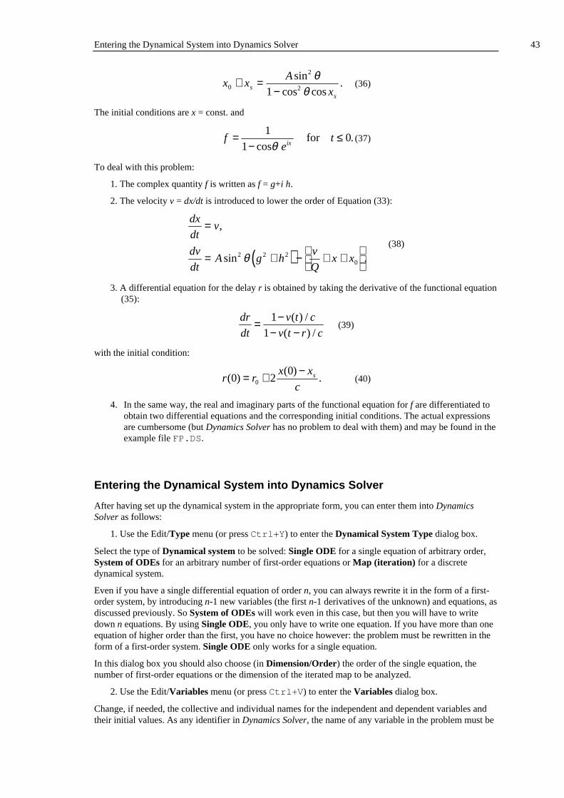
Entering the Dynamical System into Dynamics Solver 43
x xA
xss
0
2
21+ =
−sin
cos cos.
θθ
(36)
The initial conditions are x = const. and
fe
tix
=−
≤1
10
cos.
θfor (37)
To deal with this problem:
1. The complex quantity f is written as f = g+i h.
2. The velocity v = dx/dt is introduced to lower the order of Equation (33):
( )
dx
dtv
dv
dtA g h
v
Qx x
=
= + − + +
,
sin .2 2 20θ
(38)
3. A differential equation for the delay r is obtained by taking the derivative of the functional equation(35):
dr
dt
v t c
v t r c= −
− −1
1
( ) /
( ) /(39)
with the initial condition:
r rx x
cs( )
( ).0 2
00= + −
(40)
4. In the same way, the real and imaginary parts of the functional equation for f are differentiated toobtain two differential equations and the corresponding initial conditions. The actual expressionsare cumbersome (but Dynamics Solver has no problem to deal with them) and may be found in theexample file FP.DS.
Entering the Dynamical System into Dynamics Solver
After having set up the dynamical system in the appropriate form, you can enter them into DynamicsSolver as follows:
1. Use the Edit/Type menu (or press Ctrl+Y ) to enter the Dynamical System Type dialog box.
Select the type of Dynamical system to be solved: Single ODE for a single equation of arbitrary order,System of ODEs for an arbitrary number of first-order equations or Map (iteration) for a discretedynamical system.
Even if you have a single differential equation of order n, you can always rewrite it in the form of a first-order system, by introducing n-1 new variables (the first n-1 derivatives of the unknown) and equations, asdiscussed previously. So System of ODEs will work even in this case, but then you will have to writedown n equations. By using Single ODE, you only have to write one equation. If you have more than oneequation of higher order than the first, you have no choice however: the problem must be rewritten in theform of a first-order system. Single ODE only works for a single equation.
In this dialog box you should also choose (in Dimension/Order) the order of the single equation, thenumber of first-order equations or the dimension of the iterated map to be analyzed.
2. Use the Edit/Variables menu (or press Ctrl+V ) to enter the Variables dialog box.
Change, if needed, the collective and individual names for the independent and dependent variables andtheir initial values. As any identifier in Dynamics Solver, the name of any variable in the problem must be
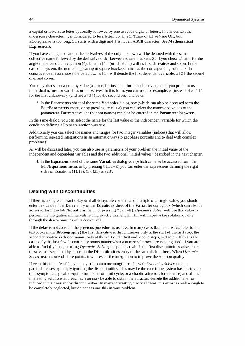
44 Dynamical Systems
a capital or lowercase letter optionally followed by one to seven digits or letters. In this context theunderscore character, _, is considered to be a letter. So, t , s1 , Time or time0 are OK, butalongname is too long, 1t starts with a digit and á is not an ASCII character. See MathematicalExpressions.
If you have a single equation, the derivatives of the only unknown will be denoted with the samecollective name followed by the derivative order between square brackets. So if you chose theta for theangle in the pendulum equation (4), theta[1] (or theta' ) will its first derivative and so on. In thecase of a system, the number appearing in square brackets indicates the corresponding subindex. Inconsequence if you choose the default x , x[1] will denote the first dependent variable, x[2] the secondone, and so on..
You may also select a dummy value (a space, for instance) for the collective name if you prefer to useindividual names for variables or derivatives. In this form, you can use, for example, x (instead of x[1] )for the first unknown, y (and not x[2] ) for the second one, and so on.
3. In the Parameters sheet of the same Variables dialog box (which can also be accessed form theEdit/Parameters menu, or by pressing Ctrl+A ) you can select the names and values of theparameters. Parameter values (but not names) can also be entered in the Parameter browser.
In the same dialog, you can select the name for the last value of the independent variable for which thecondition defining a Poincaré section was true.
Additionally you can select the names and ranges for two integer variables (indices) that will allowperforming repeated integrations in an automatic way (to get phase portraits and to deal with complexproblems).
As will be discussed later, you can also use as parameters of your problem the initial value of theindependent and dependent variables and the two additional “initial values” described in the next chapter.
4. In the Equations sheet of the same Variables dialog box (which can also be accessed form theEdit/Equations menu, or by pressing Ctrl+E ) you can enter the expressions defining the rightsides of Equations (1), (3), (5), (25) or (28).
Dealing with Discontinuities
If there is a single constant delay or if all delays are constant and multiple of a single value, you shouldenter this value in the Delay entry of the Equations sheet of the Variables dialog box (which can also beaccessed form the Edit/Equations menu, or pressing Ctrl+E ). Dynamics Solver will use this value toperform the integration in intervals having exactly this length. This will improve the solution qualitythrough the discontinuities of its derivatives.
If the delay is not constant the previous procedure is useless. In many cases (but not always: refer to thetextbooks in the Bibliography ) the first derivative is discontinuous only at the start of the first step, thesecond derivative is discontinuous only at the start of the first and second steps, and so on. If this is thecase, only the first few discontinuity points matter when a numerical procedure is being used. If you areable to find (by hand, or using Dynamics Solver) the points at which the first discontinuities arise, enterthese values separated by spaces in the Discontinuities entry of the same dialog sheet. When DynamicsSolver reaches one of these points, it will restart the integration to improve the solution quality.
If even this is not feasible, you may still obtain meaningful results with Dynamics Solver in someparticular cases by simply ignoring the discontinuities. This may be the case if the system has an attractor(an asymptotically stable equilibrium point or limit cycle, or a chaotic attractor, for instance) and all theinteresting solutions approach it. You may be able to obtain the attractor, despite the additional errorinduced in the transient by discontinuities. In many interesting practical cases, this error is small enough tobe completely neglected, but do not assume this in your problem.

Initial Conditions for Ordinary Differential Equations 45
Initial Values
We saw in Dynamical Systems how to define the equation(s) corresponding to a dynamical system andthe way to enter them into Dynamics Solver; but in order to have a well-posed mathematical probleminitial conditions or boundary conditions are also needed. This chapter describes the form in which initialconditions must be specified and entered into Dynamics Solver. Boundary Conditions will be consideredin the next chapter.
See also Repeated Integration/Iteration and Phase Portraits,
Initial Conditions for Ordinary Differential Equations
In the case of a first-order differential equation in normal form,
dx
dtf t x= ( , ), (41)
a well-posed initial value problem requires the initial value of the unknown at the initial value of theindependent variable:
x t x( ) .0 0= (42)
For a single equation of order n,
d x
dtf t x
dx
dt
d x
dt
n
n
n
n=
−
−, , ,..., ,1
1 (43)
the n initial values of the unknown and its first n-1 derivatives must be given:
x t x
dx
dtt
dx
dt
d x
dtt
d x
dt
n
n
n
n
( ) ,
( ) ,
. . .
( ) .
0 0
00
1
1 0
1
10
=
=
=
−
−
−
−
(44)
A system of n first-order equations,
( )
( )
( ),,...,,
...
,,...,,
,,...,,
1
122
111
nnn
n
n
xxtfdt
dx
xxtfdt
dx
xxtfdt
dx
=
=
=
(45)
needs the n initial values of the n unknowns:
x t x
x t x
x t xn n
1 0 10
2 0 20
0 0
( ) ,
( ) ,
...
( ) .
==
=
(46)

46 Initial Values
Constrained Initial Conditions
In some cases you may want to have the value of one or some initial values defined in terms of the valuesof other initial conditions or parameters. For instance, if you want to explore a subspace of the phasespace of the problem, you must make sure that initial conditions lay in that subspace.
In the Kepler problem discussed in Dynamical Systems, you may want to parameterize it in terms of thetwo main constants of motion: the energy
( )E u vx y
= + −+
1
2
12 2
2 2(47)
and the angular momentum
L xv yu= − . (48)
(A system of units has been selected in which m =1 and GM = 1. Recall the discussion in ChoosingParameters.) The definitions of these constants of motion can be solved for the velocity to give:
( )
( )
ux x y E x y L Ly
x y
vy x y E x y L Lx
x y
=+ + + − −
+
=+ + + − +
+
2 2
2 2
2 2 2 2 2
2 2
2 2 2 2 2
2 2
,
.
(49)
You can now then select at will the initial values of the coordinates x and y and then compute the initialcomponents of the velocity by using Equation (49). Actually, you are not completely free when selectingx0and y0 , because they must satisfy the condition that the argument in the first square root of Equation
(49) cannot be negative! If you try values that do not satisfy this condition, Dynamics Solver will issue anerror message.
Constrained initial conditions must also be used when additional variables have been introduced or theoriginal equations have been differentiated. This has been already discussed in Dynamical Systems, inwhich these procedures have been suggested to rewrite equations in a more appropriate form. Forexample, if you take the derivative of the Friedmann equation,
dR
dt R
= −2
11, (50)
to obtain
d R
dt R
2
2 2
1
2= − , (51)
you can choose the initial value of R, but its derivative must satisfy the original equation:
dR
dt R
= ± −0 0
11. (52)
Sometimes, the constraints are conserved along the exact solution of the system. This is the case in thetwo examples described above, because the constraints were constants of motion (i.e., first integrals) ofthe resulting system. It should be obvious that the inherent errors of every numerical calculation willdegrade the accuracy of the imposed constraints as the independent variable increases. In some cases thisis not a real problem, but if the constraints are unstable, the error can grow very quickly, leading to anunacceptable solution. This problem may be completely unavoidable due to mathematical instabilities andthe approximate nature of numerical computations.

Initial Conditions for Functional-Differential Equations 47
You should always (or, at least, in some preliminary runs) monitor from time to time the conservedconstraints to see if they are stable or not. This task can be easily carried out in Dynamics Solver, asdescribed in Output Parameters.
In fact, this kind of problem can arise even in very simple cases. Often it is practically impossible tocompute numerically an unstable solution. Suppose you want to compute:
′′ = = ′ = −y y y y100 0 1 0 10, ( ) , ( ) . (53)
The solution is y = exp(-10x), but the general solution of (53) is y = A exp(-10x)+B exp(10x) for arbitraryconstants A and B. Because of numerical errors, the solution, which starts as an approximation to exp(-10x), becomes an approximation to something like A exp(-10x)+B exp(10x) with very low values for A-1and B. Since the second term grows exponentially while the first decreases, the numerical solution willquickly go to infinity, while the exact one goes to 0! (See the example in ODES\UNSTABLE.DS. )
Nevertheless, in many cases good approximations to unstable solutions can be computed by integratingbackward in time. For example, the so-called “stable manifold” of a saddle point in a two-dimensionaldynamical system (refer to the textbooks in the Bibliography , if you do not understand this paragraph) isan unstable solution, but a reasonable approximation can be easily computed integrating backward from apoint near the equilibrium point. See, for instance, the example in MECH\PENDULUM.DS where the“stable manifold” and the “unstable manifold” of a saddle point can be computed by starting very close tothe fixed point and integrating in both directions.
See also Boundary Conditions.
Initial Conditions for Functional-Differential Equations
With functional-differential equations, it is not enough to specify a finite number of initial conditions: fullfunctions must be provided instead. The full discussion of this topic lies out of the scope of this manual,but there is a rule of thumb that will work in most practical cases: you must provide all the informationneeded to have known values for the arguments in the functions defining the equations for every value ofthe independent variable in the range you are interested in. In other words, you must specify the valuesthat will be needed but not actually computed in the integration process.
For instance, suppose you want to solve Ikeda's delay-differential equation
( )dx
dtt x t A B x t r( ) ( ) cos ( ) ,= − + + −2 1 2 (54)
for t t≥ 0 . Due to the delay r, to evaluate the right side of Equation (54) when t t t r0 0≤ ≤ + , the values
of the solution x for t r t t0 0− ≤ ≤ must be known. Since they will not be computed in the integration
process, they must be provided in the form of initial conditions that in this case will be precisely the valueof x in the interval t r t t0 0− ≤ ≤ . Notice that to evaluate Equation (54) for t r t t r0 0 2+ ≤ ≤ + the
corresponding values of x(t-r) have already been calculated in the previous interval, so no initial conditionis needed here.
Remember also the problem of discontinuities.
See also Entering Initial Functions and Constrained Initial Conditions .
Initial Conditions for Discrete Dynamical Systems
In the case of iterated n-dimensional maps, the initial conditions of a discrete dynamical system are the setof values the n unknowns (or coordinates of the unknown) for the initial value of the independent variable(the index). In this respect, these systems are not different from system of first-order equations and youcan refer to the discussion in Initial Conditions for Ordinary Differential Equations .

48 Initial Values
For more general recurrences in which the new values of the unknowns depend at each step of values frommore than one previous step (as in the example of Fibonacci numbers discussed in Discrete DynamicalSystems: Iterated Maps and Recurrences), one have to provide all the values necessary to start theiteration. In this respect, these systems are not different from functional-differential equations and theinitial conditions can be entered by using initial functions as discussed in Initial Conditions forFunctional-Differential Equations. But in this case, unlike in the case of differential equations, thesystem has still a finite dimension and it can be easily rewritten as an iterated map with needs onlyordinary initial conditions which are easier to enter and change (even on the screen): see DiscreteDynamical Systems: Iterated Maps and Recurrences.
Entering Initial Values
In the Initial values sheet of the Variables dialog box (which can also be accessed form the Edit/Initialconditions menu, or pressing Ctrl+I ) you can enter the initial values for the independent and dependentvariables. (The names of these initial values are selected in the Variables sheet of the same dialog box.)
You should note here that for a single equation of order n, for a system of n first-order equations or for an-dimensional map you can in fact enter n+2 initial values. The two additional “initial values” are not trueinitial conditions but additional parameters, the values of which can be graphically selected on the screen,as described in the next section.
Entering Initial Values on the Screen
In many cases you will change very often the initial values to see different solutions of the same problem.You may also want to change often the value of some parameters to see their influence. In either case,Dynamics Solver lets you choose two of these values in a very intuitive and fast way when you are alreadyintegrating the system. This is accomplished by moving (with the mouse or the cursor keys) a cursor onthe graphics screen, as described in detail in Selecting Initial Conditions on the Screen. But, beforedoing it, you must choose which values will be selected on the screen. Since the screen is two-dimensional, only two values can be simultaneously selected in this way. The initial values or parametersthat will be selected on the screen are chosen in the Variable in axis X and Variable in axis Y entries ofthe Cursor sheet of every graphics window.
In the same place you can use the Horizontal step and Vertical step entries to change, if necessary, thevalue of the elementary step that the cursor will advance on the screen when selecting initial conditions byusing the cursor keys (instead of the mouse pointer).
The initial values can also be viewed and edited in the Initial Values browser.
Solutions Arriving to a Predefined Point
If you want to “final conditions”, i.e., compute the solution finishing at a predefined point (for instance, todraw the stable manifolds of saddle points), the easiest method is to start at that point (or very close to it,if it is an equilibrium point) and integrate backward in time. Of course, this is not possible for delay-differential equations. You might also use Boundary Conditions.
Multiple Sets of Initial Conditions
You may select consecutively as many sets of initial conditions as you please, but in some cases (whilestudying the sensitive dependence on initial conditions that defines deterministic chaos, for example) it isbetter to see in real time the evolution of more than one solution. This can be achieved in the followingway:

Entering Initial Functions and Constrained Initial Conditions 49
1. If you want to integrate m sets of initial conditions of a system of n equations (or a single equation oforder n) define a new system of nxm equations by repeating m times the n equations in the system withdifferent names for the dependent variables. A single equation must be first converted to the equivalentsystem of first-order equations.
2. Define a window to collect the output corresponding to each set of initial conditions and redirect theoutput from all these windows to one of them.
Let us consider the interesting example in CHAOS\DUFFING4.DS. One has to solve the Duffingequation
x x ax x f t•• •
+ − − =γ ( ) cos ,1 2 (55)
for two sets of very near initial conditions to see how evolve the distance between them. One starts bydefining the equivalent system
x v
v x ax x f t
•
• •
=
= − + − +
,
( ) cos ,γ 1 2(56)
And then duplicates it as follows:
x v
v x ax x f t
x v
v x ax x f t
•
• •
•
• •
=
= − + − +
=
= − + − +
1 1
1 1 1 12
2 21
2 2 2 22
1
1
,
( ) cos ,
,
( ) cos .
γ
γ
(57)
The two sets of initial conditions are applied to ( , )x v1 1 and ( , )x v2 2 , and a window is defined to
display each of these pairs of coordinates, but the output of one of them is redirected to the other, whichwill then display both solutions simultaneously.
See Output Ranges.
Entering Initial Functions and Constrained Initial Conditions
Use the Initial values sheet of the Variables dialog box (which can also be accessed form the Edit/Initialconditions menu, or pressing Ctrl+I ) to enter both constrained initial conditions for ordinarydifferential equations and initial functions for functional-differential systems and general recurrences. In asingle equation of order n, in a system of n first-order equations or in a n-dimensional discrete dynamicalsystem, exactly n functions must be specified. They will be used to provide all the unknown initial valuesin the case of a delay-differential equation or general recurrence. In the case of ordinary differentialequations and iterated maps, these initial functions are not generally necessary. If defined, they are appliedto the currently selected initial values to find the actual initial values Dynamics Solver will use. In thisway, the effective initial values are computed (in terms of other initial values, parameters, etc.) just beforeintegration starts. If the constraint equations are not solved for the initial values, or you have constarintsinvolving more than one value of the independent variable, you have to use Boundary Conditions.
Reading Initial Conditions from Data Files
In the Initial values sheet of the Variables dialog box (which can also be accessed form the Edit/InitialConditions menu, or pressing Ctrl+I ) you can enter both constrained initial conditions for ordinarydifferential equations and initial functions for functional-differential systems. But this functions can be

50 Initial Values
also used to read the actual initial values from an external input file by using read(i) (orread(resetread(i,i)) , if you want to start reading again from the beginning of the file). Thispossibility is especially useful when Repeated Integration/Iteration is being performed.

Boundary Conditions for Ordinary Differential Equations 51
Boundary Conditions
A problem that can be solved by means of Dynamics Solver is not completely defined by specifying thecorresponding equations as discussed in Equations. A second element is necessary in order to have awell-posed mathematical problem: initial conditions or boundary conditions. This chapter is devoted tothe form in which boundary conditions must be first set up mathematically and then entered into DynamicsSolver.
See also Boundary Conditions, Repeated Integration/Iteration and Phase Portraits,
Boundary Conditions for Ordinary Differential Equations
A very general boundary-value problem for a single equation of order n,
d x
dtf t x
dx
dt
d x
dt
n
n
n
n=
−
−, , ,..., ,1
1
is a set of n conditions that the values of the unknown and its first n-1 derivatives at given, but notnecessarily equal, times must satisfy:
Φ
Φ
Φ
1 1 11 12
1
1 1
2 2 21 22
1
1 2
1 2
1
1
0
0
0
t x tdx
dtt
d x
dtt
t x tdx
dtt
d x
dtt
t x tdx
dtt
d x
dtt
n
n n
n
n n
n n n n
n
n nn
, ( ), ( ),..., ( ) ,
, ( ), ( ),..., ( ) ,
...
, ( ), ( ),..., ( ) .
−
−
−
−
−
−
=
=
=
It might even appear derivatives of order higher than n-1. As the notation suggests the independentvariable may be evaluated at any number of points, not just the initial and final ones (intermediary valuesmay also appear). On the other hand, it may happen that all these values are the same, in which case wecan think of these conditions as constrained initial conditions that are not necessarily solved for the initialvalues of the unknown and its derivatives. (See also Constrained Initial Conditions.)
In an analogous way, a system of n first-order equations,
( )
( )
( )
dx
dtf t x x
dx
dtf t x x
dx
dtf t x x
n
n
nn n
11 1
22 1
1
=
=
=
, ,..., ,
, ,..., ,
...
, ,..., .
needs the n boundary conditions on the values of the n unknowns at given times:
( )( )
( )
Φ
Φ
Φ
1 1 1 11 2 12 1
2 2 1 21 2 22 2
1 1 2 2
0
0
0
t x t x t x t
t x t x t x t
t x t x t x t
n n
n n
n n n n n nn
, ( ), ( ),..., ( ) ,
, ( ), ( ),..., ( ) ,
...
, ( ), ( ),..., ( ) .
=
=
=

52 Boundary Conditions
Derivatives could appear instead of the unknowns and the independent variable may be evaluated at anynumber of points, not just the initial and final ones (intermediary values may also appear). If all thesevalues happen to be the same, we can think of these conditions as constrained initial conditions that arenot necessarily solved for the initial values of the unknown and its derivatives. (See also ConstrainedInitial Conditions .)
Boundary conditions may be also imposed to discrete dynamical systems in exactly the same way.
See also Solving Boundary-value Problems.

Defining Boundary Conditions 53
Defining Boundary Conditions
You may use Dynamics Solver to solve very general boundary-value problems, because you may specifyany n general expressions as Conditions in the Boundary sheet of the Variables dialog box (which canalso be accessed form the Edit/Boundary Conditions menu, or pressing Ctrl+Z ). In the same sheet youspecify the Point until which the integrations necessary to compute the conditions must be performed. Itmust be equal or greater (smaller) than the largest (smallest) value of the independent variable appearingin Conditions when integrating forward (backward). The value Iterations indicates the maximum numberof times the program must try to integrate the system before it announces the procedure has failed. Finally,Error indicates the maximum absolute value a Condition may have to be considered satisfied.
If Iterations is 1 or greater, the program will:
1. Use the current initial values (see Entering Initial Values ).
2. Apply initial functions (see Entering Initial Functions and Constrained Initial Conditions ), ifany. In most cases these functions are not used, but they may help guess good initial values.
3. Solve the problem according to the current settings until the value Point of the independent variable.No graphics or text output happens, but you are remembered in the status line that this process is inprogress and the ESC key may be used to stop it. This step is not performed if Point coincides withthe starting integration point.
4. Evaluate the Conditions. They are completely general expressions and they may involve the initialvalues, the values at Point or any intermediate value if the corresponding interpolated solution isavailable.
5. If the Conditions have an absolute value over Error their values are used to estimate new (andhopefully better) initial values and steps 2 to 5 are repeated; but if the number of repetitions exceedsIterations an error is issued and the procedure ends.
6. If the Conditions are met, the current initial values are used to perform the actual integration isperformed, with normal output, until the maximum value indicated in the Range dialog sheet.
Let us assume that we have to solve the following (admittedly artificial) problem:
( )
( )
d x
dt
d x
dtx
x
d x
dt
d x
dt
xd x
dt
dx
dt
4
4
2
2
2
2
2
2
6
6
5 4 0
0 1
22
2 2
1
+ + =
=
+ =
= −
= −
,
( ) ,
,
,
.
ππ
π π
π
(58)
We would choose Point equal to 3.14159265358979, Iterations to, say, 15, Error as 1E-7 (for instance)and the following Conditions:
x0-1
x(2,1.570796326794897)+x[2]-2
x(0,1.570796326794897)+x(6,1.570796326794897)
x[1]+1
After a short computation one would obtain a good approximation to the solution:
cos t - sin t - sin 2t.

54 Boundary Conditions
Solving Boundary-Value Problems
Though the Newton method used by Dynamics Solver to find the initial values that satisfy a given set ofboundary conditions converges quadratically when it starts from a close enough set of values, it should beclear that:
• Not every boundary-value problem has a solution. In fact, the existence of a solution is often theexception. Recall, for instance, that the fact that some boundary-value problems for the Schrödingerequation have solutions only for certain values of the energy is one of the main results of QuantumMechanics.
• Even is the problem has a solution, the method is not guaranteed to find the solution except if westart close enough.
The interactive nature of Dynamics Solver helps deal with the last problem. The user may easily changethe initial values from which the Newton search starts. Often it it convenient to start with high values forIterations and Error and once the solution has been determined with low accuracy one can select lowervalues for those parameters in order to refine the solution.
As for the first problem, if one is interested in finding the values of the energy (or any other parameter)for which the problem has a solution, this can be easily performed by including the energy (or theparameter) among the dynamical variables. One simply, converts the problem into a system of n+1equations of first order for the original variables and the parameter and includes a trivial equation (nullderivative) for the latter.
In QUANTUM\QOSCILL.DS you may see how to guess good starting values for the initial conditions,which are then used in QUANTUM\HARMONIC.DS and QUANTUM\QUARTIC.DS to find accuratevalues for the energy spectrum. In QUANTUM\SPECTRUM.DS repeated integration is used as analternative, but far less convenient, way to compute the spectrum. Finally QUANTUM\PENK.DS showshow to deal with boundary conditions that should be imposed at infinity and how to get high accuracy inthe energy values.

Solution Range 55
Solution Options
Although in many cases the default values will work fine, at least to start analyzing the problem, you willhave to change at some time the values of some settings related to the solution method. This chapter isdevoted to describe them.
Solution Range
Dynamics Solver will start computing the solution at the initial value of the independent variable that youhave selected in the Initial values dialog sheet. You may want the solution to end when a certain value forthe independent variable is reached, or when the solution becomes too large, or any other condition issatisfied. As explained below, all these possibilities can be readily implemented in Dynamics Solver. Youmay also want to compute but exclude from output an initial transient, say for t0 < t < t2, in order to seeonly the asymptotic behavior of the solution. This is especially useful to analyze attractors and can beaccomplished easily in Dynamics Solver. However, it must be stressed that the interactive nature ofDynamics Solver gives you the best way to select the effective integration range: simply press a key to endthe integration or erase the screen to forget a transient.
In special cases you might want to end the computation (maybe to continue with another set of initialconditions) when some conditions that have to be computed at run time are met.
Selecting the Integration Range
After selecting the initial value of the independent variable at which solution starts as described in InitialValues, you may use the Range dialog sheet (which can be activated from the Edit/Range menu entry orby pressing Ctrl+R ) to choose among other things:
1. The Last value defining the end point of the integration interval.
2. The Infinity value to stop the integration when it “runs wild.” If the absolute value of anydependent variable or derivative reaches this value, a warning is issued (if the option Warningwhen infinity reached in Preferences/Other is selected) and the integration ends. In fact, theintegration halts when
• The user presses the Esc key or uses the Go/Stop menu entry.
• An error occurs.
• The Last value is reached by the independent variable.
• The absolute value of any dependent variable reaches the Infinity value.
• The first argument of a break function in an expression is not equal to zero.
• The first argument of a continue function in an expression is equal to zero.
In all but the first two cases the next iteration (if any has been scheduled by using the Repeated solutionsand phase portraits entries in the Parameters dialog sheet) starts.
3. If you want to exclude from output a transient interval, enter its end value in the First Valueentry. Dynamics Solver will compute the values from the initial value for the independent variable(in the Initial values dialog sheet) on, but will start output only when the independent variablereaches that First Value.
In most cases you want to see the complete integration range; that is, usually you will have a First Valueequal to the initial value for the independent variable. Since it would be rather awkward to change FirstValue every time the initial value for the independent variable is changed, a special meaning is attached inDynamics Solver to the value 0 of First Value. When First Value is 0, Dynamics Solver will interpretthat you want the output started precisely at the initial value for the independent variable. This lets youchange the later value freely without worrying about First Value. In the rather improbable case that you

56 Solution Options
want precisely a null First Value and a negative initial value for the independent variable, you must selectin First Value a tiny non-null value, as 1E-307 for instance.
In the case of discrete dynamical systems, you can select in the same dialog box, the parameters to drawbifurcation diagrams.
Selecting When to Have Output
You may want to get (graphics and text) output in different windows precisely every time DynamicsSolver computes a new solution point. If this is the case, set off the Interpolate entry in the Range dialogsheet.
Since the integration step length is automatically selected by the program (unless a fixed step size methodis used), successive solution points will be unevenly separated and, worse, the distance between them canbe large. If this happens and successive points are being joined by a segment to have a continuoussolution, the latter would appear in the form of a rather awkward polygonal. You could lower Toleranceor Max. h in the Method dialog sheet to force Dynamics Solver to compute more points, but this wouldincrease the computational effort unnecessarily. A better alternative is available.
As discussed previously, the numerical code used by Dynamics Solver returns not only isolated solutionpoints but also a global piecewise polynomial approximation to the solution. You can take advantage ofthis important feature to have dense output. Set on the Interpolate entry in the Range dialog sheet andselect in the Step entry of the same sheet the independent variable interval between two successive outputpoints. Then the expressions in Horizontal axis and Vertical axis (in the Graphics Output dialog box)of each graphics window and those corresponding to each text window (as defined in the Text Outputdialog box)and the will be evaluated and output by intervals of length Step. To do this, Dynamics Solverneeds to store at least the last computed point in memory, so you cannot have Saved points set to zero.
Notice, however, that in some cases the rate of change of plotted quantities is much higher in some pointsthan in other places of the same solution. If Interpolate is selected in and the interpolation step in Step ismoderate, successive solution points can be located far away and look odd when the velocity is high. Ifyou try correcting this by lowering the value in Step, you can find that the program spends too much timewhen plotting the part of the solution corresponding to low velocity. If this happens, you can try disablingthe interpolation, because often the integration routine automatically computes more points when thevelocity is higher. You can then use Max. h and Tolerance (in the Method dialog sheet) to control howfar away consecutive points are plotted. (See the example in DIPOLE.DS).
It is possible to skip the output of a graphics or text result, maybe because it lies outside the range ofinterest and will only waste memory. See Skip function.
Forcing the Program to Wait
Normally Dynamics Solver will output the integration results as fast as it can, and this is what you willprefer in most cases. But sometimes you may want to have the time to see each new point is plotted oreach new numerical value. Then, use the Pause entry in the Range dialog sheet to select the time (intenths of second) the program will wait after each solution point is computed and before integrationcontinues. By default this value is null (i.e., there is no pause). By default this value is null (i.e., there isno pause). The status line will display Pausing and you may press any key to stop the current pause (ifthe value is negative, you must press a key to break the pause). You are reminded to do this by the bottomline of the screen. See the examples in CHAOS\DISKS.DS and GRAPH.DS.
Furthermore, in numerical simulations you may want the real time between two succesive outputs to beproportional to the corresponding range of the independent variable (or index). For instance, whensimulating the motion of a body around a gravitational center, you may want the output to be faster whenthe body is nearer the center, because as a consequence of Kepler’s second laws the velocity will behigher there. You may simulate the real time to some extent by setting a non-zero value in the Real timeentry of the Range or Iteration Range dialog boxes. Since the simulation of real time has some overheadand the time resolution of Windows is rather limited, you may need to experiment somewhat with the

Storing the Solution in Memory 57
value in Real time in order to get good results. Better results are obtained with a fast computer (and bychecking in the Interpolate entry in the Range dialog sheet for a continuous system). See the examples inMECH\KEPLER.DS and R3BODY1.DS.
Storing the Solution in Memory
Dynamics Solver computes (if Saved points is different from zero, as it is by default) not only somesolution points, but also a piecewise polynomial approximation to the global solution. This allows youintegrating many functional-differential equations, to compute periods, Poincaré sections and derivativesof the solution and to have a dense graphical output with a moderate computation effort. The samepossibility is useful for advanced purposes and to deal with general recurrences, if you do not desire towrite them in the form of an iterated map (see Discrete Dynamical Systems: Iterated Maps andRecurrences).
The number of points saved in memory is the value in the Saved points entry of the Range dialog sheet(which can be activated from the Edit/Range menu entry or by pressing Ctrl+R ).
The maximum value that can be used here is bounded by the amount of free memory but usually a ratherlow value will be enough.
Integration Step and Integration Error
Numerical codes to solve differential equations proceed by steps. After computing the approximations tothe solution for a certain number of points, t t tn0 1, ,..., , a new step is performed to find the approximation
to the solution at next point t t hn n+ = +1 . In general (but not always because of the finite precision
arithmetic used by any computer), choosing a smaller step length h gives a better approximation to the realsolution, but more time will be spent because more points must be computed. In practice, a compromisebetween numerical accuracy and integration time must always be reached. There is no general rule to dothat, only practice and knowledge of the problem will help, but Dynamics Solver lets you try differentchoices with great ease.
The exact relation between integration step length and solution error is unknown except in academicexamples. Furthermore, in different pieces of a single solution, different integration errors occur with thesame step length. So in general you would prefer to select the accuracy goal the integration routine mustmeet instead of the step length. This is precisely the approach taken in Dynamics Solver. The program willautomatically decrease the integration step if the error is too big, and when the error becomes smaller, thestep will increase to save computational effort.
As a final remark, noticee that “local errors” are being addressed here; that is, the errors that theapproximate nature of the numerical code produces when a single step is computed, even if the startingpoint is completely exact. The error that is accumulated along the full process of computing the solution ina given interval is called, for obvious reasons, the “global error,” and its relation with the integration stepis even more involved. Nevertheless, smaller integration steps would give smaller errors, as long as thestep does not become too small.
The previous discussion does not apply to discrete dynamical systems because their solution isstraightforward and the only error is due to the finite precision of computer arithmetic.
Selecting the Integration Method
To solve discrete dynamical systems Dynamics Solver simply uses their definition, because the solutionprocess is trivial. To integrate differential equations, Dynamics Solver uses the routine selected in theIntegration code entry of the Method dialog sheet (which can be activated from the Edit/Method menuentry or by pressing Ctrl+H ). In the same sheet you choose the Tolerance, Step h and Max. h values, aswell as any other parameter of the integration code.

58 Solution Options
Currently 17 integration codes are distributed with Dynamics Solver, but you can easily add your ownmethod and install it by using the Configuration/External codes menu. See Writing ExternalIntegration Codes.
First of all, note that the default method, Dormand-Prince 8(5,3), and the alternative Dormand-Prince5(4) are the most general, robust and flexible methods in Dynamics Solver. They will work in most casesand you will not use another method except in special cases, because the remaining routines havelimitations that do not apply to these two codes. For instance, if retarded values of the variables (in delay-differential equations or computing periods) or accurate interpolated values (when computing Poincarésections or derivatives of the solution) are needed, these are the method of choice. Nevertheless, for stiffproblems you should use Implicit Gear and for quick solution of very regular problems you could tryExtrapolation . Of course, you are free to experiment and to compare methods. Dynamics Solver makes iteasy.
The available codes can be classified as follows: Code Type Order Step size Interpolation
Dormand-Prince 8(5,3) embedded Runge-Kutta 8(5,3) variable 7th order polynomial
Dormand-Prince 5(4) embedded Runge-Kutta 5(4) variable 4th order polynomial
Dormand-Prince 8 embedded Runge-Kutta 8(5,3) variable Hermite (3rd order)
Extrapolation extrapolation variable variable Hermite (3rd order)
Cash-Karp 5 embedded Runge-Kutta 5(4) variable Hermite (3rd order)
Runge-Kutta-Fehlberg embedded Runge-Kutta 4(5) variable Hermite (3rd order)
Adams-Bashforth-Moulton predictor-corrector 4 variable Hermite (3rd order)
Implicit Gear implicit 4 variable Hermite (3rd order)
Gear predictor-corrector 5 fixed Hermite (3rd order)
Hamming predictor-corrector 4 fixed Hermite (3rd order)
Runge-Kutta 4 Runge-Kutta 4 fixed Hermite (3rd order)
Adams-Bashforth-Moulton 4 predictor-corrector 4 fixed Hermite (3rd order)
Milne predictor-corrector 4 fixed Hermite (3rd order)
Runge-Kutta 2 elementary 2 fixed Linear (1st order)
Adams-Bashforth-Moulton 2 elementary 2 fixed Linear (1st order)
Heun elementary 2 fixed Linear (1st order)
Euler elementary 1 fixed Linear (1st order)
Type of the Integration Code
Although predictor-corrector methods are faster than Runge-Kutta of the same order and extrapolationmethods are, in general, even faster, Runge-Kutta methods are more reliable and robust and continueworking when the others fail. Elementary methods can often be classified in more than one type andshould not be used except for pedagogical purposes (i.e., to see the reason not to use them). Implicitmethods are codes of choice for stiff systems.
Order of the Integration Code
In a method of order n, the local error in a step of length h is O( hn+1 ). In embedded Runge-Kuttamethods two simultaneous methods of different order are used. The first one actually integrates theproblem. The second one, whose order appears between parentheses, is used to estimate the error in orderto change appropriately the integration step. Extrapolation methods typically have a very high variableorder. Roughly speaking, higher order means faster and more accurate methods. Methods of order 3 andbelow are described in the table as elementary and, as discussed before, should not be used except inspecial cases.
Step Size of the Integration Code
Methods with a variable step size choose automatically the step length to keep the estimated relative errorof each step below Tolerance (in the Method dialog sheet). They are much faster and easier to use than

Selecting the Integration Method 59
methods that use the fixed step length in Step h in the same dialog. (For a complete discussion includingthe way in which the estimated error can be used to change the step size, see Hairer [1993].)
Interpolation in the Integration Code
Numerical methods compute only the (approximated) values of the solution at some discrete points. Toestimate the remaining values, interpolation must be used at least in the following cases:
1. Dense output. Graphics output looks often awkward if successive points are simply joined with asegment. Of course, the problem can be solved if more points are computed by choosing a lowerTolerance (or Step h, in fixed step methods), but interpolation is much faster.
2. Computing Poincaré sections.
3. Computing derivatives.
4. Solving equations with retarded arguments.
The linear interpolation of elementary methods is very poor and a waste of time for dense graphics output.
The Hermite interpolation uses a third order spline that passes through two consecutive points withprescribed tangents. This gives acceptable dense output except with the very long steps that may arisewhen using Extrapolation and a moderate Tolerance.
The interpolation of Dormand-Prince 8(5,3) and Dormand-Prince 5(4) methods is very good. It shouldbe used when computing derivatives and Poincaré sections and to solve equations with retardedarguments.
In the following sections you can find a short description of each routine. To obtain more information, youshould refer to the help file describing each method: it can be activated from the Examine button of theInstall External Methods dialog box (which is accessed form the Configuration/External codes menu).The help file corresponding to the currently selected method is also available from the Help menu.
Dormand-Prince 8(5,3)
This integration code is based on the embedded Runge-Kutta method of order 8 with automatic step sizecontrol developed by Prince and Dormand in 1981, as described in Hairer [1993]. It is a continuousmethod that provides a global piecewise polynomial approximation of seventh order to the solution. Thelatter is thus available for dense graphical output, to solve a large class of functional-differentialequations, to calculate derivatives of the solution and to compute Poincaré sections. This routine andDormand-Prince 5(4) are the most robust and flexible methods in Dynamics Solver. They will work inmost cases and you should use one of them except in special cases. Note that the remaining routines havelimitations that do not apply to these two codes. This method can be used when high precision results areneeded, because for stringent Tolerances (say 1E-7 and below), the results are usually better and fasterthan those provided by Dormand-Prince 5(4). Since this method is too complex to be described here, youshould refer to the mentioned reference.
Dormand-Prince 5(4)
This is an embedded Runge-Kutta method with automatic step size control of order 5(4) developed byDormand and Prince in 1980. It is a continuous method that provides a global piecewise polynomialapproximation of fourth order to the solution. The latter is thus available for dense graphical output, tosolve a large class of functional-differential equations, to calculate derivatives of the solution and tocompute Poincaré sections. This default value and Dormand-Prince 8(5,3) are the most robust andflexible methods in Dynamics Solver. They will work in most cases and you should use one of themexcept in special cases. Note that the remaining routines have limitations that do not apply to these twocodes. This method is described in detail in Hairer [1993].
Dormand-Prince 8
This embedded Runge-Kutta method is included for pedagogical purposes, because it is Dormand-Prince 8(5,3) with a poorer interpolation routine. It uses a third order Hermite interpolator. This fact and

60 Solution Options
might give poor results when integrating functional-differential equations or computing Poincaré sectionsand derivatives (only up to the third one) with moderate values of Tolerance. For the same reason,graphics output often looks awkward or inconsistent. Fourth order derivatives of the interpolated solutionare unavailable. Since this method is too complex to be describes here, you should refer to Hairer [1993].
Extrapolation
A variable order extrapolation method with automatic step size control based on the code ODEX from theprevious reference. It uses the explicit midpoint rule and polynomial extrapolation. It can be used whenvery high precision results are needed. But, the current version uses a third order Hermite interpolator.This fact and the typical long steps of this method can give poor results when integrating functional-differential equations or computing Poincaré sections and derivatives (only up to the third one) withmoderate values of Tolerance. For the same reason, graphics output often looks awkward or inconsistent.This is not usually a problem for low values (say 1E-8 and below) of Tolerance. Fourth order derivativesof the interpolated solution are unavailable.
Still, for low values of Tolerance, the results are often far better and much faster than those provided byDormand-Prince 8(5,3).
For a complete discussion including the way in which the order and step size are controlled, see Hairer[1993].
Cash-Karp 5
A fifth order embedded Runge-Kutta method with step size control. Hermite interpolation is used. It isnot very different from Dormand-Prince 5(4), but the interpolation is poorer. It is discussed in detail inPress [1992] (but the routine in Dynamics Solver uses the step size control of Hairer [1993]).
Runge-Kutta-Fehlberg
The classical embedded Runge-Kutta-Fehlberg method of order 4(5) with automatic step size control.Fourth order derivatives of the solution are unavailable due to the use of a third order Hermiteinterpolation.
Adams-Bashforth-Moulton
The classical fourth order Adams-Bashforth predictor and Adams-Moulton corrector with automatic stepsize control. Hermite interpolation is used for retarded values. Fourth order derivatives of the solution areunavailable. The final and the first three steps are computed by means of Runge-Kutta 4.
Implicit Gear
The fourth-order implicit method of Gear with automatic step size control. It is specially suited to dealwith stiff systems (especially with moderate tolerances) and is described in Engeln [1996]. (Try it withNUMERIC\OREGO.DS, or NUMERIC\EULER.DS for instance.) Hermite interpolation is used forretarded values and interpolation.
Fourth order derivatives of the solution are unavailable and it cannot be used to integrate backward.
Gear
The classical fifth order predictor-corrector method of Gear with fixed step size. The first and final stepsare computed by using a Runge-Kutta 4 method with a step equal to Step h divided by 10. Hermiteinterpolation is used for retarded values and interpolation.
It can be used for pedagogical purposes. Fourth order derivatives of the solution are unavailable.

Selecting the Integration Method 61
Hamming
The classical fourth order predictor-corrector method of Hamming with fixed step size. The first and finalsteps are computed by using a Runge-Kutta 4 method with a step equal to Step h divided by 2. Hermiteinterpolation is used for retarded values and interpolation.
It can be used for pedagogical purposes. Fourth order derivatives of the solution are unavailable.
Runge-Kutta 4
The classical fourth order Runge-Kutta method with fixed step size. Hermite interpolation is used forretarded values. It can be used for pedagogical purposes and to test difficult cases, because it is veryreliable (and slow). Fourth order derivatives of the solution are unavailable.
This is the most popular and most widely used routine. Many people do not feel comfortable until theyhave tested at least some special cases with it. (But nowadays one should probably use instead Dormand-Prince 5(4).)
Adams-Bashforth-Moulton 4
The classical fourth order Adams-Bashforth predictor and Adams-Moulton corrector with fixed step size.Hermite interpolation is used for retarded values. It can be used only for pedagogical purposes. Fourthorder derivatives of the solution are unavailable. The final and the first three steps are computed by meansof Runge-Kutta 4.
Milne 4
The classical fourth order predictor-corrector method of Milne with fixed step size. The first and finalsteps are computed by using a Runge-Kutta 4 method. Hermite interpolation is used for retarded valuesand interpolation.
It should be used only for pedagogical purposes, because it is unstable. (See, for instance, R3BODY.DSwith equal to Step h = 0.003, 0.001.) Fourth order derivatives of the solution are unavailable.
Runge-Kutta 2
The complete family of second order Runge-Kutta method with linear interpolation and fixed step length.It should be used only for pedagogical purposes. Only first derivatives of the solution are available.
This method has an additional parameter, Omega For Omega = 1 this method is the modified Eulermethod, for Omega = 1/2 the Heun method and for Omega = 2/3 the method in the family having theoptimal error bound.
Adams-Bashforth-Moulton 2
The classical second order Adams-Bashforth predictor and Adams-Moulton corrector with fixed step size.Linear interpolation is used for retarded values. It should be used only for pedagogical purposes. Onlyfirst derivatives of the solution are available. The first and final steps are computed by means of Heun.
Heun
The classical second order Heun method with fixed step size. Linear interpolation to compute retardedvalues. It is both a second order Runge-Kutta and a predictor-corrector method. It should be used only forpedagogical purposes. Only first derivatives of the solution can be computed.

62 Solution Options
Euler
The elementary first-order Euler method with fixed step size. Linear interpolation to compute retardedvalues. It should be used only for pedagogical purposes, because it is very unstable and very slow. Onlyfirst derivatives of the solution can be computed.
Selecting the Integration Step
When solving differential equations in Dynamics Solver by means of a variable step method, you do notselect directly the value of the integration step, but rather the accuracy the solution must have.
Set in the Tolerance entry of the Method dialog sheet (which can be activated from the Edit/Methodmenu entry or by pressing Ctrl+H ) the maximum error Dynamics Solver must accept.
The exact meaning of this parameter is rather technical and lies beyond the scope of this manual. Theinterested user must refer to the complete explanation given in Hairer [1993]. Suffice it to say that theDormand-Prince method used by default (see Selecting the Integration Method), computessimultaneously two approximations of each solution point. By comparing them, the routine is able to makean estimate of the integration error. If it finds that this probable error is greater than the value inTolerance, the integration step length will be decreased. If, on the contrary, the estimated error is lowerthan Tolerance, the step length will increase, though it will never be larger than the value Max. h.
In fact, the best practical rule to use to know if the solution just computed is accurate enough, is to repeatthe calculation with a lower Tolerance to see if the results change significantly. Just as in other branchesof numerical calculus, integrating differential equations is something of an art and requires someexperimentation. Previous experience with numerical calculus and knowledge of the concrete problem arethe best aids in this task. Dynamics Solver is designed precisely to help try different values and to increaseknowledge of the problem quickly.
The program automatically increases or decreases the effective integration step to fulfill the specifiedTolerance. You cannot directly set the step length; but two related values can be controlled from the samedialog sheet. Though in most cases the default values will work fine, in some instances you may need tochange them. The first value, Step h, is the starting step length. When Dynamics Solver tries for the firsttime to find the step length appropriate for the current setting of Tolerance, it must start by using a givenstep to estimate the magnitude of the error and, then, the effective step length. This is precisely themeaning of Step h. Most often any value will be adequate here, but sometimes an error occurs whenstarting or continuing the integration. The most frequent cause is some singularity in the equations, but itis also possible to have an initial value that is too high for the integration step, Step h. In this case, trylowering it.
You can also control the maximum value of the integration step with the Max. h entry of the same dialogsheet. The main reason to change this entry will be discussed in Interactive Solution: if, when trying tostop an integration the Esc key (or the Go/Stop menu entry), does not get immediate attention, it may bedue to having values too high for Step or Max. h. You could also find convenient to select lower valuesfor those entries in order no to miss points in Poincaré sections (or satisfying some special conditions).
In methods with fixed step size, its value is entered in Step h, and Max. h and Tolerance are ignored.

Graphics Output 63
Output Parameters
If we have specified a well-posed mathematical problem (a dynamical system and a set of initial orboundary conditions) and selected the right solution parameters, as described in previous chapters,Dynamics Solver is able to start solving (approximately, of course) the problem; but it would becompletely worthless right now because we have also to indicate what kind of results we want, and in whatformat we want them. In other words, we have to select the output options.
The good news is that Dynamics Solver is able to output any general mathematical expression involvingthe solution and the parameters of the problem, and it can do it in different formats. This lets you analyzeany quantity related to the problem, for instance, the energy or the angular momentum of a mechanicalsystem. Furthermore, you can analyze at any time even previously computed solution points (as long asthey are still in memory).
Probably the most useful output format in Dynamics Solver is the graphical output. You will see thesolution (or the desired quantities) plotted on one or some windows as it is being computed by theprogram. You can easily stop and continue the integration, and select and change the part of the solutionspace to be seen on the screen. The results can be viewed (in perspective or not) from any direction, andthey can be plotted in any available color, in the form of discrete points or as a continuous curve. Usuallyyou will use the continuous line, but the discrete format will preferable for discrete dynamical systems, orif the solution points are unrelated or if you want to have the solution points at regular intervals of time,for example. This stroboscopic feature lets you have simultaneous information on three quantities in atwo-dimensional screen. You can open several windows to view different quantities or different views ofthe same quantities. It is also possible to draw the direction field of the equation or system under study.Finally, you may have multiple output in a single window (to see how evolve multiple bodies, or to solvesimultaneously for more than one set of initial conditions, for instance,).
The graphics screen can be printed (in different ways), and for higher quality drawings you can use anHPGL compatible plotter, a PostScript printer or any other device for which an appropriate driver isavailable. You can also add letters and other graphical elements.
It is also possible to have any number of quantities in text format and one can send them to an externalfile. The output file can be the printer (if you want a usually long list of points) or any ASCII file. Thelatter is especially useful for additional numerical or graphical processing by means of Dynamics Solveror other programs. Since the output format is very flexible, you will be able to use the results obtainedwith Dynamics Solver in most programs.
It is also possible to have simultaneous output of one or two additional quantities in numerical format atthe bottom of the screen, in the status line. This can be useful to see the current value of the time (or of theactual independent variable) or of any important quantity (such as the energy) that you want to monitor.For instance, this lets you test if a conserved quantity is really kept constant by the numerical algorithm.This is often a good test of the quality of the integration method and lets you see if the system obtainedfrom the original problem, by taking derivatives or by introducing additional variables, is being integratedappropriately (see Dynamical Systems and Initial Values). You may use any two general quantities andselect the preferred frequency output and the format to be used. See also Graphics Elements, Printing, Advanced Procedures, Phase Portraits, Projections,Direction Field, Poincaré Sections, Bifurcation Diagrams, Repeated Integration/Iteration,Constrained Initial Conditions, Periods, Liapunov Exponents, Histograms, Cobwebs and SomeExamples.
Graphics Output
Use the Output/New graph window menu entry (or press Ctrl+G ) to open a new window for graphicsoutput. After creating the new window, Dynamics Solver will open the Graphics Output dialog box(which you can invoke at any time from the Output/Graphics format menu or by using Ctrl+F ). In itsfour sheets you can define and control the graphics output.
You have to enter in the Horizontal axis and Vertical axis entries the expressions to be displayed in eachaxis. By default they are x and x[1 ] for equations and x[1] and x[2] for systems, but you may want to

64 Output Parameters
display other variable, derivative or full expression. The default settings are intended to plot the phasespace (position vs. velocity) of a two-dimensional dynamical system, but by selecting appropriateexpressions, you can see on the screen the evolution of a single variable or more general quantity in a (t,x)diagram. In a three-dimensional problem you may prefer the projection of the solution in a differentcoordinate plane, etc. Any two expressions can be used, and they can involve the independent variable,the solution and its derivatives at the current or previous values of the independent variable, theparameters in the problem, and the initial conditions.
It is easy to undervalue the power and flexibility of having the full solution through the interpolatedfunctions x(i,t) . Try using it. As an advanced use, you can easily draw pseudo phase spaces by plottingx(t) vs. x(t-T) (see Moon [1987]). For example, very interesting results are obtained with Lorenz equationsby setting Horizontal axis and Vertical axis to x[1] and x(1,t-1) , respectively. Note that, since oneof the values is retarded, you must set First value in the Range dialog sheet to 1.
You need a graphics window for each pair of quantities you want displayed on the screen. By default, theywill be plotted in their own window (and the Window entry of the Graphics Output dialog box will haveits default value: this window ). But in some cases you will prefer to output to a single window morethan one pair of expressions, in order to see how several members of a system, for instance. This can beeasily accomplished: you still need a graphics window for each pair of quantities, but you may select inthe aforementioned Window entry the caption of another graphics window. In this case, all outputparameters (color, pen width and so on) will continue to be selected in their window, but thecorresponding graphics output will be redirected to the window whose caption is selected. Notice thatplotter output will not be redirected (you may get this, at your own risk, by specifying the same plotter fordifferent windows).
Additional control of the graphics output can be gained by means of the Graphics Functions.
Output Ranges
You can select in the same Graphics Output dialog box (which you can invoke at any time from theOutput/Graphics format menu or by using Ctrl+F ) the ranges displayed in the two axes:
1. In Min. x , set the minimum value along the x-axis.
2. In Max. x, set the maximum value along the x-axis.
3. In Min. y , set the minimum value along the y-axis.
4. In Max. y, set the maximum value along the y-axis.
Note also that, as explained in the next chapter, these values can also be changed in a more intuitive wayby zooming in or out on the current window or selecting with the mouse a portion of the screen. Theyvalue can be recovered by using Graphics Functions.
You can also select (by using Windows standard methods for the mouse and the cursor keys) the part ofthe physical screen to be used for graphical output. In some cases (when displaying special solutions thatare expected to have a certain form, circular for instance) you may want to have always a 1:1 aspect ratioby selecting in the Aspect ratio entry of the Format sheet in the same dialog box one of the followingvalues: Value Meaning Arbitrary Ignore aspect ratio Adjust X range Change Min. x and Max. x Adjust Y range Change Min. y and Max. y Square The window is always square Adjust width Change the window width Adjust height Change the window height
In very special cases, especially when using repeated integration or drawing bifurcation diagrams, youwant to prescribe exact values, in pixels, for the width and/or height of the client part of the outputwindow, instead of choosing the window size with the mouse or keyboard. This can be achieved byentering the corresponding value(s) in the Width and Height entries of the same dialog sheet. Keep in

Screen and Solution Attributes 65
mind that null values for these entries are ignored and that Windows sets minimum values for windowdimensions.
Remember that you need a graphics window for each pair of quantities you want displayed on the screen.By default, they will be plotted in their own window (and the Window entry of the Graphics Outputdialog box will have its default value: this window ). But in some cases you will prefer to output to asingle window more than one pair of expressions, in order to see how several members of a system, forinstance. This can be easily accomplished: you still need a graphics window for each pair of quantities,but you may select in the aforementioned Window entry the caption of another graphics window. In thiscase, all output parameters (color, pen width and so on) will continue to be selected in their window, butthe corresponding graphics output will be redirected to the window whose caption is selected. Notice thatplotter output will not be redirected (you may get this, at your own risk, by specifying the same plotter fordifferent windows). The Min. x , Max. x, Min. Y and Max. y values of the window that will receive theoutput will be used. If you need different values for each pair of quantities, you have to scale thecorresponding expressions.
In MECH\BURRAU.DS the evolution of three bodies is displayed in a single window while inCHAOS\DUFFING4.DS you may see how to use this feature to solve simultaneously for more than onesingle set of initial conditions.
Screen and Solution Attributes
You can change the appearance of the screen and the solution being drawn on it by changing the followingsettings in the Format sheet:
1. Use the Color button to open the Colors dialog box (which you can also invoke at any timefrom the Output/Color menu, from or by using Ctrl+O ). There you can select the colors and penwidths used to display solutions, axes, direction fields and background. The new colors will beused for the next solution curve or if the Window/Erase or Erase all entries (or the equivalentDel and Ctrl+Del keys) are used. You can also use the PenColor , PenWidth , HSV and RGBfunctions in the Horizontal axis and Vertical axis entries of the Graphics Output dialog box.
2. Enter in the Axes entry a list of straight lines to be drawn on screen. They can be used asrudimentary axes or to mark interesting points. Each line is indicated by means of a set of fournumbers, a, b, c and d, separated by spaces. They give the axis start (a,b) and end (c,d). Sets ofcoordinates corresponding to different lines are also separated by spaces. This entry is providedmainly for backward compatibility. An alternative and more powerful alternative is provided by theuse of graphics elements.
3. Use the Continuous line entry to indicate if you want successive points drawn on the screenjoined by a segment. The solution looks better with this setting selected, unless you are solving adiscrete dynamical system, drawing a Poincaré section or you want a stroboscopic analysis of thesolution.
Plotting Functions and Curves
Dynamics Solver to be used as a general tool for evaluating and plotting functions and parametric curvesin two and three dimensions: you may use a graphics element of type 2-curve or 3-curve, but there isalso another, more convoluted way, that however allows using the arrow keys and the mouse cursor toselect some function parameters.
Since you have no actual equation to integrate, you can select the simplest one: y’ = 0. Dynamics Solver isobviously able to integrate such a simple equation with very high accuracy, so you should choose a ratherlow value for Max. h in the Method dialog sheet, say 1, to avoid a long wait each time you want to stopthe integration.
To plot or evaluate the function f(t) it is enough to choose t in the Horizontal axis entry and f(t) inVertical axis. For a parametric curve in the plane in the form x = f(t), y = g(t), you must choose f(t) and

66 Output Parameters
g(t) . In a similar way, for a projection of a three-dimensional curve given in the form x = f(t), y = g(t) , z= h(t), the right values are projx(f(t),g(t),h(t)) and projy(f(t),g(t),h(t)). Youshould also define the range of t by means of First value and Last value in the Range dialog sheet.
As usual, you can have parameters and two of them, x0[1] and x0[2] , can be selected with the cursor.
An alternative and better way is using a graphics element of type 2-curve or 3-curve.
Saving and Loading Graphics and Text Screens
The current screen can be saved to the disk or to the clipboard (and retrieved from there) by using theWindow menu:
1. Use Get screen (or press Ctrl+C or Ctrl+Ins ) to save to the clipboard the current graphicsor text screen. The graphics formats saved to the clipboard are controlled in the Copy to clipboardentries of the Graphics sheet of the Preferences dialog box.
2. Use Put screen (or press Ctrl+V or Shift+Ins ) to load from the clipboard a graphicsscreen. The Mode dialog box will open to let you select the format to be pasted and the way tohandle the previous size and contents of the screen.
3. Use Save screen to save to the disk the current graphics or text screen, after selecting the filename and type in the corresponding Save Screen as dialog box.
4. Use Load screen to load from the disk a graphics screen, after selecting the file name in thecorresponding Load Screen From dialog box. The Mode dialog box will open to let you select theway to handle the previous size and contents of the screen.
The Windows standard formats for graphics files that are copied to the clipboard are controlled from the,Bitmap output and Save output in memory entries in the Format sheet and from the Copy toclipboard entry in the Preferences/Graphics dialog sheet.
In the metafile format, the integration/iteration results will be saved only if the Save output in memoryentry in the Format sheet was not null when they were computed.
In the bitmap format, you could get only a partial window snapshot if the Bitmap output entry in theFormat sheet was No bitmap when they were computed and the current windows is not completelyvisible.
Notice that, unlike graphics windows, text windows may be directly saved but not restored. You can stillretrieve them from the disk or from the clipboard to any text editor or to an Dynamics Solver EditWindow.
Text Output
Use the Output/New text window menu entry (or press Ctrl+T ) to open a new window for text output.After creating the new window, Dynamics Solver will open the Text Output dialog box (which you caninvoke at any time from the Output/Text format menu or by using Ctrl+X ). There you can define andcontrol the expressions to be output, along with the corresponding format strings and other controlparameters.
If the Lines in memory is not null, the lines currently held in the text window can be saved to theclipboard or to an external text file (see Saving and Loading Graphics and Text Screens).
You may also want to save to the disk the complete (and often long) text output as described in SendingOutput to External Files.
It is possible to skip the output of a graphics result, maybe because it lies outside the range of interest andwill only waste memory (and disk space if it is being sent to an external file). See Skip function.

Numerical Output 67
Numerical Output
Dynamics Solver can use the last line of the screen (the status line) to display (among other usefulinformation) the numerical values of two expressions which are entered, along with the correspondingformat strings and other control parameters in the Numerical Output in Status Line dialog box, which isaccessed from the Output/Status line menu (or by pressing Ctrl+S ).
This possibility is handy while solving a problem, at least, to monitor conserved quantities and constraints(refer to Constrained Initial Conditions), to know where the solution is if it is not visible on the screenor it changes slowly and to know the current value of any variable or expression. Nevertheless, you shouldtake into account that the information in the status line disappears easily, because that line has manyfunctions.
You can also issue a single numerical x value in its own message box by using message(x) .
To have a more permanent numeric output use Text Output.
Sending the Results to an External File
If you want to save in an external text file one or several numerical quantities (they can be completelygeneric expressions) in order to process them by means of another program or from Dynamics Solver as adata graphics element, proceed as follows:
1. Use the Output/New text window menu entry (or press Ctrl+T ) to open a new window forgraphics output. After creating the new window, Dynamics Solver will open the Text Outputdialog box (which you can invoke at any time from the Output/Text format menu or by usingCtrl+X ). There you can define and control the expressions to be output, along with thecorresponding format strings and space between results, as well as other control parameters.
2. Though this is not important for the text seen on the screen, you should probably make sure thatthe \r\n control characters end the last format string to separate different points.
3. Set on the Capture entry in the same dialog box and use Output file and Browse to select thename and location of the text file.
4. Use the Separator entry to enter the string to be inserted after each run (which wouldcorrespond to a polygonal line if drawn on the screen with the Continuous line option selected in).If the text file is to be used for a data graphics element, the default \r\n control characters arefine, but for other programs you might have to change this.
5. Select in Output frequency the number of points that have to be draw on the screen to have aline output to the file. Since Dynamics Solver is able to generate many solution points very quickly,you might want to select here a high value (say form 10 to 1000) in order to avoid generating verylong output files.
6. You might want to minimize the text window to avoid seeing a long list of numbers, which slowdown the global operation.
There is a easier (but more limited) method to send data to an external file: if the Save output in memoryentry in the Format sheet of a graphics windows is not zero, you can use Save points to send thecoordinates of the currently drawn points to an external file. This is fast and convenient because you mayselect initial conditions and erase the screen until you get the picture (maybe a phase-space) you want andthen save it quickly, so that then you can use it as a data graphics element. The limitations are that singleprecision is used to store coordinate points in memory, and that you cannot change the number and formatof data (two numbers per line), which however will be understood by many programs.
A more primitive (but sometimes useful) way of sending output to external files is using the mathematicalfunctions openwrite , write and deletewrite to write to output files.
See also Reading Dynamics Solver’s Output in Mathematica and Reading Dynamics Solver’s Outputin GNUplot.

68 Output Parameters
Reading Values from the Keyboard or External Files
It is possible to use input(i) to ask the user for a single numerical value in an Input Value dialog box.
On the other hand, a primitive but sometimes useful way of reading input from external files is using themathematical functions openread , read and resetread to read from input files.
Reading Dynamics Solver’s Output in Mathematica
The output from Dynamics Solver can be easily read in Mathematica. Let us assume that you useDynamics Solver to generate a data file, C:\W\PENDULUM.DAT, by using the PENDULUM.DS problemfile. If you use the procedure described in Sending the Results to an External File (make sure that therespaces bewteen coordinates, that the \r\n control characters end the last format string and thatSeparator has its default value: the \r\n characters) and you send for each solution point its twocoordinates, x and y, you can easily read the points in Mathematica by using the following command:
data = ReadList["C:\\W\\PENDULUM.DAT",{Real,Real},
RecordSeparators->{"\n\n"},RecordLists->True];
The result data will contain a list of lists in the form:
{{{x1,y},{x2,y2},...,{xn,yn}},{{x1,y},{x2,y2},...,{xn,yn}},...,{{x1,y},{x2,y2},...,{xn,yn}}}.
Each sublist, {{x1,y},{x2,y2},...,{xn,yn}}, contains the coordinates of the points generated in a run(which starts when you use Enter or Go/Start and end when using Esc or Go/Stop) and they would beplot as a polygonal line in a graphics window if a continuous line is used for output).
In the same way you can easily write a function that automatically reads and displays (with your preferredgraphics options) the data file:
PlotDS[filename_,opts___] := Module[{r},
r = ReadList[filename,{Real,Real},
RecordSeparators->{"\n\n"},
RecordLists->True];
r = Map[ListPlot[#,DisplayFunction->Identity]&,r];
Apply[Show,Union[{r,DisplayFunction->$DisplayFunction},{opts}]]
]
So using the command
PlotDS["C:\\W\\PENDULUM.DAT",
PlotRange->{{-10,10},{-4,4}},
PlotLabel->"Pendulum (phase portrait)"]
you will get the following drawing:

Reading Dynamics Solver’s Output in GNUplot 69
Notice the use of an explicit PlotRange option to clip the data. You might need to select in aMathematica menu the Make Lines Thin entry to have thin lines as shown in the previous figure.
Also, remember to use in Dynamics Solver the Output frequency option (in the Text Output dialog box)to control the number of points, because Mathematica is rather slow plotting long lists.
Reading Dynamics Solver’s Output in GNUplot
The output from Dynamics Solver can be easily read in GNUplot (see http://www.gnu.org ). Let usassume that you use Dynamics Solver to generate a data file, C:\W\PENDULUM.DAT, by using thePENDULUM.DS problem file. If you use the procedure described in Sending the Results to an ExternalFile (make sure that there spaces bewteen coordinates, that the \r\n control characters end the lastformat string and that Separator has its default value: the \r\n characters) and you send for eachsolution point its two coordinates, x and y. Then, you can plot the points in GNUplot. For instance, byusing the command
plot [-10:10] [-5:5] '\w\pendulum.dat' notitle with lines
you will get the following drawing:
Also, remember to use in Dynamics Solver the Output frequency option (in the Text Output dialog box)to control the number of points, because Dynamics Solver can easily generate too many points.
Format String
Format strings are used to send numerical output to text windows, external files and the status line, and toread data from external files. They are ASCII character strings which may contain special escapecharacters that start with a backslash, \ , and are translated according to the following table:
Sequence C form Value Meaning \ n n Explicit decimal value \a \a 7 Bell character \b \b 8 Backspace \e 27 Esc character \f \f 12 Form feed \n \n 10 New line (line feed) \r \r 13 Carriage return \o n \ n n Explicit octal value \t \t 9 Horizontal Tab \v \v 11 Vertical Tab \x n \x n n Explicit hexadecimal value \z 0 Null character
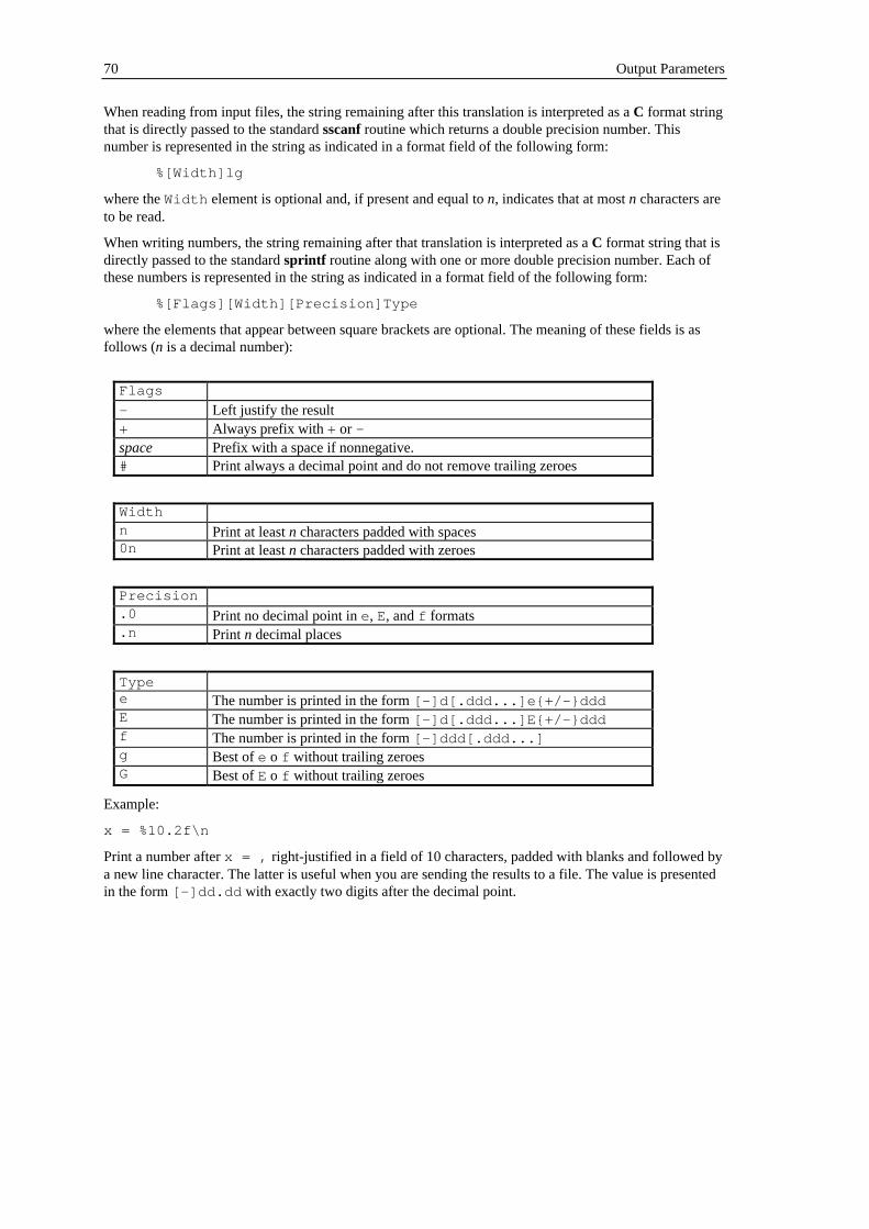
70 Output Parameters
When reading from input files, the string remaining after this translation is interpreted as a C format stringthat is directly passed to the standard sscanf routine which returns a double precision number. Thisnumber is represented in the string as indicated in a format field of the following form:
%[Width]lg
where the Width element is optional and, if present and equal to n, indicates that at most n characters areto be read.
When writing numbers, the string remaining after that translation is interpreted as a C format string that isdirectly passed to the standard sprintf routine along with one or more double precision number. Each ofthese numbers is represented in the string as indicated in a format field of the following form:
%[Flags][Width][ Precision]Type
where the elements that appear between square brackets are optional. The meaning of these fields is asfollows (n is a decimal number):
Flags - Left justify the result + Always prefix with + or - space Prefix with a space if nonnegative. # Print always a decimal point and do not remove trailing zeroes
Width n Print at least n characters padded with spaces 0n Print at least n characters padded with zeroes
Precision .0 Print no decimal point in e, E, and f formats .n Print n decimal places
Type e The number is printed in the form [-]d[.ddd...]e{+/-}ddd E The number is printed in the form [-]d[.ddd...]E{+/-}ddd f The number is printed in the form [-]ddd[.ddd...] g Best of e o f without trailing zeroes G Best of E o f without trailing zeroes
Example:
x = %10.2f\n
Print a number after x = , right-justified in a field of 10 characters, padded with blanks and followed bya new line character. The latter is useful when you are sending the results to a file. The value is presentedin the form [-]dd.dd with exactly two digits after the decimal point.

Selecting Initial Conditions on the Screen 71
Interactive Solution
After setting a problem (as described in Dynamical Systems, Initial Values, Boundary Conditions,Solution Options, and Output Parameters), you are ready to start solving it. This chapter describes howto do that in an interactive and user-friendly way.
Selecting Initial Conditions on the Screen
Before starting solving the problem, remember that if the current Dynamics Solver window is a graphicswindow, a cursor in the form of a flashing cross inside a circle will appear on the screen. Its coordinatesare permanently indicated in the middle panel of the bottom line. They are two initial conditions orparameters whose value can be changed by merely moving the cursor with the mouse pointer or thedirection keys. The two initial conditions selected in this way are by default x and x[1] for an equationand x[1] and x[2] for a system, but this can be changed in the Variable in axis X and Variable in axisY entries of the Cursor dialog sheet of the current graphics windows.
This possibility is very useful to interactively change initial conditions (or parameters). You can selecteasily the solution starting at a certain point, or arriving to it. Simply start from the selected point andintegrate forward or backward. It can also be used to find the coordinates of interesting points in thesolution window.
To move the cursor (and change the initial conditions or parameters) you can use the direction keys, whichwill move the cursor by an amount equal to the corresponding elementary step value selected in the entriesHorizontal step and Vertical step of the Cursor dialog sheet. Holding down the Ctrl key while using adirection key will move the cursor by a length equal to ten times the corresponding elementary step value.The cursor elementary step length can be doubled (halved) by pressing * (/ ) in the numeric keypad.
You may also use the mouse pointer (whose coordinates are displayed in the right panel of the bottomline. Locate it at the desired location and double click on the left button. (A single click will be enough ifyou have set off the Double click to select option in the Other sheet of the Preferences/Other dialog.)
The initial values can also be viewed and edited in the Initial Values browser.
Starting, Stopping and Resuming the Solution
To start solving a problem, press Enter or use the Go/Start menu. First, Dynamics Solver will try tocompile all the expressions defined in the problem. In the event of an error, you will be prompted tocorrect it. A Compiler Error dialog displaying the type and probable location of the error will be opened.You can then correct it and continue solving the problem, or stop the compilation at this point.
After a successful compilation, the different kinds of output will start (refer to Output Parameters). Mostof the menus are disabled while the computation is being performed, but you can, for instance, erase one(or all) windows as described in Erasing and Refreshing Windows.
To stop the solution, press Esc or use the Go/Stop menu. Please note that, to have the possibility of asmooth continuation, the Esc key is only read after each solution point is computed. This can supposeseveral, or even many, points plotted on the screen and, thus, the action is not always immediate ifInterpolation is on (in the Range dialog) and Step low, or if Max. h (in the Method dialog) is high, or ifthe Tolerance is very low.
In fact, the integration halts when any of the following things happens:
• The user presses the Esc key or uses the Go/Stop menu entry.
• An error happens.
• The Last value is reached by the independent variable.

72 Interactive Solution
• The absolute value of any dependent variable reaches the Infinity value.
• The first argument of a break function in an expression is not equal to zero.
• The first argument of a continue function in an expression is equal to zero.
In all but the first two cases the next iteration (if any has been scheduled by using the Repeated solutionsand phase portraits entries in the Parameters dialog sheet) starts.
The solution might also be paused if the Pause (see Forcing the Program to Wait) is not null. If thatvalue is negative, you will have to press a key to get the next solution point. You are reminded to do thisby the bottom line of the main window. See the examples in CHAOS\DISKS.DS and GRAPH.DS.
When the integration is over but you are still in the output window, you can select other initial conditionsand start solving again. It is possible to have automatically repeated solutions for different initial values orsettings (see Repeated Integration/Iteration).
Selecting the Solution Direction
Most ordinary differential equations can be easily solved for decreasing values of the independentvariable: you simple use the Go/Backward menu entry (or press Ctrl+U ) and then Go/Continue orGo/Start. Use again the menu (or press again the key combination) to resume solving forward. Note thatmost functional-differential equations can not be solved backward because previous solution values mustbe known at each step. If you try solving backward one of these equations you will get an error, mostprobably an ’argument out of range' Interpolation Error .
In the case of discrete dynamical systems, Dynamics Solver will always iterate forward, because mostmaps are not invertible. If the particular map you are analyzing is invertible, you have to invert it by handand then solved the inverse map forward.
Erasing and Refreshing Windows
1. To erase the current window, use Del or the Window/Erase window menu entry.
2. To erase all windows, use Ctrl+Del or the Window/Erase all menu entry.
3. To redraw the current window, use D or the Draw/Refresh window menu entry.
4. To redraw the current window, use Ctrl+D or the Draw/Refresh all menu entry.
Zooming a Graphics Window
The ranges displayed in a graphics window can be selected in the Graphics Output dialog box, but youcan also zoom in a window piece in two different ways.
If you want to select a rectangular piece of a window and amplify it to fill the window:
1. Locate the mouse at one of the new rectangle corners,
2. While holding down the Shift key and the left mouse button, move the pointer to the othercorner on the same rectangle diagonal. The pointer location will be displayed, as usual, on the rightpanel of the status (bottom) line, Furthermore, the two corners of the new window will bedisplayed in the format (x1,y1)-(x2,y2) inside the rectangle that is currently selected.
3. If you release the left mouse button before the Shift key, the rectangle will be the newwindow. If, on the contrary, the Shift key is released before the left button, the previous windowranges will be retained.
Zooming a Graphics Window 73
If you want only to zoom in provisionally to see some detail and then recover easily the previous window,proceed as follows:
1. Select the Action/Move around mode for the cursor. (This can also be accomplished by pressingM.)
2. Locate the cursor (with the mouse pointer or the direction keys, as described in Selecting InitialConditions on the Screen) in the center of the area you want to amplify.
3. Use Zoom, step and order/Zoom in (or press I ). The amplification level is controlled in theZooming factor of the Cursor dialog sheet for that window. The default value is 10. If you preferto see a larger area, instead of peering into smaller details, use Zoom, step and order/Zoom out.
4. Repeat steps 2 and 3 as many times as necessary.
5. To recover the original window, use Zoom, step and order/Actual size (or press Z).
6. You should probably use Action/Initial conditions (or press X) to be able to select initialconditions on the screen to start solving the problem again.

74 Advanced Procedures
Advanced Procedures
This chapter describes how to get some special kinds or results that often result very useful. See also Constrained Initial Conditions, Seeing and Editing the Whole Problem, Printing, UsingGraphics Elements, Writing External Integration Codes, Adding Mathematical Functions andConstants, Reading Dynamics Solver’s Output in Mathematica and Saving and Loading Graphicsand Text Screens.
Repeated Integration/Iteration
Dynamics Solver can be instructed to automatically repeat the solving process any number of times. Sincethe dynamical systems solved by Dynamics Solver are deterministic, you might think that a repeatedsolution will necessarily reproduce the first one. This is not always the case, however, because DynamicsSolver can be instructed to select different values of initial conditions or parameters before starting eachnew solution.
Each solution (each run) is identified by the value of one or two index variables whose names (by defaultnx and ny ) and ranges are selected in the entries of the Parameters dialog box. The integration/iterationprocess is repeated for each integer value of these index variables in the selected ranges. Since theseranges have, by default, null starting and ending values, the process is usually executed exactly once, asyou will want most often.
If one or both ranges are not empty, the solution process will be repeated. If the names and ranges for theindex variables are x1 <= nx <= x2 and y1 <= ny <= y2 , the whole solution process can beunderstood in the following pseudo-code:
for nx from x1 to x2 by steps of 1 do
for ny from y1 to y2 by steps of 1 do
integrate/iterate once
If you take advantage of the possibility to use Initial functions (in the Initial values dialog sheet) you canobtain different solutions each time. You can even read them from external data files: see Reading InitialFunctions from Data Files. (See also Constrained Initial Conditions.) You may use as initial functionany expression, so it is possible, for instance:
1. Change parameters from run to run. Though Initial functions are only applied to the dependentvariables, nothing prevents you from deciding that one or some of the parameters in the problemare dependent variables. You simple define an higher Order/Dimension (in Type) and enterappropriate equations (null derivatives in differential equations and identity transformations initerated maps) for the new dependent variables/parameters.
2. Use the random function to analyze a problem by changing at random initial values orparameters.
3. Use expressions in the form x1+nx*(x2-x1)/10 and y1+ny*(y2-y1)/10 (or morecomplex expressions) to draw phase portraits (see Drawing Phase Portraits).
4. Use something like read(i) to read the initial values from external input files. You will havethe opportunity to enter the file name the first time the program needs it.
5. Use the last results of a previous integration to determine, in a simple or complex expression, thenew initial conditions (or parameters), because their value is still in the corresponding variables.
Notice that you must make sure that each integration is automatically ended in a reasonable amount oftime. This can be achieved by using the Last value entry (or Infinity in some cases) in the Range menusheet). The functions break and continue are also very useful to check for termination conditions.
If you need only one non-empty range, select the corresponding to the first index variable, because aninterrupted calculation can be resumed more smoothly (as described in Starting, Stopping andResuming the Solution). A resumed computation starts with the next value (if more than one) of the first

Drawing Phase Portraits 75
index variable and uses all the possible values of the second index. If you only use the second index,resuming the integration will be equivalent to starting it, all index values will be used in turn.
Index ranges can also be viewed and edited in the Parameter browser.
The most usual application for this feature will be the drawing of phase portraits (see the example inODES\PHASE.DS and HENONMAP.DS), but, with a bit of ingenuity, the possibilities are infinite. Let usonly mention the drawing of basins of attraction (CHAOS\BAS.DS and BASIN.DS ) and the analysis ofchaotic scattering (CHAOS\DISKSCAT.DS and SCAT.DS). This is also the only way to get bifurcationdiagrams of continuous dynamical systems (CHAOS\LORENZL.DS). Often one can take advantage of thePenColor , PenWidth , HSV and RGB functions, as shown in the CHAOS\HENONMAP.DS, andART\COS1.DS examples.
Drawing Phase Portraits
The best way to draw phase spaces is to use your knowledge of the problem, which you can get by tryingdifferent initial conditions to know how the phase space will look. Then you wisely choose a number ofinitial conditions and integrate them (often both forward and backward, as discussed below). The portraitwill most probably look far better than any automatic drawing.
Anyway, you can get automatically phase portraits as a particular case of repeated integration.
Let us assume that the displayed ranges (selected in Graphics Output) are (x1 ,x2 ) and (y1 ,y2 ), and youwant nxm evenly spaced initial conditions in the phase portrait.
1. Choose in the entries of the Parameters dialog box the names of the two index variables thatwill by used to draw the phase portrait. In most cases the default nx and ny names will be fine.
2. Make sure that the corresponding ranges go from 0 to n-1 and from 0 to m-1 , respectively.
3. Use expressions in the form x1+nx*(x2-x1)/n and y1+ny*(y2-y1)/m in the Initialfunctions entry of the Initial values dialog sheet. Sometimes you will prefer usingx1+(nx+0.5)*(x2-x1)/(n+1) and y1+(ny+0.5)*(y2-y1)/(m+1) . In other casesmore complex functions will be necessary (to have logarithmic spacing, instead of linear spacing,for instance). A even more complex example is given in ODES\PHASE.DS.
4. In many cases, to have complete solution curves, you will run the complete process twice, oncefor each solution direction selected in the Go/Backward menu. Notice that backward integration isonly possible for ordinary differential equations. The process will most probably fail withfunctional-differential equations and Dynamics Solver does not iterate backward discretedynamical systems (see Selecting the Solution Direction).
You must make sure that each integration is automatically ended in a reasonable amount of time. This canbe achieved by using the Last value entry (or Infinity in some cases) in the Range menu sheet). Thefunctions break and continue are also very useful to check for termination conditions.
Often one can take advantage of the PenColor , PenWidth , HSV and RGB functions, as shown in theCHAOS\HENONMAP.DS and ART\COS1.DS examples.
See also the ODES\PHASE.DS, CHAOS\STANDARD.DS example.
Using Projections
You can use the Three-Variable functions projx and projy (in the form projx(x,y,z) ,projy(x[1],x[2],x[3]) etc.) to have projections in any expression output in a graphics or textwindow. The view point and other projection options are selected in the View Point dialog box.
The projection functons give the x and y coordinates in a new reference system defined as follows:

76 Advanced Procedures
1. One goes from the original system S to a new one, S1, by means of a counterclockwise rotationof angle 0° <= Phi < 360° around the Z axis, as described by the rotation matrix
cos sin 0
-sin cos 0
0 0 1
ϕ ϕϕ ϕ
.
2. A second counterclockwise rotation of angle 0° <= Theta <= 180° around the Y1 axis is used todefine system S2:
cos -sin
sin cos
θ θ
θ θ
0
0 1 0
0
.
As a consequence, the view line lies along the direction of the new Z2 axis, defined in the original systemby the polar angles (Theta,Phi).
3. A counterclockwise rotation of angle 0° <= Psi < 360° around the Z2 axis changes theorientation of the projection axes and defines a new system, S3,
cos sin 0
-sin cos 0
0 0 1
ψ ψψ ψ
.
4. A fourth system, S4, is obtained from S3 by a translation of value Origin along the Z3 (= Z2=Z4)axis, so that x4 =x3, y4 = y3 and z4 = z3-Origin . The view point is the origin of the new system andits position with respect to S is given by the polar coordinates Origin , Theta, and Phi. The valueof Origin is ignored unless the following value is different from zero.
5. If Distance is null, the projection functions return parallel projections, i.e., the componentsalong the new X4 and Y4 axes. If, on the contrary, Distance is different from 0, true perspectiveprojections are returned and the opposite of Distance is the z value where the projection planeintersects perpendicularly the axis Z4. The values returned by the projection functions are thus x' =-x4 Distance/z4 and y'= -y4 Distance/z4.
The easiest way to understand the result is to look at the sample cube displayed in the View Point dialogbox, whose orientation can by changing by dragging it with the mouse.
The default values are Phi = 30°, Theta = 60° and Psi = 90°, and other common view lines are as follows:
View line Proj. plane Phi Theta Psi

Drawing the Direction Field 77
Z (X,Y) 0° 0° 0° X (Y,Z) 0° 90° 90° Y (Z,X) 90° 90° 180°
To see the axes with the same projection settings, use three 3-curves with trivial definitions: (t0 ,0),(0,t ,0) and (0,0,t ).
See the examples ODES\AUTOCAT.DS, TORUS.DS and CHAOS\LORENZ.DS.
Drawing the Direction Field
With one- and two-dimensional systems, drawing the associated direction field (i.e., a set of shortsegments which are tangent to the solution curves) may help understand the qualitative properties of theproblem. To display it, select the Direction field entry of the Format dialog sheet. In the same dialog youcan select the distance between contiguous segments (in the Cell entry) and the segment length (inLength). These two quantities are measured in pixels, and their default values will be right in most cases.Once the equations have been compiled (see Starting, Stopping and Resuming the Solution) or whenthe window is erased), the direction field is displayed in the color selected in the Colors dialog.
Unless you do not care about strange results, in order to guarantee that the solution curves are tangent tothe direction field you should use this option only in one of the following three cases:
1. With a single first-order equation, y' = f(x,y), to display the independent variable x in the X axisand the dependent variable y in the Y axis. The slope of the direction field at each point will be y' =dy/dx.
2. With a single second-order equation, y" = f(x,y,y'), to display the dependent variable y in the Xaxis and its derivative y' in the Y axis. The slope of the direction field at each point will be y"/y'.
3. With a system of two first-order equations, y' = f(x,y,z), z' = g(x,y,z), to display the firstdependent variable y in the X axis and the second dependent variable z in the Y axis. The slope ofthe direction field at each point will be z'/y'.
Since many derivatives must be computed, the drawing of the direction field may be a bit long in slowmachines. Pressing Esc will stop the process.
See the example in MECH\PENDULUM.DS.
Using Poincaré Sections
To analyze orbits in three or more dimensions you can use, apart from projections, the so-called “Poincarésections.” In this case, you are interested not in the full solution but only in the solution points that satisfyan additional condition. For instance, often you will want to plot the intersection points of the solutionwith a given plane (or a more general surface) in the phase space. In Dynamics Solver, the Poincarésection can be defined by any condition that can be put in the form f(...) = 0, f being any function of theindependent variable, the solution components, the parameters, and the initial conditions.
Dynamics Solver is able to find the value of the independent variable for which a certain condition writtenin the very general form f(...) = 0 is satisfied. You may impose one Poincaré condition for each graphicsor text window you are using for output. You only have to set the corresponding definitions and options inthe Graphics Output or Text Output dialog box.
1. Enter in Condition the expression f(...) (without the = 0 part) that must be zero.
2. Select Increasing if you want the value of the independent variable for which f(...) is nullwhile increasing from negative to positive values.
3. Select Decreasing if you want the value of the independent variable for which f(...) is nullwhile decreasing from positive to negative values.
4. Specify in Error the tolerance the root finding routine uses to consider that f(...) vanishes.

78 Advanced Procedures
5. Specify in Last Poincaré time (in the Parameters dialog sheet) the name of the value of theindependent variable for which the condition is satisfied. The default name is tp .
Noticee that Increasing and Decreasing are completely independent settings; you can set both or onlyone of them as you wish.
In the previous sentences f(...) stands for any expression containing the independent variable, thesolution, the parameters and the initial conditions. However, since the point to be found does notnecessarily correspond to any of the actually computed points, the solution and its derivatives (or thedifferent dependent variables) are not directly available as x , x[1] , etc., but through the interpolatedvalue x(i,t) that, as usual, returns the n-th derivative or component of the computed solution.(Remember that in the solution points actually computed by Dynamics Solver, x = x(0,t) , x[1] =x(1,t) , etc., but the solution x(i,t) is defined not only for those points, but also for any value of t inthe range still in memory. In fact, x(i,t) is the global piecewise polynomial approximation to thesolution that has been already discussed in Interpolated Solution.) Notice also that this global solution isstored only is Saved points (in the Range dialog box) has not been set to 0, because the value in thatentry is precisely the number of computed points stored in memory.
For instance, to compute the intersections of the solution of a three-dimensional system with the plane 2x-y+az = 13 you must enter 2*x(1,t)-x(2,t)+a*x(3,t)-13 if you have the default names x[1] ,x[2] and x[3] for the unknowns, or 2*x(t)-y(t)+a*z(t)-13 if you have changed the names tox , y and z . Dynamics Solver will complain if you try 2*x[1]-x[2]+a*x[3]-13 or 2*x-y+a*z-13 .
The program will monitor continuously the value of f(...) and when its sign changes according to thesettings Increasing and/or Decreasing, it will try to find the value of the independent variable for whichf(...) = 0 within the tolerance selected in Error . If the value is found, it is stored under the nameselected in Last Poincaré time and it can be then used in any expression.
In some cases a sign change can be missed if Interpolate (in the Range dialog box) is not set or Step (inthe same dialog box) is too high. On the other hand, if the latter value is too small the program can spenda long time testing the condition sign.
The tolerance in the root determination of the condition defining the Poincaré section is set in Error .With lower tolerance, the error is smaller, of course, but it would be meaningless to compute these zeroeswith better approximation than the solution. Arule of thumb is to take it equal or slightly higher than theTolerance (in the Method dialog box) used by the integration method.
A common mistake is to forget writing the expression in such a way that a sign change actually happenswhen the condition is null. In particular, special care must be taken with discontinuous functions andoperators (% and mod, for instance). So, to find the points at which x = 0 mod 2pi, you must typesomething like (x+pi)%(2*pi)-pi , instead of the more natural condition x%(2*pi) , which will bealways nonnegative.
The value for which Condition is true is computed, if Increasing or Decreasing are set, even if you donot want the Poincaré section drawn on the screen or sent to a text window: you may want this valuecomputed only to find the period of a limit cycle or periodic orbit, for instance. (See the examples inMECH\R3BODYP.DS and ODES\VDPOLP.DS and the discussion in Computing Periods.)
Even if this value is being computed, the output routines work as usual, drawing or writing the expressionsselected in the Graphics Output or Text Output dialog box every time a new solution point is computedor, if Interpolate is set (in the Range dialog box), every interval of length Step. If you want to draw theexpressions only at the points in which the Condition is true (i.e., if you want the Poincaré section on thescreen or in the text window):
1. Set on the Poincaré section entry to have output every time the Condition defining the sectionis met (and not according to the settings in the Range dialog box).
2. In the case of a graphics window, turn off the Continuous line option in the Format sheet. Thisis not truly necessary, but successive points in the Poincaré section correspond normally to ratherdifferent values of the independent variable and usually are not very close. Seeing they joined by asegment would be odd in most cases.
See the examples in ODES\TORUS.DS, and CHAOS\HENONHEI.DS.

Computing Periods 79
In the special case of Poincaré sections of the type t = b mod a (i.e., a “stroboscopic” Poincaré section forthe values t = n a + b) can be found by using a condition in the form t%a-b or, better, by merely usingFirst value = b and Step = a (in the Range dialog box), without searching for any root. See the examplein CHAOS\DUFFING.DS and DUFFING1.DS.
See also Computing Periods.
Computing Periods
This topic can be understood as a special application of the possibility to compute Poincaré Sections.
1. Start from a point located in the periodic solution. If you do not know any point in the periodicsolution you can use Dynamics Solver to locate it by trying different initial conditions. If it is anattracting limit cycle (thus, an isolated periodic solution), you can easily locate one of its points bymeans of Dynamics Solver: simply run the problem until the solution is redrawing once and againthe periodic solution and stop the integration. You can use a Text Window (and in bidimensionalsystems the status line) to get the coordinates of a point, but it is easier to simply enter in Firstvalue (in the Range dialog box) a value high enough to make sure that the output starts only whenthe periodic orbit has been reached.
2. Use a Text Window to get the numerical value of the period.
3. Enter in Condition an expression f(...) (without the = 0 part) that that has a null valuewhen an orbit repeats over itself. (See below.)
4. Select Increasing if you want the value of the independent variable for which f(...) is nullwhile increasing from negative to positive values.
5. Select Decreasing if you want the value of the independent variable for which f(...) is nullwhile decreasing from positive to negative values. Note that Increasing and Decreasing arecompletely independent settings; you can set both or only one of them, as you wish.
6. If necessary change in Error the tolerance the root finding routine uses to consider thatf(...) vanishes. Make it equal or slightly higher than the Tolerance (in the Method dialog box)used by the integration routine.
7. If necessary, change in Last Poincaré time (in the Parameters dialog sheet) the name of thevalue of the independent variable for which the condition is satisfied. The default name is tp .
8. Set on the Poincaré section entry to have output every time the Condition defining the sectionis met (and not according to the settings in the Range dialog box).
f(...) can be any expression containing the independent variable, the solution, the parameters and theinitial conditions. However, since the point to be found does not necessarily correspond to any of theactually computed points, the solution and its derivatives (or the different dependent variables) are notdirectly available as x , x[1] , etc., but as x(i,t) that always (and not only in this context) means the n-th derivative or component of the computed solution. So, in the solution points actually computed byDynamics Solver, x = x(0,t) , x[1] = x(1,t) , etc., but the solution x(i,t) is defined not only forthose points, but also for any value of t in the range still in memory. In fact, this x(i,t) is just theglobal piecewise polynomial approximation to the solution that has been already discussed (refer toInterpolated Solution). Note that this global solution is stored only is Saved points (in the Range dialogbox) has not been set to 0, because the value in that menu entry is precisely the number of computedpoints stored in memory.
The program will monitor the value of f(...) and when its sign changes in a selected sense, it will try tofind the value of the independent variable for which f(...) = 0 within the tolerance selected inError . If the value is found, it is stored under the name selected in Last Poincaré time and it can be thenused in any expression.
A sign change can be missed if Interpolate (in the Range dialog box) is not set or Step (in the samedialog box) is too high. On the other hand, if the latter value is too small the program can spend a longtime testing the condition sign.

80 Advanced Procedures
Note also that you must write the expression in such a way that a sign change happens when the conditionis null. For instance, you could be tempted to use for a bidimensional system a condition of the formabs (x(0,t)-x(0,0))+ abs (x(1,t)-x(1,0)) , if the integration starts from a null value of theindependent variable, or abs (x(0,t)-x(0,100))+ abs (x(1,t)-x(1,100)) , if First value hasbeen set to 100 , because these functions will be null if and only if the orbit repeats over itself.Unfortunately, this will not work, because such an expression is never negative. Use, instead, x(0,t)-x(0,0) or x(0,t)-x(0,100) . Of course, x can repeat before a full period has elapsed, but you cancontrol if the true necessary and sufficient condition (such as the one discussed before) is (nearly) null toknow if the independent variable value correspond to a period.
See the examples in ODES\VDPOLP.DS and MECH\R3BODYP.DS (in the latter case a very simpleCondition, y(t) , is used).
Drawing Bifurcation Diagrams
The only way to get bifurcation diagrams (see Strogatz [1994] for the definition of bifurcation diagrams)of continuous dynamical systems is the use of Repeated Integration as shown inCHAOS\LORENZL.DS.
In the case of discrete dynamical systems an easier method is provided by Dynamics Solver:
1. Enter the name of the bifurcation parameter in the Bifurcation parameter entry of theParameters dialog sheet.
2. Select in the First value and Last value entries of the Iteration Range dialog sheet the indexrange for which output will occur in each run (i.e., for each value of the bifurcation parameter).You might want to try first low values for these entries to avoid having to wait very long beforeyou know if everything else is right.
3. Select the Begin and End values for the bifurcation parameter in the Iteration Range dialogsheet.
4. Select the Step value (in the Iteration Range dialog sheet) that will increment the bifurcationparameter after each run. You might want to try first a rather high value (say (End-Begin)/100)and once everything else is right, a value small enough to avoid having void vertical lines in thewindow. It may be convenient to adjust accordingly the dimension of the output window. To helpin this task, its dimensions (in pixels) are drawn in the status line when it is resized. You may alsoprescribe exact values, in pixels, for the width and/or height of the client part of the outputwindow, instead of choosing the window size with the mouse or keyboard. This can be achieved byentering the corresponding value(s) in the Width and Height entries of the same dialog sheet.Keep in mind that null values for these entries are ignored and that Windows sets minimum valuesfor window dimensions.
5. Set in the Horizontal axis entry of the Graphics Output dialog sheet the name of thebifurcation parameter. You will probably want to make the values in the Min. X and Max. Xentries equal to those on Begin and End.
6. Set in the Vertical axis entry of the Graphics output dialog sheet the name of expression to beanalyzed for each value of the bifurcation parameter. It will be usually, but not necessarily, avariable. It may be the derivative of a one-dimensional map if you want to compute Liapunovexponents (refer to Computing Liapunov Exponents).
7. As usually when analyzing maps, set off the Continuous line option in the Format dialog sheet.
See the examples in CHAOS\BIFURCAT.DS, CHAOS\HENONB.DS, and CHAOS\HENONL.DS.

Computing Liapunov Exponents 81
Computing Liapunov Exponents
Dynamics Solver can be instructed to compute Liapunov exponents (for their definition, see Strogatz[1994]).
When analyzing discrete dynamical systems (iterated maps) of first order, you can draw a bifurcationdiagram, for the Liapunov exponent. It is enough to select in the Vertical axis of the Graphics Outputdialog sheet the expression defining the absolute value of the derivative of the map, and set on theAverage value entry of the same dialog. In this way, you will get a single average value when the indexreaches Last value, instead of all the values computed from First value to Last value (in IterationRange).
In more complex systems you can use a bit of ingenuity and the general methods described in Ott [1993].Do not forget that many problem can be solved by using the full power of Dynamics Solver’s expressionsand the possibility to increase the order of the problem to introduce new unknowns that will be computedalong the problem (see Hints). You can analyze the examples CHAOS\CAT.DS (Liapunov exponent for abidimensional map), HENONL.DS (bifurcation diagram of the Liapunov exponent of a bidimensionalmap) and LORENZL.DS (bifurcation diagram for the Liapunov exponent of a three-dimensional systemof ordinary differential equations).
Computing Histograms
When analyzing discrete dynamical systems, histograms are very useful to compute the natural invariantmeasure (see Ott [1993]). They can be drawn easily with Dynamics Solver. Let us assume that you want todivide the (a,b) interval of a variable or expression in n subintervals (“bins”) of length l = (b-a)/n and plotthe relative frequency with which each subinterval is visited by the solution; that is, the relative number oftimes the value of the selected variable or expression is in each subinterval.
1. Select in the Begin and End entries of the Iteration Range dialog sheet the interval end points,a and b respectively.
2. Select in the Step value of the Iteration Range dialog sheet) the bin length l. The numbers ofbins will be (End-Begin)/Step. You might want to try first a rather high value (say (End-Begin)/100) and once everything else is right, a value small enough to avoid having void verticallines in the window. It may be convenient to adjust accordingly the dimension of the outputwindow. To help in this task, its dimensions (in pixels) are drawn in the status line when it isresized. You may also prescribe exact values, in pixels, for the width and/or height of the clientpart of the output window, instead of choosing the window size with the mouse or keyboard. Thiscan be achieved by entering the corresponding value(s) in the Width and Height entries of thesame dialog sheet. Keep in mind that null values for these entries are ignored and that Windowssets minimum values for window dimensions.
3. Set in the Horizontal axis entry of the Graphics Output dialog sheet the variable or expressionto be analyzed. The value in Vertical axis will be ignored. You will probably want to enter in Min.X and Max. X the values in Begin and End.
4. Select in Histogram the number of iterations between consecutive redrawings of the histogram.If this value is 10000, for instance, each time 10000 new values have been computed the window iserased and for each bin in the interval a vertical line of length equal to relative number of times thatbin has been visited is drawn. The sum of heights is equal to 1/Step, because one normally wantsthe integral of the invariant measure to be normalized to 1.
See the example in CHAOS\HISTOGRA.DS.
Drawing Cobwebs
When analyzing discrete dynamical systems, cobwebs are very useful to understand many results:pitchfork bifurcations, intermittence, etc. (see Strogatz [1994]). They can be drawn easily with Dynamics

82 Advanced Procedures
Solver by using the Direct graph power and Inverse graph power entries of the Graphics Outputdialog box.
If Direct graph power has a non null value n, the graph of the n-th iterated of the map will be drawn. IfInverse is null, the line y = x will be drawn and the iteration will be represented by a line that goeshorizontally from the last point the diagonal and from there vertically to the graph. The points ofintersection of the curve with the diagonal line will correspond to (stable or unstable) n-cycles (i.e., fixedpoints of the n-th iterate of the map).
If Inverse graph power is non null, the graph of the n-th iterated of the inverse map will be drawn. IfDirect graph power is null, the n-th iterate of the map will also be drawn. You can also select differentnon null values for these entries (for instance 2 and 1 to analyze 3-cycles). The iteration will berepresented by a line that goes from one graph to the other, alternatively. The points of intersection ofcurves corresponding to values n and m will represent (stable or unstable) (n+m)-cycles (i.e., fixed pointsof the (n+m)-th iterate of the map).
Often it will be helpful to select a non-null value for Pause (see Forcing the Program to Wait). This willmake easier seeing the position of each solution point.
The use of these possibilities is incompatible with the drawing of bifurcation diagrams or histograms orthe calculation of Average values.
See the examples in CHAOS\GRAPH.DS, INTER.DS and SINGER.DS.
Some Examples
Dynamics Solver includes well over 100 problem files, which go from elementary examples to verysophisticated uses of the program. You might want to study them to learn how to use Dynamics Solver inthe most effective way. (If the examples files are not installed into your hard disk, you can run INSTALLagain.)
Let us mention only the following problem files, which are among the advanced examples: Illustrated techniques File Basins of attraction of a continuous system CHAOS\BAS.DS
Basins of attraction of a discrete system CHAOS\BASIN.DS
Bifurcation diagram CHAOS\BIFURCAT.DS
Bifurcation diagram for the Liapunov exponent CHAOS\HENONL.DS
Bifurcation diagram for the Liapunov exponent CHAOS\LIAPUNOV.DS
Boundary conditions: quantum spectrum QUANTUM\HARMONIC.DS
Boundary conditions: quantum spectrum QUANTUM\PENK.DS
Boundary conditions: quantum spectrum QUANTUM\QUARTIC.DS
Cobwebs CHAOS\GRAPH.DS
Complex quantities and additional variables DELAY\FP.DS
Constrained initial conditions and Poincaré map CHAOS\HENONHEI.DS
Current/field lines. Avoiding divergences DRAWING\DIPOLE.DS
Cursor and nontrivial initial conditions ART\ELLIPTI1.DS
Devil's staircase. Using additional unknowns CHAOS\DEVIL.DS
Direction field MECH\PENDULUM.DS
Drawing lines and erasing automatically the screen tocreate animated output
MECH\ROD.DS
Equations not solved for the derivative ODES\FRW2.DS
Histograms CHAOS\HISTOGRA.DS
Integro-differential equation NUMERIC\VOLTERRA.DS
Liapunov exponent of a continuous system CHAOS\LORENZL.DS
Liapunov exponent of a two-dimensional map CHAOS\CAT.DS
Multiple output in a single window MECH\BURRAU.DS
Multiple simultaneous initial conditions in a singlewindow
CHAOS\DUFFING4.DS

Some Examples 83
Numerical quadrature NUMERIC\ERF.DS
Parameters selected with the cursor DELAY\DELAY1.DS
Periods MECH\R3BODYP.DS
Periods ODES\VDPOLP.DS
Phase space ODES\PHASE.DS
Poincaré map and projections ODES\TORUS.DS
Projections CHAOS\LORENZ.DS
Projections and 3-curves DRAWING\EMWAVES.DS
Projections and lettering ODES\AUTOCATA.DS
Pseudo phase space reconstruction CHAOS\LORENZR.DS
Real time simulation MECH\R3BODY1.DS
Recurrences DELAY\FIBONAC.DS
Repeated integration, Power and Pause CHAOS\DISKS.DS
Repeated integration: chaotic scattering CHAOS\DISKSCAT.DS
Repeated integration, (very complex) CHAOS\DISKS.DS
Repeated integration: KAM theorem CHAOS\HENONMAP.DS
Repeated integration: quantum spectrum QUANTUM\SPECTRUM.DS
Single precision numbers CHAOS\HENON1.DS
Stroboscopic Poincaré map CHAOS\DUFFING1.DS
Stroboscopic Poincaré map and the if function CHAOS\DUFFING2.DS
Stroboscopic Poincaré map ODES\VDPOLF.DS
Successive maxima of z in Lorenz system CHAOS\LORENZZ.DS
Using LastT , MaxX and MoveTo MECH\ELASPEN1.DS
Using LineTo CHAOS\HENON3.DS

84 Using Graphics Elements
Using Graphics Elements
You can use graphics elements to add lettering and other informative items (axes, curves, and so on) to thegraphics result of your problem files, or simply to draw some figures when preparing graphics for papersand courseware.
If you want to draw a figure with no associated differential or discrete dynamical system, open a graphicswindow with the Output/New graph window entry. You should probably select the in the Aspect ratioentry of the Format sheet any value different from Arbitrary . In this way, circles will look round andother elements can be rotated with no distortion. With graphics elements, the Axes entry of the same sheetis obsolete and you may want to clear it.
The graphics elements are created, edited and deleted from the Draw, Action and Zoom, step and ordermenus or the equivalent toolbar elements, which you can display by using the Configuration/Toolbar andpopup menu entry.
Most of the actions are also available through the following keyboard shortcuts:
Key Menu entry F1 Open the help Index F2 File/Save F3 File/Open Shift+F3 Window/Tile vertical Shift+F4 Window/Tile horizontal F5 Edit/All settings Shift+F5 Window/Cascade F10 File/Print + * Draw/Next element - * Draw/Previous element * * Zoom/Larger step / * Zoom/Smaller step Enter Go/Start Esc Go/Stop (or stop the redrawing of graphics
elements and metafiles) Del Window/Erase window Ctrl+Del Window/Erase all Ctrl+Ins Window/Get screen Shift+Ins Window/Put screen Ctrl+A Edit/Parameters Ctrl+B Go/Backward Ctrl+C Window/Get screen Ctrl+D Draw/Refresh all Ctrl+E Edit/Equations Ctrl+F Output/Graphics format Ctrl+G Output/New graphics window Ctrl+H Edit/Method Ctrl+I Edit/Initial conditions Ctrl+L Edit/Variables Ctrl+N Edit/Notes Ctrl+O Output/Color Ctrl+P Window/Save points Ctrl+R Edit/Range Ctrl+S Output/Status line Ctrl+T Output/New text window Ctrl+U Go/Continue Ctrl+V Window/Put screen Ctrl+W Output/View point

Graphics Elements 85
Ctrl+X Output/Text format Ctrl+Y Edit/Type Ctrl+Z Edit/Boundary conditions Shift+Ctrl+I Edit/Initial Values browser Shift+Ctrl+P Edit/Parameter browser C Draw/Copy element D Draw/Refresh window E Draw/Edit element F Action/First value I Zoom/Zoom in L Action/Last value M Action/Move around N Draw/New element O Action/Origin P Action/Point R Action/Rotate S Action/Select an element T Action/Third point X Action/Initial condition W Zoom/Zoom out Z Zoom/Actual size Direction keys To move the cursor, origin, point, third point, or
to rotate, and to select first and last values.
*These keys are those in the numeric keypad
You can also use the Graphics Element dialog box to manage graphics elements.
Finally, many useful actions can be accomplished by using the mouse.
To select an element you can use the Graphics Element dialog box or the + and - in the numeric keypad;but it is often more convenient to use Action/Select an element (or the corresponding toolbar button, orpress S) and, then, locate the mouse cursor near the element and double click on the left button (seePreferences/Other).
Once the element has been selected, you may use again the entries of Action (or the equivalent keys ortoolbar buttons) to chose the action that will be performed when using the direction keys (or, in mostcases, the mouse) to adjust the element origin, size, direction and so on.
For fine adjustment, you can use the zoom facilities (see Zooming a Graphics Window), maybe afterselecting the Action/Move mode to locate the center of the zoomed window.
Graphics Elements
You can add to any graphics window any number of elements of the following types:
Name Meaning Segment Segment Circle (Arc of) circumference Ellipse (Arc of) ellipse Arrow Arrow head Text Text string 2-curve Parametric plane curve 3-curve Projection of parametric spatial curve Special Special data to be sent directly to the plotter/printer Data Read numerical data from an external file Fractal Fractal curves

86 Using Graphics Elements
Segment
A straight line starting at the point of coordinates X and Y and having a Length and a Direction. A pointis obtained, obviously, as a segment of null Length.
Attribute Meaning X x coordinate of the origin Y y coordinate of the origin Length Segment length Direction Direction in degrees Color Drawing color Line type Line width (if negative, a dashed line is used) Steps Number of segments (dashes)
Circle
A circle or an arc of circumference defined by its center (the point of coordinates X and Y) its Radius, itsDirection and its Begin and End angle values. The last two values are the limit values of the angle a inthe usual definition:
x = x0+r*cos(a),
y = y0+r*sin(a).
Attribute Meaning X x0 coordinate of the center Y y0 coordinate of the center Radius Circle radius r Begin First angle value in degrees End Last angle value in degrees Direction Direction in degrees Color Drawing color Line type Line width (if negative, a dashed line is used) Steps Number of segments (dashes)
Ellipse
A (arc of) ellipse defined by its center (the point of coordinates X and Y) its Horizontal and Verticalsemi-axes, its Direction and its Begin and End angle values. The last two values are the limit values ofthe angle a in the usual definition:
x = x0+r*cos(a),
y = y0+s*sin(a).
Attribute Meaning X x coordinate of the center Y y coordinate of the center Vertical Vertical semi-axis s Horizontal Horizontal semi-axis r Begin First angle value in degrees End Last angle value in degrees Direction Direction in degrees Color Drawing color Line type Line width (if negative, a dashed line is used) Steps Number of segments (dashes)

Graphics Elements 87
If s and r are equal we have, obviously, a circle.
Arrow
An arrowhead starting at the point of coordinates X and Y, and having a Size and a definite Direction andan Angle.
Attribute Meaning X x coordinate of the head Y y coordinate of the head Size Arrow size Angle Arrow angle divided by two Direction Direction in degrees Color Drawing color Line type Line width
See the problem files in EXAMPLES\DRAWING.
Text
A character or string of characters defined in String. Its left lower corner starts at the point of coordinatesX and Y, and the string is displayed along a Direction. Each letter's Width and Height, can also becontrolled by means of Editing Graphics Elements. The font used to draw the letters is selected in Font.
Attribute Meaning String Text string (including Escape Sequences) X x coordinate of the string origin Y y coordinate of the string origin Height Letter height Width Letter width Direction Direction in degrees Color Drawing color Line type Line width Font Font number
If a character is not defined in the font, a space is used instead.
Escape Sequences
In an element of type text, a sequence of characters starting by '\' has a special meaning according to thefollowing table:
Symbol Meaning \0 Reset all default values \ n ASCII character 0 < n < 256 \+ n Advance -128 < n < 128 points5
\- n Move back -128 < n < 128 points \^ n Go up -128 < n < 128 points \_ n Go down -128 < n < 128 points \* n Multiply height and width by n
5 A character is given by a set of polygonals joining set of points, whose coordinates, x and y, aremeasured in arbitrary units called “points” (-128 < x < 128, -128 < y < 128). The usual letter height isabout 42 for capital letters and its width ranges from 26 to 54. An undefined character is 0 points width.

88 Using Graphics Elements
\/ n Divide height and width by n \. Do nothing (useful as separator) \: n Select font 0 <= n <= 9
Any space following a number is skipped. This is a convenient feature to separate the sequence from acontiguous numeric character, but if you actually need a space after a sequence, '\ ' must be used.
Characters 169-172, 176-197 and 198-223 are accessible as \A -\D , \E -\Z and \a -\z . In some fonts (butnot all, see Show fonts) they represent Greek characters as follows:
Capital Normal Meaning \A \a alpha \B \b beta \C \c chi \D \d delta \E \e epsilon \F \f phi \G \g gamma \H \h eta \I \i iota \J \j theta*, phi* \K \k kappa \L \l lambda \M \m mu \N \n nu \O \o omicron \P \p pi \Q \q theta \R \r rho \S \s sigma \T \t tau \U \u upsilon \V \v sigma*, omega* \W \w omega \X \x xi \Y \y psi \Z \z zeta
*This is an alternative shape for the same letter
The remaining escape sequences are the User Defined Sequences, which can be viewed and edited in theEscape Sequences dialog box.
User Defined Escape Sequences
In an element of type text, you can use any of the following 24 sequences, which can be viewed and editedin Escape Sequences dialog box. They are defined in terms of the built-in Escape Sequences and theirdefault values are as follows:
Symbol Meaning \! (undefined by default) \« (undefined by default) \# (undefined by default) \$ (undefined by default) \% (undefined by default) \& (undefined by default) \' (undefined by default)

Graphics Elements 89
\( \_20\/1.2 (index for roman font) \) \^30\/1.2 (exponent for roman font) \, (undefined by default) \; (undefined by default) \< (undefined by default) \= (undefined by default) \> (undefined by default) \? (undefined by default) \@ (undefined by default) \[ \-10\_20\/1.2 (index for italics) \\ \92 (the backslash character) \] \+10\^30\/1.2 (exponent for italics) \` (undefined by default) \{ (undefined by default) \| (undefined by default) \} (undefined by default) \~ (undefined by default)
A sequence of this type can freely use other escape sequences or user defined sequences, but direct andindirect recursion does not work. A sequence cannot be longer than 76 characters.
2-curves
An element of this type is defined by its two-dimensional parametric equations:
x = f(t,x0,y0,s,r,d,t1,t2),
y = g(t,x0,y0,s,r,d,t1,t2).
The parameter, t , goes between t1 and t2 ), and you can freely use the x0 , y0 , s , r and d parameters.
Attribute Meaning x Equation for the x coordinate y Equation for the y coordinate x0 x0 parameter y0 y0 parameter s s parameter r r parameter t1 First value of t = t1 t2 Last value of t = t2 d d parameter Color Drawing color Line type Line width (if negative, dashed line) Steps Number of segments (dashes)
In the equation defining the curves you can also use the problem parameters (defined in Parameters),except those named as one of the above parameters.
To avoid premature errors when they are about to be defined, 3-curves with a null x or y entry are notdisplayed at all.
See the problem files in EXAMPLES\DRAWING (especially SPRINGS.DS).
3-curves
An element of this type is defined by its three-dimensional parametric equations:
x = f(t,x0,y0,s,r,d,t1,t2),
y = g(t,x0,y0,s,r,d,t1,t2),

90 Using Graphics Elements
z = h(t,x0,y0,s,r,d,t1,t2).
The points are automatically projected by using projx and projy and the settings in View Point. Anequivalent, but rather messy, way to do the same would be using projx(f(...),g(...),h(...))and projy(f(...),g(...),h(...)) in a 2-curve element.
The parameter, t , goes between t1 and t2 ), and you can freely use the x0 , y0 , s , r and d parameters. Attribute Meaning x Equation for the x coordinate y Equation for the y coordinate z Equation for the z coordinate x0 x0 parameter y0 y0 parameter s s parameter r r parameter t1 First value of t = t1 t2 Last value of t = t2 d d parameter Color Drawing color Line type Line width (if negative, dashed line) Steps Number of segments (dashes)
In the equation defining the curves you can also use the problem parameters (defined in Parameters),except those named as one of the above parameters.
To avoid premature errors when they are about to be defined, 3-curves with a null x, y or z entry are notdisplayed at all.
One useful application of these elements is the drawing of axes when using projections (seeCHAOS\LORENZ.DS and ODES\AUTOCAT.DS, for instance).
Special
An element of this type is a string that is directly sent to the plotter device after translating the followingsequences: Sequence ASCII name Meaning \ nnn a decimal code for a character \a Bel character #7 \b Backspace character #8 \e Esc character #27 \f FF character #12 \n LF character #10 \o nnn an octal code for a character \r CR character #13 \t Tab character #9 \v VT character #5 \x nnn an hexadecimal code for a character \z Nul character #0 \ c the character c in the remaining cases
Data
An element of this type is an external data file whose complete specification is given in File. You can addafter the file specification four numbers if the form:
filename x1 y1 x2 y2
to automatically clip the input data (after eventual translation, scaling and rotation, see below) to therectangle whose diagonal points are (x1 ,y1 ) and (x2 ,y2 ).

Graphics Elements 91
Attribute Meaning File filename or filename x1 y1 x2 y2 X Horizontal translation Y Vertical translation Vertical Vertical scale factor Horizontal Horizontal scale factor Direction Direction in degrees Color Drawing color Line type Line width Segments If 0, only points are drawn
The file lines must be composed by two floating points numbers: the coordinates of successive points of apolygonal. A line which has not this structure (if it is void, for instance) starts a new polygonal.Nevertheless, if Segments is 0, successive points are never joined by a segment.
Before being drawn, the x and y coordinates are scaled (multiplied) by Horizontal and Vertical ,respectively. These values are ignored if equal to zero (or one). The scaled coordinates are then rotatedaccording to Direction and translated by X and Y.
In many cases it will be better to use relative paths for filename . If the data file is located in theproblem file directory and you specify only the file name and extension, the drive and path of the latterwill be used to open the data file, after trying the current drive and directory.
To avoid repeated errors in some graphics cards, no error is reported if the file has not been defined or theprogram cannot open it.
Fractal
An element of this type is an autosimilar fractal based on a straight line starting at the point of coordinatesX and Y and having a Length and a Direction.
The minimum/maximum order (iteration level) is selected in Min. order / Max. order. The actualiteration level is obtained adding Fractal order (in the Cursor dialog sheet) to Min. order , as long as thesum is not greater than Max. order.
Attribute Meaning Divisors Divisors to obtain the relative lengths of segments in the next generation Angles Angles of the relative directions in the next generation. In degrees X x coordinate of the origin Y y coordinate of the origin Length Length of basic segment Min. order Minimum fractal order Max. order Maximum fractal order Direction Direction in degrees of basic segment Color Drawing color Line type Line width
In the following example (the von Koch curve)

92 Using Graphics Elements
we see the basic (blue) segment of Length s. The next generation is formed by four red segments oflength s/3 and with relative orientations as indicated in the figure. So, four values are needed in Divisors(3 3 3 3 ) to indicate that the length of each new segment is one third of the segment in the previousgeneration. Another four values (0 60 -60 0 ) are entered in Angles to indicate the relative directionsin degrees of each new segment with respect to the one of the previous generation. This construction isrepeated again and again up to the desired generation which is indicated by the sum of Min. order andFractal order in the Cursor dialog sheet, but always less or equal to Max. order. See the exampleVONKOCH.DS.
See also the problem files in EXAMPLES\FRACTAL.
String, x equation, File and Divisors
This entry of Edit Element contains the following element information:
Element Name Meaning Text String Text string (including Escape Sequences) 2-curve x Equation for the x coordinate 3-curve x Equation for the x coordinate Special String Literal string to be included in the output Data File filename or filename x1 y1 x2 y2 Fractal Divisors Divisors to obtain the relative length of segments in next generation
If the graphics element is of Data type you can specify only the file name and extension, if it is located inthe problem file directory. The drive and path of the latter will be used to open the data file, after tryingthe current drive and directory.
y equation and Angles
This entry of Edit Element contains the following element information:
Element Name Meaning 2-curve y Equation for the y coordinate 3-curve y Equation for the y coordinate Fractal Angles Angles to add to the global direction for each segment in the next
generation

Graphics Elements 93
z equation
This entry of Edit Element contains the following element information:
Element Name Meaning 3-curve z Equation for the z coordinate
X coordinate and x0 parameter
This entry of Edit Element contains the following element information:
Element Name Meaning Segment X x coordinate of the origin Circle X x coordinate of the center Ellipse X x coordinate of the center Arrow X x coordinate of the head Text X x coordinate of the string start 2-curve x0 x0 parameter 3-curve x0 x0 parameter Data X Horizontal translation Fractal X x coordinate of the origin
Y coordinate and y0 parameter
This entry of Edit Element contains the following element information:
Element Name Meaning Segment Y y coordinate of the origin Circle Y y coordinate of the center Ellipse Y y coordinate of the center Arrow Y y coordinate of the head Text Y y coordinate of the string start 2-curve y0 y0 parameter 3-curve y0 y0 parameter Data Y Horizontal translation Fractal Y y coordinate of the origin
Length, Vertical, Size, Height and s parameter
This entry of Edit Element contains the following element information:
Element Name Meaning Segment Length Segment length Ellipse Vertical Vertical semi-axis Arrow Size Size Text Height Letter height 2-curve s s parameter 3-curve s s parameter Data Vertical Vertical scaling factor Fractal Length Length of basic segment

94 Using Graphics Elements
Radius, Horizontal, Width and r parameter
This entry of Edit Element contains the following element information:
Element Name Meaning Circle Radius Radius Ellipse Horizontal Horizontal semi-axis Text Width Letter width 2-curve r r parameter 3-curve r r parameter Data Horizontal Horizontal scaling factor
Begin, Angle, t1parameter and Min. order
This entry of Edit Element contains the following element information:
Element Name Meaning Circle Begin First angle value in degrees Ellipse Begin First angle value in degrees Arrow Angle Arrow semi-angle 2-curve t1 t1 parameter 3-curve t1 t1 parameter Fractal Min. order Minimum fractal order
End, t2 parameter and Max. order
This entry of Edit Element contains the following element information:
Element Name Meaning Circle End Last angle value in degrees Ellipse End Last angle value in degrees 2-curve t2 t2 parameter 3-curve t2 t2 parameter Fractal Max. order Maximum fractal order
Direction and d parameter
This entry of Edit Element contains the following element information:
Element Name Meaning Segment Direction Direction in degrees Circle Direction Direction in degrees Ellipse Direction Direction in degrees Arrow Direction Direction in degrees Text Direction Direction in degrees 2-curve d d parameter 3-curve d d parameter Data Direction Direction in degrees Fractal Direction Direction in degrees

Graphics Elements 95
Line type
This entry of Edit Element contains the line type (width) of the current element. For some elements, anegative value indicates that the element will be drawn with as a dashed curve with a Steps. The absolutevalue will be used as line width.
Type Meaning Segment Line width (if negative, dashed line) Circle Line width (if negative, dashed line) Ellipse Line width (if negative, dashed line) Arrow Line width Text Line width 2-curve Line width (if negative, dashed line) 3-curve Line width (if negative, dashed line) Data Line width Fractal Line width
Color
This entry of Edit Element contains the color to draw the element. You can use the button or double clickon the color bar to select a new value.
Steps, Font and Segments
This entry of Edit Element contains the number of segments that must be used to draw the currentelement. In addition, the range of the parameter defining the curve, between the values in Begin and Endis divided by this number.
By convention, a negative value of Line type indicates that only alternate segments will be drawn, to havea dashed element. This value indicates the number of segments (alternatively drawn and skipped) to beused. In most cases an odd value looks better.
In an element of type Text this value is necessarily between 0 and 9 and it indicates the font used to drawthe text. If a value n is used, the corresponding font file is called as defined in the Font files dialog box.
In an element of type Data if this value is null, successive points are not joined by a segment.
Element Name Meaning Segment Steps Number of subsegments Circle Steps Number of segments Ellipse Steps Number of segments Text Font Font number (from 0 to 9) 2-curve Steps Number of values of the t parameter 3-curve Steps Number of values of the t parameter Data Segments If 0, do not join points with segments

96 Printing
Printing
Since Dynamics Solver is designed to obtain high quality results, there are different ways to print, whichwill be discussed in detail in the next sections.
Printing Text
You can print the currently active text window by using File/Print (or F10 or the corresponding toolbar
button ). The standard Print dialog box will appear. You can there select the printer and someprinting options.
Fast Graphics Printing
You can print the currently active graphics window by using File/Print (or F10 or the corresponding
toolbar button ). The Print dialog box will appear. You can there select the printing options.
The bitmap formats are rather appropriate for problems in which the graphics results are points, ratherthan continuous lines (as is often the case in discrete dynamical systems: iterated maps). If the resultsappear in the form of lines, printing bitmaps will often produce poor results because printers have usuallyan much higher resolution than screens (and, in consequence, bitmaps). Notice also that you could getonly a partial window snapshot (the piece currently visible) if the Bitmap output entry in the Formatsheet was No bitmap when they were computed.
Moreover, some graphics card drivers have problems translating bitmaps in some graphics modes. Forexample, we have found that the drivers of some very popular cards render the white background ofwindows in 256 and more color modes as a gray texture in PostScript printers (they give the correct whitebackground in injection printers!). Notice that this is a problem (bug) in the graphics driver, not inDynamics Solver. The only thing you can do to avoid it to use another printing mode, as described below.
To obtain good print results you should have prepared the printing before starting solving the problem.See Preparing Graphics Printing.
Preparing Printing
Before starting solving the problem (especially if it is a complex one and a large computation time isneeded to get the results) you should paid some attention to the kind of printed results you want.
The bitmap formats are rather appropriate for problems in which the graphics results are points, ratherthan continuous lines (as is often the case in discrete dynamical systems: iterated maps). If the resultsappear in the form of lines, printing bitmaps will often produce poor results because printers have usuallyan much higher resolution than screens (and, in consequence, bitmaps). Notice also that you could getonly a partial window snapshot (the piece currently visible) if the Bitmap output entry in the Formatsheet was No bitmap when they were computed.
The metafile format will produce in most cases better results, but you have to select an appropriate valuefor the Basic width entry in the Print dialog box, in order not to have too fine lines. Notice also that thismode will be available only if the Save output in memory entry in the Format sheet was not null whenthe integration/iteration results were computed.
Check also the default values in the Bitmap output and Memory output entries of thePreferences/Graphics dialog sheet.
On the other hand, you may want to collect in a single printout the results displayed in different graphicswindows. The easier way is to output all the output you want to print to a single window. Though youneed a graphics window for each pair of quantities you want displayed on the screen, you may select in the

PostScript Printing 97
Window entry of the corresponding Graphics Output dialog box the caption of another graphicswindow, which will then receive all its output (but not its graphics elements). Notice that plotter output,which is described below, will not be redirected (you may get this, at your own risk, by specifying thesame plotter for different windows). The Min. x , Max. x, Min. Y and Max. y values of the window thatwill receive the output will be used. If you need different values for each pair of quantities, you have toscale the corresponding expressions.
PostScript Printing
Many formatting programs (such as TEX, and its dialects LATEX, AMSTEX, and so on) and wordprocessors accept PostScript or, more often, Encapsulated PostScript files. They provide a standard(and, more important, platform-independent) form to include graphics in other documents.
You can easily generate Encapsulated PostScript files from the Print dialog box: simply check in theEncapsulated PostScript option and select the output file in the Port/File entry (maybe by using theBrowse button).
If the amount of memory necessary to save all the graphics output exceeds your RAM size, you mustconsider using the Plotter Output mode.
Plotter Output
This possibility is reserved to power user who can take advantage of it at least in three instances:
1. When the amount of memory necessary to save all the graphics output exceeds your RAM sizeand you want to get quality prints from metafiles (maybe to send them to an EncapsulatedPostScript file).
2. When the output is to be sent to a plotter, rather than to a printer.
3. When you are a power user that have special output/printing needs. For example, you could be ateacher preparing a collection of exercises that includes many figures to be inserted in the output toa laser printer from a LaTeX source.
In these cases the plotter facilities in Dynamics Solver should be used, even if the output will be sent to aprinter (probably a laser printer). The process is as follows:
1. Starting from any of the examples provided with the program in the PLOTTER directory, createa plotter driver appropriate for your printer/plotter and printing needs.
2. Install the plotter driver by using the Configuration/Plotter drivers menu
3. Select the driver in the Driver entry of the Plotter dialog sheet.
4. In the same dialog, select the Output file and the appropriate values for the remainingparameters (Frame, Pen, Width , Speed and Line type). Make sure that On is selected.
5. Perform some preliminary runs to get a feel of the kind of results you want.
6. For each solution (initial value) that you want sent to the plotter/printer, select theOutput/Plotter output global setting (or equivalent toolbar button) and start solving the problem.You can set off this setting to continue experimenting with other initial conditions.
7. If you want to include Axes or graphics elements, use the Output/Draw to plotter menu entry,or equivalent toolbar button.
8. If necessary, use the Output/Eject page menu.
9. If necessary, use the Output/Write epilog menu.
The plotter drivers are ordinary text files with an extension defaulting to .DRV. They can be adapted todifferent plotting devices and to different settings of the same plotter/printer (to use different parts of thepaper, for instance). Some examples are provided in the distribution disk(s) and the corresponding help

98 Printing
files (which can be accesed from the Examine button in the dialog that displays with theConfiguration/Plotter drivers menu or by using Driver help in the Plotter dialog box) describe indetail their structure, and how they can be modified. See, for instance, the EPS.HLP help file.

File 99
Reference Information
Menu commands
Menu Meaning File File and printer management Edit View and change problem settings Output Control output options Window Manage windows Go Solve the problem Draw Edit drawing elements Action Control cursor action Zoom Change viewing scale Configuration Set preferences Help Help system
File
The entries in this menu are used to manage the printer and problem files.
Entry Key Meaning New Start a new problem Open F3 Get a problem file from the disk Save F2 Save the current problem to the disk Save as Save the current problem to the disk, under a new name Printer setup Specify the printer to be used and the corresponding options Print F10 Print the current output window Mail Send the current problem to the FAX and mail system Quit Alt+F4 Exit the program
After the previous menu entries there can appear the file specifications of the last recently used problems.This feature is very convenient to resume previous works. At most four file names are retained. The lengthof these entries is controlled from the Filename length in menus entry of the Other dialog sheet.
You will be prompted for a file name when using Open, Save as and also if Save is used when noprevious name (i.e., if the problem file was not loaded with Open but created with New) or if the file wasconverted from a previous version of the program.
New
Use this entry of the File menu (which can be also accessed by using the toolbar button) to erase allcurrent definitions, close all windows and start analyzing a new problem file.
Open
This entry of the File menu (which can be also accessed by pressing F3 or using the toolbar button)starts an Open dialog box that lets you load a problem file from the disk.

100 Menu commands
Save
This entry of the File menu (which can be also accessed by pressing F2 or using the toolbar button)saves the current problem file to the disk under its current name. (If it has never been saved before, a Savedialog box lets you choose it.)
Save as
This entry of the File menu (which can be also accessed by using the toolbar button) starts a Savedialog box that lets you save the current problem file to the disk under a new name (or in a different diskor directory).
Printer setup
This entry of the File menu (which can be also accessed by using the toolbar button) opens thePrinter Setup standard dialog box that lets you choose the printer and its options.
This entry of the File menu (which can be also accessed by pressing F10 or using the toolbar button)opens the Print dialog box that lets you print the current window.
This entry of the File menu (which can be also accessed by using the toolbar button) send the currentproblem to FAX or mail system (as an attachment).
Quit
This entry of the File menu (which can be also accessed by pressing Alt+F4 or using the toolbarbutton) ends the current Dynamics Solver session. If the current problem file has been modified, you willbe prompted and have an opportunity to save the changes.
Most Recently Used Problem Files
The last entries in the File menu (from zero to four) are the names (and the corresponding filespecifications, if the Filename length in menus entry of the Other dialog sheet is long enough) of the lastrecently used problem files. This is a convenient way to resume the analysis of a problem.
Edit
The entries of this menu are used to define the dynamical system under study
Entry Key Meaning Type Ctrl+Y Select the type of dynamical system Variables Ctrl+L Select names of variables Parameters Ctrl+A Select names and values of parameters Equations Ctrl+E View and edit the equations defining the problem Initial conditions Ctrl+I Select initial values (and functions) Range Ctrl+R Select the solution range Method Ctrl+H Select the integration method

Edit 101
Notes Ctrl+N View and edit problem notes All settings F5 View and edit all problem settings in a text
windowInitial valuesbrowser
Shift+Ctrl+I Display and activate the Initial Values browser
Parameter browserShift+Ctrl+P Display and activate the Parameter browser
Type
This entry of the Edit menu (which can be also accessed by pressing Ctrl+Y or using the toolbarbutton) opens the Type dialog sheet where you can select the type of dynamical system to analyze. UsingOK will open a warning box, because all settings will be lost. To change the type while saving the currentsettings you may use Edit/All settings.
Definitions
This toolbar button, , is equivalent to the Edit/Variables menu and is included for convenience,because the corresponding hint6 and tip7 indicate that from the same dialog box other settings(Parameters, Equations and Initial conditions ) can be changed.
Variables
This entry of the Edit menu (which can be also accessed by pressing Ctrl+L or using the toolbarbutton) opens the Variables dialog sheet where you can change the names for the independent anddependent variables and for their initial values.
Parameters
This entry of the Edit menu (which can be also accessed by pressing Ctrl+A or using the toolbarbutton) opens the Parameters dialog sheet where you can change the names and values for parameters,bifurcation variable, Poincaré time and iteration variables. See also Parameter browser.
Equations
This entry of the Edit menu (which can be also accessed by pressing Ctrl+E or using the toolbarbutton) opens the Equations dialog sheet where you can change the equations defining the dynamicalsystem and some other options.
Initial conditions
This entry of the Edit menu (which can be also accessed by pressing Ctrl+I or using the toolbarbutton) opens the Initial values dialog sheet where you can change the initial conditions and functions forthe current dynamical system.
The initial values can also be viewed and edited in the Initial Values browser.
6 The status line is used, among other things, to display a short string describing the currently selectedmenu entry or the toolbar button located under the mouse pointer.
7You may get a short description inside a small text window when the mouse pointer has paused for aboutone second over a toolbar button.Notice that this feature is disabled by default, because some video cards drivers redraw too often thewindow under the popup tip. You should check if this is the case with your video card driver. You caneasily enable thhem by using the Preferences dialog box.

102 Menu commands
Boundary conditions
This entry of the Edit menu (which can be also accessed by pressing Ctrl+Z or using the toolbarbutton) opens the Boundary conditions dialog sheet where you can change the boundary conditions forthe current dynamical system.
Range and Method
This toolbar button ( ) is equivalent to the Edit/Range menu and is included for convenience, becausethe corresponding hint and tip indicate that from the same dialog box other settings (Method) can bechanged.
Range
This entry of the Edit menu (which can be also accessed by pressing Ctrl+R or using the toolbarbutton) opens the Range dialog sheet where you can select the options for the solution range.
Method
This entry of the Edit menu (which can be also accessed by pressing Ctrl+H or using the toolbarbutton) opens the Method dialog sheet where you can select the method to solve the differential system(this menu is not available for discrete dynamical systems) and the corresponding options.
Notes
This entry of the Edit menu (which can be also accessed by pressing Ctrl+N or using the toolbarbutton) opens a text window where you can view and edit notes related to the current project. If such awindow is already opened, it is activated, instead or creating a new one.
See also Edit Project Notes.
All settings
This entry of the Edit menu (which can be also accessed by pressing F5 or using the toolbar button)opens a text window where you can view and edit all the settings of the current problem. If such a windowis already opened, it is activated, instead or creating a new one.
See also Edit all Settings in a Text Window.
Initial Values browser
This entry of the Edit menu (which can be also accessed by pressing Shift+Ctrl+I or using the toolbar button) displays the Initial Values browser where you can view and edit all the initial conditionsof the current problem. If the browser is already opened, it is activated, instead or creating a new one.
See also Parameter browser and Edit all Settings in a Text Window.
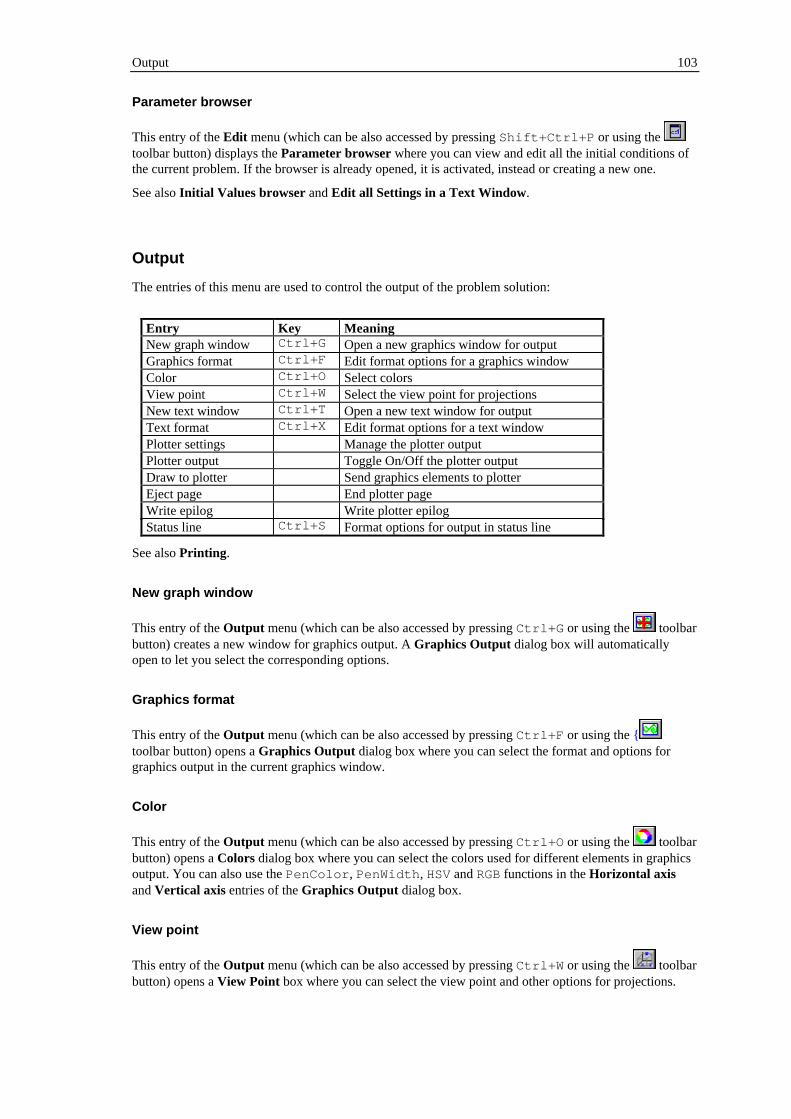
Output 103
Parameter browser
This entry of the Edit menu (which can be also accessed by pressing Shift+Ctrl+P or using the toolbar button) displays the Parameter browser where you can view and edit all the initial conditions ofthe current problem. If the browser is already opened, it is activated, instead or creating a new one.
See also Initial Values browser and Edit all Settings in a Text Window.
Output
The entries of this menu are used to control the output of the problem solution:
Entry Key Meaning New graph window Ctrl+G Open a new graphics window for output Graphics format Ctrl+F Edit format options for a graphics window Color Ctrl+O Select colors View point Ctrl+W Select the view point for projections New text window Ctrl+T Open a new text window for output Text format Ctrl+X Edit format options for a text window Plotter settings Manage the plotter output Plotter output Toggle On/Off the plotter output Draw to plotter Send graphics elements to plotter Eject page End plotter page Write epilog Write plotter epilog Status line Ctrl+S Format options for output in status line
See also Printing .
New graph window
This entry of the Output menu (which can be also accessed by pressing Ctrl+G or using the toolbarbutton) creates a new window for graphics output. A Graphics Output dialog box will automaticallyopen to let you select the corresponding options.
Graphics format
This entry of the Output menu (which can be also accessed by pressing Ctrl+F or using the {toolbar button) opens a Graphics Output dialog box where you can select the format and options forgraphics output in the current graphics window.
Color
This entry of the Output menu (which can be also accessed by pressing Ctrl+O or using the toolbarbutton) opens a Colors dialog box where you can select the colors used for different elements in graphicsoutput. You can also use the PenColor , PenWidth , HSV and RGB functions in the Horizontal axisand Vertical axis entries of the Graphics Output dialog box.
View point
This entry of the Output menu (which can be also accessed by pressing Ctrl+W or using the toolbarbutton) opens a View Point box where you can select the view point and other options for projections.

104 Menu commands
New text window
This entry of the Output menu (which can be also accessed by pressing Ctrl+T or using the toolbarbutton) creates a new window for text output. A Text Output dialog box will automatically open to letyou select the corresponding options.
Text format
This entry of the Output menu (which can be also accessed by pressing Ctrl+X or using the }toolbar button) opens a Text Output dialog box where you can select the format and options for textoutput in the current text window.
Plotter settings
This entry of the Output menu (which can be also accessed by using the toolbar button) opens aPlotter dialog box where you can select the options for plotter output.
See also Printing .
Plotter output
This entry of the Output menu (which can be also accessed by using the toolbar button) lets youswitch On/Off the plotter output.
See also Printing .
Draw to plotter
This entry of the Output menu (which can be also accessed by using the toolbar button) send to thehigh-quality printing device the graphics elements.
See also Printing .
Eject page
This entry of the Output menu (which can be also accessed by using the toolbar button) starts a newpage in the high-quality printing device.
See also Printing .
Write epilog
This entry of the Output menu (which can be also accessed by using the toolbar button) send to thehigh-quality printing device an epilog. (This is only necessary in very special cases.)
See also Printing .
Status line
This entry of the Output menu (which can be also accessed by pressing Ctrl+S or using the toolbarbutton) opens a Numerical Output in Status Line dialog box where you can control the format andoptions for numerical output to the status line.

Window 105
Window
The entries of this menu are used to manage windows and their contents:
Entry Key Meaning Erase window Del Clear the current output window Erase all Ctrl+Del Clear all output windows Get screen Ctrl+Ins or
Ctrl+C Copy screen contents to the clipboard
Put screen Shift+Ins orCtrl+V
Copy screen contents from the clipboard
Save screen Copy screen contents to a disk file Load screen Copy screen contents from a disk file Save points Ctrl+P Copy coordinates of points in a graphics screen
to an external file Cascade Shift+F5 Cascade output windows Tile horizontal Shift+F4 Tile horizontally output windows Tile vertical Shift+F3 Tile vertically output windows Arrange icons Arrange icons of minimized output windows Close Ctrl+F4 Close the current output window Close all Close all output windows
After the previous menu entries there appear the caption of all the output windows in the problem. This isvery convenient to locate and access them quickly.
Erase window
This entry of the Window menu (which can be also accessed by pressing Del or using the toolbarbutton) deletes the contents of the currently active (graphics or text) window. In the case of graphicswindows, the solution computed so far is lost, but the graphics elements are drawn again.
Erase all
This entry of the Window menu (which can be also accessed by pressing Ctrl+Del or using the toolbar button) deletes the contents of every (graphics and text) window. In the case of graphics windows,the solution computed so far is lost, but the graphics elements are drawn again.
Get screen
This entry of the Window menu (which can be also accessed by pressing Ctrl+C or Ctrl+Ins or
using the toolbar button) copies the contents of the current (graphics or text) window to theclipboard, from where it can be pasted in other windows or applications.
See the Saving and loading graphics and text screens section.
Put screen
This entry of the Window menu (which can be also accessed by pressing Ctrl+V or Shift+Del or
using the toolbar button) copies the contents of the clipboard to the current graphics window.
Save screen
This entry of the Window menu (which can be also accessed by using the toolbar button) saves thecontents of the current (graphics or text) window to an external file, which is selected in a standard Savedialog box.

106 Menu commands
See the Saving and loading graphics and text screens section.
Load screen
This entry of the Window menu (which can be also accessed by using the toolbar button) send to thecurrent graphics window the context of an external file, which is selected in a standard Open dialog box.
Save points
This entry of the Window menu (which can be also accessed by pressing Ctrl+P or using the toolbar button) saves the coordinates of the solution points currently drawn on the current graphicswindow, provided that they have been saved in memory, to an external file, which is selected in the Savepoints in memory to external file dialog box.
See the Sending the results to an external file section.
Cascade
This entry of the Window menu (which can be also accessed by pressing Shift+F5 or using the toolbar button) stacks all open edit windows and overlaps them so that each is the same size as all othersand only part of each underlying client window is visible.
Tile horizontal
This entry of the Window menu (which can be also accessed by pressing Shift+F4 or using the toolbar button) arranges your open windows from top to bottom so that they cover the entire width of theclient window without overlapping one another, in a manner that allows more width than height for eachwindow.
Tile vertical
This entry of the Window menu (which can be also accessed by pressing Shift+F3 or using the toolbar button) arranges your open windows from left to right so that they display next to each other, in amanner that allows more height than width for each window.
Arrange icons
This entry of the Window menu (which can be also accessed by using the toolbar button) rearrangesany icons on the client window. The rearranged icons are evenly spaced, beginning at the lower left cornerof the client window.
Close
This entry of the Window menu (which can be also accessed by pressing Ctrl+F4 or using the toolbar button) closes the currently active (graphics or text) window.
Close all
This entry of the Window menu (which can be also accessed by using the toolbar button) closes all(graphics and text) windows.

Go 107
List of Windows
At the end of the Window menu there appears a list of all the (graphics and text) output windows. Youcan switch to any of them by simply selecting the corresponding menu entry.
Go
The entries of this menu are used to solve the mathematical problem:
Entry Key Meaning Start! Enter Start solving the problem Stop! Esc Stop solving the problem Continue Ctrl+U Continue solving the problem Backward Ctrl+B Solve for decreasing values of the independent variable
Start!
This entry of the Go menu (which can be also accessed by pressing Enter or using the toolbarbutton) starts solving the continuous or discrete dynamical system.
See also Solving the system.
Stop!
This entry of the Go menu (which can be also accessed by pressing Esc or using the toolbar button)stops the solution of the continuous or discrete dynamical system. Depending of the complexity of theproblem and the selected tolerance, it may be necessary to wait for a while before the solution really stops.
See also Solving the system.
Continue
This entry of the Go menu (which can be also accessed by pressing Ctrl+U or using the toolbarbutton) continues, if possible, with a stopped solution of the continuous or discrete dynamical system.
See also Solving the system.
Backward
This entry of the Go menu (which can be also accessed by pressing Ctrl+B or using the toolbarbutton) lets you switch the solution direction, but only in the case of continuous (differential) systems.
See also Solving the system.
Draw
The entries of this menu are used to manage graphics elements:
Entry Key Meaning Refresh window D Redraw graphics elements in current output window Refresh all Ctrl+D Redraw graphics elements in all output windows Full screen Ctrl+Home Use the full screen to display only graph and text

108 Menu commands
windows. New element N Create a new graphics element Edit element E Edit the current graphics element Next element + * Select the next element Previous element - * Select the previous element Copy element C Duplicate the current element Remove element Remove the current element Remove all Remove all graphics elements Action Select the action of the cursor and the mouse pointer Zoom, step and order Open the zoom menu
*These keys are those in the numeric keypad
Refresh window
This entry of the Draw menu (which can be also accessed by pressing D or using the toolbar button)redraws the contents (including graphics elements) of the current graphics window.
Refresh all
This entry of the Draw menu (which can be also accessed by pressing Ctrl+D or using the toolbarbutton) redraws the contents (including graphics elements) of every graphics window.
Full screen
This entry of the Draw menu (which can be also accessed by pressing Ctrl+Home or using the toolbar button) uses the full screen to display only the graph and text windows. No caption, menu, toolbaror status line is visible. They can still be accessed by using keyboard shortcuts.
The popup menu that opens by clicking on the right mouse button is also available. Use it (orCtrl+Home , or Alt+D F ) to return to the usual display style.
New element
This entry of the Draw menu (which can be also accessed by pressing N or using the toolbar button)creates a new graphics element. You will select the element type in a New graphics element dialog boxand the remaining options in a Graphics Element dialog.
Edit element
This entry of the Draw menu (which can be also accessed by pressing E or using the toolbar button)opens the Graphics Element dialog box where you can edit the graphics elements. The dialog initiallydisplays the options for the current element, but you may easily view and edit any element.
Next element
This entry of the Draw menu (which can be also accessed by pressing + in the numeric keypad or using
the toolbar button) selects the next graphics element.
Previous element
This entry of the Draw menu (which can be also accessed by pressing - in the numeric keypad or using
the toolbar button) selects the previous graphics element.

Zoom, step and order 109
Copy element
This entry of the Draw menu (which can be also accessed by pressing C or using the toolbar button)makes a duplicate of the current graphics element.
Remove element
This entry of the Draw menu (which can be also accessed by using the toolbar button) removes thecurrent graphics element.
Remove all
This entry of the Draw menu (which can be also accessed by using the toolbar button) removes allthe graphics elements.
Zoom, step and order
The entries of this menu are used to control the viewing scale, the cursor step size and the fractal order:
Entry Key Meaning Zoom in I Show finer details around the cursor Zoom out W Show a wider area around the cursor Actual size Z Recover viewing scale before zoom Larger step * * Multiply by 2 the cursor step Smaller step / * Divide by 2 the cursor step Next fractal order Increase the current fractal order and redraw the window Previous fractal order Decrease the current fractal order and redraw the window
*These keys are the multiplication and fraction bar in the numeric keypad
Zoom in
This entry of the Zoom, step and order menu (which can be also accessed by pressing I or using the toolbar button) will change the current window ranges to show finer details around the cursor. Using theGraphics Output dialog box will make permanent these changes. The Zooming factor is controlled fromthe Cursor dialog sheet.
Use Actual size to recover the original ranges. In particular, you should use it before starting or resumingsolving the problem, because if the window does not have its natural scale, the graphics output will not besaved in the bitmap even if the Bitmap output entry in the Format sheet is different from No bitmap.The metafile output, on the other hand, is always saved if the Save output in memory entry in theFormat sheet is not null, even if the window is zoomed.
Zoom out
This entry of the Zoom, step and order menu (which can be also accessed by pressing W or using the toolbar button) will change the current window ranges to show a wider area around the cursor. Using theGraphics Output dialog box will make permanent these changes. The Zooming factor is controlled fromthe Cursor dialog sheet.
Use Actual size to recover the original ranges. In particular, you should use it before starting or resumingsolving the problem, because if the window does not have its natural scale, the graphics output will not besaved in the bitmap even if the Bitmap output entry in the Format sheet is different from No bitmap.

110 Menu commands
The metafile output, on the other hand, is always saved if the Save output in memory entry in theFormat sheet is not null, even if the window is zoomed.
Actual size
This entry of the Zoom, step and order menu (which can be also accessed by pressing Z or using the toolbar button) will recover the window ranges active before using Zoom in or Zoom out, if possible.
You should use it before starting or resuming solving the problem, because if the window does not haveits natural scale, the graphics output will not be saved in the bitmap even if the Bitmap output entry inthe Format sheet is different from No bitmap. The metafile output, on the other hand, is always saved ifthe Save output in memory entry in the Format sheet is not null, even if the window is zoomed.
Larger step
This entry of the Zoom, step and order menu (which can be also accessed by pressing * on the numeric
keypad or using the toolbar button) doubles the elementary step that the cursor will move while usingthe direction keys, or the angle step in First value, Last value, and Rotate modes. These values are alsocontrolled in the Horizontal step, Vertical step and Angle entries of the Cursor dialog sheet.
Smaller step
This entry of the Zoom, step and order menu (which can be also accessed by pressing / on the numeric
keypad or using the toolbar button) halves the elementary step that the cursor will move while usingthe direction keys, or the angle step in First value, Last value, and Rotate modes. These values are alsocontrolled in the Horizontal step, Vertical step and Angle entries of the Cursor dialog sheet.
Next fractal order
This entry of the Zoom, step and order menu (which can be also accessed by using the toolbarbutton) increases the fractal order to be added to the Begin value of each fractal element to get the actualorder (always below End and above Begin). This value is also controlled in the Fractal order entry of theCursor dialog sheet.
Previous fractal order
This entry of the Zoom, step and order menu (which can be also accessed by using the toolbarbutton) decreases the fractal order to be added to the Begin value of each fractal element to get the actualorder (always below End and above Begin). This value is also controlled in the Fractal order entry of theCursor dialog sheet.
Action
The entries of this menu are used to define the action of the cursor and the mouse pointer:
Entry Key Meaning Initial conditions X The cursor will select new initial conditions Select an element S The cursor will select a graphics element Move around M The cursor will show its coordinates Origin O The cursor will select the origin Point P The cursor will select the point Third point T The cursor will select the third point

Action 111
First value F The cursor will select the first value Last value L The cursor will select the last value Rotate R The cursor will select the rotation angle
Initial conditions
If this entry of the Action menu (which can be also accessed by pressing X or using the toolbarbutton) is used the direction keys and the mouse pointer will select new initial conditions.
See also Solving the system.
Select an element
If this entry of the Action menu (which can be also accessed by pressing S or using the toolbarbutton) is used the direction keys and the mouse pointer will select the nearest graphics element when youdouble click on the left button. (If you have complex graphics elements, you may have to wait while theprogram computes the nearest element.)
Move around
If this entry of the Action menu (which can be also accessed by pressing M or using the toolbarbutton) is used the direction keys and the mouse pointer will do nothing but show their coordinates in thestatus line. Use this to select a point and then zoom around it for fine tuning.
Origin
If this entry of the Action menu (which can be also accessed by pressing O or using the toolbarbutton) is used the direction keys and the mouse pointer will
select change Segment the origin x and y Circle the center x and y Ellipse the center x and y Arrow the arrow head x and y Text the string start x and y 2-curve x0 and y0 parameters 3-curve x0 and y0 parameters Special (not used) Data the translation values x and y Fractal the origin of the basic segment x and y
Point
if this entry of the Action menu (which can be also accessed by pressing P or using the toolbarbutton) is used the direction keys and the mouse pointer will
select change Segment the end Size and Direction Circle a perimeter point Radius and Direction Ellipse a perimeter point Radius and Direction Arrow (not used) Text the string end Radius and Direction 2-curve (not used) 3-curve (not used) Special (not used)

112 Menu commands
Data the horizontal scale and direction Radius and Direction Fractal the end of the basic segment Size and Direction
Third point
If this entry of the Action menu (which can be also accessed by pressing T or using the toolbarbutton) is used the direction keys and the mouse pointer will
select change Segment (not used) Circle (not used) Ellipse the minor semiaxis Size Arrow (not used) Text the string height Size 2-curve (not used) 3-curve (not used) Special (not used) Data the vertical scale Size Fractal (not used)
First value
If this entry of the Action menu (which can be also accessed by pressing F or using the toolbarbutton) is used the direction keys and the mouse pointer will
select change Segment (not used) Circle the arc start First value Ellipse the arc start First value Arrow the arrow angle First value Text (not used) 2-curve the range start First value 3-curve the range start First value Special (not used) Data (not used) Fractal (not used)
Last value
If this entry of the Action menu (which can be also accessed by pressing L or using the toolbarbutton) is used the direction keys and the mouse pointer will
select change Segment (not used) Circle the arc end Last value Ellipse the arc end Last value Arrow (not used) Text (not used) 2-curve the range end Last value 3-curve the range end Last value Special (not used) Data (not used) Fractal (not used)

Configuration 113
Rotate
If this entry of the Action menu (which can be also accessed by pressing R or using the toolbarbutton) is used the direction keys and the mouse pointer will
select change Segment the direction Direction Circle the arc direction Direction Ellipse the arc direction Direction Arrow the direction Direction Text the direction Direction 2-curve d parameter 3-curve d parameter Special (not used) Data the direction Direction Fractal the direction of the basic segment Direction
Configuration
The entries of this menu are used to define your preferences, and to manage the installed external libraries,plotter drivers, fonts and escape sequences:
Entry Meaning Preferences Miscellaneous options Toolbar and popup menu Manage the popup menu and toolbars External codes Manage external integration methods Mathematical extensions Manage mathematical extensions Plotter drivers Manage plotter drivers Font files Manage font files Escape sequences Manage escape sequences
See also Customization
Preferences
This entry of the Configuration menu (which can be also accessed by using the toolbar button)opens the Preferences dialog box where you can select different options to customize your copy ofDynamics Solver.
See also Customizing Dynamics Solver.
Toolbar and popup menu
This entry of the Configuration menu (which can be also accessed by using the toolbar button)opens the Customize Toolbars and Popup Menu dialog box where you can control the toolbars and thepopup menu that opens when using the right mouse button.
See also Customizing Dynamics Solver.
External codes
This entry of the Configuration menu (which can be also accessed by using the toolbar button)opens the Install External Methods dialog box where you can control the integration codes contained inexternal .DLL libraries.

114 Menu commands
See also Writing external integration codes.
Mathematical extensions
This entry of the Configuration menu (which can be also accessed by using the toolbar button)opens the Install Mathematical DLLs dialog box where you can control the mathematical extensionscontained in external .DLL libraries.
See also Adding mathematical functions and constants.
Plotter drivers
This entry of the Configuration menu (which can be also accessed by using the toolbar button)opens the Install Plotter Drivers dialog box where you can control the plotter drivers for plotter output.
Font files
This entry of the Configuration menu (which can be also accessed by using the toolbar button)opens the Install Font Files dialog box where you can control the font files needed while using graphicselements.
Escape sequences
This entry of the Configuration menu (which can be also accessed by using the toolbar button)opens the Escape Sequences dialog box where you can edit the escape sequences (macros) used in textelements.
See also Using graphics elements.
Help
The entries of this menu may be used to access different points of this and other help files. They alsoprovide information on the installed fonts.
Entry Key Meaning Index F1 Open the Table of Contents of the help system Search for help on Search for keywords in help topics Help on Help Show how to use the help system Show fonts Display characters in different fonts About Dynamics Solver Display the (amusing) information dialog
After the previous menu entries there can appear the names of the help files corresponding to externallibraries (integration methods or mathematical extensions) currently in use.
Index
This entry of the Help menu (which can be also accessed by pressing F1 or using the toolbar button)opens the Table of Contents of this help file. There is also a Tutorial .
Search for help on
This entry of the Help menu opens a dialog menu from where you can search for keywords across the helpfile.

Help 115
Help on Help
This entry of the Help menu opens the Getting Help topic where you can learn the different ways ofgetting help. You should read it.
Show fonts
This entry of the Help menu (which can be also accessed by using the toolbar button) displayscharacters in different fonts. Useful to know if a character is in a given font, or to know how to get aspecial symbol.
About Dynamics Solver
This entry of the Help menu displays the (amusing) information dialog. You should try it at least once.Double click on the left panel!
Help for External DLLs
The last entries in the Help menu, if present, will open the table of contents of the help files correspondingto integration codes and mathematical extensions contained in external .DLL libraries.
See also Writing external integration codes and Adding mathematical functions and constants.

116 Dialog Boxes
Dialog Boxes Dialog name Meaning Dynamical System Type Type of dynamical system Advanced settings and advanced settings Definitions Defining variables, Parameters parameters, Equations equations and Initial values initial values and functions Boundary conditions boundary conditions Iteration Range Iteration range or Numerical Method Numerical integration method and Range integration range Graphics Output Defining graphics output (ODEs) Graphics Output for maps Defining graphics output (maps) Format format, Cursor cursor definitions and Plotter plotter settings Colors Select output colors View Point for Projections Select view point for projections Text Output Defining text output (ODEs) Text Output for maps Defining text output (maps) Numerical Output in Status Line Numerical values in status line Preferences Select several options, including Boxes box output and Graphics options for graphics output Other other options Print Print current window External Libraries Manage external integration methods/
mathematical extensions/plotter drivers or font files
Graphics Element Define graphics element New Graphics Element Create a new graphics element Escape Sequences Manage escape sequences Customize Toolbars and Popup Menu Manage popup menu and toolbars About Dynamics Solver Information on Dynamics Solver Dynamics Solver is already running To select a previous copy of the program Mode How to paste/import a graphics screen Compiler Error Error in expression compiler Input File Select file and format to read data from Output File Select file and format to write data to Input Value Input a numeric value Save points in memory to external file Save integration data to disk Tip of the Day Optional useful tip at startup
Common Dialog Boxes Meaning Color Customizing colors Open/Save Open files for reading/writing Print Select printer driver Printer Setup Select printer options Find Find string expressions Replace Replace string expressions

Dynamical System Type 117
Dynamical System Type
This dialog box is started from the Edit/Type menu entry or by pressing Ctrl+Y .
Entry Meaning Dynamical system Select one of the following three radio buttons Single ODE To solve a single differential equation of arbitrary order System of ODEs To solve an arbitrary number of first-order differential equations Map (iteration) To solve a discrete dynamical system: an iterated map Dimension/Order Enter here the order of the only equation, the number of first-order equations or
the dimension of the map Advanced settings Open other sheet of the same dialog to select some advanced options OK Accept changes and close the dialog Cancel Cancel changes and close the dialog Help Open this help entry
Before accepting changes to these options, you will be given the opportunity to saved the current settingsbecause changing anything in this dialog will reset all definitions. You may also Cancel and use the Editall settings menu.
Advanced settings
This is a sheet of the Type dialog box, which is started from the Edit/Type menu entry or by pressingCtrl+Y .
Entry Meaning Compiler options The following entries should be changed only for very complex problems Stack length The number of bytes to be used as stack to evaluate expressions P-code length The number of bytes to store compiled expressions Mathematical option Select below the value of the Heaviside function at the origin Heaviside(0) The most usual values are 1/2, 0 and 1. Type Open another sheet in the same dialog to select the type of dynamical system OK Accept changes and close the dialog Cancel Cancel changes and close the dialog Help Open this help entry
Definitions
In the sheets of this dialog box, which opens with Ctrl+L or by using the Edit/Variables menu entry,you can select names and values for variables, parameters, equations, initial values and functions andboundary conditions.
Entry Meaning Independent variable Name of the independent variable Index Name of iteration index (in maps) Initial value Name of the initial value of the independent variable or iteration index Dependent variable(s) Collective and individual names for the dependent variables Initial value(s) and their initial values Collective name(s) Collective names to use in the form x[1] Individual name(s) Individual names Parameters Open another sheet of the same dialog to select the names and values of the
parameters
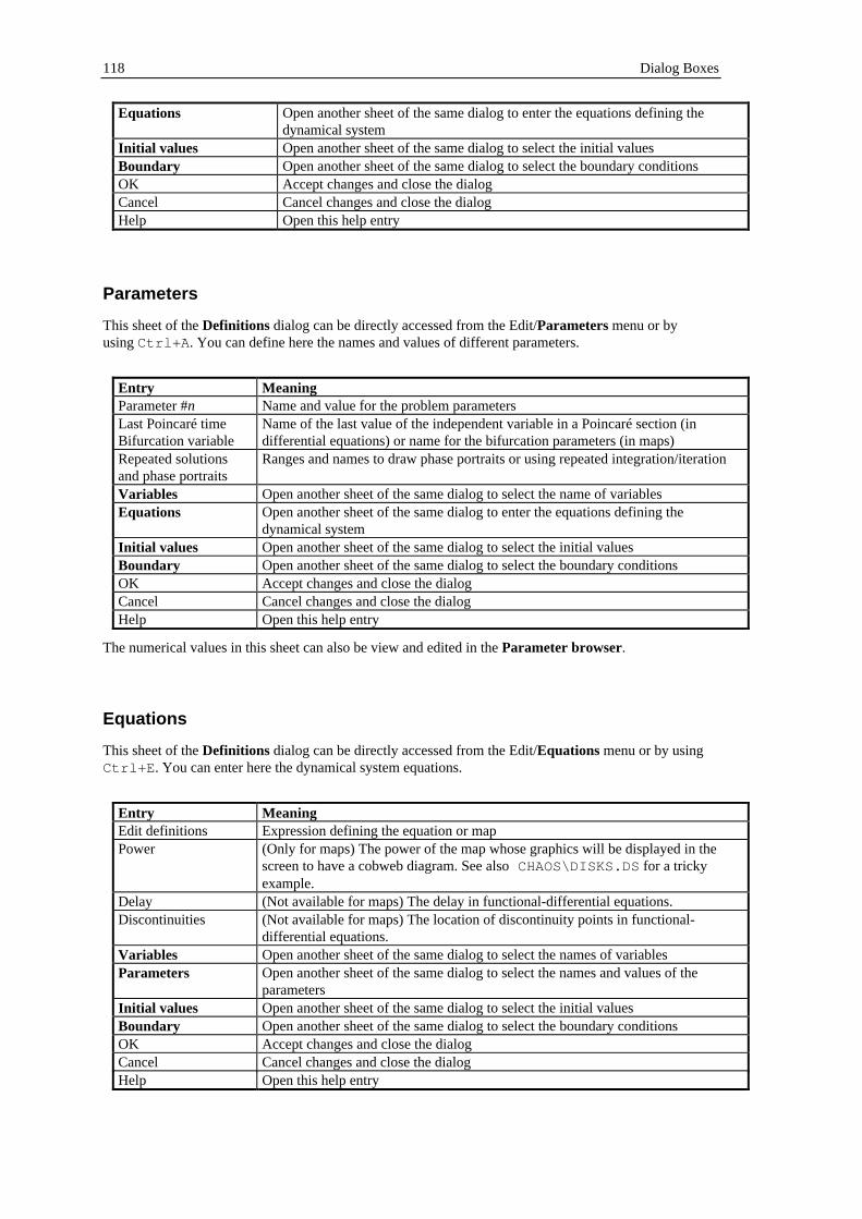
118 Dialog Boxes
Equations Open another sheet of the same dialog to enter the equations defining thedynamical system
Initial values Open another sheet of the same dialog to select the initial values Boundary Open another sheet of the same dialog to select the boundary conditions OK Accept changes and close the dialog Cancel Cancel changes and close the dialog Help Open this help entry
Parameters
This sheet of the Definitions dialog can be directly accessed from the Edit/Parameters menu or byusing Ctrl+A . You can define here the names and values of different parameters.
Entry Meaning Parameter #n Name and value for the problem parameters Last Poincaré time Bifurcation variable
Name of the last value of the independent variable in a Poincaré section (indifferential equations) or name for the bifurcation parameters (in maps)
Repeated solutionsand phase portraits
Ranges and names to draw phase portraits or using repeated integration/iteration
Variables Open another sheet of the same dialog to select the name of variables Equations Open another sheet of the same dialog to enter the equations defining the
dynamical system Initial values Open another sheet of the same dialog to select the initial values Boundary Open another sheet of the same dialog to select the boundary conditions OK Accept changes and close the dialog Cancel Cancel changes and close the dialog Help Open this help entry
The numerical values in this sheet can also be view and edited in the Parameter browser.
Equations
This sheet of the Definitions dialog can be directly accessed from the Edit/Equations menu or by usingCtrl+E . You can enter here the dynamical system equations.
Entry Meaning Edit definitions Expression defining the equation or map Power (Only for maps) The power of the map whose graphics will be displayed in the
screen to have a cobweb diagram. See also CHAOS\DISKS.DS for a trickyexample.
Delay (Not available for maps) The delay in functional-differential equations. Discontinuities (Not available for maps) The location of discontinuity points in functional-
differential equations. Variables Open another sheet of the same dialog to select the names of variables Parameters Open another sheet of the same dialog to select the names and values of the
parameters Initial values Open another sheet of the same dialog to select the initial values Boundary Open another sheet of the same dialog to select the boundary conditions OK Accept changes and close the dialog Cancel Cancel changes and close the dialog Help Open this help entry
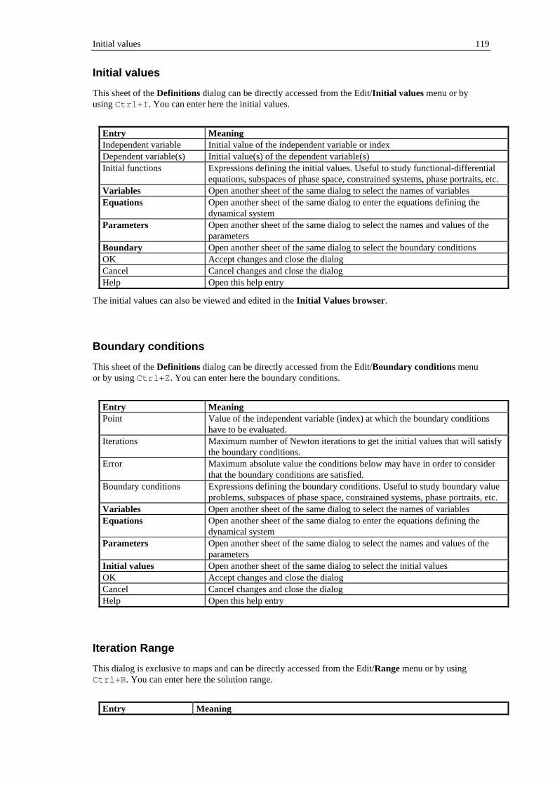
Initial values 119
Initial values
This sheet of the Definitions dialog can be directly accessed from the Edit/Initial values menu or byusing Ctrl+I . You can enter here the initial values.
Entry Meaning Independent variable Initial value of the independent variable or index Dependent variable(s) Initial value(s) of the dependent variable(s) Initial functions Expressions defining the initial values. Useful to study functional-differential
equations, subspaces of phase space, constrained systems, phase portraits, etc. Variables Open another sheet of the same dialog to select the names of variables Equations Open another sheet of the same dialog to enter the equations defining the
dynamical system Parameters Open another sheet of the same dialog to select the names and values of the
parameters Boundary Open another sheet of the same dialog to select the boundary conditions OK Accept changes and close the dialog Cancel Cancel changes and close the dialog Help Open this help entry
The initial values can also be viewed and edited in the Initial Values browser.
Boundary conditions
This sheet of the Definitions dialog can be directly accessed from the Edit/Boundary conditions menuor by using Ctrl+Z . You can enter here the boundary conditions.
Entry Meaning Point Value of the independent variable (index) at which the boundary conditions
have to be evaluated. Iterations Maximum number of Newton iterations to get the initial values that will satisfy
the boundary conditions. Error Maximum absolute value the conditions below may have in order to consider
that the boundary conditions are satisfied. Boundary conditions Expressions defining the boundary conditions. Useful to study boundary value
problems, subspaces of phase space, constrained systems, phase portraits, etc. Variables Open another sheet of the same dialog to select the names of variables Equations Open another sheet of the same dialog to enter the equations defining the
dynamical system Parameters Open another sheet of the same dialog to select the names and values of the
parameters Initial values Open another sheet of the same dialog to select the initial values OK Accept changes and close the dialog Cancel Cancel changes and close the dialog Help Open this help entry
Iteration Range
This dialog is exclusive to maps and can be directly accessed from the Edit/Range menu or by usingCtrl+R . You can enter here the solution range.
Entry Meaning

120 Dialog Boxes
First value The output starts when the index equals this value (or the index initial value if thisentry is 0). It is useful to skip over transients.
Last value The output ends when the index equals this value Infinity The output ends with a warning if the absolute value of any variable reaches this
value. A warning is issued, if the option Warning when infinity reached inPreferences/Other is selected.
Pause The time (in tenths of second) a blinking cursor will show the last output value. Ifthe value is negative you must press a key to get the next output point. See theexamples in CHAOS\DISKS.DS and GRAPH.DS.
Saved points The number of solution points to be retained in memory Bifurcation diagram Select it if you want to draw a bifurcation diagram Begin The first value of the parameter in the bifurcation diagram Step The step to increase the parameter value in the bifurcation diagram End The last value of the parameter in the bifurcation diagram Real time If not null, the number of real seconds corresponding to the unity of the
independent variable or index. See Forcing the Program to Wait OK Accept changes and close the dialog Cancel Cancel changes and close the dialog Help Open this help entry
Range
This sheet of the Numerical Method dialog can be directly accessed from the Edit/Range menu or byusing Ctrl+R . You can enter here the solution range.
Entry Meaning First value The output starts when the independent variable equals this value (or the initial value for
the independent variable if this entry is 0). It is useful to skip over transients. Last value The output ends when the independent variable equals this value Infinity The output ends with a warning if the absolute value of any variable or derivative
reaches this value. A warning is issued, if the option Warning when infinity reachedin Preferences/Other is selected.
Pause The time (in tenths of second) a blinking cursor will show the last output value. If thevalue is negative you must press a key to get the next output point.
Interpolate If this entry is not selected, the output happens every time the numerical code computesa new point. If it is selected ,the output happens in steps equal to the value selectedbelow.
Step The independent variable step for interpolated output Backward Select the entry to integrate backward Saved points The number of solution points to be retained in memory. A non-zero value is necessary
to have interpolated output, compute derivatives or Poincaré maps or to solve delay-differential equations
Real time If not null, the number of real seconds corresponding to the unity of the independentvariable or index. See Forcing the Program to Wait
Method Open another sheet in the same dialog with options for the integration method OK Accept changes and close the dialog Cancel Cancel changes and close the dialog Help Open this help entry

Numerical Method 121
Numerical Method
This sheet of the Numerical Method dialog can be directly accessed from the Edit/Method menu or byusing Ctrl+H . You can enter here the parameters of the numerical method. This dialog does not existfor maps.
Entry Meaning Tolerance The tolerance value to be achieved by the integration code Step h The starting value of the integration step Max. h The maximum value of the integration step Integration code The integration code to be used (it may have additional parameters) Code help Open the help file corresponding to the selected integration code Range Open another sheet to define the integration and output ranges OK Accept changes and close the dialog Cancel Cancel changes and close the dialog Help Open this help entry
Graphics Output
This sheet of the Graphics Output dialog can be directly accessed from the Output/Graphics formatmenu or by using Ctrl+F . You can enter here the output expressions.
See also the Graphics Output for Maps.
Entry Meaning Title The caption for the graphics window Window If the default value (this window) is used, the output appears in the current
graphics window. Select another window’s caption if you want to redirect the outputthere, in order to have multiple output to a single window.
Min. x The minimum value of the expression plotter in the horizontal axis Horizontal axis The expression represented in the horizontal axis Max. x The maximum value of the expression plotter in the horizontal axis Min. y The minimum value of the expression plotter in the vertical axis Vertical axis The expression represented in the vertical axis Max. y The maximum value of the expression plotter in the vertical axis Poincaré section Select this to plot a Poincaré section Increasing Select this to output a Poincaré map point when the Condition becomes null while
increasing from negative to positive Decreasing Select this to output a Poincaré map point when the Condition becomes null while
decreasing from positive to negative Error Select here the tolerance to accept that the Condition is met Condition The expression defining the Poincaré map Colors Open another dialog to select the output color View point Open another dialog to select the projection view point Format Open another sheet in the same dialog to define the output format Cursor Open another sheet in the same dialog to select the meaning of cursor and mouse
action Plotter Open another sheet in the same dialog to select driver and options for the plotter OK Accept changes and close the dialog Cancel Cancel changes and close the dialog Help Open this help entry

122 Dialog Boxes
Graphics Output for Maps
This sheet of the Graphics Output dialog can be directly accessed from the Output/Graphics formatmenu or by using Ctrl+F . You can enter here the output expressions.
See also Graphics Output.
Entry Meaning Title The caption for the graphics window Min. x The minimum value of the expression plotter in the horizontal axis Horizontal axis The expression represented in the horizontal axis Max. y The maximum value of the expression plotter in the horizontal axis Min. x The minimum value of the expression plotter in the vertical axis Vertical axis The expression represented in the vertical axis Max. y The maximum value of the expression plotter in the vertical axis Direct graph power The power of the map in a cobweb (ignored if 0) Inverse graph power The power of the inverse map in a cobweb (ignored if 0) Histogram The number of points between successive drawing of the histogram Average value Select this if an averaged value is desired instead of all the values computed
from First value to Last value (in Iteration Range). Useful to compute LiapunovExponents)
Format Open another sheet in the same dialog to define the output format Cursor Open another sheet in the same dialog to select the meaning of cursor and mouse
action Plotter Open another sheet in the same dialog to select driver and options for the plotter OK Accept changes and close the dialog Cancel Cancel changes and close the dialog Help Open this help entry
Format
This sheet of the Graphics Output dialog can be accessed from the Output/Graphics format menu orby using Ctrl+F . You can enter here the graphics format parameters.
Entry Meaning Continuous line Select this to have the plotted point joined by segments Frequency The frequency of graphics output Axes Sequence of groups of four coordinates defining the starting and end point of
segments. When the graphics screen is created a default value is entered hereif the Default axes entry in the Graphics sheet is set.
Direction field Select this to plot a direction field (this is not available for maps) Cell The distance (in pixels) between point in the direction field (this is not
available for maps) Length The length (in pixels) of the segment of the direction field (this is not
available for maps) Width Prescribed value for window width (0 is ignored). Height Prescribed value for window height (0 is ignored). Aspect ratio To have a 1:1 aspect ratio in the graphics window:
Arbitrary Ignore Adjust X range Change Min. x and Max. x Adjust Y range Change Min. y and Max. y Square Window is always squareAdjust width Change window width Adjust height Change window height

Cursor 123
When the graphics screen is created the default value is in the Aspect ratioentry of the Graphics sheet.
Bitmap output Copy output to bitmap No bitmap No bitmap output Copy bitmap Discard bitmap if the window dimensions change Stretch bitmap Stretch bitmap to new window dimensionsWhen the graphics screen is created the default value is in the Bitmapoutput entry of the Graphics sheet.
Save output in memory Memory (in multiples of 10 kb) to save graphics output Colors Open another dialog to select the output color View point Open another dialog to select the projection view point Output Open another sheet in the same dialog to define the output expressions Cursor Open another sheet in the same dialog to select the meaning of cursor and
mouse action Plotter Open another sheet in the same dialog to select driver and options for the
plotter OK Accept changes and close the dialog Cancel Cancel changes and close the dialog Help Open this help entry
Cursor
This sheet of the Graphics Output dialog can be accessed from the Output/Graphics format menu orby using Ctrl+F . You can enter here the action of the mouse/cursor movements.
Entry Meaning Variable in axis X The variable whose initial value is selected with the cursor x coordinate Horizontal step The horizontal step when moving the cursor with the direction keys Variable in axis Y The variable whose initial value is selected with the cursor y coordinate Vertical step The vertical step when moving the cursor with the direction keys Angle Step when changing angles Zooming factor Scale factor Fractal order Fractal order to be added to that of each fractal curve Output Open another sheet in the same dialog to define the output expressions Format Open another sheet in the same dialog to define the output format Plotter Open another sheet in the same dialog to select plotter options OK Accept changes and close the dialog Cancel Cancel changes and close the dialog Help Open this help entry
Colors
This dialog can be directly accessed from the Output/Color menu or by using Ctrl+O , and also fromthe Format dialog sheet. You can enter here the output colors.
Entry Meaning Drawing pen Select this entry to edit the color for points and lines Axes Select this entry to edit the color for axes Direction field Select this entry to edit the color for segments in the direction field Background Select this entry to edit the color for the window background Select Click once to select a color, twice to customize it

124 Dialog Boxes
Width Enter here the pen width or select it with the mouse in the list below OK Accept changes and close the dialog Cancel Cancel changes and close the dialog Help Open this help entry
You can also use the PenColor , PenWidth , HSV and RGB functions in the Horizontal axis andVertical axis entries of the Graphics Output dialog box.
View Point for Projections
This dialog can be directly accessed from the Output/View point menu or by using Ctrl+W , and alsofrom the Graphics Output dialog. You can enter here the parameter for projections.
Most of the entries below can be changed by entering a numerical value, by using a scroll bar or bydragging the cube on the graphics pane.
Entry Meaning Theta First Euler angle (see figure) Phi Second Euler angle (see figure) Psi Third Euler angle (see figure) Distance Distance between observation point and projection plane (see figure) Origin Distance between observation point and coordinate origin (see figure) OK Accept changes and close the dialog Cancel Cancel changes and close the dialog Help Open this help entry
Plotter
This sheet of the Graphics Output dialog can be directly accessed from the Output/Plotter settingsmenu. You can enter here the plotter driver parameters.
Entry Meaning On Plotter output enabled/disabled for this window. To enable/disable any/all plotter output use
the Output/Plotter output menu or the corresponding button. Frame Select this entry to send a frame around the plotter output Pen Select here the pen (this entry is highly driver dependent, see Driver help below)

Text Output 125
Width Select here the pen width (this entry is highly driver dependent, see Driver help below) Speed Select here the pen speed (this entry is highly driver dependent, see Driver help below) Line type Select here the line type (this entry is highly driver dependent, see Driver help below) Output file Write here the device (AUX, COM1, COM2, etc.) to collect the plotter output or press the
button to open a Open/Save common dialog box to select a file for plotter output Driver Select here the plotter driver Driver help Pressing this button will provide help on the plotter driver, if available Output Open another sheet in the same dialog to define the output expressions Format Open another sheet in the same dialog to define the output format Cursor Open another sheet in the same dialog to select the meaning of cursor and mouse action OK Accept changes and close the dialog Cancel Cancel changes and close the dialog Help Open this help entry
Text Output
This dialog can be accessed from the Output/Text format menu or by using Ctrl+X . You can enterhere the text format parameters.
Entry Meaning Title The caption for the graphics window Expression # The expression(s) to be output Format The format string to be used for each Expression Separator The format string to be separate different lines/points Output frequency The number of solutions points (+1) between to text output lines Lines in memory The number of text output line to be retained in memory for backscrolling Capture Select this if you want to send the text output to a text file Output file Set here the device (PRN, LPT1, LPT2, etc.) to collect the plotter output or Browse press this button to open an Open/Save common dialog box to select a file to collect
the text output View point Open another dialog to select the projection view point Poincaré section Select this entry to have a Poincaré section Condition The expression defining the Poincaré section Error Select here the tolerance to accept that the Condition is met Increasing Select this to output a Poincaré map point when the Condition becomes null while
increasing from negative to positive Decreasing Select this to output a Poincaré map point when the Condition becomes null while
decreasing from positive to negative OK Accept changes and close the dialog Cancel Cancel changes and close the dialog Help Open this help entry
Text Output for Maps
This sheet of the Text Output dialog can be accessed from the Output/Text format menu or by usingCtrl+X . You can enter here the text format parameters.
Entry Meaning Title The caption for the graphics window Expression # The expression(s) to be output

126 Dialog Boxes
Format The format string to be used for each Expression Separator The format string to be separate different lines/points Output frequency The number of solutions points (+1) between to text output lines Lines in memory The number of text output line to be retained in memory for backscrolling Capture Select this if you want to send the text output to a text file Output file Set here the device (PRN, LPT1, LPT2, etc.) to collect the plotter output or Browse Press this button to open an Open/Save common dialog box to select a file to
collect the text output View point Open another dialog to select the projection view point Histogram The number of points between successive writings of the histogram Average value Select this if an averaged value is desired (useful to compute Liapunov exponents) OK Accept changes and close the dialog Cancel Cancel changes and close the dialog Help Open this help entry
Numerical Output in Status Line
This dialog can be directly accessed from the Output/Status line menu or by using Ctrl+S . You canenter here a couple of expressions to be monitored in the status line.
Entry Meaning First quantity The first expression to be output Second quantity The second expression to be output Format string The format string to be used for each quantity Frequency The number of solutions points (+1) between to text output lines OK Accept changes and close the dialog Cancel Cancel changes and close the dialog Help Open this help entry
Compiler Error
This dialog box is opened when the expression compiler finds an error. Entry Meaning (first line) The name of the expression in error (edit box) The expression in error. You can see and change it (last line) The error type (see Messages) OK Accept changes and close the dialog Cancel Cancel changes, abort compilation and close the dialog Help Open this help entry
Mode
This dialog will open when you try to send to the current window the graphics contents of the clipboard(Window/Put screen or Ctrl+V or Shift+Ins ) or an external file (Window/Load screen):
Entry Meaning Put Sometimes more than one of the following formats is
available in the clipboard. Select the one you want: Device dependent bitmap The fastest one Device independent bitmap Portable among different displays Windows metafile Portable and scaleable
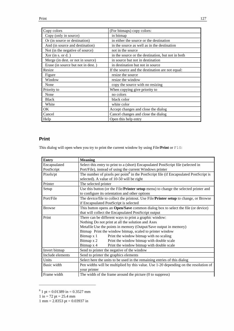
Print 127
Copy colors (For bitmaps) copy colors: Copy (only in source) in bitmap Or (in source or destination) in either the source or the destination And (in source and destination) in the source as well as in the destination Not (in the negative of source) not in the source Xor (in s. or d. ) in the source or the destination, but not in both Merge (in dest. or not in source) in source but not in destination Erase (in source but not in dest. ) in destination but not in source Resize If the source and the destination are not equal: Figure resize the source Window resize the window None copy the source with no resizing Priority to When copying give priority to None no colors Black black color White white color OK Accept changes and close the dialog Cancel Cancel changes and close the dialog Help Open this help entry
This dialog will open when you try to print the current window by using File/Print or F10:
Entry Meaning EncapsulatedPostScript
Select this entry to print to a (short) Encapsulated PostScript file (selected inPort/File), instead of using the current Windows printer
Pixels/pt The number of pixels per point8 in the PostScript file (if Encapsulated PostScript isselected). A value of 10-50 will be right
Printer The selected printer Setup Use this button (or the File/Printer setup menu) to change the selected printer and
to configure its orientation and other options Port/File The device/file to collect the printout. Use File/Printer setup to change, or Browse
if Encapsulated PostScript is selected Browse This button opens an Open/Save common dialog box to select the file (or device)
that will collect the Encapsulated PostScript output Print There can be different ways to print a graphic window:
NothingDo not print at all the solution and AxesMetafileUse the points in memory (Output/Save output in memory)Bitmap Print the window bitmap, scaled to printer windowBitmap x 1 Print the window bitmap with no scalingBitmap x 2 Print the window bitmap with double scaleBitmap x 4 Print the window bitmap with double scale
Invert bitmap Send to printer the negative of the window Include elements Send to printer the graphics elements Units Select here the units to be used in the remaining entries of this dialog Basic width Pen widths will be multiplied by this value. Use 1-20 depending on the resolution of
your printer Frame width The width of the frame around the picture (0 to suppress)
8 1 pt = 0.01389 in = 0.3527 mm1 in = 72 pt = 25.4 mm1 mm = 2.8353 pt = 0.03937 in

128 Dialog Boxes
Min. distance When printing to an Encapsulated Postscript file, if the difference between the x(and y) coordinates of a point and the preceding one in a line is less or equal thanthis value, the point is not sent to the printer (to create smaller files). Once the datahas been sent to an Encapsulated Postscript file you can still discard points differingby less than a given value by using the CompEPS utility.
Rotate PostScript If Encapsulated PostScript is allowed and this entry is selected, an explicit rotateinstruction is included in the EPS file. Do not use it, unless you want a landscapeprintout when directly uploading the EPS file to the laser printer
Preserve aspect ratio If this entry is selected, the relative horizontal and vertical dimensions will be thesame in the screen and in the printout
Top margin The margin above the picture† Height The picture height‡ Bottom margin The margin below the picture† Left margin The left margin† Width The picture width‡ Right margin The right margin† OK Accept changes and close the dialog Cancel Cancel changes and close the dialog Help Open this help entry
† You can also use the mouse to change this value in the right panel displaying the output size andposition.
‡ You can also use the mouse while pressing the Shift key to change this value in the right paneldisplaying the output size and position.
Graphics Element
This dialog can be accessed from the Draw/Edit menu entry. It is used to view and change theparameters of the current (and all the remaining) graphics element:
Entry Meaning + Display the next graphics element - Display the previous graphics element <<-- Exchange this element and the previous one -->> Exchange this element and the next one New Create a new element Copy Copy the current element to a new one Remove Remove the current element Erase all Remove all elements Type Select here the element type OK Accept changes and close the dialog Cancel Cancel changes and close the dialog Help Open this help entry
The number and names of the remaining entries in this dialog depend on the Type of the element that iscurrently displayed. It can be one of the following types:
Segment Circle Ellipse Arrow Text 2-curve 3-curve Special

New Graphics Element 129
Data Fractal
New Graphics Element
This dialog is open when a new element is created by using the Draw/Edit menu entry. It is used toview and change the parameters of the current (and all the remaining) graphics element:
Entry Meaning Type Select here the type of the new element OK Accept changes. The Edit Element dialog will open Cancel Cancel changes and close the dialog Help Open this help entry
Preferences
This sheet of the Preferences dialog can be accessed from the Configuration/Preferences menu. Youcan enter here your preferences to customize some aspects of Dynamics Solver’s behavior:
Entry Meaning Toolbar Options for toolboxes Change cursor over disabled buttons The cursor shape will change for disabled buttons Button size Size of toolbar buttons: Small Medium Big Disabled Disabled buttons will appear: Hidden Normal Grayed Status hints Display in status bar hints for menus/toolbars: Always always Enabled only for enabled buttons/menu entries Never never Popup tips Display popup tips: Always for all toolbar buttons Enabled only for enabled buttons Never never (to avoid continuous screen redrawing) Hide browsers when running Hide Initial Values and Parameter browsers when
computing the solution. Otherwise make them inactive. Boxes Open another sheet with options for edit boxes Graphics Open another sheet with options for graphics Other Open another sheet with miscellaneous options OK Accept changes and close the dialog Cancel Cancel changes and close the dialog Help Open this help entry
See also Customization and the Configuration menu.

130 Dialog Boxes
Boxes
This is a sheet of the Preferences dialog, which can be accessed from the Configuration/Preferencesmenu. You can enter here your preferences to customize some aspects of Dynamics Solver’s behavior:
Entry Meaning Dialog boxes The font used for dialog boxes will have the following: Point size (This entry is not available in the 32-bit edition) Edit boxes In edit boxes: Fixed pitch font use a fixed pitch font (better for math expressions) Enter key use the Enter key to start a new line (instead of OK) Use bold font in Use a bold font in: Status line Text windows Edit windows Startup tips Control the Tip of the Day displayed at program startup Next tip Number of the next tip. 0 to disable this feature. Toolbox Open another sheet with options for toolbars and menus Graphics Open another sheet with options for graphics Other Open another sheet with miscellaneous options OK Accept changes and close the dialog Cancel Cancel changes and close the dialog Help Open this help entry
See also Customization and the Configuration menu.
Graphics
This is a sheet of the Preferences dialog, which can be accessed from the Configuration/Preferencesmenu. You can enter here your preferences to customize some aspects of Dynamics Solver’s behavior:
Entry Meaning Copy to clipboard When copying a graphic window to the clipboard include: Bitmap Device dependent bitmap DIB Device independent bitmap Metafile Windows metafile Aspect ratio Default value for the same entry in Format
To have a 1:1 aspect ratio in the graphics window:Arbitrary Ignore Adjust X range Change Min. x and Max. x Adjust Y range Change Min. y and Max. y Square Window is always squareAdjust width Change window width Adjust height Change window heightWhen the graphics screen is created the default value is in theAspect ratio entry of the Graphics sheet.
Bitmap output Default value for the same entry in Format No bitmap No bitmap output Copy bitmap Discard bitmap if the dimensions change Stretch bitmap Stretch bitmap to new window dimensions
Memory output Default memory size (in multiples of 10 kb) to save graphicsoutput, -1 uses as much memory as necessary
Default axes Check this entry if you want to use default values for Axes inFormat when creating a new graph windows
Redraw while editing elements Continuous redrawing of graphics elements Toolbox Open another sheet with options for toolbars and menus Boxes Open another sheet with options for edit boxes

Other 131
Other Open another sheet with miscellaneous options OK Accept changes and close the dialog Cancel Cancel changes and close the dialog Help Open this help entry
See also Customization and the Configuration menu.
Other
This is a sheet of the Preferences dialog, which can be accessed from the Configuration/Preferencesmenu. You can enter here your preferences to customize some aspects of Dynamics Solver’s behavior:
Entry Meaning Identifier Enter here the identifier (1 to 8 letters/digits/_) to be able to recover
from disk taste-dependent options. (See Special Settings.) Extensions By default, Dynamics Solver searches problem files with the .DS
extension. This will be fine in most cases, but you might have a lot ofproblem files with another extension. If you want to search problemfiles with extensions, say, .DS , .MAP and .EF , you should enterhere *.ds;*.map;*.ef
Filename length in menus The maximum length of a filename in the File menu. Select 0 if youwant only file names with no path
Show extensions (Windows 3.1+) Check this entry to show problem file extensions (the default inWindows 3.1).
Show full paths (Windows95/98/NT4)
In Windows 95/98/NT4 extensions are hidden by default, but if thisis checked the full filename is displayed instead of using the currentExplorer settings.
Double click to select If this entry is selected, a double click will be necessary to select newinitial conditions or a new graphics element
Check previous instances If this entry is checked and the program is directly started with noproblem file, a Dynamics Solver is already running dialog box willopen
Save main window and browsersposition
Save the main window position and size for the next session. Thesame is done with Initial Values and Parameter browsers.
Release button to show popup menu Check this entry to have to release the right mouse button to see thepopup menu (the default in Windows 95/98/NT4). In Windows 3.1the menu will appear by default before releasing the button.
Warning when infinity reached By default when the infinity (defined in the Range dialog sheet) isreached a warning message is issued. Uncheck this option to avoidthe message: the solution will end silently.
Do not default to My Documents A new “feature” of Windows 98 makes your My Documentsfolder the default directory when trying to open or save a new file. Ifyou find this annoying, check this entry and Dynamics Solver willdefault to the current directory, as under previous Windows versions.(Available only in the 32-bit version.)
Toolbox Open another sheet with options for toolbars and menus Boxes Open another sheet with options for edit boxes Graphics Open another sheet with options for graphics OK Accept changes and close the dialog Cancel Cancel changes and close the dialog Help Open this help entry
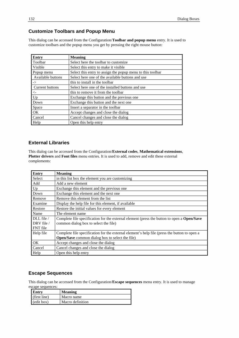
132 Dialog Boxes
Customize Toolbars and Popup Menu
This dialog can be accessed from the Configuration/Toolbar and popup menu entry. It is used tocustomize toolbars and the popup menu you get by pressing the right mouse button:
Entry Meaning Toolbar Select here the toolbar to customize Visible Select this entry to make it visible Popup menu Select this entry to assign the popup menu to this toolbar Available buttons Select here one of the available buttons and use -> this to install in the toolbar Current buttons Select here one of the installed buttons and use <- this to remove it from the toolbar Up Exchange this button and the previous one Down Exchange this button and the next one Space Insert a separator in the toolbar OK Accept changes and close the dialog Cancel Cancel changes and close the dialog Help Open this help entry
External Libraries
This dialog can be accessed from the Configuration/External codes, Mathematical extensions,Plotter drivers and Font files menu entries. It is used to add, remove and edit these externalcomplements:
Entry Meaning Select in this list box the element you are customizing Add Add a new element Up Exchange this element and the previous one Down Exchange this element and the next one Remove Remove this element from the list Examine Display the help file for this element, if available Restore Restore the initial values for every element Name The element name DLL file / DRV file /FNT file
Complete file specification for the external element (press the button to open a Open/Savecommon dialog box to select the file)
Help file Complete file specification for the external element’s help file (press the button to open aOpen/Save common dialog box to select the file)
OK Accept changes and close the dialog Cancel Cancel changes and close the dialog Help Open this help entry
Escape Sequences
This dialog can be accessed from the Configuration/Escape sequences menu entry. It is used to manageescape sequences:
Entry Meaning (first line) Macro name (edit box) Macro definition

Initial Values browser 133
OK Accept changes and close the dialog Cancel Cancel changes and close the dialog Help Open this help entry
Initial Values browser
This browser can be open or activated from the Edit/Initial Values browser menu, by pressing
Shift+Ctrl+I or using the toolbar button. Here you can view and edit all the initial conditions(up to a maximum of 20) of the current problem. This provides a way to see and edit all constant valuesin the Initial values sheet of the Variables dialog box.
The most effective way to use this browser includes using the following keyboard shortcuts:Shortcut MeaningShift+Ctrl+I Open and/or activate the browserEsc Close the browser (you can also use Alt+F4 or the Close button)Enter Activate the program main window (to access other menus, etc.)Enter, Enter Start the solution (equivalent to using Go/Start)
The visibility and position of the browser will be saved from session to session if the Save main windowand browsers position option in the Other sheet is checked.
When a solution is being computed the browser is automatically hidden if the Hide browsers whenrunning option in Toolbox sheet is checked. Otherwise, it just made inactive: you cannot change theinitial values when they are being used to compute the solution.
See also Parameter browser and Edit all Settings in a Text Window.
Parameter browser
This browser can be open or activated from the Edit/Parameter browser menu, by pressing
Shift+Ctrl+P or using the toolbar button. Here you can view and edit all the parameter (up to amaximum of 20) of the current problem, as well as the minimum and maximum values used in Repeatedsolutions and phase portraits. This provides a way to see and edit all numerical values in theParameters sheet of the Variables dialog box.
The most effective way to use this browser includes using the following keyboard shortcuts:Shortcut MeaningShift+Ctrl+I Open and/or activate the browserEsc Close the browser (you can also use Alt+F4 or the Close button)Enter Activate the program main window (to access other menus, etc.)Enter, Enter Start the solution (equivalent to using Go/Start)
The visibility and position of the browser will be saved from session to session if the Save main windowand browsers position option in the Other sheet is checked.
When a solution is being computed the browser is automatically hidden if the Hide browsers whenrunning option in Toolbox sheet is checked. Otherwise, it just made inactive: you cannot change theinitial values when they are being used to compute the solution.
See also Initial Values browser and Edit all Settings in a Text Window.
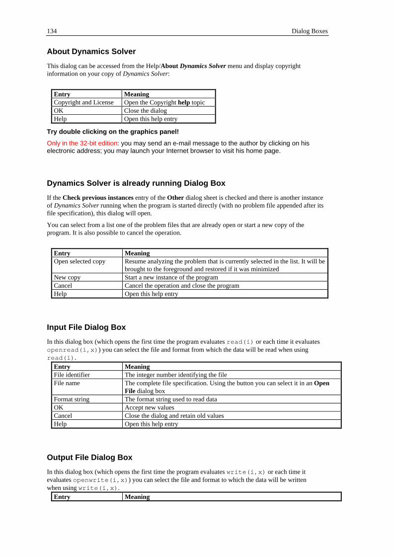
134 Dialog Boxes
About Dynamics Solver
This dialog can be accessed from the Help/About Dynamics Solver menu and display copyrightinformation on your copy of Dynamics Solver:
Entry Meaning Copyright and License Open the Copyright help topic OK Close the dialog Help Open this help entry
Try double clicking on the graphics panel!
Only in the 32-bit edition: you may send an e-mail message to the author by clicking on hiselectronic address; you may launch your Internet browser to visit his home page.
Dynamics Solver is already running Dialog Box
If the Check previous instances entry of the Other dialog sheet is checked and there is another instanceof Dynamics Solver running when the program is started directly (with no problem file appended after itsfile specification), this dialog will open.
You can select from a list one of the problem files that are already open or start a new copy of theprogram. It is also possible to cancel the operation.
Entry Meaning Open selected copy Resume analyzing the problem that is currently selected in the list. It will be
brought to the foreground and restored if it was minimized New copy Start a new instance of the program Cancel Cancel the operation and close the program Help Open this help entry
Input File Dialog Box
In this dialog box (which opens the first time the program evaluates read(i) or each time it evaluatesopenread(i,x) ) you can select the file and format from which the data will be read when usingread(i) .
Entry Meaning File identifier The integer number identifying the file File name The complete file specification. Using the button you can select it in an Open
File dialog box Format string The format string used to read data OK Accept new values Cancel Close the dialog and retain old values Help Open this help entry
Output File Dialog Box
In this dialog box (which opens the first time the program evaluates write(i,x) or each time itevaluates openwrite(i,x) ) you can select the file and format to which the data will be writtenwhen using write(i,x) .
Entry Meaning

Input Value Dialog Box 135
File identifier The integer number identifying the file File name The complete file specification. Using the button you can select it in an Open
File dialog box Format string The format string used to write data OK Accept new values Cancel Close the dialog and retain old values Help Open this help entry
Input Value Dialog Box
In this dialog box (which opens every time the program evaluates input(i) ) you have to enter anumeric value to be returned by the function input(i) .
Entry Meaning Input # The integer number identifying the input value. In the edit box next to this string
you have to enter a numeric value OK Return the value Cancel Close the dialog, return i and end the current iteration (equivalent to returning
break(1,i) ) Help Open this help entry
Save points in memory to external file
This dialog can be directly accessed from the Window/Save points menu or by using Ctrl+P or the
toolbar button). You can select here the output file and options to save the integration datacurrently in memory to the disk, so that they can be used as a data graphics element or by means ofanother program. (See the Sending the results to an external file.)
Entry Meaning File Browse disk(s) to select the output file, which must be entered in the following edit box Ignore points with distanceunder
If the difference between the x (and y) coordinates of a point and thepreceding one in a line is less or equal than this value, the point is not sentto the file (to create smaller files).
Clip points inside the followingrectangle
Check this option to make the output points to lie inside the rectangle withvertices defined below.
Minimum x x coordinate of the lower left vertex of the clipping rectangle. Maximum x x coordinate of the lower left vertex of the clipping rectangle. Minimum y y coordinate of the upper right vertex of the clipping rectangle. Maximum y y coordinate of the upper right vertex of the clipping rectangle. OK Send data and close the dialog Cancel Cancel sending data and close the dialog Help Open this help entry
Once the data has been stored in a disk file you can clip it and discard points differing by less than a givenvalue by using the ClipData utility.
Tip of the Day Dialog Box
In this dialog box (which opens every time the program starts) you may find some useful hints. Entry Meaning

136 Dialog Boxes
Show tips at startup Uncheck this entry to disable the Tip of the Day. It may be re-enabled from theNext tip entry of the Boxes dialog box.
Next tip Display the next tip (its number is stored in the aforementioned entry). Close Close the dialog Help Open this help entry
Color Common Dialog Box
This common dialog is invoked by Dynamics Solver but managed by Windows itself. Refer to yourWindows documentation.
Open/Save Common Dialog Box
This common dialog is invoked by Dynamics Solver but managed by Windows itself. Refer to yourWindows documentation.
Print Common Dialog Box
This common dialog is invoked by Dynamics Solver but managed by Windows itself. Refer to yourWindows documentation.
Printer Setup Common Dialog Box
This common dialog is invoked by Dynamics Solver but managed by Windows itself. Refer to yourWindows documentation.
Find Common Dialog Box
This common dialog is invoked by Dynamics Solver but managed by Windows itself. Refer to yourWindows documentation.
Replace Common Dialog Box
This common dialog is invoked by Dynamics Solver but managed by Windows itself. Refer to yourWindows documentation.

Menu Entries 137
Keyboard
With a few exceptions, everything can be achieved in Dynamics Solver by means of the keyboard. We listbelow the key actions that are specific to Dynamics Solver or standard Windows keys.
Menu Entries
Many entry menus can be directly activated by using one of the following shortcuts: Key Menu entry F1 Open the help Index F2 File/Save F3 File/Open Shift+F3 Window/Tile vertical Shift+F4 Window/Tile horizontal F5 Edit/All settings Shift+F5 Window/Cascade F10 File/Print + * Draw/Next element - * Draw/Previous element * * Zoom/Larger step / * Zoom/Smaller step Enter Go/Start (or redraw current element) Esc Go/Stop (or stop the redrawing of
graphics elements and metafiles) Del Window/Erase window Ctrl+Del Window/Erase all Ctrl+Ins Window/Get screen Shift+Ins Window/Put screen Ctrl+A Edit/Parameters Ctrl+B Go/Backward Ctrl+C Window/Get screen Ctrl+D Draw/Refresh all Ctrl+E Edit/Equations Ctrl+F Output/Graphics format Ctrl+G Output/New graphics window Ctrl+H Edit/Method Ctrl+I Edit/Initial conditions Ctrl+L Edit/Variables Ctrl+N Edit/Notes Ctrl+O Output/Color Ctrl+P Window/Save points Ctrl+R Edit/Range Ctrl+S Output/Status line Ctrl+T Output/New text window Ctrl+U Go/Continue Ctrl+V Window/Put screen Ctrl+W Output/View point Ctrl+X Output/Text format Ctrl+Y Edit/Type Ctrl+Z Edit/Boundary conditions Shift+Ctrl+I Edit/Initial Values browser Shift+Ctrl+P Edit/Parameter browser C Draw/Copy

138 Keyboard
D Draw/Refresh window E Draw/Edit F Action/First value I Zoom/Zoom in L Action/Last value M Action/Move around N Draw/New element O Action/Origin P Action/Point R Action/Rotate S Action/Select an element T Action/Third point X Action/Initial condition W Zoom/Zoom out Z Zoom/Actual size Direction keys To move the cursor, origin, point, third
point, or to rotate, and to select first andlast values.
*These keys are those in the numeric keypad
Cursor Movement Keys
Key(s) Function Direction key Moves the cursor left, right, up, or down in a field or a
graphics window. Shift+ direction key Moves ten times the cursor left, right, up, or down in a
graphics window. End orCtrl+Right Arrow
Moves to the end of a field.
Home orCtrl+Left Arrow
Moves to the beginning of a field.
Page Up orPage Down
Moves up or down in a field, one screen at a time.
Dialog Box Keys
Key(s) Function Tab Moves from field to field (left to right and top to bottom). Shift+Tab Moves from field to field in reverse order. Alt+ letter Moves to the option or group whose underlined letter matches
the one you type. Direction key Moves from option to option within a group of options. Enter Executes a command button. Or, chooses the selected item in a list box and executes the
command. Esc Closes a dialog box without completing the command. (Same
as Cancel) Alt+Down Arrow Opens a drop-down list box. Alt+Up orDown Arrow
Selects item in a drop-down list box.
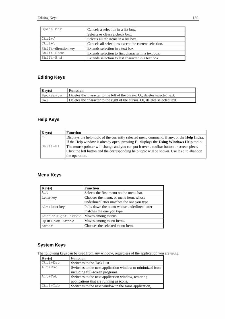
Editing Keys 139
Space bar Cancels a selection in a list box. Selects or clears a check box. Ctrl+/ Selects all the items in a list box. Ctrl+\ Cancels all selections except the current selection. Shift+ direction key Extends selection in a text box. Shift+Home Extends selection to first character in a text box. Shift+End Extends selection to last character in a text box
Editing Keys
Key(s) Function Backspace Deletes the character to the left of the cursor. Or, deletes selected text. Del Deletes the character to the right of the cursor. Or, deletes selected text.
Help Keys
Key(s) Function F1 Displays the help topic of the currently selected menu command, if any, or the Help Index.
If the Help window is already open, pressing F1 displays the Using Windows Help topic. Shift+F1 The mouse pointer will change and you can put it over a toolbar button or screen piece.
Click the left button and the corresponding help topic will be shown. Use Esc to abandonthe operation.
Menu Keys
Key(s) Function Alt Selects the first menu on the menu bar. Letter key Chooses the menu, or menu item, whose
underlined letter matches the one you type. Alt+ letter key Pulls down the menu whose underlined letter
matches the one you type. Left or Right Arrow Moves among menus. Up or Down Arrow Moves among menu items. Enter Chooses the selected menu item.
System Keys
The following keys can be used from any window, regardless of the application you are using. Key(s) Function Ctrl+Esc Switches to the Task List. Alt+Esc Switches to the next application window or minimized icon,
including full-screen programs. Alt+Tab Switches to the next application window, restoring
applications that are running as icons. Ctrl+Tab Switches to the next window in the same application,

140 Keyboard
restoring minimized windows. Alt+PrtSc Copies the entire screen to Clipboard. Ctrl+F4 Closes the active window. F1 Gets Help (See Help Keys)
Text Selection Keys
Key(s) Function Shift+Left orRight Arrow
Selects text one character at a time to the left or right.
Shift+Down orUp
Selects one line of text up or down.
Shift+End Selects text to the end of the line. Shift+Home Selects text to the beginning of the line. Shift+Page Down Selects text down one window. Or, cancels the selection if the next
window is already selected. Shift+Page Up Selects text up one window. Or, cancels the selection if the previous
window is already selected. Ctrl+Shift+Left orRight Arrow
Selects text to the next or previous word.
Ctrl+Shift+Up orDown Arrow
Selects text to the beginning (Up Arrow) or end (Down Arrow) of theparagraph.
Ctrl+Shift+End Selects text to the end of the document. Ctrl+Shift+Home Selects text to the beginning of the document.
Window Keys
Key(s) Function Alt+Space bar Opens the Control menu for the main window. Alt+- Opens the Control menu for a child (graphics or text) window. Alt+F4 Closes the main window. Ctrl+F4 Closes a child (graphics or text) window. Alt+Esc Switches to the next application window or minimized icon, including
full-screen programs. Ctrl+Esc Opens the task list manager. Alt+Tab Switches to the next application window, restoring applications that
are running as icons. Ctrl+Tab or Ctrl+F6 Switches to the next child (graphics or text) window, restoring
iconized windows. Alt+Enter Switches a non-Windows application between running in a window
and running full screen. Direction key Moves a window when you have chosen Move from the Control menu.
Or, changes the size of a window when you have chosen Size from theControl menu.

Window Keys 141
Edit Windows
Edit windows are used in Dynamics Solver to edit all settings in a text window and to edit project notes.
The caret (a vertical bar) indicates the current insertion (or overwriting) position and its coordinates (lineand column) permanently displayed in the window last line. To learn how to use editing keys, refer to theKeyboard topic.
Notice that Windows limits the maximum line length in an edit window to about 4092 characters (1024 inthe 16-bit edition), while Dynamics Solver is able to deal with lines five times longer. Problem files withvery long lines can be viewed and changed by means of a good editor. In the 16-bit edition Windowslimits the total amount of text in an edit window to 64 Kb, while the limit in the 32-bit edition is of 1Mb.
The menu in edit windows is as follows:
Entry Meaning File File and printer management Edit Edit commands Search Find and replace commands Help Help system
File
The entries of this menu of edit windows are used to manage the printer and files:
Entry Meaning Accept changes Save changes, close edit window and go to current output window Abandon changes Discard changes, close edit window and go to current output window. The
problem could be incomplete! Switch to main window Set focus to the current output window. Do not close the text window New Clear the edit window Open Get a file from the disk Save Save the current file to the disk Save as Save the current file to the disk under a new name Print Print the current file
Edit
The entries of this menu of edit windows are used to manage the clipboard, text changes and textselection:
Entry Key Meaning Undo Alt+Backspace
orCtrl+Z
Revert the last change
Cut Shift+Del Move to clipboard the current selection Copy Ctrl+Ins
or Ctrl+C
Copy to clipboard the current selection
Paste Shift+Ins or Ctrl+V
Copy clipboard to the cursor position
Clear Del Remove the current selection Select All Select all text

142 Edit Windows
Search
The entries of this menu of edit windows are used to find and replace pieces of text:
Entry Meaning Search Open the Find common dialog box Replace Open the Replace common dialog box
Help
The entries of this menu of edit windows are used to access some help entry points:
Entry Meaning Edit window Open the edit window entry Index Open the index entry Keyboard Open the keyboard entry Help on Help Open the help on help entry
Edit all Settings in a Text Window
You can use F5 or the File/All settings menu (or even the button) to open a text window where youcan view an edit all the settings in the current problem.
In the text window you will see and edit the text representation of the problem under study. In fact youwill see the problem file text that will by saved to (or loaded from) the disk. This is a convenient way todo extensive changes to the problem, or to start a new one using an old problem as template.
When you close the window (using Alt+F4 , the File/Accept changes menu or the system menu) thesettings will be read. If an error happens, you will we informed and the text window will show you themost probable location of the error. You can correct it, or give up by using the File/Abandon changesmenu entry, but in the latter case you will probably have an incomplete problem in memory.
See also Initial Values browser and Parameter browser.
Edit Project Notes
You can use Ctrl+N or the File/Notes menu (or even the button) to open a text window where youcan view and edit notes related to the current project: information on bibliography, known results,interesting values of parameters or other settings, or whatever information you want to keep with theproblem. The contents and format of these notes are completely arbitrary, but its length is limited byWindows.
The notes are part of the problem file and, in consequence, they can be also edited form the All settingstext window. They will be saved to the disk and recovered from there when you use the File menu to saveand load problem files in the usual way. You can also save them to (or load from) a separate text file byusing the window File menu.

Numbers 143
Mathematical Expressions
You must enter mathematical expressions to define equations, initial functions, values to plot or display,and so forth. In Dynamics Solver an expression is formed, in a very standard way, by the following itemsoptionally separated by spaces:
Numbers Mathematical Operators Comparison Operators Logical Operators Conditional Operator Parentheses Variables for Graphics Elements Independent Variable Dependent Variables Interpolated Solution Initial Values User-defined Parameters Predefined Constants One-Variable Functions Two-Variable Functions Three-Variable Functions Graphics Functions Other Functions Mathematical Extensions
Each of these topics is described below in its proper section, but the main differences with the usualmathematical notation and the notation used is Dynamics Solver can be summarized as follows:
1. The whole expression must fit on a single line. You must write g/l , e^x , 1.5E5 , x[1] (forderivatives or indexes), x_2 , and arccot(x) .
2. Identifiers cannot be Greek letters, but they can have up to eighty letters or digits after the firstcharacter. The underscore character, _, is considered a letter in this context. You can use x2 (orx_2 ) and theta as identifiers.
3. Many symbols are lacking: |x| must be written as abs(x) , the square root is sqrt(x) andyou write x <= y for the less or equal operator.
4. Multiplication must be explicitly indicated by means of * . So, xy is an two-letter identifier notthe product x*y . On the other hand x y is not allowed and will raise an error message.
5. Functional arguments must be enclosed between parentheses. For instance, cos x must be writtencos(x) .
6. The precedence of operators is clearly defined: 1/2*pi is always interpreted as (1/2)*piand not as 1/(2*pi) . If you have any doubt, add some more parentheses.
Numbers
The usual format of computer languages is used by Dynamics Solver: -2 , 1E-12 , -1.02e2 , .2 , etc.(Refer to the Compiler Description.)
Notice that the exponential notation used by most calculators must be used, as in 1.2E7 in dialog boxentries that only have numerical values, but if full expressions can be entered, then the form 1.2*10^7 isalso possible.
Mathematical Operators
Operator Equivalent function Meaning + Addition - Subtraction * Multiplication / Division % mod Modulus: x%y = x mod y

144 Mathematical Expressions
pow Exponentiation
Comparison Operators
They return 1 for True and 0 for False:
Operator Meaning < Less than <= Less or equal to > Greater than / Greater or equal to == Equal to != Not equal to
Logical Operators
They return 1 for True and 0 for False:
Operator Meaning && and || or ! not
Only the operands that are necessary to establish the result are evaluated.
Conditional Operator
The expression
c ? t : f
is equivalent to if(c,t,f) and returns t if c != 0 and f if c == 0 .
Operator Precedence
From lowest to highest:
Order Operator Type 1 ? : Conditional operator 2 || Or 3 && And 4 == != (In)equality 5 < <= > >= Comparison 6 + - Binary addition/subtraction operators 7 * / % Multiplication/division 8 Exponentiation 9 ! + - Unary operators: not and signs

Parentheses 145
Parentheses
Use them to change the usual precedence of operators and functions. They are required around functionarguments and for any kind of mathematical extensions, even if they are constants.
Identifiers
The user can select the names of variables, parameters, initial values and the interpolated solutions,though most of them have a default value. They are case-sensitive and composed by a letter optionallyfollowed by one to seven letters or digits. In this context, the underscore character, _, is considered to be aletter. The identifiers for predefined constants and functions are not case-sensitive.
Variables for Graphics Elements
When using expressions for graphics elements (2-curves and 3-curves) only the following variables areavailable:
Variable Meaning t The parameter defining the x , y and z equations
It runs from t1 to t2 x0 Arbitrary parameter y0 Arbitrary parameter s Arbitrary parameter r Arbitrary parameter t1 Minimum value of t t2 Maximum value of t d Arbitrary parameter
Since the expressions defining curves are entered by the user, the actual meaning of x0 , y0 , s , r , d (oreven t1 and t2 if they are used explicitly) is completely arbitrary.
Independent Variable
This identifier’s default name, t for continuous systems and n for maps, can be changed in the Variablesdialog box.
Dependent Variables
These identifiers default names are x[1] , x[2] , etc., in the case of a system and for a single equation,x[0] = x (x[1] = x' , x[2] = x'' , etc., are used for derivatives). These default names can bechanged in the Variables dialog box, where it is also possible to choose individual names for eachvariable or derivative.
Dependent variable(s) and the solution are different things.
Interpolated Solution
Usually numerical codes used to integrate differential equations compute only isolated solution points atdiscrete values of the independent variable. The default Dormand-Prince method, as well as othermethods, used in Dynamics Solver provide much more with the same computational effort: a global

146 Mathematical Expressions
piecewise polynomial approximation to the solution. This powerful characteristic is responsible of themost advanced possibilities in Dynamics Solver including fast dense graphics output and the ability tosolve a large class of functional-differential equations, compute derivatives of the solution and drawPoincaré sections.
The i -th variable or derivative at a previously computed value t of the independent variable is x(i,t) ,if the collective name in the Variables dialog box is the default x . If you have selected there an individualname for each variable or derivative, the shorter form x(t) can be used for a variable called x .
You can even use up to the seventh derivative of a variable or derivative of the solution. So, if the order of
the equation is n, the derivatives d x dtn n/ = x(n,t) , d x dtn n+ +1 1/ = x(n+1,t) , ... d x dtn n+ +6 6/= x(n+7,t) are also available. In the case of a system with n equations, d x dtk k/ = x(i+k*n,t) ,with 1 <= k <= 7 , 1 <= i <= n , is the k -th derivative of x(i,t) . It should be clear that higherderivatives have lower precision, so you should not use them except in very special cases.
Note that the value t must be a retarded one and that this global solution is stored only is Saved points inthe Range dialog box has not been set to 0, because the value in that menu entry is precisely the numberof computed points stored in memory.
The interpolated solution includes the initial function values, if defined in the Edit initial functions entryin Initial values dialog sheet.
You should not confuse the dependent variables of the previous section and the interpolated solution justdiscussed. Let us describe their meaning in different contexts.
1. When defining equations and initial values, x[i ] refers to the value of xi or d x dti i/ that is
being computed currently, while x(i,t) corresponds to an already known value. You can usex(i,t') for any previous value t' of the independent variable, provided that it is still stored inmemory or defined in the form of an initial function. On the other hand, if you try using x(i,t)instead of x[i] for the current value of the independent variable, you will get an interpolationerror.
2. When specifying the output quantities in different contexts, both x[i] and x(i,t) are alreadycomputed and correspond to the last point. In this case, you can use either of them, though theindex notation will be slightly faster. You can still use the x(i,t) notation for any previousvalue of the independent variable, or to compute derivatives of the solution.
3. When entering the Condition defining a Poincaré section, x[i] is simply unavailable, becausein general you are not evaluating the condition at one of the computed points. In this context,Dynamics Solver will refuse to compile an expression containing dependent variables. Here youmust use the functional notation x(i,t) .
If individual names have been assigned in the Variables dialog box, you can replace x[i] by x andx(i,t) by x(t) in the previous discussion.
Notice that in the case of discrete dynamical systems, the solution is defined only for integer values of theindependent variable (the index) and no interpolation is available (it would be meaningless). So, youshould make sure that the n value in x(i,n) and x(n) is an integer.
Initial Values
The default names (t0 , x0 , x0[1] , etc.) can be changed in the Variables dialog box. Their values areselected in the Initial values dialog sheet or using the mouse or the direction keys.
User-defined Parameters
Their name and values are entered in the Variables dialog box.

Predefined Constants 147
Predefined Constants
They are searched for after the user-defined parameters and are case-insensitive:
Name Value Comment Catalan 0.915965... Catalan constant degree pi/180 Useful to enter angles in degrees EulerGamma 0.577215... Euler-Mascheroni constant GoldenRatio 1.61803... Golden ratio (1+sqrt(5))/2 e 2.71828... Euler constant pi 3.14159... Circular constant
Remember that you migth also write your own mathematical extensions.
One-Variable Functions
Name Alias Comments abs fabs Absolute value acos arccos Inverse cosinus function asin arcsin Inverse sinus function atan arctan Result in [-pi/2,pi/2] ceil ceil(x) = -floor(-x) cos Cosinus cosh Hyperbolic cosinus erf Error function erfc Complementary error function. exp Exponential factorial Factorial function for x >= 0 (it need not be integer) floor int Integer part E(x): larger integer not higher than x fracc fracc(x) = x-floor(x) input input(i) ask the user to input a value ln log Natural logarithm: log(x) = ln(x) lnGamma Natural logarithm of Euler Gamma function for x > 0 log10 Decimal logarithm: log10(x) = ln(x)/ln(10) message message(x) displays a message with x and returns x read read(i) reads a number from the i -th input file round Nearest integer sign sgn sign(x) = x/abs(x), sign(0) = 0 sin Sinus single Returns the number rounded to IEEE single precision
(6-7 digits and decimal exponents from -38 to 38) sinh Hyperbolic sinus sqr sqr(x) = x*x sqrt Square root step Heaviside function: step(x) = (x > 0) ? 1 : 0
step(0) defined in Advanced settings tan Tangent tanh Hyperbolic tangent time time(x) returns the time in milliseconds since:
- the current iteration started if x = 0 , - the current set of iterations started if x > 0 , - the current Dynamics Solver session started if x < 0 . (The result accuracy depends heavily on the underlying

148 Mathematical Expressions
operating system.)
The following functions are defined in the external library BESSEL.DLL (which can be installed byrunning again INSTALL if you did not install it before). You will find specific information on them in thehelp file that can be accessed by using the Help/Elliptic functions menu.
Name Comment AiryAi Airy function Ai AiryBi Airy function Bi
Remember that you can also write your own mathematical extensions.
Two-Variable Functions
Name Alias Comments arctan2 atan2 arctan2(y,x) = polar angle of (x,y) in (-pi,pi] break break(c,r) returns r and starts a new iteration9 if c is true
(non-zero) continue continue(c,r) returns r and starts a new iteration if c is false
(zero) deletewrite deletewrite(i,x) deletes the i -th output file and returns x div div(x,y) = int(x/y) = (x-x%y)/y hypot hypot(x,y) = sqrt(x^2+y^2) mod mod(x,y) = x%y = x mod y openread openread(i,x) allows selecting name and format for the i -th
input file and returns x openwrite openwrite(i,x) allows selecting name and format for the i -th
output file and returns x pow pow(x,y) = x^y random random(x,y) = random number in (x ,y )
floor(random(a,b+1)) to select an integer from a to b) resetread resetread(i,x) rewinds the i -th input file and returns x skip skip(c,r) returns r and skips the output of the current graphics
or text valueif c is true (non-zero). See below Skip function. write write(i,x) writes x to the i -th output file and returns x
The following functions are defined in the external library ELLIPTIC.DLL (which can be installed byrunning again INSTALL if you did not install it before). You will find specific information on them in thehelp file that can be accessed by using the Help/Elliptic functions menu.
Name Comment EllipticF Legendre elliptic integral of first kind EllipticE Legendre elliptic integral of second kind JacobiSN Jacobi elliptic function sn JacobiCN Jacobi elliptic function cn
9 The next computation in a bifurcation diagram or when using Repeated Integration/Iteration or drawingsPhase Portraits. If there is no more iteration the problem solving stops.

Two-Variable Functions 149
JacobiDN Jacobi elliptic function dn
Likewise, the following functions are defined in the external library BESSEL.DLL (which can beinstalled by running again INSTALL if you did not install it before). You will find specific information onthem in the help file that can be accessed by using the Help/Elliptic functions menu.
Name Comment BesselJ Bessel function J BesselY Bessel function Y Besselj Spherical Bessel function j Bessely Spherical Bessel function j BesselI Modified Bessel function I BesselK Modified Bessel function K
Remember that you might also write your own mathematical extensions.

150 Mathematical Expressions
Skip function
To skip the output of the current graphics or text result (maybe because it lies outside the range of interestand will only waste memory, and disk space if the results are being sent to an external file) you may usethe skip function in the Horizontal axis and Vertical axis entries of the Graphics Output dialog boxcorresponding to a graphics window or in the Expressions entries of a Text Output dialog boxcorresponding to a text window. In fact skip(c,r) returns r and skips the output of the currentgraphics or text result if c is true (non-zero). If this function is used in other expressions, it simply returnx and has no side effect.
Notice that in a graphics window with the Continuous line selected in the Format sheet skippingintermediary points may look awkward. See the example in CHAOS\DUFFING.DS.
Input File
You may have global input files that are identified by an integer and used through the complete run of aninstance of Dynamics Solver. They must be ordinary ASCII files with a list of numbers generated byDynamics Solver or any other program. At least one space, tabulation or end of line should separateconsecutive numbers.
The complete specification of the i -th input file name has to be entered in a input file dialog box the firsttime the program evaluates read(i) or each time it evaluates openread(i,x) . A good place tolocate the last function if the input file should change from run to run is one of the Initial functions in theInitial values dialog sheet.
Each time read(i) is evaluated a value is read from the i -th input file and the corresponding pointer isadvanced to the next value. The pointer can be reset to point to the first value by usingresetread(i,x) .
For special applications you might change the default format string from its default value, %lg , in theInput file dialog box.
Input and output files are independent but nothing prevents you from assigning (at your own risk) an inputfile and an output file to the same physical file.
Output File
You may have global output files that are identified by an integer and used through the complete run of aninstance of Dynamics Solver. They are ordinary ASCII files with a list of numbers generated by theprogram.
The complete specification of the i -th output file name has to be entered in a Output file dialog box thefirst time the program evaluates write(i,x) or each time it evaluates openwrite(i,x) . A goodplace to locate the last function if the output file should change from run to run is one of the Initialfunctions in the Initial values dialog sheet.
Each time write(i,x) is evaluated the value x is appended to the end of the i -th output file. Theoutput file can be erased by using deletewrite(i,x) .
For special applications you might change the default format string from its default value, %g\n , in theOutput file dialog box.
Output and input files are independent but nothing prevents you from assigning (at your own risk) an inputfile and an output file to the same physical file.

Three-Variable Functions 151
Three-Variable Functions
The functions projx and projy take three arguments and return the two coordinates of the projectionof the corresponding point. See Projections.
The following function is defined in an external library, ELLIPTIC.DLL (which can be installed byrunning again INSTALL if you did not install it before). You will find specific information on it in thehelp file that can be accessed by using the Help/Elliptic functions menu.
Name Comment EllipticPi Legendre elliptic integral of third kind
Remember that you might also write your own mathematical extensions.
Graphics Functions
These functions can be used for advanced graphics output by dynamically changing output color, width,position etc.
Drawing color and width control
Use these functions can be used to dynamically change (from time to time, or by using computedexpressions) the color and width used to draw graphics results.
HSV(h,s,v) sets the drawing color of the current graphics window according to the indicated hue, h,saturation, h, and value, v , components, which value must be in the range 0...1. This subjective colormodel corresponds to the way painters form colors. Pure pigments are given for s = v = 1:
Function Color HSV(0,1,1) Red HSV(1/6,1,1) Yellow HSV(1/3,1,1) Green HSV(1/2,1,1) Cyan HSV(2/3,1,1) Blue HSV(5/6,1,1) Magenta HSV(1,1,1) Red
On the other hand, tints are formed by decreasing s (i.e., by adding white). Shades are formed bydecreasing v (i.e., by adding black) and tones by decreasing both v and s . If s = 0, the colors are gray(i.e., achromatic).
RGB(r,g,b) sets the drawing color of the current graphics window according to the indicated red, r ,green, g, and blue, b, components, which value must be in the range 0...255. In this additive scheme, mayuse:
Function Color RGB(255,0,0) Red RGB(0,255,0) Green RGB(0,0,255) Blue RGB(255,255,0) Yellow RGB(255,0,255) Magenta RGB(0,255,255) Cyan RGB(255,255,255) White RGB(n,n,n) Gray shades
and different gray shades are obtained by using RGB(n,n,n) .

152 Mathematical Expressions
PenColor(c) sets the pen color used to draw in the current graphics window to the indicated value c =0,1,2,...,16777215. Notice that PenColor(c) = RGB(r,g,b) if c = r+256*(g+256*b) . If c isnegative, PenColor(-n) sets the pen color used to draw in the current graphics window to the n-thcolor defined in the Colors dialog box.
PenWidth(w) sets the pen width used to draw in the current graphics window to the indicated value w =0,1,2,...
These two functions always return 0. In consequence, a convenient way to use them is to add them to anexpression. See the examples EXAMPLES\ART\COS1.DS, EXAMPLES\ART\JUMP.DS andEXAMPLES\CHAOS\HENONMAP.DS.
Erasing and redrawing the screen
Use Erase() to clear the current graphics window and Redraw() to force redrawing it. They areequivalent to using Window/Erase and Draw/Refresh window, respectively but can be used (inside anappropriate if function, for instance) to automatically erase or redraw the screen at appropriate times.This may be used to create an elementary animation. These two functions always return 0. Inconsequence, a convenient way to use them is to add them to an expression. See the examples in theMECH directory, such as MECH\ELASPEN1.DS.
Drawing points and lines
Use MoveTo(x,y) to draw a point with coordinates (x ,y ). This also sets the current output point there,so that the next segment will start there if the Continuous line option in the Format dialog sheet isselected.
Use LineTo(x,y) to draw a line from the current point (set with MoveTo or by the usual outputroutine) to the point with coordinates (x ,y ). This also sets the last one as the current output point, so thatthe next segment will start there if the Continuous line option in the Format dialog sheet is selected. Theline is drawn even if that option is not selected.
These two functions always return 0. In consequence, a convenient way to use them is to add them to anexpression. See the examples in MECH\ELASPEN1.DS MECH\ROD.DS and CHAOS\HENON3.DS.
Auxiliary functions
These functions help use the previous ones at appropriate times:
LastT() returns the previous value of the independent variable and is useful to compare current valueswith the one used the previous time graphics output was generated.
MinX() , MinY() , MaxX() and MaxY() return the values of the same name in Graphics Outputdialog box for the current graphics window.
These functions also always return 0. In consequence, a convenient way to use them is to add them to anexpression. See the example in MECH\ELASPEN1.DS where LastT and MaxX are used to decide whenthe output must be restarted at the left, which is performed by using MoveTo.
Notice that all these graphics functions are available only in the Horizontal axis and Vertical axis entriesof the Graphics Output dialog box.
Other Functions
The max and min functions take an arbitrary number of arguments and return the largest and smaller ofthem, respectively.
The if function has two meanings: Expression returns if

Mathematical Extensions 153
if(cond,true,false) true cond != 0 false cond == 0 . if(cond,pos,nul,neg) pos cond > 0 nul cond == 0 neg cond < 0
Only cond and the argument returned are evaluated and they can be full expressions. This function canbe seen as a simple control structure and is very useful when dealing with piecewise defined functions.See the example in ODES\SCROLL.DS.
Note that if(c,t,f) is equivalent to (c) ? t : f .
IterationOrder() takes no argument and returns the number of times the integration correspondingto the current step has been repeated. It is used only by some advanced methods of solution of singulardifferential equations.
Backward() takes no argument and returns 1 if you are integrating backward and 0 otherwise.
Mathematical Extensions
One can use the External Libraries dialog box which open with the Configuration/Mathematicalextensions menu entry to add constants (which must be followed by () ) and functions. They will usuallybe described in a help file that can be accessed from the Help menu. Some of them (implementing ellipticfunctions, for example) are provided with the package.
Compiler Description
To describe formally the expression compiler, we will use a simplified version of the metalanguage knownas “Backus-Naur-Form.” The metasymbol ::= denotes equality and a vertical bar | indicates an option.In consequence, a line in the form
a ::= b c | d
means that a is either bc (the concatenation of b and c ) or d. Elements between curly braces are optionaland may appear repeatedly. So,
d ::= e { f }
indicates that d is equal to e, or to ef , or to eff , etc.
The “Backus-Naur-Form” description of the expression compiler/interpreter is as follows:
expression ::= or-expression | or-expression ? expression :expression
or-expression ::= and-expression {|| and-expression}
and-expression ::= equality {&& equality}
equality ::= relation | relation equality-operator relation
equality-operator ::= == | !=
relation ::= addend | addend comparison-operator addend
comparison-operator ::= < | > | <= | >=
addend ::= term {adding-operator term}
term ::= signed-power-factor {multiplying-operator signed-power-factor}
adding-operator ::= + | -
signed-power-factor ::= power-factor | sign power-factor

154 Mathematical Expressions
power-factor ::= factor | factor ^ signed-factor
signed-factor ::= factor | sign factor
multiplying-operator ::= * | / | div | %
factor ::= constant | variable | number | function | (expression )
sign ::= + | -
variable ::= identifier | identifier [ integer ] |identifier ' {'}
constant ::= identifier
number ::= digit {digit . {digit scale | digit {digit . {digit | digit {digit scale | digit {digit |. digit {digit scale |. digit {digit
function ::= identifier ( expression {, expression } )
identifier ::= letter {letter | digit}
integer ::= digit {digit}
letter ::= A | B | ... | Z | a | b | ... | z | _
digit ::= 0 | 1 | 2 | 3 | 4 | 5 | 6 | 7 | 8 | 9
scale ::= E scale-factor | e scale-factor
scale-factor ::= digit {digit} | sign digit {digit}
Examples
In the following table you may find some examples:
Mathematical expression Dynamics Solver expression
θθsin
l
g
dt
d + theta[1]+g/l*sin(theta)
σ ( )y x− sigma*(y-x)
( )−
+
GMx
x y2 2 3 2/
-G*M*x/(x^2+y^2)^(3/2)
1
1R
− sqrt(1/R-1)
( )− + + −x t A B x t r( ) cos ( )2 1 2 -x+A^2*(1+2*B*cos(x(t-r)))
( )dx
dtt x t− ( )
x(1,t-x(0,t))
( )c au cu u− ′ − ′ (c-a*u[1]-c*u)*u[1] or, in the case of a single equation, (c-a*u'-c*u)*u'
( )A g hv
Qx xsin2 2 2
0θ + − + +
A*sin(theta)^2*(g^2+h^2)-(v/Q+x+x0)
1
1−
+ −v t c
v t r c
( ) /
( ) /
(1-v/c)/(1+v(t-r)/c)

Examples 155

156 Customization
Appendices
Customization
The program can be easily customized by using the entries in the Configuration menu and thePreferences dialog box.
There exists a couple of advanced settings that have not been included in that menu, because it will beneeded only by power users in very special cases.
The installation program has copied the help file, DSOLVER.HLP, to the directory containing theexecutable program, DSOLVER.EXE. If, for some reason, you prefer the help file in another directory,Dynamics Solver will find it if your enter in the Options section of DSOLVER.INI configuration file(the registry entry HKEY_LOCAL_MACHINE\SOFTWARE\Juan M.Aguirregabiria\Dynamics Solver\Current version for the 32-bit edition) a line with thefull file specification in the form:
Help file=c:\newdir\dsolver.hlp
By default, Dynamics Solver assigns to each graphics window its own graphics context. This speeds upthe output and should not be a problem except, perhaps, if the memory is very low. You could try settingin the Options section of DSOLVER.INI configuration file (the registry entryHKEY_CURENT_USER\SOFTWARE\Juan M. Aguirregabiria\Dynamics Solver\Current version for the 32-bit edition) an entry in the form:
Own DC=0
If the Mask 87 option is set to 1, the floating point exceptions raised by the numeric data processor aremasked off. The reason for this is that there seems to be an important amount of flawed or bad installedcoprocessors. I have personally had problems with coprocessors in different systems. My old 8087 treatedunderflows in a way contrary to the documented one (this error happened in all the 8087 I tried). I alsoknow an 80387 that hangs systematically the system if an invalid argument exception occurs, and only inthis case. Several years ago I tested a 486 system with a bad installed error line: the system failedcompletely after the second floating point exception. Finally, in my 486 the difficulties arise sometimeswhen an invalid argument exception occurs. (I never detected problems in an 80287 I used during threeyears and my new Pentiums seem to work correctly.)
When using Dynamics Solver to explore problems, floating point errors occur rather often. This is normaland the program handles them well, in most cases. If you are experiencing problems with floating pointerrors, you could set to 1 the Mask 87 option: floating point exceptions will be masked off. Instead ofusing them to detect errors when they happen, the program will test periodically the coprocessor status tosee if any error happened so far. This seems to work in all systems. The main drawback is that the errorreport can be delayed and that, in some cases, instead of the first error it is reported an error that happenedas consequence of the first one. Then, it can be more difficult to identify the source of trouble.
On the other hand, by default Dynamics Solver will mask off the denormal, underflow and inexact floatingpoint exceptions. But you can change this by setting the control word you prefer in the 'hidden' optioncalled Control 87 . You have only to specify its decimal value by summing up the valuescorresponding to each exception:
Exception value invalid operation (0/0, ...) 1 denormal value (precision loss) 2 divide by zero (1/0, ...) 4 overflow (too big) 8 underflow (too small) 16 inexact operation (sin 10^200) 32

Writing External Integration Codes 157
See also Writing External Integration Codes, Adding Mathematical Functions, Constants andEditing Fonts.
Writing External Integration Codes
Dynamics Solver includes 15 integration methods to solve ordinary differential equations (see Selectingthe Integration Method).
Moreover Dynamics Solver is extensible, you can easily add new integration methods. You have to createa Windows DLL library in your language of choice and follow some simple rules. The subdirectoryDEMOMET (which can be created by running again INSTALL if you did not install it before) containscomplete examples in Borland C++, Turbo Pascal for Windows and Microsoft FORTRAN. The filesinclude complete documentation and can be used as templates to write your own libraries. If you are usinga different programming language, you can still use the information in those files to write the extension.Once the library has been written you can install it in Dynamics Solver by using theConfiguration/External codes menu and the Install External Methods dialog box that will open.
Adding Mathematical Functions and Constants
Dynamics Solver includes a large class of mathematical constants and functions that can be used in anyexpression. Some of them are included in external libraries (CONSTANT.DLL for some less usualconstants and ELLIPTIC.DLL for some elliptic functions).
Moreover Dynamics Solver is extensible, you can easily add new constants and functions. You have tocreate a Windows DLL library in your language of choice and follow some simple rules. The subdirectoryDEMOMATH (which can be created by running again INSTALL if you did not install it before) containscomplete examples in Borland C++, Turbo Pascal for Windows and Microsoft FORTRAN. The filesinclude complete documentation and can be used as templates to write your own libraries. If you are usinga different programming language, you can still use the information in those files to write the extension.Once the library has been written you can install it in Dynamics Solver by using theConfiguration/Mathematical extensions menu and the Install Mathematical DLLs dialog box that willopen.
Editing Fonts
Dynamics Solver does not use Windows fonts in graphics elements, but some special fonts that look worseon the screen but are more portable among platforms and printing devices. The printed result is reasonablygood and the files in portable format (PostScript and HPGL, for instance) are small. Some of these fontsare provided with the program, and the user can easily modify them (or create new fonts) by using theFont Manager program, FM.EXE. If you have not installed it, run again INSTALL . The new fonts will beused by Dynamics Solver once you they are installed in the Install Font Files dialog box .
If you want to use Windows fonts (including TrueType fonts), you can copy the screen to the clipboardand from there to any drawing program, like Paintbrush. You can then add lettering with Windows fonts.

158 Problem Files
Problem Files
The mathematical problem definition is saved to the disk (and retrieved from there) by using the Filemenu in the form of a text file that you can view and edit in any text editor (or word processor, butremember to save it as a text file) or by using the All settings command.
This feature allows the knowledgeable user preparing difficult problems with other programs. Forinstance, you could use a computer algebra system to generate the equations to be solved.
Since the structure of the problem file is rather strict, you should always start from a problem filegenerated by the program.
Any line whose first nonblank character is a semicolon is considered a comment that is ignored. On theother hand, completely blank lines are not ignored. They represent undefined values and cannot be addedor erased at will.
Some special settings are configuration- or taste-dependent and will be taken into account only if you arereading the problem file from a All settings text window or (when reading from the disk) if Identifier isset and has the same value in the problem file and in the Preferences/Other dialog sheet.
See also Example Files.
Special Settings
The following options are configuration- or taste-dependent and will be taken into account only if you arereading the problem file from a All settings text window or (when reading from the disk) if Identifier isset and has the same value in the problem file and in the Preferences/Other dialog sheet.
Setting Dialog box entry Stack length Advanced settings/Stack length P-code length Advanced settings/P-code length Capture Format/Save output in memory Plotter Plotter/On Device Plotter/Output file No bitmap Format/Bitmap output Copy bitmap Format/Bitmap output Stretch bitmap Format/Bitmap output Capture Text Output/Capture Output file Text Output/Output file
Example Files
The current Dynamics Solver release includes a lot of problem files. They can be used as examples whenteaching ordinary differential equations, mechanics, nonlinear dynamics and chaos. They are also veryuseful to learn how to use the program for complex tasks (see also Some Examples).
They collected in different directories (but take into account that many files c would fit in more than onedirectory.
Decorative Examples
The EXAMPLES\ART directory contains the following example files. Apart from their decorative interest,some of they are important examples in some scientific fields.
Name Comment ARCS Decorative arcs COS Decorative map COS1 COS with automatic parameter selection

Example Files 159
ELLIPTI1 ELLIPTIC with rotated initial functions and variables ELLIPTIC Gingerman map GSIN Decorative map GUMOWSKI Decorative map JUMP Decorative map MOIRE Parametric resonance used to get a decorative motif NESSIE Decorative map SIN Decorative iteration TORMAP Decorative map TWIST Another decorative chaotic map VOLUTE1 Decorative map VOLUTE2 Decorative map
Deterministic Chaos
The EXAMPLES\CHAOS directory contains the following example files. They show some uses ofDynamics Solver when analyzing chaotic dynamics.
Name Comment ANOSOV Ergodic toral automorphism of Anosov/Arnold (cat map) BAKER Baker map BALL Bouncing ball BAS Basins of attraction of the Duffing equation BASIN Basins of attraction of a map BIFURCAT Bifurcation diagram of the logistic equation CAT Arnold’s cat map and its Liapunov exponent CIRCLE Arnold's circle map: bifurcation diagram and Liapunov exponent CRUTCHFI Bifurcation diagram for the Crutchfield map CURRYY The map of Curry and Yorke DEVIL Devil's staircase. Using more unknowns DISKS Chaotic scattering around hard disks. Tricky! DISKSCAT Chaotic scattering around hard disks. Very tricky! DUFFING Duffing equation and stroboscopic Poincaré maps DUFFING1 Duffing equation and multiple stroboscopic Poincaré maps DUFFING2 A trickier version of the previous problem file DUFFING3 Another version of the previous problem file DUFFING4 Duffing equation and sensitive dependence on initial conditions GEISEL A diffusive chaotic system GRAPH Cobweb for the logistic map HENON Hénon map HENON1 Generates HENON2.DAT with double and single precision HENON2 HENON2.DAT shows sensible dependence on working precision HENON3 A better way to do what HENON1.DS and HENON2.DS do HENONB Hénon map: bifurcation diagram HENONHEI Hénon-Heiles system: Poincaré application HENONL Bifurcation diagram for the Liapunov exponent of Hénon map HENONMAP Hénon simplectic map HISTOGRA Histogram for the logistic map INTER Intermittence and cobweb diagrams JULIA Julia set LIAPUNOV Logistic map: Bifurcation diagram and Liapunov exponent LOGISTIC Logistic map LORENZ Lorenz attractor: projections

160 Problem Files
LORENZL Liapunov exponent of the Lorenz attractor LORENZR Pseudo phase space reconstruction of the Lorenz attractor LORENZZ Computes the maxima of z in the Lorenz system and the plots z[n+1] vs. z[n] LOZI Lozi's map: a chaotic attractor MANDEL Mandelbrot set NEWTON Newton method to find the square roots of 1 NOCHAOT Strange nonchaotic attractor PREYPRED Discrete prey-predator model ROSSLER Rossler system SCAT Chaotic scattering function SCATTER Chaotic scattering orbit. Uses SCATTER.DAT SCROLL Double scroll attractor of Chua's circuit SHIFTED A shifted map SINGER A one-hump map with two attractors STANDARD The standard map SYMMETRY A symmetric map TAN Intermittence in a map and cobweb TENT Tent map: bifurcation diagram YAMAGUCH A map analyzed by Yamaguchi and Isima
Functional-Differential Equations
The EXAMPLES\DELAY directory contains the following example files of functional-differentialequations:
Name Comment DELAY1 Functional-differential equation with constant delay DELAY2 Functional-differential equation with variable delay EPIDEMIC Model of Kermack-McKendrick for epidemics propagation FIBONAC Recurrence to compute the Fibonacci numbers FP Very complex example: a Fabri-Pérot cavity IKEDA Ikeda's functional-differential equation
Drawing Examples
The EXAMPLES\DRAWING directory contains the following example files. They show how one can useDynamics Solver as a drawing tool to prepare figures for courseware and scientific papers.
Name Comment 2-CURVES Drawing complex elements with 2-curves 2-PEND Drawing of a double pendulum for a physics exercise BESSEL Drawing mathematical functions CURVE1 Using Dynamics Solver to draw curves CURVE2 A better way to draw curves in Dynamics Solver DIPOLE Current lines of the electrostatic dipolar field EMWAVES Electromagnetic waves. Using 3-curves GAMMA Using Dynamics Solver to draw Euler Γ function LISSAJ A table of Lissajous figures LISSAJO3 Lissajous three-dimensional curves LISSAJOU Lissajous figures SPHER True spherical coordinates

Example Files 161
SPRING Typical drawing for an exercise in mechanics SPRINGS How to draw a circular spring WAVES Wave propagation in a three-dimensional drawing
Fractal Examples
The EXAMPLES\FRACTAL directory contains the following example files with beautiful autosimilarfractal curves.
Name Comment C-CURVE C-like fractal curve FILL2 Peano curve filling von Koch island FILLSNOW Peano curve filling von Koch island ISLAND von Koch island PEANO Peano curve QUADRAT A finite area inside an infinitely long perimeter SNOWFLAK The von Koch fractal TREE Fractal trees VONKOCH von Koch fractal
Classical Mechanics
The EXAMPLES\MECH directory contains the following example files. They show how to use DynamicsSolver in courses on Classical Mechanics.
Name Comment BURREAU Chaotic planar 3-body problem BINARY Moving around two Newtonian poles CENTRAL Bertrand's theorem DISCRETE Discrete analogue of Kepler's problem DOUBLE Double pendulum DOUBLE Double pendulum: stroboscopic motion DRY Spring-mass motion with dry friction ELASPEN1 Elastic pendulum: Complex evolution ELASPEN2 Elastic pendulum: Regular motion ELASPEN3 Elastic pendulum: Nonlinear Lissajous curves INVERTED Stability of the inverted driven pendulum KEPLER Kepler's problem KEPLERAN Anisotropic Kepler's problem LAGRANGE Lagrangian points in the Earth-Moon system PENDULUM Pendulum phase space R3BODY Restricted three-body problem: Arenstorf’s periodic orbit R3BODY1 Restricted three-body problem: aperiodic orbit R3BODYP Computing periods in the restricted three-body problem ROD A rod falling in a vertical plane between the wall and the floor TOP Axially symmetric top spinning about a fixed point
Numerical Calculus
The EXAMPLES\NUMERIC directory contains the following example files.

162 Problem Files
Name Comment ELLIPTIC Numerical quadrature: Legendre elliptic integral of first kind ERF Numerical quadrature: erf function EULER Break down of integration methods NEWTON Square roots by the Newton-Raphson method OREGO Oregonator: famous stiff system RANDOM Testing congruential generators for random numbers STIFF A stiff system UNSTABLE Getting numerical approximations to unstable solutions VDPSTIFF Stiff case with van der Pol’s oscillator VOLTERRA Integro-differential equation
Ordinary Differential Equations
The EXAMPLES\ODES directory contains the following example files. They are (only) some examples tobe used in course on differential equations.
Name Comment AUTOCATA Autocatalator model CYCLE Saddle point, sinks and a limit cycle CYCLES Fixed point and two limit cycles FRW1 Dealing with equations not solved for the derivative FRW2 Dealing with equations not solved for the derivative NOHYPER Non hyperbolic equilibrium point PHASE Drawing phase spaces SYSTEM2 A general second-order differential system TORUS Toroidal attractor TRANSIEN Very long transient due to Volta VDPOL Limit cycle in the van der Pol oscillator VDPOLF Forced van der Pol oscillator and additional variables VDPOLP Period of the van der Pol oscillator
Quantum Mechanics
The EXAMPLES\QUANTUM directory contains the following example files. Only some simple examplesare contained in this directory.
Name Comment HARMONIC Spectrum and wave-functions of the harmonic oscillator PENK Ground-level for a quartic potential with high accuracy QOSCILL Quantum oscillator. Guessing energy levels HARMONIC Spectrum and wave-functions of the harmonic oscillator SPECTRUM Shooting the spectrum of the quantum harmonic oscillator

Example Files 163
Technical Information
To save memory, the numbers stored to redraw graphics windows are single precision numbers (7 decimaldigits and values ranging approximately from 3.4E-38 and 3.4E38).
IEEE double precision (15-16 decimal digits and values ranging approximately from 1.7E-308 to1.7E308) is used everywhere else in Dynamics Solver,
You may explicitly use single to convert any quantity to single precision (see the example inCHAOS\HENON1.DS).
The default integration method is the embedded Runge-Kutta method of order 8(5,3) with automatic stepsize control developed by Prince and Dormand in 1981. It is a continuous method that provides a globalpiecewise polynomial approximation of seventh order to the solution. The latter is thus available for densegraphical output, to solve a large class of functional-differential equations, to calculate derivatives of thesolution and to compute Poincaré sections. It is described in Hairer [1993]. See also Selecting theIntegration Method.
We have developed the algorithm to compute derivatives by using the classical central-point formulaealong with Richardson’s h2 extrapolation (deferred approach to the limit).
Some other numerical algorithms are based on ideas from the excellent netlib(http://www.netlib.org ), as well as from the books listed in the bibliography.

164 Dynamics Solver files
Dynamics Solver files
The INSTALL program has copied the following files to the Dynamics Solver directory of your hard disk.(Of course, if you do not have selected the Complete Install option, some of the files will be missing.)
Directory File Meaning Dynamics Solver directory Readme.txt Last minute notes DSolver.exe Executable program … Data filesfor the uninstaller DemoMath *.* How to add mathematical functions in Borland C++, Microsoft
Fortran and Borland Turbo Pascal DemoMet *.* How to add integration methods in Borland C++, Microsoft
FORTRAN and Borland Turbo Pascal Examples Problem files Art\*.ds Decorative examples Chaos\*.ds Nonlinear dynamics and chaos (see also DELAY and MECH) Chaos\*.dat Data files generated and displayed by problem files Delay\*.ds Functional-differential equations Drawing\*.ds Dynamics Solver as a drawing tool Fractal\*.ds Fractal examples Mech\*.ds Examples in Mechanics Numeric\*.ds Examples in Numerical Calculus Odes\*.ds Ordinary differential equations Quantum\*.ds Examples in Quantum Mechanics Fonts Fonts *.ft Font files Fonts.hlp Help file describing the font files FM.exe Font Manager program for DOS FM.hlp Help file for Font Manager FM.ico Icon for Font Manager Help *.hlp Help and tutorial files *.cnt Contents file (only in the 32-bit edition) Math *.dll Additional mathematical functions Methods *.dll Additional integration methods Plotter *.drv Plotter drivers Windows LLATSNI.EXE
or UNINST.EXE
Uninstaller
It should be noted that, as a consequence of the installation process, the font files, mathematical functionlibraries, additional integration methods and plotter drivers of the last four directories are alreadyintegrated in the program. The same happen with the corresponding help files, which can be directlyaccessed from the Help menu and the Plotter dialog box. The settings for all these files can be checkedand changed from the Configuration menu.
The installation program has also created (unless you have chosen not to do it) a Start/Programs menu(or, in the 16-bit edition a Program Manager group), called Dynamics Solver, with some entries.

Example Files 165
The 16-bit program will also create the file DSOLVER.INI in the Windows directory. Do not delete it,because it contains important information. The 32-bit edition saves its options in the registry.
In the same way, the 16-bit edition installer will put the file RDSEXAM1.DLL in the WINDOWS\SYSTEMdirectory. This file is used by the help and tutorial system to start example files when you click in theirnames. The 32-bit edition has an equivalent file, RDSEXAM2.DLL, but it is located in the same directoryas the help and tutorial files.
Finally, the 16-bit installer will put, if necessary, the CTL3DV2.DLL file in your WINDOWS\SYSTEMdirectory. This file is necessary and provides three-dimensional dialog boxes. In the 32-bit edition there isno equivalent file, because Windows 95/98/NT4 automatically provide the 3D effect.

166 Warning and Error Messages
Warning and Error Messages
1. Every time Dynamics Solver evaluates the function message(x) it will issue a message containingthe numeric value x .
Dynamics Solver Message
Every time Dynamics Solver evaluates the function message(x) it will issue a message containing thenumeric value of expression x . This allows power users dealing with some complex problems.
See also the Input File and Output File sections.
2. Warning messages. You should consider carefully your answer (Yes/No/Cancel or OK/Cancel),because some irreversible changes might happen. (Click on the button to obtain information on thecorresponding message.)
File already exits, OK to overwrite?
You have selected a file specification corresponding to an already existing file. If you press Enter or useOK , the previous file contents will be lost. Consider pressing Esc (or using Cancel) and choosing adifferent file name or path.
EPS files do not usually contain rotation statements. Do you want to include an explicitrotation?
The Print /Rotate PostScript option should be used only to get a landscape printout when uploading theEPS file directly to the printer. When inserting the file in a document, the page orientation will be underthe control of the program that is currently managing the whole document. Most programs will ignore therotation instruction, but a less careful program might get confused.
Not enough memory OK to exit the program?
This very rare warning will be issued if there is not enough memory to analyze the current problem (itmust be really big!).
Press Esc (or use Cancel), to continue trying. You should lower the Dimension/Order entry in theDynamical System Type dialog box that will open.
Using Enter or OK will close the program.
The problem has changed, do you want to save it?
You have changed some settings in the current problem file and are trying to load a new file (or changesomething in the Dynamical System Type dialog). Answer:
• Yes to save the current settings to the disk and load the new file (or accept the type change).
• No to abandon the current settings and load the new file (or accept the type change).
• Cancel (or press Esc ) to cancel the loading of the new file (or the type change). The currentproblem and settings will be retained.
If you have changed some settings in the Dynamical System Type dialog box (such as the type ofdynamical system or its dimension), Dynamics Solver cannot retain your definitions for equations,variables etc. If you press Enter or use Yes, those definitions will be lost. You could instead trymodifying directly the problem file by using the Edit/All settings menu.
3. Error messages. (Click on the button to obtain information on the corresponding message.)

Example Files 167
[ expected
In an expression a collective name needs a square bracket to select one of its components.
The error location is indicated by a flashing cursor in the edit box of a Compiler Error dialog box.
) expected
There is an unbalanced parenthesis in an expression.
The error location is indicated by a flashing cursor in the edit box of a Compiler Error dialog box.
] expected
There is an unbalanced square bracket in an expression.
The error location is indicated by a flashing cursor in the edit box of a Compiler Error dialog box.
: expected
There is an incomplete ? : operator in an expression.
The error location is indicated by a flashing cursor in the edit box of a Compiler Error dialog box.
, expected
There is a function that requires more arguments in an expression.
The error location is indicated by a flashing cursor in the edit box of a Compiler Error dialog box.
Argument domain error
While evaluating an expression, a function error happened because a function was given an invalidargument such as log(-1), arcsin(2), etc. The function and argument are included in the first line of theerror message.
Argument out of range
The value of the independent variable in the interpolated solution lies out of the stored range. See thediscussion in ’argument out of range' Interpolation Error .
This error can be annoying and difficult to interpret in some cases. First, if you forget a * sign and write,for instance, x(a+b) instead of x*(a+b) , Dynamics Solver may try to find an interpolated value for x(or the value of a function called x) and fail because it is unknown.
In functional-differential equations there can be other reasons for this error. It can be issued if you aretrying to integrate backward the problem. This is not possible in most cases, because at each step theprevious values must be known. It may also be due to a delay that is too long for the number of pointsstored in memory. Try increasing the Tolerance or the Saved points entries in the Range dialog sheet(which can be activated from the Edit/Range menu entry or by pressing Ctrl+R ). Another more subtlecause for this error may be that in an integration step, from t to t+h, the functions defining the equationsmust be evaluated at an intermediate value lying between t and t+h when the solution is not yet known inthis interval. So, if the solution, x(i,t) , appears in these functions and it is evaluated for such anintermediate value of t, the aforementioned error will stop the integration. x(i,t) must always be usedwith already known values of t. For instance, you cannot use x(i,t) instead of x[i] (refer tosolution). It is also impossible to start from a null value of t the integration of equations with variabledelays in the form x(i,t-a*t) , for example, because the initial delay will be null. Instead try a smallbut not null value for the initial value of the independent variable. Even in a truly retarded equation theerror could happen if the integration step size is (or becomes later) larger than the delay. This can be

168 Warning and Error Messages
avoided with smaller values for the Step h and Max. h entries in the Method dialog sheet (which can beactivated from the Edit/Method menu entry or by pressing Ctrl+H ).
Argument singularity
While evaluating an expression, a function error happened because a function was given an invalidargument such as 0^-2, etc. The function and argument are included in the first line of the error message.
Bad name or file
You have an incomplete name or file specification of an external library, font or plotter driver. PressEnter or use OK and you will return to the External Libraries dialog box where the incompletedefinition happened.
Bad plotter driver Line: # n
Line n in the current plotter driver is incorrect. Refer to the Plotter Drivers section.
Cannot create child window
This very rare error indicates that an output window could not be open. Maybe there are too manywindows, or the memory is very low.
Cannot get the screen
The program was not able to copy the contents of the current output window to the clipboard. Maybethere is not enough memory (or your video card driver is too old).
Cannot load the screen
The program was not able to load a graphics screen from the disk. Maybe there is not enough memory (oryour video card driver is too old).
Cannot print
The program was not able to print the current window from the disk. Maybe there is not enough memory.
Cannot put the screen
The program was not able to paste from the clipboard to the current graphics window. Maybe there is notenough memory (or your video card driver is too old).
Cannot save the screen
The program was not able to save to the disk the contents of the current output window. Maybe there isnot enough memory (or your video card driver is too old).
Code DLL already in use
Some integration codes contained in external libraries cannot be used by more than one instance of theprogram at the same time. You must make sure that no other copy of the program is using that externalintegration code (check the Integration code entry in the Method dialog box).

Example Files 169
Code DLL error # n
A poorly designed external library (containing an integration method or additional mathematical function)could issue this message instead or giving a more explicit error. Refer to the library author. The librariesprovided with the program do not use this message.
Code for erf failed
This very rare error indicates that the numerical code used to evaluate the error functions erf and erfcis not converging. Probably the argument is out of range.
Could not print
The Print Manager reported this obscure error while trying to send to the printer the Dynamics Solveroutput. Check the printer setup.
Could not send the mail
An error happened while trying to send the current problem to the FAX and mail system.
Could not solve in real time\nNeed at least # s
The value in Range/Real time is too low.
Could not start Dynamics Solver
This very rare error indicates that the program could not complete the initialization process. Probably theWindows session is in an unstable state or the resources are very low.
Denormal operand
This floating point error should not occur. See Bugs, Suggestions and Fixed Versions.
Division by 0
While evaluating an expression, a floating point error (like trying to compute 1/0) happened.
Error in problem line # n. Do you want to correct it?
Line n in the problem file you are trying to load from the disk or from an All settings edit window isincorrect.
If you press Enter (or use Yes), an All settings edit window will open and you can correct there theerror, or give up by using the File/Abandon changes menu. Notice that in the latter case you will mostprobably have an incomplete problem file in memory and you will have to change it before it could berun.
If you answer No, the error will not be corrected and you will have an incomplete problem in memory.
Extra character(s)
Some characters appear after a complete expression. Check for unbalanced parentheses, operators and soon.
The error location is indicated by a flashing cursor in the edit box of a Compiler Error dialog box.

170 Warning and Error Messages
Gauss method failed
Probably the boundary value problem has no solution. However, you may try changing the initial values,decreasing the Error and increasing the Iterations.
General error
The Print Manager reported this obscure error while trying to send to the printer the Dynamics Solveroutput. Check the printer setup.
Index out of bounds
In an expression an index is negative or larger than the highest available derivative or component.
The error location is indicated by a flashing cursor in the edit box of a Compiler Error dialog box.
Inexact operation
This floating point error should not occur. See Bugs, Suggestions and Fixed Versions.
Infinity reached
The problem solution was automatically stopped because the value of a variable or derivative has reachedthe Infinity value you chose in the Range dialog box.
Insufficient disk space
The Print Manager reports that there is not enough disk space to store the metafile.
Insufficient memory
While trying to send to the printer the Dynamics Solver output, the Print Manager reported that there inthis not enough memory to create the metafile necessary to create the printout.
Integer division by 0
This error should not happen. See Bugs, Suggestions and Fixed Versions.
Integer overflow
This error should not happen. See Bugs, Suggestions and Fixed Versions.
Invalid character
In an expression there appears an invalid character.
The error location is indicated by a flashing cursor in the edit box of a Compiler Error dialog box.
Invalid code
This internal error of the expression interpreter should not happen. See Bugs, Suggestions and FixedVersions.
Invalid dimension
This internal error of the expression interpreter should not happen. See Bugs, Suggestions and FixedVersions.

Example Files 171
Invalid font file
You are trying to use an incompatible font file. See Editing Fonts.
Invalid index
In an expression an index is not a constant integer.
The error location is indicated by a flashing cursor in the edit box of a Compiler Error dialog box.
Invalid operation
While evaluating an expression, a floating point error (like trying to compute 0/0) happened.
Invalid printer
No printer has been specified. Use the File/Printer setup menu entry.
Invalid stack
This internal error of the expression interpreter should not happen. See Bugs, Suggestions and FixedVersions.
name library not found
An external library (with additional mathematical functions or integration methods) has not been found.Check the installation in the Configuration menu.
Newton’s method failed
Probably the boundary value problem has no solution. However, you may try changing the initial values,decreasing the Error and increasing the Iterations.
No available timer
Windows has no available timer because too many programs are using these scarce resources (or, maybe,some impolite program forgot to free unused timers).
Dynamics Solver will not be able to do timed pauses (according to the Pause setting in the Range dialogbox). If you need this ability, try closing some other applications or, as the last resort; restarting Windows.
No font file
Dynamics Solver has not found a font file. Check the installed fonts in the Configuration/Font files menu(or run INSTALL again).
No help file was specified for this driver
Dynamics Solver has not found the help file for a potter driver. Check the installation of the driver in theConfiguration/Plotter drivers menu.
No input file
No file name has been provided for a graphics element of type data. You must provide a file specificationfor the data file.

172 Warning and Error Messages
No line in memory
It is not possible to print a text window because no line is stored in memory. Check the Lines in Memoryentry in the Text Output dialog box.
No line to print
Nothing to print because the Edit Window is empty.
No print mode
No format is available to print a graphics screen. This error should only happen if you are trying to printto a device that does not support bitmaps (as some plotters) and the solution has not been stored inmemory by setting a non-zero value for Save output in memory in the Format dialog box.
No segment length in element # n
Incorrect definition of a graphics element of type Fractal: you have provided no Divisor.
Not enough memory
This very rare error indicates that your system has not enough memory to solve a problem. Try closingother applications or simplifying the problem..
Only # n solution point(s) will be retained!
You are trying to solve a differential equation by means of an external integration method that will notstore in memory more than n solution points. This will be only a real problem if you need to evaluate theinterpolated solution for very retarded values of the independent variable.
Order too high
In an expression a derivative order is too high. The exact number of available derivatives depend on theintegration method you are using.
The error location is indicated by a flashing cursor in the edit box of a Compiler Error dialog box.
Output to file failed
When trying to send the text output to an external file an error happened. The most probable cause is thatan incorrect file specification has been entered in the Output file box of the Text Output dialog box.
The error could also happen, for the same reasons, when using the write function to send values to anoutput file.
Overflow
While evaluating an expression, a floating point error happened because the result was too large. Forexample, the program might be trying to evaluate 1E200*1E200, but the result is higher that the maximumIEEE double precision value. See Technical Information.
Overflow range error
While evaluating an expression, a function error happened because the result was too large. For example,the program might be trying to evaluate E^2000, but the result is higher that the maximum IEEE doubleprecision value. See Technical Information.

Example Files 173
P-code too long
This rare error could happen when trying to analyze a very complex problem if an expression happens tobe too complex. You must increase the value in the P-code length entry in the Advanced settings dialogbox.
Partial loss of significance
This function error should not occur. See Bugs, Suggestions and Fixed Versions.
Root finding failed
This very rare error could happen when trying to compute a Poincaré section. Try increasing the Errorentry in the corresponding Graphics Output or Text Output dialog box.
Stack overflow
Dynamics Solver tried to evaluate a too complex expression. This should not happen: see Bugs,Suggestions and Fixed Versions.
Stack overflow
Dynamics Solver tried to evaluate a too complex expression You must change the Stack length in theAdvanced settings dialog box.
Step too small
The integration step became too small because it is not possible to meet the current value of Tolerance inthe Numerical Method dialog box. Try increasing that value, but take into account that very often thiserror indicates that the differential system is stiff or that some kind of singularity arises (the right sidevalue might being approaching zero, for instance).
To read correctly this problem file, version n or newer is required. Continue anyway?
You should upgrade your copy of Dynamics Solver to avoid errors reading this problem file, which hasbeen created with a newer version.
Too few angles in element # n
Incorrect definition of a graphics element of type Fractal: the number of Angles must be equal to that ofDivisors.
Too many steps
The integration code failed to meet the current value of Tolerance in the Numerical Method dialog box.Try increasing that value, but take into account that very often this error indicates that the differentialsystem is stiff or that some kind of singularity arises (the right side value might being approaching zero,for instance).
Too much text
When trying to load a problem file or to edit it (or another kind of external file) in an Edit WindowDynamics Solver found that the file exceeds the maximum length the program can handle. This maximumlength is about 64Kb for the 16-bit edition of Dynamics Solver due to the limitations of edit boxes in 16-bit versions of Windows. Sorry, you can do nothing about that, except to use the 32-bit version of thisprogram under a 32-bit environment.

174 Warning and Error Messages
Total loss of significance
While evaluating an expression, a function error happened because a function was given a legal but veryunusual (probably too large) argument, such as sin(1E70) etc.
Underflow
This floating point error should not occur. See Bugs, Suggestions and Fixed Versions.
Underflow range error
This floating point error should not occur. See Bugs, Suggestions and Fixed Versions.
Unexpected end of expression
In an expression there is an incomplete expression. Check for unbalanced parentheses and operators.
The error location is indicated by a flashing cursor in the edit box of a Compiler Error dialog box.
Unknown Windows error
This very rare message indicates that an undocumented Windows error happened.
Unknown function
Dynamics Solver has found some unknown function in an expression.
The error location is indicated by a flashing cursor in the edit box of a Compiler Error dialog box.
Unknown identifier
Dynamics Solver has found an unknown variable or constant in an expression.
The error location is indicated by a flashing cursor in the edit box of a Compiler Error dialog box.
User canceled printing
You're always right.
Variable with no name
Check the entries in Variables: a variable has no name.
Windows error
This error message is issued by the underlying operating system and is probably due to the fact that youare trying to read from or write to a non-existing file or directory. Refer to your Windows referencemanual for more information about Windows error messages.

Example Files 175
Hints
1. Use this documentation and the help file! Lots of tricks are described here. Try using the Searchfunction of the help engine. Read the Getting help topic.
2. Each error message and dialog box has its own help button, which can be used to obtaininformation on how to deal with it.
3. Read the Customization and the Frequently Asked Questions sections and all their subsections.
4. The right mouse button opens a useful (and customizable) menu. The contents of the popup menuis controlled from Configuration/Toolbar and popup menu.
5. You can use toolbar buttons for every menu entry. The displayed toolbars and buttons arecontrolled from Configuration/Toolbar and popup menu.
6. To improve the visibility of toolbar buttons you can change their size from the Preferences dialogbox.
7. Many menu entries can be directly activated from the keyboard. See Keyboard.
8. Useful information is displayed in the status line when the mouse pointer is over a toolbar button ora menu entry. If you find that the character font used to display these hints is too small, try settingthe Use bold font / in status line entry of the Boxes dialog box.
9. Depending on the settings in the Preferences dialog box, you may also get a short description inthe form of a popup window when the mouse pointer is over a toolbar button. But, notice that thisfeature is disabled by default, because some video cards drivers redraw too often the window underthe popup tip.
10. Read the Zooming a Graphics Window section.
11. Use Move around and Zoom in to see the details around some point and fine tune graphicselements.
12. If you want to see on the screen the finest detail, try using the Full screen mode.
13. By default, Dynamics Solver searches problem files with the .DS extension. This will be fine inmost cases, but you might have a lot of problem files with another extension. If you want to searchproblem files with extensions, say, .DS , .MAP and .EF , you should enter in the Extensions entryof the Preferences/Other dialog sheet the string *.ds;*.map;*.ef .
14. Spend some time understanding all the Printing and Plotting Features.
15. Many complex problems can be solved by increasing the order of the problem and introducingnew unknowns. In this way a finite equation can be differentiated to obtain a more complexdifferential equation (but Dynamics Solver is expert in differential equation). See Equations NotWritten in Normal Form , Integro-Differential Equations, Definite Integrals, Complexquantities and the examples BAS.DS, BASIN.DS , HENONL.DS, CAT.DS, FP.DS, FRW2.DSand DEVIL.DS , for instance. A tricky example is shown in DISKSCAT.DS.
16. A wise combination of the full power of Dynamics Solver’s Expressions, RepeatedIntegration/Iteration and Constrained Initial Conditions gives unlimited possibilities. Trythem!
17. In highly complex problems, you could take advantage of the ability to write externalmathematical functions and constants. Let us assume that you have a very complex equation (sayten pages of output from a computer algebra system, like Mathematica). Even if you write it inDynamics Solver the repeated evaluation of such a function could be exceedingly slow. You couldinstead write a procedure in your language of choice (FORTRAN, C, C++, Pascal, etc.) and call itfrom Dynamics Solver.
18. In many cases, errors that are issued by the program when evaluating expressions can be avoidedby using a mathematically equivalent form, which is evaluated in a different way by DynamicsSolver. Suppose you need the expression x*log(x) evaluated at x == 0 . We know that thislimit is finite but Dynamics Solver stops with an error when trying to compute log(0) . The

176 Hints
problem is readily solved by using the equivalent, but messy, x*log(x+step(-x^2)) . Thiskind of tricks often involves the Heaviside step function and need step(0) != 0 inHeaviside(0) of Advanced settings. You may also use the if function: if(x,x*log(x),0) orthe equivalent x ? x*log(x) : 0 .
19. Use graphics elements to add letters, axes and other informative elements to your graphics results.
20. When using Dynamics Solver to draw figures (with graphics elements), you should probablyselect the in the Aspect ratio entry of the Format sheet any value different from Arbitrary . In thisway, circles will look round and other elements can be rotated with no distortion. With graphicselements, the Axes entry of the same sheet is obsolete and you may want to clear it.
21. Very artistic results can be achieved by dynamically changing the color and pen width used todraw the results by means of the PenColor , PenWidth , HSV and RGB functions. See theexamples in ART\COS1.DS and CHAOS\HENONMAP.DS.
22. Explore the examples included with the program. You may find there a lot of inspiring advancedtechniques.

Example Files 177
Frequently Asked Questions
How may I stop a long window redrawing?
Press Esc
How may I print the results?
This is a complex issue. Please read carefully Printing and the following sections.
How may I add lettering to a figure?
Use graphics elements.
How may I uninstall Dynamics Solver?
For the 16-bit edition, use the uninstaller program from the Dynamics Solver group of ProgramManager. It will uninstall the program, if the FILOG.INI file has not been deleted. To complete theuninstallation you could delete the DSOLVER.INI file from the Windows directory.
For the 32-bit edition use the Control Panel as usual. You may have to uninstall by hand some files youhave added.
May I use TrueType fonts (and other Windows fonts) in Dynamics Solver?
Dynamics Solver does not use Windows fonts in graphics elements, but some special fonts that look worseon the screen but are more portable among platforms and printing devices. The printed result is reasonablygood and the files in portable format (PostScript and HPGL, for instance) are small. Some of these fontsare provided with the program, and the user can easily modify them (or create new fonts) by using theFont Manager program, FM.EXE. If you have not installed it, run again INSTALL . The new fonts will beused by Dynamics Solver once you they are installed in the Install Font Files dialog box .
If you want to use Windows fonts (including TrueType fonts), you can copy the screen to theclipboard and from there to any drawing program, like Paintbrush. You can then add lettring withWindows fonts.

178 Utilities
Utilities
The 32-bit edition includes some command line utilities that may be used to reduce the size of the dataand EPS files generated by the program:
ClipData Clip data generated by Save points and discard successive points if too close.
CompEPS Discard too close points from Encapsulated Postscript files.
ClipData
The 32-bit edition includes this command line utilities that may be used to reduce the size of the data filesgenerated by the program. It clips data generated by Save points and discards successive points if tooclose.
Use: ClipData [/options] [< infile] [>[>] outfile]
Options are case-insensitive and start by / or - :
Option Meaning
/C x0,y0,x1,y1 Clipping rectangle. Default: no clipping
/D min Exclude points if distance is min or less
/I infile Input file. Default: console
/O outfile Output file. Default: console
/P Data is made up of points (instead of lines)
/R " string" Use this format string to read data. Default: "%lg%lg"
/S " string" Use this string to separate lines. Default: "\n"
/W " string" Use this format string to write data. Default: "%lg %lg"
To make easier using the program the ClipData.CmdSh script is provided. Once the right path for theClipData.exe program in your system is set, the Command Line Shell program, which can be getfrom Author's site may be used for a user-friendly interface to this utility.
CompEPS
The 32-bit edition includes this command line utilities that may be used to reduce the size of the data filesgenerated by the program. It discards too close points from Encapsulated Postscript files.
Use: CompEPS [/options] [< infile] [>[>] outfile]
Options are case-insensitive and start by / or - :
Option Meaning
/D min Exclude points if distance is min or less
/I infile Input file. Default: console
/O outfile Output file. Default: console
To make easier using the program the CompEPS.CmdSh script is provided. Once the right path for theCompEPS.exe program in your system is set, the Command Line Shell program, which can be get fromAuthor's site may be used for a user-friendly interface to this utility.

CompEPS 179
Bugs, Suggestions and Fixed Versions
I would greatly appreciate receiving information on bugs, as well as suggestions to improve DynamicsSolver. Bug fixes will be available as fast as possible, and the last version can be downloaded from theprogram page:
http://tp.lc.ehu.es/jma/ds/ds.html
Help with the documentation and the help files would be especially useful: I have not had the time torevise it and corrections to my English will be welcome.
Clever solutions to complex or unusual problems will be acknowledged and included in thedocumentation with full credit to their author.
Contact the author preferably through e-mail: <[email protected]> .

180 Bibliography
Bibliography
Dynamical Systems
R. L. Borelli, C. Coleman and W. E. Boyce, Differential Equations Laboratory Workbook, Wiley, NewYork (1992).
W. E. Boyce and R. C. DiPrima, Elementary Differential Equations and Boundary Value ProblemsWiley, New York (1977).
W. R. Derrick and S. I. Grossman,, Elementary Differential Equations with Boundary Value Problems,4th ed., Addison-Wesley, New York (1997).
R. D. Driver, Ordinary and Delay Differential Equations, Springer, New York (1973).
M. W. Hirsch and S. Smale, Differential Equations, Dynamical Systems and Linear Algebra, AcademicPress, New York (1974).
T. L. Saaty, Modern Nonlinear Equations, Dover, New York (1981).
Nonlinear Systems and Chaos
R. H. Abraham and C. D. Shaw, Dynamics: The Geometry of Behavior, Aerial Press, Santa Cruz, CA(1983).
R. C. Hilborn, Chaos and Nonlinear Dynamics, Oxford University Press, New York (1994).
F. C. Moon, Chaotic Vibrations, Wiley, New York (1987).
E. Ott, Chaos in dynamical systems, Cambridge University Press, Cambridge (1993).
S. H .Strogatz, Nonlinear dynamics and chaos, Addison-Wesley, Reading, Mass. (1994).
J. M. T. Thompson and H. B. Stewart, Nonlinear Dynamics and Chaos, Wiley, Chichester (1986).
Numerical Calculus
G. Engeln-Müllges and F. Uhlig, Numerical Algorithms with C, Springer, Berlin (1996).
E. Hairer, S. P. Norsett and G. Wanner, Solving Ordinary Differential Equations I: Nonstiff Problems,2nd ed., Springer, Berlin (1993).
T. S. Parker and L. O. Chua, Practical Numerical Algorithms for Chaotic Systems, Springer, New York(1989).
W. H. Press, S. A. Flannery, B. P. Teukolsky and W. T. Vetterling, Numerical Recipes: The Art ofScientific Programming, 2nd ed., Cambridge University Press, Cambridge (1992).
J. Stoer, and R. Bulirsch, Introduction to Numerical Analysis, Springer, New York,1980).