Embed Size (px)
Citation preview

DYNAMOMETER PROPORTIONAL LOAD CONTROL
SRUJAN KUSUMBA
Bachelor of Engineering in Electrical and Electronics Engineering
Kakatiya University, India
May, 2001
Submitted in partial fulfillment of requirements for the degree
MASTER OF SCIENCE IN ELECTRICAL ENGINEERING
at the
CLEVELAND STATE UNIVERSITY
December, 2004

To my beloved parents Dr. Seetha Rama Rao & Revathi, brother Kiran,
Babai, Pinnai, Manish, Niteesh, Atha, Mama, Swetha &Thirumal.

ACKNOWLEDGEMENT
I would like to express my sincere indebtness and gratitude to my thesis advisor
Dr. Dan Simon, for the ingenious commitment, encouragement and highly valuable
advice he provided me over the entire course of this thesis.
I would also like to thank Dennis Feucht of Innovatia Labs, and Tom Priolo for
providing the hardware support and technical assistance during the development of thesis
project.
I would also like to thank my committee members Dr. Ana Stankovic and Dr.
Majid Rashidhi for their support and advice. I should not forget to thank Dr. Eugenio
Villaseca for funding me through my course of study and his academic advice.
I also like to thank my lab mates at the Embedded Control Systems Research
Laboratory for their encouragement and intellectual input during the entire course of this
thesis, without which this work wouldn’t have been possible.
Finally, I wish to thank my parents and my roommates who have always been a
constant source of inspiration to me.

DYNAMOMETER PROPORTIONAL LOAD CONTROL
SRUJAN KUSUMBA
ABSTRACT
Dynamometers are electro-mechanical instruments used to place a controlled
mechanical load on torque-producing devices such as motors. They are used to
characterize motor torque as a function of speed. A dyno is a controlled, mechanical,
rotational load. It controls either speed or torque and measures both. With a dyno, the
torque-speed curves of motors can be plotted, and their motor-drives can be tested over
the intended operating range. Dynos are to motors and motor drives as oscilloscopes are
to electronics – a basic test instrument.
A typical bench-top dyno costs $10,000 or more. The corresponding electronics
test instrument, the digital storage oscilloscope, can be bought for around $1,000, a rather
sizeable difference. Consequently, for small laboratories on limited budgets, it can make
sense to build a dynamometer for testing the motors. The goal of this thesis is to build a
cost efficient dynamometer for small motor performance testing.
Speed control is done using an H-bridge configuration of the MOSFETs to PWM
the load current through Rload (load resistance). The speed at which the motor is running
is measured by using an optical encoder attached on the shaft of the generator and the
reference speed is set by the user by using a potentiometer. The error speed then is sent to
the controller which changes the duty cycle of the PWM (switching of the MOSFETs) to
change the load current.

CONTENTS
LIST OF FIGURES ............................................................................................................... X
LIST OF TABLES ............................................................................................................. Xii
CHAPTER I -- INTRODUCTION.................................................................................. 1
1.1 DYNAMOMETER SYSTEM ................................................................................... 2
1.2 MOTIVATION...................................................................................................... 3
1.3 THESIS ORGANIZATION ...................................................................................... 4
CHAPTER II -- DYNAMOMETERS........................................................................... 6
2.1 INTRODUCTION................................................................................................... 6
2.1.1 Motivation ..................................................................................................... 7
2.1.2 Dynamometer Applications............................................................................ 9
2.2 TYPES OF DYNAMOMETERS................................................................................ 9
2.2.1Hysteresis Dynamometers................................................................... 9
2.2.1.1 The Hysteresis Braking System................................... 10
2.2.1.2 Advantages of Hysteresis Devices ............................. 12
2.2.1.3 Other Types of Hysteresis Dynamometers.................. 13
2.2.2 Eddy Current Dynamometers .......................................................... 14
2.2.3 Powder Brake Dynamometers ......................................................... 16
2.2.4 Baby Dynamometers ........................................................................ 17

CHAPTER III – PERMANENT MAGNET DC MOTORS ...................................... 21
3.1 INTRODUCTION................................................................................................. 21
3.2 CONSTRUCTION................................................................................................ 22
3.3 PERFORMANCE................................................................................................. 24
3.4 ADVANTAGES AND DISADVANTAGES .............................................................. 26
3.4.1 Advantages....................................................................................... 26
3.4.2 Disadvantages.................................................................................. 27
3.5 MOTOR EQUATIONS ......................................................................................... 28
3.5.1 Internal Generated Voltage ............................................................. 28
3.5.2 Induced Torque ................................................................................ 30
3.6 DYNAMOMETER PMDC MOTORS SPECIFICATIONS AND CALCULATIONS ....... 32
CHAPTER IV—MOTOR CONTROL DEVELOPMENT BOARD......................... 35
4.1 INTRODUCTION................................................................................................. 36
4.2 SYSTEM SPECIFICATIONS ................................................................................. 38
4.2.1 Processor ..................................................................................... 38
4.2.1.1 High Performance Modified RISC CPU.................. 39
4.2.1.2 DSP Engine Features................................................ 40
4.2.1.3 Peripheral Features .................................................. 40
4.2.1.4 Motor Control PWM Module Features ..................... 41
4.2.1.5 Quadrature Encoder Interface Module Features ....... 42
4.2.1.6 Analog Features........................................................... 44

4.2.1.7 Special Microcontroller Features..................................... 46
4.2.2Power Supply .................................................................................... 46
4.2.3Incircuit Debugging and ICSP.......................................................... 47
4.2.4Motor Position Feedback Interface .................................................. 48
4.2.5Oscillator .......................................................................................... 49
4.2.6 RS-232 Serial Port ........................................................................... 49
4.2.7 RS-485 Serial Bus ............................................................................ 49
4.2.8 CAN Bus........................................................................................... 50
4.2.9 LCD Display .................................................................................... 50
4.2.10 LED’s ............................................................................................. 51
4.2.11 Push Button Switches..................................................................... 51
4.2.12Potentiometers ................................................................................ 52
4.2.13Prototyping Area............................................................................. 52
CHAPTER V – DC MOTOR MODELING AND PID CONTROL .......................... 53
5.1 INTRODUCTION................................................................................................. 53
5.2 ARMATURE OR RHEOSTATIC CONTROL METHOD............................................. 54
5.3 PMDC MOTOR/GENERATOR MATHEMATICAL MODELING.............................. 56
5.3.1 Modeling ...................................................................................... 56
5.3.2 Simulations................................................................................... 61
5.4 PMDC MOTOR GENERATOR SET MATHEMATICAL MODELING ....................... 63
5.4.1 Modeling ...................................................................................... 63
5.4.2 Simulations for Dyno Model ........................................................ 66

5.5 PROPORTIONAL INTEGRAL DERIVATIVE CONTROL .......................................... 69
5.5.1 Introduction.................................................................................. 69
5.5.2PID Controller .............................................................................. 70
5.5.3 PID Characteristics ..................................................................... 71
5.5.4 Simulations for the Dyno System using PID Controller .............. 72
5.6 EXPERIMENTAL RESULTS................................................................................. 75
CHAPTER VI – CONCLUSIONS AND FUTURE WORK....................................... 80
6.1 CONCLUSIONS .................................................................................................. 80
6.2 FUTURE WORK................................................................................................. 81
REFERENCES................................................................................................................ 82

LIST OF FIGURES
FIGURE ................................................................................................................... PAGE
2.1 Hysteresis braking system ........................................................................................ 11
2.2 Water circulation system ...........................................................................................15
2.3 Inside view of powder dynamometer ....................................................................... 16
2.4 Block diagram of baby dynamometer system .......................................................... 19
2.5 Dynamometer system used for the project ............................................................... 20
3.1 PMDC motor construction ....................................................................................... 23
3.2 PMDC motor performance curves ........................................................................... 25
3.3 PMDC motor performance curves varying with voltage.......................................... 25
3.4 PMDC motors used in the dynamometer project...................................................... 32
4.1 MC1 motor control development board ................................................................... 37
4.2 dsPIC30F6010 pin diagram ..................................................................................... 38
4.3 PWM module block diagram ................................................................................... 41
4.4 Quadrature encoder interface signals ....................................................................... 43
4.5 10 bit A/D block diagram ........................................................................................ 45
5.1 (a) Armature resistance control................................................................................. 54
5.1 (b) Speed/armature current characteristics ............................................................... 54
5.2 Schematic representation of PMDC machine .......................................................... 56
5.3 Schematic diagram of permanent-magnet electrical machine (current direction
corresponds to motor operation) .............................................................................. 57
5.4 Simulink block diagram of a permanent-magnet DC motor .................................... 58
5.5 Torque speed characteristic curves for permanent magnet motors .......................... 59
1

5.6 Torque speed and load characteristic curves for dyno motor ................................... 60
5.7 Simulink model to simulate the dyno motor ............................................................ 62
5.8 Motor angular velocity waveform ........................................................................... 63
5.9 Schematic diagram of permanent magnet DC generator driven by DC motor (MUT)
................................................................................................................................... 64
5.10 Simulink diagram to simulate the motor-generator dynamics ................................. 67
5.11 Plot of angular speeds (ω) for different loads (RL) .................................................. 68
5.12 Plot of steady state angular speeds (ω) for different loads (RL) .............................. 69
5.13 Unity feedback system ............................................................................................. 70
5.14 Speed plot with a P controller for a reference speed of 80 rad/sec .......................... 73
5.15 Speed plot with a PD controller for a reference speed of 80 rad/sec........................ 74
5.16 Speed plot with a PID controller for a reference speed of 80 rad/sec....................... 75
5.17 Tachometer and PWM signals for reference speed of 1023 rpm.............................. 76
5.18 Watch window for reference speed of 1023 rpm...................................................... 76
5.19 Tachometer and PWM signals for reference speed of 765 rpm................................ 77
5.20 Watch window for reference speed of 765 rpm........................................................ 78
5.21 Tachometer and PWM signals for reference of speed of 434 rpm ........................... 78
5.22 Watch window for reference speed of 434 rpm........................................................ 79

LIST OF TABLES
TABLE...................................................................................................................... PAGE
I. PID Characteristics …………………........................................................................72

CHAPTER I
INTRODUCTION
The dynamometer system is intended to be used as a test instrument to test the
speed and torque capabilities of a motor and controller combination. Dynamometers are
electro-mechanical instruments used to place a controlled mechanical load on torque-
producing devices such as motors. They can be used to characterize motor torque as a
function of speed. A dynamometer (dyno) is a basic electro-mechanical instrument used
in the development of motors and motor drives. A dyno is a controlled, mechanical,
rotational load. It controls either speed or torque and measures both. With a dyno, the
torque-speed curves of motor can be plotted, and their motor drives can be tested over the
intended operating range. Dynos are to motors and motor drives as oscilloscopes are to
electronics – a basic test instrument [1].
A typical bench-top dyno costs $10,000 or more. The corresponding electronics
test instrument, the digital storage oscilloscope, can be bought for around $1,000, a rather
sizeable difference. Consequently, for small laboratories on limited budgets, it can make

sense to build a dynamometer for testing the motors. This thesis project goal is to build a
cost efficient dynamometer for small motor testing [2].
1.1 Dynamometer System
The dynamometer that has been developed in this thesis will be discussed in this
section. The dynamometer system has two major component assemblies. The first is a
1.25 HP DC motor fastened to an MUT (motor under test) shaft. The second major
component assembly is the dynamometer controller cabinet. A single board motor control
development (dsPIC30F6010) is the microcontroller used to control the motor.
Developing C code using a C-compiler for the controller and hardware assembly is done
as part of the thesis.
Usually, the test operator will fasten his MUT to the dyno test plate and use a
shaft coupling to tie the MUT shaft to the load module or generator. The two motor shafts
must be exactly on the same axis. On the dyno controller, the operator sets the counter-
torque that he wants to force against his motor. The dyno has a tachometer takeoff point
and a tachometer read-out on a visual display. The operator can see if his controller and
motor combination are strong enough to keep the motor spinning at the assigned speed
against the dyno counter-torque. The operator can also set the speed or torque to which
the MUT can be driven to, and test the motor speed torque capabilities.
The dyno counter-torque can be steadily increased to find the point at which the
MUT can no longer spin against the counter-torque. Readings of the MUT winding
current can be made under these conditions to see the operational limits of its controller.

The speed and torque control are done using an H-Bridge configuration of the FET’s to
PWM the load current through the load resistance Rload. The PWM signal is obtained
from the controller cabinet (dsPIC30F6010).
1.2 Motivation
This baby dynamometer development was started about seven years ago by
Dennis Feucht and Jim Skinner [2]. For several years the equipment was not used and the
dyno was unfinished. Before this thesis project, Tom Priolo worked on it for his senior
design project [1] but he could not implement an automatic controller. When this thesis
was begun, most of the hardware circuitry was not working and a fundamental change in
the theory of operation was made. The servo amplifier was not working so the theory of
operation for speed control of the DC motor was changed to varying load current by a
PWM method. There are no specific books or material on dynamometers but Tom
Priolo’s report was helpful for understanding the dyno. Some literature search on
websites such as Magtrol, a dyno manufacturer, was also helpful in understanding the
dyno and its working. The microcontroller that was originally designed into the dyno
controller was obsolete by the time this thesis was begun, and was programmed in Forth
and 6502 assembly language. At the beginning of this thesis work the microcontroller
was changed to use the MC1 motor control development board from Microchip, which
involved more changes to the dyno hardware.
Initial literature search on dynamometers provided a quick start on the thesis, and
also the manual for Magtrol’s [3] DSP6000 programmable dynamometer controller was
helpful in understanding how to build a controller for a dyno. The Embedded Control
Systems Research Lab at CSU has a Magtrol hysteresis brake dynamometer, and the baby
dynamometer was built along the same lines. There are some functions which are not
considered in the design of the baby dynamometer due to its limitations.
1.3 Thesis organization
The current thesis makes an attempt to build a low cost, energy efficient
dynamometer. Dynamometers for low cost applications are not readily available on the
market and if they are available they are expensive compared to other test equipment.
Instead of using hysteresis braking which dissipates the energy as heat, in this thesis a
generator was used as a brake. The generated DC voltage can be converted to AC which
can be controlled and can be supplied to the main power supply thus providing energy
savings.
Chapter II introduces dynamometers, their applications, and their various types.
The chapter also discuses various types of dynamometer braking. The chapter supports
the explanation with suitable figures describing the hardware. The applications, and the
advantages and disadvantages of different types of dynamometers are explained in
separate sections. The last section of Chapter II describes the kind of dynamometer built
for this thesis, along with its theory of operation.
Chapter III describes the construction, operation, performance, and equations
governing the PMDC motor used in the dyno. Torque-speed characteristics of the motor
are shown. The specifications of the PMDC motors that have been used for the thesis are
mentioned and used in motor performance calculations. Section 3.2 discusses the
construction of the PMDC motors and the type of materials used for the permanent

magnets. Section 3.3 deals with the performance of PMDC motors and discusses their
torque-speed curves. Section 3.4 describes some of the advantages and disadvantages of
PMDC motors. Section 3.5 discusses the operation of a PMDC motor and develops the
model equations. Section 3.6 gives the name plate details for both of the motors used in
this thesis. Some calculations are shown for use in the simulations of the motor and
generator, which are presented in Chapter V.
Chapter IV discusses the second major component of the dynamometer system −
the motor control development board. Section 4.1 introduces the development board and
its components with Figure 4.1 showing the hardware circuitry. Section 4.2 discusses the
MC1 development board specifications and provides detailed data on all the components
used in this thesis. The processor that is used is a Microchip dsPIC30F6010, with
capabilities such as QEI, motor control PWM, LCD display, and A/D conversion.
Chapter V presents the control method adopted in the thesis. Chapter V also has
the simulation results after the motor and dynamometer modeling is described. Different
control algorithms along with the simulation results are clearly shown towards the end of
the chapter. At the end of the chapter experimental results obtained with the controller
applied are discussed.

CHAPTER II
DYNAMOMETERS
2.1 Introduction
The dynamometer system is intended to be used as a test instrument to test the
speed and torque capabilities of a motor and controller combination. Dynamometers are
electro-mechanical instruments used to place a controlled mechanical load on torque-
producing devices such as motors. They are used to characterize motor torque as a
function of speed. A dynamometer (dyno) is a basic electro-mechanical instrument used
in the development of motors and motor drives. A dyno is a controlled, mechanical,
rotational load. It controls either speed or torque and measures both. With a dyno, the
torque-speed curves of motors can be plotted, and their motor-drives can be tested over
the intended operating range. Dynos are to motors and motor drives as oscilloscopes are
to electronics – a basic test instrument [1].
Rotational speed is usually measured with a shaft encoder, and torque with a
torque sensor. The load is usually a brake or a generator. A brake is an active
electromechanical device. Its resistance to rotation is controlled by a small field current.

For smaller dynos, total mechanical power loss in the load can be tolerable. These
hysteresis brakes are found on dynos of leading suppliers, such as Magtrol and Vibrac.
2.1.1 Motivation
Bench-top dynamometers (dynos) are a specialized kind of instrument and are
typically costly due to limited market demand. Consequently, motor designers or users
who have a limited budget may not be able to afford the $10,000 commercial units, and
may not be able to find a less costly unit in the used or surplus markets. The remaining
alternative is to build a dyno from low-cost components. Instead of using a hysteresis
brake for the motor load, we are using a 1 KW brush motor interfaced to a commercial
motor-drive with regenerative braking. The drive input will be a microcomputer that will
close either a commanded speed or torque loop and also drive the front-panel [2].
A typical bench-top dyno costs $10,000 or more. The corresponding electronics
test instrument, the digital storage oscilloscope, can be bought for around $1,000, a rather
sizeable difference. Consequently, for small laboratories on limited budgets, it can make
sense to build a dyno.
A more elegant approach than a brake is to regenerate, not dissipate, load power
using a generator. Generated electric power can be inverted and fed back into the power
line, completing the circuit of power back to the motor-drive under test. The only losses
are conversion losses in the test set-up. More simply, though less efficiently, it can be
dissipated in a resistor bank.
Motors are also generators. Brush motors are being replaced with Permanent
Magnet Stepper (PMS) motors and are relatively low-cost on the surplus market. PMS
motors can also be used. Not only can the motor (used as a generator) provide loading,
when calibrated, its output current can be a measure of load torque. This eliminates
having to buy an expensive torque sensor. In low power motor testing applications one
can design a dynamometer without expensive braking schemes such as hysteresis or eddy
Current braking schemes. This thesis work hence emphasizes the construction of low
power (less than 1 KW) motor testing equipment.
The dynamometer system that has been developed for this thesis has two major
component assemblies. The first is a 1.25 HP DC motor fastened to a motor under test
(MUT) shaft. The second major component assembly is the dynamometer controller
cabinet. A single motor control development (microchips DSP processor, dsPIC30F6010)
board is the microcontroller used to control the motor. Developing C code using a C-
compiler for the controller and hardware assembly is done as part of the thesis.
Usually, the test operator will fasten his MUT to the dyno test plate and use a
shaft coupling to tie the MUT shaft to the load module or generator. The two motor shafts
must be exactly on the same axis. On the dyno controller, the operator sets the counter-
torque that he wants to force against his motor. The dyno has a tachometer takeoff point
and a tachometer read-out on the LCD. The operator can see if his controller and motor
combination are strong enough to keep the motor spinning at the assigned speed against
the dyno counter-torque. The operator can also set the speed or torque to which the MUT
can be driven to and test the motor speed torque capabilities.
The dyno counter-torque can be steadily increased to find the point at which the
MUT can no longer spin against the counter-torque. Readings of MUT winding current
can be made under these conditions to see the operational limits of its controller.
2.1.2 Dynamometer Applications
Some of the applications of a dynamometer are:
1. A dyno can be used to simulate the operating conditions of a motor
application.
2. The motor’s response to torque loading or speed change commands under
load can be studied and recorded.
3. A motor’s suitability for a particular application can be determined.
4. Dynos can be used in motor repair or rewind shops to test for the effectiveness
of repair.
5. Motor control research
6. Production line testing.
2.2 Types of dynamometers
Depending on the brakes or type of control used dynamometers are classified into
four types. Each type of dynamometer has advantages and limitations and choosing the
correct one will depend largely on the type of testing to be performed. They are:
1. Hysteresis Dynamometers (HD).
2. Eddy-Current Dynamometers (WB).
3. Powder Brake Dynamometers (PB).
4. Baby Dynamometers.
2.2.1 Hysteresis dynamometers (HD)
Hysteresis dynamometers get their name from the type of braking system that is
used − hysteresis braking. Hysteresis braking system provides precise torque loading

independent of shaft speed. Hysteresis brake dynamometers (HD series) are versatile and
ideal for testing in the low to middle power range (max. 14 KW intermittent duty).
Hysteresis brakes do not require speed to create torque, and therefore can provide a full
motor ramp from free-run to locked rotor. Brake cooling is provided by convection (no
external source) or by air (compressed air or dedicated blower) depending on the model.
Hysteresis dynamometers have both continuous and intermittent power ratings where the
dynamometer is capable of dissipating more power for shorter periods of time. All
hysteresis dynamometers have accuracy ratings of ±0.25% to ±0.5% full scale, depending
on size and system configuration. Also available are special designs for high-speed motor
testing [4].
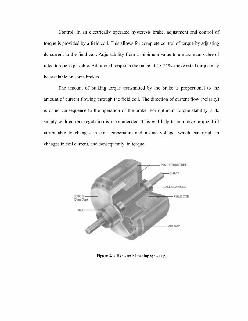
2.2.1.1 The hysteresis braking system
Overview: The hysteresis effect in magnetism is applied to torque control by the
use of two basic components –a reticulated pole structure and a specialty steel rotor/shaft
assembly–fastened together but not in physical contact. Until the field coil is energized,
the drag cup can spin freely on the ball bearings. When a magnetizing force from either a
field coil or magnet is applied to the pole structure, the air gap becomes a flux field. The
rotor is magnetically restrained, providing a braking action between the pole structure
and rotor. Because torque is produced strictly through a magnetic air gap, without the use
of friction or shear forces, hysteresis brakes provide absolutely smooth, infinitely
controllable torque loads, independent of speed, and they operate quietly without any
physical contact of interactive members [5]. As a result, with the exception of shaft
bearings, no wear components exist. Hysteresis braking system can be seen in Figure 2.1
Control: In an electrically operated hysteresis brake, adjustment and control of
torque is provided by a field coil. This allows for complete control of torque by adjusting
dc current to the field coil. Adjustability from a minimum value to a maximum value of
rated torque is possible. Additional torque in the range of 15-25% above rated torque may
be available on some brakes.
The amount of braking torque transmitted by the brake is proportional to the
amount of current flowing through the field coil. The direction of current flow (polarity)
is of no consequence to the operation of the brake. For optimum torque stability, a dc
supply with current regulation is recommended. This will help to minimize torque drift
attributable to changes in coil temperature and in-line voltage, which can result in
changes in coil current, and consequently, in torque.
Figure 2.1: Hysteresis braking system [5]

2.2.1.2 Advantages of hysteresis devices
1) Long, maintenance-free life: Hysteresis brakes produce torque strictly through
a magnetic air gap, making them distinctly different from mechanical-friction and
magnetic particle devices. Because hysteresis devices do not depend on friction or shear
forces to produce torque, they do not suffer the problems of wear, particle aging, and seal
leakage. As a result, hysteresis devices typically have life expectancies many times that
of friction and magnetic particle devices.
2) Life cycle cost advantages: While the initial cost of hysteresis devices may be
the same or slightly more than that of their counterparts, the high cost of replacing,
repairing and maintaining friction and magnetic particle devices often makes hysteresis
devices the most cost-effective means of tension and torque control available.
3) Operational smoothness: Because they do not depend on mechanical friction
or particles in shear, Hysteresis brakes are absolutely smooth at any slip ratio. This
feature is often critical in wire drawing, packaging and many other converting
applications.
4) Superior torque repeatability: Because torque is generated magnetically
without any contacting parts or particles, Hysteresis brakes provide superior torque
repeatability. Friction and magnetic particle devices are usually subject to wear and aging
with resultant loss of repeatability. Hysteresis devices will repeat their performance
precisely, to ensure the highest level of process control.
5) Broad speed range: Hysteresis devices offer the highest slip speed range of all
electric torque control devices. Depending on size, kinetic power requirements and
bearing loads, many hysteresis brakes can be operated at speeds in excess of 10,000 rpm.

In addition, full torque is available even at zero slip speed and torque remains absolutely
smooth at any slip speed.
6) Excellent environmental stability: Hysteresis devices can withstand significant
variation in temperature and other operating conditions. In addition, because they have no
particles or contacting active parts, hysteresis brakes are extremely clean.
2.2.1.3 Other types of hysteresis dynamometers
2.2.1.3.1 Engine dynamometers
With an engine dynamometer, high performance motor testing is available for
small gas engines. Engine dynamometers have been designed to address the severe, high
vibration conditions inherent in internal combustion engine testing [6].
Engine dynamometers are part of hysteresis dynamometers so they are highly accurate
(±0.25% of full scale) and can be controlled either manually or via a PC-based
dynamometer controller. For a small engine test stand, engine dynamometer offers a full
line of controllers, readouts and data acquisition software.
An engine dynamometer is ideally suited for emissions testing as set forth in
CARB and EPA clean air regulations. The dynamometers will offer superior performance
on the production line, at incoming inspection or in the R&D lab.
As with all hysteresis dynamometers, engine loading is provided by hysteresis
braking, which provides: torque independent of speed, including full load at 0 rpm,
excellent repeatability; frictionless torque with no wearing parts (other than bearings);
and long operating life with low maintenance
2.2.1.3.2 Dial weight dynamometers
The most important characteristic of any measurement instrument is repeatability
and accuracy. The dial weight dynamometer uses the combination of a hysteresis brake
and gravity to insure constant, reliable results. The brake torque rise is directly
proportional to applied current. The calibrated weight system provides readings in
standard engineering units through the use of multiple torque range scales provided on
each size dynamometer.
Dial weight dynamometers are a lower cost alternative to the standard (load cell)
hysteresis dynamometers. The dial weight dynamometers are easy to operate, provide
repeatable and accurate results, and will operate for many years with minimal
maintenance. A dial weight dynamometer system can only operate manually in an open
loop mode [7].
Load can be adjusted from no load to full scale through simple potentiometer
control on power supply. Magnetically coupled hysteresis brake provides smooth torque
application independent of shaft speed. This permits testing motors from no load to
locked rotor or armature.
2.2.2 Eddy-current dynamometers (WB)
Eddy-current brake dynamometers (WB) are ideal for applications requiring high
speeds and also when operating in the middle to high power range. Eddy-current brakes
provide increasing torque as the speed increases, reaching peak torque at rated speed. The
dynamometers have low inertia as a result of small rotor diameter. Brake cooling is
provided by a water circulation system, which passes inside the stator to dissipate heat

generated by the braking power. The water cooling in the WB provides high continuous
power ratings (max. 140 KW). The eddy-current brake dynamometers have accuracy
ratings of ±0.3% to 0.5% full scale, depending on size and system configuration.
Additional options include: high-speed version, speed pick-up, mechanical rotor blocking
device and vertical mounting [8].
Regulated Cooler and Heat Exchanger: Eddy-current (WB) and powder
dynamometer (PB) brakes are cooled by a water circuit. The water/air exchanger allows
the energy of the closed-loop cooling circuit to dissipate. The circulation pump works
permanently in order to maintain the temperature of the water in the tank. The
temperature detector permanently measures and displays the temperature of the water at
the output in order to regulate it.
In an effort to reduce the noise level, the regulator has two fan speeds that can be
used depending on the demand for cooling. An alarm triggers if the water temperature
exceeds pre-determined values. The dynamometer controller switches off the power to
the dynamometer brake when it reaches the alarm threshold.
Figure 2.2: Water circulation system [9]

2.2.3 Powder brake dynamometers (PB)
The powder brake dynamometer (PB) contains, as its name suggests, a magnetic
powder. The electrical current passing through the coil generates a magnetic field, which
changes the property of the powder, thus producing a smooth braking torque through
friction. They are ideal for applications operating in the low to middle speed range or
when operating in the middle to high torque range. Like hysteresis brakes, powder brakes
provide full torque at zero speed. Like the eddy-current brake dynamometers, the powder
brake dynamometers are water cooled, allowing for power ratings up to 48 KW. The
powder brake dynamometers have accuracy ratings of ±0.3% to 0.5% full scale,
depending on size and system configuration.
Figure 2.3: Inside view of powder dynamometer [10]

The dyno components shown in Figure 2.3 are as follows.
1. Rotor of powder dynamometer.
2. Rotor of eddy-current dynamometer.
3. Speed pickup.
4. Stator.
5. Cooling water.
6. Excitation coil.
7. Trunnion bearing.
8. Labyrinth seal.
9. Transport locking security.
10. Thermo-switch.
11. Force transducer.
2.2.4 Baby dynamometers
Baby dynamometers are used in low power braking applications where the brake
doesn’t dissipate lot of heat. They are ideal for applications operating in the low to
middle speed range or when operating in the middle to high torque range. Motor
designers or users who have a limited budget may not be able to afford the $10,000
commercial dynamometers, and may not be able to find a less costly unit in the used or
surplus markets. The remaining alternative is to build a baby dyno from low-cost
components. Instead of using a hysteresis brake for the motor load, we are using a 1 KW
brush motor interfaced to a commercial motor-drive with regenerative braking.

A more elegant approach than a brake is to regenerate, not dissipate, load power
using a generator. Generated electric power can be inverted and fed back into the power
line, completing the circuit of power back to the motor-drive under test. The only losses
are conversion losses in the test set-up. More simply, though less efficiently, it can be
dissipated in a resistor bank. The baby dynamometer designed in this project the load
power is dissipated in the load resistor bank.
The dynamometer system has two major component assemblies. The first is a
1.25 HP DC motor fastened to a motor under test (MUT) shaft. The second major
component assembly is the dynamometer controller cabinet. A single motor control
development (microchips DSP processor, dsPIC30F6010) board is the microcontroller
used to control the motor. Developing C code using a C-compiler for the controller and
hardware assembly is done as part of the project.
Usually, the test operator will fasten his MUT to the dyno test plate and use a
shaft coupling to tie the MUT shaft to the load module or generator. The two motor shafts
must be exactly on the same axis. On the dyno controller, the operator sets the counter-
torque that he wants to force against his motor. The dyno has a tachometer takeoff point
and a tachometer read-out on the LCD. The operator can see if his controller and motor
combination are strong enough to keep the motor spinning at the assigned speed against
the dyno counter-torque. The operator can also set the speed or torque to which the MUT
can be driven to and test the motor speed torque capabilities.
The dyno counter-torque can be steadily increased to find the point at which the
MUT can no longer spin against the counter-torque. Readings of MUT winding current

can be made under these conditions to see the operational limits of its controller. The
dyno can also be interfaced to the computer and data can be saved or the data can be
inputted from the computer. A user friendly GUI can be developed and used to control
the dyno and also data can be fetch from the microcontroller.
The basic dyno scheme used in the project is shown below:
FET_1
-
SENS AMP
+
-
OUT
D2
FET_4
D3
DSPIC
24 VDC
12
Brake/Generator
R_SENSE0.05 ohms
FET_2
Coupled Shafts
FET_3
MotorUnder Test
D1
D1-D4 formBridgeRectifier
D4
R_load
1-40 ohms
+1
2
Figure 2.4: Block diagram of baby dynamometer system
The speed and torque control are done using H-bridge configuration of the FET’s
to PWM the load current through Rload. A bridge rectifier is placed between the generator
and the load resistance Since no matter which way the generator rotates the FET’s drain
will always be connected to the positive (+) side of the generator, and the FET’s source
will be always connected to the negative (−) side of the generator output. Speed at which

the motor is running is measured by using an optical encoder attached on the shaft of the
generator.
The optical encoder generates a pulse the frequency of the pulse is measured by
the motor control development board and thus the speed. The speed measured is used for
speed control by closing the loop. The current is measured using a sense resistor and thus
the torque can be calculated and used for generating the PWM for the torque control.
The baby dynamometer system that has been developed for the project is shown
in Figure 2.5
Figure 2.5: Dynamometer system used for the project

CHAPTER III
PERMANENT MAGNET DC MOTORS
3.1 Introduction
The 1.25 HP DC motor (working in generator mode) fastened to a motor under
test (MUT) shaft is a permanent magnet DC motor. A permanent magnet DC (PMDC)
motor is a DC motor whose poles are made of permanent magnets. This motor is used in
generator mode and the current produced from it is controlled. Therefore the speed as
well as the torque in the dyno system is controlled. A permanent magnet DC motor is
similar to an ordinary DC shunt motor except that its field is provided by permanent
magnets instead of salient pole wound field structures. The permanent magnets of the
PMDC motor are supported by a cylindrical steel stator which also serves as a return path
for the magnetic flux. The rotor has winding slots, commutator segments and brushes as
in conventional DC machines.
This chapter describes the construction, working, performance and also equations
governing the PMDC motor. Torque-speed characteristics of the motor are shown and
also the specifications of the PMDC motors that have been used for the project is

mentioned and some calculations are done in the end of the chapter. Section 3.2 discusses
the construction of the PMDC motors and the type of materials used for the permanent
magnets. Section 3.3 deals with the performance of such a machine with the torque-speed
curves. Section 3.4 describes some of the advantages and disadvantages of a PMDC
motor. Next section 3.5 informs the working of a PMDC motor with the equations. Last
section 3.6 has the name plate details for both the motors used in the project and also few
calculations are shown, used in the simulations for the motor and generator, discussed in
Chapter V.
3.2 Construction
There are three types of permanent magnets used for such motors. The materials used
have residual flux density and high coercivity [11].
i. Alnico magnets – they are used in motors having ratings in the range of 1 kW to
150 kW.
ii. Ceramic (ferrite) magnets – they are economical in fractional kilowatt motors.
iii. Rare-earth magnets – made of samarium cobalt and neodymium iron cobalt which
have the highest energy product. Such magnetic materials are costly but are the
best economic choice for small as well as large motors.
Another form of the stator construction is the one in which permanent-magnet
material is cast in continuous form of in two pieces.
Most of these motors usually run on 6V, 12V or 24V DC supply obtained either from
batteries or rectified alternating current. In such motors, torque is produced by interaction
35

between the axial current-carrying rotor conductors and the magnetic flux produced by
the permanent magnets.
Small, 12 V PMDC motors are used for driving automobile heater and air
conditioner blowers, windshield wipers, windows, fans, radio antennas, etc. They are also
used for electric fuel pumps, marine engine starters, wheelchairs and cordless power
tools.
The toy industry uses millions of such motors which are also used in other
applications such as the toothbrush, food mixer, ice crusher, portable vacuum cleaner and
shoe polisher and also in portable electric tools such as drills, saber saws, hedge
trimmers, etc.
The basic construction of a PMDC motor is as shown in Figure 3.1.
Figure 3.1: PMDC motor construction

A good material for the poles of a PMDC motor should have as large a residual
flux density as possible, while simultaneously having as large a coercive magnetizing
intensity as possible. The large residual flux density produces a large flux in the machine,
while the large coercive magnetizing intensity means that a very large current would be
required to demagnetize the poles.
In the last 40 years, a number of new magnetic materials have been developed
which have desirable characteristics for making permanent magnets. The major types of
materials are the ceramic (ferrite) magnetic materials and the rare-earth magnetic
materials. The best rare-earth magnets produce the same residual flux as the best
conventional ferromagnetic alloys, while simultaneously being largely immune to
demagnetization problems due to armature reaction.
3.3 Performance
To calculate the performance for this motor, one must predict the air gap flux and
calculate the no-load speed and current and the stall torque and current [12]. A straight
line drawn between the no-load speed and the stall torque represents the speed-torque
curve of the motor. A straight line drawn between the no-load current and the stall current
represents the current-torque performance curve. The PMDC motor performance curves
are shown in Figure 3.2

Figure 3.2: PMDC motor performance curves
The PMDC motor speed-torque curve is a straight line which makes this motor
ideal for a servomotor. Moreover, input current increases linearly with load torque. The
efficiency of such motors is higher as compared to wound-field DC motors because, in
their case, there is no field copper loss. PMDC motor performance varying with voltage
curve is shown in Figure 3.3 below
Figure 3.3: PMDC motor performance varying with voltage

As seen from the performance curves above the PMDC motor has a definite no-
load speed. Hence, it doesn’t ‘run away’ when load is suddenly thrown off, provided the
field circuit remains closed. The drop in speed from no-load to full-load is small; hence
this motor is usually referred to as constant speed motor. The speed for any load within
the operating range of the motor can be readily obtained by varying the field current by
means of a field rheostat.
It is seen from the curves that a certain value of current is required even when
output is zero. The motor input under no-load conditions goes to meet the various losses
occurring within the machine.
As compared to other motors, a PMDC motor is said to have a lower starting
torque. But this should not be taken to mean that a shunt motor is incapable of starting a
heavy load. Actually it means that series and compound motors are capable of starting
heavy loads with less excess of current inputs over normal values than the PMDC motors
and that consequently the depreciation on the motor will be relatively less.
3.4 Advantages and Disadvantages
3.4.1 Advantages
Permanent magnet DC motors offer a number of benefits compared with shunt dc
motors in some applications. Since these motors do not require an external field circuit,
they do not have the field circuit copper losses associated with shunt DC motors. PMDC
motors are especially common in smaller fractional and sub fractional horsepower sizes,
where the expense and space of a separate field circuit can not be justified [11].

(i) In very small ratings, use of permanent-magnet excitation results in lower
manufacturing costs.
(ii) In many cases a PMDC motor is smaller in size than a wound-field DC motor of
equal power rating.
(iii) Since field excitation current is not required, the efficiency of these motors is
generally higher than that of the wound-field motors.
(iv) Low-voltage PMDC motors produce less air noise.
(v) When designed for low-voltage (12V or less) these motors produced very little
radio and TV interference.
3.4.2 Disadvantages
PMDC motors also have disadvantages too. Permanent magnets cannot produce as
high a flux density as an externally supplied shunt field, so a PMDC motor will have a
lower induced torque τind per ampere of armature current IA than a shunt motor of the
same size and construction. In addition, PMDC motors run the risk of demagnetization.
The armature current IA in a DC machine produces an armature magnetic field of it own.
The armature magneto motive force (mmf) subtracts from the mmf of the poles under
some portions of pole faces and adds to the mmf of the poles under other portions of the
pole faces, reducing the overall net flux in the machine. This is the armature reaction
effect. In a PMDC machine, the pole flux is just the residual flux in the permanent
magnets. If the armature current becomes very large, there is some risk that the armature
mmf may demagnetize the poles, permanently reducing and reorienting the residual flux

in them. Demagnetization may also be caused by the excessive heating which can occur
during prolonged periods of overload [11].
(i) Since their magnetic field is active at all times even when motor is not being used,
these motors are made totally enclosed to prevent their magnets from collecting
magnetic junk from the neighborhood. Hence, as compared to wound-field motors,
their temperature tends to be higher. However, it may not be much of a disadvantage
in situations where motor is used for short intervals.
(ii) A more serious disadvantage is that the permanent magnets can be demagnetized by
armature reaction mmf causing the motor to become inoperative. Demagnetization
can result from (a) improper design (b) excessive armature current caused by a fault
or transient or improper connection in the armature circuit (c) improper brush shift
and (d) temperature effects.
3.5 Motor Equations
3.5.1 Internal Generated Voltage
The induced voltage in any given PMDC machine depends on three factors:
1. The flux φ in the machine.
2. The speed ω of the machine’s rotor.
3. A constant depending on the construction of the machine.
The voltage out of the armature of a PMDC motor is equal to the number of
conductors per current path times the voltage on each conductor. The voltage in any
single conductor under the pole faces is known [12] to be
inde e vBl= = (3.5.1)

where, ν is velocity of each conductor, B is flux density under the pole, l is length of the
conductor.
The voltage out of the armature of a PMDC is:
AZvBlE
a= (3.5.2)
Where Z is the total number of conductors and a is the number of current paths. The
velocity of each conductor (ν) in the rotor can be expressed as ν = rω, where r is the
radius.
AZr BlE
aω
= (3.5.3)
This voltage can be reexpressed in a more convenient form by noting that the flux
of a pole is the equal to the flux density (B) under the pole times the pole’s area ( PA ):
PBAφ =
The rotor of the machine is shaped like a cylinder, so its area is
2A rlπ= (3.5.4)
If there are P poles on the PMDC, then the portion of the area associated with each pole
is the total area A divided by the number of poles P:
2P
A rlAP P
π= = (3.5.5)
The total flux per pole in the PMDC motor is thus
(2 ) 2P
B rl rlBBAP Pπ πφ = = = (3.5.6)
Therefore, the internal generated voltage in the machine can be expressed as:
AZr BlE
aω
= (3.5.7)
22ZP rlB
a Pπ ω
π =
2A aZPE φω= (3.5.8) π
Finally,
AE Kφω= (3.5.9)
where
2ZPK
aπ= (3.5.10)
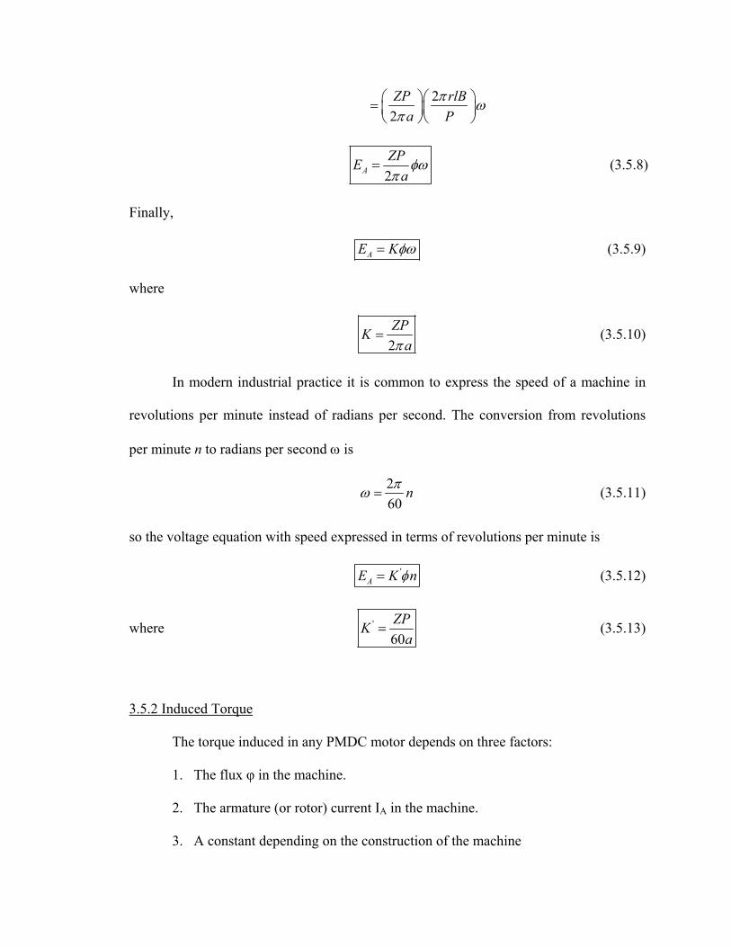
In modern industrial practice it is common to express the speed of a machine in
revolutions per minute instead of radians per second. The conversion from revolutions
per minute n to radians per second ω is
260
nπω = (3.5.11)
so the voltage equation with speed expressed in terms of revolutions per minute is
'AE K nφ= (3.5.12)
where '
60ZPK
a= (3.5.13)
3.5.2 Induced Torque
The torque induced in any PMDC motor depends on three factors:
1. The flux φ in the machine.
2. The armature (or rotor) current IA in the machine.
3. A constant depending on the construction of the machine

The torque on the armature of a real machine is equal to the number of conductors
Z times the torque on each conductor. The torque in any single conductor under the pole
faces is known [12] to be:
cond condrI lBτ = (3.5.14)
If there are a current paths in the machine, then the total armature current IA is
split among the a current paths, so the current in a single conductor is given by
Acond
IIa
= (3.5.15)
and the torque in a single conductor on the motor may be expressed as
Acond
rI lBa
τ = (3.5.16)
Since there are Z conductors, the total induced torque in a PMDC rotor is
Aind
ZrlBIa
τ = (3.5.17)
The flux per pole in this motor can be expressed as
(2 ) 2P
B rl rlBBAP Pπ πφ = = = (3.5.18)
so the total induced torque can be reexpressed as
2ind AZP I
aτ φ
π= (3.5.19)
Finally,
ind AK Iτ φ= (3.5.20)
where
2ZPK
aπ= (3.5.21)

Both the internal generated voltage and the induced torque equations given above
are only approximations, because not all the conductors in the motor are under the pole
faces at any given time and also because the surfaces of each pole do not cover the entire
1/P fraction of the rotor’s surface. To achieve greater accuracy, the number of conductors
under the pole faces could be used instead of the total number of conductors on the rotor.
3.6 Dynamometer PMDC Motors Specifications and Calculations
The PMDC motors that are used in the dynamometer project are shown in
Figure 3.4 below.
MUT (motor under test)
DYNO Motor (PMDC)
Tachometer (Speed Measuring Device)
Figure 3.4 PMDC motors used in the dynamometer project
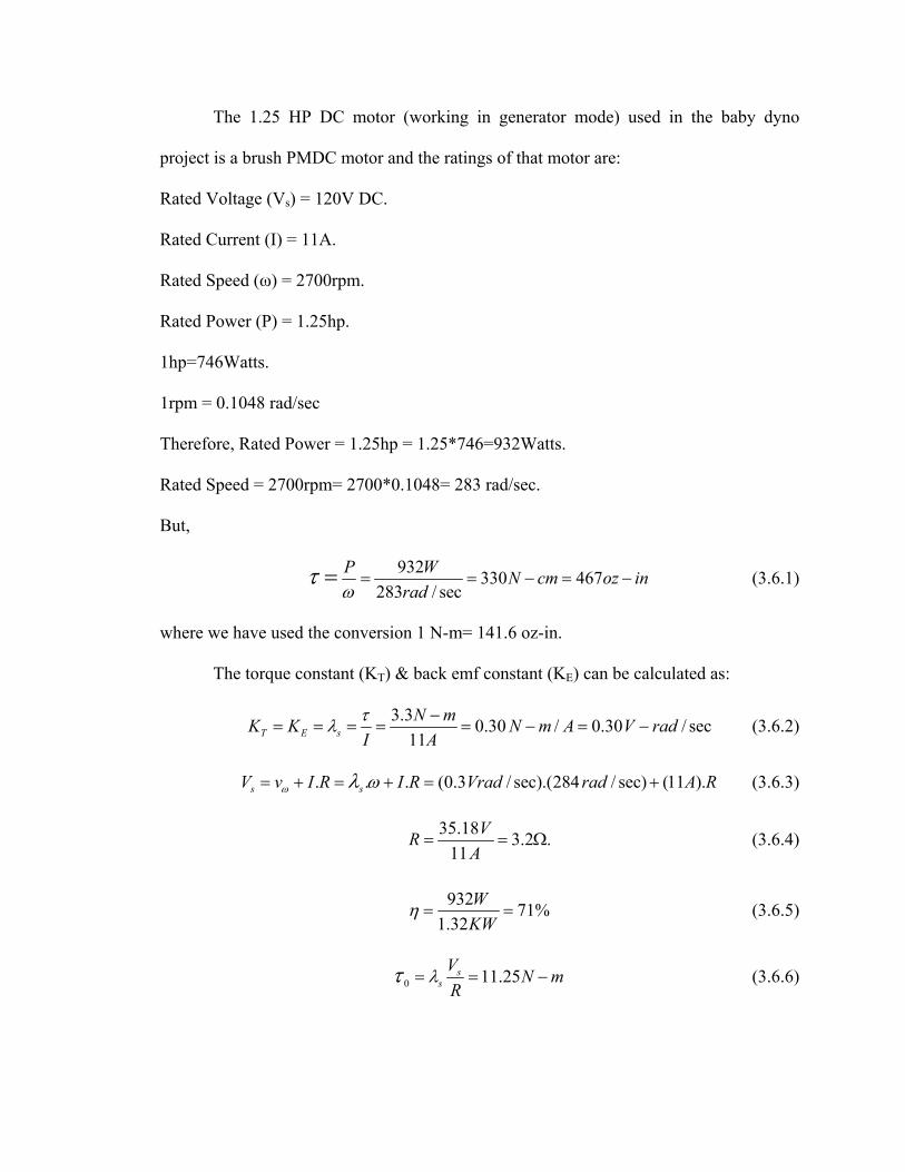
The 1.25 HP DC motor (working in generator mode) used in the baby dyno
project is a brush PMDC motor and the ratings of that motor are:
Rated Voltage (Vs) = 120V DC.
Rated Current (I) = 11A.
Rated Speed (ω) = 2700rpm.
Rated Power (P) = 1.25hp.
1hp=746Watts.
1rpm = 0.1048 rad/sec
Therefore, Rated Power = 1.25hp = 1.25*746=932Watts.
Rated Speed = 2700rpm= 2700*0.1048= 283 rad/sec.
But,
932 330 467283 / sec
P W N cm oz inradω
τ = = − == − (3.6.1)
where we have used the conversion 1 N-m= 141.6 oz-in.
The torque constant (KT) & back emf constant (KE) can be calculated as:
3.3 0.30 / 0.30 / sec11T E sN mK K N m A V rad
I Aτλ −
= = = = = − = − (3.6.2)
. . . (0.3 / sec).(284 / sec) (11 ).s sV v I R I R Vrad rad A Rω ωλ= + = + = + (3.6.3)
35.18 3.2 .11
VRA
= = Ω (3.6.4)
932 71%1.32
WKW
η = = (3.6.5)
0 11.25ssV N mR
λτ = = − (3.6.6)
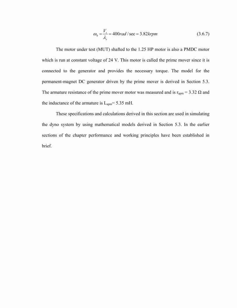
0 400 / sec 3.82s
s
V rad krpmωλ
= = = (3.6.7)
The motor under test (MUT) shafted to the 1.25 HP motor is also a PMDC motor
which is run at constant voltage of 24 V. This motor is called the prime mover since it is
connected to the generator and provides the necessary torque. The model for the
permanent-magnet DC generator driven by the prime mover is derived in Section 5.3.
The armature resistance of the prime mover motor was measured and is rapm = 3.32 Ω and
the inductance of the armature is Lapm= 5.35 mH.
These specifications and calculations derived in this section are used in simulating
the dyno system by using mathematical models derived in Section 5.3. In the earlier
sections of the chapter performance and working principles have been established in
brief.

CHAPTER IV
MC1 Motor Control Development Board
The second major component in the dyno system is the motor control
development board. The Microchip dsPIC30F Motor Control Development Board which
is fitted with a dsPIC30F6010 processor has been used in the project. The main purpose
of the MC1 board is data acquisition, data processing and also display. The speed is
obtained using a tachometer on the shaft of the PMDC motor which generates pulses and
is read through a quadrature encoder interface (QEI) on the MC1 board. The current is
also measured using sense resistors and an A/D module. The reference speed and torque
are obtained from the potentiometers on the board. The speed and torque are calculated
and control loops are used to process the data obtained and also calculated data is
displayed on the LCD of the development board. The control loops also generate the
PWM signals which are used to change the load resistance.
Section 4.1 introduces to the development board and its components with the Figure 4.1
showing the hardware circuitry. Next Section 4.2 discusses the MC1 development board
specifications with detailed data on all the used components in the baby dyno project.

The processor being dsPIC30F6010 and its capabilities such as QEI, motor
control PWM, LCD display, A/D module being used for the reference speed. The
application of each component in the project is discussed in the respective section.
4.1 Introduction
The Microchip dsPIC30F Motor Control Development Board is used in the rapid
evaluation and development of motor control applications using the motor control parts
of the dsPIC family. To maximize flexibility, the largest device variant in the dsPIC
family has been used. The board may be used in two different ways. First is to interface
to one of the custom power modules that have been developed to complement the control
board. The interface is via the 37-pin D-type connector. In this way, all the user has to
supply is a motor and they are ready to go without having to worry about the power stage
and signal conditioning. The power module has its own fault protection and signal
isolation circuitry. There are many different feedback signals that the user can select
between to customize the system to the intended application. These are selected internally
within the power module. The second use of the board is for customers who already have
their own power stage but are interested in evaluating the dsPIC microcontroller unit in
their application. In this instance, the user can easily interface to their own system via the
connectors provided on the board. Although targeted primarily at motor control
applications, the board is also well suited to static power conversion applications, such as
Uninterruptible Power Supplies (UPS), Power Factor Correctors (PFC) and Switch Mode
Power Supplies (SMPS) [13].
80

All the advanced peripheral features such as LCD display, A/D modules, QEI,
and PWM modules are well suited for the DYNO application hence this board is used in
the project and will also help in further development of the project. Data can be
transferred using this board to PC using multiple and easy methods such as RS-232 serial
port, RS-485 serial bus and CAN bus. User interface can be developed on the PC for
plotting the speed torque curves.
The MC1 Motor Control Development Board is shown in Figure 4.1
Figure 4.1: MC1 motor control development board [16]

4.2 System specifications
4.2.1 Processor
The system has the dsPIC30F6010 80-pin TQFP part fitted as the standard
processor. An array of pins around the device allows the appropriate MPLAB ICE device
adapter to plug directly into the board without the need for the transition socket [13]. The
dsPIC30F6010 80-pin TQFP fitted on the board pin diagram is shown in Figure 4.2
Figure 4.2: dsPIC30F6010 pin diagram [15]

The dsPIC30F devices contain extensive Digital Signal Processor (DSP)
functionality within a high performance 16-bit microcontroller (MCU) architecture.
4.2.1.1 High Performance Modified RISC CPU
The dsPIC30F core is a 16-bit (data) modified Harvard architecture with an
enhanced instruction set, including support for DSP. The core has a 24-bit instruction
word, with a variable length opcode field. The program counter (PC) is 23-bits wide and
addresses up to 4M x 24 bits of user program memory space [15].
The dsPIC30F instruction set has two classes of instructions: the MCU class of
instructions and the DSP class of instructions. These two instruction classes are
seamlessly integrated into the architecture and execute from a single execution unit. The
instruction set includes many addressing modes and was designed for optimum C
compiler efficiency. The dsPIC30F instruction set contains 84 instructions, which can be
grouped into the ten functional categories. Each data word consists of 2 bytes (16 bits),
and most instructions can address data either as words or bytes. The data space is 64
Kbytes (32 K words) and is split into two blocks, referred to as X and Y data memory.
Each block has its own independent Address Generation Unit (AGU). Most instructions
operate solely through the X memory AGU, which provides the appearance of a single
unified data space.
The dsPIC30F family of devices contains 144 Kbytes of on-chip flash program
space (instruction words) for executing user code. The dsPIC30F family of devices
contains 4 Kbytes of non-volatile data EEPROM. The dsPIC30F6010 processor can
execute up to 30 MIPS (Million Instructions Per Second). The dsPIC30F6010 has 44

interrupt sources and 4 processor exceptions (traps), which must be arbitrated based on a
priority scheme. Eight user selectable priority levels for each interrupt source is another
feature where the user can assign priorities for interrupts. The dsPIC30F has sixteen, 16-
bit working registers. Each of the working registers can act as a data, address or offset
register. The 16th working register (W15) operates as a software stack pointer for
interrupts and calls.
4.2.1.2 DSP Engine Features
The DSP engine features a high speed, 17-bit by 17-bit multiplier, a 40-bit ALU,
two 40-bit saturating accumulators and a 40-bit bi-directional barrel shifter. The barrel
shifter is capable of shifting a 40-bit value up to 15 bits right, or up to 16 bits left, in a
single cycle. The DSP instructions operate seamlessly with all other instructions and have
been designed for optimal real-time performance. The MAC instruction and other
associated instructions can concurrently fetch two data operands from memory while
multiplying two W registers. This requires that the data space be split for these
instructions and linear for all others. This is achieved in a transparent and flexible manner
through dedicating certain working registers to each address space [15].
4.2.1.3 Peripheral Features
The dsPIC30F6010 device has a high current sink/source I/O pins which are
25 mA/25 mA. The dsPIC30F6010 device offers five 16-bit timers with programmable
prescaler. These timers are designated as Timer1, Timer2, Timer3, etc. The 16-bit timers
can also be optionally paired to obtain 32-bit timer modules. The dsPIC30F6010 device

has eight 16-bit capture channels. The features provided by this module are useful in
applications requiring Frequency (Period) and Pulse measurement. The device I2CTM
module supports Multi-Master/Slave mode and 7-bit/10-bit addressing. It has two UART
modules with FIFO Buffers and two CAN modules, 2.0B compliant [15].
4.2.1.4 Motor Control PWM Module Features
This module simplifies the task of generating multiple, synchronized Pulse Width
Modulated (PWM) outputs. In particular, three phase AC induction motor, switched
reluctance (SR) motor, brushless DC (BLDC) motor and uninterruptible power supply
(UPS) applications are supported by the PWM module. This module contains four duty
cycle generators, numbered 1 through 4 with 16-bit resolution. The module has eight
PWM output pins, numbered PWM1H/PWM1L through PWM4H/PWM4L. The eight
I/O pins are grouped into high/low numbered pairs, denoted by the suffix H or L,
respectively. For complementary loads, the low PWM pins are always the complement of
the corresponding high I/O pin. The PWM module allows several modes of operation
which are beneficial for specific power control applications.
Figure 4.3: PWM module block diagram [16]

The user has the ability of changing PWM frequency ‘on-the-fly’. The PWM
module can be operated in edge, center aligned output and single pulse generation modes.
The module also has a feature of interrupting for asymmetrical updates in center aligned
mode. The module has more advanced features such as output override control for
Electrically Commutative Motor (ECM) operation, ‘Special Event’ comparator for
scheduling other peripheral events, and FAULT pins to optionally drive each of the PWM
output pins to a defined state [15].
4.2.1.5 Quadrature Encoder Interface Module Features
Quadrature encoders (incremental encoders or optical encoders) are used in
position and speed detection of rotating motion systems. Quadrature encoders enable
closed loop control of many motor control applications, such as switched reluctance (SR)
motors and AC induction motors (ACIM).
A typical incremental encoder includes a slotted wheel attached to the shaft of the
motor and an emitter/detector module sensing the slots in the wheel. Typically, three
outputs, termed Phase A, Phase B and INDEX, provide information that can be decoded
to provide information on the movement of the motor shaft including distance and
direction.
The two channels, Phase A (QEA) and Phase B (QEB), have a unique
relationship. If Phase A leads Phase B, then the direction of the motor is deemed positive
or forward. If Phase A lags Phase B then the direction of the motor is deemed negative or
reverse. A third channel, termed index pulse, occurs once per revolution and is used as a
reference to establish an absolute position.

The quadrature signals produced by the encoder can have four unique states.
These states are indicated for one count cycle. Note that the order of the states are
reversed when the direction of travel is changed. A quadrature decoder captures the phase
signals and index pulse and converts the information into a numeric count of the position
pulses. Generally, the count will increment when the shaft is rotating one direction and
decrement when the shaft is rotating in the other direction.
The Quadrature Encoder Interface (QEI) module provides an interface to
incremental encoders. The QEI consists of quadrature decoder logic to interpret the Phase
A and Phase B signals and an up/down counter to accumulate the count. Digital glitch
filters on the inputs condition the input signal.
Figure 4.4: Quadrature encoder interface signals [14]

4.2.1.6 Analog Features
There is a 10-bit high-speed analog-to-digital converter (A/D) on the MC1
development board. The 10-bit high-speed analog-to-digital converter (A/D) allows
conversion of an analog input signal to a 10-bit digital number. This module is based on
Successive Approximation Register (SAR) architecture, and provides a maximum
sampling rate of 500 ksps. The A/D module has 16 analog inputs which are multiplexed
into four sample and hold amplifiers. The output of the sample and hold is the input into
the converter, which generates the result. The analog reference voltages are software
selectable to either the device supply voltage (AVDD/AVSS) or the voltage level on the
(VREF+/VREF-) pin. The A/D converter has a unique feature of being able to operate
while the device is in sleep mode.
A block diagram of the 10-bit A/D is shown in Figure 4.5. The 10-bit A/D
converter can have up to 16 analog input pins, designated AN0-AN15. In addition, there
are two analog input pins for external voltage reference connections. These voltage
reference inputs may be shared with other analog input pins. The actual number of analog
input pins and external voltage reference input configuration will depend on the specific
dsPIC30F device.
The analog inputs are connected via multiplexers to four S/H amplifiers,
designated CH0-CH3. One, two, or four of the S/H amplifiers may be enabled for
acquiring input data. The analog input multiplexers can be switched between two sets of
analog inputs during conversions. Unipolar differential conversions are possible on all
channels using certain input pins (see Figure 4.5).

An Analog Input Scan mode may be enabled for the CH0 S/H amplifier. A
control register specifies which analog input channels will be included in the scanning
sequence.
The 10-bit A/D is connected to a 16-word result buffer. Each 10-bit result is
converted to one of four 16-bit output formats when it is read from the buffer.
Figure 4.5: 10 bit A/D block diagram [16]
The ADCON1, ADCON2 and ADCON3 registers control the operation of the
A/D module. The ADCHS register selects the input pins to be connected to the S/H
amplifiers. The ADPCFG register configures the analog input pins as analog inputs or as
digital I/O. The ADCSSL register selects inputs to be sequentially scanned. The module
contains a 16-word dual port RAM, called ADCBUF, to buffer the A/D results. The 16
buffer locations are referred to as ADCBUF0, ADCBUF1…. ADCBUFE, ADCBUFF.
4.2.1.7 Special Microcontroller Features
These area few special microcontroller features worth mentioning:
• Enhanced Flash program memory:
- 10,000 erase/write cycle (min.) for industrial temperature range, 100K (typical).
• Data EEPROM memory:
- 100,000 erase/write cycle (min.) for industrial temperature range, 1M (typical).
• Self-reprogrammable under software control.
• Power-on Reset (POR), Power-up Timer (PWRT) and Oscillator Start-up Timer (OST).
• Flexible Watchdog Timer (WDT) with on-chip low power RC oscillator for reliable
operation.
• Fail-Safe clock monitor operation detects clock failure and switches to on-chip low
power RC oscillator.
• Programmable code protection.
• In-Circuit Serial Programming.
• Selectable Power Management modes.
- Sleep, Idle and Alternate Clock modes.
4.2.2 Power Supply
The main supply input to the system is via J2 (Figure 4.1). Any power supply
with a 2.1 mm plug capable of delivering 9 V, up to 1 A with an unregulated AC or DC
output, may be used. After rectification and filtering, the digital +5 V is created by U1
(Figure 4.1), a 1 A 2% tolerance linear regulator. The tighter than standard tolerance is
used to ensure correct optoisolator drive and FAULT trip levels when using one of the

power modules. The digital +5 V is available in the prototyping area (VDD) as well as on
several of the interface connectors [13].
A low current analog supply (AVDD) is created from the digital supply via a
passive RC filter. This is used for the ADC in the dsPIC device and for the analog
feedback signals via J1 (Figure 4.1). It is also available in the prototyping area.
4.2.3 In-Circuit Debugging and In-Circuit Serial Programming (ICSP)
In-circuit debugging and serial programming of the FLASH memory contained
within the dsPIC device is supported via J4 (Figure 4.1). This allows direct connection to
the MPLAB ICD 2 or the PRO MATE II via the appropriate ICSP module.
The default pins used for dsPIC emulator communication and device programming are
AN1 and AN0. In order to maximize the number of ADC channels for use in motor
control, provision has been made to switch the emulator and programming pins to the
alternative pins of 59 and 60. These pins are shared with the low power secondary
oscillator module that is not used in the design. Switching between the two sets of
programming pins should be done using S2 (Figure 4.1) and the appropriate
configuration bit settings within the MPLAB environment [13].
When S2 is switched to the ICD position, the analog feedback signals are
disconnected from the AN0 and AN1 pins. The programming lines on J4 (Figure 4.1) are
connected. When S2 is switched to the ‘Analog’ position, the programming lines are
disconnected and the analog signals are connected to AN0 and AN1.

4.2.4 Motor Position Feedback Interface
Interface to two different types of commonly used motor position feedback
devices is provided. Note that no electrical isolation is provided on the board. We must
ensure that the motor frame is correctly earthed (grounded) and that the position feedback
devices are isolated from the motor windings [13].
J3 (Halls) is intended for electrical commutation signals from (typically) Hall
Effect devices. These signals are used for BLDC and SR motors and have edge
transitions aligned to the electrical cycle of the motor phases. The three inputs (A, B, C)
are connected to 3 input capture channels (IC1 - IC3) of the dsPIC device. Pull-up
resistors and a small amount of filtering are provided on the board. The inputs are
therefore, suitable for either open-collector or driven use. Clearly, the inputs can be used
for any input capture or I/O requirements that we may have.
J5 (QEI) is intended for a Quadrature (or Incremental) Encoder Interface. These
devices produce two position related pulse train outputs, 90° apart (A and B) and an
optionally index output (Z) that pulses once per revolution. A typical device will produce
many hundreds of pulses per revolution allowing high resolution position feedback and
high bandwidth speed measurement. The inputs have a very small amount of filtering.
Weak pull-down resistors are also fitted. The three inputs are connected through to the
dedicated inputs of the QEI module of the dsPIC device.
The digital power supply (+5 V and 0 V - "G") is brought out to the connectors
for powering the transducers. Series inductors are used to reduce electrical noise entering
the board. The user should ensure there is adequate local decoupling of the power supply
at the position transducer end of the cable. The maximum current that may be drawn from

the +5 V supply is 200 mA. If we wish to use a transducer that requires more current,
then an external power supply can be used with a common connection between the
grounds made on the G pin. To minimize electrical noise, a shielded cable should be
used.
4.2.5 Oscillator
A 7.3728 MHz, low profile crystal (Y1) is provided on the board. In combination
with the internal PLL and programmable postscaler of the dsPIC device, this allows a
wide range of system clock frequencies to be generated. A low profile component is used
to clear the emulator device adapter [13].
4.2.6 RS-232 Serial Port
One of the dsPIC UARTs is connected to J8 (Figure 4.1) via an RS-232 level
shifting interface implemented by U5 (MAX232A). Using RG2 and RG3 as port pins
also provides optional hardware handshaking using CTS and RTS. To use the
handshaking, we must install links LK6 and LK7. As RG2 and RG3 are multiplexed with
the I2C clock and data lines available on the digital prototyping header J7 (Figure 4.1),
both features can not be used at once.
4.2.7 RS-485 Serial Bus
The second dsPIC UART is connected to J10 (Figure 4.1) via an RS-485 level
shifting interface implemented by U8 (MAX485). A 120 Ω terminating resistor may be
connected across the bus lines (A, B) by installing LK9. We may (optionally) control the
RX and TX enable lines by driving RG0 and RG1. Pull-down resistors are used to ensure
the RX is enabled and the TX is disabled by default [13].
4.2.8 CAN bus
One of the CAN modules is connected to J9 (Figure 4.1) via a Microchip
MCP2551 CAN Transceiver IC. A 120 Ω terminating resistor may be connected across
the bus lines by installing LK8. A pull-down resistor ensures the TX stays inactive during
RESET or if the CAN module is not being used.
The second CAN module is available on the digital prototyping header on RG0 and RG1.
As these pins are used for the RS-485 RX and TX control, the RS-485 and the second
CAN module may not be used at the same time.
4.2.9 LCD Display
A 16x2 LCD display (U7) is included on the board. Communication to the display
is via the standard 4-bit interface method based on the well known Hitachi style
communication standard.
• The LCD data lines are on RD0-RD3.
• The Enable line is on RD13.
• The Read/Write is on RC1.
• The Data/Command Select (LCDRS) is on RC3.

4.2.10 LEDs
Four general purpose LEDs (D6-D9) are provided on the board. These are
connected to RA9, RA10, RA14 and RA15, respectively. A single LED (D2) is provided
to indicate the +5 V supply is on. A single LED (D5) is provided to indicate direction of
rotation. This is connected to RD7. When using a quadrature encoder via J5, RD7 may be
automatically driven by the QEI module to indicate direction. Otherwise, this line must
be driven as a port pin.
4.2.11 Push Button Switches
Four general purpose push button switches are provided (S4-S7). These are
connected to RG6-RG9, respectively. A RESET switch is also provided (S1) and
connected to the MCLR line of the dsPIC device.
A TRIP switch (S3) is provided which is wire ORed with an active low FAULT
signal from J1 (Figure 4.1). The resulting signal (FAULT) is connected to the FLTA
input of the PWM module and the OCFB input of the Output Compare module. When
correctly configured in software, the TRIP switch will therefore, cause all the PWM
channels to be driven to their inactive state and OC channels 5-8 to be tri-stated. Thus,
the power stage may be shut down independent of software intervention. To configure the
OC channels to use this feature, the OCM bits of OCxCON (x = 5-8) should all be set. To
configure the PWM module to use this feature, the appropriate bits in the FLTACON
register should be set.

4.2.12 Potentiometers
Two potentiometers (VR1 and VR2) are provided on the board.
VR2 is permanently connected to the AN7 input of the ADC.
VR1 is only brought to the analog prototyping header J6 as POT1 owing to analog
channel constraints. If the user is not using the VPH_#1 analog feedback signal from J1,
then VR2 may be easily connected to AN12 by placing a 0.1" jumper across J6.
Alternatively, VR2 may be connected to any other spare analog channel by soldering a
wire link between the appropriate pins of J6.
4.2.13 Prototyping Area
A 0.1" pitch prototyping area is provided on the board. Digital (VDD/VSS) and
analog (AVDD/AVSS) power supplies are provided in the four corners. J6 provides
access to all the ADC channels as well as having unassigned analog signals on it. J7
provides access to any optional or unassigned digital I/O pins.

CHAPTER V
DC Motor Modeling and PID Control
5.1 Introduction
DC motor speed can be controlled in different ways, some of which are by
varying:
(i) flux /pole, Ф (Flux Control)
(ii) resistance Ra of the armature circuit (Rheostatic Control)
(iii) applied voltage V (Voltage Control).
These methods are not all discussed here. However, rheostatic control is discussed
here since this has been used for the dynamometer project for the control of the PMDC
motor. This chapter discusses the armature or rheostatic control method, next describes
armature controlled DC motor modeling, and then discusses the theory of the control
method adopted for the DC motor. The results for the simulations using the motor model
also will be discussed in this chapter, along with experimental results.

5.2 Armature or Rheostatic Control Method
Armature or rheostatic control method is used when speeds below the no-load
speed are required. As the supply voltage is normally constant, the voltage across the
armature is varied by inserting a variable rheostat or resistance (called control resistance)
in series with the armature circuit. As controller resistance is increased, the potential
difference across the armature is decreased, thereby decreasing the armature speed. For a
load of constant torque, speed is approximately proportional to the potential difference
across the armature. From the speed/armature current characteristic [Fig. 5.1 (b)], it is
seen that the greater the resistance in the armature circuit, the greater the decrease in
speed [11].
Spee
d, N
No Resistance in Armature
Resistance in the armature
Armature Current Ia
Figure 5.1 (a) Armature resistance control [11] (b) Speed/armature current characteristics.
Let, Ia1 = armature current without armature resistance.
Ia2 = armature current with armature resistance.

If Ia1 = Ia2, then the load is of constant torque)
N1, N2 = corresponding speeds, V = supply voltage
Ra = Armature Resistance, Eb1= back emf without armature resistance.
Then 1 1a a bN V I R E∝ − ∝ 1
2
Let some controller resistance of value R be added to the armature circuit
resistance so that its value becomes (R+Ra) = Rt
Then . Therefore 2 2a t bN V I R E∝ − ∝ 22
1 1
b
b
ENN E
=
Considering no-load speed, we have 0 0
a t
a a
V I RNN V I R
−=
−
Neglecting Ia0 Ra with respect to V, (since Ia0 Ra << V) we get
0 1 a tI RN NV
= −
.
From the above equation we see that for a given resistance Rt the speed is a linear
function of armature current Ia.
The load current for which the speed would be zero is found by putting N=0 in the above
relation.
00 1 a tI RNV
= −
or at
VIR
= .
This is the maximum current and is known as the stalling current. This method is
very expensive and unsuitable for rapidly changing loads because for a given value of Rt,
speed will change with load. A more stable operation can be obtained by using a divertor
across the armature in addition to armature control resistance.

5.3 PMDC Motor/Generator Mathematical Modeling
5.3.1 Modeling
Permanent-magnet motors have been widely used in high-performance electric
drives and servo-systems, while permanent-magnet generators are used in the power
systems. Figure 5.2 illustrates the permanent-magnet DC machine which can be used as
motor and generator.
Stator
Rotor
rotor magnetic axis of armature windingquadrature axis
Perm
anentM
agnet
Slip ring
Brush
Air gap
ua
stator magnetic axisdirect axis
Per
man
ent
Mag
net
Figure 5.2 Schematic representation of a PMDC machine [17]

The permanent-magnet motors and generators are high-performance permanent-
magnet electric machines, and the name plate details for the motor that was used in the
project are provided in Section 2.5. We need the following parameters for the machines
armature resistance , armature inductance , back emf or torque constant , moment
of inertia of the shaft J and viscous friction coefficient . The angular velocity of the
generator is measured using the tachometer. All the data is measured in SI units.
ra La ka
Bm
The mathematical model for a PMDC motor will be discussed first and then the
model for the motor-generator system will be derived. The mathematical model for a
PMDC is derived from both the electrical armature equations and the mechanical
equations of motion [17]. A schematic diagram of a PMDC machines that is used to
derive a mathematical model is illustrated in Figure 5.3.
rarar
La
ia
ωr eT,TL
ua
Load
E ka a r= ωdirectaxis
quadrature axis
ArmatureField
+
−
−
+
Permanent Magnet
Figure 5.3 Schematic diagram of permanent-magnet electric machine (current direction
corresponds to the motor operation) [17]

Using Kirchhoff’s voltage law and Newton’s second law of motion, the
differential equations for permanent-magnet DC machines can be easily derived.
Assuming that the susceptibility is constant (in reality, Curie’s constant varies as a
function of temperature), one supposes that the flux, established by the permanent magnet
poles, is constant. Then, denoting the back emf and torque constants as , we have the
following differential equations describing the transient behavior of the armature winding
and torsion-mechanical dynamics.
ka
If ia is the armature current in a PMDC motor, ra is the armature resistance of a
PMDC motor, ka is the torque constant or back emf constant, ωr is the speed of the rotor
or shaft of the PMDC motor, ua is the applied voltage to the motor, La is the armature
inductance, TL is the load torque, J is the moment of inertia of the shaft or rotor, Bm is the
viscous friction coefficient, then
1a a aa r
a a a
di r kidt L L L
ω= − − + au (5.3.1)
1a mra r
k Bd idt J J J LTω ω= − − (5.3.2)
An s-domain block diagram of a permanent-magnet DC motor is shown in Figure 5.4
+-
+
-1
L s ra a+
ua ia ka
Te
TLωr1
Js Bm+
ka
Figure 5.4 Simulink block diagram of permanent-magnet DC motor [17]

The angular velocity can be reversed if the polarity of the applied voltage is
changed (the direction of the field flux cannot be changed). The steady-state torque-speed
characteristic curves obey the following equation.
2a a a a a
ra a a
u r i u r Tk k k
ω e−
= = − (5.3.3)
and the torque-speed characteristics are illustrated in Figure 5.5. The Figure 5.5 is the
plot of steady state torque (Te) when different voltages are applied and the plot also
shows specific load torque TL with speed.
Current limit
ωr
ua2
ua3
u u ua a a1 2 3> >
ua max
T Te L,
ua1
ωroa
a
uk
=
T fL r= ( )ω
0
Figure 5.5 Torque-speed characteristic curves for permanent-magnet motors [17]
The steady state torque-speed curves are obtained from the specifications of the
motor when they are calculated using the equations for speed and torque. A family of
torque-speed characteristic curves was found applying equation 4.2.3.

In particular, plugging the different values of the armature voltage in the
equation
ua
2a a a a a
ra a a
u r i u r Tk k k
ω −= = − e , the steady-state characteristics are found and plotted
in Figure 5.6. The load characteristic is given by ( )T fL r= = +ω ω0 05 0 0001 2. . r .
The torque–speed and load characteristics for the dyno motor are simulated using
MATLAB and are plotted for different input voltages varying from one to twenty-four in
increments of four and are shown in Figure 5.6. The dotted lines are the no-load
characteristics and the solid line is the load characteristic curve.
0 0.2 0.4 0.6 0.8 10
50
100
150
200
250
Te, TL [N-m]
wr,
[rad
/sec
]
Dashed = TeSolid = TL
Ua=4 volts
Ua=8 volts
Ua=12 volts
Ua= 16 volts
Ua= 20 volts
Ua=24 volts
Figure 5.6 Torque-speed and load characteristic curves for DYNO Motor.
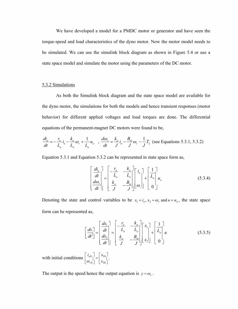
We have developed a model for a PMDC motor or generator and have seen the
torque-speed and load characteristics of the dyno motor. Now the motor model needs to
be simulated. We can use the simulink block diagram as shown in Figure 5.4 or use a
state space model and simulate the motor using the parameters of the DC motor.
5.3.2 Simulations
As both the Simulink block diagram and the state space model are available for
the dyno motor, the simulations for both the models and hence transient responses (motor
behavior) for different applied voltages and load torques are done. The differential
equations of the permanent-magnet DC motors were found to be,
1a a aa r
a a a
di r ki udt L L L
ω= − − + a , 1a mra r
k Bidt J J J LTdω ω= − − (see Equations 5.3.1, 5.3.2)
Equation 5.3.1 and Equation 5.3.2 can be represented in state space form as,
1
0
a aaa
a a aa
r a mr
r kdi iL Ldt L u
d k Bdt J Jω
ω
− − = + −
(5.3.4)
Denoting the state and control variables to be ara uuxix === and , 21 ω , the state space
form can be represented as,
11
22
1
0
a a
a a a
a m
r kdx xL Ldx dt L u
dxdt k B xdt J J
− − = = + −
(5.3.5)
with initial conditions .
=
20
10
0
0
xxi
r
a
ω
The output is the speed hence the output equation is ry ω= .

Hence, . [ ] [ ] [ ] [ ]1
2
0 1 0 0 1 0ar a
r
i xy Cx Du u
xω
ω
= = + = + = +
u
Using Simulink’s State-Space block, the modeling can be performed. To attain
flexibility, symbolic notations are used. The simulink diagram to simulate the motor
dynamics is shown in Figure 5.7
x' = Ax+Bu y = Cx+Du
State-SpaceSignalGenerator: (ua)
Scope: x2 (wr)
Figure 5.7 Simulink model to simulate the dyno motor.
The simulation can be performed assigning the motor parameters and initial
conditions. The following motor parameters are used: r =3.2 ohms, = 0.00535 H,
=0.3 V-sec/rad, =0.3 N-m/A, J=0.0005 kg-m
a
B
La
ka ka2 and =0.00001 N-m-sec/rad. The
voltage is u =50 rect(t) V.
m
a
The initial conditions are: 0 10
0 20
00
a
r
i xxω
= =
To perform the simulations, in the command window we download the motor
parameters and initial conditions which are mentioned above. Running the simulations
and the output plot for the angular speed is as shown in Figure 5.8 below. The input
voltage applied is a square wave with a period of 1 sec. As you can see from the
Figure 5.8 the velocity profile follows the input voltage.

0 1 2 3 4 5-200
-150
-100
-50
0
50
100
150
200
Time (sec)
Spee
d ra
d/se
c)
Motor Angular Velocity Waveform
Figure 5.8 Motor angular velocity waveform.
5.4 PMDC Motor-Generator Set Mathematical Modeling
5.4.1 Modeling
The dyno system consists of a 1.25 HP DC motor (used in generator mode)
fastened to an MUT (motor under test) shaft. The model for the permanent-magnet DC
generator driven by the prime mover will be derived in this section and used to simulate
the complete dyno model, and then the controller will be designed. The goal is to
thoroughly study the transient dynamics and perform a steady-state analysis of the dyno
model. To solve these problems, a mathematical model will be derived, and simulations

will be performed. Let us assume that the permanent-magnet DC motor is used as a prime
mover, and the power generation system considered is illustrated in Figure 5.9 below.
agr
agL
agi
rpmagag kE ω=
+
−
+apmr
apmL
apmi
apmu
rpmapmapm kE ω=
+
−
−
+
epmrpm T,ωegT
uL RL
−
Load+
moverrimeP Generator
MagnetPermanent MagnetPermanent
Figure 5.9 Schematic diagram of permanent-magnet DC generator driven by DC motor (MUT) [17]
The mathematical model for the permanent-magnet DC generator circuitry
dynamics, if the resistive load is studied, is found using Kirchoff’s law as follows [17],
ag ag L agag rpm
ag ag
di r R ki
dt L Lω
+= − + (5.4.1)
Newton’s second law of motion maps the torsional-mechanical dynamics of the generator–
prime mover system.
( ) ( ) rpmepm mpm mg rpm eg pm g
dT B B T J J
dtω
ω− + − = + (5.4.2)
where is the generator armature current; agi rpmω is the angular velocity of the prime
mover and generator; and are the armature resistance and inductance of the agr agL

generator rotor winding; is the load resistance; is the back emf (torque) constant
of the generator; and are the viscous friction coefficients; and and are
the moments of inertia of the prime mover and generator.
LR
B
agk
mpmB mg
epm
pmJ gJ
agi
rp grpm
Bi
pm
d ki
ωω
apmdidt pm +
apm
dt= − apm
apmapm apm
Lagi
ag
RL
r += −
The electromagnetic torque developed by the permanent-magnet DC motor (prime
mover), which is denoted as T , is T kepm apm apmi= , where is the armature current in
the prime mover rotor winding, and is the back emf (torque) constant of the prime
mover.
apmi
apmk
The load torque for the prime mover is the generator electromagnetic torque, and
we haveT . ageg k=
Thus one obtains,
m apm mpm m agapm ag
g pm g pm g
B kdt J J J J J J
+= − −
+ + + (5.4.3)
The mathematical model for the prime mover circuitry dynamics is,
1apm apmapm r apm
apm apm apm
r ki
L L Lω= − − (5.4.4) u
where is the voltage applied to the armature winding of the prime mover; and
and are the armature resistance and inductance of the prime mover rotor winding.
apmu
apm
apmr
L
We have
1apmrpm
apm apm
di r ki u
L L Lω− + (5.4.5)
ag ag agrpm
ag
di kdt L
ω+ (5.4.6)

rpm apm mpm mg agapm rpm ag
pm g pm g pm g
d k B B ki i
dt J J J J J Jω
ω+
= − −+ + +
. (5.4.7)
5.4.2 Simulations for the dyno model
In the MATLAB environment, the mathematical model derived for the
permanent-magnet DC generator-DC motor generation system is used to perform
simulations. In particular, a Simulink diagram is developed based upon differential
equations 5.3.5, 5.3.6 and 5.3.7. Equations 5.4.5, 5.4.6 can be represented in state space
form as,
10
00
0
apm apmapm
apm apm apmapm
ag ag L agag apm
ag agrpm
rpm apm ag mpm mg
pm g pm g pm g
r kdiL L Ldt i
di r R ki u
dt L Ld k k B B
dt J J J J J J
ωω
− − + = − + + − − + + +
(5.4.8)
Denoting the state and control variables as 1 2 3, , and apm ag r apmx i x i x u uω= = = = , the
state space form can be represented as,
1
12
2
33
10
00
0
apm apm
apm apm apm
ag L ag
ag ag
apm ag mpm mg
pm g pm g pm g
r kdxL L Ldt x
r R kdx x udt L L
xdx k k B Bdt J J J J J J
− − + = − + + − − + + +
(5.4.9)
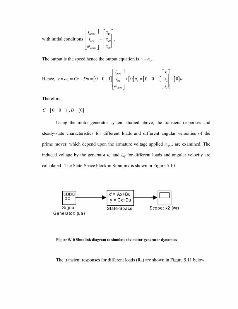
with initial conditions 0 1
0 2
0 3
apm
ag
apm
i xi x
0
0
0xω
=
.
The output is the speed hence the output equation is ry ω= .
Hence, [ ] [ ] [ ] [1
2
3
0 0 1 0 0 0 1 0apm
r ag a
apm
i xy Cx Du i u x
xω
ω
= = + = + = +
]u
Therefore,
[ ]0 0 1 , [0C D= = ]
Using the motor-generator system studied above, the transient responses and
steady-state characteristics for different loads and different angular velocities of the
prime mover, which depend upon the armature voltage applied uapm, are examined. The
induced voltage by the generator uL and iag for different loads and angular velocity are
calculated. The State-Space block in Simulink is shown in Figure 5.10.
x' = Ax+Bu y = Cx+Du
State-SpaceSignalGenerator: (ua)
Scope: x2 (wr)
Figure 5.10 Simulink diagram to simulate the motor-generator dynamics
The transient responses for different loads (RL) are shown in Figure 5.11 below.

0 1 2 3 4 50
20
40
60
80
100
120
Time (sec)
Spee
d (r
ad/s
ec)
Rl = 50(ohms)Rl = 40(ohms) Rl = 30(ohms)
Rl = 20(ohms)
Rl = 10(ohms)
Rl = 0(ohms)
Figure 5.11 Plot of angular speeds (ω) for different loads (RL).
The steady state response of angular velocities with different loads is also shown
in Figure 5.12 below.

0 10 20 30 40 5030
40
50
60
70
80
90
100
110
120
Load Resistance (ohms)
Stea
dy S
tate
Spe
ed (r
ad/s
ec)
Figure 5.12 Plot of steady state angular speed (ω) for different loads (RL).
5.5 Proportional Integral Derivative (PID) Control
5.5.1 Introduction
When the control problem is to regulate the process output around a set point, it is
natural to consider error as an input, and it follows that the integral of the error and the
derivative of the error may be useful inputs as well. One such widely used form of
controller to regulate the process output around a set point is the PID or three-term
controller. This form of control is used extensively in industry and yet is understood, for
the most part, in a way that is limited and superficial. To fully understand this type of
control it is imperative that each individual component be considered separately. The

proportional component responds to present error and provides a decrease in system rise
time. The integral component responds to past error by accumulating the area beneath the
error curve. The integration process provides zero steady-state error with a tendency to
increase overshoot and settling time. The derivative component looks at future error by
responding to rate of change of error. This tends to reduce overshoot and settling time but
at the same time is very susceptible to noise in the system [18].
5.5.2 PID Controller
This section will describe the characteristics of the each of proportional (P), the
integral (I), and the derivative (D) controls, and how to use them to obtain a desired
response. In this section, the unity feedback system of Figure 5.13 is considered.
Figure 5.13 Unity feedback system [18]
In Figure 5.13 the plant is a system to be controlled, and the controller provides
the excitation for the plant, designed to control the overall system behavior. The transfer
function of the PID controller looks like the following:
where, Kp = Proportional gain, KI = Integral gain and KD = Derivative gain.

The variable (e) represents the tracking error, the difference between the desired
input value (R) and the actual output (Y). This error signal (e) will be sent to the PID
controller, and the controller computes both the derivative and the integral of this error
signal. The signal (u) just past the controller is now equal to the proportional gain (Kp)
times the magnitude of the error plus the integral gain (KI) times the integral of the error
plus the derivative gain (KD) times the derivative of the error.
This signal (u) will be sent to the plant, and the new output (Y) will be obtained.
This new output (Y) will be sent back to the sensor again to find the new error signal (e).
The controller takes this new error signal and computes its derivative and it’s integral
again. This process goes on and on.
5.5.3 PID Characteristics
A proportional controller (KP) will have the effect of reducing the rise time and
will reduce, but never eliminate, the steady-state error. An integral control (KI) will have
the effect of eliminating the steady-state error, but it may make the transient response
worse. A derivative control (KD) will have the effect of increasing the stability of the
system, reducing the overshoot, and improving the transient response. Effects of each of
controllers KP, KD, and KI on a closed-loop system are summarized in Table I below.
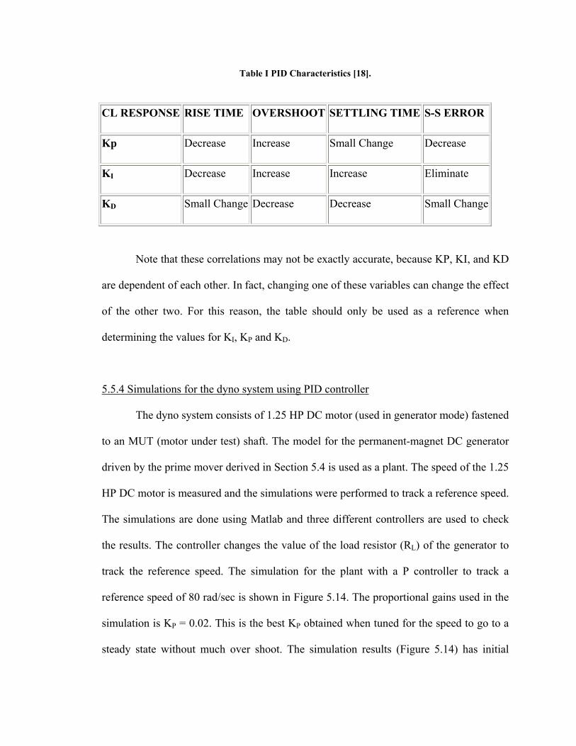
Table I PID Characteristics [18].
CL RESPONSE RISE TIME OVERSHOOT SETTLING TIME S-S ERROR
Kp Decrease Increase Small Change Decrease
KI Decrease Increase Increase Eliminate
KD Small Change Decrease Decrease Small Change
Note that these correlations may not be exactly accurate, because KP, KI, and KD
are dependent of each other. In fact, changing one of these variables can change the effect
of the other two. For this reason, the table should only be used as a reference when
determining the values for KI, KP and KD.
5.5.4 Simulations for the dyno system using PID controller
The dyno system consists of 1.25 HP DC motor (used in generator mode) fastened
to an MUT (motor under test) shaft. The model for the permanent-magnet DC generator
driven by the prime mover derived in Section 5.4 is used as a plant. The speed of the 1.25
HP DC motor is measured and the simulations were performed to track a reference speed.
The simulations are done using Matlab and three different controllers are used to check
the results. The controller changes the value of the load resistor (RL) of the generator to
track the reference speed. The simulation for the plant with a P controller to track a
reference speed of 80 rad/sec is shown in Figure 5.14. The proportional gains used in the
simulation is KP = 0.02. This is the best KP obtained when tuned for the speed to go to a
steady state without much over shoot. The simulation results (Figure 5.14) has initial

overshoot because there is always a tradeoff between overshoot and the speed tracking
the reference speed.
0 0.5 1 1.5 20
10
20
30
40
50
60
70
80
90Sp
eed
(Rad
/Sec
)
Time (Sec)
Kp=0.02
Figure 5.14 Speed plot with a P controller for a reference speed of 80 rad/sec
Figure 5.15 below shows the speed of the motor with PD control. From
Figure 5.15 it can be inferred that with the PD controller applied to the plant (dyno
system) overshoot decreases as compared to P controller. The number of oscillations as
well as the magnitude of the oscillations decreases. With PD controller it can be observed
that the settling time has decreased too. There are no oscillations of the speed of the
motor after 1.5 seconds. The KP and KD values used in the simulations are KP = 0.02 and

KD = 0.0042. These are the best KP and KD obtained when tuned for the speed to go to a
steady state without much overshoot and steady state error.
0 0.5 1 1.5 20
10
20
30
40
50
60
70
80
Time(Sec)
Spee
d (R
ad/S
ec)
Kp=0.02 & Kd=0.0042
Figure 5.15 Speed plot with a PD controller for a reference speed of 80 rad/sec
Figure 5.16 shows the speed of the motor with PID control. From Figure 5.16 it
can be inferred that the PID controller applied to the plant (dyno system) is the best
possible controller. It can be observed that the steady state error has been removed and
there are no oscillations in the system. The reference speed is reached quickly and also
the response is faster compared to just a P controller. The simulations results can be basis
for the experimental results. The simulations results are obtained for an initial load
resistance of 40Ω. The KP, KD and KI values used in the simulations are KP = 0.2, KD =
0.008 and KI = 0.00472. These are the best KP, KD and KI obtained when tuned for the

speed to go to a steady state faster (0.2Sec), without much overshoot and no steady state
error.
0 0.5 1 1.5 20
10
20
30
40
50
60
70
80
90
Time (Sec)
Spee
d (r
ad/S
ec)
Kp=0.2 Kd=0.008 Ki=0.00472
Figure 5.16 Speed plot with a PID controller for a reference speed of 80 rad/sec
5.6 Experimental Results
The experimental results are obtained by running the motor and P controller. The
speed is measured using the tachometer attached to the dyno motor by the motor control
development board controller using change notification on the pin technique. The user
sets the reference speed using the potentiometer on the controller. Depending on the
reference speed the controller (MC1 board) generates the PWM signal by varying the
duty cycle in the control loop. The error speed has a proportional gain (0.5) which is

tuned for best response of the system. The no load speed of the motor is observed to be
1076 rpm. Using the potentiometer the speed is varied from 0 to 1023 rpm.
Figure 5.17 shows the waveforms obtained from the oscilloscope at motor speed of 1023
rpm. The channel 3 waveform is the tachometer (optical encoder) signal and channel 4 is
the PWM signal generated from the controller. The frequency signal of the tachometer
signal linearly decreases with the speed.
Figure 5.17 Tachometer and PWM signals for reference speed of 1023rpm
Figure 5.18 shows the watch window of the microcontroller development system, and
how the speed has changed to 1023 rpm which is same as the reference speed.

Figure 5.18 Watch window for reference speed of 1023rpm
Figure 5.19 shows the waveforms obtained from the oscilloscope at motor speed of 765
rpm. It is observed that the tachometer signal’s frequency has decreased compared to the
1023 rpm signal. The duty cycle applied by the controller for a speed of 765 rpm is
shown in channel 4 signal which is 92.81%.
Figure 5.19 Tachometer and PWM signals for reference speed of 765rpm

Figure 5.20 shows the watch window how the speed has changed to 765 rpm which is
close to the reference speed.
Figure 5.20 Watch window for reference speed of 765rpm
Figure 5.21 shows the waveforms obtained from the oscilloscope at motor speed of 434
rpm. It is observed that the tachometer signal’s frequency has further decreased compared
to the 1023 rpm signal. The duty cycle applied by the controller for a speed of 765 rpm is
shown in channel 4 signal which is 75.371%.
Figure 5.21 Tachometer and PWM signals for reference speed of 434rpm
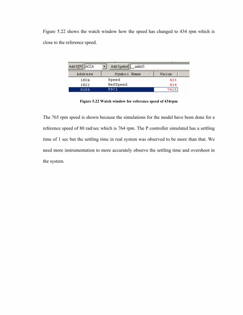
Figure 5.22 shows the watch window how the speed has changed to 434 rpm which is
close to the reference speed.
Figure 5.22 Watch window for reference speed of 434rpm
The 765 rpm speed is shown because the simulations for the model have been done for a
reference speed of 80 rad/sec which is 764 rpm. The P controller simulated has a settling
time of 1 sec but the settling time in real system was observed to be more than that. We
need more instrumentation to more accurately observe the settling time and overshoot in
the system.

CHAPTER VI
CONCLUSIONS AND FUTURE WORK
6.1 Conclusions
In this thesis a dynamometer which can be used for small power applications has
been designed, tested and simulated. In industry it is hard to find a typical bench-top
dynamometer, and even when one is found it may not be economically feasible for a
small lab to purchase. This thesis takes dyno cost into consideration. In this thesis the
traditional dynamometer with mechanical brakes has been replaced with a fully automatic
digital controller. In this thesis PID control has been applied but other control techniques
may also be applied to the dyno.
The mathematical model for the dynamometer has been developed which includes
not just the motor model but also the PMDC generator rotated by a PMDC prime mover.
The Matlab simulations for the model for different applied prime mover voltages were
shown. The torque speed characteristics for the motor are also obtained and compared to
the experimental results.

The simulations were performed by applying P, PD, and PID control to track a
reference speed, and the results of such controls were discussed. The P control was
implemented experimentally and compared to the simulation results.
6.2 Future Work
Though the automatic controller has been implemented for the dynamometer
system the hardware is not fully assembled. The microcontroller and servo amplifier
which were used in the originally developed dynamometer have been replaced with the
MC1 motor control development board but the hardware assembly is not complete.
The control of the speed is done by dissipating heat in the load resistor by using the dyno
motor in generator mode. A better method such as regenerative braking can be used, in
which the DC voltage generated is converted to AC by using an inverter to supply the
main power supply. The AC voltage can then be frequency controlled, and hence the
speed of the motor can be controlled.
Due to time constraints only speed control has been implemented in hardware, but
this work can be extended to torque control. Torque control can be done by measuring the
current in the armature of the dyno motor working in generator mode.
The dynamometer 1.25 HP motor is a large motor and the shaft of the motor has
high moment of inertia so the motor could be replaced with a smaller PMDC motor. The
dynamometer project is an evolving project, and the final result of its development is not
yet known. This thesis is an attempt to help the next developer in understanding the dyno
and coming up to speed on the on-going dyno project.

REFERENCES
[1] Tom Priolo, “Baby Dynamometer Design Project,” Department of Electrical &
Computer Engineering, Cleveland State University, senior design project, spring
2003.
[2] Dennis Feucht, “Build Your Own Dynamometer,” 1999.
http://innovatia.com/Design_Center/dyno_project.htm.
[3] Magtrol, “DSP 6000 Programmable Dynamometer Controller,” user’s manual,
July 1997, Buffalo, New York.
[4] Magtrol motor testing products description, “Dynamometers.”
http://www.magtrol.com/motortesting/dynamometers.htm.
[5] Magtrol, “Hysteresis Dynamometer,” User’s Manual, July 1997, Buffalo, New
York.
[6] Magtrol motor testing products description, “Engine Dynamometers.”
http://www.magtrol.com/motortesting/ed_dynamometers.htm.
[7] Magtrol motor testing products description, “Dial Weight Dynamometers.”
http://www.magtrol.com/motortesting/dialweight_dynamometers.htm.
[8] Magtrol motor testing products description, “Eddy-Current Dynamometers.”
http://www.magtrol.com/motortesting/wb_dynamometers.htm
[9] Magtrol motor testing products description, “Regulator Cooler and Heat
Exchanger”. http://www.magtrol.com/motortesting/rer-exchanger.htm
[10] “Inside the Eddy-Current/ Powder Dynamometers.”
http://www.magtrol.com/motortesting/wbpb_dynamometer_inside.htm

[11] B.L.Theraja, A.K.Theraja, “A textbook of Electrical Technology in S.I units,
Volume II, A.C and D.C Machines,” 1998, S. Chand & Company Ltd, New
Delhi.
[12] Stephen J. Chapman, “Electric Machinery Fundamentals,” 1999, Third Edition,
WCB McGraw-Hill.
[13] Microchip Technology Inc, Chandler, Arizona, 2003, “dsPICDEM MC1 Motor
Control Development Board User’s Guide” (DS70098A).
[14] Microchip Technology Inc, Chandler, Arizona, 2003, “dsPIC30F Family
Reference Manual,” “High Performance Digital Signal Controllers” (DS 70046B).
[15] Microchip Technology Inc, Chandler, Arizona, 2004, “dsPIC30F6010 Data
Sheet” “High Performance Digital Signal Controllers” (DS70091A).
[16] Microchip Technology Inc, Chandler, Arizona, 2004, “dsPIC Digital Signal
Controller (DSC) Introductory Seminar 2004” “30 MIPS Computing Power in a
6x6 mm² Package”
[17] Rochester Institute of Technology, Department of Electrical Engineering,
Mechatronics Lab, Experiment # 3, “Permanent-Magnet Direct-Current Machines
(Motors, Generators, and Motor-Generator System).”
www.rit.edu/~labeee/531/EE531Lab3.DOC
[18] University of Michigan, Carnegie Melon, “Control Tutorials for Matlab, PID
Tutorial.” http://www.engin.umich.edu/group/ctm/PID/PID.html#controller.