中導民國第十五屆海洋工程研討會論文華氏國 82年11月Proc.15th C04nf.onOceanEngineering in Repub11COF ChinaNov.1993

DYNAR4IC DETERMINATION OF/OFFSHOREPILE CAPACITY

Ming-Te Liang1 and Jong-Liang Wang2

ABSTRACT

The main purpose of this paper is to inves七igate 七he axial bearing capacity of singlesteel pipe-pile used in oEshore structures.This investigation is~divided into expermentalstudy and numerical simulation. In the case of experimental research，twelve model pilesare driven into the saturated sandby means of pile rig. The experimental resu1ts arerecorded from data acquisition of Labwindows system through sensors，electric equipmentand personal computer-For numerical simulation，the assumption of Hookean pile andKelvin 血odel placed of the interaction between pile and soils are used to analyze themechanical behavior of the hammer-pile-soil system when hammer impact on the pilehead.

The investigated resu1ts are drawn for the single steel pipe-pile used in offshorestructures. For the same pile length，the less slenderness ratio，the more axial bearin!rcapacity.Under the same pile length and slenderness ratio，the axial bearing capacityJthe closed-end pile is higher than the open-end pile does.However ，this result is inversivewhen the sle吋erness ratio is greater than 10. This may be due to soil plug. The ultimatebearíng capacity obtained from dynamic measurernent is higher than the static loadingtest does.Particularly ，the dynamic method is suitable for the higher slenderness ratio.In addition ，the，generally dynamic formulas such as the simplified Hiley formula and themodified Engineering formula result in higher error occurred from their uncertainty. Hence，the 叫 hod of wave propagation is suggest仙 op叫 ict the 叫al b叫時 capacityofmgl;steel pipe-pile used in offshore struct'ures.

keywords: bearing capacity，dynamic measurement ，static loading test，interaction ，impact.

1. INTRODUCTION

Wave equation provides a mathematical mo<Ìel.This model can be estimated andpredicted the axially pile bearing capacity for the mechanical behavior of the hammer-pile 司

soil system.Recently ，the dynamic measurement technique used the wave propagation -developed v叮y well. This technique is widely applied to the construction practice and

1Associa七e professor，NationalTaiwanOceanUniversity;Keelung，Taiwan，R.O.C2Assis峙的 planner，Dept.ofRåpidτÌ'ansit8ystem，TaipeiMunicipalGovernment

一453 一

monitoring for pile foundations all over the world. This technique is also used to predict七he bearing capacity of offshore piles.

An analytical method 叫時 the wave equation concept was proposed by Smith (1960).He assumed that (1) thepile is a Hookean solid，(2) the Soil is a Kelvin- Voigt solid and(3) the pile is represented by a model consisting of a set of discrete spring-masses. Smith'smethod is a finite difference solution which can be carried out by electronic computers bynurnerical integration.

The principal purpose of this paper is to study the dynamic analysis of stess wavepropagation in a steel-pipe pile used in offshore structures. This investigation is dividedinto'two parts: one is numerical model，the other is experimental research. The results oftwelve mode piles tests in saturated sand are then described in which the axial response ofthe piles are investtgated. The pile-soil interaction from each type of test is compared andthe dynamic response from axial load tests is used to predict the static load of piles. Theresults indicate 七hat the numerical program and the Case method regarding the utility ofdynamic pile load tests are in agreement with respectancy.

2. THEORETICAL BACKGROUND2.1 NUMERICAL METHOD

Bowles (1974) used the Smith (1960) model to establish the numerical technique fordescribing transmission of a shock wave along the pile. The wave-propagation mode ofthis numerical method can be examined as shown in Fig. 1 and experssed as followed:

a. The ram impact on the spring with an initial velocity V1 at time t1 = 1. This velocitydisplaces the cap-block spring at the end of first time interval an amount accordingto the equation Yl = V1L:':>t.

b. This displacement induces a cap-block -force estimates 品几= K2Yl' The forceacc.elerates the pile cap downward according toF2 = M a，where M is the 'mass ofpile cap. At present，the active time t of the' first stage is finished.

c. At the end of the second stage interval，the cap block has moved a distance with avelocity 巧 of Y2 = V2L:':>t，

d. Based on the acceleration of the pile cap due to 凡 to obtain a velocity of 几=前，where a is the acceleration of pile cap，the pile cap has moved a distance of Y3 = V3L:':>t.

e. Resulting in a new cap-block force based on 七he net compression of the cap blockof Yl - Y2 to obtain 七he force as 凡= K2(Yl - Y2) and also resulting in a force 凡between the pile cap and the first pile segment based on the displacement Y2 and thespring constant of the first pile segment K3 as force F3 = K3Y2.

f. In the following stage，wave propagation process mentioned above will downward actrepeatedly. The computed step is of five formulas derived by Smith (1960):

一454一

where

m = pile element counter

t = time

f':::.t = time interval

C(m ，t) = spring compression of pile element m at tD(m ，t) = displacement of pile element m at ，t

D' (m，t)= displacement of soil element m at t - 1F(m ，t) = force of spring m at t

g =、acceleration of gravity

J(m) = damping constant of pile elerilent m

K (m) = spring constant of pile element m

K' (m)= spring constant of soil element m

R(m ，t) = soil resistance of pile element m at time tV (m，t) = velocity of pile element m at time tW (m) = weight of pile element m

the impact energy would be loss during driv~ngprocess because the cap-block material isquite different form ram and pile cap materia1. Thus，the deformation is really nonlinear;The cap block subjected force should be modified 部

F(m ，t) = K(m)C(m ，t)ma"，+ K(m) [C(m ，t) 一C(m ，t)ma"，Jj[e(m)j2

where e(m) = the coe血cient of restitution of pile element m 、

C(m ，t)ma"，= the maximum compression of spring m at time t

2.2 CASE METHOD

(1f)

Goble et al (1975) used the one-dimensional wave equation to derive the total resis-

- 455 一

tance RTL during pile driven as fol1ows

RT L == [F(td + F(t2)Jj2 + (MC j2L)(V(t1) 一V(t2)J

in which

t1 = t~me used for starting computation of total driving resistance

t2 = t1 十2LjC

L = pile length

C = the elastic wave velocity in the pile

M = pile mass

(2a)

The 10叫 resistance RTL is the sum of削 ic resistance RSP and dynamic resistance Rd，that is

RTL = RSP+Rd (2b)

叫 1e dampingeFctofpilesha 此 is neglec叫出 en the dynamic resistance Rd is propor-tional to the velocity at pile toe.Thus

Rd = Jvtoe = Jclvtoe == Jc(MCjL)vtoe

in which

vtoe = the velocity at pile toe

J = damping coeffi.ciant

Jc = damping facto~

1 =impedance of pile = EAjC=MCjL (for uniform pile)

E = Young's modulus of pile

A = cross-sectional area of pile

The toe velocity can be calculated as

只oe = V(td + [F(t1) - RTLJlI

Substituted Eqs. (2c) and (2d) intó Eq. (2b)，one gets

RSP = RTL - Jc[2F(t1) - RTL]

- 456 一

(2c)

(2d)

(2e)

2.3 DYNAMIC PILE DRIVING FORMULAE2.3.1 THE MODIF‘IED ENGINEERING NEWS FORMULA

The modified Engineering News formula was described by Das (1984) 自

QUZ 防'rhWr +n2Wp- -一一一一-*s+e Wr +Wp

in which

E = hammer effi.ciency

h ~ the drop height of hammer

Wr = hammer weight

Wp = pile weight

n = the coeffi.cientof restitutionof cap block

s = pile penetration

e = 0.254 cm

Qu = the ultimate bearing capacity of pile

2.3.2 THE SIMPLIFIED HILEY FORMULA

The Hiley formula was described by Little (1961) as

R..=ehWhh*Wh +n2Wp

u- s+(k1+k2+k3)/2 小 Wh十Wp'

in which

Ru = the ultimate bearing capacity of pile

eh = hammer effi.ciency

h = drop height of hammer

Wh = hammer weight

Wp = pile weight

n = the coeffi.ciant of restitution of cap block

s = pile penetration

k1 = the elastic compression of pile cap

k2 = the elas七ic compression of pile

k3 = the elastic compression of soil

- 457 一

(3) 、

(4a)

\

Broms and Choo (1988) indicated that the principal uncertainty of using the Hileyformula is dependent on three parameter of旬，k1 and n. these uncertainty factor can beovercome by trsnsfer energy Emax. Thus，one gets a simplified formula

R 一一些竺-u - s 十 (k2十的 )/2

(4b)

in which Emaz (or ENTHRU) = the energy w品 transfered from hammer to pile. The valueof Emaz can be measured from experiment such as

ιaz =!F(t)V(t)dtin which F(t) = force，V(t) = velocity.

3. EXPERIMENTAL INVESTIGATION3.1 THE MEASUREMENT OF ACOUSTIC VELOCITY

(4c)

Pu七 the model pile on the ground and instal1，the accelerometer at pile h~ad asshown in Fig. 2. The stress waves propagates repeatedly back and forth in the pile dueto hand-held hammer impact at pile head. The signal of particle velocity at pile headis recorded by acceleromenter and transfers to the Labwindows sy:stem. Thus the A/Dconverter and record are fiI由hed. From these digital data the velocity of stress wave (c)can be calculated. Fig. 3 indicates the wave pattern of model pile LBO.

3.2 DYNAMIC EXPERIMENT

In order to perform experimental research，twelve steel-pipe piles (see table 1) areused to study the dynamic bearing capacity due to hammer drop at pile head. Each modelpile are pl缸ed strain gauge on the shaft undér 5cm pile head. Water tank is used toinvestigate the dynamic analysis of stress wave in the pile driven and embedded intosand(see Ta叫e 2 and Table 3) undeJ:"water.

The velocity of data acquistion of Labwindows K = 200kHz

The calculation formula of stress-wave velocity: C = 2LKn/(n2 - nl)The accelerometer (see Fig. 4) are instal1ed under two-diametter distance of pile

head in order to measure pile settlement caused by hammer impact. The drop hammeris control by the pile driven ring. When pile head is axial1y by the drop hammer，thedata of force velocity and disp抖la缸.ce閒e缸meacquisition system) through the amplifier system of strain gauge and accelerometer. Thesedata are used to analyze the pile dynamic behavior and soil reaction.

4. RESULTS AND ANALYSIS4.1 CASE METHOD

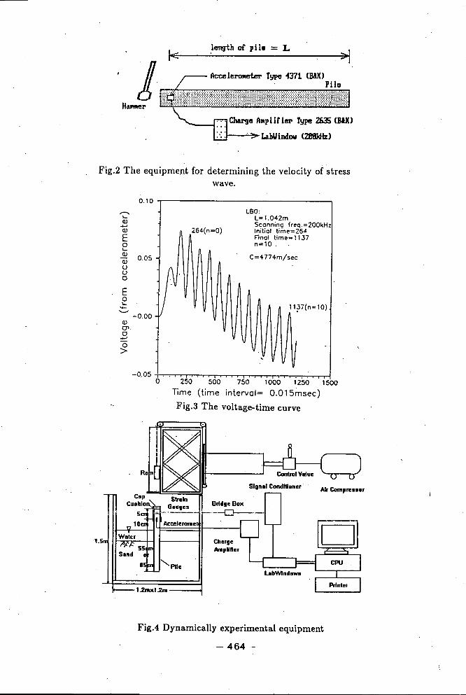
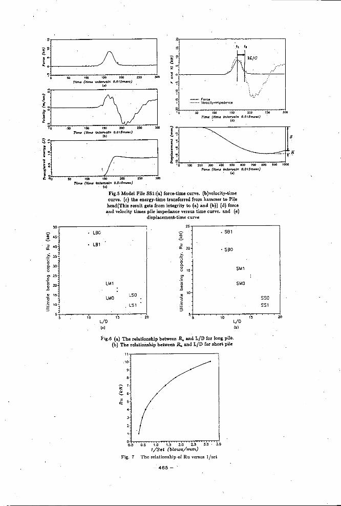
Fig. 5 shows the results of dynamic experiment for model pile 881. From Fig. 5(d)

一458一

one reads the force and velocity and substitutes into Eqs (2a) and (2e) to get static capacity.as shown in Table 4，in which RSP，Rsh and ENR represent the static beaiing capacityob七ained from the Case method，也e simplified Hiley formula and the modified EngineeringNews forrriula，respectively. The other pile can be obtained from the same ana廿tic processmentioned above. Fig. 6 indicates the reationship between ultimate bearing capacityRtJ= RS P and slenderness ratio L / D (L = length of pile，D = diameter of pile) .

From Fig. 6 indicates the important results as follows: (a). For saÌne pile length~ial capacity is corresponding to.，increase. (b). Under the same pile length and L/D ，the位 ial capaci七y of closed-end Pile is generally larger than the open-end pile does. However，for L/D 三凹，one gets the reverse results due to the phenomenon of soil plug.

4.2 DYNA 孔lIC PILE DRIVING FORMULAS

Since the response of LVDT in experiment is only of 300 Hz，the response of dis-placement of the particle with high frequency can not be plotted. Hovever，thevariableprocesser can be acquired. Based on these data，one can calculate the values .ofPile pen-etration S and rebound K = K2 + K3• Substituting S and K into Eqs. (3) and (4b)，thepredicated bearing capacity ofthe modified Engineering News formula and the simplifedHiley formula are obtained and shown as in Table 5，in which RSP，Rsh，ENR andPROGindicate the static bearing capacity obtained from the Case method; the simplified Hileyformula，the modified Engineering News formrila and numerical method.

4.3 NUMERICAL METHOD

Choose the suitable parameters (see-Table 6) such as model pile，soil properties andpile driving sys七em for the input data of computer program. After calculation the set ofpile driving under the asumptions of the ultimate bearingcapacity (Ru) of each pile canbe obtained~ Then one may make a plot of Rù versus l/set (i.e.need blow number (Nf)due to depth lmm per blow) to present a feature of the wave equation. Fig. 7 indicatesthe Ru-l/set relationship of model pile SSl.

Fig. 5(e) shows t出ha前t the disp抖la缸兀肘閒e缸memodel pile SSl. The penetration (S) during pile driving can be estimated the differencebetween the initial and final displacement. The reverse value of S(set) means the blownumber Nf. Substituting Nf value into the Ru-l/set curve one can gets the correspoingultimate beari時 capacity (see Table 5). The value presents the 位 ial bearing capacityobtained from the numerical analysis based on the one-diIÌlensionalwave equation.'

5. DISCUSSION

From this study some disscussion are drawn out as follows:

a. Table 5 indicates 七hat the difference of static bearing capcaity obtained from the Case

- 459 一

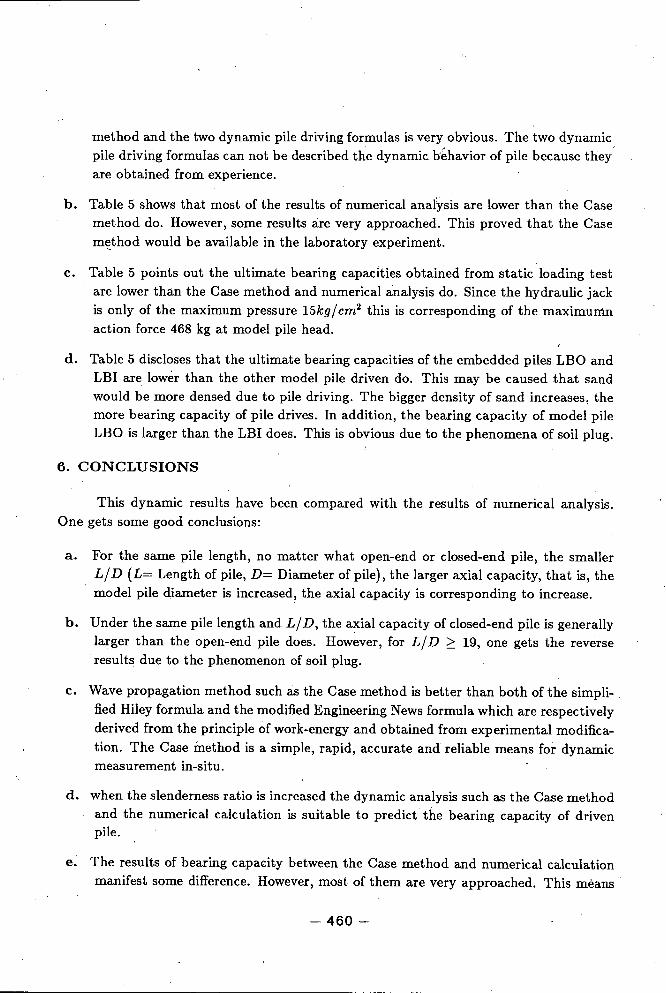
method and the two dynamic pile driving formulas is very obvious. The two dynamicpile driving formulas can no七 be described 七he dynamic hehavior of pile because theyare obtained from experience.

b. Table 5 shows that most of the results of numerical analysis are lower than the Casemethod do. However，some results are very approached. This proved that the Casemφhod would be available in the laboratory experiment.

c. Table 5 points out the ultimate bearing capacities obtained from static loading 七estare lower than the Case method and numerical analysis do. Since the hydraulic jackis only of the maximum pressure 15kg / cm2 出is is corresponding of the maximuIrtnaction force 468 kg at model pile head.

d. Table 5 discloses that the ultimate bearing capacities of the embedded piles LBO andLBI are lower than the other model pile driven do. This may be caused that sandwould be more densed due to pile driving. The bigger density of sand increases，themore bearing capacity of pile drives. In addition，the bearing capacity of model pileLBO is larger than the LBI does. This is obvious due to the phenomena of soil plug.

6. CONCLUSIONS

This dynamic results have been compared with the results of numerical analysis.One gets some good conclusions:

R. For the same pile length，no matter what open-end or closed-end pile，the smallerL/D (L= Length of pile，D= Diameter of pile)，七he larger 缸 ial capacity ，that is，themodel pile diameter is increased，the axial capacity is corresponding to increase.

b. Under the same pile length and L/ D，the 缸 ial capacity of closed-end pile is generallylarger than the open-end pile does. However，for L / D 主 19，one gets the reverseresults due to the phenomenon of soil plug.

c. Wave propagation method such as the Case method is better than both of the simpli-fied Hiley formula and the modified Engineering News formula which are respectivelyderived from the principle of work-energy and obtained from experimental modifica-tion. The Case Ínethod is a simple，rapid，accurate and reliable means for dynamicmeasurement in":situ.

d. when the slenderness ratio is increased the dynamic analysis such as the Case methodand the numerical calculation is suitable to predict the bearing capacity of drivenpile.

e. The results of bearing capacity between the Case method and numerical calculationmanifest some difference. However，most of them are very approached. This mèans

- 46。一

that the dynamic measurement of the Case method can be applied in the laboratoryexperiment.

REFERENCES

1. Broms，B.B.，and Choo，L.P. (1988)，"A Simple Pile Driving Formula Based 0∞nS飢伽t衍re闊s臼sWave Me凹as叩u叮1叮remen叫1此ts吋，" Proceedings of the Third International Conference on Aþpli-C臼at“io叩n of S凱tr凹es臼s-Wa叮.veThe叩or叮ytωoPiles，Ot“tawa，Canada ，pp. 591-600.

2. Bowles. J. E. (1974)，“Analytical andComputer Methods inFòundation Engineering;"McGraw-Hill，Inc.，pp. 349-387.

3. Das，B.M.，(1984)，“Principles of Foundation Engineering ，"Wadsworth Inc.

4. Fellenius，B且 (1980)，“TheA 叫ysis of Restilts from Routine pile Load Tests，"Ground Engineering ，Vol. 13，No. 6，pp. 19-31.

5. Gob峙，G;G.，Likins，G.E.Jr. and Ra叫le，F. (1975)，“Beari時 Capacity of Piles fromDynamic Measurements ，"Fmal Report ，Department of Civil Engineering ，Case West-ern Reserve University，77p.

6. Little ，A.L. (1961)，“Foundations ，"firs七 Edition ，Edward Arnold '(Publishers) Ltd. ，London，pp. 190-195.

7. Smith，E.A.L. (1960)，“Pile-Driving analysis by the Wave Equation ，"Journal of theSoil Mechanics and Foundations Division，ASCE，Vol. 86，No. SM4，pp.36四61.

、、

- 461 一

Table 1 The narne and size of rnodel steel-p~pe piles

Name Length Outside Thickness Open or close Slender ratio

(L) (D) Diameter at pile bottom (L/D)

SBO 82 6 open 1日

SB1 mm mm close

SMO 80 54 6 open 15

SM1 cm mm mm close

SSO 43 6 open 19

SSl mm mm close

LBO 108 8 open 10

LB1 mm mm close

LMO 110 73 6 open 15

LMl cm mm mm close

1S0 57 6 open 19

LS1 口1m mm close

All the model piles are made from soft steel and of Young's modulus 2.1 *106kg/em3

Table 2 The physical propertiesof sand

specifìc gravity G. 2.71

maximum dry density dm..(g/em3) 1.693

minimum dry density dm叫g/em3) 1.406

elfective size D叫mm) 0.13

average Slze D曲 (mm) 0.33

uniformity cofficient Cu 2.92

angle of unit weight φ(0) 41.67

saturated unit weight 'Y...(g/em3) 1.95

dry unit weight 加 (g/em3) 1.51

water content w(%) 29.33

void ratio e 0.795

relative density Dr(%) 39.68

unifìed soil classifìcation SP

Table 3 Velocity of stress wave of rnodel、steel-pipe piles

length initial terminal number of velocity of

model L time time period stress wave

pile (m) n， n， n C(m/see)

LBO 1.042 264 1137 10 4774

LB1 1.053 269 1152 10 4770

LMO 1.050 258 1125 10 4854

LM1 1.065 212 1105 10 4770

LSO 1.051 242 1106 10 4866

LS1 1.058 245 1131 10 4776， I

SBO 0.748 232 880 10 4617

SB1 0.778 153 813 10 4715

SMO 0.745 537 1159 10 4791

SM1 0.770 266 597 5 4653

SSO 0.752 522 1153 10 4767

SSl 0.770 461 1104 10 4790

Table 4 The axial bearing capacity of pile SSl

*881*RTL(KN) RSP(KN)O Rd(Kn) S(mm) K(mm) E(J) R，h(KN)O ENR(KN) 。8.753 8.367 口 .386 1.103 6.566 0.762 。174 。2599.418 9.1∞ 0.318 1.051 6.847 0.801 。179 。2598.563 8.131 0.432 。981 7.223 。742 。162 。260

4 6.950 6.561 0.389 。963 5.743 。523 。136 。2605 7.777 7.342 0.435 0.0ω 6.987 。523 0.117 0.260

AVE 8.292 7.9∞ 0.392 1.017 6.673 0.670 。153 。260- 462 一

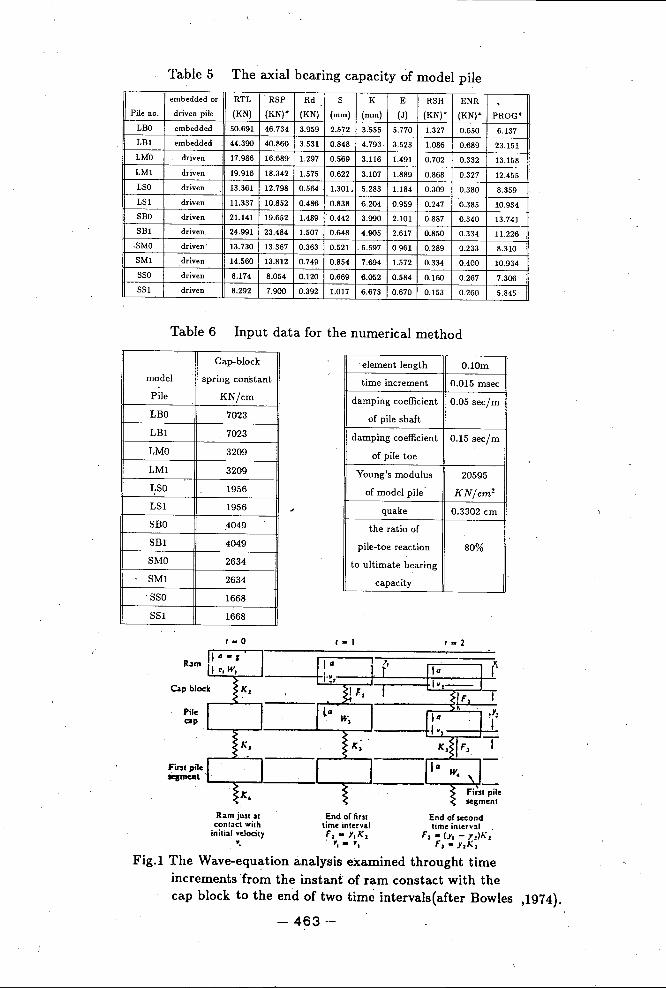
Table 5 The 位 ial bearing capacity of model pileembedded or RTL RSP Rd s K E RSH ENR

嗯，

Pile no driven pile (KN) (KNγ (KN) (mm) (mm) (J) (KN)* (KNγ PROG*LBO embedded 50.691 46.734 3.959 2.572 3:555 5.770 1.327 0.650 6.137LB1 embedded 44.3訓3 40.860 3.531 0.848 4.793、 3.523 1.086 0.689 23.151LMO driven 17.986 16.689 1.297 0.569 3.116 1.491 。702 0.332 13.158LM1 driven 19.916 18.342 1.575 0.622 3.107 1.889 0.868 。327 12.455LSO driven 13.361 12.798 。564 1.301. 5.283 1.184 。309 。380 8.359LS1 driven 11.337 10.852 。486 0.838 6.204 。959 。.247 。385 10.934SBO drÎven 21.141 19.652 1.489 0.442 3.990 2.101 0.887 。340 13.741SB1 driven 24.991 23.484 1.507 。648 4.!泊5 2.617 。.850 。334 11.226、SMO driven' 13.730 13.367 。.363 。521 5.597 。961 0.289 。233 8.310SM1 driven 14.5的 13.812 0.749 0.854 7.694 1.572 0.334 。400 10.934SSO drÎven 8.174 8.054 0.120 0.669 6.052 。58壘 0.160 。267 7.306SS1 driven 8.292 7.900 0.392 1.017 6.673 0.670 。153 。260 5.845

Table 6 Input data for the numerical method

Cap-block

model spring cOlÍstan 也

Pile KN/cm

LBO 7023

LB1 7023

LMO 3209

LM1 3209

LSO 1956

LS1 1956

SBO 4049

SB1 4049

SMO 2634

SM1 2634

SSO 1668

SS1 1668

element length O.lOm

time increment 0.015 msec

damping coeflìcient 0.05 sec/m

of pile shaft

damping coeflìcient 0.15 see/m

of pile toe

Young's modulus 20595

。f model pile KN/cm2

quake 0.3302 em

the ratio of

pile 句 toe reaction 80%

to ultimate bearing

capaeity

R~m

PileClP

F尬SI pile圖書"回..t

1- 0

Ramju.c 刮

cont3ct wilhinili~J vèlocily‧.

1- I

End o(firsltime intcrvalF，-Y，K，t'. _，..- ..

1 _ 2

End o( secondtimc inlcrv:lI

F，_(y，-y，)".F，﹒y，K，

Fig.1 The Wave-equation analysis examined throught timeincrementsfrom the instant of ram constact with thecap block to the end of two time intervals(after Bowles ，1974).

- 463 一

叫length of pll. = L

1:;也立;:::::2ZtmJ

|唔

Fig.2 The equipment for determining the velocity of stresswave.

0.10 ，

264(n=0)

L80:L=1.042mSconning freq. =200kHzIniliol lime=264Fïnol lime= 1137n=10

0.05 C=4774m/sec

051. .，，".，，，'，~，~，V~~，~，~""Io 250 500 750 1000 1250 1500

Time (time interval= O.015msec)Fig.3 The voltage-time curve

EO~、.-.、--'-;-0.0。心。、o國‧‧‧‧‧

。>

1137(n= 10)

1.2mx1.2m

ChargeAmpllfter

5lgn.1 Condltloner划r Compre..or

Fig.4 Dynamically experimental equipment

- 464 一

300

"

'，，一句，、'、'

‘﹒'..'.‘，一-、，

t1 tJ

J府也 /C I

50 100 150 200 'Z~

Tirne (“me int間的 0.Ol6m..c)﹒{叫

-一-F'orc﹒一---Velocity.lnipedenCt

z"

ij| 三之J;

~。老』

h•..宮。.‧昌、?。"的-a，ó

ι50 100 150 200 250

Time(timt Ú\twvCll=0.0' 6m..s.r:)(.)

Fig.5 Model Pile SSl:(a) force-time curve. (b)velocity-timecurve. (c) the energy-time tran伽 red from ha血mer to Pilehead(This result gets from integrity t。但)and (b)) (耐心rceand veloci ty tim回 pile impedance versus ti血e curve. and (e)

displacement-time curve

50 '0。可 50 200 2.50 JO。Timf (帥，四師.....叫11; O.Ol6.，."，..r:)

的一

-，

圓、。』豆 -1、-，.".妞，"，。'、。早闕，'T。

:jf\ 川

• L80 . s日1

• L81. SBO

LMl

LMO LSO

LS1

SMl

SMO

SSOSS1

10L/O(0)

15 20sI

:'; 10 15 20

L/O(bl

Fig.6 (a) The relationship between R，.and L/D for long pile.(b) The relatioÌ1ship between 丸 and L/D for short pile

11 ~ 1

1:1//

Fig.7

-~ I

OLb 。h1b1b Z-b 'zb3blht/Set (bLows/mm)

The 叫“ ionshi p of Ru versus 1/set

465一

動態方法決定海域基樁承載力

梁明德 1 王忠良 2

摘要

本文主要目的是研究海域銅管單樁之軸向承載力，以實驗方法及數值模擬進行研究，就實驗研究而言，十二恨模型基樁分別以打樁機打設於飽和砂土中之後，利用感應器、電子儀器設備、訊號擷取系統及電腦等進，行實驗。至於數值分析，假設基樁為虎克物體，基樁與土壤間之互制作用以凱因模式等效之，當樁鍾打擊樁頭時，數值模擬樁鍾一基樁一土壤之力學行為。

海域結構銅管單樁在飽和砂土中之研究結果簡述如下:同樣樁長，長細比愈小，軸向承載力愈大;同樣樁長及長細比，閉口樁趾之基樁承載力大於閉口樁趾之基樁承載力，然而，當長細比大於 19時，上述結果就相反，此相反結果起因於土塞現象。由動態量測得到承載力大於靜態載重試驗預測的承載力，值得一握的是動態方法適合於高的長細比之基樁，再者，像簡化的海利公式及修正的工程新聞公式等動態公式，由於未定性導致誤差很大，因此，建議以波傅的動態方法預測海域銅管單樁之軸向承載力。

1. 團立臺灣海洋大學河海工程學系副教授

2. 台北市政府提運局助理規劃師

- 466 一