Embed Size (px)
Citation preview
Post-print note
Main results from this thesis have been summarized in the article Ref1 listed below. This articlecovers part 3, 4 and partially part 6 of this thesis in a more concise way. Thank you for usingthis official peer-reviewed publication if reference to these parts are needed. This thesis is madeaccessible online since the access via DTU library was difficult. Further work from the author on thetopic may be found in Ref2 which presents an analytical tip-loss factor and study the effect of wakeexpansion. Simpler expressions(and typo-free) for the helical vortex filament solution presented inappendix A.2 can also be found in Ref2. The earlier article Ref3 is a less detailed version thanRef2. Some figure references in this document may be undefined due to confidential restrictions.
- Ref1 : Emmanuel Branlard, Kristian Dixon, Mac Gaunaa - “Vortex methods to answer theneed for improved understanding and modelling of tip-loss factors” - 2013 - IET RenewablePower Generation - ISSN 1752-1416 - doi: 10.1049/iet-rpg.2012.0283
- Ref2 : Emmanuel Branlard, Mac Gaunaa - “Development of new tip-loss corrections based onvortex theory and vortex methods”. In: Proceedings of Torque 2012, the science of makingtorque from wind. 2012.
- Ref3 : Emmanuel Branlard, Kristian Dixon, Mac Gaunaa - “An improved tip-loss correctionbased on vortex code results”. In: Proceedings of EWEA 2012 - European Wind EnergyConference & Exhibition. EWEA - The European Wind Energy Association, 2012.
E. Branlard, May 2013
Technical University of Denmark
Master’s Thesis
Wind turbine tip-loss correctionsReview, implementation and investigation of new models
Emmanuel BranlardSeptember 2011

Master’s Thesis
Wind turbine tip-loss correctionsReview, implementation and investigation of new models
Emmanuel BranlardSeptember 2011

Wind turbine tip-loss correctionsReview, implementation and investigation of new models
Author Emmanuel Branlard (s090961)
Supervisors Mac Gaunaa (Risø-DTU)Kristian Dixon (Siemens)Kevin Standish (Siemens)
Time Period April 18th - September 30th
Firt Release Date September 30th
Edition 09/05/2013
Category Partially confidential
Comments This report is part of the requirements ro achieve the Master ofScience in Wind Energy at the Technical University of Denmark.
Credits 30 ECTS
Risø National LaboratoryTechnical University of DenmarkP.O.Box 49DK-4000 RoskildeDenmarkTel: (+45) 4677 4004Fax: (+45) 4677 4013www.risoe.dk
Siemens Energy Inc.Renewables - Wind1050 Walnut St. - Suite 303Boulder, Co 80302USATel: (+01) 303 895 2100Fax: (+01) 303 895 2101www.energy.siemens.com

AbstractThe focus of this study is the use of a lifting-line free wake vortex code to derivetip-loss corrections that could be implemented in Blade Element Momentum(BEM) codes. The different theories and three dimensional effects that arerelated to tip-losses are progressively introduced: lifting-line concepts, wakedynamics and its vortex modelling, far-wake analysis. The different tip-losscorrections found in the literature are reviewed with a focus on the main the-ories, namely the work of Betz, Prandtl, Goldstein and Theodorsen, and thedifferent implementations in BEM codes found in the literature are presented.The method of Okulov to compute Goldstein’s factor at a reasonable computa-tional cost is provided with details. The computation of Goldstein’s factor beingaccessible, a method to use this factor in the BEM method is presented. Vari-ous form of Prandtl’s tip-loss factor are also listed for reference. Tip-losses areinvestigated using a free wake vortex code and with Computational Fluid Dy-namics(CFD), and results from both approaches are compared and discussed.For the use of CFD data, the question of definition of the local induction factoron the blade is risen and different method to define it are investigated. Theauthor introduces the naming of “performance tip-loss” factor, which is a cor-rection to the airfoil coefficients due to the tri-dimensionality of the flow at thetip. A preliminary model for the performance tip-loss function is introduced.For the representation of various circulation shapes, a new method using theformulation of Bézier curves is described and developed. Such method can bewidely used to describe curves such as lift, circulation or chord distribution.Last, a method to determine tip-losses using a vortex code is described and im-plemented. From this method, a new tip-loss model is implemented in a BEMcode in order to reproduce the 3D effects inherently present in a vortex code.
E. Branlard i

E. Branlard ii

Contents
Introduction 1
1 Tip-losses: context and challenges 7
1.1 Tip-losses in the historical context of wind turbine aerodynamics . . . . . . . . . . . 7
1.1.1 Losses inherent to a rotating extracting device . . . . . . . . . . . . . . . . . 7
1.1.2 Introducing notions used for the study of three dimensional effects . . . . . . 10
1.1.3 Description of the wake dynamics . . . . . . . . . . . . . . . . . . . . . . . . . 13
1.1.4 Methods to overcome the limitations of the momentum theory . . . . . . . . 17
1.1.5 Far wake analysis: optimal distribution and the birth of tip-losses . . . . . . . 20
1.1.6 Numerical vortex methods . . . . . . . . . . . . . . . . . . . . . . . . . . . . . 21
1.2 Considerations on the local aerodynamics of a rotating blade . . . . . . . . . . . . . 25
1.2.1 Angle of attack . . . . . . . . . . . . . . . . . . . . . . . . . . . . . . . . . . . 25
1.2.2 Rotational effects . . . . . . . . . . . . . . . . . . . . . . . . . . . . . . . . . . 27
1.2.3 Airfoil corrections . . . . . . . . . . . . . . . . . . . . . . . . . . . . . . . . . 28
1.3 Preliminary considerations for the study and modelling of tip-losses . . . . . . . . . . 31
1.3.1 Physical considerations expected to be modelled . . . . . . . . . . . . . . . . 31
1.3.2 Definition of the tip loss factor . . . . . . . . . . . . . . . . . . . . . . . . . . 31
1.3.3 Distribution of axial induction . . . . . . . . . . . . . . . . . . . . . . . . . . 32
1.3.4 Subtleties of the BEM method relevant for this study . . . . . . . . . . . . . 33
1.3.5 Final remarks . . . . . . . . . . . . . . . . . . . . . . . . . . . . . . . . . . . . 36
2 Theories of optimal circulation and tip-losses 37
2.1 Introduction . . . . . . . . . . . . . . . . . . . . . . . . . . . . . . . . . . . . . . . . . 37
2.1.1 Preliminary remarks and notations . . . . . . . . . . . . . . . . . . . . . . . . 37
iii

CONTENTS
2.1.2 Relation with rotor parameters . . . . . . . . . . . . . . . . . . . . . . . . . . 41
2.1.3 Final remarks . . . . . . . . . . . . . . . . . . . . . . . . . . . . . . . . . . . . 42
2.2 Betz theory of optimal circulation . . . . . . . . . . . . . . . . . . . . . . . . . . . . . 43
2.2.1 Betz’s optimal circulation . . . . . . . . . . . . . . . . . . . . . . . . . . . . . 43
2.2.2 Overview of Betz’s demonstration . . . . . . . . . . . . . . . . . . . . . . . . 44
2.2.3 Inclusion of drag . . . . . . . . . . . . . . . . . . . . . . . . . . . . . . . . . . 45
2.3 Generalized Prandtl’s theory . . . . . . . . . . . . . . . . . . . . . . . . . . . . . . . 45
2.3.1 Qualitative description . . . . . . . . . . . . . . . . . . . . . . . . . . . . . . . 46
2.3.2 Detailed derivation of Prandtl’s tip-loss factor . . . . . . . . . . . . . . . . . . 47
2.3.3 General expression . . . . . . . . . . . . . . . . . . . . . . . . . . . . . . . . . 52
2.3.4 Different uses of Prandtl’s generalized tip-loss factor . . . . . . . . . . . . . . 53
2.4 Goldstein’s optimal circulation . . . . . . . . . . . . . . . . . . . . . . . . . . . . . . 55
2.4.1 Goldstein’s theory and its derivatives . . . . . . . . . . . . . . . . . . . . . . . 55
2.4.2 Computation of Goldstein’s factor . . . . . . . . . . . . . . . . . . . . . . . . 56
2.4.3 Comparison with Prandtl’s factor . . . . . . . . . . . . . . . . . . . . . . . . . 57
3 Tip-loss corrections and their implementation 59
3.1 Overview of the different tip-loss corrections . . . . . . . . . . . . . . . . . . . . . . . 59
3.1.1 Theoretical tip-loss corrections . . . . . . . . . . . . . . . . . . . . . . . . . . 59
3.1.2 Semi-Empirical tip-loss corrections . . . . . . . . . . . . . . . . . . . . . . . . 60
3.1.3 Semi-Empirical performance tip-loss corrections . . . . . . . . . . . . . . . . . 61
3.1.4 The historical approach of radius reduction . . . . . . . . . . . . . . . . . . . 62
3.2 On the applicability of the tip-loss factor . . . . . . . . . . . . . . . . . . . . . . . . . 63
3.2.1 Introduction . . . . . . . . . . . . . . . . . . . . . . . . . . . . . . . . . . . . . 63
3.2.2 Applications in the literature . . . . . . . . . . . . . . . . . . . . . . . . . . . 63
3.2.3 Critics in the literature . . . . . . . . . . . . . . . . . . . . . . . . . . . . . . 65
3.3 Comparisons of the different tip-loss factors . . . . . . . . . . . . . . . . . . . . . . . 65
3.3.1 Comparison for one BEM run . . . . . . . . . . . . . . . . . . . . . . . . . . . 65
3.3.2 Impact on performances . . . . . . . . . . . . . . . . . . . . . . . . . . . . . . 67
3.4 New applications and methods . . . . . . . . . . . . . . . . . . . . . . . . . . . . . . 69
3.4.1 Possible new applications using the Goldstein factor . . . . . . . . . . . . . . 69
3.4.2 Further applications . . . . . . . . . . . . . . . . . . . . . . . . . . . . . . . . 70
4 Using a vortex code to investigate tip-losses 71
4.1 Approach description . . . . . . . . . . . . . . . . . . . . . . . . . . . . . . . . . . . . 71
E. Branlard iv

CONTENTS
4.1.1 Introduction . . . . . . . . . . . . . . . . . . . . . . . . . . . . . . . . . . . . . 71
4.1.2 Method description . . . . . . . . . . . . . . . . . . . . . . . . . . . . . . . . . 71
4.2 Family of circulation curves . . . . . . . . . . . . . . . . . . . . . . . . . . . . . . . . 72
4.2.1 Existing parametrization . . . . . . . . . . . . . . . . . . . . . . . . . . . . . . 73
4.2.2 Parametrization using Bézier curves . . . . . . . . . . . . . . . . . . . . . . . 73
4.2.3 Illustration of the parametrization using existing circulation curves . . . . . . 75
4.3 Sensitivity analysis . . . . . . . . . . . . . . . . . . . . . . . . . . . . . . . . . . . . . 78
4.3.1 External parameters . . . . . . . . . . . . . . . . . . . . . . . . . . . . . . . . 78
4.3.2 Sensitivity to the database parameters . . . . . . . . . . . . . . . . . . . . . . 81
4.3.3 Discussion, preliminary results and method implementation . . . . . . . . . . 82
5 Using CFD to investigate tip-losses 85
5.1 Tip-losses and axial induction . . . . . . . . . . . . . . . . . . . . . . . . . . . . . . . 85
5.1.1 Introduction . . . . . . . . . . . . . . . . . . . . . . . . . . . . . . . . . . . . . 85
5.1.2 Data available and methods investigated . . . . . . . . . . . . . . . . . . . . . 85
5.1.3 Results . . . . . . . . . . . . . . . . . . . . . . . . . . . . . . . . . . . . . . . 86
5.2 Tip-losses and aerodynamic coefficients . . . . . . . . . . . . . . . . . . . . . . . . . . 88
5.2.1 Introduction . . . . . . . . . . . . . . . . . . . . . . . . . . . . . . . . . . . . . 88
5.2.2 Data available . . . . . . . . . . . . . . . . . . . . . . . . . . . . . . . . . . . 89
5.2.3 Polar comparison between 2D and 3D CFD . . . . . . . . . . . . . . . . . . . 89
5.2.4 Tip-loss function from the ratio of Cl . . . . . . . . . . . . . . . . . . . . . . . 90
5.2.5 Ratio of drag coefficient . . . . . . . . . . . . . . . . . . . . . . . . . . . . . . 92
5.2.6 Generalization, discussion and comparison with literature . . . . . . . . . . . 94
6 Results and comparison of the different codes and approaches 97
6.1 General comparisons . . . . . . . . . . . . . . . . . . . . . . . . . . . . . . . . . . . . 97
6.1.1 Induced velocities at the rotor plane . . . . . . . . . . . . . . . . . . . . . . . 97
6.1.2 Wake deficit plots . . . . . . . . . . . . . . . . . . . . . . . . . . . . . . . . . 98
6.1.3 General comparison of the different codes . . . . . . . . . . . . . . . . . . . . 99
6.2 Examples of BEM results using the new tip-loss models . . . . . . . . . . . . . . . . 101
6.2.1 Comparison between the vortex code and a BEM code with the new tip-lossmodel . . . . . . . . . . . . . . . . . . . . . . . . . . . . . . . . . . . . . . . . 101
6.2.2 Comparison of BEM with CFD - Performance tip-loss factor . . . . . . . . . 103
6.3 Comparison of tip-loss factors using CFD as a reference . . . . . . . . . . . . . . . . 106
6.4 Discussion . . . . . . . . . . . . . . . . . . . . . . . . . . . . . . . . . . . . . . . . . . 107
E. Branlard v

CONTENTS
Conclusion 109
Acknowledgements 113
Bibliography 115
E. Branlard vi
CONTENTS
Appendices 122
A Goldstein’s factor - Derivation and computation 123
A.1 Short guide to follow Goldstein’s article . . . . . . . . . . . . . . . . . . . . . . . . . 123
A.2 Computation of Goldstein’s factor using helical vortex solution . . . . . . . . . . . . 128
A.3 Computation of optimum power with finite number of blades . . . . . . . . . . . . . 129
A.4 Fitting functions for fast Goldstein’s circulation computation . . . . . . . . . . . . . 130
B Implementation and validation of a vortex code 133
B.1 Implementation of a vortex code . . . . . . . . . . . . . . . . . . . . . . . . . . . . . 133
B.2 Validation of Vortex code with prescribed wake . . . . . . . . . . . . . . . . . . . . . 136
B.3 Unsteady vortex code . . . . . . . . . . . . . . . . . . . . . . . . . . . . . . . . . . . 141
C The BEM method 155
C.1 Introduction to the BEM method . . . . . . . . . . . . . . . . . . . . . . . . . . . . . 155
C.2 Common corrections to the BEM method . . . . . . . . . . . . . . . . . . . . . . . . 161
D Supplementary notes and results regarding CFD 165
D.1 Notes on the Post-processing of CFD data . . . . . . . . . . . . . . . . . . . . . . . . 165
D.2 Aerodynamic Coefficients for Blade 1 . . . . . . . . . . . . . . . . . . . . . . . . . . . 168
D.3 Aerodynamic Coefficients for Blade 2 . . . . . . . . . . . . . . . . . . . . . . . . . . . 170
D.4 CFD visualization of tip-vortex formation . . . . . . . . . . . . . . . . . . . . . . . . 172
E German abstracts 173
F Source Codes 175
F.1 C code for vortex code . . . . . . . . . . . . . . . . . . . . . . . . . . . . . . . . . . . 175
List of figures and tables 179
Index 184
E. Branlard vii
Introduction
Context and motivations Early investigations of wind turbine performances revealed that thepower produced was lower than the one expected by the blade element momentum theory, theproduction was as if the size of the rotor had been reduced in a proportion of approximately 3%.The main reason for this power loss is the circulation of flow around the tip of the blade which is awell known phenomenon in the study of aircraft wings where a vortex is emitted at the extremityof each wing. These vortices are commonly known as they can be observed under some particularpressure and humidity characteristics of the air. At the beginning of the 20th century, Prandtlwas among the first to investigate the losses accounted by these vortices for a wing and later fora propeller. The losses appear for the former when the wing has a finite span, and for the laterwhen the rotating devises has a finite number of blades. Prandtl’s research led to the introductionof a tip-loss factor which is now widely used in wind turbine aerodynamic codes to account for thetip-losses. The load reduction at the tip due to this effect has a dramatic influence on the producedpower because the tip being at a great distance to the hub it has the possibility to generate a lotof torque by a simple lever arm rule. Summing up over the entire range of operation of a windturbine these losses can represent a reduction of 10% on the Annual Energy Production. A properblade design can reduce the power losses and thus increase the productivity of the blade but thisrequire of course a better understanding of tip-losses. It is the purpose of this document to focuson this aspect.
Approach description The notion of tip-losses requires for its understanding a wide picture ofthe different theories applied to wind turbines but also general notions of wing and wind turbines 3Daerodynamics. Historically, tip-losses appeared in the context of investigation of optimal propellerswith an important contribution from authors of the German school: Prandtl, Betz, and Goldstein.Glauert in a later work applied these notions and integrated them into a wind turbine performanceprediction algorithm called the Blade Element Momentum(BEM) theory. The formulations andnotions of these theories will be presented in this study. A pragmatic approach will have to betaken when studying the different tip-loss functions and their implementations for they have andare still rising debates in the scientific community. These foundations established, tools like vortexcodes and Computational Fluid Dynamics (CFD) will be used to investigate further the notion oftip-losses and possibly improve the performances of BEM codes.
Content This document is structured with a succession of six chapters which follow the approachmentioned in the above paragraph. All chapters are progressively built upon each other, except forchapters 4 and 5 that can be read in different order. Different chapters were placed in appendicesfor a clearer and smoother reading, despite the fact that a large part of the corpus rely on them.In a first chapter, the different theories and three dimensional effects that are connected to tip-
1
CONTENTS
losses are progressively introduced. In a second time, the different tip-loss corrections found in theliterature are reviewed with a focus on the main theories and their implementations. The nextchapters both investigate tip-losses using a specific code. The focus of this study was to use avortex code to derive tip-loss corrections that could be implemented in BEM codes. The study ofCFD data give rise to more discussion and interesting results comparisons which be summarizedin a final chapter.
Contribution from this work The different aspects on which this study contributes to existingwork on the matter of tip-losses can be listed as follow:
- This document is the first one to the author’s knowledge to be entirely dedicated to windturbine tip-losses. Along this line, a listing of all the different tip-loss corrections implementedwas performed and important distinctions were made.
- In this study, a new method to determine tip-losses using a vortex code has been describedand implemented. From this method, a new tip-loss model was implemented in a BEM codein order to reproduce the 3D effects inherently present in a vortex code.
- A method to fit curves using the formulation of Bézier curves was described and developed.Such method can be widely used to describe curves such as lift, circulation or chord distribu-tion.
- The author introduced the naming of “performance tip-loss” factor, which is a correction tothe airfoil coefficients due to the tri-dimensionality of the flow at the tip. Such corrections havebeen investigated for instance in [98] in a slightly different way. A model for the performancetip-loss function is introduced in Sect. 5.2.6.
- In Appendix A, a detailed description of Goldstein’s article from 1929[36] can be found. Thisarticle is generally considered as a complex article so that the details presented in this reportis intended to help the curious reader to go quickly through this essential reference on thetopic of tip-losses.
- In Sect. A.2, the method of Okulov[79] to compute Goldstein’s factor at a reasonable com-putational cost is provided with more details than in the original article in order to shareit.
- Eighth order polynomial that fits Goldstein’s factor for different operating conditions are alsoprovided in Sect. A.4.
- The computation of Goldstein’s factor being accessible, a method to use this factor in theBEM method was presented in Sect. 3.4.1.
- Analysis from [43] and [48] use CFD to investigate the axial induction. In this study similaranalysis were performed with focus this time on the tip-loss factor.
- Along the same line than the point above, the question of definition of the local inductionfactor aB on the blade was risen. Different method to define it were investigated in Sect. 5.1
- All the figures are done with the wind turbine convention, rotating clockwise and with arelative wake velocity in the opposite of the stream direction. When studying the theory ofhelical wakes, most references uses different or inconsistent conventions.
About this document This document was entirely written by the author. All the figures presentin this document are from the author, either drawn or generated using Matlab or Mathematica. Ifa figure was inspired by others a reference is mentioned. The author borrowed figures from his ownprevious work, mainly[15]. All references cited in this document have been consulted by the authorexcept for the following which were not available[90][68][91][16][89][45][95][21]. This document waswritten in LATEX using a template from the author. The paper size chosen is A4.
E. Branlard 2

CONTENTS
Notations
Lower case lettersa Axial induction factora′ Tangential induction factoraB Axial induction factor local to the bladea Axial induction factor from 2D momentum theorya Azimuthally averaged axial induction factorc Chordh Helix pitchhB Apparent pitch h/Bh Normalized pitch h/Rl Helix torsional parameterl Normalized torsional parameter l/Rnrot Rotational speed in revolutions per second: Ω/(2π)p Static pressurer Radial position along the blader Dimensionless radial position r/Rs Normal distance between two vortex sheetsuiθ Tangential induced velocityuiz Axial induced velocityw Wake relative longitudinal velocityz0 Surface roughness length
Upper case lettersA AreaAR see AbbreviationsB Number of bladesCΓ Dimensionless circulationCd Drag coefficientsCl Lift coefficientsCn Normal component of the aerodynamic coefficientsCp Power coefficientCQ Torque coefficientCt Tangential component of the aerodynamic coefficientsCT Thrust coefficientD Drag forceD Rotor diameterF Tip-loss factorFa Tip-loss factor based on axial inductionFΓ Tip-loss factor based on circulationFCl Performance tip-loss factorFGo Goldstein’s tip-loss factorFGl Glauert’s tip-loss factorFPr Prandtl’s tip-loss factorFSh Shen’s tip-loss factorIt Turbulence intensityL Lift forceP Power
E. Branlard 3

CONTENTS
Q Rotor torqueR Rotor radiusS Rotor surfaceT Thrust forceU Longitudinal velocity at the rotor in 1DU Relative velocity at the rotorU0 Longitudinal velocity far upstreamUi Induced velocity in 1DUn Velocity normal to the rotorUt Velocity tangent to the rotorUw Longitudinal velocity in the far wake in 1DV Velocity vectorVn Normal velocity in the far wakeVr Rotor velocity ΩrVrel Relative velocityVt Tangential velocity in the far wakeW Induced velocity vector at the rotor
Lower case Greek lettersα Angle of attackβ Twist angleγ Distributed circulationε Pitch angle of the wake helix screwεl/d Lift-over-drag ratioη Efficiencyθ Azimuthal coordinate in polar coordinates, same as ψκ Goldstein’s factorλ Tip speed ratio = ΩR/U0λr Local speed ratio = λr/Rµ Dynamic viscosity [kg m−1 s−1]ν Kinematic viscosity = µ/ρ [m2 s−1]ρ Air density ≈ 1.225 kg/m3
σ Local blade solidity = Bc/2πrτ Shear stressφ Flow angleψ Azimuthal coordinate, positive with the rotor rotation, same as θω Rotational speed of the wake
Upper case Greek lettersΓ Circulation [ m2 /s ]Φ Velocity PotentialΨ Stream functionΩ Rotational speed of the rotor
Abbreviations1D One dimension2D Two dimensions3D Three dimensions
E. Branlard 4

CONTENTS
AD Actuator DiskAEP Annual Energy OutputAR Aspect ratio of a wing: length squared divided by its surfaceBEM Blade Element MomentumBET Blade Element TheoryCFD Computational Fluid DynamicsDOF Degree of FreedomIEC International Electrotechnical CommissionMT Momentum TheoryVL Vortex LatticeWS Wind speedWD Wind directionWT Wind TurbineLSS Low Speed ShaftHSS High Speed Shaft
E. Branlard 5

CONTENTS
E. Branlard 6
Chapter 1Tip-losses: context and challenges
1.1 Tip-losses in the historical context of wind turbine aerody-namics
The origin of the most common tip-loss correction, Prandtl’s correction, comes from the broaderproblem of loss minimization for lifting devises. An historical review of the topic will reveal theintellectual path followed by the scientists at the beginning of the 20th century with the studyof problems of growing complexity, while also shedding light on the different theoretical toolsavailable and on the assumptions under which they operate. The problem is first taken as thedetermination of induced power losses in general to further focus on the tip-loss aspects only.Notions of local aerodynamics of the blade will be required to understand how tip-losses can affectthe angle of attack and the airfoil performances. The tip-loss factor will be defined in Sect. 1.3where preliminary considerations on this challenging topic will be introduced.
1.1.1 Losses inherent to a rotating extracting device
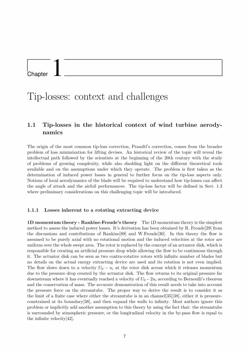
1D momentum theory - Rankine-Froude’s theory The 1D momentum theory is the simplestmethod to assess the induced power losses. It’s derivation has been obtained by R. Froude[29] fromthe discussions and contributions of Rankine[89] and W.Froude[30]. In this theory the flow isassumed to be purely axial with no rotational motion and the induced velocities at the rotor areuniform over the whole swept area. The rotor is replaced by the concept of an actuator disk, which isresponsible for creating an artificial pressure drop while allowing the flow to be continuous throughit. The actuator disk can be seen as two contra-rotative rotors with infinite number of blades butno details on the actual energy extracting device are used and its rotation is not even implied.The flow slows down to a velocity U0 − ui at the rotor disk across which it releases momentumdue to the pressure drop created by the actuator disk. The flow returns to its original pressure fardownstream where it has eventually reached a velocity of U0−2ui according to Bernoulli’s theoremand the conservation of mass. The accurate demonstration of this result needs to take into accountthe pressure force on the streamtube. The proper way to derive the result is to consider it asthe limit of a finite case where either the streamtube is in an channel[35][38], either it is pressure-constrained at its boundary[38], and then expand the walls to infinity. Most authors ignore thisproblem or implicitly add another assumption to this theory by using the fact that: the streamtubeis surrounded by atmospheric pressure, or the longitudinal velocity in the by-pass flow is equal tothe infinite velocity[42].
7
CHAPTER 1. TIP-LOSSES: CONTEXT AND CHALLENGES
Pressure
Velocity
Streamtube
Actuator diskp0
U0
U0
p0
Uw
Uw
UT
p0
U0
p0
U0
U
p0 p0
p+
StagnationPressure
p−
Figure 1.1: One dimensional momentum theory.
E. Branlard 8
CHAPTER 1. TIP-LOSSES: CONTEXT AND CHALLENGES
Parallel work down within 5 years from the authors Lanchester[58, (1915)], Joukowski1[51, (1920)]and Betz[10, (1920)], led to the theoretical limit of power than can be extracted: the Betz-Joukowskilimit2 with a value of power coefficient of 16/27. It should be noted that some authors found thatthe power coefficient tends to infinity for low tip speed ratio but it has been argued[104] that thisis the result of neglecting the pressure forces on the streamtube for highly-loaded rotors. Below, itwill be seen that the theoretical Betz-Joukowski limit has to be reduced in practice while releasingassumptions from the momentum theory.
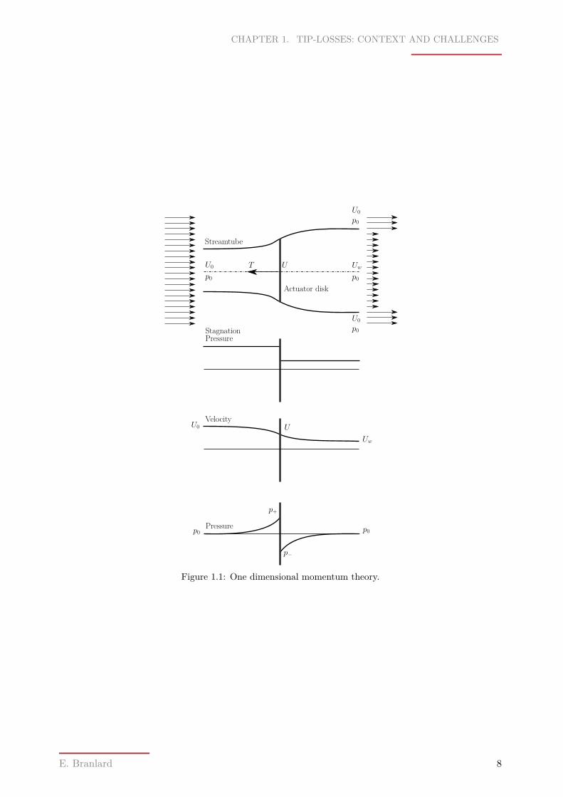
2D momentum theory The 2D momentum theory as derived by Joukowski[50] in 1918, reportedby Glauert[35] in 1935 and further formalized in 2010 by Sørensen and van Kuik[104] uses anactuator disk that impart a pressure drop and a tangential rotational speed to the fluid withoutdiscontinuity in the axial and radial flow passing the disk. No friction losses are considered in thistheory which is why the rotation of the flow has to be introduced artificially by the actuator disk andalso why the rotational velocity in front of the disk is zero. This theory allows for radial variationsof velocities and pressure at the rotor and at the wake, and accounts for pressure changes due towake rotation. Nevertheless the theory leads to a system of equations which is not closed. Eithertwo variables needs to be given or assumptions made to simplify the theory. The Joukowski modeluses the assumption of constant circulation, which imply that the flow is irrotational everywhereexcept along the axis of rotation and that the rotational momentum of the slipstream in the wakeωr2 is constant for each radial elements. Under this assumption, it is found that in general theaxial induced velocity in the wake is not twice the one at the rotor. Nevertheless, the results getreally close for tip speed ratio above 2. To avoid inconsistency near the rotor center, a Rankinevortex core can be used instead of a line vortex for a better representation of the flow[104]. In thiscase, the equations become more complex, but still lead to a closed form solution.
0
+−
w
dr
r θ
er θ
eθ
ez
e′θ
e′r
Ω
ω
ωw
rw
Figure 1.2: Two-dimensional momentum theory notation scheme.
Simplified equations are obtained by adding the assumption that the rotor is lightly loaded and therotation of the wake is small compared to the rotational speed of the rotor. This can be interpretedas the pressure in the far wake equals the pressure upstream. Consequently the thrust and axialinduction results from the 1D momentum apply and the tangential axial induction factor can bedetermined as a function of the local speed ratio and the axial induction factor. This relation isoften drawn as a velocity triangle and can also be interpreted as an energy equation. The final
1Nikolai Egorovich Zhukovsky, different writing of this name can be found when using latin alphabet.2In 2007[113] the naming Lanchester-Betz-Joukowski limit was suggested, but further historical research[81] at-
tributed this result to the independent work of Betz and Joukowski.
E. Branlard 9
CHAPTER 1. TIP-LOSSES: CONTEXT AND CHALLENGES
equations resulting from the use of 2D momentum theory results linked to 1D momentum resultswill be further referred to as “simplified-2D momentum theory”. It should be kept in mind thatonly under the assumption of this simplified theory holds the fact that the induced velocity in thewake is twice the one at the rotor.
1.1.2 Introducing notions used for the study of three dimensional effects
Limitation of momentum theory The methods mentioned above do no fully capture thevariations of the flow nor the physics of the energy extraction device. The momentum theory givesan upper limit for the maximum power that can be extracted from the flow but does not giveindication on the design of the device itself. Also the assumption of uniform induced velocity at therotor used in the momentum theory does not hold for a real flow where three dimensional effectstakes place and the rotor obviously does not have an infinite number of blades. One example ofthese effects in the appearance of vortices at the tip of a finite span wing as described among thefollowing paragraphs. Tip-vortices have been first investigated for aircrafts by Prandtl who derivedthe lifting line theory to determine the losses related to this vorticity.
Simulation of actuator disks Under the 1D and simplified-2D momentum theory, the induc-tions factors are assumed uniform over the entire disk. The validity of these assumptions werestudied using computational fluid dynamic tools to model the actuator disk[103, 67, 73, 66]. Re-sults from these analysis showed that the axial velocity was underestimated(a overestimated) inthe inner part of the disk due to the neglecting of the pressure term from wake rotation. On theouter part of the blade the axial velocity is overestimated(a underestimated) due to the neglectingof the radial expansion of the streamtube. The assumption of uniform axial induction factor is thusnot valid, and it will be expected to be, among others, a function of the radius:
a = a(r, . . .) (1.1)
Such variations are captured by the general 2D momentum theory in which the axial induction ispurely a function of radius, written in this document a = a(r). Despite this radial-dependency, itis worth mentioning that using both a simple vortex model and a actuator disk model, it has beenfound[110] that each annular element seem to behaves locally as predicted by the 1D momentumtheory, meaning that in a first approximation each annular strip can be reasonably consideredindependent.
Finite number of blades The concept of actuator disk used previously is equivalent to theassumption of infinite number of blades, which is that all particles passing through the disk willexperience the same change of momentum due to the presence of the blades. This no longer holdsfor a rotor with a finite number of blades for which the local axial induction will be larger close tothe blades than in between the blades. As a result of this, an azimuthal dependency of the axialinduction factor should be accounted for on top of the radial dependency mentioned in the aboveparagraph, viz.
a = a(r, ψ, . . .) (1.2)The local induction factor at the blade which characterize the incoming speed on the blade andthus determine the local aerodynamic load is written distinctively aB. The average axial inductionfactor a(r) is defined as:
a(r) = 12π
∫ 2π
0a(r, ψ)dψ [ - ] (1.3)
In the case of infinite number of blade aB and a are the same. Axisymmetric flows, i.e. flowazimuthally independent such as the one described by 2D momentum or 2D vortex theories can
E. Branlard 10
CHAPTER 1. TIP-LOSSES: CONTEXT AND CHALLENGES
only be found for wind turbines with infinite number of blades. With finite number of blades, thesetheories no longer apply but are still used in BEM codes by introduction of a “tip-loss factor” (seediscussion on Sect. 1.3 and Sect. 3.2).
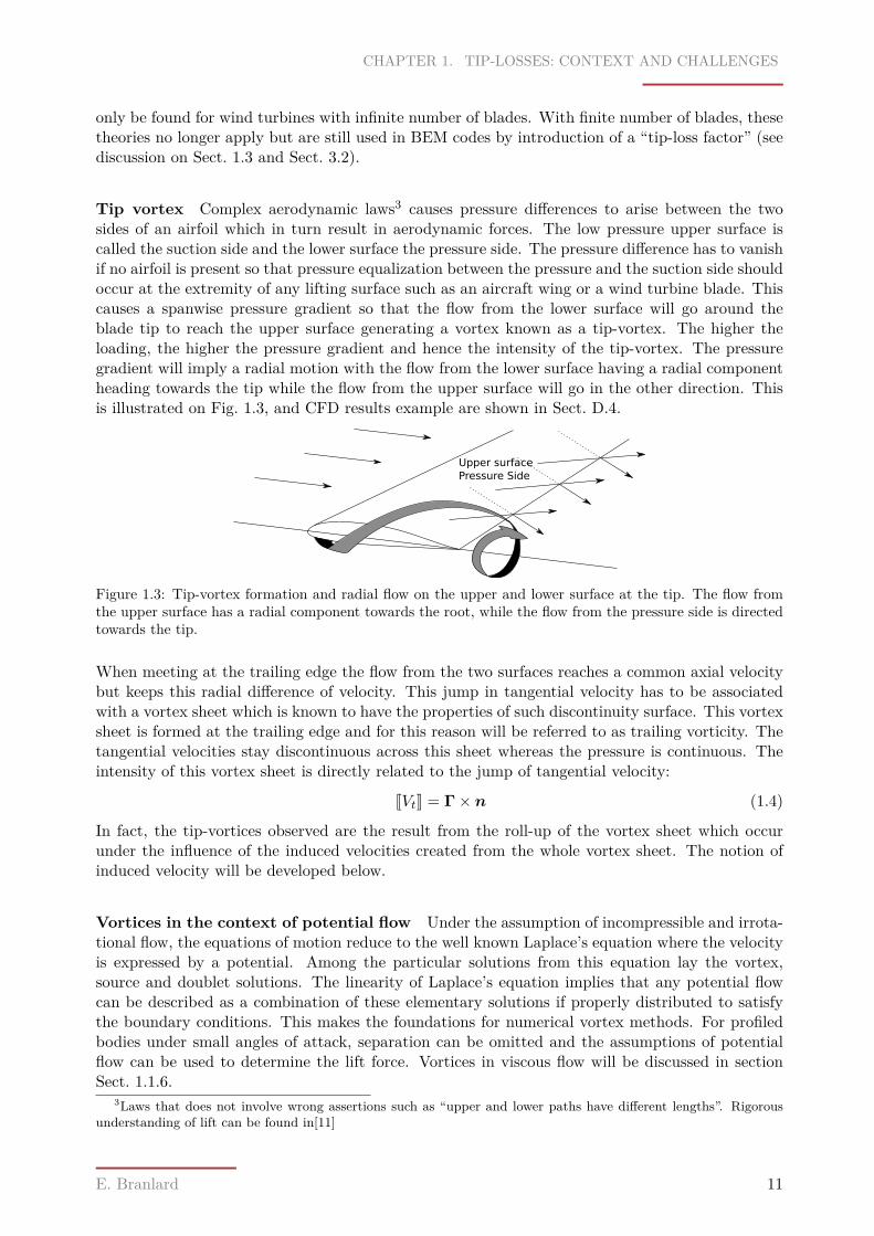
Tip vortex Complex aerodynamic laws3 causes pressure differences to arise between the twosides of an airfoil which in turn result in aerodynamic forces. The low pressure upper surface iscalled the suction side and the lower surface the pressure side. The pressure difference has to vanishif no airfoil is present so that pressure equalization between the pressure and the suction side shouldoccur at the extremity of any lifting surface such as an aircraft wing or a wind turbine blade. Thiscauses a spanwise pressure gradient so that the flow from the lower surface will go around theblade tip to reach the upper surface generating a vortex known as a tip-vortex. The higher theloading, the higher the pressure gradient and hence the intensity of the tip-vortex. The pressuregradient will imply a radial motion with the flow from the lower surface having a radial componentheading towards the tip while the flow from the upper surface will go in the other direction. Thisis illustrated on Fig. 1.3, and CFD results example are shown in Sect. D.4.
Upper surfacePressure Side
Figure 1.3: Tip-vortex formation and radial flow on the upper and lower surface at the tip. The flow fromthe upper surface has a radial component towards the root, while the flow from the pressure side is directedtowards the tip.
When meeting at the trailing edge the flow from the two surfaces reaches a common axial velocitybut keeps this radial difference of velocity. This jump in tangential velocity has to be associatedwith a vortex sheet which is known to have the properties of such discontinuity surface. This vortexsheet is formed at the trailing edge and for this reason will be referred to as trailing vorticity. Thetangential velocities stay discontinuous across this sheet whereas the pressure is continuous. Theintensity of this vortex sheet is directly related to the jump of tangential velocity:
JVtK = Γ× n (1.4)
In fact, the tip-vortices observed are the result from the roll-up of the vortex sheet which occurunder the influence of the induced velocities created from the whole vortex sheet. The notion ofinduced velocity will be developed below.
Vortices in the context of potential flow Under the assumption of incompressible and irrota-tional flow, the equations of motion reduce to the well known Laplace’s equation where the velocityis expressed by a potential. Among the particular solutions from this equation lay the vortex,source and doublet solutions. The linearity of Laplace’s equation implies that any potential flowcan be described as a combination of these elementary solutions if properly distributed to satisfythe boundary conditions. This makes the foundations for numerical vortex methods. For profiledbodies under small angles of attack, separation can be omitted and the assumptions of potentialflow can be used to determine the lift force. Vortices in viscous flow will be discussed in sectionSect. 1.1.6.
3Laws that does not involve wrong assertions such as “upper and lower paths have different lengths”. Rigorousunderstanding of lift can be found in[11]
E. Branlard 11
CHAPTER 1. TIP-LOSSES: CONTEXT AND CHALLENGES
Upwash
Downwash
Upwash
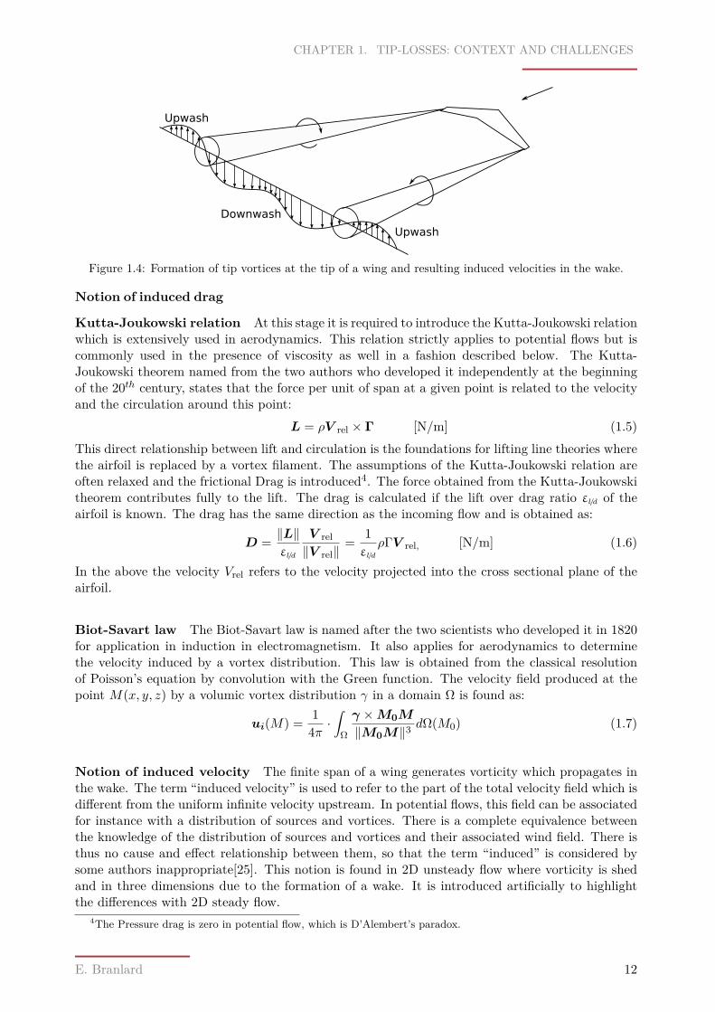
Figure 1.4: Formation of tip vortices at the tip of a wing and resulting induced velocities in the wake.
Notion of induced drag
Kutta-Joukowski relation At this stage it is required to introduce the Kutta-Joukowski relationwhich is extensively used in aerodynamics. This relation strictly applies to potential flows but iscommonly used in the presence of viscosity as well in a fashion described below. The Kutta-Joukowski theorem named from the two authors who developed it independently at the beginningof the 20th century, states that the force per unit of span at a given point is related to the velocityand the circulation around this point:
L = ρV rel × Γ [N/m] (1.5)This direct relationship between lift and circulation is the foundations for lifting line theories wherethe airfoil is replaced by a vortex filament. The assumptions of the Kutta-Joukowski relation areoften relaxed and the frictional Drag is introduced4. The force obtained from the Kutta-Joukowskitheorem contributes fully to the lift. The drag is calculated if the lift over drag ratio εl/d of theairfoil is known. The drag has the same direction as the incoming flow and is obtained as:
D = ‖L‖εl/d
V rel‖V rel‖
= 1εl/d
ρΓV rel, [N/m] (1.6)
In the above the velocity Vrel refers to the velocity projected into the cross sectional plane of theairfoil.
Biot-Savart law The Biot-Savart law is named after the two scientists who developed it in 1820for application in induction in electromagnetism. It also applies for aerodynamics to determinethe velocity induced by a vortex distribution. This law is obtained from the classical resolutionof Poisson’s equation by convolution with the Green function. The velocity field produced at thepoint M(x, y, z) by a volumic vortex distribution γ in a domain Ω is found as:
ui(M) = 14π ·
∫Ω
γ ×M0M
‖M0M‖3dΩ(M0) (1.7)
Notion of induced velocity The finite span of a wing generates vorticity which propagates inthe wake. The term “induced velocity” is used to refer to the part of the total velocity field which isdifferent from the uniform infinite velocity upstream. In potential flows, this field can be associatedfor instance with a distribution of sources and vortices. There is a complete equivalence betweenthe knowledge of the distribution of sources and vortices and their associated wind field. There isthus no cause and effect relationship between them, so that the term “induced” is considered bysome authors inappropriate[25]. This notion is found in 2D unsteady flow where vorticity is shedand in three dimensions due to the formation of a wake. It is introduced artificially to highlightthe differences with 2D steady flow.
4The Pressure drag is zero in potential flow, which is D’Alembert’s paradox.
E. Branlard 12
CHAPTER 1. TIP-LOSSES: CONTEXT AND CHALLENGES
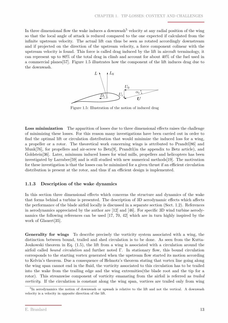
In three dimensional flow the wake induces a downwash5 velocity at any radial position of the wingso that the local angle of attack is reduced compared to the one expected if calculated from theinfinite upstream velocity. The actual lift can thus be seen as rotated accordingly downstreamand if projected on the direction of the upstream velocity, a force component colinear with theupstream velocity is found. This force is called drag induced by the lift in aircraft terminology, itcan represent up to 80% of the total drag in climb and account for about 40% of the fuel used ina commercial planes[57]. Figure 1.5 illustrates how the component of the lift induces drag due tothe downwash.
L L0
U0αi
UUiDi
Figure 1.5: Illustration of the notion of induced drag
Loss minimization The apparition of losses due to three dimensional effects raises the challengeof minimizing these losses. For this reason many investigations have been carried out in order tofind the optimal lift or circulation distribution that would minimize the induced loss for a wing,a propeller or a rotor. The theoretical work concerning wings is attributed to Prandtl[86] andMunk[76], for propellers and air-screw to Betz[9], Prandtl(in the appendix to Betz article), andGoldstein[36]. Later, minimum induced losses for wind mills, propellers and helicopters has beeninvestigated by Larrabee[59] and is still studied with new numerical methods[19]. The motivationfor these investigation is that the losses can be minimized for a given thrust if an efficient circulationdistribution is present at the rotor, and thus if an efficient design is implemented.
1.1.3 Description of the wake dynamics
In this section three dimensional effects which concerns the structure and dynamics of the wakethat forms behind a turbine is presented. The description of 3D aerodynamic effects which affectsthe performance of the blade airfoil locally is discussed in a separate section (Sect. 1.2). Referencesin aerodynamics appreciated by the author are [12] and [46]. For specific 3D wind turbine aerody-namics the following references can be used [17, 70, 42] which are in turn highly inspired by thework of Glauert[35].
Generality for wings To describe precisely the vorticity system associated with a wing, thedistinction between bound, trailed and shed circulation is to be done. As seen from the Kutta-Joukowski theorem in Eq. (1.5), the lift from a wing is associated with a circulation around theairfoil called bound circulation and further noted Γ. In stationary flow, this bound circulationcorresponds to the starting vortex generated when the upstream flow started its motion accordingto Kelvin’s theorem. Due a consequence of Helmotz’s theorem stating that vortex line going alongthe wing span cannot end in the fluid, the vorticity associated to this circulation has to be trailedinto the wake from the trailing edge and the wing extremities(the blade root and the tip for arotor). This streamwise component of vorticity emanating from the airfoil is referred as trailedvorticity. If the circulation is constant along the wing span, vortices are trailed only from wing
5In aerodynamics the notion of downwash or upwash is relative to the lift and not the vertical. A downwashvelocity is a velocity in opposite direction of the lift.
E. Branlard 13
CHAPTER 1. TIP-LOSSES: CONTEXT AND CHALLENGES
extremities, whereas if the circulation varies along the blade span, trailing vortices are created fromeach radial position r forming a continuous vortex sheet. The strength per unit of length of thetrailed vorticity is directly equal to the bound circulation’s gradient which writes:
Γt(r) = −∂Γ(r)∂r
dr [m2/s] (1.8)
For a real flow, the bound circulation gradient along the span will obviously be present becausethe circulation has to vanish continuously at the wing extremities. As a result of this, the strengthof the vortex sheets usually increases towards the wing extremities where the circulation gradientis expected to be the highest. These higher intensities of trailed vorticity at the tip will inducea roll-up of the wake into concentrated tip-vortex. Prandtl neglected this roll-up to develop hislifting-line theory where the blade was modelled as a superposition of horseshoe vortices laying onthe wing and expending towards infinity.
The last form of vorticity found is the one generated by time variations of the bound circulationwhich shed spanwise vorticity in the wake. This shed circulation is directly related to the changeof vorticity on the blade as:
Γs(r) = ∂Γ(r)∂t
dt [m2/s] (1.9)
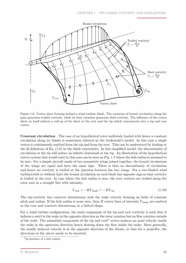
The vorticity sheets are convected downstream with the wake velocity. According to Biot-Savartlaw, the distributed vorticity from the wake and the blade induces a velocity field in the domain.In particular this field acts on the fluid particle of the wake sheet which then tends to roll-upinto concentrated tip-vortex as it propagates downstream. It should be noted that in potentialflow, there can be no flow through these surfaces and they can be considered impermeable. Anillustration inspired and adapted from [93] of the different type of circulations involved is foundon Fig. 1.6. The above discussion is valid for rotary wings, but the structure of the wake is morecomplex and will deserve more attention in the following.
Rotor wake specificity For a rotating wing, the vorticity structures are mainly transporteddownstream in the axial direction and because they are continuously shed from different azimuthallocation due to the rotation of the rotor the resulting wake shape “looks” helical. The influence ofthe wake on itself will distort the wake shape so that the wake does not hold its nominal helicalshape. For instance, the edges of the vortex sheet roll up into concentrated tip vortices. Forsimplicity this roll-up can be ignored, as for the propeller case for instance where the high axialvelocity in the streamwise direction transport the wake quickly downstream. For airplane propellerand helicopters the induced velocities are often small compared to the speed of flight but this isnot the case for wind energy applications in which they are appreciable and moreover opposite tothe streamwise direction. As the wake propagates downstream, the distance between the differentvortex sheets tend to decrease while the wake radius expands. The stability of the wake is quitecomplex and depends mainly on the loading of the rotor. The loading can be related to the thrustcoefficient, which in turns is related to the inductions factors and the tip speed ratio. Studies ofwake stability can be found in [78], but in all theoretical derivations presented in this study thewake is assumed stable.
Lightly-loaded assumption When a rotor is lightly-loaded it is argued that the wake expansionbehind the rotor is small and so is its distortion. When the assumption of lightly-loaded rotor ismade, it thus implies no wake expansion and distortion, so that the wake shape is a perfect helixheld in a cylinder with periodicity between the vortex sheet. For applications where the thrustcoefficient is low(usually high wind speed, low tip-speed ratio), the lightly-loaded assumption isoften used for its convenient simplicity.
E. Branlard 14
CHAPTER 1. TIP-LOSSES: CONTEXT AND CHALLENGES
U0
Vortex sheet
Trailed vorticityΓt = dΓB
dr
Shed vorticityΓs = dΓB
dt
Γroot
Γtip
ΩΓB
Bound circulation
Γt
Γs
Figure 1.6: Vortex sheet forming behind a wind turbine blade. The variation of bound circulation along thespan generates trailed vorticity, while its time variation generates shed vorticity. The influence of the vortexsheet on itself induces a roll-up of the sheet at the root and the tip which concentrates into a tip and rootvortex.
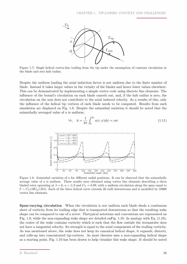
Constant circulation The case of an hypothetical rotor uniformly loaded with hence a constantcirculation along its blades is sometimes referred as the Joukowski’s model. In this case a singlevortex is continuously emitted from the tip and from the root. This can be understood by looking atthe ill-definition of Eq. (1.8) at the blade extremities. In this simplified model, the discontinuity ofcirculation at the tip will induce an infinite downwash at the tip. An illustration of the hypotheticalvortex system that would exist in this case can be seen on Fig. 1.7 where the hub radius is assumed tobe zero. For a simple aircraft made of two symmetric wings joined together, the bound circulationsof the wings are equal and have the same sign. There is thus no discontinuity of circulationand hence no vorticity is trailed at the junction between the two wings. For a two-bladed windturbine(with or without hub) the bound circulation on each blade has opposite sign so that vorticityis trailed at the root. In case where the hub radius is zero, the root vortices are trailed along therotor axis in a straight line with intensity:
Γaxis = −B Γblade = −B Γtip (1.10)
The tip-vorticity line convects downstream with the wake velocity forming an helix of constantpitch and radius. If the hub radius is none zero, then B vortex lines of intensity Γblade are emittedat the root and convects downstream in a helical shape.
For a wind turbine configuration, the axial component of the tip and root vorticity is such that itinduces a swirl in the wake in the opposite direction as the rotor rotation but no flow rotation outsideof the wake. The azimuthal component of the tip and root6 vortex induces an axial velocity insidethe wake in the upstream direction hence slowing down the flow inside the wake. More generally,the axially induced velocity is in the opposite direction of the thrust, so that for a propeller, thedirections in the above needs to be inverted.
6In presence of a hub radius.
E. Branlard 15
CHAPTER 1. TIP-LOSSES: CONTEXT AND CHALLENGES
U0
Ω
φΓtip
Γaxis
Figure 1.7: Single helical vortex-line trailing from the tip under the assumption of constant circulation atthe blade and zero hub radius.
Despite the uniform loading the axial induction factor is not uniform due to the finite number ofblade. Instead it takes larger values in the vicinity of the blades and hence lower values elsewhere.This can be demonstrated by implementing a simple vortex code using discrete line elements. Theinfluence of the bound’s circulation on each blade cancels out, and, if the hub radius is zero, thecirculation on the axis does not contribute to the axial induced velocity. As a results of this, onlythe influence of the helical tip vortices of each blade needs to be computed. Results from suchsimulation are displayed on Fig. 1.8. Despite the azimuthal variation it should be noted that theazimuthally averaged value of a is uniform:
∀r, a = 12π
∫ 2π
0a(r, ψ)dψ = cst (1.11)
Azimuthal angle [deg]
Axialinductionfactora[.]
0 30 60 90 120 150 180 210 240 270 300 330 3600
0.2
0.4
0.6
0.8
1r/R = 30%r/R = 76%r/R = 90%r/R = 96%
Figure 1.8: Azimuthal variation of a for different radial positions. It can be observed that the azimuthallyaverage value of a is uniform. These results were obtained using vortex line elements describing a threebladed rotor operating at λ = 6, a = 1/3 and CT = 0.89, with a uniform circulation along the span equal toΓ = CTπRU0/(Bλ). Each of the three helical curve extends 40 radii downstream and is modelled by 10000vortex line elements.
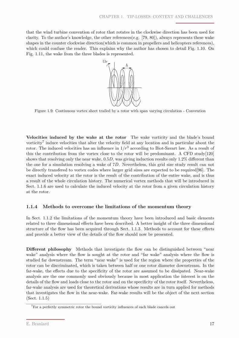
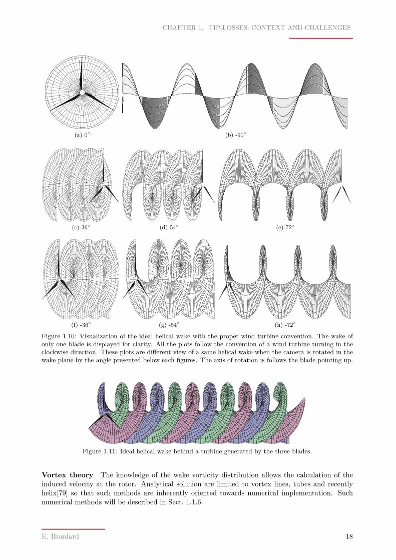
Span-varying circulation When the circulation is not uniform each blade sheds a continuoussheet of vorticity from its trailing edge that is transported downstream so that the resulting wakeshape can be compared to one of a screw. Thetypical notations and conventions are represented onFig. 1.9, while the non-expanding wake shape are detailed onFig. 1.10. In analogy with Eq. (1.10),the center of the wake contains vorticity which is such that the flow outside the streamtube doesnot have a tangential velocity. Its strength is equal to the axial components of the trailing vorticity.As was mentioned above, the wake does not keep its canonical helical shape, it expands, distorts,and rolls-up into concentrated tip-vortices. As most theories uses a non-expanding helical shapeas a starting point, Fig. 1.10 has been drawn to help visualize this wake shape. It should be noted
E. Branlard 16
CHAPTER 1. TIP-LOSSES: CONTEXT AND CHALLENGES
that the wind turbine convention of rotor that rotates in the clockwise direction has been used forclarity. To the author’s knowledge, the other references(e.g. [79, 80]), always represents these wakeshapes in the counter clockwise direction(which is common in propellers and helicopters references),which could confuse the reader. This explains why the author has chosen to detail Fig. 1.10. OnFig. 1.11, the wake from the three blades is represented.
Ωrh
Figure 1.9: Continuous vortex sheet trailed by a rotor with span varying circulation - Convention
Velocities induced by the wake at the rotor The wake vorticity and the blade’s boundvorticity7 induce velocities that alter the velocity field at any location and in particular about therotor. The induced velocities has an influence in 1/r3 according to Biot-Savart law. As a result ofthis the contribution from the vortex close to the rotor will be predominant. A CFD study[120]shows that resolving only the near wake, 0.5D, was giving induction results only 1.2% different thanthe one for a simulation resolving a wake of 7D. Nevertheless, this grid size study result can notbe directly transfered to vortex codes where larger grid sizes are expected to be required[96]. Theexact induced velocity at the rotor is the result of the contribution of the entire wake, and is thusa result of the whole circulation history. The numerical vortex methods that will be introduced inSect. 1.1.6 are used to calculate the induced velocity at the rotor from a given circulation historyat the rotor.
1.1.4 Methods to overcome the limitations of the momentum theory
In Sect. 1.1.2 the limitations of the momentum theory have been introduced and basic elementsrelated to three dimensional effects have been described. A better insight of the three dimensionalstructure of the flow has been acquired through Sect. 1.1.3. Methods to account for these effectsand provide a better view of the details of the flow should now be presented.
Different philosophy Methods that investigate the flow can be distinguished between “nearwake” analysis where the flow is sought at the rotor and “far wake” analysis where the flow isstudied far downstream. The term “near wake” is used for the region where the properties of therotor can be discriminated, which is taken between half or one rotor diameter downstream. In thefar-wake, the effects due to the specificity of the rotor are assumed to be dissipated. Near-wakeanalysis are the one commonly used obviously because in most application the interest is on thedetails of the flow and loads close to the rotor and on the specificity of the rotor itself. Nevertheless,far-wake analysis are used for theoretical derivations whose results are in turn applied for methodsthat investigates the flow in the near-wake. Far-wake results will be the object of the next section(Sect. 1.1.5)
7For a perfectly symmetric rotor the bound vorticity influences of each blade cancels out
E. Branlard 17
CHAPTER 1. TIP-LOSSES: CONTEXT AND CHALLENGES
(a) 0
(b) -90
(c) 36
(d) 54
(e) 72
(f) -36
(g) -54
(h) -72
Figure 1.10: Visualization of the ideal helical wake with the proper wind turbine convention. The wake ofonly one blade is displayed for clarity. All the plots follow the convention of a wind turbine turning in theclockwise direction. These plots are different view of a same helical wake when the camera is rotated in thewake plane by the angle presented below each figures. The axis of rotation is follows the blade pointing up.
Figure 1.11: Ideal helical wake behind a turbine generated by the three blades.
Vortex theory The knowledge of the wake vorticity distribution allows the calculation of theinduced velocity at the rotor. Analytical solution are limited to vortex lines, tubes and recentlyhelix[79] so that such methods are inherently oriented towards numerical implementation. Suchnumerical methods will be described in Sect. 1.1.6.
E. Branlard 18
CHAPTER 1. TIP-LOSSES: CONTEXT AND CHALLENGES
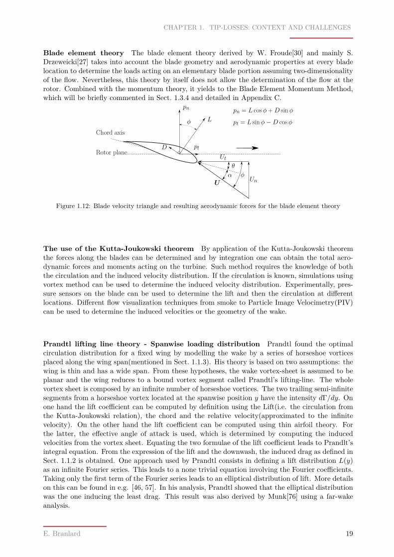
Blade element theory The blade element theory derived by W. Froude[30] and mainly S.Drzeweicki[27] takes into account the blade geometry and aerodynamic properties at every bladelocation to determine the loads acting on an elementary blade portion assuming two-dimensionalityof the flow. Nevertheless, this theory by itself does not allow the determination of the flow at therotor. Combined with the momentum theory, it yields to the Blade Element Momentum Method,which will be briefly commented in Sect. 1.3.4 and detailed in Appendix C.
Rotor planeUt
UnUφ
θ
α
φ L
D pt
pn pn = L cosφ + D sinφ
pt = L sinφ−D cosφChord axis
Figure 1.12: Blade velocity triangle and resulting aerodynamic forces for the blade element theory
The use of the Kutta-Joukowski theorem By application of the Kutta-Joukowski theoremthe forces along the blades can be determined and by integration one can obtain the total aero-dynamic forces and moments acting on the turbine. Such method requires the knowledge of boththe circulation and the induced velocity distribution. If the circulation is known, simulations usingvortex method can be used to determine the induced velocity distribution. Experimentally, pres-sure sensors on the blade can be used to determine the lift and then the circulation at differentlocations. Different flow visualization techniques from smoke to Particle Image Velocimetry(PIV)can be used to determine the induced velocities or the geometry of the wake.
Prandtl lifting line theory - Spanwise loading distribution Prandtl found the optimalcirculation distribution for a fixed wing by modelling the wake by a series of horseshoe vorticesplaced along the wing span(mentioned in Sect. 1.1.3). His theory is based on two assumptions: thewing is thin and has a wide span. From these hypotheses, the wake vortex-sheet is assumed to beplanar and the wing reduces to a bound vortex segment called Prandtl’s lifting-line. The wholevortex sheet is composed by an infinite number of horseshoe vortices. The two trailing semi-infinitesegments from a horseshoe vortex located at the spanwise position y have the intensity dΓ/dy. Onone hand the lift coefficient can be computed by definition using the Lift(i.e. the circulation fromthe Kutta-Joukowski relation), the chord and the relative velocity(approximated to the infinitevelocity). On the other hand the lift coefficient can be computed using thin airfoil theory. Forthe latter, the effective angle of attack is used, which is determined by computing the inducedvelocities from the vortex sheet. Equating the two formulae of the lift coefficient leads to Prandlt’sintegral equation. From the expression of the lift and the downwash, the induced drag as defined inSect. 1.1.2 is obtained. One approach used by Prandtl consists in defining a lift distribution L(y)as an infinite Fourier series. This leads to a none trivial equation involving the Fourier coefficients.Taking only the first term of the Fourier series leads to an elliptical distribution of lift. More detailson this can be found in e.g. [46, 57]. In his analysis, Prandtl showed that the elliptical distributionwas the one inducing the least drag. This result was also derived by Munk[76] using a far-wakeanalysis.
E. Branlard 19
CHAPTER 1. TIP-LOSSES: CONTEXT AND CHALLENGES
1.1.5 Far wake analysis: optimal distribution and the birth of tip-losses
Introduction Far wake theories applies under the assumptions of inviscid and irrotational flow,and they rely on the fact that there is a direct relation between the loading and hence the circulationat the lifting devise and the momentum in the wake. Such theories are often quite complex andrequire a high level of abstraction so that only few historical elements and basic concepts arereferenced in this section. They are introduced in this study because all theoretical derivationsconcerning tip-losses are based in the far-wake.
The motivations for such analysis is that the flow is way more complicated in the near wake dueto the interaction with blades, boundary layers at the blade and separation effects. These effectsdissipates and are thus no more present in the far wake. For helicopter flows the blade tip reachestransonic speeds so that compressibility effects should be accounted for. For wind turbines suchspeeds are not found but the Mach number can be found to be quite larger than 0.38 which is theupper limit usually taken to justify incompressibility. In the far wake the induced velocities arereduced so the assumptions of inviscid and irrotational flow can be further justified.
Far wake analysis - elliptical wing elliptical distribution By applying momentum theory on abox surrounding the wing and extending the boundaries to infinity, only the plane perpendicular tothe direction of flight in the far wake is left in the calculation of the drag[57, chap. 9]. This concep-tual plane or “front view”, called the Trefftz plane, leaves the chord as a secondary considerationby focusing on the wake at the Trefftz plane only. The lift and drag at the lifting devise can bedetermined by integration of the velocity potential in the Trefftz plane, and by application of theGauss theorem, reduces to a line integral on the wake. By using a variation method on the velocitypotential, Munk[76] derived the minimum drag and found the result of elliptic lift distribution ina different way than Prandtl.
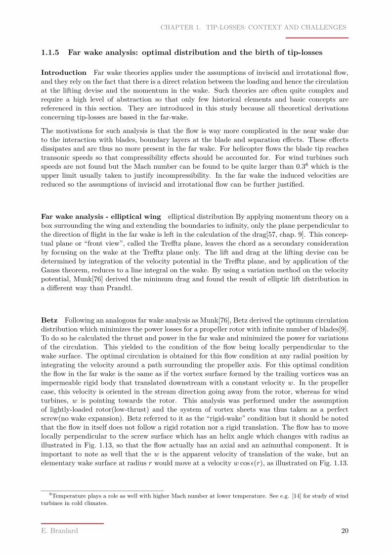
Betz Following an analogous far wake analysis as Munk[76], Betz derived the optimum circulationdistribution which minimizes the power losses for a propeller rotor with infinite number of blades[9].To do so he calculated the thrust and power in the far wake and minimized the power for variationsof the circulation. This yielded to the condition of the flow being locally perpendicular to thewake surface. The optimal circulation is obtained for this flow condition at any radial position byintegrating the velocity around a path surrounding the propeller axis. For this optimal conditionthe flow in the far wake is the same as if the vortex surface formed by the trailing vortices was animpermeable rigid body that translated downstream with a constant velocity w. In the propellercase, this velocity is oriented in the stream direction going away from the rotor, whereas for windturbines, w is pointing towards the rotor. This analysis was performed under the assumptionof lightly-loaded rotor(low-thrust) and the system of vortex sheets was thus taken as a perfectscrew(no wake expansion). Betz referred to it as the “rigid-wake” condition but it should be notedthat the flow in itself does not follow a rigid rotation nor a rigid translation. The flow has to movelocally perpendicular to the screw surface which has an helix angle which changes with radius asillustrated in Fig. 1.13, so that the flow actually has an axial and an azimuthal component. It isimportant to note as well that the w is the apparent velocity of translation of the wake, but anelementary wake surface at radius r would move at a velocity w cos ε(r), as illustrated on Fig. 1.13.
8Temperature plays a role as well with higher Mach number at lower temperature. See e.g. [14] for study of windturbines in cold climates.
E. Branlard 20
CHAPTER 1. TIP-LOSSES: CONTEXT AND CHALLENGES
h
h
r1
r2
(a)
r1
r2
w
ε1
ε2
(b)
Figure 1.13: Helix angle change with radius. (a) Side-view of an helix of pitch h for two different radii - (b)Close up on the change of helix angle ε along r and decomposition of the helix velocity along the normal ofthe helix surface. Each wake section has a velocity equal to w cos ε(r). The apparent translation velocity ofthe wake w has been represented for the case of a propeller, its sign should be opposite for a wind turbine.
Prandtl As a discussion following the work of Betz, Prandtl derived an approximation to correctfor the finite number of blades [88]. By doing so, he introduced a correction factor which madethe optimal circulation from Betz go to zero at the tip of the blade. This physical effect is referredas tip-losses and the correction factor called the tip-loss factor usually noted F . A more detailedstudy of Prandtl tip-loss factor will follow in Sect. 2.3.
Goldstein Advised by him, Goldstein[36] completed the work from Betz using the same as-sumptions except with a finite number of blades and derived an exact solution as opposed to theapproximation from Prandtl. He used Betz’s results stating that the optimal circulation distribu-tion for a given thrust was producing the same far-wake flow: a rigid screw moving axially witha constant velocity. Goldstein took advantage of the periodicity of the flow between two screwsurfaces to solve Poisson’s equation which reduces to solving both the homogeneous and the inho-mogeneous modified Bessel differential equations. Goldstein’s makes use of infinite series to solvethese equations with the proper boundary conditions. Once the potential is known he determinesthe circulation at a given radial position, for a given tip-speed ratio by the jump of potential acrossthe sheet at this radial position(in the far wake). The velocity at any point of the far wake isobtained by differentiation of the potential (V = gradφ). With the no-wake expansion assump-tion, the velocities at the rotor are found as twice as much as the velocity in the far-wake and theflow-angle can be derived. The calculation of the thrust and torque follow with and without thepresence of profile drag using the Kutta-Joukowski theorem. A guide to follow Goldstein’s articlecan be found in Appendix A and overview of the results and challenges from his theory will followin Sect. 2.4.1.
1.1.6 Numerical vortex methods
Vortex methods determine the induced velocities at the rotor generated by the bound and wakevorticity of the wake by using the Biot-Savart law. As opposed to the momentum theory, the vortextheory is based on local flow characteristics and can thus provide more information about the flow.It is important to note that the vortex theory gives the same results as the momentum theorywhen using the same assumptions, that is, assuming an infinite number of blade, with the vorticitydistributed throughout the wake volume[49, 84]. Different vortex methods are found depending
E. Branlard 21
CHAPTER 1. TIP-LOSSES: CONTEXT AND CHALLENGES
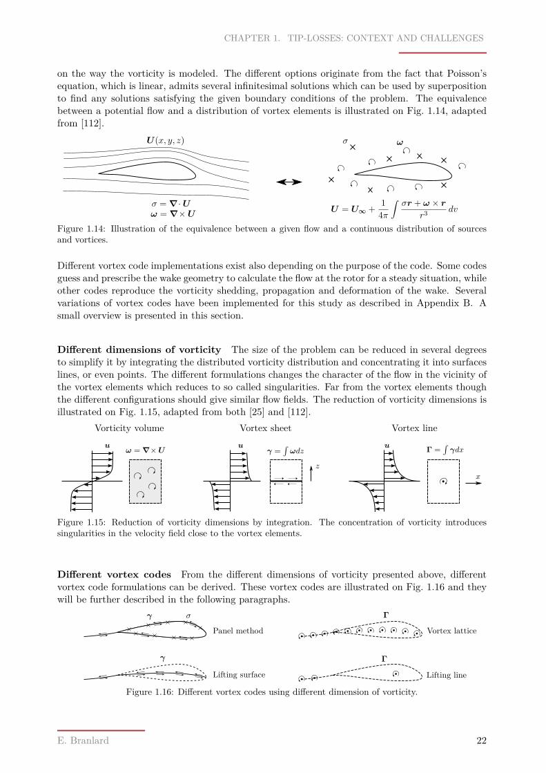
on the way the vorticity is modeled. The different options originate from the fact that Poisson’sequation, which is linear, admits several infinitesimal solutions which can be used by superpositionto find any solutions satisfying the given boundary conditions of the problem. The equivalencebetween a potential flow and a distribution of vortex elements is illustrated on Fig. 1.14, adaptedfrom [112].
σ ω
U = U∞ + 14π
∫σr + ω × r
r3 dv
U(x, y, z)
ω = ∇×Uσ = ∇·U
Figure 1.14: Illustration of the equivalence between a given flow and a continuous distribution of sourcesand vortices.
Different vortex code implementations exist also depending on the purpose of the code. Some codesguess and prescribe the wake geometry to calculate the flow at the rotor for a steady situation, whileother codes reproduce the vorticity shedding, propagation and deformation of the wake. Severalvariations of vortex codes have been implemented for this study as described in Appendix B. Asmall overview is presented in this section.
Different dimensions of vorticity The size of the problem can be reduced in several degreesto simplify it by integrating the distributed vorticity distribution and concentrating it into surfaceslines, or even points. The different formulations changes the character of the flow in the vicinity ofthe vortex elements which reduces to so called singularities. Far from the vortex elements thoughthe different configurations should give similar flow fields. The reduction of vorticity dimensions isillustrated on Fig. 1.15, adapted from both [25] and [112].
ω = ∇×U γ =∫ωdz Γ =
∫γdx
Vorticity volume Vortex sheet Vortex line
z
x
u u u
Figure 1.15: Reduction of vorticity dimensions by integration. The concentration of vorticity introducessingularities in the velocity field close to the vortex elements.
Different vortex codes From the different dimensions of vorticity presented above, differentvortex code formulations can be derived. These vortex codes are illustrated on Fig. 1.16 and theywill be further described in the following paragraphs.
σγ
γ
Lifting line
Vortex latticePanel method
Lifting surface
Γ
Γ
Figure 1.16: Different vortex codes using different dimension of vorticity.
E. Branlard 22
CHAPTER 1. TIP-LOSSES: CONTEXT AND CHALLENGES
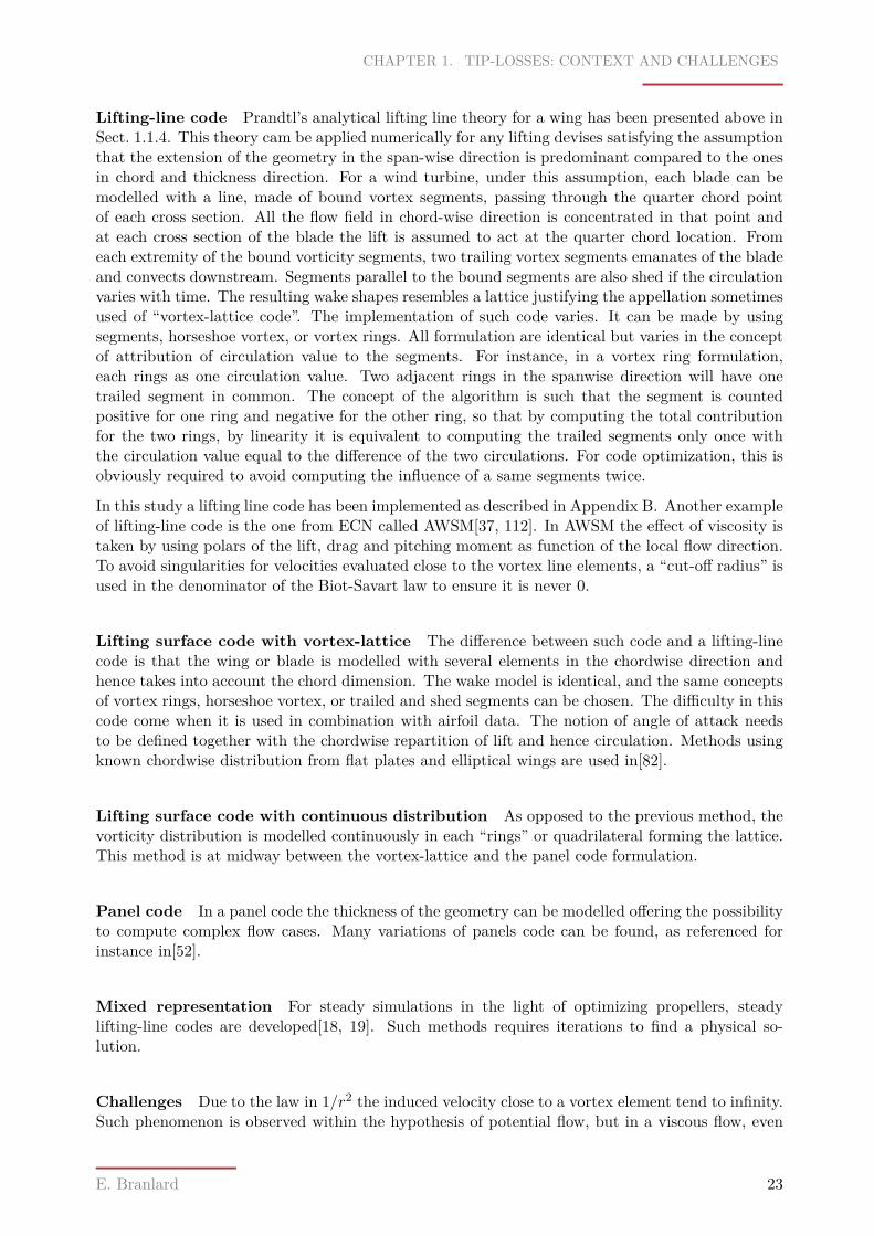
Lifting-line code Prandtl’s analytical lifting line theory for a wing has been presented above inSect. 1.1.4. This theory cam be applied numerically for any lifting devises satisfying the assumptionthat the extension of the geometry in the span-wise direction is predominant compared to the onesin chord and thickness direction. For a wind turbine, under this assumption, each blade can bemodelled with a line, made of bound vortex segments, passing through the quarter chord pointof each cross section. All the flow field in chord-wise direction is concentrated in that point andat each cross section of the blade the lift is assumed to act at the quarter chord location. Fromeach extremity of the bound vorticity segments, two trailing vortex segments emanates of the bladeand convects downstream. Segments parallel to the bound segments are also shed if the circulationvaries with time. The resulting wake shapes resembles a lattice justifying the appellation sometimesused of “vortex-lattice code”. The implementation of such code varies. It can be made by usingsegments, horseshoe vortex, or vortex rings. All formulation are identical but varies in the conceptof attribution of circulation value to the segments. For instance, in a vortex ring formulation,each rings as one circulation value. Two adjacent rings in the spanwise direction will have onetrailed segment in common. The concept of the algorithm is such that the segment is countedpositive for one ring and negative for the other ring, so that by computing the total contributionfor the two rings, by linearity it is equivalent to computing the trailed segments only once withthe circulation value equal to the difference of the two circulations. For code optimization, this isobviously required to avoid computing the influence of a same segments twice.
In this study a lifting line code has been implemented as described in Appendix B. Another exampleof lifting-line code is the one from ECN called AWSM[37, 112]. In AWSM the effect of viscosity istaken by using polars of the lift, drag and pitching moment as function of the local flow direction.To avoid singularities for velocities evaluated close to the vortex line elements, a “cut-off radius” isused in the denominator of the Biot-Savart law to ensure it is never 0.
Lifting surface code with vortex-lattice The difference between such code and a lifting-linecode is that the wing or blade is modelled with several elements in the chordwise direction andhence takes into account the chord dimension. The wake model is identical, and the same conceptsof vortex rings, horseshoe vortex, or trailed and shed segments can be chosen. The difficulty in thiscode come when it is used in combination with airfoil data. The notion of angle of attack needsto be defined together with the chordwise repartition of lift and hence circulation. Methods usingknown chordwise distribution from flat plates and elliptical wings are used in[82].
Lifting surface code with continuous distribution As opposed to the previous method, thevorticity distribution is modelled continuously in each “rings” or quadrilateral forming the lattice.This method is at midway between the vortex-lattice and the panel code formulation.
Panel code In a panel code the thickness of the geometry can be modelled offering the possibilityto compute complex flow cases. Many variations of panels code can be found, as referenced forinstance in[52].
Mixed representation For steady simulations in the light of optimizing propellers, steadylifting-line codes are developed[18, 19]. Such methods requires iterations to find a physical so-lution.
Challenges Due to the law in 1/r2 the induced velocity close to a vortex element tend to infinity.Such phenomenon is observed within the hypothesis of potential flow, but in a viscous flow, even
E. Branlard 23
CHAPTER 1. TIP-LOSSES: CONTEXT AND CHALLENGES
a strong vortex will generate finite induced velocity due to viscous shear forces within the fluidelements[4]. The vorticity is diffused into a small tube called the vortex-core. Vortex methodscircumvent the infinite velocity by introducing these vortex core to simulate viscous effects[52, 49].Nevertheless, the choice of the core size is empirical and affects significantly the results. In numericalvortex methods where the vortex elements are allowed to move freely, numerical instabilities canarise if two elements become too close to each other, even if a vortex core model is used.
Wake model The wake shape formed by the vortex elements has a critical influence on theinduced velocities found at the rotor. It has been seen that for real flow the wake convects, expands,rolls up and distorts. To capture these phenomena, the induced velocities at every point of the wakeshould be calculated and used to determine how each vortex element will move and what will betheir location at the next time step. Such model is referred to as a free wake model. Running such amodel requires an important computational time and raises different problems such as the handlingof vortex elements as they get close to each other(viscous model, re-meshing) and the modellingof the stretching of vortex elements. These problems are often circumvented by using a prescribedwake model which specifies the wake shape and hence the locations of each vortex elements. Thedetermination of the wake shape is usually empirical or based on free-wake simulations. For agiven prescribed wake the induced velocities at the rotor are known in a deterministic way, sothat the accuracy of the solution is entirely dependent on how realistic the wake shape is. Giventhe large number of parameters influencing the wake shape(CT , λ,Γ, etc.) prescribed wake modelsclearly appears limited. Nevertheless, a common approach consists in using mixed representationsetting the close-wake free in order to capture local phenomena, while modelling the far-wake as aprescribed helix of constant pitch and radius. Wake modelling for vortex methods has an importantnumber of variations which are beyond the scope of this document(see for instance [33]).
E. Branlard 24
CHAPTER 1. TIP-LOSSES: CONTEXT AND CHALLENGES
1.2 Considerations on the local aerodynamics of a rotating blade
The understanding of the 3D aerodynamics of a rotating blade is fundamentally required in thisstudy. The 3D effects influencing the airfoil performance are investigated because they need to bethe modelled in BEM codes and sometimes vortex codes as well. The challenge in these codes isto use tabulated 2D airfoil data which by essence does not reveal three dimensional effects. Twomain levers are found:
- The angle of attack: a wrong assessment of the angle of attack will lead to a wrong data fromthe table.
- The airfoil performances: the relevance of 2D airfoil data for wind turbine is rather limited[114],the airfoil performances have to be known for the exact flow conditions(stall, radial flow, extensionof the boundary layer, etc.) they are evaluated at.
The problem is really critical for simulation quality but also really challenging. The notion oftip-loss is greatly implicated in this problem as it is used to determine the flow angle and thus theangle of attack either in direct or inverse BEM codes. Inversed BEM codes can be used to find thelocal angle of attack for a given load distribution on the blade. For this reason a wrong tip-lossimplementation will not value a good 3D correction model, and an inaccurate 3D correction modelwill give no hope to find a good tip-loss correction. An uncertainty analysis was carried out[74] bystudents from Georgia Tech that showed that the uncertainty on the airfoil coefficients was the onewhich had the greatest influence on the determination of Goldstein’s tip-loss factor(see Sect. 2.4.1).On the other hand, rotational effects and stall are mainly found in the inner part of the blade, soit is likely that the tip-losses won’t have effects in this area. It has also been observed[32], that aslong as the airfoil section is not stalled, the 2D data were a good approximation in wind energyapplications.
In Sect. D.2 a comparative study between the airfoil coefficients found with 3D CFD compared tothe one found with 2D CFD is presented. These data will be used in Sect. 5.2 to assess a “liftcoefficient” tip-loss factor. It will be indeed seen that tip-losses can (partially) by viewed as airfoilcorrections (as defined e.g. by Eq. (1.28)). The following paragraphs will be useful to discuss thisdefinition.
1.2.1 Angle of attack
Definition of angle of attack The notion of angle of attack is only well defined in a 2D situationwhereas in 3D the introduction of span-wise velocity and induced velocities make it ill-defined. Intwo dimensions, the angle of attack is defined as the angle between the velocity vector and thechord direction vector. In the 2D lifting line theory, the angle of attack has been found to bedefined as the angle between the local chord direction and the local effective velocity which is takenas the sum of the undisturbed velocity and the velocity induced by the wake. This definition ismade more general, by considering the projection of the total velocity into the plane of the airfoilsection. This distinction is important when radial flows are present and in the case of swept andconed blades.
In [101] the induced velocities used for the angle of attack are taken as the one resulting from allvorticity except the one from the bound vortices. In a same fashion, Pitot tube measurements ona rotating blade must be corrected to account for the bound circulation and for the finite numberof blade. In the BEM method(see Appendix C), such considerations are not needed because theinduced velocities will not be calculated using the Biot-Savart law, but using a force-momentumequilibrium law.
E. Branlard 25
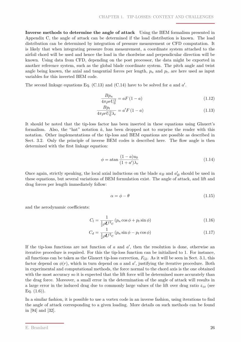
CHAPTER 1. TIP-LOSSES: CONTEXT AND CHALLENGES
Inverse methods to determine the angle of attack Using the BEM formalism presented inAppendix C, the angle of attack can be determined if the load distribution is known. The loaddistribution can be determined by integration of pressure measurement or CFD computation. Itis likely that when integrating pressure from measurement, a coordinate system attached to theairfoil chord will be used and hence the load in the chordwise and perpendicular direction will beknown. Using data from CFD, depending on the post processor, the data might be exported inanother reference system, such as the global blade coordinate system. The pitch angle and twistangle being known, the axial and tangential forces per length, pn and pt, are here used as inputvariables for this inverted BEM code.
The second linkage equations Eq. (C.13) and (C.14) have to be solved for a and a′.
Bpn4πρrU2
0= aF (1− a) (1.12)
Bpt4πρrU2
0λr= a′F (1− a) (1.13)
It should be noted that the tip-loss factor has been inserted in these equations using Glauert’sformalism. Also, the “hat” notation a, has been dropped not to surprise the reader with thisnotation. Other implementations of the tip-loss and BEM equations are possible as described inSect. 3.2. Only the principle of inverse BEM codes is described here. The flow angle is thendetermined with the first linkage equation:
φ = atan (1− a)u0(1 + a′)λr
(1.14)
Once again, strictly speaking, the local axial inductions on the blade aB and a′B should be used inthese equations, but several variations of BEM formulation exist. The angle of attack, and lift anddrag forces per length immediately follow:
α = φ− θ (1.15)
and the aerodynamic coefficients:
Cl = 112ρU
2c(pn cosφ+ pt sinφ) (1.16)
Cd = 112ρU
2c(pn sinφ− pt cosφ) (1.17)
If the tip-loss functions are not function of a and a′, then the resolution is done, otherwise aniterative procedure is required. For this the tip-loss function can be initialized to 1. For instance,all functions can be taken as the Glauert tip-loss correction, FGl. As it will be seen in Sect. 3.1, thisfactor depend on φ(r), which in turn depend on a and a′, justifying the iterative procedure. Bothin experimental and computational methods, the force normal to the chord axis is the one obtainedwith the most accuracy so it is expected that the lift force will be determined more accurately thanthe drag force. Moreover, a small error in the determination of the angle of attack will results ina large error in the induced drag due to commonly large values of the lift over drag ratio εl/d (seeEq. (1.6)).
In a similar fashion, it is possible to use a vortex code in an inverse fashion, using iterations to findthe angle of attack corresponding to a given loading. More details on such methods can be foundin [94] and [32].
E. Branlard 26
CHAPTER 1. TIP-LOSSES: CONTEXT AND CHALLENGES
Other methods to determined the angle of attack The averaging technique is probably themost widely used method to determine the angle of attack for CFD data. This method presentedin [43, 48] consists in averaging the axial induction in annuli located at different distance to therotor to extrapolate the value of the axial induction at the rotor. In its simplest form, only twoannuli symmetric with respect to the rotor can be used. In [97] an iterative method is presentedwhich can be used for both CFD and Pitot tubes measurements. This method uses the loading onthe blade and the flow angle parameter to determine the bound circulation and the correspondinginduced velocities, that will in turn modify the flow angle. A similar method, but using this time adistributed circulation instead of a point vortex to assess the induced velocities is presented in[47].The advantage of this method, is that it is less dependent on the distance to the leading edge wherethe velocity is evaluated.
1.2.2 Rotational effects
Rotational effects In the middle of the 20th century, Himmeslkamp[45] has observed on aircraftpropellers that the lift coefficients of the airfoils were increased due to rotational effects implyingradial flows. This observation was mainly seen in the smaller radial sections where it was alsoobserved that the stall was occurring at higher angle of attack. One of the first simulation that couldinclude rotational effects and carried out for a wind turbine was done by Sørensen in 1986[102]. Theeffects of lift increase and stall delay were found in these simulations and confirmed by observationsof Savino and Nyland[95, 1985], and later by Rasmussen et al.[90, 1988], Madsen and Rasmussen[68,1988], Ronsten[91, 1991], Bruining[16, 1993], with other references found in[63] and a throughoutcomparison in[62].
- Lift coefficient: In the inner part of the blade, increase of lift coefficient up to 30% can be found.Nevertheless, the quantification of increase of lift is difficult and clearly airfoil dependent. As ageneral trend, the difference between the 2D and 3D lift coefficients increases going from the mid-span to the hub, in the region where stall occurs. It was also found that the 3D aerodynamiccoefficients mainly starts to differ from the 2D coefficient from the angle of attack of maximum lift.
- Radial component: It was found that the laminar flow was hardly influenced by rotational effectsand followed the chord direction from the leading edge. Nevertheless, when the flow encounters anadverse pressure gradient and separates, the fluid is significantly moved outwards by the centrifugalforce. This effect is referred as “centrifugal pumping”.
- Drag coefficient: Studies of the NREl phase VI experiment[62, 107] showed an increase of dragnear the root and a small decrease near the tip. In his study, Sørensen found almost no differencebut slightly lower Cd. In general, there is no full consensus yet concerning the drag coefficient,though it has been observed that the pressure in the 3D separated zone is lower than the one in2D, resulting in higher drag. The tapered ratio of the tip is likely to have an influence on the dragcoefficient towards the tip.
- Separation Point: Stall can be delayed of few percent of the chord length.
The current understanding of rotational effects can be described as follow. The centrifugal loadsacts on all volume of air for which the relative tangential velocity differs from the relative velocityof the blade, Ωr. This radial flow can only occurs in regions of strongly retarded flows as theseparated boundary layer and separation bubble present on the suction side of the blade. Due tocentrifugal loads the air is accelerated radially towards the tip of the blade. This radial velocitycomponent will induce a Coriolis acceleration in the main flow direction, acting as a favourablepressure gradient. The displacement thickness of the separated boundary layer is decreased, leadingto less de-cambering and higher lift coefficients[101]. .
E. Branlard 27
CHAPTER 1. TIP-LOSSES: CONTEXT AND CHALLENGES
1.2.3 Airfoil corrections
Data for large angles of attack Data for large angles of attack are usually not available fromwind tunnel measurement so extrapolation techniques are often used. For high incidences(e.g.α ∈ [−170 ; −30] ∪ [30 ; 170]) airfoil characteristics are considered to become rather independentof the geometry so that data from a flat plate can be used. This is for instance mentioned in [98] butwith the flat plate airfoil characteristics reduced by a factor of 85%. In [5] the fully separated(fs)coefficients for high angle of attack are computed as:
CL,fs = 2 cosα sinα (1.18)CD,fs = 1.3 sin2 α (1.19)
Cm,fs = −14Cn with Cn = 1.0 sinα (1.20)
and a function g is used to ensure a smooth transition between the original data and the extrapolateddata, as C• = gC•+ (1− g)C•,fs, with e.g. the function g defined with three parameters αd, α0 and∆α as:
g(α) = 0.5 + 0.5 tanh[αd + α0 − |α|
∆α
](1.21)
Another model is the one from Viterna and Corrigan[115] which extrapolates the airfoil coefficientsafter stall. The authors looked at a way to obtain an idealized stall that would keep a constanttorque at high wind speeds and thus high angles of attack. This approach was developed to fitmeasured and predicted performances of two specific stall regulated wind turbine. This correctionrequires that the lift over drag ratio at the initial angle of attack matches the lift over drag ratio ofa flat plate. This is unfortunately not a common case and in[107] it is argued that an incompleteunderstanding of the stall process existed at the time of this method’s development. In[107],the Viterna’s method is applied with as input the angle of attack and the average aerodynamiccoefficients values over the blade span for which the lift over drag ratio matches the flat platetheory. A review of aerodynamics coefficients at high angles of attack can be found in [61].
Airfoil data 3D corrections The 2D airfoil coefficients found from measurements in wind tunnelor by simulations such as CFD or panel methods tools such as Xfoil[26], are usually corrected tobe used in BEM or aeroelastic codes. It should be noted that though there are uncertaintiesin simulations results, measurements data also have quite a spread as seen in the comparison ofresults from 4 different renown wind tunnels [69]. Most 3D correction methods can be written inthe following form:
C•,3D = C•,2D + fC•∆C• (1.22)
where • stands for L, D, m, the indexes of Lift, Drag and moment coefficients. ∆C• is the differencebetween the coefficient C• estimated in inviscid flow(i.e. without separation) and its its steady 2Dvalue evaluated for instance from a wind tunnel measurement(where obviously separation willoccur). The inviscid lift coefficient can be approximated with the one for the Joukowski’s airfoilfamily[46] approximated for a thin airfoil of trailing edge parameter a, chord of ≈ 4a, at small angleof attack α and small camber parameter β :
Cl,inv,thin ≈ 8πac
sin(α+ β) ≈ 2π(α− α0) (1.23)
Nevertheless, the author would like to point out that such approximations is often inappropriatefor airfoils used in wind energy. This remark will also apply when commenting the performancetip-loss correction from Lindenburg in Sect. 3.1. The result from Eq. (1.23) apply to thin airfoils
E. Branlard 28
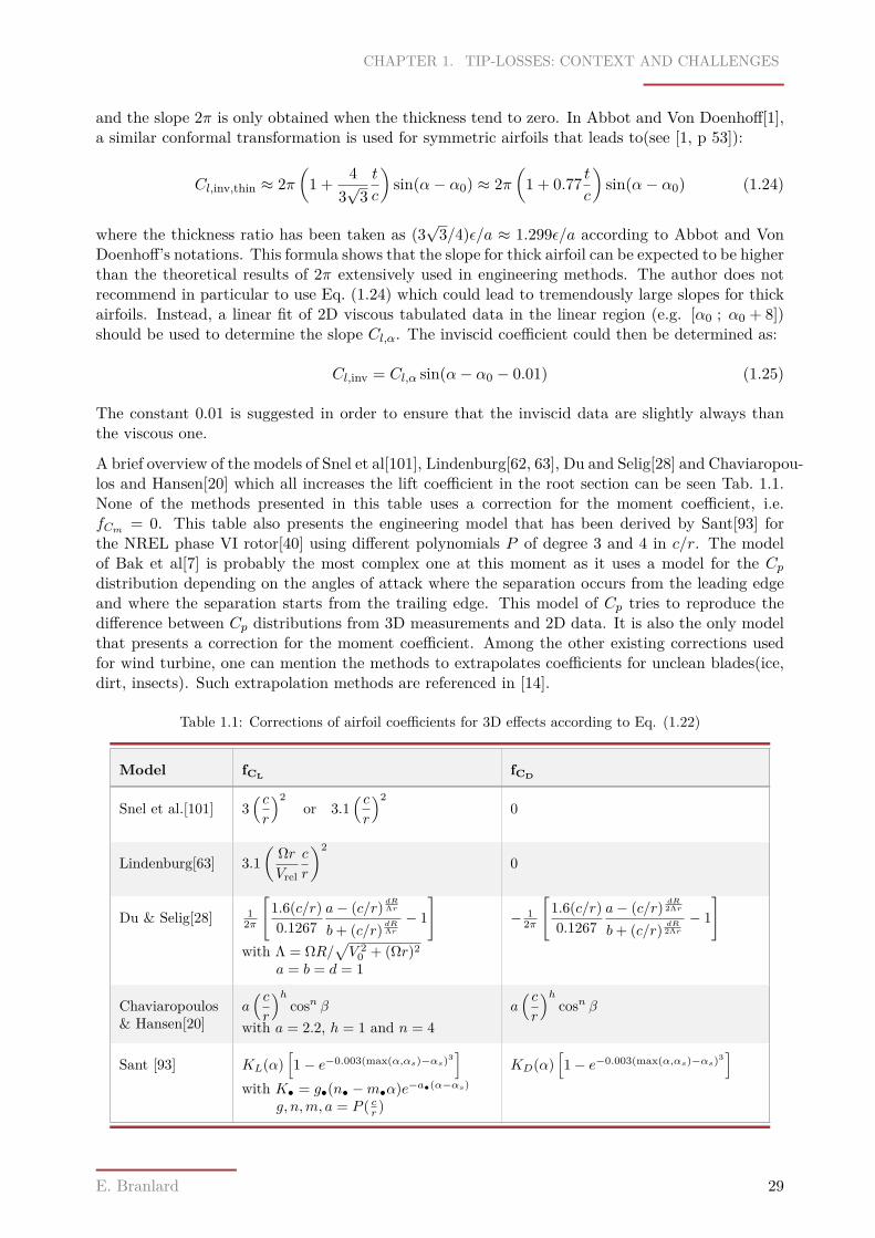
CHAPTER 1. TIP-LOSSES: CONTEXT AND CHALLENGES
and the slope 2π is only obtained when the thickness tend to zero. In Abbot and Von Doenhoff[1],a similar conformal transformation is used for symmetric airfoils that leads to(see [1, p 53]):
Cl,inv,thin ≈ 2π(
1 + 43√
3t
c
)sin(α− α0) ≈ 2π
(1 + 0.77 t
c
)sin(α− α0) (1.24)
where the thickness ratio has been taken as (3√
3/4)ε/a ≈ 1.299ε/a according to Abbot and VonDoenhoff’s notations. This formula shows that the slope for thick airfoil can be expected to be higherthan the theoretical results of 2π extensively used in engineering methods. The author does notrecommend in particular to use Eq. (1.24) which could lead to tremendously large slopes for thickairfoils. Instead, a linear fit of 2D viscous tabulated data in the linear region (e.g. [α0 ; α0 + 8])should be used to determine the slope Cl,α. The inviscid coefficient could then be determined as:
Cl,inv = Cl,α sin(α− α0 − 0.01) (1.25)
The constant 0.01 is suggested in order to ensure that the inviscid data are slightly always thanthe viscous one.
A brief overview of the models of Snel et al[101], Lindenburg[62, 63], Du and Selig[28] and Chaviaropou-los and Hansen[20] which all increases the lift coefficient in the root section can be seen Tab. 1.1.None of the methods presented in this table uses a correction for the moment coefficient, i.e.fCm = 0. This table also presents the engineering model that has been derived by Sant[93] forthe NREL phase VI rotor[40] using different polynomials P of degree 3 and 4 in c/r. The modelof Bak et al[7] is probably the most complex one at this moment as it uses a model for the Cpdistribution depending on the angles of attack where the separation occurs from the leading edgeand where the separation starts from the trailing edge. This model of Cp tries to reproduce thedifference between Cp distributions from 3D measurements and 2D data. It is also the only modelthat presents a correction for the moment coefficient. Among the other existing corrections usedfor wind turbine, one can mention the methods to extrapolates coefficients for unclean blades(ice,dirt, insects). Such extrapolation methods are referenced in [14].
Table 1.1: Corrections of airfoil coefficients for 3D effects according to Eq. (1.22)
Model fCL fCD
Snel et al.[101] 3( cr
)2or 3.1
( cr
)20
Lindenburg[63] 3.1(
ΩrVrel
c
r
)20
Du & Selig[28] 12π
[1.6(c/r)0.1267
a− (c/r) dRΛrb+ (c/r) dRΛr
− 1]
with Λ = ΩR/√V 2
0 + (Ωr)2
a = b = d = 1
− 12π
[1.6(c/r)0.1267
a− (c/r) dR2Λr
b+ (c/r) dR2Λr− 1]
Chaviaropoulos& Hansen[20]
a( cr
)hcosn β
with a = 2.2, h = 1 and n = 4a( cr
)hcosn β
Sant [93] KL(α)[1− e−0.003(max(α,αs)−αs)3
]with K• = g•(n• −m•α)e−a•(α−αs)
g, n,m, a = P ( cr )
KD(α)[1− e−0.003(max(α,αs)−αs)3
]
E. Branlard 29

CHAPTER 1. TIP-LOSSES: CONTEXT AND CHALLENGES
Stall Delay The most common stall delay model is the one from Corrigan and Shillings[21, 62].Most models for stall delay modify only the lift coefficient, but not exclusively. For wind turbinesapplications, a modification of the drag coefficient is most probably required due to difference ofpressure intensity observed in the separated regions between 2D and 3D stall.
Tip-losses The tip-loss correction of Shen et al.[98] suggests of correction on Cn and Ct to accountfor the pressure equalization at the tip of the blade which should lead to the loads vanishing. Thiscorrection will be presented in more details in Sect. 3.1.3 and 3.2.2. In his PhD thesis[93], Santsuggests a correction for the lift and drag coefficient in a similar fashion than Shen. This correctionis presented in Sect. 3.1.3.
E. Branlard 30
CHAPTER 1. TIP-LOSSES: CONTEXT AND CHALLENGES
1.3 Preliminary considerations for the study and modelling of tip-losses
1.3.1 Physical considerations expected to be modelled
- The force on the blade should go to zero at the tip due to the pressure balance between the uppersurface and the lower surface
- The relative velocity at the blade tip cannot be equal to the upstream velocity due to shear at theboundary of the “ideal” streamtube and to the presence of the tip vortex that will clearly modifythe flow structure at this particular location.
- The average axial induction drops towards zero at the tip, but does not have to be exactly zero atthe tip. The radial and rotational flow at the tip due to the tip-vortex transfers axial kinetic energytowards rotational kinetic energy so that the flow is not likely to have it’s full upstream velocity atthe tip. This is supported by the considerations of the previous point, and CFD simulations.
- The relative velocity is not uniform in a annular section to the limited number of blades. Theaxial and tangential induction factor are thus azimuthally dependent.
- The flow has a radial component, simply due to the expansion of the streamtube and also moresubtly due to 3D aerodynamic effects[67]. As a result of this the 2D airfoil coefficients could notbe suitable to give the exact aerodynamic loads.
- The circulation along the blade is not constant due to e.g. root and hub losses. This will implya radial dependency of the induction factors.
- The optimal circulation distribution derived by Goldstein and reasonably simplified by Prandtlare never obtained in reality. Moreover they are derived for optimal frictionless rotors, so theirapplicability to rotors in general is uncertain.
1.3.2 Definition of the tip loss factor
It will be seen that several definitions and interpretations of the tip-loss factor can be found inthe literature. These definitions will be introduced in this section, but more detailed will be foundthroughout this document, particularly in chapter 2 where the theoretical work are presented. Asa result of these different definitions, the implementation of the tip-loss factor will also have severalvariations. This will be the focus of Sect. 3.2.
Definition in terms of axial induction The fact that the axial induction factor is azimuthallydependent suggests the introduction of the average induction factor in an annulus a (see Eq. (1.3)).It is also expected that this factor will reach an extremum in the vicinity of the blade so that theparticular value taken at the blade is relevant and will be denoted aB. With these definition, thetip-loss factor F has been defined by Glauert as the ratio between the azimuthally averaged axialinduction factor and its value at the blade:
F = a
aB(1.26)
The difference between a and aB can be read on Fig. 1.8. Reading the plot at the azimuthalpositions of the blades(e.g. 120), and doing the ratio of the inductions factors at different radial
E. Branlard 31
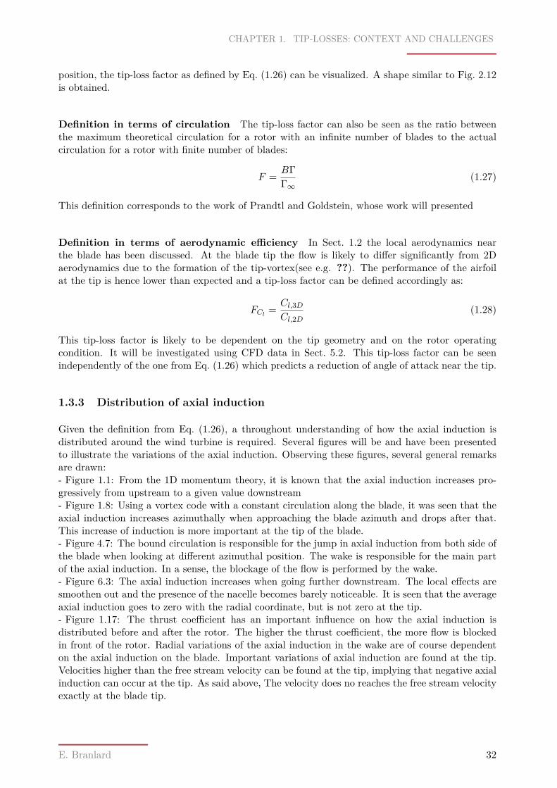
CHAPTER 1. TIP-LOSSES: CONTEXT AND CHALLENGES
position, the tip-loss factor as defined by Eq. (1.26) can be visualized. A shape similar to Fig. 2.12is obtained.
Definition in terms of circulation The tip-loss factor can also be seen as the ratio betweenthe maximum theoretical circulation for a rotor with an infinite number of blades to the actualcirculation for a rotor with finite number of blades:
F = BΓΓ∞
(1.27)
This definition corresponds to the work of Prandtl and Goldstein, whose work will presented
Definition in terms of aerodynamic efficiency In Sect. 1.2 the local aerodynamics nearthe blade has been discussed. At the blade tip the flow is likely to differ significantly from 2Daerodynamics due to the formation of the tip-vortex(see e.g. ??). The performance of the airfoilat the tip is hence lower than expected and a tip-loss factor can be defined accordingly as:
FCl = Cl,3DCl,2D
(1.28)
This tip-loss factor is likely to be dependent on the tip geometry and on the rotor operatingcondition. It will be investigated using CFD data in Sect. 5.2. This tip-loss factor can be seenindependently of the one from Eq. (1.26) which predicts a reduction of angle of attack near the tip.
1.3.3 Distribution of axial induction
Given the definition from Eq. (1.26), a throughout understanding of how the axial induction isdistributed around the wind turbine is required. Several figures will be and have been presentedto illustrate the variations of the axial induction. Observing these figures, several general remarksare drawn:- Figure 1.1: From the 1D momentum theory, it is known that the axial induction increases pro-gressively from upstream to a given value downstream- Figure 1.8: Using a vortex code with a constant circulation along the blade, it was seen that theaxial induction increases azimuthally when approaching the blade azimuth and drops after that.This increase of induction is more important at the tip of the blade.- Figure 4.7: The bound circulation is responsible for the jump in axial induction from both side ofthe blade when looking at different azimuthal position. The wake is responsible for the main partof the axial induction. In a sense, the blockage of the flow is performed by the wake.- Figure 6.3: The axial induction increases when going further downstream. The local effects aresmoothen out and the presence of the nacelle becomes barely noticeable. It is seen that the averageaxial induction goes to zero with the radial coordinate, but is not zero at the tip.- Figure 1.17: The thrust coefficient has an important influence on how the axial induction isdistributed before and after the rotor. The higher the thrust coefficient, the more flow is blockedin front of the rotor. Radial variations of the axial induction in the wake are of course dependenton the axial induction on the blade. Important variations of axial induction are found at the tip.Velocities higher than the free stream velocity can be found at the tip, implying that negative axialinduction can occur at the tip. As said above, The velocity does no reaches the free stream velocityexactly at the blade tip.
E. Branlard 32
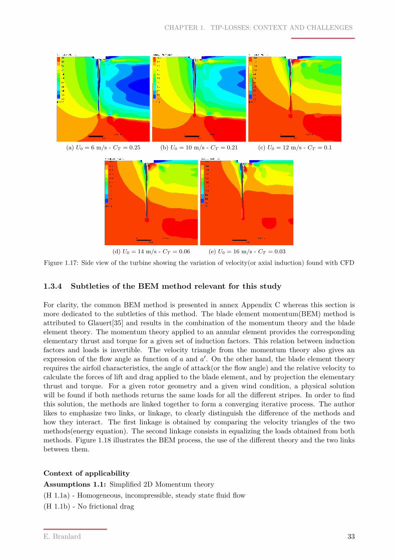
CHAPTER 1. TIP-LOSSES: CONTEXT AND CHALLENGES
(a) U0 = 6 m/s - CT = 0.25 (b) U0 = 10 m/s - CT = 0.21 (c) U0 = 12 m/s - CT = 0.1
(d) U0 = 14 m/s - CT = 0.06 (e) U0 = 16 m/s - CT = 0.03
Figure 1.17: Side view of the turbine showing the variation of velocity(or axial induction) found with CFD
1.3.4 Subtleties of the BEM method relevant for this study
For clarity, the common BEM method is presented in annex Appendix C whereas this section ismore dedicated to the subtleties of this method. The blade element momentum(BEM) method isattributed to Glauert[35] and results in the combination of the momentum theory and the bladeelement theory. The momentum theory applied to an annular element provides the correspondingelementary thrust and torque for a given set of induction factors. This relation between inductionfactors and loads is invertible. The velocity triangle from the momentum theory also gives anexpression of the flow angle as function of a and a′. On the other hand, the blade element theoryrequires the airfoil characteristics, the angle of attack(or the flow angle) and the relative velocity tocalculate the forces of lift and drag applied to the blade element, and by projection the elementarythrust and torque. For a given rotor geometry and a given wind condition, a physical solutionwill be found if both methods returns the same loads for all the different stripes. In order to findthis solution, the methods are linked together to form a converging iterative process. The authorlikes to emphasize two links, or linkage, to clearly distinguish the difference of the methods andhow they interact. The first linkage is obtained by comparing the velocity triangles of the twomethods(energy equation). The second linkage consists in equalizing the loads obtained from bothmethods. Figure 1.18 illustrates the BEM process, the use of the different theory and the two linksbetween them.
Context of applicabilityAssumptions 1.1: Simplified 2D Momentum theory(H 1.1a) - Homogeneous, incompressible, steady state fluid flow(H 1.1b) - No frictional drag
E. Branlard 33
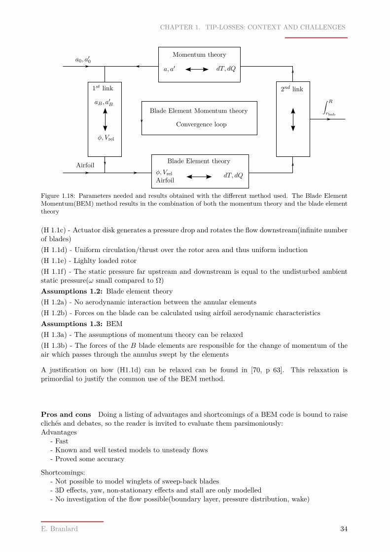
CHAPTER 1. TIP-LOSSES: CONTEXT AND CHALLENGES
Blade Element Momentum theory
1st link
Momentum theory
a, a′ dT, dQ
Blade Element theoryφ, VrelAirfoil
dT, dQ
Airfoil
φ, Vrel
aB, a′B
a0, a′0
Convergence loop
2nd link ∫ R
rhub
Figure 1.18: Parameters needed and results obtained with the different method used. The Blade ElementMomentum(BEM) method results in the combination of both the momentum theory and the blade elementtheory
(H 1.1c) - Actuator disk generates a pressure drop and rotates the flow downstream(infinite numberof blades)(H 1.1d) - Uniform circulation/thrust over the rotor area and thus uniform induction(H 1.1e) - Lighlty loaded rotor(H 1.1f) - The static pressure far upstream and downstream is equal to the undisturbed ambientstatic pressure(ω small compared to Ω)Assumptions 1.2: Blade element theory(H 1.2a) - No aerodynamic interaction between the annular elements(H 1.2b) - Forces on the blade can be calculated using airfoil aerodynamic characteristicsAssumptions 1.3: BEM(H 1.3a) - The assumptions of momentum theory can be relaxed(H 1.3b) - The forces of the B blade elements are responsible for the change of momentum of theair which passes through the annulus swept by the elements
A justification on how (H1.1d) can be relaxed can be found in [70, p 63]. This relaxation isprimordial to justify the common use of the BEM method.
Pros and cons Doing a listing of advantages and shortcomings of a BEM code is bound to raiseclichés and debates, so the reader is invited to evaluate them parsimoniously:Advantages
- Fast- Known and well tested models to unsteady flows- Proved some accuracy
Shortcomings:- Not possible to model winglets of sweep-back blades- 3D effects, yaw, non-stationary effects and stall are only modelled- No investigation of the flow possible(boundary layer, pressure distribution, wake)
E. Branlard 34
CHAPTER 1. TIP-LOSSES: CONTEXT AND CHALLENGES
Observed performance of BEM codes The performance of BEM codes will be extremelydependent on the model implemented. As an illustrations of this, several observations found in theliterature are listed. It is see that these observations are sometimes contradictory and they shouldthus not be taken as general. Different observations are found when comparing with measurements.
- Underprediction of power, especially after stall [92].- Underprediction of power in the stalled conditions[102].- Overprediciton of power for 2-bladed rotors[62]- Prandtl tip loss correction overestimate the loads at the tip[98]- Under prediction of the power coefficient in the inner part of the blade and over prediction in
the outer part of the blade (without tip or hub corrections ) [66, 67]
Debate on the drag In linking the blade element theory and the momentum theory, it is arguedthat the drag should not be included.
- References advising not to include the drag:[117, 62, 23, 70]- References including the drag:[42, 6]- References arguing both:[70]
From an analysis of the following references [17, 62, 46, 117], the following can be mentionedconcerning the debate on the inclusion of the drag. The viscous effects emerging from the boundarylayer of the airfoil are propagated in the wake into helical filaments enclosed by vorticity. Thevelocity deficit caused by drag is confined to this narrow wake emerging from the trailing edge. Itis argued that these filaments are diffused behind the rotor and are only a feature of the wake,so that they induced no velocity in the rotor plane. The momentum equations uses the inducedvelocities at the rotor plane and thus from the argument above the drag coefficient should not beused.
This argumentation requires the understanding and distinction of pressure drag and friction drag.Friction drag comes from the tangential component of the strain vector at the wall which arisesfrom viscosity. Pressure drag is the result of the normal component of the strain vector. Forprofiled bodies at high Reynolds number, at a first approximation separation can be neglected andthe pressure solution would be close to the one found for the corresponding potential flow9. Thepressure drag force could then be neglected as a general result of potential flow. Nevertheless, thefrictional drag associated with the viscous strain in the boundary layer is non zero and makes themost part of the total drag. In the contrary, when separation clearly occurs, the pressure drag islikely to be the predominant term in the total drag. The friction drag is barely dependent on therelative thickness of the profile whereas the pressure drag clearly is. Assuming attached flow athigh Reynolds number then, the pressure drag could be considered as zero and thus the drag wouldnot contribute to the pressure drop across the rotor. This analysis though is to be taken with careand its results can be argued.
Steady BEM Code patches BEM Code patches listed here with a minimum of detail. Therepresentation as a list of different items should be taken with care as most of them are overlappingor interlinked.
- Momentum theory break down: The actuator disk stops all the fluid if a = 1/2, but this cannotbe stored it has to flow away so correction is needed. The common corrections are the one fromSpera or Glauert. Typically CT = f(a) inverted in a = f(CT )
- Hub and tip losses due to 3D effects and the intrinsic generation of vorticity from the lift- Corrections of airfoil coefficients accounting for 3D effects, extrapolation, smoothing of airfoil
data9For moderate Reynolds number though, the pressure drag due to the presence of the boundary layer, even if thin,
can be quite important.
E. Branlard 35
CHAPTER 1. TIP-LOSSES: CONTEXT AND CHALLENGES
- Stall delay model accounting for some 3D effects
Each of these “patches” offers a different levers to correct for the difference between the simplifiedtheory and the real situation. There are indeed different physical phenomenon observed such ascentrifugal pumping, stall delay, tip losses, and it seems reasonable to treat these different problemindependently, but obviously non-linearity in the overall problem will make the modelling andverification difficult. The different models mentioned above have proven good when combined alltogether in the BEM algorithm, but there is no guarantee that improving one model with morephysical sense will make the overall BEM code more accurate.
1.3.5 Final remarks
Note on potential flows The 1D and 2D momentum theory relies on the assumption of potentialflow, which mainly implies that the drag is zero. The blade element theory on the other hand doesnot have this constraint. Using both the simplified 2D momentum theory and the BET, the BEMequations should in theory be constraint to the absence of drag but nevertheless BEM codes areused with drag. The same apply to vortex theory which relies on potential flow, and vortex codeswhich are sometimes used as predictive wind turbine tools, using drag. All wind turbine codesall have to relax the assumptions on which they are based, hence loosing rigour and introducingpotential inconsistency.
Pragmatic approach All of the above being kept in mind the physical problem of tip-losseswill be investigated. Such investigation will require the observation of this phenomenon throughexperiments and simulation, together with an interpretation and understanding of its physics. Bystudying the different existing models, understanding their limitations and confronting them todifferent datasets, an insight of the challenges raised when modeling this problem will be acquired.Due to the different “BEM patches” acting as as many levers, a global view of the field of influenceof each of them is necessary. Such analysis should eventually give suitable basis for trying to searchfor improvements.
E. Branlard 36
Chapter 2Theories of optimal circulation and tip-losses
2.1 Introduction
As seen in the historical review(Sect. 1.1), the notion of tip-losses appeared in the research ofthe optimal circulation distribution that would give the minimum losses for a given thrust. Thetheories from Prandtl and Munk[76] for the elliptical distribution applied on a finite-span wing arenot described here. Nevertheless, the theories that apply for propellers and wind turbine directlyfollow their early analysis. The main articles presenting the optimal circulation for rotors arefurther studied below, including the one from Betz[9] with its comment from Prandtl[87], writtenin german, they are reported by Prandtl in english in [88]. Advised by Betz, Goldstein[36] extendedthe theory and the work of all the mentioned authors is reported by Glauert[35] in 1935.
All theories are based on a prescribed wake shape made of helix surfaces. For this reason, theliteral, mathematical and physical formalism of the helical wake surface will be presented firstbefore approaching the different theories. This introduction will also allow to tackle the differenttheories in a slightly more general way than presented originally by the authors. The followinganalysis is performed in light of the modern wind energy references such as [117, 17, 42], andmodern research articles as [79, 80], and tries to reduce the confusion a reader can encounter whenfollowing the old and modern references with their different (sometimes implicit) assumptions.
2.1.1 Preliminary remarks and notations
Notes on old references Going through the old references on this subject requires a lot of care:- The references uses different notations from one to another, which is of course not a big issue,
but some of them are extremely confusing. As an advise, care should be taken when readingvariables: r, r′, x, λ, µ, h, l.
- The convention used in the old references is the convention for propellers, so that the axialinduced velocity has actually an opposite sign to the one given in this document. Also, the lon-gitudinal relative wake of a propeller is in the downwind direction whereas it is in the upstreamdirection for a wind turbine.
- Most references apply under the assumption of lightly loaded rotor, and omit the inducevelocities in the velocity triangle. Some references mentioned as an appendix that their formulaeshould be modified to include the induced velocities. Two modifications are often mentioned anexact one, and an approximation. The exact one account for both induced velocity, whereas theapproximation accounts only for the axial induced velocity.
37
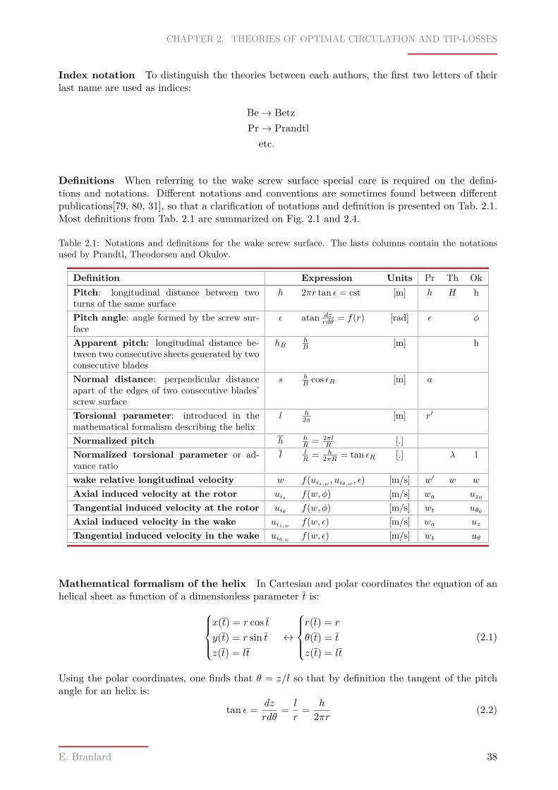
CHAPTER 2. THEORIES OF OPTIMAL CIRCULATION AND TIP-LOSSES
Index notation To distinguish the theories between each authors, the first two letters of theirlast name are used as indices:
Be→ BetzPr→ Prandtl
etc.
Definitions When referring to the wake screw surface special care is required on the defini-tions and notations. Different notations and conventions are sometimes found between differentpublications[79, 80, 31], so that a clarification of notations and definition is presented on Tab. 2.1.Most definitions from Tab. 2.1 are summarized on Fig. 2.1 and 2.4.
Table 2.1: Notations and definitions for the wake screw surface. The lasts columns contain the notationsused by Prandtl, Theodorsen and Okulov.
Definition Expression Units Pr Th OkPitch: longitudinal distance between twoturns of the same surface
h 2πr tan ε = cst [m] h H h
Pitch angle: angle formed by the screw sur-face
ε atan dzrdθ = f(r) [rad] ε φ
Apparent pitch: longitudinal distance be-tween two consecutive sheets generated by twoconsecutive blades
hBhB [m] h
Normal distance: perpendicular distanceapart of the edges of two consecutive blades’screw surface
s hB cos εR [m] a
Torsional parameter: introduced in themathematical formalism describing the helix
l h2π [m] r′
Normalized pitch h hR = 2πl
R [.]Normalized torsional parameter or ad-vance ratio
l lR = h
2πR = tan εR [.] λ l
wake relative longitudinal velocity w f(uiz,w , uiθ,w , ε) [m/s] w′ w w
Axial induced velocity at the rotor uiz f(w, φ) [m/s] wa uz0Tangential induced velocity at the rotor uiθ f(w, φ) [m/s] wt uθ0Axial induced velocity in the wake uiz,w f(w, ε) [m/s] wa uz
Tangential induced velocity in the wake uiθ,w f(w, ε) [m/s] wt uθ
Mathematical formalism of the helix In Cartesian and polar coordinates the equation of anhelical sheet as function of a dimensionless parameter t is:
x(t) = r cos ty(t) = r sin tz(t) = lt
↔
r(t) = r
θ(t) = t
z(t) = lt
(2.1)
Using the polar coordinates, one finds that θ = z/l so that by definition the tangent of the pitchangle for an helix is:
tan ε = dz
rdθ= l
r= h
2πr (2.2)
E. Branlard 38
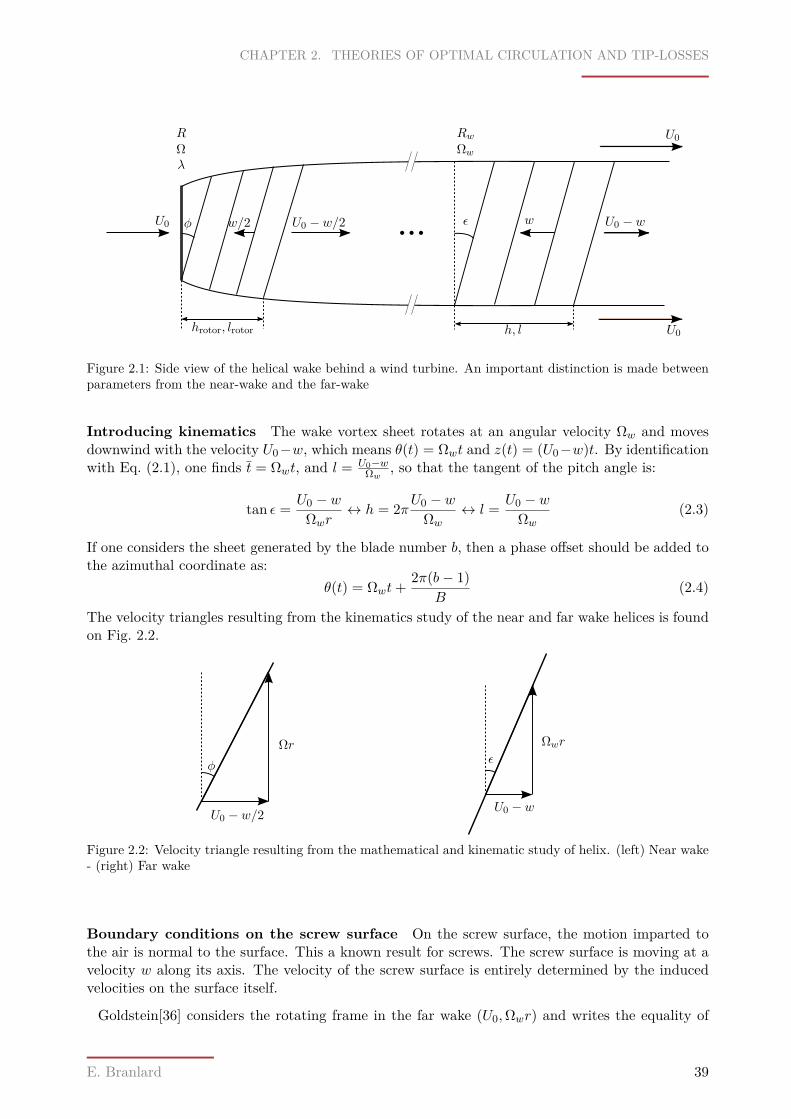
CHAPTER 2. THEORIES OF OPTIMAL CIRCULATION AND TIP-LOSSES
φ ε ww/2
hrotor, lrotor h, l
λ
RΩ
RwΩw
U0 U0 − w/2 U0 − w
U0
U0
Figure 2.1: Side view of the helical wake behind a wind turbine. An important distinction is made betweenparameters from the near-wake and the far-wake
Introducing kinematics The wake vortex sheet rotates at an angular velocity Ωw and movesdownwind with the velocity U0−w, which means θ(t) = Ωwt and z(t) = (U0−w)t. By identificationwith Eq. (2.1), one finds t = Ωwt, and l = U0−w
Ωw , so that the tangent of the pitch angle is:
tan ε = U0 − wΩwr
↔ h = 2πU0 − wΩw
↔ l = U0 − wΩw
(2.3)
If one considers the sheet generated by the blade number b, then a phase offset should be added tothe azimuthal coordinate as:
θ(t) = Ωwt+ 2π(b− 1)B
(2.4)
The velocity triangles resulting from the kinematics study of the near and far wake helices is foundon Fig. 2.2.
φε
Ωr
U0 − w/2U0 − w
Ωwr
Figure 2.2: Velocity triangle resulting from the mathematical and kinematic study of helix. (left) Near wake- (right) Far wake
Boundary conditions on the screw surface On the screw surface, the motion imparted tothe air is normal to the surface. This a known result for screws. The screw surface is moving at avelocity w along its axis. The velocity of the screw surface is entirely determined by the inducedvelocities on the surface itself.
Goldstein[36] considers the rotating frame in the far wake (U0,Ωwr) and writes the equality of
E. Branlard 39
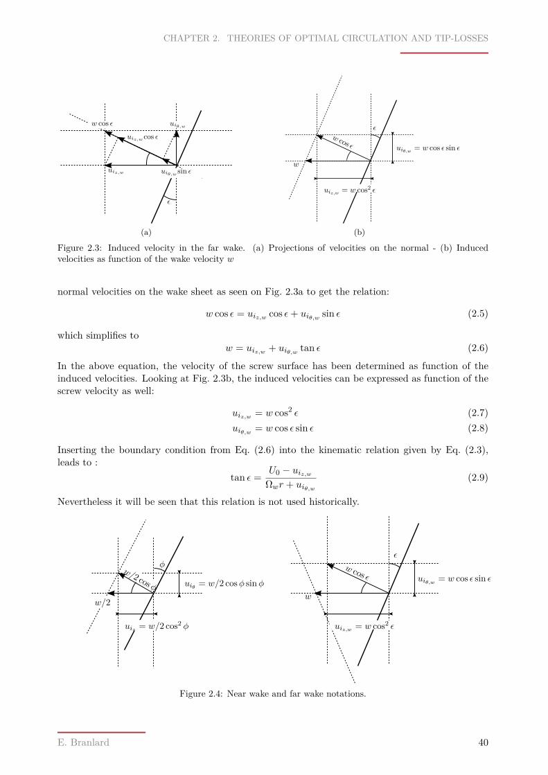
CHAPTER 2. THEORIES OF OPTIMAL CIRCULATION AND TIP-LOSSES
uiz,w
uiθ,w
uiz,wcos ε
uiθ,w sin ε
w cos ε
ε
(a)
w
w cos ε
uiz,w = w cos2 ε
uiθ,w = w cos ε sin ε
ε
(b)
Figure 2.3: Induced velocity in the far wake. (a) Projections of velocities on the normal - (b) Inducedvelocities as function of the wake velocity w
normal velocities on the wake sheet as seen on Fig. 2.3a to get the relation:
w cos ε = uiz,w cos ε+ uiθ,w sin ε (2.5)
which simplifies tow = uiz,w + uiθ,w tan ε (2.6)
In the above equation, the velocity of the screw surface has been determined as function of theinduced velocities. Looking at Fig. 2.3b, the induced velocities can be expressed as function of thescrew velocity as well:
uiz,w = w cos2 ε (2.7)uiθ,w = w cos ε sin ε (2.8)
Inserting the boundary condition from Eq. (2.6) into the kinematic relation given by Eq. (2.3),leads to :
tan ε =U0 − uiz,w
Ωwr + uiθ,w(2.9)
Nevertheless it will be seen that this relation is not used historically.
εφ
ww/2
w/2 cosφ
w cos ε
uiz,w = w cos2 εuiz = w/2 cos2 φ
uiθ = w/2 cosφ sinφ uiθ,w = w cos ε sin ε
Figure 2.4: Near wake and far wake notations.
E. Branlard 40
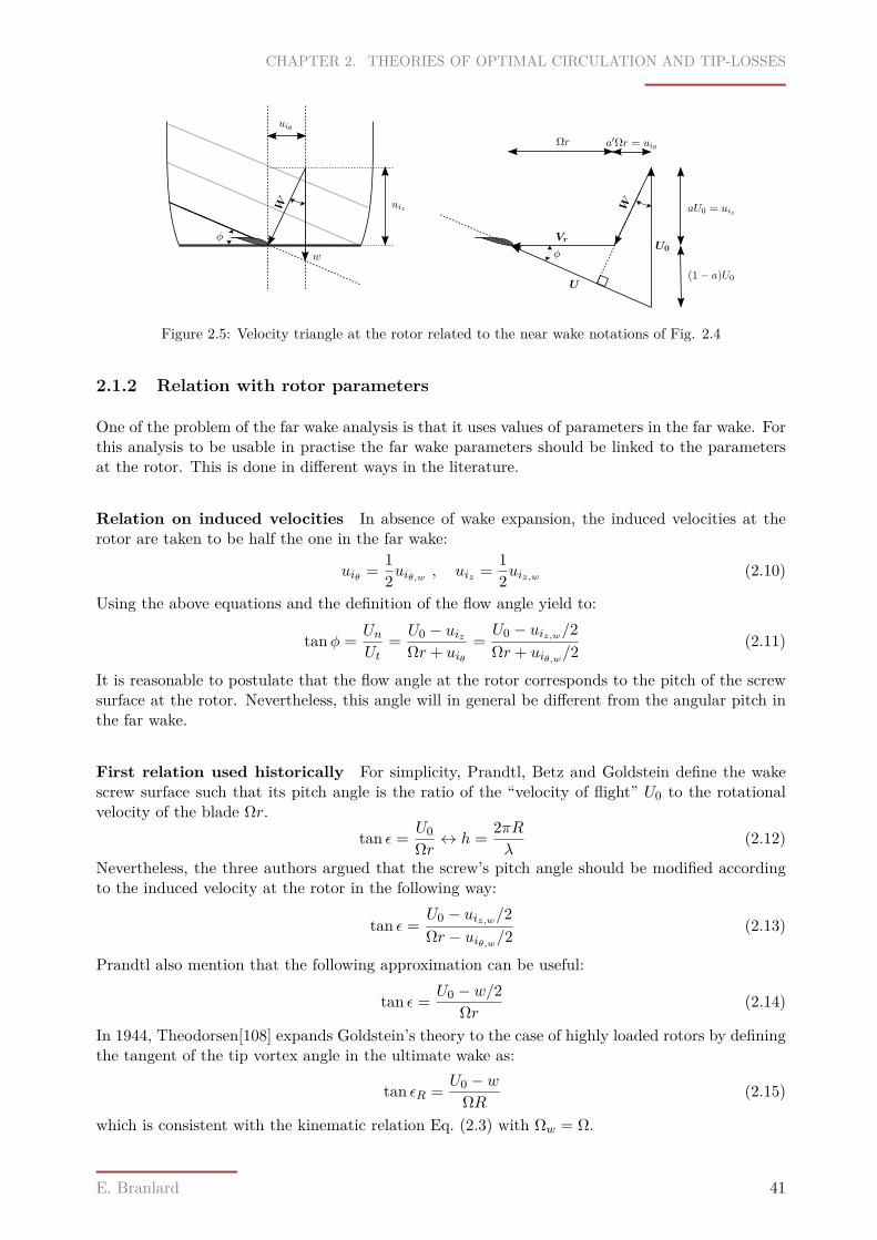
CHAPTER 2. THEORIES OF OPTIMAL CIRCULATION AND TIP-LOSSES
w
W uiz
uiθ
W
U0
U
φ
a′Ωr = uiθΩr
φ
aU0 = uiz
(1− a)U0
Vr
Figure 2.5: Velocity triangle at the rotor related to the near wake notations of Fig. 2.4
2.1.2 Relation with rotor parameters
One of the problem of the far wake analysis is that it uses values of parameters in the far wake. Forthis analysis to be usable in practise the far wake parameters should be linked to the parametersat the rotor. This is done in different ways in the literature.
Relation on induced velocities In absence of wake expansion, the induced velocities at therotor are taken to be half the one in the far wake:
uiθ = 12uiθ,w , uiz = 1
2uiz,w (2.10)
Using the above equations and the definition of the flow angle yield to:
tanφ = UnUt
= U0 − uizΩr + uiθ
=U0 − uiz,w/2Ωr + uiθ,w/2
(2.11)
It is reasonable to postulate that the flow angle at the rotor corresponds to the pitch of the screwsurface at the rotor. Nevertheless, this angle will in general be different from the angular pitch inthe far wake.
First relation used historically For simplicity, Prandtl, Betz and Goldstein define the wakescrew surface such that its pitch angle is the ratio of the “velocity of flight” U0 to the rotationalvelocity of the blade Ωr.
tan ε = U0Ωr ↔ h = 2πR
λ(2.12)
Nevertheless, the three authors argued that the screw’s pitch angle should be modified accordingto the induced velocity at the rotor in the following way:
tan ε =U0 − uiz,w/2Ωr − uiθ,w/2
(2.13)
Prandtl also mention that the following approximation can be useful:
tan ε = U0 − w/2Ωr (2.14)
In 1944, Theodorsen[108] expands Goldstein’s theory to the case of highly loaded rotors by definingthe tangent of the tip vortex angle in the ultimate wake as:
tan εR = U0 − wΩR (2.15)
which is consistent with the kinematic relation Eq. (2.3) with Ωw = Ω.
E. Branlard 41
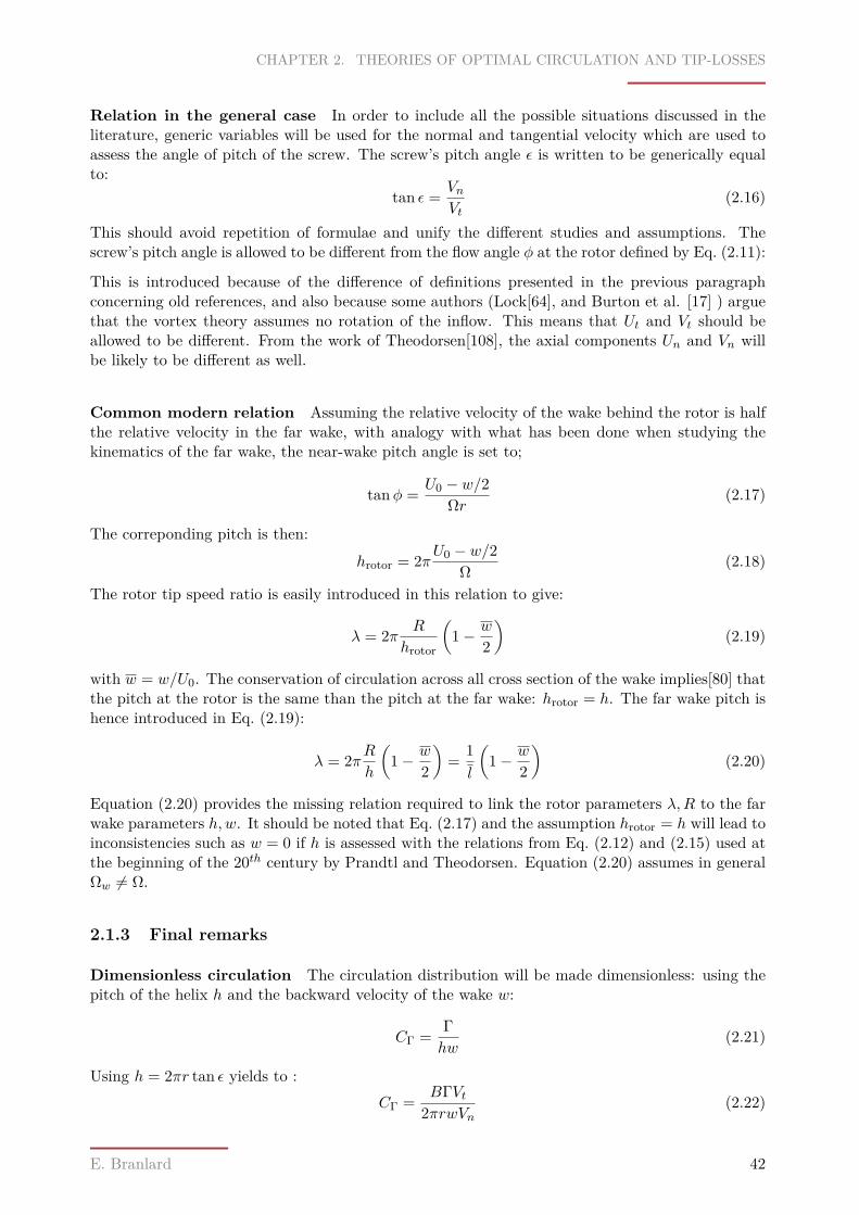
CHAPTER 2. THEORIES OF OPTIMAL CIRCULATION AND TIP-LOSSES
Relation in the general case In order to include all the possible situations discussed in theliterature, generic variables will be used for the normal and tangential velocity which are used toassess the angle of pitch of the screw. The screw’s pitch angle ε is written to be generically equalto:
tan ε = VnVt
(2.16)
This should avoid repetition of formulae and unify the different studies and assumptions. Thescrew’s pitch angle is allowed to be different from the flow angle φ at the rotor defined by Eq. (2.11):
This is introduced because of the difference of definitions presented in the previous paragraphconcerning old references, and also because some authors (Lock[64], and Burton et al. [17] ) arguethat the vortex theory assumes no rotation of the inflow. This means that Ut and Vt should beallowed to be different. From the work of Theodorsen[108], the axial components Un and Vn willbe likely to be different as well.
Common modern relation Assuming the relative velocity of the wake behind the rotor is halfthe relative velocity in the far wake, with analogy with what has been done when studying thekinematics of the far wake, the near-wake pitch angle is set to;
tanφ = U0 − w/2Ωr (2.17)
The correponding pitch is then:
hrotor = 2πU0 − w/2Ω (2.18)
The rotor tip speed ratio is easily introduced in this relation to give:
λ = 2π R
hrotor
(1− w
2
)(2.19)
with w = w/U0. The conservation of circulation across all cross section of the wake implies[80] thatthe pitch at the rotor is the same than the pitch at the far wake: hrotor = h. The far wake pitch ishence introduced in Eq. (2.19):
λ = 2πRh
(1− w
2
)= 1l
(1− w
2
)(2.20)
Equation (2.20) provides the missing relation required to link the rotor parameters λ,R to the farwake parameters h,w. It should be noted that Eq. (2.17) and the assumption hrotor = h will lead toinconsistencies such as w = 0 if h is assessed with the relations from Eq. (2.12) and (2.15) used atthe beginning of the 20th century by Prandtl and Theodorsen. Equation (2.20) assumes in generalΩw 6= Ω.
2.1.3 Final remarks
Dimensionless circulation The circulation distribution will be made dimensionless: using thepitch of the helix h and the backward velocity of the wake w:
CΓ = Γhw
(2.21)
Using h = 2πr tan ε yields to :CΓ = BΓVt
2πrwVn(2.22)
E. Branlard 42
CHAPTER 2. THEORIES OF OPTIMAL CIRCULATION AND TIP-LOSSES
In the particular case where Vt = Ωr and Vn = U0 + w, which is used by [108, 79] it writes:
CΓ = BΩΓ2πw(U0 + w) (2.23)
In the particular case where Vt = Ωr and Vn = U0, which is used by [36, 35] it writes:
CΓ = BΩΓ2πwU0
(2.24)
Tip-loss factor The total circulation found by Betz, Γ∞, is used as a reference case as it corre-sponds to an infinite number of blades. Obvisouly this is not a circulation per blade. If one uses theresult of Betz and distributes it artificially over the B blades of the rotor, then each blade wouldhave a reference circulation Γ∞/B. For a given blade circulation distribution Γ, the tip loss factoris expressed with respect to the reference distribution1:
F = ΓΓ∞/B
(2.25)
Dependency in r In the following, most parameters are dependent on the radial position rbut this dependence is not formally written. Nevertheless, when parameters are evaluated at aparticular position, like r = R, then this dependence is explicitly written.
2.2 Betz theory of optimal circulation
2.2.1 Betz’s optimal circulation
In the following the results of Betz optimal circulation are presented. In a second time, elementsof the demonstration are given but the reader is invited to refer to the original articles of Betz[9]and Munk[76] for a throughout understanding of the derivation of optimum lifting devises.Assumptions 2.1:(H 2.1a) - Inviscid, irrotational fluid(H 2.1b) - Lighlty-loaded rotor(H 2.1c) - Infinite number of blades(H 2.1d) - Uniform flow
Betz[9] obtained the fact that for the optimum rotor, the flow far behind the rotor is the same as ifthe wake surface formed by the trailing vortices was rigid and moved downstream with a constantvelocity. This assumption is hence added to the list above:(H 2.1e) - Optimal rotor (“rigid wake”)Assumption (H2.1c) deserves a little attention regarding the definition of the circulation. If ΓB(r)designs the circulation around one blade at radius r, then the circulation for an infinite number ofblade is
Γ∞(r) = limB→∞ΓB→0
B · ΓB(r) (2.26)
1This can of course be thought inversely as the comparison of the total circulation BΓ with respect to the totalcirculation Γ∞ of Betz’s rotor
E. Branlard 43
CHAPTER 2. THEORIES OF OPTIMAL CIRCULATION AND TIP-LOSSES
and the above limit is assumed to be finite. Historically, Betz uses the helix angle from Eq. (2.12),that will be replaced here for general purposes by Eq. (2.16). The boundary conditions on the“rigid wake” Eq. (2.8) and Eq. (2.7) then writes:
uiz,w = wV 2t
V 2n + V 2
t
(2.27)
uiθ,w = wVnVt
V 2n + V 2
t
(2.28)
Integrating the tangential velocity along a circle of radius r gives Betz optimum circulation:
Γ∞(r) =∫ 2π
0uiθ,wrdθ = 2πruiθ,w = 2πwVnΩ
V 2t
V 2n + V 2
t
(2.29)
Assuming this results apply for a rotor with B blades then the circulation of each blade is:
ΓBe = Γ∞B
= 2πB
wVnΩ
V 2t
V 2n + V 2
t
(2.30)
which writes in dimensionless form:
CΓBe =(VtΩr
)V 2t
V 2n + V 2
t
(2.31)
In the special and historical case of Vt = Ωr and Vn = U0,i.e. using the helix angle from Eq. (2.12),the Betz circulation reduces to:
ΓBe,0 = 2πB
wU0Ω
λ2r
1 + λ2r
(2.32)
and in dimensionless form:CΓBe,0 = λ2
r
1 + λ2r
(2.33)
2.2.2 Overview of Betz’s demonstration
Betz demonstration relies on quite advanced statements and theorems which make the reproductionof the demonstration quite difficult. The major elements of the demonstration are here mentionedfor reference.
- The “staggered theorem”: This theorem derived by Munk states that the total drag of any liftingsystem is always independent of longitudinal coordinate of the lifting elements. These elements canbe displaced in the direction of flight if the lift force stays the same(the angle of attack might changebut not the effective angle of attack)[76]. An equivalent theorem was derived by Betz, though itsformulation is more complex due to the fact that the vortex system considered has the shape of ascrew. The result is that lifting elements can be displaced along the screw lines without changingthe total energy-loss.
- The principle of determination of minimum induced drag found by Munk is somehow extendedby Betz in terms of work loss(for wind energy, this translates to maximum power extraction). Thebasics of these two formulations consists in the consideration of two lifting elements. The optimaldistribution of circulation is obtained if the displacements of these two elements(by means of thestaggered theorem) while keeping the total thrust (or total lift in case of a wing) unchanged doesnot reduces the energy loss. By reductio ad absurdum, if this was not the case then the energy loss
E. Branlard 44
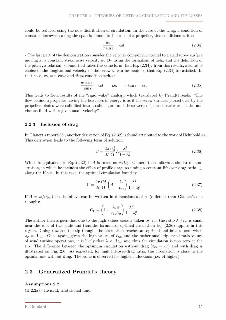
CHAPTER 2. THEORIES OF OPTIMAL CIRCULATION AND TIP-LOSSES
could be reduced using the new distribution of circulation. In the case of the wing, a condition ofconstant downwash along the span is found. In the case of a propeller, this conditions writes:
wnr sin ε = cst (2.34)
- The last part of the demonstration consider the velocity component normal to a rigid screw surfacemoving at a constant streamwise velocity w. By using the formalism of helix and the definition ofthe pitch , a relation is found that takes the same form than Eq. (2.34). from this results, a suitablechoice of the longitudinal velocity of the screw w can be made so that Eq. (2.34) is satisfied. Inthat case, wn = w cos ε and Betz condition writes:
w cos εr sin ε = cst i.e. r tan ε = cst (2.35)
This leads to Betz results of the “rigid wake” analogy, which translated by Prandtl reads: “Theflow behind a propeller having the least loss in energy is as if the screw surfaces passed over by thepropeller blades were solidified into a solid figure and these were displaced backward in the nonviscous fluid with a given small velocity”.
2.2.3 Inclusion of drag
In Glauert’s report[35], another derivation of Eq. (2.32) is found attributed to the work of Helmbold[44].This derivation leads to the following form of solution:
Γ = 2πB
U20
Ω Aλ2r
1 + λ2r
(2.36)
Which is equivalent to Eq. (2.32) if A is taken as w/U0. Glauert then follows a similar demon-stration, in which he includes the effect of profile drag, assuming a constant lift over drag ratio εl/dalong the blade. In this case, the optimal circulation found is:
Γ = 2πB
U20
Ω
(A− λr
εl/d
)λ2r
1 + λ2r
(2.37)
If A = w/U0, then the above can be written in dimensionless form(different than Glauert’s onethough):
CΓ =(
1− λrw
εl/dU0
)λ2r
1 + λ2r
(2.38)
The author then argues that due to the high values usually taken by εl/d, the ratio λr/εl/d is smallnear the root of the blade and thus the formula of optimal circulation Eq. (2.36) applies in thisregion. Going towards the tip though, the circulation reaches an optimal and falls to zero whenλr = Aεl/d. Once again, given the high values of εl/d, and the rather small tip-speed ratio valuesof wind turbine operations, it is likely that λ < Aεl/d and thus the circulation is non zero at thetip. The difference between the optimum circulation without drag (εl/d = ∞) and with drag isillustrated on Fig. 2.6. As expected, for high lift-over-drag ratio, the circulation is close to theoptimal one without drag. The same is observed for higher inductions (i.e. A higher).
2.3 Generalized Prandtl’s theory
Assumptions 2.2:(H 2.2a) - Inviscid, irrotational fluid
E. Branlard 45
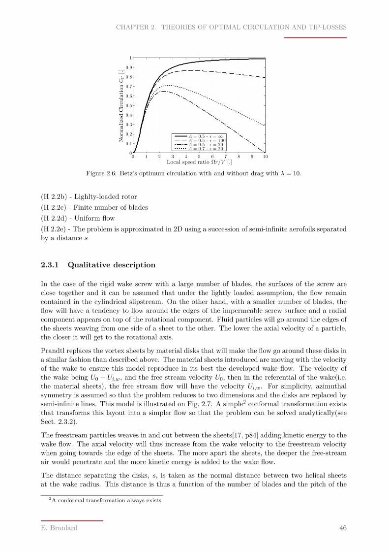
CHAPTER 2. THEORIES OF OPTIMAL CIRCULATION AND TIP-LOSSES
Local speed ratio Ωr/V [.]
Norm
alizedCirculationCΓ[.]
0 1 2 3 4 5 6 7 8 9 100
0.1
0.2
0.3
0.4
0.5
0.6
0.7
0.8
0.9
1
A = 0.5 - ǫ = ∞A = 0.5 - ǫ = 100A = 0.5 - ǫ = 20A = 0.7 - ǫ = 20
Figure 2.6: Betz’s optimum circulation with and without drag with λ = 10.
(H 2.2b) - Lighlty-loaded rotor(H 2.2c) - Finite number of blades(H 2.2d) - Uniform flow(H 2.2e) - The problem is approximated in 2D using a succession of semi-infinite aerofoils separatedby a distance s
2.3.1 Qualitative description
In the case of the rigid wake screw with a large number of blades, the surfaces of the screw areclose together and it can be assumed that under the lightly loaded assumption, the flow remaincontained in the cylindrical slipstream. On the other hand, with a smaller number of blades, theflow will have a tendency to flow around the edges of the impermeable screw surface and a radialcomponent appears on top of the rotational component. Fluid particles will go around the edges ofthe sheets weaving from one side of a sheet to the other. The lower the axial velocity of a particle,the closer it will get to the rotational axis.
Prandtl replaces the vortex sheets by material disks that will make the flow go around these disks ina similar fashion than described above. The material sheets introduced are moving with the velocityof the wake to ensure this model reproduce in its best the developed wake flow. The velocity ofthe wake being U0 − Ui,w, and the free stream velocity U0, then in the referential of the wake(i.e.the material sheets), the free stream flow will have the velocity Ui,w. For simplicity, azimuthalsymmetry is assumed so that the problem reduces to two dimensions and the disks are replaced bysemi-infinite lines. This model is illustrated on Fig. 2.7. A simple2 conformal transformation existsthat transforms this layout into a simpler flow so that the problem can be solved analytically(seeSect. 2.3.2).
The freestream particles weaves in and out between the sheets[17, p84] adding kinetic energy to thewake flow. The axial velocity will thus increase from the wake velocity to the freestream velocitywhen going towards the edge of the sheets. The more apart the sheets, the deeper the free-streamair would penetrate and the more kinetic energy is added to the wake flow.
The distance separating the disks, s, is taken as the normal distance between two helical sheetsat the wake radius. This distance is thus a function of the number of blades and the pitch of the
2A conformal transformation always exists
E. Branlard 46
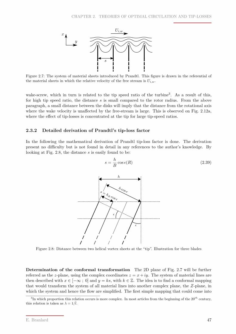
CHAPTER 2. THEORIES OF OPTIMAL CIRCULATION AND TIP-LOSSES
Ui,w
s
y
x
Figure 2.7: The system of material sheets introduced by Prandtl. This figure is drawn in the referential ofthe material sheets in which the relative velocity of the free stream is Ui,w.
wake-screw, which in turn is related to the tip speed ratio of the turbine3. As a result of this,for high tip speed ratio, the distance s is small compared to the rotor radius. From the aboveparagraph, a small distance between the disks will imply that the distance from the rotational axiswhere the wake velocity is unaffected by the free-stream is large. This is observed on Fig. 2.12a,where the effect of tip-losses is concentrated at the tip for large tip-speed ratios.
2.3.2 Detailed derivation of Prandtl’s tip-loss factor
In the following the mathematical derivation of Prandtl tip-loss factor is done. The derivationpresent no difficulty but is not found in detail in any references to the author’s knowledge. Bylooking at Fig. 2.8, the distance s is easily found to be:
s = h
Bcos ε(R) (2.39)
h cos ε
ε
ε
h
s = hB cos ε
Figure 2.8: Distance between two helical vortex sheets at the “tip”. Illustration for three blades
Determination of the conformal transformation The 2D plane of Fig. 2.7 will be furtherreferred as the z-plane, using the complex coordinates z = x+ iy. The system of material lines arethen described with x ∈ [−∞ ; 0] and y = ks, with k ∈ Z. The idea is to find a conformal mappingthat would transform the system of all material lines into another complex plane, the Z-plane, inwhich the system and hence the flow are simplified. The first simple mapping that could come into
3In which proportion this relation occurs is more complex. In most articles from the beginning of the 20th century,this relation is taken as λ = 1/l.
E. Branlard 47
CHAPTER 2. THEORIES OF OPTIMAL CIRCULATION AND TIP-LOSSES
mind is the logarithm one which transforms concentric circle in the Z planes into parallel lines inthe z planes. The problem is that the flow around an infinite number of concentric circles is notknown so this idea should be discarded. Clearly a way to simplify the problem and remove thefact that an infinite number of lines are present should be found. By looking at the symmetry ofthe problem, and by the knowledge of the periodicity of the complex exponential function, thisreduction can easily be done. Writing y = kπ sπ , then the semi-infinite lines are transformed by theexponential to:
eπzs = e
πxs eikπ = e
πxs
1 k ∈ 2Z−1 k ∈ 2Z + 1
(2.40)
Given the values of x ∈ [−∞ ; 0], eπxs covers the segment [0 ; 1], and e
πzs covers the segment
[−1 ; 1]. By using the transformationz = s
πlogZ (2.41)
the problem of reducing the complexity of the infinite number of lines has been solved. The problemreduces to determining the flow around a segment. This is a well known problem in fluid dynamicswhich is solved by using another conformal mapping: Joukowski’s conformal mapping.
The most famous conformal mapping in aeronautics is the one from Joukowski, defined as :
z = 12
(Z + 1
Z
)(2.42)
The idea is that the flow around a circle in the Z plane is analytically known by superposition ofthree elementary potential solutions: the uniform flow, a vortex and a doublet, the two latter beingat the circle’s center. All the circles considered by Joukowski intersect the real axis at coordinate1. The transformation is such that depending on the location of the circle’s center a different airfoilprofile is obtained in the z plane by inverse transformation. The typical example is the one of theunitary circle, which is transformed by Eq. (2.42) into the segment [−1 ; 1]. This is easily seen byinserting Z = eiθ into Eq. (2.42).
z = 12(eiθ + e−iθ
)= cos θ (2.43)
From the two paragraphs above the pieces are easily put together to derive the conformal mappingthat transforms the infinite system of semi-infinite segments into the unit-circle around which theflow is known. The transformation writes:
z = s
πlog
[12
(Z + 1
Z
)](2.44)
It should be noted that the function z(Z) is an injection which covers only two semi infinite lines ifthe complex logarithm is defined with an imaginary part in [π ; π[. A definition of the logarithmas function of the argument of Z should be used to cover the infinite number of lines, viz.
log(reiθ) = log r + iθ with θ ∈ R and r ∈ R+ (2.45)
Determination of the complex velocity It was said above that the flow around a circle isknown from the superposition of the infinite flow, a vortex and a doublet. In the current problem,only the induced velocities due to the circulation flow is sought so that only the vortex contributionis considered. It is recalled that the complex potential F is defined in term of the potential functionΦ and the stream function Ψ as:
F(Z) = Φ + iΨ (2.46)
E. Branlard 48
CHAPTER 2. THEORIES OF OPTIMAL CIRCULATION AND TIP-LOSSES
For a single vortex located at the origin the complex potential is known to be of the form:
F(Z) = −i Γ2π logZ (2.47)
where the circulation Γ is a constant to be determined. The variable Z can be eliminated betweenEq. (2.44) and (2.47), to yield:
Z = exp[2π
Γ (Φ + iΨ)]
(2.48)
Inserting Z back into Eq. (2.44) gives:
z = s
πlog cos
[2πΓ (Φ + iΨ)
](2.49)
The potential can be solved by considering the streamline Ψ = 0 which corresponds to the surfaceformed by the unit circle (or the equivalent vortex lines), and by equating the real parts:
Φ = ± Γ2π acos exp xπ
s(2.50)
The uncertainty on the sign comes from the inversion of the cosine(cf. cos(x) = cos(−x)). Thecomplex velocity wZ in the Z plane is defined as dF/dZ, which can be related to the complexvelocity wz in the z plane as:
wz = dFdZ· dZdz
(2.51)
The two parts of this product are:
dFdZ
= − iΓ2π1Z
(2.52)
dz
dZ= s
πZ
Z2 − 1Z2 + 1 (2.53)
Eventually, the complex velocity in the z-plane is:
wz = −i Γ2sZ2 + 1Z2 − 1 (2.54)
It should be remembered that the real velocity components are obtained by taking the conjugateof the complex velocity, i.e. u = Rewz and v = − Imwz. In order to find a multiplicative factorfor the velocity, Prandtl defines the potential in such way that the free stream velocity is equal to1. Making |Z| → ∞ in Eq. (2.54), this condition leads to the determination of the constant Γ as:
Γ = 2s (2.55)
Equation (2.54) is enough to draw the streamlines around the vortex lines by using different con-centric circles in the Z−plane. Nevertheless, this equation is a little disappointing for it expressesthe velocity in the z plane as function of the Z coordinate instead of the z coordinate. It is possibleto obtain a closed form equation but only between two vortex lines due to the fact that z(Z) is aninjection as was discussed above. This problem is of course minor because given the periodicity ofthe flow solving it between two lines is enough. Writing for simplicity e = exp (πz/a), and withthe minimum rigor required, Eq. (2.44) is written:
Z2 − 2Ze+ 1 = 0 (2.56)
which can be solved as:Z = e± i
√1− e (2.57)
E. Branlard 49
CHAPTER 2. THEORIES OF OPTIMAL CIRCULATION AND TIP-LOSSES
Using Eq. (2.56), Z2 + 1 and Z2 − 1 can easily be expressed and Eq. (2.54) writes:
wz = e
i (e− 1/Z) = ±e√1− e2
=± exp
(πza
)√1− exp
(2πza
) (2.58)
The velocity field found from Eq. (2.54)a is displayed on Fig. 2.9 for a series of concentric circlesin the Z planes.
The work of Prandtl Using the scaling constant from Eq. (2.55), the velocity potential is:
Φ = ± sπ
acos exp xπs
(2.59)
The shape of the velocity potential is displayed in Eq. (2.54)b. Prandtl interprets the surfaceformed by this figure, which is the integral of the difference of potential along the vortex lines, asa factor which can be directly used for the determination of the lift(see examples of applications ine.g. [88]). From this point, the derivation of the tip-loss factor can be done in different ways. Theinduced velocities between two vortex lines can be integrated analytically. This was presented byGlauert and will be described in the next paragraph. Another way of seeing it consists in lookingat the difference of potential on both side of a vortex line, which is related to the circulation. Bydividing this difference by the distance between two vortex lines s, a factor between 0 and 1 isobtained, which corresponds to the tip-loss factor :
F = 2π
acos exp πxs
(2.60)
In his article[87] Prandtl uses this factor as a multiplicative factor for the optimal circulation foundby Betz, viz:
Γ = F · Γ∞B
(2.61)
Prandtl also computes the distance of which the lines must be reduced in order to have the sameoverall losses but a constant velocity between the vortex lines. In the English version of his report[88]though, a typographic error is found, the correct expression of this distance being:
a′ = s
πlog 2 (2.62)
In the original papers log(2)/π is approximated by 0.2207, whereas a more accurate rounding wouldbe 0.2206. Different ways of determining this factor are possible, by looking at the velocity, thepotential, etc. A simple numerical way is to look at the area lost compared to unity:
a′ =∫ 0
−∞(1− F )dx (2.63)
For an analytical derivation it is easier to consider the velocity as done in[35].
The work of Glauert Instead of using the scaling to unity from Eq. (2.55), Glauert[35] uses therelative velocity outside of the system of lines that he writes v′. Equation (2.58) is simply modifiedby multiplying it by v′. From the discussion of Sect. 2.3.1, the relative velocity of the free streamoutside the system of lines is v′ = Ui,w. The notation v′ will be kept below for harmony with thisreference. Glauert uses Eq. (2.58) as a starting point to derive Prandtl’s tip-loss factor. It will
E. Branlard 50
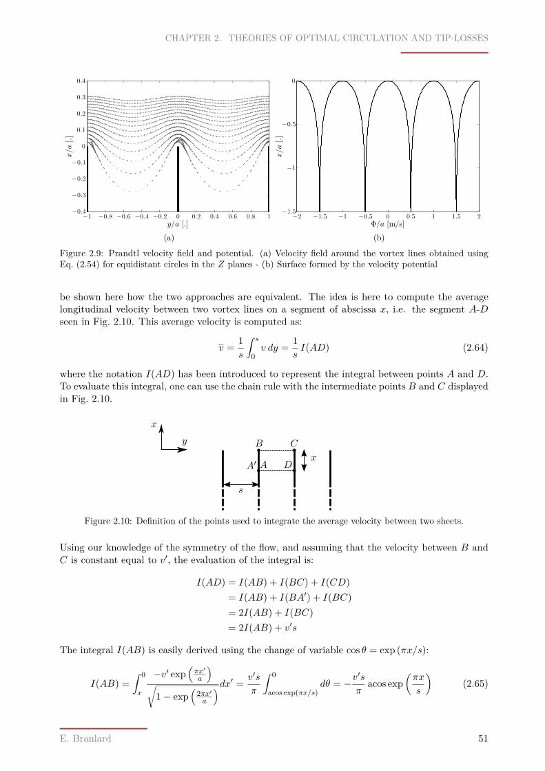
CHAPTER 2. THEORIES OF OPTIMAL CIRCULATION AND TIP-LOSSES
y/a [.]
x/a[.]
−1 −0.8 −0.6 −0.4 −0.2 0 0.2 0.4 0.6 0.8 1−0.4
−0.3
−0.2
−0.1
0
0.1
0.2
0.3
0.4
(a)Φ/a [m/s]
x/a[.]
−2 −1.5 −1 −0.5 0 0.5 1 1.5 2−1.5
−1
−0.5
0
(b)
Figure 2.9: Prandtl velocity field and potential. (a) Velocity field around the vortex lines obtained usingEq. (2.54) for equidistant circles in the Z planes - (b) Surface formed by the velocity potential
be shown here how the two approaches are equivalent. The idea is here to compute the averagelongitudinal velocity between two vortex lines on a segment of abscissa x, i.e. the segment A-Dseen in Fig. 2.10. This average velocity is computed as:
v = 1s
∫ s
0v dy = 1
sI(AD) (2.64)
where the notation I(AD) has been introduced to represent the integral between points A and D.To evaluate this integral, one can use the chain rule with the intermediate points B and C displayedin Fig. 2.10.
s
y
x
A D
CB
A′x
Figure 2.10: Definition of the points used to integrate the average velocity between two sheets.
Using our knowledge of the symmetry of the flow, and assuming that the velocity between B andC is constant equal to v′, the evaluation of the integral is:
I(AD) = I(AB) + I(BC) + I(CD)= I(AB) + I(BA′) + I(BC)= 2I(AB) + I(BC)= 2I(AB) + v′s
The integral I(AB) is easily derived using the change of variable cos θ = exp (πx/s):
I(AB) =∫ 0
x
−v′ exp(πx′
a
)√
1− exp(
2πx′a
)dx′ = v′s
π
∫ 0
acos exp(πx/s)dθ = −v
′s
πacos exp
(πx
s
)(2.65)
E. Branlard 51
CHAPTER 2. THEORIES OF OPTIMAL CIRCULATION AND TIP-LOSSES
So that the average velocity eventually writes
v = 1s
(v′s− 2I(AB)
)= v′
[1− 2
πacos exp
(πx
s
)](2.66)
from which the factor F is defined as:
F = 2π
acos exp πxs
(2.67)
Transferring Eq. (2.66) back to the referential of the ground velocity(i.e. adding U0 − v′) andre-establishing our notation v′ = Ui,w, the average velocity between two vortex sheets of the wakeis:
Uw = U0 − FUi,w (2.68)
Using the 1D momentum theory results for the induced velocity in the far wake, Ui,w = 2aU0, theabove writes:
Uw = U0(1− 2aF ) (2.69)
which is assumed to be extended to the rotor as well, viz:
U = U0(1− aF ) (2.70)
Going back to the rotor geometry The system of vortex sheets in the z plane as an xcoordinate that extends from −∞ to 0. The analogy with the rotor is done by replacing x by R−r,so that eventually the tip-loss factor is derived as:
F = 2π
acos exp[−πR− r
s
](2.71)
Literal expression From the analysis above, the tip-loss factor is usually decomposed into twoexpressions interpreted as follow by Larrabee[59]:
F = Average fluid velocityVortex line velocity = 2
πacos exp(−f) (2.72)
f = πEdge distance
Vortex line spacing = πR− rs
(2.73)
2.3.3 General expression
The demonstration done by Prandtl[87] is followed but this time in the idea of extending his workto the most general case where the tangent of the helix angle is determined by the arbitrary ratioof Vn and Vt. By doing so the following circulation is found:
ΓPr = 2πB
wVnΩ
V 2t
V 2n + V 2
t
2π
acos exp[−πR− r
s
](2.74)
In this equation one recognizes the expression of Γ∞ so that the tip-loss factor stands out easily:
FPr = 2π
acos exp[−πR− r
s
](2.75)
The distance between two screw surface at the tip defines s as :
s = h(R)B
cos (ε(R)) (2.76)
E. Branlard 52
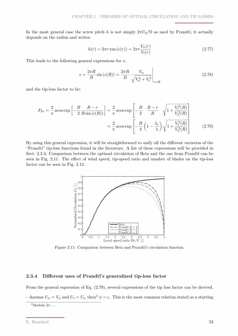
CHAPTER 2. THEORIES OF OPTIMAL CIRCULATION AND TIP-LOSSES
In the most general case the screw pitch h is not simply 2πU0/Ω as used by Prandtl, it actuallydepends on the radius and writes:
h(r) = 2πr tan (ε(r)) = 2πrVn(r)Vt(r)
(2.77)
This leads to the following general expressions for s:
s = 2πRB
sin (ε(R)) = 2πRB
Vn√V 2n + V 2
t
∣∣∣∣∣∣r=R
(2.78)
and the tip-loss factor to be:
FPr = 2π
acos exp[−B2
R− rR sin (ε(R))
]= 2π
acos exp
−B2 R− rR
√1 + V 2
t (R)V 2n (R)
= 2π
acos exp
−B2(
1− λrλ
)√1 + V 2
t (R)V 2n (R)
(2.79)
By using this general expression, it will be straightforward to unify all the different variation of the“Prandtl” tip-loss functions found in the literature. A list of these expressions will be provided inSect. 2.3.4. Comparison between the optimal circulation of Betz and the one from Prandtl can beseen in Fig. 2.11. The effect of wind speed, tip-speed ratio and number of blades on the tip-lossfactor can be seen in Fig. 2.12.
Local speed ratio Ωr/V [.]
Norm
alizedCirculationCΓ[.]
0 0.5 1 1.5 2 2.5 3 3.5 4 4.5 50
0.1
0.2
0.3
0.4
0.5
0.6
0.7
0.8
0.9
1
BetzPrandtl B = 4Prandtl B = 3Prandtl B = 2
Figure 2.11: Comparison between Betz and Prandtl’s circulation function.
2.3.4 Different uses of Prandtl’s generalized tip-loss factor
From the general expression of Eq. (2.79), several expressions of the tip loss factor can be derived.
- Assume Un = Vn and Ut = Ut, then4 φ = ε. This is the most common relation stated as a starting4Modulo 2π . . .
E. Branlard 53
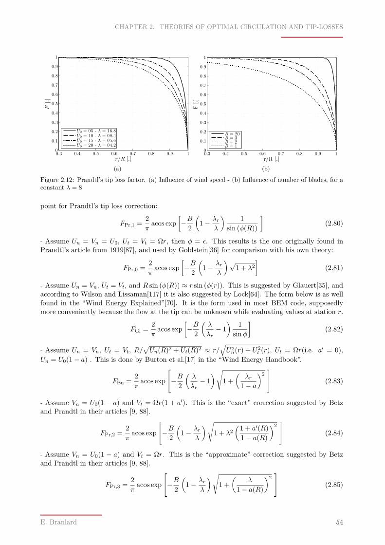
CHAPTER 2. THEORIES OF OPTIMAL CIRCULATION AND TIP-LOSSES
r/R [.]
F[.]
0.3 0.4 0.5 0.6 0.7 0.8 0.9 10
0.1
0.2
0.3
0.4
0.5
0.6
0.7
0.8
0.9
1
U0 = 05 - λ = 16.8U0 = 10 - λ = 08.4U0 = 15 - λ = 05.6U0 = 20 - λ = 04.2
(a)r/R [.]
F[.]
0.3 0.4 0.5 0.6 0.7 0.8 0.9 10
0.1
0.2
0.3
0.4
0.5
0.6
0.7
0.8
0.9
1
B = 20B = 3B = 2B = 1
(b)
Figure 2.12: Prandtl’s tip loss factor. (a) Influence of wind speed - (b) Influence of number of blades, for aconstant λ = 8
point for Prandtl’s tip loss correction:
FPr,1 = 2π
acos exp[−B2
(1− λr
λ
) 1sin (φ(R))
](2.80)
- Assume Un = Vn = U0, Ut = Vt = Ωr, then φ = ε. This results is the one originally found inPrandtl’s article from 1919[87], and used by Goldstein[36] for comparison with his own theory:
FPr,0 = 2π
acos exp[−B2
(1− λr
λ
)√1 + λ2
](2.81)
- Assume Un = Vn, Ut = Vt, and R sin (φ(R)) ≈ r sin (φ(r)). This is suggested by Glauert[35], andaccording to Wilson and Lissaman[117] it is also suggested by Lock[64]. The form below is as wellfound in the “Wind Energy Explained”[70]. It is the form used in most BEM code, supposedlymore conveniently because the flow at the tip can be unknown while evaluating values at station r.
FGl = 2π
acos exp[−B2
(λ
λr− 1
) 1sinφ
](2.82)
- Assume Un = Vn, Ut = Vt, R/√Un(R)2 + Ut(R)2 ≈ r/
√U2n(r) + U2
t (r), Ut = Ωr(i.e. a′ = 0),Un = U0(1− a) . This is done by Burton et al.[17] in the “Wind Energy Handbook”.
FBu = 2π
acos exp
−B2(λ
λr− 1
)√1 +
(λr
1− a
)2 (2.83)
- Assume Vn = U0(1 − a) and Vt = Ωr(1 + a′). This is the “exact” correction suggested by Betzand Prandtl in their articles [9, 88].
FPr,2 = 2π
acos exp
−B2(
1− λrλ
)√1 + λ2
(1 + a′(R)1− a(R)
)2 (2.84)
- Assume Vn = U0(1 − a) and Vt = Ωr. This is the “approximate” correction suggested by Betzand Prandtl in their articles [9, 88].
FPr,3 = 2π
acos exp
−B2(
1− λrλ
)√1 +
(λ
1− a(R)
)2 (2.85)
E. Branlard 54
CHAPTER 2. THEORIES OF OPTIMAL CIRCULATION AND TIP-LOSSES
- Assume Vn = U0(1 −√F a
2 ) and Vt = Ωr(1 + 2√F a′
2 ). This is an interesting suggestion fromLindenburg[62] to account for more realistic wake dynamics that will deserve a justification of theassumptions in Sect. 3.1.2.
FLi = 2π
acos exp
−B2(
1− λrλ
)√√√√1 + λ2r
(1 + 2
√FLi a′/2
1−√FLi a/2
)2 (2.86)
The list is probably not an exhaustive list as some assumptions can be combined, it certainlyappears confusing but should unify the different forms of tip-loss corrections accounted for thework of Prandtl and Glauert in the literature.
2.4 Goldstein’s optimal circulation
Despite its relevancy for this study it is not in the scope of this report to explicit the article ofGoldstein from 1929[36]. Instead, a short guide to read through this article is suggested becausethis theory is often left apart for its complexity whereas it provides a more suitable representationof the flow’s potential than Prandtl’s theory. The reader is thus invited to follow this short guide inAppendix A which is followed by a detailed description on how to calculate the Goldstein’s factorusing Okulov’s method[79].
2.4.1 Goldstein’s theory and its derivatives
The assumptions of Goldstein’s work are as follow:Assumptions 2.3:(H 2.3a) - Inviscid, irrotational fluid(H 2.3b) - Lighlty-loaded rotor(H 2.3c) - Optimum rotor in Betz’s sense(“rigid wake” with constant velocity)(H 2.3d) - Finite number of blades(H 2.3e) - Uniform flow(H 2.3f) - Un = Vn = U0, Ut = Ut = Ωr
Goldstein used infinite series, sometimes referred as Kaptain series, to find a solution for thepotential flow. The circulation found for a propeller with finite number of blades corresponding toa minimum energy loss in the slipstream for a prescribed thrust is obtained as5:
ΓGo = 2πB
wU0Ω
[8π2
∞∑m=0
T1,ν (νλr)(2m+ 1)2 + 2
π
∞∑m=0
amIν (νλr)Iν (νλ)
](2.87)
where ν = B(m+ 1
2
). The corresponding tip-loss factor is thus:
κ = FGo =(
λ2r
1 + λ2r
)−1 [ 8π2
∞∑m=0
T1,ν (νλr)(2m+ 1)2 + 2
π
∞∑m=0
amIν (νλr)Iν (νλ)
](2.88)
This tip-loss factor was historically called the Goldstein factor and can be found noted as κ inseveral references[109, 85]. Using the formal calculator Mathematica[71], Goldstein’s factor hasbeen calculated for this study and an example of optimal circulation distribution for different tip-speed ratio is found in Fig. 2.13 for a two and three bladed rotor. It is seen that the difference
5See Appendix A
E. Branlard 55
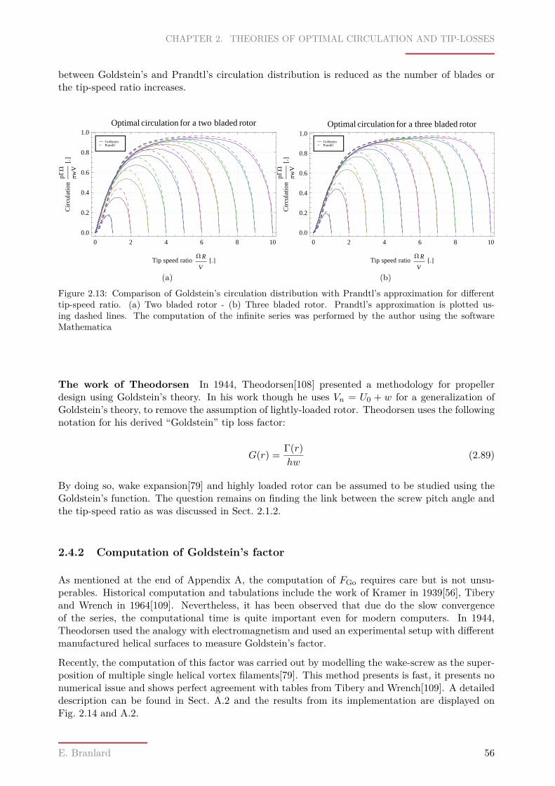
CHAPTER 2. THEORIES OF OPTIMAL CIRCULATION AND TIP-LOSSES
between Goldstein’s and Prandtl’s circulation distribution is reduced as the number of blades orthe tip-speed ratio increases.
0 2 4 6 8 10
0.0
0.2
0.4
0.6
0.8
1.0
Tip speed ratioW R
Cir
cula
tion
pGW
Πw
Optimal circulation for a two bladed rotor
GoldsteinPrandtl
(a)
0 2 4 6 8 10
0.0
0.2
0.4
0.6
0.8
1.0
Tip speed ratioW R
Cir
cula
tion
pGW
Πw
Optimal circulation for a three bladed rotor
GoldsteinPrandtl
(b)
Figure 2.13: Comparison of Goldstein’s circulation distribution with Prandtl’s approximation for differenttip-speed ratio. (a) Two bladed rotor - (b) Three bladed rotor. Prandtl’s approximation is plotted us-ing dashed lines. The computation of the infinite series was performed by the author using the softwareMathematica
The work of Theodorsen In 1944, Theodorsen[108] presented a methodology for propellerdesign using Goldstein’s theory. In his work though he uses Vn = U0 + w for a generalization ofGoldstein’s theory, to remove the assumption of lightly-loaded rotor. Theodorsen uses the followingnotation for his derived “Goldstein” tip loss factor:
G(r) = Γ(r)hw
(2.89)
By doing so, wake expansion[79] and highly loaded rotor can be assumed to be studied using theGoldstein’s function. The question remains on finding the link between the screw pitch angle andthe tip-speed ratio as was discussed in Sect. 2.1.2.
2.4.2 Computation of Goldstein’s factor
As mentioned at the end of Appendix A, the computation of FGo requires care but is not unsu-perables. Historical computation and tabulations include the work of Kramer in 1939[56], Tiberyand Wrench in 1964[109]. Nevertheless, it has been observed that due do the slow convergenceof the series, the computational time is quite important even for modern computers. In 1944,Theodorsen used the analogy with electromagnetism and used an experimental setup with differentmanufactured helical surfaces to measure Goldstein’s factor.
Recently, the computation of this factor was carried out by modelling the wake-screw as the super-position of multiple single helical vortex filaments[79]. This method presents is fast, it presents nonumerical issue and shows perfect agreement with tables from Tibery and Wrench[109]. A detaileddescription can be found in Sect. A.2 and the results from its implementation are displayed onFig. 2.14 and A.2.
E. Branlard 56
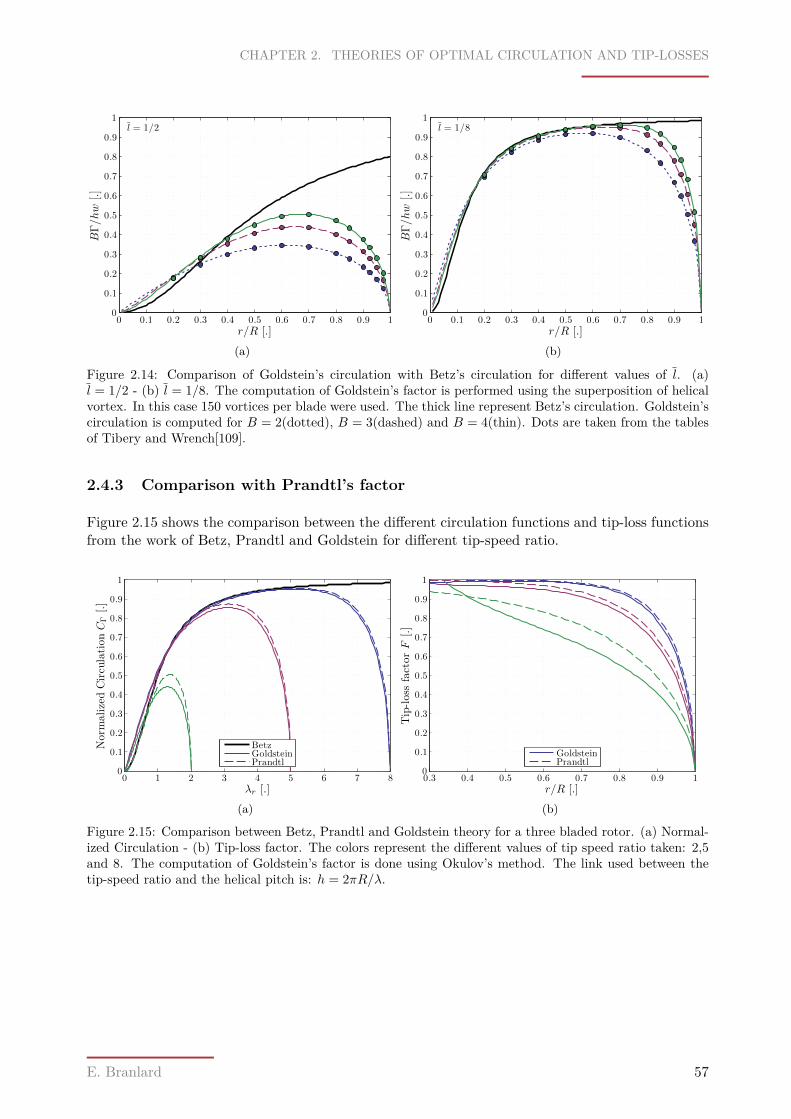
CHAPTER 2. THEORIES OF OPTIMAL CIRCULATION AND TIP-LOSSES
l = 1/2
r/R [.]
BΓ/hw
[.]
0 0.1 0.2 0.3 0.4 0.5 0.6 0.7 0.8 0.9 10
0.1
0.2
0.3
0.4
0.5
0.6
0.7
0.8
0.9
1
(a)
l = 1/8
r/R [.]
BΓ/hw
[.]
0 0.1 0.2 0.3 0.4 0.5 0.6 0.7 0.8 0.9 10
0.1
0.2
0.3
0.4
0.5
0.6
0.7
0.8
0.9
1
(b)
Figure 2.14: Comparison of Goldstein’s circulation with Betz’s circulation for different values of l. (a)l = 1/2 - (b) l = 1/8. The computation of Goldstein’s factor is performed using the superposition of helicalvortex. In this case 150 vortices per blade were used. The thick line represent Betz’s circulation. Goldstein’scirculation is computed for B = 2(dotted), B = 3(dashed) and B = 4(thin). Dots are taken from the tablesof Tibery and Wrench[109].
2.4.3 Comparison with Prandtl’s factor
Figure 2.15 shows the comparison between the different circulation functions and tip-loss functionsfrom the work of Betz, Prandtl and Goldstein for different tip-speed ratio.
λr [.]
Norm
alizedCirculationCΓ[.]
0 1 2 3 4 5 6 7 80
0.1
0.2
0.3
0.4
0.5
0.6
0.7
0.8
0.9
1
BetzGoldsteinPrandtl
(a)r/R [.]
Tip-loss
factorF
[.]
0.3 0.4 0.5 0.6 0.7 0.8 0.9 10
0.1
0.2
0.3
0.4
0.5
0.6
0.7
0.8
0.9
1
GoldsteinPrandtl
(b)
Figure 2.15: Comparison between Betz, Prandtl and Goldstein theory for a three bladed rotor. (a) Normal-ized Circulation - (b) Tip-loss factor. The colors represent the different values of tip speed ratio taken: 2,5and 8. The computation of Goldstein’s factor is done using Okulov’s method. The link used between thetip-speed ratio and the helical pitch is: h = 2πR/λ.
E. Branlard 57

CHAPTER 2. THEORIES OF OPTIMAL CIRCULATION AND TIP-LOSSES
E. Branlard 58
Chapter 3Tip-loss corrections and their implementation
3.1 Overview of the different tip-loss corrections
The main “theoretical” tip-losses correction have already been presented in chapter 2, they willbe briefly repeated here for the sake of establishing a brief summary of the different tip-lossescorrection found in the literature. This time, empirical relation will be presented as well. Thedifferent ways to implement the tip-loss factor will be described in the following section(Sect. 3.2).
3.1.1 Theoretical tip-loss corrections
The derivations from these theories assume no expansion and distortion of the wake, which corre-sponds to the assumption of lightly-loaded rotors. It is recalled that λ is the tip-speed ratio, λrthe local speed ratio and B the number of blades.
Prandtl’s tip-loss correction Betz derived the optimal circulation for a rotor with infinitenumber of blades in [9] and as an appendix to his article Prandtl suggested a correction for a finitenumber of blades(reported in english in[88]). The tip-loss correction introduced by Prandtl is thefollowing:
FPr,0 = 2π
acos[exp
(−B2
(1− λr
λ
)√1 + λ2
)](3.1)
The reader is referred to Sect. 2.3.4 were several variations of Prandtl’s tip-loss factor were pre-sented.
Goldstein’s tip-loss correction Using Goldstein’s notations[36] of the T functions, the tip-losscorrection derived by Goldstein writes:
FGo =(
λ2r
1 + λ2r
)−1 [ 8π2
∞∑m=0
T1,ν (νλr)(2m+ 1)2 + 2
π
∞∑m=0
amIν (νλr)Iν (νλ)
](3.2)
where ν = B(m+ 1
2
). A detailed description of Goldstein’s article can be followed in Appendix A.
59
CHAPTER 3. TIP-LOSS CORRECTIONS AND THEIR IMPLEMENTATION
Glauert’s correction Contrary to Goldstein and Prandtl who focused on the optimal circulation,Glauert uses this correction in the Blade Element Method. Glauert reported[35] the work of Prandtland derived the tip-loss correction in the following terms:
FPr,1 = 2π
acos[exp
(−B2
R− rR sinφR
)](3.3)
where φR is the flow angle at the tip. The above formula is modified in most BEM codes as advisedby Glauert to use the local flow angle φ instead, which leads to:
FGl = 2π
acos[exp
(−B2
R− rr sinφ
)](3.4)
Several variations of Prandtl tip-loss factor including the one from Glauert were also presented inSect. 2.3.4. Glauert uses this tip-loss factor to correct the axial induction factor a only, but doesnot uses this correction on the mass flux. This will be discussed in Sect. 3.2.
Just like Prandtl correction, Glauert’s correction is accurate for low tip speed ratio and high numberof blades. Its accuracy decreases as the tip speed ratio increases, or as the number of blade decreases(usually less than three). These statements can be observed for instance on Fig. 2.13 and 2.15.
3.1.2 Semi-Empirical tip-loss corrections
Xu and Sankar Xu and Sankar[92, 75] developed an empirical model based on CFD data sim-ulating the NREL Phase VI experiment[40]. The empirical correction suggested for this specificwind turbine is the following:
FX,S =1
2(F 0.85
Gl + 0.5)
when r/R ≥ 0.71− r
R1−FX,S(r=0.7R)
0.7 when r/R < 0.7(3.5)
In this model the tip loss factor does no go to zero at the tip which is for some authors consideredphysically unrealistic whereas argued to be required by other authors.
Lindenburg The following correction is suggested in[62] for application in ECN codes PHATASand BLADEMODE.
FLi = 2π
acos exp
−B2(
1− λrλ
)√√√√1 + λ2r
(1 + 2
√FLi a′/2
1−√FLi a/2
)2 (3.6)
This correction uses the velocity triangle just behind the rotor because, at it has already been seenin Sect. 1.1.3, this is the part of the wake which has the most influence on the induced velocities.The screw’s pitch angle is assessed behind the rotor1 where the radial velocity is Ωr(1 + 2a′) andthe axial velocity U0(1 − a). Prandtl defines the pitch angle at the wake radius, but Lindenburgargues that the trailing vorticity is not concentrated at the tip, but rather distributed mainly overthe outer part of the blade. As a result of this, the pitch angle is assessed using averaged inducedvelocities. In absence of tip vortex, the induced velocities from the momentum theory would be used(i.e. multiplied by 1), and in presence of a concentrated tip-vortex, the induced velocity shouldbe multiplied by F according to Prandtl’s theory. In between those two situations, to accountfor the distributed trailing vorticity, a factor of
√F is retained to assess the average tip-vortex
velocity. Due to the recursion introduced, this factors is evaluated using the tip-loss value at theprevious BEM iteration step. Moreover, in comparison with roller bearings between two surfaces,Lindenburg assumes that the tip vortices travel with a velocity averaged between the outside andthe inside of the wake. This explains the factor 1/2 applied on both induction factors.
1This definition differs from the pitch screw angle of Prandtl and Goldstein which are presumably considered inthe far wake
E. Branlard 60
CHAPTER 3. TIP-LOSS CORRECTIONS AND THEIR IMPLEMENTATION
3.1.3 Semi-Empirical performance tip-loss corrections
In this section tip-loss factors that applies to the airfoil coefficients are presented. The definitionof such tip-loss factor was presented in Eq. (1.28). The implementation is discussed in Sect. 3.2.
Shen et al. A new correction is suggested by Shen[98] for which the flow angle at the tip is notzero but the forces tend to zero at the tip owing to pressure equalization between the upper andlower surface of the blade. This correction differ from the above in the way the tip-loss factor isapplied. It is actually a second tip-loss correction applied this time on the airfoil data and whichis is used together with the classical Prandtl’s correction. The airfoil coefficients Cl and Cd, areindirectly corrected by multiplying the normal and tangential force coefficient, Cn and Ct, by asame factor FSh. Whether the drag should be included in the computation of the inductions isdiscussed, and eventually the drag is discarded(see Sect. 3.2). The correction takes a form similarto the one suggested by Glauert:
FCn,Sh = 2π
acos exp[−g(λ)B(R− r)
2R sinφR
](3.7)
whereg(λ) = exp [−c1(Bλ− c2)] + c3 (3.8)
and the two first constants fitted from experimental data and the third one empirically suggestedas (c1, c2, c3) = (0.125, 21, 0.1).
Lindenburg In [62] an empirical correction is suggested for the lift coefficient based on the NRELphase VI[40] experiment. This correction writes:
FCl,Li = 1−( ΩrVrel
)2· e−2 ARout · Cl,inv − Cl,2D
Cl,inv(3.9)
This formula as been adapted to the formalism of the current document(i.e. Eq. (1.28)), so thatthe 3D lift coefficient is obtained as:
Cl,3D = FCl,Li · Cl,2D (3.10)
In the above, Cl,inv refers to the inviscid, or potential, 2D lift coefficient that Lindenburg suggeststo take as 2π sin(α − α0), as in Eq. (1.23). Nevertheless, in Sect. 1.2.3, it was discussed by theauthor that such approximation is not suitable for wind turbines, and a method such as Eq. (1.25)is recommended to avoid having negative values of the difference of Cl,inv−Cl,2D when the 2D slopeis actually higher than 2π. The definition of ARout is the “aspect-ratio2 of the part of the bladeoutboard of the section under consideration”.
Sant Together with the stall delay correction presented in Sect. 1.2.3, Sant[93] suggest an engi-neering tip-loss correction for the NREL Phase VI rotor[40]. As for the Shen correction, the tip-lossfactor is applied on the airfoil data, but this time, directly on Cl ad Cd. The corrective factor isgiven as:
FCl,Sa = 2π
acos exp[−181− r/R
r/R
](3.11)
2See Notations on page 3
E. Branlard 61
CHAPTER 3. TIP-LOSS CORRECTIONS AND THEIR IMPLEMENTATION
It should be noted, that a root correction is also included in the original formula of Sant. Also,this correction is applied on the coefficients corrected for stall delay, which, according to Eq. (1.22)writes:
C•,3D,Sa = FSa [C•,2D + f•,Sa∆C•] (3.12)
with the symbol • referring to both L and D.
3.1.4 The historical approach of radius reduction
At the time where the BEM had to be computed manually, a common method to account for thetip-losses was to reduce the size of the rotor by a given factor. Prandtl[87] suggested for instanceto reduce the rotor radius by his integrated factor:
ReR
= (1− log 2π
s
R) (3.13)
where s = h/B cos ε(R) is the distance between two vortex-sheets in Prandtl’s analysis of thetip-loss. Glauert[35] adapted this correction into the following:
ReR
= 1− 1.386B
λ√1 + λ2
(3.14)
In [106], the following radius correction are mentioned:
ReR
= 1− 0.5 cR
(3.15)
where c is the average blade chord. Sissingh[100] suggested the following correction:
ReR
= 1− croot1 + 0.7etaper
1.5R ≈ 1− 3.56 c
πR(3.16)
where croot is the chord at the root of the blade and etaper is the taper ratio defined as croot/c. In1944 Wald[106] presented a correction as function of the thrust coefficient:
ReR
= 1− 1.98
√CTB
(3.17)
These corrections are now left apart due to the advancement of computers and the possibility torun fast BEM code computations.
E. Branlard 62
CHAPTER 3. TIP-LOSS CORRECTIONS AND THEIR IMPLEMENTATION
3.2 On the applicability of the tip-loss factor
3.2.1 Introduction
Different interpretations The way the tip-loss factor is applied mainly depends on its defini-tion. The following interpretations can be found:- Circulation: the tip-loss can be seen as a loss in circulation compared to the circulation foundwith momentum theory.- Induced velocities: the tip-loss factor can be applied to the induced velocities. The way this affectthe momentum and the mass flow will be discussed below.- Thrust coefficient: in a similar fashion than the circulation correction, the thrust coefficient canbe corrected with the tip-loss factor.- Airfoil coefficients: on top of the above corrections, a performance tip-loss factor is sometimesapplied to the airfoil coefficients
In the following, the practical applicability and implementation of the tip-loss factor described byseveral authors in the literature will be presented. In a second time, different critics found in theliterature will be mentioned to give a perspective of the debates the applicability of the tip-lossfactor raises.
Axial induction To best follow the concepts used by the different authors, the distinctions onthe axial induction factors that were used earlier in this document are recalled:- a = a(r, ψ) refers to the local axial induction at a given point on the rotor plane. The threedimensionality effects and the finite number of blades are accounted for.- a = a(r) refers to the 2D momentum theory axial induction, i.e. the axial induction for anactuator disk(infinite number of blades and no tip-losses). This is often simply written as a whenpresenting BEM equations (as was done in Appendix C). In this section, the distinction will bedone for clarity.- a = a(r) refers to the azimuthally averaged axial induction defined by Eq. (1.3). At a firstapproximation, the results from the 2D momentum theory can be applied to an annulus, or stripe,using this average axial induction. Nevertheless, if the 2D momentum theory is applied on its own,the axial induction a(r) that would be found would be different than a. Indeed for a 3D flow, withfinite number of blades a decreases towards the tip. The two would match only if the circulationis constant along the blade.- aB = aB(r) refers to the axial induction at the blade. This should be used in the Blade ElementTheory, to determines the proper velocity triangle and hence aerodynamic loads. Its definition israther difficult due to the spatial extent of the blade and the strong variations of the flow aroundthe blade due to the bound circulation.
The definitions and notations above are further extended to the tangential induction factor a′.From the above it is seen that a definition of the tip-loss factor as F = a
aB, F = a
a or F = aaB
canbe envisaged. These distinctions will appear when studying the work of the different authors.
3.2.2 Applications in the literature
The equations from the BEM method presented in Appendix C have to be modified to introduce theeffects of tip-losses. The tip-loss function is applied either on the circulation, the induced velocityor the thrust. The different ways this is performed in the literature is presented here withoutcomments and argumentations on the validity of the application. The discussion is postponed toSect. 3.2.3.
E. Branlard 63
CHAPTER 3. TIP-LOSS CORRECTIONS AND THEIR IMPLEMENTATION
Glauert Glauert follows the demonstration of Prandtl’s tip-loss factor(see Sect. 2.3), and hencelook at this factor as a change in the longitudinal average induced velocity between two vortexsheets (vortex lines). Quoting his report[35, p267]:
The physical fact represented by the tip correction is virtually that the maximum in-crease of axial velocity 2aU0 in the slipstream occurs only on the vortex sheets andthat the average increase of axial velocity in the slipstream is only a fraction F of thisvelocity. [. . . ] Similarly also the angular momentum equation [. . . ]
In this correction, it is the change of velocity between the upstream and wake velocity U0 − Uw =2aU0 which is corrected to 2aFU0, not the velocity on the rotor. Following the momentum theoryequations, this leads to the multiplication of the thrust and torque by the factor F as:
dT = 12ρU
20 (2πrdr) [4aF (1− a)] (3.18)
dQ = 12ρU
20 (2πrdr)r
[4a′F (1− a)λr
](3.19)
From the above it is seen that the definition F = aa is used, which is to say that the azimuthally
averaged axial induction a decreases towards the tip, which is not the case of the actuator disk axialinduction a. In the above aF should be replaced with aBF to correspond with Shen’s analysis.The mass flux is not corrected here.
Wilson and Lissaman In their document from 1974, Wilson and Lissaman[117] present thesame correction as Glauert. They also suggest a refinement by assuming that the axial mass fluxshould also be corrected due to tip-losses. From momentum theory, the mass flux expressed at therotor in an annular element is m = 1
2ρdAU0(1− a(r)). This flux is corrected in 12ρdAU0(1−F a(r)).
The authors argue that this should affect the coefficient a but not a′.
dT = 12ρU
20 (2πrdr) [4aF (1− F a)] (3.20)
dQ = 12ρU
20 (2πrdr)r
[4a′F (1− a)λr
](3.21)
The authors argue that the drag should not be used in the analysis therefore only Cl is used in thismodel for the blade element theory.In the above aF should be replaced with aBF to correspondwith Shen’s analysis.
De Vries To satisfy the orthogonality of the induced velocity with the relative velocity, DeVries derived a correction in the mass flux in the tangential momentum equation. Higher ordercorrections are also suggested which are beyond the scope of this report. For more information thereader should refer to the following reference[23].
Larrabee In his article from 1983[59], Larrabee suggests to modify the BEM equations by mod-ifying the angle of attack by using an analogy with the lifting line theory. Larrabee provides acomplex expression for the induced angle of attack as:
αi = asin
14σ√λ2r + 1F
√(λ2r + 1)
λ2r +
(1 + w
2U0
)2−(w
2U0
)2
λ2r +
(1 + w
2U0
)2 Cl
(3.22)
E. Branlard 64
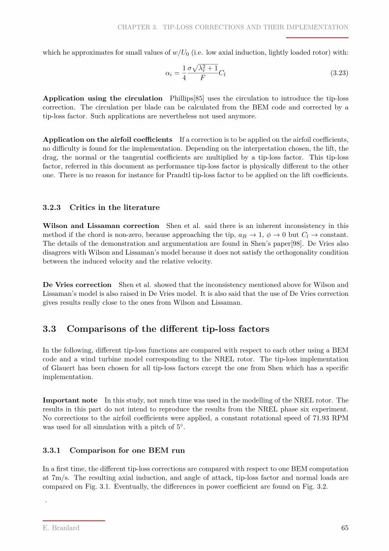
CHAPTER 3. TIP-LOSS CORRECTIONS AND THEIR IMPLEMENTATION
which he approximates for small values of w/U0 (i.e. low axial induction, lightly loaded rotor) with:
αi = 14σ√λ2r + 1F
Cl (3.23)
Application using the circulation Phillips[85] uses the circulation to introduce the tip-losscorrection. The circulation per blade can be calculated from the BEM code and corrected by atip-loss factor. Such applications are nevertheless not used anymore.
Application on the airfoil coefficients If a correction is to be applied on the airfoil coefficients,no difficulty is found for the implementation. Depending on the interpretation chosen, the lift, thedrag, the normal or the tangential coefficients are multiplied by a tip-loss factor. This tip-lossfactor, referred in this document as performance tip-loss factor is physically different to the otherone. There is no reason for instance for Prandtl tip-loss factor to be applied on the lift coefficients.
3.2.3 Critics in the literature
Wilson and Lissaman correction Shen et al. said there is an inherent inconsistency in thismethod if the chord is non-zero, because approaching the tip, aB → 1, φ → 0 but Cl → constant.The details of the demonstration and argumentation are found in Shen’s paper[98]. De Vries alsodisagrees with Wilson and Lissaman’s model because it does not satisfy the orthogonality conditionbetween the induced velocity and the relative velocity.
De Vries correction Shen et al. showed that the inconsistency mentioned above for Wilson andLissaman’s model is also raised in De Vries model. It is also said that the use of De Vries correctiongives results really close to the ones from Wilson and Lissaman.
3.3 Comparisons of the different tip-loss factors
In the following, different tip-loss functions are compared with respect to each other using a BEMcode and a wind turbine model corresponding to the NREL rotor. The tip-loss implementationof Glauert has been chosen for all tip-loss factors except the one from Shen which has a specificimplementation.
Important note In this study, not much time was used in the modelling of the NREL rotor. Theresults in this part do not intend to reproduce the results from the NREL phase six experiment.No corrections to the airfoil coefficients were applied, a constant rotational speed of 71.93 RPMwas used for all simulation with a pitch of 5.
3.3.1 Comparison for one BEM run
In a first time, the different tip-loss corrections are compared with respect to one BEM computationat 7m/s. The resulting axial induction, and angle of attack, tip-loss factor and normal loads arecompared on Fig. 3.1. Eventually, the differences in power coefficient are found on Fig. 3.2.
.
E. Branlard 65
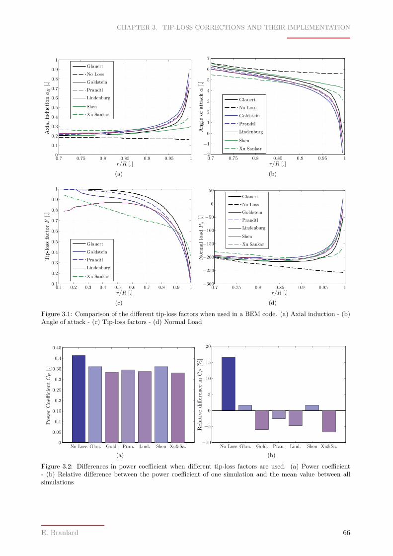
CHAPTER 3. TIP-LOSS CORRECTIONS AND THEIR IMPLEMENTATION
r/R [.]
AxialinductionaB
[.]
0.7 0.75 0.8 0.85 0.9 0.95 10
0.1
0.2
0.3
0.4
0.5
0.6
0.7
0.8
0.9
1
Glauert
No Loss
Goldstein
Prandtl
Lindenburg
Shen
Xu Sankar
(a)r/R [.]
Angle
ofattack
α[.]
0.7 0.75 0.8 0.85 0.9 0.95 1−2
−1
0
1
2
3
4
5
6
7
Glauert
No Loss
Goldstein
Prandtl
Lindenburg
Shen
Xu Sankar
(b)
r/R [.]
Tip-loss
factorF
[.]
0.1 0.2 0.3 0.4 0.5 0.6 0.7 0.8 0.9 10.1
0.2
0.3
0.4
0.5
0.6
0.7
0.8
0.9
1
Glauert
Goldstein
Prandtl
Lindenburg
Xu Sankar
(c)r/R [.]
Norm
alloadPn[.]
0.7 0.75 0.8 0.85 0.9 0.95 1−300
−250
−200
−150
−100
−50
0
50
Glauert
No Loss
Goldstein
Prandtl
Lindenburg
Shen
Xu Sankar
(d)
Figure 3.1: Comparison of the different tip-loss factors when used in a BEM code. (a) Axial induction - (b)Angle of attack - (c) Tip-loss factors - (d) Normal Load
Pow
erCoeffi
cientCP
[.]
No Loss Glau. Gold. Pran. Lind. Shen Xu&Sa.0
0.05
0.1
0.15
0.2
0.25
0.3
0.35
0.4
0.45
(a)
Relative
difference
inCP[%
]
No Loss Glau. Gold. Pran. Lind. Shen Xu&Sa.−10
−5
0
5
10
15
20
(b)
Figure 3.2: Differences in power coefficient when different tip-loss factors are used. (a) Power coefficient- (b) Relative difference between the power coefficient of one simulation and the mean value between allsimulations
E. Branlard 66
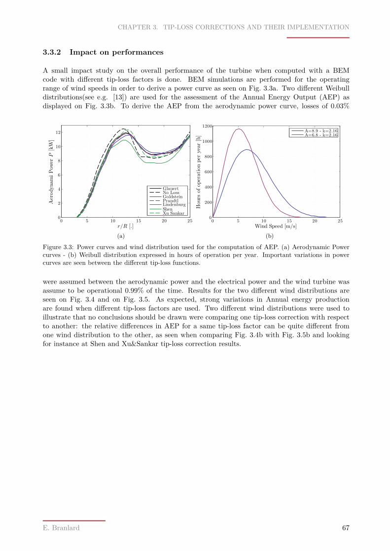
CHAPTER 3. TIP-LOSS CORRECTIONS AND THEIR IMPLEMENTATION
3.3.2 Impact on performances
A small impact study on the overall performance of the turbine when computed with a BEMcode with different tip-loss factors is done. BEM simulations are performed for the operatingrange of wind speeds in order to derive a power curve as seen on Fig. 3.3a. Two different Weibulldistributions(see e.g. [13]) are used for the assessment of the Annual Energy Output (AEP) asdisplayed on Fig. 3.3b. To derive the AEP from the aerodynamic power curve, losses of 0.03%
r/R [.]
AerodynamiPow
erP
[kW]
0 5 10 15 20 250
2
4
6
8
10
12
GlauertNo LossGoldsteinPrandtlLindenburgShenXu Sankar
(a)Wind Speed [m/s]
Hours
ofoperationper
year[h]
0 5 10 15 20 250
200
400
600
800
1000
1200A=8.9 - k=2.16A=6.8 - k=2.16
(b)
Figure 3.3: Power curves and wind distribution used for the computation of AEP. (a) Aerodynamic Powercurves - (b) Weibull distribution expressed in hours of operation per year. Important variations in powercurves are seen between the different tip-loss functions.
were assumed between the aerodynamic power and the electrical power and the wind turbine wasassume to be operational 0.99% of the time. Results for the two different wind distributions areseen on Fig. 3.4 and on Fig. 3.5. As expected, strong variations in Annual energy productionare found when different tip-loss factors are used. Two different wind distributions were used toillustrate that no conclusions should be drawn were comparing one tip-loss correction with respectto another: the relative differences in AEP for a same tip-loss factor can be quite different fromone wind distribution to the other, as seen when comparing Fig. 3.4b with Fig. 3.5b and lookingfor instance at Shen and Xu&Sankar tip-loss correction results.
E. Branlard 67
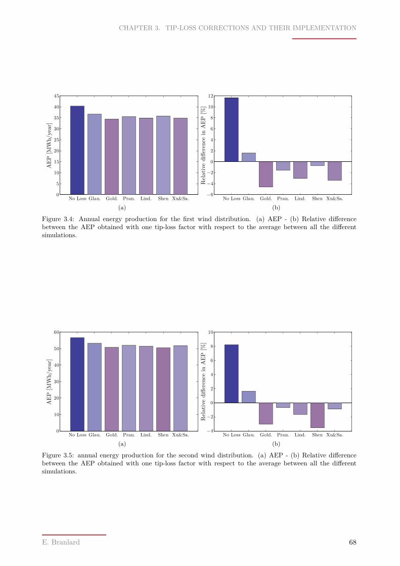
CHAPTER 3. TIP-LOSS CORRECTIONS AND THEIR IMPLEMENTATION
AEP
[MWh/year]
No Loss Glau. Gold. Pran. Lind. Shen Xu&Sa.0
5
10
15
20
25
30
35
40
45
(a)Relative
difference
inAEP
[%]
No Loss Glau. Gold. Pran. Lind. Shen Xu&Sa.−6
−4
−2
0
2
4
6
8
10
12
(b)
Figure 3.4: Annual energy production for the first wind distribution. (a) AEP - (b) Relative differencebetween the AEP obtained with one tip-loss factor with respect to the average between all the differentsimulations.
AEP
[MWh/year]
No Loss Glau. Gold. Pran. Lind. Shen Xu&Sa.0
10
20
30
40
50
60
(a)
Relative
difference
inAEP
[%]
No Loss Glau. Gold. Pran. Lind. Shen Xu&Sa.−4
−2
0
2
4
6
8
10
(b)
Figure 3.5: annual energy production for the second wind distribution. (a) AEP - (b) Relative differencebetween the AEP obtained with one tip-loss factor with respect to the average between all the differentsimulations.
E. Branlard 68
CHAPTER 3. TIP-LOSS CORRECTIONS AND THEIR IMPLEMENTATION
3.4 New applications and methods
3.4.1 Possible new applications using the Goldstein factor
With the method described in Sect. A.2, the computation of Goldstein’s factor is made at a reallylow computational cost and its use in BEM codes can be considered. The methods described below,and more certainly the second one, on how to implement the Goldstein’s factor in a BEM code,are not known by the author to be present in the literature. The reading of Sect. 2.1.2 is advisedfor the considerations of the following paragraphs.
Simplest method - FGo = FGo(λ,B) = FGo(l, B) In its original form, the tip loss factorfrom Prandtl, FPr,0 was a direct function of the tip-speed ratio λ (see Sect. 2.3.4). The samecan apply for the Goldstein function if Eq. (2.12) is used to relate the far-wake parameters to therotor parameters. This relation writes λ = 1/l, and it can be seen that under these conditions theGoldstein tip-loss factor FGo = BΓGo/Γ∞ is independent of w, and a function of λ and B only.Using the numerical method described in Sect. A.2 or the engineering fit provided in Sect. A.4, theGoldstein circulation ΓGo is computed. In this context the Betz circulation is
Γ∞ = 2πwU0Ω
λ2r
1 + λ2r
(3.24)
and the tip-loss factor is easily derived. This method was used for comparison of the Betz, Prandtland Goldstein circulation on Fig. 2.15.
Iterative method - FGo = FGo(λ,B,w) = FGo(l, B,w) Using Eq. (2.20) to relate the far-wakeparameters to the rotor parameters, then the Goldstein’s factor is not anymore linear in w and aniterative method must be used to compute the tip-losses. In its simpliest form, the method wouldbe:
1. Initialize w to 0. The computation of FGo = FGo(λ,B) reduces to the method described inthe previous paragraph, the dimensionless pitch is simply l = 1/λ.
2. Perform BEM computation using the previously computed tip loss factor.
3. Compute a value for w. Unlike the Betz theory, it is unlikely that the induction will beconstant along the span, and thus velocity of the wake w is not a constant anymore. Tomatch with the theory, w is kept a constant by defining it as e.g. the mean longitudinal wakeinduced velocity along the span3:
w =∫ Rw
0uiz,wdr → w ≈ 2
∫ R
0adr (3.25)
4. Compute a new value of l using Eq. (2.20):
l = 1λ
(1− w
2
)(3.26)
5. Compute the Goldstein circulation ΓGo = ΓGo(l, B,w) using the new values of l and w.3Other choice of relation than the mean can be considered
E. Branlard 69

CHAPTER 3. TIP-LOSS CORRECTIONS AND THEIR IMPLEMENTATION
6. To eventually compute the new tip-loss factor FGo = BΓGo/Γ∞, the Betz circulation is re-quired. For the simplicity of the model this circulation is taken in its simpliest form fromEq. (3.24) but more general formulation such as the one presented in Sect. 2.2 can be consid-ered.
7. Repeat steps 2-6 till the value of the pitch parameter l has converged.
The convergence of the process above is neither guaranteed nor enforced but the experience showedno divergence problem.
3.4.2 Further applications
In the following part of this study different methods to obtain and apply the tip-loss factor will bedeveloped. Each of these methods and their applicability will be described in their correspondingsections: chapter 4, chapter 5.
E. Branlard 70
Chapter 4Using a vortex code to investigate tip-losses
4.1 Approach description
4.1.1 Introduction
During the period of time accorded to this study, a vortex code has been implemented to furtherstudy tip-losses. Different vortex code versions have been implemented as described in Sect. B.1.The wake geometry can be prescribed, set free, or set as a combination of the two. The influencevelocities can be computed using line by line methods, or ring by ring methods. The blade can bemodelled using several rings elements along the chord, or just one ring element so that the codereduces to a simple lifting-line code. Examples of applications of these different variation of vortexcode and their validation can be found in Sect. B.2. In this section, the lifting-line version of thecode is used. The first portion of the wake is set free and is progressively forming behind the rotorjust like other unsteady free vortex code(e.g. AWSM[112]). Behind this free wake, a prescribedhelical wake is attached to model the far wake.
The interest of such a vortex code is that it intrinsically contains or models 3D effects such as tipvortices, wake roll-up and expansion. As a result of this, this code does not need to be correctedwith a tip-loss function as the BEM code. Contrarily, it can be used to determine the tip-lossfunction resulting from these 3D effects for further application in BEM codes. The methodologyused to perform this is described in the following paragraph.
4.1.2 Method description
In order to find tip-loss functions that could be used for BEM codes, a representative samples ofcharacteristics simulations need to be found. For this, the parameters expecting to influence thetip-loss function need to be found. The parameters selected are the circulation distribution alongthe blade and two “rotor state” parameters: the tip-speed ratio λ and the thrust coefficient CT .The number of blade B has a critical importance, but it is here chosen to restrict this study to threebladed wind turbines. The idea is then to determine tip-loss functions for representative sets ofthese parameters so that these tip-loss functions can then be used directly for a BEM simulationswhich corresponds to a set of these parameters. The question that remains is to find a way tocharacterize all the different shapes of circulation that can be found in wind energy. Obviouslyto parametrize a curve that varies along the blade, several parameters will have to be used. Thisspecific topic will be discussed in Sect. 4.2.
71
CHAPTER 4. USING A VORTEX CODE TO INVESTIGATE TIP-LOSSES
The vortex code can be run with a prescribed circulation, a defined tip-speed ratio and a definedgeometry. The geometry dependence obviously has to be dropped for generality, and a way tocircumvent the fact that the thrust coefficient is dependent on the circulation has to be found. Thegeometry dependence is only based on the rotor radius. The chord and twist distribution should nothave an influence on the lifting line code which reduces the blade to a simple segment. An existingwind turbine geometry will be used, with the rotor radius scaled to unity. All the simulation will berun with this generic rotor which makes the definition of the tip-speed ratio somehow independentof the rotor radius. The second step is to solve the problem of interdependence between the totalthrust coefficient and the circulation. To do this, the circulation as a parameter is normalized tounity. The thrust coefficient wanted for a given simulation will determine the multiplicative factorthat should be applied to the normalized-circulation. To find this multiplicative factor prior tothe vortex code simulation, a specific BEM code that takes as input a prescribed circulation wasimplemented. This BEM code uses no drag in his formulation according to the Kutta-Joukowskiformula, so that the lift coefficient is determined as:
Cl = 2ΓVrelc
(4.1)
An iterative procedure is used to find the multiplicative factor that should be applied to thenormalized-circulation so that the BEM code returns the desired thrust coefficient for the righttip-speed ratio and normalized-circulation shape. This multiplicative factor is then used as inputto the vortex code. At the end of the vortex code simulation, the thrust coefficient is computedto check if the right multiplicative constant was found. In all cases, the two thrust coefficientsmatched within less than 2% of error, hence validating the procedure.
Using the above approach, the vortex code was run for all the chosen characteristic sets of param-eters. For each simulation, the tip-loss function was computed according to Eq. (1.26):
F = 〈a〉aB
In a lifting-line code the definition of the rotor plane is rather simple as it indeed reduces to a planesurface or a coned-surface if the rotor is coned. In this case, the typical rotor chosen does not havea cone angle as the context of applicability for a BEM code is the 2D momentum theory1. Eachtip-loss function obtained is stored in a database for further use in a BEM code. The way thistip-loss function can be implemented in a BEM code is described in Sect. 4.3.3.
The advantages of such a method is that it will provide tip-loss functions more adapted to the rotorconfiguration than the specific and simplified function derived by Prandtl. This tip-loss functionincludes wake expansion effects, local aerodynamics on the blade, uses a realistic wake geometry(compared to the system of vortex planes of Prandtl). Other interesting aspects will be discussedin Sect. 4.3.3.
4.2 Family of circulation curves
In order to establish a database of tip-loss corrections for different family of circulation curves, aparametrization of these curves needs to be found.
1Of course, BEM codes are extended to coned rotor, but from the independence of the streamtube, the represen-tation behind it is as if all the annular segments of the coned rotor where in the same plane.
E. Branlard 72
CHAPTER 4. USING A VORTEX CODE TO INVESTIGATE TIP-LOSSES
4.2.1 Existing parametrization
In [33], a set of load cases are generated to study the aerodynamic performance of rotors withwinglets using a prescribed and a free wake code. The circulation is modelled at the tip and rootusing the form of Prandtl hub and tip-loss factor. Further, a spanwise linear variation of thecirculation is added to load the tip and the root in different ways. The model takes the form:
Γ = Ftip · Froot,Γlin (4.2)
with
Ftip = 2π
acos exp (−Ctip(1− r)) (4.3)
Froot =[ 2π
acos exp (−Crootr)]1.5
(4.4)
Γlin = rΓtip + (1− r)Γroot (4.5)
The author defines the constants as function of the tip-speed ratio and uses multiplicative constantsto define different load case scenarios. Examples of load cases as defined in the original reference[33]can be found on Fig. 4.1.
r/R [.]
Γ[m
2/s]
0 0.1 0.2 0.3 0.4 0.5 0.6 0.7 0.8 0.9 10
0.05
0.1
0.15
0.2
0.25
0.3
0.35
HighMediumLowLow-HighHigh-Low
(a)r/R [.]
Γ[m
2/s]
0 0.1 0.2 0.3 0.4 0.5 0.6 0.7 0.8 0.9 10
0.01
0.02
0.03
0.04
0.05
0.06
0.07
0.08
0.09
0.1
HighMediumLowLow-HighHigh-Low
(b)
Figure 4.1: Different circulation translating different loading cases for two different tip-speed ratios. Themodel from [33] has been used. The constants in Eq. (4.2) have been determined in the same way thanthe original author to define the different loading cases: High, Medium, Low, High-Low and Low-High. (a)λ = 3 - (b) λ = 10
4.2.2 Parametrization using Bézier curves
Examples of modelled circulation have been seen on Fig. 4.1 and more examples from existingblades can be found on Fig. 4.4. From the variety of shapes the circulation curve can take, anexplicit mathematical formalism is hard to find to parametrize all of them. From the knowledgeof Bézier curve, it has been decided to develop a curve-fitting method to parametrize circulationcurves using this formalism. The formalism of Bézier curve is attributed and named after Frenchengineer Pierre Bézier who used them for the body design of the Renault car in the 1970’s. Sincethen, they have been used by the drawing industry for fonts and vectorial drawing. The parametric
E. Branlard 73
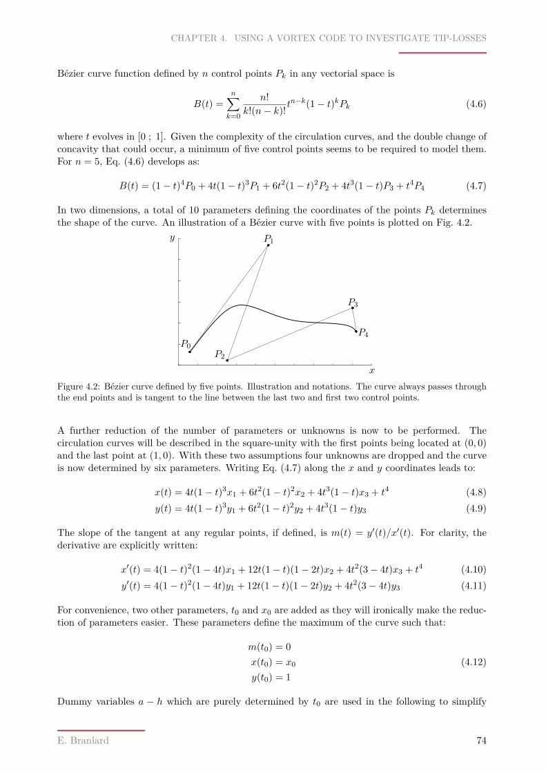
CHAPTER 4. USING A VORTEX CODE TO INVESTIGATE TIP-LOSSES
Bézier curve function defined by n control points Pk in any vectorial space is
B(t) =n∑k=0
n!k!(n− k)! t
n−k(1− t)kPk (4.6)
where t evolves in [0 ; 1]. Given the complexity of the circulation curves, and the double change ofconcavity that could occur, a minimum of five control points seems to be required to model them.For n = 5, Eq. (4.6) develops as:
B(t) = (1− t)4P0 + 4t(1− t)3P1 + 6t2(1− t)2P2 + 4t3(1− t)P3 + t4P4 (4.7)
In two dimensions, a total of 10 parameters defining the coordinates of the points Pk determinesthe shape of the curve. An illustration of a Bézier curve with five points is plotted on Fig. 4.2.
P0
P1
P2
P3
P4
x
y
Figure 4.2: Bézier curve defined by five points. Illustration and notations. The curve always passes throughthe end points and is tangent to the line between the last two and first two control points.
A further reduction of the number of parameters or unknowns is now to be performed. Thecirculation curves will be described in the square-unity with the first points being located at (0, 0)and the last point at (1, 0). With these two assumptions four unknowns are dropped and the curveis now determined by six parameters. Writing Eq. (4.7) along the x and y coordinates leads to:
x(t) = 4t(1− t)3x1 + 6t2(1− t)2x2 + 4t3(1− t)x3 + t4 (4.8)y(t) = 4t(1− t)3y1 + 6t2(1− t)2y2 + 4t3(1− t)y3 (4.9)
The slope of the tangent at any regular points, if defined, is m(t) = y′(t)/x′(t). For clarity, thederivative are explicitly written:
x′(t) = 4(1− t)2(1− 4t)x1 + 12t(1− t)(1− 2t)x2 + 4t2(3− 4t)x3 + t4 (4.10)y′(t) = 4(1− t)2(1− 4t)y1 + 12t(1− t)(1− 2t)y2 + 4t2(3− 4t)y3 (4.11)
For convenience, two other parameters, t0 and x0 are added as they will ironically make the reduc-tion of parameters easier. These parameters define the maximum of the curve such that:
m(t0) = 0x(t0) = x0 (4.12)y(t0) = 1
Dummy variables a − h which are purely determined by t0 are used in the following to simplify
E. Branlard 74
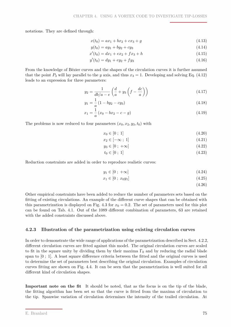
CHAPTER 4. USING A VORTEX CODE TO INVESTIGATE TIP-LOSSES
notations. They are defined through:
x(t0) = ax1 + bx2 + cx3 + g (4.13)y(t0) = ay1 + by2 + cy3 (4.14)x′(t0) = dx1 + ex2 + fx3 + h (4.15)y′(t0) = dy1 + ey2 + fy3 (4.16)
From the knowledge of Bézier curves and the shapes of the circulation curves it is further assumedthat the point P3 will lay parallel to the y axis, and thus x3 = 1. Developing and solving Eq. (4.12)leads to an expression for three parameters:
y2 = 1db/a− e
(d
a+ y3
(f − dc
a
))(4.17)
y1 = 1a
(1− by2 − cy3) (4.18)
x1 = 1a
(x0 − bx2 − c− g) (4.19)
The problems is now reduced to four parameters (x0, x2, y3, t0) with
x0 ∈ [0 ; 1] (4.20)x2 ∈ [−∞ ; 1] (4.21)y3 ∈ [0 ; +∞] (4.22)t0 ∈ [0 ; 1] (4.23)
Reduction constraints are added in order to reproduce realistic curves:
y1 ∈ [0 ; +∞] (4.24)x1 ∈ [0 ; x0y1] (4.25)
(4.26)
Other empirical constraints have been added to reduce the number of parameters sets based on thefitting of existing circulations. An example of the different curve shapes that can be obtained withthis parametrization is displayed on Fig. 4.3 for x0 = 0.2. The set of parameters used for this plotcan be found on Tab. 4.1. Out of the 1089 different combination of parameters, 63 are retainedwith the added constraints discussed above.
4.2.3 Illustration of the parametrization using existing circulation curves
In order to demonstrate the wide range of applications of the parametrization described in Sect. 4.2.2,different circulation curves are fitted against this model. The original circulation curves are scaledto fit in the square unity by dividing them by their maxima Γ0 and by reducing the radial bladespan to [0 ; 1]. A least square difference criteria between the fitted and the original curves is usedto determine the set of parameters best describing the original circulation. Examples of circulationcurves fitting are shown on Fig. 4.4. It can be seen that the parametrization is well suited for alldifferent kind of circulation shapes.
Important note on the fit It should be noted, that as the focus is on the tip of the blade,the fitting algorithm has been set so that the curve is fitted from the maxima of circulation tothe tip. Spanwise variation of circulation determines the intensity of the trailed circulation. At
E. Branlard 75
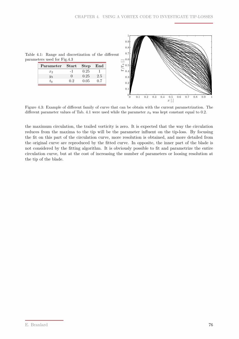
CHAPTER 4. USING A VORTEX CODE TO INVESTIGATE TIP-LOSSES
Table 4.1: Range and discretization of the differentparameters used for Fig.4.3
Parameter Start Step Endx2 -1 0.25 1y3 0 0.25 2.5t0 0.2 0.05 0.7
x [.]
Γ/Γ0[.]
0 0.1 0.2 0.3 0.4 0.5 0.6 0.7 0.8 0.9 10
0.1
0.2
0.3
0.4
0.5
0.6
0.7
0.8
0.9
1
Figure 4.3: Example of different family of curve that can be obtain with the current parametrization. Thedifferent parameter values of Tab. 4.1 were used while the parameter x0 was kept constant equal to 0.2.
the maximum circulation, the trailed vorticity is zero. It is expected that the way the circulationreduces from the maxima to the tip will be the parameter influent on the tip-loss. By focusingthe fit on this part of the circulation curve, more resolution is obtained, and more detailed fromthe original curve are reproduced by the fitted curve. In opposite, the inner part of the blade isnot considered by the fitting algorithm. It is obviously possible to fit and parametrize the entirecirculation curve, but at the cost of increasing the number of parameters or loosing resolution atthe tip of the blade.
E. Branlard 76
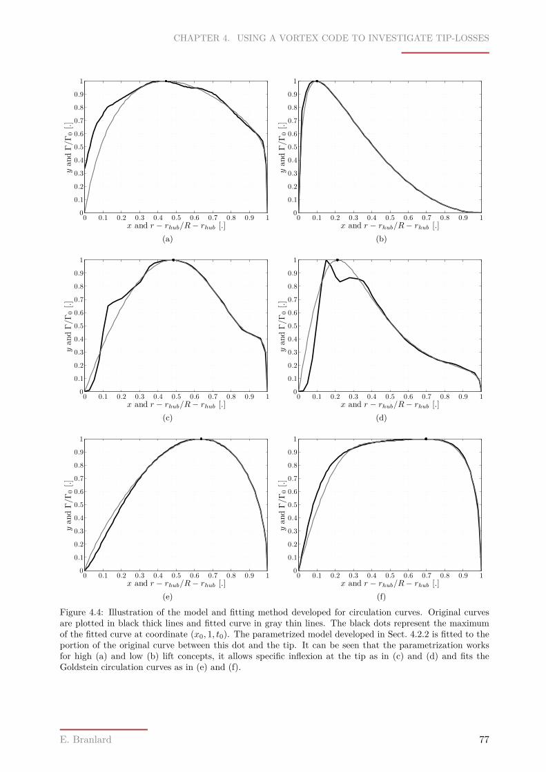
CHAPTER 4. USING A VORTEX CODE TO INVESTIGATE TIP-LOSSES
x and r − rhub/R− rhub [.]
yandΓ/Γ0[.]
0 0.1 0.2 0.3 0.4 0.5 0.6 0.7 0.8 0.9 10
0.1
0.2
0.3
0.4
0.5
0.6
0.7
0.8
0.9
1
(a)x and r − rhub/R− rhub [.]
yandΓ/Γ0[.]
0 0.1 0.2 0.3 0.4 0.5 0.6 0.7 0.8 0.9 10
0.1
0.2
0.3
0.4
0.5
0.6
0.7
0.8
0.9
1
(b)
x and r − rhub/R− rhub [.]
yandΓ/Γ0[.]
0 0.1 0.2 0.3 0.4 0.5 0.6 0.7 0.8 0.9 10
0.1
0.2
0.3
0.4
0.5
0.6
0.7
0.8
0.9
1
(c)x and r − rhub/R− rhub [.]
yandΓ/Γ0[.]
0 0.1 0.2 0.3 0.4 0.5 0.6 0.7 0.8 0.9 10
0.1
0.2
0.3
0.4
0.5
0.6
0.7
0.8
0.9
1
(d)
x and r − rhub/R− rhub [.]
yandΓ/Γ0[.]
0 0.1 0.2 0.3 0.4 0.5 0.6 0.7 0.8 0.9 10
0.1
0.2
0.3
0.4
0.5
0.6
0.7
0.8
0.9
1
(e)x and r − rhub/R− rhub [.]
yandΓ/Γ0[.]
0 0.1 0.2 0.3 0.4 0.5 0.6 0.7 0.8 0.9 10
0.1
0.2
0.3
0.4
0.5
0.6
0.7
0.8
0.9
1
(f)
Figure 4.4: Illustration of the model and fitting method developed for circulation curves. Original curvesare plotted in black thick lines and fitted curve in gray thin lines. The black dots represent the maximumof the fitted curve at coordinate (x0, 1, t0). The parametrized model developed in Sect. 4.2.2 is fitted to theportion of the original curve between this dot and the tip. It can be seen that the parametrization worksfor high (a) and low (b) lift concepts, it allows specific inflexion at the tip as in (c) and (d) and fits theGoldstein circulation curves as in (e) and (f).
E. Branlard 77
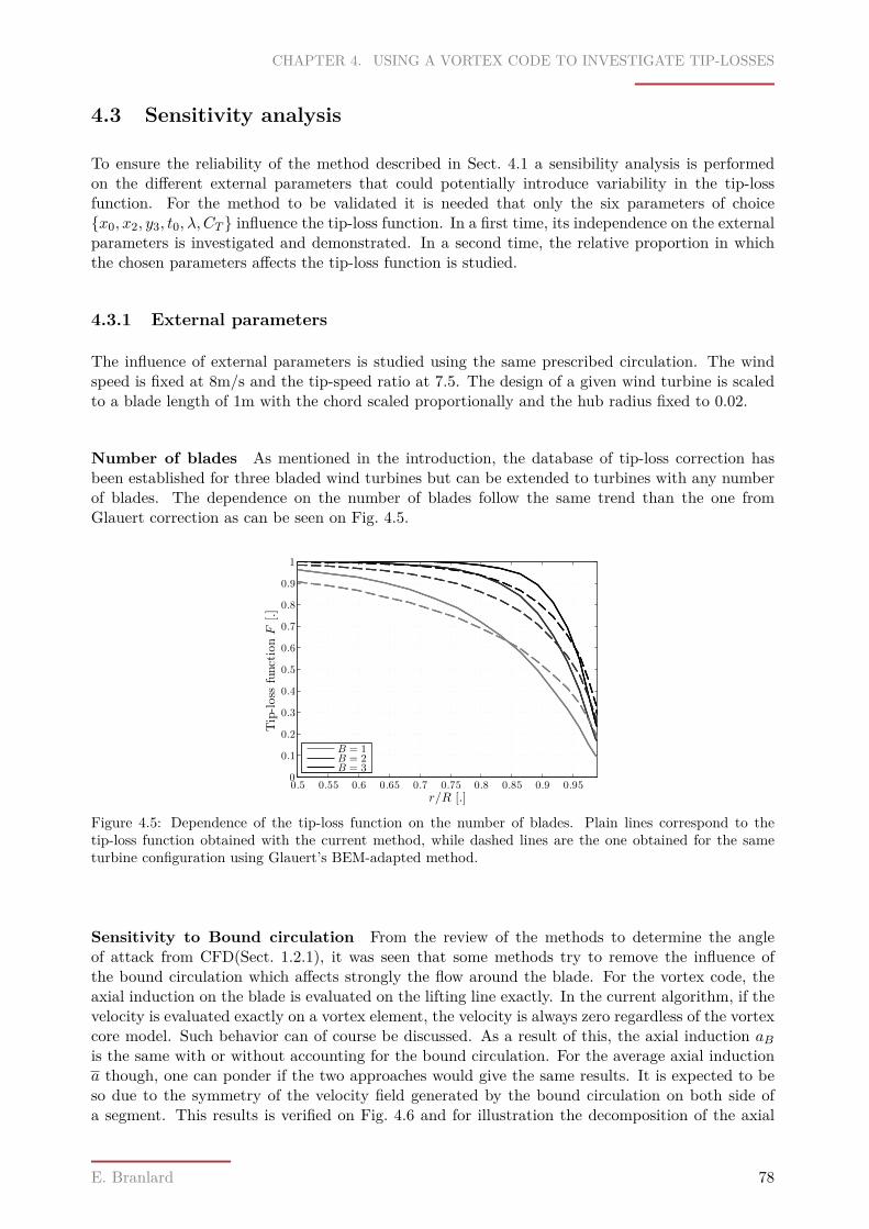
CHAPTER 4. USING A VORTEX CODE TO INVESTIGATE TIP-LOSSES
4.3 Sensitivity analysis
To ensure the reliability of the method described in Sect. 4.1 a sensibility analysis is performedon the different external parameters that could potentially introduce variability in the tip-lossfunction. For the method to be validated it is needed that only the six parameters of choicex0, x2, y3, t0, λ, CT influence the tip-loss function. In a first time, its independence on the externalparameters is investigated and demonstrated. In a second time, the relative proportion in whichthe chosen parameters affects the tip-loss function is studied.
4.3.1 External parameters
The influence of external parameters is studied using the same prescribed circulation. The windspeed is fixed at 8m/s and the tip-speed ratio at 7.5. The design of a given wind turbine is scaledto a blade length of 1m with the chord scaled proportionally and the hub radius fixed to 0.02.
Number of blades As mentioned in the introduction, the database of tip-loss correction hasbeen established for three bladed wind turbines but can be extended to turbines with any numberof blades. The dependence on the number of blades follow the same trend than the one fromGlauert correction as can be seen on Fig. 4.5.
r/R [.]
Tip-loss
functionF
[.]
0.5 0.55 0.6 0.65 0.7 0.75 0.8 0.85 0.9 0.950
0.1
0.2
0.3
0.4
0.5
0.6
0.7
0.8
0.9
1
B = 1B = 2B = 3
Figure 4.5: Dependence of the tip-loss function on the number of blades. Plain lines correspond to thetip-loss function obtained with the current method, while dashed lines are the one obtained for the sameturbine configuration using Glauert’s BEM-adapted method.
Sensitivity to Bound circulation From the review of the methods to determine the angleof attack from CFD(Sect. 1.2.1), it was seen that some methods try to remove the influence ofthe bound circulation which affects strongly the flow around the blade. For the vortex code, theaxial induction on the blade is evaluated on the lifting line exactly. In the current algorithm, if thevelocity is evaluated exactly on a vortex element, the velocity is always zero regardless of the vortexcore model. Such behavior can of course be discussed. As a result of this, the axial induction aBis the same with or without accounting for the bound circulation. For the average axial inductiona though, one can ponder if the two approaches would give the same results. It is expected to beso due to the symmetry of the velocity field generated by the bound circulation on both side ofa segment. This results is verified on Fig. 4.6 and for illustration the decomposition of the axial
E. Branlard 78
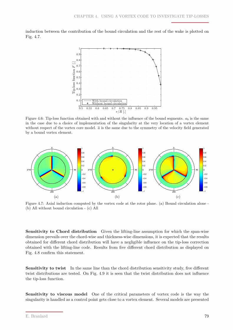
CHAPTER 4. USING A VORTEX CODE TO INVESTIGATE TIP-LOSSES
induction between the contribution of the bound circulation and the rest of the wake is plotted onFig. 4.7.
r/R [.]
Tip-loss
functionF
[.]
0.5 0.55 0.6 0.65 0.7 0.75 0.8 0.85 0.9 0.950
0.1
0.2
0.3
0.4
0.5
0.6
0.7
0.8
0.9
1
With bound circulationWithout bound circulation
Figure 4.6: Tip-loss function obtained with and without the influence of the bound segments. ab is the samein the case due to a choice of implementation of the singularity at the very location of a vortex elementwithout respect of the vortex core model. a is the same due to the symmetry of the velocity field generatedby a bound vortex element.
0
270
180
90
−1
−0.8
−0.6
−0.4
−0.2
0
0.2
0.4
0.6
0.8
1
(a)
0
270
180
90
−1
−0.8
−0.6
−0.4
−0.2
0
0.2
0.4
0.6
0.8
1
(b)
0
270
180
90
−1
−0.8
−0.6
−0.4
−0.2
0
0.2
0.4
0.6
0.8
1
(c)
Figure 4.7: Axial induction computed by the vortex code at the rotor plane. (a) Bound circulation alone -(b) All without bound circulation - (c) All
Sensitivity to Chord distribution Given the lifting-line assumption for which the span-wisedimension prevails over the chord-wise and thickness-wise dimensions, it is expected that the resultsobtained for different chord distribution will have a negligible influence on the tip-loss correctionobtained with the lifting-line code. Results from five different chord distribution as displayed onFig. 4.8 confirm this statement.
Sensitivity to twist In the same line than the chord distribution sensitivity study, five differenttwist distributions are tested. On Fig. 4.9 it is seen that the twist distribution does not influencethe tip-loss function.
Sensitivity to viscous model One of the critical parameters of vortex code is the way thesingularity is handled as a control point gets close to a vortex element. Several models are presented
E. Branlard 79
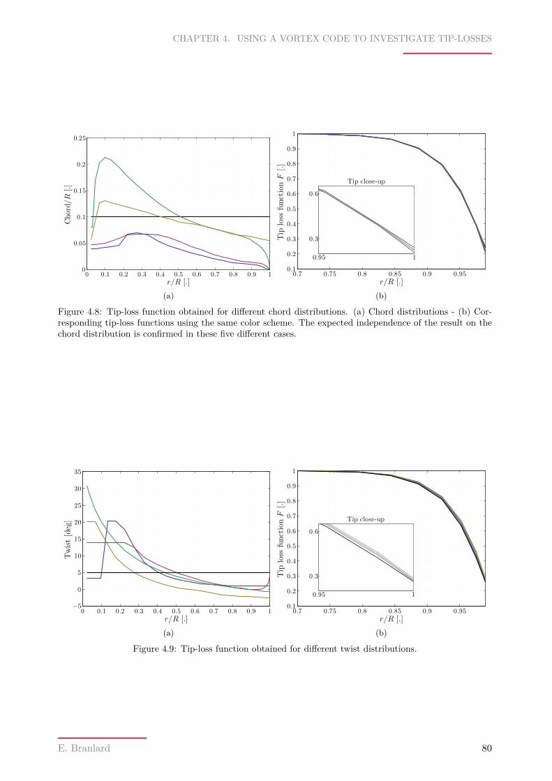
CHAPTER 4. USING A VORTEX CODE TO INVESTIGATE TIP-LOSSES
r/R [.]
Chord/R
[.]
0 0.1 0.2 0.3 0.4 0.5 0.6 0.7 0.8 0.9 10
0.05
0.1
0.15
0.2
0.25
(a)r/R [.]
Tip
loss
functionF
[.]
0.7 0.75 0.8 0.85 0.9 0.950.1
0.2
0.3
0.4
0.5
0.6
0.7
0.8
0.9
1
Tip close-up
0.95 1
0.3
0.6
(b)
Figure 4.8: Tip-loss function obtained for different chord distributions. (a) Chord distributions - (b) Cor-responding tip-loss functions using the same color scheme. The expected independence of the result on thechord distribution is confirmed in these five different cases.
r/R [.]
Twist[deg]
0 0.1 0.2 0.3 0.4 0.5 0.6 0.7 0.8 0.9 1−5
0
5
10
15
20
25
30
35
(a)r/R [.]
Tip
loss
functionF
[.]
0.7 0.75 0.8 0.85 0.9 0.950.1
0.2
0.3
0.4
0.5
0.6
0.7
0.8
0.9
1
Tip close-up
0.95 1
0.3
0.6
(b)
Figure 4.9: Tip-loss function obtained for different twist distributions.
E. Branlard 80
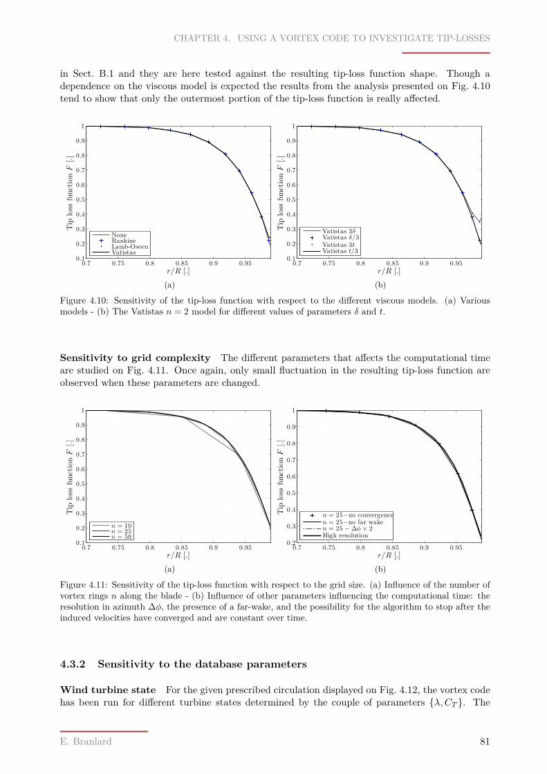
CHAPTER 4. USING A VORTEX CODE TO INVESTIGATE TIP-LOSSES
in Sect. B.1 and they are here tested against the resulting tip-loss function shape. Though adependence on the viscous model is expected the results from the analysis presented on Fig. 4.10tend to show that only the outermost portion of the tip-loss function is really affected.
r/R [.]
Tip
loss
functionF
[.]
0.7 0.75 0.8 0.85 0.9 0.950.1
0.2
0.3
0.4
0.5
0.6
0.7
0.8
0.9
1
NoneRankineLamb-OseenVatistas
(a)r/R [.]
Tip
loss
functionF
[.]
0.7 0.75 0.8 0.85 0.9 0.950.1
0.2
0.3
0.4
0.5
0.6
0.7
0.8
0.9
1
Vatistas 3δVatistas δ/3Vatistas 3tVatistas t/3
(b)
Figure 4.10: Sensitivity of the tip-loss function with respect to the different viscous models. (a) Variousmodels - (b) The Vatistas n = 2 model for different values of parameters δ and t.
Sensitivity to grid complexity The different parameters that affects the computational timeare studied on Fig. 4.11. Once again, only small fluctuation in the resulting tip-loss function areobserved when these parameters are changed.
r/R [.]
Tip
loss
functionF
[.]
0.7 0.75 0.8 0.85 0.9 0.950.1
0.2
0.3
0.4
0.5
0.6
0.7
0.8
0.9
1
n = 10n = 25n = 50
(a)r/R [.]
Tip
loss
functionF
[.]
0.7 0.75 0.8 0.85 0.9 0.950.2
0.3
0.4
0.5
0.6
0.7
0.8
0.9
1
n = 25−no convergencen = 25−no far waken = 25 − ∆φ × 2High resolution
(b)
Figure 4.11: Sensitivity of the tip-loss function with respect to the grid size. (a) Influence of the number ofvortex rings n along the blade - (b) Influence of other parameters influencing the computational time: theresolution in azimuth ∆φ, the presence of a far-wake, and the possibility for the algorithm to stop after theinduced velocities have converged and are constant over time.
4.3.2 Sensitivity to the database parameters
Wind turbine state For the given prescribed circulation displayed on Fig. 4.12, the vortex codehas been run for different turbine states determined by the couple of parameters λ,CT . The
E. Branlard 81
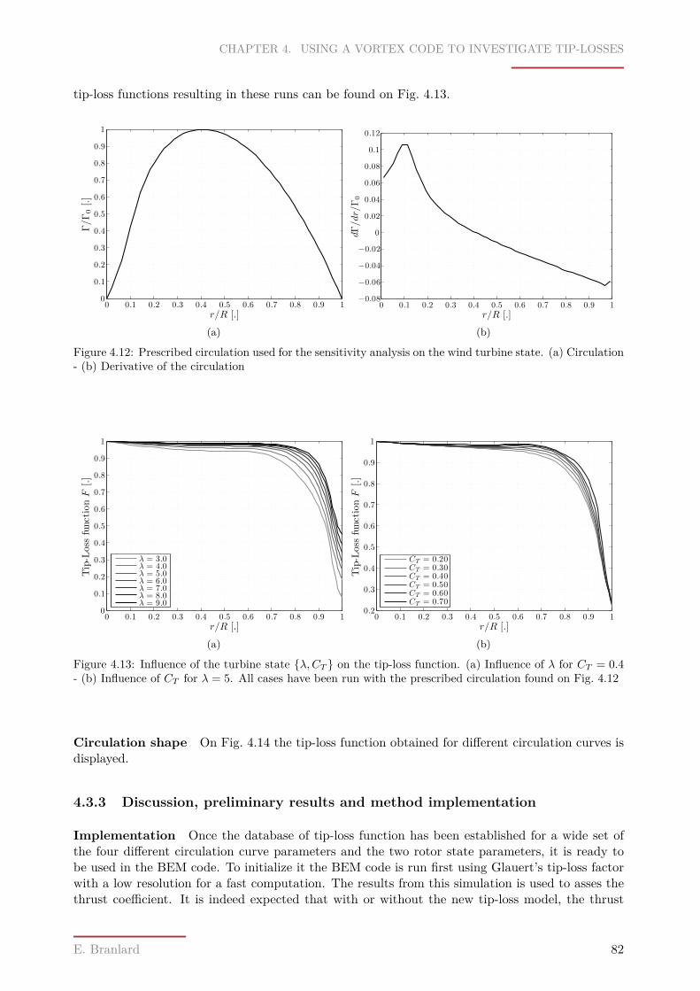
CHAPTER 4. USING A VORTEX CODE TO INVESTIGATE TIP-LOSSES
tip-loss functions resulting in these runs can be found on Fig. 4.13.
r/R [.]
Γ/Γ0[.]
0 0.1 0.2 0.3 0.4 0.5 0.6 0.7 0.8 0.9 10
0.1
0.2
0.3
0.4
0.5
0.6
0.7
0.8
0.9
1
(a)r/R [.]
dΓ/dr/
Γ0
0 0.1 0.2 0.3 0.4 0.5 0.6 0.7 0.8 0.9 1−0.08
−0.06
−0.04
−0.02
0
0.02
0.04
0.06
0.08
0.1
0.12
(b)
Figure 4.12: Prescribed circulation used for the sensitivity analysis on the wind turbine state. (a) Circulation- (b) Derivative of the circulation
r/R [.]
Tip-Loss
functionF
[.]
0 0.1 0.2 0.3 0.4 0.5 0.6 0.7 0.8 0.9 10
0.1
0.2
0.3
0.4
0.5
0.6
0.7
0.8
0.9
1
λ = 3.0λ = 4.0λ = 5.0λ = 6.0λ = 7.0λ = 8.0λ = 9.0
(a)r/R [.]
Tip-Loss
functionF
[.]
0 0.1 0.2 0.3 0.4 0.5 0.6 0.7 0.8 0.9 10.2
0.3
0.4
0.5
0.6
0.7
0.8
0.9
1
CT = 0.20CT = 0.30CT = 0.40CT = 0.50CT = 0.60CT = 0.70
(b)
Figure 4.13: Influence of the turbine state λ,CT on the tip-loss function. (a) Influence of λ for CT = 0.4- (b) Influence of CT for λ = 5. All cases have been run with the prescribed circulation found on Fig. 4.12
Circulation shape On Fig. 4.14 the tip-loss function obtained for different circulation curves isdisplayed.
4.3.3 Discussion, preliminary results and method implementation
Implementation Once the database of tip-loss function has been established for a wide set ofthe four different circulation curve parameters and the two rotor state parameters, it is ready tobe used in the BEM code. To initialize it the BEM code is run first using Glauert’s tip-loss factorwith a low resolution for a fast computation. The results from this simulation is used to asses thethrust coefficient. It is indeed expected that with or without the new tip-loss model, the thrust
E. Branlard 82
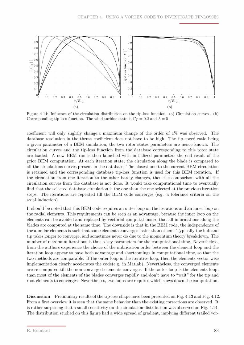
CHAPTER 4. USING A VORTEX CODE TO INVESTIGATE TIP-LOSSES
r/R [.]
Γ/Γ0[.]
0 0.1 0.2 0.3 0.4 0.5 0.6 0.7 0.8 0.9 10
0.1
0.2
0.3
0.4
0.5
0.6
0.7
0.8
0.9
1
(a)r/R [.]
Tip-Loss
functionF
[.]
0 0.1 0.2 0.3 0.4 0.5 0.6 0.7 0.8 0.9 10.1
0.2
0.3
0.4
0.5
0.6
0.7
0.8
0.9
1
(b)
Figure 4.14: Influence of the circulation distribution on the tip-loss function. (a) Circulation curves - (b)Corresponding tip-loss function. The wind turbine state is CT = 0.2 and λ = 5
coefficient will only slightly change:a maximum change of the order of 1% was observed. Thedatabase resolution in the thrust coefficient does not have to be high. The tip-speed ratio beinga given parameter of a BEM simulation, the two rotor states parameters are hence known. Thecirculation curves and the tip-loss function from the database corresponding to this rotor stateare loaded. A new BEM run is then launched with initialized parameters the end result of theprior BEM computation. At each iteration state, the circulation along the blade is compared toall the circulations curves present in the database. The closest one to the current BEM circulationis retained and the corresponding database tip-loss function is used for this BEM iteration. Ifthe circulation from one iteration to the other barely changes, then the comparison with all thecirculation curves from the database is not done. It would take computational time to eventuallyfind that the selected database circulation is the one than the one selected at the previous iterationsteps. The iterations are repeated till the BEM code converges (e.g. a tolerance criteria on theaxial induction).
It should be noted that this BEM code requires an outer loop on the iterations and an inner loop onthe radial elements. This requirements can be seen as an advantage, because the inner loop on theelements can be avoided and replaced by vectorial computations so that all informations along theblades are computed at the same time. The downside is that in the BEM code, the independence ofthe annular elements is such that some elements converges faster than others. Typically the hub andtip takes longer to converge, and sometimes never do due to the momentum theory breakdown. Thenumber of maximum iterations is thus a key parameters for the computational time. Nevertheless,from the authors experience the choice of the imbrication order between the element loop and theiteration loop appear to have both advantage and shortcomings in computational time, so that thetwo methods are comparable. If the outer loop is the iterative loop, then the elements vector-wiseimplementation clearly accelerates the code(e.g. in Matlab). Nevertheless, the converged elementsare re-computed till the non-converged elements converges. If the outer loop is the elements loop,than most of the elements of the blades converges rapidly and don’t have to “wait” for the tip androot elements to converges. Nevertheless, two loops are requires which slows down the computation.
Discussion Preliminary results of the tip-loss shape have been presented on Fig. 4.13 and Fig. 4.12.From a first overview it is seen that the same behavior than the existing corrections are observed. Itis rather surprising that a small sensitivity on the circulation distribution was observed on Fig. 4.14.The distribution studied on this figure had a wide spread of gradient, implying different trailed vor-
E. Branlard 83
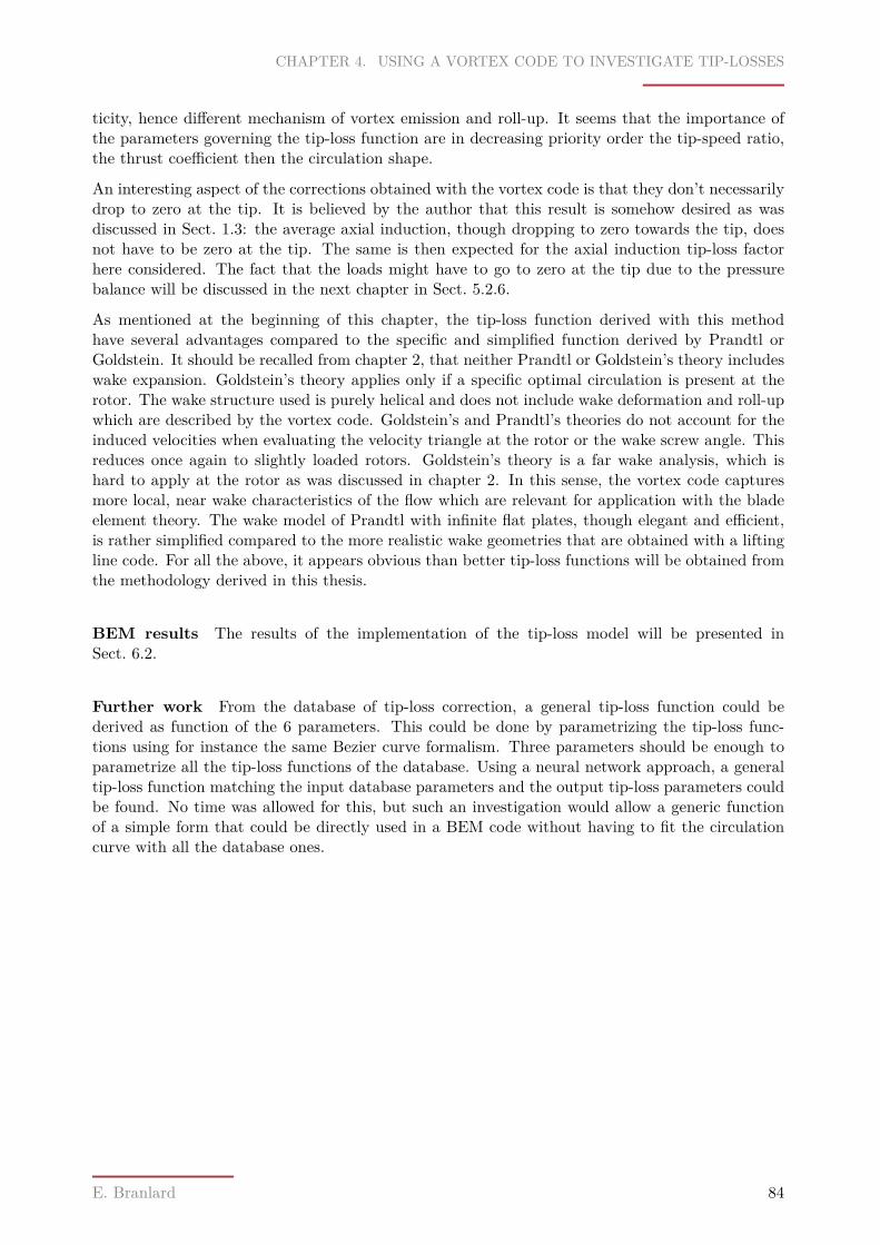
CHAPTER 4. USING A VORTEX CODE TO INVESTIGATE TIP-LOSSES
ticity, hence different mechanism of vortex emission and roll-up. It seems that the importance ofthe parameters governing the tip-loss function are in decreasing priority order the tip-speed ratio,the thrust coefficient then the circulation shape.
An interesting aspect of the corrections obtained with the vortex code is that they don’t necessarilydrop to zero at the tip. It is believed by the author that this result is somehow desired as wasdiscussed in Sect. 1.3: the average axial induction, though dropping to zero towards the tip, doesnot have to be zero at the tip. The same is then expected for the axial induction tip-loss factorhere considered. The fact that the loads might have to go to zero at the tip due to the pressurebalance will be discussed in the next chapter in Sect. 5.2.6.
As mentioned at the beginning of this chapter, the tip-loss function derived with this methodhave several advantages compared to the specific and simplified function derived by Prandtl orGoldstein. It should be recalled from chapter 2, that neither Prandtl or Goldstein’s theory includeswake expansion. Goldstein’s theory applies only if a specific optimal circulation is present at therotor. The wake structure used is purely helical and does not include wake deformation and roll-upwhich are described by the vortex code. Goldstein’s and Prandtl’s theories do not account for theinduced velocities when evaluating the velocity triangle at the rotor or the wake screw angle. Thisreduces once again to slightly loaded rotors. Goldstein’s theory is a far wake analysis, which ishard to apply at the rotor as was discussed in chapter 2. In this sense, the vortex code capturesmore local, near wake characteristics of the flow which are relevant for application with the bladeelement theory. The wake model of Prandtl with infinite flat plates, though elegant and efficient,is rather simplified compared to the more realistic wake geometries that are obtained with a liftingline code. For all the above, it appears obvious than better tip-loss functions will be obtained fromthe methodology derived in this thesis.
BEM results The results of the implementation of the tip-loss model will be presented inSect. 6.2.
Further work From the database of tip-loss correction, a general tip-loss function could bederived as function of the 6 parameters. This could be done by parametrizing the tip-loss func-tions using for instance the same Bezier curve formalism. Three parameters should be enough toparametrize all the tip-loss functions of the database. Using a neural network approach, a generaltip-loss function matching the input database parameters and the output tip-loss parameters couldbe found. No time was allowed for this, but such an investigation would allow a generic functionof a simple form that could be directly used in a BEM code without having to fit the circulationcurve with all the database ones.
E. Branlard 84
Chapter 5Using CFD to investigate tip-losses
5.1 Tip-losses and axial induction
5.1.1 Introduction
The first approach considered here is the definition of the tip-loss factor in terms of axial inductionas described in Sect. 1.3.2, Eq. (1.26):
Fa = a
aB
with a the azimuthally averaged axial induction defined by Eq. (1.3) and aB the axial induction onthe blade which is here to be defined. In case of a lifting line code indeed it is possible to define theaxial induction on the blade by computing the induced velocity on the lifting line. Such methodis not possible with CFD data and a way to reduce the complex velocity field around the blade toone value has to be determined.
5.1.2 Data available and methods investigated
For a single CFD simulation case1, 3D velocity fields have been outputted in different planes parallelto the rotor plane. Due to the assumed symmetry of the flow only the sector of 120sectors con-taining one of the three blades is used. These planes are located at distances −3.3,−1.3, 1.3, 3.3from the rotor plane where the lengths are expressed in % of the blade radius, and counting neg-ative values for upstream locations. For a rotor radius R of 60m this corresponds to locations−2.0,−0.8, 0.8, 2.0m. Using the velocity fields of two planes located symmetrically with respectto the rotor plane, an estimate of the tip-loss factor at the rotor is sought. The velocity field inthe rotor plane is assumed to be the average of the velocity field in the two surrounding planes(seea scheme of the planes on Fig. 5.1a). The flow field at the rotor plane can not be determinedotherwise due to the presence of the blade and the fast variation of the flow around the blade.This first averaging smears out the complex longitudinal variation of the flow and a can now becomputed. This method to determine the axial induction can be seen as a simple version of theone suggest in [48] that was discussed in Sect. 1.2.1.
To determine aB a second averaging needs to be performed to account for the spatial extent of theblade projected in the rotor plane. The three methods suggested and studied here are illustrated onFig. 5.1b where the dark-gray area represents the area over which the axial induction is averaged to
1Blade 1, three-bladed rotor, 12rpm and 10m/s
85
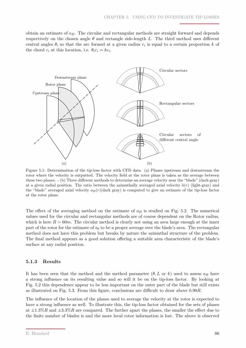
CHAPTER 5. USING CFD TO INVESTIGATE TIP-LOSSES
obtain an estimate of aB. The circular and rectangular methods are straight forward and dependsrespectively on the chosen angle θ and rectangle side-length L. The third method uses differentcentral angles θi so that the arc formed at a given radius ri is equal to a certain proportion k ofthe chord ci at this location, i.e. θiri = kci.
Upstream plane
Downstream plane
Rotor plane
(a)
Rectangular sectors
Circular sectors
Circular sectors ofdifferent central angle
(b)
Figure 5.1: Determination of the tip-loss factor with CFD data. (a) Planes upstream and downstream therotor where the velocity is outputted. The velocity field at the rotor plane is taken as the average betweenthese two planes. - (b) Three different methods to determine an average velocity near the “blade” (dark-gray)at a given radial position. The ratio between the azimuthally averaged axial velocity a(r) (light-gray) andthe “blade” averaged axial velocity aB(r)(dark gray) is computed to give an estimate of the tip-loss factorat the rotor plane.
The effect of the averaging method on the estimate of aB is studied on Fig. 5.2. The numericalvalues used for the circular and rectangular methods are of course dependent on the Rotor radius,which is here R = 60m. The circular method is clearly not using an area large enough at the innerpart of the rotor for the estimate of ab to be a proper average over the blade’s area. The rectangularmethod does not have this problem but breaks by nature the azimuthal structure of the problem.The final method appears as a good solution offering a suitable area characteristic of the blade’ssurface at any radial position.
5.1.3 Results
It has been seen that the method and the method parameter (θ, L or k) used to assess aB havea strong influence on its resulting value and so will it be on the tip-loss factor. By looking atFig. 5.2 this dependence appear to be less important on the outer part of the blade but still existsas illustrated on Fig. 5.3. From this figure, conclusions are difficult to draw above 0.98R.
The influence of the location of the planes used to average the velocity at the rotor is expected tohave a strong influence as well. To illustrate this, the tip-loss factor obtained for the sets of planesat ±1.3%R and ±3.3%R are compared. The further apart the planes, the smaller the effect due tothe finite number of blades is and the more local rotor information is lost. The above is observed
E. Branlard 86
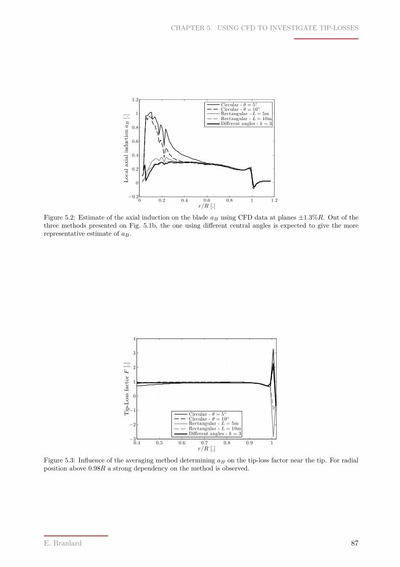
CHAPTER 5. USING CFD TO INVESTIGATE TIP-LOSSES
r/R [.]
LocalaxialinductionaB
[.]
0 0.2 0.4 0.6 0.8 1 1.2−0.2
0
0.2
0.4
0.6
0.8
1
1.2Circular - θ = 5Circular - θ = 10Rectangular - L = 5mRectangular - L = 10mDifferent angles - k = 3
Figure 5.2: Estimate of the axial induction on the blade aB using CFD data at planes ±1.3%R. Out of thethree methods presented on Fig. 5.1b, the one using different central angles is expected to give the morerepresentative estimate of aB .
r/R [.]
Tip-Loss
factorF
[.]
0.4 0.5 0.6 0.7 0.8 0.9 1−3
−2
−1
0
1
2
3
4
Circular - θ = 5Circular - θ = 10Rectangular - L = 5mRectangular - L = 10mDifferent angles - k = 3
Figure 5.3: Influence of the averaging method determining aB on the tip-loss factor near the tip. For radialposition above 0.98R a strong dependency on the method is observed.
E. Branlard 87
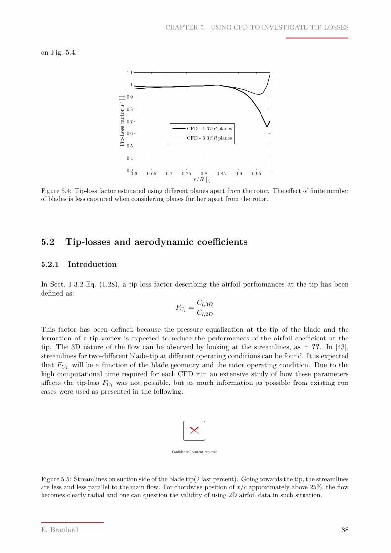
CHAPTER 5. USING CFD TO INVESTIGATE TIP-LOSSES
on Fig. 5.4.
r/R [.]
Tip-Loss
factorF
[.]
0.6 0.65 0.7 0.75 0.8 0.85 0.9 0.950.3
0.4
0.5
0.6
0.7
0.8
0.9
1
1.1
CFD - 1.3%R planes
CFD - 3.3%R planes
Figure 5.4: Tip-loss factor estimated using different planes apart from the rotor. The effect of finite numberof blades is less captured when considering planes further apart from the rotor.
5.2 Tip-losses and aerodynamic coefficients
5.2.1 Introduction
In Sect. 1.3.2 Eq. (1.28), a tip-loss factor describing the airfoil performances at the tip has beendefined as:
FCl = Cl,3DCl,2D
This factor has been defined because the pressure equalization at the tip of the blade and theformation of a tip-vortex is expected to reduce the performances of the airfoil coefficient at thetip. The 3D nature of the flow can be observed by looking at the streamlines, as in ??. In [43],streamlines for two-different blade-tip at different operating conditions can be found. It is expectedthat FCL will be a function of the blade geometry and the rotor operating condition. Due to thehigh computational time required for each CFD run an extensive study of how these parametersaffects the tip-loss FCl was not possible, but as much information as possible from existing runcases were used as presented in the following.
Confidential content removed
Figure 5.5: Streamlines on suction side of the blade tip(2 last percent). Going towards the tip, the streamlinesare less and less parallel to the main flow. For chordwise position of x/c approximately above 25%, the flowbecomes clearly radial and one can question the validity of using 2D airfoil data in such situation.
E. Branlard 88
CHAPTER 5. USING CFD TO INVESTIGATE TIP-LOSSES
5.2.2 Data available
CFD simulations of different blades with different tip-shapes for different operating condition wereavailable. They are summarized on Tab. 5.1. These simulations were run for other purposesthan this study so that performing a sensitivity analysis on the parameters that can influence theperformances losses is made more difficult. Most of the simulations offer the advantages of coveringa wide range of operating conditions for a given blade. From these data it is possible to comparethe 3D airfoil performances from 3D CFD with 2D lookup table data, mostly obtained from 2DCFD. A complete overview of such comparisons can be found in Sect. D.2.
Table 5.1: Available CFD cases for investigation of aerodynamic performance losses
Name Tip Number of runs TypeBlade 1 Tip 1 6 “Rough” - pitch sweep with off-design cases
Tip 2 4 “Rough” - pitch sweep with off-design casesBlade 2 Tip 1 7 “Rough” - operating conditions
Tip 1 7 “Clean” - operating conditionsBlade 1 swept Tip 1 4 “Rough” - rpm sweep with off-design cases
2D airfoil characteristics are known for different thicknesses. The thickness distributions of the twoblades considered can be found on Fig. 5.6.
r/R [.]
Relative
thicknesst/c[%
]
0 0.1 0.2 0.3 0.4 0.5 0.6 0.7 0.8 0.9 110
20
30
40
50
60
70
80
90
100Blade distributionProfiles Available
Figure 5.6: Thickness distribution and available 2D profile data of the two blades considered. B1 (black) -B2 (gray)
5.2.3 Polar comparison between 2D and 3D CFD
As a first step, the profile coefficients obtained from 3D CFD are confronted to the 2D lookuptable data(obtain with CFD). As seen on Fig. 5.6, only a finite number of 2D airfoil coefficienttabled are known for a given thickness. For each thickness value and each simulation, the lift anddrag coefficients together with the angle of attack from CFD data are extracted at the first radialposition where this thickness is encountered along the blade span. These values are then comparedwith the 2D polars. The results for all different polars(i.e. thickness values), all different bladesand all different simulations can be found in Sect. D.2. Among these results it is interesting topoint out that rotational augmentation is observed for large relative thickness values (inner part ofthe blade), but of prime interest here are the effects at the tip of the blade. For this reason, the
E. Branlard 89
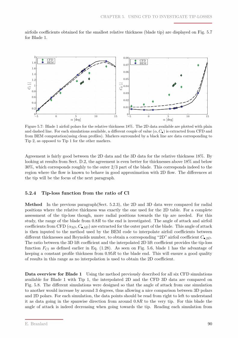
CHAPTER 5. USING CFD TO INVESTIGATE TIP-LOSSES
airfoils coefficients obtained for the smallest relative thickness (blade tip) are displayed on Fig. 5.7for Blade 1.
α [deg]
Cl[.]
−5 0 5 10 150
0.2
0.4
0.6
0.8
1
1.2
1.4
1.6
1.8
2CFDBEM
α [deg]Cd[.]
−5 0 5 10 150
0.01
0.02
0.03
0.04
0.05
0.06
0.07
0.08CFDBEM
Figure 5.7: Blade 1 airfoil polars for the relative thickness 18%. The 2D data available are plotted with plainand dashed line. For each simulations available, a different couple of value (α,C•) is extracted from CFD andfrom BEM computation(using clean profiles). Markers surrounded by a black line are data corresponding toTip 2, as opposed to Tip 1 for the other markers.
Agreement is fairly good between the 2D data and the 3D data for the relative thickness 18%. Bylooking at results from Sect. D.2, the agreement is even better for thicknesses above 18% and below30%, which corresponds roughly to the outer 2/3 part of the blade. This corresponds indeed to theregion where the flow is known to behave in good approximation with 2D flow. The differences atthe tip will be the focus of the next paragraph.
5.2.4 Tip-loss function from the ratio of Cl
Method In the previous paragraph(Sect. 5.2.3), the 2D and 3D data were compared for radialpositions where the relative thickness was exactly the one used for the 2D table. For a completeassessment of the tip-loss though, more radial positions towards the tip are needed. For thisstudy, the range of the blade from 0.8R to the end is investigated. The angle of attack and airfoilcoefficients from CFD (α3D, C•,3D) are extracted for the outer part of the blade. This angle of attackis then inputed to the method used by the BEM code to interpolate airfoil coefficients betweendifferent thicknesses and Reynolds number, to obtain a corresponding “2D” airfoil coefficient C•,2D.The ratio between the 3D lift coefficient and the interpolated 2D lift coefficient provides the tip-lossfunction FCl as defined earlier in Eq. (1.28). As seen on Fig. 5.6, blade 1 has the advantage ofkeeping a constant profile thickness from 0.95R to the blade end. This will ensure a good qualityof results in this range as no interpolation is used to obtain the 2D coefficient.
Data overview for Blade 1 Using the method previously described for all six CFD simulationsavailable for Blade 1 with Tip 1, the interpolated 2D and the CFD 3D data are compared onFig. 5.8. The different simulations were designed so that the angle of attack from one simulationto another would increase by around 3 degrees, thus allowing a nice comparison between 3D polarsand 2D polars. For each simulation, the data points should be read from right to left to understandit as data going in the spanwise direction from around 0.8R to the very tip. For this blade theangle of attack is indeed decreasing when going towards the tip. Reading each simulation from
E. Branlard 90
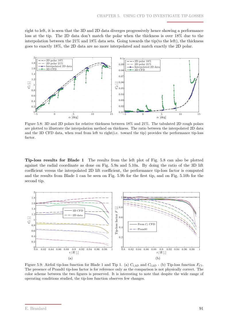
CHAPTER 5. USING CFD TO INVESTIGATE TIP-LOSSES
right to left, it is seen that the 3D and 2D data diverges progressively hence showing a performanceloss at the tip. The 2D data don’t match the polar when the thickness is over 18% due to theinterpolation between the 21% and 18% data sets. Going towards the tip(to the left), the thicknessgoes to exactly 18%, the 2D data are no more interpolated and match exactly the 2D polar.
α [deg]
Cl[.]
−5 0 5 10 150
0.2
0.4
0.6
0.8
1
1.2
1.4
1.6
1.8
22D polar 18%2D polar 21%Interpolated 2D data3D CFD
α [deg]Cd[.]
−5 0 5 10 150.01
0.02
0.03
0.04
0.05
0.06
0.07
0.08
0.09
0.12D polar 18%2D polar 21%Interpolated 2D data3D CFD
Figure 5.8: 3D and 2D polars for relative thickness between 18% and 21%. The tabulated 2D rough polarsare plotted to illustrate the interpolation method on thickness. The ratio between the interpolated 2D dataand the 3D CFD data, when read from left to right(i.e. toward the tip) provides the performance tip-lossfactor.
Tip-loss results for Blade 1 The results from the left plot of Fig. 5.8 can also be plottedagainst the radial coordinate as done on Fig. 5.9a and 5.10a. By doing the ratio of the 3D liftcoefficient versus the interpolated 2D lift coefficient, the performance tip-loss factor is computedand the results from Blade 1 can be seen on Fig. 5.9b for the first tip, and on Fig. 5.10b for thesecond tip.
r/R [.]
Cl[.]
0.8 0.82 0.84 0.86 0.88 0.9 0.92 0.94 0.96 0.98 10
0.2
0.4
0.6
0.8
1
1.2
1.4
1.6
1.8
2
3D CFD
2D data
(a)r/R [.]
Tip-loss
factorF
[.]
0.8 0.82 0.84 0.86 0.88 0.9 0.92 0.94 0.96 0.98 10
0.2
0.4
0.6
0.8
1
From Cl CFD
Prandtl
(b)
Figure 5.9: Airfoil tip-loss function for Blade 1 and Tip 1. (a) Cl,3D and Cl,2D - (b) Tip-loss function FCl.The presence of Prandtl tip-loss factor is for reference only as the comparison is not physically correct. Thecolor scheme between the two figures is preserved. It is interesting to note that despite the wide range ofoperating conditions studied, the tip-loss function observes few changes.
E. Branlard 91
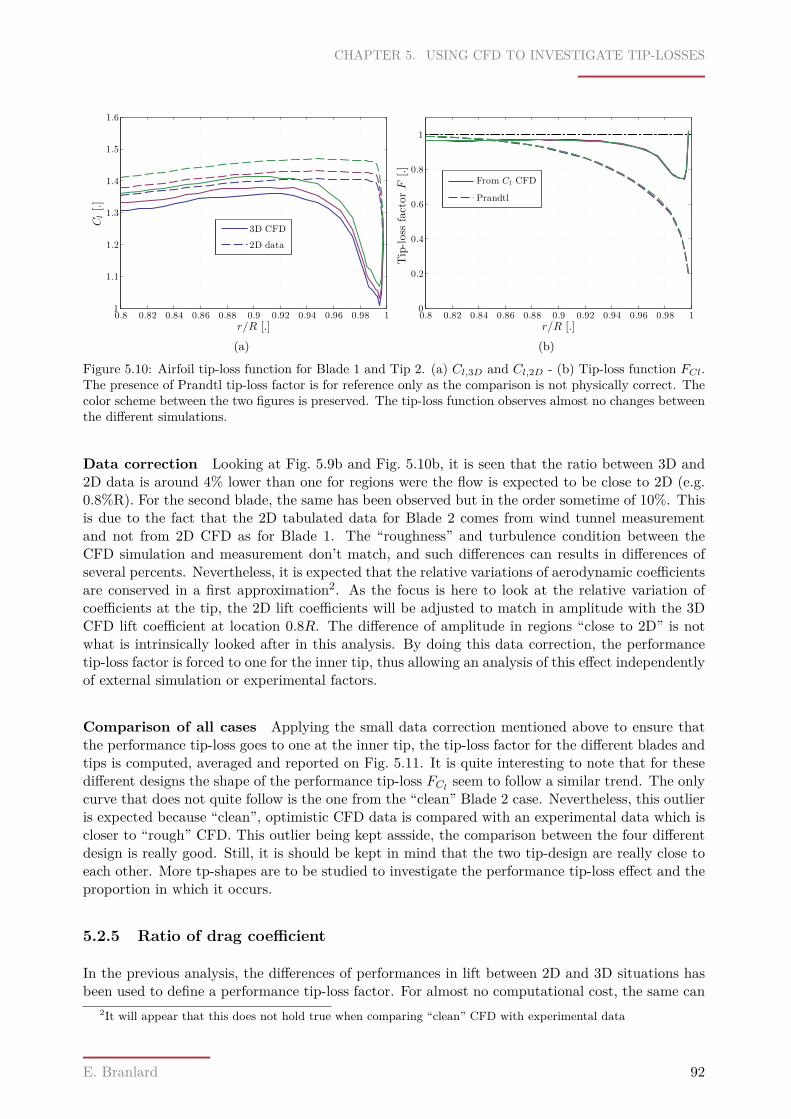
CHAPTER 5. USING CFD TO INVESTIGATE TIP-LOSSES
r/R [.]
Cl[.]
0.8 0.82 0.84 0.86 0.88 0.9 0.92 0.94 0.96 0.98 11
1.1
1.2
1.3
1.4
1.5
1.6
3D CFD
2D data
(a)r/R [.]
Tip-loss
factorF
[.]
0.8 0.82 0.84 0.86 0.88 0.9 0.92 0.94 0.96 0.98 10
0.2
0.4
0.6
0.8
1
From Cl CFD
Prandtl
(b)
Figure 5.10: Airfoil tip-loss function for Blade 1 and Tip 2. (a) Cl,3D and Cl,2D - (b) Tip-loss function FCl.The presence of Prandtl tip-loss factor is for reference only as the comparison is not physically correct. Thecolor scheme between the two figures is preserved. The tip-loss function observes almost no changes betweenthe different simulations.
Data correction Looking at Fig. 5.9b and Fig. 5.10b, it is seen that the ratio between 3D and2D data is around 4% lower than one for regions were the flow is expected to be close to 2D (e.g.0.8%R). For the second blade, the same has been observed but in the order sometime of 10%. Thisis due to the fact that the 2D tabulated data for Blade 2 comes from wind tunnel measurementand not from 2D CFD as for Blade 1. The “roughness” and turbulence condition between theCFD simulation and measurement don’t match, and such differences can results in differences ofseveral percents. Nevertheless, it is expected that the relative variations of aerodynamic coefficientsare conserved in a first approximation2. As the focus is here to look at the relative variation ofcoefficients at the tip, the 2D lift coefficients will be adjusted to match in amplitude with the 3DCFD lift coefficient at location 0.8R. The difference of amplitude in regions “close to 2D” is notwhat is intrinsically looked after in this analysis. By doing this data correction, the performancetip-loss factor is forced to one for the inner tip, thus allowing an analysis of this effect independentlyof external simulation or experimental factors.
Comparison of all cases Applying the small data correction mentioned above to ensure thatthe performance tip-loss goes to one at the inner tip, the tip-loss factor for the different blades andtips is computed, averaged and reported on Fig. 5.11. It is quite interesting to note that for thesedifferent designs the shape of the performance tip-loss FCl seem to follow a similar trend. The onlycurve that does not quite follow is the one from the “clean” Blade 2 case. Nevertheless, this outlieris expected because “clean”, optimistic CFD data is compared with an experimental data which iscloser to “rough” CFD. This outlier being kept assside, the comparison between the four differentdesign is really good. Still, it is should be kept in mind that the two tip-design are really close toeach other. More tp-shapes are to be studied to investigate the performance tip-loss effect and theproportion in which it occurs.
5.2.5 Ratio of drag coefficient
In the previous analysis, the differences of performances in lift between 2D and 3D situations hasbeen used to define a performance tip-loss factor. For almost no computational cost, the same can
2It will appear that this does not hold true when comparing “clean” CFD with experimental data
E. Branlard 92
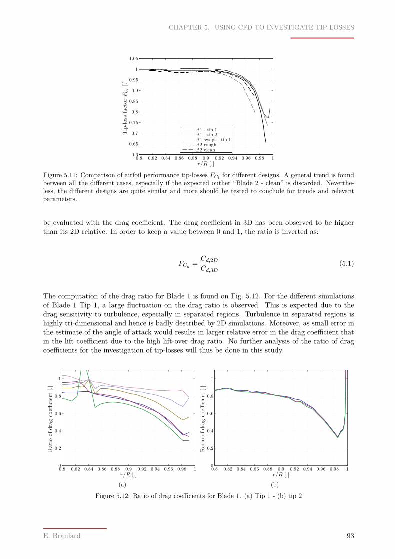
CHAPTER 5. USING CFD TO INVESTIGATE TIP-LOSSES
r/R [.]
Tip-loss
factorFC
l[.]
0.8 0.82 0.84 0.86 0.88 0.9 0.92 0.94 0.96 0.98 10.6
0.65
0.7
0.75
0.8
0.85
0.9
0.95
1
1.05
B1 - tip 1B1 - tip 2B1 swept - tip 1B2 roughB2 clean
Figure 5.11: Comparison of airfoil performance tip-losses FCl for different designs. A general trend is foundbetween all the different cases, especially if the expected outlier “Blade 2 - clean” is discarded. Neverthe-less, the different designs are quite similar and more should be tested to conclude for trends and relevantparameters.
be evaluated with the drag coefficient. The drag coefficient in 3D has been observed to be higherthan its 2D relative. In order to keep a value between 0 and 1, the ratio is inverted as:
FCd = Cd,2DCd,3D
(5.1)
The computation of the drag ratio for Blade 1 is found on Fig. 5.12. For the different simulationsof Blade 1 Tip 1, a large fluctuation on the drag ratio is observed. This is expected due to thedrag sensitivity to turbulence, especially in separated regions. Turbulence in separated regions ishighly tri-dimensional and hence is badly described by 2D simulations. Moreover, as small error inthe estimate of the angle of attack would results in larger relative error in the drag coefficient thatin the lift coefficient due to the high lift-over drag ratio. No further analysis of the ratio of dragcoefficients for the investigation of tip-losses will thus be done in this study.
r/R [.]
Ratioofdragco
efficient[.]
0.8 0.82 0.84 0.86 0.88 0.9 0.92 0.94 0.96 0.98 10
0.2
0.4
0.6
0.8
1
(a)r/R [.]
Ratioofdragco
efficient[.]
0.8 0.82 0.84 0.86 0.88 0.9 0.92 0.94 0.96 0.98 10
0.2
0.4
0.6
0.8
1
(b)
Figure 5.12: Ratio of drag coefficients for Blade 1. (a) Tip 1 - (b) tip 2
E. Branlard 93
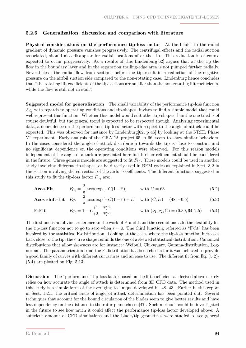
CHAPTER 5. USING CFD TO INVESTIGATE TIP-LOSSES
5.2.6 Generalization, discussion and comparison with literature
Physical considerations on the performance tip-loss factor At the blade tip the radialgradient of dynamic pressure vanishes progressively. The centrifugal effects and the radial suctionassociated, should also disappear for radial locations after the tip. This reduction is of courseexpected to occur progressively. As a results of this Lindenburg[62] argues that at the tip theflow in the boundary layer and in the separation trailing-edge area is not pumped further radially.Nevertheless, the radial flow from sections before the tip result in a reduction of the negativepressure on the airfoil suction side compared to the non-rotating case. Lindenburg hence concludesthat “the rotating lift coefficients of the tip sections are smaller than the non-rotating lift coefficients,while the flow is still not in stall”.
Suggested model for generalization The small variability of the performance tip-loss functionFCl with regards to operating conditions and tip-shapes, invites to find a simple model that couldwell represent this function. Whether this model would suit other tip-shapes than the one tried is ofcourse doubtful, but the general trend is expected to be respected though. Analyzing experimentaldata, a dependence on the performance tip-loss factor with respect to the angle of attack could beexpected. This was observed for instance by Lindenburg[62, p 45] by looking at the NREL PhaseVI experiment. Early analysis of the CRADA project[65, p 66] seem to show similar behaviors.In the cases considered the angle of attack distribution towards the tip is close to constant andno significant dependence on the operating conditions were observed. For this reason modelsindependent of the angle of attack are presented here but further refinement should be consideredin the future. Three generic models are suggested to fit FCl . These models could be used in anotherstudy involving different tip-shapes, or be directly used in BEM codes as explained in Sect. 3.2 inthe section involving the correction of the airfoil coefficients. The different functions suggested inthis study to fit the tip-loss factor FCl are:
Acos-Fit FCl = 2π
acos exp [−C(1− r)] with C = 63 (5.2)
Acos shift-Fit FCl = 2π
acos exp [−C(1− r) +D] with (C,D) = (48,−0.5) (5.3)
F-Fit FCl = 1− C (1− r)ν1
(2− r)ν2with (ν1, ν2, C) = (0.39, 64, 2.5) (5.4)
The first one is an obvious reference to the work of Prandtl and the second one add the flexibility forthe tip-loss function not to go to zero when r = 0. The third function, referred as “F-fit” has beeninspired by the statistical F-distribution. Looking at the cases where the tip-loss function increasesback close to the tip, the curve shape reminds the one of a skewed statistical distribution. Canonicaldistributions that allow skewness are for instance: Weibull, Chi-square, Gamma-distribution, Log-normal. The parametrization from the F-distribution has been chosen for it was believed to providea good family of curves with different curvatures and an ease to use. The different fit from Eq. (5.2)-(5.4) are plotted on Fig. 5.13.
Discussion The “performance” tip-loss factor based on the lift coefficient as derived above clearlyrelies on how accurate the angle of attack is determined from 3D CFD data. The method used inthis study is a simple form of the averaging technique developed in [48, 43]. Earlier in this reportin Sect. 1.2.1, the critical issue of angle of attack determination has been pointed out. Severaltechniques that account for the bound circulation of the blades seem to give better results and haveless dependency on the distance to the rotor plane chosen[47]. Such methods could be investigatedin the future to see how much it could affect the performance tip-loss factor developed above. Asufficient amount of CFD simulations and the blade/tip geometries were studied to see general
E. Branlard 94
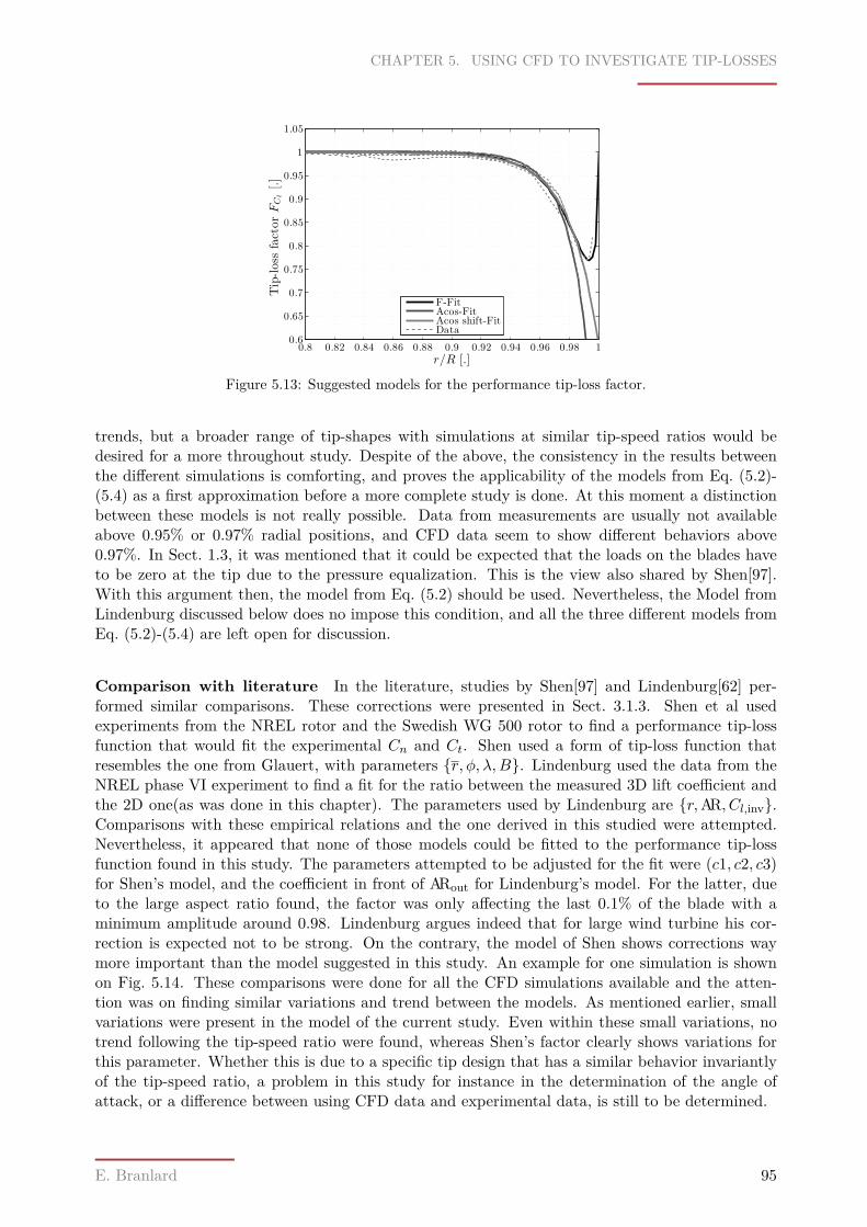
CHAPTER 5. USING CFD TO INVESTIGATE TIP-LOSSES
r/R [.]
Tip-loss
factorFC
l[.]
0.8 0.82 0.84 0.86 0.88 0.9 0.92 0.94 0.96 0.98 10.6
0.65
0.7
0.75
0.8
0.85
0.9
0.95
1
1.05
F-FitAcos-FitAcos shift-FitData
Figure 5.13: Suggested models for the performance tip-loss factor.
trends, but a broader range of tip-shapes with simulations at similar tip-speed ratios would bedesired for a more throughout study. Despite of the above, the consistency in the results betweenthe different simulations is comforting, and proves the applicability of the models from Eq. (5.2)-(5.4) as a first approximation before a more complete study is done. At this moment a distinctionbetween these models is not really possible. Data from measurements are usually not availableabove 0.95% or 0.97% radial positions, and CFD data seem to show different behaviors above0.97%. In Sect. 1.3, it was mentioned that it could be expected that the loads on the blades haveto be zero at the tip due to the pressure equalization. This is the view also shared by Shen[97].With this argument then, the model from Eq. (5.2) should be used. Nevertheless, the Model fromLindenburg discussed below does no impose this condition, and all the three different models fromEq. (5.2)-(5.4) are left open for discussion.
Comparison with literature In the literature, studies by Shen[97] and Lindenburg[62] per-formed similar comparisons. These corrections were presented in Sect. 3.1.3. Shen et al usedexperiments from the NREL rotor and the Swedish WG 500 rotor to find a performance tip-lossfunction that would fit the experimental Cn and Ct. Shen used a form of tip-loss function thatresembles the one from Glauert, with parameters r, φ, λ,B. Lindenburg used the data from theNREL phase VI experiment to find a fit for the ratio between the measured 3D lift coefficient andthe 2D one(as was done in this chapter). The parameters used by Lindenburg are r,AR, Cl,inv.Comparisons with these empirical relations and the one derived in this studied were attempted.Nevertheless, it appeared that none of those models could be fitted to the performance tip-lossfunction found in this study. The parameters attempted to be adjusted for the fit were (c1, c2, c3)for Shen’s model, and the coefficient in front of ARout for Lindenburg’s model. For the latter, dueto the large aspect ratio found, the factor was only affecting the last 0.1% of the blade with aminimum amplitude around 0.98. Lindenburg argues indeed that for large wind turbine his cor-rection is expected not to be strong. On the contrary, the model of Shen shows corrections waymore important than the model suggested in this study. An example for one simulation is shownon Fig. 5.14. These comparisons were done for all the CFD simulations available and the atten-tion was on finding similar variations and trend between the models. As mentioned earlier, smallvariations were present in the model of the current study. Even within these small variations, notrend following the tip-speed ratio were found, whereas Shen’s factor clearly shows variations forthis parameter. Whether this is due to a specific tip design that has a similar behavior invariantlyof the tip-speed ratio, a problem in this study for instance in the determination of the angle ofattack, or a difference between using CFD data and experimental data, is still to be determined.
E. Branlard 95
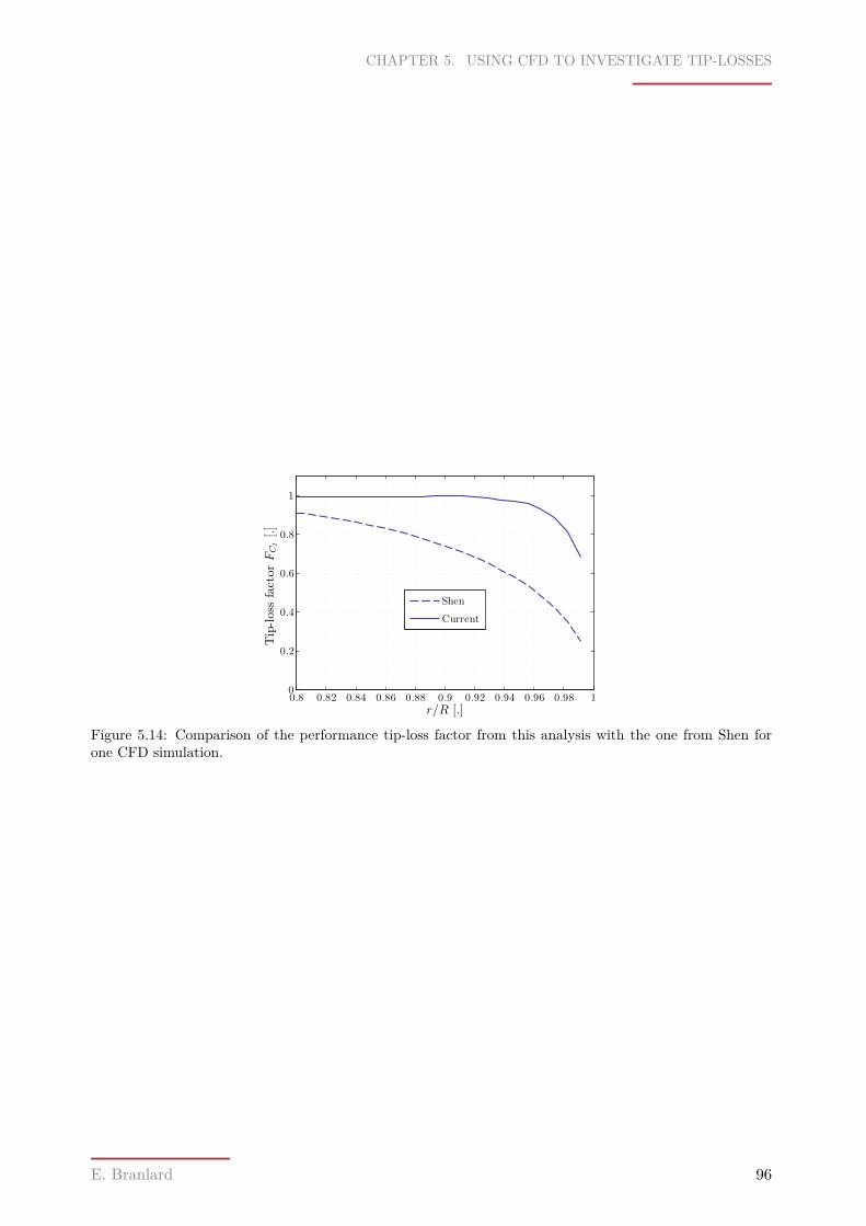
CHAPTER 5. USING CFD TO INVESTIGATE TIP-LOSSES
r/R [.]
Tip-loss
factorFC
l[.]
0.8 0.82 0.84 0.86 0.88 0.9 0.92 0.94 0.96 0.98 10
0.2
0.4
0.6
0.8
1
Shen
Current
Figure 5.14: Comparison of the performance tip-loss factor from this analysis with the one from Shen forone CFD simulation.
E. Branlard 96
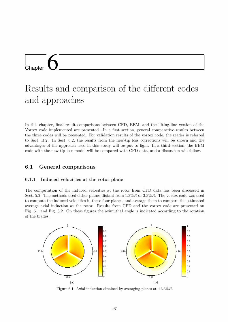
Chapter 6Results and comparison of the different codesand approaches
In this chapter, final result comparisons between CFD, BEM, and the lifting-line version of theVortex code implemented are presented. In a first section, general comparative results betweenthe three codes will be presented. For validation results of the vortex code, the reader is referredto Sect. B.2. In Sect. 6.2, the results from the new-tip loss corrections will be shown and theadvantages of the approach used in this study will be put to light. In a third section, the BEMcode with the new tip-loss model will be compared with CFD data, and a discussion will follow.
6.1 General comparisons
6.1.1 Induced velocities at the rotor plane
The computation of the induced velocities at the rotor from CFD data has been discussed inSect. 5.2. The methods used either planes distant from 1.3%R or 3.3%R. The vortex code was usedto compute the induced velocities in these four planes, and average them to compare the estimatedaverage axial induction at the rotor. Results from CFD and the vortex code are presented onFig. 6.1 and Fig. 6.2. On these figures the azimuthal angle is indicated according to the rotationof the blades.
0
270
180
90
0
0.1
0.2
0.3
0.4
0.5
0.6
0.7
0.8
0.9
1
(a)
0
270
180
90
0
0.1
0.2
0.3
0.4
0.5
0.6
0.7
0.8
0.9
1
(b)
Figure 6.1: Axial induction obtained by averaging planes at ±3.3%R.
97
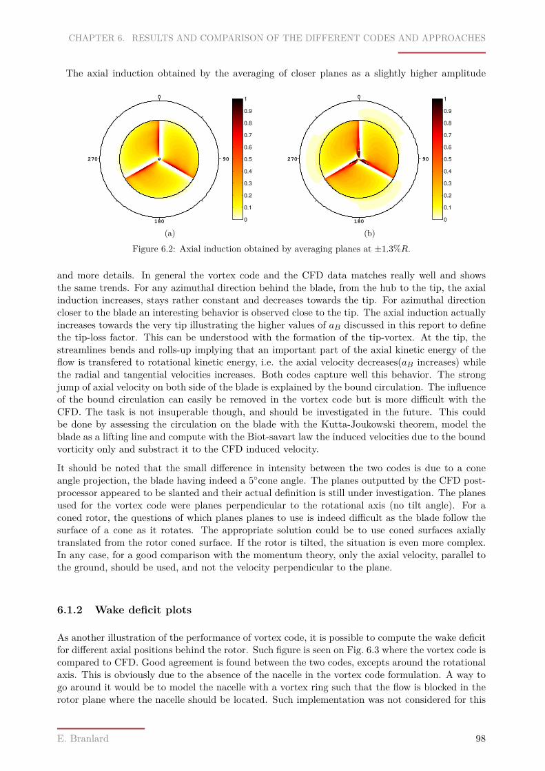
CHAPTER 6. RESULTS AND COMPARISON OF THE DIFFERENT CODES AND APPROACHES
The axial induction obtained by the averaging of closer planes as a slightly higher amplitude
0
270
180
90
0
0.1
0.2
0.3
0.4
0.5
0.6
0.7
0.8
0.9
1
(a)
0
270
180
90
0
0.1
0.2
0.3
0.4
0.5
0.6
0.7
0.8
0.9
1
(b)
Figure 6.2: Axial induction obtained by averaging planes at ±1.3%R.
and more details. In general the vortex code and the CFD data matches really well and showsthe same trends. For any azimuthal direction behind the blade, from the hub to the tip, the axialinduction increases, stays rather constant and decreases towards the tip. For azimuthal directioncloser to the blade an interesting behavior is observed close to the tip. The axial induction actuallyincreases towards the very tip illustrating the higher values of aB discussed in this report to definethe tip-loss factor. This can be understood with the formation of the tip-vortex. At the tip, thestreamlines bends and rolls-up implying that an important part of the axial kinetic energy of theflow is transfered to rotational kinetic energy, i.e. the axial velocity decreases(aB increases) whilethe radial and tangential velocities increases. Both codes capture well this behavior. The strongjump of axial velocity on both side of the blade is explained by the bound circulation. The influenceof the bound circulation can easily be removed in the vortex code but is more difficult with theCFD. The task is not insuperable though, and should be investigated in the future. This couldbe done by assessing the circulation on the blade with the Kutta-Joukowski theorem, model theblade as a lifting line and compute with the Biot-savart law the induced velocities due to the boundvorticity only and substract it to the CFD induced velocity.
It should be noted that the small difference in intensity between the two codes is due to a coneangle projection, the blade having indeed a 5cone angle. The planes outputted by the CFD post-processor appeared to be slanted and their actual definition is still under investigation. The planesused for the vortex code were planes perpendicular to the rotational axis (no tilt angle). For aconed rotor, the questions of which planes planes to use is indeed difficult as the blade follow thesurface of a cone as it rotates. The appropriate solution could be to use coned surfaces axiallytranslated from the rotor coned surface. If the rotor is tilted, the situation is even more complex.In any case, for a good comparison with the momentum theory, only the axial velocity, parallel tothe ground, should be used, and not the velocity perpendicular to the plane.
6.1.2 Wake deficit plots
As another illustration of the performance of vortex code, it is possible to compute the wake deficitfor different axial positions behind the rotor. Such figure is seen on Fig. 6.3 where the vortex code iscompared to CFD. Good agreement is found between the two codes, excepts around the rotationalaxis. This is obviously due to the absence of the nacelle in the vortex code formulation. A way togo around it would be to model the nacelle with a vortex ring such that the flow is blocked in therotor plane where the nacelle should be located. Such implementation was not considered for this
E. Branlard 98
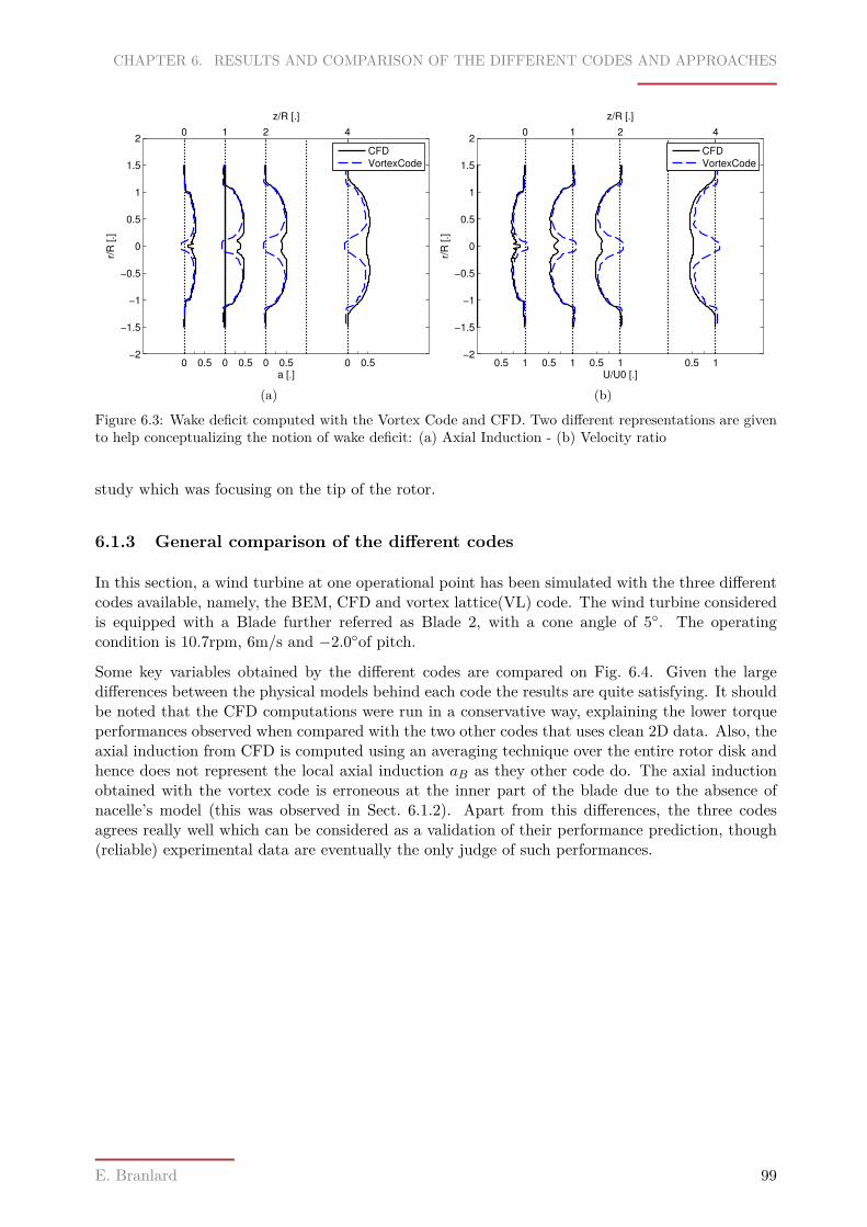
CHAPTER 6. RESULTS AND COMPARISON OF THE DIFFERENT CODES AND APPROACHES
0 0.5 0 0.5 0 0.5 0 0.5−2
−1.5
−1
−0.5
0
0.5
1
1.5
2
a [.]
r/R
[.]
CFD
VortexCode
0 1 2 4
z/R [.]
(a)
0.5 1 0.5 1 0.5 1 0.5 1−2
−1.5
−1
−0.5
0
0.5
1
1.5
2
U/U0 [.]
r/R
[.]
CFD
VortexCode
0 1 2 4
z/R [.]
(b)
Figure 6.3: Wake deficit computed with the Vortex Code and CFD. Two different representations are givento help conceptualizing the notion of wake deficit: (a) Axial Induction - (b) Velocity ratio
study which was focusing on the tip of the rotor.
6.1.3 General comparison of the different codes
In this section, a wind turbine at one operational point has been simulated with the three differentcodes available, namely, the BEM, CFD and vortex lattice(VL) code. The wind turbine consideredis equipped with a Blade further referred as Blade 2, with a cone angle of 5. The operatingcondition is 10.7rpm, 6m/s and −2.0of pitch.
Some key variables obtained by the different codes are compared on Fig. 6.4. Given the largedifferences between the physical models behind each code the results are quite satisfying. It shouldbe noted that the CFD computations were run in a conservative way, explaining the lower torqueperformances observed when compared with the two other codes that uses clean 2D data. Also, theaxial induction from CFD is computed using an averaging technique over the entire rotor disk andhence does not represent the local axial induction aB as they other code do. The axial inductionobtained with the vortex code is erroneous at the inner part of the blade due to the absence ofnacelle’s model (this was observed in Sect. 6.1.2). Apart from this differences, the three codesagrees really well which can be considered as a validation of their performance prediction, though(reliable) experimental data are eventually the only judge of such performances.
E. Branlard 99
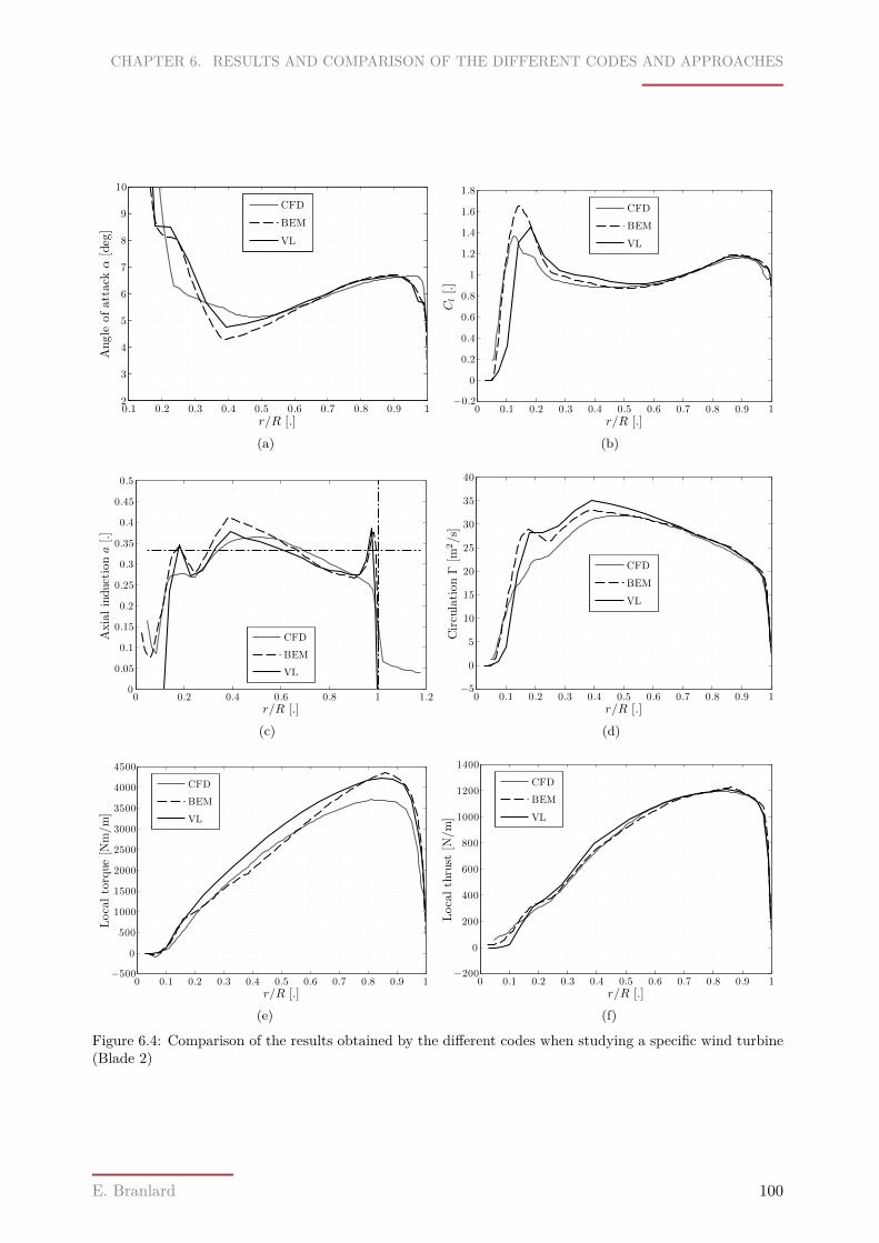
CHAPTER 6. RESULTS AND COMPARISON OF THE DIFFERENT CODES AND APPROACHES
r/R [.]
Angle
ofattack
α[deg]
0.1 0.2 0.3 0.4 0.5 0.6 0.7 0.8 0.9 12
3
4
5
6
7
8
9
10
CFD
BEM
VL
(a)r/R [.]
Cl[.]
0 0.1 0.2 0.3 0.4 0.5 0.6 0.7 0.8 0.9 1−0.2
0
0.2
0.4
0.6
0.8
1
1.2
1.4
1.6
1.8
CFD
BEM
VL
(b)
r/R [.]
Axialinductiona[.]
0 0.2 0.4 0.6 0.8 1 1.20
0.05
0.1
0.15
0.2
0.25
0.3
0.35
0.4
0.45
0.5
CFD
BEM
VL
(c)r/R [.]
CirculationΓ[m
2/s]
0 0.1 0.2 0.3 0.4 0.5 0.6 0.7 0.8 0.9 1−5
0
5
10
15
20
25
30
35
40
CFD
BEM
VL
(d)
r/R [.]
Localtorque[N
m/m]
0 0.1 0.2 0.3 0.4 0.5 0.6 0.7 0.8 0.9 1−500
0
500
1000
1500
2000
2500
3000
3500
4000
4500
CFD
BEM
VL
(e)r/R [.]
Localthrust
[N/m]
0 0.1 0.2 0.3 0.4 0.5 0.6 0.7 0.8 0.9 1−200
0
200
400
600
800
1000
1200
1400
CFD
BEM
VL
(f)
Figure 6.4: Comparison of the results obtained by the different codes when studying a specific wind turbine(Blade 2)
E. Branlard 100
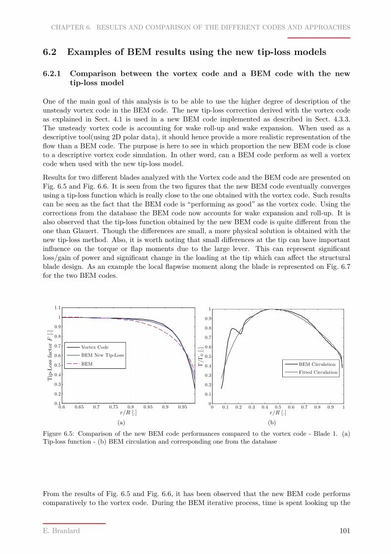
CHAPTER 6. RESULTS AND COMPARISON OF THE DIFFERENT CODES AND APPROACHES
6.2 Examples of BEM results using the new tip-loss models
6.2.1 Comparison between the vortex code and a BEM code with the newtip-loss model
One of the main goal of this analysis is to be able to use the higher degree of description of theunsteady vortex code in the BEM code. The new tip-loss correction derived with the vortex codeas explained in Sect. 4.1 is used in a new BEM code implemented as described in Sect. 4.3.3.The unsteady vortex code is accounting for wake roll-up and wake expansion. When used as adescriptive tool(using 2D polar data), it should hence provide a more realistic representation of theflow than a BEM code. The purpose is here to see in which proportion the new BEM code is closeto a descriptive vortex code simulation. In other word, can a BEM code perform as well a vortexcode when used with the new tip-loss model.
Results for two different blades analyzed with the Vortex code and the BEM code are presented onFig. 6.5 and Fig. 6.6. It is seen from the two figures that the new BEM code eventually convergesusing a tip-loss function which is really close to the one obtained with the vortex code. Such resultscan be seen as the fact that the BEM code is “performing as good” as the vortex code. Using thecorrections from the database the BEM code now accounts for wake expansion and roll-up. It isalso observed that the tip-loss function obtained by the new BEM code is quite different from theone than Glauert. Though the differences are small, a more physical solution is obtained with thenew tip-loss method. Also, it is worth noting that small differences at the tip can have importantinfluence on the torque or flap moments due to the large lever. This can represent significantloss/gain of power and significant change in the loading at the tip which can affect the structuralblade design. As an example the local flapwise moment along the blade is represented on Fig. 6.7for the two BEM codes.
r/R [.]
Tip-Loss
factorF
[.]
0.6 0.65 0.7 0.75 0.8 0.85 0.9 0.950.1
0.2
0.3
0.4
0.5
0.6
0.7
0.8
0.9
1
1.1
Vortex Code
BEM New Tip-Loss
BEM
(a)r/R [.]
Γ/Γ0[.]
0 0.1 0.2 0.3 0.4 0.5 0.6 0.7 0.8 0.9 10
0.1
0.2
0.3
0.4
0.5
0.6
0.7
0.8
0.9
1
BEM Circulation
Fitted Circulation
(b)
Figure 6.5: Comparison of the new BEM code performances compared to the vortex code - Blade 1. (a)Tip-loss function - (b) BEM circulation and corresponding one from the database
From the results of Fig. 6.5 and Fig. 6.6, it has been observed that the new BEM code performscomparatively to the vortex code. During the BEM iterative process, time is spent looking up the
E. Branlard 101
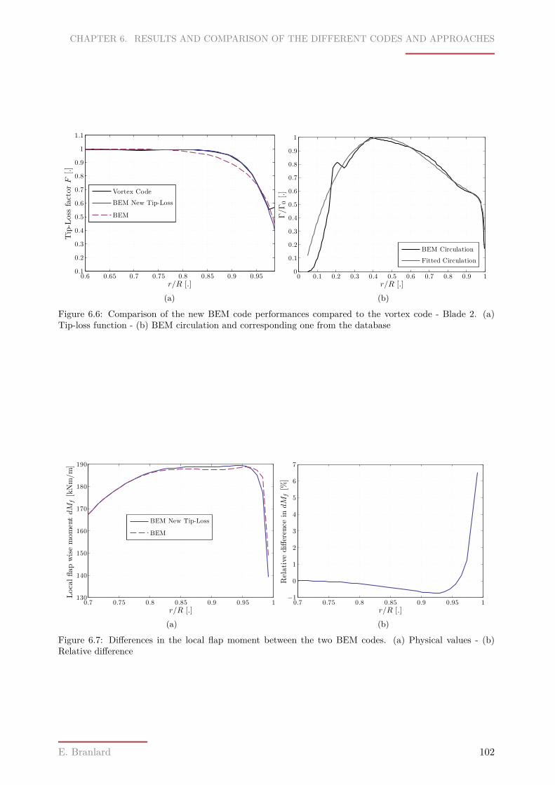
CHAPTER 6. RESULTS AND COMPARISON OF THE DIFFERENT CODES AND APPROACHES
r/R [.]
Tip-Loss
factorF
[.]
0.6 0.65 0.7 0.75 0.8 0.85 0.9 0.950.1
0.2
0.3
0.4
0.5
0.6
0.7
0.8
0.9
1
1.1
Vortex Code
BEM New Tip-Loss
BEM
(a)r/R [.]
Γ/Γ0[.]
0 0.1 0.2 0.3 0.4 0.5 0.6 0.7 0.8 0.9 10
0.1
0.2
0.3
0.4
0.5
0.6
0.7
0.8
0.9
1
BEM Circulation
Fitted Circulation
(b)
Figure 6.6: Comparison of the new BEM code performances compared to the vortex code - Blade 2. (a)Tip-loss function - (b) BEM circulation and corresponding one from the database
r/R [.]
LocalflapwisemomentdM
f[kNm/m]
0.7 0.75 0.8 0.85 0.9 0.95 1130
140
150
160
170
180
190
BEM New Tip-Loss
BEM
(a)r/R [.]
Relative
difference
indM
f[%
]
0.7 0.75 0.8 0.85 0.9 0.95 1−1
0
1
2
3
4
5
6
7
(b)
Figure 6.7: Differences in the local flap moment between the two BEM codes. (a) Physical values - (b)Relative difference
E. Branlard 102
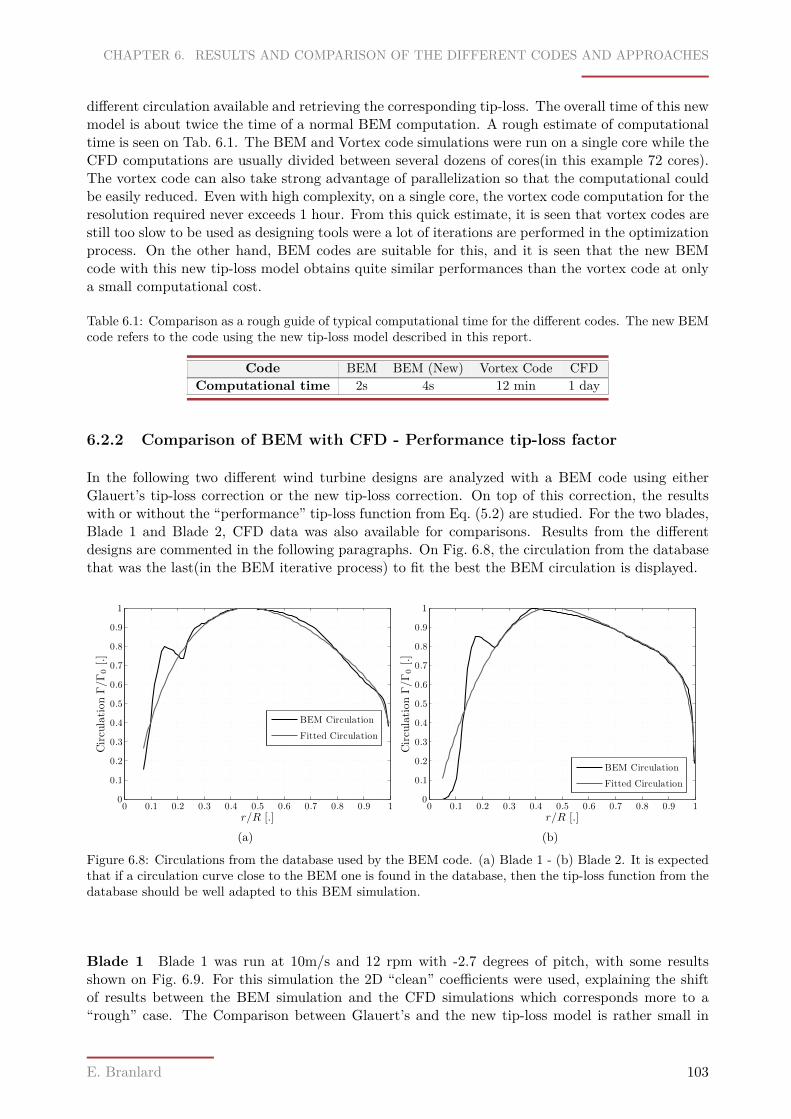
CHAPTER 6. RESULTS AND COMPARISON OF THE DIFFERENT CODES AND APPROACHES
different circulation available and retrieving the corresponding tip-loss. The overall time of this newmodel is about twice the time of a normal BEM computation. A rough estimate of computationaltime is seen on Tab. 6.1. The BEM and Vortex code simulations were run on a single core while theCFD computations are usually divided between several dozens of cores(in this example 72 cores).The vortex code can also take strong advantage of parallelization so that the computational couldbe easily reduced. Even with high complexity, on a single core, the vortex code computation for theresolution required never exceeds 1 hour. From this quick estimate, it is seen that vortex codes arestill too slow to be used as designing tools were a lot of iterations are performed in the optimizationprocess. On the other hand, BEM codes are suitable for this, and it is seen that the new BEMcode with this new tip-loss model obtains quite similar performances than the vortex code at onlya small computational cost.
Table 6.1: Comparison as a rough guide of typical computational time for the different codes. The new BEMcode refers to the code using the new tip-loss model described in this report.
Code BEM BEM (New) Vortex Code CFDComputational time 2s 4s 12 min 1 day
6.2.2 Comparison of BEM with CFD - Performance tip-loss factor
In the following two different wind turbine designs are analyzed with a BEM code using eitherGlauert’s tip-loss correction or the new tip-loss correction. On top of this correction, the resultswith or without the “performance” tip-loss function from Eq. (5.2) are studied. For the two blades,Blade 1 and Blade 2, CFD data was also available for comparisons. Results from the differentdesigns are commented in the following paragraphs. On Fig. 6.8, the circulation from the databasethat was the last(in the BEM iterative process) to fit the best the BEM circulation is displayed.
r/R [.]
CirculationΓ/Γ0[.]
0 0.1 0.2 0.3 0.4 0.5 0.6 0.7 0.8 0.9 10
0.1
0.2
0.3
0.4
0.5
0.6
0.7
0.8
0.9
1
BEM Circulation
Fitted Circulation
(a)r/R [.]
CirculationΓ/Γ0[.]
0 0.1 0.2 0.3 0.4 0.5 0.6 0.7 0.8 0.9 10
0.1
0.2
0.3
0.4
0.5
0.6
0.7
0.8
0.9
1
BEM Circulation
Fitted Circulation
(b)
Figure 6.8: Circulations from the database used by the BEM code. (a) Blade 1 - (b) Blade 2. It is expectedthat if a circulation curve close to the BEM one is found in the database, then the tip-loss function from thedatabase should be well adapted to this BEM simulation.
Blade 1 Blade 1 was run at 10m/s and 12 rpm with -2.7 degrees of pitch, with some resultsshown on Fig. 6.9. For this simulation the 2D “clean” coefficients were used, explaining the shiftof results between the BEM simulation and the CFD simulations which corresponds more to a“rough” case. The Comparison between Glauert’s and the new tip-loss model is rather small in
E. Branlard 103
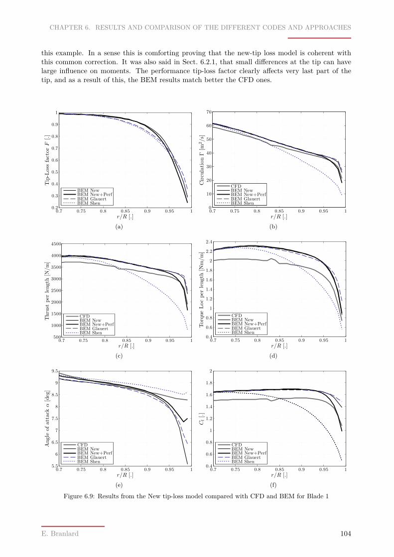
CHAPTER 6. RESULTS AND COMPARISON OF THE DIFFERENT CODES AND APPROACHES
this example. In a sense this is comforting proving that the new-tip loss model is coherent withthis common correction. It was also said in Sect. 6.2.1, that small differences at the tip can havelarge influence on moments. The performance tip-loss factor clearly affects very last part of thetip, and as a result of this, the BEM results match better the CFD ones.
r/R [.]
Tip-Loss
factorF
[.]
0.7 0.75 0.8 0.85 0.9 0.95 10.2
0.3
0.4
0.5
0.6
0.7
0.8
0.9
1
BEM NewBEM New+PerfBEM GlauertBEM Shen
(a)r/R [.]
CirculationΓ[m
2/s]
0.7 0.75 0.8 0.85 0.9 0.95 10
10
20
30
40
50
60
70
CFDBEM NewBEM New+PerfBEM GlauertBEM Shen
(b)
r/R [.]
Thrust
per
length
[N/m]
0.7 0.75 0.8 0.85 0.9 0.95 1500
1000
1500
2000
2500
3000
3500
4000
4500
CFDBEM NewBEM New+PerfBEM GlauertBEM Shen
(c)r/R [.]
TorqueLocper
length
[Nm/m]
0.7 0.75 0.8 0.85 0.9 0.95 10.4
0.6
0.8
1
1.2
1.4
1.6
1.8
2
2.2
2.4
CFDBEM NewBEM New+PerfBEM GlauertBEM Shen
(d)
r/R [.]
Angle
ofattack
α[deg]
0.7 0.75 0.8 0.85 0.9 0.95 15.5
6
6.5
7
7.5
8
8.5
9
9.5
CFDBEM NewBEM New+PerfBEM GlauertBEM Shen
(e)r/R [.]
Cl[.]
0.7 0.75 0.8 0.85 0.9 0.95 10.4
0.6
0.8
1
1.2
1.4
1.6
1.8
2
CFDBEM NewBEM New+PerfBEM GlauertBEM Shen
(f)
Figure 6.9: Results from the New tip-loss model compared with CFD and BEM for Blade 1
E. Branlard 104
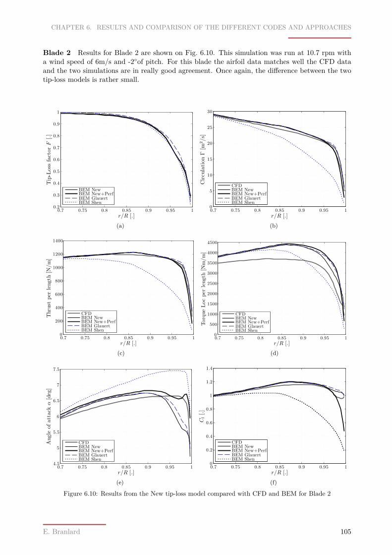
CHAPTER 6. RESULTS AND COMPARISON OF THE DIFFERENT CODES AND APPROACHES
Blade 2 Results for Blade 2 are shown on Fig. 6.10. This simulation was run at 10.7 rpm witha wind speed of 6m/s and -2of pitch. For this blade the airfoil data matches well the CFD dataand the two simulations are in really good agreement. Once again, the difference between the twotip-loss models is rather small.
r/R [.]
Tip-Loss
factorF
[.]
0.7 0.75 0.8 0.85 0.9 0.95 10.2
0.3
0.4
0.5
0.6
0.7
0.8
0.9
1
BEM NewBEM New+PerfBEM GlauertBEM Shen
(a)r/R [.]
CirculationΓ[m
2/s]
0.7 0.75 0.8 0.85 0.9 0.95 10
5
10
15
20
25
30
CFDBEM NewBEM New+PerfBEM GlauertBEM Shen
(b)
r/R [.]
Thrust
per
length
[N/m]
0.7 0.75 0.8 0.85 0.9 0.95 10
200
400
600
800
1000
1200
1400
CFDBEM NewBEM New+PerfBEM GlauertBEM Shen
(c)r/R [.]
TorqueLocper
length
[Nm/m]
0.7 0.75 0.8 0.85 0.9 0.95 10
500
1000
1500
2000
2500
3000
3500
4000
4500
CFDBEM NewBEM New+PerfBEM GlauertBEM Shen
(d)
r/R [.]
Angle
ofattack
α[deg]
0.7 0.75 0.8 0.85 0.9 0.95 14.5
5
5.5
6
6.5
7
7.5
CFDBEM NewBEM New+PerfBEM GlauertBEM Shen
(e)r/R [.]
Cl[.]
0.7 0.75 0.8 0.85 0.9 0.95 10
0.2
0.4
0.6
0.8
1
1.2
1.4
CFDBEM NewBEM New+PerfBEM GlauertBEM Shen
(f)
Figure 6.10: Results from the New tip-loss model compared with CFD and BEM for Blade 2
E. Branlard 105
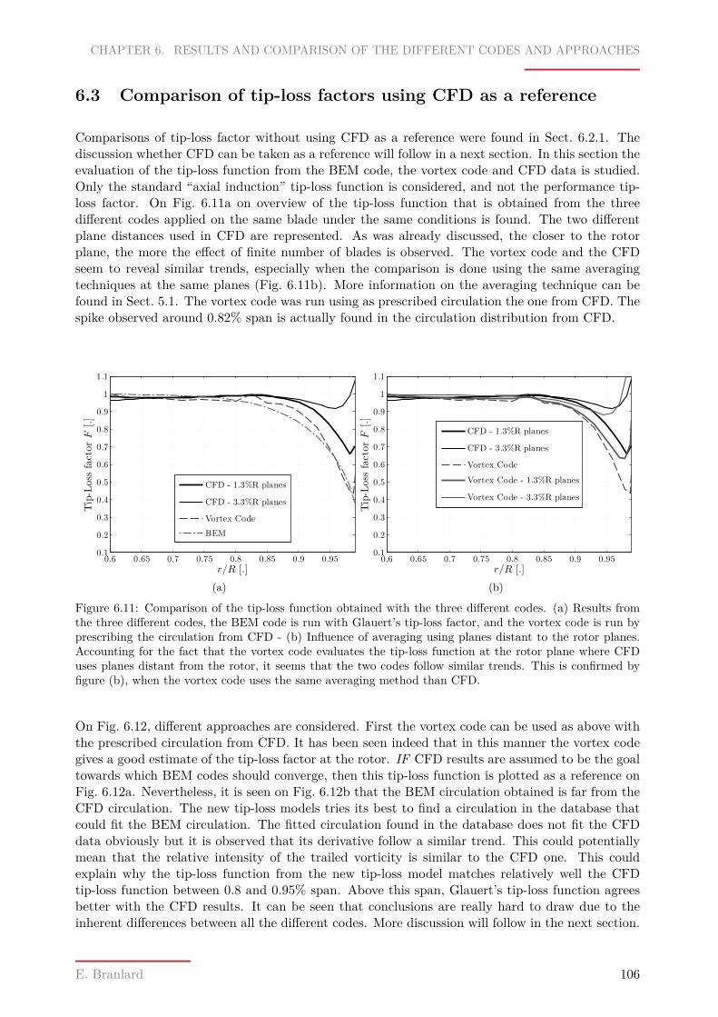
CHAPTER 6. RESULTS AND COMPARISON OF THE DIFFERENT CODES AND APPROACHES
6.3 Comparison of tip-loss factors using CFD as a reference
Comparisons of tip-loss factor without using CFD as a reference were found in Sect. 6.2.1. Thediscussion whether CFD can be taken as a reference will follow in a next section. In this section theevaluation of the tip-loss function from the BEM code, the vortex code and CFD data is studied.Only the standard “axial induction” tip-loss function is considered, and not the performance tip-loss factor. On Fig. 6.11a on overview of the tip-loss function that is obtained from the threedifferent codes applied on the same blade under the same conditions is found. The two differentplane distances used in CFD are represented. As was already discussed, the closer to the rotorplane, the more the effect of finite number of blades is observed. The vortex code and the CFDseem to reveal similar trends, especially when the comparison is done using the same averagingtechniques at the same planes (Fig. 6.11b). More information on the averaging technique can befound in Sect. 5.1. The vortex code was run using as prescribed circulation the one from CFD. Thespike observed around 0.82% span is actually found in the circulation distribution from CFD.
r/R [.]
Tip-Loss
factorF
[.]
0.6 0.65 0.7 0.75 0.8 0.85 0.9 0.950.1
0.2
0.3
0.4
0.5
0.6
0.7
0.8
0.9
1
1.1
CFD - 1.3%R planes
CFD - 3.3%R planes
Vortex Code
BEM
(a)r/R [.]
Tip-Loss
factorF
[.]
0.6 0.65 0.7 0.75 0.8 0.85 0.9 0.950.1
0.2
0.3
0.4
0.5
0.6
0.7
0.8
0.9
1
1.1
CFD - 1.3%R planes
CFD - 3.3%R planes
Vortex Code
Vortex Code - 1.3%R planes
Vortex Code - 3.3%R planes
(b)
Figure 6.11: Comparison of the tip-loss function obtained with the three different codes. (a) Results fromthe three different codes, the BEM code is run with Glauert’s tip-loss factor, and the vortex code is run byprescribing the circulation from CFD - (b) Influence of averaging using planes distant to the rotor planes.Accounting for the fact that the vortex code evaluates the tip-loss function at the rotor plane where CFDuses planes distant from the rotor, it seems that the two codes follow similar trends. This is confirmed byfigure (b), when the vortex code uses the same averaging method than CFD.
On Fig. 6.12, different approaches are considered. First the vortex code can be used as above withthe prescribed circulation from CFD. It has been seen indeed that in this manner the vortex codegives a good estimate of the tip-loss factor at the rotor. IF CFD results are assumed to be the goaltowards which BEM codes should converge, then this tip-loss function is plotted as a reference onFig. 6.12a. Nevertheless, it is seen on Fig. 6.12b that the BEM circulation obtained is far from theCFD circulation. The new tip-loss models tries its best to find a circulation in the database thatcould fit the BEM circulation. The fitted circulation found in the database does not fit the CFDdata obviously but it is observed that its derivative follow a similar trend. This could potentiallymean that the relative intensity of the trailed vorticity is similar to the CFD one. This couldexplain why the tip-loss function from the new tip-loss model matches relatively well the CFDtip-loss function between 0.8 and 0.95% span. Above this span, Glauert’s tip-loss function agreesbetter with the CFD results. It can be seen that conclusions are really hard to draw due to theinherent differences between all the different codes. More discussion will follow in the next section.
E. Branlard 106
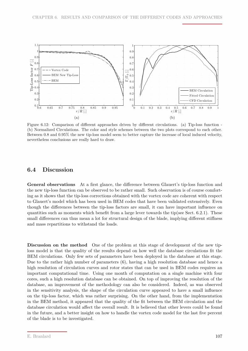
CHAPTER 6. RESULTS AND COMPARISON OF THE DIFFERENT CODES AND APPROACHES
r/R [.]
Tip-Loss
factorF
[.]
0.6 0.65 0.7 0.75 0.8 0.85 0.9 0.950.1
0.2
0.3
0.4
0.5
0.6
0.7
0.8
0.9
1
1.1
Vortex Code
BEM New Tip-Loss
BEM
(a)r/R [.]
Γ/Γ0[.]
0 0.1 0.2 0.3 0.4 0.5 0.6 0.7 0.8 0.9 10
0.1
0.2
0.3
0.4
0.5
0.6
0.7
0.8
0.9
1
BEM Circulation
Fitted Circulation
CFD Circulation
(b)
Figure 6.12: Comparison of different approaches driven by different circulations. (a) Tip-loss function -(b) Normalized Circulations. The color and style schemes between the two plots correspond to each other.Between 0.8 and 0.95% the new tip-loss model seem to better capture the increase of local induced velocity,nevertheless conclusions are really hard to draw.
6.4 Discussion
General observations At a first glance, the difference between Glauert’s tip-loss function andthe new tip-loss function can be observed to be rather small. Such observation is of course comfort-ing as it shows that the tip-loss corrections obtained with the vortex code are coherent with respectto Glauert’s model which has been used in BEM codes that have been validated extensively. Eventhough the differences between the tip-loss factors are small, it can have important influence onquantities such as moments which benefit from a large lever towards the tip(see Sect. 6.2.1). Thesesmall differences can thus mean a lot for structural design of the blade, implying different stiffnessand mass repartitions to withstand the loads.
Discussion on the method One of the problem at this stage of development of the new tip-loss model is that the quality of the results depend on how well the database circulations fit theBEM circulations. Only few sets of parameters have been deployed in the database at this stage.Due to the rather high number of parameters (6), having a high resolution database and hence ahigh resolution of circulation curves and rotor states that can be used in BEM codes requires animportant computational time. Using one month of computation on a single machine with fourcores, such a high resolution database can be obtained. On top of improving the resolution of thedatabase, an improvement of the methodology can also be considered. Indeed, as was observedin the sensitivity analysis, the shape of the circulation curve appeared to have a small influenceon the tip-loss factor, which was rather surprising. On the other hand, from the implementationin the BEM method, it appeared that the quality of the fit between the BEM circulation and thedatabase circulation would affect the overall result. It is believed that other levers could be foundin the future, and a better insight on how to handle the vortex code model for the last five percentof the blade is to be investigated.
E. Branlard 107
CHAPTER 6. RESULTS AND COMPARISON OF THE DIFFERENT CODES AND APPROACHES
Comparison with CFD When doing comparisons with CFD the results should be taken witha grain of salt. On one hand, the quality of the 2D coefficients used by the BEM code is onekey parameters that influences the quality of the results so that the evaluation of the new tip-lossfunction is rather difficult. It has been seen for instance in Fig. 6.12b) that the circulation foundwith a standard BEM code and CFD can be quite different. One can thus questions if it is wiseto compare CFD results with the BEM method with the new-tip-loss model knowing that suchdifferences exists. On the other hand, the source of uncertainty from CFD data should not beforgotten. Many parameters come into play in the solving process that can affects the CFD results(turbulence model, transition model, convergence criteria, grid, etc.).
Performance tip-loss factor From the work of Shen[97], Lindenburg[62] and the current, aneed to correct airfoil coefficient towards the tip is confirmed.
Performance of the vortex code It has been seen that when used with the prescribed circu-lation from CFD, the vortex code was giving results in good agreement with CFD. In this sense, itis also expected to give a good assessment of the tip-loss function at the rotor plane, thing whichis currently not possible with CFD.
Experimental data A need to compare the existing models with experimental data clearlyappears. It is nevertheless difficult to instrument a blade at its tip. Comparisons are of courseenvisaged for the future of this work using both internal experiments and reference experimentssuch as the NREL phase six experiment.
Benefit of the method As was discussed in Sect. 4.3.3, there is high potential for such amethodology to give results in many aspects more realistic and more precise than the theoreti-cal approaches of Prandtl and Goldstein. The parametrization and methodology could need tobe re-thought and the vortex code slightly improved, but is is believed that such approach canhighly improve the knowledge on tip-losses and make BEM codes more realistic. The preliminarystudy done in Sect. 6.2.1 showed a great benefit of the method. The new BEM code seems tooffer performances really close to the vortex code for almost no computational time. The BEMmodel is improved and can be further used for design and optimization purposes due to the smallcomputational cost added with the new tip-loss model.
E. Branlard 108
Conclusion
From theory to the development of a vortex code A better insight on the origin of tip-lossesboth historically and physically has been acquired through the first part of this study. Going fromsimple models with infinite number of blades to more advanced ones, the 3D flow characteristicsaround a wind turbine were progressively put to light. The notion of tip-losses appeared whenstudying the 3D effects that affect the wind turbine performances. In this study the distinctionbetween flow characteristics close to the rotor and far behind it was emphasized, giving rise tothe notions of near-wake and far-wake. The structure of the wake and its dynamics has beenpresented. Given the important vorticity found in the wake and its concentration to vortex sheetsand tip-vortices, a great descriptive and predictive tool was found to be the vortex theory. On onehand, this theory led to the development of important theorem from Munk and Betz which werelater complemented by the only two theoretical studies of tip-losses: the work from Prandtl andGoldstein. On the other hand, vortex theory can be applied for numerical methods which leads tothe development of different vortex codes. The implementation of a vortex-lattice code was hencechosen to further study tip-losses and account for higher complexity than the theoretical work fromthe beginning of the 20th century.
Historical work on tip-losses Historically, the concept of tip-losses appeared when looking forthe circulation that would lead to the minimum energy loss. By focusing on the theories of Betz andPrandtl, the original notion of tip-losses and its applicability was presented. Nevertheless, it wasseen that several interpretations could be given due to the simplicity of Prandtl model comparedto a real wake flow. The study of Goldstein’s theory which model the wake in a better way also ledroom for discussion. Results from the theories apply to the far-wake and their relations to the rotorparameters is not straightforward. The pitch of the helix, its rotation and the induced velocitiesare different than the one at the rotor. Using assumptions of no wake expansion and conservationof circulation relations between far-wake parameters and rotor parameters were established. It hasbeen pointed out that the relations used in contemporary articles are different than the one usedoriginally. As many figures as possible were provided to illustrate the different relations and thefocus has been on applying this figure to the wind turbine case to avoid any further confusions.Hopefully with this report, the reader can assimilate the historical work of the German schoolwithout going through the original articles which uses different notations and conventions. Theirreading is nevertheless quite interesting and the author highly recommends the curious reader todiscover them.
Different tip-loss factors In this study, a review of all the existing tip-loss correction,s to theauthor’s knowledge, was performed. By using a general formalism for the parameters of the farwake, the theories of Betz, Goldstein and Prandtl were generalized. From these derivations, it
109
CONCLUSION
was possible to unify all the different tip-loss factors than authors usually refer to as “Prandtl”tip-loss factor even-though they use a different formulation than the one from the original author.Hopefully, more clarity on the matter should follow from this analysis. On top of the existence ofmany tip-loss factor equations, different definitions, interpretations and implementations are foundin BEM codes. This study clearly made the distinction between the standard tip-loss factor andthe so called “performance” tip-loss factor which stand in the line of airfoil coefficients corrections.
Standard tip-loss factor The standard tip-loss factor can be defined as a ratio of circulation,like in the original articles of Prandtl and Goldstein, or as a ratio of induced velocities. The latercase deserve particular attention. The factor can describe in which proportion the axial inductionon the blade is different than the average azimuthal axial induction. In this case though, it shouldbe noted that for a real flow the average azimuthal axial induction goes continuously towards zeroin the vicinity of the tip. The axial induction on the blade can take a wide range of values towardsthe tip due to the formation of the tip-vortex so that the ratio can be hard to define at the verytip of the blade (last 1%). The advantage of this definition of the tip-loss factor, is that is gives agood definition of the angle of attack and thus a better estimate of the loads on the blade usingthe blade element theory. When used in BEM codes a different definition of the tip-loss factor interms of induced velocities is found. BEM codes are based on momentum theory which modelsthe rotor with an infinite number of blades and hence no tip-losses are present. In that case thetip-loss factor has conceptually the role of reducing the axial induction from momentum theory toensure is goes towards zero in the vicinity of the tip. In this sense the tip-loss factor would be theratio of the real azimuthally averaged axial induction to the momentum theory axial induction.In most BEM code implementations though, the tip-loss factor is applied as a momentum (andsometimes mass flow) change. The tip-loss factor then reduces the loads at the tip. In most BEMequations, the distinction between the average axial induction and the induction on the blade isnot done. The introduction of the tip-loss factor in the equations has thus the effect of increasingthe axial induction locally to the blade. As a result of this, the velocity triangle is correct as inthe previous formulation of the tip-loss factor described. The author believe that BEM equationsshould be rewritten by carefully making the difference between the axial induction on the bladeand the azimuthally averaged axial induction. This is done for instance by Shen[98]. Also, themomentum theory equations should be derived in two steps. The first step consisting in derivingthe equations for infinite number of blades. The second step should emphasize the assumption ofindependence of the different annuli, and hence justify that the axial induction(which is azimuthallyaveraged by definition), can be changed in each annuli to ensure that it goes towards zero in thevicinity of the tip and hence account for finite number of blades. This should clarify the distinctionbetween a, a, and aB made in this report.
Zero at the tip From the above discussion and the analysis of this report, the question of the tip-loss factor going to zero at the tip was mentioned. Depending on the meaning of the tip-loss factordifferent conclusions can be drawn. Clearly, the author believes that the average axial inductiongoes towards zero in the vicinity of the tip. Nevertheless, this is most likely to happen after thetip accounting for the shear stress at the slip stream boundaries. This is observed from CFD dataas well. For this reason, forcing the tip-loss factor to go to zero at the tip might be inappropriate.Also, the flow at the tip is very complex close to the blade. Changes in flow direction might evenhappen in some situations. Hence if the definition F = a/aB is used then the values at the tip ishard to define and is hence not likely to be exactly zero. If on the other hand, the tip-loss is seenas a circulation factor. Then, one can argue that even-though the velocity is none-zero from theabove discussion, the loads are likely to be reduced to zero due to the pressure balance occurringat the tip.
E. Branlard 110
CONCLUSION
Performance tip-loss factor The definition of this performance tip-loss factor and its imple-mentation does not rise as many questions, even though controversy has followed the introductionof Shen’s tip-loss factors. This performance tip-loss factor can translate two things. First it can beseen as the results of the pressure equalization at the tip, which should make the loads go to zeroat the very tip. Also, it can model the fact that the airfoil does not perform as in 2D in the tip areadue to the presence of the tip-vortex and complex flows occurring. Reasons for this are multiple:radial flow, interaction of the tip-vortex with the boundary layer, separation at the very tip andcentrifugal forces, etc. This difference in performance is independent to the other tip-loss factorwhich affects the relative velocity both in amplitude and in direction. Even if the relative velocityis known perfectly, the 2D airfoil data (in the situations observed) do not apply at the very tip.The performance tip-loss factor is hence defined as the ratio between 3D to 2D airfoil polars. Theimplementation of such correction is straight-forward in BEM codes. The question that remains isthe determination of such factor. Experimental data and CFD data can be used but at this timethe imprecision in both methods are quite high at the tip of the blade so no conclusion or persistentmodel can be derived yet.
Tip-losses and CFD data As mentioned in the previous paragraph, the study of the perfor-mance tip-loss factor can be done using CFD data. An attempt to derive a model for BEM codesfrom the available data was done in this study. Nevertheless, imprecisions in CFD and 2D airfoildata leaves the discussion open on the matter. On a different perspective, CFD data was used toanalysed tip-losses in terms of axial induction. Interesting results where obtained which matchedwell the results from the vortex code. This study pointed out the importance of choosing planesas close as possible as the rotor plane in order to assess the tip-loss factor. The definition of theaxial induction on the blade was discussed. This definition is difficult due to the spatial extentof the blade and the strong flow fluctuations due to the bound circulation around the blade. Dif-ferent methods were investigated in this report to assess the axial induction on the blade usingCFD data. The method of circular sector with different central angle is preferred by the authorfor it performs a more physical comparison. On the other hand, only small differences betweenthe methods were found for studying the tip-loss factor only the very tip showed great deviationsbetween the methods.
A new method to investigate tip-losses using a vortex code In this study, a new methodwas derived to analyse tip-losses using a vortex code. The idea behind this method is that anunsteady free wake vortex code accounts for finite number of blades, wake expansion and wakeroll-up. Due to the simple lifting line formulation, the definition of axial induction on the bladeand at the rotor plane is made easy, and so is the derivation of the tip-loss factor. To perform awide range of characteristic analysis, simulations for different tip-speed ratio, thrust coefficients anddifferent family of circulation curves were run. The derivation of the family of circulation curveswas done using Bézier curves. The parametrization method derived in this study can be used tocharacterize typical circulation curve, chord or lift distributions. The author encourages the usesof this method for such applications due to the wide range of curves that can be obtained for onlya few parameters. Results from the different vortex code simulations were stored in a database forlater use in a BEM code.
Improved BEM code A new BEM code was implemented using the new tip-loss factors derivedby the vortex code. The performances of this new BEM code were compared with the one fromthe vortex code and from a classical BEM code that uses Glauert tip-loss factor. The new BEMcode produces results really similar to the vortex code, and quite different at the tip than Glauert’sBEM code. It is recalled here that the theory of Prandtl is really simplified and moreover does not
E. Branlard 111
CONCLUSION
account for wake expansion and wake roll-up. The vortex code accounts for this, and the fact thatthe new BEM code reproduces fairly well the results from the vortex code shows that the goal ofimproving the physical model of the BEM code has been reached. The computational time for thenew BEM code is slightly increased, but still small compared to a vortex code or CFD simulation.From its small computational time the new BEM code can be used as a design tools for new blade,and performance prediction of wind turbine.
Further From the discussions above, it has been seen how difficult the definition of tip-losses was,and how sensitive the implementation of the tip-losses in a BEM code could be. This study intendedto give an overview of the existing work on tip-losses and to clarify and distinguish them. Furtherwork is required for the development of BEM equations which clearly distinguish the differentaxial induction factor introduced in this report. Using either a vortex code, CFD, or experimentaldata, the link between far-wake and rotor parameters has to be studied in order for the theory ofGoldstein to be used more precisely. The use of a vortex code to investigate tip-losses was shown inthis study, and the way it could improve BEM code was demonstrated. Methodology similar to theone employed can be derived for further improvements. It is also believed that improvement in thedevelopment of vortex code can lead to better results in the determination of the tip-loss factor.The investigation of tangential induction factor is also to be considered. Indeed, one can ponder thevalidity of using a same correction factor for the axial and tangential induction. Discussions fromthe definition of tip-loss and their implementation will follow this study, making it a challengingbut exciting topic.
E. Branlard 112

Acknowledgements
This master’s thesis adventure was made possible thanks to the contribution and help of manypeople, colleagues and friends. First, I would like to thank Kevin Standish for offering me theopportunity to do my master’s thesis at Siemens and to join the dynamic team of Boulder’s office.I am grateful for his patience, his perseverance and his generosity and I really appreciated his effortsto make be feel welcomed and part of the team. My thanks are also going to my two supervisors,Kristian Dixon and Mac Gaunaa who regularly followed my work, provided me with valuableadvises and guided me with patience. They helped me to focus my study, but discussing with themwould arouse my interest and curiosity for the topic and would motivate me to investigate moretopics. I hence really appreciated that they offered me this freedom of inquiring and spending timein different directions. During this study I appreciated that several scientists took the time to replyto my emails and questions. Being aware of the few time they have for such considerations, andgiven the fact that not all my emails received a reply, I am deeply thank full to the one who tookthis time: Gijs van Kuik, Valery Okulov, Helge Madsen, Christian Bak and Wen Zhong Shen. Myexperience in Boulder would have not been possible without the help and discussion of Jakob Mannand Jeppe Johansen who oriented me towards Boulder.
I really appreciated the six months spent amongst Boulder’s team and I would like to thank themall for welcoming me in such a nice working environment and for bringing a rich human dimensionto this project. They all contributed in a way to this work, and it is difficult not of mention all ofthem. For this reason, I will mention in the following the ones I thank for their direct contributionto this study: Alonzo Zamora for his collaboration and discussion and for providing all the CFDdata this study was based on; Paul Medina for some fun and interesting aerodynamic discussions;Arni Steingrimsson for his interest in converting my code to GPU; Khanh Nguyen for looking overmy screen once in while to give me feedback and discuss vortex codes with me; Drew Eisenbergfor some programming experience exchanges; and of course Kristian Dixon for supervising me withpatience. My stay in Boulder would not have been the same without the spare time activities spentwith colleagues and friends. Adding to the above my family together with the not mentioned andforgotten ones, I’d like to thank them all for making this project such a rich adventure.
113

ACKNOWLEDGMENTS
E. Branlard 114
Bibliography
[1] Abbott, I., and Von Doenhoff, A. Theory of wind sections - Including a summary ofairfoil data. Dover Publications Inc, New York, 1959.
[2] Abramowitz, M., and Stegun, I. Handbook of Mathematical Functions with Formulas,Graphs, and Mathematical Tables. Dover, New York, 1964.
[3] Anderson, J. Fundamentals of aerodynamics - Third Edition. Mc Graw Hill, 2001.
[4] Bailey, S. The interaction of a Wing-Tip Vortex and Free-Stream Turbulence. PhD thesis,University of Ottawa, 2006.
[5] Bak, C. Aerodynamic airfoil characteristics for wind turbines - 2d and 3d. In DTU courses(2010).
[6] Bak, C. Aerodynamic design of wind turbine rotors. Risø-I-Report, October 2010.
[7] Bak, C., Johansen, J., and Andersen, P. Three-dimensional corrections of airfoil char-acteristics based on pressure distributions. European Wind Energy Conference & Exhibition- Athens, Greece (2006).
[8] Bertin, J., and Cummings, R. Aerodynamics for engineers - 5th Edition. Pearson PrenticeHall, 2009.
[9] Betz, A. Schraubenpropeller mit geringstem energieverlust - mit einem zusatz von l. prandtl.Göttinger Klassiker der Strömungsmechanik Bd. 3 (1919), p68–88. (in German).
[10] Betz, A. Das maximum der theoretisch möglichen ausnützung des windes durch windmo-toren. Zeitschrift für das gesante Turbinewesen 26 (1920), p307–309. (in German).
[11] Bonnet, A. La portance ou comment tuer un mythe. I.S.A.E. - SUPAERO (2005). (inFrench).
[12] Bonnet, A., and Luneau, J. Aerodynamique: Theorie de la dynamique des fluides.Cepades Edition - SUPAERO, 1989. (in French).
[13] Branlard, E. On the statistics of gusts and their propagation through a wind farm. ECN -Wind-Memo-09-005, February 2009.
[14] Branlard, E. Wind power in arctic conditions: The experience of Greenland. Risø-DTU -Arctic Technologies, December 2010.
[15] Branlard, E. Wind energy: physics and engineering. Development version, March 2011.
115
ACKNOWLEDGMENTS
[16] Bruining, A. Pressure measurements on a rotating wind turbine blade on the open air rotorresearch facility of the delft technical university. EWEC (1993).
[17] Burton, T., Sharpe, D., Jenkins, N., and Bossanyi, E. Wind Energy Handbook. J.Wiley & Sons, 2001.
[18] Chattot, J.-J. Optimization of propellers using helicoidal vortex model. ComputationalFluid Dynamics Journal (2001).
[19] Chattot, J.-J. Design and analysis of wind turbines using helicoidal vortex model. Com-putational Fluid Dynamics Journal (2002).
[20] Chaviaropoulos, P., and Hansen, M. Investigating three-dimensional and rotationaleffects on wind turbine blades by means of quasi-3d navier stokes solver. J. Fluids Engineering122 (June 2000), p330–336.
[21] Corrigan, J., and Schillings, J. Empirical model for stall delay due to rotation. Amer-ican Helicopter Society Aeromechanics Specialists conference (1994).
[22] Crigler, C. Application of theodorsen’s theory to propeller design. Tech. rep., NACAreport 924, 1949.
[23] De Vries, O. Fluid dynamic aspects of wind energy conversion. AGARD report AG-243(1979), p1–50.
[24] Donadon, M., and Iannucci, L. A vortex lattice program for steady state aerodynamicanalysis of flapped and twisted uav wing planforms. Brazilian Symposium on Aerospace Eng.& Applications (2009).
[25] Drela, M. Assorted views on teaching of aerodynamics. AIAA Paper 98-2792 (1998).
[26] Drela, M. XFOIL - http://raphael.mit.edu/xfoil/. MIT, 2000.
[27] Drzewiecki, S. Méthode pour la détermination des éléments mécaniques des propulseurshélicoïdaux. Bulletin de l’Association Technique Maritime No. 3 - Session de 1892 (1893),p11–31. (in French).
[28] Du, Z., and Selig, M. A 3-d stall delay model for horizontal axis wind turbie performancepredictio. AIAA (1998), p9–19.
[29] Froude, R. On the part played in propulsion by differences of fluid pressure. Transactionsof the Institute of Naval Architects 30 (1889), p390–405.
[30] Froude, W. Unknown title. Transactions of the Institute of Naval Architects 19 (1878),p47.
[31] Fukumoto, Y., and Okulov, V. The velocity field induced by a helical vortex tube.Physics of fluids 17 (2005).
[32] Gaunaa, M., Rhétoré, P.-E., and Sørensen, N. Risø contributions to final reportefp-vingetipper. Tech. Rep. Riso-R-xxxx, Risø-DTU, 2011.
[33] Gaunaa, M., Sørensen, N., and Døssing, M. Prediction of steady aerodynamic perfor-mance of rotors with winglets using simple prescribed ake methods. AIAA Aerospace SciencesMeeting 543 (2011).
[34] Giguiere, P., and Selig, M. Design of a tapered and twisted blade for the nrel combinedexperiment rotor. Tech. rep., NREL, 1999.
E. Branlard 116
ACKNOWLEDGMENTS
[35] Glauert, H. Airplane propellers, division l. Aerodynamic Theory 4 (1935), p169–360.
[36] Goldstein, S. On the vortex theory of screw propellers. Tech. rep., St. John’s College,Cambridge, January 1929.
[37] Grasso, F., van Garrel, A., and Schepers, G. Development and validation of general-ized lifting line based code for wind turbine aerodynamics. Tech. Rep. ECN-M–11-004, ECN,2011.
[38] G.T. Houlsby, S. D., and Oldfield, M. Application of linear momentum actuator disctheory to open channel flow. Tech. rep., University of Oxford, Department of EngineeringScience, 2008. Report No. OUEL 2296/08.
[39] Gupta, S., and Leishman, J. Comparison of momentum and vortex methods for theaerodynamic analysis of wind turbines. 43rd AIAA Aerospace Scieces and Exhibit (2005).
[40] Hand, M., Simms, D., Fingersh, L., Jager, D., Cotrell, J., Schreck, S., , andLarwood, S. Unsteady aerodynamics experiments phase vi: Wind tunnel test configurationsand available data campaigns. Tech. rep., NREL - TP-500-29955, 2001.
[41] Hansen, K. Description of Nordtank 500/41 at RisøNational Laboratories. Risø, 2003.
[42] Hansen, M. Aerodynamics of Wind Turbines - Second Edition. Earthscan, London, Sterling,VA, 2008.
[43] Hansen, M., and Johansen, J. Tip studies using cfd and comparison with tip loss models.Wind Energy 7 (2004), 343–356.
[44] Helmbold, H. Zur aerodynamik der treibschraube. Zeitschrift f ur Flugtechnik und Motor-luftschiffahrt (ZFM) 15 (1924), 150. (in German).
[45] Himmelskamp, H. Profile investigations on a rotating airscrew. PhD thesis, MAP Volken-rode, Translation 832, 1947.
[46] Huerre, P. Mécanique des Fluides - Tome 1. Ecole Polytechnique - France, 2006. (inFrench).
[47] Johansen, J., Sørensen, N., Madsen, H., Shen, W. Z., and Okulov, V. Advancedrotor aerodynamics including tip and root aerodynamics. Tech. Rep. Riso-R-1559, Risø -DTU, 2005.
[48] Johansen, J., and Sørensen, N. N. Aerofoil characteristics from 3d cfd rotor computa-tions. Wind Energy 7, 4 (2004), 283–294.
[49] Johnson, W. Helicopter theory. Dover books on physics. Dover Publications, 1994.
[50] Joukowski, N. Travaux du bureau des calculs et essais aeronautiques. Tech. rep., EcoleSuperieure Technique de Moscou, 1918. Republished by editions Gauthier-Villars in “ThéorieTourbillonaire de l’hélice Propulsive”, Paris 1929 (in French).
[51] Joukowski, N. Windmill of the nej type. Transactions of the Central Institute for Aero-Hydrodynamics of Moscow (1920). Also published in Joukowsky NE. Collected Papers VolVI. The Joukowsky Institute for AeroHydrodynamics, Moscow: vol VI, 405-409, 1937 (inRussian).
[52] Katz, J., and Plotkin, A. Low-Speed Aerodynamics, 2nd Edition. Cambridge UniversityPress, 2001.
E. Branlard 117
ACKNOWLEDGMENTS
[53] Kida, T. A theoretical treatment of lifting surface theory of an elliptic wing. ZAMM 60(1980), p645–651.
[54] Kloosterman, M. Development of the near wake behind a horizontal axis wind turbine.Master’s thesis, Delft University of Technology, 2009.
[55] Komninos, K. Modeling considerations of the optimum rotor using vortex method. Master’sthesis, DTU, 2007.
[56] Kramer, K. The induced efficiency of optimum propellers having a finite number of blades.Tech. rep., NACA - TM - 884, 1939.
[57] Kroo, I. Applied aerodynamics: a digital textbook. Desktop Aeronautics, 1996-2007.
[58] Lanchester, F. A contribution to the theory of propulsion and the screw propeller. Trans-actions of the Institution of Naval Architects 57 (1920), p98–116.
[59] Larrabee, E. E., and French, S. E. Minimum induced loss windmills and propellers.Journal of wind Engineering and Industrial Aerodynamics 15 (December 1983), p317–327.
[60] Leishman, J. Principles of Helicopter Aerodynamics - Second Edition. Cambridge UniversityPress, 2006.
[61] Lindenburg, C. Stall coefficients - aerodynamic airfoil coefficients at large angles of attack.Tech. rep., ECN - RX01004, 2001.
[62] Lindenburg, C. Investigation into rotor blade aerodynamics. Tech. Rep. ECN-C-03-025,ECN, 2003.
[63] Lindenburg, C. Modelling of rotational augmentation based on engineering considerationsand measurements. European Wind Energy Conference - London (2004).
[64] Lock, C. N. H., Bateman, H., and Townend, H. C. H. An extension of the vortextheory of airscrew with applications to airscrews of small pitch, including experimental results.Report and Memoranda 1014 (September 1925).
[65] Machevaux, E. Analysis of airfoil characteristics from pressure distribution. Master’s thesis,DTU - Siemens, 2011.
[66] Madsen, H., Bak, C., Døssing, M., Mikkelsen, R., and Øye, S. Validation andmodification of the blade element momentum theory based on comparisons with actuatordisc simulations. Wind Energy 13 (2010), p373–389.
[67] Madsen, H., Mikkelsen, R., Øye, S., Bak, C., and Johansen, J. A detailed investiga-tion of the blade element momentum (bem) model based on analytical and numerical resultsand proposal for modifications of the bem model. Journal of Physics: Conference Series 75(2007).
[68] Madsen, H., and Rasmussen, F. Derivation of three-dimensional airfoil data on the basisof experiment and theory. AWEA Conference (1988).
[69] Madsen et al. The dan-aero mw experiments - final report. Tech. Rep. Riso-R-1726,Risø-DTU, 2010.
[70] Manwell, J., McGowan, J., and Rogers, A. Wind Energy Explained. J. Wiley andSons, LTD, August 2003.
[71] Mathworld. http://www.mathworld.wolfram.com/. Wolfram, 2011.
E. Branlard 118
ACKNOWLEDGMENTS
[72] Melin, T. A vortex lattice matlab implementation for linear aerodynamic wing applications.Master’s thesis, Royal Institude of Technology (KTH), December 2000.
[73] Mikkelsen, R., Madsen, H. A., Hansen, M., Shen, W., and Øye, S. Research inaeroelasticity efp-2007 - chapter 2: Analysis of induction near tip. Tech. Rep. Risø-R-1649,Risø-DTU, 2007.
[74] Moffitt, B., Bradley, T., Parekh, D., and D.Mavris. Validation of vortex propellertheory for uav design with uncertainty analysis. unpublished.
[75] Moriarty, P. J., and Hansen, A. AeroDyn Theory Manual, 2005.
[76] Munk, M. The minimum induced drag of aerofoils. NACA report No. 121, 1923.
[77] NIST. Digital library of mathematical functions from http://dlmf.nist.gov/ - release 2010-05-07.
[78] Okulov, V., and Sørensen, J. Instability of a vortex wake behind wind turbines. DokladyPhysics 49 (2004), p772–777.
[79] Okulov, V., and Sørensen, J. Optimum operating regimes for the ideal wind turbinee.Journal of Physics - Conference series 75 (2007).
[80] Okulov, V., and Sørensen, J. An ideal wind turbine with a finite number of blades.Doklady Physics 53 (2008), p337–342.
[81] Okulov, V., and van Kuik, G. The betz-joukowsky limit: on the contribution to rotoraerodynamics by the british, german and russian scientific schools. Wind Energy 464 (2011).
[82] Olsen, A. Optimisation of propellers using the vortex-lattice method. PhD thesis, TechnicalUniversity of Denmark - DTU, 2001.
[83] Olver, F., Lozier, D., Boisvert, R., and Clark, C. NIST Handbook of Mathematicalfunctions. Cambrideg University Press, 2010.
[84] Øye, S. A simple cortex model. IEA (1990).
[85] Phillipps, W. Mechanics of Flight. John Wiley and Sons, 2004.
[86] Prandtl, L. Tragflügeltheorie. Göttinger Klassiker der Strömungsmechanik Bd. 3 (1918).(in German).
[87] Prandtl, L. Schraubenpropeller mit geringstem energieverlust - mit einem zusatz von l.prandtl. Göttinger Klassiker der Strömungsmechanik Bd. 3 (1919), p89–92. (in German).
[88] Prandtl, L. Applications of modern hydrodynamics to aeronautics. NACA report No. 116,1921.
[89] Rankine, W. J. Unknown title. Transactions of the Institute of Naval Architects 6 (1865),p13.
[90] Rasmussen, F., Petersen, S., Larsen, G., Kretz, A., and Andersen, P. Investi-gations of aerodynamics, structural dynamics and fatigue on danwin 180 kw. Riso-M-2727(1988).
[91] Ronsten, G. Static pressure measurements on a rotating and a non-rotating 2,375m windturbine blade. EWEC (1991).
E. Branlard 119
ACKNOWLEDGMENTS
[92] Sankar, L. Computational studies of horizontal axis wind turbines - annual status report2000-2001. Tech. rep., NREL - Georgia institute of technology, 2001.
[93] Sant, T. Improving BEM-based aerodynamics models in Wind turbine design codes. PhDthesis, DU Wind - Delft University Wind Energy Research Institute, 2007.
[94] Sant, T., van Kuik, G., and van Bussel, G. Estimating the angle of attack from bladepressure measurements on the nrel phase vi rotor using a free wake vortex model: axialconditions. Wind energy 9 (2006), 549–577.
[95] Savino, J., and Nyland, T. Wind turbine flow visualization studies. NASA lewis ResearchCenter, Cleeveland, Ohio (1985).
[96] Schmitz, S., and Chattot, J.-J. Influence of the vortical wake behind wind turbines usinga coupled navier-stokes/vortex-panel methodology. Third MIT Conference on ComputationalFluid and Solid Mechanics (2005), p832–836.
[97] Shen, W., Hansen, M., and Sørensen, J. Determination of angle of attack for rotatingblades. Proceedings of the Euromech colloquium - DTU 37 (2007).
[98] Shen, W. Z., Mikkelsen, R., Sørensen, J. N., and Bak, C. Tip loss corrections forwind turbine computations. Wind Energy 8 (2005), p457–475.
[99] Shenkar, R. Design and optimization of planar and non planar wind turbine blades usingvortex methods. Master’s thesis, Technical University of Denmark - DTU, September 2010.
[100] Sissingh, G. Contribution to the aerodynamics of rotating-wing aircraft. Tech. rep., NACA- TM - 921, 1939.
[101] Snel, H., Houwink, R., and Bosschers, J. Sectional prediction of lift coefficient onrotating wind turbine blades in stall. Tech. Rep. ECN-C-93-052, ECN, 1993.
[102] Sørensen, J. Three-level, viscous-inviscid interaction technique for the prediction of sepa-rated flow past rotating wing. PhD thesis, Technical University of Denmark - DTU, 1986.
[103] Sørensen, J., Shen, W., and Munduate, X. Analysis of wake states by a full-fieldactuator disc model. Wind Energ. 1 (1998), 73–88.
[104] Sørensen, J., and van Kuik, G. General momentum theory for wind turbines at low tipspeed ratios. Wind Energy (2010).
[105] Squire, H. The growth of a vortex in a turbulent flow. Aeronautical Quaterly 16 (1965),302–306.
[106] Stepniewski, W., and Keys, C. Rotary-Wings Aerodynamics. Dover Publication, 1984.
[107] Tangler, J., and Kocurek, J. D. Wind turbines post-stall airfoil performance character-istics guidelines for blade-element momentum methods. Tech. rep., NREL, 2005.
[108] Theodorsen, T. The theory of propellers i-iv. Tech. rep., NACA reports 775-778, 1944.
[109] Tibery, C., and Wrench, J. Tables of goldstein factor. Tech. rep., Applied mathematicslaboratory - Department of the navy - report 1534, 1964.
[110] Troldborg, N., Gaunaa, M., and Mikkelsen, R. Actuator disc simulations of influenceof wind shear on power production of wind turbines. Torque 2010, The science of makingtorque from wind, EWEA (2010), p271–297.
E. Branlard 120
ACKNOWLEDGMENTS
[111] Tuck, E. Some accurate solutions of the lifting surface integral equation. J. Austral. Math.Soc. Ser. B 35 (1993), p127–144.
[112] van Garrel, A. Development of a wind turbine aerodynamics simulation module. Tech.Rep. ECN-C–03-079, ECN, 2003.
[113] van Kuik, G. The lanchester-betz-joukowsky limit. Wind Energy 10 (2007), p289–291.
[114] Vermeer, L., Sørensen, J., and Crespo, A. Wind turbine wake aerodynamics. Progressin Aerospace Sciences, 39 (2003), p467–510.
[115] Viterna, L., and Corrigan, R. Fixed pitch rotor performance of large horizontal axiswind turbines. DOE/NASA Workshop on large horizontal axis wind turbines (1981).
[116] Watson, G. A treatise on the theory of Bessel functions. Cambridge at the University Press,1922.
[117] Wilson, R., and Lissaman, P. Applied aerodynamics of wind power machines. Tech. rep.,Oregon State University, May 1974.
[118] Wilson, R., Lissaman, P., and Walker, S. Aerodynamic performance of wind turbines.Tech. rep., Oregon State University, June 1976.
[119] Yang, K. Y.-L. Helicopter rotor lift distribution for minimum induced power loss. Master’sthesis, M.I.T., 1991.
[120] Zahle, F., and Sørensen, N. On the influence of far-wake resolution on wind turbine flowsimulations. Journal of Physics - Conference Series 75 (2007).
E. Branlard 121

APPENDICES
APPENDICES
E. Branlard 122
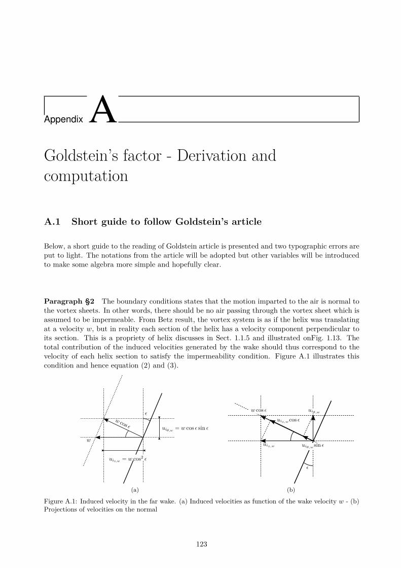
Appendix AGoldstein’s factor - Derivation andcomputation
A.1 Short guide to follow Goldstein’s article
Below, a short guide to the reading of Goldstein article is presented and two typographic errors areput to light. The notations from the article will be adopted but other variables will be introducedto make some algebra more simple and hopefully clear.
Paragraph §2 The boundary conditions states that the motion imparted to the air is normal tothe vortex sheets. In other words, there should be no air passing through the vortex sheet which isassumed to be impermeable. From Betz result, the vortex system is as if the helix was translatingat a velocity w, but in reality each section of the helix has a velocity component perpendicular toits section. This is a propriety of helix discusses in Sect. 1.1.5 and illustrated onFig. 1.13. Thetotal contribution of the induced velocities generated by the wake should thus correspond to thevelocity of each helix section to satisfy the impermeability condition. Figure A.1 illustrates thiscondition and hence equation (2) and (3).
w
w cos ε
uiz,w = w cos2 ε
uiθ,w = w cos ε sin ε
ε
(a)
uiz,w
uiθ,w
uiz,wcos ε
uiθ,w sin ε
w cos ε
ε
(b)
Figure A.1: Induced velocity in the far wake. (a) Induced velocities as function of the wake velocity w - (b)Projections of velocities on the normal
123

APPENDIX A. GOLDSTEIN’S FACTOR - DERIVATION AND COMPUTATION
Equation (5) is quickly derived with:∂φ
∂z= ∂φ
∂ζ
−ωv
(A.1)
∂φ
∂θ= ∂φ
∂ζ(A.2)
Letting the ratio wv/ω equal to 1 is not an assumption, it’s just a way to take advantage of linearity.This can be formalized by letting k = wv/ω, and φ = φ/k, then by linearity both φ and φ satisfyLaplace equation, but φ satisfies the BC from equation (5) whereas φ satisfies equation (7). Oncethe solution for φ is found in §3.5, then the solution is simply multiplied by k to obtain the solutionfor φ. That’s what Goldstein does but of course dropping the tilde notation. Equation (7) and (8)are easily derived with:
∇2 = ∂2
∂r2 + 1r
(∂
∂r+ 1r
∂2
∂θ2
)+ ∂2
∂z2 (A.3)
∂φ
∂r= ω
v
∂φ
∂µ(A.4)
∂
∂r= ω
v
∂
∂µ(A.5)(
µ∂
∂µ
)2φ = µ2∂
2φ
∂µ2 + µ∂φ
∂µ(A.6)
Equation (8) is called the homogeneous modified Bessel differential equations and admits for so-lution the modified Bessel function In(µ) and Kn(µ) (see for instance [2, p 374] or [83, chap.10]).
Paragraph §3.1 The form of equation (3) is suggested by the boundary condition. Insertingequation (3) in §2 (8) leads to equation (4), and inserting (3) in the boundary condition leads toequation (5). Now the problem reduces to solving equation (4) with the boundary condition (5).
Equation (6) is simply the Fourier series of the function f(ζ) = ζ on [0 ; π] (or the Fourier decom-position of |ζ| on [−π ; π]). This decomposition will be used for the right-hand side of equation(4). The idea is then to use a decomposition of the same nature for φ1 to allow an identificationterm by term between the left hand side and the right hand side, hence the assumption of equation(7). Equation (8) and (9) are purely the result of this identification term by term.
Equation (8) can be directly solved: noting H the operator (µdµdµ)2, and g0 = π/2µ2/(1 + µ2) thenequation (8) is just H(f0) = H(g0), which means that f0 = g0 + k where k is a function verifyingH(k) = 0. This writes µ2k′′+µk′ = 0, which can be integrated twice to find that k = A ln(µ) +B.The term in log has to disappear for finiteness at µ = 0, and the term B is just a constant whichis of no interest when dealing with potentials because they are defined relatively. We found thatf0 = g0 which is equation (10).
Going from (9) to (12) is quickly derived using the above notation and some dummy variables A,B, g: Equation (11) is written fm = B(g − gm), (9) written H(fm)− Afm = H(Bg), in which wecan insert the above expression of fm to get after simplification –H(−BGm)−ABg0−ABgm = 0,simplify by B and get equation (12).
The solving of equation (12) involves some mathematical formalism which will be briefly presentedhere for clarity and to have a broader perspective of the context. The inhomogeneous Besselequation of the function y(z) writes:(
zd
dz
)2y + (z2 − ν2)y = kzµ+1 (A.7)
E. Branlard 124
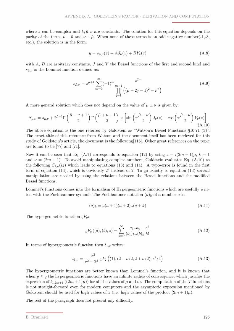
APPENDIX A. GOLDSTEIN’S FACTOR - DERIVATION AND COMPUTATION
where z can be complex and k, µ, ν are constants. The solution for this equation depends on theparity of the terms ν + µ and ν − µ. When none of these terms is an odd negative number(-1,-3,etc.), the solution is in the form:
y = sµ,ν(z) +AJν(z) +BYν(z) (A.8)
with A, B are arbitrary constants, J and Y the Bessel functions of the first and second kind andsµ,ν is the Lommel function defined as:
sµ,ν = zµ+1∞∑m=0
(−1)m z2m
m+1∏j=1
((µ+ 2j − 1)2 − ν2
) (A.9)
A more general solution which does not depend on the value of µ± ν is given by:
Sµ,ν = sµ,ν + 2µ−1Γ(µ− ν + 1
2
)Γ(µ+ ν + 1
2
)×[sin(πµ− ν
2
)Jν(z)− cos
(πµ− ν
2
)Yν(z)
](A.10)
The above equation is the one referred by Goldstein as “Watson’s Bessel Functions §10.71 (3)”.The exact title of this reference from Watson and the document itself has been retrieved for thisstudy of Goldstein’s article, the document is the following[116]. Other great references on the topicare found to be [77] and [71].
Now it can be seen that Eq. (A.7) corresponds to equation (12) by using z = i(2m + 1)µ, k = 1and ν = (2m + 1). To avoid manipulating complex numbers, Goldstein evaluates Eq. (A.10) asthe following S1,ν(iz) which leads to equations (13) and (14). A typo-error is found in the firstterm of equation (14), which is obviously 22 instead of 2. To go exactly to equation (13) severalmanipulation are needed by using the relations between the Bessel functions and the modifiedBessel functions.
Lommel’s functions comes into the formalism of Hypergeometric functions which are usefully writ-ten with the Pochhammer symbol. The Pochhammer notation (a)k of a number a is:
(a)k = a(a+ 1)(a+ 2)..(a+ k) (A.11)
The hypergeometric function pFq:
pFq ((a), (b), z) =∞∑k=0
a1..ap(b1)k..(b)k
zk
k! (A.12)
In terms of hypergeometric function then t1,ν writes:
t1,ν = −z2
ν2 − 22 1F2((1), (2− ν/2, 2 + ν/2), z2/4
)(A.13)
The hypergeometric functions are better known than Lommel’s function, and it is known thatwhen p ≤ q the hypergeometric functions have an infinite radius of convergence, which justifies theexpression of t1,2m+1 ((2m+ 1)µ)) for all the values of µ andm. The computation of the T functionsis not straight-forward even for modern computers and the asymptotic expression mentioned byGoldstein should be used for high values of z (i.e. high values of the product (2m+ 1)µ).
The rest of the paragraph does not present any difficulty.
E. Branlard 125
APPENDIX A. GOLDSTEIN’S FACTOR - DERIVATION AND COMPUTATION
Paragraph §3.2 In equation (2) Goldstein assumes another form of solution for equation §3.1(12). There is no obvious reason for it to be exactly the same solution than the one found in theprevious paragraph. We will write this series:
X =∞∑k=0
τ2kZ2k (A.14)
where Z = 2m+ 1. Introducing this series in equation(12) yields to∞∑k=0
1Z2k
11 + µ2H(τ2k)−
∞∑k=1
τ2k − τ0 = −µ2
1 + µ2 (A.15)
And after some rearrangements on the indexes:∞∑k=1
1Z2k
[ 11 + µ2H(τ2k−2)− τ2k
]− τ0 = −µ2
1 + µ2 (A.16)
By identifying term by terms the coefficient of 1/Z between the left hand side and the right handside, it yields to equation (4) and (5). The recurrence equation (4) come in handy to calculate thesuccessive τi manually. The question is whether the function denoted X above is really T1,(2m+1).Goldstein justifies it by looking at the numerical values. Further is finds that these functions areclose to µ2
1+µ2 hence the introduction of F which is expected to go to zero and thus will simplifymanual computations and allow further approximation in next paragraphs.
In this paragraph Goldstein introduces two function F and G to conveniently highlight the functionµ2/(1 + µ2) and reveal terms that goes to zero. In practice, the definition of these functions is notrequired. In equation (9) Goldstein uses:
∞∑m=0
1(2m+ 1)2 = π2
8 (A.17)
which can be found from equation §3.1 (6) expressed at ζ = 0.
Paragraph §3.3 Equation (1) is the Fourier decomposition of the function cos ((2m+ 1)ζ) on[0 ; π]. To go between the two equal signs of equation (5), the following result has been used:
∞∑m=0
1(2m+ 1)2 [4n2 − (2m+ 1)2] = 1
4n2
∞∑m=0
[ 1(2m+ 1)2 + 1
4n2 − (2m+ 1)2
](A.18)
= 14n2
[π2
8 −π tan(πn)
8n
]= π2
32n2 (A.19)
The coefficients am are determined for the approximate equation first and then a term εm is addedto account for the error. The terms are evaluated numerically only. For the case of any number ofblades, Goldstein neglects completely these error terms.
Paragraph §3.4 To obtain equation (2) one should recall our previous discussion on φ and φ,notation which isn’t used by Goldstein of course. No further difficulties in the different calculations.
Paragraph §5 It should be noted that the definitions for the thrust and torque coefficients aredifferent than the one commonly used in wind energy(differ from a factor 2). A typo-error is foundin equation (8) which should be corrected as:
dT
dr= pρΓ(rω + 1
2uθ) (A.20)
E. Branlard 126

APPENDIX A. GOLDSTEIN’S FACTOR - DERIVATION AND COMPUTATION
Computation Even with recent computer the computation of Goldstein’s factor is tedious andrequire some care. Without the help of modern computers, the calculation of Bessel’s function forarguments above 50 was difficult and asymptotic approximation of these function had to be used.Recommendations from [109] can still be used for an easier implementation because numericalinstabilities can occur, the convergence can be slow, some formulae are indeed more suitable thanothers and indeed asymptotic expansion should be used. Also, the summations can’t be numericallyperformed to infinity so a trade off has to be found. The Euler-Maclaurin formula can be used forgreat values of m, when the T functions are close to 1. The computation of the coefficients am alsorequires some attention. The use of a software that does formal algebra greatly simplifies the task.In this study the software Mathematica[71] was used for the calculations.
E. Branlard 127
APPENDIX A. GOLDSTEIN’S FACTOR - DERIVATION AND COMPUTATION
A.2 Computation of Goldstein’s factor using helical vortex solu-tion
The optimal circulation found by Goldstein can be obtained by modelling the wake as a super-position of helical vortex lines. If h = 2πl is the dimensional pitch of an helical vortex, then theinduced velocities for a helical vortex line of unitary circulation has been approximated by Okulovas:
Vf =
0− l
rA
[B · Sl
(r
l,a
l, θ
)+ Sm
(r
l,a
l, θ
)]r < a
l
r− l
rA
[B · Sl
(a
l,r
l, θ
)− Sm
(a
l,r
l, θ
)]r ≥ a
Vz = 12πl
1 + A
[B · Sl
(r
l,a
l, θ
)+ Sm
(r
l,a
l, θ
)]r < a
0 + A
[B · Sl
(a
l,r
l, θ
)− Sm
(a
l,r
l, θ
)]r ≥ a
Vθ = 12πl
l
r(1−Vz (r, a, l, θ))
Vx = −rl2πlVz (r, a, l, θ) + Vf (r, a, l, θ)
with
A =(a2 + l2
) 14
(r2 + l2)14
B = l
24
(3r2 − 2l2
(r2 + l2)32
+ 9a2 + 2l2
(a2 + l2)32
)
Sl(x, y, θ) = Re
− log
1− eiθ+log
(x(1+
√1+y2)
y(1+√
1+x2)
)+√
1+x2−√
1+y2
Sm(x, y, θ) = Re
eiθ
e−[
log(x(1+
√1+y2)
y(1+√
1+x2)
)+√
1+x2−√
1+y2
]− eiθ
The vortex sheet is modelled by a superposition of helical vortex curves of intensity γv,j to bedetermined using the boundary conditions as follow. Assuming N vortices at radial positions rj ,and N − 1 control points located at radial positions ri(for instance taken in between the vortexposition), the velocity at the control point ri, sum of the velocity contribution from all vortices is:
u(ri) =N∑j=1uj(ri) =
N∑j=1
γv,jaj(ri) (A.21)
The above equation can be decomposed on the three components x, θ, z.
The control points are taken to be on the vortex sheet so that they should verify the boundaryconditions on this sheet, which is that the velocity reduction is maximum on the vortex sheet.
E. Branlard 128
APPENDIX A. GOLDSTEIN’S FACTOR - DERIVATION AND COMPUTATION
These boundary conditions (derived in Eq. (2.8) and Eq. (2.7)) are found for uθ and uz and can bederived for the ux component. They write for each point located at radius r on the vortex sheet:
uθ,0 = w−rl
l2 + r2
(A.22)
uz,0 = wr2
l2 + r2
(A.23)
ux,0 = wr (A.24)
with l = l/R and r = r/R. Writing the boundary conditions at the control points ri and combiningthese with the three component of equation Eq. (A.21) leads to a set of three linear system ofequations of size (N−1)×N which unknowns are the N vortex intensities γv,j . These three systemequations are written in matrix form:
Aθ · Γv = Uθ,0 (A.25)Az · Γv = Uz,0 (A.26)Ax · Γv = Ux,0 (A.27)
The matrices of velocity influence A∗ have dimension N − 1×N , the vector of vortex intensity Γvis N × 1 and the vectors of boundary conditions U∗ are N − 1× 1. Let us now assume a vector Γv(a set of N − 1 γv,j) solution of Eq. (A.21). Inserting the solution Γv into Eq. (A.25) it is foundthat it is also a solution for ux if the sum of all the helical vortices circulation is equal to zero, i.e.:
N∑j=1
γj = 0 (A.28)
This condition is simply added to the A∗ matrix and the U∗ vectors in order to close the system,and make the problem entirely solvable by inversion of the newly formed N × N matrices. Anyof the three system will give a satisfactory solution for Γv so only one system has to be solved.Eventually, the total circulation, or Goldstein’s circulation at a radial position r, is the integralof the tangential induced velocity on a circle of perimeter 2πr, or more simply, is the sum of theintensity of the helical vortices contained in this circle:
Γ(r) =∮C(r)
uθ · dl =∑
j/ rj<r
γv,j (A.29)
Results from this calculation have been compared with the results of Tibery and Wrench[109] byOkulov[79] and showed perfect agreement. This simulation was reproduced here and showed perfectagreement as well as seen on Fig. A.2. The circulation has also been calculated for other values ofh than the one used by Okulov, and are shown on Fig. 2.14 for reference.
A.3 Computation of optimum power with finite number of blades
In vortex theory, the application of the Kutta-Joukowski leads to the calculation of local loads asfunction of the relative velocity and the circulation. By decomposing the loads on the normal andtangential component, the total power and thrust can be derived as:
P = ΩρB∫ R
0Γ (U0 − uiz) rdr (A.30)
T = ρB
∫ R
0Γ (Ωr + uiθ) dr (A.31)
E. Branlard 129
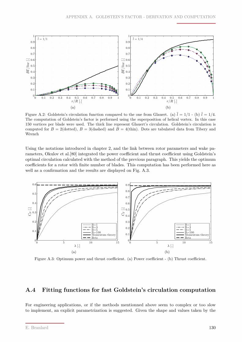
APPENDIX A. GOLDSTEIN’S FACTOR - DERIVATION AND COMPUTATION
l = 1/1
r/R [.]
BΓ/hw
[.]
0 0.1 0.2 0.3 0.4 0.5 0.6 0.7 0.8 0.9 10
0.1
0.2
0.3
0.4
0.5
0.6
0.7
0.8
0.9
1
(a)
l = 1/4
r/R [.]
BΓ/hw
[.]
0 0.1 0.2 0.3 0.4 0.5 0.6 0.7 0.8 0.9 10
0.1
0.2
0.3
0.4
0.5
0.6
0.7
0.8
0.9
1
(b)
Figure A.2: Goldstein’s circulation function compared to the one from Glauert. (a) l = 1/1 - (b) l = 1/4.The computation of Goldstein’s factor is performed using the superposition of helical vortex. In this case150 vortices per blade were used. The thick line represent Glauert’s circulation. Goldstein’s circulation iscomputed for B = 2(dotted), B = 3(dashed) and B = 4(thin). Dots are tabulated data from Tibery andWrench
Using the notations introduced in chapter 2, and the link between rotor parameters and wake pa-rameters, Okulov et al.[80] integrated the power coefficient and thrust coefficient using Goldstein’soptimal circulation calculated with the method of the previous paragraph. This yields the optimumcoefficients for a rotor with finite number of blades. This computation has been performed here aswell as a confirmation and the results are displayed on Fig. A.3.
λ [.]
CP
[.]
0 5 10 150
0.1
0.2
0.3
0.4
0.5
0.6
B=1B=3B=5B=100Momentum theoryBetz
(a)λ [.]
CT[.]
0 5 10 150
0.1
0.2
0.3
0.4
0.5
0.6
0.7
0.8
0.9
B=1B=3B=5B=100Momentum theoryBetz
(b)
Figure A.3: Optimum power and thrust coefficient. (a) Power coefficient - (b) Thrust coefficient.
A.4 Fitting functions for fast Goldstein’s circulation computation
For engineering applications, or if the methods mentionned above seem to complex or too slowto implement, an explicit parametrization is suggested. Given the shape and values taken by the
E. Branlard 130
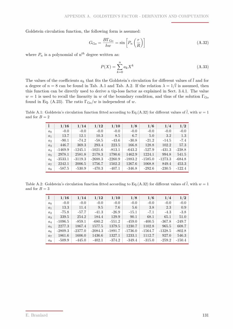
APPENDIX A. GOLDSTEIN’S FACTOR - DERIVATION AND COMPUTATION
Goldstein circulation function, the following form is assumed:
GGo = BΓGohw
= sin[Pn
(r
R
)](A.32)
where Pn is a polynomial of nth degree written as:
P (X) =n∑k=0
akXk (A.33)
The values of the coefficients ak that fits the Goldstein’s circulation for different values of l and fora degree of n = 8 can be found in Tab. A.1 and Tab. A.2. If the relation λ = 1/l is assumed, thenthis function can be directly used to derive a tip-loss factor as explained in Sect. 3.4.1. The valuew = 1 is used to recall the linearity in w of the boundary condition, and thus of the solution ΓGofound in Eq. (A.23). The ratio ΓGo/w is independent of w.
Table A.1: Goldstein’s circulation function fitted according to Eq.(A.32) for different values of l, with w = 1and for B = 2
l 1/16 1/14 1/12 1/10 1/8 1/6 1/4 1/2a0 -0.0 -0.0 -0.0 -0.0 -0.0 -0.0 -0.0 -0.0a1 13.7 12.1 10.3 8.5 6.7 5.0 3.2 1.3a2 -90.1 -74.2 -58.5 -43.6 -30.8 -21.2 -14.5 -7.4a3 446.7 369.3 293.4 223.5 166.8 128.8 102.2 57.3a4 -1469.9 -1245.1 -1021.6 -813.1 -643.2 -527.9 -431.3 -238.8a5 2978.1 2581.8 2178.3 1790.6 1462.9 1224.1 994.8 541.5a6 -3533.1 -3119.3 -2688.3 -2260.9 -1883.2 -1585.0 -1273.3 -684.8a7 2242.1 2006.5 1756.7 1502.2 1267.6 1068.8 849.4 453.3a8 -587.5 -530.9 -470.3 -407.1 -346.8 -292.6 -230.5 -122.4
Table A.2: Goldstein’s circulation function fitted according to Eq.(A.32) for different values of l, with w = 1and for B = 3
l 1/16 1/14 1/12 1/10 1/8 1/6 1/4 1/2a0 -0.0 -0.0 -0.0 -0.0 -0.0 -0.0 -0.0 -0.0a1 13.3 11.4 9.5 7.6 5.6 3.8 2.3 0.9a2 -75.8 -57.7 -41.3 -26.9 -15.1 -7.1 -4.3 -3.8a3 339.5 254.2 184.4 129.9 90.1 68.1 65.1 51.0a4 -1096.5 -859.1 -680.2 -551.2 -459.0 -400.5 -367.8 -249.7a5 2277.3 1867.4 1577.5 1379.5 1230.7 1102.8 965.5 608.7a6 -2809.3 -2377.0 -2084.3 -1891.7 -1736.0 -1564.7 -1328.5 -802.8a7 1861.6 1606.0 1436.6 1327.1 1233.1 1112.7 927.0 546.3a8 -509.9 -445.0 -402.1 -374.2 -349.4 -315.0 -259.2 -150.4
E. Branlard 131

APPENDIX A. GOLDSTEIN’S FACTOR - DERIVATION AND COMPUTATION
E. Branlard 132
Appendix BImplementation and validation of a vortex code
B.1 Implementation of a vortex code
Description
The vortex code will not be described in detail in this document. For the implementation of thecode and a general descriptions of vortex codes(panel codes, vortex lattice codes,etc.) the followingreferences were used:[52], [8]. For references on lifting line code implementations the reader can referto the following references:[37],[32],[99],[54][72],[82], [24],[93]. Part of the source code of the vortexcode implemented is available in Appendix F. Only the core function on which the vortex codeis based is given. This function correspond to the induced velocity created by a vortex segment.Given a vortex line delimited by the points x1 and x2, the velocity induced by this filament at apoint xp is given by:
Ui = Γ4πr0 ·
(r1r1− r2r2
)r1 × r2‖r1 × r2‖2
(B.1)
= Γ4π
(r1 + r2)r1r2(r1r2 + r1 · r2)r1 × r2 (B.2)
with
r1 = xp − x1 (B.3)r2 = xp − x2 (B.4)r0 = x2 − x1 = r1 − r2 (B.5)
and where the relation ‖r1 × r2‖2 = (r1r2)2 − (r1 · r2)2 has been used.
The different vortex code implemented
Core computational methods The core computational methods were implemented in C (seeAppendix F for source code fragments). In a later stage of the study, this code has been used as abenchmark for GPU code implementation. Three main functions are implemented:
- Line-by-Line function: computes the induced velocities of a series of vortex segments arbi-trarily distributed in space on a series of given control points.
- Lattice function: computes the total induced velocities of a vortex lattice (grid) on a seriesof given control points
133
APPENDIX B. IMPLEMENTATION AND VALIDATION OF A VORTEX CODE
- Lattice Ring-By-Ring function: same as the above but returns the influence of each ring oneach control points instead of the total contribution of the whole lattice.
Wake model The wake can be set free or prescribed. The wake can be shed progressively ateach time step behind the rotor, or prescribed since the beginning of the simulation. A far wakemodel consisting of a series of single root-tip rings associated to form an helix of a given pitch canbe added behind the free wake. This gives a better estimates of the induced velocities. The pitchof the far wake is determined at each time step depending on the axial induced velocity in the farwake. The number of helix rotations of the far wake is prescribed by the user.
Blade/wing representation The blade or the wing can be represented by a lattice of vortexrings forming a grid of any dimensions nchord × nspan. In its simpliest form the code can reduce toa lifting line formulation with the wing represented by a lattice of dimension 2× nspan.
Circulation at the blade The way the circulation can be handled depends on the blade/wingrepresentation.
- Prescribed circulation: always possible(blade lattice or lifting line).- Solved circulation using non-penetration condition: always possible.- Solved circulation using 2D data: only possible in the lifting line case1
Vortex viscous model
To resolve the singularity occurring when a calculation point is close to the vortex line, differentcorrections are commonly employed. A viscous core radius rc is used to define the radial locationfor which the tangential velocity induced by the vortex is maximum. Several methods reduces toa multiplicative factor Kv directly applied to the induced velocity Ui from Eq. (B.2) to eliminatethe singularity. These methods are for instance described in [60] and their expressions are:
Rankine Kv = max
1 , r2/r2c
(B.6)
Lamb-Oseen Kv = 1− exp(−αr2/r2
c
)α = 1.25643 (B.7)
Vatistas - n Kv = r2/r2c(
1 + (r/rc)2n) 1n
(B.8)
Vatistas - n=2 Kv = r2√r4c + r4 (B.9)
The model of Vatistas for n = 2 has been detailed as it is a fairly good approximation of theanalytical but simplified result from Lamb-Oseen. In the above, the radial distance r is replacedby the orthogonal distance related to a vortex filament: h = ‖r1 × r2‖/r0. A common model forthe vortex core radius computation is the one from Squire 1965[105][60, p 592] which writes in theform:
rc(t) =√
4αδν(t− t0) (B.10)
where α is the viscous core growth constant from the Lamb-Oseen model, δ is the viscous corediffusivity coefficient (or effective turbulent viscosity coefficient) and ν is the kinematic viscosity.
1Methods to extend to vortex lattice are possible using the spanwise distribution of circulation of a flat plate forinstance, see e.g. [82]. No time was allowed for this implementation.
E. Branlard 134

APPENDIX B. IMPLEMENTATION AND VALIDATION OF A VORTEX CODE
The time parameters model the growth of the vortex as the wake ages, and allows the vortex to bealready in a stage of decay immediately after it’s formation. This model showed good agreementwhen compared to measurement[60, p 592].
Another way of removing the singularity is to use a cut-off radius that is artificially inserted in thedenominator of Eq. (B.2) to prevent it to go to zero:
Ui = Γ4π
(r1 + r2)r1r2(r1r2 + r1 · r2) + (δc r0)2r1 × r2 (B.11)
with r0 being the length of the vortex filament. Suggested values of cut-off radius parameters δcfound in [37] are of 1-10% for the wake roll-up computation and 0.01% for bound vortex calculations.
E. Branlard 135
APPENDIX B. IMPLEMENTATION AND VALIDATION OF A VORTEX CODE
B.2 Validation of Vortex code with prescribed wake
Flat plate
As a first validation step, the lift coefficient for a flat plate of infinite aspect ratio AR is computedwith the vortex lattice code. The simulation results seen on Fig. B.1a agree perfectly with theJoukowski result Cl = 2π sinα which approximates to 2π at low angles of attack. The influence ofaspect ratio2 is then studied with results displayed on Fig. B.1b. Prandtl’s formula for an ellipticfinite wing is slightly modified by introducing a factor τ which is different of 0 for non ellipticalwing:
Clα =Clα,0
1 +Clα,0πAR (1 + τ)
(B.12)
where Clα is the lift slope of a finite wing and Clα,0 the lift slope of the airfoil section, with ingeneral Clα < Clα,0 . A modification of this formula has been suggested by Helmbold in 1942[3] fora better fit at lower aspect ratios:
Clα =Clα,0√
1 +(Clα,0πAR
)2+
Clα,0πAR
(B.13)
Tuck[111] derived an accurate method to assess the lift slope for an flat plate with a lifting surfaceformulation. He fitted his results with the empirical relation of Koemiawan at high aspect ratioproviding the following relation:
Clα = 2π − π 1AR (logAR + 2.5620) + 1.404 1
AR2 (logAR + 3.645) (B.14)
Values from the above formulation and experimental data are used for comparison with the simu-lation results on Fig. B.1b. Perfect agreement is found with the semi-analytical result from Tuckat high aspect ratio, and good agreement is found with the vortex lattice code from Jones 1960.Differences between the lifting surface results and the lifting line results from Prandtl are expecteddue to the difference in formulation(see for instance [111]).
Elliptical wing
Infinite aspect ratio The lifting line theory is easily verified for an the case of an elliptic wingwith infinite aspect ratio. Results for the case α = 5.7106, U0 = 1m/s and c0 = 1m is displayedon Fig. B.2 where a perfect match with the theory is found.
Influence of aspect ratio Analytical derivation from Kida [53][111] provides the exact liftcoefficient Clα of an elliptical wing from the three-dimensional lifting surface theory. Kida usestrigonometric series of Lamé polynomials for the analytical derivations and resulting numericaltabulated values are provided as function of a geometrical parameter defined as k2 = (a2 − b2)/a2,with a and b the two semi-axis of the ellipse. The notation b should not be mistaken in this contextwith the full-span of a wing often noted with the same letter. In his table 3[53] Kida separatesvalues for aspect ratio higher and lower than the circular wing. Vortex code simulation of thedifferent wing corresponding to these different values of k2 and different aspect ratio have beenperformed to be compared with the numerical values of Kida. Results are shown on Fig. B.3(a-b)where perfect agreement is found.
2See Notations on page 3
E. Branlard 136
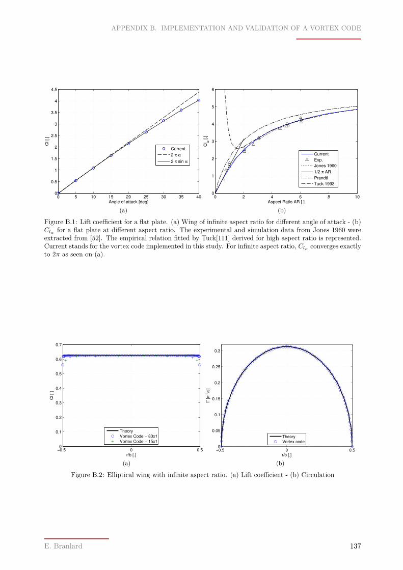
APPENDIX B. IMPLEMENTATION AND VALIDATION OF A VORTEX CODE
0 5 10 15 20 25 30 35 400
0.5
1
1.5
2
2.5
3
3.5
4
4.5
Angle of attack [deg]
Cl [.]
Current
2 π α
2 π sin α
(a)
0 2 4 6 8 100
1
2
3
4
5
6
Aspect Ratio AR [.]C
l α
[.]
Current
Exp.
Jones 1960
1/2 π AR
Prandtl
Tuck 1993
(b)
Figure B.1: Lift coefficient for a flat plate. (a) Wing of infinite aspect ratio for different angle of attack - (b)Clα for a flat plate at different aspect ratio. The experimental and simulation data from Jones 1960 wereextracted from [52]. The empirical relation fitted by Tuck[111] derived for high aspect ratio is represented.Current stands for the vortex code implemented in this study. For infinite aspect ratio, Clα converges exactlyto 2π as seen on (a).
−0.5 0 0.50
0.1
0.2
0.3
0.4
0.5
0.6
0.7
r/b [.]
Cl [.
]
Theory
Vortex Code − 80x1
Vortex Code − 15x1
(a)
−0.5 0 0.50
0.05
0.1
0.15
0.2
0.25
0.3
r/b [.]
Γ [
m2/s
]
Theory
Vortex code
(b)
Figure B.2: Elliptical wing with infinite aspect ratio. (a) Lift coefficient - (b) Circulation
E. Branlard 137

APPENDIX B. IMPLEMENTATION AND VALIDATION OF A VORTEX CODE
0 0.1 0.2 0.3 0.4 0.5 0.6 0.7 0.8 0.90
0.5
1
1.5
2
2.5
3
3.5
4
Geometrical parameter k2 [.]
Asp
ect
Ra
tio
[.]
,
Cl α
[.]
Cl
α
− Vortex code
Clα
− Theory
AR
(a)
0 0.5 1 1.5 2 2.5 3 3.5 4 4.50
0.5
1
1.5
2
2.5
3
3.5
4
Aspect Ratio AR [.]
k2 [
.],
Cl α
[.]
Cl
α
− Vortex code
Clα
− Theory
k2
(b)
Figure B.3: Lift coefficient of an elliptical wing for different aspect ratios. Figures (a) and (b) are twodifferent representations of identical results. Plain lines and blue symbols correspond to aspect ratios higherthan the circular wing in contrast to dashed lines and red symbols. The smaller semi-axis of the ellipse isalways taken as 1/2, hence an aspect ratio of 4/π for the circular wing.
Swept wing
In their book Bertin et al[8] detail an analytical solution of the vortex-lattice method applied to aswept wing. The wing has a sweep angle of Λ = 45, an arbitrary span b, an aspect ratio of AR = 5and is modelled by 8×1 panels. The vortex code applied with this geometry and number of panelsshowed perfect agreement with the derivation of Bertin as seen on Fig. B.4a. The influence ofincreasing the grid resolution and the influence of the wake roll-up is also displayed on this figure.Simulation results show good agreement with the experimental results of Weber and Brebner from1958 found in [8]. A modification of Eq. (B.13) has been suggested by Kuchemann[3] to computethe lift slope of a swept wing as function of the sweep angle Λ. This empirical relation writes:
Clα =Clα,0 cos Λ√
1 +(Clα,0 cos Λ
πAR
)2+
Clα,0 cos ΛπAR
(B.15)
On Fig. B.4b, this relation is confronted to the results from the vortex code. Good agreement isfound for low aspect ratio only. For higher aspect ratio, the current vortex code and the one fromJones[52] separates from the empirical relation while staying close to the experimental results.
Goldstein’s circulation function
The values of Goldstein’s circulation function can be obtained by prescribing an helical wake struc-ture of a given pitch with a sufficiently long extent to be an approximation of the infinite helicalwake studied by Goldstein(see Fig. B.6). The method used for the computation is similar to theone described in Sect. A.2. Using the conservation of circulation along the wake, and writing theboundary condition of normal velocity on the screw surface at collocation points located in the cen-ter of the wake, the circulation is obtained. Results from such computations displayed on Fig. B.5show great agreement with the computation of Goldstein’s analytical factor by Tibery and Wrench.
E. Branlard 138
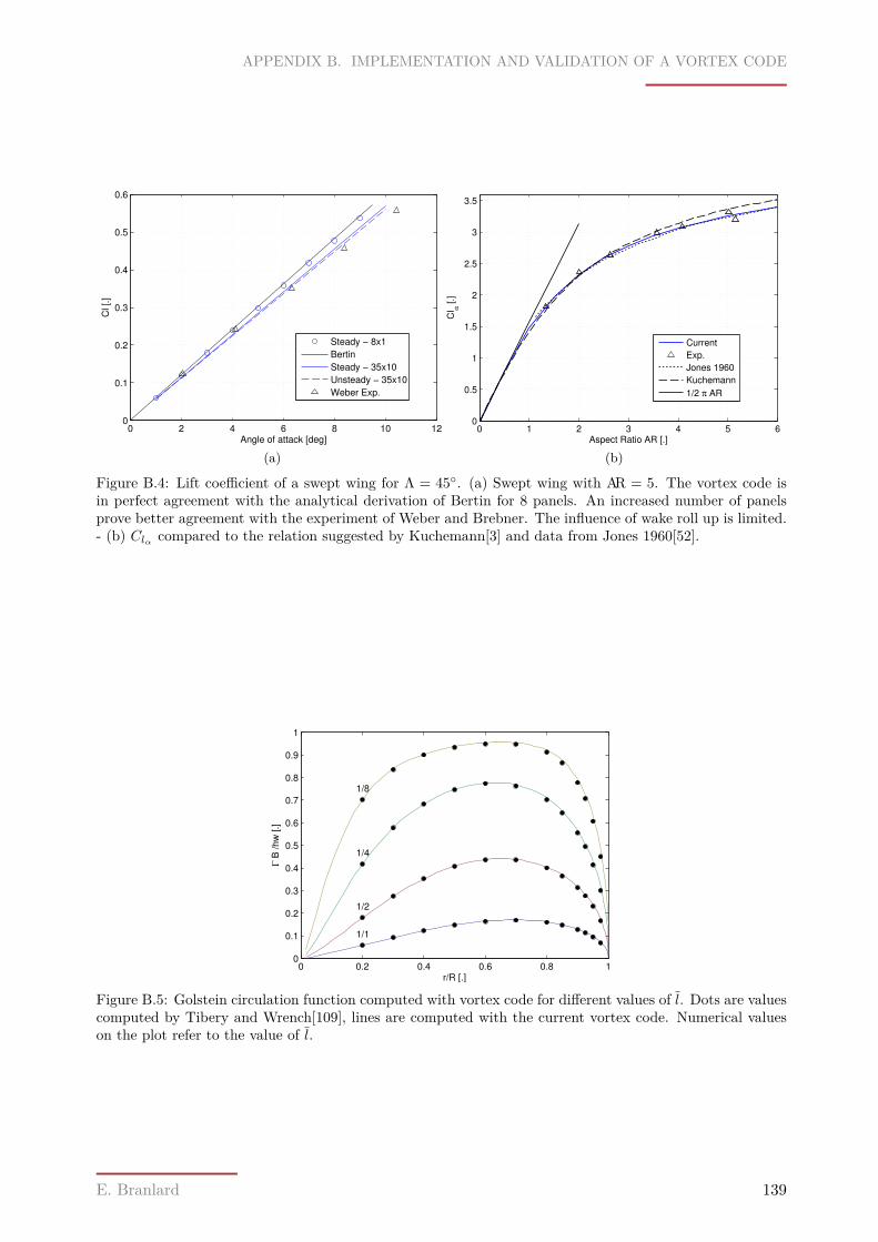
APPENDIX B. IMPLEMENTATION AND VALIDATION OF A VORTEX CODE
0 2 4 6 8 10 120
0.1
0.2
0.3
0.4
0.5
0.6
Angle of attack [deg]
Cl [.]
Steady − 8x1
Bertin
Steady − 35x10
Unsteady − 35x10
Weber Exp.
(a)
0 1 2 3 4 5 60
0.5
1
1.5
2
2.5
3
3.5
Aspect Ratio AR [.]C
l α
[.]
Current
Exp.
Jones 1960
Kuchemann
1/2 π AR
(b)
Figure B.4: Lift coefficient of a swept wing for Λ = 45. (a) Swept wing with AR = 5. The vortex code isin perfect agreement with the analytical derivation of Bertin for 8 panels. An increased number of panelsprove better agreement with the experiment of Weber and Brebner. The influence of wake roll up is limited.- (b) Clα compared to the relation suggested by Kuchemann[3] and data from Jones 1960[52].
0 0.2 0.4 0.6 0.8 10
0.1
0.2
0.3
0.4
0.5
0.6
0.7
0.8
0.9
1
1/1
1/2
1/4
1/8
r/R [.]
Γ B
/hw
[.]
Figure B.5: Golstein circulation function computed with vortex code for different values of l. Dots are valuescomputed by Tibery and Wrench[109], lines are computed with the current vortex code. Numerical valueson the plot refer to the value of l.
E. Branlard 139
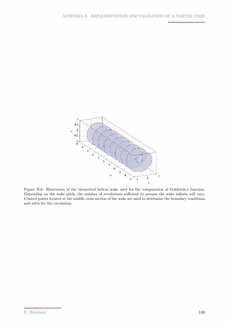
APPENDIX B. IMPLEMENTATION AND VALIDATION OF A VORTEX CODE
Figure B.6: Illustration of the theoretical helical wake used for the computation of Goldstein’s function.Depending on the wake pitch, the number of revolutions sufficient to assume the wake infinite will vary.Control points located at the middle cross section of the wake are used to determine the boundary conditionsand solve for the circulation.
E. Branlard 140
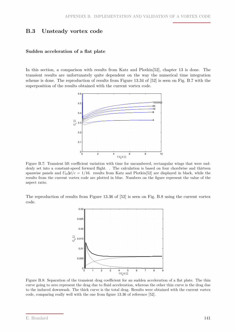
APPENDIX B. IMPLEMENTATION AND VALIDATION OF A VORTEX CODE
B.3 Unsteady vortex code
Sudden acceleration of a flat plate
In this section, a comparison with results from Katz and Plotkin[52], chapter 13 is done. Thetransient results are unfortunately quite dependent on the way the numerical time integrationscheme is done. The reproduction of results from Figure 13.34 of [52] is seen on Fig. B.7 with thesuperposition of the results obtained with the current vortex code.
0 2 4 6 8 100
0.1
0.2
0.3
0.4
0.5
0.6
4
8
1220
1000000
t U0/c [.]
CL [
.]
Figure B.7: Transient lift coefficient variation with time for uncambered, rectangular wings that were sud-denly set into a constant-speed forward flight. . The calculation is based on four chordwise and thirteenspanwise panels and U0∆t/c = 1/16. results from Katz and Plotkin[52] are displayed in black, while theresults from the current vortex code are plotted in blue. Numbers on the figure represent the value of theaspect ratio.
The reproduction of results from Figure 13.36 of [52] is seen on Fig. B.8 using the current vortexcode.
0 1 2 3 4 5 6 7 8 90
0.005
0.01
0.015
0.02
0.025
0.03
t U0/c [.]
CD [.]
Figure B.8: Separation of the transient drag coefficient for an sudden acceleration of a flat plate. The thincurve going to zero represent the drag due to fluid acceleration, whereas the other thin curve is the drag dueto the induced downwash. The thick curve is the total drag. Results were obtained with the current vortexcode, comparing really well with the one from figure 13.36 of reference [52].
E. Branlard 141
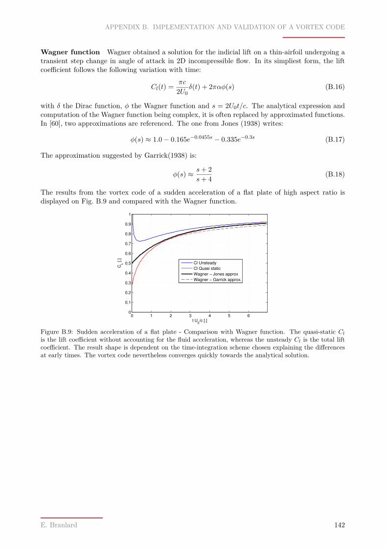
APPENDIX B. IMPLEMENTATION AND VALIDATION OF A VORTEX CODE
Wagner function Wagner obtained a solution for the indicial lift on a thin-airfoil undergoing atransient step change in angle of attack in 2D incompressible flow. In its simpliest form, the liftcoefficient follows the following variation with time:
Cl(t) = πc
2U0δ(t) + 2παφ(s) (B.16)
with δ the Dirac function, φ the Wagner function and s = 2U0t/c. The analytical expression andcomputation of the Wagner function being complex, it is often replaced by approximated functions.In [60], two approximations are referenced. The one from Jones (1938) writes:
φ(s) ≈ 1.0− 0.165e−0.0455s − 0.335e−0.3s (B.17)
The approximation suggested by Garrick(1938) is:
φ(s) ≈ s+ 2s+ 4 (B.18)
The results from the vortex code of a sudden acceleration of a flat plate of high aspect ratio isdisplayed on Fig. B.9 and compared with the Wagner function.
0 1 2 3 4 5 60
0.1
0.2
0.3
0.4
0.5
0.6
0.7
0.8
0.9
1
t U0/c [.]
CL [.]
Cl Unsteady
Cl Quasi static
Wagner − Jones approx
Wagner − Garrick approx.
Figure B.9: Sudden acceleration of a flat plate - Comparison with Wagner function. The quasi-static Clis the lift coefficient without accounting for the fluid acceleration, whereas the unsteady Cl is the total liftcoefficient. The result shape is dependent on the time-integration scheme chosen explaining the differencesat early times. The vortex code nevertheless converges quickly towards the analytical solution.
E. Branlard 142
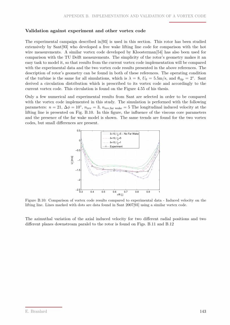
APPENDIX B. IMPLEMENTATION AND VALIDATION OF A VORTEX CODE
Validation against experiment and other vortex code
The experimental campaign described in[93] is used in this section. This rotor has been studiedextensively by Sant[93] who developed a free wake lifting line code for comparison with the hotwire measurements. A similar vortex code developed by Kloosterman[54] has also been used forcomparison with the TU Delft measurements. The simplicity of the rotor’s geometry makes it aneasy task to model it, so that results from the current vortex code implementation will be comparedwith the experimental data and the two vortex code results presented in the above references. Thedescription of rotor’s geometry can be found in both of these references. The operating conditionof the turbine is the same for all simulations, which is λ = 8, U0 = 5.5m/s, and θtip = 2. Santderived a circulation distribution which is prescribed to its vortex code and accordingly to thecurrent vortex code. This circulation is found on the Figure 4.55 of his thesis.
Only a few numerical and experimental results from Sant are selected in order to be comparedwith the vortex code implemented in this study. The simulation is performed with the followingparameters: n = 21, ∆φ = 10, nrev = 3, nrev,far wake = 5 The longitudinal induced velocity at thelifting line is presented on Fig. B.10. In this figure, the influence of the viscous core parametersand the presence of the far wake model is shown. The same trends are found for the two vortexcodes, but small differences are present.
0.3 0.4 0.5 0.6 0.7 0.8 0.9 1−2.5
−2
−1.5
−1
−0.5
0
0.5
r/R [.]
Ui [
m/s
]
δ=10, t0=5 − No Far Wake
δ=10, t0=5
δ=10, t0=1
Experiment
Figure B.10: Comparison of vortex code results compared to experimental data - Induced velocity on thelifting line. Lines marked with dots are data found in Sant 2007[93] using a similar vortex code.
The azimuthal variation of the axial induced velocity for two different radial positions and twodifferent planes downstream paralel to the rotor is found on Figs. B.11 and B.12
E. Branlard 143
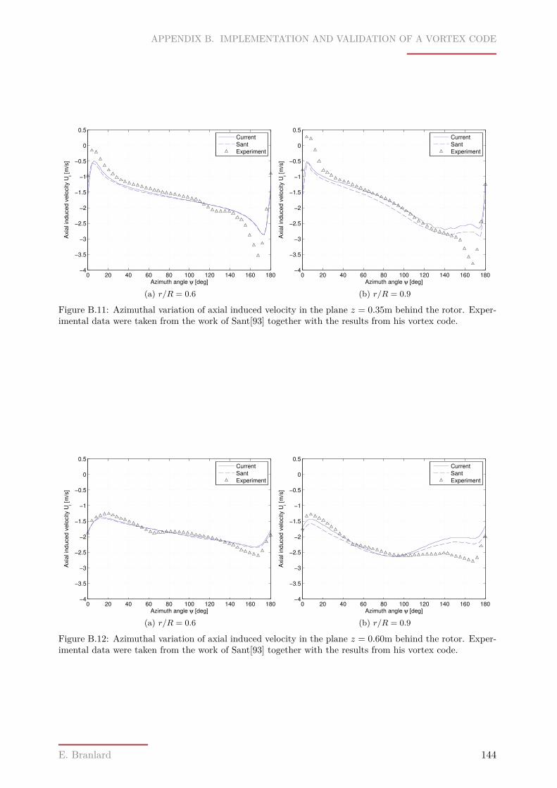
APPENDIX B. IMPLEMENTATION AND VALIDATION OF A VORTEX CODE
0 20 40 60 80 100 120 140 160 180−4
−3.5
−3
−2.5
−2
−1.5
−1
−0.5
0
0.5
Azimuth angle ψ [deg]
Axia
l in
du
ce
d v
elo
city U
i [m
/s]
Current
Sant
Experiment
(a) r/R = 0.6
0 20 40 60 80 100 120 140 160 180−4
−3.5
−3
−2.5
−2
−1.5
−1
−0.5
0
0.5
Azimuth angle ψ [deg]A
xia
l in
du
ce
d v
elo
city U
i [m
/s]
Current
Sant
Experiment
(b) r/R = 0.9
Figure B.11: Azimuthal variation of axial induced velocity in the plane z = 0.35m behind the rotor. Exper-imental data were taken from the work of Sant[93] together with the results from his vortex code.
0 20 40 60 80 100 120 140 160 180−4
−3.5
−3
−2.5
−2
−1.5
−1
−0.5
0
0.5
Azimuth angle ψ [deg]
Axia
l in
du
ce
d v
elo
city U
i [m
/s]
Current
Sant
Experiment
(a) r/R = 0.6
0 20 40 60 80 100 120 140 160 180−4
−3.5
−3
−2.5
−2
−1.5
−1
−0.5
0
0.5
Azimuth angle ψ [deg]
Axia
l in
du
ce
d v
elo
city U
i [m
/s]
Current
Sant
Experiment
(b) r/R = 0.9
Figure B.12: Azimuthal variation of axial induced velocity in the plane z = 0.60m behind the rotor. Exper-imental data were taken from the work of Sant[93] together with the results from his vortex code.
E. Branlard 144

APPENDIX B. IMPLEMENTATION AND VALIDATION OF A VORTEX CODE
On Figs. B.13, contour plots similar to the one found in [54] have been obtained with the currentvortex code and compared with the experimental results of Sant and vortex code results of Kloost-erman, as reported in [54]. Good agreement is found between Kloosterman’s vortex code and theone implemented in this study.
E. Branlard 145
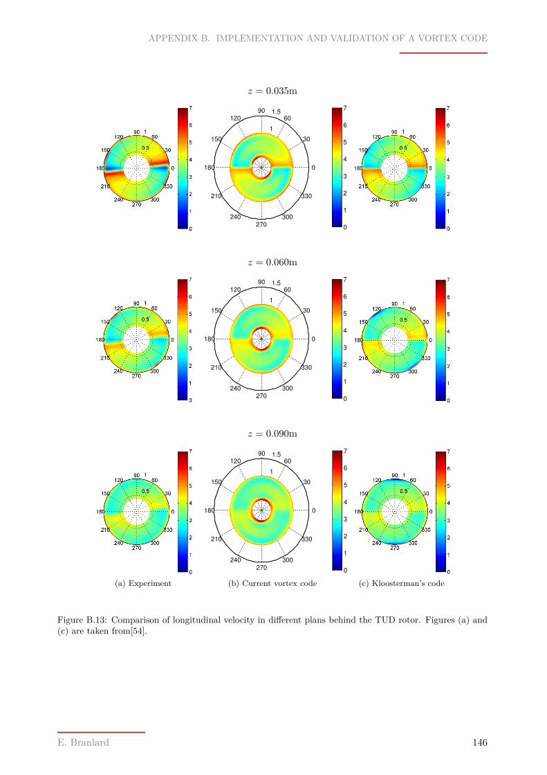
APPENDIX B. IMPLEMENTATION AND VALIDATION OF A VORTEX CODE
z = 0.035m
0.5
1
1.5
30
210
60
240
90
270
120
300
150
330
180 0
0
1
2
3
4
5
6
7
z = 0.060m
0.5
1
1.5
30
210
60
240
90
270
120
300
150
330
180 0
0
1
2
3
4
5
6
7
z = 0.090m
(a) Experiment
0.5
1
1.5
30
210
60
240
90
270
120
300
150
330
180 0
0
1
2
3
4
5
6
7
(b) Current vortex code (c) Kloosterman’s code
Figure B.13: Comparison of longitudinal velocity in different plans behind the TUD rotor. Figures (a) and(c) are taken from[54].
E. Branlard 146
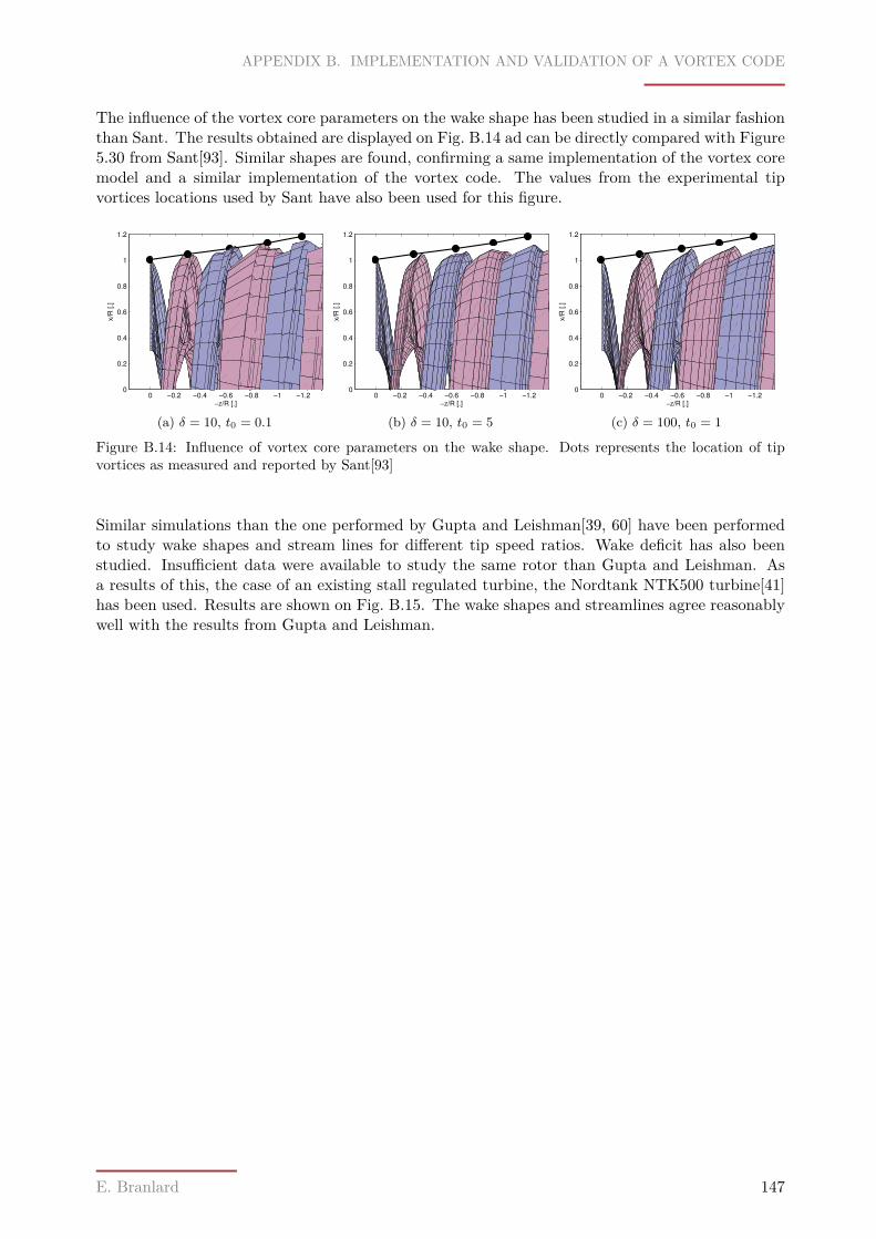
APPENDIX B. IMPLEMENTATION AND VALIDATION OF A VORTEX CODE
The influence of the vortex core parameters on the wake shape has been studied in a similar fashionthan Sant. The results obtained are displayed on Fig. B.14 ad can be directly compared with Figure5.30 from Sant[93]. Similar shapes are found, confirming a same implementation of the vortex coremodel and a similar implementation of the vortex code. The values from the experimental tipvortices locations used by Sant have also been used for this figure.
0
0.2
0.4
0.6
0.8
1
1.2
−1.2−1−0.8−0.6−0.4−0.20−z/R [.]
x/R
[.]
(a) δ = 10, t0 = 0.1
0
0.2
0.4
0.6
0.8
1
1.2
−1.2−1−0.8−0.6−0.4−0.20−z/R [.]
x/R
[.]
(b) δ = 10, t0 = 5
0
0.2
0.4
0.6
0.8
1
1.2
−1.2−1−0.8−0.6−0.4−0.20−z/R [.]
x/R
[.]
(c) δ = 100, t0 = 1
Figure B.14: Influence of vortex core parameters on the wake shape. Dots represents the location of tipvortices as measured and reported by Sant[93]
Similar simulations than the one performed by Gupta and Leishman[39, 60] have been performedto study wake shapes and stream lines for different tip speed ratios. Wake deficit has also beenstudied. Insufficient data were available to study the same rotor than Gupta and Leishman. Asa results of this, the case of an existing stall regulated turbine, the Nordtank NTK500 turbine[41]has been used. Results are shown on Fig. B.15. The wake shapes and streamlines agree reasonablywell with the results from Gupta and Leishman.
E. Branlard 147
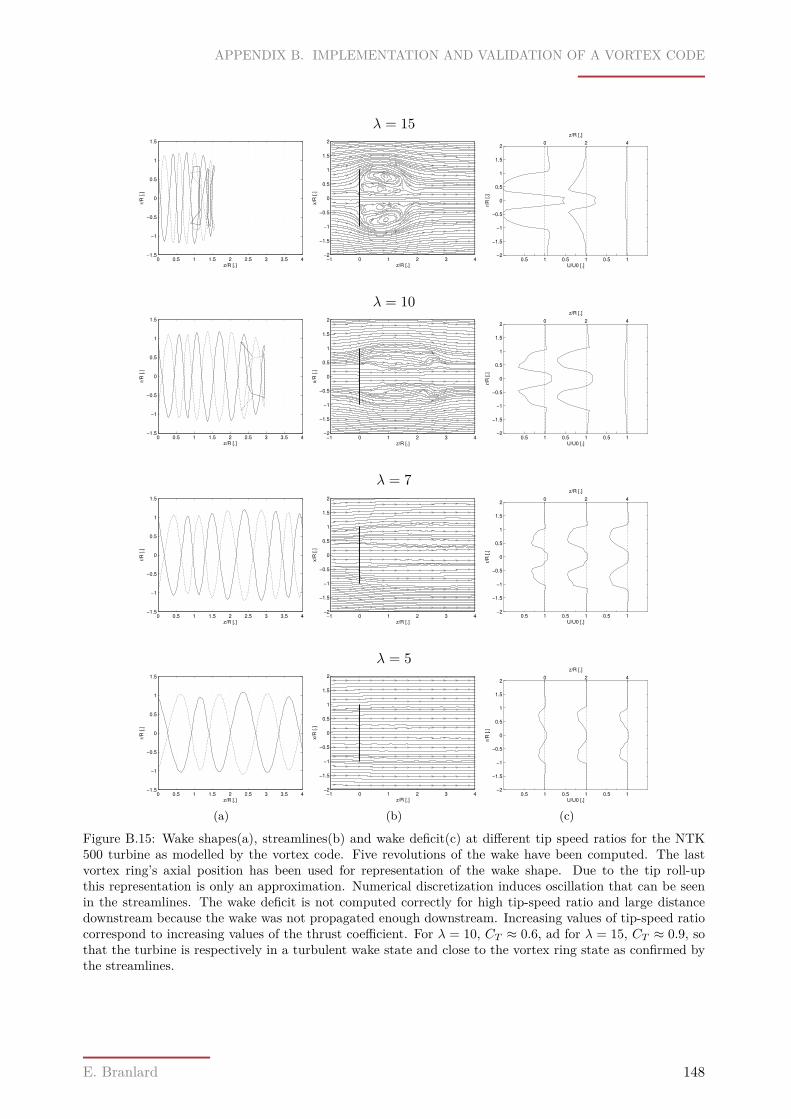
APPENDIX B. IMPLEMENTATION AND VALIDATION OF A VORTEX CODE
λ = 15
0 0.5 1 1.5 2 2.5 3 3.5 4−1.5
−1
−0.5
0
0.5
1
1.5
z/R [.]
r/R
[.]
−1 0 1 2 3 4−2
−1.5
−1
−0.5
0
0.5
1
1.5
2
z/R [.]
x/R
[.]
0.5 1 0.5 1 0.5 1−2
−1.5
−1
−0.5
0
0.5
1
1.5
2
U/U0 [.]
r/R
[.]
0 2 4
z/R [.]
λ = 10
0 0.5 1 1.5 2 2.5 3 3.5 4−1.5
−1
−0.5
0
0.5
1
1.5
z/R [.]
r/R
[.]
−1 0 1 2 3 4−2
−1.5
−1
−0.5
0
0.5
1
1.5
2
z/R [.]
x/R
[.]
0.5 1 0.5 1 0.5 1−2
−1.5
−1
−0.5
0
0.5
1
1.5
2
U/U0 [.]
r/R
[.]
0 2 4
z/R [.]
λ = 7
0 0.5 1 1.5 2 2.5 3 3.5 4−1.5
−1
−0.5
0
0.5
1
1.5
z/R [.]
r/R
[.]
−1 0 1 2 3 4−2
−1.5
−1
−0.5
0
0.5
1
1.5
2
z/R [.]
x/R
[.]
0.5 1 0.5 1 0.5 1−2
−1.5
−1
−0.5
0
0.5
1
1.5
2
U/U0 [.]
r/R
[.]
0 2 4
z/R [.]
λ = 5
0 0.5 1 1.5 2 2.5 3 3.5 4−1.5
−1
−0.5
0
0.5
1
1.5
z/R [.]
r/R
[.]
(a)
−1 0 1 2 3 4−2
−1.5
−1
−0.5
0
0.5
1
1.5
2
z/R [.]
x/R
[.]
(b)
0.5 1 0.5 1 0.5 1−2
−1.5
−1
−0.5
0
0.5
1
1.5
2
U/U0 [.]
r/R
[.]
0 2 4
z/R [.]
(c)
Figure B.15: Wake shapes(a), streamlines(b) and wake deficit(c) at different tip speed ratios for the NTK500 turbine as modelled by the vortex code. Five revolutions of the wake have been computed. The lastvortex ring’s axial position has been used for representation of the wake shape. Due to the tip roll-upthis representation is only an approximation. Numerical discretization induces oscillation that can be seenin the streamlines. The wake deficit is not computed correctly for high tip-speed ratio and large distancedownstream because the wake was not propagated enough downstream. Increasing values of tip-speed ratiocorrespond to increasing values of the thrust coefficient. For λ = 10, CT ≈ 0.6, ad for λ = 15, CT ≈ 0.9, sothat the turbine is respectively in a turbulent wake state and close to the vortex ring state as confirmed bythe streamlines.
E. Branlard 148
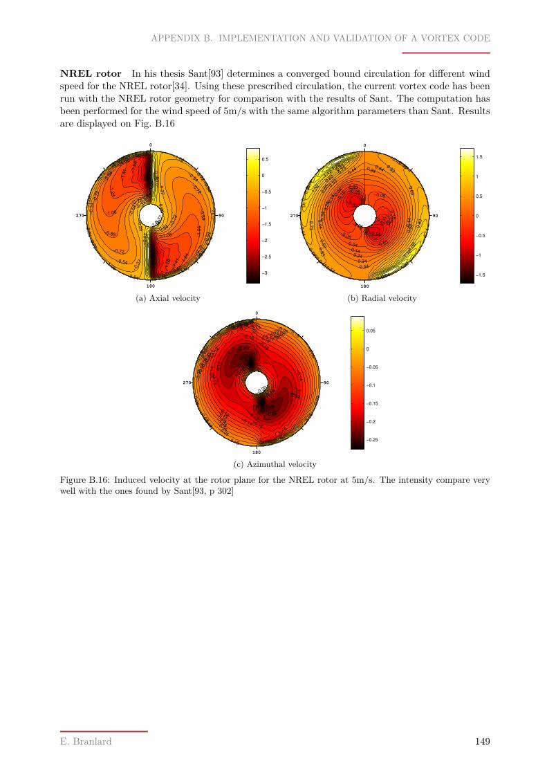
APPENDIX B. IMPLEMENTATION AND VALIDATION OF A VORTEX CODE
NREL rotor In his thesis Sant[93] determines a converged bound circulation for different windspeed for the NREL rotor[34]. Using these prescribed circulation, the current vortex code has beenrun with the NREL rotor geometry for comparison with the results of Sant. The computation hasbeen performed for the wind speed of 5m/s with the same algorithm parameters than Sant. Resultsare displayed on Fig. B.16
0
270
180
90
−1.06
−1.06
−1.06
−1.0
6
−1.06
−1.06
−1.06
−1.0
6
−1.06
−0.8
9
−0.89
−0.89
−0.7
2
−0.7
2−0.7
2
−0.7
2
−0.72
−0.7
2
−0.72
−0.72
−0.5
4
−0.5
4
−0.54
−0.5
4
−0.5
4
−0.5
4
−0.54
−0.5
4−0.3
7
−0.37
−0.3
7
−0.3
7
−0.3
7
−0.54
−0.5
4
−0.5
4
−0.7
2
−0.7
2
−0.7
2
−0.89
−0.8
9
−1.06 −1.0
6
−1.2
4
−1.2
4
−1.2
4
−0.2
0
−0.2
0
−0.2
0
−1.4
1
−1.4
1
−1.5
8
−1.5
8
−0.0
3
−0.0
3
0.1
5
−0.20−0.20
−2.7
9
−0.03
0.15
−3
−2.5
−2
−1.5
−1
−0.5
0
0.5
(a) Axial velocity
0
270
180
90
−0.45
−0.4
5
−0.45
−0.3
5
−0.25
−0.25
−0.2
5
−0.1
5
−0.1
5
−0.1
5
−0.05
−0.05
−0.05
−0.05
0.04
0.04
0.0
4
0.0
4
0.0
4
0.04
0.1
4
0.1
4
0.14
0.1
4
0.1
4
0.1
4
0.14
0.2
4
0.24
0.3
4
0.34
0.34
0.4
4
0.44
0.4
4
0.44
0.4
4
0.44
0.5
3
0.5
3
0.53
0.53
0.5
3
0.5
3
0.6
30.6
3
0.6
3
0.73
0.7
3 0.8
3
0.8
3
0.93
0.9
3
1.0
2
1.0
2
1.1
2
1.12
1.22
1.22
−0.54
−0.54
−1.5
−1
−0.5
0
0.5
1
1.5
(b) Radial velocity0
270
180
90
−0.20
−0.20
−0.20
−0.18
−0.1
8
−0.1
8
−0.1
8
−0.18
−0.1
7
−0.1
7
−0.1
7
−0.15
−0.15
−0.1
5
−0.15
−0.1
5
−0.1
5
−0.14
−0.1
4
−0.14
−0.1
4
−0.1
4
−0.12
−0.1
2
−0.1
2
−0.12
−0.11
−0.1
1
−0.1
1
−0.11
−0.0
9
−0.0
9
−0.09
−0.08
−0.0
8
−0.08
−0.08
−0.06
−0.0
6
−0.06
−0.06
−0.0
5
−0.0
5
−0.0
5
−0.0
5
−0.05
−0.0
5
−0.05
−0.05
−0.1
8
−0.1
8
−0.15
−0.22
−0.22
−0.0
3
−0.0
3
−0.0
3
−0.0
2
−0.23
−0.2
3
−0.1
1
0.010.03
−0.25
−0.2
−0.15
−0.1
−0.05
0
0.05
(c) Azimuthal velocity
Figure B.16: Induced velocity at the rotor plane for the NREL rotor at 5m/s. The intensity compare verywell with the ones found by Sant[93, p 302]
E. Branlard 149
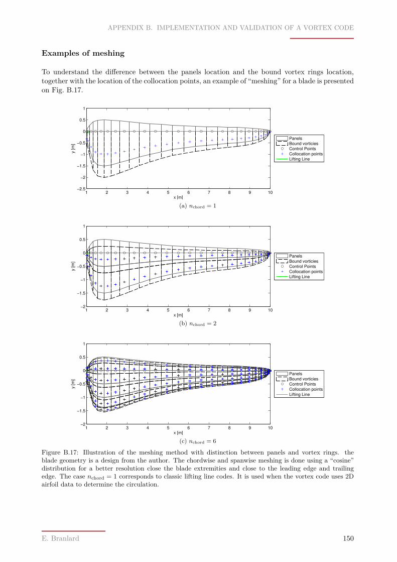
APPENDIX B. IMPLEMENTATION AND VALIDATION OF A VORTEX CODE
Examples of meshing
To understand the difference between the panels location and the bound vortex rings location,together with the location of the collocation points, an example of “meshing” for a blade is presentedon Fig. B.17.
1 2 3 4 5 6 7 8 9 10−2.5
−2
−1.5
−1
−0.5
0
0.5
1
x [m]
y [m
]
Panels
Bound vorticies
Control Points
Collocation points
Lifting Line
(a) nchord = 1
1 2 3 4 5 6 7 8 9 10−2
−1.5
−1
−0.5
0
0.5
1
x [m]
y [m
]
Panels
Bound vorticies
Control Points
Collocation points
Lifting Line
(b) nchord = 2
1 2 3 4 5 6 7 8 9 10−2
−1.5
−1
−0.5
0
0.5
1
x [m]
y [m
]
Panels
Bound vorticies
Control Points
Collocation points
Lifting Line
(c) nchord = 6
Figure B.17: Illustration of the meshing method with distinction between panels and vortex rings. theblade geometry is a design from the author. The chordwise and spanwise meshing is done using a “cosine”distribution for a better resolution close the blade extremities and close to the leading edge and trailingedge. The case nchord = 1 corresponds to classic lifting line codes. It is used when the vortex code uses 2Dairfoil data to determine the circulation.
E. Branlard 150
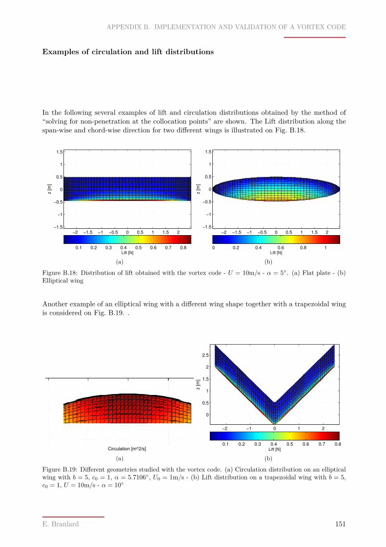
APPENDIX B. IMPLEMENTATION AND VALIDATION OF A VORTEX CODE
Examples of circulation and lift distributions
In the following several examples of lift and circulation distributions obtained by the method of“solving for non-penetration at the collocation points” are shown. The Lift distribution along thespan-wise and chord-wise direction for two different wings is illustrated on Fig. B.18.
−2 −1.5 −1 −0.5 0 0.5 1 1.5 2−1.5
−1
−0.5
0
0.5
1
1.5
x [m]
z [m
]
Lift [N]
0.1 0.2 0.3 0.4 0.5 0.6 0.7 0.8
(a)
−2 −1.5 −1 −0.5 0 0.5 1 1.5 2
−1.5
−1
−0.5
0
0.5
1
1.5
x [m]
z [m
]
Lift [N]
0 0.2 0.4 0.6 0.8 1
(b)
Figure B.18: Distribution of lift obtained with the vortex code - U = 10m/s - α = 5. (a) Flat plate - (b)Elliptical wing
Another example of an elliptical wing with a different wing shape together with a trapezoidal wingis considered on Fig. B.19. .
Circulation [m^2/s]
(a)
−2 −1 0 1 2
0
0.5
1
1.5
2
2.5
x [m]
z [m
]
Lift [N]
0.1 0.2 0.3 0.4 0.5 0.6 0.7 0.8
(b)
Figure B.19: Different geometries studied with the vortex code. (a) Circulation distribution on an ellipticalwing with b = 5, c0 = 1, α = 5.7106, U0 = 1m/s - (b) Lift distribution on a trapezoidal wing with b = 5,c0 = 1, U = 10m/s - α = 10
E. Branlard 151
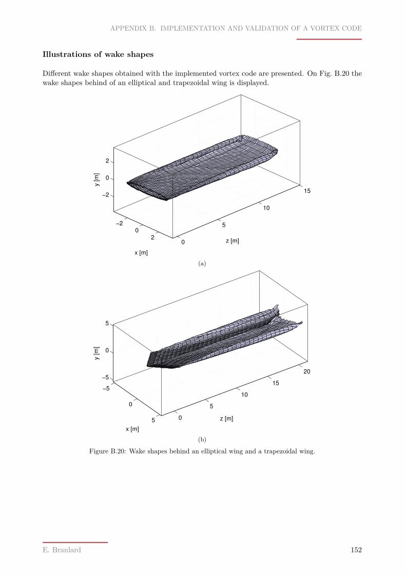
APPENDIX B. IMPLEMENTATION AND VALIDATION OF A VORTEX CODE
Illustrations of wake shapes
Different wake shapes obtained with the implemented vortex code are presented. On Fig. B.20 thewake shapes behind of an elliptical and trapezoidal wing is displayed.
−20
20
5
10
15−2
0
2
z [m]
x [m]
y [m
]
(a)
−5
0
5 0
5
10
15
20−5
0
5
z [m]
x [m]
y [
m]
(b)
Figure B.20: Wake shapes behind an elliptical wing and a trapezoidal wing.
E. Branlard 152
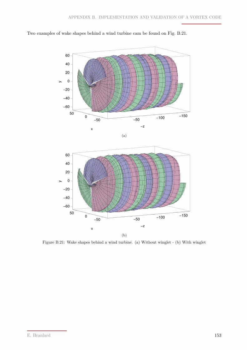
APPENDIX B. IMPLEMENTATION AND VALIDATION OF A VORTEX CODE
Two examples of wake shapes behind a wind turbine cam be found on Fig. B.21.
−500
50−150
−100−50
−60
−40
−20
0
20
40
60
−z
x
y
(a)
−500
50−150
−100−50
−60
−40
−20
0
20
40
60
−z
x
y
(b)
Figure B.21: Wake shapes behind a wind turbine. (a) Without winglet - (b) With winglet
E. Branlard 153

APPENDIX B. IMPLEMENTATION AND VALIDATION OF A VORTEX CODE
E. Branlard 154
Appendix CThe BEM method
C.1 Introduction to the BEM method
The blade element momentum(BEM) method results in the combination of the momentum theoryand the blade element theory. Figure 1.18 illustrates the differences between these methods and howthey are combined to form the BEM theory. The momentum theory applied to a stripe provides thecorresponding elementary thrust and torque for a given set of both induction factors. This relationbetween induction factors and loads is invertible. The velocity triangle from the momentum theoryalso gives an expression of the flow angle as function of a and a′. On the other hand, the bladeelement theory requires the airfoil characteristics, the angle of attack and the relative velocity tocalculate the forces of lift and drag applied to the blade element, and by projection the elementarythrust and torque. For a given rotor geometry and a given wind condition, a physical solution willbe found if both methods returns the same loads for all the different stripes. In order to find thissolution, the methods are linked together to form a converging iterative process. The author likesto emphasize two links, or linkage, to clearly distinguish the difference of the methods and howthey interact. The first linkage is obtained by comparing the velocity triangles of the two methods.The second linkage consists in equalizing the loads obtained from both methods. It should benoted that due to the hypothesis of independence of each stripe, the convergence loop and the loopover the different stripes can be indifferently switched. Depending on this choice, the convergencecriteria can be implemented in several way. The choice of the variable on which the convergenceis tested is multiple as well, the most common choices being: the angle of attack, the inductionfactor or, which is suggested here, the total Power. In practice the implementation of the BEMalgorithm is slightly different from the one shown on Fig. 1.18 because the succession of blocks canbe simplified mathematically. The final algorithm will be presented in Sect. C.1 after derivation ofthe linkage equations and simplifications.
Note In the following the BEM algorithm as described by Glauert[35], or [42] is presented. Nopressure terms accounting for wake rotations are used. These authors don’t explicitly uses thenotations aB and a so that the same will be done here to avoid confusion. Controversy also appearas soon as the tip-loss factor is applied. For instance the velocity triangle presented in the nextsection is for some author local to the blade but on the other hand it is derived from 2D momentumtheory which has infinite number of blades. Discussion on BEM formalism are still open.
155
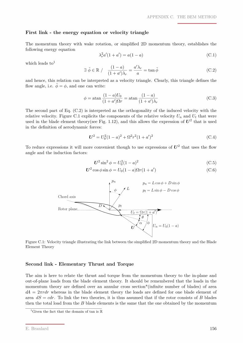
APPENDIX C. THE BEM METHOD
First link - the energy equation or velocity triangle
The momentum theory with wake rotation, or simplified 2D momentum theory, establishes thefollowing energy equation
λ2ra′(1 + a′) = a(1− a) (C.1)
which leads to1
∃ φ ∈ R /(1− a)
(1 + a′)λr= a′λr
a= tan φ (C.2)
and hence, this relation can be interpreted as a velocity triangle. Clearly, this triangle defines theflow angle, i.e. φ = φ, and one can write:
φ = atan (1− a)U0(1 + a′)Ωr = atan (1− a)
(1 + a′)λr(C.3)
The second part of Eq. (C.2) is interpreted as the orthogonality of the induced velocity with therelative velocity. Figure C.1 explicits the components of the relative velocity Un and Ut that wereused in the blade element theory(see Fig. 1.12), and this allows the expression of U2 that is usedin the definition of aerodynamic forces:
U2 = U20 (1− a)2 + Ω2r2(1 + a′)2 (C.4)
To reduce expressions it will more convenient though to use expressions of U2 that uses the flowangle and the induction factors:
U2 sin2 φ = U20 (1− a)2 (C.5)
U2 cosφ sinφ = U0(1− a)Ωr(1 + a′) (C.6)
Rotor planeUt = Ωr(1 + a′)
Un = U0(1− a)Uφ
θ
α
φ L
D pt
pn pn = L cosφ + D sinφ
pt = L sinφ−D cosφChord axis
Figure C.1: Velocity triangle illustrating the link between the simplified 2D momentum theory and the BladeElement Theory
Second link - Elementary Thrust and Torque
The aim is here to relate the thrust and torque from the momentum theory to the in-plane andout-of-plane loads from the blade element theory. It should be remembered that the loads in themomentum theory are defined over an annular cross section*(infinite number of blades) of areadA = 2πrdr whereas in the blade element theory the loads are defined for one blade element ofarea dS = cdr. To link the two theories, it is thus assumed that if the rotor consists of B bladesthen the total load from the B blade elements is the same that the one obtained by the momentum
1Given the fact that the domain of tan is R
E. Branlard 156
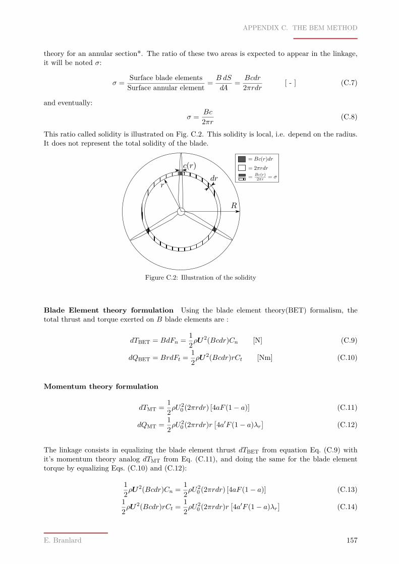
APPENDIX C. THE BEM METHOD
theory for an annular section*. The ratio of these two areas is expected to appear in the linkage,it will be noted σ:
σ = Surface blade elementsSurface annular element = B dS
dA= Bcdr
2πrdr [ - ] (C.7)
and eventually:
σ = Bc
2πr (C.8)
This ratio called solidity is illustrated on Fig. C.2. This solidity is local, i.e. depend on the radius.It does not represent the total solidity of the blade.
Figure C.2: Illustration of the solidity
Blade Element theory formulation Using the blade element theory(BET) formalism, thetotal thrust and torque exerted on B blade elements are :
dTBET = BdFn = 12ρU
2(Bcdr)Cn [N] (C.9)
dQBET = BrdFt = 12ρU
2(Bcdr)rCt [Nm] (C.10)
Momentum theory formulation
dTMT = 12ρU
20 (2πrdr) [4aF (1− a)] (C.11)
dQMT = 12ρU
20 (2πrdr)r
[4a′F (1− a)λr
](C.12)
The linkage consists in equalizing the blade element thrust dTBET from equation Eq. (C.9) withit’s momentum theory analog dTMT from Eq. (C.11), and doing the same for the blade elementtorque by equalizing Eqs. (C.10) and (C.12):
12ρU
2(Bcdr)Cn = 12ρU
20 (2πrdr) [4aF (1− a)] (C.13)
12ρU
2(Bcdr)rCt = 12ρU
20 (2πrdr)r
[4a′F (1− a)λr
](C.14)
E. Branlard 157
APPENDIX C. THE BEM METHOD
Introducing the linkage equations to simplify equations
In this section the linkage equations are written in different forms to allow analysis of certain termsand comparison with other references. The equations are presented with or without the inclusionof the drag coefficient in the axial induction.
Simplifications of the Blade Element theory equations using the first link Using thefirst link, the loads from the BET can be written indifferently in the following forms2:
dTBET = ρBc
2U2
0 (1− a)2
sin2 φCndr = σπρ
U20 (1− a)2
sin2 φCnrdr (C.15)
dQBET = ρBcr
2U0(1− a)Ωr(1 + a′)
sinφ cosφ Ctdr = ρBcr
2U2
0 (1− a)2
sin2 φCtdr = σπρ
U20 (1− a)2
sin2 φCtr
2dr
(C.16)
From now on, in this paragraph, the subscript BET is dropped, but it should be remembered thatno results from the momentum theory are used. The above relations can be expressed with respectto a′ as used e.g. in [64]:
dT = σπρΩ2r2(1 + a′)2
cos2 φCnrdr (C.17)
dQ = σπρΩ2r2(1 + a′)2
cos2 φCtr
2dr (C.18)
The global thrust and torque coefficients defined with respect to the whole rotor area πR2 can bewritten in a differential form(for comparison with e.g. [35]):
RdCTdr
= RdT
dr
112ρU
20πR
2 = 2λ2σ
(r
R
)3 (1 + a′)2
cos2 φCn (C.19)
RdCQdr
= RdQ
dr
112ρU
20πR
3 = 2λ2σ
(r
R
)4 (1 + a′)2
cos2 φCt (C.20)
or
The local thrust and torque coefficients defined for each annular section of surface 2πrdr are foundto be:
CTr = dT12ρU
20 2πrdr
= (1− a)2σ
sin2 φCn (C.21)
CQr = dQ12ρU
20 r2πrdr
= (1− a)2σ
sin2 φCt (C.22)
orCQrCTr
= CnCt
(C.23)
Simplifications using the two links Simplifying Eqs. (C.13) and (C.14) leads to:a
1− a = 14F sin2 φ
cB
2πrCn = σ
4F sin2 φCn (C.24)
a′
1 + a′= 1
4F sinφ cosφcB
2πrCt = σ
4F sinφ cosφCt (C.25)
2There are indeed many variation possible due to the different relations between the parameters. These forms aredeveloped here for an easy comparison with literature
E. Branlard 158
APPENDIX C. THE BEM METHOD
or in a different form (for comparison with e.g. [64])
11− a = 1 + σ
4F1
tan2 φ
Cncos2 φ
(C.26)
11 + a′
= 1− σ
4F1
tan2 φ
Ctcos2 φ
(C.27)
which solves to:
a = 14F sin2 φ
σCn+ 1
(C.28)
a′ = 14F sinφ cosφ
σCt− 1
(C.29)
Equations without drag In the calculation of induction factors, a and a′, it is argued by someauthors that Cd should be set equal to zero(see discussion in Sect. 1.3.4, and e.g.[117, 23]). WithCl = 0, Eq. (C.24) and Eq. (C.25) reduces to
a
1− a = σ cosφ4F sin2 φ
Cl (C.30)
a′
1 + a′= σ
4F cosφCl (C.31)
Then Eq. (C.28) and Eq. (C.29) writes:
a = 14F sin2 φ
σCl cosφ + 1(C.32)
a′ = 14F cosφσCl
− 1(C.33)
Using the two above equations with the first linkage equation and after some algebra an expressioncan be obtained for the lift coefficient:
Cl = 4 sinφσ
cosφ− λr sinφsinφ+ λr cosφ (C.34)
It can be noted that in the case where the drag is omitted, then then the ratio to the two loadingcoefficients Eq. (C.23) reduces to a simple function of φ:
CQrCTr
= tanφ (C.35)
Also, the ratio of Eq. (C.30) and (C.31) leads to:
tanφ = λra′
a(C.36)
which recalls equation Eq. (C.2). Hence when the drag is ignored, the energy equation is satisfiedand so is the condition of orthogonality between the induced velocity and the relative velocity.
E. Branlard 159
APPENDIX C. THE BEM METHOD
Note on other conventions Several conventions are found in the old literature for the thrustand torque coefficients. For propellers, due to the large rotational speeds, the velocity taken as areference is ΩR. In propellers aerodynamics the advance ratio J = U0/nrotD plays the equivalentrole of the tip-speed ratio. The two are related with: J = π/λ. In[64] the thrust and torquecoefficients kT and kQ are defined as:
T = kT · ρn2rotD
4 = kT · 4ρΩ2
π2R4 ⇔ CT = kT ·
8π3λ
2 (C.37)
Q = kQ · ρn2rotD
5 = kQ · 8ρΩ2
π2R5 ⇔ CQ = kQ ·
16π3λ
2 (C.38)
P = kP · ρn3rotD
5 = kP · 4ρΩ3
π3R5 ⇔ CP = kp ·
8π3λ
3 (C.39)
In [35], the thrust and torque coefficients are defined as:
T = Tc · ρπΩ2R4 ⇔ CT = Tc · 2λ2 (C.40)Q = Qc · ρπΩ2R5 ⇔ CQ = Qc · 2λ2 (C.41)
Summary of BEM algorithm
Assumptions C.1:(H C.1a) - The forces of the B blade elements are responsible for the change of momentum of theair which passes through the annulus swept by the elements(H C.1b) - No aerodynamic interaction between the flow stripes(H C.1c) - Uniform circulation around the blades (a uniform)(H C.1d) - Homogeneous, incompressible, steady state fluid flow(H C.1e) - No frictional drag(H C.1f) - Infinite number of blades(H C.1g) - Uniform thrust over the rotor area(H C.1h) - The static pressure far upstream and downstream is equal to the undisturbed ambientstatic pressure
A justification on how (HC.1c) can be relaxed can be found in [70, p 63]. This relaxation isprimordial to justify the common use of the BEM method.
Dependency Using a and a′ as main parameters the following dependencies are observed betweenthe different variables of the BEM code:
Parameter at iteration n+ 1 = f(Parameters at iteration n)φ = f(a, a′) (C.42)α = f(φ) = f(a, a′) (C.43)Cn = f(α, φ) = f(a, a′) (C.44)Ct = f(α, φ) = f(a, a′) (C.45)F = f(φ) = f(a, a′) (C.46)a = f(F, φ,Cn) = f(a, a′) (C.47)a′ = f(F, φ,Ct) = f(a, a′) (C.48)
All parameters, including a and a′ are dependent of a and a′, so that the BEM code is by naturean iterative process
E. Branlard 160
APPENDIX C. THE BEM METHOD
The BEM process is the following for a given geometry and a given tip speed raio:
1. Initial guesses for a and a′
2. Calculation of the flow angle φ with Eq. (C.3).
3. Calculation of the angle of attack α from α = φ− β
4. Calculation of Cl and Cd from the data
5. Projection of the lift and drag coefficients:
Cn = Cl cosφ+ Cd sinφ (C.49)Ct = Cl sinφ− Cd cosφ (C.50)
6. Calculation of new values of a and a′(Eq. (C.28) and (C.29)):
an+1 = 14F sin2 φσCn
+ 1
∣∣∣∣∣∣n
(C.51)
7. Go back to step 2 till convergence of the algorithm
Reproducing the BEM process for different tip speed ratio will allow the plotting of Cp − λ orCp −WS curves characteristic for the studied rotor.
C.2 Common corrections to the BEM method
Discrete number of blades - tip losses
Correction for discrete number of blades are the topic of this document.
Correcting due to the momentum theory break down
The 1D momentum theory with wake rotation assumes no or small expansion of the wake, assump-tion which fails for large values of the axial induction factor when the rotor is said to be in theturbulent wake state. Moreover, looking at the equation Uw = U0(1 − 2a) from 1D momentumtheory, it is seen that the momentum theory breaks down for values of a above 0.5 because it wouldgive negative velocity in the far wake.Also, comparison with measurement shows that the BEMcode is not in agreement with real rotor flow when the axial induction factor a is over a criticalvalue ac usually taken around 0.4 which would correspond to a velocity at the rotor equal to 60%the free stream velocity. When operating at high winds induction factors up to 1 are observed,therefore an empirical relation should be found to correct the thrust from the momentum theoryfor a > ac. These corrections are commonly expressed in terms of the local thrust coefficient butthey can obviously be written in term of elementary thrust dT as well. The link between the twois recalled here to avoid any confusion between the local thrust coefficient CTr and the total thrustcoefficient CT :
CTr = dT12ρU
20 2πrdr
(C.52)
Different corrections close are described below: Glauert’s and the Spera’s correction. It should benoted that these corrections apply above a certain critical value ac. Below this value, the momentum
E. Branlard 161
APPENDIX C. THE BEM METHOD
theory is assumed to be valid, and Eq. (C.28) is used to compute the axial induction factor. Forthe physical modelling of the problem, the correction will have to ensure continuity and continuityof the derivative at this critical point. A graphical comparison of the different corrections is foundon Fig. C.3.
It should be kept in mind that these corrections are empirical relation. For most practical designsthe axial induction factor never exceeds 0.6 and for well-designed blade, it will be in the vicinityof 0.33 for most of its operational range[70].
Glauert’s correction
The following correction introduced by Glauert uses a third order polynomial between a = ac = 1/3and a = 1 so that the thrust coefficient at a = 1 equals 2:
CTr = 4aF (1− fGa) =
4aF (1− a) when a ≤ 13 i.e. fG = 1
4aF(1− 1
4(5− 3a)a)
when a > 13 i.e. fG = 1
4(5− 3a)(C.53)
In practice, if a > 1/3 this relation is inverted using the expression of the local thrust coefficientfrom the BET (Eq. (C.21)) to obtain a as:
a = Root of[−K + a(1 + 4F + 2K)− a2(5F +K) + 3Fa3
]∈[1
3 ; 1]
(C.54)
with the following constant defined for simplification:
K = σCnsin2 φ
The three complex roots of this polynomial can be obtained analytically, but their expressions arelong and won’t be written here. Using the analytical solutions also raises the problem of choicebetween the three real/complex roots. On modern computer solving this equation numerically isnot be a problem.
Spera’s correction
Spera’s correction consists in using a straight line that would be tangent to the momentum theorythrust parabola at the critical point ac. The slope of this line is thus:
dCTr,parabolada
∣∣∣∣a=ac
= 4F (1− 2ac) (C.55)
Using as a parameter CT1 , the maximum thrust value at a = 1, the equation of the line tangent tothe parabola at ac is:
CTr,linear = CT1 − 4F (1− 2ac)(1− a) (C.56)
For a given value of CT1 the intersection* point ac is found as:
ac = 1− 12
√CT1
F(C.57)
So eventually the tangent equation is:
CTr,linear = CT1 − 4F (
√CTF− 1)(1− a) (C.58)
E. Branlard 162
APPENDIX C. THE BEM METHOD
Spera’s correction uses the tangent’s equation after the point ac:
CTr =
4aF (1− a) when a ≤ 1− 12
√CT1F
CT1 − 4F (√
CTF − 1)(1− a) when a > 1− 1
2
√CT1F
(C.59)
The above formulation used CT1 as a parameter, but it is also possible to use ac as a parameterwhich would lead to the following equivalent formulation:
CTr = 4aF (1− fSa) =
4aF (1− a) when a ≤ ac i.e. fS = 14F
(a2c + (1− 2ac)a
)when a > ac i.e. fS = ac
a
(2− ac
a
) (C.60)
The value used by is ac = 0.2, but this value will be argued in a following paragraph where thedifferent corrections are compared. Using Eq. (C.57) the correspondence between CT1 and ac isshown on Tab. C.1 for some typical values. As it was done for Glauert’s correction, if a > acEq. (C.60) is inverted using the local thrust coefficient from the BET (Eq. (C.21)) giving:
a = 12
[2 +K(1− 2ac)−
√(K(1− 2ac) + 2)2 + 4(Ka2
c − 1)]
(C.61)
where the following variable has been defined for simplification:
K = 4F sin2 φ
σCn
Table C.1: Maximum thrust coefficient and transitional value for the axial induction factor in the contextof Spera’s correction
ac CT1 Note/Reference0.2 2.56 Wilson and walker 1984 Spera 1994 [42]0.29 2 Glauert’s corrections0.33 1.816 Fit to Glauert’s experiment[70]0.37 1.6 Wilson et Lissaman 1974 [117]0.46 1.17 Flat disc Hoerner 1965
Glauert’s empirical correction
Another empirical correction found in Manwell et al[70] and attributed to Glauert can be used asfollow:
CT =aF (1− a) when a ≤ 0.4(aF−0.143)2−0.0203+0.6427×0.889
0.6427 = 0.96 + F (a−0.4)[F (a+0.4)−0.286]0.6427 when a > 0.4
(C.62)
Expression which is inverted for a > 0.4 as:
a = 1F
[0.143 +
√0.0203− 0.6427 (0.889− CTr)
](C.63)
Comparison of the different corrections
The different corrections are plotted on Fig. C.3.
E. Branlard 163
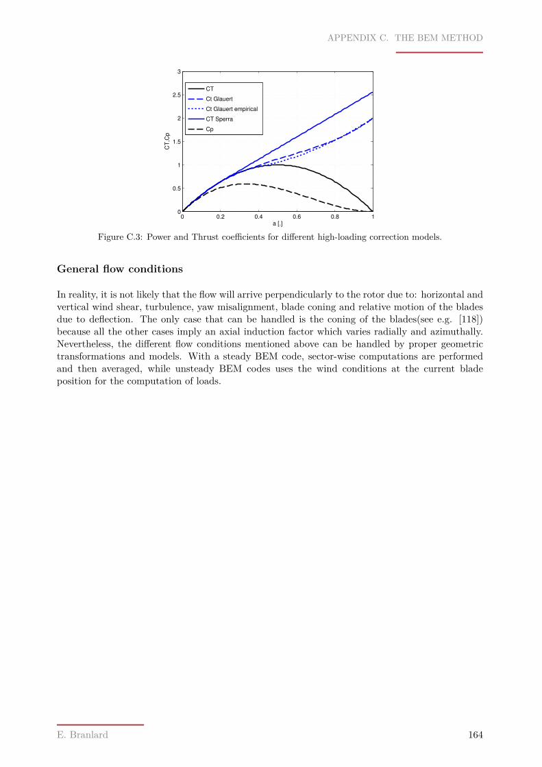
APPENDIX C. THE BEM METHOD
0 0.2 0.4 0.6 0.8 10
0.5
1
1.5
2
2.5
3
a [.]
CT
,Cp
CT
Ct Glauert
Ct Glauert empirical
CT Sperra
Cp
Figure C.3: Power and Thrust coefficients for different high-loading correction models.
General flow conditions
In reality, it is not likely that the flow will arrive perpendicularly to the rotor due to: horizontal andvertical wind shear, turbulence, yaw misalignment, blade coning and relative motion of the bladesdue to deflection. The only case that can be handled is the coning of the blades(see e.g. [118])because all the other cases imply an axial induction factor which varies radially and azimuthally.Nevertheless, the different flow conditions mentioned above can be handled by proper geometrictransformations and models. With a steady BEM code, sector-wise computations are performedand then averaged, while unsteady BEM codes uses the wind conditions at the current bladeposition for the computation of loads.
E. Branlard 164
Appendix DSupplementary notes and results regardingCFD
D.1 Notes on the Post-processing of CFD data
The following reference the basic equations that were used for post-processing of CFD data.
The total force applied on an obstacle is:
F = −∫∫
Spn dS +
∫∫S
(τ · n) dS (D.1)
where p and τ are respectively the static pressure and the viscous shear stress tensor of the flowon the obstacle surface S. The wall shear stress is given by:
τw = µ
(∂u
∂y
)y=0
(D.2)
with u the velocity parallel to the wall and y the distance to the wall. The drag force is thecomponent parallel to the upstream velocity, and the drag the force perpendicular to it:
Fd = F · U∞‖U∞‖
(D.3)
The skin friction coefficient is defined as
Cf = τw12ρU
2∞
(D.4)
An approximate formulation for flat plate with 5 · 105Rex < 107 is:
Cf = 0.0576Re−1/5x (D.5)
The pressure coefficient is defined as:Cp = p− p∞
12ρU
2∞
(D.6)
It typically takes negative values of the suction sides and positive values at the pressure side. In thefree stream, Cp = 0, and at a stagnation point the pressure is maximum and the pressure coefficientis 1.
165

APPENDIX D. SUPPLEMENTARY NOTES AND RESULTS REGARDING CFD
The normal aerodynamic coefficient can be computed from the pressure distribution as:
Cn =∫ TE
LE(Cp,sup(x)− Cp,inf(x)) dx
c(D.7)
The integration of the frictional coefficient was also performed but had insignificant contribution tothe lift as expected. The contribution of the frictional coefficient on the drag has a large influence,but only small investigations were done on this subject. This method of integration was used tocompare with the values obtained with the post-processor and double check the determination ofthe angle of attack. This steps also allowed a clearer exportation of Cp data. After this step, valuesfrom the post-processors were directly used. An example of integration of the Cp coefficient isdisplayed on Fig. D.1.
E. Branlard 166
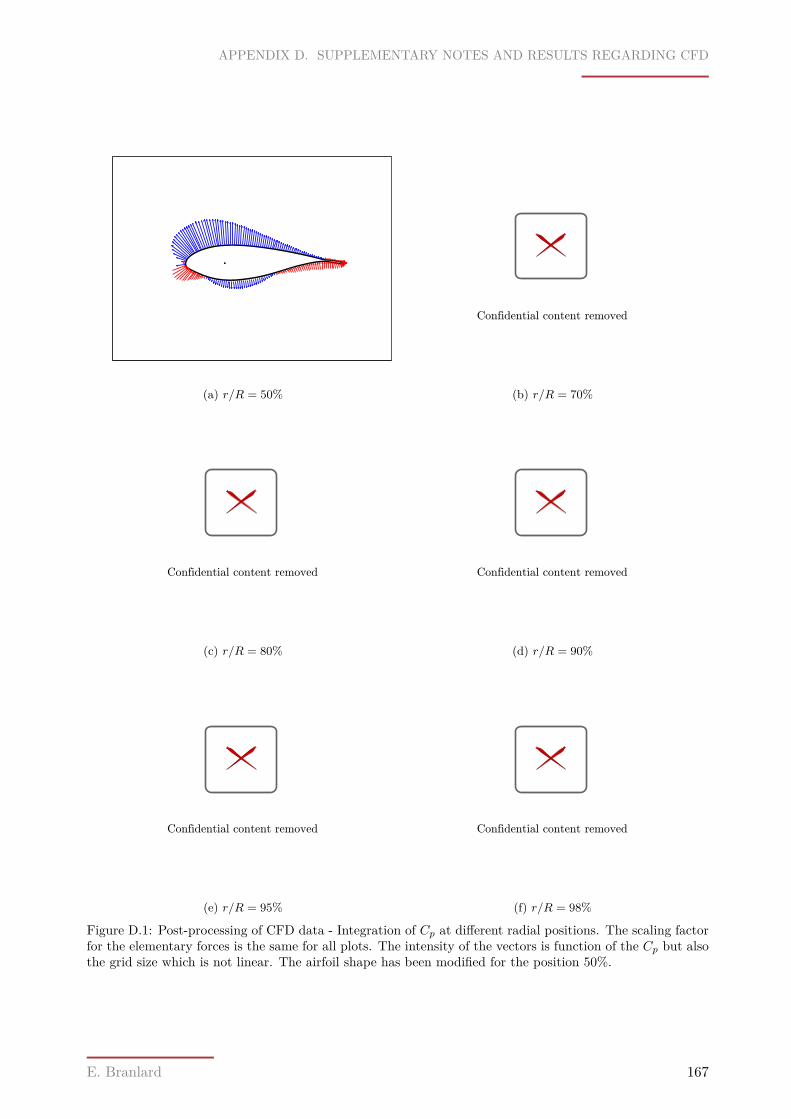
APPENDIX D. SUPPLEMENTARY NOTES AND RESULTS REGARDING CFD
(a) r/R = 50%
Confidential content removed
(b) r/R = 70%
Confidential content removed
(c) r/R = 80%
Confidential content removed
(d) r/R = 90%
Confidential content removed
(e) r/R = 95%
Confidential content removed
(f) r/R = 98%
Figure D.1: Post-processing of CFD data - Integration of Cp at different radial positions. The scaling factorfor the elementary forces is the same for all plots. The intensity of the vectors is function of the Cp but alsothe grid size which is not linear. The airfoil shape has been modified for the position 50%.
E. Branlard 167

APPENDIX D. SUPPLEMENTARY NOTES AND RESULTS REGARDING CFD
D.2 Aerodynamic Coefficients for Blade 1
Comparisons of 2D versus 3D polar for different thicknesses(i.e.) locations on the blades, are foundon Fig. D.2 and Fig. D.3 for Blade 1.
Confidential content removed
(a)
Confidential content removed
(b)
Confidential content removed
(c)
Figure D.2: Comparison of 2D and 3D polars for Blade 1 at different thicknesses
E. Branlard 168

APPENDIX D. SUPPLEMENTARY NOTES AND RESULTS REGARDING CFD
Confidential content removed
(a)
Confidential content removed
(b)
Confidential content removed
(c)
Figure D.3: Comparison of 2D and 3D polars for Blade 1 at different thicknesses
E. Branlard 169

APPENDIX D. SUPPLEMENTARY NOTES AND RESULTS REGARDING CFD
D.3 Aerodynamic Coefficients for Blade 2
Comparisons of 2D versus 3D polar for different thicknesses(i.e.) locations on the blades, are foundon Fig. D.4 and Fig. D.5 for Blade 2.
Confidential content removed
(a)
Confidential content removed
(b)
Confidential content removed
(c)
Figure D.4: Comparison of 2D and 3D polars for Blade 2 at different thicknesses
E. Branlard 170

APPENDIX D. SUPPLEMENTARY NOTES AND RESULTS REGARDING CFD
Confidential content removed
(a)
Confidential content removed
(b)
Confidential content removed
(c)
Figure D.5: Comparison of 2D and 3D polars for Blade 2 at different thicknesses
E. Branlard 171
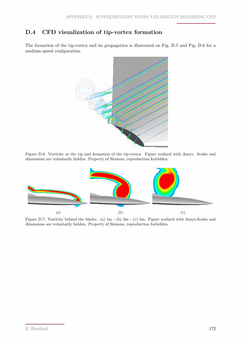
APPENDIX D. SUPPLEMENTARY NOTES AND RESULTS REGARDING CFD
D.4 CFD visualization of tip-vortex formation
The formation of the tip-vortex and its propagation is illustrated on Fig. D.7 and Fig. D.6 for amedium speed configuration.
Figure D.6: Vorticity at the tip and formation of the tip-vortex. Figure realized with Ansys. Scales anddimensions are voluntarily hidden. Property of Siemens, reproduction forbidden.
(a) (b) (c)
Figure D.7: Vorticity behind the blades. (a) 1m - (b) 3m - (c) 5m. Figure realized with Ansys.Scales anddimensions are voluntarily hidden. Property of Siemens, reproduction forbidden.
E. Branlard 172
Appendix EGerman abstracts
Few german abstracts of the original article from Betz and Prandtl[9] are presented here as theyhave been used for the understanding of this article. Such abstracts don’t exists in a numericalform.
Die Ergebnisse dieser Betrachtung, die ebenso wie die Betz’sche Theorie nur für denGrenzfall sehr schwach belasteter Schrauben streng gültig sing, lassen sich auf starkbelastete Schrauben erweitern, wenn man, wie Herr Betz in einer anderen noch zuveröffentlichenden Untersuchung gezeigt hat, in den obigen Formeln für ”v“ und ”rw‘ die genauen Werte der Strömungsgeschwindigkeiten relativ zu den Flügelprofilen“v+wa” und “rw-wt” setzt, wobei unter “v” die Zuflussgeschwindigkeit im Unendlichenvor der Schraube und unter “wa” und “wt” die zusätzlichen Geschwindigkeitskomponen-ten weit hinter der Schraube verstanden werden. Eine brauchbare Näherung für mässigbelastete Schrauben erhält man übrigens schon dadurch, dass in den obigen Formeln “v”durch “v+w/2” ersetzt wird, wobei die einfache Vorstellung von in die Luft geschnit-tenen Schraubenflächen, die sonst hinfällig wird, beibehalten werden kann. Von dieserletzteren Näherung ist in Formel 8 Gebrauch gemacht.
Diese Radialgeschwindigkeiten klingen aber, wenn die Schraubenflächen hinreichenddicht stehen, nach dem Innern zu sehr rasch ab, so dass es hier ausreicht, die tangentialeKomponente “wt” und die axiale Komponente “wa” der Luftbewegung zu betrachten.Die Bewegung, die bei dem Stoss erzeugt wird, erfolgt im Innern, wie leicht zu stehen,normal zu den Schraubenflächen, mittelst derer der Stoss auf die Flüssigkeit ausgeübtwird. Ist “v” die Geschwindigkeit, mit der die luftschraube gegen die Luft fortschreibet,“w” deren Winkelgeschwindigkeit, dann ist die Steigung der Schraubenflächen “H=vT”,wo “T=2pi/ww” die Umlaufszeit ist.
[. . . ] Für due Randzone gilt die folgende Sonderbetrachtung. Es sei “a” der senkrechteAbstand von zwei benachbarten Randkurven der Schraubenflächen. An die Stelle derUmströmung der Ränder der Schraubenflächen mag nun die Umströmung der Rändereines äquidistanten Ebenensystems vom Abstand “a”, gemäss fig2, gesetz werden, umden Abfall der Zirkulation an der Flügelspitzen zu studieren [. . . ]
Mit “a” nach Gleichung (4), in der ebenfalls gemäss der Anmerkung “v” durch “v+w/2”ersetzt werden kann. Die Gleichung gilt um so genauer, je mehr Schraubenflügel vorhan-
173

APPENDIX E. GERMAN ABSTRACTS
den sind, es ist aber zu erwarten, dass sie auch bei wenigen, ja selbst bei zwei Flügeln,immer noch brauchbare Resultate ergibt.
E. Branlard 174

Appendix FSource Codes
F.1 C code for vortex code
Confidential content removed
175

APPENDIX F. SOURCE CODES
Confidential content removed
E. Branlard 176

APPENDIX F. SOURCE CODES
Confidential content removed
E. Branlard 177

APPENDIX F. SOURCE CODES
Confidential content removed
E. Branlard 178
List of Figures
1.1 One dimensional momentum theory . . . . . . . . . . . . . . . . . . . . . . . . . . . 8
1.2 Two-dimensional momentum theory notation scheme . . . . . . . . . . . . . . . . . . 9
1.3 Tip-vortex formation and radial flow on the upper and lower surface at the tip . . . 11
1.4 Formation of tip vortices at the tip of a wing and resulting induced velocities in thewake . . . . . . . . . . . . . . . . . . . . . . . . . . . . . . . . . . . . . . . . . . . . . 12
1.5 Illustration of the notion of induced drag . . . . . . . . . . . . . . . . . . . . . . . . . 13
1.6 Vortex sheet forming behind a wind turbine blade . . . . . . . . . . . . . . . . . . . 15
1.7 Single helical vortex-line trailing from the tip under the assumption of constantcirculation at the blade and zero hub radius . . . . . . . . . . . . . . . . . . . . . . . 16
1.8 Azimuthal variation of a for different radial positions . . . . . . . . . . . . . . . . . . 16
1.9 Continuous vortex sheet trailed by a rotor with span varying circulation - Convention 17
1.10 Visualization of the ideal helical wake with the proper wind turbine convention . . . 18
1.11 Ideal helical wake behind a turbine generated by the three blades . . . . . . . . . . . 18
1.12 Blade velocity triangle and resulting aerodynamic forces for the blade element theory 19
1.13 Helix angle change with radius . . . . . . . . . . . . . . . . . . . . . . . . . . . . . . 21
1.14 Illustration of the equivalence between a given flow and a continuous distribution ofsources and vortices . . . . . . . . . . . . . . . . . . . . . . . . . . . . . . . . . . . . 22
1.15 Reduction of vorticity dimensions by integration . . . . . . . . . . . . . . . . . . . . 22
1.16 Different vortex codes using different dimension of vorticity . . . . . . . . . . . . . . 22
1.17 Side view of the turbine showing the variation of velocity(or axial induction) foundwith CFD . . . . . . . . . . . . . . . . . . . . . . . . . . . . . . . . . . . . . . . . . . 33
1.18 Parameters needed and results obtained with the different method used . . . . . . . 34
2.1 Side view of the helical wake behind a wind turbine . . . . . . . . . . . . . . . . . . 39
2.2 Velocity triangle resulting from the mathematical and kinematic study of helix . . . 39
2.3 Induced velocity in the far wake . . . . . . . . . . . . . . . . . . . . . . . . . . . . . . 40
179
LIST OF FIGURES
2.4 Near wake and far wake notations . . . . . . . . . . . . . . . . . . . . . . . . . . . . 40
2.5 Velocity triangle at the rotor related to the near wake notations of Fig. 2.4 . . . . . 41
2.6 Betz’s optimum circulation with and without drag with λ = 10 . . . . . . . . . . . . 46
2.7 The system of material sheets introduced by Prandtl . . . . . . . . . . . . . . . . . . 47
2.8 Distance between two helical vortex sheets at the “tip” . . . . . . . . . . . . . . . . . 47
2.9 Prandtl velocity field and potential . . . . . . . . . . . . . . . . . . . . . . . . . . . . 51
2.10 Definition of the points used to integrate the average velocity between two sheets . . 51
2.11 Comparison between Betz and Prandtl’s circulation function . . . . . . . . . . . . . 53
2.12 Prandtl’s tip loss factor . . . . . . . . . . . . . . . . . . . . . . . . . . . . . . . . . . 54
2.13 Comparison of Goldstein’s circulation distribution with Prandtl’s approximation fordifferent tip-speed ratio . . . . . . . . . . . . . . . . . . . . . . . . . . . . . . . . . . 56
2.14 Comparison of Goldstein’s circulation with Betz’s circulation for different values of l 57
2.15 Comparison between Betz, Prandtl and Goldstein theory for a three bladed rotor . . 57
3.1 Comparison of the different tip-loss factors when used in a BEM code . . . . . . . . 66
3.2 Differences in power coefficient when different tip-loss factors are used . . . . . . . . 66
3.3 Power curves and wind distribution used for the computation of AEP . . . . . . . . 67
3.4 Annual energy production for the first wind distribution . . . . . . . . . . . . . . . . 68
3.5 annual energy production for the second wind distribution . . . . . . . . . . . . . . . 68
4.1 Different circulation translating different loading cases for two different tip-speed ratios 73
4.2 Bézier curve defined by five points . . . . . . . . . . . . . . . . . . . . . . . . . . . . 74
4.3 Example of different family of curve that can be obtain with the current parametriza-tion . . . . . . . . . . . . . . . . . . . . . . . . . . . . . . . . . . . . . . . . . . . . . 76
4.4 Illustration of the model and fitting method developed for circulation curves . . . . . 77
4.5 Dependence of the tip-loss function on the number of blades . . . . . . . . . . . . . . 78
4.6 Tip-loss function obtained with and without the influence of the bound segments . . 79
4.7 Axial induction computed by the vortex code at the rotor plane . . . . . . . . . . . . 79
4.8 Tip-loss function obtained for different chord distributions . . . . . . . . . . . . . . . 80
4.9 Tip-loss function obtained for different twist distributions . . . . . . . . . . . . . . . 80
4.10 Sensitivity of the tip-loss function with respect to the different viscous models . . . . 81
4.11 Sensitivity of the tip-loss function with respect to the grid size . . . . . . . . . . . . 81
4.12 Prescribed circulation used for the sensitivity analysis on the wind turbine state . . 82
4.13 Influence of the turbine state λ,CT on the tip-loss function . . . . . . . . . . . . . 82
4.14 Influence of the circulation distribution on the tip-loss function . . . . . . . . . . . . 83
E. Branlard 180
LIST OF FIGURES
5.1 Determination of the tip-loss factor with CFD data . . . . . . . . . . . . . . . . . . . 86
5.2 Estimate of the axial induction on the blade aB using CFD data at planes ±1.3%R . 87
5.3 Influence of the averaging method determining aB on the tip-loss factor near the tip 87
5.4 Tip-loss factor estimated using different planes apart from the rotor . . . . . . . . . 88
5.5 Streamlines on suction side of the blade tip(2 last percent) . . . . . . . . . . . . . . . 88
5.6 Thickness distribution and available 2D profile data of the two blades considered . . 89
5.7 Blade 1 airfoil polars for the relative thickness 18% . . . . . . . . . . . . . . . . . . . 90
5.8 3D and 2D polars for relative thickness between 18% and 21% . . . . . . . . . . . . . 91
5.9 Airfoil tip-loss function for Blade 1 and Tip 1 . . . . . . . . . . . . . . . . . . . . . . 91
5.10 Airfoil tip-loss function for Blade 1 and Tip 2 . . . . . . . . . . . . . . . . . . . . . . 92
5.11 Comparison of airfoil performance tip-losses FCl for different designs . . . . . . . . . 93
5.12 Ratio of drag coefficients for Blade 1 . . . . . . . . . . . . . . . . . . . . . . . . . . . 93
5.13 Suggested models for the performance tip-loss factor . . . . . . . . . . . . . . . . . . 95
5.14 Comparison of the performance tip-loss factor from this analysis with the one fromShen for one CFD simulation . . . . . . . . . . . . . . . . . . . . . . . . . . . . . . . 96
6.1 Axial induction obtained by averaging planes at ±3.3%R . . . . . . . . . . . . . . . 97
6.2 Axial induction obtained by averaging planes at ±1.3%R . . . . . . . . . . . . . . . 98
6.3 Wake deficit computed with the Vortex Code and CFD . . . . . . . . . . . . . . . . 99
6.4 Comparison of the results obtained by the different codes when studying a specificwind turbine (Blade 2) . . . . . . . . . . . . . . . . . . . . . . . . . . . . . . . . . . . 100
6.5 Comparison of the new BEM code performances compared to the vortex code - Blade 1101
6.6 Comparison of the new BEM code performances compared to the vortex code - Blade 2102
6.7 Differences in the local flap moment between the two BEM codes . . . . . . . . . . . 102
6.8 Circulations from the database used by the BEM code . . . . . . . . . . . . . . . . . 103
6.9 Results from the New tip-loss model compared with CFD and BEM for Blade 1 . . . 104
6.10 Results from the New tip-loss model compared with CFD and BEM for Blade 2 . . . 105
6.11 Comparison of the tip-loss function obtained with the three different codes . . . . . 106
6.12 Comparison of different approaches driven by different circulations . . . . . . . . . . 107
A.1 Induced velocity in the far wake . . . . . . . . . . . . . . . . . . . . . . . . . . . . . . 123
A.2 Goldstein’s circulation function compared to the one from Glauert . . . . . . . . . . 130
A.3 Optimum power and thrust coefficient . . . . . . . . . . . . . . . . . . . . . . . . . . 130
B.1 Lift coefficient for a flat plate . . . . . . . . . . . . . . . . . . . . . . . . . . . . . . . 137
B.2 Elliptical wing with infinite aspect ratio . . . . . . . . . . . . . . . . . . . . . . . . . 137
E. Branlard 181
LIST OF FIGURES
B.3 Lift coefficient of an elliptical wing for different aspect ratios . . . . . . . . . . . . . 138
B.4 Lift coefficient of a swept wing for Λ = 45 . . . . . . . . . . . . . . . . . . . . . . . . 139
B.5 Golstein circulation function computed with vortex code for different values of l . . . 139
B.6 Illustration of the theoretical helical wake used for the computation of Goldstein’sfunction . . . . . . . . . . . . . . . . . . . . . . . . . . . . . . . . . . . . . . . . . . . 140
B.7 Transient lift coefficient variation with time for uncambered, rectangular wings thatwere suddenly set into a constant-speed forward flight. . . . . . . . . . . . . . . . . 141
B.8 Separation of the transient drag coefficient for an sudden acceleration of a flat plate 141
B.9 Sudden acceleration of a flat plate - Comparison with Wagner function . . . . . . . . 142
B.10 Comparison of vortex code results compared to experimental data - Induced velocityon the lifting line . . . . . . . . . . . . . . . . . . . . . . . . . . . . . . . . . . . . . . 143
B.11 Azimuthal variation of axial induced velocity in the plane z = 0.35m behind the rotor144
B.12 Azimuthal variation of axial induced velocity in the plane z = 0.60m behind the rotor144
B.13 Comparison of longitudinal velocity in different plans behind the TUD rotor . . . . . 146
B.14 Influence of vortex core parameters on the wake shape . . . . . . . . . . . . . . . . . 147
B.15 Wake shapes, streamlines and wake deficit at different tip speed ratios for the NTK500 turbine as modelled by the vortex code . . . . . . . . . . . . . . . . . . . . . . . 148
B.16 Induced velocity at the rotor plane for the NREL rotor at 5m/s . . . . . . . . . . . . 149
B.17 Illustration of the meshing method with distinction between panels and vortex rings 150
B.18 Distribution of lift obtained with the vortex code - U = 10m/s - α = 5 . . . . . . . 151
B.19 Different geometries studied with the vortex code . . . . . . . . . . . . . . . . . . . . 151
B.20 Wake shapes behind an elliptical wing and a trapezoidal wing . . . . . . . . . . . . . 152
B.21 Wake shapes behind a wind turbine . . . . . . . . . . . . . . . . . . . . . . . . . . . 153
C.1 Velocity triangle illustrating the link between the simplified 2D momentum theoryand the Blade Element Theory . . . . . . . . . . . . . . . . . . . . . . . . . . . . . . 156
C.2 Illustration of the solidity . . . . . . . . . . . . . . . . . . . . . . . . . . . . . . . . . 157
C.3 Power and Thrust coefficients for different high-loading correction models . . . . . . 164
D.1 Post-processing of CFD data - Integration of Cp at different radial positions . . . . . 167
D.2 Comparison of 2D and 3D polars for Blade 1 at different thicknesses . . . . . . . . . 168
D.3 Comparison of 2D and 3D polars for Blade 1 at different thicknesses . . . . . . . . . 169
D.4 Comparison of 2D and 3D polars for Blade 2 at different thicknesses . . . . . . . . . 170
D.5 Comparison of 2D and 3D polars for Blade 2 at different thicknesses . . . . . . . . . 171
D.6 Vorticity at the tip and formation of the tip-vortex . . . . . . . . . . . . . . . . . . . 172
D.7 Vorticity behind the blades . . . . . . . . . . . . . . . . . . . . . . . . . . . . . . . . 172
E. Branlard 182
List of Tables
1.1 Corrections of airfoil coefficients for 3D effects according to Eq. (1.22) . . . . . . . . 29
2.1 Notations and definitions for the wake screw surface. The lasts columns contain thenotations used by Prandtl, Theodorsen and Okulov. . . . . . . . . . . . . . . . . . . 38
4.1 Range and discretization of the different parameters used for Fig.4.3 . . . . . . . . . 76
5.1 Available CFD cases for investigation of aerodynamic performance losses . . . . . . . 89
6.1 Comparison as a rough guide of typical computational time for the different codes.The new BEM code refers to the code using the new tip-loss model described in thisreport. . . . . . . . . . . . . . . . . . . . . . . . . . . . . . . . . . . . . . . . . . . . . 103
A.1 Goldstein’s circulation function fitted according to Eq.(A.32) for different values ofl, with w = 1 and for B = 2 . . . . . . . . . . . . . . . . . . . . . . . . . . . . . . . . 131
A.2 Goldstein’s circulation function fitted according to Eq.(A.32) for different values ofl, with w = 1 and for B = 3 . . . . . . . . . . . . . . . . . . . . . . . . . . . . . . . . 131
C.1 Maximum thrust coefficient and transitional value for the axial induction factor inthe context of Spera’s correction . . . . . . . . . . . . . . . . . . . . . . . . . . . . . 163
183
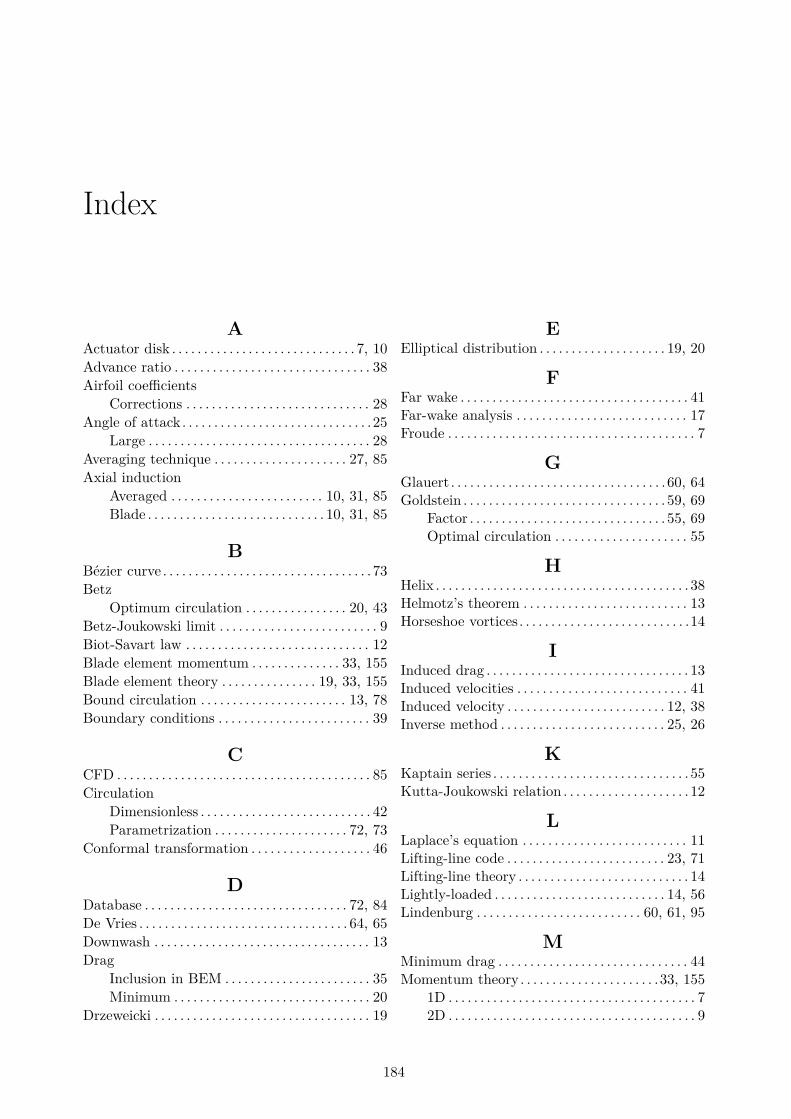
Index
AActuator disk . . . . . . . . . . . . . . . . . . . . . . . . . . . . . 7, 10Advance ratio . . . . . . . . . . . . . . . . . . . . . . . . . . . . . . . 38Airfoil coefficients
Corrections . . . . . . . . . . . . . . . . . . . . . . . . . . . . . 28Angle of attack. . . . . . . . . . . . . . . . . . . . . . . . . . . . . .25
Large . . . . . . . . . . . . . . . . . . . . . . . . . . . . . . . . . . . 28Averaging technique . . . . . . . . . . . . . . . . . . . . . 27, 85Axial induction
Averaged . . . . . . . . . . . . . . . . . . . . . . . . 10, 31, 85Blade . . . . . . . . . . . . . . . . . . . . . . . . . . . . 10, 31, 85
BBézier curve . . . . . . . . . . . . . . . . . . . . . . . . . . . . . . . . . 73Betz
Optimum circulation . . . . . . . . . . . . . . . . 20, 43Betz-Joukowski limit . . . . . . . . . . . . . . . . . . . . . . . . . 9Biot-Savart law . . . . . . . . . . . . . . . . . . . . . . . . . . . . . 12Blade element momentum . . . . . . . . . . . . . . 33, 155Blade element theory . . . . . . . . . . . . . . . 19, 33, 155Bound circulation . . . . . . . . . . . . . . . . . . . . . . . 13, 78Boundary conditions . . . . . . . . . . . . . . . . . . . . . . . . 39
CCFD . . . . . . . . . . . . . . . . . . . . . . . . . . . . . . . . . . . . . . . . 85Circulation
Dimensionless . . . . . . . . . . . . . . . . . . . . . . . . . . . 42Parametrization . . . . . . . . . . . . . . . . . . . . . 72, 73
Conformal transformation . . . . . . . . . . . . . . . . . . . 46
DDatabase . . . . . . . . . . . . . . . . . . . . . . . . . . . . . . . . 72, 84De Vries . . . . . . . . . . . . . . . . . . . . . . . . . . . . . . . . . 64, 65Downwash . . . . . . . . . . . . . . . . . . . . . . . . . . . . . . . . . . 13Drag
Inclusion in BEM . . . . . . . . . . . . . . . . . . . . . . . 35Minimum . . . . . . . . . . . . . . . . . . . . . . . . . . . . . . . 20
Drzeweicki . . . . . . . . . . . . . . . . . . . . . . . . . . . . . . . . . . 19
EElliptical distribution . . . . . . . . . . . . . . . . . . . . 19, 20
FFar wake . . . . . . . . . . . . . . . . . . . . . . . . . . . . . . . . . . . . 41Far-wake analysis . . . . . . . . . . . . . . . . . . . . . . . . . . . 17Froude . . . . . . . . . . . . . . . . . . . . . . . . . . . . . . . . . . . . . . . 7
GGlauert . . . . . . . . . . . . . . . . . . . . . . . . . . . . . . . . . .60, 64Goldstein . . . . . . . . . . . . . . . . . . . . . . . . . . . . . . . . 59, 69
Factor . . . . . . . . . . . . . . . . . . . . . . . . . . . . . . . 55, 69Optimal circulation . . . . . . . . . . . . . . . . . . . . . 55
HHelix . . . . . . . . . . . . . . . . . . . . . . . . . . . . . . . . . . . . . . . . 38Helmotz’s theorem . . . . . . . . . . . . . . . . . . . . . . . . . . 13Horseshoe vortices. . . . . . . . . . . . . . . . . . . . . . . . . . .14
IInduced drag . . . . . . . . . . . . . . . . . . . . . . . . . . . . . . . . 13Induced velocities . . . . . . . . . . . . . . . . . . . . . . . . . . . 41Induced velocity . . . . . . . . . . . . . . . . . . . . . . . . . 12, 38Inverse method . . . . . . . . . . . . . . . . . . . . . . . . . . 25, 26
KKaptain series . . . . . . . . . . . . . . . . . . . . . . . . . . . . . . . 55Kutta-Joukowski relation . . . . . . . . . . . . . . . . . . . . 12
LLaplace’s equation . . . . . . . . . . . . . . . . . . . . . . . . . . 11Lifting-line code . . . . . . . . . . . . . . . . . . . . . . . . . 23, 71Lifting-line theory . . . . . . . . . . . . . . . . . . . . . . . . . . . 14Lightly-loaded . . . . . . . . . . . . . . . . . . . . . . . . . . . 14, 56Lindenburg . . . . . . . . . . . . . . . . . . . . . . . . . . 60, 61, 95
MMinimum drag . . . . . . . . . . . . . . . . . . . . . . . . . . . . . . 44Momentum theory. . . . . . . . . . . . . . . . . . . . . .33, 155
1D . . . . . . . . . . . . . . . . . . . . . . . . . . . . . . . . . . . . . . . 72D . . . . . . . . . . . . . . . . . . . . . . . . . . . . . . . . . . . . . . . 9
184
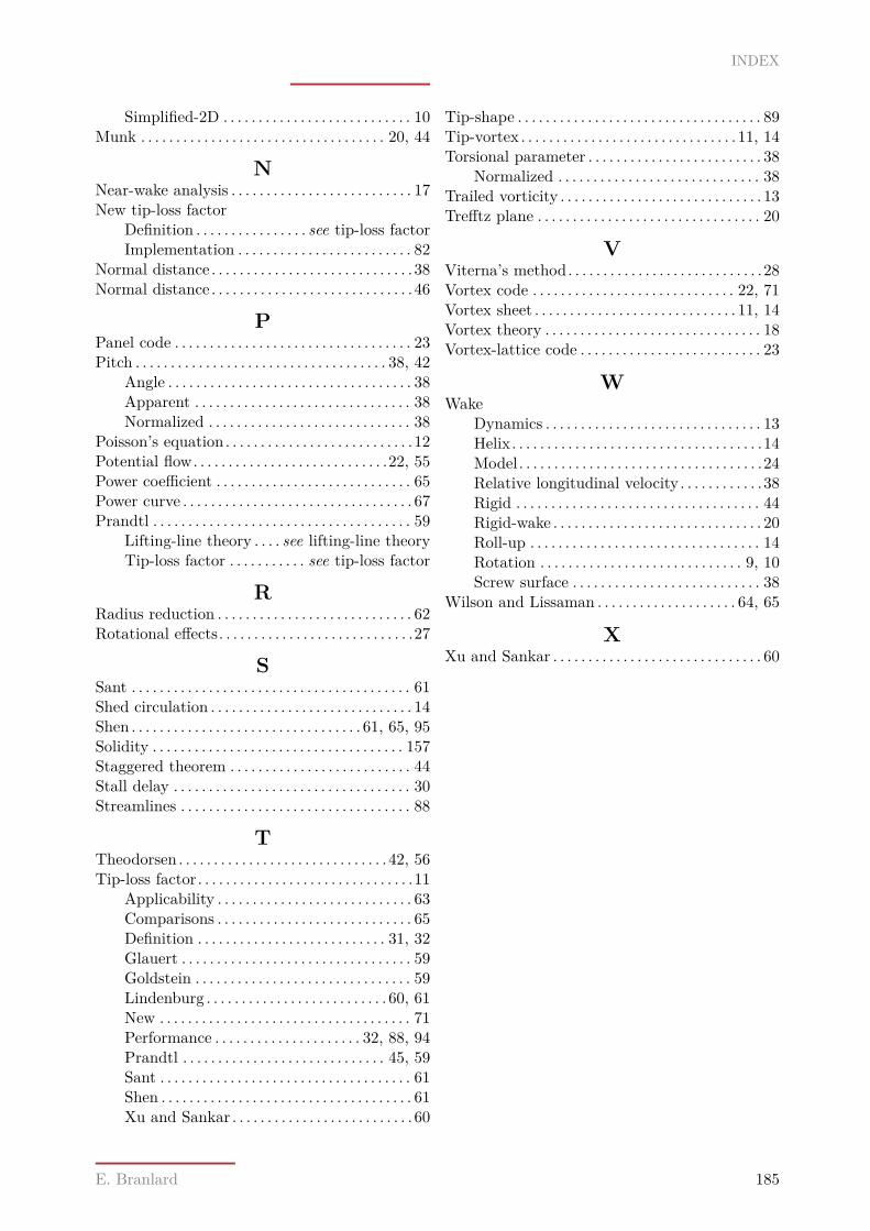
INDEX
Simplified-2D . . . . . . . . . . . . . . . . . . . . . . . . . . . 10Munk . . . . . . . . . . . . . . . . . . . . . . . . . . . . . . . . . . . 20, 44
NNear-wake analysis . . . . . . . . . . . . . . . . . . . . . . . . . . 17New tip-loss factor
Definition . . . . . . . . . . . . . . . . see tip-loss factorImplementation . . . . . . . . . . . . . . . . . . . . . . . . . 82
Normal distance . . . . . . . . . . . . . . . . . . . . . . . . . . . . . 38Normal distance . . . . . . . . . . . . . . . . . . . . . . . . . . . . . 46
PPanel code . . . . . . . . . . . . . . . . . . . . . . . . . . . . . . . . . . 23Pitch . . . . . . . . . . . . . . . . . . . . . . . . . . . . . . . . . . . . 38, 42
Angle . . . . . . . . . . . . . . . . . . . . . . . . . . . . . . . . . . . 38Apparent . . . . . . . . . . . . . . . . . . . . . . . . . . . . . . . 38Normalized . . . . . . . . . . . . . . . . . . . . . . . . . . . . . 38
Poisson’s equation . . . . . . . . . . . . . . . . . . . . . . . . . . .12Potential flow. . . . . . . . . . . . . . . . . . . . . . . . . . . .22, 55Power coefficient . . . . . . . . . . . . . . . . . . . . . . . . . . . . 65Power curve . . . . . . . . . . . . . . . . . . . . . . . . . . . . . . . . . 67Prandtl . . . . . . . . . . . . . . . . . . . . . . . . . . . . . . . . . . . . . 59
Lifting-line theory . . . . see lifting-line theoryTip-loss factor . . . . . . . . . . . see tip-loss factor
RRadius reduction . . . . . . . . . . . . . . . . . . . . . . . . . . . . 62Rotational effects. . . . . . . . . . . . . . . . . . . . . . . . . . . .27
SSant . . . . . . . . . . . . . . . . . . . . . . . . . . . . . . . . . . . . . . . . 61Shed circulation . . . . . . . . . . . . . . . . . . . . . . . . . . . . . 14Shen . . . . . . . . . . . . . . . . . . . . . . . . . . . . . . . . . 61, 65, 95Solidity . . . . . . . . . . . . . . . . . . . . . . . . . . . . . . . . . . . . 157Staggered theorem . . . . . . . . . . . . . . . . . . . . . . . . . . 44Stall delay . . . . . . . . . . . . . . . . . . . . . . . . . . . . . . . . . . 30Streamlines . . . . . . . . . . . . . . . . . . . . . . . . . . . . . . . . . 88
TTheodorsen . . . . . . . . . . . . . . . . . . . . . . . . . . . . . . 42, 56Tip-loss factor. . . . . . . . . . . . . . . . . . . . . . . . . . . . . . .11
Applicability . . . . . . . . . . . . . . . . . . . . . . . . . . . . 63Comparisons . . . . . . . . . . . . . . . . . . . . . . . . . . . . 65Definition . . . . . . . . . . . . . . . . . . . . . . . . . . . 31, 32Glauert . . . . . . . . . . . . . . . . . . . . . . . . . . . . . . . . . 59Goldstein . . . . . . . . . . . . . . . . . . . . . . . . . . . . . . . 59Lindenburg . . . . . . . . . . . . . . . . . . . . . . . . . . 60, 61New . . . . . . . . . . . . . . . . . . . . . . . . . . . . . . . . . . . . 71Performance . . . . . . . . . . . . . . . . . . . . . 32, 88, 94Prandtl . . . . . . . . . . . . . . . . . . . . . . . . . . . . . 45, 59Sant . . . . . . . . . . . . . . . . . . . . . . . . . . . . . . . . . . . . 61Shen . . . . . . . . . . . . . . . . . . . . . . . . . . . . . . . . . . . . 61Xu and Sankar . . . . . . . . . . . . . . . . . . . . . . . . . . 60
Tip-shape . . . . . . . . . . . . . . . . . . . . . . . . . . . . . . . . . . . 89Tip-vortex . . . . . . . . . . . . . . . . . . . . . . . . . . . . . . . 11, 14Torsional parameter . . . . . . . . . . . . . . . . . . . . . . . . . 38
Normalized . . . . . . . . . . . . . . . . . . . . . . . . . . . . . 38Trailed vorticity . . . . . . . . . . . . . . . . . . . . . . . . . . . . . 13Trefftz plane . . . . . . . . . . . . . . . . . . . . . . . . . . . . . . . . 20
VViterna’s method. . . . . . . . . . . . . . . . . . . . . . . . . . . .28Vortex code . . . . . . . . . . . . . . . . . . . . . . . . . . . . . 22, 71Vortex sheet . . . . . . . . . . . . . . . . . . . . . . . . . . . . . 11, 14Vortex theory . . . . . . . . . . . . . . . . . . . . . . . . . . . . . . . 18Vortex-lattice code . . . . . . . . . . . . . . . . . . . . . . . . . . 23
WWake
Dynamics . . . . . . . . . . . . . . . . . . . . . . . . . . . . . . . 13Helix. . . . . . . . . . . . . . . . . . . . . . . . . . . . . . . . . . . .14Model. . . . . . . . . . . . . . . . . . . . . . . . . . . . . . . . . . .24Relative longitudinal velocity. . . . . . . . . . . .38Rigid . . . . . . . . . . . . . . . . . . . . . . . . . . . . . . . . . . . 44Rigid-wake . . . . . . . . . . . . . . . . . . . . . . . . . . . . . . 20Roll-up . . . . . . . . . . . . . . . . . . . . . . . . . . . . . . . . . 14Rotation . . . . . . . . . . . . . . . . . . . . . . . . . . . . . 9, 10Screw surface . . . . . . . . . . . . . . . . . . . . . . . . . . . 38
Wilson and Lissaman . . . . . . . . . . . . . . . . . . . . 64, 65
XXu and Sankar . . . . . . . . . . . . . . . . . . . . . . . . . . . . . . 60
E. Branlard 185