Embed Size (px)
Citation preview

자료구조와 알고리즘
1
충북대학교
소프트웨어학과
이충세

알고리즘 : 주제
기초 자료구조
알고리즘의 분석 기법
트리와 그래프
점화식
알고리즘 기법
분할정복, 동적 프로그램, Greedy 방법
3
4
1.1 데이터와 데이터 객체
1.1.1 데이터의 개념
* 정보(information) : 어떤 목적을 가진 활동에 직접 또는 간접적
인 도움을 주는 지식
* 데이터(data) : 정보라는 제품의 생산에 입력되는 원재료 자원->
사실(fact), 개념(concept), 명령(instruction)의 총칭
* 데이터 형(data type) : 프로그래밍 언어의 변수(variable)들이
가질 수 있는 데이터의 종류
- a collection of objects and a set of operations that act on
those objects

5
FORTRAN : 정수형(integer), 실수형(real),논리형
(logical),복소수형(complex), 배정도 실수형(double
precision) 등
PL/I : 문자형(character)
SNOBOL : 문자열(character string)
LISP : 리스트(list) 또는 s-수식(s-expression)
Pascal : 정수형, 실수형, 논리형(boolean), 문자형
및 배열
6
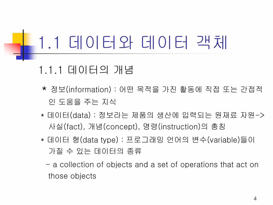
1.1.2 데이터와 전산학
전산학의 연구범위
* 데이터를 저장하는 기계(machine)
* 데이터 취급에 관련된 내용을 기술하는 언어
(language)
* 원시 데이터로부터 생성할 수 있는 여러 종
류의 정제된 데이터를 기술하는 기초 내용
* 표현되는 데이터에 대한 구조

7
* 데이터 객체 : 데이터 형의 실체를 구성하는 집합(set)
의 원소(element)
* 변수(variable) : 데이터 객체의 명칭
* 정수형 데이터 객체 : D = …,-2, -1, 0, 1, 2, …
* 길이가 30자 이내인 영문자 문자열(alphabetic
character string)의 데이터 객체 :
D = ‘’, ‘A’, …, ‘Z’, ‘AA’, …
1.1.3 데이터 객체

8
1.2 데이터 구조의 개념
1.2.1 데이터 구조
* 데이터 구조(data structure)란:데이터 객체의 집합
및 이들 사이의 관계를 기술-> 데이터 객체의 원소에
적용될 연산(operation)이 수행되는 방법을 보여줌
- the organized collections of data to get more
efficient algorithms
9
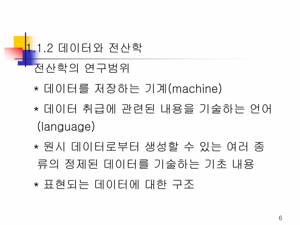
* 추상적 데이터 형(abstract data type)
D: 데이터 구조의 정의 영역(domain)
의 집합
F: 함수(function) 집합
A: 공리(axiom) 집합
d = (D, F, A)
- a data type that is organized in such a way that the specification of
the objects and the specification of the operations on the objects
is separated from the representation of the objects and the
implementation of the operations
1.2.2 데이터 구조의 표현
10
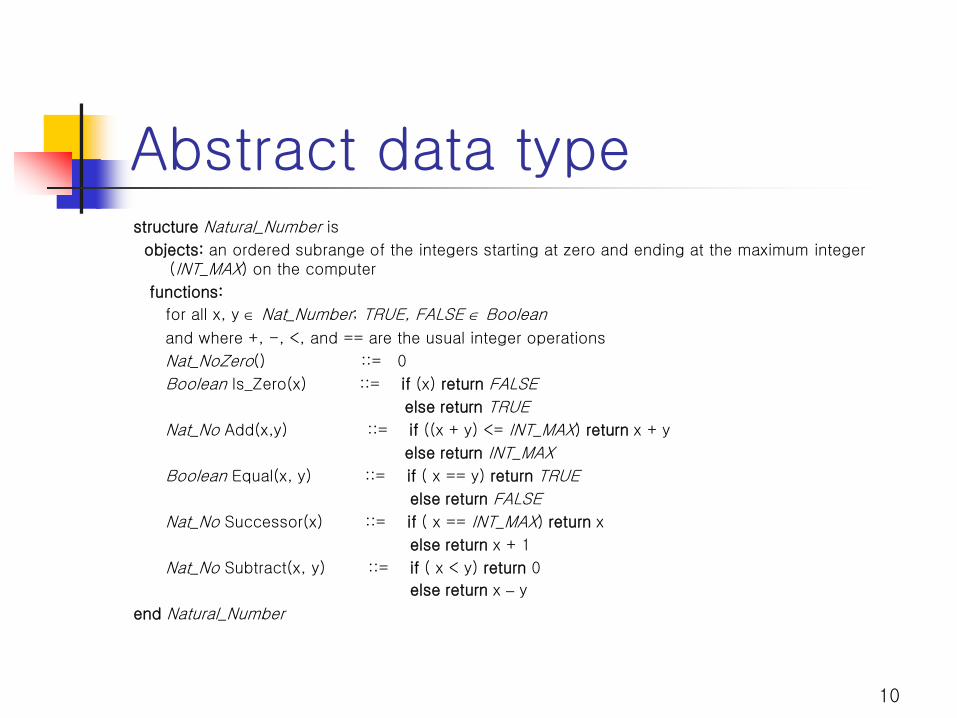
Abstract data type structure Natural_Number is
objects: an ordered subrange of the integers starting at zero and ending at the maximum integer (INT_MAX) on the computer
functions:
for all x, y ∈ Nat_Number; TRUE, FALSE ∈ Boolean
and where +, -, <, and == are the usual integer operations
Nat_NoZero() ::= 0
Boolean Is_Zero(x) ::= if (x) return FALSE
else return TRUE
Nat_No Add(x,y) ::= if ((x + y) <= INT_MAX) return x + y
else return INT_MAX
Boolean Equal(x, y) ::= if ( x == y) return TRUE
else return FALSE
Nat_No Successor(x) ::= if ( x == INT_MAX) return x
else return x + 1
Nat_No Subtract(x, y) ::= if ( x < y) return 0
else return x – y
end Natural_Number
11
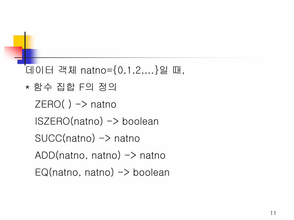
데이터 객체 natno=0,1,2,…일 때,
* 함수 집합 F의 정의
ZERO( ) -> natno
ISZERO(natno) -> boolean
SUCC(natno) -> natno
ADD(natno, natno) -> natno
EQ(natno, natno) -> boolean
12
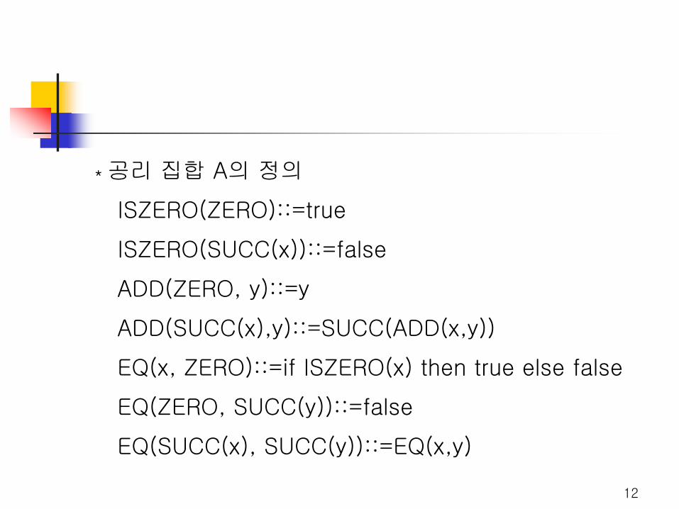
* 공리 집합 A의 정의
ISZERO(ZERO)::=true
ISZERO(SUCC(x))::=false
ADD(ZERO, y)::=y
ADD(SUCC(x),y)::=SUCC(ADD(x,y))
EQ(x, ZERO)::=if ISZERO(x) then true else false
EQ(ZERO, SUCC(y))::=false
EQ(SUCC(x), SUCC(y))::=EQ(x,y)
13
1.3 데이터 구조의 영역
1.3.1 데이터 구조론
* 데이터 구조론: 데이터 처리 시스템에서 취급
하는 데이터 객체들을 기억 공간 내에 표현하
고 저장하는 방법과, 데이터 상호간의 관계를
파악하여 수행할 수 있는 연산과 관련된 알고
리즘을 연구하는 학문
14
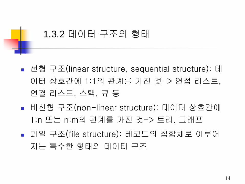
선형 구조(linear structure, sequential structure): 데
이터 상호간에 1:1의 관계를 가진 것-> 연접 리스트,
연결 리스트, 스택, 큐 등
비선형 구조(non-linear structure): 데이터 상호간에
1:n 또는 n:m의 관계를 가진 것-> 트리, 그래프
파일 구조(file structure): 레코드의 집합체로 이루어
지는 특수한 형태의 데이터 구조
1.3.2 데이터 구조의 형태

15
- 처리 능률 : 어떤 데이터 구조를 선택함에 따라 영향을 크게 받음
- 데이터 구조를 선택하는 기준
* 데이터의 양
* 데이터의 활용 빈도
* 데이터의 갱신 정도
* 데이터 처리를 위하여 사용 가능한
기억 용량
* 데이터 처리 시간의 제한
* 데이터 처리를 위한 프로그래밍의 용이성
1.3.3 데이터 구조의 선택
16
알고리즘과 프로그램 2
2.1 알고리즘
2.2 프로그램
2.3 프로그램의 분석
17
2.1 알고리즘
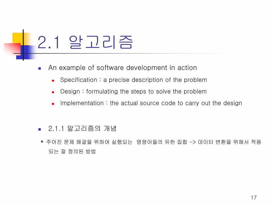
An example of software development in action
Specification : a precise description of the problem
Design : formulating the steps to solve the problem
Implementation : the actual source code to carry out the design
2.1.1 알고리즘의 개념
* 주어진 문제 해결을 위하여 실행되는 명령어들의 유한 집합 -> 데이터 변환을 위해서 적용
되는 잘 정의된 방법
18
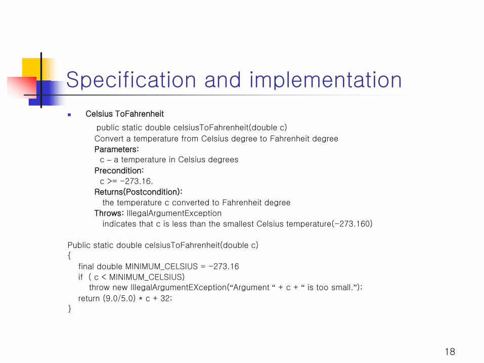
Specification and implementation
Celsius ToFahrenheit
public static double celsiusToFahrenheit(double c)
Convert a temperature from Celsius degree to Fahrenheit degree
Parameters:
c – a temperature in Celsius degrees
Precondition:
c >= -273.16.
Returns(Postcondition):
the temperature c converted to Fahrenheit degree
Throws: IllegalArgumentException
indicates that c is less than the smallest Celsius temperature(-273.160)
Public static double celsiusToFahrenheit(double c)
final double MINIMUM_CELSIUS = -273.16
if ( c < MINIMUM_CELSIUS)
throw new IllegalArgumentEXception(“Argument “ + c + “ is too small.”); return (9.0/5.0) * c + 32;

19
알고리즘이 만족 해야 할 조건
입력(input)
출력(output)
명확성(definiteness)
유한성(finiteness)
효과성(effectiveness)

20
2.1.2 알고리즘과 전산학
컴퓨터: 데이터 변환을 위해 사용하는 수단 -
> 알고리즘
전산학의 연구영역
* 컴퓨터 시스템의 기계구성과 조직 형태
* 언어의 설계와 번역
* 알고리즘의 기초(추상적 컴퓨터 모델)
* 알고리즘의 분석
알고리즘
Finite number od instruction to solve a problem : well defined
The theoretical study of computer-program
performance and resource usage.
What’s more important than performance
21
알고리즘의 고려사항
What’s more important than performance?
• modularity • correctness
• maintainability • functionality
• robustness • user-friendliness
• programmer time • simplicity
• extensibility • reliability
22
23
2.2 프로그램
2.2.1 프로그램 작성 절차
* 요구 사항(requirement)의 정의
* 설계(design)
* 평가(evaluation)
* 상세화 및 코딩(refinement and
coding)
* 검증(verification)
* 문서화(documentation)
24
2.2.2 프로그램의 작성 요령
하향식 방법(top-down method)
논리적 모듈(module)
부 프로그램(subprogram)을 사용
순차(sequencing), 분기(branching),
반복(repeating)등 세가지 표준 논리 제어 구조
GOTO문의 사용을 피한다
연상 이름(mnemonic-name)
문서화
25
2.2.3 순환 기법
순환(recursion): 자기 자신을 호출하도록 구
성하는 것 -> 프로그램을 단순화하고 이해하
기 용이 할 경우가 많음
순환 프로그램의 작성단계
* 순환관계 파악
* 알고리즘 구성
* 프로그램 언어로 기술
26
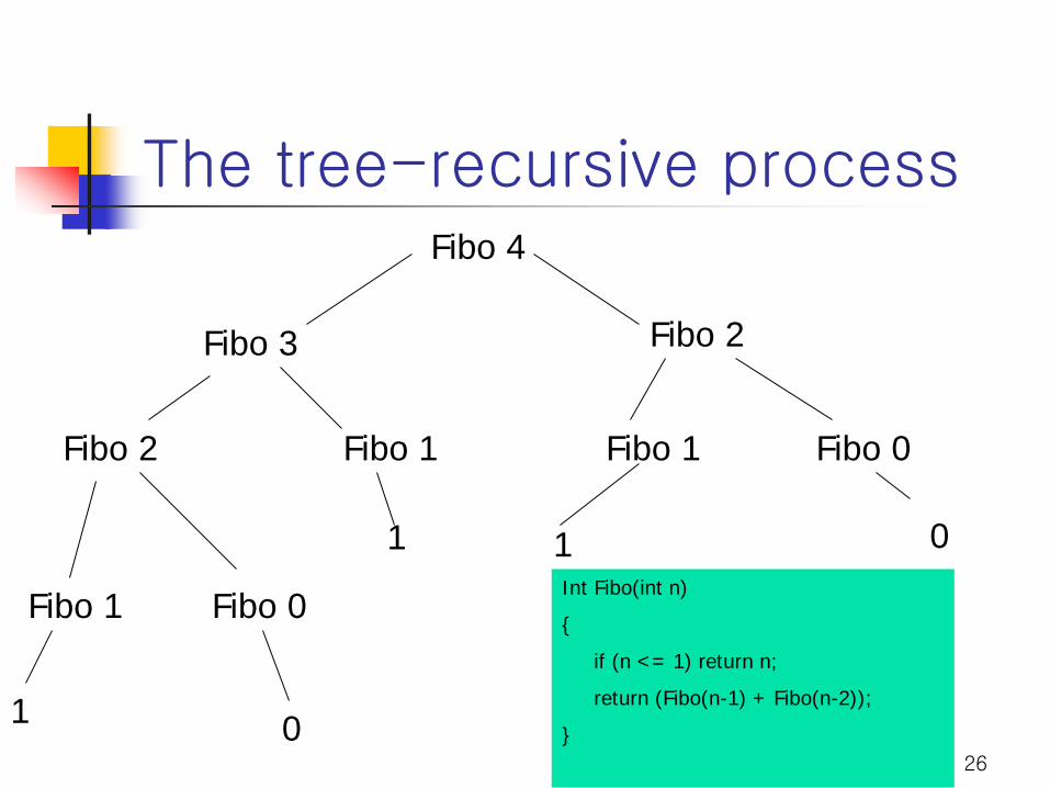
The tree-recursive process Fibo 4
Fibo 3 Fibo 2
Fibo 2 Fibo 1 Fibo 1 Fibo 0
Fibo 1 Fibo 0
1 0
1 1 0 Int Fibo(int n)
if (n <= 1) return n;
return (Fibo(n-1) + Fibo(n-2));
27
2.3 프로그램의 분석
2.3.1 프로그램의 평가 기준
* 바른 수행
* 정확한 동작
* 설명서
* 부 프로그램
* 해독
28
다른 평가 기준
프로그램의 수행에 필요한 기억장치의 용량 -> 비교적 용이
프로그램의 연산시간 -> 매우 어려움
* 기계
* 기계의 명령어의 집합
* 명령어의 수행시간
* 컴파일러의 번역 시간
-> 정확한 판정이 불가능 -> 명령문의 수행 빈도수를 계산
29
2.3.2 분석 기법
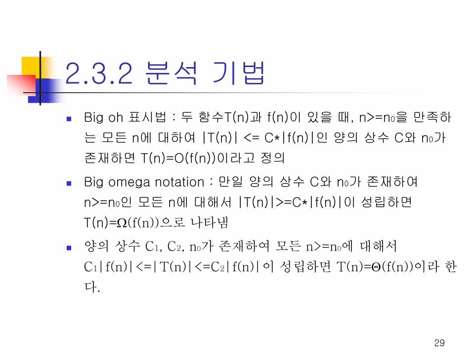
Big oh 표시법 : 두 함수T(n)과 f(n)이 있을 때, n>=n0을 만족하
는 모든 n에 대하여 |T(n)| <= C*|f(n)|인 양의 상수 C와 n0가
존재하면 T(n)=O(f(n))이라고 정의
Big omega notation : 만일 양의 상수 C와 n0가 존재하여
n>=n0인 모든 n에 대해서 |T(n)|>=C*|f(n)|이 성립하면
T(n)=Ω(f(n))으로 나타냄
양의 상수 C1, C2, n0가 존재하여 모든 n>=n0에 대해서
C1|f(n)|<=|T(n)|<=C2|f(n)|이 성립하면 T(n)=Θ(f(n))이라 한
다.

30
3. How to Measure Complexities
How good is our measure of work done to compare algorithms ?
How precisely can we compare two algorithms using our measure of work ?
Measure of work
# of passes of a loop
# of basic operations
Time complexity
c ⋅ (measure of work)
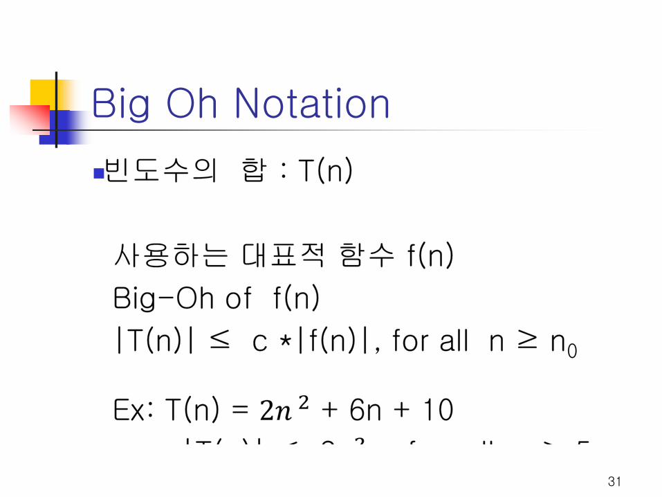
Big Oh Notation
31

32
For solving a problem P, suppose that two algorithms A1 and A2 need 106n and 5n basic operations, respectively, i.e.
basic operations
A1 106n
A2 5n
Which one is better ?
What are their time complexities ?

33
Now, suppose that algorithms A1 and A2 need the following amount of time:
time complexity
A1 106n O(n)
A2 n2 O(n2)
Which one is better ?
A1 is better if n > 106
A2 is better if n < 106
Then, why time complexity ?
Suppose that n → ∞
Then, n2 grows much faster than 106n. i.e.,
Under the assumption that n → ∞
A1 is better than A2
∴ Asymptotic growth rate !!!
∴ Time complexity (measure of work) compares and classifies algorithms by the asymptotic growth rate.
∞→∞→ n
nn 6
2
10lim
106 n
T(n)
34
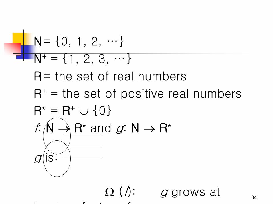
N = 0, 1, 2, …
N+ = 1, 2, 3, …
R = the set of real numbers
R+ = the set of positive real numbers
R* = R+ ∪ 0
f: N → R* and g: N → R*
g is:
Ω (f): g grows at l t f t f
35
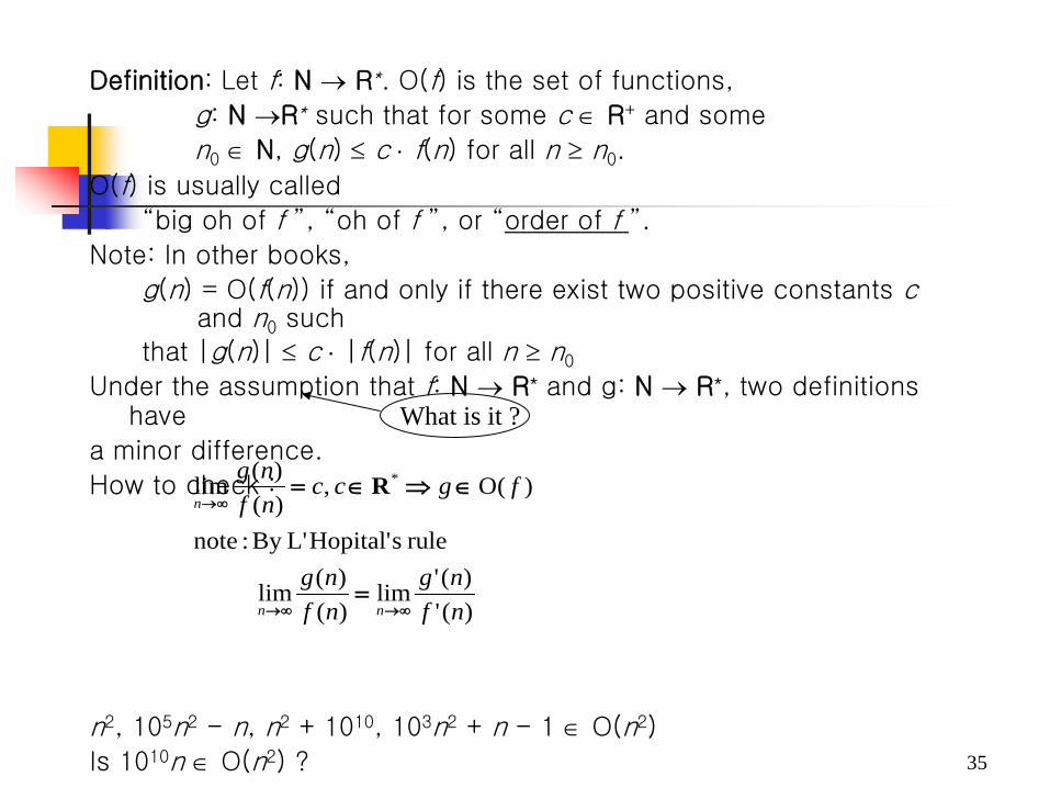
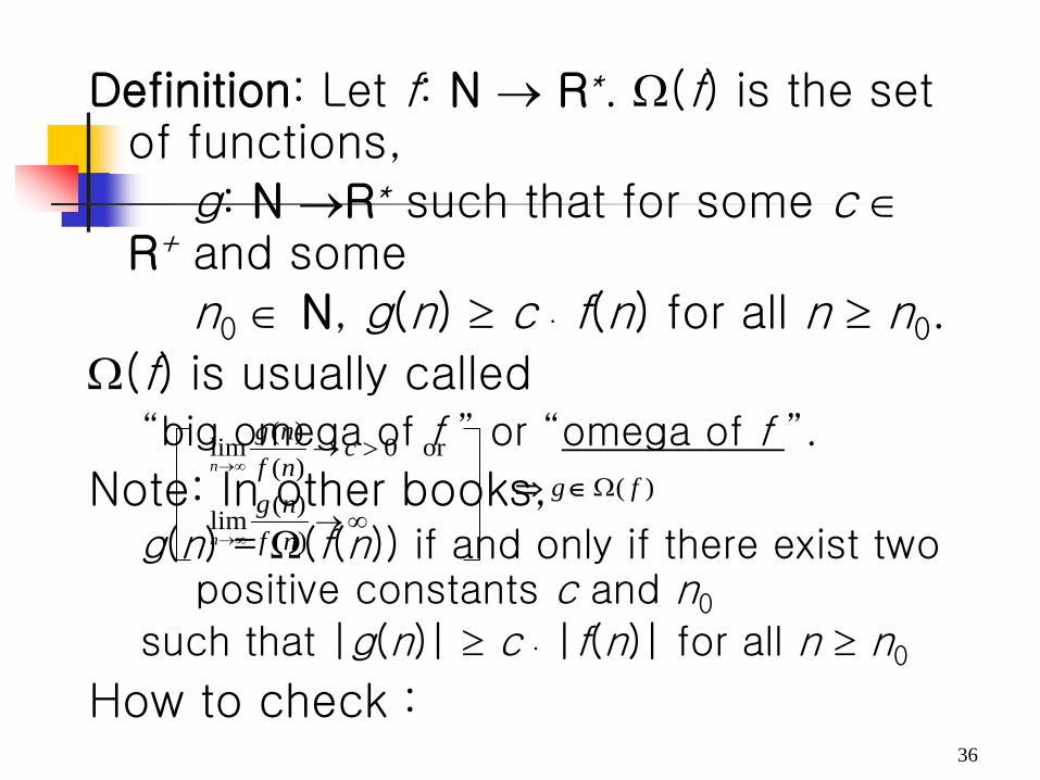
Definition: Let f: N → R*. O(f) is the set of functions,
g: N →R* such that for some c ∈ R+ and some
n0 ∈ N, g(n) ≤ c ⋅ f(n) for all n ≥ n0.
O(f) is usually called
“big oh of f ”, “oh of f ”, or “order of f ”.
Note: In other books,
g(n) = O(f(n)) if and only if there exist two positive constants c and n0 such
that |g(n)| ≤ c ⋅ |f(n)| for all n ≥ n0
Under the assumption that f: N → R* and g: N → R*, two definitions have
a minor difference.
How to check :
n2, 105n2 - n, n2 + 1010, 103n2 + n - 1 ∈ O(n2)
Is 1010n ∈ O(n2) ?
)(')('lim
)()(lim
rule sHopital'L'By :note
)(O ,)()(lim *
nfng
nfng
fgccnfng
nn
n
∞→∞→
∞→
=
∈⇒∈= R
What is it ?
36
Definition: Let f: N → R*. Ω(f) is the set of functions,
g: N →R* such that for some c ∈ R+ and some
n0 ∈ N, g(n) ≥ c ⋅ f(n) for all n ≥ n0.
Ω(f) is usually called “big omega of f ” or “omega of f ”.
Note: In other books, g(n) = Ω(f(n)) if and only if there exist two
positive constants c and n0
such that |g(n)| ≥ c ⋅ |f(n)| for all n ≥ n0
How to check :
)( fg Ω∈⇒
or 0 )()(lim >→
∞→c
nfng
n
∞→∞→ )(
)(limnfng
n
37
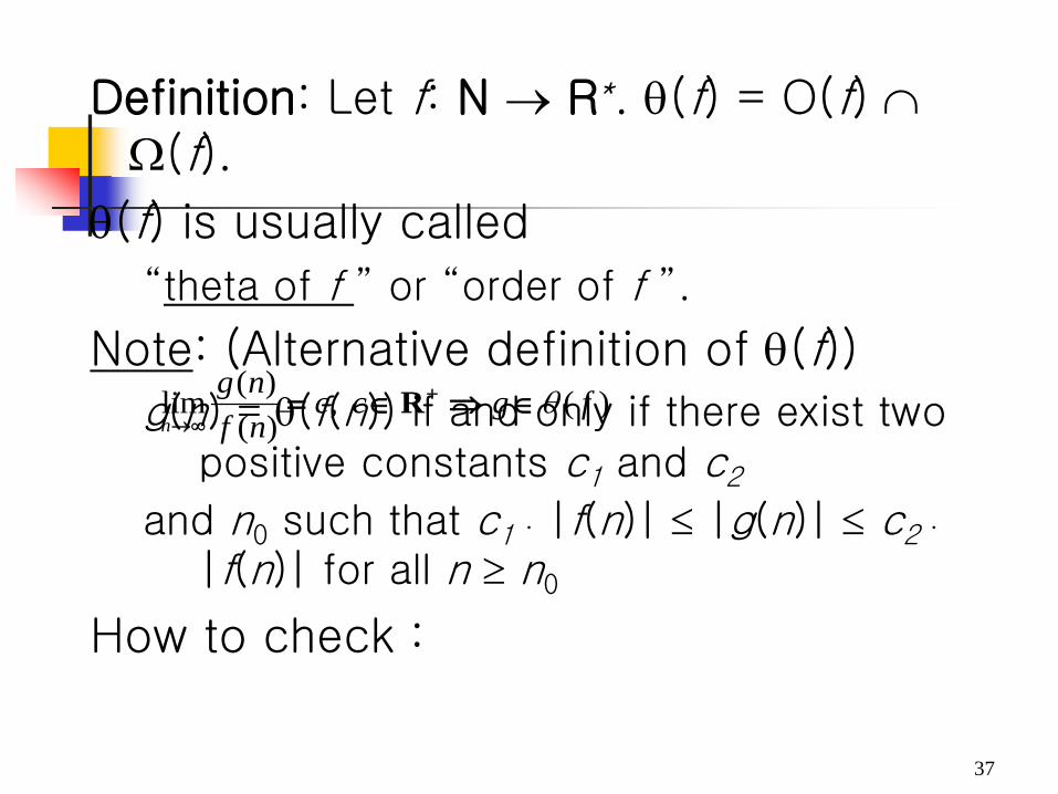
Definition: Let f: N → R*. θ(f) = O(f) ∩ Ω(f).
θ(f) is usually called
“theta of f ” or “order of f ”.
Note: (Alternative definition of θ(f)) g(n) = θ(f(n)) if and only if there exist two
positive constants c1 and c2
and n0 such that c1 ⋅ |f(n)| ≤ |g(n)| ≤ c2 ⋅ |f(n)| for all n ≥ n0
How to check :
)( ,)()(lim fgcc
nfng
nθ∈⇒∈= +
∞→R
38
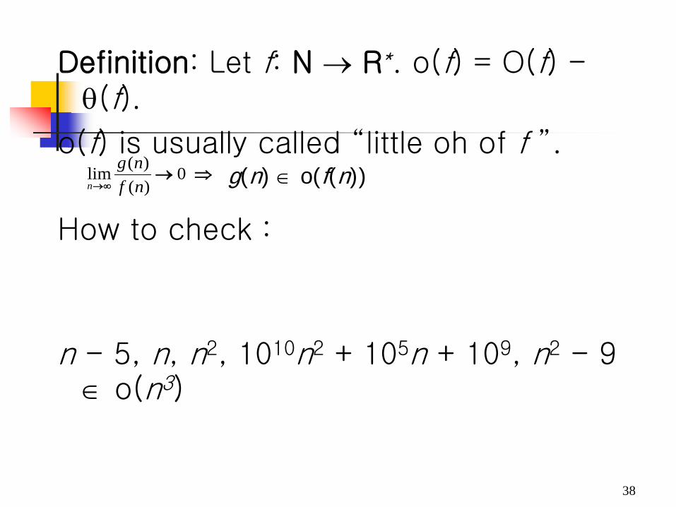
Definition: Let f: N → R*. o(f) = O(f) - θ(f).
o(f) is usually called “little oh of f ”.
How to check :
n - 5, n, n2, 1010n2 + 105n + 109, n2 - 9 ∈ o(n3)
⇒→∞→
0)()(lim
nfng
n g(n) ∈ o(f(n))

Definition: Let f: N → R*. ω(f) = Ω(f) - θ(f).
ω(f) is usually called “little omega of f”
How to check :
39
⇒∞→∞→ )(
)(limnfng
n
∈−++ 9,101010, 3952102 nnnn ω(n)
Note: ∈⇔∈ )())(()( nfnfong ω(g(n))
g(n) = ω(f(n))

40
How important is time complexity ?

41
42
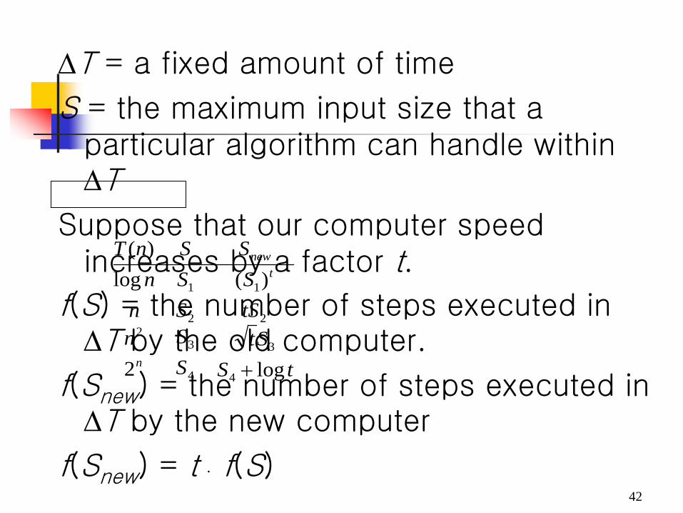
∆T = a fixed amount of time
S = the maximum input size that a particular algorithm can handle within ∆T
Suppose that our computer speed increases by a factor t.
f(S) = the number of steps executed in ∆T by the old computer.
f(Snew) = the number of steps executed in ∆T by the new computer
f(Snew) = t ⋅ f(S)
tSSt
SSn
tSSnSSnSSnT
n
tnew
log2
)(log)(
4
3
4
32
22
11
+
43
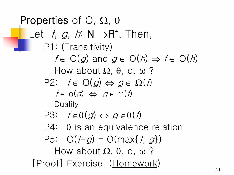
Properties of O, Ω, θ Let f, g, h: N →R*. Then,
P1: (Transitivity)
f ∈ O(g) and g ∈ O(h) ⇒ f ∈ O(h)
How about Ω, θ, o, ω ?
P2: f ∈ O(g) ⇔ g ∈ Ω(f) f ∈ o(g) ⇔ g ∈ ω(f)
Duality
P3: f ∈θ(g) ⇔ g ∈θ(f) P4: θ is an equivalence relation
P5: O(f+g) = O(maxf, g)
How about Ω, θ, o, ω ?
[Proof] Exercise. (Homework)
44
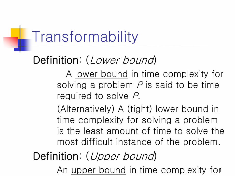
Transformability
Definition: (Lower bound)
A lower bound in time complexity for solving a problem P is said to be time required to solve P.
(Alternatively) A (tight) lower bound in time complexity for solving a problem is the least amount of time to solve the most difficult instance of the problem.
Definition: (Upper bound)
An upper bound in time complexity for
45
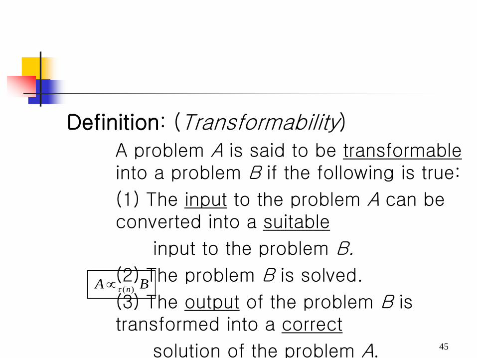
Definition: (Transformability)
A problem A is said to be transformable into a problem B if the following is true:
(1) The input to the problem A can be converted into a suitable
input to the problem B.
(2) The problem B is solved.
(3) The output of the problem B is transformed into a correct
solution of the problem A.
BA n)(τ∝
46
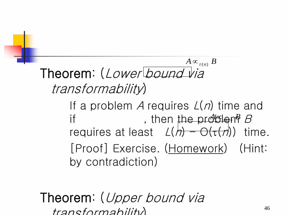
Theorem: (Lower bound via transformability)
If a problem A requires L(n) time and if , then the problem B requires at least L(n) - O(τ(n)) time.
[Proof] Exercise. (Homework) (Hint: by contradiction)
Theorem: (Upper bound via transformability)
BA n)(τ∝
BA n)(τ∝
47
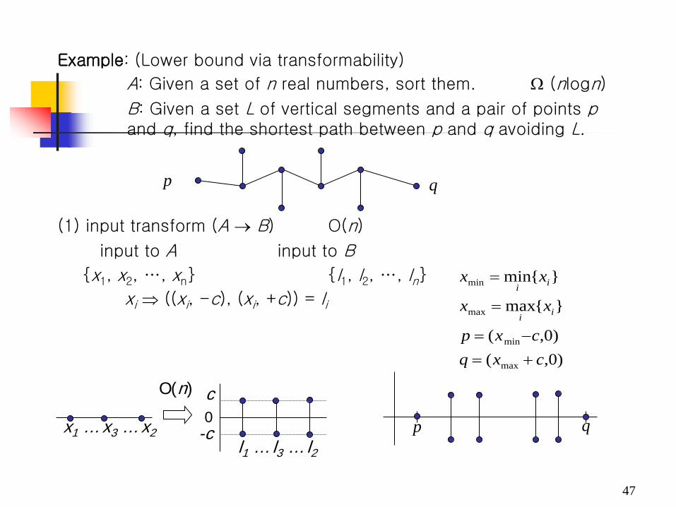
Example: (Lower bound via transformability)
A: Given a set of n real numbers, sort them. Ω (nlogn)
B: Given a set L of vertical segments and a pair of points p and q, find the shortest path between p and q avoiding L.
(1) input transform (A → B) O(n)
input to A input to B
x1, x2, …, xn l1, l2, …, ln
xi ⇒ ((xi, -c), (xi, +c)) = li
p q
c
-c 0
l1 … l3 … l2 x1 … x3 … x2
O(n)
)0,()0,(
max
min
max
min
max
min
cxqcxp
xx
xx
ii
ii
+=−=
=
=
p q
48
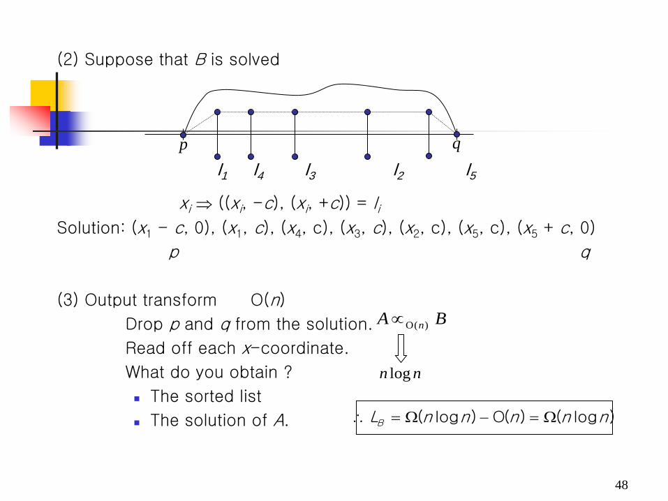
(2) Suppose that B is solved
xi ⇒ ((xi, -c), (xi, +c)) = Ii Solution: (x1 - c, 0), (x1, c), (x4, c), (x3, c), (x2, c), (x5, c), (x5 + c, 0)
p q
(3) Output transform O(n)
Drop p and q from the solution.
Read off each x-coordinate.
What do you obtain ?
The sorted list
The solution of A.
p q l1 l4 l3 l2 l5
BA n)(O∝
nn log
)log()(O)log( nnnnnLB Ω=−Ω=∴
49
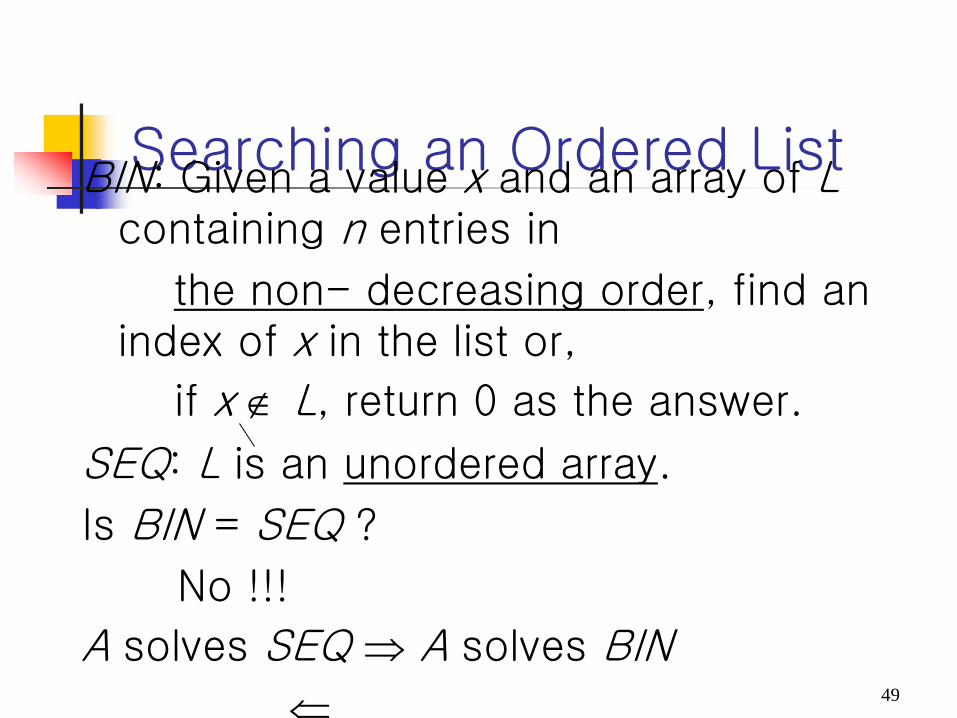
Searching an Ordered List BIN: Given a value x and an array of L containing n entries in
the non- decreasing order, find an index of x in the list or,
if x ∉ L, return 0 as the answer.
SEQ: L is an unordered array.
Is BIN = SEQ ?
No !!!
A solves SEQ ⇒ A solves BIN
⇐
50
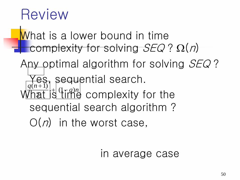
Review
What is a lower bound in time complexity for solving SEQ ? Ω(n)
Any optimal algorithm for solving SEQ ?
Yes, sequential search.
What is time complexity for the sequential search algorithm ?
O(n) in the worst case,
in average case
nqnq )1( 2
)1(−+
+
51
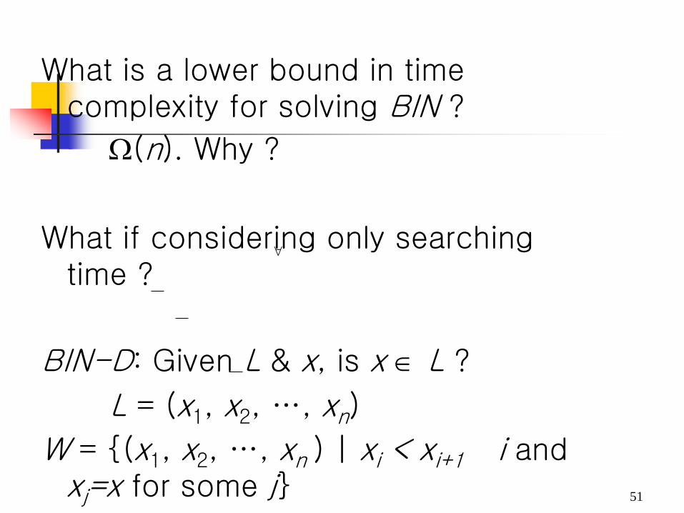
What is a lower bound in time complexity for solving BIN ?
Ω(n). Why ?
What if considering only searching time ?
BIN-D: Given L & x, is x ∈ L ?
L = (x1, x2, …, xn)
W = (x1, x2, …, xn ) | xi < xi+1 i and xj=x for some j
∀
52
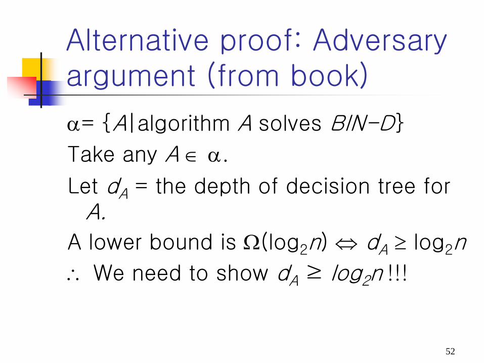
Alternative proof: Adversary argument (from book)
α= A|algorithm A solves BIN-D
Take any A ∈ α.
Let dA = the depth of decision tree for A.
A lower bound is Ω(log2n) ⇔ dA ≥ log2n
∴ We need to show dA ≥ log2n !!!
53
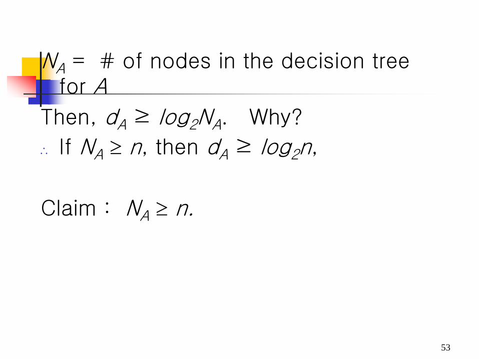
NA = # of nodes in the decision tree for A
Then, dA ≥ log2NA. Why?
∴ If NA ≥ n, then dA ≥ log2n,
Claim : NA ≥ n.
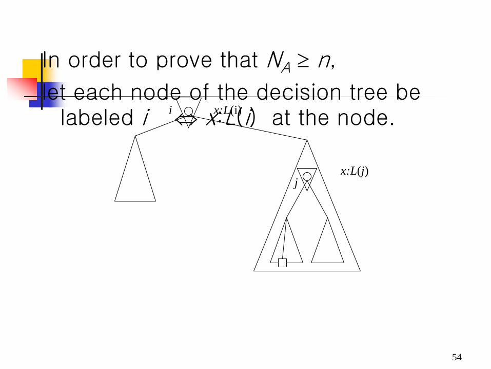
In order to prove that NA ≥ n,
let each node of the decision tree be labeled i ⇔ x:L(i) at the node.
54
i
x:L(j) j
x:L(i)
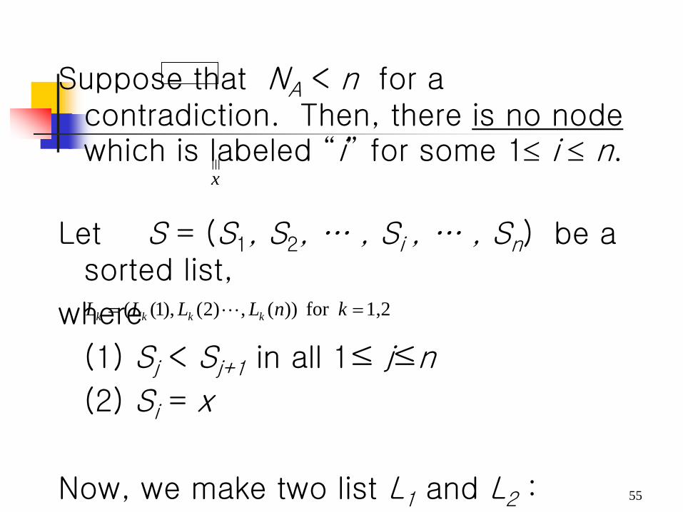
Suppose that NA < n for a contradiction. Then, there is no node which is labeled “i” for some 1≤ i ≤ n.
Let S = (S1, S2, … , Si , … , Sn) be a sorted list,
where
(1) Sj < Sj+1 in all 1≤ j≤n
(2) Si = x
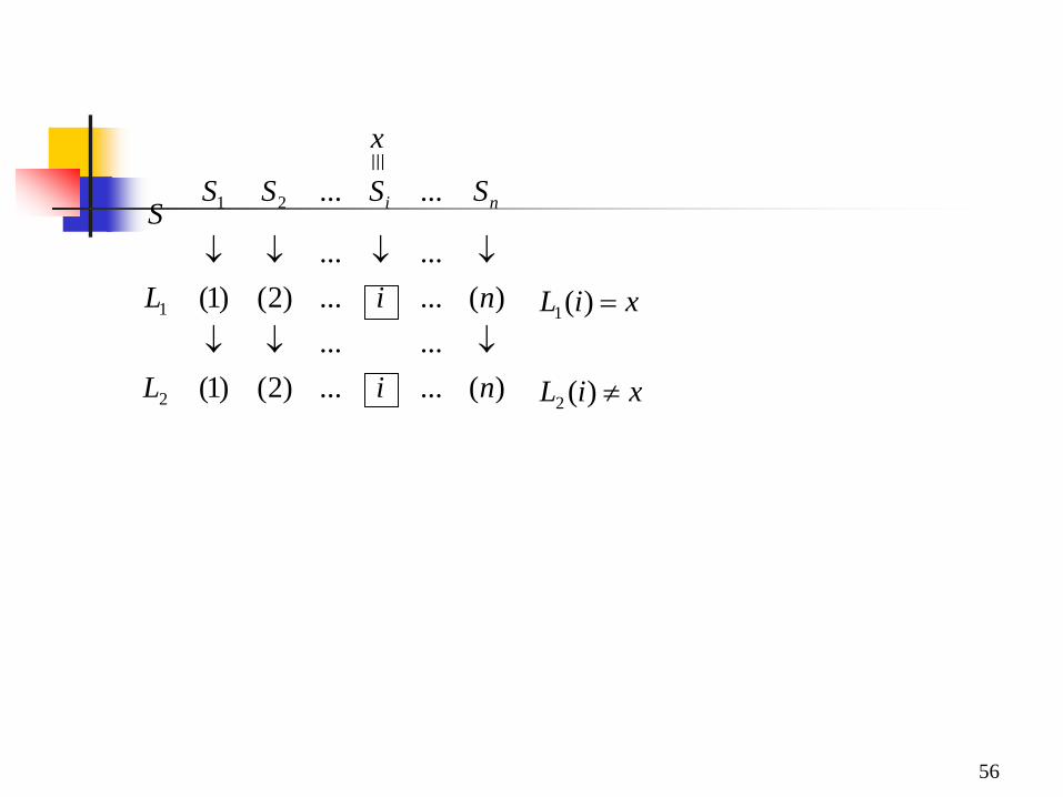
Now, we make two list L1 and L2 :
55
1,2for ))(,)2(),1(( == knLLLL kkkk
x
≡
56
)(......)2()1(......
)(......)2()1(......
......
2
1
21
niL
niL
SSSSS ni
↓↓↓
↓↓↓↓
x ≡
xiL ≠)(2
xiL =)(1
57
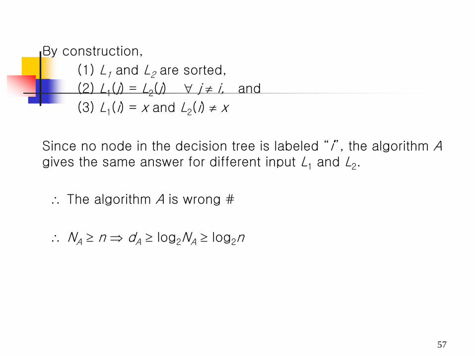
By construction,
(1) L1 and L2 are sorted,
(2) L1(j) = L2(j) ∀ j ≠ i, and
(3) L1(i) = x and L2(i) ≠ x
Since no node in the decision tree is labeled “i”, the algorithm A gives the same answer for different input L1 and L2.
∴ The algorithm A is wrong #
∴ NA ≥ n ⇒ dA ≥ log2NA ≥ log2n
58
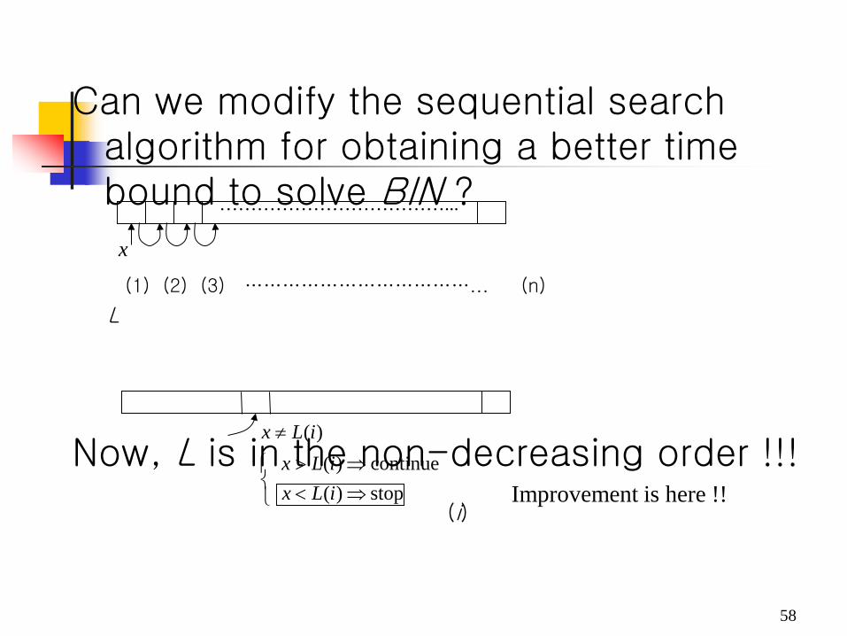
Can we modify the sequential search algorithm for obtaining a better time bound to solve BIN ?
(1) (2) (3) ………………………………... (n)
L
Now, L is in the non-decreasing order !!!
(i)
x
………………………………...
⇒<⇒>
≠
stop)( continue)(
)(
iLxiLx
iLx
Improvement is here !!

59
Compare x to the every kth elements in L !!!
(k) (2k)
x > L((r-1)k) x < L(rk)
However O(n) anyway !!!
case worst in the scomparison )1(
+−knk Why ?
elements)1( −k
60
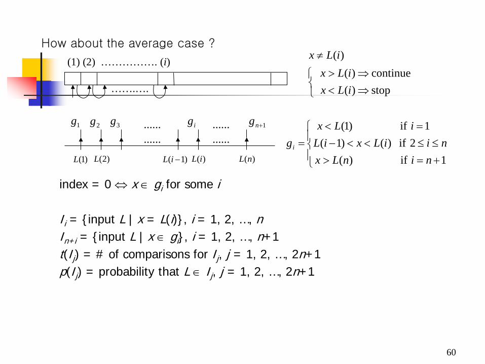
How about the average case ?
index = 0 ⇔ x ∈ gi for some i Ii = input L | x = L(i), i = 1, 2, …, n In+i = input L | x ∈ gi, i = 1, 2, …, n+1 t(Ij) = # of comparisons for Ij, j = 1, 2, …, 2n+1 p(Ij) = probability that L ∈ Ij, j = 1, 2, …, 2n+1
…….….
(1) (2) ……………. (i)
⇒<⇒>
≠
stop)( continue)(
)(
iLxiLx
iLx
+=>≤≤<<−
=<=
1 if )(2 if )()1(
1 if )1(
ninLxniiLxiL
iLxgi
1g 2g 3g ig 1+ng
)1(L )2(L )1( −iL )(iL )(nL
......
...... ............
61
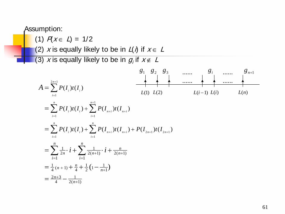
Assumption: (1) P(x ∈ L) = 1/2 (2) x is equally likely to be in L(i) if x ∈ L (3) x is equally likely to be in gi if x ∉ L
2 1
1
1
1 1
2 1 2 11 1
1 12 2( 1) 2( 1)
1 1
1 1 1( 1) 14 4 2 12 3 1
4 2( 1)
( ) ( )
( ) ( ) ( ) ( )
( ) ( ) ( ) ( ) ( ) ( )
( )
n
i ii
n n
i i n i n ii i
n n
i i n i n i n ni i
n nn
n n ni i
nn nn
n
P I t I
P I t I P I t I
P I t I P I t I P I t I
A
i i
+
=
+
+ += =
+ + + += =
+ += =
+ +
++
+
+ +
=
=
=
= ⋅ + ⋅ +
= + + −
= −
∑
∑ ∑
∑ ∑
∑ ∑
1g 2g 3g ig 1+ng
)1(L )2(L )1( −iL )(iL )(nL
......
...... ............
62
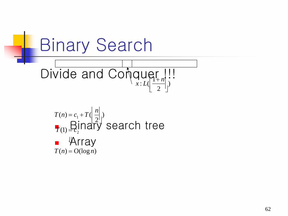
Binary Search
Divide and Conquer !!!
Binary search tree
Array
)(logO)(
)1(
)2
()(
2
1
nnT
cT
nTcnT
=⇓
=
+=
)2
1(:
+ nLx

63
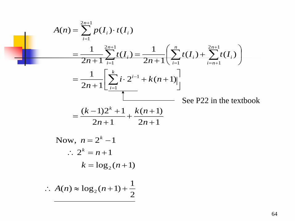
Average-case Analysis Ii = input L | x = L(i), i = 1, 2, …, n
In+i = input L | x ∈ gi, i = 1, 2, …, n+1
t(Ij) = # of comparisons for Ij, j = 1, 2, …, 2n+1
p(Ij) = probability that L ∈ Ij, j = 1, 2, …, 2n+1
Assumptions:
(1) p(Ij) = 1/(2n+1)
(2) n = 2k - 1, k ≥1
# of comp. # of node 1 20 2 21 3 22
….………….. k 2k-1 k 2k
……....……….….…………..
………...
comparison k
2 1
12 1
1
( ) ( ) ( )
1 ( )2 1
n
i ii
n
ii
A n P I t I
t In
+
=
+
=
= ⋅
=+
∑
∑? Lx∈
Lx∉
64
12)1(
1212)1(
)1(212
1
)()(12
1)(12
1
)()()(
1
1
12
11
12
1
12
1
++
++
+−=
++⋅
+=
+
+=
+=
⋅=
∑
∑∑∑
∑
=
−
+
+==
+
=
+
=
nnk
nk
nkin
ItItn
Itn
ItIpnA
k
k
i
i
n
nii
n
ii
n
ii
n
iii
12 Now, −= kn12 +=∴ nk
)1(log2 += nk
21)1(log)( 2 ++≈∴ nnA
See P22 in the textbook