Effective Computational Geometry

for Curves and Surfaces

Chapter 7

Computational Topology: An Introduction

Gunter Rote and Gert Vegter

We give an introduction to combinatorial topology, with an emphasis on subjects that areof interest for computational geometry in two and three dimensions. We cover the notions ofhomotopy and isotopy, simplicial homology, Betti numbers, and basic results from Morse Theory.

This survey appeared as a chapter of the book Effective Computational Geometry for Curves andSurfaces, (Jean-Daniel Boissonnat, Monique Teillaud, editors), published by Springer-Verlag, 2007,ISBN 3-540-33258-8. Page references to other chapters are to the pages of the book. The originalpublication is available on-line at link.springer.com. DOI:10.1007/978-3-540-33259-6_7.

Contents

7 Computational Topology: An Introduction 1

7.1 Introduction . . . . . . . . . . . . . . . . . . . . . . . . . . . . . . . . . . . . . . . . 1

7.2 Simplicial complexes . . . . . . . . . . . . . . . . . . . . . . . . . . . . . . . . . . . 2Topological spaces. . . . . . . . . . . . . . . . . . . . . . . . . . . . . 2Homeomorphisms. . . . . . . . . . . . . . . . . . . . . . . . . . . . . 2Simplices. . . . . . . . . . . . . . . . . . . . . . . . . . . . . . . . . . 3Simplicial complexes. . . . . . . . . . . . . . . . . . . . . . . . . . . . 3Combinatorial surfaces. . . . . . . . . . . . . . . . . . . . . . . . . . 4Homotopy and Isotopy: Continuous Deformations. . . . . . . . . . . 4

7.3 Simplicial homology . . . . . . . . . . . . . . . . . . . . . . . . . . . . . . . . . . . 5A calculus of closed loops. . . . . . . . . . . . . . . . . . . . . . . . . 5Chain spaces and simplicial homology. . . . . . . . . . . . . . . . . . 6Example: One-homologous chains. . . . . . . . . . . . . . . . . . . . 6Example: Zero-homology of a connected simplicial complex. . . . . . 7Example: One-homologous chains. . . . . . . . . . . . . . . . . . . . 7Betti numbers. . . . . . . . . . . . . . . . . . . . . . . . . . . . . . . 7Euler characteristic and Betti numbers. . . . . . . . . . . . . . . . . 10Incremental algorithm for computation of Betti numbers. . . . . . . 10Chain maps and chain homotopy. . . . . . . . . . . . . . . . . . . . . 12Simplical collapse. . . . . . . . . . . . . . . . . . . . . . . . . . . . . 12Example: Betti numbers of the projective plane. . . . . . . . . . . . 13Example: Betti numbers depend on field of scalars. . . . . . . . . . . 13

7.4 Morse Theory . . . . . . . . . . . . . . . . . . . . . . . . . . . . . . . . . . . . . . . 14

7.4.1 Smooth functions and manifolds . . . . . . . . . . . . . . . . . . . . . . . . 14Differential of a smooth map. . . . . . . . . . . . . . . . . . . . . . . 14Regular surfaces in R3. . . . . . . . . . . . . . . . . . . . . . . . . . . 14Submanifolds of Rn. . . . . . . . . . . . . . . . . . . . . . . . . . . . 15Tangent space of a manifold. . . . . . . . . . . . . . . . . . . . . . . 16Smooth function on a submanifold. . . . . . . . . . . . . . . . . . . . 16Regular and critical points. . . . . . . . . . . . . . . . . . . . . . . . 16Implicit surfaces and manifolds. . . . . . . . . . . . . . . . . . . . . . 17Hessian at a critical point. . . . . . . . . . . . . . . . . . . . . . . . . 17Non-degenerate critical point. . . . . . . . . . . . . . . . . . . . . . . 18

7.4.2 Basic Results from Morse Theory . . . . . . . . . . . . . . . . . . . . . . . . 18Morse function. . . . . . . . . . . . . . . . . . . . . . . . . . . . . . . 18Regular level sets. . . . . . . . . . . . . . . . . . . . . . . . . . . . . 18The Morse Lemma. . . . . . . . . . . . . . . . . . . . . . . . . . . . . 18Abundance of Morse functions. . . . . . . . . . . . . . . . . . . . . . 19Passing critical levels. . . . . . . . . . . . . . . . . . . . . . . . . . . 19Morse inequalities. . . . . . . . . . . . . . . . . . . . . . . . . . . . . 20Gradient vector fields. . . . . . . . . . . . . . . . . . . . . . . . . . . 20Integral lines, and their local structure near singular points. . . . . . 20Stable and unstable manifolds. . . . . . . . . . . . . . . . . . . . . . 21The Morse-Smale complex. . . . . . . . . . . . . . . . . . . . . . . . 22Reeb graphs and contour trees. . . . . . . . . . . . . . . . . . . . . . 22

7.5 Exercises . . . . . . . . . . . . . . . . . . . . . . . . . . . . . . . . . . . . . . . . . 25

i

Chapter 7

Computational Topology: AnIntroduction

Gunter Rote, Gert Vegter1

7.1 Introduction

Topology studies point sets and their invariants under continuous deformations, invariants suchas the number of connected components, holes, tunnels, or cavities. Metric properties such as theposition of a point, the distance between points, or the curvature of a surface, are irrelevant totopology. Computational topology deals with the complexity of topological problems, and withthe design of efficient algorithms for their solution, in case these problems are tractable. Thesealgorithms can deal only with spaces and maps that have a finite representation. To this end werestrict ourselves to simplicial complexes and maps. In particular we study algebraic invariantsof topological spaces like Euler characteristics and Betti numbers, which are in general easier tocompute than topological invariants.

Many computational problems in topology are algorithmically undecidable. The mathematicalliterature of the 20th century contains many (beautiful) topological algorithms, usually reducingto decision procedures, in many cases with exponential-time complexity. The quest for efficientalgorithms for topological problems has started rather recently. The overviews by Dey, Edelsbrun-ner and Guha [6], Edelsbrunner [7], Vegter [21], and the book by Zomorodian [22] provide furtherbackground on this fascinating area.

This chapter provides a tutorial introduction to computational aspects of algebraic topology. Itintroduces the language of combinatorial topology, relevant for a rigorous mathematical descriptionof geometric objects like meshes, arrangements and subdivisions appearing in other chapters ofthis book, and in the computational geometry literature in general.

Computational methods are emphasized, so the main topological objects are simplicial com-plexes, combinatorial surfaces and submanifolds of some Euclidean space. These objects are intro-duced in Sect. 7.2. Here we also introduce the notions of homotopy and isotopy, which also featurein other parts of this book, like Chapter 5. Most of the computational techniques are introducedin Sect. 7.3. Topological invariants, like Betti numbers and Euler characteristic, are introducedand methods for computing such invariants are presented. Morse theory plays an important rolein many recent advances in computational geometry and topology. See, e.g., Sect. 5.5.2. Thistheory is introduced in Sect. 7.4.

Given our focus on computational aspects, topological invariants like Betti numbers are definedusing simplicial homology, even though a more advanced study of deeper mathematical aspectsof algebraic topology could better be based on singular homology, introduced in most modern

1Coordinator

1

2 CHAPTER 7. COMPUTATIONAL TOPOLOGY: AN INTRODUCTION

textbooks on algebraic topology. Other topological invariants, like homotopy groups, are harderto compute in general; These are not discussed in this chapter.

The chapter is far from a complete overview of computational algebraic topology, and it doesnot discuss recent advances in this field. However, reading this chapter paves the way for studyingrecent books and papers on computational topology. Topological algorithms are currently beingused in applied fields, like image processing and scattered data interpolation. Most of theseapplications use some of the tools presented in this chapter.

7.2 Simplicial complexes

Topological spaces. In this chapter a topological space X (or space, for short) is a subset of someEuclidean space Rd, endowed with the induced topology of Rd. In particular, an ε-neighborhood(ε > 0) of a point x in X is the set of all points in X within Euclidean distance ε from x. A subsetO of X is open if every point of O contains an ε-neighborhood contained in O, for some ε > 0.A subset of X is closed if its complement in X is open. The interior of a set X is the set of allpoints having an ε-neighborhood contained in X, for some ε > 0. The closure of a subset X of Rdis the set of points x in Rd every ε-neigborhood of which has non-empty intersection with X. Theboundary of a subset X is the set of points in the closure of X that are not interior points of X.In particular, every ε-neighborhood of a point in the boundary of X has non-empty intersectionwith both X and the complement of X. See [1, Sect. 2.1] for a more complete introduction of thebasic concepts and properties of point set topology.

The space Rd is called the ambient space of X. Examples of topological spaces are:

1. The interval [0, 1] in R;

2. The open unit d-ball: Bd = {(x1, . . . , xd) ∈ Rd | x21 + · · ·+ x2d < 1};

3. The closed unit d-ball: Bd = {(x1, . . . , xd) ∈ Rd | x21 + · · ·+ x2d ≤ 1} (the closure of Bd);

4. The unit d-sphere Sd = {(x1, . . . , xd+1) ∈ Rd+1 | x21 + · · ·+ x2d+1 = 1} (the boundary of the(d+1)-ball);

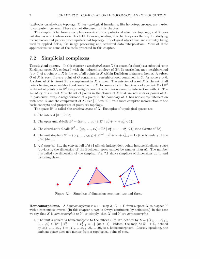
5. A d-simplex, i.e., the convex hull of d+1 affinely independent points in some Euclidean space(obviously, the dimension of the Euclidean space cannot be smaller than d). The numberd is called the dimension of the simplex. Fig. 7.1 shows simplices of dimensions up to andincluding three.

Figure 7.1: Simplices of dimension zero, one, two and three.

Homeomorphisms. A homeomorphism is a 1–1 map h : X → Y from a space X to a space Ywith a continuous inverse. (In this chapter a map is always continuous by definition.) In this casewe say that X is homeomorphic to Y , or, simply, that X and Y are homeomorphic.

1. The unit d-sphere is homeomorphic to the subset Σ of Rm defined by Σ = {(x1, . . . , xd+1,0, . . . , 0) ∈ Rm | x21 + · · · + x2d+1 = 1} (m > d). Indeed, the map h : Sd → Σ, definedby h(x1, . . . , xd+1) = (x1, . . . , xd+1, 0, . . . , 0), is a homeomorphism. Loosely speaking, theambient space does not matter from a topological point of view.

7.2. SIMPLICIAL COMPLEXES 3

2. The map h : Rk → Rm, m > k, defined by

h(x1, . . . , xk) = (x1, . . . , xk, 0, . . . , 0),

is not a homeomorphism.

3. Any invertible affine map between two Euclidean spaces (of necessarily equal dimension) isa homeomorphism.

4. Any two d-simplices are homeomorphic. (If the simplices lie in the same ambient space ofdimension d − 1, there is a unique invertible affine map sending the vertices of the firstsimplex to the vertices of the second simplex. For other, possibly unequal dimensions ofthe ambient space one can construct an invertible affine map between the affine hulls of thesimplices.)

5. The boundary of a d-simplex is homeomorphic to the unit d-sphere. (Consider a d-simplex inRd+1. The projection of its boundary from a fixed point in its interior onto its circumscribedd-sphere is a homeomorphism. See Fig. 7.2. The circumscribed d-sphere is homeomorphicto the unit d-sphere.)

2

1

Figure 7.2: The point p on the boundary of a 3-simplex is mapped onto the point p′ on the2-sphere. This mapping defines a homeomorphism between the 2-simplex and the 2-sphere.

Simplices. Consider a k-simplex σ, which is the convex hull of a set A of k + 1 independentpoints a0, . . . , ak in some Euclidean space Rd (so d ≥ k). A is said to span the simplex σ. Asimplex spanned by a subset A′ of A is called a face of σ. If τ is a face of σ we write τ � σ. Theface is proper if ∅ 6= A′ 6= A. The dimension of the face is |A′| − 1. A 0-dimensional face is calleda vertex, a 1-dimensional face is called an edge. An orientation of σ is induced by an ordering ofits vertices, denoted by 〈a0 · · · ak〉, as follows: For any permutation π of 0, . . . , k, the orientation〈aπ(0) · · · aπ(k)〉 is equal to (−1)sign(π)〈a0 · · · ak〉, where sign(π) is the number of transpositionsof π (so each simplex has two distinct orientations). A simplex together with a specific choiceof orientation is called an oriented simplex. If τ is a (k−1)-dimensional face of σ, obtained byomitting the vertex ai, then the induced orientation on τ is (−1)i〈a0 · · · ai · · · ak〉, where the hatindicates omission of ai.

Simplicial complexes. A simplicial complex K is a finite set of simplices in some Euclideanspace Rm, such that (i) if σ is a simplex of K and τ is a face of σ, then τ is a simplex of K, and(ii) if σ and τ are simplices of K, then σ ∩ τ is either empty or a common face of σ and τ . Thedimension of K is the maximum of the dimensions of its simplices. The underlying space of K,

4 CHAPTER 7. COMPUTATIONAL TOPOLOGY: AN INTRODUCTION

denoted by |K|, is the union of all simplices of K, endowed with the subspace topology of Rm.The i-skeleton of K, denoted by Ki, is the union of all simplices of K of dimension at most i. Asubcomplex L of K is a subset of K that is a simplicial complex. A triangulation of a topologicalspace X is a pair (K,h), where K is a simplicial complex and h is a homeomorphism from theunderlying space |K| to X. The Euler characteristic of a simplicial d-complex K, denoted by

χ(K), is the number∑di=0(−1)iαi, where αi is the number of i-simplices of K. Examples of

simplicial complexes are:

1. A graph is a 1-dimensional simplicial complex (think of a graph as being embedded in R3).The complete graph with n vertices is the 1-skeleton of an (n−1)-simplex.

2. The Delaunay triangulation of a set of points in general position in Rd is a simplicial complex.

Combinatorial surfaces. A Combinatorial closed surface is a finite two-dimensional simplicialcomplex in which each edge (1-simplex) is incident with two triangles (2-simplices), and the setof triangles incident to a vertex can be cyclically ordered t0, t1, . . . , tk−1 so that ti has exactly oneedge in common with ti+1mod k, and these are the only common edges. Stillwell [20, page 69 ff]contains historical background and the basic theorem on the classification combinatorial surfaces.

Homotopy and Isotopy: Continuous Deformations. Homotopy is a fundamental topo-logical concept that describes equivalence between curves, surfaces, or more general topologicalsubspaces within a given topological space, up to “continuous deformations”.

Technically, homotopy is defined between two maps g, h : X → Y from a space X into aspace Y . The maps g and h are homotopic if there is a continuous map

f : X × [0, 1]→ Y

such that f(x, 0) = g(x) and f(x, 1) = h(x) for all x ∈ X. The map f is then called a homotopybetween g and h. It is easy to see that homotopy is an equivalence relation, since a homotopy canbe “inverted” and two homotopies can be “concatenated”.

When g and h are two curves in Y = Rn defined over the same interval X = [a, b], the homotopyf defines, for each “time” t, 0 ≤ t ≤ 1, a curve f(·, t) : [a, b] → Rn that interpolates smoothlybetween f(·, 0) = g and f(·, 1) = h.2

To define homotopy for two surfaces or more general spaces S and T , we start with the identitymap on S and deform it into a homeomorphism from S to T . Two topological subspaces S, T ⊆ Xare called homotopic if there is a continuous mapping

γ : S × [0, 1]→ X

such that γ(·, 0) is the identity map on S and γ(·, 1) is a homeomorphism from S to T .By the requirement that we have a homeomorphism at time t = 1, one can see that this

definition is symmetric in S and T . Note that we do not require γ(·, t) to be a homeomorphismat all times t. Thus, a clockwise cycle and a counterclockwise cycle in the plane are homotopic.In fact, all closed curves in the plane are homotopic: every cycle can be contracted into a point(which is a special case of a closed curve). A connected topological space with this property iscalled simply connected.

Examples of spaces which are not simply connected are a plane with a point removed, or a(solid or hollow) torus. For example, on the hollow torus in Fig. 7.3, the closed curve in the figureis not homotopic to its inverse.

If we require that γ(·, t) is a homeomorphism at all times during the deformation we arrive thestronger concept of isotopy. For example, the smooth closed curves without self-intersections in theplane fall into two isotopy classes, according to their orientation (clockwise or counterclockwise).Isotopy is usually what is meant when speaking about a “topologically correct” approximation of

2In the case of curves with the same endpoints g(a) = h(a) and g(b) = h(b), one usually requires also that theseendpoints remain fixed during the deformation: f(a, t) = g(a) and f(b, t) = g(b) for all t.

7.3. SIMPLICIAL HOMOLOGY 5

a given surface, as discussed in Sect. 5.1, where the stronger concept of ambient isotopy is alsodefined (Definition 1, p. 183).

A map f : X → Y is a homotopy equivalence if there is a map g : Y → X such that the composedmaps gf and fg are homotopy equivalent to the identity map (on X and Y , respectively). Themap g is a homotopy inverse of f . The spaces X and Y are called homotopy equivalent. A spaceis contractible if it is homotopy equivalent to a point.

1. The unit ball in a Euclidean space is contractible. Let f : {0} → Bd be the inclusion map.The constant map g : Bd → {0} is a homotopy inverse of f . To see this, observe that themap fg is the identity, and gf is homotopic to the identity map on Bd, the homotopy beingthe map F : Bd × [0, 1]→ Bd defined by F (x, t) = tx.

2. The solid torus is homotopy equivalent to the circle. More generally, the cartesian productof a topological space X and a contractible space is homotopy equivalent to X.

3. A punctured d-dimensional Euclidean space Rd \ {0} is homotopy equivalent to a (d − 1)-sphere.

Note that homotopy equivalent spaces need not be homeomorphic. However, such spaces shareimportant topological properties, like having the same Betti numbers (to be introduced in the nextsection). Section 6.2.3 (p. 250) describes how this concept is applied in surface reconstruction.

7.3 Simplicial homology

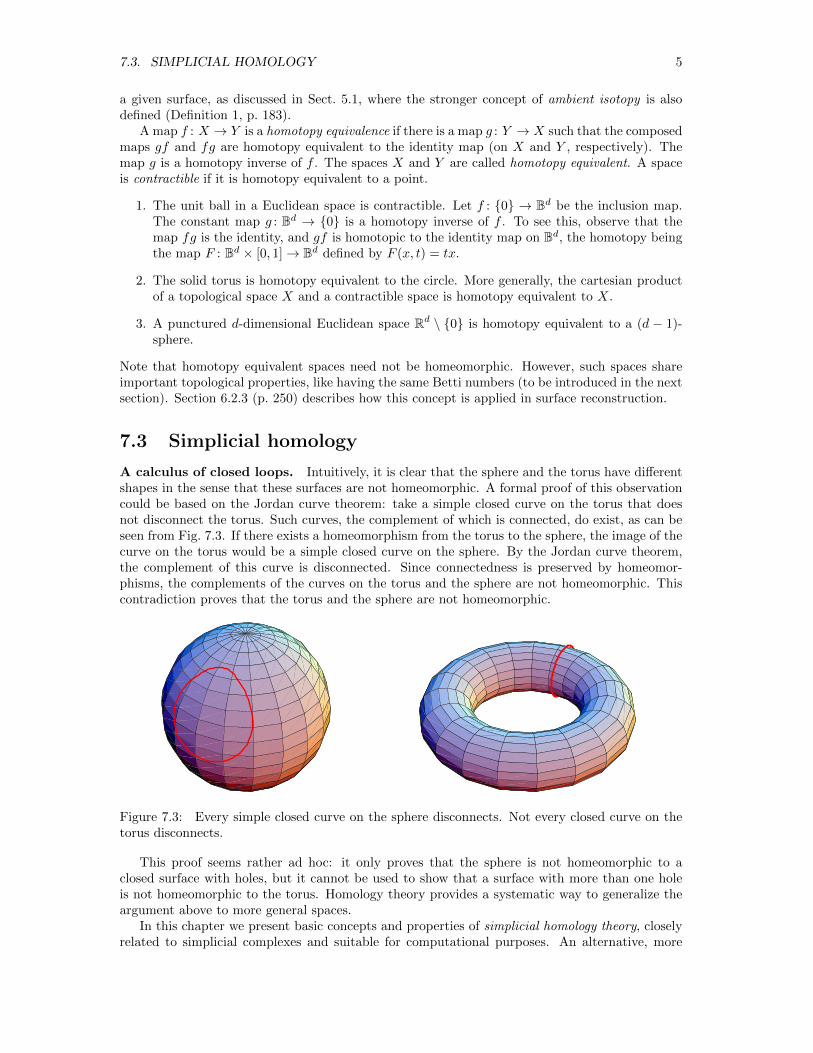
A calculus of closed loops. Intuitively, it is clear that the sphere and the torus have differentshapes in the sense that these surfaces are not homeomorphic. A formal proof of this observationcould be based on the Jordan curve theorem: take a simple closed curve on the torus that doesnot disconnect the torus. Such curves, the complement of which is connected, do exist, as can beseen from Fig. 7.3. If there exists a homeomorphism from the torus to the sphere, the image of thecurve on the torus would be a simple closed curve on the sphere. By the Jordan curve theorem,the complement of this curve is disconnected. Since connectedness is preserved by homeomor-phisms, the complements of the curves on the torus and the sphere are not homeomorphic. Thiscontradiction proves that the torus and the sphere are not homeomorphic.

Figure 7.3: Every simple closed curve on the sphere disconnects. Not every closed curve on thetorus disconnects.

This proof seems rather ad hoc: it only proves that the sphere is not homeomorphic to aclosed surface with holes, but it cannot be used to show that a surface with more than one holeis not homeomorphic to the torus. Homology theory provides a systematic way to generalize theargument above to more general spaces.

In this chapter we present basic concepts and properties of simplicial homology theory, closelyrelated to simplicial complexes and suitable for computational purposes. An alternative, more

6 CHAPTER 7. COMPUTATIONAL TOPOLOGY: AN INTRODUCTION

abstract approach is followed in the context of singular homology theory. This theory is morepowerful when proving general results like topological invariance of homology spaces. Since wefocus on basic computational techniques we will not discuss this theory here, but refer the readerto standard textbooks on algebraic topology, like [11]. The equivalence of Simplicial and SingularHomology is proven in [11, Sect. 2.1].

Chain spaces and simplicial homology. Let K be a finite simplicial complex. In this chapter,an simplicial k-chain is a formal sum of the form

∑j ajσj over the oriented k-simplices σj in K,

with coefficients aj in the field Q of rational numbers. In other words, it can be regarded asa rational vector whose entries are indexed by the oriented k-simplices of K. Furthermore, bydefinition, −σ = (−1)σ is the simplex obtained from σ by reversing its orientation. With theobvious definition for addition and multiplication by scalars (i.e., rational numbers), the set of allsimplicial k-chains forms a vector space Ck(K,Q), called the vector space of simplicial k-chains ofK. The dimension of this vector space is equal to the number of k-simplices of K. Therefore, theEuler characteristic of a d-dimensional simplicial complex K can be expressed as an alternatingsum of dimensions of the spaces of k-chains:

χ(K) =

d∑i=0

(−1)i dimCk(K,Q). (7.1)

The boundary operator ∂k : Ck(K,Q)→ Ck−1(K,Q) is defined as follows. For a single k-simplexσ = 〈vi0 · · · vik〉, k > 0, let

∂kσ =

k∑h=0

(−1)h〈vi0 · · · vih · · · vik〉,

and then let ∂k be extended linearly, viz., ∂k(∑j ajσj) =

∑j aj∂kσj . For consistency we define

C−1(K,Q) = 0, and we let ∂0 : C0(K,Q)→ C−1(K,Q) be the zero-map. The boundary operatoris a linear map between vector spaces. It is easy to check that it verifies the relation ∂k∂k+1 = 0.

Example: One-homologous chains. In the simplicial complex of Fig. 7.4 we consider the2-chain γ = 〈v1v4v2〉 + 〈v2v4v5〉 + 〈v2v5v3〉 + 〈v3v5v6〉 + 〈v1v3v6〉 + 〈v1v6v4〉. Then ∂2γ = α − β,where α = 〈v4v5〉+ 〈v5v6〉 − 〈v4v6〉 and β = 〈v1v2〉+ 〈v2v3〉 − 〈v1v3〉. Since ∂1α = 0 and ∂1β = 0,it follows that ∂1∂2γ = 0.

6

5

21

4

3

Figure 7.4: One- and two-chains in an annulus.

The vector space Zk(K,Q) = ker ∂k is called the vector space of simplicial k-cycles. Thevector space Bk(K,Q) = im ∂k+1 is called vector space of simplicial k-boundaries. Since theboundary of a boundary is 0, Bk(K,Q) is a subspace of Zk(K,Q). The quotient vector spaceHk(K,Q) = Zk(K,Q)/Bk(K,Q) is the k-th homology vector space of K. In particular, two k-cycles α and β are k-homologous if their difference is a k-boundary, i.e., if there is a k + 1-chainγ such that α − β = ∂k+1γ. The homology class of α ∈ Zk(K,Q) is denoted by [α]. The k-th

7.3. SIMPLICIAL HOMOLOGY 7

Betti number of the simplicial complex K, denoted by βk(K,Q), is the dimension of Hk(K,Q).In particular:

βk(K,Q) = dimZk(K,Q)− dimBk(K,Q). (7.2)

Remark. In this chapter, the coefficients of simplicial chains are rational numbers. One usuallytakes these coefficients in a ring, like the set of integers. In that case one obtains homology groupsin stead of homology vector spaces. Then, the Betti numbers are the ranks of these groups.

Example: Zero-homology of a connected simplicial complex. Consider the connectedsimplicial complex K of Fig. 7.5. The 0-chains α = 〈v6〉 and β = 〈v2〉 are 0-homologous sincetheir difference is the boundary of the 1-chain γ = −〈v1v2〉+ 〈v1v4〉+ 〈v4v6〉, since ∂1γ = −(〈v2〉−〈v1〉) + (〈v4〉 − 〈v1〉) + (〈v6〉 − 〈v4〉) = α− β. In the same way one shows that every 0-chain of the

1

2

3

4

5

6

Figure 7.5: Zero-homology of a graph.

form 〈vi〉, 1 ≤ i ≤ 6, is homologous to α. This implies that every 0-chain of K is of the form c〈α〉,for some c ∈ Q. Hence: H0(K,Q) = Q. It is not hard to generalize this property to all connectedsimplicial complexes: if K is a finite connected simplicial complex, then H0(K,Q) = Q.

Example: One-homologous chains. The boundary chains of the annulus in Fig. 7.4 are one-homologous. Indeed, the difference of the boundary chains α = 〈v4v5〉 + 〈v5v6〉 − 〈v4v6〉 andβ = 〈v1v2〉+ 〈v2v3〉 − 〈v1v3〉 is the boundary of the 2-chain γ = 〈v1v4v2〉+ 〈v2v4v5〉+ 〈v2v5v3〉+〈v3v5v6〉+ 〈v1v3v6〉+ 〈v1v6v4〉.

Betti numbers. We present a few examples, demonstrating the computation of Betti numbersdirectly from the definition.

1. Connected simplicial complex. If K is a connected simplicial complex, then β0(K,Q) = 1. Infact, we already did the example on 0-homologous chains of a connected simplicial complex K,proving that H0(K,Q) = Q.

2. Betti numbers of a tree. The tree of Fig. 7.6 is a simplicial complex K with edges orientedaccording to the direction of the arrows, i.e., e1 = 〈v1v2〉 and so on. Since it is connected, we haveβ0(K,Q) = 1. Furthermore, the matrix of the boundary operator ∂1 : C1(K,Q)→ C0(K,Q) withrespect to the basis e1, e2, e3, e4, e5 of C1(K,Q) and 〈v0〉, 〈v1〉, 〈v2〉, 〈v3〉, 〈v4〉, 〈v5〉 of C0(K,Q) is

∂1 e1 e2 e3 e4 e5〈v0〉 1 0 0 0 0〈v1〉 −1 1 1 0 0〈v2〉 0 −1 0 0 0〈v3〉 0 0 −1 1 1〈v4〉 0 0 0 −1 0〈v5〉 0 0 0 0 −1

8 CHAPTER 7. COMPUTATIONAL TOPOLOGY: AN INTRODUCTION

0

1

2

3

4

5

e1

e2

e3

e4

e5

Figure 7.6: A tree.

(E.g., ∂1(e1) = 〈v0〉 − 〈v1〉 = 1 · 〈v0〉 + (−1) · 〈v1〉 + 0 · 〈v2〉 + 0 · 〈v3〉 + 0 · 〈v4〉 + 0 · 〈v5〉.) Sincethe columns of this matrix are independent (why?), the image of ∂1 has dimension 5. Therefore,β1(K,Q) = dim ker ∂1 = dimC1(K,Q)− dim im ∂1 = 0.

3. Betti numbers of the 2-sphere. The simplicial complex K of Fig. 7.7 is the boundary of a3-simplex, consisting of four 2-simplices, six 1-simplices and four 0-simplices. For convenience itis shown flattened on the plane, after cutting the edges incident to 0-simplex v4. The underlyingspace |K| is homeomorphic to the 2-sphere. Vertices with the same label have to be identified,like edges between vertices with the same label. The matrix of the boundary operator ∂1 with

1 2

3

4

44

Figure 7.7: A 2-sphere.

respect to the canonical bases of C1(K,Q) and C0(K,Q) is

∂1 〈v1v2〉 〈v1v3〉 〈v1v4〉 〈v2v3〉 〈v2v4〉 〈v3v4〉〈v1〉 −1 −1 −1 0 0 0〈v2〉 1 0 0 −1 −1 0〈v3〉 0 1 0 1 0 −1〈v4〉 0 0 1 0 1 1

It follows that dimC0(K,Q) = 4, dim im ∂1 = 3, and dim ker ∂1 = 3. The matrix of the boundaryoperator ∂2 with respect to the canonical bases of C2(K,Q) and C1(K,Q) is

7.3. SIMPLICIAL HOMOLOGY 9

∂2 〈v1v2v3〉 〈v1v3v4〉 〈v1v4v2〉 〈v2v4v3〉〈v1v2〉 1 0 −1 0〈v1v3〉 −1 1 0 0〈v1v4〉 0 −1 1 0〈v2v3〉 1 0 0 −1〈v2v4〉 0 0 −1 1〈v3v4〉 0 1 0 −1

Therefore, dim im ∂2 = 3 and dim ker ∂2 = 1. Combining the previous results, we conclude thatβ0(K,Q) = 1, β1(K,Q) = 0 and β2(K,Q) = 1.

4. Betti numbers of the torus. Consider the simplicial complex of Fig. 7.8, which is a triangulationof the torus. It has 7 vertices, 21 oriented edges, and 14 oriented faces. The matrix of ∂2 with

1 4 51

1 4 51

2 2

3 3

6 7

Figure 7.8: A triangulation of the torus.

respect to the canonical bases of C1(K,Q) and C2(K,Q) is

∂2 142 245 253 356 165 126 276 237 173 157 475 467 134 364

12 1 0 0 0 0 1 0 0 0 0 0 0 0 013 0 0 0 0 0 0 0 0 −1 0 0 0 1 014 1 0 0 0 0 0 0 0 0 0 0 0 −1 015 0 0 0 0 −1 0 0 0 0 1 0 0 0 016 0 0 0 0 1 −1 0 0 0 0 0 0 0 017 0 0 0 0 0 0 0 0 1 −1 0 0 0 023 0 0 −1 0 0 0 0 1 0 0 0 0 0 024 −1 1 0 0 0 0 0 0 0 0 0 0 0 025 0 −1 1 0 0 0 0 0 0 0 0 0 0 026 0 0 0 0 0 1 −1 0 0 0 0 0 0 027 0 0 0 0 0 0 1 −1 0 0 0 0 0 034 0 0 0 0 0 0 0 0 0 0 0 0 1 −135 0 0 −1 1 0 0 0 0 0 0 0 0 0 036 0 0 0 −1 0 0 0 0 0 0 0 0 0 137 0 0 0 0 0 0 0 1 −1 0 0 0 0 045 0 1 0 0 0 0 0 0 0 0 −1 0 0 046 0 0 0 0 0 0 0 0 0 0 0 1 0 −147 0 0 0 0 0 0 0 0 0 0 1 −1 0 056 0 0 0 1 −1 0 0 0 0 0 0 0 0 057 0 0 0 0 0 0 0 0 0 1 −1 0 0 067 0 0 0 0 0 0 −1 0 0 0 0 1 0 0

10 CHAPTER 7. COMPUTATIONAL TOPOLOGY: AN INTRODUCTION

The matrix of ∂1 with respect to the canonical bases of C0(K,Q) and C1(K,Q) is obtained similarly(preferably using a computer algebra system). Computing the dimensions of the kernel and imageof these operators we finally get

β0(K,Q) = 1, β1(K,Q) = 2, β2(K,Q) = 1

Euler characteristic and Betti numbers. One of the fundamental results of simplicial ho-mology theory states that Betti numbers of the underlying space of finite simplicial complex doesnot depend on the triangulation.

Theorem 1. Betti numbers are homotopy invariants: if K and L are simplicial complexeswith homotopy equivalent underlying spaces, then the i-th homology vector spaces of K and L areisomorphic. In particular,

βi(K,Q) = βi(L,Q), for all i.

The proof of this theorem is beyond the scope of these introductory notes. One usually intro-duces the more general singular homology groups for a topological space X, which are independentof any triangulation. Then one proves that these groups are isomorphic to the simplicial homologygroups, obtained by taking simplicial chains with integer coefficients in stead of rational coeffi-cients. In particular, the corresponding Betti numbers, being the ranks of these groups, are equal.

Theorem 2. Let K be a d-dimensional simplicial complex. Then

χ(K) =

d∑i=0

(−1)iβi(K,Q).

Proof. Recall from (7.1) that χ(K) =∑di=0 (−1)i dimCk(K,Q). Since

Hi(K,Q) =ker ∂i

/im ∂i+1

.

we see that

βi(K,Q) = dimHi(K,Q)

= dim ker ∂i − dim im ∂i+1

= dimCi(K,Q)− dim im ∂i − dim im ∂i+1.

Now:d∑i=0

(−1)i (dim im ∂i + dim im ∂i+1) = 0.

Hence:d∑i=0

(−1)iβi(K,Q) = χ(K,Q).

The claimed identities follow from the preceding derivation.

If X is a topological space with a simplicial complex K triangulating it, then we define χ(X) =χ(K,Q). It follows from Theorem 1 and Theorem 2 that the Euler characteristic does not dependon the specific choice of the triangulation K.

Incremental algorithm for computation of Betti numbers. As can be seen in the caseof a simple space like the torus, the matrices of the boundary map become rather large, even forsimple examples. Therefore alternative approaches have been developed for special cases. We startwith an incremental approach, in which the simplical complex is constructed by adding simplicesone at a time, making sure that during the process all partial constructs are indeed simplicialcomplexes. The key idea is to maintain the Betti numbers of the partial complexes. The followingresult indicates how to do this.

7.3. SIMPLICIAL HOMOLOGY 11

Proposition 1. Let K be a simplicial complex, and let K ′ be a simplicial complex such thatK ′ = K ∪σ for some k-simplex σ. Let ∂i and ∂′i be the boundary operators of the chain complexesassociated with K and K ′, respectively. Furthermore, let γ = ∂′kσ. If γ also bounds in K, i.e.,∂′kσ ∈ im ∂k, then

βi(K′,Q) =

{βi(K,Q) if i 6= k

βk(K,Q) + 1 if i = k

If γ does not bound in K, i.e., ∂′kσ 6∈ im ∂k, then

βi(K′,Q) =

{βi(K,Q) if i 6= k − 1

βk−1(K,Q)− 1 if i = k − 1

Proof.

· · ·∂′k+1−−−−→ Ck(K ′,Q)

∂′k−−−−→ Ck−1(K ′,Q)∂′k−1−−−−→ · · ·∥∥∥ ∥∥∥

Ck(K,Q)⊕Q[σ] Ck−1(K,Q)

Case 1: ∂′kσ ∈ im ∂k. Then im ∂′i = im ∂i, for all i, so dim im ∂′i = dim im ∂i, for all i. Therefore:

dim ker ∂′k = dimCk(K ′,Q)− dim im ∂′k

= 1 + dimCk(K,Q)− dim im ∂k

= 1 + dim ker ∂k

Furthermore, for i 6= k we have dim ker ∂′i = dim ker ∂i. Hence (recall dimHi(K′,Q) = dim ker ∂′i−

dim im ∂′i+1):

βi(K′,Q) = dimHi(K

′,Q) =

{dimHi(K,Q) if i 6= k

1 + dimHk(K,Q) if i = k

Case 2: ∂′kσ 6∈ im ∂k. Then

dim im ∂′i =

{dim im ∂i if i 6= k

dim im ∂k + 1 if i = k.

Hence:

dim ker ∂′i = dimCi(K′,Q)− dim im ∂′i

=

{dimCi(K,Q)− dim im ∂i if i 6= k

1 + dimCk(K,Q)− (1 + dim im ∂k) if i = k

= dim ker ∂i

This result yields an incremental algorithm for the computation of Betti numbers. Whether thisalgorithm is efficient depends on the implementation of the test ‘∂′kσ 6∈ im ∂k’. The paper [5]presents an efficient implementation of this algorithm for subcomplexes of the three-sphere. Thisincremental method can be used to compute the Betti numbers of some familiar spaces. Beforeshowing how to do this, we introduce some additional tools that are helpful in the computationof Betti numbers.

12 CHAPTER 7. COMPUTATIONAL TOPOLOGY: AN INTRODUCTION

Chain maps and chain homotopy. Just like maps between spaces provide information aboutthe topology of these spaces, maps between homology spaces provide information about the ho-mology of these spaces. The key stepping stone towards these maps are chain maps.

Let K and L be finite simplicial complexes. A chain map from K to L is a sequence of linearmaps fk : Ck(K,Q) → Ck(L,Q) such that ∂k+1 ◦ fk+1 = fk ◦ ∂k+1. In other words, the sequence{fk} is a chain map if the following diagram is commutative:

. . .∂k+2−−−−→ Ck+1(K,Q)

∂k+1−−−−→ Ck(K,Q)∂k−−−−→ . . .yfk+1

yfk. . .

∂k+2−−−−→ Ck+1(L,Q)∂k+1−−−−→ Ck(L,Q)

∂k−−−−→ . . .

This chain map is denoted by f : C(K,Q) → C(L,Q). In fact, a chain map is a family of maps,containing one linear map for each dimension.

Proposition 2. Let K, L and M be finite simplicial complexes.

1. The sequence of identity maps idk : Ck(K,Q)→ Ck(K,Q) is a chain map.

2. The composition of a chain map from K to L and a chain map from L to M is a chain mapfrom K to M .

The proof of this result is straightforward and left as an exercise (Exercise 4). Let f : C(K,Q)→C(L,Q) be a chain map. The linear map f∗ : H(K,Q)→ H(L,Q) is defined by

f∗k([α]) = [fk(α)],

for α ∈ Zk(K,Q). We say that f∗ is the map induced by f at the level of homology. Usingcommutativity of the diagram above, it is easy to see that this map is well-defined, i.e., that[fk(α)] is independent of the choice of the representative α of the homology class [α]. This maphas some natural properties, following in a straightforward way from the definition.

Proposition 3. Let K, L and M be finite simplicial complexes.

1. The identity chain map generates the identity map at the level of homology.

2. The map induced by a composition of chain maps is the composition of the maps induced by eachchain map. In other words, for chain maps f : C(K,Q)→ C(L,Q) and g : C(L,Q)→ C(M,Q):

(g ◦ f)∗ = g∗ ◦ f∗.

A chain homotopy between two chain maps f, g : C(K,Q) → C(L,Q) is a sequence {Tk} oflinear maps Tk : Ck(K,Q)→ Ck+1(L,Q) such that

Tk−1 ◦ ∂k + ∂k+1 ◦ Tk = fk − gk.

If such a chain homotopy exists, then f and g are called chain-homotopic. We shall frequently usethe following result, the proof of which is a simple exercise in Linear Algebra (see Exercise 4).

Proposition 4. Chain homotopic chain maps induce the same linear map at the level of homology.

Simplical collapse. We now consider simplicial collapse, a very simple transformation of sim-plicial complexes which does not alter homology in positive dimensions. This operation allows usto compute the Betti numbers of a simplicial complex K by simplifying K until we obtain anothersimplical complex L for which the Betti numbers are known or easy to compute.

Let K be a finite simplicial complex, and let α and β be two simplices of K such that α is aface of β, and α is not a face of any other simplex of K. Let L be the subcomplex of K obtained bydeleting the simplices α and β. The transformation from K to L is called an elementary collapse.See Fig. 7.9.

More generally, we say that K collapses onto a subcomplex L, denoted by K ↘ L, if there isa finite sequence of elementary collapses transforming K into L.

7.3. SIMPLICIAL HOMOLOGY 13

2

3

4

2

3

4

1 1

Figure 7.9: An elementary collapse removes the simplices v0v1v2v3 and v1v2v3 from the leftmostsimplex.

Proposition 5. Let K and L be finite simplicial complexes such that K collapses onto L. ThenHk(K,Q) and Hk(L,Q) are isomorphic.

Proof. We give the proof for positive k, the case k = 0 being trivial. Our strategy consists offinding a chain homotopy inverse to the inclusion chain map ι : C(L,Q)→ C(K,Q). To this endlet α be a k-simplex, positively oriented in the boundary ∂β of the k + 1-simplex β. Introducethe map f : C(K,Q) → C(L,Q) by putting fk(α) = α − ∂β, fk+1(β) = 0, fi(σ) = σ for everyi-simplex different from α and β, and extending linearly. It is not hard to prove that f is a chainmap. Furthermore, f ◦ ι is the identity chain map on C(L,Q).

Let the sequence of linear maps Pi : Ci(K,Q) → Ci+1(K,Q) be defined by Pk(α) = β, andPi(σ) = 0 for each i-simplex σ different from α. A straightforward computation shows that thesequence {Pi} is a chain homotopy between the identity map on C(K,Q) and the chain map ι ◦ f .From this we conclude that ιi : Hi(L,Q)→ Hi(K,Q) is an isomorphism, for i > 0. In particular,K and L have the same Betti numbers in positive dimension.

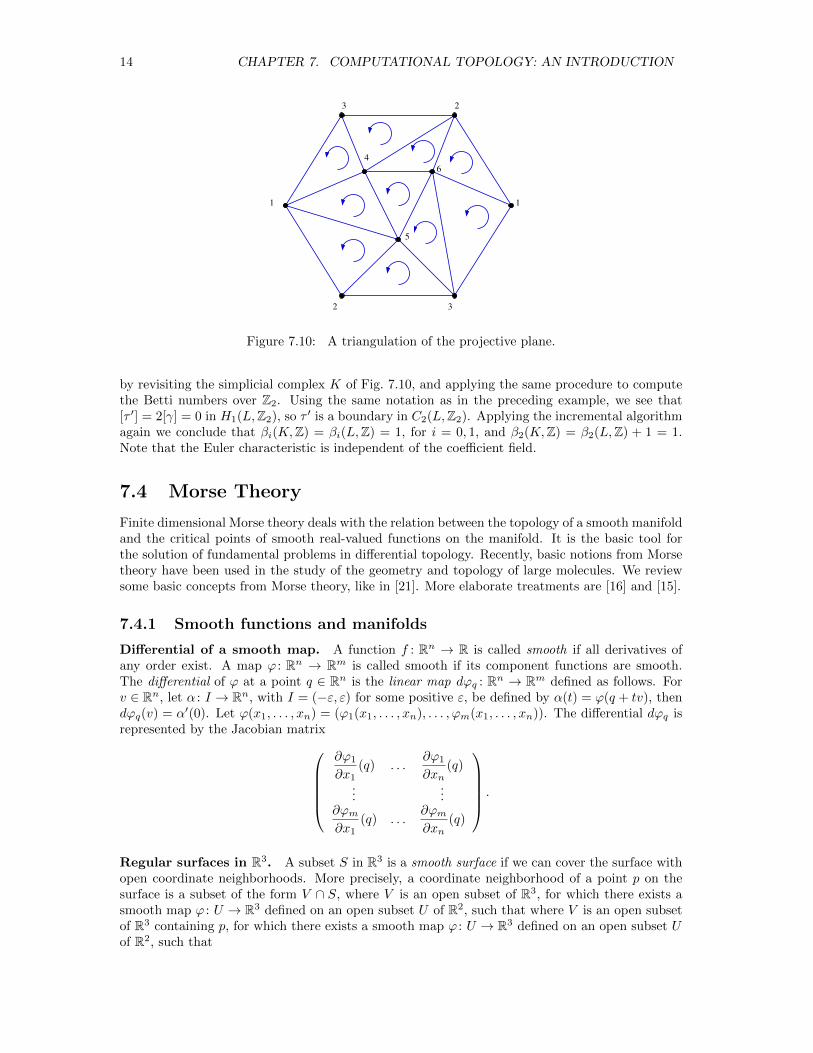
Example: Betti numbers of the projective plane. The incremental algorithm, combinedwith the method of simplicial collapse, allows for rather painless computation of Betti numbersof familiar spaces. In this example we compute the Betti numbers of the projective plane RP2.The simplicial complex K of Fig. 7.10 is the unique triangulation of the projective plane with aminimal number of vertices. The vertices and edges on the boundary of the six-gon are identifiedin pairs, as indicated by the double occurrence of the vertex-labels v1, v2 and v3. The arrowsindicate the orientation of the simplices forming the basis of the chain space C2(K). We orientthe edges of the simplex from the vertex with lower index to the vertex with higher index.

Let L be the simplicial complex obtained from K by deleting the oriented simplex τ = 〈v4v5v6〉.The Betti numbers of L are easy to compute, since a sequence of simplicial collapses transformsL into the subcomplex L0 with vertices v1, v2 and v3, and oriented edges 〈v1v2〉, 〈v2v3〉 and〈v1v3〉. The simplicial complex L0 is a 1-sphere, so β0(L) = β0(L0) = 1, β1(L) = β1(L0) = 1, andβi(L) = βi(L0) = 0 for i > 1.

To relate the Betti numbers of K with those of L, we have to determine whether τ ′ = ∂2τ is aboundary in L. Consider the special 2-chain α, which is the formal sum of all oriented 2-simplicesin L. Taking the boundary of α, we see that all oriented 1-simplices not in ∂2τ occur twice, thosein the interior of the six-gon in Fig. 7.10 with opposite coefficients and those in the boundary withthe same coefficient. In other words, ∂2α = 2γ−∂2τ , where γ is the 1-cycle 〈v1v2〉+〈v2v3〉−〈v1v3〉of L. Therefore, [τ ′] = 2[γ] in H1(L). Since [γ] forms a basis for H1(L), we conclude that [τ ′] 6= 0in H1(L). Hence τ ′ is not a boundary in L. Applying the incremental algorithm we see thatβ0(K) = β0(L) = 1, β1(K) = β1(L)− 1 = 0, and β2(K) = β2(L) = 0.

Example: Betti numbers depend on field of scalars. Homology theory can be set up withcoefficients in a general field. A priory, this leads to different Betti numbers. This is illustrated

14 CHAPTER 7. COMPUTATIONAL TOPOLOGY: AN INTRODUCTION

6

23

1

5

32

4

1

Figure 7.10: A triangulation of the projective plane.

by revisiting the simplicial complex K of Fig. 7.10, and applying the same procedure to computethe Betti numbers over Z2. Using the same notation as in the preceding example, we see that[τ ′] = 2[γ] = 0 in H1(L,Z2), so τ ′ is a boundary in C2(L,Z2). Applying the incremental algorithmagain we conclude that βi(K,Z) = βi(L,Z) = 1, for i = 0, 1, and β2(K,Z) = β2(L,Z) + 1 = 1.Note that the Euler characteristic is independent of the coefficient field.

7.4 Morse Theory

Finite dimensional Morse theory deals with the relation between the topology of a smooth manifoldand the critical points of smooth real-valued functions on the manifold. It is the basic tool forthe solution of fundamental problems in differential topology. Recently, basic notions from Morsetheory have been used in the study of the geometry and topology of large molecules. We reviewsome basic concepts from Morse theory, like in [21]. More elaborate treatments are [16] and [15].

7.4.1 Smooth functions and manifolds

Differential of a smooth map. A function f : Rn → R is called smooth if all derivatives ofany order exist. A map ϕ : Rn → Rm is called smooth if its component functions are smooth.The differential of ϕ at a point q ∈ Rn is the linear map dϕq : Rn → Rm defined as follows. Forv ∈ Rn, let α : I → Rn, with I = (−ε, ε) for some positive ε, be defined by α(t) = ϕ(q + tv), thendϕq(v) = α′(0). Let ϕ(x1, . . . , xn) = (ϕ1(x1, . . . , xn), . . . , ϕm(x1, . . . , xn)). The differential dϕq isrepresented by the Jacobian matrix

∂ϕ1

∂x1(q) . . .

∂ϕ1

∂xn(q)

......

∂ϕm∂x1

(q) . . .∂ϕm∂xn

(q)

.

Regular surfaces in R3. A subset S in R3 is a smooth surface if we can cover the surface withopen coordinate neighborhoods. More precisely, a coordinate neighborhood of a point p on thesurface is a subset of the form V ∩ S, where V is an open subset of R3, for which there exists asmooth map ϕ : U → R3 defined on an open subset U of R2, such that where V is an open subsetof R3 containing p, for which there exists a smooth map ϕ : U → R3 defined on an open subset Uof R2, such that

7.4. MORSE THEORY 15

(i) The map ϕ is a homeomorphism from U onto V ∩ S;

(ii) If ϕ(u, v) = (x(u, v), y(u, v), z(u, v)), then the two tangent vectors∂x

∂u∂y

∂u∂z

∂u

,

∂x

∂v∂y

∂v∂z

∂v

are non-zero and not parallel.

The map ϕ is called a parametrization or a system of local coordinates in p. The set S is a smoothsurface if each point of S has a coordinate neighborhood. Note that condition (ii) is equivalent tothe fact that the differential of ϕ at (u, v) is an injective map.

Example: spherical coordinates. Let S be a 2-sphere in R3 with radius R and center (0, 0, 0) ∈ R3.Consider the set U = { (u, v) | 0 < u < 2π,−π/2 < v < π/2 }. The map ϕ : U → S, given by

ϕ(u, v) = (R cosu cos v,R sinu cos v,R sin v).

corresponds to the well-known spherical coordinates. Note that ϕ(U) is the 2-sphere minus ameridian. Each point of ϕ(U) has a system of local coordinates given by ϕ.

Example: coordinates on the upper and lower hemisphere. Again, let S be the sphere with radiusR and center at the origin of R3, and let U = { (x, y) | x2 + y2 < R2 }. The (open) upper andlower hemispheres of the torus are the graph of a smooth function. More precisely, each point ofthe upper hemisphere has local coordinates given by the map

ϕ(x, y) = (x, y,√R2 − x2 − y2).

A similar expression defines local coordinates at each point of the lower hemisphere. Covering thesphere by six hemispheres yields a system (at least one) of local coordinate system for each pointof the sphere. Therefore, the sphere is a regular surface.

Example: coordinates on the torus of revolution. Let S be the torus obtained by rotating the circlein x, y-plane with center (0, R, 0) and radius r around the x-axis, where R > r. We show that S isa smooth surface by introducing a system of local coordinates for all points of the torus. To thisend, let U = {(u, v) | 0 < u, v < 2π} and let ϕ : U → R3 be the map defined by

ϕ(u, v) = (r sinu, (R− r cosu) sin v, (R− r cosu) cos v).

It is not hard to check that ϕ(U) ⊂ S. In fact, the map ϕ covers the torus except for onemeridian and one parallel circle. It is easy to find local coordinates in points of these two circlesby translating the parameter domain U a little bit. Therefore, the torus is a regular surface.

Example: Local form of torus of revolution near (0, 0,±(R−r)). As in the example of hemispheres,parts of the torus are graphs of a smooth function. In particular, the points (0, 0,±(R− r)) havelocal coordinates of the form ϕ(x, y) = (x, y, f±(x, y)), where

f±(x, y) = ±√R2 + r2 − x2 − y2 − 2R

√r2 − x2.

Submanifolds of Rn. More generally, a subset M of Rn is an m-dimensional smooth subman-ifold of Rn, m ≤ n, if for each p ∈ M , there is an open set V in Rn, containing p, and a mapϕ : U → M ∩ V from an open subset U in Rm onto V ∩M such that (i) ϕ is a smooth homeo-morphism, (ii) the differential dϕq : Rm → Rn is injective for each q ∈ U . Again, the map ϕ iscalled a parametrization or a system of local coordinates on M in p. In particular, the space Rn

16 CHAPTER 7. COMPUTATIONAL TOPOLOGY: AN INTRODUCTION

is a submanifold of Rn. A subset N of a submanifold M of Rn is a submanifold of M if it is asubmanifold of Rn. The difference of the dimensions of M and N is called the codimension of N(in M).

Example: linear subspaces are submanifolds. The Euclidean space Rm is a smooth submanifold ofRn, for m ≤ n. For m < n, we identify Rm with the subset {(x1, . . . , xn) ∈ Rn | xm+1 = · · · =xn = 0} of Rn.

Example: Sn−1 is a smooth submanifold of Rn. A smooth parametrization of Sn−1 at (0, . . . , 0, 1) ∈Sn−1 is given by ϕ : U → Rn, with

U = {(x1, . . . , xn−1) ∈ Rn−1 | x21 + · · ·+ x2n−1 < 1},

and

ϕ(x1, . . . , xn−1) = (x1, . . . , xn−1,√

1− x21 − · · · − x2n−1).

In fact, ϕ is a parametrization in every point of the upper hemisphere, i.e., the intersection ofSn−1 and the upper half space {(y1, . . . , yn) | yn > 0}.

Example: codimension one submanifolds. The equator S1 = {(x1, x2, 0) | x21 + x22 = 1} is acodimension one submanifold of S2 = {(x1, x2, x3) | x21 + x22 + x23 = 1}. More generally, everyintersection of the 2-sphere with a plane at distance less than one from the origin is a codimensionone submanifold.

Tangent space of a manifold. The tangent vectors at a point p of a manifold form a vectorspace, called the tangent space of the manifold at p. More formally, a tangent vector of M at p isthe tangent vector α′(0) of some smooth curve α : I →M through p. Here a smooth curve througha point p on a smooth submanifold M of Rn is a smooth map α : I → Rn, with I = (−ε, ε) forsome positive ε, satisfying α(t) ∈M , for t ∈ I, and α(0) = p. The set TpM of all tangent vectorsof M at p is the tangent space of M at p.

If ϕ : U → M is a smooth parametrization of M at p, with 0 ∈ U and ϕ(0) = p, then TpM isthe m-dimensional subspace dϕ0(Rm) of Rn, which passes through ϕ(0) = p. Let {e1, . . . , em} bethe standard basis of Rm; define the tangent vector ei ∈ TpM by ei = dϕ0(ei). Then {e1, . . . , em}is a basis of TpM .

Example: tangent space of the sphere. The tangent space of the unit sphere Sn−1 = {(x1, . . . , xn) |x21 + · · · + x2n = 1} at a point p is the hyperplane through p, perpendicular to the normal vectorof the sphere at p.

Smooth function on a submanifold. A function f : M → R on an m-dimensional smoothsubmanifold M of Rn is smooth at p ∈M if there is a smooth parametrization ϕ : U →M∩V , withU an open set in Rm and V an open set in Rn containing p, such that the function f ◦ϕ : U → R issmooth. A function on a manifold is called smooth if it is smooth at every point of the manifold.

Example: height function on a surface. The height function h : S → R on a surface S in R3 isdefined by h(x, y, z) = z, for (x, y, z) ∈ S. Let ϕ(u, v) = (x(u, v), y(u, v), z(u, v)) be a system oflocal coordinates in a point of the surface, then h ◦ ϕ(u, v) = z(u, v) is smooth. Therefore, theheight function is a smooth function on S.

Regular and critical points. A point p ∈M is a critical point of a smooth function f : M → Rif there is a local parametrization ϕ : U → Rn of M at p, with ϕ(0) = p, such that 0 is a criticalpoint of f ◦ϕ : U → R (i.e., the differential of f ◦ϕ at q is the zero function on Rn). This conditiondoes not depend on the particular parametrization.A real number c ∈ R is a regular value of f if f(p) 6= c for all critical points p of f , and a criticalvalue otherwise.

Example: critical points of height function on the sphere. Consider the height function on the unitsphere in R3. Spherical coordinates define a parametrization ϕ(u, v) in every point, except for the

7.4. MORSE THEORY 17

poles (0, 0,±1). With respect to this parametrization the height function h has the expressionh(u, v) = h(ϕ(u, v)) = sin v, so none of these points is singular (since −π/2 < v < π/2 away fromthe poles). Near the poles (0, 0,±1) we consider the sphere as the graph of a function, corre-

sponding to the parametrization ψ(x, y) = (x, y,√

1− x2 − y2). The height function is expressed

in these local coordinates as h(x, y) = h(ψ(x, y)) = ±√

1− x2 − y2, so the singular points of hare (0, 0,−1) (minimum), and (0, 0, 1) (maximum).

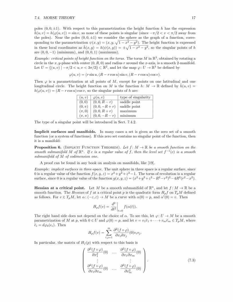
Example: critical points of height function on the torus. The torus M in R3, obtained by rotating acircle in the x, y-plane with center (0, R, 0) and radius r around the x-axis, is a smooth 2-manifold.Let U = {(u, v) | −π/2 < u, v < 3π/2} ⊂ R2, and let the map ϕ : U → R3 be defined by

ϕ(u, v) = (r sinu, (R− r cosu) sin v, (R− r cosu) cos v).

Then ϕ is a parametrization at all points of M , except for points on one latitudinal and onelongitudinal circle. The height function on M is the function h : M → R defined by h(u, v) =h(ϕ(u, v)) = (R− r cosu) cos v, so the singular points of h are:

(u, v) ϕ(u, v) type of singularity(0, 0) (0, 0, R− r) saddle point(0, π) (0, 0,−R+ r) saddle point(π, 0) (0, 0, R+ r) maximum(π, π) (0, 0,−R− r) minimum

The type of a singular point will be introduced in Sect. 7.4.2.

Implicit surfaces and manifolds. In many cases a set is given as the zero set of a smoothfunction (or a system of functions). If this zero set contains no singular point of the function, thenit is a manifold:

Proposition 6. (Implicit Function Theorem). Let f : M → R be a smooth function on thesmooth submanifold M of Rn. If c is a regular value of f , then the level set f−1(c) is a smoothsubmanifold of M of codimension one.

A proof can be found in any book on analysis on manifolds, like [19].

Example: implicit surfaces in three-space. The unit sphere in three space is a regular surface, since0 is a regular value of the function f(x, y, z) = x2 +y2 +z2−1. The torus of revolution is a regularsurface, since 0 is a regular value of the function g(x, y, z) = (x2+y2+z2−R2−r2)2−4R2(r2−x2).

Hessian at a critical point. Let M be a smooth submanifold of Rn, and let f : M → R be asmooth function. The Hessian of f at a critical point p is the quadratic form Hpf on TpM definedas follows. For v ∈ TpM , let α : (−ε, ε)→M be a curve with α(0) = p, and α′(0) = v. Then

Hpf(v) =d2

dt2

∣∣∣∣t=0

f(α(t)).

The right hand side does not depend on the choice of α. To see this, let ϕ : U →M be a smoothparametrization of M at p, with 0 ∈ U and ϕ(0) = p, and let v = v1e1 + · · ·+vmem ∈ TpM , whereei = dϕ0(ei). Then

Hpf(v) =

m∑i,j=1

∂2(f ◦ ϕ)

∂xi∂xj(0)vivj .

In particular, the matrix of Hf (p) with respect to this basis is∂2(f ◦ ϕ)

∂x21(0) . . .

∂2(f ◦ ϕ)

∂x1∂xm(0)

......

∂2(f ◦ ϕ)

∂x1∂xm(0) . . .

∂2(f ◦ ϕ)

∂x2m(0)

. (7.3)

18 CHAPTER 7. COMPUTATIONAL TOPOLOGY: AN INTRODUCTION

It is not hard to check that the numbers of positive and negative eigenvalues of the Hessian donot depend on the choice of ϕ, since p is a critical point of f .

Non-degenerate critical point. The critical point p of f : M → R is non-degenerate if theHessian Hpf is non-degenerate. The index of the non-degenerate critical point p is the number ofnegative eigenvalues of the Hessian at p. If M is 2-dimensional, then a critical point of index 0, 1,or 2, is called a minimum, saddle point, or maximum, respectively.

7.4.2 Basic Results from Morse Theory

Morse function. A smooth function on a manifold is a Morse function if all critical points arenon-degerate. The k-th Morse number of a Morse function f , denoted by µk(f), is the number ofcritical points of f of index k.

Example: quadratic function on Rm. The function f : Rm → R, defined by f(x1, . . . , xm) = −x21−. . .−x2k+x2k+1+ . . .+x2m, is a Morse function, with a single critical point (0, . . . , 0). This point is anon-degenerate critical point, since the Hessian matrix at this point is diag(−2, . . . ,−2, 2, . . . , 2),with k entries on the diagonal equal to −2. In particular, the index of the critical point is k.

Example: singularities of the height function on Sm−1. The height function on the standardunit sphere Sm−1 in Rm is a Morse function. This function is defined by h(x1, . . . , xm) = xmfor (x1, . . . , xm) ∈ Sm−1, With respect to the parametrization ϕ(x1, . . . , xm−1) = (x1, . . . , xm−1,√

1− x21 − · · · − x2m−1), the expression of the height function is

h ◦ ϕ(x1, . . . , xm−1) =√

1− x21 − · · · − x2m−1.

Therefore, the only critical point of h on the upper hemisphere is (0, . . . , 0, 1). The Hessian matrix(7.3) is the diagonal matrix diag(−1,−1, . . . ,−1), so this critical point has index m−1. Similarly,(0, . . . , 0,−1) is the only critical point on the lower hemisphere. It is a critical point of index 0.

Example: singularities of the height function on the torus. The singular points of the heightfunction on the torus of revolution with radii R and r are (0, 0,−R−r), (0, 0,−R+r), (0, 0, R−r),and (0, 0, R + r). See also Sect. 7.4.1. A parametrization of this torus near the singular points

±(R− r) is ϕ(x, y) = (x, y, f±(x, y)), where f±(x, y) = ±√R2 + r2 − x2 − y2 − 2R

√r2 − x2. The

expression h(x, y) = f±(x, y) of the height function with respect to these local coordinates at(x, y) = (0, 0) is

h(x, y) = ±(R− r − 1

2rx2 +

1

2(R− r)y2)

+ Higher Order Terms.

Hence the singular points corresponding to (x, y) = (0, 0), i.e., (0, 0,±(R− r)), are saddle points,i.e., singular points of index one. Similarly, the singular point (0, 0, R + r) is a maximum (indextwo), and the singular point (0, 0,−R− r) is a minimum (index zero), and the

Regular level sets. Let M be an m-dimensional submanifold of Rn, and let f : M → R bea smooth function. The set f−1(h) := {q ∈ M |f(q) = h} of points where f has a fixed valueh is called a level set (at level h). If h ∈ R is a regular value of f , then f−1(h) is a smooth(m− 1)-dimensional submanifold of Rn.Similarly, we define the lower level set (also called excursion set) at some level h ∈ R as Mh ={ q ∈M | f(q) ≤ h }. If f has no critical values in [a, b], for a < b, then the subsets Ma and Mb ofM are homeomorphic (and even isotopic).

The Morse Lemma. Let f : M → R be a smooth function on a smooth m-dimensional sub-manifold M of Rn, and let p be a non-degenerate critical point of index k. Then there is a smooth

7.4. MORSE THEORY 19

parametrization ϕ : U → M of M at p, with U an open neighborhood of 0 ∈ Rm and ϕ(0) = p,such that

f ◦ ϕ(x1, . . . , xm) = f(p)− x21 − · · · − x2k + x2k+1 + · · ·+ x2m.

In particular, a critical point of index 0 is a local minimum of f , whereas a critical point of indexm is a local maximum of f . See Fig. 7.11.

Figure 7.11: Passing a critical level set of a Morse function in three-space. The critical point hasindex 1. A local model of the function near the critical point is f(x1, x2, x3) = −x21 + x22 + x23,with the x1-axis running vertically.

Abundance of Morse functions. (i) Morse functions are generic. Every smooth compactsubmanifold of Rn has a Morse function. (In fact, if we endow the set C∞(M) of smooth functionson M with the so-called Whitney topology, then the set of Morse functions on M is an open anddense subset of C∞(M). In particular, there are Morse functions arbitrarily close to any smoothfunction on M .)(ii) Generic height functions are Morse functions. Let M be an m-dimensional submanifold ofRm+1 (e.g., a smooth surface in R3). For v ∈ Sm, the height-function hv : M → R with respect tothe direction v is defined by hv(p) = 〈v, p〉. The set of v for which hv is not a Morse function hasmeasure zero in Sm.

Passing critical levels. One can build complicated spaces from simple ones by attaching anumber of cells. Let X and Y be topological spaces, such that X ⊂ Y . We say that Y is obtainedby attaching a k-cell to X if Y \X is homeomorphic to an open k-ball. More precisely, there is

a map f : Bk → Y \X, such that f(Sk−1) ⊂ X and the restriction f | Bk is a homeomorphismBk → Y \ X. Let f : M → R be a smooth Morse function with exactly one critical level in(a, b), and a and b are regular values of f . Then Mb is homotopy equivalent to Ma with a cell ofdimension k attached, where k is the index of the critical point in f−1([a, b]). See Fig. 7.12.

Figure 7.12: Passing a critical level of index 1 corresponds to attaching a 1-cell. Here M is the2-torus embedded in R3, in standard vertical position, and f is the height function with respectto the vertical direction. Left: Ma, for a below the critical level of the lower saddle point of f .Middle: Ma with a 1-cell attached to it. Right: Mb, for b above the critical level of the lowersaddle point of f . This set is homotopy equivalent to the set in the middle part of the figure.

20 CHAPTER 7. COMPUTATIONAL TOPOLOGY: AN INTRODUCTION

Morse inequalities. Let f be a Morse function on a compact m-dimensional smooth submani-fold of Rn. For each k, 0 ≤ k ≤ m, the k-th Morse number of f dominates the k-th Betti numberof M :

µk(f) ≥ βk(M,Q).

An intuitive explanation is based on the observation that passing a critical level of a critical point ofindex k is equivalent corresponds to the attachment of a k-cell at the level of homotopy equivalence.Therefore, either the k-th Betti number increases by one, or the k − 1-st Betti number decreasesby one, cf the incremental algorithm for computing Betti numbers in Sect. 7.3, while none of theother Betti numbers changes. Since only the k-th Morse number changes, more precisely, increasesby one, the Morse inequalities are invariant upon passage of a critical level.

In the same spirit one can show that the Morse numbers of f are related to the Betti numbersand the Euler characteristic of M by the following identity:

m∑k=1

(−1)kµk(f) =

m∑k=1

(−1)kβk(M,Q) = χ(M).

Gradient vector fields. Consider a smooth function f : M → R, where M is a smooth m-dimensional submanifold of Rn. The gradient of f is a smooth map grad f : M → Rn, whichassigns to each point p ∈M a vector grad f(p) ∈ TpM ⊂ Rn, such that

〈grad f(p), v〉 = dfp(v), for all v ∈ TpM .

Since dfp(v) is a linear form in v, the vector grad f(p) is well defined by the preceding identity.This definition has a few straightforward implications. The gradient of f vanishes at a point p ifand only if p is a singular point of f . If p is not a singular point of f , then dfp(v) is maximal fora unit vector v ∈ TpM iff v = grad f(p)/‖ grad f(p)‖. In other words, grad f(p) is the direction ofsteepest ascent of f at p. Furthermore, if c ∈ R is a regular value of the function f , then grad fis perpendicular to the level set f−1(c) at every point.

To express grad f in local coordinates, let ϕ : U → M be a system of local coordinates atp ∈M . Let e1, . . . , em be the basis of TpM corresponding to the standard basis e1, . . . , em of Rm.In other words: ei = dϕq(ei), where q ∈ U is the pre-image of p under ϕ. We denote the standardcoordinates on Rm by x1, . . . , xm. Then

grad f(p) =

m∑i=1

ai(q)ei,

where ai : U → R is the smooth function defined by the set of linear equations

m∑j=1

gij(q)aj(q) =∂(f ◦ ϕ)

∂xi(q), (1 ≤ i ≤ m),

with gij(q) = 〈ei, ej〉. Since the coefficients are the entries 〈ei, ej〉 of a Gram matrix, the system

is non-singular. Note that ai =∂(f ◦ ϕ)

∂xiif the system of coordinates is orthonormal at p, that is

gij(q) = 1, if i = j and gij(q) = 0, if i 6= j. This holds in particular if U = M = Rn and ϕ is theidentity map on U , so the definition agrees with the usual definition in a Euclidean space.

Integral lines, and their local structure near singular points. In the sequel M is acompact submanifold of Rn. The gradient of a smooth function f on M is a smooth vector fieldon M . For every point p of M , there is a unique curve x : R → M , such that x(0) = p andx′(t) = grad f(x(t)), for all t ∈ R. The image x(R) is called the integral curve of the gradientvector field through p.

Lemma 1. Let f : M → R be a smooth function on a submanifold M of Rn.

7.4. MORSE THEORY 21

1. The integral curves of a gradient vector field of f form a partition of M .

2. The integral curve x(t) through a singular point p of f is the constant curve x(t) = p.

3. The integral curve x(t) through a regular point p of f is injective, and both limt→∞ x(t) andlimt→−∞ x(t) exist. These limits are singular points of f .

4. The function f is strictly increasing along the integral curve of a regular point of f .

5. Integral curves are perpendicular to regular level sets of f .

The proof is a bit technical, so we skip it. See [10] for details. The first property implies thatthe integral curves through two points of M are disjoint or coincide. The third property impliesthat a gradient vector field does not have closed integral curves. The limit limt→∞ x(t) is calledthe ω-limit of p, and is denoted by ω(p). Similarly, limt→−∞ x(t) is the α-limit of p, denotedby α(p). Note that all points on an integral curve have the same α-limit and the same ω-limit.Therefore, it makes sense to refer to these points as the α-limit and ω-limit of the integral curve.It follows from Lemma 1.2 that ω(p) = p and α(p) = p for a singular point p.

Stable and unstable manifolds. The structure of integral lines of a gradient vector field grad fnear a singular point can be quite complicated. However, for Morse functions, the situation issimple. To gain some intuition, let us consider the simple example of the function f(x1, x2) =x21 − x22 on a neighborhood of the non-degenerate singular point 0 ∈ R2. The gradient vector fieldis 2x1e1 − 2x2e2, where e1, e2 is the standard basis of R2. The integral line (x1(t), x2(t)) througha point p = (p1, p2) is determined by x1(0) = p1, x2(0) = p2, and{

x′1(t) = 2x1(t)

x′2(t) = −2x2(t)

Therefore, the integral curve through p is (x1(t), x2(t)) = (p1e2t, p2e

−2t), which is of the formx1x2 = c. See Fig. 7.13 (Left). The singular point o = (0, 0) is the α-limit of all points on the

p

Figure 7.13: Left: Integral curves of the gradient of f(x1, x2) = x21 − x22 on a neighborhood ofthe singular point (0, 0) ∈ R2. Right: Integral curves of the gradient vector field near a generalsaddle point of a function on R2.

horizontal axis, and the ω-limit of all points on the vertical axis. The general structure of integralcurves near a saddle point is similar, as indicated by Fig. 7.13 (Right). The stable curve of pconsists of all points with ω-limit equal to p. The unstable curve is defined similarly. These curvesintersect each other at p, and are perpendicular there.

More generally, the stable manifold of a singular point p is the set W s(p) = {q ∈M | ω(q) = p}.Similarly, the unstable manifold of p is the set Wu(p) = {q ∈ M | α(q) = p}. Note that bothW s(p) and Wu(p) contain the singular point p itself. Furthermore, the intersection of the stable

22 CHAPTER 7. COMPUTATIONAL TOPOLOGY: AN INTRODUCTION

and unstable manifolds of a singular point consists just of the singular point: W s(p)∩Wu(p) = {p}.Stable and unstable manifolds of gradient systems are submanifolds [12, Chapter 6]. The dimensionof W s(p) is equal to the number of negative eigenvalues of the Hessian of f at p, whereas thedimension of Wu(p) is equal to the number of positive eigenvalues of this Hessian. Stable andunstable manifolds of gradient systems are submanifolds [12, Chapter 6].

The Morse-Smale complex. A Morse function on M is called a Morse-Smale function if itsstable and unstable manifolds intersect transversally, i.e., at a point of intersection the tangentspaces of the stable and unstable manifolds together span the tangent space of M . If p and qare distinct singular points, the intersection W s(p) ∩Wu(q) consists of all regular integral curveswith ω-limit equal to p and α-limit equal to q. In particular, a Morse-Smale function on a two-dimensional manifold has no integral curves connecting two saddle points, since the stable manifoldof one of the saddle points and the unstable manifold of the second saddle point would intersectnon-transversally along this connecting integral curve.

Morse-Smale functions form an open and dense subset of the space of functions on a compactmanifold [18].

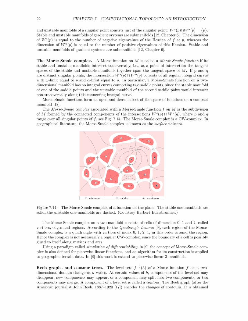
The Morse-Smale complex associated with a Morse-Smale function f on M is the subdivisionof M formed by the connected components of the intersections W s(p) ∩Wu(q), where p and qrange over all singular points of f , see Fig. 7.14. The Morse-Smale complex is a CW-complex. Ingeographical literature, the Morse-Smale complex is known as the surface network.

maximumminimum saddle

Figure 7.14: The Morse-Smale complex of a function on the plane. The stable one-manifolds aresolid, the unstable one-manifolds are dashed. (Courtesy Herbert Edelsbrunner.)

The Morse-Smale complex on a two-manifold consists of cells of dimension 0, 1 and 2, calledvertices, edges and regions. According to the Quadrangle Lemma [9], each region of the Morse-Smale complex is a quadrangle with vertices of index 0, 1, 2, 1, in this order around the region.Hence the complex is not necessarily a regular CW-complex, since the boundary of a cell is possiblyglued to itself along vertices and arcs.

Using a paradigm called simulation of differentiability, in [9] the concept of Morse-Smale com-plex is also defined for piecewise linear functions, and an algorithm for its construction is appliedto geographic terrain data. In [8] this work is extend to piecewise linear 3-manifolds.

Reeb graphs and contour trees. The level sets f−1(h) of a Morse function f on a two-dimensional domain change as h varies. At certain values of h, components of the level set maydisappear, new components may appear, or a component may split into two components, or twocomponents may merge. A component of a level set is called a contour. The Reeb graph (after theAmerican journalist John Reeb, 1887–1920 [17]) encodes the changes of contours. It is obtained

7.4. MORSE THEORY 23

200 200

300

300

400

300

400

500 500

600

600

h

200

300

400

500

600

AB

C

D

E

F G

H

I

J

L KM

NOx

y

A

B

C

D

E

F

G

H

I

J

L

K

MN

O

(a) (b)

300

400400400400

400

hA

B

C

D

E

F G

H

I

J

L KM

NO

(c)

hA

B

C

D

E

F G

H

I

J

LKM

NO

(d)

Figure 7.15: (a) a contour map of level sets (isolines), (b) the corresponding contour tree, (c) thejoin tree, and (d) the split tree. As in Fig. 7.14, minima and maxima are indicated by empty andfull circles, and crosses denote saddle points. The points where a contour touches the boundaryplay also a role in the contour tree (for example, they may be local minima or maxima) but theyare not critical points in the sense of having derivative 0. The level sets in (a) are labeled with theheight values, and these values are indicated in the trees of (b), (c), and (d). The critical point Fchanges only the topology of a contour and not the number of contours; when the contour tree isviewed as a discrete structure, F is not a vertex of the tree.

by contracting every contour to a single point. When f is defined on a simply connected domain(for example, a box), the Reeb graph is a tree, and it is also referred to as the contour tree.Fig. 7.15b shows an example of a contour tree of a bivariate function h = f(x, y) defined on asquare domain. The vertical axis of the contour tree represents the value h of the function. Theintersection of a horizontal line at a given value h with the contour tree yields all contours at thatlevel, and the merging or splitting, appearance or disappearance of contours is reflected in verticesof degree 3 and 1 in the contour tree, respectively. Saddle points become vertices of degree 3,and minima and maxima become vertices of degree 1. A contour tree is therefore a good tool tovisualize the behavior of a function on a global scale, in particular when it is a function of morethan two variables, see [14, 13]. In these applications, f is usually a continuous piecewise linearfunction interpolating data at given sample points. These functions are not smooth and thereforenot Morse functions, but the notion of level sets and Reeb graphs extends without difficulty tothis class of functions. It is not uncommon to have multiple saddle points, where more than twocontours meet at the same time. The Reeb graph has then vertices of degree higher than three.More examples of contour trees are shown in Fig. 5.23 of Sect. 5.5.2.

Note that the Reeb graph only regards the number of components (the 0-homology) of the levelsets, it does not reflect every change of topology. For example, in three dimensions, a contourmight start as a ball, and as h increases, it might extrude two arms that meet each other, forminga torus, without changing the connectivity between contours. (At this point, we have a saddle ofindex 1.) In two dimensions, this phenomenon happens only for points on the boundary of thedomain, such as the point F in Fig. 7.15.

Figure 7.15c displays the join tree, which is defined analogously to the contour tree, exceptthat it describes the evolution of the lower level sets Mh = f−1([−∞, h]) instead of the “ordinary”

24 CHAPTER 7. COMPUTATIONAL TOPOLOGY: AN INTRODUCTION

200 200

300

300

400

300

400

500 500

600

600

200

300

400

500

600

x

y

A

B

C

D

E

F

G

H

I

J

L

K

MN

O

(a) (b)

300

400400400400

400

hA

B

C

D

E

F G

H

I

J

L KM

NO

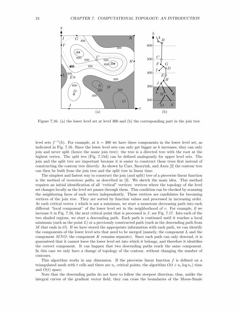
Figure 7.16: (a) the lower level set at level 300 and (b) the corresponding part in the join tree

level sets f−1(h). For example, at h = 300 we have three components in the lower level set, asindicated in Fig. 7.16. Since the lower level sets can only get bigger as h increases, they can onlyjoin and never split (hence the name join tree): the tree is a directed tree with the root at thehighest vertex. The split tree (Fig. 7.15d) can be defined analogously for upper level sets. Thejoin and the split tree are important because it is easier to construct these trees first instead ofconstructing the contour tree directly. As shown by Carr, Snoeyink, and Axen [2] the contour treecan then be built from the join tree and the split tree in linear time.

The simplest and fastest way to construct the join (and split) tree of a piecewise linear functionis the method of monotone paths, as described in [3]. We sketch the main idea. This methodrequires an initial identification of all “critical” vertices: vertices where the topology of the levelset changes locally as the level set passes through them. This condition can be checked by scanningthe neighboring faces of each vertex independently. These vertices are candidates for becomingvertices of the join tree. They are sorted by function values and processed in increasing order.At each critical vertex v which is not a minimum, we start a monotone decreasing path into eachdifferent “local component” of the lower level set in the neighborhood of v. For example, if weincrease h in Fig. 7.16, the next critical point that is processed is J , see Fig. 7.17. Into each of thetwo shaded regions, we start a descending path. Each path is continued until it reaches a localminimum (such as the point L) or a previously constructed path (such as the descending path fromM that ends in O). If we have stored the appropriate information with each path, we can identifythe components of the lower level sets that need to be merged (namely, the component L and thecomponent MNO; the component K remains separate). Since each path can only descend, it isguaranteed that it cannot leave the lower level set into which it belongs, and therefore it identifiesthe correct component. It can happen that two descending paths reach the same component.In this case we only have a change of topology of the contour, without changing the number ofcontours.

This algorithm works in any dimension. If the piecewise linear function f is defined on atriangulated mesh with t cells and there are nc critical points, the algorithm O(t+nc log nc) timeand O(t) space.

Note that the descending paths do not have to follow the steepest direction; thus, unlike theintegral curves of the gradient vector field, they can cross the boundaries of the Morse-Smale

7.5. EXERCISES 25

200 200

300

300

400

300

400

500 500

600

600

200

300

400

500

600

x

y

A

B

C

D

E

F

G

H

I

J

L

K

MN

O

(a) (b)

300

400400400400

400

hA

B

C

D

E

F G

H

I

J

L KM

NO

Figure 7.17: Identifying the components that are to be merged by growing descending paths

complex.With few exeptions [4], the efficient computation of Reeb graphs has been studied mostly for

functions on simply connected domains, and hence under the heading of contour trees.

7.5 Exercises

Exercise 1 (Triangulations of surfaces). Prove that the number of vertices in a finite triangulationof a boundaryless surface with Euler characteristic χ is at least⌈

7 +√

49− 24χ

2

⌉.

(You should be able to do this exercise without any knowledge of homology theory.)

Exercise 2 (Non-homeomorphic spaces with equal Betti numbers). Give an example of twosimplicial complexes with equal Betti numbers, but with non-homeomorphic underlying spaces.

Exercise 3 (Homology of connected graphs). Let G be a tree. Prove that β0(G,Q) = 1 andβ1(G,Q) = 0 using the matrix of the boundary map. (Hint: Consider an enumeration of thevertices and oriented edges such that edge ei is directed from vertex vj to vertex vi, with j > i.)

Exercise 4 (Chain maps and chain homotopy). Prove Propositions 2, 3 and 4.

Exercise 5 (Cone construction and Betti numbers of spheres). Let L be a finite simplicial complexin Rn, and regard Rn as the subspace of Rn+1 with final coordinate zero. Let v be a point inRn+1 \Rn. If σ is a k-simplex of L with vertices v0, . . . , vk, then the (k+ 1)-simplex with verticesv, v0, . . . , vk is called the join of σ and v. The cone of L with apex v is the simplicial complexconsisting of the simplices of L, the join of each of these simplices and v, and the 0-simplex 〈v〉itself. (One can check that these simplices form a simplicial complex.) Let K be the cone of L.

1. Let the map Tk : Ck(K,Q) → Ck+1(K,Q) be defined as follows: Let σ = 〈v0, . . . , vk〉 bea k-simplex of K. If σ is also a k-simplex of L, then Tk(σ) = 〈v, v0, . . . , vk〉, otherwiseTk(σ) = 0. Prove that the sequence {Tk} is a chain homotopy between the identity map andthe zero map on the chain complex C(K,Q).

26 CHAPTER 7. COMPUTATIONAL TOPOLOGY: AN INTRODUCTION

2. Conclude that Hk(K,Q) = 0, for k > 0. What is H0(K,Q)?

3. Determine the Betti numbers of the d-dimensional disk, i.e., the space Bd = {(x1, . . . , xd) ∈Rd | x21 + · · ·+ x2d ≤ 1}. (Hint: Note that a disk is homeomorphic to a d-simplex.)

4. Use the previous result, and the incremental homology algorithm to determine the Bettinumbers of the d-sphere.

Exercise 6 (Homology of orientable surfaces). 1. Prove that β0(K) = 1 for every triangula-tion K of an orientable surface of genus g (a sphere with g handles).

2. Let K be a simplicial complex whose underlying space is the torus, and let all simplices of Kbe oriented compatibly. Let α =

∑σ σ, where the sum ranges over all (oriented) simplices

of K. Prove that Z2(K,Q) = Qα, and that β2(K,Q) = 1.

3. Use the same technique as in part 2 of this exercise to prove that β2(K,Q) = 1 for everytriangulation K of an orientable surface of genus g.

4. Let L be the subcomplex of K obtained by deleting an arbitrary 2-simplex. Use the in-cremental algorithm to prove that β2(L,Q) = β2(K,Q) − 1, and βi(L,Q) = βi(K,Q), fori = 0, 1.

5. Now let K be the simplicial complex of Fig. 7.8. Prove that L simplicially collapses onto thesubcomplex M , the subgraph of L consisting of the vertices v1, . . . , v5 and the edges v1v2,v2v3, v3v1, v1v4, v4v5, and v5v1. Conclude that β1(K,Q) = 2, and β0(K,Q) = 1.

6. Try to generalize this exercise to an orientable surface of genus g.

Exercise 7 (Morse Theory yields Betti numbers). 1. Use Morse theory to compute the Bettinumbers of the d-sphere Sd.

2. Compute the Euler characteristic of a surface M with g handles by defining a suitable Morsefunction on it. Then compute the Betti numbers of this surface. (Hint: You may want touse the first and third result of Exercise 6).

3. For a Morse function f , let s be a critical point with Morse index i. Consider the intersectionL−(s) of the lower level set f−1((−∞, f(s)]) with a small sphere around s. Prove that theEuler characteristic of L−(s) equals 1− (−1)i.

Exercise 8 (The mountaineer’s equation). For a smooth Morse function on the 2-sphere S2, thenumber of peaks and pits (maxima and minima) exceeds the number of passes (saddles) by 2.

Exercise 9 (Contour trees for bivariate Morse functions). Show that, for a smooth Morse functionon the 2-sphere S2, a saddle point will always generate a vertex of degree three in the Reeb graph.Use this observation and the previous exercise to prove that the Reeb graph is in fact a tree inthis case.

Bibliography

[1] M. Armstrong. Basic Topology. Undergraduate Texts in Mathematics. Springer-Verlag, NewYork, Berlin, Heidelberg, 1983. [2]

[2] H. Carr, J. Snoeyink, and U. Axen. Computing contour trees in all dimensions. ComputationalGeometry, 24:75–94, 2003. [24]

[3] Y.-J. Chiang, T. Lenz, X. Lu, and G. Rote. Simple and optimal output-sensitive constructionof contour trees using monotone paths. Computational Geometry, Theory and Applications,30:165–195, 2005. [24]

[4] K. Cole-McLaughlin, H. Edelsbrunner, J. Harer, V. Natarajan, and V. Pascucci. Loops inReeb graphs of 2-manifolds. Discrete Comput. Geom., 32(2):231–244, 2004. [25]

[5] C. J. A. Delfinado and H. Edelsbrunner. An incremental algorithm for Betti numbers ofsimplicial complexes on the 3-sphere. Comput. Aided Geom. Des., 12(7):771–784, 1995. [11]

[6] T. K. Dey, H. Edelsbrunner, and S. Guha. Computational topology. In B. Chazelle, J. E.Goodman, and R. Pollack, editors, Advances in Discrete and Computational Geometry - Proc.1996 AMS-IMS-SIAM Joint Summer Research Conf. Discrete and Computational Geometry:Ten Years Later, number 223 in Contemporary Mathematics, pages 109–143. American Math-ematical Society, 1999. [1]

[7] H. Edelsbrunner. Biological applications of computational topology. In J. Goodman andJ. O’Rourke, editors, CRC Handbook of Discrete and Computational Geometry, chapter 63,pages 1395–1412. Chapman & Hall/CRC, 2004. [1]

[8] H. Edelsbrunner, J. Harer, V. Natarajan, and V. Pascucci. Morse-Smale complexes for piece-wise linear 3-manifolds. In Proc. 19th Ann. Sympos. Comput. Geom., pages 361–370, 2003.[22]

[9] H. Edelsbrunner, J. Harer, and A. Zomorodian. Hierarchical Morse-Smale complexes forpiecewise linear 2-manifolds. Discrete Comput. Geom., 30(1):87–107, 2003. [22]

[10] V. Guillemin and A. Pollack. Differential Topology. Prentice Hall, Englewood Cliffs, NJ,1974. [21]

[11] A. Hatcher. Algebraic Topology. Cambridge University Press, 2002. [6]

[12] J. Jost. Riemannian Geometry and Geometric Analysis. Universitext. Springer-Verlag, 2002.[22]

[13] L. Kettner, J. Rossignac, and J. Snoeyink. The Safari interface for visualizing time-dependentvolume data using iso-surfaces and contour spectra. Computational Geometry: Theory andApplications, 25:97–116, 2003. [23]

[14] L. Kettner and J. Snoeyink. A prototype system for visualizing time-dependent volume data.In Proc. 17th Ann. Symp. Computational Geometry, pages 327–328. ACM Press, 2001. [23]

[15] Y. Matsumoto. An Introduction to Morse Theory, volume 208 of Translations of MathematicalMonographs. American Mathematical Society, 2002. [14]

[16] J. W. Milnor. Morse Theory. Princeton University Press, Princeton, NJ, 1963. [14]

[17] G. Reeb. Sur les points singuliers d’une forme de Pfaff completement integrable ou d’unefonction numerique. Comptes Rendus Acad. Sciences Paris, 222:847–849, 1946. [22]

27

28 BIBLIOGRAPHY

[18] S. Smale. On gradient dynamical systems. Ann. of Math., 74:199–206, 1961. [22]

[19] M. Spivak. Analysis on Manifolds. Perseus Book Publishing, 1965. [17]

[20] J. Stillwell. Classical Topology and Combinatorial Group Theory. Springer-Verlag, New York,1993. [4]

[21] G. Vegter. Computational topology. In J. Goodman and J. O’Rourke, editors, CRC Handbookof Discrete and Computational Geometry, chapter 32, pages 719–742. Chapman & Hall/CRC,2004. [1, 14]

[22] A. Zomorodian. Topology for Computing, volume 16 of Cambridge Monographs on Appliedand Computational Mathematics. Cambridge University Press, 2005. [1]

IndexBetti numbers, 7

dependence on coefficient field, 13incremental computation, 10of a tree, 7of the 2-sphere, 8of the projective plane, 13of the torus, 9topological invariance, 10

boundary operator, 6

chain homotopy, 12chain map, 12codimension, 16collapse, 12

elementary, 12simplicial, 12

complexsimplicial, 3

contour, 22contour tree, 23contractible, 5critical point, 16

maximum, 18minimum, 18non-degenerate, 18saddle, 18

critical value, 16

differential, 14

Euler characteristic, 4excursion set, see lower level set

gradient vector field, 20

height function, 16Hessian, 17homeomorphism, 2homologous, 6homology, 5homology vector space, 6homotopy, 4homotopy equivalence, 5

Implicit Function Theorem, 17index

Morse index, 18isotopy, 4

join tree, 23

level set, 18

lower level set, 18lower level set, 18

map (continuous function), 2maximum, 18minimum, 18Morse function, 18

genericity, 19Morse inequalities, 20Morse Lemma, 18Morse number, 18Morse theory, 14Morse-Smale complex, 22Morse-Smale function, 22

oriented simplex, 3

Reeb graph, 22regular value, 16

saddle point, 18simplex, 2

d-dimensional, 2oriented, 3

simplicial k-chain, 6simplicial k-cycle, 6simplicial collapse, 12simplicial complex, 3simplicial homology, 5simply connected, 4smooth surface, 14split tree, 24stable manifold, 21subcomplex, 4submanifold, 15surface

smooth, 14surface network, 22

tangent space, 16tangent vector, 16topological space, 2triangulation, 4

unstable manifold, 21

29