Earnings Management and Annual Report Readability · Earnings Management and Annual Report ... Earnings management and annual report readability ... we may soon be looking to the

Earnings Management and Annual Report Readability

Presented by

Dr Rafael Rogo

Assistant Professor The University of British Columbia

#2015/16-09

The views and opinions expressed in this working paper are those of the author(s) and not necessarily those of the School of Accountancy, Singapore Management University.

1

Earnings management and annual report readability

Kin Lo*

Sauder School of Business

The University of British Columbia

Vancouver, BC, Canada

Felipe Ramos

FUCAPE Business School

Vitoria, ES, Brazil

and

Rafael Rogo

Sauder School of Business

The University of British Columbia

Vancouver, BC, Canada

September 2015

Abstract

We explore how the readability of annual reports varies with earnings management. Using the

Fog Index to measure readability (Li 2008), and focusing on the management discussion and

analysis section of the annual report (MD&A), we predict and find that firms that are most likely

to have managed earnings to beat the prior year’s earnings have MD&As that are more difficult

to read. In addition, we find that readability has marginal but incremental power in predicting

financial misstatements when added to the F-Score model of Dechow et al. (2011)

Key Words: Annual report readability, profitability, earnings management

JEL Classification: D82; G14; G18; M41; M45

We appreciate the helpful comments from our colleagues at UBC, participants of the UBCOW

conference, 2015 Conference on Convergence of Financial and Managerial Accounting

Research, and ANPCONT 2014. Funding was provided in part by the Institute of Chartered

Accountants of BC and the Social Sciences and Humanities Research Council.

* Contact author: Ph. 604-822-8430; Email: [email protected]; Mail: 2053 Main Mall,

Vancouver, BC, Canada, V6T 1Z2

2

1. INTRODUCTION

The seminal work of Li (2008) explored the relationship between the readability of annual

reports and financial performance. Borrowing the Fog Index from computation linguistics, where

a higher reading on the Fog Index indicates disclosures that are more difficult to understand, Li

finds a negative relationship between Fog and the level of earnings. It is unclear whether this

result is due to managers providing complex disclosures to obfuscate bad performance or that

bad news is simply harder to be communicated (Li, 2008; Bloomfield, 2008). To further explore

these two explanations, obfuscation or ontology, and to better understand managers’ use of

complex disclosures, we look at instances in which firms are more likely to have managed

earnings upwards to meet or beat an earnings benchmark (Burgstahler and Dichev, 1997). When

financial performance is achieved partly by earnings management, we expect the explanations

management provides for that performance will be less readable than explanations provided by

firms not engaging in earnings management. In other words, we expect that when reported

performance differs from underlying fundamentals, we expect managers to try to make it harder

for investors to identify such earnings management behavior, in line with the “Incomplete

Revelation Hypothesis” (Bloomfield, 2002). Our results suggest that the readability level of

financial disclosures goes beyond the one derived from the ontological explanation of good vs.

bad news being disclosed. Instead, we find that managers strategically use corporate disclosure

to mislead or to influence investors’ understanding of firm’s value.

Our study is motivated by the large number of papers that build on results from Li

(2008), but rely mostly on the Obfuscation Hypothesis when developing their predictions, and

disregard Li’s cautionary statement and Bloomfield (2008) discussion that there are alternative

explanations to Li’s empirical findings, and their call for more research required to distinguish

between Obfuscation and Ontology.

3

Our paper is also motivated by the importance and richness of the textual component of

corporate reports—an average of 80% of an annual report, for instance. The SEC highlighted the

importance of textual disclosures when it issued a set of rules requiring plain English disclosures.

Christopher Cox, Chairman of the SEC, went further and suggested “just as the Black-Scholes

model is commonplace when it comes to compliance with the stock option compensation rules,

we may soon be looking to the Gunning-Fog and Flesch-Kincaid models to judge the level of

compliance with the plain English rules.” If readability is going to be used as a measure of

compliance, then we should understand the factors that affect how managers choose the level of

readability.

Our analysis focuses on the readability of the management discussion and analysis

(MD&A) section of the annual report—a section that is required by law but also a medium where

managers have discretion on how to present an explanation of the company’s business, financial

conditions, and results of operation. The MD&A is one the most read and most important

components of financial statements, and the argument that it has information content is supported

by prior literature (Li [2010] for a review of the literature). The fixed structure, content and

periodicity in MD&As trade off with the flexibility and spontaneity in alternative settings, such

as conference calls. Although conference calls may provide researchers with more room to

identify management behavior, managers may have more discretion over the content, and

therefore, more chances to avoid sensitive issues. Bloomfield (2012) argues that “[t]he structure

of conference calls might also reduce [predictive] power,” in line with findings in Mayew

(2008). Mayew shows that managers are more likely to grant permission to ask questions to

analysts that are more favorable. By doing so, managers limit “the direct questions that would be

most likely to elicit direct deception and associated linguistic behavior.”

4

The earnings benchmark we use is the prior year’s earnings (rather than earnings

forecasts or zero earnings) because anecdotal evidence suggests that management’s discussions

in the annual report are more likely to compare and contrast performance in the current fiscal

year with that in the prior year (or years). Forecasted earnings, whether by sell-side analysts or

by management, are seldom referenced in annual reports. Zero and small positive earnings

events are relatively infrequent, so we reserve this benchmark for supplemental analyses.

Our setting allows us to consider all three conditions leading to earnings manipulation, as

presented by Turner, Mock, and Srivastava [2003]; namely, there are three conditions generally

identified when fraud occurs: Incentive/Pressure, Opportunity, and Attitude/Rationalizations. Li

(2012) highlights the importance of not relying solely on the Attitude/Rationalizations condition.

In order to increase the power of our tests, we combine the role of textual analysis with

variations in incentives and opportunities. In particular, we explore management’s incentives to

engage in myopic behavior to beat benchmarks. Bhojra, Hribar, Picconi, and McInnis (2009)

find that firms that just meet earnings expectations likely to be due to earnings management via

accruals and/or real activities exhibit a short-term stock price benefit relative to firms that miss

earnings expectations with no earnings management. To leave room for management’s

opportunities, we focus on management’s use of discretion over accruals and expenses to meet

earnings expectations.

Our findings on the attitude/rationalizations are consistent with our hypotheses.

Controlling for the relationship between Fog and the overall earnings level as well as other

known factors, we find robust evidence that Fog is higher for firms that meet or just beat prior

year’s earnings (MBE). We further identify firms in the MBE sample that are more likely to have

managed earnings upwards using accruals or real activities, and find consistently higher Fog for

5

this subgroup but not for other MBE firms. In two further tests, we use firm-years with earnings

that were misstated or required subsequent restatement as clear indicators of earnings

management. In these smaller samples, we find that Fog is higher for firm-years with restated or

misstated earnings.

In addition to exploring whether firms that manage earnings have less readable financial

reports, we turn the analysis on its head and test whether readability predicts financial

misstatements along the lines of Dechow et al. (2011). We find that the Fog Index is a marginal

but statistically significant predictor when added to the F-score model of Dechow et al.

Our contribution to the literature is two-fold. First, we add to our understanding of the

determinants of readability. More specifically, we refine the overall relationship between

readability and financial performance. While the overall pattern documented by Li (2008) is one

where higher earnings associates with lower Fog, we provide evidence that this relationship is

discontinuous (or at least non-monotonic) around the benchmark of the prior year’s earnings,

particularly for firms that are likely to have managed accruals. Second, we show that earnings

management, that is, using accounting discretion with the aim of concealing underlying

performance, manifests itself as more complex disclosures. Our evidence is consistent with

managers strategically choosing higher reporting complexity in conjunction with earnings

management in an attempt to conceal the latter, which is a new finding in the literature. Overall,

we add to a more complete understanding of the relationship between financial report readability

and reported performance.

Aside from Li (2008), this paper is also closely related to Larcker and Zakolyukina

(2012, “LZ”). However, LZ and this paper differ in a number of important ways. First, LZ’s

primary interest is finding linguistic predictors for financial restatements (i.e., restatements are

6

the dependent variable) whereas this paper’s primary interest is in understanding the

determinants of readability (i.e., the Fog score is the dependent variable). Second, whereas LZ

examine voluntary conference calls, we examine MD&A disclosures that are required by law.

Third, LZ analyze verbal communication but we examine textual disclosures, which result in

differing levels of preparation, forethought, and spontaneity. This last difference is important

because our hypothesis is based upon management’s deliberate attempt to obscure the financial

picture to hide earnings management, whereas LZ’s hypothesized effect derives in large part

from inadvertent signals conveyed (e.g., use of different pronouns, hesitations, expression of

anxiety). In sum, this paper differs from LZ in research question, whether the disclosure is

mandatory, as well as the degree of preparation possible for the different avenues of disclosure.

The remainder of this paper is organized as follows. The next section describes our

hypotheses. Sections 3 and 4 contain our analyses of the first and second hypotheses,

respectively. Section 4 concludes.

2. HYPOTHESIS DEVELOPMENT

In computational linguistics, the Gunning Fog Index, or just Fog Index, is a function of the

number of words per sentence plus the percentage of words that are complex (i.e., having three

or more syllables). This sum is scaled by a constant (0.4) such that the Fog value approximates

the number of years of formal education required to understand the text.

The Fog Index was first brought into the accounting literature by Li (2008), who

examined how readability of annual reports varies with financial performance. Li found a

negative relationship between profitability and Fog (i.e., profitable firms have less complex

reports compared with firms with losses). He also found that firms with more persistent positive

earnings have lower Fog.

7

In the discussion of Li (2008), Bloomfield (2008) provides a number of potential

explanations for the observed relationships between readability and financial performance. Two

are particularly salient here. First is obfuscation—that managers try to hide bad news by writing

text that is more difficult to decipher. Second is ontology—that bad news is inherently more

difficult to communicate.

Bloomfield provides two other potential explanations that could also be considered

variation of ontology. He suggests that loss firms need to provide more explanation as a result of

“management by exception.” He also suggests that the nature of accounting conservatism—

recognizing bad news in a more timely fashion than good news—requires managers to provide

more explanation about the future when there are losses. In sum, obfuscation requires conscious

actions to affect readability, whereas the ontological explanations suggest that readability is

inherently a function of the circumstances. As will be seen below, our analyses will have bearing

on these two explanations.

With regard to financial performance, there is a substantial literature documenting the

frequency, motivations, and benefits that accrue to firms that are able to meet or beat

benchmarks. In recent decades, some two-third to three-quarters of firms will meet or beat

expectations in the capital market (as proxied by analyst forecasts). The rewards of doing so are

higher stock returns, lower information asymmetry, and lower cost of capital (Bartov et al., 2002;

Brown et al., 2009). These firm-level effects translate into personal benefits via executive

compensation directly through higher stock and option value, or indirectly through discretionary

bonuses.

The incentives for management to meet or beat earnings benchmarks also lead some

managers to use their accounting discretion to achieve their performance. For instance,

8

Burghstahler and Dichev (1997) document unusually low (high) frequencies of firms reporting

small earnings decreases (increases) and small losses (profits), suggesting that earnings

management is the source of these irregular distributions of earnings outcomes.

Depending on the context, some benchmarks will be more salient than others. In the

capital market context, the expectations in the market is the most relevant—meeting or falling

short of the market’s expectations is what determines changes in stock prices. In other instances,

zero earnings is the relevant benchmark—maintaining a positive level of earnings is important

for reasons of contractual provisions and general loss aversion, for examples. A third benchmark

is the prior year’s performance, which is equivalent to a benchmark of zero change in earnings.

We focus on the third benchmark for two reasons. First, our analysis of readability

focuses on annual reports, and the MD&A section in particular. MD&A is a disclosure required

by the Securities and Exchange Commission (SEC).1 As a regulated disclosure, it is reasonable

to expect management to discuss facts and figures that are already contained in the audited

financial statements and elsewhere in the annual report rather than information from the capital

markets, such as analyst forecasts, which can change frequently. Second, the requirement to

comment on trends suggests that management would rather have a zero or positive earnings

change rather than having to explain a decline in earnings, which could arguably be interpreted

as the beginning of a downward trend. Third, we focus on the zero earnings change benchmark

rather than the zero earnings benchmark to obtain more time-series variation in meeting/beating

vs. missing the benchmark. That is, there are some firms that are persistently profitable while

others are persistently not; the number of firms at or close to zero profitability is relatively small.

(Nevertheless, we provide some supplementary tests of this alternative benchmark to augment

1 SEC Regulation S-K, Item 303 specifies the MD&A requirement. Among other things, it requires registrants to

discuss financial condition, results of operation, and “currently known trends, events, and uncertainties …”

(Securities Act Release No. 6835, May 18, 1989).

9

our main analyses.)

While the relationship between Fog and earnings levels documented by Li (2008) is

negative overall, we expect that firms at or just above the zero earnings change benchmark will

tend to show a different relationship. First, if at least some of the firms in this region of earnings

performance are able to do so via upward earnings management, then the underlying

performance that they would have otherwise reported would have been lower, which would have

a commensurately higher Fog. That is, all else equal, the readability for the underlying

performance is lower than for the reported performance. We expect this first effect to be small

because our analysis focuses on a small range of earnings (i.e., earnings changes close to zero).

Earnings management involves degrees of untruth. Within the accounting discretion

available, management makes biased choices to increase earnings. In some cases, the earnings

management falls outside acceptable levels and is considered (fraudulent) misrepresentation. In

either case, management must try to hide the deception so as not to be discovered; i.e., earnings

management cannot be transparent for management to believe that it would have the intended

effect. Deceptive communication is linguistically more complex and also cognitively more

demanding.2 Because it is difficult to be untruthful, liars will tend to tell simpler stories, which

can counteract the tendency of lies to be linguistically more complex. Which of these two forces

dominates is an empirical question.

Based on the above discussion, our first hypothesis is as follows (stated in alternative

form):

H1: Firms that have managed earnings in a particular year have annual report

disclosures in that year that are less readable, ceteris paribus.

2 “… from a cognitive perspective, truth tellers should be able to discuss exactly what did and did not happen

because they were actually there to witness the event being discussed. Liars, on the other hand, would be forced to

keep track of what they have previously said to avoid contradicting themselves later” (Hancock et al., 2007).

10

Beyond this general hypothesis, we have three subsidiary hypotheses with increasing specificity:

H1A: Firm-years with zero or slightly positive earnings changes will have annual

report disclosures that are less readable, ceteris paribus.

H1B: Firm-years with (i) zero or slightly positive earnings changes and (ii)

income-increasing discretionary accruals or real activities earnings management

will have annual report disclosures that are less readable, ceteris paribus.

H1C: Firm-years with (i) zero or slightly positive earnings changes and (ii) high

income increasing discretionary accruals or real activities earnings management

will have annual report disclosures that are less readable, ceteris paribus.

These three predictions relate to firm-years that we suspect of containing managed earnings.

However, these classification schemes use purely quantitative data and there is likely a certain

amount of misidentification (Dechow et al. 1995). Therefore, we use the superior accuracy of

human investigators to identify instances of earnings management. Therefore, we also make two

additional predictions using restatements and misstatements.

H1D: Firm-years with financial information that was subsequently restated will

have annual report disclosures that are less readable, ceteris paribus.

H1E: Firm-years with misstatements will have annual report disclosures that are

less readable, ceteris paribus.

Restatements are adjustments to financial statements as tracked by Audit Analytics; we do not

examine all restatements, but only those identified by Audit Analytics as relating to fraud or SEC

investigations. Misstatements are those reported in Accounting and Auditing Enforcement

Releases (AAER), which may or may not subsequently result in restatements. Using restatements

and misstatements is more accurate in identifying instances of earnings management, but also

potentially misses some earnings management activity that has not been the subject of regulatory

action. In this regard, this identification strategy is complementary to the earlier strategy using

small positive earnings changes, which likely classifies too many firms as having managed

earnings.

11

Although not the main focus of this study, our second hypothesis further explores the

idea that deception results in more complex writing. Dechow et al. (2011) used the sample of

firms reporting misstatements in AAER published by the SEC to estimate a model that produced

a likelihood of financial misstatement (“F-Score”). Along with this model, we hypothesize that

writing complexity can be used as a factor to help identify firms misstating financial statements.

Our second hypothesis is as follows:

H2: Firms with less readable financial reports are more likely to have misstated

financial statements.

In the next two sections, we describe our empirical analyses and results of testing these

two hypotheses.

3. TEST OF HYPOTHESIS 1

To test the first hypotheses, we use a sample of firm-years with available data between 2000 and

2012. We require financial data from Computat as well as MD&A disclosures on the SEC’s

Edgar system. Details of required financial data items will be provided below. We exclude firms

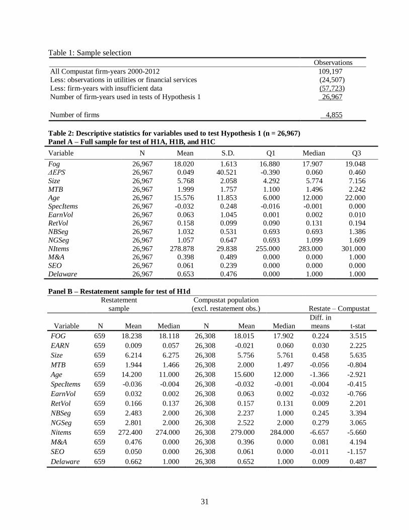
in the utilities and financial services industries (SIC 4400-5000 and 6000-6999). Table 1 shows

the results of the sample selection procedure. The final sample consists of 26,967 firm-years and

4,855 unique firms.

The first hypothesis concerns the influence of earnings management on readability. To

test this hypothesis, we require measures of readability, earnings management, and control

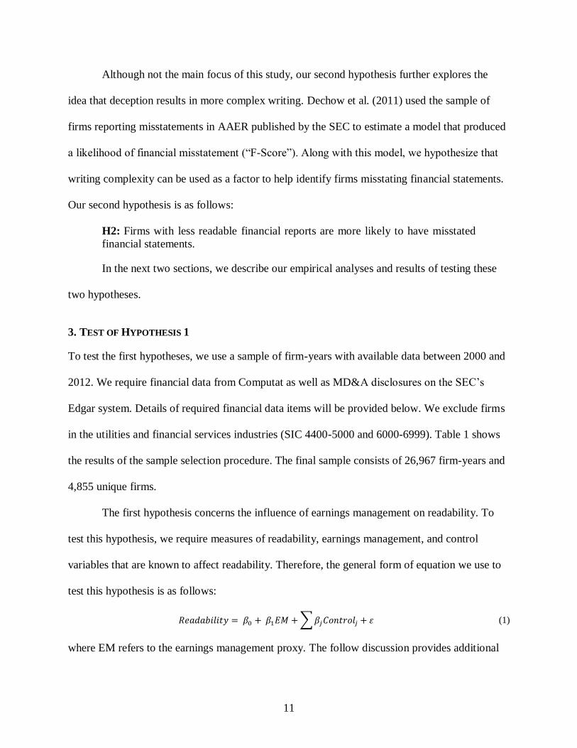
variables that are known to affect readability. Therefore, the general form of equation we use to

test this hypothesis is as follows:

𝑅𝑒𝑎𝑑𝑎𝑏𝑖𝑙𝑖𝑡𝑦 = 𝛽0 + 𝛽1𝐸𝑀 + ∑ 𝛽𝑗𝐶𝑜𝑛𝑡𝑟𝑜𝑙𝑗 + 𝜀 (1)

where EM refers to the earnings management proxy. The follow discussion provides additional

12

details for this equation.

3.1 Readability

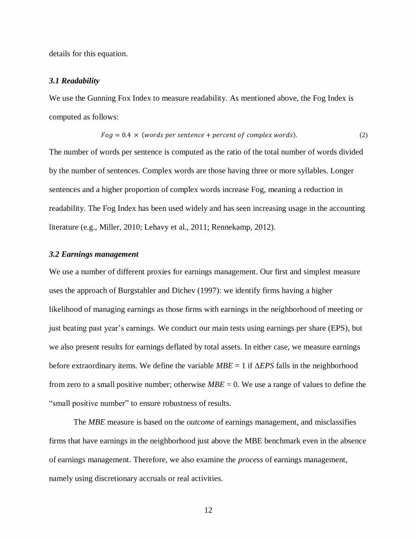
We use the Gunning Fox Index to measure readability. As mentioned above, the Fog Index is

computed as follows:

𝐹𝑜𝑔 = 0.4 × (𝑤𝑜𝑟𝑑𝑠 𝑝𝑒𝑟 𝑠𝑒𝑛𝑡𝑒𝑛𝑐𝑒 + 𝑝𝑒𝑟𝑐𝑒𝑛𝑡 𝑜𝑓 𝑐𝑜𝑚𝑝𝑙𝑒𝑥 𝑤𝑜𝑟𝑑𝑠). (2)

The number of words per sentence is computed as the ratio of the total number of words divided

by the number of sentences. Complex words are those having three or more syllables. Longer

sentences and a higher proportion of complex words increase Fog, meaning a reduction in

readability. The Fog Index has been used widely and has seen increasing usage in the accounting

literature (e.g., Miller, 2010; Lehavy et al., 2011; Rennekamp, 2012).

3.2 Earnings management

We use a number of different proxies for earnings management. Our first and simplest measure

uses the approach of Burgstahler and Dichev (1997): we identify firms having a higher

likelihood of managing earnings as those firms with earnings in the neighborhood of meeting or

just beating past year’s earnings. We conduct our main tests using earnings per share (EPS), but

we also present results for earnings deflated by total assets. In either case, we measure earnings

before extraordinary items. We define the variable MBE = 1 if ΔEPS falls in the neighborhood

from zero to a small positive number; otherwise MBE = 0. We use a range of values to define the

“small positive number” to ensure robustness of results.

The MBE measure is based on the outcome of earnings management, and misclassifies

firms that have earnings in the neighborhood just above the MBE benchmark even in the absence

of earnings management. Therefore, we also examine the process of earnings management,

namely using discretionary accruals or real activities.

13

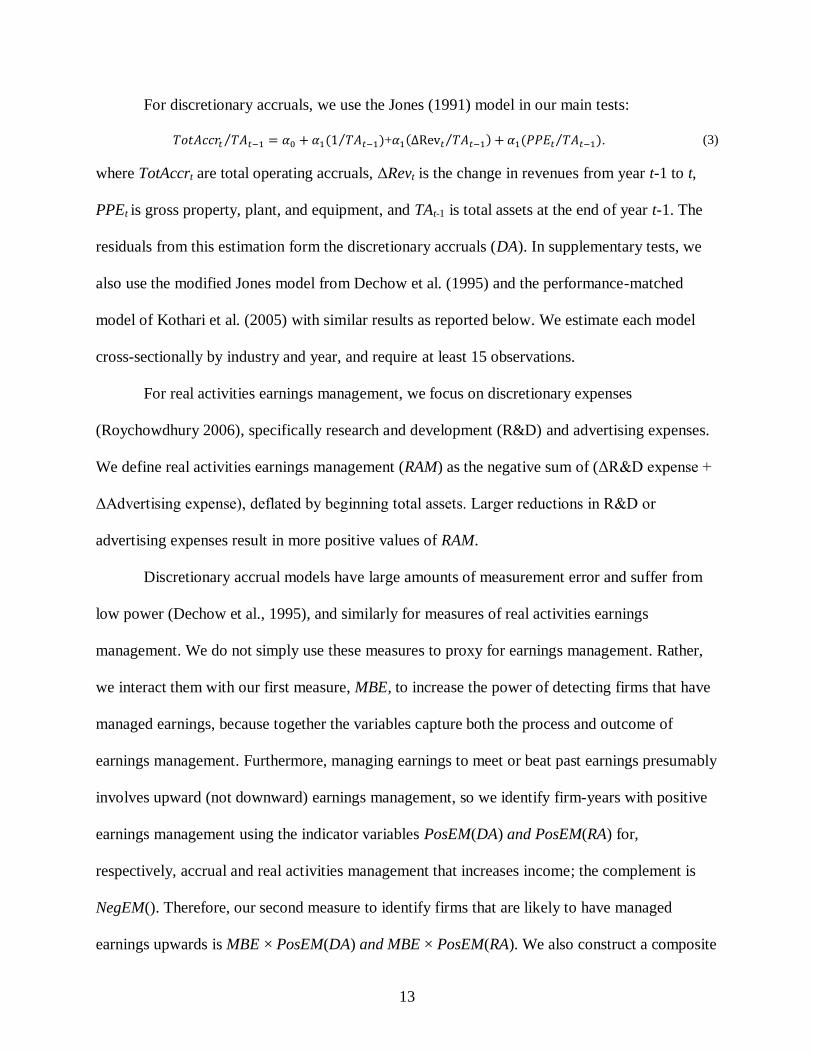
For discretionary accruals, we use the Jones (1991) model in our main tests:

𝑇𝑜𝑡𝐴𝑐𝑐𝑟𝑡 𝑇𝐴𝑡−1⁄ = 𝛼0 + 𝛼1(1 𝑇𝐴𝑡−1⁄ )+𝛼1(ΔRev𝑡 𝑇𝐴𝑡−1⁄ ) + 𝛼1(𝑃𝑃𝐸𝑡 𝑇𝐴𝑡−1⁄ ). (3)

where TotAccrt are total operating accruals, ΔRevt is the change in revenues from year t-1 to t,

PPEt is gross property, plant, and equipment, and TAt-1 is total assets at the end of year t-1. The

residuals from this estimation form the discretionary accruals (DA). In supplementary tests, we

also use the modified Jones model from Dechow et al. (1995) and the performance-matched

model of Kothari et al. (2005) with similar results as reported below. We estimate each model

cross-sectionally by industry and year, and require at least 15 observations.

For real activities earnings management, we focus on discretionary expenses

(Roychowdhury 2006), specifically research and development (R&D) and advertising expenses.

We define real activities earnings management (RAM) as the negative sum of (ΔR&D expense +

ΔAdvertising expense), deflated by beginning total assets. Larger reductions in R&D or

advertising expenses result in more positive values of RAM.

Discretionary accrual models have large amounts of measurement error and suffer from

low power (Dechow et al., 1995), and similarly for measures of real activities earnings

management. We do not simply use these measures to proxy for earnings management. Rather,

we interact them with our first measure, MBE, to increase the power of detecting firms that have

managed earnings, because together the variables capture both the process and outcome of

earnings management. Furthermore, managing earnings to meet or beat past earnings presumably

involves upward (not downward) earnings management, so we identify firm-years with positive

earnings management using the indicator variables PosEM(DA) and PosEM(RA) for,

respectively, accrual and real activities management that increases income; the complement is

NegEM(). Therefore, our second measure to identify firms that are likely to have managed

earnings upwards is MBE × PosEM(DA) and MBE × PosEM(RA). We also construct a composite

14

variable to capture both types of earnings management: PosEM(Comb) = PosEM(DA) +

PosEM(RA).

Our third measure of earnings management refines the second one just described but uses

not only the sign of the earnings management, but also the magnitude. We separate firms with

positive discretionary accruals into high and low partitions using the median value, resulting in

HighPosEM(DA) and LowPosEM(DA); similary for positive real activities earnings

management. Our third measure of firms most likely to have managed earnings upwards is thus

MBE × HighPosEM(DA).

Our fourth proxy for earnings management is whether a firm-year’s financial statements

had been restated, as identified in Audit Analytics. Because some restatements result from

relatively benign reasons, we focus on restatements that Audit Analytics has flagged as (i)

resulting from fraud or (ii) being initiated by or resulted in an SEC investigation. Our fifth proxy

is whether a firm-year’s financial statements were misstated according to AAER.

3.3 Control variables

Our list of control variables derives from Li (2008). The most important of these in our context

are the earnings-related variables. The first is Earnings, which is the level of earnings reported,

which is expected to be negatively associated with Fog (i.e., firm-years with high earnings have

more readable MD&A) based on Li (2008). Depending on the specification, Earnings is either

EPS before extraordinary items, or earnings before extraordinary items deflated by beginning

total assets. Closely related in the variable NegEarnChg, which equals 1 if the change in

Earnings is negative. We also control for firm-years with losses with the indicator Loss, which

equal 1 when Earnings < 0, because losses are presumably bad news, which is likely to make

disclosures less readable Li (2008).

15

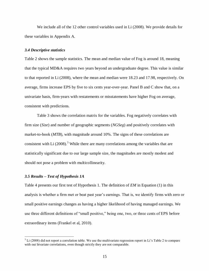
We include all of the 12 other control variables used in Li (2008). We provide details for

these variables in Appendix A.

3.4 Descriptive statistics

Table 2 shows the sample statistics. The mean and median value of Fog is around 18, meaning

that the typical MD&A requires two years beyond an undergraduate degree. This value is similar

to that reported in Li (2008), where the mean and median were 18.23 and 17.98, respectively. On

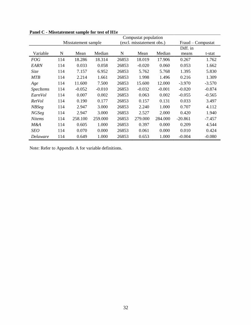
average, firms increase EPS by five to six cents year-over-year. Panel B and C show that, on a

univariate basis, firm-years with restatements or misstatements have higher Fog on average,

consistent with predictions.

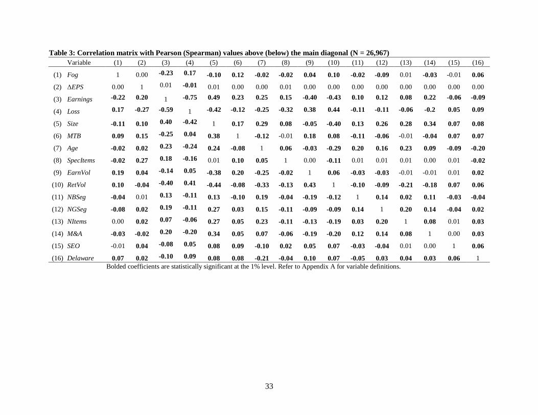
Table 3 shows the correlation matrix for the variables. Fog negatively correlates with

firm size (Size) and number of geographic segments (NGSeg) and positively correlates with

market-to-book (MTB), with magnitude around 10%. The signs of these correlations are

consistent with Li (2008).3 While there are many correlations among the variables that are

statistically significant due to our large sample size, the magnitudes are mostly modest and

should not pose a problem with multicollinearity.

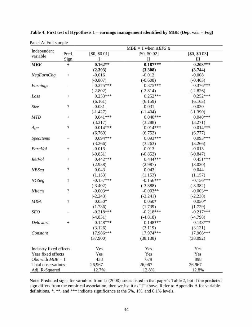
3.5 Results – Test of Hypothesis 1A

Table 4 presents our first test of Hypothesis 1. The definition of EM in Equation (1) in this

analysis is whether a firm met or beat past year’s earnings. That is, we identify firms with zero or

small positive earnings changes as having a higher likelihood of having managed earnings. We

use three different definitions of “small positive,” being one, two, or three cents of EPS before

extraordinary items (Frankel et al, 2010).

3 Li (2008) did not report a correlation table. We use the multivariate regression report in Li’s Table 2 to compare

with out bivariate correlations, even though strictly they are not comparable.

16

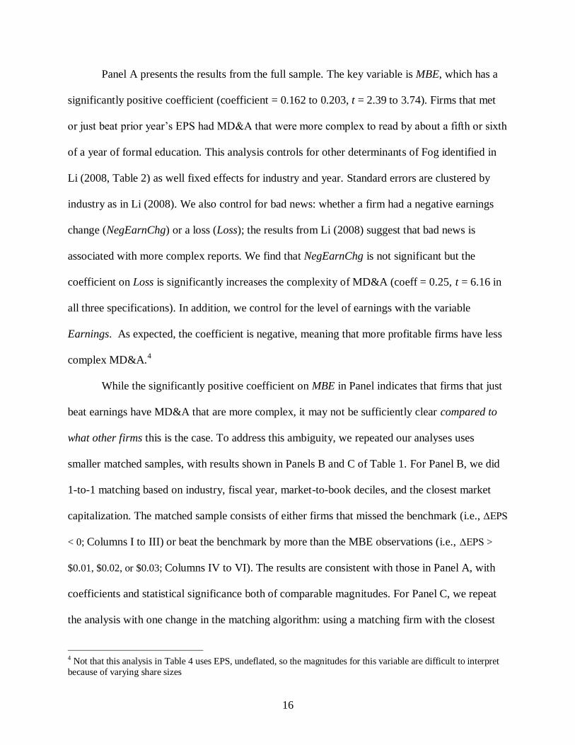
Panel A presents the results from the full sample. The key variable is MBE, which has a

significantly positive coefficient (coefficient = 0.162 to 0.203, t = 2.39 to 3.74). Firms that met

or just beat prior year’s EPS had MD&A that were more complex to read by about a fifth or sixth

of a year of formal education. This analysis controls for other determinants of Fog identified in

Li (2008, Table 2) as well fixed effects for industry and year. Standard errors are clustered by

industry as in Li (2008). We also control for bad news: whether a firm had a negative earnings

change (NegEarnChg) or a loss (Loss); the results from Li (2008) suggest that bad news is

associated with more complex reports. We find that NegEarnChg is not significant but the

coefficient on Loss is significantly increases the complexity of MD&A (coeff = 0.25, t = 6.16 in

all three specifications). In addition, we control for the level of earnings with the variable

Earnings. As expected, the coefficient is negative, meaning that more profitable firms have less

complex MD&A.4

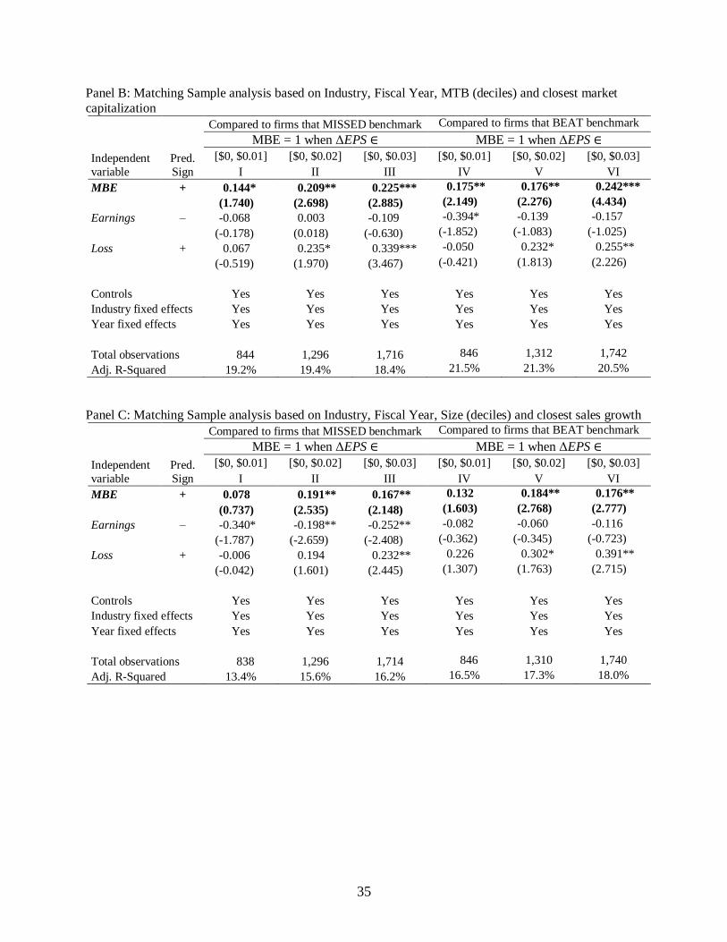
While the significantly positive coefficient on MBE in Panel indicates that firms that just

beat earnings have MD&A that are more complex, it may not be sufficiently clear compared to

what other firms this is the case. To address this ambiguity, we repeated our analyses uses

smaller matched samples, with results shown in Panels B and C of Table 1. For Panel B, we did

1-to-1 matching based on industry, fiscal year, market-to-book deciles, and the closest market

capitalization. The matched sample consists of either firms that missed the benchmark (i.e., ΔEPS

< 0; Columns I to III) or beat the benchmark by more than the MBE observations (i.e., ΔEPS >

$0.01, $0.02, or $0.03; Columns IV to VI). The results are consistent with those in Panel A, with

coefficients and statistical significance both of comparable magnitudes. For Panel C, we repeat

the analysis with one change in the matching algorithm: using a matching firm with the closest

4 Not that this analysis in Table 4 uses EPS, undeflated, so the magnitudes for this variable are difficult to interpret

because of varying share sizes

17

sales growth instead of closest market capitalization. Again, the results remain consistent with

the exception of Column I.

Overall, this first set of results—firms with relatively good news of a small positive

earnings change having MD&A sections that are on average less readable than firms disclosing

worse news—is inconsistent with a purely ontological explanation.

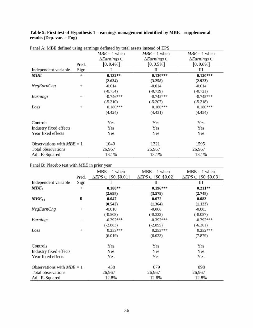
To address the scale issue related to using EPS, we show results of measuring

profitability as earnings before extraordinary items deflated by total assets. Table 5 Panel A

shows the results of this analysis, with MBE defined to equal 1 when deflated earnings is from

zero to 0.4%, 0.5% or 0.6%. For brevity, we do not report the coefficients for the control

variables. Similar to Table 4, we find results as predicted. The coefficient on MBE ranges from

0.127 to 0.137, somewhat smaller than in Table 4 but significant at the 1% level or better (t =

2.63 to 3.26).

We also conduct a placebo test to confirm that the results found are not spurious due to

persistent firm-specific factors. In particular, we want to reduce the possibility that some

unmodelled factors omitted from our analysis but correlated with the propensity to meet/beat

explain the variation in MD&A readability. To this end, we include MBEt-1 to see if meeting or

beating in the prior year is at all associated with current MD&A readability. Table 5 Panel B

shows that the coefficient on MBEt-1 is not significantly different from zero (t = 0.445), while the

coefficient on MBEt continues to be significantly positive and with similar magnitudes as in

Table 4. This placebo test suggests that the result on MBE found in Table 4 is unlikely to be

spuriously caused by omitted variables.

A third test that we conduct to confirm our results in Table 4 is to increase the precision

of the MBE variable to distinguish firms that beat the benchmark with earnings management

18

from firm that do so without earnings management. (Later analyses in Tables 6 and 7 will also do

this using models of discretionary accruals and real activities; the test here uses the properties of

the earnings themselves.) We identify firms that just met or beat the past year’s EPS, with the

added condition of EPS in the first three fiscal quarters current year having fallen behind the

amount in the first three quarter of the preceding year. We denote this indicator variable as

MBE_ByQ4. The additional condition increases the likelihood of identifying firms that managed

earnings upwards in the final quarter of the fiscal year to meet or beat the annual earnings of the

prior year. Panel C of Table 5 contains the results of this analysis. Again, the indicator variable

of earnings management, MBE_ByQ4, is significantly positive (coeff = 0.22 to 0.25, t = 2.19 to

2.27).

Overall, the adjusted R-squared values in both Tables 4 and 5 are around 13% (and

higher in the matched samples), which are similar but slightly higher than the 10% reported in Li

(2008). The results so far support Hypothesis 1A. We find consistent evidence that, while higher

earnings is associated with more readable MD&A, losses are associated with less readable

reports, but meeting or just beating is also associated less readable reports. The ontology

explanation suggests that it is possible and even likely that good news is inherently easier and

bad new is inherently more difficult to explain. Our evidence suggests that the good new of

meeting or just beating past earnings is also harder to explain, which is contrary to the

ontological explanation. This result could arise if the good news is artificial and some amount of

obfuscation is required to make the underlying performance less transparent. We investigate this

possibility further in the next tests of H1B and H1C.

3.6 Results – tests of Hypotheses 1B and 1C

Considering only whether a firm met or just beat the prior year’s earnings as we did in the test of

19

H1A involves misclassifying firms that would have met or just beat prior year’s earnings without

any earnings management. To improve the identification of firms that are more likely to have

managed earnings, we consider the process of earnings management used to achieve that

earnings outcome. We estimate firms’ discretionary accruals and real activity earnings

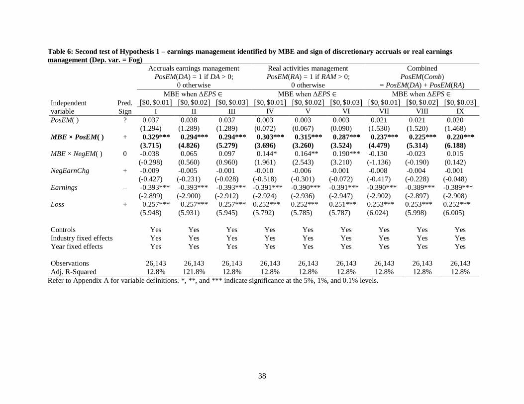
management in addition to whether it met or beat prior earnings. Table 6 shows the results of

regressing Fog on MBE interacted with PosEM( ) (positive earnings management), as well as the

main effect for PosEM( ) and control variables. The results in Columns I to III are as predicted:

MBE × PosEM(DA) is significantly positive (coefficient = 0.29 to 0.33, t = 3.72 to 5.28). Firms

that are likely to have used earnings-increasing discretionary accruals to meet or beat prior

earnings have less readable MD&A. The magnitudes of the coefficient are about 1.5 to 2 times as

large as those estimated in Table 4 for MBE alone without considering accruals. Consistent with

this larger magnitude, we find the coefficient for MBE × NegDA to be insignificant; that is, the

effect found in Table 4 is concentrated in the subset with positive discretionary accruals. Firms

that met or just beat prior earnings but have negative discretionary accruals do not exhibit more

complex MD&A. This evidence supports Hypothesis 1B.

The results for real activities earnings management are similar, shown in Columns IV to

VI in Table 6. The coefficients on MBE × PosEM(RA) are similar to those for accruals

management. Combining the two sources of earnings management, Columns VII to IX show

similar results with significantly positive coefficients on MBE × PosEM(Comb). Note that the

coefficient value is somewhat smaller (0.22 to 0.24), but the variable’s range is 0 to 2 (instead of

0 to 1), so the magnitude of the effect is similar to that in Columns I to VI.

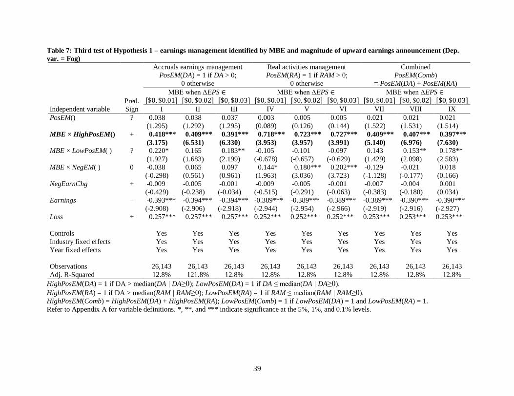
We further refine the definition of earnings management by identifying firms that have

highly positive vs. less positive earnings management by splitting at the median value of PosEM(

20

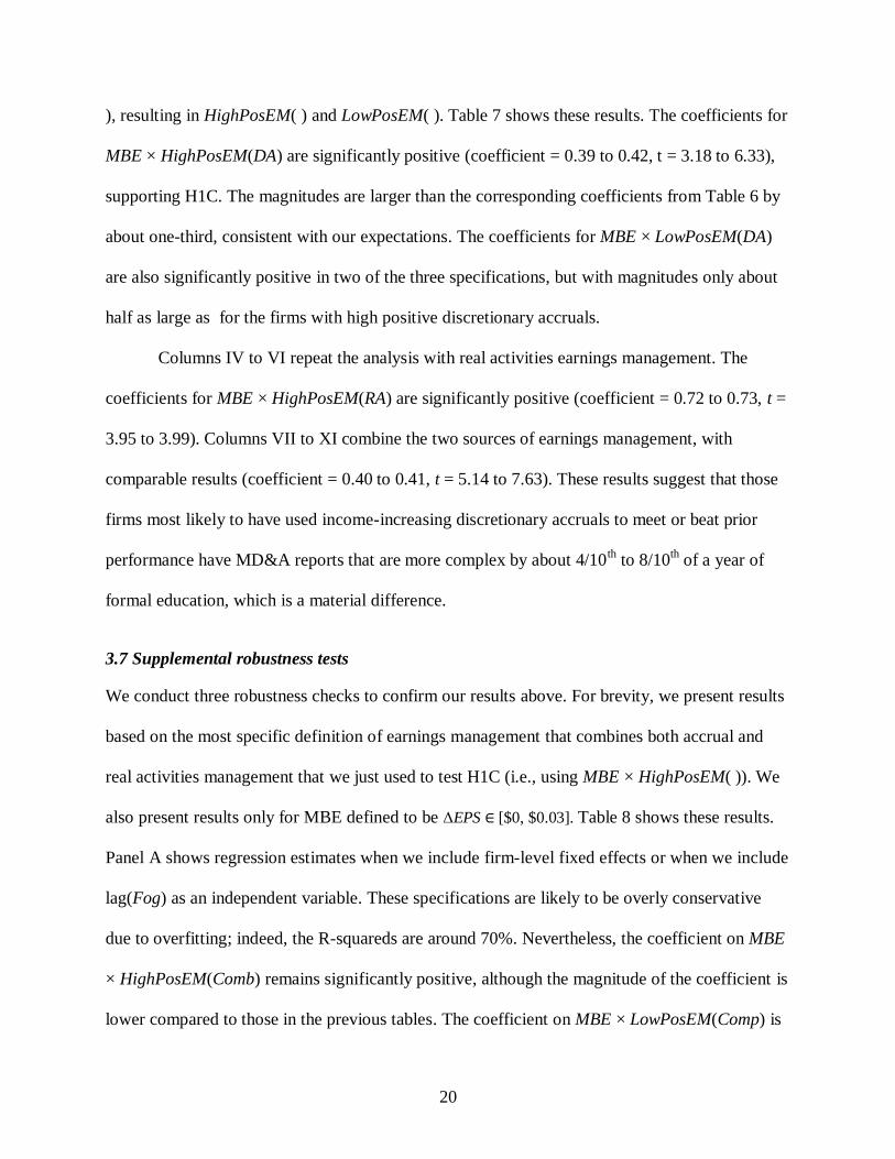
), resulting in HighPosEM( ) and LowPosEM( ). Table 7 shows these results. The coefficients for

MBE × HighPosEM(DA) are significantly positive (coefficient = 0.39 to 0.42, t = 3.18 to 6.33),

supporting H1C. The magnitudes are larger than the corresponding coefficients from Table 6 by

about one-third, consistent with our expectations. The coefficients for MBE × LowPosEM(DA)

are also significantly positive in two of the three specifications, but with magnitudes only about

half as large as for the firms with high positive discretionary accruals.

Columns IV to VI repeat the analysis with real activities earnings management. The

coefficients for MBE × HighPosEM(RA) are significantly positive (coefficient = 0.72 to 0.73, t =

3.95 to 3.99). Columns VII to XI combine the two sources of earnings management, with

comparable results (coefficient = 0.40 to 0.41, t = 5.14 to 7.63). These results suggest that those

firms most likely to have used income-increasing discretionary accruals to meet or beat prior

performance have MD&A reports that are more complex by about 4/10th to 8/10

th of a year of

formal education, which is a material difference.

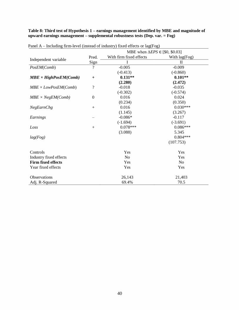
3.7 Supplemental robustness tests

We conduct three robustness checks to confirm our results above. For brevity, we present results

based on the most specific definition of earnings management that combines both accrual and

real activities management that we just used to test H1C (i.e., using MBE × HighPosEM( )). We

also present results only for MBE defined to be ΔEPS ∈ [$0, $0.03]. Table 8 shows these results.

Panel A shows regression estimates when we include firm-level fixed effects or when we include

lag(Fog) as an independent variable. These specifications are likely to be overly conservative

due to overfitting; indeed, the R-squareds are around 70%. Nevertheless, the coefficient on MBE

× HighPosEM(Comb) remains significantly positive, although the magnitude of the coefficient is

lower compared to those in the previous tables. The coefficient on MBE × LowPosEM(Comp) is

21

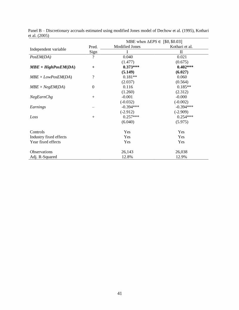
no longer significant. Panel B explores the potential effect of using other accrual models.

Column I uses the modified Jones model of Dechow et al. (1995) to measure discretionary

accruals, and the results remain essentially the same as those reported in Table 7, which uses the

simpler Jones (1991) model. Column II uses the performance-matched accrual model of Kothari

et al. (2005). Again, the results are very similar to those reported in Table 7 except that the

coefficient on MBE × LowPosDA is no longer significant, which is similar to what was found

with firm-level fixed effects in Panel A.

Panel C of Table 8 considers the zero-earnings benchmark, instead of the zero earnings

change benchmark we have examined in all the above analyses. We again observe very

consistent results: whether we look at discretional accruals, real activities management, or both

combined, the Fog score is higher for firms that meet or just beat the zero earnings benchmark

and have high amounts of income-increase earnings management (coefficient = 0.28 to 0.49; t =

2.31 to 5.68). The magnitudes of the coefficients are similar to that found previously (compare

with Table 7 Columns III, VI, and IX).

Thus far, we have used quantitative techniques to identify firm-years that are more likely

to contain significant earnings management. Turning to the human-assisted identification of

earnings management, we now look at the results. Table 9 shows the results when earnings

management is identified by financial restatements that have been identified as fraudulent or

relating to SEC investigations. In the first specification, the indicator variable Restate is

significantly positive (coefficient = 0.254, t = 2.297), meaning that firm-years with restatements

have more complex MD&A. Now, since some restatements may be small in magnitude, we

incorporate the magnitude of restatement in the variable RestateSeverityDecile, which ranges

from 0 to 10, where 10 is the decile with the largest restatement and 1 the smallest, and 0 for no

22

restatement. The result using this variable is also significantly positive (coefficient = 0.036, t =

2.156).

Table 10 looks at the AAER sample of misstatements. Again, we find that firm-years

with earnings management have less readable MD&A (Misstated coefficient = 0.318, t = 2.08).

In sum, we find consistent and robust evidence supporting Hypothesis 1 with different

definitions of earnings management, different accrual models, controlling for different fixed

effects, and using a placebo test. Next we examine whether readability is predictive of financial

misstatements.

4. TEST OF HYPOTHESIS 2

Hypothesis 2 predicts that firm-years with less readable financial reports are more likely to have

misstated financial statements. To test this hypothesis, we continue to focus on the readability of

MD&A as above. For the misstatements, we use the information provided in Accounting and

Auditing Enforcement Releases (AAER) issued by the SEC. Table 11 shows how we obtain the

216 firm-years of misstatement observations used in out tests. The frequency of the

misstatements peaked at 39 cases in the year 1999, and has been markedly less frequent in the

latter years.

4.1 Model of misstatement

To test whether low readability is predictive of misstatements, we use the model F-Score model

of Dechow et al. (2011). Specifically, we use the variables in Model 2 of Table 7 of Dechow et

al. and augment it with Fog to identify whether readability has incremental predictive power for

misstatements.5

5 Dechow et al.’s Model 3 also includes current year and lagged market-adjusted stock returns. We opt to use their

Model 2 without stock return variables because including them would result in a substantial further reduction in the

23

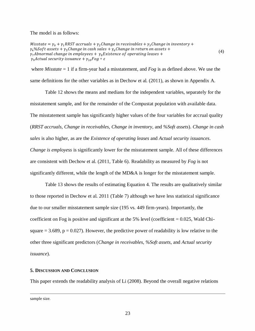
The model is as follows:

𝑀𝑖𝑠𝑠𝑡𝑎𝑡𝑒 = 𝛾0 + 𝛾1𝑅𝑅𝑆𝑇 𝑎𝑐𝑐𝑟𝑢𝑎𝑙𝑠 + 𝛾2𝐶ℎ𝑎𝑛𝑔𝑒 𝑖𝑛 𝑟𝑒𝑐𝑒𝑖𝑣𝑎𝑏𝑙𝑒𝑠 + 𝛾3𝐶ℎ𝑎𝑛𝑔𝑒 𝑖𝑛 𝑖𝑛𝑣𝑒𝑛𝑡𝑜𝑟𝑦 +𝛾4%𝑆𝑜𝑓𝑡 𝑎𝑠𝑠𝑒𝑡𝑠 + 𝛾5𝐶ℎ𝑎𝑛𝑔𝑒 𝑖𝑛 𝑐𝑎𝑠ℎ 𝑠𝑎𝑙𝑒𝑠 + 𝛾6𝐶ℎ𝑎𝑛𝑔𝑒 𝑖𝑛 𝑟𝑒𝑡𝑢𝑟𝑛 𝑜𝑛 𝑎𝑠𝑠𝑒𝑡𝑠 +𝛾7𝐴𝑏𝑛𝑜𝑟𝑚𝑎𝑙 𝑐ℎ𝑎𝑛𝑔𝑒 𝑖𝑛 𝑒𝑚𝑝𝑙𝑜𝑦𝑒𝑒𝑠 + 𝛾8𝐸𝑥𝑖𝑠𝑡𝑒𝑛𝑐𝑒 𝑜𝑓 𝑜𝑝𝑒𝑟𝑎𝑡𝑖𝑛𝑔 𝑙𝑒𝑎𝑠𝑒𝑠 + 𝛾9𝐴𝑐𝑡𝑢𝑎𝑙 𝑠𝑒𝑐𝑢𝑟𝑖𝑡𝑦 𝑖𝑠𝑠𝑢𝑎𝑛𝑐𝑒 + 𝛾10𝐹𝑜𝑔 + 𝜀

(4)

where Misstate = 1 if a firm-year had a misstatement, and Fog is as defined above. We use the

same definitions for the other variables as in Dechow et al. (2011), as shown in Appendix A.

Table 12 shows the means and medians for the independent variables, separately for the

misstatement sample, and for the remainder of the Compustat population with available data.

The misstatement sample has significantly higher values of the four variables for accrual quality

(RRST accruals, Change in receivables, Change in inventory, and %Soft assets). Change in cash

sales is also higher, as are the Existence of operating leases and Actual security issuances.

Change is employess is significantly lower for the misstatement sample. All of these differences

are consistent with Dechow et al. (2011, Table 6). Readability as measured by Fog is not

significantly different, while the length of the MD&A is longer for the misstatement sample.

Table 13 shows the results of estimating Equation 4. The results are qualitatively similar

to those reported in Dechow et al. 2011 (Table 7) although we have less statistical significance

due to our smaller misstatement sample size (195 vs. 449 firm-years). Importantly, the

coefficient on Fog is positive and significant at the 5% level (coefficient = 0.025, Wald Chi-

square = 3.689, p = 0.027). However, the predictive power of readability is low relative to the

other three significant predictors (Change in receivables, %Soft assets, and Actual security

issuance).

5. DISCUSSION AND CONCLUSION

This paper extends the readability analysis of Li (2008). Beyond the overall negative relations

sample size.

24

between the Fog Index and financial performance (i.e., the positive relationship between

readability and performance), we hypothesize and document a disruption to that overall pattern.

In the region where a firm meets or just beats the prior year’s earnings, the Fog score increases

and readability deteriorates. The effect is larger when we focus on subsets of firms within this

neighborhood of earnings performance that are more likely to have engaged in accruals or real

activities management to increase earnings. Overall, we find consistent and robust evidence that

firms that are likely to have managed earnings to meet or beat the benchmark of the prior year’s

earnings on average have more complex MD&A reports. We find similar results for firms that

meet or just beat the zero earnings benchmark. Using the F-Score model of Dechow et al. (2011),

we also show that the Fog Index has modest predictive power incremental to known predictors.

If the ontological explanation proposed by Bloomfield (2008) were a sufficient

explanation (i.e., that good performance is inherently easier to communicate than bad

performance), then we should not observe the pattern we found. Our evidence suggests that, at

least for firms that are most suspected of having managed earnings, obfuscation is involved in

making the financial report more difficult to read.

Our results are also consistent with the commonly held belief, supported by empirical

evidence, that telling the truth is easier than telling lies (Hancock et al., 2007). Lying is difficult

if it is to be convincing because the communicator has to ensure the consistency of the supposed

“facts.” While earnings management in many cases do not outright fall into the category of lying,

the activity does involve some active efforts on the part of management to bias the financial

statements through accruals or other means. Such actions create a discrepancy between

unmanaged performance and reported performance, which can make it mentally more taxing to

explain reported performance when management knows the underlying, unmanaged performance

25

to be different. Earnings management also challenges managers’ ethical standards, which again

can cause cognitive stress, which can be indirectly connected to readability of their writing.

Further research can go beyond readability and explore how the specific content of the

MD&A relates to benchmark beating and earnings management. For instance, do firms suspected

of having managed earnings use different pronouns or a more passive writing style? Another

avenue is to investigate other earnings benchmarks and the corresponding disclosures that would

focus on those benchmarks (e.g., meeting or beating market expectations and conference calls).

26

Appendix A

Variable definitions

Readability variables

Fog = 0.4 × (words per sentence + percent of complex words).

Variables in test of Hypothesis 1

ΔEPS = change in EPS from year t-1 to t.

MBE = 1 if ΔEPS falls in the neighborhood from zero to a small positive number; 0 otherwise.

(The small positive number is identified in each test.)

DA = discretionary accruals estimated using the Jones (1991) model; in robustness tests,

discretionary accruals are estimated using the modified Jones model of Dechow et al. (1995),

or the performance-matched model of Kothari et al. (2005).

PosEM(DA) = 1 if DA ≥ 0; otherwise 0. Indicates income increasing earnings management using

discretionary accruals.

HighPosEM(DA) = 1 if DA > median(DA | DA≥0); otherwise 0.

RAM = real activities earnings management = – (ΔR&D expense + ΔAdvertising expense) / total

assets.

PosEM(RA) = 1 if RAM 0; otherwise 0. Indicates income increasing earnings management

using real activities.

HighPosEM(RA) = 1 if RAM > median(RAM | RAM≥0); otherwise 0.

PosEM(Comb) = PosEM(DA) + PosEM(RA) = {0, 1, 2}. Identifies firm-years that have income

increasing earnings management using either discretional accruals or real activities, or both.

HighPosEM(Comb) = HighPosEM(DA) + HighPosEM(RA) = {0, 1, 2}.

Restated = 1 if restatement in Audit Analytics is identified as (i) relating to fraud or (ii) being

initiated by or resulted in an SEC investigation.

RestateSeverityDecile = decile rank of (total dollar change in Net Income due to the restatement

scaled by Total Assets)

Misstated = 1 if a firm-year was reported in an AAER (SEC Accounting and Auditing

Enforcement Release.)

Earnings = EPS before extraordinary items (or earnings before extraordinary items deflated by

total assets)

NegEarnChg = 1 if ΔEarnings < 0.

27

Loss = 1 if Earnings < 0.

Size = log of market value of equity at fiscal year-end.

MTB = (market value of equity + book value of liabilities) / book value of total assets, measured

at the end of the fiscal year.

Age = number of years since a firm first appears in the CRSP monthly stock return file.

SpecItems = amount of special items divided by total assets.

EarnVol = standard deviation of operating earnings during the prior five years.

RetVol = standard deviation of monthly stock returns in the prior year.

NBSeg = natural log of the number of business segments.

NGSeg = natural log of the number of geographic segments.

NItems = number of items in Compustat with non-missing values.

M&A = 1 for firm-years in which a company is an acquirer according to SDC Platinum M&A

database; 1 otherwise.

SEO =1 for firm-years in which a company has a seasoned equity offering according to SDC

Global New Issues database; 0 otherwise.

Delaware = 1 if the firm is incorporated in Delaware; 0 otherwise.

Variables in test of Hypothesis 2

Variable Calculation

Accrual quality variables

RSST accruals (ΔWC + ΔNCO + ΔFIN) / Average total assets, where

WC = [Current Assets (ACT) – Cash and Short-term Investments (CHE)] –

[Current Liabilities (LCT) – Debt in Current Liabilities (DLC)];

NCO = [Total Assets (AT) – Current Assets (ACT) – Investments and

Advances (IVAO)] – [Total Liabilities (DATA 181) – Current

Liabilities (LCT) – Long-term Debt (DLTT)];

FIN = [Short-term Investments (IVST) + Long-term Investments (IVAO)]

– [Long-term Debt (DLTT) + Debt in Current Liabilities (DLC) +

Preferred Stock (PSTK)]; following Richardson et al. 2005.

Change in

receivables

ΔAccounts Receivable (RECT) / Average total assets

Change in

inventory

ΔInventory (INVT) / Average total assets

%Soft assets (Total Assets (AT) - PP&E (PPENT) - Cash Equivalent (CHE)) / Total

Assets (AT)

28

Performance variables Change in cash

sales

Percentage change in cash sales [Sales (SALE) – ΔAccounts Receivable

(RECT)]

Change in return

on assets

[Earningst (IB) / Average total Assetst] - [Earningst-1 / Average total

Assetst-1]

Market-related incentives

Actual security

issuance

An indicator variable coded 1 if firm issued securities during year t (i.e., an

indicator variable coded 1 if SSTK > 0 or DLTIS > 0)

Nonfinancial variables

Abnormal change

in employees

Percentage change in the number of employees (EMP) – Percentage change

in Assets (AT)

Off-balance-sheet variables

Existence of

operating leases

An indicator variable coded 1 if future operating lease obligations are

greater than zero

Note: “RSST” refers to the accrual model of Richarson, Sloan, Soliman, and Tuna (2005).

29

References

Bartov, E., D. Givoly, C. Hayn, 2002. The rewards to meeting or beating earnings expectations.

Journal of Accounting and Economics 33, 173-204.

Bloomfield, R.J., 2002. The ‘‘incomplete revelation hypothesis’’ and financial reporting.

Accounting Horizons 16, 233–243.

Bloomfield, R.J., 2008.Discussion of “Annual report readability, current earnings, and earnings

persistence”. Journal of Accounting and Economics 45, 248-252.

Bloomfield, R.J., 2012. Discussion of Detecting Deceptive Discussions in Conference Calls.

Journal of Accounting Research 50, 541-551.

Bhojraj, S., P. Hribar, M. Picconi, J. McInnis. 2009. Making Sense of Cents: An Examination of

Firms That Marginally Miss or Beat Analyst Forecasts. Journal of Finance, Vol. 64, pp.

2361-2388

Bradshaw, M., S. Richardson, R.G. Sloan, 2001. Do analysts and auditors use information in

accruals? Journal of Accounting Research 39, 45-74.

Brown, S., S.A. Hillegeist, K. Lo, 2009. The effect of earnings surprises on information

asymmetry. Journal of Accounting and Economics 47, 208-225.

Burgstahler, D., I. Dichev, I., 1997. Earnings management to avoid earnings decreases and

losses. Journal of Accounting and Economics 24, 99-126.

Dechow, P.M., I. Dichev, 2002. The quality of accruals and earnings: the role of accrual

estimation errors. The Accounting Review 77, 35-39.

Dechow, P.M., W. Ge, C.R. Larson, R.G. Sloan, 2011. Predicting material accounting

misstatements. Contemporary Accounting Research 28, 17-82.

Dechow, P., R.G. Sloan, A. Sweeney, 1995. Detecting Earnings Management. The Accounting

Review 70, 193-225.

Frankel, R., W.J. Mayew, and Y. Sun, 2010. Do pennies matter? Investor relations consequences

of small negative earnings surprises. Review of Accounting Studies 15, 220-242.

Hancock, J.T., L.E. Curry, S. Goorha, M. Woodworth, 2007. On lying and being lied to: A

linguistic analysis of deception in computer-mediated communication. Discourse Processes

45, 1-23.

Jones, J., 1991. Earnings management during import relief investigation. Journal of Accounting

Research 29, 193-228.

Kothari, S.P., A.J. Leone, C.E. Wasley, 2005. Performance matched discretionary accrual

measures. Journal of Accounting and Economics 39, 163-197.

30

Lang, M., R. Lundholm, 2000. Voluntary disclosure and equity offerings: reducing information

asymmetry or hyping the stock? Contemporary Accounting Research 17, 623-62.

Larcker, D.F., and A.A. Zakolyukina, 2012. Detecting deceptive discussions in conference calls.


Lehavy, R., F. Li, and K. Merkley, 2011. The effect of annual report readability on analyst

following and the properties of their earnings forecasts. The Accounting Review 86, 1087-

1115.

Li, F., 2008. Annual report readability, current earnings, and persistence. Journal of Accounting

and Economics 45, 221-247.Li, F. 2011. Textual analysis of corporate disclosures: A survey

of the literature. Journal of Accounting Literature. 02/2011; 29

Li, F. 2012. Discussion of Analyzing Speech to Detect Financial Misreporting. Journal of

Accounting Research 50, 393-400.

Mayew, W. 2008. Evidence of Management Discrimination Among Analysts During Earnings

Conference Calls.” Journal of Accounting Research 45 (2008): 627–59.

Miller, B.P., 2010. The effects of reporting complexity on small and large investor trading. The

Accounting Review 85, 2107-2143.

Rennekamp, K., 2012. Processing fluency and investors’ reactions to disclosure readability.


Richardson, S.R., R. Sloan, M. Soliman, and I. Tuna, 2005. Accrual reliability, earnings

persistence, and stock prices. Journal of Accounting and Economics 39, 437-85.

Roychowdhury, S., 2006. Earnings management through real activities manipulation. Journal of

Accounting and Economics 42, 335-370.

Schrand, C., B. Walther, 2000. Strategic benchmarks in earnings announcements: the selective

disclosure of prior-period earnings components. The Accounting Review 75, 151-177.

Turner, J. L.; T. J. Mock; AND R. P. Srivastava. “An Analysis of the Fraud Triangle.” AAA

Round Table Paper, 2003. Available at http://aaahq.org/audit/midyear/03midyear/

papers/Research%20Roundtable%203-Turner-Mock-Srivastava.pdf.

31

Table 1: Sample selection

Observations

All Compustat firm-years 2000-2012 109,197 Less: observations in utilities or financial services (24,507)

Less: firm-years with insufficient data (57,723)

Number of firm-years used in tests of Hypothesis 1 26,967

Number of firms 4,855

Table 2: Descriptive statistics for variables used to test Hypothesis 1 (n = 26,967)

Panel A – Full sample for test of H1A, H1B, and H1C

Variable N Mean S.D. Q1 Median Q3

Fog 26,967 18.020 1.613 16.880 17.907 19.048 ΔEPS 26,967 0.049 40.521 -0.390 0.060 0.460

Size 26,967 5.768 2.058 4.292 5.774 7.156

MTB 26,967 1.999 1.757 1.100 1.496 2.242 Age 26,967 15.576 11.853 6.000 12.000 22.000

SpecItems 26,967 -0.032 0.248 -0.016 -0.001 0.000

EarnVol 26,967 0.063 1.045 0.001 0.002 0.010 RetVol 26,967 0.158 0.099 0.090 0.131 0.194

NBSeg 26,967 1.032 0.531 0.693 0.693 1.386

NGSeg 26,967 1.057 0.647 0.693 1.099 1.609

NItems 26,967 278.878 29.838 255.000 283.000 301.000 M&A 26,967 0.398 0.489 0.000 0.000 1.000

SEO 26,967 0.061 0.239 0.000 0.000 0.000

Delaware 26,967 0.653 0.476 0.000 1.000 1.000

Panel B – Restatement sample for test of H1d

Restatement

sample

Compustat population

(excl. restatement obs.) Restate – Compustat

Variable N Mean Median N Mean Median

Diff. in

means t-stat

FOG 659 18.238 18.118 26,308 18.015 17.902 0.224 3.515

EARN 659 0.009 0.057 26,308 -0.021 0.060 0.030 2.225

Size 659 6.214 6.275 26,308 5.756 5.761 0.458 5.635

MTB 659 1.944 1.466 26,308 2.000 1.497 -0.056 -0.804

Age 659 14.200 11.000 26,308 15.600 12.000 -1.366 -2.921

SpecItems 659 -0.036 -0.004 26,308 -0.032 -0.001 -0.004 -0.415

EarnVol 659 0.032 0.002 26,308 0.063 0.002 -0.032 -0.766

RetVol 659 0.166 0.137 26,308 0.157 0.131 0.009 2.201

NBSeg 659 2.483 2.000 26,308 2.237 1.000 0.245 3.394

NGSeg 659 2.801 2.000 26,308 2.522 2.000 0.279 3.065

Nitems 659 272.400 274.000 26,308 279.000 284.000 -6.657 -5.660

M&A 659 0.476 0.000 26,308 0.396 0.000 0.081 4.194

SEO 659 0.050 0.000 26,308 0.061 0.000 -0.011 -1.157

Delaware 659 0.662 1.000 26,308 0.652 1.000 0.009 0.487

32

Panel C - Misstatement sample for test of H1e

Misstatement sample Compustat population

(excl. misstatement obs.) Fraud – Compustat


Diff. in

means t-stat

FOG 114 18.286 18.314 26853 18.019 17.906 0.267 1.762

EARN 114 0.033 0.058 26853 -0.020 0.060 0.053 1.662

Size 114 7.157 6.952 26853 5.762 5.768 1.395 5.830

MTB 114 2.214 1.661 26853 1.998 1.496 0.216 1.309

Age 114 11.600 7.500 26853 15.600 12.000 -3.970 -3.570

SpecItems 114 -0.052 -0.010 26853 -0.032 -0.001 -0.020 -0.874

EarnVol 114 0.007 0.002 26853 0.063 0.002 -0.055 -0.565

RetVol 114 0.190 0.177 26853 0.157 0.131 0.033 3.497

NBSeg 114 2.947 3.000 26853 2.240 1.000 0.707 4.112

NGSeg 114 2.947 3.000 26853 2.527 2.000 0.420 1.940

Nitems 114 258.100 259.000 26853 279.000 284.000 -20.861 -7.457

M&A 114 0.605 1.000 26853 0.397 0.000 0.209 4.544

SEO 114 0.070 0.000 26853 0.061 0.000 0.010 0.424

Delaware 114 0.649 1.000 26853 0.653 1.000 -0.004 -0.080

Note: Refer to Appendix A for variable definitions.

33

Table 3: Correlation matrix with Pearson (Spearman) values above (below) the main diagonal (N = 26,967)

Variable (1) (2) (3) (4) (5) (6) (7) (8) (9) (10) (11) (12) (13) (14) (15) (16)

(1) Fog 1 0.00 -0.23 0.17 -0.10 0.12 -0.02 -0.02 0.04 0.10 -0.02 -0.09 0.01 -0.03 -0.01 0.06

(2) ΔEPS 0.00 1 0.01 -0.01 0.01 0.00 0.00 0.01 0.00 0.00 0.00 0.00 0.00 0.00 0.00 0.00

(3) Earnings -0.22 0.20 1 -0.75 0.49 0.23 0.25 0.15 -0.40 -0.43 0.10 0.12 0.08 0.22 -0.06 -0.09

(4) Loss 0.17 -0.27 -0.59 1 -0.42 -0.12 -0.25 -0.32 0.38 0.44 -0.11 -0.11 -0.06 -0.2 0.05 0.09

(5) Size -0.11 0.10 0.40 -0.42 1 0.17 0.29 0.08 -0.05 -0.40 0.13 0.26 0.28 0.34 0.07 0.08

(6) MTB 0.09 0.15 -0.25 0.04 0.38 1 -0.12 -0.01 0.18 0.08 -0.11 -0.06 -0.01 -0.04 0.07 0.07

(7) Age -0.02 0.02 0.23 -0.24 0.24 -0.08 1 0.06 -0.03 -0.29 0.20 0.16 0.23 0.09 -0.09 -0.20

(8) SpecItems -0.02 0.27 0.18 -0.16 0.01 0.10 0.05 1 0.00 -0.11 0.01 0.01 0.01 0.00 0.01 -0.02

(9) EarnVol 0.19 0.04 -0.14 0.05 -0.38 0.20 -0.25 -0.02 1 0.06 -0.03 -0.03 -0.01 -0.01 0.01 0.02

(10) RetVol 0.10 -0.04 -0.40 0.41 -0.44 -0.08 -0.33 -0.13 0.43 1 -0.10 -0.09 -0.21 -0.18 0.07 0.06

(11) NBSeg -0.04 0.01 0.13 -0.11 0.13 -0.10 0.19 -0.04 -0.19 -0.12 1 0.14 0.02 0.11 -0.03 -0.04

(12) NGSeg -0.08 0.02 0.19 -0.11 0.27 0.03 0.15 -0.11 -0.09 -0.09 0.14 1 0.20 0.14 -0.04 0.02

(13) NItems 0.00 0.02 0.07 -0.06 0.27 0.05 0.23 -0.11 -0.13 -0.19 0.03 0.20 1 0.08 0.01 0.03

(14) M&A -0.03 -0.02 0.20 -0.20 0.34 0.05 0.07 -0.06 -0.19 -0.20 0.12 0.14 0.08 1 0.00 0.03

(15) SEO -0.01 0.04 -0.08 0.05 0.08 0.09 -0.10 0.02 0.05 0.07 -0.03 -0.04 0.01 0.00 1 0.06

(16) Delaware 0.07 0.02 -0.10 0.09 0.08 0.08 -0.21 -0.04 0.10 0.07 -0.05 0.03 0.04 0.03 0.06 1

Bolded coefficients are statistically significant at the 1% level. Refer to Appendix A for variable definitions.

34

Table 4: First test of Hypothesis 1 – earnings management identified by MBE (Dep. var. = Fog)

Panel A: Full sample

Independent variable

Pred.

Sign

MBE = 1 when ΔEPS ∈

[$0, $0.01] [$0, $0.02] [$0, $0.03]

I II III

MBE + 0.162** 0.187*** 0.203***

(2.393) (3.308) (3.744)

NegEarnChg + -0.016 -0.012 -0.008

(-0.807) (-0.608) (-0.403)

Earnings – -0.375*** -0.375*** -0.376***

(-2.802) (-2.814) (-2.826)

Loss + 0.253*** 0.252*** 0.252***

(6.161) (6.159) (6.163)

Size ? -0.031 -0.031 -0.030

(-1.427) (-1.404) (-1.390)

MTB + 0.041*** 0.040*** 0.040***

(3.317) (3.288) (3.271)

Age ? 0.014*** 0.014*** 0.014***

(6.769) (6.752) (6.777)

SpecItems – 0.094*** 0.093*** 0.093***

(3.266) (3.263) (3.266)

EarnVol + -0.013 -0.013 -0.013

(-0.851) (-0.852) (-0.847)

RetVol + 0.442*** 0.444*** 0.451***

(2.958) (2.987) (3.030)

NBSeg ? 0.043 0.043 0.044

(1.153) (1.153) (1.157)

NGSeg ? -0.157*** -0.156*** -0.156***

(-3.402) (-3.388) (-3.382)

NItems ? -0.003** -0.003** -0.003**

(-2.243) (-2.241) (-2.238)

M&A ? 0.050* 0.050* 0.050*

(1.736) (1.739) (1.729)

SEO – -0.218*** -0.218*** -0.217***

(-4.831) (-4.818) (-4.798)

Delaware + 0.148*** 0.148*** 0.148***

(3.126) (3.119) (3.121)

Constant

17.986*** 17.974*** 17.966***

(37.900) (38.138) (38.092)

Industry fixed effects Yes Yes Yes

Year fixed effects Yes Yes Yes

Obs with MBE = 1 438 679 898

Total observations 26,967 26,967 26,967

Adj. R-Squared 12.7% 12.8% 12.8%

Note: Predicted signs for variables from Li (2008) are as listed in that paper’s Table 2, but if the predicted

sign differs from the empirical association, then we list it as “?” above. Refer to Appendix A for variable

definitions. *, **, and *** indicate significance at the 5%, 1%, and 0.1% levels.

35

Panel B: Matching Sample analysis based on Industry, Fiscal Year, MTB (deciles) and closest market

capitalization

Independent

variable

Pred.

Sign

Compared to firms that MISSED benchmark Compared to firms that BEAT benchmark

MBE = 1 when ΔEPS ∈ MBE = 1 when ΔEPS ∈

[$0, $0.01] [$0, $0.02] [$0, $0.03] [$0, $0.01] [$0, $0.02] [$0, $0.03]

I II III IV V VI

MBE + 0.144* 0.209** 0.225*** 0.175** 0.176** 0.242***

(1.740) (2.698) (2.885) (2.149) (2.276) (4.434)

Earnings – -0.068 0.003 -0.109 -0.394* -0.139 -0.157

(-0.178) (0.018) (-0.630) (-1.852) (-1.083) (-1.025)

Loss + 0.067 0.235* 0.339*** -0.050 0.232* 0.255**

(-0.519) (1.970) (3.467) (-0.421) (1.813) (2.226)

Controls Yes Yes Yes Yes Yes Yes

Industry fixed effects Yes Yes Yes Yes Yes Yes

Year fixed effects Yes Yes Yes Yes Yes Yes

Total observations 844 1,296 1,716 846 1,312 1,742

Adj. R-Squared 19.2% 19.4% 18.4% 21.5% 21.3% 20.5%

Panel C: Matching Sample analysis based on Industry, Fiscal Year, Size (deciles) and closest sales growth

Independent

variable

Pred.

Sign

Compared to firms that MISSED benchmark Compared to firms that BEAT benchmark

MBE = 1 when ΔEPS ∈ MBE = 1 when ΔEPS ∈

[$0, $0.01] [$0, $0.02] [$0, $0.03] [$0, $0.01] [$0, $0.02] [$0, $0.03]

I II III IV V VI

MBE + 0.078 0.191** 0.167** 0.132 0.184** 0.176**

(0.737) (2.535) (2.148) (1.603) (2.768) (2.777)

Earnings – -0.340* -0.198** -0.252** -0.082 -0.060 -0.116

(-1.787) (-2.659) (-2.408) (-0.362) (-0.345) (-0.723)

Loss + -0.006 0.194 0.232** 0.226 0.302* 0.391**

(-0.042) (1.601) (2.445) (1.307) (1.763) (2.715)

Controls Yes Yes Yes Yes Yes Yes

Industry fixed effects Yes Yes Yes Yes Yes Yes

Year fixed effects Yes Yes Yes Yes Yes Yes

Total observations 838 1,296 1,714 846 1,310 1,740

Adj. R-Squared 13.4% 15.6% 16.2% 16.5% 17.3% 18.0%

36

Table 5: First test of Hypothesis 1 – earnings management identified by MBE – supplemental

results (Dep. var. = Fog)

Panel A: MBE defined using earnings deflated by total assets instead of EPS


Pred.

Sign

MBE = 1 when

ΔEarnings ∈ [0, 0.4%]

MBE = 1 when


MBE = 1 when


I II III

MBE + 0.132** 0.130*** 0.120***

(2.634) (3.258) (2.923) NegEarnChg + -0.014 -0.014 -0.014

(-0.754) (-0.739) (-0.721)

Earnings – -0.746*** -0.745*** -0.745***

(-5.210) (-5.207) (-5.218)

Loss + 0.180*** 0.180*** 0.180***

(4.424) (4.431) (4.454)

Controls Yes Yes Yes



Observations with MBE = 1 1040 1321 1595


Adj. R-Squared 13.1% 13.1% 13.1%

Panel B: Placebo test with MBE in prior year

MBE = 1 when MBE = 1 when MBE = 1 when


Pred.

Sign

ΔEPS ∈ [$0, $0.01] ΔEPS ∈ [$0, $0.02] ΔEPS ∈ [$0, $0.03] I II III

MBEt + 0.180** 0.196*** 0.211**

(2.698) (3.579) (2.748)

MBEt-1 0 0.047 0.072 0.083

(0.542) (1.364) (1.123)

NegEarnChg + -0.010 -0.006 -0.003

(-0.508) (-0.323) (-0.087)

Earnings – -0.392*** -0.392*** -0.392*** (-2.883) (-2.895) (-6.361) Loss + 0.253*** 0.253*** 0.252*** (6.019) (6.023) (7.879)




Observations with MBE = 1 438 679 898


Adj. R-Squared 12.8% 12.8% 12.8%

37

Panel C: Using performance in first 3 fiscal quarters to identify distance to MBE

MBE = 1 when MBE = 1 when MBE = 1 when

Independent variable Pred.

Sign

ΔEPS ∈ [$0, $0.01] ΔEPS ∈ [$0, $0.02] ΔEPS ∈ [$0, $0.03] I II III

MBE_ByQ4t + 0.223** 0.245** 0.216**

(2.271) (2.401) (2.187) NegEarnChg + -0.020 -0.020 -0.020

(-1.043) (-1.057) (-1.055)

Earnings – -0.745*** -0.745*** -0.744*** (-5.085) (-5.085) (-5.084)

Loss + 0.175*** 0.176*** 0.176***

(4.452) (4.471) (4.469)




Average MBE_sprint 0.029 0.020 0.010


Adj. R-Squared 12.8% 12.8% 12.8%

MBE_ByQ4t measures by how far a firm is underperforming in the first 3 fiscal quarters compared with

the same period in the prior year. Specifically, it is EPS in the first 3 quarter of year t-1 less EPS in the

first 3 quarters of year t. Refer to Appendix A for definitions of other variables. *, **, and *** indicate

significance at the 5%, 1%, and 0.1% levels.

38

Table 6: Second test of Hypothesis 1 – earnings management identified by MBE and sign of discretionary accruals or real earnings

management (Dep. var. = Fog)

Accruals earnings management

PosEM(DA) = 1 if DA > 0;

0 otherwise

Real activities management

PosEM(RA) = 1 if RAM > 0;

0 otherwise

Combined

PosEM(Comb)

= PosEM(DA) + PosEM(RA)

MBE when ΔEPS ∈ MBE when ΔEPS ∈ MBE when ΔEPS ∈ Independent

variable

Pred.

Sign

[$0, $0.01] [$0, $0.02] [$0, $0.03] [$0, $0.01] [$0, $0.02] [$0, $0.03] [$0, $0.01] [$0, $0.02] [$0, $0.03] I II III IV V VI VII VIII IX

PosEM( ) ? 0.037 0.038 0.037 0.003 0.003 0.003 0.021 0.021 0.020

(1.294) (1.289) (1.289) (0.072) (0.067) (0.090) (1.530) (1.520) (1.468)

MBE × PosEM( ) + 0.329*** 0.294*** 0.294*** 0.303*** 0.315*** 0.287*** 0.237*** 0.225*** 0.220***

(3.715) (4.826) (5.279) (3.696) (3.260) (3.524) (4.479) (5.314) (6.188)

MBE × NegEM( ) 0 -0.038 0.065 0.097 0.144* 0.164** 0.190*** -0.130 -0.023 0.015

(-0.298) (0.560) (0.960) (1.961) (2.543) (3.210) (-1.136) (-0.190) (0.142)

NegEarnChg + -0.009 -0.005 -0.001 -0.010 -0.006 -0.001 -0.008 -0.004 -0.001

(-0.427) (-0.231) (-0.028) (-0.518) (-0.301) (-0.072) (-0.417) (-0.228) (-0.048)

Earnings – -0.393*** -0.393*** -0.393*** -0.391*** -0.390*** -0.391*** -0.390*** -0.389*** -0.389***

(-2.899) (-2.900) (-2.912) (-2.924) (-2.936) (-2.947) (-2.902) (-2.897) (-2.908)

Loss + 0.257*** 0.257*** 0.257*** 0.252*** 0.252*** 0.251*** 0.253*** 0.253*** 0.252***

(5.948) (5.931) (5.945) (5.792) (5.785) (5.787) (6.024) (5.998) (6.005)

Controls Yes Yes Yes Yes Yes Yes Yes Yes Yes

Industry fixed effects Yes Yes Yes Yes Yes Yes Yes Yes Yes

Year fixed effects Yes Yes Yes Yes Yes Yes Yes Yes Yes

Observations 26,143 26,143 26,143 26,143 26,143 26,143 26,143 26,143 26,143

Adj. R-Squared 12.8% 121.8% 12.8% 12.8% 12.8% 12.8% 12.8% 12.8% 12.8%

Refer to Appendix A for variable definitions. *, **, and *** indicate significance at the 5%, 1%, and 0.1% levels.

39

Table 7: Third test of Hypothesis 1 – earnings management identified by MBE and magnitude of upward earnings announcement (Dep.

var. = Fog)

Accruals earnings management

PosEM(DA) = 1 if DA > 0;

0 otherwise

Real activities management

PosEM(RA) = 1 if RAM > 0;

0 otherwise

Combined

PosEM(Comb)

= PosEM(DA) + PosEM(RA)

MBE when ΔEPS ∈ MBE when ΔEPS ∈ MBE when ΔEPS ∈


Pred.

Sign

[$0, $0.01] [$0, $0.02] [$0, $0.03] [$0, $0.01] [$0, $0.02] [$0, $0.03] [$0, $0.01] [$0, $0.02] [$0, $0.03] I II III IV V VI VII VIII IX

PosEM() ? 0.038 0.038 0.037 0.003 0.005 0.005 0.021 0.021 0.021

(1.295) (1.292) (1.295) (0.089) (0.126) (0.144) (1.522) (1.531) (1.514)

MBE × HighPosEM() + 0.418*** 0.409*** 0.391*** 0.718*** 0.723*** 0.727*** 0.409*** 0.407*** 0.397***

(3.175) (6.531) (6.330) (3.953) (3.957) (3.991) (5.140) (6.976) (7.630)

MBE × LowPosEM( ) ? 0.220* 0.165 0.183** -0.105 -0.101 -0.097 0.143 0.153** 0.178**

(1.927) (1.683) (2.199) (-0.678) (-0.657) (-0.629) (1.429) (2.098) (2.583)

MBE × NegEM( ) 0 -0.038 0.065 0.097 0.144* 0.180*** 0.202*** -0.129 -0.021 0.018

(-0.298) (0.561) (0.961) (1.963) (3.036) (3.723) (-1.128) (-0.177) (0.166)

NegEarnChg + -0.009 -0.005 -0.001 -0.009 -0.005 -0.001 -0.007 -0.004 0.001

(-0.429) (-0.238) (-0.034) (-0.515) (-0.291) (-0.063) (-0.383) (-0.180) (0.034)

Earnings – -0.393*** -0.394*** -0.394*** -0.389*** -0.389*** -0.389*** -0.389*** -0.390*** -0.390***

(-2.908) (-2.906) (-2.918) (-2.944) (-2.954) (-2.966) (-2.919) (-2.916) (-2.927)

Loss + 0.257*** 0.257*** 0.257*** 0.252*** 0.252*** 0.252*** 0.253*** 0.253*** 0.253***

Controls Yes Yes Yes Yes Yes Yes Yes Yes Yes

Industry fixed effects Yes Yes Yes Yes Yes Yes Yes Yes Yes

Year fixed effects Yes Yes Yes Yes Yes Yes Yes Yes Yes

Observations 26,143 26,143 26,143 26,143 26,143 26,143 26,143 26,143 26,143

Adj. R-Squared 12.8% 121.8% 12.8% 12.8% 12.8% 12.8% 12.8% 12.8% 12.8%

HighPosEM(DA) = 1 if DA > median(DA | DA≥0); LowPosEM(DA) = 1 if DA ≤ median(DA | DA≥0).

HighPosEM(RA) = 1 if DA > median(RAM | RAM≥0); LowPosEM(RA) = 1 if RAM ≤ median(RAM | RAM≥0).

HighPosEM(Comb) = HighPosEM(DA) + HighPosEM(RA); LowPosEM(Comb) = 1 if LowPosEM(DA) = 1 and LowPosEM(RA) = 1.

Refer to Appendix A for variable definitions. *, **, and *** indicate significance at the 5%, 1%, and 0.1% levels.

40

Table 8: Third test of Hypothesis 1 – earnings management identified by MBE and magnitude of

upward earnings management – supplemental robustness tests (Dep. var. = Fog)

Panel A – Including firm-level (instead of industry) fixed effects or lag(Fog)

MBE when ΔEPS ∈ [$0, $0.03]


Sign

With firm fixed effects With lag(Fog)

I II

PosEM(Comb) ? -0.005 -0.009

(-0.413) (-0.860)

MBE × HighPosEM(Comb) + 0.131** 0.101**

(2.280) (2.472)

MBE × LowPosEM(Comb) ? -0.018 -0.035

(-0.302) (-0.574)

MBE × NegEM(Comb) 0 0.016 0.024

(0.234) (0.350)

NegEarnChg + 0.016 0.030***

(1.145) (3.267)

Earnings – -0.086* -0.117

(-1.694) (-3.691)

Loss + 0.078*** 0.086***

(3.088) 5.345

lag(Fog) 0.804***

(107.753)

Controls Yes Yes

Industry fixed effects No Yes

Firm fixed effects Yes No

Year fixed effects Yes Yes

Observations 26,143 21,403

Adj. R-Squared 69.4% 70.5

41

Panel B – Discretionary accruals estimated using modified Jones model of Dechow et al. (1995), Kothari

et al. (2005)

MBE when ΔEPS ∈ [$0, $0.03]


Sign

Modified Jones Kothari et al.

I II

PosEM(DA) ? 0.040 0.021

(1.477) (0.675)

MBE × HighPosEM(DA) + 0.373*** 0.402***

(5.149) (6.027)

MBE × LowPosEM(DA) ? 0.181** 0.060

(2.037) (0.564)

MBE × NegEM(DA) 0 0.116 0.185**

(1.260) (2.312)

NegEarnChg + -0.001 -0.000

(-0.032) (-0.002)

Earnings – -0.394*** -0.394***

(-2.912) (-2.909)

Loss + 0.257*** 0.254***

(6.040) (5.975)

Controls Yes Yes

Industry fixed effects Yes Yes



Adj. R-Squared 12.8% 12.9%

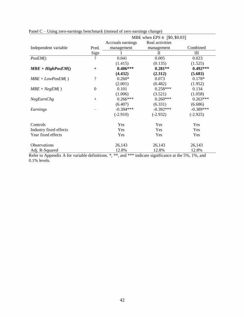
42

Panel C – Using zero-earnings benchmark (instead of zero earnings change)

MBE when EPS ∈ [$0, $0.03]


Sign

Accruals earnings

management

Real activities

management Combined

I II III

PosEM() ? 0.041 0.005 0.023

(1.415) (0.135) (1.525)

MBE × HighPosEM() + 0.406*** 0.281** 0.492***

(4.432) (2.312) (5.683)

MBE × LowPosEM( ) ? 0.260* 0.073 0.178*

(2.001) (0.482) (1.952)

MBE × NegEM( ) 0 0.101 0.258*** 0.134

(1.006) (3.521) (1.058)

NegEarnChg + 0.266*** 0.260*** 0.263***

(6.407) (6.331) (6.686)

Earnings – -0.394*** -0.392*** -0.389***

(-2.910) (-2.932) (-2.925)




Observations 26,143 26,143 26,143

Adj. R-Squared 12.8% 12.8% 12.8%

Refer to Appendix A for variable definitions. *, **, and *** indicate significance at the 5%, 1%, and

0.1% levels.

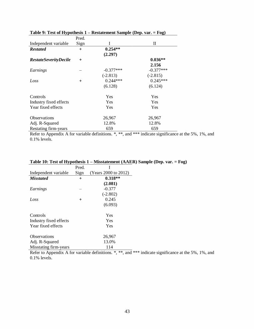
43

Table 9: Test of Hypothesis 1 – Restatement Sample (Dep. var. = Fog)

Independent variable Pred. Sign I II

Restated + 0.254**

(2.297)

RestateSeverityDecile + 0.036**

2.156

Earnings – -0.377*** -0.377***

(-2.813) (-2.815)

Loss + 0.244*** 0.245***

(6.128) (6.124)

Controls Yes Yes

Industry fixed effects Yes Yes



Adj. R-Squared 12.8% 12.8%

Restating firm-years 659 659


0.1% levels.

Table 10: Test of Hypothesis 1 – Misstatement (AAER) Sample (Dep. var. = Fog)


Pred.

Sign

I

(Years 2000 to 2012)

Misstated + 0.318**

(2.081)

Earnings – -0.377

(-2.802)

Loss + 0.245

(6.093)

Controls Yes

Industry fixed effects Yes

Year fixed effects Yes

Observations 26,967

Adj. R-Squared 13.0%

Misstating firm-years 114


0.1% levels.

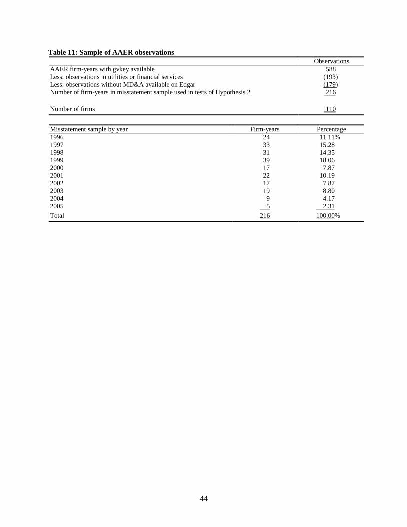
44

Table 11: Sample of AAER observations

Observations

AAER firm-years with gvkey available 588

Less: observations in utilities or financial services (193)

Less: observations without MD&A available on Edgar (179)

Number of firm-years in misstatement sample used in tests of Hypothesis 2 216

Number of firms 110

Misstatement sample by year Firm-years Percentage

1996 24 11.11%

1997 33 15.28

1998 31 14.35

1999 39 18.06

2000 17 7.87

2001 22 10.19

2002 17 7.87

2003 19 8.80

2004 9 4.17

2005 5 2.31

Total 216 100.00%

45

Table 12: Descriptive statistics for misstatement sample and Compustat population

Misstatement sample Compustat population

Misstate –

Compustat


Diff. in

means t-stat

Accruals quality variables

RSST accruals 211 0.091 0.051 26,545 0.038 0.028 0.053 2.84

Change in receivables 214 0.049 0.028 28,629 0.020 0.011 0.030 5.36

Change in inventory 213 0.025 0.000 28,498 0.008 0.000 0.017 4.51

% Soft assets 215 0.670 0.690 28,861 0.557 0.588 0.113 6.34

Performance variables

Change in cash sales 211 0.348 0.200 27,941 0.187 0.084 0.161 2.44

Change in return on assets 211 -0.010 -0.005 28,304 -0.005 0.000 -0.005 -0.39

Nonfinancial variables

Abnormal change in employees 199 -0.155 -0.077 26,271 -0.083 -0.033 -0.073 -2.08

Off-balance-sheet variables

Existence of operating leases 216 0.894 1.000 29,032 0.811 1.000 0.083 3.09

Market-related variables

Actual security issuance 216 0.972 1.000 29,032 0.868 1.000 0.104 4.52

Readability proxies

Fog 216 18.440 18.208 29,032 18.278 18.022 0.161 0.80 Length

(for info only – not used in

tests) 216 8.476 8.592 29,032 8.357 8.418 0.118 1.95

Firm-years ranging from 1996 to 2005. Refer to Appendix A for variable definitions.

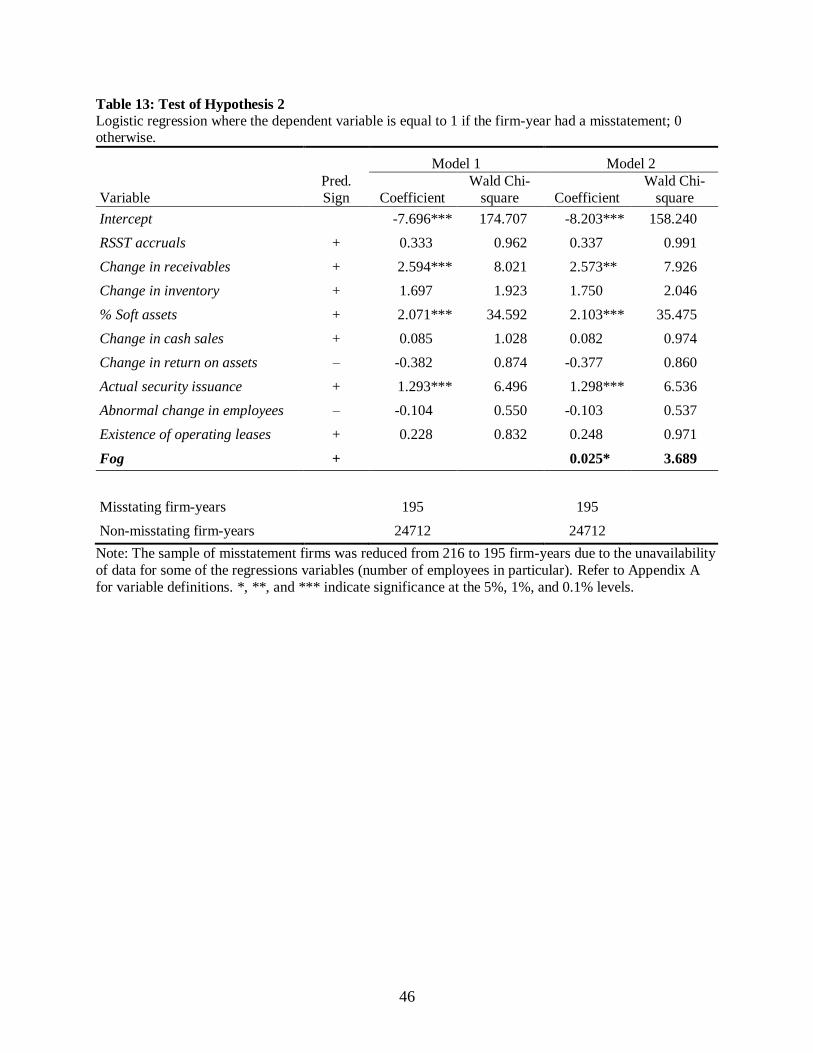
46

Table 13: Test of Hypothesis 2

Logistic regression where the dependent variable is equal to 1 if the firm-year had a misstatement; 0 otherwise.

Model 1 Model 2

Variable

Pred.

Sign Coefficient

Wald Chi-

square Coefficient

Wald Chi-

square

Intercept -7.696*** 174.707 -8.203*** 158.240

RSST accruals + 0.333 0.962 0.337 0.991

Change in receivables + 2.594*** 8.021 2.573** 7.926

Change in inventory + 1.697 1.923 1.750 2.046

% Soft assets + 2.071*** 34.592 2.103*** 35.475

Change in cash sales + 0.085 1.028 0.082 0.974

Change in return on assets – -0.382 0.874 -0.377 0.860

Actual security issuance + 1.293*** 6.496 1.298*** 6.536

Abnormal change in employees – -0.104 0.550 -0.103 0.537

Existence of operating leases + 0.228 0.832 0.248 0.971

Fog +

0.025* 3.689

Misstating firm-years 195

195

Non-misstating firm-years 24712 24712

Note: The sample of misstatement firms was reduced from 216 to 195 firm-years due to the unavailability

of data for some of the regressions variables (number of employees in particular). Refer to Appendix A

for variable definitions. *, **, and *** indicate significance at the 5%, 1%, and 0.1% levels.

Documents

Earnings Management and Annual Report Readability · Earnings Management and Annual Report ... Earnings management and annual report readability ... we may soon be looking to the