Earnings volatility and earnings predictability

ARTICLE IN PRESS

Contents lists available at ScienceDirect

Journal of Accounting and Economics

Journal of Accounting and Economics 47 (2009) 160–181

0165-41

doi:10.1

� Cor

E-m

journal homepage: www.elsevier.com/locate/jae

Earnings volatility and earnings predictability

Ilia D. Dichev a,�, Vicki Wei Tang b

a Stephen M. Ross School of Business, University of Michigan, 701 Tappan St., Ann Arbor, MI 48109, USAb McDonough School of Business, Georgetown University, USA

a r t i c l e i n f o

Article history:

Received 8 March 2007

Received in revised form

23 September 2008

Accepted 24 September 2008Available online 1 November 2008

JEL classification:

M41

G17

Keywords:

Earnings volatility

Earnings predictability

Analyst forecasts

Fundamental analysis

01/$ - see front matter & 2008 Elsevier B.V. A

016/j.jacceco.2008.09.005

responding author. Tel.: +1734 647 2842.

ail address: [email protected] (I.D. Dichev).

a b s t r a c t

Survey evidence indicates widely held managerial beliefs that earnings volatility is

negatively related to earnings predictability. In addition, existing research suggests that

earnings volatility is determined by economic and accounting factors, and both of these

factors reduce earnings predictability. We find that the consideration of earnings

volatility brings substantial improvements in the prediction of both short- and long-

term earnings. Conditioning on volatility information also allows one to identify

systematic errors in analyst forecasts, which implies that analysts do not fully

understand the implications of earnings volatility for earnings predictability.

& 2008 Elsevier B.V. All rights reserved.

1. Introduction

This study investigates the link between earnings volatility and earnings predictability. The motivation for this topiccomes from several sources. First, a number of applications require the prediction of earnings (e.g., equity valuation) whileour knowledge in this area remains limited, especially for long-run forecasts of earnings. Second, recent survey evidencereveals widely held managerial beliefs that earnings volatility reduces earnings predictability (Graham et al., 2005). Thisstudy is a test of the validity and utility of these beliefs. Third, existing findings offer some conjectures about themechanism that drives the relation between earnings volatility and earnings predictability. We view earnings volatility asarising from two factors, volatility due to economic shocks and volatility due to problems in the accounting determinationof income, and both of these factors reduce the predictability of earnings. We present a simple theoretical framework thatoperationalizes these concepts, and link them to the empirical tests that follow.

The empirical specifications focus on establishing the relation between earnings volatility and short- and long-termearnings predictability. To alleviate concerns about a mechanical relation, we use pre-determined measures of volatility topartition the data into volatility quintiles and then use prospective data to estimate earnings predictability. The short-termspecifications indicate that low-volatility earnings have much higher persistence as compared to high-volatility earnings,for a range of persistence of 0.93 vs. 0.51 across quintile portfolios. We also find that the strength of the earnings volatilityeffect exceeds that of several plausible benchmarks, including cash flows volatility, the accrual effect from Sloan (1996) andthe extreme-earnings mean-reversion effect from Freeman et al. (1982). The results from the long-run tests indicate that

ll rights reserved.

www.sciencedirect.com/science/journal/jae

www.elsevier.com/locate/jae

dx.doi.org/10.1016/j.jacceco.2008.09.005

mailto:[email protected]

ARTICLE IN PRESS

I.D. Dichev, V.W. Tang / Journal of Accounting and Economics 47 (2009) 160–181 161

earnings volatility has substantial predictive power for up to 5 years in the future. Earnings with low volatility haveremarkably high persistence and R2 during the entire predictive horizon, while earnings with high volatility show quickreversion to the mean and little reliable predictability. We also document that the results remain qualitatively the sameafter controlling for two correlated and competing explanations. First, volatile earnings tend to be extreme earnings, andextreme earnings tend to mean-revert faster (e.g., Freeman et al., 1982), which implies an alternative explanation for whyvolatile earnings are less persistent. However, the results remain largely unchanged after a control for the level of earnings.Second, volatile earnings are more likely to include transitory items, and since transitory items are less persistent, thedocumented relation between earnings volatility and earnings predictability could be an artifact of the effect of transitoryitems. However, the tenor of the results remains the same after controlling for transitory items. A number of additionalchecks confirm the robustness of the documented relations.

Finally, we investigate whether financial information users understand the implications of earnings volatility forearnings predictability. We use analysts’ forecasts as a proxy for sophisticated users’ expectation of earnings. We find thatconditioning on earnings volatility information allows one to identify large and predictable errors in analysts’ forecasts,which suggests that analysts do not fully understand the implications of earnings volatility for future earnings. Inquantitative terms, we estimate that analysts impound less than half of the full implications of earnings volatility forearnings predictability.

The remainder of the paper is organized as follows. Section 2 presents the theory of the paper. Section 3 presents themain empirical tests and results, Section 4 contains robustness checks and additional results, and Section 5 presents theresults for analyst forecasts tests. Section 6 concludes.

2. Theory and relation to existing research

A number of important applications of accounting data require the prediction of earnings. For example, valuationresearch and practice typically use projections of earnings to derive estimates of firm and equity value. In fact, existingexperience with valuation models like DCF and residual-income suggests that the conceptual differences betweenvaluation models are not that important; what really matters is the extent to which these models help in the empiricalprojection of future fundamentals, usually based on projected future earnings. A related application is the use of accountingdata to derive and possibly improve on analysts’ earnings forecasts. On the one hand, analysts are continually looking fornew ways to more accurately predict earnings. On the other hand, investors are interested in ways in which they canidentify biases in analysts’ forecasts and improve on the accuracy of existing forecasts. On a more general level, suchapplications and needs are related to the rise of ‘‘fundamental analysis’’ research in accounting, where fundamentalanalysis can be defined as identifying ways to use accounting data to produce superior forecasts of earnings (e.g., Nissimand Penman, 2001).

Given these needs, our knowledge about the predictability of earnings is limited, especially for long-term predictability.There are a number of useful models and results for 1-year-ahead forecasts, e.g., mean reversion, the Foster (1977) model ofquarterly earnings, the accrual effect due to Sloan (1996), and the fundamental analysis signals due to Lev and Thiagarajan(1993) and investigated in Abarbanell and Bushee (1997). In contrast, there are few useful long-term results. This dearth ofresults seems unsatisfactory because some key applications (e.g., equity valuation) require long-term forecasts of earnings,and it is the accuracy of the forecasts which drives the success of these applications. In fact, the typical projection of long-term earnings relies only on mean reversion, and the only real differences between various empirical specifications areabout what the eventual ‘‘steady-state’’ mean is, and about the rate of fading to that mean. Thus, in spite of somecontributions in this area due to Finger (1994) and Penman and Zhang (2002), our knowledge about the long-termpredictability of earnings remains rudimentary.

We aim to enhance the knowledge in this area by investigating the relation between earnings volatility and earningspredictability. Our motivation stems from several sources which suggest that earnings volatility captures aspects of thedetermination of earnings which are related to the predictability of earnings. First, recent survey evidence offers strongmotivation for the link between earnings volatility and earnings predictability. Graham et al. (2005) survey 401 financialexecutives to determine the key factors that drive decisions related to reported earnings and find a pronounced aversion toearnings volatility (97% of respondents express a preference for smooth earnings). In exploring the reasons for this finding,the authors find that executives abhor volatility because it is thought to reduce the predictability of earnings (80% ofrespondents express this belief). Thus, our investigation is a test of widely held managerial beliefs that earnings volatility isnegatively related to earnings predictability. The investigation also helps to map out the specific content of this relation.The survey evidence leaves little doubt that executives believe that more volatile earnings are less predictable. However, itis less clear what the executives have in mind by ‘‘predictable’’, and it is possible that the executives view these concepts assemantic or tautological opposites, so to them the relation obtains by construction. The analysis later provides a frameworkfor defining and operationalizing the difference between these concepts, which is then reflected in the empirical tests.

Although the survey evidence does not provide clues about the specific mechanism relating earnings volatility toearnings predictability, we posit that this relation is due to both economic and accounting factors. On the more obviouslevel, earnings volatility captures the effects of real and unavoidable economic volatility. Intuitively, firms operating inenvironments subject to large economic shocks are likely to have both more volatile earnings and less predictable earnings.

ARTICLE IN PRESS

I.D. Dichev, V.W. Tang / Journal of Accounting and Economics 47 (2009) 160–181162

Although the theory about this link seems straightforward, there is little empirical evidence about it. To our knowledge,only Lipe (1990) explores the relation between economic volatility and earnings predictability in a short-horizon setting.However, this relation is a side issue for Lipe (1990) and from his evidence it is difficult to gauge the economic and long-term importance of this relation.

On a more subtle level, the volatility of reported earnings also reflects important aspects of the accountingdetermination of income, which also provide a link to earnings predictability. One such aspect is the quality of matching ofexpenses to revenues, as modeled in Dichev and Tang (2008). The basic idea in Dichev and Tang is that poor matching actsas noise in the economic relation between revenues and expenses, and thus the volatility of reported earnings increases inpoor matching. Poor matching is also associated with poor earnings predictability because the matching noise in reportedearnings obscures the underlying economic relation that governs the evolution of earnings over successive periods. Thus,the joint effect of poor matching on earnings volatility and earnings predictability suggests another link between these twovariables. The quality of accruals effect in Dechow and Dichev (2002) is another aspect of the determination of earningswhich provides an accounting link between earnings volatility and earnings predictability. Dechow and Dichev argue thatmany accruals estimate future cash flows, and therefore large magnitudes of estimation errors in accruals signal lowerquality of earnings and lower predictability of earnings. Since estimation errors are likely to be more serious in volatileenvironments, this suggests a negative relation between earnings volatility and earnings predictability.

It is also possible that the link between earnings volatility and earnings predictability reflects other factors, e.g.,earnings smoothing behavior, where managers smooth earnings to provide a more predictable measure of firmperformance. In any case, for our purposes the distinction among plausible causes is not that important because the focus ison investigating for the existence and the economic importance of the relation between earnings volatility and earningspredictability, rather than on its explanations. Later, we provide evidence on the relative role of common economic andaccounting factors in the documented relations.

We start our investigation with some theoretical considerations. The goal is to provide a simple framework thatformalizes the preceding motivations and link them to the empirical analysis that follows. Our analysis of the relationbetween earnings volatility and earnings predictability relies on commonly used autoregressive regressions of current on1-year lagged earnings:

Et ¼ aþ bEt�1 þ � (1)

Taking the variance of both sides yields

VarðEtÞ ¼ b2 VarðEt�1Þ þ Varð�Þ (2)

Assuming that the variance of earnings is stationary over time,1 and re-arranging obtains

Varð�Þ ¼ VarðEÞð1� b2Þ (3)

Expression (3) is a useful summary of the key variables and relations of our study. Var(E) is our proxy for volatility ofearnings. Var(e) is our (inverse) proxy for ‘‘earnings predictability’’, because the variance of the error term captures thevariation in earnings remaining after accounting for the effect of the autoregressive coefficient, b.

Eq. (3) is also a useful guide to the mechanism of the link between earnings volatility and earnings predictability,revealing a two-fold relation. First, holding earnings persistence constant, earnings volatility is inversely related to earningspredictability. Second, this negative relation is likely strengthened through the effect of the persistence coefficient because,as discussed above, there are reasons to believe that b itself is negatively related to volatility of earnings. For example,economic or accounting noise in earnings is likely to both increase the volatility of earnings and decrease the persistence ofearnings. Note that there is no statistical reason to expect a relation between Var(E) and b. The volatility of theautoregressive variable can be high or low, and it has no necessary relation to persistence. To illustrate this point, considerthe behavior of stock prices. Under the maintained assumption of market efficiency, stock prices are random walks, andthus, the persistence of the autoregressive relation in prices is always one, regardless of the volatility of the stock.

To formally examine the mechanism of the link between earnings volatility and earnings predictability, we take the totalderivative of the variance of the error term with respect to earnings volatility. Using expression (3), and denoting total(partial) derivative as d (d), yields

d½Varð�Þ�=dVarðEÞ ¼ ð1� b2Þ � 2VarðEÞðdb=dVarðEÞÞ (4)

The first term in Eq. (4) suggests that the strength of the direct relation between earnings volatility and earningspredictability is determined by earnings persistence, where higher persistence signifies more predictable earnings. Thesecond term in Eq. (4) represents the second link between earnings volatility and earnings predictability through the effectof earnings volatility on earnings persistence. More specifically, the hypothesized negative effect of earnings volatility onearnings persistence should reinforce the base negative relation between earnings volatility and earnings predictability.

1 Existing research indicates that the volatility of earnings has approximately doubled over the last 40 years, see Givoly and Hayn (2000) and Dichev

and Tang (2008). However, the stationarity argument holds reasonably well for the 1-year horizon used here.

ARTICLE IN PRESS


Note that the notion of predictability captured in Var(e) is ‘‘absolute’’ predictability, unadjusted for volatility in theearnings environment. If one is interested in ‘‘relative’’ predictability, a natural scalar for Var(e) is Var(E). Taking (3),dividing it by Var(E), and re-arranging leads to

1� Varð�Þ=VarðEÞ ¼ b2 (5)

Expression (5) simply says that relative predictability is the R2 of the regression, which is equal to the squaredpersistence coefficient. Thus, identifying the relation between earnings volatility and earnings persistence is a key to ourinvestigation of both absolute and relative earnings predictability.

We use the insights from this framework in the empirical tests on two dimensions. First, we map out the economicimportance of the conjectured negative relation between earnings volatility and short- and long-term earnings persistence.Second, we investigate whether and how the use of earnings volatility information leads to appreciable gains in earningspredictability. Specifically, in out-of-sample tests we investigate whether conditioning on earnings volatility informationleads to lower prediction errors as compared to other popular models of earnings prediction. In further tests, we checkwhether analyst forecasts impound the implications of earnings volatility information by investigating whetherconditioning on volatility information allows one to identify systematic errors in analyst forecasts.

The exploration of the link between earnings volatility and earnings predictability seems warranted because we are notaware of other studies that provide a direct and comprehensive investigation of this relation. Minton et al. (2002) use anunderinvestment motivation and find that firms with high cash flow volatility have lower levels of future cash flows andearnings. Note that this is different from our prediction that high earnings volatility results in lower persistence andpredictability in future earnings. Thus, the Minton et al. effect and our effect are complementary, and in fact we illustratehow to combine these two effects later in our study.

3. Main empirical tests

3.1. Sample selection, descriptive statistics, and test specification

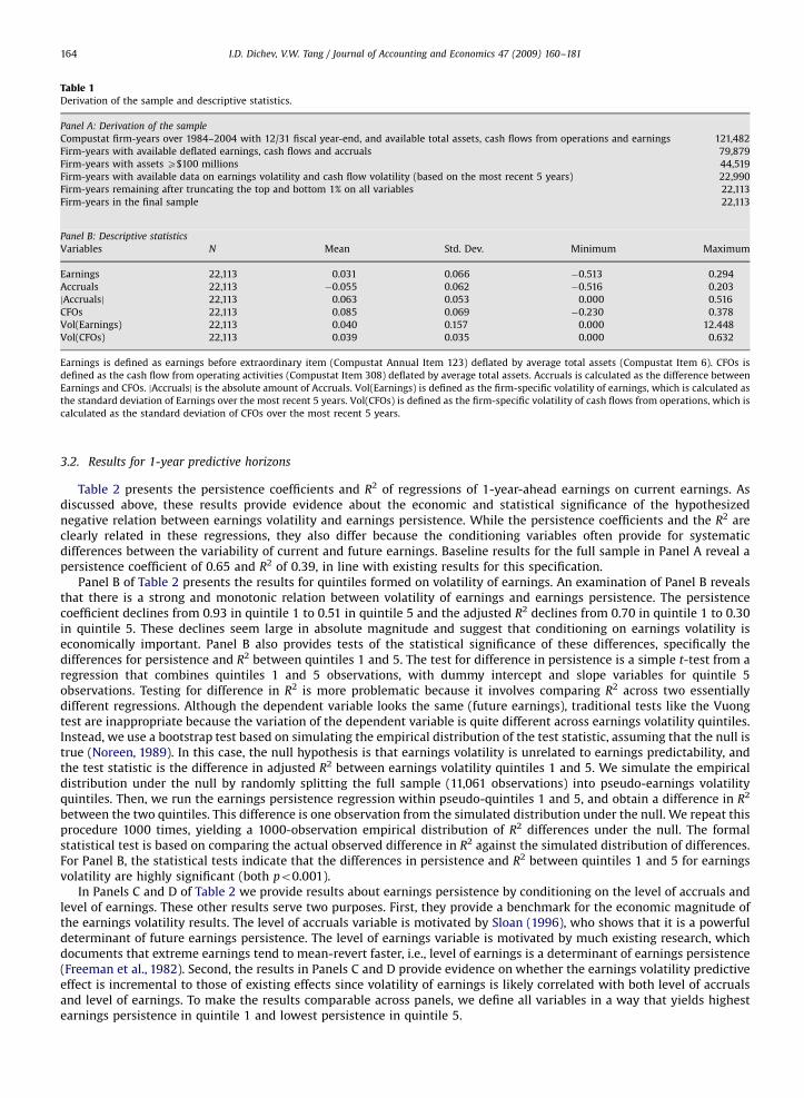
Table 1, Panel A summarizes the sample selection. Our sample is obtained from the Compustat annual industrial andresearch files over 1984–2004. We restrict the sample to this period because we need cash flow statement data for theaccurate estimation of accruals and cash flows (Collins and Hribar, 2002). Cash flow statements become widely availablesince 1988, and we use the preceding years over 1984–1988 to calculate the volatility of earnings. The sample is restrictedto firm-years with complete data for assets (Compustat Item 6), earnings (item 123), cash flow from operations (item 308),and preceding 4 years of earnings and cash flows from operations. Accruals are estimated by taking the difference betweenearnings and cash flows from operations. Earnings, accruals and cash flow from operations (CFO) are deflated using averageassets.2 Earnings volatility is calculated by taking the standard deviation of the deflated earnings for the most recent5 years (the tenor of the results remains the same if the earnings volatility variable is based on the 5 years of earningspreceding the current year). Cash flow volatility is calculated by taking the standard deviation of the deflated cash flows forthe most recent 5 years. To avoid the influence of extreme observations, we truncate the top and bottom 1% of earnings,accruals and cash flows from operations. In addition to these fairly common sample selection criteria, we imposetwo additional requirements. First, we limit the sample to economically substantial firms, defined as a minimum of$100 million in assets. Our concern is that small firms tend to be economically negligible but statistically influential(because of extreme realizations). Second, we limit the sample to 12/31 fiscal year-end firms to simplify the tests and theinterpretation of the results. Later, we provide some evidence on the effect of these restrictions on our results. After allrequirements, the final sample includes 22,113 firm-years over 1988–2004.

Descriptive statistics for the full sample are presented in Table 1, Panel B. The results are in line with much otherresearch that explores similar variables and time period. Cash flow from operations is typically higher than earnings (meanof 8.5% vs. 3.1%), and accruals are negative (mean of �5.5%). Firm-specific volatility of scaled earnings has a mean of 4.0%and a large standard deviation of 15.7%, indicating large differences in earnings volatility across firms. The descriptivestatistics for volatility of earnings also reveal that this variable has a highly non-normal distribution, bounded at 0 on theleft and heavily right skewed. To address such non-linearities and aiming for a more robust estimation in general, much ofthe subsequent analysis relies on quintile portfolios formed on conditioning variables, mainly volatility of earnings. Theportfolio-based analysis also provides an immediate and clear reflection of the economic importance of the results.

Firms in the full sample are randomly assigned into two sub-samples. We use the first sub-sample(observations ¼ 11,061) for a comprehensive exploratory analysis of the predictive power of earnings volatility forearnings predictability, while the second sub-sample (observations ¼ 11,052) is used to perform out-of-sample tests offorecasting accuracy.

2 Results are similar using an undeflated (EPS) specification. Results using a price deflator have the same tenor but are substantially weaker than

those using an asset deflator, possibly because price itself is a function of earnings rather than being a neutral deflator.

ARTICLE IN PRESS

Table 1Derivation of the sample and descriptive statistics.

Panel A: Derivation of the sample

Compustat firm-years over 1984–2004 with 12/31 fiscal year-end, and available total assets, cash flows from operations and earnings 121,482

Firm-years with available deflated earnings, cash flows and accruals 79,879

Firm-years with assets X$100 millions 44,519

Firm-years with available data on earnings volatility and cash flow volatility (based on the most recent 5 years) 22,990

Firm-years remaining after truncating the top and bottom 1% on all variables 22,113

Firm-years in the final sample 22,113

Panel B: Descriptive statistics

Variables N Mean Std. Dev. Minimum Maximum

Earnings 22,113 0.031 0.066 �0.513 0.294

Accruals 22,113 �0.055 0.062 �0.516 0.203

jAccrualsj 22,113 0.063 0.053 0.000 0.516

CFOs 22,113 0.085 0.069 �0.230 0.378

Vol(Earnings) 22,113 0.040 0.157 0.000 12.448

Vol(CFOs) 22,113 0.039 0.035 0.000 0.632

Earnings is defined as earnings before extraordinary item (Compustat Annual Item 123) deflated by average total assets (Compustat Item 6). CFOs is

defined as the cash flow from operating activities (Compustat Item 308) deflated by average total assets. Accruals is calculated as the difference between

Earnings and CFOs. jAccrualsj is the absolute amount of Accruals. Vol(Earnings) is defined as the firm-specific volatility of earnings, which is calculated as

the standard deviation of Earnings over the most recent 5 years. Vol(CFOs) is defined as the firm-specific volatility of cash flows from operations, which is

calculated as the standard deviation of CFOs over the most recent 5 years.


3.2. Results for 1-year predictive horizons

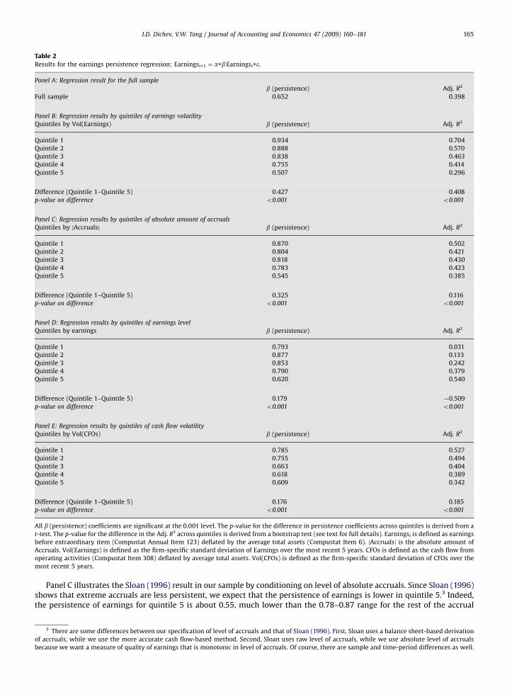
Table 2 presents the persistence coefficients and R2 of regressions of 1-year-ahead earnings on current earnings. Asdiscussed above, these results provide evidence about the economic and statistical significance of the hypothesizednegative relation between earnings volatility and earnings persistence. While the persistence coefficients and the R2 areclearly related in these regressions, they also differ because the conditioning variables often provide for systematicdifferences between the variability of current and future earnings. Baseline results for the full sample in Panel A reveal apersistence coefficient of 0.65 and R2 of 0.39, in line with existing results for this specification.

Panel B of Table 2 presents the results for quintiles formed on volatility of earnings. An examination of Panel B revealsthat there is a strong and monotonic relation between volatility of earnings and earnings persistence. The persistencecoefficient declines from 0.93 in quintile 1 to 0.51 in quintile 5 and the adjusted R2 declines from 0.70 in quintile 1 to 0.30in quintile 5. These declines seem large in absolute magnitude and suggest that conditioning on earnings volatility iseconomically important. Panel B also provides tests of the statistical significance of these differences, specifically thedifferences for persistence and R2 between quintiles 1 and 5. The test for difference in persistence is a simple t-test from aregression that combines quintiles 1 and 5 observations, with dummy intercept and slope variables for quintile 5observations. Testing for difference in R2 is more problematic because it involves comparing R2 across two essentiallydifferent regressions. Although the dependent variable looks the same (future earnings), traditional tests like the Vuongtest are inappropriate because the variation of the dependent variable is quite different across earnings volatility quintiles.Instead, we use a bootstrap test based on simulating the empirical distribution of the test statistic, assuming that the null istrue (Noreen, 1989). In this case, the null hypothesis is that earnings volatility is unrelated to earnings predictability, andthe test statistic is the difference in adjusted R2 between earnings volatility quintiles 1 and 5. We simulate the empiricaldistribution under the null by randomly splitting the full sample (11,061 observations) into pseudo-earnings volatilityquintiles. Then, we run the earnings persistence regression within pseudo-quintiles 1 and 5, and obtain a difference in R2

between the two quintiles. This difference is one observation from the simulated distribution under the null. We repeat thisprocedure 1000 times, yielding a 1000-observation empirical distribution of R2 differences under the null. The formalstatistical test is based on comparing the actual observed difference in R2 against the simulated distribution of differences.For Panel B, the statistical tests indicate that the differences in persistence and R2 between quintiles 1 and 5 for earningsvolatility are highly significant (both po0.001).

In Panels C and D of Table 2 we provide results about earnings persistence by conditioning on the level of accruals andlevel of earnings. These other results serve two purposes. First, they provide a benchmark for the economic magnitude ofthe earnings volatility results. The level of accruals variable is motivated by Sloan (1996), who shows that it is a powerfuldeterminant of future earnings persistence. The level of earnings variable is motivated by much existing research, whichdocuments that extreme earnings tend to mean-revert faster, i.e., level of earnings is a determinant of earnings persistence(Freeman et al., 1982). Second, the results in Panels C and D provide evidence on whether the earnings volatility predictiveeffect is incremental to those of existing effects since volatility of earnings is likely correlated with both level of accrualsand level of earnings. To make the results comparable across panels, we define all variables in a way that yields highestearnings persistence in quintile 1 and lowest persistence in quintile 5.

ARTICLE IN PRESS

Table 2

Results for the earnings persistence regression: Earningst+1 ¼ a+bEarningst+e.

Panel A: Regression result for the full sample

b (persistence) Adj. R2

Full sample 0.652 0.398

Panel B: Regression results by quintiles of earnings volatility

Quintiles by Vol(Earnings) b (persistence) Adj. R2

Quintile 1 0.934 0.704

Quintile 2 0.888 0.570

Quintile 3 0.838 0.463

Quintile 4 0.755 0.414

Quintile 5 0.507 0.296

Difference (Quintile 1–Quintile 5) 0.427 0.408

p-value on difference o0.001 o0.001

Panel C: Regression results by quintiles of absolute amount of accruals

Quintiles by jAccrualsj b (persistence) Adj. R2

Quintile 1 0.870 0.502

Quintile 2 0.804 0.421

Quintile 3 0.818 0.430

Quintile 4 0.783 0.423

Quintile 5 0.545 0.385



Panel D: Regression results by quintiles of earnings level

Quintiles by earnings b (persistence) Adj. R2

Quintile 1 0.793 0.031

Quintile 2 0.877 0.133

Quintile 3 0.853 0.242

Quintile 4 0.790 0.379

Quintile 5 0.620 0.540

Difference (Quintile 1–Quintile 5) 0.179 �0.509


Panel E: Regression results by quintiles of cash flow volatility

Quintiles by Vol(CFOs) b (persistence) Adj. R2

Quintile 1 0.785 0.527

Quintile 2 0.755 0.494

Quintile 3 0.663 0.404

Quintile 4 0.618 0.389

Quintile 5 0.609 0.342



All b (persistence) coefficients are significant at the 0.001 level. The p-value for the difference in persistence coefficients across quintiles is derived from a

t-test. The p-value for the difference in the Adj. R2 across quintiles is derived from a bootstrap test (see text for full details). Earningst is defined as earnings

before extraordinary item (Compustat Annual Item 123) deflated by the average total assets (Compustat Item 6). jAccrualsj is the absolute amount of

Accruals. Vol(Earnings) is defined as the firm-specific standard deviation of Earnings over the most recent 5 years. CFOs is defined as the cash flow from

operating activities (Compustat Item 308) deflated by average total assets. Vol(CFOs) is defined as the firm-specific standard deviation of CFOs over the

most recent 5 years.


Panel C illustrates the Sloan (1996) result in our sample by conditioning on level of absolute accruals. Since Sloan (1996)shows that extreme accruals are less persistent, we expect that the persistence of earnings is lower in quintile 5.3 Indeed,the persistence of earnings for quintile 5 is about 0.55, much lower than the 0.78–0.87 range for the rest of the accrual

3 There are some differences between our specification of level of accruals and that of Sloan (1996). First, Sloan uses a balance sheet-based derivation

of accruals, while we use the more accurate cash flow-based method. Second, Sloan uses raw level of accruals, while we use absolute level of accruals

because we want a measure of quality of earnings that is monotonic in level of accruals. Of course, there are sample and time-period differences as well.

ARTICLE IN PRESS


quintiles. R2 for quintile 5 is also lower, and both the persistence and the R2 differences across extreme quintiles arestatistically significant. Turning to a comparison of the results across Panels B and C, we find that the decline in persistenceacross earnings volatility quintiles (0.43) is moderately higher than the decline for the accrual quintiles (0.33). The samepattern of results is observed for R2 but the decline in R2 across earnings volatility quintiles (0.41) is much larger than thecorresponding decline for the accrual quintiles (0.12).

We also perform bootstrap tests for the statistical significance of the across-quintile differences across panels, e.g., is theacross-quintiles difference in persistence in Panel B (0.43) greater than the across-quintile difference in Panel C (0.33).Specifically, the tests construct random pseudo-earnings volatility quintiles, run regressions within the quintiles, andobtain a difference in persistence and R2 across quintiles. Then another pseudo-level of accruals simulation is run andacross-the-panels differences in persistence and R2 are produced.4 This procedure is repeated 1000 times, and the actualdifferences are compared to the simulated distribution of differences. The results indicate that the difference in persistenceranges across Panels B and C (0.43 vs. 0.33) has a p-value of 0.009 and the difference in R2 ranges (0.41 vs. 0.13) has ap-value o0.001. Summarizing, a comparison of the results across Panels B and C suggests that earnings volatility dominateslevel of accruals in terms of predictive power.5

Panel D presents the results for level of earnings quintiles. Earnings are first sorted on their magnitude into deciles 1–10,and then the deciles are combined into quintiles, where deciles 1 and 10 form quintile 5, deciles 2 and 9 form quintile 4,and so on. Since quintile 5 comprises the most extreme earnings, we expect it to have the least persistent earnings; theopposite holds for quintile 1. Indeed, an inspection of Panel D reveals that the persistence of earnings decreases acrossquintiles, from 0.79 in quintile 1 to 0.62 in quintile 5. However, the resulting range of 0.18 is much smaller than thecorresponding range of 0.43 for earnings volatility, and this difference has a p-value o0.001 in bootstrap tests ofsignificance. Thus, these results suggest that the earnings volatility effect cannot be subsumed by the level of earningseffect in earnings predictability. We provide further and more specific evidence about the incremental effect of these twovariables in the section on long-run earnings predictability. Also, note the pattern in R2 goes in the opposite direction,decreasing from 0.54 in quintile 5 to 0.03 in quintile 1, which at first seems surprising. Further reflection suggest that this isto be expected, given that R2

¼ b2 Var(Et)/Var(Et+1) and that by construction the variance of the independent variable ismuch more limited for the lower quintiles in Panel D.

Panel E presents results for one more conditioning variable, volatility of cash flows, which serves as a proxy foreconomic volatility. Recall that Section 2 suggests that one advantage of the earnings volatility variable is that it combinesthe explanatory power of both economic volatility and accounting problems-based volatility with respect to earningspredictability. If this conjecture is true, we expect that earnings volatility has higher explanatory power than cash flowvolatility with respect to earnings predictability. An examination of Panel E reveals that volatility of cash flows provides agood ranking on earnings predictability, with range in persistence of 0.18 and range in R2 of 0.19. However, the ranges inpersistence and R2 for the earnings volatility variable in Panel B are more than double those in Panel E and the across-paneldifferences in persistence and R2 have highly significant p-values. Thus, the results in Panel E suggest that earningsvolatility dominates cash flow volatility with respect to earnings predictability. Having in mind that the volatility of cashflows is similar in magnitude to the volatility of earnings (see Table 1, Panel B), this result implies that the volatility inearnings due to the accounting process is important in relation to earnings predictability. In additional untabulated tests,we use sales volatility as another proxy for economic volatility and find that the results for sales volatility are similar tothose for cash flow volatility.

3.3. Results for 5-year predictive horizons

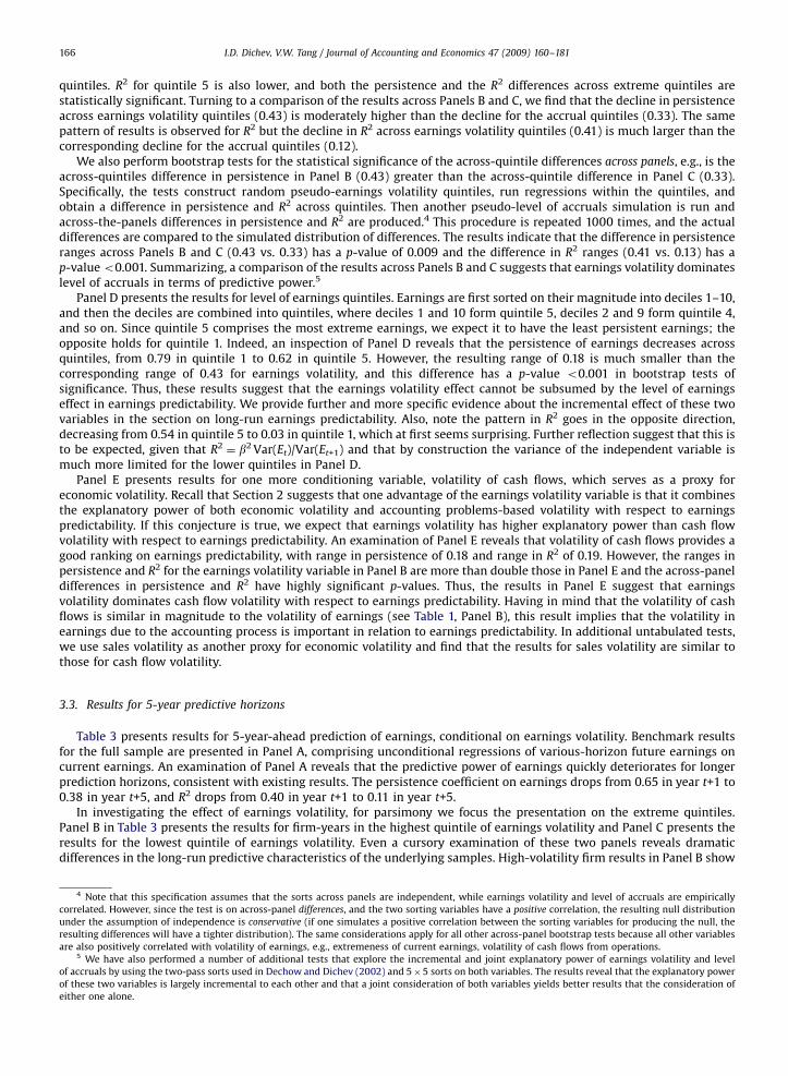
Table 3 presents results for 5-year-ahead prediction of earnings, conditional on earnings volatility. Benchmark resultsfor the full sample are presented in Panel A, comprising unconditional regressions of various-horizon future earnings oncurrent earnings. An examination of Panel A reveals that the predictive power of earnings quickly deteriorates for longerprediction horizons, consistent with existing results. The persistence coefficient on earnings drops from 0.65 in year t+1 to0.38 in year t+5, and R2 drops from 0.40 in year t+1 to 0.11 in year t+5.

In investigating the effect of earnings volatility, for parsimony we focus the presentation on the extreme quintiles.Panel B in Table 3 presents the results for firm-years in the highest quintile of earnings volatility and Panel C presents theresults for the lowest quintile of earnings volatility. Even a cursory examination of these two panels reveals dramaticdifferences in the long-run predictive characteristics of the underlying samples. High-volatility firm results in Panel B show

4 Note that this specification assumes that the sorts across panels are independent, while earnings volatility and level of accruals are empirically

correlated. However, since the test is on across-panel differences, and the two sorting variables have a positive correlation, the resulting null distribution

under the assumption of independence is conservative (if one simulates a positive correlation between the sorting variables for producing the null, the

resulting differences will have a tighter distribution). The same considerations apply for all other across-panel bootstrap tests because all other variables

are also positively correlated with volatility of earnings, e.g., extremeness of current earnings, volatility of cash flows from operations.5 We have also performed a number of additional tests that explore the incremental and joint explanatory power of earnings volatility and level

of accruals by using the two-pass sorts used in Dechow and Dichev (2002) and 5�5 sorts on both variables. The results reveal that the explanatory power

of these two variables is largely incremental to each other and that a joint consideration of both variables yields better results that the consideration of

either one alone.

ARTICLE IN PRESS

Table 3The implications of earnings volatility for long-term earnings.

b Adj. R2 Number of observations

Panel A: Regression results for the full sample

Earningst+1 ¼ a+bEarningst 0.652 0.398 9102





Panel B: Regression results for the highest earnings volatility quintile






Panel C: Regression results for the lowest earnings volatility quintile






Panel D: Regression results for the highest earnings volatility quintile, controlling for the level of current earnings






Panel E: Regression results for the lowest earnings volatility quintile, controlling for the level of current earnings






All b coefficients are statistically significant at the 0.001 level. Earnings is defined as earnings before extraordinary item (Compustat Annual Item 123)

deflated by average total assets (Compustat Item 6). Vol(Earnings) is the firm-specific standard deviation of Earnings over the most recent 5 years.

Earningst is current year Earning, Earningst+1 is the one-year ahead Earnings, and so on..


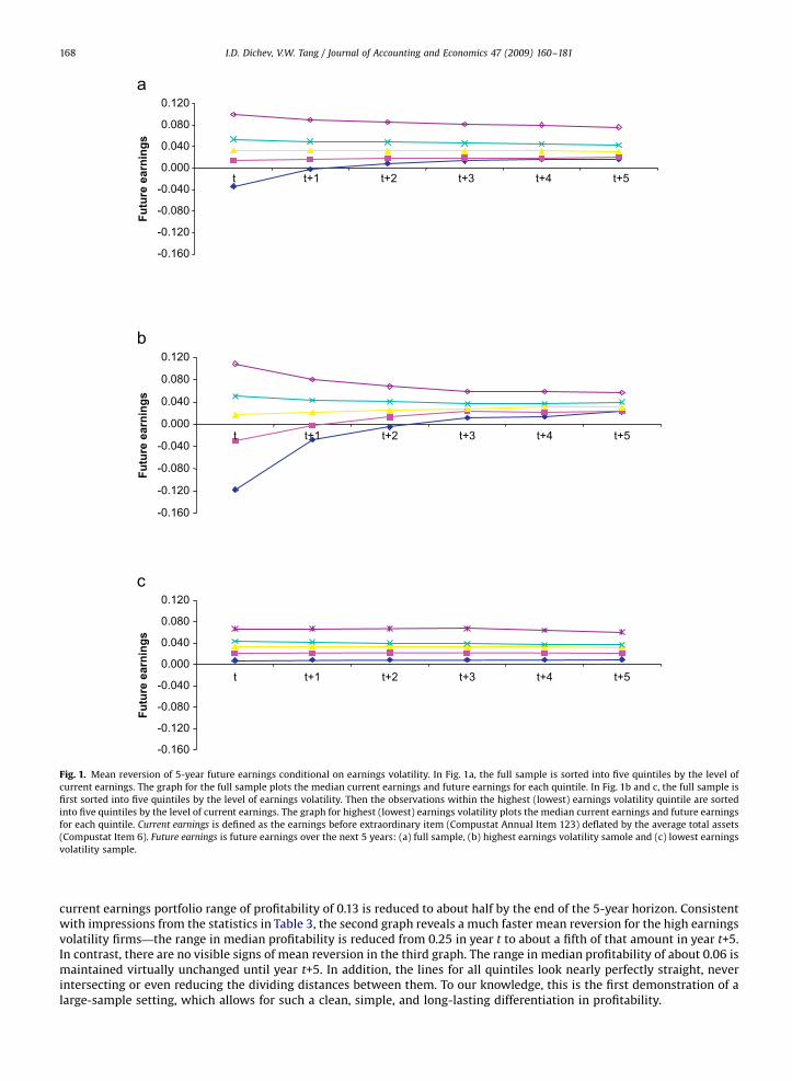
a quick deterioration of persistence (0.51–0.18) and R2 (0.30–0.03) over the 5-year predictive horizon, where at all timehorizons the numbers in Panel B are lower than those in Panel A. In contrast, the results for low-volatility firms in Panel Creveal a robust predictive power over the entire 5-year horizon. The persistence coefficient is high in year t+1 (0.93) anddeteriorates only modestly to 0.81 in year t+5. The erosion in R2 is more substantial (0.70–0.32) but in terms of absolutemagnitude even for year t+5 one retains a considerable amount of confidence in the prediction of earnings. In fact, a literalreading of these numbers implies that it is easier to predict earnings 5 years ahead for low-volatility firms than to predictearnings 1 year ahead for high volatility or even all firms. The combined pattern of these results suggests that earningsvolatility has a remarkable differentiating power in the long-run prediction of earnings.6

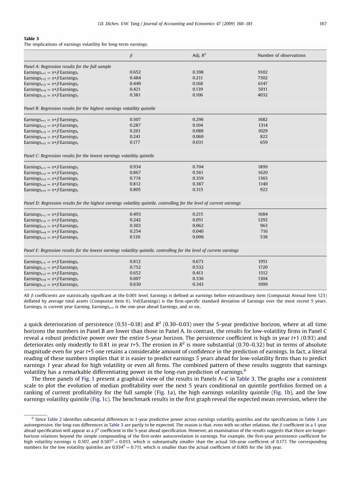
The three panels of Fig. 1 present a graphical view of the results in Panels A–C in Table 3. The graphs use a consistentscale to plot the evolution of median profitability over the next 5 years conditional on quintile portfolios formed on aranking of current profitability for the full sample (Fig. 1a), the high earnings volatility quintile (Fig. 1b), and the lowearnings volatility quintile (Fig. 1c). The benchmark results in the first graph reveal the expected mean reversion, where the

6 Since Table 2 identifies substantial differences in 1-year predictive power across earnings volatility quintiles and the specifications in Table 3 are

autoregressive, the long-run differences in Table 3 are partly to be expected. The reason is that, even with no other relations, the b coefficient in a 1-year

ahead specification will appear as a b5 coefficient in the 5-year ahead specification. However, an examination of the results suggests that there are longer-

horizon relations beyond the simple compounding of the first-order autocorrelation in earnings. For example, the first-year persistence coefficient for

high volatility earnings is 0.507, and 0.5075¼ 0.033, which is substantially smaller than the actual 5th-year coefficient of 0.177. The corresponding

numbers for the low volatility quintiles are 0.9345¼ 0.711, which is smaller than the actual coefficient of 0.805 for the 5th year.

ARTICLE IN PRESS

-0.160

-0.120

-0.080

-0.040

0.000

0.040

0.080

0.120

Futu

re e

arni

ngs

-0.160

-0.120

-0.080

-0.040

0.000

0.040

0.080

0.120

t t+1

Futu

re e

arni

ngs

-0.160

-0.120

-0.080

-0.040

0.000

0.040

0.080

0.120

Futu

re e

arni

ngs

t+2 t+3 t+4 t+5

t t+1 t+2 t+3 t+4 t+5

t t+1 t+2 t+3 t+4 t+5

Fig. 1. Mean reversion of 5-year future earnings conditional on earnings volatility. In Fig. 1a, the full sample is sorted into five quintiles by the level of

current earnings. The graph for the full sample plots the median current earnings and future earnings for each quintile. In Fig. 1b and c, the full sample is

first sorted into five quintiles by the level of earnings volatility. Then the observations within the highest (lowest) earnings volatility quintile are sorted

into five quintiles by the level of current earnings. The graph for highest (lowest) earnings volatility plots the median current earnings and future earnings

for each quintile. Current earnings is defined as the earnings before extraordinary item (Compustat Annual Item 123) deflated by the average total assets

(Compustat Item 6). Future earnings is future earnings over the next 5 years: (a) full sample, (b) highest earnings volatility samole and (c) lowest earnings

volatility sample.


current earnings portfolio range of profitability of 0.13 is reduced to about half by the end of the 5-year horizon. Consistentwith impressions from the statistics in Table 3, the second graph reveals a much faster mean reversion for the high earningsvolatility firms—the range in median profitability is reduced from 0.25 in year t to about a fifth of that amount in year t+5.In contrast, there are no visible signs of mean reversion in the third graph. The range in median profitability of about 0.06 ismaintained virtually unchanged until year t+5. In addition, the lines for all quintiles look nearly perfectly straight, neverintersecting or even reducing the dividing distances between them. To our knowledge, this is the first demonstration of alarge-sample setting, which allows for such a clean, simple, and long-lasting differentiation in profitability.

ARTICLE IN PRESS


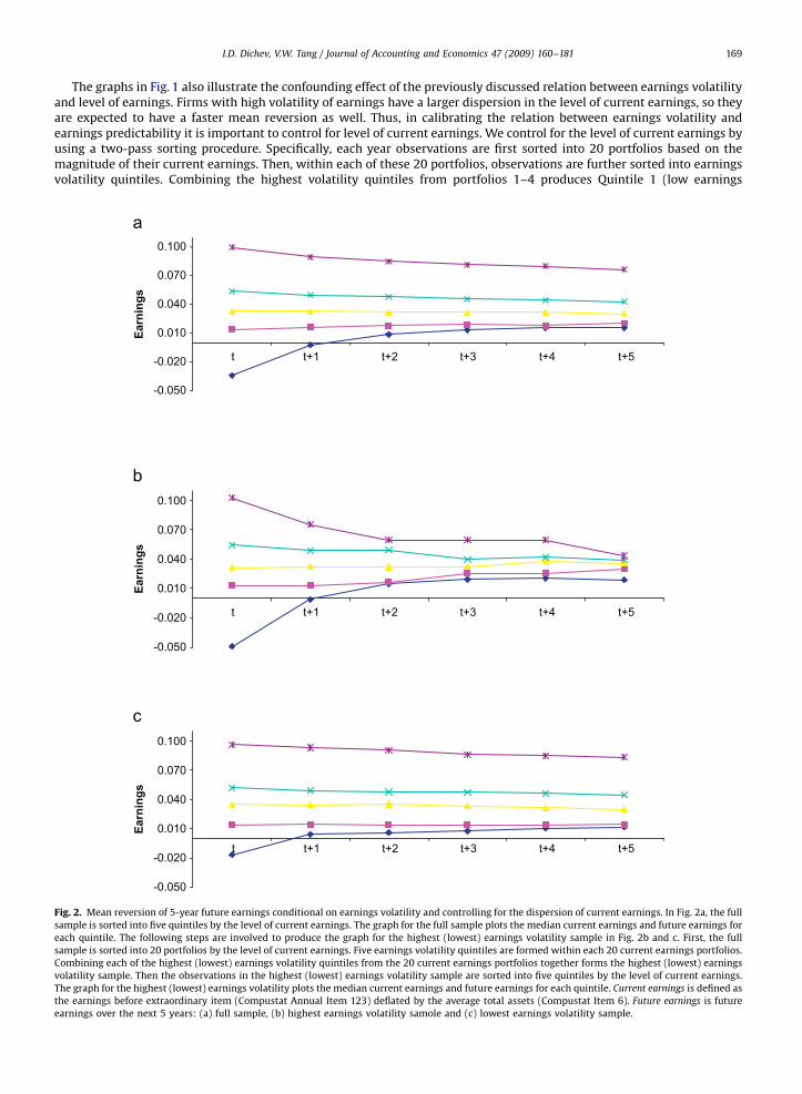
The graphs in Fig. 1 also illustrate the confounding effect of the previously discussed relation between earnings volatilityand level of earnings. Firms with high volatility of earnings have a larger dispersion in the level of current earnings, so theyare expected to have a faster mean reversion as well. Thus, in calibrating the relation between earnings volatility andearnings predictability it is important to control for level of current earnings. We control for the level of current earnings byusing a two-pass sorting procedure. Specifically, each year observations are first sorted into 20 portfolios based on themagnitude of their current earnings. Then, within each of these 20 portfolios, observations are further sorted into earningsvolatility quintiles. Combining the highest volatility quintiles from portfolios 1–4 produces Quintile 1 (low earnings

-0.050

-0.020

0.010

0.040

0.070

0.100

Earn

ings

-0.050

-0.020

0.010

0.040

0.070

0.100

Earn

ings

-0.050

-0.020

0.010

0.040

0.070

0.100

Earn

ings

t t+1 t+2 t+3 t+4 t+5

t t+1 t+2 t+3 t+4 t+5

t t+1 t+2 t+3 t+4 t+5

Fig. 2. Mean reversion of 5-year future earnings conditional on earnings volatility and controlling for the dispersion of current earnings. In Fig. 2a, the full

sample is sorted into five quintiles by the level of current earnings. The graph for the full sample plots the median current earnings and future earnings for

each quintile. The following steps are involved to produce the graph for the highest (lowest) earnings volatility sample in Fig. 2b and c. First, the full

sample is sorted into 20 portfolios by the level of current earnings. Five earnings volatility quintiles are formed within each 20 current earnings portfolios.

Combining each of the highest (lowest) earnings volatility quintiles from the 20 current earnings portfolios together forms the highest (lowest) earnings

volatility sample. Then the observations in the highest (lowest) earnings volatility sample are sorted into five quintiles by the level of current earnings.

The graph for the highest (lowest) earnings volatility plots the median current earnings and future earnings for each quintile. Current earnings is defined as

the earnings before extraordinary item (Compustat Annual Item 123) deflated by the average total assets (Compustat Item 6). Future earnings is future

earnings over the next 5 years: (a) full sample, (b) highest earnings volatility samole and (c) lowest earnings volatility sample.

ARTICLE IN PRESS

Table 4

The implications of earnings volatility for the sum of earnings over the next 5 years: S(Earningst+1 to Earningst+5) ¼ a+bEarningst+e.

b Adj. R2 Number of

observations

Panel A: Regression results for the full sample

2.359 0.311 4032

Panel B: Regression results for the highest earnings volatility quintile

1.372 0.172 659

Panel C: Regression results for the lowest earnings volatility quintile

4.205 0.633 922

(Difference from Panel B) 2.933 0.461

(p-value of difference) o0.001 o0.001

All b coefficients are statistically significant at the 0.001 level. Earnings is defined as earnings before extraordinary item (Compustat Annual Item 123)

deflated by average total assets (Compustat Item 6). Vol(Earnings) is the firm-specific standard deviation of Earnings over the most recent 5 years.

Earningst is current year Earnings. Earningst+1 is the 1-year ahead Earnings, and so on. The p-value for the difference in persistence and the Adj. R2 across

panels is derived from a bootstrap test (see text for full details).


magnitude) for our high earnings volatility sub-sample, combining the highest volatility quintiles from portfolios 5 to 8produces Quintile 2, and so on. We repeat the same procedure to derive the quintiles for the low earnings volatilitysub-sample.

The results from this two-pass sorting are presented in the three graphs in Fig. 2. The first graph in Fig. 2 presents thebenchmark results for the full sample, and is identical to the first graph in Fig. 1, except for a different scaling. The secondgraph presents the results for the high-volatility sub-sample, and the third graph present the results for the low-volatilitysub-sample, where both should have similar dispersion of current earnings. A comparison of the second and third graphswith the first graph reveals that the two-pass procedure is successful in controlling for the dispersion of current earnings.Median current earnings for Quintiles 2–5 are nearly identical across graphs, while the control is less successful but seemssatisfactory for Quintile 1. An examination of the rest of the graphs reveals clear evidence of differential mean-reversionsacross graphs, where higher volatility firms revert faster and stronger. While the range in current median earnings is 0.13and deteriorates to 0.06 in year t+5 for the full sample of firms, the corresponding numbers are 0.15–0.02 for the high-volatility sub-sample, and 0.11–0.07 for the low-volatility sub-sample. To complete the analysis with control for thedispersion of current earnings, Panels D and E in Table 3 include regression results for the high and low-volatility sub-samples, controlling for the level of current earnings. The results in Panels D and E largely agree with the corresponding no-control results in Panels B and C in Table 3—high-volatility firms have considerably lower predictability of long-run futureearnings. In fact, the control for the dispersion of current earnings seems to have only a marginal effect on the magnitude ofthe results. Thus, the volatility of earnings effect seems to be largely incremental to the level of earnings effect in thepredictability of earnings.

For a cleaner and more compact version of the long-run results and for formal statistical tests, Table 4 provides anotherspecification of the relation between earnings volatility and long-run earnings predictability. In this case, the sum ofsubsequent 5-year earnings is regressed on current earnings. Thus, the coefficient on the independent variable can beinterpreted as the 5-year sum of the yearly persistence coefficients, while the R2 provides an aggregate measure ofexplanatory power over the 5-year horizon. The statistical tests in Table 4 are similar to those in the 1-year specifications inTable 2, with t-tests of difference in persistence and bootstrap tests for differences in R2. For clarity of exposition, the resultsof Panels A–C in Table 4 correspond to the results in Panels A–C in Table 3. An inspection of the results in Table 4 indicatesthat both the tenor and the magnitude of the results are much the same as in Table 3. The persistence and R2 for the high-volatility sample (1.37 and 0.17) are substantially lower than those for the benchmark full sample (2.36 and 0.31) and muchlower than those for the low-volatility sample (4.21 and 0.63). The persistence and R2 differences between the high andlow-volatility samples are both significant at the 0.001 level.7

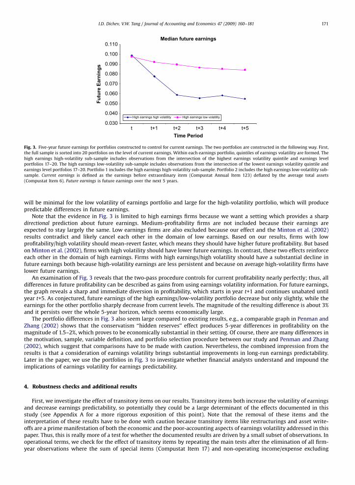
In Fig. 3 we present a portfolio specification that provides an intuitive feel for the economic importance of our long-runearnings volatility results. Fig. 3 presents medians of 5-year future earnings for two portfolios constructed to control for thelevel of current profitability and maximize future earnings differences based on earnings volatility information. Specifically,the full sample of firm-years is first sorted yearly into 20 portfolios based on the magnitude of current earnings, which arethen further sorted into earnings volatility quintiles. Then we combine the four sub-portfolios, which have the highestcurrent profitability but fall in the lowest quintile of earnings volatility (high earnings/low volatility) and compare it withthe four sub-portfolios, which have the highest current profitability and fall in the highest quintile of earnings volatility(high earnings/high volatility). The motivation is that high earnings are expected to mean-revert but the mean-reversion

7 Additional tests corresponding to Panels D and E in Table 3 confirm that all results hold after control for level of current earnings.

ARTICLE IN PRESS

Median future earnings

0.030

0.040

0.050

0.060

0.070

0.080

0.090

0.100

0.110

Time Period

Futu

re E

arni

ngs

High earnings high volatility High earnings low volatility

t t+1 t+2 t+3 t+4 t+5

Fig. 3. Five-year future earnings for portfolios constructed to control for current earnings. The two portfolios are constructed in the following way. First,

the full sample is sorted into 20 portfolios on the level of current earnings. Within each earnings portfolio, quintiles of earnings volatility are formed. The

high earnings high-volatility sub-sample includes observations from the intersection of the highest earnings volatility quintile and earnings level

portfolios 17–20. The high earnings low-volatility sub-sample includes observations from the intersection of the lowest earnings volatility quintile and

earnings level portfolios 17–20. Portfolio 1 includes the high earnings high-volatility sub-sample. Portfolio 2 includes the high earnings low-volatility sub-

sample. Current earnings is defined as the earnings before extraordinary item (Compustat Annual Item 123) deflated by the average total assets

(Compustat Item 6). Future earnings is future earnings over the next 5 years.


will be minimal for the low volatility of earnings portfolio and large for the high-volatility portfolio, which will producepredictable differences in future earnings.

Note that the evidence in Fig. 3 is limited to high earnings firms because we want a setting which provides a sharpdirectional prediction about future earnings. Medium-profitability firms are not included because their earnings areexpected to stay largely the same. Low earnings firms are also excluded because our effect and the Minton et al. (2002)results contradict and likely cancel each other in the domain of low earnings. Based on our results, firms with lowprofitability/high volatility should mean-revert faster, which means they should have higher future profitability. But basedon Minton et al. (2002), firms with high volatility should have lower future earnings. In contrast, these two effects reinforceeach other in the domain of high earnings. Firms with high earnings/high volatility should have a substantial decline infuture earnings both because high-volatility earnings are less persistent and because on average high-volatility firms havelower future earnings.

An examination of Fig. 3 reveals that the two-pass procedure controls for current profitability nearly perfectly; thus, alldifferences in future profitability can be described as gains from using earnings volatility information. For future earnings,the graph reveals a sharp and immediate diversion in profitability, which starts in year t+1 and continues unabated untilyear t+5. As conjectured, future earnings of the high earnings/low-volatility portfolio decrease but only slightly, while theearnings for the other portfolio sharply decrease from current levels. The magnitude of the resulting difference is about 3%and it persists over the whole 5-year horizon, which seems economically large.

The portfolio differences in Fig. 3 also seem large compared to existing results, e.g., a comparable graph in Penman andZhang (2002) shows that the conservatism ‘‘hidden reserves’’ effect produces 5-year differences in profitability on themagnitude of 1.5–2%, which proves to be economically substantial in their setting. Of course, there are many differences inthe motivation, sample, variable definition, and portfolio selection procedure between our study and Penman and Zhang(2002), which suggest that comparisons have to be made with caution. Nevertheless, the combined impression from theresults is that a consideration of earnings volatility brings substantial improvements in long-run earnings predictability.Later in the paper, we use the portfolios in Fig. 3 to investigate whether financial analysts understand and impound theimplications of earnings volatility for earnings predictability.

4. Robustness checks and additional results

First, we investigate the effect of transitory items on our results. Transitory items both increase the volatility of earningsand decrease earnings predictability, so potentially they could be a large determinant of the effects documented in thisstudy (see Appendix A for a more rigorous exposition of this point). Note that the removal of these items and theinterpretation of these results have to be done with caution because transitory items like restructurings and asset write-offs are a prime manifestation of both the economic and the poor-accounting aspects of earnings volatility addressed in thispaper. Thus, this is really more of a test for whether the documented results are driven by a small subset of observations. Inoperational terms, we check for the effect of transitory items by repeating the main tests after the elimination of all firm-year observations where the sum of special items (Compustat Item 17) and non-operating income/expense excluding

ARTICLE IN PRESS

Table 5Robustness checks on the influence of past earnings persistence on the documented results.

Panel A: Regression results from the model Earningst+1 ¼ a+b Earningst+e by quintiles of AR(1) residual volatility

Quintiles by Vol(Residual) b (persistence) Adj. R2

Quintile 1 0.839 0.606

Quintile 2 0.889 0.607

Quintile 3 0.823 0.502

Quintile 4 0.727 0.381

Quintile 5 0.521 0.285



Panel B: Earnings persistence using independent sorting on past persistence and past volatility of earnings

Quintiles by past persistence Quintiles by Vol(Earnings)

Quintile 1 Quintile 2 Quintile 3 Quintile 4 Quintile 5 Difference quintile (1–5)

Quintile 1 0.958 0.859 0.767 0.797 0.432 0.526

Quintile 2 0.907 0.889 0.997 0.725 0.486 0.421

Quintile 3 0.941 0.905 0.720 0.678 0.607 0.334

Quintile 4 0.968 0.886 0.915 0.823 0.507 0.461

Quintile 5 0.904 0.917 0.825 0.724 0.503 0.401

Difference quintile (1–5) 0.054 �0.058 0.058 0.073 �0.071

All b (persistence) coefficients are significant at the 0.001 level. The p-value for the difference in persistence coefficients across quintiles is derived from a

t-test. The p-value for the difference in the Adj. R2 across quintiles is derived from a bootstrap test (see text for full details). Earningst is defined as earnings

before extraordinary item (Compustat Annual Item 123) deflated by the average total assets (Compustat Item 6). Vol(Earnings) is the firm-specific

standard deviation of Earnings over the most recent 5 years. Past persistence is the persistence coefficient from the model Earningst ¼ a+bEarningst�1

using the most recent 5 years. Vol(Residual) is defined as the firm-specific standard deviation of the residuals from the above model.


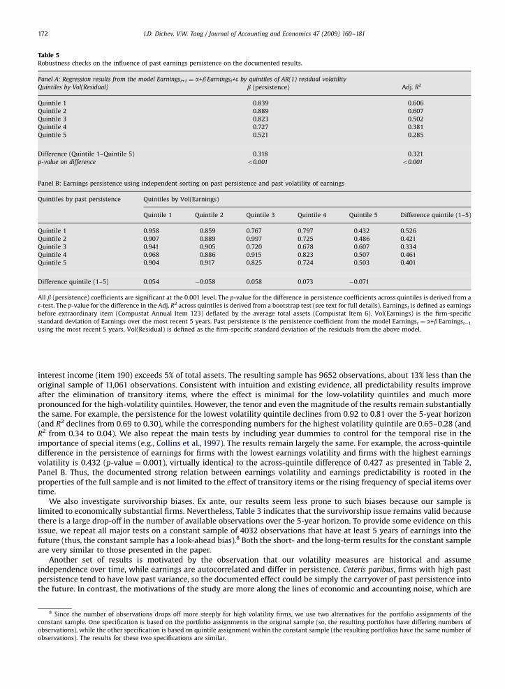
interest income (item 190) exceeds 5% of total assets. The resulting sample has 9652 observations, about 13% less than theoriginal sample of 11,061 observations. Consistent with intuition and existing evidence, all predictability results improveafter the elimination of transitory items, where the effect is minimal for the low-volatility quintiles and much morepronounced for the high-volatility quintiles. However, the tenor and even the magnitude of the results remain substantiallythe same. For example, the persistence for the lowest volatility quintile declines from 0.92 to 0.81 over the 5-year horizon(and R2 declines from 0.69 to 0.30), while the corresponding numbers for the highest volatility quintile are 0.65–0.28 (andR2 from 0.34 to 0.04). We also repeat the main tests by including year dummies to control for the temporal rise in theimportance of special items (e.g., Collins et al., 1997). The results remain largely the same. For example, the across-quintiledifference in the persistence of earnings for firms with the lowest earnings volatility and firms with the highest earningsvolatility is 0.432 (p-value ¼ 0.001), virtually identical to the across-quintile difference of 0.427 as presented in Table 2,Panel B. Thus, the documented strong relation between earnings volatility and earnings predictability is rooted in theproperties of the full sample and is not limited to the effect of transitory items or the rising frequency of special items overtime.

We also investigate survivorship biases. Ex ante, our results seem less prone to such biases because our sample islimited to economically substantial firms. Nevertheless, Table 3 indicates that the survivorship issue remains valid becausethere is a large drop-off in the number of available observations over the 5-year horizon. To provide some evidence on thisissue, we repeat all major tests on a constant sample of 4032 observations that have at least 5 years of earnings into thefuture (thus, the constant sample has a look-ahead bias).8 Both the short- and the long-term results for the constant sampleare very similar to those presented in the paper.

Another set of results is motivated by the observation that our volatility measures are historical and assumeindependence over time, while earnings are autocorrelated and differ in persistence. Ceteris paribus, firms with high pastpersistence tend to have low past variance, so the documented effect could be simply the carryover of past persistence intothe future. In contrast, the motivations of the study are more along the lines of economic and accounting noise, which are

8 Since the number of observations drops off more steeply for high volatility firms, we use two alternatives for the portfolio assignments of the

constant sample. One specification is based on the portfolio assignments in the original sample (so, the resulting portfolios have differing numbers of

observations), while the other specification is based on quintile assignment within the constant sample (the resulting portfolios have the same number of

observations). The results for these two specifications are similar.

ARTICLE IN PRESS


more naturally captured in the residual from past persistence. To offer some evidence on the relative roles of these factors,we employ two specifications. The first specification is to sort on the variance of the residuals from an AR(1) model over thelast 5 years (instead of the variance of raw earnings over the same period); by construction these residuals capture thevariation in earnings after the effect of persistence is taken out. An examination of the results in Table 5, Panel A revealsthat the extreme-quintile spread in the persistence coefficient is 0.318 and the spread in R2 is 0.321, both statisticallysignificant. A comparison with the corresponding benchmark results in Table 2, Panel B (0.427 and 0.408) reveals that theeffect of residuals dominates that of persistence. The second specification estimates historical persistence directly and thenexamines whether the effect of historical volatility is incremental to the effect of historical persistence in a 5�5 sort inTable 5, Panel B.9 The results indicate that past persistence has little effect on forward-looking persistence after controllingfor volatility of earnings. In contrast, there are large spreads in forward-looking persistence across volatility quintiles aftercontrolling for past persistence. Thus, both specifications indicate that the role of past persistence in explaining thedocumented results is small.

We also explore the effect of cross-sectional dependence in earnings on our tests of significance. Cross-sectionaldependence arises because of economy-wide, industry, and other systematic factors in earnings, and could result inunderstated standard errors and inflated levels of significance. Since most of our tests rely on bootstrap methods ofassessing significance, we limit our robustness checks to only the relevant subset of OLS results. We use Fama–MacBethregressions, which rely on time-series independence to provide tests of significance, and are the most common remedy forcross-sectional dependence. Note that Fama–MacBeth tests are a rather conservative method to estimate statisticalsignificance in our sample because the time-series is relatively short (only 16 years). The results confirm that thedocumented relations are significant, e.g., the 0.427 range of persistence coefficients across earnings volatility quintiles inTable 2, Panel B has a p-value of 0.001.

We also provide evidence on the relative role of time-series vs. cross-sectional earnings predictability effects on ourresults.10 Note that our motivation largely relies on economic and accounting arguments which suggest a relation betweenfirm-level volatility and persistence in earnings. Similar to other existing studies, though, the main regressions arerun on panel data and thus, the estimated coefficients are a function of both firm-level autoregressive persistence andvariation in mean profitability across firms (see Appendix A for a more rigorous exposition of this point). Since ourpaper aims for enhancing practical earnings prediction, we are interested in total earnings persistence and total predictiveability, regardless of whether it comes from the autoregressive or the cross-sectional aspect of the regression. Thus, themain results in the paper rely on the estimated coefficients of persistence, with no adjustment for possible cross-sectionaleffects. However, since our motivation is largely in terms of autoregressive effects, it is useful to provide evidence on therelative roles of the autoregressive vs. the cross-sectional effects on the estimated persistence. We accomplish this byre-running the main regression in Table 2, Panel B in a firm fixed-effects specification, where the resulting coefficients areentirely due to autoregressive persistence effects. The tenor of the results remains largely unchanged with thisspecification. Specifically, the across-quintiles range in persistence in Table 2, Panel B is 0.427, while the correspondingrange is 0.454 in the fixed-effects specification. Thus, the predictive power of earnings volatility for earnings predictabilityis largely due to autoregressive effects rather than to cross-sectional variation in mean profitability.

Recall that our sample is limited to large firms with December year-end; here we provide evidence on the effect of theserestrictions on our results. Fiscal year-end does not seem to matter, the results for non-12/31 firms are much the same asthose presented above. Small firms, though, have less reliable relation between volatility and persistence—for firms withassets between $20 million and $100 million, the range in persistence across volatility quintiles is only about a third to ahalf that for large firms, and the relation disappears for firms with assets of less than $20 million. These results, however,should be treated with caution. Our impression from working with the small firms is that this sub-sample is problematic,e.g., it has a massive outlier problem. In any case, the small firms excluded from our main tests are economically negligible;they comprise less than 3% of the aggregate market value of all firms.

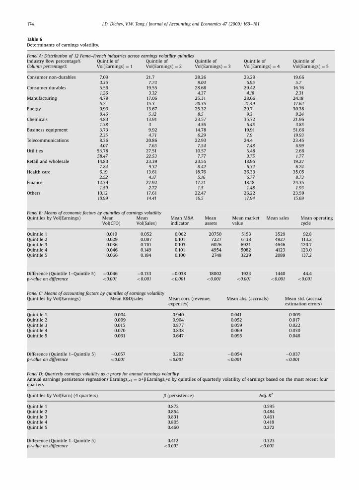
We also provide evidence on the economic and accounting determinants of earnings volatility and its relationto earnings persistence. These results serve two purposes; first, they provide evidence on the construct validity andpossible alternative interpretations of the earnings volatility variable; second, they can potentially provide an empiricalinstrument which avoids the substantial time-series data requirements to compute the earnings volatility variable. On theeconomic determinants side, we first explore the relation between earnings volatility and industry membership using theFama–French classification of 12 industry clusters. We find reliable links between industry membership and earningsvolatility quintiles, results presented in Table 6, Panel A. Specifically, we find that utility firms strongly cluster anddominate in the lowest volatility quintile, with more than half of the utility firms in the lowest volatility quintile, and morethan half of the firms in that quintile being utility firms. There are also reliable clusters in the upper volatility quintiles,with Energy, Health Care, and especially Business Equipment exhibiting a strong presence.

9 The 5�5 sort in Panel B uses independent sorting on the two variables to avoid handicapping one variable vs. the other. In any case, the Spearman

correlation between historical persistence and historical volatility is �0.015, (p-value ¼ 0.124), which suggests that the results under sequential sorting

schemes will be similar.10 We thank an anonymous referee for pointing out this distinction and suggesting the test.

ARTICLE IN PRESS

Table 6Determinants of earnings volatility.

Panel A: Distribution of 12 Fama–French industries across earnings volatility quintilesIndustry Row percentage%Column percentage%

Quintile ofVol(Earnings) ¼ 1





Consumer non-durables 7.09 21.7 28.26 23.29 19.663.36 7.74 9.04 6.95 5.7

Consumer durables 5.59 19.55 28.68 29.42 16.761.26 3.32 4.37 4.18 2.31

Manufacturing 4.79 17.06 25.31 28.66 24.185.7 15.3 20.35 21.49 17.62

Energy 0.93 13.67 25.32 29.7 30.380.46 5.12 8.5 9.3 9.24

Chemicals 4.83 13.91 23.57 35.72 21.961.38 3 4.56 6.45 3.85

Business equipment 3.73 9.92 14.78 19.91 51.662.35 4.71 6.29 7.9 19.93

Telecommunications 8.36 20.86 22.93 24.4 23.454.07 7.65 7.54 7.48 6.99

Utilities 53.78 27.51 10.57 5.48 2.6658.47 22.53 7.77 3.75 1.77

Retail and wholesale 14.83 23.39 23.55 18.95 19.277.84 9.32 8.42 6.32 6.24

Health care 6.19 13.61 18.76 26.39 35.052.52 4.17 5.16 6.77 8.73

Finance 12.34 27.92 17.21 18.18 24.351.59 2.72 1.5 1.48 1.93

Others 10.12 17.61 22.47 26.22 23.5910.99 14.41 16.5 17.94 15.69

Panel B: Means of economic factors by quintiles of earnings volatilityQuintiles by Vol(Earnings) Mean

Vol(CFO)MeanVol(Sales)

Mean M&Aindicator

Meanassets

Mean marketvalue

Mean sales Mean operatingcycle

Quintile 1 0.019 0.052 0.062 20750 5153 3529 92.8Quintile 2 0.029 0.087 0.101 7227 6138 4927 113.2Quintile 3 0.036 0.110 0.103 6026 6921 4646 120.7Quintile 4 0.046 0.149 0.101 4954 5082 4123 123.0Quintile 5 0.066 0.184 0.100 2748 3229 2089 137.2

Difference (Quintile 1–Quintile 5) �0.046 �0.133 �0.038 18002 1923 1440 44.4p-value on difference o0.001 o0.001 o0.001 o0.001 o0.001 o0.001 o0.001

Panel C: Means of accounting factors by quintiles of earnings volatilityQuintiles by Vol(Earnings) Mean R&D/sales Mean corr. (revenue,

expenses)Mean abs. (accruals) Mean std. (accrual

estimation errors)

Quintile 1 0.004 0.940 0.041 0.009Quintile 2 0.009 0.904 0.052 0.017Quintile 3 0.015 0.877 0.059 0.022Quintile 4 0.070 0.838 0.069 0.030Quintile 5 0.061 0.647 0.095 0.046

Difference (Quintile 1–Quintile 5) �0.057 0.292 �0.054 �0.037p-value on difference o0.001 o0.001 o0.001 o0.001

Panel D: Quarterly earnings volatility as a proxy for annual earnings volatilityAnnual earnings persistence regressions Earningst+1 ¼ a+bEarningst+e by quintiles of quarterly volatility of earnings based on the most recent fourquarters

Quintiles by Vol(Earn) (4 quarters) b (persistence) Adj. R2

Quintile 1 0.872 0.595Quintile 2 0.854 0.484Quintile 3 0.831 0.461Quintile 4 0.805 0.418Quintile 5 0.460 0.272

Difference (Quintile 1–Quintile 5) 0.412 0.323p-value on difference o0.001 o0.001


ARTICLE IN PRESS

Annual earnings persistence regressions Earningst+1 ¼ a+b Earningst+e by quintiles of quarterly volatility of earnings based on the most recent eight

quarters

Quintiles by Vol(Earn) (8 quarters) b (persistence) Adj. R2

Quintile 1 0.884 0.637

Quintile 2 0.881 0.509

Quintile 3 0.842 0.469

Quintile 4 0.765 0.401

Quintile 5 0.458 0.259


p-Value on difference o0.001 o0.001

Table 6 (continued)


We also explore the relation between earnings volatility and the following variables:

Volatility of cash flow from operations and volatility of sales: proxies for real economic volatility, predict positive relationwith earnings volatility.Assets, market value, and sales: proxies for size, because of diversification effects predict negative relation with earningsvolatility.Operating cycle: since longer operating cycles indicate more vulnerability to economic shocks, expect positive relationwith earnings volatility.Mergers and acquisitions: sign unclear; possible diversification or size effects argue for a negative relation but weaknessin targets and integration problems point to a possible positive relation with earnings volatility.Correlation of revenues and expenses: recall that Dichev and Tang (2008) argue that volatility is increasing with worsematching of revenues and expenses; based on this argument, expect a negative relation with earnings volatility.R&D levels: proxy for poor matching and/or involvement in new-economy winner-take-all activities. Predict a positiverelation with earnings volatility.Level of absolute accruals and level of accrual estimation errors (as in Dechow and Dichev, 2002): proxies for accrualquality. Low-quality accruals are expected to manifest as noise in the determination of earnings, leading to highervolatility of earnings.

The mean of these variables across earnings volatility quintiles are presented in Table 6, Panels B and C (results formedians have the same tenor). An inspection of these results reveals that they are largely consistent with expectations,with all variables exhibiting strong economic and statistical associations in predicted direction; the only exception ismergers and acquisitions, where we find little in terms of a reliable economic relation. One upshot from these results issupport for the economic and accounting conjectures underpinning the earnings volatility variable. Another upshot is thatperhaps these relations can be used to build an instrument for earnings volatility, which avoids the taxing time-series datarequirement. Our initial efforts in this direction were not successful. We tested a number of specifications, where earningsvolatility is regressed on various combinations of variables, and then the resulting loadings are used to produce theinstrument. The explanatory power of these regressions was only moderate, and the resulting proxy was inferior toearnings volatility in capturing earnings persistence.11

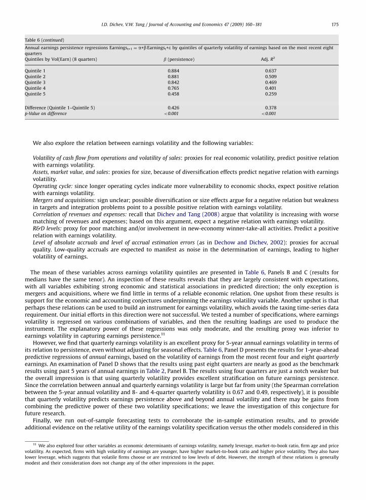
However, we find that quarterly earnings volatility is an excellent proxy for 5-year annual earnings volatility in terms ofits relation to persistence, even without adjusting for seasonal effects. Table 6, Panel D presents the results for 1-year-aheadpredictive regressions of annual earnings, based on the volatility of earnings from the most recent four and eight quarterly

earnings. An examination of Panel D shows that the results using past eight quarters are nearly as good as the benchmarkresults using past 5 years of annual earnings in Table 2, Panel B. The results using four quarters are just a notch weaker butthe overall impression is that using quarterly volatility provides excellent stratification on future earnings persistence.Since the correlation between annual and quarterly earnings volatility is large but far from unity (the Spearman correlationbetween the 5-year annual volatility and 8- and 4-quarter quarterly volatility is 0.67 and 0.49, respectively), it is possiblethat quarterly volatility predicts earnings persistence above and beyond annual volatility and there may be gains fromcombining the predictive power of these two volatility specifications; we leave the investigation of this conjecture forfuture research.

Finally, we run out-of-sample forecasting tests to corroborate the in-sample estimation results, and to provideadditional evidence on the relative utility of the earnings volatility specification versus the other models considered in this

11 We also explored four other variables as economic determinants of earnings volatility, namely leverage, market-to-book ratio, firm age and price

volatility. As expected, firms with high volatility of earnings are younger, have higher market-to-book ratio and higher price volatility. They also have

lower leverage, which suggests that volatile firms choose or are restricted to low levels of debt. However, the strength of these relations is generally

modest and their consideration does not change any of the other impressions in the paper.

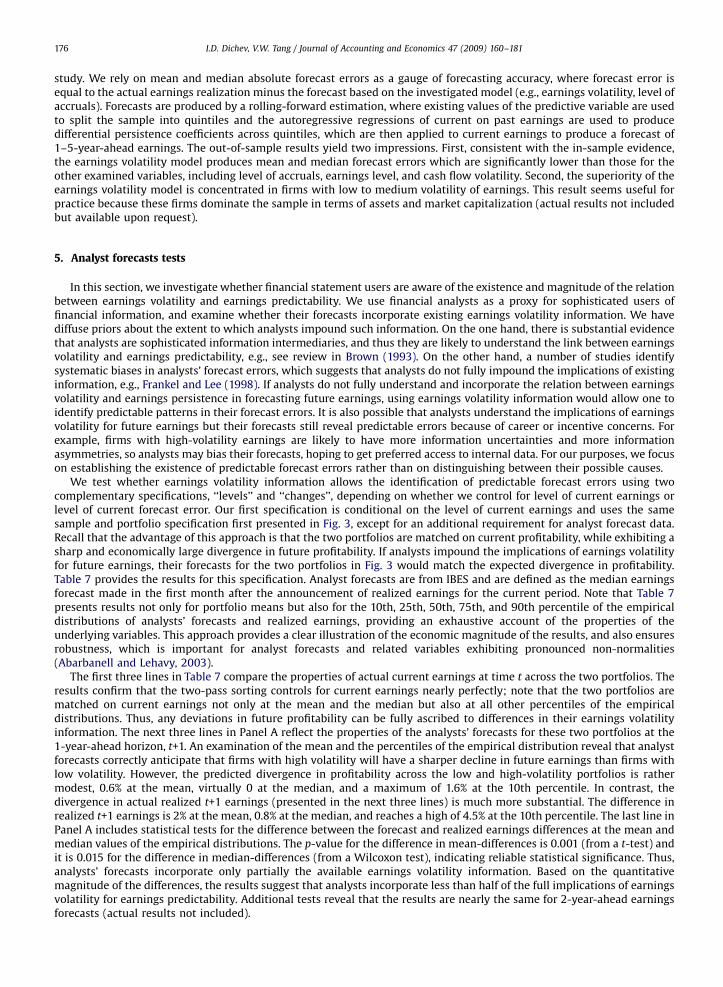
ARTICLE IN PRESS


study. We rely on mean and median absolute forecast errors as a gauge of forecasting accuracy, where forecast error isequal to the actual earnings realization minus the forecast based on the investigated model (e.g., earnings volatility, level ofaccruals). Forecasts are produced by a rolling-forward estimation, where existing values of the predictive variable are usedto split the sample into quintiles and the autoregressive regressions of current on past earnings are used to producedifferential persistence coefficients across quintiles, which are then applied to current earnings to produce a forecast of1–5-year-ahead earnings. The out-of-sample results yield two impressions. First, consistent with the in-sample evidence,the earnings volatility model produces mean and median forecast errors which are significantly lower than those for theother examined variables, including level of accruals, earnings level, and cash flow volatility. Second, the superiority of theearnings volatility model is concentrated in firms with low to medium volatility of earnings. This result seems useful forpractice because these firms dominate the sample in terms of assets and market capitalization (actual results not includedbut available upon request).

5. Analyst forecasts tests

In this section, we investigate whether financial statement users are aware of the existence and magnitude of the relationbetween earnings volatility and earnings predictability. We use financial analysts as a proxy for sophisticated users offinancial information, and examine whether their forecasts incorporate existing earnings volatility information. We havediffuse priors about the extent to which analysts impound such information. On the one hand, there is substantial evidencethat analysts are sophisticated information intermediaries, and thus they are likely to understand the link between earningsvolatility and earnings predictability, e.g., see review in Brown (1993). On the other hand, a number of studies identifysystematic biases in analysts’ forecast errors, which suggests that analysts do not fully impound the implications of existinginformation, e.g., Frankel and Lee (1998). If analysts do not fully understand and incorporate the relation between earningsvolatility and earnings persistence in forecasting future earnings, using earnings volatility information would allow one toidentify predictable patterns in their forecast errors. It is also possible that analysts understand the implications of earningsvolatility for future earnings but their forecasts still reveal predictable errors because of career or incentive concerns. Forexample, firms with high-volatility earnings are likely to have more information uncertainties and more informationasymmetries, so analysts may bias their forecasts, hoping to get preferred access to internal data. For our purposes, we focuson establishing the existence of predictable forecast errors rather than on distinguishing between their possible causes.

We test whether earnings volatility information allows the identification of predictable forecast errors using twocomplementary specifications, ‘‘levels’’ and ‘‘changes’’, depending on whether we control for level of current earnings orlevel of current forecast error. Our first specification is conditional on the level of current earnings and uses the samesample and portfolio specification first presented in Fig. 3, except for an additional requirement for analyst forecast data.Recall that the advantage of this approach is that the two portfolios are matched on current profitability, while exhibiting asharp and economically large divergence in future profitability. If analysts impound the implications of earnings volatilityfor future earnings, their forecasts for the two portfolios in Fig. 3 would match the expected divergence in profitability.Table 7 provides the results for this specification. Analyst forecasts are from IBES and are defined as the median earningsforecast made in the first month after the announcement of realized earnings for the current period. Note that Table 7presents results not only for portfolio means but also for the 10th, 25th, 50th, 75th, and 90th percentile of the empiricaldistributions of analysts’ forecasts and realized earnings, providing an exhaustive account of the properties of theunderlying variables. This approach provides a clear illustration of the economic magnitude of the results, and also ensuresrobustness, which is important for analyst forecasts and related variables exhibiting pronounced non-normalities(Abarbanell and Lehavy, 2003).

The first three lines in Table 7 compare the properties of actual current earnings at time t across the two portfolios. Theresults confirm that the two-pass sorting controls for current earnings nearly perfectly; note that the two portfolios arematched on current earnings not only at the mean and the median but also at all other percentiles of the empiricaldistributions. Thus, any deviations in future profitability can be fully ascribed to differences in their earnings volatilityinformation. The next three lines in Panel A reflect the properties of the analysts’ forecasts for these two portfolios at the1-year-ahead horizon, t+1. An examination of the mean and the percentiles of the empirical distribution reveal that analystforecasts correctly anticipate that firms with high volatility will have a sharper decline in future earnings than firms withlow volatility. However, the predicted divergence in profitability across the low and high-volatility portfolios is rathermodest, 0.6% at the mean, virtually 0 at the median, and a maximum of 1.6% at the 10th percentile. In contrast, thedivergence in actual realized t+1 earnings (presented in the next three lines) is much more substantial. The difference inrealized t+1 earnings is 2% at the mean, 0.8% at the median, and reaches a high of 4.5% at the 10th percentile. The last line inPanel A includes statistical tests for the difference between the forecast and realized earnings differences at the mean andmedian values of the empirical distributions. The p-value for the difference in mean-differences is 0.001 (from a t-test) andit is 0.015 for the difference in median-differences (from a Wilcoxon test), indicating reliable statistical significance. Thus,analysts’ forecasts incorporate only partially the available earnings volatility information. Based on the quantitativemagnitude of the differences, the results suggest that analysts incorporate less than half of the full implications of earningsvolatility for earnings predictability. Additional tests reveal that the results are nearly the same for 2-year-ahead earningsforecasts (actual results not included).

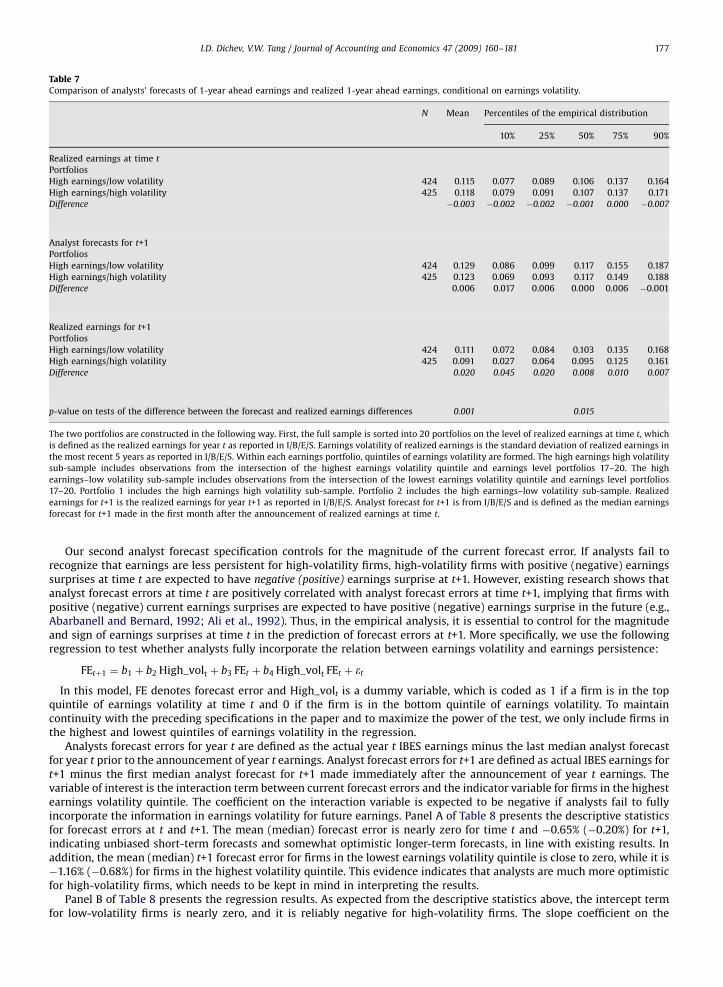
ARTICLE IN PRESS

Table 7Comparison of analysts’ forecasts of 1-year ahead earnings and realized 1-year ahead earnings, conditional on earnings volatility.

N Mean Percentiles of the empirical distribution

10% 25% 50% 75% 90%

Realized earnings at time t

Portfolios

High earnings/low volatility 424 0.115 0.077 0.089 0.106 0.137 0.164

High earnings/high volatility 425 0.118 0.079 0.091 0.107 0.137 0.171

Difference �0.003 �0.002 �0.002 �0.001 0.000 �0.007

Analyst forecasts for t+1

Portfolios



Difference 0.006 0.017 0.006 0.000 0.006 �0.001

Realized earnings for t+1

Portfolios



Difference 0.020 0.045 0.020 0.008 0.010 0.007

p-value on tests of the difference between the forecast and realized earnings differences 0.001 0.015

The two portfolios are constructed in the following way. First, the full sample is sorted into 20 portfolios on the level of realized earnings at time t, which

is defined as the realized earnings for year t as reported in I/B/E/S. Earnings volatility of realized earnings is the standard deviation of realized earnings in

the most recent 5 years as reported in I/B/E/S. Within each earnings portfolio, quintiles of earnings volatility are formed. The high earnings high volatility

sub-sample includes observations from the intersection of the highest earnings volatility quintile and earnings level portfolios 17–20. The high

earnings–low volatility sub-sample includes observations from the intersection of the lowest earnings volatility quintile and earnings level portfolios

17–20. Portfolio 1 includes the high earnings high volatility sub-sample. Portfolio 2 includes the high earnings–low volatility sub-sample. Realized

earnings for t+1 is the realized earnings for year t+1 as reported in I/B/E/S. Analyst forecast for t+1 is from I/B/E/S and is defined as the median earnings

forecast for t+1 made in the first month after the announcement of realized earnings at time t.


Our second analyst forecast specification controls for the magnitude of the current forecast error. If analysts fail torecognize that earnings are less persistent for high-volatility firms, high-volatility firms with positive (negative) earningssurprises at time t are expected to have negative (positive) earnings surprise at t+1. However, existing research shows thatanalyst forecast errors at time t are positively correlated with analyst forecast errors at time t+1, implying that firms withpositive (negative) current earnings surprises are expected to have positive (negative) earnings surprise in the future (e.g.,Abarbanell and Bernard, 1992; Ali et al., 1992). Thus, in the empirical analysis, it is essential to control for the magnitudeand sign of earnings surprises at time t in the prediction of forecast errors at t+1. More specifically, we use the followingregression to test whether analysts fully incorporate the relation between earnings volatility and earnings persistence:

FEtþ1 ¼ b1 þ b2 High_volt þ b3 FEt þ b4 High_volt FEt þ �t

In this model, FE denotes forecast error and High_volt is a dummy variable, which is coded as 1 if a firm is in the topquintile of earnings volatility at time t and 0 if the firm is in the bottom quintile of earnings volatility. To maintaincontinuity with the preceding specifications in the paper and to maximize the power of the test, we only include firms inthe highest and lowest quintiles of earnings volatility in the regression.

Analysts forecast errors for year t are defined as the actual year t IBES earnings minus the last median analyst forecastfor year t prior to the announcement of year t earnings. Analyst forecast errors for t+1 are defined as actual IBES earnings fort+1 minus the first median analyst forecast for t+1 made immediately after the announcement of year t earnings. Thevariable of interest is the interaction term between current forecast errors and the indicator variable for firms in the highestearnings volatility quintile. The coefficient on the interaction variable is expected to be negative if analysts fail to fullyincorporate the information in earnings volatility for future earnings. Panel A of Table 8 presents the descriptive statisticsfor forecast errors at t and t+1. The mean (median) forecast error is nearly zero for time t and �0.65% (�0.20%) for t+1,indicating unbiased short-term forecasts and somewhat optimistic longer-term forecasts, in line with existing results. Inaddition, the mean (median) t+1 forecast error for firms in the lowest earnings volatility quintile is close to zero, while it is�1.16% (�0.68%) for firms in the highest volatility quintile. This evidence indicates that analysts are much more optimisticfor high-volatility firms, which needs to be kept in mind in interpreting the results.

Panel B of Table 8 presents the regression results. As expected from the descriptive statistics above, the intercept termfor low-volatility firms is nearly zero, and it is reliably negative for high-volatility firms. The slope coefficient on the

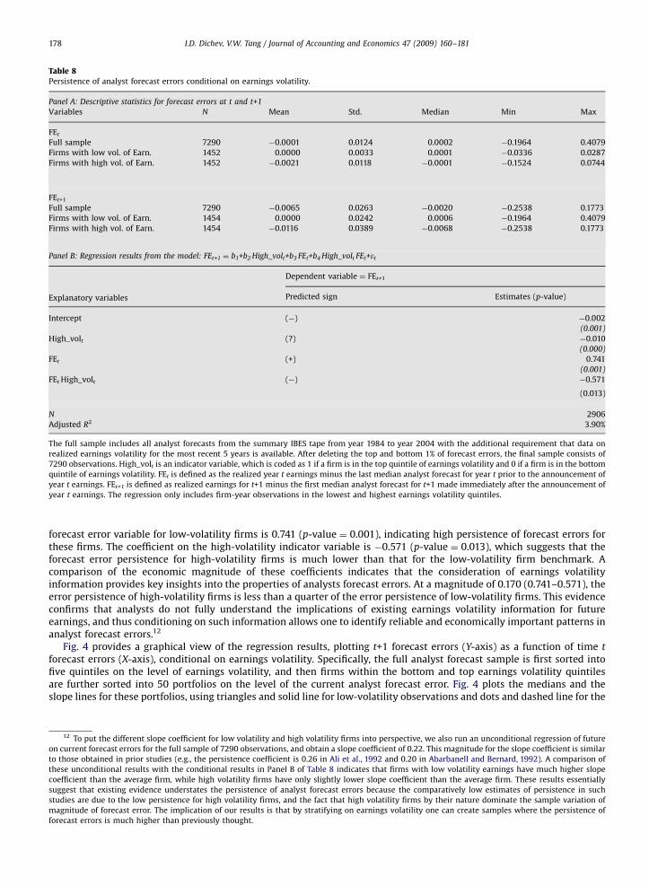
ARTICLE IN PRESS

Table 8Persistence of analyst forecast errors conditional on earnings volatility.

Panel A: Descriptive statistics for forecast errors at t and t+1

Variables N Mean Std. Median Min Max

FEt

Full sample 7290 �0.0001 0.0124 0.0002 �0.1964 0.4079

Firms with low vol. of Earn. 1452 0.0000 0.0033 0.0001 �0.0336 0.0287

Firms with high vol. of Earn. 1452 �0.0021 0.0118 �0.0001 �0.1524 0.0744

FEt+1

Full sample 7290 �0.0065 0.0263 �0.0020 �0.2538 0.1773

Firms with low vol. of Earn. 1454 0.0000 0.0242 0.0006 �0.1964 0.4079

Firms with high vol. of Earn. 1454 �0.0116 0.0389 �0.0068 �0.2538 0.1773

Panel B: Regression results from the model: FEt+1 ¼ b1+b2 High_volt+b3 FEt+b4 High_volt FEt+et

Dependent variable ¼ FEt+1

Explanatory variables Predicted sign Estimates (p-value)

Intercept (�) �0.002

(0.001)

High_volt (?) �0.010

(0.000)

FEt (+) 0.741

(0.001)

FEt High_volt (�) �0.571

(0.013)

N 2906

Adjusted R2 3.90%

The full sample includes all analyst forecasts from the summary IBES tape from year 1984 to year 2004 with the additional requirement that data on

realized earnings volatility for the most recent 5 years is available. After deleting the top and bottom 1% of forecast errors, the final sample consists of

7290 observations. High_volt is an indicator variable, which is coded as 1 if a firm is in the top quintile of earnings volatility and 0 if a firm is in the bottom

quintile of earnings volatility. FEt is defined as the realized year t earnings minus the last median analyst forecast for year t prior to the announcement of

year t earnings. FEt+1 is defined as realized earnings for t+1 minus the first median analyst forecast for t+1 made immediately after the announcement of

year t earnings. The regression only includes firm-year observations in the lowest and highest earnings volatility quintiles.


forecast error variable for low-volatility firms is 0.741 (p-value ¼ 0.001), indicating high persistence of forecast errors forthese firms. The coefficient on the high-volatility indicator variable is �0.571 (p-value ¼ 0.013), which suggests that theforecast error persistence for high-volatility firms is much lower than that for the low-volatility firm benchmark. Acomparison of the economic magnitude of these coefficients indicates that the consideration of earnings volatilityinformation provides key insights into the properties of analysts forecast errors. At a magnitude of 0.170 (0.741–0.571), theerror persistence of high-volatility firms is less than a quarter of the error persistence of low-volatility firms. This evidenceconfirms that analysts do not fully understand the implications of existing earnings volatility information for futureearnings, and thus conditioning on such information allows one to identify reliable and economically important patterns inanalyst forecast errors.12

Fig. 4 provides a graphical view of the regression results, plotting t+1 forecast errors (Y-axis) as a function of time t

forecast errors (X-axis), conditional on earnings volatility. Specifically, the full analyst forecast sample is first sorted intofive quintiles on the level of earnings volatility, and then firms within the bottom and top earnings volatility quintilesare further sorted into 50 portfolios on the level of the current analyst forecast error. Fig. 4 plots the medians and theslope lines for these portfolios, using triangles and solid line for low-volatility observations and dots and dashed line for the

12 To put the different slope coefficient for low volatility and high volatility firms into perspective, we also run an unconditional regression of future

on current forecast errors for the full sample of 7290 observations, and obtain a slope coefficient of 0.22. This magnitude for the slope coefficient is similar

to those obtained in prior studies (e.g., the persistence coefficient is 0.26 in Ali et al., 1992 and 0.20 in Abarbanell and Bernard, 1992). A comparison of

these unconditional results with the conditional results in Panel B of Table 8 indicates that firms with low volatility earnings have much higher slope

coefficient than the average firm, while high volatility firms have only slightly lower slope coefficient than the average firm. These results essentially

suggest that existing evidence understates the persistence of analyst forecast errors because the comparatively low estimates of persistence in such

studies are due to the low persistence for high volatility firms, and the fact that high volatility firms by their nature dominate the sample variation of

magnitude of forecast error. The implication of our results is that by stratifying on earnings volatility one can create samples where the persistence of

forecast errors is much higher than previously thought.

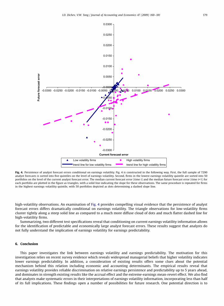
ARTICLE IN PRESS

-0.0300

-0.0250

-0.0200

-0.0150

-0.0100

-0.0050

0.0000

0.0050

0.0100

0.0150

0.0200

0.0250

0.0300

-0.0300

Current forecast error

Futu

re fo

reca

st e

rror

Low volatility firms High volatility firmstrend line for low volatility firms trend line for high volatility firms

-0.0250 -0.0200 -0.0150 -0.0100 -0.0050 0.0000 0.0050 0.0100 0.0150 0.0200 0.0250 0.0300

Fig. 4. Persistence of analyst forecast errors conditional on earnings volatility. Fig. 4 is constructed in the following way. First, the full sample of 7290

analyst forecasts is sorted into five quintiles on the level of earnings volatility. Second, firms in the lowest earnings volatility quintile are sorted into 50

portfolios on the level of the current analyst forecast error. The median current forecast error (time t) and the median future forecast error (time t+1) for

each portfolio are plotted in the figure as triangles, with a solid line indicating the slope for these observations. The same procedure is repeated for firms

in the highest earnings volatility quintile, with 50 portfolios depicted as dots determining a dashed slope line.


high-volatility observations. An examination of Fig. 4 provides compelling visual evidence that the persistence of analystforecast errors differs dramatically conditional on earnings volatility. The triangle observations for low-volatility firmscluster tightly along a steep solid line as compared to a much more diffuse cloud of dots and much flatter dashed line forhigh-volatility firms.

Summarizing, two different test specifications reveal that conditioning on current earnings volatility information allowsfor the identification of predictable and economically large analyst forecast errors. These results suggest that analysts donot fully understand the implication of earnings volatility for earnings predictability.

6. Conclusion

This paper investigates the link between earnings volatility and earnings predictability. The motivation for thisinvestigation relies on recent survey evidence which reveals widespread managerial beliefs that higher volatility indicateslower earnings predictability. In addition, a consideration of existing results offers some clues about the potentialmechanism behind this relation including economic and accounting determinants. The empirical results reveal thatearnings volatility provides reliable discrimination on relative earnings persistence and predictability up to 5 years ahead,and dominates in strength existing results like the accrual effect and the extreme-earnings mean-revert effect. We also findthat analysts make systematic errors in their interpretations of earnings volatility information, incorporating less than halfof its full implications. These findings open a number of possibilities for future research. One potential direction is to

ARTICLE IN PRESS


expand and solidify these results using other samples and variable definitions. Another future direction is exploring thelink between the identified fundamental relations and derived or observed equity values.

Acknowledgments

We thank workshop participants at the 2007 Journal of Accounting and Economics Conference, University of Michigan,Emory University, University of North Carolina, University of Rochester, University of Manchester and London BusinessSchool, an anonymous referee, Richard Frankel (the discussant) and S.P. Kothari (the editor) for helpful comments. Financialhelp from the Michael and Joan Sakkinen Scholarship Fund and the Paton Fund is gratefully acknowledged.

Appendix A

A1. The effect of transitory components on earnings persistence

Consider a company with earnings consisting of two components Et ¼ Xt+Zt where Xt ¼ gXt�1+et and Zt ¼ dZt�1+Zt, suchthat et?Zt. Further assume that Xt is more persistent than Zt, i.e., g4d.

Running the regression

Et ¼ b0 þ b1Et�1 þ mt (A.1)

will result in a slope coefficient with the following expected value:

Eðb1Þ ¼CovðXt þ Zt ;Xt�1 þ Zt�1Þ

VarðXt�1 þ Zt�1Þ¼

CovðgXt�1 þ �t þ dZt�1 þ Zt ;Xt�1 þ Zt�1Þ

VarðXt�1 þ Zt�1Þ

¼ g VarðXt�1Þ

VarðXt�1 þ Zt�1Þþ d

VarðZt�1Þ

VarðXt�1 þ Zt�1Þ¼ gð1�oÞ þ do (A.2)

where o is the fraction of variance attributable to the less persistent components of earnings. In high-volatilityenvironments o will be larger, so it immediately follows that the estimated slope b1 (and adjusted R2) will be lower in suchcircumstances (because g4d).

A2. Effects of time-series autoregressive and cross-sectional effects on the estimated persistence coefficient

Suppose earnings Eit consist of a firm-level mi (e.g., time-series mean) which has cross-sectional variance VarðmiÞ ¼ s2u

and the autoregressive process Xit with firm-specific variance VarðXitÞ ¼ s2i . Specifically

Xit ¼ bXit�1 þ Zit and Eit ¼ mi þ Xit ðfor simplicity mi ? XitÞ (A.3)

Running the regression using panel data

Et ¼ b0 þ b1Et�1 þ e (A.4)

will result in the following expectation for the slope coefficient:

Eðb1Þ ¼Covðmi þ Xit ;mi þ Xit�1Þ

Varðmi þ Xit�1Þ¼s2m þ bs2

i

s2m þ s2

i

(A.5)

Eq. (A.5) indicates that the resulting slope coefficient is a weighted-average of the time-series autoregressive persistence(within firms) and cross-sectional (between firms) variation in mean profitability.

References

Abarbanell, J., Bernard, V., 1992. Tests of analysts’ overreaction/underreaction to earnings information as an explanation for anomalous stock pricebehavior. The Journal of Finance 47, 1181–1207.

Abarbanell, J., Bushee, B., 1997. Fundamental analysis, future earnings, and stock prices. Journal of Accounting Research, 1–24.Abarbanell, J., Lehavy, R., 2003. Biased forecasts or biased earnings? The role of reported earnings in explaining apparent over/underreaction in analysts’

earnings forecasts. Journal of Accounting and Economics (36), 105–146.Ali, A., Klein, A., Rosenfeld, J., 1992. Analysts’ use of information about permanent and transitory earnings components in forecasting annual EPS. The

Accounting Review 67, 183–198.Brown, L.D., 1993. Earnings forecasting research: its implications for capital markets research. International Journal of Forecasting 9, 295–320.Collins, D.W., Hribar, P., 2002. Errors in estimating accruals: implications for empirical research. Journal of Accounting Research 40, 105–134.Collins, D.W., Maydew, E.L., Weiss, I.S., 1997. Changes in the value-relevance of earnings and book values over the past forty years. Journal of Accounting

and Economics 24, 39–67.Dechow, P., Dichev, I., 2002. The quality of accruals and earnings: the role of accrual estimation errors. The Accounting Review 77 (Supplement), 35–59.Dichev, I.D., Tang, V.W., 2008. Matching and the changing properties of accounting earnings over the last 40 years. The Accounting Review 83, 1–36.Finger, C.A., 1994. The ability of earnings to predict future earnings and cash flows. Journal of Accounting Research 32, 210–223.Frankel, R., Lee, C., 1998. Accounting valuation, market expectation, and cross-sectional stock returns. Journal of Accounting and Economics 25, 283–319.

ARTICLE IN PRESS


Freeman, R.N., Ohlson, J.A., Penman, S.H., 1982. Book rate-of-return and prediction of earnings changes: an empirical investigation. Journal of AccountingResearch 20 (2, Autumn), 639–653.

Foster, G., 1977. Quarterly accounting data: time-series properties and predictive-ability results. The Accounting Review 52, 1–21.Graham, J., Campbell, H., Rajgopal, S., 2005. The economic implications of corporate financial reporting. Journal of Accounting and Economics 40, 3–73.Givoly, D., Hayn, C., 2000. The changing time-series properties of earnings, cash flows and accruals: has financial reporting become more conservative.

Journal of Accounting and Economics 29, 287–320.Lev, B., Thiagarajan, R.S., 1993. Fundamental information analysis. Journal of Accounting Research 31 (2), 190–215.Lipe, R., 1990. The relation between stock returns and accounting earnings given alternative information. The Accounting Review 65 (1), 49–71.Minton, B.A., Schrand, C.M., Walther, B.R., 2002. The role of volatility in forecasting. Review of Accounting Studies 7, 195–215.Nissim, D., Penman, S.H., 2001. Ratio analysis and equity valuation: from research to practice. Review of Accounting Studies 6, 109–154.Noreen, E., 1989. Computer-Intensive Methods for Testing Hypotheses: An Introduction. Wiley, New York.Penman, S.H., Zhang, X., 2002. Accounting conservatism, the quality of earnings, and stock returns. The Accounting Review 77 (2), 237–264.Sloan, R., 1996. Do stock prices fully reflect information in accruals and cash flows about future earnings? The Accounting Review 71, 289–316.

Documents

Earnings volatility and earnings predictability