In collaboration with the Evansville Area Earthquake Hazards Mapping Project (EAEHMP)

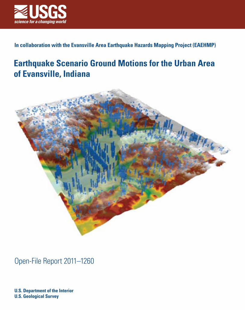
Earthquake Scenario Ground Motions for the Urban Areaof Evansville, Indiana

Open-File Report 2011–1260

U.S. Department of the InteriorU.S. Geological Survey

Earthquake Scenario Ground Motions for the Urban Area of Evansville, Indiana

By Jennifer S. Haase, Robert L. Nowack, Chris H. Cramer, Oliver S. Boyd, and Robert A. Bauer

In collaboration with the Evansville Area Earthquake Hazards Mapping Project (EAEHMP)

Open-File Report 2011–1260

U.S. Department of the Interior U.S. Geological Survey

ii

U.S. Department of the Interior KEN SALAZAR, Secretary

U.S. Geological Survey Marcia K. McNutt, Director

U.S. Geological Survey, Reston, Virginia: 2011

For product and ordering information: World Wide Web: http://www.usgs.gov/pubprod Telephone: 1-888-ASK-USGS

For more information on the USGS—the Federal source for science about the Earth, its natural and living resources, natural hazards, and the environment: World Wide Web: http://www.usgs.gov Telephone: 1-888-ASK-USGS

Suggested citation: Haase, J.S., Nowack, R.L., Cramer, C.H., Boyd, O.S., and Bauer, R.A., 2011, Earthquake scenario ground motions for the urban area of Evansville, Indiana: U.S. Geological Survey Open-File Report 2011–1260, 17 p.

Any use of trade, product, or firm names is for descriptive purposes only and does not imply endorsement by the U.S. Government.

Although this report is in the public domain, permission must be secured from the individual copyright owners to reproduce any copyrighted material contained within this report.

iii

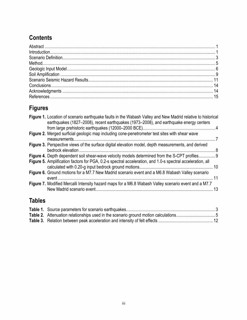
Contents Abstract ......................................................................................................................................................... 1 Introduction .................................................................................................................................................... 1 Scenario Definition......................................................................................................................................... 3 Method........................................................................................................................................................... 5 Geologic Input Model ..................................................................................................................................... 6 Soil Amplification ........................................................................................................................................... 9 Scenario Seismic Hazard Results................................................................................................................ 11 Conclusions ................................................................................................................................................. 14 Acknowledgments ....................................................................................................................................... 14 References .................................................................................................................................................. 15

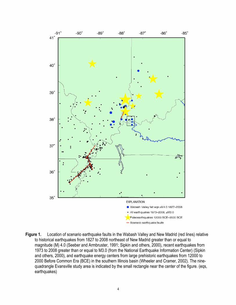
Figures Figure 1. Location of scenario earthquake faults in the Wabash Valley and New Madrid relative to historical

earthquakes (1827–2008), recent earthquakes (1973–2008), and earthquake energy centers from large prehistoric earthquakes (12000–2000 BCE)................................................................. 4

Figure 2. Merged surficial geologic map including cone-penetrometer test sites with shear wave measurements ............................................................................................................................... 7

Figure 3. Perspective views of the surface digital elevation model, depth measurements, and derived bedrock elevation .......................................................................................................................... 8

Figure 4. Depth dependent soil shear-wave velocity models determined from the S-CPT profiles ............... 9 Figure 5. Amplification factors for PGA, 0.2-s spectral acceleration, and 1.0-s spectral acceleration, all

calculated with 0.20-g input bedrock ground motions .................................................................. 10 Figure 6. Ground motions for a M7.7 New Madrid scenario event and a M6.8 Wabash Valley scenario

event ........................................................................................................................................... 11 Figure 7. Modified Mercalli Intensity hazard maps for a M6.8 Wabash Valley scenario event and a M7.7

New Madrid scenario event ......................................................................................................... 13

Tables Table 1. Source parameters for scenario earthquakes ................................................................................ 3 Table 2. Attenuation relationships used in the scenario ground motion calculations. .................................. 5 Table 3. Relation between peak acceleration and intensity of felt effects ................................................. 12

1

Earthquake Scenario Ground Motions for the Urban Area of Evansville, Indiana

By Jennifer S. Haase,1 Robert L. Nowack,1 Chris H. Cramer,2 Oliver S. Boyd,3 and Robert A. Bauer4

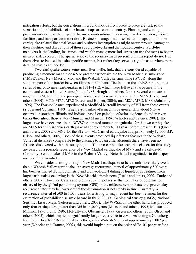
Abstract The Wabash Valley seismic zone and the New Madrid seismic zone are the closest large

earthquake source zones to Evansville, Indiana. The New Madrid earthquakes of 1811–1812, over 180 kilometers (km) from Evansville, produced ground motions with a Modified Mercalli Intensity of VII near Evansville, the highest intensity observed in Indiana. Liquefaction evidence has been documented less than 40 km away from Evansville resulting from two large earthquakes in the past 12,000 years in the Wabash Valley. Two earthquake scenarios are described in this paper that demonstrate the expected ground motions for a 33×42-km region around Evansville based on a repeat earthquake from each of these source regions. We perform a one-dimensional analysis for a grid of sites that takes into account the amplification or deamplification of ground motion in the unconsolidated soil layer using a new three-dimensional model of seismic velocity and bedrock depth. There are significant differences in the calculated amplification from that expected for National Earthquake Hazard Reduction Program site class D conditions, with deamplification at many locations within the ancient bedrock valley underlying Evansville. Ground motions relative to the acceleration of gravity (g) in the Evansville area from a simulation of a magnitude (M) 7.7 New Madrid earthquake range from 0.15 to 0.25 g for peak ground acceleration, 0.14 to 0.7 g for 0.2-second (s) spectral acceleration, and 0.05 to 0.25 g for 1.0-s spectral acceleration. Ground motions from a M6.8 Wabash Valley earthquake centered 40 km northwest of the city produce ground motions that decrease with distance from 1.5 to 0.3 g for 0.2-s spectral acceleration when they reach the main part of Evansville, but then increase in amplitude from 0.3 to 0.6 g south of the city and the Ohio River. The densest urbanization in Evansville and Henderson, Ky., is within the area of preferential amplification at 1.0-s period for both scenarios, but the area experiences relatively less amplification than surrounding areas at 0.2 s, consistent with expected resonance periods based on the soil profiles.

Introduction Calculating ground motions based on scenario earthquake events is an invaluable tool for

evaluating direct and indirect losses from specific credible earthquakes. Public and private groups can use these maps for planning, mitigation, and response efforts. Probabilistic seismic hazard maps, in which all possible sources are considered, are also well suited to planning and 1 Department of Earth and Atmospheric Sciences, Purdue University, West Lafayette, IN 47906 2 Center for Earthquake Research and Information, University of Memphis, Memphis, TN 3 United States Geological Survey, Memphis, TN 4 Illinois State Geological Survey, Champaign, IL

2

mitigation efforts, but the correlations in ground motion from place to place are lost, so the scenario and probabilistic seismic hazard maps are complementary. Planning and zoning professionals can use the maps for hazard considerations in locating new development, critical facilities, and transportation corridors. Business managers can use scenario maps to minimize earthquake-related financial losses and business interruption as might occur through damage to their facilities and disruptions of their supply networks and distribution centers. Portfolio managers in the lending, insurance, and wealth management industries can use the maps to better manage risk exposure. The spatial scale of the scenario maps presented in this report do not lend themselves to be used in a site-specific manner, but rather they serve as a guide as to where more detailed studies are needed.

Two earthquake source zones near Evansville, Ind., that are considered capable of producing a moment magnitude 6.5 or greater earthquake are the New Madrid seismic zone (NMSZ), near New Madrid, Mo., and the Wabash Valley seismic zone (WVSZ) along the southern part of the border between Illinois and Indiana. The faults in the NMSZ ruptured in a series of major to great earthquakes in 1811–1812, which were felt over a large area in the central and eastern United States (Nuttli, 1983; Hough and others, 2000). Several estimates of magnitude (M) for the three principal events have been made: M7.2, M7.0, M7.5 (Hough and others, 2000); M7.6, M7.5, M7.8 (Bakun and Hopper, 2004); and M8.1, M7.8, M8.0 (Johnston, 1996). The Evansville area experienced a Modified Mercalli Intensity of VII from these events (Stover and Coffman, 1993). Eight earthquakes of a magnitude greater than about 6 have occurred in southern Illinois and Indiana, based on paleoliquefaction evidence found in river banks throughout those states (Munson and Munson, 1996; Wheeler and Cramer, 2002). The largest two have occurred in the WVSZ; estimated moment magnitudes for the two earthquakes are M7.5 for the Vincennes earthquake at approximately 6,100 years before present (BP) (Green and others, 2005) and M6.7 for the Skelton–Mt. Carmel earthquake at approximately 12,000 B.P. (Olson and others, 2005). Both of these events produced liquefaction features in the Wabash Valley at distances comparable to the distance to Evansville, although there have been no features discovered within the study region. The two earthquake scenarios chosen for this study are based on a possible recurrence of a New Madrid earthquake of M7.7 and a Skelton–Mt. Carmel type earthquake of M6.8 in the Wabash Valley. Note that all magnitudes in this paper are moment magnitude.

We consider a strong-to-major New Madrid earthquake to be a much more likely event than a Wabash Valley earthquake. An average recurrence interval of approximately 500 years has been estimated from radiometric and archaeological dating of liquefaction features from large earthquakes occurring in the New Madrid seismic zone (Tuttle and others, 2002; Tuttle and others, 2005). However, Calais and Stein (2009) hypothesize that low rates of deformation observed by the global positioning system (GPS) in the midcontinent indicate that present day recurrence rates may be lower or that the deformation is not steady in time. Currently, a recurrence interval of 500 to 1,000 years for a strong-to-major event has been retained for the estimation of probabilistic seismic hazard in the 2008 U.S. Geological Survey (USGS) National Seismic Hazard Maps (Petersen and others, 2008). The WVSZ, on the other hand, has produced only four earthquakes greater than M6 in 14,000 years (Munson and others, 1995; Munson and Munson, 1996; Pond, 1996; McNulty and Obermeier, 1999; Green and others, 2005; Olson and others, 2005), which implies a significantly longer recurrence interval. Assuming a Gutenberg-Richter relation for M6 earthquakes in the greater Wabash Valley of approximately 0.002 per year (Wheeler and Cramer, 2002), this would imply a rate on the order of 7×10-6 per year for a

3

reduced area within 15 kilometers (km) of the prehistoric earthquake that occurred closest to Evansville, the Skelton–Mt. Carmel event. Probabilistic seismic hazard estimates for the area reflect this large difference in probability of occurrence (Petersen and others, 2008). Deaggregation of the 2008 USGS National Seismic Hazard Maps using the method of Harmsen and others (1999) for peak ground accelerations with 2-percent probability of being exceeded in 50 years shows that more than 25 percent of the contribution to the seismic hazard in Evansville comes from a New Madrid–type earthquake of M7 or greater, and less than 10 percent of the hazard comes from large magnitude (>M6.8) Wabash Valley–type events. However, it is useful to provide estimates of the hazard to Evansville from the WVSZ, since the city is within the zone where strong to major earthquakes occurred throughout the Holocene and back into the Pleistocene, as shown by extensive observations of prehistoric liquefaction features (Munson and Munson, 1996) and recorded moderate earthquakes during historic times.

Scenario Definition Two scenarios were defined: a M7.7 earthquake for the NMSZ and a M6.8 for the

WVSZ. The fault trace for the NMSZ scenario follows the current earthquake activity that we expect to coincide with the locations of the 1811–1812 New Madrid earthquakes. The fault is chosen to correspond to the three fault segments that are thought to have ruptured in the 1811–1812 earthquakes, although the greatest contribution comes from the closest (northern) segment. The fault trace for the WVSZ scenario follows the trend of Paleozoic geologic structures in the Wabash Valley near the location of the Skelton–Mt. Carmel earthquake. The fault is placed near the Skelton–Mt. Carmel earthquake because it is the closest location to Evansville in which a M6 or greater earthquake is known to have occurred. The WVSZ scenario fault length was assigned using a magnitude-length scaling relationship (Wells and Coppersmith, 1994). As there are no data to constrain the endpoints of this fault, it should be considered an illustration of one of many possible scenarios. Similarly, no attempt has been made to consider source directivity or variations in radiation pattern, depth, or stress drop. Because directivity of the source is not included, the greatest ground motions are generated by the closest fault segment of the three hypothetical faults. The scenario faults are shown in figure 1 and described in table 1.

Table 1. Source parameters for scenario earthquakes.

Source zone Magnitude Distance to Evansville (kilometers)

Fault coordinates (latitude, longitude)

Wabash Valley 6.8 40 km 38.29, -87.89 38.03, -88.02

New Madrid 7.7 180 km 35.56, -90.48 36.32, -89.48 36.07, -89.36 36.59, -89.63 36.50, -89.70 37.01, -89.25

4

Figure 1. Location of scenario earthquake faults in the Wabash Valley and New Madrid (red lines) relative to historical earthquakes from 1827 to 2008 northeast of New Madrid greater than or equal to magnitude (M) 4.0 (Seeber and Armbruster, 1991; Sipkin and others, 2000), recent earthquakes from 1973 to 2008 greater than or equal to M3.0 (from the National Earthquake Information Center) (Sipkin and others, 2000), and earthquake energy centers from large prehistoric earthquakes from 12000 to 2000 Before Common Era (BCE) in the southern Illinois basin (Wheeler and Cramer, 2002). The nine-quadrangle Evansville study area is indicated by the small rectangle near the center of the figure. (eqs, earthquakes)

5

Method The calculation of the ground motion level at each grid point in the nine quadrangle map

area around Evansville (shown in fig. 1) was based on the magnitude of the earthquake, the distance from the grid point to the fault, and the effects of local site geology, which may amplify or deamplify ground motions. We characterized the local geology in the map area using surficial and subsurface geologic information, bedrock depth data, and subsurface shear-wave (S-wave) velocity measurements, which are described in the following section. The method is similar to the approach of Cramer and others (2004) for Memphis, Tenn.

The amplification factor due to local site geology was calculated using a frequency domain approach assuming shear waves vertically incident on a localized one-dimensional (1D) bedrock/soil profile (SHAKE91; Idriss and Sun, 1992). The approach takes into account inelastic behavior of the soil column using an iterative equivalent linear method. For each site, 100 realizations of the soil profile were generated that have the distribution of shear-wave velocities and soil-layer thicknesses that are found in the set of measured profiles representative of that site geology. The set of realizations also introduces variations from the average modulus reduction curves and damping curves.

For each realization of the soil column, a random selection from one of 16 scaled bedrock ground motions derived from ground-motion recordings and synthetic time series is propagated up through the soil column. The bedrock ground motions are scaled such that the amplitude at the given spectral ordinate—such as peak ground acceleration (PGA) or 0.2-second (s) or 1.0-s spectral acceleration (SA)—is set equal to each of 20 input ground motion values, thereby producing 20 distributions of site amplification.

Ground-motion attenuation relations estimate the median ground motion level at different frequencies as a function of distance from and magnitude of the source. Because of the few instrumental recordings from moderate events and the lack of instrumental recordings from large events in the central and eastern United States (CEUS), there is significant uncertainty in predicted ground motions, especially for large magnitude earthquakes. For this reason, a weighted average of estimates from a suite of ground-motion attenuation relationships was used (table 2), the same ground-motion attenuation relationships and respective weights that are used in the probabilistic hazard calculation for the Evansville area (Haase and others, 2011a) and for the USGS National Seismic Hazard Maps (Petersen and others, 2008).

The function of median site amplification versus input ground motion is then interpolated to find the amplified ground motion associated with the weighted average of eight firm-rock ground-motion attenuation relations. The firm-rock ground motion is then scaled by this site amplification factor to produce the final ground motion at the site.

Table 2. Attenuation relationships used in the scenario ground motion calculations.

Attenuation curve reference Weight Toro and others (1997) 0.2 Frankel and others (1996) 0.1 Campbell and Bozorgnia (2003) 0.1 Atkinson and Boore (2006)—140 bar stress drop 0.1 Atkinson and Boore (2006)—200 bar stress drop 0.1 Tavakoli and Pezeshk (2005) 0.1 Silva and others (2002) 0.1 Somerville and others (2001) 0.2

6

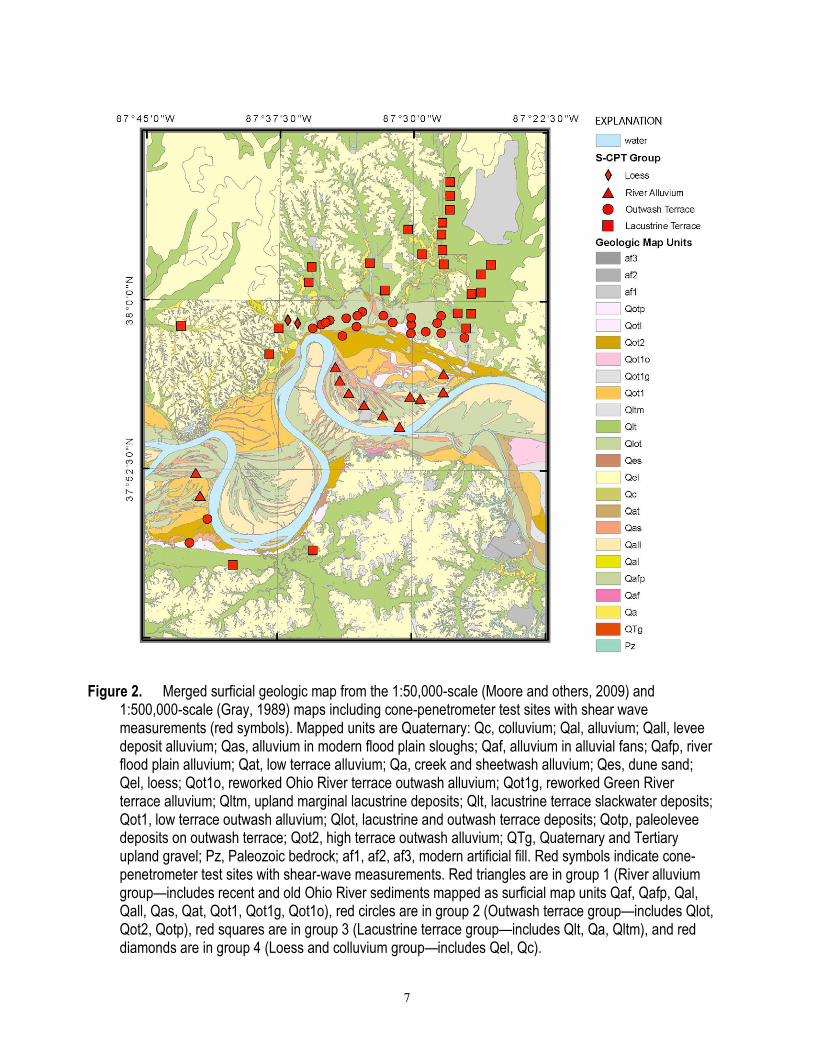
Geologic Input Model The geologic input model for the amplification calculation represents the geologic

material, bedrock depth, and seismic velocity profile at each point on a 0.01o by 0.01o grid for the nine-quadrangle region surrounding Evansville. At this scale, the maps presented here do not allow them to be used in a site-specific manner, but rather as a guide to where more detailed studies are needed. The surficial geology (Gray, 1989; Moore and others, 2009) along the Ohio River valley near Evansville consists primarily of fluvial and lake deposits that fill incised bedrock valleys formed in Pennsylvanian age bedrock (fig. 2). Wind-deposited loess covers the surrounding upland hills. Beneath the terraces bordering the current river valley are alternating layers of outwash, slackwater lake deposits, and fluvial deposits. The geologic maps, in conjunction with subsurface information, were used to associate regions of similar depositional history and similar properties to produce representative shear-wave velocity profiles.

7

Figure 2. Merged surficial geologic map from the 1:50,000-scale (Moore and others, 2009) and 1:500,000-scale (Gray, 1989) maps including cone-penetrometer test sites with shear wave measurements (red symbols). Mapped units are Quaternary: Qc, colluvium; Qal, alluvium; Qall, levee deposit alluvium; Qas, alluvium in modern flood plain sloughs; Qaf, alluvium in alluvial fans; Qafp, river flood plain alluvium; Qat, low terrace alluvium; Qa, creek and sheetwash alluvium; Qes, dune sand; Qel, loess; Qot1o, reworked Ohio River terrace outwash alluvium; Qot1g, reworked Green River terrace alluvium; Qltm, upland marginal lacustrine deposits; Qlt, lacustrine terrace slackwater deposits; Qot1, low terrace outwash alluvium; Qlot, lacustrine and outwash terrace deposits; Qotp, paleolevee deposits on outwash terrace; Qot2, high terrace outwash alluvium; QTg, Quaternary and Tertiary upland gravel; Pz, Paleozoic bedrock; af1, af2, af3, modern artificial fill. Red symbols indicate cone-penetrometer test sites with shear-wave measurements. Red triangles are in group 1 (River alluvium group—includes recent and old Ohio River sediments mapped as surficial map units Qaf, Qafp, Qal, Qall, Qas, Qat, Qot1, Qot1g, Qot1o), red circles are in group 2 (Outwash terrace group—includes Qlot, Qot2, Qotp), red squares are in group 3 (Lacustrine terrace group—includes Qlt, Qa, Qltm), and red diamonds are in group 4 (Loess and colluvium group—includes Qel, Qc).

8

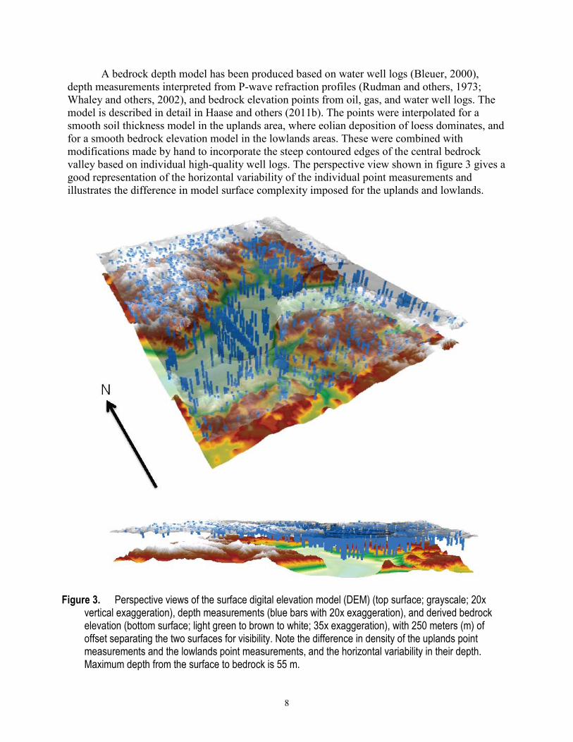
A bedrock depth model has been produced based on water well logs (Bleuer, 2000), depth measurements interpreted from P-wave refraction profiles (Rudman and others, 1973; Whaley and others, 2002), and bedrock elevation points from oil, gas, and water well logs. The model is described in detail in Haase and others (2011b). The points were interpolated for a smooth soil thickness model in the uplands area, where eolian deposition of loess dominates, and for a smooth bedrock elevation model in the lowlands areas. These were combined with modifications made by hand to incorporate the steep contoured edges of the central bedrock valley based on individual high-quality well logs. The perspective view shown in figure 3 gives a good representation of the horizontal variability of the individual point measurements and illustrates the difference in model surface complexity imposed for the uplands and lowlands.

Figure 3. Perspective views of the surface digital elevation model (DEM) (top surface; grayscale; 20x vertical exaggeration), depth measurements (blue bars with 20x exaggeration), and derived bedrock elevation (bottom surface; light green to brown to white; 35x exaggeration), with 250 meters (m) of offset separating the two surfaces for visibility. Note the difference in density of the uplands point measurements and the lowlands point measurements, and the horizontal variability in their depth. Maximum depth from the surface to bedrock is 55 m.

9

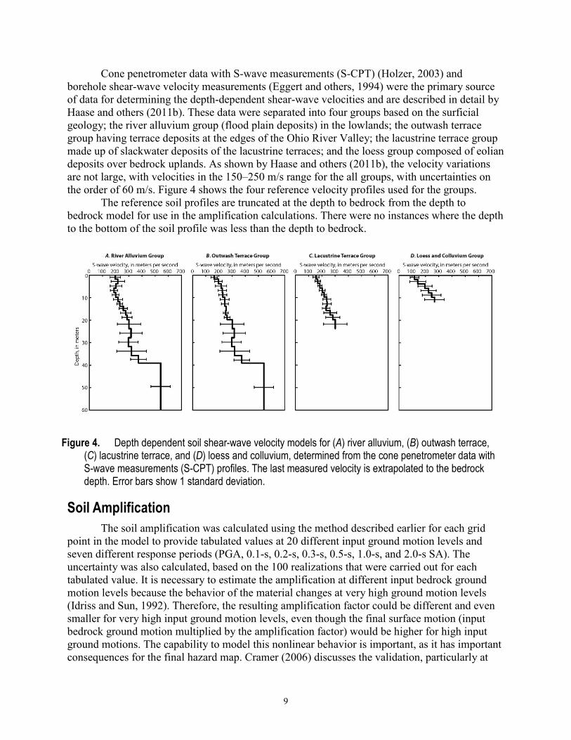
Cone penetrometer data with S-wave measurements (S-CPT) (Holzer, 2003) and borehole shear-wave velocity measurements (Eggert and others, 1994) were the primary source of data for determining the depth-dependent shear-wave velocities and are described in detail by Haase and others (2011b). These data were separated into four groups based on the surficial geology; the river alluvium group (flood plain deposits) in the lowlands; the outwash terrace group having terrace deposits at the edges of the Ohio River Valley; the lacustrine terrace group made up of slackwater deposits of the lacustrine terraces; and the loess group composed of eolian deposits over bedrock uplands. As shown by Haase and others (2011b), the velocity variations are not large, with velocities in the 150–250 m/s range for the all groups, with uncertainties on the order of 60 m/s. Figure 4 shows the four reference velocity profiles used for the groups.

The reference soil profiles are truncated at the depth to bedrock from the depth to bedrock model for use in the amplification calculations. There were no instances where the depth to the bottom of the soil profile was less than the depth to bedrock.

Figure 4. Depth dependent soil shear-wave velocity models for (A) river alluvium, (B) outwash terrace, (C) lacustrine terrace, and (D) loess and colluvium, determined from the cone penetrometer data with S-wave measurements (S-CPT) profiles. The last measured velocity is extrapolated to the bedrock depth. Error bars show 1 standard deviation.

Soil Amplification The soil amplification was calculated using the method described earlier for each grid

point in the model to provide tabulated values at 20 different input ground motion levels and seven different response periods (PGA, 0.1-s, 0.2-s, 0.3-s, 0.5-s, 1.0-s, and 2.0-s SA). The uncertainty was also calculated, based on the 100 realizations that were carried out for each tabulated value. It is necessary to estimate the amplification at different input bedrock ground motion levels because the behavior of the material changes at very high ground motion levels (Idriss and Sun, 1992). Therefore, the resulting amplification factor could be different and even smaller for very high input ground motion levels, even though the final surface motion (input bedrock ground motion multiplied by the amplification factor) would be higher for high input ground motions. The capability to model this nonlinear behavior is important, as it has important consequences for the final hazard map. Cramer (2006) discusses the validation, particularly at

10

strong levels of input ground motion, of the modified version of SHAKE91 used in this application with other equivalent linear and nonlinear codes.

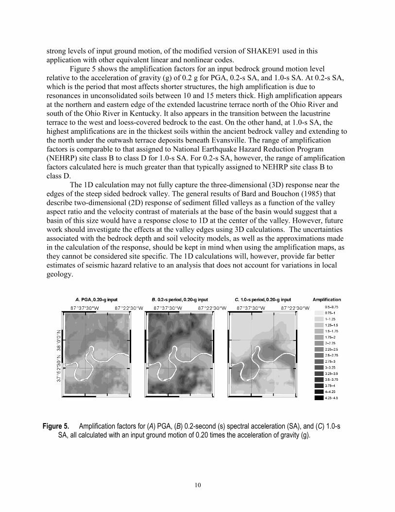
Figure 5 shows the amplification factors for an input bedrock ground motion level relative to the acceleration of gravity (g) of 0.2 g for PGA, 0.2-s SA, and 1.0-s SA. At 0.2-s SA, which is the period that most affects shorter structures, the high amplification is due to resonances in unconsolidated soils between 10 and 15 meters thick. High amplification appears at the northern and eastern edge of the extended lacustrine terrace north of the Ohio River and south of the Ohio River in Kentucky. It also appears in the transition between the lacustrine terrace to the west and loess-covered bedrock to the east. On the other hand, at 1.0-s SA, the highest amplifications are in the thickest soils within the ancient bedrock valley and extending to the north under the outwash terrace deposits beneath Evansville. The range of amplification factors is comparable to that assigned to National Earthquake Hazard Reduction Program (NEHRP) site class B to class D for 1.0-s SA. For 0.2-s SA, however, the range of amplification factors calculated here is much greater than that typically assigned to NEHRP site class B to class D.

The 1D calculation may not fully capture the three-dimensional (3D) response near the edges of the steep sided bedrock valley. The general results of Bard and Bouchon (1985) that describe two-dimensional (2D) response of sediment filled valleys as a function of the valley aspect ratio and the velocity contrast of materials at the base of the basin would suggest that a basin of this size would have a response close to 1D at the center of the valley. However, future work should investigate the effects at the valley edges using 3D calculations. The uncertainties associated with the bedrock depth and soil velocity models, as well as the approximations made in the calculation of the response, should be kept in mind when using the amplification maps, as they cannot be considered site specific. The 1D calculations will, however, provide far better estimates of seismic hazard relative to an analysis that does not account for variations in local geology.

Figure 5. Amplification factors for (A) PGA, (B) 0.2-second (s) spectral acceleration (SA), and (C) 1.0-s SA, all calculated with an input ground motion of 0.20 times the acceleration of gravity (g).

11

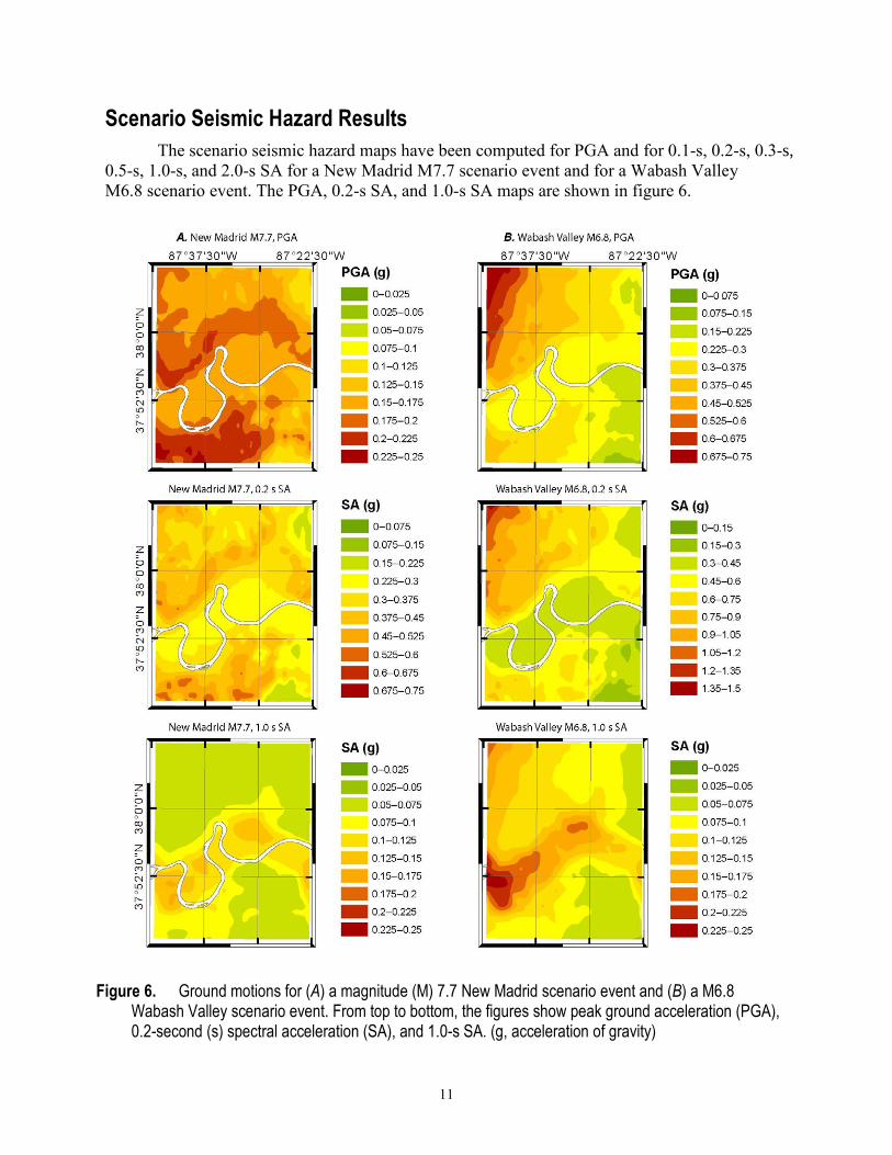
Scenario Seismic Hazard Results The scenario seismic hazard maps have been computed for PGA and for 0.1-s, 0.2-s, 0.3-s,

0.5-s, 1.0-s, and 2.0-s SA for a New Madrid M7.7 scenario event and for a Wabash Valley M6.8 scenario event. The PGA, 0.2-s SA, and 1.0-s SA maps are shown in figure 6.

Figure 6. Ground motions for (A) a magnitude (M) 7.7 New Madrid scenario event and (B) a M6.8 Wabash Valley scenario event. From top to bottom, the figures show peak ground acceleration (PGA), 0.2-second (s) spectral acceleration (SA), and 1.0-s SA. (g, acceleration of gravity)

12

For the New Madrid scenario PGA, the highest accelerations of 0.15–0.2 g are along the western border of the study area, which is consistent with the fact that the New Madrid fault is to the southwest of Evansville, but there is little overall variation across the area. At 0.2-s SA, the highest values of 0.4–0.6 g are again seen away from the bedrock valleys and correspond to thin soils and therefore shorter periods. It is impressive to note that the accelerations at such high frequencies are significant despite the fact that the source is 180 km away, which re-emphasizes the low attenuation of seismic waves in the center of North America. Fortunately, the highest ground motions at this period occur north of the major urban areas in Evansville and south and east of the major urban sections of Henderson. The highest 1.0-s SA are 0.15–0.17 g and occur where the soil thickness is greatest, which is in the area overlying the ancient bedrock valley. This region of higher ground motion (up to 0.17 g) extends into the terrace deposits on which most of Evansville is built. It also extends significantly east from the river under Henderson. Therefore, the 1.0-s SA ground motions should be of special concern here.

Table 3. Relation between peak acceleration as a fraction of the acceleration of gravity (g) and intensity of felt effects (Wald and others, 1999).

Instrumental

intensity Perceived shaking Not felt Weak Light Moderate Strong Very strong Severe Violent Extreme

Potential damage None None None Very light Light Moderate Moderate/heavy Heavy Very heavy

Peak acc (g) <0.0017 0.0017–0.014

0.014–0.039

0.039–0.092

0.092–0.18 0.18–0.34 0.34–0.65 0.65–

1.24 >1.24

For the Wabash Valley scenario, the highest PGA are 0.6–0.8 g in the northwest corner of

the map area with accelerations decreasing towards the southeast. Peak ground acceleration values in Evansville are in the 0.2–0.4 g range. The decrease in acceleration towards the southeast corner is a direct result of the increase in distance from the seismic source. For the 0.2-s SA, the values exceed 1.0 g in the northwest corner and decrease to levels of about 0.3 g in the central Evansville urban area north of the Ohio River. The 0.2-s SA increases again south of the river with very high values of 0.4–0.7 g. At 1.0-s SA the pattern of amplified ground motion above the bedrock valley is superimposed on the distance-dependent decrease in ground motion levels. The 1.0-s SA is 0.2–0.25 g in soil deposits north of the Ohio River and in the Ohio River Valley. As in the case for the New Madrid event, the variation in soil thickness has a far greater effect on 0.2-s SA relative to 1.0-s SA having both greater amplification and spatial variability.

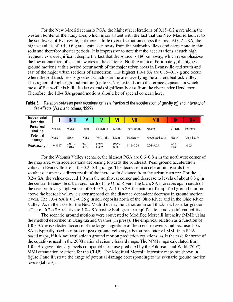
The scenario ground motions were converted to Modified Mercalli Intensity (MMI) using the method described in Dangkua and Cramer (in press). The empirical relation as a function of 1.0-s SA was selected because of the large magnitude of the scenario events and because 1.0-s SA is typically used to represent peak ground velocity, a better predictor of MMI than PGA-based maps, if it is not available in ground motion prediction equations, as is the case for some of the equations used in the 2008 national seismic hazard maps. The MMI maps calculated from 1.0-s SA gave intensity levels comparable to those predicted by the Atkinson and Wald (2007) MMI attenuation relations for the CEUS. The Modified Mercalli Intensity maps are shown in figure 7 and illustrate the range of potential damage corresponding to the scenario ground motion levels (table 3).

13

Figure 7. Modified Mercalli Intensity hazard maps for 2010 scenarios. A, Wabash Valley scenario event, magnitude (M) 6.8, (WVF2, Wabash Valley fault #2) with geology. B, New Madrid scenario event, M7.7, (NMNF, New Madrid north fault) with geology.

14

Conclusions Ground motions from a magnitude 6.8 Wabash Valley scenario earthquake, similar to what

may have occurred during the Skelton–Mt. Carmel earthquake about 12,000 years ago, would be very strong across the Evansville area. Peak ground acceleration would vary from 0.8 g in the region northwest of Evansville to 0.1 g in the southeast as distance increases from the causative fault. Local soil conditions have a major effect on the ground motions predicted for the scenario earthquakes. At 0.2-s spectral acceleration, the amplification of ground motions due to local variations in the soil thicknesses makes accelerations south of the river 15 km farther away from the earthquake source comparable to motions north of the river. The majority of the urban area is constructed on alluvial and lacustrine terrace deposits north of the Ohio River, over an ancient incised bedrock valley. The thicknesses of the deposits are such that resonances produce strong amplification at the 1.0-s period. The resulting ground motions for the Wabash Valley scenario event at 1.0-s spectral accelerations are 0.1–0.25 g in the Ohio River valley. Variations in the level of acceleration caused by local soil conditions are comparable to or greater than the variations due to the distance from the source.

The peak ground acceleration level for a magnitude 7.7 New Madrid scenario event, similar to what may have occurred during the 1811–1812 New Madrid earthquakes, would be about 0.15–0.25 g with significant local variations across the study area. However, 0.2-s spectral accelerations would be very high, between 0.4 and 0.5 g, north and east of the main urban center of Evansville. The 1.0-s spectral accelerations would be 0.1–0.2 g, with higher values confined to the bedrock valley.

The objective of this work is to demonstrate the local variability in ground motions due to one component of the ground motion equation: local site effects. This study does not attempt to examine complexity in the source or 3D wave propagation that may also cause variability in the ground motions. These components would be more significant for the closer Wabash Valley event. We expect that the more distant New Madrid source would be more likely to produce a more nearly homogeneous wavefield impinging on the study area, so that the pattern of variations calculated here would be realistic representation of ground motion variability.

These scenario maps are a valuable complement to the probabilistic seismic hazard maps for the Evansville area (Haase and others, 2011a) because the scenario maps illustrate the simple relationship between earthquake source and potential hazard. Also, the scenario ground motions can be used to calculate liquefaction hazard (Haase and others, 2011b). However, scenario ground motions do not communicate effectively the relative probability of occurrence of these events, which may be as infrequent as one in 4,000 years for the Wabash Valley event (that is, very rare) to one in 500–1,000 years for the New Madrid event. The scenario maps are most effective in combination with the probabilistic seismic hazard maps, which indicate the probability that a given ground motion level will be exceeded in a specified period of time.

Acknowledgments This work was supported by the USGS National Earthquake Hazards Reduction Program

(grant G09AP00057). We would like to thank the members of the Evansville Area Earthquake Hazards Mapping Project Technical Working Group for their invaluable efforts in geological mapping and data collection and for their input into the decisions for the choice of scenario earthquakes. Key motivation for this project came from the Southwest Indiana Disaster Resistant Community Corporation. We thank Stephen Harmsen, Charles Mueller, and David Perkins for insightful reviews that helped improve the manuscript.

15

References Atkinson, G.M., and Boore, D.M., 2006, Earthquake groundmotion prediction equations for

eastern North America: Bulletin of the Seismological Society of America, v. 96, no. 6, p. 2181–2205.

Atkinson, G.M., and Wald, D.J., 2007, “Did you feel it?” Intensity data—A surprisingly good measure of earthquake ground motion: Seismological Research Letters, v. 78, no. 3, p. 362–368.

Bakun, W.H., and Hopper, M.G., 2004, Magnitudes and locations of the 1811–1212 New Madrid, Missouri, and the 1886 Charleston, South Carolina, earthquakes: Bulletin of the Seismological Society of America, v. 94, no. 1, p. 64–75.

Bard, P.Y., and Bouchon, Michel, 1985, The two-dimensional resonance of sediment-filled valleys: Bulletin of the Seismological Society of America, v. 75, no. 2, p. 519.

Bleuer, N.K., 2000, iLITH database of the Indiana Geological Survey CD-ROM: Indiana Geological Survey Open File Study 00-8.

Calais, Eric, and Stein, Seth, 2009, Time-variable deformation in the New Madrid seismic zone: Science, v. 323, no. 5920, p. 1442–1442.

Campbell, K.W., and Bozorgnia, Yousef, 2003, Updated near-source ground-motion (attenuation) relations for the horizontal and vertical components of peak ground acceleration and acceleration response spectra: Bulletin of the Seismological Society of America, v. 93, no. 1, p. 314–331.

Cramer, C.H., 2006, Quantifying the uncertainty in site amplification modeling and its effects on site-specific seismic hazard estimation in the upper Mississippi embayment and adjacent areas: Bulletin of the Seismological Society of America, v. 96, no. 6, p. 2008–2020.

Cramer, C.H., Gomberg, J.S., Schweig, E.S., Waldron, B.A., and Tucker, Kathy, 2004, The Memphis, Shelby County, Tennessee, seismic hazard maps: United States Geological Survey Open-File Report 2004–1294, 46 p.

Dangkua, D.T., and Cramer, C.H., in press, Felt intensity vs. instrumental ground motion—A difference between California and Eastern North America?: Bulletin of the Seismological Society of America.

Eggert, D.L., Samuelson, A.C., Bray, J.D., Chang, C.W., Eckhoff, W.R., Kayabali, K., McClees, E.J., West, T.R., Woodfield, M.C., and Zheng, B., 1994, Final report to the city of Evansville—Shear-wave and earthquake hazard mapping of Evansville, Indiana: Indiana Geological Survey Open File Studies, OFS94-19, 17 p.

Frankel, A.D., Mueller, C., Barnhard, Theodore, Perkins, D.M., Leyendecker, E.V., Dickman, Nancy, Hanson, Stanley, and Hopper, Margaret, 1996, National seismic hazard maps—Documentation June 1996: United States Geological Survey Open-File Report 96–532, 110 p.

Gray, H.H., 1989, Quaternary geologic map of Indiana: Indiana Geological Survey Miscellaneous Map 49, scale 1:500,000.

Green, R.A., Obermeier, S.F., and Olson, S.M., 2005, Engineering geologic and geotechnical analysis of paleoseismic shaking using liquefaction effects—Field examples: Engineering Geology, v. 76, p. 263–293.

Haase, J.S., Nowack, R.L., Choi, Y.S., Bowling, T., Cramer, C.H., Boyd, O.S., and Bauer, R.A., 2011a, Probabilistic seismic hazard assessment including site effects for Evansville, Indiana, and the surrounding region United States Geological Survey Open-File Report 2011ï1231, 29 p.

16

Haase, J.S., Nowack, R.L., Choi, Y.S., Cramer, C.H., Boyd, O.S., and Bauer, R.A., 2011b, Liquefaction hazard for the Evansville, Indiana, region United States Geological Survey Open File Report 2011–1203, 38 p.

Harmsen, S.C., Perkins, D.M., and Frankel, A.D., 1999, Deaggregation of probabilistic ground motions in the central and eastern United States: Bulletin of the Seismological Society of America, v. 89, no. 1, p. 1–13.

Holzer, T.L., 2003, USGS CPT data—Evansville Indiana area: United States Geological Survey Earthquake Hazards Program, accessed January 14, 2004, at http://earthquake.usgs.gov/ regional/nca/cpt/data.

Hough, S.E., Armbruster, J.G., Seeber, Leonardo, and Hough, J.F., 2000, On the Modified Mercalli Intensities and magnitudes of the 1811–1812 New Madrid earthquakes: Journal of Geophysical Research–Solid Earth, v. 105, no. B10, p. 23839–23864.

Idriss, I.M., and Sun, J.I., 1992, User's manual for SHAKE91: University of California, Department of Civil and Environmental Engineering, Center for Geotechnical Modeling.

Johnston, A.C., 1996, Seismic moment assessment of earthquakes in stable continental regions—III. New Madrid 1811–1812, Charleston 1886 and Lisbon 1755: Geophysical Journal International, v. 126, no. 2, p. 314–344.

McNulty, W.E., and Obermeier, S.F., 1999, Liquefaction evidence for at least two strong Holocene paleo-earthquakes in central and southwestern Illinois, USA: Environmental and Engineering Geoscience, v. 5, no. 2, p. 133–146.

Moore, D.W., Lundstrom, S.C., Counts, R.C., Martin, S.L., Andrews, W.M., Jr., Newell, W.L., Murphy, M.L., Thompson, M.F., Taylor, E.M., Kvale, E.P., and Brandt, T.R., 2009, Surficial geologic map of the Evansville, Indiana and Henderson, Kentucky area: United States Geological Survey Scientific Investigations Map SIM-3069, scale 1:50,000.

Munson, P.J., and Munson, C.A., 1996, Paleoliquefaction evidence for recurrent strong earthquakes since 20 000 yr BP in the Wabash Valley area of Indiana: Indiana University Final Technical Report for United States Geological Survey Grant #14-08-0001-G2117, 137 p.

Munson, P.J., Munson, C.A., and Pond, E.C., 1995, Paleoliquefaction evidence for a strong holocene earthquake in south-central Indiana: Geology, v. 23, no. 4, p. 325–328.

Nuttli, O.W., 1983, Catalog of Central United States earthquakes since 1800 of mb = 3.0: St. Louis University.

Olson, S.M., Green, R.A., and Obermeier, S.F., 2005, Revised magnitude-bound relation for the Wabash Valley seismic zone of the central United States: Seismological Research Letters, v. 76, no. 6, p. 756–771.

Petersen, M.D., Frankel, A.D., Harmsen, S.C., Mueller, C.S., Haller, K.M., Wheeler, R.L., Wesson, R.L., Zeng, Y.H., Boyd, O.S., Perkins, D.M., Luco, Nicolas, Field, E.H., Wills, C.J., and Rukstales, K.S., 2008, Documentation for the 2008 update of the national seismic hazard maps: United States Geological Survey Open-File Report 2008–1128, 60 p.

Pond, E.C., 1996, Seismic parameters for the central United States based on paleoliquefaction evidence in the Wabash Valley: Blacksburg, Vir., Virginia Polytechnic Institute, Ph.D. dissertation, 583 p.

Rudman, A.J., Biggs, M.E., Blakely, R.F., and Whaley, J.F., 1973, Statistical studies of Indiana bedrock velocities—Mapping applications: Indiana Academy of Science, v. 83, no. 1973, p. 284–290.

17

Seeber, Leonardo, and Armbruster, J.G., 1991, The NCEER-91 earthquake catalog—Improved intensity-based magnitudes and recurrence relations for U.S. earthquakes east of New Madrid: National Center for Earthquake Engineering Research NCEER-91-0021.

Silva, Walter, Gregor, Nick, and Darragh, Robert, 2002, Development of hard rock attenuation relations for central and eastern North America: Pacific Engineering Internal Report, 27 p.

Sipkin, S.A., Person, W.J., and Presgrave, B.W., 2000, Earthquake bulletins and catalogs at the USGS National Earthquake Information Center: IRIS Newsletter, v. 2000, no. 1, p. 2–4.

Somerville, P.G., Collins, N.F., Abrahamson, N.A., Graves, R.W., and Saikia, C.K., 2001, Ground motion attenuation relations for the central and eastern United States: URS Group Final Technical Report for United States Geological Survey Grant No. 99HQGR0098, 38 p.

Stover, C.W., and Coffman, J.L., 1993, Seismicity of the United States, 1568–1989 (revised): United States Geological Survey Professional Paper 1527, 418 p.

Tavakoli, Behrooz, and Pezeshk, Shahram, 2005, Empirical-stochastic ground-motion prediction for eastern North America: Bulletin of the Seismological Society of America, v. 95, no. 6, p. 2283–2296.

Toro, G.R., Abrahamson, N.A., and Schneider, J.F., 1997, Model of strong ground motions from earthquakes in central and eastern North America—Best estimates and uncertainties: Seismological Research Letters, v. 68, no. 1, p. 41–57.

Tuttle, M.P., Schweig, E.S., Cambell, Janice, Thomas, P.J., Sims, J.D., and Lafferty, R.H., 2005, Evidence for New Madrid earthquakes in A.D. 300 and 2350 B.C.: Seismological Research Letters, v. 76, no. 4, p. 489–501.

Tuttle, M.P., Schweig, E.S., Sims, J.D., Lafferty, R.H., Wolf, L.W., and Haynes, M.L., 2002, The earthquake potential of the New Madrid seismic zone: Bulletin of the Seismological Society of America, v. 92, no. 6, p. 2080–2089.

Wald, D.J., Quitoriano, Vincent, Heaton, T.H., and Kanamori, Hiroo, 1999, Relationships between peak ground acceleration, peak ground velocity and Modified Mercalli Intensity in California: Earthquake Spectra, v. 15, p. 557–564.

Wells, D.L., and Coppersmith, K.J., 1994, New empirical relationships among magnitude, rupture length, rupture width, rupture area, and surface displacement: Bulletin of the Seismological Society of America, v. 84, no. 4, p. 974–1002.

Whaley, J.F., Blakely, R.F., Like, K.K., and James, C.L., 2002, Seismic refraction data for Indiana (Point Shapefile): Bloomington, Ind., Indiana Geological Survey, accessed October 7, 2002, at http://inmap.indiana.edu/dload_page/geology.html.

Wheeler, R.L., and Cramer, C.H., 2002, Updated seismic hazard in the southern Illinois Basin—Geological and geophysical foundations for use in the 2002 USGS National Seismic Hazard Maps: Seismological Research Letters, v. 73, no. 5, p. 776–791.

Publishing support provided by: Denver Publishing Service Center For more information concerning this publication, contact: Center Director, USGS Geologic Hazards Science Center Box 25046, Mail Stop 966 Denver, CO 80225 (303) 273-8579 Or visit Geologic Hazards Science Center Web site at: http://geohazards.cr.usgs.gov/