EARTHQUAKES’ MAIN SHOCK AND AFTERSHOCK ANALYSIS USING POINT PROCESS MODELING TECHNIQUES

7/29/2019 EARTHQUAKES’ MAIN SHOCK AND AFTERSHOCK ANALYSIS USING POINT PROCESS MODELING TECHNIQUES

http://slidepdf.com/reader/full/earthquakes-main-shock-and-aftershock-analysis-using-point-process-modeling 1/11

EARTHQUAKES’ MAIN SHOCK AND AFTERSHOCK ANALYSIS USING THE

POINT PROCESS MODELING TECHNIQUES

1 INTRODUCTION

There is a saying “if you cannot predict you cannot prevent”, actually for earthquakes preventing is notpossible but at least if it is predicted some precautions can be taken in order to decrease the destruction

effect on settlements. Modeling the earthquakes will help to predict the possible earthquake locations

or at least the trend of possible locations. Earthquakes are resulted of an energy release which is

observed in earth surface and this called as main shocks, aftershocks are the smaller earthquakes

which fallow the main shocks. And the location of the aftershocks is dependent on the magnitude,

depth and location of the main shocks (Lieshout and Stein 2011). Earthquakes are complicated

disasters; it will be unrealistic to minimize the earthquake only with location and magnitude. But for

this study the main research question will be the relation between the main shocks and aftershocks

using the magnitude and the location information of the earthquakes.

2 CASE STUDY

Figure 1: Fault map for the Turkey

Turkey lies between Latitudes: 36°- 42° and Longitudes: 26° - 45°. It is one of the countries where

there are many earthquakes happened with big destruction. Most of them lies on the Anatolian plate.

Many of Turkey's most severe quakes occur on one of the two faults that flank the Anatolian plate, the

north and the east Anatolian faults. Between 1939 and 1999 Turkey's major earthquakes were

marching westward along the north Anatolian fault. In 1999 a magnitude-7.6 quake struck near Izmit, just 70 kilometers from Istanbul, killing around 17,000 people. Since 2003 activity has shifted to the

East Anatolian fault.

The case study region is located in eastern part of the Turkey where the North Anatolian and East

Anatolian faults are intersecting. The main reason of the selecting this region is that it has been

affected by many earthquakes and new earthquakes are expected in this region because of the

movement in these two faults. If the relation earthquakes modeled it will be easy to take precautions.



1

Figure 2: Earthquake locations in Eastern Anatolia Region (mag>4, year 1973-2012)

2.1 DATA

Data downloaded from Geological Survey web side which is storing the updated worldwide

earthquakes. And the earthquakes happened between the years 1973 till 2012 have been used. In order

to make calculations easy; the data transferred from polar coordinates to metric coordinates. For this

study only the earthquakes with magnitude bigger than 4 used.

3 METHODSEarthquake data can be classified as point process which means an existing point pattern localize in

space or time and the magnitude of them can be used as marks of the point process. Point process

modeling consists of determining the first and second order characteristic of the process. (Baddeley,

2010). The first order characteristics show the intensity of the each point in each unit. This can be can

be indicated by intensity and density test (Baddeley, 2010). The second order characteristics represent

variation of point number in each unit, interaction between different and same type of points.

(Baddeley, 2010). According to the characteristic of the point pattern or process, it can be fitted to a

model by using point pattern model (ppm) object in R.

Here are the main models can be applied to the data which have been explained in the R spatstat

package:

Poisson Point Process and conditional intensity λ>0 can be expressed as: λ(u, x) = ß(1)

The inhomogeneous Poisson process is a model with intensity function ß(u):

λ(u, x) = ß(u) (2)

For clustered point patterns, the distribution depends on the interaction parameter, interaction

distance between each point pair, and distribution density. Strauss point process is one of the

models used to investigate these clustered relationships as proposed by Strauss. The Strauss Point

Process is a pair-wise interaction model with interaction constant γ, and the distance radius lessthan ‘r’. The t (u, x) represent how many points from X ar e located within the ‘r’ radius.



2

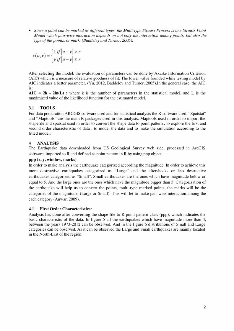
Since a point can be marked as different types, the Multi-type Strauss Process is one Strauss Point

Model which pair-wise interaction depends on not only the interaction among points, but also the

type of the points, or mark. (Baddeley and Turner, 2005):

After selecting the model, the evaluation of parameters can be done by Akaike Information Criterion

(AIC) which is a measure of relative goodness of fit. The lower value founded while testing model by

AIC indicates a better parameter. (Yu, 2012, Baddeley and Turner, 2005).In the general case, the AIC

is:

AIC = 2k - 2ln(L) : where k is the number of parameters in the statistical model, and L is the

maximized value of the likelihood function for the estimated model.

3.1 TOOLS

For data preparation ARCGIS software used and for statistical analysis the R software used. “Spatstat”

and “Maptools” are the main R packages used in this analysis. Maptools used in order to import the

shapefile and spatstat used in order to convert the shape data to point pattern , to explore the first and

second order characteristic of data , to model the data and to make the simulation according to the

fitted model.

4 ANALYSISThe Earthquake data downloaded from US Geological Survey web side, processed in ArcGIS

software, imported to R and defined as point pattern in R by using ppp object.

ppp (x, y, window, marks)

In order to make analysis the earthquake categorized according the magnitude. In order to achieve this

more destructive earthquakes categorized as “Large” and the aftershocks or less destructive

earthquakes categorized as “Small”. Small earthquakes are the ones which have magnitude below or

equal to 5. And the large ones are the ones which have the magnitude bigger than 5. Categorization of

the earthquake will help us to convert the points, multi-type marked points; the marks will be the

categories of the magnitude, (Large or Small). This will let to make pair-wise interaction among the

each category (Anwar, 2009).

4.1 First Order Characteristics:

Analysis has done after converting the shape file to R point pattern class (ppp), which indicates the

basic characteristic of the data. In figure 5 all the earthquakes which have magnitude more than 4,

between the years 1973-2012 can be observed. And in the figure 6 distributions of Small and Large

categories can be observed. As it can be observed the Large and Small earthquakes are mainly located

in the North-East of the region.



3

Figure 3 : The distribution of earthquakes

In figure 6 the distribution of the Large and small categories spitted into different window to observe

the locations of the Large and Small earthquakes separately.

Figure 4 : The distribution of each category of earthquakes

In the table below the summary of the earthquake data printed in order to observe the intensity of the

points.

Summary of Earthquake Data:

Marked planar point pattern: 151 points

Average intensity 2.15e-09 points per square unit

Multitype:

frequency proportion intensity

Large 28 0.185 3.99e-10

Small 123 0.815 1.75e-09

Window: rectangle = [870245.3, 1215970]x[4205154, 4408218]units

Window area = 70204400000 square units

In the figure 7 and 8 the frequancy of the magnitude and depth can be observed.And as it can be seen

the frequency of the earthqukes below than 5 are more frequent , this poins are indicatind the

aftershocks and aftershocks are fallowed by mainshocks and can last for years. And for the depth the

more frequent ones are the ones which have a lover depth .



4

Figure 5 Histogram of magnitude Figure 6 : Histogram of Depth (m)

The density map of the data can help us to observe the accumulation regions of the earthquakes. As we

observed in the figure 5 the earthquakes are mainly located in the northeast of the region. And small

ones are more densely located.

Figure 7: Density of Large and Small earthquakes

4.2 Second Order Characteristics

In order to make the further categorization of the earthquake data the second order characteristics need

to be investigated. We can observe the pattern of data with G, K, L, J, F functions. For earthquake data

distance based G function used. G function will help us to understand if the data is Poisson or

clustered.



5

Figure 8: Cumulative distribution of nearest-neighbor distance of each category (between and within)

Figure 10 shows the cumulative distribution of nearest-neighbor distance of each category to

other one and to the same category. Since the entire estimated curve for nearest neighbor distances lies

far above the theoretical curve of Poisson case, we can say that the data is not Poisson. Moreover we

can observe from the pattern of observation line: the clustering radius between the small earthquakes is

within 40 km, the clustering radius of large earthquakes is within 8 km and the clustering radius

between small and large categories is within 15 km. Naturally the aftershocks are fallowing the main

shocks and the clustering distance between large and small earthquakes needs to be shorter. And sincethe large earthquakes are resulted in a big energy release they can be resulted in new large earthquakes

as we can be observed from the G test also.

Interaction radius calculated by the G nearest neighbor test:

Small Large

Small 40km 15km

Large 15km 8km

G test can help us to categorize the pattern of data but still to make it sure using envelopes (confidence

intervals) can be helpful.



6

Figure 9: Goodness of fit (Envelopes) for G function

In figure 11 we can observe that the data observation line is above the envelope this is indication that

earthquake data is clustered. Since we reject the Poisson case we need to use a model which can

explain the clustered patterns. The Strauss Modeling can be used for this study.

5 RESULTS

The data is a multi-type and for this data using Multi-type Strauss model can be useful to model it. An

R object named “ppm” is built to fit the Multi-type Strauss Model.

For stratus model the trend need to be defined according to the complexity of the model. It can be

~1 stationary Strasuss process

~x+y non-stationary Poisson process with a loglinear intensity

or ~ polynom(x, y, 2) under 2 order polynoms in the Cartesian coordinates in which the

intensity is in a log-quadratic spatial trend (Baddeley and Turner, 2005).

In order to understand the best trend AIC (Akaike Information Criterion) evaluation used. For this

study the polynom model is the appropriate one because it achieves the lowest fit with the 3231.033

AIC. ( fit <- ppm (data, ~ polynom (x, y, 2), MultiStrauss (c ("Large","Small"), r)))



7

The result of the Multi-type Strauss model is:

Nonstationary Multitype Strauss process

Possible marks:

Large Small

Trend formula: ~polynom(x, y, 2)Fitted coefficients for trend formula:

(Intercept) polynom(x, y, 2)[x] polynom(x, y, 2)[y]

-6.307075e+03 -1.297204e-03 3.252873e-03

polynom(x, y, 2)[x^2] polynom(x, y, 2)[x.y] polynom(x, y, 2)[y^2]

-1.508262e-10 3.774811e-10 -4.260369e-10

Interaction: Pairwise interaction family

Interaction: Multitype Strauss process

2 types of points

Possible types:

[1] "Large" "Small"Interaction radii:

Large Small

Large 8000 15000

Small 15000 40000

Fitted interaction parameters gamma_ij:

Large Small

Large 1.3643 1.2040

Small 1.2040 1.0946

Relevant coefficients:

markLargexLarge markLargexSmall markSmallxSmall

0.31064590 0.18565418 0.09035526

The interaction parameter value shows the clustering relationships among different categories.As it

can be observed in table above the interaction parameter values are higher than 1 , which means there

is a high correlation between the earthquakes .This result is expected , because movement on the

ground will lead the another movement.

The fitted trends of each type of earthquake are shown in Figure 12 illustrating the possibility of

earthquake events by graduated colors. Fitted cif is illustrating the simulation according to fittedconditional intensity in each category.



8

Figure 10: Fitted trend and conditional intensity from Multitype Strauss Modeling of the probability of

occurrence among small and large magnitude earthquakes.

Simulation according to multi-type Strauss point process had done, now by using the G and K function

the goodness of fit can be measured, in this test lover and upper boundaries are developed by

randomly generating the realistic data under fitted model which is calculating distance to nearest

neighbor. In this test if the observation line is between upper and lower part of the envelope the model

can be considered as sufficient to explain the pattern. In figure 13 it can be observed most of the parts

of the observation line are inside and also according to K test (figure 14) the observation line is inside

the envelope. So we can say the model is fitting the data and explaining most of the variability of it.For the observations outside the envelope we can say these are related to the seismic pattern are still

unexplained.

Figure 11: Result of G test Figure 12: Result of K test



9

6 CONCLUSION

The earthquakes are complicated disasters to observe their pattern, the time; ground properties,

location of faults etc. need to be considered too. For this work the other indicators didn’t considered

but as a further study this can be done. In this work the main findings are the interactions between the

Large and Small earthquakes. Surprisingly the Large earthquakes have a closer cluster than the smaller

ones. But in reality the aftershocks which have lower magnitude are happening near each other. And

according to results the Small earthquakes are close to large one, this was an expected result.

Another result of the model according to fitted model is matching with the real location of the fault

which can indicate even though the parameters are not enough still this model can lead us to find the

new earthquakes locations (figure 13).

Figure 13 : Comparison of the fault location and fitted trend direction.



10

7 REFERENCES

1. Baddeley, A., 2010, Analysing spatial point patterns in R. Workshop notes. Version 4.1.

CSIRO online technical publication.

I. Anwar, S., 2009. Implementation of Strauss point process model to earthquake data. M.Sc.

Thesis, University of Twenty, Enschede, 47pp.

II. M.N.M. van Lieshout and A. Stein, “Earthquake modelling at the country level usingaggregated spatio-temporal point processes”, Tech. Rep. PNA-1102, CWI, Netherlands, 2011.

III. Yu, j.,May 2012 “Seismicity Analysis Through Multitype Strauss Process Modeling: A CaseStudy Of The 1975 Magnitude 6.1 Earthquake And Its Aftershocks, Yellowstone National

Park”, 71pp. IV. Baddeley, A. and Turner, R., 2005, Spatstat: an R package for analyzing spatial point patterns.

Journal of Statistical Software 12:6, 1-42p.

V. Lewin-Koh N.,Bivand R., 2012 ,The maptools R package

VI. Yu, j., 2012 “Seismicity Analysis Through Multitype Strauss Process Modeling: A Case StudyOf The 1975 Magnitude 6.1 Earthquake And Its Aftershocks, Yellowstone National Park”,

71pp.VII. http://www.usgs.gov/

Documents

EARTHQUAKES’ MAIN SHOCK AND AFTERSHOCK ANALYSIS USING POINT PROCESS MODELING TECHNIQUES