Embed Size (px)
Citation preview

DEATH AND THE MEDIA: ASYMMETRIES IN INFECTIOUS DISEASE REPORTING DURING THE
HEALTH TRANSITION
by
Dora L. CostaUCLA and NBER
Matthew E. KahnUCLA and NBER
April 21, 2015
We thank Hoyt Bleakley, Ed Glaeser, Rick Hornbeck and seminar participants at the 2015 AEAMeetings, Washington University, St. Louis and Yale University for helpful comments. DoraCosta gratefully gratefully acknowledges the support of NIH grant P01 AG10120 and the use offacilities and resources at the California Center for Population Research, UCLA, which issupported in part by NICDH grant R24HD041022.

Death and the Media: Asymmetries in Infectious Disease Reporting During the Health
Transition
Abstract
JEL Classifications: I19, L82, N31
In the late 19th Century, cities in Western Europe and the United States suffered from high
levels of infectious disease. Over a 40 year period, there was a dramatic decline in infectious
disease deaths in cities. As such objective progress in urban quality of life took place, how did the
media report this trend? At that time newspapers were the major source of information educating
urban households about the risks they faced. By constructing a unique panel data base, we find
that news reports were positively associated with government announced typhoid mortality counts
and the size of this effect actually grew after the local governments made large investments in
public goods intended to reduce typhoid rates. News coverage was more responsive to unexpected
increases in death rates than to unexpected decreases in death rates. Together, these facts suggest
that consumers find bad news is more useful than good news.
Dora L. CostaUCLA Department of Economics9272 Bunche HallLos Angeles, CA 90095-1477and [email protected]
Matthew E. [email protected]

In the early twentieth century, typhoid fever, a water-borne illness for which there was no
cure, ravaged US cities. Five years prior to the filtration and chlorination of Philadelphia’s water,
weekly deaths from typhoid fever averaged 1.09 per 100,000. Five years after both filtration and
chlorination, weekly deaths averaged 0.15 per 100,000. Typhoid rates in Philadelphia, which drew
its water from the contaminated river, were unusually high. But even in New York City, where
some but not all areas had access to clean water, weekly death rates from typhoid were 0.33 per
100,000 prior to the construction of the New Croton Dam. After the further construction of the
Ashokan Reservoir and Catskill Aqueduct, weekly death rates fell to 0.06 per 100,000.1 Declines
in the level and variance of a disease which killed 10-20% of its victims and affected all age groups
were rapid after the introduction of clean water technologies (Alsan and Goldin 2015; Cutler and
Miller 2005; Troesken 1999).
How did the media react to changes in typhoid death rates? The media may both provide
readers with the information they want (Gentzkow and Shapiro 2008) and carry out public health
campaigns in the editorial and news pages. In neither case will news reports be unbiased, i.e. cov-
erage determined purely by death or case rates. If readers want sensationalist stories newspapers
will focus on the unusual and thus over-emphasize low-risk causes of death (as found in Frost,
Frank, and Maibach 1997). If consumers find “bad” news more useful than “good” news then
increases rather than decreases in mortality will be emphasized. Editors’ desire to nudge politi-
cians on public health expenditures and readers on private measures of self-protection may lead
to “over-reporting.” Newspaper campaigns in 1894 and 1895 contributed to the public acceptance
of diphtheria antitoxin and to public funding for antitoxin (Hammonds 1999 93-117). Case stud-
ies suggest that recent media campaigns have reduced smoking, cocaine use by teenagers, HIV
infection rates, and deaths from Reye’s syndrome (Hornik 2008) but that the media also spread
sensationalist misinformation about vaccines (Freed, Katz, and Clark 1996). Several different re-
1Mortality rates are estimated from the data used in the paper.
1

search designs have yielded clear evidence of the impact of media on behavior. Outcome variables
have included voter turnout (Gentzkow 2006; Gentzkow, Shapiro, and Sinkinson 2011), voting
outcomes (DellaVigna and Kaplan 2007; cf., Gentzkow, Shapiro, and Sinkinson 2011), disaster re-
lief contributions (Eisensee and Stromberg 2007), and corruption (Larreguy, Marshall, and Snyder
(2014).
We have created a database of weekly counts of articles mentioning typhoid from major US
newspapers from 1890 to 1938 to document how news reports responded to weekly death rates in
6 US cities. We focus on typhoid because weekly data are readily available; because there were
sharp declines in typhoid case and death rates after the clean water interventions thus allowing us to
examine news reports under very different mortality regimes; and because individuals had a clear
self-interest in knowing what the trends were so they could protect themselves against typhoid
outbreaks, and by the 1890s they knew how to do so.
We find that although news reports were positively associated with mortality and case rates,
coverage was biased and not just because of public health campaigns. The responsiveness of news
reporting to changes in typhoid mortality and case rates differed before the clean water interven-
tions compared to after the clean water interventions. News coverage also was more responsive to
unexpected increases in death rates than to unexpected decreases in death rates. Several hypothe-
ses could explain our results. Although we cannot distinguish between them, all of the hypotheses
emphasize that what mattered was how useful the information was to consumers. After the clean
water interventions, individuals probably cut back on costly self-protection actions. Knowledge
of disease outbreaks may thus have been more valuable after the interventions because the returns
to self-protective actions were greater. Knowledge of disease outbreaks may also have been more
valuable after the intervention if the stigma of a disease transmitted through contaminated fecal
matter was greater after the intervention, thus making costly self-protection measures even more
valuable. After the interventions, both the mean and variance of death and case rates fell, thus
2

making any information more informative in a classical signal extraction model. Our findings on
asymmetries in reporting are consistent either with high gains in survival probabilities to making
the correct self-protection choices or with prospect and psychological theories of reference points
in which information on “bad” events is more useful than information on “good” events.
1 Economic Framework
We assume that consumers demanded typhoid information. In recent times the number of news-
paper articles on topics of concern to consumers such as crime, inflation, and disease closely track
self-reports of concern in polls and ameliorative actions by consumers (Lowenstein and Mather
1990). Why did consumers demand typhoid information?
Typhoid spread primarily through drinking water contaminated with the wastes of infected
individuals. Other modes of transmission were direct contact with a contaminated privy, with
the wastes of a typhoid patient, with food prepared by a typhoid carrier, or indirect contact with
a contaminated privy through flies. Precautions individuals could take included using individual
water filters, bringing water to a roiling boil, pasteurizing milk, thoroughly cooking all vegetables,
peeling fruit, disinfecting privies and homes, and sealing privies and homes from flies.
An individual’s probability of survival p thus depends on self-protection measures, S, such as
filtering or boiling water and on water, Ws, in state s. We are assuming that there is a stochastic
component to water quality. Water quality is a random variable, ranging from polluted to clean.
Individuals do not know the probabilty distribution but they update their subjective assessment of
the severity of the water pollution risk based on announced death and case rates reported in news
reports. In our empirical work below, we assume that such news reports are urbanites’ main source
of information concerning the evolving threat of infectious disease.
We also assume that health, H depends on self protection measures and on water in state s,
3

H(S,Ws) and that self-protection and clean water are substitutes. Following Ehrlich and Becker
(1972), the consumer’s utility in state of world s is weighted by the survival probability
p(SO, SN ,Ws)× U(H(S,Ws, C)) (1)
and must satisfy the budget constraint
I = pSSO + pWWs + pcC. (2)
where I is income and pS, pW , and pc are the prices of self-protection, water, and consumption
goods. In the linear case, we can re-write the probability of survival as an index function
Y ∗ = γ1S + γ2Ws (3)
where an individual survives if Y ∗ is greater than 0.2 News stories convey information about recent
changes in water quality and this should affect household self-protection levels.
During the time period we study, many cities made major investments in water treatment and
other public goods with the intent of reducing infectious disease. Households are assumed to be
aware of the dates of these investment regime shifts. Such local public goods investment should
reduce the probability that a water pollution outbreak occurs. Anticipating this fact, such public
investments may crowd out private investment in costly self-protection. Because H is concave,
the returns to increasing self-protection are greater at lower levels of self-protection, i.e. after the
clean water interventions. Information about poor water quality is more valuable after the clean
2We are modeling a household’s self protection choice as if its location within a city is not a relevant factor. Ina more realistic model, households would select a residential neighborhood and neighborhoods would differ withrespect to their disease risk. Real estate rents should be lower in high risk neighborhoods. Once a person has selecteda neighborhood, one’s infection risk would be a function of overall water quality, neighbor self-protection investmentsand one’s own investments. Self protection by neighbors would be especially important in cases where people live inhigh density areas.
4

water interventions because at lower levels of self-protection, the rates of return to increasing self-
protection measures is greater. Such information also may be more valuable after the clean water
interventions because individuals can better interpret deviations from trend. A change in mortality
rates, whether high or low, represents a sharper deviation from trend in the low level and low
variance regime which prevailed after the clean water intervention (the classical signal extraction
problem). This phenomenon has been noted in the literature about inflation expectations, where
disagreement about the future path of inflation tends to rise both with inflation and with sharp
inflation changes (Mankiw, Rise, and Wolfers 2004).
Our model could be modified to account for the stigma or fear effects of a disease. Because
typhoid was transmitted through the fecal-oral route, stigma may have been greater after the in-
tervention when the disease was rarer. For example, there is a cancer premium for the value of a
statistical life either because cancer is a dreaded disease or because of the accompanying morbidity
(Viscusi, Huber, and Bell 2014).
Our model also implies that “bad” news is more important than “good” news. “Bad” news will
lead individuals to revise upwards their probabilities that the water supply is dirty. Because there
is a high gain in the probability of survival if individuals make the correct self-protection choices,
accurately weighting “bad” events is more important than accurately weighting “good” events.
Both prospect theory and psychological theories also imply that individuals react more to an
increase in mortality rates than to declines. Kahneman and Tversky (1979) argued that individuals
care more about loss in utility than gain. The psychology literature argues that asymmetries arise
because of differences in perceptions and because individuals are mildly optimistic. If impressions
are based on reference points, the loss is felt more keenly (Helson 1964). If more attention is given
to new or novel information, which is extreme information, then negative information is given
more weight (Fiske 1980). In examining inflation expectations Carroll (2003) found that not only
did the volume of news matter, but also news that represented sharp and negative break from the
5

past.
We therefore hypothesize that
1. An increase (decrease) in typhoid death or case rates will lead to more (less) news reports.
2. An increase (decrease) in typhoid death or case rates will lead to more (less) news reports
about typhoid after clean water interventions than before these interventions. This could
arise either because of diminishing rates of return to self-protection before the intervention,
increased stigma after the intervention, or a clearer signal from change in death and case
rates after the intervention.
3. An unexpected change in typhoid death or case rates will have a bigger impact on news
reports when the change is an unexpected increase. This phenomenon could arise either
from endowment or reference point effects or from bad news being more valuable in a world
where there are high gains in the probability of survival to making the correct self-protection
choices.
2 Econometric Specifications
As discussed above, we seek to document whether the urban media was responsive to changes in
”objective reality”. Put simply, when the death count increased from infectious disease, did the
media cover the story? We then seek to test whether the media’s response differs before and after
the major local public health interventions. To study this, we estimate count models of how the
number of weekly news reports (r) depends on current weekly death or case rates (d), the clean
water intervention (I), and the interaction between the clean water intervention and the death rate.
In a linear form, we have
r = γ1d+ γ2I + γ3(d× I).
6

Our second hypothesis, that the media reacts asymmetrically to increases and decreases in
death rates, implies that the the number of weekly news reports depends on the unexpected change
in expected death or case rates (D) and on whether this change is an unpleasant surprise,
r = δ1D + δ2(D × (Dummy=1 if bad news).
We adopt a simple forecasting model to determine whether “good” and “bad” news are treated
asymmetrically. Urban households having read past newspapers are aware of past trends in typhoid
death rates. We posit that households act as if they use all of the recent typhoid past data and fit a
trend line to predict the current death rate from typhoid. For example during a time when typhoid
death rates are declining, it may not be ”new news” that typhoid death rates are low. In such a
setting, new ”bad news” would be if the typhoid death rate in that week is larger than would be
expected given the recent time trend. We test whether the media was more responsive to such
”unexpected bad news”.
To operationalize our explanatory variable measuring ”new news”, we assume that expecta-
tions about current typhoid death or case rates are determined in one of two ways.
1. Individuals de-trend death or case rates, accounting for intercept changes caused by clean
water interventions. A surprise in death or case rates is a deviation from trend. Thus, in
current time period i, the deviation from death rate trend (D) is
D0i = di − di (4)
where di is the predicted death rate and di is the death rate. The death rate is predicted at
each date i by running a regression using all prior death rates (from 2 years of data to all
7

years in the final period),
di = α + β1ti + β2t2i + β3t
3i +
n∑
k=0
δkIk
where d is the death rate, t is time, and Ik is a set of dummy variables indicating that inter-
vention k has occurred.
2. Individuals de-trend as above but then adjust for the standard deviation of death rates (σ),
that is
D1i = (di − di)/σi. (5)
We specify the relationship between the count of articles and death rates or unexpected devia-
tions in death rates using a negative zero inflated binomial model to account for excess zeros and
over-dispersion. Assume that the observed count of articles yi is the product of two latent variables,
zi and y∗i ,
yi = ziy∗i
where zi is binary variable with values 0 or 1, and y∗i has a negative binomial distribution. Then,
Pr(yi = 0) = Pr(zi = 0) + Pr(zi = 1, y∗i = 0)
= qi + (1− qi)f(0)
Pr(yi = k) = (1− qi)f(k), k = 1, 2, ...
where qi is the probability of no article and f(·) is the negative binomial probability distribution
for y∗i . We model the binary process zi using a logit model. We perform Vuong tests to determine
8

if the excess number of zeros leads us to prefer a zero-inflated negative binomial model to a stan-
dard negative binomial model (a statistically significant statistic suggests yes). Assuming that we
reject the negative binomial model in favor of the zero-inflated negative binomial model, we will
then test whether the dispersion parameter (α) is 0 (or the logarithm of α is negative infinity). A
statistically insignificant dispersion parameter suggests that we instead should be using a Poisson
model. We estimate our zero-inflated negative binomial regression models with robust standard
errors, clustered on the city.
We specify the logit part of the zero-inflated negative binomial regression as
Pr(y = 0) = L(dummy=1 if news event, dummy=1 if holiday week, city and year fixed effects) (6)
We specify the negative binomial part of the zero-inflated binomial regression model in three
different ways. In our first specification, Equation 4 below, we examine differential reactions
to typhoid death or case rates before and after the clean water interventions. Our specification
includes typhoid death or case rates (d), two clean water interventions (I1 and I2), and interactions
between deaths rates and the clean water interventions.
Pr(y = k) = F (d, I1, I2, I1 × d, I2 × d, number of total articles) (7)
When possible (i.e. when convergence was not an issue), we also control for city and year fixed
effects.
In our other two specifications, Equations 5 and 6 below, of the negative binomial part of the
zero-inflated binomial regression model, we examine differential reactions to better and worse than
expected typhoid death or case rates. We include either D0 or D1, our deviations from expected
death or case rates specified in Equations 1 and 2, the interaction between either D0 or D1 and a
dummy variable indicating whether D0 or D1 are positive (and thus death or case rates are greater
9

than expected),
Pr(y = k) = F (D0 × (Dummy=1 if D0 > 0), number of total articles) (8)
Pr(y = k) = F (D1 × (Dummy=1 if D1 > 0), number of total articles). (9)
3 Data
We created a panel data set from newspaper articles and from weekly typhoid death and case rates
for New York City, Baltimore, Boston, Chicago, Washington DC, Philadelphia. Weekly deaths
and cases for New York City are from our digitization of Emerson and Hughes (1941), which
provides continuous data from 1890 until 1938. Weekly deaths and cases for our other cities are
from Project Tycho (https://www.tycho.pitt.edu/), which digitized data from the weekly national
publication, Public Health Reports. These data are incomplete; the number of cases only begins
to be published in 1906 and both deaths and cases are more likely to be missing once typhoid
deaths have fallen to close to zero. Deaths are available up to 1932. We have used data from the
published censuses of population to estimate yearly city populations (adjusted for city annexations
of neighboring communities) and thus yearly death and case rates.
We obtained daily counts of the total number of newspaper articles and the number of news-
paper articles mentioning typhoid and also typhoid and the city using mechanized searches of The
New York Times, The Baltimore Sun, The Boston Globe, The Chicago Tribune, Washington Post
and The Philadelphia Inquirer.3 (For a comparison of mechanized and manual searches see Ap-
pendix A.) These were the major “serious” newspapers within each city (their rivals have not been
digitized and indexed).4
3The first five newspapers are available from Proquest Historical Newspapers. The Philadelphia Inquirer is avail-able from Readex America’s Historical Newspapers.
4At least in the case of political bias, there is no evidence that the party in power affected the partisan compositionof the press in this time period (Gentzkow, Petek, Shapiro, and Sinkinson 2015). Newspapers were becoming moreinformative (Gentzkow, Glaeser, and Goldin 2006).
10

We aggregated our daily counts to the weekly level. Reports include all types of news, in-
cluding reports from local public health officials, stories of outbreaks, society news, obituaries of
well-known individuals, editorials, and appeals to charity.
Cities had to have both digitized and indexed newspapers and good weekly typhoid death data
to be included in our panel data set. Our final panel data set has data for New York City for all
weeks for 1890-1938, and, with some weeks missing, for Chicago for 1896-1932, Baltimore for
1900-1932, Boston for 1890-1932, Philadelphia for 1901-1922, and Washington DC for 1890-
1932. We also created dummy indicators for a holiday during that specific week and for a major
news event that week. What constituted a major news event was a judgement call. Recurring
events such as the day after elections and the World Series were labeled major news events, as were
outbreaks of war and major war events, natural disasters, New York City ticker tape parades and
the events meriting these parades, new world records, and famous trials, murders, and kidnappings.
4 Typhoid Death and Case Rates
The major interventions in each of our cities (see Table 1) take the form either of cleaning up the
water supply obtained from the nearby river through chlorination or filtration or of obtaining new,
clean sources of water. For each city we could identify two interventions from Cutler and Miller
(2005) for Chicago, Baltimore, and Philadelphia and from histories of local water supply systems
for New York City, Boston, and Washington, DC. (Although we could identify a third for New
York City, the effect of this intervention was negligible.)
Figure 1, which also shows missing data, and Table 2 suggest that the interventions were effec-
tive in lowering typhoid mortality and case rates. In the sample as a whole, typhoid death rates per
100,000 were 0.8 prior to any intervention, 0.4 after the first intervention but before the second,
and 0.1 after the second intervention. Prior to the first intervention, death rates per 100,000 varied
11

widely across cities with highs of 1.0 and 1.5 in Philadelphia and Washington, DC, respectively
and a low of 0.4 in New York City. After both interventions, death rates per 100,000 varied from a
high of 0.2 in Baltimore to a low of 0.03 in New York City. Case rates also fell after an intervention
and converged across cities. These interventions were statistically significant negative predictors
of death rates, controlling for a year trend (see Appendix B).
Figure 2 plots the deviation from the expected death rates adjusted for the standard deviation
of death rates in each city. In all cities deviations were high prior to any interventions and then
narrow after both interventions.
5 Results: Death and the Media
Figure 3, which shows smoothed plots of typhoid death rates and of the percentage of typhoid
articles, suggests that while on the whole reports of typhoid followed mortality patterns, with more
reporting in a high mortality regime than in a low mortality regime, an increase in city death rates
led to more news reports in a low than in a high mortality regime. For example, in New York City,
the up-tick in typhoid mortality rates in the 1920s is associated with an increase in news reports
that is greater than the increase in the early 1890s when typhoid mortality rates spiked up higher.
The increases in reporting that are not related to city death rates were often associated with world
events such as concern over typhoid epidemics during the Spanish-American War and World War I.
We find that the media are more likely to report changes in typhoid after the clean water inter-
ventions than before. Table 3 shows that increases in typhoid death rates increase reporting both
pre- and post-intervention but there is a stronger positive effect after both interventions. Prior to any
intervention, a half standard deviation increase in post first intervention typhoid death rates (0.141)
leads to an increase of at least 0.05 in the count of the logarithm of typhoid articles (=0.141 ×0.335). After both interventions, this half standard deviation increase of 0.141 in death rates yields
12

an additional increase in the count of the logarithm of typhoid articles of 0.06 (=0.141 × 0.417) to
0.20 (=0.141 × 1.422). Table 4, which gives the marginal effects, implies that this half standard
deviation increase of 0.141 in death rates increases the number of typhoid articles by at least 0.14
(=0.141 × 1.023) prior to any interventions. After both interventions, this half standard deviation
increase raises the number of typhoid articles by an additional 0.18 to 0.61. The total increase of
0.32 to 0.75 represents an 11 to 26% increase relative to the mean number of articles. Although
the interaction between death rates and the second intervention is not statistically significant when
both the count and zero article part of the negative binomial include both city and fixed effects,
the joint effect of both interventions interacted with the death rate becomes statistically signifi-
cant when Philadelphia (which has few observations after the intervention) is excluded. Excluding
Philadelphia and including both city and year fixed effects in both parts of the negative binomial
(not shown), yields an additional, statistically significant increase of 0.242 in the number of articles
after both interventions.
Media responses to death rates after the two interventions are even greater, and are always
statistically significant, when we examine local typhoid articles (see Tables 5 and 6). Prior to any
intervention, an increase in the death rate of 0.141 leads to an increase of at least 0.06 (=.141 ×.418) in the number of local typhoid articles. After both interventions, this same increase in the
death rate leads to an additional increase of 0.10 (=0.141 × 0.742) to 0.19 (=0.141 × 1.350) in the
number of typhoid articles. The total increase of 0.16 to 0.25 represents a 15 to 17% increase in
the number of local news articles relative to the mean.
We find that the media respond more to “bad” than to “good” news. Our specifications for
mortality expectations were based on deviations from trend, both unadjusted and adjusted for the
standard deviation of death rates, and these show that an unexpected increase in death rates (a
positive residual) leads to more news reports than an unexpected decrease in death rates (see Ta-
bles 7 and 8). A half standard deviation change in the deviation from expected death rates (0.188
13

over all time periods) leads to a statistically insignificant decrease of 0.062 (=0.188 × -0.329) in
the logarithm of the total number of articles and of 0.202 (=0.188 × -1.072) in the total number
of articles when the change leads to mortality rates being lower than expected. When mortality
rates are higher than expected, a half standard deviation change leads to a statistically significant
increase of 0.185 (=0.188 × 0.982) in the logarithm of the number of articles and of 0.600 (=0.188
× 3.194), a 21% increase relative to the mean, in the number of articles. Effects on the number of
local typhoid articles are not statistically significant. However, when we modeled expectations as
deviations from the trend adjusted for the standard deviation of death rates we found statistically
significant effects both for all and local typhoid articles. A half standard deviation change in the
deviation from expected death rates adjusted for the standard deviation of death rates (0.334 over
all time periods) produces a statistically significant decrease of 0.09 (=0.334 × -0.256) in the loga-
rithm of the total number of articles and of 0.267 (=0.334 × -0.798) in the total number of articles
when the change leads to mortality rates being lower than expected. When mortality rates are
higher than expected, a half standard deviation change leads to a statistically significant increase
of 0.20 (=0.334 × 0.586) in the logarithm of the number of articles and of 0.610 (=0.334 × 1.826)
in the number of articles, a 21% increase relative to the mean. When we examined local articles,
we found statistically insignificant effects when mortality rates were lower than expected but a
statistically significant effect of 0.22 articles (=0.334 × 0.663), a 20% increase, for a half standard
deviation increase in expected mortality rates adjusted for the standard deviation of mortality.
We examined how accurately our three different specifications predicted the mean number of
articles to determine if how we modeled expectations of mortality rates made a difference. The
difference between the observed mean and the predicted mean was 0.002 for all newspaper articles
and 0.008 for local newspaper articles when we included the death rate and intervention interac-
tions. When we used deviations from expected death rates we found that the difference between
the observed and predicted means was 0.199 for all news and 0.005 for local news. When we ad-
14

justed deviations from expected death rates by the standard deviation of death rates we found that
the differences were 0.076 and 0.004, for all news and local news, respectively. We interpret these
results as indicating that using deviations from expected death rates alone is the least preferred
specification.
Controlling for case rates, newspapers were more likely to report on typhoid after the clean
water interventions, when case rates were lower. We found statistically significant effects of both
intervention case rate interactions, even controlling for year fixed effects in both the count and the
logit part of the negative binomial (see Tables 9 and 10). After the first intervention, the standard
deviation of case rates was 1.682. A half standard deviation increase in case rates increased the
logarithm of the number of articles after both interventions by at least an additional 0.10 (=0.841
× 0.114) relative to the pre-intervention period and the number of articles by an additional 0.25,
a 35% increase relative to the mean. The increase in the number of local articles was at least 0.10
(=0.841 × 0.119), a 12% increase.
We also found that newspapers were more likely to report on typhoid when case rates deviated
from expected case rates (see Tables 11 and 12). A half standard deviation change in the deviation
from expected case rates (0.601 over all time periods) leads to a statistically significant decrease
of 0.12 (=0.601 × -0.200) in the logarithm of the total number of articles and of 0.305 (=0.601
× -0.507) in the total number of articles when the change leads to case rates being lower than
expected. When case rates are higher than expected, a half standard deviation change leads to
a statistically significant increase of 0.16 (=0.601 × 0.269) in the logarithm of the number of
articles and of 0.409 (=0.601 × 0.681), a 17% increase relative to the mean, in the number of
articles. When we adjusted the deviation in expected case rates for the standard deviation of case
rates we found that a half standard deviation change leads to a statistically significant decrease of
0.33 (=0.325 × -1.022) in the number of articles when case rates are lower than expected and to
statistically significant increase of 0.45 (=0.325 × 1.382) when case rates are higher than expected.
15

We observe the same asymmetry when we examined the number of local articles.
A newspaper article on typhoid was more likely when there was a news event. The effect
was statistically significant when we examined unexpected deviations in typhoid death or case
rates (see Tables 7, 8, 11, and 12.) Because large news events such as wars or natural disasters
were associated with typhoid outbreaks (or fear of such outbreaks), we interpret this effect as
dominating the displacement of typhoid news from a sensational trial or murder case. In some of
our specifications, holidays also had a statistically significant, positive effect on news reports. We
would expect a positive effect either if articles about typhoid can be written ahead of time or if
appeals to charity (e.g. the New York Times’ Neediest column) are more likely during holidays.
6 The Editorial Page’s Response to Death Rates
Was newspaper reporting on typhoid fever determined by editors’ campaigns favoring the adoption
of clean water technologies? If yes, we would expect more editorials on typhoid prior to the
intervention. This “campaign” effect would therefore counteract our first hypothesis.
Figure 4 shows that only in Chicago was there a large number of editorials prior to the first
intervention – the closing of the sewer outfalls of Lake Michigan. There were many editorials on
the incompetence of the city for delays in sanitary reforms. The upsurge in editorials in New York
City and in Boston prior to the sanitary reforms was associated with worries about typhoid during
the Spanish-American War and the building of the Panama Canal. The editorials in Washington DC
after the first intervention were largely articles about clean water interventions in other cities. The
editorials in Boston after the second intervention focused on the dangers of typhoid on vacation.
There were no editorials in Baltimore about typhoid.
16

7 Robustness: Diphtheria and the Media in New York City
We test the robustness of our findings by comparing results for typhoid articles in New York City
with diphtheria articles. Diphtheria, an upper respiratory tract infection, is spread through physical
contact or breathing the aerosolized secretions of infected individuals. In New York City, diph-
theria death rates fell rapidly once antitoxin became widely available in 1895 (it was provided by
the City). We would therefore not expect a positive effect of the interaction between typhoid death
rates and typhoid interventions on the number of diphtheria articles. However, we would expect a
more positive response to death rates after diphtheria antitoxin became widely available.
Tables 13 and 14 show that in New York City the effect of typhoid death rates on all and local
typhoid news reports is greater after the second intervention but that there is no effect on diphtheria
news reports. Diphtheria death rates, however, have a greater effect on diphtheria news reports
once antitoxin become widely available. In New York City, the standard deviation of typhoid
deaths after the first clean water intervention was 0.096 and the standard deviation of diphtheria
deaths was 0.563 after antitoxin became widely available. A half standard deviation increase in
typhoid deaths led to an increase of 0.11 (=0.048 × 2.404) in the total number of articles and an
increase of 0.073 (=0.048 × 1.514) in the number of local articles before any intervention and to
an additional increase of 0.430 total articles (=0.048 × 8.956) and 0.23 local articles (=0.048 ×4.781) after both interventions. These last two increases were, respectively, increases of 15% and
23%. Typhoid interventions interacted with typhoid death rates were not statistically significant
predictors of diphtheria news reports. A half standard deviation increase in diphtheria death rates
had a statistically insignificant effect on diphtheria reports prior to the intervention and led to a
statistically significant increase of 0.09 (=0.282 × 0.304) in the total number of local articles, a
17% increase.5
5We could not estimate a similar specification for all articles because of convergence problems.
17

8 Conclusion
At a time before television, radio and the Internet, newspapers played a central role in dissem-
inating information and thus guiding their readers’ choices and viewpoints. The availability of
weekly typhoid death and case reports permits us to test how major urban newspapers responded
to emerging public health trends during a key time in urban history.
Between 1880 and 1940, today’s developed countries experienced a major urban public health
transition (see Haines 2001 on the US, Kestzenbaum and Rosenthal 2011 on France, and Brown
2000 on the UK and Germany). How does the media cover the emerging story during a time of
rapid progress? Studies of newspapers in the economics literature have focused on political bias
(e.g. Gentzkow and Shapiro 2008). We instead have focused on news stories about a disease. We
found that news reports were positively associated with typhoid death and case rates but that the
size of the effect grew after cities cleaned up their water supplies. In addition, we also found that
news coverage was more responsive to bad news (i.e., unexpected increases in death rates) than
to good news (unexpected decreases in death rates). The losses to individuals of not knowing bad
news are likely to outweigh the losses of not knowing good news. Not knowing good news may
lead to too much time and money spent on self-protection. Not knowing bad news may lead to
death if not enough time and money is spent on self-protection.
Our findings also have implications for the economic incidence of urban public health im-
provements. If improvements are common knowledge both to incumbent city residents and to
non-residents, then standard no arbitrage compensating differentials logic implies that landowners
in the cities and neighborhoods that experienced the largest reduction in death would enjoy the
windfall of higher prices. But, if outsiders are unaware of the localized quality of life improve-
ments then incumbent renters could gain the windfall. If the media devoted extra coverage to
deaths during good times, then the public may perceive a higher risk of infectious disease risk than
was actually present, thus leading to rents for incumbents.
18

References
[1] Alsan, Marcella and Claudia Goldin. 2015. Watersheds in Infant Mortality: The Role of Ef-fective Water and Sewerage Infrastructure, 1880-1915. Unpublished MS, Harvard University.http://scholar.harvard.edu/goldin/publications
[2] Brown, John C. 2000b. Wer bezahlte die hygienische Stadt? Finanzielle Aspekte der sanitarenReformen in England, USA, und Deutschland um 1910 [Who Paid for the Sanitary City?Issues and Evidence Ca. 1910]. In Jorg Vogele and Wolfgang Woelk, eds. Stadt, Krankheit,und Tod. Berlin: Duncker and Humblot: 237-257.
[3] Cutler, David and Grant Miller. 2005. The Role of Public Health Improvements in HealthAdvances: The Twentieth-Century United States. Demography. 42(1): 1-22.
[4] Cutler, David and Grant Miller. 2006. Water, Water Everywhere: Municipal Finance andWater Supply in American Cities. In Glaeser and Goldin, Eds., Corruption and Reform:Lessons from America’s Economic History.
[5] DellaVigna, Stefano and Ethan Kaplan. 2007. The Fox News Effect: Media Bias and Voting.Quarterly Journal of Economics. 122(3): 1187-234.
[6] Ehrlich, Isaac and Gary Becker. 1972. Market Insurance, Self-Insurance, and Self-Protection.The Journal of Political Economy. 80(4): 623-48.
[7] Eisensee, Thomas, and David Stromberg. 2007. News droughts, news floods, and US disasterrelief. The Quarterly Journal of Economics. 122(2): 693-728.
[8] Emerson, Haven and Harriet E. Hughes. 1941. Population, Births, Notifiable Diseases, andDeaths, Assembled for New York City, NY: 1866-1938.
[9] Fiske, Susan T. 1980. Attention and Weight in Person Perception: The Impact of Negativeand Extreme Behavior. Journal of Personality and Social Psychology. 38(6): 889-906.
[10] Freed, Gary L., Samuel L. Katz, Sarah J. Clark. 1996. Safety of Vacciantions: Miss America,the Media, and Public Health. Journal of the American Medical Association. 276(23): 1869-1872.
[11] Frost, Karen, Erica Frank, and Edward Maibach. 1997. American Journal of Public Health.87(5): 842-45.
[12] Gentzkow, Matthew, Edward Glaeser, and Claudia Goldin. 2006. The Rise of the FourthEstate: How Newspapers Became Informative and Why It Mattered. In Glaeser and Goldin(Eds), Corruption and Reform: Lessons from America’s Economic History.
[13] Gentzkow, Matthew, Nathan Petek, Jesse M. Shapiro, and Michael Sinkinson. 2015. DoNewspapers Serve the State? Incumbent Party Influence on the US Press, 1869-1928. Journalof the European Economic Association. 31(1).
19

[14] Gentzkow, Matthew and Jesse M. Shapiro. 2008. Competition and Truth in the Market forNews. Journal of Economic Perspectives. 22(2): 133-54.
[15] Gentzkow, Matthew, Jesse M. Shapiro, and Michael Sinkinson. 2011. The Effect of Newspa-per Entry and Exit on Electoral Politics. American Economic Review. 101(7): 2980-3018.
[16] Haines, Michael. R. 2001. The Urban Mortality Transition in the United States, 1800 to 1940.Annales De Demographie Historique. 1: 33-64.
[17] Hammonds, Evelynn Maxine. 1999. Childhood’s Deadly Scourge: The Campaign to ControlDiphtheria in New York City, 1880-1930. Baltimore and London: Johns Hopkins UniversityPress.
[18] Helson, H. 1964. Adaptation-level Theory. New York: Harper.
[19] Hornik, Robert C. (Ed.) 2002. Public Health Communication: Evidence for BehaviorChange. Mahwah, NJ: Lawrence Erlbaum Associaes, Inc.
[20] Kahneman, Daniel and Amos Tversky. 1979. Prospect Theory: An Analysis of DecisionUnder Risk. Econometrica. 47(2): 263-92.
[21] Kesztenbaum, Lionel, and Jean-Laurent Rosenthal. 2011. ”The health cost of living in a city:The case of France at the end of the 19th century.” Explorations in Economic History. 48(2):207-225.
[22] Larreguy, Horacio A., John Marshall, and James M. Snyder, Jr. 2014. Revealing Malfeasance:How Local Media Facilitates Electoral Sanctions of Mayors in Mexico. NBER Working PaperNo. 20697.
[23] Mankiw, N. Gregory, Ricardo Reis, and Justin Wolfers. 2004. Disagreement about InflationExpectations. In Gertler and Rogoff (Eds), NBER Macroeconomics Annual 2003, Volume 18.
[24] Troesken, Werner. 1999. Typhoid Rates and the Public Acquisition of Private Waterworks,1880-1920. Journal of Economic History. 59(4): 927-948.
[25] Troesken, Werner. 2004. Water, Race and Disease. MIT Press, Cambridge, MA.
[26] Villarreal, Carlos. 2014. Where the Other Half Lives: Evidence on the Origin andPersistence of Poor Neighborhoods from New York City 1830-2012. Unpublished MS.https://sites.google.com/site/carlosrvillarreal/
20

Figure 1: Weekly Typhoid Death Rates by City
NewCrotonDam
Ashokan
CatskillReservoir/
SchoharieReservoirandShandakenTunnel
Aqueduct
0.5
11.5
1890 1900 1910 1920 1930Year, Week
NYCLake MichiganSewer OutfallsClosed
Water Chlorination
01
23
1900 1910 1920 1930Year, Week
Chicago
WaterChlorination
Water
Filtration
01
23
1900 1910 1920 1930Year, Week
BaltimoreFayville Dam/
SudburyReservoir
Wachusett/Weston Aqueduct
01
23
4
1890 1900 1910 1920 1930Year, Week
Boston
WaterFiltration
WaterChlorination
01
23
(Typ
hoid
Death
s/P
opula
tion)*
100000
1900 1910 1920Year, Week
PhiladelphiaWater Filtration Water
Chlorination
02
46
8
1890 1900 1910 1920 1930Year, Week
Washington, DC
See the text for sources.
21

Figure 2: Deviations from Expected Typhoid Death Rates Adjusted for the Standard Deviation ofTyphoid Death Rates
−2
02
4
1890 1900 1910 1920 1930Year
NYC
−2
02
46
1900 1910 1920 1930Year
Chicago
−2
02
46
1900 1910 1920 1930Year
Baltimore
−2
02
46
8
1890 1900 1910 1920 1930Year
Boston
−4
−2
02
4
(Pre
dic
ted D
eath
Rate
−D
eath
Rate
)/(S
td D
ev
Death
Rate
)
1900 1910 1920 1930Year
Philadelphia
−2
02
46
1890 1900 1910 1920 1930Year
Washington, DC
Estimated using Equation 2. See the text for details.
22

Figure 3: Weekly Typhoid Death Rates and Percentage of Typhoid Articles by City
New CrotonDam
Ashokan ReservoirCatskill Aqueduct
0.1
.2.3
.4.5
0.1
.2.3
.4.5
1890 1900 1910 1920 1930Year, Week
New York CityChlorinationLake Michigan
Sewer OutfallsClosed
0.2
.4.6
.8
0.2
.4.6
.81
1900 1910 1920 1930
Year, Week
Chicago
Filtration
Chlorination
0.2
.4.6
.8
0.2
.4.6
.8
1900, 26 1910, 26 1920, 26 1930, 26Year, Week
BaltimoreFayville Dam Wachusett/Weston Aqueduct
0.1
.2.3
.4
Perc
ent T
yphoid
Art
icle
s
0.2
.4.6
.8
1890 1900 1910 1920 1930
Year, Week
Boston
FiltrationChlorination
.1.2
.3.4
.5
0.5
11.5
(Typ
hoid
Death
s/P
opula
tion)*
100000
1900 1910 1920Year, Week
Philadelphia
Death Rate
FiltrationChlorination
0.2
.4.6
.8
0.5
11.5
2
1890 1900 1910 1920 1930Year, Week
Washington, DC
All Articles Local Articles
See the text for sources. Death rates and the percentage of articles were smoothed using a lowess estimator.
23
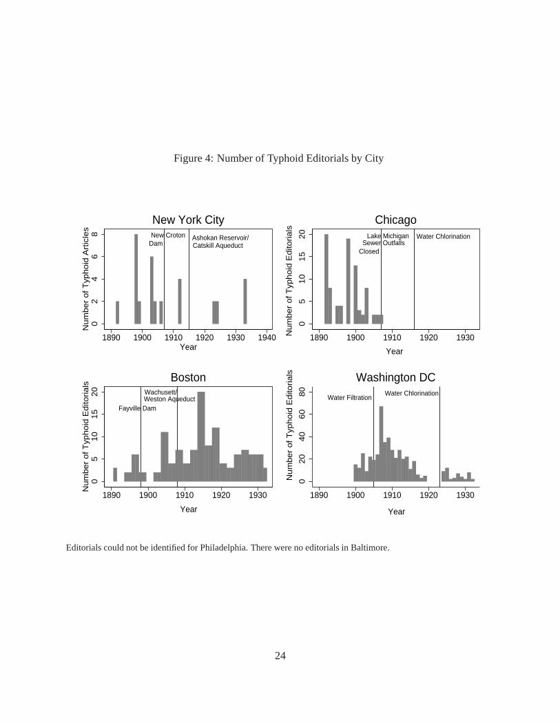
Figure 4: Number of Typhoid Editorials by City
New CrotonDam
Ashokan Reservoir/Catskill Aqueduct
02
46
8N
um
be
r o
f T
yph
oid
Art
icle
s
1890 1900 1910 1920 1930 1940Year
New York CityLake Michigan
Sewer OutfallsClosed
Water Chlorination
05
10
15
20
Nu
mb
er
of T
yph
oid
Edito
rials
1890 1900 1910 1920 1930
Year
Chicago
Fayville Dam
Wachusett/Weston Aqueduct
05
10
15
20
Nu
mb
er
of T
yph
oid
Ed
itoria
ls
1890 1900 1910 1920 1930
Year
Boston
Water FiltrationWater Chlorination
02
04
06
08
0
Nu
mb
er
of T
yph
oid
Ed
itoria
ls
1890 1900 1910 1920 1930
Year
Washington DC
Editorials could not be identified for Philadelphia. There were no editorials in Baltimore.
24

Table 1: Clean Water Intervention Dates
City Intervention InterventionBaltimore 1911 1914
water chlorination water filtrationBoston 1898 1908
Fayville Dam/Sudbury Reservoir Wachusett/Weston AqueductChicago 1907 1916
Lake Michigan sewer outfalls closed water chlorinationNew York City 1907 1915
New Croton Dam Ashokan Reservoir/Catskill AqueductPhiladelphia 1908 1913
water filtration water chlorinationWashington DC 1905 1923
water filtration water chlorination
25

Table 2: Mean Death and Case Rates, Before, Between, and After Interventions
Before First Intervention Between Interventions After Second InterventionDeath Case Death Case Death CaseRate Rate Rate Rate Rate Rate
Baltimore 0.726 4.437 0.490 2.843 0.156 0.878(0.525) (4.921) (0.311) (2.410) (0.198) (1.282)
Boston 0.687 0.489 3.358 0.110 0.629(0.461) (0.390) (5.253) (0.150) (0.819)
Chicago 0.554 0.471 0.199 1.231 0.026 0.156(0.403) (0.440) (0.135) (1.053) (0.034) (0.199)
New York City 0.366 1.444 0.185 1.243 0.034 0.266(0.231) (1.112) (0.118) (0.972) (0.040) (0.292)
Philadelphia 0.971 6.949 0.343 2.141 0.131 0.664(0.600) (5.746) (0.252) (1.596) (0.089) (0.579)
Washington DC 1.494 0.596 2.662 0.061 0.324(1.072) (0.538) (3.091) (0.124) (0.429)
All Cities 0.765 2.449 0.382 2.067 0.080 0.484(0.717) (3.409) (0.385) (2.596) (0.129) (0.772)
See text for death and case rate sources. Standard deviations in parentheses. Case rates are not available for Bostonand Washington DC prior to the first intervention.
26

Table 3: Negative Binomial Regression of Effect of Typhoid Death Rates on Newspaper Reports
Std. Std. Std.Coef. Err. Coef. Err. Coef. Err.
Number of Typhoid ArticlesDeath rate 0.335** 0.158 0.386*** 0.122 0.350*** 0.0861st intervention -0.296* 0.151 -0.159 0.098 -0.278*** 0.0922nd intervention -0.639*** 0.067 -0.537*** 0.127 -0.121 0.1461st intervention x death rate 0.107 0.230 0.153 0.166 0.173* 0.0922nd intervention x death rate 1.316*** 0.205 0.617*** 0.214 0.244 0.264Number of total articles 0.014** 0.006 0.006 0.007 0.005 0.006Constant 1.133*** 0.215 1.409*** 0.124 0.834*** 0.279City Fixed Effects N Y YYear Fixed Effects N N Y
Dummy=1 if no typhoid articleDummy=1 if big news event -0.742 0.453 -0.936** 0.434 -0.823** 0.340Dummy=1 if holiday week -0.292* 0.166 -0.453 0.461 -0.908*** 0.186Constant -20.318*** 5.659 -6.177 8.369 -30.486 28.637City Fixed Effects Y Y YYear Fixed Effects Y Y Y
Both interventions -0.935*** 0.135 -0.697*** 0.204 -0.398* 0.214Both intervention death rate interactions 1.422*** 0.217 0.769*** 0.198 0.417 0.318ln(alpha) -0.798*** 0.148 -0.914*** 0.229 -1.335*** 0.136Vuong test, z= 9.22*** 7.55*** 7.771***Observations 9,492 9,492 9,492Zero observations 2,127 2,127 2,127
The dependent variable for the count part of the negative zero-inflated binomial is number of typhoid articles. Thedependent variable for the logit part of the model is a dummy equal to 1 if there was no typhoid article. Robuststandard errors in parentheses, clustered on the city. *** p<0.01, ** p<0.05, * p<0.1
27

Table 4: Marginals from Negative Binomial Regression of Effect of Typhoid Death Rates on News-paper Reports
Std. Std. Std.∂y∂x
Err. ∂y∂x
Err. ∂y∂x
Err.
Death rate 1.023* 0.539 1.174*** 0.385 1.062*** 0.2691st intervention -0.905* 0.482 -0.485 0.298 -0.842*** 0.2902nd intervention -1.952*** 0.359 -1.633*** 0.404 -0.367 0.4451st intervention x death rate 0.326 0.691 0.464 0.499 0.526* 0.2802nd intervention x death rate 4.022*** 0.852 1.875*** 0.661 0.740 0.807Number of total articles 0.043*** 0.015 0.018 0.021 0.016 0.017Dummy=1 if big news event 0.155 0.130 0.147 0.096 0.168 0.125Dummy=1 if holiday week 0.061 0.051 0.071 0.105 0.186 0.115City FE in count regression N Y YYear FE in count regression N N YCity FE in zero value logit Y Y YYear FE in zero value logit Y Y Y
Both interventions -2.857*** 0.597 -2.118*** 0.632 -1.209* 0.664Both intervention death rate interactions 4.348*** 0.765 2.338*** 0.594 1.266 0.971Mean number of typhoid articles 2.917 2.917 2.917Observations 9,492 9,494 9,492
Marginals are for the regression in Table 3. Robust standard errors in parentheses, clustered on the city. *** p<0.01,** p<0.05, * p<0.1
28

Table 5: Negative Binomial Regression of Effect of Typhoid Death Rates on Local NewspaperReports
Std. Std. Std.Coef. Err. Coef. Err. Coef. Err.
Number of Typhoid ArticlesDeath rate 0.405 0.319 0.373** 0.175 0.366** 0.1491st intervention -0.549* 0.303 -0.334*** 0.086 -0.274** 0.1072nd intervention -0.575*** 0.109 -0.774*** 0.183 -0.282*** 0.0721st intervention x death rate 0.217 0.361 0.275 0.204 0.244* 0.1472nd intervention x death rate 0.947*** 0.254 0.667*** 0.252 0.408*** 0.061Number of total articles -0.008 0.005 0.003 0.008 -0.000 0.007Constant 0.778* 0.399 0.328*** 0.120 0.507 0.315City Fixed Effects N Y YYear Fixed Effects N N Y
Dummy=1 if no local typhoid articleDummy=1 if big news event -0.180 0.236 -0.252 0.339 -0.195 0.290Dummy=1 if holiday week 0.006 0.164 -0.025 0.289 0.039 0.056Constant -15.258*** 0.809 -14.551 10.733 -0.766** 0.303City Fixed Effects Y Y YYear Fixed Effects Y Y Y
Both interventions -1.124*** 0.405 -1.108*** 0.253 -0.556*** 0.104Both intervention death rate interactions 1.164*** 0.333 0.942*** 0.105 0.651*** 0.174ln(alpha) -0.494*** 0.094 -0.797*** 0.278 -0.997*** 0.373Vuong test, z= 19.81*** 13.08*** 13.50***Observations 8,596 8,596 8,596Zero observations 3,792 3,792 3,792
The regressions exclude Philadelphia because we could not mechanically identify local articles. The dependent vari-able for the count part of the negative zero-inflated binomial is number of typhoid articles. The dependent variable forthe logit part of the model is a dummy equal to 1 if there was no typhoid article. Robust standard errors in parentheses,clustered on the city. *** p<0.01, ** p<0.05, * p<0.1
29

Table 6: Marginals from Negative Binomial Regression of Effect of Typhoid Death Rates on LocalNewspaper Reports
Std. Std. Std.∂y∂x
Err. ∂y∂x
Err. ∂y∂x
Err.
Death rate 0.470 0.424 0.424** 0.213 0.418** 0.1751st intervention -0.637 0.420 -0.380*** 0.105 -0.312*** 0.1202nd intervention -0.667*** 0.243 -0.881*** 0.233 -0.322*** 0.0831st intervention x death rate 0.252 0.400 0.313 0.228 0.278* 0.1632nd intervention x death rate 1.099** 0.506 0.759** 0.308 0.465*** 0.069Number of total articles -0.009 0.006 0.003 0.009 -0.000 0.008Dummy=1 if big news event 0.036 0.050 0.041 0.066 0.024 0.037Dummy=1 if holiday week -0.001 0.033 0.004 0.049 -0.005 0.007City FE in count regression N Y YYear FE in count regression N N YCity FE in zero value logit Y Y YYear FE in zero value logit Y Y Y
Both interventions -1.304** 0.643 -1.262*** 0.321 -0.634*** 0.117Both intervention death rate interactions 1.350*** 0.524 1.073*** 0.154 0.742*** 0.188Mean number of typhoid articles 1.097 1.097 1.097Observations 8,596 8,596 8,596
Marginals are for the regression in Table 5. Robust standard errors in parentheses, clustered on the city. *** p<0.01,** p<0.05, * p<0.1
30

Tabl
e7:
Neg
ativ
eB
inom
ialR
egre
ssio
nof
Eff
ecto
fD
evia
tions
inE
xpec
ted
Typh
oid
Dea
thR
ates
onN
ewsp
aper
Rep
orts
All
Art
icle
sL
ocal
Art
icle
sSt
d.St
d.St
d.St
d.C
oef.
Err
.C
oef.
Err
.C
oef.
Err
.C
oef.
Err
.
Num
ber
ofTy
phoi
dA
rtic
les
Pred
icte
d-
deat
hra
te-0
.329
0.38
3-0
.345
0.49
1(P
redi
cted
-de
ath
rate
)x
(Dum
my=
1if
posi
tive)
1.31
1*0.
677
1.28
60.
937
(Pre
dict
ed-
deat
hra
te)/
(Std
deat
hra
te)
-0.2
56*
0.14
3-0
.224
0.24
1(P
redi
cted
-de
ath
rate
)/(S
tdde
ath
rate
)x
0.84
2***
0.18
90.
802*
*0.
349
(Dum
my=
1if
posi
tive)
Num
ber
ofto
tala
rtic
les
-0.0
010.
010
-0.0
000.
010
-0.0
30**
*0.
008
-0.0
30**
*0.
007
Con
stan
t1.
044*
**0.
276
0.99
4***
0.25
40.
770*
**0.
241
0.73
0***
0.20
4C
ityFi
xed
Eff
ects
NN
NN
Yea
rFi
xed
Eff
ects
NN
NN
Dum
my=
1if
noty
phoi
dar
ticle
Dum
my=
1if
big
new
sev
ent
-0.5
18**
*0.
119
-0.5
22**
*0.
131
-0.2
630.
203
-0.2
650.
202
Dum
my=
1if
holid
ayw
eek
-0.5
30**
*0.
150
-0.5
65**
*0.
143
-0.0
850.
115
-0.1
080.
127
Con
stan
t-4
.437
2.98
8-4
.906
3.99
7-6
.810
100.
905
-13.
430*
**3.
108
City
Fixe
dE
ffec
tsY
YY
YY
ear
Fixe
dE
ffec
tsY
YY
Y
Tota
leff
ecto
fpo
s(Pr
edic
ted-
deat
hra
te)
0.98
2***
0.00
10.
942*
*0.
477
Tota
leff
ecto
fpo
s((P
redi
cted
-dea
thra
te)/
Std
Dev
)0.
586*
**0.
056
0.57
8***
0.12
8ln
(alp
ha)
-0.5
45**
*0.
129
-0.5
75**
*0.
150
-0.3
21**
*0.
114
-0.3
76**
*0.
132
Vuo
ngte
st,z
=9.
54**
*9.
36**
*21
.62*
**21
.62*
**O
bser
vatio
ns9,
114
9,11
48,
269
8,26
9Z
ero
obse
rvat
ions
2,04
02,
040
4,61
94,
619
The
loca
lart
icle
regr
essi
ons
excl
ude
Phila
delp
hia.
The
depe
nden
tvar
iabl
efo
rth
eco
untp
arto
fth
ene
gativ
eze
ro-i
nflat
edbi
nom
iali
snu
mbe
rof
typh
oid
artic
les.
The
depe
nden
tvar
iabl
efo
rthe
logi
tpar
toft
hem
odel
isa
dum
my
equa
lto
1if
ther
ew
asno
typh
oid
artic
le.R
obus
tsta
ndar
der
rors
inpa
rent
hese
s,cl
uste
red
onth
eci
ty.*
**p<
0.01
,**
p<0.
05,*
p<0.
1
31

Tabl
e8:
Mar
gina
lsfr
omN
egat
ive
Bin
omia
lReg
ress
ion
ofE
ffec
tof
Dev
iatio
nsin
Typh
oid
Dea
thR
ates
onN
ewsp
aper
Rep
orts
All
Art
icle
sL
ocal
Art
icle
sSt
d.St
d.St
d.St
d.∂y
∂x
Err
.∂y
∂x
Err
.∂y
∂x
Err
.∂y
∂x
Err
.
Pred
icte
d-
deat
hra
te-1
.072
1.37
5-0
.415
0.70
5(P
redi
cted
-de
ath
rate
)x
(Dum
my=
1if
posi
tive)
4.26
62.
790
1.54
61.
571
(Pre
dict
ed-
deat
hra
te)/
(Std
case
rate
)-0
.798
*0.
457
-0.2
570.
313
(Pre
dict
ed-
deat
hra
te)/
(Std
case
rate
)x
2.62
5***
0.69
80.
920*
0.54
9(D
umm
y=1
ifpo
sitiv
e)N
umbe
rof
tota
lart
icle
s-0
.002
0.03
3-0
.002
0.03
0-0
.036
**0.
015
-0.0
35**
0.01
3D
umm
y=1
ifbi
gne
ws
even
t0.
119*
*0.
048
0.11
2**
0.05
60.
062
0.06
60.
059
0.05
5D
umm
y=1
ifho
liday
wee
k0.
122*
**0.
043
0.12
1***
0.03
00.
020
0.03
40.
024
0.03
2C
ityFE
inco
untr
egre
ssio
nN
NN
NY
ear
FEin
coun
treg
ress
ion
NN
NN
City
FEin
zero
valu
elo
git
YY
YY
Yea
rFE
inze
rova
lue
logi
tY
YY
Y
Tota
leff
ecto
fpo
s(Pr
edic
ted-
deat
hra
te)
3.19
4**
1.48
51.
132
0.89
5To
tale
ffec
tof
pos(
(Pre
dict
ed-d
eath
rate
)/St
dD
ev)
1.82
6***
0.32
40.
663*
**0.
248
Mea
nnu
mbe
rof
typh
oid
artic
les
2.91
73.
489
2.91
73.
489
1.09
72.
019
1.09
72.
019
Obs
erva
tions
9,11
49,
114
8,26
98,
269
Mar
gina
lsar
efo
rth
ere
gres
sion
inTa
ble
7.R
obus
tsta
ndar
der
rors
inpa
rent
hese
s,cl
uste
red
onth
eci
ty.*
**p<
0.01
,**
p<0.
05,*
p<0.
1
32

Tabl
e9:
Neg
ativ
eB
inom
ialR
egre
ssio
nof
Eff
ecto
fTy
phoi
dC
ase
Rat
eson
New
spap
erR
epor
ts
All
Art
icle
sL
ocal
Art
icle
sSt
d.St
d.St
d.St
d.C
oef.
Err
.C
oef.
Err
.C
oef.
Err
.C
oef.
Err
.
Num
ber
ofty
phoi
dar
ticle
sC
ase
rate
0.09
3***
0.02
20.
078*
**0.
019
0.14
1**
0.05
70.
105*
**0.
034
1sti
nter
vent
ion
-0.3
78**
*0.
109
-0.2
85*
0.16
1-0
.303
0.25
7-0
.297
0.20
42n
din
terv
entio
n-0
.605
***
0.10
5-0
.128
0.16
5-0
.660
***
0.08
1-0
.217
0.17
51s
tint
erve
ntio
nx
case
rate
0.00
50.
026
0.01
00.
014
-0.0
260.
055
0.00
10.
026
2nd
inte
rven
tion
xca
sera
te0.
213*
**0.
063
0.10
4***
0.03
40.
171*
**0.
016
0.12
9***
0.01
7N
umbe
rof
tota
lart
icle
s0.
013*
**0.
003
0.01
1*0.
005
-0.0
030.
004
0.01
6***
0.00
6C
onst
ant
1.17
3***
0.10
30.
711*
0.36
30.
512
0.38
8-0
.215
0.37
0C
ityFi
xed
Eff
ects
NY
NY
Yea
rFi
xed
Eff
ects
NY
NY
Dum
my=
1if
noty
phoi
dar
ticle
Dum
my=
1if
big
new
sev
ent
-0.6
75**
*0.
227
-0.9
93**
*0.
180
-0.3
260.
280
-0.5
040.
333
Dum
my=
1if
holid
ayw
eek
-0.3
78**
0.15
6-1
.001
***
0.20
2-0
.170
0.24
5-0
.134
0.15
8C
onst
ant
-5.4
15**
*1.
452
-19.
704*
**1.
521
-2.9
03**
1.38
0-0
.520
***
0.09
4C
ityFi
xed
Eff
ects
YY
YY
Yea
rFi
xed
Eff
ects
YY
YY
Bot
hin
terv
entio
ns-0
.984
***
0.06
6-4
.129
0.25
6-0
.963
***
0.32
6-0
.514
*0.
294
Bot
hin
terv
entio
nca
sera
tein
tera
ctio
ns0.
218*
**0.
066
0.11
4***
0.02
90.
145*
**0.
051
0.13
0***
0.01
3ln
(alp
ha)
-1.0
97**
*0.
121
-1.5
23**
*0.
126
-0.9
71**
*0.
177
-1.2
50**
*0.
177
Vuo
ngte
st,z
=8.
61**
*6.
45**
*17
.32*
**11
.07*
**O
bser
vatio
ns8,
214
8,21
47,
467
7,46
7Z
ero
obse
rvat
ions
2,07
82,
078
4,43
84,
438
The
loca
lart
icle
regr
essi
ons
excl
ude
Phila
delp
hia.
The
depe
nden
tvar
iabl
efo
rth
eco
untp
arto
fth
ene
gativ
eze
ro-i
nflat
edbi
nom
iali
snu
mbe
rof
typh
oid
artic
les.
The
depe
nden
tvar
iabl
efo
rthe
logi
tpar
toft
hem
odel
isa
dum
my
equa
lto
1if
ther
ew
asno
typh
oid
artic
le.R
obus
tsta
ndar
der
rors
inpa
rent
hese
s,cl
uste
red
onth
eci
ty.*
**p<
0.01
,**
p<0.
05,*
p<0.
1
33

Tabl
e10
:M
argi
nals
from
Neg
ativ
eB
inom
ialR
egre
ssio
nof
Eff
ecto
fTy
phoi
dC
ase
Rat
eson
New
spap
erR
epor
ts
All
Art
icle
sL
ocal
Art
icle
sSt
d.St
d.St
d.St
d.∂y
∂x
Err
.∂y
∂x
Err
.∂y
∂x
Err
.∂y
∂x
Err
.
Cas
era
te0.
245*
**0.
056
0.20
1***
0.05
10.
133*
*0.
056
0.09
6***
0.03
31s
tint
erve
ntio
n-0
.998
***
0.28
1-0
.736
*0.
415
-0.2
860.
241
-0.2
720.
181
2nd
inte
rven
tion
-1.5
95**
*0.
282
-0.3
320.
429
-0.6
23**
*0.
060
-0.1
980.
159
1sti
nter
vent
ion
xca
sera
te0.
013
0.07
00.
026
0.03
7-0
.024
0.05
20.
001
0.02
42n
din
terv
entio
nx
case
rate
0.56
1***
0.16
60.
269*
**0.
089
0.16
1***
0.01
90.
118*
**0.
017
Num
ber
ofto
tala
rtic
les
0.03
5***
0.00
70.
028*
*0.
014
-0.0
030.
004
0.01
5***
0.00
5D
umm
y=1
ifbi
gne
ws
even
t0.
107*
*0.
054
0.17
2***
0.03
90.
042
0.03
50.
049*
*0.
024
Dum
my=
1if
holid
ayw
eek
0.06
0*0.
033
0.17
3***
0.03
40.
022
0.03
00.
013
0.01
3C
ityFE
inco
untr
egre
ssio
nN
YN
YY
ear
FEin
coun
treg
ress
ion
NY
NY
City
FEin
zero
valu
elo
git
YY
YY
Yea
rFE
inze
rova
lue
logi
tY
YY
Y
Bot
hin
terv
entio
ns-2
.593
***
0.16
5-1
.068
0.66
6-0
.909
***
0.29
8-0
.469
***
0.26
0B
oth
inte
rven
tion
case
rate
inte
ract
ions
0.57
4***
0.17
80.
295*
**0.
077
0.13
7***
0.05
00.
119*
**0.
011
Mea
nnu
mbe
rof
typh
oid
artic
les
2.43
72.
847
2.43
72.
847
0.82
01.
483
0.82
01.
483
Obs
erva
tions
8,21
48,
214
7,46
77,
467
Mar
gina
lsar
efo
rth
ere
gres
sion
inTa
ble
9.R
obus
tsta
ndar
der
rors
inpa
rent
hese
s,cl
uste
red
onth
eci
ty.*
**p<
0.01
,**
p<0.
05,*
p<0.
1
34

Tabl
e11
:N
egat
ive
Bin
omia
lReg
ress
ion
ofE
ffec
tof
Dev
iatio
nin
Exp
ecte
dTy
phoi
dC
ase
Rat
eson
New
spap
erR
epor
ts
All
Art
icle
sL
ocal
Art
icle
sSt
d.St
d.St
d.St
d.C
oef.
Err
.C
oef.
Err
.C
oef.
Err
.C
oef.
Err
.
Num
ber
ofar
ticle
sPr
edic
ted
-ca
sera
te-0
.200
***
0.05
1-0
.193
***
0.07
2(P
redi
cted
-ca
sera
te)
x(D
umm
y=1
ifpo
sitiv
e)0.
468*
**0.
059
0.47
0***
0.05
5(P
redi
cted
-ca
sera
te)/
(Std
case
rate
)-0
.403
***
0.14
8-0
.341
0.29
5(P
redi
cted
-ca
sera
te)/
(Std
case
rate
)x
0.94
8***
0.22
00.
893*
*0.
390
(Dum
my=
1if
posi
tive)
Num
ber
ofto
tala
rtic
les
0.00
40.
007
0.00
30.
007
-0.0
13**
*0.
002
-0.0
18**
*0.
003
Con
stan
t0.
748*
**0.
263
0.73
3***
0.24
80.
226
0.15
30.
275
0.17
5C
ityFi
xed
Eff
ects
NN
NN
Yea
rFi
xed
Eff
ects
NN
NN
Dum
my=
1if
noty
phoi
dar
ticle
Dum
my=
1if
big
new
sev
ent
-0.4
86**
*0.
114
-0.5
08**
*0.
126
-0.3
27*
0.18
6-0
.348
*0.
202
Dum
my=
1if
holid
ayw
eek
-0.2
400.
175
-0.2
84*
0.16
7-0
.084
0.10
8-0
.106
0.13
2C
onst
ant
-3.4
30**
*0.
896
-4.0
93**
*1.
328
-1.4
83**
*0.
316
-0.7
45**
*0.
094
City
Fixe
dE
ffec
tsY
YY
YY
ear
Fixe
dE
ffec
tsY
YY
Y
Tota
leff
ecto
fpo
s(Pr
edic
ted-
case
rate
)0.
269*
**0.
035
0.27
7***
0.03
8To
tale
ffec
tof
pos(
(Pre
dict
ed-c
ase
rate
)/St
dde
v)0.
545*
**0.
077
0.55
1***
0.09
8ln
(alp
ha)
-0.7
97**
*0.
069
-0.7
98**
*0.
074
-0.7
65**
*0.
084
-2.0
71**
1.00
1V
uong
test
,z=
10.2
4***
9.81
***
19.4
4***
20.2
2***
Obs
erva
tions
7,70
67,
706
7,06
27,
062
Zer
oob
serv
atio
ns2,
004
2,00
44,
268
4,26
8
The
loca
lart
icle
regr
essi
ons
excl
ude
Phila
delp
hia.
The
depe
nden
tvar
iabl
efo
rth
eco
untp
arto
fth
ene
gativ
eze
ro-i
nflat
edbi
nom
iali
snu
mbe
rof
typh
oid
artic
les.
The
depe
nden
tvar
iabl
efo
rthe
logi
tpar
toft
hem
odel
isa
dum
my
equa
lto
1if
ther
ew
asno
typh
oid
artic
le.R
obus
tsta
ndar
der
rors
inpa
rent
hese
s,cl
uste
red
onth
eci
ty.*
**p<
0.01
,**
p<0.
05,*
p<0.
1
35

Tabl
e12
:M
argi
nals
from
Neg
ativ
eB
inom
ialR
egre
ssio
nof
Eff
ecto
fD
evia
tions
inTy
phoi
dC
ase
Rat
eson
New
spap
erR
epor
ts
All
Art
icle
sL
ocal
Art
icle
sSt
d.St
d.St
d.St
d.∂y
∂x
Err
.∂y
∂x
Err
.∂y
∂x
Err
.∂y
∂x
Err
.
Pred
icte
d-
case
rate
-0.5
07**
*0.
097
-0.1
69**
*0.
051
(Pre
dict
ed-
case
rate
)x
(Dum
my=
1if
posi
tive)
1.18
8***
0.16
80.
411*
**0.
050
(Pre
dict
ed-
case
rate
)/(S
tdca
sera
te)
-1.0
22**
*0.
377
-0.2
870.
261
(Pre
dict
ed-
case
rate
)/(S
tdca
sera
te)
x2.
405*
**0.
588
0.75
0**
0.36
2(D
umm
y=1
ifpo
sitiv
e)N
umbe
rof
tota
lart
icle
s0.
010
0.01
80.
007
0.01
7-0
.012
***
0.00
3-0
.015
***
0.00
3D
umm
y=1
ifbi
gne
ws
even
t0.
112*
*0.
046
0.11
2**
0.05
10.
053
0.03
90.
058
0.04
3D
umm
y=1
ifho
liday
wee
k0.
055
0.04
20.
063*
0.03
60.
014
0.01
90.
018
0.02
3C
ityFE
inco
untr
egre
ssio
nN
NN
NY
ear
FEin
coun
treg
ress
ion
NN
NN
City
FEin
zero
valu
elo
git
YY
YY
Yea
rFE
inze
rova
lue
logi
tY
YY
Y
Tota
leff
ecto
fpo
s(Pr
edic
ted-
case
rate
)0.
681*
**0.
143
0.24
2***
0.05
6To
tale
ffec
tof
pos(
(Pre
dict
ed-c
ase
rate
)/St
dde
v)1.
382*
**0.
237
0.46
3***
0.10
6M
ean
num
ber
ofty
phoi
dar
ticle
s2.
436
2.84
72.
436
2.84
70.
820
1.48
30.
820
1.48
3Z
ero
obse
rvat
ions
Mar
gina
lsar
efo
rth
ere
gres
sion
inTa
ble
11.R
obus
tsta
ndar
der
rors
inpa
rent
hese
s,cl
uste
red
onth
eci
ty.*
**p<
0.01
,**
p<0.
05,*
p<0.
1
36

Tabl
e13
:N
egat
ive
Bin
omia
lReg
ress
ion
ofE
ffec
tof
Typh
oid
and
Dip
hthe
ria
Dea
thR
ates
onTy
phoi
dan
dD
ipht
heri
aN
ewsp
aper
Rep
orts
All
Art
icle
sL
ocal
Art
icle
sTy
phoi
dD
ipht
heri
aTy
phoi
dD
ipht
heri
aD
ipht
heri
aSt
d.St
d.St
d.St
d.St
d.C
oef.
Err
.C
oef.
Err
.C
oef.
Err
.C
oef.
Err
.C
oef.
Err
.
Num
ber
ofar
ticle
sTy
phoi
dde
ath
rate
0.80
6***
0.09
20.
221*
0.12
21.
507*
**0.
173
-0.0
090.
189
1stt
ypho
idin
terv
entio
n-0
.080
0.08
3-0
.395
***
0.13
9-0
.092
0.12
8-0
.589
**0.
252
2nd
typh
oid
inte
rven
tion
-0.5
63**
*0.
110
-0.1
600.
152
-0.5
40**
*0.
166
-0.1
220.
287
1stt
ypho
idin
terv
entio
nx
deat
hra
te0.
430
0.27
6-0
.466
0.50
40.
548
0.41
20.
096
0.76
32n
dty
phoi
din
terv
entio
nx
deat
hra
te2.
572*
**0.
844
-1.7
521.
201
4.20
8***
1.56
2-0
.640
1.88
3D
ipht
heri
ade
ath
rate
-0.0
570.
087
Dip
hthe
ria
inte
rven
tion
-0.8
87**
*0.
287
Dip
ther
iain
terv
entio
nx
deat
hra
te0.
599*
**0.
121
Num
ber
ofto
tala
rtic
les
0.00
6**
0.00
30.
016*
**0.
003
0.00
70.
005
0.01
8***
0.00
60.
019*
**0.
004
Con
stan
t1.
072*
**0.
065
0.44
6***
0.08
1-0
.202
*0.
110
-0.3
08**
0.15
0-0
.223
0.26
5D
umm
y=1
ifno
artic
leD
umm
y=1
ifbi
gne
ws
even
t-1
.113
**0.
464
-0.2
690.
274
-1.0
44**
0.46
4-0
.106
0.30
4-0
.141
0.29
4D
umm
y=1
ifho
liday
wee
k-0
.757
*0.
400
-0.2
550.
228
-0.8
48**
0.41
4-0
.397
*0.
241
-0.3
94*
0.23
0C
onst
ant
-3.6
693.
460
-27.
033
45,6
14.2
42-1
.915
1.67
0-1
.249
0.81
9-1
.314
0.85
8Y
ear
Fixe
dE
ffec
tsY
YY
Bot
hin
terv
entio
ns-0
.643
***
0.10
6-0
.556
***
0.12
2-0
.632
***
0.17
10.
711*
**0.
230
Bot
hin
terv
entio
nde
ath
rate
inte
ract
ions
3.00
2***
0.81
0-2
.219
**1.
108
4.75
6***
1.53
2-0
.544
1.75
4ln
(alp
ha)
-1.5
07**
*0.
102
-1.5
13**
*0.
134
-0.9
90**
*0.
124
-1.8
05**
*0.
422
-2.1
39**
*0.
590
Vuo
ngte
st,z
=5.
74**
*8.
51**
*5.
98**
*7.
82**
*8.
08**
*O
bser
vatio
ns2,
548
2,54
82,
548
2,54
82,
548
Zer
oob
serv
atio
ns49
71,
607
1,27
11,
695
1,69
5
The
depe
nden
tvar
iabl
efo
rth
eco
untp
arto
fth
ene
gativ
eze
ro-i
nflat
edbi
nom
iali
snu
mbe
rof
typh
oid
ordi
phth
eria
artic
les.
The
depe
nden
tvar
iabl
efo
rthe
logi
tpar
tof
the
mod
elis
adu
mm
yeq
ualt
o1
ifth
ere
was
noty
phoi
dor
diph
ther
iaar
ticle
.Rob
usts
tand
ard
erro
rsin
pare
nthe
ses.
***
p<0.
01,*
*p<
0.05
,*
p<0.
1
37

Tabl
e14
:M
argi
nals
from
Neg
ativ
eB
inom
ialR
egre
ssio
nof
Eff
ecto
fD
evia
tions
inTy
phoi
dC
ase
Rat
eson
New
spap
erR
epor
ts
All
Art
icle
sL
ocal
Art
icle
sTy
phoi
dD
ipht
heri
aTy
phoi
dD
ipht
heri
aD
ipht
heri
aSt
d.St
d.St
d.St
d.St
d.∂y
∂x
Err
.∂y
∂x
Err
.∂y
∂x
Err
.∂y
∂x
Err
.∂y
∂x
Err
.
Typh
oid
deat
hra
te2.
404*
**0.
279
0.32
21,
086.
555
1.51
4***
0.19
1-0
.005
0.09
51s
ttyp
hoid
inte
rven
tion
-0.2
390.
248
-0.5
761,
944.
205
-0.0
930.
128
-0.2
98**
0.12
82n
dty
phoi
din
terv
entio
n-1
.680
***
0.32
9-0
.234
788.
692
-0.5
43**
*0.
168
-0.0
610.
145
1stt
ypho
idin
terv
entio
nx
deat
hra
te1.
283
0.82
4-0
.679
2,29
3.07
50.
551
0.41
20.
049
0.38
62n
dty
phoi
din
terv
entio
nx
deat
hra
te7.
673*
**2.
522
-2.5
528,
617.
404
4.23
0***
1.58
4-0
.324
0.95
2D
ipht
heri
ade
ath
rate
-0.0
290.
044
Dip
hthe
ria
inte
rven
tion
-0.4
50**
*0.
147
Dip
ther
iain
terv
entio
nx
deat
hra
te0.
304*
**0.
063
Num
ber
ofto
tala
rtic
les
0.01
7**
0.00
80.
024
80.7
630.
007
0.00
50.
009*
**0.
003
0.01
0***
0.00
2D
umm
y=1
ifbi
gne
ws
even
t0.
256*
*0.
104
0.05
840
5.57
50.
110*
*0.
050
0.01
40.
042
0.02
00.
042
Dum
my=
1if
holid
ayw
eek
0.17
4*0.
092
0.05
538
4.32
40.
090*
0.04
90.
054
0.03
40.
056*
0.03
3Y
ear
FEin
zero
valu
elo
git
YY
YY
Y
Bot
hin
terv
entio
ns-1
.919
***
0.31
6-0
.891
2732
.897
-0.6
36**
*0.
172
-0.3
59**
*0.
118
Bot
hin
terv
entio
nde
ath
rate
inte
ract
ions
8.95
6***
2.42
3-3
.232
1091
0.48
4.78
1***
1.55
2-0
.275
0.88
7M
ean
num
ber
ofty
phoi
dar
ticle
s2.
996
1.00
8M
ean
num
ber
ofdi
phth
eria
artic
les
1.45
60.
505
0.50
5O
bser
vatio
ns2,
548
2,54
82,
548
2,54
82,
548
Mar
gina
lsar
efo
rth
ere
gres
sion
inTa
ble
13.R
obus
tsta
ndar
der
rors
inpa
rent
hese
s.**
*p<
0.01
,**
p<0.
05,*
p<0.
1
38

Appendix A
Figure A1 compares our mechanized searches of The New York Times for typhoid fever with
manual searches for 1900-1932. Except for some learning by doing by data inputters in the early
manual searches, peaks and troughs in the percentage of articles mentioning typhoid coincide
across the two samples. However, the mechanized searches for mentions of local typhoid fever
yield a consistently greater percentage than the manual searches. The mechanized searches also
capture deaths or illnesses of New Yorkers outside of the city.
39

Figure A1: Comparison of Manual and Mechanized Searches, The New York Times 1900-1932
0.1
.2.3
Pe
rce
nt
Typ
ho
id A
rtic
les
1900 1910 1920 1930Year, Week
All Articles, Manual Search All Articles, Mechanized Search
Local Articles, Mechanized Search Local Articles, Manual Search
New York City
Source: The New York Times.
40

Appendix B
Table B1 shows that in all cities the first intervention was a statistically significant predict of
death rates, controlling for a year trend. Controlling for the effects of the first intervention, in all
cities except for Washington DC the second intervention was a statistically significant predictor of
death rates and the combined effect of both interventions was statistically significant in all cities
except for Washington DC. The inclusion of lagged death rates in the specification also yielded
statistically significant effects of the interventions (results not shown).
41

Table B1: OLS Regression of Effect of Clean Water Interventions on Typhoid Death Rates
NYC Chicago Baltimore Boston Philadelphis DC
1st intervention -0.116*** -0.158*** -0.080* -0.075** -0.614*** -0.257***(0.010) (0.020) (0.042) (0.030) (0.056) (0.084)
2nd intervention -0.073*** 0.088*** -0.112*** -0.127*** -0.197*** 0.050(0.009) (0.021) (0.039) (0.030) (0.046) (0.060)
Combined interventions -0.189*** -0.070** -0.192** -0.202*** -0.811*** -0.207(0.013) (0.035) (0.043) (0.037) (0.090) (0.132)
Observations 2,548 1,538 1,387 1,588 904 1,558R2 0.517 0.503 0.391 0.396 0.476 0.428
All regressions include a linear time trend and constant term. Robust standard errors in parentheses. *** p<0.01, **p<0.05, * p<0.1
42