Embed Size (px)
DESCRIPTION
solubilatea gazelor
Citation preview

HANSEN SOLUBILITY PARAMETERSA User’s Handbook
Second Edition
7248_C000.fm Page i Thursday, May 24, 2007 1:40 PM

7248_C000.fm Page ii Thursday, May 24, 2007 1:40 PM
HANSEN SOLUBILITY PARAMETERSA User’s Handbook
Second Edition
Charles M. Hansen
7248_C000.fm Page iii Thursday, May 24, 2007 1:40 PM
CRC Press
Taylor & Francis Group
6000 Broken Sound Parkway NW, Suite 300
Boca Raton, FL 33487-2742
© 2007 by Taylor & Francis Group, LLC
CRC Press is an imprint of Taylor & Francis Group, an Informa business
No claim to original U.S. Government works
Printed in the United States of America on acid-free paper
10 9 8 7 6 5 4 3 2 1
International Standard Book Number-10: 0-8493-7248-8 (Hardcover)
International Standard Book Number-13: 978-0-8493-7248-3 (Hardcover)
This book contains information obtained from authentic and highly regarded sources. Reprinted material is quoted
with permission, and sources are indicated. A wide variety of references are listed. Reasonable efforts have been made to
publish reliable data and information, but the author and the publisher cannot assume responsibility for the validity of
all materials or for the consequences of their use.
No part of this book may be reprinted, reproduced, transmitted, or utilized in any form by any electronic, mechanical, or
other means, now known or hereafter invented, including photocopying, microfilming, and recording, or in any informa-
tion storage or retrieval system, without written permission from the publishers.
For permission to photocopy or use material electronically from this work, please access www.copyright.com (http://
www.copyright.com/) or contact the Copyright Clearance Center, Inc. (CCC) 222 Rosewood Drive, Danvers, MA 01923,
978-750-8400. CCC is a not-for-profit organization that provides licenses and registration for a variety of users. For orga-
nizations that have been granted a photocopy license by the CCC, a separate system of payment has been arranged.
Trademark Notice: Product or corporate names may be trademarks or registered trademarks, and are used only for
identification and explanation without intent to infringe.
Library of Congress Cataloging-in-Publication Data
Hansen solubility parameters : a user’s handbook. -- 2nd ed. / edited by Charles Hansen.
p. cm.
Rev. ed. of: Hansen solubility parameters / Charles M. Hansen. c2000.
Includes bibliographical references and index.
ISBN 0-8493-7248-8 (alk. paper)
1. Solution (Chemistry) 2. Polymers--Solubility. 3. Thin films. I. Hansen, Charles M. II. Hansen,
Charles M. Hansen solubility parameters.
QD543.H258 2007
547’.70454--dc22 2006051083
Visit the Taylor & Francis Web site at
http://www.taylorandfrancis.com
and the CRC Press Web site at
http://www.crcpress.com
7248_C000.fm Page iv Thursday, May 24, 2007 1:40 PM
Contributors
Dr. John Durkee
Consultant in Critical and Metal Cleaning Hunt, Texas U.S.A.
Dr. techn. Charles M. Hansen
ConsultantHoersholm, Denmark
Prof. Georgios M. Kontogeorgis
Technical University of DenmarkDepartment of Chemical EngineeringLyngby, Denmark
Prof. Costas Panayiotou
Department of Chemical EngineeringUniversity of ThessalonikiThessaloniki, Greece
Tim S. Poulsen
Sr. Research ScientistMolecular PathologyGlostrup, Denmark
Dr. rer. nat. Hanno Priebe
Sr. Research ScientistChemical Development – Process ResearchGE HealthcareAmersham Health ASOslo, Norway
Per Redelius
Research ManagerNynas BitumenProduct TechnologyNynashamn, Sweden
Prof. Laurie L. Williams
Department of Physics & EngineeringFort Lewis CollegeDurango, ColoradoU.S.A.
7248_C000.fm Page v Thursday, May 24, 2007 1:40 PM

7248_C000.fm Page vi Thursday, May 24, 2007 1:40 PM
Preface to the First Edition
My w ork with solv ents started in Denmark in 1962 when I w as a graduate student. The majorresults of this w ork were the realization that polymer film formation by sol ent evaporation tookplace in two distinct phases and the de velopment of what has come to be called Hansen solubility(or cohesion) parameters, abbre viated in the follo wing by HSP. The first phase of film formatiby solvent evaporation is controlled by surf ace phenomena such as solv ent vapor pressure, windvelocity, heat transfer, etc., and the second phase is controlled by concentration-dependent diffusionof solvent molecules from within the film to the air sur ace. It is not controlled by the binding ofsolvent molecules to polymer molecules by h ydrogen bonding as w as pre viously thought. Mysolubility parameter work was actually started to define a finities between sol ent and polymer tohelp predict the de gree of this binding which w as thought to control solv ent retention. This wasclearly a futile endeavor as there was absolutely no correlation. The solvents with smaller and morelinear molecular structure dif fused out of the films more quickly than those with la ger and morebranched molecular structure. HSP were de veloped in the process, ho wever.
HSP ha ve been used widely since 1967 to accomplish correlations and to mak e systematiccomparisons which one would not have thought possible earlier. The effects of hydrogen bonding,for e xample, are accounted for quantitati vely. Man y of these correlations are discussed later ,including polymer solubility , swelling, and permeation; surf ace wetting and de wetting; solubilityof inorganic salts; and biological applications including w ood, cholesterol, etc. The experimentallimits on this seemingly universal ability to predict molecular affinities are apparently g verned bythe limits represented by energies of the liquid test solvents themselves. There had/has to be a moresatisfactory explanation of this uni versality than just “semiempirical” correlations.
I decided to try to collect my e xperience for the purpose of a reference book, both for myselfand for others. At the same time, a search of the major theories of polymer solution thermodynamicswas undertaken to e xplore how the approaches compared. A key element in this w as to e xplainwhy the correlations all seemed to fit with an apparently “unversal” 4 (or 0.25 depending on whichreference is used). This is described in more detail in Chapter 2 (Equation 2.5 and Equation 2.6).My present view is that the “4” is the result of the v alidity of the geometric mean rule to describenot only dispersion interactions but also permanent dipole–permanent dipole and hydrogen bonding(electron interchange) interactions in mixtures of unlik e molecules. The Hildebrand approach usesthis and w as the basis of my earliest approach. The Prigogine corresponding states theory yieldsthe “4” in the appropriate manner when the geometric mean rule is adopted (Chapter 2, Equation2.11). Any other kind of averaging gives the wrong result. Considering these facts and the massiveamount of data that has been correlated using the “4” in the follo wing, it appears pro ven beyonda reasonable doubt that the geometric mean assumption is v alid not only for dispersion-typeinteractions (or perhaps more correctly in the present context those interactions typical of aliphatichydrocarbons) but also for permanent dipole–permanent dipole and h ydrogen bonding as well.
For those who wish to try to understand the Prigogine theory , I recommend starting with anarticle by Donald P atterson.
1
This article e xplains the corresponding states/free v olume theory ofPrigogine and co workers in a much simpler form than in the original source. P atterson
2
has alsoreviewed in understandable language the progression of developments in polymer solution thermo-dynamics from the Flory–Huggins theory, through that of Prigogine and coworkers, to the so-called“New Flory Theory.”
3
Patterson also has been so kind as to aid me in the representations of theearlier theories as the y are presented here (especially Chapter 2). All of the pre vious theories andtheir extensions also can be found in a more recent book.
4
For this reason, these more classical
7248_C000.fm Page vii Thursday, May 24, 2007 1:40 PM
theories are not treated extensively as such in this book. The striking aspect about all of this previouswork is that no one has dared to enter into the topic of h ydrogen bonding. The present quantitativetreatment of permanent dipole–permanent dipole interactions and h ydrogen bonding is central tothe results reported in e very chapter in this book. An attempt to relate this back to the pre vioustheories is gi ven briefly here and more xtensively in Chapter 2. This attempt has been directedthrough Patterson,
1
which may be called the Prigogine–Patterson approach, rather than through theFlory theory, as the relations with the former are more ob vious.
I strongly recommend that studies be undertak en to confirm the usefulness of the “structuraparameters” in the Prigogine theory (or the Flory theory). It is recognized that the effects of solventmolecular size, segment size, and polymer molecular size (and shapes) are not fully accounted forat the present time. There is hope that this can be done with structural parameters.
The material presented here corresponds to my knowledge and experience at the time of writing,with all due respect to confidentiality agreements, etc
I am greatly indebted to man y colleagues and supporters who ha ve understood that at timesone can be so preoccupied and lost in deep thought that the present just seems not to e xist.
Charles M. Hansen
October 19, 1998
REFERENCES
1. Patterson, D., Role of Free Volume Changes in Polymer Solution Thermodynamics
, J. Polym. Sci.Part C
, 16, 3379–3389, 1968.2. Patterson, D., Free Volume and Polymer Solubility . A Qualitati ve View,
Macromolecules
, 2(6),672–677, 1969.
3. Flory, P. J., Thermodynamics of Polymer Solutions
, Discussions of the Faraday Society
, 49, 7–29,1970.
4. Lipatov, Y. S. and Nestero v, A. E.,
Polymer Thermodynamics Library, Vol. 1, Thermodynamics ofPolymer Blends
, Technomic Publishing Co., Inc., Lancaster , PA, 1997.
7248_C000.fm Page viii Thursday, May 24, 2007 1:40 PM
Preface to the Second Edition
When the question about a second edition of this handbook w as posed, I w as not in doubt thatseveral additional authors were necessary to meet the demands it w ould require. The writings ofthe fi e contributors that were chosen speak for themselv es. There is theoretical impact in Chapter3 (Costas Panayiotou) and in Chapter 4 (Georgios M. Kontogeorgis). Chapter 3 introduces statisticalthermodynamics to confirm the d vision of cohesi ve ener gy into three parts enabling separatecalculation of each. Chapter 4 describes ho w the Hansen solubility parameters (HSP) fit into othetheories of polymer solutions. The practical applications and understanding pro vided in Chapter 9(Per Redelius) related to asphalt, bitumen, and crude oil should accelerate new thinking in this areaand emphasize that simple e xplanations of seemingly comple x phenomena are usually the rightones. The thermodynamic treatment of carbon dioxide gi ven in Chapter 10 (Laurie L. Williams)is a model for similar w ork with other g ases and emphatically confirms the usefulness of Hansesolubility parameters for predicting the solubility beha vior of g ases in liquids and therefore alsoin polymers.
Chapter 11 (John Durkee) goes through the process of demonstrating ho w “designer” solventscan be used in cleaning operations to replace, or partly replace, ozone-depleting solv ents, in spiteof the problem of their HSP not being sufficiently close to the HSP of the soils that are to be remved.
I have added two chapters because of apparent need. Chapter 14 discusses environmental stresscracking (ESC). ESC is a major cause of unexpected and sometimes catastrophic failure of plastics.The recent impro ved understanding pro vided by HSP seemed appropriate for inclusion in thiscontext. Chapter 16 discusses absorption and dif fusion in polymers. Many of the HSP correlationspresented in this handbook cannot stand on HSP alone but must include consideration of absorptionand diffusion of chemicals in polymers. These effects are often disguised by use of a molecularvolume, as molecular size/volume correlates reasonably well with diffusion coefficients, especiallat low concentrations. Polymer surface layers are often significantly diferent from the bulk polymer.Surface mobility of polymer chain se gments plays an important role in surf ace dewetting, ESC,and resistance and/or delays to the absorption of chemicals. This chapter tries to unify the ef fectsof a v erifiable sur ace resistance and v erifiable concentration-dependent di fusion coef ficientsSolutions to the diffusion equation simultaneously considering these two effects explain the “anom-alies” of absorption and also correctly model desorption phenomena, including the drying of alacquer film from start to finis
Each of the chapters in the first edition has been r viewed and added to where this w as feltappropriate without increasing the number of pages unduly . There is still a lack of significanactivity in the biological area, in controlled release applications, and in other areas discussed inChapter 18, such as nanotechnology . The relative affinity of molecules or s gments of moleculesfor each other can be predicted and in many cases controlled in self-assembly with the understandingprovided by HSP.
Chapter 15 treating biological materials has been e xpanded more than the others included inthe first edition.This was done with the help of Tim Svenstrup Poulsen. Perhaps the most surprisingof the additions in Chapter 15 is a HSP correlation for the (nonco valent) solvent interactions withDNA. The
δ
D
;
δ
P
;
δ
H
values of 19.0;20.0;11.0 for DN A, all in MP a
1/2
, clearly sho w that h ydrogenbonding interactions (H) contrib ute much less to the nonco valent interactions that determine thestructure of the DN A than the dispersion (D) and dipolar interactions (P). Only about 14% of thecohesion energy involved in what is commonly called “h ydrogen bonding” derives from hydrogenbonding.
7248_C000.fm Page ix Thursday, May 24, 2007 1:40 PM
Table Appendix A.1 is greatly e xpanded both in number and in information. The latter is dueto the generous help of Hanno Priebe, the extent of which is clearly evident for those familiar withthe first edition. There are close to 1200 entries in this table vs. the approximately 860 in the firsedition. However, please be advised that most of these are calculated and not e xperimental valuesas indicated in the comments to the table. Table Appendix A.2 is not greatly expanded. There havebeen too many restrictions on what may be published to allo w any major expansion of this table.The majority of my work as a consultant has usually involved agreements that prohibit or severelylimit publication of results paid for by pri vate sources. I have also included Appendix A.3 with theoriginal solubility data on which the di vision of the ener gy was based. I ha ve regularly found thismore specific data of considerable interest
Once more resources and timing ha ve not been conduci ve to do a complete literature searchto provide additional explanations of phenomena that should have had Hansen solubility parametersincluded in their interpretation. In view of the large expansion in the number of pages over the firsedition it is hoped that the principles, both theoretical and practical, are well illuminated. For thosewho still lack information in a gi ven situation I can suggest a search using the k ey words “Hansensolubility parameters” followed by additional k ey words as required. This is true both for Internetsearches as well as for searches in the more traditional literature.
It has been satisfying to see ho w much can be interpreted with v ery simple observ ations andcalculations. If it cannot be done simply , then rethink.
I want to once more thank those who have contributed to this second edition. Let us hope otherswill take up the ef fort and relate their findings for the benefit of al
Charles M. Hansen
7248_C000.fm Page x Thursday, May 24, 2007 1:40 PM
The Author
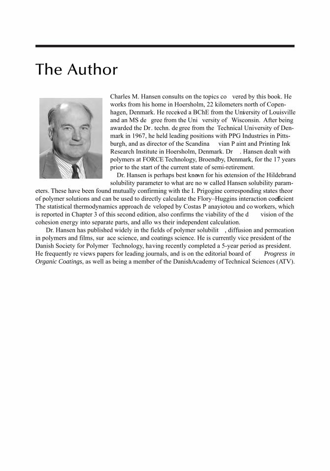
Charles M. Hansen consults on the topics co vered by this book. Heworks from his home in Hoersholm, 22 kilometers north of Copen-hagen, Denmark. He received a BChE from the University of Louisvilleand an MS de gree from the Uni versity of Wisconsin. After beingawarded the Dr. techn. de gree from the Technical University of Den-mark in 1967, he held leading positions with PPG Industries in Pitts-burgh, and as director of the Scandina vian P aint and Printing InkResearch Institute in Hoersholm, Denmark. Dr . Hansen dealt withpolymers at FORCE Technology, Broendby, Denmark, for the 17 yearsprior to the start of the current state of semi-retirement.
Dr. Hansen is perhaps best known for his extension of the Hildebrandsolubility parameter to what are no w called Hansen solubility param-
eters. These have been found mutually confirming with the I. Prigogine corresponding states theorof polymer solutions and can be used to directly calculate the Flory–Huggins interaction coefficientThe statistical thermodynamics approach de veloped by Costas P anayiotou and co workers, whichis reported in Chapter 3 of this second edition, also confirms the viability of the d vision of thecohesion energy into separate parts, and allo ws their independent calculation.
Dr. Hansen has published widely in the fields of polymer solubilit , diffusion and permeationin polymers and films, sur ace science, and coatings science. He is currently vice president of theDanish Society for Polymer Technology, having recently completed a 5-year period as president.He frequently re views papers for leading journals, and is on the editorial board of
Progress inOrganic Coatings
, as well as being a member of the Danish Academy of Technical Sciences (ATV).
7248_C000.fm Page xi Thursday, May 24, 2007 1:40 PM

7248_C000.fm Page xii Thursday, May 24, 2007 1:40 PM

Key to Symbols
Note
: The symbols used in Chapters 3 and 16 are so numerous and dif ferent that the y have beenplaced in these chapters, respecti vely.
A
12
Energy difference defined by Chapter 2, Equation 2.1D Diffusion coefficient in Chapter1D Dispersion cohesion (solubility) parameter — in tables and computer printoutsDM Dipole moment — debyesE
D
Dispersion cohesion energyE
P
Polar cohesion energyE
H
Hydrogen bonding cohesion ener gy
Δ
E
v
Energy of vaporization (=) cohesion ener gyG Number of “good” solv ents in a correlation, used in tables of correlationsG Gibbs Energy in Chapter 4
Δ
G
M
Molar free energy of mixing
Δ
G
Mnoncomb
Noncombinatorial molar free ener gy of mixingH Hydrogen bonding cohesion (solubility) parameter — in tables and computer
printouts
Δ
H
v
Molar heat of v aporization
Δ
H
M
Molar heat of mixingK
H
Henry’s law constant in Equation 10.5
L
Ostwald coefficient in Equation 10.
P
Permeation coefficient in Chapter 1P Polar cohesion (solubility) parameter — in tables and computer printoutsP Pressure in Chapter 10Q Solvent quality numberP* Total pressure, atm. (Chapter 13, Figures 13.4 and 13.5)R Gas constant (1.987 cal/mol K)Ra Distance in Hansen space, see Chapter 1, Equation 1.9 or Chapter 2, Equation 2.5RA Distance in Hansen space, see Chapter 2, Equation 2.7R
M
Maximum distance in Hansen space allo wing solubility (or other “good” interaction)
Ro Radius of interaction sphere in Hansen spaceRED Relative energy difference (Chapter 1, Equation 1.10)
S
Solubility coefficient in Chapter 1
Δ
S
M
Molar entropy of mixingT Absolute temperatureT “Total” number of solv ents used in a correlation as gi ven in tablesT
b
(Normal) boiling point, de grees KT
c
Critical temperature, degrees KT
r
Reduced temperature, Chapter 1, Equation 1.12V Molar volume, cm
3
/gram molecular weight
7248_C000.fm Page xiii Thursday, May 24, 2007 1:40 PM

V
Total volume in Chapter 4
V
f
Free volume (Equation 4.2)
V
*
Hard core or close pack ed volume in Equation 4.2
V
W
van der Waals volumeV
M
Volume of mixturea Constant in van der Waals equation of state (Chapter 4)a
i
Activity coefficient of the “i”th component in Appendix 10.A.1b
i
Coefficients in Equations 10.17 and 10.1b Constant in van der Waals equation of state (Chapter 4)c Dispersion cohesion energy density from Chapter 1, Figure 1.2 or Figure 1.3c Concentration in Chapter 8, Equation 8.4c
i
Coefficients (state constants) in Equations 10.17 and 10.1f Fractional solubility parameters, defined by Chapter 5, Equations 5.1 to 5.
f
i
Fugacity of the “i”th component in Appendix 10.A.1
f
i0
Fugacity at standard state in Appendix 10.A.1i Component “i” in a mixturek Constant in Equation 6.1k Constant in Equations 10.21–10.23n Coefficient in Equation 10.1n Coefficient in Equaitons 10.21, 10.22, and 10.2n
D
Index of refraction in Equation 10.25p Partial pressure (of carbon dioxide) in Chapter 10p
i
Partial pressure of the “i”th component in Appendix 10.A.1p
is
Saturation pressure of the “i”th component in Appendix 10.A.1r Number of segments in a gi ven molecule, Chapter 2r Ratio of polymer v olume to solvent volume (Chapter 4)t
s
Sedimentation time, see Chapter 7, Equation 7.1x Mole fraction in liquid phase (Chapter 13, Figures 13.4 and 13.5, and Chapter 10)y Mole fraction in vapor phase (Chapter 13, Figures 13.4 and 13.5, and Chapter 10)H Ratio of cohesive energy densities; Chapter 2, Equation 2.6
Ω
Bunsen coefficient (Equation 10.6
Ω
I
∞
Infinite dilution act vity coefficien
Σ
Summation
Δ
T
Lydersen critical temperature group contrib ution
α
Thermal expansion coefficien
α
Constant in Equation 4.15
β
Constant in Chapter 2, Equation 2.1
β
Compressibility in Chapter 10
δ
D
Dispersion cohesion (solubility) parameter
δ
H
Hydrogen bonding cohesion (solubility) parameter
δ
P
Polar cohesion (solubility) parameter
δ
t
Total (Hildebrand) cohesion (solubility) parameterδδδδ
Prigogine normalized interaction parameter , Chapter 2, Equation 2.8
ε
Cohesive energy for a polymer se gment or solvent in Chapter 2
ε
Dielectric constant in Equation 10.25
γ
Surface free energy of a liquid in air or its o wn vapor
γ
Activity coefficient in Chapter
7248_C000.fm Page xiv Thursday, May 24, 2007 1:40 PM
η
Viscosity of solvent, Chapter 7, Equation 7.1
η
s
Viscosity of solution
η
o
Viscosity of solvent[
η
] Intrinsic viscosity, see Chapter 8, Equation 8.4[
η
]
N
Normalized intrinsic viscosity
ϕ
i
Volume fraction of component “i”
μ
Dipole moment
ν
Interaction parameter, see Chapter 2, Equation 2.11
Θ
Contact angle between liquid and surf ace
Θ
a
Advancing contact angle
Θ
r
Receding contact angle
ρ
Prigogine parameter for dif ferences is size in polymer se gments and solvent, Chapter 2, Equation 2.10
ρ
Density in Chapter 7, Equation 7.1
ρ
Density in Chapter 10
ρ
p
Particle density in Chapter 7, Equation 7.1
ρ
s
Solvent density in Chapter 7, Equation 7.1
σ
Prigogine segmental distance parameter, Chapter 2, Equation 2.10
χ
Polymer–liquid interaction parameter (Flory–Huggins), Chapter 2
χ
12
Interaction parameter — “Ne w Flory Theory”
χ
c
Critical polymer–liquid interaction parameter , Chapter 2
χ
lit
Representative
χ
value from general literature
χ
s
Entropy component of
χ
1 (Subscript) indicates a solv ent2 (Subscript) indicates a polymer (or second material in contact with a solv ent)D (Subscript) dispersion componentP (Subscript) polar componentH (Subscript) hydrogen bonding componentd (Subscript) dispersion componentp (Subscript) polar componenth (Subscript) hydrogen bonding component
7248_C000.fm Page xv Thursday, May 24, 2007 1:40 PM

7248_C000.fm Page xvi Thursday, May 24, 2007 1:40 PM
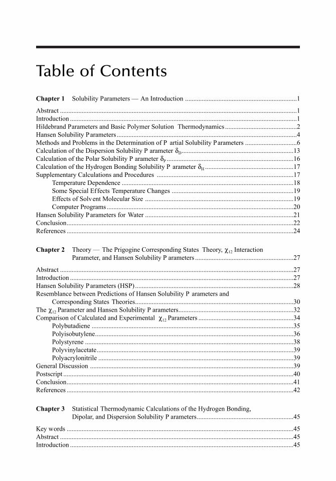
Table of Contents
Chapter 1
Solubility Parameters — An Introduction ...................................................................1
Abstract ..............................................................................................................................................1Introduction ........................................................................................................................................1Hildebrand Parameters and Basic Polymer Solution Thermodynamics ...........................................2Hansen Solubility Parameters ............................................................................................................4Methods and Problems in the Determination of P artial Solubility Parameters ...............................6Calculation of the Dispersion Solubility P arameter
δ
D
...................................................................13Calculation of the Polar Solubility P arameter
δ
P
............................................................................16Calculation of the Hydrogen Bonding Solubility P arameter
δ
H
.....................................................17Supplementary Calculations and Procedures ..................................................................................17
Temperature Dependence .......................................................................................................18Some Special Effects Temperature Changes .........................................................................19Effects of Solvent Molecular Size .........................................................................................19Computer Programs ................................................................................................................20
Hansen Solubility Parameters for Water .........................................................................................21Conclusion........................................................................................................................................22References ........................................................................................................................................24
Chapter 2 Theory — The Prigogine Corresponding States Theory, χ12 Interaction Parameter, and Hansen Solubility P arameters ...........................................................27
Abstract ............................................................................................................................................27Introduction ......................................................................................................................................27Hansen Solubility Parameters (HSP) ...............................................................................................28Resemblance between Predictions of Hansen Solubility P arameters and
Corresponding States Theories...............................................................................................30The χ12 Parameter and Hansen Solubility P arameters.....................................................................32Comparison of Calculated and Experimental χ12 Parameters .........................................................34
Polybutadiene .........................................................................................................................35Polyisobutylene.......................................................................................................................36Polystyrene .............................................................................................................................38Polyvinylacetate......................................................................................................................39Polyacrylonitrile .....................................................................................................................39
General Discussion ..........................................................................................................................39Postscript ..........................................................................................................................................40Conclusion........................................................................................................................................41References ........................................................................................................................................42
Chapter 3 Statistical Thermodynamic Calculations of the Hydrogen Bonding, Dipolar, and Dispersion Solubility P arameters..........................................................45
Key words ........................................................................................................................................45Abstract ............................................................................................................................................45Introduction ......................................................................................................................................45
7248_C000.fm Page xvii Thursday, May 24, 2007 1:40 PM
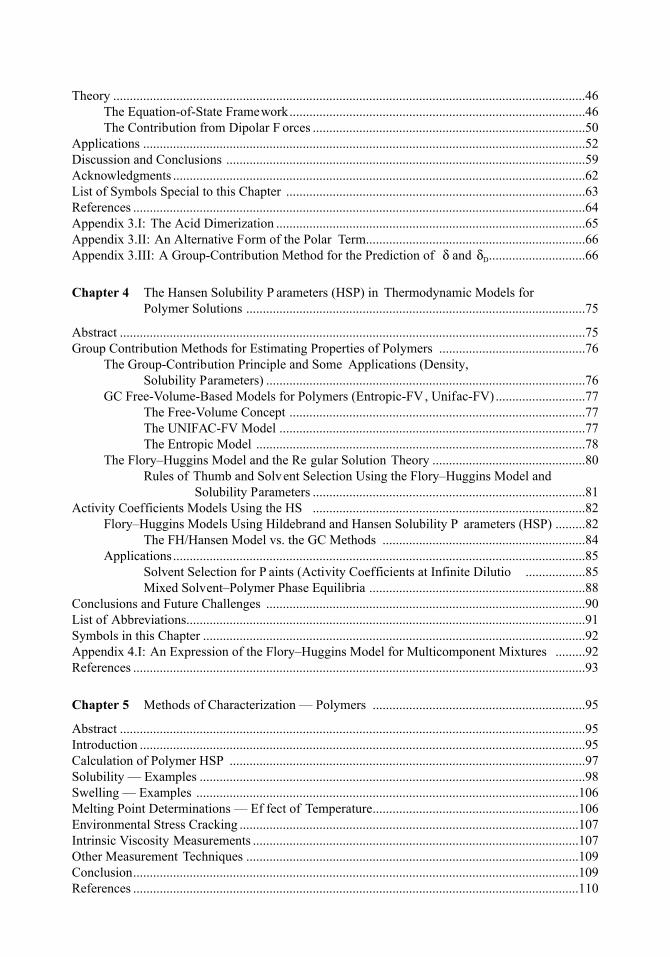
Theory ..............................................................................................................................................46The Equation-of-State Framework.........................................................................................46The Contribution from Dipolar F orces ..................................................................................50
Applications .....................................................................................................................................52Discussion and Conclusions ............................................................................................................59Acknowledgments ............................................................................................................................62List of Symbols Special to this Chapter ..........................................................................................63References ........................................................................................................................................64Appendix 3.I: The Acid Dimerization .............................................................................................65Appendix 3.II: An Alternative Form of the Polar Term..................................................................66Appendix 3.III: A Group-Contribution Method for the Prediction of δ and δD.............................66
Chapter 4 The Hansen Solubility P arameters (HSP) in Thermodynamic Models for Polymer Solutions ......................................................................................................75
Abstract ............................................................................................................................................75Group Contribution Methods for Estimating Properties of Polymers ............................................76
The Group-Contribution Principle and Some Applications (Density, Solubility Parameters) ................................................................................................76
GC Free-Volume-Based Models for Polymers (Entropic-FV, Unifac-FV)...........................77The Free-Volume Concept .........................................................................................77The UNIFAC-FV Model ............................................................................................77The Entropic Model ...................................................................................................78
The Flory–Huggins Model and the Re gular Solution Theory ..............................................80Rules of Thumb and Solvent Selection Using the Flory–Huggins Model and
Solubility Parameters ..................................................................................81Activity Coefficients Models Using the HS ..................................................................................82
Flory–Huggins Models Using Hildebrand and Hansen Solubility P arameters (HSP) .........82The FH/Hansen Model vs. the GC Methods .............................................................84
Applications............................................................................................................................85Solvent Selection for P aints (Activity Coefficients at Infinite Dilutio ..................85Mixed Solvent–Polymer Phase Equilibria .................................................................88
Conclusions and Future Challenges ................................................................................................90List of Abbreviations........................................................................................................................91Symbols in this Chapter ...................................................................................................................92Appendix 4.I: An Expression of the Flory–Huggins Model for Multicomponent Mixtures .........92References ........................................................................................................................................93
Chapter 5 Methods of Characterization — Polymers ................................................................95
Abstract ............................................................................................................................................95Introduction ......................................................................................................................................95Calculation of Polymer HSP ...........................................................................................................97Solubility — Examples ....................................................................................................................98Swelling — Examples ...................................................................................................................106Melting Point Determinations — Ef fect of Temperature..............................................................106Environmental Stress Cracking ......................................................................................................107Intrinsic Viscosity Measurements ..................................................................................................107Other Measurement Techniques ....................................................................................................109Conclusion......................................................................................................................................109References ......................................................................................................................................110
7248_C000.fm Page xviii Thursday, May 24, 2007 1:40 PM
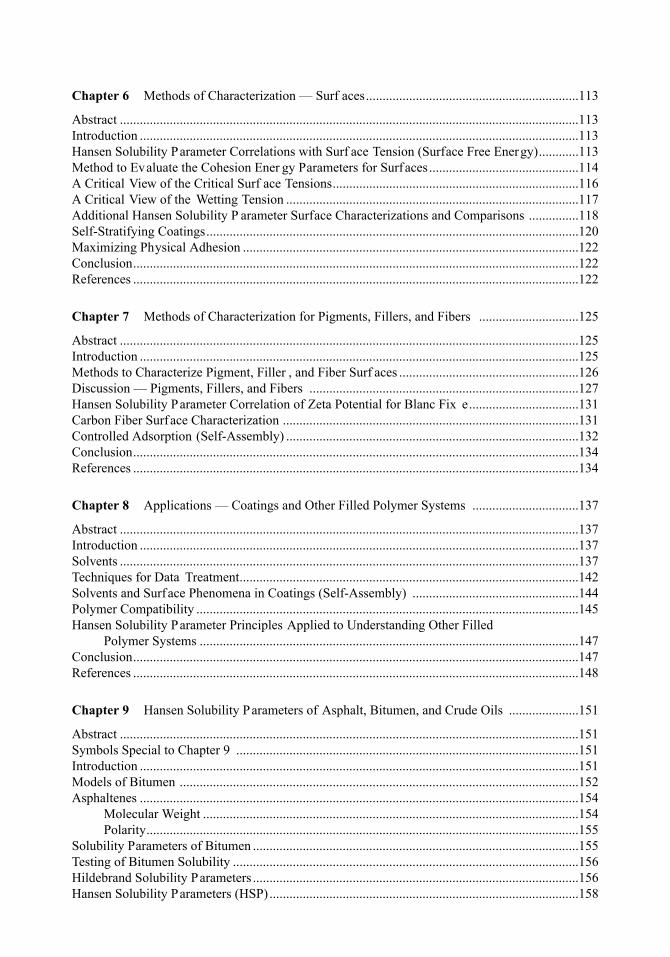
Chapter 6 Methods of Characterization — Surf aces................................................................113
Abstract ..........................................................................................................................................113Introduction ....................................................................................................................................113Hansen Solubility Parameter Correlations with Surf ace Tension (Surface Free Energy)............113Method to Evaluate the Cohesion Ener gy Parameters for Surfaces.............................................114A Critical View of the Critical Surf ace Tensions..........................................................................116A Critical View of the Wetting Tension ........................................................................................117Additional Hansen Solubility P arameter Surface Characterizations and Comparisons ...............118Self-Stratifying Coatings................................................................................................................120Maximizing Physical Adhesion .....................................................................................................122Conclusion......................................................................................................................................122References ......................................................................................................................................122
Chapter 7 Methods of Characterization for Pigments, Fillers, and Fibers ..............................125
Abstract ..........................................................................................................................................125Introduction ....................................................................................................................................125Methods to Characterize Pigment, Filler , and Fiber Surf aces ......................................................126Discussion — Pigments, Fillers, and Fibers .................................................................................127Hansen Solubility Parameter Correlation of Zeta Potential for Blanc Fix e.................................131Carbon Fiber Surface Characterization .........................................................................................131Controlled Adsorption (Self-Assembly) ........................................................................................132Conclusion......................................................................................................................................134References ......................................................................................................................................134
Chapter 8 Applications — Coatings and Other Filled Polymer Systems ................................137
Abstract ..........................................................................................................................................137Introduction ....................................................................................................................................137Solvents ..........................................................................................................................................137Techniques for Data Treatment......................................................................................................142Solvents and Surface Phenomena in Coatings (Self-Assembly) ..................................................144Polymer Compatibility ...................................................................................................................145Hansen Solubility Parameter Principles Applied to Understanding Other Filled
Polymer Systems ..................................................................................................................147Conclusion......................................................................................................................................147References ......................................................................................................................................148
Chapter 9 Hansen Solubility Parameters of Asphalt, Bitumen, and Crude Oils .....................151
Abstract ..........................................................................................................................................151Symbols Special to Chapter 9 .......................................................................................................151Introduction ....................................................................................................................................151Models of Bitumen ........................................................................................................................152Asphaltenes ....................................................................................................................................154
Molecular Weight .................................................................................................................154Polarity..................................................................................................................................155
Solubility Parameters of Bitumen ..................................................................................................155Testing of Bitumen Solubility ........................................................................................................156Hildebrand Solubility Parameters ..................................................................................................156Hansen Solubility Parameters (HSP) .............................................................................................158
7248_C000.fm Page xix Thursday, May 24, 2007 1:40 PM
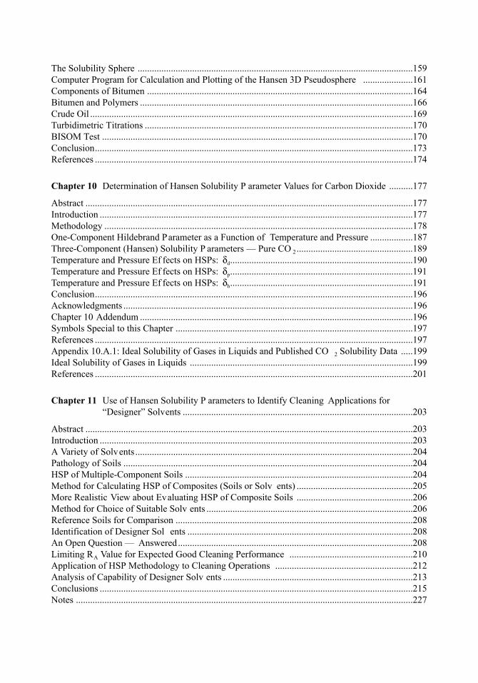
The Solubility Sphere ....................................................................................................................159Computer Program for Calculation and Plotting of the Hansen 3D Pseudosphere .....................161Components of Bitumen ................................................................................................................164Bitumen and Polymers ...................................................................................................................166Crude Oil ........................................................................................................................................169Turbidimetric Titrations .................................................................................................................170BISOM Test ...................................................................................................................................170Conclusion......................................................................................................................................173References ......................................................................................................................................174
Chapter 10 Determination of Hansen Solubility P arameter Values for Carbon Dioxide ..........177
Abstract ..........................................................................................................................................177Introduction ....................................................................................................................................177Methodology ..................................................................................................................................178One-Component Hildebrand Parameter as a Function of Temperature and Pressure ..................187Three-Component (Hansen) Solubility P arameters — Pure CO 2.................................................189Temperature and Pressure Ef fects on HSPs: δd.............................................................................190Temperature and Pressure Ef fects on HSPs: δp.............................................................................191Temperature and Pressure Ef fects on HSPs: δh.............................................................................191Conclusion......................................................................................................................................196Acknowledgments ..........................................................................................................................196Chapter 10 Addendum ...................................................................................................................196Symbols Special to this Chapter ....................................................................................................197References ......................................................................................................................................197Appendix 10.A.1: Ideal Solubility of Gases in Liquids and Published CO 2 Solubility Data .....199Ideal Solubility of Gases in Liquids ..............................................................................................199References ......................................................................................................................................201
Chapter 11 Use of Hansen Solubility P arameters to Identify Cleaning Applications for “Designer” Solvents .................................................................................................203
Abstract ..........................................................................................................................................203Introduction ....................................................................................................................................203A Variety of Solvents.....................................................................................................................204Pathology of Soils ..........................................................................................................................204HSP of Multiple-Component Soils ................................................................................................204Method for Calculating HSP of Composites (Soils or Solv ents) .................................................205More Realistic View about Evaluating HSP of Composite Soils .................................................206Method for Choice of Suitable Solv ents .......................................................................................206Reference Soils for Comparison ....................................................................................................208Identification of Designer Sol ents ...............................................................................................208An Open Question — Answered...................................................................................................208Limiting RA Value for Expected Good Cleaning Performance ....................................................210Application of HSP Methodology to Cleaning Operations ..........................................................212Analysis of Capability of Designer Solv ents ................................................................................213Conclusions ....................................................................................................................................215Notes ..............................................................................................................................................227
7248_C000.fm Page xx Thursday, May 24, 2007 1:40 PM
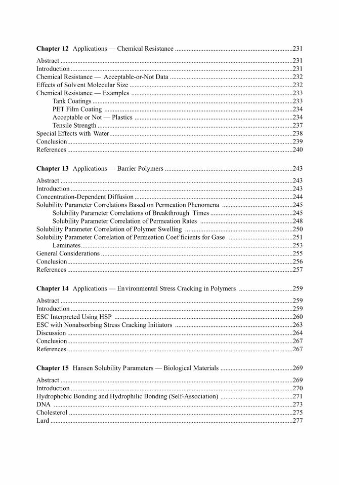
Chapter 12 Applications — Chemical Resistance ......................................................................231
Abstract ..........................................................................................................................................231Introduction ....................................................................................................................................231Chemical Resistance — Acceptable-or-Not Data .........................................................................232Effects of Solvent Molecular Size .................................................................................................232Chemical Resistance — Examples ................................................................................................233
Tank Coatings .......................................................................................................................233PET Film Coating ................................................................................................................234Acceptable or Not — Plastics ..............................................................................................234Tensile Strength ....................................................................................................................237
Special Effects with Water.............................................................................................................238Conclusion......................................................................................................................................239References ......................................................................................................................................240
Chapter 13 Applications — Barrier Polymers ............................................................................243
Abstract ..........................................................................................................................................243Introduction ....................................................................................................................................243Concentration-Dependent Diffusion ..............................................................................................244Solubility Parameter Correlations Based on Permeation Phenomena ..........................................245
Solubility Parameter Correlations of Breakthrough Times .................................................245Solubility Parameter Correlation of Permeation Rates .......................................................248
Solubility Parameter Correlation of Polymer Swelling ................................................................250Solubility Parameter Correlation of Permeation Coef ficients for Gase ......................................251
Laminates..............................................................................................................................253General Considerations ..................................................................................................................255Conclusion......................................................................................................................................256References ......................................................................................................................................257
Chapter 14 Applications — Environmental Stress Cracking in Polymers ................................259
Abstract ..........................................................................................................................................259Introduction ....................................................................................................................................259ESC Interpreted Using HSP ..........................................................................................................260ESC with Nonabsorbing Stress Cracking Initiators ......................................................................263Discussion ......................................................................................................................................264Conclusion......................................................................................................................................267References ......................................................................................................................................267
Chapter 15 Hansen Solubility Parameters — Biological Materials ...........................................269
Abstract ..........................................................................................................................................269Introduction ....................................................................................................................................270Hydrophobic Bonding and Hydrophilic Bonding (Self-Association) ...........................................271DNA ..............................................................................................................................................273Cholesterol .....................................................................................................................................275Lard ................................................................................................................................................277
7248_C000.fm Page xxi Thursday, May 24, 2007 1:40 PM
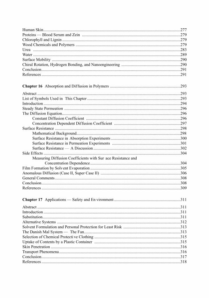
Human Skin....................................................................................................................................277Proteins — Blood Serum and Zein ...............................................................................................279Chlorophyll and Lignin ..................................................................................................................279Wood Chemicals and Polymers .....................................................................................................279Urea ..............................................................................................................................................283Water ..............................................................................................................................................289Surface Mobility ............................................................................................................................290Chiral Rotation, Hydrogen Bonding, and Nanoengineering .........................................................290Conclusion......................................................................................................................................291References ......................................................................................................................................291
Chapter 16 Absorption and Diffusion in Polymers ....................................................................293
Abstract ..........................................................................................................................................293List of Symbols Used in This Chapter ..........................................................................................293Introduction ....................................................................................................................................294Steady State Permeation ................................................................................................................296The Diffusion Equation..................................................................................................................296
Constant Diffusion Coefficient ...........................................................................................296Concentration Dependent Diffusion Coefficient ................................................................297
Surface Resistance .........................................................................................................................298Mathematical Background....................................................................................................298Surface Resistance in Absorption Experiments ...................................................................300Surface Resistance in Permeation Experiments ..................................................................301Surface Resistance — A Discussion ....................................................................................302
Side Effects ....................................................................................................................................304Measuring Diffusion Coefficients with Sur ace Resistance and
Concentration Dependence.......................................................................................304Film Formation by Solvent Evaporation .......................................................................................305Anomalous Diffusion (Case II, Super Case II) .............................................................................306General Comments .........................................................................................................................308Conclusion......................................................................................................................................308References ......................................................................................................................................309
Chapter 17 Applications — Safety and En vironment ................................................................311
Abstract ..........................................................................................................................................311Introduction ....................................................................................................................................311Substitution.....................................................................................................................................311Alternative Systems .......................................................................................................................312Solvent Formulation and Personal Protection for Least Risk .......................................................313The Danish Mal System — The Fan.............................................................................................313Selection of Chemical Protecti ve Clothing ...................................................................................315Uptake of Contents by a Plastic Container ...................................................................................315Skin Penetration .............................................................................................................................316Transport Phenomena.....................................................................................................................316Conclusion......................................................................................................................................317References ......................................................................................................................................318
7248_C000.fm Page xxii Thursday, May 24, 2007 1:40 PM
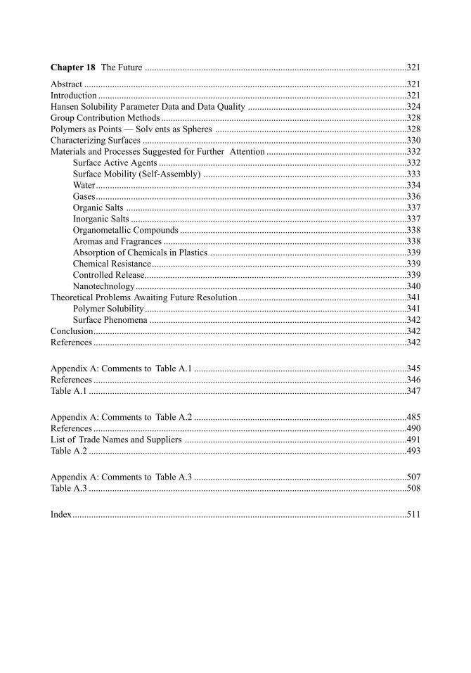
Chapter 18 The Future ................................................................................................................321
Abstract ..........................................................................................................................................321Introduction ....................................................................................................................................321Hansen Solubility Parameter Data and Data Quality ....................................................................324Group Contribution Methods .........................................................................................................328Polymers as Points — Solv ents as Spheres ..................................................................................328Characterizing Surfaces .................................................................................................................330Materials and Processes Suggested for Further Attention ............................................................332
Surface Active Agents ..........................................................................................................332Surface Mobility (Self-Assembly) .......................................................................................333Water.....................................................................................................................................334Gases.....................................................................................................................................336Organic Salts ........................................................................................................................337Inorganic Salts ......................................................................................................................337Organometallic Compounds .................................................................................................338Aromas and Fragrances ........................................................................................................338Absorption of Chemicals in Plastics ....................................................................................339Chemical Resistance.............................................................................................................339Controlled Release................................................................................................................339Nanotechnology....................................................................................................................340
Theoretical Problems Awaiting Future Resolution ........................................................................341Polymer Solubility ................................................................................................................341Surface Phenomena ..............................................................................................................342
Conclusion......................................................................................................................................342References ......................................................................................................................................342
Appendix A: Comments to Table A.1 ...........................................................................................345References ......................................................................................................................................346Table A.1 ........................................................................................................................................347
Appendix A: Comments to Table A.2 ...........................................................................................485References ......................................................................................................................................490List of Trade Names and Suppliers ...............................................................................................491Table A.2 ........................................................................................................................................493
Appendix A: Comments to Table A.3 ...........................................................................................507Table A.3 ........................................................................................................................................508
Index...............................................................................................................................................511
7248_C000.fm Page xxiii Thursday, May 24, 2007 1:40 PM

7248_C000.fm Page xxiv Thursday, May 24, 2007 1:40 PM
1
1
Solubility Parameters — An Introduction
Charles M. Hansen
ABSTRACT
Solubility parameters have found their greatest use in the coatings industry to aid in the selectionof solv ents. They are used in other industries, ho wever, to predict compatibility of polymers,chemical resistance, and permeation rates, and even to characterize the surfaces of pigments, fibersand fillers. Liquids with similar solubility parameters will be miscible, and polymers will dissol ein solvents whose solubility parameters are not too dif ferent from their o wn. The basic principlehas been “like dissolves like.” More recently, this has been modified to “li e seeks like,” as manysurface characterizations ha ve also been made, and surf aces do not (usually) dissolv e. Solubilityparameters help put numbers into this simple qualitati ve idea. This chapter describes the toolscommonly used in Hansen solubility parameter (HSP) studies. These include liquids used as energyprobes and computer programs to process data. The goal is to arri ve at the HSP for interestingmaterials either by calculation or , if necessary , by e xperiment and preferably with agreementbetween the two.
INTRODUCTION
The solubility parameter has been used for man y years to select solv ents for coatings materials. Alack of total success has stimulated further research. The skill with which solvents can be optimallyselected with respect to cost, solv ency, workplace environment, external environment, evaporationrate, flash point, etc., has impr ved over the years as a result of a series of impro vements in thesolubility parameter concept and widespread use of computer techniques. Most commercial sup-pliers of solv ents ha ve computer programs to help with solv ent selection. One can no w easilypredict how to dissolve a given polymer in a mixture of two solvents, neither of which can dissolvethe polymer by itself.
Unfortunately, this book cannot include discussion of all the significant e forts leading to ourpresent knowledge of the solubility parameters. An attempt is made to outline developments, providesome background for a basic understanding, and gi ve examples of uses in practice. The key factoris to determine those af finities that the important components in a system h ve for each other. Formany products this means e valuating or estimating the relati ve af finities of sol ents, polymers,additives, pigment surfaces, filler sur aces, fiber sur aces, and substrates.
It is note worthy that the concepts presented here ha ve developed toward not just predictingsolubility that requires high affinity between sol ent and solute, but for predicting affinities betweedifferent polymers, leading to compatibility , and af finities to sur aces to impro ve dispersion andadhesion. In these applications the solubility parameter has become a tool, using well-defineliquids as energy probes, to measure the similarity, or lack of the same, of key components. Materialswith widely different chemical structures may be v ery close in affinities. Only those materials thainteract differently with dif ferent solvents can be characterized in this manner . It can be e xpectedthat many inorganic materials, such as fillers, will not interact di ferently with these energy probes
7248_C001.fm Page 1 Monday, April 23, 2007 1:56 PM
2
Hansen Solubility Parameters: A User’s Handbook
as their energies are very much higher. An adsorbed layer of w ater on the high-energy surface canalso play an important role. Re gardless of these concerns, it has been possible to characterizepigments, both or ganic and inor ganic, as well as fillers li e barium sulf ate, zinc oxide, etc., andalso inorganic fibers (see Chapter 7). Changing the sur ace energies by various treatments can leadto a surf ace that can be characterized more readily and often interacts more strongly with gi venorganic solvents. When the same solvents that dissolve a polymeric binder are those which interactmost strongly with a surf ace, it can be e xpected that the binder and the surf ace have high affinitfor each other.
Solubility parameters are sometimes called
cohesion energy parameters
as the y are deri vedfrom the energy required to convert a liquid to a gas. The energy of vaporization is a direct measureof the total (cohesi ve) energy holding the liquid’ s molecules together. All types of bonds holdingthe liquid together are brok en by e vaporation, and this has led to the concepts described in moredetail later . The term
cohesion energy parameter
is more appropriately used when referring tosurface phenomena.
HILDEBRAND PARAMETERS AND BASIC POLYMER SOLUTION THERMODYNAMICS
The term
solubility parameter
w as first used by Hildebrand and Scott
1,2
The earlier w ork ofScatchard and others w as contributory to this de velopment. The Hildebrand solubility parameteris defined as the square root of the cohes ve energy density:
δ
= (E/V)
1/2
(1.1)
Where V
is the molar volume of the pure solvent, and
E
is its (measurable) energy of vaporization(see Equation 1.15). The numerical v alue of the solubility parameter in MP a
1/2
is 2.0455 timeslarger than that in (cal/cm
3
)
1/2
. The solubility parameter is an important quantity for predictingsolubility relations, as can be seen from the follo wing brief introduction.
Thermodynamics requires that the free ener gy of mixing must be zero or ne gative for thesolution process to occur spontaneously . The free energy change for the solution process is gi venby the relation:
Δ
G
M
=
Δ
H
M
–
Δ
TS
M
(1.2)
where
Δ
G
M
is the free energy of mixing,
Δ
H
M
is the heat of mixing, T is the absolute temperature,and
Δ
S
M
is the entrop y change in the mixing process.Equation 1.3 gives the heat of mixing as proposed by Hildebrand and Scott:
Δ
H
M
=
ϕ
1
ϕ
2
V
M
(
δ
1
–
δ
2
)
2
(1.3)
The
φ
1
and
φ
2
are volume fractions of solvent and polymer, and V
M
is the volume of the mixture.Equation 1.3 is not correct, and it has often been cited as a shortcoming of this theory in that onlypositive heats of mixing are allo wed. It has been sho wn by Patterson, Delmas, and coworkers that
Δ
G
Mnoncomb
is given by the right-hand side of Equation 1.3 and not
Δ
G
M
. This is discussed more inChapter 2. The correct relation is
3–8
:
Δ
G
Mnoncomb
=
ϕ
1
ϕ
2
V
M
(
δ
1
–
δ
2
)
2
(1.4)
The noncombinatorial free energy of solution,
Δ
G
Mnoncomb
, includes all free energy effects otherthan the combinatorial entropy of solution that results by simply mixing the components. Equation
7248_C001.fm Page 2 Monday, April 23, 2007 1:56 PM
Solubility Parameters — An Introduction
3
1.4 is consistent with the Prigogine corresponding states theory (CST) of polymer solutions (seeChapter 2) and can be dif ferentiated to gi ve expressions
3,4
predicting both positi ve and ne gativeheats of mixing. Therefore, both positi ve and ne gative heats of mixing can be e xpected fromtheoretical considerations and ha ve been measured accordingly . It has been clearly sho wn thatsolubility parameters can be used to predict both positi ve and ne gative heats of mixing. Pre viousobjections to the ef fect that only positi ve values are allowed in this theory are incorrect.
This discussion clearly demonstrates wh y the solubility parameter should be considered as afree energy parameter. This is more in agreement with the use of the solubility parameter plots tofollow. These use solubility parameters as ax es and have experimentally determined boundaries ofsolubility defined by the act that the free ener gy of mixing is zero. The combinatorial entrop yenters as a constant f actor in the plots of solubility in dif ferent solv ents, for e xample, as theconcentrations are usually constant for a gi ven study.
It is important to note that the solubility parameter , or rather the dif ference in solubilityparameters for the solv ent–solute combination, is important in determining the solubility of thesystem. It is clear that a match in solubility parameters leads to a zero change in noncombinatorialfree energy, and the positi ve entropy change (the combinatorial entrop y change), found on simplemixing to result in a disordered mixture compared to the pure components, will ensure that asolution is possible from a thermodynamic point of vie w. The maximum dif ference in solubilityparameters that can be tolerated where the solution still occurs is found by setting the noncombi-natorial free energy change equal to the combinatorial entrop y change:
Δ
G
Mnoncomb
= T
Δ
S
Mcomb
(1.5)
This equation clearly sho ws that an alternate vie w of the solubility situation at the limit ofsolubility is that it is the entrop y change that dictates ho w closely the solubility parameters mustmatch each other for the solution to occur .
It will be seen in Chapter 2 that solv ents with smaller molecular v olumes will be thermody-namically better than lar ger ones having identical solubility parameters. A practical aspect of thiseffect is that solv ents with relati vely low molecular v olumes, such as methanol and acetone, candissolve a polymer at larger solubility parameter differences than might be expected from compar-isons with other solv ents with larger molecular volumes. An average solvent molecular volume isusually taken as about 100 cc/mol. The converse is also true. Lar ger molecular species may notdissolve, even though solubility parameter considerations might predict the y would. This can be adifficulty in predicting the beh vior of plasticizers solely based on data for lower molecular weightsolvents. These effects are also discussed elsewhere in this book, particularly in Chapter 2, Chapter12, Chapter 13, and Chapter 16.
A shortcoming of the earlier solubility parameter w ork is that the approach w as limited toregular solutions, as defined by Hildebrand and Scott
2
and does not account for association betweenmolecules, such as those that polar and h ydrogen-bonding interactions w ould require. The latterproblem seems to have been largely solved with the use of multicomponent solubility parameters;however, the lack of accurac y with which the solubility parameters can be assigned will al waysremain a problem. Using the dif ference between two large numbers to calculate a relati vely smallheat of mixing, for e xample, will always be problematic.
A more detailed description of the theory presented by Hildebrand, and the succession ofresearch reports that have attempted to improve on it, can be found in Barton’s extensive handbook.
9
The slightly older , excellent contribution of Gardon and Teas
10
is also a good source of relatedinformation, particularly for coatings and adhesion phenomena. The approach of Burrell,
11
whodivided solv ents into h ydrogen bonding classes, has found numerous practical applications; theapproach of Blanks and Prausnitz
12
divided the solubility parameter into tw o components, “non-polar” and “polar.” Both are w orthy of mention, ho wever, in that the first has found wide use anthe second greatly influenced the author s earlier activities. The Prausnitz article, in particular, was
7248_C001.fm Page 3 Monday, April 23, 2007 1:56 PM

4
Hansen Solubility Parameters: A User’s Handbook
farsighted in that a corresponding states procedure was introduced to calculate the dispersion energycontribution to the cohesi ve energy. This is discussed in more detail in Chapter 2.
It can be seen from Equation 1.2 that the entrop y change is beneficial to mixing. Whenmultiplied by the temperature, this will w ork in the direction of promoting a more ne gative freeenergy of mixing. This is the usual case, although there are e xceptions. Increasing temperaturedoes not always lead to impro ved solubility relations. Indeed, this w as the basis of the pioneeringwork of Patterson and coworkers,
3–8
to show that subsequent increases in temperature can predict-ably lead to insolubility. Their work was done in essentially nonpolar systems. Increasing temper -ature can also lead to a nonsolv ent becoming a solvent and, subsequently, a nonsolvent again withstill further increase in temperature. Polymer solubility parameters do not change much withtemperature, but those of a liquid frequently decrease rapidly with temperature. This situation allowsa nonsolvent, with a solubility parameter that is initially too high, to pass through a soluble conditionto once more become a nonsolv ent as the temperature increases. These are usually “boundary”solvents on solubility parameter plots.
The entropy changes associated with polymer solutions will be smaller than those associatedwith liquid–liquid miscibility, for example, as the “monomers” are already bound into the configuration dictated by the polymer the y make up. They are no longer free in the sense of a liquidsolvent and cannot mix freely to contrib ute to a lar ger entropy change. This is one reason poly-mer–polymer miscibility is dif ficult to achi ve. The free ener gy criterion dictates that polymersolubility parameters match extremely well for mutual compatibility , as there is little to be g ainedfrom the entrop y contribution when progressi vely larger molecules are in volved. However, poly-mer–polymer miscibility can be promoted by the introduction of suitable copolymers or comono-mers that interact specifically within the system. Further discussion of these phenomena is b yondthe scope of the present discussion; ho wever, see Chapter 5.
HANSEN SOLUBILITY PARAMETERS
A solubility parameter approach proposed by the author for predicting polymer solubility has beenin wide use. The basis of these so-called HSPs is that the total ener gy of vaporization of a liquidconsists of se veral individual parts.
13–17
These arise from (atomic) dispersion forces, (molecular)permanent dipole–permanent dipole forces, and (molecular) hydrogen bonding (electron exchange).Needless to say, without the work of Hildebrand and Scott
1,2
and others not specifically referencehere, such as Scatchard, this postulate could ne ver have been made. The total cohesive energy, E,can be measured by e vaporating the liquid, i.e., breaking all the cohesi ve bonds. Thus the totalcohesive energy is considered as being identical to the ener gy of v aporization. It should also benoted that these cohesive energies arise from interactions of a given solvent molecule with anotherof its o wn kind. The basis of the approach is, therefore, v ery simple, and it is surprising that somany different applications ha ve been possible since 1967 when the idea w as first published. Arather large number of applications are discussed in this book. Others are found in the w orks ofBarton.
9
A lucid discussion by Barton
18
enumerates typical situations where problems occur whenusing solubility parameters. These appear most often where the en vironment causes the solv entmolecules to interact, with or within themselv es, dif ferently from the w ay they do in situationswhere they make up their own environment, i.e., as pure liquids. Several cases are discussed whereappropriate in the follo wing chapters.
Materials with similar HSP ha ve high affinity for each othe . The extent of the similarity in agiven situation determines the e xtent of the interaction. The same cannot be said of the total orHildebrand solubility parameter .
1,2
Ethanol and nitromethane, for e xample, have similar total sol-ubility parameters (26.1 vs. 25.1 MPa
1/2
, respectively), but their affinities are quite di ferent. Ethanolis water soluble, whereas nitromethane is not. Indeed, mixtures of nitroparaf fins and alcohols werdemonstrated in man y cases to pro vide syner gistic mixtures of tw o nonsolv ents that dissolv ed
7248_C001.fm Page 4 Monday, April 23, 2007 1:56 PM
Solubility Parameters — An Introduction
5
polymers.
13
This could ne ver ha ve been predicted by Hildebrand parameters, whereas the HSPconcept readily confirms the reason for this e fect.
There are three major types of interactions in common organic materials. The most general arethe nonpolar interactions. These are derived from atomic forces and have also been called
dispersioninteractions
in the literature. As molecules are b uilt up from atoms, all molecules contain thosetypes of attractive forces. For the saturated aliphatic hydrocarbons, for example, these are essentiallythe only cohesi ve interactions, and the ener gy of v aporization is assumed to be the same as thedispersion cohesive energy, E
D
. Finding the dispersion cohesi ve energy as the cohesion ener gy ofthe homomorph, or h ydrocarbon counterpart, is the starting point for calculating the three Hansenparameters for a gi ven liquid. As discussed in more detail later , this is based on a correspondingstates calculation.
The permanent dipole–permanent dipole interactions cause a second type of cohesion ener gy,
the polar cohesive energy
, E
P
. These are inherently molecular interactions and are found in mostmolecules to one extent or another. The dipole moment is the primary parameter used to calculatethese interactions. A molecule can be mainly polar in character without being w ater soluble, hencethere is a misuse of the term
polar
in the general literature. The polar solubility parameters referredto here are well-defined, xperimentally verified, and can be estimated from molecular parameteras described later. As noted previously, the most polar of the solv ents include those with relativelyhigh total solubility parameters that are not particularly w ater soluble, such as nitroparaf finspropylene carbonate, and tri-n-butyl phosphate. Induced dipoles ha ve not been treated specificallin this approach but are recognized as a potentially important f actor, particularly for solvents withzero dipole moments (see the Calculation of the Polar Solubility P arameter section).
The third major cohesi ve ener gy source is h ydrogen bonding, E
H
. This can be called moregenerally an
electron exchange parameter
. Hydrogen bonding is a molecular interaction and resem-bles the polar interactions in this respect. The basis of this type of cohesi ve energy is attractionamong molecules because of the h ydrogen bonds. In this perhaps o versimplified approach, thhydrogen bonding parameter has been used to more or less collect the ener gies from interactionsnot included in the other two parameters. Alcohols, glycols, carboxylic acids, and other hydrophilicmaterials have high-hydrogen-bonding parameters. Other researchers ha ve divided this parameterinto separate parts — for e xample, acid and base cohesion parameters — to allo w both positi veand negative heats of mixing. These approaches will not be dealt with here b ut are described inBarton’s handbook
9
and else where.
19–21
The most e xtensive division of the cohesi ve ener gy hasbeen done by Karger et al.,
22
who developed a system with fi e parameters: dispersion, orientation,induction, proton donor, and proton acceptor. As a single parameter, the Hansen hydrogen bondingparameter has serv ed remarkably well in the e xperience of the author and k eeps the number ofparameters to a le vel that allows ready practical usage.
It is clear that there are other sources of cohesion ener gy arising in various types of moleculesfrom, for example, induced dipoles, metallic bonds, electrostatic interactions, or whate ver type ofseparate energy can be defined. The author stopped with the three major types found in or ganicmolecules. It has been recognized that additional parameters could be assigned to separate ener gytypes. F or e xample, the description of or ganometallic compounds could be an intriguing study .This would presumably parallel similar characterizations of surf ace-active materials, where eachpart of the molecule requires separate characterization for completeness. The Hansen parametershave mainly been used in connection with solubility relations, mostly , but not e xclusively, in thecoatings and related industries.
Solubility and swelling have been used to confirm the solubility parameter assignments of mayof the liquids. Group contrib ution methods and suitable equations based on molecular propertieswere then derived from these. They make possible estimates of the three parameters for additionalliquids. The goal of a prediction is to determine the similarity or dif ference of the cohesion energyparameters. The strength of a particular type of hydrogen bond or any other bond is important onlyto the extent that it influences the cohes ve energy density.
7248_C001.fm Page 5 Monday, April 23, 2007 1:56 PM
6
Hansen Solubility Parameters: A User’s Handbook
HSPs do have direct applications in other scientific disciplines, such as sur ace science, wherethey have been used to characterize the wettability of various surfaces and the adsorption propertiesof pigment surfaces,
10,14,16,23–26
and have even led to systematic surface treatment of inorganic fiberso that the y could be readily incorporated into polymers of lo w-solubility parameters such aspolypropylene
27
(see also Chapter 7). Man y widely dif ferent applications ha ve been discussed byBarton
9
and Gardon.
28
Surface characterizations have not been given the attention deserved in termsof a unified similarity-of-ene gy approach. The author can certify that thinking in terms of similarityof energy, whether surface or cohesive energies, can lead to rapid decisions and plans of action incritical situations that lack data. In other w ords, the e veryday industrial crisis situation often canbe reduced in scope by appropriate systematic approaches based on similarity of energy. The successof the HSPs for surf ace applications are not surprising in vie w of the similarity of predictionsoffered by these, and the Prigogine corresponding states theory of polymer solutions discussed inChapter 2. Flory also emphasized that it is the surf ace of molecules that interact to producesolutions,
29
so the interactions of molecules residing in surf aces should clearly be included in an ygeneral approach to interactions among molecules. Surf ace mobility and surf ace rotation areimportant f actors in en vironmental stress cracking (Chapter 14), certain biological phenomena(Chapter 15), the wetting of surfaces, and in other important phenomena relating to nanotechnology(Chapter 18).
The basic equation go verning the assignment of Hansen parameters is that the total cohesionenergy, E, must be the sum of the indi vidual energies that make it up.
E = E
D
+ E
P
+ E
H
(1.6)
Dividing this by the molar v olume gi ves the square of the total (or Hildebrand) solubilityparameter as the sum of the squares of the Hansen D, P , and H components.
E/V = E
D
/V + E
P
/V + E
H
/V
(1.7)
δ
2
=
δ
2D
+
δ
2P
+
δ
2H
(1.8)
To sum up this section, it is emphasized that HSPs quantitati vely account for the cohesionenergy (density). Up to this point of time, an e xperimental latent heat of v aporization has beenconsidered a more reliable method to arrive at a cohesion energy rather than using molecular orbitalcalculations or other calculations based on potential functions. Indeed, the goal of such e xtensivecalculations for polar and hydrogen bonding molecules should be to accurately arrive at the energyof vaporization. The statistical thermodynamics approach of Panayiotou and coworkers reported inChapter 3 may ha ve changed this. An alternative method of calculating the three parameters hasbeen presented, but full evaluation of this ne w information has not been possible as yet.
METHODS AND PROBLEMS IN THE DETERMINATION OF PARTIAL SOLUBILITY PARAMETERS
The best method to calculate individual HSPs depends to a great extent on what data are available.The author originally adopted an essentially e xperimental procedure and established v alues for 90liquids based on solubility data for 32 polymers.
13
This procedure in volved calculation of thenonpolar parameter according to the procedure outlined by Blanks and Prausnitz.
12
This calculationprocedure is still in use and is considered the most reliable and consistent one for this parameter .It is outlined in the follo wing section. The division of the remaining cohesi ve energy between thepolar and h ydrogen bonding interactions w as initially done by trial and error to fit xperimentalpolymer solubility data. A key to parameter assignments in this initial trial-and-error approach was
7248_C001.fm Page 6 Monday, April 23, 2007 1:56 PM
Solubility Parameters — An Introduction
7
that mixtures of two nonsolvents could be systematically and synergistically (but predictably) foundto dissolve given polymers. This meant that these had parameters placing them on opposite sidesof the solubility re gion, a spheroid. Using a lar ge number of such predictably syner gistic systemsas a basis, reasonably accurate di visions into the three ener gy types were possible.
Using the experimentally established, approximate,
δ
P
and
δ
H
parameters, Hansen and Skaarup
15
found that the Böttcher equation (Equation 10.25) could be used to calculate the polar parameterquite well, and this led to a revision of the earlier values to those now accepted for the same liquids.These values were also consistent with the e xperimental solubility data for 32 polymers a vailableat that time and with Equation 1.6. Furthermore, Skaarup de veloped the equation for the solubilityparameter “distance,” Ra, between tw o materials based on their respecti ve partial solubility para-meter components:
(Ra)
2
= 4(
δ
D2
–
δ
D1
)
2
+ (
δ
P2
–
δ
P1
)
2
+ (
δ
H2
–
δ
H1
)
2
(1.9)
This equation was developed from plots of experimental data where the constant “4” was foundconvenient and correctly represented the solubility data as a sphere encompassing the good solvents(see Chapter 5). When the scale for the dispersion parameter is doubled, in comparison with theother two parameters essentially spherical, rather than spheroidal, re gions of solubility are found.This greatly aids two-dimensional plotting and visualization. There are, of course, boundary regionswhere deviations can occur. These are most frequently found to involve the larger molecular speciesas being less ef fective solvents compared to their smaller counterparts that define the solubilitsphere. Likewise, smaller molecular species such as acetone, methanol, nitromethane, and othersoften appear as outliers, in that they dissolve a polymer even though they have solubility parametersplacing them at a distance greater than the experimentally-determined radius of the solubility sphere,Ro. This dependence on molar v olume is inherent in the theory de veloped by Hildebrand, Scott,and Scatchard discussed pre viously. Smaller molar v olume f avors lo wer
Δ
G
M
, as discussed inChapter 2. This in turn promotes solubility . Such smaller -molecular-volume species that dissolv e“better” than predicted by comparisons, based on solubility parameters alone, should not necessarilybe considered outliers.
The molar v olume is frequently and successfully used as a fourth parameter to describe theeffects of molecular size. F or e xample, these are especially important in correlating dif fusionalphenomena with HSP (see Chapter 12, Chapter 13, and Chapter 16). The author has preferred toretain the three, well-defined partial-solubility parameters with a fourth, separate, molar olumeparameter, rather than multiplying the solubility parameters by the molar v olume raised to somepower to redefine them
The reason for the e xperimentally determined constant 4 in Equation 1.9 will be discussed inmore detail in Chapter 2. It will be noted here, however, that the constant 4 is theoretically predictedby the Prigogine corresponding states theory of polymer solutions when the geometric mean isused to estimate the interaction in mixtures of dissimilar molecules.
30
The constant 4 differentiatesbetween atomic and molecular intereactions. This is exceptionally strong evidence that dispersion,permanent dipole–permanent dipole, and h ydrogen bonding interactions all follo w the geometricmean rule. P atterson and co workers have been especially instrumental in relating the Prigoginetheory to solubility parameters and to the Flory–Huggins theory of polymer solutions.
3–8
The HSPapproach of dividing the cohesive energy into parts derived from different types of cohesive forceshas been confirmed both by xperimental studies, as well as the Prigogine theory . The use of thegeometric mean is basic to this agreement between the HSP approach and that of Prigogine (seeChapter 2).
The approach of optimizing solubility data to spheres is still very much in use. Plotting regionsof solubility based on experimental solubility data, or computer-optimizing boundaries of solubilityby locating the maximum dif ference in solubility parameters allo wed by Equation 1.9 are bothused. The total free energy of mixing,
Δ
G
M
, is equal to zero on the boundary. It should be recognized
7248_C001.fm Page 7 Monday, April 23, 2007 1:56 PM
8
Hansen Solubility Parameters: A User’s Handbook
that using the solubility parameters relating to
Δ
G
Mnoncomb
in Equation 1.4 dif fers from this by thecombinatorial entropy of mixing.
Another promising approach to arri ve at the HSP for materials based on e xperimental data isto use multivariable analysis of one type or another, as discussed in Chapter 5. This type of approachhas not been attempted by the author , but it clearly has adv antages in some cases. The author’spreferred approach of locating the polymer HSP as the center of a sphere has a problem in that itis, in reality, the poor solv ents or nonsolvents located near the boundary of the sphere that fix thboundary (and center) rather than the best solv ents in the middle. This may present problems forsmaller sets of data, b ut it is an adv antage when e xtrapolating into re gions of HSP higher thanthose of an y liquid that can be used in testing. This is discussed in more detail in Chapter 5 andthe definition of the limited s gment of the boundary of the HSP sphere deri vable from suchcorrelations is based on Equation 1.9.
Equation 1.9 is readily used on a computer (or on a hand calculator), and supplementaryrelations allow easier scanning of lar ge sets for data. It is ob vious that solubility, or high af finit ,requires that Ra be less than Ro. The ratio Ra/Ro has been called the
RED number
, reflecting threlative energy difference.
RED = Ra/Ro (1.10)
A RED number of 0 is found for no ener gy difference, RED numbers less than 1.0 indicatehigh affinity; RED equal to or close to 1.0 is a boundary condition; and progress vely higher REDnumbers indicate progressively lower affinities. Scanning a computer output for RED numbers lesthan 1.0, for example, rapidly allows location of the most interesting liquids for a given application.
Parenthetically, it should be noted that the ratio of Ra to Ro is really a ratio of quantities havingthe same units as the solubility parameter . The ratio (Ra/Ro)
2 = (RED) 2 is a ratio of cohesionenergies. The latter quantity is important for relating the HSP approach to that of Huggins andFlory, as discussed in Chapter 2.
The revised set of parameters for the 90 original solv ents was the basis for group contrib utionprocedures developed (most notably) by van Krevelen,31 Beerbower,32 and Hansen and Beerbower,17
who also used Fedors’ w ork.33 These v arious de velopments ha ve been summarized by Barton, 9
although Beerbo wer’s latest v alues ha ve only appeared in the National Aeronautics and SpaceAdministration (NASA) document.32 Table 1.1 is an expanded table of Beerbower group contribu-tions, which w as distributed among those who were in contact with Beerbo wer in the late 1970s.The majority of the data in this table, as well as Table 1.2, ha ve also appeared in Reference 34.Beerbower also de veloped a simple equation for the polar parameter ,17 which in volved only thedipole moment and the square root of the molar v olume. This is also gi ven later (Equation 1.13)and has been found quite reliable by Koenhen and Smolders.35 This equation has been found reliableby the author as well, giving results generally consistent with Equation 1.6 to Equation 1.8, which,again, is the basis of the whole approach. K oenhen and Smolders also give correlation coefficientfor other calculation procedures to arri ve at the indi vidual Hansen parameters.
The group contributions in Table 1.1 have been used e xtensively to arrive at the collection ofHSP data in Appendix Table A.1. Most of the chemicals of primary interest for which full data areavailable are presumably already in this table. The trend has been to calculate HSP for lar ger andstill larger molecules. Many of these have multiple groups, and it becomes more and more difficulto make decisions as to ho w to treat them best. At times the HSP for the lar ger molecules can beestimated from the HSP of lar ger segments that mak e them up. Rather than e xpanding Table 1.1with additional data, e xcept as noted briefly late , the usual practice has been to locate chemicalswith similar groups and to use their HSP v alues in a group contrib ution-type calculation.
The procedure has de veloped to the point where its principle features can be identified in thfollowing table. If a boiling point is a vailable, the procedures for calculating δD have been used.If a boiling point is not a vailable, the similarity with related molecules has been used. If a dipole
7248_C001.fm Page 8 Monday, April 23, 2007 1:56 PM
Solubility Parameters — An Introduction 9
moment is available, the procedures gi ven here were used in preference to group contrib utions. Ifnecessary, group contributions can be derived from similar molecules to the one in question, whendipole moments are a vailable for these, and not for the molecule in question. There is often achange in the group contrib ution as a function of molecular size. This is the main reason for thelack of e xpansion of Table 1.1. It is thought best that the uncertainty be clear to the user . F orexample, it has been found that the group contrib ution for the polar component of aliphatic estersshould not be less than 300 cal/mol as gi ven in Table 1.1. This is necessary to pre vent δP formaterials like plasticizers from being clearly too low, based on their compatibility with, for example,polyvinyl chloride. Sulfur containing compounds have also been somewhat difficult in this respectwith major changes in estimated group contributions depending on molecular weight of the chemicalin question. Group contrib utions for sulfur , amides, and other groups not found in Table 1.1 canbe easily derived from the data on similar compounds reported in Appendix Table A.1. The sameis true of the δH component. The problem with this procedure is ob vious: any error or distortionof value for a class of compounds is perpetuated. This has been recognized and dealt with to theextent possible, but there are limits to what can be done with limited data. The scope of this situationhas been be yond the resources a vailable for its fully satisf actory resolution. The extensive list ofgroup contributions at the end of Chapter 3 pro vides what may be a partial replacement and/or asupplement for Table 1.1. This requires some e xperience with the techniques in volved.
A sizable number of materials ha ve been assigned HSPs using the procedures described here.Many of these have not been published. Exxon Chemical Corporation36,37 has indicated a computerprogram with data for o ver 500 solv ents and plasticizers, 450 resins and polymers, and 500pesticides. The author’s files contain the three parameters for about 1200 chemicals (See AppendixTable A.1), although several of them appear with two sets of possible values awaiting experimentalconfirmation. In some cases, this is due to questionable p ysical data, for example, for latent heatsof vaporization, or wide variations in reported dipole moments. Another reason is that some liquidsare chameleonic,38 as defined by H y, in that the y adopt configurations depending on their e vi-ronment. Hoy38 cites the formation of c yclic structures for glycol ethers with (nominally) linearstructure. The formation of h ydrogen-bonded tetramers of alcohols in a fluoropolymer has alsbeen pointed out.39 The term compound formation can be found in the older literature, particularlywhere mixtures with w ater were in volved and structured species were postulated to e xplain phe-nomena based on specific interactions among the components of the mixtures. Barton has discussesome of the situations where cohesion parameters need a more careful use, and points out thatHildebrand or Hansen parameters must be used with particular caution where the e xtent ofdonor–acceptor interactions, especially , h ydrogen bonding within a compound, is v ery dif ferentfrom that between compounds. 18 Amines, for e xample, are kno wn to associate with each other .Pure component data cannot be e xpected to predict the beha vior in such cases.
Still another reason for dif ficulties is the la ge variation of dipole moments reported for thesame liquid. The dipole moment for some liquids depends on their environment, as discussed later.A given solvent can be listed with dif ferent values in files to eep these phenomena in mind.
Large data sources greatly enhance a search for similar materials and the locating of ne wsolvents, as an e xample, for a polymer for which there are limited data. Unfortunately , differentauthors have used different group contribution techniques, and there is a proliferation of dif ferent“Hansen” parameters for the same chemicals in the literature. This would seem to be an unfortunatesituation, b ut may ultimately pro vide benefits. In particula , partial solubility parameter v aluesfound in Ho y’s e xtensive tables 9,40 are not compatible with the customary Hansen parametersreported here. Hoy has provided an excellent source of total solubility parameters. He independentlyarrived at the same type of di vision of cohesion ener gies as Hansen, although the methods ofcalculation were quite dif ferent.
Many solvent suppliers ha ve also presented tables of solv ent properties and/or use computertechniques with these tables in their technical service. Partial solubility parameters not taken directlyfrom earlier well-documented sources should be used with caution. The Hoy dispersion parameter,
7248_C001.fm Page 9 Monday, April 23, 2007 1:56 PM
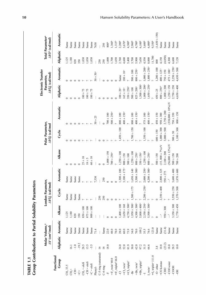
10 Hansen Solubility Parameters: A User’s Handbook
TAB
LE 1
.1G
roup
Con
trib
utio
ns t
o Pa
rtia
l So
lubi
lity
Para
met
ers
Mol
ar V
olum
e,a
ΔV (
cm3 /
mol
)Lo
ndon
Par
amet
er,
ΔVδ D2
(cal
/mol
)Po
lar
Para
met
er,
ΔVδ P2
(cal
/mol
Elec
tron
ic T
rans
fer
Para
met
er,
ΔVδ H2
(cal
/mol
)To
tal
Para
met
era
ΔVδ2
(cal
/mol
)
Fun
ctio
nal
Gro
upA
lipha
tic
Aro
mat
icA
lkan
eC
yclo
Aro
mat
icA
lkan
eC
yclo
Aro
mat
icA
lipha
tic
Aro
mat
icA
lipha
tic
Aro
mat
ic
CH
3 33.
5Sa
me
1,12
5Sa
me
Sam
e0
00
00
1,12
5Sa
me
CH
2<16
.1Sa
me
1,18
0Sa
me
Sam
e0
00
00
1,18
0Sa
me
–CH
<–1
.0Sa
me
820
Sam
eSa
me
00
00
082
0Sa
me
>C<
–19.
2Sa
me
350
Sam
eSa
me
00
00
035
0Sa
me
CH
2 = o
lefi
28.5
Sam
e85
0 ±
100
??
25 ±
10
??
180
± 75
?1,
030
Sam
e–C
H =
ole
fi13
.5Sa
me
875
± 10
0?
?18
± 5
??
180
± 75
?1,
030
Sam
e>C
= o
lefi
–5.5
Sam
e80
0 ±
100
??
60 ±
10
??
180
± 75
?1,
030
Sam
ePh
enyl
-—
71.4
——
7,53
0—
—50
± 2
5—
50 ±
50c
—76
30C
-5 ri
ng (s
atur
ated
)16
——
250
—0
0—
0—
250
—C
-6 ri
ng16
Sam
e—
250
250
00
00
025
0 2
50–F
18.0
22.0
00
01,
000
± 15
0?
700
± 10
00
01,
000
800
b
�F 2
twin
f 40.
048
.00
00
700
± 25
0c?
500
± 25
0c0
01,
700
1,36
0b
�F 3
trip
letf 6
6.0
78.0
00
0?
??
00
1,65
01,
315b
–Cl
24.0
28.0
1,40
0 ±
100
?1,
300
± 10
01,
250
± 10
01,
450
± 10
080
0 ±
100
100
± 20
cSa
me
2,76
02,
200b
�C
l 2 tw
inf
52.0
60.0
3,65
0 ±
160
?3,
100
± 17
5c80
0 ±
150
?40
0 ±
150c
165
± 10
c18
0 ±
10c
4,60
03,
670b
�C
l 3 tri
plet
f 81
.973
.94,
750
± 30
0c?
?30
0 ±
100
??
350
± 25
0c?
5,40
04,
300b
–Br
30.0
34.0
1,95
0 ±
300c
1,50
0 ±
175
1,65
0 ±
140
1,25
0 ±
100
1,70
0 ±
150
800
± 10
050
0 ±
100
500
± 10
03,
700
2,96
0b
�B
r 2 tw
inf
62.0
70.0
4,30
0 ±
300c
?3,
500
± 30
0c80
0 ±
250c
?40
0 ±
150c
825
± 20
0c80
0 ±
250c
5,90
04,
700b
�B
r 3 tri
plet
f 97
.210
9.2
5,80
0 ±
400c
??
350
± 15
0c?
?1,
500
± 30
0c?
7,65
06,
100b
–I31
.535
.52,
350
± 25
0c2,
200
± 25
0c2,
000
± 25
0c1,
250
± 10
01,
350
± 10
057
5 ±
100
1,00
0 ±
200c
1,00
0 ±
200c
4,55
03,
600b
I 2 tw
ine
66.6
74.6
5,50
0 ±
300c
?4,
200
± 30
0c80
0 ±
250c
?40
0 ±
150c
1,65
0 ±
250c
1,80
0 ±
250c
8,00
06,
400b
�I 3
tripl
ete 1
11.0
123.
0?
??
??
??
?11
,700
9,35
0b
–O–
ethe
r3.
8Sa
me
00
050
0 ±
150
600
± 15
045
0 ±
150
450
± 25
1,20
0 ±
100
800
(1,6
50 ±
150
)>C
O k
eton
e10
.8Sa
me
—e
2,35
0 ±
400
2,80
0 ±
325
(15,
000
± 7
%)/V
1,00
0 ±
300
950
± 30
080
0 ±
250d
400
± 12
5c4,
150
Sam
e–C
HO
(23.
2)(3
1.4)
950
± 30
0?
550
± 27
52,
100
± 20
03,
000
± 50
02,
750
± 20
01,
000
± 20
075
0 ±
150
(4,0
50)
Sam
e–C
OO
-est
er18
.0Sa
me
—f
?—
f(5
6,00
0 ±
12%
)/V?
(338
,000
± 1
0%)/V
1,25
0 ±
150
475
± 10
0c4,
300
Sam
e–C
OO
H28
.5Sa
me
3,35
0 ±
300
3,55
0 ±
250
3,60
0 ±
400
500
± 15
030
0 ±
5075
0 ±
350
2,75
0 ±
250
2,25
0 ±
250c
6,60
0Sa
me
–OH
10.0
Sam
e1,
770
± 45
01,
370
± 50
01,
870
± 60
070
0 ±
200
1,10
0 ±
300
800
± 1
504,
650
± 40
04,
650
± 50
07,
120
Sam
e
7248_C001.fm Page 10 Monday, April 23, 2007 1:56 PM
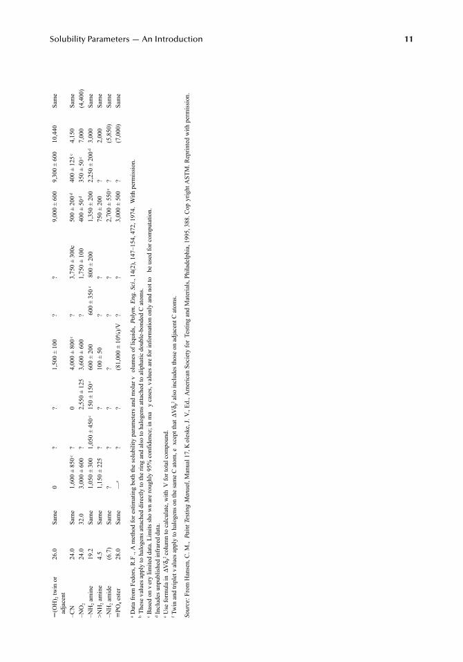
Solubility Parameters — An Introduction 11
�(O
H) 2
twin
or
adja
cent
26.0
Sam
e0
??
1,50
0 ±
100
??
9,00
0 ±
600
9,30
0 ±
600
10,4
40Sa
me
–CN
24.0
Sam
e1,
600
± 85
0c?
04,
000
± 80
0c?
3,75
0 ±
300c
500
± 20
0d40
0 ±
125c
4,15
0Sa
me
–NO
224
.032
.03,
000
± 60
0?
2,55
0 ±
125
3,60
0 ±
600
?1,
750
± 10
040
0 ±
50d
350
± 50
c7,
000
(4,4
00)
–NH
2 am
ine
19.2
Sam
e1,
050
± 30
01,
050
± 45
0c15
0 ±
150c
600
± 20
0 6
00 ±
350
c 8
00 ±
200
1,35
0 ±
200
2,25
0 ±
200d
3,00
0Sa
me
>NH
2 am
ine
4.5
Sam
e1,
150
± 22
5?
?10
0 ±
50?
?75
0 ±
200
?2,
000
Sam
e–N
H2 a
mid
e(6
.7)
Sam
e?
??
??
?2,
700
± 55
0c?
(5,8
50)
Sam
e�
PO4 e
ster
28.0
Sam
e—
e?
?(8
1,00
0 ±
10%
)/V?
?3,
000
± 50
0?
(7,0
00)
Sam
e
a Dat
a fr
om F
edor
s, R
.F.,
A m
etho
d fo
r est
imat
ing
both
the
solu
bilit
y pa
ram
eter
s and
mol
ar v
olum
es o
f liq
uids
, Po
lym
. E
ng.
Sci.,
14(
2), 1
47–1
54, 4
72, 1
974.
With
per
mis
sion
.b T
hese
val
ues a
pply
to h
alog
ens a
ttach
ed d
irect
ly to
the
ring
and
also
to h
alog
ens a
ttach
ed to
alip
hatic
dou
ble-
bond
ed C
ato
ms.
c Bas
ed o
n v
ery
limite
d da
ta. L
imits
sho
wn
are
roug
hly
95%
con
fiden
ce; i
n m
ay
case
s, va
lues
are
for i
nfor
mat
ion
only
and
not
to
be u
sed
for c
ompu
tatio
n.d I
nclu
des u
npub
lishe
d in
frar
ed d
ata.
e Use
form
ula
in Δ
Vδ P
2 colu
mn
to c
alcu
late
, with
V fo
r tot
al c
ompo
und.
f Tw
in a
nd tr
iple
t val
ues a
pply
to h
alog
ens o
n th
e sa
me
C a
tom
, exc
ept t
hat Δ
Vδ P
2 also
incl
udes
thos
e on
adj
acen
t C a
tom
s.
Sour
ce: F
rom
Han
sen,
C. M
., Pa
int
Test
ing
Man
ual,
Man
ual 1
7, K
oles
ke, J
. V.,
Ed.,
Am
eric
an S
ocie
ty fo
r Te
stin
g an
d M
ater
ials
, Phi
lade
lphi
a, 1
995,
388
. Cop
yrig
ht A
STM
. Rep
rinte
d w
ith p
erm
issi
on.
7248_C001.fm Page 11 Monday, April 23, 2007 1:56 PM
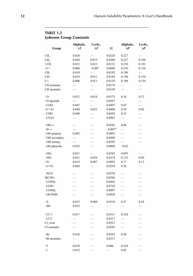
12 Hansen Solubility Parameters: A User’s Handbook
TABLE 1.2Lydersen Group Constants
GroupAliphatic,
ΔT Cyclic,
ΔT ΔPT
Aliphatic,ΔP
Cyclic,ΔP
CH3 0.020 — 0.0226 0.227 —CH2 0.020 0.013 0.0200 0.227 0.184>CH– 0.012 0.012 0.0131 0.210 0.192>C< 0.000 –0.007 0.0040 0.210 0.154CH2 0.018 — 0.0192 0.198 —CH– 0.018 0.011 0.0184 0.198 0.154C< 0.000 0.011 0.0129 0.198 0.154CH aromatic — — 0.0178 — —CH aromatic — — 0.0149 — —
–O– 0.021 0.014 0.0175 0.16 0.12>O epoxide — — 0.0267 — —–COO– 0.047 — 0.0497 0.47 —>C�O 0.040 0.033 0.0400 0.29 0.02–CHO 0.048 — 0.0445 0.33 —–CO2O — — 0.0863 — —
–OH→ — — 0.0343 0.06 —–H→ — — –0.0077 — —–OH primary 0.082 — 0.0493 — —–OH secondary — — 0.0440 — —–OH tertiary — — 0.0593 — —–OH phenolic 0.035 — 0.0060 –0.02
–NH2 0.031 — 0.0345 0.095 —–NH– 0.031 0.024 0.0274 0.135 0.09>N– 0.014 0.007 0.0093 0.17 0.13–C�N 0.060 — 0.0539 0.36 —
–NCO — — 0.0539 — —HCON< — — 0.0546 — —–CONH– — — 0.0843 — —–CON< — — 0.0729 — —–CONH2 — — 0.0897 — —–OCONH– — — 0.0938 — —
–S– 0.015 0.008 0.0318 0.27 0.24–SH 0.015 — — — —
–Cl 1° 0.017 — 0.0311 0.320 —–Cl 2° — — 0.0317 — —Cl1 twin — — 0.0521 — —Cl aromatic — — 0.0245 — —
–Br 0.010 — 0.0392 0.50 —–Br aromatic — — 0.0313 — —
–F 0.018 — 0.006 0.224 —–I 0.012 — — 0.83 —
7248_C001.fm Page 12 Monday, April 23, 2007 1:56 PM
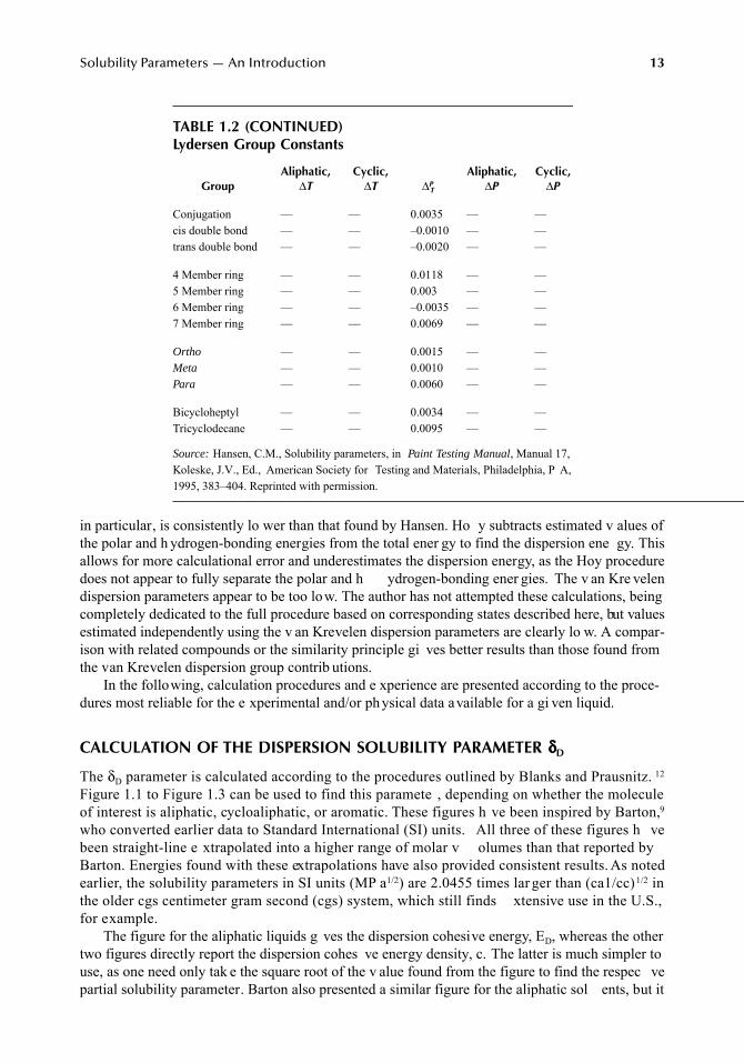
Solubility Parameters — An Introduction 13
in particular, is consistently lo wer than that found by Hansen. Ho y subtracts estimated v alues ofthe polar and h ydrogen-bonding energies from the total ener gy to find the dispersion ene gy. Thisallows for more calculational error and underestimates the dispersion energy, as the Hoy proceduredoes not appear to fully separate the polar and h ydrogen-bonding ener gies. The v an Kre velendispersion parameters appear to be too low. The author has not attempted these calculations, beingcompletely dedicated to the full procedure based on corresponding states described here, but valuesestimated independently using the v an Krevelen dispersion parameters are clearly lo w. A compar-ison with related compounds or the similarity principle gi ves better results than those found fromthe van Krevelen dispersion group contrib utions.
In the following, calculation procedures and e xperience are presented according to the proce-dures most reliable for the e xperimental and/or physical data available for a gi ven liquid.
CALCULATION OF THE DISPERSION SOLUBILITY PARAMETER δδδδD
The δD parameter is calculated according to the procedures outlined by Blanks and Prausnitz. 12
Figure 1.1 to Figure 1.3 can be used to find this paramete , depending on whether the moleculeof interest is aliphatic, cycloaliphatic, or aromatic. These figures h ve been inspired by Barton,9who converted earlier data to Standard International (SI) units. All three of these figures h vebeen straight-line e xtrapolated into a higher range of molar v olumes than that reported byBarton. Energies found with these extrapolations have also provided consistent results. As notedearlier, the solubility parameters in SI units (MP a1/2) are 2.0455 times lar ger than (ca1/cc)1/2 inthe older cgs centimeter gram second (cgs) system, which still finds xtensive use in the U.S.,for example.
The figure for the aliphatic liquids g ves the dispersion cohesive energy, ED, whereas the othertwo figures directly report the dispersion cohes ve energy density, c. The latter is much simpler touse, as one need only tak e the square root of the v alue found from the figure to find the respec vepartial solubility parameter. Barton also presented a similar figure for the aliphatic sol ents, but it
TABLE 1.2 (CONTINUED)Lydersen Group Constants
GroupAliphatic,
ΔT Cyclic,
ΔT ΔPT
Aliphatic,ΔP
Cyclic,ΔP
Conjugation — — 0.0035 — —cis double bond — — –0.0010 — —trans double bond — — –0.0020 — —
4 Member ring — — 0.0118 — —5 Member ring — — 0.003 — —6 Member ring — — –0.0035 — —7 Member ring — — 0.0069 — —
Ortho — — 0.0015 — —Meta — — 0.0010 — —Para — — 0.0060 — —
Bicycloheptyl — — 0.0034 — —Tricyclodecane — — 0.0095 — —
Source: Hansen, C.M., Solubility parameters, in Paint Testing Manual, Manual 17,Koleske, J.V., Ed., American Society for Testing and Materials, Philadelphia, P A,1995, 383–404. Reprinted with permission.
7248_C001.fm Page 13 Monday, April 23, 2007 1:56 PM
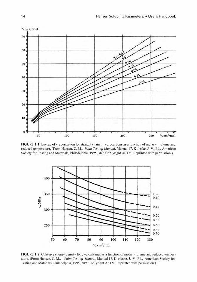
14 Hansen Solubility Parameters: A User’s Handbook
FIGURE 1.1 Energy of v aporization for straight chain h ydrocarbons as a function of molar v olume andreduced temperature. (From Hansen, C. M., Paint Testing Manual, Manual 17, Koleske, J. V., Ed., AmericanSociety for Testing and Materials, Philadelphia, 1995, 389. Cop yright ASTM. Reprinted with permission.)
FIGURE 1.2 Cohesive energy density for c ycloalkanes as a function of molar v olume and reduced temper -ature. (From Hansen, C. M., Paint Testing Manual, Manual 17, K oleske, J. V., Ed., American Society forTesting and Materials, Philadelphia, 1995, 389. Cop yright ASTM. Reprinted with permission.)
50 100 150 200 250 V, cm3/mol
Δ ED kJ/mol
70
60
50
40
30
20
10
0
Tr = 0.40
0.45
0.50
0.55
0.60
0.65
0.70
V, cm3/mol
50 60 70 80 90 100 110 120 130
Tr = 0.40
0.45
0.50
0.55
0.60
0.65 0.70
400
350
300
250
c,
MP
a
7248_C001.fm Page 14 Monday, April 23, 2007 1:56 PM
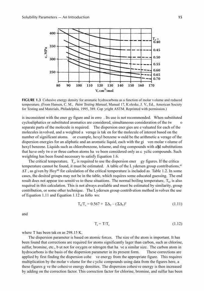
Solubility Parameters — An Introduction 15
is inconsistent with the ener gy figure and in erro . Its use is not recommended. When substitutedcycloaliphatics or substituted aromatics are considered, simultaneous consideration of the tw oseparate parts of the molecule is required. The dispersion ener gies are e valuated for each of themolecules involved, and a weighted a verage is tak en for the molecule of interest based on thenumber of significant atoms. or example, hexyl benzene w ould be the arithmetic a verage of thedispersion energies for an aliphatic and an aromatic liquid, each with the gi ven molar v olume ofhexyl benzene. Liquids such as chlorobenzene, toluene, and ring compounds with alkyl substitutionsthat have only tw o or three carbon atoms ha ve been considered only as c yclic compounds. Suchweighting has been found necessary to satisfy Equation 1.6.
The critical temperature, Tc, is required to use the dispersion ener gy figures. If the criticatemperature cannot be found, it must be estimated. A table of the L ydersen group contributions,41
ΔT , as given by Hoy40 for calculation of the critical temperature is included as Table 1.2. In somecases, the desired groups may not be in the table, which requires some educated guessing. The endresult does not appear too sensiti ve to these situations. The normal boiling temperature, Tb, is alsorequired in this calculation. This is not always available and must be estimated by similarity, groupcontribution, or some other technique. The Lydersen group contrib ution method in volves the useof Equation 1.11 and Equation 1.12 as follo ws:
Tb/Tc = 0.567 + ΣΔT – ( ΣΔT)2 (1.11)
and
Tr = T/Tc (1.12)
where T has been tak en as 298.15 K.The dispersion parameter is based on atomic forces. The size of the atom is important. It has
been found that corrections are required for atoms significantly lager than carbon, such as chlorine,sulfur, bromine, etc., b ut not for oxygen or nitrogen that ha ve a similar size. The carbon atom inhydrocarbons is the basis of the dispersion parameter in its present form. These corrections areapplied by first finding the dispersion cohe ve energy from the appropriate figure. This requiresmultiplication by the molar v olume for the c yclic compounds using data from the figures here, athese figures g ve the cohesive energy densities. The dispersion cohesive energy is then increasedby adding on the correction factor. This correction factor for chlorine, bromine, and sulfur has been
FIGURE 1.3 Cohesive energy density for aromatic hydrocarbons as a function of molar volume and reducedtemperature. (From Hansen, C. M., Paint Testing Manual, Manual 17, K oleske, J. V., Ed., American Societyfor Testing and Materials, Philadelphia, 1995, 389. Cop yright ASTM. Reprinted with permission.)
V, cm3/mol
80 90 100 110 120 140130 150 160 170
Tr = 0.40
0.45
0.50
0.55
0.60
0.65 0.70
400
350
300
250
c,
MP
a
7248_C001.fm Page 15 Monday, April 23, 2007 1:56 PM
16 Hansen Solubility Parameters: A User’s Handbook
taken as 1650 J/mol for each of these atoms in the molecule. Di viding by the molar v olume andthen taking the square root gi ves the (large atom corrected) dispersion solubility parameter .
The need for these corrections has been confirmed ma y times, both for interpretation ofexperimental data and to allo w Equation 1.6 to Equation 1.8 to balance. Research is definitelneeded in this area. The impact of these corrections is, of course, lar ger for the smaller molecularspecies. Taking square roots of the lar ger numbers in volved with the lar ger molecular speciesreduces the errors in volved in these cases, as the corrections are relati vely small.
It can be seen from the dispersion parameters of the c yclic compounds that the ring has aneffect similar to increasing the ef fective size of the interacting species. The dispersion energies forcycloaliphatic compounds are lar ger than their aliphatic counterparts, and the y are higher foraromatic compounds than their corresponding c ycloaliphatics. Similar effects also appear with theester group. This group appears to act as if it were, in ef fect, an entity that is lar ger than thecorresponding compound containing only carbon (i.e., its homomorph), and it has a higher disper -sion solubility parameter without an y special need for corrections.
The careful evaluation of the dispersion cohesi ve energy may not ha ve a major impact on thevalue of the dispersion solubility parameter, because square roots of rather large numbers are taken.Larger problems arise because of Equation 1.6. Ener gy assigned to the dispersion portion cannotbe reused when finding the other partial parameters using Equation 1.6 (or Equation 1.8). This isone reason group contrib utions are recommended in some cases, as discussed later .
CALCULATION OF THE POLAR SOLUBILITY PARAMETER δδδδP
The earliest assignments of a “polar” solubility parameter were gi ven by Blanks and Prausnitz. 12
These parameters were, in f act, the combined polar and h ydrogen bonding parameters as used byHansen, and the y cannot be considered polar in the current conte xt. The first Hansen polaparameters13 were reassigned new values by Hansen and Skaarup according to the Böttcher equation(Equation 10.25).15 This equation requires the molar volume, the dipole moment (DM), the refractiveindex, and the dielectric constant. These are not available for many compounds, and the calculationused is more dif ficult than the much simpler equation d veloped by Hansen and Beerbo wer17:
δP = 37.4(DM)/V1/2 (1.13)
The constant 37.4 gi ves this parameter in SI units.Equation 1.13 has been consistently used by the author over the past years, particularly in view
of its reported reliability.35 This reported reliability appears to be correct. The molar volume mustbe known or estimated in one w ay or another. This leaves only the dipole moment to be found orestimated. Standard reference works have tables of dipole moments, with the most extensive listingstill being McClellan.42 Other data sources also have the same, as well as other relevant parameters,and data such as latent heats and critical temperatures. The Design Institute for Ph ysical PropertyResearch (DIPPR)43 database has been found useful for man y compounds of reasonably commonusage, but many interesting compounds are not included in the DIPPR. When no dipole momentis available, similarity with other compounds, group contrib utions, or e xperimental data can beused to estimate the polar solubility parameter .
It must be noted that the f act of zero dipole moment in symmetrical molecules is not basisenough to assign a zero polar solubility parameter . An outstanding e xample of v ariations of thiskind can be found with carbon disulfide. The reported dipole moments are mostly 0 for g as phasemeasurements, supplemented by 0.08 in hexane, 0.4 in carbon tetrachloride, 0.49 in chlorobenzene,and 1.21 in nitrobenzene. There is a clear increase with increasing solubility parameter of the media.The latter and the highest v alue has been found e xperimentally most fitting for correlating permeation through a fluoropolymer film used for chemical protec ve clothing.44 Many fluoropolymer
7248_C001.fm Page 16 Monday, April 23, 2007 1:56 PM
Solubility Parameters — An Introduction 17
have considerable polarity. The lower dipole moments seem to fit in other instances. Diet yl etherhas also presented problems as an outlier in terms of dissolving or not and permeating rapidly ornot. Here, the reported dipole moments 42 vary from 0.74 to 2.0, with a preferred v alue of 1.17 and1.79 in chloroform. Choosing a gi ven value seems rather arbitrary . The chameleonic cyclic formsof the linear glycol ethers would also seem to provide a basis for altered dipole moments in variousmedia.38
When Equation 1.13 cannot be used, the polar solubility parameter has been found using theBeerbower table of group contrib utions, by similarity to related compounds and/or by subtractionof the dispersion and h ydrogen bonding cohesi ve ener gies from the total cohesi ve ener gy. Thequestion in each case is, “Which data are a vailable and judged most reliable?” Ne w group contri-butions can also be developed from related compounds whose dipole moments are available. Thesenew polar group contrib utions then become supplementary to the Beerbo wer table.
For large molecules, especially those with long h ydrocarbon chains, the accurate calculationof the relatively small polar (and h ydrogen bonding) contributions present special difficulties. Thelatent heats are not generally a vailable with suf ficient accura y to allo w subtraction of tw o largenumbers from each other to find a ery small one. In such cases, the similarity and group contributionmethods are thought best. Unfortunately , latent heats found in a widely used handbook 45 are notclearly reported as to the reference temperature. There is an indication that these are 25°C data,but checking indicated many of the data to be identical with boiling point data reported else wherein the literature. Subsequent editions of this handbook 46 have a completely different section for thelatent heat of e vaporation. Again, even moderate v ariations in reported heats of v aporization cancause severe problems in calculating the polar (or h ydrogen bonding) parameter when Equation1.6 or Equation 1.8 are strictly adhered to.
CALCULATION OF THE HYDROGEN BONDING SOLUBILITY PARAMETER δδδδH
In the earliest work, the hydrogen bonding parameter was almost always found by subtracting thepolar and dispersion ener gies of v aporization from the total ener gy of v aporization. This is stillwidely used where the required data are a vailable and reliable. At this stage, ho wever, the groupcontribution techniques are considered reasonably reliable for most of the required calculationsand, in f act, more reliable than estimating se veral other parameters to ultimately arri ve at thesubtraction step just mentioned. Therefore, in the absence of reliable latent heat and dipole momentdata, group contributions are judged to be the best alternative. Similarity to related compounds canalso be used, of course, and the result of such a procedure should be essentially the same as forusing group contributions.
The above paragraph is not changed from the first edition of this handbook.This is to emphasizethe importance of the w ork of P anayiotou and co workers reported in Chapter 3. It no w appearspossible not only to calculate the h ydrogen bonding parameter independently, but also to arrive atall three parameters by statistical mechanics. This is clearly a major step forw ard. Whether or notone understands all of the equations and methodology of Chapter 3, the procedure in itself confirmthe need for (at least) three cohesion ener gy parameters, and similar results are found by theapproach of the first paragraph as well as with statistical thermodynamics
SUPPLEMENTARY CALCULATIONS AND PROCEDURES
The procedures listed pre viously are those most frequently used by the author in calculating thethree partial solubility parameters for liquids when some data are a vailable. There are a number ofother calculations and procedures that are also helpful. Latent heat data at 25°C ha ve been foundconsistently from those at another temperature, using the relation gi ven by Fishtine. 47
7248_C001.fm Page 17 Monday, April 23, 2007 1:56 PM
18 Hansen Solubility Parameters: A User’s Handbook
ΔHv(T1)/ΔH(T2) = [(1 – Tr1)/(1 – Tr2)]0.38 (1.14)
This is done even if the melting point of the compound being considered is higher than 25°C.The result is consistent with all the other parameters, and to date no problems with particularlyfaulty predictions ha ve been noted. It appears as if the predictions are not significantly in errowhen experimental data are a vailable for checking. When the latent heat at the boiling point isgiven in cal/mol, Equation 1.14 is used to estimate the latent heat at 25°C. RT equal to 592 cal/molis then subtracted from this according to Equation 1.15, to find the total cohesion ene gy, E, in cgsunits at this temperature:
E = ΔEv = ΔHV – RT (1.15)
where R is the g as constant and T is the absolute temperature.A computer program has been de veloped by the author to assign HSP to solv ents, based on
experimental data alone. This has been used in se veral cases where the parameters for the gi venliquids were desired with a high degree of accuracy. The procedure is to enter solvent quality, goodor bad, into the program for a reasonably large number of polymers where the solubility parameters,and appropriate radius of interaction for the polymers are kno wn. The program then locates thatset of δD, δP, and δH parameters for the solv ent that best satisfies the requirements of a locatiowithin the spheres of the appropriate polymers, that ha ve good solv ent quality, and outside theappropriate spheres where the solv ent quality is bad.
An additional aid in estimating HSP for many compounds is that these parameters can be foundby interpolation or e xtrapolation, especially for homologous series. The first member may nonecessarily be a straight-line extrapolation, but comparisons with related compounds should alwaysbe made where possible to confirm assignments. Plotting the parameters for homologous serieamong the esters, nitroparaf fins, etones, alcohols, and glycol ethers has aided in finding thparameters for related compounds.
TEMPERATURE DEPENDENCE
Only very limited attempts have been made to calculate solubility parameters at a higher temperatureprior to the second edition of this handbook. The inclusion of Chapter 3 and Chapter 10 in thishandbook helps by pro viding a more accurate treatment of temperature dependence when thesituation warrants it. Solubility parameter correlations of phenomena at higher temperatures ha vegenerally been found satisfactory when the established 25°C parameters ha ve been used. Recalcu-lation to higher temperatures is possible b ut has not generally been found necessary . In this directbut approximate approach, it is assumed that the parameters all demonstrate the same temperaturedependence, which, of course, is not the case. It might be noted in this connection that the hydrogen-bonding parameter, in particular, is the most sensitive to temperature. As the temperature increases,more and more h ydrogen bonds are progressi vely brok en or weak ened, and this parameter willdecrease more rapidly than the others.
The gas-phase dipole moment is not temperature dependent, although the v olume of a fluidoes change with the temperature, which will also change its cohesi ve energy density. The changeof the δD, δP , and δH parameters for liquids with temperature, T, can be estimated by the followingequations, where α is the coef ficient of thermal xpansion17:
dδD/dT = –1.25 αδD (1.16)
dδP/dT = –0.5 αδP (1.17)
dδH/dT = – δH(1.22 × 10⁻³ + 0.5 α) (1.18)
7248_C001.fm Page 18 Monday, April 23, 2007 1:56 PM
Solubility Parameters — An Introduction 19
Higher temperature means a general increase in rate of solubility/dif fusion/permeation, as wellas larger solubility parameter spheres. δD, δP, and δH decrease with increased temperature, as canbe seen by a comparison of Equation 1.16, through Equation 1.18. This means that alcohols,phenols, glycols, and glycol ethers become better solv ents for polymers of lower solubility param-eters as the temperature increases. Thus, increasing the temperature can cause a nonsolv ent tobecome a good solv ent, a f act that is often noted in practice. As mentioned earlier , it is possiblethat a boundary solv ent can be a good solv ent at a gi ven temperature, but turn bad with either anincrease or a decrease in temperature. These phenomena are discussed in great detail by P attersonand coworkers.3,4 They can be explained either by the change in solubility parameter with temper -ature or more completely by the Prigogine CST . The effects of temperature changes on solubilityrelations are most ob vious with systems having a high h ydrogen-bonding character. Examples aregiven in the ne xt section for some special situations in volving water and methanol.
SOME SPECIAL EFFECTS TEMPERATURE CHANGES
Water (and methanol) uptak e in most polymers increases with increasing temperature. This isbecause the solubility parameters of the w ater and the polymer are closer at higher temperatures.The δH parameter of water (and methanol) falls with increasing temperature, whereas that of mostpolymers remains reasonably constant. Water is also well known as an exceptionally good plasticizerbecause of its small molecular size. The presence of dissolved water not only softens (reduces theglass transition temperature) a polymer as such, b ut it also means dif fusion rates of other specieswill be increased. The presence of water in a film can also influence the upt e of other materials,such as in solubility parameter studies or resistance testing, with h ydrophilic materials being moreprone to enter the film
This can cause blistering on rapid cooling as discussed in Chapter 12 and in Reference 48 (seeChapter 8 and Chapter 12). Figure 8.3 sho ws how rapid cooling from a w ater-saturated state athigher temperature can lead to blistering. Figure 12.3 and Figure 12.4 sho w how this effect can bemeasured e xperimentally with an increase in w ater content abo ve the equilibrium v alue whentemperature cycling is encountered. This leads to premature f ailure of polymeric products used insuch environments.
A related problem has been encountered with methanol. It w as intended to follo w the rate ofuptake of methanol in an epoxy coating at room temperature by weighing coated-metal panelsperiodically on an analytical balance. Blistering was encountered in the coating near the air surfaceshortly after the experiment began. The methanol that had been absorbed into the coating near thesurface became insoluble as the temperature of the coating near the surf ace was lowered by theevaporation of e xcess methanol during the handling and weighing of the panels. This is a ratherextreme case, and, as mentioned earlier , use of the HSP (determined at 25°C) at ele vated temper-atures can most often be done without too much trouble from a practical point of view. One shouldbe aware that the changes in the δH parameter would be larger than those in the other parameters,and this effect would be most significant for those liquids with la ger δH values.
EFFECTS OF SOLVENT MOLECULAR SIZE
The size of both solv ent and solute molecules is important for solubility , permeation, dif fusion,and chemical resistance phenomena. Smaller molecules tend to be more readily soluble than largerones. As stated previously, the Hildebrand solubility parameter theory also points to smaller molarvolume solvents as being better than those with lar ger molar volumes, even though they may haveidentical solubility parameters. 1,2 This fact of e xpected improved solvency for smaller moleculesis also known from the Flory–Huggins theory of polymer solutions.29 Solvents with smaller molec-ular size ha ve also been repeatedly noted as being superior to those with lar ger molecular size,when highly crystalline polymers or solids are being tested for solubility . So it is not surprising
7248_C001.fm Page 19 Monday, April 23, 2007 1:56 PM
20 Hansen Solubility Parameters: A User’s Handbook
that solvent molecular size can be an important fourth parameter in solubility and, in some cases,in chemical resistance. Specific xamples are given in Chapter 5 and Chapter 12.
The size and shape of the solvent molecule are also very important for kinetic phenomena suchas diffusion, permeation, and attainment of equilibrium. Smaller and more linear molecules diffusemore rapidly than lar ger and more b ulky ones. The dif fusion coef ficient may be so l w thatequilibrium is not attained for hundreds of years at room temperature. This was demonstrated incommon solvent exposures of rigid polymers like polyphenylene sulfide (PPS) with thicknesses oseveral millimeters.49 Likewise, the second stage in the tw o-stage drying process in polymer filformation by solvent evaporation can last for man y years.16,50 Polymer samples used for solubilityparameter or other testing may well retain solvent or monomer for many years, and this may affectthe evaluations.
Attempts to include the molecular v olume in ne w composite solubility and size parametershave not been particularly successful. 20,21 This may be because the size ef fect is most often notcaused due to the thermodynamic considerations on which the solubility parameters are based, b utrather through a kinetic effect of diffusion rates or other free volume considerations. The similaritiesin the HSP approach and the Prigogine theory, discussed in Chapter 2, indicate a remarkably close,if not identical, relation between the Prigogine ρ (segment size parameter) and the δD parameter,suggesting that molecular size dif ferences are at least partially accounted for in the δD parameter.The Prigogine theory also has a parameter to describe “structural effects,” including size of polymermolecules, but this has not been e xplored in relation to the present discussion. The increase of δDwith increasing molecular size among the aliphatic hydrocarbons, the higher δD values for the largerunits represented by cycloaliphatic and aromatic rings, and the need for corrections for larger atomsdiscussed earlier tend to support the molecular size dif ferences.
Sorting output data according to the molecular volume of the test solvents in a computer analysishelps to discover whether solvent molecular size is indeed an additional significant actor in a givencorrelation or testing program.
COMPUTER PROGRAMS
The author has used two computer programs extensively in his own studies and in collecting materialfor this book. These are called SPHERE and SPHERE1. They are very similar, the only differencebeing that SPHERE optimizes the polymer (or other material, of course) parameters based on allthe data, whereas SPHERE1 considers data for only those solvents considered as “good.” It neglectsthe nonsolv ent data. SPHERE1 has been most useful in correlations with pigments, fillers, anfibers, as described in Chapter 7
The data input is by solv ent number follo wed by an indication of the quality of interactionwith that solv ent. A “1” indicates a “good” solv ent, whereas a “0” is used for a “bad” solv ent.What is considered good or bad varies according to the level of interaction being studied. This canbe solution or not, a gi ven percentage of swelling or uptak e, breakthrough time being less than agiven interval, permeation coefficients higher than a gven value, long-time suspension of a pigment,etc.
The program systematically e valuates the input data using a quality-of-fit function called thdesirability function.51 This suggestion w as made by a reputed statistician man y years ago as themost appropriate statistical treatment for this type of problem. It has been in use since the late1960s. The function has the form:
DATA FIT = (A 1 * A2 *...An)1/n (1.19)
where n is the number of solv ents for which there is e xperimental data in the correlation. TheDATA FIT approaches 1.0 as the fit impr ves during an optimization and reaches 1.0 when all thegood solvents are included within the sphere and all the bad ones are outside the sphere.
7248_C001.fm Page 20 Monday, April 23, 2007 1:56 PM
Solubility Parameters — An Introduction 21
Ai = e –(ERROR DISTANCE) (1.20)
The Ai quotient for a given good solvent within the sphere and a bad solvent outside the spherewill be 1.0. The error distance is the distance of the solv ent in error to the sphere boundary . Itcould either denote being good and outside the sphere or being bad and inside the sphere.
Ro is the radius of the sphere, and Ra is the distance from a gi ven solvent point to the centerof the sphere. F or a good solv ent outside the sphere, an error enters the D ATA FIT according to:
Ai = e +(Ro – Ra) (1.21)
Such errors are often found for solv ents having low molecular volumes.For a bad solv ent inside the sphere, the contrib ution to the D ATA FIT is
Ai = e +(Ra – Ro) (1.22)
Such errors can sometimes be found for lar ger molecular species such as plasticizers. This isnot unexpected for the reasons mentioned earlier .
Solvents with large and/or small molecules that give the “errors” can sometimes be (temporarily)disregarded by generating a ne w correlation; this gi ves an excellent DATA FIT for an abbre viatedrange of molecular v olumes. There is a special printout with the solv ents arranged in order ofmolecular volume that helps to analyze such situations. The computer printouts all include a columnfor the RED number .
The program assumes a starting point, based on an a verage of each of the HSP for the goodsolvents only. The program then e valuates eight points at the corners of a cube, with the currentbest values as center. Different radii are evaluated at each of these points in the optimization process.When better fits are found among the eight points, the point with the best fit is t en as a ne wcenter, and eight points around it are e valuated in a similar manner. This continues until the DATAFIT cannot be impro ved upon. The length of the edge of the cube is then reduced in size to finetune the fit. The initial length of the cube is 1 unit, which is reduced to 0.3 unit, and finally to 0.unit in the last optimization step.
Experimental data for the solv ents are entered with solv ent number (comma) and a “1” for agood solvent, or a “0” for a bad one.
Errors in the correlations are indicated with an “*” in the SOLUB column where the e xperi-mental input data are indicated. As stated abo ve, systematic errors can sometimes be seen in themolar volume printout. This may suggest a new analysis of the data. Nonsystematic errors may bereal, such as for reactions or some e xtraneous effect not predictable by the solubility parameter .They may also be bad data, and rechecking data indicated with an “*” in the output has becomea routine practice. The output of this program is for the least radius allo wing the maximum DATAFIT. An example is found in Table 5.4.
Results from the SPHERE program reported in this book generally include the HSP , given asD (δD), P (δP), and H (δH), respectively, and Ro for the correlation in question, as well as the DATAFIT, the number of good solv ents (G), and the total solv ents (T) in the correlation. This latterinformation has not always been recorded and may be lacking for some correlations, especially theolder ones.
HANSEN SOLUBILITY PARAMETERS FOR WATER
Water is such an important material that a special section is dedicated to its HSP at this point. Thebehavior of w ater often depends on its local en vironment, which mak es general predictions v erydifficult. Water is still so unpredictable that its use as a test solv ent in solubility parameter studies
7248_C001.fm Page 21 Monday, April 23, 2007 1:56 PM
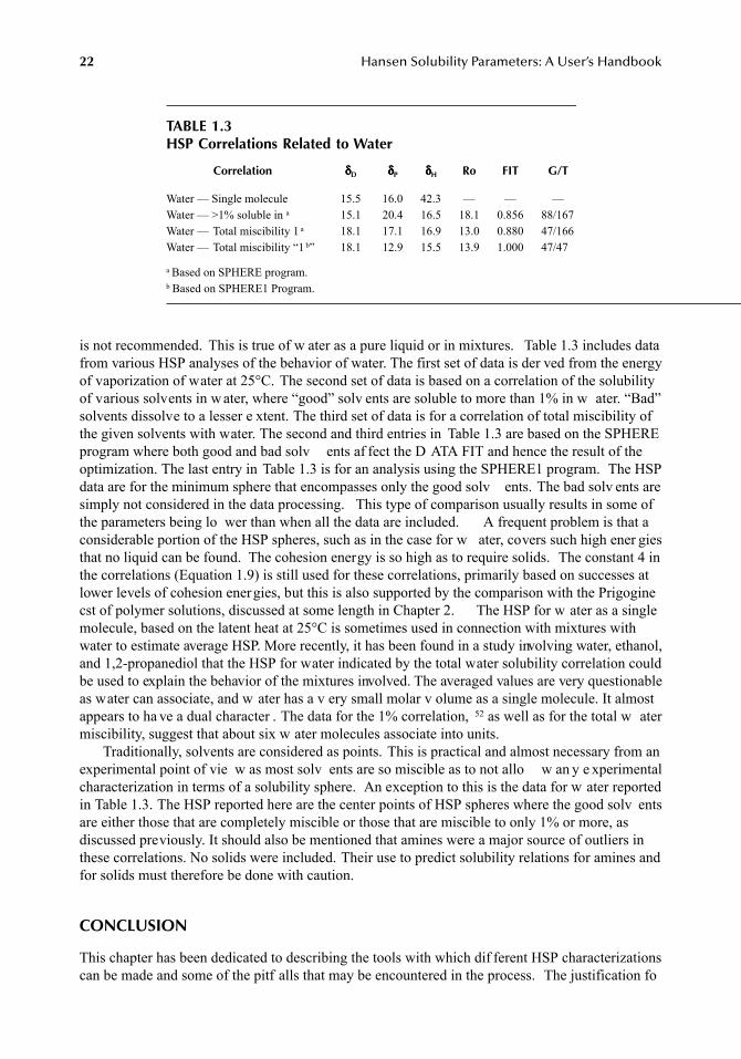
22 Hansen Solubility Parameters: A User’s Handbook
is not recommended. This is true of w ater as a pure liquid or in mixtures. Table 1.3 includes datafrom various HSP analyses of the behavior of water. The first set of data is der ved from the energyof vaporization of water at 25°C. The second set of data is based on a correlation of the solubilityof various solvents in w ater, where “good” solv ents are soluble to more than 1% in w ater. “Bad”solvents dissolve to a lesser e xtent. The third set of data is for a correlation of total miscibility ofthe given solvents with water. The second and third entries in Table 1.3 are based on the SPHEREprogram where both good and bad solv ents af fect the D ATA FIT and hence the result of theoptimization. The last entry in Table 1.3 is for an analysis using the SPHERE1 program. The HSPdata are for the minimum sphere that encompasses only the good solv ents. The bad solv ents aresimply not considered in the data processing. This type of comparison usually results in some ofthe parameters being lo wer than when all the data are included. A frequent problem is that aconsiderable portion of the HSP spheres, such as in the case for w ater, covers such high ener giesthat no liquid can be found. The cohesion energy is so high as to require solids. The constant 4 inthe correlations (Equation 1.9) is still used for these correlations, primarily based on successes atlower levels of cohesion energies, but this is also supported by the comparison with the Prigoginecst of polymer solutions, discussed at some length in Chapter 2. The HSP for w ater as a singlemolecule, based on the latent heat at 25°C is sometimes used in connection with mixtures withwater to estimate average HSP. More recently, it has been found in a study involving water, ethanol,and 1,2-propanediol that the HSP for water indicated by the total water solubility correlation couldbe used to explain the behavior of the mixtures involved. The averaged values are very questionableas water can associate, and w ater has a v ery small molar v olume as a single molecule. It almostappears to ha ve a dual character . The data for the 1% correlation, 52 as well as for the total w atermiscibility, suggest that about six w ater molecules associate into units.
Traditionally, solvents are considered as points. This is practical and almost necessary from anexperimental point of vie w as most solv ents are so miscible as to not allo w an y e xperimentalcharacterization in terms of a solubility sphere. An exception to this is the data for w ater reportedin Table 1.3. The HSP reported here are the center points of HSP spheres where the good solv entsare either those that are completely miscible or those that are miscible to only 1% or more, asdiscussed previously. It should also be mentioned that amines were a major source of outliers inthese correlations. No solids were included. Their use to predict solubility relations for amines andfor solids must therefore be done with caution.
CONCLUSION
This chapter has been dedicated to describing the tools with which dif ferent HSP characterizationscan be made and some of the pitf alls that may be encountered in the process. The justification fo
TABLE 1.3HSP Correlations Related to Water
Correlation δδδδD δδδδP δδδδH Ro FIT G/T
Water — Single molecule 15.5 16.0 42.3 — — —Water — >1% soluble in a 15.1 20.4 16.5 18.1 0.856 88/167Water — Total miscibility 1 a 18.1 17.1 16.9 13.0 0.880 47/166Water — Total miscibility “1 b” 18.1 12.9 15.5 13.9 1.000 47/47
a Based on SPHERE program.b Based on SPHERE1 Program.
7248_C001.fm Page 22 Monday, April 23, 2007 1:56 PM
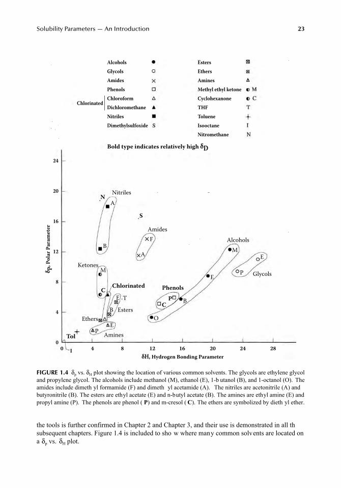
Solubility Parameters — An Introduction 23
the tools is further confirmed in Chapter 2 and Chapter 3, and their use is demonstrated in all thsubsequent chapters. Figure 1.4 is included to sho w where many common solvents are located ona δp vs. δH plot.
FIGURE 1.4 δp vs. δH plot showing the location of various common solvents. The glycols are ethylene glycoland propylene glycol. The alcohols include methanol (M), ethanol (E), 1-b utanol (B), and 1-octanol (O). Theamides include dimeth yl formamide (F) and dimeth yl acetamide (A). The nitriles are acetonitrile (A) andbutyronitrile (B). The esters are ethyl acetate (E) and n-butyl acetate (B). The amines are ethyl amine (E) andpropyl amine (P). The phenols are phenol ( P) and m-cresol ( C). The ethers are symbolized by dieth yl ether.
Bold type indicates relatively high δD
δ P,
Po
lar
Pa
ram
ete
r
δH, Hydrogen Bonding Parameter
Chlorinated
Alcohols
Glycols
Amides
Phenols
Chloroform
Dichloromethane
Nitriles
Dimethylsulfoxide
Esters
Ethers
Amines
Methyl ethyl ketone
Cyclohexanone
THF
Toluene
Isooctane
Nitromethane
24
20
16
12
8
4
00 4 8 12 16 20 24 28I
Tol
Chlorinated Phenols
Amines
Amides
Nitriles
Alcohols
Ketones
Ethers
Esters
PE
E
E
EM
B
B
B
A
T
C
M
N
S
F
A
O
CP
P Glycols
7248_C001.fm Page 23 Monday, April 23, 2007 1:56 PM
24 Hansen Solubility Parameters: A User’s Handbook
REFERENCES
1. Hildebrand, J. and Scott, R.L., The Solubility of Nonelectrolytes, 3rd ed., Reinhold, New York, 1950.2. Hildebrand, J. and Scott, R.L., Regular Solutions, Prentice-Hall, Englewood Cliffs, NJ, 1962.3. Patterson, D. and Delmas, G., Ne w aspects of polymer solution thermodynamics, Off. Dig. Fed. Soc.
Paint Technol., 34(450), 677–692, 1962.4. Delmas, D., Patterson, D., and Somcynsky, T., Thermodynamics of polyisobutylene-n-alkane systems,
J. Polym. Sci., 57, 79–98, 1962.5. Bhattacharyya, S.N., Patterson, D., and Somcynsky, T., The principle of corresponding states and the
excess functions of n-alkane mixtures, Physica, 30, 1276–1292, 1964.6. Patterson, D., Role of free v olume changes in polymer solution thermodynamics, J. Polym. Sci. Part
C, 16, 3379–3389, 1968.7. Patterson, D.D., Introduction to thermodynamics of polymer solubility , J. Paint Technol., 41(536),
489–493, 1969.8. Biros, J., Zeman, L., and Patterson, D., Prediction of the C parameter by the solubility parameter and
corresponding states theories, Macromolecules, 4(1), 30–35, 1971.9. Barton, A.F.M., Handbook of Solubility Parameters and Other Cohesion Parameters, CRC Press,
Boca Raton, FL, 1983; 2nd ed., 1991.10. Gardon, J.L. and Teas, J.P., Solubility parameters, in Treatise on Coatings, Vol. 2, Characterization
of Coatings: Physical Techniques, Part II, Myers, R.R. and Long, J.S., Eds., Marcel Dekk er, NewYork, 1976, chap. 8.
11. Burrell, H., Solubility parameters for film formers, Off. Dig. Fed. Soc. Paint Technol., 27(369),726–758, 1972; Burrell, H., A solvent formulating chart, Off. Dig. Fed. Soc. Paint Technol., 29(394),1159–1173, 1957; Burrell, H., The use of the solubility parameter concept in the United States, VIFederation d’Associations de Techniciens des Industries des Peintures, Vernis, Emaux et Encresd’Imprimerie de l’Europe Continentale, Congress Book, 21–30, 1962.
12. Blanks, R.F . and Prausnitz, J.M., Thermodynamics of polymer solubility in polar and nonpolarsystems, Ind. Eng. Chem. Fundam., 3(1), 1–8, 1964.
13. Hansen, C.M., The three dimensional solubility parameter — k ey to paint component af finities I, J.Paint Technol., 39(505), 104–117, 1967.
14. Hansen, C.M., The three dimensional solubility parameter — k ey to paint component af finities II, J.Paint Technol., 39(511), 505–510, 1967.
15. Hansen, C.M. and Skaarup, K., The three dimensional solubility parameter — key to paint componentaffinities III, J. Paint Technol., 39(511), 511–514, 1967.
16. Hansen, C.M., The Three Dimensional Solubility Parameter and Solvent Diffusion Coefficient, Doctoral dissertation, Danish Technical Press, Copenhagen, 1967.
17. Hansen, C.M. and Beerbo wer, A., Solubility parameters, in Kirk-Othmer Encyclopedia of ChemicalTechnology, Suppl. Vol., 2nd ed., Standen, A., Ed., Interscience, Ne w York, 1971, pp. 889–910.
18. Barton, A.F.M., Applications of solubility parameters and other cohesion ener gy parameters, Polym.Sci. Technol. Pure Appl. Chem., 57(7), 905–912, 1985.
19. Sørensen, P ., Application of the acid/base concept describing the interaction between pigments,binders, and solvents, J. Paint Technol., 47(602), 31–39, 1975.
20. Van Dyk, J.W ., P aper presented at the F ourth Chemical Congress of America, Ne w York, August25–30, 1991.
21. Anonymous [Note: This was, in fact, Van Dyk, J.W., but this does not appear on the b ulletin], UsingDimethyl Sulfoxide (DMSO) in Industrial F ormulations, Bulletin No. 102, Gaylord Chemical Corp.,Slidell, LA, 1992.
22. Karger, B.L., Sn yder, L.R., and Eon, C., Expanded solubility parameter treatment for classificatioand use of chromatographic solv ents and adsorbents, Anal. Chem., 50(14), 2126–2136, 1978.
23. Hansen, C.M. and Wallström, E., On the use of cohesion parameters to characterize surfaces, J. Adhes.,15, 275–286, 1983.
24. Hansen, C.M., Characterization of surfaces by spreading liquids, J. Paint Technol., 42(550), 660–664,1970.
25. Hansen, C.M., Surface dewetting and coatings performance, J. Paint Technol., 44(570), 57–60, 1972.
7248_C001.fm Page 24 Monday, April 23, 2007 1:56 PM
Solubility Parameters — An Introduction 25
26. Hansen, C.M. and Pierce, P.E., Surface effects in coatings processes, Ind. Eng. Chem. Prod. Res. Dev.,13(4), 218–225, 1974.
27. Hennissen, L., Systematic Modification of Filler/Fiber Sur aces to Achieve Maximum Compatibilitywith Matrix Polymers, Lecture for the Danish Society for Polymer Technology, Copenhagen, February10, 1996.
28. Gardon, J.L., Critical review of concepts common to cohesive energy density, surface tension, tensilestrength, heat of mixing, interf acial tension and b utt joint strength , J. Colloid Interface Sci., 59(3),582–596, 1977.
29. Flory, P.J., Principles of Polymer Chemistry, Cornell University Press, New York, 1953.30. Prigogine, I. (with the collaboration of Bellemans, A. and Mathot, A.), The Molecular Theory of
Solutions, North-Holland, Amsterdam, 1957, chap. 16, 17.31. van Krevelen, D.W. and Hoftyzer, P.J., Properties of Polymers: Their Estimation and Correlation with
Chemical Structure, 2nd ed., Else vier, Amsterdam, 1976.32. Beerbower, A., Environmental Capability of Liquids, in Interdisciplinary Approach to Liquid Lubri-
cant Technology, NASA Publication SP-318, 1973, 365–431.33. Fedors, R.F., A method for estimating both the solubility parameters and molar v olumes of liquids,
Polym. Eng. Sci., 14(2), 147–154, 472, 1974.34. Hansen, C.M., Solubility parameters, in Paint Testing Manual, Manual 17, Koleske, J.V., Ed., American
Society for Testing and Materials, Philadelphia, P A, 1995, pp. 383–404.35. Koenhen, D.N. and Smolders, C.A., The determination of solubility parameters of solv ents and
polymers by means of correlation with other physical quantities, J. Appl. Polym. Sci., 19, 1163–1179,1975.
36. Anonymous, Brochure: Co-Act — A Dynamic Program for Solv ent Selection, Exxon ChemicalInternational Inc., 1989.
37. Dante, M.F., Bittar , A.D., and Caillault, J.J., Program calculates solv ent properties and solubilityparameters, Mod. Paint Coat., 79(9), 46–51, 1989.
38. Hoy, K.L., New values of the solubility parameters from vapor pressure data, J. Paint Technol., 42(541),76–118, 1970.
39. Myers, M.M. and Abu-Isa, I.A., Elastomer solv ent interactions III — ef fects of methanol mixtureson fluorocarbon elastomers, J. Appl. Polym. Sci., 32, 3515–3539, 1986.
40. Hoy, K.L., Tables of Solubility Parameters, Union Carbide Corp., Research and De velopment Dept.,South Charleston, WV, 1985; 1st ed. 1969.
41. Reid, R.C. and Sherw ood, T.K., Properties of Gases and Liquids, McGra w-Hill, New York, 1958(Lydersen Method — see also Reference 31).
42. McClellan, A.L., Tables of Experimental Dipole Moments, W.H. Freeman, San Francisco, 1963.43. Tables of Physical and Thermodynamic Properties of Pure Compounds, American Institute of Chem-
ical Engineers Design Institute for Physical Property Research, Project 801, Data Compilation, Danner,R.P. and Daubert, T.E., Project Supervisors, DIPPR Data Compilation Project, Department of ChemicalEngineering, Pennsylvania State University, University Park.
44. Hansen, C.M., Selection of Chemicals for Permeation Testing Based on Ne w Solubility P arameterModels for Challenge 5100 and Challenge 5200, under contract DTCG50-89-P-0333 for the U.S.Coast Guard, June 1989, Danish Isotope Centre, Copenhagen.
45. Weast, R.C., (Editor-in-Chief), CRC Handbook of Chemistry and Physics, 65th ed., CRC Press, BocaRaton, FL, 1988–1989, pp. C-672–C-683.
46. Majer, V., Enthalpy of v aporization of or ganic compounds, in Handbook of Chemistry and Physics,72nd ed., Lide, D.R., (Editor -in-Chief), CRC Press, Boca Raton, FL, 1991–1992, pp. 6-100–6-107.
47. Fishtine, S.H., Reliable latent heats of v aporization, Ind. Eng. Chem., 55(4), 20–28, 1963; Ind. Eng.Chem., 55(5), 55–60; Ind. Eng. Chem., 55(6), 47–56.
48. Hansen, C.M., Ne w developments in corrosion and blister formation in coatings, Prog. Org. Coat.,26, 113–120, 1995.
49. Hansen, C.M., Solvent Resistance of Polymer Composites — Glass Fiber Reinforced PolyphenyleneSulfide, Centre for Polymer Composites (Denmark), Danish Technological Institute, Taastrup, 1993,1–62, ISBN 87-7756-286-0.
50. Hansen, C.M., A mathematical description of film drying by sol ent evaporation, J. Oil Color Chem.Assoc., 51(1), 27–43, 1968.
7248_C001.fm Page 25 Monday, April 23, 2007 1:56 PM

26 Hansen Solubility Parameters: A User’s Handbook
51. Harrington, E.C., Jr., The desirability function, Ind. Qual. Control, 21(10), 494–498, April 1965.52. Hansen, C.M. and Andersen, B.H., The affinities of o ganic solvents in biological systems, Am. Ind.
Hyg. Assoc. J., 49(6), 301–308, 1988.
7248_C001.fm Page 26 Monday, April 23, 2007 1:56 PM
27
2
Theory — The Prigogine Corresponding States Theory,
χ
12
Interaction Parameter, and Hansen Solubility Parameters
Charles M. Hansen
ABSTRACT
Patterson has sho wn that the
χ
12
interaction parameter can be estimated from the correspondingstates theory (CST) of Prigogine. Correlations using Hansen solubility parameters (HSP) confirthe usage of the term
cohesive energy difference
proposed in the Prigogine CST . Therefore, theHSP approach can be expected to be useful to predict the Flory interaction coefficient,
χ
12
. Equationsfor this purpose are presented and discussed based on comparisons of calculated and e xperimentalvalues for fi e polymers. There is agreement in man y cases, especially for essentially nonpolarsystems, b ut full understanding of the interrelationship has not yet been achie ved. The lack ofaccounting for permanent dipole–permanent dipole and h ydrogen bonding (electron interchange)in the “New Flory” theory leading to the coefficient
χ
12
” is thought to be largely responsible for this.It does appear , however, that the constant “4” (or 0.25) in the HSP correlations and the 0.25
in the leading term of the Prigogine theory ha ve identical functions. They modify the specifiinteractions described by the Prigogine
δδδδ
and also the polar and h ydrogen bonding HSP (
δ
P
and
δ
H
). This could imply that the Prigogine
ρ
attempts to describe what the
δ
D
parameter describes,that is, the nondirectional (nonpolar) atomic interactions.
Neither the Flory nor the Prigogine approaches can lead to the type of predictions possiblewith the HSP approach. The many correlations and other predictions contained in this book w ouldnot be possible with these theories, as the y do not separate the polar and h ydrogen bonding effectsindependently. The Prigogine theory must be used with the geometric mean to estimate the inter -action between different species. The Hildebrand and HSP approaches inherently use the geometricmean. This implies that the geometric mean is capable of describing not only dispersion interactionsbut also those due to permanent dipoles and h ydrogen bonding.
INTRODUCTION
The Flory–Huggins “chi” parameter,
χ
, has been used for man y years in connection with polymersolution behavior,
1,2
but now the
χ
12
parameter derived from the New Flory theory is being currentlyaccepted for general use instead of the older
χ
. It w ould be desirable to relate the widely usedHSP
3–10
more directly to
χ
12
. This would allow estimates of
χ
12
for systems where the HSP areknown, b ut
χ
12
is not. The re verse is not possible as a single
χ
12
parameter cannot be used todivide the cohesion ener gy into contrib utions from dispersion (nonpolar) forces, permanent
7248_C002.fm Page 27 Wednesday, May 9, 2007 8:25 AM
28
Hansen Solubility Parameters: A User’s Handbook
dipole–permanent dipole forces, and h ydrogen bonding (electron interchange), which is the basisof the HSP. Reliable
χ
12
values for numerous solvents and the same polymer can be used to determinethe HSP for the polymer, in the same manner as solvency or swelling data being used for a similarpurpose. In principle, the weighting schemes (described in Chapter 5) to a verage the solv entparameters for obtaining the polymer HSP can also be used with the
χ
12
parameter, just as they areused with weight g ain or intrinsic viscosity .
Patterson
15
and coworkers
17
have shown how to predict the
χ
12
parameter using correspondingstates theories (CST),
2,11–17
as well as using the Hildebrand solubility parameter in (strictly) nonpolarsystems. They use the symbol
ν
2
instead of
χ
12
for the same quantity . The Hildebrand solubilityparameter is the square root of the cohesi ve ener gy density (ced).
18,19
Also, it has been sho wnrecently that HSP and the Prigogine/P atterson CST are mutually confirming and g ve similarpredictions.
20,21
This is discussed in more detail later .The customary equation to calculate
χ
12
from the Hildebrand solubility parameters for anonpolar solvent and a nonpolar polymer is:
χ
12
= [V(
δ
1
–
δ
2
)
2
]/RT +
β
(2.1)
where V is the molar volume of the solvent,
δ
is the Hildebrand solubility parameter for the solvent(1) and polymer (2), R is the g as constant, and T is the absolute temperature.
The empirical constant
β
has been discussed as being necessary for polymer systems,
22
as acorrection to the Flory combinatorial entrop y.
β
, although combinatorial in origin, w as attached to
χ
12
in order to preserv e the Flory form of the chemical potential e xpression.
β
has a generallyaccepted average value near 0.34. Biros et al.
17
state that this v alue of
β
presents difficulties as aexplanation of an error in the Flory combinatorial entrop y approximation. These authors state that
β
should be interpreted as aligning the
χ
12
values from the solubility parameters with those foundfrom CST. The CST predict
χ
to be about 0.3 units larger than that found when using the Hildebrandsolubility parameter.
β
is not required for essentially nonpolar systems when HSP are used in arelation similar to Equation 2.1, as sho wn later.
The Hildebrand parameters are applicable to re gular solutions, which, in the current conte xt,implies strictly nonpolar systems. Hildebrand solubility parameters ha ve been shown to reflect thnoncombinatorial free ener gy directly via the first term in Equation 2.
12,13
(see also Chapter 1,Equation 1.3 and Equation 1.4). It w as previously thought that the heat of mixing w as given bythe Hildebrand theory as
φ
1
φ
2
V
M
(
δ
1
–
δ
2
)
2
, where V
M
is the v olume of the mixture and the
ϕ
s arevolume fractions of the solvent and polymer, respectively. This is not true. The heat of mixing mustbe found by dif ferentiating this relation as sho wn by Delmas and co workers.
12,13
The w ork ofDelmas, Patterson, and coworkers has shown that predictions with the nonpolar Hildebrand solu-bility parameter and the Prigogine CST are in e xcellent agreement with each other with re gard toheats of mixing in essentially nonpolar systems. Both positi ve and ne gative heats of mixing areallowed, predicted, and found. The argument that solubility parameters are inadequate, as the y donot allow for negative heats of mixing, is not valid. These studies also show that subsequent increasesin temperature lead to improved solvency when a solvent has higher solubility parameters than thepolymer. When the solv ent has lo wer solubility parameters than the polymer , an increase intemperature leads to poorer solv ency. Precipitation can e ven occur with increasing temperature.This temperature is called the
lower critical solution temperature
. (See also the discussion inChapter 1.)
HANSEN SOLUBILITY PARAMETERS (HSP)
It has been shown that the total energy of vaporization can be divided into at least three parts.
6
Theseparts come from the nonpolar/dispersion (atomic) forces, E
D
; the permanent dipole–permanent dipole
7248_C002.fm Page 28 Wednesday, May 9, 2007 8:25 AM
Theory
29
(molecular) forces, E
P
; and h ydrogen bonding (molecular) forces, E
H
. The latter is more generallycalled the
electron exchange energy
.
E
= E
D
+ E
P
+ E
H
(2.2)
E/V = E
D
/V + E
P
/V + E
H
/V (2.3)
δ
2
=
δ
D2
+
δ
P2
+
δ
H2
(2.4)
δ
D
,
δ
P
, and
δ
H
are the HSP for the dispersion, polar, and hydrogen bonding interactions, respectively.
δ
is the Hildebrand solubility parameter , (E/V)
1/2
. It might be noted that the v alue of a solubilityparameter in MPa
1/2
is 2.0455 times lar ger than in the often used (cal/cm
3
)
1/2
units.As described in Chapter 1, a corresponding states calculation using h ydrocarbons as reference
is used to find the part of the cohes ve energy of a liquid that is attributable to dispersion (nonpolar)forces. Subtracting this nonpolar contrib ution from the total cohesion ener gy then gi ves the sumof the permanent dipole–permanent dipole and h ydrogen bonding (electron interchange) contrib u-tions to the total cohesion ener gy. These can then be separated by calculation and/or e xperimentinto the polar and h ydrogen bonding parameters. HSP also include v olume ef fects, as the y arebased on cohesion energy density. Volume effects are also basic to the Prigogine CST. As describedin Chapter 3, P anayiotou and co workers ha ve used a statistical thermodynamics approach tocalculate all three parameters, thus giving support to the approach used in Equation 2.2 to Equation2.4.
HSPs have been applied to the study of polymer solubility and swelling, biological materials,barrier properties of polymers, surf aces,
4,20,23–26
etc. and ha ve been described in greater detailelsewhere
7,8,10
(see also the follo wing chapters). The three parameters described in Equation 2.4are fundamental energy parameters that can be calculated from the mutual interactions of identicalmolecules in a pure liquid. The quantities required are E, V, the dipole moment (and perhaps therefractive index and the dielectric constant), and generalized corresponding states correlations forhydrocarbons, (E
D
). Group contrib ution methods and simpler calculational procedures ha ve alsobeen established.
10
These procedures were described in Chapter 1. The calculated values for a largenumber of the liquids ha ve been confirmed xperimentally by solubility tests.
The usual equation used in HSP correlations is:
(Ra)
2
= 4(
δ
D2
–
δ
D1
)
2
+ (
δ
P2
–
δ
P1
)
2
+ (
δ
H2
–
δ
H1
)
2
(2.5)
Ra, in this equation, is a modified di ference between the HSP for a solv ent (1) and polymer(2). Ra must not e xceed Ro, the radius of interaction of a HSP solubility sphere, if solubility is tobe maintained. Both Ra and Ro ha ve the same units as solubility parameters. These correlationshave been v ery convenient for practical use, for e xample, in solv ent selection. The constant “4”has been found empirically useful to convert spheroidal plots of solubility into spherical ones using
δ
D
and either of the other parameters (see Chapter 5). It has been used with success in well o ver1000 HSP correlations with a computer program that optimizes a solubility sphere according toEquation 2.5, where all the good solv ents are within the sphere and the bad ones are outside. Thisprogram was described in Chapter 1. This experimental procedure is still thought to be the bestway to arri ve at the HSP for polymers; the polymer HSPs being gi ven by the coordinates for thecenter of the sphere. The reliability of the spherical characterizations and the need to di vide thetotal cohesion ener gy (E) into at least three parts has been confirmed by systematically locatinnondissolving solvents that are syner gistic and dissolve a given polymer when mix ed.
3
They onlyneed to be located on opposite sides of the sphere of solubility for the gi ven polymer.
7248_C002.fm Page 29 Wednesday, May 9, 2007 8:25 AM
30
Hansen Solubility Parameters: A User’s Handbook
For present purposes of comparison, Equation 2.5 must be normalized by 4R
M2
to mak e itspredictions consistent with the quantities commonly used in the literature, in connection with theCSTs and
χ
12
:
Η
= (RA)
2
/R
M2
= [(
δ
D2
–
δ
D1
)
2
+ (
δ
P2
–
δ
P1
)
2
/4 + (
δ
H2
–
δ
H1
)
2
/4]/R
M2
(2.6)
RA = Ra/2; R
M
= Ro/2 (2.7)
R
M
is the maximum solubility parameter dif ference that still allo ws the polymer to dissolv ebased on Equation 2.6. R
M
is the radius of a HSP sphere (spheroid) based on Equation 2.7. TheHSP difference between solv ent and polymer , RA, must be less than R
M
for solution to occur . Itcan be seen that the quantities RA/R
M
and H = (RA/R
M
)
2
will be 1.0 on the boundary surf ace ofa sphere describing polymer solubility . RA/R
M
is a ratio of solubility parameters, whereas H is aratio of cohesion ener gy densities. H is zero when the solubility parameters for the solv ent andpolymer match and subsequently increases to lar ger values as the differences between solvent andpolymer increase.
RESEMBLANCE BETWEEN PREDICTIONS OF HANSEN SOLUBILITY PARAMETERS AND CORRESPONDING STATES THEORIES
Patterson and co workers 15,17 have explained the Prigogine theory in concise form and simplifiesome of the most important aspects. A key parameter is the Prigogine δδδδ. This describes normalizedcohesive energy differences between polymer se gments and solvents.
The Prigogine δδδδ parameter is defined a
δδδδ = ( ε2 – ε1)/ε1 2.8)
where ε is the cohesi ve energy for a polymer se gment (2) or for a solv ent (1).For the present discussion, it is adv antageous to define the Prigogine δδδδ using cohesive energy
densities as follows:
δδδδ = [(ced 2)1/2 – (ced 1)1/2]2/(ced1) = ( δ1 – δ2)2/δ12 (2.9)
The numerator is the difference in cohesion energy densities between solvent and polymer, andthis is normalized by the ced of the solv ent. As indicated abo ve, cohesion ener gies (HSP) forsolvents can be calculated whereas those for polymers currently require e xperimental data onsolubility or other rele vant testing procedures.
The Prigogine ρ accounts for differences in the size of the solv ent and polymer segments. Thesegmental distance parameter is s. ρ is defined a
ρ = ( σ2 – σ1)/σ1 (2.10)
Another key parameter in the Prigogine/P atterson CST is ν2, which is in f act equal to χ12.15
“ν2” is approximated by
ν2 app = ( δδδδ2/4 + 9 ρ2) app = ( δδδδ/2 – 3 ρ/2)2 (2.11)
“ν2” includes effects from differences in segmental energy (the δ effect) and in segmental size (theρ effect). The geometric mean rule [ ε12 = ( ε1ε2)1/2] was used to arri ve at this result, just as it w asused to arrive at the equations having differences in solubility parameters. Patterson states that the
7248_C002.fm Page 30 Wednesday, May 9, 2007 8:25 AM
Theory 31
coefficient in front of ρ is uncertain15 and, furthermore,27 that “ρ was a (misguided) attempt to takeinto account segment-size differences.”
Patterson27 has recently helped the author to clarify some points about the relations among thetheories. I feel a fe w quotes from these communications, in addition to the one just cited, are inorder at this point:
In my opinion, the Flory theory w as a v ery usable and particularly successful case of the Prigoginetheory (which was in f act difficult to use). An additional point that Flory made much of b ut was onlytouched by Prigogine, is that surf ace/volume fraction of the polymers are v ery different from those ofsolvents, i.e., the polymer is very bulky. These are interesting differences between the Flory theory andthat of Prigogine. But, again in my opinion, Flory always presented his theory as something absolutelydifferent from that of Prigogine’s, using different symbols, different names for concepts, etc. In reactionagainst this I ha ve always liked to call the whole thing the Prigogine–Flory theory. However, sinceabout 1970, I ha ve done v ery little with polymer solutions and, hence, when using the term Prigog-ine–Flory theory, I have used it with respect to mixtures of small molecules and not polymer solutions.I think that the w ork by a lot of people has established the utility of the Prigogine–Flory theory , or ifyou like, the Flory theory , for small-molecule mixtures.
Also:
Very specificall , the Prigogine parameters delta and rho are no w out of f ashion, and the y have beenlumped together in the χ12 parameter. Particularly, the rho parameter does not ha ve nearly as muchimportance as Prigogine thought, and Flory completely discarded it.
I think, too, the origin of the parameter beta in the solubility parameter approach w ould, in thePrigogine–Flory approach, be ascribed to free-volume differences, which must inevitably exist betweenany polymer and an y solvent and which gi ve a contribution to the chi parameter ….
This demonstrates that there is not complete agreement among those who ha ve concernedthemselves with these theories. The following is an attempt to unify all of these thoughts. The ideashave not been fully tested as of yet, b ut the implications appear v ery clear to the author , at least.The discussion concentrates on the ν2 parameter, being loyal to the P atterson article15 (sometimesreferred to as the Prigogine–Patterson theory) where this part of the book got its start.
More specificall , ν2 accounts for se gmental ener gy dif ferences, and dif ferences in size ofsolvent and polymer segments for breakage of solv ent–solvent (1–1) bonds and polymer–polymer(2–2) bonds to allo w formation of solv ent–polymer (1–2) bonds.
In nonpolar systems, the Prigogine δδδδ is small (perhaps zero in this conte xt), and the quantityν2 depends on se gmental-size differences only. The Prigogine δδδδ parameter becomes important insystems with specific interactions, i.e., those with polar and ydrogen bonding. Differences in cedarising from these sources in such systems are modified by a actor of 0.25 according to Equation2.11.
If we no w consider Equation 2.6, it can be seen that each of the three terms in this equationis in the form of a Prigogine δδδδ as given by Equation 2.9. These terms describe normalized differencesin the respective types of cohesive energy in corresponding states terminology. The cohesive energydifferences in Equation 2.6 are normalized by R M
2, the ced of the worst possible good solvent, i.e.,a solvent located on the boundary of a Hansen solubility sphere rather than the ced of a gi vensolvent under consideration.
In strictly nonpolar systems, the polar and h ydrogen bonding terms in Equation 2.6 are zero,and the interaction is described by the dif ference in δD. One is led to the conclusion that the firsterm in Equation 2.6 relates directly to the second term (the ρ ef fect) in Equation 2.11. In thefuture, this relationship could be explored in more detail with the hope of experimental verificatioof the coefficient in front of ρ.
7248_C002.fm Page 31 Wednesday, May 9, 2007 8:25 AM
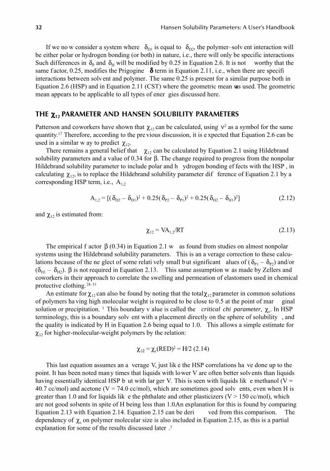
32 Hansen Solubility Parameters: A User’s Handbook
If we no w consider a system where δD1 is equal to δD2, the polymer–solv ent interaction willbe either polar or hydrogen bonding (or both) in nature, i.e., there will only be specific interactionsSuch differences in δP and δH will be modified by 0.25 in Equation 2.6. It is not worthy that thesame f actor, 0.25, modifies the Prigogine δδδδ term in Equation 2.11, i.e., when there are specifiinteractions between solvent and polymer. The same 0.25 is present for a similar purpose both inEquation 2.6 (HSP) and in Equation 2.11 (CST) where the geometric mean was used. The geometricmean appears to be applicable to all types of ener gies discussed here.
THE χχχχ12 PARAMETER AND HANSEN SOLUBILITY PARAMETERS
Patterson and coworkers have shown that χ12 can be calculated, using ν2 as a symbol for the samequantity.17 Therefore, according to the pre vious discussion, it is e xpected that Equation 2.6 can beused in a similar w ay to predict χ12.
There remains a general belief that χ12 can be calculated by Equation 2.1 using Hildebrandsolubility parameters and a value of 0.34 for β. The change required to progress from the nonpolarHildebrand solubility parameter to include polar and h ydrogen bonding ef fects with the HSP , incalculating χ12, is to replace the Hildebrand solubility parameter dif ference of Equation 2.1 by acorresponding HSP term, i.e., A1,2
A1,2 = [( δD2 – δD1)2 + 0.25( δP2 – δP1)2 + 0.25( δH2 – δH1)2] (2.12)
and χ12 is estimated from:
χ12 = VA1,2/RT (2.13)
The empirical f actor β (0.34) in Equation 2.1 w as found from studies on almost nonpolarsystems using the Hildebrand solubility parameters. This is an a verage correction to these calcu-lations because of the ne glect of some relati vely small b ut significant alues of ( δP1 – δP2) and/or(δH1 – δH2). β is not required in Equation 2.13. This same assumption w as made by Zellers andcoworkers in their approach to correlate the swelling and permeation of elastomers used in chemicalprotective clothing.28–31
An estimate for χ12 can also be found by noting that the total χ12 parameter in common solutionsof polymers ha ving high molecular weight is required to be close to 0.5 at the point of mar ginalsolution or precipitation. 1 This boundary v alue is called the critical chi parameter, χc. In HSPterminology, this is a boundary solv ent with a placement directly on the sphere of solubility , andthe quality is indicated by H in Equation 2.6 being equal to 1.0. This allows a simple estimate forχ12 for higher-molecular-weight polymers by the relation:
χ12 = χc(RED)2 = Η/2 (2.14)
This last equation assumes an a verage V, just lik e the HSP correlations ha ve done up to thepoint. It has been noted many times that liquids with lower V are often better solvents than liquidshaving essentially identical HSP b ut with lar ger V. This is seen with liquids lik e methanol (V =40.7 cc/mol) and acetone (V = 74.0 cc/mol), which are sometimes good solv ents, even when H isgreater than 1.0 and for liquids lik e the phthalate and other plasticizers (V > 150 cc/mol), whichare not good solvents in spite of H being less than 1.0. An explanation for this is found by comparingEquation 2.13 with Equation 2.14. Equation 2.15 can be deri ved from this comparison. Thedependency of χc on polymer molecular size is also included in Equation 2.15, as this is a partialexplanation for some of the results discussed later .1
7248_C002.fm Page 32 Wednesday, May 9, 2007 8:25 AM
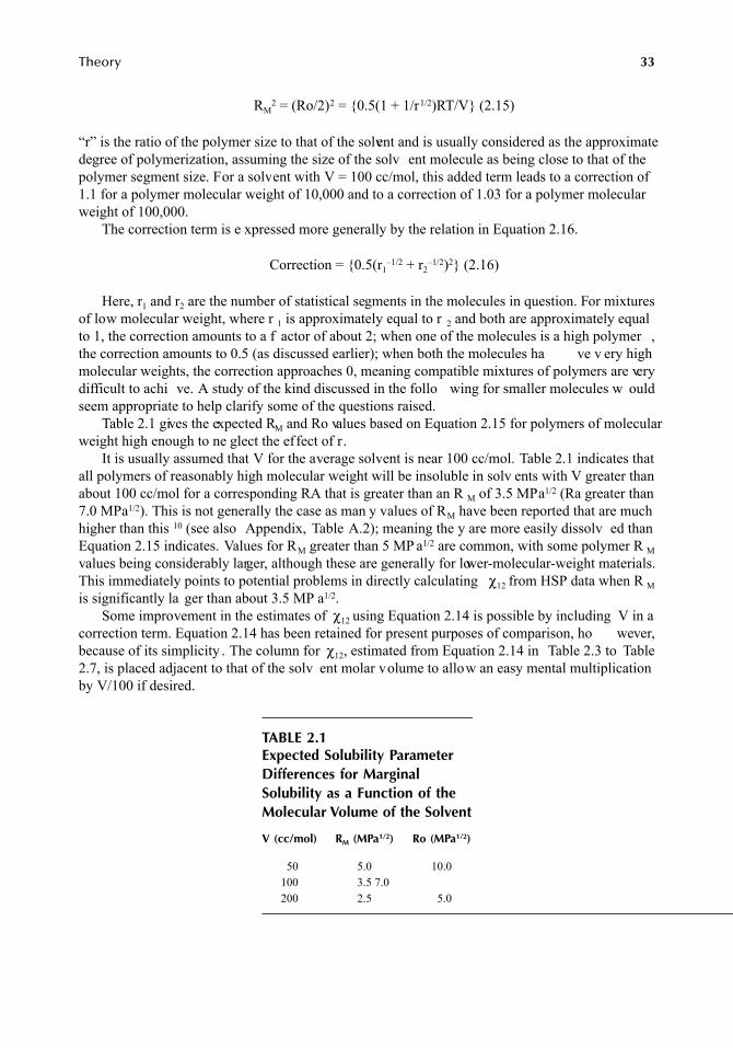
Theory 33
RM2 = (Ro/2)2 = {0.5(1 + 1/r1/2)RT/V} (2.15)
“r” is the ratio of the polymer size to that of the solvent and is usually considered as the approximatedegree of polymerization, assuming the size of the solv ent molecule as being close to that of thepolymer segment size. For a solvent with V = 100 cc/mol, this added term leads to a correction of1.1 for a polymer molecular weight of 10,000 and to a correction of 1.03 for a polymer molecularweight of 100,000.
The correction term is e xpressed more generally by the relation in Equation 2.16.
Correction = {0.5(r1–1/2 + r2
–1/2)2} (2.16)
Here, r1 and r2 are the number of statistical segments in the molecules in question. For mixturesof low molecular weight, where r 1 is approximately equal to r 2 and both are approximately equalto 1, the correction amounts to a f actor of about 2; when one of the molecules is a high polymer ,the correction amounts to 0.5 (as discussed earlier); when both the molecules ha ve v ery highmolecular weights, the correction approaches 0, meaning compatible mixtures of polymers are verydifficult to achi ve. A study of the kind discussed in the follo wing for smaller molecules w ouldseem appropriate to help clarify some of the questions raised.
Table 2.1 gives the expected RM and Ro values based on Equation 2.15 for polymers of molecularweight high enough to ne glect the effect of r.
It is usually assumed that V for the average solvent is near 100 cc/mol. Table 2.1 indicates thatall polymers of reasonably high molecular weight will be insoluble in solv ents with V greater thanabout 100 cc/mol for a corresponding RA that is greater than an R M of 3.5 MPa1/2 (Ra greater than7.0 MPa1/2). This is not generally the case as man y values of RM have been reported that are muchhigher than this 10 (see also Appendix, Table A.2); meaning the y are more easily dissolv ed thanEquation 2.15 indicates. Values for RM greater than 5 MP a1/2 are common, with some polymer R Mvalues being considerably larger, although these are generally for lower-molecular-weight materials.This immediately points to potential problems in directly calculating χ12 from HSP data when R Mis significantly la ger than about 3.5 MP a1/2.
Some improvement in the estimates of χ12 using Equation 2.14 is possible by including V in acorrection term. Equation 2.14 has been retained for present purposes of comparison, ho wever,because of its simplicity . The column for χ12, estimated from Equation 2.14 in Table 2.3 to Table2.7, is placed adjacent to that of the solv ent molar volume to allow an easy mental multiplicationby V/100 if desired.
TABLE 2.1Expected Solubility Parameter Differences for Marginal Solubility as a Function of the Molecular Volume of the Solvent
V (cc/mol) RM (MPa1/2) Ro (MPa1/2)
50 5.0 10.0100 3.5 7.0200 2.5 5.0
7248_C002.fm Page 33 Wednesday, May 9, 2007 8:25 AM
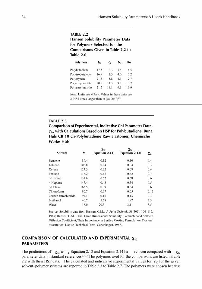
34 Hansen Solubility Parameters: A User’s Handbook
COMPARISON OF CALCULATED AND EXPERIMENTAL χχχχ12
PARAMETERS
The predictions of χ12 using Equation 2.13 and Equation 2.14 ha ve been compared with χ12parameter data in standard references.32,33 The polymers used for the comparisons are listed in Table2.2 with their HSP data. The calculated and indicati ve experimental values for χ12 for the gi vensolvent–polymer systems are reported in Table 2.3 to Table 2.7. The polymers were chosen because
TABLE 2.2Hansen Solubility Parameter Data for Polymers Selected for the Comparisons Given in Table 2.2 to Table 2.6
Polymers δδδδD δδδδP δδδδH Ro
Polybutadiene 17.5 2.3 3.4 6.5Polyisobutylene 16.9 2.5 4.0 7.2Polystyrene 21.3 5.8 4.3 12.7Polyvinylacetate 20.9 11.3 9.7 13.7Polyacrylonitrile 21.7 14.1 9.1 10.9
Note: Units are MPa1/2. Values in these units are2.0455 times larger than in (cal/cm 3)1/2.
TABLE 2.3Comparison of Experimental, Indicative Chi Parameter Data, χlit, with Calculations Based on HSP for Polybutadiene, Buna Hüls CB 10 cis-Polybutadiene Raw Elastomer, Chemische Werke Hüls
Solvent Vχχχχ12
(Equation 2.14)χχχχ12
(Equation 2.13) χχχχlit
Benzene 89.4 0.12 0.10 0.4Toluene 106.8 0.04 0.04 0.3Xylene 123.3 0.02 0.08 0.4Pentane 116.2 0.62 0.62 0.7n-Hexane 131.6 0.52 0.58 0.6n-Heptane 147.4 0.43 0.54 0.5n-Octane 163.5 0.39 0.54 0.6Chloroform 80.7 0.07 0.05 0.15Carbon tetrachloride 97.1 0.16 0.13 0.3Methanol 40.7 5.68 1.97 3.3Water 18.0 20.3 3.1 3.5
Source: Solubility data from Hansen, C.M., J. Paint Technol., 39(505), 104–117,1967; Hansen, C.M., The Three Dimensional Solubility P arameter and Solv entDiffusion Coefficient, Their Importance in Surface Coating Formulation, Doctoraldissertation, Danish Technical Press, Copenhagen, 1967.
7248_C002.fm Page 34 Wednesday, May 9, 2007 8:25 AM
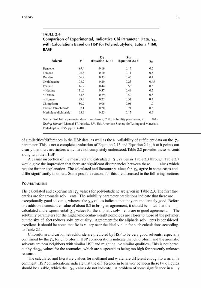
Theory 35
of similarities/differences in the HSP data, as well as the a vailability of suf ficient data on the χ12parameter. This is not a complete e valuation of Equation 2.13 and Equation 2.14, b ut it points outclearly that there are factors which are not completely understood. Table 2.8 provides these solventsalong with their HSP.
A casual inspection of the measured and calculated χ12 values in Table 2.3 through Table 2.7would gi ve the impression that there are significant discrepancies between these alues whichrequire further e xplanation. The calculated and literature v alues for χ12 agree in some cases anddiffer significantly in others. Some possible reasons for this are discussed in the foll wing sections.
POLYBUTADIENE
The calculated and experimental χ12 values for polybutadiene are given in Table 2.3. The first threentries are for aromatic solv ents. The solubility parameter predictions indicate that these areexceptionally good solvents, whereas the χ12 values indicate that they are moderately good. Beforeone adds on a constant v alue of about 0.3 to bring an agreement, it should be noted that thecalculated and e xperimental χ12 values for the aliphatic solv ents are in good agreement. Thesolubility parameters for the higher-molecular-weight homologs are closer to those of the polymer,but the size ef fect reduces solv ent quality . Agreement for the aliphatic solv ents is consideredexcellent. It should be noted that Ro is v ery near the ideal v alue for such calculations accordingto Table 2.1.
Chloroform and carbon tetrachloride are predicted by HSP to be very good solvents, especiallyconfirmed by the χlit for chloroform. HSP considerations indicate that chloroform and the aromaticsolvents are near neighbors with similar HSP and might ha ve similar qualities. This is not borneout by the χlit values for the aromatics, which are suspected as being too high for presently unknownreasons.
The calculated and literature v alues for methanol and w ater are dif ferent enough to w arrant acomment. HSP considerations indicate that the dif ference in beha vior between these tw o liquidsshould be sizable, which the χlit values do not indicate. A problem of some significance in a y
TABLE 2.4Comparison of Experimental, Indicative Chi Parameter Data, χlit, with Calculations Based on HSP for Polyisobutylene, Lutonal® I60, BASF
Solvent Vχχχχ12
(Equation 2.14)χχχχ12
(Equation 2.13) χχχχlit
Benzene 89.4 0.19 0.17 0.5Toluene 106.8 0.10 0.11 0.5Decalin 156.9 0.35 0.43 0.4Cyclohexane 108.7 0.20 0.23 0.45Pentane 116.2 0.44 0.53 0.5n-Hexane 131.6 0.37 0.49 0.5n-Octane 163.5 0.29 0.50 0.5n-Nonane 179.7 0.27 0.51 0.3+ Chloroform 80.7 0.06 0.05 1.0Carbon tetrachloride 97.1 0.20 0.21 0.5Methylene dichloride 63.9 0.25 0.17 0.6
Source: Solubility parameter data from Hansen, C.M., Solubility parameters, in PaintTesting Manual, Manual 17, Koleske, J.V., Ed., American Society for Testing and Materials,Philadelphia, 1995, pp. 383–404.
7248_C002.fm Page 35 Wednesday, May 9, 2007 8:25 AM
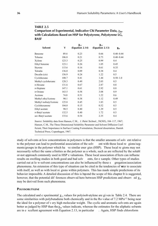
36 Hansen Solubility Parameters: A User’s Handbook
study of solvents at low concentrations in polymers is that the smaller amounts of solv ent relativeto the polymer can lead to preferential association of the solv ent with those local re gions/seg-ments/groups in the polymer which ha ve similar ener gies (HSP). These local re gions may notnecessarily reflect the same a finities as the polymer as a whole, such as are reflected by the solublor-not approach commonly used in HSP e valuations. These local association ef fects can influencresults on swelling studies in both good and bad solv ents, for e xample. Other types of studiescarried out at lo w-solvent concentrations can also be influenced by these s gregation/associationphenomena. An extension of this type of situation can be cited in the tendencies of water to associatewith itself, as well as with local re gions within polymers. This has made simple predictions of itsbehavior impossible. A detailed discussion of this is beyond the scope of this chapter. It is suggested,however, that the potential dif ferences observed here between HSP predictions and observ ed χlitmay be derived from such phenomena.
POLYISOBUTYLENE
The calculated and e xperimental χ12 values for polyisob utylene are gi ven in Table 2.4. There aresome similarities with polybutadiene both chemically and in the Ro value of 7.2 MPa1/2 being nearthe ideal for a polymer of v ery high molecular weight. The cyclic and aromatic solvents are againbetter as judged by HSP than the χlit values indicate, whereas the estimates for the aliphatic solventsare in e xcellent agreement with Equation 2.13, in particular . Again, HSP finds chloroform
TABLE 2.5Comparison of Experimental, Indicative Chi Parameter Data, χlit, with Calculations Based on HSP for Polystyrene, Polystyrene LG, BASF
Solvent Vχχχχ12
(Equation 2.14)χχχχ12
(Equation 2.13) χχχχlit
Benzene 89.4 0.23 0.66 0.40–0.44Toluene 106.8 0.21 0.73 0.40–0.44Xylene 123.3 0.25 0.99 0.4Ethyl benzene 123.1 0.26 1.05 0.45Styrene 115.6 0.16 0.61 0.35Tetralin 136.0 0.09 0.38 0.4Decalin (cis) 156.9 0.24 1.22 0.5Cyclohexane 108.7 0.41 1.44 0.50–1.0Methyl cyclohexane 128.3 0.49 2.03 0.5n-Hexane 131.6 0.67 2.87 0.8n-Heptane 147.1 0.61 2.92 0.8n-Octane 163.5 0.58 3.08 0.9Acetone 74.0 0.51 1.22 0.6Methyl ethyl ketone 90.1 0.38 1.12 0.49Methyl isobutyl ketone 125.8 0.45 1.83 0.5Cyclohexanone 104.0 0.15 0.52 0.5Ethyl acetate 98.5 0.40 1.29 0.5n-Butyl acetate 132.5 0.40 1.72 0.5sec-Butyl acetate 133.6 0.54 2.35 0.4
Source: Solubility data from Hansen, C.M., J. Paint Technol., 39(505), 104–117, 1967;Hansen, C.M., The Three Dimensional Solubility Parameter and Solvent Diffusion Coef-ficient, Their Importance in Surface Coating Formulation, Doctoral dissertation, DanishTechnical Press, Copenhagen, 1967.
7248_C002.fm Page 36 Wednesday, May 9, 2007 8:25 AM
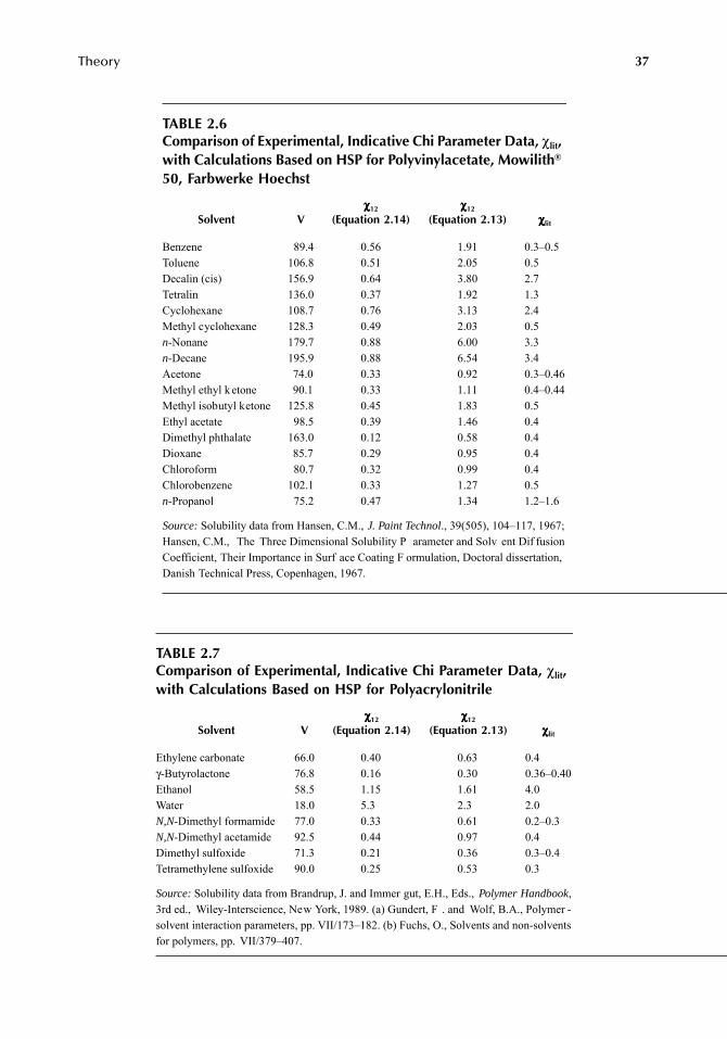
Theory 37
TABLE 2.6Comparison of Experimental, Indicative Chi Parameter Data, χlit, with Calculations Based on HSP for Polyvinylacetate, Mowilith® 50, Farbwerke Hoechst
Solvent Vχχχχ12
(Equation 2.14)χχχχ12
(Equation 2.13) χχχχlit
Benzene 89.4 0.56 1.91 0.3–0.5Toluene 106.8 0.51 2.05 0.5Decalin (cis) 156.9 0.64 3.80 2.7Tetralin 136.0 0.37 1.92 1.3Cyclohexane 108.7 0.76 3.13 2.4Methyl cyclohexane 128.3 0.49 2.03 0.5n-Nonane 179.7 0.88 6.00 3.3n-Decane 195.9 0.88 6.54 3.4Acetone 74.0 0.33 0.92 0.3–0.46Methyl ethyl ketone 90.1 0.33 1.11 0.4–0.44Methyl isobutyl ketone 125.8 0.45 1.83 0.5Ethyl acetate 98.5 0.39 1.46 0.4Dimethyl phthalate 163.0 0.12 0.58 0.4Dioxane 85.7 0.29 0.95 0.4Chloroform 80.7 0.32 0.99 0.4Chlorobenzene 102.1 0.33 1.27 0.5n-Propanol 75.2 0.47 1.34 1.2–1.6
Source: Solubility data from Hansen, C.M., J. Paint Technol., 39(505), 104–117, 1967;Hansen, C.M., The Three Dimensional Solubility P arameter and Solv ent Dif fusionCoefficient, Their Importance in Surf ace Coating F ormulation, Doctoral dissertation,Danish Technical Press, Copenhagen, 1967.
TABLE 2.7Comparison of Experimental, Indicative Chi Parameter Data, χlit, with Calculations Based on HSP for Polyacrylonitrile
Solvent Vχχχχ12
(Equation 2.14)χχχχ12
(Equation 2.13) χχχχlit
Ethylene carbonate 66.0 0.40 0.63 0.4γ-Butyrolactone 76.8 0.16 0.30 0.36–0.40Ethanol 58.5 1.15 1.61 4.0Water 18.0 5.3 2.3 2.0N,N-Dimethyl formamide 77.0 0.33 0.61 0.2–0.3N,N-Dimethyl acetamide 92.5 0.44 0.97 0.4Dimethyl sulfoxide 71.3 0.21 0.36 0.3–0.4Tetramethylene sulfoxide 90.0 0.25 0.53 0.3
Source: Solubility data from Brandrup, J. and Immer gut, E.H., Eds., Polymer Handbook,3rd ed., Wiley-Interscience, New York, 1989. (a) Gundert, F . and Wolf, B.A., Polymer -solvent interaction parameters, pp. VII/173–182. (b) Fuchs, O., Solvents and non-solventsfor polymers, pp. VII/379–407.
7248_C002.fm Page 37 Wednesday, May 9, 2007 8:25 AM
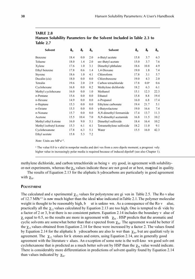
38 Hansen Solubility Parameters: A User’s Handbook
methylene dichloride, and carbon tetrachloride as being v ery good, in agreement with solubility-or-not experiments, whereas the χlit values indicate these are not good or at best, marginal in quality.
The results of Equation 2.13 for the aliphatic h ydrocarbons are particularly in good agreementwith χlit.
POLYSTYRENE
The calculated and e xperimental χ12 values for polystyrene are gi ven in Table 2.5. The Ro v alueof 12.7 MPa1/2 is now much higher than the ideal value indicated in Table 2.1. The polymer molecularweight is thought to be reasonably high, b ut is unkno wn. As a consequence of the Ro v alue,practically all the χ12 values calculated by Equation 2.13 are too high. One is tempted to di vide bya factor of 2 or 3, b ut there is no consistent pattern. Equation 2.14 includes the boundary v alue ofχc equal to 0.5, so the results are more in agreement with χlit . HSP predicts that the aromatic andcyclic solvents are somewhat better than that e xpected from χlit. The agreement would be better ifthe χ12 values obtained from Equation 2.14 for these were increased by a factor 2. The values foundby Equation 2.14 for the aliphatic h ydrocarbons are also lo wer than χlit, but are qualitati vely inagreement. The χ12 values for k etones and esters, using Equation 2.14, are in generally goodagreement with the literature v alues. An exception of some note is the well-kno wn good solv entcyclohexanone that is predicted as a much better solvent by HSP than the χlit value would indicate.There is considerably more differentiation in predictions of solvent quality found by Equation 2.14than values indicated by χlit.
TABLE 2.8Hansen Solubility Parameters for the Solvent Included in Table 2.3 to Table 2.7
Solvent δδδδD δδδδP δδδδH Solvent δδδδD δδδδP δδδδH
Benzene 18.4 0.0 2.0 n-Butyl acetate 15.8 3.7 6.3Toluene 18.0 1.4 2.0 sec-Butyl acetate 15.0 3.7 7.6Xylene 17.6 1.0 3.1 Dimethyl phthalate 18.6 10.8 4.9Ethyl benzene 17.8 0.6 1.4 1,4-Dioxane 19.0 1.8 7.4Styrene 18.6 1.0 4.1 Chloroform 17.8 3.1 5.7Decalin (cis) 18.0 0.0 0.0 Chlorobenzene 19.0 4.3 2.0Tetralin 19.6 2.0 2.9 Carbon tetrachloride 17.8 0.0a 0.6Cyclohexane 16.8 0.0 0.2 Methylene dichloride 18.2 6.3 6.1Methyl cyclohexane 16.0 0.0 1.0 Methanol 15.1 12.3 22.3n-Pentane 15.6 0.0 0.0 Ethanol 15.8 8.8 19.4n-Hexane 14.9 0.0 0.0 n-Propanol 16.0 6.8 17.4n-Heptane 15.3 0.0 0.0 Ethylene carbonate 19.4 21.7 5.1n-Octane 15.5 0.0 0.0 γ-Butyrolactone 19.0 16.6 7.4n-Nonane 15.7 0.0 0.0 N,N-dimethyl formamide 17.4 13.7 11.3Acetone 15.5 10.4 7.0 N,N-dimethyl acetamide 16.8 11.5 10.2Methyl ethyl ketone 16.0 9.0 5.1 Dimethyl sulfoxide 18.4 16.4 10.2Methyl isobutyl ketone 15.3 6.1 4.1 Tetramethylene sulfoxide 18.2 11.0 9.1Cyclohexanone 17.8 6.3 5.1 Water 15.5 16.0 42.3Ethyl acetate 15.8 5.3 7.2
Note: Units are MP a1/2.
a The value 0.0 is v alid in nonpolar media and deri ves from a zero dipole moment; a progressi velyhigher value in increasingly polar media is required because of induced dipoles10 (see also Chapter 1).
7248_C002.fm Page 38 Wednesday, May 9, 2007 8:25 AM
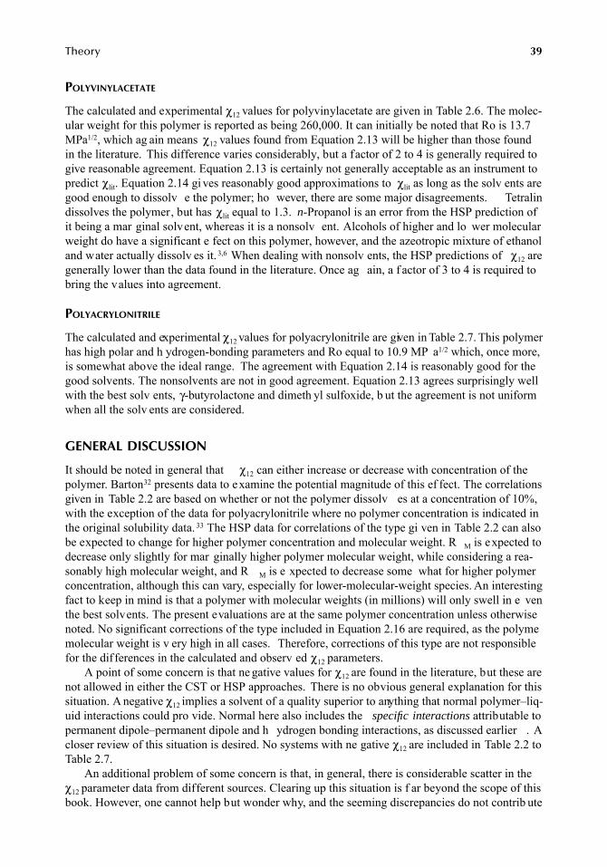
Theory 39
POLYVINYLACETATE
The calculated and experimental χ12 values for polyvinylacetate are given in Table 2.6. The molec-ular weight for this polymer is reported as being 260,000. It can initially be noted that Ro is 13.7MPa1/2, which ag ain means χ12 values found from Equation 2.13 will be higher than those foundin the literature. This difference varies considerably, but a factor of 2 to 4 is generally required togive reasonable agreement. Equation 2.13 is certainly not generally acceptable as an instrument topredict χlit. Equation 2.14 gi ves reasonably good approximations to χlit as long as the solv ents aregood enough to dissolv e the polymer; ho wever, there are some major disagreements. Tetralindissolves the polymer, but has χlit equal to 1.3. n-Propanol is an error from the HSP prediction ofit being a mar ginal solvent, whereas it is a nonsolv ent. Alcohols of higher and lo wer molecularweight do have a significant e fect on this polymer, however, and the azeotropic mixture of ethanoland water actually dissolv es it. 3,6 When dealing with nonsolv ents, the HSP predictions of χ12 aregenerally lower than the data found in the literature. Once ag ain, a f actor of 3 to 4 is required tobring the values into agreement.
POLYACRYLONITRILE
The calculated and experimental χ12 values for polyacrylonitrile are given in Table 2.7. This polymerhas high polar and h ydrogen-bonding parameters and Ro equal to 10.9 MP a1/2 which, once more,is somewhat above the ideal range. The agreement with Equation 2.14 is reasonably good for thegood solvents. The nonsolvents are not in good agreement. Equation 2.13 agrees surprisingly wellwith the best solv ents, γ-butyrolactone and dimeth yl sulfoxide, b ut the agreement is not uniformwhen all the solv ents are considered.
GENERAL DISCUSSION
It should be noted in general that χ12 can either increase or decrease with concentration of thepolymer. Barton32 presents data to examine the potential magnitude of this ef fect. The correlationsgiven in Table 2.2 are based on whether or not the polymer dissolv es at a concentration of 10%,with the exception of the data for polyacrylonitrile where no polymer concentration is indicated inthe original solubility data. 33 The HSP data for correlations of the type gi ven in Table 2.2 can alsobe expected to change for higher polymer concentration and molecular weight. R M is expected todecrease only slightly for mar ginally higher polymer molecular weight, while considering a rea-sonably high molecular weight, and R M is e xpected to decrease some what for higher polymerconcentration, although this can vary, especially for lower-molecular-weight species. An interestingfact to keep in mind is that a polymer with molecular weights (in millions) will only swell in e venthe best solvents. The present evaluations are at the same polymer concentration unless otherwisenoted. No significant corrections of the type included in Equation 2.16 are required, as the polymemolecular weight is v ery high in all cases. Therefore, corrections of this type are not responsiblefor the differences in the calculated and observ ed χ12 parameters.
A point of some concern is that ne gative values for χ12 are found in the literature, but these arenot allowed in either the CST or HSP approaches. There is no obvious general explanation for thissituation. A negative χ12 implies a solvent of a quality superior to anything that normal polymer–liq-uid interactions could pro vide. Normal here also includes the specific interactions attributable topermanent dipole–permanent dipole and h ydrogen bonding interactions, as discussed earlier . Acloser review of this situation is desired. No systems with ne gative χ12 are included in Table 2.2 toTable 2.7.
An additional problem of some concern is that, in general, there is considerable scatter in theχ12 parameter data from different sources. Clearing up this situation is f ar beyond the scope of thisbook. However, one cannot help but wonder why, and the seeming discrepancies do not contrib ute
7248_C002.fm Page 39 Wednesday, May 9, 2007 8:25 AM
40 Hansen Solubility Parameters: A User’s Handbook
to blind confidence in a y of the reported χ12 values. Indicative χ12 values are used here. One canalso find ariations in HSP values for polymers from different sources,32 so there are also problemsin determining which v alues are best in this approach. The χ12 parameter does not specificallaccount for permanent dipole–permanent dipole or h ydrogen bonding interactions, which must beconsidered a major source of potential dif ferences.
There has been some discussion as to whether the coef ficient 4 in Equation 2.5 (correspondinto a coefficient of 0.25 in Equation 2.12) should be a di ferent number. Barton cites a case wherea coefficient of 0.2 (rather than 0.25) in Equation 2.12 as determined.34 Skaarup has mentioneda case of 5 (rather than 4) as a v alue for the coef ficient in Equation 2.5, which, of course, g ves0.2 in Equation 2.12. 35 The author has also e xplored situations involving water, where the D ATAFIT was equal for either a constant 4 or 5 in Equation 2.5. Zellers and coworkers used this coefficienas an adjustable parameter for individual solvents in their studies.28–31 One significant actor in thisdiscussion is that solv ents with higher solubility parameters generally ha ve lower molecular v ol-umes. This means they will be better than e xpected by average comparisons of behavior. This facttends to lead one to stretch the spheres a little more in the δP and δH directions to encompass thesegood solvents that would otherwise lie outside of the spheroids. This would lead to a number thatis slightly higher than the 4 in Equation 2.5, and it is the author’ s feeling that this could be thecase whenever a complete understanding of the ef fect of solvent molecular volume, and other sizeeffects is accomplished. The use of the coef ficient 4 is also confirmed in Chapter
The Prigogine theory contains structural parameters that have not been explored in this context.There are also structural parameters in the New Flory theory. It is possible that the use of structuralparameters will allow better understanding, enhance the possibility of impro ved calculations, andreduce the need for e xperimental studies. The experimentally-determined radius for the solubilityspheres automatically tak es these f actors into account, b ut reliable calculation of the radius ofinteraction has not been possible as yet.
POSTSCRIPT
The author has al ways experienced consistency in the quality of the predictions using the HSP .Care is required to generate the necessary data, and there should al ways be a ree valuation ofexperimental data based on an initial correlation. The solv ent parameters ha ve been used withsuccess for many years in industrial practice to predict solv ent quality using computer techniquesby most, if not all, major solvent suppliers. Mixing rules have been established for even complicatedsolvent blends. These are usually based on summing up simple volume fraction times the solubilityparameter values. (An e valuation of the quality of the χ12 values in the literature could be madewith precipitation e xperiments for mixtures to see whether a mixing rule gi ves consistent resultsfor these as well.)
The solvent δD, δP, and δH values that were established with e xtensive calculations ha ve beensupported by tens of thousands of experimental data points based on solubility, permeation, surfacewetting, etc.10 It has become quite clear that the HSP for the solv ents are not precise enough forsophisticated calculations, but they certainly represent a good and satisf actory means for practicalapplications. The HSP for the solv ents relative to each other are correct for the majority of thecommon solvents. The “nearest neighbors” to a good solv ent are clearly e xpected to be of nearlycomparable quality unless they are in a boundary re gion of the HSP solubility sphere. The solventquality indicated by the ratio Ra/Ro (the RED number) has been particularly satisfactory. This ratiowas defined years ago as a ratio of solubility parameters, as plotting and interpretation of data usesolubility parameters. Use of the ratio of cohesion ener gy densities is also possible, of course, asthis is indeed closer to an energy difference number and would agree more with the Flory approachas seen in Equation 2.6 and Equation 2.14, as H is really nothing other than (RED) 2.
7248_C002.fm Page 40 Wednesday, May 9, 2007 8:25 AM
Theory 41
As a result of ha ving reviewed all of this here, the author senses that the HSP approach is apractical extension in complete agreement with the Prigogine–Flory theory when the geometricmean is used, at least as f ar as the major f actors discussed earlier are concerned. The comparisonspresented previously confirm some relation, ut the single χ12 parameter may have been oversim-plified, such that the more complete HSP approach cannot be immediately recognized. The abilityof HSP to describe molecular affinities among so ma y different materials listed in this book speaksfor the general application of both the Prigogine and the HSP treatments. The Prigogine treatmentis acknowledged as difficult to use in practice. This is not true of the HSP approach.
CONCLUSION
The Prigogine/Patterson CST and the HSP approach (which also in volves a corresponding statescalculation) are shown to have very close resemblance. Both can be used to estimate the Flory χ12.Two equations involving HSP are given for this purpose. Reasonably good predictions are possibleunder f avorable circumstances. F avorable circumstances in volve a system with an essentiallynonpolar polymer whose Ro v alue is not too dif ferent from 7.0 MP a1/2. χ12values for the bettersolvents are calculated by HSP at lo wer levels than those found in the literature. χ12 values fornonsolvents are also generally calculated by HSP as being significantly l wer than the reportedliterature values. The most f avorable circumstances are, of course, not al ways present, and someproblems still e xist and need to be solv ed before these calculations can be used with confidencto estimate χ12 values for any solvent–polymer system. The HSP values for the polymers used forthe present comparisons are based on solubility-or-not type experiments which reflect the propertieof the polymer as a whole. These may not completely correspond to the type of e valuation oftenused to find χ12, as less-than-dissolving amounts of solv ent may be used, and the solv ent mayassociate with given segments or groups in the polymer and not reflect the beh vior of the polymeras a whole (see also the discussion in Chapter 5).
An empirical f actor, β, equal to about 0.34 appears in man y sources in the literature inconnection with calculation of χ12 using Hildebrand solubility parameters. β disappears when HSPare used for this purpose, b ut the resulting equation has not been studied enough to allo w generaluse of HSP to calculate χ12 parameters.
Studies on the ef fect of molecular size, se gmental size, and polymer size are still required. Itis suggested that the structural f actors discussed by Prigogine be tried in this respect. 11 Use of thegeometric mean in conjunction with the Prigogine theory brings the HSP and Prigogine approachesinto agreement. The massive amount of experimental data presented in this book strongly supportsthe use of the geometric mean. As a curiosity, it might be noted that the use of the geometric mean(Lorenz–Berthelot mixtures) generated an ellipsoidal miscibility plot essentially identical to thosegiven in Chapter 5, Figure 5.1 and Figure 5.2. 36 This approach w as not continued because it w asstated that “the boundary of this ellipse is of little practical importance as there are no known casesof immiscibility in mixtures kno wn to conform to the Lorenz–Berthelot equations. ”
As stated in the Pref ace to this book, it has not been its purpose to recite the de velopments ofpolymer solution thermodynamics in a historical manner with full e xplanations of each theory ormodifications thereof. The references cited in the Pref ace do this already . Chapter 3 and Chapter4 have been added to this edition of this handbook to gi ve broader co verage in this respect. Thischapter has attempted to sho w relations between the classical theories of polymer solution ther -modynamics and the HSP approach, which includes a quantitati ve accounting of both permanentdipole–permanent dipole and h ydrogen bonding interactions as an inte gral part. The relationbetween the Prigogine–Patterson theory and HSP w as the most ob vious.
7248_C002.fm Page 41 Wednesday, May 9, 2007 8:25 AM
42 Hansen Solubility Parameters: A User’s Handbook
REFERENCES
1. Flory, P.J., Principles of Polymer Chemistry, Cornell University Press, New York, 1953.2. Eichinger, B.E. and Flory , P.J., Thermodynamics of polymer solutions, Trans. Faraday Soc., 64(1),
2035–2052, 1968; Trans. Faraday Soc. (2), 2053–2060; Trans. Faraday Soc. (3), 2061–2065; Trans.Faraday Soc. (4), 2066–2072.
3. Hansen, C.M., The three dimensional solubility parameter — k ey to paint component af finities ISolvents, plasticizers, polymers, and resins, J. Paint Technol., 39(505), 104–117, 1967.
4. Hansen, C.M., The three dimensional solubility parameter — k ey to paint component af finities IIDyes, emulsifiers, mutual solubility and compatibilit , and pigments, J. Paint Technol., 39(511),505–510, 1967.
5. Hansen, C.M. and Skaarup, K., The three dimensional solubility parameter — key to paint componentaffinities III. Independent calculation of the parameter components J. Paint Technol., 39(511),511–514, 1967.
6. Hansen, C.M., The Three Dimensional Solubility Parameter and Solvent Diffusion Coefficient, TheirImportance in Surf ace Coating F ormulation, Doctoral dissertation, Danish Technical Press, Copen-hagen, 1967.
7. Hansen, C.M., The universality of the solubility parameter , Ind. Eng. Chem. Prod. Res. Dev., 8(1),2–11, 1969.
8. Hansen, C.M. and Beerbo wer, A., Solubility parameters, in Kirk-Othmer Encyclopedia of ChemicalTechnology, Suppl. Vol., 2nd ed., Standen, A., Ed., Interscience, Ne w York, 1971, pp. 889–910.
9. Hansen, C.M., 25 Years with solubility parameters (25 År med Opløselighedsparametrene, in Danish),Dan. Kemi, 73(8), 18–22, 1992.
10. Hansen, C.M., Solubility parameters, in Paint Testing Manual, Manual 17, Koleske, J.V., Ed., AmericanSociety for Testing and Materials, Philadelphia, 1995, pp. 383–404.
11. Prigogine, I. (with the collaboration of Bellemans, A. and Mathot, A.), The Molecular Theory ofSolutions, North-Holland, Amsterdam, 1957, chap. 16, 17.
12. Patterson, D. and Delmas, G., Ne w aspects of polymer solution thermodynamics, Off. Dig. Fed. Soc.Paint Technol., 34(450), 677–692, 1962.
13. Delmas, D., Patterson, D., and Somcynsky, T., Thermodynamics of polyisobutylene-n-alkane systems,J. Polym. Sci., 57, 79–98, 1962.
14. Bhattacharyya, S.N., Patterson, D., and Somcynsky, T., The principle of corresponding states and theexcess functions of n-alkane mixtures, Physica, 30, 1276–1292, 1964.
15. Patterson, D., Role of free v olume changes in polymer solution thermodynamics , J. Polym. Sci. PartC, 16, 3379–3389, 1968.
16. Patterson, D.D., Introduction to thermodynamics of polymer solubility , J. Paint Technol., 41(536),489–493, 1969.
17. Biros, J., Zeman, L., and P atterson, D., Prediction of the χ parameter by the solubility parameter andcorresponding states theories, Macromolecules, 4(1), 30–35, 1971.
18. Hildebrand, J. and Scott, R.L., The Solubility of Nonelectrolytes, 3rd ed., Reinhold, New York, 1950.19. Hildebrand, J. and Scott, R.L., Regular Solutions, Prentice-Hall, Englewood Cliffs, NJ, 1962.20. Hansen, C.M., Cohesion parameters for surf aces, pigments, and fillers ( ohæsionsparametre for
Overflade , Pigmenter, og Fyldstoffer, in Danish), Färg och Lack Scand., 43(1), 5–10, 1997.21. Hansen, C.M., Polymer solubility — prigogine theory and Hansen Solubility parameter theory mutu-
ally confirmed (Polymeropløselighed — Prigogine Teori og Hansen OpløselighedsparameterteoriGensidigt Bekræftet, in Danish), Dan. Kemi, 78(9), 4–6, 1997.
22. Hildebrand, J. and Scott, R.L., The Solubility of Nonelectrolytes, 3rd ed., Reinhold, New York, 1950,chap. 20.
23. Hansen, C.M., Characterization of surfaces by spreading liquids, J. Paint Technol., 42(550), 660–664,1970.
24. Hansen, C.M., Surface dewetting and coatings performance, J. Paint Technol., 44(570), 57–60, 1972.25. Hansen, C.M. and Pierce, P .E., Surface effects in coatings processes, XII Federation d’Associations
de Techniciens des Industries des Peintures, Vernis, Emaux et Encres d’Imprimerie de l’EuropeContinentale, Congress Book, Verlag Chemie, Weinheim/Bergstrasse, 1974, 91–99; Ind. Eng. Chem.,Prod. Res. Dev., 13(4), 218–225, 1974.
7248_C002.fm Page 42 Wednesday, May 9, 2007 8:25 AM
Theory 43
26. Hansen, C.M. and Wallström, E., On the use of cohesion parameters to characterize surfaces, J. Adhes.,15(3/4), 275–286, 1983.
27. Patterson, D., personal communication, 1997.28. Zellers, E.T., Three-dimensional solubility parameters and chemical protecti ve clothing permeation.
I. Modeling the solubility of organic solvents in Viton® gloves, J. Appl. Polym. Sci., 50, 513–530, 1993.29. Zellers, E.T . and Zhang G.-Z., Three-dimensional solubility parameters and chemical protecti ve
clothing permeation. II. Modeling diffusion coefficients, breakthrough times, and steady-state permeation rates of or ganic solvents in Viton® gloves, J. Appl. Polym. Sci., 50, 531–540, 1993.
30. Zellers, E.T., Anna, D.H., Sulewski, R., and Wei, X., Critical analysis of the graphical determinationof Hansen’s solubility parameters for lightly crosslinked polymers, J. Appl. Polym. Sci., 62, 2069–2080,1996.
31. Zellers, E.T., Anna, D.H., Sule wski, R., and Wei, X., Impro ved methods for the determination ofHansen’s solubility parameters and the estimation of solv ent uptake for lightly crosslinked polymers,J. Appl. Polym. Sci., 62, 2081–2096, 1996.
32. Barton, A.F.M., Handbook of Polymer-Liquid Interaction Parameters and Solubility Parameters, CRCPress, Boca Raton, FL, 1990.
33. Brandrup, J. and Immer gut, E.H., Eds., Polymer Handbook, 3rd ed., Wiley-Interscience, New York,1989. (a) Gundert, F . and Wolf, B.A., Polymer -solvent interaction parameters, pp. VII/173–182. (b)Fuchs, O., Solvents and non-solvents for polymers, pp. VII/379–407.
34. Barton, A.F.M., Applications of solubility parameters and other cohesion ener gy parameters, Polym.Sci. Technol. Pure Appl. Chem., 57(7), 905–912, 1985.
35. Skaarup, K., private communication, 1997.36. Rowlinson, J.S., Liquids and Liquid Mixtures, Butterworths Scientific Publications, London, 1959
chap. 9.
7248_C002.fm Page 43 Wednesday, May 9, 2007 8:25 AM

7248_C002.fm Page 44 Wednesday, May 9, 2007 8:25 AM
45
3
Statistical Thermodynamic Calculations of the Hydrogen Bonding, Dipolar, and Dispersion Solubility Parameters
Costas Panayiotou
KEY WORDS
Statistical thermodynamics, cohesive energy density, Hansen solubility parameters, solvent screening.
ABSTRACT
The main objecti ve of this chapter is the presentation of an equation-of-state frame work for thecalculation of the h ydrogen-bonding component of the solubility parameter as well as the otherpartial solubility parameters. A new statistical thermodynamic approach has been de veloped forthe estimation of these partial components o ver a broad range of temperature and pressure. K ey tothis approach is the development of explicit expressions for the contribution of hydrogen bonding,dispersion, and dipolar interactions to the potential ener gy of the fluid. The approach is applicableto ordinary solvents, supercritical fluids, and high polymers. Information on various thermodynamicproperties of fluids is used in order to estimate the three solubility parameter components. Extensivetables with the k ey parameters are presented. When information on h ydrogen bonding interactionis a vailable from other sources, the proposed method is essentially a predicti ve method for thehydrogen bonding component of the solubility parameter. On the other hand, available informationon these separate components is exploited for extracting information on the thermodynamic behav-ior of the fluids o ver an extended range of e xternal conditions.
INTRODUCTION
The conceptual simplicity of the solubility parameter ,
δ
, makes it most attracti ve in industry andin academia as well. Originally introduced by Hildebrand,
1
it remains today one of the k eyparameters for selecting solv ents in industry , characterizing surf aces, predicting solubility anddegree of rubber swelling, polymer compatibility , chemical resistance, permeation rates, and fornumerous other applications. There is also much interest in utilizing solubility parameters forrationally designing new processes, such as the supercritical fluid, the coating, and the drug deliveryprocesses.
2–8
Of course, the use of solubility parameter, or the closely related cohesive density is not alwayssuccessful and this lack of total success stimulates continuing research. The central principle behindthe use of
δ
is the historic alchemist maxim,
similia similibus solvuntur
(“lik e dissolves lik e”),
7248_book.fm Page 45 Tuesday, April 24, 2007 9:19 AM
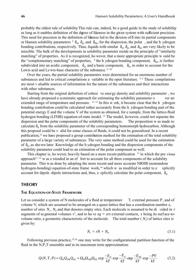
46
Hansen Solubility Parameters: A User’s Handbook
probably the oldest rule of solubility. This rule can, indeed, be a good guide in the study of solubility,as long as it enables definition of the degree of likeness in the given system with sufficient precision.This need for precision in the definition of likeness led to the division of
δ
into its partial componentsor Hansen solubility parameters
5
δ
d
,
δ
p
, and
δ
hb
, for the dispersion, the polar , and the h ydrogenbonding contributions, respectively. Thus, liquids with similar
δ
d
,
δ
p
, and
δ
hb
are very likely to bemiscible. The bulk of the developments in solubility parameter reside on the principle of “similaritymatching” of properties. As it is recognized, ho wever, that a more appropriate principle w ould bethe “complementary matching” of properties,
9
the h ydrogen bonding component,
δ
hb
, is furthersubdivided into an acidic component,
δ
a
, and a basic component,
δ
b
, in order to account for theLewis acid and Le wis-base character of the substance.
8–10
Over the years, the partial solubility parameters were determined for an enormous number ofsubstances and led to critical compilations a vailable in the open literature.
3–5
These compilationsare most v aluable sources of information for the nature of the substances and their interactionswith other substances.
Starting from the original definition of cohesi ve energy density and solubility parameter , wehave already proposed a systematic approach for estimating the solubility parameter o ver anextended range of temperature and pressure.
11–12
In this w ork, it became clear that the h ydrogenbonding contribution could be calculated rather accurately from the h ydrogen bonding part of thepotential energy E and the volume V of the system as obtained, for e xample, from the lattice-fluidhydrogen bonding (LFHB) equation-of-state model.
13
The model, however, could not separate thedispersion and the polar components of the solubility parameters. The proposition w as made tocalculate
δ
d
from the solubility parameter of the corresponding homomorph hydrocarbon. Althoughthis proposal could be v alid for some classes of fluids, it could not be generalized. In a recentpublication,
14
we have proposed a group contribution method for the estimation of the total solubilityparameter of a large variety of substances. The very same method could be used for the estimationof
δ
d
, as sho wn later. Knowledge of the h ydrogen bonding and the dispersion components of thesolubility parameter could lead to an estimation of the polar component as well.
This chapter is, ho wever, heavily based on a more recent publication
15
in which the pre viousapproach
11–12
w as e xtended in an ef fort to account for all three components of the solubilityparameter. This w as done by adopting the more recent and more accurate NRHB (nonrandomhydrogen-bonding) equation-of-state frame work,
16
which w as modified in order to e xplicitlyaccount for dipole–dipole interactions and, thus, e xplicitly calculate the polar component,
δ
p
.
THEORY
T
HE
E
QUATION
-
OF
-S
TATE
F
RAMEWORK
Let us consider a system of N molecules of a fluid at temperature T, external pressure P, and ofvolume V, which are assumed to be arranged on a quasi-lattice that has a coordination number z,number of sites
N
r
,
N
0
and that denotes empty sites. Each molecule is assumed to be di vided in
r
segments of se gmental volumes
v
*
, and to ha ve
zq = zrs
external contacts,
s
being its surf ace-to-volume ratio, a geometric characteristic of the molecule. The total number (
N
r
) of lattice sites isgiven by:
N
r
= rN + N
0
(3.1)
Following previous practice,
15,16
one may write for the configurational partition function of thefluid in the N,P,T ensemble and in its maximum term approximation:
(3.2)Q N T P Q Q QE
kT
E
kTR NR hb R NR hbd p( , , ) exp exp e= = − −
Ω Ω Ω xxp exp− −E
kT
PV
kThb
7248_book.fm Page 46 Tuesday, April 24, 2007 9:19 AM
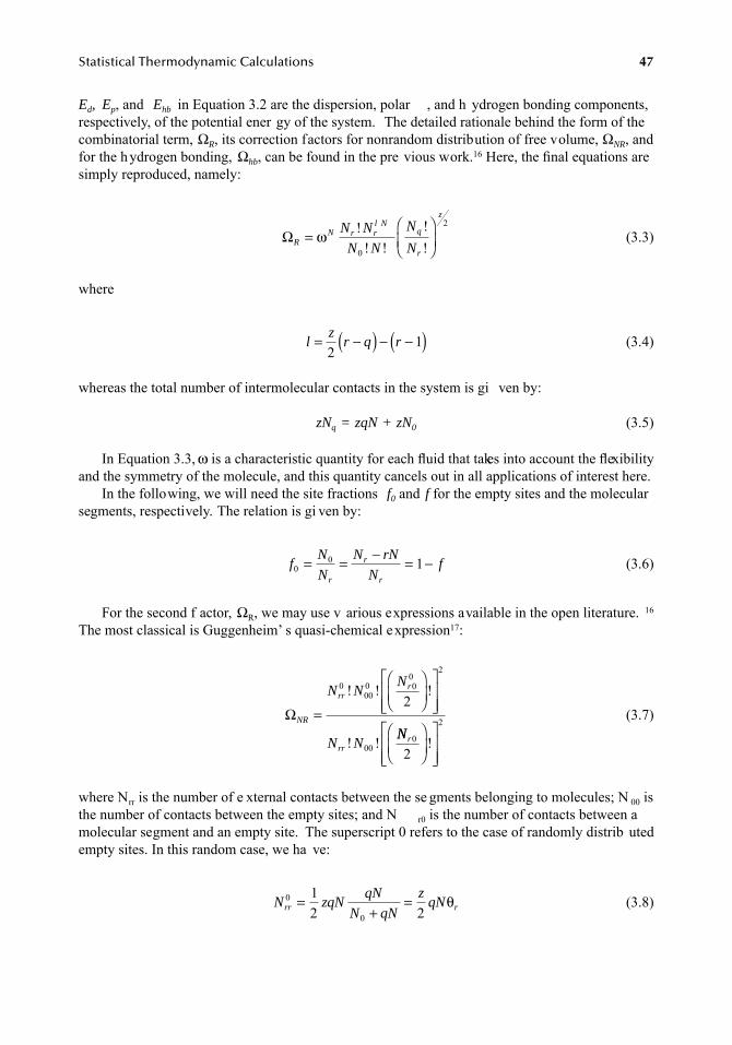
Statistical Thermodynamic Calculations
47
E
d
, E
p
, and
E
hb
in Equation 3.2 are the dispersion, polar , and h ydrogen bonding components,respectively, of the potential ener gy of the system. The detailed rationale behind the form of thecombinatorial term,
Ω
R
, its correction factors for nonrandom distribution of free volume,
Ω
NR
, andfor the hydrogen bonding,
Ω
hb
, can be found in the pre vious work.
16
Here, the final equations aresimply reproduced, namely:
(3.3)
where
(3.4)
whereas the total number of intermolecular contacts in the system is gi ven by:
zN
q
= zqN + zN
0
(3.5)
In Equation 3.3,
ω
is a characteristic quantity for each fluid that takes into account the flexibilityand the symmetry of the molecule, and this quantity cancels out in all applications of interest here.
In the following, we will need the site fractions
f
0
and
f
for the empty sites and the molecularsegments, respectively. The relation is gi ven by:
(3.6)
For the second f actor,
Ω
R
, we may use v arious expressions available in the open literature.
16
The most classical is Guggenheim’ s quasi-chemical expression
17
:
(3.7)
where N
rr
is the number of e xternal contacts between the se gments belonging to molecules; N
00
isthe number of contacts between the empty sites; and N
r0
is the number of contacts between amolecular segment and an empty site. The superscript 0 refers to the case of randomly distrib utedempty sites. In this random case, we ha ve:
(3.8)
ΩRN r r
l Nq
r
z
N N
N N
N
N=
⎛
⎝⎜⎞
⎠⎟ω !
! !!!0
2
lz
r q r= −( ) − −( )21
fN
N
N rN
Nf
r
r
r0
0 1= = − = −
ΩNR
rrr
rr
N NN
N N
=
⎛
⎝⎜⎞
⎠⎟⎡
⎣⎢⎢
⎤
⎦⎥⎥
0000 0
02
00
2! ! !
! ! NNr0
2
2⎛
⎝⎜⎞
⎠⎟⎡
⎣⎢⎢
⎤
⎦⎥⎥
!
N zqNqN
N qN
zqNrr r
0
0
12 2
=+
= θ
7248_book.fm Page 47 Tuesday, April 24, 2007 9:19 AM
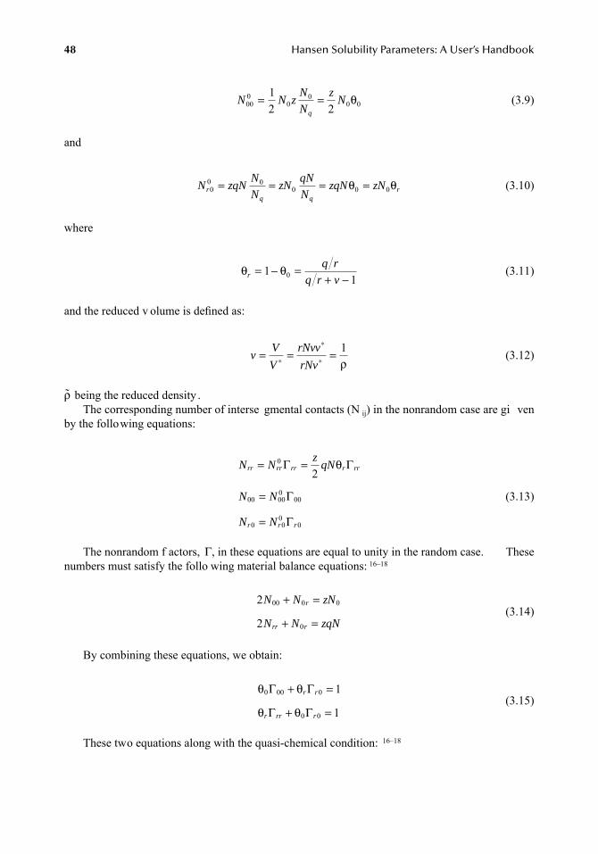
48
Hansen Solubility Parameters: A User’s Handbook
(3.9)
and
(3.10)
where
(3.11)
and the reduced v olume is defined as:
(3.12)
ρ
˜ being the reduced density .The corresponding number of interse gmental contacts (N
ij
) in the nonrandom case are gi venby the following equations:
(3.13)
The nonrandom f actors,
Γ
, in these equations are equal to unity in the random case. Thesenumbers must satisfy the follo wing material balance equations:
16–18
(3.14)
By combining these equations, we obtain:
(3.15)
These two equations along with the quasi-chemical condition:
16–18
N N zN
N
zN
q000
00
0 012 2
= = θ
N zqNN
NzN
qN
NzqN zNr
q qr0
0 00 0 0= = = =θ θ
θ θr
q r
q r v= − =
+ −1
10
vV
V
rNvv
rNv= = =∗
∗
∗
1ρ
N Nz
qN
N N
N N
rr rr rr r rr
r r r
= =
=
=
0
00 000
00
0 00
0
2Γ Γ
Γ
Γ
θ
2
2
00 0 0
0
N N zN
N N zqN
r
rr r
+ =
+ =
θ θ
θ θ
0 00 0
0 0
1
1
Γ Γ
Γ Γ
+ =
+ =
r r
r rr r
7248_book.fm Page 48 Tuesday, April 24, 2007 9:19 AM
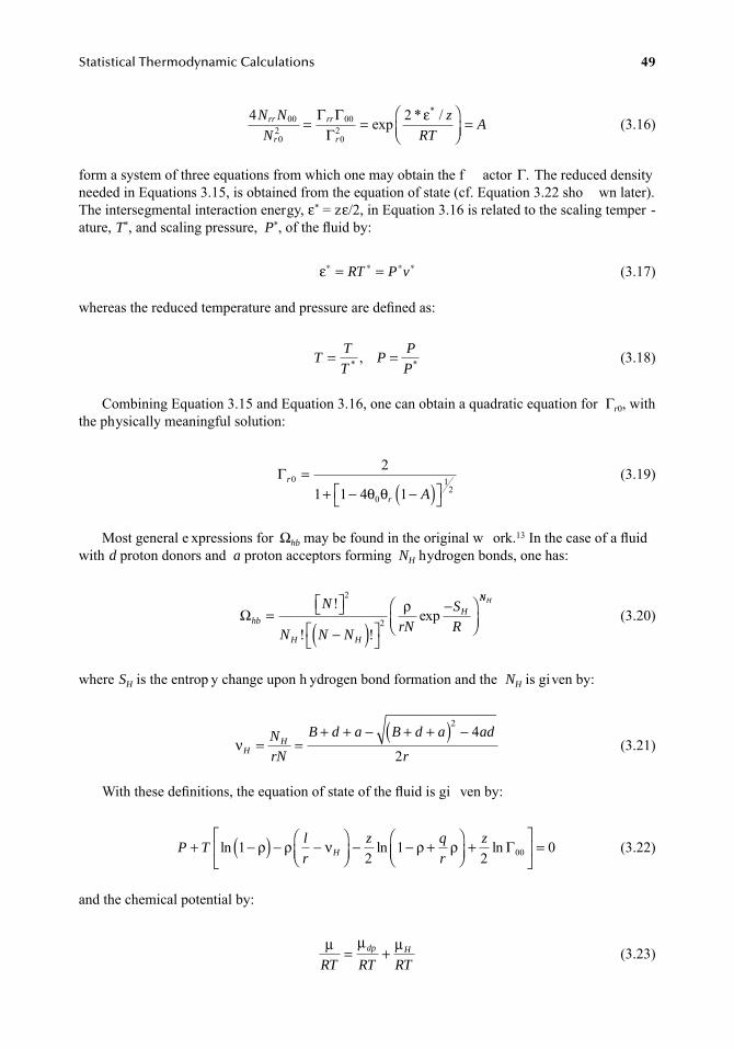
Statistical Thermodynamic Calculations
49
(3.16)
form a system of three equations from which one may obtain the f actor
Γ
. The reduced densityneeded in Equations 3.15, is obtained from the equation of state (cf. Equation 3.22 sho wn later).The intersegmental interaction energy,
ε
*
= z
ε
/2, in Equation 3.16 is related to the scaling temper -ature,
T
*
, and scaling pressure,
P
*
, of the fluid by:
(3.17)
whereas the reduced temperature and pressure are defined as:
(3.18)
Combining Equation 3.15 and Equation 3.16, one can obtain a quadratic equation for
Γ
r
0
, withthe physically meaningful solution:
(3.19)
Most general e xpressions for
Ω
hb
may be found in the original w ork.
13
In the case of a fluidwith
d
proton donors and
a
proton acceptors forming
N
H
hydrogen bonds, one has:
(3.20)
where
S
H
is the entrop y change upon h ydrogen bond formation and the
N
H
is given by:
(3.21)
With these definitions, the equation of state of the fluid is gi ven by:
(3.22)
and the chemical potential by:
(3.23)
4 200
02
00
02
N N
N
z
RTArr
r
rr
r
= =⎛⎝⎜
⎞⎠⎟
=Γ ΓΓ
exp * /*ε
ε∗ ∗ ∗ ∗= =RT P v
TT
TP
P
P= =* *,
Γr
r A0
0
12
2
1 1 4 1=
+ − −( )⎡⎣ ⎤⎦θ θ
Ωhb
H H
HN
N N NrN
S
R=
⎡⎣ ⎤⎦
−( )⎡⎣
⎤⎦
−⎛⎝⎜
⎞⎠⎟
!
! !exp
2
2
ρNNH
νHHN
rN
B d a B d a ad
r= =
+ + − + +( ) −2
4
2
P Tl
r
z q
rH+ −( ) − −⎛⎝⎜
⎞⎠⎟
− − +⎛⎝
ln ln12
1ρ ρ ν ρ ρ⎜⎜⎞⎠⎟
+⎡
⎣⎢
⎤
⎦⎥ =z
2000ln Γ
μ μ μRT RT RT
dp H= +
7248_book.fm Page 49 Tuesday, April 24, 2007 9:19 AM
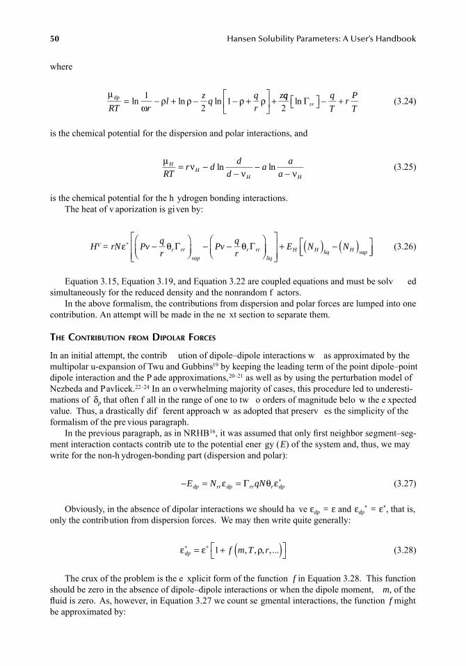
50 Hansen Solubility Parameters: A User’s Handbook
where
(3.24)
is the chemical potential for the dispersion and polar interactions, and
(3.25)
is the chemical potential for the h ydrogen bonding interactions.The heat of v aporization is given by:
HV = (3.26)
Equation 3.15, Equation 3.19, and Equation 3.22 are coupled equations and must be solv edsimultaneously for the reduced density and the nonrandom f actors.
In the above formalism, the contributions from dispersion and polar forces are lumped into onecontribution. An attempt will be made in the ne xt section to separate them.
THE CONTRIBUTION FROM DIPOLAR FORCES
In an initial attempt, the contrib ution of dipole–dipole interactions w as approximated by themultipolar u-expansion of Twu and Gubbins19 by keeping the leading term of the point dipole–pointdipole interaction and the P ade approximations,20–21 as well as by using the perturbation model ofNezbeda and Pavlicek.22–24 In an o verwhelming majority of cases, this procedure led to underesti-mations of δp that often f all in the range of one to tw o orders of magnitude belo w the e xpectedvalue. Thus, a drastically dif ferent approach w as adopted that preserv es the simplicity of theformalism of the pre vious paragraph.
In the previous paragraph, as in NRHB16, it was assumed that only first neighbor segment–seg-ment interaction contacts contrib ute to the potential ener gy (E) of the system and, thus, we maywrite for the non-h ydrogen-bonding part (dispersion and polar):
(3.27)
Obviously, in the absence of dipolar interactions we should ha ve εdp = ε and εdp* = ε*, that is,
only the contribution from dispersion forces. We may then write quite generally:
(3.28)
The crux of the problem is the e xplicit form of the function f in Equation 3.28. This functionshould be zero in the absence of dipole–dipole interactions or when the dipole moment, m, of thefluid is zero. As, however, in Equation 3.27 we count se gmental interactions, the function f mightbe approximated by:
μω
ρ ρ ρ ρdp
RT rl
zq
q
r
z= − + − − +⎡
⎣⎢
⎤
⎦⎥ +ln ln ln1
21 qq q
Tr
P
Trr2
ln Γ⎡⎣ ⎤⎦ − +
μ νν ν
HH
H HRTr d
d
da
a
a= −
−−
−ln ln
rN Pvq
rPv
q
rr rr
vap
r rrε θ θ∗ −⎛⎝⎜
⎞⎠⎟
− −⎛⎝⎜
⎞⎠
Γ Γ ⎟⎟⎡
⎣⎢⎢
⎤
⎦⎥⎥
+ ( ) − ( )⎡⎣⎢
⎤⎦⎥
liq
H H liq H vapE N N
− = = ∗E N qNdp rr dp rr r dpε θ εΓ
ε ε ρdp f m T r∗ ∗= + ( )⎡⎣
⎤⎦1 , , , ,...
7248_book.fm Page 50 Tuesday, April 24, 2007 9:19 AM
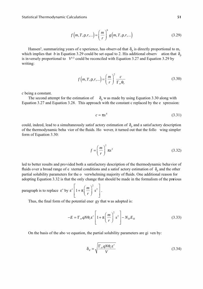
Statistical Thermodynamic Calculations 51
(3.29)
Hansen5, summarizing years of e xperience, has observed that δp is directly proportional to m,which implies that b in Equation 3.29 could be set equal to 2. His additional observ ation that δp
is in versely proportional to V1/2 could be reconciled with Equation 3.27 and Equation 3.29 bywriting:
(3.30)
c being a constant.The second attempt for the estimation of δp w as made by using Equation 3.30 along with
Equation 3.27 and Equation 3.28. This approach with the constant c replaced by the e xpression:
(3.31)
could, indeed, lead to a simultaneously satisf actory estimation of δp and a satisf actory descriptionof the thermodynamic beha vior of the fluids. Ho wever, it turned out that the follo wing simplerform of Equation 3.30:
(3.32)
led to better results and provided both a satisfactory description of the thermodynamic behavior offluids over a broad range of e xternal conditions and a satisf actory estimation of δp and the otherpartial solubility parameters for the o verwhelming majority of fluids. One additional reason foradopting Equation 3.32 is that the only change that should be made in the formalism of the previous
paragraph is to replace ε* by .
Thus, the final form of the potential ener gy that was adopted is:
(3.33)
On the basis of the abo ve equation, the partial solubility parameters are gi ven by:
(3.34)
f m T rm
rg m T r
b
, , , ,... , , , ,...ρ ρ( ) =⎛⎝⎜
⎞⎠⎟ ( )
f m T rm
r
c
rr r
, , , ,...ρθ( ) =
⎛⎝⎜
⎞⎠⎟
2
Γ
c s= π 4
fm
rs=
⎛⎝⎜
⎞⎠⎟
22π
ε π∗ +⎛⎝⎜
⎞⎠⎟
⎡
⎣⎢⎢
⎤
⎦⎥⎥
12
2m
rs
− = +⎛⎝⎜
⎞⎠⎟
⎡
⎣⎢⎢
⎤
⎦⎥⎥
−∗E qNm
rs N Err r H HΓ θ ε π1
22
δ θ εd
rr rqN
V=
∗Γ
7248_book.fm Page 51 Tuesday, April 24, 2007 9:19 AM
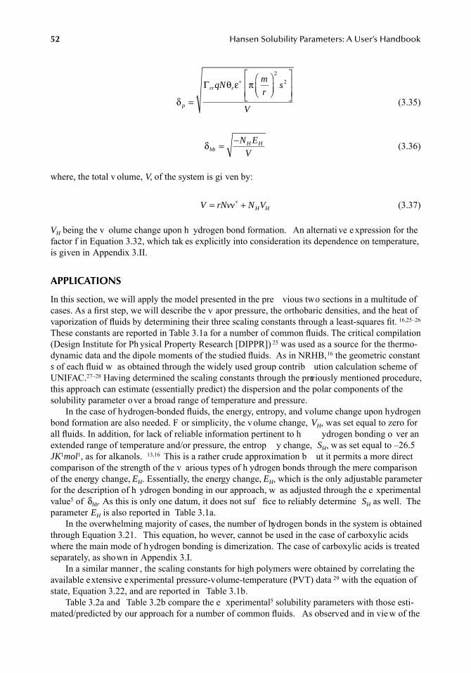
52 Hansen Solubility Parameters: A User’s Handbook
(3.35)
(3.36)
where, the total v olume, V, of the system is gi ven by:
(3.37)
VH being the v olume change upon h ydrogen bond formation. An alternati ve e xpression for thefactor f in Equation 3.32, which tak es explicitly into consideration its dependence on temperature,is given in Appendix 3.II.
APPLICATIONS
In this section, we will apply the model presented in the pre vious two sections in a multitude ofcases. As a first step, we will describe the v apor pressure, the orthobaric densities, and the heat ofvaporization of fluids by determining their three scaling constants through a least-squares fit. 16,25–26
These constants are reported in Table 3.1a for a number of common fluids. The critical compilation(Design Institute for Ph ysical Property Research [DIPPR]) 25 was used as a source for the thermo-dynamic data and the dipole moments of the studied fluids. As in NRHB,16 the geometric constants of each fluid w as obtained through the widely used group contrib ution calculation scheme ofUNIFAC.27–28 Having determined the scaling constants through the previously mentioned procedure,this approach can estimate (essentially predict) the dispersion and the polar components of thesolubility parameter over a broad range of temperature and pressure.
In the case of hydrogen-bonded fluids, the energy, entropy, and volume change upon hydrogenbond formation are also needed. F or simplicity, the volume change, VH, was set equal to zero forall fluids. In addition, for lack of reliable information pertinent to h ydrogen bonding o ver anextended range of temperature and/or pressure, the entrop y change, SH, w as set equal to –26.5JK1mol1, as for alkanols. 13,16 This is a rather crude approximation b ut it permits a more directcomparison of the strength of the v arious types of h ydrogen bonds through the mere comparisonof the energy change, EH. Essentially, the energy change, EH, which is the only adjustable parameterfor the description of h ydrogen bonding in our approach, w as adjusted through the e xperimentalvalue5 of δhb. As this is only one datum, it does not suf fice to reliably determine SH as well. Theparameter EH is also reported in Table 3.1a.
In the overwhelming majority of cases, the number of hydrogen bonds in the system is obtainedthrough Equation 3.21. This equation, ho wever, cannot be used in the case of carboxylic acidswhere the main mode of hydrogen bonding is dimerization. The case of carboxylic acids is treatedseparately, as shown in Appendix 3.I.
In a similar manner , the scaling constants for high polymers were obtained by correlating theavailable extensive experimental pressure-volume-temperature (PVT) data 29 with the equation ofstate, Equation 3.22, and are reported in Table 3.1b.
Table 3.2a and Table 3.2b compare the e xperimental5 solubility parameters with those esti-mated/predicted by our approach for a number of common fluids. As observed and in vie w of the
δ
θ ε π
p
rr rqNm
rs
V=
⎛⎝⎜
⎞⎠⎟
⎡
⎣⎢⎢
⎤
⎦⎥⎥
∗Γ2
2
δhbH HN E
V= −
V rNvv N VH H= +∗
7248_book.fm Page 52 Tuesday, April 24, 2007 9:19 AM
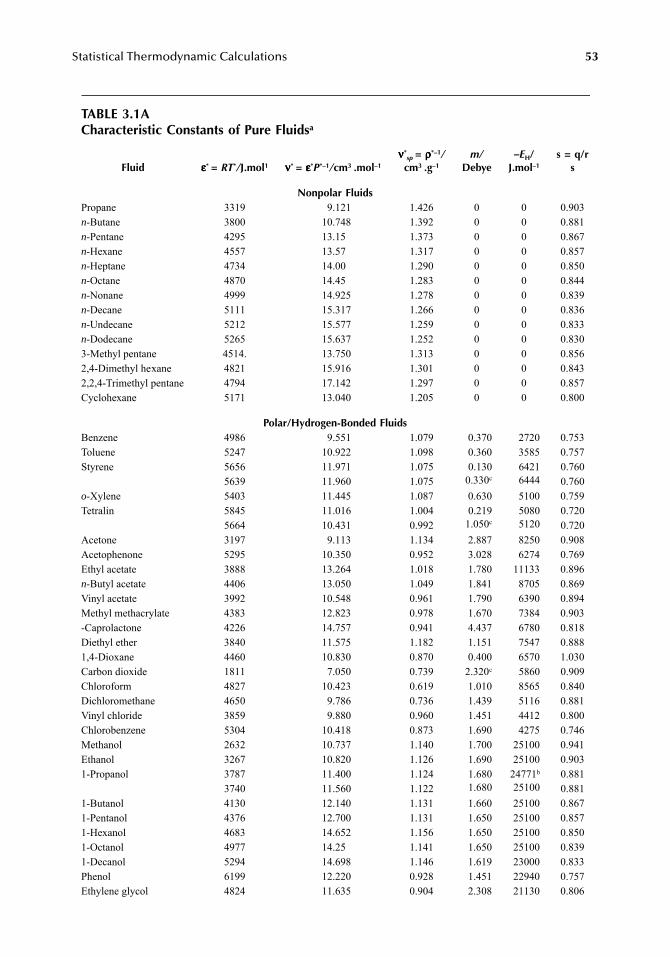
Statistical Thermodynamic Calculations 53
TABLE 3.1ACharacteristic Constants of Pure Fluidsa
Fluid εεεε* = RT*/J.mol1 νννν* = εεεε*P*–1/cm3 .mol–1
νννν*sp = ρρρρ*–1/cm3 .g–1
m/Debye
–EH/J.mol–1
s = q/rs
Nonpolar FluidsPropane 3319 9.121 1.426 0 0 0.903n-Butane 3800 10.748 1.392 0 0 0.881n-Pentane 4295 13.15 1.373 0 0 0.867n-Hexane 4557 13.57 1.317 0 0 0.857n-Heptane 4734 14.00 1.290 0 0 0.850n-Octane 4870 14.45 1.283 0 0 0.844n-Nonane 4999 14.925 1.278 0 0 0.839n-Decane 5111 15.317 1.266 0 0 0.836n-Undecane 5212 15.577 1.259 0 0 0.833n-Dodecane 5265 15.637 1.252 0 0 0.8303-Methyl pentane 4514. 13.750 1.313 0 0 0.8562,4-Dimethyl hexane 4821 15.916 1.301 0 0 0.8432,2,4-Trimethyl pentane 4794 17.142 1.297 0 0 0.857Cyclohexane 5171 13.040 1.205 0 0 0.800
Polar/Hydrogen-Bonded FluidsBenzene 4986 9.551 1.079 0.370 2720 0.753Toluene 5247 10.922 1.098 0.360 3585 0.757Styrene 5656
563911.97111.960
1.0751.075
0.1300.330c
64216444
0.7600.760
o-Xylene 5403 11.445 1.087 0.630 5100 0.759Tetralin 5845
566411.01610.431
1.0040.992
0.2191.050c
50805120
0.7200.720
Acetone 3197 9.113 1.134 2.887 8250 0.908Acetophenone 5295 10.350 0.952 3.028 6274 0.769Ethyl acetate 3888 13.264 1.018 1.780 11133 0.896n-Butyl acetate 4406 13.050 1.049 1.841 8705 0.869Vinyl acetate 3992 10.548 0.961 1.790 6390 0.894Methyl methacrylate 4383 12.823 0.978 1.670 7384 0.903-Caprolactone 4226 14.757 0.941 4.437 6780 0.818Diethyl ether 3840 11.575 1.182 1.151 7547 0.8881,4-Dioxane 4460 10.830 0.870 0.400 6570 1.030Carbon dioxide 1811 7.050 0.739 2.320c 5860 0.909Chloroform 4827 10.423 0.619 1.010 8565 0.840Dichloromethane 4650 9.786 0.736 1.439 5116 0.881Vinyl chloride 3859 9.880 0.960 1.451 4412 0.800Chlorobenzene 5304 10.418 0.873 1.690 4275 0.746Methanol 2632 10.737 1.140 1.700 25100 0.941Ethanol 3267 10.820 1.126 1.690 25100 0.9031-Propanol 3787
374011.40011.560
1.1241.122
1.6801.680
24771b
251000.8810.881
1-Butanol 4130 12.140 1.131 1.660 25100 0.8671-Pentanol 4376 12.700 1.131 1.650 25100 0.8571-Hexanol 4683 14.652 1.156 1.650 25100 0.8501-Octanol 4977 14.25 1.141 1.650 25100 0.8391-Decanol 5294 14.698 1.146 1.619 23000 0.833Phenol 6199 12.220 0.928 1.451 22940 0.757Ethylene glycol 4824 11.635 0.904 2.308 21130 0.806
7248_book.fm Page 53 Tuesday, April 24, 2007 9:19 AM
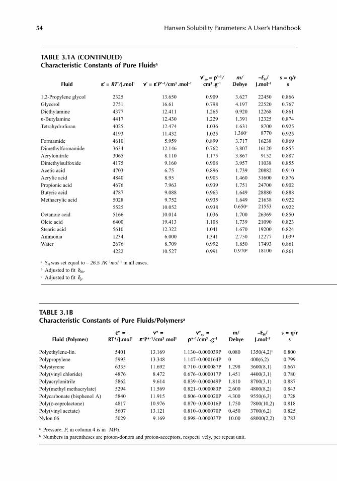
54 Hansen Solubility Parameters: A User’s Handbook
TABLE 3.1A (CONTINUED)Characteristic Constants of Pure Fluidsa
Fluid εεεε* = RT*/J.mol1 νννν* = εεεε*P*–1/cm3 .mol–1
νννν*sp = ρρρρ*–1/cm3 .g–1
m/Debye
–EH/J.mol–1
s = q/rs
1,2-Propylene glycol 2325 13.650 0.909 3.627 22450 0.866Glycerol 2751 16.61 0.798 4.197 22520 0.767Diethylamine 4377 12.411 1.265 0.920 12268 0.861n-Butylamine 4417 12.430 1.229 1.391 12325 0.874Tetrahydrofuran 4025
419312.47411.432
1.0361.025
1.6311.360c
87008770
0.9250.925
Formamide 4610 5.959 0.899 3.717 16238 0.869Dimethylformamide 3634 12.146 0.762 3.807 16120 0.855Acrylonitrile 3065 8.110 1.175 3.867 9152 0.887Dimethylsulfoxide 4175 9.160 0.908 3.957 11038 0.855Acetic acid 4703 6.75 0.896 1.739 20882 0.910Acrylic acid 4840 8.95 0.903 1.460 31600 0.876Propionic acid 4676 7.963 0.939 1.751 24700 0.902Butyric acid 4787 9.088 0.963 1.649 28880 0.888Methacrylic acid 5028
55259.752
10.0520.9350.938
1.6490.650c
2163821553
0.9220.922
Octanoic acid 5166 10.014 1.036 1.700 26369 0.850Oleic acid 6400 19.413 1.108 1.739 21090 0.823Stearic acid 5610 12.322 1.041 1.670 19200 0.824Ammonia 1234 6.000 1.341 2.750 12277 1.039Water 2676
42228.709
10.5270.9920.991
1.8500.970c
1749318100
0.8610.861
a SH was set equal to – 26.5 JK–1mol–1 in all cases.b Adjusted to fit δhb.c Adjusted to fit δp.
TABLE 3.1BCharacteristic Constants of Pure Fluids/Polymersa
Fluid (Polymer)εεεε* =
RT*/J.mol1νννν* =
εεεε*P*–1/cm3 mol1νννν*sp =
ρρρρ*–1/cm3 .g–1
m/Debye
–EH/J.mol–1
s = q/rs
Polyethylene-lin. 5401 13.169 1.130–0.000039P 0.080 1350(4,2)b 0.800Polypropylene 5993 13.348 1.147–0.000164P 0 400(6,2) 0.799Polystyrene 6335 11.692 0.710–0.000087P 1.298 3600(8,1) 0.667Poly(vinyl chloride) 4876 8.472 0.676–0.000017P 1.451 4400(3,1) 0.780Polyacrylonitrile 5862 9.614 0.839–0.000049P 1.810 8700(3,1) 0.887Poly(methyl methacrylate) 5294 11.569 0.821–0.000083P 2.600 4800(8,2) 0.843Polycarbonate (bisphenol A) 5840 11.915 0.806–0.000020P 4.300 9550(6,3) 0.728Poly(ε-caprolactone) 4817 10.976 0.870–0.000016P 1.750 7800(10,2) 0.818Poly(vinyl acetate) 5607 13.121 0.810–0.000070P 0.450 3700(6,2) 0.825Nylon 66 5029 9.169 0.898–0.000037P 10.00 68000(2,2) 0.783
a Pressure, P, in column 4 is in MPa.b Numbers in parentheses are proton-donors and proton-acceptors, respecti vely, per repeat unit.
7248_book.fm Page 54 Tuesday, April 24, 2007 9:19 AM

Statistical Thermodynamic Calculations 55
TABLE 3.2ATotal and Partial Solubility Parameters (in MPa1/2) of Pure Fluids
Fluid
δδδδ Total δδδδ HB δδδδ P
Exp5 Calc Exp5 Exp5 Calc
Nonpolar FluidsPropane 13.10 12.85 0 0 0 0n-Butane 14.10 14.10 0 0 0 0n-Pentane 14.40 14.34 0 0 0 0n-Hexane 14.90 14.58 0 0 0 0n-Heptane 15.20 15.12 0 0 0 0n-Octane 15.40 15.21 0 0 0 0n-Nonane 15.60 15.25 0 0 0 0n-Decane 15.70 15.30 0 0 0 0n-Undecane 15.80 15.40 0 0 0 0n-Dodecane 15.90 15.52 0 0 0 03-Methyl pentane 14.67 14.65 0 0 0 02,4-Dimethyl hexane 14.65 14.39 0 0 0 02,2,4-Trimethyl pentane 14.08 13.90 0 0 0 0Cyclohexane 16.76 16.30 0 0 0 0
Polar/Hydrogen-Bonded FluidsBenzene 18.41 18.27 2.05 2.05 1.02 1.01Toluene 18.32 17.78 2.00 2.00 1.40 0.92Styrene 19.07
19.0718.2918.30
4.104.10
4.044.05
1.001.00
0.331.00
o-Xylene 18.20 18.01 3.10 3.10 1.00 1.48Tetralin 19.80
19.8018.8019.07
2.902.90
2.902.90
2.002.00
0.432.00
Acetone 19.95 20.04 6.95 7.00 10.43 10.14Acetophenone 21.73 20.48 3.68 3.68 8.59 7.04Ethyl acetate 18.48 18.31 9.20 9.33 5.85 6.07n-Butyl acetate 17.59 17.43 6.30 6.30 3.70 4.70Vinyl acetate 18.58 18.33 5.90 5.90 7.20 5.90Methyl methacrylate 17.92 17.77 5.40 5.40 6.50 5.60ε-Caprolactone 21.41 21.28 7.40 7.40 15.0 13.22Diethyl ether 15.66 15.73 5.11 5.12 2.86 3.481,4-Dioxane 20.47 20.08 7.36 7.36 1.84 1.91Carbon dioxide 14.56 11.64 4.10 4.09 6.90 6.86Chloroform 18.94 19.18 5.73 5.74 3.07 3.79Dichloromethane 20.79 19.92 4.09 4.09 7.36 5.63Vinyl chloride 17.77 16.00 2.40 2.40 6.50 5.07Chlorobenzene 19.61 18.91 2.05 2.05 4.30 4.33Methanol 29.61 29.89 22.30 24.08 12.27 11.34Ethanol 26.13 26.08 19.43 19.98 8.80 8.241-Propanol 24.45
24.4524.1924.17
17.4017.40
17.4117.58
6.806.80
6.796.79
1-Butanol 23.35 22.90 15.80 15.80 5.70 5.721-Pentanol 21.65 21.95 13.91 14.52 4.50 4.991-Octanol 20.87 20.27 11.86 11.94 3.27 3.751-Decanol 20.32 19.37 10.00 10.03 2.60 3.15Phenol 24.63 24.69 14.90 14.95 5.90 5.16Ethylene glycol 33.70 33.64 25.77 25.74 11.05 12.231,2-Propylene glycol 29.52 29.19 23.32 23.73 9.41 12.56
7248_book.fm Page 55 Tuesday, April 24, 2007 9:19 AM
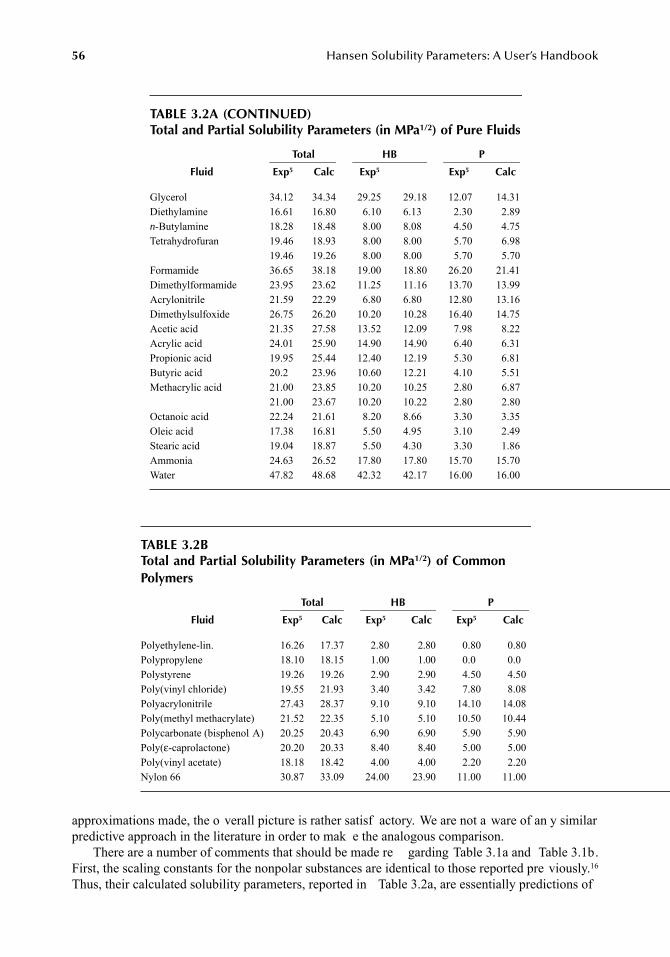
56 Hansen Solubility Parameters: A User’s Handbook
approximations made, the o verall picture is rather satisf actory. We are not a ware of an y similarpredictive approach in the literature in order to mak e the analogous comparison.
There are a number of comments that should be made re garding Table 3.1a and Table 3.1b.First, the scaling constants for the nonpolar substances are identical to those reported pre viously.16
Thus, their calculated solubility parameters, reported in Table 3.2a, are essentially predictions of
TABLE 3.2A (CONTINUED)Total and Partial Solubility Parameters (in MPa1/2) of Pure Fluids
Fluid
Total HB P
Exp5 Calc Exp5 Exp5 Calc
Glycerol 34.12 34.34 29.25 29.18 12.07 14.31Diethylamine 16.61 16.80 6.10 6.13 2.30 2.89n-Butylamine 18.28 18.48 8.00 8.08 4.50 4.75Tetrahydrofuran 19.46
19.4618.9319.26
8.008.00
8.008.00
5.705.70
6.985.70
Formamide 36.65 38.18 19.00 18.80 26.20 21.41Dimethylformamide 23.95 23.62 11.25 11.16 13.70 13.99Acrylonitrile 21.59 22.29 6.80 6.80 12.80 13.16Dimethylsulfoxide 26.75 26.20 10.20 10.28 16.40 14.75Acetic acid 21.35 27.58 13.52 12.09 7.98 8.22Acrylic acid 24.01 25.90 14.90 14.90 6.40 6.31Propionic acid 19.95 25.44 12.40 12.19 5.30 6.81Butyric acid 20.2 23.96 10.60 12.21 4.10 5.51Methacrylic acid 21.00
21.0023.8523.67
10.2010.20
10.2510.22
2.802.80
6.872.80
Octanoic acid 22.24 21.61 8.20 8.66 3.30 3.35Oleic acid 17.38 16.81 5.50 4.95 3.10 2.49Stearic acid 19.04 18.87 5.50 4.30 3.30 1.86Ammonia 24.63 26.52 17.80 17.80 15.70 15.70Water 47.82 48.68 42.32 42.17 16.00 16.00
TABLE 3.2BTotal and Partial Solubility Parameters (in MPa1/2) of Common Polymers
Fluid
Total HB P
Exp5 Calc Exp5 Calc Exp5 Calc
Polyethylene-lin. 16.26 17.37 2.80 2.80 0.80 0.80Polypropylene 18.10 18.15 1.00 1.00 0.0 0.0Polystyrene 19.26 19.26 2.90 2.90 4.50 4.50Poly(vinyl chloride) 19.55 21.93 3.40 3.42 7.80 8.08Polyacrylonitrile 27.43 28.37 9.10 9.10 14.10 14.08Poly(methyl methacrylate) 21.52 22.35 5.10 5.10 10.50 10.44Polycarbonate (bisphenol A) 20.25 20.43 6.90 6.90 5.90 5.90Poly(ε-caprolactone) 20.20 20.33 8.40 8.40 5.00 5.00Poly(vinyl acetate) 18.18 18.42 4.00 4.00 2.20 2.20Nylon 66 30.87 33.09 24.00 23.90 11.00 11.00
7248_book.fm Page 56 Tuesday, April 24, 2007 9:19 AM
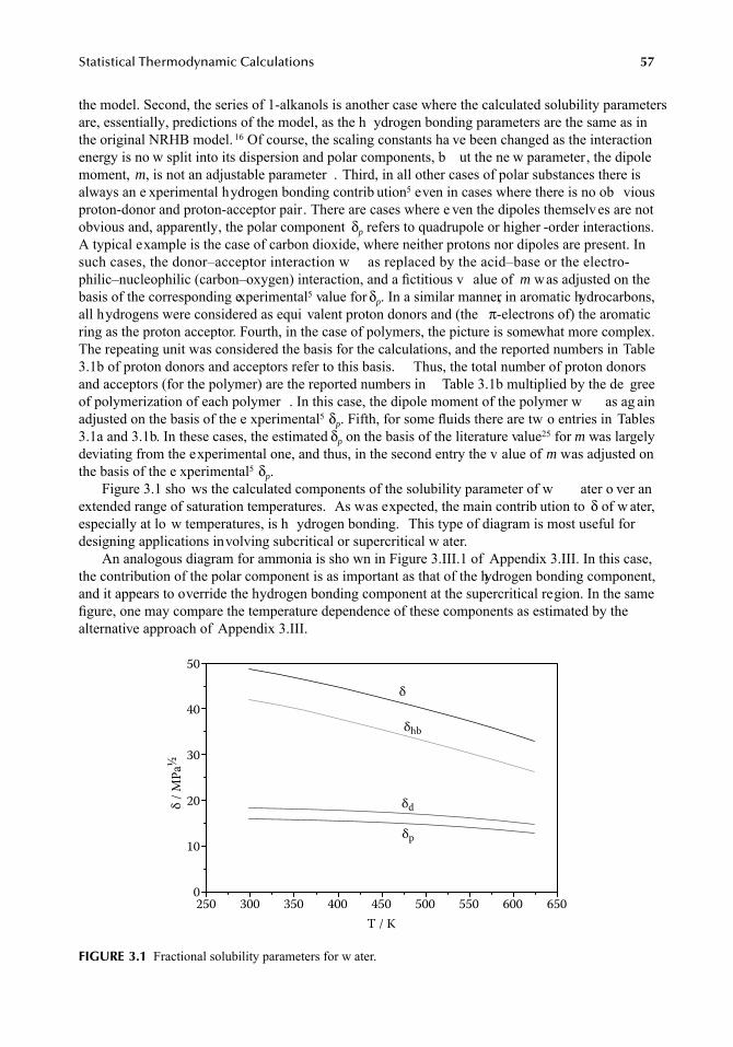
Statistical Thermodynamic Calculations 57
the model. Second, the series of 1-alkanols is another case where the calculated solubility parametersare, essentially, predictions of the model, as the h ydrogen bonding parameters are the same as inthe original NRHB model. 16 Of course, the scaling constants ha ve been changed as the interactionenergy is no w split into its dispersion and polar components, b ut the ne w parameter, the dipolemoment, m, is not an adjustable parameter . Third, in all other cases of polar substances there isalways an e xperimental hydrogen bonding contrib ution5 even in cases where there is no ob viousproton-donor and proton-acceptor pair. There are cases where e ven the dipoles themselves are notobvious and, apparently, the polar component δp refers to quadrupole or higher -order interactions.A typical example is the case of carbon dioxide, where neither protons nor dipoles are present. Insuch cases, the donor–acceptor interaction w as replaced by the acid–base or the electro-philic–nucleophilic (carbon–oxygen) interaction, and a fictitious v alue of m was adjusted on thebasis of the corresponding experimental5 value for δp. In a similar manner, in aromatic hydrocarbons,all hydrogens were considered as equi valent proton donors and (the π-electrons of) the aromaticring as the proton acceptor. Fourth, in the case of polymers, the picture is somewhat more complex.The repeating unit was considered the basis for the calculations, and the reported numbers in Table3.1b of proton donors and acceptors refer to this basis. Thus, the total number of proton donorsand acceptors (for the polymer) are the reported numbers in Table 3.1b multiplied by the de greeof polymerization of each polymer . In this case, the dipole moment of the polymer w as ag ainadjusted on the basis of the e xperimental5 δp. Fifth, for some fluids there are tw o entries in Tables3.1a and 3.1b. In these cases, the estimated δp on the basis of the literature value25 for m was largelydeviating from the experimental one, and thus, in the second entry the v alue of m was adjusted onthe basis of the e xperimental5 δp.
Figure 3.1 sho ws the calculated components of the solubility parameter of w ater o ver anextended range of saturation temperatures. As was expected, the main contrib ution to δ of w ater,especially at lo w temperatures, is h ydrogen bonding. This type of diagram is most useful fordesigning applications involving subcritical or supercritical w ater.
An analogous diagram for ammonia is sho wn in Figure 3.III.1 of Appendix 3.III. In this case,the contribution of the polar component is as important as that of the hydrogen bonding component,and it appears to override the hydrogen bonding component at the supercritical region. In the samefigure, one may compare the temperature dependence of these components as estimated by thealternative approach of Appendix 3.III.
FIGURE 3.1 Fractional solubility parameters for w ater.
250
50
40
30
20
10
0300 350 400 450
T / K
500 550 600 650
δhb
δd
δp
δ
δ /
MP
a½
7248_book.fm Page 57 Tuesday, April 24, 2007 9:19 AM
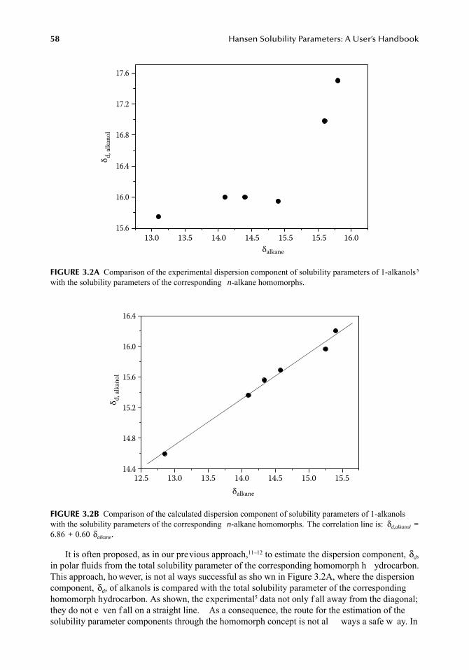
58 Hansen Solubility Parameters: A User’s Handbook
It is often proposed, as in our previous approach,11–12 to estimate the dispersion component, δd,in polar fluids from the total solubility parameter of the corresponding homomorph h ydrocarbon.This approach, ho wever, is not al ways successful as sho wn in Figure 3.2A, where the dispersioncomponent, δd, of alkanols is compared with the total solubility parameter of the correspondinghomomorph hydrocarbon. As shown, the experimental5 data not only f all away from the diagonal;they do not e ven f all on a straight line. As a consequence, the route for the estimation of thesolubility parameter components through the homomorph concept is not al ways a safe w ay. In
FIGURE 3.2A Comparison of the experimental dispersion component of solubility parameters of 1-alkanols5
with the solubility parameters of the corresponding n-alkane homomorphs.
FIGURE 3.2B Comparison of the calculated dispersion component of solubility parameters of 1-alkanolswith the solubility parameters of the corresponding n-alkane homomorphs. The correlation line is: δd,alkanol =6.86 + 0.60 δalkane.
13.0 13.5 14.0 14.5 15.5 15.5 16.0
17.6
17.2
16.8
16.4
16.0
15.6
δalkane
δd
, alk
ano
l
12.5 13.0 13.5 14.0 14.5 15.0 15.5
16.4
16.0
15.6
15.2
14.8
14.4
δalkane
δd
, alk
ano
l
7248_book.fm Page 58 Tuesday, April 24, 2007 9:19 AM
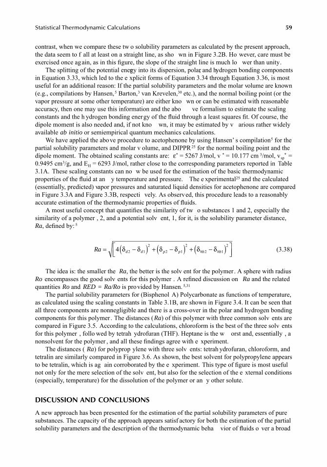
Statistical Thermodynamic Calculations 59
contrast, when we compare these tw o solubility parameters as calculated by the present approach,the data seem to f all at least on a straight line, as sho wn in Figure 3.2B. Ho wever, care must beexercised once again, as in this figure, the slope of the straight line is much lo wer than unity.
The splitting of the potential energy into its dispersion, polar, and hydrogen bonding componentsin Equation 3.33, which led to the e xplicit forms of Equation 3.34 through Equation 3.36, is mostuseful for an additional reason: If the partial solubility parameters and the molar volume are known(e.g., compilations by Hansen,5 Barton,3 van Krevelen,30 etc.), and the normal boiling point (or thevapor pressure at some other temperature) are either kno wn or can be estimated with reasonableaccuracy, then one may use this information and the abo ve formalism to estimate the scalingconstants and the h ydrogen bonding energy of the fluid through a least squares fit. Of course, thedipole moment is also needed and, if not kno wn, it may be estimated by v arious rather widelyavailable ab initio or semiempirical quantum mechanics calculations.
We have applied the above procedure to acetophenone by using Hansen’ s compilation5 for thepartial solubility parameters and molar v olume, and DIPPR25 for the normal boiling point and thedipole moment. The obtained scaling constants are: ε* = 5267 J/mol, v * = 10.177 cm 3/mol, vsp
* =0.9495 cm3/g, and EH = 6293 J/mol, rather close to the corresponding parameters reported in Table3.1A. These scaling constants can no w be used for the estimation of the basic thermodynamicproperties of the fluid at an y temperature and pressure. The e xperimental25 and the calculated(essentially, predicted) vapor pressures and saturated liquid densities for acetophenone are comparedin Figure 3.3A and Figure 3.3B, respecti vely. As observed, this procedure leads to a reasonablyaccurate estimation of the thermodynamic properties of fluids.
A most useful concept that quantifies the similarity of tw o substances 1 and 2, especially thesimilarity of a polymer , 2, and a potential solv ent, 1, for it, is the solubility parameter distance,Ra, defined by: 5
(3.38)
The idea is: the smaller the Ra, the better is the solv ent for the polymer. A sphere with radiusRo encompasses the good solv ents for this polymer . A refined discussion on Ra and the relatedquantities Ro and RED = Ra/Ro is provided by Hansen. 5,31
The partial solubility parameters for (Bisphenol A) Polycarbonate as functions of temperature,as calculated using the scaling constants in Table 3.1B, are shown in Figure 3.4. It can be seen thatall three components are nonnegligible and there is a cross-over in the polar and hydrogen bondingcomponents for this polymer . The distances (Ra) of this polymer with three common solv ents arecompared in Figure 3.5. According to the calculations, chloroform is the best of the three solv entsfor this polymer , follo wed by tetrah ydrofuran (THF). Heptane is the w orst and, essentially , anonsolvent for the polymer , and all these findings agree with e xperiment.
The distances ( Ra) for polyprop ylene with three solv ents: tetrah ydrofuran, chloroform, andtetralin are similarly compared in Figure 3.6. As shown, the best solvent for polypropylene appearsto be tetralin, which is ag ain corroborated by the e xperiment. This type of figure is most usefulnot only for the mere selection of the solv ent, but also for the selection of the e xternal conditions(especially, temperature) for the dissolution of the polymer or an y other solute.
DISCUSSION AND CONCLUSIONS
A new approach has been presented for the estimation of the partial solubility parameters of puresubstances. The capacity of the approach appears satisf actory for both the estimation of the partialsolubility parameters and the description of the thermodynamic beha vior of fluids o ver a broad
Ra d d p p hb hb= −( ) + −( ) + −( )⎡⎣⎢
⎤⎦
4 2 12
2 12
2 12
δ δ δ δ δ δ ⎥⎥
7248_book.fm Page 59 Tuesday, April 24, 2007 9:19 AM
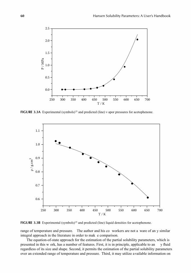
60 Hansen Solubility Parameters: A User’s Handbook
range of temperature and pressure. The author and his co workers are not a ware of an y similarintegral approach in the literature in order to mak e comparison.
The equation-of-state approach for the estimation of the partial solubility parameters, which ispresented in this w ork, has a number of features. First, it is in principle, applicable to an y fluidregardless of its size and shape. Second, it permits the estimation of the partial solubility parametersover an extended range of temperature and pressure. Third, it may utilize available information on
FIGURE 3.3A Experimental (symbols)25 and predicted (line) v apor pressures for acetophenone.
FIGURE 3.3B Experimental (symbols)25 and predicted (line) liquid densities for acetophenone.
250
2.5
2.0
1.5
1.0
0.5
0.0
300 350 400 450T / K
500 550 600 650 700
P /
MP
a
250
1.1
1.0
0.9
0.8
0.7
0.6
300 350 400 450T / K
500 550 600 650 700
ρ /
g.c
m3
7248_book.fm Page 60 Tuesday, April 24, 2007 9:19 AM
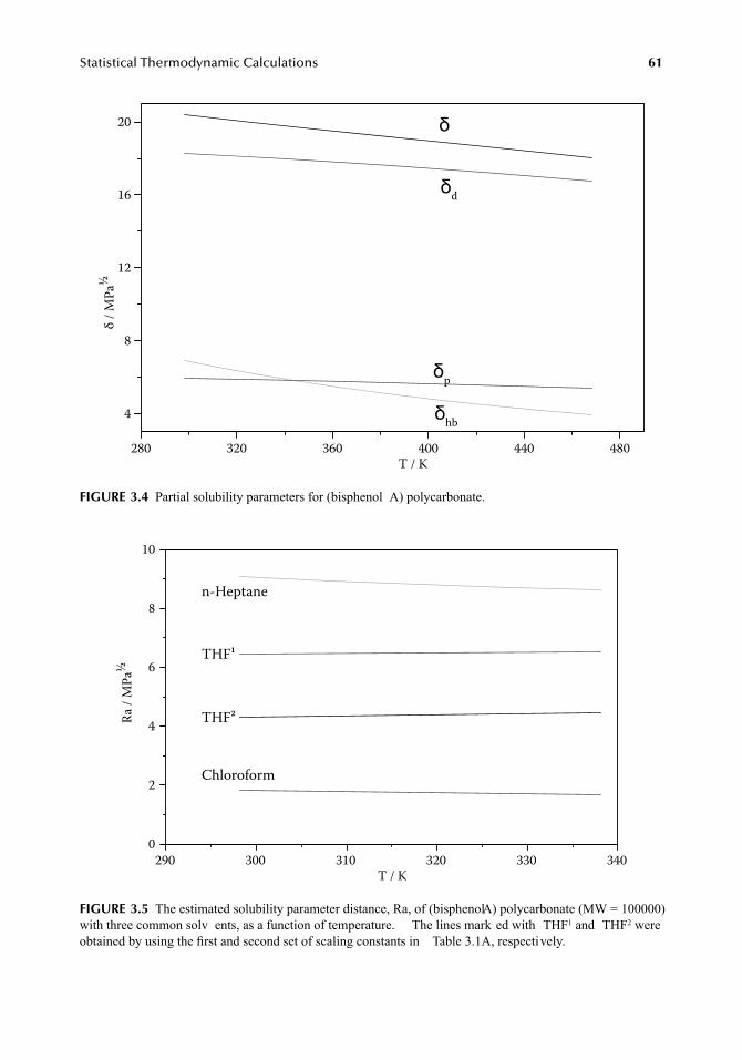
Statistical Thermodynamic Calculations 61
FIGURE 3.4 Partial solubility parameters for (bisphenol A) polycarbonate.
FIGURE 3.5 The estimated solubility parameter distance, Ra, of (bisphenol A) polycarbonate (MW = 100000)with three common solv ents, as a function of temperature. The lines mark ed with THF1 and THF2 wereobtained by using the first and second set of scaling constants in Table 3.1A, respectively.
hb
p
d
280
20
16
12
8
4
320 360 400 440T / K
480
δ /
MP
a½
290
10
8
6
4
2
0
300
n-Heptane
THF¹
THF²
Chloroform
310 320 330T / K
340
Ra
/ M
Pa½
7248_book.fm Page 61 Tuesday, April 24, 2007 9:19 AM
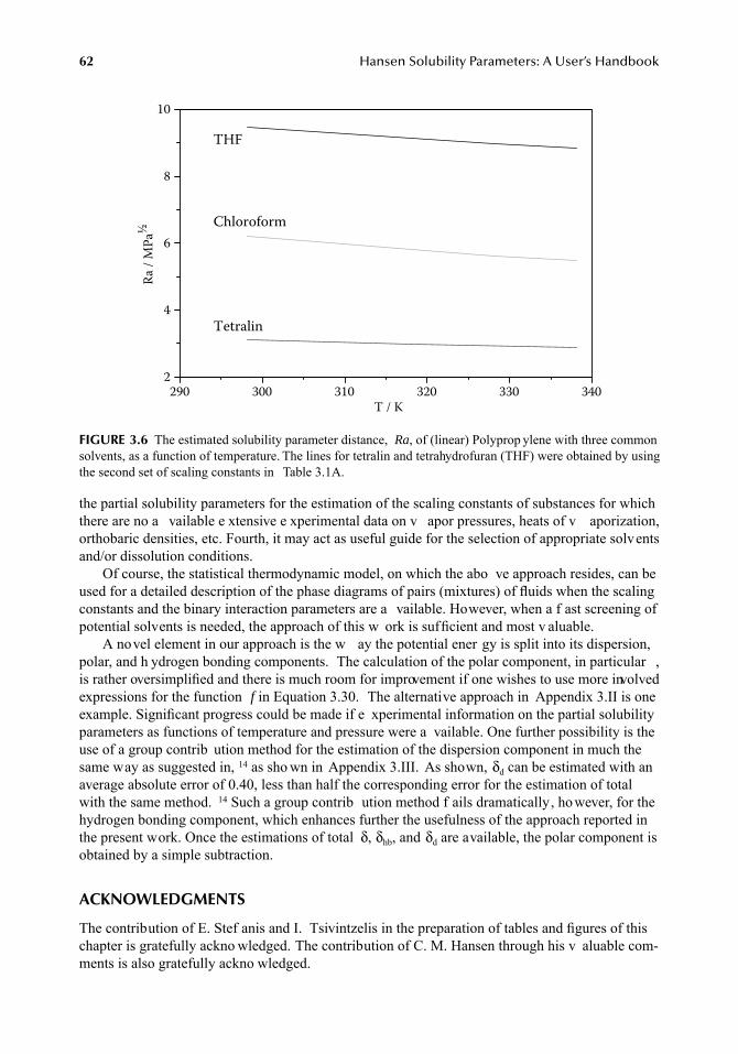
62 Hansen Solubility Parameters: A User’s Handbook
the partial solubility parameters for the estimation of the scaling constants of substances for whichthere are no a vailable e xtensive e xperimental data on v apor pressures, heats of v aporization,orthobaric densities, etc. Fourth, it may act as useful guide for the selection of appropriate solventsand/or dissolution conditions.
Of course, the statistical thermodynamic model, on which the abo ve approach resides, can beused for a detailed description of the phase diagrams of pairs (mixtures) of fluids when the scalingconstants and the binary interaction parameters are a vailable. However, when a f ast screening ofpotential solvents is needed, the approach of this w ork is sufficient and most v aluable.
A novel element in our approach is the w ay the potential ener gy is split into its dispersion,polar, and h ydrogen bonding components. The calculation of the polar component, in particular ,is rather oversimplified and there is much room for improvement if one wishes to use more involvedexpressions for the function f in Equation 3.30. The alternative approach in Appendix 3.II is oneexample. Significant progress could be made if e xperimental information on the partial solubilityparameters as functions of temperature and pressure were a vailable. One further possibility is theuse of a group contrib ution method for the estimation of the dispersion component in much thesame way as suggested in, 14 as sho wn in Appendix 3.III. As shown, δd can be estimated with anaverage absolute error of 0.40, less than half the corresponding error for the estimation of totalwith the same method. 14 Such a group contrib ution method f ails dramatically, however, for thehydrogen bonding component, which enhances further the usefulness of the approach reported inthe present work. Once the estimations of total δ, δhb, and δd are available, the polar component isobtained by a simple subtraction.
ACKNOWLEDGMENTS
The contribution of E. Stef anis and I. Tsivintzelis in the preparation of tables and figures of thischapter is gratefully ackno wledged. The contribution of C. M. Hansen through his v aluable com-ments is also gratefully ackno wledged.
FIGURE 3.6 The estimated solubility parameter distance, Ra, of (linear) Polyprop ylene with three commonsolvents, as a function of temperature. The lines for tetralin and tetrahydrofuran (THF) were obtained by usingthe second set of scaling constants in Table 3.1A.
290
10
8
6
4
2300 310 320 330
T / K340
Ra
/ M
Pa½
Chloroform
Tetralin
THF
7248_book.fm Page 62 Tuesday, April 24, 2007 9:19 AM

Statistical Thermodynamic Calculations 63
LIST OF SYMBOL SPECIAL TO THIS CHAPTER
GREEK LETTERS
E Potential energyG Gibbs free energyH EnthalpyK Boltzmann’s constantL Staverman’s parameter N Number of experimental points N Number of moleculesNr Total number of lattice sitesNo Number of empty lattice sitesNij Number of contacts of type i-jP PressureR Gas constantR Number of segments per moleculem Dipole momentS Entropys Surface to volume fractionT TemperatureQ(N, P, T) Configurational partition function of fluid in the N, P , T ensemble, see
Equation 3.2, p. 46V* Average segmental volumeV VolumeX ole fraction in liquid phaseY ole fraction in v apor phasez Lattice coordination numberzq Average number of e xternal contacts per molecule
ν* Segmental volumeΓ Non random factorΔ Solubility parameterE Interaction energyΘ Surface (contact) fractionΘ Hole-free surface (contact) fractionM Chemical potentialP Densityφ Segment fractionΩ Geometric–flexibility parameterΩ Combinatorial term (In Equation 3.7 and Equation 3.20)
7248_book.fm Page 63 Tuesday, April 24, 2007 9:19 AM
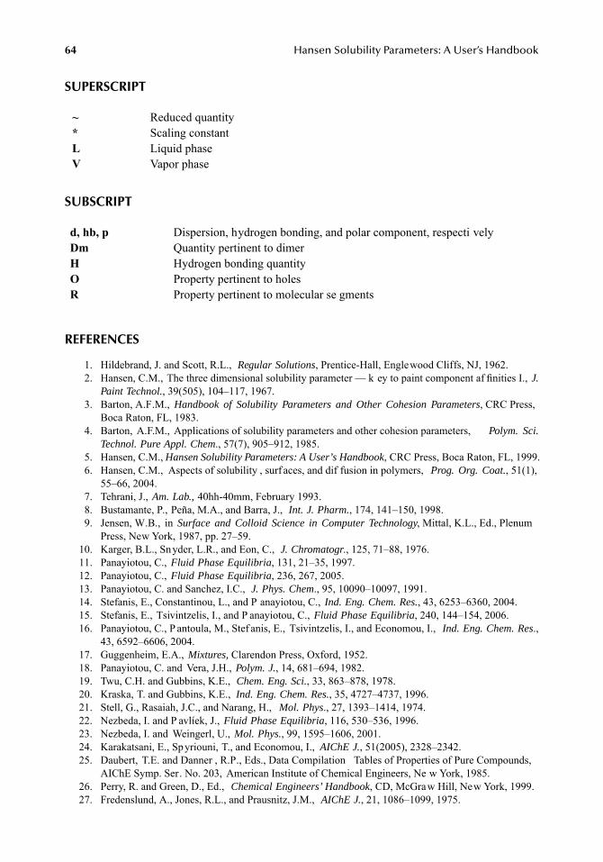
64 Hansen Solubility Parameters: A User’s Handbook
SUPERSCRIPT
SUBSCRIPT
REFERENCES
1. Hildebrand, J. and Scott, R.L., Regular Solutions, Prentice-Hall, Englewood Cliffs, NJ, 1962.2. Hansen, C.M., The three dimensional solubility parameter — k ey to paint component af finities I., J.
Paint Technol., 39(505), 104–117, 1967.3. Barton, A.F.M., Handbook of Solubility Parameters and Other Cohesion Parameters, CRC Press,
Boca Raton, FL, 1983.4. Barton, A.F.M., Applications of solubility parameters and other cohesion parameters, Polym. Sci.
Technol. Pure Appl. Chem., 57(7), 905–912, 1985.5. Hansen, C.M., Hansen Solubility Parameters: A User’s Handbook, CRC Press, Boca Raton, FL, 1999.6. Hansen, C.M., Aspects of solubility , surf aces, and dif fusion in polymers, Prog. Org. Coat., 51(1),
55–66, 2004.7. Tehrani, J., Am. Lab., 40hh-40mm, February 1993.8. Bustamante, P., Peña, M.A., and Barra, J., Int. J. Pharm., 174, 141–150, 1998.9. Jensen, W.B., in Surface and Colloid Science in Computer Technology, Mittal, K.L., Ed., Plenum
Press, New York, 1987, pp. 27–59.10. Karger, B.L., Snyder, L.R., and Eon, C., J. Chromatogr., 125, 71–88, 1976.11. Panayiotou, C., Fluid Phase Equilibria, 131, 21–35, 1997.12. Panayiotou, C., Fluid Phase Equilibria, 236, 267, 2005.13. Panayiotou, C. and Sanchez, I.C., J. Phys. Chem., 95, 10090–10097, 1991.14. Stefanis, E., Constantinou, L., and P anayiotou, C., Ind. Eng. Chem. Res., 43, 6253–6360, 2004.15. Stefanis, E., Tsivintzelis, I., and P anayiotou, C., Fluid Phase Equilibria, 240, 144–154, 2006.16. Panayiotou, C., P antoula, M., Stef anis, E., Tsivintzelis, I., and Economou, I., Ind. Eng. Chem. Res.,
43, 6592–6606, 2004.17. Guggenheim, E.A., Mixtures, Clarendon Press, Oxford, 1952.18. Panayiotou, C. and Vera, J.H., Polym. J., 14, 681–694, 1982.19. Twu, C.H. and Gubbins, K.E., Chem. Eng. Sci., 33, 863–878, 1978.20. Kraska, T. and Gubbins, K.E., Ind. Eng. Chem. Res., 35, 4727–4737, 1996.21. Stell, G., Rasaiah, J.C., and Narang, H., Mol. Phys., 27, 1393–1414, 1974.22. Nezbeda, I. and P avlíek, J., Fluid Phase Equilibria, 116, 530–536, 1996.23. Nezbeda, I. and Weingerl, U., Mol. Phys., 99, 1595–1606, 2001.24. Karakatsani, E., Spyriouni, T., and Economou, I., AIChE J., 51(2005), 2328–2342.25. Daubert, T.E. and Danner , R.P., Eds., Data Compilation Tables of Properties of Pure Compounds,
AIChE Symp. Ser. No. 203, American Institute of Chemical Engineers, Ne w York, 1985.26. Perry, R. and Green, D., Ed., Chemical Engineers’ Handbook, CD, McGraw Hill, New York, 1999.27. Fredenslund, A., Jones, R.L., and Prausnitz, J.M., AIChE J., 21, 1086–1099, 1975.
~ Reduced quantity * Scaling constant L Liquid phaseV Vapor phase
d, hb, p Dispersion, hydrogen bonding, and polar component, respecti velyDm Quantity pertinent to dimerH Hydrogen bonding quantityO Property pertinent to holesR Property pertinent to molecular se gments
7248_book.fm Page 64 Tuesday, April 24, 2007 9:19 AM
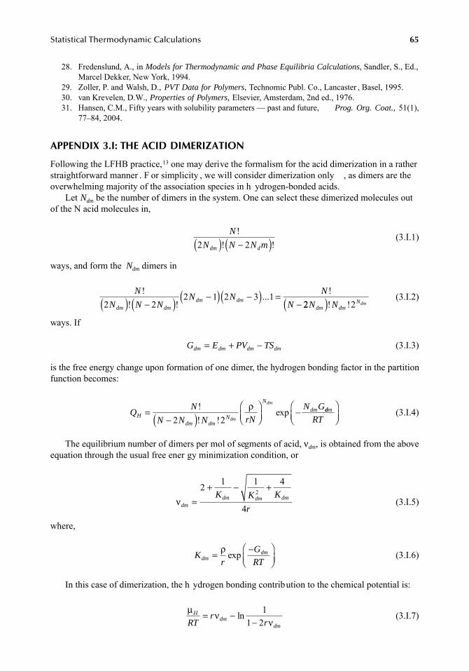
Statistical Thermodynamic Calculations 65
28. Fredenslund, A., in Models for Thermodynamic and Phase Equilibria Calculations, Sandler, S., Ed.,Marcel Dekker, New York, 1994.
29. Zoller, P. and Walsh, D., PVT Data for Polymers, Technomic Publ. Co., Lancaster , Basel, 1995.30. van Krevelen, D.W., Properties of Polymers, Elsevier, Amsterdam, 2nd ed., 1976.31. Hansen, C.M., Fifty years with solubility parameters — past and future, Prog. Org. Coat., 51(1),
77–84, 2004.
APPENDIX 3.I: THE ACID DIMERIZATION
Following the LFHB practice,13 one may derive the formalism for the acid dimerization in a ratherstraightforward manner . F or simplicity , we will consider dimerization only , as dimers are theoverwhelming majority of the association species in h ydrogen-bonded acids.
Let Ndm be the number of dimers in the system. One can select these dimerized molecules outof the N acid molecules in,
(3.I.1)
ways, and form the Ndm dimers in
(3.I.2)
ways. If
(3.I.3)
is the free energy change upon formation of one dimer, the hydrogen bonding factor in the partitionfunction becomes:
(3.I.4)
The equilibrium number of dimers per mol of segments of acid, νdm, is obtained from the aboveequation through the usual free ener gy minimization condition, or
(3.I.5)
where,
(3.I.6)
In this case of dimerization, the h ydrogen bonding contribution to the chemical potential is:
(3.I.7)
N
N N N mdm d
!! !2 2( ) −( )
N
N N NN N
N
Ndm dmdm dm
!! !
... !2 2
2 1 2 3 1( ) −( ) −( ) −( ) =− 22 2N Ndm dm
Ndm( )! !
G E PV TSdm dm dm dm= + −
QN
N N N rN
N GH
dm dmN
N
dm
dm
dm
=−( )
⎛⎝⎜
⎞⎠⎟
−!! !
exp2 2
ρ ddm
RT
⎛⎝⎜
⎞⎠⎟
νdmdm dm dmK K K
r=
+ − +2 1 1 4
4
2
Kr
G
RTdmdm= −⎛
⎝⎜⎞⎠⎟
ρ exp
μ νν
Hdm
dmRTr
r= −
−ln 1
1 2
7248_book.fm Page 65 Tuesday, April 24, 2007 9:19 AM
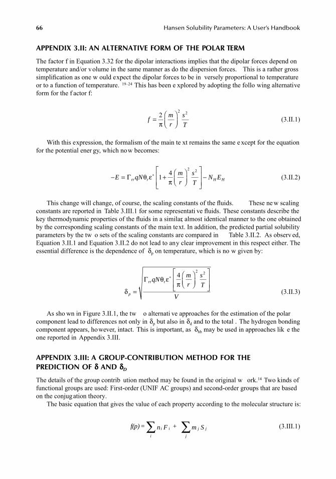
66 Hansen Solubility Parameters: A User’s Handbook
APPENDIX 3.II: AN ALTERNATIVE FORM OF THE POLAR TERM
The factor f in Equation 3.32 for the dipolar interactions implies that the dipolar forces depend ontemperature and/or volume in the same manner as do the dispersion forces. This is a rather grosssimplification as one w ould expect the dipolar forces to be in versely proportional to temperatureor to a function of temperature. 19–24 This has been e xplored by adopting the follo wing alternativeform for the f actor f:
(3.II.1)
With this expression, the formalism of the main te xt remains the same e xcept for the equationfor the potential ener gy, which now becomes:
(3.II.2)
This change will change, of course, the scaling constants of the fluids. These ne w scalingconstants are reported in Table 3.III.1 for some representati ve fluids. These constants describe thekey thermodynamic properties of the fluids in a similar, almost identical manner to the one obtainedby the corresponding scaling constants of the main text. In addition, the predicted partial solubilityparameters by the tw o sets of the scaling constants are compared in Table 3.II.2. As observ ed,Equation 3.II.1 and Equation 3.II.2 do not lead to any clear improvement in this respect either. Theessential difference is the dependence of δp on temperature, which is no w given by:
(3.II.3)
As sho wn in Figure 3.II.1, the tw o alternati ve approaches for the estimation of the polarcomponent lead to differences not only in δp but also in δd and to the total . The hydrogen bondingcomponent appears, however, intact. This is important, as δhb may be used in approaches lik e theone reported in Appendix 3.III.
APPENDIX 3.III: A GROUP-CONTRIBUTION METHOD FOR THE PREDICTION OF δδδδ AND δδδδD
The details of the group contrib ution method may be found in the original w ork.14 Two kinds offunctional groups are used: First-order (UNIF AC groups) and second-order groups that are basedon the conjugation theory.
The basic equation that gives the value of each property according to the molecular structure is:
(3.III.1)
fm
r
s
T=
⎛⎝⎜
⎞⎠⎟
22 2
π
− = +⎛⎝⎜
⎞⎠⎟
⎡
⎣⎢⎢
⎤
⎦⎥⎥
−∗E qNm
r
s
TN Err r H HΓ θ ε
π1 4
2 2
δ
θ επ
p
rr rqNm
r
s
T
V=
⎛⎝⎜
⎞⎠⎟
⎡
⎣⎢⎢
⎤
⎦⎥⎥
∗Γ 42 2
f(p) = n F + m Si
i i
j
j j∑ ∑
7248_book.fm Page 66 Tuesday, April 24, 2007 9:19 AM
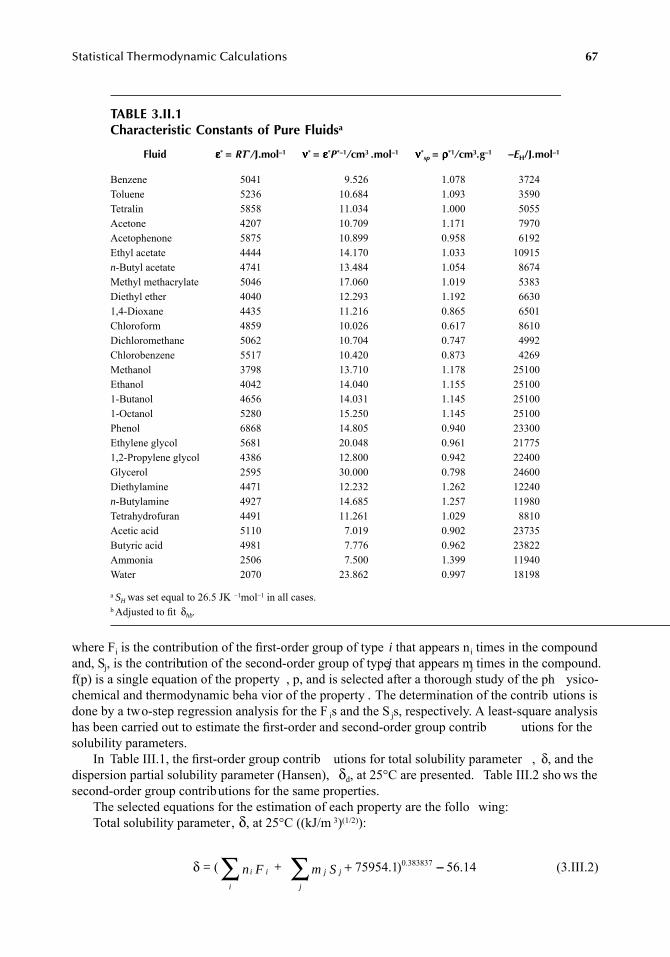
Statistical Thermodynamic Calculations 67
where Fi is the contribution of the first-order group of type i that appears ni times in the compoundand, Sj, is the contribution of the second-order group of type j that appears mj times in the compound.f(p) is a single equation of the property , p, and is selected after a thorough study of the ph ysico-chemical and thermodynamic beha vior of the property . The determination of the contrib utions isdone by a two-step regression analysis for the F is and the S js, respectively. A least-square analysishas been carried out to estimate the first-order and second-order group contrib utions for thesolubility parameters.
In Table III.1, the first-order group contrib utions for total solubility parameter , δ, and thedispersion partial solubility parameter (Hansen), δd, at 25°C are presented. Table III.2 sho ws thesecond-order group contributions for the same properties.
The selected equations for the estimation of each property are the follo wing:Total solubility parameter, δ, at 25°C ((kJ/m 3)(1/2)):
(3.III.2)
TABLE 3.II.1Characteristic Constants of Pure Fluidsa
Fluid εεεε* = RT*/J.mol–1 νννν* = εεεε*P*–1/cm3 .mol–1 νννν*sp = ρρρρ*1/cm3.g–1 –EH/J.mol–1
Benzene 5041 9.526 1.078 3724Toluene 5236 10.684 1.093 3590Tetralin 5858 11.034 1.000 5055Acetone 4207 10.709 1.171 7970Acetophenone 5875 10.899 0.958 6192Ethyl acetate 4444 14.170 1.033 10915n-Butyl acetate 4741 13.484 1.054 8674Methyl methacrylate 5046 17.060 1.019 5383Diethyl ether 4040 12.293 1.192 66301,4-Dioxane 4435 11.216 0.865 6501Chloroform 4859 10.026 0.617 8610Dichloromethane 5062 10.704 0.747 4992Chlorobenzene 5517 10.420 0.873 4269Methanol 3798 13.710 1.178 25100Ethanol 4042 14.040 1.155 251001-Butanol 4656 14.031 1.145 251001-Octanol 5280 15.250 1.145 25100Phenol 6868 14.805 0.940 23300Ethylene glycol 5681 20.048 0.961 217751,2-Propylene glycol 4386 12.800 0.942 22400Glycerol 2595 30.000 0.798 24600Diethylamine 4471 12.232 1.262 12240n-Butylamine 4927 14.685 1.257 11980Tetrahydrofuran 4491 11.261 1.029 8810Acetic acid 5110 7.019 0.902 23735Butyric acid 4981 7.776 0.962 23822Ammonia 2506 7.500 1.399 11940Water 2070 23.862 0.997 18198
a SH was set equal to 26.5 JK –1mol–1 in all cases.b Adjusted to fit δhb.
δ = n F + m Si
i i
j
j j( )∑ ∑ + 75954.1 0.383837 −− 56.14
7248_book.fm Page 67 Tuesday, April 24, 2007 9:19 AM
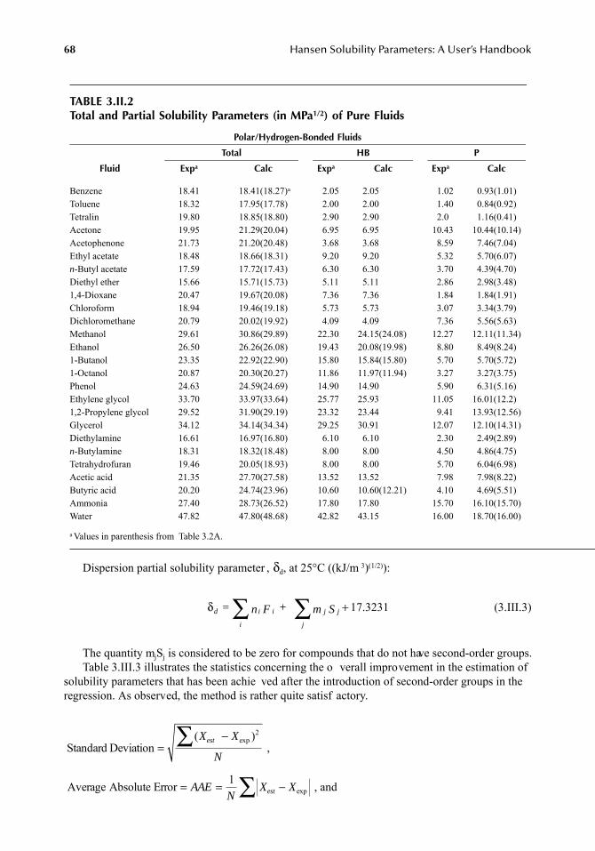
68 Hansen Solubility Parameters: A User’s Handbook
Dispersion partial solubility parameter , δd, at 25°C ((kJ/m 3)(1/2)):
(3.III.3)
The quantity mjSj is considered to be zero for compounds that do not have second-order groups.Table 3.III.3 illustrates the statistics concerning the o verall improvement in the estimation of
solubility parameters that has been achie ved after the introduction of second-order groups in theregression. As observed, the method is rather quite satisf actory.
,
, and
TABLE 3.II.2Total and Partial Solubility Parameters (in MPa1/2) of Pure Fluids
Polar/Hydrogen-Bonded Fluids
Fluid
Total HB P
Expa Calc Expa Calc Expa Calc
Benzene 18.41 18.41(18.27)a 2.05 2.05 1.02 0.93(1.01)Toluene 18.32 17.95(17.78) 2.00 2.00 1.40 0.84(0.92)Tetralin 19.80 18.85(18.80) 2.90 2.90 2.0 1.16(0.41)Acetone 19.95 21.29(20.04) 6.95 6.95 10.43 10.44(10.14)Acetophenone 21.73 21.20(20.48) 3.68 3.68 8.59 7.46(7.04)Ethyl acetate 18.48 18.66(18.31) 9.20 9.20 5.32 5.70(6.07)n-Butyl acetate 17.59 17.72(17.43) 6.30 6.30 3.70 4.39(4.70)Diethyl ether 15.66 15.71(15.73) 5.11 5.11 2.86 2.98(3.48)1,4-Dioxane 20.47 19.67(20.08) 7.36 7.36 1.84 1.84(1.91)Chloroform 18.94 19.46(19.18) 5.73 5.73 3.07 3.34(3.79)Dichloromethane 20.79 20.02(19.92) 4.09 4.09 7.36 5.56(5.63)Methanol 29.61 30.86(29.89) 22.30 24.15(24.08) 12.27 12.11(11.34)Ethanol 26.50 26.26(26.08) 19.43 20.08(19.98) 8.80 8.49(8.24)1-Butanol 23.35 22.92(22.90) 15.80 15.84(15.80) 5.70 5.70(5.72)1-Octanol 20.87 20.30(20.27) 11.86 11.97(11.94) 3.27 3.27(3.75)Phenol 24.63 24.59(24.69) 14.90 14.90 5.90 6.31(5.16)Ethylene glycol 33.70 33.97(33.64) 25.77 25.93 11.05 16.01(12.2)1,2-Propylene glycol 29.52 31.90(29.19) 23.32 23.44 9.41 13.93(12.56)Glycerol 34.12 34.14(34.34) 29.25 30.91 12.07 12.10(14.31)Diethylamine 16.61 16.97(16.80) 6.10 6.10 2.30 2.49(2.89)n-Butylamine 18.31 18.32(18.48) 8.00 8.00 4.50 4.86(4.75)Tetrahydrofuran 19.46 20.05(18.93) 8.00 8.00 5.70 6.04(6.98)Acetic acid 21.35 27.70(27.58) 13.52 13.52 7.98 7.98(8.22)Butyric acid 20.20 24.74(23.96) 10.60 10.60(12.21) 4.10 4.69(5.51)Ammonia 27.40 28.73(26.52) 17.80 17.80 15.70 16.10(15.70)Water 47.82 47.80(48.68) 42.82 43.15 16.00 18.70(16.00)
a Values in parenthesis from Table 3.2A.
δd
i
i i
j
j j= n F + m S∑ ∑ + 17 3231.
Standard Deviation =−∑ ( )expX X
N
est2
Average Absolute Error = = −∑AAEN
X Xest
1exp
7248_book.fm Page 68 Tuesday, April 24, 2007 9:19 AM
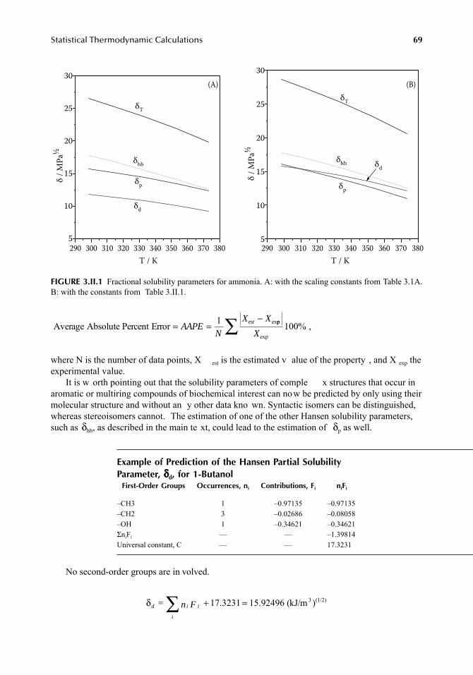
Statistical Thermodynamic Calculations 69
,
where N is the number of data points, X est is the estimated v alue of the property , and X exp theexperimental value.
It is w orth pointing out that the solubility parameters of comple x structures that occur inaromatic or multiring compounds of biochemical interest can now be predicted by only using theirmolecular structure and without an y other data kno wn. Syntactic isomers can be distinguished,whereas stereoisomers cannot. The estimation of one of the other Hansen solubility parameters,such as δhb, as described in the main te xt, could lead to the estimation of δp as well.
No second-order groups are in volved.
FIGURE 3.II.1 Fractional solubility parameters for ammonia. A: with the scaling constants from Table 3.1A.B: with the constants from Table 3.II.1.
Example of Prediction of the Hansen Partial Solubility Parameter, δδδδd, for 1-Butanol First-Order Groups Occurrences, ni Contributions, Fi niFi
–CH3 1 –0.97135 –0.97135–CH2 3 –0.02686 –0.08058–OH 1 –0.34621 –0.34621ΣniFi — — –1.39814Universal constant, C — — 17.3231
290 300 310 320 330 340 350 360 370 380
30
25
20
15
10
5
30
25
20
15
10
5
T / K
290 300 310 320 330 340 350 360 370 380
T / K
δ /
MP
a½
δ /
MP
a½
(A) (B)
δd
δd
δp δ
p
δhb
δhb
δT
δT
Average Absolute Percent Error = =−
AAPEN
X Xest1 expp
exp%
X100∑
δd
i
i i= n F∑ + =17 3231. 15.92496 (kJ/m )3 (1/2)
7248_book.fm Page 69 Tuesday, April 24, 2007 9:19 AM
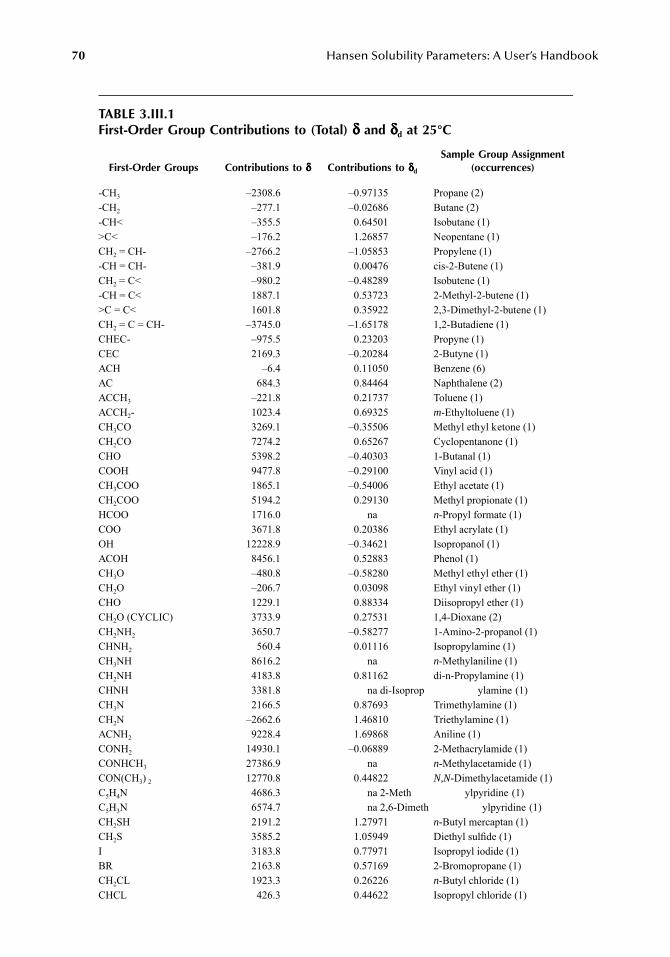
70 Hansen Solubility Parameters: A User’s Handbook
TABLE 3.III.1First-Order Group Contributions to (Total) δδδδ and δδδδd at 25°C
First-Order Groups Contributions to δδδδ Contributions to δδδδd
Sample Group Assignment(occurrences)
-CH3 –2308.6 –0.97135 Propane (2)-CH2 –277.1 –0.02686 Butane (2)-CH< –355.5 0.64501 Isobutane (1)>C< –176.2 1.26857 Neopentane (1)CH2 = CH- –2766.2 –1.05853 Propylene (1)-CH = CH- –381.9 0.00476 cis-2-Butene (1)CH2 = C< –980.2 –0.48289 Isobutene (1)-CH = C< 1887.1 0.53723 2-Methyl-2-butene (1)>C = C< 1601.8 0.35922 2,3-Dimethyl-2-butene (1)CH2 = C = CH- –3745.0 –1.65178 1,2-Butadiene (1)CHEC- –975.5 0.23203 Propyne (1)CEC 2169.3 –0.20284 2-Butyne (1)ACH –6.4 0.11050 Benzene (6)AC 684.3 0.84464 Naphthalene (2)ACCH3 –221.8 0.21737 Toluene (1)ACCH2- 1023.4 0.69325 m-Ethyltoluene (1)CH3CO 3269.1 –0.35506 Methyl ethyl ketone (1)CH2CO 7274.2 0.65267 Cyclopentanone (1)CHO 5398.2 –0.40303 1-Butanal (1)COOH 9477.8 –0.29100 Vinyl acid (1)CH3COO 1865.1 –0.54006 Ethyl acetate (1)CH2COO 5194.2 0.29130 Methyl propionate (1)HCOO 1716.0 na n-Propyl formate (1)COO 3671.8 0.20386 Ethyl acrylate (1)OH 12228.9 –0.34621 Isopropanol (1)ACOH 8456.1 0.52883 Phenol (1)CH3O –480.8 –0.58280 Methyl ethyl ether (1)CH2O –206.7 0.03098 Ethyl vinyl ether (1)CHO 1229.1 0.88334 Diisopropyl ether (1)CH2O (CYCLIC) 3733.9 0.27531 1,4-Dioxane (2)CH2NH2 3650.7 –0.58277 1-Amino-2-propanol (1)CHNH2 560.4 0.01116 Isopropylamine (1)CH3NH 8616.2 na n-Methylaniline (1)CH2NH 4183.8 0.81162 di-n-Propylamine (1)CHNH 3381.8 na di-Isoprop ylamine (1)CH3N 2166.5 0.87693 Trimethylamine (1)CH2N –2662.6 1.46810 Triethylamine (1)ACNH2 9228.4 1.69868 Aniline (1)CONH2 14930.1 –0.06889 2-Methacrylamide (1)CONHCH3 27386.9 na n-Methylacetamide (1)CON(CH3) 2 12770.8 0.44822 N,N-Dimethylacetamide (1)C5H4N 4686.3 na 2-Meth ylpyridine (1)C5H3N 6574.7 na 2,6-Dimeth ylpyridine (1)CH2SH 2191.2 1.27971 n-Butyl mercaptan (1)CH2S 3585.2 1.05949 Diethyl sulfide (1)I 3183.8 0.77971 Isopropyl iodide (1)BR 2163.8 0.57169 2-Bromopropane (1)CH2CL 1923.3 0.26226 n-Butyl chloride (1)CHCL 426.3 0.44622 Isopropyl chloride (1)
7248_book.fm Page 70 Tuesday, April 24, 2007 9:19 AM
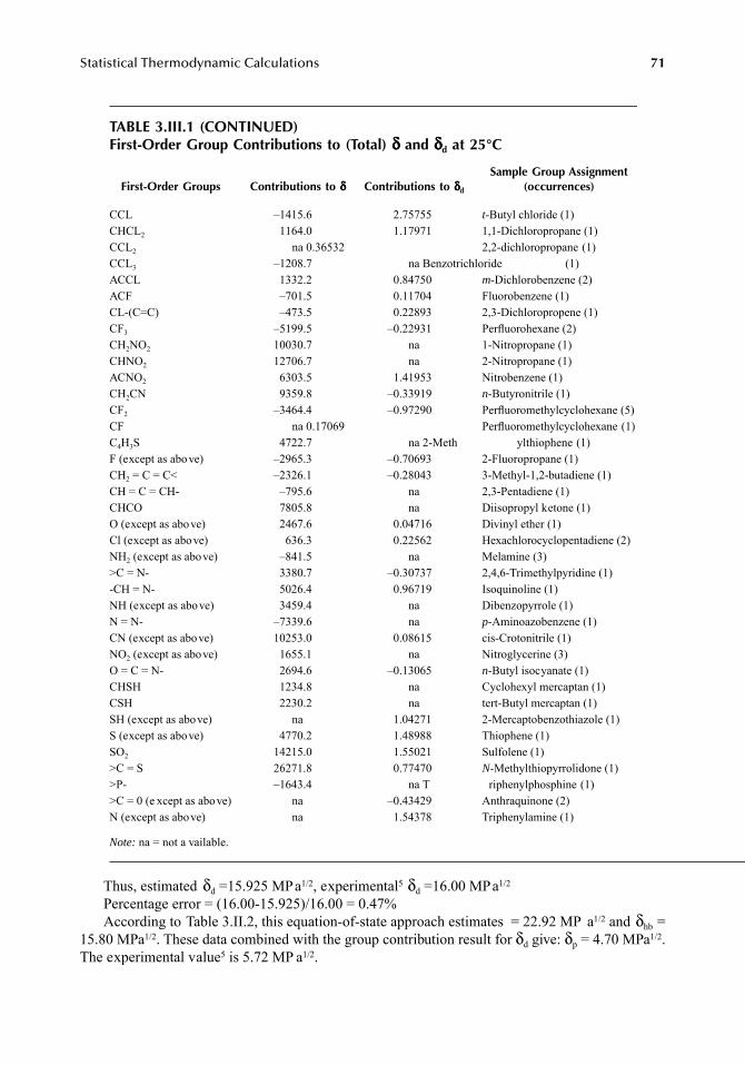
Statistical Thermodynamic Calculations 71
Thus, estimated δd =15.925 MPa1/2, experimental5 δd =16.00 MPa1/2
Percentage error = (16.00-15.925)/16.00 = 0.47%According to Table 3.II.2, this equation-of-state approach estimates = 22.92 MP a1/2 and δhb =
15.80 MPa1/2. These data combined with the group contribution result for δd give: δp = 4.70 MPa1/2.The experimental value5 is 5.72 MP a1/2.
TABLE 3.III.1 (CONTINUED)First-Order Group Contributions to (Total) δδδδ and δδδδd at 25°C
First-Order Groups Contributions to δδδδ Contributions to δδδδd
Sample Group Assignment(occurrences)
CCL –1415.6 2.75755 t-Butyl chloride (1)CHCL2 1164.0 1.17971 1,1-Dichloropropane (1)CCL2 na 0.36532 2,2-dichloropropane (1)CCL3 –1208.7 na Benzotrichloride (1)ACCL 1332.2 0.84750 m-Dichlorobenzene (2)ACF –701.5 0.11704 Fluorobenzene (1)CL-(C=C) –473.5 0.22893 2,3-Dichloropropene (1)CF3 –5199.5 –0.22931 Perfluorohexane (2)CH2NO2 10030.7 na 1-Nitropropane (1)CHNO2 12706.7 na 2-Nitropropane (1)ACNO2 6303.5 1.41953 Nitrobenzene (1)CH2CN 9359.8 –0.33919 n-Butyronitrile (1)CF2 –3464.4 –0.97290 Perfluoromethylcyclohexane (5)CF na 0.17069 Perfluoromethylcyclohexane (1)C4H3S 4722.7 na 2-Meth ylthiophene (1)F (except as above) –2965.3 –0.70693 2-Fluoropropane (1)CH2 = C = C< –2326.1 –0.28043 3-Methyl-1,2-butadiene (1)CH = C = CH- –795.6 na 2,3-Pentadiene (1)CHCO 7805.8 na Diisopropyl ketone (1)O (except as above) 2467.6 0.04716 Divinyl ether (1)Cl (except as above) 636.3 0.22562 Hexachlorocyclopentadiene (2)NH2 (except as above) –841.5 na Melamine (3)>C = N- 3380.7 –0.30737 2,4,6-Trimethylpyridine (1)-CH = N- 5026.4 0.96719 Isoquinoline (1)NH (except as above) 3459.4 na Dibenzopyrrole (1)N = N- –7339.6 na p-Aminoazobenzene (1)CN (except as above) 10253.0 0.08615 cis-Crotonitrile (1)NO2 (except as above) 1655.1 na Nitroglycerine (3)O = C = N- 2694.6 –0.13065 n-Butyl isocyanate (1)CHSH 1234.8 na Cyclohexyl mercaptan (1)CSH 2230.2 na tert-Butyl mercaptan (1)SH (except as above) na 1.04271 2-Mercaptobenzothiazole (1)S (except as above) 4770.2 1.48988 Thiophene (1)SO2 14215.0 1.55021 Sulfolene (1)>C = S 26271.8 0.77470 N-Methylthiopyrrolidone (1)>P- –1643.4 na T riphenylphosphine (1)>C = 0 (e xcept as above) na –0.43429 Anthraquinone (2)N (except as above) na 1.54378 Triphenylamine (1)
Note: na = not a vailable.
7248_book.fm Page 71 Tuesday, April 24, 2007 9:19 AM
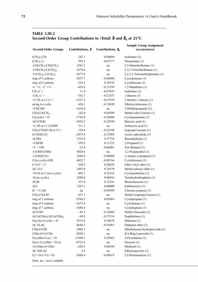
72 Hansen Solubility Parameters: A User’s Handbook
TABLE 3.III.2Second-Order Group Contributions to (Total) δδδδ and δδδδd at 25°C
Second-Order Groups Contributions, δδδδ Contributions, δδδδd
Sample Group Assignment(occurrences)
(CH3)2-CH- 142.1 0.04604 Isobutane (1)(CH3)3-C- 592.3 –0.07377 Neopentane (1)-CH(CH3)-CH(CH3)- 1581.2 na 2,3-Dimethylbutane (1)-CH(CH3)-C(CH3)2- 2678.4 na 2,2,3-Trimethylbutane (1)-C(CH3)2-C(CH3)2- 5677.6 na 2,2,3,3-Tetramethylpentane (1)ring of 5 carbons –2637.7 –0.66808 Cyclopentane (1)ring of 6 carbons –524.2 0.38742 Cyclohexane (1)-C = C - C = C- –426.8 –0.13554 1,3-Butadiene (1)CH3-C = 11.9 –0.07853 Isobutene (2)-CH2-C = –762.7 –0.32357 1-Butene (1)>C{H or C}-C = –1257.2 –0.27979 3-Methyl-1-butene (1)string in cyclic 626.1 –0.19450 Ethylcyclohexane (1)>CHCHO –1634.4 na 2-Methylpropanal (1)CH3(CO)CH2- 142.0 –0.04509 Methyl ethyl ketone (1)C(cyclic) = O –3745.0 –0.29806 Cyclopentanone (1)ACCOOH –3076.5 –0.22930 Benzoic acid (1)>C{H or C}-COOH 511.1 na Isobutyric acid (1)CH3(CO)OC{H or C}< 134.4 –0.52196 Isopropyl acetate (1)(CO)O(CO) –2875.9 –0.27069 Acetic anhydride (1)ACHO 3315.0 0.37724 Benzaldehyde (1)>CHOH –359.5 0.11231 2-Propanol (1)>C < OH –23.4 –0.06801 Tert-Butanol (1)-C(OH)C(OH)- 5020.6 na 1,2-Propanediol (1)-C(OH)C(N) 3306.4 –0.08088 1-Amino-2-propanol (1)C(in cyclic)-OH 4022.7 –0.08764 Cyclohexanol (1)C-O-C = C –228.5 0.20629 Ethyl vinyl ether (1)AC-O-C 2493.0 0.25679 Methyl phenyl ether (1)>N{H or C}(in c yclic) –492.7 0.22183 Cyclopentimine (1)-S-(in cyclic) 2389.4 0.48916 Tetrahydrothiophene (1)ACBr 337.4 0.12341 Bromobenzene (1)ACI 1267.1 0.00000 Iodobenzene (1)(C = C)-Br na –0.40589 2-bromo-propene (1)CH3(CO)CH< –437.1 na Methyl isopropyl ketone (1)ring of 3 carbons –9764.5 0.02003 Cyclopropane (1)ring of 4 carbons –3673.4 na Cyclobutane (1)ring of 7 carbons –1486.4 na Cycloheptane (1)ACCOO –83.5 –0.18466 Methyl benzoate (1)AC(ACHm)2AC(ACHn)2 –69.8 –0.37514 Naphthalene (1)Ocyclic-Ccyclic = O 9215.6 0.24676 Diketene (1)AC-O-AC –4646.5 –0.56461 Diphenyl ether (1)CHn-O-OH 2002.5 na Ethylbenzene hydroperoxide (1)CHm-O-O-CHn –2029.1 na di-t-Butyl peroxide (1)NcycHm-Ccyc = O 11489.1 0.29563 2-Pyrrolidone (1)Ocyc-CcycHm = Ncyc –8721.6 na Oxazole (1)-O-CHm-O-CHn- –620.3 0.08394 Methylal (1)AC-NH-AC 2.8 na Dibenzopyrrole (1)C(= O)-C-C(= O) –3668.9 –0.48615 2,4-Pentanedione (1)
Note: na = not a vailable.
7248_book.fm Page 72 Tuesday, April 24, 2007 9:19 AM

Statistical Thermodynamic Calculations 73
TABLE 3.III.3Comparison of the First- and Second-Order Approximations
PropertyDataPoints
StandardDeviation
First-Order
StandardDeviation
Second-OrderAAE
First-OrderAAE
Second-OrderAAPE (%)First-Order
AAPE (%)Second-Order
δ 1017 1.47 1.31 1.00 0.90 5.15 4.67δd 344 0.61 0.58 0.44 0.41 2.62 2.42
7248_book.fm Page 73 Tuesday, April 24, 2007 9:19 AM

7248_book.fm Page 74 Tuesday, April 24, 2007 9:19 AM
75
4
The Hansen Solubility Parameters (HSP) in Thermodynamic Models for Polymer Solutions
Georgios M. Kontogeorgis
ABSTRACT
Polymer thermodynamics plays an important role in a lar ge number of processes and in the designof many different polymer-based products. Examples include:
1. The removal of unreacted monomers, colorants, by-products, toxic compounds, and otheradditives after polymerization
2. The selection of mix ed solvents in the paints and coatings industry to ward designingenvironmentally-friendly paints (water-based, fewer VOC)
3. The control of emissions from paints as well as the swelling of the film in the presencof water
4. The recycling of polymers based on ph ysicochemical methods like selective dissolution5. The compatibility of polymer blends including those with no vel structures (star -like,
dendrimers), permeabilities of g ases in fl xible polymeric pipes used in the North Seaand other major oil and g as producing areas for transporting of h ydrocarbons on theseabed and from the seabed to the surf ace
6. Compatibility of plasticizers in PVC7. In the biotechnology , aqueous tw o-phase systems based on polymers for separating
proteins
This is only a short list, and man y more applications of polymer thermodynamics e xist. Inseveral of these cases it is not suf ficient to empl y only the Hansen solubility parameters (HSP),as much more detailed calculations may be needed, including solv ent activities, for e xample, forsolvent emission assessment or even full phase diagrams and at both low (e.g., biotechnology) andhigh pressures (e.g., polyolefin industr , gas permeabilities in polymers).
Polymers form highly nonideal liquid solutions with lo w-molecular weight chemicals andliquid–liquid phase separation (LLE) is the rule rather than the e xception in polymer -solventmixtures. Moreo ver, such LLE may tak e v arious forms; UCST , LCST , closed loop, etc., andtemperature, polymer molecular weight, and polydispersity have great effects. Free-volume effects,special structures and crystallinity cause additional comple xities.
It is rather tempting to combine the e xtensive use/tables available for the HSP with a rigorousthermodynamic approach and compare the performance of this method to more adv ancedapproaches. This is the purpose of this chapter . As several of the literature approaches used for
7248_C004.fm Page 75 Thursday, May 10, 2007 12:51 PM
76
Hansen Solubility Parameters: A User’s Handbook
comparison purposes are based on the group-contrib ution principle, a short introduction to thisprinciple is provided first
GROUP CONTRIBUTION METHODS FOR ESTIMATING PROPERTIES OF POLYMERS
T
HE
G
ROUP
-C
ONTRIBUTION
P
RINCIPLE
AND
S
OME
A
PPLICATIONS
(D
ENSITY
, S
OLUBILITY
P
ARAMETERS
)
Many properties of pure polymers and polymer solutions can be estimated with group contributions(GC), e.g., density, the solubility parameter (Hildebrand and HSP), the melting and glass transitiontemperatures, activity coefficients, and the sur ace tension.
The GC method is based on the assumption that the properties of molecules can be estimatedusing additive rules from the values of the corresponding groups they are composed of. For example,n-hexane (CH
3
-(CH
2
)
4
-CH
3
) can be considered to ha ve two CH
3
and four CH
2
groups. Similarly ,butanone has one CH
3
, one CH
2
, and one CH
3
CO group. If the group values are known for a specifiproperty
F
, then the total v alue of the property for the whole molecule is often e xpressed by ageneral additive rule of the form:
(4.1)
or similar additive equations.In Equation 4.1,
n
i
is the number of groups of type i and
F
i
is the corresponding group v alue.In some cases,
F
i
values are also functions of temperature for temperature-dependent propertiessuch as the v olume and the v apor pressure. For several properties, the general GC equation has amore complicated form than that indicated by Equation 4.1.
The GC methodology has been applied to man y properties and for both lo w molecular weightcompounds and polymers. Activity coefficients h ve also been predicted with group contrib utions,e.g., the UNIFAC model by Fredenslund et al.
1
Van Krevelen
2
gives an overview of the applicationof group contrib ution methods to se veral properties of pure polymers, including also mechanicaland environmentally-related properties. Van Krevelen provides extensive GC tables for the Hilde-brand and Hansen solubility parameters as well. An alternative GC method for the polymer (andsolvent) density has been developed by Elbro et al.
3
(GCVOL) and was recently extended to coverseveral group families.
4,5
A list of GCVOL parameters is provided elsewhere.
6
GCVOL can predictsatisfactorily the density of solvents, oligomers, and polymers, including copolymers, often within2%.
7
The great advantage of the group contribution method is its simplicity: Even though there maybe thousands of different molecules (and mixtures), the corresponding number of groups is signif-icantly smaller (no more than 100 or so). Thus, instead of kno wing the parameter v alues of aspecific property for thousands of molecules, it is su ficient to kn w the group parameters for amuch smaller number of groups. Two limitations of the approach should be k ept in mind:
1. The GC methodology is a v ery useful technique leading to good results in man y cases.However, it is an approximation, based often on a some what unjustified d vision of themolecule into groups. F or some properties, such as for density , GC methods performmuch better than for others, e.g., melting point. Specific molecules are assigned aseparate groups (e.g., methanol) because further di vision is not possible if good resultsare to be obtained. Problems can also be e xpected for multifunctional groups and wheremore than one polar groups are close to each other (e.g., in alcohols and acids with more
F n Fi i
i
= ∑
7248_C004.fm Page 76 Thursday, May 10, 2007 12:51 PM
The Hansen Solubility Parameters (HSP) in Thermodynamic Models for Polymer Solutions
77
than one OH and COOH groups; for h ydroxyl-acids or for alkanolamines). Ho wever,despite these problems, the GC principle is e xtensively used for property calculationsfor specific molecules and also, in the r verse w ay, for selecting suitable compoundshaving a required set of properties. The latter technique is called
computer aided productdesign
.2. The exact definition of groups may be di ferent from method to method. In some cases,
even two different methods for the same property may emplo y different definitions fothe groups. For example, the division of butadiene rubber according to the van Krevelenand GCVOL methods for density is different. In other cases, and for the same GC method,a particular molecule can be di vided into groups in tw o different ways that may yielddifferent results. The latter problem will be further discussed later .
GC F
REE
-V
OLUME
-B
ASED
M
ODELS
FOR
P
OLYMERS
(E
NTROPIC
-FV, U
NIFAC
-FV)
The Free-Volume Concept
The classical Flory–Huggins model (See Equation 4.9 later) pro vides a first approximation fopolymer solutions. Both the combinatorial and the energetic terms need improvement via inclusionof free-volume effects and nonrandom local-composition terms such as those of the UNIQ UAC,NRTL, and UNIFAC models.
The concept of free-volume (FV) is rather loose b ut still very important. Elbro
8
showed, usinga simple definition for the FV (Equation 4.2), that the FV percentages of sol ents (40–50%) aregreater than those of polymers (30–40%), with the e xception of w ater and polydimeth yl siloxane(PDMS). Many mathematical expressions have been proposed for the FV. One of the simplest andmost successful equations is:
(4.2)
originally proposed by Bondi
9
and later adopted by Elbro et al.
10
and others
11
in the Entropic-FVmodel. In Equation 4.2, free-volume is simply the “empty” volume available to the molecule whenthe molecules’ own (hard-core or closed-packed V*) volume is subtracted. But what is actually thehard-core volume? This also is rather difficult to determine. Elbr
8,10
suggested using V* = V
w
, i.e.,equal to the v an der Waals volume (V
w
), which is obtained from the group increments of Bondiand is tabulated for almost all existing groups in the UNIFAC tables. Other investigators interpretedthe hard-core volume somewhat differently; most agree today that V
*
> V
w
due to the closed packedstructure of molecules. For example, the closed-packed cubic structure suggests that V* = 1.35V
w
,and Bondi mentions that for many organic molecules it can be expected that the ratio V*/V
w
shouldbe between 1.28 and 1.43.
The UNIFAC-FV Model
The original UNIF AC model does not account for the free-v olume differences between solv entsand polymers; consequently , it highly underestimates the solv ent activities in polymer solutions.Empirical modified UNI AC v ersions (de veloped in L yngby and Dortmund) with e xponentialsegment fractions are also inadequate for polymer solutions; the y systematically overestimate thesolvent activities.
Various modifications — xtensions of the classical UNIF AC approach to polymers — ha vebeen proposed. All of these approaches include the FV effects, which are neglected in the UNIFACcombinatorial term, and most of them emplo y the energetic (residual) term of UNIFAC. The mostwell-known is the UNIFAC-FV model by Oishi and Prausnitz
12
:
V V V V Vf w= − = −*
7248_C004.fm Page 77 Thursday, May 10, 2007 12:51 PM
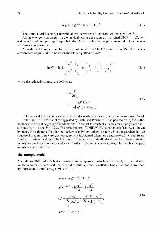
78
Hansen Solubility Parameters: A User’s Handbook
(4.3)
The combinatorial (comb) and residual (res) terms are tak en from original UNIFAC.
1
All the ener getic parameters in the residual term are the same as in original UNIF AC, i.e.,estimated based on vapor-liquid equilibria data for low molecular weight compounds. No parameterreestimation is performed.
An additional term is added for the free-volume effects. The FV term used in UNIFAC-FV hasa theoretical origin, and it is based on the Flory equation of state:
(4.4)
where the reduced v olumes are defined as
(4.5)
In Equation 4.5, the volumes V
i
and the van der Waals volumes V
i,W
are all expressed in cm
3
/mol.In the UNIFAC-FV model as suggested by Oishi and Prausnitz
12
the parameters
c
i
(
3c
i
is thenumber of e xternal de grees of freedom) and
b
are set to constant v alues for all polymers andsolvents (
c
i
= 1.1 and
b
= 1.28). The performance of UNIFAC-FV is rather satisf actory, as shownby man y in vestigators, for a lar ge v ariety of polymer -solvent systems. Some researchers ha vesuggested that, in some cases, better agreement is obtained when these parameters (
c
i
and
b
) arefitted to xperimental data.
13
The UNIFAC-FV model was originally developed for solvent activitiesin polymers and does not give satisfactory results for polymer activities; thus, it has not been appliedto polymer-solvent LLE.
The Entropic Model
A similar to UNIF AC-FV b ut some what simpler approach, which can be readily e xtended tomulticomponent systems and liquid-liquid equilibria, is the so-called Entropic-FV model proposedby Elbro et al.
10
and Kontogeorgis et al.
11
:
(4.6)
ln ln ln lnγ γ γ γi icomb
ires
ifv= + +
ln ln
/
/γ i
fvi
i
m
icv
vc=
−( )−( )
⎡
⎣
⎢⎢⎢
⎤
⎦
⎥⎥⎥
−31
1
1 3
1 3
vv
v v
i
m
−⎛
⎝⎜⎞
⎠⎟−
⎛
⎝⎜⎞
⎠⎟⎡
⎣⎢⎢
⎤
⎦⎥⎥
−
1 1 1
11 3
1
/
vV
bV
vx V x V
b x V x V
ii
i w
m
w w
=
= ++( )
,
, ,
1 1 2 2
1 1 2 2
ln ln ln
ln ln
γ γ γ
γ ϕ
i icomb fv
ires
icomb fv i
fv
x
= +
=
−
−
ii
ifv
i
ifv i i fv
j j fv
j
i i wi
x
x V
x V
x V V
+ −
= =−( )
∑
1 ϕ
ϕ ,
. xx V V
UNIFAC
j j wj
j
ires
−( )
→
∑ln γ
7248_C004.fm Page 78 Thursday, May 10, 2007 12:51 PM
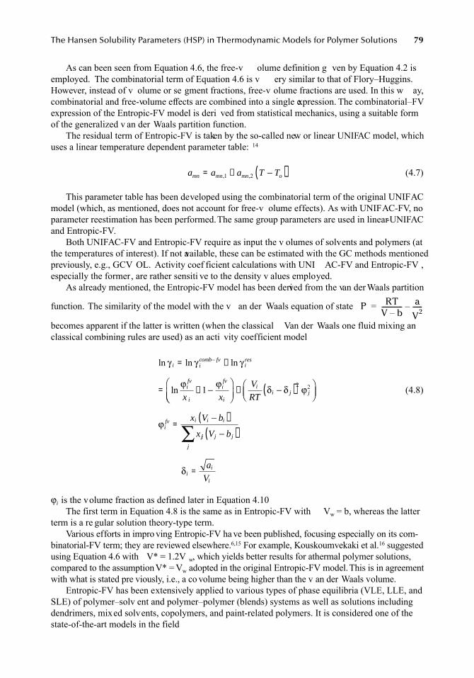
The Hansen Solubility Parameters (HSP) in Thermodynamic Models for Polymer Solutions
79
As can been seen from Equation 4.6, the free-v olume definition g ven by Equation 4.2 isemployed. The combinatorial term of Equation 4.6 is v ery similar to that of Flory–Huggins.However, instead of v olume or se gment fractions, free-v olume fractions are used. In this w ay,combinatorial and free-volume effects are combined into a single expression. The combinatorial–FVexpression of the Entropic-FV model is deri ved from statistical mechanics, using a suitable formof the generalized v an der Waals partition function.
The residual term of Entropic-FV is taken by the so-called new or linear UNIFAC model, whichuses a linear temperature dependent parameter table:
14
(4.7)
This parameter table has been developed using the combinatorial term of the original UNIFACmodel (which, as mentioned, does not account for free-v olume effects). As with UNIFAC-FV, noparameter reestimation has been performed. The same group parameters are used in linear-UNIFACand Entropic-FV.
Both UNIFAC-FV and Entropic-FV require as input the v olumes of solvents and polymers (atthe temperatures of interest). If not available, these can be estimated with the GC methods mentionedpreviously, e.g., GCV OL. Activity coef ficient calculations with UNI AC-FV and Entropic-FV ,especially the former, are rather sensiti ve to the density v alues employed.
As already mentioned, the Entropic-FV model has been derived from the van der Waals partition
function. The similarity of the model with the v an der Waals equation of state
becomes apparent if the latter is written (when the classical Van der Waals one fluid mixing anclassical combining rules are used) as an acti vity coefficient model
(4.8)
ϕ
i
is the volume fraction as defined later in Equation 4.10The first term in Equation 4.8 is the same as in Entropic-FV with V
w
= b, whereas the latterterm is a re gular solution theory-type term.
Various efforts in impro ving Entropic-FV ha ve been published, focusing especially on its com-binatorial-FV term; they are reviewed elsewhere.
6,15
For example, Kouskoumvekaki et al.
16
suggestedusing Equation 4.6 with V* = 1.2V
w
, which yields better results for athermal polymer solutions,compared to the assumption V* = V
w
adopted in the original Entropic-FV model. This is in agreementwith what is stated pre viously, i.e., a co volume being higher than the v an der Waals volume.
Entropic-FV has been extensively applied to various types of phase equilibria (VLE, LLE, andSLE) of polymer–solv ent and polymer–polymer (blends) systems as well as solutions includingdendrimers, mixed solvents, copolymers, and paint-related polymers. It is considered one of thestate-of-the-art models in the field
a a a T Tmn mn mn o= + −( ), ,1 2
P RTV b–------------- a
V2------–=
ln ln ln
ln
γ γ γ
ϕ ϕ
i icomb fv
ires
ifv
i
ifv
ix x
= +
= + −⎛
−
1⎝⎝⎜
⎞⎠⎟
+ −( )⎛⎝⎜
⎞⎠⎟
=−( )
V
RT
x V b
x
ii j j
ifv i i i
δ δ ϕ
ϕ
2 2
jj j j
j
ii
i
V b
a
V
−( )
=
∑
δ
7248_C004.fm Page 79 Thursday, May 10, 2007 12:51 PM
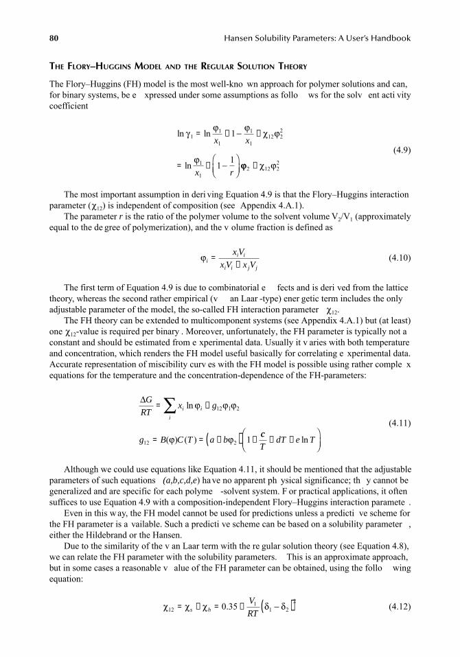
80
Hansen Solubility Parameters: A User’s Handbook
T
HE
F
LORY
–H
UGGINS
M
ODEL
AND
THE
R
EGULAR
S
OLUTION
T
HEORY
The Flory–Huggins (FH) model is the most well-kno wn approach for polymer solutions and can,for binary systems, be e xpressed under some assumptions as follo ws for the solv ent acti vitycoefficient
(4.9)
The most important assumption in deri ving Equation 4.9 is that the Flory–Huggins interactionparameter (
χ
12
) is independent of composition (see Appendix 4.A.1).The parameter
r
is the ratio of the polymer volume to the solvent volume V
2
/V
1
(approximatelyequal to the de gree of polymerization), and the v olume fraction is defined as
(4.10)
The first term of Equation 4.9 is due to combinatorial e fects and is deri ved from the latticetheory, whereas the second rather empirical (v an Laar -type) ener getic term includes the onlyadjustable parameter of the model, the so-called FH interaction parameter
χ
12
.The FH theory can be extended to multicomponent systems (see Appendix 4.A.1) but (at least)
one
χ
12
-value is required per binary . Moreover, unfortunately, the FH parameter is typically not aconstant and should be estimated from e xperimental data. Usually it v aries with both temperatureand concentration, which renders the FH model useful basically for correlating e xperimental data.Accurate representation of miscibility curv es with the FH model is possible using rather comple xequations for the temperature and the concentration-dependence of the FH-parameters:
(4.11)
Although we could use equations like Equation 4.11, it should be mentioned that the adjustableparameters of such equations
(a,b,c,d,e
) have no apparent ph ysical significance; th y cannot begeneralized and are specific for each polyme -solvent system. F or practical applications, it oftensuffices to use Equation 4.9 with a composition-independent Flory–Huggins interaction paramete .
Even in this w ay, the FH model cannot be used for predictions unless a predicti ve scheme forthe FH parameter is a vailable. Such a predicti ve scheme can be based on a solubility parameter ,either the Hildebrand or the Hansen.
Due to the similarity of the v an Laar term with the re gular solution theory (see Equation 4.8),we can relate the FH parameter with the solubility parameters. This is an approximate approach,but in some cases a reasonable v alue of the FH parameter can be obtained, using the follo wingequation:
(4.12)
ln ln
ln
γ ϕ ϕ χ ϕ
ϕ
11
1
1
112 2
2
1
1
1
1 1
= + − +
= + −⎛⎝⎜
⎞⎠⎟
x x
x rϕϕ χ ϕ2 12 2
2+
ϕii i
i i j j
x V
x V x V=
+
ΔG
RTx g
g B C T a b
i i
i
= +
= = +( ) +
∑ ln
( ) ( )
ϕ ϕ ϕ
ϕ ϕ
12 1 2
12 2 1 cc
TdT e T+ +
⎛⎝⎜
⎞⎠⎟
ln
χ χ χ δ δ121
1 22
0 35= + = + −( )s h
V
RT.
7248_C004.fm Page 80 Thursday, May 10, 2007 12:51 PM
The Hansen Solubility Parameters (HSP) in Thermodynamic Models for Polymer Solutions 81
Equation 4.12, without the empirical 0.35 term, is deri ved from the re gular solution theory(compare Equation 4.8 and Equation 4.9). The constant 0.35 is added for correcting for thedeficiencies of the FH combinatorial and residual terms. These deficiencies become vident whencomparing experimental data for athermal polymer and other asymmetric solutions to the resultsobtained with the FH model. A consistent underestimation of the acti vity coef ficient data iobserved, which is often attributed to the inability of the FH model to account for the free-v olumedifferences between polymers and solv ents or between compounds dif fering significantly in sizsuch as n-alkanes with v ery dif ferent chain lengths. The term, which contains the 0.35 f actor,corrects in an empirical w ay for these free-v olume ef fects. Ho wever, and although satisf actoryresults are obtained in some cases, we cannot generally recommend using Equation 4.12 forestimating the FH parameter. Moreover, for many nonpolar systems with compounds having similarsolubility parameters, the empirical f actor 0.35 should be dropped.
Rules of Thumb and Solvent Selection Using the Flory–Huggins Model and Solubility Parameters
The FH model and the solubility parameters of fer v arious alternati ve approaches for solv entselection for polymers, and these rules of thumb are summarized here. A chemical (1) will be goodsolvent for a specific polymer (2), or in other ords, the tw o compounds will be miscible if one(or more) of the follo wing “rules of thumb” are v alid:
1. Using Hildebrand solubility parameters.If the polymer and the solvent have “similar polar and hydrogen bonding degrees:”
(4.13)
2. Using Hansen solubility parameters (HSP).If the polymer and the solvent have very different polar and hydrogen bonding degrees:
(4.14)
where R is the Hansen solubility parameter sphere radius.3. χ12 ≤ 0.5 (the lo wer the Flory–Huggins parameter v alue, the greater the miscibility or ,
in other words, the better a solvent is a specific chemical).Values much above 0.5 indicatenonsolvency.
4. (the lower the infinite dilution act vity coefficient of the sol ent, the greater thesolvency of a chemical). Values of the infinite dilution actvity coefficient ab ve 8 indicatenonsolvency.17 In the intermediate region (between 6 and 8), it is dif ficult to conclude ithe specific chemical is a sol ent or a nonsolv ent.
This latter rule of thumb requires some further e xplanations. The weight-based acti vity coef-ficient at infinite dilution is defined
δ δ1 2 3
1 2
1 8− ≤ ⎛⎝⎜
⎞⎠⎟
./
cal
cm
4 1 22
1 22
1 22
δ δ δ δ δ δd d p p h h R−( ) + −( ) + −( ) ≤
Ω1 6∞ ≤
γ γ
γ γ
i x i
i wi i
i
i
i
x
w
M
M
∞→
∞ ∞
=
=⎛⎝⎜
⎞⎠⎟
=→
lim
lim
0
12
0Ω
11
7248_C004.fm Page 81 Thursday, May 10, 2007 12:51 PM
82 Hansen Solubility Parameters: A User’s Handbook
(The latter part of the equation is v alid for a binary solv ent(1)-polymer(2) mixture.)Extensive collections of experimental data are available;18 otherwise, these can be estimated
by thermodynamic models lik e the ones mentioned abo ve (UNIF AC-FV, Entropic-FV , andFlory–Huggins). Thermodynamic models often perform better for this type of calculation ratherthan for predicting full LLE phase diagrams. However, the results depend not only on the accuracyof the model b ut also on the reliability of the rule of thumb, which in turns depends on theassumptions of the Flory–Huggins approach. A thermodynamically more correct method is tocalculate the acti vity–concentration diagram with a thermodynamic model lik e Entropic-FV orUNIFAC-FV; the maximum indicates phase split, whereas a monotonic increase of acti vity withconcentration indicates a single liquid phase (homogeneous solution).
ACTIVITY COEFFICIENTS MODELS USING THE HSP
FLORY–HUGGINS MODELS USING HILDEBRAND AND HANSEN SOLUBILITY PARAMETERS (HSP)
Several of the problems of the Flory–Huggins model are associated with the difficulties in predictinthe FH interaction parameter and the f act that this parameter depends on both temperature andconcentration.
Recently, Lindvig et al. 19 proposed an e xtension of the Flory–Huggins equation using theHansen solubility parameters for estimating activity coefficients of compl x polymer solutions. Theexpression for the solv ent activity coefficient in a binary sol ent-polymer solution is:
(4.15)
This model is hereafter abbre viated as FH/Ha(nsen) or FH/HSP .Lindvig et al. 19 have tested three dif ferent combinatorial e xpressions, i.e., dif ferent w ays of
expressing the composition fraction ϕi:
1. Based on volume fractions (Equation 4.10)2. FV fractions (Equation 4.6)3. Segment fractions, the latter being defined via Equation 4.10 ut with v an der Waals
volumes used instead of v olumes.
The universal parameter α has been fitted in each case to a la ge number of polymer -solventVLE data. In total, 358 data points ha ve been considered for solutions containing acrylates andacetates (PBMA, PMMA, PEMA, PVAc). A minimum does exist for the different types of solutions,as can be seen in Figure 4.1. In particular , the minima for the nonpolar and h ydrogen bondingsolvents are very close, whereas there is little sensiti vity to the parameter for polar solv ents. Thismeans that a uni versal α value can be established. These are shown for the v arious combinatorialterms in Table 4.1. In all cases, the results are better when the optimum v alue is used than whenα is set equal to one or when the term with the Hansen solubility parameters is ignored ( α = 0).The best results are obtained when the v olume-based combinatorial term is used (Equation 4.10)together with α = 0.6 (see also Figure 4.1).
Table 4.2 pro vides results for se veral polymer solutions with the FH/Hansen model (FHHa,Equation 4.15) using the volume-based combinatorial with both the optimum parameter and α = 1.
Ω1∞
ln lnγ ϕ ϕ χ ϕ
χ α δ δ
11
1
1
112 2
2
121
1 2
1= + − +
= −( )
x x
V
RTd d
221 2
21 2
20 25 0 25+ −( ) + −( )⎡⎣
⎤⎦. .δ δ δ δp p h h
7248_C004.fm Page 82 Thursday, May 10, 2007 12:51 PM
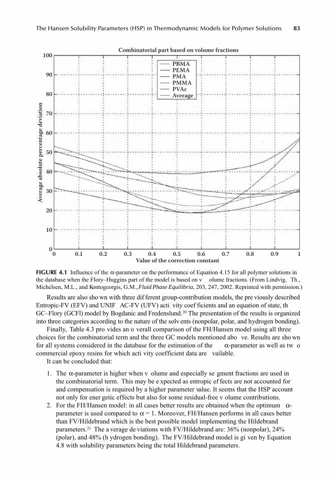
The Hansen Solubility Parameters (HSP) in Thermodynamic Models for Polymer Solutions 83
Results are also sho wn with three dif ferent group-contribution models, the pre viously describedEntropic-FV (EFV) and UNIF AC-FV (UFV) acti vity coef ficients and an equation of state, thGC–Flory (GCFl) model by Bogdanic and Fredenslund.20 The presentation of the results is organizedinto three categories according to the nature of the solv ents (nonpolar, polar, and hydrogen bonding).
Finally, Table 4.3 pro vides an o verall comparison of the FH/Hansen model using all threechoices for the combinatorial term and the three GC models mentioned abo ve. Results are sho wnfor all systems considered in the database for the estimation of the α-parameter as well as tw ocommercial epoxy resins for which acti vity coefficient data are vailable.
It can be concluded that:
1. The α-parameter is higher when v olume and especially se gment fractions are used inthe combinatorial term. This may be e xpected as entropic ef fects are not accounted forand compensation is required by a higher parameter value. It seems that the HSP accountnot only for ener getic effects but also for some residual-free v olume contributions.
2. For the FH/Hansen model: in all cases better results are obtained when the optimum α-parameter is used compared to α = 1. Moreover, FH/Hansen performs in all cases betterthan FV/Hildebrand which is the best possible model implementing the Hildebrandparameters.21 The a verage de viations with FV/Hildebrand are: 36% (nonpolar), 24%(polar), and 48% (h ydrogen bonding). The FV/Hildebrand model is gi ven by Equation4.8 with solubility parameters being the total Hildebrand parameters.
FIGURE 4.1 Influence of the α-parameter on the performance of Equation 4.15 for all polymer solutions inthe database when the Flory–Huggins part of the model is based on v olume fractions. (From Lindvig, Th.,Michelsen, M.L., and Kontogeorgis, G.M., Fluid Phase Equilibria, 203, 247, 2002. Reprinted with permission.)
Combinatorial part based on volume fractionsAv
erag
e abs
olut
e per
cent
age d
eviat
ion
Value of the correction constant
PBMAPEMAPMAPMMAPVAcAverage
100
90
80
70
60
50
40
30
20
10
00 0.1 0.2 0.3 0.4 0.5 0.6 0.7 0.8 0.9 1
7248_C004.fm Page 83 Thursday, May 10, 2007 12:51 PM
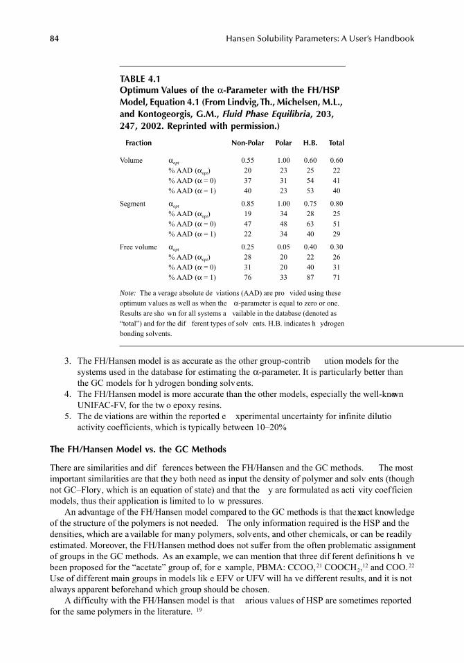
84 Hansen Solubility Parameters: A User’s Handbook
3. The FH/Hansen model is as accurate as the other group-contrib ution models for thesystems used in the database for estimating the α-parameter. It is particularly better thanthe GC models for h ydrogen bonding solvents.
4. The FH/Hansen model is more accurate than the other models, especially the well-knownUNIFAC-FV, for the tw o epoxy resins.
5. The de viations are within the reported e xperimental uncertainty for infinite dilutioactivity coefficients, which is typically between 10–20%
The FH/Hansen Model vs. the GC Methods
There are similarities and dif ferences between the FH/Hansen and the GC methods. The mostimportant similarities are that they both need as input the density of polymer and solv ents (thoughnot GC–Flory, which is an equation of state) and that the y are formulated as acti vity coefficienmodels, thus their application is limited to lo w pressures.
An advantage of the FH/Hansen model compared to the GC methods is that the exact knowledgeof the structure of the polymers is not needed. The only information required is the HSP and thedensities, which are available for many polymers, solvents, and other chemicals, or can be readilyestimated. Moreover, the FH/Hansen method does not suffer from the often problematic assignmentof groups in the GC methods. As an example, we can mention that three dif ferent definitions h vebeen proposed for the “acetate” group of, for e xample, PBMA: CCOO,21 COOCH2,12 and COO. 22
Use of different main groups in models lik e EFV or UFV will ha ve different results, and it is notalways apparent beforehand which group should be chosen.
A difficulty with the FH/Hansen model is that arious values of HSP are sometimes reportedfor the same polymers in the literature. 19
TABLE 4.1Optimum Values of the α-Parameter with the FH/HSP Model, Equation 4.1 (From Lindvig, Th., Michelsen, M.L., and Kontogeorgis, G.M., Fluid Phase Equilibria, 203, 247, 2002. Reprinted with permission.)
Fraction Non-Polar Polar H.B. Total
Volume αopt 0.55 1.00 0.60 0.60% AAD (αopt) 20 23 25 22% AAD (α = 0) 37 31 54 41% AAD (α = 1) 40 23 53 40
Segment αopt 0.85 1.00 0.75 0.80% AAD (αopt) 19 34 28 25% AAD (α = 0) 47 48 63 51% AAD (α = 1) 22 34 40 29
Free volume αopt 0.25 0.05 0.40 0.30% AAD (αopt) 28 20 22 26% AAD (α = 0) 31 20 40 31% AAD (α = 1) 76 33 87 71
Note: The a verage absolute de viations (AAD) are pro vided using theseoptimum values as well as when the α-parameter is equal to zero or one.Results are sho wn for all systems a vailable in the database (denoted as“total”) and for the dif ferent types of solv ents. H.B. indicates h ydrogenbonding solvents.
7248_C004.fm Page 84 Thursday, May 10, 2007 12:51 PM
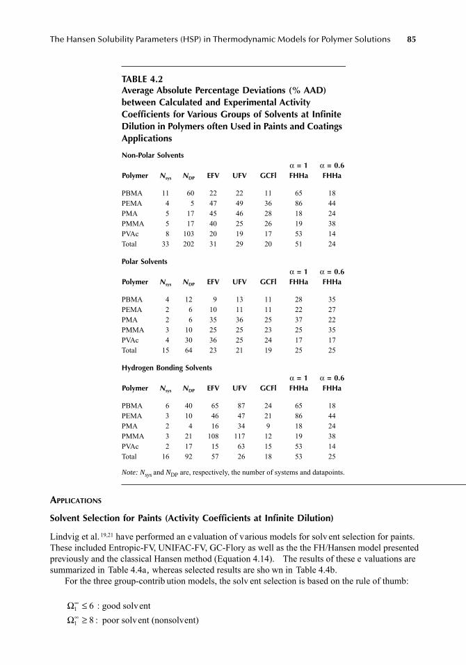
The Hansen Solubility Parameters (HSP) in Thermodynamic Models for Polymer Solutions 85
APPLICATIONS
Solvent Selection for Paints (Activity Coefficients at Infinite Dilution)
Lindvig et al. 19,21 have performed an e valuation of various models for solv ent selection for paints.These included Entropic-FV, UNIFAC-FV, GC-Flory as well as the the FH/Hansen model presentedpreviously and the classical Hansen method (Equation 4.14). The results of these e valuations aresummarized in Table 4.4a, whereas selected results are sho wn in Table 4.4b.
For the three group-contrib ution models, the solv ent selection is based on the rule of thumb:
: good solvent poor solvent (nonsolvent)
TABLE 4.2Average Absolute Percentage Deviations (% AAD) between Calculated and Experimental Activity Coefficients for Various Groups of Solvents at Infinite Dilution in Polymers often Used in Paints and Coatings Applications
Non-Polar Solventsα = 1 α = 0.6
Polymer Nsys NDP EFV UFV GCFl FHHa FHHa
PBMA 11 60 22 22 11 65 18PEMA 4 5 47 49 36 86 44PMA 5 17 45 46 28 18 24PMMA 5 17 40 25 26 19 38PVAc 8 103 20 19 17 53 14Total 33 202 31 29 20 51 24
Polar Solventsα = 1 α = 0.6
Polymer Nsys NDP EFV UFV GCFl FHHa FHHa
PBMA 4 12 9 13 11 28 35PEMA 2 6 10 11 11 22 27PMA 2 6 35 36 25 37 22PMMA 3 10 25 25 23 25 35PVAc 4 30 36 25 24 17 17Total 15 64 23 21 19 25 25
Hydrogen Bonding Solventsα = 1 α = 0.6
Polymer Nsys NDP EFV UFV GCFl FHHa FHHa
PBMA 6 40 65 87 24 65 18PEMA 3 10 46 47 21 86 44PMA 2 4 16 34 9 18 24PMMA 3 21 108 117 12 19 38PVAc 2 17 15 63 15 53 14Total 16 92 57 26 18 53 25
Note: Nsys and NDP are, respectively, the number of systems and datapoints.
Ω1 6∞ ≤Ω1 8∞ ≥ :
7248_C004.fm Page 85 Thursday, May 10, 2007 12:51 PM
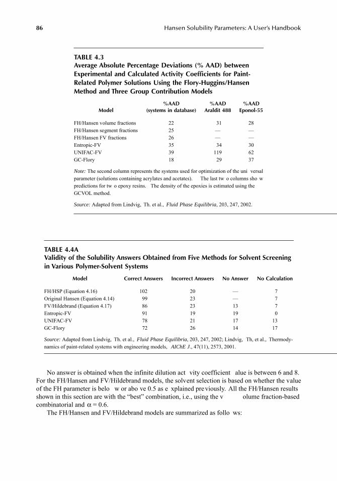
86 Hansen Solubility Parameters: A User’s Handbook
No answer is obtained when the infinite dilution act vity coefficient alue is between 6 and 8.For the FH/Hansen and FV/Hildebrand models, the solvent selection is based on whether the valueof the FH parameter is belo w or abo ve 0.5 as e xplained pre viously. All the FH/Hansen resultsshown in this section are with the “best” combination, i.e., using the v olume fraction-basedcombinatorial and α = 0.6.
The FH/Hansen and FV/Hildebrand models are summarized as follo ws:
TABLE 4.3Average Absolute Percentage Deviations (% AAD) between Experimental and Calculated Activity Coefficients for Paint-Related Polymer Solutions Using the Flory-Huggins/Hansen Method and Three Group Contribution Models
Model%AAD
(systems in database)%AAD
Araldit 488%AAD
Eponol-55
FH/Hansen volume fractions 22 31 28FH/Hansen segment fractions 25 — —FH/Hansen FV fractions 26 — —Entropic-FV 35 34 30UNIFAC-FV 39 119 62GC-Flory 18 29 37
Note: The second column represents the systems used for optimization of the uni versalparameter (solutions containing acrylates and acetates). The last tw o columns sho wpredictions for tw o epoxy resins. The density of the epoxies is estimated using theGCVOL method.
Source: Adapted from Lindvig, Th. et al., Fluid Phase Equilibria, 203, 247, 2002.
TABLE 4.4AValidity of the Solubility Answers Obtained from Five Methods for Solvent Screening in Various Polymer-Solvent Systems
Model Correct Answers Incorrect Answers No Answer No Calculation
FH/HSP (Equation 4.16) 102 20 — 7Original Hansen (Equation 4.14) 99 23 — 7FV/Hildebrand (Equation 4.17) 86 23 13 7Entropic-FV 91 19 19 0UNIFAC-FV 78 21 17 13GC-Flory 72 26 14 17
Source: Adapted from Lindvig, Th. et al., Fluid Phase Equilibria, 203, 247, 2002; Lindvig, Th, et al., Thermody-namics of paint-related systems with engineering models, AIChE J., 47(11), 2573, 2001.
7248_C004.fm Page 86 Thursday, May 10, 2007 12:51 PM
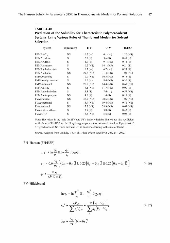
The Hansen Solubility Parameters (HSP) in Thermodynamic Models for Polymer Solutions 87
FH–Hansen (FH/HSP)
(4.16)
FV–Hildebrand
(4.17)
TABLE 4.4BPrediction of the Solubility for Characteristic Polymer-Solvent Systems Using Various Rules of Thumb and Models for Solvent Selection
System Experiment EFV UFV FH/HSP
PBMA/nC10 NS 6.5 ( – ) 6.1 ( – ) 1.20 (NS)PBMA/xylene S 2.3 (S) 3.6 (S) 0.41 (S)PBMA/CHCl3 S 1.9 (S) 9.1 (NS) 0.14 (S)PBMA/acetone S 0.2 (NS) 14.1 (NS) 0.2 (S)PBMA/ethyl acetate S 6.7 ( – ) 6.7 ( – ) 0.27 (S)PBMA/ethanol NS 29.2 (NS) 31.3 (NS) 1.01 (NS)PMMA/acetone S 10.0 (NS) 16.5 (NS) 0.18 (S)PMMA/ethyl acetate S 6.6 (– ) 8.4 (NS) 0.36 (S)PMMA/butanol NS 26.8 (NS) 14.4 (NS) 0.67 (NS)PEMA/MEK S 8.1 (NS) 11.7 (NS) 0.09 (S)PEMA/diethyl ether S 5.8 (S) 7.6 ( – ) 0.57 (NS)PEMA/nitropropane NS 4.5 (S) 1.4 (S) 0.11 (S)PVAc/hexane NS 38.7 (NS) 38.6 (NS) 1.09 (NS)PVAc/methanol S 18.9 (NS) 19.4 (NS) 0.71 (NS)PVAc/ethanol NS 15.2 (NS) 38.9 (NS) 0.63 (NS)PVAc/nitromethane S 3.9 (S) 3.8 (S) 0.43 (S)PVAc/THF S 8.4 (NS) 5.6 (S) 0.05 (S)
Note: The values in the table for EFV and UFV indicate infinite dilution act vity coefficientwhile those of FH/HSP are the Flory-Huggins parameters estimated based on Equation 4.16.S = good solv ent, NS = non solv ent, - = no answer according to the rule of thumb .
Source: Adapted from Lindvig, Th. et al., Fluid Phase Equilibria, 203, 247, 2002.
ln ln
.
γ ϕ ϕ χ ϕ
χ δ δ
11
1
1
112 2
2
121
1 2
1
0 6
= + − +
= −
x x
V
RTd d(( ) + −( ) + −( )⎡
⎣⎤⎦
=
21 2
21 2
20 25 0 25. .δ δ δ δ
ϕ
p p h h
iix VV
x V x Vi
i i j j+
ln ln
,
γ ϕ ϕ χ ϕ
ϕ
1 12 221= + − +
=
ifv
i
ifv
i
ifv i i fv
j
x x
x V
x VV
x V V
x V V
V
RT
j fv
j
i i wi
j j wj
j
.∑ ∑=
−( )−( )
= −χ δ δ121
1 222( )
7248_C004.fm Page 87 Thursday, May 10, 2007 12:51 PM
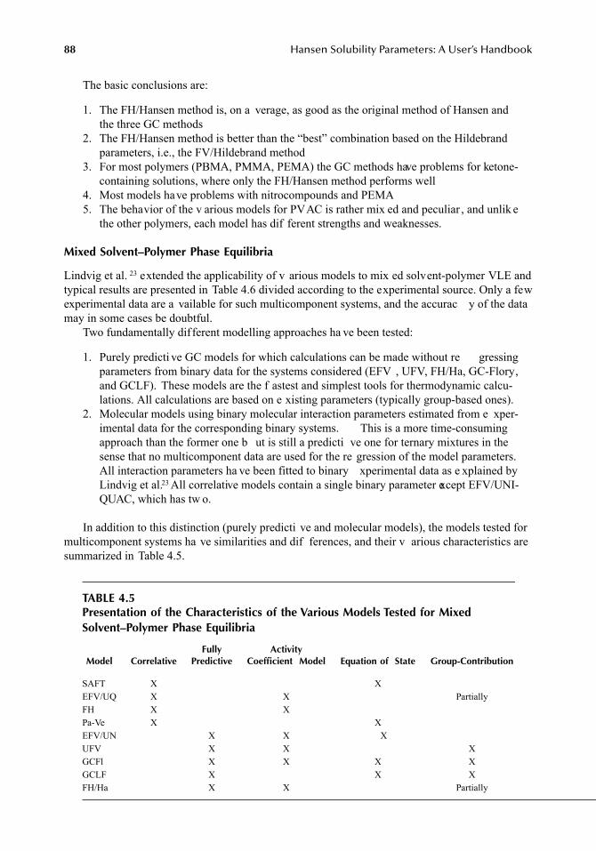
88 Hansen Solubility Parameters: A User’s Handbook
The basic conclusions are:
1. The FH/Hansen method is, on a verage, as good as the original method of Hansen andthe three GC methods
2. The FH/Hansen method is better than the “best” combination based on the Hildebrandparameters, i.e., the FV/Hildebrand method
3. For most polymers (PBMA, PMMA, PEMA) the GC methods have problems for ketone-containing solutions, where only the FH/Hansen method performs well
4. Most models have problems with nitrocompounds and PEMA5. The behavior of the v arious models for PVAC is rather mix ed and peculiar , and unlik e
the other polymers, each model has dif ferent strengths and weaknesses.
Mixed Solvent–Polymer Phase Equilibria
Lindvig et al. 23 extended the applicability of v arious models to mix ed solvent-polymer VLE andtypical results are presented in Table 4.6 divided according to the experimental source. Only a fewexperimental data are a vailable for such multicomponent systems, and the accurac y of the datamay in some cases be doubtful.
Two fundamentally different modelling approaches ha ve been tested:
1. Purely predicti ve GC models for which calculations can be made without re gressingparameters from binary data for the systems considered (EFV , UFV, FH/Ha, GC-Flory,and GCLF). These models are the f astest and simplest tools for thermodynamic calcu-lations. All calculations are based on e xisting parameters (typically group-based ones).
2. Molecular models using binary molecular interaction parameters estimated from e xper-imental data for the corresponding binary systems. This is a more time-consumingapproach than the former one b ut is still a predicti ve one for ternary mixtures in thesense that no multicomponent data are used for the re gression of the model parameters.All interaction parameters ha ve been fitted to binary xperimental data as e xplained byLindvig et al.23 All correlative models contain a single binary parameter except EFV/UNI-QUAC, which has tw o.
In addition to this distinction (purely predicti ve and molecular models), the models tested formulticomponent systems ha ve similarities and dif ferences, and their v arious characteristics aresummarized in Table 4.5.
TABLE 4.5Presentation of the Characteristics of the Various Models Tested for Mixed Solvent–Polymer Phase Equilibria
Model CorrelativeFully
PredictiveActivity
Coefficient Model Equation of State Group-Contribution
SAFT X XEFV/UQ X X PartiallyFH X XPa-Ve X X EFV/UN X X XUFV X X XGCFl X X X XGCLF X X XFH/Ha X X Partially
7248_C004.fm Page 88 Thursday, May 10, 2007 12:51 PM
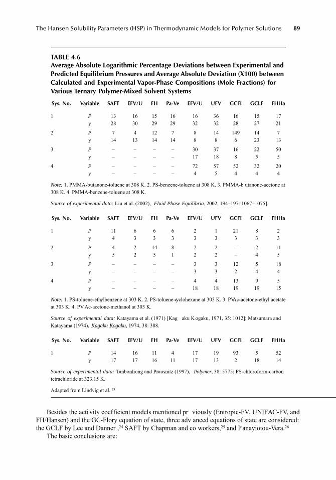
The Hansen Solubility Parameters (HSP) in Thermodynamic Models for Polymer Solutions 89
Besides the activity coefficient models mentioned pr viously (Entropic-FV, UNIFAC-FV, andFH/Hansen) and the GC-Flory equation of state, three adv anced equations of state are considered:the GCLF by Lee and Danner ,24 SAFT by Chapman and co workers,25 and Panayiotou-Vera.26
The basic conclusions are:
TABLE 4.6Average Absolute Logarithmic Percentage Deviations between Experimental and Predicted Equilibrium Pressures and Average Absolute Deviation (X100) between Calculated and Experimental Vapor-Phase Compositions (Mole Fractions) for Various Ternary Polymer-Mixed Solvent Systems
Sys. No. Variable SAFT EFV/U FH Pa-Ve EFV/U UFV GCFI GCLF FHHa
1 P 13 16 15 16 16 36 16 15 17y 28 30 29 29 32 32 28 27 21
2 P 7 4 12 7 8 14 149 14 7y 14 13 14 14 8 8 6 23 13
3 P – – – – 30 37 16 22 50y – – – – 17 18 8 5 5
4 P – – – – 72 57 52 32 20y – – – – 4 5 4 4 4
Note: 1. PMMA-butanone-toluene at 308 K. 2. PS-benzene-toluene at 308 K. 3. PMMA-b utanone-acetone at308 K. 4. PMMA-benzene-toluene at 308 K.
Source of experimental data: Liu et al. (2002), Fluid Phase Equilibria, 2002, 194–197: 1067–1075].
Sys. No. Variable SAFT EFV/U FH Pa-Ve EFV/U UFV GCFI GCLF FHHa
1 P 11 6 6 6 2 1 21 8 2y 4 3 3 3 3 3 3 3 3
2 P 4 2 14 8 2 2 – 2 11y 5 2 5 1 2 2 – 4 5
3 P – – – – 3 3 12 5 18y – – – – 3 3 2 4 4
4 P – – – – 4 4 13 9 5y – – – – 18 18 19 19 15
Note: 1. PS-toluene-ethylbenzene at 303 K. 2. PS-toluene-cyclohexane at 303 K. 3. PVAc-acetone-ethyl acetateat 303 K. 4. PVAc-acetone-methanol at 303 K.
Source of experimental data: Katayama et al. (1971) [Kag aku K ogaku, 1971, 35: 1012]; Matsumara andKatayama (1974), Kagaku Kogaku, 1974, 38: 388.
Sys. No. Variable SAFT EFV/U FH Pa-Ve EFV/U UFV GCFI GCLF FHHa
1 P 14 16 11 4 17 19 93 5 52y 17 17 16 11 17 13 2 18 14
Source of experimental data: Tanbonliong and Prausnitz (1997), Polymer, 38: 5775; PS-chloroform-carbontetrachloride at 323.15 K.
Adapted from Lindvig et al. 23
7248_C004.fm Page 89 Thursday, May 10, 2007 12:51 PM
90 Hansen Solubility Parameters: A User’s Handbook
1. The FH/Hansen is as successful as the GC methods and other more comple x models,both the correlative and the predicti ve.
2. The models perform sometimes dif ferently for isolated systems, b ut the o verall differ-ences are minor , and we belie ve that the y fall within the e xperimental uncertainties ofthe data considered. In many cases the results with the various models are closer to eachother than to the e xperimental data.
3. For 9 out of the 13 systems considered, good predictions of both the equilibrium pressuresand the vapor phase compositions are obtained by all models.
4. The correlative models do not of fer any improvements over the group-contribution models.This is a surprising result as it is e xpected that the molecular information in a model shouldlead to a better representation of phase equilibria for multicomponent mixtures. It may bethat some experimental data for such multicomponent mixtures are of lo w accuracy.
5. This investigation does not point to a “clear winner” among the models, and more dataare required for further in vestigations. However, this preliminary study pro vides confidence for use of the FH/Hansen approach.
CONCLUSIONS AND FUTURE CHALLENGES
Many successful calculations in polymer thermodynamics can be carried out using simple group-contribution methods based on UNIFAC, which contain corrections for the FV effects. Models likeEntropic-FV and UNIF AC-FV can be used for such calculations and are sho wn to satisf actorilypredict the solvent activities and vapor–liquid equilibria for binary and ternary polymer solutions.Such methods require accurate v alues of the densities and, moreo ver, are based on the a vailabilityof group parameters in the UNIF AC tables.
An alternative equally successful approach is offered by the combination of the Flory–Hugginsmodel with the Hansen solubility parameters (HSP). The FH/HSP (Equation 4.16) includes a singleuniversal parameter that has been re gressed to e xperimental data for man y polymer solv ent solu-tions. The combinatorial term that gi ves the best results is based on v olume fractions.
The FH/HSP model is sho wn to be as successful as the state of the art GC models (Entropic-FV, UNIFAC-FV, and GC-Flory) in predicting infinite dilution act vity coefficients including complex epoxy polymers, solv ent selection for paints, and VLE for mix ed solvent–polymer systems.Moreover, FH/HSP is as successful for mix ed solvent–polymer phase equilibria as comple x, the-oretically-based equations of state lik e SAFT and the Group Contrib ution Lattice Fluid.
This chapter has been limited to v apor–liquid equlibria (both at finite concentrations and infinidilution), mixed solvents, and solv ent selection. The methods can be, in principle, e xtended to poly-mer–solvent LLE, and this has been indeed done, for e xample, for Entropic-FV, GC-Flory, GCLF, andSAFT.
The predictive group contribution methods are less successful for the prediction of liquid–liquidequilibria as their parameters are based on VLE. Some results are summarized in the recentliterature.6,15 Better results are obtained when a molecular local composition model is used as, forexample, in the Entropic-FV/UNIQUAC model as shown by Pappa et al.27 As such models includethe liquid volume as input parameter, successful results have been reported even for high pressureLLE. However, solvent selection can be based on the use of infinite dilution act vity coefficientfor which these models are quite successful.
So far most acti vity coefficient models, including FH/HS , have been applied mainly to or ganicpolymer solutions of rather simple structures and VLE/solvent selection studies, although some complexpaint-related polymers ha ve been considered as well. Thorlaksen et al. 28 have recently combined theEntropic-FV term with Hildebrand's regular solution theory and developed a model for estimating g assolubilities in elastomers. A similar approach can be adopted for the FH/HSP model presented here.
Future developments can include complex structures such as dendrimers (where EFV and UFValready have been applied 29); star -like, h yperbranched polymers as well as v arious copolymers;
7248_C004.fm Page 90 Thursday, May 10, 2007 12:51 PM
The Hansen Solubility Parameters (HSP) in Thermodynamic Models for Polymer Solutions 91
liquid–liquid and solid–liquid equilibria, including the ef fect of crystallinity; and cross-linking,inorganic polymers and polyelectrolytes.
LIST OF ABBREVIATIONS
% AAD Average percentage absolute de viationComb CombinatorialComb-FV Combinatorial-free volumeCST Critical solution temperatureExper./exp. ExperimentalEFV Entropic-FVEFV/UN (Same as EFV) Entropic-FV (using UNIF AC for the residual term)EFV/UQ Entropic-FV using UNIQUAC as the residual termFH Flory–Huggins (model/equation/interaction parameter)FH/HSP The FH model using the Hansen solubility parameters, Equation 4.16FV Free-volumeGC Group contribution (method/principle)GC-F(lory) Group contribution Flory equation of stateGCLF Group contribution lattice fluiGCVOL Group contribution volume (method for estimating the density)HB Hydrogen bondingHSP Hansen solubility parametersLCST Lower critical solution temperatureLLE Liquid–liquid equilibriaMW Molecular weightNS Nonsolvent/nonsolublePa-Ve Panayiotou–Vera equation of statePBMA Polybutyl methacrylatePDMS PolydimethylsiloxanePEMA Polyethyl methacrylatePMMA Polymethyl methacrylatePred. PredictedPVAC Polyvinyl acetateRes ResidualS Solvent/solubleSAFT Statistical associating fluid theorSLE Solid–liquid equilibriaUCST Upper critical solution temperatureU-FV UNIFAC-FVUNIFAC Universal functional activity coefficientUQ UNIQUACvdW Van der Waals equation of statevdW1f Van der Waals one fluid (mixing rulesVLE Vapor–liquid equilibriaVOC Volatile organic content
7248_C004.fm Page 91 Thursday, May 10, 2007 12:51 PM
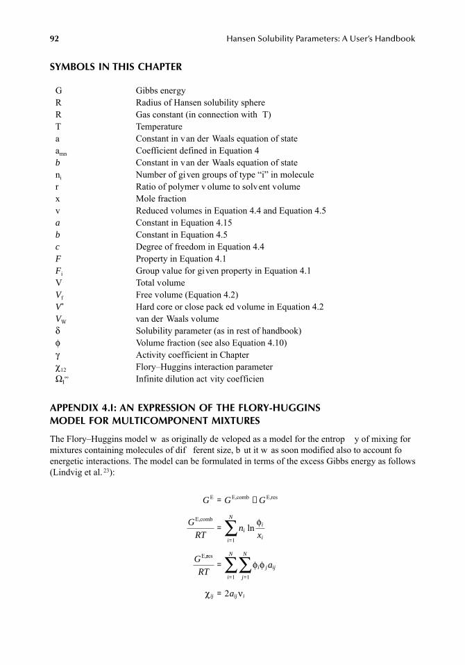
92 Hansen Solubility Parameters: A User’s Handbook
SYMBOLS IN THIS CHAPTER
APPENDIX 4.I: AN EXPRESSION OF THE FLORY-HUGGINS MODEL FOR MULTICOMPONENT MIXTURES
The Flory–Huggins model w as originally de veloped as a model for the entrop y of mixing formixtures containing molecules of dif ferent size, b ut it w as soon modified also to account foenergetic interactions. The model can be formulated in terms of the excess Gibbs energy as follows(Lindvig et al. 23):
G Gibbs energyR Radius of Hansen solubility sphereR Gas constant (in connection with T)T Temperaturea Constant in van der Waals equation of stateamn Coefficient defined in Equation 4b Constant in van der Waals equation of stateni Number of given groups of type “i” in moleculer Ratio of polymer v olume to solvent volumex Mole fractionv Reduced volumes in Equation 4.4 and Equation 4.5a Constant in Equation 4.15b Constant in Equation 4.5c Degree of freedom in Equation 4.4F Property in Equation 4.1Fi Group value for given property in Equation 4.1V Total volumeVf Free volume (Equation 4.2)V* Hard core or close pack ed volume in Equation 4.2VW van der Waals volumeδ Solubility parameter (as in rest of handbook)φ Volume fraction (see also Equation 4.10)γ Activity coefficient in Chapter χ12 Flory–Huggins interaction parameterΩI
∞ Infinite dilution act vity coefficien
G G G
G
RTn
x
G
i
i
Ni
i
E E,comb E,res
E,comb
E,
= +
==∑
1
ln φ
rres
RTa
a
i j ij
j
N
i
N
ij ij i
=
=
==∑∑ φ φ
χ ν
11
2
7248_C004.fm Page 92 Thursday, May 10, 2007 12:51 PM
The Hansen Solubility Parameters (HSP) in Thermodynamic Models for Polymer Solutions 93
Using basic thermodynamics, the follo wing expression for the acti vity coefficient is obtained
where the combinatorial term is gi ven by:
and the residual term is:
The abo ve formulation of the FH model is slightly dif ferent from the con ventionally usedformulation using the Flory–Huggins interaction parameter (χ12), although there is an interrelation-ship based on the simple equation sho wn above.
For a binary mixture, the multicomponent equation reduces to the traditional FH residual term:
REFERENCES
1. Fredenslund, Aa., Jones, R.L., and Prausnitz, J.M., Group contrib ution estimation of acti vity coefficients in nonideal liquid mixtures, AIChE J., 25(1), 1086–1098, 1975.
2. Van Krevelen, D.W., Properties of polymers, Their correlation with chemical structure; their numericalestimation and prediction from additive group contributions, Elsevier, 1990.
3. Elbro, H.S., Fredenslund, Aa., and Rasmussen, P ., Group contrib ution method for the prediction ofliquid densities as a function of temperature for solv ents, oligomers, and polymers , Ind. Eng. Chem.Res., 30, 2576, 1991.
4. Tsibanogiannis, I.N., Kalospiros, N.S., and Tassios, D.P., Extension of the GCV OL method andapplication to some comple x compounds, Ind. Eng. Chem. Res., 33, 1641, 1994.
5. Ihmels, E.C. and Gmehling, J., Extension and re vision of the group contribution method GCVOL forthe prediction of pure compound liquid densities , Ind. Eng. Chem. Res., 42(2), 408–412, 2003.
6. Kontogeorgis, G.M., Thermodynamics of polymer solutions, in Handbook of Surface and ColloidChemistry, 2nd ed., Birdi, K.S., Ed., CRC Press, Boca Raton, FL, 2003, chap.16.
7. Bogdanic, G. and Fredenslund, Aa., Prediction of VLE for mixtures with co-polymers, Ind. Eng.Chem. Res., 34, 324, 1965.
8. Elbro, H.S., Phase Equilibria of Polymer Solutions — with Special Emphasis on Free Volumes, Ph.Dthesis, Department of Chemical Engineering, Technical University of Denmark, 1992.
9. Bondi, A., Physical Properties of Molecular Crystals, Liquids and Glasses, John Wiley & Sons, NewYork, 1968.
10. Elbro, H.S., Fredenslund, Aa., and Rasmussen, P., A new simple equation for the prediction of solventactivities in polymer solutions, Macromolecules, 23, 4707, 1990.
11. Kontogeorgis, G.M., Fredenslund, Aa., and Tassios, D.P., Simple acti vity coefficient model for thprediction of solvent activities in polymer solutions, Ind. Eng. Chem. Res., 32, 362, 1993.
12. Oishi, T. and Prausnitz, M., Estimation of solv ent acti vities in polymer solutions using a group-contribution method, Ind. Eng. Chem. Process Des. Dev., 17(3), 333, 1978.
13. Fried, J.R., Jiang, J.S., and Yeh, E., Comput. Polym. Sci., 2, 95, 1992.
ln ln lnγ γ γi icomb
ires= +
ln lnγ ϕ ϕicomb i
i
i
ix x= + −1
ln γ ϕ ϕ ϕires
i j ij i j k jk
k
NC
j
NC
j
NC
v a v a= −===
∑∑2111
∑∑
ln γ χ ϕ1 12 22res =
7248_C004.fm Page 93 Thursday, May 10, 2007 12:51 PM
94 Hansen Solubility Parameters: A User’s Handbook
14. Hansen, H.K., Coto, B., and K uhlmann, B., UNIF AC with lineary temperature-dependent group-interaction parameters, IVC-SEP Internal Report 9212, 1992.
15. Kontogeorgis, G.M., Models for polymer solutions, in Computer Aided Property Estimation forProcess and Product Design, Kontogeorgis, G.M. and Gaani, R., Eds., Else vier, 2004, chap. 7.
16. Kouskoumvekaki, I., Michelsen, M.L., and Kontogeorgis, G.M., Fluid Phase Equilibria, 202(2), 325,2002.
17. Holten-Andersen, J. and Eng, K., Activity coef ficients in polymer solutions, Progress in OrganicCoatings, 16, 77, 1988.
18. High, M.S. and Danner , R.P., Polymer Solution Handbook; DIPPR 881 Project, Design Institute forPhysical Property Data, 1992.
19. Lindvig, Th., Michelsen, M.L., and K ontogeorgis, G.M., Fluid Phase Equilibria, 203, 247, 2002.20. Bogdanic, G. and Fredenslund, Aa., Ind. Eng. Chem. Res., 34, 324, 1995.21. Lindvig, Th., Michelsen, M.L., and K ontogeorgis, G.M., Thermodynamics of paint-related systems
with engineering models, AIChE J., 47(11), 2573, 2001.22. Lee, B.C. and Danner , R.P., Prediction of infinite dilution act vity coefficients in polymer solutions
comparison of prediction models, Fluid Phase Equilibria, 128, 97, 1997.23. Lindvig, Th., Economou, I.G., Danner, R.P., Michelsen, M.L., and Kontogeorgis, G.M., Modeling of
multicomponent vapor-liquid equilibria for polymer -solvent systems, Fluid Phase Equilibria, 220,11–20, 2004.
24. Lee, B.C. and Danner , R.P., Prediction of polymer -solvent phase equilibria by a modified groupcontribution EoS, AIChE, 42, 837, 1996.
25. Chapman, W.G. et al., Ne w reference equation of state for associating fluids, Ind. Eng. Chem. Res.,29, 1709–1721, 1990.
26. Panayiotou, C. and Vera, J.H., An improved lattice-fluid equation of state for pure component polymeric fluids, Polym. Eng. Sci., 22, 345, 1982.
27. Pappa, G.D., Voutsas, E.C., and Tassios, D.P., Liquid-liquid phase equilibrium in polymer -solventsystems: correlation and prediction of the polymer molecular weight and the pressure effect, Ind. Eng.Chem. Res., 40(21), 4654, 2001.
28. Thorlaksen, P., Abildskov, J., and K ontogeorgis, G.M., Prediction of g as solubilities in elastomericpolymers for the design of thermopane windo ws, Fluid Phase Equilibria, 211, 17, 2003.
29. Kouskoumvekaki, I., Giesen, R., Michelsen, M.L., and K ontogeorgis, G.M., Free-v olume acti vitycoefficient models for dendrimer solutions, Ind. Eng. Chem. Res., 41, 4848, 2002.
7248_C004.fm Page 94 Thursday, May 10, 2007 12:51 PM
95
5
Methods of Characterization — Polymers
Charles M. Hansen
ABSTRACT
The simplest e xperimental method to determine the Hansen solubility parameters (HSP) for apolymer is to e valuate whether or not it dissolv es in selected solv ents. Those solvents dissolvingthe polymer will ha ve HSP closer to those of the polymer than those solv ents that do not. Acomputer program or graphical method can then be used to find the HSP for the polyme . Othertypes of evaluations can also lead to polymer HSP. These include swelling, melting point reduction,surface attack, chemical resistance, barrier properties, viscosity measurements, and an y othermeasurement reflecting di ferences in polymer af finities among the sol ents.
Polymer HSP can be higher than the HSP of an y of the test solv ents. This means that some ofthe methods suggested in the literature to interpret data, i.e., those which use a verages of solv entHSP to arrive at the polymer HSP , must be used with care.
INTRODUCTION
Experience has sho wn that if it is at all possible, an e xperimental evaluation of the beha vior of apolymer in contact with a series of selected liquids is the best way to arrive at its HSP. Experimentaldata can be generated and treated in v arious ways to arrive at the values of interest. Examples areincluded in the follo wing.
The author’s usual approach to generate data in solubility parameter studies is to contact apolymer of interest with 40 to 45 well-chosen liquids. One may then observ e or measure a numberof different phenomena including full solution at a given concentration, degree of swelling by visualobservation or by measurement of weight change, v olume change, clarity, surface attack, etc. Theobject of the studies is to determine differences in affinity of the polymer for the di ferent solvents.These differences are then traditionally used to di vide the solv ents into tw o groups, one which isconsidered “good” and the other which is considered “bad. ” Such data can be entered into theSPHERE program as discussed in Chapter 1. Whenever possible, the author uses a set of solv entsas described belo w, often supplemented by selected solv ents depending on the purpose of theinvestigation. Supplementary test solv ents are usually in the boundary re gions as it is these thatdetermine the parameters of the sphere. Adding more good solvents well within the sphere or morebad solvents well outside of it will not change an ything but the data fit
The goal of the e xperimental work is to arrive at a set of data sho wing differences in behavioramong the test solvents. These data are then processed to arrive at the four parameters characteristicof HSP correlations, three describing the nonpolar , polar, and h ydrogen-bonding interactions forthe liquids and the fourth, Ro, a radius of interaction for the type of interaction described.
The author has most often used computer techniques to e valuate the data to find the polymeHSP. In earlier w ork simple plots were used. A simple plot of
δ
P
vs.
δ
H
is also helpful in man ypractical situations to get guidance as discussed in Chapter 8. The approximate determination ofpolymer HSP can be done with three plots of experimental data using the HSP parameters pairwise.Figure 5.1 to Figure 5.3 demonstrate how this was attempted initially.
1
The spheroids in the figureincluding the
δ
D
parameter gave problems. Hansen and Skaarup
2
simply used a scaling f actor of 2(the coefficient “4” in Chapter 1, Equation 1.9) to produce spheres in all three plots. As Ro must
7248_C005.fm Page 95 Wednesday, May 23, 2007 10:51 AM
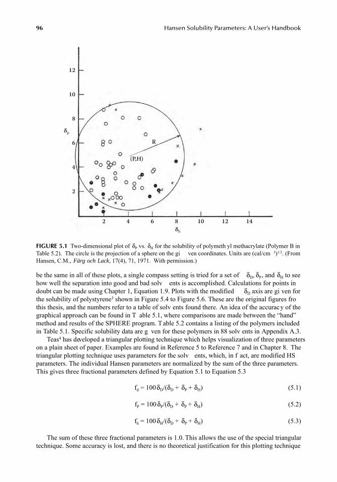
96
Hansen Solubility Parameters: A User’s Handbook
be the same in all of these plots, a single compass setting is tried for a set of
δ
D
,
δ
P
, and
δ
H
to seehow well the separation into good and bad solv ents is accomplished. Calculations for points indoubt can be made using Chapter 1, Equation 1.9. Plots with the modified
δ
D
axis are gi ven forthe solubility of polystyrene
3
shown in Figure 5.4 to Figure 5.6. These are the original figures frothis thesis, and the numbers refer to a table of solv ents found there. An idea of the accuracy of thegraphical approach can be found in T able 5.1, where comparisons are made between the “hand”method and results of the SPHERE program. T able 5.2 contains a listing of the polymers includedin Table 5.1. Specific solubility data are g ven for these polymers in 88 solv ents in Appendix A.3.
Teas
4
has developed a triangular plotting technique which helps visualization of three parameterson a plain sheet of paper. Examples are found in Reference 5 to Reference 7 and in Chapter 8. Thetriangular plotting technique uses parameters for the solv ents, which, in f act, are modified HSparameters. The individual Hansen parameters are normalized by the sum of the three parameters.This gives three fractional parameters defined by Equation 5.1 to Equation 5.3
f
d
= 100
δ
D
/(
δ
D
+
δ
P
+
δ
H
) (5.1)
f
P
= 100
δ
P
/(
δ
D
+
δ
P
+
δ
H
) (5.2)
f
h
= 100
δ
H
/(
δ
D
+
δ
P
+
δ
H
) (5.3)
The sum of these three fractional parameters is 1.0. This allows the use of the special triangulartechnique. Some accuracy is lost, and there is no theoretical justification for this plotting technique
FIGURE 5.1
Two-dimensional plot of
δ
P
vs.
δ
H
for the solubility of polymeth yl methacrylate (Polymer B inTable 5.2). The circle is the projection of a sphere on the gi ven coordinates. Units are (cal/cm
3
)
1/2
. (FromHansen, C.M.,
Färg och Lack
, 17(4), 71, 1971. With permission.)
2 4 6
R
(P,H)
8 10 12 14δh
δp
12
10
8
6
4
2
7248_C005.fm Page 96 Wednesday, May 23, 2007 10:51 AM
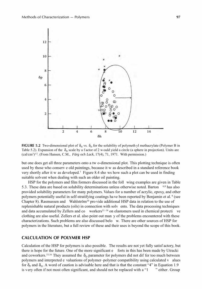
Methods of Characterization — Polymers
97
but one does get all three parameters onto a tw o-dimensional plot. This plotting technique is oftenused by those who conserv e old paintings, because it w as described in a standard reference bookvery shortly after it w as developed.
7
Figure 8.4 sho ws how such a plot can be used in finding suitable solvent when dealing with such an older oil painting.
HSP for the polymers and film formers discussed in the foll wing examples are given in Table5.3. These data are based on solubility determinations unless otherwise noted. Barton
6,8
has alsoprovided solubility parameters for many polymers. Values for a number of acrylic, epoxy, and otherpolymers potentially useful in self-stratifying coatings ha ve been reported by Benjamin et al.
9
(seeChapter 8). Rasmussen and Wahlström
10
pro vide additional HSP data in relation to the use ofreplenishable natural products (oils) in connection with solv ents. The data processing techniquesand data accumulated by Zellers and co workers
11–14
on elastomers used in chemical protecti veclothing are also useful. Zellers et al. also point out man y of the problems encountered with thesecharacterizations. Such problems are also discussed belo w. There are other sources of HSP forpolymers in the literature, but a full review of these and their uses is beyond the scope of this book.
CALCULATION OF POLYMER HSP
Calculation of the HSP for polymers is also possible. The results are not yet fully satisf actory, butthere is hope for the future. One of the more significant e forts in this has been made by Utrackiand coworkers.
15,16
They assumed the
δ
D
parameter for polymers did not dif fer too much betweenpolymers and interpreted e valuations of polymer–polymer compatibility using calculated v aluesfor
δ
P
and
δ
H
. A word of caution is advisable here and that is that the constant “4” in Equation 1.9is very often if not most often significant, and should not be replaced with a “1 ” either. Group
FIGURE 5.2
Two-dimensional plot of
δ
H
vs.
δ
D
for the solubility of polymeth yl methacrylate (Polymer B inTable 5.2). Expansion of the
δ
D
scale by a f actor of 2 w ould yield a circle (a sphere in projection). Units are(cal/cm
3
)
1/2
. (From Hansen, C.M.,
Färg och Lack
, 17(4), 71, 1971. With permission.)
2 4 6 8 10 12 14δh
δp
12
10
8
6
4
2
7248_C005.fm Page 97 Wednesday, May 23, 2007 10:51 AM
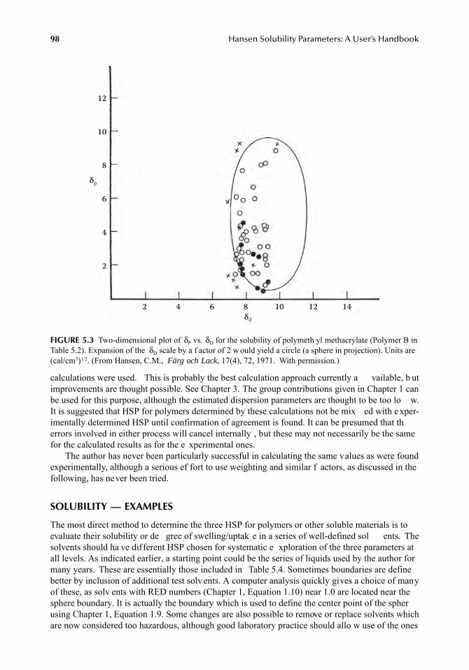
98
Hansen Solubility Parameters: A User’s Handbook
calculations were used. This is probably the best calculation approach currently a vailable, b utimprovements are thought possible. See Chapter 3. The group contributions given in Chapter 1 canbe used for this purpose, although the estimated dispersion parameters are thought to be too lo w.It is suggested that HSP for polymers determined by these calculations not be mix ed with e xper-imentally determined HSP until confirmation of agreement is found. It can be presumed that therrors involved in either process will cancel internally , but these may not necessarily be the samefor the calculated results as for the e xperimental ones.
The author has never been particularly successful in calculating the same values as were foundexperimentally, although a serious ef fort to use weighting and similar f actors, as discussed in thefollowing, has never been tried.
SOLUBILITY — EXAMPLES
The most direct method to determine the three HSP for polymers or other soluble materials is toevaluate their solubility or de gree of swelling/uptak e in a series of well-defined sol ents. Thesolvents should ha ve different HSP chosen for systematic e xploration of the three parameters atall levels. As indicated earlier, a starting point could be the series of liquids used by the author formany years. These are essentially those included in Table 5.4. Sometimes boundaries are definebetter by inclusion of additional test solvents. A computer analysis quickly gives a choice of manyof these, as solv ents with RED numbers (Chapter 1, Equation 1.10) near 1.0 are located near thesphere boundary. It is actually the boundary which is used to define the center point of the spherusing Chapter 1, Equation 1.9. Some changes are also possible to remove or replace solvents whichare now considered too hazardous, although good laboratory practice should allo w use of the ones
FIGURE 5.3
Two-dimensional plot of
δ
P
vs.
δ
D
for the solubility of polymeth yl methacrylate (Polymer B inTable 5.2). Expansion of the
δ
D
scale by a f actor of 2 w ould yield a circle (a sphere in projection). Units are(cal/cm
3
)
1/2
. (From Hansen, C.M.,
Färg och Lack
, 17(4), 72, 1971. With permission.)
2 4 6 8 10 12 14δd
δp
12
10
8
6
4
2
7248_C005.fm Page 98 Wednesday, May 23, 2007 10:51 AM
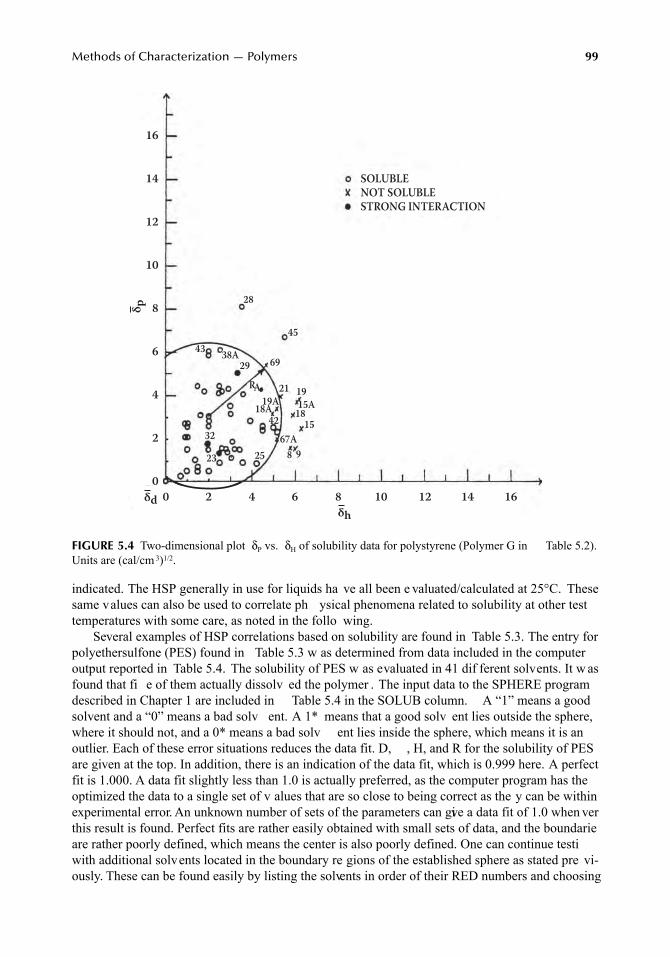
Methods of Characterization — Polymers
99
indicated. The HSP generally in use for liquids ha ve all been e valuated/calculated at 25°C. Thesesame values can also be used to correlate ph ysical phenomena related to solubility at other testtemperatures with some care, as noted in the follo wing.
Several examples of HSP correlations based on solubility are found in Table 5.3. The entry forpolyethersulfone (PES) found in Table 5.3 w as determined from data included in the computeroutput reported in Table 5.4. The solubility of PES w as evaluated in 41 dif ferent solvents. It w asfound that fi e of them actually dissolv ed the polymer . The input data to the SPHERE programdescribed in Chapter 1 are included in Table 5.4 in the SOLUB column. A “1” means a goodsolvent and a “0” means a bad solv ent. A 1*
means that a good solv ent lies outside the sphere,where it should not, and a 0* means a bad solv ent lies inside the sphere, which means it is anoutlier. Each of these error situations reduces the data fit. D, , H, and R for the solubility of PESare given at the top. In addition, there is an indication of the data fit, which is 0.999 here. A perfectfit is 1.000. A data fit slightly less than 1.0 is actually preferred, as the computer program has theoptimized the data to a single set of v alues that are so close to being correct as the y can be withinexperimental error. An unknown number of sets of the parameters can give a data fit of 1.0 when verthis result is found. Perfect fits are rather easily obtained with small sets of data, and the boundarieare rather poorly defined, which means the center is also poorly defined. One can continue testiwith additional solvents located in the boundary re gions of the established sphere as stated pre vi-ously. These can be found easily by listing the solvents in order of their RED numbers and choosing
FIGURE 5.4
Two-dimensional plot
δ
P
vs.
δ
H
of solubility data for polystyrene (Polymer G in Table 5.2).Units are (cal/cm
3
)
1/2
.
0 2 4 6 8 10 12 14 16
δ p16
14
12
10
8
6
4
2
0δd
δh
SOLUBLENOT SOLUBLESTRONG INTERACTION
28
45
69
21 1915A
1815
8 967A
4219A18A
2523
32
RA
2938A43
7248_C005.fm Page 99 Wednesday, May 23, 2007 10:51 AM
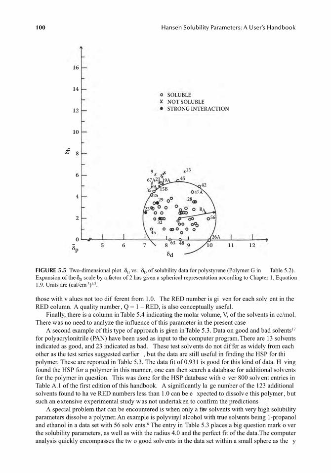
100
Hansen Solubility Parameters: A User’s Handbook
those with v alues not too dif ferent from 1.0. The RED number is gi ven for each solv ent in theRED column. A quality number, Q = 1 – RED, is also conceptually useful.
Finally, there is a column in Table 5.4 indicating the molar volume, V, of the solvents in cc/mol.There was no need to analyze the influence of this parameter in the present case
A second example of this type of approach is given in Table 5.3. Data on good and bad solvents
17
for polyacrylonitrile (PAN) have been used as input to the computer program. There are 13 solventsindicated as good, and 23 indicated as bad. These test solvents do not dif fer as widely from eachother as the test series suggested earlier , but the data are still useful in finding the HSP for thipolymer. These are reported in Table 5.3. The data fit of 0.931 is good for this kind of data. H vingfound the HSP for a polymer in this manner, one can then search a database for additional solventsfor the polymer in question. This was done for the HSP database with o ver 800 solvent entries inTable A.1 of the first edition of this handbook. A significantly la ge number of the 123 additionalsolvents found to ha ve RED numbers less than 1.0 can be e xpected to dissolv e this polymer , butsuch an extensive experimental study was not undertaken to confirm the predictions
A special problem that can be encountered is when only a few solvents with very high solubilityparameters dissolve a polymer. An example is polyvinyl alcohol with true solvents being 1-propanoland ethanol in a data set with 56 solv ents.
6
The entry in Table 5.3 places a big question mark o verthe solubility parameters, as well as with the radius 4.0 and the perfect fit of the data.The computeranalysis quickly encompasses the tw o good solvents in the data set within a small sphere as the y
FIGURE 5.5
Two-dimensional plot
δ
H
vs.
δ
D
of solubility data for polystyrene (Polymer G in Table 5.2).Expansion of the
δ
D
scale by a factor of 2 has given a spherical representation according to Chapter 1, Equation1.9. Units are (cal/cm
3
)
1/2
.
5 6 7 8 9 10 11 12
δ h16
14
12
10
8
6
4
2
0δp δd
SOLUBLENOT SOLUBLESTRONG INTERACTION
2847A
4245
15967A21 19A
693525
15B
2923
3245
56RA
486326A
7248_C005.fm Page 100 Wednesday, May 23, 2007 10:51 AM
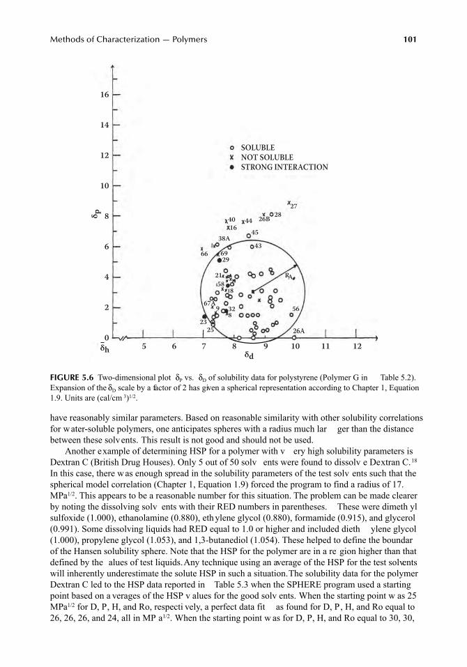
Methods of Characterization — Polymers
101
have reasonably similar parameters. Based on reasonable similarity with other solubility correlationsfor water-soluble polymers, one anticipates spheres with a radius much lar ger than the distancebetween these solvents. This result is not good and should not be used.
Another example of determining HSP for a polymer with v ery high solubility parameters isDextran C (British Drug Houses). Only 5 out of 50 solv ents were found to dissolv e Dextran C.
18
In this case, there w as enough spread in the solubility parameters of the test solv ents such that thespherical model correlation (Chapter 1, Equation 1.9) forced the program to find a radius of 17.MPa
1/2
. This appears to be a reasonable number for this situation. The problem can be made clearerby noting the dissolving solv ents with their RED numbers in parentheses. These were dimeth ylsulfoxide (1.000), ethanolamine (0.880), eth ylene glycol (0.880), formamide (0.915), and glycerol(0.991). Some dissolving liquids had RED equal to 1.0 or higher and included dieth ylene glycol(1.000), propylene glycol (1.053), and 1,3-butanediol (1.054). These helped to define the boundarof the Hansen solubility sphere. Note that the HSP for the polymer are in a re gion higher than thatdefined by the alues of test liquids. Any technique using an average of the HSP for the test solventswill inherently underestimate the solute HSP in such a situation. The solubility data for the polymerDextran C led to the HSP data reported in Table 5.3 when the SPHERE program used a startingpoint based on a verages of the HSP v alues for the good solv ents. When the starting point w as 25MPa
1/2
for D, P, H, and Ro, respecti vely, a perfect data fit as found for D, P, H, and Ro equal to26, 26, 26, and 24, all in MP a
1/2
. When the starting point w as for D, P, H, and Ro equal to 30, 30,
FIGURE 5.6
Two-dimensional plot
δ
P
vs.
δ
D
of solubility data for polystyrene (Polymer G in Table 5.2).Expansion of the
δ
D
scale by a factor of 2 has given a spherical representation according to Chapter 1, Equation1.9. Units are (cal/cm
3
)
1/2
.
5 6 7 8 9 10 11 12
δ p16
14
12
10
8
6
4
2
0δh δd
SOLUBLENOT SOLUBLESTRONG INTERACTION
26A
56329
2523
67A8
5821 RA
2969
43
4538A
66
8
1640 44 26B 28
27
7248_C005.fm Page 101 Wednesday, May 23, 2007 10:51 AM
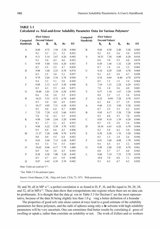
102
Hansen Solubility Parameters: A User’s Handbook
30, and 30, all in MP a
1/2
, a perfect correlation w as found to D, P , H, and Ro equal to 30, 28, 28,and 32, all in MPa
1/2
. These data show that extrapolations into regions where there are no data canbe problematic. It is thought that the data gi ven in Table 5.3 for Dectran C are the most represen-tative, because of the data fit being slightly less than 1.0 g ving a better definition of a boundar .
The properties of good solv ents alone cannot al ways lead to a good estimate of the solubilityparameters for these polymers, and the radii of spheres using only a few solvents with high solubilityparameters will be very uncertain. One can sometimes find better results by correlating d grees ofswelling or uptak e, rather than correlate on solubility or not. The work of Zellers and co workers
TABLE 5.1Calculated vs. Trial-and-Error Solubility Parameter Data for Various Polymers
a
ComputedHandtrials
(First Values) ComputedHandtrials
(First Values)(Second Values) (Second Values)
δδδδ
D
δδδδ
P
δδδδ
H
Ro FIT
δδδδ
D
δδδδ
P
δδδδ
H
Ro FIT
A 8.60 4.72 1.94 5.20 0.960 R 9.04 4.50 2.40 5.20 0.9859.2 5.3 2.1 5.3 0.923 9.2 4.5 2.6 5.0 0.972
B 9.11 5.14 3.67 4.20 0.945 S 10.53 7.30 6.00 8.20 0.9109.2 5.0 4.2 4.0 0.923 8.8 7.0 5.5 6.0 0.879
C 9.95 5.88 5.61 6.20 0.853 T 8.58 1.64 1.32 3.20 0.9748.5 5.5 5.5 4.7 0.829 8.7 1.8 1.8 3.5 0.965
D 9.98 1.68 2.23 6.70 0.974 U 9.10 4.29 2.04 4.70 0.9698.5 2.5 3.0 5.3 0.957 9.3 4.5 2.0 4.7 0.950
E 9.79 2.84 5.34 5.70 0.930 V 8.10 0.69 –0.40 4.70 0.9749.4 3.2 5.1 5.0 0.929 8.5 1.5 1.5 3.4 0.964
F 9.09 2.13 6.37 5.20 0.948 X 7.10 1.23 2.28 6.20 0.9218.5 4.3 5.5 4.8 0.871 7.8 1.0 3.6 4.0 0.881
G 10.40 2.81 2.10 6.20 0.955 Y 8.57 1.10 1.67 3.20 0.9508.6 3.0 2.0 3.5 0.915 8.8 2.5 1.2 3.8 0.914
H 10.23 5.51 4.72 6.70 0.891 Z 8.52 –0.94 7.28 4.70 0.9719.3 5.0 4.0 4.9 0.855 8.2 0.8 5.7 2.9 0.954
I 10.17 4.05 7.31 6.20 0.924 A 9.60 2.31 3.80 5.20 0.9429.5 4.0 6.4 4.7 0.909 8.7 2.5 3.5 4.2 0.951
J 7.53 7.20 4.32 5.60 0.933 B 9.95 4.17 5.20 7.20 0.9807.0 7.0 4.3 5.5 0.918 9.5 4.0 5.5 7.0 0.976
K 9.90 3.09 2.64 5.20 0.949 C 8.05 0.18 1.39 4.20 0.9669.3 3.7 2.1 4.2 0.933 8.5 1.0 2.0 3.4 0.960
L 9.08 6.22 5.38 3.70 0.921 D 10.34 6.63 6.26 6.70 0.9649.5 6.0 6.0 4.5 0.896 9.2 5.8 4.2 5.0 0.868
M 11.37 3.20 4.08 9.70 0.978 E 8.58 0.58 1.76 3.20 0.9689.0 4.0 5.5 6.4 0.923 8.5 1.5 1.8 2.6 0.956
N 9.65 5.68 7.13 6.20 0.897 F 8.91 3.68 4.08 1.70 0.9929.4 5.3 7.4 5.5 0.867 9.4 4.5 3.5 3.2 0.895
O 10.62 0.46 4.17 7.70 1.000 G 9.49 2.68 2.82 4.70 0.9618.9 3.0 3.8 4.5 0.952 8.8 2.7 2.7 4.0 0.963
P 8.58 4.58 7.00 5.20 0.942 L 9.86 7.14 7.35 5.70 0.9708.5 4.7 6.5 5.0 0.940 10.8 7.0 8.8 7.1 0.936
Q 9.87 6.43 6.39 5.70 0.942 9.3 6.2 4.7 4.2 0.892
Note:
Units are (cal/cm
3
)
1/2
.
a
See Table 5.2 for polymer types.
Source:
From Hansen, C.M.,
Färg och Lack
, 17(4), 73, 1971. With permission.
7248_C005.fm Page 102 Wednesday, May 23, 2007 10:51 AM
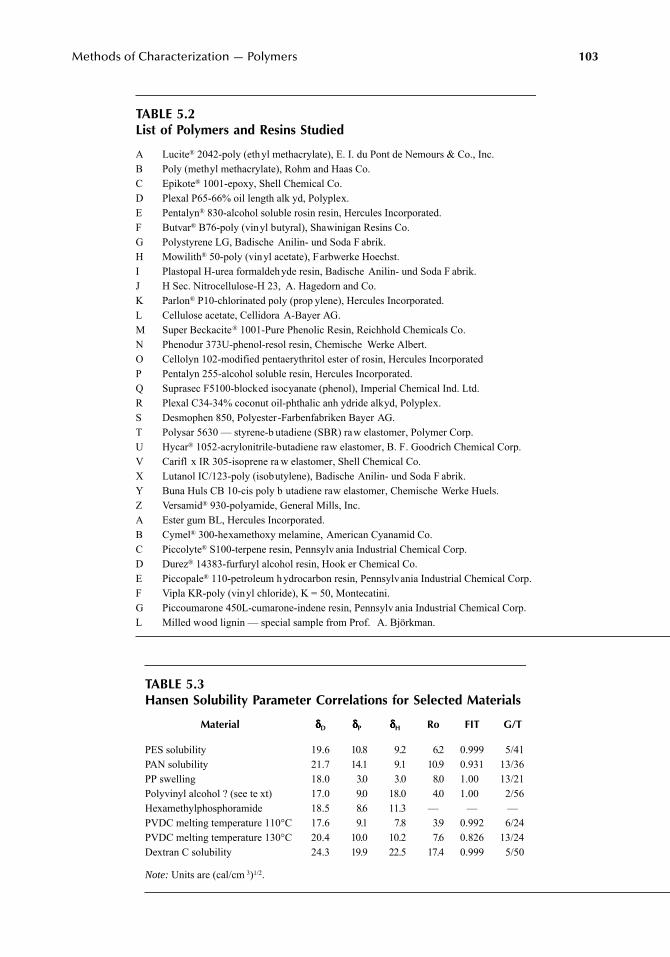
Methods of Characterization — Polymers
103
TABLE 5.2List of Polymers and Resins Studied
A Lucite
®
2042-poly (ethyl methacrylate), E. I. du Pont de Nemours & Co., Inc.B Poly (methyl methacrylate), Rohm and Haas Co.C Epikote
®
1001-epoxy, Shell Chemical Co.D Plexal P65-66% oil length alk yd, Polyplex.E Pentalyn
®
830-alcohol soluble rosin resin, Hercules Incorporated.F Butvar
®
B76-poly (vinyl butyral), Shawinigan Resins Co.G Polystyrene LG, Badische Anilin- und Soda F abrik.H Mowilith
®
50-poly (vinyl acetate), Farbwerke Hoechst.I Plastopal H-urea formaldehyde resin, Badische Anilin- und Soda F abrik.J H Sec. Nitrocellulose-H 23, A. Hagedorn and Co.K Parlon
®
P10-chlorinated poly (prop ylene), Hercules Incorporated.L Cellulose acetate, Cellidora A-Bayer AG.M Super Beckacite
®
1001-Pure Phenolic Resin, Reichhold Chemicals Co.N Phenodur 373U-phenol-resol resin, Chemische Werke Albert.O Cellolyn 102-modified pentaerythritol ester of rosin, Hercules IncorporatedP Pentalyn 255-alcohol soluble resin, Hercules Incorporated.Q Suprasec F5100-blocked isocyanate (phenol), Imperial Chemical Ind. Ltd.R Plexal C34-34% coconut oil-phthalic anh ydride alkyd, Polyplex.S Desmophen 850, Polyester -Farbenfabriken Bayer AG.T Polysar 5630 — styrene-b utadiene (SBR) raw elastomer, Polymer Corp.U Hycar
®
1052-acrylonitrile-butadiene raw elastomer, B. F. Goodrich Chemical Corp.V Carifl x IR 305-isoprene ra w elastomer, Shell Chemical Co.X Lutanol IC/123-poly (isobutylene), Badische Anilin- und Soda F abrik.Y Buna Huls CB 10-cis poly b utadiene raw elastomer, Chemische Werke Huels.Z Versamid
®
930-polyamide, General Mills, Inc.A Ester gum BL, Hercules Incorporated.B Cymel
®
300-hexamethoxy melamine, American Cyanamid Co.C Piccolyte
®
S100-terpene resin, Pennsylv ania Industrial Chemical Corp.D Durez
®
14383-furfuryl alcohol resin, Hook er Chemical Co.E Piccopale
®
110-petroleum hydrocarbon resin, Pennsylvania Industrial Chemical Corp.F Vipla KR-poly (vinyl chloride), K = 50, Montecatini.G Piccoumarone 450L-cumarone-indene resin, Pennsylv ania Industrial Chemical Corp.L Milled wood lignin — special sample from Prof. A. Björkman.
TABLE 5.3Hansen Solubility Parameter Correlations for Selected Materials
Material
δδδδ
D
δδδδ
P
δδδδ
H
Ro FIT G/T
PES solubility 19.6 10.8 9.2 6.2 0.999 5/41PAN solubility 21.7 14.1 9.1 10.9 0.931 13/36PP swelling 18.0 3.0 3.0 8.0 1.00 13/21Polyvinyl alcohol ? (see te xt) 17.0 9.0 18.0 4.0 1.00 2/56Hexamethylphosphoramide 18.5 8.6 11.3 — — —PVDC melting temperature 110°C 17.6 9.1 7.8 3.9 0.992 6/24PVDC melting temperature 130°C 20.4 10.0 10.2 7.6 0.826 13/24Dextran C solubility 24.3 19.9 22.5 17.4 0.999 5/50
Note:
Units are (cal/cm
3
)1/2.
7248_C005.fm Page 103 Wednesday, May 23, 2007 10:51 AM
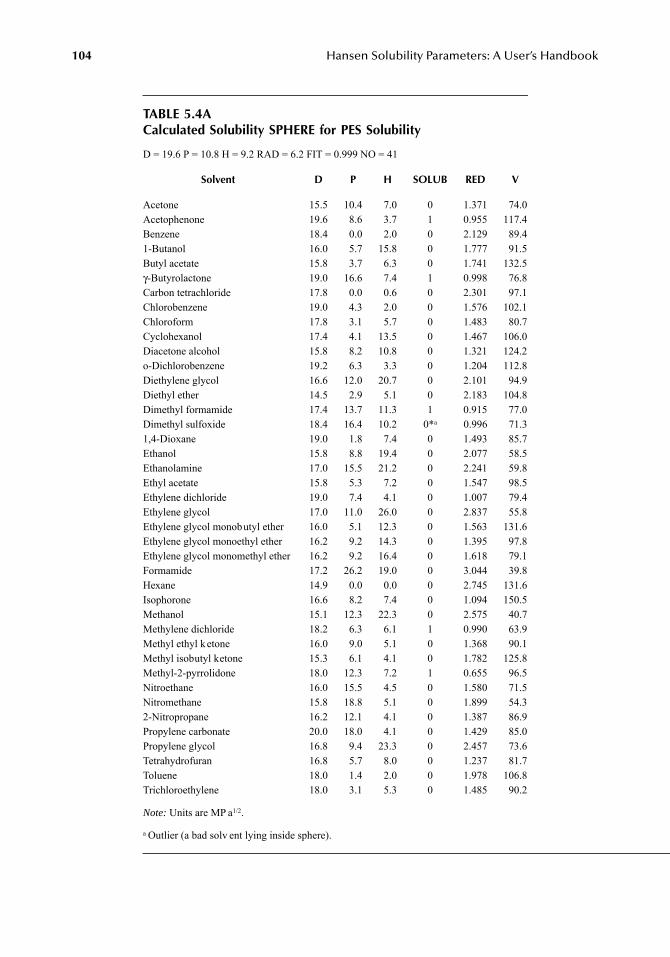
104 Hansen Solubility Parameters: A User’s Handbook
TABLE 5.4ACalculated Solubility SPHERE for PES Solubility
D = 19.6 P = 10.8 H = 9.2 RAD = 6.2 FIT = 0.999 NO = 41
Solvent D P H SOLUB RED V
Acetone 15.5 10.4 7.0 0 1.371 74.0Acetophenone 19.6 8.6 3.7 1 0.955 117.4Benzene 18.4 0.0 2.0 0 2.129 89.41-Butanol 16.0 5.7 15.8 0 1.777 91.5Butyl acetate 15.8 3.7 6.3 0 1.741 132.5γ-Butyrolactone 19.0 16.6 7.4 1 0.998 76.8Carbon tetrachloride 17.8 0.0 0.6 0 2.301 97.1Chlorobenzene 19.0 4.3 2.0 0 1.576 102.1Chloroform 17.8 3.1 5.7 0 1.483 80.7Cyclohexanol 17.4 4.1 13.5 0 1.467 106.0Diacetone alcohol 15.8 8.2 10.8 0 1.321 124.2o-Dichlorobenzene 19.2 6.3 3.3 0 1.204 112.8Diethylene glycol 16.6 12.0 20.7 0 2.101 94.9Diethyl ether 14.5 2.9 5.1 0 2.183 104.8Dimethyl formamide 17.4 13.7 11.3 1 0.915 77.0Dimethyl sulfoxide 18.4 16.4 10.2 0*a 0.996 71.31,4-Dioxane 19.0 1.8 7.4 0 1.493 85.7Ethanol 15.8 8.8 19.4 0 2.077 58.5Ethanolamine 17.0 15.5 21.2 0 2.241 59.8Ethyl acetate 15.8 5.3 7.2 0 1.547 98.5Ethylene dichloride 19.0 7.4 4.1 0 1.007 79.4Ethylene glycol 17.0 11.0 26.0 0 2.837 55.8Ethylene glycol monobutyl ether 16.0 5.1 12.3 0 1.563 131.6Ethylene glycol monoethyl ether 16.2 9.2 14.3 0 1.395 97.8Ethylene glycol monomethyl ether 16.2 9.2 16.4 0 1.618 79.1Formamide 17.2 26.2 19.0 0 3.044 39.8Hexane 14.9 0.0 0.0 0 2.745 131.6Isophorone 16.6 8.2 7.4 0 1.094 150.5Methanol 15.1 12.3 22.3 0 2.575 40.7Methylene dichloride 18.2 6.3 6.1 1 0.990 63.9Methyl ethyl ketone 16.0 9.0 5.1 0 1.368 90.1Methyl isobutyl ketone 15.3 6.1 4.1 0 1.782 125.8Methyl-2-pyrrolidone 18.0 12.3 7.2 1 0.655 96.5Nitroethane 16.0 15.5 4.5 0 1.580 71.5Nitromethane 15.8 18.8 5.1 0 1.899 54.32-Nitropropane 16.2 12.1 4.1 0 1.387 86.9Propylene carbonate 20.0 18.0 4.1 0 1.429 85.0Propylene glycol 16.8 9.4 23.3 0 2.457 73.6Tetrahydrofuran 16.8 5.7 8.0 0 1.237 81.7Toluene 18.0 1.4 2.0 0 1.978 106.8Trichloroethylene 18.0 3.1 5.3 0 1.485 90.2
Note: Units are MP a1/2.
a Outlier (a bad solv ent lying inside sphere).
7248_C005.fm Page 104 Wednesday, May 23, 2007 10:51 AM
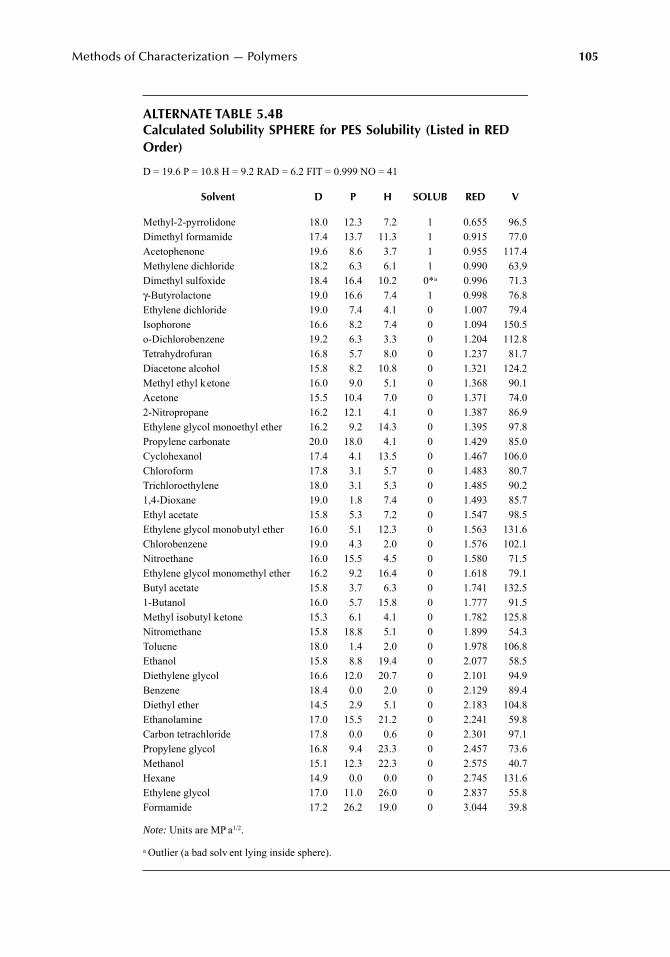
Methods of Characterization — Polymers 105
ALTERNATE TABLE 5.4BCalculated Solubility SPHERE for PES Solubility (Listed in RED Order)
D = 19.6 P = 10.8 H = 9.2 RAD = 6.2 FIT = 0.999 NO = 41
Solvent D P H SOLUB RED V
Methyl-2-pyrrolidone 18.0 12.3 7.2 1 0.655 96.5Dimethyl formamide 17.4 13.7 11.3 1 0.915 77.0Acetophenone 19.6 8.6 3.7 1 0.955 117.4Methylene dichloride 18.2 6.3 6.1 1 0.990 63.9Dimethyl sulfoxide 18.4 16.4 10.2 0*a 0.996 71.3γ-Butyrolactone 19.0 16.6 7.4 1 0.998 76.8Ethylene dichloride 19.0 7.4 4.1 0 1.007 79.4Isophorone 16.6 8.2 7.4 0 1.094 150.5o-Dichlorobenzene 19.2 6.3 3.3 0 1.204 112.8Tetrahydrofuran 16.8 5.7 8.0 0 1.237 81.7Diacetone alcohol 15.8 8.2 10.8 0 1.321 124.2Methyl ethyl ketone 16.0 9.0 5.1 0 1.368 90.1Acetone 15.5 10.4 7.0 0 1.371 74.02-Nitropropane 16.2 12.1 4.1 0 1.387 86.9Ethylene glycol monoethyl ether 16.2 9.2 14.3 0 1.395 97.8Propylene carbonate 20.0 18.0 4.1 0 1.429 85.0Cyclohexanol 17.4 4.1 13.5 0 1.467 106.0Chloroform 17.8 3.1 5.7 0 1.483 80.7Trichloroethylene 18.0 3.1 5.3 0 1.485 90.21,4-Dioxane 19.0 1.8 7.4 0 1.493 85.7Ethyl acetate 15.8 5.3 7.2 0 1.547 98.5Ethylene glycol monobutyl ether 16.0 5.1 12.3 0 1.563 131.6Chlorobenzene 19.0 4.3 2.0 0 1.576 102.1Nitroethane 16.0 15.5 4.5 0 1.580 71.5Ethylene glycol monomethyl ether 16.2 9.2 16.4 0 1.618 79.1Butyl acetate 15.8 3.7 6.3 0 1.741 132.51-Butanol 16.0 5.7 15.8 0 1.777 91.5Methyl isobutyl ketone 15.3 6.1 4.1 0 1.782 125.8Nitromethane 15.8 18.8 5.1 0 1.899 54.3Toluene 18.0 1.4 2.0 0 1.978 106.8Ethanol 15.8 8.8 19.4 0 2.077 58.5Diethylene glycol 16.6 12.0 20.7 0 2.101 94.9Benzene 18.4 0.0 2.0 0 2.129 89.4Diethyl ether 14.5 2.9 5.1 0 2.183 104.8Ethanolamine 17.0 15.5 21.2 0 2.241 59.8Carbon tetrachloride 17.8 0.0 0.6 0 2.301 97.1Propylene glycol 16.8 9.4 23.3 0 2.457 73.6Methanol 15.1 12.3 22.3 0 2.575 40.7Hexane 14.9 0.0 0.0 0 2.745 131.6Ethylene glycol 17.0 11.0 26.0 0 2.837 55.8Formamide 17.2 26.2 19.0 0 3.044 39.8
Note: Units are MP a1/2.
a Outlier (a bad solv ent lying inside sphere).
7248_C005.fm Page 105 Wednesday, May 23, 2007 10:51 AM
106 Hansen Solubility Parameters: A User’s Handbook
reports extensive studies of this type. 11–14 It should be noted, however, that the HSP-sphere param-eters usually v ary some from correlation to correlation based on the same data when dif ferentcriteria are used for good and bad solv ents. This is because the absorbed solv ent tends to locate inregions with similar solubility parameters, and there are local variations in HSP within most, if notall, polymers. This is particularly true of polymers which are not homopolymers. This situationrelates to self-assembly . Solvents or se gments of molecules with similar HSP will tend to residenear each other . An example of this is w ater residing at local h ydrophilic sites, such as alcoholgroups, in polymers. Utilization of the HSP af finity between molecules or s gments of moleculesis a viable w ay to control self-assembly . See also Chapter 18.
SWELLING — EXAMPLES
The correlation for swelling of polypropylene reported in Table 5.3 is based on solvent uptake datareported by Lieberman and Barbe at 22°C. 19 The limit of 0.5% w as arbitrarily set to dif ferentiategood solvents from bad ones. As mentioned earlier , experience has sho wn that a dif ferent limitusually gives different parameters. It should be noted that swelling data reflect the properties othe regions in the polymer where the solv ent has chosen to reside because of ener getic similarity(self-assembly). The principle is not necessarily “lik e dissolves like,” but rather “lik e seeks lik e.”If the solv ent is homogeneously distrib uted in the polymer , the solubility parameters found willreflect the properties of the whole polyme . Crystalline re gions will not contain solv ent. If thesolvent collects locally in re gions with chemical groups dif ferent from the b ulk of the polymer ,then the HSP so derived will reflect at least partially the p ysical nature of these chemical groups.The parameters reported in Table 5.3 seem appropriate for what is expected in terms of low polarityand low hydrogen-bonding properties for a polyprop ylene-type polymer.
An example of a characterization using swelling data that did not result in a good correlationis that for Viton® (The Du Pont Compan y, Wilmington, DE). This problem has been discussed byZellers and Zhang11,12 and is also discussed in Chapter 13. If one tries to force-fit data where therare several different comonomers into a single HSP sphere, the result is usually reflected in a poocorrelation coef ficient. Figure 13.3 sh ws that impro vements can be made by using a separatesphere for each comonomer. One reason for the poor correlation of swelling beha vior is that Vitonis not a homopolymer , and also contains a cross-linking chemical. The dif ferent segments havedifferent af finities. Indeed, there are s veral qualities of Viton, each of which has significantldiffering chemical resistance. Swelling of Viton has also been treated by Ev ans and Hardy 20 inconnection with predictions related to chemical protecti ve clothing, and by Nielsen and Hansen, 21
who presented curves of swelling as a function of the RED number .
MELTING POINT DETERMINATIONS — EFFECT OF TEMPERATURE
Partly crystalline polymers that are placed in dif ferent liquids will ha ve melting points which arelowered to a degree depending on the solv ent quality of the indi vidual liquids. The melting pointsof polyvinylidine chloride (PVDC) ha ve been measured in dif ferent solvents.22 These data ha vebeen analyzed by e valuating solubility parameter re gions based on those solv ents which dissolv ethe polymer at 110°C and above and also at 130°C and above. As expected, there are more solventswhich dissolve the semicrystalline polymer at the higher temperature. The results for these corre-lations are included in Table 5.3. The main reasons for the somewhat lower data fit at 130°C includtwo nondissolving solv ents within the solubility parameter sphere. These are dimeth yl phthalate,where the lar ge molecular size is a f actor, and benzyl alcohol, where temperature ef fects can belarger than e xpected compared with the other solv ents as discussed later and in Chapter 1. Thesolubility parameters for PVDC at this temperature, based on tab ulated solvent values at 25°C, arenot affected significantly by this type of situation. A single room temperature solv ent for PVDC
7248_C005.fm Page 106 Wednesday, May 23, 2007 10:51 AM
Methods of Characterization — Polymers 107
is reported by Wessling.22 This is hexamethylphosphoramide and its solubility parameters are alsoreported in Table 5.3 for comparison. The change in the values of the individual solubility parameterswith temperature is discussed in Chapter 1 (Equation 1.16 to Equation 1.18). Chapter 3 also treatsthe temperature dependence of the HSP. See also Chapter 10 where the HSP of specifically carbodioxide are treated in depth as a function of temperature and pressure.
ENVIRONMENTAL STRESS CRACKING
Environmental stress cracking (ESC) is unfortunately a v ery frequent mode of f ailure for plastics.For this reason a whole chapter is de voted to the topic (see Chapter 14). It has been possible tocorrelate HSP with ESC phenomena, and this can also provide an estimate of the HSP for the givenpolymers. Care is advised since the stress/strain le vel is important, as is the molecular size andshape of the chemicals in volved. Several collections of ESC data in the older literature 23–25 shouldnot be forgotten in these days of “Internet and only Internet.” Such collections have particular valueas it is considered impossible to get a commercially a vailable polymer without some additi ves.These can also affect ESC behavior. These older data were the basis of the ESC correlations gi venin Chapter 14.
INTRINSIC VISCOSITY MEASUREMENTS
One of the more promising methods to e valuate polymer HSP for limited data is that using theintrinsic viscosity . Van Dyk et al. found a correlation with the intrinsic viscosity of an acrylicpolymer (polyethyl methacrylate) in v arious solvents and the polymer HSP 26 (see the discussionon polymer compatibility in Chapter 8).
Segarceanu and Leca 27 have devised a method to calculate the polymer HSP from data on itsintrinsic viscosity in different solvents. The intrinsic viscosities will be higher in the better solventsbecause of greater interaction and greater polymer chain e xtension. The intrinsic viscosity gi vesan indication of the solv ent quality. It has been used earlier to calculate the Flory–Huggins chiparameter, for example.28
In the new technique, the intrinsic viscosities are normalized by the intrinsic viscosity of thatsolvent giving the highest value. These normalized data (numbers are 1.0 or less) are then used ina weighted averaging technique to arri ve at the center of the Hansen sphere.
δD2 = Σ(δDi × [η]i)/Σ[η]i (5.4)
δP2 = Σ(δPi × [η]i)/Σ[η]i (5.5)
δH2 = Σ(δHi × [η]i]/Σ[η]i (5.6)
The subscript 2 is for the polymer , and the respecti ve solvents are indicated by an “i. ” Theintrinsic viscosity in the i-th solv ent is given by [ η]i.
Those solvents with the greatest weighting factor have higher intrinsic viscosities and are closestto the geometric center of the sphere. Those solv ents which do not dissolv e the polymer wereassumed to have a zero weighting factor. The HSP for a polyesterimide were reported as an example.HSP values were assigned both by the “classical” e valuation and with this ne wer approach. Thesedata are included as the first entries in Table 5.5. This is a v ery promising method of arri ving atthe polymer HSP with limited data.
There are se veral aspects of this w ork which deserv e comment. It w as demonstrated earlierthat many polymers ha ve higher solubility parameters than an y of the solv ents which are or canbe used to test them. The present method only allows for polymer HSP within the range attainable
7248_C005.fm Page 107 Wednesday, May 23, 2007 10:51 AM
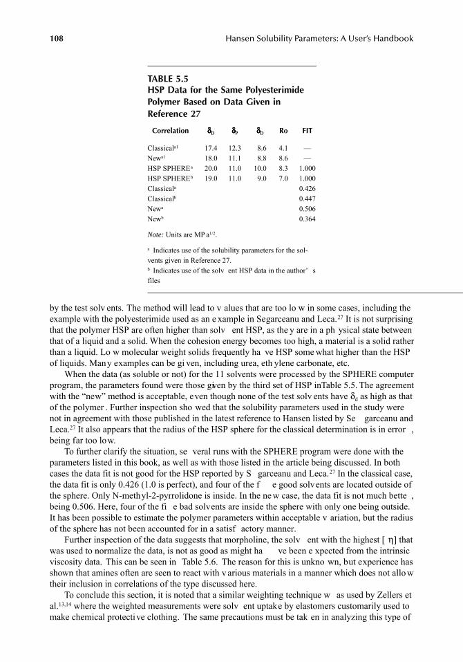
108 Hansen Solubility Parameters: A User’s Handbook
by the test solv ents. The method will lead to v alues that are too lo w in some cases, including theexample with the polyesterimide used as an e xample in Segarceanu and Leca.27 It is not surprisingthat the polymer HSP are often higher than solv ent HSP, as the y are in a ph ysical state betweenthat of a liquid and a solid. When the cohesion energy becomes too high, a material is a solid ratherthan a liquid. Lo w molecular weight solids frequently ha ve HSP some what higher than the HSPof liquids. Many examples can be gi ven, including urea, eth ylene carbonate, etc.
When the data (as soluble or not) for the 11 solvents were processed by the SPHERE computerprogram, the parameters found were those given by the third set of HSP in Table 5.5. The agreementwith the “new” method is acceptable, even though none of the test solv ents have δd as high as thatof the polymer . Further inspection sho wed that the solubility parameters used in the study werenot in agreement with those published in the latest reference to Hansen listed by Se garceanu andLeca.27 It also appears that the radius of the HSP sphere for the classical determination is in error ,being far too low.
To further clarify the situation, se veral runs with the SPHERE program were done with theparameters listed in this book, as well as with those listed in the article being discussed. In bothcases the data fit is not good for the HSP reported by S garceanu and Leca.27 In the classical case,the data fit is only 0.426 (1.0 is perfect), and four of the f e good solvents are located outside ofthe sphere. Only N-methyl-2-pyrrolidone is inside. In the ne w case, the data fit is not much bette ,being 0.506. Here, four of the fi e bad solvents are inside the sphere with only one being outside.It has been possible to estimate the polymer parameters within acceptable v ariation, but the radiusof the sphere has not been accounted for in a satisf actory manner.
Further inspection of the data suggests that morpholine, the solv ent with the highest [ η] thatwas used to normalize the data, is not as good as might ha ve been e xpected from the intrinsicviscosity data. This can be seen in Table 5.6. The reason for this is unkno wn, but experience hasshown that amines often are seen to react with v arious materials in a manner which does not allo wtheir inclusion in correlations of the type discussed here.
To conclude this section, it is noted that a similar weighting technique w as used by Zellers etal.13,14 where the weighted measurements were solv ent uptake by elastomers customarily used tomake chemical protective clothing. The same precautions must be tak en in analyzing this type of
TABLE 5.5HSP Data for the Same Polyesterimide Polymer Based on Data Given in Reference 27
Correlation δδδδD δδδδP δδδδD Ro FIT
Classicala1 17.4 12.3 8.6 4.1 —Newa1 18.0 11.1 8.8 8.6 —HSP SPHEREa 20.0 11.0 10.0 8.3 1.000HSP SPHEREb 19.0 11.0 9.0 7.0 1.000Classicala 0.426Classicalb 0.447Newa 0.506Newb 0.364
Note: Units are MP a1/2.
a Indicates use of the solubility parameters for the sol-vents given in Reference 27.b Indicates use of the solv ent HSP data in the author’ sfiles
7248_C005.fm Page 108 Wednesday, May 23, 2007 10:51 AM
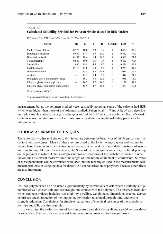
Methods of Characterization — Polymers 109
measurement, but as the polymers studied were reasonably nonpolar, some of the solvents had HSPwhich were higher than those of the polymers studied. Zellers et al. 14 and Athey29 also describemultiple variable statistical analysis techniques to find the HSP of a g ven polymer. Barton’s work6
contains many literature sources of intrinsic viscosity studies using the solubility parameter forinterpretation.
OTHER MEASUREMENT TECHNIQUES
There are man y other techniques to dif ferentiate between the beha vior of dif ferent solv ents incontact with a polymer . Man y of these are discussed in the follo wing chapters and will not betreated here. These include permeation measurements, chemical resistance determinations of variouskinds including ESC, and surface attack, etc. Some of the techniques can be very useful, dependingon the polymer in volved. Others will present problems because of the probable influence of othefactors such as solvent molar volume and length of time before attainment of equilibrium. Se veralof these phenomena can be correlated with HSP, but the techniques used in the measurements willpresent problems in using the data for direct HSP characterization of polymers because other effectsare also important.
CONCLUSION
HSP for polymers can be e valuated experimentally by correlations of data where a suitably lar genumber of well-chosen solvents are brought into contact with the polymer . The observed behaviorwhich can be correlated includes true solubility, swelling, weight gain, dimensional change, degreeof surf ace attack, reduction of melting point, permeation rate, breakthrough time, and tensilestrength reduction. Correlations for simple e valuations of chemical resistance of the suitable-or -not type and ESC are also possible.
In each case, the molecular size of the liquids used can affect the result and should be consideredin some way. The use of w ater as a test liquid is not recommended for these purposes.
TABLE 5.6Calculated Solubility SPHERE for Polyesterimide (Listed in RED Order)
D = 19.0 P = 11.0 H = 9.0 RAD = 7.0 FIT = 1.000 NO = 11
Solvent [η]a N D P H SOLUB RED V
Methyl-2-pyrrolidone 0.970 18.0 12.3 7.2 1 0.427 96.5Dimethyl formamide 0.947 17.4 13.7 11.3 1 0.682 77.0Dimethyl sulfoxide 0.182 18.4 16.4 10.2 1 0.809 71.3γ-Butyrolactone 0.689 19.0 16.6 7.4 1 0.832 76.8Morpholine 1.000 18.8 4.9 9.2 1 0.874 87.1Cyclohexanone 0.718 17.8 6.3 5.1 1 0.937 104.0Diacetone alcohol — 15.8 8.2 10.8 0 1.031 124.2Acetone — 15.5 10.4 7.0 0 1.044 74.0Diethylene glycol monomethyl ether — 16.2 7.8 12.6 0 1.055 118.0Ethylene glycol monoethyl ether — 16.2 9.2 14.3 0 1.131 97.8Ethylene glycol monoethyl ether acetate — 15.9 4.7 10.6 0 1.283 136.1
Note: Units are MP a1/2.
a Normalized intrinsic viscosity data from Reference 27.
7248_C005.fm Page 109 Wednesday, May 23, 2007 10:51 AM
110 Hansen Solubility Parameters: A User’s Handbook
REFERENCES
1. Hansen, C.M., Solubility in the coatings industry , Färg och Lack, 17(4), 69–77, 1971.2. Hansen, C.M. and Skaarup, K., The three dimensional solubility parameter — key to paint component
affinities III. Independent calculation of the parameter components, J. Paint Technol., 39(511),511–514, 1967.
3. Hansen, C.M., The Three Dimensional Solubility Parameter and Solvent Diffusion Coefficient, TheirImportance in Surf ace Coating F ormulation, Doctoral dissertation, Danish Technical Press, Copen-hagen, 1967.
4. Teas, J.P., Graphic analysis of resin solubilities, J. Paint Technol., 40(516), 19–25, 1968.5. Gardon, J.L. and Teas, J.P., Solubility parameters, in Treatise on Coatings, Vol. 2, Characterization
of Coatings: Physical Techniques, Part II, Myers, R.R. and Long, J.S., Eds., Marcel Dekk er, NewYork, 1976, chap. 8.
6. Barton, A.F.M., Handbook of Solubility Parameters and Other Cohesion Parameters, CRC Press,Boca Raton, FL, 1983; 2nd ed., 1991.
7. Torraca, G., Solubility and Solvents for Conservation Problems, 2nd ed., International Centre for theStudy of the Preserv ation and the Restoration of Cultural Property (ICCR OM), Rome, 1978.
8. Barton, A.F.M., Handbook of Polymer-Liquid Interaction Parameters and Solubility Parameters, CRCPress, Boca Raton, FL, 1990.
9. Benjamin, S., Carr , C., and Wallbridge, D.J., Self-stratifying coatings for metallic substrates, Prog.Org. Coat., 28(3), 197–207, 1996.
10. Rasmussen, D. and Wahlström, E., HSP — solubility parameters: a tool for de velopment of ne wproducts — modelling of the solubility of binders in pure and used solv ents, Surf. Coat. Int., 77(8),323–333, 1994.
11. Zellers, E.T., Three-dimensional solubility parameters and chemical protecti ve clothing permeation.I. Modeling the solubility of organic solvents in Viton® gloves, J. Appl. Polym. Sci., 50, 513–530, 1993.
12. Zellers, E.T . and Zhang, G.-Z., Three-dimensional solubility parameters and chemical protecti veclothing permeation. II. Modeling diffusion coefficients, breakthrough times, and steady-state permeation rates of or ganic solvents in Viton® gloves, J. Appl. Polym. Sci., 50, 531–540, 1993.
13. Zellers, E.T., Anna, D.H., Sulewski, R., and Wei, X., Critical analysis of the graphical determinationof Hansen’s solubility parameters for lightly crosslinked polymers, J. Appl. Polym. Sci., 62, 2069–2080,1996.
14. Zellers, E.T., Anna, D.H., Sule wski, R., and Wei, X., Impro ved methods for the determination ofHansen’s solubility parameters and the estimation of solv ent uptake for lightly crosslinked polymers,J. Appl. Polym. Sci., 62, 2081–2096, 1996.
15. Luciani, A., Champagne, M.F., and Utracki, L.A., Interfacial tension in polymer blends. Part 1: Theory,Polym. Networks Blends, 6(1), 41–50, 1996.
16. Luciani, A., Champagne, M.F ., and Utracki, L.A., Interf acial tension in polymer blends. P art 2:Measurements, Polym. Networks Blends, 6(2), 51–62, 1996.
17. Fuchs, O., Solvents and non-solvents for polymers, in Polymer Handbook, 3rd ed., Brandrup, J. andImmergut, E.H., Eds., Wiley-Interscience, New York, 1989, p. VII/385.
18. Hansen, C.M., The universality of the solubility parameter , Ind. Eng. Chem. Prod. Res. Dev., 8(1),2–11, 1969.
19. Lieberman, R.B. and Barbe, P .C., Polypropylene polymers, in Encyclopedia of Polymer Science andEngineering, 2nd ed., Vol. 13, Mark, H.F ., Bikales, N.M., Ov erberger, C.G., Menges, G., andKroschwitz, J.I., Eds., Wiley-Interscience, New York, 1988, pp. 482–483.
20. Evans, K.M. and Hardy , J.K., Predicting solubility and permeation properties of or ganic solvents inViton glove material using Hansen’s solubility parameters, J. Appl. Polym. Sci., 93, 2688–2698, 2004.
21. Nielsen, T.B. and Hansen, C.M., Elastomer swelling and Hansen solubility parameters, Polym. Testing,24, 1054–1061, 2005.
22. Wessling, R.A., The solubility of poly(vinylidine chloride), J. Appl. Polym. Sci., 14, 1531–1545, 1970.23. Wyzgoski, M.G., The role of solubility in stress cracking of n ylon 6,6, in Macromolecular Solutions,
Seymour, R.B. and Stahl, G.A., Eds., Per gamon Press, New York, 1982, pp. 41–60.24. Mai, Y.-W., Environmental stress cracking of glassy polymers and solubility parameters, J. Mater.
Sci., 21, 904–916, 1986.
7248_C005.fm Page 110 Wednesday, May 23, 2007 10:51 AM

Methods of Characterization — Polymers 111
25. White, S.A., Weissman, S.R., and Kambour , R.P., Resistance of a polyetherimide to en vironmentalstress crazing and cracking, J. Appl. Polym. Sci., 27, 2675–2682, 1982.
26. Van Dyk, J.W., Frisch, H.L., and Wu, D.T., Solubility, solvency, and solubility parameters, Ind. Eng.Chem. Prod. Res. Dev., 24(3), 473–478, 1985.
27. Segarceanu, O. and Leca, M., Improved method to calculate Hansen solubility parameters of a polymer,Prog. Org. Coat., 31(4), 307–310, 1997.
28. Kok, C.M. and Rudin, A., Prediction of Flory-Huggins interaction parameters from intrinsic viscos-ities, J. Appl. Polym. Sci., 27, 353–362, 1982.
29. Athey, R.D., Testing coatings: 6. Solubility parameter determination, Eur. Coat. J., 5, 367–372, 1993.
7248_C005.fm Page 111 Wednesday, May 23, 2007 10:51 AM

7248_C005.fm Page 112 Wednesday, May 23, 2007 10:51 AM
113
6
Methods of Characterization — Surfaces
Charles M. Hansen
ABSTRACT
Relations between cohesion parameters and surface energy parameters and their practical significancare discussed. Cohesion parameters (solubility parameters) can be used with full theoretical justification to characterize man y surf aces, including substrates, coatings, plastics, pigment and fillesurfaces, etc., in addition to the binder or polymer used in a gi ven product. Important molecularrelations between a binder in a coating or adhesi ve and its surroundings then become ob vious. Useof cohesion parameters, i.e., Hansen solubility parameters in a total characterization of surface energy,clearly shows how the single point concepts of the (Zisman) critical surf ace tension and the wettingtension fit into a la ger energy concept. A complete match of surface energies of two surfaces requiresthat exactly the same liquids (in a lar ger number of well-chosen test liquids) spontaneously spreadon both surfaces. The dewetting behavior (wetting tension test) of the liquids must also be the same,in that the same liquids should not retract when applied to the surf aces as films
INTRODUCTION
Interfacial free ener gy and adhesion properties result from intermolecular forces. It has beenrecognized for man y years that molecules interact by (molecular) surf ace to (molecular) surf acecontacts to enable solutions to be formed.
1
As molecular surf ace-to-surface contacts control bothsolution phenomena and surface phenomena, it is not surprising that various correlations of cohesionparameters and surface phenomena can be found. This idea has been well e xplored and dealt withelsewhere.
2
The various treatments and correlations in the literature will not be explicitly dealt withhere, other than those directly related to Hansen solubility parameters (HSP). In this chapter ,solubility parameters are called
cohesion (energy) parameters
and refer more specifically to HS .Solubility as such does not necessarily enter into the ener getics of interf acial phenomena, but theenergy characteristics of surf aces can still be correlated with HSP .
This chapter will emphasize methods of surface characterization using HSP. The orientation ofadsorbed molecules is a significant added e fect that must also be considered in man y cases. The“like dissolves like” concept is e xtended and applied as “lik e seeks like” (self-assembly).
HANSEN SOLUBILITY PARAMETER CORRELATIONS WITH SURFACE TENSION (SURFACE FREE ENERGY)
Skaarup w as the first to establish a correlation between liquid sur ace tension and HSP . Thiscorrelation with surface tension had been long lost in an internal report
to members of the DanishPaint and Printing Ink Research Laboratory in 1967, as well as in an abstract for a presentation tothe Nordic Chemical Congress in 1968.
3,4
γ
= 0.0688V
1/3
[
δ
D2
+ k(
δ
P2
+
δ
H2
)] (6.1)
7248_C006.fm Page 113 Wednesday, May 23, 2007 11:00 AM
114
Hansen Solubility Parameters: A User’s Handbook
γ
is the surface tension, and k is a constant depending on the liquids in volved. This k was reportedas 0.8 for se veral homologous series, 0.265 for normal alcohols, and 10.3 for n-alk yl benzenes.
Beerbower independently published essentially the same type of correlation in 1971.
5,6
Withthe exception of aliphatic alcohols and alkali halides, Beerbo wer found
γ
= 0.0715V
1/3
[
δ
D2
+ 0.632(
δ
P2
+
δ
H2
)] (6.2)
where
γ
is the surf ace tension. The constant w as actually found to be 0.7147 in the empiricalcorrelation. The units for the cohesion parameters are (cal/cm
3
)
1/2
, and those of the surf ace tensionare dyn/cm in both Equation 6.1 and Equation 6.2. Ho wever, values in dyn/cm are numericallyequal to those in mN/m. The constant w as separately deri ved as being equal to 0.7152 by amathematical analysis in which the number of nearest neighbors lost in surf ace formation w asconsidered, assuming that the molecules tend to occup y the corners of re gular octahedra.
The correlations presented by K oenhen and Smolders
7
are also rele vant to estimating surf acetension from HSP. The author has never explored them in detail, however, so they are not discussedhere.
It is interesting to note that
δ
P
and
δ
H
have the same coefficient in the surace tension correlations.They also have the same coef ficient when solubility is correlated (see Chapter 1, Equation 1.9 oChapter 2, Equation 2.6). The reason for this is the molecular orientation in the specific interactionderived from permanent dipole–permanent dipole and h ydrogen bonding (electron interchange)interactions. The dispersion or London forces arise because of electrons rotating around a positi veatomic nucleus. This causes local dipoles and attraction among atoms. This is a completely differenttype of interaction and requires a different coefficient in the correlations. It is this diference betweenatomic and molecular interactions that is basic to the entire discussion of similarity between HSPand the Prigogine corresponding states theory in Chapter 2. The finding that the polar and ydrogenbonding (electron interchange) ef fects require the same coef ficient for both ulk and surf acecorrelations suggests that the net effects of the (often mentioned) unsymmetrical nature of hydrogenbonding are no dif ferent from the net ef fects occurring with permanent dipole–permanent dipoleinteractions. The lack of specific consideration that ydrogen bonding is an unsymmetrical inter -action led Erbil
8
to state that HSP has limited theoretical justification, for xample. The previousdiscussion and the contents of Chapter 1 and Chapter 2 clearly indicate that the author is not infull agreement with this viewpoint. In fact, it appears that this book presents massi ve experimentalevidence, related both to b ulk and surf ace phenomena, which sho ws that the geometric mean isvalid for estimating interactions between dissimilar liquids. This includes dispersion, permanentdipole–permanent dipole, and h ydrogen bonding (electron interchange) interactions.
METHOD TO EVALUATE THE COHESION ENERGY PARAMETERS FOR SURFACES
One can determine the cohesion parameters for surf aces by observing whether or not spontaneousspreading is found for a series of widely dif ferent liquids. The liquids used in standard solubilityparameter determinations are suggested for this type of surf ace characterization. It is stronglysuggested that none of the liquids be a mixture, as this introduces an additional f actor into theevaluations. The liquids in the series often used by the author are indicated in Chapter 5, Table 5.4or Chapter 7, Table 7.2. Droplets of each of the liquids are applied to the surf ace and one simplyobserves what happens. If a droplet remains as a droplet, there is an adv ancing contact angle andthe cohesion ener gy/surface energy of the liquid is (significantly) higher than that of the sur ace.The contact angle need not necessarily be measured in this simplified procedure, h wever. Contactangles have generally been found to increase for greater differences in cohesion parameters betweenthe surface and liquid
9
(see also Figure 6.5). If spontaneous spreading is found, there is presumed
7248_C006.fm Page 114 Wednesday, May 23, 2007 11:00 AM
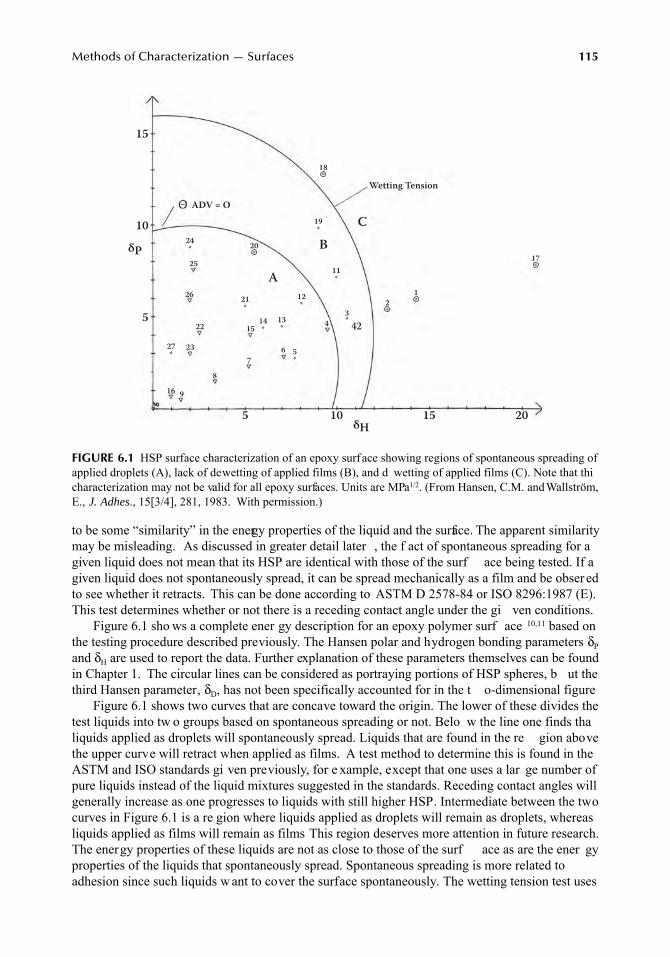
Methods of Characterization — Surfaces
115
to be some “similarity” in the energy properties of the liquid and the surface. The apparent similaritymay be misleading. As discussed in greater detail later , the f act of spontaneous spreading for agiven liquid does not mean that its HSP are identical with those of the surf ace being tested. If agiven liquid does not spontaneously spread, it can be spread mechanically as a film and be obser edto see whether it retracts. This can be done according to ASTM D 2578-84 or ISO 8296:1987 (E).This test determines whether or not there is a receding contact angle under the gi ven conditions.
Figure 6.1 sho ws a complete ener gy description for an epoxy polymer surf ace
10,11
based onthe testing procedure described previously. The Hansen polar and hydrogen bonding parameters
δ
P
and
δ
H
are used to report the data. Further explanation of these parameters themselves can be foundin Chapter 1. The circular lines can be considered as portraying portions of HSP spheres, b ut thethird Hansen parameter,
δ
D
, has not been specifically accounted for in the t o-dimensional figureFigure 6.1 shows two curves that are concave toward the origin. The lower of these divides the
test liquids into tw o groups based on spontaneous spreading or not. Belo w the line one finds thaliquids applied as droplets will spontaneously spread. Liquids that are found in the re gion abovethe upper curve will retract when applied as films. A test method to determine this is found in theASTM and ISO standards gi ven previously, for e xample, except that one uses a lar ge number ofpure liquids instead of the liquid mixtures suggested in the standards. Receding contact angles willgenerally increase as one progresses to liquids with still higher HSP. Intermediate between the twocurves in Figure 6.1 is a re gion where liquids applied as droplets will remain as droplets, whereasliquids applied as films will remain as films This region deserves more attention in future research.The energy properties of these liquids are not as close to those of the surf ace as are the ener gyproperties of the liquids that spontaneously spread. Spontaneous spreading is more related toadhesion since such liquids w ant to cover the surface spontaneously. The wetting tension test uses
FIGURE 6.1
HSP surface characterization of an epoxy surface showing regions of spontaneous spreading ofapplied droplets (A), lack of dewetting of applied films (B), and d wetting of applied films (C). Note that thicharacterization may not be valid for all epoxy surfaces. Units are MPa
1/2
. (From Hansen, C.M. and Wallström,E.,
J. Adhes
., 15[3/4], 281, 1983. With permission.)
5 10 15 20
δP
15
10
5
δH
Wetting Tension– ADV = O
42
CB
A1*2
*3*4
11*
12*
13*
6 5*
14*
21*
15
78
22
27*
23
26
25
24* 20
*
16 9
19*
18*
17*
7248_C006.fm Page 115 Wednesday, May 23, 2007 11:00 AM
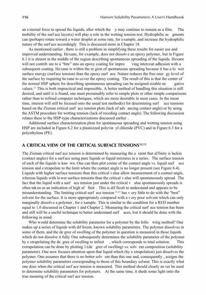
116
Hansen Solubility Parameters: A User’s Handbook
an external force to spread the liquids, after which the y may continue to remain as a film. Themobility of the surf ace layer(s) will play a role in the wetting tension test. Hydrophilic se gmentscan (perhaps) rotate toward a water droplet at some rate, for example, and increase the hydrophilicnature of the surf ace accordingly. This is discussed more in Chapter 18.
As mentioned earlier , there is still a problem in simplifying these results for easier use andimproved understanding. Hexane, for example, does not dissolve an epoxy polymer, but in Figure6.1 it is almost in the middle of the region describing spontaneous spreading of the liquids. Hexanewill not contrib ute to a “bite” into an epoxy coating for impro ving intercoat adhesion with asubsequent coating. He xane is within the re gion of spontaneous spreading because it has a lo wersurface energy (surface tension) than the epoxy surf ace. Nature reduces the free ener gy level ofthe surface by requiring he xane to cover the epoxy coating. The result of this is that the center ofthe normal HSP sphere for describing spontaneous spreading can be assigned sizable ne gativevalues.
11
This is both impractical and impossible. A better method of handling this situation is stilldesired, and until it is found, one must presumably refer to simple plots or other simple comparisonsrather than to refined computer techniques, which are more desirable in most cases. In the meantime, interest will still be focused onto the usual test method(s) for determining surf ace tensionsbased on the Zisman critical surf ace tension plots (lack of adv ancing contact angle) or by usingthe ASTM procedure for wetting tension (lack of receding contact angle). The following discussionrelates these to the HSP-type characterizations discussed earlier .
Additional surface characterization plots for spontaneous spreading and wetting tension usingHSP are included in Figure 6.2 for a plasticized polyvin yl chloride (PVC) and in Figure 6.3 for apolyethylene (PE).
A CRITICAL VIEW OF THE CRITICAL SURFACE TENSIONS
12,13
The Zisman critical surf ace tension is determined by measuring the e xtent that af finity is lackin(contact angles) for a surf ace using pure liquids or liquid mixtures in a series. The surface tensionof each of the liquids is kno wn. One can then plot cosine of the contact angle vs. liquid surf acetension and extrapolate to the limit where the contact angle is no longer present (see Figure 6.4).Liquids with higher surface tensions than this critical value allow measurement of a contact angle,whereas liquids with lower surface tensions than the critical v alue will spontaneously spread. Thefact that the liquid with a surf ace tension just under the critical v alue spontaneously spreads isoften tak en as an indication of high af finit . This is dif ficult to understand and appears to be misunderstanding. The limiting critical surf ace tension
12,13
has v ery little to do with the “best”solvent for the surface. It is more appropriately compared with a v ery poor solvent which can onlymarginally dissolve a polymer , for e xample. This is similar to the condition for a RED numberequal to 1.0 discussed in Chapter 1 and Chapter 2. Measuring the critical surf ace tension has beenand still will be a useful technique to better understand surf aces, but it should be done with thefollowing in mind.
Who would determine the solubility parameter for a polymer by the follo wing method? Onemakes up a series of liquids with dif ferent, known solubility parameters. The polymer dissolves insome of them, and the de gree of swelling of the polymer in question is measured in those liquidswhich do not dissolve it fully. One subsequently determines the solubility parameter of the polymerby e xtrapolating the de gree of swelling to infinit , which corresponds to total solution. Thisextrapolation can be done by plotting 1/(de gree of swelling) vs. solv ent composition (solubilityparameter). One now focuses attention upon that liquid which (by e xtrapolation) just dissolves thepolymer. One assumes that there is no better solv ent than this one and, consequently , assigns thepolymer solubility parameters corresponding to those of this boundary solvent. This is exactly whatone does when the critical surf ace tension is measured. This method should clearly ne ver be usedto determine solubility parameters for polymers. At the same time, it sheds some light onto thetrue meaning of the critical surf ace tension.
7248_C006.fm Page 116 Wednesday, May 23, 2007 11:00 AM
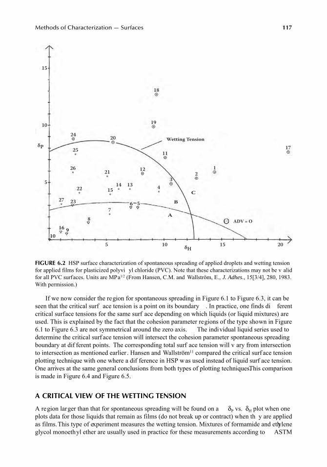
Methods of Characterization — Surfaces
117
If we now consider the region for spontaneous spreading in Figure 6.1 to Figure 6.3, it can beseen that the critical surf ace tension is a point on its boundary . In practice, one finds di ferentcritical surface tensions for the same surf ace depending on which liquids (or liquid mixtures) areused. This is explained by the fact that the cohesion parameter regions of the type shown in Figure6.1 to Figure 6.3 are not symmetrical around the zero axis. The individual liquid series used todetermine the critical surf ace tension will intersect the cohesion parameter spontaneous spreadingboundary at dif ferent points. The corresponding total surf ace tension will v ary from intersectionto intersection as mentioned earlier . Hansen and Wallström
11
compared the critical surf ace tensionplotting technique with one where a dif ference in HSP w as used instead of liquid surf ace tension.One arrives at the same general conclusions from both types of plotting techniques. This comparisonis made in Figure 6.4 and Figure 6.5.
A CRITICAL VIEW OF THE WETTING TENSION
A region larger than that for spontaneous spreading will be found on a
δ
P
vs.
δ
H
plot when oneplots data for those liquids that remain as films (do not break up or contract) when th y are appliedas films.This type of experiment measures the wetting tension. Mixtures of formamide and ethyleneglycol monoethyl ether are usually used in practice for these measurements according to ASTM
FIGURE 6.2
HSP surface characterization of spontaneous spreading of applied droplets and wetting tensionfor applied films for plasticized polyvi yl chloride (PVC). Note that these characterizations may not be v alidfor all PVC surfaces. Units are MPa
1/2
(From Hansen, C.M. and Wallström, E.,
J. Adhes
., 15[3/4], 280, 1983.With permission.)
5 10 15 20
δP
15
10
5
δH
Wetting Tension
C
B
– ADV = O
18*
19*
11*
17*
1*2
*3*4
*13*
14*15
*
7*
21*
26*
25*
22*
27* 23
8
12*
20*
24*
16 910
6 5
A
7248_C006.fm Page 117 Wednesday, May 23, 2007 11:00 AM
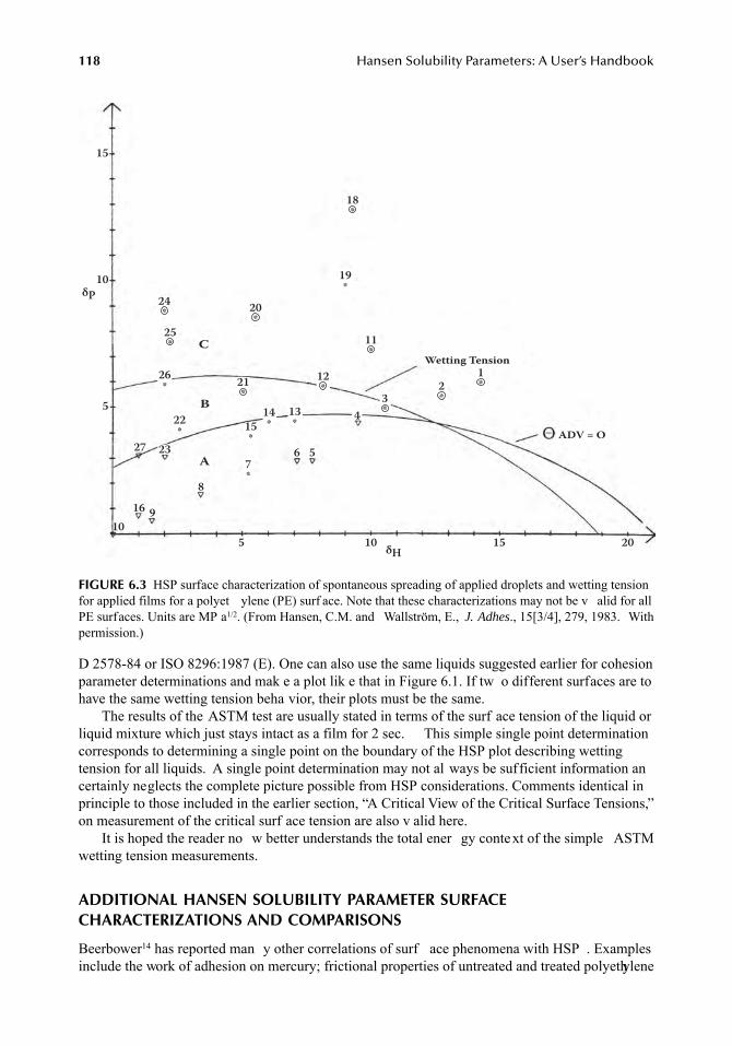
118
Hansen Solubility Parameters: A User’s Handbook
D 2578-84 or ISO 8296:1987 (E). One can also use the same liquids suggested earlier for cohesionparameter determinations and mak e a plot lik e that in Figure 6.1. If tw o different surfaces are tohave the same wetting tension beha vior, their plots must be the same.
The results of the ASTM test are usually stated in terms of the surf ace tension of the liquid orliquid mixture which just stays intact as a film for 2 sec. This simple single point determinationcorresponds to determining a single point on the boundary of the HSP plot describing wettingtension for all liquids. A single point determination may not al ways be sufficient information ancertainly neglects the complete picture possible from HSP considerations. Comments identical inprinciple to those included in the earlier section, “A Critical View of the Critical Surface Tensions,”on measurement of the critical surf ace tension are also v alid here.
It is hoped the reader no w better understands the total ener gy context of the simple ASTMwetting tension measurements.
ADDITIONAL HANSEN SOLUBILITY PARAMETER SURFACE CHARACTERIZATIONS AND COMPARISONS
Beerbower
14
has reported man y other correlations of surf ace phenomena with HSP . Examplesinclude the work of adhesion on mercury; frictional properties of untreated and treated polyethylene
FIGURE 6.3
HSP surface characterization of spontaneous spreading of applied droplets and wetting tensionfor applied films for a polyet ylene (PE) surf ace. Note that these characterizations may not be v alid for allPE surfaces. Units are MP a
1/2
. (From Hansen, C.M. and Wallström, E.,
J. Adhes
., 15[3/4], 279, 1983. Withpermission.)
5 10 15 20
δP
15
10
5
δH
Wetting Tension
C
B
A
– ADV = O
18*
20*
19*
24*25*
21*
26*
22*
7*
15*
14*
13*
27 23
16 910
8
6 5
4
12*
11*
3*
2*
1*
7248_C006.fm Page 118 Wednesday, May 23, 2007 11:00 AM
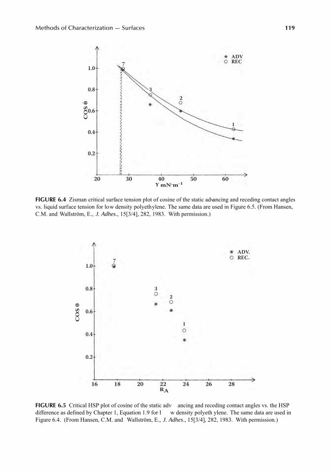
Methods of Characterization — Surfaces
119
FIGURE 6.4
Zisman critical surface tension plot of cosine of the static advancing and receding contact anglesvs. liquid surface tension for low density polyethylene. The same data are used in Figure 6.5. (From Hansen,C.M. and Wallström, E.,
J. Adhes
., 15[3/4], 282, 1983. With permission.)
FIGURE 6.5
Critical HSP plot of cosine of the static adv ancing and receding contact angles vs. the HSPdifference as defined by Chapter 1, Equation 1.9 for l w density polyeth ylene. The same data are used inFigure 6.4. (From Hansen, C.M. and Wallström, E.,
J. Adhes
., 15[3/4], 282, 1983. With permission.)
20 30 40 50 60
1.0
0.8
0.6
0.4
0.2
CO
S θ
γ mN.m-1
ADVREC7
3
2
1
16 18 20 22 24 26 28
1.0
0.8
0.6
0.4
0.2
CO
S θ
RA
ADV.REC.
2
1
3
7
7248_C006.fm Page 119 Wednesday, May 23, 2007 11:00 AM
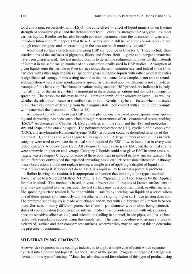
120
Hansen Solubility Parameters: A User’s Handbook
for 2 and 5 min, respectively, with H
2
S
2
O
7
; the Joffé effect — effect of liquid immersion on fracturestrength of soda-lime glass; and the Rehbinder ef fect — crushing strength of Al
2
O
3
granules undervarious liquids. Beerbower has also brought cohesion parameters into the discussion of wear andboundary lubrication.
14
It appears that these f actors should still ha ve some consideration, e venthough recent progress and understanding in the area are much more adv anced.
15
Additional surface characterizations using HSP are reported in Chapter 7. These include char-acterizations of the surf aces of pigments, fillers, and fibers. Both ganic and inor ganic materialshave been characterized. The test method used is to determine sedimentation rates for the materialsof interest in the same lar ge number of solv ents traditionally used in HSP studies. Adsorption ofgiven liquids onto the particle or fiber sur ace slows the sedimentation rate, and indeed some (fineparticles with rather high densities suspend for years in organic liquids with rather modest densities.A significant ad antage in this testing method is that he xane, for e xample, is not able to retardsedimentation where it may spontaneously spread, as discussed abo ve. Hexane is not an isolatedexample of this beha vior. The characterizations using standard HSP procedures indicate it is trulyhigh affinity for the sur ace, which is important in these characterizations and not just spontaneousspreading. The reason for this may be the e xtent (or depth) of the adsorption layer , as well aswhether the adsorption occurs at specific sites, or both. Results may be a fected when moleculesin a surface can orient differently from their original state upon contact with a liquid, for e xample,with water (see the discussion in Chapter 18).
An indirect correlation between HSP and the phenomena discussed above, spontaneous spread-ing and de wetting, has been established through measurements of en vironmental stress cracking(ESC).
16
As discussed in Chapter 14, ESC correlates with the strain and the HSP and molecularsize and shape of the cracking agent. The polymers polycarbonate (PC), cyclic olefinic copolyme(COC), and acrylonitrile/b utadiene/styrene (ABS) terpolymer could be described in terms of theregions A, B, and C as sho wn in Figure 6.1 to Figure 6.3. A large number of test liquids in eachcategory were used to evaluate the critical strain required for ESC. It w as found that in every casetested, category A liquids gave ESC. All category B liquids also g ave ESC, but the critical strainswere somewhat higher on an a verage. Category C liquids could also gi ve ESC in some cases. n-hexane was a category C liquid for some of these polymers in spite of its lo w surface tension. TheHSP differences outweighed the expected spreading based on surface tension differences. Althoughthese observ ations should not replace testing, a simple test of applying a droplet of liquid andpossibly spreading it, if it does not do so itself, is a rapid w ay to assess a potential problem.
Before lea ving this section, it is appropriate to mention that thinking of the type describedabove has led to a Nordtest Method, NT POL Y 176, “Spreading Surf ace Tension by the AppliedDroplet Method.” This method is based on visual observation of droplets of known surface tensionafter they are applied to a test surface. The test surface may be a polymer, metal, or other material.The spreading surface tension is found to within ±1 mN/m by locating two liquids in a series whereone of them spreads spontaneously and the other with a slightly higher surf ace tension does not.The preferred set of liquids is made with ethanol and w ater with a dif ference of 2 mN/m betweenthem. Surfaces of man y different geometries (from 4
μ
m diameter wire to ships being painted),states of contamination (from clean for internal medical use to contamination with oil, silicones,pressure sensitive adhesive, etc.), and orientation (ceiling in a tunnel, inside pipes, etc.) ha ve beentested with remarkable success using this simple test. The usual procedure is to assign a v alue toa clean(ed) surface and then compare test surfaces, wherever they may be, against this to determinethe presence of contamination.
SELF-STRATIFYING COATINGS
A newer development in the coatings industry is to apply a single coat of paint which separatesby itself into a primer and topcoat. A special issue of the journal Progress in Organic Coatings wasdevoted to this type of coating.
17
Misev has also discussed formulation of this type of product using
7248_C006.fm Page 120 Wednesday, May 23, 2007 11:00 AM
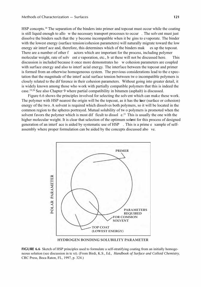
Methods of Characterization — Surfaces
121
HSP concepts.
18
The separation of the binders into primer and topcoat must occur while the coatingis still liquid enough to allo w the necessary transport processes to occur . The solvent must justdissolve the binders such that the y become incompatible when it be gins to evaporate. The binderwith the lowest energy (surface tension/cohesion parameters) will naturally migrate toward the lowenergy air interf ace and, therefore, this determines which of the binders mak es up the topcoat.There are a number of other f actors which are important for the process, including polymermolecular weight, rate of solv ent e vaporation, etc., b ut these will not be discussed here. Thisdiscussion is included because it once more demonstrates ho w cohesion parameters are coupledwith surface energy and also to interf acial energy. The interface between the topcoat and primeris formed from an otherwise homogeneous system. The previous considerations lead to the e xpec-tation that the magnitude of the interf acial surface tension between tw o incompatible polymers isclosely related to the dif ference in their cohesion parameters. Without going into greater detail, itis widely known among those who work with partially compatible polymers that this is indeed thecase.
19,20
See also Chapter 9 where partial compatibility in bitumen (asphalt) is discussed.Figure 6.6 shows the principles involved for selecting the solvent which can make these work.
The polymer with HSP nearest the origin will be the topcoat, as it has the lower (surface or cohesion)energy of the two. A solvent is required which dissolves both polymers, so it will be located in thecommon region to the spheres portrayed. Mutual solubility of tw o polymers is promoted when thesolvent favors the polymer which is most dif ficult to dissol e.
21
This is usually the one with thehigher molecular weight. It is clear that selection of the optimum solvent for this process of designedgeneration of an interf ace is aided by systematic use of HSP . This is a prime e xample of self-assembly where proper formulation can be aided by the concepts discussed abo ve.
FIGURE 6.6
Sketch of HSP principles used to formulate a self-stratifying coating from an initially homoge-neous solution (see discussion in te xt). (From Birdi, K.S., Ed.,
Handbook of Surface and Colloid Chemistry
,CRC Press, Boca Raton, FL, 1997, p. 324.)
HYDROGEN BONDING SOLUBILITY PARAMETER
POLA
R P
ARA
MET
ER
TOP COAT(LOWEST ENERGY)
PARAMETERS REQUIREDFOR COMMONSOLVENT
PRIMER
7248_C006.fm Page 121 Wednesday, May 23, 2007 11:00 AM
122
Hansen Solubility Parameters: A User’s Handbook
MAXIMIZING PHYSICAL ADHESION
If one wishes to maximize ph ysical adhesion, the ph ysical similarity (same HSP) of the tw ointerfaces being joined must be as close as possible. The previous discussion suggests that physicalsimilarity can be obtained when tw o criteria are met. The first criterion is that xactly the sameliquids spontaneously spread on each of the surf aces to be joined. The second criterion is thatexactly the same liquids maintain films when spread (ASTM method for wetting tension) on eacof the surf aces to be joined. Any dif ferences in this spontaneous spreading or wetting tensionbehavior can be interpreted as being a dif ference in ph ysical similarity . The dif ferences in thebehavior of liquid droplets or films that are obser ed may suggest which steps can be tak en tominimize differences, if this is required. Should one add aliphatic segments to reduce the polar andhydrogen bonding contrib utions? Should alcohol and/or acid groups be incorporated to increasethe hydrogen bonding in the system? This type of approach can be used to establish guidelines foraction relative to each of the HSP parameters. Aromatic character and halogens other than fluorincharacteristically increase
δ
D
; nitro and phosphate groups characteristically increase
δ
P
; and alcohol,acid, and primary amine groups characteristically increase
δ
H
. Reference can be made to the tableof group contrib utions in Chapter 1 (T able 1.1) for more precise comparisons. The discussion offorming good anchors on pigments and other surf aces found in Chapter 8 is also rele vant to thepresent discussion, as such anchors can also be used to enhance adhesion.
CONCLUSION
Greater insight into the mak eup of a product is possible when one not only kno ws the cohesionparameters, i.e., HSP, for polymers and solvents it contains, but also the HSP for the various surfaceswhich these encounter . The surf aces of substrates, pigments, fillers, plastics, fibers, and othmaterials can also be characterized by HSP (see Chapter 5 and Chapter 7). This allows mutualinteractions to be inferred by comparisons of which materials are similar and which materials aredifferent in terms of their HSP . Similar materials in this conte xt have similar HSP re gardless ofdifferences in composition.
The critical surf ace tension and wetting tension are single point determinations. Cohesionparameters allow a more complete characterization of surfaces than do these single point measure-ments and, at the same time, allo w insight as to ho w the single point measurements fit into thoverall ener gy picture for the product. Guidelines for systematically changing the af finities osurfaces can also be obtained from HSP concepts.
Both the spontaneous spreading re gion and the wetting tension re gion on HSP plots for tw odifferent surfaces must be identical if the y are to ha ve identical overall surface characteristics.
REFERENCES
1. Flory, P.J.,
Principles of Polymer Chemistry
, Cornell University Press, New York, 1953.2. Barton, A.F.M., Applications of solubility parameters and other cohesion ener gy parameters,
Polym.Sci. Technol. Pure Appl. Chem.
, 57(7), 905–912, 1985.3. Skaarup, K. and Hansen, C.M., The Three-Dimensional Solubility Parameter and Its Use (Det Tred-
imensionale Opløselighedsparametersystem og dets Anvendelse), Rapport No. 54 (TM 2-67), Lak-og Farveindustriens Forskningslaboratorium, København, 1967 (in Danish).
4. Skaarup, K., Surf ace Tension and 3-D Solubility P arameters (Ov erfladespænding og 3-D Opløselighedsparametre), Nordiske Kemikermøde, København, 1968 (in Danish).
5. Beerbower, A., Surface free energy: a new relationship to bulk energies,
J. Colloid Interface Sci.
, 35,126–132, 1971.
6. Hansen, C.M. and Beerbo wer, A., Solubility parameters, in
Kirk-Othmer Encyclopedia of ChemicalTechnology
, 2nd ed., Suppl. Vol., Standen, A., Ed., Interscience, Ne w York, 1971, pp. 889–910.
7248_C006.fm Page 122 Wednesday, May 23, 2007 11:00 AM
Methods of Characterization — Surfaces
123
7. Koenhen, D.N. and Smolders, C.A., The determination of solubility parameters of solv ents andpolymers by means of correlation with other physical quantities,
J. Appl. Polym. Sci.
, 19, 1163–1179,1975.
8. Erbil, H.Y., Surface tension of polymers, in
Handbook of Surface and Colloid Chemistry
, Birdi, K.S.,Ed., CRC Press, Boca Raton, FL, 1997, pp. 265–312.
9. Hansen, C.M., Characterization of liquids by spreading liquids,
J. Paint Technol.
, 42(550), 660–664,1970.
10. Hansen, C.M. and Pierce, P .E., Surface effects in coatings processes, XII Federation d’Associationsde Techniciens des Industries des Peintures, Vernis, Emaux et Encres d’Imprimerie de l’EuropeContinentale, Congress Book, Verlag Chemie, Weinheim/Bergstrasse, 91–99, 1974;
Ind. Eng. Chem.Prod. Res. Dev.
, 13(4), 218–225, 1974.11. Hansen, C.M. and Wallström, E., On the use of cohesion parameters to characterize surfaces,
J. Adhes.
,15(3/4), 275–286, 1983.
12. Zisman, W.A., Relation of the equilibrium contact angle to liquid and solid constitution, in
ContactAngle, Wettability and Adhesion
, Advances in Chemistry Series No. 43, Gould, R.F ., Ed., AmericanChemical Society, Washington, D.C., 1964, chap. 1.
13. Zisman, W.A., Surface energetics of wetting, spreading, and adhesion,
J. Paint Technol.
, 44(564), 41,1972.
14. Beerbower, A., Boundary Lubrication — Scientific and Technical Applications Forecast, AD747336,Office of the Chief of Research and D velopment, Department of the Army, Washington, D.C., 1972.
15. Krim, J., Friction at the Atomic Scale,
Scientific American
, 275(4), October 1996, pp. 48–56.16. Nielsen, T.B. and Hansen, C.M., Surf ace wetting and the prediction of en vironmental stress cracking
(ESC) in polymers,
Polym. Degradation Stability
, 89, 513–516, 2005.17. Special issue devoted to self-stratifying coatings,
Prog. Org. Coat.
, 28(3), July 1996.18. Misev, T.A., Thermodynamic analysis of phase separation in self-stratifying coatings — solubility
parameters approach,
J. Coat. Technol.
, 63(795), 23–28, 1991.19. Luciani, A., Champagne, M.F., and Utracki, L.A., Interfacial tension in polymer blends. Part 1: Theory,
Polym. Networks Blends
, 6(1), 41–50, 1996.20. Luciani, A., Champagne, M.F ., and Utracki, L.A., Interf acial tension in polymer blends. P art 2:
Measurements,
Polym. Networks Blends
, 6(2), 51–62, 1996.21. Hansen, C.M., On application of the three dimensional solubility parameter to the prediction of mutual
solubility and compatibility,
Färg och Lack
, 13(6), 132–138, 1967.
7248_C006.fm Page 123 Wednesday, May 23, 2007 11:00 AM

7248_C006.fm Page 124 Wednesday, May 23, 2007 11:00 AM
125
7
Methods of Characterization for Pigments, Fillers, and Fibers
Charles M. Hansen
ABSTRACT
Cohesion parameters for pigments, fillers, and fibers can often be valuated by observation of thesuspension and/or sedimentation beha vior of particulate matter in dif ferent liquids. These charac-terizations are based on relatively stronger adsorption by some of the liquids compared with others.Those liquids with stronger interaction can suspend finer fractions of solids indefinitely or retasedimentation, compared with the other liquids. Data should be interpreted by accounting fordifferences in the densities and viscosities of the test liquids, such that a relative sedimentation ratecan be used for comparisons. The absolute sedimentation rates are generally not of primary interest.Data from such evaluations can be computer-processed to assign Hansen cohesion parameters (HSP)to the material in question. Cohesion parameter data are gi ven for some ne wer pigments, fillersand a carbon fiber to demonstrate the principles
INTRODUCTION
The possibilities offered by cohesion parameter characterization of pigments, fillers, and fibers venot been generally recognized, judging from the relatively small number of publications appearingon the topic. Pigments and a few fillers were characterized in some of the author s first publicationdealing with the solubility parameter .
1,2
These were gi ven
δ
D
,
δ
P
, and
δ
H
parameters (HSP) and acharacteristic radius of interaction exactly analogous to the polymer characterizations discussed inChapter 2 and Chapter 5. These data together with some more recent pigment characterizations areincluded in Table 7.1, Table 7.2A, and Table 7.2B. Shareef et al.
3
have also characterized pigmentsurfaces, including metal oxides. Gardon and Teas
4
clearly sho wed the dif ferences between zincoxides treated and untreated with or ganic phosphate using a cohesion parameter characterization.Inorganic fibers h ve also been characterized.
5
All of these characterizations ag ain confirm thuniversality possible with these parameters. They reflect molecule–molecule interactions whetheat surfaces or in b ulk.
In the future, more systematic selection of dispersion aids should be possible, as these can alsobe described with the same energy parameters. Hansen and Beerbower have touched on this topic.
6
Each se gment of such molecules requires its o wn HSP. The discussion in Chapter 15 for theinteractions within cell walls in wood demonstrates how this could be done. It has been sho wn bycalculation that hemicelluloses act lik e surface-active agents, with some se gments seeking lower-energy lignin regions and some segments (those with alcohol groups) orienting to ward the higher-energy cellulose.
7248_C007.fm Page 125 Wednesday, April 4, 2007 1:00 PM
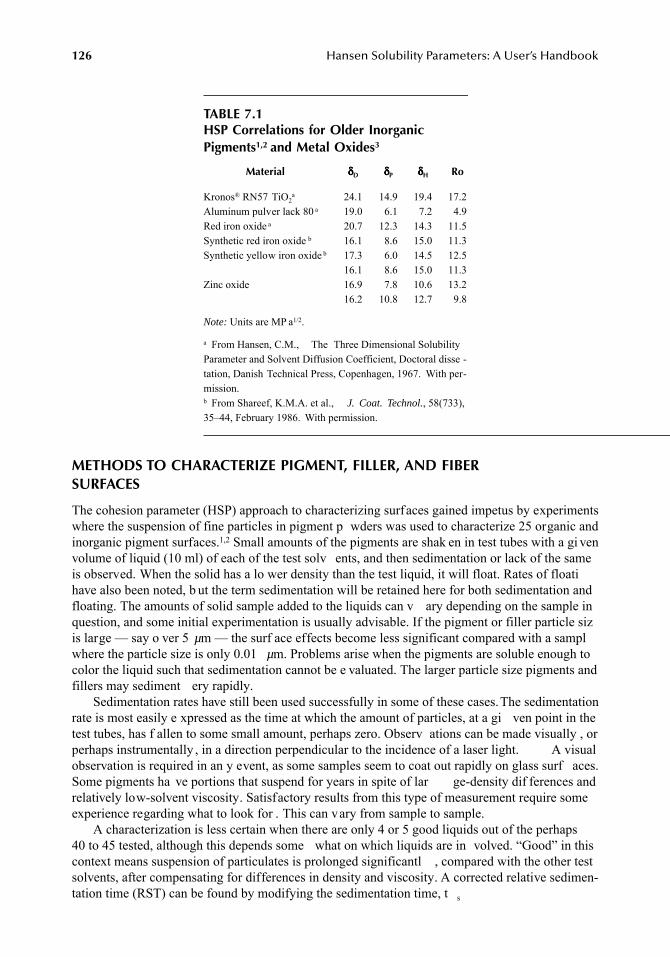
126
Hansen Solubility Parameters: A User’s Handbook
METHODS TO CHARACTERIZE PIGMENT, FILLER, AND FIBER SURFACES
The cohesion parameter (HSP) approach to characterizing surfaces gained impetus by experimentswhere the suspension of fine particles in pigment p wders was used to characterize 25 organic andinorganic pigment surfaces.
1,2
Small amounts of the pigments are shak en in test tubes with a gi venvolume of liquid (10 ml) of each of the test solv ents, and then sedimentation or lack of the sameis observed. When the solid has a lo wer density than the test liquid, it will float. Rates of floatihave also been noted, b ut the term sedimentation will be retained here for both sedimentation andfloating. The amounts of solid sample added to the liquids can v ary depending on the sample inquestion, and some initial experimentation is usually advisable. If the pigment or filler particle sizis large — say o ver 5
µ
m — the surf ace effects become less significant compared with a samplwhere the particle size is only 0.01
µ
m. Problems arise when the pigments are soluble enough tocolor the liquid such that sedimentation cannot be e valuated. The larger particle size pigments andfillers may sediment ery rapidly.
Sedimentation rates have still been used successfully in some of these cases. The sedimentationrate is most easily e xpressed as the time at which the amount of particles, at a gi ven point in thetest tubes, has f allen to some small amount, perhaps zero. Observ ations can be made visually , orperhaps instrumentally , in a direction perpendicular to the incidence of a laser light. A visualobservation is required in an y event, as some samples seem to coat out rapidly on glass surf aces.Some pigments ha ve portions that suspend for years in spite of lar ge-density dif ferences andrelatively low-solvent viscosity. Satisfactory results from this type of measurement require someexperience regarding what to look for . This can vary from sample to sample.
A characterization is less certain when there are only 4 or 5 good liquids out of the perhaps40 to 45 tested, although this depends some what on which liquids are in volved. “Good” in thiscontext means suspension of particulates is prolonged significantl , compared with the other testsolvents, after compensating for differences in density and viscosity. A corrected relative sedimen-tation time (RST) can be found by modifying the sedimentation time, t
s
TABLE 7.1HSP Correlations for Older Inorganic Pigments
1,2
and Metal Oxides
3
Material
δδδδ
D
δδδδ
P
δδδδ
H
Ro
Kronos
®
RN57 TiO
2a
24.1 14.9 19.4 17.2Aluminum pulver lack 80
a
19.0 6.1 7.2 4.9Red iron oxide
a
20.7 12.3 14.3 11.5Synthetic red iron oxide
b
16.1 8.6 15.0 11.3Synthetic yellow iron oxide
b
17.3 6.0 14.5 12.516.1 8.6 15.0 11.3
Zinc oxide 16.9 7.8 10.6 13.216.2 10.8 12.7 9.8
Note:
Units are MP a
1/2
.
a
From Hansen, C.M., The Three Dimensional SolubilityParameter and Solvent Diffusion Coefficient, Doctoral disse -tation, Danish Technical Press, Copenhagen, 1967. With per-mission.
b
From Shareef, K.M.A. et al.,
J. Coat. Technol.
, 58(733),35–44, February 1986. With permission.
7248_C007.fm Page 126 Wednesday, April 4, 2007 1:00 PM
Methods of Characterization for Pigments, Fillers, and Fibers
127
RST = t
s
(
ρ
p
–
ρ
s
)/
η
(7.1)
ρ
p
and
ρ
s
are densities of particle and test liquid, respecti vely, and
η
is the liquid viscosity .A prolonged RST implies greater adsorption of the gi ven solvent onto the surface in question.
Characterizations based on these techniques tend to place emphasis on the nature of the surf acesfor the smaller -particle-size fractions.
An example of a data sheet used for such studies is included in Table 7.3.
DISCUSSION — PIGMENTS, FILLERS, AND FIBERS
It can be reasoned that a pigment, fille , or fiber is most beneficial when the pigment su ace andthe binder in question ha ve the same cohesion parameters. There are apparently no publicationsindicating a systematic modification of pigment sur aces to achieve a given set of cohesion param-eters. The characterizations for some or ganic pigments are given in Table 7.4. These data indicatethat their respecti ve surf aces are essentially identical. An e xception is the first one in the tablwhere the analysis is based on only three good solv ents that were able to e xtend sedimentationsignificantly relat ve to the other solv ents tested.
TABLE 7.2AList of Pigments Studied. HSP Results are Given in Table 7.2B
Pigment Description
1. TiO
2
, Kronos RN 57, Titan Co. A/S., Frederikstad, Norway.2. Phthalocyanine Blue, B6, E. I. du Pont de Nemours and Co. (1949).3. Isolbonared Nr. 7522, C. I. Pigment Red 48 (C.I. 15865) (MnSalt), Køge Chemical Works, Køge, Denmark.4. Peerless Carbon Black5. Isol Fast Yellow IO GX 2505, C.I. Pigment Yellow 3, Køge Chemical Works, Køge, Denmark.6. Refl x Blau TBK Ext. (No C.I. Inde x-pigment mixture), Farbwerke Hoechst, Frankfurt (M), German y.7. Isol Ruby BKS 7520, C.I. Pigment Red 57 (C.I. 15850) (Ca Salt), Køge Chemical Works, Køge, Denmark.8. Hansagelb 10 G, C.I. Pigment Yellow 3 (C.I. 11710), F arbwerke Hoechst, Frankfurt (M), German y.9. Fanalrosa G Supra Pulv er, Pigment Red 81 (C.I. 45160), B ASF, Ludwigshafen, Germany.
10. Heliogenblau B Pulver, C.I. Pigment Blue 15 (C.I. 74160), B ASF, Ludwigshafen, Germany.11. Heliogengrün GN, C.I. Pigment Green 7, (C.I. 74260), B ASF, Ludwigshafen, Germany.12. Permanentgelb H 10 G, C.I. Pigment Yellow 81, (No C.I. index), Farbwerke Hoechst, Frankfurt (M), Germany.13. Permanent Bordeaux FRR, C.I. Pigment Red 12 (C.I. 12385), F arbwerke Hoechst, Frankfurt (M), Germany.14. Permanent Violet RL Supra, C.I. Pigment Violet 23, (C.I. 12505), F arbwerke Hoechst, Frankfurt (M),
Germany.15. Isol Benzidine Yellow G 2537, C.I. Pigment Yellow 12 (C.I. 21090), Køge Chemical Works, Køge, Denmark.16. Brillfast Sky Blue 3862, C.I. Pigment Blue 3 (C.I. 42140), J. W. and T. A. Smith Ltd., London.17. Permanent Orange G, C.I. Pigment Orange 13 (C.I. 21110), F arbwerke Hoechst, Frankfurt (M), German y.18. Permanent Red, FGR Extra Pulver, C.I. Pigment Red 112, (C.I. 12370). Farbwerke Hoechst, Frankfurt (M),
Germany.19. Isol Fast Red 2G 2516, C.I. Pigment Orange 5, (C.I. 12075), Køge Chemical Works, Køge, Denmark.20. Monolite Fast Blue 3 RS, Po wder, C.I. Vat Blue 4 (C.I. 69801), Imperial Chemical Industries.21. Heliogenblau LG, Pulver, C.I. Pigment Blue 16 (C.I. 74100), B ASF., Ludwigshafen, Germany.22. Red Iron Oxide.23. Carbon Black, Printex V (5519-1), Degussa, Frankfurt (M), German y.24. Aluminum Pulver Lack 80, Eckart-Werke, 851 Fürth/Bayern, German y.25. Isol Benzidene Yellow GA-PR, 9500, C.I. Pigment Yellow 12, Køge Chemical Works, Køge, Denmark.
Source:
From Hansen, C.M., The Three Dimensional Solubility P arameter and Solv ent Diffusion Coefficient, Doctoradissertation, Danish Technical Press, Copenhagen, 1967. With permission.
7248_C007.fm Page 127 Wednesday, April 4, 2007 1:00 PM
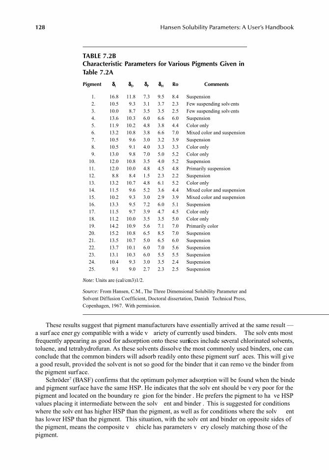
128
Hansen Solubility Parameters: A User’s Handbook
These results suggest that pigment manufacturers have essentially arrived at the same result —a surf ace ener gy compatible with a wide v ariety of currently used binders. The solv ents mostfrequently appearing as good for adsorption onto these surfaces include several chlorinated solvents,toluene, and tetrahydrofuran. As these solvents dissolve the most commonly used binders, one canconclude that the common binders will adsorb readily onto these pigment surf aces. This will givea good result, provided the solvent is not so good for the binder that it can remo ve the binder fromthe pigment surface.
Schröder
7
(BASF) confirms that the optimum polymer adsorption will be found when the bindeand pigment surface have the same HSP. He indicates that the solv ent should be very poor for thepigment and located on the boundary re gion for the binder . He prefers the pigment to ha ve HSPvalues placing it intermediate between the solv ent and binder . This is suggested for conditionswhere the solv ent has higher HSP than the pigment, as well as for conditions where the solv enthas lower HSP than the pigment. This situation, with the solv ent and binder on opposite sides ofthe pigment, means the composite v ehicle has parameters v ery closely matching those of thepigment.
TABLE 7.2BCharacteristic Parameters for Various Pigments Given in Table 7.2A
Pigment
δδδδ
t
δδδδ
D
δδδδ
P
δδδδ
H
Ro Comments
1. 16.8 11.8 7.3 9.5 8.4 Suspension2. 10.5 9.3 3.1 3.7 2.3 Few suspending solvents3. 10.0 8.7 3.5 3.5 2.5 Few suspending solvents4. 13.6 10.3 6.0 6.6 6.0 Suspension5. 11.9 10.2 4.8 3.8 4.4 Color only 6. 13.2 10.8 3.8 6.6 7.0 Mixed color and suspension7. 10.5 9.6 3.0 3.2 3.9 Suspension8. 10.5 9.1 4.0 3.3 3.3 Color only9. 13.0 9.8 7.0 5.0 5.2 Color only
10. 12.0 10.8 3.5 4.0 5.2 Suspension11. 12.0 10.0 4.8 4.5 4.8 Primarily suspension12. 8.8 8.4 1.5 2.3 2.2 Suspension13. 13.2 10.7 4.8 6.1 5.2 Color only14. 11.5 9.6 5.2 3.6 4.4 Mixed color and suspension15. 10.2 9.3 3.0 2.9 3.9 Mixed color and suspension16. 13.3 9.5 7.2 6.0 5.1 Suspension17. 11.5 9.7 3.9 4.7 4.5 Color only18. 11.2 10.0 3.5 3.5 5.0 Color only19. 14.2 10.9 5.6 7.1 7.0 Primarily color20. 15.2 10.8 6.5 8.5 7.0 Suspension21. 13.5 10.7 5.0 6.5 6.0 Suspension22. 13.7 10.1 6.0 7.0 5.6 Suspension23. 13.1 10.3 6.0 5.5 5.5 Suspension24. 10.4 9.3 3.0 3.5 2.4 Suspension25. 9.1 9.0 2.7 2.3 2.5 Suspension
Note:
Units are (cal/cm3)1/2.
Source:
From Hansen, C.M., The Three Dimensional Solubility Parameter andSolvent Diffusion Coefficient, Doctoral dissertation, Danish Technical Press,Copenhagen, 1967. With permission.
7248_C007.fm Page 128 Wednesday, April 4, 2007 1:00 PM
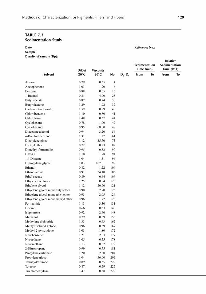
Methods of Characterization for Pigments, Fillers, and Fibers
129
TABLE 7.3Sedimentation Study
Date Reference No.:Sample:Density of sample (Dp):
D(Ds)20°C
Viscosity20°C
Sedimentation
Time (min)
RelativeSedimentation
Time (RST)
Solvent No. D
p
- D
s
From To From To
Acetone 0.79 0.35 4Acetophenone 1.03 1.90 6Benzene 0.88 0.65 131-Butanol 0.81 4.00 28Butyl acetate 0.87 0.74 30Butyrolactone 1.29 1.92 37Carbon tetrachloride 1.59 0.99 40Chlorobenzene 1.10 0.80 41Chloroform 1.48 0.37 44Cyclohexane 0.78 1.00 47Cyclohexanol 0.95 68.00 48Diacetone alcohol 0.94 3.20 56
o
-Dichlorobenzene 1.31 1.27 61Diethylene glycol 1.12 35.70 75Diethyl ether 0.72 0.23 82Dimethyl formamide 0.95 0.82 90DMSO 1.10 1.98 941,4-Dioxane 1.04 1.31 96Dipropylene glycol 1.03 107.0 98Ethanol 0.82 1.22 104Ethanolamine 0.91 24.10 105Ethyl acetate 0.89 0.44 106Ethylene dichloride 1.25 0.84 120Ethylene glycol 1.12 20.90 121Ethyelene glycol monobutyl ether 0.90 2.90 123Ethyelene glycol monoethyl ether 0.93 2.05 124Ethyelene glycol monomethyl ether 0.96 1.72 126Formamide 1.13 3.30 131Hexane 0.66 0.33 140Isophorone 0.92 2.60 148Methanol 0.79 0.59 153Methylene dichloride 1.33 0.43 162Methyl isobutyl ketone 0.96 0.59 167Methyl-2-pyrrolidone 1.03 1.80 172Nitrobenzene 1.21 2.03 177Nitroethane 1.05 0.55 178Nitromethane 1.13 0.62 1792-Nitropropane 0.99 0.75 181Propylene carbonate 1.20 2.80 204Propylene glycol 1.04 56.00 205Tetrahydrofurane 0.89 0.55 222Toluene 0.87 0.59 225Trichloroethylene 1.47 0.58 229
7248_C007.fm Page 129 Wednesday, April 4, 2007 1:00 PM
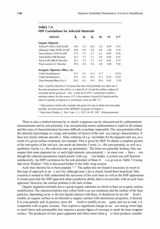
130
Hansen Solubility Parameters: A User’s Handbook
There is also a relation between ho w clearly a pigment can be characterized by sedimentationmeasurements and its zeta potential. Low zeta potential means sedimentation is rapid in all solvents,and this type of characterization becomes difficult or perhaps impossible.The zeta potential reflectthe intensity (percentage co verage and number of layers) of the surf ace energy characteristics. Itdoes not clearly indicate specific a finity relations of a g ven binder for the pigment surf ace, as aresult of a given surface treatment, for example. This is given by HSP. To obtain a complete pictureof the ener getics of the surf ace, one needs an intensity f actor, i.e., the zeta potential, as well as aqualitative factor, i.e., the cohesion ener gy parameters. The latter are generally lacking. One cansuspect that some pigments ha ve such high-intensity zeta potential — at some cost — that e venthough the cohesion parameters match poorly with a gi ven binder , a system can still functionsatisfactorily. An HSP correlation for the zeta potential of blanc fi e is gi ven in Table 7.4 usingdata from Winkler.
8
This is discussed further in the follo wing section.Acid–base theories ha ve been popular .
9–11
The author has not found it necessary to resort tothis type of approach in an y acti vity, although man y ha ve clearly found them beneficial. Morresearch is needed to fully understand the successes of the acid–base as well as the HSP approaches.It would seem that the HSP approach allows predictive ability that is not possible with an acid–baseapproach. However, the current problem is the lack of data.
Organic pigments normally have a good organic substrate on which to base an or ganic surfacemodification. The characterizations may reflect both a sur ace treatment and the surface of the baseparticles, depending on ho w the test liquids interact with these. It should not be too dif ficult tmodify an organic surface to an alternative organic surface with satisfactory properties, if desired.It is conceptually and, in practice, more dif ficult to modify an ino ganic surf ace to mak e itcompatible with or ganic systems. This requires a significant change in sur ace energy from highto much lower and, presumably, also requires a greater degree of coverage to mask the base inorganicsurface. The producers of inor ganic pigments and fillers must either g ve their products suitable
TABLE 7.4HSP Correlations for Selected Materials
Material
δδδδ
D
δδδδ
P
δδδδ
H
Ro Fit G/T
Organic Pigments
Paliotol
®
Gelb L1820 B ASF 18.9 3.5 10.5 5.4 0.99 3/35 Heliogen
®
Blau 6930L B ASF 18.0 4.0 4.0 4.0 1.00 5/34 Socco Rosso L3855 B ASF 17.3 5.7 2.7 4.1 0.99 4/34 Perm Rubin F6B Hoechst 16.7 3.7 3.1 4.8 0.88 6/33 Perm Gelb GRL02 Hoechst 16.7 2.5 3.7 4.5 0.95 5/37 Perm Lackrot LC Hoechst 19.0 5.0 5.0 4.0 1.00 7/28
Inorganic Pigments, Fillers, etc.
Cabot Hochdisperse
a
16.7 9.3 11.5 11.7 — 23/23 Cabot Hochdisperse 19.3 9.5 10.3 12.7 0.79 23/31 Zeta Potential Blanc Fix e
b
26.5 19.1 14.5 20.4 0.95 5/19
Note:
A perfect data fit of 1.0 means that there most probably are other sets othe same parameters that will ha ve a data fit of 1.0 and also define a sphere thsurrounds all the good solv ents. A data fit of 0.99+ is preferred to define toptimum sphere for this reason. G/T is the number of good (G) liquids and thetotal (T) number of liquids in a correlation. Units are MP a
1/2
.
a
Data analysis which only considers the good solv ents to define the least spherpossible. See discussion of the SPHERE1 program in Chapter 1.
b
Data from Winkler, J.,
Eur. Coat. J.
, 1–2/97, 38–42, 1997. With permission.
7248_C007.fm Page 130 Wednesday, April 4, 2007 1:00 PM
Methods of Characterization for Pigments, Fillers, and Fibers
131
surfaces, probably after much ef fort, or else one needs one or more superef fective additives to beable to achieve a good and stable dispersion. It helps to incorporate gi ven (high-cohesion energy)groups in a grinding resin, such as acid, alcohol, amine, etc. The relatively high local cohesionparameters in the binder that are associated with these groups w ould indicate a high af finity fothe high-cohesion-energy surface of the inor ganic material. At the same time, these local re gionsof adsorbed polymer se gments are not particularly soluble or are insoluble in the cheaper h ydro-carbon solvents — for example, those that have much lower cohesion parameters. This provides agood, stable anchor on the pigment surf ace. The solvent will not dissolve that polymer or polymersegment away from the surface. Binders with high-acid numbers are frequently used, with success,in printing inks for the same reason. This is discussed in more detail in the follo wing section.
It is felt that those who understand the use of cohesion parameters are able to more systemat-ically modify surfaces of inorganic materials to optimize or improve their compatibility with organicpolymers and binders. This has been done for inorganic Rockwool
®
fibers that are to be incorporateinto polypropylene.
5
It must be presumed that this type of systematic procedure can guide surf acetreatment of other inor ganic materials in a more directed w ay toward a desired goal.
Data fits h ve been generally lo wer for characterizations of particulate solid surf aces, such asfillers, than for characterizations of polymers based on solubilit . When testing is finished, thpolymeric macromolecule is no longer a solid in the good solv ents, whereas the particulate filleremains a solid. A macromolecule has v arious possibilities for contortions and the positioning ofsignificant act ve groups in solution (or when swollen), giving a large number of possible (dynamic)structures that can be formed with the solv ent. A rigid solid surf ace does not ha ve this potentialfor adopting ener getically desirable positions for its acti ve groups. The adjustments for optimumlocal association must be made by the solv ent molecules alone in the sedimentation testing. Thereare many solvents that do not retard sedimentation significantl , whereas the predictions based onthe behavior of other solv ents that do significantly retard sedimentation indicate that this shoulbe the case. A contribution to the formation of the ener getically desirable geometrical structures isnot possible from the mo vement of rigid solid surf aces. Therefore, some solvents may not be ableto retard sedimentation because the y cannot adopt the geometrical positioning required to do thiswithout the help of a mobile substrate. This lack of e xpected performance may be also partly dueto solvent size, the location of the active groups, or combinations of these. These phenomena appearto be a significant area for future research
HANSEN SOLUBILITY PARAMETER CORRELATION OF ZETA POTENTIAL FOR BLANC FIXE
Winkler
8
has reported zeta potentials measured for 1% v/v blanc fi e with 0.34% moisture content.There were 19 liquids included in this careful study. These liquids could easily be divided into twogroups. There were 5 systems with zeta potentials greater than about 10 mV and 14 systems withzeta potentials less than about 5 mV . Table 7.3 includes the results of the correlation of these datawith cohesion parameters. The only major “error” was for hexamethylphosphoramide, with a REDof 0.951 and a zeta potential of 1.9 mV . This correlation supports the contention that cohesionparameters are significant for characterization of pigment, fill , and fiber sur aces. This is a goodcorrelation and supports the views presented earlier. According to Winkler, there was no correlationwith the acceptor or donor numbers (acid–base).
CARBON FIBER SURFACE CHARACTERIZATION
Hansen solubility parameters have been assigned to a carbon fiber sur ace, Panex 33 from Zoltek.After considerable refinement of the xperimental technique, it w as determined that tw o separatesets of HSP are required to describe the fiber sur ace. One of these sets has
δ
D
;
δ
P
;
δ
H
equal to
7248_C007.fm Page 131 Wednesday, April 4, 2007 1:00 PM
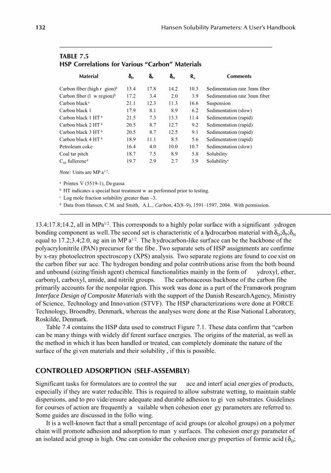
132
Hansen Solubility Parameters: A User’s Handbook
13.4;17.8;14.2, all in MPa
1/2
. This corresponds to a highly polar surface with a significant ydrogenbonding component as well. The second set is characteristic of a hydrocarbon material with
δ
D
;
δ
P
;
δ
H
equal to 17.2;3.4;2.0, ag ain in MP a
1/2
. The hydrocarbon-like surface can be the backbone of thepolyacrylonitrile (PAN) precursor for the fibe. Two separate sets of HSP assignments are confirmeby x-ray photoelectron spectroscopy (XPS) analysis. Two separate regions are found to coe xist onthe carbon fiber sur ace. The hydrogen bonding and polar contrib utions arise from the both boundand unbound (sizing/finish agent) chemical functionalities mainly in the form of ydroxyl, ether,carbonyl, carboxyl, amide, and nitrile groups. The carbonaceous backbone of the carbon fibeprimarily accounts for the nonpolar region. This work was done as a part of the Framework program
Interface Design of Composite Materials
with the support of the Danish Research Agency, Ministryof Science, Technology and Innovation (STVF). The HSP characterizations were done at FORCETechnology, Broendby, Denmark, whereas the analyses were done at the Risø National Laboratory,Roskilde, Denmark.
Table 7.4 contains the HSP data used to construct Figure 7.1. These data confirm that “carboncan be many things with widely dif ferent surface energies. The origins of the material, as well asthe method in which it has been handled or treated, can completely dominate the nature of thesurface of the gi ven materials and their solubility , if this is possible.
CONTROLLED ADSORPTION (SELF-ASSEMBLY)
Significant tasks for formulators are to control the sur ace and interf acial ener gies of products,especially if they are water reducible. This is required to allow substrate wetting, to maintain stabledispersions, and to pro vide/ensure adequate and durable adhesion to gi ven substrates. Guidelinesfor courses of action are frequently a vailable when cohesion ener gy parameters are referred to.Some guides are discussed in the follo wing.
It is a well-known fact that a small percentage of acid groups (or alcohol groups) on a polymerchain will promote adhesion and adsorption to man y surfaces. The cohesion ener gy parameter ofan isolated acid group is high. One can consider the cohesion ener gy properties of formic acid (
δ
D
;
TABLE 7.5HSP Correlations for Various “Carbon” Materials
Material
δδδδ
D
δδδδ
P
δδδδ
H
R
o
Comments
Carbon fiber (high r gion)
b
13.4 17.8 14.2 10.3 Sedimentation rate
3mm fiberCarbon fiber (l w region)
b
17.2 3.4 2.0 3.9 Sedimentation rate
3mm fiberCarbon black
a
21.1 12.3 11.3 16.6 SuspensionCarbon black 1 17.9 8.1 8.9 6.2 Sedimentation (slow)Carbon black 1 HT
b
21.5 7.3 13.3 11.4 Sedimentation (rapid)Carbon black 2 HT
b
20.5 8.7 12.7 9.2 Sedimentation (rapid)Carbon black 3 HT
b
20.5 8.7 12.5 9.1 Sedimentation (rapid)Carbon black 4 HT
b
18.9 11.1 8.5 5.6 Sedimentation (rapid)Petroleum coke 16.4 4.0 10.0 10.7 Sedimentation (slow)Coal tar pitch 18.7 7.5 8.9 5.8 SolubilityC
60
fullerene
d
19.7 2.9 2.7 3.9 Solubility
c
Note:
Units are MP a
1/2
.
a
Printex V (5519-1), Degussa
b
HT indicates a special heat treatment w as performed prior to testing.
c
Log mole fraction solubility greater than –3.
d
Data from Hansen, C.M. and Smith, A.L.,
Carbon
, 42(8–9), 1591–1597, 2004. With permission.
7248_C007.fm Page 132 Wednesday, April 4, 2007 1:00 PM
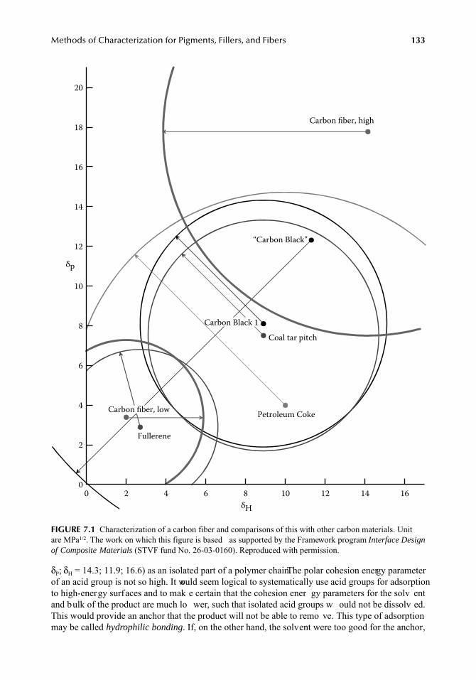
Methods of Characterization for Pigments, Fillers, and Fibers
133
δ
P
;
δ
H
= 14.3; 11.9; 16.6) as an isolated part of a polymer chain. The polar cohesion energy parameterof an acid group is not so high. It would seem logical to systematically use acid groups for adsorptionto high-energy surfaces and to mak e certain that the cohesion ener gy parameters for the solv entand bulk of the product are much lo wer, such that isolated acid groups w ould not be dissolv ed.This would provide an anchor that the product will not be able to remo ve. This type of adsorptionmay be called
hydrophilic bonding
. If, on the other hand, the solvent were too good for the anchor,
FIGURE 7.1
Characterization of a carbon fiber and comparisons of this with other carbon materials. Unitare MPa
1/2
. The work on which this figure is based as supported by the Framework program
Interface Designof Composite Materials
(STVF fund No. 26-03-0160). Reproduced with permission.
0 2 4 6 8 10 12 14 16
δH
δp
20
18
16
14
12
10
8
6
4
2
0
Fullerene
Carbon fiber, lowPetroleum Coke
Coal tar pitch
Carbon Black 1
“Carbon Black”
Carbon fiber, high
7248_C007.fm Page 133 Wednesday, April 4, 2007 1:00 PM
134
Hansen Solubility Parameters: A User’s Handbook
it could be presumed that e ven an acid group may be too readily dissolv ed off the surf ace or atleast take part in a dynamic equilibrium of adsorption and desorption. Absorbed/adsorbed watercan sometimes interfere with such anchors at high-ener gy surfaces.
The reverse of this thinking is systematically used by those designing associati ve thickenersand also by nature, such as the h ydrophobic bonding in proteins. Certain se gments of gi venmolecules have such low cohesive energy parameters that they are no longer soluble in the media,which is usually aqueous, and they either seek out their own kind (associate) or perhaps adsorb onor penetrate into a low-energy surface where cohesion energy parameters more suitably match. Thepositive effects of associative thickeners can be counteracted by the presence of solv ents preferen-tially locating where the hydrophobic bonding is to occur. The hydrophobic bonds lose strength ormay even dissolve away.
A challenge to the creati ve mind is to deri ve new uses for high-ener gy groups that are notparticularly water soluble or sensitive. The division of the cohesion energy into at least three partsallows these considerations to be made in a reasonably quantitati ve manner. One can choose nitrogroups or perhaps groups containing phosphorus as e xamples of species characterized by high-polar-cohesion-energy parameters and lo w or moderate h ydrogen bonding parameters. The totalcohesion energy parameters for ethanol and nitromethane are v ery close: 26.1 and 25.1 MP a
1/2
,respectively. Ethanol is soluble in water, nitromethane is not. Ethanol has a relatively high-hydrogenbonding parameter (19.4 MP a
1/2
) compared with nitromethane (5.1 MP a
1/2
). This mak es all thedifference. Would not the nitro group be a suitable anchor analogous to the pre vious discussionconcerning acid groups? Also, it w ould not be h ydrophilic with the inherent problems of w atersensitivity associated with high-hydrogen bonding parameters. Several of the pigments reported inTable 7.4 did indeed ha ve moderate af finity for the nitropara fins, for xample, b ut the y wereincluded in the lesser interacting group by the arbitrary di vision into good and bad groups.
CONCLUSION
Many pigments and fillers h ve now been characterized by Hansen cohesion parameters (HSP).Many examples are gi ven. A method based on relati ve sedimentation time and/or suspension isdescribed for doing this. This method has generally allowed useful characterizations, although someexperience is helpful. For example, the data are often scattered and not nearly of the quality usuallyfound when observing polymer solution beha vior. This scatter of data for untreated surf aces inparticular may cause some to disre gard the method; hopefully, they can develop a better one. Theobvious advantages of ha ving solvents, plasticizers, polymers, pigments, fillers, fibers, etc., ch -acterized with the same ener gy parameters should pro vide incentive for improving on the presentstate, both in terms of numbers of characterizations as well as improved methodology. One assumesthat maximum physical adsorption is accompanied by closely matching HSP . Local adsorption byso-called active groups (alcohol, acid, amine) ha ving the required match, can gi ve anchors on asurface that may no longer be soluble in the continuous media, and therefore will remain in placeas required.
REFERENCES
1. Hansen, C.M., The Three Dimensional Solubility Parameter and Solvent Diffusion Coefficient, Doctoral dissertation, Danish Technical Press, Copenhagen, 1967.
2. Hansen, C.M., The three dimensional solubility parameter — k ey to paint component af finities II.
J.Paint Technol.
, 39(511), 505–510, 1967.3. Shareef, K.M.A., Yaseen, M., Mahmood Ali, M., and Reddy, P.J.,
J. Coat. Technol.
, 58(733), 35–44,February 1986.
7248_C007.fm Page 134 Wednesday, April 4, 2007 1:00 PM
Methods of Characterization for Pigments, Fillers, and Fibers 135
4. Gardon, J.L. and Teas, J.P., Solubility parameters, in Treatise on Coatings, Vol. 2, Characterizationof Coatings: Physical Techniques, Part II, Myers, R.R. and Long, J.S., Eds., Marcel Dekk er, NewYork, 1976, chap. 8.
5. Hennissen, L., Systematic Modification of Filler/Fibre Sur aces to Achieve Maximum Compatibilitywith Matrix Polymers, Lecture for the Danish Society for Polymer Technology, Copenhagen, February10, 1996.
6. Hansen, C.M. and Beerbo wer, A., Solubility parameters, in Kirk-Othmer Encyclopedia of ChemicalTechnology, Suppl. Vol., 2nd ed., Standen, A., Ed., Interscience, Ne w York, 1971, pp. 889–910.
7. Schröder, J., Colloid chemistry aids to formulating inks and paints, Eur. Coat. J., 5/98, 334–340, 1998.8. Winkler, J., Zeta potential of pigments and fillers, Eur. Coat. J., 1–2/97, 38–42, 1997.9. Vinther, A., Application of the concepts solubility parameter and pigment char ge, Chim. Peint.
(England), 34(10), 363–372, 1971.10. Soerensen, P., Application of the acid/base concept describing the interaction between pigments,
binders, and solvents, J. Paint Technol., 47(602), 31–39, 1975.11. Soerensen, P., Cohesion parameters used to formulate coatings (K ohaesionsparametre an vendt til
formulering af f arver og lak), Färg och Lack Scand., 34(4), 81–93, 1988 (in Danish).12. Hansen, C.M. and Smith, A.L., Using Hansen solubility parameters to correlate solubility of C 60
fullerene in organic solvents and in polymers, Carbon, 42(8–9), 1591–1597, 2004.
7248_C007.fm Page 135 Wednesday, April 4, 2007 1:00 PM

7248_C007.fm Page 136 Wednesday, April 4, 2007 1:00 PM
137
8
Applications — Coatings and Other Filled Polymer Systems
Charles M. Hansen
ABSTRACT
Hansen solubility parameters (HSP) are widely used in the coatings industry to help find optimusolvents and solvent combinations. They also aid in substitution to less hazardous formulations invarious other types of products such as cleaners, printing inks, adhesi ves, etc. The discussion inthis chapter includes the ph ysical chemical reasons wh y solv ents function as the y do in man ypractical cases. The behavior of solvents in connection with surf aces of various kinds and the useof HSP to understand and control surf ace phenomena is especially emphasized. Products whereHSP concepts can be used in a manner similar to coatings include other (filled) polymer systemof various types such as adhesi ves, printing inks, che wing gum, etc. There are many examples ofcontrolled self-assembly.
INTRODUCTION
There are many applications documented in the literature where HSP ha ve aided in the selection ofsolvents, understanding and controlling processes, and, in general, of fering guidance where affinitieamong materials are of prime importance
1–5
(see also the follo wing chapters and e xamples below).This chapter emphasizes coatings applications and discusses the practical application of HSP to solventselection. Computer techniques are helpful, b ut not necessary. The same principles useful for under -standing the behavior of coatings are useful in understanding beha vior in a lar ger number of relatedproducts, including adhesives, printing inks, and chewing gum, to mention a few. These contain widelydifferent materials, both liquid and solid, which can be characterized by HSP. This allows their relativeaffinities to be established. Pr vious chapters ha ve discussed ho w to assign HSP to solv ents, plasti-cizers, polymers, and resins, as well as to the surf aces of substrates, pigments, fillers, and fiberVarious additives such as resins, surf actants, fl vors, aromas, scents, drugs, etc., can also be charac-terized by HSP to infer ho w they behave in seemingly comple x systems.
SOLVENTS
In order to find the optimum sol ent for a polymer , one must ha ve or estimate its HSP . Matchingthe HSP of an already e xisting solvent or combination of solv ents can be done, b ut this proceduredoes not necessarily optimize the ne w situation. The optimum depends on what is desired of thesystem. A solvent with the highest possible affinity for the polymer is both xpensive and probablynot necessary and will rarely be optimum. In more recent years, optimization increasingly includesconsiderations of worker safety and the e xternal environment. Volatile organic compounds (VOC)are to be reduced to the greatest extent possible. Chapter 11 is devoted to replacing ozone-depletingchemicals in cleaning operations.
7248_C008.fm Page 137 Wednesday, May 23, 2007 11:05 AM
138
Hansen Solubility Parameters: A User’s Handbook
Whereas hand calculations and plotting of data are still quite useful and at times more rapidthan computer processing, it is becoming almost mandatory that computers be used. To this end,most solvent suppliers and many large users of solvents have computer programs to predict solutionbehavior as well as e vaporation phenomena. In spite of these pressures to let the computer do thethinking, an experienced formulator can often arri ve at a near -optimum result without recourse topaper or to computers. A major f actor in this almost immediate o verview is the decrease in thenumber of solvents useful in coatings. By putting this together with other necessary considerationssuch as flash point, proper vaporation rate, cost, odor, availability, etc., the experienced formulatorwho knows the HSP for the relati vely few solvents possible in a gi ven situation will be able toselect a near -optimum combination by a process of e xclusion and simple mental arithmetic. Thisdoes not mean the use of HSP is on the w ay out. The real benefit of this concept is in interpretinmore complicated behavior, such as affinities of polymers with polymers and polymers with suracesas described in the follo wing. Much more work needs to be done in these areas, b ut the followinggives an indication of what might be e xpected.
As indicated previously, computer techniques can be v ery useful but are not always necessary,and simple two-dimensional plots using
δ
P
and
δ
H
can often be used by those with limited experiencewith these techniques to solve practical problems. The nonpolar cohesion parameter,
δ
D
, cannot beneglected in every case, but, for example, when comparing noncyclic solvents in practical situations,it has been found that their dispersion parameters will be rather close regardless of structure. Cyclicsolvents, and those containing atoms significantly la ger than carbon, such as chlorine, bromine,metals, etc., will ha ve higher dispersion parameters. The total solubility parameter for aliphatichydrocarbon solvents is identical with their dispersion parameter and increases only slightly withincreased chain length. This same trend is expected for oligomers of a polymer as molecular weightincreases. Re gardless of the means of processing data, the follo wing e xamples are intended toillustrate principles on which to base a systematic course of action.
Most coatings applications involve solvents reasonably well within the solubility limit which isindicated by the boundary of a solubility plot such as that sho wn in Figure 8.1.
1
A maximum ofcheaper hydrocarbon solvent is also desired and can frequently be used to arri ve at such a situationfor common polymers used in coatings. Some safety mar gin in terms of e xtra solvency is advisedbecause of temperature changes, potential variations in production, etc. These can lead to a situationwhere solvent quality changes in an adv erse manner. Balance of solv ent quality on e vaporation ofmixed solvents is also necessary. Here again, computer approaches are possible, and calculations ofsolvent quality can be made at all stages of evaporation. It is usually good practice to include a smallor moderate amount of slo wly evaporating solvent of good quality and lo w water sensitivity to takecare of this situation. These have frequently been slo wly evaporating ketones and esters.
An oxygenated solv ent which is frequently added to h ydrocarbon solvents and has been costeffective in increasing the v ery important h ydrogen-bonding parameter has been
n-
butanol (orsometimes 2-butanol). The mixture of equal parts xylene and
n-
butanol has been widely used inconjunction with man y polymers such as epoxies, b ut a third solv ent, such as a k etone, ester, orglycol ether, is often included in small amounts to increase the polar parameter/solv ency of themixture. Neither xylene nor
n-
butanol satisfactorily dissolves an epoxy of higher molecular weightby itself. These are located in boundary regions of the solubility region for epoxies, but on oppositesides of the characteristic Hansen spheres (see Figure 8.2).
1
Glycol ethers also can be added tohydrocarbon solvents with advantage, and the polar and h ydrogen-bonding parameters are higherthan if
n-
butanol had been added to the same concentration. There are man y possibilities, and asolubility parameter approach is particularly valuable in quickly limiting the number of candidates.The addition of glycol ethers or other w ater-soluble solv ents can ha ve adv erse ef fects, such asincreased water sensitivity and poorer corrosion resistance of the final film, as some soent retentionmust be anticipated, and the least v olatile solvent is enriched and left behind.
Relative costs for impro ving solvency from a h ydrocarbon base solv ent can be estimated bythe relation (
δ
P2
+
δ
H2
)
1/2
/cost. This relation has generally pointed to the use of
n-
butanol, for
7248_C008.fm Page 138 Wednesday, May 23, 2007 11:05 AM
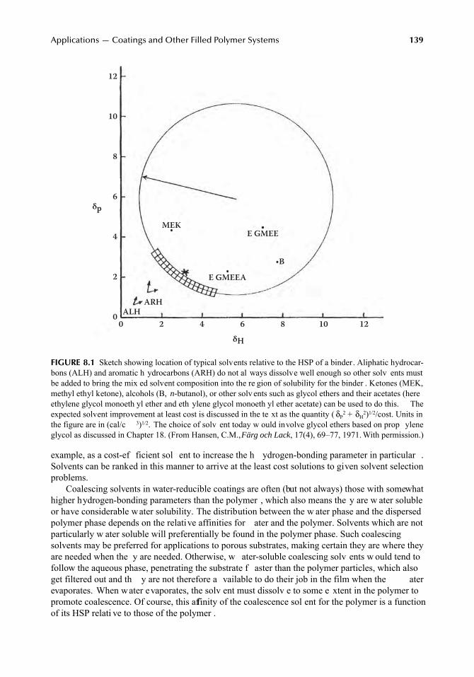
Applications — Coatings and Other Filled Polymer Systems
139
example, as a cost-ef ficient sol ent to increase the h ydrogen-bonding parameter in particular .Solvents can be ranked in this manner to arrive at the least cost solutions to given solvent selectionproblems.
Coalescing solvents in water-reducible coatings are often (but not always) those with somewhathigher hydrogen-bonding parameters than the polymer , which also means the y are w ater solubleor have considerable water solubility. The distribution between the w ater phase and the dispersedpolymer phase depends on the relative affinities for ater and the polymer. Solvents which are notparticularly w ater soluble will preferentially be found in the polymer phase. Such coalescingsolvents may be preferred for applications to porous substrates, making certain they are where theyare needed when the y are needed. Otherwise, w ater-soluble coalescing solv ents w ould tend tofollow the aqueous phase, penetrating the substrate f aster than the polymer particles, which alsoget filtered out and th y are not therefore a vailable to do their job in the film when the aterevaporates. When water evaporates, the solv ent must dissolv e to some e xtent in the polymer topromote coalescence. Of course, this affinity of the coalescence sol ent for the polymer is a functionof its HSP relati ve to those of the polymer .
FIGURE 8.1
Sketch showing location of typical solvents relative to the HSP of a binder. Aliphatic hydrocar-bons (ALH) and aromatic h ydrocarbons (ARH) do not al ways dissolve well enough so other solv ents mustbe added to bring the mix ed solvent composition into the re gion of solubility for the binder . Ketones (MEK,methyl ethyl ketone), alcohols (B,
n-
butanol), or other solv ents such as glycol ethers and their acetates (hereethylene glycol monoeth yl ether and eth ylene glycol monoeth yl ether acetate) can be used to do this. Theexpected solvent improvement at least cost is discussed in the te xt as the quantity (
δ
P2
+
δ
H2
)
1/2
/cost. Units inthe figure are in (cal/c
3
)
1/2
. The choice of solv ent today w ould involve glycol ethers based on prop yleneglycol as discussed in Chapter 18. (From Hansen, C.M.,
Färg och Lack
, 17(4), 69–77, 1971. With permission.)
•E GMEE
•E GMEEA•B
MEK•
ALHARH
12
10
8
6
4
2
0
δp
δH
0 2 4 6 8 10 12
7248_C008.fm Page 139 Wednesday, May 23, 2007 11:05 AM
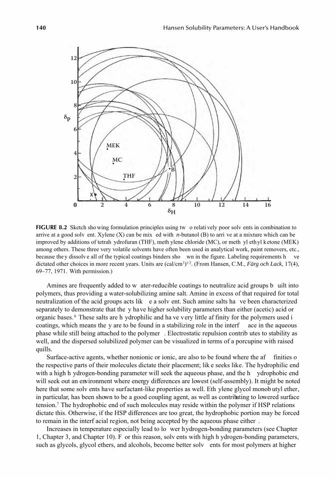
140
Hansen Solubility Parameters: A User’s Handbook
Amines are frequently added to w ater-reducible coatings to neutralize acid groups b uilt intopolymers, thus providing a water-solubilizing amine salt. Amine in excess of that required for totalneutralization of the acid groups acts lik e a solv ent. Such amine salts ha ve been characterizedseparately to demonstrate that the y have higher solubility parameters than either (acetic) acid ororganic bases.
6
These salts are h ydrophilic and ha ve very little af finity for the polymers used icoatings, which means the y are to be found in a stabilizing role in the interf ace in the aqueousphase while still being attached to the polymer . Electrostatic repulsion contrib utes to stability aswell, and the dispersed solubilized polymer can be visualized in terms of a porcupine with raisedquills.
Surface-active agents, whether nonionic or ionic, are also to be found where the af finities othe respective parts of their molecules dictate their placement; lik e seeks like. The hydrophilic endwith a high h ydrogen-bonding parameter will seek the aqueous phase, and the h ydrophobic endwill seek out an environment where energy differences are lowest (self-assembly). It might be notedhere that some solv ents have surfactant-like properties as well. Eth ylene glycol monob utyl ether,in particular, has been shown to be a good coupling agent, as well as contributing to lowered surfacetension.
7
The hydrophobic end of such molecules may reside within the polymer if HSP relationsdictate this. Otherwise, if the HSP differences are too great, the hydrophobic portion may be forcedto remain in the interf acial region, not being accepted by the aqueous phase either .
Increases in temperature especially lead to lo wer hydrogen-bonding parameters (see Chapter1, Chapter 3, and Chapter 10). F or this reason, solv ents with high h ydrogen-bonding parameters,such as glycols, glycol ethers, and alcohols, become better solv ents for most polymers at higher
FIGURE 8.2
Sketch sho wing formulation principles using tw o relati vely poor solv ents in combination toarrive at a good solv ent. Xylene (X) can be mix ed with
n-
butanol (B) to arri ve at a mixture which can beimproved by additions of tetrah ydrofuran (THF), meth ylene chloride (MC), or meth yl ethyl ketone (MEK)among others. These three very volatile solvents have often been used in analytical work, paint removers, etc.,because the y dissolv e all of the typical coatings binders sho wn in the figure. Labeling requirements h vedictated other choices in more recent years. Units are (cal/cm
3
)
1/2
. (From Hansen, C.M.,
Färg och Lack
, 17(4),69–77, 1971. With permission.)
•B
MEK•
MC•
THF•
12
10
8
6
4
2
0
δp
δH0 2 4 6 8 1210 14 16
7248_C008.fm Page 140 Wednesday, May 23, 2007 11:05 AM
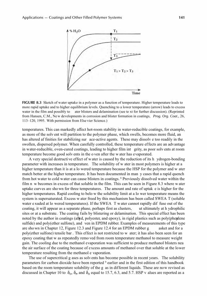
Applications — Coatings and Other Filled Polymer Systems
141
temperatures. This can markedly affect hot-room stability in water-reducible coatings, for example,as more of the solv ent will partition to the polymer phase, which swells, becomes more fluid, anhas altered af finities for stabilizing sur ace-active agents. These may dissolv e too readily in theswollen, dispersed polymer. When carefully controlled, these temperature ef fects are an advantagein water-reducible, oven-cured coatings, leading to higher film int grity, as poor solv ents at roomtemperature become good solv ents in the o ven after the w ater has evaporated.
A very special destructi ve effect of w ater is caused by the reduction of its h ydrogen-bondingparameter with increases in temperature. The solubility of w ater in most polymers is higher at ahigher temperature than it is at a lo wered temperature because the HSP for the polymer and w atermatch better at the higher temperature. It has been documented in man y cases that a rapid quenchfrom hot water to cold water can cause blisters in coatings.
8
Previously dissolved water within thefilm n w becomes in excess of that soluble in the film. This can be seen in Figure 8.3 where w ateruptake curves are sho wn for three temperatures. The amount and rate of uptak e is higher for thehigher temperatures. Rapid cooling to belo w the solubility limit at a lo wer temperature means thesystem is supersaturated. Excess w ater freed by this mechanism has been called SWEA T (solublewater e xuded at lo wered temperatures). If the SWEA T w ater cannot rapidly dif fuse out of thecoating, it will appear as a separate phase, perhaps first as clusters, ut ultimately at h ydrophilicsites or at a substrate. The coating fails by blistering or delamination. This special effect has beennoted by the author in coatings (alkyd, polyester, and epoxy), in rigid plastics such as poly(phenylenesulfide) and poly(ether sulfone), and ven in EPDM rubber. Examples of measurements of this typeare sho wn in Chapter 12, Figure 12.3 and Figure 12.4 for an EPDM rubber g asket and for apoly(ether sulfone) tensile bar . This effect is not restricted to w ater; it has also been seen for anepoxy coating that w as repeatedly remo ved from room temperature methanol to measure weightgain. The cooling due to the methanol evaporation was sufficient to produce methanol blisters neathe air surface of the coating because of excess amounts of methanol over that soluble at the lowertemperature resulting from the methanol e vaporation.
The use of supercritical g ases as solvents has become possible in recent years. The solubilityparameters for carbon dioxide have been reported
9
earlier and in the first edition of this handbookbased on the room temperature solubility of the g as in different liquids. These are now revised asdiscussed in Chapter 10 to
δ
D
,
δ
P
, and
δ
H
equal to 15.7, 6.3, and 5.7. HSP v alues are reported as a
FIGURE 8.3
Sketch of water uptake in a polymer as a function of temperature. Higher temperature leads tomore rapid uptake and to higher equilibrium levels. Quenching to a lower temperature (arrow) leads to excesswater in the film and possibly to ater blisters and delamination (see te xt for further discussion). (Reprintedfrom Hansen, C.M., Ne w developments in corrosion and blister formation in coatings,
Prog. Org. Coat
., 26,113–120, 1995. With permission from Else vier Science.)
Time
T1 > T2 > T3
% H2O
T3
T2
T1
7248_C008.fm Page 141 Wednesday, May 23, 2007 11:05 AM
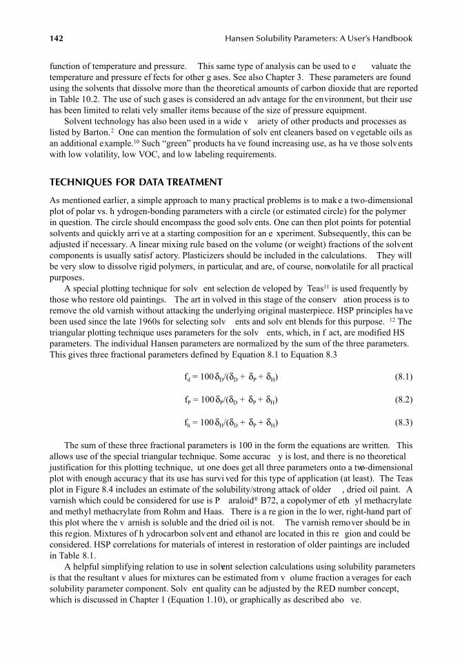
142
Hansen Solubility Parameters: A User’s Handbook
function of temperature and pressure. This same type of analysis can be used to e valuate thetemperature and pressure ef fects for other g ases. See also Chapter 3. These parameters are foundusing the solvents that dissolve more than the theoretical amounts of carbon dioxide that are reportedin Table 10.2. The use of such g ases is considered an adv antage for the environment, but their usehas been limited to relati vely smaller items because of the size of pressure equipment.
Solvent technology has also been used in a wide v ariety of other products and processes aslisted by Barton.
2
One can mention the formulation of solv ent cleaners based on vegetable oils asan additional example.
10
Such “green” products ha ve found increasing use, as ha ve those solventswith low volatility, low VOC, and low labeling requirements.
TECHNIQUES FOR DATA TREATMENT
As mentioned earlier, a simple approach to many practical problems is to make a two-dimensionalplot of polar vs. h ydrogen-bonding parameters with a circle (or estimated circle) for the polymerin question. The circle should encompass the good solv ents. One can then plot points for potentialsolvents and quickly arri ve at a starting composition for an e xperiment. Subsequently, this can beadjusted if necessary. A linear mixing rule based on the volume (or weight) fractions of the solventcomponents is usually satisf actory. Plasticizers should be included in the calculations. They willbe very slow to dissolve rigid polymers, in particular, and are, of course, nonvolatile for all practicalpurposes.
A special plotting technique for solv ent selection de veloped by Teas
11
is used frequently bythose who restore old paintings. The art in volved in this stage of the conserv ation process is toremove the old varnish without attacking the underlying original masterpiece. HSP principles havebeen used since the late 1960s for selecting solv ents and solv ent blends for this purpose.
12
Thetriangular plotting technique uses parameters for the solv ents, which, in f act, are modified HSparameters. The individual Hansen parameters are normalized by the sum of the three parameters.This gives three fractional parameters defined by Equation 8.1 to Equation 8.3
f
d
= 100
δ
D
/(
δ
D
+
δ
P
+
δ
H
) (8.1)
f
P
= 100
δ
P
/(
δ
D
+
δ
P
+
δ
H
) (8.2)
f
h
= 100
δ
H
/(
δ
D
+
δ
P
+
δ
H
) (8.3)
The sum of these three fractional parameters is 100 in the form the equations are written. Thisallows use of the special triangular technique. Some accurac y is lost, and there is no theoreticaljustification for this plotting technique, ut one does get all three parameters onto a two-dimensionalplot with enough accuracy that its use has survi ved for this type of application (at least). The Teasplot in Figure 8.4 includes an estimate of the solubility/strong attack of older , dried oil paint. Avarnish which could be considered for use is P araloid
®
B72, a copolymer of eth yl methacrylateand methyl methacrylate from Rohm and Haas. There is a re gion in the lo wer, right-hand part ofthis plot where the v arnish is soluble and the dried oil is not. The varnish remover should be inthis region. Mixtures of h ydrocarbon solvent and ethanol are located in this re gion and could beconsidered. HSP correlations for materials of interest in restoration of older paintings are includedin Table 8.1.
A helpful simplifying relation to use in solvent selection calculations using solubility parametersis that the resultant v alues for mixtures can be estimated from v olume fraction a verages for eachsolubility parameter component. Solv ent quality can be adjusted by the RED number concept,which is discussed in Chapter 1 (Equation 1.10), or graphically as described abo ve.
7248_C008.fm Page 142 Wednesday, May 23, 2007 11:05 AM
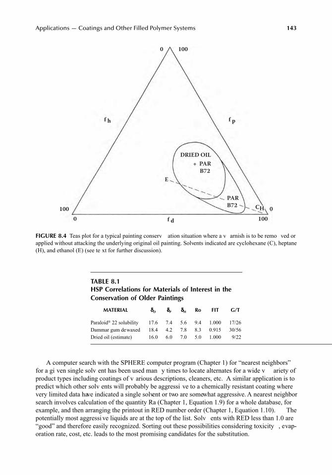
Applications — Coatings and Other Filled Polymer Systems
143
A computer search with the SPHERE computer program (Chapter 1) for “nearest neighbors”for a gi ven single solv ent has been used man y times to locate alternates for a wide v ariety ofproduct types including coatings of v arious descriptions, cleaners, etc. A similar application is topredict which other solv ents will probably be aggressi ve to a chemically resistant coating wherevery limited data have indicated a single solvent or two are somewhat aggressive. A nearest neighborsearch involves calculation of the quantity Ra (Chapter 1, Equation 1.9) for a whole database, forexample, and then arranging the printout in RED number order (Chapter 1, Equation 1.10). Thepotentially most aggressi ve liquids are at the top of the list. Solv ents with RED less than 1.0 are“good” and therefore easily recognized. Sorting out these possibilities considering toxicity , evap-oration rate, cost, etc. leads to the most promising candidates for the substitution.
FIGURE 8.4
Teas plot for a typical painting conserv ation situation where a v arnish is to be remo ved orapplied without attacking the underlying original oil painting. Solvents indicated are cyclohexane (C), heptane(H), and ethanol (E) (see te xt for further discussion).
TABLE 8.1HSP Correlations for Materials of Interest in the Conservation of Older Paintings
MATERIAL
δδδδ
D
δδδδ
P
δδδδ
H
Ro FIT G/T
Paraloid
®
22 solubility 17.6 7.4 5.6 9.4 1.000 17/26Dammar gum dewaxed 18.4 4.2 7.8 8.3 0.915 30/56Dried oil (estimate) 16.0 6.0 7.0 5.0 1.000 9/22
DRIED OIL
+ PAR
B72
PAR
B72 CH 0
0 100
100
0 100
f d
f h f p
E
7248_C008.fm Page 143 Wednesday, May 23, 2007 11:05 AM
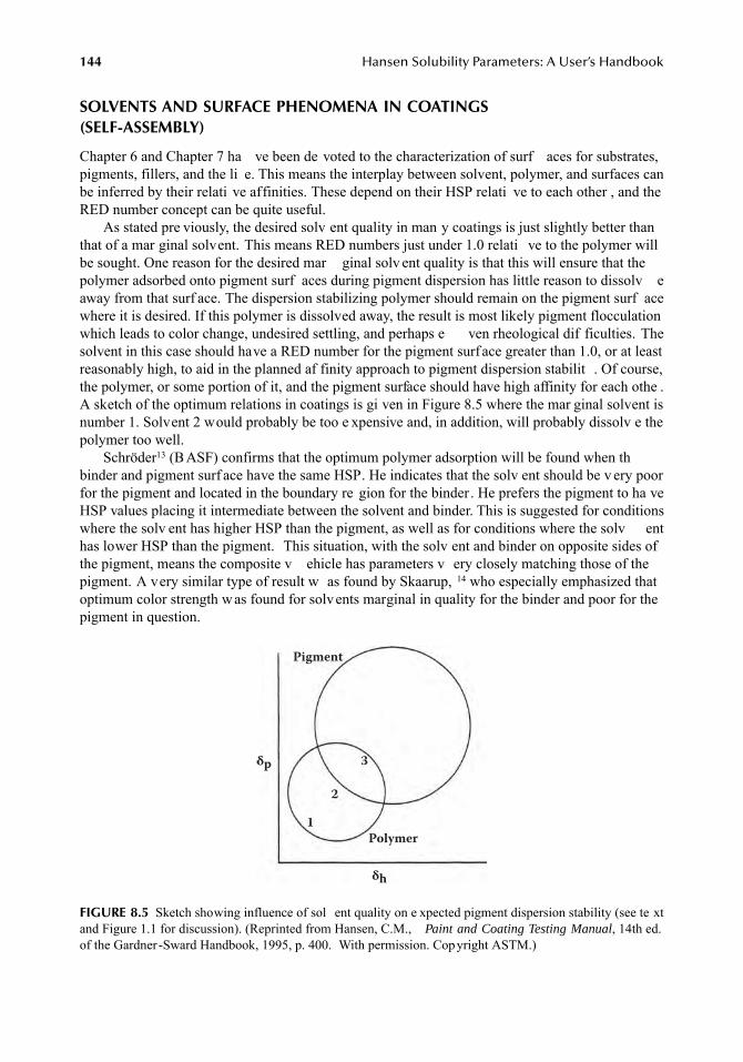
144
Hansen Solubility Parameters: A User’s Handbook
SOLVENTS AND SURFACE PHENOMENA IN COATINGS (SELF-ASSEMBLY)
Chapter 6 and Chapter 7 ha ve been de voted to the characterization of surf aces for substrates,pigments, fillers, and the li e. This means the interplay between solvent, polymer, and surfaces canbe inferred by their relati ve affinities. These depend on their HSP relati ve to each other , and theRED number concept can be quite useful.
As stated pre viously, the desired solv ent quality in man y coatings is just slightly better thanthat of a mar ginal solvent. This means RED numbers just under 1.0 relati ve to the polymer willbe sought. One reason for the desired mar ginal solv ent quality is that this will ensure that thepolymer adsorbed onto pigment surf aces during pigment dispersion has little reason to dissolv eaway from that surf ace. The dispersion stabilizing polymer should remain on the pigment surf acewhere it is desired. If this polymer is dissolved away, the result is most likely pigment flocculationwhich leads to color change, undesired settling, and perhaps e ven rheological dif ficulties. Thesolvent in this case should have a RED number for the pigment surf ace greater than 1.0, or at leastreasonably high, to aid in the planned af finity approach to pigment dispersion stabilit . Of course,the polymer, or some portion of it, and the pigment surface should have high affinity for each othe .A sketch of the optimum relations in coatings is gi ven in Figure 8.5 where the mar ginal solvent isnumber 1. Solvent 2 would probably be too e xpensive and, in addition, will probably dissolv e thepolymer too well.
Schröder
13
(B ASF) confirms that the optimum polymer adsorption will be found when thbinder and pigment surf ace have the same HSP. He indicates that the solv ent should be v ery poorfor the pigment and located in the boundary re gion for the binder. He prefers the pigment to ha veHSP values placing it intermediate between the solvent and binder. This is suggested for conditionswhere the solv ent has higher HSP than the pigment, as well as for conditions where the solv enthas lower HSP than the pigment. This situation, with the solv ent and binder on opposite sides ofthe pigment, means the composite v ehicle has parameters v ery closely matching those of thepigment. A very similar type of result w as found by Skaarup,
14
who especially emphasized thatoptimum color strength was found for solvents marginal in quality for the binder and poor for thepigment in question.
FIGURE 8.5
Sketch showing influence of sol ent quality on e xpected pigment dispersion stability (see te xtand Figure 1.1 for discussion). (Reprinted from Hansen, C.M.,
Paint and Coating Testing Manual
, 14th ed.of the Gardner-Sward Handbook, 1995, p. 400. With permission. Copyright ASTM.)
Polymer
δh
δp
1
2
3
Pigment
7248_C008.fm Page 144 Wednesday, May 23, 2007 11:05 AM
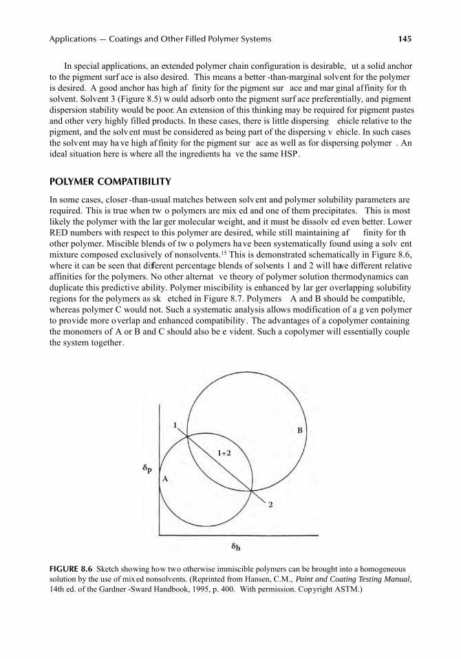
Applications — Coatings and Other Filled Polymer Systems
145
In special applications, an extended polymer chain configuration is desirable, ut a solid anchorto the pigment surf ace is also desired. This means a better -than-marginal solvent for the polymeris desired. A good anchor has high af finity for the pigment sur ace and mar ginal affinity for thsolvent. Solvent 3 (Figure 8.5) w ould adsorb onto the pigment surf ace preferentially, and pigmentdispersion stability would be poor. An extension of this thinking may be required for pigment pastesand other very highly filled products. In these cases, there is little dispersing ehicle relative to thepigment, and the solvent must be considered as being part of the dispersing v ehicle. In such casesthe solvent may ha ve high af finity for the pigment sur ace as well as for dispersing polymer . Anideal situation here is where all the ingredients ha ve the same HSP.
POLYMER COMPATIBILITY
In some cases, closer -than-usual matches between solvent and polymer solubility parameters arerequired. This is true when tw o polymers are mix ed and one of them precipitates. This is mostlikely the polymer with the lar ger molecular weight, and it must be dissolv ed even better. LowerRED numbers with respect to this polymer are desired, while still maintaining af finity for thother polymer. Miscible blends of tw o polymers have been systematically found using a solv entmixture composed exclusively of nonsolvents.
15
This is demonstrated schematically in Figure 8.6,where it can be seen that different percentage blends of solvents 1 and 2 will have different relativeaffinities for the polymers. No other alternat ve theory of polymer solution thermodynamics canduplicate this predictive ability. Polymer miscibility is enhanced by lar ger overlapping solubilityregions for the polymers as sk etched in Figure 8.7. Polymers A and B should be compatible,whereas polymer C would not. Such a systematic analysis allows modification of a g ven polymerto provide more overlap and enhanced compatibility . The advantages of a copolymer containingthe monomers of A or B and C should also be e vident. Such a copolymer will essentially couplethe system together.
FIGURE 8.6
Sketch showing how two otherwise immiscible polymers can be brought into a homogeneoussolution by the use of mixed nonsolvents. (Reprinted from Hansen, C.M.,
Paint and Coating Testing Manual
,14th ed. of the Gardner -Sward Handbook, 1995, p. 400. With permission. Copyright ASTM.)
δh
δp
2
1
1+2
A
B
7248_C008.fm Page 145 Wednesday, May 23, 2007 11:05 AM
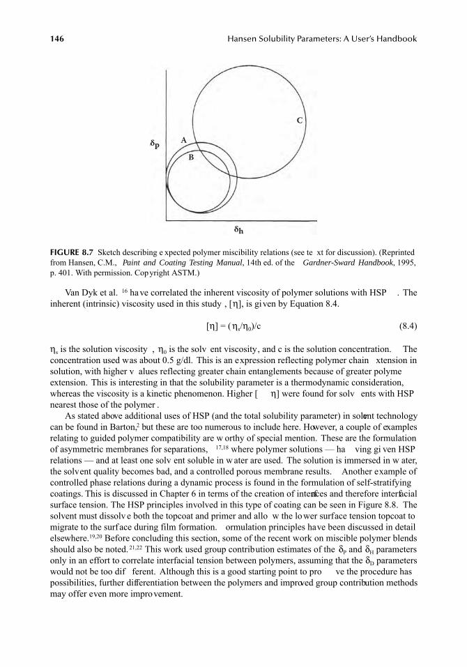
146
Hansen Solubility Parameters: A User’s Handbook
Van Dyk et al.
16
have correlated the inherent viscosity of polymer solutions with HSP . Theinherent (intrinsic) viscosity used in this study , [
η
], is given by Equation 8.4.
[
η
] = (
η
s
/
η
0
)/c (8.4)
η
s
is the solution viscosity ,
η
0
is the solv ent viscosity, and c is the solution concentration. Theconcentration used was about 0.5 g/dl. This is an expression reflecting polymer chain xtension insolution, with higher v alues reflecting greater chain entanglements because of greater polymeextension. This is interesting in that the solubility parameter is a thermodynamic consideration,whereas the viscosity is a kinetic phenomenon. Higher [
η
] were found for solv ents with HSPnearest those of the polymer .
As stated above additional uses of HSP (and the total solubility parameter) in solvent technologycan be found in Barton,
2
but these are too numerous to include here. However, a couple of examplesrelating to guided polymer compatibility are w orthy of special mention. These are the formulationof asymmetric membranes for separations,
17,18
where polymer solutions — ha ving gi ven HSPrelations — and at least one solv ent soluble in w ater are used. The solution is immersed in w ater,the solvent quality becomes bad, and a controlled porous membrane results. Another example ofcontrolled phase relations during a dynamic process is found in the formulation of self-stratifyingcoatings. This is discussed in Chapter 6 in terms of the creation of interfaces and therefore interfacialsurface tension. The HSP principles involved in this type of coating can be seen in Figure 8.8. Thesolvent must dissolv e both the topcoat and primer and allo w the lower surface tension topcoat tomigrate to the surface during film formation. ormulation principles have been discussed in detailelsewhere.
19,20
Before concluding this section, some of the recent work on miscible polymer blendsshould also be noted.
21,22
This work used group contribution estimates of the
δ
P
and
δ
H
parametersonly in an effort to correlate interfacial tension between polymers, assuming that the
δ
D
parameterswould not be too dif ferent. Although this is a good starting point to pro ve the procedure haspossibilities, further differentiation between the polymers and improved group contribution methodsmay offer even more improvement.
FIGURE 8.7
Sketch describing e xpected polymer miscibility relations (see te xt for discussion). (Reprintedfrom Hansen, C.M.,
Paint and Coating Testing Manual
, 14th ed. of the
Gardner-Sward Handbook
, 1995,p. 401. With permission. Copyright ASTM.)
δh
δpA
B
C
7248_C008.fm Page 146 Wednesday, May 23, 2007 11:05 AM
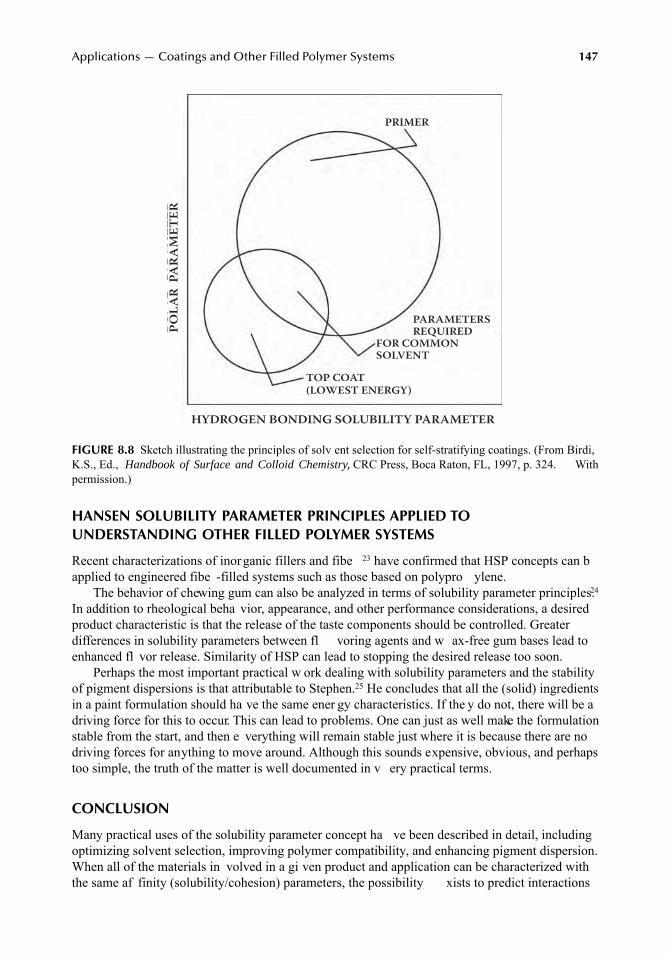
Applications — Coatings and Other Filled Polymer Systems
147
HANSEN SOLUBILITY PARAMETER PRINCIPLES APPLIED TO UNDERSTANDING OTHER FILLED POLYMER SYSTEMS
Recent characterizations of inorganic fillers and fibe
23
have confirmed that HSP concepts can bapplied to engineered fibe -filled systems such as those based on polypro ylene.
The behavior of chewing gum can also be analyzed in terms of solubility parameter principles.
24
In addition to rheological beha vior, appearance, and other performance considerations, a desiredproduct characteristic is that the release of the taste components should be controlled. Greaterdifferences in solubility parameters between fl voring agents and w ax-free gum bases lead toenhanced fl vor release. Similarity of HSP can lead to stopping the desired release too soon.
Perhaps the most important practical w ork dealing with solubility parameters and the stabilityof pigment dispersions is that attributable to Stephen.
25
He concludes that all the (solid) ingredientsin a paint formulation should ha ve the same ener gy characteristics. If the y do not, there will be adriving force for this to occur. This can lead to problems. One can just as well make the formulationstable from the start, and then e verything will remain stable just where it is because there are nodriving forces for anything to move around. Although this sounds expensive, obvious, and perhapstoo simple, the truth of the matter is well documented in v ery practical terms.
CONCLUSION
Many practical uses of the solubility parameter concept ha ve been described in detail, includingoptimizing solvent selection, improving polymer compatibility, and enhancing pigment dispersion.When all of the materials in volved in a gi ven product and application can be characterized withthe same af finity (solubility/cohesion) parameters, the possibility xists to predict interactions
FIGURE 8.8
Sketch illustrating the principles of solv ent selection for self-stratifying coatings. (From Birdi,K.S., Ed.,
Handbook of Surface and Colloid Chemistry,
CRC Press, Boca Raton, FL, 1997, p. 324. Withpermission.)
HYDROGEN BONDING SOLUBILITY PARAMETER
POLA
R P
ARA
MET
ER
TOP COAT(LOWEST ENERGY)
PARAMETERS REQUIREDFOR COMMONSOLVENT
PRIMER
7248_C008.fm Page 147 Wednesday, May 23, 2007 11:05 AM
148
Hansen Solubility Parameters: A User’s Handbook
among them. This is true e ven in complicated situations, such as the formulation of v arious typesof filled systems including coatings, printing inks, adhes ves, and other filled polymer systemincluding chewing gum.
REFERENCES
1. Hansen, C.M., Solubility in the coatings industry ,
Färg och Lack
, 17(4), 69–77, 1971.2. Barton, A.F.M.,
Handbook of Solubility Parameters and Other Cohesion Parameters
, CRC Press,Boca Raton, FL, 1983; 2nd ed., 1991.
3. Gardon, J.L. and Teas, J.P., Solubility parameters, in
Treatise on Coatings, Vol. 2, Characterizationof Coatings: Physical Techniques
, Part II, Myers, R.R. and Long, J.S., Eds., Marcel Dekk er, NewYork, 1976, chap. 8.
4. Beerbower, A., Boundary Lubrication — Scientific and Technical Applications Forecast, AD747336,Office of the Chief of Research and D velopment, Department of the Army, Washington, D.C., 1972.
5. Hansen, C.M. and Beerbo wer, A., Solubility parameters, in
Kirk-Othmer Encyclopedia of ChemicalTechnology
, Suppl. Vol., 2nd ed., Standen, A., Ed., Interscience, Ne w York, 1971, pp. 889–910.6. Hansen, C.M., Some aspects of acid/base interactions (Einige Aspekte der Säure/Base-W echsel-
wirkung, in German),
Farbe und Lack
, 83(7), 595–598, 1977.7. Hansen, C.M., Solv ents in w ater-borne coatings, Ind. Eng. Chem. Prod. Res. Dev., 16(3), 266–268,
1977.8. Hansen, C.M., Ne w developments in corrosion and blister formation in coatings, Prog. Org. Coat.,
26, 113–120, 1995.9. Hansen, C.M., 25 years with solubility parameters (25 År med Opløselighedsparametrene, in Danish),
Dan. Kemi, 73(8), 18–22, 1992.10. Rasmussen, D. and Wahlström, E., HSP-solubility parameters: a tool for development of new products
— modelling of the solubility of binders in pure and used solv ents, Surf. Coat. Int., 77(8), 323–333,1994.
11. Teas, J.P., Graphic analysis of resin solubilities, J. Paint Technol., 40(516), 19–25, 1968.12. Torraca, G., Solubility and Solvents for Conservation Problems, 2nd ed., International Centre for the
Study of the Preservation and the Restoration of Cultural Property (ICCR OM), Rome, 1978. (13, ViaDi San Michelle, 00153 Rome)
13. Schröder, J., Colloid chemistry aids to formulating inks and paints, Eur. Coat. J., 5/98, 334–340, 1998.14. Skaarup, K., The three dimensional solubility parameter and its use. II. Pigmented systems, skandi-
navisk tidskrift for Fårg och Lack, 14(2), 28–42, 1968; 14(3), 45–56, 1968.15. Hansen, C.M., On application of the three dimensional solubility parameter to the prediction of mutual
solubility and compatibility, Färg och Lack, 13(6), 132–138, 1967.16. Van Dyk, J.W., Frisch, H.L., and Wu, D.T., Solubility, solvency, solubility parameters, Ind. Eng. Chem.
Prod. Res. Dev., 24(3), 473–478, 1985.17. Klein, E. and Smith, J.K., Assymetric membrane formation, Ind. Eng. Chem. Prod. Res. Dev., 11(2),
207–210, 1972.18. Chawla, A.S. and Chang, T.M.S., Use of solubility parameters for the preparation of hemodialysis
membranes, J. Appl. Polym. Sci., 19, 1723–1730, 1975.19. Misev, T.A., Thermodynamic analysis of phase separation in self-stratifying coatings — solubility
parameters approach, J. Coat. Technol., 63(795), 23–28, 1991.20. Special issue devoted to self-stratifying coatings, Prog. Org. Coat., 28(3), July 1996.21. Luciani, A., Champagne, M.F., and Utracki, L.A., Interfacial tension in polymer blends. Part 1: Theory,
Polym. Networks Blends, 6(1), 41–50, 1996.22. Luciani, A., Champagne, M.F ., and Utracki, L.A., Interf acial tension in polymer blends. P art 2:
Measurements, Polym. Networks Blends, 6(2), 51–62, 1996.23. Hennissen, L., Systematic Modification of Filler/Fibre Sur aces to Achieve Maximum Compatibility
with Matrix Polymers, Lecture for the Danish Society for Polymer Technology, Copenhagen, February10, 1996.
7248_C008.fm Page 148 Wednesday, May 23, 2007 11:05 AM

Applications — Coatings and Other Filled Polymer Systems 149
24. Song, J.H. and Reed, M.A., Petroleum Wax-Free Chewing Gums Ha ving Improved Flavor Release,U.S. Patent No. 5,286,501, February 15, 1994, assigned to Wm. Wrigley Jr. Company, Chicago, IL.
25. Stephen, H.G., Parameters controlling colour acceptance in late x paints, J. Oil Colour Chem. Assoc.,69(3), 53–61, 1986.
7248_C008.fm Page 149 Wednesday, May 23, 2007 11:05 AM

7248_C008.fm Page 150 Wednesday, May 23, 2007 11:05 AM
151
9
Hansen Solubility Parameters of Asphalt, Bitumen, and Crude Oils
Per Redelius
ABSTRACT
Hansen solubility parameters (HSP) are sho wn to be a useful ne w tool for understanding compat-ibility relations among bitumens and crude oils. Bitumen and crude oils are comple x mixtures ofhydrocarbons which are k ept in solution mainly by their mutual solubility . They are not colloidaldispersions as previously thought. Although the solubility of the hydrocarbons is mainly determinedby the dispersive interactions, it is not possible to mak e correct estimates of their stability withoutalso taking polar interactions and h ydrogen-bonding interactions into consideration. HSP ha veproven their ability to gi ve a good estimate of the stability of bitumen and/or crude oil ha vingdifferent origins in relation to solv ents and polymers. Relations between the HSP of dif ferentmaterials is visualized using 3D plots showing the HSP as ellipsoids. A more precise determinationof the extension of the ellipsoids can be found by turbidimetric titrations with three different titrants,each representing a direction in the HSP space, respecti vely. It is no w possible with the help ofsimple laboratory e xperiments to predict the consequences of dif ferent courses of action, thuseliminating expensive trial and error testing.
SYMBOLS SPECIAL TO CHAPTER 9
INTRODUCTION
Even if most of us are not familiar with bitumen, we all know the “black” roads on which we driveevery day. The majority of road surf aces are black because the binding agent used to manuf acturethe surfacing is bitumen, which is mix ed with crushed rock aggre gate. Road surf aces can also begrey to white in color, in which case an alternative binder has been used: Portland cement concrete.
Bitumen is a semisolid material that can be produced from certain crude oils by distillation. Itcan also be found in nature as “natural asphalt.” It consists of a mixture of hydrocarbons of differentmolecular sizes containing small amounts of heteroatoms such as sulfur , nitrogen, and oxygen, aswell as traces of metals like vanadium and nickel. Bitumen behaves as a viscoelastic thermoplasticsolid at ambient temperature and turns into a viscous liquid at high temperature. It presents uniqueadhesive and waterproofing properties, which ma e it ideal in the manuf acture of asphalt for road
C Amount of bitumen/total amount of solv ent and titrant
P
Stability index given by Equation 9.3FR Volume of solvent/total volume of solvent plus titrant
p
a
Defined by Equation 9.
p
o
Defined by Equation 9.
7248_book.fm Page 151 Tuesday, April 24, 2007 9:19 AM
152
Hansen Solubility Parameters: A User’s Handbook
construction and to use in a wide range of industrial application, from waterproofing in constructioto sound dampening in the automoti ve industry.
The term
bitumen
is not completely unambiguous as it has been gi ven different meanings indifferent parts of our world. In Europe the term is defined as abve, whereas in Canada, for example,it is used for hea vy crude oils. In the U.S. the term
asphalt
is used instead of
bitumen
. Sometimesbitumen is confused with tar, which is a product of completely dif ferent origin. Tar is produced bydry distillation of coal or w ood.
The most common process for production of bitumen is by distillation under vacuum of properlyselected crude oils. There are ho wever just a limited number of crude oils which permit directdistillation to proper bitumen grades suitable for production of road asphalt. Although the reservesof such crude oils are v ery large worldwide, they are not primarily produced as the y contain toosmall amounts of fuel, which is the most important and profitable product for refiner
The functional properties of bitumen are usually related to its use as binder in asphalt for roads.Thus, the most common properties are related to the rheology of bitumen. As the road constructionarea is very conservative, and bitumen has been used for about 100 years, most tests are empiricaland have been used for a long time. Two of the most common tests are penetration at 25
°
C andsoftening point Ring&Ball. The penetration gives a measure of the stiffness of the bitumen at mostcommon service temperatures of a road, whereas the Ring&Ball gi ves the stif fness close to thehighest expected temperature in practice. In Europe bitumens are graded according to their pene-tration at 25
°
C — for e xample, 50/70, where the tw o numbers gi ve the highest and lo west limitfor the particular grade. It is also common, particularly in the U.S., to use viscosity gradation basedon viscosity at 60
°
C. Bitumen is, ho wever, a viscoelastic material with a comple x rheology andcan thus not be completely described by simple penetration testing and softening point. Thedevelopment of modern and reliable rheometers — for e xample, the dynamic shear rheometer(DSR) — has made it possible to describe the full rheology of bitumen.
During the last 20 years we ha ve seen an increase in the use of polymer modified bitume(PMB) with impro ved properties. The main reason for modification of bitumen is to impr ve therheological properties, particularly to mak e the binder less sensiti ve to temperatures. It is desiredto have a reasonable stif fness of the binder e ven at the highest surf ace temperatures a road canreach on a hot summer day , as well as being reasonably fl xible at the lo west temperatures on acold winter day. Another reason for modification with polymers is to increase durabilit . This willbe improved if a proper polymer is selected.
A large number of dif ferent polymers ha ve been tested as modifiers for bitumen. In the endjust a fe w of them ha ve reached lar ger commercial use. The main restriction for the choice ofpolymer is the e xpected improvement of the rheological properties in comparison with the priceof the polymer . But e ven more important is the compatibility or the solubility of the polymer inthe bitumen. Until now, there have been very few tools for prediction of compatibility between thepolymer and bitumen, so the de velopment of new PMB has to a lar ge extent been done on a “trialand error” basis. The better understanding of the true nature and the solubility properties of bitumenprovided by Hansen solubility parameters (HSP) has given a new tool for understanding of polymercompatibility with bitumen as discussed in the follo wing.
MODELS OF BITUMEN
Crude oils ha ve been found in man y places around the w orld. Although the true origin of crudeoils is still under discussion, most scientists agree that the y have been formed by de gradation andtransformation of ancient or ganisms. The properties of crude oil v ary depending on age andconditions during formation. Some crude oils are liquids with lo w viscosity, whereas others aresemisolid materials that ha ve a viscosity making them impossible to handle at room temperature.The low viscosity crude oils contain lar ge amounts of fuel b ut very little bitumen, if an y, and thehigh viscosity crude oils contain v ery little fuel b ut large amounts of bitumen.
7248_book.fm Page 152 Tuesday, April 24, 2007 9:19 AM
Hansen Solubility Parameters of Asphalt, Bitumen, and Crude Oils
153
From a chemical point of vie w crude oil is an e xtremely complex mixture of h ydrocarbons.Usually small amounts of heteroatom lik e nitrogen, oxygen, and sulfur , as well as trace amountsof metals like vanadium and nickel, are found, although the content v aries depending on type andorigin of the crude oil. The smallest molecules are the gaseous methane, ethane, and propane. Theseare dissolved in the liquid h ydrocarbons. The heaviest molecules ha ve molecular weights higherthan 1000 and are thus h ydrocarbons with 70 carbon atoms or more. The separation of crude oilsinto different fractions is done in refineries by distillation, with the diferent fractions being collectedbased on their boiling points. The lo w-boiling fractions consist of g asoline and g as oils. Theconstituents in these fractions have been characterized by modern analytical techniques until almostevery single component has been identified. The heavier fractions (heavy gas oil), and particularlythe residue after distillation, ha ve escaped such detailed characterization. Most residual oils arefurther upgraded by dif ferent refining processes to fuels. Bitumen may be produced only after proper distillation process of a selected crude oil using v acuum. Although the residual oil andbitumen have been extensively analyzed with modern equipment, most of the understanding is interms of averages of dif ferent chemical functional groups or structures. From these data tentati vestructures of the molecules ha ve been suggested.
1
In fact hardly any one single molecule from thecomplex mixture has been chemically analyzed. There are se veral reason wh y this has been asuperior challenge:
• The number of dif ferent molecules is v ery large. • There is no major population of identical molecules. • The material is black and viscous. • The range of molecules of dif ferent polarities and sizes is continuous. • The boiling point is higher than approximately 450°C, making the molecules fairly large.
The most common approach for chemical characterization of bitumen in volves a separationinto generic fractions based on chromatographic principles. The most common separation procedureis called
SARA analysis
(saturates, aromatics, resins, and asphaltenes). It consists of two principallydifferent steps: first, creation and precipitation of a solid fraction by dilution of the bitumen wit
n-
heptane, and then a separation of the soluble fraction with respect to polarity . The precipitatedfraction is called
asphaltenes
and is defined as the fraction of bitumen that is insoluble in
n-
heptane.The
n-
heptane soluble fraction is named
maltenes
and is further separated by polarity into threemore fractions. These fractions have been given names like “resins,” “aromatics,” and “saturates.”The most common and widespread h ypothesis about the structure of bitumen, which is found inmost books and papers on bitumen chemistry , teaches that bitumen is a colloidal dispersion ofasphaltenes in maltenes. The dispersion is assumed to be stabilized by the resins. The first one tintroduce this concept was Nelensteyn (1924).
2
The model was later refined by Pfei fer and Saal.
3
Although the model might be attracti ve for mechanical engineering, it is more dif ficult to accepfor an organic chemist, particularly since colloidal dispersions of h ydrocarbons in other h ydrocar-bons are rare, except in the case of polymers. A number of questions are immediately raised: “Dothe asphaltenes have enough different chemistry to permit dispersion rather than dissolution?” and“If it is a colloidal dispersion, what is the mechanism for its stabilization?”
Other models that question the e xistence of micelles ha ve also been proposed. Examples ofmodels are the continuous thermodynamic model by P ark and Mansoori
4
and Buduszynski et al.,
5
and the micro structural model as a result from the SHRP development program in the U.S.
6
Recentresearch has shown that the asphaltenes do not form micelles b ut are soluble in the maltenes, andthus no micelles can exist in the bitumen.
7,8
These models describe bitumen as a solution of organicmaterial of different polarity and dif ferent molecular weight ha ving a kind of mutual solubility ineach other. When a solvent such as
n-
heptane is added to the system, the balance is disturbed. P artof the system precipitates. The precipitation beha vior of asphaltenes is what could be predictedfrom regular solution theory and could be described as
flocculation
. In spite of the solubility model
7248_book.fm Page 153 Tuesday, April 24, 2007 9:19 AM
154
Hansen Solubility Parameters: A User’s Handbook
being a more precise description of the true nature of bitumen, it has recei ved surprisingly lo wacceptance in the research on bitumen and crude oils.
ASPHALTENES
During production, transport, and refining of certain crude oils there are sometimes problems witthe formation of precipitates and deposits. The deposits have been claimed to be asphaltenes, andtherefore there is considerable interest in them and mone y spent to sa ve, if the formation ofprecipitates could be controlled. Thus, extensive research has been performed to in vestigate thechemistry of asphaltenes
9,10
as well as mechanisms of formation of the precipitates. There is a cleardefinition of the term
asphaltenes
11,12
as the material that precipitates on dilution of bitumen orcrude oil with
n-
heptane. Most of the characterization w ork has been conducted on precipitatedasphaltenes, and very little attention has been gi ven to asphaltenes in their natural en vironment inthe bitumen. Much confusion has come from the misuse of the term
asphaltenes
to mean all kindsof precipitates from bitumen, suggesting that the insolubles in
n-
heptane could represent precipitatesin general. This assumption might have been correct if the asphaltenes were a colloidal fraction inbitumen, but this it is not the case. As will be pro ven later in this chapter the cause of formationof precipitates is more related to general solubility rather than just solubility in
n-
heptane. Themechanism of precipitate formation is certainly not only an academic matter b ut is of majorimportance for the whole oil industry as precipitates may cause blocking and fouling of equipmentused in crude oil production as well as in transport and refining. It is orth discussing some of themore common statements about the chemistry of asphaltenes and to compare them with e xperi-mental facts.
M
OLECULAR
W
EIGHT
A general statement about the molecular weight of asphaltenes would be that they are high molecularweight material. The true molecular weight of asphaltenes has been under discussion for man yyears. Investigations using vapor phase osmometry (VPO) on precipitated asphaltenes dissolved indifferent solvents have shown molecular weights from 1000 up to 10000, depending on the sourceof asphaltenes. The apparent molecular weight is strongly dependent on the solv ent. This indicatesthat the asphaltenes associate in solution.
1
Other attempts to determine molecular weight usingfield ionization mass spectrometry (FIMS) r veal an apparent molecular weight of 700–1000. Theseresults also vary depending on crude oil source.
5
It is obvious that the VPO overestimates the truemolecular weight due to interactions between the molecules, and FIMS lik ely gives a more correctvalue, although there might be a risk that some de gradation has tak en place in the ion source.Recent studies with fluorescence depolarization techniques h ve confirmed the FIMS results
13
Itmay be speculated that lar ge size molecules are less soluble in
n-
heptane, and thus asphaltenesshould consist mainly of high molecular weight material. A high dependency of molecular weightson solubility is well kno wn from polymers. There are, ho wever, several h ydrocarbons of lo wermolecular weight that are not soluble in
n-
heptane (for example, coronene or dibenz(a,h)anthracene,where the very high aromatic content leads to v ery high dispersion parameters compared with therelatively low dispersion parameter for
n-
heptane in the HSP concept), and similar molecules maybe part of the asphaltenes fraction. It is thus reasonable to assume that the lowest molecular weightin the asphaltenes is equal to the smallest molecule with a boiling point at the cut-point of thebitumen. This varies with different crude oils b ut may be estimated as being 500°C. This roughlycorresponds to h ydrocarbons with 35 carbon atom, less for polyc yclic aromatics and more for
n-
alkanes. The conclusion is that the asphaltenes fraction lik ely consists of a range of molecules ofdifferent molecular weight, which might range from as lo w as 300 up to more than 1000.
7248_book.fm Page 154 Tuesday, April 24, 2007 9:19 AM
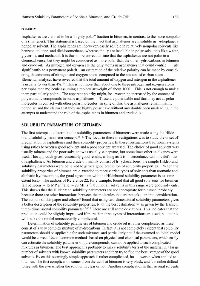
Hansen Solubility Parameters of Asphalt, Bitumen, and Crude Oils
155
POLARITY
Asphaltenes are claimed to be a “highly polar” fraction in bitumen, in contrast to the more nonpolaroils (maltenes). This statement is based on the f act that asphaltenes are insoluble in
n-
heptane, anonpolar solvent. The asphaltenes are, ho wever, easily soluble in relati vely nonpolar solvents likebenzene, toluene, and dichloromethane, whereas the y are insoluble in polar solv ents like water,glycerine, and methanol. It is thus more correct to state that the asphaltenes are not polar in achemical sense, but they might be considered as more polar than the other hydrocarbons in bitumenand crude oil. As nitrogen and oxygen are the only atoms in asphaltenes that could contrib utesignificantly to a permanent polarit , an estimation of the relati ve polarity can be made by consid-ering the amounts of nitrogen and oxygen atoms compared to the amount of carbon atoms.Elemental analyses have revealed that the total amount of oxygen and nitrogen in the asphaltenesis usually lo wer than 4%.
14
This is not more than about one to three nitrogen and oxygen atomsper asphaltene molecule assuming a molecular weight of about 1000. This is not enough to mak ethem particularly polar . The apparent polarity might, ho wever, be increased by the content ofpolyaromatic compounds in some asphaltenes. These are polarizable and thus may act as polarmolecules in contact with other polar molecules. In spite of this, the asphaltenes remain mainlynonpolar, and the claims that they are highly polar have without any doubts been misleading in theattempts to understand the role of the asphaltenes in bitumen and crude oils.
SOLUBILITY PARAMETERS OF BITUMEN
The first attempts to determine the solubility parameters of bitumens were made using the Hildebrand solubility parameter concept.
15–20
The focus in these investigations was to study the onset ofprecipitation of asphaltenes and their solubility properties. In these investigations traditional systemsusing ratios between a good solv ent and a poor solv ent are used. The choice of good solv ent wasusually toluene and the poor solv ent was usually
n-
heptane, but sometimes other
n-
alkanes wereused. This approach gives reasonably good results, as long as it is in accordance with the definitioof asphaltenes. As bitumen and crude oil mainly consist of h ydrocarbons, the simple Hildebrandsolubility parameters were belie ved to gi ve a good prediction of solubility properties. When thesolubility properties of bitumen are e xtended to more v aried types of solv ents than aromatic andaliphatic hydrocarbons, the good agreement with the Hildebrand solubility parameter is to someextent lost.
21
The authors of Reference 22, for e xample, found that all good solv ents for bitumenfall between = 15 MP a
1/2
and = 23 MP a
1/2
, but not all solv ents in this range were good solv ents.This shows that the Hildebrand solubility parameters are not appropriate for bitumen, probablybecause there are other interactions between the molecules that are not tak en into consideration.The authors of this paper and others
23
found that using two-dimensional solubility parameters givesa better description of the solubility properties, b ut the best estimation w as given by the Hansenthree- dimensional solubility parameter.
24,25
There are still some de viations. This indicates that theprediction could be slightly impro ved if more than three types of interactions are used, b ut thiswill make the model unnecessarily complicated.
Determination of solubility parameters of bitumen and crude oil is rather complicated as theseconsist of a very complex mixture of hydrocarbons. In fact, it is not completely evident that solubilityparameters should be applicable for such mixtures, and particularly not if the assumed colloidal modelwould be correct. Use of common methods based on ph ysical and chemical parameters, which easilycan estimate the solubility parameter of pure compounds, cannot be applied to such complicatedmixtures as bitumen. The best approach is probably to mak e solubility tests of the material in a lar genumber of solvents with known solubility parameters and then try to find the best verage of the goodsolvents. Ev en this seemingly simple approach is rather complicated, ho wever, when applied tobitumen. The first complication comes from the act that bitumen is very black, and it is rather difficulto see with the e ye whether the solution is clear or not. Another complication is that several solvents
7248_book.fm Page 155 Tuesday, April 24, 2007 9:19 AM
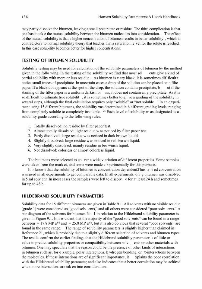
156
Hansen Solubility Parameters: A User’s Handbook
may partly dissolve the bitumen, leaving a small precipitate or residue. The third complication is thatone has to tak e the mutual solubility between the bitumen molecules into consideration. The effectof the mutual solubility is that a higher concentration of bitumen results in better solubility , which iscontradictory to normal solubility theory that teaches that a saturation le vel for the solute is reached.In this case solubility becomes better for higher concentrations.
TESTING OF BITUMEN SOLUBILITY
Solubility testing may be used for calculation of the solubility parameters of bitumen by the methodgiven in the follo wing. In the testing of the solubility we find that most sol ents give a kind ofpartial solubility with more or less residue. As bitumen is v ery black, it is sometimes dif ficult tnotice small traces of precipitate. In uncertain cases a drop of the solution can be placed on a filtepaper. If a black dot appears at the spot of the drop, the solution contains precipitate, b ut if thestaining of the filter paper is a uniform darkish br wn, it does not contain an y precipitate. As it isso difficult to estimate true solubilit , it is sometimes better to gi ve a grading of the solubility inseveral steps, although the final calculation requires only “soluble” or “not soluble ” In an e xperi-ment using 15 different bitumens, the solubility was determined in 6 different grading levels, rangingfrom completely soluble to completely insoluble.
26
Each le vel of solubility w as designated as asolubility grade according to the follo wing rules:
1. Totally dissolved: no residue by filter paper test2. Almost totally dissolved: light residue w as noticed by filter paper test3. Partly dissolved: large residue was noticed in dark bro wn liquid.4. Slightly dissolved: large residue was noticed in red-bro wn liquid.5. Very slightly dissolved: mainly residue in bro wnish liquid.6. Not dissolved: colorless or almost colorless liquid.
The bitumens were selected to co ver a wide v ariation of dif ferent properties. Some sampleswere taken from the mark et, and some were made e xperimentally for this purpose.
It is known that the solubility of bitumen is concentration dependent. Thus, a fi ed concentrationwas used in all experiments to get comparable data. In all experiments, 0.5 g bitumen was dissolvedin 5 ml solv ent. In most cases the samples were left to dissolv e for at least 24 h and sometimesfor up to 48 h.
HILDEBRAND SOLUBILITY PARAMETERS
Solubility data for 15 different bitumens are given in Table 9.1. All solvents with no visible residue(grade 1) were considered as “good solv ents,” and all others were considered “poor solv ents.” Abar diagram of the solvents for bitumen No. 1 in relation to the Hildebrand solubility parameter isgiven in Figure 9.1. It is e vident that the majority of the “good solv ents” can be found in a rangebetween = 17.8 MP a
1/2
and = 25.8 MP a
1/2
, but it is also ob vious that several “poor solvents” arefound in the same range. The range of solubility parameters is slightly higher than claimed inReference 21, which is probably due to a slightly different selection of solvents and bitumen types.The results confirm the earlier findings that the Hildebrand solubility parameter is of little or value to predict solubility properties or compatibility between solv ents or other materials withbitumen. One may speculate that the reason could be the presence of other kinds of interactionsin bitumen such as, for e xample, polar interactions, h ydrogen bonding, or
π
-interactions betweenthe molecules. If these interactions are of significant importance, it xplains the poor correlationwith the Hildebrand solubility parameter, and also indicates that a better correlation may be achievedwhen more interactions are tak en into consideration.
7248_book.fm Page 156 Tuesday, April 24, 2007 9:19 AM
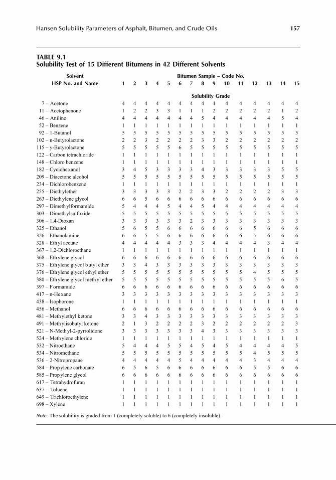
Hansen Solubility Parameters of Asphalt, Bitumen, and Crude Oils
157
TABLE 9.1Solubility Test of 15 Different Bitumens in 42 Different Solvents
Solvent Bitumen Sample – Code No.HSP No. and Name 1 2 3 4 5 6 7 8 9 10 11 12 13 14 15
Solubility Grade
7 – Acetone 4 4 4 4 4 4 4 4 4 4 4 4 4 4 411 – Acetophenone 1 2 2 3 3 1 1 1 2 2 2 2 2 1 246 – Aniline 4 4 4 4 4 4 4 5 4 4 4 4 4 5 452 – Benzene 1 1 1 1 1 1 1 1 1 1 1 1 1 1 192 – 1-Butanol 5 5 5 5 5 5 5 5 5 5 5 5 5 5 5
102 – n-Butyrolactone 2 2 3 2 2 2 2 3 3 2 2 2 2 2 2115 – y-Butyrolactone 5 5 5 5 5 6 5 5 5 5 5 5 5 5 5122 – Carbon tetrachioride 1 1 1 1 1 1 1 1 1 1 1 1 1 1 1148 – Chloro benzene 1 1 1 1 1 1 1 1 1 1 1 1 1 1 1182 – Cyciohexanol 3 4 5 3 3 3 3 4 3 3 3 3 3 5 5209 – Diacetone alcohol 5 5 5 5 5 5 5 5 5 5 5 5 5 5 5234 – Dichlorobenzene 1 1 1 1 1 1 1 1 1 1 1 1 1 1 1255 – Diethylether 3 3 3 3 3 2 2 3 3 2 2 2 2 3 3263 – Diethylene glycol 6 6 5 6 6 6 6 6 6 6 6 6 6 6 6297 – Dimethylformamide 5 4 4 4 5 4 4 5 4 4 4 4 4 4 4303 – Dimethylsulfoxide 5 5 5 5 5 5 5 5 5 5 5 5 5 5 5306 – 1,4-Dioxan 3 3 3 3 3 3 2 3 3 3 3 3 3 3 3325 – Ethanol 5 6 5 5 6 6 6 6 6 6 6 5 6 6 6326 – Ethanolamine 6 6 5 5 6 6 6 6 6 6 6 5 6 6 6328 – Ethyl acetate 4 4 4 4 4 3 3 3 4 4 4 4 3 4 4367 – 1,2-Dichloroethane 1 1 1 1 1 1 1 1 1 1 1 1 1 1 1368 – Ethylene glycol 6 6 6 6 6 6 6 6 6 6 6 6 6 6 6375 – Ethylene glycol butyl ether 3 3 4 3 3 3 3 3 3 3 3 3 3 3 3376 – Ethylene glycol ethyl ether 5 5 5 5 5 5 5 5 5 5 5 4 5 5 5380 – Ethylene glycol methyl ether 5 5 5 5 5 5 5 5 5 5 5 5 5 6 5397 – Formamide 6 6 6 6 6 6 6 6 6 6 6 6 6 6 6417 – n-Hexane 3 3 3 3 3 3 3 3 3 3 3 3 3 3 3438 – Isophorone 1 1 1 1 1 1 1 1 1 1 1 1 1 1 1456 – Methanol 6 6 6 6 6 6 6 6 6 6 6 6 6 6 6481 – Methylethyl ketone 3 3 4 3 3 3 3 3 3 3 3 3 3 3 3491 – Methylisobutyl ketone 2 1 3 2 2 2 2 3 2 2 2 2 2 2 3521 – N-Methyl-2-pyrrolidone 3 3 3 3 3 3 3 4 3 3 3 3 3 3 3524 – Meth ylene chloride 1 1 1 1 1 1 1 1 1 1 1 1 1 1 1532 – Nitroethane 5 4 4 4 5 5 4 5 4 5 4 4 4 4 5534 – Nitromethane 5 5 5 5 5 5 5 5 5 5 5 4 5 5 5536 – 2-Nitropropane 4 4 4 4 4 5 4 4 4 4 4 3 4 4 4584 – Propylene carbonate 6 5 6 5 6 6 6 6 6 6 6 5 5 6 6585 – Propylene glycol 6 6 6 6 6 6 6 6 6 6 6 6 6 6 6617 – Tetrahydrofuran 1 1 1 1 1 1 1 1 1 1 1 1 1 1 1637 – Toluene 1 1 1 1 1 1 1 1 1 1 1 1 1 1 1649 – Trichloroethylene 1 1 1 1 1 1 1 1 1 1 1 1 1 1 1698 – Xylene 1 1 1 1 1 1 1 1 1 1 1 1 1 1 1
Note
: The solubility is graded from 1 (completely soluble) to 6 (completely insoluble).
7248_book.fm Page 157 Tuesday, April 24, 2007 9:19 AM
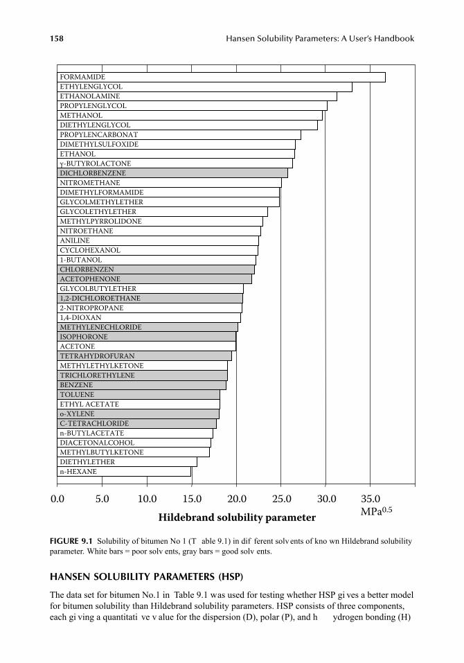
158
Hansen Solubility Parameters: A User’s Handbook
HANSEN SOLUBILITY PARAMETERS (HSP)
The data set for bitumen No.1 in Table 9.1 was used for testing whether HSP gi ves a better modelfor bitumen solubility than Hildebrand solubility parameters. HSP consists of three components,each gi ving a quantitati ve v alue for the dispersion (D), polar (P), and h ydrogen bonding (H)
FIGURE 9.1
Solubility of bitumen No 1 (T able 9.1) in dif ferent solv ents of kno wn Hildebrand solubilityparameter. White bars = poor solv ents, gray bars = good solv ents.
Hildebrand solubility parameter
0.0 5.0 10.0 15.0 20.0 25.0 30.0 35.0MPa0.5
FORMAMIDE
ETHYLENGLYCOL
ETHANOLAMINE
PROPYLENGLYCOL
METHANOL
DIETHYLENGLYCOL
PROPYLENCARBONAT
DIMETHYLSULFOXIDE
ETHANOL
γ-BUTYROLACTONE
DICHLORBENZENE
NITROMETHANE
DIMETHYLFORMAMIDE
GLYCOLMETHYLETHER
GLYCOLETHYLETHER
METHYLPYRROLIDONE
NITROETHANE
ANILINE
CYCLOHEXANOL
1-BUTANOL
CHLORBENZEN
ACETOPHENONE
GLYCOLBUTYLETHER
1,2-DICHLOROETHANE
2-NITROPROPANE
1,4-DIOXAN
METHYLENECHLORIDE
ISOPHORONE
ACETONE
TETRAHYDROFURAN
METHYLETHYLKETONE
TRICHLORETHYLENE
BENZENE
TOLUENE
ETHYL ACETATE
o-XYLENE
C-TETRACHLORIDE
n-BUTYLACETATE
DIACETONALCOHOL
METHYLBUTYLKETONE
DIETHYLETHER
n-HEXANE
7248_book.fm Page 158 Tuesday, April 24, 2007 9:19 AM
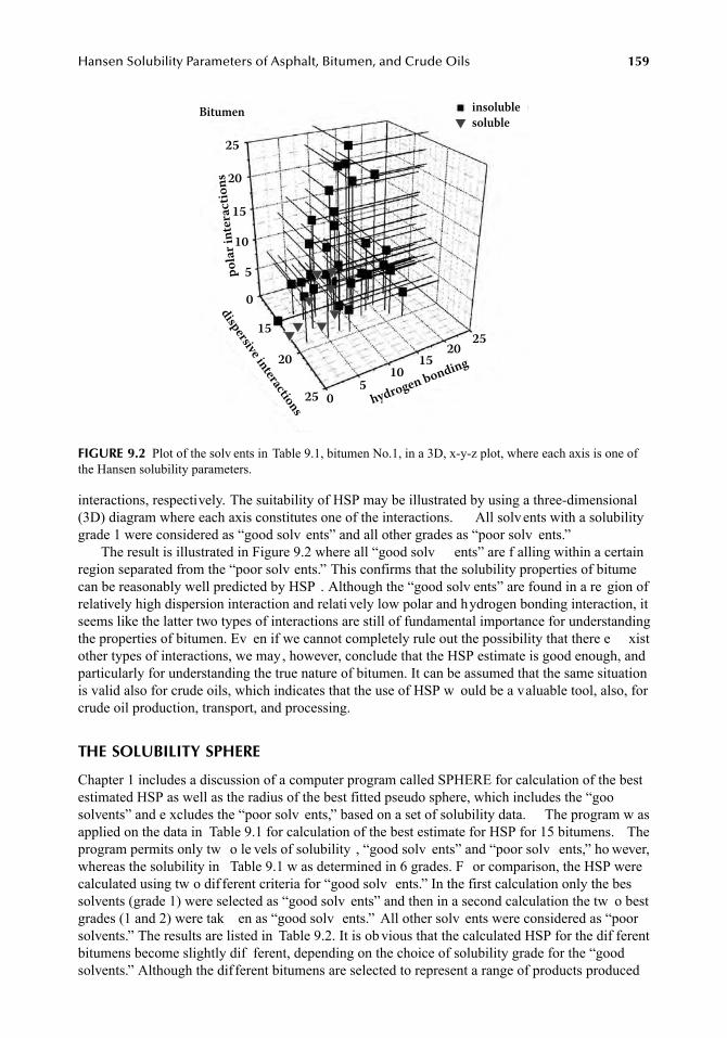
Hansen Solubility Parameters of Asphalt, Bitumen, and Crude Oils
159
interactions, respectively. The suitability of HSP may be illustrated by using a three-dimensional(3D) diagram where each axis constitutes one of the interactions. All solvents with a solubilitygrade 1 were considered as “good solv ents” and all other grades as “poor solv ents.”
The result is illustrated in Figure 9.2 where all “good solv ents” are f alling within a certainregion separated from the “poor solv ents.” This confirms that the solubility properties of bitumecan be reasonably well predicted by HSP . Although the “good solv ents” are found in a re gion ofrelatively high dispersion interaction and relati vely low polar and hydrogen bonding interaction, itseems like the latter two types of interactions are still of fundamental importance for understandingthe properties of bitumen. Ev en if we cannot completely rule out the possibility that there e xistother types of interactions, we may, however, conclude that the HSP estimate is good enough, andparticularly for understanding the true nature of bitumen. It can be assumed that the same situationis valid also for crude oils, which indicates that the use of HSP w ould be a valuable tool, also, forcrude oil production, transport, and processing.
THE SOLUBILITY SPHERE
Chapter 1 includes a discussion of a computer program called SPHERE for calculation of the bestestimated HSP as well as the radius of the best fitted pseudo sphere, which includes the “goosolvents” and e xcludes the “poor solv ents,” based on a set of solubility data. The program w asapplied on the data in Table 9.1 for calculation of the best estimate for HSP for 15 bitumens. Theprogram permits only tw o le vels of solubility , “good solv ents” and “poor solv ents,” ho wever,whereas the solubility in Table 9.1 w as determined in 6 grades. F or comparison, the HSP werecalculated using tw o dif ferent criteria for “good solv ents.” In the first calculation only the bessolvents (grade 1) were selected as “good solv ents” and then in a second calculation the tw o bestgrades (1 and 2) were tak en as “good solv ents.” All other solv ents were considered as “poorsolvents.” The results are listed in Table 9.2. It is ob vious that the calculated HSP for the dif ferentbitumens become slightly dif ferent, depending on the choice of solubility grade for the “goodsolvents.” Although the dif ferent bitumens are selected to represent a range of products produced
FIGURE 9.2
Plot of the solv ents in Table 9.1, bitumen No.1, in a 3D, x-y-z plot, where each axis is one ofthe Hansen solubility parameters.
Bitumen insolublesoluble
polar
inte
ract
ions
dispersive interactions
25
20
15
10
5
0
15
1510
5
2020
25
25
0 hydrogen bonding
▼
▼▼ ▼
▼▼
▼▼
▼
7248_book.fm Page 159 Tuesday, April 24, 2007 9:19 AM
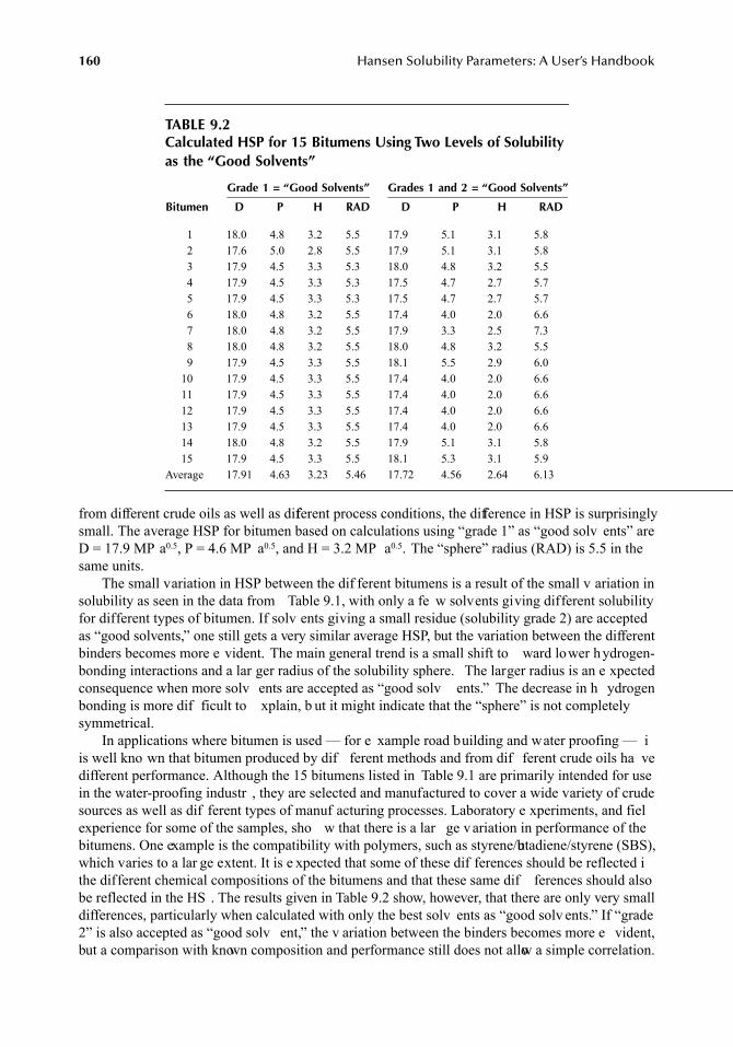
160
Hansen Solubility Parameters: A User’s Handbook
from different crude oils as well as different process conditions, the difference in HSP is surprisinglysmall. The average HSP for bitumen based on calculations using “grade 1” as “good solv ents” areD = 17.9 MP a
0.5
, P = 4.6 MP a
0.5
, and H = 3.2 MP a
0.5
. The “sphere” radius (RAD) is 5.5 in thesame units.
The small variation in HSP between the dif ferent bitumens is a result of the small v ariation insolubility as seen in the data from Table 9.1, with only a fe w solvents giving different solubilityfor different types of bitumen. If solv ents giving a small residue (solubility grade 2) are acceptedas “good solvents,” one still gets a very similar average HSP, but the variation between the differentbinders becomes more e vident. The main general trend is a small shift to ward lower hydrogen-bonding interactions and a lar ger radius of the solubility sphere. The larger radius is an e xpectedconsequence when more solv ents are accepted as “good solv ents.” The decrease in h ydrogenbonding is more dif ficult to xplain, b ut it might indicate that the “sphere” is not completelysymmetrical.
In applications where bitumen is used — for e xample road building and water proofing — iis well kno wn that bitumen produced by dif ferent methods and from dif ferent crude oils ha vedifferent performance. Although the 15 bitumens listed in Table 9.1 are primarily intended for usein the water-proofing industr , they are selected and manufactured to cover a wide variety of crudesources as well as dif ferent types of manuf acturing processes. Laboratory e xperiments, and fielexperience for some of the samples, sho w that there is a lar ge variation in performance of thebitumens. One example is the compatibility with polymers, such as styrene/butadiene/styrene (SBS),which varies to a lar ge extent. It is e xpected that some of these dif ferences should be reflected ithe different chemical compositions of the bitumens and that these same dif ferences should alsobe reflected in the HS . The results given in Table 9.2 show, however, that there are only very smalldifferences, particularly when calculated with only the best solv ents as “good solv ents.” If “grade2” is also accepted as “good solv ent,” the v ariation between the binders becomes more e vident,but a comparison with known composition and performance still does not allow a simple correlation.
TABLE 9.2Calculated HSP for 15 Bitumens Using Two Levels of Solubility as the “Good Solvents”
Grade 1 = “Good Solvents”
Grades 1 and 2 = “Good Solvents”
Bitumen D P H RAD D P H RAD
1 18.0 4.8 3.2 5.5 17.9 5.1 3.1 5.82 17.6 5.0 2.8 5.5 17.9 5.1 3.1 5.83 17.9 4.5 3.3 5.3 18.0 4.8 3.2 5.54 17.9 4.5 3.3 5.3 17.5 4.7 2.7 5.75 17.9 4.5 3.3 5.3 17.5 4.7 2.7 5.76 18.0 4.8 3.2 5.5 17.4 4.0 2.0 6.67 18.0 4.8 3.2 5.5 17.9 3.3 2.5 7.38 18.0 4.8 3.2 5.5 18.0 4.8 3.2 5.59 17.9 4.5 3.3 5.5 18.1 5.5 2.9 6.0
10 17.9 4.5 3.3 5.5 17.4 4.0 2.0 6.611 17.9 4.5 3.3 5.5 17.4 4.0 2.0 6.612 17.9 4.5 3.3 5.5 17.4 4.0 2.0 6.613 17.9 4.5 3.3 5.5 17.4 4.0 2.0 6.614 18.0 4.8 3.2 5.5 17.9 5.1 3.1 5.815 17.9 4.5 3.3 5.5 18.1 5.3 3.1 5.9
Average 17.91 4.63 3.23 5.46 17.72 4.56 2.64 6.13
7248_book.fm Page 160 Tuesday, April 24, 2007 9:19 AM
Hansen Solubility Parameters of Asphalt, Bitumen, and Crude Oils
161
This lack of correlation is without an y doubt disappointing. We may however speculate that itis mainly due to a lack of precision. The solvents in Table 9.1 are selected to co ver a large area inthe 3D solubility space, whereas most bitumens are mixtures of hydrocarbons where the differencesin chemical properties are relatively small. Obviously it is necessary to have much better precisionthan the solubility testing as shown in Table 9.2. The better precision may be achieved in two ways.The first impr vement is to use a better selection of solv ents for the solubility testing. Solv entsthat have HSP close to the border of solubility are preferred to better define the borde . Anotherapproach is to perform turbidimetric titrations to estimate the e xact HSP at the precipitation pointcalculated from the ratio of a “good solv ent” and a “poor solv ent” at precipitation. This approachis further discussed as BISOM titrations below. An improved selection of solvents should focus onsolvents with RED v alues around 1, as these are close to the boundary . The RED (relative energydifference) concept is discussed in Chapter 1. As much v ariation as possible with respect to thedispersion, polar, and h ydrogen bonding interactions is desired. This requires, of course, that anapproximate HSP of the material is already available. And finall , nontoxic and inexpensive solventsare preferred. A suggested set of solv ents, optimized for determination of HSP of bitumens andsimilar materials is presented in Table 9.3. These solvents have RED between 0 and 2 related tothe estimated HSP of bitumen as presented above. When using this set of solvents for a Venezuelanbinder, the HSP is D = 18.6 MP a
0.5
, P = 3.0 MP a
0.5
, H = 3.4 MP a
0.5
, and the radius of the sphereis 6.3 in the same units. This set of numbers is dif ferent from the pre viously estimated v alues inTable 9.2. A comparison can be made with binder No. 9 (D = 17.9 MP a
0.5
, P = 4.5 MP a
0.5
, H =3.3 MP a
0.5
, and a radius of 5.5 MP a
0.5
), which is similar to the binder used to obtain the datareported in Table 9.3. If the HSP of other types of materials than bitumen are going to be measured,also in the petroleum area, it is suggested that other sets of solv ents may be needed to get the bestprecision. Examples are light crude oils, distillates, base oils, petroleum w axes, etc.
COMPUTER PROGRAM FOR CALCULATION AND PLOTTING OF THE HANSEN 3D PSEUDOSPHERE
The SPHERE program described in Chapter 1 has gi ven very good approximations of the HSP aswell as the diameter of the (solubility) sphere for a lar ge number of materials. In the SPHEREprogram, a f actor 4 is used as a multiplier for the dif ference in the dispersion interactions of thespecies concerned. This means that the “sphere, ” with the three dif ferent types of interactions ascoordinates, is in f act an ellipsoid (spheroid). A disadvantage with the SPHERE program is thelack of a tool for plotting the ellipsoid in a diagram that would be beneficial for illustration purposesThus, an improved program which permits 3D plotting of the ellipsoid w as developed. During thedevelopment it was discussed that although the factor 4 has been proven to be a good approximationfor most materials there might be complex mixtures which could give a better fit with xperimentaldata if other f actors were used. The new program has the follo wing features:
• Permits plotting of the HSP solubility ellipsoid in a 3D diagram.• Permits plotting of up to three ellipsoids representing dif ferent materials in the same 3D
diagram.• The input data should be based on “poor solv ents,” “good solv ents,” and “borderline
solvents.”• There should be an option to mak e other types of fitting than the SPHERE program t
the available data.• Negative values of HSP interaction coef ficients are not ta en into consideration.
7248_book.fm Page 161 Tuesday, April 24, 2007 9:19 AM
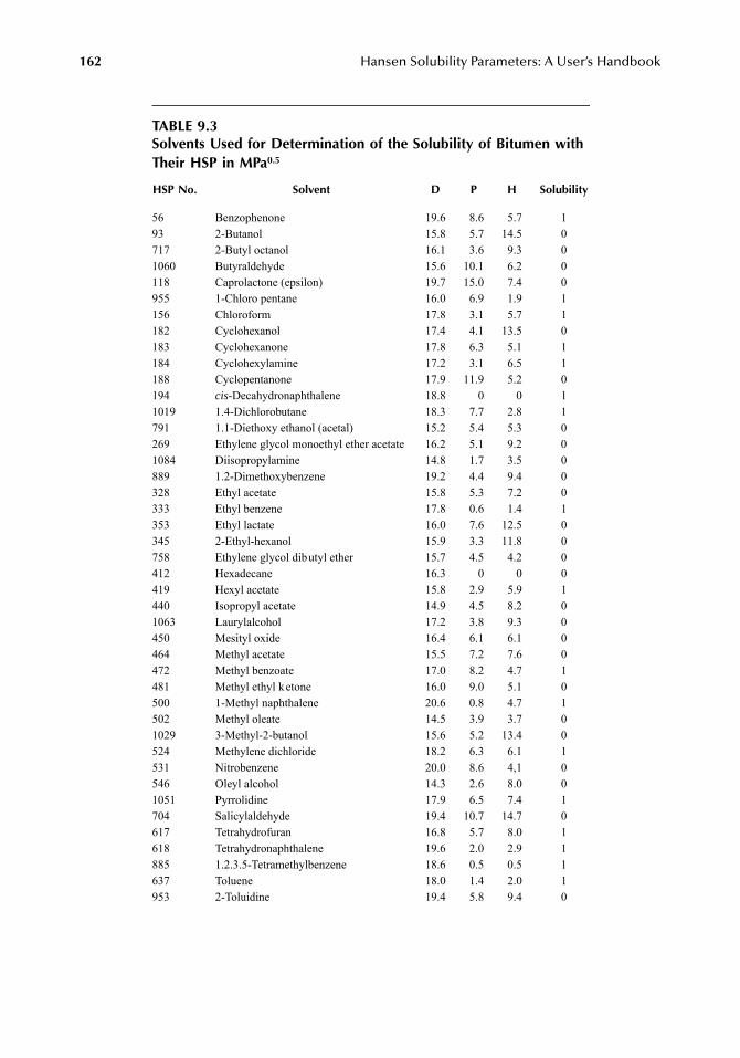
162
Hansen Solubility Parameters: A User’s Handbook
TABLE 9.3Solvents Used for Determination of the Solubility of Bitumen with Their HSP in MPa
0.5
HSP No. Solvent D P H Solubility
56 Benzophenone 19.6 8.6 5.7 193 2-Butanol 15.8 5.7 14.5 0717 2-Butyl octanol 16.1 3.6 9.3 01060 Butyraldehyde 15.6 10.1 6.2 0118 Caprolactone (epsilon) 19.7 15.0 7.4 0955 1-Chloro pentane 16.0 6.9 1.9 1156 Chloroform 17.8 3.1 5.7 1182 Cyclohexanol 17.4 4.1 13.5 0183 Cyclohexanone 17.8 6.3 5.1 1184 Cyclohexylamine 17.2 3.1 6.5 1188 Cyclopentanone 17.9 11.9 5.2 0194
cis
-Decahydronaphthalene 18.8 0 0 11019 1.4-Dichlorobutane 18.3 7.7 2.8 1791 1.1-Diethoxy ethanol (acetal) 15.2 5.4 5.3 0269 Ethylene glycol monoethyl ether acetate 16.2 5.1 9.2 01084 Diisopropylamine 14.8 1.7 3.5 0889 1.2-Dimethoxybenzene 19.2 4.4 9.4 0328 Ethyl acetate 15.8 5.3 7.2 0333 Ethyl benzene 17.8 0.6 1.4 1353 Ethyl lactate 16.0 7.6 12.5 0345 2-Ethyl-hexanol 15.9 3.3 11.8 0758 Ethylene glycol dibutyl ether 15.7 4.5 4.2 0412 Hexadecane 16.3 0 0 0419 Hexyl acetate 15.8 2.9 5.9 1440 Isopropyl acetate 14.9 4.5 8.2 01063 Laurylalcohol 17.2 3.8 9.3 0450 Mesityl oxide 16.4 6.1 6.1 0464 Methyl acetate 15.5 7.2 7.6 0472 Methyl benzoate 17.0 8.2 4.7 1481 Methyl ethyl ketone 16.0 9.0 5.1 0500 1-Methyl naphthalene 20.6 0.8 4.7 1502 Methyl oleate 14.5 3.9 3.7 01029 3-Methyl-2-butanol 15.6 5.2 13.4 0524 Methylene dichloride 18.2 6.3 6.1 1531 Nitrobenzene 20.0 8.6 4,1 0546 Oleyl alcohol 14.3 2.6 8.0 01051 Pyrrolidine 17.9 6.5 7.4 1704 Salicylaldehyde 19.4 10.7 14.7 0617 Tetrahydrofuran 16.8 5.7 8.0 1618 Tetrahydronaphthalene 19.6 2.0 2.9 1885 1.2.3.5-Tetramethylbenzene 18.6 0.5 0.5 1637 Toluene 18.0 1.4 2.0 1953 2-Toluidine 19.4 5.8 9.4 0
7248_book.fm Page 162 Tuesday, April 24, 2007 9:19 AM
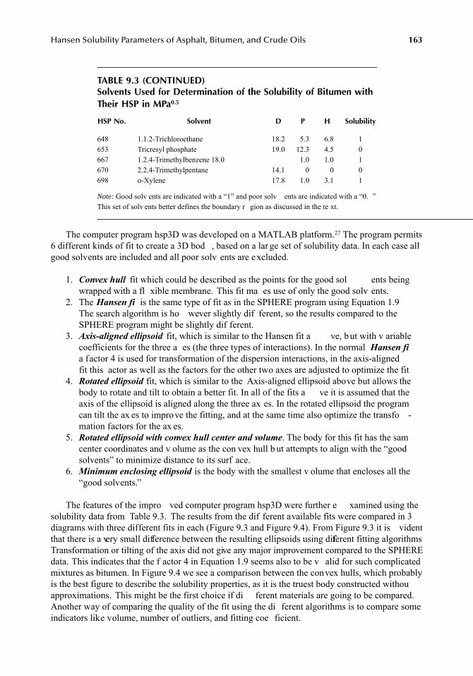
Hansen Solubility Parameters of Asphalt, Bitumen, and Crude Oils
163
The computer program hsp3D was developed on a MATLAB platform.
27
The program permits6 different kinds of fit to create a 3D bod , based on a lar ge set of solubility data. In each case allgood solvents are included and all poor solv ents are excluded.
1.
Convex hull
fit which could be described as the points for the good sol ents beingwrapped with a fl xible membrane. This fit ma es use of only the good solv ents.
2. The
Hansen fi
is the same type of fit as in the SPHERE program using Equation 1.9The search algorithm is ho wever slightly dif ferent, so the results compared to theSPHERE program might be slightly dif ferent.
3.
Axis-aligned ellipsoid
fit, which is similar to the Hansen fit a ve, but with v ariablecoefficients for the three a es (the three types of interactions). In the normal
Hansen fi
a factor 4 is used for transformation of the dispersion interactions, in the axis-alignedfit this actor as well as the factors for the other two axes are adjusted to optimize the fit
4.
Rotated ellipsoid
fit, which is similar to the Axis-aligned ellipsoid above but allows thebody to rotate and tilt to obtain a better fit. In all of the fits a ve it is assumed that theaxis of the ellipsoid is aligned along the three ax es. In the rotated ellipsoid the programcan tilt the ax es to improve the fitting, and at the same time also optimize the transfo -mation factors for the ax es.
5.
Rotated ellipsoid with convex hull center and volume
. The body for this fit has the samcenter coordinates and v olume as the con vex hull b ut attempts to align with the “goodsolvents” to minimize distance to its surf ace.
6.
Minimum enclosing ellipsoid
is the body with the smallest v olume that encloses all the“good solvents.”
The features of the impro ved computer program hsp3D were further e xamined using thesolubility data from Table 9.3. The results from the dif ferent available fits were compared in 3diagrams with three different fits in each (Figure 9.3 and Figure 9.4). From Figure 9.3 it is videntthat there is a very small difference between the resulting ellipsoids using different fitting algorithmsTransformation or tilting of the axis did not give any major improvement compared to the SPHEREdata. This indicates that the f actor 4 in Equation 1.9 seems also to be v alid for such complicatedmixtures as bitumen. In Figure 9.4 we see a comparison between the convex hulls, which probablyis the best figure to describe the solubility properties, as it is the truest body constructed withouapproximations. This might be the first choice if di ferent materials are going to be compared.Another way of comparing the quality of the fit using the di ferent algorithms is to compare someindicators like volume, number of outliers, and fitting coe ficient.
TABLE 9.3 (CONTINUED)Solvents Used for Determination of the Solubility of Bitumen with Their HSP in MPa
0.5
HSP No. Solvent D P H Solubility
648 1.1.2-Trichloroethane 18.2 5.3 6.8 1653 Tricresyl phosphate 19.0 12.3 4.5 0667 1.2.4-Trimethylbenzene 18.0 1.0 1.0 1670 2.2.4-Trimethylpentane 14.1 0 0 0698
o
-Xylene 17.8 1.0 3.1 1
Note:
Good solv ents are indicated with a “1” and poor solv ents are indicated with a “0. ”This set of solv ents better defines the boundary r gion as discussed in the te xt.
7248_book.fm Page 163 Tuesday, April 24, 2007 9:19 AM
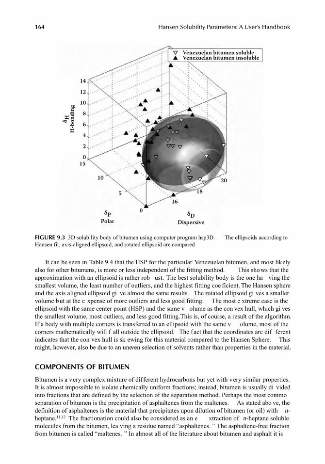
164
Hansen Solubility Parameters: A User’s Handbook
It can be seen in Table 9.4 that the HSP for the particular Venezuelan bitumen, and most likelyalso for other bitumens, is more or less independent of the fitting method. This shows that theapproximation with an ellipsoid is rather rob ust. The best solubility body is the one ha ving thesmallest volume, the least number of outliers, and the highest fitting coe ficient. The Hansen sphereand the axis aligned ellipsoid gi ve almost the same results. The rotated ellipsoid gi ves a smallervolume but at the e xpense of more outliers and less good fitting. The most e xtreme case is theellipsoid with the same center point (HSP) and the same v olume as the con vex hull, which gi vesthe smallest volume, most outliers, and less good fitting.This is, of course, a result of the algorithm.If a body with multiple corners is transferred to an ellipsoid with the same v olume, most of thecorners mathematically will f all outside the ellipsoid. The fact that the coordinates are dif ferentindicates that the con vex hull is sk ewing for this material compared to the Hansen Sphere. Thismight, however, also be due to an uneven selection of solvents rather than properties in the material.
COMPONENTS OF BITUMEN
Bitumen is a very complex mixture of different hydrocarbons but yet with very similar properties.It is almost impossible to isolate chemically uniform fractions; instead, bitumen is usually di videdinto fractions that are defined by the selection of the separation method. Perhaps the most commoseparation of bitumen is the precipitation of asphaltenes from the maltenes. As stated abo ve, thedefinition of asphaltenes is the material that precipitates upon dilution of bitumen (or oil) with
n-
heptane.
11,12
The fractionation could also be considered as an e xtraction of
n-
heptane solublemolecules from the bitumen, lea ving a residue named “asphaltenes. ” The asphaltene-free fractionfrom bitumen is called “maltenes. ” In almost all of the literature about bitumen and asphalt it is
FIGURE 9.3
3D solubility body of bitumen using computer program hsp3D. The ellipsoids according toHansen fit, axis-aligned ellipsoid, and rotated ellipsoid are compared
Venezuelan bitumen solubleVenezuelan bitumen insoluble
δ HH-
bond
ing
δPPolar
δDDispersive
141210
86420
15
10
5
016
1820
7248_book.fm Page 164 Tuesday, April 24, 2007 9:19 AM
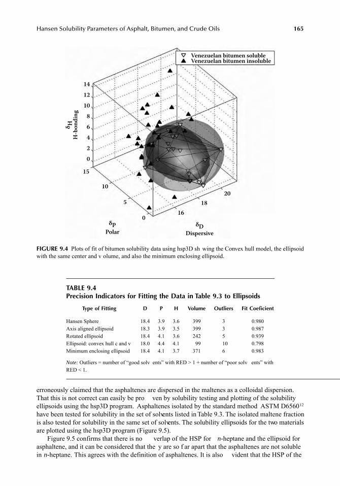
Hansen Solubility Parameters of Asphalt, Bitumen, and Crude Oils
165
erroneously claimed that the asphaltenes are dispersed in the maltenes as a colloidal dispersion.That this is not correct can easily be pro ven by solubility testing and plotting of the solubilityellipsoids using the hsp3D program. Asphaltenes isolated by the standard method ASTM D6560
12
have been tested for solubility in the set of solvents listed in Table 9.3. The isolated maltene fractionis also tested for solubility in the same set of solvents. The solubility ellipsoids for the two materialsare plotted using the hsp3D program (Figure 9.5).
Figure 9.5 confirms that there is no verlap of the HSP for n-heptane and the ellipsoid forasphaltene, and it can be considered that the y are so f ar apart that the asphaltenes are not solublein n-heptane. This agrees with the definition of asphaltenes. It is also vident that the HSP of the
FIGURE 9.4 Plots of fit of bitumen solubility data using hsp3D sh wing the Convex hull model, the ellipsoidwith the same center and v olume, and also the minimum enclosing ellipsoid.
TABLE 9.4Precision Indicators for Fitting the Data in Table 9.3 to Ellipsoids
Type of Fitting D P H Volume Outliers Fit Coeficient
Hansen Sphere 18.4 3.9 3.6 399 3 0.980Axis aligned ellipsoid 18.3 3.9 3.5 399 3 0.987Rotated ellipsoid 18.4 4.1 3.6 242 5 0.939Ellipsoid: convex hull c and v 18.0 4.4 4.1 99 10 0.798Minimum enclosing ellipsoid 18.4 4.1 3.7 371 6 0.983
Note: Outliers = number of “good solv ents” with RED > 1 + number of “poor solv ents” withRED < 1.
Venezuelan bitumen solubleVenezuelan bitumen insoluble
δ HH-
bond
ing
δPPolar
δDDispersive
141210
86420
15
10
5
016
1820
7248_book.fm Page 165 Tuesday, April 24, 2007 9:19 AM
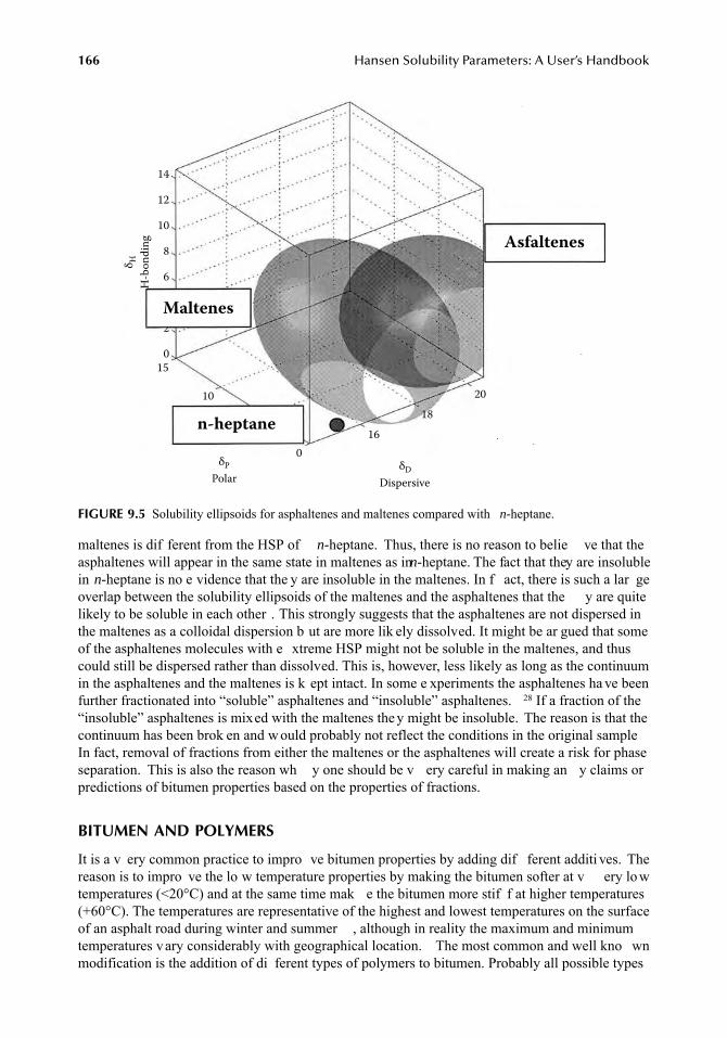
166 Hansen Solubility Parameters: A User’s Handbook
maltenes is dif ferent from the HSP of n-heptane. Thus, there is no reason to belie ve that theasphaltenes will appear in the same state in maltenes as in n-heptane. The fact that they are insolublein n-heptane is no e vidence that the y are insoluble in the maltenes. In f act, there is such a lar geoverlap between the solubility ellipsoids of the maltenes and the asphaltenes that the y are quitelikely to be soluble in each other . This strongly suggests that the asphaltenes are not dispersed inthe maltenes as a colloidal dispersion b ut are more lik ely dissolved. It might be ar gued that someof the asphaltenes molecules with e xtreme HSP might not be soluble in the maltenes, and thuscould still be dispersed rather than dissolved. This is, however, less likely as long as the continuumin the asphaltenes and the maltenes is k ept intact. In some e xperiments the asphaltenes ha ve beenfurther fractionated into “soluble” asphaltenes and “insoluble” asphaltenes. 28 If a fraction of the“insoluble” asphaltenes is mixed with the maltenes the y might be insoluble. The reason is that thecontinuum has been brok en and w ould probably not reflect the conditions in the original sampleIn fact, removal of fractions from either the maltenes or the asphaltenes will create a risk for phaseseparation. This is also the reason wh y one should be v ery careful in making an y claims orpredictions of bitumen properties based on the properties of fractions.
BITUMEN AND POLYMERS
It is a v ery common practice to impro ve bitumen properties by adding dif ferent additi ves. Thereason is to impro ve the lo w temperature properties by making the bitumen softer at v ery lo wtemperatures (<20°C) and at the same time mak e the bitumen more stif f at higher temperatures(+60°C). The temperatures are representative of the highest and lowest temperatures on the surfaceof an asphalt road during winter and summer , although in reality the maximum and minimumtemperatures vary considerably with geographical location. The most common and well kno wnmodification is the addition of di ferent types of polymers to bitumen. Probably all possible types
FIGURE 9.5 Solubility ellipsoids for asphaltenes and maltenes compared with n-heptane.
Maltenes
n-heptane
Asfaltenes
0
16
18
20
14
12
10
8
6
0
2
15
10
δP δDPolar Dispersive
H-b
on
din
g
δH
7248_book.fm Page 166 Tuesday, April 24, 2007 9:19 AM
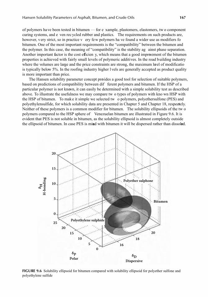
Hansen Solubility Parameters of Asphalt, Bitumen, and Crude Oils 167
of polymers have been tested in bitumen — for e xample, plastomers, elastomers, tw o componentcuring systems, and e ven rec ycled rubber and plastics. The requirements on such products are,however, very strict, so in practice v ery few polymers ha ve found a wider use as modifiers fobitumen. One of the most important requirements is the “compatibility” between the bitumen andthe polymer. In this case, the meaning of “compatibility” is the stability ag ainst phase separation.Another important factor is the cost efficien y, which means that a good improvement of the bitumenproperties is achieved with fairly small levels of polymeric additives. In the road building industrywhere the volumes are large and the price constraints are strong, the maximum level of modificatiois typically below 5%. In the roofing industry higher l vels are generally accepted as product qualityis more important than price.
The Hansen solubility parameter concept provides a good tool for selection of suitable polymers,based on predictions of compatibility between dif ferent polymers and bitumen. If the HSP of aparticular polymer is not known, it can easily be determined with a simple solubility test as describedabove. To illustrate the usefulness we may compare tw o types of polymers with kno wn HSP withthe HSP of bitumen. To make it simple we selected tw o polymers, polyethersulfone (PES) andpolyethylensulfide, for which solubility data are presented in Chapter 5 and Chapter 18, respectvely.Neither of these polymers is a common modifier for bitumen. The solubility ellipsoids of the tw opolymers compared to the HSP sphere of Venezuelan bitumen are illustrated in Figure 9.6. It isevident that PES is not soluble in bitumen, as the solubility ellipsoid is almost completely outsidethe ellipsoid of bitumen. In case PES is mixed with bitumen it will be dispersed rather than dissolved.
FIGURE 9.6 Solubility ellipsoid for bitumen compared with solubility ellipsoid for polyether sulfone andpolyethylene sulfide
Bitumen
Polyether sulphone
Polyethylene sulphide
δ HH-
bond
ing
δPPolar δD
Dispersive
20
15
10
5
0
1015
2025
50
1618
20
7248_book.fm Page 167 Tuesday, April 24, 2007 9:19 AM
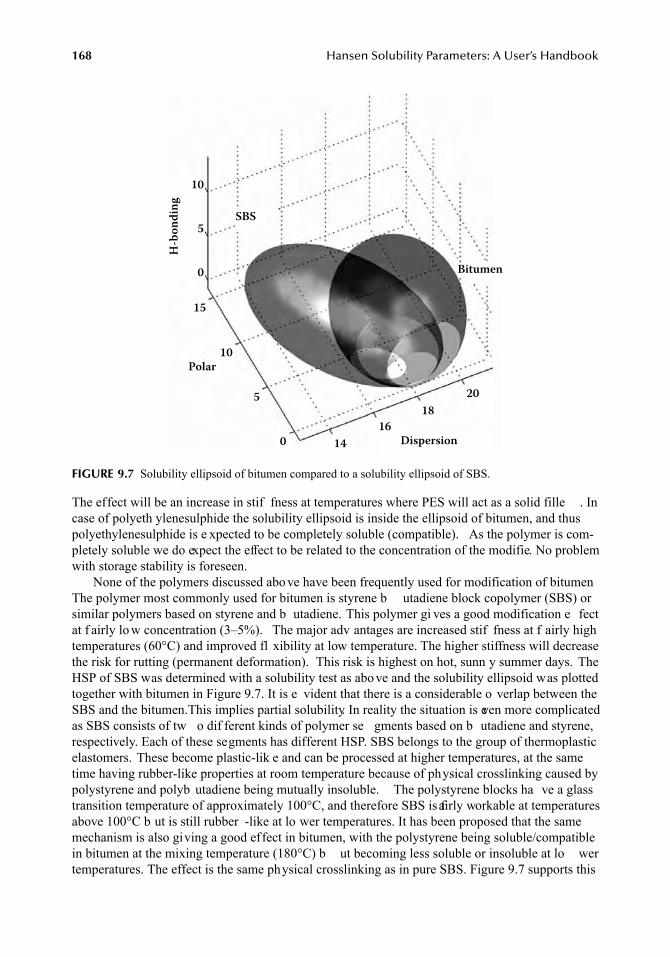
168 Hansen Solubility Parameters: A User’s Handbook
The effect will be an increase in stif fness at temperatures where PES will act as a solid fille . Incase of polyeth ylenesulphide the solubility ellipsoid is inside the ellipsoid of bitumen, and thuspolyethylenesulphide is e xpected to be completely soluble (compatible). As the polymer is com-pletely soluble we do expect the effect to be related to the concentration of the modifie. No problemwith storage stability is foreseen.
None of the polymers discussed above have been frequently used for modification of bitumenThe polymer most commonly used for bitumen is styrene b utadiene block copolymer (SBS) orsimilar polymers based on styrene and b utadiene. This polymer gi ves a good modification e fectat f airly lo w concentration (3–5%). The major adv antages are increased stif fness at f airly hightemperatures (60°C) and improved fl xibility at low temperature. The higher stiffness will decreasethe risk for rutting (permanent deformation). This risk is highest on hot, sunn y summer days. TheHSP of SBS was determined with a solubility test as abo ve and the solubility ellipsoid was plottedtogether with bitumen in Figure 9.7. It is e vident that there is a considerable o verlap between theSBS and the bitumen. This implies partial solubility. In reality the situation is even more complicatedas SBS consists of tw o dif ferent kinds of polymer se gments based on b utadiene and styrene,respectively. Each of these segments has different HSP. SBS belongs to the group of thermoplasticelastomers. These become plastic-lik e and can be processed at higher temperatures, at the sametime having rubber-like properties at room temperature because of physical crosslinking caused bypolystyrene and polyb utadiene being mutually insoluble. The polystyrene blocks ha ve a glasstransition temperature of approximately 100°C, and therefore SBS is fairly workable at temperaturesabove 100°C b ut is still rubber -like at lo wer temperatures. It has been proposed that the samemechanism is also giving a good effect in bitumen, with the polystyrene being soluble/compatiblein bitumen at the mixing temperature (180°C) b ut becoming less soluble or insoluble at lo wertemperatures. The effect is the same physical crosslinking as in pure SBS. Figure 9.7 supports this
FIGURE 9.7 Solubility ellipsoid of bitumen compared to a solubility ellipsoid of SBS.
Bitumen
SBS
H-bo
ndin
g
Polar
Dispersion
10
5
0
15
10
5
016
14
1820
7248_book.fm Page 168 Tuesday, April 24, 2007 9:19 AM
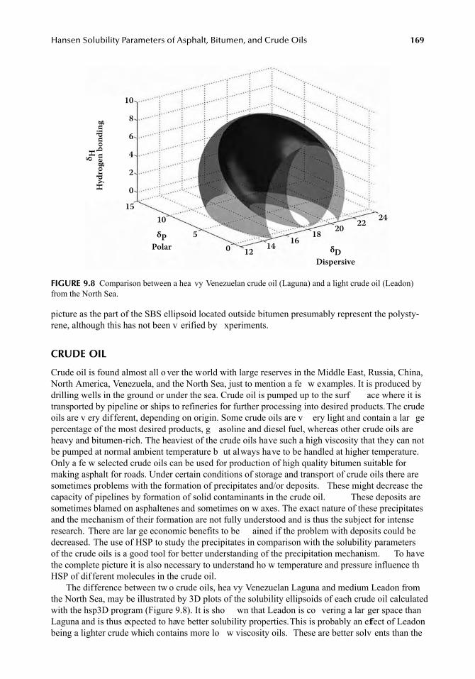
Hansen Solubility Parameters of Asphalt, Bitumen, and Crude Oils 169
picture as the part of the SBS ellipsoid located outside bitumen presumably represent the polysty-rene, although this has not been v erified by xperiments.
CRUDE OIL
Crude oil is found almost all o ver the world with large reserves in the Middle East, Russia, China,North America, Venezuela, and the North Sea, just to mention a fe w examples. It is produced bydrilling wells in the ground or under the sea. Crude oil is pumped up to the surf ace where it istransported by pipeline or ships to refineries for further processing into desired products.The crudeoils are v ery dif ferent, depending on origin. Some crude oils are v ery light and contain a lar gepercentage of the most desired products, g asoline and diesel fuel, whereas other crude oils areheavy and bitumen-rich. The heaviest of the crude oils have such a high viscosity that they can notbe pumped at normal ambient temperature b ut always have to be handled at higher temperature.Only a fe w selected crude oils can be used for production of high quality bitumen suitable formaking asphalt for roads. Under certain conditions of storage and transport of crude oils there aresometimes problems with the formation of precipitates and/or deposits. These might decrease thecapacity of pipelines by formation of solid contaminants in the crude oil. These deposits aresometimes blamed on asphaltenes and sometimes on w axes. The exact nature of these precipitatesand the mechanism of their formation are not fully understood and is thus the subject for intenseresearch. There are lar ge economic benefits to be ained if the problem with deposits could bedecreased. The use of HSP to study the precipitates in comparison with the solubility parametersof the crude oils is a good tool for better understanding of the precipitation mechanism. To havethe complete picture it is also necessary to understand ho w temperature and pressure influence thHSP of different molecules in the crude oil.
The difference between tw o crude oils, hea vy Venezuelan Laguna and medium Leadon fromthe North Sea, may be illustrated by 3D plots of the solubility ellipsoids of each crude oil calculatedwith the hsp3D program (Figure 9.8). It is sho wn that Leadon is co vering a lar ger space thanLaguna and is thus expected to have better solubility properties. This is probably an effect of Leadonbeing a lighter crude which contains more lo w viscosity oils. These are better solv ents than the
FIGURE 9.8 Comparison between a hea vy Venezuelan crude oil (Laguna) and a light crude oil (Leadon)from the North Sea.
δ HHy
drog
en b
ondi
ng
δPPolar δD
Dispersive
10
8
6
4
2
0
1015
50
161412
18 20 22 24
7248_book.fm Page 169 Tuesday, April 24, 2007 9:19 AM
170 Hansen Solubility Parameters: A User’s Handbook
higher molecular weight components of the Laguna. It is also seen that the solubility ellipsoid forthe Laguna is located completely inside the solubility ellipsoid for the Leadon. This means thatthe Laguna crude should be completely soluble in the Leadon crude, and no problems with theformation of precipitates are to be expected by dilution of Laguna crude oil with Leadon crude oil.
TURBIDIMETRIC TITRATIONS
Although the determination and visualization of solubility parameters for bitumen and other mineral-oil-derived materials have proven to be very illustrative, there is still a desire for better precision. Thishas partly been met, as discussed abo ve, by a better selection of test solv ents and by better methods tooptimize the ellipsoid. There are very obvious differences when it comes to practical applications, andparticularly with modification with SBS polymers, among bitumens h ving v ery similar solubilityellipsoids (Table 9.2). Bitumens that are seemingly very similar with respect to solubility give still verydifferent properties after mixing with SBS. One of the most important properties is the separationstability. Most mixtures of bitumen and SBS sho w a tendency for separation if the y are stored at hightemperature for a long time. A typical separation test is made at 180°C for 3 d. The separation is usuallyseen as the polymer floating to the surace, but sometimes, particularly at concentrations of SBS between10 and 15%, a phase separation can tak e place, also in the bitumen. This is seen as a hard precipitateat the bottom of the bitumen tank. The separation tendency can be o vercome by a proper selection ofbitumen, alternatively by selection of a suitable polymer . The selection of components is mainly doneon a “trial and error” basis, although there are some empirical rules. HSP may be an e xcellent tool forselection of suitable combinations of bitumen and polymer , but better precision is required than canbe obtained with simple solubility testing with pure liquids. Impro ved estimation of the best solubilityellipsoid is required for optimal use of the HSP concept.
BISOM TEST
The procedure discussed in the follo wing has been developed at Nynas Bitumen based on turbidi-metric titrations to precisely determine the boundary of the surf ace of solubility. The procedure iscalled BISOM, an acron ym for BItumen Solubility Model. The principle of the test method isvisualized in Figure 9.9. The HSP ellipsoid of the bitumen is constructed using the “poor solvents”illustrated as solid triangles in the figure and the “good sol ents” being illustrated with opentriangles. Three nonsolvents have been selected. These have HSP placing them just outside thesurface of the solubility ellipsoid. They may be seen as the black triangles in the center of thecircles in Figure 9.9. In the case of BISOM titration the selected “poor solvents” are 2,2,4-trimethylpentane (isooctane), 2-butanone (methyl ethyl ketone), and 2-ethyl hexanol. As bitumen is a highviscosity liquid or a semisolid material, it has to be diluted to decrease the viscosity to permitproper stirring during the titrations. For this purpose, a solvent with a solubility parameter as closeto the center of the ellipsoid as possible has to be selected. For the BISOM titration we have selectedtoluene (or in some cases xylene) as the good solv ent.
The titration is illustrated as arro ws, going from the HSP of the good solv ent toluene to an yof the three poor solv ents. The titration can be considered as a dilution of the bitumen with amixture of a good solv ent and a poor solv ent. The HSP of the mixture is proportional to theconcentration of each solv ent. A precipitate will appear when the HSP of the mixture has a v alueplacing it on the surf ace of the solubility ellipsoid.
An important ef fect to tak e into consideration in the turbidimetric titration of bitumen is theconcentration effect. This comes from the f act that bitumen is k ept homogeneous by the mutualsolubility of all its dif ferent molecules. The ef fect is seen as a higher concentration of bitumengiving better solubility . This situation is contradictory to what is usually kno wn for solubility ofpure substances. To understand this phenomenon we must consider that the first sign of turbidit
7248_book.fm Page 170 Tuesday, April 24, 2007 9:19 AM
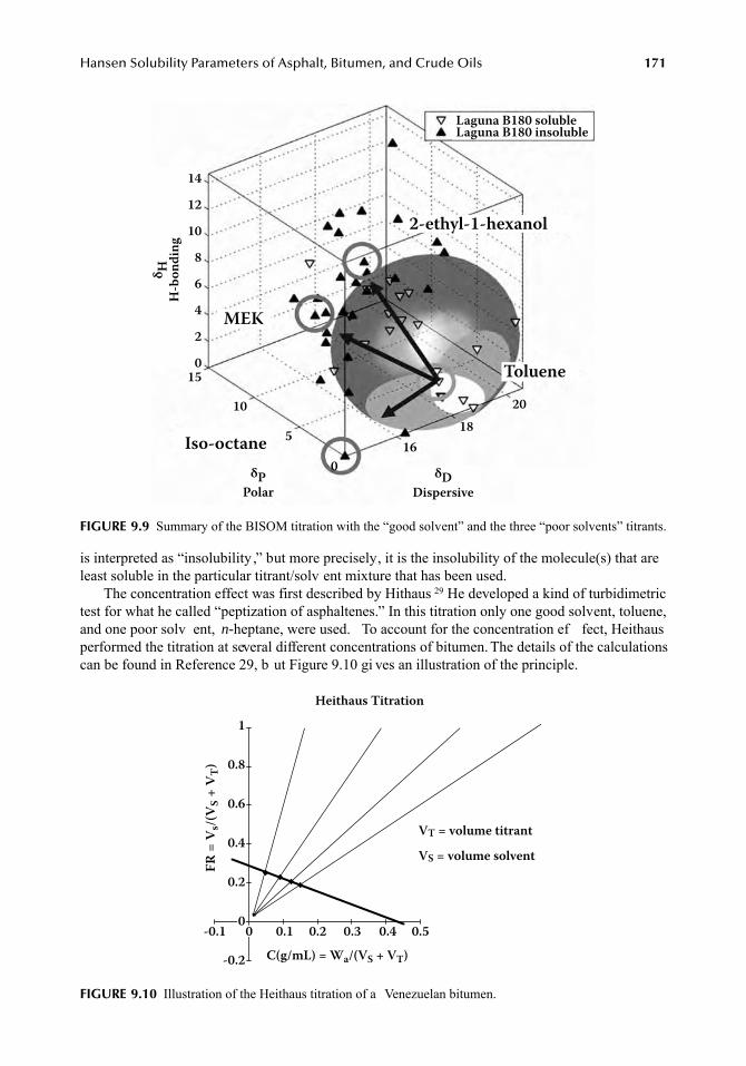
Hansen Solubility Parameters of Asphalt, Bitumen, and Crude Oils 171
is interpreted as “insolubility ,” but more precisely, it is the insolubility of the molecule(s) that areleast soluble in the particular titrant/solv ent mixture that has been used.
The concentration effect was first described by Hithaus 29 He developed a kind of turbidimetrictest for what he called “peptization of asphaltenes.” In this titration only one good solvent, toluene,and one poor solv ent, n-heptane, were used. To account for the concentration ef fect, Heithausperformed the titration at several different concentrations of bitumen. The details of the calculationscan be found in Reference 29, b ut Figure 9.10 gi ves an illustration of the principle.
FIGURE 9.9 Summary of the BISOM titration with the “good solvent” and the three “poor solvents” titrants.
FIGURE 9.10 Illustration of the Heithaus titration of a Venezuelan bitumen.
Laguna B180 solubleLaguna B180 insoluble
δ HH-
bond
ing
δPPolar
δDDispersive
141210
86420
15
10
516
1820
MEK
Iso-octane
2-ethyl-1-hexanol
Toluene
0
Heithaus Titration
VT = volume titrantVS = volume solvent
C(g/mL) = Wa/(VS + VT)
FR =
Vs/(
V S +
VT)
1
0.8
0.6
0.4
0.2
0
-0.2
-0.1 0 0.1 0.2 0.3 0.4 0.5
7248_book.fm Page 171 Tuesday, April 24, 2007 9:19 AM
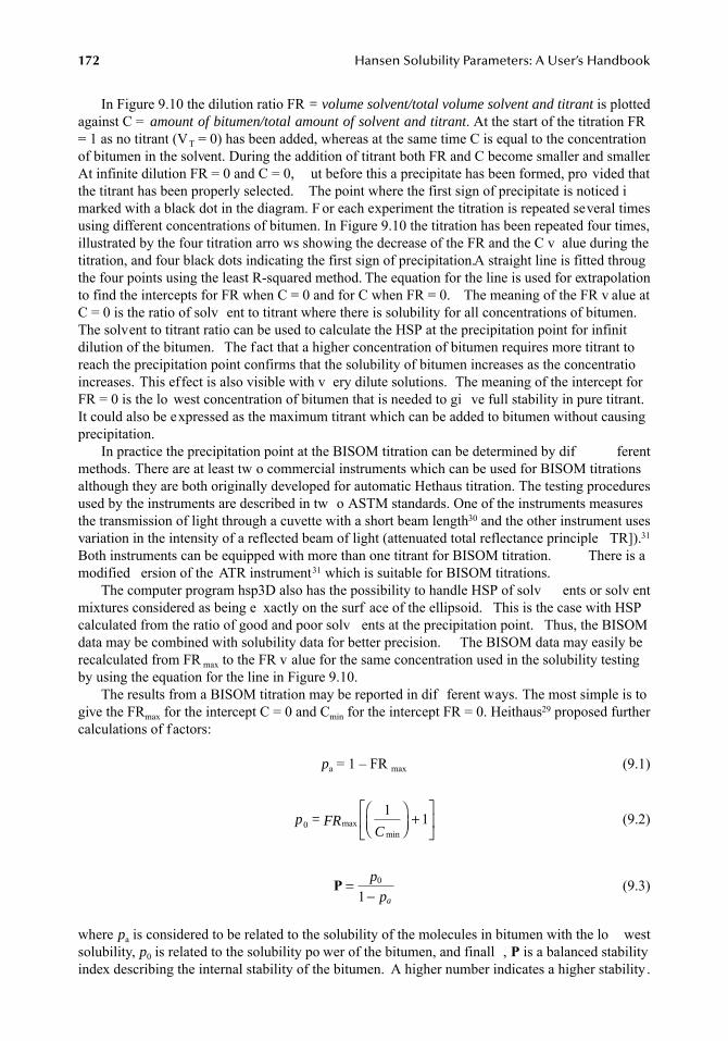
172 Hansen Solubility Parameters: A User’s Handbook
In Figure 9.10 the dilution ratio FR = volume solvent/total volume solvent and titrant is plottedagainst C = amount of bitumen/total amount of solvent and titrant. At the start of the titration FR= 1 as no titrant (VT = 0) has been added, whereas at the same time C is equal to the concentrationof bitumen in the solvent. During the addition of titrant both FR and C become smaller and smaller.At infinite dilution FR = 0 and C = 0, ut before this a precipitate has been formed, pro vided thatthe titrant has been properly selected. The point where the first sign of precipitate is noticed imarked with a black dot in the diagram. F or each experiment the titration is repeated several timesusing different concentrations of bitumen. In Figure 9.10 the titration has been repeated four times,illustrated by the four titration arro ws showing the decrease of the FR and the C v alue during thetitration, and four black dots indicating the first sign of precipitation.A straight line is fitted througthe four points using the least R-squared method. The equation for the line is used for extrapolationto find the intercepts for FR when C = 0 and for C when FR = 0. The meaning of the FR v alue atC = 0 is the ratio of solv ent to titrant where there is solubility for all concentrations of bitumen.The solvent to titrant ratio can be used to calculate the HSP at the precipitation point for infinitdilution of the bitumen. The fact that a higher concentration of bitumen requires more titrant toreach the precipitation point confirms that the solubility of bitumen increases as the concentratioincreases. This effect is also visible with v ery dilute solutions. The meaning of the intercept forFR = 0 is the lo west concentration of bitumen that is needed to gi ve full stability in pure titrant.It could also be expressed as the maximum titrant which can be added to bitumen without causingprecipitation.
In practice the precipitation point at the BISOM titration can be determined by dif ferentmethods. There are at least tw o commercial instruments which can be used for BISOM titrationsalthough they are both originally developed for automatic Hethaus titration. The testing proceduresused by the instruments are described in tw o ASTM standards. One of the instruments measuresthe transmission of light through a cuvette with a short beam length30 and the other instrument usesvariation in the intensity of a reflected beam of light (attenuated total reflectance principle TR]).31
Both instruments can be equipped with more than one titrant for BISOM titration. There is amodified ersion of the ATR instrument31 which is suitable for BISOM titrations.
The computer program hsp3D also has the possibility to handle HSP of solv ents or solv entmixtures considered as being e xactly on the surf ace of the ellipsoid. This is the case with HSPcalculated from the ratio of good and poor solv ents at the precipitation point. Thus, the BISOMdata may be combined with solubility data for better precision. The BISOM data may easily berecalculated from FR max to the FR v alue for the same concentration used in the solubility testingby using the equation for the line in Figure 9.10.
The results from a BISOM titration may be reported in dif ferent ways. The most simple is togive the FRmax for the intercept C = 0 and Cmin for the intercept FR = 0. Heithaus29 proposed furthercalculations of factors:
pa = 1 – FR max (9.1)
(9.2)
(9.3)
where pa is considered to be related to the solubility of the molecules in bitumen with the lo westsolubility, p0 is related to the solubility po wer of the bitumen, and finall , P is a balanced stabilityindex describing the internal stability of the bitumen. A higher number indicates a higher stability .
01 1p = FR
Cmax
min
⎛⎝⎜
⎞⎠⎟
+⎡
⎣⎢
⎤
⎦⎥
P =−p
pa
0
1
7248_book.fm Page 172 Tuesday, April 24, 2007 9:19 AM
Hansen Solubility Parameters of Asphalt, Bitumen, and Crude Oils 173
A high internal stability can be seen as a high allo wance for blending with additi ves, polymers,solvents, or other types of bitumen or crude oil.
The interpretation of the BISOM titration is a determination of the internal stability of thebitumen or crude oil, rather than determination of HSP , although it is based on the principles ofHSP. The BISOM could also be seen as an identification of those molecules that are the leassoluble in the bitumen or crude oil, and ho w close to insolubility the y are. To have a completepicture it is necessary to ha ve several titrants with dif ferent HSP as the traditional determinationsof internal stability using only n-heptane as precipitant will usually gi ve an incomplete picture. Itis not e xpected that the material precipitated by addition of n-heptane would be the same as thatprecipitated by the addition of 2-eth yl-1-hexanol or 2-b utanone. The use of three titrants permitscalculation of the HSP at three precipitation points, each of which could be considered to be onthe surface of the solubility ellipsoid. It is, however, not possible to estimate the solubility ellipsoidfrom only three points on the surf ace, particularly since the exact center point is not kno wn. If theHSP calculated from turbidimetric titrations are going to be compared to the HSP ellipsoid of thesame material, the concentration at the solubility testing has to be tak en into consideration. Theprecipitation point at a certain concentration can easily be estimated from data such as are reportedin Figure 9.10.
CONCLUSION
• The Hansen solubility parameters of a comple x material such as bitumen or crude oilcan be estimated by determination of its solubility in a lar ge number of solv ents withknown HSP.
• To have the best precision, the test solvents should be selected with respect to the materialto be tested. It is preferred to ha ve solvents near or at the borderline of solubility .
• The factor 4 in Equation 1.9 as a multiplier for the difference in the dispersion parametersfor the materials being considered seems to be v alid, also for comple x mixtures lik ebitumen.
• Comparison of HSP for bitumen, asphaltenes, and maltenes confirms that asphalteneare soluble in maltenes, and bitumen should thus not be considered as a colloidaldispersion as is frequently claimed.
• The best estimated HSP v alues for Venezuelan bitumen are D = 18.6 MP a0.5, P = 3.0MPa0,5, H = 3.4 MP a0.5.
• A computer program hsp3D can estimate the best fit to the solubility data and from thicalculate the HSP.
• The program can also estimate the best coef ficients for the ellipsoid model to illustratthe extension of solubility re gions in a 3D diagram.
• Up to three dif ferent materials can be compared in the same 3D plot. • The program is not limited to bitumen and crude oils, b ut could equally well be used
for other types of materials.• A procedure for turbidimetric titrations has been de veloped to further impro ve the
precision to determine the surf ace of the HSP solubility ellipsoid. This procedure iscalled a BISOM titration.
• BISOM titration is well suited for measurement of the internal stability of comple xhydrocarbon mixtures like bitumen or crude oils.
• BISOM titration is also a determination of the least soluble molecules in bitumen orcrude oils.
7248_book.fm Page 173 Tuesday, April 24, 2007 9:19 AM
174 Hansen Solubility Parameters: A User’s Handbook
REFERENCES
1. Speight, J.G., The Chemistry and Technology of Petroleum, 2nd ed., Marcel Dekker, New York, 1991.2. Nellensteyn, F.J., Relation of the micelle to the medium in asphalt, Inst. Pet. Technol., 14, 134–138,
1928.3. Pfeiffer, J.P. and Saal, R.N.J., Asphaltic bitumen as colloidal system, Phys. Chem., 44 139–149, 1940.4. Park, S.J. and Mansoori, G.A ., Aggregation and deposition of hea vy organics in petroleum crudes,
Energy Sources, 10, 109–125, 1988.5. Boduszynski, M.M., McKay , J.F., and Lathham, D.R., Asphaltenes where are you? Proc. Assoc of
Asphalt Paving Technologists, 49, 1980, pp. 124–143.6. Petersen, J.C., Robertson, R.E., Branthaver, J.F., Harnsberger, P.M., Duvall, J.J., Kim, S.S., Anderson,
D.A., Christiansen, D.W., and Bahia, H.U., Binder Characterization and Ev aluation, Vol. 1: PhysicalCharacterization, Strategic Highway Research Program SHRP-A-367, 1994.
7. Redelius, P .G., Bitumen solubility model using Hansen solubility parameter , Energy Fuels, 18,1087–1092, 2004.
8. Sirota, E.B., Understanding the Physical Structure of Asphaltenes to Optimize Bitumen Manufacture,3rd Euroasphalt and Eurobitume Congress Vienna, Paper 097, 930–939, 2004.
9. Yen, T.F. and Chilingarian, G.V., Asphaltenes and Asphalts, 1 in Developments in Petroleum Science40 A, Elsevier Science BV, Amsterdam 1994.
10. Sheu, E.Y. and Mullins, O.C., Asphaltenes, Fundamentals and Applications, Plenum Press, New York,1995.
11. Test Method for n-heptane Insolubles. Annual book of ASTM Standards Section 04.03, ASTM D3279-97, 2001.
12. Test Method for Determination of Asphaltenes (Heptane insolubles) in Crude Petroleum and PetroleumProducts, Annual book of ASTM Standards Section 05.04, ASTM D6560-00.
13. Buch, L., Groenzin, H., Buenrostro-Gonzales, E., Andersen, S.I., Lira-Galena, C., Mullins, O.C.,Molecular size of asphaltene fractions obtained from residuum hydrotreatment, Fuel, 82, 1075–1084,2003.
14. Boduszynski, M.M., Asphaltenes in petroleum asphalts: composition and formation, Am. Chem. Soc.Meet., Div. Pet. Chem., Washington, D.C., September 9–14, 1979.
15. Mitchell, D.L. and Speight, J.G., The solubility of asphaltenes in h ydrocarbon solv ents, Fuel, 52,149–152, 1973.
16. Hirschberg, A., deJong, L.N.J., Schipper , B.A., Meijer , J.G., Influence of temperature and pressuron asphaltene flocculation, Soc. Pet. Eng. J., 283–293, June 1984.
17. Hildebrand, J.H. and Scott, R.L., The Solubility of Nonelectrolytes, 3rd ed., Do ver, New York, 1964.18. Laux, H. and Rahimian, I., Colloid-disperse Crude Oil Systems; Phase Behaviour and Stability, Erdöl
und Kohle — Erdgas — Petrochemie vereinigt mit Brennstoff-Chemie, 47(11), 430–435, 1994.19. Hirschberg, A. and Hermans, L., Asphaltene phase beha viour: a molecular thermodynamic model ,
Proc. Characterisation of Heavy Crude Oils and Petroleum Residues, Lyon, June 25–27, 1984.20. Burke, N.E., Hobbs, R.E., Kashou, S.F ., Measurement and modelling of asphaltene precipitating, J.
Pet. Technol., November, 1440–1446, 1990.21. Rahimian, I. and Zenk e, G., Zum Verhalten organicher Lösemittel ge genüber Bitumen, Bitumen 1,
2–8, 1986 (in German).22. Neumann, H.J., Rahimian, I., Zenk e, G., Einfluss der Löslich eitseigenschaften von Asphaltene auf
die Rückstandsverarbeitung. Erdöl und Kohle –Erdgas, 42(7/8), 278–286, 1989 (in German).23. Hagen, A.H., Jones, R., Hofner , R.M., Randolf, B.B., Johnson, M.P ., Characterisation of asphalt by
solubility profiles, J. Assoc. Asphalt Paving Technol., 53, 119–137, 1984.24. Redelius, P.G., Solubility parameters and bitumen , Fuel, 79, 27–35, 2000.25. Hansen, C.M., Skaarup, K., The three dimensional parameter — k ey to paint component af finities
III. Independent calculation of the parameter components, J. Paint Technol., 39(511), 511–514, 1967.26. Warnez, M. and Redelius, P .G., unpublished results from Icopal – Nynas joint research project:
Correlation between Bitumen Characteristics and Fire Properties of Roofing Membranes, 2001–200327. Turner, F. and Redelius, P ., The program hsp3D is a vailable as share w are in Europe from: Nynas
Petroleum, S-149 82 Nynäshamn, Sweden, www .nynas.com or in USA from Western ResearchInstitute, 265 North 9th Street, Laramie, Wyoming 82070–3380, www.westernresearch.org.
7248_book.fm Page 174 Tuesday, April 24, 2007 9:19 AM

Hansen Solubility Parameters of Asphalt, Bitumen, and Crude Oils 175
28. Östlund, J.-A., Wattana, P., Nydén, M., and Fogler, H.S., Characterisation of fractionated asphaltenesby UV-VIS and NMR self-dif fusion spectroscopy, J. Colloid Interface Sci., 271(2), 372–380, 2004.
29. Heithaus J.J., Measurement and significance of asphatene pepetization, J. Inst. Pet., 48(458), 45–53,1962.
30. Standard Test Method for Automated Heithaus Titrimetry, Annual book of ASTM Standards Section04.03, ASTM D6703-01.
31. Standard Test Method for Determining Stability and Compatibility of Hea vy Fuel Oils and CrudeOils by Hea vy Fuel Oil Stability Analyzer (Optical Detection), Annual book of ASTM StandardsSection 05.04, ASTM D7112-05a
7248_book.fm Page 175 Tuesday, April 24, 2007 9:19 AM

7248_book.fm Page 176 Tuesday, April 24, 2007 9:19 AM
177
10
Determination of Hansen Solubility Parameter Values for Carbon Dioxide
Laurie L. Williams
ABSTRACT
Reference values of the Hansen solubility parameters (HSP) for carbon dioxide (CO
2
) have beendetermined. The methodology adopted for this is based on room temperature solubility of the g asin different liquids of known HSP values. CO
2
gas solubility data, at 25°C and a CO
2
partial pressureof 1 atmosphere, in 101 liquid solv ents have been g athered and evaluated, yielding the v alues:
δ
d
= 15.6 MP a
1/2
,
δ
p
= 5.2 MP a
1/2
, and
δ
h
= 5.8 MP a
1/2
. A methodology for e xtending this referenceset of HSP v alues to an y temperature and pressure has been de veloped utilizing an equation ofstate (EOS) of the form P =
f
(
ρ
, T).
INTRODUCTION
The HSP concept is widely used for selecting suitable solvents for organic compounds. In addition,HSPs ha ve been applied to biological materials, barrier properties of polymers, as well as thecharacterization of surf aces, pigments, fillers, and fibers.
1
The basis of the HSP approach is theassumption that the total cohesi ve ener gy (
E
) of a pure compound is made up of the additi vecontributions from nonpolar (dispersion) interactions (
E
d
), polar (dipole–dipole and dipole–induceddipole) interactions (
E
p
), and hydrogen bonding or other specific association interactions includingLewis acid–base interactions (
E
h
):
(10.1)
Dividing each contribution by the molar v olume,
(10.2)
gives the square of the total solubility parameter as the sum of the squares of the Hansen dispersion(
δ
d
), polar (
δ
p
), and hydrogen bonding (
δ
h
) solubility parameters, so that
(10.3)
where
E E E Ed P h= + +
E
V
E
V
E
V
E
Vd p h= + +
δ δ δ δt d p h2 2 2 2= + +
7248_book.fm Page 177 Tuesday, April 24, 2007 9:19 AM
178
Hansen Solubility Parameters: A User’s Handbook
(10.4)
The determination of HSPs for compounds that are gases at ambient conditions is usually basedon room temperature solubility of the g as in a range of dif ferent liquids of kno wn
δ
d
,
δ
p
, and
δ
h
.Those liquids that show the highest solubility for the gas are assumed to have HSPs closer to thoseof the g as than those liquids that ha ve lo wer solubilities for the g as. In the follo wing section,published data of CO
2
gas solubility at 25°C and a CO
2
partial pressure of 1 atmosphere in a lar genumber of liquid solv ents are evaluated. From this data, a set of HSP v alues at a single referencetemperature and pressure is determined.
METHODOLOGY
Literature values of CO
2
solubility in v arious liquid solvents at 25°C ha ve been collected and aresummarized in Table 10.1. All the solubility data sho wn in Table 10.1 w as either e xperimentallydetermined at a CO
2
partial pressure of 0.1 MPa, or has been corrected to
p
CO2
MPa using Henry’slaw,
2
(10.5)
where
K
H
is the Henry’ s law coefficient,
p
CO2
is the partial pressure of CO
2
, and
x
CO2
is the molefraction of dissolv ed CO
2
. In addition to correcting CO
2
partial pressure to 0.1 MP a, it has beennecessary to correct the reported values of CO
2
gas solubility to a common set of units. Generally ,solubilities ha ve been reported as mole fraction of dissolv ed CO
2
,
x
CO2
, or as one of the tw odimensionless quantities; the Bunsen coefficient or the Ostwald coefficient. The Bunsen coefficient,
Ω
, is defined as the v olume of g as, reduced to 0°C and 0.1 MP a, dissolved per unit v olume ofsolvent at a system temperature,
T
, under a gas pressure of 1 atmosphere. The Ostwald coefficient,
L
, is defined as the ratio of the v olume of gas absorbed to the v olume of the absorbing liquid, allmeasured at the same temperature.
3
If the solubility is small and the gas phase is ideal, the Ostwaldcoefficient is independent of total pressure and these tw o coefficients are simply related by
4
:
(10.6)
The mole fraction of dissolv ed CO
2
can then be calculated using
2
(10.7)
where R is the g as constant, T is the absolute temperature, and
V
10
the molar v olume of the puresolvent. The Hansen dispersion, polar , and h ydrogen bonding parameters in Table 10.1 are fromHansen’s solublity parameter handbook,
5
and the total solubility parameter value is calculated fromEquation 10.3, noted earlier .
Using the collected v alues of
x
CO2
at 25
°
C and
p
CO2
= .1
MPa
,
HSP values were calculatedbased on a simple weighted a verage using the data set in Table 10.1, hereafter called
data set #1
.Where multiple CO
2
gas solubility data were a vailable for an indi vidual solvent, an average valuefor that solvent was used.
δ δ δdd
pp
hhE
V
E
V
E
V2 2 2= = =; ; and
COCO
2xp
KH
= 2
TL =
273Ω
CO2x
RT
Lp VCO
=⎛
⎝⎜
⎞
⎠⎟ +
⎡
⎣⎢⎢
⎤
⎦⎥⎥
−
2 10
1
1
7248_book.fm Page 178 Tuesday, April 24, 2007 9:19 AM
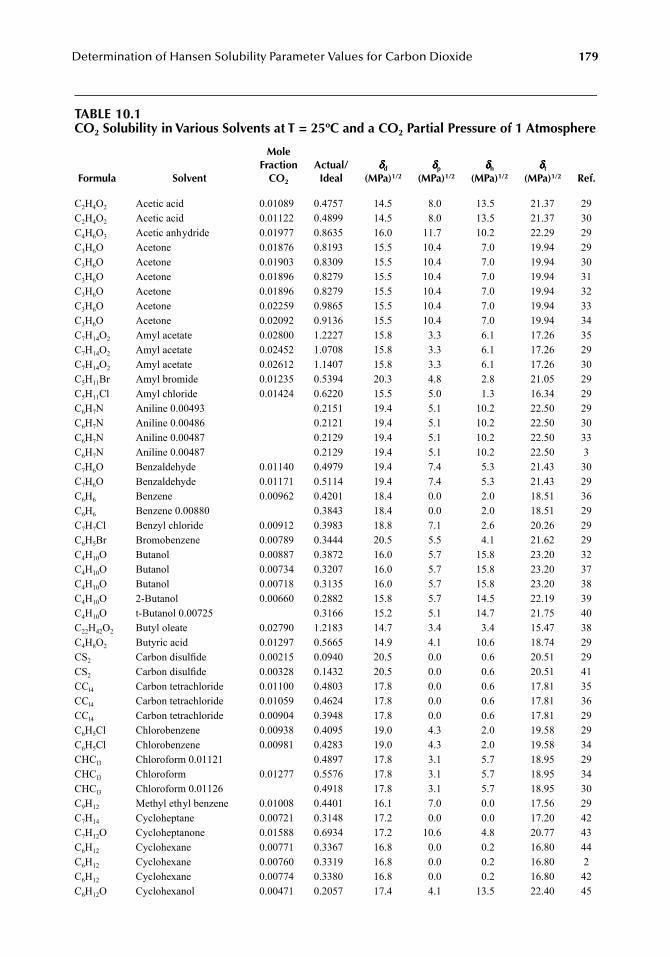
Determination of Hansen Solubility Parameter Values for Carbon Dioxide
179
TABLE 10.1CO
2
Solubility in Various Solvents at T = 25ºC and a CO
2
Partial Pressure of 1 Atmosphere
Formula Solvent
MoleFraction
CO
2
Actual/Ideal
δδδδ
d
(MPa)
1/2
δδδδ
p
(MPa)
1/2
δδδδ
h
(MPa)
1/2
δδδδ
t
(MPa)
1/2
Ref.
C
2
H
4
O
2
Acetic acid 0.01089 0.4757 14.5 8.0 13.5 21.37 29C
2
H
4
O
2
Acetic acid 0.01122 0.4899 14.5 8.0 13.5 21.37 30C
4
H
6
O
3
Acetic anhydride 0.01977 0.8635 16.0 11.7 10.2 22.29 29C
3
H
6
O Acetone 0.01876 0.8193 15.5 10.4 7.0 19.94 29C
3
H
6
O Acetone 0.01903 0.8309 15.5 10.4 7.0 19.94 30C
3
H
6
O Acetone 0.01896 0.8279 15.5 10.4 7.0 19.94 31C
3
H
6
O Acetone 0.01896 0.8279 15.5 10.4 7.0 19.94 32C
3
H
6
O Acetone 0.02259 0.9865 15.5 10.4 7.0 19.94 33C
3
H
6
O Acetone 0.02092 0.9136 15.5 10.4 7.0 19.94 34C
7
H
14
O
2
Amyl acetate 0.02800 1.2227 15.8 3.3 6.1 17.26 35C
7
H
14
O
2
Amyl acetate 0.02452 1.0708 15.8 3.3 6.1 17.26 29C
7
H
14
O
2
Amyl acetate 0.02612 1.1407 15.8 3.3 6.1 17.26 30C
5
H
11
Br Amyl bromide 0.01235 0.5394 20.3 4.8 2.8 21.05 29C
5
H
11
Cl Amyl chloride 0.01424 0.6220 15.5 5.0 1.3 16.34 29C
6
H
7
N Aniline 0.00493 0.2151 19.4 5.1 10.2 22.50 29C
6
H
7
N Aniline 0.00486 0.2121 19.4 5.1 10.2 22.50 30C
6
H
7
N Aniline 0.00487 0.2129 19.4 5.1 10.2 22.50 33C
6
H
7
N Aniline 0.00487 0.2129 19.4 5.1 10.2 22.50 3C
7
H
6
O Benzaldehyde 0.01140 0.4979 19.4 7.4 5.3 21.43 30C
7
H
6
O Benzaldehyde 0.01171 0.5114 19.4 7.4 5.3 21.43 29C
6
H
6
Benzene 0.00962 0.4201 18.4 0.0 2.0 18.51 36C
6
H
6
Benzene 0.00880 0.3843 18.4 0.0 2.0 18.51 29C
7
H
7
Cl Benzyl chloride 0.00912 0.3983 18.8 7.1 2.6 20.26 29C
6
H
5
Br Bromobenzene 0.00789 0.3444 20.5 5.5 4.1 21.62 29C
4
H
10
O Butanol 0.00887 0.3872 16.0 5.7 15.8 23.20 32C
4
H
10
O Butanol 0.00734 0.3207 16.0 5.7 15.8 23.20 37C
4
H
10O Butanol 0.00718 0.3135 16.0 5.7 15.8 23.20 38C4H10O 2-Butanol 0.00660 0.2882 15.8 5.7 14.5 22.19 39C4H10O t-Butanol 0.00725 0.3166 15.2 5.1 14.7 21.75 40C22H42O2 Butyl oleate 0.02790 1.2183 14.7 3.4 3.4 15.47 38C4H8O2 Butyric acid 0.01297 0.5665 14.9 4.1 10.6 18.74 29CS2 Carbon disulfide 0.00215 0.0940 20.5 0.0 0.6 20.51 29CS2 Carbon disulfide 0.00328 0.1432 20.5 0.0 0.6 20.51 41CCl4 Carbon tetrachloride 0.01100 0.4803 17.8 0.0 0.6 17.81 35CCl4 Carbon tetrachloride 0.01059 0.4624 17.8 0.0 0.6 17.81 36CCl4 Carbon tetrachloride 0.00904 0.3948 17.8 0.0 0.6 17.81 29C6H5Cl Chlorobenzene 0.00938 0.4095 19.0 4.3 2.0 19.58 29C6H5Cl Chlorobenzene 0.00981 0.4283 19.0 4.3 2.0 19.58 34CHCl3 Chloroform 0.01121 0.4897 17.8 3.1 5.7 18.95 29CHCl3 Chloroform 0.01277 0.5576 17.8 3.1 5.7 18.95 34CHCl3 Chloroform 0.01126 0.4918 17.8 3.1 5.7 18.95 30C9H12 Methyl ethyl benzene 0.01008 0.4401 16.1 7.0 0.0 17.56 29C7H14 Cycloheptane 0.00721 0.3148 17.2 0.0 0.0 17.20 42C7H12O Cycloheptanone 0.01588 0.6934 17.2 10.6 4.8 20.77 43C6H12 Cyclohexane 0.00771 0.3367 16.8 0.0 0.2 16.80 44C6H12 Cyclohexane 0.00760 0.3319 16.8 0.0 0.2 16.80 2C6H12 Cyclohexane 0.00774 0.3380 16.8 0.0 0.2 16.80 42C6H12O Cyclohexanol 0.00471 0.2057 17.4 4.1 13.5 22.40 45
7248_book.fm Page 179 Tuesday, April 24, 2007 9:19 AM
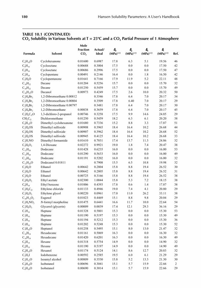
180 Hansen Solubility Parameters: A User’s Handbook
TABLE 10.1 (CONTINUED)CO2 Solubility in Various Solvents at T = 25ºC and a CO2 Partial Pressure of 1 Atmosphere
Formula Solvent
MoleFraction
CO2
Actual/Ideal
δδδδd
(MPa)1/2
δδδδp
(MPa)1/2
δδδδh
(MPa)1/2
δδδδt
(MPa)1/2 Ref.
C6H10O Cyclohexanone 0.01600 0.6987 17.8 6.3 5.1 19.56 46C8H16 Cyclooctane 0.00688 0.3004 17.5 0.0 0.0 17.50 42C8H16 Cyclooctane 0.00686 0.2996 17.5 0.0 0.0 17.50 47C5H10 Cyclopentane 0.00491 0.2146 16.4 0.0 1.8 16.50 42C5H8O Cyclopentanone 0.01641 0.7166 17.9 11.9 5.2 22.11 48C10H22 Decane 0.01204 0.5256 15.7 0.0 0.0 15.70 32C10H22 Decane 0.01250 0.5459 15.7 0.0 0.0 15.70 49C10H22O Decanol 0.00973 0.4249 17.5 2.6 10.0 20.32 50C2H4Br2 1,2-Dibromoethane 0.00812 0.3546 17.8 6.4 7.0 20.17 34C2H4Br2 1,2-Dibromoethane 0.00804 0.3509 17.8 6.40 7.0 20.17 29C2H4Br2 1,2-Dibromoethane 0.00797 0.3481 17.8 6.4 7.0 20.17 30C2H4Br2 1,2-Dibromoethane 0.00838 0.3659 17.8 6.4 7.0 20.17 45C3H6Cl2O 1,3-dichloro-2-propanol 0.00746 0.3258 17.5 9.9 14.6 24.85 29CH2Cl2 Dichloromethane 0.01250 0.5459 18.2 6.3 6.1 20.20 38C8H14O Dimethyl cyclohexanone 0.01680 0.7336 15.2 8.8 3.3 17.87 51C2H6OS Dimethyl sulfoxide 0.00908 0.3965 18.4 16.4 10.2 26.68 44C2H6OS Dimethyl sulfoxide 0.00907 0.3962 18.4 16.4 10.2 26.68 52C2H6OS Dimethyl sulfoxide 0.00945 0.4125 18.4 16.4 10.2 26.68 33C3H7NO Dimethyl formamide 0.01610 0.7031 17.4 13.7 11.3 24.86 32C4H8O2 1,4-Dioxane 0.02272 0.9921 19.0 1.8 7.4 20.47 38C12H26 Dodecane 0.01428 0.6235 16.0 0.0 0.0 16.00 53C12H26 Dodecane 0.01290 0.5633 16.0 0.0 0.0 16.00 49C12H26 Dodecane 0.01191 0.5202 16.0 0.0 0.0 16.00 32C12H26O Dodecanol 0.01811 0.7908 15.5 6.5 10.8 19.98 32C2H6O Ethanol 0.00642 0.2804 15.8 8.8 19.4 26.52 30C2H6O Ethanol 0.00642 0.2805 15.8 8.8 19.4 26.52 31C2H6O Ethanol 0.00725 0.3166 15.8 8.8 19.4 26.52 38C4H8O2 Ethyl acetate 0.02300 1.0044 15.8 5.3 7.2 18.15 38C8H10 Ethyl benzene 0.01006 0.4393 17.8 0.6 1.4 17.87 38C2H4Cl2 Ethylene chloride 0.01133 0.4946 19.0 7.4 4.1 20.80 29C2H6O2 Ethylene glycol 0.00220 0.0961 17.0 11.0 26.2 33.11 38C10H12O2 Eugenol 0.01023 0.4469 15.1 8.8 9.8 20.04 29C5H9NO2 N-formyl morpholine 0.01475 0.6441 16.6 11.7 10.0 22.64 54C3H8O3 Glycerol (glycerin) 0.00009 0.0039 17.4 12.1 29.3 36.16 29C7H16 Heptane 0.01328 0.5801 15.3 0.0 0.0 15.30 53C7H16 Heptane 0.01190 0.5197 15.3 0.0 0.0 15.30 49C7H16 Heptane 0.01194 0.5212 15.3 0.0 0.0 15.30 36C7H16 Heptane 0.01202 0.5248 15.3 0.0 0.0 15.30 52C7H16O Heptanol 0.01258 0.5495 15.1 8.0 13.0 21.47 32C16H34 Hexadecane 0.01161 0.5069 16.3 0.0 0.0 16.30 32C16H34 Hexadecane 0.01420 0.6201 16.3 0.0 0.0 16.30 49C6H14 Hexane 0.01318 0.5754 14.9 0.0 0.0 14.90 32C6H14 Hexane 0.01190 0.5197 14.9 0.0 0.0 14.90 49C6H14O Hexanol 0.01174 0.5124 14.1 8.6 12.7 20.83 32C5H5I Iodobenzene 0.00592 0.2585 19.5 6.0 6.1 21.29 29C5H12O Isoamyl alcohol 0.00809 0.3530 15.8 5.2 13.3 21.30 30C4H10O Isobutanol 0.00696 0.3041 15.1 5.7 15.9 22.66 2C4H10O Isobutanol 0.00690 0.3014 15.1 5.7 15.9 22.66 29
7248_book.fm Page 180 Tuesday, April 24, 2007 9:19 AM
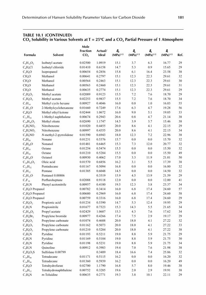
Determination of Hansen Solubility Parameter Values for Carbon Dioxide 181
TABLE 10.1 (CONTINUED)CO2 Solubility in Various Solvents at T = 25ºC and a CO2 Partial Pressure of 1 Atmosphere
Formula Solvent
MoleFraction
CO2
Actual/Ideal
δδδδd
(MPa)1/2
δδδδp
(MPa)1/2
δδδδh
(MPa)1/2
δδδδt
(MPa)1/2 Ref.
C6H12O2 Isobutyl acetate 0.02500 1.0919 15.1 3.7 6.3 16.77 29C4H9Cl Isobutyl chloride 0.01410 0.6158 14.7 5.3 0.9 15.65 29C3H8O Isopropanol 0.00654 0.2856 15.8 6.1 16.4 23.58 38CH4O Methanol 0.00641 0.2797 15.1 12.3 22.3 29.61 32CH4O Methanol 0.00564 0.2463 15.1 12.3 22.3 29.61 30CH4O Methanol 0.00563 0.2460 15.1 12.3 22.3 29.61 31CH4O Methanol 0.00635 0.2774 15.1 12.3 22.3 29.61 29C3H6O2 Methyl acetate 0.02089 0.9123 15.5 7.2 7.6 18.70 29C3H6O2 Methyl acetate 0.02253 0.9837 15.5 7.2 7.6 18.70 34C7H14 Methyl cyclo hexane 0.00927 0.4046 16.0 0.0 1.0 16.03 55C7H12O 2-Methylcyclohexanone 0.01660 0.7249 17.6 6.3 4.7 19.28 56C4H8O Methyl ethyl ketone 0.02444 1.0672 16.0 9.0 5.1 19.05 33C11H10 1-Methyl naphthalene 0.00674 0.2943 20.6 0.8 4.7 21.14 38C19H36O2 Methyl oleate 0.02690 1.1747 14.5 3.9 3.7 15.46 38C6H5NO2 Nitrobenzene 0.01020 0.4455 20.0 8.6 4.1 22.15 29C6H5NO2 Nitrobenzene 0.00997 0.4355 20.0 8.6 4.1 22.15 34C5H9NO N-methyl-2-pyrrolidone 0.01590 0.6943 18.0 12.3 7.2 22.96 38C9H20 Nonane 0.01231 0.5376 15.7 0.0 0.0 15.70 32C9H20O Nonanol 0.01481 0.6465 15.3 7.3 12.0 20.77 32C8H18 Octane 0.01254 0.5474 15.5 0.0 0.0 15.50 32C8H18 Octane 0.01210 0.5284 15.5 0.0 0.0 15.50 49C8H18O Octanol 0.00930 0.4062 17.0 3.3 11.9 21.01 50C18H34O2 Oleic acid 0.01570 0.6856 16.2 3.1 5.5 17.39 38C15H32 Pentadecane 0.01167 0.5094 16.8 0.0 0.0 16.80 32C5H12 Pentane 0.01385 0.6048 14.5 0.0 0.0 14.50 32C5H12O Pentanol 0.00806 0.3519 15.9 4.5 13.9 21.59 29C7F16 Perfluroheptane 0.02088 0.9118 12.0 0.0 0.0 12.00 41C8H7N Phenyl acetonitrile 0.00957 0.4180 19.5 12.3 3.8 23.37 34C3H8O Propanol 0.00782 0.3414 16.0 6.8 17.4 24.60 57C3H8O Propanol 0.00680 0.2969 16.0 6.8 17.4 24.60 58C3H8O Propanol 0.00759 0.3316 16.0 6.8 17.4 24.60 29C3H6O2 Propionic acid 0.01234 0.5390 14.7 5.3 12.4 19.95 29C3H5N Propionitrile 0.01677 0.7323 15.3 14.3 5.5 21.65 34C5H10O2 Propyl acetate 0.02429 1.0607 15.3 4.3 7.6 17.62 34C3H6Br2 Propylene bromide 0.00977 0.4266 17.4 7.5 2.9 19.17 29C4H6O3 Propylene carbonate 0.01074 0.4688 20.0 18.0 4.1 27.22 32C4H6O3 Propylene carbonate 0.01162 0.5073 20.0 18.0 4.1 27.22 33C4H6O3 Propylene carbonate 0.01210 0.5284 20.0 18.0 4.1 27.22 38C5H5N Pyridine 0.01193 0.5211 19.0 8.8 5.9 21.75 29C5H5N Pyridine 0.01169 0.5104 19.0 8.8 5.9 21.75 30C5H5N Pyridine 0.01198 0.5231 19.0 8.8 5.9 21.75 34C9H7N Quinoline 0.00912 0.3983 19.4 7.0 7.6 21.98 38C4H8O2S Sulfolane 0.00799 0.3489 18.4 16.6 7.4 25.86 32C14H30 Tetradecane 0.01171 0.5115 16.2 0.0 0.0 16.20 32C14H30 Tetradecane 0.01360 0.5939 16.2 0.0 0.0 16.20 49C4H8O Tetrahydrofuran 0.02700 1.1790 16.8 5.7 8.0 19.46 38C10H12 Tetrahydronaphthalene 0.00752 0.3285 19.6 2.0 2.9 19.91 38C7H9N m-Toluidine 0.00635 0.2771 19.3 3.8 10.1 22.11 29
7248_book.fm Page 181 Tuesday, April 24, 2007 9:19 AM
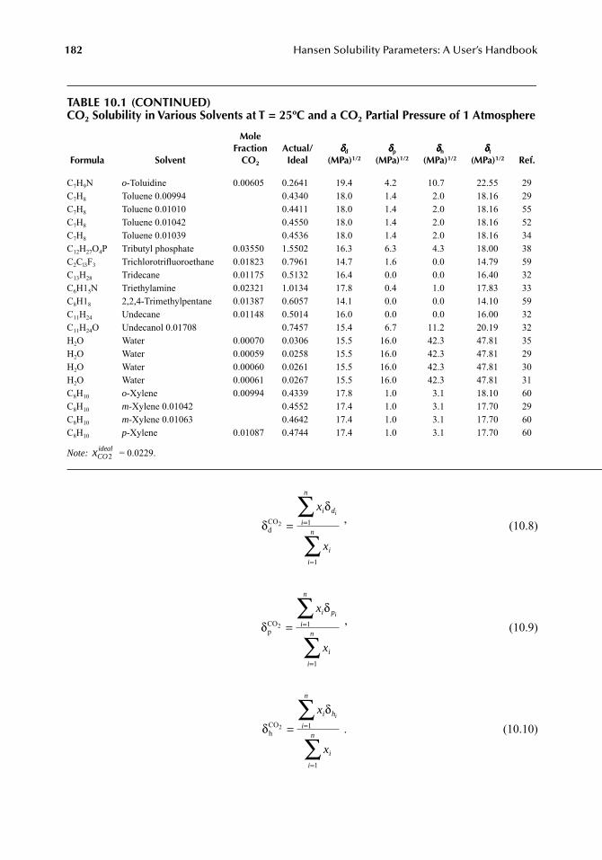
182 Hansen Solubility Parameters: A User’s Handbook
’ (10.8)
’ (10.9)
. (10.10)
TABLE 10.1 (CONTINUED)CO2 Solubility in Various Solvents at T = 25ºC and a CO2 Partial Pressure of 1 Atmosphere
Formula Solvent
MoleFraction
CO2
Actual/Ideal
δδδδd
(MPa)1/2
δδδδp
(MPa)1/2
δδδδh
(MPa)1/2
δδδδt
(MPa)1/2 Ref.
C7H9N o-Toluidine 0.00605 0.2641 19.4 4.2 10.7 22.55 29C7H8 Toluene 0.00994 0.4340 18.0 1.4 2.0 18.16 29C7H8 Toluene 0.01010 0.4411 18.0 1.4 2.0 18.16 55C7H8 Toluene 0.01042 0.4550 18.0 1.4 2.0 18.16 52C7H8 Toluene 0.01039 0.4536 18.0 1.4 2.0 18.16 34C12H27O4P Tributyl phosphate 0.03550 1.5502 16.3 6.3 4.3 18.00 38C2Cl3F3 Trichlorotrifluoroethane 0.01823 0.7961 14.7 1.6 0.0 14.79 59C13H28 Tridecane 0.01175 0.5132 16.4 0.0 0.0 16.40 32C6H15N Triethylamine 0.02321 1.0134 17.8 0.4 1.0 17.83 33C8H18 2,2,4-Trimethylpentane 0.01387 0.6057 14.1 0.0 0.0 14.10 59C11H24 Undecane 0.01148 0.5014 16.0 0.0 0.0 16.00 32C11H24O Undecanol 0.01708 0.7457 15.4 6.7 11.2 20.19 32H2O Water 0.00070 0.0306 15.5 16.0 42.3 47.81 35H2O Water 0.00059 0.0258 15.5 16.0 42.3 47.81 29H2O Water 0.00060 0.0261 15.5 16.0 42.3 47.81 30H2O Water 0.00061 0.0267 15.5 16.0 42.3 47.81 31C8H10 o-Xylene 0.00994 0.4339 17.8 1.0 3.1 18.10 60C8H10 m-Xylene 0.01042 0.4552 17.4 1.0 3.1 17.70 29C8H10 m-Xylene 0.01063 0.4642 17.4 1.0 3.1 17.70 60C8H10 p-Xylene 0.01087 0.4744 17.4 1.0 3.1 17.70 60
Note: = 0.0229.xCOideal
2
dCO2δ
δ= =
=
∑
∑
x
x
i d
i
n
i
i
n
i
1
1
pCO2δ
δ= =
=
∑
∑
x
x
i p
i
n
i
i
n
i
1
1
hCO2δ
δ= =
=
∑
∑
x
x
i h
i
n
i
i
n
i
1
1
7248_book.fm Page 182 Tuesday, April 24, 2007 9:19 AM
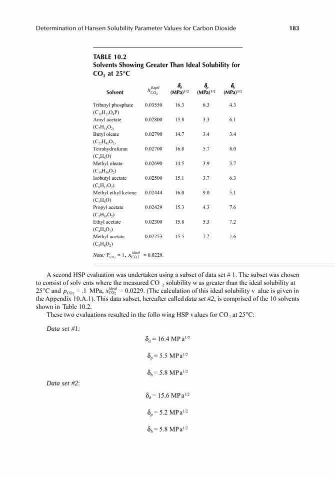
Determination of Hansen Solubility Parameter Values for Carbon Dioxide 183
A second HSP evaluation was undertaken using a subset of data set # 1. The subset was chosento consist of solv ents where the measured CO 2 solubility w as greater than the ideal solubility at25°C and pCO2 = .1 MPa, = 0.0229. (The calculation of this ideal solubility v alue is given inthe Appendix 10.A.1). This data subset, hereafter called data set #2, is comprised of the 10 solventsshown in Table 10.2.
These two evaluations resulted in the follo wing HSP values for CO 2 at 25°C:
Data set #1:
δd = 16.4 MP a1/2
δp = 5.5 MPa1/2
δh = 5.8 MPa1/2
Data set #2:
δd = 15.6 MPa1/2
δp = 5.2 MPa1/2
δh = 5.8 MPa1/2
TABLE 10.2Solvents Showing Greater Than Ideal Solubility for CO2 at 25°C
Solventδδδδd
(MPa)1/2
δδδδp
(MPa)1/2
δδδδh
(MPa)1/2
Tributyl phosphate(C12H27O4P)
0.03550 16.3 6.3 4.3
Amyl acetate(C7H14O2)
0.02800 15.8 3.3 6.1
Butyl oleate(C22H42O2)
0.02790 14.7 3.4 3.4
Tetrahydrofuran(C4H8O)
0.02700 16.8 5.7 8.0
Methyl oleate(C19H36O2)
0.02690 14.5 3.9 3.7
Isobutyl acetate(C6H12O2)
0.02500 15.1 3.7 6.3
Methyl ethyl ketone(C4H8O)
0.02444 16.0 9.0 5.1
Propyl acetate(C5H10O2)
0.02429 15.3 4.3 7.6
Ethyl acetate(C4H8O2)
0.02300 15.8 5.3 7.2
Methyl acetate(C3H6O2)
0.02253 15.5 7.2 7.6
Note: PCO2 = 1, = 0.0229.
xCOExptl
2
xCOideal
2
xidealCO2
7248_book.fm Page 183 Tuesday, April 24, 2007 9:19 AM
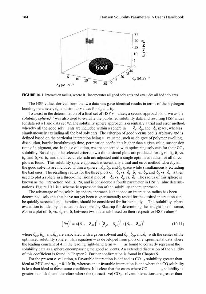
184 Hansen Solubility Parameters: A User’s Handbook
The HSP values derived from the two data sets gave identical results in terms of the h ydrogenbonding parameter, δh, and similar v alues for δp and δd.
To assist in the determination of a final set of HSP v alues, a second approach, kno wn as thesolubility sphere,5–7 was also used to evaluate the published solubility data and resulting HSP valuesfor data set #1 and data set #2. The solubility sphere approach is essentially a trial and error method,whereby all the good solv ents are included within a sphere in δd, δp, and δh space, whereassimultaneously excluding all the bad solv ents. The criterion of good v ersus bad is arbitrary and isdefined based on the particular interaction being e valuated, such as de gree of polymer swelling,dissolution, barrier breakthrough time, permeation coefficients higher than a given value, suspensiontime of a pigment, etc. In this e valuation, we are concerned with optimizing solv ents for their CO2solubility. Based upon the selected criteria, two-dimensional plots are produced for δd vs. δp, δd vs.δh, and δp vs. δh, and the three circle radii are adjusted until a single optimized radius for all threeplots is found. This solubility sphere approach is essentially a trial and error method whereby allthe good solvents are included within a sphere in δd, δp, and δh space while simultaneously excludingthe bad ones. The resulting radius for the three plots of δd vs. δp, δd vs. δh, and δp vs. δh, is thenused to plot a sphere in a three-dimensional plot of δd vs. δp vs. δh. The radius of this sphere isknown as the interaction radius, Ro, and is considered a fourth parameter in HSP v alue determi-nations. Figure 10.1 is a schematic representation of the solubility sphere approach.
The advantage of the solubility sphere approach is that once an interaction radius has beendetermined, solvents that ha ve not yet been e xperimentally tested for the desired interaction canbe quickly screened and, therefore, should be considered for further study . This solubility sphereevaluation is aided by an equation developed by Skaarup for determining the straight-line distance,Ra, in a plot of δd vs. δp vs. δh between two materials based on their respecti ve HSP values,5
(10.11)
where δd2, δp2, and δh2 are associated with a given solvent and δd1, δp1, and δh1 with the center of theoptimized solubility sphere. This equation w as developed from plots of e xperimental data wherethe leading constant of 4 in the leading right-hand term w as found to correctly represent thesolubility data as a sphere encompassing the good solv ents. An extended discussion of the validityof this coefficient is found in Chapter 2. Further confirmation is found in Chapter 9.
For the present e valuation, a f avorable interaction is defined as CO 2 solubility greater thanideal at 25°C and pCO2 = 0.1 MPa, whereas an unfavorable interaction is one where the CO2 solubilityis less than ideal at these same conditions. It is clear that for cases where CO 2 solubility isgreater than ideal, and therefore where the (attracti ve) CO 2–solvent interactions are greater than
FIGURE 10.1 Interaction radius, where R o incorporates all good solv ents and excludes all bad solv ents.
δd (M Pa)½δp (M Pa)½
δ h (M
Pa)
½
25 20 151050
20151050
5 10 15 20 25
Ra d d p p h h( ) = −( ) + −( ) + −( )22 1
22 1
22 1
24 δ δ δ δ δ δ
7248_book.fm Page 184 Tuesday, April 24, 2007 9:19 AM
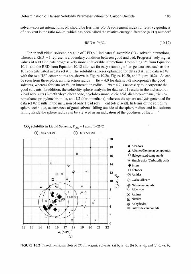
Determination of Hansen Solubility Parameter Values for Carbon Dioxide 185
solvent–solvent interactions, Ra should be less than Ro. A convenient index for relative goodnessof a solvent is the ratio Ra/Ro, which has been called the relative energy difference (RED) number5
(10.12)
For an indi vidual solvent, a v alue of RED < 1 indicates f avorable CO 2–solvent interactions,whereas a RED ≈ 1 represents a boundary condition between good and bad. Progressi vely highervalues of RED indicate progressively more unfavorable interactions. Computing Ra from Equation10.11 and the RED from Equation 10.12 allo ws for easy scanning of lar ge data sets, such as the101 solvents listed in data set #1. The solubility spheres optimized for data set #1 and data set #2with the two HSP center points are shown in Figure 10.2a, Figure 10.2b, and Figure 10.2c. As canbe seen from these plots, an interaction radius Ro = 4.0 for data set #2 incorporates the goodsolvents, whereas for data set #1, an interaction radius Ro = 4.7 is necessary to incorporate thegood solvents. In addition, the solubility sphere analysis for data set #1 results in the inclusion of7 bad solv ents (2-meth ylcyclohexanone, c yclohexanone, oleic acid, dichloromethane, trichlo-romethane, propylene bromide, and 1,2-dibromoethane), whereas the sphere analysis generated fordata set #2 results in the inclusion of only 1 bad solv ent (oleic acid). In terms of the solubilitysphere technique, occurrences of good solvents falling outside of the sphere radius, and bad solventsfalling inside the sphere radius can be vie wed as an indication of the goodness of the fit. 5
FIGURE 10.2 Two-dimensional plots of CO2 in organic solvents. (a) δp vs. δd, (b) δh vs. δp, and (c) δh vs. δd.
RED Ra Ro=
CO2 Solubility in Liquid Solvents, PCO2 = 1 atm., T=25°CData Set #11 Data Set #2
δ P (M
Pa)½
δd (MPa)½
20
18
16
14
12
10
8
6
4
2
0
AlcoholsAlkanes/Nonpolar compoundsHalogenated compoundsSimple acids/Carboxylic acidsEstersKetonesAmidesCyclic AlkenesNitro compoundsAldehydeAminesNitrilesAnhydridesSulfoxide compounds
(a)
1312 14 15 16 17 18 19 20 21 22
2
7248_book.fm Page 185 Tuesday, April 24, 2007 9:19 AM
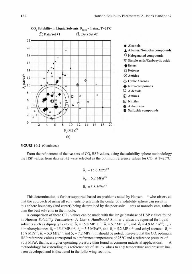
186 Hansen Solubility Parameters: A User’s Handbook
From the refinement of the two sets of CO2 HSP values, using the solubility sphere methodology,the HSP values from data set #2 were selected as the optimum reference values for CO2 at T=25°C;
This determination is further supported based on problems noted by Hansen, 5 who observ edthat the approach of using all solv ents to establish the center of a solubility sphere can result inthis sphere boundary (and center) being determined by the poor solv ents or nonsolv ents, ratherthan the best solv ents in the middle.
A comparison of these CO 2 values can be made with the lar ge database of HSP v alues foundin Hansen Solubility Parameters: A User’s Handbook.5 Similar v alues are reported for liquidsolvents such as diprop yl k etone: δd = 15.8 MP a1/2, δp = 5.7 MP a1/2, and δh = 4.9 MP a1/2; 1,3-dimethoxybutane: δd = 15.6 MP a1/2, δp = 5.5 MP a1/2, and δh = 5.2 MP a1/2; and ethyl acetate: δd =15.8 MPa1/2, δp = 5.3 MPa1/2, and δh = 7.2 MPa1/2. It should be noted, however, that the CO2 optimumHSP reference v alues correspond to a reference temperature of 25°C and a reference pressure of90.5 MPa8, that is, a higher operating pressure than found in common industrial applications. Amethodology for e xtending this reference set of HSP v alues to an y temperature and pressure hasbeen developed and is discussed in the follo wing sections.
FIGURE 10.2 (Continued)
CO2 Solubility in Liquid Solvents, PCO2 = 1 atm., T=25°CData Set #11 Data Set #22
δ h (MPa
)½
δp (MPa)½
22
20
18
16
14
12
10
8
6
4
2
0
AlcoholsAlkanes/Nonpolar compoundsHalogenated compoundsSimple acids/Carboxylic acidsEstersKetonesAmidesCyclic AlkenesNitro compoundsAldehydeAminesNitrilesAnhydridesSulfoxide compounds
(b)
2 4 6 8 10 12 14 16 18 20
δ
δ
δ
d
p
h
MPa
MPa
MPa
=
=
=
15 6
5 2
5 8
1 2
1 2
1 2
.
.
.
/
/
/
7248_book.fm Page 186 Tuesday, April 24, 2007 9:19 AM
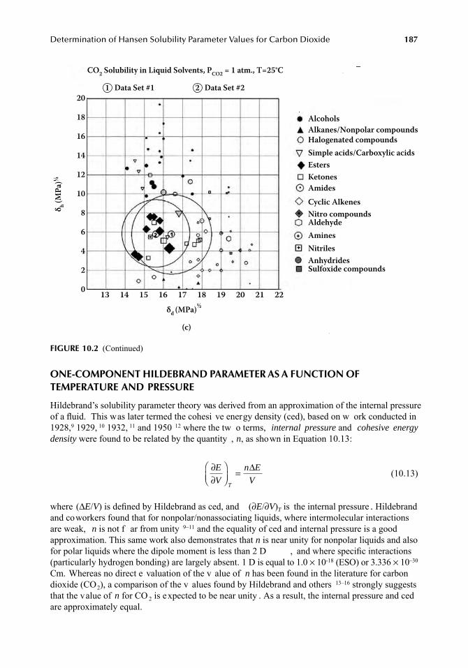
Determination of Hansen Solubility Parameter Values for Carbon Dioxide 187
ONE-COMPONENT HILDEBRAND PARAMETER AS A FUNCTION OF TEMPERATURE AND PRESSURE
Hildebrand’s solubility parameter theory was derived from an approximation of the internal pressureof a fluid. This was later termed the cohesi ve energy density (ced), based on w ork conducted in1928,9 1929, 10 1932, 11 and 1950 12 where the tw o terms, internal pressure and cohesive energydensity were found to be related by the quantity , n, as shown in Equation 10.13:
(10.13)
where (ΔE/V) is defined by Hildebrand as ced, and (∂E/∂V)T is the internal pressure . Hildebrandand coworkers found that for nonpolar/nonassociating liquids, where intermolecular interactionsare weak, n is not f ar from unity 9–11 and the equality of ced and internal pressure is a goodapproximation. This same work also demonstrates that n is near unity for nonpolar liquids and alsofor polar liquids where the dipole moment is less than 2 D , and where specific interactions(particularly hydrogen bonding) are largely absent. 1 D is equal to 1.0 × 10⁻¹⁸ (ESO) or 3.336 × 10⁻³⁰
Cm. Whereas no direct e valuation of the v alue of n has been found in the literature for carbondioxide (CO2), a comparison of the v alues found by Hildebrand and others 13–16 strongly suggeststhat the value of n for CO 2 is expected to be near unity . As a result, the internal pressure and cedare approximately equal.
FIGURE 10.2 (Continued)
CO2 Solubility in Liquid Solvents, PCO2 = 1 atm., T=25°C
Data Set #11 Data Set #22
δd (MPa)½
AlcoholsAlkanes/Nonpolar compoundsHalogenated compoundsSimple acids/Carboxylic acidsEstersKetonesAmidesCyclic AlkenesNitro compoundsAldehydeAminesNitrilesAnhydridesSulfoxide compounds
(c)
13 14 15 16 17 18 19 20 21 22
δ h (MPa
)½
20
18
16
14
12
10
8
6
4
2
0
∂∂
⎛⎝⎜
⎞⎠⎟
=E
V
n E
VT
Δ
7248_book.fm Page 187 Tuesday, April 24, 2007 9:19 AM
188 Hansen Solubility Parameters: A User’s Handbook
Accordingly, Hildebrand's solubility parameter, defined as the square root of the ced,12 can alsobe approximated by the square root of the internal pressure for nonpolar/nonassociating fluids.
(10.14)
And the internal pressure can be calculated from the thermodynamic equation of state, Equation10.15.
(10.15)
so that
(10.16)
Total (one-component) solubility parameters can therefore be calculated using an EOS of theform, P = f (ρ,T). This approach is used in this w ork to calculate the total solubility parameter forpure CO2, using the empirical EOS of Huang et al. 17
(10.17)
where
(10.18)
and,
(10.19)
The state constants (c i) are as defined in the Huang reference.
δ =⎛⎝⎜
⎞⎠⎟
≈ ∂∂
⎛⎝⎜
⎞⎠⎟
ΔE
V
E
VT T
1 2 1 2/ /
∂∂
⎛⎝⎜
⎞⎠⎟
= ∂∂
⎛⎝⎜
⎞⎠⎟
−E
VT
P
TP
T V
δ2 ≈ ∂∂
⎛⎝⎜
⎞⎠⎟
= ∂∂
⎛⎝⎜
⎞⎠⎟
−E
VT
P
TP
T V
P R T
b b b b b b
=
+ + + + + +
ρ
ρ ρ ρ ρ ρ ρ1 2 32
43
54
65
72' ' ' ' ' ' expp exp
exp
' ' '
'
−( ) + −( )+ −
c b c
c c
212
84
212
222
27
ρ ρ ρ
ρ ΔΔ Δ Δ ΔT c c c T( )⎡⎣⎢
⎤⎦⎥
+ − ( ) − ( )⎡⎣
223 25
227
2ρρ
ρ' exp ⎢⎢⎤⎦⎥
+ − ( ) − ( )⎡⎣⎢
⎤⎦⎥
⎡
⎣
⎢
c c c T24 262
272Δ Δ Δρ
ρρ' exp
⎢⎢⎢⎢⎢⎢⎢⎢⎢
⎤
⎦
⎥⎥⎥⎥⎥⎥⎥⎥⎥
′ = = − ′ ′ = = − ′T T T T Tc c; ; ; / Δ Δ1 1 1ρ ρ ρ ρ ρ
b cc
T
c
T
c
T
c
T
c
T2 1
2 32
43
54
65= + + + + +
⎛⎝⎜
⎞⎠⎟' ' ' ' ' ; b
c
T
b cc
T
c
T
614
3 78 9
2
=⎛⎝⎜
⎞⎠⎟
= + +⎛⎝⎜
⎞
'
' ' ⎠⎠⎟; b77
153
164
175
4 1011
= + +⎛⎝⎜
⎞⎠⎟
= +⎛⎝
c
T
c
T
c
T
b cc
T
' ' '
'⎜⎜⎞⎠⎟
; bc
T
c
T
c
T
b c
818
319
420
5
5
= + +⎛⎝⎜
⎞⎠⎟
=
' ' '
11213+
⎛⎝⎜
⎞⎠⎟
c
T '
7248_book.fm Page 188 Tuesday, April 24, 2007 9:19 AM
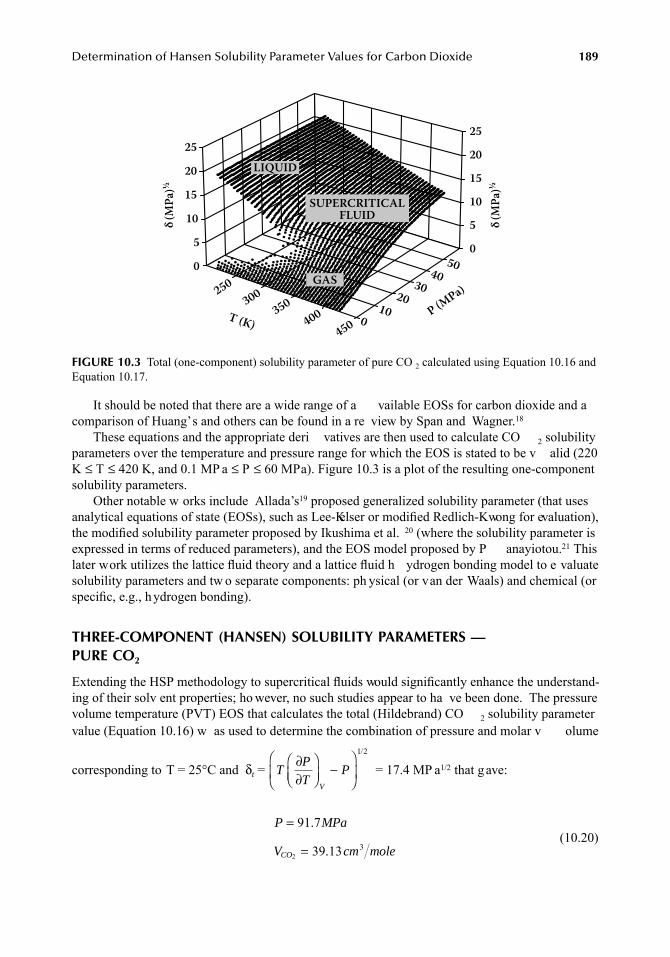
Determination of Hansen Solubility Parameter Values for Carbon Dioxide 189
It should be noted that there are a wide range of a vailable EOSs for carbon dioxide and acomparison of Huang’s and others can be found in a re view by Span and Wagner.18
These equations and the appropriate deri vatives are then used to calculate CO 2 solubilityparameters over the temperature and pressure range for which the EOS is stated to be v alid (220K ≤ T ≤ 420 K, and 0.1 MP a ≤ P ≤ 60 MPa). Figure 10.3 is a plot of the resulting one-componentsolubility parameters.
Other notable w orks include Allada’s19 proposed generalized solubility parameter (that usesanalytical equations of state (EOSs), such as Lee-Kelser or modified Redlich-Kwong for evaluation),the modified solubility parameter proposed by Ikushima et al. 20 (where the solubility parameter isexpressed in terms of reduced parameters), and the EOS model proposed by P anayiotou.21 Thislater work utilizes the lattice fluid theory and a lattice fluid h ydrogen bonding model to e valuatesolubility parameters and tw o separate components: ph ysical (or van der Waals) and chemical (orspecific, e.g., hydrogen bonding).
THREE-COMPONENT (HANSEN) SOLUBILITY PARAMETERS — PURE CO2
Extending the HSP methodology to supercritical fluids would significantly enhance the understand-ing of their solv ent properties; ho wever, no such studies appear to ha ve been done. The pressurevolume temperature (PVT) EOS that calculates the total (Hildebrand) CO 2 solubility parametervalue (Equation 10.16) w as used to determine the combination of pressure and molar v olume
corresponding to T = 25°C and δt = = 17.4 MP a1/2 that gave:
(10.20)
FIGURE 10.3 Total (one-component) solubility parameter of pure CO 2 calculated using Equation 10.16 andEquation 10.17.
LIQUID
GAS
SUPERCRITICALFLUIDδ (M
Pa)½
δ (MPa
)½
25
20
15
10
5
0
25 20 15 1050
250300
350400
450T (K)
P (MPa)
010
2030
4050
TP
TP
V
∂∂
⎛⎝⎜
⎞⎠⎟
−⎛
⎝⎜
⎞
⎠⎟
1 2/
P MPa
V cm moleCO
=
=
91 7
39 1323
.
.
7248_book.fm Page 189 Tuesday, April 24, 2007 9:19 AM
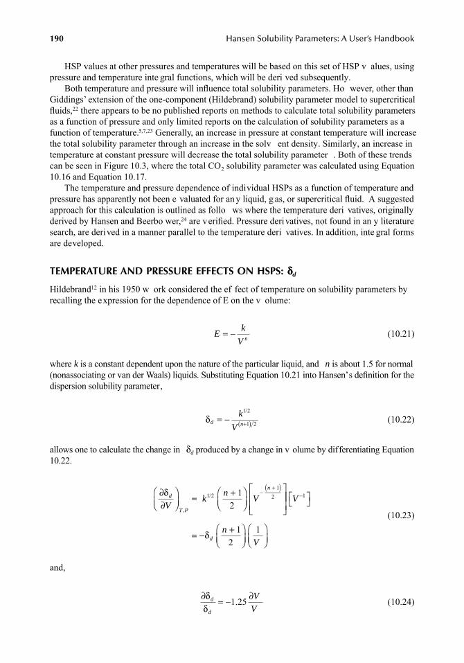
190 Hansen Solubility Parameters: A User’s Handbook
HSP values at other pressures and temperatures will be based on this set of HSP v alues, usingpressure and temperature inte gral functions, which will be deri ved subsequently.
Both temperature and pressure will influence total solubility parameters. Ho wever, other thanGiddings’ extension of the one-component (Hildebrand) solubility parameter model to supercriticalfluids,22 there appears to be no published reports on methods to calculate total solubility parametersas a function of pressure and only limited reports on the calculation of solubility parameters as afunction of temperature.5,7,23 Generally, an increase in pressure at constant temperature will increasethe total solubility parameter through an increase in the solv ent density. Similarly, an increase intemperature at constant pressure will decrease the total solubility parameter . Both of these trendscan be seen in Figure 10.3, where the total CO2 solubility parameter was calculated using Equation10.16 and Equation 10.17.
The temperature and pressure dependence of individual HSPs as a function of temperature andpressure has apparently not been e valuated for an y liquid, g as, or supercritical fluid. A suggestedapproach for this calculation is outlined as follo ws where the temperature deri vatives, originallyderived by Hansen and Beerbo wer,24 are verified. Pressure derivatives, not found in an y literaturesearch, are derived in a manner parallel to the temperature deri vatives. In addition, inte gral formsare developed.
TEMPERATURE AND PRESSURE EFFECTS ON HSPS: δδδδd
Hildebrand12 in his 1950 w ork considered the ef fect of temperature on solubility parameters byrecalling the expression for the dependence of E on the v olume:
(10.21)
where k is a constant dependent upon the nature of the particular liquid, and n is about 1.5 for normal(nonassociating or van der Waals) liquids. Substituting Equation 10.21 into Hansen’s definition for thedispersion solubility parameter,
(10.22)
allows one to calculate the change in δd produced by a change in v olume by differentiating Equation10.22.
(10.23)
and,
(10.24)
Ek
V n= −
δd n
k
V= − +( )
1 2
1 2
/
∂∂
⎛⎝⎜
⎞⎠⎟
= +⎛⎝⎜
⎞⎠⎟
⎡
⎣⎢⎢
⎤
⎦
−+( )δd
T P
n
Vk
nV
,
/1 21
212
⎥⎥⎥
⎡⎣ ⎤⎦
= − +⎛⎝⎜
⎞⎠⎟
⎛⎝⎜
⎞⎠⎟
−V
n
Vd
1
12
1δ
∂ = − ∂δδ
d
d
V
V1 25.
7248_book.fm Page 190 Tuesday, April 24, 2007 9:19 AM
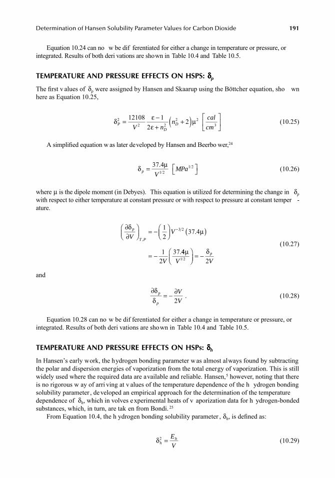
Determination of Hansen Solubility Parameter Values for Carbon Dioxide 191
Equation 10.24 can no w be dif ferentiated for either a change in temperature or pressure, orintegrated. Results of both deri vations are shown in Table 10.4 and Table 10.5.
TEMPERATURE AND PRESSURE EFFECTS ON HSPS: δδδδp
The first v alues of δp were assigned by Hansen and Skaarup using the Böttcher equation, sho wnhere as Equation 10.25,
(10.25)
A simplified equation w as later developed by Hansen and Beerbo wer,24
(10.26)
where μ is the dipole moment (in Debyes). This equation is utilized for determining the change in δp
with respect to either temperature at constant pressure or with respect to pressure at constant temper -ature.
(10.27)
and
. (10.28)
Equation 10.28 can no w be dif ferentiated for either a change in temperature or pressure, orintegrated. Results of both deri vations are shown in Table 10.4 and Table 10.5.
TEMPERATURE AND PRESSURE EFFECTS ON HSPs: δδδδh
In Hansen’s early work, the hydrogen bonding parameter was almost always found by subtractingthe polar and dispersion energies of vaporization from the total energy of vaporization. This is stillwidely used where the required data are available and reliable. Hansen,5 however, noting that thereis no rigorous w ay of arri ving at v alues of the temperature dependence of the h ydrogen bondingsolubility parameter , developed an empirical approach for the determination of the temperaturedependence of δh, which in volves experimental heats of v aporization data for h ydrogen-bondedsubstances, which, in turn, are tak en from Bondi. 25
From Equation 10.4, the h ydrogen bonding solubility parameter , δh, is defined as:
(10.29)
δ εε
μPD
DV n
n22 2
2 212108 12
2= −+
+( ) cal
cm3
⎡
⎣⎢
⎤
⎦⎥
δ μp
V= 37 4
1 2
./ MPa1 2/⎡⎣ ⎤⎦
∂∂
⎛⎝⎜
⎞⎠⎟
= − ⎛⎝⎜
⎞⎠⎟ ( )
= −
−δμp
T PVV
V
,
.
.
12
37 4
12
37
3 2
4421 2
μ δV V
p/
⎛⎝⎜
⎞⎠⎟
= −
∂= − ∂δ
δp
p
V
V2
δhhE
V2 =
7248_book.fm Page 191 Tuesday, April 24, 2007 9:19 AM
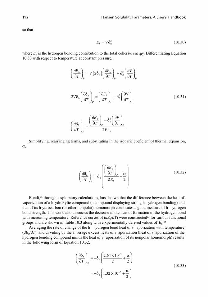
192 Hansen Solubility Parameters: A User’s Handbook
so that
(10.30)
where Eh is the hydrogen bonding contribution to the total cohesive energy. Differentiating Equation10.30 with respect to temperature at constant pressure,
(10.31)
Simplifying, rearranging terms, and substituting in the isobaric coefficient of thermal expansion,α,
(10.32)
Bondi,25 through e xploratory calculations, has sho wn that the dif ference between the heat ofvaporization of a h ydroxylic compound (a compound displaying strong h ydrogen bonding) andthat of its h ydrocarbon (or other nonpolar) homomorph constitutes a good measure of h ydrogenbond strength. This work also discusses the decrease in the heat of formation of the hydrogen bondwith increasing temperature. Reference curves of (dEh/dT) were constructed23 for various functionalgroups and are sho wn in Table 10.3 along with e xperimentally derived values of Eh.25
Averaging the rate of change of the h ydrogen bond heat of v aporization with temperature(dEh/dT), and di viding by the a verage e xcess heats of v aporization (heat of v aporization of thehydrogen bonding compound minus the heat of v aporization of its nonpolar homomorph) resultsin the following form of Equation 10.32,
(10.33)
E Vh h= δ2
∂∂
⎛⎝⎜
⎞⎠⎟
= ( ) ∂∂
⎛⎝⎜
⎞⎠⎟
+ ∂∂
⎛⎝⎜
⎞E
TV
T
V
Th
P
hh
P
h2 2δ δ δ⎠⎠⎟
∂∂
⎛⎝⎜
⎞⎠⎟
= ∂∂
⎛⎝⎜
⎞⎠⎟
− ∂∂
⎛⎝
P
hh
P
h
P
hVT
E
T
V
T2 2δ δ δ ⎜⎜
⎞⎠⎟
∂∂
⎛⎝⎜
⎞⎠⎟
=
∂∂
⎛⎝⎜
⎞⎠⎟
− ∂∂
⎛⎝⎜
⎞
P
h
P
h
P
h
T
E
T
V
Tδδ2
⎠⎠⎟P
hV2 δ
∂∂
⎛⎝⎜
⎞⎠⎟
=
∂∂
⎛⎝⎜
⎞⎠⎟
−
⎛
⎝
⎜⎜⎜⎜
⎞
⎠
⎟⎟δ δ αh
P
h
h
P
hT
E
T
E2 2 ⎟⎟⎟
∂∂
⎛⎝⎜
⎞⎠⎟
= − × +⎛
⎝⎜⎞
⎠⎟
= −
−δ δ α
δ
h
P
h
h
T
2 64 102 2
1 32
3.
. ×× +⎛⎝⎜
⎞⎠⎟
−102
3 α
7248_book.fm Page 192 Tuesday, April 24, 2007 9:19 AM
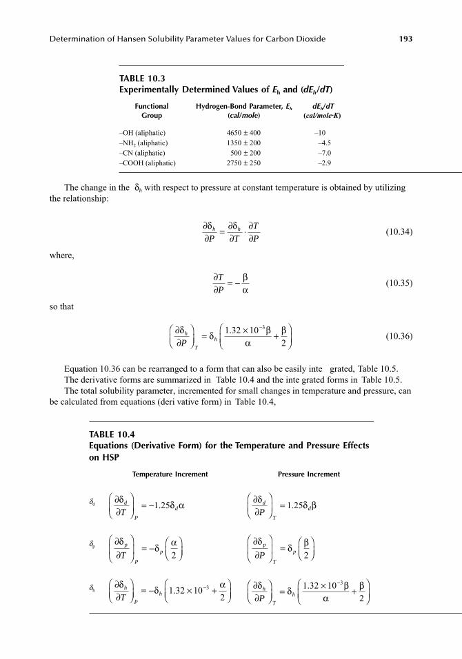
Determination of Hansen Solubility Parameter Values for Carbon Dioxide 193
The change in the δh with respect to pressure at constant temperature is obtained by utilizingthe relationship:
(10.34)
where,
(10.35)
so that
(10.36)
Equation 10.36 can be rearranged to a form that can also be easily inte grated, Table 10.5.The derivative forms are summarized in Table 10.4 and the inte grated forms in Table 10.5.The total solubility parameter, incremented for small changes in temperature and pressure, can
be calculated from equations (deri vative form) in Table 10.4,
TABLE 10.3Experimentally Determined Values of Eh and (dEh/dT)
FunctionalGroup
Hydrogen-Bond Parameter, Eh
(cal/mole)dEh/dT
(cal/mole·K)
–OH (aliphatic) 4650 ± 400 –10–NH2 (aliphatic) 1350 ± 200 –4.5–CN (aliphatic) 500 ± 200 –7.0–COOH (aliphatic) 2750 ± 250 –2.9
TABLE 10.4Equations (Derivative Form) for the Temperature and Pressure Effects on HSP
Temperature Increment Pressure Increment
δd
δp
δh
∂∂
= ∂∂
⋅ ∂∂
δ δh h
P T
T
P
∂∂
= −T
P
βα
∂∂
⎛⎝⎜
⎞⎠⎟
= × +⎛
⎝⎜⎞
⎠⎟−δ δ β
αβh
T
hP
1 32 102
3.
∂∂
⎛
⎝⎜⎞
⎠⎟= −δ δ αd
P
dT1 25. ∂
∂⎛
⎝⎜⎞
⎠⎟=δ δ βd
T
dP1 25.
∂∂
⎛
⎝⎜
⎞
⎠⎟ = −
⎛⎝⎜
⎞⎠⎟
δδ αp
P
pT 2∂∂
⎛
⎝⎜
⎞
⎠⎟ =
⎛⎝⎜
⎞⎠⎟
δδ βp
T
pP 2
∂∂
⎛⎝⎜
⎞⎠⎟
= − × +⎛⎝⎜
⎞⎠⎟
−δ δ αh
P
hT1 32 10
23. ∂
∂⎛⎝⎜
⎞⎠⎟
= × +⎛
⎝⎜⎞
⎠⎟−δ δ β
αβh
T
hP
1 32 102
3.
7248_book.fm Page 193 Tuesday, April 24, 2007 9:19 AM
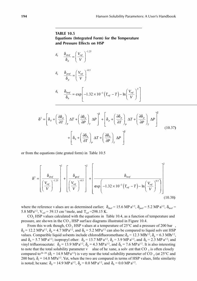
194 Hansen Solubility Parameters: A User’s Handbook
(10.37)
or from the equations (inte grated form) in Table 10.5
(10.38)
where the reference v alues are as determined earlier; δdref = 15.6 MP a1/2, δpref = 5.2 MP a1/2, δhref =5.8 MPa1/2, Vref = 39.13 cm 3/mole, and Tref =298.15 K.
CO2 HSP values calculated with the equations in Table 10.4, as a function of temperature andpressure, are shown in the CO 2 HSP surface diagrams illustrated in Figure 10.4.
From this work though, CO 2 HSP values at a temperature of 25°C and a pressure of 200 bar ,δd = 12.2 MPa1/2, δp = 4.7 MPa1/2, and δh = 5.2 MPa1/2 can also be compared to liquid solv ent HSPvalues. Comparible liquid solvents include chlorodifluoromethane: δd = 12.3 MPa1/2, δp = 6.3 MPa1/2,and δh = 5.7 MP a1/2; isopropyl ether: δd = 13.7 MP a1/2, δp = 3.9 MP a1/2, and δh = 2.3 MP a1/2; andvinyl trifluoroacetate: δd = 13.9 MPa1/2, δp = 4.3 MPa1/2, and δh = 7.6 MPa1/2. It is also interestingto note that the total solubility parameter v alue of he xane, a solv ent that CO 2 is often closelycompared to26–28 (δt = 14.9 MPa1/2) is very near the total solubility parameter of CO 2 (at 25°C and200 bar), δt = 14.0 MPa1/2. Yet, when the two are compared in terms of HSP values, little similarityis noted; hexane: δd = 14.9 MP a1/2, δp = 0.0 MP a1/2, and δh = 0.0 MP a1/2.
TABLE 10.5Equations (Integrated Form) for the Temperature and Pressure Effects on HSP
δd
δp
δh
δδdref
d
refV
V=
⎛
⎝⎜⎞
⎠⎟
−1 25.
δδpref
p
refV
V=
⎛
⎝⎜⎞
⎠⎟
−0 5.
δδhref
href
refT TV
V= − × −( ) −
⎛
⎝⎜⎞
⎠⎟−exp . ln1 32 10 3
..5⎡
⎣
⎢⎢
⎤
⎦
⎥⎥
δ δ δ δ2 = + ∂∂
⎛⎝⎜
⎞⎠⎟
+ ∂∂
⎛⎝⎜
⎞⎠⎟
⎡
⎣⎢⎢
⎤
⎦⎥⎥
dd
P
d
TT
TP
PΔ Δ22
+ +∂∂
⎛
⎝⎜⎞
⎠⎟+
∂∂
⎛
⎝⎜⎞
⎠⎟⎡
⎣
⎢⎢
⎤
⎦
⎥⎥
δδ δ
pp
P
p
TT
TP
PΔ Δ
22
+ + ∂∂
⎛⎝⎜
⎞⎠⎟
+ ∂∂
⎛⎝⎜
⎞⎠⎟
⎡
⎣⎢⎢
⎤
⎦⎥⎥
δ δ δh
h
P
h
TT
TP
PΔ Δ
22
δδ δ2
1 25
2
=⎛
⎝⎜⎞
⎠⎟
⎡
⎣
⎢⎢⎢⎢⎢⎢
⎤
⎦
⎥⎥⎥⎥⎥⎥
+−dref
refV
V
.ppref
ref
href
V
V
⎛
⎝⎜⎞
⎠⎟
⎡
⎣
⎢⎢⎢⎢⎢⎢
⎤
⎦
⎥⎥⎥⎥⎥⎥
+−0 5
2
.
δ
eexp . ln.
− × −( ) −⎛
⎝⎜⎞
⎠⎟⎛
⎝⎜⎜
−1 32 10 3
0 5
T TV
Vrefref
⎞⎞
⎠⎟⎟
⎡
⎣
⎢⎢⎢⎢⎢⎢⎢
⎤
⎦
⎥⎥⎥⎥⎥⎥⎥
2
7248_book.fm Page 194 Tuesday, April 24, 2007 9:19 AM
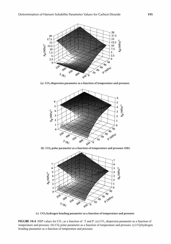
Determination of Hansen Solubility Parameter Values for Carbon Dioxide 195
FIGURE 10.4 HSP values for CO 2 as a function of T and P. (a) CO 2 dispersion parameter as a function oftemperature and pressure. (b) CO2 polar parameter as a function of temperature and pressure. (c) CO2 hydrogenbonding parameter as a function of temperature and pressure.
(a) CO2 dispersion parameter as a function of temperature and pressure.
(b) CO2 polar parameter as a function of temperature and pressure 45K)
(c) CO2 hydrogen bonding parameter as a function of temperature and pressure
δ d (M
Pa)½
δ d (M
Pa)½
20 17.5
15 12.5
10 7.5
52.5
0
δ p (M
Pa)½
δ p (M
Pa)½
65 4 3 2 1 0
6 5 4 3 2 10
20 17.5 15 12.5 10 7.5 52.50
250300
350400
450T (K)
250300
350400
450T (K)
P (MPa)
010
2030
4050
P (MPa)
010
2030
4050
δ h (M
Pa)½
δ h (M
Pa)½
765 4 3 2 1 0
7 65 4 3210
250300
350400
450T (K)P (M
Pa)
010
2030
4050
7248_book.fm Page 195 Tuesday, April 24, 2007 9:19 AM
196 Hansen Solubility Parameters: A User’s Handbook
CONCLUSION
A set of Hansen solubility parameters at T = 25°C ha ve been determined for CO 2, based on theroom temperature solubility in different liquid solvents of known HSP values: δd = 15.6 MPa1/2, δp
= 5.2 MP a1/2, and δh = 5.8 MP a1/2. Further, this set of HSPs were refined using the RED af finitynumber and Hansen solubility plots to correlate the solubility of carbon dioxide in the solv entsidentified in Table 10.1.
It is important to note that the solubility parameter, or rather the difference in solubility parameters,for a given solvent–solute combination has been foremost in determining the mutual solubility of thesystem.5 An analogy to “lik e dissolv es lik e” is appropriate. Therefore, the accurac y to which thesolubility parameters for a binary pair can be kno wn will be v aluable in predicting the system’ sbehavior. This work introduces a theoretical methodology for generating solubility parameter v alues,both one-component Hildebrand and three-component Hansen parameters, for a pure supercriticalfluid, using CO 2 as an e xample. The ability to e xpress molecular interactions, in terms of HSPs, fora pure fluid solv ent in a w ay that unites the liquid, g as, and supercritical phases, represents anadvancement in the understanding of the role of solv ents in both e xisting and new applications.
ACKNOWLEDGMENTS
Special thanks to James Rubin of Los Alamos National Laboratory for his excellent assistance andcollaboration in the de velopment of this w ork.
CHAPTER 10 ADDENDUM
Research has been the k ey to man y progressive developments. Significant steps to ward improvedunderstanding have been made with limited resources, and these result in still other impro vements inthe same direction when other resources are applied. The HSP for carbon dioxide reported in thechapter ( δd, δp, and δh equal to 15.6 MP a1/2, 5.2 MP a1/2, and 5.8 MP a1/2) were found by a plottingtechnique with a radius for the solubility sphere of 4.0 MP a1/2. The data used were collected from awide variety of sources, and the criterion for a good solvent was solubility in excess of the theoretical.A computer analysis of the same data has no w shown that it is possible to describe the solubility ofcarbon dioxide with a slightly dif ferent solubility sphere. The δd, δp, and δh values 15.7 MP a1/2, 6.3MPa1/2, and 5.7 MP a1/2 were found to gi ve a perfect data fit of 1.000 (v ersus 0.981) with a radius ofonly 3.3 MPa1/2. Both correlations emphatically sho w the ability of this procedure, whether by handor by computer , to correlate g as/liquid solubility data for a wide v ariety of chemically dif ferentsolvents. It has not been possible, nor has it been deemed necessary , to re vise the contents of thischapter using these slightly dif ferent numbers. This note is only to indicate wh y a slightly dif ferentset of HSP is reported else where in this handbook (T able A-1 and Chapter 13, Table 13.4).
7248_book.fm Page 196 Tuesday, April 24, 2007 9:19 AM
Determination of Hansen Solubility Parameter Values for Carbon Dioxide 197
SYMBOLS SPECIAL TO THIS CHAPTER
REFERENCES
1. Hansen, C.M., The three dimensional solubility parameter — k ey to paint component af finities. I.Solvents, plasticizers, polymers, and resins, J. Paint Technol., Vol. 39, No. 505, 104–117, 1967.
2. Wilhelm, E. and Battino, R., Thermodynamic functions of the solubilities of gases in liquids at 25°C,Chem. Rev., Vol. 73, No. 1, 1–9, 1973.
3. Battino, R. and Cle ver, H.L., The solubility of g ases in liquids, Solutions and Solubilities, Dack,M.R.J., Ed., John Wiley & Sons, Ne w York, 1965, p. 379, chap. 7.
4. Reid, R.C., Prausnitz, J.M., and Poling, B.E., The Properties of Gases and Liquids, 4th ed., McGrawHill, New York, 1987, p. 334.
5. Hansen, C.M., Hansen Solubility Parameters: A User’s Handbook, CRC Press, Boca Raton, FL, 1999.6. Hansen, C.M., The Three Dimensional Solubility Parameter and Solvent Diffusion Coefficient, Copen-
hagen Danish Technical Press, Denmark, 1967, pp. 33–38.7. Barton, A.F.M., CRC Handbook of Solubility Parameters and Other Cohesion Parameters, 2nd ed.,
CRC Press, Boca Raton, FL, 1991.8. Williams, L.L., Rubin, J.B., and Edw ards, H.W., Calculation of Hansen solubility parameter v alues
for a range of pressure and temperature conditions, including the supercritical fluid re gion, Ind. Eng.Chem. Res., Vol. 43, 4967–4972, 2004.
9. Westwater, W., Frantz, H.W., and Hildebrand, J.H., The internal pressure of pure and mix ed liquids,Phys. Rev., Vol. 31, 135–144, 1928.
10. Hildebrand, J.H., Intermolecular forces in liquids, Phys. Rev., Vol. 34, 984–993, 1929.11. Hildebrand, J.H. and Carter , J.M., A study of van der Waals forces between tetrahalide molecules, J.
Am. Chem. Soc., Vol. 54, 3592–3603, 1932.12. Hildebrand, J.H. and Scott, R.L., The Solubility of Nonelectrolytes, 3rd ed., Reinhold, New York, 1950.13. Dack, M.R.J., Solvent structure. The use of internal pressure and cohesive energy density to examine
contributions to solvent-solvent interactions, Aust. J. Chem., Vol. 28, 1643–1648, 1975.14. Renuncio, J.A.R., Breedveld, G.J.F., and Prausnitz, J.M., Internal pressures and solubility parameters
for carbon disulfide, benzene, and c yclohexane, J. Phys. Chem., Vol. 81, No. 4, 324–327, 1977.15. Allen, G., Gee, G., and Wilson, G.J., Intermolecular forces and chain fle xibilities in polymers: I.
Internal presssures and cohesive energy densities of simple liquids, Polymer, Vol. 1, No. 4, 456–476,1960.
16. MacDonald, D.D. and Hyne, J.B., The thermal pressure and energy-volume coefficients of the methylalcohol-water and t-butyl alcohol-water systems, Can. J. Chem., Vol. 49, 2636–2642, 1971.
17. Huang, F., Li, M., Lee, L., and Starling, K., An accurate equation of state for carbon dioxide, J. Chem.Eng. Jpn., Vol. 18, No. 6, 490–496, 1985.
KH Henry’s law constant (Equation 10.5)L Ostwald coefficient in Equation 10.7P Pressureai Activity coefficient of the “i”th component in Appendix 10.A.1, Equation 10.A.1fi Fugacity of the “i”th component in Appendix 10.A.1, Equation 10.A.1fi
o Fugacity at standard state in Appendix 10.A.1, Equation 10.A.1k Constant in Equation 10.21–Equation 10.23pi Partial pressure of the “i”th component in Equation 10.A.2pi
s Saturation pressure of the “i”th component in Equation 10.A.2ΩΩΩΩ Bunsen coefficient in Equation 10.6ββββ Compressibilityρρρρ Density
7248_book.fm Page 197 Tuesday, April 24, 2007 9:19 AM
198 Hansen Solubility Parameters: A User’s Handbook
18. Span, R. and Wagner, W., A new equation of state for carbon dioxide co vering the fluid re gion fromthe triple-point temperature to 1100 K at pressures up to 800 MP a, J. Phys. Chem. Ref. Data, Vol. 25No. 6, 1509, 1996.
19. Allada, S.R., Solubility parameters of supercritical fluids, Ind. Eng. Chem. Process Des. Dev., Vol.23, 344, 1984.
20. Ikushima, Y., Goto, T., and Arai, M., Modified solubility parameter as an inde x to correlate thesolubility in supercritical fluids, Bull. Chem. Soc. Jpn., Vol. 60, 4145, 1987.
21. Panayiotou, C., Solubility parameter revisited: an equation-of-state approach for its estimation, FluidPhase Equilibria, Vol. 131, 21, 1997.
22. Giddings, C.J., Myers, M.N., McLaren, L., and K eller, R.A., High Pressure Gas Chromatograph y ofNonvolatile Species, Science, Vol. 162, 1968, pp. 67–73.
23. Bondi, A., Physical Properties of Molecular Crystals, Liquids, and Glasses, John Wiley & Sons, NewYork, 1968.
24. Hansen, C. and Beerbo wer, A., Solubility parameters, Kirk-Othmer Encyclopedia of Chemical Tech-nology, Suppl. Vol., Interscience, New York, 1971.
25. Bondi, A. and Simkin, D.J., Heats of v aporization of h ydrogen bonded substances, AIChE J., Vol. 3No. 4, 473, 1957.
26. O’Neill, M.L., Cao, Q., F ang, M., Johnston, K.P., Wilkinson, S.P., Smith, C.D., K erschner, J.L., andJureller, S.H., Solubility of homopolymers and copolymers in carbon dioxide, Ind. Eng. Chem. Res.,Vol. 37, 3067–3079, 1998.
27 Fedotov, A.N., Sinevich, E.A., and Simonov, A.P., Intermolecular interactions of supercritical carbondioxide with polymers of dif ferent types, Russ. J. Phys. Chem., Vol. 71, No. 11, 1900–1903, 1997.
28. Hyatt, J.A., Liquid and supercritical carbon dioxide as or ganic solv ents, J. Org. Chem., Vol. 49,5097–5101, 1984.
29. Just, G., Z. Phys. Chem., Vol. 37, p. 342, 1901.30. Kunerth, W., Solubility of CO 2 and N 2O in certain solv ents, Phys. Rev., Vol. 19, 512–524, 1922.31. De Ligny, C.L. and v an der Veen, N.G., On the applicability of Pierotti’ s theory for the solubiliy of
gases in liquids, J. Solution Chem., Vol. 4, No. 10, 841–851, 1975.32. Pirig, Y.N., Polyuzhin, I.V., and Makitra, R.G., Carbon dioxide solubility , Russ. J. Appl. Chem., Vol.
66, No. 4, P art 2, 691–695, 1993.33. Podvigaylova, I.G., Zaynalov, B.K., Kruglikov, A.A., Radzhabov, D.T., Shagidanov, E.N., Shestakova,
T.G., K orbutova, Z.V., and Mel’nik ova, L.I., Solubility of CO2 in Organic Solvents, The SovietChemical Industry, No. 5, pp. 19–21, 1970.
34. Gjaldbaek, J.C. and Anderson, E.K., The solubility of carbon dioxide, oxygen, carbon monoxide, andnitrogen in polar solv ents, Acta Chem. Scand., Vol. 8, 1398–1413, 954.
35. Gerrard, W., Solubility of Gases and Liquids: A Graphic Approach, Plenum Press, Ne w York, 1976,p. 73.
36. Gjaldbaek, J.C., The solubility of carbon dioxide in perfluoro-n-heptane, normal heptane, c yclo-hexane, carbon tetrachloride, benzene, carbon disulphide, and aqueous solution in aerosol, Acta Chem.Scand., Vol. 7, 537–544, 1953.
37. Pardo, J., Lopez, M.C., Santafe, J., Ro yo, F.M., and Urieta, J.S., Solubility of g ases in b utanols. I.,Fluid Phase Equilibria, Vol. 109, 29–37, 1995.
38. Fogg, P.G.T., Ed., Carbon Dioxide in Nonaqueous Solvents, Solubility Data Series, Vol. 50 1992International Union of Pure and Applied Chemistry (IUPAC), Research Triangle Park, NC.
39. Pardo, J., Lopez, M.C., Mayoral, J.A., Ro yo, F.M., and Urieta, J.S., Solubility of g ases in b utanols.III., Fluid Phase Equilibria, Vol. 134, 133–140, 1997.
40. Pardo, J., Mainar , A.M., Lopez, M.C., Ro yo, F.M., and Urieta, J.S., Solubility of g ases in b utanols.IV., Fluid Phase Equilibria, Vol. 155, 127–137, 1999.
41. Kobatake, Y. and Hildebrand, J.H., Solubility and entrop y of solution of He, N 2, A, O2, CH4, C2H6,CO2 and SF6 in various solvents; regularity of gas solubilities, J. Phys. Chem., Vol. 65, 331–334, 1961.
42. Gironi, F. and La vecchia, R., A simple method for determining the solubility of g ases in liquids:application to CO 2-cycloparaffin systems, Fluid Phase Equilibria, Vol. 87, 153–161, 1993.
43. Gallardo, M.A., Lopez, M.C., Urieta, J.S., and Losa, C.G., Solubility of 15 non-polar g ases incycloheptanone, Fluid Phase Equilibria, Vol. 58, 159–172, 1990.
7248_book.fm Page 198 Tuesday, April 24, 2007 9:19 AM
Determination of Hansen Solubility Parameter Values for Carbon Dioxide 199
44. Dymond, J.H., The solubility of a series of g ases in c yclohexane and dimeth ylsulfoxide, J. Phys.Chem., Vol. 71, 1829–1831, 1967.
45. Begley, J.W., Maget, H.J.R., and Williams, B., Solubility of carbon dioxide in c yclohexanol, 1,2-dibromoethane, a mixture of 1-chloro-2-bromopropane and 2-chloro-1-bromopropane, and mineraloil, J. Chem. Eng. Data, Vol. 10, No. 1, 4–8, 1965.
46. Gallardo, M.A., Melendo, J.M., Urieta, J.S., and Losa, C.G., Solubility of non-polar g ases in cyclo-hexanone between 273.15 and 303.15 K at 101.32 kP a partial pressure of g as, Can. J. Chem., Vol.65, 2198–2202, 1987.
47. Wilcock, R.J., Battino, R., and Wilhelm, E., The solubility of gases in liquids 10., J. Chem. Thermo-dynamics, Vol. 9, 111–115, 1977.
48. Gallardo, M.A., Melendo, J.M., Urieta, J.S., and Losa, C.G., Solubility of He, Ne, Ar, Kr, Xe, H 2,D2, N 2, O 2, CH 4, C 2H4, C 2H6, CF 4, SF 6, and CO 2 in c yclopentanone from 273.15 and 303.15 K at101.32 kPa partial pressure of g as, Fluid Phase Equilibria, Vol. 50, 223–233, 1989.
49. King, M.B. and Al-Najjar, H., The solubilities of carbon dioxide, h ydrogen sulphide and propane insome normal alkane solv ents I, Chem. Eng. Sci., Vol. 32, 241–1246, 1977.
50. Wilcock, R.J., Battino, R., Danforth, W.F., and Wilhelm, E., J. Chem. Thermodynamics, Vol. 10,817–822, 1978.
51. Gallardo, M.A., Melendo, J.M., Urieta, J.S., and Losa, C.G., Solubility of nonpolar g ases in 2,6-dimethylcyclohexanone, Can. J. Chem., Vol. 68, 435–439, 1990.
52. De Ligny, C.L. and van der Veen, N.G., A test of Pierotti’s theory for the solubility of gases in liquids,by means of literature data on solubility and entrop y of solution, Chem. Eng. Sci., Vol. 27, 391–401,1972.
53. Hayduk, W., Walter, E.B., and Simpson, P ., Solubility of propane and carbon dioxide in heptane,dodecane, and hexadecane, J. Chem. Eng. Data, Vol. 17, No. 1, 59–61, 1972.
54. Jou, F.-Y., Deshmukh, R.D., Otto, F .D., and Mather , A.E., Solubility of H 2S, CO 2 and CH 4 in N-Formyl Morpholine, J. Chem. Soc., Faraday Trans. I, Vol. 85, No. 9, 2675–2682, 1989.
55. Field, L.R., Wilhelm, E., and Battino, R., The solubility of g ases in liquids. 6. , J. Chem. Thermody-namics, Vol. 6, 237–243, 1974.
56. Gallardo, M.A., Lopez, M.C., Urieta, J.S., and Losa, C.G., Solubility of nonpolar g ases in 2-methyl-cyclohexanone between 273.15 and 303.15 K at 101.32 kP a partial pressure of g as, Can. J. Chem.,Vol. 67, 809–811, 1989.
57. Makranczy, J., Rusz, L., and Balog-Me gyery, K., Hung. J. Ind. Chem., Vol. 7, No. 1, 41–46, 1979.58. Tokunaga, J., J. Chem. Eng. Data, Vol. 20, 41–46, 1975.59. Hiraoka, H. and Hildebrand, J.H., The solubility and entrop y solution of certain g ases in (C4F9)3N,
CCl2F CClF2, and 2,24-(CH3)3C5H9, J. Phys. Chem., Vol. 68, No. 1, 213–214, 1964.60. Byrne, J.E., Battino, R., and Wilhelm, The solubility of gases in liquids. 8., J. Chem. Thermodynamics,
Vol. 7, 515–522, 1975.
APPENDIX 10.A.1: IDEAL SOLUBILITY OF GASES IN LIQUIDS AND PUBLISHED CO2 SOLUBILITY DATA.
Published CO2 gas solubility data in 103 liquid solvents were gathered from the available literatureand is presented in Table 10.1. Two of these solv ents, triethylamine and 1,4-dioxane were subse-quently deleted from the data set based on their kno wn tendency to chemically react with CO 2.1
IDEAL SOLUBILITY OF GASES IN LIQUIDS
Solutions that come close to approximating ideal solutions are those which are very dilute, or thosewhere the molecular species are so nearly alik e that a gi ven molecule is subject to the sameintermolecular forces (both attracti ve and repulsi ve) in the mixture as in its o wn pure phase. (Invery dilute solutions, the intermolecular forces on a solute molecule may be quite dif ferent thanin the pure solute phase, but the solute molecules are far enough apart that solute–solute interactionsdo not manifest themselves.) The concept of an ideal solution is often an appropriate approximation
7248_book.fm Page 199 Tuesday, April 24, 2007 9:19 AM
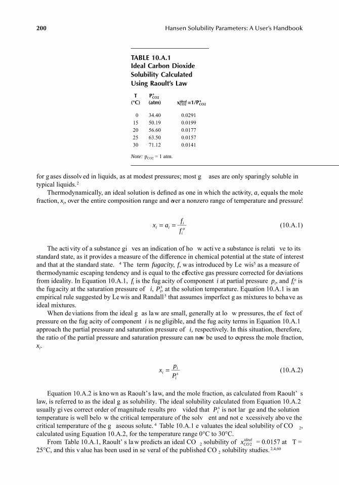
200 Hansen Solubility Parameters: A User’s Handbook
for g ases dissolved in liquids, as at modest pressures; most g ases are only sparingly soluble intypical liquids.2
Thermodynamically, an ideal solution is defined as one in which the activity, a, equals the molefraction, xi, over the entire composition range and over a nonzero range of temperature and pressure.3
(10.A.1)
The acti vity of a substance gi ves an indication of ho w acti ve a substance is relati ve to itsstandard state, as it provides a measure of the difference in chemical potential at the state of interestand that at the standard state. 4 The term fugacity, f, w as introduced by Le wis5 as a measure ofthermodynamic escaping tendency and is equal to the effective gas pressure corrected for deviationsfrom ideality. In Equation 10.A.1, fi is the fug acity of component i at partial pressure pi, and fio isthe fugacity at the saturation pressure of i, Pi,
s at the solution temperature. Equation 10.A.1 is anempirical rule suggested by Le wis and Randall5 that assumes imperfect g as mixtures to behave asideal mixtures.
When deviations from the ideal g as law are small, generally at lo w pressures, the ef fect ofpressure on the fug acity of component i is ne gligible, and the fug acity terms in Equation 10.A.1approach the partial pressure and saturation pressure of i, respectively. In this situation, therefore,the ratio of the partial pressure and saturation pressure can now be used to express the mole fraction,xi.
(10.A.2)
Equation 10.A.2 is kno wn as Raoult’s law, and the mole fraction, as calculated from Raoult’ slaw, is referred to as the ideal g as solubility. The ideal solubility calculated from Equation 10.A.2usually gi ves correct order of magnitude results pro vided that Pi
s is not lar ge and the solutiontemperature is well belo w the critical temperature of the solv ent and not e xcessively above thecritical temperature of the g aseous solute. 4 Table 10.A.1 e valuates the ideal solubility of CO 2,calculated using Equation 10.A.2, for the temperature range 0°C to 30°C.
From Table 10.A.1, Raoult’ s la w predicts an ideal CO 2 solubility of = 0.0157 at T =25°C, and this v alue has been used in se veral of the published CO 2 solubility studies. 2,4,60
TABLE 10.A.1Ideal Carbon Dioxide Solubility Calculated Using Raoult’s Law
T(°C)
PCO2s
(atm) CO2xideal =1/PCO2
s
0 34.40 0.029115 50.19 0.019920 56.60 0.017725 63.50 0.015730 71.12 0.0141
Note: pCO2 = 1 atm.
x af
fi i
i
io
= =
xp
Pi
i
is
=
xCOideal
2
7248_book.fm Page 200 Tuesday, April 24, 2007 9:19 AM
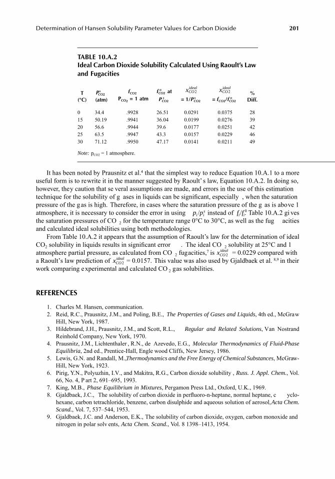
Determination of Hansen Solubility Parameter Values for Carbon Dioxide 201
It has been noted by Prausnitz et al.4 that the simplest way to reduce Equation 10.A.1 to a moreuseful form is to rewrite it in the manner suggested by Raoult’ s law, Equation 10.A.2. In doing so,however, they caution that se veral assumptions are made, and errors in the use of this estimationtechnique for the solubility of g ases in liquids can be significant, especially , when the saturationpressure of the g as is high. Therefore, in cases where the saturation pressure of the g as is above 1atmosphere, it is necessary to consider the error in using pi /pi
s instead of fi/fi.0 Table 10.A.2 gi vesthe saturation pressures of CO 2 for the temperature range 0°C to 30°C, as well as the fug acitiesand calculated ideal solubilities using both methodologies.
From Table 10.A.2 it appears that the assumption of Raoult’s law for the determination of idealCO2 solubility in liquids results in significant error . The ideal CO 2 solubility at 25°C and 1atmosphere partial pressure, as calculated from CO 2 fugacities,7 is = 0.0229 compared witha Raoult’s law prediction of = 0.0157. This value was also used by Gjaldbaek et al. 8,9 in theirwork comparing experimental and calculated CO 2 gas solubilities.
REFERENCES
1. Charles M. Hansen, communication.2. Reid, R.C., Prausnitz, J.M., and Poling, B.E., The Properties of Gases and Liquids, 4th ed., McGraw
Hill, New York, 1987.3. Hildebrand, J.H., Prausnitz, J.M., and Scott, R.L., Regular and Related Solutions, Van Nostrand
Reinhold Company, New York, 1970.4. Prausnitz, J.M., Lichtenthaler , R.N., de Azevedo, E.G., Molecular Thermodynamics of Fluid-Phase
Equilibria, 2nd ed., Prentice-Hall, Engle wood Cliffs, New Jersey, 1986.5. Lewis, G.N. and Randall, M., Thermodynamics and the Free Energy of Chemical Substances, McGraw-
Hill, New York, 1923.6. Pirig, Y.N., Polyuzhin, I.V., and Makitra, R.G., Carbon dioxide solubility , Russ. J. Appl. Chem., Vol.
66, No. 4, P art 2, 691–695, 1993.7. King, M.B., Phase Equilibrium in Mixtures, Pergamon Press Ltd., Oxford, U.K., 1969.8. Gjaldbaek, J.C., The solubility of carbon dioxide in perfluoro-n-heptane, normal heptane, c yclo-
hexane, carbon tetrachloride, benzene, carbon disulphide and aqueous solution of aerosol, Acta Chem.Scand., Vol. 7, 537–544, 1953.
9. Gjaldbaek, J.C. and Anderson, E.K., The solubility of carbon dioxide, oxygen, carbon monoxide andnitrogen in polar solv ents, Acta Chem. Scand., Vol. 8 1398–1413, 1954.
TABLE 10.A.2Ideal Carbon Dioxide Solubility Calculated Using Raoult’s Law and Fugacities
T(°C)
PsCO2
(atm)
fCO2
PCO2 = 1 atmfCO2
o atPCO2
s = 1/PCO2s = fCO2/fCO2
o %
Diff.
0 34.4 .9928 26.51 0.0291 0.0375 2815 50.19 .9941 36.04 0.0199 0.0276 3920 56.6 .9944 39.6 0.0177 0.0251 4225 63.5 .9947 43.3 0.0157 0.0229 4630 71.12 .9950 47.17 0.0141 0.0211 49
Note: pCO2 = 1 atmosphere.
xCOideal
2 xCOideal
2
xCOideal
2xCO
ideal2
7248_book.fm Page 201 Tuesday, April 24, 2007 9:19 AM

7248_book.fm Page 202 Tuesday, April 24, 2007 9:19 AM
203
11
Use of Hansen Solubility Parameters to Identify Cleaning Applications for “Designer” Solvents
John Durkee
ABSTRACT
Choosing the most ef fective solvents for cleaning requires characterization of both solv ents andsoils. Hansen solubility parameters (HSP) can be used whether or not single or multiple componentsare present in either the soil composite or the solv ent blend.
These HSP characterizations of solv ents and soils can be compared as v alues in HSP spacejust as similar values of solvents and polymers are compared to determine if a solvent can dissolvea polymer. A previously developed value of R
A
for cleaning operations allows prediction of usefulcleaning performance by solv ent on soil.
In this chapter , six representati ve soils and 13 base solv ents, so-called
“
designer
”
solv ents,were selected as feedstocks for formulation of binary azeotropes, using a literature database.
The selected solvent azeotropes were predicted to clean fi e or six representative soils. In thischapter, it will be sho wn that the base azeotropic feedstock must display significant polar anhydrogen bonding intermolecular forces if the azeotrope is to clean a soil composite that alsocontains significant polar and ydrogen bonding intermolecular forces.
INTRODUCTION
Since the early 1990s, more than a dozen ne w solvents have been commercialized for cleaning
1
,such as vapor degreasing, and other applications.
The sobriquet
“
designer
”
has been applied to them as their structure w as designed to pro videcertain benefits. Chief , these benefits are a relat vely nonhazardous e xposure to humans andcompliance with nearly all en vironmental regulations (including the Montreal Protocol) of mostnations. As designer goods vs. commodities, the y are high priced, which limits applications.
Another limitation is their character as solv ents. Given the relative inertness of these designersolvents to both humans and the en vironment, it is not surprising to find them to be inert to ma ysoils.
The purpose of this chapter is to illustrate ho w to use HSPs to aid in identifying v aluableapplications for these and other solv ents in cleaning applications. The approach tak en is thetraditional one used in cleaning work: matching the solvent to the soil.
2
HSP values of the solventswill be those matched to soil materials.
3
7248_C011.fm Page 203 Thursday, May 10, 2007 8:00 AM
204
Hansen Solubility Parameters: A User’s Handbook
A VARIETY OF SOLVENTS
There are almost too man y types of cleaning solv ents. It can be hard to discriminate among them.Simple chemicals such as he xane, more comple x chemicals such as
N
-methyl-2-pyrrolidone,flammable chemicals such as acetone, carcinogenic chemicals such as benzene, ozone-depletinchemicals such as carbon tetrachloride, and lo w-cost common chemicals such as w ater have allbeen used as cleaning solv ents. One of the strengths of solv ent-cleaning technology is the v arietyof solvents that can be used in v arious solvent cleaning processes.
Yet, no cleaning solv ent is perfect. All have fl ws, both general and specific. Sol ents withgeneral fl ws
4
may pose environmental, safety, or health hazards. They may be physically unsuitedto the application because of mismatched ph ysical properties such as surf ace tension, density , orviscosity; have excessive or limited v olatility; or simply be too e xpensive.
However, the specific f w that is usually f atal to an application is the solv ent
’
s not beingcompatible with the soil materials. Pre vention of a mismatch of intermolecular forces between acleaning solvent and a soil (an incompatibility) is a role uniquely fulfilled by HS .
5
A soil materialis probably soluble in a solv ent (or solv ent blend) if the Hansen parameters for the solv ent liewithin the solubility sphere for the soil.
6
PATHOLOGY OF SOILS
Those managing cleaning w ork must know at least as much about soils as the y do about cleaningagents, if their cleaning w ork is to meet their requirements. After all, the soil is the enemy to beconquered.
Soils are multicomponent mixtures. They are composed of occasionally unkno wn ingredientsprepared with unknown and variable proportions, which are not homogenized. They may include
“
tramp
”
materials or contain une xpected components that are not al ways present or recognized atbest, often inadv ertently produced by users. Soil can also be the outcome of incomplete cleaningwork.
Cleaning of multiple soil components usually produces multiple cleaning results. The bettermatched cleaning agents and processes are to a soil, the better the result, while poor matches willstill be apparent.
A good e xample is h ydrocarbon-based w ax, which must normally be melted in order to beremoved from surfaces. Microcrystalline wax, used as a binder in polishing compounds, has a sharpmelting point because the range of molecular weights of its component paraf fins is narr w. Waxused in box-coating operations has a mixture of molecular weights and a broad melting point. Ifthe boiling point of the cleaning solv ent only matches the a verage melting point of both w axmixtures, the higher melting fractions of the coating wax probably will not be well-cleaned becausethey are not heated to a high enough temperature.
In other words, the soil least matched to the cleaning solvent is likely to be the soil least cleaned.(See
“
More Realistic View about Evaluating HSP of Composite Soils.
”
)
HSP OF MULTIPLE-COMPONENT SOILS
How then is a user to match a single (or azeotropic) cleaning solv ent with a multicomponent soil?The answer combines observation along with conventional solubility theory and is seen in the
following list:
• First, one observes
7
if the soil is a single- or multiple-phase mixture. If the soil materialis a single phase (presumably a solution and not an emulsion), the components musthave similar intermolecular forces, and a useful solvent can probably be found from theirstudy. If the mixture contains multiple phases, it is lik ely that a cleaning process must
7248_C011.fm Page 204 Thursday, May 10, 2007 8:00 AM
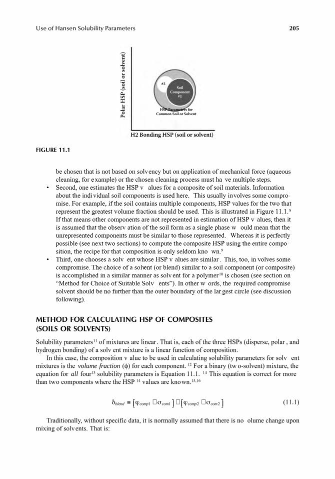
Use of Hansen Solubility Parameters
205
be chosen that is not based on solvency but on application of mechanical force (aqueouscleaning, for example) or the chosen cleaning process must ha ve multiple steps.
• Second, one estimates the HSP v alues for a composite of soil materials. Informationabout the individual soil components is used here. This usually involves some compro-mise. For example, if the soil contains multiple components, HSP values for the two thatrepresent the greatest volume fraction should be used. This is illustrated in Figure 11.1.
8
If that means other components are not represented in estimation of HSP v alues, then itis assumed that the observ ation of the soil form as a single phase w ould mean that theunrepresented components must be similar to those represented. Whereas it is perfectlypossible (see next two sections) to compute the composite HSP using the entire compo-sition, the recipe for that composition is only seldom kno wn.
9
• Third, one chooses a solv ent whose HSP v alues are similar . This, too, in volves somecompromise. The choice of a solvent (or blend) similar to a soil component (or composite)is accomplished in a similar manner as solv ent for a polymer
10
is chosen (see section on
“
Method for Choice of Suitable Solv ents
”
). In other w ords, the
required compromisesolvent should be no further than the outer boundary of the lar gest circle (see discussionfollowing).
METHOD FOR CALCULATING HSP OF COMPOSITES (SOILS OR SOLVENTS)
Solubility parameters
11
of mixtures are linear. That is, each of the three HSPs (disperse, polar , andhydrogen bonding) of a solv ent mixture is a linear function of composition.
In this case, the composition v alue to be used in calculating solubility parameters for solv entmixtures is the
volume fraction
(
φ
) for each component.
12
For a binary (tw o-solvent) mixture, theequation for
all
four
13
solubility parameters is Equation 11.1.
14
This equation is correct for morethan two components where the HSP
14
values are known.
15,16
(11.1)
Traditionally, without specific data, it is normally assumed that there is no olume change uponmixing of solvents. That is:
FIGURE 11.1
H2 Bonding HSP (soil or solvent)
Polar
HSP
(soi
l or s
olve
nt)
HSP Parameters forCommon Soil or Solvent
SoilComponent
#1
#2
δ ϕ σ ϕ σblend comp com comp com≡ ×⎡⎣ ⎤⎦ + ×⎡⎣ ⎤⎦1 1 2 2
7248_C011.fm Page 205 Thursday, May 10, 2007 8:00 AM
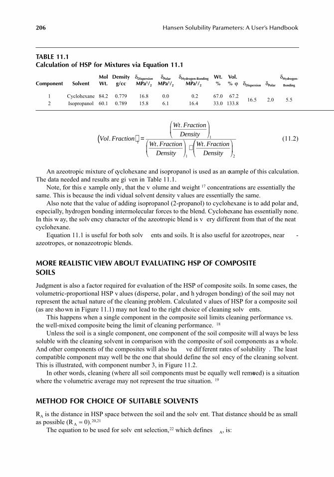
206
Hansen Solubility Parameters: A User’s Handbook
(11.2)
An azeotropic mixture of cyclohexane and isopropanol is used as an example of this calculation.The data needed and results are gi ven in Table 11.1.
Note, for this e xample only, that the v olume and weight
17
concentrations are essentially thesame. This is because the indi vidual solvent density values are essentially the same.
Also note that the value of adding isopropanol (2-propanol) to cyclohexane is to add polar and,especially, hydrogen bonding intermolecular forces to the blend. Cyclohexane has essentially none.In this w ay, the solv ency character of the azeotropic blend is v ery different from that of the neatcyclohexane.
Equation 11.1 is useful for both solv ents and soils. It is also useful for azeotropes, near -azeotropes, or nonazeotropic blends.
MORE REALISTIC VIEW ABOUT EVALUATING HSP OF COMPOSITE SOILS
Judgment is also a factor required for evaluation of the HSP of composite soils. In some cases, thevolumetric-proportional HSP v alues (disperse, polar , and h ydrogen bonding) of the soil may notrepresent the actual nature of the cleaning problem. Calculated v alues of HSP for a composite soil(as are shown in Figure 11.1) may not lead to the right choice of cleaning solv ents.
This happens when a single component in the composite soil limits cleaning performance vs.the well-mixed composite being the limit of cleaning performance.
18
Unless the soil is a single component, one component of the soil composite will al ways be less
soluble with the cleaning solvent in comparison with the composite of soil components as a whole.And other components of the composites will also ha ve dif ferent rates of solubility . The leastcompatible component may well be the one that should define the sol ency of the cleaning solvent.This is illustrated, with component number 3, in Figure 11.2.
In other words, cleaning (where all soil components must be equally well removed) is a situationwhere the volumetric average may not represent the true situation.
19
METHOD FOR CHOICE OF SUITABLE SOLVENTS
R
A
is the distance in HSP space between the soil and the solv ent. That distance should be as smallas possible (R
A
≈
0).
20,21
The equation to be used for solv ent selection,
22
which defines
A
, is:
TABLE 11.1Calculation of HSP for Mixtures via Equation 11.1
Component SolventMolWt.
Densityg/cc
δ
Dispersion
MPa
1
/
2
δ
Polar
MPa
1
/
2
δ
Hydrogen-Bonding
MPa
1
/
2
Wt.%
Vol.%
ϕ δ
Dispersion
δ
Polar
δ
Hydrogen-
Bonding
1 Cyclohexane 84.2 0.779 16.8 0.0 0.2 67.0 67.216.5 2.0 5.5
2 Isopropanol 60.1 0.789 15.8 6.1 16.4 33.0 133.8
Vol Fraction
Wt FractionDensity
Wt.
.
( ) =
⎛
⎝⎜
⎞
⎠⎟
11
.. .FractionDensity
Wt FractionDensity
⎛
⎝⎜
⎞
⎠⎟ +
1
⎛⎛
⎝⎜
⎞
⎠⎟
2
7248_C011.fm Page 206 Thursday, May 10, 2007 8:00 AM

Use of Hansen Solubility Parameters
207
(11.3)
The preceding equation comprises the follo wing data:
• The basic data for Equation 11.3 is the three pre viously estimated HSP values for eithera soil composite (via Equation 11.1) or HSP v alues for a component e xpected to belimiting.
• The independent variable in the equation is the choice of solv ent. • The dependent variable in the equation shows how well the soil is dissolved, that is, how
closely R
A
approaches zero.
The individual values for HSPs for the soil are either those computed from Equation 11.1 orthat for the single soil component judged to limit cleaning performance as sho wn in Figure 11.2.
HSP data and a spreadsheet can aid in making this complex choice because they allow evaluationof solution performance for man y solvents (or blends) ag ainst all components of the soil. Graph-ically, the matching of solvent (or blend of solvents) to soil (of one of more components) is describedin Reference 3 as Figure 4.6 (reproduced here as Figure 11.3
23
). If the distance between the loci
FIGURE 11.2
FIGURE 11.3
H2 Bonding HSP (soil or solvent)
Polar
HSP
(soi
l or s
olve
nt)
#3
SoilComponent
#1
HSP Parameters forCommon Soil or Solvent
#2
R Solution Polar for Solvent Polar for SoilA2 = (δ δ– ))+
2
2 2δ δH Bonding for Solvent H Bonding for Soi– – – ll
Disperse for Solvent Disperse for Soi
( )
+ ×
2
4 δ δ– ll( )⎡⎣
⎤⎦
2
H2 Bonding HSP (soil or solvent)
Polar
HSP
(soi
l or s
olve
nt)
Soil orSolvent
#2
Soil orSolvent
#1
HSP Parameters forCommon Soil or Solvent
7248_C011.fm Page 207 Thursday, May 10, 2007 8:00 AM
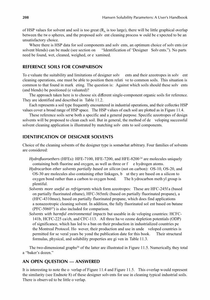
208
Hansen Solubility Parameters: A User’s Handbook
of HSP values for solvent and soil is too great (R
A
is too large), there will be little graphical overlapbetween the tw o spheres, and the proposed solv ent cleaning process w ould be e xpected to be anunsatisfactory choice.
Where there is HSP data for soil components and solv ents, an optimum choice of solv ents (orsolvent blends) can be made (see section on
“
Identification of ‘Designer Solv ents.
”
). No partsneed be found, wet, cleaned, weighed, or e xamined.
REFERENCE SOILS FOR COMPARISON
To e valuate the suitability and limitations of designer solv ents and their azeotropes in solv entcleaning operations, one must be able to position them relati ve to common soils. This situation iscommon to that found in mark eting. The question is: Against which soils should these solv ents(and blends) be positioned (e valuated)?
The approach taken here is to choose six different single-component organic soils for reference.They are identified and described in Table 11.2.
Each represents a soil type frequently encountered in industrial operations, and their collective HSPvalues cover a broad range of HSP space. The HSP values of each soil are plotted as in Figure 11.4.
These reference soils serve both a specific and a general purpose. Specific azeotropes of designsolvents will be proposed to clean each soil. But in general, the method of de veloping successfulsolvent cleaning application is illustrated by matching solv ents to soil components.
IDENTIFICATION OF DESIGNER SOLVENTS
Choice of the cleaning solvents of the designer type is somewhat arbitrary. Four families of solventsare considered:
Hydrofluoroethers
(HFEs): HFE-7100, HFE-7200, and HFE-8200
24
are molecules uniquelycontaining both fluorine and oxygen, as well as three or f e hydrogen atoms.
Hydrocarbon ether solvents
partially based on silicon
(not on carbon):
OS-10, OS-20, andOS-30 are molecules also containing ether linkages, b ut they are based on a silicon tooxygen bond rather than a carbon to oxygen bond. The h ydrocarbon meth yl group isplentiful.
Solvents more useful as refrigerants
which form azeotropes: These are HFC-245f a (basedon partially fluorinated ethane), HFC-365mfc (based on partially fluorinated propane), a(HFC-4310mee), based on partially fluorinated propane, which does find applications a nonazeotropic cleaning solvent. In addition, the fully fluorinated sol ent based on butane(PFC-5060
25
) is also included for comparison.
Solvents with harmful environmental impacts
but useable in de veloping countries: HCFC-141b, HCFC-225 ca/cb, and CFC-113. All three ha ve ozone depletion potentials (ODP)of significance, which has led to a ban on their production in industrialized countries pethe Montreal Protocol. Ho wever, their production and use in unde veloped countries ispermitted for se veral years be yond the publication date for this book. Their structuralformulas, physical, and solubility properties are gi ven in Table 11.3.
The two-dimensional graphs
26
of the latter are illustrated in Figure 11.5. Numerically, they totala
“
baker
’
s dozen.
”
AN OPEN QUESTION — ANSWERED
It is interesting to note the o verlap of Figure 11.4 and Figure 11.5. This overlap would representthe similarity (see Endnote 8) of these designer solvents for use in cleaning typical industrial soils.There is observed to be little o verlap.
7248_C011.fm Page 208 Thursday, May 10, 2007 8:00 AM
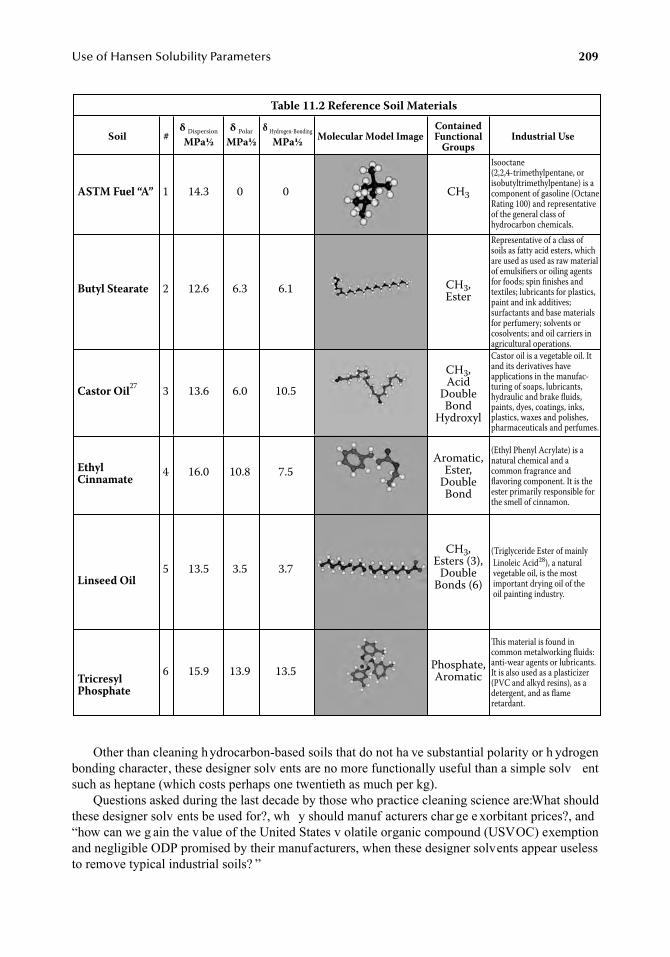
Use of Hansen Solubility Parameters
209
Other than cleaning hydrocarbon-based soils that do not ha ve substantial polarity or h ydrogenbonding character, these designer solv ents are no more functionally useful than a simple solv entsuch as heptane (which costs perhaps one twentieth as much per kg).
Questions asked during the last decade by those who practice cleaning science are: What shouldthese designer solv ents be used for?, wh y should manuf acturers char ge e xorbitant prices?, and
“
how can we g ain the value of the United States v olatile organic compound (USVOC) exemptionand negligible ODP promised by their manufacturers, when these designer solvents appear uselessto remove typical industrial soils?
”
(Ethyl Phenyl Acrylate) is anatural chemical and acommon fragrance andflavoring component. It is theester primarily responsible forthe smell of cinnamon.
(Triglyceride Ester of mainly
Linoleic Acid28), a natural vegetable oil, is the most important drying oil of the oil painting industry.
This material is found incommon metalworking fluids:anti-wear agents or lubricants.It is also used as a plasticizer(PVC and alkyd resins), as adetergent, and as flameretardant.
EthylCinnamate
Linseed Oil
TricresylPhosphate
4
5
6
16.0
13.5
15.9
10.8
3.5
13.9
7.5
3.7
13.5
Aromatic,Ester,
DoubleBond
CH3,Esters (3),
DoubleBonds (6)
Phosphate,Aromatic
Table 11.2 Reference Soil Materials
Soil Molecular Model Image Industrial Use
Isooctane(2,2,4-trimethylpentane, orisobutyltrimethylpentane) is acomponent of gasoline (OctaneRating 100) and representativeof the general class of hydrocarbon chemicals.
Representative of a class ofsoils as fatty acid esters, whichare used as used as raw materialof emulsifiers or oiling agentsfor foods; spin finishes andtextiles; lubricants for plastics,paint and ink additives;surfactants and base materialsfor perfumery; solvents orcosolvents; and oil carriers inagricultural operations.
Castor oil is a vegetable oil. Itand its derivatives haveapplications in the manufac-turing of soaps, lubricants,hydraulic and brake fluids,paints, dyes, coatings, inks,plastics, waxes and polishes,pharmaceuticals and perfumes.
ContainedFunctional
Groups#
δ Dispersion
MPa½
δ Polar
MPa½
δ Hydrogen-Bonding
MPa½
ASTM Fuel “A”
Butyl Stearate
Castor Oil27
1
2
3
14.3
12.6
13.6
0
6.3
6.0
0
6.1
10.5
CH3
CH3,Ester
CH3,Acid
DoubleBond
Hydroxyl
7248_C011.fm Page 209 Thursday, May 10, 2007 8:00 AM
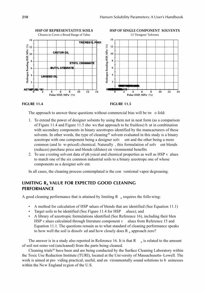
210
Hansen Solubility Parameters: A User’s Handbook
The approach to answer these questions without commercial bias will be tw o fold:
1. To extend the power of designer solvents by using them not in neat form (as a comparisonof Figure 11.4 and Figure 11.5 sho ws that approach to be fruitless) b ut in combinationwith secondary components in binary azeotropes identified by the manuacturers of thesesolvents. In other words, the type of cleaning
29
solvent evaluated in this study is a binaryazeotrope with one component being a designer solv ent and the other being a morecommon (and lo w-priced) chemical. Naturally , this formulation of solv ent blends(reduces) purchase price and blends (dilutes) en vironmental benefits
2. To use existing solvent data of ph ysical and chemical properties as well as HSP v aluesto match one of the six common industrial soils to a binary azeotrope one of whosecomponents as a designer solv ent.
In all cases, the cleaning process contemplated is the con ventional vapor degreasing.
LIMITING R
A
VALUE FOR EXPECTED GOOD CLEANING PERFORMANCE
A good cleaning performance that is attained by limiting R
A
requires the follo wing:
• A method for calculation of HSP values of blends that are identified (See Equation 11.1)• Target soils to be identified (See Figure 11.4 for HSP alues); and• A library of azeotropic formulations identified (See Reference 16), including their blen
HSP v alues calculated through literature component v alues from Reference 15 andEquation 11.1. The questions remain as to what standard of cleaning performance speaksto how well the soil is dissolv ed and how closely does R
A
approach zero?
The answer is in a study also reported in Reference 16. It is that R
A
is related to the amountof soil not remo ved (uncleaned) from the parts being cleaned.
Cleaning trials
30
have been and are being conducted by the Surface Cleaning Laboratory withinthe Toxic Use Reduction Institute (TURI), located at the Uni versity of Massachusetts–Lowell. Thework is aimed at pro viding practical, useful, and en vironmentally sound solutions to b usinesseswithin the New England region of the U.S.
FIGURE 11.4 FIGURE 11.5
HSP OF REPRESENTATIVE SOILSChosen to Cover a Broad Range of Value
HSP OF SINGLE COMPONENT SOLVENTS13 ‘Designer’ Solvents
Hyd
roge
n B
on
din
g H
SP,
MP
a ˆ (
½)
Polar HSP, MPaˆ (½) Polar HSP, MPaˆ (½)
14
12
10
8
6
4
2
0
Hyd
roge
n B
on
din
g H
SP,
MP
a ˆ (
½)
14
12
10
8
6
4
2
00 2 4 6 8 10 12 14 0 2 4 6 8 10 12 14
7248_C011.fm Page 210 Thursday, May 10, 2007 8:00 AM
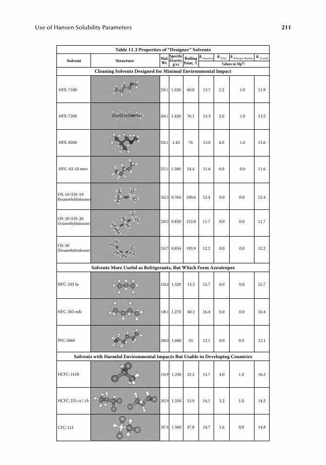
Use of Hansen Solubility Parameters
211
StructureSolvent
HFE-7100
HFE-7200
HFE-8200
HFC-43-10 mee
250.1
264.1
250.1
252.1
1.520
1.430
1.43
1.580
60.0
76.1
76
54.4
13.7
13.3
13.0
11.6
2.2
2.0
4.0
0.0
1.0
1.0
1.0
0.0
13.9
13.5
13.6
11.6
δ Dispersion δ Polar δ Hydrogen-Bonding δ OverallMol.Wt.
BoilingPoint, °C
SpecificGravity,
g/cc Values in Mp½
OS-10 (OS-10Hexamethyldisiloxane)
OS-20 (OS-20Octamethyldisiloxane)
OS-30(Decamethyltrisiloxane)
HFC-245 fa
HFC-365 mfc
162.3
236.5
310.7
134.0
148.1
0.764
0.820
0.854
1.320
1.270
100.6
152.8
193.9
15.3
40.2
12.4
11.7
12.2
15.7
16.4
12.4
11.7
12.2
15.7
16.4
0.0
0.0
0.0
0.0
0.0
0.0
0.0
0.0
0.0
0.0
PFC-5060
HCFC-141B
HCFC-225 ca / cb
CFC-113
288.0
116.9
202.9
187.4
1.680
1.230
1.550
1.560
55
32.2
53.9
47.8
12.1
15.7
14.1
14.7
0.0
4.0
3.2
1.6
0.0
1.0
1.0
0.0
12.1
16.2
14.5
14.8
Cleaning Solvents Designed for Minimal Environmental Impact
Table 11.3 Properties of “Designer” Solvents
Solvents More Useful as Refrigerants, But Which Form Azeotropes
Solvents with Harmful Environmental Impacts But Usable in Developing Countries
7248_C011.fm Page 211 Thursday, May 10, 2007 8:00 AM
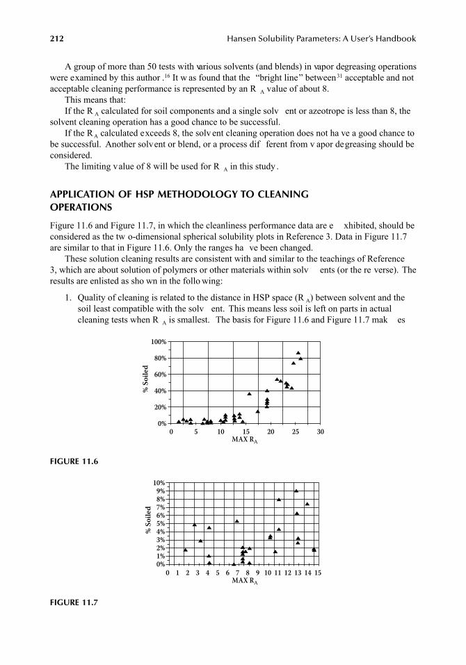
212
Hansen Solubility Parameters: A User’s Handbook
A group of more than 50 tests with various solvents (and blends) in vapor degreasing operationswere examined by this author .
16
It w as found that the
“
bright line
”
between
31
acceptable and notacceptable cleaning performance is represented by an R
A
value of about 8. This means that:If the R
A
calculated for soil components and a single solv ent or azeotrope is less than 8, thesolvent cleaning operation has a good chance to be successful.
If the R
A
calculated exceeds 8, the solv ent cleaning operation does not ha ve a good chance tobe successful. Another solvent or blend, or a process dif ferent from v apor degreasing should beconsidered.
The limiting value of 8 will be used for R
A
in this study .
APPLICATION OF HSP METHODOLOGY TO CLEANING OPERATIONS
Figure 11.6 and Figure 11.7, in which the cleanliness performance data are e xhibited, should beconsidered as the tw o-dimensional spherical solubility plots in Reference 3. Data in Figure 11.7are similar to that in Figure 11.6. Only the ranges ha ve been changed.
These solution cleaning results are consistent with and similar to the teachings of Reference3, which are about solution of polymers or other materials within solv ents (or the re verse). Theresults are enlisted as sho wn in the follo wing:
1. Quality of cleaning is related to the distance in HSP space (R
A
) between solvent and thesoil least compatible with the solv ent. This means less soil is left on parts in actualcleaning tests when R
A
is smallest. The basis for Figure 11.6 and Figure 11.7 mak es
FIGURE 11.6
FIGURE 11.7
▲▲▲▲▲
▲▲▲▲▲▲
▲▲▲▲▲ ▲
▲▲
▲▲▲
▲
▲▲
▲▲▲▲
▲▲▲▲▲▲
▲▲
▲
% So
iled
100%
80%
60%
40%
20%
0%
MAX RA
0 5 10 15 20 25 30
▲
▲
▲▲
▲
▲ ▲ ▲▲▲▲▲▲▲▲
▲
▲▲
▲
▲
▲▲
▲
▲
▲
▲
▲▲
% So
iled
10%9%8%7%6%5%4%3%2%1%0%
MAX RA
0 1 2 3 4 5 6 7 8 9 10 11 12 13 14 15
7248_C011.fm Page 212 Thursday, May 10, 2007 8:00 AM
Use of Hansen Solubility Parameters
213
physical sense; the material not cleaned (percentage soiled) by a solv ent is related to thesoil least soluble.
2. There is a limit (breakpoint,
“
bright line,
” demarcation, or separation) between one typeof behavior (acceptable cleanliness) and the opposite (unacceptable cleanliness). Thereare very few or ne gligible anomalies (situations where HSP v alues suggest that thereshould be poor compatibility , and there is good compatibility , as well as the re verse).There are no results of poor cleaning when R A is 8 or belo w.
3. The value of R A (8), chosen to dif ferentiate acceptable and unacceptable cleanliness, issimilar to the interaction radius between polymers and solv ents typical for selectedcorrelations given in Appendix Table A.2 of Reference 3 and Appendix Table A.2 of thisHandbook. The average value in Appendix Table A.2 is about 10.
Results of calculation of the HSP values for each binary32 azeotrope blend based on the solventsin Table 11.3 and in Table 11.4 33 through Table 11.15 are gi ven and illustrated in Figure 11.8through Figure 11.20.
ANALYSIS OF CAPABILITY OF DESIGNER SOLVENTS
The limited utility 34 of neat designer solv ents has been e xperienced in the decade since the y werecommercialized and is characterized via HSP methodology in Figure 11.5.
As viewed within the HSP space, the v alue of the components from which these azeotropesare formed is to add h ydrogen bonding and polar intermolecular forces to designer solv ents thatgenerally do not display those forces.
This is illustrated schematically in Figure 11.21, and is essentially the approach described in thesection on “An Open Question — Answered,” to find verlap between Figure 11.4 and Figure 11.5.
Each azeotropic blend noted abo ve35 is a fluid with a single boiling point, ut with dif ferentphysical properties, safety , health, en vironmental impacts, and economic consequences than aremanifested by the 13 chosen designer solv ents.
The proper metric 36 for discrimination among these azeotropes is the ef fective completion ofthe proposed cleaning work. That metric is the magnitude of the mismatch between intermolecularforces of the solvent (single or azeotropic blend) and composite soil. Quantization of this mismatchis produced for specific soils by the parameter A. As described in the section on limiting RA valuefor good cleaning performance (at least 95% remo val of all soils) is around 8.
The capability to clean v arious soils with azeotropes of designer solv ents is gi ven in Table11.16. The information is sorted to meet the needs of users by gi ving the various designer solventsthat can be blended to clean the stated soil.
Users can use HSP to dif ferentiate one solv ent or solv ent blend from another based on thevalues of the soil found in the specific application. Information in the preceding tables can be useto screen azeotropes formulated from designer solvents and reduce the needed burden of feasibilitytesting. Reference 3 or Reference 15, as well as the appendices in this book, can be used as sourcesof HSP v alues when the six soils chosen to be representati ve in this study are not representati veof those in the current application.
This analysis, using HSP methodology, clearly shows the superiority of the fluoroether structur(HFE) as a feedstock for azeotropes. F our to fi e units (MPa1/2) of polar HSP v alue can be addedthrough addition of secondary solv ents to form constant-boiling 37 azeotropes.
HSP methodology further allo ws recognition of the limits of azeotropic blends based ondesigner solvents. No composition is e xpected to be capable of cleaning soil number 6 (tricresylphosphate). This is because the amount of polar and hydrogen bonding intermolecular forces neededto produce a compatible solution cannot be obtained by adding a second solvent rich in those forcesto designer solvents that are nearly de void of them.
7248_C011.fm Page 213 Thursday, May 10, 2007 8:00 AM
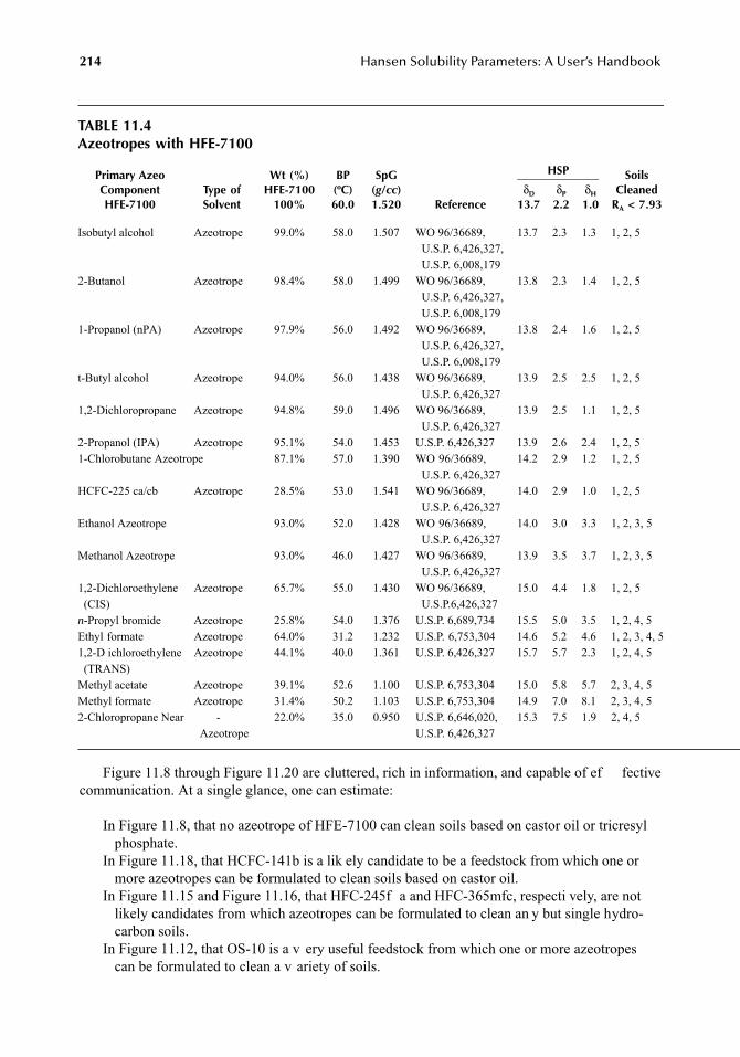
214 Hansen Solubility Parameters: A User’s Handbook
Figure 11.8 through Figure 11.20 are cluttered, rich in information, and capable of ef fectivecommunication. At a single glance, one can estimate:
In Figure 11.8, that no azeotrope of HFE-7100 can clean soils based on castor oil or tricresylphosphate.
In Figure 11.18, that HCFC-141b is a lik ely candidate to be a feedstock from which one ormore azeotropes can be formulated to clean soils based on castor oil.
In Figure 11.15 and Figure 11.16, that HFC-245f a and HFC-365mfc, respecti vely, are notlikely candidates from which azeotropes can be formulated to clean an y but single hydro-carbon soils.
In Figure 11.12, that OS-10 is a v ery useful feedstock from which one or more azeotropescan be formulated to clean a v ariety of soils.
TABLE 11.4Azeotropes with HFE-7100
Primary AzeoComponent HFE-7100
Type ofSolvent
Wt (%)HFE-7100
100%
BP(ºC)60.0
SpG(g/cc) 1.520 Reference
HSP SoilsCleaned
RA < 7.93δD
13.7δP
2.2δH
1.0
Isobutyl alcohol Azeotrope 99.0% 58.0 1.507 WO 96/36689, U.S.P. 6,426,327, U.S.P. 6,008,179
13.7 2.3 1.3 1, 2, 5
2-Butanol Azeotrope 98.4% 58.0 1.499 WO 96/36689, U.S.P. 6,426,327, U.S.P. 6,008,179
13.8 2.3 1.4 1, 2, 5
1-Propanol (nPA) Azeotrope 97.9% 56.0 1.492 WO 96/36689, U.S.P. 6,426,327, U.S.P. 6,008,179
13.8 2.4 1.6 1, 2, 5
t-Butyl alcohol Azeotrope 94.0% 56.0 1.438 WO 96/36689, U.S.P. 6,426,327
13.9 2.5 2.5 1, 2, 5
1,2-Dichloropropane Azeotrope 94.8% 59.0 1.496 WO 96/36689, U.S.P. 6,426,327
13.9 2.5 1.1 1, 2, 5
2-Propanol (IPA) Azeotrope 95.1% 54.0 1.453 U.S.P. 6,426,327 13.9 2.6 2.4 1, 2, 51-Chlorobutane Azeotrope 87.1% 57.0 1.390 WO 96/36689,
U.S.P. 6,426,327 14.2 2.9 1.2 1, 2, 5
HCFC-225 ca/cb Azeotrope 28.5% 53.0 1.541 WO 96/36689, U.S.P. 6,426,327
14.0 2.9 1.0 1, 2, 5
Ethanol Azeotrope 93.0% 52.0 1.428 WO 96/36689, U.S.P. 6,426,327
14.0 3.0 3.3 1, 2, 3, 5
Methanol Azeotrope 93.0% 46.0 1.427 WO 96/36689, U.S.P. 6,426,327
13.9 3.5 3.7 1, 2, 3, 5
1,2-Dichloroethylene(CIS)
Azeotrope 65.7% 55.0 1.430 WO 96/36689, U.S.P.6,426,327
15.0 4.4 1.8 1, 2, 5
n-Propyl bromide Azeotrope 25.8% 54.0 1.376 U.S.P. 6,689,734 15.5 5.0 3.5 1, 2, 4, 5Ethyl formate Azeotrope 64.0% 31.2 1.232 U.S.P. 6,753,304 14.6 5.2 4.6 1, 2, 3, 4, 51,2-D ichloroethylene(TRANS)
Azeotrope 44.1% 40.0 1.361 U.S.P. 6,426,327 15.7 5.7 2.3 1, 2, 4, 5
Methyl acetate Azeotrope 39.1% 52.6 1.100 U.S.P. 6,753,304 15.0 5.8 5.7 2, 3, 4, 5Methyl formate Azeotrope 31.4% 50.2 1.103 U.S.P. 6,753,304 14.9 7.0 8.1 2, 3, 4, 52-Chloropropane Near -
Azeotrope22.0% 35.0 0.950 U.S.P. 6,646,020,
U.S.P. 6,426,327 15.3 7.5 1.9 2, 4, 5
7248_C011.fm Page 214 Thursday, May 10, 2007 8:00 AM
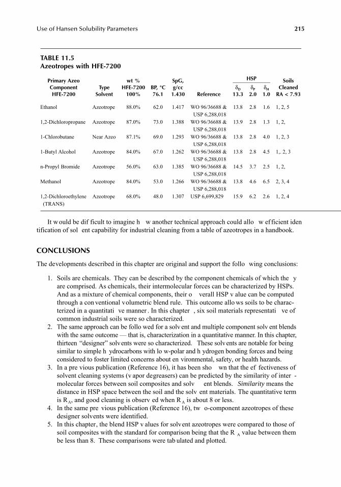
Use of Hansen Solubility Parameters 215
It w ould be dif ficult to imagine h w another technical approach could allo w ef ficient identification of sol ent capability for industrial cleaning from a table of azeotropes in a handbook.
CONCLUSIONS
The developments described in this chapter are original and support the follo wing conclusions:
1. Soils are chemicals. They can be described by the component chemicals of which the yare comprised. As chemicals, their intermolecular forces can be characterized by HSPs.And as a mixture of chemical components, their o verall HSP v alue can be computedthrough a con ventional volumetric blend rule. This outcome allo ws soils to be charac-terized in a quantitati ve manner . In this chapter , six soil materials representati ve ofcommon industrial soils were so characterized.
2. The same approach can be follo wed for a solv ent and multiple component solv ent blendswith the same outcome — that is, characterization in a quantitative manner. In this chapter,thirteen “designer” solvents were so characterized. These solvents are notable for beingsimilar to simple h ydrocarbons with lo w-polar and h ydrogen bonding forces and beingconsidered to foster limited concerns about en vironmental, safety, or health hazards.
3. In a pre vious publication (Reference 16), it has been sho wn that the ef fectiveness ofsolvent cleaning systems (v apor degreasers) can be predicted by the similarity of inter -molecular forces between soil composites and solv ent blends. Similarity means thedistance in HSP space between the soil and the solv ent materials. The quantitative termis RA, and good cleaning is observ ed when R A is about 8 or less.
4. In the same pre vious publication (Reference 16), tw o-component azeotropes of thesedesigner solvents were identified.
5. In this chapter, the blend HSP v alues for solvent azeotropes were compared to those ofsoil composites with the standard for comparison being that the R A value between thembe less than 8. These comparisons were tab ulated and plotted.
TABLE 11.5Azeotropes with HFE-7200
Primary AzeoComponentHFE-7200
TypeSolvent
wt %HFE-7200
100%BP, °C76.1
SpG,g/cc
1.430 Reference
HSP SoilsCleaned
RA < 7.93δD
13.3δP
2.0δH
1.0
Ethanol Azeotrope 88.0% 62.0 1.417 WO 96/36688 & USP 6,288,018
13.8 2.8 1.6 1, 2, 5
1,2-Dichloropropane Azeotrope 87.0% 73.0 1.388 WO 96/36688 & USP 6,288,018
13.9 2.8 1.3 1, 2,
1-Chlorobutane Near Azeo 87.1% 69.0 1.293 WO 96/36688 & USP 6,288,018
13.8 2.8 4.0 1, 2, 3
1-Butyl Alcohol Azeotrope 84.0% 67.0 1.262 WO 96/36688 & USP 6,288,018
13.8 2.8 4.5 1,. 2, 3
n-Propyl Bromide Azeotrope 56.0% 63.0 1.385 WO 96/36688 & USP 6,288,018
14.5 3.7 2.5 1, 2,
Methanol Azeotrope 84.0% 53.0 1.266 WO 96/36688 & USP 6,288,018
13.8 4.6 6.5 2, 3, 4
1,2-Dichloroethylene(TRANS)
Azeotrope 68.0% 48.0 1.307 USP 6,699,829 15.9 6.2 2.6 1, 2, 4
7248_C011.fm Page 215 Thursday, May 10, 2007 8:00 AM
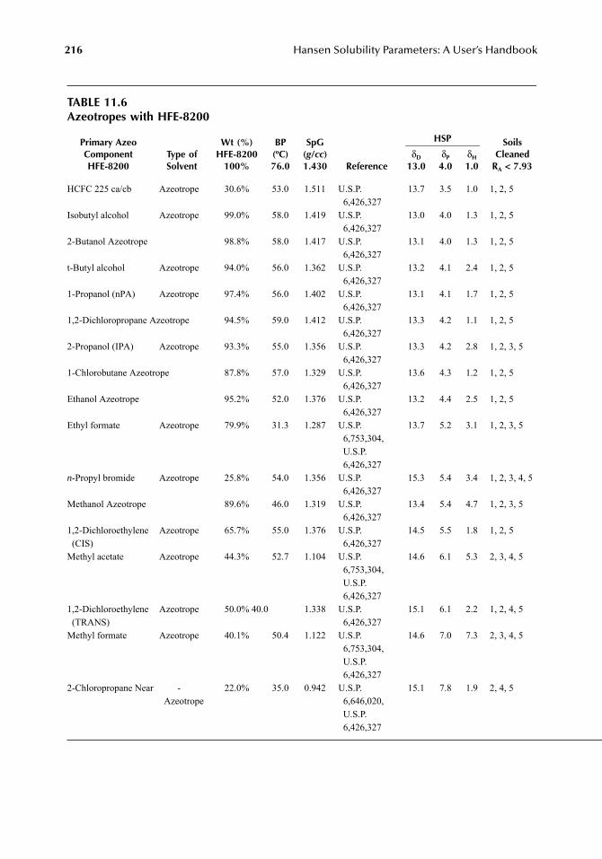
216 Hansen Solubility Parameters: A User’s Handbook
TABLE 11.6Azeotropes with HFE-8200
Primary AzeoComponentHFE-8200
Type ofSolvent
Wt (%)HFE-8200
100%
BP(ºC)76.0
SpG(g/cc)1.430 Reference
HSP SoilsCleaned
RA < 7.93 δD
13.0 δP
4.0 δH 1.0
HCFC 225 ca/cb Azeotrope 30.6% 53.0 1.511 U.S.P. 6,426,327
13.7 3.5 1.0 1, 2, 5
Isobutyl alcohol Azeotrope 99.0% 58.0 1.419 U.S.P. 6,426,327
13.0 4.0 1.3 1, 2, 5
2-Butanol Azeotrope 98.8% 58.0 1.417 U.S.P. 6,426,327
13.1 4.0 1.3 1, 2, 5
t-Butyl alcohol Azeotrope 94.0% 56.0 1.362 U.S.P. 6,426,327
13.2 4.1 2.4 1, 2, 5
1-Propanol (nPA) Azeotrope 97.4% 56.0 1.402 U.S.P. 6,426,327
13.1 4.1 1.7 1, 2, 5
1,2-Dichloropropane Azeotrope 94.5% 59.0 1.412 U.S.P. 6,426,327
13.3 4.2 1.1 1, 2, 5
2-Propanol (IPA) Azeotrope 93.3% 55.0 1.356 U.S.P. 6,426,327
13.3 4.2 2.8 1, 2, 3, 5
1-Chlorobutane Azeotrope 87.8% 57.0 1.329 U.S.P. 6,426,327
13.6 4.3 1.2 1, 2, 5
Ethanol Azeotrope 95.2% 52.0 1.376 U.S.P. 6,426,327
13.2 4.4 2.5 1, 2, 5
Ethyl formate Azeotrope 79.9% 31.3 1.287 U.S.P. 6,753,304, U.S.P. 6,426,327
13.7 5.2 3.1 1, 2, 3, 5
n-Propyl bromide Azeotrope 25.8% 54.0 1.356 U.S.P. 6,426,327
15.3 5.4 3.4 1, 2, 3, 4, 5
Methanol Azeotrope 89.6% 46.0 1.319 U.S.P. 6,426,327
13.4 5.4 4.7 1, 2, 3, 5
1,2-Dichloroethylene(CIS)
Azeotrope 65.7% 55.0 1.376 U.S.P. 6,426,327
14.5 5.5 1.8 1, 2, 5
Methyl acetate Azeotrope 44.3% 52.7 1.104 U.S.P. 6,753,304, U.S.P. 6,426,327
14.6 6.1 5.3 2, 3, 4, 5
1,2-Dichloroethylene(TRANS)
Azeotrope 50.0% 40.0 1.338 U.S.P. 6,426,327
15.1 6.1 2.2 1, 2, 4, 5
Methyl formate Azeotrope 40.1% 50.4 1.122 U.S.P. 6,753,304, U.S.P. 6,426,327
14.6 7.0 7.3 2, 3, 4, 5
2-Chloropropane Near -Azeotrope
22.0% 35.0 0.942 U.S.P. 6,646,020, U.S.P. 6,426,327
15.1 7.8 1.9 2, 4, 5
7248_C011.fm Page 216 Thursday, May 10, 2007 8:00 AM
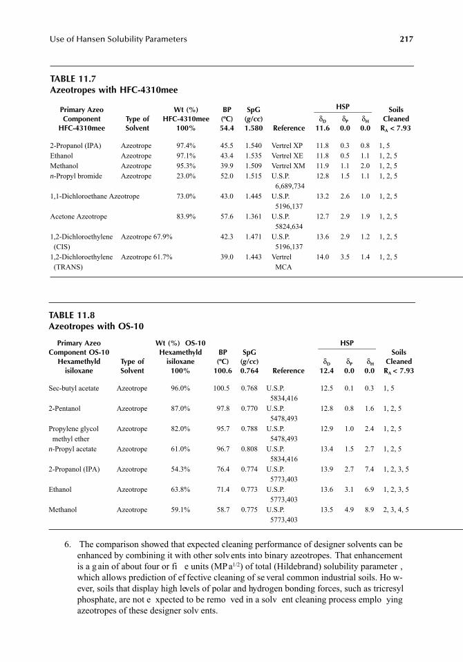
Use of Hansen Solubility Parameters 217
6. The comparison showed that expected cleaning performance of designer solvents can beenhanced by combining it with other solvents into binary azeotropes. That enhancementis a g ain of about four or fi e units (MP a1/2) of total (Hildebrand) solubility parameter ,which allows prediction of ef fective cleaning of se veral common industrial soils. Ho w-ever, soils that display high levels of polar and hydrogen bonding forces, such as tricresylphosphate, are not e xpected to be remo ved in a solv ent cleaning process emplo yingazeotropes of these designer solv ents.
TABLE 11.7Azeotropes with HFC-4310mee
Primary AzeoComponent
HFC-4310mee Type ofSolvent
Wt (%)HFC-4310mee
100%
BP(ºC)54.4
SpG(g/cc)1.580 Reference
HSP SoilsCleaned
RA < 7.93 δD
11.6 δP
0.0 δH 0.0
2-Propanol (IPA) Azeotrope 97.4% 45.5 1.540 Vertrel XP 11.8 0.3 0.8 1, 5 Ethanol Azeotrope 97.1% 43.4 1.535 Vertrel XE 11.8 0.5 1.1 1, 2, 5Methanol Azeotrope 95.3% 39.9 1.509 Vertrel XM 11.9 1.1 2.0 1, 2, 5n-Propyl bromide Azeotrope 23.0% 52.0 1.515 U.S.P.
6,689,73412.8 1.5 1.1 1, 2, 5
1,1-Dichloroethane Azeotrope 73.0% 43.0 1.445 U.S.P. 5196,137
13.2 2.6 1.0 1, 2, 5
Acetone Azeotrope 83.9% 57.6 1.361 U.S.P. 5824,634
12.7 2.9 1.9 1, 2, 5
1,2-Dichloroethylene(CIS)
Azeotrope 67.9% 42.3 1.471 U.S.P. 5196,137
13.6 2.9 1.2 1, 2, 5
1,2-Dichloroethylene(TRANS)
Azeotrope 61.7% 39.0 1.443 Vertrel MCA
14.0 3.5 1.4 1, 2, 5
TABLE 11.8Azeotropes with OS-10
Primary AzeoComponent OS-10
Hexamethyldisiloxane
Type ofSolvent
Wt (%) OS-10Hexamethyld
isiloxane100%
BP(ºC)
100.6
SpG(g/cc)0.764 Reference
HSPSoils
CleanedRA < 7.93
δD
12.4 δP
0.0 δH 0.0
Sec-butyl acetate Azeotrope 96.0% 100.5 0.768 U.S.P. 5834,416
12.5 0.1 0.3 1, 5
2-Pentanol Azeotrope 87.0% 97.8 0.770 U.S.P. 5478,493
12.8 0.8 1.6 1, 2, 5
Propylene glycol methyl ether
Azeotrope 82.0% 95.7 0.788 U.S.P. 5478,493
12.9 1.0 2.4 1, 2, 5
n-Propyl acetate Azeotrope 61.0% 96.7 0.808 U.S.P. 5834,416
13.4 1.5 2.7 1, 2, 5
2-Propanol (IPA) Azeotrope 54.3% 76.4 0.774 U.S.P. 5773,403
13.9 2.7 7.4 1, 2, 3, 5
Ethanol Azeotrope 63.8% 71.4 0.773 U.S.P. 5773,403
13.6 3.1 6.9 1, 2, 3, 5
Methanol Azeotrope 59.1% 58.7 0.775 U.S.P. 5773,403
13.5 4.9 8.9 2, 3, 4, 5
7248_C011.fm Page 217 Thursday, May 10, 2007 8:00 AM
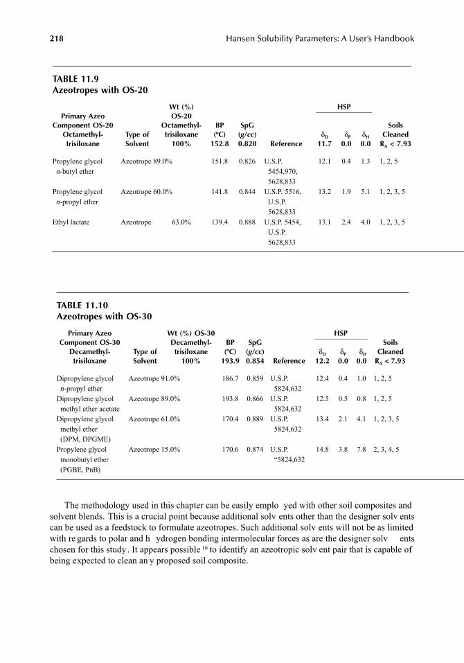
218 Hansen Solubility Parameters: A User’s Handbook
The methodology used in this chapter can be easily emplo yed with other soil composites andsolvent blends. This is a crucial point because additional solv ents other than the designer solv entscan be used as a feedstock to formulate azeotropes. Such additional solv ents will not be as limitedwith re gards to polar and h ydrogen bonding intermolecular forces as are the designer solv entschosen for this study . It appears possible 16 to identify an azeotropic solv ent pair that is capable ofbeing expected to clean an y proposed soil composite.
TABLE 11.9Azeotropes with OS-20
Primary AzeoComponent OS-20
Octamethyl-trisiloxane
Type ofSolvent
Wt (%)OS-20
Octamethyl-trisiloxane
100%
BP(ºC)
152.8
SpG(g/cc)0.820 Reference
HSP
SoilsCleaned
RA < 7.93δD
11.7 δP
0.0δH
0.0
Propylene glycol n-butyl ether
Azeotrope 89.0% 151.8 0.826 U.S.P. 5454,970, 5628,833
12.1 0.4 1.3 1, 2, 5
Propylene glycol n-propyl ether
Azeotrope 60.0% 141.8 0.844 U.S.P. 5516, U.S.P. 5628,833
13.2 1.9 5.1 1, 2, 3, 5
Ethyl lactate Azeotrope 63.0% 139.4 0.888 U.S.P. 5454, U.S.P. 5628,833
13.1 2.4 4.0 1, 2, 3, 5
TABLE 11.10Azeotropes with OS-30
Primary AzeoComponent OS-30
Decamethyl-trisiloxane
Type ofSolvent
Wt (%) OS-30Decamethyl-trisiloxane
100%
BP(ºC)
193.9
SpG(g/cc)0.854 Reference
HSP Soils
CleanedRA < 7.93
δD
12.2 δP
0.0 δH
0.0
Dipropylene glycol n-propyl ether
Azeotrope 91.0% 186.7 0.859 U.S.P.5824,632
12.4 0.4 1.0 1, 2, 5
Dipropylene glycol methyl ether acetate
Azeotrope 89.0% 193.8 0.866 U.S.P.5824,632
12.5 0.5 0.8 1, 2, 5
Dipropylene glycol methyl ether (DPM, DPGME)
Azeotrope 61.0% 170.4 0.889 U.S.P.5824,632
13.4 2.1 4.1 1, 2, 3, 5
Propylene glycol monobutyl ether (PGBE, PnB)
Azeotrope 15.0% 170.6 0.874 U.S.P.“5824,632
14.8 3.8 7.8 2, 3, 4, 5
7248_C011.fm Page 218 Thursday, May 10, 2007 8:00 AM
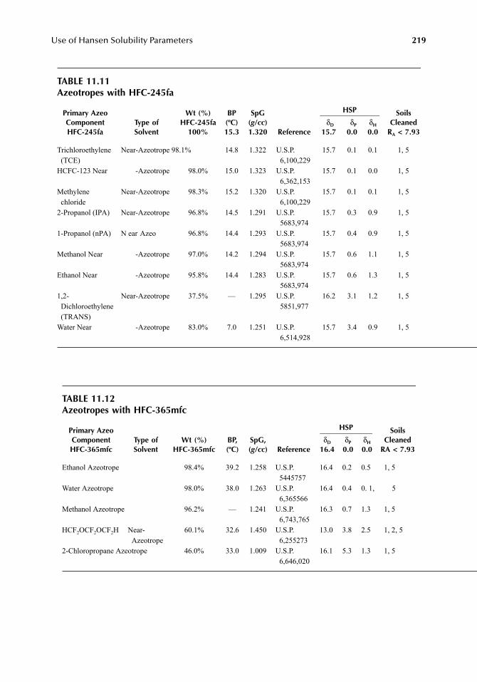
Use of Hansen Solubility Parameters 219
TABLE 11.11Azeotropes with HFC-245fa
Primary AzeoComponentHFC-245fa
Type ofSolvent
Wt (%)HFC-245fa
100%
BP(ºC)15.3
SpG(g/cc)1.320 Reference
HSP SoilsCleaned
RA < 7.93 δD
15.7 δP
0.0 δH 0.0
Trichloroethylene(TCE)
Near-Azeotrope 98.1% 14.8 1.322 U.S.P.6,100,229
15.7 0.1 0.1 1, 5
HCFC-123 Near -Azeotrope 98.0% 15.0 1.323 U.S.P. 6,362,153
15.7 0.1 0.0 1, 5
Methylene chloride
Near-Azeotrope 98.3% 15.2 1.320 U.S.P. 6,100,229
15.7 0.1 0.1 1, 5
2-Propanol (IPA) Near-Azeotrope 96.8% 14.5 1.291 U.S.P. 5683,974
15.7 0.3 0.9 1, 5
1-Propanol (nPA) N ear Azeo 96.8% 14.4 1.293 U.S.P. 5683,974
15.7 0.4 0.9 1, 5
Methanol Near -Azeotrope 97.0% 14.2 1.294 U.S.P. 5683,974
15.7 0.6 1.1 1, 5
Ethanol Near -Azeotrope 95.8% 14.4 1.283 U.S.P. 5683,974
15.7 0.6 1.3 1, 5
1,2-Dichloroethylene (TRANS)
Near-Azeotrope 37.5% — 1.295 U.S.P. 5851,977
16.2 3.1 1.2 1, 5
Water Near -Azeotrope 83.0% 7.0 1.251 U.S.P. 6,514,928
15.7 3.4 0.9 1, 5
TABLE 11.12Azeotropes with HFC-365mfc
Primary Azeo ComponentHFC-365mfc
Type ofSolvent
Wt (%)HFC-365mfc
BP,(ºC)
SpG,(g/cc) Reference
HSP SoilsCleaned
RA < 7.93δD
16.4δP
0.0δH
0.0
Ethanol Azeotrope 98.4% 39.2 1.258 U.S.P.5445757
16.4 0.2 0.5 1, 5
Water Azeotrope 98.0% 38.0 1.263 U.S.P. 6,365566
16.4 0.4 0. 1, 5
Methanol Azeotrope 96.2% — 1.241 U.S.P. 6,743,765
16.3 0.7 1.3 1, 5
HCF2OCF2OCF2H Near-Azeotrope
60.1% 32.6 1.450 U.S.P. 6,255273
13.0 3.8 2.5 1, 2, 5
2-Chloropropane Azeotrope 46.0% 33.0 1.009 U.S.P. 6,646,020
16.1 5.3 1.3 1, 5
7248_C011.fm Page 219 Thursday, May 10, 2007 8:00 AM
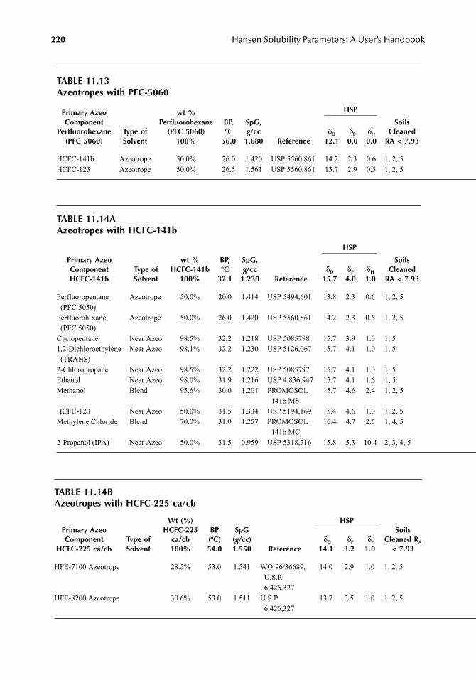
220 Hansen Solubility Parameters: A User’s Handbook
TABLE 11.13Azeotropes with PFC-5060
Primary AzeoComponent
Perfluorohexane(PFC 5060)
Type ofSolvent
wt %Perfluorohexane
(PFC 5060)100%
BP,°C
56.0
SpG,g/cc
1.680 Reference
HSP
δD
12.1δP 0.0
δH
0.0
SoilsCleaned
RA < 7.93
HCFC-141b Azeotrope 50.0% 26.0 1.420 USP 5560,861 14.2 2.3 0.6 1, 2, 5HCFC-123 Azeotrope 50.0% 26.5 1.561 USP 5560,861 13.7 2.9 0.5 1, 2, 5
TABLE 11.14AAzeotropes with HCFC-141b
Primary AzeoComponentHCFC-141b
Type ofSolvent
wt %HCFC-141b
100%
BP,°C
32.1
SpG,g/cc
1.230 Reference
HSP
δD
15.7δP 4.0
δH
1.0
SoilsCleaned
RA < 7.93
Perfluoropentane(PFC 5050)
Azeotrope 50.0% 20.0 1.414 USP 5494,601 13.8 2.3 0.6 1, 2, 5
Perfluoroh xane (PFC 5050)
Azeotrope 50.0% 26.0 1.420 USP 5560,861 14.2 2.3 0.6 1, 2, 5
Cyclopentane Near Azeo 98.5% 32.2 1.218 USP 5085798 15.7 3.9 1.0 1, 51,2-Dichloroethylene(TRANS)
Near Azeo 98.1% 32.2 1.230 USP 5126,067 15.7 4.1 1.0 1, 5
2-Chloropropane Near Azeo 98.5% 32.2 1.222 USP 5085797 15.7 4.1 1.0 1, 5Ethanol Near Azeo 98.0% 31.9 1.216 USP 4,836,947 15.7 4.1 1.6 1, 5Methanol Blend 95.6% 30.0 1.201 PROMOSOL
141b MS15.7 4.6 2.4 1, 2, 5
HCFC-123 Near Azeo 50.0% 31.5 1.334 USP 5194,169 15.4 4.6 1.0 1, 2, 5Methylene Chloride Blend 70.0% 31.0 1.257 PROMOSOL
141b MC16.4 4.7 2.5 1, 4, 5
2-Propanol (IPA) Near Azeo 50.0% 31.5 0.959 USP 5318,716 15.8 5.3 10.4 2, 3, 4, 5
TABLE 11.14BAzeotropes with HCFC-225 ca/cb
Primary AzeoComponent
HCFC-225 ca/cb Type ofSolvent
Wt (%)HCFC-225
ca/cb 100%
BP(ºC)54.0
SpG(g/cc)1.550 Reference
HSP Soils
Cleaned RA
< 7.93 δD
14.1 δP
3.2 δH
1.0
HFE-7100 Azeotrope 28.5% 53.0 1.541 WO 96/36689, U.S.P. 6,426,327
14.0 2.9 1.0 1, 2, 5
HFE-8200 Azeotrope 30.6% 53.0 1.511 U.S.P. 6,426,327
13.7 3.5 1.0 1, 2, 5
7248_C011.fm Page 220 Thursday, May 10, 2007 8:00 AM
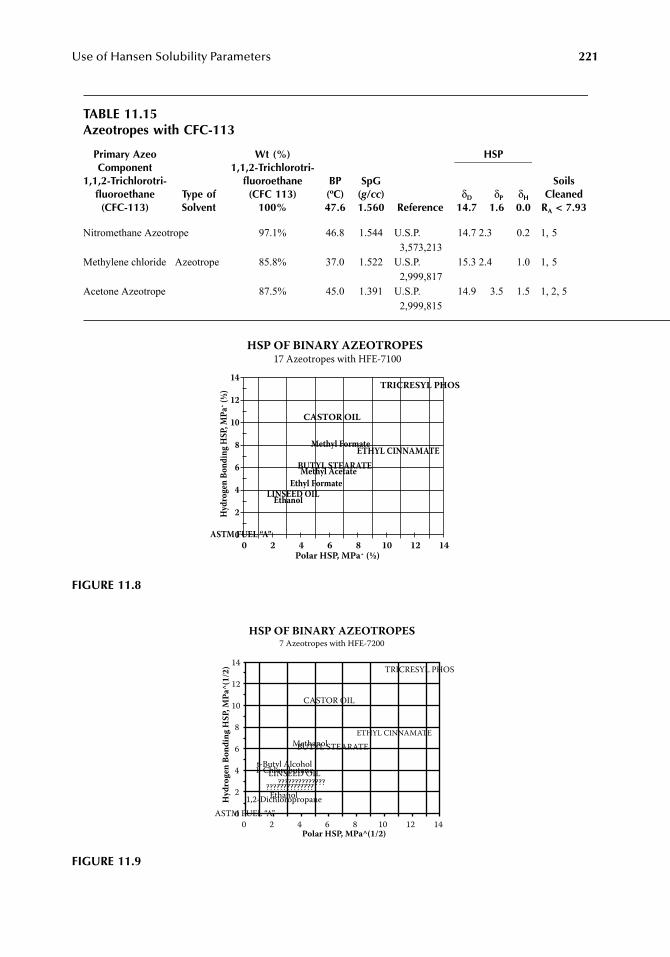
Use of Hansen Solubility Parameters 221
TABLE 11.15Azeotropes with CFC-113
Primary AzeoComponent
1,1,2-Trichlorotri-fluoroethane(CFC-113)
Type ofSolvent
Wt (%)1,1,2-Trichlorotri-
fluoroethane(CFC 113)
100%
BP(ºC)47.6
SpG(g/cc)1.560 Reference
HSP
SoilsCleaned
RA < 7.93δD
14.7 δP
1.6 δH 0.0
Nitromethane Azeotrope 97.1% 46.8 1.544 U.S.P.3,573,213
14.7 2.3 0.2 1, 5
Methylene chloride Azeotrope 85.8% 37.0 1.522 U.S.P. 2,999,817
15.3 2.4 1.0 1, 5
Acetone Azeotrope 87.5% 45.0 1.391 U.S.P. 2,999,815
14.9 3.5 1.5 1, 2, 5
FIGURE 11.8
FIGURE 11.9
HSP OF BINARY AZEOTROPES
TRICRESYL PHOS
CASTOR OIL
17 Azeotropes with HFE-7100
ETHYL CINNAMATEMethyl Formate
Methyl Acetate
Ethyl Formate
Ethanol
BUTYL STEARATE
LINSEED OIL
ASTM FUEL “A”
Hyd
roge
n B
on
din
g H
SP,
MP
a ˆ (
½)
Polar HSP, MPaˆ (½)
14
12
10
8
6
4
2
00 2 4 6 8 10 12 14
HSP OF BINARY AZEOTROPES7 Azeotropes with HFE-7200
Polar HSP, MPa^(1/2)
Hy
dro
ge
n B
on
din
g H
SP
, M
Pa
^(1
/2)
0
0
2
2
4
4
6
6
8
8
10
10
12
12
14
14TRICRESYL PHOS
CASTOR OIL
ETHYL CINNAMATE
MethanolBUTYL STEARATE
t-Butyl Alcohol1-ChlorobutaneLINSEED OIL
????????????????????????????Ethanol
1,2-Dichloropropane
ASTM FUEL “A”
7248_C011.fm Page 221 Thursday, May 10, 2007 8:00 AM
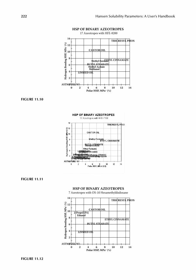
222 Hansen Solubility Parameters: A User’s Handbook
FIGURE 11.10
FIGURE 11.11
FIGURE 11.12
HSP OF BINARY AZEOTROPES
TRICRESYL PHOS
CASTOR OIL
17 Azeotropes with HFE-8200
ETHYL CINNAMATEMethyl Formate
Methyl AcetateMethanol
BUTYL STEARATE
LINSEED OIL
ASTM FUEL “A”
Hyd
roge
n B
on
din
g H
SP,
MP
a ˆ (
½)
Polar HSP, MPaˆ (½)
14
12
10
8
6
4
2
00 2 4 6 8 10 12 14
HSP OF BINARY AZEOTROPES
TRICRESYL PHOS
CASTOR OIL
7 Azeotropes with OS-10 Hexamethyldisiloxane
ETHYL CINNAMATE
BUTYL STEARATE
LINSEED OIL
2-Propyl (PA)Ethanol
ASTM FUEL “A”
Hyd
roge
n B
on
din
g H
SP,
MP
a ˆ (
½)
Polar HSP, MPaˆ (½)
14
12
10
8
6
4
2
00 2 4 6 8 10 12 14
7248_C011.fm Page 222 Thursday, May 10, 2007 8:00 AM

Use of Hansen Solubility Parameters 223
FIGURE 11.13
FIGURE 11.14
FIGURE 11.15
HSP OF BINARY AZEOTROPES
TRICRESYL PHOS
CASTOR OIL
3 Azeotropes with OS-20 Octamethyltrisiloxane
ETHYL CINNAMATE
BUTYL STEARATE
LINSEED OIL
Propylene Glycol n-Propyl Ether
ASTM FUEL “A”
Hyd
roge
n B
on
din
g H
SP,
MP
a ˆ (
½)
Polar HSP, MPaˆ (½)
14
12
10
8
6
4
2
00 2 4 6 8 10 12 14
HSP OF BINARY AZEOTROPES
TRICRESYL PHOS
CASTOR OIL
4 Azeotropes with OS-30 Decamethyltrisiloxane
ETHYL CINNAMATE
BUTYL STEARATE
LINSEED OIL
Propylene Glycol n-Propyl Ether
ASTM FUEL “A”
Hyd
roge
n B
on
din
g H
SP,
MP
a ˆ (
½)
Polar HSP, MPaˆ (½)
14
12
10
8
6
4
2
00 2 4 6 8 10 12 14
HSP OF BINARY AZEOTROPES
TRICRESYL PHOS
CASTOR OIL
9 Azeotropes with HFC-245fa
ETHYL CINNAMATE
BUTYL STEARATE
LINSEED OIL
ASTM FUEL “A”
Hyd
roge
n B
on
din
g H
SP,
MP
a ˆ (
½)
Polar HSP, MPaˆ (½)
14
12
10
8
6
4
2
00 2 4 6 8 10 12 14
7248_C011.fm Page 223 Thursday, May 10, 2007 8:00 AM
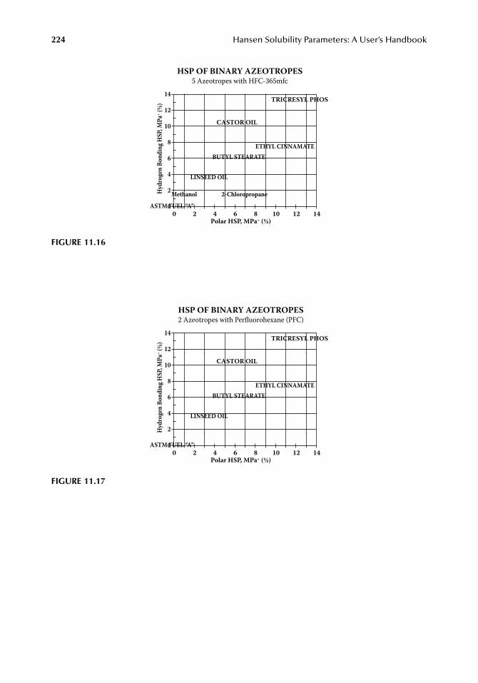
224 Hansen Solubility Parameters: A User’s Handbook
FIGURE 11.16
FIGURE 11.17
HSP OF BINARY AZEOTROPES
TRICRESYL PHOS
CASTOR OIL
5 Azeotropes with HFC-365mfc
ETHYL CINNAMATE
BUTYL STEARATE
LINSEED OIL
Methanol 2-Chloropropane
ASTM FUEL “A”
Hyd
roge
n B
on
din
g H
SP,
MP
a ˆ (
½)
Polar HSP, MPaˆ (½)
14
12
10
8
6
4
2
00 2 4 6 8 10 12 14
HSP OF BINARY AZEOTROPES
TRICRESYL PHOS
CASTOR OIL
2 Azeotropes with Perfluorohexane (PFC)
ETHYL CINNAMATE
BUTYL STEARATE
LINSEED OIL
ASTM FUEL “A”
Hyd
roge
n B
on
din
g H
SP,
MP
a ˆ (
½)
Polar HSP, MPaˆ (½)
14
12
10
8
6
4
2
00 2 4 6 8 10 12 14
7248_C011.fm Page 224 Thursday, May 10, 2007 8:00 AM
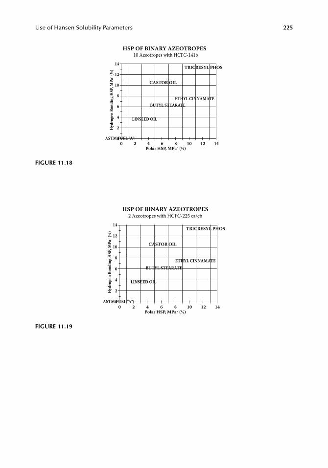
Use of Hansen Solubility Parameters 225
FIGURE 11.18
FIGURE 11.19
HSP OF BINARY AZEOTROPES
TRICRESYL PHOS
CASTOR OIL
10 Azeotropes with HCFC-141b
ETHYL CINNAMATE
BUTYL STEARATE
LINSEED OIL
ASTM FUEL “A”
Hyd
roge
n B
on
din
g H
SP,
MP
a ˆ (
½)
Polar HSP, MPaˆ (½)
14
12
10
8
6
4
2
00 2 4 6 8 10 12 14
HSP OF BINARY AZEOTROPES
TRICRESYL PHOS
CASTOR OIL
2 Azeotropes with HCFC-225 ca/cb
ETHYL CINNAMATE
BUTYL STEARATE
LINSEED OIL
ASTM FUEL “A”
Hyd
roge
n B
on
din
g H
SP,
MP
a ˆ (
½)
Polar HSP, MPaˆ (½)
14
12
10
8
6
4
2
00 2 4 6 8 10 12 14
7248_C011.fm Page 225 Thursday, May 10, 2007 8:00 AM
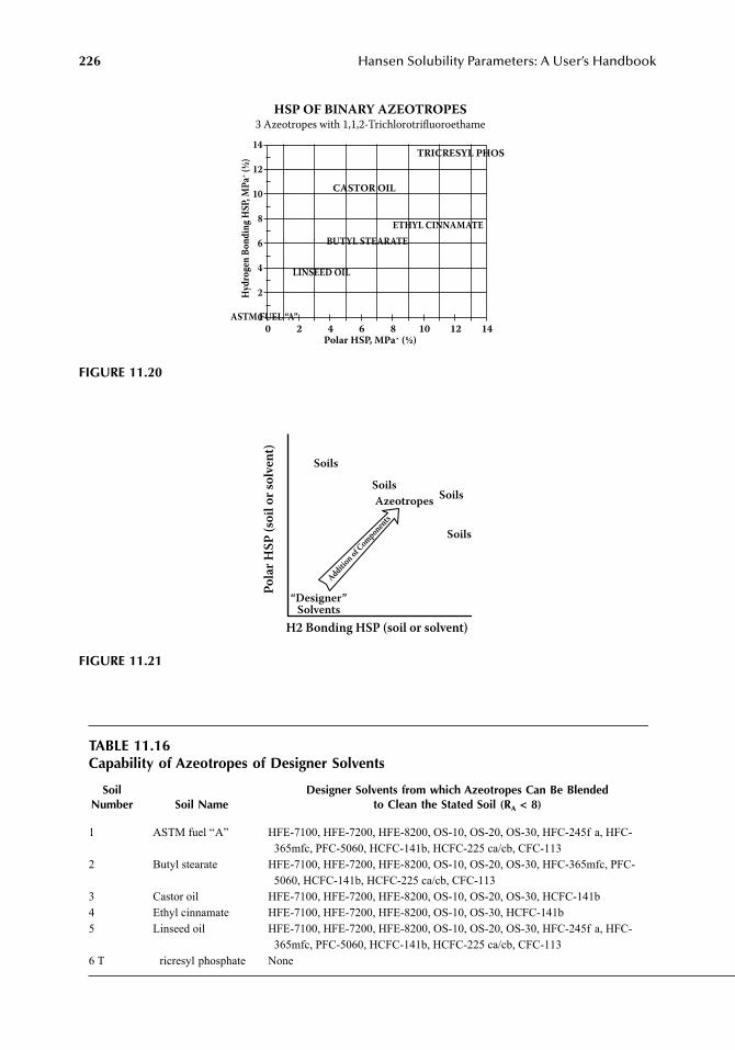
226 Hansen Solubility Parameters: A User’s Handbook
FIGURE 11.20
FIGURE 11.21
TABLE 11.16Capability of Azeotropes of Designer Solvents
SoilNumber Soil Name
Designer Solvents from which Azeotropes Can Be Blendedto Clean the Stated Soil (RA < 8)
1 ASTM fuel “A” HFE-7100, HFE-7200, HFE-8200, OS-10, OS-20, OS-30, HFC-245f a, HFC-365mfc, PFC-5060, HCFC-141b, HCFC-225 ca/cb, CFC-113
2 Butyl stearate HFE-7100, HFE-7200, HFE-8200, OS-10, OS-20, OS-30, HFC-365mfc, PFC-5060, HCFC-141b, HCFC-225 ca/cb, CFC-113
3 Castor oil HFE-7100, HFE-7200, HFE-8200, OS-10, OS-20, OS-30, HCFC-141b 4 Ethyl cinnamate HFE-7100, HFE-7200, HFE-8200, OS-10, OS-30, HCFC-141b 5 Linseed oil HFE-7100, HFE-7200, HFE-8200, OS-10, OS-20, OS-30, HFC-245f a, HFC-
365mfc, PFC-5060, HCFC-141b, HCFC-225 ca/cb, CFC-113 6 T ricresyl phosphate None
HSP OF BINARY AZEOTROPES
TRICRESYL PHOS
CASTOR OIL
3 Azeotropes with 1,1,2-Trichlorotrifluoroethame
ETHYL CINNAMATE
BUTYL STEARATE
LINSEED OIL
ASTM FUEL “A”
Hyd
roge
n B
on
din
g H
SP,
MP
a ˆ (
½)
Polar HSP, MPaˆ (½)
14
12
10
8
6
4
2
00 2 4 6 8 10 12 14
H2 Bonding HSP (soil or solvent)
Polar
HSP
(soi
l or s
olve
nt)
“Designer”Solvents
SoilsSoils
Soils
Soils
Azeotropes
Addition of C
omponents
7248_C011.fm Page 226 Thursday, May 10, 2007 8:00 AM
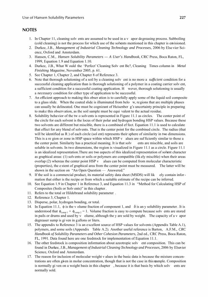
Use of Hansen Solubility Parameters 227
NOTES
1. In Chapter 11, cleaning solv ents are assumed to be used in a v apor degreasing process. Subboiling(cold cleaning) is not the process for which use of the solvents mentioned in this chapter is envisioned.
2. Durkee, J.B., Management of Industrial Cleaning Technology and Processes, 2006 by Else vier Sci-ence, Oxford and Amsterdam.
3. Hansen, C.M., Hansen Solubility Parameters — A User’s Handbook, CRC Press, Boca Raton, FL,1999, Equation 1.9 and Equation 1.10.
4. Durkee, J.B., What W ould the ‘Perfect’ Cleaning Solv ent Be?, Cleaning Times column in MetalFinishing Magazine, November 2005, p. 61.
5. See Chapter 1, Chapter 2, and Chapter 8 of Reference 3.6. Note that thorough solutioning of a soil by a cleaning solv ent is no more a sufficient condition for a
successful cleaning application than is thorough solutioning of a polymer in a coating carrier solv ent,a sufficient condition for a successful coating application. H wever, thorough solutioning is usuallya necessary condition for either type of application to be successful.
7. An efficient approach to making this obser ation is to carefully apply some of the liquid soil compositeto a glass slide. When the coated slide is illuminated from belo w, regions that are multiple phasescan usually be delineated. One must be cognizant of Heisenber g’s uncertainty principle in preparingto make this observation, as the soil sample must be equi valent to the actual residue.
8. Solubility behavior of the tw o solvents is represented in Figure 11.1 as circles. The center point ofthe circle for each solvent is the locus of their polar and hydrogen bonding HSP values. Because thesetwo solvents are different but miscible, there is a combined ef fect. Equation 11.1 is used to calculatethat effect for any blend of solvents. That is the center point for the combined circle. The radius (thatwill be identified as R ) of each circle (sol ent) represents their sphere of similarity in two dimensions.This is a re gion or zone in HSP space within which HSP v alues are suf ficiently similar to those athe center point. Similarity has a practical meaning. It is that solv ents are miscible, and soils aresoluble in solvents. In two dimensions, the region is visualized in Figure 11.1 as a circle. Figure 11.1is an idealized representation. There are two aspects of this idealized representation of solvent characteras graphical areas: (1) solvents or soils or polymers are compatible (lik ely miscible) when their areasoverlap (2) whereas the center point HSP v alues can be computed from molecular characteristic(properties), the e xtent of graphical area from the center point must be measured. The latter will beshown in the section on “An Open Question — Answered.”
9. If the soil is a commercial product, its material safety data sheet (MSDS) will lik ely contain infor -mation that either is the recipe or from which a suitable estimate of the recipe can be inferred.
10. See Equation 1.9 in Chapter 1 in Reference 3, and Equation 11.3 in “Method for Calculating HSP ofComposites (Soils or Solv ents)” in this chapter .
11. Refers to the total or Hildebrand solubility parameter .12. Reference 3, Chapter 1.13. Disperse, polar, hydrogen bonding, or total.14. In Equation 11.1, φ is the v olume fraction of component 1, and δ is an y solubility parameter . It is
understood that φcomp 1 + φcomp 2 = 1. Volume fraction is easy to compute because solv ents are storedin pails or drums and used by v olume, although the y are sold by weight. The capacity of a v apordegreaser sump is gi ven in gallons or liters.
15. The appendix to Reference 3 is an excellent source of HSP values for solvents (Appendix Table A.1),polymers, and some soils (Appendix Table A.2). Another useful reference is Barton, A.F.M., CRCHandbook of Solubility Parameters and Other Cohesion Parameters, 2nd ed., CRC Press, Boca Raton,FL, 1991. Data found here are one feedstock for implementation of Equation 11.1.
16. The other feedstock is composition information about azeotropic solv ent composition. This can befound in Durkee, J.B., Management of Industrial Cleaning Technology and Processes, 2006 by ElsevierScience, Oxford and Amsterdam.
17. The reason for inclusion of molecular weight v alues in the basic data is because the mixture concen-trations are often given in molar concentration, though that is not the case in this example. Compositionis normally gi ven on a weight basis in this chapter , because it is that basis by which solv ents arenormally sold.
7248_C011.fm Page 227 Thursday, May 10, 2007 8:00 AM
228 Hansen Solubility Parameters: A User’s Handbook
18. In this w ay, cleaning is unlik e construction of coatings. In a coating, all components are generallycompatible with the carrier solv ent. In cleaning, where there can be destruction of coatings, allcomponents must be manageable. In solv ent cleaning, soil components can be partially soluble,swollen, insoluble, or soluble. Generally , a cleaning process can be designed to manage remo val ofsoil components from surf aces without re gard to their relationship to the solv ent. In cleaning, man-agement involves hydrodynamic (mechanical) force, heat, and solv ency.
19. Said in a colloquial manner , “A chain is only as strong as its weak est link.”20. Hansen, C.M. and Skaarup, K., The three dimensional solubility parameter — key to paint component
affinities, J. Paint Technol., Vol. 305, No. 511, 511–514, 1967.21. Finding the number 4 in Equation 11.3 may be surprising. There is considerable discussion in the
literature about the need for it. It has been found empirically useful o ver several decades of practicalexperience. There are two justifications for it: (1) it co verts three-dimensional spheroidal plots withdispersion solubility parameters to spherical ones, and (2) theoretical considerations associated withthe Prigogine theory of corresponding states. See Chapter 5 in this book.
22. Unfortunately, selection of a suitable cleaning solv ent based on similarity of intermolecular forces isbut a necessary first step in d velopment of cleaning process applications. Certain selection criteriaare listed as follo ws:• A solvent that has a strong af finity for a soil ut a lo w holding capacity for it (mass solubility)would be a poor choice.• A solvent selected to do cleaning w ork must be able to dissolv e the soil to the e xtent desired in thetime allotted under the pre vailing conditions. Cleaning is a transport process.• Also, a poor choice is a solv ent that only gradually penetrates and swells the soil and allo ws it tobe removed by rinse fluids• Finally, a solvent that efficiently dissol es an adequate mass of soil in an ef ficient time ut only ata temperature above its boiling point is nearly useless. Pressurized contacting equipment is expensive.Yet, without successful completion of a screening evaluation via use of HSP, development of cleaningprocess applications becomes either resource intensi ve or based on hearsay e vidence.
23. Note that Figure 11.1 is a generalized presentation. Soils can be matched to solv ents for the purposeof solvent selection; solvents can be matched to other solv ents for the purpose of producing a blendwith certain physical properties, or soils can be matched to other soils for the purpose of e valuatingif solution-based or force-based (aqueous technology) should be used, depending upon whether thesoils are expected to combine in a single or multiple phases.
24. HFE-8200 is actually a component of the product sold as HFE-7100. The latter is mixture of Perfluoron-butyl methyl ether (35%) and perfluoroiso utyl methyl ether (65%). HFE-8200 is the pure perfluoroisobutyl methyl ether. United States Pharmacopeia (USP) 6,426,327 teaches that azeotropic behav-ior of mixtures of the two isomers and another component is relati vely independent of distribution ofisomers in the HFE material. Consequently, in this analysis, HFE-7100 and HFE-8200 are consideredequivalent in terms of the boiling point and composition of azeotropes. Ho wever, the HSP propertiesof HFE-7100 and HFE-8200 are slightly different. This difference has been retained in the calculationsof solubility behavior of the azeotropes.
25. Owing to its inertness as a solv ent, high specific gr vity, and lo w surf ace tension, it finds use icleaning work as a rinsing agent. Yet, because of its inertness, PFC-5060 is a designer solv ent thaton emission migrates without de gradation to the Earth ’s stratospheric layer and acts as a globalwarming agent. Hence, its use is limited “by design.”
26. The disperse HSP v alue is momentarily ne glected in the interests of graphical clarity when a tw o-dimensional graph is used. These values are relatively similar.
27. The structure shown represents the most common (89%) component (ricinolenic acid, 12-hydroxyoleicacid) of castor oil. Castor oil is also referred to as the triglyceride of this acid.
28. The structure shown, linoleic acid, is the most common (52%) acidic component of linseed oil. Theother major acidic component of the triglyceride is linolenic acid that has one fe wer double bond.
7248_C011.fm Page 228 Thursday, May 10, 2007 8:00 AM
Use of Hansen Solubility Parameters 229
29. In the main, these azeotropes are claimed in U.S. patents whose grant date is during the 1990s. Thepatent assignee is most often the manuf acturer of the designer solv ent. There is no published tableof these binary azeotropes e xcept that found in Reference 15, which lists around 450 of them. Theywere identified in 2004 during an xtensive search of the world patent literature. Readers are remindedthat the normal interpretation of U.S. patent law is that when a third component is added to a claimedbinary composition, the ternary mixture is still co vered by the U.S. patent. In other w ords, if thesebinary azeotropes are not commercial products, users cannot formulate them without permission fromthe patent holder.
30. The parts used are those from the b usiness operation. The soils are those identified by the usinessas being of concern and are applied as pure components to pre viously cleaned parts (or coupons).The method of assaying cleanliness is gra vimetric. All information is publicly a vailable. Seehttp://www.cleanersolutions.org. Most work was done around 2004.There are se veral uncertainties about use of these 53 data points: (1) a v ariety of v apor degreasingprocesses, test conditions, and test e xposure times were used, (2) soil components were identified bchemical abstracts service (CAS) number from the manufacturer’s MSDS that is not always a completelisting of ingredients, and (3) whereas the soil components were identified, their concentration in thapplied soil mix w as not.Yet, there w as considerable le vel of replicates a vailable through the use of multiple runs where thesame solvent was used under a dif ferent product identification. Hence, one can say with 95% confdence that if the R A value is less than 8, then the w orst level of cleanliness of the least compatiblesoil component would be 94%. The expected value of cleanliness w ould be around 97%.
31. Normally, the limit of acceptability re garding cleaning performance is set by the requirements of thenext processing or use step. F or these laboratory trials, no such information w as available.
32. Both ternary and quaternary azeotropes containing designer solvents have been identified and patentedSome find applications in aerosol-p wered cleaning products. Here, there is little concern aboutcomposition change in use, as the entire v olume applied evaporated quickly after application. But invapor degreasing operations, which is the venue of this chapter, the concern about composition changeof ternary and quaternary (vs. binary) azeotropes with use cannot be ne glected.
33. Azeotropes in Table 11.4 through Table 11.14 are sorted by increasing v alue of polar HSP with thatof the base designer solv ent given in the initial ro w. Boiling points are also gi ven, but not the ro wsthat are not sorted by that parameter . In this study , all azeotropes noted are minimum-boiling azeo-tropes. As all of these designer solv ents have commercial v alue as unique compounds, the azeotropes the yform with other solv ents are claimed in patents. U.S. patent numbers are gi ven as references whereavailable.
34. No denigration of designer solvents is intended in this work. Rather, these solvents represent the resultof significant and successful chemical research into identification and man acture of chemicalstructures, which alle viate man y of the safety , health, and en vironmental concerns about solv entscommonly used in cleaning (and other) w ork in the late 20 th century. Elimination of those concernswas roundly and justifiably applauded by users.In a sense, that research w as too successful. Seemingly, as a class of product, designer solv ents werethose whose use raised fe wer concerns, but whose value in use w as more limited. Binary azeotropes based on designer solv ents are an attempt to span the g ap between absence ofconcern and absence of v alue in use.
35. Only blends defined by measured p ysical property and boiling point data are included. Theoreticalor predicted azeotropes are not included because the y cannot be purchased as blends for cleaningwork. A good source of information about predicted azeotropes is Harding, S.T ., Locating All Heter-ogeneous and Reactive Azeotropes, distrib uted by the American Institute of Chemical Engineers,(January 1, 1998), ASIN: B0006R4J04.
36. A secondary standard is to fulfill the co ventional requirements upon which solv ent cleaning w ork(vapor degreasing) is based. See Reference 2 for details.
37. This phrase refers to the identifying characteristic of an azeotrope, that the composition of the v aporand the composition of the boiling liquid are identical. In other w ords, as the mixture boils, thecomposition (like that of a single component solv ent) remains constant.
7248_C011.fm Page 229 Thursday, May 10, 2007 8:00 AM

7248_C011.fm Page 230 Thursday, May 10, 2007 8:00 AM
231
12
Applications — Chemical Resistance
Charles M. Hansen
ABSTRACT
Hansen solubility parameters (HSP) can correlate dif ferences in ph ysical beha vior observ ed inchemical resistance testing of polymers and polymer -containing systems when a suf ficiently la genumber of dif ferent organic solvents are included in a study . These correlations can then be usedto predict the chemical attack expected in systems that have not yet been tested. Examples of HSPcorrelations included here are for solubility , degree of surf ace attack, tensile strength reduction,and simple e valuations of chemical resistance of the suitable-for -use or not type. En vironmentalstress cracking is discussed in more detail in Chapter 14. In each case, the molecular size of theliquids used can affect the result and should be considered in some way. Chapter 16 treats absorptionand diffusion in polymers with this in mind. A common problem is that tests with larger molecularweight liquids have not reached equilibrium absorption within the timeframe of the exposure. HSPcorrelations are presented for chemical resistance studies of epoxy and zinc silicate tank coatings,PET, POM, PA6/66, PUR, PPS, PEI, Neoprene
®
, etc.
INTRODUCTION
HSP are widely used in the coatings industry to select solv ents for dissolving polymers and binders.This has been discussed in Chapter 8 and also in References 1 through 12, as well as else where. Thefact of solution is in itself clearly one simple form of chemical attack of the polymers the y dissolve.This means that chemical resistance for some polymers can be partly inferred from HSP correlationsof their solubility and/or swelling. HSP correlations of this type ha ve been discussed in Chapter 5. Anexample is that if a chemical does not dissolve an epoxy component or the curing agent, then it is quiteunlikely that it will attack a fully crosslink ed epoxy coating or glue. The HSP correlations of surf acephenomena, which have been discussed in Chapters 6 and 7 and else where,
13–18
can also provide someinsight into chemical resistance. Liquids not wetting a surf ace are not as likely to attack it as those thatdo wet it, although there are no guarantees. A relation between spontaneous spreading and de wettingof liquids and en vironmental stress cracking has been found.
19
This is discussed in more detail inChapter 14. Liquids that spontaneously spread were found to induce en vironmental stress cracking atlower critical strains than those liquids that do not. Some surf ace studies may in volve evaluation of amore direct form of chemical attack, such as the attack/whitening of PET coated with “amorphous”PET to improve weldability. This example is discussed in more detail later. Whatever is being correlated,the general considerations of the HSP characterizations discussed in earlier chapters are the same forthe HSP correlations of chemical resistance reported here. However, there are certain additional pitfallsto be aware of when correlating chemical resistance. These include (lack of) attainment of equilibrium,the effects of molecular size of the test chemical, dif ference in local se gments of polymers (e ven inhomopolymers), and acid/base reactions.
Once a reliable HSP characterization of chemical resistance is a vailable, it can be used tocalculate the behavior of other systems that have not been tested. Obtaining a good HSP correlationof chemical resistance that allo ws reliable predictions depends v ery much on careful treatment ofthe available data or generation of data with such a correlation in mind. Unfortunately , very few
7248_C012.fm Page 231 Wednesday, May 23, 2007 11:14 AM
232
Hansen Solubility Parameters: A User’s Handbook
studies of chemical resistance have been designed with the purpose of generating HSP correlations.Also, it must be clear that the chemical attack discussed in this chapter does not include truechemical reactions leading to covalent bonding or destruction, such as with acids and bases, whetherthey are or ganic or inor ganic. Chemical reactions forming ne w compounds are often found withamines and or ganic acids. These reactions often lead to discoloration in systematic solubilityparameter testing with one or more of the amines used as test solv ents. Discolored systems shouldsimply be neglected in HSP correlations of physical (reversible) solubility. The products of reactionsof well-defined o ganic bases with well-defined o ganic acids ha ve actually been studied system-atically from a solubility parameter point of vie w.
20
Some of the results of this study are discussedin Chapters 15 and 18.
CHEMICAL RESISTANCE — ACCEPTABLE-OR-NOT DATA
Additional sources of data for solubility parameter characterizations include chemical resistancetables reported by ra w material suppliers
21–26
or collected in books
27–29
and other sources such asthose supplied on electronic media by the Plastics Design Library.
30
Although these data are certainlyvaluable in themselv es, it has been found that gi ven data sets are not al ways as reliable/consis-tent/coherent as could be desired for solubility parameter correlations. Attainment of equilibriummay not have been achieved, and this ef fect is rarely confirmed or ven considered. Solvents withlow dif fusion coef ficients will appear to be less aggress ve than the y might become at longerexposure times or at higher concentrations. As discussed earlier , true chemical attack with acidsand bases must sometimes be sorted out. Likewise, the data are often limited in number and scope,and the chemical reagents have not been chosen for the purpose of solubility parameter correlations.Nevertheless, with the use of due caution, it is often possible to find xcellent solubility parametercorrelations using chemical resistance data of the acceptable-or -not type, particularly when the listof agents is long. Additional precautions with re gard to data of the acceptable-or -not type includewhether a molecular size ef fect is present as discussed in the follo wing. Also, it can be assumedthat if a chemical attacks a polymer at, say , 20°C, then it will also attack it at, say , 70°C. It canthen be included as data in a 70°C correlation, e ven though it may not ha ve been tested at thattemperature (and in principle the HSP are only v alid at room temperature).
EFFECTS OF SOLVENT MOLECULAR SIZE
It has been emphasized in Chapters 1, 2, and 5 that the size of solv ent molecules is important forpolymer solubility. HSP correlations ha ve confirmed that this e fect is even more important whenchemical resistance is being considered. Smaller molecules are e xpected to be better, that is, moreaggressive from a thermodynamic point of view than larger ones, all else being equal. This is knownfrom the theories of polymer solubility discussed in Chapters 1 through 4, and also from thediscussion of barrier polymers and dif fusion found in Chapter 13 and 16, respecti vely. So it is notsurprising that solv ent molecular size can be an important fourth parameter in correlations ofchemical resistance. An appropriate w ay to check this is sorting output data from a computer (orother) HSP optimization according to the molecular v olume of the test solv ents. What appear tobe errors in the correlation may become systematically arranged. It can easily be seen, if the topof the list includes the type of “error” where the smaller molecular species are “better” than expectedby comparison with all the other solv ents. This may tak e the form of une xpectedly dissolving,being more aggressive than expected, penetrating more rapidly, or reducing mechanical propertiesmore severely. Larger molecular species which are “poorer” than expected by comparison with thedata for the other solvents are often seen at the bottom of the list. One can focus upon the molecularsize range of greatest interest in such cases and repeat the correlation, ne glecting those specieswhich are outside of this range of molecular v olumes. The correlation is then strictly v alid only
7248_C012.fm Page 232 Wednesday, May 23, 2007 11:14 AM
Applications — Chemical Resistance
233
for the size range specified. Some indication of the beh vior of the solvents with V larger than theupper limit is possible if their RED numbers are greater than 1.0. These would not be expected toattack under an y circumstances. Lik ewise, the solv ents with V less than the lo wer limit can beexpected to attack if their RED numbers are less than 1.0. Lar ger numbers of solv ents are neededin the study if this is to be done with an y benefit
As stated abo ve, the size and shape of solv ent molecules are v ery important for kineticphenomena such as dif fusion, permeation, and attainment of equilibrium. Chapters 13 and 16,respectively, discuss correlations of HSP and elaborate on dif fusion phenomena in more detail.However, it will be repeated here that smaller and more linear molecules dif fuse more rapidly thanlarger and more bulky ones. The diffusion coefficient may be so l w that equilibrium is not attainedfor hundreds of years at room temperature in common solv ent exposures of rigid polymers lik epolyphenylene sulfide (PPS) with thicknesses of s veral millimeters.
31
Such ef fects lead to com-parisons where some systems may ha ve reached an equilibrium uptak e, whereas others ha ve not.Likewise, the second stage in the tw o-stage drying process in polymer film formation by sol entevaporation can last for man y years.
4,31
See Chapter 16. Polymer samples used for solubilityparameter or chemical resistance testing may contain retained solvent or monomer for many years,and this may also af fect the e valuations. However, the ef fects of w ater can be e xtremely rapid asdiscussed in the follo wing.
32
Attempts to include the molecular v olume into a new composite solubility parameter and size
parameter have not been particularly successful.
33,34
This may be because the size ef fects are notnecessarily caused through the thermodynamic considerations on which the solubility parametersare based, but rather through a kinetic ef fect of diffusion rate.
CHEMICAL RESISTANCE — EXAMPLES
Chemical resistance means dif ferent things in dif ferent contexts. Various examples of HSP corre-lations of chemical resistance are included in the follo wing. The HSP data for the correlationsdiscussed are included in Table 12.1.
Experimental data are always preferred over predicted behavior based on a correlation. However,a good HSP correlation can be used to find ma y chemicals that will clearly attack or that willclearly not attack. There are also situations where the attack is mild, and whether or not satisfactoryresults are found with a product depends on its use. Data in chemical resistance tables are oftenof the type +, +/–, –, or satisf actory/questionable/unsatisfactory, recommended/not recommended(R/NR), or something similar . The liquids which attack are clearly good solv ents for the materialin question and will be located within the HSP spheres with RED numbers being successi velylower for more severe attack, all other things being equal. The correlations can include the solventswith mild attack (+/, questionable) either in the attacking (NR) group or in the nonattacking (R)group. They can also be neglected, not knowing which group to put them into. The treatment usedin the individual correlations presented here is indicated in the following. Unless otherwise specifiedthe results are for room temperature.
T
ANK
C
OATINGS
Chemical resistance is important for tank coatings used in the transport of b ulk chemicals. Thedata in Table 12.1 include two older HSP correlations for chemical resistance for two types of tankcoatings supplied by Hempel’s Marine Paints. These are for a tw o-component epoxy type and fora zinc silicate type. The data and correlations are about 20 years old. They are included here forpurposes of demonstration. Impro vements in chemical resistance are kno wn to ha ve been imple-mented in a newer epoxy tank coating, b ut no HSP correlation has been made. A HSP correlationof the solubility of a lower molecular weight epoxy, Epon
®
1001 (Shell Chemical Corp.), is includedfor comparison. The numbers are not too dif ferent from those of the HSP correlation for chemical
7248_C012.fm Page 233 Wednesday, May 23, 2007 11:14 AM
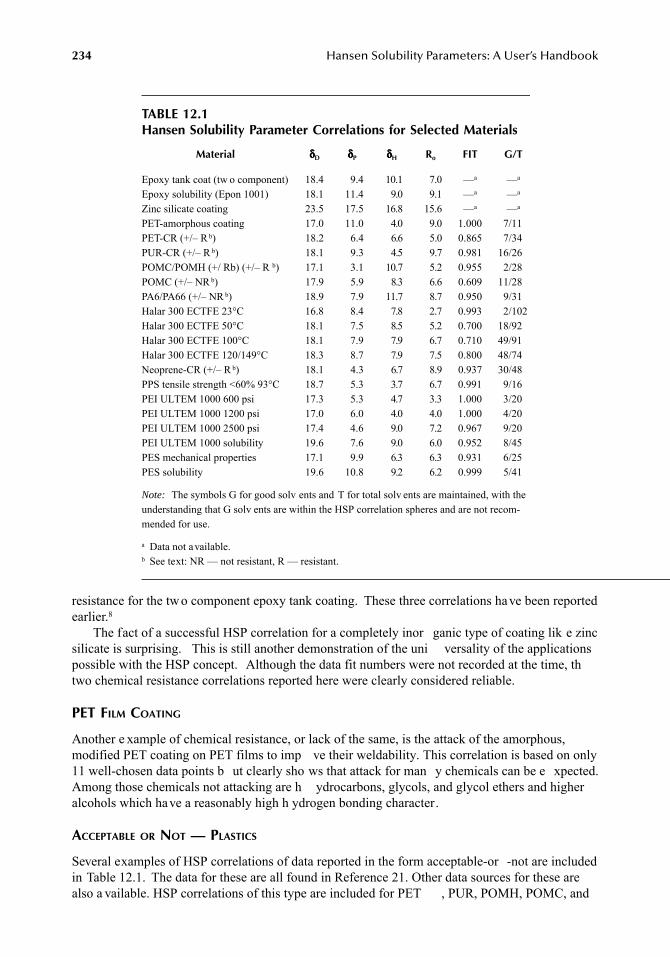
234
Hansen Solubility Parameters: A User’s Handbook
resistance for the two component epoxy tank coating. These three correlations have been reportedearlier.
8
The fact of a successful HSP correlation for a completely inor ganic type of coating lik e zincsilicate is surprising. This is still another demonstration of the uni versality of the applicationspossible with the HSP concept. Although the data fit numbers were not recorded at the time, thtwo chemical resistance correlations reported here were clearly considered reliable.
PET F
ILM
C
OATING
Another e xample of chemical resistance, or lack of the same, is the attack of the amorphous,modified PET coating on PET films to imp ve their weldability. This correlation is based on only11 well-chosen data points b ut clearly sho ws that attack for man y chemicals can be e xpected.Among those chemicals not attacking are h ydrocarbons, glycols, and glycol ethers and higheralcohols which have a reasonably high h ydrogen bonding character.
A
CCEPTABLE
OR
N
OT
— P
LASTICS
Several examples of HSP correlations of data reported in the form acceptable-or -not are includedin Table 12.1. The data for these are all found in Reference 21. Other data sources for these arealso a vailable. HSP correlations of this type are included for PET , PUR, POMH, POMC, and
TABLE 12.1Hansen Solubility Parameter Correlations for Selected Materials
Material
δδδδ
D
δδδδ
P
δδδδ
H
R
o
FIT G/T
Epoxy tank coat (tw o component) 18.4 9.4 10.1 7.0 —
a
—
a
Epoxy solubility (Epon 1001) 18.1 11.4 9.0 9.1 —
a
—
a
Zinc silicate coating 23.5 17.5 16.8 15.6 —
a
—
a
PET-amorphous coating 17.0 11.0 4.0 9.0 1.000 7/11PET-CR (+/– R
b
) 18.2 6.4 6.6 5.0 0.865 7/34PUR-CR (+/– R
b
) 18.1 9.3 4.5 9.7 0.981 16/26POMC/POMH (+/ Rb) (+/– R
b
) 17.1 3.1 10.7 5.2 0.955 2/28POMC (+/– NR
b
) 17.9 5.9 8.3 6.6 0.609 11/28PA6/PA66 (+/– NR
b
) 18.9 7.9 11.7 8.7 0.950 9/31Halar 300 ECTFE 23°C 16.8 8.4 7.8 2.7 0.993 2/102Halar 300 ECTFE 50°C 18.1 7.5 8.5 5.2 0.700 18/92Halar 300 ECTFE 100°C 18.1 7.9 7.9 6.7 0.710 49/91Halar 300 ECTFE 120/149°C 18.3 8.7 7.9 7.5 0.800 48/74Neoprene-CR (+/– R
b
) 18.1 4.3 6.7 8.9 0.937 30/48PPS tensile strength <60% 93°C 18.7 5.3 3.7 6.7 0.991 9/16PEI ULTEM 1000 600 psi 17.3 5.3 4.7 3.3 1.000 3/20PEI ULTEM 1000 1200 psi 17.0 6.0 4.0 4.0 1.000 4/20PEI ULTEM 1000 2500 psi 17.4 4.6 9.0 7.2 0.967 9/20PEI ULTEM 1000 solubility 19.6 7.6 9.0 6.0 0.952 8/45PES mechanical properties 17.1 9.9 6.3 6.3 0.931 6/25PES solubility 19.6 10.8 9.2 6.2 0.999 5/41
Note:
The symbols G for good solv ents and T for total solv ents are maintained, with theunderstanding that G solv ents are within the HSP correlation spheres and are not recom-mended for use.
a
Data not available.
b
See text: NR — not resistant, R — resistant.
7248_C012.fm Page 234 Wednesday, May 23, 2007 11:14 AM
Applications — Chemical Resistance
235
PA6/PA66 using data from Reference 21. The first three correlations of this type consider reporteevaluations of minor attack which will require further e valuation (+/–) as if these systems weresuitable for use (resistant). The last two correlations consider this condition as not suitable for use(not resistant). This is to demonstrate that dif ferences are found, depending on ho w the data areconsidered and that outliers are often found when correlating this type of data. It is for this reasonthat more e xtensive tables of HSP correlations of chemical resistance are not reported here. Toomuch space is required to try to e xplain why given results are outliers. Ho wever, some reasonshave been given earlier and others are in the follo wing.
The HSP v alues for PET based on chemical resistance are some what different from those ofthe amorphous PET coating, which is readily attack ed by far more solvents. The compositions arealso different. The POM correlations ha ve typical problems in that the correlation considering allminor attack as negligible is based on only tw o severely attacking solvents among the 28 solv entstested. When the solv ents demonstrating minor attack are considered as being in the attackinggroup, the data fit sh ws that there are man y outliers. A systematic analysis of wh y this is foundwill not be attempted for reasons of space, e ven if all the outliers could be e xplained in one w ayor another.
The HSP found for a polymer in this type of correlation may not be representati ve of thatpolymer in all aspects of its beha vior. There is a question as to co verage over the whole range ofsolvent HSP possible by the test solvents. Additional solvents may be required to make an improvedcorrelation based on the improved coverage possible. There is also a question as to which segmentsof the polymer may be subject to attack by which solv ents. Block copolymers may demonstratetwo separate (o verlapping) correlations that cannot be reasonably force fitted into a single HScorrelation. Viton
®
is an e xample of this. The most se vere attack or swelling may occur in oneregion or another of the polymer or maybe e ven on a third component, such as a cross-linkingsegment. Viton
®
is discussed in Chapter 5 and Chapter 13 in more detail.In spite of these pitf alls, it is strongly suggested that those generating this type of resistance
data should try HSP correlations to evaluate the consistency of the data before reporting it. Outlierscan be reconsidered; whether or not equilibrium has been attained can be inferred, and the probableeffects of solvent molecular size may become apparent.
The effects of temperature on the chemical resistance of poly(eth ylene co-chlorotrifluoroethylene) (ECTFE) Halar
®
300 can be seen in Figure 12.1. The data on which these correlations arebased are of the recommended-or -not type and were found in Reference 26. This figure haaffectionately been dubbed a “b ullseye,” as there appears to be symmetry about a central point,although this is not strictly true as the HSP data confirm. The radius of the chemical resistancespheres increases with increasing temperature, as e xpected, as more solv ents then become moresevere in their attack. The HSP data for these correlations are also included in Table 12.1. The datafits are not particularly good at the higher temperatures
To complete this section, a correlation of chemical resistance data for Neoprene
®
rubber (DuPont)
22
is included. Solv ents in the intermediate cate gory, i.e., that of a questionable-for -userecommendation, are considered as being in the nonattacking group for this correlation.
Previously it w as indicated wh y HSP correlations of this type lead most often to guidancerather than to a firm recommendation. There are man y pitfalls to be a ware of both in generatingsuch correlations as well as in using them, b ut their usefulness becomes clearer with some e xpe-rience.
A suitable goal for a future project is to determine the effective HSP for various media frequentlyencountered in resistance lists, such as mustard, certain detergents and oils, etc. This could perhapsbe done by composition in some cases. In other cases, one could see whether beha vior paralleledthat of a kno wn chemical. A third method is to determine these parameters by recognizing asimilarity to all materials attack ed and a dif ference from those not attack ed. This approach hasbeen used to assign HSP to some liquids when calculations were uncertain. A computer programwas de veloped similar to the SPHERE program as described in Chapter 1, b ut w orking in the
7248_C012.fm Page 235 Wednesday, May 23, 2007 11:14 AM
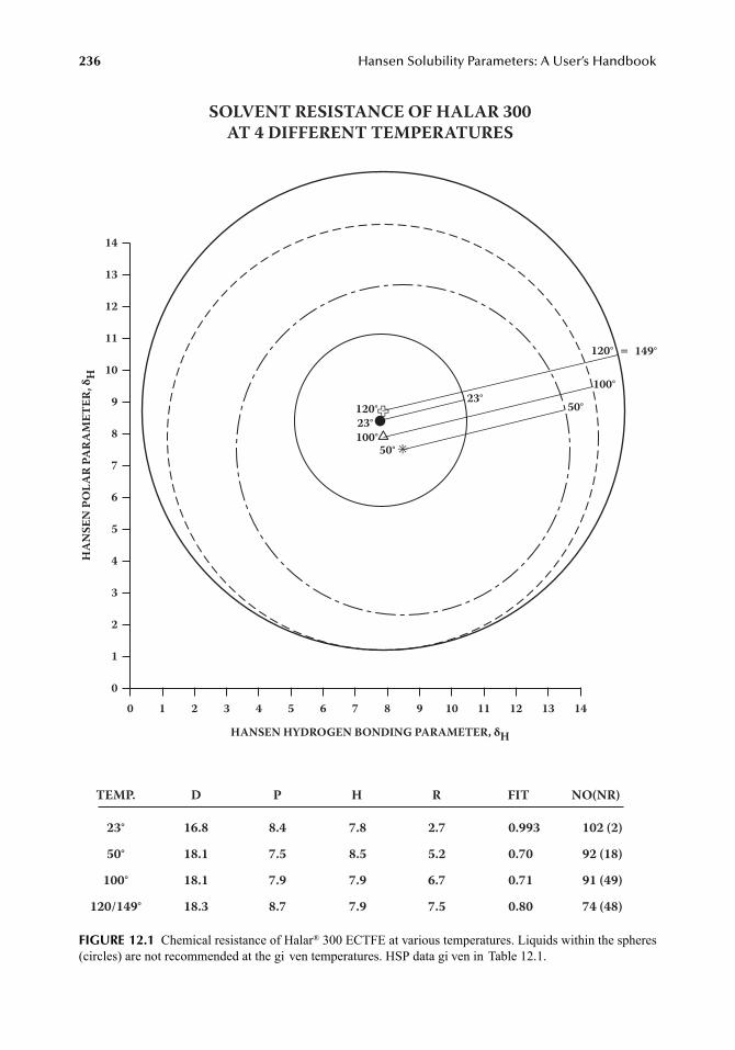
236
Hansen Solubility Parameters: A User’s Handbook
FIGURE 12.1
Chemical resistance of Halar
®
300 ECTFE at various temperatures. Liquids within the spheres(circles) are not recommended at the gi ven temperatures. HSP data gi ven in Table 12.1.
HANSEN HYDROGEN BONDING PARAMETER, δH
SOLVENT RESISTANCE OF HALAR 300
AT 4 DIFFERENT TEMPERATURES
HA
NS
EN
PO
LA
R P
AR
AM
ET
ER
, δ
H
TEMP. D P H R FIT NO(NR)
23°
50°
100°
120/149°
16.8
18.1
18.1
18.3
8.4
7.5
7.9
8.7
7.8
8.5
7.9
7.9
2.7
5.2
6.7
7.5
0.993
0.70
0.71
0.80
102 (2)
92 (18)
91 (49)
74 (48)
14
13
12
11
10
9
8
7
6
5
4
3
2
1
0
14131211109876543210
149°120°
100°
50°
50°
23°
23°
120°
100°
✚●▲
✳
=
7248_C012.fm Page 236 Wednesday, May 23, 2007 11:14 AM
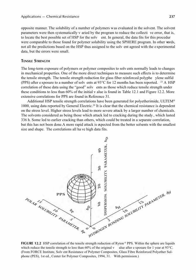
Applications — Chemical Resistance
237
opposite manner. The solubility of a number of polymers was evaluated in the solvent. The solventparameters were then systematically v aried by the program to reduce the collecti ve error, that is,to locate the best possible set of HSP for the solv ent. In general, the data fits for this procedurwere comparable to those found for polymer solubility using the SPHERE program. In other words,not all the predictions based on the HSP thus assigned to the solv ent agreed with the experimentaldata, but the errors were small.
T
ENSILE
S
TRENGTH
The long-term exposure of polymers or polymer composites to solv ents normally leads to changesin mechanical properties. One of the more direct techniques to measure such effects is to determinethe tensile strength. The tensile strength reduction for glass fiber reinforced polyphe ylene sulfid(PPS) after e xposure to a number of solv ents at 93°C for 12 months has been reported.
23
A HSPcorrelation of these data using the “good” solv ents as those which reduce tensile strength underthese conditions to less than 60% of the initial v alue is found in Table 12.1 and Figure 12.2. Moreextensive correlations for PPS are found in Reference 31.
Additional HSP tensile strength correlations have been generated for polyetherimide, ULTEM
®
1000, using data reported by General Electric.
24
It is clear that the chemical resistance is dependenton the stress level. Higher stress levels lead to more severe attack by a larger number of chemicals.The solvents considered as being those which attack led to cracking during the study , which lasted336 h. Some led to earlier cracking than others, which could be treated in a separate correlation,but this has not been done. A more rapid attack is expected from the better solvents with the smallestsize and shape. The correlations all ha ve high data fits.
FIGURE 12.2
HSP correlation of the tensile strength reduction of Ryton
®
PPS. Within the sphere are liquidswhich reduce the tensile strength to less than 60% of the original v alue after e xposure for 1 year at 93°C.(From FORCE Institute, Solv ent Resistance of Polymer Composites, Glass Fibre Reinforced Polyether Sul-phone (PES), 1st ed., Center for Polymer Composites, 1994, 31. With permission.)
PPS
δPδ Hδ D
5
7248_C012.fm Page 237 Wednesday, May 23, 2007 11:14 AM
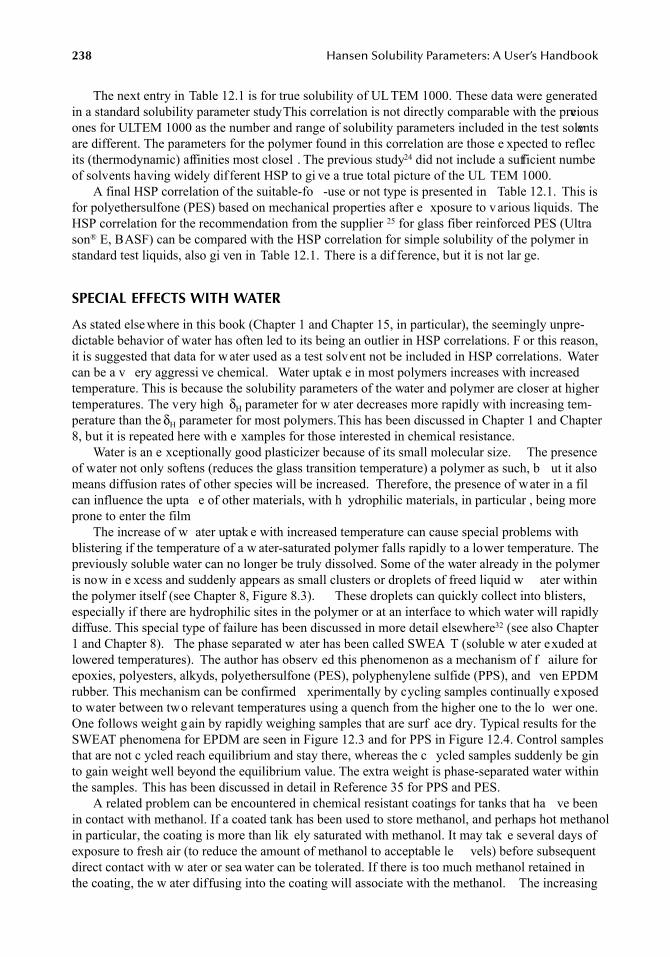
238
Hansen Solubility Parameters: A User’s Handbook
The next entry in Table 12.1 is for true solubility of UL TEM 1000. These data were generatedin a standard solubility parameter study. This correlation is not directly comparable with the previousones for ULTEM 1000 as the number and range of solubility parameters included in the test solventsare different. The parameters for the polymer found in this correlation are those e xpected to reflecits (thermodynamic) affinities most closel . The previous study
24
did not include a sufficient numbeof solvents having widely different HSP to gi ve a true total picture of the UL TEM 1000.
A final HSP correlation of the suitable-fo -use or not type is presented in Table 12.1. This isfor polyethersulfone (PES) based on mechanical properties after e xposure to various liquids. TheHSP correlation for the recommendation from the supplier
25
for glass fiber reinforced PES (Ultrason
®
E, BASF) can be compared with the HSP correlation for simple solubility of the polymer instandard test liquids, also gi ven in Table 12.1. There is a dif ference, but it is not lar ge.
SPECIAL EFFECTS WITH WATER
As stated else where in this book (Chapter 1 and Chapter 15, in particular), the seemingly unpre-dictable behavior of water has often led to its being an outlier in HSP correlations. F or this reason,it is suggested that data for w ater used as a test solvent not be included in HSP correlations. Watercan be a v ery aggressi ve chemical. Water uptak e in most polymers increases with increasedtemperature. This is because the solubility parameters of the water and polymer are closer at highertemperatures. The very high
δ
H
parameter for w ater decreases more rapidly with increasing tem-perature than the
δ
H
parameter for most polymers. This has been discussed in Chapter 1 and Chapter8, but it is repeated here with e xamples for those interested in chemical resistance.
Water is an e xceptionally good plasticizer because of its small molecular size. The presenceof water not only softens (reduces the glass transition temperature) a polymer as such, b ut it alsomeans diffusion rates of other species will be increased. Therefore, the presence of water in a filcan influence the upta e of other materials, with h ydrophilic materials, in particular , being moreprone to enter the film
The increase of w ater uptak e with increased temperature can cause special problems withblistering if the temperature of a w ater-saturated polymer falls rapidly to a lower temperature. Thepreviously soluble water can no longer be truly dissolved. Some of the water already in the polymeris now in e xcess and suddenly appears as small clusters or droplets of freed liquid w ater withinthe polymer itself (see Chapter 8, Figure 8.3). These droplets can quickly collect into blisters,especially if there are hydrophilic sites in the polymer or at an interface to which water will rapidlydiffuse. This special type of failure has been discussed in more detail elsewhere
32
(see also Chapter1 and Chapter 8). The phase separated w ater has been called SWEA T (soluble w ater exuded atlowered temperatures). The author has observ ed this phenomenon as a mechanism of f ailure forepoxies, polyesters, alkyds, polyethersulfone (PES), polyphenylene sulfide (PPS), and ven EPDMrubber. This mechanism can be confirmed xperimentally by cycling samples continually exposedto water between two relevant temperatures using a quench from the higher one to the lo wer one.One follows weight gain by rapidly weighing samples that are surf ace dry. Typical results for theSWEAT phenomena for EPDM are seen in Figure 12.3 and for PPS in Figure 12.4. Control samplesthat are not c ycled reach equilibrium and stay there, whereas the c ycled samples suddenly be ginto gain weight well beyond the equilibrium value. The extra weight is phase-separated water withinthe samples. This has been discussed in detail in Reference 35 for PPS and PES.
A related problem can be encountered in chemical resistant coatings for tanks that ha ve beenin contact with methanol. If a coated tank has been used to store methanol, and perhaps hot methanolin particular, the coating is more than lik ely saturated with methanol. It may tak e several days ofexposure to fresh air (to reduce the amount of methanol to acceptable le vels) before subsequentdirect contact with w ater or sea water can be tolerated. If there is too much methanol retained inthe coating, the w ater diffusing into the coating will associate with the methanol. The increasing
7248_C012.fm Page 238 Wednesday, May 23, 2007 11:14 AM
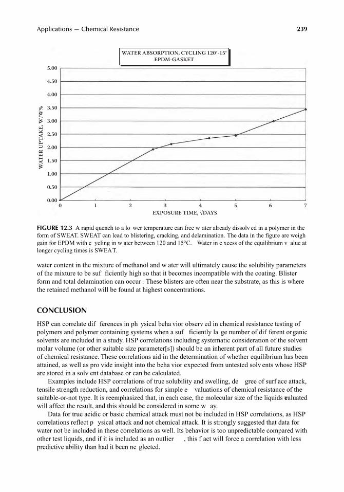
Applications — Chemical Resistance
239
water content in the mixture of methanol and w ater will ultimately cause the solubility parametersof the mixture to be suf ficiently high so that it becomes incompatible with the coating. Blisterform and total delamination can occur . These blisters are often near the substrate, as this is wherethe retained methanol will be found at highest concentrations.
CONCLUSION
HSP can correlate dif ferences in ph ysical beha vior observ ed in chemical resistance testing ofpolymers and polymer containing systems when a suf ficiently la ge number of dif ferent organicsolvents are included in a study. HSP correlations including systematic consideration of the solventmolar volume (or other suitable size parameter[s]) should be an inherent part of all future studiesof chemical resistance. These correlations aid in the determination of whether equilibrium has beenattained, as well as pro vide insight into the beha vior expected from untested solv ents whose HSPare stored in a solv ent database or can be calculated.
Examples include HSP correlations of true solubility and swelling, de gree of surf ace attack,tensile strength reduction, and correlations for simple e valuations of chemical resistance of thesuitable-or-not type. It is reemphasized that, in each case, the molecular size of the liquids evaluatedwill affect the result, and this should be considered in some w ay.
Data for true acidic or basic chemical attack must not be included in HSP correlations, as HSPcorrelations reflect p ysical attack and not chemical attack. It is strongly suggested that data forwater not be included in these correlations as well. Its behavior is too unpredictable compared withother test liquids, and if it is included as an outlier , this f act will force a correlation with lesspredictive ability than had it been ne glected.
FIGURE 12.3
A rapid quench to a lo wer temperature can free w ater already dissolv ed in a polymer in theform of SWEAT. SWEAT can lead to blistering, cracking, and delamination. The data in the figure are weighgain for EPDM with c ycling in w ater between 120 and 15°C. Water in e xcess of the equilibrium v alue atlonger cycling times is SWEAT.
EXPOSURE TIME, √DAYS
WAT
ER U
PTAK
E, W
/W%
76543210
5.00
4.50
4.00
3.50
3.00
2.50
2.00
1.50
1.00
0.50
0.00
WATER ABSORPTION, CYCLING 120°-15°EPDM-GASKET
7248_C012.fm Page 239 Wednesday, May 23, 2007 11:14 AM
240
Hansen Solubility Parameters: A User’s Handbook
REFERENCES
1. Hansen, C.M., The three dimensional solubility parameter — k ey to paint component af finities ISolvents, plasticizers, polymers, and resins,
J. Paint Technol
., 39(505), 104–117, 1967.2. Hansen, C.M., The three dimensional solubility parameter — k ey to paint component af finities II
Dyes, emulsifiers, mutual solubility and compatibilit , and pigments
, J. Paint Technol.
, 39(511),505–510, 1967.
3. Hansen, C.M. and Skaarup, K., The three dimensional solubility parameter — key to paint componentaffinities III. Independent calculation of the parameter component
, J. Paint Technol.,
39(511),511–514, 1967.
4. Hansen, C.M., The Three Dimensional Solubility Parameter and Solvent Diffusion Coefficient, TheirImportance in Surf ace Coating F ormulation, Doctoral dissertation, Danish Technical Press, Copen-hagen, 1967.
5. Hansen, C.M., The universality of the solubility parameter ,
Ind. Eng. Chem. Prod. Res. Dev.
, 8(1),2–11, 1969.
6. Hansen, C.M. and Beerbo wer, A., Solubility parameters, in
Kirk-Othmer Encyclopedia of ChemicalTechnology
, Suppl. Vol., 2nd ed., Standen, A., Ed., Interscience, Ne w York, 1971, pp. 889–910.7. Hansen, C.M., 25 years with solubility parameters (25 År med Opløselighedsparametrene, in Danish),
Dan. Kemi
, 73(8), 18–22, 1992.8. Hansen, C.M., Solubility parameters, in
Paint Testing Manual
, Manual 17, Koleske, J.V., Ed., AmericanSociety for Testing and Materials, Philadelphia, P A, 1995, pp. 383–404.
FIGURE 12.4
A rapid quench to a lo wer temperature can free w ater already dissolv ed in a polymer in theform of SWEAT. SWEAT can lead to blistering, cracking, and delamination. The data in the figure are weighgain for PPS with cycling in water between 90 and 23°C. Water in excess of the equilibrium value is SWEAT.(From Hansen, C.M., The Resistance of PPS, PES and PA Polymer Composites to Temperature Cycling DuringWater Exposure, Center for Polymer Composites (Denmark), Danish Technological Institute, Taastrup, 1994,11. With permission.)
▲
▲ ▲▲▲▲▲▲▲▲▲▲▲
▲▲
▲▲▲
▲▲▲▲▲▲
▲▲
▲▲▲
▲▲
▲▲
SQUARE ROOT OF TIME / THICKNESS SQRT (HRS)/mm
WATER ABSORPTION VS.TEMPERATURE
RYTON R4 XT-HV, plate thickness 1 and 2 mm
WE
IGH
T G
AIN
(%
)
80706050403020100
2
1.5
1
.5
0
-.5
-1
140 C, 2 mm
90 C, 2 mm
90 C, 1 mm
90 C, 1 mm
50 C, 1 mm
23 C, 1 mm
■
■
■
■■■
■■
■
■
▲▲▲▲▲▲▲▲▲
▲▲▲
▲▲▲
▼▼
▼
▼▼
▼▼▼▼▼▼
▼▼
▼▼
▼▼
▲
■
✕✕
✕✕✕✕✕
✛✛✛✛✛✛✛
■
▼
7248_C012.fm Page 240 Wednesday, May 23, 2007 11:14 AM
Applications — Chemical Resistance
241
9. Barton, A.F.M.,
Handbook of Solubility Parameters and Other Cohesion Parameters
, CRC Press,Boca Raton, FL, 1983.
10. Barton, A.F.M.,
Handbook of Polymer-Liquid Interaction Parameters and Solubility Parameters,
CRCPress, Boca Raton, FL, 1990.
11. Anonymous, Brochure: Co-Act — A Dynamic Program for Solv ent Selection, Exxon ChemicalInternational Inc., 1989.
12. Dante, M.F., Bittar , A.D., and Caillault, J.J., Program calculates solv ent properties and solubilityparameters,
Mod. Paint Coat
., 79(9), 46–51, 1989.13. Hansen, C.M., Characterization of surfaces by spreading liquids,
J. Paint Technol.,
42(550), 660–664,1970.
14. Hansen, C.M., Surface dewetting and coatings performance,
J. Paint Technol
., 44(570), 57–60, 1972.15. Hansen, C.M. and Pierce, P.E., Surface effects in coatings processes,
Ind. Eng. Chem. Prod. Res. Dev
.,13(4), 218–225, 1974.
16. Hansen, C.M. and Wallström, E., On the use of cohesion parameters to characterize surfaces,
J. Adhes.,
15(3/4), 275–286, 1983.17. Shareef, K.M.A., Yaseen, M., and Reddy , O.J., Suspension interaction of pigments in solv ents.
Characterization of pigments surfaces in terms of three-dimensional solubility parameters of solvents,
J. Coat. Technol.,
58(733), 35–44, February 1986.18. Beerbower, A., Surface free energy: a new relationship to bulk energies,
J. Colloid Interface Sci.
, 35,126–132, 1971.
19. Nielsen, T.B. and Hansen, C.M., Surf ace wetting and the prediction of en vironmental stress cracking(ESC) in polymers,
Polym. Degradation Stability
, 89, 513–516, 2005.20. Hansen, C.M., Some aspects of acid/base interactions (Einige Aspekte der Säure/Base-W echsel-
wirkung, in German),
Farbe und Lack
, 7, 595–598, 1977.21. Anonymous, Plastguide, SCS Dukadan AS, Randers, Denmark, 1990.22. Anonymous, Fluid Resistance of Viton
®
, Du Pont Compan y, Polymer Products Department, Elas-tomers Division, Wilmington, DE, 1989.
23. Anonymous, RYTON
®
PPS Polyphen ylene Sulfide Resins — Corrosion Resistance Guide, PhilipPetroleum Co., U.S.
24. Anonymous, Ultem
®
Resin Design Guide, GE Plastics, Pittsfield, MA, 198925. Anonymous, Verhalten v on Ultrason
®
ge gen Chemikalien — B ASF Technische InformationTI-KTE/TH-01 d 82132, October 1991.
26. Anonymous, Expanded List — Chemical Resistance of Halar
®
Fluoropolymer, Ausimont, USA, Inc.27. Carlowitz, B., Thermoplastic Plastics (in German),
Thermoplastische Kunststoffe
, Zechner und Hüthig,Speyer am Rhein, 1980.
28. Anonymous,
Chemical Resistance Data Sheets Volume 1 Plastics; Volume 2 Rubbers
, new ed., RapraTechnology Limited, Shawbury, Shrewsbury, Shropshire, 1993.
29. Anonymous, Chemical Resistance of Plastics and Elastomers used in Pipeline Construction, Geor geFischer +GF+, 1992.
30. Plastics Design Library, Chemical resistance data, William Andrew, Inc., Norwich, NY.31. Hansen, C.M
.,
Solvent Resistance of Polymer Composites — Glass Fibre Reinforced Polyphen yleneSulfide, Centre for Polymer Composites (Denmark), Danish Technological Institute, Taastrup, 1993,pp. 1–62.
32. Hansen, C.M., Ne w developments in corrosion and blister formation in coatings,
Prog. Org. Coat
.,26, 113–120, 1995.
33. Van Dyk, J.W ., P aper presented at the F ourth Chemical Congress of America, Ne w York, August25–30, 1991.
34. Anonymous [Note: This was, in fact, Van Dyk, J.W., but this does not appear on the b ulletin], UsingDimethyl Sulfoxide (DMSO) in Industrial F ormulations, Bulletin No. 102, Gaylord Chemical Corp.,Slidell, LA, 1992.
35. Hansen, C.M., The Resistance of PPS, PES and P A Polymer Composites to Temperature CyclingDuring Water Exposure, Centre for Polymer Composites (Denmark), Danish Technological Institute,Taastrup, 1994.
7248_C012.fm Page 241 Wednesday, May 23, 2007 11:14 AM

7248_C012.fm Page 242 Wednesday, May 23, 2007 11:14 AM
243
13
Applications — Barrier Polymers
Charles M. Hansen
ABSTRACT
The permeation coef ficient,
P
, of a liquid or a g as through a polymer is gi ven by the product ofthe diffusion coefficient,
D
, and the solubility coefficient,
S
:
P
=
DS
.
S
correlates with the Hansensolubility parameters (HSP). At lo w permeant concentrations
D
is a constant. Ho wever, as thepermeant concentration increases, its plasticizing ef fect on the polymer becomes significant, anthe dif fusion coef ficient increases mar edly. This ef fect can be v ery significant. The successfulcorrelations of permeation phenomena with HSP are thought to be largely a result of this exceptionaldependence of
D
on the dissolved permeant. As the amount of permeant being dissolv ed increaseswith closer matches of the HSP for permeant and barrier polymer , the end result is that both
S
and
D
, and therefore
P
, are functions of the HSP match. HSP correlations are gi ven for breakthroughtimes in chemical protecti ve clothing, permeation rates through barrier polymers, and barrierpolymer swelling. Both liquids and g ases are treated. Absorption and dif fusion in polymers istreated extensively in Chapter 16.
INTRODUCTION
The permeation of a liquid or a g as through a polymer can be described by the relation
P
=
DS
(13.1)
P
, the permeation coef ficient, is the product of the di fusion coefficient,
D
, and the solubilitycoefficient,
S
. The diffusion coefficient indicates h w fast the permeant molecules can move throughthe polymer. The solubility coefficient indicates h w much of the permeant can be dissolved in thepolymer. The amount dissolved in the polymer determines the concentration gradient o ver a filmand the concentration gradient is the dri ving force for mass transport. When solubility is higher ,the concentration gradient is correspondingly higher, and, assuming the same diffusion coefficientmass transport will be proportionately higher .
S
will be lo wer when the HSP of the barrier filand a solvent are very different.
A significant actor af fecting
D
is the molecular size and shape of the permeant molecules.Larger molecular size and more comple x and bulky molecular shape are major f actors that lead tolower diffusion coefficients. The diffusion coefficient for oxygen in polyvi yl chloride (PVC) iswell over a million times greater than that of
n
-hexane (at low concentrations) in the same polymer.
1
This difference in diffusion coefficients is a result of di ferences in molecular size. Likewise, it hasbeen found that the rate of dif fusion at the same concentration is about the same for dif ferentsolvents with approximately the same size and shape, even though they may have different solubilityparameters (b ut not so dif ferent that both are able to dissolv e in the polymer at the le vel ofcomparison).
2–4
The polymers in these studies were a copolymer of 87% vin yl chloride and 13%vinyl acetate, polyvinyl acetate, and polymeth yl methacrylate.
7248_C013.fm Page 243 Wednesday, May 23, 2007 11:18 AM
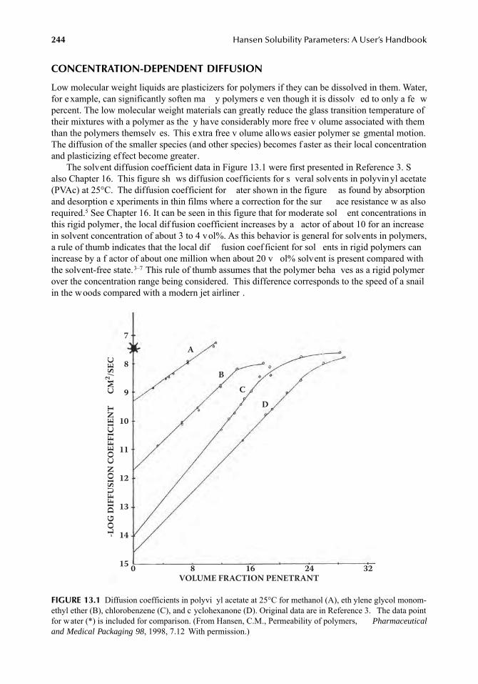
244
Hansen Solubility Parameters: A User’s Handbook
CONCENTRATION-DEPENDENT DIFFUSION
Low molecular weight liquids are plasticizers for polymers if they can be dissolved in them. Water,for e xample, can significantly soften ma y polymers e ven though it is dissolv ed to only a fe wpercent. The low molecular weight materials can greatly reduce the glass transition temperature oftheir mixtures with a polymer as the y have considerably more free v olume associated with themthan the polymers themselv es. This extra free v olume allows easier polymer se gmental motion.The diffusion of the smaller species (and other species) becomes f aster as their local concentrationand plasticizing effect become greater.
The solvent diffusion coefficient data in Figure 13.1 were first presented in Reference 3. Salso Chapter 16. This figure sh ws diffusion coefficients for s veral solvents in polyvin yl acetate(PVAc) at 25°C. The diffusion coefficient for ater shown in the figure as found by absorptionand desorption e xperiments in thin films where a correction for the sur ace resistance w as alsorequired.
5
See Chapter 16. It can be seen in this figure that for moderate sol ent concentrations inthis rigid polymer, the local dif fusion coefficient increases by a actor of about 10 for an increasein solvent concentration of about 3 to 4 vol%. As this behavior is general for solvents in polymers,a rule of thumb indicates that the local dif fusion coef ficient for sol ents in rigid polymers canincrease by a f actor of about one million when about 20 v ol% solvent is present compared withthe solvent-free state.
3–7
This rule of thumb assumes that the polymer beha ves as a rigid polymerover the concentration range being considered. This difference corresponds to the speed of a snailin the woods compared with a modern jet airliner .
FIGURE 13.1
Diffusion coefficients in polyvi yl acetate at 25°C for methanol (A), eth ylene glycol monom-ethyl ether (B), chlorobenzene (C), and c yclohexanone (D). Original data are in Reference 3. The data pointfor water (*) is included for comparison. (From Hansen, C.M., Permeability of polymers,
Pharmaceuticaland Medical Packaging 98
, 1998, 7.12 With permission.)
VOLUME FRACTION PENETRANT
-LO
G D
IFF
US
ION
CO
EF
FIC
IEN
T
C
M2/S
EC
0 8 16 24 32
7
8
9
10
11
12
13
14
15
A
B
C
D
7248_C013.fm Page 244 Wednesday, May 23, 2007 11:18 AM

Applications — Barrier Polymers
245
Concentration-dependent diffusion coefficients are also found for elastomers. Here, the rule othumb is that the dif fusion coefficient increases by a actor of about 10 for an increase in solv entconcentration of about 15 vol%.
7
This shows that liquid contact with chemical protecti ve clothing,for example, leads to concentration-dependent dif fusion coefficients because the amount ta en upat the contact surf ace on liquid contact is v ery often more than 15%.
Concentration-dependent diffusion has been discussed at length by Crank.
8
It is also discussedhere because it is a major factor in the success of HSP correlations of permeation phenomena. TheCrank-Nicholsen finite di ference treatment for concentration-dependent dif fusion
8
was extendedby Hansen
3
and used to describe film formation by sol ent evaporation,
4
to explore what is termedanomalous diffusion,
5
to develop an easy method to e valuate data leading to concentration-depen-dent diffusion coefficients
6
and to account for the effects of concentration-dependent diffusion andsurface boundary resistance simultaneously .
5–7
Klopfer
9
developed analytical solutions in volvingconcentration-dependent dif fusion for man y situations found in practical b uilding applications,particularly with respect to transport of w ater in b uilding materials. Concentration-dependentdiffusion can be handled properly without great dif ficulty for most situations of practical interestNeglect of this ef fect can lead to errors, the significance of which will increase with increasinamounts of the dissolv ed materials.
In addition to demonstrating concentration dependence, the diffusion coefficient data for P Acin Figure 13.1 also sho w the well-established relations that those solv ents with lar ger and morecomplicated chemical structures are those with lower diffusion coefficients. Water has one “signif-icant” atom, methanol has tw o, and eth ylene glycol monometh yl ether (EGMME) has fi e. Thediffusion coefficient for ater in PVAc at lo w concentration, Do, is 10,000 times lar ger than thatfor the latter. An example of how to estimate diffusion coefficients in P Ac for other liquids, suchas methylene chloride, is as follo ws. The diffusion coefficients in P Ac for meth ylene chloride,with three significant atoms, can be xpected to be some what lower than those for methanol, b utmuch higher than those for EGMME. Planar chlorobenzene dif fuses more rapidly than nonplanarcyclohexanone, even though the number of significant atoms is the same. Another type of compar-ison which is possible is to state that the dif fusion coefficients for toluene are xpected to be closeto those for chlorobenzene because of a similarity in molecular size and shape. This was confirmeby solvent retention studies where toluene and chlorobenzene were retained in identical amountsin a film ofVYHH
®
(87 wt% vinyl chloride, 13 wt% vinyl acetate, Union Carbide). Toluene, whichdoes not dissolv e this polymer , w as introduced by placing a completely dry polymer film in closed container over toluene vapors.
Diffusion can be e xpected to be slo wer in more rigid polymers, i.e., those with higher glasstransition temperatures, unless the rigidity is such as to allo w decided holes of suitable size toenable quite rapid dif fusion of much smaller molecules. These considerations lead to the bestcombination of properties for a barrier polymer as being one with a high glass transition temperatureand with HSP far removed from those of the permeant. If, in practice, this leads to water sensitivity,an alternate strategy, such as a laminated system, may be required.
SOLUBILITY PARAMETER CORRELATIONS BASED ON PERMEATION PHENOMENA
S
OLUBILITY
P
ARAMETER
C
ORRELATIONS
OF
B
REAKTHROUGH
T
IMES
Extensive permeation studies and collections of permeation data are a vailable within the chemicalprotective clothing industry.
10,11
Such data can also be used to establish correlations with HSP . Alist of HSP for barrier polymers used in chemical protecti ve clothing has been published
12
basedon data by Forsberg and Olsson.
10
Some of these correlations have been improved in most instancesby correlating the more e xtensive data of Forsberg and Keith.
11
The definition of a “good” sol entwhich was used for these correlations w as that the breakthrough time w as less than some selected
7248_C013.fm Page 245 Wednesday, May 23, 2007 11:18 AM
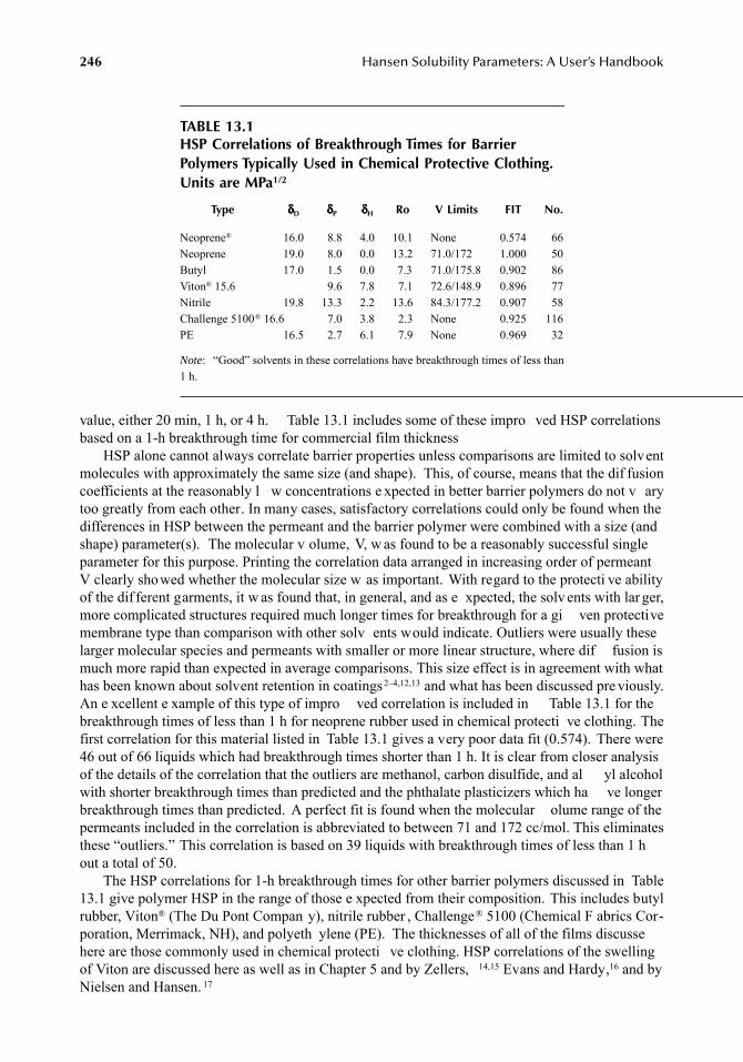
246
Hansen Solubility Parameters: A User’s Handbook
value, either 20 min, 1 h, or 4 h. Table 13.1 includes some of these impro ved HSP correlationsbased on a 1-h breakthrough time for commercial film thickness
HSP alone cannot always correlate barrier properties unless comparisons are limited to solventmolecules with approximately the same size (and shape). This, of course, means that the dif fusioncoefficients at the reasonably l w concentrations e xpected in better barrier polymers do not v arytoo greatly from each other. In many cases, satisfactory correlations could only be found when thedifferences in HSP between the permeant and the barrier polymer were combined with a size (andshape) parameter(s). The molecular v olume, V, w as found to be a reasonably successful singleparameter for this purpose. Printing the correlation data arranged in increasing order of permeantV clearly showed whether the molecular size w as important. With regard to the protecti ve abilityof the dif ferent garments, it w as found that, in general, and as e xpected, the solv ents with lar ger,more complicated structures required much longer times for breakthrough for a gi ven protectivemembrane type than comparison with other solv ents would indicate. Outliers were usually theselarger molecular species and permeants with smaller or more linear structure, where dif fusion ismuch more rapid than expected in average comparisons. This size effect is in agreement with whathas been known about solvent retention in coatings
2–4,12,13
and what has been discussed pre viously.An e xcellent e xample of this type of impro ved correlation is included in Table 13.1 for thebreakthrough times of less than 1 h for neoprene rubber used in chemical protecti ve clothing. Thefirst correlation for this material listed in Table 13.1 gives a very poor data fit (0.574). There were46 out of 66 liquids which had breakthrough times shorter than 1 h. It is clear from closer analysisof the details of the correlation that the outliers are methanol, carbon disulfide, and al yl alcoholwith shorter breakthrough times than predicted and the phthalate plasticizers which ha ve longerbreakthrough times than predicted. A perfect fit is found when the molecular olume range of thepermeants included in the correlation is abbreviated to between 71 and 172 cc/mol. This eliminatesthese “outliers.” This correlation is based on 39 liquids with breakthrough times of less than 1 hout a total of 50.
The HSP correlations for 1-h breakthrough times for other barrier polymers discussed in Table13.1 give polymer HSP in the range of those e xpected from their composition. This includes butylrubber, Viton
®
(The Du Pont Compan y), nitrile rubber , Challenge
®
5100 (Chemical F abrics Cor-poration, Merrimack, NH), and polyeth ylene (PE). The thicknesses of all of the films discussehere are those commonly used in chemical protecti ve clothing. HSP correlations of the swellingof Viton are discussed here as well as in Chapter 5 and by Zellers,
14,15
Evans and Hardy,
16
and byNielsen and Hansen.
17
TABLE 13.1HSP Correlations of Breakthrough Times for Barrier Polymers Typically Used in Chemical Protective Clothing. Units are MPa
1/2
Type
δδδδ
D
δδδδ
P
δδδδ
H
Ro V Limits FIT No.
Neoprene
®
16.0 8.8 4.0 10.1 None 0.574 66Neoprene 19.0 8.0 0.0 13.2 71.0/172 1.000 50Butyl 17.0 1.5 0.0 7.3 71.0/175.8 0.902 86Viton
®
15.6 9.6 7.8 7.1 72.6/148.9 0.896 77Nitrile 19.8 13.3 2.2 13.6 84.3/177.2 0.907 58Challenge 5100
®
16.6 7.0 3.8 2.3 None 0.925 116PE 16.5 2.7 6.1 7.9 None 0.969 32
Note
: “Good” solvents in these correlations have breakthrough times of less than1 h.
7248_C013.fm Page 246 Wednesday, May 23, 2007 11:18 AM
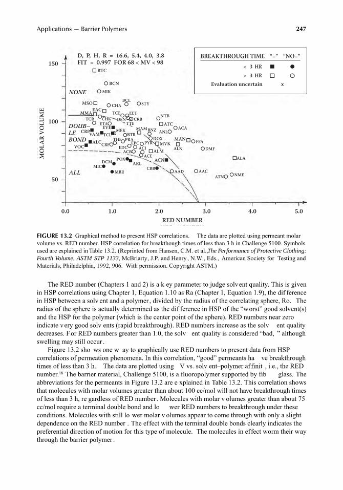
Applications — Barrier Polymers
247
The RED number (Chapters 1 and 2) is a k ey parameter to judge solvent quality. This is givenin HSP correlations using Chapter 1, Equation 1.10 as Ra (Chapter 1, Equation 1.9), the dif ferencein HSP between a solv ent and a polymer , divided by the radius of the correlating sphere, Ro. Theradius of the sphere is actually determined as the dif ference in HSP of the “worst” good solvent(s)and the HSP for the polymer (which is the center point of the sphere). RED numbers near zeroindicate very good solv ents (rapid breakthrough). RED numbers increase as the solv ent qualitydecreases. For RED numbers greater than 1.0, the solv ent quality is considered “bad, ” althoughswelling may still occur .
Figure 13.2 sho ws one w ay to graphically use RED numbers to present data from HSPcorrelations of permeation phenomena. In this correlation, “good” permeants ha ve breakthroughtimes of less than 3 h. The data are plotted using V vs. solv ent–polymer af finit , i.e., the REDnumber.
18
The barrier material, Challenge 5100, is a fluoropolymer supported by fib glass. Theabbreviations for the permeants in Figure 13.2 are e xplained in Table 13.2. This correlation showsthat molecules with molar volumes greater than about 100 cc/mol will not have breakthrough timesof less than 3 h, re gardless of RED number. Molecules with molar v olumes greater than about 75cc/mol require a terminal double bond and lo wer RED numbers to breakthrough under theseconditions. Molecules with still lo wer molar v olumes appear to come through with only a slightdependence on the RED number . The effect with the terminal double bonds clearly indicates thepreferential direction of motion for this type of molecule. The molecules in effect worm their waythrough the barrier polymer .
FIGURE 13.2
Graphical method to present HSP correlations. The data are plotted using permeant molarvolume vs. RED number. HSP correlation for breakthough times of less than 3 h in Challenge 5100. Symbolsused are explained in Table 13.2. (Reprinted from Hansen, C.M. et al.,
The Performance of Protective Clothing:Fourth Volume, ASTM STP 1133
, McBriarty, J.P. and Henry , N.W., Eds., American Society for Testing andMaterials, Philadelphia, 1992, 906. With permission. Copyright ASTM.)
RED NUMBER
MO
LAR
VOLU
ME
0.0 1.0 2.0 3.0 4.0 5.0
150
100
50ALL
DOUB–LEBOND
NONE
■ BTC
■ ATC
■ MVK■ ALM
MSO ■
MMA ■
ACN ■
■ALC VOC ■
CRP ■ EVE ■
■ARL
VAM ■
EAC ■
MAN ■
● BCN● MIK
● CHA
● CRBTCE
●DEN●
EDC●ACB●
CRF●
MIC● CBB●
POX●DCM●
ETA●
TCL ●THF● ●PRA
●BTR ANL●
ATN●
● STY
● CHK
● DOX
● MBR
● PYR
● ACA
● FFA● DMF
● NME● AAD
● ACE
● AAC
● EET
● NTB
BCL●
TCR ●
EPC● ACI
●
■ALN
■ALA
BNZ●
MAM ■
D, P, H, R = 16.6, 5.4, 4.0, 3.8FIT = 0.997 FOR 68 < MV < 98
BREAKTHROUGH TIME “=” “NO=”< 3 HR> 3 HR
Evaluation uncertain x
■ ●
●■
TTEMEK
■
7248_C013.fm Page 247 Wednesday, May 23, 2007 11:18 AM
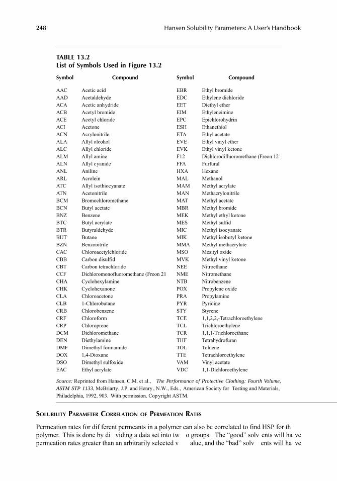
248
Hansen Solubility Parameters: A User’s Handbook
S
OLUBILITY
P
ARAMETER
C
ORRELATION
OF
P
ERMEATION
R
ATES
Permeation rates for dif ferent permeants in a polymer can also be correlated to find HSP for thpolymer. This is done by di viding a data set into tw o groups. The “good” solv ents will ha vepermeation rates greater than an arbitrarily selected v alue, and the “bad” solv ents will ha ve
TABLE 13.2List of Symbols Used in Figure 13.2
Symbol Compound Symbol Compound
AAC Acetic acid EBR Ethyl bromideAAD Acetaldehyde EDC Ethylene dichlorideACA Acetic anhydride EET Diethyl etherACB Acetyl bromide EIM EthyleneimineACE Acetyl chloride EPC EpichlorohydrinACI Acetone ESH EthanethiolACN Acrylonitrile ETA Ethyl acetateALA Allyl alcohol EVE Ethyl vinyl etherALC Allyl chloride EVK Ethyl vinyl ketoneALM Allyl amine F12 Dichlorodifluoromethane (Freon 12ALN Allyl cyanide FFA FurfuralANL Aniline HXA HexaneARL Acrolein MAL MethanolATC Allyl isothiocyanate MAM Methyl acrylateATN Acetonitrile MAN MethacrylonitrileBCM Bromochloromethane MAT Methyl acetateBCN Butyl acetate MBR Methyl bromideBNZ Benzene MEK Methyl ethyl ketoneBTC Butyl acrylate MES Methyl sulfidBTR Butyraldehyde MIC Methyl isocyanateBUT Butane MIK Methyl isobutyl ketoneBZN Benzonitrile MMA Methyl methacrylateCAC Chloroacetylchloride MSO Mesityl oxideCBB Carbon disulfid MVK Methyl vinyl ketoneCBT Carbon tetrachloride NEE NitroethaneCCF Dichloromonofluoromethane (Freon 21 NME NitromethaneCHA Cyclohexylamine NTB NitrobenzeneCHK Cyclohexanone POX Propylene oxideCLA Chloroacetone PRA PropylamineCLB 1-Chlorobutane PYR PyridineCRB Chlorobenzene STY StyreneCRF Chloroform TCE 1,1,2,2,-TetrachloroethyleneCRP Chloroprene TCL TrichloroethyleneDCM Dichloromethane TCR 1,1,1-TrichloroethaneDEN Diethylamine THF TetrahydrofuranDMF Dimethyl formamide TOL TolueneDOX 1,4-Dioxane TTE TetrachloroethyleneDSO Dimethyl sulfoxide VAM Vinyl acetateEAC Ethyl acrylate VDC 1,1-Dichloroethylene
Source:
Reprinted from Hansen, C.M. et al.,
The Performance of Protective Clothing: Fourth Volume,ASTM STP 1133
, McBriarty, J.P. and Henry , N.W., Eds., American Society for Testing and Materials,Philadelphia, 1992, 903. With permission. Copyright ASTM.
7248_C013.fm Page 248 Wednesday, May 23, 2007 11:18 AM
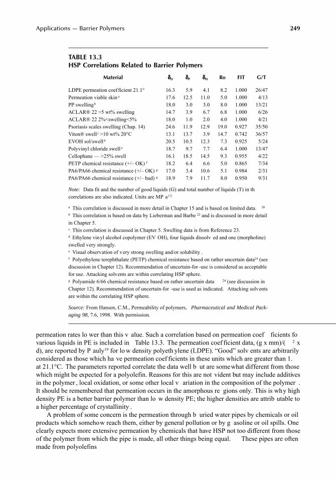
Applications — Barrier Polymers
249
permeation rates lo wer than this v alue. Such a correlation based on permeation coef ficients fovarious liquids in PE is included in Table 13.3. The permeation coef ficient data, (g x mm)/(
2
xd), are reported by P auly
19
for lo w density polyeth ylene (LDPE). “Good” solv ents are arbitrarilyconsidered as those which ha ve permeation coef ficients in these units which are greater than 1.at 21.1°C. The parameters reported correlate the data well b ut are somewhat different from thosewhich might be expected for a polyolefin. Reasons for this are not vident but may include additivesin the polymer , local oxidation, or some other local v ariation in the composition of the polymer .It should be remembered that permeation occurs in the amorphous re gions only. This is why highdensity PE is a better barrier polymer than lo w density PE; the higher densities are attrib utable toa higher percentage of crystallinity .
A problem of some concern is the permeation through b uried water pipes by chemicals or oilproducts which somehow reach them, either by general pollution or by g asoline or oil spills. Oneclearly expects more extensive permeation by chemicals that have HSP not too different from thoseof the polymer from which the pipe is made, all other things being equal. These pipes are oftenmade from polyolefins
TABLE 13.3HSP Correlations Related to Barrier Polymers
Material
δδδδ
D
δδδδ
P
δδδδ
H
Ro FIT G/T
LDPE permeation coefficient 21.1° 16.3 5.9 4.1 8.2 1.000 26/47Permeation viable skin
a
17.6 12.5 11.0 5.0 1.000 4/13PP swelling
b
18.0 3.0 3.0 8.0 1.000 13/21ACLAR® 22 >5 wt% swelling 14.7 3.9 6.7 6.8 1.000 6/26ACLAR® 22 2%<swelling<5% 18.0 1.0 2.0 4.0 1.000 4/21Psoriasis scales swelling (Chap. 14) 24.6 11.9 12.9 19.0 0.927 35/50Viton® swell
c
>10 wt% 20°C 13.1 13.7 3.9 14.7 0.742 36/57EVOH sol/swell
d
20.5 10.5 12.3 7.3 0.925 5/24Polyvinyl chloride swell
e
18.7 9.7 7.7 6.4 1.000 13/47Cellophane — >25% swell 16.1 18.5 14.5 9.3 0.955 4/22PETP chemical resistance (+/– OK)
f
18.2 6.4 6.6 5.0 0.865 7/34PA6/PA66 chemical resistance (+/– OK)
g
17.0 3.4 10.6 5.1 0.984 2/31PA6/PA66 chemical resistance (+/– bad)
g
18.9 7.9 11.7 8.0 0.950 9/31
Note
: Data fit and the number of good liquids (G) and total number of liquids (T) in thcorrelations are also indicated. Units are MP a
1/2.
a
This correlation is discussed in more detail in Chapter 15 and is based on limited data.
20
b
This correlation is based on data by Lieberman and Barbe
22
and is discussed in more detailin Chapter 5.
c
This correlation is discussed in Chapter 5. Swelling data is from Reference 23.
d
Ethylene vinyl alcohol copolymer (EV OH), four liquids dissolv ed and one (morpholine)swelled very strongly.
e
Visual observation of very strong swelling and/or solubility .
f
Polyethylene terephthalate (PETP) chemical resistance based on rather uncertain data
24
(seediscussion in Chapter 12). Recommendation of uncertain-for -use is considered as acceptablefor use. Attacking solvents are within correlating HSP sphere.
g
Polyamide 6/66 chemical resistance based on rather uncertain data
24
(see discussion inChapter 12). Recommendation of uncertain-for -use is used as indicated. Attacking solventsare within the correlating HSP sphere.
Source:
From Hansen, C.M., Permeability of polymers,
Pharmaceutical and Medical Pack-aging 98
, 7.6, 1998. With permission.
7248_C013.fm Page 249 Wednesday, May 23, 2007 11:18 AM
250
Hansen Solubility Parameters: A User’s Handbook
A HSP correlation has been possible in a v ery special case of polymer permeability where thebarrier polymer is viable human skin.
20
This is discussed in more detail in Chapter 15. Human skinis a polymeric barrier with se veral functions, one of which is to help k eep undesirable chemicalsout of the body . Some chemicals readily permeate this boundary , and this f act has been used toestablish a tentative HSP correlation for the permeation rate of viable human skin. This correlationalso has a relation to the HSP correlation for the swelling of psoriasis scales,
21
which is alsodiscussed in Chapter 15.
SOLUBILITY PARAMETER CORRELATION OF POLYMER SWELLING
Solubility is a major f actor in the equation
P
=
DS
, so correlations of solv ent uptake in polymersare important to understand their barrier properties. The correlation for swelling of polyprop ylenereported in Table 13.3 is based on solv ent uptake data reported by Lieberman and Barbe.
22
Thelimit of 0.5% weight g ain was arbitrarily set to dif ferentiate “good” solv ents from “bad” ones. Adifferent limit might gi ve different parameters. The HSP found in a gi ven correlation of swellingdepends on which polymer se gments the smaller amounts of permeant prefer to associate with.The predictive ability of the correlation will depend on the number of test liquids used in the studyand their gi ven HSP v alues. How different are the HSP of the test liquids? What are their v aluescompared with the predictions desired? The parameters reported in Table 13.3 for polyprop yleneseem to accurately reflect what is xpected in terms of lo w polarity and lo w hydrogen bondingproperties for this type of polymer .
As stated pre viously, a problem of some significance in a y study of solv ents at lo wconcentrations in polymers is that the smaller amounts of solv ent relative to the polymer canlead to preferential association of solv ent with those local re gions/segments/groups in thepolymer that have energies (HSP) most similar to their own. Like seeks like. These local regionsmay not necessarily reflect the same a finities as the polymer as a whole, such as are indicateby the totally soluble-or -not approach most commonly used in HSP e valuations. These localassociation effects can influence results on swelling studies at l w solvent uptakes in both goodand bad solv ents, for e xample. Copolymers, such as Viton, are particularly susceptible to thisproblem. Swelling data for Viton
23
are correlated by the HSP v alues included in Table 13.3. Apoor data fit can be anticipated when a single HSP sphere is used to describe what should brepresented by (at least) tw o overlapping HSP spheres (see also Figure 13.3). Zellers
14,15
alsohad difficulty correlating the swelling ofViton. Other types of studies carried out at low solventconcentrations can also be influenced by this s gregation/association phenomena. An extensionof this type of situation can be cited in the tendencies of w ater to associate with itself as wellas with local hydrophilic regions within polymers. The amount of water taken up at equilibriumis not reflected by an verall HSP correlation of polymer solubility or swelling. As little as 1%of hydrophilic additive can ef fectively destroy the w ater barrier properties of a polymer filmbut this small amount cannot be measured in swelling or solubility studies leading to HSPcorrelations. This f act, among other things, has made simple predictions of the beha vior ofwater very difficult
Correlations of polymer solubility and swelling ha ve led to se veral of the HSP data setsreported in Table 13.3 (see also the data reported in Chapter 5). The HSP correlations for chemicalresistance based on data of the acceptable-for -use or recommended/not recommended type arenot as reliable as those usually found for solubility and swelling where a suitably lar ge numberof liquids are used in the testing. The reasons for this are discussed in depth in Chapter 12.The data used in the chemical resistance correlations reported in Table 8.3 were tak en fromReference 24.
7248_C013.fm Page 250 Wednesday, May 23, 2007 11:18 AM
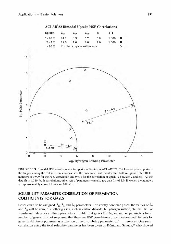
Applications — Barrier Polymers
251
SOLUBILITY PARAMETER CORRELATION OF PERMEATION COEFFICIENTS FOR GASES
Gases can also be assigned
δ
D
,
δ
P
, and
δ
H
parameters. For strictly nonpolar g ases, the values of
δ
P
and
δ
H
will be zero, b ut other g ases, such as carbon dioxide, h ydrogen sulfide, etc., will h vesignificant alues for all three parameters. Table 13.4 gi ves the
δ
D
,
δ
P
, and
δ
H
parameters for anumber of gases. It is not surprising that there are HSP correlations of permeation coef ficients fogases in dif ferent polymers as a function of their solubility parameter dif ferences. One suchcorrelation using the total solubility parameter has been given by König and Schuch,
25 who showed
FIGURE 13.3 Bimodal HSP correlation(s) for uptak e of liquids in ACLAR® 22. Trichloroethylene uptake isthe lar gest among the test solv ents because it is the only solv ent found within both re gions. It has REDnumbers of 0.999 for the >5% correlation and 0.978 for the correlation of uptak e between 2 and 5%. As thedata fit is 1.0 for both correlations, other sets of parameters can also gve data fits of 1.0. H wever, the numbersare approximately correct. Units are MP a1/2.
δH, Hydrogen Bonding Parameter
ACLAR®22 Bimodal Uptake HSP Correlations
δ P, P
olar
Par
amet
er
14121086420
12
10
8
6
4
2
0(18.0)
(14.7)
Ro = 4.0
Ro = 6.8
Uptake R FITδ D δ P δ H
5 - 10 %2 - 5 %> 10 %
14.718.0
3.91.0
Trichloroethylene within both
6.72.0
6.84.0
1.0001.000
●
■
✕✕
7248_C013.fm Page 251 Wednesday, May 23, 2007 11:18 AM
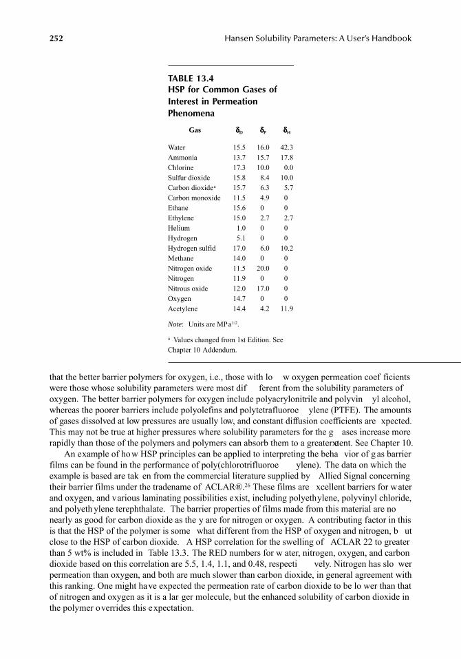
252 Hansen Solubility Parameters: A User’s Handbook
that the better barrier polymers for oxygen, i.e., those with lo w oxygen permeation coef ficientswere those whose solubility parameters were most dif ferent from the solubility parameters ofoxygen. The better barrier polymers for oxygen include polyacrylonitrile and polyvin yl alcohol,whereas the poorer barriers include polyolefins and polytetrafluoroe ylene (PTFE). The amountsof gases dissolved at low pressures are usually low, and constant diffusion coefficients are xpected.This may not be true at higher pressures where solubility parameters for the g ases increase morerapidly than those of the polymers and polymers can absorb them to a greater extent. See Chapter 10.
An example of how HSP principles can be applied to interpreting the beha vior of g as barrierfilms can be found in the performance of poly(chlorotrifluoroe ylene). The data on which theexample is based are tak en from the commercial literature supplied by Allied Signal concerningtheir barrier films under the tradename of ACLAR®.26 These films are xcellent barriers for waterand oxygen, and various laminating possibilities exist, including polyethylene, polyvinyl chloride,and polyeth ylene terephthalate. The barrier properties of films made from this material are nonearly as good for carbon dioxide as the y are for nitrogen or oxygen. A contributing factor in thisis that the HSP of the polymer is some what different from the HSP of oxygen and nitrogen, b utclose to the HSP of carbon dioxide. A HSP correlation for the swelling of ACLAR 22 to greaterthan 5 wt% is included in Table 13.3. The RED numbers for w ater, nitrogen, oxygen, and carbondioxide based on this correlation are 5.5, 1.4, 1.1, and 0.48, respecti vely. Nitrogen has slo werpermeation than oxygen, and both are much slower than carbon dioxide, in general agreement withthis ranking. One might have expected the permeation rate of carbon dioxide to be lo wer than thatof nitrogen and oxygen as it is a lar ger molecule, but the enhanced solubility of carbon dioxide inthe polymer overrides this expectation.
TABLE 13.4HSP for Common Gases of Interest in Permeation Phenomena
Gas δδδδD δδδδP δδδδH
Water 15.5 16.0 42.3Ammonia 13.7 15.7 17.8Chlorine 17.3 10.0 0.0Sulfur dioxide 15.8 8.4 10.0Carbon dioxidea 15.7 6.3 5.7Carbon monoxide 11.5 4.9 0Ethane 15.6 0 0Ethylene 15.0 2.7 2.7Helium 1.0 0 0Hydrogen 5.1 0 0Hydrogen sulfid 17.0 6.0 10.2Methane 14.0 0 0Nitrogen oxide 11.5 20.0 0Nitrogen 11.9 0 0Nitrous oxide 12.0 17.0 0Oxygen 14.7 0 0Acetylene 14.4 4.2 11.9
Note: Units are MPa1/2.
a Values changed from 1st Edition. SeeChapter 10 Addendum.
7248_C013.fm Page 252 Wednesday, May 23, 2007 11:18 AM
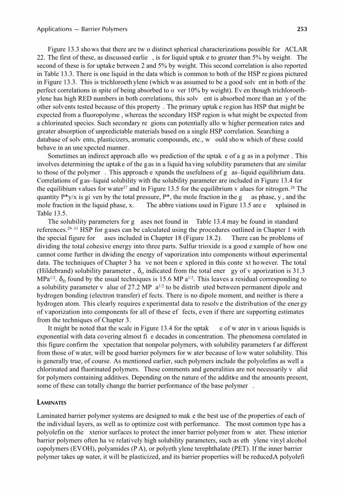
Applications — Barrier Polymers 253
Figure 13.3 shows that there are tw o distinct spherical characterizations possible for ACLAR22. The first of these, as discussed earlie , is for liquid uptak e to greater than 5% by weight. Thesecond of these is for uptake between 2 and 5% by weight. This second correlation is also reportedin Table 13.3. There is one liquid in the data which is common to both of the HSP re gions picturedin Figure 13.3. This is trichloroeth ylene (which w as assumed to be a good solv ent in both of theperfect correlations in spite of being absorbed to o ver 10% by weight). Ev en though trichloroeth-ylene has high RED numbers in both correlations, this solv ent is absorbed more than an y of theother solvents tested because of this property . The primary uptak e region has HSP that might beexpected from a fluoropolyme , whereas the secondary HSP region is what might be expected froma chlorinated species. Such secondary re gions can potentially allo w higher permeation rates andgreater absorption of unpredictable materials based on a single HSP correlation. Searching adatabase of solv ents, plasticizers, aromatic compounds, etc., w ould sho w which of these couldbehave in an une xpected manner.
Sometimes an indirect approach allo ws prediction of the uptak e of a g as in a polymer . Thisinvolves determining the uptake of the gas in a liquid having solubility parameters that are similarto those of the polymer . This approach e xpands the usefulness of g as–liquid equilibrium data.Correlations of g as–liquid solubility with the solubility parameter are included in Figure 13.4 forthe equilibium values for water27 and in Figure 13.5 for the equilibrium v alues for nitrogen.28 Thequantity P*y/x is gi ven by the total pressure, P*, the mole fraction in the g as phase, y , and themole fraction in the liquid phase, x. The abbre viations used in Figure 13.5 are e xplained inTable 13.5.
The solubility parameters for g ases not found in Table 13.4 may be found in standardreferences.29–31 HSP for gases can be calculated using the procedures outlined in Chapter 1 withthe special figure for ases included in Chapter 18 (Figure 18.2). There can be problems ofdividing the total cohesive energy into three parts. Sulfur trioxide is a good e xample of how onecannot come further in dividing the energy of vaporization into components without experimentaldata. The techniques of Chapter 3 ha ve not been e xplored in this conte xt ho wever. The total(Hildebrand) solubility parameter , δt, indicated from the total ener gy of v aporization is 31.3MPa1/2. δD found by the usual techniques is 15.6 MP a1/2. This leaves a residual corresponding toa solubility parameter v alue of 27.2 MP a1/2 to be distrib uted between permanent dipole andhydrogen bonding (electron transfer) ef fects. There is no dipole moment, and neither is there ahydrogen atom. This clearly requires e xperimental data to resolv e the distribution of the ener gyof vaporization into components for all of these ef fects, even if there are supporting estimatesfrom the techniques of Chapter 3.
It might be noted that the scale in Figure 13.4 for the uptak e of w ater in v arious liquids isexponential with data covering almost fi e decades in concentration. The phenomena correlated inthis figure confirm the xpectation that nonpolar polymers, with solubility parameters f ar differentfrom those of water, will be good barrier polymers for w ater because of low water solubility. Thisis generally true, of course. As mentioned earlier, such polymers include the polyolefins as well achlorinated and fluorinated polymers. These comments and generalities are not necessarily v alidfor polymers containing additives. Depending on the nature of the additive and the amounts present,some of these can totally change the barrier performance of the base polymer .
LAMINATES
Laminated barrier polymer systems are designed to mak e the best use of the properties of each ofthe individual layers, as well as to optimize cost with performance. The most common type has apolyolefin on the xterior surfaces to protect the inner barrier polymer from w ater. These interiorbarrier polymers often ha ve relatively high solubility parameters, such as eth ylene vinyl alcoholcopolymers (EVOH), polyamides (P A), or polyeth ylene terephthalate (PET). If the inner barrierpolymer takes up water, it will be plasticized, and its barrier properties will be reduced. A polyolefi
7248_C013.fm Page 253 Wednesday, May 23, 2007 11:18 AM
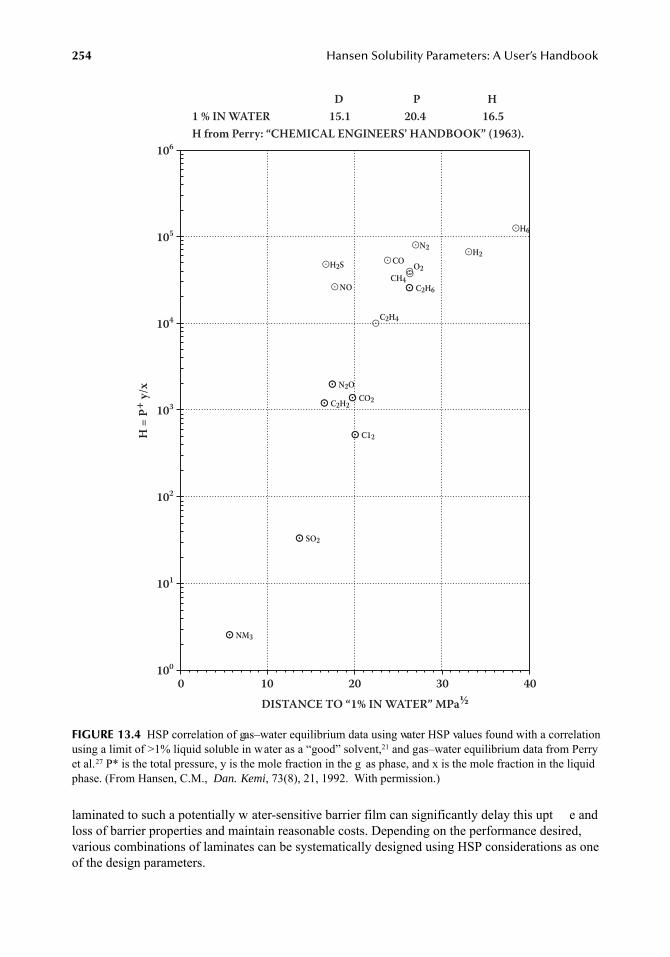
254 Hansen Solubility Parameters: A User’s Handbook
laminated to such a potentially w ater-sensitive barrier film can significantly delay this upt e andloss of barrier properties and maintain reasonable costs. Depending on the performance desired,various combinations of laminates can be systematically designed using HSP considerations as oneof the design parameters.
FIGURE 13.4 HSP correlation of gas–water equilibrium data using water HSP values found with a correlationusing a limit of >1% liquid soluble in water as a “good” solvent,21 and gas–water equilibrium data from Perryet al.27 P* is the total pressure, y is the mole fraction in the g as phase, and x is the mole fraction in the liquidphase. (From Hansen, C.M., Dan. Kemi, 73(8), 21, 1992. With permission.)
DISTANCE TO “1% IN WATER” MPa½
H =
P+ y/
x
403020100
106
105
104
103
102
101
100
D P H1 % IN WATER 15.1 20.4 16.5H from Perry: “CHEMICAL ENGINEERS’ HANDBOOK” (1963).
�H2S
�N2
�H6
�H2
CH4�
� � C2H6
� � N2O� � CO2� � C2H2
� � C12
� � SO2
� � NM3
� O2
�C2H4
� NO
� CO
7248_C013.fm Page 254 Wednesday, May 23, 2007 11:18 AM
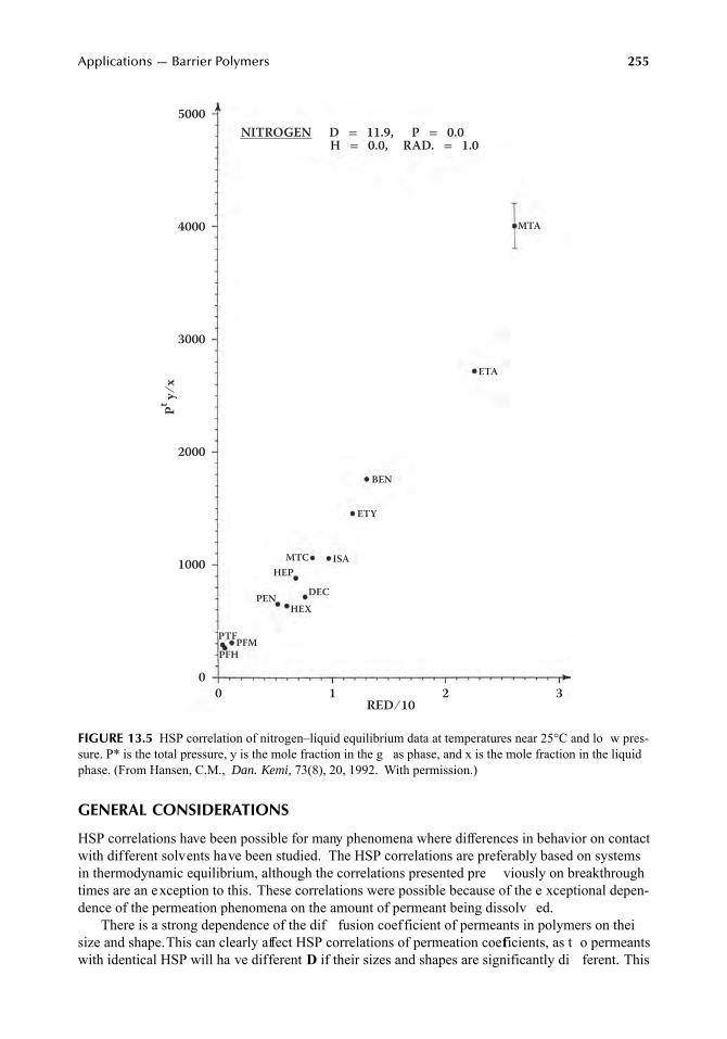
Applications — Barrier Polymers 255
GENERAL CONSIDERATIONS
HSP correlations have been possible for many phenomena where differences in behavior on contactwith different solvents have been studied. The HSP correlations are preferably based on systemsin thermodynamic equilibrium, although the correlations presented pre viously on breakthroughtimes are an exception to this. These correlations were possible because of the e xceptional depen-dence of the permeation phenomena on the amount of permeant being dissolv ed.
There is a strong dependence of the dif fusion coefficient of permeants in polymers on theisize and shape. This can clearly affect HSP correlations of permeation coefficients, as t o permeantswith identical HSP will ha ve different D if their sizes and shapes are significantly di ferent. This
FIGURE 13.5 HSP correlation of nitrogen–liquid equilibrium data at temperatures near 25°C and lo w pres-sure. P* is the total pressure, y is the mole fraction in the g as phase, and x is the mole fraction in the liquidphase. (From Hansen, C.M., Dan. Kemi, 73(8), 20, 1992. With permission.)
RED ⁄ 10
Pt y ⁄ x
5000
4000
3000
2000
1000
00 1 2 3
HEXDECPEN
HEPMTC ISA
PTFPFMPFH
ETY
BEN
ETA
MTA
NITROGEN D = 11.9, P = 0.0 H = 0.0, RAD. = 1.0
7248_C013.fm Page 255 Wednesday, May 23, 2007 11:18 AM
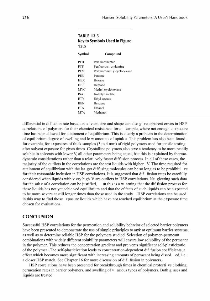
256 Hansen Solubility Parameters: A User’s Handbook
differential in diffusion rate based on solv ent size and shape can also gi ve apparent errors in HSPcorrelations of polymers for their chemical resistance, for e xample, where not enough e xposuretime has been allowed for attainment of equilibrium. This is clearly a problem in the determinationof equilibrium degree of swelling and lo w amounts of uptak e. This problem has also been found,for example, for exposures of thick samples (3 to 4 mm) of rigid polymers used for tensile testingafter solvent exposure for given times. Crystalline polymers also have a tendency to be more readilysoluble in solvents with lower V, all other parameters being equal, but this is explained by thermo-dynamic considerations rather than a relati vely faster diffusion process. In all of these cases, themajority of the outliers in the correlations are the test liquids with higher V. The time required forattainment of equilibrium with the lar ger diffusing molecules can be so long as to be prohibiti vefor their reasonable inclusion in HSP correlations. It is suggested that dif fusion rates be carefullyconsidered when liquids with v ery high V are outliers in HSP correlations. Ne glecting such datafor the sak e of a correlation can be justified, ut this is a w arning that the dif fusion process forthese liquids has not yet achie ved equilibrium and that the ef fects of such liquids can be e xpectedto be more se vere at still longer times than those used in the study . HSP correlations can be usedin this way to find those xposure liquids which have not reached equilibrium at the exposure timechosen for evaluations.
CONCLUSION
Successful HSP correlations for the permeation and solubility behavior of selected barrier polymershave been presented to demonstrate the use of simple principles to arrive at optimum barrier systems,as well as to determine reliable HSP for the polymers studied. Selection of polymer–permeantcombinations with widely different solubility parameters will ensure low solubility of the permeantin the polymer. This reduces the concentration gradient and pre vents significant self-plasticizatioof the polymer . The self-plasticization leads to concentration-dependent dif fusion coefficients, aeffect which becomes more significant with increasing amounts of permeant being dissol ed, i.e.,a closer HSP match. See Chapter 16 for more discussion of dif fusion in polymers.
HSP correlations have been presented for breakthrough times in chemical protecti ve clothing,permeation rates in barrier polymers, and swelling of v arious types of polymers. Both g ases andliquids are treated.
TABLE 13.5Key to Symbols Used in Figure 13.5
Symbol Compound
PFH PerfluoroheptanPTF Perfluorotri utylaminePFM Perfluoromet ylcyclohexanePEN PentaneHEX HexaneHEP HeptaneMYC Methyl cyclohexaneISA Isobutyl acetateETY Ethyl acetateBEN BenzeneETA EthanolMTA Methanol
7248_C013.fm Page 256 Wednesday, May 23, 2007 11:18 AM
Applications — Barrier Polymers 257
REFERENCES
1. Rogers, C.E., Permeation of gases and vapours in polymers, in Polymer Permeability, Comyn, J., Ed.,Elsevier Applied Science, London, 1985, pp. 11–73.
2. Hansen, C.M., Some aspects of the retention of solvents in high polymer films, Färg och Lack, 10(7),169–186, 1964.
3. Hansen, C.M., The Three Dimensional Solubility Parameter and Solvent Diffusion Coefficient, Doctoral dissertation, Danish Technical Press, Copenhagen, 1967.
4. Hansen, C.M., A mathematical description of film drying by sol ent evaporation, J. Oil Colour Chem.Assoc., 51(1), 27–43, 1968.
5. Hansen, C.M., Diffusion in polymers, Polym. Eng. Sci., 20(4), 252–258, 1980.6. Hansen, C.M., The measurement of concentration-dependent diffusion coefficients — the xponential
case, Ind. Eng. Chem. Fundam., 6(4), 609–614, 1967.7. Hansen, C.M., Dif fusion coef ficient measurements by sol ent absorption in concentrated polymer
solutions, J. Appl. Polym. Sci., 26, 3311–3315, 1981.8. Crank, J., The Mathematics of Diffusion, Oxford University Press, Oxford, 1956.9. Klopfer, H., Water Transport by Diffusion in Solid Materials (Wassertransport durch Diffusion in
Feststoffen, in German), Bauv erlag GMBH, Wiesbaden, 1974.10. Forsberg, K. and Olsson, K.G., Guidelines for Selecting Chemical Protective Gloves, (Riktlinjer för
val av kemiskyddshandskar, in Swedish), Förening Teknisk Företagshälso vård (FTF), Stockholm,1985.
11. Forsberg, K. and Kieth, L.H., Chemical Protective Clothing Performance Index, 4th ed., InstantReference Sources, Austin, TX, 1991.
12. Hansen, C.M. and Hansen, K.M., Solubility parameter prediction of the barrier properties of chemicalprotective clothing, Performance of Protective Clothing: Second Symposium. ASTM STP 989, Mans-dorf, S.Z., Sager, R., and Nielsen, A.P., Eds., American Society for Testing and Materials, Philadelphia,PA, 1988, pp. 197–208.
13. Hansen, C.M., The free v olume interpretation of plasticizing ef fectiveness and dif fusion in highpolymers, Off. Dig., 37(480), 57–77, 1965.
14. Zellers, E.T., Three-dimensional solubility parameters and chemical protecti ve clothing permeation.I. Modelling the solubility of organic solvents in Viton gloves, J. Appl. Polym. Sci., 50, 513–530, 1993.
15. Zellers, E.T., Three-dimensional solubility parameters and chemical protective clothing. II. Modellingdiffusion coefficients, breakthrough times, and steady-state permeation rates of o ganic solvents inViton gloves, J. Appl. Polym. Sci., 50, 531–540, 1993.
16. Evans, K.M. and Hardy , J.K., Predicting solubility and permeation properties of or ganic solvents inViton Glove material using Hansen’s solubility parameters, J. Appl. Polym. Sci., 93, 2688–2698, 2004.
17. Nielsen, T.B. and Hansen, C.M., Elastomer swelling and Hansen solubility parameters, Polym. Testing,24, 1054–1061, 2005.
18. Hansen, C.M., Billing, C.B., Jr., and Bentz, A.P., Selection and use of molecular parameters to predictpermeation through fluoropolyme -based protective clothing materials, in The Performance of Pro-tective Clothing: Fourth Volume, ASTM STP 1133, McBriarty, J.P. and Henry, N.W., Eds., AmericanSociety for Testing and Materials, Philadelphia, P A, 1992, pp. 894–907.
19. Pauly, S., Permeability and diffusion data, in Polymer Handbook, 3rd ed., Branderup, J. and Immergut,E.H., Eds., Wiley-Interscience, New York, 1989, pp. VI/445–446.
20. Ursin, C., Hansen, C.M., Van Dyk, J.W., Jensen, P.O., Christensen, I.J., and Ebbehoej, J., Permeabilityof commercial solvents through living human skin, Am. Ind. Hyg. Assoc. J., 56, 651–660, 1995.
21. Hansen, C.M. and Andersen, B.H., The affinities of o ganic solvents in biological systems, Am. Ind.Hyg. Assoc. J., 49(6), 301–308, 1988.
22. Lieberman, R.B. and Barbe, P .C., Polypropylene polymers, in Encyclopedia of Polymer Science andEngineering, 2nd ed., Vol. 13, Mark, H.F ., Bikales, N.M., Ov erberger, C.G., Menges, G., andKroschwitz, J.I., Eds., Wiley-Interscience, New York, 1988, pp. 482–483.
23. Anonymous, Fluid Resistance of Viton®, Du Pont Compan y, Polymer Products Department, Elas-tomers Division, Wilmington, DE, 1989.
24. Anonymous, Plastguide, SCS Dukadan AS, Randers, Denmark, 1990.
7248_C013.fm Page 257 Wednesday, May 23, 2007 11:18 AM

258 Hansen Solubility Parameters: A User’s Handbook
25. König, U. and Schuch, H., Structure and permeability of polymers (K onstitution und Permeabilitätvon Kunststoffen, in German), Kunststoffe, 67(1), 27–31, 1977.
26. Anonymous, ACLAR® Barrier Films, AlliedSignal — Advanced Materials, Allied Signal Inc., Mor -ristown, NJ.
27. Perry, J.H., Chilton, C.H., and Kirkpatrick, S.D., Eds., Chemical Engineers’ Handbook, 4th ed.,McGraw-Hill, New York, 1963, Section 14, pp. 2–7.
28. Hansen, C.M., 25 years with solubility parameters (25 År med Opløselighedsparametrene, in Danish),Dan. Kemi, 73(8), 18–22, 1992.
29. Hildebrand, J. and Scott, R.L., The Solubility of Nonelectrolytes, 3rd ed., Reinhold, New York, 1950.30. Hildebrand, J. and Scott, R.L., Regular Solutions, Prentice-Hall Inc., Engle wood Cliffs, NJ, 1962.31. Barton, A.F.M., Handbook of Polymer-Liquid Interaction Parameters and Solubility Parameters, CRC
Press, Boca Raton, FL, 1990.
7248_C013.fm Page 258 Wednesday, May 23, 2007 11:18 AM
259
14
Applications — Environmental Stress Cracking in Polymers
Charles M. Hansen
ABSTRACT
Hansen solubility parameters (HSP) can be used to help predict which chemicals can causeenvironmental stress cracking (ESC) in polymers. ESC requires tensile stress and correlates whenthe RED number (relati ve energy difference in the polymer -solvent interaction) found from HSPconsiderations is plotted vs. a molecular size parameter , the molar v olume, V. There are threedistinct regions on this plot. There is a re gion at lo w RED including those challenge liquids thatdissolve the polymer or are v ery aggressive, and ESC is not found as such. There is a re gion athigh RED where the absorption is zero or not great enough to matter or else the absorption rate isslow enough to allo w relaxation of the polymer in preference to ESC. ESC can occur in anintermediate re gion where there is some absorption of challenge liquid, although e xamples aregiven where ESC takes place without measurable absorption for good matches in HSP at relativelyhigh stress/strain. The ESC re gion on these plots increases in size with increased tensile stressand/or increased critical strain.
INTRODUCTION
The pre vious chapter dealt with the chemical resistance of polymers and briefly touched oenvironmental stress cracking (ESC) as one aspect of chemical attack. This chapter e xpands theprevious discussion of this special type of ph ysical chemical attack on polymers. This form offailure represents at least 25% of all f ailures in plastics and therefore deserv es special attention.
1
A failure by ESC can appear almost immediately , after minutes, after hours, or e ven after years,and often occurs without prior w arning. There is a considerable literature on ESC. An excellentgeneral source of the ESC literature is Wright’s encompassing book on f ailures in polymers ingeneral.
1
The present chapter is in man y ways a supplement to this e xcellent work.It is no w clear that the polymer and the chemical that initiates the stress cracking must ha ve
similar or reasonably similar HSP . The ESC initiator need not dissolv e the polymer as such. It hasgenerally been assumed that some similarity in HSP is required such that some absorption occurs.More recently it has been recognized that measurable absorption is not al ways necessary for ESC tooccur in some polymers. It is theorized that some physical movement, such as rotation of the polymerchain segments at the contact surface, can initiate the cracking process. In the latter case the similarityof the HSP of the challenge liquid may be to the HSP of an entity in the polymer chain that otherwisemight be oriented away from the polymer surface. Under given conditions of strain it may prefer theenvironment of the ESC initiator once there is contact with the polymer . An understanding of thisphenomenon seems to be e volving, but it is not complete as discussed belo w.
As stated above, the generally accepted mechanism for ESC has been that some absorption ofthe active chemical weakens the polymer structure locally , such that the tensile stress increases inadjacent regions. The tensile stress must be suf ficient to locally pull polymer chains or s gmentsof chains from the bulk. As the structure weakens locally, there is added stress in adjacent re gions.This may be suf ficient to cause a craze or crack, ut in man y cases further absorption or furtherchemical penetration seems necessary to repeat the same process until finally the stress become
7248_C014.fm Page 259 Wednesday, May 23, 2007 11:24 AM
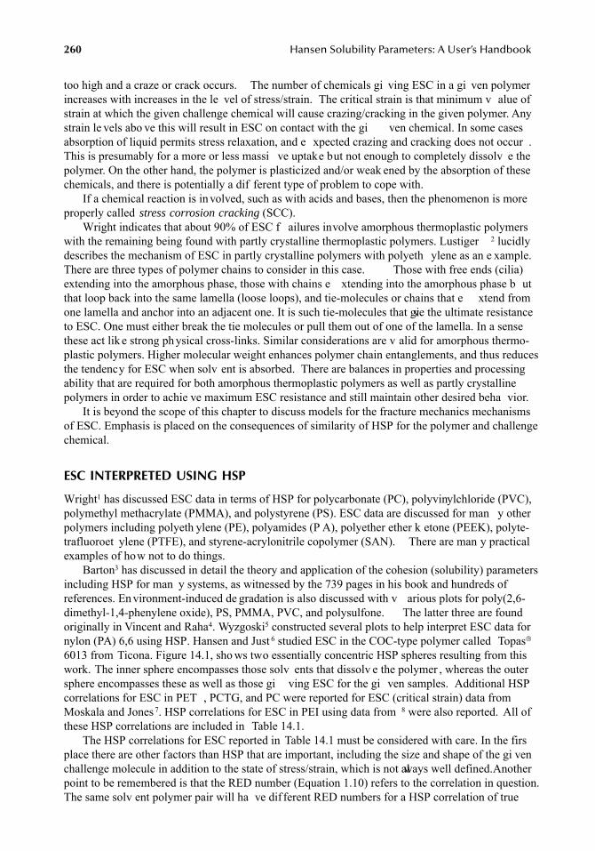
260
Hansen Solubility Parameters: A User’s Handbook
too high and a craze or crack occurs. The number of chemicals gi ving ESC in a gi ven polymerincreases with increases in the le vel of stress/strain. The critical strain is that minimum v alue ofstrain at which the given challenge chemical will cause crazing/cracking in the given polymer. Anystrain le vels abo ve this will result in ESC on contact with the gi ven chemical. In some casesabsorption of liquid permits stress relaxation, and e xpected crazing and cracking does not occur .This is presumably for a more or less massi ve uptake but not enough to completely dissolv e thepolymer. On the other hand, the polymer is plasticized and/or weak ened by the absorption of thesechemicals, and there is potentially a dif ferent type of problem to cope with.
If a chemical reaction is in volved, such as with acids and bases, then the phenomenon is moreproperly called
stress corrosion cracking
(SCC).Wright indicates that about 90% of ESC f ailures involve amorphous thermoplastic polymers
with the remaining being found with partly crystalline thermoplastic polymers. Lustiger
2
lucidlydescribes the mechanism of ESC in partly crystalline polymers with polyeth ylene as an e xample.There are three types of polymer chains to consider in this case. Those with free ends (cilia)extending into the amorphous phase, those with chains e xtending into the amorphous phase b utthat loop back into the same lamella (loose loops), and tie-molecules or chains that e xtend fromone lamella and anchor into an adjacent one. It is such tie-molecules that give the ultimate resistanceto ESC. One must either break the tie molecules or pull them out of one of the lamella. In a sensethese act like strong ph ysical cross-links. Similar considerations are v alid for amorphous thermo-plastic polymers. Higher molecular weight enhances polymer chain entanglements, and thus reducesthe tendency for ESC when solv ent is absorbed. There are balances in properties and processingability that are required for both amorphous thermoplastic polymers as well as partly crystallinepolymers in order to achie ve maximum ESC resistance and still maintain other desired beha vior.
It is beyond the scope of this chapter to discuss models for the fracture mechanics mechanismsof ESC. Emphasis is placed on the consequences of similarity of HSP for the polymer and challengechemical.
ESC INTERPRETED USING HSP
Wright
1
has discussed ESC data in terms of HSP for polycarbonate (PC), polyvinylchloride (PVC),polymethyl methacrylate (PMMA), and polystyrene (PS). ESC data are discussed for man y otherpolymers including polyeth ylene (PE), polyamides (P A), polyether ether k etone (PEEK), polyte-trafluoroet ylene (PTFE), and styrene-acrylonitrile copolymer (SAN). There are man y practicalexamples of how not to do things.
Barton
3
has discussed in detail the theory and application of the cohesion (solubility) parametersincluding HSP for man y systems, as witnessed by the 739 pages in his book and hundreds ofreferences. En vironment-induced de gradation is also discussed with v arious plots for poly(2,6-dimethyl-1,4-phenylene oxide), PS, PMMA, PVC, and polysulfone. The latter three are foundoriginally in Vincent and Raha
4
. Wyzgoski
5
constructed several plots to help interpret ESC data fornylon (PA) 6,6 using HSP. Hansen and Just
6
studied ESC in the COC-type polymer called Topas
®
6013 from Ticona. Figure 14.1, sho ws two essentially concentric HSP spheres resulting from thiswork. The inner sphere encompasses those solv ents that dissolv e the polymer , whereas the outersphere encompasses these as well as those gi ving ESC for the gi ven samples. Additional HSPcorrelations for ESC in PET , PCTG, and PC were reported for ESC (critical strain) data fromMoskala and Jones
7
. HSP correlations for ESC in PEI using data from
8
were also reported. All ofthese HSP correlations are included in Table 14.1.
The HSP correlations for ESC reported in Table 14.1 must be considered with care. In the firsplace there are other factors than HSP that are important, including the size and shape of the gi venchallenge molecule in addition to the state of stress/strain, which is not always well defined.Anotherpoint to be remembered is that the RED number (Equation 1.10) refers to the correlation in question.The same solv ent polymer pair will ha ve dif ferent RED numbers for a HSP correlation of true
7248_C014.fm Page 260 Wednesday, May 23, 2007 11:24 AM
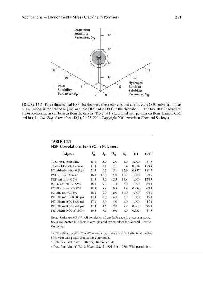
Applications — Environmental Stress Cracking in Polymers
261
FIGURE 14.1
Three-dimensional HSP plot sho wing those solv ents that dissolv e the COC polymer , Topas6013, Ticona, in the shaded re gion, and those that induce ESC in the clear shell. The two HSP spheres arealmost concentric as can be seen from the data in Table 14.1. (Reprinted with permission from Hansen, C.M.and Just, L.,
Ind. Eng. Chem. Res.
, 40(1), 21–25, 2001. Cop yright 2001 American Chemical Society.)
TABLE 14.1HSP Correlations for ESC in Polymers
Polymer
δδδδ
D
δδδδ
P
δδδδ
H
R
0
FIT G/T
a
Topas 6013 Solubility 18.0 3.0 2.0 5.0 1.000 8/43Topas 6013 Sol. + cracks 17.3 3.1 2.1 6.4 0.974 15/43PC critical strain <0.6%
b
21.5 9.5 5.1 12.9 0.857 18/47PVC crit.str. <0.6%
c
16.0 10.0 5.0 10.7 1.000 5/16PET crit. str. <0.6% 21.3 4.5 12.3 13.9 1.000 12/19PCTG crit. str. <0.55% 18.3 9.3 11.3 8.0 1.000 8/19PCTG crit. str. <0.50% 18.8 8.8 10.8 7.9 0.989 6/19PC crit. str. <0.31% 18.0 9.0 6.0 10.0 1.000 9/18PEI Ultem
®
1000 600 psi 17.3 5.3 4.7 3.3 1.000 3/20PEI Ultem 1000 1200 psi 17.0 6.0 4.0 4.0 1.000 4/20PEI Ultem 1000 2500 psi 17.4 4.6 9.0 7.2 0.967 9/20PEI Ultem 1000 solubility 19.6 7.6 9.0 6.0 0.952 8/45
Note
: Units are MP a
1/2
. All correlations from Reference 6, e xcept as noted.See also Chapter 12; Ultem is a re gistered trademark of the General ElectricCompany.
a
G/T is the number of “good” or attacking solvents relative to the total numberof solvent data points used in this correlation.
b
Data from Reference 10 through Reference 14.
c
Data from Mai, Y.-W.,
J. Mater. Sci.
, 21, 904–916, 1986. With permission.
HydrogenBondingSolubilityParameter, δH
PolarSolubilityParameter, δP
DispersionSolubilityParameter, δD
15
10
5
0
40
30
20
10
15
10
5
0
7248_C014.fm Page 261 Wednesday, May 23, 2007 11:24 AM
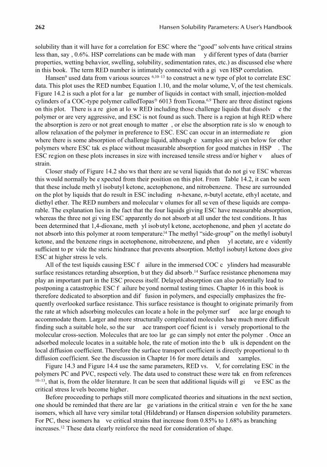
262
Hansen Solubility Parameters: A User’s Handbook
solubility than it will have for a correlation for ESC where the “good” solvents have critical strainsless than, say , 0.6%. HSP correlations can be made with man y dif ferent types of data (barrierproperties, wetting behavior, swelling, solubility, sedimentation rates, etc.) as discussed else wherein this book. The term RED number is intimately connected with a gi ven HSP correlation.
Hansen
9
used data from various sources
6,10–13
to construct a new type of plot to correlate ESCdata. This plot uses the RED number, Equation 1.10, and the molar volume, V, of the test chemicals.Figure 14.2 is such a plot for a lar ge number of liquids in contact with small, injection-moldedcylinders of a COC-type polymer called Topas
®
6013 from Ticona.
6,9
There are three distinct regionson this plot. There is a re gion at lo w RED including those challenge liquids that dissolv e thepolymer or are very aggressive, and ESC is not found as such. There is a region at high RED wherethe absorption is zero or not great enough to matter , or else the absorption rate is slo w enough toallow relaxation of the polymer in preference to ESC. ESC can occur in an intermediate re gionwhere there is some absorption of challenge liquid, although e xamples are gi ven below for otherpolymers where ESC tak es place without measurable absorption for good matches in HSP . TheESC region on these plots increases in size with increased tensile stress and/or higher v alues ofstrain.
Closer study of Figure 14.2 sho ws that there are se veral liquids that do not gi ve ESC whereasthis would normally be e xpected from their position on this plot. From Table 14.2, it can be seenthat these include meth yl isobutyl ketone, acetophenone, and nitrobenzene. These are surroundedon the plot by liquids that do result in ESC including
n
-hexane,
n
-butyl acetate, ethyl acetate, anddiethyl ether. The RED numbers and molecular v olumes for all se ven of these liquids are compa-rable. The explanation lies in the fact that the four liquids giving ESC have measurable absorption,whereas the three not gi ving ESC apparently do not absorb at all under the test conditions. It hasbeen determined that 1,4-dioxane, meth yl isobutyl ketone, acetophenone, and phen yl acetate donot absorb into this polymer at room temperature.
14
The methyl “side-group” on the methyl isobutylketone, and the benzene rings in acetophenone, nitrobenzene, and phen yl acetate, are e videntlysufficient to pr vide the steric hindrance that prevents absorption. Methyl isobutyl ketone does giveESC at higher stress le vels.
All of the test liquids causing ESC f ailure in the immersed COC c ylinders had measurablesurface resistances retarding absorption, b ut they did absorb.
14
Surface resistance phenomena mayplay an important part in the ESC process itself. Delayed absorption can also potentially lead topostponing a catastrophic ESC f ailure be yond normal testing times. Chapter 16 in this book istherefore dedicated to absorption and dif fusion in polymers, and especially emphasizes the fre-quently overlooked surface resistance. This surface resistance is thought to originate primarily fromthe rate at which adsorbing molecules can locate a hole in the polymer surf ace large enough toaccommodate them. Larger and more structurally complicated molecules have much more difficultfinding such a suitable hole, so the sur ace transport coef ficient is i versely proportional to themolecular cross-section. Molecules that are too lar ge can simply not enter the polymer . Once anadsorbed molecule locates in a suitable hole, the rate of motion into the b ulk is dependent on thelocal diffusion coefficient. Therefore the surface transport coefficient is directly proportional to thdiffusion coefficient. See the discussion in Chapter 16 for more details and xamples.
Figure 14.3 and Figure 14.4 use the same parameters, RED vs. V, for correlating ESC in thepolymers PC and PVC, respecti vely. The data used to construct these were tak en from references
10–13
, that is, from the older literature. It can be seen that additional liquids will gi ve ESC as thecritical stress levels become higher.
Before proceeding to perhaps still more complicated theories and situations in the next section,one should be reminded that there are lar ge variations in the critical strain e ven for the he xaneisomers, which all have very similar total (Hildebrand) or Hansen dispersion solubility parameters.For PC, these isomers ha ve critical strains that increase from 0.85% to 1.68% as branchingincreases.
12
These data clearly reinforce the need for consideration of shape.
7248_C014.fm Page 262 Wednesday, May 23, 2007 11:24 AM
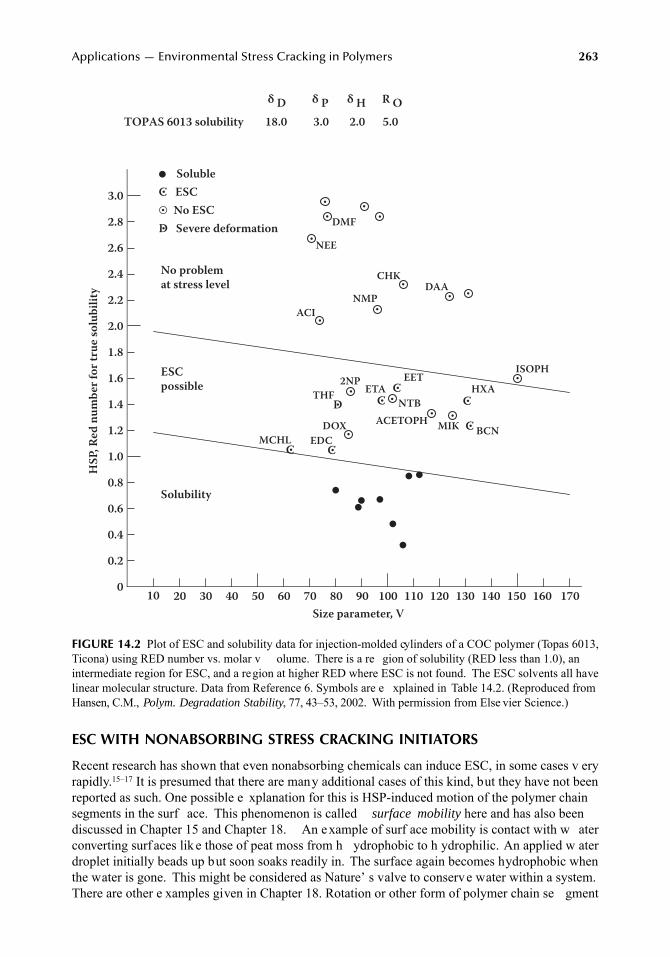
Applications — Environmental Stress Cracking in Polymers
263
ESC WITH NONABSORBING STRESS CRACKING INITIATORS
Recent research has shown that even nonabsorbing chemicals can induce ESC, in some cases v eryrapidly.
15–17
It is presumed that there are many additional cases of this kind, but they have not beenreported as such. One possible e xplanation for this is HSP-induced motion of the polymer chainsegments in the surf ace. This phenomenon is called
surface mobility
here and has also beendiscussed in Chapter 15 and Chapter 18. An example of surf ace mobility is contact with w aterconverting surf aces lik e those of peat moss from h ydrophobic to h ydrophilic. An applied w aterdroplet initially beads up but soon soaks readily in. The surface again becomes hydrophobic whenthe water is gone. This might be considered as Nature’ s valve to conserve water within a system.There are other e xamples given in Chapter 18. Rotation or other form of polymer chain se gment
FIGURE 14.2
Plot of ESC and solubility data for injection-molded cylinders of a COC polymer (Topas 6013,Ticona) using RED number vs. molar v olume. There is a re gion of solubility (RED less than 1.0), anintermediate region for ESC, and a region at higher RED where ESC is not found. The ESC solvents all havelinear molecular structure. Data from Reference 6. Symbols are e xplained in Table 14.2. (Reproduced fromHansen, C.M.,
Polym. Degradation Stability
, 77, 43–53, 2002. With permission from Else vier Science.)
TOPAS 6013 solubility 18.0 3.0 2.0 5.0δ D δ P δ H R O
● SolubleC ESC� No ESCD Severe deformation DMF
NEE
NMPACI
CHKDAA
EETETA
NTB
2NPTHF
EDCMCHLACETOPH MIK BCN
HXAISOPH
DOX
C
D
C
CC
C
C
● ●
●●●
●
●
●
No problemat stress level
ESCpossible
Solubility
Size parameter, V
HSP
, Red
num
ber f
or tr
ue so
lubi
lity
5040302010 60 70 80 90 100 110 120 130 140 150 160 170
3.0
2.8
2.6
2.4
2.2
2.0
1.8
1.6
1.4
1.2
1.0
0.8
0.6
0.4
0.2
0
7248_C014.fm Page 263 Wednesday, May 23, 2007 11:24 AM
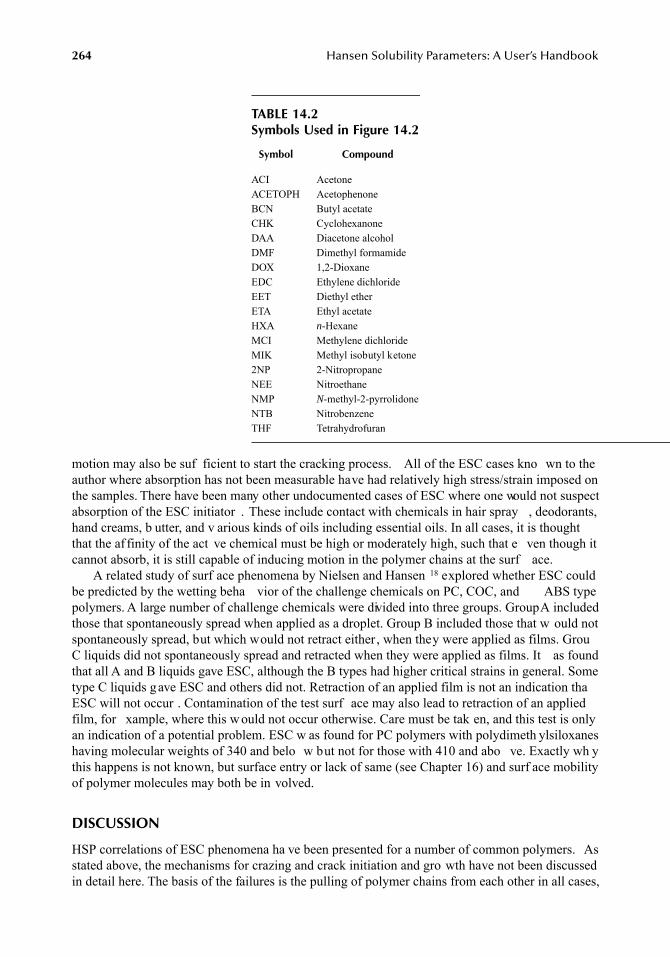
264
Hansen Solubility Parameters: A User’s Handbook
motion may also be suf ficient to start the cracking process. All of the ESC cases kno wn to theauthor where absorption has not been measurable have had relatively high stress/strain imposed onthe samples. There have been many other undocumented cases of ESC where one would not suspectabsorption of the ESC initiator . These include contact with chemicals in hair spray , deodorants,hand creams, b utter, and v arious kinds of oils including essential oils. In all cases, it is thoughtthat the af finity of the act ve chemical must be high or moderately high, such that e ven though itcannot absorb, it is still capable of inducing motion in the polymer chains at the surf ace.
A related study of surf ace phenomena by Nielsen and Hansen
18
explored whether ESC couldbe predicted by the wetting beha vior of the challenge chemicals on PC, COC, and ABS typepolymers. A large number of challenge chemicals were divided into three groups. Group A includedthose that spontaneously spread when applied as a droplet. Group B included those that w ould notspontaneously spread, but which would not retract either, when they were applied as films. GrouC liquids did not spontaneously spread and retracted when they were applied as films. It as foundthat all A and B liquids gave ESC, although the B types had higher critical strains in general. Sometype C liquids gave ESC and others did not. Retraction of an applied film is not an indication thaESC will not occur . Contamination of the test surf ace may also lead to retraction of an appliedfilm, for xample, where this w ould not occur otherwise. Care must be tak en, and this test is onlyan indication of a potential problem. ESC w as found for PC polymers with polydimeth ylsiloxaneshaving molecular weights of 340 and belo w but not for those with 410 and abo ve. Exactly wh ythis happens is not known, but surface entry or lack of same (see Chapter 16) and surf ace mobilityof polymer molecules may both be in volved.
DISCUSSION
HSP correlations of ESC phenomena ha ve been presented for a number of common polymers. Asstated above, the mechanisms for crazing and crack initiation and gro wth have not been discussedin detail here. The basis of the failures is the pulling of polymer chains from each other in all cases,
TABLE 14.2Symbols Used in Figure 14.2
Symbol Compound
ACI AcetoneACETOPH AcetophenoneBCN Butyl acetateCHK CyclohexanoneDAA Diacetone alcoholDMF Dimethyl formamideDOX 1,2-DioxaneEDC Ethylene dichlorideEET Diethyl etherETA Ethyl acetateHXA
n
-HexaneMCI Methylene dichlorideMIK Methyl isobutyl ketone2NP 2-NitropropaneNEE NitroethaneNMP
N
-methyl-2-pyrrolidoneNTB NitrobenzeneTHF Tetrahydrofuran
7248_C014.fm Page 264 Wednesday, May 23, 2007 11:24 AM
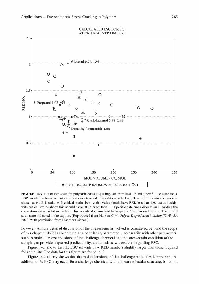
Applications — Environmental Stress Cracking in Polymers
265
however. A more detailed discussion of the phenomena in volved is considered be yond the scopeof this chapter . HSP has been used as a correlating parameter , necessarily with other parameterssuch as molecular size and shape of the challenge chemical and the stress/strain condition of thesamples, to provide improved predictability, and to ask ne w questions regarding ESC.
Figure 14.1 shows that the ESC solvents have RED numbers slightly larger than those requiredfor solubility. The data for this figure are found in
6
Figure 14.2 clearly shows that the molecular shape of the challenge molecules is important inaddition to V. ESC may occur for a challenge chemical with a linear molecular structure, b ut not
FIGURE 14.3
Plot of ESC data for polycarbonate (PC) using data from Mai
10
and others
11–13
to establish aHSP correlation based on critical strain since true solubility data w as lacking. The limit for critical strain waschosen as 0.6%. Liquids with critical strains belo w this value should have RED less than 1.0, just as liquidswith critical strains above this should have RED larger than 1.0. Specific data and a discussion r garding thecorrelation are included in the te xt. Higher critical strains lead to lar ger ESC regions on this plot. The criticalstrains are indicated in the caption. (Reproduced from Hansen, C.M.,
Polym. Degradation Stability
, 77, 43–53,2002. With permission from Else vier Science.)
� � 0-0.2�0.2-0.4 ◆ 0.4-0.6 ▲ 0.6-0.8 � 0.8-1 ●>1MOL VOLUME - CC/MOL
CALCULATED ESC FOR PCAT CRITICAL STRAIN = 0.6
RED
NO.
300 350250200150100500
2.5
2
1.5
1
0.5
0
�
���
��
���
�� �
�
�
��
� ��
�
�
●
● ●
● ●●
●●
●
●
●
●●
Glycerol 0.77, 1.99
2-Propanol 1.02
Dimethylformamide 1.55
Cyclohexanol 0.98, 1.48
▲
▲▲
▲
◆
◆
◆◆◆◆
◆◆
◆
7248_C014.fm Page 265 Wednesday, May 23, 2007 11:24 AM
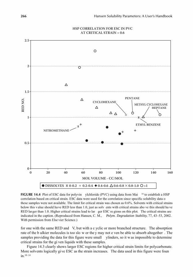
266
Hansen Solubility Parameters: A User’s Handbook
for one with the same RED and V, but with a c yclic or more branched structure. The absorptionrate of the b ulkier molecules is too slo w or the y may not e ven be able to absorb altogether . Thesamples providing the data for this figure were small ylinders, so it w as impossible to determinecritical strains for the gi ven liquids with these samples.
Figure 14.3 clearly shows larger ESC regions for higher critical strain limits for polycarbonate.More solvents logically give ESC as the strain increases. The data used in this figure were founin.
10–14
FIGURE 14.4
Plot of ESC data for polyvin ylchloride (PVC) using data from Mai
10
to establish a HSPcorrelation based on critical strain. ESC data were used for the correlation since specific solubility data othese samples were not available. The limit for critical strain was chosen as 0.6%. Solvents with critical strainsbelow this value should have RED less than 1.0, just as solv ents with critical strains abo ve this should ha veRED larger than 1.0. Higher critical strains lead to lar ger ESC re gions on this plot. The critical strains areindicated in the caption. (Reproduced from Hansen, C. M.,
Polym. Degradation Stability
, 77, 43–53, 2002.With permission from Else vier Science.)
● DISSOLVES � 0-0.2 � 0.2-0.4 ◆ 0.4-0.6 ▲ 0.6-0.8 � 0.8-1.0 ● >1
MOL VOLUME - CC/MOL
RED
NO.
HSP CORRELATION FOR ESC IN PVCAT CRITICAL STRAIN = 0.6
120 160140100806040200
2.5
2
1.5
1
0.5
0
��
��
� �
●
●
●●
●
●
●●
●
▲
▲
▲
▲ ▲▲
NITROMETHANE
CYCLOHEXANEPENTANE
METHYL CYCLOHEXANEHEPTANE
ETHYL BENZENE
7248_C014.fm Page 266 Wednesday, May 23, 2007 11:24 AM
Applications — Environmental Stress Cracking in Polymers
267
Figure 14.4 shows the ESC behavior of PVC using data taken from the literature.
10
This figurconfirms the ability to use this type of plot to correlate and predict ESC in polymers
It is not unusual for suppliers of polymers to change compositions without indicating what hasbeen done and to continue to use the general indication of polymer type, such as PC. Thus, the PCdata in Figure 14.3 and the PVC data in Figure 14.4 may not be v alid for all polymers of thesenominal types. This is a significant problem in further research and d veloping fundamentalunderstanding. Researchers either must w ork with commercial materials the y do not ha ve fullknowledge of, or else tak e the path of making test materials to be certain of what is being dealtwith. In the latter case, the information may not apply directly in practice because the practicalmaterials may have added components. This dilemma apparently has no fully satisfactory solution.
CONCLUSION
HSP have been used to de velop correlations of ESC. It w ould appear that testing is still requiredto ascertain what beha vior is to be e xpected, b ut these correlations clearly indicate where theproblems will be greatest. It is usually the une xpected events that cause the catastrophic f ailures,but designs or changes in designs that lead to increased tensile stress ha ve also been the causes ofESC in practice. Care is especially required whene ver the HSP of the polymer gets too close tothe HSP of potential challenge chemicals. The required af finity between act ve chemical andpolymer allows correlations of ESC with HSP , most often with the simultaneous need to considerthe size and shape of the acti ve chemical and the stress/strain condition of the polymer .
REFERENCES
1. Wright, D.,
Failure of Plastics and Rubber Products
, Rapra Technology Limited, Shawbury, Shrews-bury, Shropshire, U.K., 2001.
2. Lustiger, A., Understanding En vironmental Stress Cracking in Polyeth ylene,
Medical Plastics andBiomaterials Magazine
, MPB Article Inde x (originally published July 1996), http://www .device-link.com/mpb/archive/96/07/001.html.
3. Barton, A.F.M.,
Handbook of Solubility Parameters and Other Cohesion Parameters
, 2nd ed., CRCPress, Boca Raton, FL, 1991.
4. Vincent, P.I. and Raha, S., Influence of ydrogen bonding on crazing and cracking of amorphousthermoplastics,
Polymer
, 13, 283–287, 1972.5. Wyzgoski, M.G., The role of solubility in stress cracking on nylon 6,6, in
Macromolecular Solutions
,Seymour, R.B. and Stahl, G.A., Eds., Per gamon Press, New York, 1982, pp. 41–60.
6. Hansen, C.M. and Just, L., Prediction of en vironmental stress cracking in plastics with Hansensolubility parameters,
Ind. Eng. Chem. Res.
, 40(1), 21–25, 2001.7. Moskala, E.J. and Jones, M., Evaluating Environmental Stress Cracking of Medical Plastics,
MedicalPlastics and Biomaterials Magazine
, May, 1998, pp. 34–45.8. Anonymous,
Ultem Resin Design Guide
, GE Plastics, Pittsfield, MA, 19899. Hansen, C.M., On Predicting En vironmental Stress Cracking in Polymers,
Polym. Degradation Sta-bility
, 77, 43–53, 2002.10. Mai, Y.-W., Environmental stress cracking of glassy polymers and solubility parameters,
J. Mater.Sci.
, 21, 904–916, 1986.11. Kambour, R.P., Gruner, C.L., and Romagosa, E.E., Bisphenol-A polycarbonate immersed in or ganic
media. Swelling and response to stress,
Macromolecules
, 7, 248–253, 1974.12. Jacques, C.H.M. and Wyzgoski, M.G., Prediction of en vironmental stress cracking of polycarbonate
from solubility considerations,
J. Appl. Polym. Sci.
, 23, 1153–1166, 1979.13. Henry, L.F., Prediction and evaluation of the susceptibilities of glassy thermoplastics to environmental
stress cracking,
Polym. Eng. Sci.
, 14(March), 167–176, 1974.14. Nielsen, T.B. and Hansen, C.M., Significance of sur ace resistance in absorption by polymers,
Ind.Eng. Chem. Res.
, 44(11), 3959–3965, 2005.
7248_C014.fm Page 267 Wednesday, May 23, 2007 11:24 AM

268
Hansen Solubility Parameters: A User’s Handbook
15. Al-Saidi, L.F., Mortensen, K., and Almdal, K., En vironmental stress cracking resistance. Beha viourof polycarbonate in different chemicals by determination of the time-dependence of stress at constantstrains,
Polym. Degradation Stability
, 82, 451–461, 2003.16. Hansen, C.M., Environmental stress cracking of PTFE in kerosene,
Polym. Degradation Stability
, 77,511–513, 2002.
17. Kjellander, C.K., Publications being prepared.18. Nielsen, T.B. and Hansen, C.M., Surf ace wetting and the prediction of en vironmental stress cracking
(ESC) in polymers,
Polym. Degradation Stability
, 89, 513–516, 2005.
7248_C014.fm Page 268 Wednesday, May 23, 2007 11:24 AM
269
15
Hansen Solubility Parameters — Biological Materials
Charles M. Hansen and Tim S. Poulsen
ABSTRACT
The Hansen solubility parameters (HSP) of man y biological materials can be found from correla-tions of ho w the y interact with well-defined liquids. The three HSP parameters,
δ
D
,
δ
P
, and
δ
H
quantitatively account for the cohesion ener gy density arising from atomic, dispersion type inter -actions (D), molecular, dipolar interactions (P), and molecular, hydrogen bonding interactions (H).Examples of HSP correlations included in this chapter are DN A, cholesterol, chloroph yll, woodchemicals, polypeptides (proteins), human skin, nicotine, lard, and urea. The often-quoted “lik edissolves like” has been expanded to “like seeks like” (self-association) to discuss the implicationsof these correlations. The ability of HSP to correlate surf ace phenomena has made this changemandatory.
Biological materials such as proteins and DN A have well defined structures in a g ven envi-ronment. DNA adopts double helices, whereas proteins consist of a combined shape of the sec-ondary, tertiary, and in some cases quaternary structure that together determine the conformationof the protein. The ultrastructure of wood is another example of Nature’s way of establishing orderin complex systems. The proper function of a protein requires that certain functional groups are atprecise locations within its tertiary and/or in some cases quaternary structure. The conformationof proteins and DN A can be influenced, and in ma y cases controlled, by solv ent quality. Thesolvent quality in a gi ven environment is expected to determine whether a protein is dissolv ed ornot, and also to control the w ay it adsorbs onto other materials or interacts with itself. Controlledchanges in solv ent quality can lead to controlled changes in conformation. Solv ents can changenot only the ability of noncovalent interactions such as van der Waals, hydrogen bonding, and ionicbonding, but also induce chiral rotation. The key to the importance of nonco valent interaction isthat such interactions can continually be brok en and reformed under physiological conditions. Theportion of the molecule with ener gy properties most similar to the surrounding liquid will beoriented toward the liquid (“lik e seeks like”).
The term
hydrogen bonding
is generally used to describe the noncovalent interactions in DNA,proteins, and other biological molecules, implying that this is the dominating interaction. The HSPcorrelation based on solv ent interactions with DN A resulted in
δ
D
;
δ
P
;
δ
H
v alues equal to19.0;20.0;11.0. These numbers clearly sho w that h ydrogen bonding pro vides by f ar the smallestcontribution of the three types of interaction, representing only about 14% of the cohesi ve energyinvolved (using Chapter 1, Equations 1.6–1.8). The term
hydrogen bonding
must be considered asan insufficient description of the interactions that determine the structure in such molecules
7248_C015.fm Page 269 Wednesday, May 9, 2007 9:37 AM
270
Hansen Solubility Parameters: A User’s Handbook
INTRODUCTION
HSP have been used to characterize man y biological materials.
1–7
Most of the materials discussedin these references are also included in the present discussion, b ut many more can be added byexperiment or calculation.
There are man y simple e xperimental methods to determine the HSP for biological materials.These involve contacting a material of interest with a series of well-chosen liquids. The fact ofsolubility, differences in degree of equilibrium swelling, rapid permeation or not, significant suraceadsorption or not, or other measurable quantity significantly influenced by ysical affinity relationcan be observed and used to find the HSP for a material being studied. These methods have beendiscussed in more detail in earlier chapters. The basis of the division of the cohesive energy densityinto three parts accounting for the atomic dispersion (D), molecular dipolar (P), and molecularhydrogen bonding (H) interactions, respecti vely, is given in detail in Chapter 1.
The HSP for simpler compounds can be calculated according to the methods gi ven in Chapter1. HSP v alues for nicotine, skatole, w ood chemicals, etc., that are discussed in this chapter werecalculated using these methods. Figure 15.1 sho ws a typical HSP sphere correlating e xperimentalsolubility data for lignin.
1
The good solv ents are located within the sphere which is based onChapter 1, Equation 1.9. Again, as stated in pre vious chapters, this equation is in agreement withthe Prigogine corresponding states theory of polymer solutions as discussed in Chapter 2. Thestatistical thermodynamics approach presented in Chapter 3 also shows agreement with the conceptsto which this book is dedicated. Furthermore, this equation has also been sho wn to be correct forsuch comple x materials as asphalt and bitumen, as described in Chapter 9, and carbon dioxidesolubility in solvents, as described in Chapter 10.
A HSP correlation can, of course, be used to predict the beha vior of solv ents not included inthe experimental work. It is con venient to print the solv ent database in order from best solv ent toworst solvent to aid in finding alternat ves. This is a quantitati ve application of the generally usedstatement “Like Dissolves Like.” In the follo wing discussion, this concept is e xpanded to “Lik eSeeks Lik e” (self-association). This implies that se gments of molecules seek re gions of similarHSP if this is possible. This may result in solutions or in selecti ve orientation of se gments ofmolecules in more complicated systems.
Table 15.1 contains HSP data for se veral biologically interesting materials. These are discussedin the following in more detail with an indication of ho w such data may be used. The data includedin this table are the
δ
D
,
δ
P
, and
δ
H
parameters; the radius of interaction for the HSP correlation, Ro;if appropriate, the data fit (where a fit of 1.000 is perfect as discussed in Chapter 1). G is number “good” solvents and the total number of solvents in a given correlation is T. The units for the solubilityparameters and Ro are MP a
1/2
. Plots of the kind gi ven in Figure 15.1 for lignin are sometimes usedto interpret relations among dif ferent materials. RED numbers indicate solv ent quality with lo wervalues being indicati ve of better solv ents (see Chapter 1, Equation 1.10). The correlations reportedhere are a result of data processing with the SPHERE program described in Chapter 1. The output isoften arranged with the best solv ent (lowest RED number) at the top of the list.
A most interesting and important class of molecules are called amphipathic. These exhibit bothhydrophilic and h ydrophobic properties simultaneously . An example from biology is the amphi-pathic molecules (lipids) that form the basis of the biological membrane bilayers that surroundcells. Such amphipathic molecules ha ve a head group that is strongly h ydrophilic, coupled to ahydrophobic tail – usually h ydrocarbon in nature. When one attempts to dissolv e these moleculesin water, they form special structures. These may be monolayers on the w ater surface, with onlythe head groups immersed. Alternatively, if the mixture is vigorously stirred, micelles (sphericalstructures stabilized by a single layer of molecules at the w ater interface) or bilayer v esicles mayform. Another example is amino acid side chains. These are by nature not only dif ferent in sizeand shape, but also in the charge they carry, their general affinity for ater (hydrophilicity) and/ortheir general a version to w ater (hydrophobicity). The native conformation of proteins is a strong
7248_C015.fm Page 270 Wednesday, May 9, 2007 9:37 AM
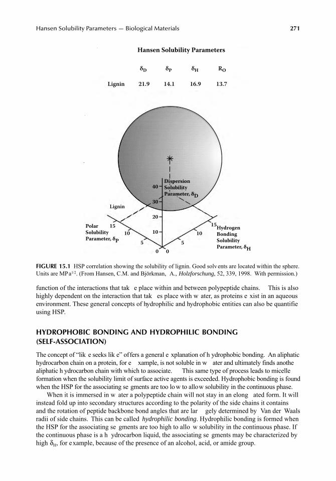
Hansen Solubility Parameters — Biological Materials
271
function of the interactions that tak e place within and between polypeptide chains. This is alsohighly dependent on the interaction that tak es place with w ater, as proteins e xist in an aqueousenvironment. These general concepts of hydrophilic and hydrophobic entities can also be quantifieusing HSP.
HYDROPHOBIC BONDING AND HYDROPHILIC BONDING (SELF-ASSOCIATION)
The concept of “lik e seeks lik e” offers a general e xplanation of h ydrophobic bonding. An aliphatichydrocarbon chain on a protein, for e xample, is not soluble in w ater and ultimately finds anothealiphatic h ydrocarbon chain with which to associate. This same type of process leads to micelleformation when the solubility limit of surface active agents is exceeded. Hydrophobic bonding is foundwhen the HSP for the associating se gments are too lo w to allow solubility in the continuous phase.
When it is immersed in w ater a polypeptide chain will not stay in an elong ated form. It willinstead fold up into secondary structures according to the polarity of the side chains it containsand the rotation of peptide backbone bond angles that are lar gely determined by Van der Waalsradii of side chains. This can be called
hydrophilic bonding
. Hydrophilic bonding is formed whenthe HSP for the associating se gments are too high to allo w solubility in the continuous phase. Ifthe continuous phase is a h ydrocarbon liquid, the associating se gments may be characterized byhigh
δ
H
, for example, because of the presence of an alcohol, acid, or amide group.
FIGURE 15.1
HSP correlation showing the solubility of lignin. Good solv ents are located within the sphere.Units are MPa
1/2
. (From Hansen, C.M. and Björkman, A.,
Holzforschung
, 52, 339, 1998. With permission.)
HydrogenBondingSolubilityParameter, δH
PolarSolubilityParameter, δP
DispersionSolubilityParameter, δD
15
10
5
0
40
30
20
1015
10
5
0
Lignin
Hansen Solubility Parameters
Lignin
21.9 14.1 16.9 13.7
δD δP δH RO
7248_C015.fm Page 271 Wednesday, May 9, 2007 9:37 AM
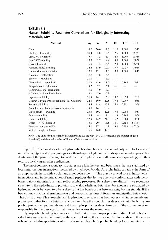
272
Hansen Solubility Parameters: A User’s Handbook
Figure 15.2 demonstrates how hydrophilic bonding between v ersamid polymer blocks reactedinto an alkyd (polyester) polymer gives a thixotropic alkyd paint with its special nondrip properties.Agitation of the paint is enough to break the h ydrophilic bonds allowing easy spreading, b ut theyreform quickly again after application.
The most common secondary structures are alpha helices and beta sheets that are stabilized bylocal inter-residue interactions mediated by h ydrogen bonds. An alpha helix can tak e the form ofan amphipathic helix with a polar and a nonpolar side. This plays a crucial role in helix–helixinteractions and in the interaction of small peptides that ha ve a helical conformation with mem-branes, air–w ater interf aces, and self-assembly processes. Beta sheets are alternati ve secondarystructure to the alpha-helix in proteins. Lik e alpha-helices, beta-sheet backbones are stabilized byhydrogen bonds between two beta sheets, but the bonds occur between neighboring strands. If thebeta
−
strand contains alternating polar and non-polar residues it forms an amphipathic beta sheet.This distrib ution of h ydrophilic and h ydrophobic residues has been observ ed in the membraneprotein porin that forms a beta-barrel structure. Here the nonpolar residues stick into the h ydro-phobic part of the lipid membrane and the h ydrophilic residues form part of the channel interiorresponsible for the passage of small molecules across the membrane.
Hydrophobic bonding is a major ef fect that dri ves proper protein folding. Hydrophobicsidechains are oriented to minimize the ener gy lost by the intrusion of amino acids into the w atersolvent, which disrupts lattices of w ater molecules. Hydrophobic bonding forms an interior ,
TABLE 15.1Hansen Solubility Parameter Correlations for Biologically Interesting Materials, MPa
1/2
Material
δδδδ
D
δδδδ
P
δδδδ
H
Ro FIT G/T
DNA 19.0 20.0 11.0 11.0 1.000 6/12Cholesterol solubility 20.4 2.8 9.4 12.6 1.000 25/41Lard 37°C solubility 15.9 1.2 5.4 12.0 1.000 29/50Lard 23°C solubility 17.7 2.7 4.4 8.0 1.000 21/50Olive oil solubility 15.9 1.2 5.4 12.0 1.000 29/50Psoriasis scales swelling 24.6 11.9 12.9 19.0 0.927 35/50Human skin — permeation 17.6 12.5 11.0 5.0 1.000 4/13Nicotine — calculation 18.8 7.8 6.4 — — —Skatole — calculation 20.0 7.1 6.2 — — —Chlorophyll — solubility 20.2 15.6 18.2 11.1 0.864 7/35Sinapyl alcohol calculation 19.2 7.3 16.1 — — —Coniferyl alcohol calculation 19.0 7.0 16.3 — — —
p
-Coumaryl alcohol calculation 19.1 7.0 17.3 — — —Lignin — solubility 21.9 14.1 16.9 13.7 0.990 16/82Dextran C (= amorphous cellulose) See Chapter 5 24.3 19.9 22.5 17.4 0.999 5/50Sucrose solubility 23.4 18.4 20.8 16.0 0.981 6/50
N
-methyl-morpholine-N-oxide calculation 19.0 16.1 10.2Blood serum — swelling 25.5 10.3 22.1 17.8 0.980 4/51Zein — solubility 22.4 9.8 19.4 11.9 0.964 4/50Urea — solubility 22.9 14.9 21.3 16.2 0.984 14/50Water — >1% soluble in 15.1 20.4 16.5 18.1 0.856 88/167Water — totally miscible 18.1 17.1 16.9 13.0 0.880 47/166Water — single molecule 15.5 16.0 42.3 — — —
Note
: The units for the solubility parameters and Ro are MP a
1/2
. G/T represents the number of goodliquids (G) and the total number of liquids (T) in the correlation.
7248_C015.fm Page 272 Wednesday, May 9, 2007 9:37 AM
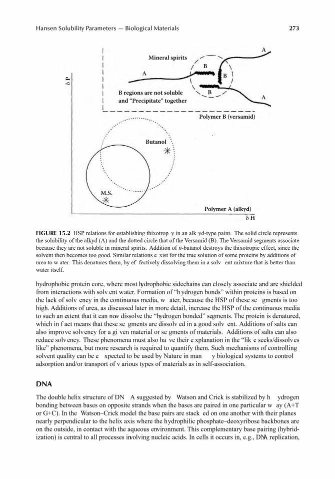
Hansen Solubility Parameters — Biological Materials
273
hydrophobic protein core, where most hydrophobic sidechains can closely associate and are shieldedfrom interactions with solv ent water. Formation of “h ydrogen bonds” within proteins is based onthe lack of solv ency in the continuous media, w ater, because the HSP of these se gments is toohigh. Additions of urea, as discussed later in more detail, increase the HSP of the continuous mediato such an extent that it can now dissolve the “hydrogen bonded” segments. The protein is denatured,which in f act means that these se gments are dissolv ed in a good solv ent. Additions of salts canalso improve solvency for a gi ven material or se gments of materials. Additions of salts can alsoreduce solvency. These phenomena must also ha ve their e xplanation in the “lik e seeks/dissolveslike” phenomena, but more research is required to quantify them. Such mechanisms of controllingsolvent quality can be e xpected to be used by Nature in man y biological systems to controladsorption and/or transport of v arious types of materials as in self-association.
DNA
The double helix structure of DN A suggested by Watson and Crick is stabilized by h ydrogenbonding between bases on opposite strands when the bases are paired in one particular w ay (A+Tor G+C). In the Watson–Crick model the base pairs are stack ed on one another with their planesnearly perpendicular to the helix axis where the hydrophilic phosphate–deoxyribose backbones areon the outside, in contact with the aqueous environment. This complementary base pairing (hybrid-ization) is central to all processes involving nucleic acids. In cells it occurs in, e.g., DNA replication,
FIGURE 15.2
HSP relations for establishing thixotrop y in an alk yd-type paint. The solid circle representsthe solubility of the alkyd (A) and the dotted circle that of the Versamid (B). The Versamid segments associatebecause they are not soluble in mineral spirits. Addition of
n
-butanol destroys the thixotropic effect, since thesolvent then becomes too good. Similar relations e xist for the true solution of some proteins by additions ofurea to w ater. This denatures them, by ef fectively dissolving them in a solv ent mixture that is better thanwater itself.
Polymer A (alkyd)
δ H
δ P
M.S.
Butanol
Polymer B (versamid)
Mineral spirits
A
A
A
B
B
B
B regions are not soluble
and “Precipitate” together
7248_C015.fm Page 273 Wednesday, May 9, 2007 9:37 AM
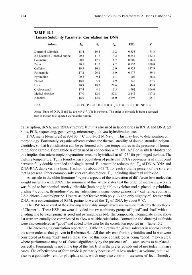
274
Hansen Solubility Parameters: A User’s Handbook
transcription, rRNA, and tRNA structure, but it is also used in laboratories in RN A and DNA gelblots, PCR, sequencing, genotyping, microarrays,
in situ
hybridization, etc. DNA melts (denatures) at 90-100
°
C in 0.1-0.2 M Na+. This may lead to deterioration ofmorphology. Fortunately, organic solvents reduce the thermal stability of double-stranded polynu-cleotides, so that h ybridization can be performed at lo wer temperatures in the presence of forma-mide, for e xample. Formamide is often used in connection with DN A.
8
For in situ h ybridizationthis implies that microscopic preparations must be hybridized at 65–75° for prolonged periods. Themelting temperature, T
m
, is found when a population of particular DNA sequences is at a midpointbetween fully double-stranded and single-strand. F ormamide reduces the T
m
of DN A-DNA andDNA-RNA duplexes in a linear f ashion by about 0.65
°
C for each v olume percent of the solv entthat is present. Other common solv ents can also reduce T
m
, including dimethyl sulfoxide. An article in the older literature
9
reports aspects of the interaction of dif ferent low molecularweight materials with DNA. The summary of this article states that the order of increasing acti vitywas found to be: adonitol, meth yl riboside (both negligible) < cyclohexanol < phenol, pyrimidine,uridine < cytidine, thymidine < purine, adenosine, inosine, deoxyguanosine < caf feine, coumarin,2,6-dichloro-7-methylpurine. Urea w as inef fective with poly A and only slightly ef fective withDNA. At a concentration of 0.3M, purine lo wered the T
m
of DNA by about 9
°
C. The HSP for se veral of these ha ving reasonably simple structures were estimated by the methods
of Chapter 1. These HSP data were di vided into tw o arbitrary groups of “good” and “bad” with adividing line between purine as good and pyrimidine as bad. The compounds intermediate in the abovelist were structurally too complicated to allow a reliable calculation. Formamide and dimethyl sulfoxidewere also considered as “good” and added to the data for the correlation reported in Table 15.2.
The encouraging correlation reported in Table 15.2 ranks the gi ven solvents in approximatelythe same order as that gi ven in Reference 9. All the solv ents from p yrimidine and lo wer wereconsidered as being “bad” and all those abo ve this were considered as being “good. ” Even urea,where performance may be af fected significantly by the presence of ater, seems to be placedcorrectly. Formamide is not at the top of the list, b ut is the preferred solv ent of use today in man ycases. The effectiveness of formamide is primarily because of its low molecular volume, but it willalso be a good solv ent for phosphate salts, which may also contrib ute some ef fect. Dimeth yl
TABLE 15.2Hansen Solubility Parameter Correlation for DNA
Solvent
δδδδ
D
δδδδ
P
δδδδ
H
RED V
Dimethyl sulfoxide 18.4 16.4 10.2 0.353 71.32,6-Dichloro-7-methyl purine 20.5 11.7 14.2 0.651 162.4Coumarin 20.0 12.5 6.7 0.807 156.3Purine 20.5 11.7 14.2 0.853 100.0Caffeine 19.5 10.1 13.0 0.923 157.9Formamide 17.2 26.2 19.0 0.977 39.8Pyrimidine 20.5 9.4 11.3 1.002 78.8Phenol 18.0 5.9 14.9 1.342 87.5Urea 20.9 18.7 26.4 1.447 45.8Cyclohexanol 17.4 4.1 13.5 1.492 106.0Methyl riboside 17.0 12.0 32.8 2.142 117.2Adonitol 18.0 12.0 36.0 2.393 95.1
DNA D = 19.0 P = 20.0 H = 11.0 R
o
= 11.0 FIT = 1.000 NO = 12
Note
: Units of D, P, H and Ro are MP a
1/2
. V is in cc/mole. The order in the table is from e xpectedbest at the top to e xpected worst at the bottom.
7248_C015.fm Page 274 Wednesday, May 9, 2007 9:37 AM
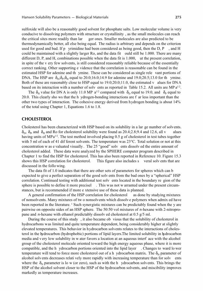
Hansen Solubility Parameters — Biological Materials
275
sulfoxide will also be a reasonably good solvent for phosphate salts. Low molecular volume is veryconducive to dissolving polymers with structure or crystallinity , as the small molecules can reachthe critical sites more readily than lar ger ones. Smaller molecules are also predicted to bethermodynamically better, all else being equal. The radius is arbitrary and depends on the criterionused for good and bad. If p yrimidine had been considered as being good, then the D, P , and Hcould be maintained with a slightly larger Ro, and the data fit ould still be 1.000. There are manydifferent D, P, and H, combinations possible when the data fit is 1.000, ut the present correlation,in spite of the v ery few solvents, is still considered reasonably reliable because of the essentiallycorrect ranking. Other supporting e vidence that the correlation is reasonable can be found in theestimated HSP for adenine and th ymine. These can be considered as single rele vant portions ofDNA. The HSP are
δ
D
;
δ
P
;
δ
H
equal to 20.0;16.0;14.9 for adenine and 19.0;20.5;13.0 for th ymine.Both of these are reasonably close to HSP equal to 19.0;20.0;11.0, the estimated v alues for DNAbased on its interaction with a number of solv ents as reported in Table 15.2. All units are MP a
1/2
.The
δ
H
value for DN A is only 11.0 MP a
1/2
compared with
δ
D
equal to 19.0, and
δ
P
equal to20.0. This clearly sho ws that the h ydrogen-bonding interactions are f ar less important than theother two types of interaction. The cohesive energy derived from hydrogen bonding is about 14%of the total using Chapter 1, Equations 1.6 to 1.8.
CHOLESTEROL
Cholesterol has been characterized with HSP based on its solubility in a lar ge number of solvents.
δ
D
,
δ
P
, and
δ
H
and Ro for cholesterol solubility were found as 20.4;2.8;9.4 and 12.6, all v alueshaving units of MPa
1/2
. The test method involved placing 0.5 g of cholesterol in test tubes togetherwith 5 ml of each of 41 dif ferent solvents. The temperature was 23°C. Total solution or not at thisconcentration w as e valuated visually . The 25 “good” solv ents dissolv ed the entire amount ofcholesterol added. These data were analyzed by the SPHERE computer program described inChapter 1 to find the HSP for cholesterol. This has also been reported in Reference 10. Figure 15.3shows this HSP correlation for cholesterol. This figure also includes s veral solv ents that arediscussed in the follo wing.
The data fit of 1.0 indicates that there are other sets of parameters for spheres which can bexpected to give a perfect separation of the good solv ents from the bad ones by a “spherical” HSPcorrelation. Continued testing with additional test solv ents located in the boundary re gion of thesphere is possible to define it more precisel . This was not w arranted under the present circum-stances, but is recommended if more e xtensive use of these data is planned.
A general confirmation of the HSP correlation for cholesterol as done by studying mixturesof nonsolvents. Many mixtures of tw o nonsolvents which dissolv e polymers when admix ed havebeen reported in the literature.
1
Such synergistic mixtures can be predictably found when the y arepairwise on opposite sides of an HSP sphere. The 50:50 vol mixtures of
n
-hexane with 2-nitropro-pane and
n
-hexane with ethanol predictably dissolv ed cholesterol at 0.5 g/5 ml.During the course of this study , it also became ob vious that the solubility of cholesterol in
hydrocarbons was limited and quite temperature dependent, being considerably higher at slightlyelevated temperatures. This behavior in hydrocarbon solvents relates to the interactions of choles-terol in the hydrocarbon (hydrophobic) portions of lipid layers. The limited solubility in hydrocarbonmedia and v ery low solubility in w ater favors a location at an aqueous interf ace with the alcoholgroup of the cholesterol molecule oriented toward the high energy aqueous phase, where it is morecompatible, and the h ydrocarbon portions oriented into the lipid layer . Changes to ward lo wertemperature will tend to force more cholesterol out of a h ydrocarbon matrix. The
δ
H
parameter ofalcohol solvents decreases relati vely more rapidly with increasing temperature than for solv entswhere the
δ
H
parameter is lo w (or zero), such as with the h ydrocarbon solvents. This brings theHSP of the alcohol solvent closer to the HSP of the hydrocarbon solvents, and miscibility improvesmarkedly as temperature increases.
7248_C015.fm Page 275 Wednesday, May 9, 2007 9:37 AM
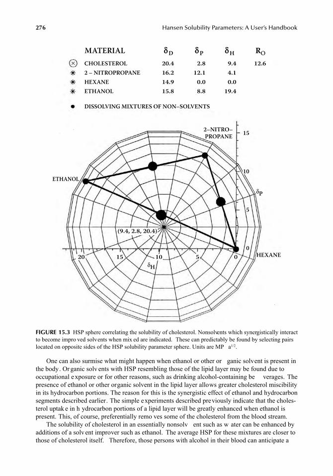
276
Hansen Solubility Parameters: A User’s Handbook
One can also surmise what might happen when ethanol or other or ganic solvent is present inthe body. Or ganic solv ents with HSP resembling those of the lipid layer may be found due tooccupational e xposure or for other reasons, such as drinking alcohol-containing be verages. Thepresence of ethanol or other organic solvent in the lipid layer allows greater cholesterol miscibilityin its hydrocarbon portions. The reason for this is the synergistic effect of ethanol and hydrocarbonsegments described earlier. The simple experiments described previously indicate that the choles-terol uptak e in h ydrocarbon portions of a lipid layer will be greatly enhanced when ethanol ispresent. This, of course, preferentially remo ves some of the cholesterol from the blood stream.
The solubility of cholesterol in an essentially nonsolv ent such as w ater can be enhanced byadditions of a solvent improver such as ethanol. The average HSP for these mixtures are closer tothose of cholesterol itself. Therefore, those persons with alcohol in their blood can anticipate a
FIGURE 15.3
HSP sphere correlating the solubility of cholesterol. Nonsolvents which synergistically interactto become impro ved solvents when mix ed are indicated. These can predictably be found by selecting pairslocated on opposite sides of the HSP solubility parameter sphere. Units are MP a
1/2
.
CHOLESTEROL
2 – NITROPROPANE
HEXANE
ETHANOL
DISSOLVING MIXTURES OF NON–SOLVENTS
20.4
16.2
14.9
15.8
2.8
12.1
0.0
8.8
9.4
4.1
0.0
19.4
MATERIAL δδ D δ P δ H RO
12.6
2–NITRO– PROPANE
15
10
5
0HEXANE
ETHANOL
δP
δH05101520
(9.4, 2.8, 20.4)
7248_C015.fm Page 276 Wednesday, May 9, 2007 9:37 AM
Hansen Solubility Parameters — Biological Materials
277
slightly higher solubility of cholesterol in their blood because the continuous phase has solubilityparameters closer to those of cholesterol. This effect and that discussed earlier should help to reducecholesterol levels in the blood and blood v essels of those who ingest small to moderate amountsof alcohol on a re gular basis.
LARD
Experimental data and HSP correlations for the solubility of refined lard at 23°C and 37°C h vebeen reported.
2
The criterion for a good solv ent is that it totally dissolv es the sample at the gi ventemperature. The concentrations chosen were 10%. The results of the correlations are gi ven inTable 15.1. The refined lard is a semisolid with a melting point of 42°C
The composition of refined lard is ery similar to that of human depot f at, so the conclusionsdrawn for the solubility of lard will also be generally v alid for depot f at. Olive oil is a con venientmaterial to use at room temperature to study the beha vior of depot f at (lard), as the same solv entsthat dissolve it at room temperature also dissolv e lard at 37°C. This is reported in Table 15.1.
The best room temperature solv ents for lard include trichloroeth ylene, styrene, toluene, andmethyl methacrylate. Octyl alcohol does not ha ve a strong af finity for lard at room temperaturwith a RED number (see Chapters 1 and 2) of 0.96. The good solvents reflect the crystalline naturof the lard, as toluene, for e xample, is an e xcellent swelling solvent for partly crystalline polyeth-ylene. Esters are among the best solv ents for lard at 37°C, reflecting the presence of the estegroups in the lard, which is v ery nearly a liquid at this temperature.
HUMAN SKIN
A first attempt to characterize human skin with HSP as made by visually evaluating the swellingof psoriasis scales immersed for a prolonged time in dif ferent solvents.
2
Uptake could clearly beseen by dimensional changes and a mark ed enhancement of clarity . It w as anticipated that thesolubility parameter correlation for the psoriasis scales (k eratin) w ould to some e xtent reflecpermeation in human skin b ut that other f actors, such as the presence of w ater and lipids, forexample, would also be important. The data fit for this correlation (0.927) indicates that a reasonablreliable correlation for swelling of the psoriasis scales (k eratin) has been found. Ho wever, the
δ
D
parameter is thought to be too high.Permeation data generated in an e xtensive study allowed placement of the tested solv ents into
groups according to actual permeation rates through viable human skin.
4
Figure 15.4 graphicallyshows the HSP correlation that resulted. There are too fe w data to establish a reliable correlation,but a sphere with center at
δ
D
,
δ
P
, and
δ
H
of 17.6, 12.5, and 11.0, which has a radius of 5.0,encompasses the parameters for the four solvents with the highest permeation rates while excludingthe others. The units for these parameters are MP a
1/2
. n-octyl acetate has a near zero permeationrate. This correlation cannot be considered precise because of insuf ficient data, and there are, ifact, numerous spheres with some what similar b ut different combinations of the parameters thatalso can accomplish this. Ne vertheless, there is a good guideline for future w ork, whether it be anexpanded correlation or formulation of products designed for a prescribed compatibility with humanskin. Calculations for skatole and nicotine predict that moderate rates of skin permeation can alsobe expected for these.
It might be noted that the four solv ents with high permeation rates also ha ve very high affinitfor psoriasis scales according to the correlation pre viously noted. Lik ewise, the c yclic solv entspropylene carbonate, gamma-butyrolactone, and sulfolane have, or are predicted to have, high affinitfor psoriasis scales, b ut the y are placed in the lo w permeation rate group for actual permeationthrough viable human skin. These all have high
δ
P
and low
δ
H
. n-butyl acetate and toluene are alsoin this group. This reflects the compl xity of actual skin permeation and the importance of usingviable skin for testing. The cyclic nature of the solv ents, however, is also e xpected to slow the rate
7248_C015.fm Page 277 Wednesday, May 9, 2007 9:37 AM
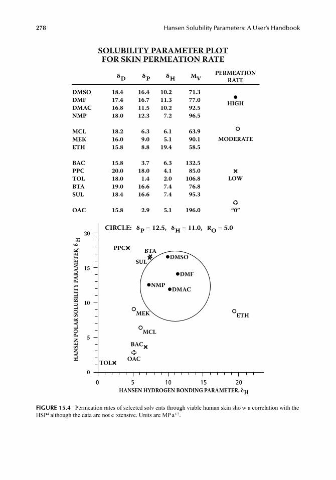
278
Hansen Solubility Parameters: A User’s Handbook
FIGURE 15.4
Permeation rates of selected solv ents through viable human skin sho w a correlation with theHSP
4
although the data are not e xtensive. Units are MP a
1/2
.
HANSEN HYDROGEN BONDING PARAMETER, δ H
HA
NS
EN
PO
LA
R S
OL
UB
ILIT
Y P
AR
AM
ET
ER
, δ H
20151050
20
15
10
5
0
DMSO
DMF
DMAC
NMP
MCL
MEK
ETH
BAC
PPC
TOL
BTA
SUL
OAC
18.4
17.4
16.8
18.0
18.2
16.0
15.8
15.8
20.0
18.0
19.0
18.4
15.8
16.4
16.7
11.5
12.3
6.3
9.0
8.8
3.7
18.0
1.4
16.6
16.6
2.9
10.2
11.3
10.2
7.2
6.1
5.1
19.4
6.3
4.1
2.0
7.4
7.4
5.1
71.3
77.0
92.5
96.5
63.9
90.1
58.5
132.5
85.0
106.8
76.8
95.3
196.0
δHδPδD MV
SOLUBILITY PARAMETER PLOTFOR SKIN PERMEATION RATE
PERMEATION
RATE
lHIGH
lNMPlDMAC
lDMF
lDMSO
l
MODERATE
lMCL
lMEK l
ETH
�LOW
BAC�
PPC�
TOL�
BTA�
SUL�
Ó0”
ÃOAC
CIRCLE: δP = 12.5, δH = 11.0, RO = 5.0
7248_C015.fm Page 278 Wednesday, May 9, 2007 9:37 AM
Hansen Solubility Parameters — Biological Materials
279
of permeation relati ve to linear solv ents of comparable af finit . Factors affecting permeation ha vebeen discussed at length in Chapter 13. Of course, the presence of water and/or other skin componentscan also have an effect on the permeation rate. Finally , the swelling of the psoriasis scales in volvedequilibrium swelling of the individual systems, whereas the permeation rate studies did not have thisuniformity. Concentration gradients are required for permeation to occur .
PROTEINS — BLOOD SERUM AND ZEIN
HSP correlations for the swelling of blood serum and for the solubility of zein, a protein deri vedfrom corn, are included in Table 15.1. The data used in these correlations are found in Reference3. Solvents with the lo west RED numbers in the correlation for the solubility of zein are listed inTable 15.3. The HSP parameters for blood serum and zein are not too dif ferent. The blood serumdata are based on visual observ ation of swelling, while the zein data are for visual observ ation oftrue solution. It is note worthy that there are only four good solv ents in the data set reported inTable 15.3, and that the HSP parameters for the proteins are much higher than for any liquid whichcan be used in such testing. These HSP parameters are found by a form of e xtrapolation, whereall of the good solv ents are located in the boundary re gion of the respecti ve spheres. The valuesare very much dependent on the mathematical model which includes the coefficient “4” (see Chapte1 and Chapter 2). The saturated solution of urea and w ater is also a (predictably) good solv ent inthat it swells blood serum and dissolv es zein, b ut it w as not included as a data point in thecorrelations as such. Mixtures of solv ents, water, and mixtures of solv ents with w ater have beenavoided as test solvents to the extent possible because of too many interactions, which are apparentlynot always predictable by these simple considerations. The general prediction that additions of ureato water will improve solvency of proteins is discussed belo w.
CHLOROPHYLL AND LIGNIN
5
The results of HSP correlations of solubility for lignin and chloroph yll are gi ven in Table 15.1.More specific information on the lignin correlation is found in Table 15.4A and Table 15.4B. Itcan be seen that these indeed ha ve high affinity/p ysical resemblance to each other , with the HSPvalues not being too different. A major difference is that chlorophyll is soluble in ethanol, whereaslignin is not. This indicates a higher h ydrophilicity, of course, and gi ves a higher
δ
H
parameter tochlorophyll compared with lignin.
It can be presumed that the HSP for these materials are the result of natural selection by naturefor optimum compatibility relations with immediate surroundings and function. A discussion ofthis is beyond the scope of this work, but this point has been studied in more detail for the relationsamong w ood chemicals and w ood polymers as outlined in the ne xt section. Here, the HSP forlignin have a demonstrated clear importance with re gard to compatibility relations.
WOOD CHEMICALS AND POLYMERS
The results of HSP calculations and correlations for se veral w ood chemicals and polymers aregiven in Table 15.1. These results are part of a study considering the ultrastructure of w ood froma solubility parameter point of vie w.
6
The study is based on the principle of “lik e seeks like” andleads to a proposed configuration of the ultrastructure. The HSP for amorphous cellulose arepresumed to be similar to those of De xtran (Dextran C, British Drug Houses). The crystallinity incellulose will require that good solv ents have higher af finity/HSP than most of those dissolvinDextran, however. N-methyl-morpholine-N-oxide is an e xample. The HSP for De xtran are higherthan those of sucrose (which v alues are similar to the other sug ars as well). It is common forpolymers to ha ve higher HSP than the monomers from which the y are made. It is also common
7248_C015.fm Page 279 Wednesday, May 9, 2007 9:37 AM
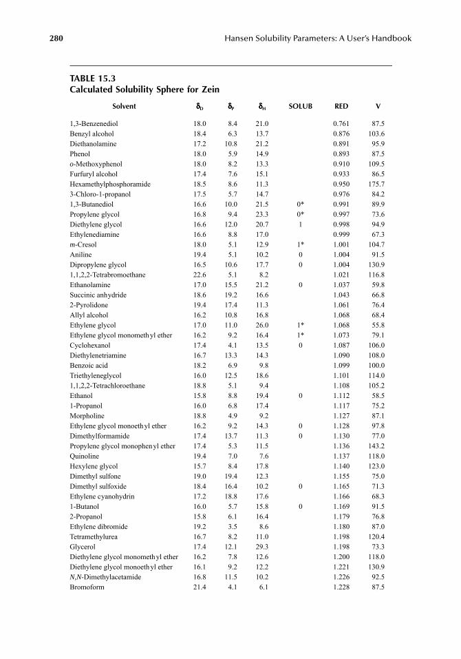
280
Hansen Solubility Parameters: A User’s Handbook
TABLE 15.3Calculated Solubility Sphere for Zein
Solvent
δδδδ
D
δδδδ
P
δδδδ
H
SOLUB RED V
1,3-Benzenediol 18.0 8.4 21.0 0.761 87.5Benzyl alcohol 18.4 6.3 13.7 0.876 103.6Diethanolamine 17.2 10.8 21.2 0.891 95.9Phenol 18.0 5.9 14.9 0.893 87.5
o
-Methoxyphenol 18.0 8.2 13.3 0.910 109.5Furfuryl alcohol 17.4 7.6 15.1 0.933 86.5Hexamethylphosphoramide 18.5 8.6 11.3 0.950 175.73-Chloro-1-propanol 17.5 5.7 14.7 0.976 84.21,3-Butanediol 16.6 10.0 21.5 0* 0.991 89.9Propylene glycol 16.8 9.4 23.3 0* 0.997 73.6Diethylene glycol 16.6 12.0 20.7 1 0.998 94.9Ethylenediamine 16.6 8.8 17.0 0.999 67.3
m
-Cresol 18.0 5.1 12.9 1* 1.001 104.7Aniline 19.4 5.1 10.2 0 1.004 91.5Dipropylene glycol 16.5 10.6 17.7 0 1.004 130.91,1,2,2-Tetrabromoethane 22.6 5.1 8.2 1.021 116.8Ethanolamine 17.0 15.5 21.2 0 1.037 59.8Succinic anhydride 18.6 19.2 16.6 1.043 66.82-Pyrolidone 19.4 17.4 11.3 1.061 76.4Allyl alcohol 16.2 10.8 16.8 1.068 68.4Ethylene glycol 17.0 11.0 26.0 1* 1.068 55.8Ethylene glycol monomethyl ether 16.2 9.2 16.4 1* 1.073 79.1Cyclohexanol 17.4 4.1 13.5 0 1.087 106.0Diethylenetriamine 16.7 13.3 14.3 1.090 108.0Benzoic acid 18.2 6.9 9.8 1.099 100.0Triethyleneglycol 16.0 12.5 18.6 1.101 114.01,1,2,2-Tetrachloroethane 18.8 5.1 9.4 1.108 105.2Ethanol 15.8 8.8 19.4 0 1.112 58.51-Propanol 16.0 6.8 17.4 1.117 75.2Morpholine 18.8 4.9 9.2 1.127 87.1Ethylene glycol monoethyl ether 16.2 9.2 14.3 0 1.128 97.8Dimethylformamide 17.4 13.7 11.3 0 1.130 77.0Propylene glycol monophenyl ether 17.4 5.3 11.5 1.136 143.2Quinoline 19.4 7.0 7.6 1.137 118.0Hexylene glycol 15.7 8.4 17.8 1.140 123.0Dimethyl sulfone 19.0 19.4 12.3 1.155 75.0Dimethyl sulfoxide 18.4 16.4 10.2 0 1.165 71.3Ethylene cyanohydrin 17.2 18.8 17.6 1.166 68.31-Butanol 16.0 5.7 15.8 0 1.169 91.52-Propanol 15.8 6.1 16.4 1.179 76.8Ethylene dibromide 19.2 3.5 8.6 1.180 87.0Tetramethylurea 16.7 8.2 11.0 1.198 120.4Glycerol 17.4 12.1 29.3 1.198 73.3Diethylene glycol monomethyl ether 16.2 7.8 12.6 1.200 118.0Diethylene glycol monoethyl ether 16.1 9.2 12.2 1.221 130.9
N,N
-Dimethylacetamide 16.8 11.5 10.2 1.226 92.5Bromoform 21.4 4.1 6.1 1.228 87.5
7248_C015.fm Page 280 Wednesday, May 9, 2007 9:37 AM
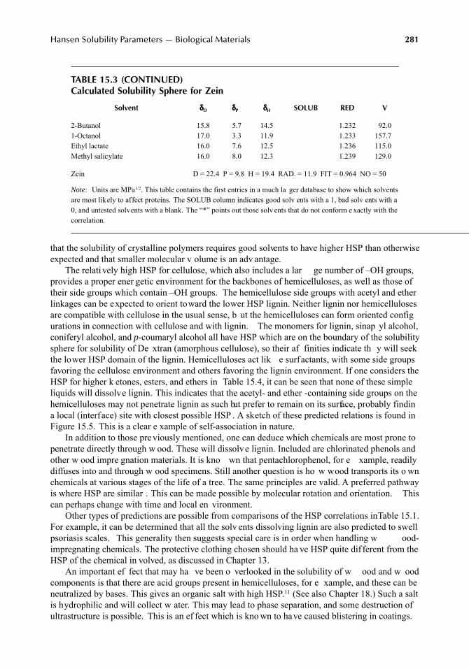
Hansen Solubility Parameters — Biological Materials
281
that the solubility of crystalline polymers requires good solvents to have higher HSP than otherwiseexpected and that smaller molecular v olume is an adv antage.
The relatively high HSP for cellulose, which also includes a lar ge number of –OH groups,provides a proper ener getic environment for the backbones of hemicelluloses, as well as those oftheir side groups which contain –OH groups. The hemicellulose side groups with acetyl and etherlinkages can be expected to orient toward the lower HSP lignin. Neither lignin nor hemicellulosesare compatible with cellulose in the usual sense, b ut the hemicelluloses can form oriented configurations in connection with cellulose and with lignin. The monomers for lignin, sinap yl alcohol,coniferyl alcohol, and
p
-coumaryl alcohol all have HSP which are on the boundary of the solubilitysphere for solubility of De xtran (amorphous cellulose), so their af finities indicate th y will seekthe lower HSP domain of the lignin. Hemicelluloses act lik e surfactants, with some side groupsfavoring the cellulose environment and others favoring the lignin environment. If one considers theHSP for higher k etones, esters, and ethers in Table 15.4, it can be seen that none of these simpleliquids will dissolve lignin. This indicates that the acetyl- and ether -containing side groups on thehemicelluloses may not penetrate lignin as such but prefer to remain on its surface, probably findina local (interface) site with closest possible HSP . A sketch of these predicted relations is found inFigure 15.5. This is a clear e xample of self-association in nature.
In addition to those previously mentioned, one can deduce which chemicals are most prone topenetrate directly through w ood. These will dissolve lignin. Included are chlorinated phenols andother w ood impre gnation materials. It is kno wn that pentachlorophenol, for e xample, readilydiffuses into and through w ood specimens. Still another question is ho w wood transports its o wnchemicals at various stages of the life of a tree. The same principles are valid. A preferred pathwayis where HSP are similar . This can be made possible by molecular rotation and orientation. Thiscan perhaps change with time and local en vironment.
Other types of predictions are possible from comparisons of the HSP correlations in Table 15.1.For example, it can be determined that all the solv ents dissolving lignin are also predicted to swellpsoriasis scales. This generality then suggests special care is in order when handling w ood-impregnating chemicals. The protective clothing chosen should ha ve HSP quite dif ferent from theHSP of the chemical in volved, as discussed in Chapter 13.
An important ef fect that may ha ve been o verlooked in the solubility of w ood and w oodcomponents is that there are acid groups present in hemicelluloses, for e xample, and these can beneutralized by bases. This gives an organic salt with high HSP.
11
(See also Chapter 18.) Such a saltis hydrophilic and will collect w ater. This may lead to phase separation, and some destruction ofultrastructure is possible. This is an ef fect which is kno wn to have caused blistering in coatings.
TABLE 15.3 (CONTINUED)Calculated Solubility Sphere for Zein
Solvent
δδδδ
D
δδδδ
P
δδδδ
H
SOLUB RED V
2-Butanol 15.8 5.7 14.5 1.232 92.01-Octanol 17.0 3.3 11.9 1.233 157.7Ethyl lactate 16.0 7.6 12.5 1.236 115.0Methyl salicylate 16.0 8.0 12.3 1.239 129.0
Zein D = 22.4 P = 9.8 H = 19.4 RAD. = 11.9 FIT = 0.964 NO = 50
Note
: Units are MPa1/2. This table contains the first entries in a much la ger database to show which solventsare most likely to affect proteins. The SOLUB column indicates good solv ents with a 1, bad solv ents with a0, and untested solvents with a blank. The “*” points out those solv ents that do not conform e xactly with thecorrelation.
7248_C015.fm Page 281 Wednesday, May 9, 2007 9:37 AM
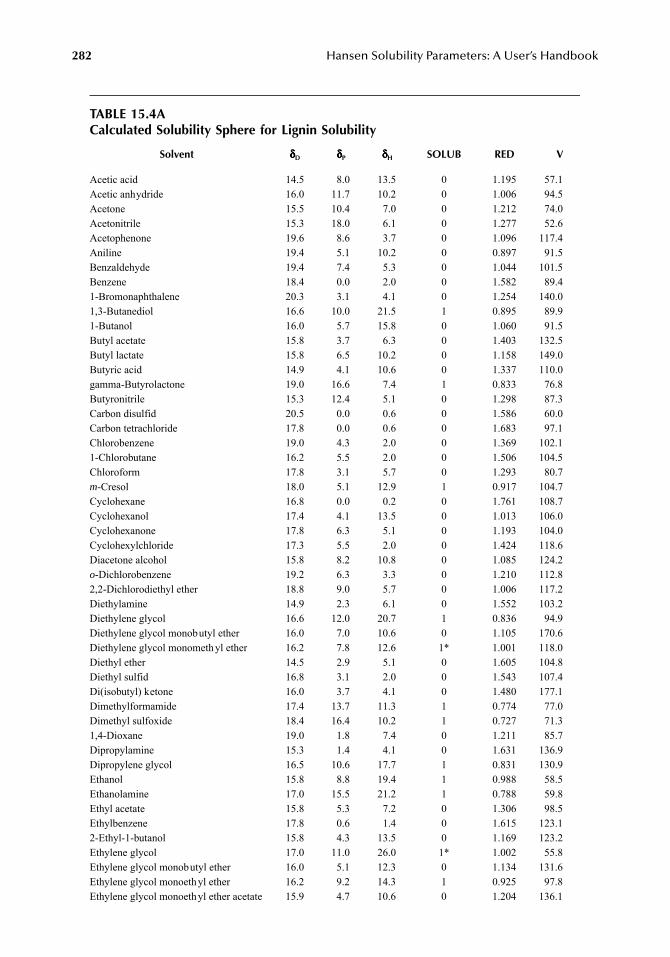
282 Hansen Solubility Parameters: A User’s Handbook
TABLE 15.4ACalculated Solubility Sphere for Lignin Solubility
Solvent δδδδD δδδδP δδδδH SOLUB RED V
Acetic acid 14.5 8.0 13.5 0 1.195 57.1Acetic anhydride 16.0 11.7 10.2 0 1.006 94.5Acetone 15.5 10.4 7.0 0 1.212 74.0Acetonitrile 15.3 18.0 6.1 0 1.277 52.6Acetophenone 19.6 8.6 3.7 0 1.096 117.4Aniline 19.4 5.1 10.2 0 0.897 91.5Benzaldehyde 19.4 7.4 5.3 0 1.044 101.5Benzene 18.4 0.0 2.0 0 1.582 89.41-Bromonaphthalene 20.3 3.1 4.1 0 1.254 140.01,3-Butanediol 16.6 10.0 21.5 1 0.895 89.91-Butanol 16.0 5.7 15.8 0 1.060 91.5Butyl acetate 15.8 3.7 6.3 0 1.403 132.5Butyl lactate 15.8 6.5 10.2 0 1.158 149.0Butyric acid 14.9 4.1 10.6 0 1.337 110.0gamma-Butyrolactone 19.0 16.6 7.4 1 0.833 76.8Butyronitrile 15.3 12.4 5.1 0 1.298 87.3Carbon disulfid 20.5 0.0 0.6 0 1.586 60.0Carbon tetrachloride 17.8 0.0 0.6 0 1.683 97.1Chlorobenzene 19.0 4.3 2.0 0 1.369 102.11-Chlorobutane 16.2 5.5 2.0 0 1.506 104.5Chloroform 17.8 3.1 5.7 0 1.293 80.7m-Cresol 18.0 5.1 12.9 1 0.917 104.7Cyclohexane 16.8 0.0 0.2 0 1.761 108.7Cyclohexanol 17.4 4.1 13.5 0 1.013 106.0Cyclohexanone 17.8 6.3 5.1 0 1.193 104.0Cyclohexylchloride 17.3 5.5 2.0 0 1.424 118.6Diacetone alcohol 15.8 8.2 10.8 0 1.085 124.2o-Dichlorobenzene 19.2 6.3 3.3 0 1.210 112.82,2-Dichlorodiethyl ether 18.8 9.0 5.7 0 1.006 117.2Diethylamine 14.9 2.3 6.1 0 1.552 103.2Diethylene glycol 16.6 12.0 20.7 1 0.836 94.9Diethylene glycol monobutyl ether 16.0 7.0 10.6 0 1.105 170.6Diethylene glycol monomethyl ether 16.2 7.8 12.6 1* 1.001 118.0Diethyl ether 14.5 2.9 5.1 0 1.605 104.8Diethyl sulfid 16.8 3.1 2.0 0 1.543 107.4Di(isobutyl) ketone 16.0 3.7 4.1 0 1.480 177.1Dimethylformamide 17.4 13.7 11.3 1 0.774 77.0Dimethyl sulfoxide 18.4 16.4 10.2 1 0.727 71.31,4-Dioxane 19.0 1.8 7.4 0 1.211 85.7Dipropylamine 15.3 1.4 4.1 0 1.631 136.9Dipropylene glycol 16.5 10.6 17.7 1 0.831 130.9Ethanol 15.8 8.8 19.4 1 0.988 58.5Ethanolamine 17.0 15.5 21.2 1 0.788 59.8Ethyl acetate 15.8 5.3 7.2 0 1.306 98.5Ethylbenzene 17.8 0.6 1.4 0 1.615 123.12-Ethyl-1-butanol 15.8 4.3 13.5 0 1.169 123.2Ethylene glycol 17.0 11.0 26.0 1* 1.002 55.8Ethylene glycol monobutyl ether 16.0 5.1 12.3 0 1.134 131.6Ethylene glycol monoethyl ether 16.2 9.2 14.3 1 0.925 97.8Ethylene glycol monoethyl ether acetate 15.9 4.7 10.6 0 1.204 136.1
7248_C015.fm Page 282 Wednesday, May 9, 2007 9:37 AM
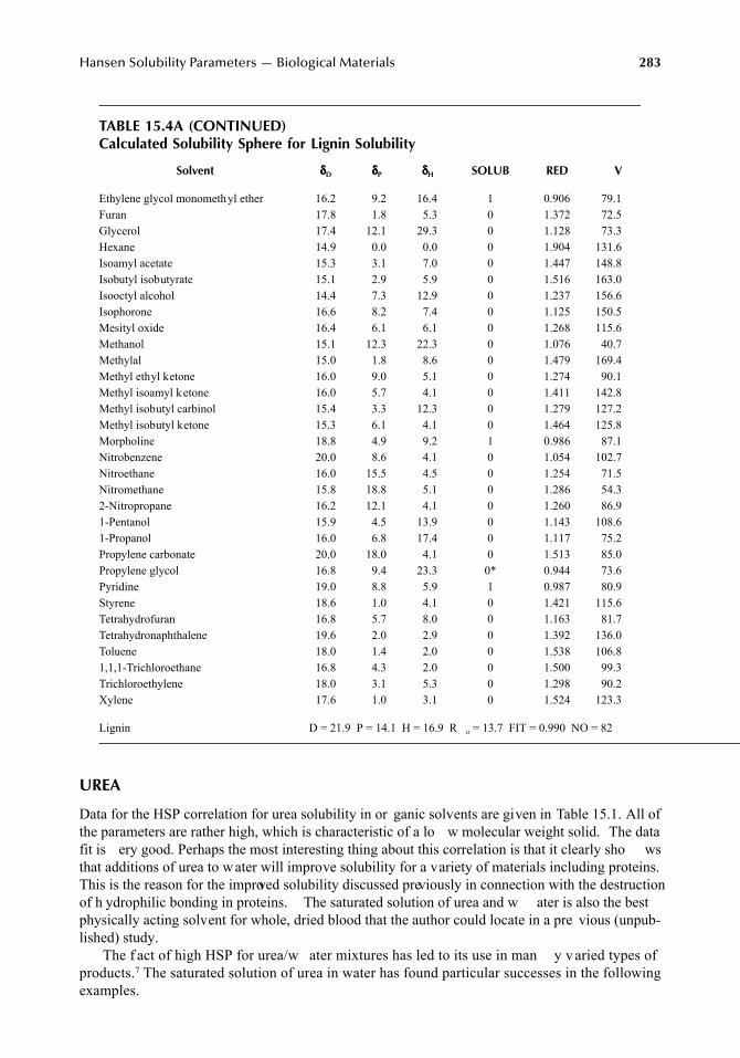
Hansen Solubility Parameters — Biological Materials 283
UREA
Data for the HSP correlation for urea solubility in or ganic solvents are given in Table 15.1. All ofthe parameters are rather high, which is characteristic of a lo w molecular weight solid. The datafit is ery good. Perhaps the most interesting thing about this correlation is that it clearly sho wsthat additions of urea to water will improve solubility for a variety of materials including proteins.This is the reason for the improved solubility discussed previously in connection with the destructionof h ydrophilic bonding in proteins. The saturated solution of urea and w ater is also the bestphysically acting solvent for whole, dried blood that the author could locate in a pre vious (unpub-lished) study.
The f act of high HSP for urea/w ater mixtures has led to its use in man y v aried types ofproducts.7 The saturated solution of urea in water has found particular successes in the followingexamples.
TABLE 15.4A (CONTINUED)Calculated Solubility Sphere for Lignin Solubility
Solvent δδδδD δδδδP δδδδH SOLUB RED V
Ethylene glycol monomethyl ether 16.2 9.2 16.4 1 0.906 79.1Furan 17.8 1.8 5.3 0 1.372 72.5Glycerol 17.4 12.1 29.3 0 1.128 73.3Hexane 14.9 0.0 0.0 0 1.904 131.6Isoamyl acetate 15.3 3.1 7.0 0 1.447 148.8Isobutyl isobutyrate 15.1 2.9 5.9 0 1.516 163.0Isooctyl alcohol 14.4 7.3 12.9 0 1.237 156.6Isophorone 16.6 8.2 7.4 0 1.125 150.5Mesityl oxide 16.4 6.1 6.1 0 1.268 115.6Methanol 15.1 12.3 22.3 0 1.076 40.7Methylal 15.0 1.8 8.6 0 1.479 169.4Methyl ethyl ketone 16.0 9.0 5.1 0 1.274 90.1Methyl isoamyl ketone 16.0 5.7 4.1 0 1.411 142.8Methyl isobutyl carbinol 15.4 3.3 12.3 0 1.279 127.2Methyl isobutyl ketone 15.3 6.1 4.1 0 1.464 125.8Morpholine 18.8 4.9 9.2 1 0.986 87.1Nitrobenzene 20.0 8.6 4.1 0 1.054 102.7Nitroethane 16.0 15.5 4.5 0 1.254 71.5Nitromethane 15.8 18.8 5.1 0 1.286 54.32-Nitropropane 16.2 12.1 4.1 0 1.260 86.91-Pentanol 15.9 4.5 13.9 0 1.143 108.61-Propanol 16.0 6.8 17.4 0 1.117 75.2Propylene carbonate 20.0 18.0 4.1 0 1.513 85.0Propylene glycol 16.8 9.4 23.3 0* 0.944 73.6Pyridine 19.0 8.8 5.9 1 0.987 80.9Styrene 18.6 1.0 4.1 0 1.421 115.6Tetrahydrofuran 16.8 5.7 8.0 0 1.163 81.7Tetrahydronaphthalene 19.6 2.0 2.9 0 1.392 136.0Toluene 18.0 1.4 2.0 0 1.538 106.81,1,1-Trichloroethane 16.8 4.3 2.0 0 1.500 99.3Trichloroethylene 18.0 3.1 5.3 0 1.298 90.2Xylene 17.6 1.0 3.1 0 1.524 123.3
Lignin D = 21.9 P = 14.1 H = 16.9 R o = 13.7 FIT = 0.990 NO = 82
7248_C015.fm Page 283 Wednesday, May 9, 2007 9:37 AM
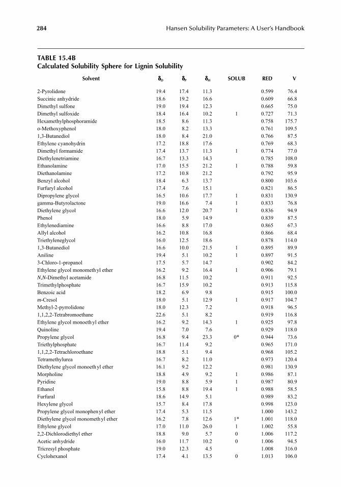
284 Hansen Solubility Parameters: A User’s Handbook
TABLE 15.4BCalculated Solubility Sphere for Lignin Solubility
Solvent δδδδD δδδδP δδδδH SOLUB RED V
2-Pyrolidone 19.4 17.4 11.3 0.599 76.4Succinic anhydride 18.6 19.2 16.6 0.609 66.8Dimethyl sulfone 19.0 19.4 12.3 0.665 75.0Dimethyl sulfoxide 18.4 16.4 10.2 1 0.727 71.3Hexamethylphosphoramide 18.5 8.6 11.3 0.758 175.7o-Methoxyphenol 18.0 8.2 13.3 0.761 109.51,3-Butanediol 18.0 8.4 21.0 0.766 87.5Ethylene cyanohydrin 17.2 18.8 17.6 0.769 68.3Dimethyl formamide 17.4 13.7 11.3 1 0.774 77.0Diethylenetriamine 16.7 13.3 14.3 0.785 108.0Ethanolamine 17.0 15.5 21.2 1 0.788 59.8Diethanolamine 17.2 10.8 21.2 0.792 95.9Benzyl alcohol 18.4 6.3 13.7 0.800 103.6Furfuryl alcohol 17.4 7.6 15.1 0.821 86.5Dipropylene glycol 16.5 10.6 17.7 1 0.831 130.9gamma-Butyrolactone 19.0 16.6 7.4 1 0.833 76.8Diethylene glycol 16.6 12.0 20.7 1 0.836 94.9Phenol 18.0 5.9 14.9 0.839 87.5Ethylenediamine 16.6 8.8 17.0 0.865 67.3Allyl alcohol 16.2 10.8 16.8 0.866 68.4Triethyleneglycol 16.0 12.5 18.6 0.878 114.01,3-Butanediol 16.6 10.0 21.5 1 0.895 89.9Aniline 19.4 5.1 10.2 1 0.897 91.53-Chloro-1-propanol 17.5 5.7 14.7 0.902 84.2Ethylene glycol monomethyl ether 16.2 9.2 16.4 1 0.906 79.1N,N-Dimethyl acetamide 16.8 11.5 10.2 0.911 92.5Trimethylphosphate 16.7 15.9 10.2 0.913 115.8Benzoic acid 18.2 6.9 9.8 0.915 100.0m-Cresol 18.0 5.1 12.9 1 0.917 104.7Methyl-2-pyrrolidone 18.0 12.3 7.2 0.918 96.51,1,2,2-Tetrabromoethane 22.6 5.1 8.2 0.919 116.8Ethylene glycol monoethyl ether 16.2 9.2 14.3 1 0.925 97.8Quinoline 19.4 7.0 7.6 0.929 118.0Propylene glycol 16.8 9.4 23.3 0* 0.944 73.6Triethylphosphate 16.7 11.4 9.2 0.965 171.01,1,2,2-Tetrachloroethane 18.8 5.1 9.4 0.968 105.2Tetramethylurea 16.7 8.2 11.0 0.973 120.4Diethylene glycol monoethyl ether 16.1 9.2 12.2 0.981 130.9Morpholine 18.8 4.9 9.2 1 0.986 87.1Pyridine 19.0 8.8 5.9 1 0.987 80.9Ethanol 15.8 8.8 19.4 1 0.988 58.5Furfural 18.6 14.9 5.1 0.989 83.2Hexylene glycol 15.7 8.4 17.8 0.998 123.0Propylene glycol monophenyl ether 17.4 5.3 11.5 1.000 143.2Diethylene glycol monomethyl ether 16.2 7.8 12.6 1* 1.001 118.0Ethylene glycol 17.0 11.0 26.0 1 1.002 55.82,2-Dichlorodiethyl ether 18.8 9.0 5.7 0 1.006 117.2Acetic anhydride 16.0 11.7 10.2 0 1.006 94.5Tricresyl phosphate 19.0 12.3 4.5 1.008 316.0Cyclohexanol 17.4 4.1 13.5 0 1.013 106.0
7248_C015.fm Page 284 Wednesday, May 9, 2007 9:37 AM
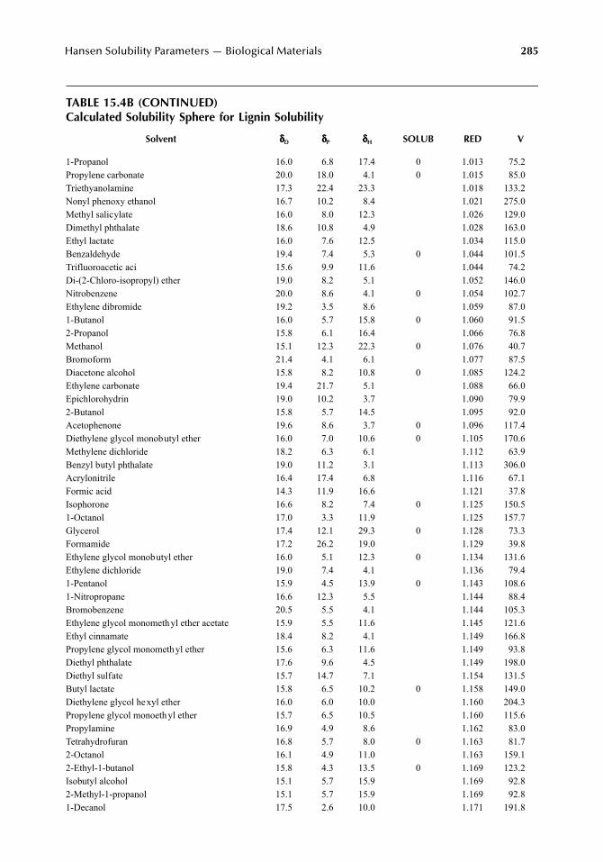
Hansen Solubility Parameters — Biological Materials 285
TABLE 15.4B (CONTINUED)Calculated Solubility Sphere for Lignin Solubility
Solvent δδδδD δδδδP δδδδH SOLUB RED V
1-Propanol 16.0 6.8 17.4 0 1.013 75.2Propylene carbonate 20.0 18.0 4.1 0 1.015 85.0Triethyanolamine 17.3 22.4 23.3 1.018 133.2Nonyl phenoxy ethanol 16.7 10.2 8.4 1.021 275.0Methyl salicylate 16.0 8.0 12.3 1.026 129.0Dimethyl phthalate 18.6 10.8 4.9 1.028 163.0Ethyl lactate 16.0 7.6 12.5 1.034 115.0Benzaldehyde 19.4 7.4 5.3 0 1.044 101.5Trifluoroacetic aci 15.6 9.9 11.6 1.044 74.2Di-(2-Chloro-isopropyl) ether 19.0 8.2 5.1 1.052 146.0Nitrobenzene 20.0 8.6 4.1 0 1.054 102.7Ethylene dibromide 19.2 3.5 8.6 1.059 87.01-Butanol 16.0 5.7 15.8 0 1.060 91.52-Propanol 15.8 6.1 16.4 1.066 76.8Methanol 15.1 12.3 22.3 0 1.076 40.7Bromoform 21.4 4.1 6.1 1.077 87.5Diacetone alcohol 15.8 8.2 10.8 0 1.085 124.2Ethylene carbonate 19.4 21.7 5.1 1.088 66.0Epichlorohydrin 19.0 10.2 3.7 1.090 79.92-Butanol 15.8 5.7 14.5 1.095 92.0Acetophenone 19.6 8.6 3.7 0 1.096 117.4Diethylene glycol monobutyl ether 16.0 7.0 10.6 0 1.105 170.6Methylene dichloride 18.2 6.3 6.1 1.112 63.9Benzyl butyl phthalate 19.0 11.2 3.1 1.113 306.0Acrylonitrile 16.4 17.4 6.8 1.116 67.1Formic acid 14.3 11.9 16.6 1.121 37.8Isophorone 16.6 8.2 7.4 0 1.125 150.51-Octanol 17.0 3.3 11.9 1.125 157.7Glycerol 17.4 12.1 29.3 0 1.128 73.3Formamide 17.2 26.2 19.0 1.129 39.8Ethylene glycol monobutyl ether 16.0 5.1 12.3 0 1.134 131.6Ethylene dichloride 19.0 7.4 4.1 1.136 79.41-Pentanol 15.9 4.5 13.9 0 1.143 108.61-Nitropropane 16.6 12.3 5.5 1.144 88.4Bromobenzene 20.5 5.5 4.1 1.144 105.3Ethylene glycol monomethyl ether acetate 15.9 5.5 11.6 1.145 121.6Ethyl cinnamate 18.4 8.2 4.1 1.149 166.8Propylene glycol monomethyl ether 15.6 6.3 11.6 1.149 93.8Diethyl phthalate 17.6 9.6 4.5 1.149 198.0Diethyl sulfate 15.7 14.7 7.1 1.154 131.5Butyl lactate 15.8 6.5 10.2 0 1.158 149.0Diethylene glycol hexyl ether 16.0 6.0 10.0 1.160 204.3Propylene glycol monoethyl ether 15.7 6.5 10.5 1.160 115.6Propylamine 16.9 4.9 8.6 1.162 83.0Tetrahydrofuran 16.8 5.7 8.0 0 1.163 81.72-Octanol 16.1 4.9 11.0 1.163 159.12-Ethyl-1-butanol 15.8 4.3 13.5 0 1.169 123.2Isobutyl alcohol 15.1 5.7 15.9 1.169 92.82-Methyl-1-propanol 15.1 5.7 15.9 1.169 92.81-Decanol 17.5 2.6 10.0 1.171 191.8
7248_C015.fm Page 285 Wednesday, May 9, 2007 9:37 AM
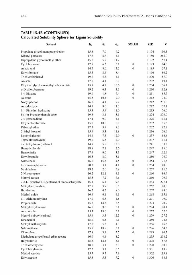
286 Hansen Solubility Parameters: A User’s Handbook
TABLE 15.4B (CONTINUED)Calculated Solubility Sphere for Lignin Solubility
Solvent δδδδD δδδδP δδδδH SOLUB RED V
Propylene glycol monopropyl ether 15.8 7.0 9.2 1.174 130.3Dibutyl phthalate 17.8 8.6 4.1 1.180 266.0Dipropylene glycol methyl ether 15.5 5.7 11.2 1.192 157.4Cyclohexanone 17.8 6.3 5.1 0 1.193 104.0Acetic acid 14.5 8.0 13.5 0 1.195 57.1Ethyl formate 15.5 8.4 8.4 1.196 80.2Trichlorobiphenyl 19.2 5.3 4.1 1.200 187.0Anisole 17.8 4.1 6.7 1.202 119.1Ethylene glycol monoethyl ether acetate 15.9 4.7 10.6 0 1.204 136.1o-Dichlorobenzene 19.2 6.3 3.3 0 1.210 112.81,4-Dioxane 19.0 1.8 7.4 0 1.211 85.7Acetone 15.5 10.4 7.0 0 1.212 74.0Nonyl phenol 16.5 4.1 9.2 1.212 231.0Acetaldehyde 14.7 8.0 11.3 1.212 57.11,1-Dimethyl hydrazine 15.3 5.9 11.0 1.213 76.0bis-(m-Phenoxyphenyl) ether 19.6 3.1 5.1 1.224 373.02,4-Pentanedione 17.1 9.0 4.1 1.226 103.1Ethyl chloroformate 15.5 10.0 6.7 1.232 95.6Dibenzyl ether 17.3 3.7 7.3 1.232 192.72-Ethyl hexanol 15.9 3.3 11.8 1.236 156.6Isooctyl alcohol 14.4 7.3 12.9 0 1.237 156.6Tetrachloroethylene 19.0 6.5 2.9 1.237 101.12-(Diethylamino) ethanol 14.9 5.8 12.0 1.241 133.2Benzyl chloride 18.8 7.1 2.6 1.247 115.0Benzonitrile 17.4 9.0 3.3 1.247 102.6Ethyl bromide 16.5 8.0 5.1 1.250 76.9Nitroethane 16.0 15.5 4.5 0 1.254 71.51-Bromonaphthalene 20.3 3.1 4.1 0 1.254 140.0Naphthalene 19.2 2.0 5.9 1.257 111.52-Nitropropane 16.2 12.1 4.1 0 1.260 86.9Methyl acetate 15.5 7.2 7.6 1.260 79.72,2,4-Trimethyl 1,3-pentanediol monoisobutyrate 15.1 6.1 9.8 1.263 227.4Methylene diiodide 17.8 3.9 5.5 1.267 80.5Butylamine 16.2 4.5 8.0 1.267 99.0Mesityl oxide 16.4 6.1 6.1 0 1.268 115.61,1-Dichloroethylene 17.0 6.8 4.5 1.271 79.0Propionitrile 15.3 14.3 5.5 1.273 70.9Methyl ethyl ketone 16.0 9.0 5.1 0 1.274 90.1Acetonitrile 15.3 18.0 6.1 0 1.277 52.6Methyl isobutyl carbinol 15.4 3.3 12.3 0 1.279 127.2Ethanethiol 15.7 6.5 7.1 1.280 74.3Methyl methacrylate 17.5 5.5 4.3 1.286 106.5Nitromethane 15.8 18.8 5.1 0 1.286 54.3Chloroform 17.8 3.1 5.7 0 1.293 80.7Diethylene glycol butyl ether acetate 16.0 4.1 8.2 1.295 208.2Butyronitrile 15.3 12.4 5.1 0 1.298 87.3Trichloroethylene 18.0 3.1 5.3 0 1.298 90.2Cyclohexylamine 17.2 3.1 6.5 1.301 113.8Methyl acrylate 15.3 9.3 5.9 1.302 113.8Ethyl acetate 15.8 5.3 7.2 0 1.306 98.5
7248_C015.fm Page 286 Wednesday, May 9, 2007 9:37 AM
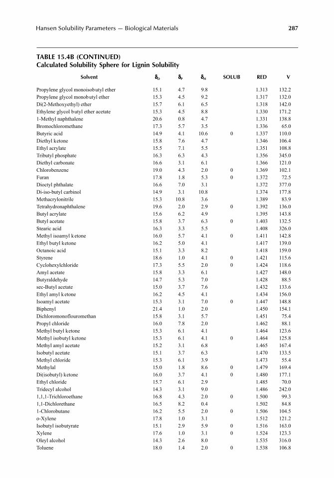
Hansen Solubility Parameters — Biological Materials 287
TABLE 15.4B (CONTINUED)Calculated Solubility Sphere for Lignin Solubility
Solvent δδδδD δδδδP δδδδH SOLUB RED V
Propylene glycol monoisobutyl ether 15.1 4.7 9.8 1.313 132.2Propylene glycol monobutyl ether 15.3 4.5 9.2 1.317 132.0Di(2-Methoxyethyl) ether 15.7 6.1 6.5 1.318 142.0Ethylene glycol butyl ether acetate 15.3 4.5 8.8 1.330 171.21-Methyl naphthalene 20.6 0.8 4.7 1.331 138.8Bromochloromethane 17.3 5.7 3.5 1.336 65.0Butyric acid 14.9 4.1 10.6 0 1.337 110.0Diethyl ketone 15.8 7.6 4.7 1.346 106.4Ethyl acrylate 15.5 7.1 5.5 1.351 108.8Tributyl phosphate 16.3 6.3 4.3 1.356 345.0Diethyl carbonate 16.6 3.1 6.1 1.366 121.0Chlorobenzene 19.0 4.3 2.0 0 1.369 102.1Furan 17.8 1.8 5.3 0 1.372 72.5Dioctyl phthalate 16.6 7.0 3.1 1.372 377.0Di-iso-butyl carbinol 14.9 3.1 10.8 1.374 177.8Methacrylonitrile 15.3 10.8 3.6 1.389 83.9Tetrahydronaphthalene 19.6 2.0 2.9 0 1.392 136.0Butyl acrylate 15.6 6.2 4.9 1.395 143.8Butyl acetate 15.8 3.7 6.3 0 1.403 132.5Stearic acid 16.3 3.3 5.5 1.408 326.0Methyl isoamyl ketone 16.0 5.7 4.1 0 1.411 142.8Ethyl butyl ketone 16.2 5.0 4.1 1.417 139.0Octanoic acid 15.1 3.3 8.2 1.418 159.0Styrene 18.6 1.0 4.1 0 1.421 115.6Cyclohexylchloride 17.3 5.5 2.0 0 1.424 118.6Amyl acetate 15.8 3.3 6.1 1.427 148.0Butyraldehyde 14.7 5.3 7.0 1.428 88.5sec-Butyl acetate 15.0 3.7 7.6 1.432 133.6Ethyl amyl ketone 16.2 4.5 4.1 1.434 156.0Isoamyl acetate 15.3 3.1 7.0 0 1.447 148.8Biphenyl 21.4 1.0 2.0 1.450 154.1Dichloromonoflouromethan 15.8 3.1 5.7 1.451 75.4Propyl chloride 16.0 7.8 2.0 1.462 88.1Methyl butyl ketone 15.3 6.1 4.1 1.464 123.6Methyl isobutyl ketone 15.3 6.1 4.1 0 1.464 125.8Methyl amyl acetate 15.2 3.1 6.8 1.465 167.4Isobutyl acetate 15.1 3.7 6.3 1.470 133.5Methyl chloride 15.3 6.1 3.9 1.473 55.4Methylal 15.0 1.8 8.6 0 1.479 169.4Di(isobutyl) ketone 16.0 3.7 4.1 0 1.480 177.1Ethyl chloride 15.7 6.1 2.9 1.485 70.0Tridecyl alcohol 14.3 3.1 9.0 1.486 242.01,1,1-Trichloroethane 16.8 4.3 2.0 0 1.500 99.31,1-Dichlorethane 16.5 8.2 0.4 1.502 84.81-Chlorobutane 16.2 5.5 2.0 0 1.506 104.5o-Xylene 17.8 1.0 3.1 1.512 121.2Isobutyl isobutyrate 15.1 2.9 5.9 0 1.516 163.0Xylene 17.6 1.0 3.1 0 1.524 123.3Oleyl alcohol 14.3 2.6 8.0 1.535 316.0Toluene 18.0 1.4 2.0 0 1.538 106.8
7248_C015.fm Page 287 Wednesday, May 9, 2007 9:37 AM
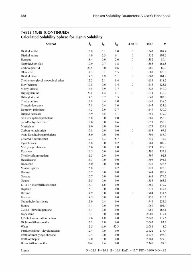
288 Hansen Solubility Parameters: A User’s Handbook
TABLE 15.4B (CONTINUED)Calculated Solubility Sphere for Lignin Solubility
Solvent δδδδD δδδδP δδδδH SOLUB RED V
Diethyl sulfid 16.8 3.1 2.0 0 1.543 107.4Diethyl amine 14.9 2.3 6.1 0 1.552 103.2Benzene 18.4 0.0 2.0 0 1.582 89.4Naphtha.high-flas 17.9 0.7 1.8 1.585 181.8Carbon disulfid 20.5 0.0 0.6 0 1.586 60.0Oleic acid 14.3 3.1 5.5 1.603 320.0Diethyl ether 14.5 2.9 5.1 0 1.605 104.8Triethylene glycol monooleyl ether 13.3 3.1 8.4 1.614 418.5Ethylbenzene 17.8 0.6 1.4 0 1.615 123.1Methyl oleate 14.5 3.9 3.7 1.628 340.0Dipropylamine 5.3 1.4 4.1 0 1.631 136.9Dibutyl stearate 14.5 3.7 3.5 1.643 382.0Triethylamine 17.8 0.4 1.0 1.645 138.6Trimethylbenzene 17.8 0.4 1.0 1.645 133.6Isopropyl palmitate 14.3 3.9 3.7 1.647 330.0Dibutyl sebacate 13.9 4.5 4.1 1.652 339.0cis-Decahydronaphthalene 18.8 0.0 0.0 1.669 156.9para-Diethyl benzene 18.0 0.0 0.6 1.673 156.9Mesitylene 18.0 0.0 0.6 1.673 139.8Carbon tetrachloride 17.8 0.0 0.6 0 1.683 97.1trans-Decahydronaphthalene 18.0 0.0 0.0 1.704 156.9Chlorodiflouromethan 12.3 6.3 5.7 1.719 72.9Cyclohexane 16.8 0.0 0.2 0 1.761 108.7Methyl cyclohexane 16.0 0.0 1.0 1.774 128.3Eicosane 16.5 0.0 0.0 1.790 359.8Trichlorofluoromethan 15.3 2.0 0.0 1.797 92.8Hexadecane 16.3 0.0 0.0 1.803 294.1Dodecane 16.0 0.0 0.0 1.823 228.6Mineral spirits 15.8 0.1 0.2 1.823 125.0Decane 15.7 0.0 0.0 1.844 195.9Nonane 15.7 0.0 0.0 1.844 179.7Octane 15.5 0.0 0.0 1.858 163.51,1,2-Trichlorotrifluoroethan 14.7 1.6 0.0 1.860 119.2Heptane 15.3 0.0 0.0 1.873 147.4Hexane 14.9 0.0 0.0 0 1.904 131.6Pentane 14.5 0.0 0.0 1.936 116.2Tetraethylorthosilicate 13.9 0.4 0.6 1.944 224.0Butane 14.1 0.0 0.0 1.969 101.42,2,2,4-Trimethylpentane 14.1 0.0 0.0 1.969 166.1Isopentane 13.7 0.0 0.0 2.003 117.41,2-Dichlorotetrafluoroethan 12.6 1.8 0.0 2.042 117.6Dichlorodifluoromethan 12.3 2.0 0.0 2.065 92.3Water 15.5 16.0 42.3 2.081 18.0Perfluoro(dimet ylcyclohexane) 12.4 0.0 0.0 2.122 217.4Perfluoromet ylcyclohexane 12.4 0.0 0.0 2.122 196.0Perfluoroheptan 12.0 0.0 0.0 2.161 227.3Bromotrifluoromethan 9.6 2.4 0.0 2.340 97.0
Lignin D = 21.9 P = 14.1 H = 16.9 RAD. = 13.7 FIT = 0.990 NO = 82
7248_C015.fm Page 288 Wednesday, May 9, 2007 9:37 AM
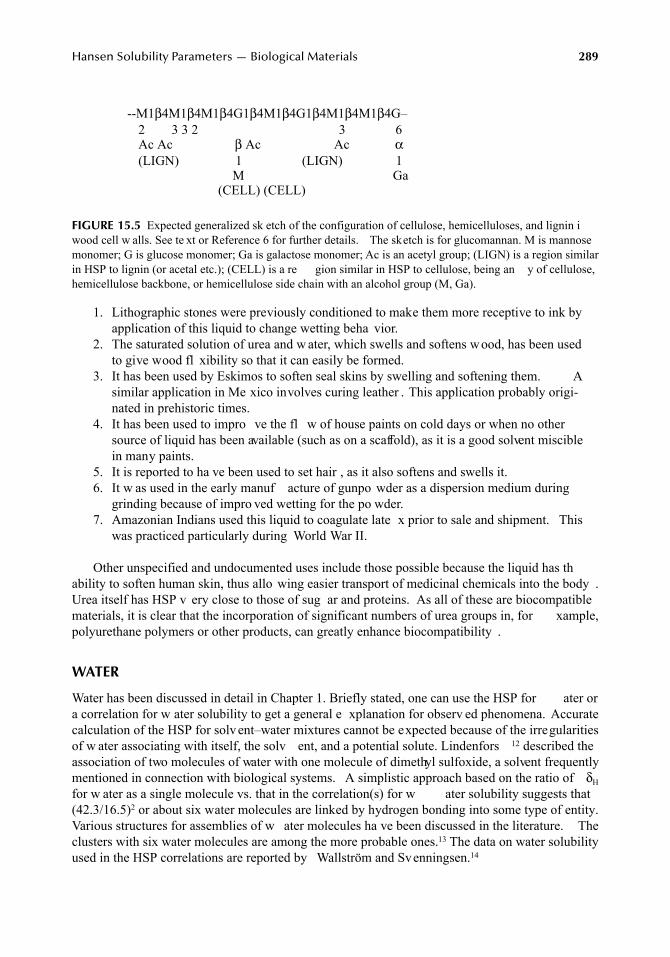
Hansen Solubility Parameters — Biological Materials 289
1. Lithographic stones were previously conditioned to make them more receptive to ink byapplication of this liquid to change wetting beha vior.
2. The saturated solution of urea and w ater, which swells and softens wood, has been usedto give wood fl xibility so that it can easily be formed.
3. It has been used by Eskimos to soften seal skins by swelling and softening them. Asimilar application in Me xico involves curing leather . This application probably origi-nated in prehistoric times.
4. It has been used to impro ve the fl w of house paints on cold days or when no othersource of liquid has been available (such as on a scaffold), as it is a good solvent misciblein many paints.
5. It is reported to ha ve been used to set hair , as it also softens and swells it.6. It w as used in the early manuf acture of gunpo wder as a dispersion medium during
grinding because of impro ved wetting for the po wder.7. Amazonian Indians used this liquid to coagulate late x prior to sale and shipment. This
was practiced particularly during World War II.
Other unspecified and undocumented uses include those possible because the liquid has thability to soften human skin, thus allo wing easier transport of medicinal chemicals into the body .Urea itself has HSP v ery close to those of sug ar and proteins. As all of these are biocompatiblematerials, it is clear that the incorporation of significant numbers of urea groups in, for xample,polyurethane polymers or other products, can greatly enhance biocompatibility .
WATER
Water has been discussed in detail in Chapter 1. Briefly stated, one can use the HSP for ater ora correlation for w ater solubility to get a general e xplanation for observ ed phenomena. Accuratecalculation of the HSP for solv ent–water mixtures cannot be expected because of the irregularitiesof w ater associating with itself, the solv ent, and a potential solute. Lindenfors 12 described theassociation of two molecules of water with one molecule of dimethyl sulfoxide, a solvent frequentlymentioned in connection with biological systems. A simplistic approach based on the ratio of δHfor w ater as a single molecule vs. that in the correlation(s) for w ater solubility suggests that(42.3/16.5)2 or about six water molecules are linked by hydrogen bonding into some type of entity.Various structures for assemblies of w ater molecules ha ve been discussed in the literature. Theclusters with six water molecules are among the more probable ones.13 The data on water solubilityused in the HSP correlations are reported by Wallström and Svenningsen.14
--M1β4M1β4M1β4G1β4M1β4G1β4M1β4M1β4G–2 3 3 2 3 6Ac Ac β Ac Ac α(LIGN) 1 (LIGN) 1
M Ga(CELL) (CELL)
FIGURE 15.5 Expected generalized sk etch of the configuration of cellulose, hemicelluloses, and lignin iwood cell w alls. See te xt or Reference 6 for further details. The sketch is for glucomannan. M is mannosemonomer; G is glucose monomer; Ga is galactose monomer; Ac is an acetyl group; (LIGN) is a region similarin HSP to lignin (or acetal etc.); (CELL) is a re gion similar in HSP to cellulose, being an y of cellulose,hemicellulose backbone, or hemicellulose side chain with an alcohol group (M, Ga).
7248_C015.fm Page 289 Wednesday, May 9, 2007 9:37 AM
290 Hansen Solubility Parameters: A User’s Handbook
SURFACE MOBILITY
Surface mobility allows given segments of molecules to orient at surfaces in a direction where theirHSP match more closely . The surfaces of h ydrophobic polymers (peat moss) can become h ydro-philic when contacted with w ater. One can speculate as to wh y this occurs. One possibility is thatthis phenomenon conserves water within the structure. Whenever water is present on an otherwisehydrophobic surf ace, it can become h ydrophilic if the surf ace molecules can rotate or mo vehydrophilic entities toward the water. This allows the water to spontaneously spread and potentiallyenter the structure if there are suitable passages. When this is accomplished, and contact with waterceases, the surface dries and becomes h ydrophobic once more. The molecules rotate with a lo werenergy moiety toward the air. This hydrophobic surface helps prevent evaporation of water, as wateris not particularly soluble in it, and the h ydrophilic segments oriented to ward the interior of thestructure will help bind the w ater where it is. The basis of the orientation ef fects described earlierfor hemicelluloses is another e xample of orientation to ward regions where HSP matches better .These phenomena are also discussed in Chapter 18. It is also appropriate to repeat that solv entquality has a great deal to do with pigment dispersion stability , in that the adsorbed stabilizingpolymer should remain on the pigment surf ace. A solvent which is too good can remo ve it. Thisis discussed in detail in Chapter 5.
The implication of these e xamples is that solv ent quality is v ery important for the orientationof molecules at interf aces. A change in solv ent quality can easily lead to a change in the configuration of molecules at surfaces. It is not surprising that Nature has used this to advantage in variousways.
CHIRAL ROTATION, HYDROGEN BONDING, AND NANOENGINEERING
It has been found that anthracene units appended to a single scre w-sense helical polyguanidinechanged orientation when the temperature was increased beyond 38.5°C.15 The configuration founabove 38.5°C was the same as that found in tetrah ydrofurane. At temperatures lower than this, theorientation of the appended anthracene was that found in toluene. A mixture of tetrahydrofurane/tol-uene equal to 90/10 v ol% approximated the conditions at the critical temperature. F or those whohave diligently read this handbook, it w ould appear obvious that it is the cohesi ve energy densityjust above or just belo w the critical temperature that controls the structure. More specifically it ithe set of HSP values that do this, as these reflect the mix of sources of the cohes ve energy densityaccording to Equation 1.6 to Equation 1.8. There is also massi ve e vidence sho wing that theinteractions can be interpreted as the dif ference in HSP using Equation 1.9. It is well kno wn thatsolubility limits can be passed by lo wering the temperature in some cases and by increasing it inother cases. When the cohesi ve energy density of the solv ent is higher than that of the polymer ,solvency increases with increased temperature. When the cohesive energy density of the solvent islower than that of the polymer, solvency decreases with increases in temperature. This is discussedin Chapter 2 and has been thoroughly treated by P atterson.16,17 In the present case the HSP oftoluene are comparable to those of anthracene whereas tetrah ydrofuran has much higher v alues.δD, δP, and δH equal to 18.7, 4.1, and 3.3 for anthracene have been reported by a multiple regressiontechnique based on its solubility in a lar ge number of solv ents.18 The corresponding v alues are18.0, 1.4, and 2.0 for toluene and 16.8, 5.7, and 8.0 for tetrah ydrofurane. Thus increasing thetemperature will increase the solv ency in tetrah ydrofurane to the point where it becomes able tocause the appended anthracene to adopt the same orientation as it has in toluene. As toluene haslower HSP than anthracene, the solv ency will decrease with increases in temperature.
Extending this w ay of thinking to the problem of mo ving very large biological molecules —while they are being assembled, for example — is presumably one of controlling the local solubility.When the molecule is locally able to reside in the surrounding fluid, it can m ve much more readily
7248_C015.fm Page 290 Wednesday, May 9, 2007 9:37 AM
Hansen Solubility Parameters — Biological Materials 291
than when it is not. An insoluble molecule or molecular se gment will adsorb at a location wherethe ener gies (HSP) match, and where the geometry is also accommodating. This is most oftencalled hydrogen bonding, b ut it must be all three (or more) types of cohesi ve ener gy that arecollectively acti ve. The molecule or molecular se gment can be remo ved ag ain when it and thesurrounding liquid have a favorable energy relation.
CONCLUSION
Many materials of biological significance h ve been assigned HSP based on their interaction witha large number of solv ents whose HSP are kno wn. A correlation for solv ent effects on DN A hasranked the extent of these effects for different solvents in essentially the same order as that reportedin an older study .9 This correlation for DN A can presumably be impro ved by additional data, b utstill reflects the magnitudes of the types of ene gies that are in volved in forming/destro ying thedouble helices. The δD;δP;δH found for DN A are 19.0;20.0;11.0, all in MP a1/2. This clearly showsthat hydrogen bonding is by far the smallest of the energies involved in the noncovalent interactionsthat determine the DN A structure.
A HSP correlation has been used to find predictably syne gistic solvent mixtures where tw ononsolvents dissolve cholesterol when mix ed. The ethanol/aliphatic h ydrocarbon synergistic mix-ture is discussed as being of particular interest to the f ate of cholesterol in lipid layers. The HSPof chlorophyll and lignin are quite similar , indicating they will be compatible with v ery much thesame kind of surroundings. The physical interrelationships for wood chemicals and wood polymers(lignin, hemicelluloses, and cellulose) are discussed. The side chains on hemicelluloses whichcontain alcohol groups and the hemicellulose backbone will be most compatible with cellulose andwill orient to ward this. The hemicellulose side chains without alcohol groups (acetal, acid) arecloser in HSP to lignin and will orient in this direction. The acetal side chains actually ha ve lowerHSP than will dissolve lignin, for which reason they are expected to lie on the surface of the ligninor perhaps penetrate slightly into the lignin at v ery special local points where the HSP match isbetter than the a verage values seen over the lignin molecule as a whole.
Molecular design of molecules or structures that change conformation with slight changes inthe cohesive energy characteristics of given continuous media seems possible using HSP concepts.The changes are caused by preferred orientation of se gments of one conformation to ward thecontinuous phase, where its HSP match better , thus reducing the free ener gy of the system. If thecohesive energy characteristics of the continuous media change in a direction that no longer f avorsthis orientation, the molecule will change configuration to one where the free ene gy is lower. Theattraction of the se gments not oriented to ward the continuous phase to neighboring molecules iscommonly called hydrogen bonding in proteins and similar materials. This attraction is causedcollectively by all the types of ener gy involved through the pre vailing difference in HSP and is aresult of insolubility (rejection by) the continuous media. Geometrical considerations are clearlyalso a major f actor in addition to the cohesi ve energy density focused upon here.
HSP analyses of relative affinities can be applied to a la ge number of other biological materialsand may pro vide insights into relationships which are not readily ob vious or cannot be studiedotherwise. The best situation is where the materials in question can be tested directly , otherwisethe calculation procedures described in Chapter 1 can be used with some loss of reliability in thepredictions.
REFERENCES
1. Hansen, C.M., The three dimensional solubility parameter — k ey to paint component af finities ISolvents, plasticizers, polymers, and resins, J. Paint Technol., 39(505), 104–117, 1967.
7248_C015.fm Page 291 Wednesday, May 9, 2007 9:37 AM
292 Hansen Solubility Parameters: A User’s Handbook
2. Hansen, C.M. and Andersen, B.H., The affinities of o ganic solvents in biological systems, Am. Ind.Hyg. Assoc. J., 49(6), 301–308, 1988.
3. Hansen, C.M., The universality of the solubility parameter , Ind. Eng. Chem. Prod. Res. Dev., 8(1),2–11, 1969.
4. Ursin, C., Hansen, C.M., Van Dyk, J.W., Jensen, P.O., Christensen, I.J., and Ebbehoej, J., Permeabilityof commercial solvents through living human skin, Am. Ind. Hyg. Assoc. J., 56, 651–660, 1995.
5. Hansen, C.M., 25 years with the solubility parameter (25 År med Opløselighedsparametrene, inDanish), Dan. Kemi, 73(8), 18–22, 1992.
6. Hansen, C.M. and Björkman, A., The ultrastructure of w ood from a solubility parameter point ofview, Holzforschung, 52(4), 335–344, 1998.
7. Hansen, C.M., Solvents for coatings, Chem. Technol., 2(9), 547–553, 1972.8. Blake, R.D. and Delcourt, S.G., Thermodynamic effects of formamide on DN A stability, Nucl. Acid
Res., 24, 2095–2103, 1996.9. Ts’o, P.O.P., Helmkamp, G.K., and Sander, C., Interaction of nucleosides and related compounds with
nucleic acids as indicated by the change of helix-coil transition temperature, Proc. Natl. Acad. Sci.U S A, 48, 686–698, 1962.
10. Hansen, C.M., Cohesion energy parameters applied to surface phenomena, Handbook of Surface andColloid Chemistry, Birdi, K.S., Ed., CRC Press, Boca Raton, FL, 1997, pp. 313–332.
11. Hansen, C.M., Some aspects of acid/base interactions (Einige Aspekte der Säure/Base-W echsel-wirkung, in German), Farbe und Lack, 7, 595–598, 1977.
12. Lindenfors, S., Solubility of cellulose ethers (Löslichkeit der Celluloseeäther, in German), Das Papier,21, 65–69, 1967.
13. Gregory, J.K., Clary, D.C., Liu, K., Bro wn, M.G., and Saykally , R.J., The Water Dipole Moment inWater Clusters, Science, 275, 1997, pp. 814–817.
14. Wallström, E. and Svenningsen, I., Handbook of Solvent Properties, Report T1-84, Scandinavian Paintand Printing Ink Research Institute, Hoersholm, Denmark, 1984.
15. Tang, H.-Z., No vak, B.M., He, J., and Pola varapu, P.L., A thermal and solv ocontrollable cylindricalnanoshutter based on a single scre w-sense helical polyguanidine, Angew. Chem. Int. Ed., 44,7298–7301, 2005.
16. Patterson, D. and Delmas, G., Ne w aspects of polymer solution thermodynamics, Off. Dig. Fed. Soc.Paint Technol., 34(450), 677–692, 1962.
17. Delmas, D., Patterson, D., and Somcynsky, T., Thermodynamics of polyisobutylene-n-alkane systems,J. Polym. Sci., 57, 79–98, 1962.
18. Wu, P.L., Beerbower, A., and Martin, A., Extended Hansen approach: calculating partial solubilityparameters of solid solutes, J. Pharm. Sci., 71(11), 1285–1287 (1982).
7248_C015.fm Page 292 Wednesday, May 9, 2007 9:37 AM
293
16
Absorption and Diffusion in Polymers
Charles M. Hansen
ABSTRACT
Predicting whether or not a gi ven chemical will attack a gi ven polymer is important. Hansensolubility parameters (HSP) ha ve been used for this purpose as discussed else where in this book.Consideration of the absorption and dif fusion of the chemical in the polymer is often required inaddition to HSP in order to make reliable predictions, however. This has been discussed in particularin Chapter 12 through Chapter 14, where chemical resistance, barrier properties, and environmentalstress cracking are treated in detail. Chemicals with smaller and more linear molecules absorb anddiffuse more readily than those with lar ger and more b ulky structures. Surf ace resistance toabsorption is sometimes so dominating that absorption does not occur in some cases, e ven thoughthis might be e xpected based on simple HSP considerations. This chapter examines surface resis-tances in connection with absorption and dif fusion in polymers in order to help impro ve under-standing of these f actors and to emphasize the necessity of simultaneous consideration of surf aceresistance when absorption rates and dif fusion within the bulk of the polymer itself are of interest.Methods to measure surf ace resistance and concentration-dependent dif fusion coef ficients ardiscussed. Solving the diffusion equation with simultaneous consideration of surface resistance andwith a concentration dependent dif fusion correctly models absorption, desorption, film formatioby solvent evaporation, and various forms of so-called anomalous dif fusion such as “time-depen-dent,” Case II, and Super Case II. Surf ace phenomena such as surf ace resistance to absorptiondeserve far more attention than has been gi ven in the past.
LIST OF SYMBOLS USED IN THIS CHAPTER
(Please note that these are dif ferent from those used in the other chapters.)
A Minimum cross-sectional area of molecule in Equation 16.20B Ratio of diffusion resistance to surf ace resistance. See Equation 16.13C Dimensionless concentration. See Equation 16.5C
A
Concentration at break in curv e in Figure 16.1C
s
Dimensionless surface concentrationD Diffusion coefficient. Preferred units are c
2
/sD
0
Diffusion coefficient at zero concentration or l west concentration in an e xperimentD
1
Diffusion coefficient on xposed side of filD
2
Diffusion coefficient on xit side of filD
app
Apparent diffusion coefficienD
av
Average diffusion coefficienD
max
Maximum diffusion coefficient in an xperimentD
v
Increase in the dif fusion coefficient ver zero conditions for a gi ven situationF Mass fluF
M
Correction factor for concentration dependent dif fusion in Equation 16.11F
B
Correction factor for surface resistance in Equation 16.11F
a
Correction factor for concentration dependent dif fusion in absorption e xperiments
7248_C016.fm Page 293 Wednesday, May 23, 2007 11:36 AM
294
Hansen Solubility Parameters: A User’s Handbook
F
d
Correction factor for concentration dependent dif fusion in desorption e xperimentsL Film thicknessM
t
Absorbed mass at time tM
∞
Mass at equilibrium conditionsP Permeation coefficienP
app
Apparent permeation coefficienP
∞
True permeation coefficienR Radius of cylindrical sample in Equation 16.24R
d
Resistance to mass transport from dif fusionR
i
Resistances to permeation from sources 1, 2, 3, etc., in Equation 16.17 to 16.19R
s
Resistance to mass transport by surf ace resistance(s)T Dimensionless time given by Equation 16.3X Dimensionless distanceV
f
Volume fraction of dif fusing materialV
t
Constant in Figure 16.4 used to find local di fusion coefficients at V
f
greater than 0.20V
2
Diffusion coefficients at V
f
equal 0.20 relative to diffusion coefficient at zero concentration (Figure 16.1 and Figure 16.4)
b Thickness of cylindrical sample in Equation 16.24c Concentration of diffusing materialc
s
Surface concentrationc
0
Initial concentrationc
1
Concentration on exposed side of samplec
2
Concentration on exit side of samplec
∞
Concentration at equilibrium conditionsh Surface mass transfer coef ficienh
av
Average surface mass transfer coef ficienk Constant in Equation 16.6k
2
Constant in Equation 16.20l Length of sample in Equation 16.23t Timet
1/2
Time required to absorb (or desorb) one half of the equilibrium amountw Width of sample in Equation 16.23x Distance
Δ
p Pressure difference of diffusing material across membrane
Φ
R
Local concentration is Figure 16.6
INTRODUCTION
Chapters 12 through 14 ha ve dealt with chemical resistance, en vironmental stress cracking, andbarrier polymers, respectively. Absorption and diffusion of the chemicals into polymers are impor -tant in each of these. F actors af fecting absorption and dif fusion in polymers are therefore ofconsiderable importance and must frequently be included along with the Hansen solubility param-eters (HSP) to mak e correlations and predictions for these phenomena. This chapter emphasizesthe importance of surface resistance for absorption in polymers as this has been largely overlookedin the literature. The focus of much of the rele vant literature has been on anomalous dif fusion, buteven in this context the influence of sur ace resistance has largely been neglected. Surface resistancecan delay or pre vent the absorption of solv ents that should absorb readily based on simple HSPconsiderations. This could lead to a f alse sense of security based on short time testing only .
Absorption requires some de gree of solubility . Therefore, equilibrium absorption can beexpected to correlate with HSP. In studies of the absorption of a chemical into a polymer, its surfaceconcentration is usually assumed to reach the equilibrium v alue immediately. As discussed in the
7248_C016.fm Page 294 Wednesday, May 23, 2007 11:36 AM
Absorption and Diffusion in Polymers
295
following, this is not al ways true. Whatever the rate at which the surf ace concentration increases,absorption will proceed according to the la ws of dif fusion, Fick’s First La w, Equation 16.1, andFick’s Second Law, Equation 16.2. The latter is often called the dif fusion equation. Its deri vationcan be found in Crank.
1
For the sake of simplicity, these equations are gi ven here for dif fusion inone dimension (x) only . For a constant dif fusion coefficient
F = - D
0
(
∂
c/
∂
x) (16.1)
∂
c/
∂
t =
∂
/
∂
x (D
0
∂
c/
∂
x) (16.2)
The diffusion equation is deri ved in a v ery general w ay and also accounts for concentrationdependent diffusion coefficients when ver this is encountered. F is the mass flux,
0
is the (constant)diffusion coefficient or the di fusion coefficient at the l west concentration if there is concentrationdependence (see below), c is the local concentration, x is the distance in the x dimension, and t isthe time. The solutions to the diffusion equation given in this chapter use the dry film thickness areference. This is because it is f ar simpler to keep track of what is going on instead of continuallyadjusting local film thickness as a function of the amount of sol ent present. When a dif fusingsolvent is present, for example, then the actual local thickness should be increased proportionatelyaccording to its local v olume fraction.
The use of dimensionless v ariables to solv e these equations mak es the solutions more usefulby making them applicable to all v alues of the combined variables. For this purpose the followingare defined
Dimensionless time:
T = D
0
t/L
2
(16.3)
Dimensionless distance:
X = x/L (16.4)
Dimensionless concentration:
C = (c – c
0
)/(c
∞
– c
0
) (16.5)
L is the thickness of the plane sheet being considered. c
0
is the initial uniform concentration in thefilm. The (local) dimensionless concentrations rise from 0 to 1.0 in an absorption experiment whereequilibrium absorption, c
∞
, is finally obtained.For the sak e of completeness the predicted and e xperimentally confirmed xponential depen-
dence of the dif fusion coefficient on concentration, D(c), will be introduced at this early stage. Amore detailed discussion of its significance is g ven in a special section belo w.
D(c) = D
0
e
kc
= D
0
D
v
(16.6)
“k” is a constant that is v alid up to a gi ven concentration as discussed belo w. D
v
is the increase inthe diffusion coefficient ver that at zero conditions for a gi ven concentration. At the maximumconcentration this becomes D
max
, and for a constant dif fusion coefficient it is 1.0Using these variables, Equation 16.2 can be rewritten in dimensionless form as Equation 16.7.The dimensionless diffusion equation for an e xponential diffusion coefficient is
∂
C/
∂
T =
∂
/
∂
X (D
v
∂
C/
∂
X) (16.7)
7248_C016.fm Page 295 Wednesday, May 23, 2007 11:36 AM
296
Hansen Solubility Parameters: A User’s Handbook
The earliest edition of Crank’s monumental work
1
has the advantage of many graphical solutionsto the dimensionless dif fusion equation being presented with plots that can be used with a highdegree of accuracy. These plots include numerous reference lines not found in later editions.
STEADY STATE PERMEATION
In the absence of significant surace resistances, solving Equation 16.1 (or Equation 16.7) for steadystate permeation in one direction only for a constant dif fusion coefficient g ves Equation 16.8.
F = –D
0
(c
1
– c
2
)L (16.8)
The surface concentration on the exposed side, c
1
, is usually assumed to be c
∞
, and c
2
is usuallyassumed to be zero. Initially , c
1
will be less than c
∞
when there is a significant sur ace resistanceon the e xposed side, as discussed in the follo wing. Likewise, c
2
will be greater than c
0
if there isa significant sur ace resistance on the lo w concentration side of the film. The preferred units forthese quantities are F in g/(cm
2
×
s), L in cm, c in g/cm
3
, and D
0
in cm
2
/s. It can be seen from Equation 16.8 that the surface concentration on the exposed side determines
the concentration gradient over the film, assuming
2
is zero. This is a situation that seems to prevailin general, b ut exceptions are discussed belo w, and there will be significant sur ace resistance inpresumably all cases as film thickness approaches zero. The surface concentrations, c
1
(or c
s
), willbe higher for closer matches in HSP between challenge chemicals and polymers. Therefore, it isnot surprising that HSP correlations can be made when permeation rates for a lar ge number ofchemicals have been measured for a gi ven polymer, as reported in Chapter 13. This is particularlytrue when the molecules involved are all relatively small. When the molecular sizes of the challengechemicals become too lar ge and/or their shape becomes suf ficiently complicated with side groupand cyclic structures, simple HSP correlations are no longer possible. The diffusion coefficient iaffected by these size and shape f actors, and the HSP can no longer be used as a single correlatingparameter. In addition, surf ace resistances can also become v ery significant, as discussed bel wand in Chapter 14. The molecular volume, V, of the challenge chemical has been used with somesuccess to account for size ef fects, b ut this does not directly account for dif ferences in shape.Examples of correlations for dif fusion through chemical protecti ve clothing, for e xample, demon-strated that molecular size had to be tak en into account
2
(see also Figure 13.2 and the discussionin Chapter 13). The most reliable HSP correlations in these cases do not immediately consider thesolvents with smaller molecules that may permeate f aster than e xpected by comparison with allthe others. Likewise, improved understanding and correlations are obtained by initially ne glectingthe solvents with larger molecules that do not permeate as fast as expected, in spite of close matchesin HSP with those solvents that do permeate rapidly. Once a reliable HSP correlation is establishedwithout these obvious outliers, their beha vior is better understood. Predictions then often becomepossible for other v ery small and/or v ery large molecular species as well.
THE DIFFUSION EQUATION
C
ONSTANT
D
IFFUSION
C
OEFFICIENTS
Relevant solutions to Equation 16.2 or Equation 16.7 are used to measure dif fusion coefficientsThe diffusion equation must be solved with two boundary conditions and an initial condition. Thisdiscussion will consider a plane film xposed to absorbing chemical on tw o sides. The initialcondition is chosen as a uniform concentration within a film, so that C is 0 for all X, r gardlessof whether the initial concentration is zero or not. Dif fusion is also usually assumed to tak e placein one direction only, but side effects can become important in thicker samples as discussed below.The chemical concentration at the e xposed surf ace(s) is assumed to immediately rise to the
7248_C016.fm Page 296 Wednesday, May 23, 2007 11:36 AM
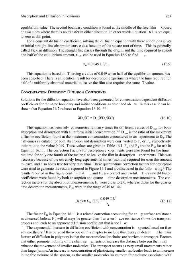
Absorption and Diffusion in Polymers
297
equilibrium value. The second boundary condition is found at the middle of the free film xposedon two sides where there is no transfer in either direction. In other words Equation 16.1 is set equalto zero at this point.
For a constant dif fusion coefficient, solving the di fusion equation with these conditions gi vesan initial straight-line absorption curv e as a function of the square root of time. This is generallycalled Fickian diffusion. The straight line passes through the origin, and the time required to absorbone-half of the equilibrium amount, t
1/2
, can be used in Equation 16.9 to find
0
.
D
0
= 0.049 L
2
/t
1/2
(16.9)
This equation is based on T having a value of 0.049 when half of the equilibrium amount hasbeen absorbed. There is an identical result for desorption e xperiments where the time required forhalf of a uniformly absorbed material to lea ve the film also requires the same T value.
C
ONCENTRATION
D
EPENDENT
D
IFFUSION
C
OEFFICIENTS
Solutions for the diffusion equation have also been generated for concentration dependent diffusioncoefficients for the same boundary and initial conditions as described ab ve. In this case it can beshown that Equation 16.7 reduces to Equation 16.10.
3–5
∂
D
v
/
∂
T = D
v
(
∂
2
D
v
/
∂
X
2
) (16.10)
This equation has been solv ed numerically man y times for dif ferent values of D
max
for bothabsorption and desorption with a uniform initial concentration.
3–5
D
max
is the ratio of the maximumdiffusion coefficient found at the maximum concentration encountered in an xperiment to D
0
. Thehalf-times calculated for both absorption and desorption were con verted to F
a
or F
d
, respectively,their ratio to the v alue 0.049. These values are given in Table 16.1. F
a
and F
d
are the F
M
for use inEquation 16.11. The correction f actors for desorption e xperiments were also found for the timerequired for only one fourth of the material to lea ve the film in desorption xperiments. This wasnecessary because of the extremely long experimental times (months) required for even this amountto leave, and also holds true for very thin films. These quarter-time correction factors for desorptionwere used to generate the results reported in Figure 16.1 and are discussed in the follo wing.
6
Theresults reported in this figure confirm that
a
and F
d
are correct and useful. The same dif fusioncoefficients were found by both absorption and quarte -time desorption measurements. The cor-rection factors for the absorption measurements, F
a
, were close to 2.0, whereas those for the quarter-time desorption measurements, F
d
, were in the range of 40 to 144.
(16.11)
The factor F
B
in Equation 16.11 is a related correction accounting for an y surface resistanceas discussed belo w. F
B
will al ways be greater than 1 as a surf ace resistance slo ws the transportprocess and leads to an apparent dif fusion coefficient that is too l w.
The exponential increase in dif fusion coefficient with concentration is xpected based on freevolume theory.
7
It is be yond the scope of this chapter to include this theory in detail. The mainfeature of diffusion in polymers is that the macromolecular chains are barriers to transport. F actorsthat either promote mobility of the chain se gments or increase the distance between them willenhance the movement of smaller molecules. The transport occurs as very small movements ratherthan larger jumps. An increase in concentration of plasticizing smaller molecules leads to an increasein the free volume of the system, as the smaller molecules ha ve more free volume associated with
D c F FL
tM B( ) .= × ×0 049 2
7248_C016.fm Page 297 Wednesday, May 23, 2007 11:36 AM
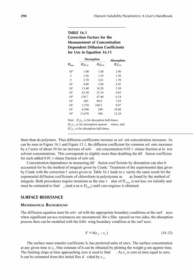
298
Hansen Solubility Parameters: A User’s Handbook
them than do polymers. Thus diffusion coefficients increase as sol ent concentration increases. Ascan be seen in Figure 16.1 and Figure 13.1, the diffusion coefficient for common sol ents increasesby a f actor of about 10 for an increase of solv ent concentration 0.03 v olume fraction at lo wersolvent concentrations. This corresponds to slightly more than doubling the dif fusion coefficienfor each added 0.01 v olume fraction of solv ent.
Concentration dependence in measuring dif fusion coef ficients by absorption can also baccounted for by the method of integrals given by Crank.
1
Treatment of the experimental data givenby Crank with the correction f actors given in Table 16.1 leads to e xactly the same result for theexponential dif fusion coef ficients of chloroform in polystyrene as as found by the method ofintegrals. Both procedures require iterations as the true v alue of D
max
is not kno wn initially andmust be estimated to find
a
(and a ne w Dmax) until convergence is obtained.
SURFACE RESISTANCE
MATHEMATICAL BACKGROUND
The diffusion equation must be solv ed with the appropriate boundary conditions at the surf aceswhen significant sur ace resistances are encountered. For a film xposed on two sides, the absorptionprocess then can be modeled with the follo wing boundary condition at the surf aces:
(16.12)
The surface mass transfer coefficient, h, has preferred units of cm/s. The surface concentrationat any given time is cs. One estimate of h can be obtained by plotting the weight g ain against time.The limiting slope at time approaching zero is used to find . As cs is zero at time equal to zero,h can be estimated from this initial flux d vided by c ∞.
TABLE 16.1Correction Factors for the Measurement of Concentration Dependent Diffusion Coefficients for Use in Equation 16.11
Desorption Absorption(Fa)1/2Dmax (Fd)1/2 (Fd)1/4
100 1.00 1.00 1.002 1.56 1.55 1.305 2.70 2.61 1.70
101 4.00 3.84 2.01102 13.40 10.20 3.30103 43.30 23.10 4.85104 138.7 47.40 6.14105 443 89.0 7.63106 1,370 160.5 8.97107 4,300 290 10.60108 13,670 506 12.10
Note: (Fd)1/2 is for desorption half-times,(Fd)1/4 is for desorption quarter -times, and(Fa)1/2 is for absorption half-times.
F h c cs= −∞( )
7248_C016.fm Page 298 Wednesday, May 23, 2007 11:36 AM
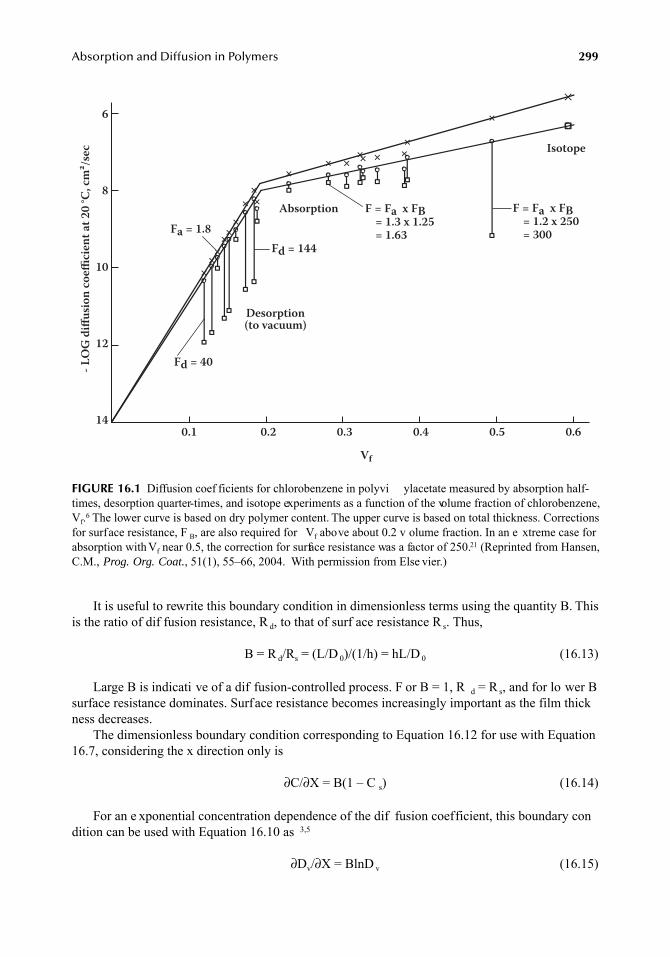
Absorption and Diffusion in Polymers 299
It is useful to rewrite this boundary condition in dimensionless terms using the quantity B. Thisis the ratio of dif fusion resistance, R d, to that of surf ace resistance R s. Thus,
B = R d/Rs = (L/D 0)/(1/h) = hL/D 0 (16.13)
Large B is indicati ve of a dif fusion-controlled process. F or B = 1, R d = R s, and for lo wer Bsurface resistance dominates. Surface resistance becomes increasingly important as the film thickness decreases.
The dimensionless boundary condition corresponding to Equation 16.12 for use with Equation16.7, considering the x direction only is
∂C/∂X = B(1 – C s) (16.14)
For an e xponential concentration dependence of the dif fusion coefficient, this boundary condition can be used with Equation 16.10 as 3,5
∂Dv/∂X = BlnD v (16.15)
FIGURE 16.1 Diffusion coef ficients for chlorobenzene in polyvi ylacetate measured by absorption half-times, desorption quarter-times, and isotope experiments as a function of the volume fraction of chlorobenzene,Vf.6 The lower curve is based on dry polymer content. The upper curve is based on total thickness. Correctionsfor surface resistance, F B, are also required for Vf above about 0.2 v olume fraction. In an e xtreme case forabsorption with Vf near 0.5, the correction for surface resistance was a factor of 250.21 (Reprinted from Hansen,C.M., Prog. Org. Coat., 51(1), 55–66, 2004. With permission from Else vier.)
- LO
G di
ffusio
n co
efficie
nt at
20 °C
, cm
²/sec
6
8
10
12
140.60.50.40.30.20.1
F = Fa x FB = 1.2 x 250 = 300
F = Fa x FB = 1.3 x 1.25 = 1.63
Isotope
Absorption
Fd = 144
Fd = 40
Fa = 1.8
Desorption(to vacuum)
Vf
7248_C016.fm Page 299 Wednesday, May 23, 2007 11:36 AM
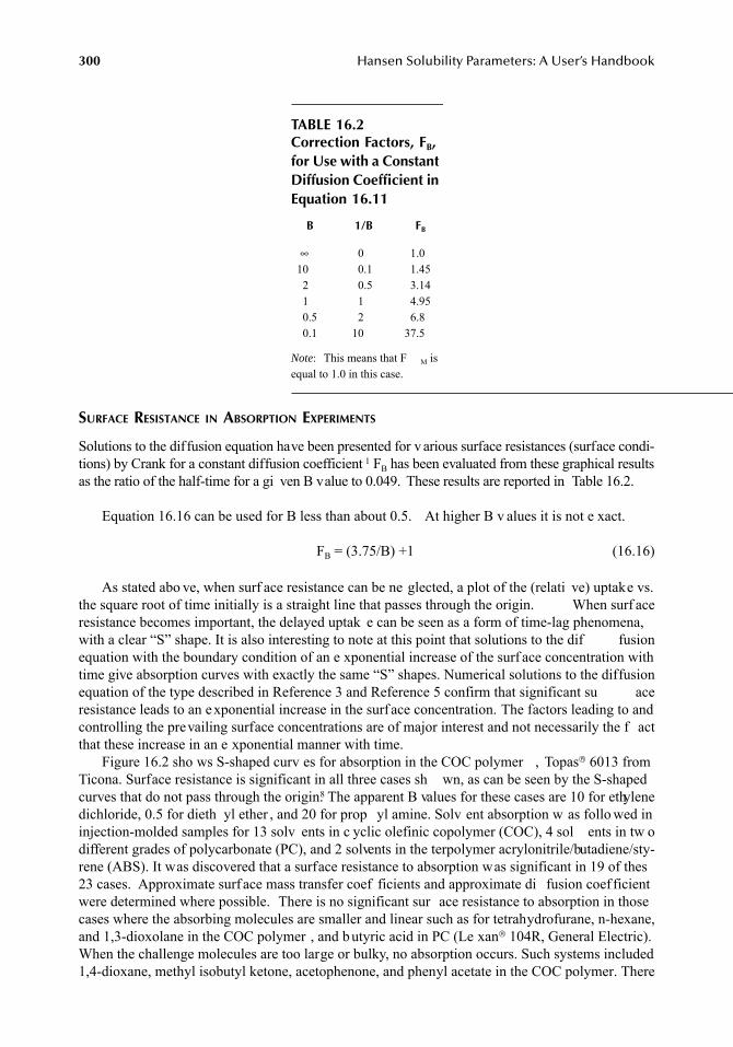
300 Hansen Solubility Parameters: A User’s Handbook
SURFACE RESISTANCE IN ABSORPTION EXPERIMENTS
Solutions to the diffusion equation have been presented for v arious surface resistances (surface condi-tions) by Crank for a constant diffusion coefficient 1 FB has been evaluated from these graphical resultsas the ratio of the half-time for a gi ven B value to 0.049. These results are reported in Table 16.2.
Equation 16.16 can be used for B less than about 0.5. At higher B v alues it is not e xact.
FB = (3.75/B) +1 (16.16)
As stated abo ve, when surf ace resistance can be ne glected, a plot of the (relati ve) uptake vs.the square root of time initially is a straight line that passes through the origin. When surf aceresistance becomes important, the delayed uptak e can be seen as a form of time-lag phenomena,with a clear “S” shape. It is also interesting to note at this point that solutions to the dif fusionequation with the boundary condition of an e xponential increase of the surf ace concentration withtime give absorption curves with exactly the same “S” shapes. Numerical solutions to the diffusionequation of the type described in Reference 3 and Reference 5 confirm that significant su aceresistance leads to an exponential increase in the surf ace concentration. The factors leading to andcontrolling the prevailing surface concentrations are of major interest and not necessarily the f actthat these increase in an e xponential manner with time.
Figure 16.2 sho ws S-shaped curv es for absorption in the COC polymer , Topas® 6013 fromTicona. Surface resistance is significant in all three cases sh wn, as can be seen by the S-shapedcurves that do not pass through the origin.8 The apparent B values for these cases are 10 for ethylenedichloride, 0.5 for dieth yl ether , and 20 for prop yl amine. Solv ent absorption w as follo wed ininjection-molded samples for 13 solv ents in c yclic olefinic copolymer (COC), 4 sol ents in tw odifferent grades of polycarbonate (PC), and 2 solvents in the terpolymer acrylonitrile/butadiene/sty-rene (ABS). It was discovered that a surface resistance to absorption was significant in 19 of thes23 cases. Approximate surf ace mass transfer coef ficients and approximate di fusion coef ficientwere determined where possible. There is no significant sur ace resistance to absorption in thosecases where the absorbing molecules are smaller and linear such as for tetrahydrofurane, n-hexane,and 1,3-dioxolane in the COC polymer , and b utyric acid in PC (Le xan® 104R, General Electric).When the challenge molecules are too large or bulky, no absorption occurs. Such systems included1,4-dioxane, methyl isobutyl ketone, acetophenone, and phenyl acetate in the COC polymer. There
TABLE 16.2Correction Factors, FB, for Use with a Constant Diffusion Coefficient in Equation 16.11
B 1/B FB
∞ 0 1.010 0.1 1.452 0.5 3.141 1 4.950.5 2 6.80.1 10 37.5
Note: This means that F M isequal to 1.0 in this case.
7248_C016.fm Page 300 Wednesday, May 23, 2007 11:36 AM
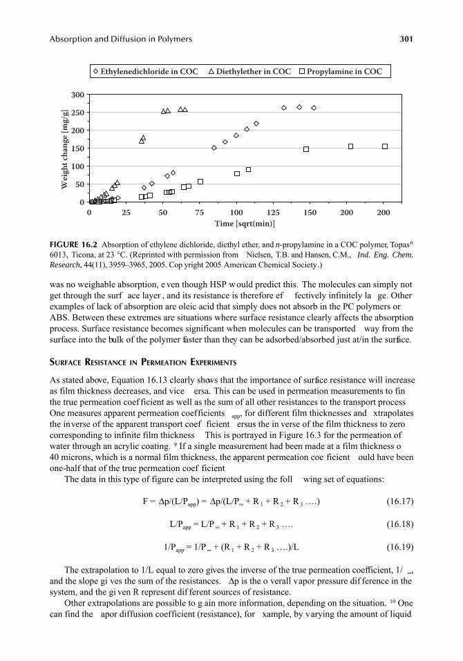
Absorption and Diffusion in Polymers 301
was no weighable absorption, e ven though HSP would predict this. The molecules can simply notget through the surf ace layer , and its resistance is therefore ef fectively infinitely la ge. Otherexamples of lack of absorption are oleic acid that simply does not absorb in the PC polymers orABS. Between these extremes are situations where surface resistance clearly affects the absorptionprocess. Surface resistance becomes significant when molecules can be transported way from thesurface into the bulk of the polymer faster than they can be adsorbed/absorbed just at/in the surface.
SURFACE RESISTANCE IN PERMEATION EXPERIMENTS
As stated above, Equation 16.13 clearly shows that the importance of surface resistance will increaseas film thickness decreases, and vice ersa. This can be used in permeation measurements to finthe true permeation coef ficient as well as the sum of all other resistances to the transport processOne measures apparent permeation coefficients app, for different film thicknesses and xtrapolatesthe inverse of the apparent transport coef ficient ersus the in verse of the film thickness to zerocorresponding to infinite film thickness This is portrayed in Figure 16.3 for the permeation ofwater through an acrylic coating. 9 If a single measurement had been made at a film thickness o40 microns, which is a normal film thickness, the apparent permeation coe ficient ould have beenone-half that of the true permeation coef ficient
The data in this type of figure can be interpreted using the foll wing set of equations:
F = Δp/(L/Papp) = Δp/(L/P∞ + R 1 + R 2 + R 3 ….) (16.17)
L/Papp = L/P ∞ + R 1 + R 2 + R 3 …. (16.18)
1/Papp = 1/P ∞ + (R 1 + R 2 + R 3 ….)/L (16.19)
The extrapolation to 1/L equal to zero gives the inverse of the true permeation coefficient, 1/ ∞,and the slope gi ves the sum of the resistances. Δp is the o verall vapor pressure dif ference in thesystem, and the gi ven R represent dif ferent sources of resistance.
Other extrapolations are possible to g ain more information, depending on the situation. 10 Onecan find the apor diffusion coefficient (resistance), for xample, by varying the amount of liquid
FIGURE 16.2 Absorption of ethylene dichloride, diethyl ether, and n-propylamine in a COC polymer, Topas®
6013, Ticona, at 23 °C. (Reprinted with permission from Nielsen, T.B. and Hansen, C.M., Ind. Eng. Chem.Research, 44(11), 3959–3965, 2005. Cop yright 2005 American Chemical Society.)
Time [sqrt(min)]
Weig
ht ch
ange
[mg/
g]
300
250
200
150
100
50
0
Ethylenedichloride in COC Diethylether in COC Propylamine in COC
2002001501251007550250
7248_C016.fm Page 301 Wednesday, May 23, 2007 11:36 AM
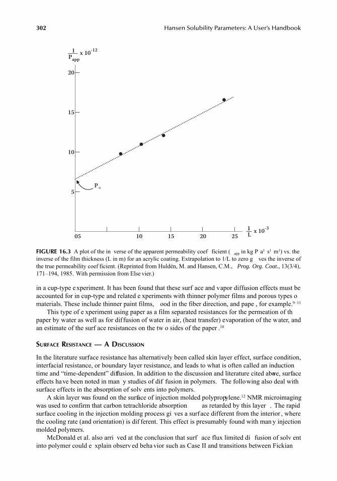
302 Hansen Solubility Parameters: A User’s Handbook
in a cup-type experiment. It has been found that these surf ace and vapor diffusion effects must beaccounted for in cup-type and related e xperiments with thinner polymer films and porous types omaterials. These include thinner paint films, ood in the fiber direction, and pape , for example.9–11
This type of e xperiment using paper as a film separated resistances for the permeation of thpaper by water as well as for dif fusion of water in air, (heat transfer) evaporation of the water, andan estimate of the surf ace resistances on the tw o sides of the paper .10
SURFACE RESISTANCE — A DISCUSSION
In the literature surface resistance has alternatively been called skin layer effect, surface condition,interfacial resistance, or boundary layer resistance, and leads to what is often called an inductiontime and “time-dependent” diffusion. In addition to the discussion and literature cited above, surfaceeffects have been noted in man y studies of dif fusion in polymers. The following also deal withsurface effects in the absorption of solv ents into polymers.
A skin layer was found on the surface of injection molded polypropylene.12 NMR microimagingwas used to confirm that carbon tetrachloride absorption as retarded by this layer . The rapidsurface cooling in the injection molding process gi ves a surface different from the interior , wherethe cooling rate (and orientation) is dif ferent. This effect is presumably found with man y injectionmolded polymers.
McDonald et al. also arri ved at the conclusion that surf ace flux limited di fusion of solv entinto polymer could e xplain observ ed beha vior such as Case II and transitions between Fickian
FIGURE 16.3 A plot of the in verse of the apparent permeability coef ficient ( app in kg P a1 s1 m1) vs. theinverse of the film thickness (L in m) for an acrylic coating. Extrapolation to 1/L to zero g ves the inverse ofthe true permeability coef ficient. (Reprinted from Huldén, M. and Hansen, C.M., Prog. Org. Coat., 13(3/4),171–194, 1985. With permission from Else vier.)
05 10 15 20 25
20
15
10
5
x 10-12Papp
P∝
1
x 10-3L1
7248_C016.fm Page 302 Wednesday, May 23, 2007 11:36 AM
Absorption and Diffusion in Polymers 303
diffusion and Case II dif fusion.13 Toluene diffusion in polystyrene is discussed in detail. Case IIdiffusion involves a linear absorption curv e when time is used rather than the customary squareroot of time. This is discussed in more detail belo w.
Shankar studied interf acial resistance in absorption e xperiments.14 The conclusions were thatnon-Fickian characteristics can result from slo w transfer to the surf ace layer, and that some of theobserved features of anomalous sorption can be e xplained with the help of this model. Surf aceresistance was found to be particularly important in thinner sheets. Systematic variations in absorp-tion phenomena with film thickness are a clear indication of a significant su ace resistance. Whenthere is a surf ace resistance, the surf ace concentration only slo wly rises to the equilibrium v alue.Surface resistance in the meth yl iodide-cellulose acetate system produced the characteristic S-shaped absorption curve.
Characteristic S-shaped absorption curves were found in the methylene chloride-PEEK systemby Gryson et al. 15 The initial rate of absorption w as found to be strongly dependent on the surf acecondition but the equilibrium v alues were not.
Surface resistance w as shown to af fect permeation through polymer films by Kim and Kammermeyer who measured actual concentration profiles in Nylon-6, cellulose acetate, and polyethylene membranes.16 Water permeation through Nylon-6 films as studied for dif ferent film thickness. It w as clearly sho wn that the surf ace concentration of w ater did not reach the equilibriumvalue at the equilibrium permeation rate unless the film thickness as greater than 0.05 cm at 35°C.Similar studies sho wed that there were also significant sur ace resistances for dioxane, benzene,and n-hexane in polyethylene, and for w ater in cellulose acetate.
Hwang and Kammermeyer showed significant sur ace resistance by studying permeation as afunction of film thickness for ater in acetyl cellulose acetate and Nylon-6, h ydrogen throughstainless steel, and p-dioxane through Nylon-6 and polyeth ylene.17
Skaarup18 performed man y permeation e xperiments on Polyamide 6 (P A 6) (B ASF UltramidB4) and polyvin ylacetate (Hoechst, Mo wilith 50) where surf ace resistance w as significant. Oparticular interest are the studies on P A 6 where the permeation of eth yl laurate, 2,4-dimeth yl-2-pentanol, benzyl alcohol, n-butanol, ethyl acetate, and n-pentane was studied. Skaarup arri ved atthe following general relation for the permeation of these liquids through P A
hav = k 2(Dav/A1/2) (16.20)
hav (in cm/s) is the average surface mass transfer coefficient, av (in cm2/s) is the average diffusioncoefficient in the film (see Equation 16.21), an A (in cm 2) is the (minimum) cross-sectional areaof the molecule in question. k 2 is a constant with the v alue approximately 4.5(10)-6. This equationindicates that a molecule in the surf ace of a polymer will proceed inw ard in direct proportion tothe diffusion coefficient. It li ewise indicates that the greater the cross-sectional area of the mole-cule, the more difficulty it will h ve to reside at the surface in a condition where it can take a smalljump into the b ulk. h on the e xposed side of the films as approximately 1/3 of that on the e xitside. The reason for this is thought to be that the orientation of molecules leaving the film is directemore toward the e xit surface, whereas the orientation of molecules approaching the entry side ismore random. A molecule landing “sideways” and hitting a polymer segment will be rejected. Theright orientation at the right place allo ws adsorption/absorption. The significance of the sur aceresistances can be demonstrated by the film thickness at which the resistance from di fusion withinthe film is equal to the sum of the t o surface resistances. This was about 180 microns or higherfor the linear aliphatic molecules, and increased for more complicated structures.
Dav can be found from Equation 16.21 as the log arithmic mean where D 1 is the dif fusioncoefficient on the xposed side and D 2 is the dif fusion coefficient on the xit side.
Dav = (D 1/D2 – 1)/ln(D 1/D2) (16.21)
7248_C016.fm Page 303 Wednesday, May 23, 2007 11:36 AM
304 Hansen Solubility Parameters: A User’s Handbook
This equation shows how much the average diffusion coefficient di fers from that at essentiallyzero concentration corresponding to D 2. If the ratio D 1/D2 is 10 then D av is 3.9 times lar ger thanD1. This implies that concentration dependent diffusion can lead to significant errors when difusionand permeation coefficients at ery low concentrations are needed. D 1/D2 equal to 10 implies thatthe concentration dif ference is only about 0.03 v olume fraction across the membrane when rigidpolymers are involved. For elastomers this same ratio implies a concentration dif ference near 0.15volume fraction, as judged from the dif fusion coefficient data reported in Figure 16.1 at concentrations above about 0.20 volume fraction where the system is above its glass transition temperature.These same considerations are v alid for permeation coef ficients since
P = DS (16.22)
P is the permeation coef ficient measured at the g ven steady state concentration dif ference,(c1 – c2), and S is the solubility coefficient. If 1 is 10 times greater than D2 then P is approximately3.9 times lar ger than w ould have been measured for an e xtremely low concentration dif ferenceacross the membrane.
SIDE EFFECTS
Corrections for absorption or desorption from the sides of thick er samples should be applied tomeasured diffusion coefficients if there is significant d fusion through the sides of thicker samples.Equation 16.23 for dif fusion in plane samples of isotropic media can be used for this purpose. 19
D0 = D app/(1 + L/l + L/w) 2 (16.23)
Dapp is the apparent dif fusion coefficient found from initial slope measurement 1 or Equation16.9 if there is a linear absorption curv e as f ar as t 1/2 when the square root of time is used. Thelength and width of the film are l and , respectively, with L being retained as the thickness. Itcan be seen that D 0 and D app are equal to the e xtent that the second and third terms in Equation16.18 are not significant. Co ventional tensile bars, for example, have significant side e fects whenthey are used to measure diffusion coefficients. The uptake is more rapid than otherwise anticipated,so the apparent diffusion coefficients must be reduced accordingl . Tensile bars that are 4 mm thickand 10 mm wide will require corrections that are at least as great as a f actor of 1.96. A squaresample that is 10 mm on each side and 1 mm thick requires a correction for end effects equal to 1.44.
For c ylindrical geometry a deri vation similar to that used to find Equation 16.23 results iEquation 16.24.
D0 = D app/(1 + b/R) 2 (16.24)
R is the radius of the c ylinder and b is its thickness. These equations are based on the initialuptake (or loss) to e valuate Dapp. Here ag ain, an easy procedure is to e xtrapolate the initial slopeon a plot of uptak e versus the square root of time to a fict ve t1/2 found when the relati ve uptake isequal to 0.5. This value for t 1/2 can be used in Equation 16.9 to find app.
MEASURING DIFFUSION COEFFICIENTS WITH SURFACE RESISTANCE AND CONCENTRATION DEPENDENCE
It was necessary to measure diffusion coefficients ver as wide a range as possible in order to solvethe dif fusion equation to simulate film formation by sol ent e vaporation.3,20 This w as done bycomparison of e xperimental results with solutions to the dif fusion equation accounting for both
7248_C016.fm Page 304 Wednesday, May 23, 2007 11:36 AM
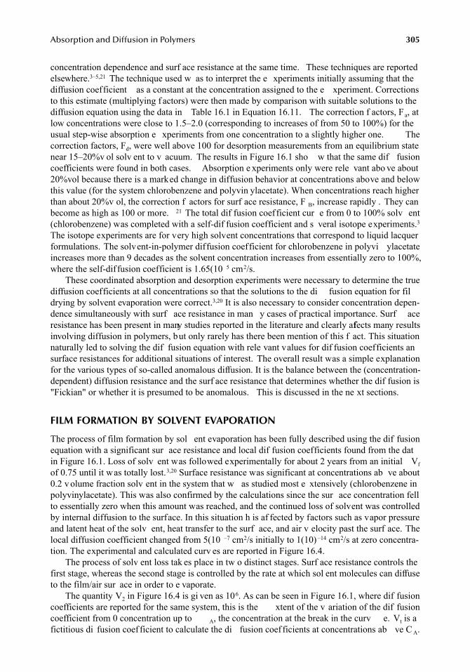
Absorption and Diffusion in Polymers 305
concentration dependence and surf ace resistance at the same time. These techniques are reportedelsewhere.3–5,21 The technique used w as to interpret the e xperiments initially assuming that thediffusion coefficient as a constant at the concentration assigned to the e xperiment. Correctionsto this estimate (multiplying f actors) were then made by comparison with suitable solutions to thediffusion equation using the data in Table 16.1 in Equation 16.11. The correction f actors, F a, atlow concentrations were close to 1.5–2.0 (corresponding to increases of from 50 to 100%) for theusual step-wise absorption e xperiments from one concentration to a slightly higher one. Thecorrection factors, Fd, were well above 100 for desorption measurements from an equilibrium statenear 15–20%v ol solv ent to v acuum. The results in Figure 16.1 sho w that the same dif fusioncoefficients were found in both cases. Absorption e xperiments only were rele vant abo ve about20%vol because there is a marked change in diffusion behavior at concentrations above and belowthis value (for the system chlorobenzene and polyvin ylacetate). When concentrations reach higherthan about 20%v ol, the correction f actors for surf ace resistance, F B, increase rapidly . They canbecome as high as 100 or more. 21 The total dif fusion coefficient cur e from 0 to 100% solv ent(chlorobenzene) was completed with a self-dif fusion coefficient and s veral isotope experiments.3The isotope experiments are for very high solvent concentrations that correspond to liquid lacquerformulations. The solvent-in-polymer diffusion coefficient for chlorobenzene in polyvi ylacetateincreases more than 9 decades as the solvent concentration increases from essentially zero to 100%,where the self-diffusion coefficient is 1.65(10 5 cm2/s.
These coordinated absorption and desorption experiments were necessary to determine the truediffusion coefficients at all concentrations so that the solutions to the di fusion equation for fildrying by solvent evaporation were correct.3,20 It is also necessary to consider concentration depen-dence simultaneously with surf ace resistance in man y cases of practical importance. Surf aceresistance has been present in many studies reported in the literature and clearly affects many resultsinvolving diffusion in polymers, but only rarely has there been mention of this f act. This situationnaturally led to solving the dif fusion equation with rele vant values for dif fusion coefficients ansurface resistances for additional situations of interest. The overall result was a simple explanationfor the various types of so-called anomalous diffusion. It is the balance between the (concentration-dependent) diffusion resistance and the surf ace resistance that determines whether the dif fusion is"Fickian" or whether it is presumed to be anomalous. This is discussed in the ne xt sections.
FILM FORMATION BY SOLVENT EVAPORATION
The process of film formation by sol ent evaporation has been fully described using the dif fusionequation with a significant sur ace resistance and local dif fusion coefficients found from the datin Figure 16.1. Loss of solv ent was followed experimentally for about 2 years from an initial Vfof 0.75 until it was totally lost.3,20 Surface resistance was significant at concentrations ab ve about0.2 v olume fraction solv ent in the system that w as studied most e xtensively (chlorobenzene inpolyvinylacetate). This was also confirmed by the calculations since the sur ace concentration fellto essentially zero when this amount was reached, and the continued loss of solvent was controlledby internal diffusion to the surface. In this situation h is af fected by factors such as vapor pressureand latent heat of the solv ent, heat transfer to the surf ace, and air v elocity past the surf ace. Thelocal diffusion coefficient changed from 5(10 –7 cm2/s initially to 1(10) –14 cm2/s at zero concentra-tion. The experimental and calculated curv es are reported in Figure 16.4.
The process of solv ent loss tak es place in tw o distinct stages. Surf ace resistance controls thefirst stage, whereas the second stage is controlled by the rate at which sol ent molecules can diffuseto the film/air sur ace in order to e vaporate.
The quantity V2 in Figure 16.4 is gi ven as 106. As can be seen in Figure 16.1, where dif fusioncoefficients are reported for the same system, this is the xtent of the v ariation of the dif fusioncoefficient from 0 concentration up to A, the concentration at the break in the curv e. Vt is afictitious di fusion coef ficient to calculate the di fusion coef ficients at concentrations ab ve C A.
7248_C016.fm Page 305 Wednesday, May 23, 2007 11:36 AM
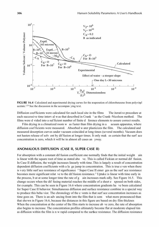
306 Hansen Solubility Parameters: A User’s Handbook
Diffusion coefficients were calculated for each local site in the films The iterative procedure ateach successive time interv al was that described in Crank 1 as the Crank–Nicolson method. Thefilms were d vided into a suf ficient number of finite d ference elements to assure correct results.
Film drying in a climatized room w as faster than film drying in a acuum apparatus, wherediffusion coef ficients were measured. Absorbed w ater plasticizes the film. The calculated andmeasured desorption curves under vacuum coincided at long times (several months). Vacuum doesnot hasten release of solv ent by dif fusion at longer times. It only mak es certain that the surf aceconcentration is zero, which it will be in almost all cases an yway.
ANOMALOUS DIFFUSION (CASE II, SUPER CASE II)
For absorption with a constant dif fusion coefficient one normally finds that the initial weight ainis linear with the square root of time as stated abo ve. This is called Fickian or normal dif fusion.In Case II diffusion, the weight increases linearly with time. This is largely a result of concentrationdependent diffusion coefficients with a la ge jump in concentration. This is true e ven when thereis very little surf ace resistance of significance 5 Super Case II emer ges as the surf ace resistancebecomes more significant relat ve to the dif fusion resistance.5 Uptake is linear with time early inthe process, b ut at some longer time the rate of g ain increases mark edly. See Figure 16.5. Thischange occurs when the dif fusing material reaches the middle of a sheet e xposed on both sides,for example. This can be seen in Figure 16.6 where concentration gradients ha ve been calculatedfor Super Case II behavior. Simultaneous diffusion and surface resistance combine in a special wayto produce this beha vior. The chronology of the e vents is that surf ace concentration increases astime goes on. There is an adv ancing front into the film that is som what more pronounced thanthat shown in Figure 16.6, because the distances in this figure are based on dry film thicknesWhen the concentration at the center of the film starts to increase ab ve zero, the rate of absorptionalso begins to increase. The concentration profiles ultimately become flat at moderate elapsed timas diffusion within the film is n w rapid compared to the surface resistance. The diffusion resistance
FIGURE 16.4 Calculated and experimental drying curves for the evaporation of chlorobenzene from polyvinylacetate.3,20 See the discussion in the accompan ying text.
Volu
me S
olve
nt /
Volu
me P
olym
er101
10
10-1
10-2
10-7 10-6 10-5 10-4Dot(L)2
10-3 10-2
DimensionslessT,
One day L=30 micronsEffect of water - a steeper slope
Experimental
Calculated
CS= OFor B=105
CS= OFor B=106
CS= OFor B=107
–CA–CA~MO
B=105B=106
B=107Exptl.22 microns
Exptl.165 microns
V2= 106
Vt= 1010
CA= 0.2B as indicated
7248_C016.fm Page 306 Wednesday, May 23, 2007 11:36 AM
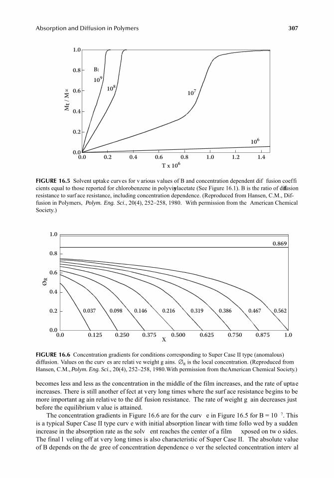
Absorption and Diffusion in Polymers 307
becomes less and less as the concentration in the middle of the film increases, and the rate of uptaeincreases. There is still another ef fect at very long times where the surf ace resistance begins to bemore important ag ain relative to the dif fusion resistance. The rate of weight g ain decreases justbefore the equilibrium v alue is attained.
The concentration gradients in Figure 16.6 are for the curv e in Figure 16.5 for B = 10 7. Thisis a typical Super Case II type curv e with initial absorption linear with time follo wed by a suddenincrease in the absorption rate as the solv ent reaches the center of a film xposed on tw o sides.The final l veling off at very long times is also characteristic of Super Case II. The absolute valueof B depends on the de gree of concentration dependence o ver the selected concentration interv al
FIGURE 16.5 Solvent uptake curves for v arious values of B and concentration dependent dif fusion coefficients equal to those reported for chlorobenzene in polyvinylacetate (See Figure 16.1). B is the ratio of diffusionresistance to surf ace resistance, including concentration dependence. (Reproduced from Hansen, C.M., Dif-fusion in Polymers, Polym. Eng. Sci., 20(4), 252–258, 1980. With permission from the American ChemicalSociety.)
FIGURE 16.6 Concentration gradients for conditions corresponding to Super Case II type (anomalous)diffusion. Values on the curv es are relati ve weight g ains. ∅R is the local concentration. (Reproduced fromHansen, C.M., Polym. Eng. Sci., 20(4), 252–258, 1980. With permission from the American Chemical Society.)
T x 1060.0 0.2 0.4 0.6 0.8 1.0 1.2 1.4
106
107108109B:
Mt /
M∝
1.0
0.8
0.6
0.4
0.2
0.0
ØR
1.0
0.8
0.6
0.4
0.2
0.00.0 0.125 0.250 0.375 0.500 0.625 0.750 0.875
0.869
0.5620.4670.3860.3190.2160.1460.0980.037
1.0X
7248_C016.fm Page 307 Wednesday, May 23, 2007 11:36 AM
308 Hansen Solubility Parameters: A User’s Handbook
in the given case. See Reference 5 for greater detail. The parameters chosen to calculate this curveare realistic.
GENERAL COMMENTS
Discussion of the v arious other e xplanations for anomalous dif fusion is be yond the scope of thischapter. These discussions are focused on time-dependent replication of the observ ed dif fusionphenomena, such as an advancing front,22 and on explanations based on stress relaxation phenomenaat the head of this adv ancing front.23,24 Whereas these may ha ve aspects of v alidity, they can onlybe convincing when the v erifiable sur ace resistances and the v erifiable xponential concentrationdependence of the dif fusion coefficient are also ta en into account. It w ould appear that enhancedstress relaxation, like the increase of dif fusion coefficient with sol ent concentration, is dependenton the increase in free v olume brought locally by the solv ent molecules themselv es. The meas-urement of surf ace resistances and concentration-dependent dif fusion coefficients did not requiruse of an y mathematical tools or e xplanations other than the dif fusion equation solv ed withappropriate initial and boundary conditions. There were adv ancing fronts in volved both in themathematics and in the samples in the e xperiments. The simple approach of solving the dif fusionequation with a v erifiable ( xponential) concentration-dependent dif fusion coefficient, along witappropriate and verifiable parameters for the boundary conditions, xplains and replicates both theabsorption and the desorption of solvents in polymers over an extremely large concentration range.This is true with and without significant sur ace resistance.
The methodology and concepts presented in this chapter on dif fusion in polymers combinedwith the methodology and concepts in the rest of this handbook should pro vide insight into man ysituations of industrial and theoretical interest. These include controlled release of drugs, absorptionand transport through polymeric packaging of v arious kinds, improved prediction of the beha viorof chemical protecti ve clothing, absorption into coatings, release of absorbed chemicals fromplastics, release of sterilization g as, etc.
CONCLUSION
Many organic liquids are aggressive with respect to many types of polymers. Predicting aggressivebehavior is important, and the absorption of the or ganic liquids into the polymers is a k ey factorin this respect. This absorption can be strongly af fected by both surf ace phenomena and the rateof diffusion within the bulk of the polymer. This chapter has emphasized the importance of surfaceresistance in this process. Additional material on dif fusion in polymers including simple mathe-matical descriptions of film drying by sol ent evaporation and so-called anomalous dif fusion havebeen included to present several aspects of the importance of surf ace resistance to contribute to itsbetter understanding.
There is no surf ace resistance to absorption where the absorbing molecules are small enoughand/or linear. When the challenge molecules are too lar ge or b ulky, no absorption occurs, e venthough Hansen solubility parameter considerations lead one to predict that this is clearly e xpected.The molecules can simply not get through the surface layer, and its resistance is therefore effectivelyinfinitely la ge. Between these extremes are situations where surf ace resistance necessarily affectsthe absorption process. Surface resistance becomes significant when molecules can be transporteaway from the surface into the bulk of the polymer f aster than they can be adsorbed/absorbed justat/in the surface.
The simple approach of solving the dif fusion equation with appropriate and v erifiable parameters for the boundary conditions e xplains and replicates both the absorption and desorption ofsolvents in polymers o ver an extremely large concentration range. It is not yet possible to predict
7248_C016.fm Page 308 Wednesday, May 23, 2007 11:36 AM
Absorption and Diffusion in Polymers 309
which systems will gi ve significant sur ace resistance to absorption. Experimental studies are stillrequired, but some similarity in HSP must be present for absorption to occur in an y event.
REFERENCES
1. Crank, J., The Mathematics of Diffusion, Oxford University Press, Oxford, 1956.2. Hansen, C.M. and Hansen, K.M., Solubility parameter prediction of the barrier properties of chemical
protective clothing, Performance of Protective Clothing: Second Symposium, ASTM STP 989, Mans-dorf, S.Z., Sager, R., and Nielsen, A.P., Eds., American Society for Testing and Materials, Philadelphia,PA, 1988, pp. 197–208.
3. Hansen, C.M., The Three Dimensional Solubility Parameter and Solvent Diffusion Coefficient, TheirImportance in Surface Coating Formulation, Doctoral dissertation, Danish Technical Press, Copen-hagen, 1967.
4. Hansen, C.M., The measurement of concentration-dependent diffusion coefficients — the xponentialcase, Ind. Eng. Chem. Fundam., 6(4), 609–614, 1967.
5. Hansen, C.M., Diffusion in polymers, Polym. Eng. Sci., 20(4), 252–258, 1980.6. Hansen, C.M., Aspects of solubility , surf aces, and dif fusion in polymers, Prog. Org. Coat., 51(1),
55–66, 2004.7. Korsmeyer, R.W., Von Meerwall, E., and Peppas, N.A., Solute and penetrant dif fusion in swellable
polymers. II. Verification of theoretical models, J. Polym. Sci.: Polym. Phys. Ed., 24, 409–434, 1986.8. Nielsen, T.B. and Hansen, C.M., Significance of sur ace resistance in absorption by polymers, Ind.
Eng. Chem. Res., 44(11), 3959–3965, 2005.9. Huldén, M. and Hansen, C.M., Water permeation in coatings, Prog. Org. Coat., 13(3/4), 171–194,
1985.10. Nilsson, E. and Hansen, C.M., Evaporation and vapor diffusion resistance in permeation measurements
by the cup method, J. Coat. Technol., 53(680), 61–64, 1981.11. Hansen, C.M., Potential errors in water/water vapor permeation measurements using the cup method,
Färg och Lack, 39(3), 57–60, 1993.12. Abbott, R.J., Chudek, J.A., Hunter , G., and Squires, L., Skin layer ef fects on the dif fusion of carbon
tetrachloride into injection moulded polyprop ylene studied by 1H NMR microimaging, J. Mater. Sci.Lett., 15, 1108–1110, 1996.
13. McDonald, P.J., Godward, J., Sackin, R., and Sear, R.P., Surface flux limited di fusion of solvent intopolymer, Macromolecules, 34, 1048–1057, 2001.
14. Shankar, V., Influence of inter acial resistance on kinetics of sorption, Polymer, 22, 748–752, 1981.15. Grayson, M.A., P ao, P.S., and Wolf, C.J., Transport of meth ylene chloride in poly(aryl-ether -ether-
ketone) (PEEK), J. Polym. Sci.: Part B: Polym. Phys., 25, 935–945, 1987.16. Kim, N.K. and Kammerme yer, K., Actual concentration profiles in membrane permeation, Sep. Sci.,
5(6), 679–697, 1970.17. Hwang, S.T. and Kammerme yer, K., Ef fect of thickness on permeability , in Permeability of Plastic
Films and Coatings, Hopfenberg, H.B. Ed., Plenum, Ne w York, 1974, pp. 197–205.18. Skaarup, K., Abstract, Lecture at Nordic Polymer Days, 1988; Grænseflademodstand ved Diffusion-
sprocesser I Polymerer, Danmarks Ingeniør Akadami, K emiafdelingen (in Danish) 1981, Surf aceResistance in Diffusion Processes in Polymers (in English).
19. Marom, G., The role of w ater transport in composite materials, in Polymer Permeability, Comyn, J.,Ed., Elsevier, London, 1985, chap. 9.
20. Hansen, C.M., A mathematical description of film drying by sol ent evaporation, J. Oil Colour Chem.Assn., 51(1), 27–43, 1968.
21. Hansen, C.M., Dif fusion coef ficient measurements by sol ent absorption in concentrated polymersolutions, J. Appl. Polym. Sci., 26, 3311–3315, 1981.
22. Windle, A.H., Case II sorption, in Polymer Permeability, Comyn, J., Ed., Else vier, London, 1985,chap. 3.
23. Petropoulos, J.H., Interpretation of anomalous sorption kinetics in polymer-penetrant systems in termsof a time-dependent solubility coef ficient, J. Poly. Sci. Polym. Phys. Ed., 22, 1885–1900, 1984.
7248_C016.fm Page 309 Wednesday, May 23, 2007 11:36 AM

310 Hansen Solubility Parameters: A User’s Handbook
24. Sanopoulou, M., and Petropolous, J.H., Systematic analysis and model interpretation of micromolec-ular non-fickian sorption kinetics in polymer films Macromolecules, 34, 1400–1410, 2001.
7248_C016.fm Page 310 Wednesday, May 23, 2007 11:36 AM
311
17
Applications — Safety and Environment
Charles M. Hansen
ABSTRACT
Hansen solubility parameters (HSP) can be used to gain insight into many safety and environmentalissues. These include substitution to more desirable materials, products, and processes, where alisting of solv ents having HSP similarity to the one(s) to be substituted pro vides an o verview ofthe potential choices for impro vement. Selection of suitable chemical protecti ve clothing can beimproved by considering HSP correlations of breakthrough time. Ev aluating risks for inadv ertentchemical uptak e in plastic can be helped by HSP correlations of chemical resistance and/orpermeation phenomena. Similarity of HSP suggests which chemicals are most lik ely to be rapidlyabsorbed into given plastic types. These same approaches can be used to e valuate the potential foruptake of chemicals through human skin.
INTRODUCTION
Many organic materials are potential safety hazards. They can also be harmful to the en vironment.Unfortunately, it is often a matter of e xperience before the risks are unco vered because of damagebeing done. Thus, over the years, there ha ve been a series of substitutions with or without the aid ofHSP to eliminate or to at least reduce such problems. An example is the lack of emphasis on the useof some eth ylene glycol ethers as solv ents because of their teratogenic ef fects, whereas the y wereused in massi ve quantities earlier . The problem of replacing ozone-depleting chemicals is a caseinvolving the e xternal environment. This is discussed a great deal in Chapter 11. Other lar ge-scalesubstitutions can also be cited where HSP can aid, b ut a list of this type is not the purpose of thischapter. The emphasis here is on the use of sound formulating principles to reduce the potential hazardin terms of reformulation or substitution. When a satisfactory substitution cannot be found, personalprotection of one type or another may be required. Here, ag ain, HSP can help.
Evaluating other forms of en vironmental risks can be aided by using HSP . An e xample is theoccasional misuse of plastic containers normally used for soft drinks to store chemicals such asherbicides and pesticides. These are lik ely to dif fuse into the plastic container w all itself, makingcustomary washing insufficient. HSP can indicate which chemicals can do this, thus pr viding infor-mation on the means to impro ve handling of the problem. This type of information can be generatedfor any polymer where HSP correlations of chemical resistance, weight g ain, etc., can be generated.
All of these situations are discussed in more detail in the follo wing.
SUBSTITUTION
Substitution involves the replacement of a potentially dangerous process or chemical with a ne wprocess or chemical ha ving less hazardous properties. The hazards can be judged using acceptedapproaches — for e xample, labeling requirements, toxicology assessments, biode gradability, andphysical properties for the chemical or products. The volatility of products is also a significan
7248_C017.fm Page 311 Wednesday, May 23, 2007 11:40 AM
312
Hansen Solubility Parameters: A User’s Handbook
factor with lower volatility being preferred due to reduced w orkplace concentrations and reducedreplacement requirements for cleaners and the like which often recirculate in nearly closed systems.On the other hand, the problem should not just be transferred from the air e xhaust system to thesewer.
The use of technologies in volving w ater or mechanical methods, such as mechanical jointsrather than the use of solv ents, are preferred. Examples of preferred coatings technologies are theuse of po wders which fl w at higher temperatures or polymerization by radiation, both of whichuse solvent-free base products to pro vide the coating. Other product types which may be tar getedinclude cutting fluids, cleaners of arious types, adhesives, sealers, and fillers
In general, one primarily wishes to substitute for
• Carcinogens or suspected carcinogens• Substances with risk phrases for being very toxic, toxic, allergenic, carcinogenic, terato-
genic, mutagenic, or causing cumulati ve or irreversible effects• Substances with moderate or serious aquatic toxicity• Nonbiodegradable substances• Substances with high predicted aquatic ef fects — for example, chemicals which prefer -
entially distribute to a nonaqueous phase to a v ery high degree
Efforts should be made to de velop products with the lo west possible hazard. Those who haveread the earlier chapters in this book will immediately recognize HSP as a tool to aid in thesubstitution and systematic formulation for reduced safety and en vironmental risks. A key elementin this is a listing of solv ents where those most resembling the candidate for substitution are at thetop of the list. The program described in Chapter 1 can do this by entering the HSP for the solv entto be replaced and requesting a listing with those solv ents most similar to it (i.e., the lo west REDnumbers as defined in Chapter 1, Equations 1.10) at the top of the list. One must then sort througthese potential replacement candidates using other information to arri ve at a better alternati ve.
It is clear that much more data than HSP are required to make the desired substitutions. However,a further discussion of this is be yond the scope of this chapter , which emphasizes HSP only . Thecurrently used HSP techniques and correlations can aid in some aspects of substitution, and it isanticipated that future correlations will help in this endeavor. Many cases of substitutions in practicehave been listed by Goldschmidt,
1
Olsen,
2
Soerensen and Petersen,
3
and Filskov et al.
4
A long listof references for the Danish experience with occupational risks and solutions is given by Soerensenand Petersen.
3
ALTERNATIVE SYSTEMS
Alternative systems with less solv ent or no solv ent ha ve been focused on by the coatings andprinting ink industries for man y years. Examples of such systems are coatings with higher solids,radiation-curable inks and coatings, po wder coatings, electrodeposition coatings, and other w ater-reducible products. It might appear that solvent technology and use of HSP will not be as importantas it has been in the past. This is not the case, ho wever, as demonstrated in earlier chapters. F orexample, HSP principles can be used to aid in impro ved stability and adhesion, to predict poly-mer/filler interactions, to impr ve barrier polymers, and to aid in understanding some biologicalphenomena.
The use of solv ents in alternati ve coatings systems has been the topic of se veral pre viouspublications by the author .
5–8
Some general principles of solv ent selection have been discussed inChapter 8 and earlier ,
9
as well as else where more recently.
10
7248_C017.fm Page 312 Wednesday, May 23, 2007 11:40 AM
Applications — Safety and Environment
313
SOLVENT FORMULATION AND PERSONAL PROTECTION FOR LEAST RISK
Solubility parameter principles have been used in formulating alternative, low VOC (volatile organiccompound) products. A number of the general formulation principles can be briefly stated for thsake of completeness. These include the follo wing:
1. Solvents with lower viscosity most often lead to polymer solutions with lo wer viscosity.Such a change allo ws the use of higher solids at the original viscosity . However, thesemay evaporate more rapidly and can be e xpected to have a lower flash point
2. Solvents with linear and smaller structures diffuse more rapidly than those with branchedand larger structures. Inclusion of slo wer evaporating, more linear solv ents can hastenthe through-drying of a coating.
3. Two (or more) mix ed solvents with lower labeling requirements may be able to replacea single solvent. HSP can be used in this type of endea vor.
4. The surface tension of w ater-reducible coatings can often be significantly reduced brelatively small additions of ethanol or other alcohol-type solv ent. These can, of course,also be used in conjunction with other surf ace active materials.
Materials with least potential risk are to be used in the Nordic countries where ver possible.The risk must be indicated by the seller/producer in terms of a labeling code. The risk can then beassessed by users or , perhaps more specificall , by primarily professional users. Such labeling isrequired on paints, printing inks, cleaners, or for an y product containing significant amounts osolvent or hazardous chemical. The labeling code dictates the personal protection required for theproduct, depending on the way it is used. Spraying product in a smaller room with limited ventilationrequires much more protection than applying paint with a brush outdoors. Tables ha ve beenpublished which gi ve the protection required (glo ves, dust mask, fresh air mask, body suit, etc.)for a gi ven set of application conditions for a wide v ariety of products from paints and printinginks through cleaners.
11
A key element in these tables is the labeling code de veloped in Denmarkaccording to the MAL (in Danish: Maleteknisk e Arbejshygieniske Luftbehov) system. For presentpurposes, this is translated as the F AN (fresh air number). Higher MAL/F AN dictate that moreextensive personal protection is required.
THE DANISH MAL SYSTEM — THE FAN
12
As indicated pre viously, the quality of the w orking environment must be considered in all caseswhere organic solvents are being used. The Danish MAL system or other labeling system can besystematically used for this purpose. The Danish MAL reflects the cubic meters of fresh air requirefor ventilation of 1 l of product to belo w the threshold limit value (TLV). This number is modifieby a constant, depending on the e vaporation rate (or v apor pressure). Higher e vaporation ratesimply greater hazard, so the multiplier is lar ger.
The concept behind the MAL system can be better understood in English by translating theMAL number as the FAN. Other numbers in addition to the TLV/GV/OEL (occupational exposurelimit) and FAN have been generated to help e valuate risks by inclusion of e vaporation rate/vaporpressure considerations. The vapor pressure di vided by the TLV is called the
vapor hazard ratio
(VHR) and the actual calculated vapor composition (using activity coefficients) d vided by the TLVhas been called
SUBFAC.
A Danish publication comparing se veral of these is a vailable.
4
Todemonstrate the principle, the simple MAL = F AN has been tab ulated in Table 17.1 for se veralsolvents.
7248_C017.fm Page 313 Wednesday, May 23, 2007 11:40 AM
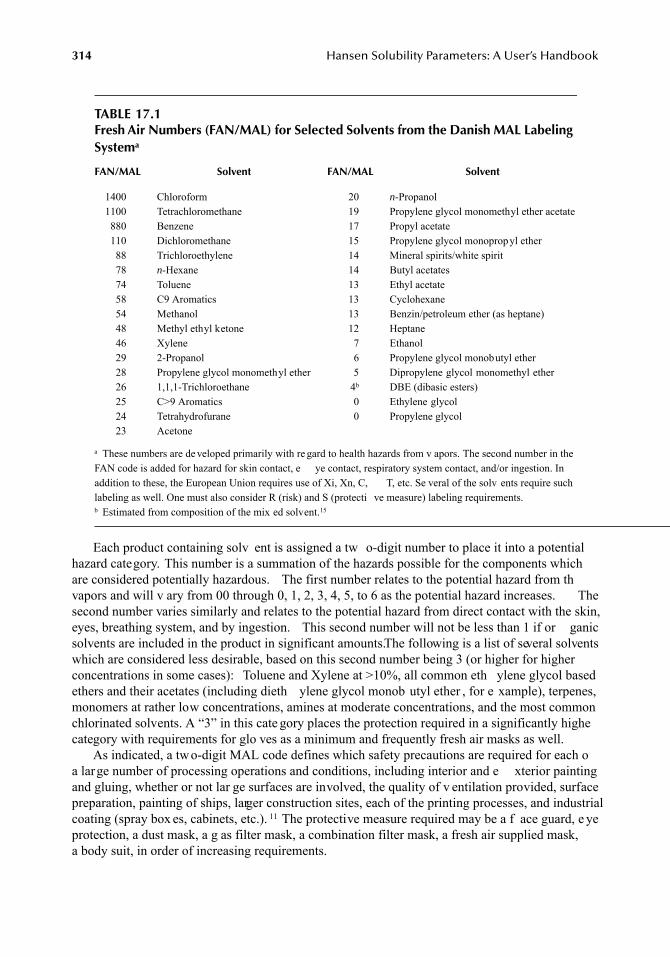
314
Hansen Solubility Parameters: A User’s Handbook
Each product containing solv ent is assigned a tw o-digit number to place it into a potentialhazard category. This number is a summation of the hazards possible for the components whichare considered potentially hazardous. The first number relates to the potential hazard from thvapors and will v ary from 00 through 0, 1, 2, 3, 4, 5, to 6 as the potential hazard increases. Thesecond number varies similarly and relates to the potential hazard from direct contact with the skin,eyes, breathing system, and by ingestion. This second number will not be less than 1 if or ganicsolvents are included in the product in significant amounts.The following is a list of several solventswhich are considered less desirable, based on this second number being 3 (or higher for higherconcentrations in some cases): Toluene and Xylene at >10%, all common eth ylene glycol basedethers and their acetates (including dieth ylene glycol monob utyl ether , for e xample), terpenes,monomers at rather low concentrations, amines at moderate concentrations, and the most commonchlorinated solvents. A “3” in this cate gory places the protection required in a significantly highecategory with requirements for glo ves as a minimum and frequently fresh air masks as well.
As indicated, a two-digit MAL code defines which safety precautions are required for each oa large number of processing operations and conditions, including interior and e xterior paintingand gluing, whether or not lar ge surfaces are involved, the quality of v entilation provided, surfacepreparation, painting of ships, larger construction sites, each of the printing processes, and industrialcoating (spray box es, cabinets, etc.).
11
The protective measure required may be a f ace guard, e yeprotection, a dust mask, a g as filter mask, a combination filter mask, a fresh air supplied mask, a body suit, in order of increasing requirements.
TABLE 17.1Fresh Air Numbers (FAN/MAL) for Selected Solvents from the Danish MAL Labeling System
a
FAN/MAL Solvent FAN/MAL Solvent
1400 Chloroform 20
n
-Propanol1100 Tetrachloromethane 19 Propylene glycol monomethyl ether acetate880 Benzene 17 Propyl acetate110 Dichloromethane 15 Propylene glycol monopropyl ether88 Trichloroethylene 14 Mineral spirits/white spirit78
n
-Hexane 14 Butyl acetates74 Toluene 13 Ethyl acetate58 C9 Aromatics 13 Cyclohexane54 Methanol 13 Benzin/petroleum ether (as heptane)48 Methyl ethyl ketone 12 Heptane46 Xylene 7 Ethanol29 2-Propanol 6 Propylene glycol monobutyl ether28 Propylene glycol monomethyl ether 5 Dipropylene glycol monomethyl ether26 1,1,1-Trichloroethane 4
b
DBE (dibasic esters)
25 C>9 Aromatics 0 Ethylene glycol24 Tetrahydrofurane 0 Propylene glycol23 Acetone
a
These numbers are de veloped primarily with re gard to health hazards from v apors. The second number in theFAN code is added for hazard for skin contact, e ye contact, respiratory system contact, and/or ingestion. Inaddition to these, the European Union requires use of Xi, Xn, C, T, etc. Se veral of the solv ents require suchlabeling as well. One must also consider R (risk) and S (protecti ve measure) labeling requirements.
b
Estimated from composition of the mix ed solvent.
15
7248_C017.fm Page 314 Wednesday, May 23, 2007 11:40 AM
Applications — Safety and Environment
315
Examples of complete labeling of products and solv ents are beyond the scope of this chapter .The purpose of the discussion is to suggest that possible substituting solv ents can be listed, suchas in Table 17.1, in an attempt to find a substitute with a l wer labeling requirement.
Systematic consideration of labeling requirements is becoming a significant parameter icommercial applications of solv ents and products containing solv ents. This is happening all o verthe world, both with regard to worker safety as well as to the external environment. Such a procedurehas been used to arri ve at optimum commercially useful solv ent compositions with the lo westpossible risk for w orkers in the serigraphic printing industry as described in Danish patents DK153797B (1989) and DK 160883 (1991) which correspond to European patents EP 0 205 505 B1and EP 0 270 654 B
13,14
The preferred compositions reduce the MAL number to a minimum andalso consider lo west possible internationally required labels as a requirement. The lo w labelrequirements of DBE (dibasic esters) ha ve been emphasized in comparison with other solv ents.
15
Systematic solvent selection procedures have also been strongly suggested for use in the selectionof solvents for restoring older paintings.
16
This is discussed in Chapter 5.
SELECTION OF CHEMICAL PROTECTIVE CLOTHING
HSP correlations for barrier properties of some types of chemical protecti ve clothing are gi ven inChapter 13, Table 13.1. These correlations are based on data presented by F orsberg and Kieth.
17
Other examples of HSP correlations of barrier properties of protecti ve clothing are discussed inChapter 13. Earlier publications also include HSP correlations of barrier properties of chemicalprotective clothing.
18–21
The procedure for using these correlations requires kno wledge of the HSP of the chemicalsinvolved. These may be found in a suitable table or can be calculated according to the proceduresoutlined in Chapter 1. One then e valuates the RED number for the situation of interest. The REDnumber is discussed in Chapter 1 (Equation 1.10). If this number is less than 1, the system in notexpected to be suitable for use. If the RED number is close to 1.0, there may be some doubt aboutthe recommendation. RED numbers significantly greater than 1.0 can be considered for use. Asdiscussed in Chapter 13, the molecular size of the chemical in volved is important in these e valu-ations.
The major use of such correlations is to e valuate potential barrier types for chemicals wheretest results are not available. One can usually divide the results into groups of clearly not acceptable,questionable, and worthy of further consideration.
There have been recent attempts to impro ve on the direct correlation of breakthrough timesand permeation rates with HSP by trying to estimate the solubility and dif fusion coef ficientseparately using HSP.
22–25
These efforts have been discussed in Chapter 2 and Chapter 13.
UPTAKE OF CONTENTS BY A PLASTIC CONTAINER
Plastic containers have become increasingly popular in recent years. They have many advantages(which will not be discussed here), but there is also one disadvantage that HSP can shed more lighton. This is the f act that plastic materials are able to absorb v arious liquids to some e xtent. Theextent of absorption clearly depends on the HSP of the plastic used in the container compared withthe HSP of the liquid which is in contact with it. Containers in contact with food ha ve been testedwell for suitability for this purpose, including barrier properties relati ve to the contents. This is notthe point of the present discussion. A problem e xists with the inadv ertent storage of hazardousliquids in the plastic container prior to its e xpected recycling as a container for a food or beverage.Many types of liquids can be temporarily stored in such containers. Whereas the earlier glass ormetal containers could not absorb potentially dangerous materials, a plastic container can do this.A simple w ashing operation cannot be e xpected to remo ve all of the absorbed material. Washing
7248_C017.fm Page 315 Wednesday, May 23, 2007 11:40 AM
316
Hansen Solubility Parameters: A User’s Handbook
only removes what is on the surface or what can diffuse to the surface during the washing process,which presumably takes place at some higher temperature.
HSP concepts can focus attention on the types of chemicals that can absorb into a gi ven typeof plastic container. This is useful information in terms of what analyses should be performed priorto recycling. The principles discussed here can possibly contrib ute in other w ays to impro ve therecycling process based on the increased le vel of knowledge. There may be other w ays to reducethe problem.
SKIN PENETRATION
Human skin is a complicated system. Nevertheless, it has been possible to characterize some aspectsof the beha vior of human skin by HSP . The HSP found in a correlation of permeation rates ofliquids in contact with viable skin
26
are similar to those found for the swelling of psoriasis scales.
27,28
This has been discussed in Chapter 15 in more detail, b ut also relates to w orker safety. The HSPfor these correlations are included in Chapter 13, Table 13.1 and Chapter 15, Table 15.1.
A skin penetration w arning has been attached to man y liquids taken up in the lists of limitingvalues for workplaces which are published in dif ferent countries. It was found earlier based on theHSP correlation with the swelling of psoriasis scales that this practice could be misleading, as HSPpredicted man y liquids without this w arning also swelled psoriasis scales (k eratin) and couldtherefore be e xpected to penetrate the skin.
27
The lack of a skin penetration w arning for theseliquids is partly attributable to the fact that this warning is based on experience. The bad experiencegiving the warning includes a combination of all effects, most notably the combination of dose andtoxicity, rather than the potential dose ef fect only which is indicated by similarity of HSP . Earlierdiscussions also led to the impression that those in volved in this area did not consider the swellingof psoriasis skin as having relevance to the permeation of li ving skin. The finding that comparabl
δ
P
and
δ
H
are found from correlating the permeation rates of solv ents through living skin is a ne winput into this discussion. It is recognized that the
δ
D
parameter is dif ferent, but reasons for thisare not clear. An improved HSP correlation of the permeation rates of solv ents through living skinbased on a lar ger number of solv ents than the 13 included in the w ork of Ursin et al.
26
is perhapsrequired to give improved predictions in marginal cases, i.e., those near the boundaries of the HSPsphere describing the situation. The size and shape of the penetrating liquid molecules must alsobe considered.
Predictions of the barrier properties of viable human skin should recei ve more attention. Inaddition, there is some discussion of the use of HSP in this respect in Chapter 15.
TRANSPORT PHENOMENA
Many chemicals have been the subject for concern in the past for v arious environmental reasons.Among these is the presence in artic re gions of chemicals that do not readily break do wn. Somechlorinated materials, such as pentachlorophenol, ha ve the ability to penetrate skin and w ood, andto be transported by animals, birds, or aquatic species after the y have taken them up. The HSP ofgiven chemicals can gi ve a clue as to whether or not the y can follo w the same pathw ays in theenvironment. An example is given in Table 17.2 where the HSP for tetrabromobisphenol A (TBBPA)are reported along with the similarity of these with other rele vant materials.
TBBPA has a distance from Pentachlorophenol (PCP) of only 3.5 units. This is very close andmeans that where PCP is soluble, TBBPA will also be soluble.
TBBPA has a distance from the center of the spherical HSP correlation for Lignin solubilityof only 6.8 units. Dividing this by the radius of the sphere to find the RED number (relat ve energydifference) shows that it is well within the solubility re gion with a RED of 0.5. TBBPA is readilysoluble in lignin (w ood).
7248_C017.fm Page 316 Wednesday, May 23, 2007 11:40 AM
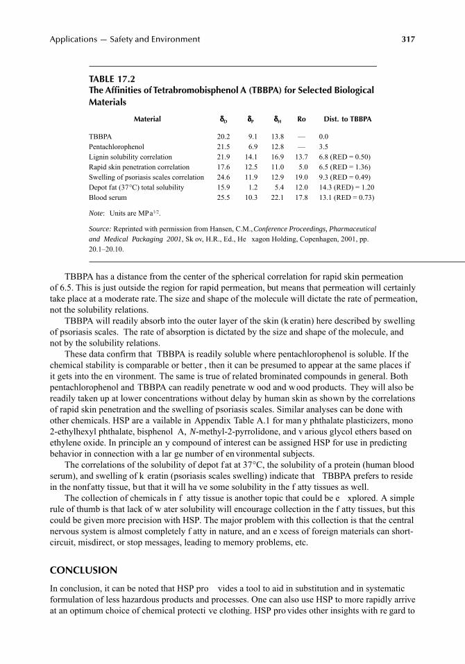
Applications — Safety and Environment
317
TBBPA has a distance from the center of the spherical correlation for rapid skin permeationof 6.5. This is just outside the region for rapid permeation, but means that permeation will certainlytake place at a moderate rate. The size and shape of the molecule will dictate the rate of permeation,not the solubility relations.
TBBPA will readily absorb into the outer layer of the skin (k eratin) here described by swellingof psoriasis scales. The rate of absorption is dictated by the size and shape of the molecule, andnot by the solubility relations.
These data confirm that TBBPA is readily soluble where pentachlorophenol is soluble. If thechemical stability is comparable or better , then it can be presumed to appear at the same places ifit gets into the en vironment. The same is true of related brominated compounds in general. Bothpentachlorophenol and TBBPA can readily penetrate w ood and wood products. They will also bereadily taken up at lower concentrations without delay by human skin as shown by the correlationsof rapid skin penetration and the swelling of psoriasis scales. Similar analyses can be done withother chemicals. HSP are a vailable in Appendix Table A.1 for man y phthalate plasticizers, mono2-ethylhexyl phthalate, bisphenol A,
N
-methyl-2-pyrrolidone, and v arious glycol ethers based onethylene oxide. In principle an y compound of interest can be assigned HSP for use in predictingbehavior in connection with a lar ge number of en vironmental subjects.
The correlations of the solubility of depot f at at 37
°
C, the solubility of a protein (human bloodserum), and swelling of k eratin (psoriasis scales swelling) indicate that TBBPA prefers to residein the nonfatty tissue, but that it will ha ve some solubility in the f atty tissues as well.
The collection of chemicals in f atty tissue is another topic that could be e xplored. A simplerule of thumb is that lack of w ater solubility will encourage collection in the f atty tissues, but thiscould be given more precision with HSP. The major problem with this collection is that the centralnervous system is almost completely f atty in nature, and an e xcess of foreign materials can short-circuit, misdirect, or stop messages, leading to memory problems, etc.
CONCLUSION
In conclusion, it can be noted that HSP pro vides a tool to aid in substitution and in systematicformulation of less hazardous products and processes. One can also use HSP to more rapidly arriveat an optimum choice of chemical protecti ve clothing. HSP pro vides other insights with re gard to
TABLE 17.2The Affinities of Tetrabromobisphenol A (TBBPA) for Selected Biological Materials
Material
δδδδ
D
δδδδ
P
δδδδ
H
Ro Dist. to TBBPA
TBBPA 20.2 9.1 13.8 — 0.0Pentachlorophenol 21.5 6.9 12.8 — 3.5Lignin solubility correlation 21.9 14.1 16.9 13.7 6.8 (RED = 0.50)Rapid skin penetration correlation 17.6 12.5 11.0 5.0 6.5 (RED = 1.36)Swelling of psoriasis scales correlation 24.6 11.9 12.9 19.0 9.3 (RED = 0.49)Depot fat (37
°
C) total solubility 15.9 1.2 5.4 12.0 14.3 (RED) = 1.20Blood serum 25.5 10.3 22.1 17.8 13.1 (RED = 0.73)
Note
: Units are MPa
1/2
.
Source:
Reprinted with permission from Hansen, C.M.,
Conference Proceedings, Pharmaceuticaland Medical Packaging 2001
, Sk ov, H.R., Ed., He xagon Holding, Copenhagen, 2001, pp.20.1–20.10.
7248_C017.fm Page 317 Wednesday, May 23, 2007 11:40 AM
318
Hansen Solubility Parameters: A User’s Handbook
uptake of undesirable chemicals in the human skin, in packaging materials, and perhaps e ven in awide variety of other materials such as those found in nature.
REFERENCES
1. Goldschmidt, G., An analytical approach for reducing workplace health hazards through substitution,
Am. Ind. Hyg. Assoc. J.
, 54, 36–43, January 1993.2. Olsen, E., Substitution: a method to fulfill the orking environment law for air quality (Substitution:
En Metode til at Overholde Arbejdsmiljoelovens Krav til Luftkvaliteten, in Danish),
Dan. Kemi
, 67(5),146–153, 1986.
3. Soerensen, F. and Petersen, H.J.S., Substitution of hazardous chemicals and the Danish e xperience,
Occup. Hyg.,
1, 261–278, 1995.4. Filskov, P., Goldschmidt, G., Hansen, M.K., Höglund, L., Johansen, T., Pedersen, C.L., and Wibroe,
L., Substitution in Practice — Experience from BST (Substitution i Praksis — Erf aringer fra BST),Arbejsmiljøfondet, in Danish), Copenhagen, 1989.
5. Hansen, C.M., Solv ents in w ater-borne coatings,
Ind. Eng. Chem. Prod. Res. Dev
., 16(3), 266–268,1977.
6. Hansen, C.M., Organic solvents in high solids and w ater-reducible coatings,
Prog. Org. Coat
., 10(3),331–352, 1982.
7. Holten-Andersen, J. and Hansen, C.M., Solv ent and w ater e vaporation from coatings,
Prog. Org.Coat
., 11(3), 219–240, 1983.8. Saarnak, A. and Hansen, C.M., Ev aporation from high solids coatings (A vdunstningen Från LF-
Fårger),
Färg och Lack
, in Swedish, 30(5), 100–105, 1984.9. Hansen, C.M., Solvents for coatings,
Chem. Technol
., 2(9), 547–553, 1972.10. Wu, D.T., F ormulating solv ents to remo ve hazardous air pollutants,
Polym. Paint Colour J
., 185,20–23, December 1995.
11. Anonymous, Directive on Work with Products Having Codes (Bekendtgørelse om arbejde med kode-nummererede produkter, Arbejdstilsynets Bekendtgørelse nr.302 af 13. maj 1993, in Danish), DanishDirectorate for Labor Inspection.
12. Anonymous, Directi ve on Determination of Codes (
Bekendtgørelse om fastsættelse af kodenumre,Arbejdstilsynets bekendtgørelse nr. 301 af 13 maj 1993,
in Danish), Danish Directorate for LaborInspection.
13. Madsen, C.H. and Hansen, C.M., EP 0 205 505 B1, 1988. Assigned to CPS K emi Aps (Now a partof the Autotype/MacDermid Concern).
14. Madsen, C.H. and Hansen, C.M., EP 0 270 654 B1, 1991. Assigned to CPS K emi Aps (Now a partof the Autotype/MacDermid Concern).
15. Altnau, G., Risik opotentiale v on Lösemitteln systematisch be werten,
Farbe+Lack
, 103(9), 34–37,1997; Systematic Evaluation of Risk Potentials of Solv ents,
Eur. Coat. J
., 6/98, 454–457, 1998.
16.
Hansen, C.M., Conserv ation and Solubility P arameters, Nordic Conserv ation Congress Preprints,Copenhagen, 1994, pp. 1–13.
17. Forsberg, K. and Kieth, L.H.,
Chemical Protective Clothing Performance Index
, 4th ed., InstantReference Sources, Inc., Austin, TX, 1991.
18. Hansen, C.M., The systematic choice of material in personal protection equipment for organic solventsin safety and health aspects of or ganic solvents,
Progress in Chemical and Biological Research 220
,Riihimäki, V. and Ulfvarson, U., Eds., Alan R. Liss, Ne w York, 1986, pp. 297–302.
19. Hansen, C.M. and Hansen, K.M., Which gloves should I put on? (Hvilk e Handsker Skal Je g TagePå?, in Danish),
Färg och Lack
, 33(3), 45–49, 1987.20. Hansen, C.M. and Hansen, K.M., Solubility parameter prediction of the barrier properties of chemical
protective clothing,
Performance of Protective Clothing: Second Symposium
, ASTM STP 989, Mans-dorf, S.Z., Sager, R., and Nielsen, A.P., Eds., American Society for Testing and Materials, Philadelphia,PA, 1988, pp. 197–208.
7248_C017.fm Page 318 Wednesday, May 23, 2007 11:40 AM
Applications — Safety and Environment
319
21. Hansen, C.M., Billing, C.B., and Bentz, A.P., Selection and use of molecular parameters to predictpermeation through fluoropolyme -based protective clothing materials,
The Performance of ProtectiveClothing
; Fourth Volume, ASTM STP 1133, McBriarty, J.P. and Henry, N.W., Eds., American Societyfor Testing and Materials, Philadelphia, P A, 1992, pp. 894–907.
22. Zellers, E.T., Three-dimensional solubility parameters and chemical protecti ve clothing permeation.I. Modeling the solubility of organic solvents in Viton
®
gloves,
J. Appl. Polym. Sci.
, 50, 513–530, 1993.23. Zellers, E.T . and Zhang, G.-Z., Three-dimensional solubility parameters and chemical protecti ve
clothing permeation. II. Modeling diffusion coefficients, breakthrough times, and steady-state permeation rates of or ganic solvents in Viton
®
gloves,
J. Appl. Polym. Sci
., 50, 531–540, 1993.24. Zellers, E.T., Anna, D.H., Sulewski, R., and Wei, X., Critical analysis of the graphical determination
of Hansen’s solubility parameters for lightly crosslinked polymers
, J. Appl. Polym. Sci
., 62, 2069–2080,1996.
25. Zellers, E.T., Anna, D.H., Sule wski, R., and Wei, X., Impro ved methods for the determination ofHansen’s solubility parameters and the estimation of solv ent uptake for lightly crosslinked polymers,
J. Appl. Polym. Sci
., 62, 2081–2096, 1996.26. Ursin, C., Hansen, C.M., Van Dyk, J.W., Jensen, P.O., Christensen, I.J., and Ebbehoej, J., Permeability
of commercial solvents through living human skin,
Am. Ind. Hyg. Assoc. J.
, 56, 651–660, 1995.27. Hansen, C.M., The Absorption of Liquids into the Skin, Report No. T 3-82, Scandinavian Paint and
Printing Ink Research Institute, Hoersholm, Denmark, 1982.28. Hansen, C.M. and Andersen, B.H., The affinities of o ganic solvents in biological systems,
Am. Ind.Hyg. Assoc. J
., 49(6), 301–308, 1988.
7248_C017.fm Page 319 Wednesday, May 23, 2007 11:40 AM

7248_C017.fm Page 320 Wednesday, May 23, 2007 11:40 AM
321
18
The Future
Charles M. Hansen
ABSTRACT
Hansen solubility parameters (HSP) help to quantify the statements “lik e dissolves like” and “lik eseeks like.” These parameters have found use in many fields of research and practice, primarily becaustheir unique predictive capabilities are based on sound theoretical principles. HSP ha ve extended theoriginal Hildebrand single solubility parameter approach by quantitati vely taking into account themolecular permanent dipole–permanent dipole and molecular h ydrogen bonding (electron inter -change) interactions. HSP and the Prigogine corresponding states theory of polymer solutions aremutually confirming with r gard to treatment of specific interactions, as sh wn in Chapter 2. This isimportant, as it confirms that the HSP correlations must continue to include a constant not too diferentfrom the currently used “4” (or 0.25). This is necessary to dif ferentiate between the atomic (
δ
D
) andthe molecular (specific) interactions
δ
P
and
δ
H
). Neglecting this differentiation will lead to misinter -pretations. The geometric mean a verage for the interaction of unlik e molecules is inherently used inthe Hildebrand approach and in the HSP approach as well. This same mean must be used in thePrigogine corresponding states theory if agreement is to be found with the HSP correlations presentedin this book. As the agreement is general, the conclusion must be that the geometric mean can beused to average not only dispersion interactions b ut also those attrib utable to permanent dipoles andto hydrogen bonding. These findings h ve been supported more recently by the statistical thermody-namics approach of P anayiotou and co workers summarized in Chapter 3. This approach allo wsindependent calculation of each of the three parameters.
Based on the large number of current uses of HSP, one can easily suppose that there are man ymore practical uses which remain to be discovered and developed. One need not necessarily extendits theoretical scope to accomplish this. The existing data can be used in a strictly empirical mannerif so desired. Ho wever, a glimpse has been gi ven of a v ery general energetic approach to system-atically predict and control molecular interactions among man y materials of widely dif ferentcomposition. The general predictions possible for these ph ysical interactions ha ve been demon-strated for both b ulk phenomena (solubility , swelling, compatibility) and surf ace phenomena(adsorption, dewetting, spontaneous spreading). In the future, the theory should be e xplored andused with this general applicability in mind.
Problems and situations clearly needing further attention are discussed in the follo wing.
INTRODUCTION
There are many matters related to HSP which still need clarification and xpansion. Some limitationsare clear, but others are not so clear . As this book is primarily directed to ward the practitioner, thefollowing discussions will start with more practical topics.
The first matter of concern is the vailability of data. This handbook attempts to help impro vethis situation by publishing HSP for a lar ger number of liquids, about 1200, primarily in theAppendix, Table A.1. This handbook also contains ne w HSP correlations not present in the firsedition. Many of these are gi ven as examples in the text, and others are included in the Appendix,Table A.2. Other sources are discussed belo w.
The second matter of concern is ho w reliable the HSP data are and ho w accurately thecorrelations can predict the beha vior of untested systems. Qualitati ve indications of this for the
7248_C018.fm Page 321 Wednesday, May 23, 2007 11:46 AM
322
Hansen Solubility Parameters: A User’s Handbook
data generated by the author are gi ven in the rele vant tables. In general correlation coef ficientapproach 1.0. This indicates perhaps only a fe w minor outliers in the correlations, as can be seenfrom those included in this handbook. There are very rarely major outliers, and these usually ha veanother explanation for their behavior, such as very large molecular size, very small molecular size,reactions, or the lik e. The experience reported in Chapter 4, Table 4.4A, for the reliability of the“original Hansen” approach does not correspond to this e xperience. Normally there are perhaps 5or 6 boundary solvents that are not predicted correctly out of about 100 test solvents in a correlationof experimental data. This was the case for the correlations presented in Table 5.1, rather than theratio of 99 correct answers with 23 incorrect answers indicated in Table 4.4A. The reason for thisdiscrepancy is not kno wn, but if group contrib ution or other estimates are in volved, especially forpolymers, then the number of “errors” will increase.
A third point which is sometimes irritating is that the scope of the characterizations possibleis limited to the cohesi ve energy spectrum of the test liquids. A situation is often met where onlya few solvents having high solubility parameters dissolv e a polymer which has still higher HSP .Similarly, only a fe w solvents may interact intimately with a surf ace which has v ery high HSP .These surfaces are clearly wet because of the lo wer surface tension of all of the liquids, b ut onlya few with high HSP prolong suspension of finer particles, for xample. The energy characteristicsof such surfaces are apparently higher than those of an y liquids which can be used to study themby these techniques. Very high cohesi ve energies lead to the formation of solids, so there are nopure liquids which can be used to test the v ery high ener gy materials. Ne w thinking and ne wtechniques are required to accurately characterize such high energy materials. A full understandingof the beha vior of w ater, or ganometallic materials, and salt solutions might be helpful in thesesituations (see the following corresponding sections). The current practice is to extrapolate into theregion of v ery high HSP using Chapter 1, Equation 1.9 which includes the constant “4. ” It isassumed that this constant is still v alid, e ven for these v ery high ener gy characterizations. Thegiven good solv ents are often in the boundary re gion of the HSP spherical characterizations. Thesolubility of De xtran C (British Drug Houses)
1
is an e xample of this as sho wn in Table 18.1 andTable 18.2. See Chapter 5 and Chapter 7 for further discussion of this problem which is presentfor both polymers and particulate matter. In a sense, the problem is similar to measuring the surfacetension of a surface which has such a high v alue that even water spontaneously spreads on it. Onecan only conclude that its surf ace tension is greater than that of w ater. In the present case, there isa model to e xtrapolate HSP to higher v alues than can be measured directly .
Another concern related to reliable HSP v alues is based on the f act that most chemicals in theintermediate molecular weight range, such as that characteristic of plasticizers, are soluble in almostall of the test liquids, e xcept for , for e xample, glycerin, w ater, and he xane. It is impossible toestablish the three HSP based on such data. One generally has to rely on group contribution methodsor other calculations or comparisons, and there will be some uncertainty in volved with this.
Once the necessary reliable HSP data are a vailable, decisions and ideas are needed on how thedata should be used. It is here that the existing theory and future extensions of it are most important.In man y cases, engineering approximations leading to a systematic course of action ha ve beenpossible using data which is currently a vailable. One can often arri ve at a prediction for e xpectedbehavior using the “lik e seeks lik e” principle, e ven though accurate numbers and an appropriatedetailed theory may be lacking. It is hoped that this book will aid in the generation of still moreHSP data ha ving a uniformly high quality , such that the interactions among still more materialscan be predicted. Logical applications for HSP will be found in self-assembling systems and inwhat is called nanotechnology , for e xample. One e xample is the self-stratifying paints discussedin Chapter 8. Another is the ultrastructure of cell w alls in wood discussed in Chapter 15.
7248_C018.fm Page 322 Wednesday, May 23, 2007 11:46 AM
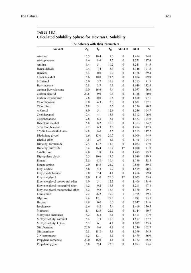
The Future
323
TABLE 18.1Calculated Solubility Sphere for Dextran C Solubility
The Solvents with Their Parameters
Solvent
δδδδ
D
δδδδ
P
δδδδ
H
SOLUB RED V
Acetone 15.5 10.4 7.0 0 1.454 74.0Acetophenone 19.6 8.6 3.7 0 1.371 117.4Aniline 19.4 5.1 10.2 0 1.241 91.5Benzaldehyde 19.4 7.4 5.3 0 1.346 101.5Benzene 18.4 0.0 2.0 0 1.776 89.41,3-Butanediol 16.6 10.0 21.5 0 1.054 89.91-Butanol 16.0 5.7 15.8 0 1.313 91.5Butyl acetate 15.8 3.7 6.3 0 1.640 132.5gamma-Butyrolactone 19.0 16.6 7.4 0 1.077 76.8Carbon disulfid 20.5 0.0 0.6 0 1.756 60.0Carbon tetrachloride 17.8 0.0 0.6 0 1.858 97.1Chlorobenzene 19.0 4.3 2.0 0 1.601 102.1Chloroform 17.8 3.1 5.7 0 1.556 80.7
m
-Cresol 18.0 5.1 12.9 0 1.246 104.7Cyclohexanol 17.4 4.1 13.5 0 1.312 106.0Cyclohexanone 17.8 6.3 5.1 0 1.473 104.0Diacetone alcohol 15.8 8.2 10.8 0 1.363 124.2
o
-Dichlorobenzene 19.2 6.3 3.3 0 1.474 112.82,2-Dichlorodiethyl ether 18.8 9.0 5.7 0 1.313 117.2Diethylene glycol 16.6 12.0 20.7 0 1.000 94.9Diethyl ether 14.5 2.9 5.1 0 1.795 104.8Dimethyl formamide 17.4 13.7 11.3 0 1.082 77.0Dimethyl sulfoxide 18.4 16.4 10.2 1* 1.000 71.31,4-Dioxane 19.0 1.8 7.4 0 1.485 85.7Dipropylene glycol 16.5 10.6 17.7 0 1.080 130.9Ethanol 15.8 8.8 19.4 0 1.180 58.5Ethanolamine 17.0 15.5 21.2 1 0.880 59.8Ethyl acetate 15.8 5.3 7.2 0 1.559 98.5Ethylene dichloride 19.0 7.4 4.1 0 1.416 79.4Ethylene glycol 17.0 11.0 26.0 1* 1.003 55.8Ethylene glycol monobutyl ether 16.0 5.1 12.3 0 1.406 131.6Ethylene glycol monoethyl ether 16.2 9.2 14.3 0 1.211 97.8Ethylene glycol monomethyl ether 16.2 9.2 16.4 0 1.170 79.1Formamide 17.2 26.2 19.0 1 0.915 39.8Glycerol 17.4 12.1 29.3 1 0.991 73.3Hexane 14.9 0.0 0.0 0 2.037 131.6Isophorone 16.6 8.2 7.4 0 1.410 150.5Methanol 15.1 12.3 22.3 0 1.144 40.7Methylene dichloride 18.2 6.3 6.1 0 1.411 63.9Methyl isobutyl carbinol 15.4 3.3 12.3 0 1.517 127.2Methyl isobutyl ketone 15.3 6.1 4.1 0 1.679 125.8Nitrobenzene 20.0 8.6 4.1 0 1.336 102.7Nitromethane 15.8 18.8 5.1 0 1.399 54.32-Nitropropane 16.2 12.1 4.1 0 1.479 86.9Propylene carbonate 20.0 18.0 4.1 0 1.172 85.0Propylene glycol 16.8 9.4 23.3 0 1.053 73.6
7248_C018.fm Page 323 Wednesday, May 23, 2007 11:46 AM
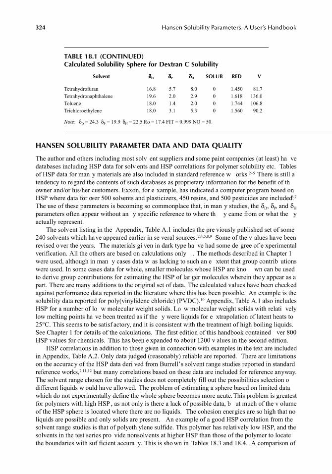
324
Hansen Solubility Parameters: A User’s Handbook
HANSEN SOLUBILITY PARAMETER DATA AND DATA QUALITY
The author and others including most solv ent suppliers and some paint companies (at least) ha vedatabases including HSP data for solv ents and HSP correlations for polymer solubility etc. Tablesof HSP data for man y materials are also included in standard reference w orks.
2–5
There is still atendency to regard the contents of such databases as proprietary information for the benefit of thowner and/or his/her customers. Exxon, for e xample, has indicated a computer program based onHSP where data for over 500 solvents and plasticizers, 450 resins, and 500 pesticides are included.
6,7
The use of these parameters is becoming so commonplace that, in man y studies, the
δ
D
,
δ
P
, and
δ
H
parameters often appear without an y specific reference to where th y came from or what the yactually represent.
The solvent listing in the Appendix, Table A.1 includes the pre viously published set of some240 solvents which have appeared earlier in se veral sources.
2,4,5,8,9
Some of the v alues have beenrevised over the years. The materials gi ven in dark type ha ve had some de gree of e xperimentalverification. All the others are based on calculations only . The methods described in Chapter 1were used, although in man y cases data w as lacking to such an e xtent that group contrib utionswere used. In some cases data for whole, smaller molecules whose HSP are kno wn can be usedto derive group contributions for estimating the HSP of lar ger molecules wherein they appear as apart. There are many additions to the original set of data. The calculated values have been checkedagainst performance data reported in the literature where this has been possible. An example is thesolubility data reported for poly(vinylidene chloride) (PVDC).
10
Appendix, Table A.1 also includesHSP for a number of lo w molecular weight solids. Lo w molecular weight solids with relati velylow melting points ha ve been treated as if the y were liquids for e xtrapolation of latent heats to25°C. This seems to be satisf actory, and it is consistent with the treatment of high boiling liquids.See Chapter 1 for details of the calculations. The first edition of this handbook contained ver 800HSP values for chemicals. This has been e xpanded to about 1200 v alues in the second edition.
HSP correlations in addition to those given in connection with examples in the text are includedin Appendix, Table A.2. Only data judged (reasonably) reliable are reported. There are limitationson the accuracy of the HSP data deri ved from Burrell’s solvent range studies reported in standardreference works,
2,11,12
but many correlations based on these data are included for reference anyway.The solvent range chosen for the studies does not completely fill out the possibilities selection odifferent liquids w ould have allowed. The problem of estimating a sphere based on limited datawhich do not experimentally define the whole sphere becomes more acute.This problem is greatestfor polymers with high HSP , as not only is there a lack of possible data, b ut much of the v olumeof the HSP sphere is located where there are no liquids. The cohesion energies are so high that noliquids are possible and only solids are present. An example of a good HSP correlation from thesolvent range studies is that of polyeth ylene sulfide. This polymer has relatively low HSP, and thesolvents in the test series pro vide nonsolvents at higher HSP than those of the polymer to locatethe boundaries with suf ficient accura y. This is sho wn in Tables 18.3 and 18.4. A comparison of
TABLE 18.1 (CONTINUED)Calculated Solubility Sphere for Dextran C Solubility
Solvent
δδδδ
D
δδδδ
P
δδδδ
H
SOLUB RED V
Tetrahydrofuran 16.8 5.7 8.0 0 1.450 81.7Tetrahydronaphthalene 19.6 2.0 2.9 0 1.618 136.0Toluene 18.0 1.4 2.0 0 1.744 106.8Trichloroethylene 18.0 3.1 5.3 0 1.560 90.2
Note
:
δ
D
= 24.3
δ
P
= 19.9
δ
H
= 22.5 Ro = 17.4 FIT = 0.999 NO = 50.
7248_C018.fm Page 324 Wednesday, May 23, 2007 11:46 AM
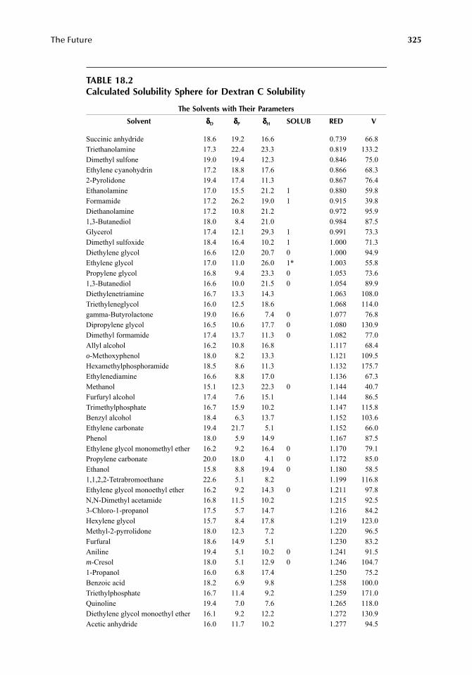
The Future
325
TABLE 18.2Calculated Solubility Sphere for Dextran C Solubility
The Solvents with Their Parameters
Solvent
δδδδ
D
δδδδ
P
δδδδ
H
SOLUB RED V
Succinic anhydride 18.6 19.2 16.6 0.739 66.8Triethanolamine 17.3 22.4 23.3 0.819 133.2Dimethyl sulfone 19.0 19.4 12.3 0.846 75.0Ethylene cyanohydrin 17.2 18.8 17.6 0.866 68.32-Pyrolidone 19.4 17.4 11.3 0.867 76.4Ethanolamine 17.0 15.5 21.2 1 0.880 59.8Formamide 17.2 26.2 19.0 1 0.915 39.8Diethanolamine 17.2 10.8 21.2 0.972 95.91,3-Butanediol 18.0 8.4 21.0 0.984 87.5Glycerol 17.4 12.1 29.3 1 0.991 73.3Dimethyl sulfoxide 18.4 16.4 10.2 1 1.000 71.3Diethylene glycol 16.6 12.0 20.7 0 1.000 94.9Ethylene glycol 17.0 11.0 26.0 1* 1.003 55.8Propylene glycol 16.8 9.4 23.3 0 1.053 73.61,3-Butanediol 16.6 10.0 21.5 0 1.054 89.9Diethylenetriamine 16.7 13.3 14.3 1.063 108.0Triethyleneglycol 16.0 12.5 18.6 1.068 114.0gamma-Butyrolactone 19.0 16.6 7.4 0 1.077 76.8Dipropylene glycol 16.5 10.6 17.7 0 1.080 130.9Dimethyl formamide 17.4 13.7 11.3 0 1.082 77.0Allyl alcohol 16.2 10.8 16.8 1.117 68.4
o
-Methoxyphenol 18.0 8.2 13.3 1.121 109.5Hexamethylphosphoramide 18.5 8.6 11.3 1.132 175.7Ethylenediamine 16.6 8.8 17.0 1.136 67.3Methanol 15.1 12.3 22.3 0 1.144 40.7Furfuryl alcohol 17.4 7.6 15.1 1.144 86.5Trimethylphosphate 16.7 15.9 10.2 1.147 115.8Benzyl alcohol 18.4 6.3 13.7 1.152 103.6Ethylene carbonate 19.4 21.7 5.1 1.152 66.0Phenol 18.0 5.9 14.9 1.167 87.5Ethylene glycol monomethyl ether 16.2 9.2 16.4 0 1.170 79.1Propylene carbonate 20.0 18.0 4.1 0 1.172 85.0Ethanol 15.8 8.8 19.4 0 1.180 58.51,1,2,2-Tetrabromoethane 22.6 5.1 8.2 1.199 116.8Ethylene glycol monoethyl ether 16.2 9.2 14.3 0 1.211 97.8N,N-Dimethyl acetamide 16.8 11.5 10.2 1.215 92.53-Chloro-1-propanol 17.5 5.7 14.7 1.216 84.2Hexylene glycol 15.7 8.4 17.8 1.219 123.0Methyl-2-pyrrolidone 18.0 12.3 7.2 1.220 96.5Furfural 18.6 14.9 5.1 1.230 83.2Aniline 19.4 5.1 10.2 0 1.241 91.5
m
-Cresol 18.0 5.1 12.9 0 1.246 104.71-Propanol 16.0 6.8 17.4 1.250 75.2Benzoic acid 18.2 6.9 9.8 1.258 100.0Triethylphosphate 16.7 11.4 9.2 1.259 171.0Quinoline 19.4 7.0 7.6 1.265 118.0Diethylene glycol monoethyl ether 16.1 9.2 12.2 1.272 130.9Acetic anhydride 16.0 11.7 10.2 1.277 94.5
7248_C018.fm Page 325 Wednesday, May 23, 2007 11:46 AM
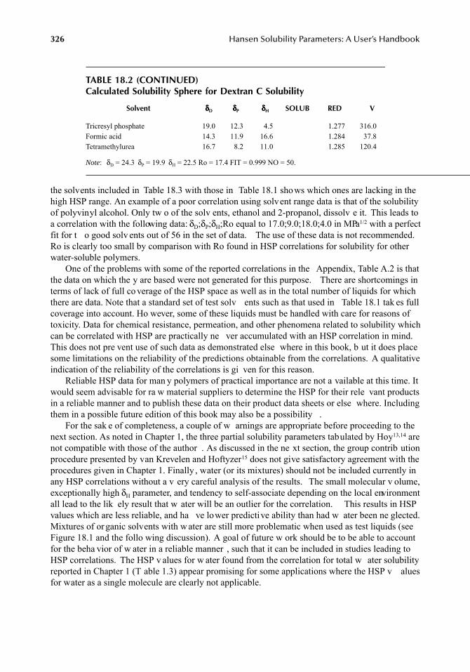
326
Hansen Solubility Parameters: A User’s Handbook
the solvents included in Table 18.3 with those in Table 18.1 shows which ones are lacking in thehigh HSP range. An example of a poor correlation using solvent range data is that of the solubilityof polyvinyl alcohol. Only tw o of the solv ents, ethanol and 2-propanol, dissolv e it. This leads toa correlation with the following data:
δ
D
;
δ
P
;
δ
H
;Ro equal to 17.0;9.0;18.0;4.0 in MPa
1/2
with a perfectfit for t o good solv ents out of 56 in the set of data. The use of these data is not recommended.Ro is clearly too small by comparison with Ro found in HSP correlations for solubility for otherwater-soluble polymers.
One of the problems with some of the reported correlations in the Appendix, Table A.2 is thatthe data on which the y are based were not generated for this purpose. There are shortcomings interms of lack of full co verage of the HSP space as well as in the total number of liquids for whichthere are data. Note that a standard set of test solv ents such as that used in Table 18.1 tak es fullcoverage into account. Ho wever, some of these liquids must be handled with care for reasons oftoxicity. Data for chemical resistance, permeation, and other phenomena related to solubility whichcan be correlated with HSP are practically ne ver accumulated with an HSP correlation in mind.This does not pre vent use of such data as demonstrated else where in this book, b ut it does placesome limitations on the reliability of the predictions obtainable from the correlations. A qualitativeindication of the reliability of the correlations is gi ven for this reason.
Reliable HSP data for man y polymers of practical importance are not a vailable at this time. Itwould seem advisable for ra w material suppliers to determine the HSP for their rele vant productsin a reliable manner and to publish these data on their product data sheets or else where. Includingthem in a possible future edition of this book may also be a possibility .
For the sak e of completeness, a couple of w arnings are appropriate before proceeding to thenext section. As noted in Chapter 1, the three partial solubility parameters tabulated by Hoy
13,14
arenot compatible with those of the author . As discussed in the ne xt section, the group contrib utionprocedure presented by van Krevelen and Hoftyzer
15
does not give satisfactory agreement with theprocedures given in Chapter 1. Finally , water (or its mixtures) should not be included currently inany HSP correlations without a v ery careful analysis of the results. The small molecular v olume,exceptionally high
δ
H
parameter, and tendency to self-associate depending on the local environmentall lead to the lik ely result that w ater will be an outlier for the correlation. This results in HSPvalues which are less reliable, and ha ve lower predictive ability than had w ater been ne glected.Mixtures of or ganic solvents with w ater are still more problematic when used as test liquids (seeFigure 18.1 and the follo wing discussion). A goal of future w ork should be to be able to accountfor the beha vior of w ater in a reliable manner , such that it can be included in studies leading toHSP correlations. The HSP v alues for w ater found from the correlation for total w ater solubilityreported in Chapter 1 (T able 1.3) appear promising for some applications where the HSP v aluesfor water as a single molecule are clearly not applicable.
TABLE 18.2 (CONTINUED)Calculated Solubility Sphere for Dextran C Solubility
Solvent
δδδδ
D
δδδδ
P
δδδδ
H
SOLUB RED V
Tricresyl phosphate 19.0 12.3 4.5 1.277 316.0Formic acid 14.3 11.9 16.6 1.284 37.8Tetramethylurea 16.7 8.2 11.0 1.285 120.4
Note
:
δ
D
= 24.3
δ
P
= 19.9
δ
H
= 22.5 Ro = 17.4 FIT = 0.999 NO = 50.
7248_C018.fm Page 326 Wednesday, May 23, 2007 11:46 AM
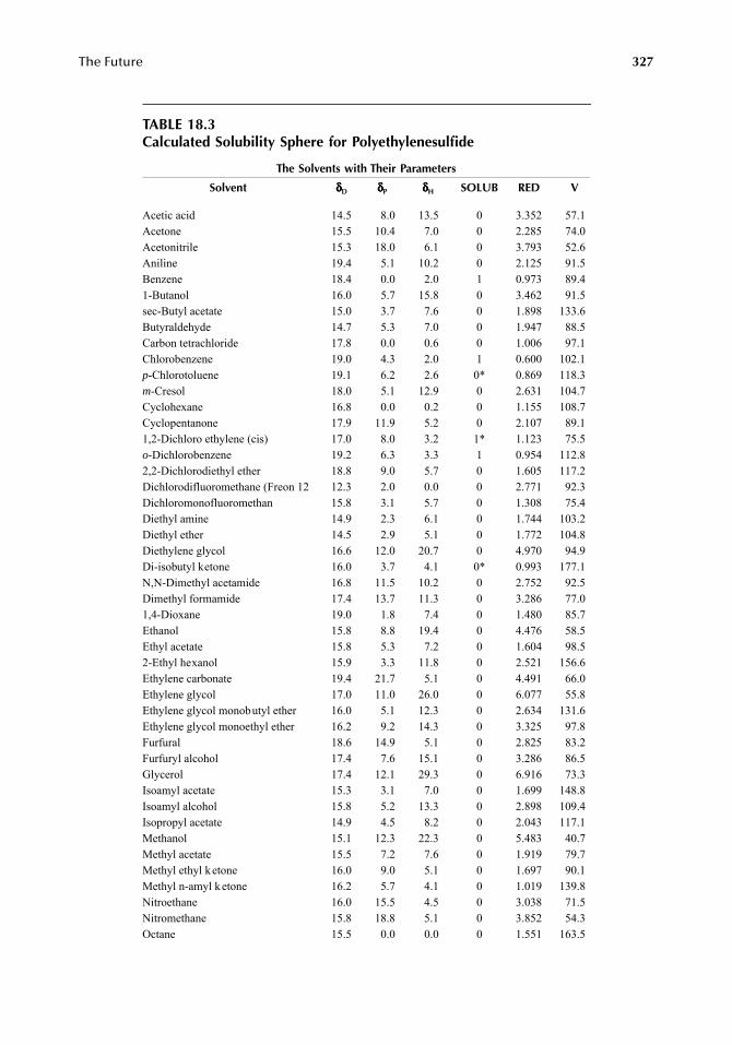
The Future
327
TABLE 18.3Calculated Solubility Sphere for Polyethylenesulfide
The Solvents with Their Parameters
Solvent
δδδδ
D
δδδδ
P
δδδδ
H
SOLUB RED V
Acetic acid 14.5 8.0 13.5 0 3.352 57.1Acetone 15.5 10.4 7.0 0 2.285 74.0Acetonitrile 15.3 18.0 6.1 0 3.793 52.6Aniline 19.4 5.1 10.2 0 2.125 91.5Benzene 18.4 0.0 2.0 1 0.973 89.41-Butanol 16.0 5.7 15.8 0 3.462 91.5sec-Butyl acetate 15.0 3.7 7.6 0 1.898 133.6Butyraldehyde 14.7 5.3 7.0 0 1.947 88.5Carbon tetrachloride 17.8 0.0 0.6 0 1.006 97.1Chlorobenzene 19.0 4.3 2.0 1 0.600 102.1
p
-Chlorotoluene 19.1 6.2 2.6 0* 0.869 118.3
m
-Cresol 18.0 5.1 12.9 0 2.631 104.7Cyclohexane 16.8 0.0 0.2 0 1.155 108.7Cyclopentanone 17.9 11.9 5.2 0 2.107 89.11,2-Dichloro ethylene (cis) 17.0 8.0 3.2 1* 1.123 75.5
o
-Dichlorobenzene 19.2 6.3 3.3 1 0.954 112.82,2-Dichlorodiethyl ether 18.8 9.0 5.7 0 1.605 117.2Dichlorodifluoromethane (Freon 12 12.3 2.0 0.0 0 2.771 92.3Dichloromonofluoromethan 15.8 3.1 5.7 0 1.308 75.4Diethyl amine 14.9 2.3 6.1 0 1.744 103.2Diethyl ether 14.5 2.9 5.1 0 1.772 104.8Diethylene glycol 16.6 12.0 20.7 0 4.970 94.9Di-isobutyl ketone 16.0 3.7 4.1 0* 0.993 177.1N,N-Dimethyl acetamide 16.8 11.5 10.2 0 2.752 92.5Dimethyl formamide 17.4 13.7 11.3 0 3.286 77.01,4-Dioxane 19.0 1.8 7.4 0 1.480 85.7Ethanol 15.8 8.8 19.4 0 4.476 58.5Ethyl acetate 15.8 5.3 7.2 0 1.604 98.52-Ethyl hexanol 15.9 3.3 11.8 0 2.521 156.6Ethylene carbonate 19.4 21.7 5.1 0 4.491 66.0Ethylene glycol 17.0 11.0 26.0 0 6.077 55.8Ethylene glycol monobutyl ether 16.0 5.1 12.3 0 2.634 131.6Ethylene glycol monoethyl ether 16.2 9.2 14.3 0 3.325 97.8Furfural 18.6 14.9 5.1 0 2.825 83.2Furfuryl alcohol 17.4 7.6 15.1 0 3.286 86.5Glycerol 17.4 12.1 29.3 0 6.916 73.3Isoamyl acetate 15.3 3.1 7.0 0 1.699 148.8Isoamyl alcohol 15.8 5.2 13.3 0 2.898 109.4Isopropyl acetate 14.9 4.5 8.2 0 2.043 117.1Methanol 15.1 12.3 22.3 0 5.483 40.7Methyl acetate 15.5 7.2 7.6 0 1.919 79.7Methyl ethyl ketone 16.0 9.0 5.1 0 1.697 90.1Methyl n-amyl ketone 16.2 5.7 4.1 0 1.019 139.8Nitroethane 16.0 15.5 4.5 0 3.038 71.5Nitromethane 15.8 18.8 5.1 0 3.852 54.3Octane 15.5 0.0 0.0 0 1.551 163.5
7248_C018.fm Page 327 Wednesday, May 23, 2007 11:46 AM
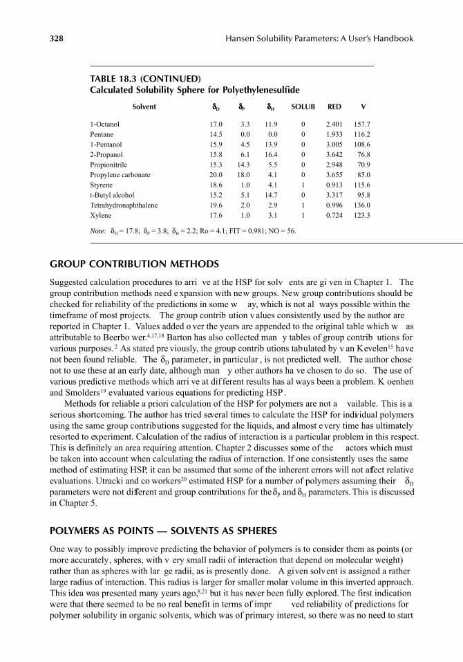
328
Hansen Solubility Parameters: A User’s Handbook
GROUP CONTRIBUTION METHODS
Suggested calculation procedures to arri ve at the HSP for solv ents are gi ven in Chapter 1. Thegroup contribution methods need e xpansion with new groups. New group contributions should bechecked for reliability of the predictions in some w ay, which is not al ways possible within thetimeframe of most projects. The group contrib ution v alues consistently used by the author arereported in Chapter 1. Values added o ver the years are appended to the original table which w asattributable to Beerbo wer.
4,17,18
Barton has also collected man y tables of group contrib utions forvarious purposes.
2
As stated pre viously, the group contrib utions tabulated by v an Kevelen
15
havenot been found reliable. The
δ
D
parameter, in particular , is not predicted well. The author chosenot to use these at an early date, although man y other authors ha ve chosen to do so. The use ofvarious predictive methods which arri ve at dif ferent results has al ways been a problem. K oenhenand Smolders
19
evaluated various equations for predicting HSP .Methods for reliable a priori calculation of the HSP for polymers are not a vailable. This is a
serious shortcoming. The author has tried several times to calculate the HSP for individual polymersusing the same group contributions suggested for the liquids, and almost e very time has ultimatelyresorted to experiment. Calculation of the radius of interaction is a particular problem in this respect.This is definitely an area requiring attention. Chapter 2 discusses some of the actors which mustbe taken into account when calculating the radius of interaction. If one consistently uses the samemethod of estimating HSP, it can be assumed that some of the inherent errors will not affect relativeevaluations. Utracki and co workers
20
estimated HSP for a number of polymers assuming their
δ
D
parameters were not different and group contributions for the
δ
P
and
δ
H
parameters. This is discussedin Chapter 5.
POLYMERS AS POINTS — SOLVENTS AS SPHERES
One way to possibly improve predicting the behavior of polymers is to consider them as points (ormore accurately, spheres, with v ery small radii of interaction that depend on molecular weight)rather than as spheres with lar ge radii, as is presently done. A given solvent is assigned a ratherlarge radius of interaction. This radius is larger for smaller molar volume in this inverted approach.This idea was presented many years ago,
8,21
but it has never been fully explored. The first indicationwere that there seemed to be no real benefit in terms of impr ved reliability of predictions forpolymer solubility in organic solvents, which was of primary interest, so there was no need to start
TABLE 18.3 (CONTINUED)Calculated Solubility Sphere for Polyethylenesulfide
Solvent
δδδδ
D
δδδδ
P
δδδδ
H
SOLUB RED V
1-Octanol 17.0 3.3 11.9 0 2.401 157.7Pentane 14.5 0.0 0.0 0 1.933 116.21-Pentanol 15.9 4.5 13.9 0 3.005 108.62-Propanol 15.8 6.1 16.4 0 3.642 76.8Propionitrile 15.3 14.3 5.5 0 2.948 70.9Propylene carbonate 20.0 18.0 4.1 0 3.655 85.0Styrene 18.6 1.0 4.1 1 0.913 115.6t-Butyl alcohol 15.2 5.1 14.7 0 3.317 95.8Tetrahydronaphthalene 19.6 2.0 2.9 1 0.996 136.0Xylene 17.6 1.0 3.1 1 0.724 123.3
Note
:
δ
D
= 17.8;
δ
P
= 3.8;
δ
H
= 2.2; Ro = 4.1; FIT = 0.981; NO = 56.
7248_C018.fm Page 328 Wednesday, May 23, 2007 11:46 AM
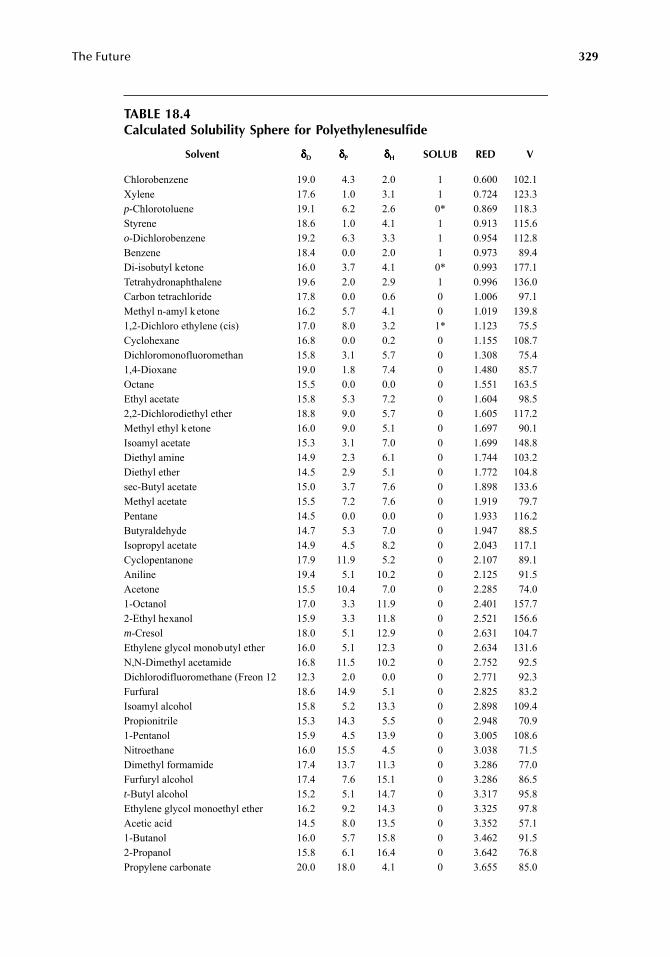
The Future
329
TABLE 18.4Calculated Solubility Sphere for Polyethylenesulfide
Solvent
δδδδ
D
δδδδ
P
δδδδ
H
SOLUB RED V
Chlorobenzene 19.0 4.3 2.0 1 0.600 102.1Xylene 17.6 1.0 3.1 1 0.724 123.3
p
-Chlorotoluene 19.1 6.2 2.6 0* 0.869 118.3Styrene 18.6 1.0 4.1 1 0.913 115.6
o
-Dichlorobenzene 19.2 6.3 3.3 1 0.954 112.8Benzene 18.4 0.0 2.0 1 0.973 89.4Di-isobutyl ketone 16.0 3.7 4.1 0* 0.993 177.1Tetrahydronaphthalene 19.6 2.0 2.9 1 0.996 136.0Carbon tetrachloride 17.8 0.0 0.6 0 1.006 97.1Methyl n-amyl ketone 16.2 5.7 4.1 0 1.019 139.81,2-Dichloro ethylene (cis) 17.0 8.0 3.2 1* 1.123 75.5Cyclohexane 16.8 0.0 0.2 0 1.155 108.7Dichloromonofluoromethan 15.8 3.1 5.7 0 1.308 75.41,4-Dioxane 19.0 1.8 7.4 0 1.480 85.7Octane 15.5 0.0 0.0 0 1.551 163.5Ethyl acetate 15.8 5.3 7.2 0 1.604 98.52,2-Dichlorodiethyl ether 18.8 9.0 5.7 0 1.605 117.2Methyl ethyl ketone 16.0 9.0 5.1 0 1.697 90.1Isoamyl acetate 15.3 3.1 7.0 0 1.699 148.8Diethyl amine 14.9 2.3 6.1 0 1.744 103.2Diethyl ether 14.5 2.9 5.1 0 1.772 104.8sec-Butyl acetate 15.0 3.7 7.6 0 1.898 133.6Methyl acetate 15.5 7.2 7.6 0 1.919 79.7Pentane 14.5 0.0 0.0 0 1.933 116.2Butyraldehyde 14.7 5.3 7.0 0 1.947 88.5Isopropyl acetate 14.9 4.5 8.2 0 2.043 117.1Cyclopentanone 17.9 11.9 5.2 0 2.107 89.1Aniline 19.4 5.1 10.2 0 2.125 91.5Acetone 15.5 10.4 7.0 0 2.285 74.01-Octanol 17.0 3.3 11.9 0 2.401 157.72-Ethyl hexanol 15.9 3.3 11.8 0 2.521 156.6
m
-Cresol 18.0 5.1 12.9 0 2.631 104.7Ethylene glycol monobutyl ether 16.0 5.1 12.3 0 2.634 131.6N,N-Dimethyl acetamide 16.8 11.5 10.2 0 2.752 92.5Dichlorodifluoromethane (Freon 12 12.3 2.0 0.0 0 2.771 92.3Furfural 18.6 14.9 5.1 0 2.825 83.2Isoamyl alcohol 15.8 5.2 13.3 0 2.898 109.4Propionitrile 15.3 14.3 5.5 0 2.948 70.91-Pentanol 15.9 4.5 13.9 0 3.005 108.6Nitroethane 16.0 15.5 4.5 0 3.038 71.5Dimethyl formamide 17.4 13.7 11.3 0 3.286 77.0Furfuryl alcohol 17.4 7.6 15.1 0 3.286 86.5
t
-Butyl alcohol 15.2 5.1 14.7 0 3.317 95.8Ethylene glycol monoethyl ether 16.2 9.2 14.3 0 3.325 97.8Acetic acid 14.5 8.0 13.5 0 3.352 57.11-Butanol 16.0 5.7 15.8 0 3.462 91.52-Propanol 15.8 6.1 16.4 0 3.642 76.8Propylene carbonate 20.0 18.0 4.1 0 3.655 85.0
7248_C018.fm Page 329 Wednesday, May 23, 2007 11:46 AM
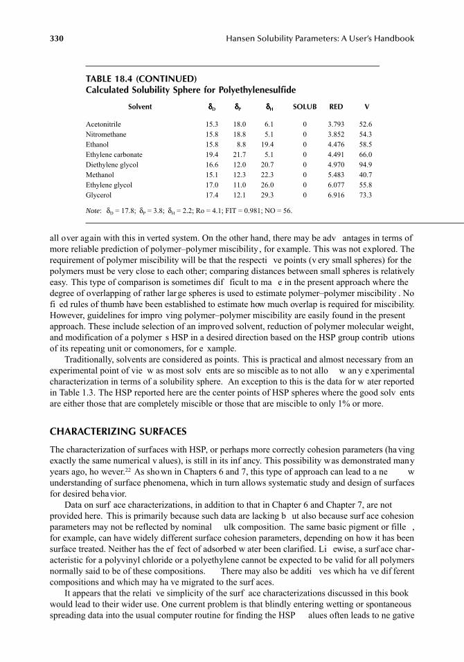
330
Hansen Solubility Parameters: A User’s Handbook
all over again with this in verted system. On the other hand, there may be adv antages in terms ofmore reliable prediction of polymer–polymer miscibility , for example. This was not explored. Therequirement of polymer miscibility will be that the respecti ve points (v ery small spheres) for thepolymers must be very close to each other; comparing distances between small spheres is relativelyeasy. This type of comparison is sometimes dif ficult to ma e in the present approach where thedegree of overlapping of rather large spheres is used to estimate polymer–polymer miscibility . Nofi ed rules of thumb have been established to estimate how much overlap is required for miscibility.However, guidelines for impro ving polymer–polymer miscibility are easily found in the presentapproach. These include selection of an improved solvent, reduction of polymer molecular weight,and modification of a polymer s HSP in a desired direction based on the HSP group contrib utionsof its repeating unit or comonomers, for e xample.
Traditionally, solvents are considered as points. This is practical and almost necessary from anexperimental point of vie w as most solv ents are so miscible as to not allo w an y e xperimentalcharacterization in terms of a solubility sphere. An exception to this is the data for w ater reportedin Table 1.3. The HSP reported here are the center points of HSP spheres where the good solv entsare either those that are completely miscible or those that are miscible to only 1% or more.
CHARACTERIZING SURFACES
The characterization of surfaces with HSP, or perhaps more correctly cohesion parameters (ha vingexactly the same numerical v alues), is still in its inf ancy. This possibility was demonstrated manyyears ago, ho wever.
22
As sho wn in Chapters 6 and 7, this type of approach can lead to a ne wunderstanding of surface phenomena, which in turn allows systematic study and design of surfacesfor desired behavior.
Data on surf ace characterizations, in addition to that in Chapter 6 and Chapter 7, are notprovided here. This is primarily because such data are lacking b ut also because surf ace cohesionparameters may not be reflected by nominal ulk composition. The same basic pigment or fille ,for example, can have widely different surface cohesion parameters, depending on how it has beensurface treated. Neither has the ef fect of adsorbed w ater been clarified. Li ewise, a surf ace char-acteristic for a polyvinyl chloride or a polyethylene cannot be expected to be valid for all polymersnormally said to be of these compositions. There may also be additi ves which ha ve dif ferentcompositions and which may ha ve migrated to the surf aces.
It appears that the relati ve simplicity of the surf ace characterizations discussed in this bookwould lead to their wider use. One current problem is that blindly entering wetting or spontaneousspreading data into the usual computer routine for finding the HSP alues often leads to ne gative
TABLE 18.4 (CONTINUED)Calculated Solubility Sphere for Polyethylenesulfide
Solvent
δδδδ
D
δδδδ
P
δδδδ
H
SOLUB RED V
Acetonitrile 15.3 18.0 6.1 0 3.793 52.6Nitromethane 15.8 18.8 5.1 0 3.852 54.3Ethanol 15.8 8.8 19.4 0 4.476 58.5Ethylene carbonate 19.4 21.7 5.1 0 4.491 66.0Diethylene glycol 16.6 12.0 20.7 0 4.970 94.9Methanol 15.1 12.3 22.3 0 5.483 40.7Ethylene glycol 17.0 11.0 26.0 0 6.077 55.8Glycerol 17.4 12.1 29.3 0 6.916 73.3
Note
:
δ
D
= 17.8;
δ
P
= 3.8;
δ
H
= 2.2; Ro = 4.1; FIT = 0.981; NO = 56.
7248_C018.fm Page 330 Wednesday, May 23, 2007 11:46 AM
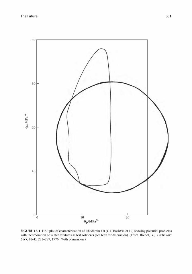
The Future
331
FIGURE 18.1
HSP plot of characterization of Rhodamin FB (C.I. Basic Violet 10) showing potential problemswith incorporation of w ater mixtures as test solv ents (see text for discussion). (From Riedel, G.,
Farbe undLack
, 82(4), 281–287, 1976. With permission.)
δp/MPa½
δ h/M
Pa½
0 10 20
40
30
20
10
0
7248_C018.fm Page 331 Wednesday, May 23, 2007 11:46 AM
332
Hansen Solubility Parameters: A User’s Handbook
numbers for one or more of them. This was discussed in Chapter 6. Currently , the best approachis to compare plots or e ven to just compare tabulated data for the test solv ents to determine wheretwo surfaces differ in af finities. Guides for action can also be found by simple comparison of thHSP of those solv ents which sho w a dif ference in beha vior. A more systematic approach for theuse of cohesion parameters to describe surf ace phenomena would be desirable.
MATERIALS AND PROCESSES SUGGESTED FOR FURTHER ATTENTION
Examples of the use of HSP for man y types of materials and phenomena ha ve been presented inearlier chapters. Some special types of materials are singled out here as worthy of still more attentionin the near future. These include surf ace active agents, w ater, gases, organic and inor ganic salts,organometallic materials, and aromatic (fragrances) materials. The uptake of potentially dangerouschemicals in recyclable packaging also needs attention. An additional area of interest may be foundin that many commonly used reaction solvents have similar HSP. These include dimethyl sulfoxide,dimethyl formamide, dimeth yl acetamide, and sulfolane, for e xample. It seems unlik ely that thisis a coincidence. It could be that the solubility of an acti vated species ha ving high polarity (
δ
P
)and moderate hydrogen bonding (
δ
H
) is determining the reaction rate(s). Still another area of majorinterest is the systematic formulation of filled systems using HS . This is also still in its inf ancy.Pigments and fillers need to be characterized. S veral of these applications are discussed in moredetail below. Surface active materials have remained essentially untouched in terms of HSP, althoughBeerbower started on this man y years ago.
8,17,23
S
URFACE
A
CTIVE
A
GENTS
Surface active agents have not been systematically characterized by HSP yet, although Beerbo werhas developed some aspects of a theory for gi ven situations.
8,17,23
The statement “lik e seeks lik e”indicates that surface active agents should be extensively treated in terms of HSP. Each end of suchmolecules will require its o wn set of HSP , as demonstrated by the e xample of lithium stearate,discussed later in the Or ganometallic Compounds section (Figure 18.3).
An example to help illustrate the type of prediction possible is to try to answer the questionof where the h ydrophobic end of a gi ven surfactant will tend to preferentially reside. An aliphaticend group w ould have lower affinity for polystyrene, for xample, than an aromatic one. Octanewill not dissolv e polystyrene, whereas toluene will. This is reflected by their cohesion ene gyparameters. This same reasoning applies to other polymers. A surfactant with a fluorinated end wilnot dissolve in man y polymers where a h ydrocarbon end will. The cohesion ener gy parameterscharacteristic of fluorocarbons are too l w. Although these e xamples are ob vious to those skilledin the science of surf aces, they point to the possibility of quantifying af finities of sur ace activematerials in terms of the cohesion energy parameters of their respective end groups. Those familiarwith cohesion energy parameters can already discern dif ferences that may improve the chances ofsuccess. The data in Chapter 11 confirm that di ferences in HSP are critical if soils are to beremoved effectively. HSP for surfactants can be assigned by experiment or by the methods describedin the next paragraph.
Each surfactant must be assigned three sets of HSP . The first is for the ydrophobic end, thesecond is for the hydrophilic end, and the third is for the molecule as a whole. Figure 18.3 confirmthe need for the first t o characterizations, and the third one is required for predictions when thewhole molecule is soluble in the system. Even in a completely dissolved condition, one anticipatessome degree of orientation of the ends of the surf actant molecule to ward regions of similar HSP.The HSP for the h ydrophobic end can be estimated by the methods discussed in Chapter 1, withgroup contributions, or by simple comparison with similar (usually) h ydrocarbon molecules of thesame size. Barton has collected group contrib utions that can also be used in connection with the
7248_C018.fm Page 332 Wednesday, May 23, 2007 11:46 AM
The Future
333
different ends of surf ace acti ve agents.
2
The HSP of the h ydrophilic end can be estimated bycomparison with existing HSP of, for e xample, sucrose or other w ater soluble entity, organic salts(see below), inorganic salts (see belo w), polyethylene oxide or polyeth ylene glycol, or whate verresembles this end best. Experiments are preferred, of course, and the estimation for given inorganicsalts is still uncertain. When a surfactant denatures a protein, there will be some similarity betweenthe HSP of the protein or urea, if this also denatures the protein (see Chapter 15), and the HSP ofthe hydrophilic end of the surf actant. If enough data of this kind can be generated, the HSP of thesurfactant can be e xperimentally confirmed. The estimation for the molecule as a whole in volvescombining the two sets of HSP for the ends. It is thought that this is best done by a veraging usingestimated molecular volumes for the respective ends relative to the molecular volume of the wholemolecule.
In closing this section, it can also be repeated that thermodynamic surf ace and interf acialphenomena correlate with HSP . This has been amply sho wn in Chapter 6 and Chapter 7. Thekinetics of the situation may also be important. Chapter 16 discusses adsorption and absorption inpolymer surfaces where there is a surf ace resistance. There will also be some form of interf acialor boundary layer resistance influencing the adsorption and absorption of sur actants into soils, forexample. If the HSP do not match sufficiently well, adsorption and absorption will presumably nooccur as readily as when the HSP do match to within some required limit for the desired ef fect,as shown in Chapter 11. The size and shape of the adsorbing/absorbing entity is also presumed tobe important from a kinetic point of vie w, as demonstrated by the e xamples in Chapter 16.
S
URFACE
M
OBILITY
(S
ELF
-A
SSEMBLY
)
The rule of thumb that “lik e seeks lik e” can be v ery useful in understanding the structure ofcomplicated systems. That this type of consideration can lead to useful results can be seen in theway that the beha vior of w ood polymers and the ultrastructure of cell w alls in w ood was treatedin Chapter 13 and in much more detail by Hansen and Björkman.
24
Hemicelluloses appear tofunction much like surfactants with the backbone and those side chains containing hydroxyl groupsfavoring placement to ward cellulose (or their o wn kind). Hemicellulose side chains containingacetyl, acid, or ether groups are expected to favor orientation toward lignin regions. In this example,it is interfacial mobility that is in focus, and it can be expected that the orientations may be changedwith the transport or presence of other materials such as w ater through a given local environment.These predictions and inferences appear to agree with what is e xpected or has been established byindependent measurement, but it is too early to say that confirmation has been obtained independently. The treatment of dif ferent segments of block copolymers as separate entities is a relatedendeavor where more quantitative predictions of compatibility should be possible. It is kno wn thatadditions of a block of polymer C to both polymer A and polymer B impro ves their chances ofcompatibility (at some molecular level). The association of blocks of polymers is also the basis forthe thermoplastic elastomers (TPE). These are made with a wide v ariety of dif ferent immiscible(hard and soft) blocks where the phase separation is critical to performance. Typical e xamplesinclude the styrene/butadiene/styrene block copolymer (SBS), the polyether/polyamide block copol-ymer (PEBA), and polyurethanes combined with polyethers or polyesters (TPU). Some types arealso vulcanized to impro ve properties.
The rotation of some hydrophobic materials to become more hydrophilic when in contact withwater is still another example of like seeking like. Peat moss is an example. A drop of water initiallypearls on the surf ace but shortly thereafter disappears into the interior in a spontaneous manner .The peat moss has become hydrophilic (but returns to the hydrophobic state on drying again). Thisphenomena was actually employed to develop an electrodeposition coating for an evaporator wherefilm-wetting by ater was required for good evaporation efficien y.
25
After several hours of exposureof a fresh coating to w ater, the static contact angles with w ater disappeared and a coherent w aterfilm as obtained.
7248_C018.fm Page 333 Wednesday, May 23, 2007 11:46 AM
334 Hansen Solubility Parameters: A User’s Handbook
Many surface phenomena can be understood from the preferences of gi ven segments or mate-rials to seek out regions of similar HSP. Some inferences may be possible from the studies performedon compatible (or nearly compatible) polymers. The HSP data leading to formulation of self-stratifying coatings also pro vides useful information 26 (see also Chapter 6). Systematic studies ofthese effects are badly needed. One such study 27 confirmed that the rotation ability (mobility) oaging polymer surfaces could be followed by measuring the (static) receding contact angle of water.Aging can be expected to lead to increased oxygenation and perhaps also to a decrease in a veragemolecular weight. These ef fects both contrib ute to the tendenc y/ability for oxygenated speciesattached to an otherwise more h ydrophobic polymer to rotate into an applied w ater droplet. Whenthe (static) receding contact angle for w ater w as measured, it fell with e xposure time/aging atshorter times, whereas the (static) advancing contact remained constant. At longer exposure times,when the surface was oxygenated to a greater extent, the advancing contact angle also started to fall.
Surface mobility also has an important role in biological processes, as described in Chapter15. The orientation of molecules to allo w given segments to locate in re gions of similar HSP ispresumed to be a general phenomenon. Hydrophilic bonding (usually referred to in the presentcontext as intermolecular h ydrogen bonding) is responsible for the configurations of proteins iwater. The proteins that can be dissolved in mixtures of water and urea or given salts, for example,are no longer “h ydrogen bonded” in the con ventional usage of the term, as the y are no w trulydissolved by an ef fectively good solv ent that can also dissolv e these se gments/bonding sites. Theusual solvent, water, does not ha ve the correct set of HSP to truly dissolv e these se gments of theprotein molecules. The urea additions correct for this deficien y, and the protein is said to bedenatured in the process. The concept of hydrophilic (hyperphilic?) bonding, which is the oppositeof hydrophobic bonding, is discussed in more detail with examples in Chapter 15. These phenomenaalso point to the use of urea or urea groups to impro ve biocompatibility.
Many of the concepts discussed here are directly applicable for self-assembling systems andto procedures and products within the concepts of nanotechnology .
WATER
The current treatment of the HSP for w ater discussed in Chapter 1 and Chapter 15 needs confi -mation and/or modification. As noted earlier on se veral occasions, w ater is v ery special becauseof its lo w molecular v olume, its v ery high δH parameter for a liquid, and its tendenc y to self-associate or to associate with other materials forming special structures. The HSP correlations forthe solubility of solvents in water presented in Chapter 1, Table 1.3 have not been tested extensivelyas yet, b ut do seem promising. They are clearly useful to mak e predictions for the solubility ofuntested solvents in w ater, but whether or not these HSP data for w ater can be used in a lar gercontext remains to be determined. General beha vior can be predicted, but can specific beh vior bepredicted? More research is needed in this area, b ut, in the meantime, w ater can be considered ashaving (at least) duality. Sometimes it acts like a single molecule, and sometimes it acts as a clusterof about six molecules (according to the HSP comparison, at least). There may also be otherpossibilities. The use of the HSP for w ater found from the correlation of total w ater solubilityappears to be the most promising set of v alues to work with at the present time. This is especiallytrue for water in lower energy systems.
It is not yet advisable to include water in a standard set of test liquids for experimental evaluationof the HSP for polymers or other materials because of its tendenc y to be an outlier . This means achallenge still exists to understand how to be able to incorporate w ater into a standard set of HSPtest liquids without al ways being concerned about special interpretations for w ater, and only forwater. An example of how this can lead to oddities is discussed in the follo wing.
A characterization problem caused by nonideal mixtures with w ater is the interpretation ofHSP correlations for materials such as the dye Rhodamin FB (C.I. Basic Violet 10). 2,16 Use ofmixtures of solv ent and w ater as test solv ents led to a v ery nonspherical (noncircular) cohesion
7248_C018.fm Page 334 Wednesday, May 23, 2007 11:46 AM
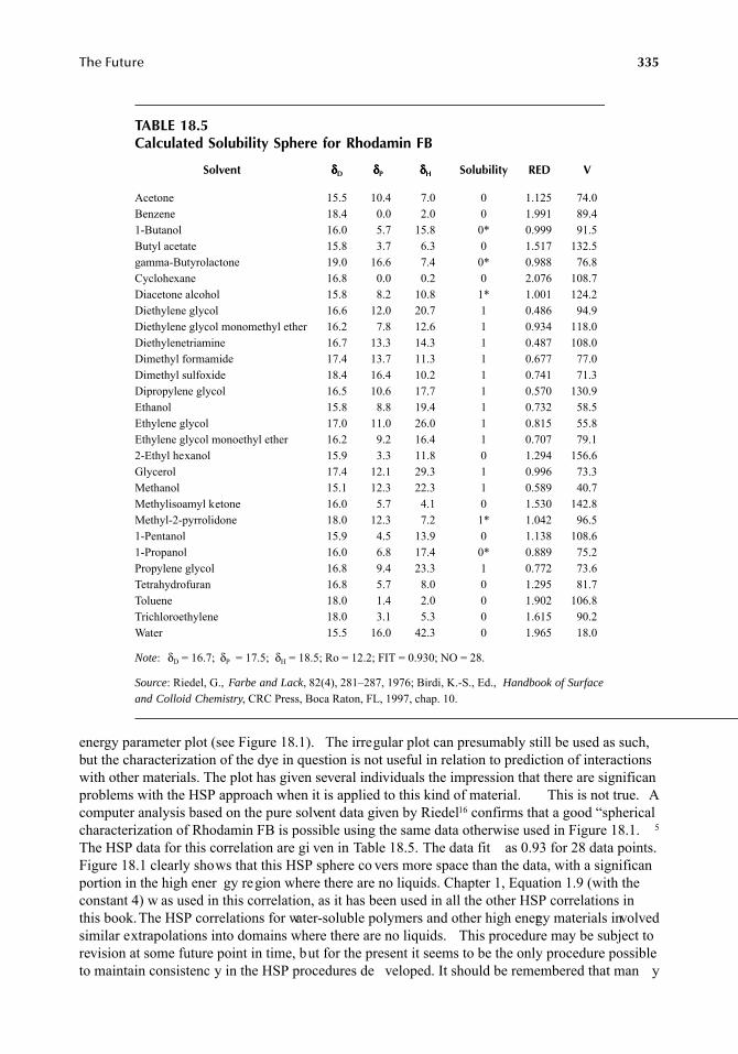
The Future 335
energy parameter plot (see Figure 18.1). The irregular plot can presumably still be used as such,but the characterization of the dye in question is not useful in relation to prediction of interactionswith other materials. The plot has given several individuals the impression that there are significanproblems with the HSP approach when it is applied to this kind of material. This is not true. Acomputer analysis based on the pure solvent data given by Riedel16 confirms that a good “sphericalcharacterization of Rhodamin FB is possible using the same data otherwise used in Figure 18.1. 5
The HSP data for this correlation are gi ven in Table 18.5. The data fit as 0.93 for 28 data points.Figure 18.1 clearly shows that this HSP sphere co vers more space than the data, with a significanportion in the high ener gy region where there are no liquids. Chapter 1, Equation 1.9 (with theconstant 4) w as used in this correlation, as it has been used in all the other HSP correlations inthis book. The HSP correlations for water-soluble polymers and other high energy materials involvedsimilar extrapolations into domains where there are no liquids. This procedure may be subject torevision at some future point in time, but for the present it seems to be the only procedure possibleto maintain consistenc y in the HSP procedures de veloped. It should be remembered that man y
TABLE 18.5Calculated Solubility Sphere for Rhodamin FB
Solvent δδδδD δδδδP δδδδH Solubility RED V
Acetone 15.5 10.4 7.0 0 1.125 74.0Benzene 18.4 0.0 2.0 0 1.991 89.41-Butanol 16.0 5.7 15.8 0* 0.999 91.5Butyl acetate 15.8 3.7 6.3 0 1.517 132.5gamma-Butyrolactone 19.0 16.6 7.4 0* 0.988 76.8Cyclohexane 16.8 0.0 0.2 0 2.076 108.7Diacetone alcohol 15.8 8.2 10.8 1* 1.001 124.2Diethylene glycol 16.6 12.0 20.7 1 0.486 94.9Diethylene glycol monomethyl ether 16.2 7.8 12.6 1 0.934 118.0Diethylenetriamine 16.7 13.3 14.3 1 0.487 108.0Dimethyl formamide 17.4 13.7 11.3 1 0.677 77.0Dimethyl sulfoxide 18.4 16.4 10.2 1 0.741 71.3Dipropylene glycol 16.5 10.6 17.7 1 0.570 130.9Ethanol 15.8 8.8 19.4 1 0.732 58.5Ethylene glycol 17.0 11.0 26.0 1 0.815 55.8Ethylene glycol monoethyl ether 16.2 9.2 16.4 1 0.707 79.12-Ethyl hexanol 15.9 3.3 11.8 0 1.294 156.6Glycerol 17.4 12.1 29.3 1 0.996 73.3Methanol 15.1 12.3 22.3 1 0.589 40.7Methylisoamyl ketone 16.0 5.7 4.1 0 1.530 142.8Methyl-2-pyrrolidone 18.0 12.3 7.2 1* 1.042 96.51-Pentanol 15.9 4.5 13.9 0 1.138 108.61-Propanol 16.0 6.8 17.4 0* 0.889 75.2Propylene glycol 16.8 9.4 23.3 1 0.772 73.6Tetrahydrofuran 16.8 5.7 8.0 0 1.295 81.7Toluene 18.0 1.4 2.0 0 1.902 106.8Trichloroethylene 18.0 3.1 5.3 0 1.615 90.2Water 15.5 16.0 42.3 0 1.965 18.0
Note: δD = 16.7; δP = 17.5; δH = 18.5; Ro = 12.2; FIT = 0.930; NO = 28.
Source: Riedel, G., Farbe and Lack, 82(4), 281–287, 1976; Birdi, K.-S., Ed., Handbook of Surfaceand Colloid Chemistry, CRC Press, Boca Raton, FL, 1997, chap. 10.
7248_C018.fm Page 335 Wednesday, May 23, 2007 11:46 AM
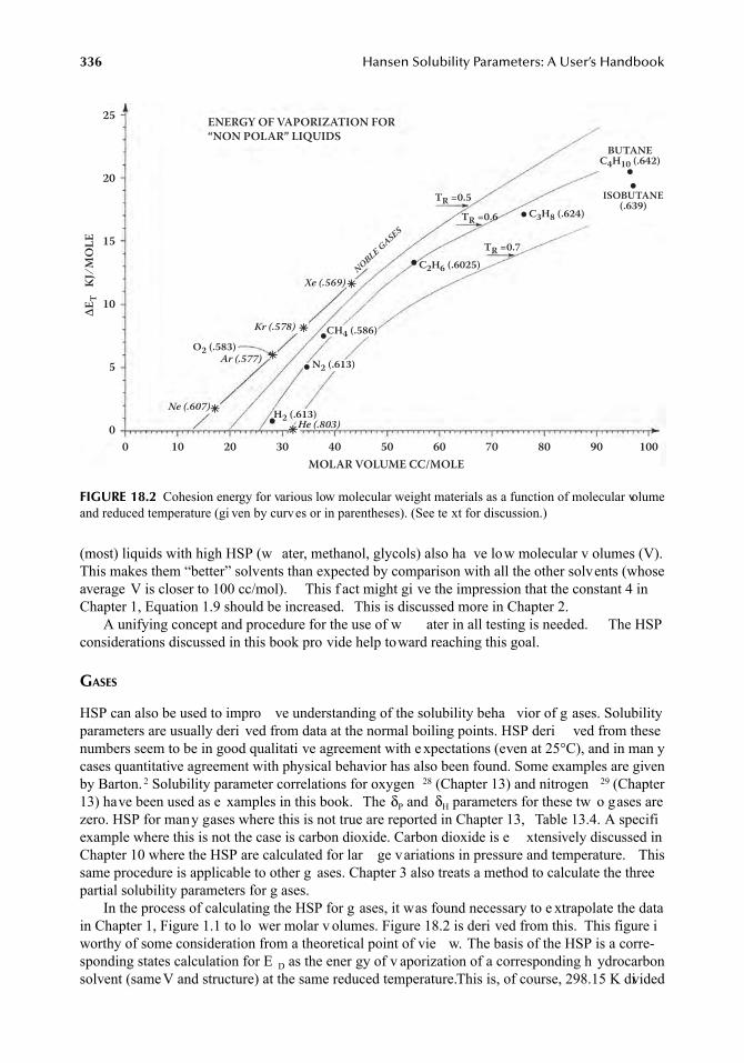
336 Hansen Solubility Parameters: A User’s Handbook
(most) liquids with high HSP (w ater, methanol, glycols) also ha ve low molecular v olumes (V).This makes them “better” solvents than expected by comparison with all the other solvents (whoseaverage V is closer to 100 cc/mol). This f act might gi ve the impression that the constant 4 inChapter 1, Equation 1.9 should be increased. This is discussed more in Chapter 2.
A unifying concept and procedure for the use of w ater in all testing is needed. The HSPconsiderations discussed in this book pro vide help toward reaching this goal.
GASES
HSP can also be used to impro ve understanding of the solubility beha vior of g ases. Solubilityparameters are usually deri ved from data at the normal boiling points. HSP deri ved from thesenumbers seem to be in good qualitati ve agreement with e xpectations (even at 25°C), and in man ycases quantitative agreement with physical behavior has also been found. Some examples are givenby Barton. 2 Solubility parameter correlations for oxygen 28 (Chapter 13) and nitrogen 29 (Chapter13) have been used as e xamples in this book. The δP and δH parameters for these tw o gases arezero. HSP for many gases where this is not true are reported in Chapter 13, Table 13.4. A specifiexample where this is not the case is carbon dioxide. Carbon dioxide is e xtensively discussed inChapter 10 where the HSP are calculated for lar ge variations in pressure and temperature. Thissame procedure is applicable to other g ases. Chapter 3 also treats a method to calculate the threepartial solubility parameters for g ases.
In the process of calculating the HSP for g ases, it was found necessary to e xtrapolate the datain Chapter 1, Figure 1.1 to lo wer molar v olumes. Figure 18.2 is deri ved from this. This figure iworthy of some consideration from a theoretical point of vie w. The basis of the HSP is a corre-sponding states calculation for E D as the ener gy of v aporization of a corresponding h ydrocarbonsolvent (same V and structure) at the same reduced temperature. This is, of course, 298.15 K divided
FIGURE 18.2 Cohesion energy for various low molecular weight materials as a function of molecular volumeand reduced temperature (gi ven by curves or in parentheses). (See te xt for discussion.)
MOLAR VOLUME CC/MOLE
ΔET
KJ ∕
MO
LE
1009080706050403020100
25
20
15
10
5
0
ENERGY OF VAPORIZATION FOR“NON POLAR” LIQUIDS
Ne (.607)He (.803)
Ar (.577)
Kr (.578)
Xe (.569)
O2 (.583)N2 (.613)
CH4 (.586)
● C2H6 (.6025)
● C3H8 (.624)
BUTANEC4H10 (.642)
●
●
ISOBUTANE(.639)
TR =0.5TR =0.6
TR =0.7
H2 (.613)
●
●
●
✳✳
✳
✳
✳
✳
NOBLE GASES
7248_C018.fm Page 336 Wednesday, May 23, 2007 11:46 AM
The Future 337
by the solv ent’s critical temperature. The reduced temperature at the boiling point is indicated inparentheses in Figure 18.2. Questions can be raised as to wh y the noble g ases dif fer from thehydrocarbon solv ents and whether the h ydrocarbon solv ents were the best choice as referencematerials. Also, why is oxygen among the noble g ases in cohesion behavior rather than rated withthe other g ases? At the time of choice for a reference for the dispersion bonding ener gies, therewere ample data on latent heats for the hydrocarbons and the aliphatic hydrocarbons were consideredas having δP and δH values equal to zero. This may not quite be true, b ut the corrections would beminor, and the necessary data for a re vised reference are lacking. It appears that the currentlychartered course of using h ydrocarbon solv ents as a basis will be maintained. Some additionalconsiderations may be found in further study of the relation of HSP to the corresponding statestheory of Prigogine and co workers as discussed in Chapter 2. The behavior of the h ydrocarbonsolvents appears to be included within the Prigogine parameter for dif ferences in size ( ρ).
ORGANIC SALTS
The HSP of se veral or ganic salts ha ve been compared with the HSP for the or ganic acids andorganic bases from which the y were made. 30 The result w as that the or ganic salts al ways hadconsiderably higher HSP than either of the components making them up. As examples, the saltsmade from formic acid and acetic acid combined indi vidually with dimeth yl ethanolamine hadδD;δP;δH equal to 17.2;21.5;22.5 and 16.8;19.8;19.8, respecti vely, whereas the δD;δP;δH are14.3;11.9;16.6 for formic acid, 14.5;8.0;13.5 for acetic acid, and 16.1;9.2;15.3 for dimeth yl etha-nolamine. All of these values are in MPa1/2. This general relationship was also found for other saltsformed by combinations of or ganic acids with a v ariety of amines. These values are reported inAppendix Table A.1 in dark type, as there are e xperimental data to justify the numbers. The HSPfor the salts are generally close to those mentioned earlier . These values are high enough to mak ethe salt entities insoluble in most polymers. Their affinities for ater will be v ery high, however,both because of high HSP and also because of the char ges associated with the salt groups. Therewas about 10% shrinkage in v olume compared with the original v olumes of the acids and bases.In some cases, the cohesion ener gy of the salts is high enough to mak e them solids rather thanliquids. This study sho wed that or ganic salts can indeed be characterized by HSP . More w ork isnecessary, however, with other types of salts. In particular , the acid groups found in nature, suchas in hemicelluloses, deserv e more attention (see Chapter 15 and Reference 24).
INORGANIC SALTS
The solubility of magnesium nitrate [Mg(NO 3)2·6H2O] was evaluated in a standard set of solvents1
and later correlated more precisely with HSP. The HSP derived from this are δD;δP;δH, and Ro equalto 19.5;22.1;21.9, and 13.2, respecti vely, all in MP a1/2. Nitrates are kno wn to be among the mostsoluble of salts. Somewhat less soluble than the nitrates are chlorides. These are only partly solublein a few organic liquids with very high HSP. Group contributions to the HSP from the nitrate groupare expected to result in lo wer HSP, and, in particular , lower δD for the nitrate portion of a saltthan would be expected from the group contrib utions from a chloride. This would lead to greatersolubility of the nitrates in or ganic solvents, which is indeed the case. The δD parameter seems tobe qualitatively capable of describing the beha vior of metals to some e xtent. It may be possible toarrive at an approximate description of inor ganic salt solubility in or ganic media (perhaps w ater,too) using HSP or some modification/ xtension thereof. The salting in and salting out of v ariouspolymers can perhaps pro vide clues to assign HSP in this connection. Finally , it should be notedthat an e xcellent HSP correlation of the chemical resistance of an inor ganic zinc silicate coatingis reported in Chapter 12, Table 12.1.
7248_C018.fm Page 337 Wednesday, May 23, 2007 11:46 AM
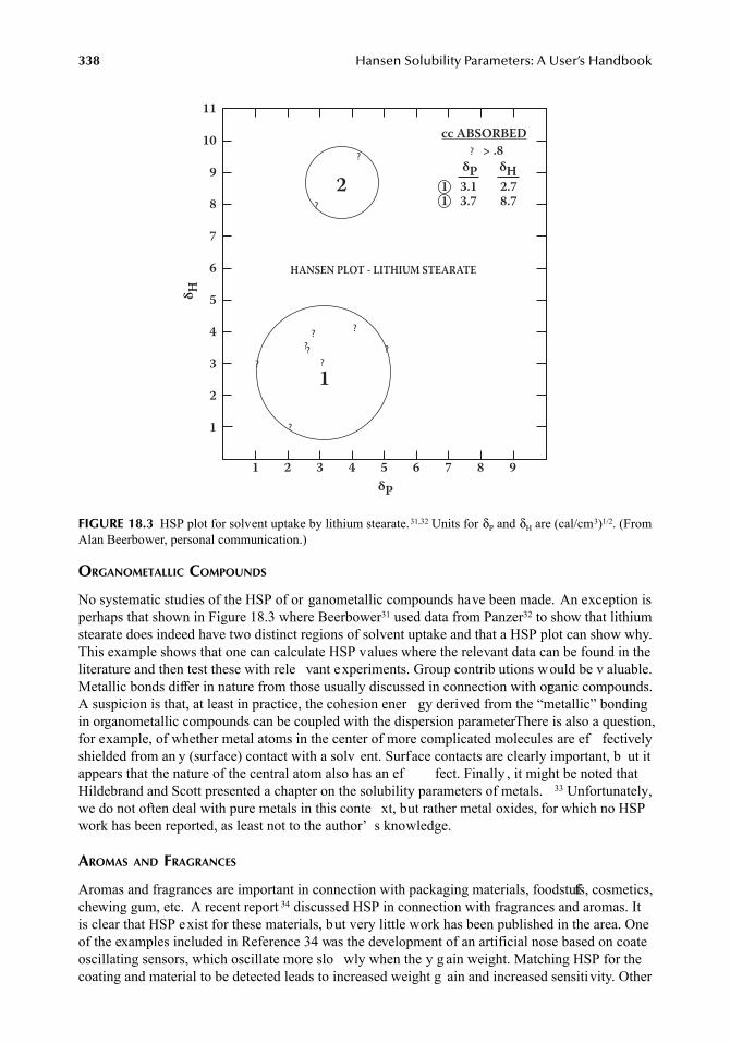
338 Hansen Solubility Parameters: A User’s Handbook
ORGANOMETALLIC COMPOUNDS
No systematic studies of the HSP of or ganometallic compounds have been made. An exception isperhaps that shown in Figure 18.3 where Beerbower31 used data from Panzer32 to show that lithiumstearate does indeed have two distinct regions of solvent uptake and that a HSP plot can show why.This example shows that one can calculate HSP values where the relevant data can be found in theliterature and then test these with rele vant experiments. Group contrib utions would be v aluable.Metallic bonds differ in nature from those usually discussed in connection with organic compounds.A suspicion is that, at least in practice, the cohesion ener gy derived from the “metallic” bondingin organometallic compounds can be coupled with the dispersion parameter. There is also a question,for example, of whether metal atoms in the center of more complicated molecules are ef fectivelyshielded from an y (surface) contact with a solv ent. Surface contacts are clearly important, b ut itappears that the nature of the central atom also has an ef fect. Finally , it might be noted thatHildebrand and Scott presented a chapter on the solubility parameters of metals. 33 Unfortunately,we do not often deal with pure metals in this conte xt, but rather metal oxides, for which no HSPwork has been reported, as least not to the author’ s knowledge.
AROMAS AND FRAGRANCES
Aromas and fragrances are important in connection with packaging materials, foodstuffs, cosmetics,chewing gum, etc. A recent report 34 discussed HSP in connection with fragrances and aromas. Itis clear that HSP exist for these materials, but very little work has been published in the area. Oneof the examples included in Reference 34 was the development of an artificial nose based on coateoscillating sensors, which oscillate more slo wly when the y g ain weight. Matching HSP for thecoating and material to be detected leads to increased weight g ain and increased sensitivity. Other
FIGURE 18.3 HSP plot for solvent uptake by lithium stearate.31,32 Units for δP and δH are (cal/cm3)1/2. (FromAlan Beerbower, personal communication.)
11
10
9
8
7
6
5
4
3
2
1
δ HδP
δP
δH1 3.11 3.7
2.78.7
? > .8?
?
?
?
?
?
???
?
2
1
cc ABSORBED
HANSEN PLOT - LITHIUM STEARATE
987654321
7248_C018.fm Page 338 Wednesday, May 23, 2007 11:46 AM
The Future 339
examples where HSP could be systematically used include: counteracting undesirable odors usingfragrances that have reasonably similar HSP; absorption of odors into plastics, coatings, sealants,etc.; development of packaging with designed HSP to either function as a barrier or as a sink; andan estimate of where a gi ven aromatic material is lik ely to reside. The key to interpretation is, asusual, that similarity of HSP means higher affinit . It is thought that the masking effect is the resultof adsorption of the fragrance on the regions of the sensory system where HSP are similar to thoseof the undesired odor . There may not be a complete match re garding steric adsorption, b ut thesensitive areas are covered anyway, and this barrier prevents the odor from arriving at the given sites.
ABSORPTION OF CHEMICALS IN PLASTICS
HSP correlations e xist for chemical resistance, permeation phenomena, and uptak e of solv ents inmany polymers. The recycling of polymeric containers has a potential problem in that the polymersused are able to readily absorb those chemicals whose HSP are not too dif ferent from their o wn.Once a chemical has absorbed into a polymer , and particularly if it is a rigid polymer with arelatively high glass transition temperature, it can be v ery difficult to get it out a ain. A relativelyslow diffusion process is required to do this. See Chapter 16. It is suggested that an e xtensive HSPanalysis be done for those polymers where potential misuse or contamination of containers priorto rec ycling is a possibility . This can point out which chemicals are most lik ely to present thegreatest problems.
CHEMICAL RESISTANCE
Chemical resistance studies ha ve generally been performed with too fe w liquids and without thenecessary spread of HSP to allow the data to be correlated with confidence. In addition, attainmenof equilibrium is not usually confirmed.These shortcomings mean that HSP correlations of chemicalresistance must be done with great care. This has been discussed in Chapter 12 in more detail. Anadditional activity, which should be done for practical reasons, is to assign effective HSP to varioustest materials such as mustard, k etchup, and other gi ven products that often appear in tests ofchemical resistance. Such data will allow greater use of the correlations since guidelines for potentialimprovements can be obtained.
CONTROLLED RELEASE
HSP considerations can provide an extra formulating parameter for the controlled release of drugs.When the HSP relations between a drug and its surroundings are known, predictions of its behaviorcan be made. When there is a good match in the HSP v alues, the drug will be more soluble withthe ability to mo ve at some rate within a polymer matrix. On the other hand it can be surroundedby a matrix with similar HSP, and this may slo w release more than desired. A poor match in HSPmay leave holes and expose the drug for more rapid release. When the match is poor, the drug willnot be able to permeate through its polymeric surroundings, b ut it can, of course, pass throughopen passageways. Drugs will also tend to adsorb at surf aces where there is a good HSP match.
It has been sho wn (personal communication, Andreas Gryczk e, De gussa Pharma Polymers,Darmstadt) that calculations of HSP for a number of drugs and for a series of EUDRAGIT® polymersprovided a correlation confirming that the drugs are soluble in those polymers where the HSmatch closely enough. When the drug and polymer HSP were within 10 MPa1/2 at the concentrationstudied (20% wgt.), what appeared to be true solubility w as found. This was evidenced by x-raydiffraction and DSC measurement that confirmed the drugs were embedded completely amorphou(solid solution). A closer match would presumably be required to do this for higher concentrationsof the drugs.
Table 18.6 contains HSP for some materials whose solubility in various media may have interest.It is possible to calculate HSP for essentially all drugs, although h ydrochlorides and other salts
7248_C018.fm Page 339 Wednesday, May 23, 2007 11:46 AM
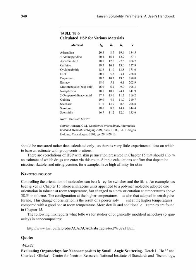
340 Hansen Solubility Parameters: A User’s Handbook
should be measured rather than calculated only , as there is v ery little experimental data on whichto base an estimate with group contrib utions.
There are correlations of HSP with skin permeation presented in Chapter 15 that should allo wan estimate of which drugs can enter via this route. Simple calculations confirm that dopaminenicotine, skatole, and nitroglycerine, for e xample, have high affinity for skin
NANOTECHNOLOGY
Controlling the orientation of molecules can be a k ey for switches and the lik e. An example hasbeen given in Chapter 15 where anthracene units appended to a polymer molecule adopted oneorientation in toluene at room temperature, but changed to a new orientation at temperatures above38.5° in toluene. The configuration at the higher temperatures as also that adopted in tetrah ydro-furane. This change of orientation is the result of a poorer solv ent at the higher temperaturescompared with a good one at room temperature. More details and additional e xamples are foundin Chapter 15.
The following link reports what follo ws for studies of or ganically modified nanoclays (o gan-oclay) in nanocomposites:
http://www.hwi.buffalo.edu/ACA/ACA03/abstracts/text/W0383.html
Quote:
W0383Evaluating Organoclays for Nanocomposites by Small Angle Scattering. Derek L. Ho 1,2 andCharles J. Glinka1, 1Center for Neutron Research, National Institute of Standards and Technology,
TABLE 18.6Calculated HSP for Various Materials
Material δδδδD δδδδP δδδδH V
Adrenaline 20.5 8.7 19.9 154.54-Aminopyridine 20.4 16.1 12.9 87.1Ascorbic Acid 18.0 12.6 27.6 106.7Caffeine 19.5 10.1 13.0 157.9Cycloheximide 18.3 11.0 13.8 171.0DDT 20.0 5.5 3.1 268.8Dopamine 18.2 10.3 19.5 180.0Ecstacy 18.0 5.1 6.1 202.9Meclofenoxate (base only) 16.0 6.2 9.0 198.3Norephedrin 18.0 10.7 24.1 141.92-Oxopyrrolidinacetamid 17.5 15.6 11.2 116.2Quinine 19.0 4.6 11.0 310.7Saccharin 21.0 13.9 8.8 206.8Serotonin 18.0 8.2 14.4 144.4Spermidin 16.7 11.2 12.0 155.6
Note: Units are MPa1/2.
Source: Hansen, C.M., Conference Proceedings, Pharmaceu-tical and Medical Packaging 2001, Skov, H. R., Ed., HexagonHolding, Copenhagen, 2001, pp. 20.1–20.10.
7248_C018.fm Page 340 Wednesday, May 23, 2007 11:46 AM
The Future 341
Gaithersburg, MD 20899, 2Dept. of Materials and Nuclear Engineering, Univ. of Maryland, CollegePark, MD 20742.
Understanding the interaction between or ganically modified clay (o ganoclay) platelets and or ganicsolvent molecules as well as the corresponding structure of or ganoclays in a suspension is a criticalstep toward tailoring and characterizing nanocomposites formed by or ganoclays in a polymer matrix.Recently, nanocomposites composed of clays and polymers ha ve been found to ha ve impro vedmechanical properties as well as enhanced thermal stability . The improved properties are related to thedegree of dispersal and e xfoliation of the clay platelets in the polymer matrix. In order to understandand optimize potential processing conditions, or ganoclays were dispersed in a number of or ganicsolvents covering a range of solubility parameters and characterized using small-angle neutron scatteringand wide-angle x-ray scattering techniques. With Hansen’s solubility parameters, δo
2 = δd2 + δp
2 + δh2,
the correlation between the de gree of e xfoliation of or ganoclays and the solv ent in which the clayplatelets are dispersed/mix ed has been analyzed. It has been found that the dispersion force of thesolvent, reflected by δd, is the principal factor determining whether the clay platelets remain suspendedin the solv ent while the polar ( δp) and h ydrogen-bonding ( δh) forces af fect primarily the tactoidformation/structure of the suspended platelets. The or ganically modified clays studied in this orkprecipitated in an y solv ent with molecules with moderately strong h ydrogen-bonding groups. Thecorrelation found has been used to correctly identify a solv ent, trichloroeth ylene, which completelyexfoliates the organoclays studied in this w ork.
These and the many other examples in this handbook related to self-assembly (see abo ve), surfaceadsorption, molecular orientation, and af finity among molecules and molecular s gments shouldprovide ample evidence that molecular guidance in nanotechnology endea vors can be found in theHSP concept.
THEORETICAL PROBLEMS AWAITING FUTURE RESOLUTION
POLYMER SOLUBILITY
The Flory chi parameter has been used to describe polymer–solvent interactions for many years.35,36
If this single parameter is to be complete in this function, it must include both the atomic/dispersioninteractions as well as the specific interactions reflected by th δP and δH parameters. Attempts tocalculate chi using HSP are reported in Chapter 2. More understanding is required before chi canbe calculated with reasonable accuracy, but intensified e forts seem warranted. Zellers and cowork-ers have recently made an attempt to use this theory in conjunction with HSP studies. 37–40 A majorproblem is the reliability of the chi parameter (and also HSP) v alues in the literature (see Chapter2 for more details). Chapter 4 is a length y discussion of the use of HSP in thermodynamic modelsfor polymer solutions.
The author’s current view as expressed in Chapter 2 is that the Flory approach is a special caseof the more general Prigogine corresponding states theory . This is in agreement with the vie w ofPatterson discussed in Chapter 2. Furthermore, the v ery general applications of the HSP approachdemonstrated in this book and else where, and the apparent agreement in the treatment of specifiinteractions by both the HSP and Prigogine treatments, leads to confidence in the HSP approachThe geometric mean must be used in the Prigogine theory to arri ve at this similarity of treatment.The statistical thermodynamic approach of P anayiotou and co workers thoroughly discussed inChapter 3 provides convincing evidence that the division of the cohesion energy density into threeparts (at least) is the correct procedure to understand af finities among ma y types of materials.Finally, Chapter 4 deals with theories of vapor–liquid equilibrium in particular and how these relateto HSP.
7248_C018.fm Page 341 Wednesday, May 23, 2007 11:46 AM
342 Hansen Solubility Parameters: A User’s Handbook
SURFACE PHENOMENA
Surfaces can clearly be characterized by HSP as demonstrated in Chapter 6 and Chapter 7. Thework of Beerbo wer contained in Reference 17 and Reference 23 has also sho wn applications ofHSP to such varied phenomena as the work of adhesion of liquids on mercury, friction of polyeth-ylene untreated and treated with sulfuric acid, the Rehbinder ef fect — the crushing of aluminumoxide (Al 2O3) under v arious liquids, and the Jof fé ef fect — ef fect of liquid immersion on thefracture strength of soda-lime glass. Here ag ain, the successful use of HSP to such applicationsmight not have been anticipated had it been considered as a parameter for use in bulk systems only.A formalized unifying theory linking HSP to both b ulk and surf ace phenomena is still lacking.Presently, the best that can be said is that the generality “lik e dissolves like” can be quantified imany cases. The extension of this, “lik e seeks lik e,” also seems to ha ve been demonstrated. It isthe surfaces of molecules which interact with each other (also in b ulk and solution phenomena),so it is not surprising that cohesion parameters can be applied with success to both solubility andsurface phenomena. Much more research needs to be done with these relations. A good startingpoint is the Handbook of Surface and Colloid Chemistry, edited by K.S. Birdi. 41 If we considerchromatographic techniques as depending primarily on surf ace phenomena, mention should alsobe made of the e xtension of the three-parameter HSP approach to a fi e-parameter approach byKarger and coworkers.42 HSP characterizations of surf actants are also badly needed.
CONCLUSION
HSP have been sho wn useful in solv ent selection; predicting polymer–polymer miscibility; char -acterizing the surfaces of polymers, fillers, and fibers; correlating permeation phenomena; charaterizing organic salts and inor ganic salts; g as solubility; etc. No other parameter can be assignedto such a range of materials spanning from g ases and liquids, o ver surf aces, to inor ganic salts.These results and the close relation with the Prigogine corresponding states theory of polymersolutions, and more recently to the w ork of P anayiotou summarized in Chapter 3, indicate that astill more general theory exists. This theory should quantify the adage “like seeks like,” i.e., includesurface phenomena as well as b ulk phenomena.
Specific areas needing more theoretical ork related to HSP in the near future include betterunderstanding of usage for predictions of beha vior for water, gases, organic salts, inorganic salts,and organometallic compounds. Water remains special because of its lo w molecular v olume andhigh δH. Most materials having HSP in the range of the customary test liquids can be studied usingHSP with reasonable success. This is not fully the case for gases, many of which have much lowerHSP than the well-studied liquids, and salts, many of which apparently have HSP very much higherthan any of the liquids. Extensions of practical applications related to chemical resistance and theuptake of potentially dangerous materials in polymers are also required. Finally there is a greatdeal to be done in the areas of controlled drug release, impro ved understanding of some biologicalprocesses, and last b ut not least, the systematic use of HSP in nanotechnology to control theassembly and orientation of molecules or se gments of molecules.
REFERENCES
1. Hansen, C.M., The universality of the solubility parameter , Ind. Eng. Chem. Prod. Res. Dev., 8(1),2–11, 1969.
2. Barton, A.F.M., Handbook of Solubility Parameters and Other Cohesion Parameters, CRC Press,Boca Raton, FL, 1983; 2nd ed., 1991.
3. Barton, A.F.M., Handbook of Polymer-Liquid Interaction Parameters and Solubility Parameters, CRCPress, Boca Raton, FL, 1990.
7248_C018.fm Page 342 Wednesday, May 23, 2007 11:46 AM
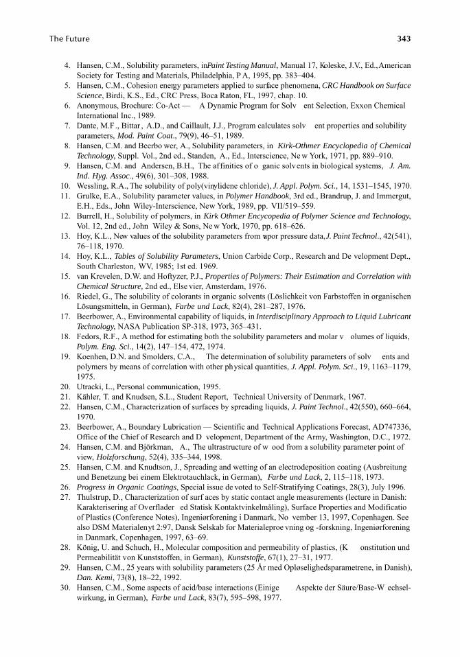
The Future 343
4. Hansen, C.M., Solubility parameters, in Paint Testing Manual, Manual 17, Koleske, J.V., Ed., AmericanSociety for Testing and Materials, Philadelphia, P A, 1995, pp. 383–404.
5. Hansen, C.M., Cohesion energy parameters applied to surface phenomena, CRC Handbook on SurfaceScience, Birdi, K.S., Ed., CRC Press, Boca Raton, FL, 1997, chap. 10.
6. Anonymous, Brochure: Co-Act — A Dynamic Program for Solv ent Selection, Exxon ChemicalInternational Inc., 1989.
7. Dante, M.F., Bittar , A.D., and Caillault, J.J., Program calculates solv ent properties and solubilityparameters, Mod. Paint Coat., 79(9), 46–51, 1989.
8. Hansen, C.M. and Beerbo wer, A., Solubility parameters, in Kirk-Othmer Encyclopedia of ChemicalTechnology, Suppl. Vol., 2nd ed., Standen, A., Ed., Interscience, Ne w York, 1971, pp. 889–910.
9. Hansen, C.M. and Andersen, B.H., The affinities of o ganic solvents in biological systems, J. Am.Ind. Hyg. Assoc., 49(6), 301–308, 1988.
10. Wessling, R.A., The solubility of poly(vinylidene chloride), J. Appl. Polym. Sci., 14, 1531–1545, 1970.11. Grulke, E.A., Solubility parameter values, in Polymer Handbook, 3rd ed., Brandrup, J. and Immergut,
E.H., Eds., John Wiley-Interscience, New York, 1989, pp. VII/519–559.12. Burrell, H., Solubility of polymers, in Kirk Othmer Encycopedia of Polymer Science and Technology,
Vol. 12, 2nd ed., John Wiley & Sons, Ne w York, 1970, pp. 618–626.13. Hoy, K.L., New values of the solubility parameters from vapor pressure data, J. Paint Technol., 42(541),
76–118, 1970.14. Hoy, K.L., Tables of Solubility Parameters, Union Carbide Corp., Research and De velopment Dept.,
South Charleston, WV, 1985; 1st ed. 1969.15. van Krevelen, D.W. and Hoftyzer, P.J., Properties of Polymers: Their Estimation and Correlation with
Chemical Structure, 2nd ed., Else vier, Amsterdam, 1976.16. Riedel, G., The solubility of colorants in organic solvents (Löslichkeit von Farbstoffen in organischen
Lösungsmitteln, in German), Farbe und Lack, 82(4), 281–287, 1976.17. Beerbower, A., Environmental capability of liquids, in Interdisciplinary Approach to Liquid Lubricant
Technology, NASA Publication SP-318, 1973, 365–431.18. Fedors, R.F., A method for estimating both the solubility parameters and molar v olumes of liquids,
Polym. Eng. Sci., 14(2), 147–154, 472, 1974.19. Koenhen, D.N. and Smolders, C.A., The determination of solubility parameters of solv ents and
polymers by means of correlation with other physical quantities, J. Appl. Polym. Sci., 19, 1163–1179,1975.
20. Utracki, L., Personal communication, 1995.21. Kähler, T. and Knudsen, S.L., Student Report, Technical University of Denmark, 1967.22. Hansen, C.M., Characterization of surfaces by spreading liquids, J. Paint Technol., 42(550), 660–664,
1970.23. Beerbower, A., Boundary Lubrication — Scientific and Technical Applications Forecast, AD747336,
Office of the Chief of Research and D velopment, Department of the Army, Washington, D.C., 1972.24. Hansen, C.M. and Björkman, A., The ultrastructure of w ood from a solubility parameter point of
view, Holzforschung, 52(4), 335–344, 1998.25. Hansen, C.M. and Knudtson, J., Spreading and wetting of an electrodeposition coating (Ausbreitung
und Benetzung bei einem Elektrotauchlack, in German), Farbe und Lack, 2, 115–118, 1973.26. Progress in Organic Coatings, Special issue de voted to Self-Stratifying Coatings, 28(3), July 1996.27. Thulstrup, D., Characterization of surf aces by static contact angle measurements (lecture in Danish:
Karakterisering af Overflader ed Statisk Kontaktvinkelmåling), Surface Properties and Modificatioof Plastics (Conference Notes), Ingeniørforening i Danmark, No vember 13, 1997, Copenhagen. Seealso DSM Materialenyt 2:97, Dansk Selskab for Materialeproe vning og -forskning, Ingeniørforeningin Danmark, Copenhagen, 1997, 63–69.
28. König, U. and Schuch, H., Molecular composition and permeability of plastics, (K onstitution undPermeabilität von Kunststoffen, in German), Kunststoffe, 67(1), 27–31, 1977.
29. Hansen, C.M., 25 years with solubility parameters (25 År med Opløselighedsparametrene, in Danish),Dan. Kemi, 73(8), 18–22, 1992.
30. Hansen, C.M., Some aspects of acid/base interactions (Einige Aspekte der Säure/Base-W echsel-wirkung, in German), Farbe und Lack, 83(7), 595–598, 1977.
7248_C018.fm Page 343 Wednesday, May 23, 2007 11:46 AM
344 Hansen Solubility Parameters: A User’s Handbook
31. Beerbower, A., Personal communication, Predicting Wetting in the Oil-Brine-Rock System, Uneditedmanuscript for presentation at the National AIChE Meeting, Tulsa, OK, March 10–13, 1974.
32. Panzer, J., Components of solid surf ace free energy from wetting measurements, J. Colloid InterfaceSci., 44(1), 142–161, July 1973.
33. Hildebrand, J. and Scott, R.L., The Solubility of Nonelectrolytes, 3rd ed., Reinhold, New York, 1950.34. Hansen, C.M., Solubility parameters for aromas and scents (Aromastof fers Opløselighedsparametre,
in Danish), Plus Process, 11(9), 16–17, 1997.35. Flory, P.J., Principles of Polymer Chemistry, Cornell University Press, New York, 1953.36. Eichinger, B.E. and Flory , P.J., Thermodynamics of polymer solutions, Trans. Faraday Soc., 64(1),
2035–2052, 1968; 64(2), 2053–2060, 1968; 64(3), 2061–2065, 1968; 64(4), 2066–2072, 1968.37. Zellers, E.T., Three-dimensional solubility parameters and chemical protecti ve clothing permeation.
I. Modelling the solubility of organic solvents in Viton® gloves, J. Appl. Polym. Sci., 50, 513–530, 1993.38. Zellers, E.T., Three-dimensional solubility parameters and chemical protective clothing. II. Modelling
diffusion coefficients, breakthrough times, and steady-state permeation rates of o ganic solvents inViton® gloves, J. Appl. Polym. Sci., 50, 531–540, 1993.
39. Zellers, E.T., Anna, D.H., Sulewski, R., and Wei, X., Critical analysis of the graphical determinationof Hansen’s solubility parameters for lightly crosslinked polymers, J. Appl. Polym. Sci., 62, 2069–2080,1996.
40. Zellers, E.T., Anna, D.H., Sule wski, R., and Wei, X., Impro ved methods for the determination ofHansen’s solubility parameters and the estimation of solv ent uptake for lightly crosslinked polymers,J. Appl. Polym. Sci., 62, 2081–2096, 1996.
41. Birdi, K.S., Handbook of Surface and Colloid Chemistry, CRC Press, Boca Raton, FL, 1997.42. Karger, B.L., Sn yder, L.R., and Eon, C., Expanded solubility parameter treatment for classificatio
and use of chromatographic solv ents and adsorbents, Anal. Chem., 50(14), 2126–2136, 1978.
7248_C018.fm Page 344 Wednesday, May 23, 2007 11:46 AM
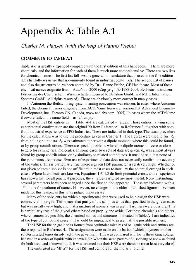
345
Appendix A: Table A.1
Charles M. Hansen (with the help of Hanno Priebe)
COMMENTS TO TABLE A.1
Table A-1 is greatly e xpanded compared with the first edition of this handbook. There are morechemicals, and the information for each of them is much more comprehensi ve. There are two listsfor chemical names. The first list foll ws the general nomenclature that is used in the first editionThis list follo ws usage that is commonly found in industrial conte xts. The second list of namesand also the structures ha ve been compiled by Dr . Hanno Priebe, GE Healthcare. Most of thesechemical names originate from AutoNom 2000 (Cop yright © 1988-2006, Beilstein-Institut zurFörderung der Chemischen Wissenschaften licensed to Beilstein GmbH and MDL InformationSystems GmbH. All rights reserved). These are obviously more correct in man y cases.
In Autonom the Beilstein ring system naming convention was chosen. In cases where Autonomfailed, the chemical names originate from ACD/Name freeware, version 8.0 (Advanced ChemistryDevelopment, Inc., Toronto ON, Canada, www.acdlabs.com, 2005). In cases where the ACD/Namefreeware failed, the name field as left empty.
Most of the HSP entries in Table A-1 are calculated v alues. Those entries ha ving someexperimental confirmation are the original 90 from Reference 1 to Reference 3, together with somfrom industrial experience at PPG Industries. These are indicated in dark type. The usual procedurefor the calculations w as to use the procedure gi ven in Chapter 1. The figures were used to fin
δ
D
from boiling point data.
δ
P
was estimated either with a dipole moment, where this could be found,or by group contrib utions. There are special problems where the dipole moment is zero or closeto zero for symmetrical molecules. In some cases tw o sets of data are given.
δ
H
was almost alwaysfound by group contrib utions or by similarity to related compounds. It must be said that none ofthe parameters are precise. Even use of experimental data does not necessarily confirm the accura yof the values. This is particularly true where a gi ven HSP parameter is relati vely high. Whether ornot given solutes dissolv e is not suf ficient in most cases to narr w the potential error(s) in suchcases. Where latent heats are kno wn, Equations 1.6–1.8 do limit potential errors, and e xperiencehas shown that for all practical purposes, the v alues assigned are most useful. Notwithstanding,several parameters have been changed since the first edition appeared. These are indicated with a“*” in the first column of names. H wever, no changes in the older , published figures h ve beenmade for this reason, as this w as judged unnecessary.
Many of the solv ents for which e xperimental data were used to help assign the HSP werecommercial in origin. This means that purity of the samples w as that specified in the g ven case,but was usually very high, and that a mixture of isomers was present if isomers were possible. Thisis particularly true of the glycol ethers based on prop ylene oxide. For these chemicals and otherswhere isomers are possible, the chemical names and structures indicated in Table A-1 are indicativeof the type of compound present. It w ould be impractical to present all the possible isomers.
The HSP for the or ganic salts formed from equimolar mixtures of or ganic acids and amines arethose reported in Reference 4. The assignments were made on the basis of which polymers or othersolutes in a test series dissolv ed in the gi ven salt. This was compared with ho w these same solutesbehaved in a series of liquids with kno wn HSP. When the same pattern of dissolving or not w as foundfor both a salt and a known liquid, it was assumed that their HSP were the same (or at least very close).
The units used are MP a
1/2
for the HSP and cc/mole for the molar v olume.
7248_A001.fm Page 345 Wednesday, May 23, 2007 12:31 PM

346
Hansen Solubility Parameters: A User’s Handbook
REFERENCES
1. Hansen, C.M., The Three Dimensional Solubility Parameter and Solvent Diffusion Coefficient, Doctoral Dissertation, Danish Technical Press, Copenhagen, 1967.
2. Hansen, C.M., The Three Dimensional Solubility Parameter — Key to Paint Component Affinities I— Solvents, Plasticizers, Polymers, and Resins,
J. Paint Techn
., 39(505), 104-117, 1967.3. Hansen, C.M., and Skaarup, K., The Three Dimensional Solubility P arameter — Key to Paint Com-
ponent Affinities III. — Independent Calculation of the arameter Components,
J. Paint Techn
.39(511), 511-514, 1967.
4. Hansen, C.M., Some Aspects of Acid/Base Interactions (in German) (Einige Aspekte der Säure/Base-Wechselwirkung),
Farbe und Lack
, 83(7), 595-598, 1977.
7248_A001.fm Page 346 Wednesday, May 23, 2007 12:31 PM
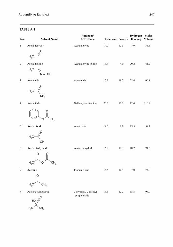
Appendix A: Table A.1
347
TABLE A.1
No. Solvent NameAutonom/
ACD Name Dispersion PolarityHydrogenBonding
MolarVolume
1 Acetaldehyde* Acetaldehyde 14.7 12.5 7.9 56.6
2 Acetaldoxime Acetaldehyde oxime 16.3 4.0 20.2 61.2
3 Acetamide Acetamide 17.3 18.7 22.4 60.8
4 Acetanilide N-Phenyl-acetamide 20.6 13.3 12.4 110.9
5
Acetic Acid
Acetic acid 14.5 8.0 13.5 57.1
6
Acetic Anhydride
Acetic anhydride 16.0 11.7 10.2 94.5
7
Acetone
Propan-2-one 15.5 10.4 7.0 74.0
8 Acetonecyanhydrin 2-Hydroxy-2-methyl-propionitrile
16.6 12.2 15.5 94.0
CH3
O
CH3
N OH
CH3
O
NH2
N CH3
O
CH3
OH
O
CH3 O
O
CH3
O
CH3 CH3
O
CH3 CH3
OHN
7248_A001.fm Page 347 Wednesday, May 23, 2007 12:31 PM
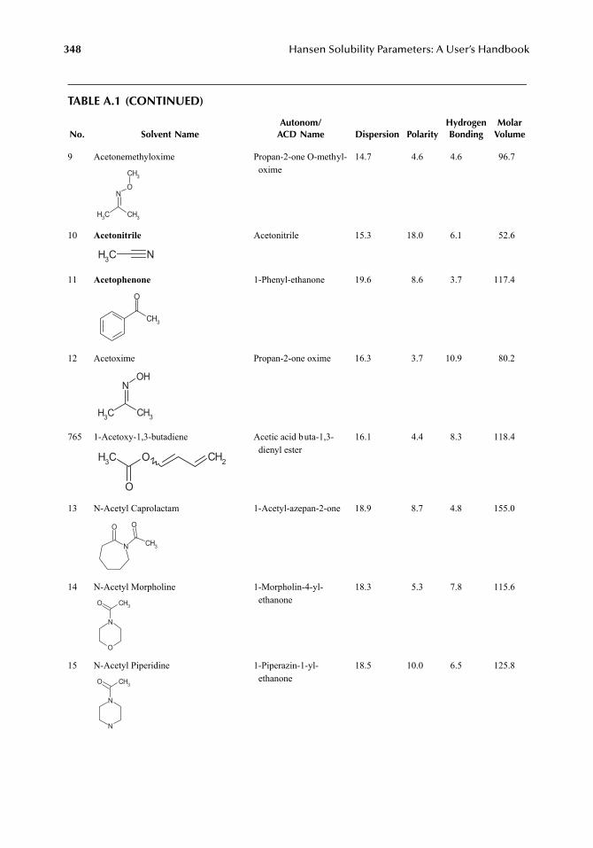
348
Hansen Solubility Parameters: A User’s Handbook
TABLE A.1 (CONTINUED)
No. Solvent NameAutonom/
ACD Name Dispersion PolarityHydrogenBonding
MolarVolume
9 Acetonemethyloxime Propan-2-one O-methyl-oxime
14.7 4.6 4.6 96.7
10
Acetonitrile
Acetonitrile 15.3 18.0 6.1 52.6
11
Acetophenone
1-Phenyl-ethanone 19.6 8.6 3.7 117.4
12 Acetoxime Propan-2-one oxime 16.3 3.7 10.9 80.2
765 1-Acetoxy-1,3-butadiene Acetic acid buta-1,3-dienyl ester
16.1 4.4 8.3 118.4
13 N-Acetyl Caprolactam 1-Acetyl-azepan-2-one 18.9 8.7 4.8 155.0
14 N-Acetyl Morpholine 1-Morpholin-4-yl-ethanone
18.3 5.3 7.8 115.6
15 N-Acetyl Piperidine 1-Piperazin-1-yl-ethanone
18.5 10.0 6.5 125.8
CH3 CH3
NO
CH3
CH3 N
CH3
O
CH3 CH3
NOH
CH2OCH3
O
N
O
CH3
O
O
N
CH3O
N
N
CH3O
7248_A001.fm Page 348 Wednesday, May 23, 2007 12:31 PM
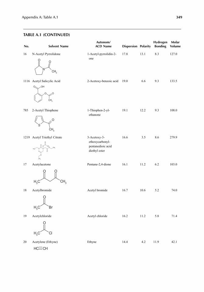
Appendix A: Table A.1
349
TABLE A.1 (CONTINUED)
No. Solvent NameAutonom/
ACD Name Dispersion PolarityHydrogenBonding
MolarVolume
16 N-Acetyl Pyrrolidone 1-Acetyl-pyrrolidin-2-one
17.8 13.1 8.3 127.0
1116 Acetyl Salicylic Acid 2-Acetoxy-benzoic acid 19.0 6.6 9.3 133.5
785 2-Acetyl Thiophene 1-Thiophen-2-yl-ethanone
19.1 12.2 9.3 108.0
1219 Acetyl Triethyl Citrate 3-Acetoxy-3-ethoxycarbonyl-pentanedioic acid diethyl ester
16.6 3.5 8.6 279.9
17 Acetylacetone Pentane-2,4-dione 16.1 11.2 6.2 103.0
18 Acetylbromide Acetyl bromide 16.7 10.6 5.2 74.0
19 Acetylchloride Acetyl chloride 16.2 11.2 5.8 71.4
20 Acetylene (Ethyne) Ethyne 14.4 4.2 11.9 42.1
N
O
CH3
O
O
OHO
CH3
O
SCH3
O
O
O
CH3
O
O
O
O
CH3
CH3
O
O
CH3
CH3
O
CH3
O
CH3 Br
O
CH3 Cl
O
CH CH
7248_A001.fm Page 349 Wednesday, May 23, 2007 12:31 PM
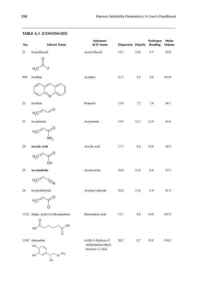
350
Hansen Solubility Parameters: A User’s Handbook
TABLE A.1 (CONTINUED)
No. Solvent NameAutonom/
ACD Name Dispersion PolarityHydrogenBonding
MolarVolume
21 Acetylfluorid Acetyl fluorid 14.7 14.0 5.7 62.0
860 Acridine Acridine 21.7 5.9 2.0 163.0
22 Acrolein Propenal 15.0 7.2 7.8 66.7
23 Acrylamide Acrylamide 15.8 12.1 12.8 63.4
24
Acrylic Acid
Acrylic acid 17.7 6.4 14.9 68.5
25
Acrylonitrile
Acrylonitrile 16.0 12.8 6.8 67.1
26 Acrylylchloride Acryloyl chloride 16.2 11.6 5.4 81.3
1152 Adipic Acid (1,6-Hexanedioic) Hexanedioic acid 17.1 9.0 14.6 107.5
1195 Adrenaline 4-((R)-1-Hydroxy-2-methylamino-ethyl)-benzene-1,2-diol
20.5 8.7 19.9 154.5
CH3 F
O
N
CH2
O
CH2
O
NH2
CH2
O
OH
CH2 N
CH2
O
Cl
OHOH
O
O
OH
OH N
OH
CH3
7248_A001.fm Page 350 Wednesday, May 23, 2007 12:31 PM
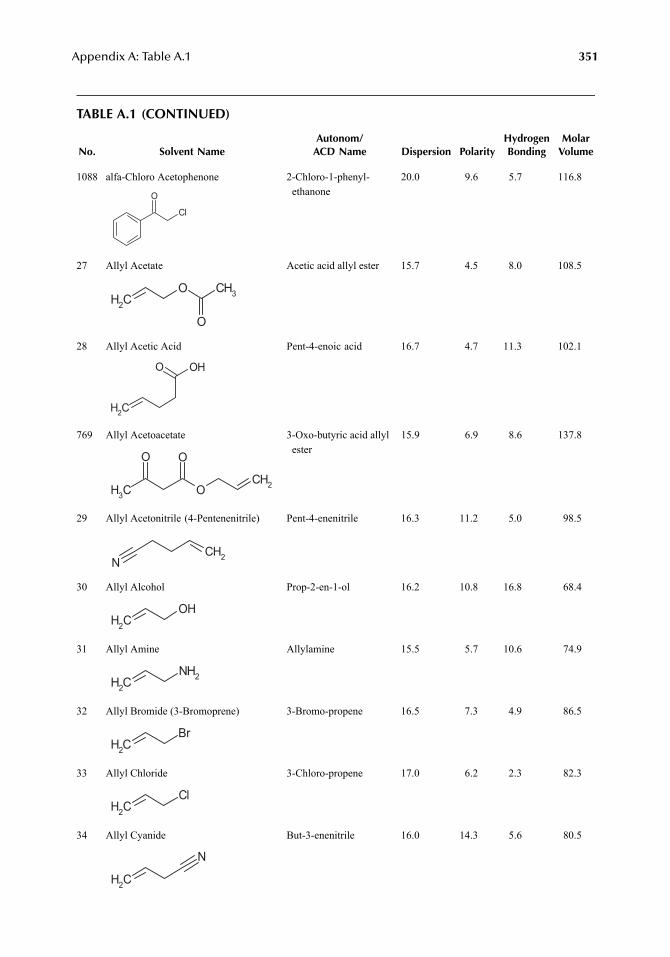
Appendix A: Table A.1
351
TABLE A.1 (CONTINUED)
No. Solvent NameAutonom/
ACD Name Dispersion PolarityHydrogenBonding
MolarVolume
1088 alfa-Chloro Acetophenone 2-Chloro-1-phenyl-ethanone
20.0 9.6 5.7 116.8
27 Allyl Acetate Acetic acid allyl ester 15.7 4.5 8.0 108.5
28 Allyl Acetic Acid Pent-4-enoic acid 16.7 4.7 11.3 102.1
769 Allyl Acetoacetate 3-Oxo-butyric acid allyl ester
15.9 6.9 8.6 137.8
29 Allyl Acetonitrile (4-Pentenenitrile) Pent-4-enenitrile 16.3 11.2 5.0 98.5
30 Allyl Alcohol Prop-2-en-1-ol 16.2 10.8 16.8 68.4
31 Allyl Amine Allylamine 15.5 5.7 10.6 74.9
32 Allyl Bromide (3-Bromoprene) 3-Bromo-propene 16.5 7.3 4.9 86.5
33 Allyl Chloride 3-Chloro-propene 17.0 6.2 2.3 82.3
34 Allyl Cyanide But-3-enenitrile 16.0 14.3 5.6 80.5
O
Cl
CH2
O CH3
O
OHO
CH2
O
O
CH3
O
CH2
CH2N
CH2
OH
CH2
NH2
CH2
Br
CH2
Cl
CH2
N
7248_A001.fm Page 351 Wednesday, May 23, 2007 12:31 PM
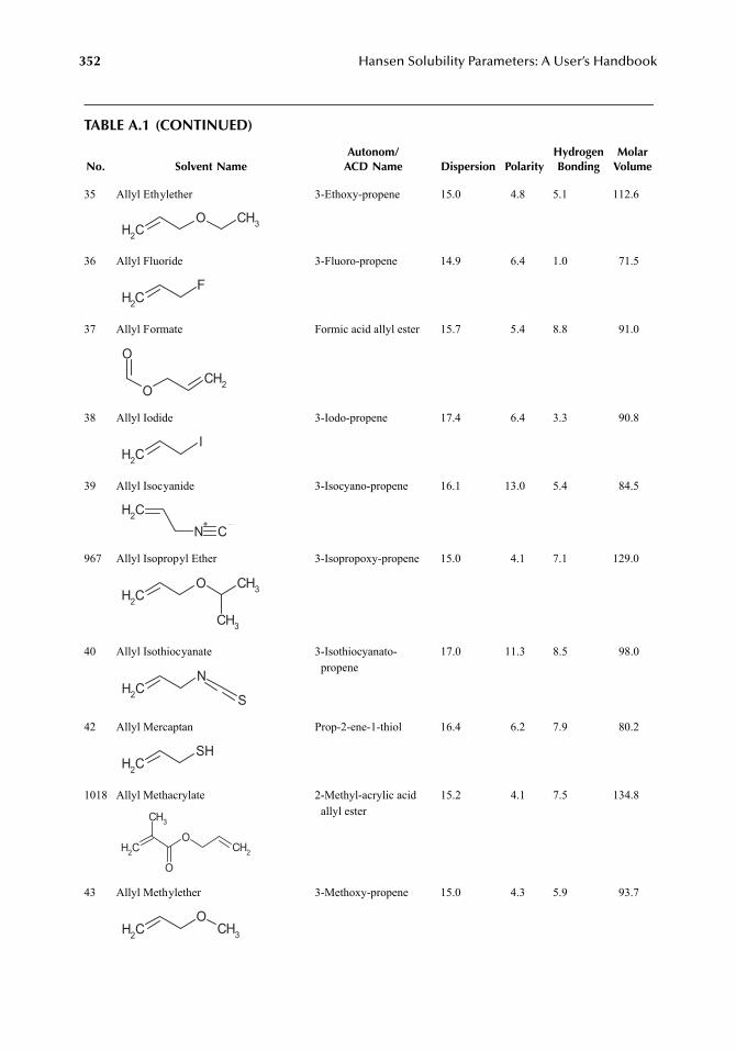
352
Hansen Solubility Parameters: A User’s Handbook
TABLE A.1 (CONTINUED)
No. Solvent NameAutonom/
ACD Name Dispersion PolarityHydrogenBonding
MolarVolume
35 Allyl Ethylether 3-Ethoxy-propene 15.0 4.8 5.1 112.6
36 Allyl Fluoride 3-Fluoro-propene 14.9 6.4 1.0 71.5
37 Allyl Formate Formic acid allyl ester 15.7 5.4 8.8 91.0
38 Allyl Iodide 3-Iodo-propene 17.4 6.4 3.3 90.8
39 Allyl Isocyanide 3-Isocyano-propene 16.1 13.0 5.4 84.5
967 Allyl Isopropyl Ether 3-Isopropoxy-propene 15.0 4.1 7.1 129.0
40 Allyl Isothiocyanate 3-Isothiocyanato-propene
17.0 11.3 8.5 98.0
42 Allyl Mercaptan Prop-2-ene-1-thiol 16.4 6.2 7.9 80.2
1018 Allyl Methacrylate 2-Methyl-acrylic acid allyl ester
15.2 4.1 7.5 134.8
43 Allyl Methylether 3-Methoxy-propene 15.0 4.3 5.9 93.7
CH2
O CH3
CH2
F
O
OCH2
CH2
I
CH2
N+C
CH2
O CH3
CH3
CH2
N
S
CH2
SH
CH2
CH3
O
OCH2
CH2
OCH3
7248_A001.fm Page 352 Wednesday, May 23, 2007 12:31 PM
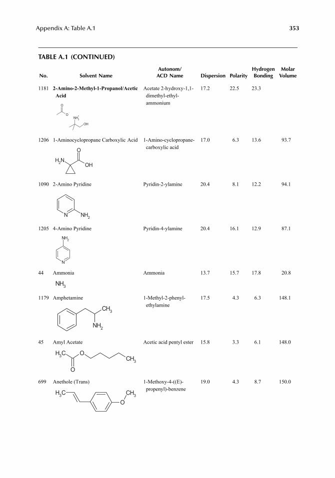
Appendix A: Table A.1
353
TABLE A.1 (CONTINUED)
No. Solvent NameAutonom/
ACD Name Dispersion PolarityHydrogenBonding
MolarVolume
1181
2-Amino-2-Methyl-1-Propanol/Acetic Acid
Acetate 2-hydroxy-1,1-dimethyl-ethyl-ammonium
17.2 22.5 23.3
1206 1-Aminocyclopropane Carboxylic Acid 1-Amino-cyclopropane-carboxylic acid
17.0 6.3 13.6 93.7
1090 2-Amino Pyridine Pyridin-2-ylamine 20.4 8.1 12.2 94.1
1205 4-Amino Pyridine Pyridin-4-ylamine 20.4 16.1 12.9 87.1
44 Ammonia Ammonia 13.7 15.7 17.8 20.8
1179 Amphetamine 1-Methyl-2-phenyl-ethylamine
17.5 4.3 6.3 148.1
45 Amyl Acetate Acetic acid pentyl ester 15.8 3.3 6.1 148.0
699 Anethole (Trans) 1-Methoxy-4-((E)-propenyl)-benzene
19.0 4.3 8.7 150.0
OH
NH3+O
O
NH2 OH
O
N NH2
N
NH2
NH3
CH3
NH2
CH3 O
O
CH3
CH3
OCH3
7248_A001.fm Page 353 Wednesday, May 23, 2007 12:31 PM
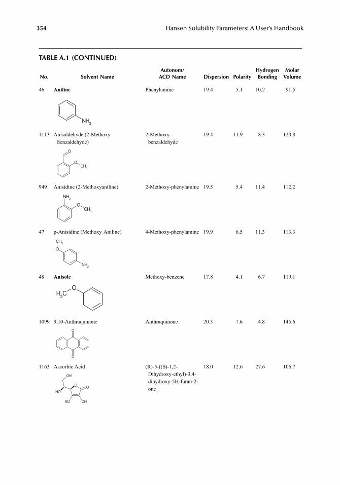
354
Hansen Solubility Parameters: A User’s Handbook
TABLE A.1 (CONTINUED)
No. Solvent NameAutonom/
ACD Name Dispersion PolarityHydrogenBonding
MolarVolume
46
Aniline
Phenylamine 19.4 5.1 10.2 91.5
1113 Anisaldehyde (2-Methoxy Benzaldehyde)
2-Methoxy-benzaldehyde
19.4 11.9 8.3 120.8
949 Anisidine (2-Methoxyaniline) 2-Methoxy-phenylamine 19.5 5.4 11.4 112.2
47 p-Anisidine (Methoxy Aniline) 4-Methoxy-phenylamine 19.9 6.5 11.3 113.3
48
Anisole
Methoxy-benzene 17.8 4.1 6.7 119.1
1099 9,10-Anthraquinone Anthraquinone 20.3 7.6 4.8 145.6
1163 Ascorbic Acid (R)-5-((S)-1,2-Dihydroxy-ethyl)-3,4-dihydroxy-5H-furan-2-one
18.0 12.6 27.6 106.7
NH2
O
OCH3
NH2
OCH3
NH2
O
CH3
OCH3
O
O
O
OH
OH
OH
O
OH
7248_A001.fm Page 354 Wednesday, May 23, 2007 12:31 PM
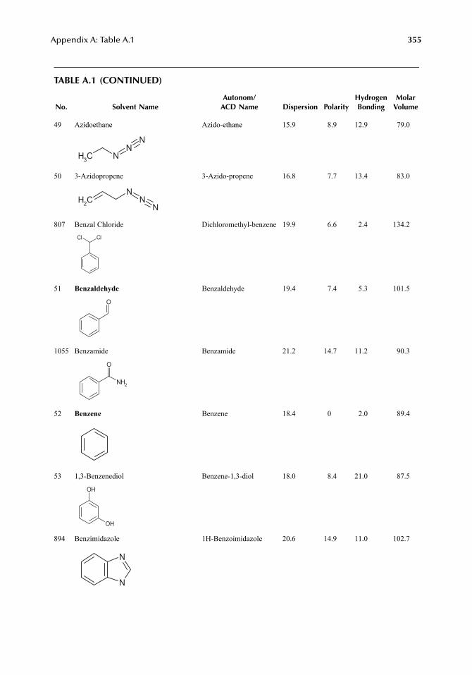
Appendix A: Table A.1
355
TABLE A.1 (CONTINUED)
No. Solvent NameAutonom/
ACD Name Dispersion PolarityHydrogenBonding
MolarVolume
49 Azidoethane Azido-ethane 15.9 8.9 12.9 79.0
50 3-Azidopropene 3-Azido-propene 16.8 7.7 13.4 83.0
807 Benzal Chloride Dichloromethyl-benzene 19.9 6.6 2.4 134.2
51
Benzaldehyde
Benzaldehyde 19.4 7.4 5.3 101.5
1055 Benzamide Benzamide 21.2 14.7 11.2 90.3
52
Benzene
Benzene 18.4 0 2.0 89.4
53 1,3-Benzenediol Benzene-1,3-diol 18.0 8.4 21.0 87.5
894 Benzimidazole 1H-Benzoimidazole 20.6 14.9 11.0 102.7
CH3 NN
N
CH2
NN
N
ClCl
O
NH2
O
OH
OH
N
N
7248_A001.fm Page 355 Wednesday, May 23, 2007 12:31 PM
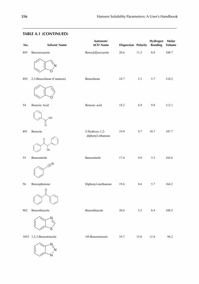
356
Hansen Solubility Parameters: A User’s Handbook
TABLE A.1 (CONTINUED)
No. Solvent NameAutonom/
ACD Name Dispersion PolarityHydrogenBonding
MolarVolume
893 Benzisoxazole Benzo[d]isoxazole 20.6 11.5 8.8 100.7
892 2,3-Benzofuran (Cumaron) Benzofuran 18.7 5.1 5.7 110.2
54 Benzoic Acid Benzoic acid 18.2 6.9 9.8 113.1
891 Benzoin 2-Hydroxy-1,2-diphenyl-ethanone
19.9 9.7 10.7 187.7
55 Benzonitrile Benzonitrile 17.4 9.0 3.3 102.6
56 Benzophenone Diphenyl-methanone 19.6 8.6 5.7 164.2
962 Benzothiazole Benzothiazole 20.6 5.2 8.4 108.5
1053 1,2,3-Benzotriazole 1H-Benzotriazole 18.7 15.6 12.4 96.2
ON
O
O
OH
OH
O
N
O
S
N
NN
N
7248_A001.fm Page 356 Wednesday, May 23, 2007 12:31 PM
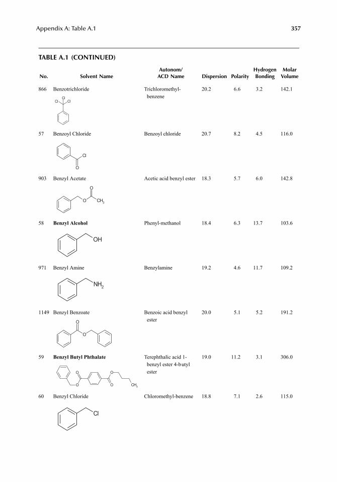
Appendix A: Table A.1
357
TABLE A.1 (CONTINUED)
No. Solvent NameAutonom/
ACD Name Dispersion PolarityHydrogenBonding
MolarVolume
866 Benzotrichloride Trichloromethyl-benzene
20.2 6.6 3.2 142.1
57 Benzoyl Chloride Benzoyl chloride 20.7 8.2 4.5 116.0
903 Benzyl Acetate Acetic acid benzyl ester 18.3 5.7 6.0 142.8
58
Benzyl Alcohol
Phenyl-methanol 18.4 6.3 13.7 103.6
971 Benzyl Amine Benzylamine 19.2 4.6 11.7 109.2
1149 Benzyl Benzoate Benzoic acid benzyl ester
20.0 5.1 5.2 191.2
59
Benzyl Butyl Phthalate
Terephthalic acid 1-benzyl ester 4-butyl ester
19.0 11.2 3.1 306.0
60 Benzyl Chloride Chloromethyl-benzene 18.8 7.1 2.6 115.0
ClClCl
O
Cl
O CH3
O
OH
NH2
O
O
O
OO
O CH3
Cl
7248_A001.fm Page 357 Wednesday, May 23, 2007 12:31 PM
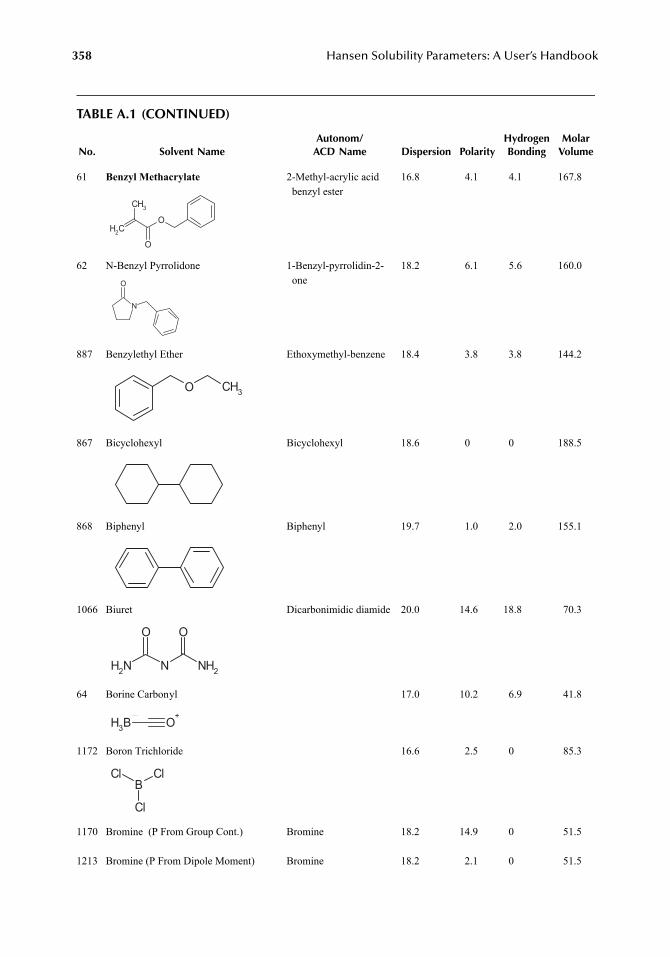
358
Hansen Solubility Parameters: A User’s Handbook
TABLE A.1 (CONTINUED)
No. Solvent NameAutonom/
ACD Name Dispersion PolarityHydrogenBonding
MolarVolume
61
Benzyl Methacrylate
2-Methyl-acrylic acid benzyl ester
16.8 4.1 4.1 167.8
62 N-Benzyl Pyrrolidone 1-Benzyl-pyrrolidin-2-one
18.2 6.1 5.6 160.0
887 Benzylethyl Ether Ethoxymethyl-benzene 18.4 3.8 3.8 144.2
867 Bicyclohexyl Bicyclohexyl 18.6 0 0 188.5
868 Biphenyl Biphenyl 19.7 1.0 2.0 155.1
1066 Biuret Dicarbonimidic diamide 20.0 14.6 18.8 70.3
64 Borine Carbonyl 17.0 10.2 6.9 41.8
1172 Boron Trichloride 16.6 2.5 0 85.3
1170 Bromine (P From Group Cont.) Bromine 18.2 14.9 0 51.5
1213 Bromine (P From Dipole Moment) Bromine 18.2 2.1 0 51.5
CH2
CH3
O
O
N
O
O CH3
NH2 N NH2
O O
O+
BH3
BClCl
Cl
7248_A001.fm Page 358 Wednesday, May 23, 2007 12:31 PM
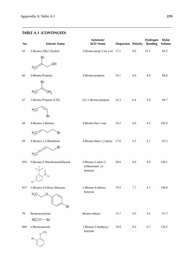
Appendix A: Table A.1
359
TABLE A.1 (CONTINUED)
No. Solvent NameAutonom/
ACD Name Dispersion PolarityHydrogenBonding
MolarVolume
65 2-Bromo Allyl Alcohol 2-Bromo-prop-2-en-1-ol 17.1 9.9 16.2 84.5
66 2-Bromo Propene 2-Bromo-propene 16.1 6.0 4.9 88.8
67 1-Bromo Propene (CIS) (Z)-1-Bromo-propene 16.3 6.4 5.0 84.7
68 4-Bromo-1-Butene 4-Bromo-but-1-ene 16.5 6.0 4.5 102.0
69 4-Bromo-1,2-Butadiene 4-Bromo-buta-1,2-diene 17.0 6.5 4.7 93.3
854 5-Bromo-2-Nitrobenzotrifluorid 4-Bromo-1-nitro-2-trifluoromet yl-benzene
20.0 6.0 4.9 150.1
815 1-Bromo-4-Ethoxy Benzene 1-Bromo-4-ethoxy-benzene
19.5 7.7 5.3 140.0
70 Bromoacetylene Bromo-ethyne 15.7 9.9 5.6 67.7
800 o-Bromoanisole 1-Bromo-2-methoxy-benzene
19.8 8.4 6.7 124.5
CH2
Br
OH
CH3 CH2
Br
CH3
Br
CH2 Br
CH2
Br
FFF
Br
N+
O
O
Br
OCH3
CH Br
OCH3
Br
7248_A001.fm Page 359 Wednesday, May 23, 2007 12:31 PM
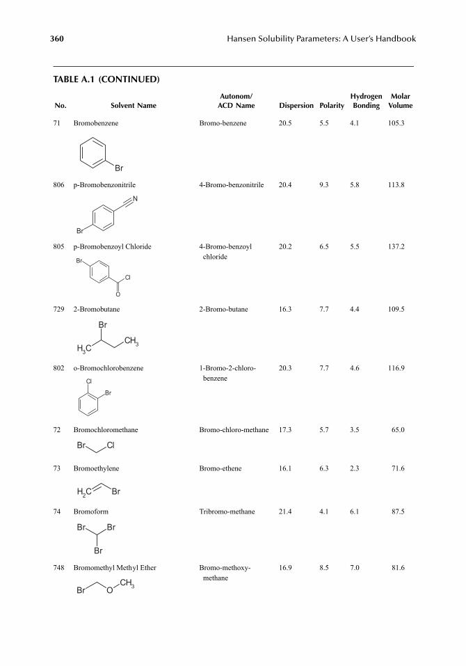
360
Hansen Solubility Parameters: A User’s Handbook
TABLE A.1 (CONTINUED)
No. Solvent NameAutonom/
ACD Name Dispersion PolarityHydrogenBonding
MolarVolume
71 Bromobenzene Bromo-benzene 20.5 5.5 4.1 105.3
806 p-Bromobenzonitrile 4-Bromo-benzonitrile 20.4 9.3 5.8 113.8
805 p-Bromobenzoyl Chloride 4-Bromo-benzoyl chloride
20.2 6.5 5.5 137.2
729 2-Bromobutane 2-Bromo-butane 16.3 7.7 4.4 109.5
802 o-Bromochlorobenzene 1-Bromo-2-chloro-benzene
20.3 7.7 4.6 116.9
72 Bromochloromethane Bromo-chloro-methane 17.3 5.7 3.5 65.0
73 Bromoethylene Bromo-ethene 16.1 6.3 2.3 71.6
74 Bromoform Tribromo-methane 21.4 4.1 6.1 87.5
748 Bromomethyl Methyl Ether Bromo-methoxy-methane
16.9 8.5 7.0 81.6
Br
N
Br
O
Cl
Br
CH3
CH3
Br
Cl
Br
ClBr
CH2 Br
BrBr
Br
Br OCH3
7248_A001.fm Page 360 Wednesday, May 23, 2007 12:31 PM
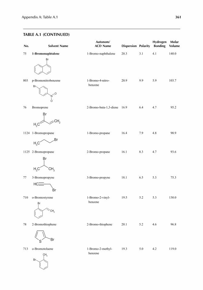
Appendix A: Table A.1
361
TABLE A.1 (CONTINUED)
No. Solvent NameAutonom/
ACD Name Dispersion PolarityHydrogenBonding
MolarVolume
75
1-Bromonaphtalene
1-Bromo-naphthalene 20.3 3.1 4.1 140.0
803 p-Bromonitrobenzene 1-Bromo-4-nitro-benzene
20.9 9.9 5.9 103.7
76 Bromoprene 2-Bromo-buta-1,3-diene 16.9 6.4 4.7 95.2
1124 1-Bromopropane 1-Bromo-propane 16.4 7.9 4.8 90.9
1125 2-Bromopropane 2-Bromo-propane 16.1 8.3 4.7 93.6
77 3-Bromopropyne 3-Bromo-propyne 18.1 6.5 5.3 75.3
710 o-Bromostyrene 1-Bromo-2-vinyl-benzene
19.5 5.2 5.3 130.0
78 2-Bromothiophene 2-Bromo-thiophene 20.1 5.2 4.6 96.8
713 o-Bromotoluene 1-Bromo-2-methyl-benzene
19.3 5.0 4.2 119.0
Br
N+
O
O
Br
CH2
Br
CH2
CH3
Br
CH3 CH3
Br
CHBr
CH2
Br
S Br
CH3
Br
7248_A001.fm Page 361 Wednesday, May 23, 2007 12:31 PM
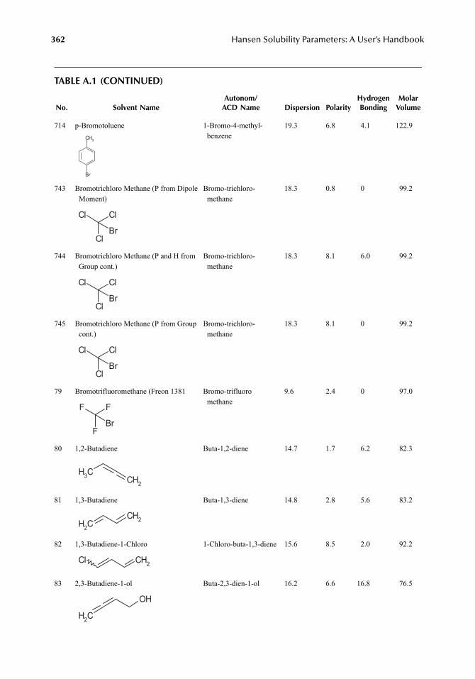
362
Hansen Solubility Parameters: A User’s Handbook
TABLE A.1 (CONTINUED)
No. Solvent NameAutonom/
ACD Name Dispersion PolarityHydrogenBonding
MolarVolume
714 p-Bromotoluene 1-Bromo-4-methyl-benzene
19.3 6.8 4.1 122.9
743 Bromotrichloro Methane (P from Dipole Moment)
Bromo-trichloro-methane
18.3 0.8 0 99.2
744 Bromotrichloro Methane (P and H from Group cont.)
Bromo-trichloro-methane
18.3 8.1 6.0 99.2
745 Bromotrichloro Methane (P from Group cont.)
Bromo-trichloro-methane
18.3 8.1 0 99.2
79 Bromotrifluoromethane (Freon 1381 Bromo-trifluoromethane
9.6 2.4 0 97.0
80 1,2-Butadiene Buta-1,2-diene 14.7 1.7 6.2 82.3
81 1,3-Butadiene Buta-1,3-diene 14.8 2.8 5.6 83.2
82 1,3-Butadiene-1-Chloro 1-Chloro-buta-1,3-diene 15.6 8.5 2.0 92.2
83 2,3-Butadiene-1-ol Buta-2,3-dien-1-ol 16.2 6.6 16.8 76.5
CH3
Br
ClCl
ClBr
ClCl
ClBr
ClCl
ClBr
FF
FBr
CH3 CH2
CH2
CH2
CH2Cl
CH2
OH
7248_A001.fm Page 362 Wednesday, May 23, 2007 12:31 PM
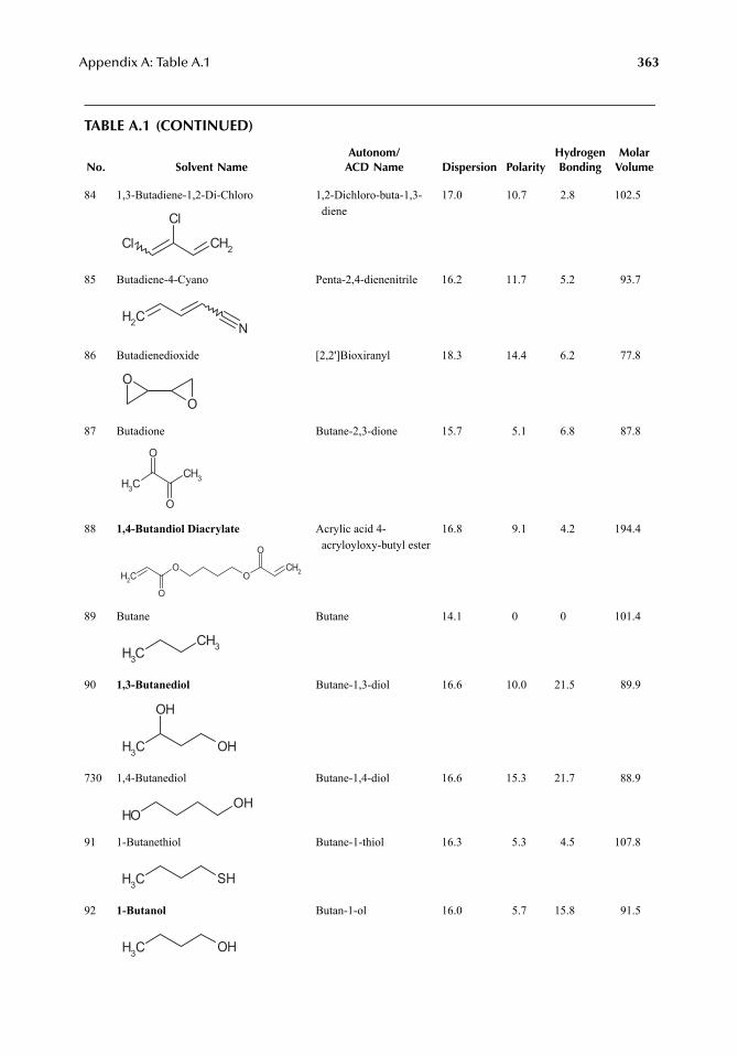
Appendix A: Table A.1
363
TABLE A.1 (CONTINUED)
No. Solvent NameAutonom/
ACD Name Dispersion PolarityHydrogenBonding
MolarVolume
84 1,3-Butadiene-1,2-Di-Chloro 1,2-Dichloro-buta-1,3-diene
17.0 10.7 2.8 102.5
85 Butadiene-4-Cyano Penta-2,4-dienenitrile 16.2 11.7 5.2 93.7
86 Butadienedioxide [2,2']Bioxiranyl 18.3 14.4 6.2 77.8
87 Butadione Butane-2,3-dione 15.7 5.1 6.8 87.8
88
1,4-Butandiol Diacrylate
Acrylic acid 4-acryloyloxy-butyl ester
16.8 9.1 4.2 194.4
89 Butane Butane 14.1 0 0 101.4
90
1,3-Butanediol
Butane-1,3-diol 16.6 10.0 21.5 89.9
730 1,4-Butanediol Butane-1,4-diol 16.6 15.3 21.7 88.9
91 1-Butanethiol Butane-1-thiol 16.3 5.3 4.5 107.8
92
1-Butanol
Butan-1-ol 16.0 5.7 15.8 91.5
CH2
Cl
Cl
CH2 N
O
O
CH3
O
O
CH3
CH2
OO
CH2
O
O
CH3
CH3
CH3 OH
OH
OHOH
CH3 SH
CH3 OH
7248_A001.fm Page 363 Wednesday, May 23, 2007 12:31 PM
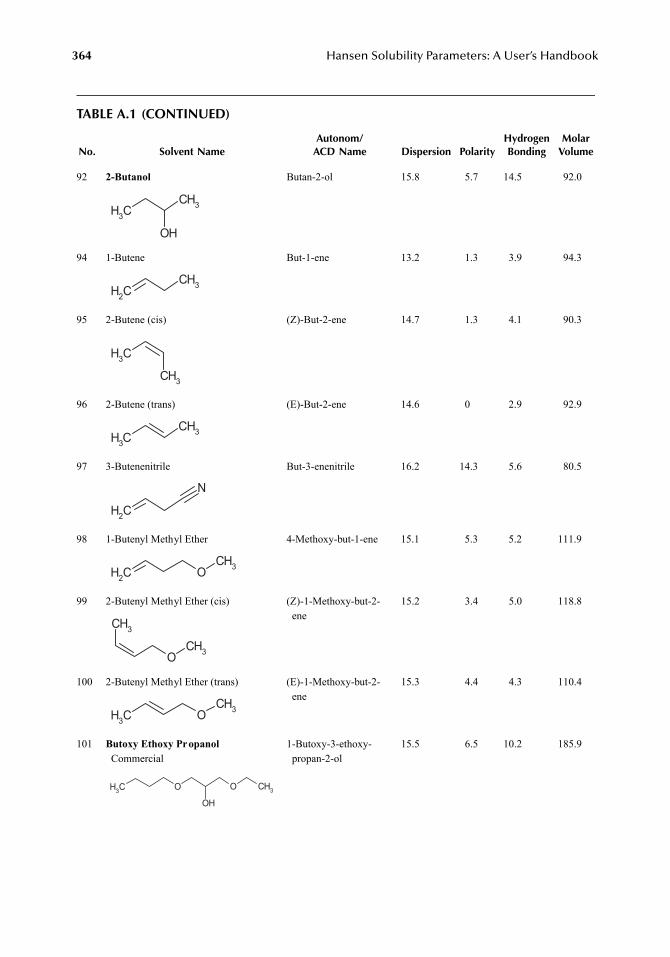
364
Hansen Solubility Parameters: A User’s Handbook
TABLE A.1 (CONTINUED)
No. Solvent NameAutonom/
ACD Name Dispersion PolarityHydrogenBonding
MolarVolume
92
2-Butanol
Butan-2-ol 15.8 5.7 14.5 92.0
94 1-Butene But-1-ene 13.2 1.3 3.9 94.3
95 2-Butene (cis) (Z)-But-2-ene 14.7 1.3 4.1 90.3
96 2-Butene (trans) (E)-But-2-ene 14.6 0 2.9 92.9
97 3-Butenenitrile But-3-enenitrile 16.2 14.3 5.6 80.5
98 1-Butenyl Methyl Ether 4-Methoxy-but-1-ene 15.1 5.3 5.2 111.9
99 2-Butenyl Methyl Ether (cis) (Z)-1-Methoxy-but-2-ene
15.2 3.4 5.0 118.8
100 2-Butenyl Methyl Ether (trans) (E)-1-Methoxy-but-2-ene
15.3 4.4 4.3 110.4
101
Butoxy Ethoxy Propanol
Commercial1-Butoxy-3-ethoxy-propan-2-ol
15.5 6.5 10.2 185.9
CH3
CH3
OH
CH2
CH3
CH3
CH3
CH3
CH3
CH2
N
CH2 OCH3
OCH3
CH3
CH3 OCH3
CH3 O O CH3
OH
7248_A001.fm Page 364 Wednesday, May 23, 2007 12:31 PM
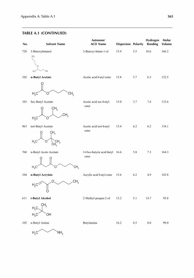
Appendix A: Table A.1
365
TABLE A.1 (CONTINUED)
No. Solvent NameAutonom/
ACD Name Dispersion PolarityHydrogenBonding
MolarVolume
728 3-Butoxybutanol 3-Butoxy-butan-1-ol 15.9 5.5 10.6 166.3
102
n-Butyl Acetate
Acetic acid butyl ester 15.8 3.7 6.3 132.5
103 Sec-Butyl Acetate Acetic acid sec-butyl ester
15.0 3.7 7.6 133.6
963 tert-Butyl Acetate Acetic acid tert-butyl ester
15.4 6.2 6.2 134.1
768 n-Butyl Aceto Acetate 3-Oxo-butyric acid butyl ester
16.6 5.8 7.3 164.3
104
n-Butyl Acrylate
Acrylic acid butyl ester 15.6 6.2 4.9 143.8
611
t-Butyl Alcohol
2-Methyl-propan-2-ol 15.2 5.1 14.7 95.8
105 n-Butyl Amine Butylamine 16.2 4.5 8.0 99.0
CH3 OH
O
CH3
CH3 O CH3
O
CH3 OCH3
O CH3
CH3 O
O
CH3
CH3
CH3
CH3 O CH3
O O
CH2
O CH3
O
CH3 OH
CH3CH3
CH3 NH2
7248_A001.fm Page 365 Wednesday, May 23, 2007 12:31 PM
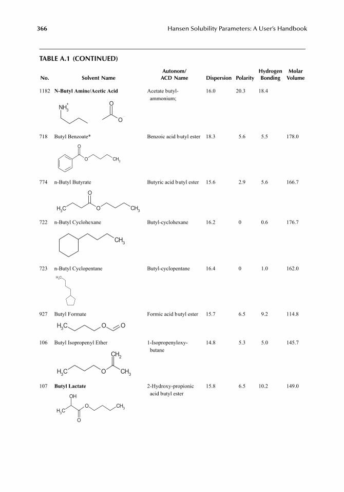
366
Hansen Solubility Parameters: A User’s Handbook
TABLE A.1 (CONTINUED)
No. Solvent NameAutonom/
ACD Name Dispersion PolarityHydrogenBonding
MolarVolume
1182
N-Butyl Amine/Acetic Acid
Acetate butyl-ammonium;
16.0 20.3 18.4
718 Butyl Benzoate* Benzoic acid butyl ester 18.3 5.6 5.5 178.0
774 n-Butyl Butyrate Butyric acid butyl ester 15.6 2.9 5.6 166.7
722 n-Butyl Cyclohexane Butyl-cyclohexane 16.2 0 0.6 176.7
723 n-Butyl Cyclopentane Butyl-cyclopentane 16.4 0 1.0 162.0
927 Butyl Formate Formic acid butyl ester 15.7 6.5 9.2 114.8
106 Butyl Isopropenyl Ether 1-Isopropenyloxy-butane
14.8 5.3 5.0 145.7
107
Butyl Lactate
2-Hydroxy-propionic acid butyl ester
15.8 6.5 10.2 149.0
NH3+
O
O
O
O
CH3
CH3 O CH3
O
CH3
CH3
O OCH3
CH3 O CH3
CH2
CH3
O CH3
OH
O
7248_A001.fm Page 366 Wednesday, May 23, 2007 12:31 PM
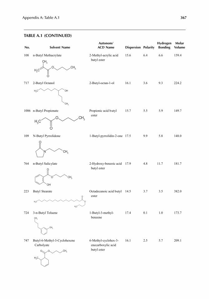
Appendix A: Table A.1
367
TABLE A.1 (CONTINUED)
No. Solvent NameAutonom/
ACD Name Dispersion PolarityHydrogenBonding
MolarVolume
108 n-Butyl Methacrylate 2-Methyl-acrylic acid butyl ester
15.6 6.4 6.6 159.4
717 2-Butyl Octanol 2-Butyl-octan-1-ol 16.1 3.6 9.3 224.2
1006 n-Butyl Propionate Propionic acid butyl ester
15.7 5.5 5.9 149.7
109 N-Butyl Pyrrolidone 1-Butyl-pyrrolidin-2-one 17.5 9.9 5.8 148.0
764 n-Butyl Salicylate 2-Hydroxy-benzoic acid butyl ester
17.9 4.8 11.7 181.7
223 Butyl Stearate Octadecanoic acid butyl ester
14.5 3.7 3.5 382.0
724 3-n-Butyl Toluene 1-Butyl-3-methyl-benzene
17.4 0.1 1.0 173.7
747 Butyl-6-Methyl-3-Cyclohexene Carbolyate
6-Methyl-cyclohex-3-enecarboxylic acid butyl ester
16.1 2.5 5.7 209.1
CH2
O CH3
CH3
O
CH3 OH
CH3
CH3
O CH3
O
N
O
CH3
OH
O
O
CH3
CH3 O
O
CH3
CH3
CH3
CH3
OO CH3
7248_A001.fm Page 367 Wednesday, May 23, 2007 12:31 PM
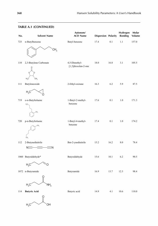
368
Hansen Solubility Parameters: A User’s Handbook
TABLE A.1 (CONTINUED)
No. Solvent NameAutonom/
ACD Name Dispersion PolarityHydrogenBonding
MolarVolume
725 n-Butylbenzene Butyl-benzene 17.4 0.1 1.1 157.0
110 2,3-Butylene Carbonate 4,5-Dimethyl-[1,3]dioxolan-2-one
18.0 16.8 3.1 105.5
111 Butyleneoxide 2-Ethyl-oxirane 16.3 6.2 5.9 87.5
719 o-n-Butyltoluene 1-Butyl-2-methyl-benzene
17.6 0.1 1.0 171.3
720 p-n-Butyltoluene 1-Butyl-4-methyl-benzene
17.4 0.1 1.0 174.2
112 2-Butynedinitrile But-2-ynedinitrile 15.2 16.2 8.0 78.4
1060 Butyraldehyde* Butyraldehyde 15.6 10.1 6.2 90.5
1072 n-Butyramide Butyramide 16.9 13.7 12.3 98.4
114
Butyric Acid
Butyric acid 14.9 4.1 10.6 110.0
CH3
OO
CH3 CH3
O
CH3 O
CH3
CH3
CH3
CH3
NN
CH3 O
CH3 NH2
O
CH3 OH
O
7248_A001.fm Page 368 Wednesday, May 23, 2007 12:31 PM
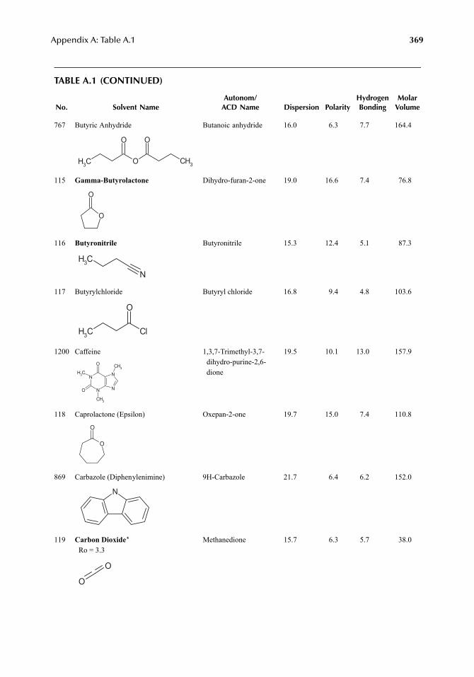
Appendix A: Table A.1
369
TABLE A.1 (CONTINUED)
No. Solvent NameAutonom/
ACD Name Dispersion PolarityHydrogenBonding
MolarVolume
767 Butyric Anhydride Butanoic anhydride 16.0 6.3 7.7 164.4
115
Gamma-Butyrolactone
Dihydro-furan-2-one 19.0 16.6 7.4 76.8
116
Butyronitrile
Butyronitrile 15.3 12.4 5.1 87.3
117 Butyrylchloride Butyryl chloride 16.8 9.4 4.8 103.6
1200 Caffeine 1,3,7-Trimethyl-3,7-dihydro-purine-2,6-dione
19.5 10.1 13.0 157.9
118 Caprolactone (Epsilon) Oxepan-2-one 19.7 15.0 7.4 110.8
869 Carbazole (Diphenylenimine) 9H-Carbazole 21.7 6.4 6.2 152.0
119
Carbon Dioxide
*
Ro = 3.3Methanedione 15.7 6.3 5.7 38.0
CH3 O CH3
O O
O
O
N
CH3
CH3 Cl
O
N
N N
N
O CH3
CH3
CH3
O
O
O
N
O
O
7248_A001.fm Page 369 Wednesday, May 23, 2007 12:31 PM
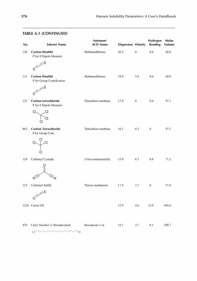
370
Hansen Solubility Parameters: A User’s Handbook
TABLE A.1 (CONTINUED)
No. Solvent NameAutonom/
ACD Name Dispersion PolarityHydrogenBonding
MolarVolume
120
Carbon Disulfid
P for 0 Dipole MomentMethanedithione 20.5 0 0.6 60.0
121
Carbon Disulfid
P for Group Contrib utionMethanedithione 19.9 5.8 0.6 60.0
122
Carbon tetrachloride
P for 0 Dipole MomentTetrachloro-methane 17.8 0 0.6 97.1
862
Carbon Tetrachloride
P by Group Cont.Tetrachloro-methane 16.1 8.3 0 97.1
124 Carbonyl Cyanide 2-Oxo-malononitrile 15.0 6.3 8.0 71.2
123 Carbonyl Sulfid Thioxo-methanone 17.4 3.7 0 51.0
1224 Castor Oil 15.9 4.6 12.0 436.0
976 Cetyl Alcohol (1-Hexadecanol) Hexadecan-1-ol 15.1 3.7 8.1 298.7
S
S
S
S
ClCl
ClCl
ClCl
Cl
Cl
O
N N
S
O
CH3 OH
7248_A001.fm Page 370 Wednesday, May 23, 2007 12:31 PM
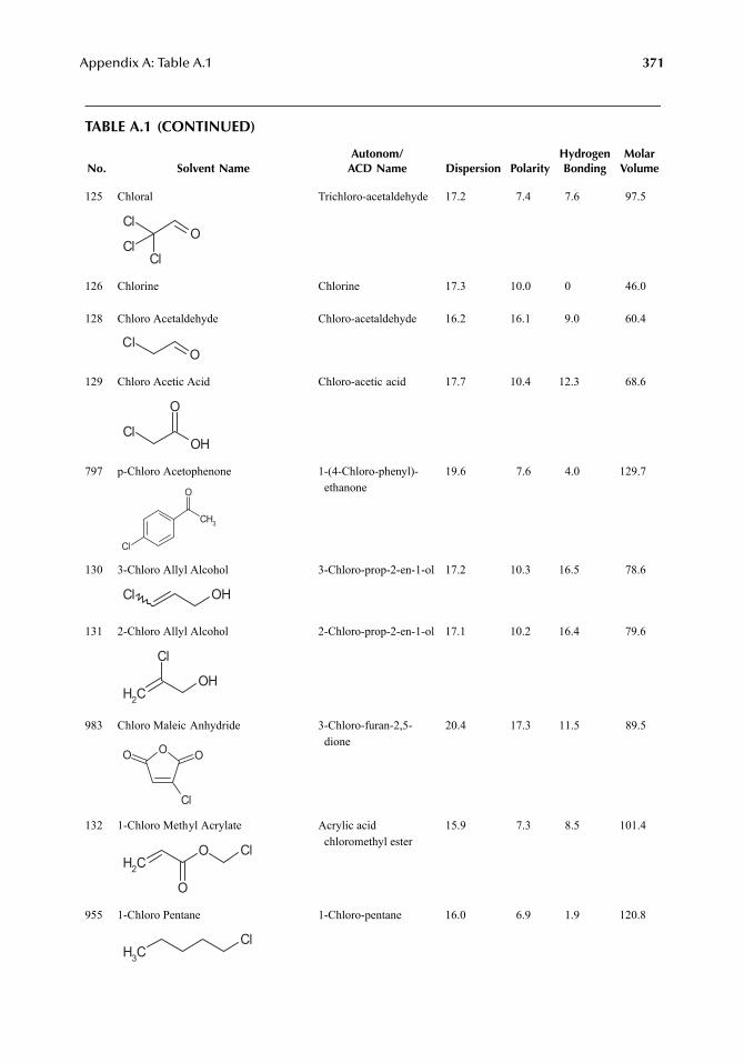
Appendix A: Table A.1
371
TABLE A.1 (CONTINUED)
No. Solvent NameAutonom/
ACD Name Dispersion PolarityHydrogenBonding
MolarVolume
125 Chloral Trichloro-acetaldehyde 17.2 7.4 7.6 97.5
126 Chlorine Chlorine 17.3 10.0 0 46.0
128 Chloro Acetaldehyde Chloro-acetaldehyde 16.2 16.1 9.0 60.4
129 Chloro Acetic Acid Chloro-acetic acid 17.7 10.4 12.3 68.6
797 p-Chloro Acetophenone 1-(4-Chloro-phenyl)-ethanone
19.6 7.6 4.0 129.7
130 3-Chloro Allyl Alcohol 3-Chloro-prop-2-en-1-ol 17.2 10.3 16.5 78.6
131 2-Chloro Allyl Alcohol 2-Chloro-prop-2-en-1-ol 17.1 10.2 16.4 79.6
983 Chloro Maleic Anhydride 3-Chloro-furan-2,5-dione
20.4 17.3 11.5 89.5
132 1-Chloro Methyl Acrylate Acrylic acid chloromethyl ester
15.9 7.3 8.5 101.4
955 1-Chloro Pentane 1-Chloro-pentane 16.0 6.9 1.9 120.8
O
Cl
Cl
Cl
OCl
OH
O
Cl
CH3
O
Cl
OHCl
CH2
Cl
OH
Cl
O OO
CH2
O
O
Cl
CH3
Cl
7248_A001.fm Page 371 Wednesday, May 23, 2007 12:31 PM
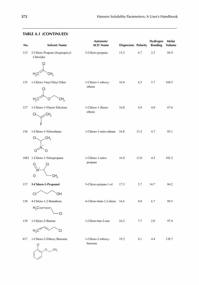
372
Hansen Solubility Parameters: A User’s Handbook
TABLE A.1 (CONTINUED)
No. Solvent NameAutonom/
ACD Name Dispersion PolarityHydrogenBonding
MolarVolume
133 2-Chloro Propene (Isopropenyl Chloride)
2-Chloro-propene 15.5 6.7 2.2 84.9
135 1-Chloro Vinyl Ethyl Ether 1-Chloro-1-ethoxy-ethene
16.8 6.5 5.7 104.5
127 1-Chloro-1-Fluoro Ethylene 1-Chloro-1-fluoroethene
16.0 6.9 4.0 67.6
136 1-Chloro-1-Nitroethane 1-Chloro-1-nitro-ethane 16.8 13.5 4.7 85.1
1083 1-Chloro-1-Nitropropane 1-Chloro-1-nitro-propane
16.8 13.0 4.5 102.2
137
3-Chloro-1-Propanol
3-Chloro-propan-1-ol 17.5 5.7 14.7 84.2
138 4-Chloro-1,2-Butadiene 4-Chloro-buta-1,2-diene 16.6 8.0 6.7 89.5
139 1-Chloro-2-Butene 1-Chloro-but-2-ene 16.2 7.7 2.0 97.4
817 1-Chloro-2-Ethoxy Benzene 1-Chloro-2-ethoxy-benzene
19.2 8.1 4.4 138.7
CH2 CH3
Cl
CH2 O
Cl
CH3
CH2Cl
F
CH3Cl
N+
O O
N+
O
O Cl
CH3
Cl OH
CH2
Cl
ClCH3
Cl
O CH3
7248_A001.fm Page 372 Wednesday, May 23, 2007 12:31 PM
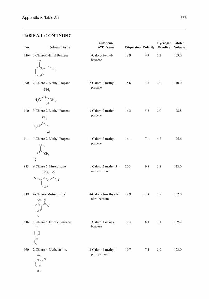
Appendix A: Table A.1
373
TABLE A.1 (CONTINUED)
No. Solvent NameAutonom/
ACD Name Dispersion PolarityHydrogenBonding
MolarVolume
1164 1-Chloro-2-Ethyl Benzene 1-Chloro-2-ethyl-benzene
18.9 4.9 2.2 133.0
970 2-Chloro-2-Methyl Propane 2-Chloro-2-methyl-propane
15.6 7.6 2.0 110.0
140 3-Chloro-2-Methyl Propene 3-Chloro-2-methyl-propene
16.2 5.6 2.0 98.8
141 1-Chloro-2-Methyl Propene 1-Chloro-2-methyl-propene
16.1 7.1 4.2 95.6
813 6-Chloro-2-Nitrotoluene 1-Chloro-2-methyl-3-nitro-benzene
20.3 9.6 3.8 132.0
819 4-Chloro-2-Nitrotoluene 4-Chloro-1-methyl-2-nitro-benzene
19.9 11.8 3.8 132.0
816 1-Chloro-4-Ethoxy Benzene 1-Chloro-4-ethoxy-benzene
19.3 6.3 4.4 139.2
950 2-Chloro-4-Methylaniline 2-Chloro-4-methyl-phenylamine
19.7 7.4 8.9 123.0
Cl
CH3
CH3 CH3
CH3
Cl
CH2
CH3
Cl
CH3
CH3
Cl
CH3
Cl N+
O
O
CH3
N+
O
O
Cl
Cl
O
CH3
NH2
Cl
CH3
7248_A001.fm Page 373 Wednesday, May 23, 2007 12:31 PM
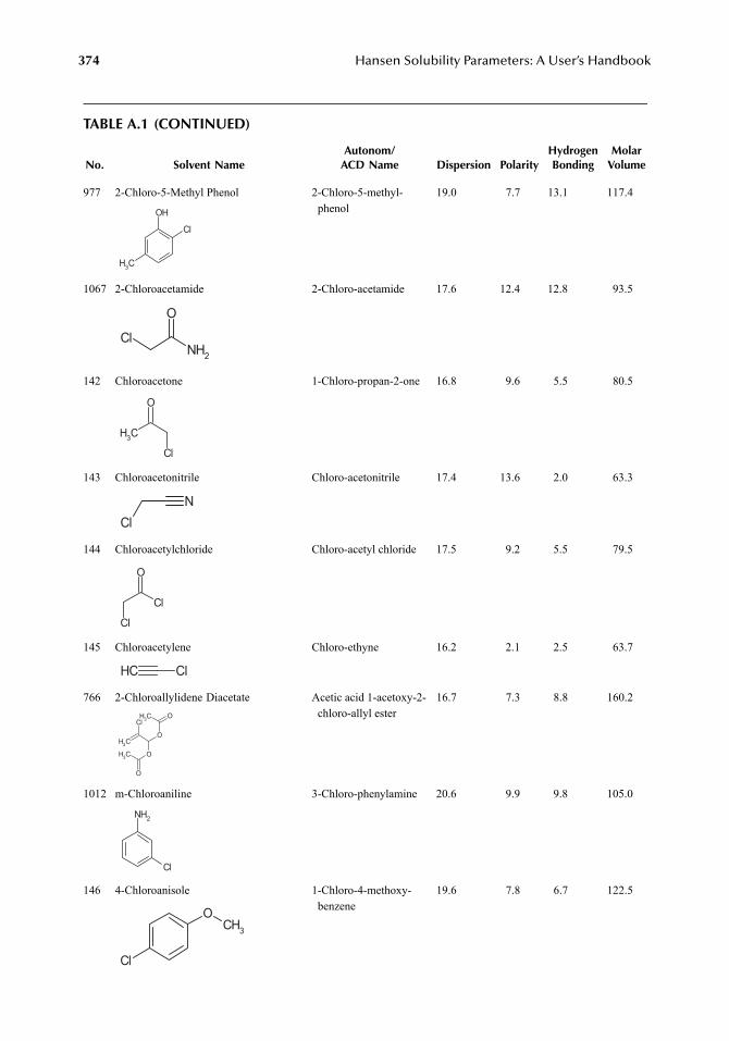
374
Hansen Solubility Parameters: A User’s Handbook
TABLE A.1 (CONTINUED)
No. Solvent NameAutonom/
ACD Name Dispersion PolarityHydrogenBonding
MolarVolume
977 2-Chloro-5-Methyl Phenol 2-Chloro-5-methyl-phenol
19.0 7.7 13.1 117.4
1067 2-Chloroacetamide 2-Chloro-acetamide 17.6 12.4 12.8 93.5
142 Chloroacetone 1-Chloro-propan-2-one 16.8 9.6 5.5 80.5
143 Chloroacetonitrile Chloro-acetonitrile 17.4 13.6 2.0 63.3
144 Chloroacetylchloride Chloro-acetyl chloride 17.5 9.2 5.5 79.5
145 Chloroacetylene Chloro-ethyne 16.2 2.1 2.5 63.7
766 2-Chloroallylidene Diacetate Acetic acid 1-acetoxy-2-chloro-allyl ester
16.7 7.3 8.8 160.2
1012 m-Chloroaniline 3-Chloro-phenylamine 20.6 9.9 9.8 105.0
146 4-Chloroanisole 1-Chloro-4-methoxy-benzene
19.6 7.8 6.7 122.5
OH
Cl
CH3
NH2
O
Cl
CH3
O
Cl
NCl
Cl
Cl
O
ClCH
CH2
Cl
O
O
OCH3
O
CH3
NH2
Cl
OCH3
Cl
7248_A001.fm Page 374 Wednesday, May 23, 2007 12:31 PM

Appendix A: Table A.1
375
TABLE A.1 (CONTINUED)
No. Solvent NameAutonom/
ACD Name Dispersion PolarityHydrogenBonding
MolarVolume
147 4-Chlorobenzaldehyde 4-Chloro-benzaldehyde 19.9 7.2 5.6 113.4
148
Chlorobenzene
Chloro-benzene 19.0 4.3 2.0 102.1
811 4-Chlorobenzonitrile 4-Chloro-benzonitrile 19.5 8.0 4.1 125.1
853 4-Chlorobenzotrichloride 1-Chloro-4-trichloromethyl-benzene
20.3 5.5 3.5 153.8
812 p-Chlorobenzoyl Chloride 4-Chloro-benzoyl chloride
19.9 6.7 5.1 127.1
149 4-Chlorobenzyl Alcohol (4-Chloro-phenyl)-methanol
19.6 7.5 13.0 117.7
150 3-Chlorobenzylchloride 1-Chloro-3-chloromethyl-benzene
19.9 9.3 2.6 117.7
151 1,2-Chlorobromoethylene 1-Bromo-2-chloro-ethene
17.2 6.6 2.3 78.7
Cl
O
Cl
Cl
N
ClClCl
Cl
Cl
Cl
O
Cl
OH
ClCl
ClBr
7248_A001.fm Page 375 Wednesday, May 23, 2007 12:31 PM
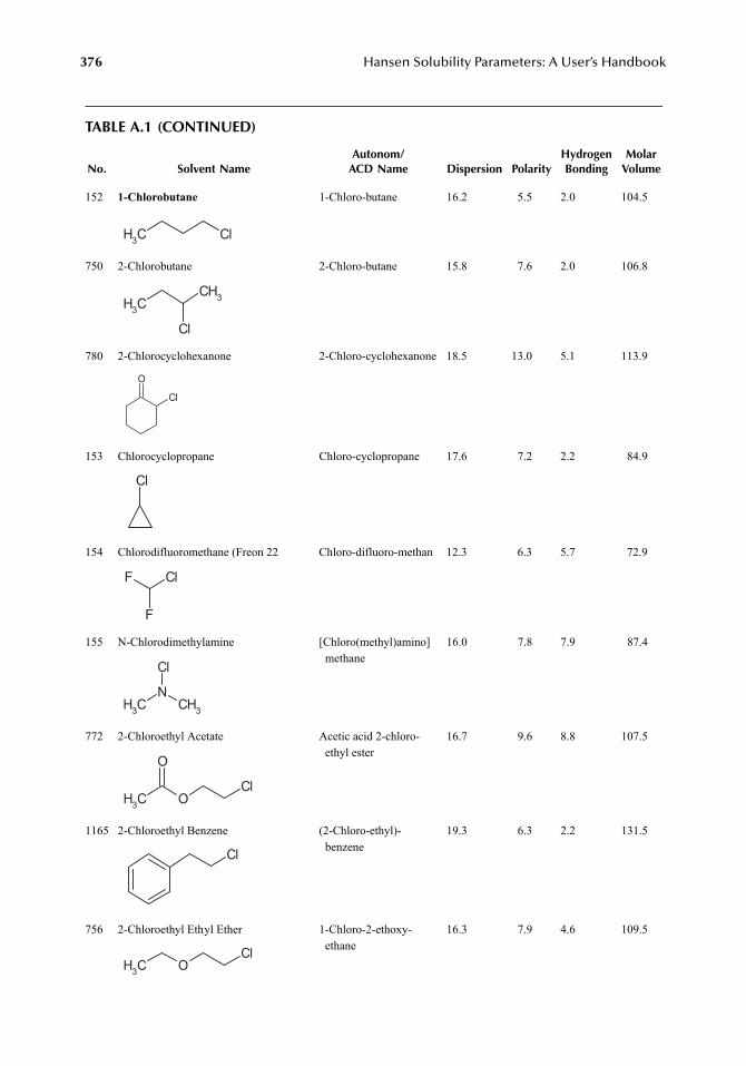
376 Hansen Solubility Parameters: A User’s Handbook
TABLE A.1 (CONTINUED)
No. Solvent NameAutonom/
ACD Name Dispersion PolarityHydrogenBonding
MolarVolume
152 1-Chlorobutane 1-Chloro-butane 16.2 5.5 2.0 104.5
750 2-Chlorobutane 2-Chloro-butane 15.8 7.6 2.0 106.8
780 2-Chlorocyclohexanone 2-Chloro-cyclohexanone 18.5 13.0 5.1 113.9
153 Chlorocyclopropane Chloro-cyclopropane 17.6 7.2 2.2 84.9
154 Chlorodifluoromethane (Freon 22 Chloro-difluoro-methan 12.3 6.3 5.7 72.9
155 N-Chlorodimethylamine [Chloro(methyl)amino]methane
16.0 7.8 7.9 87.4
772 2-Chloroethyl Acetate Acetic acid 2-chloro-ethyl ester
16.7 9.6 8.8 107.5
1165 2-Chloroethyl Benzene (2-Chloro-ethyl)-benzene
19.3 6.3 2.2 131.5
756 2-Chloroethyl Ethyl Ether 1-Chloro-2-ethoxy-ethane
16.3 7.9 4.6 109.5
CH3 Cl
CH3
CH3
Cl
Cl
O
Cl
ClF
F
CH3
NCH3
Cl
CH3 O
O
Cl
Cl
CH3 OCl
7248_A001.fm Page 376 Wednesday, May 23, 2007 12:31 PM
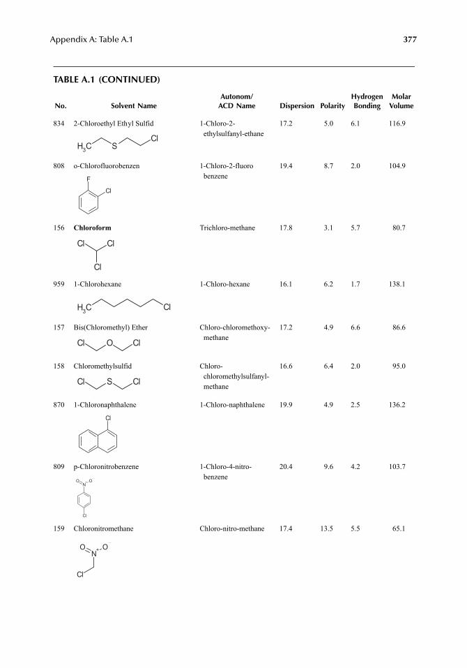
Appendix A: Table A.1 377
TABLE A.1 (CONTINUED)
No. Solvent NameAutonom/
ACD Name Dispersion PolarityHydrogenBonding
MolarVolume
834 2-Chloroethyl Ethyl Sulfid 1-Chloro-2-ethylsulfanyl-ethane
17.2 5.0 6.1 116.9
808 o-Chlorofluorobenzen 1-Chloro-2-fluorobenzene
19.4 8.7 2.0 104.9
156 Chloroform Trichloro-methane 17.8 3.1 5.7 80.7
959 1-Chlorohexane 1-Chloro-hexane 16.1 6.2 1.7 138.1
157 Bis(Chloromethyl) Ether Chloro-chloromethoxy-methane
17.2 4.9 6.6 86.6
158 Chloromethylsulfid Chloro-chloromethylsulfanyl-methane
16.6 6.4 2.0 95.0
870 1-Chloronaphthalene 1-Chloro-naphthalene 19.9 4.9 2.5 136.2
809 p-Chloronitrobenzene 1-Chloro-4-nitro-benzene
20.4 9.6 4.2 103.7
159 Chloronitromethane Chloro-nitro-methane 17.4 13.5 5.5 65.1
CH3 SCl
F
Cl
ClCl
Cl
CH3 Cl
ClOCl
ClSCl
Cl
Cl
N+ OO
N+ OO
Cl
7248_A001.fm Page 377 Wednesday, May 23, 2007 12:31 PM
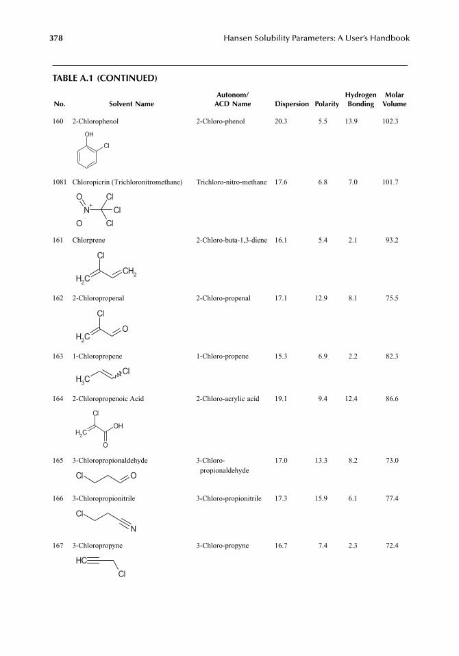
378 Hansen Solubility Parameters: A User’s Handbook
TABLE A.1 (CONTINUED)
No. Solvent NameAutonom/
ACD Name Dispersion PolarityHydrogenBonding
MolarVolume
160 2-Chlorophenol 2-Chloro-phenol 20.3 5.5 13.9 102.3
1081 Chloropicrin (Trichloronitromethane) Trichloro-nitro-methane 17.6 6.8 7.0 101.7
161 Chlorprene 2-Chloro-buta-1,3-diene 16.1 5.4 2.1 93.2
162 2-Chloropropenal 2-Chloro-propenal 17.1 12.9 8.1 75.5
163 1-Chloropropene 1-Chloro-propene 15.3 6.9 2.2 82.3
164 2-Chloropropenoic Acid 2-Chloro-acrylic acid 19.1 9.4 12.4 86.6
165 3-Chloropropionaldehyde 3-Chloro-propionaldehyde
17.0 13.3 8.2 73.0
166 3-Chloropropionitrile 3-Chloro-propionitrile 17.3 15.9 6.1 77.4
167 3-Chloropropyne 3-Chloro-propyne 16.7 7.4 2.3 72.4
Cl
OH
N+
O
O
Cl
ClCl
CH2
CH2
Cl
CH2
O
Cl
CH3
Cl
CH2
Cl
O
OH
OCl
N
Cl
CHCl
7248_A001.fm Page 378 Wednesday, May 23, 2007 12:31 PM
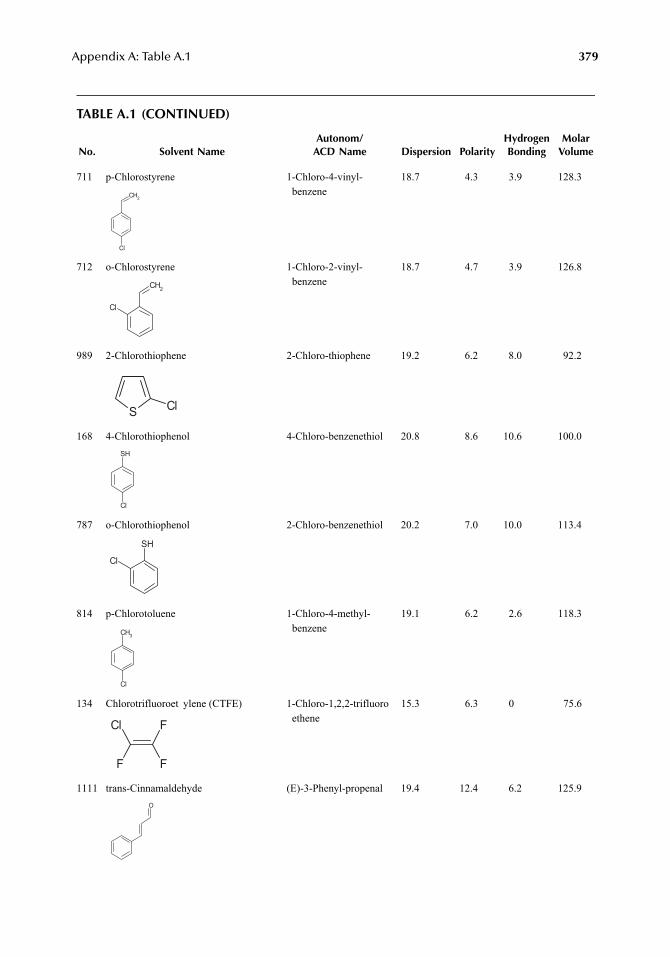
Appendix A: Table A.1 379
TABLE A.1 (CONTINUED)
No. Solvent NameAutonom/
ACD Name Dispersion PolarityHydrogenBonding
MolarVolume
711 p-Chlorostyrene 1-Chloro-4-vinyl-benzene
18.7 4.3 3.9 128.3
712 o-Chlorostyrene 1-Chloro-2-vinyl-benzene
18.7 4.7 3.9 126.8
989 2-Chlorothiophene 2-Chloro-thiophene 19.2 6.2 8.0 92.2
168 4-Chlorothiophenol 4-Chloro-benzenethiol 20.8 8.6 10.6 100.0
787 o-Chlorothiophenol 2-Chloro-benzenethiol 20.2 7.0 10.0 113.4
814 p-Chlorotoluene 1-Chloro-4-methyl-benzene
19.1 6.2 2.6 118.3
134 Chlorotrifluoroet ylene (CTFE) 1-Chloro-1,2,2-trifluoroethene
15.3 6.3 0 75.6
1111 trans-Cinnamaldehyde (E)-3-Phenyl-propenal 19.4 12.4 6.2 125.9
CH2
Cl
CH2
Cl
S Cl
Cl
SH
SH
Cl
CH3
Cl
Cl
F F
F
O
7248_A001.fm Page 379 Wednesday, May 23, 2007 12:31 PM
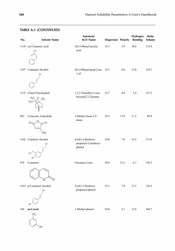
380 Hansen Solubility Parameters: A User’s Handbook
TABLE A.1 (CONTINUED)
No. Solvent NameAutonom/
ACD Name Dispersion PolarityHydrogenBonding
MolarVolume
1110 cis-Cinnamic Acid (Z)-3-Phenyl-acrylic acid
19.1 3.9 10.6 115.4
1107 Cinnamyl Alcohol (E)-3-Phenyl-prop-2-en-1-ol
19.1 6.0 13.0 129.1
1135 Cineol (Eucalyptol) 1,3,3-Trimethyl-2-oxa-bicyclo[2.2.2]octane
16.7 4.6 3.4 167.5
982 Citraconic Anhydride 3-Methyl-furan-2,5-dione
19.2 17.0 11.2 89.9
1102 Coniferyl Alcohol 4-((E)-3-Hydroxy-propenyl)-2-methoxy-phenol
19.0 7.0 16.3 171.6
974 Coumarin Chromen-2-one 20.0 12.5 6.7 156.3
1103 p-Coumaryl Alcohol 4-((E)-3-Hydroxy-propenyl)-phenol
19.1 7.0 17.3 136.5
169 m-Cresol 3-Methyl-phenol 18.0 5.1 12.9 104.7
OH
O
OH
O CH3CH3
CH3
H
CH3
O OO
O
OH
CH3
OH
O O
OH
OH
CH3
OH
7248_A001.fm Page 380 Wednesday, May 23, 2007 12:31 PM

Appendix A: Table A.1 381
TABLE A.1 (CONTINUED)
No. Solvent NameAutonom/
ACD Name Dispersion PolarityHydrogenBonding
MolarVolume
170 Crotonaldehyde (E)-But-2-enal 16.2 14.9 7.4 82.5
171 Crotonic Acid (E)-But-2-enoic acid 16.8 8.7 12.0 84.6
172 Crotonlactone 5H-Furan-2-one 19.0 19.8 9.6 76.4
173 Trans-Crotononitrile (E)-But-2-enenitrile 16.4 18.8 5.5 81.4
174 Cyanamid (Carbamonitrile) Cyanamide 15.5 27.6 16.8 32.8
175 Cyanogen Oxalonitrile 15.1 11.8 0 54.6
176 Cyanogen Bromide Cyanic bromide 18.3 15.2 0 52.6
177 Cyanogen Chloride Cyanic chloride 15.6 14.5 0 51.8
178 Cyclobutanone Cyclobutanone 18.3 11.4 5.2 73.4
179 Cyclodecanone Cyclodecanone 16.8 8.0 4.1 161.0
CH3 O
CH3 OH
O
O
O
CH3
N
NH2N
N N
BrN
ClN
O
O
7248_A001.fm Page 381 Wednesday, May 23, 2007 12:31 PM
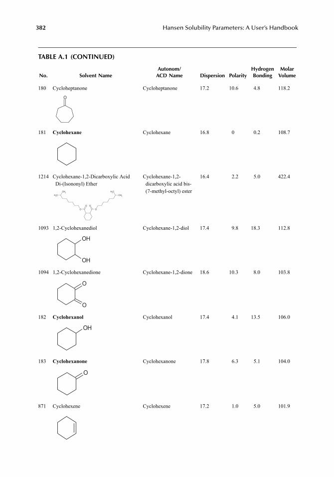
382 Hansen Solubility Parameters: A User’s Handbook
TABLE A.1 (CONTINUED)
No. Solvent NameAutonom/
ACD Name Dispersion PolarityHydrogenBonding
MolarVolume
180 Cycloheptanone Cycloheptanone 17.2 10.6 4.8 118.2
181 Cyclohexane Cyclohexane 16.8 0 0.2 108.7
1214 Cyclohexane-1,2-Dicarboxylic AcidDi-(Isononyl) Ether
Cyclohexane-1,2-dicarboxylic acid bis-(7-methyl-octyl) ester
16.4 2.2 5.0 422.4
1093 1,2-Cyclohexanediol Cyclohexane-1,2-diol 17.4 9.8 18.3 112.8
1094 1,2-Cyclohexanedione Cyclohexane-1,2-dione 18.6 10.3 8.0 103.8
182 Cyclohexanol Cyclohexanol 17.4 4.1 13.5 106.0
183 Cyclohexanone Cyclohexanone 17.8 6.3 5.1 104.0
871 Cyclohexene Cyclohexene 17.2 1.0 5.0 101.9
O
O OO O
CH3
CH3CH3
CH3
OH
OH
O
O
OH
O
7248_A001.fm Page 382 Wednesday, May 23, 2007 12:31 PM
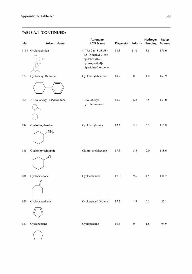
Appendix A: Table A.1 383
TABLE A.1 (CONTINUED)
No. Solvent NameAutonom/
ACD Name Dispersion PolarityHydrogenBonding
MolarVolume
1199 Cycloheximide 4-[(R)-2-((1S,3S,5S)-3,5-Dimethyl-2-oxo-cyclohexyl)-2-hydroxy-ethyl]-piperidine-2,6-dione
18.3 11.0 13.8 171.0
872 Cyclohexyl Benzene Cyclohexyl-benzene 18.7 0 1.0 169.9
969 N-Cyclohexyl-2-Pyrrolidone 1-Cyclohexyl-pyrrolidin-2-one
18.2 6.8 6.5 163.0
184 Cyclohexylamine Cyclohexylamine 17.2 3.1 6.5 113.8
185 Cyclohexylchloride Chloro-cyclohexane 17.3 5.5 2.0 118.6
186 Cyclooctanone Cyclooctanone 17.0 9.6 4.5 131.7
920 Cyclopentadiene Cyclopenta-1,3-diene 17.2 1.9 6.1 82.1
187 Cyclopentane Cyclopentane 16.4 0 1.8 94.9
OH
O
CH3
CH3
N OO
H
H
NO
NH2
Cl
O
7248_A001.fm Page 383 Wednesday, May 23, 2007 12:31 PM
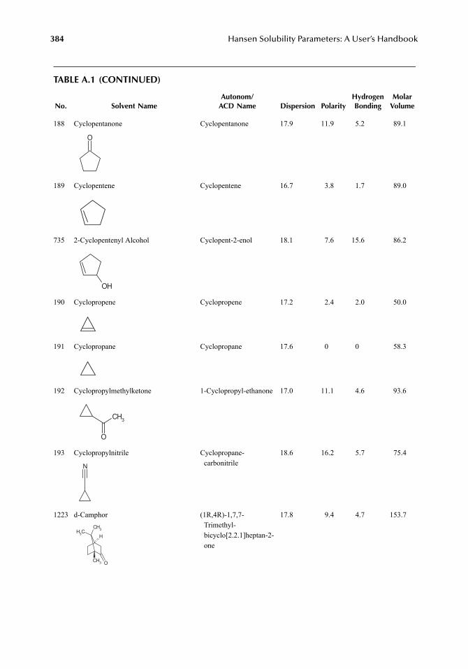
384 Hansen Solubility Parameters: A User’s Handbook
TABLE A.1 (CONTINUED)
No. Solvent NameAutonom/
ACD Name Dispersion PolarityHydrogenBonding
MolarVolume
188 Cyclopentanone Cyclopentanone 17.9 11.9 5.2 89.1
189 Cyclopentene Cyclopentene 16.7 3.8 1.7 89.0
735 2-Cyclopentenyl Alcohol Cyclopent-2-enol 18.1 7.6 15.6 86.2
190 Cyclopropene Cyclopropene 17.2 2.4 2.0 50.0
191 Cyclopropane Cyclopropane 17.6 0 0 58.3
192 Cyclopropylmethylketone 1-Cyclopropyl-ethanone 17.0 11.1 4.6 93.6
193 Cyclopropylnitrile Cyclopropane-carbonitrile
18.6 16.2 5.7 75.4
1223 d-Camphor (1R,4R)-1,7,7-Trimethyl-bicyclo[2.2.1]heptan-2-one
17.8 9.4 4.7 153.7
O
OH
O
CH3
N
CH3
CH3CH3
O
H
7248_A001.fm Page 384 Wednesday, May 23, 2007 12:31 PM
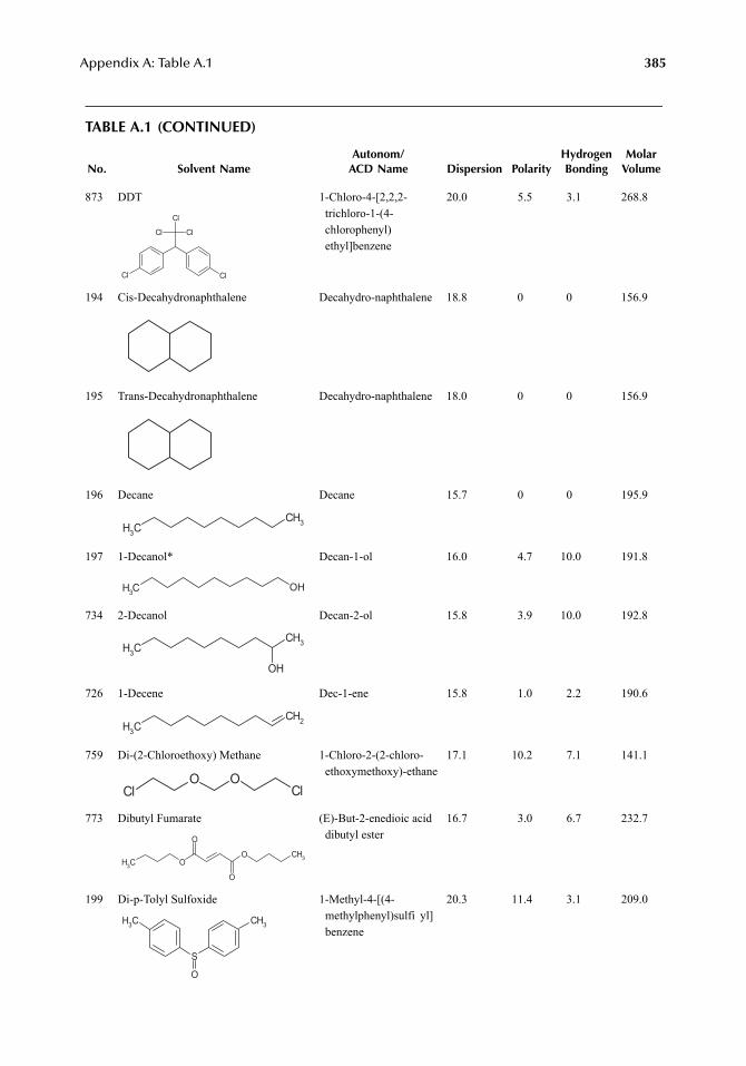
Appendix A: Table A.1 385
TABLE A.1 (CONTINUED)
No. Solvent NameAutonom/
ACD Name Dispersion PolarityHydrogenBonding
MolarVolume
873 DDT 1-Chloro-4-[2,2,2-trichloro-1-(4-chlorophenyl) ethyl]benzene
20.0 5.5 3.1 268.8
194 Cis-Decahydronaphthalene Decahydro-naphthalene 18.8 0 0 156.9
195 Trans-Decahydronaphthalene Decahydro-naphthalene 18.0 0 0 156.9
196 Decane Decane 15.7 0 0 195.9
197 1-Decanol* Decan-1-ol 16.0 4.7 10.0 191.8
734 2-Decanol Decan-2-ol 15.8 3.9 10.0 192.8
726 1-Decene Dec-1-ene 15.8 1.0 2.2 190.6
759 Di-(2-Chloroethoxy) Methane 1-Chloro-2-(2-chloro-ethoxymethoxy)-ethane
17.1 10.2 7.1 141.1
773 Dibutyl Fumarate (E)-But-2-enedioic acid dibutyl ester
16.7 3.0 6.7 232.7
199 Di-p-Tolyl Sulfoxide 1-Methyl-4-[(4-methylphenyl)sulfi yl]benzene
20.3 11.4 3.1 209.0
Cl
Cl
Cl Cl
Cl
CH3
CH3
CH3 OH
CH3
CH3
OH
CH3
CH2
ClO O
Cl
CH3 OO CH3
O
O
S
O
CH3 CH3
7248_A001.fm Page 385 Wednesday, May 23, 2007 12:31 PM
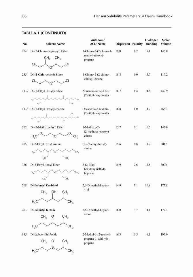
386 Hansen Solubility Parameters: A User’s Handbook
TABLE A.1 (CONTINUED)
No. Solvent NameAutonom/
ACD Name Dispersion PolarityHydrogenBonding
MolarVolume
204 Di-(2-Chloro-Isopropyl) Ether 1-Chloro-2-(2-chloro-1-methyl-ethoxy)-propane
19.0 8.2 5.1 146.0
235 Di-(2-Chloroethyl) Ether 1-Chloro-2-(2-chloro-ethoxy)-ethane
18.8 9.0 5.7 117.2
1139 Di-(2-Ethyl Hexyl)azelate Nonanedioic acid bis-(2-ethyl-hexyl) ester
16.7 1.4 4.8 449.9
1138 Di-(2-Ethyl Hexyl)sebacate Decanedioic acid bis-(2-ethyl-hexyl) ester
16.8 1.0 4.7 468.7
202 Di-(2-Methoxyethyl) Ether 1-Methoxy-2-(2-methoxy-ethoxy)-ethane
15.7 6.1 6.5 142.0
205 Di-2-Ethyl Hexyl Amine Bis-(2-ethyl-hexyl)-amine
15.6 0.8 3.2 301.5
736 Di-2-Ethyl Hexyl Ether 3-(2-Ethyl-hexyloxymethyl)-heptane
15.9 2.6 2.5 300.5
208 Di-Isobutyl Carbinol 2,6-Dimethyl-heptan-4-ol
14.9 3.1 10.8 177.8
203 Di-Isobutyl Ketone 2,6-Dimethyl-heptan-4-one
16.0 3.7 4.1 177.1
845 Di-Isobutyl Sulfoxide 2-Methyl-1-(2-methyl-propane-1-sulfi yl)-propane
16.3 10.5 6.1 195.0
O
CH3
Cl
CH3
Cl
OCl Cl
O
O
CH3
CH3
O
O
CH3
CH3
O
O
CH3O
O
CH3
CH3
CH3
CH3
OO
OCH3
CH3 N CH3
CH3 CH3
CH3 O CH3
CH3 CH3
CH3
CH3 OH
CH3
CH3
CH3
CH3 O
CH3
CH3
CH3
CH3
S
O
CH3
CH3
7248_A001.fm Page 386 Wednesday, May 23, 2007 12:31 PM
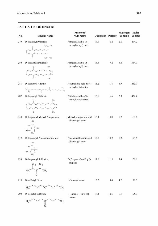
Appendix A: Table A.1 387
TABLE A.1 (CONTINUED)
No. Solvent NameAutonom/
ACD Name Dispersion PolarityHydrogenBonding
MolarVolume
279 Di-Isodecyl Phthalate Phthalic acid bis-(8-methyl-nonyl) ester
16.6 6.2 2.6 464.2
280 Di-Isoheptyl Phthalate Phthalic acid bis-(5-methyl-hexyl) ester
16.8 7.2 3.4 364.9
281 Di-Isononyl Adipate Hexanedioic acid bis-(7-methyl-octyl) ester
16.2 1.8 4.9 433.7
282 Di-Isononyl Phthalate Phthalic acid bis-(7-methyl-octyl) ester
16.6 6.6 2.9 432.4
840 Di-Isopropyl Methyl Phosphonate Methyl-phosphonic acid diisopropyl ester
16.4 10.0 5.7 184.4
842 Di-Isopropyl Phosphonofluoridat Phosphorofluoridic aciddiisopropyl ester
15.7 10.2 5.9 174.5
198 Di-Isopropyl Sulfoxide 2-(Propane-2-sulfi yl)-propane
17.0 11.5 7.4 159.9
219 Di-n-Butyl Ether 1-Butoxy-butane 15.2 3.4 4.2 170.3
200 Di-n-Butyl Sulfoxide 1-(Butane-1-sulfi yl)-butane
16.4 10.5 6.1 195.0
O
O
O
O
CH3CH3
CH3CH3
O
O
O
O
CH3
CH3
CH3
CH3
O
OO
OCH3
CH3
CH3
CH3
O
O
O
O
CH3
CH3
CH3
CH3
PO
O
CH3
OCH3
CH3
CH3
CH3
PO
O
F
OCH3
CH3
CH3
CH3
CH3 S
CH3
O
CH3
CH3
CH3 O CH3
CH3 S CH3
O
7248_A001.fm Page 387 Wednesday, May 23, 2007 12:31 PM
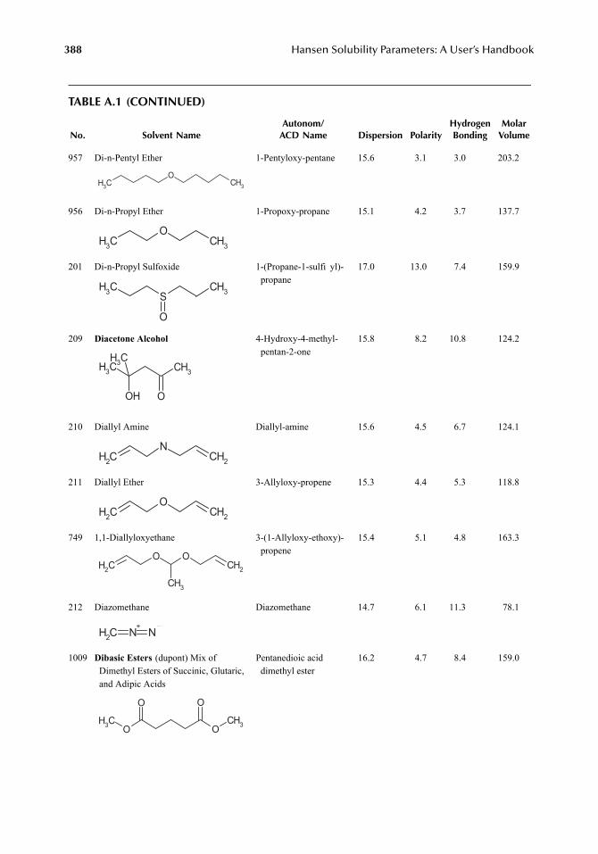
388 Hansen Solubility Parameters: A User’s Handbook
TABLE A.1 (CONTINUED)
No. Solvent NameAutonom/
ACD Name Dispersion PolarityHydrogenBonding
MolarVolume
957 Di-n-Pentyl Ether 1-Pentyloxy-pentane 15.6 3.1 3.0 203.2
956 Di-n-Propyl Ether 1-Propoxy-propane 15.1 4.2 3.7 137.7
201 Di-n-Propyl Sulfoxide 1-(Propane-1-sulfi yl)-propane
17.0 13.0 7.4 159.9
209 Diacetone Alcohol 4-Hydroxy-4-methyl-pentan-2-one
15.8 8.2 10.8 124.2
210 Diallyl Amine Diallyl-amine 15.6 4.5 6.7 124.1
211 Diallyl Ether 3-Allyloxy-propene 15.3 4.4 5.3 118.8
749 1,1-Diallyloxyethane 3-(1-Allyloxy-ethoxy)-propene
15.4 5.1 4.8 163.3
212 Diazomethane Diazomethane 14.7 6.1 11.3 78.1
1009 Dibasic Esters (dupont) Mix of Dimethyl Esters of Succinic, Glutaric, and Adipic Acids
Pentanedioic acid dimethyl ester
16.2 4.7 8.4 159.0
CH3
OCH3
CH3
OCH3
CH3 SCH3
O
CH3
O
CH3
OH
CH3
CH2
NCH2
CH2
OCH2
CH2
O O
CH3
CH2
CH2 N+N
O
O
O
O
CH3 CH3
7248_A001.fm Page 388 Wednesday, May 23, 2007 12:31 PM
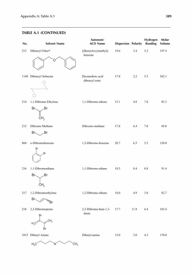
Appendix A: Table A.1 389
TABLE A.1 (CONTINUED)
No. Solvent NameAutonom/
ACD Name Dispersion PolarityHydrogenBonding
MolarVolume
213 Dibenzyl Ether* [(Benzyloxy)methyl]-benzene
19.6 3.4 5.2 197.4
1148 Dibenzyl Sebacate Decanedioic acid dibenzyl ester
17.8 2.2 5.5 362.1
214 1,1-Dibromo Ethylene 1,1-Dibromo-ethene 15.1 4.8 7.0 85.3
215 Dibromo Methane Dibromo-methane 17.8 6.4 7.0 69.8
804 o-Dibromobenzene 1,2-Dibromo-benzene 20.7 6.5 5.3 120.0
216 1,1-Dibromoethane 1,1-Dibromo-ethane 18.5 8.4 8.8 91.4
217 1,2-Dibromoethylene 1,2-Dibromo-ethene 18.0 4.9 3.0 82.7
218 2,3-Dibromoprene 2,3-Dibromo-buta-1,3-diene
17.7 11.8 6.4 103.4
1015 Dibutyl Amine Dibutyl-amine 15.0 3.0 4.3 170.0
O
O
O
O
O
BrBr
CH2
BrBr
Br
Br
BrBr
CH3
BrBr
CH2
CH2
Br
Br
CH3 N CH3
7248_A001.fm Page 389 Wednesday, May 23, 2007 12:31 PM
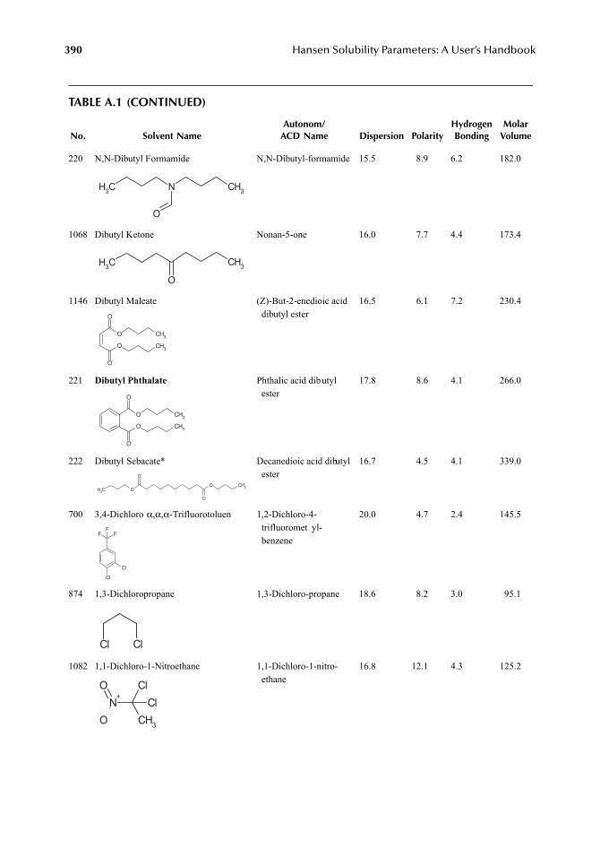
390 Hansen Solubility Parameters: A User’s Handbook
TABLE A.1 (CONTINUED)
No. Solvent NameAutonom/
ACD Name Dispersion PolarityHydrogenBonding
MolarVolume
220 N,N-Dibutyl Formamide N,N-Dibutyl-formamide 15.5 8.9 6.2 182.0
1068 Dibutyl Ketone Nonan-5-one 16.0 7.7 4.4 173.4
1146 Dibutyl Maleate (Z)-But-2-enedioic acid dibutyl ester
16.5 6.1 7.2 230.4
221 Dibutyl Phthalate Phthalic acid dibutyl ester
17.8 8.6 4.1 266.0
222 Dibutyl Sebacate* Decanedioic acid dibutyl ester
16.7 4.5 4.1 339.0
700 3,4-Dichloro α,α,α-Trifluorotoluen 1,2-Dichloro-4-trifluoromet yl-benzene
20.0 4.7 2.4 145.5
874 1,3-Dichloropropane 1,3-Dichloro-propane 18.6 8.2 3.0 95.1
1082 1,1-Dichloro-1-Nitroethane 1,1-Dichloro-1-nitro-ethane
16.8 12.1 4.3 125.2
CH3 N CH3
O
CH3 CH3
O
O
O
O
O
CH3
CH3
O
O
O
O
CH3
CH3
O
O
O
O
CH3CH3
FFF
Cl
Cl
Cl Cl
N+
O
O
CH3
ClCl
7248_A001.fm Page 390 Wednesday, May 23, 2007 12:31 PM
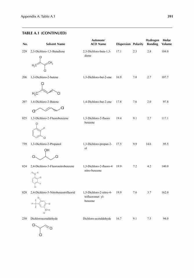
Appendix A: Table A.1 391
TABLE A.1 (CONTINUED)
No. Solvent NameAutonom/
ACD Name Dispersion PolarityHydrogenBonding
MolarVolume
229 2,3-Dichloro-1,3-Butadiene 2,3-Dichloro-buta-1,3-diene
17.1 2.3 2.8 104.0
206 1,3-Dichloro-2-butene 1,3-Dichloro-but-2-ene 16.9 7.8 2.7 107.7
207 1,4-Dichloro-2-Butene 1,4-Dichloro-but-2-ene 17.8 7.6 2.0 97.8
825 1,3-Dichloro-2-Fluorobenzene 1,3-Dichloro-2-fluorobenzene
19.4 9.1 2.7 117.1
739 1,3-Dichloro-2-Propanol 1,3-Dichloro-propan-2-ol
17.5 9.9 14.6 95.5
824 2,4-Dichloro-3-Fluoronitrobenzene 1,3-Dichloro-2-fluoro-4nitro-benzene
19.9 7.2 4.2 140.0
828 2,4-Dichloro-5-Nitrobenzotrifluorid 1,5-Dichloro-2-nitro-4-trifluoromet yl-benzene
19.9 7.6 3.7 162.0
230 Dichloroacetaldehyde Dichloro-acetaldehyde 16.7 9.1 7.5 94.0
CH2
Cl
Cl
CH2
CH3
Cl
Cl
ClCl
Cl
Cl
F
OH
Cl Cl
N+ OO
Cl
Cl
F
F
F
FN+
OO
Cl
Cl
O
Cl
Cl
7248_A001.fm Page 391 Wednesday, May 23, 2007 12:31 PM
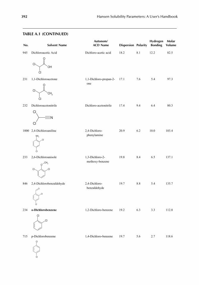
392 Hansen Solubility Parameters: A User’s Handbook
TABLE A.1 (CONTINUED)
No. Solvent NameAutonom/
ACD Name Dispersion PolarityHydrogenBonding
MolarVolume
945 Dichloroacetic Acid Dichloro-acetic acid 18.2 8.1 12.2 82.5
231 1,1-Dichloroacetone 1,1-Dichloro-propan-2-one
17.1 7.6 5.4 97.3
232 Dichloroacetonitrile Dichloro-acetonitrile 17.4 9.4 6.4 80.3
1000 2,4-Dichloroaniline 2,4-Dichloro-phenylamine
20.9 6.2 10.0 103.4
233 2,6-Dichloroanisole 1,3-Dichloro-2-methoxy-benzene
19.8 8.4 6.5 137.1
846 2,4-Dichlorobenzaldehyde 2,4-Dichloro-benzaldehyde
19.7 8.8 5.4 135.7
234 o-Dichlorobenzene 1,2-Dichloro-benzene 19.2 6.3 3.3 112.8
715 p-Dichlorobenzene 1,4-Dichloro-benzene 19.7 5.6 2.7 118.6
OH
O
Cl
Cl
CH3
O
Cl
Cl
NCl
Cl
NH2
Cl
Cl
OCH3
ClCl
O
Cl
Cl
Cl
Cl
Cl
Cl
7248_A001.fm Page 392 Wednesday, May 23, 2007 12:31 PM
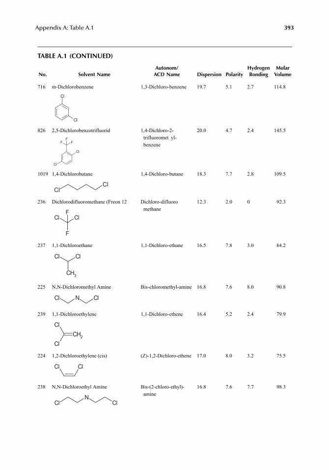
Appendix A: Table A.1 393
TABLE A.1 (CONTINUED)
No. Solvent NameAutonom/
ACD Name Dispersion PolarityHydrogenBonding
MolarVolume
716 m-Dichlorobenzene 1,3-Dichloro-benzene 19.7 5.1 2.7 114.8
826 2,5-Dichlorobenzotrifluorid 1,4-Dichloro-2-trifluoromet yl-benzene
20.0 4.7 2.4 145.5
1019 1,4-Dichlorobutane 1,4-Dichloro-butane 18.3 7.7 2.8 109.5
236 Dichlorodifluoromethane (Freon 12 Dichloro-difluoromethane
12.3 2.0 0 92.3
237 1,1-Dichloroethane 1,1-Dichloro-ethane 16.5 7.8 3.0 84.2
225 N,N-Dichloromethyl Amine Bis-chloromethyl-amine 16.8 7.6 8.0 90.8
239 1,1-Dichloroethylene 1,1-Dichloro-ethene 16.4 5.2 2.4 79.9
224 1,2-Dichloroethylene (cis) (Z)-1,2-Dichloro-ethene 17.0 8.0 3.2 75.5
238 N,N-Dichloroethyl Amine Bis-(2-chloro-ethyl)-amine
16.8 7.6 7.7 98.3
Cl
Cl
FFF
Cl
Cl
ClCl
ClCl
F
F
ClCl
CH3
N ClCl
CH2
Cl
Cl
Cl Cl
NClCl
7248_A001.fm Page 393 Wednesday, May 23, 2007 12:31 PM
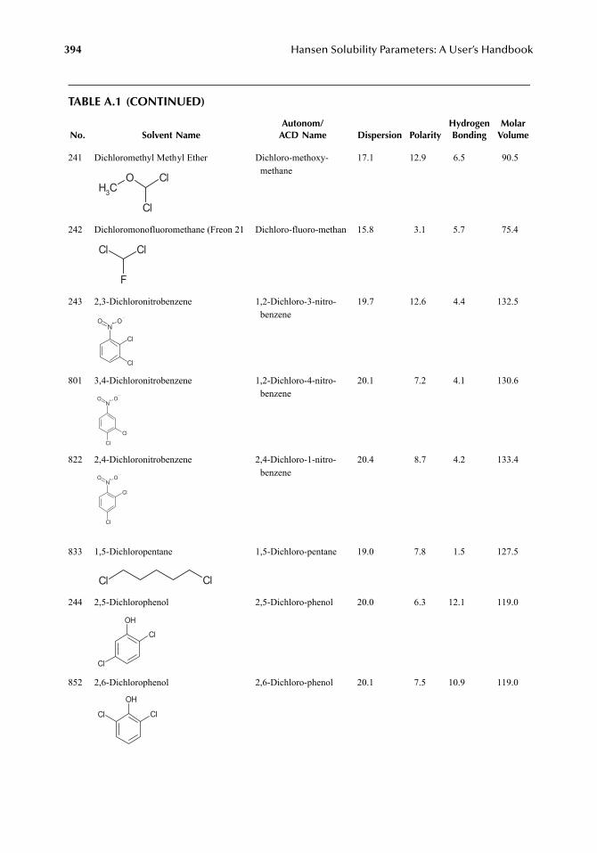
394 Hansen Solubility Parameters: A User’s Handbook
TABLE A.1 (CONTINUED)
No. Solvent NameAutonom/
ACD Name Dispersion PolarityHydrogenBonding
MolarVolume
241 Dichloromethyl Methyl Ether Dichloro-methoxy-methane
17.1 12.9 6.5 90.5
242 Dichloromonofluoromethane (Freon 21 Dichloro-fluoro-methan 15.8 3.1 5.7 75.4
243 2,3-Dichloronitrobenzene 1,2-Dichloro-3-nitro-benzene
19.7 12.6 4.4 132.5
801 3,4-Dichloronitrobenzene 1,2-Dichloro-4-nitro-benzene
20.1 7.2 4.1 130.6
822 2,4-Dichloronitrobenzene 2,4-Dichloro-1-nitro-benzene
20.4 8.7 4.2 133.4
833 1,5-Dichloropentane 1,5-Dichloro-pentane 19.0 7.8 1.5 127.5
244 2,5-Dichlorophenol 2,5-Dichloro-phenol 20.0 6.3 12.1 119.0
852 2,6-Dichlorophenol 2,6-Dichloro-phenol 20.1 7.5 10.9 119.0
CH3
O Cl
Cl
ClCl
F
N+ OO
Cl
Cl
N+ OO
Cl
Cl
N+ OO
Cl
Cl
Cl Cl
OH
Cl
Cl
OH
ClCl
7248_A001.fm Page 394 Wednesday, May 23, 2007 12:31 PM
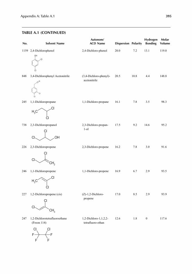
Appendix A: Table A.1 395
TABLE A.1 (CONTINUED)
No. Solvent NameAutonom/
ACD Name Dispersion PolarityHydrogenBonding
MolarVolume
1159 2,4-Dichlorophenol 2,4-Dichloro-phenol 20.0 7.2 13.1 119.0
848 3,4-Dichlorophenyl Acetonitrile (3,4-Dichloro-phenyl)-acetonitrile
20.5 10.8 4.4 148.8
245 1,1-Dichloropropane 1,1-Dichloro-propane 16.1 7.8 3.5 98.3
738 2,3-Dichloropropanol 2,3-Dichloro-propan-1-ol
17.5 9.2 14.6 95.2
226 2,3-Dichloropropene 2,3-Dichloro-propene 16.2 7.8 3.0 91.6
246 1,1-Dichloropropene 1,1-Dichloro-propene 16.9 6.7 2.9 93.5
227 1,2-Dichloropropene (cis) (Z)-1,2-Dichloro-propene
17.0 8.5 2.9 93.9
247 1,2-Dichlorotetrafluoroethane(Freon 114)
1,2-Dichloro-1,1,2,2-tetrafluoro-ethan
12.6 1.8 0 117.6
OH
Cl
Cl
N
Cl
Cl
CH3
Cl
Cl
OH
Cl
Cl
CH2
Cl
Cl
CH3
Cl
Cl
CH3
Cl
Cl
Cl Cl
FF
FF
7248_A001.fm Page 395 Wednesday, May 23, 2007 12:31 PM
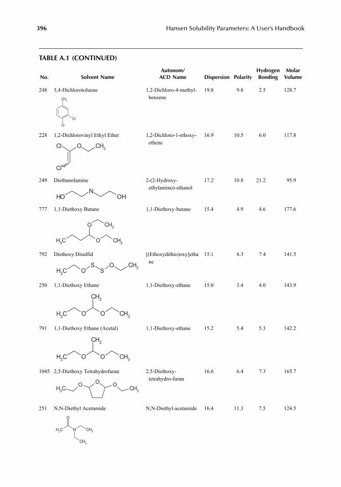
396 Hansen Solubility Parameters: A User’s Handbook
TABLE A.1 (CONTINUED)
No. Solvent NameAutonom/
ACD Name Dispersion PolarityHydrogenBonding
MolarVolume
248 3,4-Dichlorotoluene 1,2-Dichloro-4-methyl-benzene
19.8 9.8 2.5 128.7
228 1,2-Dichlorovinyl Ethyl Ether 1,2-Dichloro-1-ethoxy-ethene
16.9 10.5 6.0 117.8
249 Diethanolamine 2-(2-Hydroxy-ethylamino)-ethanol
17.2 10.8 21.2 95.9
777 1,1-Diethoxy Butane 1,1-Diethoxy-butane 15.4 4.9 4.6 177.6
792 Diethoxy Disulfid [(Ethoxydithio)oxy]ethane
15.1 8.3 7.4 141.5
250 1,1-Diethoxy Ethane 1,1-Diethoxy-ethane 15.0 3.4 4.0 143.9
791 1,1-Diethoxy Ethane (Acetal) 1,1-Diethoxy-ethane 15.2 5.4 5.3 142.2
1045 2,5-Diethoxy Tetrahydrofuran 2,5-Diethoxy-tetrahydro-furan
16.6 6.4 7.3 165.7
251 N,N-Diethyl Acetamide N,N-Diethyl-acetamide 16.4 11.3 7.5 124.5
CH3
Cl
Cl
OCl
Cl
CH3
OHN
OH
CH3 O CH3
O CH3
CH3 OS
SO CH3
CH3 O O CH3
CH3
CH3 O O CH3
CH3
O O CH3OCH3
CH3 N
O
CH3
CH3
7248_A001.fm Page 396 Wednesday, May 23, 2007 12:31 PM
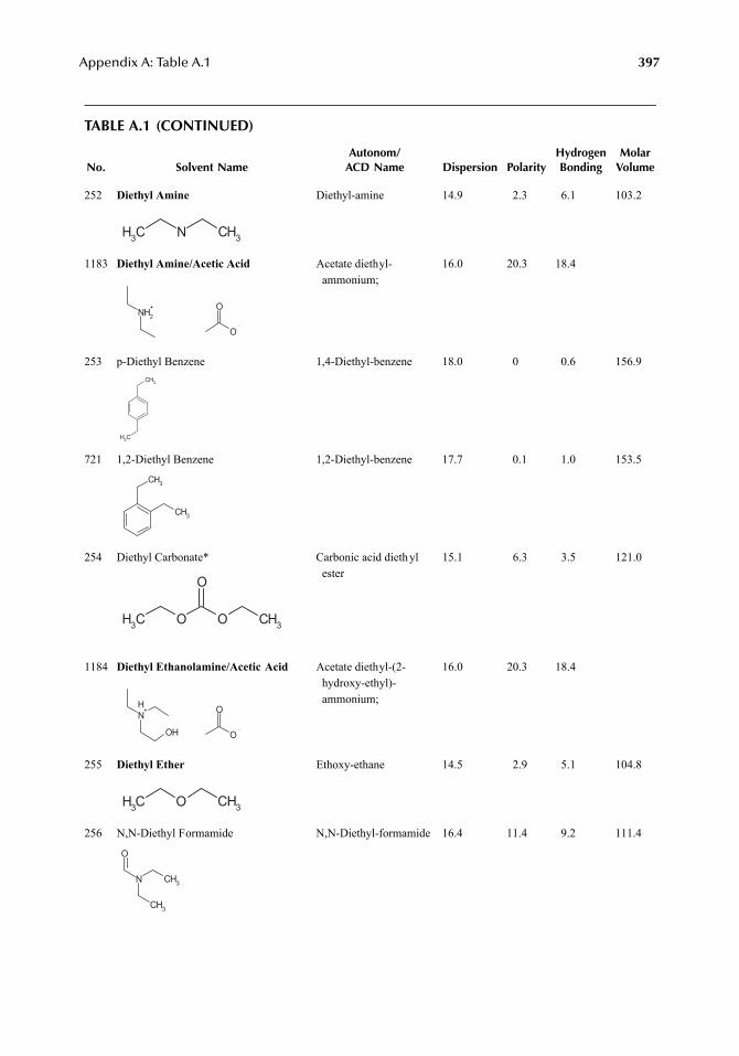
Appendix A: Table A.1 397
TABLE A.1 (CONTINUED)
No. Solvent NameAutonom/
ACD Name Dispersion PolarityHydrogenBonding
MolarVolume
252 Diethyl Amine Diethyl-amine 14.9 2.3 6.1 103.2
1183 Diethyl Amine/Acetic Acid Acetate diethyl-ammonium;
16.0 20.3 18.4
253 p-Diethyl Benzene 1,4-Diethyl-benzene 18.0 0 0.6 156.9
721 1,2-Diethyl Benzene 1,2-Diethyl-benzene 17.7 0.1 1.0 153.5
254 Diethyl Carbonate* Carbonic acid diethyl ester
15.1 6.3 3.5 121.0
1184 Diethyl Ethanolamine/Acetic Acid Acetate diethyl-(2-hydroxy-ethyl)-ammonium;
16.0 20.3 18.4
255 Diethyl Ether Ethoxy-ethane 14.5 2.9 5.1 104.8
256 N,N-Diethyl Formamide N,N-Diethyl-formamide 16.4 11.4 9.2 111.4
CH3 N CH3
NH2+
O
O
CH3
CH3
CH3
CH3
CH3 O O CH3
O
NH+
OH O
O
CH3 O CH3
O
N CH3
CH3
7248_A001.fm Page 397 Wednesday, May 23, 2007 12:31 PM
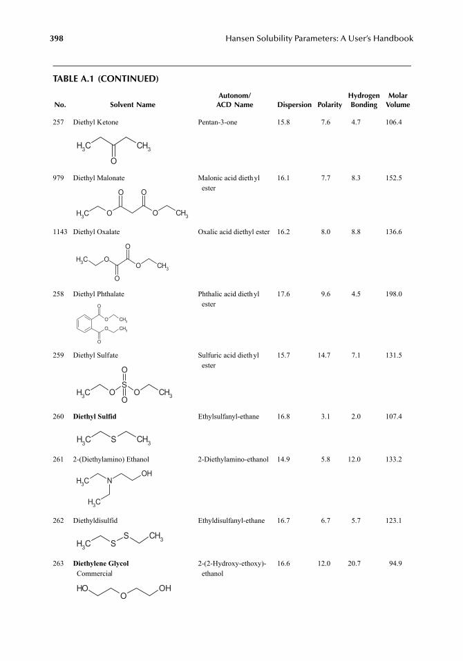
398 Hansen Solubility Parameters: A User’s Handbook
TABLE A.1 (CONTINUED)
No. Solvent NameAutonom/
ACD Name Dispersion PolarityHydrogenBonding
MolarVolume
257 Diethyl Ketone Pentan-3-one 15.8 7.6 4.7 106.4
979 Diethyl Malonate Malonic acid diethyl ester
16.1 7.7 8.3 152.5
1143 Diethyl Oxalate Oxalic acid diethyl ester 16.2 8.0 8.8 136.6
258 Diethyl Phthalate Phthalic acid diethyl ester
17.6 9.6 4.5 198.0
259 Diethyl Sulfate Sulfuric acid diethyl ester
15.7 14.7 7.1 131.5
260 Diethyl Sulfid Ethylsulfanyl-ethane 16.8 3.1 2.0 107.4
261 2-(Diethylamino) Ethanol 2-Diethylamino-ethanol 14.9 5.8 12.0 133.2
262 Diethyldisulfid Ethyldisulfanyl-ethane 16.7 6.7 5.7 123.1
263 Diethylene GlycolCommercial
2-(2-Hydroxy-ethoxy)-ethanol
16.6 12.0 20.7 94.9
CH3 CH3
O
CH3 O O CH3
O O
O
O
O
O
CH3
CH3
O
O
CH3
O
O CH3
CH3 OS
O CH3
O
O
CH3 S CH3
CH3 NOH
CH3
CH3 SS CH3
OHO
OH
7248_A001.fm Page 398 Wednesday, May 23, 2007 12:31 PM
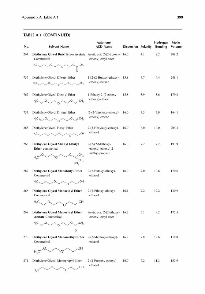
Appendix A: Table A.1 399
TABLE A.1 (CONTINUED)
No. Solvent NameAutonom/
ACD Name Dispersion PolarityHydrogenBonding
MolarVolume
264 Diethylene Glycol Butyl Ether AcetateCommercial
Acetic acid 2-(2-butoxy-ethoxy)-ethyl ester
16.0 4.1 8.2 208.2
757 Diethylene Glycol Dibutyl Ether 1-[2-(2-Butoxy-ethoxy)-ethoxy]-butane
15.8 4.7 4.4 248.1
762 Diethylene Glycol Diethyl Ether 1-Ethoxy-2-(2-ethoxy-ethoxy)-ethane
15.8 5.9 5.6 179.8
755 Diethylene Glycol Divinyl Ether [2-(2-Vinyloxy-ethoxy)-ethoxy]-ethene
16.0 7.3 7.9 164.1
265 Diethylene Glycol Hexyl Ether 2-(2-Hexyloxy-ethoxy)-ethanol
16.0 6.0 10.0 204.3
266 Diethylene Glycol Methyl t-Butyl Ether commerical
2-[2-(2-Methoxy-ethoxy)-ethoxy]-2-methyl-propane
16.0 7.2 7.2 193.9
267 Diethylene Glycol Monobutyl Ether Commercial
2-(2-Butoxy-ethoxy)-ethanol
16.0 7.0 10.6 170.6
268 Diethylene Glycol Monoethyl Ether Commerical
2-(2-Ethoxy-ethoxy)-ethanol
16.1 9.2 12.2 130.9
269 Diethylene Glycol Monoethyl Ether Acetate Commerical
Acetic acid 2-(2-ethoxy-ethoxy)-ethyl ester
16.2 5.1 9.2 175.5
270 Diethylene Glycol Monomethyl Ether Commerical
2-(2-Methoxy-ethoxy)-ethanol
16.2 7.8 12.6 118.0
271 Diethylene Glycol Monopropyl Ether 2-(2-Propoxy-ethoxy)-ethanol
16.0 7.2 11.3 153.9
OO
OCH3 CH3
O
OO
OCH3 CH3
OO
OCH3 CH3
OO
OCH2 CH2
OO
OHCH3
OO
OCH3
CH3
CH3
CH3
OO
OHCH3
OO
OHCH3
OO
OCH3 CH3
O
OO
OHCH3
OO
OHCH3
7248_A001.fm Page 399 Wednesday, May 23, 2007 12:31 PM
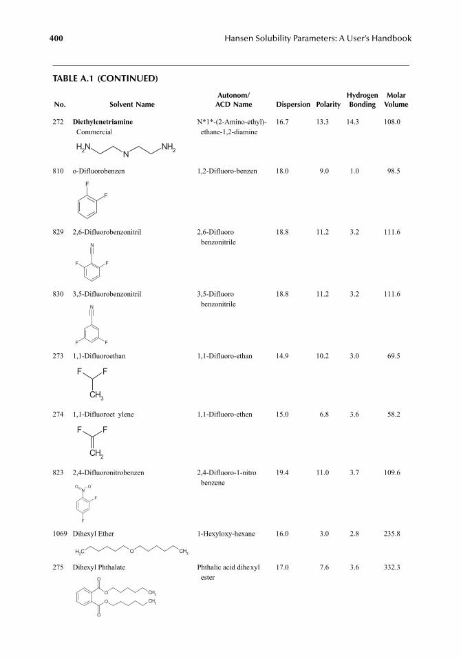
400 Hansen Solubility Parameters: A User’s Handbook
TABLE A.1 (CONTINUED)
No. Solvent NameAutonom/
ACD Name Dispersion PolarityHydrogenBonding
MolarVolume
272 DiethylenetriamineCommercial
N*1*-(2-Amino-ethyl)-ethane-1,2-diamine
16.7 13.3 14.3 108.0
810 o-Difluorobenzen 1,2-Difluoro-benzen 18.0 9.0 1.0 98.5
829 2,6-Difluorobenzonitril 2,6-Difluorobenzonitrile
18.8 11.2 3.2 111.6
830 3,5-Difluorobenzonitril 3,5-Difluorobenzonitrile
18.8 11.2 3.2 111.6
273 1,1-Difluoroethan 1,1-Difluoro-ethan 14.9 10.2 3.0 69.5
274 1,1-Difluoroet ylene 1,1-Difluoro-ethen 15.0 6.8 3.6 58.2
823 2,4-Difluoronitrobenzen 2,4-Difluoro-1-nitrobenzene
19.4 11.0 3.7 109.6
1069 Dihexyl Ether 1-Hexyloxy-hexane 16.0 3.0 2.8 235.8
275 Dihexyl Phthalate Phthalic acid dihexyl ester
17.0 7.6 3.6 332.3
NNH2NH2
F
F
N
FF
N
F F
FF
CH3
FF
CH2
N+ OO
F
F
CH3 O CH3
O
O
O
O
CH3
CH3
7248_A001.fm Page 400 Wednesday, May 23, 2007 12:31 PM
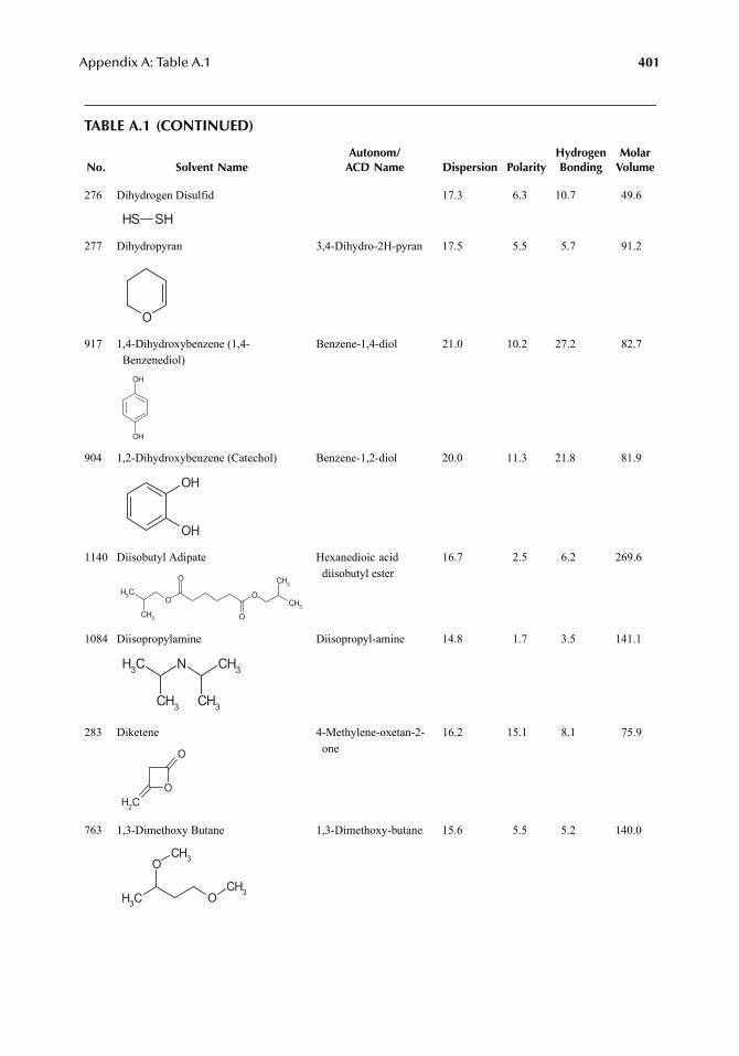
Appendix A: Table A.1 401
TABLE A.1 (CONTINUED)
No. Solvent NameAutonom/
ACD Name Dispersion PolarityHydrogenBonding
MolarVolume
276 Dihydrogen Disulfid 17.3 6.3 10.7 49.6
277 Dihydropyran 3,4-Dihydro-2H-pyran 17.5 5.5 5.7 91.2
917 1,4-Dihydroxybenzene (1,4-Benzenediol)
Benzene-1,4-diol 21.0 10.2 27.2 82.7
904 1,2-Dihydroxybenzene (Catechol) Benzene-1,2-diol 20.0 11.3 21.8 81.9
1140 Diisobutyl Adipate Hexanedioic acid diisobutyl ester
16.7 2.5 6.2 269.6
1084 Diisopropylamine Diisopropyl-amine 14.8 1.7 3.5 141.1
283 Diketene 4-Methylene-oxetan-2-one
16.2 15.1 8.1 75.9
763 1,3-Dimethoxy Butane 1,3-Dimethoxy-butane 15.6 5.5 5.2 140.0
SH SH
O
OH
OH
OH
OH
O
OCH3
CH3
O
O
CH3
CH3
NCH3
CH3
CH3
CH3
O
O
CH2
CH3 OCH3
OCH3
7248_A001.fm Page 401 Wednesday, May 23, 2007 12:31 PM
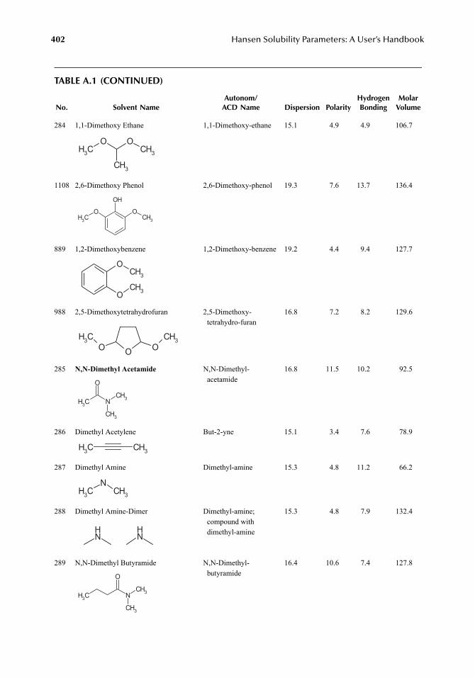
402 Hansen Solubility Parameters: A User’s Handbook
TABLE A.1 (CONTINUED)
No. Solvent NameAutonom/
ACD Name Dispersion PolarityHydrogenBonding
MolarVolume
284 1,1-Dimethoxy Ethane 1,1-Dimethoxy-ethane 15.1 4.9 4.9 106.7
1108 2,6-Dimethoxy Phenol 2,6-Dimethoxy-phenol 19.3 7.6 13.7 136.4
889 1,2-Dimethoxybenzene 1,2-Dimethoxy-benzene 19.2 4.4 9.4 127.7
988 2,5-Dimethoxytetrahydrofuran 2,5-Dimethoxy-tetrahydro-furan
16.8 7.2 8.2 129.6
285 N,N-Dimethyl Acetamide N,N-Dimethyl-acetamide
16.8 11.5 10.2 92.5
286 Dimethyl Acetylene But-2-yne 15.1 3.4 7.6 78.9
287 Dimethyl Amine Dimethyl-amine 15.3 4.8 11.2 66.2
288 Dimethyl Amine-Dimer Dimethyl-amine; compound with dimethyl-amine
15.3 4.8 7.9 132.4
289 N,N-Dimethyl Butyramide N,N-Dimethyl-butyramide
16.4 10.6 7.4 127.8
OO
CH3
CH3CH3
OH
OCH3
OCH3
OCH3
OCH3
O OCH3
OCH3
CH3 N
O
CH3
CH3
CH3CH3
CH3
NCH3
NH
NH
CH3 NCH3
O
CH3
7248_A001.fm Page 402 Wednesday, May 23, 2007 12:31 PM
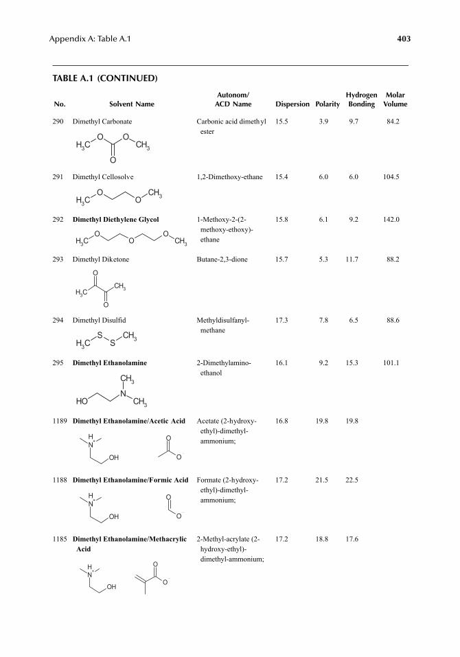
Appendix A: Table A.1 403
TABLE A.1 (CONTINUED)
No. Solvent NameAutonom/
ACD Name Dispersion PolarityHydrogenBonding
MolarVolume
290 Dimethyl Carbonate Carbonic acid dimethyl ester
15.5 3.9 9.7 84.2
291 Dimethyl Cellosolve 1,2-Dimethoxy-ethane 15.4 6.0 6.0 104.5
292 Dimethyl Diethylene Glycol 1-Methoxy-2-(2-methoxy-ethoxy)-ethane
15.8 6.1 9.2 142.0
293 Dimethyl Diketone Butane-2,3-dione 15.7 5.3 11.7 88.2
294 Dimethyl Disulfid Methyldisulfanyl-methane
17.3 7.8 6.5 88.6
295 Dimethyl Ethanolamine 2-Dimethylamino-ethanol
16.1 9.2 15.3 101.1
1189 Dimethyl Ethanolamine/Acetic Acid Acetate (2-hydroxy-ethyl)-dimethyl-ammonium;
16.8 19.8 19.8
1188 Dimethyl Ethanolamine/Formic Acid Formate (2-hydroxy-ethyl)-dimethyl-ammonium;
17.2 21.5 22.5
1185 Dimethyl Ethanolamine/Methacrylic Acid
2-Methyl-acrylate (2-hydroxy-ethyl)-dimethyl-ammonium;
17.2 18.8 17.6
CH3
O O
O
CH3
CH3
OO
CH3
CH3
OO
OCH3
CH3
O
O
CH3
CH3
SS
CH3
NCH3
CH3
OH
NH+
OH O
O
NH+
OH O
O
NH+
OHO
O
7248_A001.fm Page 403 Wednesday, May 23, 2007 12:31 PM
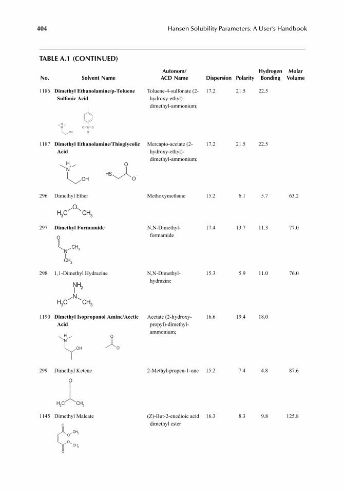
404 Hansen Solubility Parameters: A User’s Handbook
TABLE A.1 (CONTINUED)
No. Solvent NameAutonom/
ACD Name Dispersion PolarityHydrogenBonding
MolarVolume
1186 Dimethyl Ethanolamine/p-Toluene Sulfonic Acid
Toluene-4-sulfonate (2-hydroxy-ethyl)-dimethyl-ammonium;
17.2 21.5 22.5
1187 Dimethyl Ethanolamine/Thioglycolic Acid
Mercapto-acetate (2-hydroxy-ethyl)-dimethyl-ammonium;
17.2 21.5 22.5
296 Dimethyl Ether Methoxymethane 15.2 6.1 5.7 63.2
297 Dimethyl Formamide N,N-Dimethyl-formamide
17.4 13.7 11.3 77.0
298 1,1-Dimethyl Hydrazine N,N-Dimethyl-hydrazine
15.3 5.9 11.0 76.0
1190 Dimethyl Isopropanol Amine/Acetic Acid
Acetate (2-hydroxy-propyl)-dimethyl-ammonium;
16.6 19.4 18.0
299 Dimethyl Ketene 2-Methyl-propen-1-one 15.2 7.4 4.8 87.6
1145 Dimethyl Maleate (Z)-But-2-enedioic acid dimethyl ester
16.3 8.3 9.8 125.8
NH+
OH
SO O
O
NH+
OH O
O
SH
CH3
OCH3
CH3
NCH3
O
CH3
NCH3
NH2
NH+
OH O
O
CH3 CH3
O
O
O
CH3
O
O
CH3
7248_A001.fm Page 404 Wednesday, May 23, 2007 12:31 PM
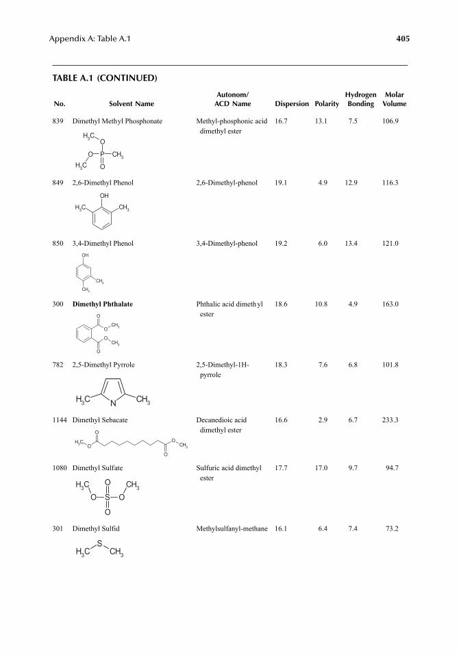
Appendix A: Table A.1 405
TABLE A.1 (CONTINUED)
No. Solvent NameAutonom/
ACD Name Dispersion PolarityHydrogenBonding
MolarVolume
839 Dimethyl Methyl Phosphonate Methyl-phosphonic acid dimethyl ester
16.7 13.1 7.5 106.9
849 2,6-Dimethyl Phenol 2,6-Dimethyl-phenol 19.1 4.9 12.9 116.3
850 3,4-Dimethyl Phenol 3,4-Dimethyl-phenol 19.2 6.0 13.4 121.0
300 Dimethyl Phthalate Phthalic acid dimethyl ester
18.6 10.8 4.9 163.0
782 2,5-Dimethyl Pyrrole 2,5-Dimethyl-1H-pyrrole
18.3 7.6 6.8 101.8
1144 Dimethyl Sebacate Decanedioic acid dimethyl ester
16.6 2.9 6.7 233.3
1080 Dimethyl Sulfate Sulfuric acid dimethyl ester
17.7 17.0 9.7 94.7
301 Dimethyl Sulfid Methylsulfanyl-methane 16.1 6.4 7.4 73.2
PO
O
CH3
OCH3
CH3
OH
CH3CH3
OH
CH3
CH3
O
O
CH3
O
OCH3
N CH3CH3
O
O
CH3O
O
CH3
O S O
O
O
CH3 CH3
CH3
SCH3
7248_A001.fm Page 405 Wednesday, May 23, 2007 12:31 PM
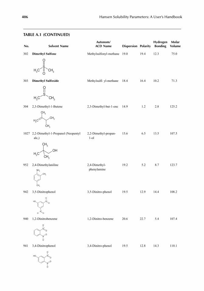
406 Hansen Solubility Parameters: A User’s Handbook
TABLE A.1 (CONTINUED)
No. Solvent NameAutonom/
ACD Name Dispersion PolarityHydrogenBonding
MolarVolume
302 Dimethyl Sulfone Methylsulfonyl-methane 19.0 19.4 12.3 75.0
303 Dimethyl Sulfoxide Methylsulfi yl-methane 18.4 16.4 10.2 71.3
304 2,3-Dimethyl-1-Butene 2,3-Dimethyl-but-1-ene 14.9 1.2 2.8 125.2
1027 2,2-Dimethyl-1-Propanol (Neopentyl alc,)
2,2-Dimethyl-propan-1-ol
15.6 6.5 13.5 107.5
952 2,4-Dimethylaniline 2,4-Dimethyl-phenylamine
19.2 5.2 8.7 123.7
942 3,5-Dinitrophenol 3,5-Dinitro-phenol 19.5 12.9 14.4 108.2
940 1,2-Dinitrobenzene 1,2-Dinitro-benzene 20.6 22.7 5.4 107.4
941 3,4-Dinitrophenol 3,4-Dinitro-phenol 19.5 12.8 14.3 110.1
CH3
SCH3
O
O
CH3
SCH3
O
CH2
CH3
CH3
CH3
CH3
OH
CH3
CH3
NH2
CH3
CH3
N+
N+
O
O
O O
OH
N+
O
O
N+
O
O
N+
O
O
N+
O
O
OH
7248_A001.fm Page 406 Wednesday, May 23, 2007 12:31 PM
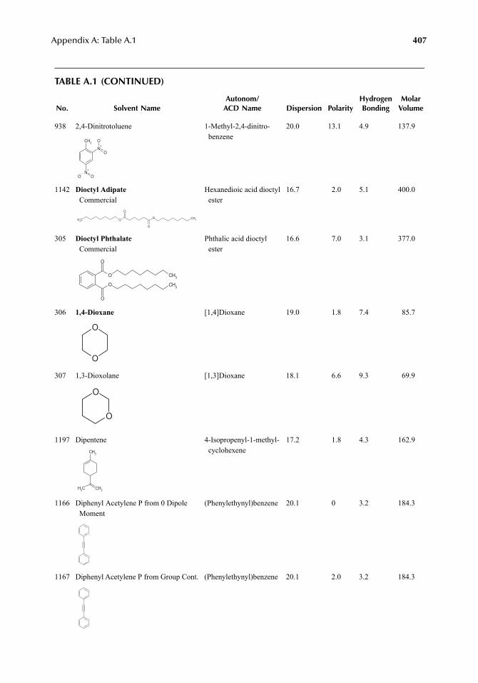
Appendix A: Table A.1 407
TABLE A.1 (CONTINUED)
No. Solvent NameAutonom/
ACD Name Dispersion PolarityHydrogenBonding
MolarVolume
938 2,4-Dinitrotoluene 1-Methyl-2,4-dinitro-benzene
20.0 13.1 4.9 137.9
1142 Dioctyl AdipateCommercial
Hexanedioic acid dioctyl ester
16.7 2.0 5.1 400.0
305 Dioctyl PhthalateCommercial
Phthalic acid dioctyl ester
16.6 7.0 3.1 377.0
306 1,4-Dioxane [1,4]Dioxane 19.0 1.8 7.4 85.7
307 1,3-Dioxolane [1,3]Dioxane 18.1 6.6 9.3 69.9
1197 Dipentene 4-Isopropenyl-1-methyl-cyclohexene
17.2 1.8 4.3 162.9
1166 Diphenyl Acetylene P from 0 Dipole Moment
(Phenylethynyl)benzene 20.1 0 3.2 184.3
1167 Diphenyl Acetylene P from Group Cont. (Phenylethynyl)benzene 20.1 2.0 3.2 184.3
CH3
N+
N+
O
O
O O
O
O
O
O
CH3CH3
O
O
O
O
CH3
CH3
O
O
O
O
CH3 CH2
CH3
7248_A001.fm Page 407 Wednesday, May 23, 2007 12:31 PM
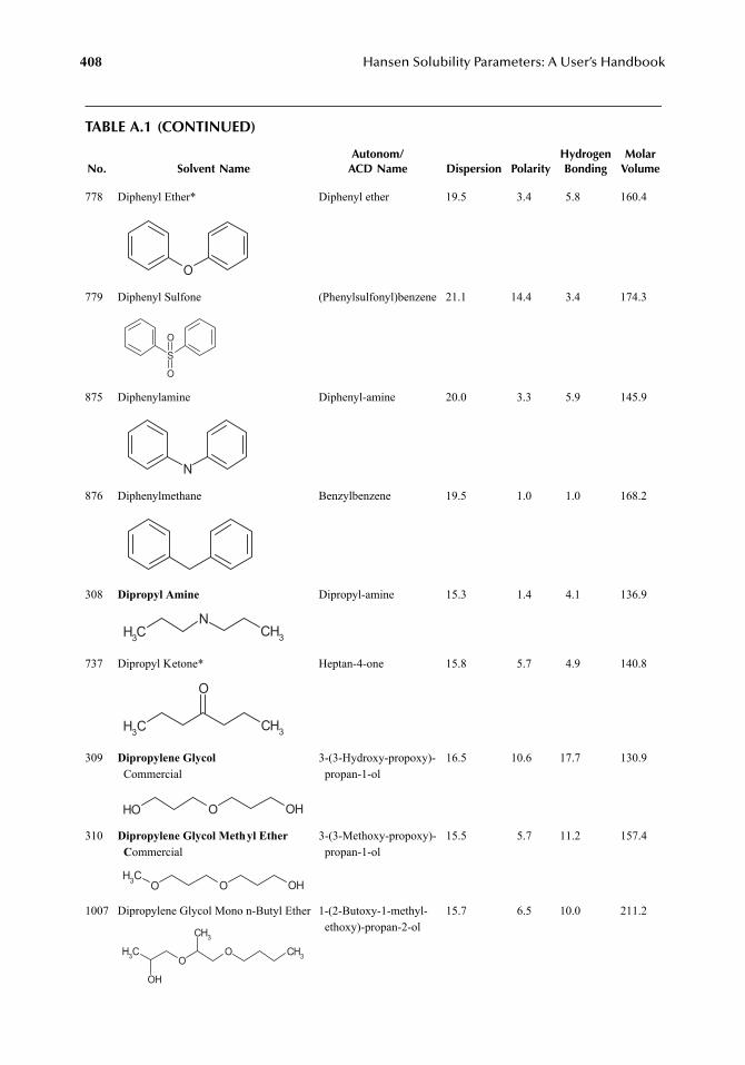
408 Hansen Solubility Parameters: A User’s Handbook
TABLE A.1 (CONTINUED)
No. Solvent NameAutonom/
ACD Name Dispersion PolarityHydrogenBonding
MolarVolume
778 Diphenyl Ether* Diphenyl ether 19.5 3.4 5.8 160.4
779 Diphenyl Sulfone (Phenylsulfonyl)benzene 21.1 14.4 3.4 174.3
875 Diphenylamine Diphenyl-amine 20.0 3.3 5.9 145.9
876 Diphenylmethane Benzylbenzene 19.5 1.0 1.0 168.2
308 Dipropyl Amine Dipropyl-amine 15.3 1.4 4.1 136.9
737 Dipropyl Ketone* Heptan-4-one 15.8 5.7 4.9 140.8
309 Dipropylene GlycolCommercial
3-(3-Hydroxy-propoxy)-propan-1-ol
16.5 10.6 17.7 130.9
310 Dipropylene Glycol Methyl EtherCommercial
3-(3-Methoxy-propoxy)-propan-1-ol
15.5 5.7 11.2 157.4
1007 Dipropylene Glycol Mono n-Butyl Ether 1-(2-Butoxy-1-methyl-ethoxy)-propan-2-ol
15.7 6.5 10.0 211.2
O
S
O
O
N
CH3
NCH3
CH3 CH3
O
OH O OH
O O OHCH3
O
CH3
OCH3
OH
CH3
7248_A001.fm Page 408 Wednesday, May 23, 2007 12:31 PM
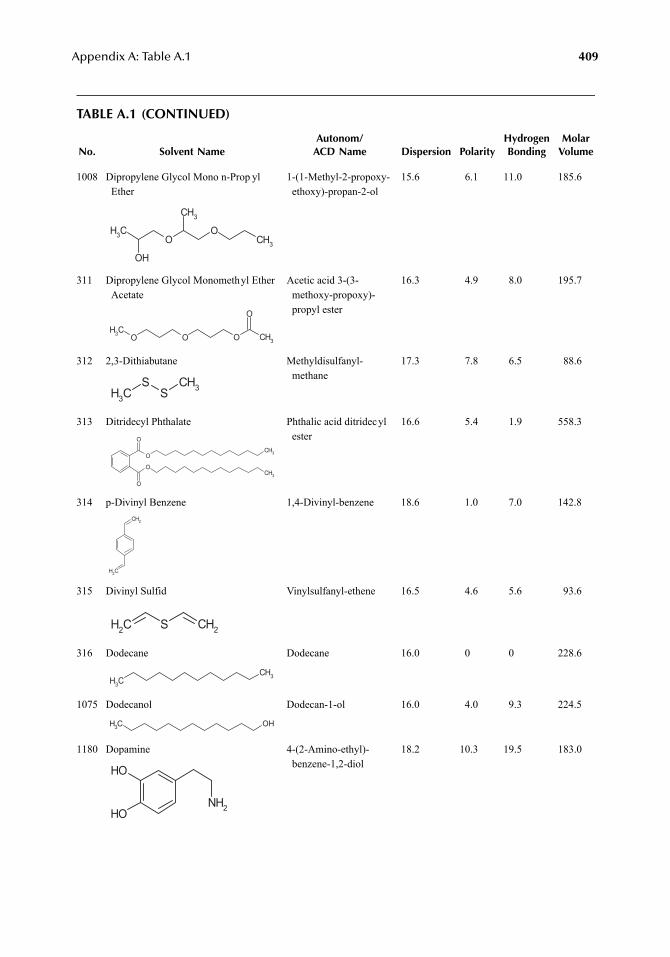
Appendix A: Table A.1 409
TABLE A.1 (CONTINUED)
No. Solvent NameAutonom/
ACD Name Dispersion PolarityHydrogenBonding
MolarVolume
1008 Dipropylene Glycol Mono n-Prop yl Ether
1-(1-Methyl-2-propoxy-ethoxy)-propan-2-ol
15.6 6.1 11.0 185.6
311 Dipropylene Glycol Monomethyl Ether Acetate
Acetic acid 3-(3-methoxy-propoxy)-propyl ester
16.3 4.9 8.0 195.7
312 2,3-Dithiabutane Methyldisulfanyl-methane
17.3 7.8 6.5 88.6
313 Ditridecyl Phthalate Phthalic acid ditridecyl ester
16.6 5.4 1.9 558.3
314 p-Divinyl Benzene 1,4-Divinyl-benzene 18.6 1.0 7.0 142.8
315 Divinyl Sulfid Vinylsulfanyl-ethene 16.5 4.6 5.6 93.6
316 Dodecane Dodecane 16.0 0 0 228.6
1075 Dodecanol Dodecan-1-ol 16.0 4.0 9.3 224.5
1180 Dopamine 4-(2-Amino-ethyl)-benzene-1,2-diol
18.2 10.3 19.5 183.0
O
CH3
OCH3
OH
CH3
O O OCH3 CH3
O
CH3
SS
CH3
O
O
O
O
CH3
CH3
CH2
CH2
CH2 S CH2
CH3
CH3
CH3 OH
OH
OHNH2
7248_A001.fm Page 409 Wednesday, May 23, 2007 12:31 PM
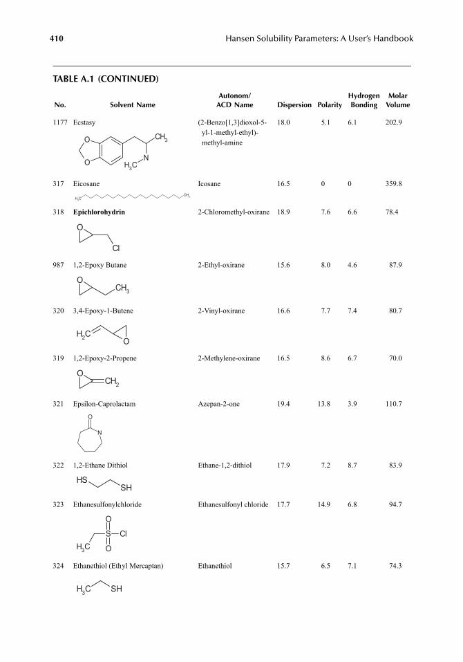
410 Hansen Solubility Parameters: A User’s Handbook
TABLE A.1 (CONTINUED)
No. Solvent NameAutonom/
ACD Name Dispersion PolarityHydrogenBonding
MolarVolume
1177 Ecstasy (2-Benzo[1,3]dioxol-5-yl-1-methyl-ethyl)-methyl-amine
18.0 5.1 6.1 202.9
317 Eicosane Icosane 16.5 0 0 359.8
318 Epichlorohydrin 2-Chloromethyl-oxirane 18.9 7.6 6.6 78.4
987 1,2-Epoxy Butane 2-Ethyl-oxirane 15.6 8.0 4.6 87.9
320 3,4-Epoxy-1-Butene 2-Vinyl-oxirane 16.6 7.7 7.4 80.7
319 1,2-Epoxy-2-Propene 2-Methylene-oxirane 16.5 8.6 6.7 70.0
321 Epsilon-Caprolactam Azepan-2-one 19.4 13.8 3.9 110.7
322 1,2-Ethane Dithiol Ethane-1,2-dithiol 17.9 7.2 8.7 83.9
323 Ethanesulfonylchloride Ethanesulfonyl chloride 17.7 14.9 6.8 94.7
324 Ethanethiol (Ethyl Mercaptan) Ethanethiol 15.7 6.5 7.1 74.3
O
O
CH3
NCH3
CH3
CH3
O
Cl
OCH3
CH2 O
OCH2
N
O
SHSH
CH3
S Cl
O
O
CH3 SH
7248_A001.fm Page 410 Wednesday, May 23, 2007 12:31 PM
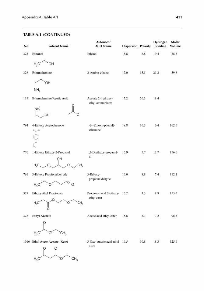
Appendix A: Table A.1 411
TABLE A.1 (CONTINUED)
No. Solvent NameAutonom/
ACD Name Dispersion PolarityHydrogenBonding
MolarVolume
325 Ethanol Ethanol 15.8 8.8 19.4 58.5
326 Ethanolamine 2-Amino-ethanol 17.0 15.5 21.2 59.8
1191 Ethanolamine/Acetic Acid Acetate 2-hydroxy-ethyl-ammonium;
17.2 20.3 18.4
794 4-Ethoxy Acetophenone 1-(4-Ethoxy-phenyl)-ethanone
18.8 10.3 6.4 162.6
776 1-Ethoxy Ethoxy-2-Propanol 1,3-Diethoxy-propan-2-ol
15.9 5.7 11.7 156.0
761 3-Ethoxy Propionaldehyde 3-Ethoxy-propionaldehyde
16.0 8.8 7.4 112.1
327 Ethoxyethyl Propionate Propionic acid 2-ethoxy-ethyl ester
16.2 3.3 8.8 155.5
328 Ethyl Acetate Acetic acid ethyl ester 15.8 5.3 7.2 98.5
1016 Ethyl Aceto Acetate (Keto) 3-Oxo-butyric acid ethyl ester
16.5 10.8 8.3 125.6
CH3 OH
OH
NH2
NH3+
OH O
O
CH3O
O
CH3
OH
OCH3 O CH3
CH3 O O
CH3
OO CH3
O
CH3 O
O
CH3
CH3 O CH3
O O
7248_A001.fm Page 411 Wednesday, May 23, 2007 12:31 PM
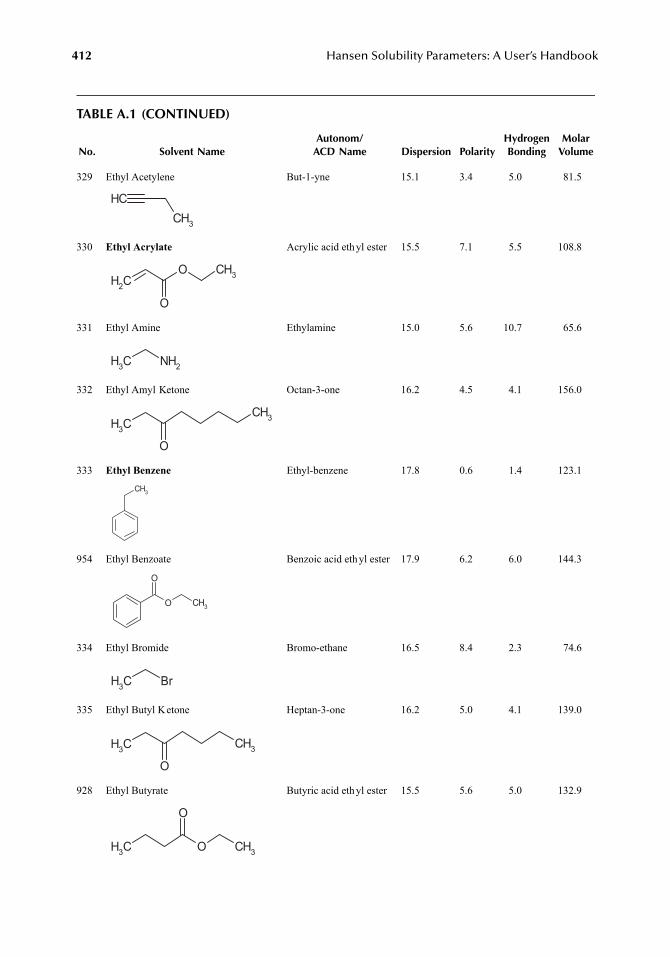
412 Hansen Solubility Parameters: A User’s Handbook
TABLE A.1 (CONTINUED)
No. Solvent NameAutonom/
ACD Name Dispersion PolarityHydrogenBonding
MolarVolume
329 Ethyl Acetylene But-1-yne 15.1 3.4 5.0 81.5
330 Ethyl Acrylate Acrylic acid ethyl ester 15.5 7.1 5.5 108.8
331 Ethyl Amine Ethylamine 15.0 5.6 10.7 65.6
332 Ethyl Amyl Ketone Octan-3-one 16.2 4.5 4.1 156.0
333 Ethyl Benzene Ethyl-benzene 17.8 0.6 1.4 123.1
954 Ethyl Benzoate Benzoic acid ethyl ester 17.9 6.2 6.0 144.3
334 Ethyl Bromide Bromo-ethane 16.5 8.4 2.3 74.6
335 Ethyl Butyl Ketone Heptan-3-one 16.2 5.0 4.1 139.0
928 Ethyl Butyrate Butyric acid ethyl ester 15.5 5.6 5.0 132.9
CHCH3
CH2
O
O
CH3
CH3 NH2
CH3
CH3
O
CH3
O
O
CH3
CH3 Br
CH3 CH3
O
CH3 O CH3
O
7248_A001.fm Page 412 Wednesday, May 23, 2007 12:31 PM
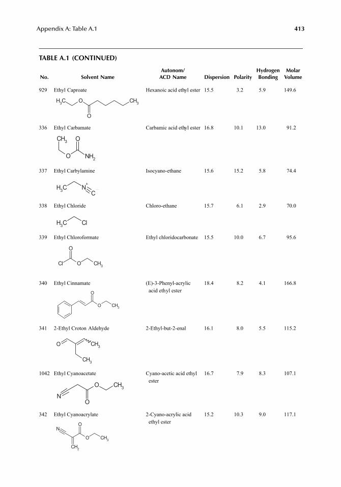
Appendix A: Table A.1 413
TABLE A.1 (CONTINUED)
No. Solvent NameAutonom/
ACD Name Dispersion PolarityHydrogenBonding
MolarVolume
929 Ethyl Caproate Hexanoic acid ethyl ester 15.5 3.2 5.9 149.6
336 Ethyl Carbamate Carbamic acid ethyl ester 16.8 10.1 13.0 91.2
337 Ethyl Carbylamine Isocyano-ethane 15.6 15.2 5.8 74.4
338 Ethyl Chloride Chloro-ethane 15.7 6.1 2.9 70.0
339 Ethyl Chloroformate Ethyl chloridocarbonate 15.5 10.0 6.7 95.6
340 Ethyl Cinnamate (E)-3-Phenyl-acrylic acid ethyl ester
18.4 8.2 4.1 166.8
341 2-Ethyl Croton Aldehyde 2-Ethyl-but-2-enal 16.1 8.0 5.5 115.2
1042 Ethyl Cyanoacetate Cyano-acetic acid ethyl ester
16.7 7.9 8.3 107.1
342 Ethyl Cyanoacrylate 2-Cyano-acrylic acid ethyl ester
15.2 10.3 9.0 117.1
O
O
CH3 CH3
O NH2
OCH3
CH3 N+
C
CH3 Cl
CH3OCl
O
O
O
CH3
CH3
O CH3
O
ON
CH3
O
O
CH2
N
CH3
7248_A001.fm Page 413 Wednesday, May 23, 2007 12:31 PM
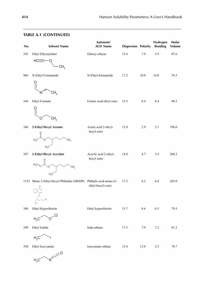
414 Hansen Solubility Parameters: A User’s Handbook
TABLE A.1 (CONTINUED)
No. Solvent NameAutonom/
ACD Name Dispersion PolarityHydrogenBonding
MolarVolume
343 Ethyl Ethynylether Ethoxy-ethyne 15.4 7.9 5.9 87.6
966 N-Ethyl Formamide N-Ethyl-formamide 17.2 10.0 14.0 76.5
344 Ethyl Formate Formic acid ethyl ester 15.5 8.4 8.4 80.2
346 2-Ethyl Hexyl Acetate Acetic acid 2-ethyl-hexyl ester
15.8 2.9 5.1 196.0
347 2-Ethyl Hexyl Acrylate Acrylic acid 2-ethyl-hexyl ester
14.8 4.7 3.4 208.2
1153 Mono 2-Ethyl-Hexyl Phthalate (MEHP) Phthalic acid mono-(2-ethyl-hexyl) ester
17.3 6.2 6.8 265.0
348 Ethyl Hypochlorite Ethyl hypochlorite 15.7 8.6 6.5 79.5
349 Ethyl Iodide Iodo-ethane 17.3 7.9 7.2 81.2
350 Ethyl Isocyanate Isocyanato-ethane 15.4 12.0 2.5 78.7
CH OCH3
N
O
CH3
O
O CH3
CH3 O
O
CH3
CH3
O
O
CH3
CH3
CH2
OH
O
O
O
CH3
CH3
CH3 OCl
CH3 I
CH3 N
O
7248_A001.fm Page 414 Wednesday, May 23, 2007 12:31 PM
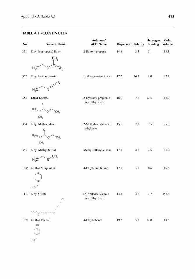
Appendix A: Table A.1 415
TABLE A.1 (CONTINUED)
No. Solvent NameAutonom/
ACD Name Dispersion PolarityHydrogenBonding
MolarVolume
351 Ethyl Isopropenyl Ether 2-Ethoxy-propene 14.8 3.5 5.1 113.3
352 Ethyl Isothiocyanate Isothiocyanato-ethane 17.2 14.7 9.0 87.1
353 Ethyl Lactate 2-Hydroxy-propionic acid ethyl ester
16.0 7.6 12.5 115.0
354 Ethyl Methacrylate 2-Methyl-acrylic acid ethyl ester
15.8 7.2 7.5 125.8
355 Ethyl Methyl Sulfid Methylsulfanyl-ethane 17.1 4.8 2.5 91.2
1085 4-Ethyl Morpholine 4-Ethyl-morpholine 17.7 5.0 6.6 116.5
1117 Ethyl Oleate (Z)-Octadec-9-enoic acid ethyl ester
14.5 3.8 3.7 357.3
1071 4-Ethyl Phenol 4-Ethyl-phenol 19.2 5.3 12.8 118.6
CH3 O CH2
CH3
CH3 N
S
O
O
CH3
OHCH3
O
O
CH3
CH2 CH3
CH3 SCH3
N
O
CH3
O
O
CH3
CH3
OH
CH3
7248_A001.fm Page 415 Wednesday, May 23, 2007 12:31 PM
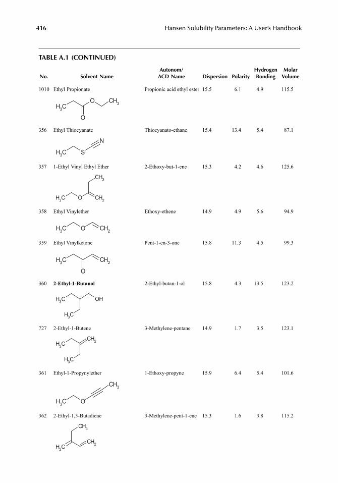
416 Hansen Solubility Parameters: A User’s Handbook
TABLE A.1 (CONTINUED)
No. Solvent NameAutonom/
ACD Name Dispersion PolarityHydrogenBonding
MolarVolume
1010 Ethyl Propionate Propionic acid ethyl ester 15.5 6.1 4.9 115.5
356 Ethyl Thiocyanate Thiocyanato-ethane 15.4 13.4 5.4 87.1
357 1-Ethyl Vinyl Ethyl Ether 2-Ethoxy-but-1-ene 15.3 4.2 4.6 125.6
358 Ethyl Vinylether Ethoxy-ethene 14.9 4.9 5.6 94.9
359 Ethyl Vinylketone Pent-1-en-3-one 15.8 11.3 4.5 99.3
360 2-Ethyl-1-Butanol 2-Ethyl-butan-1-ol 15.8 4.3 13.5 123.2
727 2-Ethyl-1-Butene 3-Methylene-pentane 14.9 1.7 3.5 123.1
361 Ethyl-1-Propynylether 1-Ethoxy-propyne 15.9 6.4 5.4 101.6
362 2-Ethyl-1,3-Butadiene 3-Methylene-pent-1-ene 15.3 1.6 3.8 115.2
CH3
O CH3
O
CH3 S
N
CH3 O CH2
CH3
CH3 O CH2
CH3
O
CH2
CH3 OH
CH3
CH3
CH2
CH3
CH3 O
CH3
CH2
CH2
CH3
7248_A001.fm Page 416 Wednesday, May 23, 2007 12:31 PM
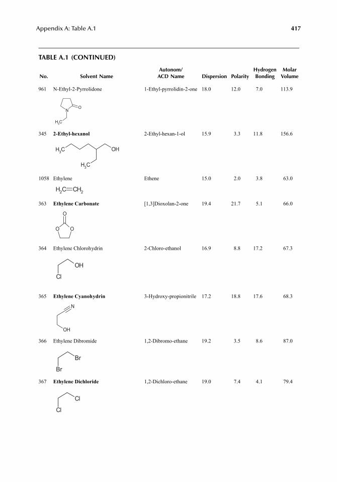
Appendix A: Table A.1 417
TABLE A.1 (CONTINUED)
No. Solvent NameAutonom/
ACD Name Dispersion PolarityHydrogenBonding
MolarVolume
961 N-Ethyl-2-Pyrrolidone 1-Ethyl-pyrrolidin-2-one 18.0 12.0 7.0 113.9
345 2-Ethyl-hexanol 2-Ethyl-hexan-1-ol 15.9 3.3 11.8 156.6
1058 Ethylene Ethene 15.0 2.0 3.8 63.0
363 Ethylene Carbonate [1,3]Dioxolan-2-one 19.4 21.7 5.1 66.0
364 Ethylene Chlorohydrin 2-Chloro-ethanol 16.9 8.8 17.2 67.3
365 Ethylene Cyanohydrin 3-Hydroxy-propionitrile 17.2 18.8 17.6 68.3
366 Ethylene Dibromide 1,2-Dibromo-ethane 19.2 3.5 8.6 87.0
367 Ethylene Dichloride 1,2-Dichloro-ethane 19.0 7.4 4.1 79.4
NO
CH3
CH3 OH
CH3
CH2 CH2
OO
O
OH
Cl
N
OH
Br
Br
Cl
Cl
7248_A001.fm Page 417 Wednesday, May 23, 2007 12:31 PM
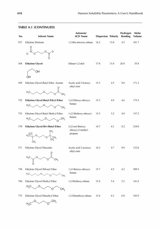
418 Hansen Solubility Parameters: A User’s Handbook
TABLE A.1 (CONTINUED)
No. Solvent NameAutonom/
ACD Name Dispersion PolarityHydrogenBonding
MolarVolume
937 Ethylene Dinitrate 1,2-Bis-nitrooxy-ethane 16.2 13.0 4.5 101.7
368 Ethylene Glycol Ethane-1,2-diol 17.0 11.0 26.0 55.8
369 Ethylene Glycol Butyl Ether Acetate Acetic acid 2-butoxy-ethyl ester
15.3 4.5 8.8 171.2
752 Ethylene Glycol Butyl Eth yl Ether 1-(2-Ethoxy-ethoxy)-butane
15.3 4.9 4.6 175.5
753 Ethylene Glycol Butyl Meth yl Ether 1-(2-Methoxy-ethoxy)-butane
15.5 5.2 4.9 157.2
370 Ethylene Glycol Di-t-Butyl Ether 2-(2-tert-Butoxy-ethoxy)-2-methyl-propane
14.7 4.1 8.2 210.0
371 Ethylene Glycol Diacetate Acetic acid 2-acetoxy-ethyl ester
16.2 4.7 9.8 132.8
758 Ethylene Glycol Dibutyl Ether 1-(2-Butoxy-ethoxy)-butane
15.7 4.5 4.2 209.5
760 Ethylene Glycol Diethyl Ether 1,2-Diethoxy-ethane 15.4 5.4 5.2 141.6
775 Ethylene Glycol Dimethyl Ether 1,2-Dimethoxy-ethane 15.4 6.3 6.0 103.9
ON+
O
OO
N+
O
O
OH
OH
OOCH3 CH3
O
OOCH3 CH3
OOCH3 CH3
OOCH3 CH3
CH3
CH3CH3
CH3
OOCH3 CH3
O
O
OOCH3 CH3
OOCH3 CH3
CH3
OO
CH3
7248_A001.fm Page 418 Wednesday, May 23, 2007 12:31 PM
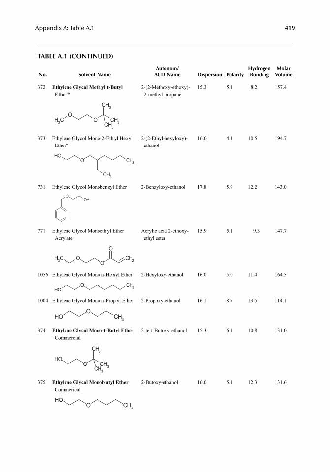
Appendix A: Table A.1 419
TABLE A.1 (CONTINUED)
No. Solvent NameAutonom/
ACD Name Dispersion PolarityHydrogenBonding
MolarVolume
372 Ethylene Glycol Methyl t-Butyl Ether*
2-(2-Methoxy-ethoxy)-2-methyl-propane
15.3 5.1 8.2 157.4
373 Ethylene Glycol Mono-2-Ethyl Hexyl Ether*
2-(2-Ethyl-hexyloxy)-ethanol
16.0 4.1 10.5 194.7
731 Ethylene Glycol Monobenzyl Ether 2-Benzyloxy-ethanol 17.8 5.9 12.2 143.0
771 Ethylene Glycol Monoethyl Ether Acrylate
Acrylic acid 2-ethoxy-ethyl ester
15.9 5.1 9.3 147.7
1056 Ethylene Glycol Mono n-He xyl Ether 2-Hexyloxy-ethanol 16.0 5.0 11.4 164.5
1004 Ethylene Glycol Mono n-Prop yl Ether 2-Propoxy-ethanol 16.1 8.7 13.5 114.1
374 Ethylene Glycol Mono-t-Butyl Ether Commercial
2-tert-Butoxy-ethanol 15.3 6.1 10.8 131.0
375 Ethylene Glycol Monobutyl Ether Commerical
2-Butoxy-ethanol 16.0 5.1 12.3 131.6
OO
CH3 CH3
CH3
CH3
OOH
CH3
CH3
OOH
OOCH3 CH2
O
OHO CH3
OCH3OH
OOH
CH3
CH3
CH3
OOH
CH3
7248_A001.fm Page 419 Wednesday, May 23, 2007 12:31 PM
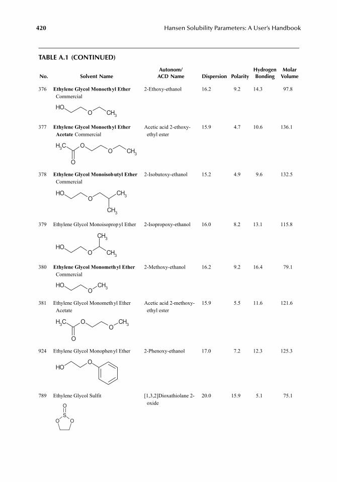
420 Hansen Solubility Parameters: A User’s Handbook
TABLE A.1 (CONTINUED)
No. Solvent NameAutonom/
ACD Name Dispersion PolarityHydrogenBonding
MolarVolume
376 Ethylene Glycol Monoethyl Ether Commercial
2-Ethoxy-ethanol 16.2 9.2 14.3 97.8
377 Ethylene Glycol Monoethyl Ether Acetate Commercial
Acetic acid 2-ethoxy-ethyl ester
15.9 4.7 10.6 136.1
378 Ethylene Glycol Monoisobutyl Ether Commercial
2-Isobutoxy-ethanol 15.2 4.9 9.6 132.5
379 Ethylene Glycol Monoisopropyl Ether 2-Isopropoxy-ethanol 16.0 8.2 13.1 115.8
380 Ethylene Glycol Monomethyl Ether Commercial
2-Methoxy-ethanol 16.2 9.2 16.4 79.1
381 Ethylene Glycol Monomethyl Ether Acetate
Acetic acid 2-methoxy-ethyl ester
15.9 5.5 11.6 121.6
924 Ethylene Glycol Monophenyl Ether 2-Phenoxy-ethanol 17.0 7.2 12.3 125.3
789 Ethylene Glycol Sulfit [1,3,2]Dioxathiolane 2-oxide
20.0 15.9 5.1 75.1
OOH
CH3
OO
CH3
CH3
O
OOH
CH3
CH3
OOH
CH3
CH3
OOH CH3
OO CH3CH3
O
OHO
OS
O
O
7248_A001.fm Page 420 Wednesday, May 23, 2007 12:31 PM
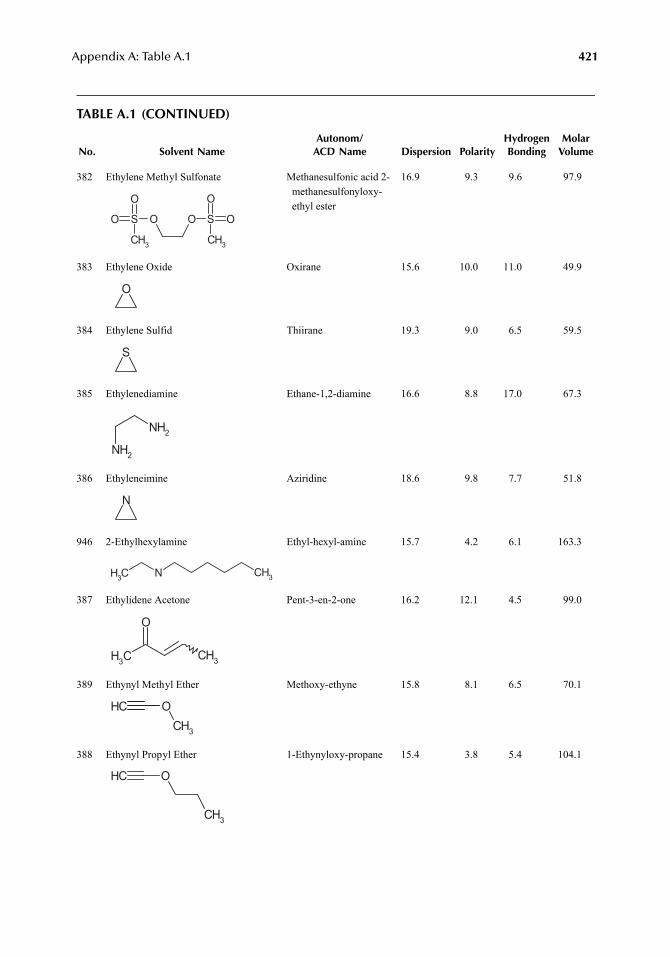
Appendix A: Table A.1 421
TABLE A.1 (CONTINUED)
No. Solvent NameAutonom/
ACD Name Dispersion PolarityHydrogenBonding
MolarVolume
382 Ethylene Methyl Sulfonate Methanesulfonic acid 2-methanesulfonyloxy-ethyl ester
16.9 9.3 9.6 97.9
383 Ethylene Oxide Oxirane 15.6 10.0 11.0 49.9
384 Ethylene Sulfid Thiirane 19.3 9.0 6.5 59.5
385 Ethylenediamine Ethane-1,2-diamine 16.6 8.8 17.0 67.3
386 Ethyleneimine Aziridine 18.6 9.8 7.7 51.8
946 2-Ethylhexylamine Ethyl-hexyl-amine 15.7 4.2 6.1 163.3
387 Ethylidene Acetone Pent-3-en-2-one 16.2 12.1 4.5 99.0
389 Ethynyl Methyl Ether Methoxy-ethyne 15.8 8.1 6.5 70.1
388 Ethynyl Propyl Ether 1-Ethynyloxy-propane 15.4 3.8 5.4 104.1
O
SO O
CH3
O
S OO
CH3
O
S
NH2
NH2
N
CH3 N CH3
CH3
O
CH3
CH OCH3
CH O
CH3
7248_A001.fm Page 421 Wednesday, May 23, 2007 12:31 PM
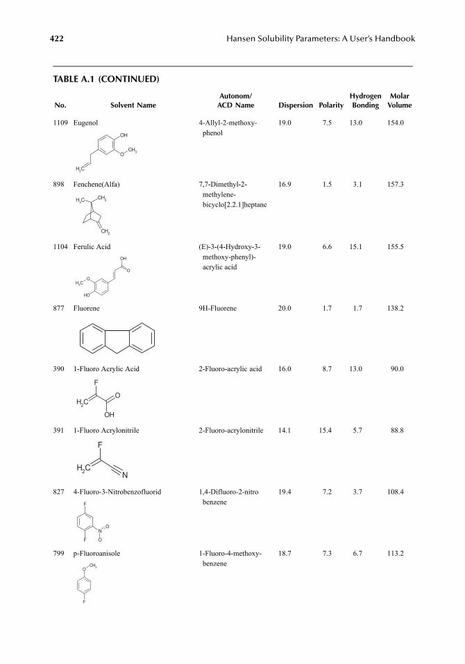
422 Hansen Solubility Parameters: A User’s Handbook
TABLE A.1 (CONTINUED)
No. Solvent NameAutonom/
ACD Name Dispersion PolarityHydrogenBonding
MolarVolume
1109 Eugenol 4-Allyl-2-methoxy-phenol
19.0 7.5 13.0 154.0
898 Fenchene(Alfa) 7,7-Dimethyl-2-methylene-bicyclo[2.2.1]heptane
16.9 1.5 3.1 157.3
1104 Ferulic Acid (E)-3-(4-Hydroxy-3-methoxy-phenyl)-acrylic acid
19.0 6.6 15.1 155.5
877 Fluorene 9H-Fluorene 20.0 1.7 1.7 138.2
390 1-Fluoro Acrylic Acid 2-Fluoro-acrylic acid 16.0 8.7 13.0 90.0
391 1-Fluoro Acrylonitrile 2-Fluoro-acrylonitrile 14.1 15.4 5.7 88.8
827 4-Fluoro-3-Nitrobenzofluorid 1,4-Difluoro-2-nitrobenzene
19.4 7.2 3.7 108.4
799 p-Fluoroanisole 1-Fluoro-4-methoxy-benzene
18.7 7.3 6.7 113.2
O
OH
CH3
CH2
CH2
CH3CH3
O
OH
CH3
OH
O
CH2
O
OH
F
CH2
F
N
F
F
N+
O
O
OCH3
F
7248_A001.fm Page 422 Wednesday, May 23, 2007 12:31 PM
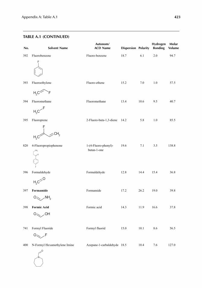
Appendix A: Table A.1
423
TABLE A.1 (CONTINUED)
No. Solvent NameAutonom/
ACD Name Dispersion PolarityHydrogenBonding
MolarVolume
392 Fluorobenzene Fluoro-benzene 18.7 6.1 2.0 94.7
393 Fluoroethylene Fluoro-ethene 15.2 7.0 1.0 57.5
394 Fluoromethane Fluoromethane 13.4 10.6 9.5 40.7
395 Fluoroprene 2-Fluoro-buta-1,3-diene 14.2 5.8 1.0 85.5
820 4-Fluoropropiophenone 1-(4-Fluoro-phenyl)-butan-1-one
19.6 7.1 3.5 138.8
396 Formaldehyde Formaldehyde 12.8 14.4 15.4 36.8
397
Formamide
Formamide 17.2 26.2 19.0 39.8
398
Formic Acid
Formic acid 14.3 11.9 16.6 37.8
741 Formyl Fluoride Formyl fluorid 15.0 10.1 8.6 56.5
400 N-Formyl Hexamethylene Imine Azepane-1-carbaldehyde 18.5 10.4 7.6 127.0
F
CH2 F
CH3
F
CH2
F
CH2
O
F
CH3
CH2
O
NH2O
OHO
FO
N
O
7248_A001A.fm Page 423 Wednesday, May 23, 2007 12:38 PM
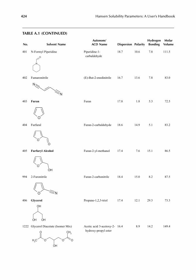
424
Hansen Solubility Parameters: A User’s Handbook
TABLE A.1 (CONTINUED)
No. Solvent NameAutonom/
ACD Name Dispersion PolarityHydrogenBonding
MolarVolume
401 N-Formyl Piperidine Piperidine-1-carbaldehyde
18.7 10.6 7.8 111.5
402 Fumaronitrile (E)-But-2-enedinitrile 16.7 13.6 7.8 83.0
403
Furan
Furan 17.8 1.8 5.3 72.5
404 Furfural Furan-2-carbaldehyde 18.6 14.9 5.1 83.2
405
Furfuryl Alcohol
Furan-2-yl-methanol 17.4 7.6 15.1 86.5
994 2-Furonitrile Furan-2-carbonitrile 18.4 15.0 8.2 87.5
406
Glycerol
Propane-1,2,3-triol 17.4 12.1 29.3 73.3
1222 Glycerol Diacetate (Isomer Mix) Acetic acid 3-acetoxy-2-hydroxy-propyl ester
16.4 8.9 14.2 149.4
N
O
N
N
O
OO
OOH
O N
OH
OHOH
OH
O OCH3
O C 3
O
H
7248_A001A.fm Page 424 Wednesday, May 23, 2007 12:38 PM
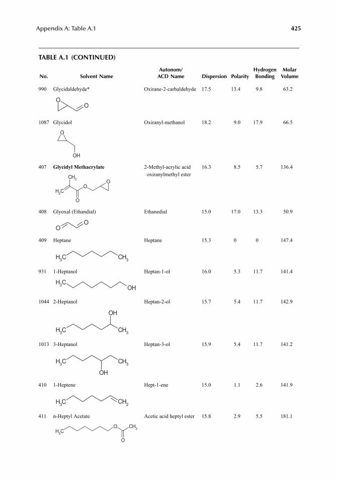
Appendix A: Table A.1
425
TABLE A.1 (CONTINUED)
No. Solvent NameAutonom/
ACD Name Dispersion PolarityHydrogenBonding
MolarVolume
990 Glycidaldehyde* Oxirane-2-carbaldehyde 17.5 13.4 9.8 63.2
1087 Glycidol Oxiranyl-methanol 18.2 9.0 17.9 66.5
407
Glycidyl Methacrylate
2-Methyl-acrylic acid oxiranylmethyl ester
16.3 8.5 5.7 136.4
408 Glyoxal (Ethandial) Ethanedial 15.0 17.0 13.3 50.9
409 Heptane Heptane 15.3 0 0 147.4
931 1-Heptanol Heptan-1-ol 16.0 5.3 11.7 141.4
1044 2-Heptanol Heptan-2-ol 15.7 5.4 11.7 142.9
1013 3-Heptanol Heptan-3-ol 15.9 5.4 11.7 141.2
410 1-Heptene Hept-1-ene 15.0 1.1 2.6 141.9
411 n-Heptyl Acetate Acetic acid heptyl ester 15.8 2.9 5.5 181.1
OO
O
OH
CH2
CH3
O
OO
OO
CH3 CH3
OHCH3
CH3 CH3
OH
CH3 CH3
OH
CH3 CH2
CH3
O CH3
O
7248_A001A.fm Page 425 Wednesday, May 23, 2007 12:38 PM
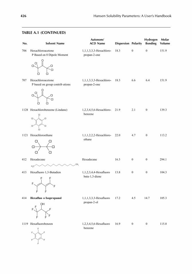
426
Hansen Solubility Parameters: A User’s Handbook
TABLE A.1 (CONTINUED)
No. Solvent NameAutonom/
ACD Name Dispersion PolarityHydrogenBonding
MolarVolume
706 HexachloroacetoneP Based on 0 Dipole Moment
1,1,1,3,3,3-Hexachloro-propan-2-one
18.3 0 0 151.9
707 HexachloroacetoneP based on group contrib utions
1,1,1,3,3,3-Hexachloro-propan-2-one
18.3 6.6 6.4 151.9
1128 Hexachlorobenzene (Lindane) 1,2,3,4,5,6-Hexachloro-benzene
21.9 2.1 0 139.3
1121 Hexachloroethane 1,1,1,2,2,2-Hexachloro-ethane
22.0 4.7 0 113.2
412 Hexadecane Hexadecane 16.3 0 0 294.1
413 Hexafluoro 1,3-Butadien 1,1,2,3,4,4-Hexafluorobuta-1,3-diene
13.8 0 0 104.3
414
Hexafluo o Isopropanol
1,1,1,3,3,3-Hexafluoropropan-2-ol
17.2 4.5 14.7 105.3
1119 Hexafluorobenzen 1,2,3,4,5,6-Hexafluorobenzene
16.9 0 0 115.8
O
Cl
Cl
Cl
Cl
ClCl
O
Cl
Cl
Cl
Cl
ClCl
Cl
Cl
Cl
Cl
Cl
Cl
Cl
ClCl
Cl
ClCl
CH3
CH3
F
F
F
F
F
F
OH
F
F
F
F
F
F
F
F
F
F
F
F
7248_A001A.fm Page 426 Wednesday, May 23, 2007 12:38 PM
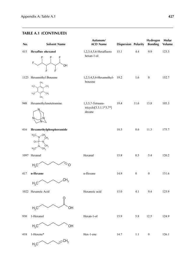
Appendix A: Table A.1
427
TABLE A.1 (CONTINUED)
No. Solvent NameAutonom/
ACD Name Dispersion PolarityHydrogenBonding
MolarVolume
415
Hexafluo ohexanol
1,2,3,4,5,6-Hexafluorohexan-1-ol
15.1 4.4 9.9 123.3
1123 Hexamethyl Benzene 1,2,3,4,5,6-Hexamethyl-benzene
19.2 1.6 0 152.7
948 Hexamethylenetetramine 1,3,5,7-Tetraaza-tricyclo[3.3.1.1*3,7*] decane
19.4 11.6 13.8 105.3
416
Hexamethylphosphoramide
18.5 8.6 11.3 175.7
1097 Hexanal Hexanal 15.8 8.5 5.4 120.2
417
n-Hexane
n-Hexane 14.9 0 0 131.6
1022 Hexanoic Acid Hexanoic acid 15.0 4.1 9.4 125.9
930 1-Hexanol Hexan-1-ol 15.9 5.8 12.5 124.9
418 1-Hexene* Hex-1-ene 14.7 1.1 0 126.1
OH
F
F
F
F
F
F
CH3
CH3
CH3
CH3
CH3
CH3
N NN
N
P N
N
N
O
CH3CH3
CH3
CH3
CH3 CH3
CH3 O
CH3
CH3
CH3 OH
O
CH3 OH
CH3
CH2
7248_A001A.fm Page 427 Wednesday, May 23, 2007 12:38 PM
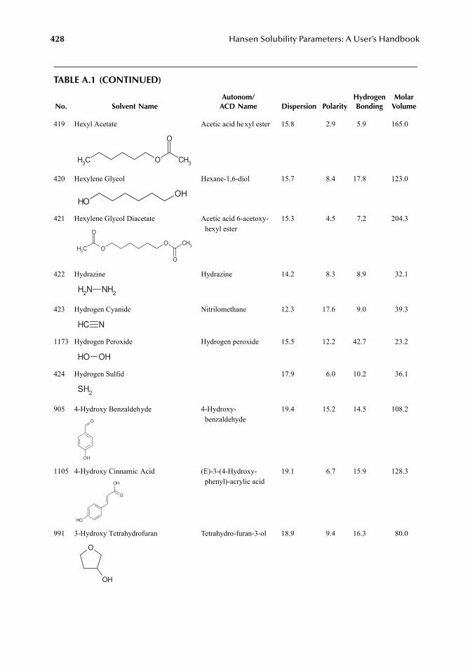
428
Hansen Solubility Parameters: A User’s Handbook
TABLE A.1 (CONTINUED)
No. Solvent NameAutonom/
ACD Name Dispersion PolarityHydrogenBonding
MolarVolume
419 Hexyl Acetate Acetic acid hexyl ester 15.8 2.9 5.9 165.0
420 Hexylene Glycol Hexane-1,6-diol 15.7 8.4 17.8 123.0
421 Hexylene Glycol Diacetate Acetic acid 6-acetoxy-hexyl ester
15.3 4.5 7.2 204.3
422 Hydrazine Hydrazine 14.2 8.3 8.9 32.1
423 Hydrogen Cyanide Nitrilomethane 12.3 17.6 9.0 39.3
1173 Hydrogen Peroxide Hydrogen peroxide 15.5 12.2 42.7 23.2
424 Hydrogen Sulfid 17.9 6.0 10.2 36.1
905 4-Hydroxy Benzaldehyde 4-Hydroxy-benzaldehyde
19.4 15.2 14.5 108.2
1105 4-Hydroxy Cinnamic Acid (E)-3-(4-Hydroxy-phenyl)-acrylic acid
19.1 6.7 15.9 128.3
991 3-Hydroxy Tetrahydrofuran Tetrahydro-furan-3-ol 18.9 9.4 16.3 80.0
CH3 O CH3
O
OHOH
OO
CH3
O
CH3
O
NH2 NH2
CH N
OH OH
SH2
OH
O
OH
OH
O
O
OH
7248_A001A.fm Page 428 Wednesday, May 23, 2007 12:38 PM
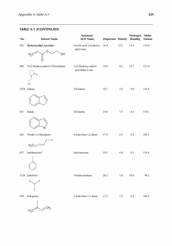
Appendix A: Table A.1
429
TABLE A.1 (CONTINUED)
No. Solvent NameAutonom/
ACD Name Dispersion PolarityHydrogenBonding
MolarVolume
425
Hydroxyethyl Acrylate
Acrylic acid 2-hydroxy-ethyl ester
16.0 13.2 13.4 114.9
960 N-(2-Hydroxyethyl)-2-Pyrrolidone 1-(2-Hydroxy-ethyl)-pyrrolidin-2-one
18.0 9.2 15.7 113.4
1078 Indene 1H-Indene 18.7 2.6 9.0 116.5
831 Indole 1H-Indole 19.8 7.5 6.5 110.1
426 4-Iodo-1,2-Butadiene 4-Iodo-buta-1,2-diene 17.4 6.3 6.2 105.1
427 Iodobenzene* Iodo-benzene 19.5 6.0 6.1 114.4
1126 Iodoform Triiodo-methane 20.2 3.6 10.6 98.2
428 Iodoprene 2-Iodo-buta-1,3-diene 17.2 2.5 6.2 104.2
CH2
O
O
OH
NO
OH
N
CH2
I
I
II
I
CH2
CH2
I
7248_A001A.fm Page 429 Wednesday, May 23, 2007 12:38 PM
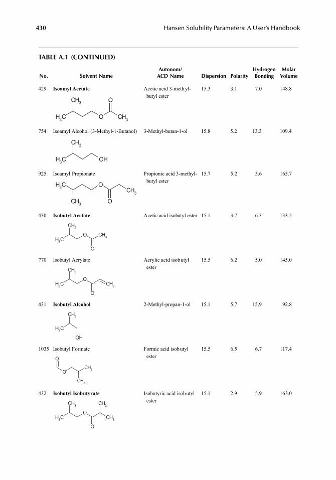
430
Hansen Solubility Parameters: A User’s Handbook
TABLE A.1 (CONTINUED)
No. Solvent NameAutonom/
ACD Name Dispersion PolarityHydrogenBonding
MolarVolume
429
Isoamyl Acetate
Acetic acid 3-methyl-butyl ester
15.3 3.1 7.0 148.8
754 Isoamyl Alcohol (3-Methyl-1-Butanol) 3-Methyl-butan-1-ol 15.8 5.2 13.3 109.4
925 Isoamyl Propionate Propionic acid 3-methyl-butyl ester
15.7 5.2 5.6 165.7
430
Isobutyl Acetate
Acetic acid isobutyl ester 15.1 3.7 6.3 133.5
770 Isobutyl Acrylate Acrylic acid isobutyl ester
15.5 6.2 5.0 145.0
431
Isobutyl Alcohol
2-Methyl-propan-1-ol 15.1 5.7 15.9 92.8
1035 Isobutyl Formate Formic acid isobutyl ester
15.5 6.5 6.7 117.4
432
Isobutyl Isobutyrate
Isobutyric acid isobutyl ester
15.1 2.9 5.9 163.0
CH3
CH3
O CH3
O
CH3 OH
CH3
O
O
CH3
CH3
CH3
CH3
CH3
O CH3
O
CH3
CH3
O
O
CH2
CH3
CH3
OH
O
OCH3
CH3
CH3
CH3
O
O
CH3
CH3
7248_A001A.fm Page 430 Wednesday, May 23, 2007 12:38 PM
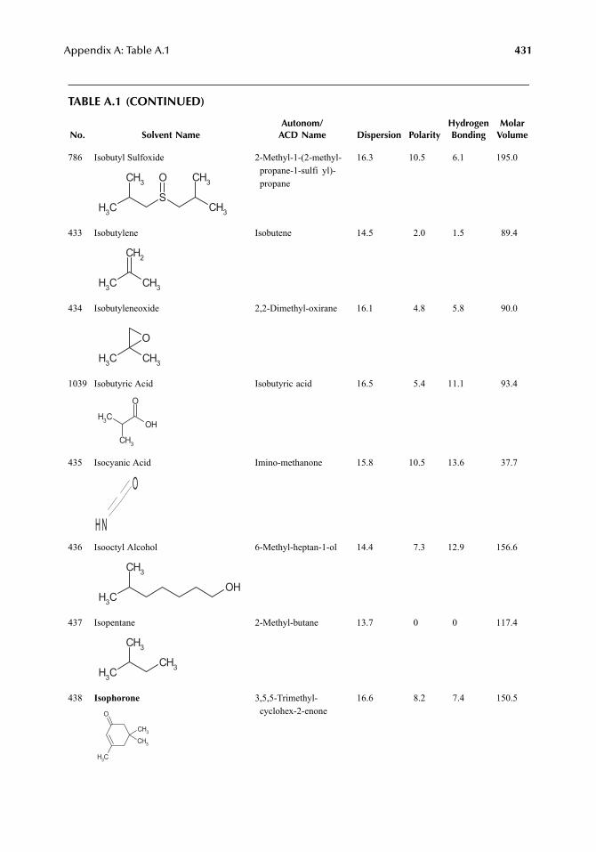
Appendix A: Table A.1
431
TABLE A.1 (CONTINUED)
No. Solvent NameAutonom/
ACD Name Dispersion PolarityHydrogenBonding
MolarVolume
786 Isobutyl Sulfoxide 2-Methyl-1-(2-methyl-propane-1-sulfi yl)-propane
16.3 10.5 6.1 195.0
433 Isobutylene Isobutene 14.5 2.0 1.5 89.4
434 Isobutyleneoxide 2,2-Dimethyl-oxirane 16.1 4.8 5.8 90.0
1039 Isobutyric Acid Isobutyric acid 16.5 5.4 11.1 93.4
435 Isocyanic Acid Imino-methanone 15.8 10.5 13.6 37.7
436 Isooctyl Alcohol 6-Methyl-heptan-1-ol 14.4 7.3 12.9 156.6
437 Isopentane 2-Methyl-butane 13.7 0 0 117.4
438
Isophorone
3,5,5-Trimethyl-cyclohex-2-enone
16.6 8.2 7.4 150.5
CH3
CH3
S
O
CH3
CH3
CH3 CH3
CH2
CH3 CH3
O
CH3 OH
O
CH3
O
NH
CH3
OH
CH3
CH3
CH3
CH3
CH3
CH3
CH3
O
7248_A001A.fm Page 431 Wednesday, May 23, 2007 12:38 PM
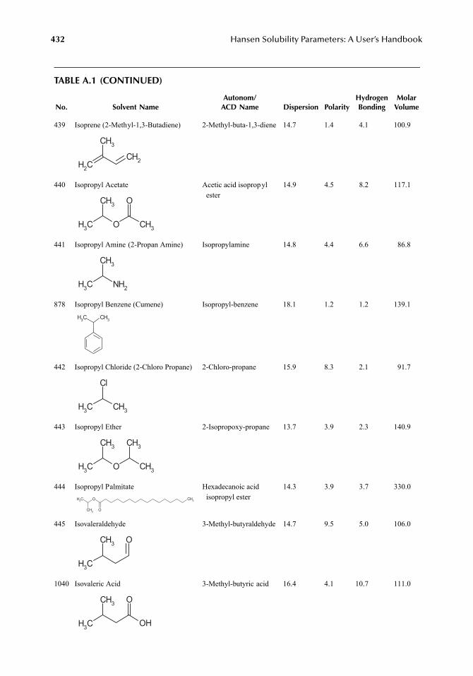
432
Hansen Solubility Parameters: A User’s Handbook
TABLE A.1 (CONTINUED)
No. Solvent NameAutonom/
ACD Name Dispersion PolarityHydrogenBonding
MolarVolume
439 Isoprene (2-Methyl-1,3-Butadiene) 2-Methyl-buta-1,3-diene 14.7 1.4 4.1 100.9
440 Isopropyl Acetate Acetic acid isopropyl ester
14.9 4.5 8.2 117.1
441 Isopropyl Amine (2-Propan Amine) Isopropylamine 14.8 4.4 6.6 86.8
878 Isopropyl Benzene (Cumene) Isopropyl-benzene 18.1 1.2 1.2 139.1
442 Isopropyl Chloride (2-Chloro Propane) 2-Chloro-propane 15.9 8.3 2.1 91.7
443 Isopropyl Ether 2-Isopropoxy-propane 13.7 3.9 2.3 140.9
444 Isopropyl Palmitate Hexadecanoic acid isopropyl ester
14.3 3.9 3.7 330.0
445 Isovaleraldehyde 3-Methyl-butyraldehyde 14.7 9.5 5.0 106.0
1040 Isovaleric Acid 3-Methyl-butyric acid 16.4 4.1 10.7 111.0
CH2
CH3
CH2
CH3 O
CH3
CH3
O
CH3 NH2
CH3
CH3CH3
CH3 CH3
Cl
CH3 O
CH3
CH3
CH3
O
O
CH3CH3
CH3
CH3
CH3
O
CH3
CH3 OH
O
7248_A001A.fm Page 432 Wednesday, May 23, 2007 12:38 PM
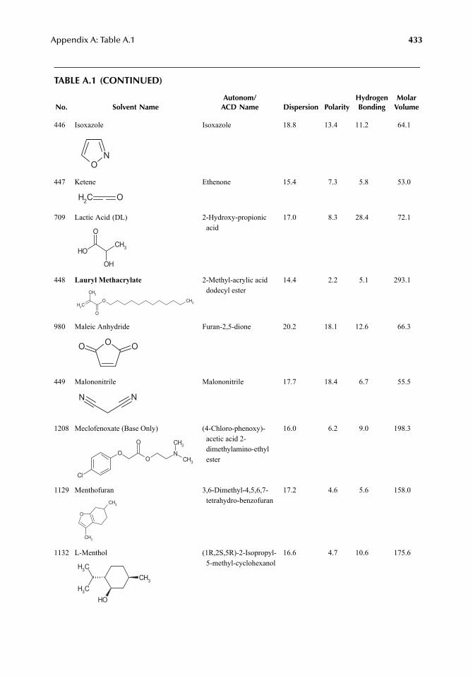
Appendix A: Table A.1
433
TABLE A.1 (CONTINUED)
No. Solvent NameAutonom/
ACD Name Dispersion PolarityHydrogenBonding
MolarVolume
446 Isoxazole Isoxazole 18.8 13.4 11.2 64.1
447 Ketene Ethenone 15.4 7.3 5.8 53.0
709 Lactic Acid (DL) 2-Hydroxy-propionic acid
17.0 8.3 28.4 72.1
448
Lauryl Methacrylate
2-Methyl-acrylic acid dodecyl ester
14.4 2.2 5.1 293.1
980 Maleic Anhydride Furan-2,5-dione 20.2 18.1 12.6 66.3
449 Malononitrile Malononitrile 17.7 18.4 6.7 55.5
1208 Meclofenoxate (Base Only) (4-Chloro-phenoxy)-acetic acid 2-dimethylamino-ethyl ester
16.0 6.2 9.0 198.3
1129 Menthofuran 3,6-Dimethyl-4,5,6,7-tetrahydro-benzofuran
17.2 4.6 5.6 158.0
1132 L-Menthol (1R,2S,5R)-2-Isopropyl-5-methyl-cyclohexanol
16.6 4.7 10.6 175.6
ON
CH2 O
CH3
OH
O
OH
O
O
CH3
CH3
CH2
OO O
N N
O
Cl
O
O
NCH3
CH3
O
CH3
CH3
OHCH3
CH3
CH3
7248_A001A.fm Page 433 Wednesday, May 23, 2007 12:38 PM
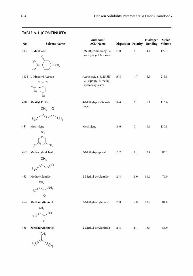
434
Hansen Solubility Parameters: A User’s Handbook
TABLE A.1 (CONTINUED)
No. Solvent NameAutonom/
ACD Name Dispersion PolarityHydrogenBonding
MolarVolume
1130 L-Menthone (2S,5R)-2-Isopropyl-5-methyl-cyclohexanone
17.0 8.1 4.4 172.3
1131 L-Menthyl Acetate Acetic acid (1R,2S,5R)-2-isopropyl-5-methyl-cyclohexyl ester
16.8 4.7 4.9 215.8
450
Mesityl Oxide
4-Methyl-pent-3-en-2-one
16.4 6.1 6.1 115.6
451 Mesitylene Mesitylene 18.0 0 0.6 139.8
452 Methacrylaldehyde 2-Methyl-propenal 15.7 11.1 7.4 83.3
453 Methacrylamide 2-Methyl-acrylamide 15.8 11.0 11.6 76.0
454
Methacrylic Acid
2-Methyl-acrylic acid 15.8 2.8 10.2 84.8
455
Methacrylonitrile
2-Methyl-acrylonitrile 15.8 15.1 5.4 83.9
OCH3
CH3
CH3
O
CH3CH3
CH3
CH3
O
CH3
CH3
CH3
O
CH3 CH3
CH3
CH2
CH3
O
CH2
CH3
O
NH2
CH2
CH3
O
OH
CH2
CH3
N
7248_A001A.fm Page 434 Wednesday, May 23, 2007 12:38 PM
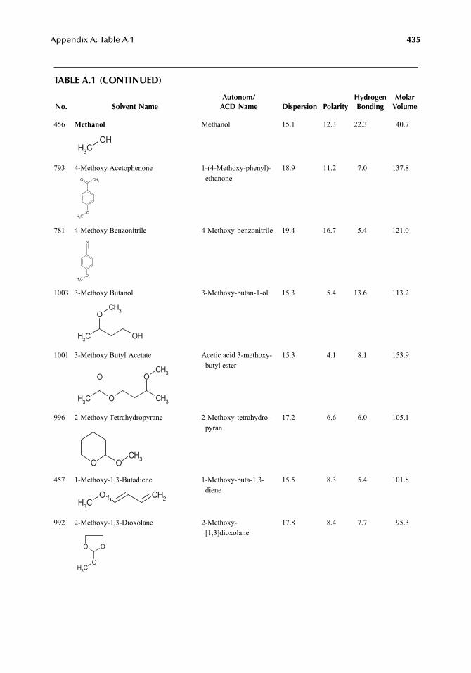
Appendix A: Table A.1
435
TABLE A.1 (CONTINUED)
No. Solvent NameAutonom/
ACD Name Dispersion PolarityHydrogenBonding
MolarVolume
456
Methanol
Methanol 15.1 12.3 22.3 40.7
793 4-Methoxy Acetophenone 1-(4-Methoxy-phenyl)-ethanone
18.9 11.2 7.0 137.8
781 4-Methoxy Benzonitrile 4-Methoxy-benzonitrile 19.4 16.7 5.4 121.0
1003 3-Methoxy Butanol 3-Methoxy-butan-1-ol 15.3 5.4 13.6 113.2
1001 3-Methoxy Butyl Acetate Acetic acid 3-methoxy-butyl ester
15.3 4.1 8.1 153.9
996 2-Methoxy Tetrahydropyrane 2-Methoxy-tetrahydro-pyran
17.2 6.6 6.0 105.1
457 1-Methoxy-1,3-Butadiene 1-Methoxy-buta-1,3-diene
15.5 8.3 5.4 101.8
992 2-Methoxy-1,3-Dioxolane 2-Methoxy-[1,3]dioxolane
17.8 8.4 7.7 95.3
CH3
OH
CH3O
OCH3
OCH3
N
CH3 OH
OCH3
CH3 O CH3
O OCH3
O OCH3
CH2CH3
O
O O
OCH3
7248_A001A.fm Page 435 Wednesday, May 23, 2007 12:38 PM
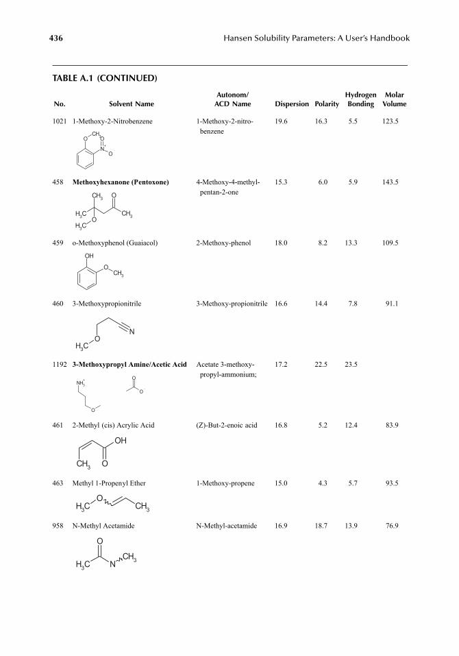
436
Hansen Solubility Parameters: A User’s Handbook
TABLE A.1 (CONTINUED)
No. Solvent NameAutonom/
ACD Name Dispersion PolarityHydrogenBonding
MolarVolume
1021 1-Methoxy-2-Nitrobenzene 1-Methoxy-2-nitro-benzene
19.6 16.3 5.5 123.5
458
Methoxyhexanone (Pentoxone)
4-Methoxy-4-methyl-pentan-2-one
15.3 6.0 5.9 143.5
459 o-Methoxyphenol (Guaiacol) 2-Methoxy-phenol 18.0 8.2 13.3 109.5
460 3-Methoxypropionitrile 3-Methoxy-propionitrile 16.6 14.4 7.8 91.1
1192
3-Methoxypropyl Amine/Acetic Acid
Acetate 3-methoxy-propyl-ammonium;
17.2 22.5 23.5
461 2-Methyl (cis) Acrylic Acid (Z)-But-2-enoic acid 16.8 5.2 12.4 83.9
463 Methyl 1-Propenyl Ether 1-Methoxy-propene 15.0 4.3 5.7 93.5
958 N-Methyl Acetamide N-Methyl-acetamide 16.9 18.7 13.9 76.9
OCH3
N+
O
O
CH3
CH3
CH3
O
OCH3
OH
OCH3
NO
CH3
NH3+
O
O
O
OH
OCH3
CH3
OCH3
CH3 N
O
CH3
7248_A001A.fm Page 436 Wednesday, May 23, 2007 12:38 PM
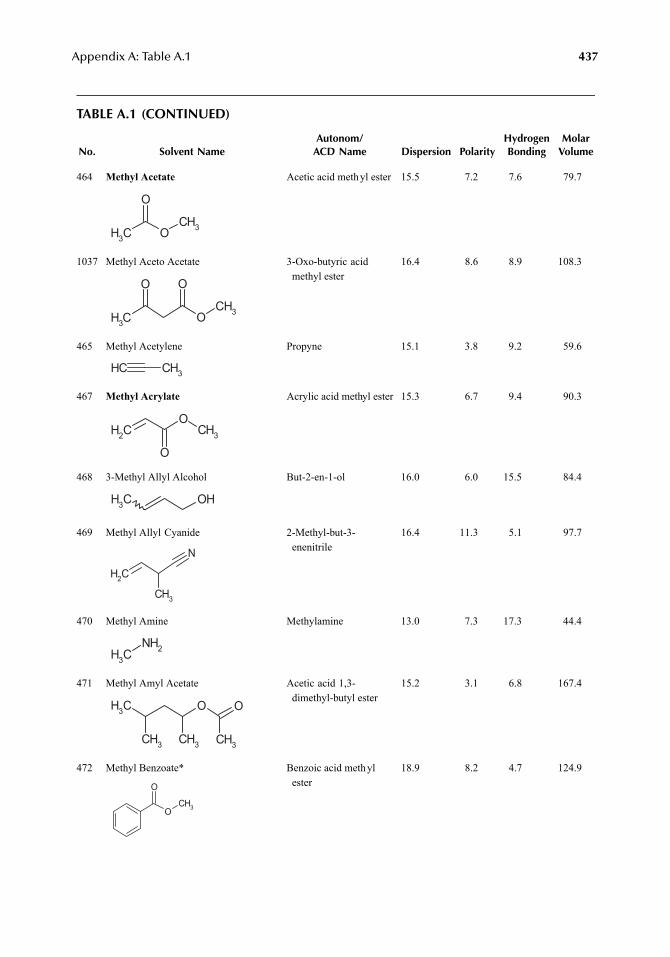
Appendix A: Table A.1
437
TABLE A.1 (CONTINUED)
No. Solvent NameAutonom/
ACD Name Dispersion PolarityHydrogenBonding
MolarVolume
464
Methyl Acetate
Acetic acid methyl ester 15.5 7.2 7.6 79.7
1037 Methyl Aceto Acetate 3-Oxo-butyric acid methyl ester
16.4 8.6 8.9 108.3
465 Methyl Acetylene Propyne 15.1 3.8 9.2 59.6
467
Methyl Acrylate
Acrylic acid methyl ester 15.3 6.7 9.4 90.3
468 3-Methyl Allyl Alcohol But-2-en-1-ol 16.0 6.0 15.5 84.4
469 Methyl Allyl Cyanide 2-Methyl-but-3-enenitrile
16.4 11.3 5.1 97.7
470 Methyl Amine Methylamine 13.0 7.3 17.3 44.4
471 Methyl Amyl Acetate Acetic acid 1,3-dimethyl-butyl ester
15.2 3.1 6.8 167.4
472 Methyl Benzoate* Benzoic acid methyl ester
18.9 8.2 4.7 124.9
CH3 O
O
CH3
CH3 OCH3
O O
CH CH3
CH2
O
O
CH3
OHCH3
CH2
N
CH3
CH3
NH2
O
CH3CH3
CH3
CH3
O
O
O
CH3
7248_A001A.fm Page 437 Wednesday, May 23, 2007 12:38 PM
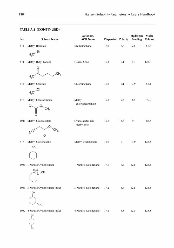
438
Hansen Solubility Parameters: A User’s Handbook
TABLE A.1 (CONTINUED)
No. Solvent NameAutonom/
ACD Name Dispersion PolarityHydrogenBonding
MolarVolume
473 Methyl Bromide Bromomethane 17.0 8.8 2.6 56.8
474 Methyl Butyl Ketone Hexan-2-one 15.3 6.1 4.1 123.6
475 Methyl Chloride Chloromethane 15.3 6.1 3.9 55.4
476 Methyl Chloroformate Methyl chloridocarbonate
16.3 9.5 8.5 77.3
1041 Methyl Cyanoacetate Cyano-acetic acid methyl ester
16.8 14.8 9.1 88.3
477 Methyl Cyclohexane Methyl-cyclohexane 16.0 0 1.0 128.3
1030 1-Methyl Cyclohexanol 1-Methyl-cyclohexanol 17.1 6.4 12.5 123.4
1031 3-Methyl Cyclohexanol (mix) 3-Methyl-cyclohexanol 17.2 6.4 12.5 124.8
1032 4-Methyl Cyclohexanol (mix) 4-Methyl-cyclohexanol 17.2 6.3 12.5 125.5
CH3
Br
CH3
O
CH3
CH3
Cl
OCl
O
CH3
O
O
CH3N
CH3
OHCH3
OH
CH3
OH
CH3
7248_A001A.fm Page 438 Wednesday, May 23, 2007 12:38 PM
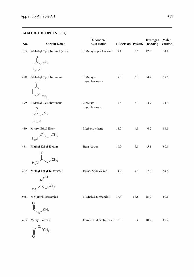
Appendix A: Table A.1
439
TABLE A.1 (CONTINUED)
No. Solvent NameAutonom/
ACD Name Dispersion PolarityHydrogenBonding
MolarVolume
1033 2-Methyl Cyclohexanol (mix) 2-Methyl-cyclohexanol 17.1 6.5 12.5 124.1
478 3-Methyl Cyclohexanone 3-Methyl-cyclohexanone
17.7 6.3 4.7 122.5
479 2-Methyl Cyclohexanone 2-Methyl-cyclohexanone
17.6 6.3 4.7 121.3
480 Methyl Ethyl Ether Methoxy-ethane 14.7 4.9 6.2 84.1
481
Methyl Ethyl Ketone
Butan-2-one 16.0 9.0 5.1 90.1
482
Methyl Ethyl Ketoxime
Butan-2-one oxime 14.7 4.9 7.8 94.8
965 N-Methyl Formamide N-Methyl-formamide 17.4 18.8 15.9 59.1
483 Methyl Formate Formic acid methyl ester 15.3 8.4 10.2 62.2
OH
CH3
O
CH3
O
CH3
CH3
O CH3
CH3
O
CH3
CH3
N
CH3
OH
N
O
CH3
OCH3
O
7248_A001A.fm Page 439 Wednesday, May 23, 2007 12:38 PM
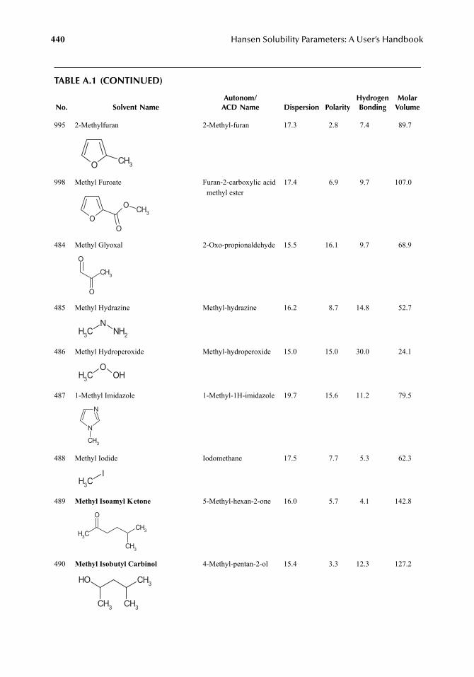
440
Hansen Solubility Parameters: A User’s Handbook
TABLE A.1 (CONTINUED)
No. Solvent NameAutonom/
ACD Name Dispersion PolarityHydrogenBonding
MolarVolume
995 2-Methylfuran 2-Methyl-furan 17.3 2.8 7.4 89.7
998 Methyl Furoate Furan-2-carboxylic acid methyl ester
17.4 6.9 9.7 107.0
484 Methyl Glyoxal 2-Oxo-propionaldehyde 15.5 16.1 9.7 68.9
485 Methyl Hydrazine Methyl-hydrazine 16.2 8.7 14.8 52.7
486 Methyl Hydroperoxide Methyl-hydroperoxide 15.0 15.0 30.0 24.1
487 1-Methyl Imidazole 1-Methyl-1H-imidazole 19.7 15.6 11.2 79.5
488 Methyl Iodide Iodomethane 17.5 7.7 5.3 62.3
489
Methyl Isoamyl Ketone
5-Methyl-hexan-2-one 16.0 5.7 4.1 142.8
490
Methyl Isobutyl Carbinol
4-Methyl-pentan-2-ol 15.4 3.3 12.3 127.2
O CH3
O
O
O
CH3
CH3
O
O
CH3
NNH2
CH3
OOH
N
N
CH3
CH3
I
CH3
CH3
CH3
O
CH3
CH3
CH3
OH
7248_A001A.fm Page 440 Wednesday, May 23, 2007 12:38 PM
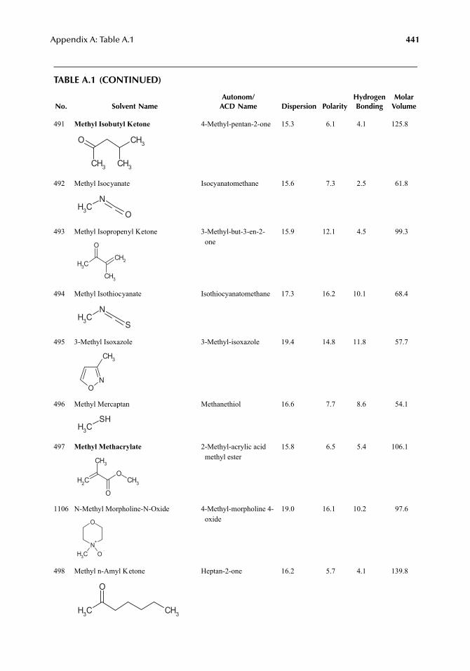
Appendix A: Table A.1
441
TABLE A.1 (CONTINUED)
No. Solvent NameAutonom/
ACD Name Dispersion PolarityHydrogenBonding
MolarVolume
491
Methyl Isobutyl Ketone
4-Methyl-pentan-2-one 15.3 6.1 4.1 125.8
492 Methyl Isocyanate Isocyanatomethane 15.6 7.3 2.5 61.8
493 Methyl Isopropenyl Ketone 3-Methyl-but-3-en-2-one
15.9 12.1 4.5 99.3
494 Methyl Isothiocyanate Isothiocyanatomethane 17.3 16.2 10.1 68.4
495 3-Methyl Isoxazole 3-Methyl-isoxazole 19.4 14.8 11.8 57.7
496 Methyl Mercaptan Methanethiol 16.6 7.7 8.6 54.1
497
Methyl Methacrylate
2-Methyl-acrylic acid methyl ester
15.8 6.5 5.4 106.1
1106 N-Methyl Morpholine-N-Oxide 4-Methyl-morpholine 4-oxide
19.0 16.1 10.2 97.6
498 Methyl n-Amyl Ketone Heptan-2-one 16.2 5.7 4.1 139.8
CH3
CH3
CH3
O
CH3
N
O
CH3
O
CH3
CH2
CH3
N
S
ON
CH3
CH3
SH
CH2
CH3
O
OCH3
N+
CH3 O
O
CH3
O
CH3
7248_A001A.fm Page 441 Wednesday, May 23, 2007 12:38 PM
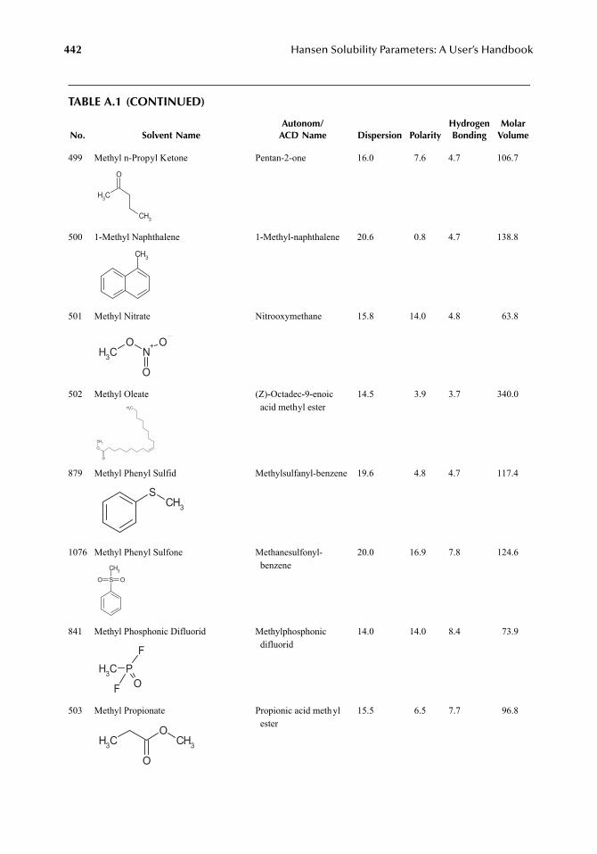
442
Hansen Solubility Parameters: A User’s Handbook
TABLE A.1 (CONTINUED)
No. Solvent NameAutonom/
ACD Name Dispersion PolarityHydrogenBonding
MolarVolume
499 Methyl n-Propyl Ketone Pentan-2-one 16.0 7.6 4.7 106.7
500 1-Methyl Naphthalene 1-Methyl-naphthalene 20.6 0.8 4.7 138.8
501 Methyl Nitrate Nitrooxymethane 15.8 14.0 4.8 63.8
502 Methyl Oleate (Z)-Octadec-9-enoic acid methyl ester
14.5 3.9 3.7 340.0
879 Methyl Phenyl Sulfid Methylsulfanyl-benzene 19.6 4.8 4.7 117.4
1076 Methyl Phenyl Sulfone Methanesulfonyl-benzene
20.0 16.9 7.8 124.6
841 Methyl Phosphonic Difluorid Methylphosphonic difluorid
14.0 14.0 8.4 73.9
503 Methyl Propionate Propionic acid methyl ester
15.5 6.5 7.7 96.8
CH3
O
CH3
CH3
CH3
ON+ O
O
O
O
CH3
CH3
CH3
S
S
CH3
OO
CH3 PO
F
F
CH3
OCH3
O
7248_A001A.fm Page 442 Wednesday, May 23, 2007 12:38 PM
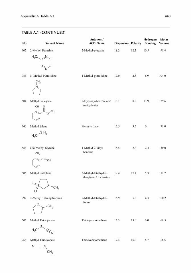
Appendix A: Table A.1
443
TABLE A.1 (CONTINUED)
No. Solvent NameAutonom/
ACD Name Dispersion PolarityHydrogenBonding
MolarVolume
902 2-Methyl Pyrazine 2-Methyl-pyrazine 18.3 12.3 10.5 91.4
986 N-Methyl Pyrrolidine 1-Methyl-pyrrolidine 17.0 2.8 6.9 104.0
504 Methyl Salicylate 2-Hydroxy-benzoic acid methyl ester
18.1 8.0 13.9 129.6
740 Methyl Silane Methyl-silane 15.5 3.3 0 71.0
886 alfa-Methyl Styrene 1-Methyl-2-vinyl-benzene
18.5 2.4 2.4 130.0
506 Methyl Sulfolane 3-Methyl-tetrahydro-thiophene 1,1-dioxide
19.4 17.4 5.3 112.7
997 2-Methyl Tetrahydrofuran 2-Methyl-tetrahydro-furan
16.9 5.0 4.3 100.2
507 Methyl Thiocyanate Thiocyanatomethane 17.3 15.0 6.0 68.5
968 Methyl Thiocyanate Thiocyanatomethane 17.4 15.0 8.7 68.5
NCH3
N
N
CH3
OH
O
O
CH3
CH3
SiH3
CH3
CH2
SO
OCH3
O CH3
CH3
S
N
SNCH3
7248_A001A.fm Page 443 Wednesday, May 23, 2007 12:38 PM
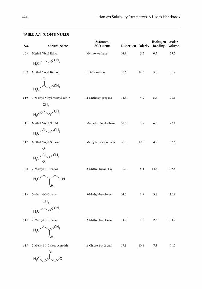
444
Hansen Solubility Parameters: A User’s Handbook
TABLE A.1 (CONTINUED)
No. Solvent NameAutonom/
ACD Name Dispersion PolarityHydrogenBonding
MolarVolume
508 Methyl Vinyl Ether Methoxy-ethene 14.9 5.3 6.3 75.2
509 Methyl Vinyl Ketone But-3-en-2-one 15.6 12.5 5.0 81.2
510 1-Methyl Vinyl Methyl Ether 2-Methoxy-propene 14.8 4.2 5.6 96.1
511 Methyl Vinyl Sulfid Methylsulfanyl-ethene 16.4 4.9 6.0 82.1
512 Methyl Vinyl Sulfone Methylsulfonyl-ethene 16.8 19.6 4.8 87.6
462 2-Methyl-1-Butanol 2-Methyl-butan-1-ol 16.0 5.1 14.3 109.5
513 3-Methyl-1-Butene 3-Methyl-but-1-ene 14.0 1.4 3.8 112.9
514 2-Methyl-1-Butene 2-Methyl-but-1-ene 14.2 1.8 2.3 108.7
515 2-Methyl-1-Chloro Acrolein 2-Chloro-but-2-enal 17.1 10.6 7.3 91.7
CH3
O CH2
CH3
O
CH2
CH2 O
CH3
CH3
CH3
S CH2
CH3
S CH2
O
O
CH3 OH
CH3
CH3
CH2
CH3
CH3
CH2
CH3
OCH3
Cl
7248_A001A.fm Page 444 Wednesday, May 23, 2007 12:38 PM
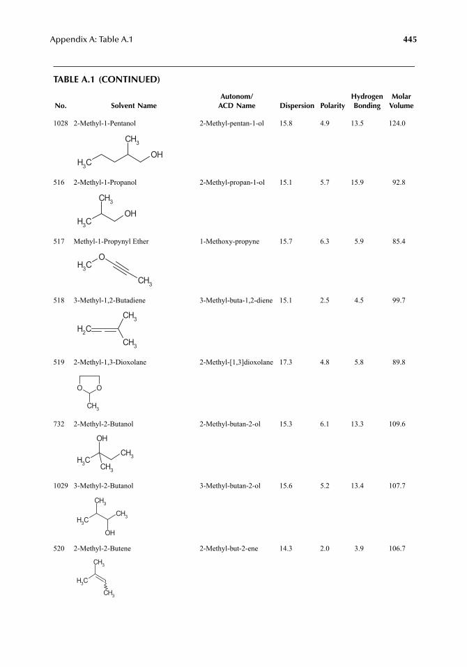
Appendix A: Table A.1
445
TABLE A.1 (CONTINUED)
No. Solvent NameAutonom/
ACD Name Dispersion PolarityHydrogenBonding
MolarVolume
1028 2-Methyl-1-Pentanol 2-Methyl-pentan-1-ol 15.8 4.9 13.5 124.0
516 2-Methyl-1-Propanol 2-Methyl-propan-1-ol 15.1 5.7 15.9 92.8
517 Methyl-1-Propynyl Ether 1-Methoxy-propyne 15.7 6.3 5.9 85.4
518 3-Methyl-1,2-Butadiene 3-Methyl-buta-1,2-diene 15.1 2.5 4.5 99.7
519 2-Methyl-1,3-Dioxolane 2-Methyl-[1,3]dioxolane 17.3 4.8 5.8 89.8
732 2-Methyl-2-Butanol 2-Methyl-butan-2-ol 15.3 6.1 13.3 109.6
1029 3-Methyl-2-Butanol 3-Methyl-butan-2-ol 15.6 5.2 13.4 107.7
520 2-Methyl-2-Butene 2-Methyl-but-2-ene 14.3 2.0 3.9 106.7
CH3
OH
CH3
CH3
OH
CH3
CH3
O
CH3
CH2
CH3
CH3
O O
CH3
CH3
CH3
OH
CH3
CH3
CH3
OH
CH3
CH3
CH3
CH3
7248_A001A.fm Page 445 Wednesday, May 23, 2007 12:38 PM
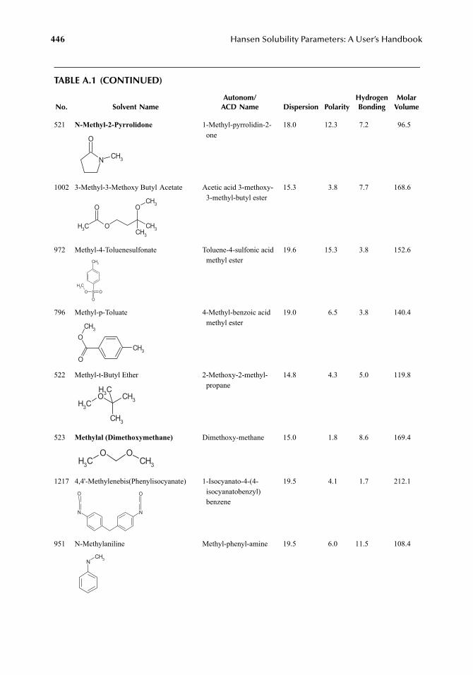
446
Hansen Solubility Parameters: A User’s Handbook
TABLE A.1 (CONTINUED)
No. Solvent NameAutonom/
ACD Name Dispersion PolarityHydrogenBonding
MolarVolume
521
N-Methyl-2-Pyrrolidone
1-Methyl-pyrrolidin-2-one
18.0 12.3 7.2 96.5
1002 3-Methyl-3-Methoxy Butyl Acetate Acetic acid 3-methoxy-3-methyl-butyl ester
15.3 3.8 7.7 168.6
972 Methyl-4-Toluenesulfonate Toluene-4-sulfonic acid methyl ester
19.6 15.3 3.8 152.6
796 Methyl-p-Toluate 4-Methyl-benzoic acid methyl ester
19.0 6.5 3.8 140.4
522 Methyl-t-Butyl Ether 2-Methoxy-2-methyl-propane
14.8 4.3 5.0 119.8
523
Methylal (Dimethoxymethane)
Dimethoxy-methane 15.0 1.8 8.6 169.4
1217 4,4'-Methylenebis(Phenylisocyanate) 1-Isocyanato-4-(4-isocyanatobenzyl) benzene
19.5 4.1 1.7 212.1
951 N-Methylaniline Methyl-phenyl-amine 19.5 6.0 11.5 108.4
N
O
CH3
CH3 O CH3
O OCH3
CH3
SO
O
OCH3
CH3
O
O
CH3
CH3
CH3
O CH3
CH3
CH3
OOCH3 CH3
NN
OO
NCH3
7248_A001A.fm Page 446 Wednesday, May 23, 2007 12:38 PM
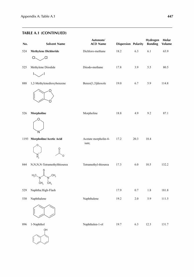
Appendix A: Table A.1
447
TABLE A.1 (CONTINUED)
No. Solvent NameAutonom/
ACD Name Dispersion PolarityHydrogenBonding
MolarVolume
524
Methylene Dichloride
Dichloro-methane 18.2 6.3 6.1 63.9
525 Methylene Diiodide Diiodo-methane 17.8 3.9 5.5 80.5
888 1,2-Methylenedioxybenzene Benzo[1,3]dioxole 19.0 6.7 5.9 114.8
526
Morpholine
Morpholine 18.8 4.9 9.2 87.1
1193
Morpholine/Acetic Acid
Acetate morpholin-4-ium;
17.2 20.3 18.4
844 N,N,N,N-Tetramethylthiourea Tetramethyl-thiourea 17.3 6.0 10.5 132.2
529 Naphtha.High-Flash 17.9 0.7 1.8 181.8
530 Naphthalene Naphthalene 19.2 2.0 5.9 111.5
896 1-Naphthol Naphthalen-1-ol 19.7 6.3 12.3 131.7
ClCl
II
O
O
N
O
O
O
NH2
+
O
N N
S
CH3
CH3 CH3
CH3
OH
7248_A001A.fm Page 447 Wednesday, May 23, 2007 12:38 PM
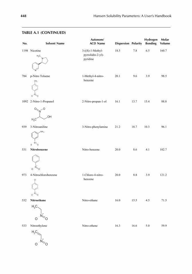
448
Hansen Solubility Parameters: A User’s Handbook
TABLE A.1 (CONTINUED)
No. Solvent NameAutonom/
ACD Name Dispersion PolarityHydrogenBonding
MolarVolume
1198 Nicotine 3-((S)-1-Methyl-pyrrolidin-2-yl)-pyridine
18.5 7.8 6.5 160.7
784 p-Nitro Toluene 1-Methyl-4-nitro-benzene
20.1 9.6 3.9 98.5
1092 2-Nitro-1-Propanol 2-Nitro-propan-1-ol 16.1 13.7 15.4 88.8
939 3-Nitroaniline 3-Nitro-phenylamine 21.2 18.7 10.3 96.1
531
Nitrobenzene
Nitro-benzene 20.0 8.6 4.1 102.7
973 4-Nitrochlorobenzene 1-Chloro-4-nitro-benzene
20.0 8.8 3.9 121.2
532
Nitroethane
Nitro-ethane 16.0 15.5 4.5 71.5
533 Nitroethylene Nitro-ethene 16.3 16.6 5.0 59.9
NCH3
N
CH3
N+
O O
CH3
OH
N+ OO
NH2
N*OO
N+
O O
Cl
N+
O O
CH3
N+
O O
CH2
N+
O O
7248_A001A.fm Page 448 Wednesday, May 23, 2007 12:38 PM
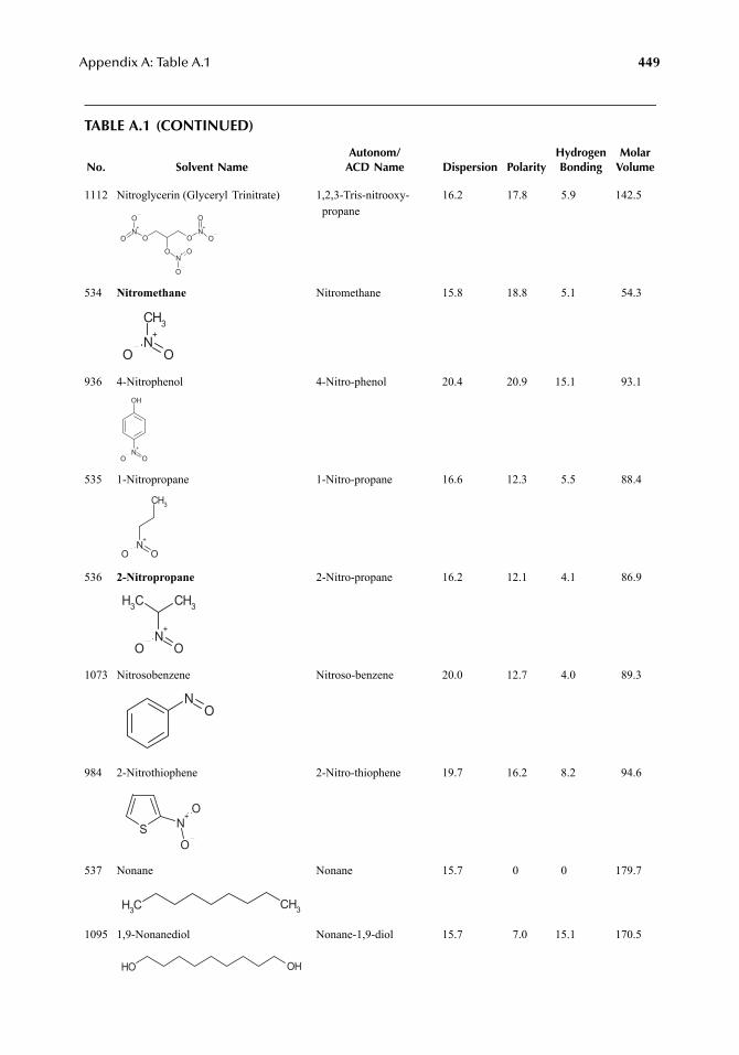
Appendix A: Table A.1
449
TABLE A.1 (CONTINUED)
No. Solvent NameAutonom/
ACD Name Dispersion PolarityHydrogenBonding
MolarVolume
1112 Nitroglycerin (Glyceryl Trinitrate) 1,2,3-Tris-nitrooxy-propane
16.2 17.8 5.9 142.5
534
Nitromethane
Nitromethane 15.8 18.8 5.1 54.3
936 4-Nitrophenol 4-Nitro-phenol 20.4 20.9 15.1 93.1
535 1-Nitropropane 1-Nitro-propane 16.6 12.3 5.5 88.4
536
2-Nitropropane
2-Nitro-propane 16.2 12.1 4.1 86.9
1073 Nitrosobenzene Nitroso-benzene 20.0 12.7 4.0 89.3
984 2-Nitrothiophene 2-Nitro-thiophene 19.7 16.2 8.2 94.6
537 Nonane Nonane 15.7 0 0 179.7
1095 1,9-Nonanediol Nonane-1,9-diol 15.7 7.0 15.1 170.5
O
OO
N+
N+
N+
O
O
O
OO
O
CH3
N+
O O
OH
N+
O O
N+
O O
CH3
N+
O O
CH3CH3
NO
S N+
O
O
CH3 CH3
OH OH
7248_A001A.fm Page 449 Wednesday, May 23, 2007 12:38 PM
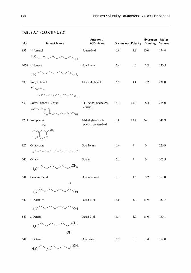
450
Hansen Solubility Parameters: A User’s Handbook
TABLE A.1 (CONTINUED)
No. Solvent NameAutonom/
ACD Name Dispersion PolarityHydrogenBonding
MolarVolume
932 1-Nonanol Nonan-1-ol 16.0 4.8 10.6 174.4
1070 1-Nonene Non-1-ene 15.4 1.0 2.2 170.5
538 Nonyl Phenol 4-Nonyl-phenol 16.5 4.1 9.2 231.0
539 Nonyl Phenoxy Ethanol 2-(4-Nonyl-phenoxy)-ethanol
16.7 10.2 8.4 275.0
1209 Norephedrin 2-Methylamino-1-phenyl-propan-1-ol
18.0 10.7 24.1 141.9
923 Octadecane Octadecane 16.4 0 0 326.9
540 Octane Octane 15.5 0 0 163.5
541 Octanoic Acid Octanoic acid 15.1 3.3 8.2 159.0
542 1-Octanol* Octan-1-ol 16.0 5.0 11.9 157.7
543 2-Octanol Octan-2-ol 16.1 4.9 11.0 159.1
544 1-Octene Oct-1-ene 15.3 1.0 2.4 158.0
OHCH3
CH3 CH2
OH
CH3
OH
N
CH3
CH3
CH3
CH3
CH3
CH3
CH3 OH
O
CH3 OH
CH3
CH3
OH
CH3
CH2CH3 CH3
7248_A001A.fm Page 450 Wednesday, May 23, 2007 12:38 PM
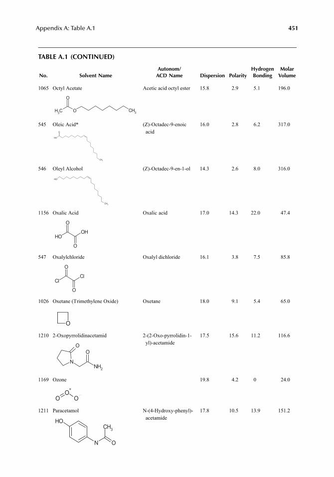
Appendix A: Table A.1
451
TABLE A.1 (CONTINUED)
No. Solvent NameAutonom/
ACD Name Dispersion PolarityHydrogenBonding
MolarVolume
1065 Octyl Acetate Acetic acid octyl ester 15.8 2.9 5.1 196.0
545 Oleic Acid* (Z)-Octadec-9-enoic acid
16.0 2.8 6.2 317.0
546 Oleyl Alcohol (Z)-Octadec-9-en-1-ol 14.3 2.6 8.0 316.0
1156 Oxalic Acid Oxalic acid 17.0 14.3 22.0 47.4
547 Oxalylchloride Oxalyl dichloride 16.1 3.8 7.5 85.8
1026 Oxetane (Trimethylene Oxide) Oxetane 18.0 9.1 5.4 65.0
1210 2-Oxopyrrolidinacetamid 2-(2-Oxo-pyrrolidin-1-yl)-acetamide
17.5 15.6 11.2 116.6
1169 Ozone 19.8 4.2 0 24.0
1211 Paracetamol N-(4-Hydroxy-phenyl)-acetamide
17.8 10.5 13.9 151.2
CH3 O CH3
O
OH
O
CH3
OH
CH3
OH
O
O
OH
ClCl
O
O
O
N
O
NH2
O
OO+
O
N
CH3
O
OH
7248_A001A.fm Page 451 Wednesday, May 23, 2007 12:38 PM
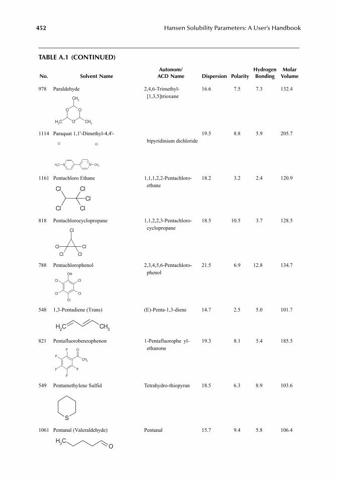
452
Hansen Solubility Parameters: A User’s Handbook
TABLE A.1 (CONTINUED)
No. Solvent NameAutonom/
ACD Name Dispersion PolarityHydrogenBonding
MolarVolume
978 Paraldehyde 2,4,6-Trimethyl-[1,3,5]trioxane
16.6 7.5 7.3 132.4
1114 Paraquat 1,1'-Dimethyl-4,4'-bipyridinium dichloride
19.5 8.8 5.9 205.7
1161 Pentachloro Ethane 1,1,1,2,2-Pentachloro-ethane
18.2 3.2 2.4 120.9
818 Pentachlorocyclopropane 1,1,2,2,3-Pentachloro-cyclopropane
18.5 10.5 3.7 128.5
788 Pentachlorophenol 2,3,4,5,6-Pentachloro-phenol
21.5 6.9 12.8 134.7
548 1,3-Pentadiene (Trans) (E)-Penta-1,3-diene 14.7 2.5 5.0 101.7
821 Pentafluorobenzophenon 1-Pentafluorophe yl-ethanone
19.3 8.1 5.4 185.5
549 Pentamethylene Sulfid Tetrahydro-thiopyran 18.5 6.3 8.9 103.6
1061 Pentanal (Valeraldehyde) Pentanal 15.7 9.4 5.8 106.4
O
O
CH3
O
CH3
CH3
N+
N+
CH3 CH3
Cl Cl
Cl
Cl Cl
ClCl
Cl
ClClCl
Cl
OH
Cl
Cl
Cl
Cl
Cl
CH2 CH3
CH3
OF
F
F
F
F
S
OCH3
7248_A001A.fm Page 452 Wednesday, May 23, 2007 12:38 PM
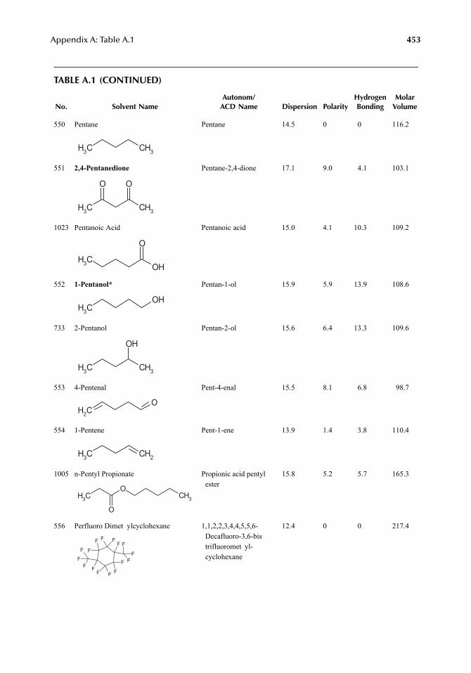
Appendix A: Table A.1
453
TABLE A.1 (CONTINUED)
No. Solvent NameAutonom/
ACD Name Dispersion PolarityHydrogenBonding
MolarVolume
550 Pentane Pentane 14.5 0 0 116.2
551
2,4-Pentanedione
Pentane-2,4-dione 17.1 9.0 4.1 103.1
1023 Pentanoic Acid Pentanoic acid 15.0 4.1 10.3 109.2
552
1-Pentanol*
Pentan-1-ol 15.9 5.9 13.9 108.6
733 2-Pentanol Pentan-2-ol 15.6 6.4 13.3 109.6
553 4-Pentenal Pent-4-enal 15.5 8.1 6.8 98.7
554 1-Pentene Pent-1-ene 13.9 1.4 3.8 110.4
1005 n-Pentyl Propionate Propionic acid pentyl ester
15.8 5.2 5.7 165.3
556 Perfluoro Dimet ylcyclohexane 1,1,2,2,3,4,4,5,5,6-Decafluoro-3,6-bistrifluoromet yl-cyclohexane
12.4 0 0 217.4
CH3 CH3
CH3
O
CH3
O
CH3 OH
O
CH3
OH
CH3 CH3
OH
CH2
O
CH3 CH2
CH3
OCH3
O
FFF
F
F
FFF
F
F
FFF
F
F
F
7248_A001A.fm Page 453 Wednesday, May 23, 2007 12:38 PM
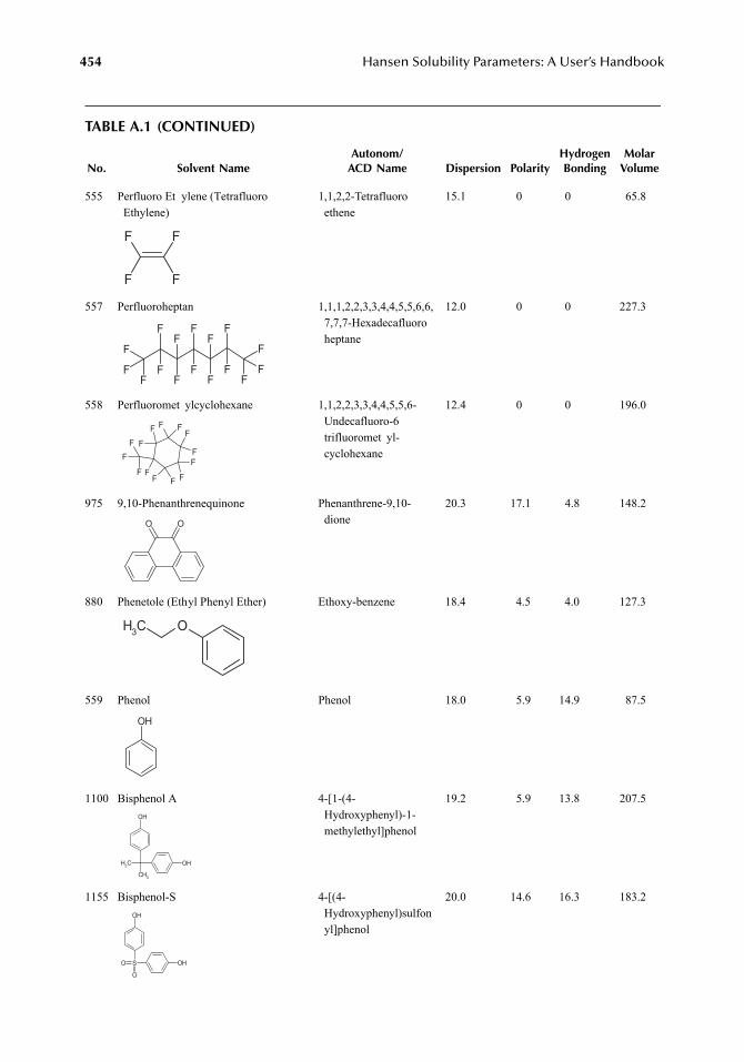
454
Hansen Solubility Parameters: A User’s Handbook
TABLE A.1 (CONTINUED)
No. Solvent NameAutonom/
ACD Name Dispersion PolarityHydrogenBonding
MolarVolume
555 Perfluoro Et ylene (TetrafluoroEthylene)
1,1,2,2-Tetrafluoroethene
15.1 0 0 65.8
557 Perfluoroheptan 1,1,1,2,2,3,3,4,4,5,5,6,6,7,7,7-Hexadecafluoroheptane
12.0 0 0 227.3
558 Perfluoromet ylcyclohexane 1,1,2,2,3,3,4,4,5,5,6-Undecafluoro-6trifluoromet yl-cyclohexane
12.4 0 0 196.0
975 9,10-Phenanthrenequinone Phenanthrene-9,10-dione
20.3 17.1 4.8 148.2
880 Phenetole (Ethyl Phenyl Ether) Ethoxy-benzene 18.4 4.5 4.0 127.3
559 Phenol Phenol 18.0 5.9 14.9 87.5
1100 Bisphenol A 4-[1-(4-Hydroxyphenyl)-1-methylethyl]phenol
19.2 5.9 13.8 207.5
1155 Bisphenol-S 4-[(4-Hydroxyphenyl)sulfonyl]phenol
20.0 14.6 16.3 183.2
F
F
F
F
F
FF
F
F
F
F
F
FF
FF
F
F
FF
FF F
F
F
F
FF
F
F
FF
F
F
OO
OCH3
OH
CH3
CH3
OH
OH
SO
O
OH
OH
7248_A001A.fm Page 454 Wednesday, May 23, 2007 12:38 PM
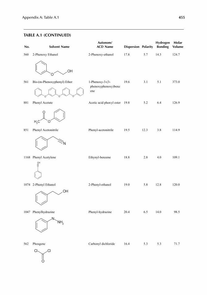
Appendix A: Table A.1 455
TABLE A.1 (CONTINUED)
No. Solvent NameAutonom/
ACD Name Dispersion PolarityHydrogenBonding
MolarVolume
560 2-Phenoxy Ethanol 2-Phenoxy-ethanol 17.8 5.7 14.3 124.7
561 Bis-(m-Phenoxyphenyl) Ether 1-Phenoxy-3-(3-phenoxyphenoxy)benzene
19.6 3.1 5.1 373.0
881 Phenyl Acetate Acetic acid phenyl ester 19.8 5.2 6.4 126.9
851 Phenyl Acetonitrile Phenyl-acetonitrile 19.5 12.3 3.8 114.9
1168 Phenyl Acetylene Ethynyl-benzene 18.8 2.8 4.0 109.1
1074 2-Phenyl Ethanol 2-Phenyl-ethanol 19.0 5.8 12.8 120.0
1047 Phenylhydrazine Phenyl-hydrazine 20.4 6.5 14.0 98.5
562 Phosgene Carbonyl dichloride 16.4 5.3 5.3 71.7
OOH
O OO
CH3 O
O
N
CH
OH
NNH2
ClCl
O
7248_A001A.fm Page 455 Wednesday, May 23, 2007 12:38 PM
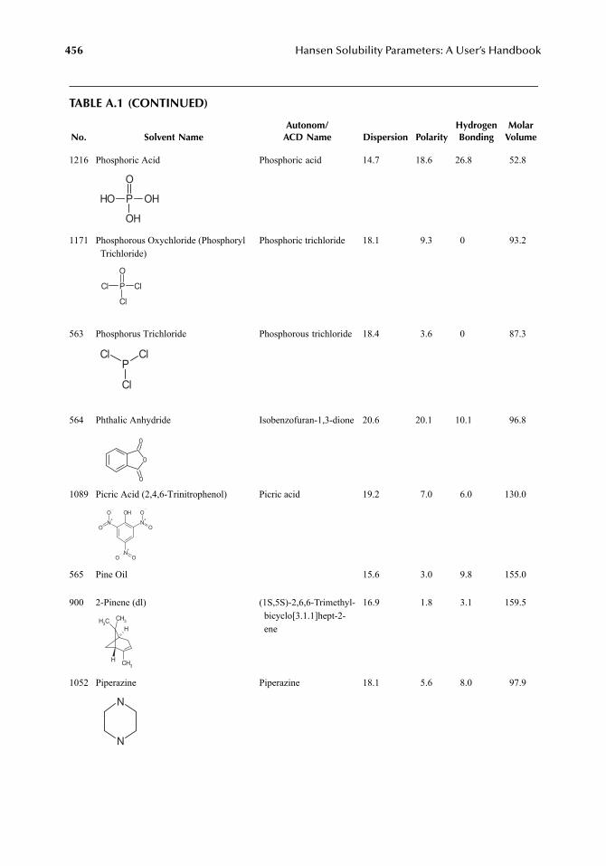
456 Hansen Solubility Parameters: A User’s Handbook
TABLE A.1 (CONTINUED)
No. Solvent NameAutonom/
ACD Name Dispersion PolarityHydrogenBonding
MolarVolume
1216 Phosphoric Acid Phosphoric acid 14.7 18.6 26.8 52.8
1171 Phosphorous Oxychloride (Phosphoryl Trichloride)
Phosphoric trichloride 18.1 9.3 0 93.2
563 Phosphorus Trichloride Phosphorous trichloride 18.4 3.6 0 87.3
564 Phthalic Anhydride Isobenzofuran-1,3-dione 20.6 20.1 10.1 96.8
1089 Picric Acid (2,4,6-Trinitrophenol) Picric acid 19.2 7.0 6.0 130.0
565 Pine Oil 15.6 3.0 9.8 155.0
900 2-Pinene (dl) (1S,5S)-2,6,6-Trimethyl-bicyclo[3.1.1]hept-2-ene
16.9 1.8 3.1 159.5
1052 Piperazine Piperazine 18.1 5.6 8.0 97.9
POH O
OH
O
H
P
O
Cl
Cl
Cl
PClCl
Cl
O
O
O
OH
N+
N+
N+
O
O O
O
O O
CH3CH3
CH3H
H
N
N
7248_A001A.fm Page 456 Wednesday, May 23, 2007 12:38 PM
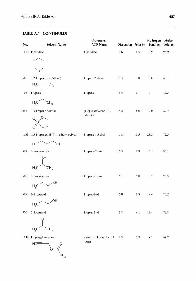
Appendix A: Table A.1 457
TABLE A.1 (CONTINUED)
No. Solvent NameAutonom/
ACD Name Dispersion PolarityHydrogenBonding
MolarVolume
1050 Piperidine Piperidine 17.6 4.5 8.9 98.9
566 1,2-Propadiene (Allene) Propa-1,2-diene 15.3 3.0 6.8 60.1
1064 Propane Propane 13.4 0 0 89.5
943 1,3-Propane Sultone [1,2]Oxathiolane 2,2-dioxide
18.4 16.0 9.0 87.7
1038 1,3-Propanediol (Trimethyleneglycol) Propane-1,3-diol 16.8 13.5 23.2 72.5
567 2-Propanethiol Propane-2-thiol 16.3 6.8 6.5 94.1
568 1-Propanethiol Propane-1-thiol 16.1 5.8 5.7 90.5
569 1-Propanol Propan-1-ol 16.0 6.8 17.4 75.2
570 2-Propanol Propan-2-ol 15.8 6.1 16.4 76.8
1036 Propargyl Acetate Acetic acid prop-2-ynyl ester
16.3 5.2 8.3 98.8
N
CH2 CH2
CH3 CH3
SOO
O
OH OH
CH3 CH3
SH
CH3
SH
CH3
OH
CH3 CH3
OH
CHO
CH3
O
7248_A001A.fm Page 457 Wednesday, May 23, 2007 12:38 PM
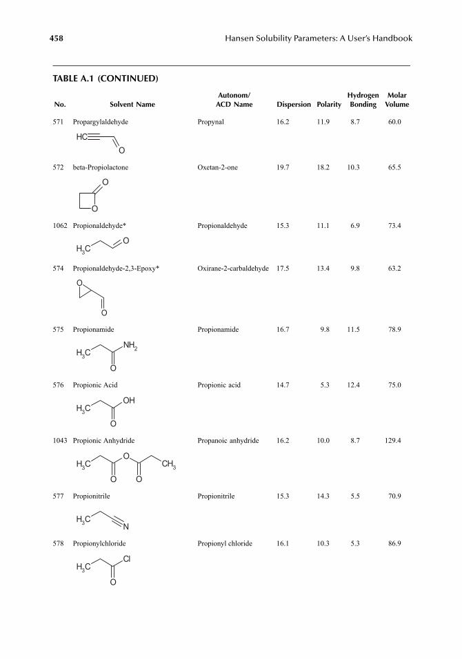
458 Hansen Solubility Parameters: A User’s Handbook
TABLE A.1 (CONTINUED)
No. Solvent NameAutonom/
ACD Name Dispersion PolarityHydrogenBonding
MolarVolume
571 Propargylaldehyde Propynal 16.2 11.9 8.7 60.0
572 beta-Propiolactone Oxetan-2-one 19.7 18.2 10.3 65.5
1062 Propionaldehyde* Propionaldehyde 15.3 11.1 6.9 73.4
574 Propionaldehyde-2,3-Epoxy* Oxirane-2-carbaldehyde 17.5 13.4 9.8 63.2
575 Propionamide Propionamide 16.7 9.8 11.5 78.9
576 Propionic Acid Propionic acid 14.7 5.3 12.4 75.0
1043 Propionic Anhydride Propanoic anhydride 16.2 10.0 8.7 129.4
577 Propionitrile Propionitrile 15.3 14.3 5.5 70.9
578 Propionylchloride Propionyl chloride 16.1 10.3 5.3 86.9
CHO
O
O
CH3
O
O
O
CH3
NH2
O
CH3
OH
O
CH3
OCH3
O O
CH3 N
CH3
Cl
O
7248_A001A.fm Page 458 Wednesday, May 23, 2007 12:38 PM
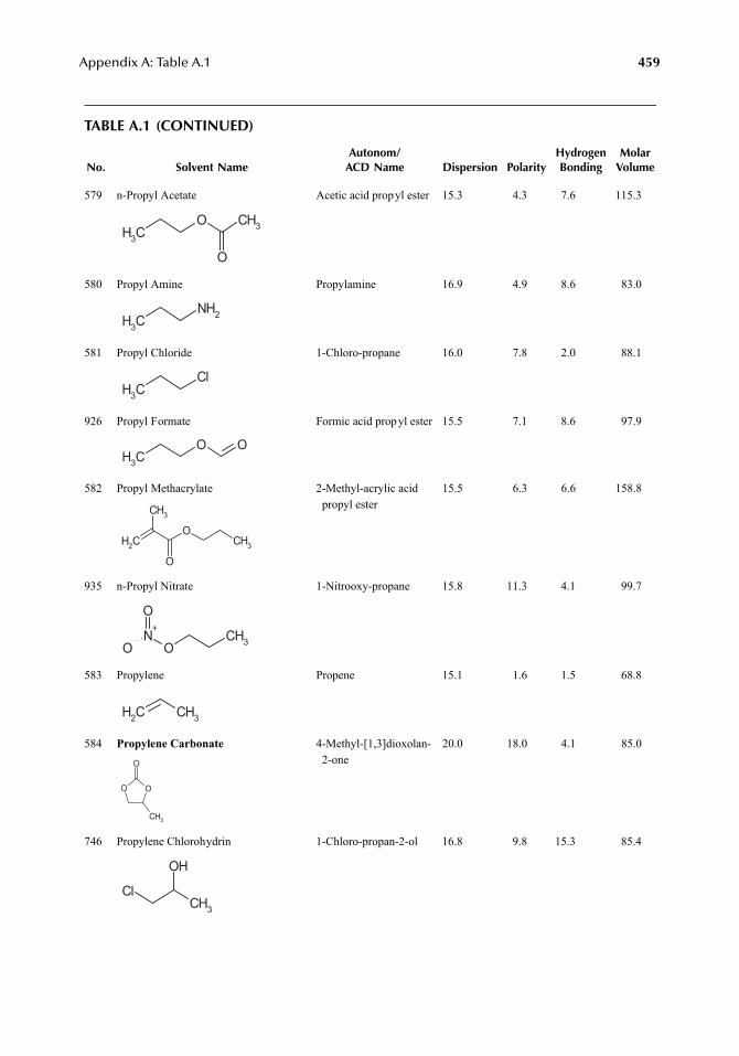
Appendix A: Table A.1 459
TABLE A.1 (CONTINUED)
No. Solvent NameAutonom/
ACD Name Dispersion PolarityHydrogenBonding
MolarVolume
579 n-Propyl Acetate Acetic acid propyl ester 15.3 4.3 7.6 115.3
580 Propyl Amine Propylamine 16.9 4.9 8.6 83.0
581 Propyl Chloride 1-Chloro-propane 16.0 7.8 2.0 88.1
926 Propyl Formate Formic acid propyl ester 15.5 7.1 8.6 97.9
582 Propyl Methacrylate 2-Methyl-acrylic acid propyl ester
15.5 6.3 6.6 158.8
935 n-Propyl Nitrate 1-Nitrooxy-propane 15.8 11.3 4.1 99.7
583 Propylene Propene 15.1 1.6 1.5 68.8
584 Propylene Carbonate 4-Methyl-[1,3]dioxolan-2-one
20.0 18.0 4.1 85.0
746 Propylene Chlorohydrin 1-Chloro-propan-2-ol 16.8 9.8 15.3 85.4
CH3
O CH3
O
CH3
NH2
CH3
Cl
CH3
O O
CH2
CH3
O
OCH3
ON+
O
OCH3
CH2 CH3
O
CH3
O
O
Cl
OH
CH3
7248_A001A.fm Page 459 Wednesday, May 23, 2007 12:38 PM
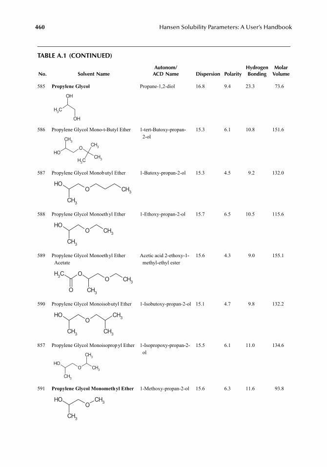
460 Hansen Solubility Parameters: A User’s Handbook
TABLE A.1 (CONTINUED)
No. Solvent NameAutonom/
ACD Name Dispersion PolarityHydrogenBonding
MolarVolume
585 Propylene Glycol Propane-1,2-diol 16.8 9.4 23.3 73.6
586 Propylene Glycol Mono-t-Butyl Ether 1-tert-Butoxy-propan-2-ol
15.3 6.1 10.8 151.6
587 Propylene Glycol Monobutyl Ether 1-Butoxy-propan-2-ol 15.3 4.5 9.2 132.0
588 Propylene Glycol Monoethyl Ether 1-Ethoxy-propan-2-ol 15.7 6.5 10.5 115.6
589 Propylene Glycol Monoethyl Ether Acetate
Acetic acid 2-ethoxy-1-methyl-ethyl ester
15.6 4.3 9.0 155.1
590 Propylene Glycol Monoisobutyl Ether 1-Isobutoxy-propan-2-ol 15.1 4.7 9.8 132.2
857 Propylene Glycol Monoisopropyl Ether 1-Isopropoxy-propan-2-ol
15.5 6.1 11.0 134.6
591 Propylene Glycol Monomethyl Ether 1-Methoxy-propan-2-ol 15.6 6.3 11.6 93.8
CH3
OH
OH
O
CH3
CH3
CH3
CH3
OH
O
CH3
OHCH3
O CH3
CH3
OH
O CH3
CH3
OCH3
O
O
CH3
OH CH3
CH3
O CH3
CH3
OH
CH3
OCH3
CH3
OH
7248_A001A.fm Page 460 Wednesday, May 23, 2007 12:38 PM
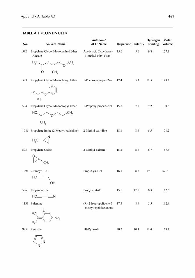
Appendix A: Table A.1 461
TABLE A.1 (CONTINUED)
No. Solvent NameAutonom/
ACD Name Dispersion PolarityHydrogenBonding
MolarVolume
592 Propylene Glycol Monomethyl Ether Acetate
Acetic acid 2-methoxy-1-methyl-ethyl ester
15.6 5.6 9.8 137.1
593 Propylene Glycol Monophenyl Ether 1-Phenoxy-propan-2-ol 17.4 5.3 11.5 143.2
594 Propylene Glycol Monopropyl Ether 1-Propoxy-propan-2-ol 15.8 7.0 9.2 130.3
1086 Propylene Imine (2-Methyl Aziridine) 2-Methyl-aziridine 18.1 8.4 6.5 71.2
595 Propylene Oxide 2-Methyl-oxirane 15.2 8.6 6.7 67.6
1091 2-Propyn-1-ol Prop-2-yn-1-ol 16.1 8.8 19.1 57.7
596 Propynonitrile Propynenitrile 15.5 17.0 6.3 62.5
1133 Pulegone (R)-2-Isopropylidene-5-methyl-cyclohexanone
17.5 8.9 5.5 162.9
985 Pyrazole 1H-Pyrazole 20.2 10.4 12.4 68.1
OCH3
CH3
OCH3
O
O
CH3
OH
O
CH3
OH CH3
NCH3
O
CH3
CHOH
CH N
OCH3
CH3
CH3
NN
7248_A001A.fm Page 461 Wednesday, May 23, 2007 12:38 PM
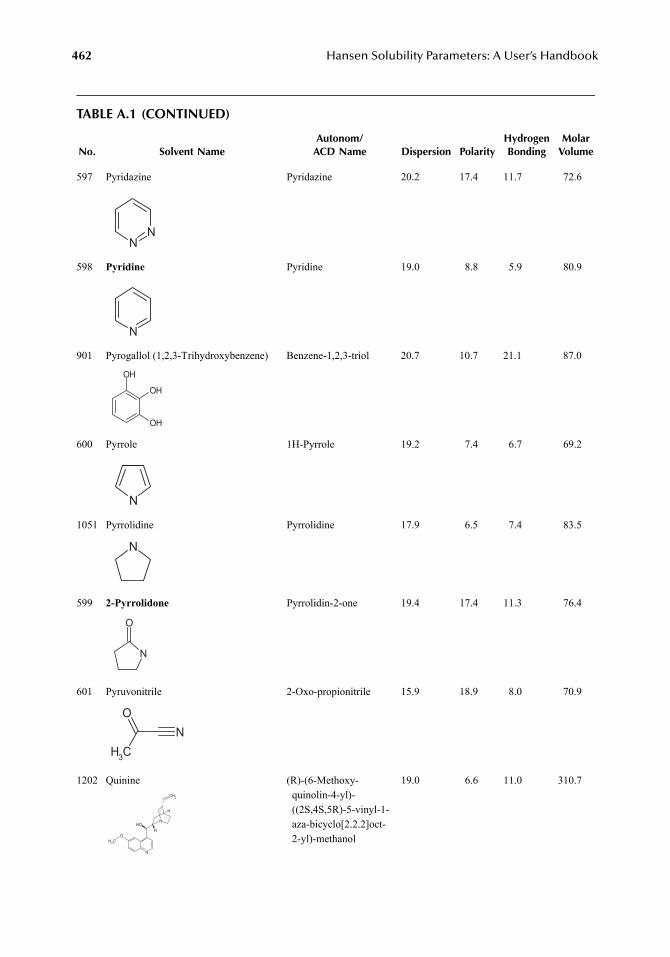
462 Hansen Solubility Parameters: A User’s Handbook
TABLE A.1 (CONTINUED)
No. Solvent NameAutonom/
ACD Name Dispersion PolarityHydrogenBonding
MolarVolume
597 Pyridazine Pyridazine 20.2 17.4 11.7 72.6
598 Pyridine Pyridine 19.0 8.8 5.9 80.9
901 Pyrogallol (1,2,3-Trihydroxybenzene) Benzene-1,2,3-triol 20.7 10.7 21.1 87.0
600 Pyrrole 1H-Pyrrole 19.2 7.4 6.7 69.2
1051 Pyrrolidine Pyrrolidine 17.9 6.5 7.4 83.5
599 2-Pyrrolidone Pyrrolidin-2-one 19.4 17.4 11.3 76.4
601 Pyruvonitrile 2-Oxo-propionitrile 15.9 18.9 8.0 70.9
1202 Quinine (R)-(6-Methoxy-quinolin-4-yl)-((2S,4S,5R)-5-vinyl-1-aza-bicyclo[2.2.2]oct-2-yl)-methanol
19.0 6.6 11.0 310.7
NN
N
OH
OH
OH
N
N
N
O
CH3
ON
N
OH
O
N
CH3
CH2
H
H
7248_A001A.fm Page 462 Wednesday, May 23, 2007 12:38 PM
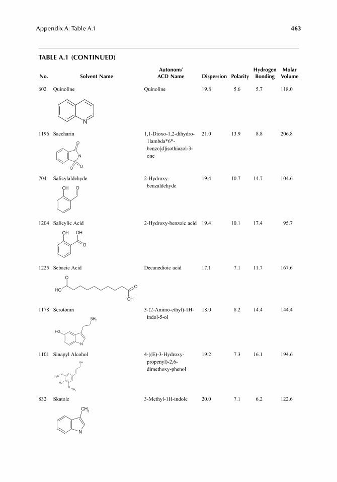
Appendix A: Table A.1 463
TABLE A.1 (CONTINUED)
No. Solvent NameAutonom/
ACD Name Dispersion PolarityHydrogenBonding
MolarVolume
602 Quinoline Quinoline 19.8 5.6 5.7 118.0
1196 Saccharin 1,1-Dioxo-1,2-dihydro-1lambda*6*-benzo[d]isothiazol-3-one
21.0 13.9 8.8 206.8
704 Salicylaldehyde 2-Hydroxy-benzaldehyde
19.4 10.7 14.7 104.6
1204 Salicylic Acid 2-Hydroxy-benzoic acid 19.4 10.1 17.4 95.7
1225 Sebacic Acid Decanedioic acid 17.1 7.1 11.7 167.6
1178 Serotonin 3-(2-Amino-ethyl)-1H-indol-5-ol
18.0 8.2 14.4 144.4
1101 Sinapyl Alcohol 4-((E)-3-Hydroxy-propenyl)-2,6-dimethoxy-phenol
19.2 7.3 16.1 194.6
832 Skatole 3-Methyl-1H-indole 20.0 7.1 6.2 122.6
N
SN
O O
O
OH O
OH OH
O
OH
O
OH
O
OH
N
NH2
O
O
OH
CH3
CH3
OH
N
CH3
7248_A001A.fm Page 463 Wednesday, May 23, 2007 12:38 PM
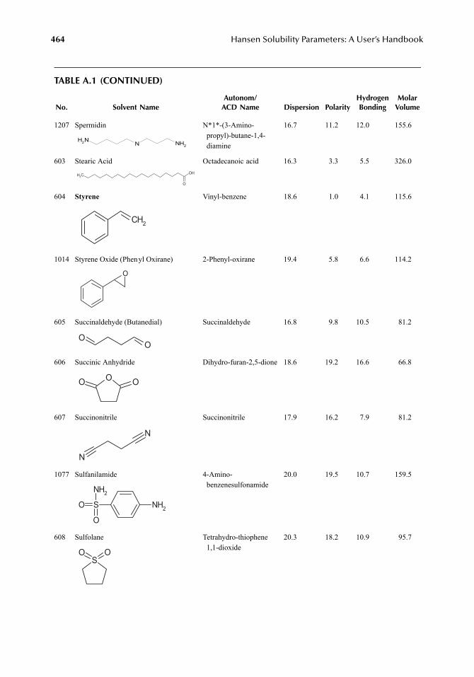
464 Hansen Solubility Parameters: A User’s Handbook
TABLE A.1 (CONTINUED)
No. Solvent NameAutonom/
ACD Name Dispersion PolarityHydrogenBonding
MolarVolume
1207 Spermidin N*1*-(3-Amino-propyl)-butane-1,4-diamine
16.7 11.2 12.0 155.6
603 Stearic Acid Octadecanoic acid 16.3 3.3 5.5 326.0
604 Styrene Vinyl-benzene 18.6 1.0 4.1 115.6
1014 Styrene Oxide (Phenyl Oxirane) 2-Phenyl-oxirane 19.4 5.8 6.6 114.2
605 Succinaldehyde (Butanedial) Succinaldehyde 16.8 9.8 10.5 81.2
606 Succinic Anhydride Dihydro-furan-2,5-dione 18.6 19.2 16.6 66.8
607 Succinonitrile Succinonitrile 17.9 16.2 7.9 81.2
1077 Sulfanilamide 4-Amino-benzenesulfonamide
20.0 19.5 10.7 159.5
608 Sulfolane Tetrahydro-thiophene 1,1-dioxide
20.3 18.2 10.9 95.7
NNH2 NH2
OH
O
CH3
CH2
O
OO
O OO
N
N
S
NH2
O
O
NH2
SO O
7248_A001A.fm Page 464 Wednesday, May 23, 2007 12:38 PM
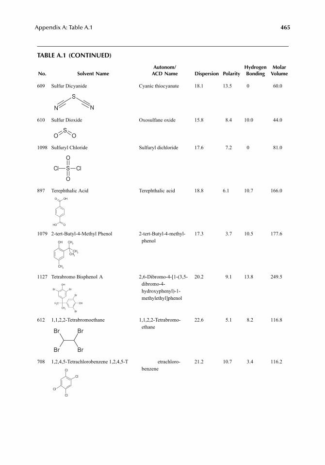
Appendix A: Table A.1 465
TABLE A.1 (CONTINUED)
No. Solvent NameAutonom/
ACD Name Dispersion PolarityHydrogenBonding
MolarVolume
609 Sulfur Dicyanide Cyanic thiocyanate 18.1 13.5 0 60.0
610 Sulfur Dioxide Oxosulfane oxide 15.8 8.4 10.0 44.0
1098 Sulfuryl Chloride Sulfuryl dichloride 17.6 7.2 0 81.0
897 Terephthalic Acid Terephthalic acid 18.8 6.1 10.7 166.0
1079 2-tert-Butyl-4-Methyl Phenol 2-tert-Butyl-4-methyl-phenol
17.3 3.7 10.5 177.6
1127 Tetrabromo Bisphenol A 2,6-Dibromo-4-[1-(3,5-dibromo-4-hydroxyphenyl)-1-methylethyl]phenol
20.2 9.1 13.8 249.5
612 1,1,2,2-Tetrabromoethane 1,1,2,2-Tetrabromo-ethane
22.6 5.1 8.2 116.8
708 1,2,4,5-Tetrachlorobenzene 1,2,4,5-T etrachloro-benzene
21.2 10.7 3.4 116.2
S
NN
OS
O
Cl S Cl
O
O
OHO
OH O
OH
CH3
CH3
CH3
CH3
CH3
CH3
OH
OH
Br Br
Br
Br
Br
Br
Br
Br
Cl
Cl
Cl
Cl
7248_A001A.fm Page 465 Wednesday, May 23, 2007 12:38 PM
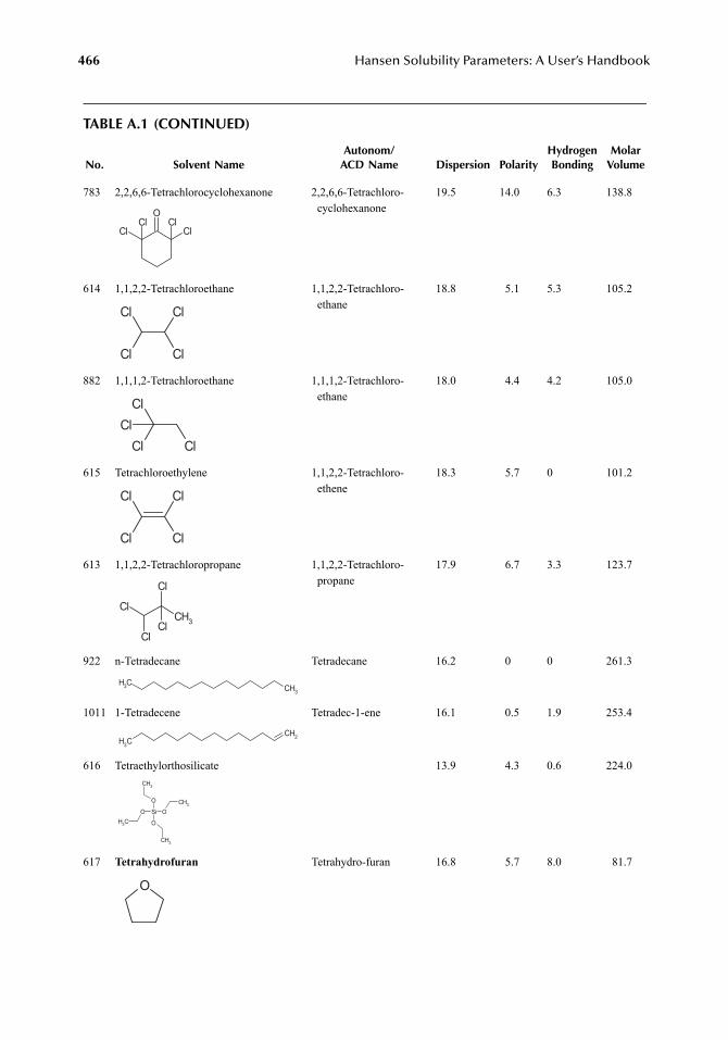
466 Hansen Solubility Parameters: A User’s Handbook
TABLE A.1 (CONTINUED)
No. Solvent NameAutonom/
ACD Name Dispersion PolarityHydrogenBonding
MolarVolume
783 2,2,6,6-Tetrachlorocyclohexanone 2,2,6,6-Tetrachloro-cyclohexanone
19.5 14.0 6.3 138.8
614 1,1,2,2-Tetrachloroethane 1,1,2,2-Tetrachloro-ethane
18.8 5.1 5.3 105.2
882 1,1,1,2-Tetrachloroethane 1,1,1,2-Tetrachloro-ethane
18.0 4.4 4.2 105.0
615 Tetrachloroethylene 1,1,2,2-Tetrachloro-ethene
18.3 5.7 0 101.2
613 1,1,2,2-Tetrachloropropane 1,1,2,2-Tetrachloro-propane
17.9 6.7 3.3 123.7
922 n-Tetradecane Tetradecane 16.2 0 0 261.3
1011 1-Tetradecene Tetradec-1-ene 16.1 0.5 1.9 253.4
616 Tetraethylorthosilicate 13.9 4.3 0.6 224.0
617 Tetrahydrofuran Tetrahydro-furan 16.8 5.7 8.0 81.7
O
ClCl
ClCl
Cl
Cl Cl
Cl
Cl
ClCl
Cl
Cl
Cl Cl
Cl
CH3
Cl
Cl
Cl
Cl
CH3 CH3
CH3
CH2
Si O
O
O
O
CH3
CH3
CH3
CH3
O
7248_A001A.fm Page 466 Wednesday, May 23, 2007 12:38 PM
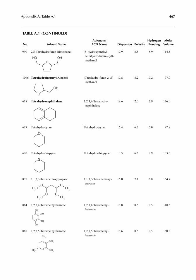
Appendix A: Table A.1 467
TABLE A.1 (CONTINUED)
No. Solvent NameAutonom/
ACD Name Dispersion PolarityHydrogenBonding
MolarVolume
999 2,5-Tetrahydrofuran Dimethanol (5-Hydroxymethyl-tetrahydro-furan-2-yl)-methanol
17.9 8.5 18.9 114.5
1096 Tetrahydrofurfuryl Alcohol (Tetrahydro-furan-2-yl)-methanol
17.8 8.2 10.2 97.0
618 Tetrahydronaphthalene 1,2,3,4-Tetrahydro-naphthalene
19.6 2.0 2.9 136.0
619 Tetrahydropyran Tetrahydro-pyran 16.4 6.3 6.0 97.8
620 Tetrahydrothiapyran Tetrahydro-thiopyran 18.5 6.3 8.9 103.6
895 1,1,3,3-Tetramethoxypropane 1,1,3,3-Tetramethoxy-propane
15.0 7.1 6.8 164.7
884 1,2,3,4-Tetramethylbenzene 1,2,3,4-Tetramethyl-benzene
18.8 0.5 0.5 148.3
885 1,2,3,5-Tetramethylbenzene 1,2,3,5-Tetramethyl-benzene
18.6 0.5 0.5 150.8
OOH OH
O
OH
O
S
CH3
O OCH3
OCH3
OCH3
CH3
CH3
CH3
CH3
CH3
CH3
CH3CH3
7248_A001A.fm Page 467 Wednesday, May 23, 2007 12:38 PM
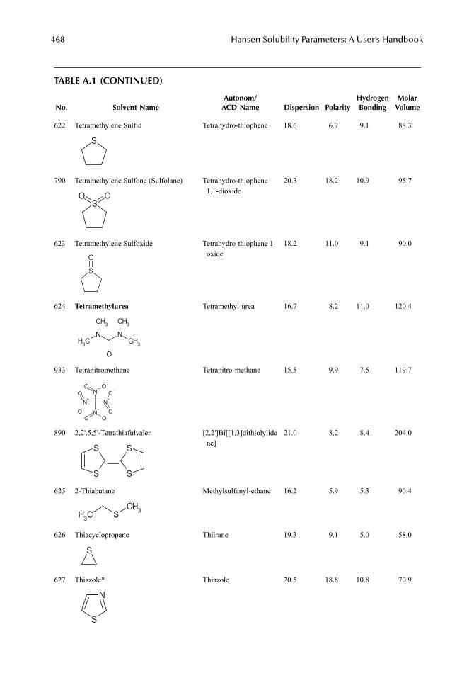
468 Hansen Solubility Parameters: A User’s Handbook
TABLE A.1 (CONTINUED)
No. Solvent NameAutonom/
ACD Name Dispersion PolarityHydrogenBonding
MolarVolume
622 Tetramethylene Sulfid Tetrahydro-thiophene 18.6 6.7 9.1 88.3
790 Tetramethylene Sulfone (Sulfolane) Tetrahydro-thiophene 1,1-dioxide
20.3 18.2 10.9 95.7
623 Tetramethylene Sulfoxide Tetrahydro-thiophene 1-oxide
18.2 11.0 9.1 90.0
624 Tetramethylurea Tetramethyl-urea 16.7 8.2 11.0 120.4
933 Tetranitromethane Tetranitro-methane 15.5 9.9 7.5 119.7
890 2,2',5,5'-Tetrathiafulvalen [2,2']Bi[[1,3]dithiolylidene]
21.0 8.2 8.4 204.0
625 2-Thiabutane Methylsulfanyl-ethane 16.2 5.9 5.3 90.4
626 Thiacyclopropane Thiirane 19.3 9.1 5.0 58.0
627 Thiazole* Thiazole 20.5 18.8 10.8 70.9
S
SO O
S
O
NNCH3
CH3
CH3
CH3
O
N+
N+
N+
N+ O
OO O
O
OO O
S
SS
S
CH3 SCH3
S
S
N
7248_A001A.fm Page 468 Wednesday, May 23, 2007 12:38 PM
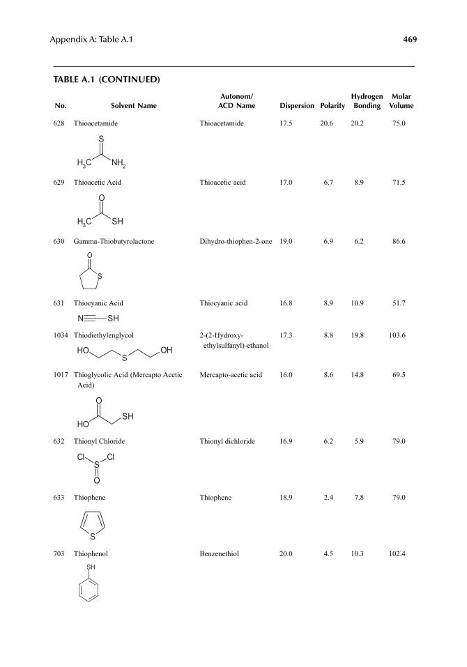
Appendix A: Table A.1 469
TABLE A.1 (CONTINUED)
No. Solvent NameAutonom/
ACD Name Dispersion PolarityHydrogenBonding
MolarVolume
628 Thioacetamide Thioacetamide 17.5 20.6 20.2 75.0
629 Thioacetic Acid Thioacetic acid 17.0 6.7 8.9 71.5
630 Gamma-Thiobutyrolactone Dihydro-thiophen-2-one 19.0 6.9 6.2 86.6
631 Thiocyanic Acid Thiocyanic acid 16.8 8.9 10.9 51.7
1034 Thiodiethylenglycol 2-(2-Hydroxy-ethylsulfanyl)-ethanol
17.3 8.8 19.8 103.6
1017 Thioglycolic Acid (Mercapto Acetic Acid)
Mercapto-acetic acid 16.0 8.6 14.8 69.5
632 Thionyl Chloride Thionyl dichloride 16.9 6.2 5.9 79.0
633 Thiophene Thiophene 18.9 2.4 7.8 79.0
703 Thiophenol Benzenethiol 20.0 4.5 10.3 102.4
CH3 NH2
S
CH3 SH
O
S
O
SHN
OHS
OH
OH
O
SH
SClCl
O
S
SH
7248_A001A.fm Page 469 Wednesday, May 23, 2007 12:38 PM
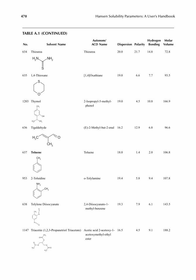
470 Hansen Solubility Parameters: A User’s Handbook
TABLE A.1 (CONTINUED)
No. Solvent NameAutonom/
ACD Name Dispersion PolarityHydrogenBonding
MolarVolume
634 Thiourea Thiourea 20.0 21.7 14.8 72.8
635 1,4-Thioxane [1,4]Oxathiane 19.0 6.6 7.7 93.5
1203 Thymol 2-Isopropyl-5-methyl-phenol
19.0 4.5 10.8 166.9
636 Tigaldehyde (E)-2-Methyl-but-2-enal 16.2 12.9 6.8 96.6
637 Toluene Toluene 18.0 1.4 2.0 106.8
953 2-Toluidine o-Tolylamine 19.4 5.8 9.4 107.8
638 Tolylene Diisocyanate 2,4-Diisocyanato-1-methyl-benzene
19.3 7.9 6.1 143.5
1147 Triacetin (1,2,3-Propanetriol Triacetate) Acetic acid 2-acetoxy-1-acetoxymethyl-ethyl ester
16.5 4.5 9.1 188.2
NH2NH2
S
O
S
OH
CH3CH3
CH3
CH3
CH3 O
CH3
NH2
CH3
N
CH3
N
O
O
O
OO
CH3
O
CH3
OCH3
O
7248_A001A.fm Page 470 Wednesday, May 23, 2007 12:38 PM
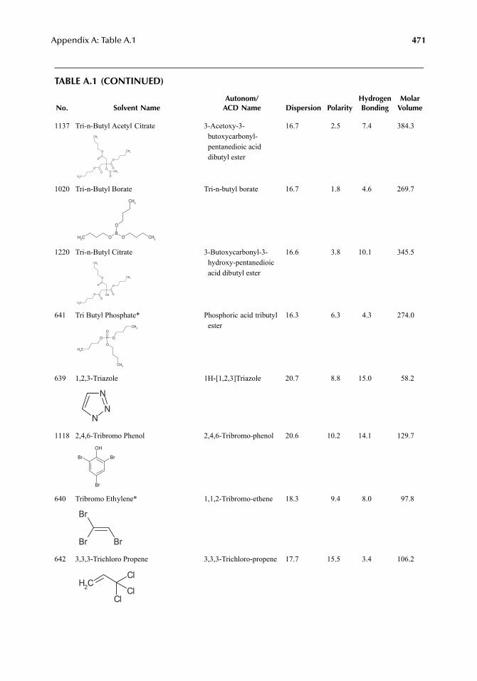
Appendix A: Table A.1 471
TABLE A.1 (CONTINUED)
No. Solvent NameAutonom/
ACD Name Dispersion PolarityHydrogenBonding
MolarVolume
1137 Tri-n-Butyl Acetyl Citrate 3-Acetoxy-3-butoxycarbonyl-pentanedioic acid dibutyl ester
16.7 2.5 7.4 384.3
1020 Tri-n-Butyl Borate Tri-n-butyl borate 16.7 1.8 4.6 269.7
1220 Tri-n-Butyl Citrate 3-Butoxycarbonyl-3-hydroxy-pentanedioic acid dibutyl ester
16.6 3.8 10.1 345.5
641 Tri Butyl Phosphate* Phosphoric acid tributyl ester
16.3 6.3 4.3 274.0
639 1,2,3-Triazole 1H-[1,2,3]Triazole 20.7 8.8 15.0 58.2
1118 2,4,6-Tribromo Phenol 2,4,6-Tribromo-phenol 20.6 10.2 14.1 129.7
640 Tribromo Ethylene* 1,1,2-Tribromo-ethene 18.3 9.4 8.0 97.8
642 3,3,3-Trichloro Propene 3,3,3-Trichloro-propene 17.7 15.5 3.4 106.2
O
O
O
O
O
OO
CH3
CH3
CH3O
CH3
CH3 OB
O CH3
O
CH3
OH
O
O
O
O
OO
CH3
CH3
CH3
P
O
O O
OCH3
CH3
CH3
NN
N
OH
Br
Br
Br
Br
Br Br
CH2
Cl
ClCl
7248_A001A.fm Page 471 Wednesday, May 23, 2007 12:38 PM
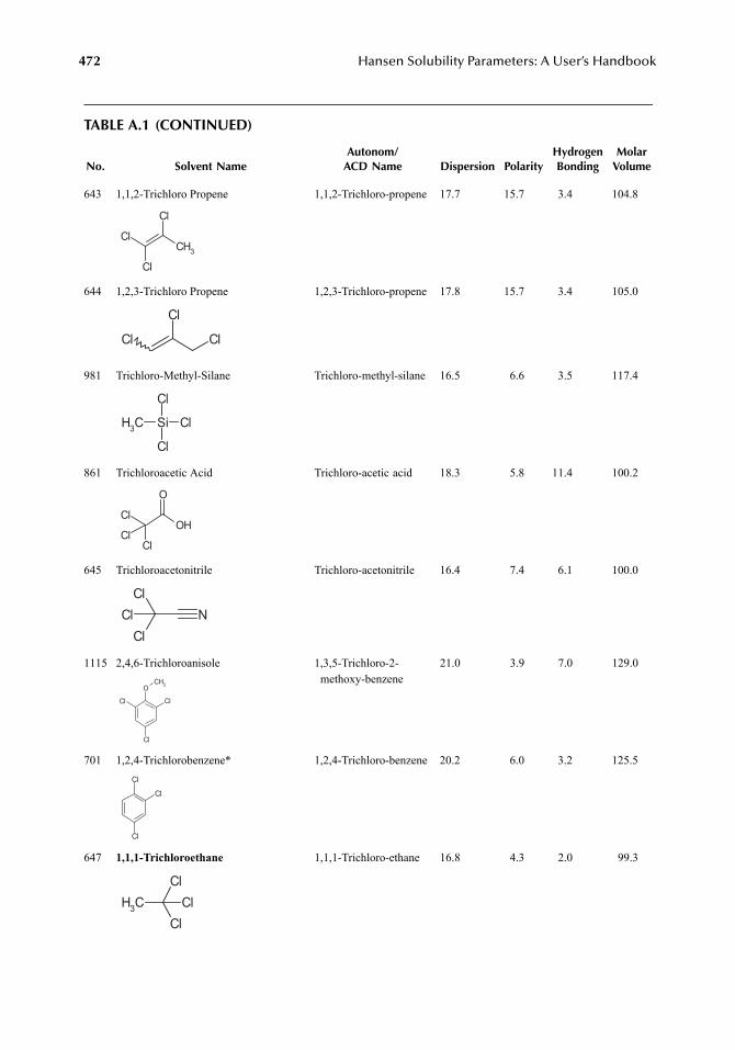
472 Hansen Solubility Parameters: A User’s Handbook
TABLE A.1 (CONTINUED)
No. Solvent NameAutonom/
ACD Name Dispersion PolarityHydrogenBonding
MolarVolume
643 1,1,2-Trichloro Propene 1,1,2-Trichloro-propene 17.7 15.7 3.4 104.8
644 1,2,3-Trichloro Propene 1,2,3-Trichloro-propene 17.8 15.7 3.4 105.0
981 Trichloro-Methyl-Silane Trichloro-methyl-silane 16.5 6.6 3.5 117.4
861 Trichloroacetic Acid Trichloro-acetic acid 18.3 5.8 11.4 100.2
645 Trichloroacetonitrile Trichloro-acetonitrile 16.4 7.4 6.1 100.0
1115 2,4,6-Trichloroanisole 1,3,5-Trichloro-2-methoxy-benzene
21.0 3.9 7.0 129.0
701 1,2,4-Trichlorobenzene* 1,2,4-Trichloro-benzene 20.2 6.0 3.2 125.5
647 1,1,1-Trichloroethane 1,1,1-Trichloro-ethane 16.8 4.3 2.0 99.3
Cl
Cl
CH3
Cl
Cl
ClCl
CH3 Si Cl
Cl
Cl
OH
O
Cl
ClCl
NCl
ClCl
OCH3
Cl
Cl
Cl
Cl
Cl
Cl
CH3
Cl
ClCl
7248_A001A.fm Page 472 Wednesday, May 23, 2007 12:38 PM
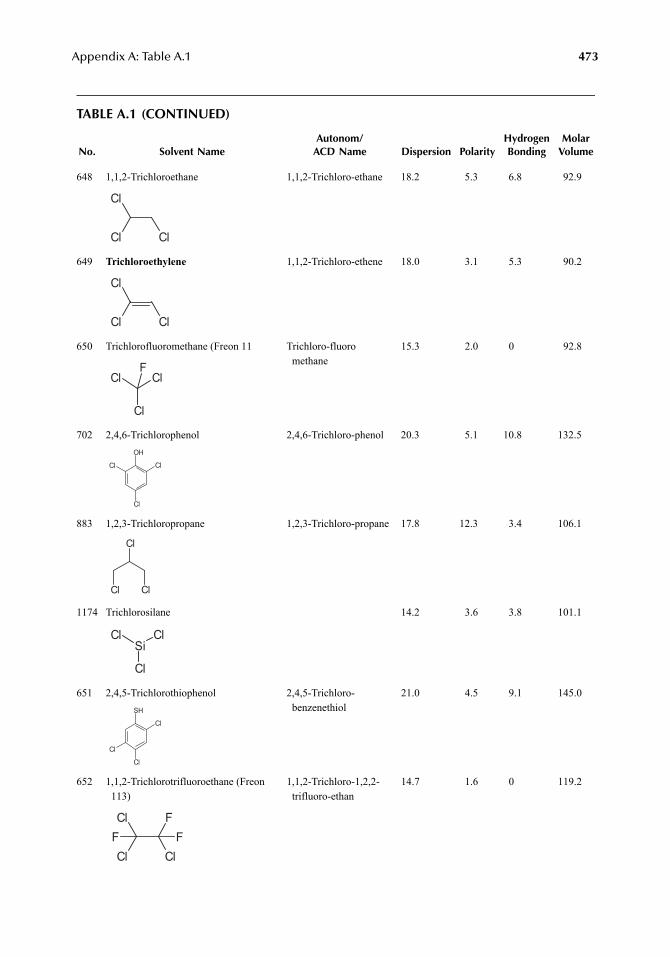
Appendix A: Table A.1 473
TABLE A.1 (CONTINUED)
No. Solvent NameAutonom/
ACD Name Dispersion PolarityHydrogenBonding
MolarVolume
648 1,1,2-Trichloroethane 1,1,2-Trichloro-ethane 18.2 5.3 6.8 92.9
649 Trichloroethylene 1,1,2-Trichloro-ethene 18.0 3.1 5.3 90.2
650 Trichlorofluoromethane (Freon 11 Trichloro-fluoromethane
15.3 2.0 0 92.8
702 2,4,6-Trichlorophenol 2,4,6-Trichloro-phenol 20.3 5.1 10.8 132.5
883 1,2,3-Trichloropropane 1,2,3-Trichloro-propane 17.8 12.3 3.4 106.1
1174 Trichlorosilane 14.2 3.6 3.8 101.1
651 2,4,5-Trichlorothiophenol 2,4,5-Trichloro-benzenethiol
21.0 4.5 9.1 145.0
652 1,1,2-Trichlorotrifluoroethane (Freon113)
1,1,2-Trichloro-1,2,2-trifluoro-ethan
14.7 1.6 0 119.2
Cl
Cl Cl
Cl
Cl Cl
ClCl
Cl
F
Cl
Cl
Cl
OH
Cl
Cl
Cl
SiClCl
Cl
SH
Cl
Cl
Cl
Cl
Cl ClF
FF
7248_A001A.fm Page 473 Wednesday, May 23, 2007 12:38 PM
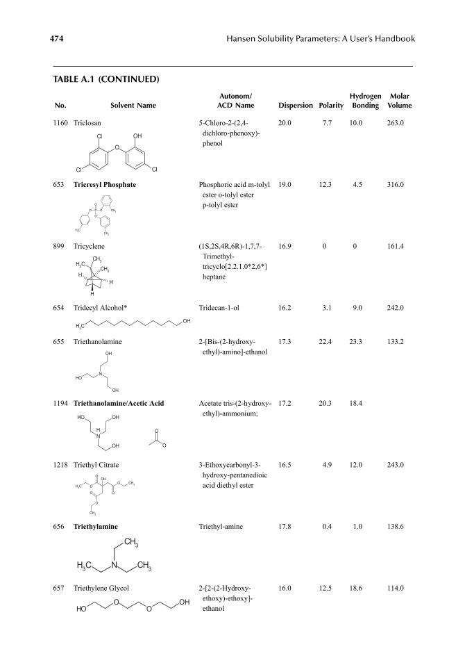
474 Hansen Solubility Parameters: A User’s Handbook
TABLE A.1 (CONTINUED)
No. Solvent NameAutonom/
ACD Name Dispersion PolarityHydrogenBonding
MolarVolume
1160 Triclosan 5-Chloro-2-(2,4-dichloro-phenoxy)-phenol
20.0 7.7 10.0 263.0
653 Tricresyl Phosphate Phosphoric acid m-tolyl ester o-tolyl ester p-tolyl ester
19.0 12.3 4.5 316.0
899 Tricyclene (1S,2S,4R,6R)-1,7,7-Trimethyl-tricyclo[2.2.1.0*2,6*] heptane
16.9 0 0 161.4
654 Tridecyl Alcohol* Tridecan-1-ol 16.2 3.1 9.0 242.0
655 Triethanolamine 2-[Bis-(2-hydroxy-ethyl)-amino]-ethanol
17.3 22.4 23.3 133.2
1194 Triethanolamine/Acetic Acid Acetate tris-(2-hydroxy-ethyl)-ammonium;
17.2 20.3 18.4
1218 Triethyl Citrate 3-Ethoxycarbonyl-3-hydroxy-pentanedioic acid diethyl ester
16.5 4.9 12.0 243.0
656 Triethylamine Triethyl-amine 17.8 0.4 1.0 138.6
657 Triethylene Glycol 2-[2-(2-Hydroxy-ethoxy)-ethoxy]-ethanol
16.0 12.5 18.6 114.0
O
OHCl
ClCl
P
O
O O
O
CH3
CH3
CH3
CH3
CH3CH3
HH
H
CH3
OH
N
OH
OH
OH
NH+
OH
OH OH
O
O
O
O
CH3
O
O
O
O
CH3
CH3
OH
NCH3
CH3
CH3
OHO
OOH
7248_A001A.fm Page 474 Wednesday, May 23, 2007 12:38 PM
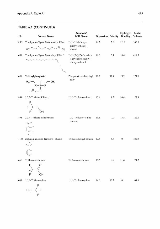
Appendix A: Table A.1 475
TABLE A.1 (CONTINUED)
No. Solvent NameAutonom/
ACD Name Dispersion PolarityHydrogenBonding
MolarVolume
856 Triethylene Glycol Monomethyl Ether 2-[2-(2-Methoxy-ethoxy)-ethoxy]-ethanol
16.2 7.6 12.5 160.0
658 Triethylene Glycol Monooleyl Ether* 2-(2-{2-[((Z)-Octadec-9-enyl)oxy]-ethoxy}-ethoxy)-ethanol
16.0 3.1 8.4 418.5
659 Triethylphosphate Phosphoric acid triethyl ester
16.7 11.4 9.2 171.0
944 2,2,2-Trifluoro Ethano 2,2,2-Trifluoro-ethano 15.4 8.3 16.4 72.3
795 2,3,4-Trifluoro Nitrobenzen 1,2,3-Trifluoro-4-nitrobenzene
19.5 7.7 3.5 122.0
1158 alpha,alpha,alpha Trifluoro oluene Trifluoromethyl-benzen 17.5 8.8 0 122.9
660 Trifluoroacetic Aci Trifluoro-acetic acid 15.6 9.9 11.6 74.2
661 1,1,1-Trifluoroethan 1,1,1-Trifluoro-ethan 14.6 10.7 0 64.6
OHO
OO
CH3
O
CH3
OHO
O
O P O
O
O
CH3
CH3
CH3
OHF
FF
N+ OO
F
F
F
FFF
OH
OF
FF
CH3
F
FF
7248_A001A.fm Page 475 Wednesday, May 23, 2007 12:38 PM
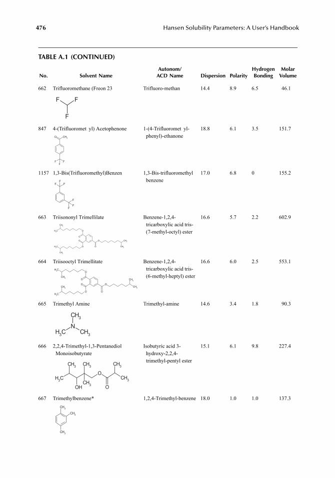
476 Hansen Solubility Parameters: A User’s Handbook
TABLE A.1 (CONTINUED)
No. Solvent NameAutonom/
ACD Name Dispersion PolarityHydrogenBonding
MolarVolume
662 Trifluoromethane (Freon 23 Trifluoro-methan 14.4 8.9 6.5 46.1
847 4-(Trifluoromet yl) Acetophenone 1-(4-Trifluoromet yl-phenyl)-ethanone
18.8 6.1 3.5 151.7
1157 1,3-Bis(Trifluoromethyl)Benzen 1,3-Bis-trifluoromethylbenzene
17.0 6.8 0 155.2
663 Triisononyl Trimellilate Benzene-1,2,4-tricarboxylic acid tris-(7-methyl-octyl) ester
16.6 5.7 2.2 602.9
664 Triisooctyl Trimellitate Benzene-1,2,4-tricarboxylic acid tris-(6-methyl-heptyl) ester
16.6 6.0 2.5 553.1
665 Trimethyl Amine Trimethyl-amine 14.6 3.4 1.8 90.3
666 2,2,4-Trimethyl-1,3-Pentanediol Monoisobutyrate
Isobutyric acid 3-hydroxy-2,2,4-trimethyl-pentyl ester
15.1 6.1 9.8 227.4
667 Trimethylbenzene* 1,2,4-Trimethyl-benzene 18.0 1.0 1.0 137.3
FF
F
CH3O
F FF
FFF
F
F
F
O
O
O
O
O
O
CH3
CH3
CH3
CH3
CH3
CH3
O
O
O
O
O
O
CH3
CH3
CH3
CH3
CH3
CH3
CH3
NCH3
CH3
CH3
O
OH
CH3
CH3
CH3
O
CH3
CH3
CH3
CH3
CH3
7248_A001A.fm Page 476 Wednesday, May 23, 2007 12:38 PM
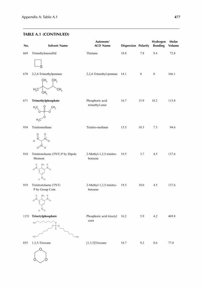
Appendix A: Table A.1 477
TABLE A.1 (CONTINUED)
No. Solvent NameAutonom/
ACD Name Dispersion PolarityHydrogenBonding
MolarVolume
669 Trimethylenesulfid Thietane 18.8 7.8 9.4 72.8
670 2,2,4-Trimethylpentane 2,2,4-Trimethyl-pentane 14.1 0 0 166.1
671 Trimethylphosphate Phosphoric acid trimethyl ester
16.7 15.9 10.2 115.8
934 Trinitomethane Trinitro-methane 15.5 10.3 7.3 94.6
918 Trinitrotoluene (TNT) P by Dipole Moment
2-Methyl-1,3,5-trinitro-benzene
19.5 3.7 4.5 137.6
919 Trinitrotoluene (TNT) P by Group Cont.
2-Methyl-1,3,5-trinitro-benzene
19.5 10.0 4.5 137.6
1151 Trioctylphosphate Phosphoric acid trioctyl ester
16.2 5.9 4.2 469.8
855 1,3,5-Trioxane [1,3,5]Trioxane 18.7 9.2 8.6 77.0
S
CH3 CH3
CH3
CH3
CH3
O P O
O
O
CH3
CH3
CH3
N+
N+
N+
O
OO
O
O O
CH3
N+
N+
N+
O
O O
O
O O
CH3
N+
N+
N+
O
O O
O
O O
OPO
O
O
CH3CH3
CH3
O O
O
7248_A001A.fm Page 477 Wednesday, May 23, 2007 12:38 PM
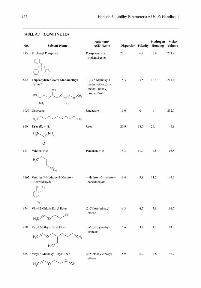
478 Hansen Solubility Parameters: A User’s Handbook
TABLE A.1 (CONTINUED)
No. Solvent NameAutonom/
ACD Name Dispersion PolarityHydrogenBonding
MolarVolume
1150 Triphenyl Phosphate Phosphoric acid triphenyl ester
20.1 6.4 6.8 271.9
672 Tripropylene Glycol Monomethyl Ether*
1-[2-(2-Methoxy-1-methyl-ethoxy)-1-methyl-ethoxy]-propan-2-ol
15.3 5.5 10.4 214.0
1059 Undecane Undecane 16.0 0 0 212.7
860 Urea (Ro = 19.4) Urea 20.9 18.7 26.4 45.8
673 Valeronitrile Pentanenitrile 15.3 11.0 4.8 103.8
1162 Vanillin (4-Hydroxy-3-Methoxy Benzaldehyde)
4-Hydroxy-3-methoxy-benzaldehyde
19.4 9.8 11.2 144.1
674 Vinyl 2-Chloro Ethyl Ether (2-Chloro-ethoxy)-ethene
16.3 6.7 5.8 101.7
908 Vinyl 2-Ethyl-Hexyl Ether 3-Vinyloxymethyl-heptane
15.6 3.4 4.2 194.2
675 Vinyl 2-Methoxy Ethyl Ether (2-Methoxy-ethoxy)-ethene
15.9 6.7 6.8 96.2
OPO
O
O
O
CH3
O
CH3CH3
OHO
CH3
CH3 CH3
NH2NH2
O
CH3
N
O
OH CH3
O
CH2 OCl
CH2 O CH3
CH3
CH2 OO
CH3
7248_A001A.fm Page 478 Wednesday, May 23, 2007 12:38 PM
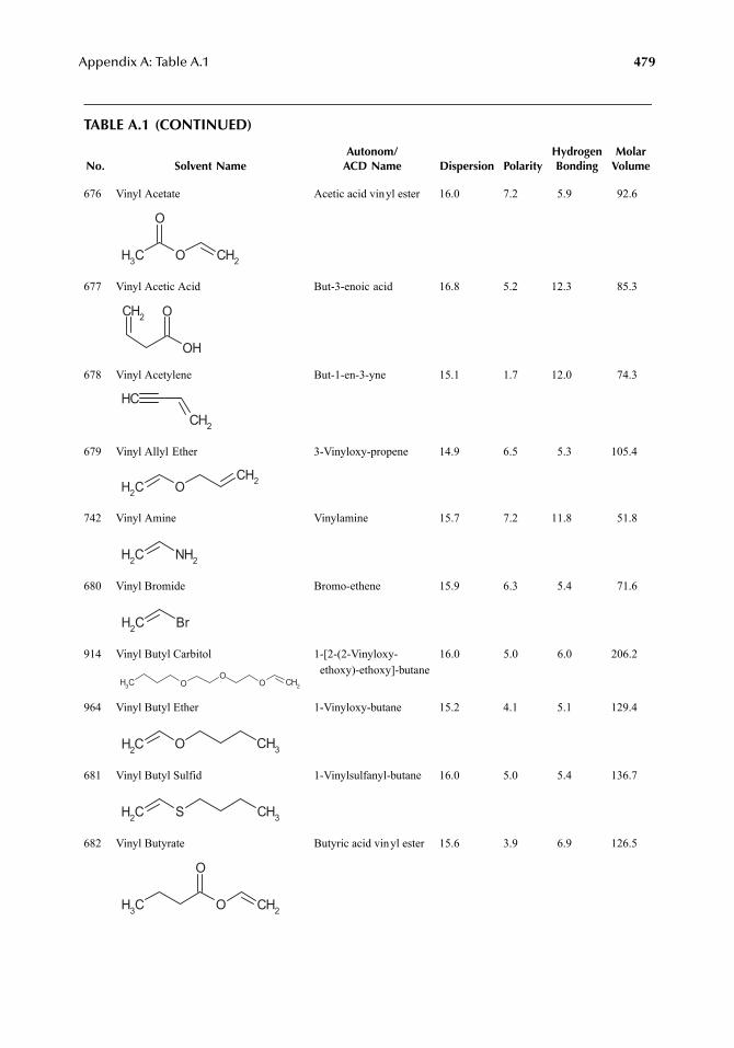
Appendix A: Table A.1 479
TABLE A.1 (CONTINUED)
No. Solvent NameAutonom/
ACD Name Dispersion PolarityHydrogenBonding
MolarVolume
676 Vinyl Acetate Acetic acid vinyl ester 16.0 7.2 5.9 92.6
677 Vinyl Acetic Acid But-3-enoic acid 16.8 5.2 12.3 85.3
678 Vinyl Acetylene But-1-en-3-yne 15.1 1.7 12.0 74.3
679 Vinyl Allyl Ether 3-Vinyloxy-propene 14.9 6.5 5.3 105.4
742 Vinyl Amine Vinylamine 15.7 7.2 11.8 51.8
680 Vinyl Bromide Bromo-ethene 15.9 6.3 5.4 71.6
914 Vinyl Butyl Carbitol 1-[2-(2-Vinyloxy-ethoxy)-ethoxy]-butane
16.0 5.0 6.0 206.2
964 Vinyl Butyl Ether 1-Vinyloxy-butane 15.2 4.1 5.1 129.4
681 Vinyl Butyl Sulfid 1-Vinylsulfanyl-butane 16.0 5.0 5.4 136.7
682 Vinyl Butyrate Butyric acid vinyl ester 15.6 3.9 6.9 126.5
CH3 O
O
CH2
OH
OCH2
CHCH2
CH2 OCH2
CH2 NH2
CH2 Br
OO CH2OCH3
CH2 O CH3
CH2 S CH3
CH3 O
O
CH2
7248_A001A.fm Page 479 Wednesday, May 23, 2007 12:38 PM
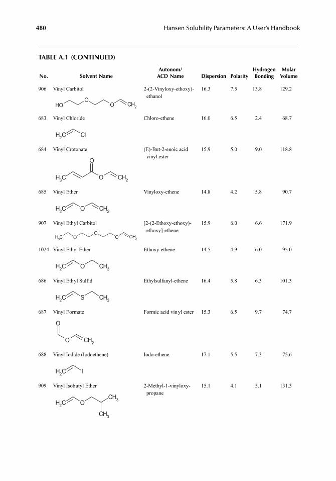
480 Hansen Solubility Parameters: A User’s Handbook
TABLE A.1 (CONTINUED)
No. Solvent NameAutonom/
ACD Name Dispersion PolarityHydrogenBonding
MolarVolume
906 Vinyl Carbitol 2-(2-Vinyloxy-ethoxy)-ethanol
16.3 7.5 13.8 129.2
683 Vinyl Chloride Chloro-ethene 16.0 6.5 2.4 68.7
684 Vinyl Crotonate (E)-But-2-enoic acid vinyl ester
15.9 5.0 9.0 118.8
685 Vinyl Ether Vinyloxy-ethene 14.8 4.2 5.8 90.7
907 Vinyl Ethyl Carbitol [2-(2-Ethoxy-ethoxy)-ethoxy]-ethene
15.9 6.0 6.6 171.9
1024 Vinyl Ethyl Ether Ethoxy-ethene 14.5 4.9 6.0 95.0
686 Vinyl Ethyl Sulfid Ethylsulfanyl-ethene 16.4 5.8 6.3 101.3
687 Vinyl Formate Formic acid vinyl ester 15.3 6.5 9.7 74.7
688 Vinyl Iodide (Iodoethene) Iodo-ethene 17.1 5.5 7.3 75.6
909 Vinyl Isobutyl Ether 2-Methyl-1-vinyloxy-propane
15.1 4.1 5.1 131.3
OO CH2OH
CH2 Cl
O
O
CH3 CH2
CH2 O CH2
OO CH2OCH3
CH2 O CH3
CH2 S CH3
O
O CH2
CH2 I
CH2 OCH3
CH3
7248_A001A.fm Page 480 Wednesday, May 23, 2007 12:38 PM
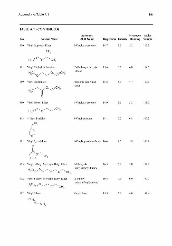
Appendix A: Table A.1 481
TABLE A.1 (CONTINUED)
No. Solvent NameAutonom/
ACD Name Dispersion PolarityHydrogenBonding
MolarVolume
910 Vinyl Isopropyl Ether 2-Vinyloxy-propane 14.7 3.5 5.2 115.3
911 Vinyl Methyl Cellosolve (2-Methoxy-ethoxy)-ethene
15.6 6.2 6.8 114.7
689 Vinyl Propionate Propionic acid vinyl ester
15.6 8.0 4.7 110.1
690 Vinyl Propyl Ether 1-Vinyloxy-propane 14.9 3.5 5.2 113.0
843 4-Vinyl Pyridine 4-Vinyl-pyridine 18.1 7.2 6.8 107.3
691 Vinyl Pyrrolidone 1-Vinyl-pyrrolidin-2-one 16.4 9.3 5.9 106.9
913 Vinyl S-Butyl Mercapto Butyl Ether 1-Ethoxy-4-vinylsulfanyl-butane
16.5 5.0 5.8 174.0
912 Vinyl S-Ethyl Mercapto Ethyl Ether (2-Ethoxy-ethylsulfanyl)-ethene
16.4 7.0 6.0 139.7
692 Vinyl Silane Vinyl-silane 15.5 2.6 4.0 89.4
CH2 O CH3
CH3
OO
CH2CH3
CH3
O
O
CH2
CH2 OCH3
N
CH2
N
O
CH2
SCH2 O CH3
SCH2 O CH3
SiH3
CH2
7248_A001A.fm Page 481 Wednesday, May 23, 2007 12:38 PM
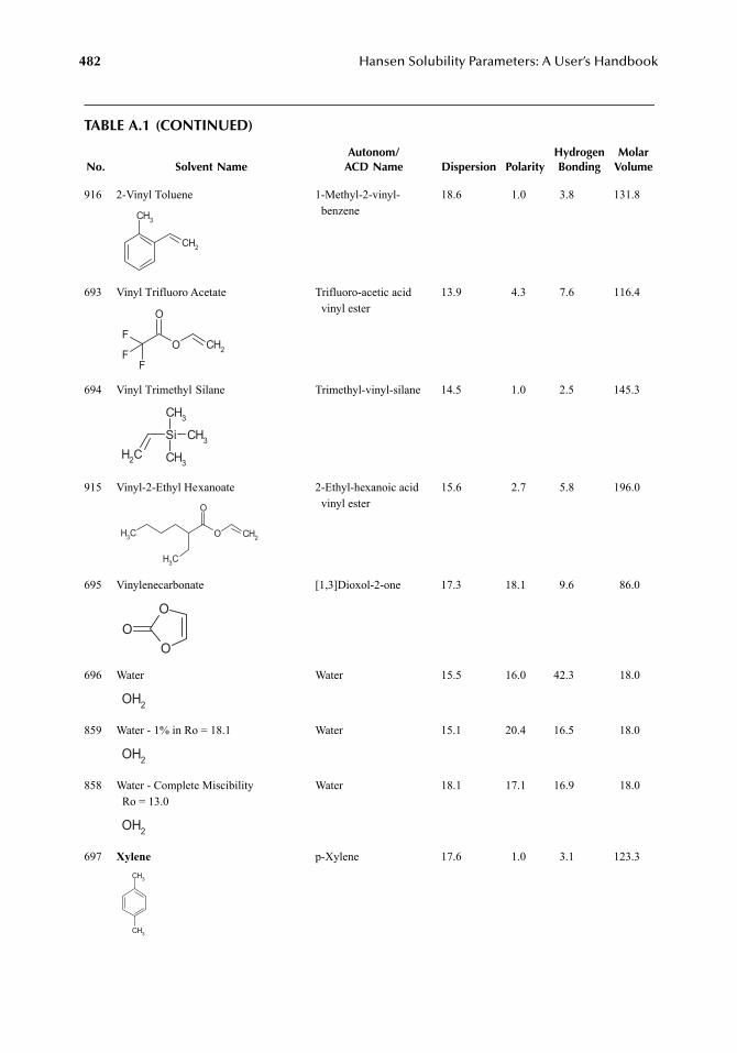
482 Hansen Solubility Parameters: A User’s Handbook
TABLE A.1 (CONTINUED)
No. Solvent NameAutonom/
ACD Name Dispersion PolarityHydrogenBonding
MolarVolume
916 2-Vinyl Toluene 1-Methyl-2-vinyl-benzene
18.6 1.0 3.8 131.8
693 Vinyl Trifluoro Acetate Trifluoro-acetic acid vinyl ester
13.9 4.3 7.6 116.4
694 Vinyl Trimethyl Silane Trimethyl-vinyl-silane 14.5 1.0 2.5 145.3
915 Vinyl-2-Ethyl Hexanoate 2-Ethyl-hexanoic acid vinyl ester
15.6 2.7 5.8 196.0
695 Vinylenecarbonate [1,3]Dioxol-2-one 17.3 18.1 9.6 86.0
696 Water Water 15.5 16.0 42.3 18.0
859 Water - 1% in Ro = 18.1 Water 15.1 20.4 16.5 18.0
858 Water - Complete MiscibilityRo = 13.0
Water 18.1 17.1 16.9 18.0
697 Xylene p-Xylene 17.6 1.0 3.1 123.3
CH3
CH2
O
O
F
FF
CH2
SiCH2
CH3
CH3
CH3
O
O
CH3
CH2CH3
O
OO
OH2
OH2
OH2
CH3
CH3
7248_A001A.fm Page 482 Wednesday, May 23, 2007 12:38 PM
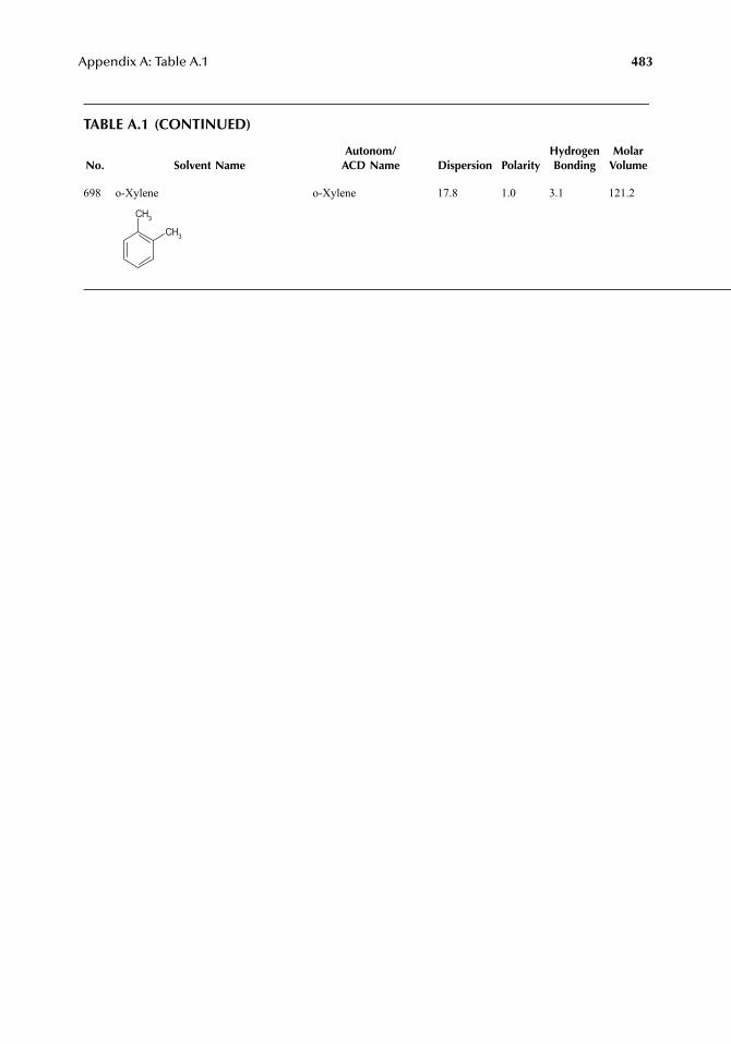
Appendix A: Table A.1 483
TABLE A.1 (CONTINUED)
No. Solvent NameAutonom/
ACD Name Dispersion PolarityHydrogenBonding
MolarVolume
698 o-Xylene o-Xylene 17.8 1.0 3.1 121.2
CH3
CH3
7248_A001A.fm Page 483 Wednesday, May 23, 2007 12:38 PM

7248_A001A.fm Page 484 Wednesday, May 23, 2007 12:38 PM
485
Appendix A: Table A.2
COMMENTS TO TABLE A.2
Documentation for the sources of data used for the HSP correlations is gi ven in the following. Thequality of the entries is sometimes less than desired because of the data being too fe w, too limitedin scope and range of HSP , or for other reasons discussed in the te xt, such as the influence omolecular weight (molecular volume) of the test solv ents in the given study. All entries have beenincluded (with some apologies) as the y have some value in terms of estimating, ho wever.
P
OLYMERS
1–109
These polymers are listed in Reference 1 with suppliers. This report from the Scandina vian Paintand Printing Ink Research Institute updates an earlier one from 1982. The institute no longer exists.See also Reference 2.
P
OLYMER
110
This is an intermediate v alue for the permeation of chemicals through Challenge
®
materials [3].See also Table 13.1 and Figure 13.2. Impro ved v alues are found belo w in 141 and 142. Thiscorrelation was based on few data to help locate additional solv ents for testing. Results from testswith these then resulted in the correlations belo w.
P
OLYMERS
111–112
These are correlations of true solubilities for the DO W epoxy Novolacs 438 and 444.
P
OLYMERS
113–114
These are correlations of the chemical resistance of coatings based on inor ganic zinc silicate anda two component epoxy produced by Hempel’ s Marine Paints. Data taken from resistance tables.
P
OLYMER
115
The data are solubilities determined for PVDF with the correlation being previously published in [4].
P
OLYMER
116
Data for coal tar pitch generated for the solubility of the solids not dissolv ed in some cases wherethe solution was darkened with only partial solution.
P
OLYMERS
117–140
Permeation correlations for chemical protecti ve clothing described in detail in Reference 5. Seealso Chapter 13, Table 13.1.
7248_A002.fm Page 485 Wednesday, May 23, 2007 12:53 PM
486
Hansen Solubility Parameters: A User’s Handbook
P
OLYMERS
141–142
Final permeation correlations for Challenge
®
5100 and 5200 materials. Data from Reference 3where there is considerable discussion. See also Chapter 13, Table 13.1, and Figure 13.2.
P
OLYMERS
143–144
These correlations are based on which solv ents dissolve PVDC at ele vated temperatures and usedata from Wessling [6]. These were additionally used to check ne w calculations for solubilityparameters of the solv ents where these were lacking.
P
OLYMERS
145–148
These chemical resistance data for PES (ICI-V ictrex
®
) and PPS (Philips-Ryton
®
) were based onsupplier data sheets and are reported in Reference 7.
Polymers 149–160
These correlations for man y common plastics types are based on the resistance tables reported inthe PLASTGUIDE (1989) published by the Danish compan y Dukadan, which no longer e xists.A single correlation for the solubility of P A 6,6 is based on its solubility only with data fromReference 8.
P
OLYMER
161
Beerbower treated several sets of data and made correlations of swelling and solubility (and otherphenomena). This one is for polyvin yl silane.
P
OLYMERS
162–163
These correlations for swelling of cellophane and solubility of eth ylene vinyl alcohol copolymerare based on data generated at NIF (Scandina vian Paint and Printing Ink Research Institute).
P
OLYMERS
164–167
These are supplementary breakthrough time correlations for Sarane x
®
, Safety 4
®
4H, and polyvi-nylalcohol protective gloves. See also Reference 5 and Chapter 13. Elimination of plasticizer datafor the 4H glo ves improved predictability for lo wer molecular weight materials.
P
OLYMERS
168–181
These correlations for common polymer types are based on data in resistance tables in the
ModernPlastics Encyclopedia
in the 1984/1985 issue [9]. Such data are not al ways sufficiently encompassing to allow good correlations.
P
OLYMER
182
Correlation based on high temperature solv ents for ECTFE.
P
OLYMER
183
Data for this correlation of solubility of polyacrylonitrile were tak en from the
Polymer Handbook
[10], Table of solvents and nonsolvents, p. VII/385-VII/386. See also Chapter 5, Table 5.3.
7248_A002.fm Page 486 Wednesday, May 23, 2007 12:53 PM
Appendix A: Table A.2
487
P
OLYMERS
184–186
Data for this correlation are the tendency of Polyethylene imide (PEI) (GE Ultem
®
) to environmentalstress crack (ESC) at dif ferent stress/strain levels. These data were generated by General Electricas published in the
Modern Plastics Encyclopedia
1984/1985 [9].
P
OLYMERS
187–224
The
Handbook of Solubility Parameters and Other Cohesion Parameters
[11] as well as the
PolymerHandbook
[12] included so-called “solvent range” data. Solvents were divided into groups of poor,moderate, and strong h ydrogen bonding, and man y experiments were run. The correlations sho wthat not all the data were well tak en, b ut a reasonable indication is possible. The full Hansensolubility parameter system is not covered very well by this limited solubility data. These polymersare included in Reference 11, Table 1, on page 280. Heating samples to speed up the solutionprocess was also done. This can easily lead to errors.
P
OLYMERS
225–346
These entries have the same problem as those in 187–224 in that the data are sometimes questionableand not suf ficient enough to do what has been done, i.e. co vert solv ent range data to Hansensolubility parameter spheres. These entries cover the acrylics, polyesters, polystyrenes, vinyls, andmiscellaneous categories. Some cate gories are not yet included. Data on page 281-289 (T able 2)in Reference 11.
Polymer 347
These values for VYHH
®
(Union Carbide) were tak en from Reference 1.
P
OLYMER
348
This questionable correlation for PVF includes only one solv ent as being good [13].
P
OLYMER
349
Data on PES true solubility tak en by author. See Chapter 5 and Table 5.4.
P
OLYMERS
350–358
These entries are not all polymers but mostly biological materials with the source of data being [14].
P
OLYMER
359
The solubility of cholesterol, data collected by the author . See Chapter 15.
P
OLYMER
360
Solubility data generated by high school students as part of project. Included in Reference 4. Sourceof chlorophyll was crushed leaves.
Polymer 361
Correlation on strength of paper immersed in dif ferent solvents reported in Reference 4. Data w astaken from Reference 15.
7248_A002.fm Page 487 Wednesday, May 23, 2007 12:53 PM
488
Hansen Solubility Parameters: A User’s Handbook
P
OLYMER
362
Solubility of ULTRASON
®
PES has been reported by BASF in their product data. These data werecombined with supplementary solubility data for this correlation. Also reported in Reference 16.See Chapter 5.
P
OLYMERS
363–364
Chemical resistance of B AREX
®
210 from data in BP Chemicals datasheet. Styrene is an outlierin the first, whereas its rem val from consideration gives a perfect fit and presumably a more usefucorrelation.
P
OLYMERS
365–367
These data were generated in connection with a lecture to the Nordic Conserv ation Congress inCopenhagen [17]. All give perfect fits, partly because of too f w data, but the correlations can beuseful. Paraloid B72 and Dammar are used as protecti ve lacquers.
P
OLYMERS
368–369
These correlations di vide the permeation coef ficients g ven in Reference 18 into >80 and >0.8,respectively. The units are (g x mm)/(m
2
x d). The fits are good. See Chapter 13.
P
OLYMERS
370–371
These are correlations of e xperimental solubility data for the Rhône-Poulenc reacti ve isocyanatesTolonate
®
HDT (which g ave the same result as Tolonate
®
HDT-LV) and Tolonate
®
HDB (whichgave the same results as Tolonate
®
HDB-LV). The fits were perfect and the numbers reasonableThe data could not include alcohol or amine solv ents because of reactions.
P
OLYMERS
372–389
The data correlated for these 18 rubbers are from a RAPRA database [19]. The information usedwas satisfactory or unsatisf actory, all other information such as limited suitability w as neglected.No precise weight g ain or other information is a vailable, just the general suitability or not.
The values in parentheses are (data fit/number of sol ents).
ACM acrylate rubbers (.981/55)ECO epichlorohydrin rubbers (.988/37)CSM chlorosulphonated polyethylene rubber (.906/53)E ebonite (.722/41)EPM ethylene-propylene copolymer (.987/47)EPDM ethylene-propylene terpolymer (.968/51)FQ fluorosilicone rubber (.844/40FKM hexafluoroprop.-vi ylidine fluoride copol. ( iton) (.769/50)NR natural rubber (1.000/59)NBR nitrile rubber (.990/65)FFKM Kalrez
®
(Du Pont) (too resistant to correlate)CR polychloroprene (.877/54)AU polyester polyurethane (.959/63)EU polyether polyurethane (.959/63)T polysulphide rubber (.799/48)Q silicone (.748/53)
7248_A002.fm Page 488 Wednesday, May 23, 2007 12:53 PM
Appendix A: Table A.2
489
SBR styrene butadiene rubber (.942/54)TFP tetrafluoroet ylene-propylene copolymer (.744/26)
P
OLYMERS
390–412
These correlations use data from the RAPRA collection of data on chemical resistance for plastics[20]. Approach same as for RAPRA rubber data just abo ve.
P
OLYMERS
413–450
These data are from the collected report of the EC project on self-stratifying coatings reported ina full issue of
Progress in Organic Coatings
. The specific reference is Reference 21.The evaluationswere made at dif ferent concentrations in man y cases. Some alk yds were omitted here.
P
OLYMERS
451–452
These data are for strong swelling of tw o different film samples of brominated utyl rubber.
P
OLYMER
453
The correlation is based on strong swelling of a film of polyisoprene
P
OLYMERS
454–458
These correlations are based on chemical resistance data from Reference 22.
P
OLYMER
459
Correlation based on solubility of Eth ylene Vinylacetate adhesive EVA 4055.
P
OLYMER
460
Correlation based on solubility of Topas
®
6013 from Ticona GmbH (Hoechst AG).
P
OLYMER
461
Correlation based on solubility of CZ
®
Resin from the West Company.
P
OLYMER
462
An older correlation for the solubility of Kauri Gum, used in the Kauri-Butanol test, w as madewith a data fit of 0.95 for the standard sol ents.
P
OLYMER
463
The data for the solubility of polyvin ylpyrrolidone used in this correlation are found in Reference23. The data fit as 0.992, b ut as with man y w ater soluble polymers, there is a considerableextrapolation into the “unkno wn” where there are no liquids.
E
NTRY
464
The data fit for the correlation of solubility of palm oil with the standard set of sol ents was 0.992.
7248_A002.fm Page 489 Wednesday, May 23, 2007 12:53 PM
490
Hansen Solubility Parameters: A User’s Handbook
E
NTRY
465
This is a correlation of the solubility of a fungicide and algaecide called Bethoxazin using solubilitydata in 19 liquids from Reference 24. The data fit as 0.976.
ENTRY 466
This is a correlation for the solubility of carbon-60 at a gi ven small level as reported in Reference25; 15 of the 87 liquids were considered as “good” gi ving a data fit of 0.972
REFERENCES
1. Saarnak, A., Hansen C.M., and Wallström E., Solubility Parameters — Characterization of Paints andPolymers, Report from Scandina vian Paint and Printing Ink Research Institute, January 1990, Hoer -sholm, Denmark
2. Hansen, C.M., Solubility Parameters, in Paint Testing Manual, Manual 17, J.V. Koleske, Ed., AmericanSociety for Testing and Materials, Philadelphia, 1995, pp. 38–404.
3. Hansen, C.M., Billing, C.B., and Bentz, A.P., Selection and Use of Molecular P arameters to PredictPermeation Through Fluoropolymer-Based Protective Clothing Materials, The Performance of Pro-tective Clothing; Fourth Volume, ASTM STP 1133, J.P. McBriarty and N.W. Henry, Eds., AmericanSociety for Testing and Materials, Philadelphia, 1992, pp. 894–907.
4. Hansen, C.M., 25 Years with Solubility Parameters (in Danish: 25 År med Opløselighedsparametrene),Dansk Kemi, 73(8), 18–22, 1992.
5. Hansen, C.M. and Hansen, K.M., Solubility Parameter Prediction of the Barrier Properties of ChemicalProtective Clothing, Performance of Protective Clothing: Second Symposium. ASTM STP 989, S.Z.Mansdorf, R. Sager, and A.P. Nielsen, Eds., American Society for Testing and Materials, Philadelphia,1988, pp. 197–208.
6. Wessling, R.A., The Solubility of Poly(vinylidene Chloride), Journal of Applied Polymer Science, 14,1531–1545, 1970.
7. Hansen, C.M., Solubility Parameters for Polyphenylene Sulfide (PPS) and Polyether Sulphone (PES),Centre for Polymer Composites (Denmark), Danish Technological Institute, Taastrup, 1991, 89 pages.ISBN 87-7756-139-2
8. Wyzgoski, M.G., The Role of Solubility in Stress Cracking of Nylon 6,6, in Macromolecular Solutions— Solvent Property Relationships in Polymers, R.B.Seymour and G.A.Stahl, Eds. Per gamon, NewYork, 1982, pp. 41–60.
9 Anonymous, Modern Plastics Enc yclopedia 1984/1985, McGraw-Hill, New York, pp. 482–455.10. Fuchs, O., Tables of Solvents and Non-solvents, Polymer Handbook, 3rd Ed., J. Branderup and E.H.
Immergut, Eds., Wiley, New York, 1989, pp. VII/379-VII/407.11. Barton, A.F.M., Handbook of Solubility Parameters and Other Cohesion Parameters, CRC Press Inc.,
Boca Raton, FL. 1983, pp. 280-289. 12. Grulke, E.A., Table 3.4, Solubility Parameter Ranges of Commercial Polymers , Polymer Handbook,
3rd Ed., J. Branderup and E.H. Immer gut, Eds., Wiley, New York, 1989, pp. VII/544–VII/550. 13. Fuchs, O., Tables of Solvents and Non-solvents, Polymer Handbook, 3rd. Ed., J. Branderup and E.H.
Immergut, Eds., Wiley, New York, 1989, p. VII/385.14. Hansen, C.M. and Andersen, B.H., The Affinities of O ganic Solvents in Biological Systems, Amer-
ican Industrial Hygiene Association Journal, 49(6), 301–308, 1988.15. Robertson, A.A., Cellulose-Liquid Interactions, Pulp and Paper Magazine of Canada, 65(4), T-171-
T-178, 1964.16. Hansen, C.M., Solvent Resistance of Polymer Composites — Glass Fibre Reinforced Polyether Sulfone
(PES), Centre for Polymer Composites (Denmark), Danish Technological Institute, Taastrup, 1994.17. Hansen, C.M., Conservation and Solubility Parameters, Nordic Conserv ation Congress Preprints,
Copenhagen, 1994, pp. 1–13.18. Pauly, S., Permeability and Dif fusion Data, Polymer Handbook, 3rd. Ed., J. Branderup and E.H.
Immergut, Eds., Wiley, New York, 1989, pp. VI/435–VI/449.
7248_A002.fm Page 490 Wednesday, May 23, 2007 12:53 PM
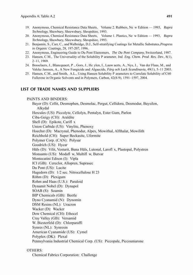
Appendix A: Table A.2 491
19. Anonymous, Chemical Resistance Data Sheets, Volume 2. Rubbers, Ne w Edition — 1993, RapraTechnology, Shawbury, Shrewsbury, Shropshire, 1993.
20. Anonymous, Chemical Resistance Data Sheets, Volume 1. Plastics, Ne w Edition — 1993, RapraTechnology, Shawbury, Shrewsbury, Shropshire, 1993.
21. Benjamin, S., Carr, C., and Walbridge, D.J., Self-stratifying Coatings for Metallic Substrates, Progressin Organic Coatings, 28, 197-207, 1996.
22. Anonymous, Engineering Guide to Du Pont Elastomers, The Du Pont Company, Switzerland, 1987.23. Hansen, C.M., The Universality of the Solubility P arameter, Ind. Eng. Chem. Prod. Res. Dev., 8(1),
2–11, 1969.24. Bosselaers, J., Blancquaert, P ., Gors, J., He ylen, I., Lauw aerts, A., Nys, J., Van der Flaas, M., and
Valcke Janssen, A., A New Fungicide and Algaecide, Färg och Lack Scandinavia, 49(1), 5–11 2003.25. Hansen, C.M., and Smith, A.L., Using Hansen Solubility P arameters to Correlate Solubility of C60
Fullerene in Organic Solvents and in Polymers, Carbon, 42(8-9), 1591–1597, 2004.
LIST OF TRADE NAMES AND SUPPLIERS
PAINTS AND BINDERS:Bayer (D): Cellit, Desmophen, Desmolac, Pergut, Cellidora, Desmodur, Baysilon,
AlkydalHercules (US): Piccolyte, Cellolyn, Pentalyn, Ester Gum, ParlonCiba-Geigy (CH): AralditeShell (D): Epikote, Carifl xUnion Carbide (US): Vinylite, PhenoxyHoechst (D): Macrynal, Phenodur, Alpex, Mowithal, Alfthalat, MowilithReichhold (CH): Super Beckasite, UformitePolymer Corp. (CAN): PolysarGoodrich (US): HycarHüls (D): Vilit, Vesturit, Buna Hüls, Lutonal, Larofl x, Plastopal, PolystrenMonsanto (US): Modafl w, Multifl w, ButvarMontecatini Edison (I): ViplaICI (GB): Cereclor, Allopren, SuprasecDu Pont (US): LuciteHagedorn (D): 1/2 sec. Nitrocellulose H 23Röhm (D): PlexigumRohm and Haas (U.S.): ParaloidDynamit Nobel (D): DynapolSOAB (S): SoaminBIP Chemicals (GB): BeetleDyno Cyanamid (N): DynominDSM Resins (NL): UracronWacker (D): WackerDow Chemical (CH): EthocelCray Valley (GB): VersamidW. Biesterfeld (D): ChlorparaffiSynres (NL): SynresinAmerican Cyanamide (US): CymelPolyplex (DK): PlexalPennsylvania Industrial Chemical Corp. (US): Piccopale, Piccoumarone
OTHERS:Chemical Fabrics Corporation: Challenge
7248_A002.fm Page 491 Wednesday, May 23, 2007 12:53 PM
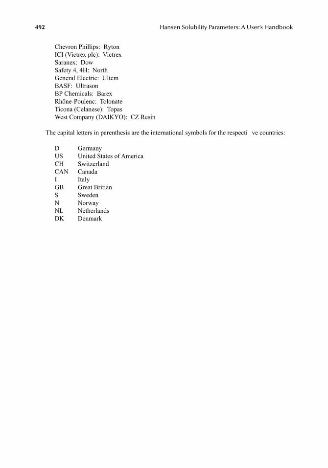
492 Hansen Solubility Parameters: A User’s Handbook
Chevron Phillips: RytonICI (Victrex plc): VictrexSaranex: DowSafety 4, 4H: NorthGeneral Electric: UltemBASF: UltrasonBP Chemicals: BarexRhône-Poulenc: TolonateTicona (Celanese): TopasWest Company (DAIKYO): CZ Resin
The capital letters in parenthesis are the international symbols for the respecti ve countries:
D GermanyUS United States of AmericaCH SwitzerlandCAN CanadaI ItalyGB Great BritianS SwedenN NorwayNL NetherlandsDK Denmark
7248_A002.fm Page 492 Wednesday, May 23, 2007 12:53 PM
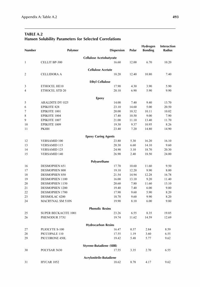
Appendix A: Table A.2 493
TABLE A.2Hansen Solubility Parameters for Selected Correlations
Number Polymer Dispersion PolarHydrogenBonding
InteractionRadius
Cellulose Acetobutyrate1 CELLIT BP-300 16.60 12.00 6.70 10.20
Cellulose Acetate2 CELLIDORA A 18.20 12.40 10.80 7.40
Ethyl Cellulose3 ETHOCEL HE10 17.90 4.30 3.90 5.904 ETHOCEL STD 20 20.10 6.90 5.90 9.90
Epoxy5 ARALDITE DY O25 14.00 7.40 9.40 13.706 EPIKOTE 828 23.10 14.60 5.00 20.507 EPIKOTE 1001 20.00 10.32 10.11 10.028 EPIKOTE 1004 17.40 10.50 9.00 7.909 EPIKOTE 1007 21.00 11.10 13.40 11.7010 EPIKOTE 1009 19.30 9.37 10.95 8.2611 PKHH 23.40 7.20 14.80 14.90
Epoxy Curing Agents12 VERSAMID 100 23.80 5.30 16.20 16.1013 VERSAMID 115 20.30 6.60 14.10 9.6014 VERSAMID 125 24.90 3.10 18.70 20.3015 VERSAMID 140 26.90 2.40 18.50 24.00
Polyurethane16 DESMOPHEN 651 17.70 10.60 11.60 9.5017 DESMOPHEN 800 19.10 12.20 9.90 8.0018 DESMOPHEN 850 21.54 14.94 12.28 16.7819 DESMOPHEN 1100 16.00 13.10 9.20 11.4020 DESMOPHEN 1150 20.60 7.80 11.60 13.1021 DESMOPHEN 1200 19.40 7.40 6.00 9.8022 DESMOPHEN 1700 17.90 9.60 5.90 8.2023 DESMOLAC 4200 18.70 9.60 9.90 8.2024 MACRYNAL SM 510N 19.90 8.10 6.00 9.80
Phenolic Resins25 SUPER BECKACITE 1001 23.26 6.55 8.35 19.8526 PHENODUR 373U 19.74 11.62 14.59 12.69
Hydrocarbon Resins27 PLIOLYTE S-100 16.47 0.37 2.84 8.5928 PICCOPALE 110 17.55 1.19 3.60 6.5529 PICCORONE 450L 19.42 5.48 5.77 9.62
Styrene-Butadiene (SBR)30 POLYSAR 5630 17.55 3.35 2.70 6.55
Acrylonitrile-Butadiene31 HYCAR 1052 18.62 8.78 4.17 9.62
7248_A002.fm Page 493 Wednesday, May 23, 2007 12:53 PM
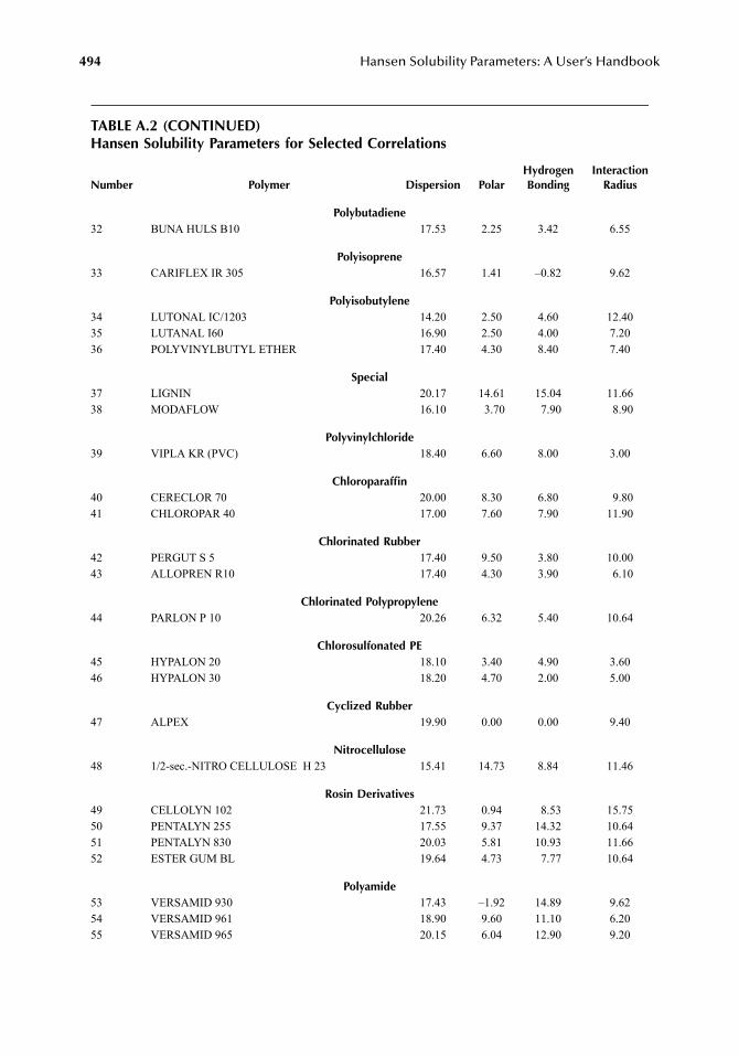
494 Hansen Solubility Parameters: A User’s Handbook
TABLE A.2 (CONTINUED)Hansen Solubility Parameters for Selected Correlations
Number Polymer Dispersion PolarHydrogenBonding
InteractionRadius
Polybutadiene32 BUNA HULS B10 17.53 2.25 3.42 6.55
Polyisoprene33 CARIFLEX IR 305 16.57 1.41 –0.82 9.62
Polyisobutylene34 LUTONAL IC/1203 14.20 2.50 4.60 12.4035 LUTANAL I60 16.90 2.50 4.00 7.2036 POLYVINYLBUTYL ETHER 17.40 4.30 8.40 7.40
Special37 LIGNIN 20.17 14.61 15.04 11.6638 MODAFLOW 16.10 3.70 7.90 8.90
Polyvinylchloride39 VIPLA KR (PVC) 18.40 6.60 8.00 3.00
Chloroparaffin40 CERECLOR 70 20.00 8.30 6.80 9.8041 CHLOROPAR 40 17.00 7.60 7.90 11.90
Chlorinated Rubber42 PERGUT S 5 17.40 9.50 3.80 10.0043 ALLOPREN R10 17.40 4.30 3.90 6.10
Chlorinated Polypropylene44 PARLON P 10 20.26 6.32 5.40 10.64
Chlorosulfonated PE45 HYPALON 20 18.10 3.40 4.90 3.6046 HYPALON 30 18.20 4.70 2.00 5.00
Cyclized Rubber47 ALPEX 19.90 0.00 0.00 9.40
Nitrocellulose48 1/2-sec.-NITRO CELLULOSE H 23 15.41 14.73 8.84 11.46
Rosin Derivatives49 CELLOLYN 102 21.73 0.94 8.53 15.7550 PENTALYN 255 17.55 9.37 14.32 10.6451 PENTALYN 830 20.03 5.81 10.93 11.6652 ESTER GUM BL 19.64 4.73 7.77 10.64
Polyamide53 VERSAMID 930 17.43 –1.92 14.89 9.6254 VERSAMID 961 18.90 9.60 11.10 6.2055 VERSAMID 965 20.15 6.04 12.90 9.20
7248_A002.fm Page 494 Wednesday, May 23, 2007 12:53 PM
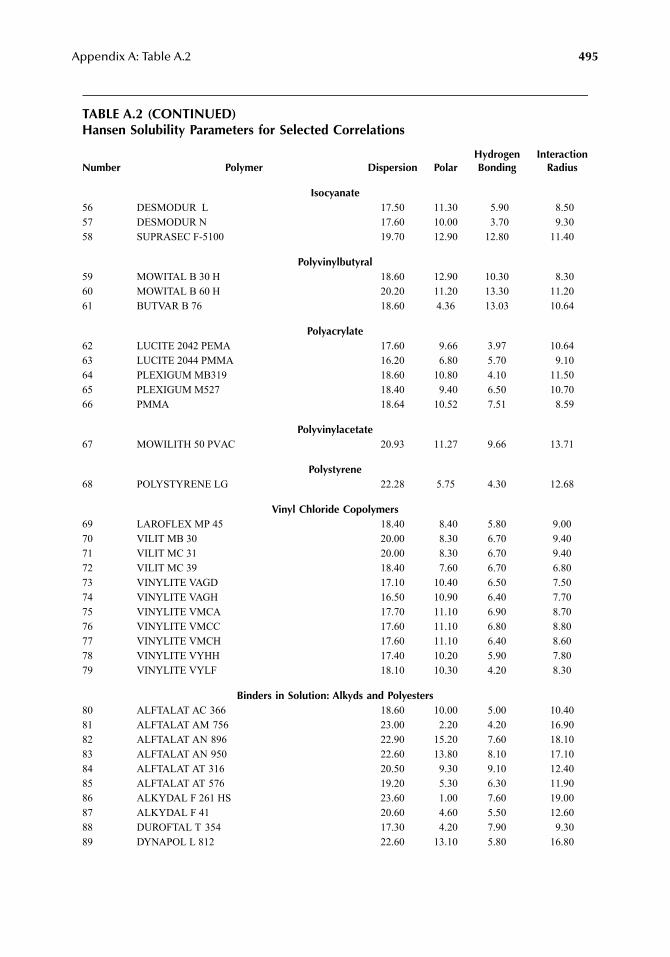
Appendix A: Table A.2 495
TABLE A.2 (CONTINUED)Hansen Solubility Parameters for Selected Correlations
Number Polymer Dispersion PolarHydrogenBonding
InteractionRadius
Isocyanate56 DESMODUR L 17.50 11.30 5.90 8.5057 DESMODUR N 17.60 10.00 3.70 9.3058 SUPRASEC F-5100 19.70 12.90 12.80 11.40
Polyvinylbutyral59 MOWITAL B 30 H 18.60 12.90 10.30 8.3060 MOWITAL B 60 H 20.20 11.20 13.30 11.2061 BUTVAR B 76 18.60 4.36 13.03 10.64
Polyacrylate62 LUCITE 2042 PEMA 17.60 9.66 3.97 10.6463 LUCITE 2044 PMMA 16.20 6.80 5.70 9.1064 PLEXIGUM MB319 18.60 10.80 4.10 11.5065 PLEXIGUM M527 18.40 9.40 6.50 10.7066 PMMA 18.64 10.52 7.51 8.59
Polyvinylacetate67 MOWILITH 50 PVAC 20.93 11.27 9.66 13.71
Polystyrene68 POLYSTYRENE LG 22.28 5.75 4.30 12.68
Vinyl Chloride Copolymers69 LAROFLEX MP 45 18.40 8.40 5.80 9.0070 VILIT MB 30 20.00 8.30 6.70 9.4071 VILIT MC 31 20.00 8.30 6.70 9.4072 VILIT MC 39 18.40 7.60 6.70 6.8073 VINYLITE VAGD 17.10 10.40 6.50 7.5074 VINYLITE VAGH 16.50 10.90 6.40 7.7075 VINYLITE VMCA 17.70 11.10 6.90 8.7076 VINYLITE VMCC 17.60 11.10 6.80 8.8077 VINYLITE VMCH 17.60 11.10 6.40 8.6078 VINYLITE VYHH 17.40 10.20 5.90 7.8079 VINYLITE VYLF 18.10 10.30 4.20 8.30
Binders in Solution: Alkyds and Polyesters80 ALFTALAT AC 366 18.60 10.00 5.00 10.4081 ALFTALAT AM 756 23.00 2.20 4.20 16.9082 ALFTALAT AN 896 22.90 15.20 7.60 18.1083 ALFTALAT AN 950 22.60 13.80 8.10 17.1084 ALFTALAT AT 316 20.50 9.30 9.10 12.4085 ALFTALAT AT 576 19.20 5.30 6.30 11.9086 ALKYDAL F 261 HS 23.60 1.00 7.60 19.0087 ALKYDAL F 41 20.60 4.60 5.50 12.6088 DUROFTAL T 354 17.30 4.20 7.90 9.3089 DYNAPOL L 812 22.60 13.10 5.80 16.80
7248_A002.fm Page 495 Wednesday, May 23, 2007 12:53 PM
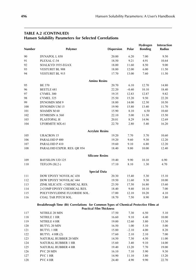
496 Hansen Solubility Parameters: A User’s Handbook
TABLE A.2 (CONTINUED)Hansen Solubility Parameters for Selected Correlations
Number Polymer Dispersion PolarHydrogenBonding
InteractionRadius
90 DYNAPOL L 850 20.00 6.20 7.00 9.5091 PLEXAL C-34 18.50 9.21 4.91 10.6492 SOALKYD 1935-EGAX 18.00 11.60 8.50 9.0093 VESTURIT BL 908 18.80 12.00 6.00 11.5094 VESTURIT BL 915 17.70 13.00 7.60 11.50
Amino Resins95 BE 370 20.70 6.10 12.70 14.8096 BEETLE 681 22.20 –0.40 10.10 18.4097 CYMEL 300 19.35 12.83 12.87 9.8298 CYMEL 325 25.50 15.20 9.50 22.2099 DYNOMIN MM 9 18.80 14.00 12.30 10.50100 DYNOMIN UM 15 19.90 15.80 13.40 11.70101 SOAMIN M 60 15.90 8.10 6.50 10.60102 SYNRESIN A 560 22.10 5.00 11.30 15.50103 PLASTOPAL H 20.81 8.29 14.96 12.69104 UFORMITE MX-61 22.70 2.80 5.40 16.20
Acrylate Resins105 URACRON 15 19.20 7.70 5.70 10.60106 PARALOID P 400 19.20 9.60 9.30 12.20107 PARALOID P 410 19.60 9.10 6.80 12.20108 PARALOID EXPER. RES. QR 954 18.40 9.80 10.00 12.40
Silicone Resins109 BAYSILON UD 125 19.40 9.90 10.10 6.90110 TEFLON (SL2-) 17.10 8.10 1.30 4.70
Special Data111 DOW EPOXY NOVOLAC 438 20.30 15.40 5.30 15.10112 DOW EPOXY NOVOLAC 444 19.50 11.60 9.30 10.00113 ZINK SILICATE - CHEMICAL RES. 23.50 17.50 16.80 15.60114 2-COMP EPOXY CHEMICAL RES. 18.40 9.40 10.10 7.00115 POLYVINYLIDINE FLUORIDE SOL. 17.00 12.10 10.20 4.10116 COAL TAR PITCH SOL. 18.70 7.50 8.90 5.80
Breakthrough Time (Bt) Correlations for Common Types of Chemical Protective Films at Practical Film Thickness
117 NITRILE 20 MIN 17.50 7.30 6.50 5.10118 NITRILE 1 HR 16.60 9.10 4.40 10.00119 NITRILE 4 HR 19.00 12.60 3.80 13.30120 BUTYL 20 MIN 16.50 1.00 5.10 5.00121 BUTYL 1 HR 15.80 –2.10 4.00 8.20122 BUTYL 4 HR (2) 17.60 2.10 2.10 7.00123 NATURAL RUBBER 20 MIN 14.50 7.30 4.50 11.00124 NATURAL RUBBER 1 HR 15.60 3.40 9.10 14.00125 NATURAL RUBBER 4 HR 19.40 13.20 7.70 19.00126 PVC 20 MIN 16.10 7.10 5.90 9.30127 PVC 1 HR 14.90 11.10 3.80 13.20128 PVC 4 HR 24.40 4.90 9.90 22.70
7248_A002.fm Page 496 Wednesday, May 23, 2007 12:53 PM
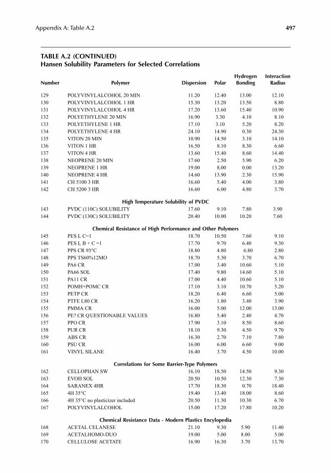
Appendix A: Table A.2 497
TABLE A.2 (CONTINUED)Hansen Solubility Parameters for Selected Correlations
Number Polymer Dispersion PolarHydrogenBonding
InteractionRadius
129 POLYVINYLALCOHOL 20 MIN 11.20 12.40 13.00 12.10130 POLYVINYLALCOHOL 1 HR 15.30 13.20 13.50 8.80131 POLYVINYLALCOHOL 4 HR 17.20 13.60 15.40 10.90132 POLYETHYLENE 20 MIN 16.90 3.30 4.10 8.10133 POLYETHYLENE 1 HR 17.10 3.10 5.20 8.20134 POLYETHYLENE 4 HR 24.10 14.90 0.30 24.30135 VITON 20 MIN 10.90 14.50 3.10 14.10136 VITON 1 HR 16.50 8.10 8.30 6.60137 VITON 4 HR 13.60 15.40 8.60 14.40138 NEOPRENE 20 MIN 17.60 2.50 5.90 6.20139 NEOPRENE 1 HR 19.00 8.00 0.00 13.20140 NEOPRENE 4 HR 14.60 13.90 2.30 15.90141 CH 5100 3 HR 16.60 5.40 4.00 3.80142 CH 5200 3 HR 16.60 6.00 4.80 3.70
High Temperature Solubility of PVDC143 PVDC (110C) SOLUBILITY 17.60 9.10 7.80 3.90144 PVDC (130C) SOLUBILITY 20.40 10.00 10.20 7.60
Chemical Resistance of High Performance and Other Polymers145 PES L C=1 18.70 10.50 7.60 9.10146 PES L B + C =1 17.70 9.70 6.40 9.30147 PPS CR 93°C 18.80 4.80 6.80 2.80148 PPS TS60%12MO 18.70 5.30 3.70 6.70149 PA6 CR 17.00 3.40 10.60 5.10150 PA66 SOL 17.40 9.80 14.60 5.10151 PA11 CR 17.00 4.40 10.60 5.10152 POMH+POMC CR 17.10 3.10 10.70 5.20153 PETP CR 18.20 6.40 6.60 5.00154 PTFE L80 CR 16.20 1.80 3.40 3.90155 PMMA CR 16.00 5.00 12.00 13.00156 PE? CR QUESTIONABLE VALUES 16.80 5.40 2.40 4.70157 PPO CR 17.90 3.10 8.50 8.60158 PUR CR 18.10 9.30 4.50 9.70159 ABS CR 16.30 2.70 7.10 7.80160 PSU CR 16.00 6.00 6.60 9.00161 VINYL SILANE 16.40 3.70 4.50 10.00
Correlations for Some Barrier-Type Polymers162 CELLOPHAN SW 16.10 18.50 14.50 9.30163 EVOH SOL 20.50 10.50 12.30 7.30164 SARANEX 4HR 17.70 18.30 0.70 18.40165 4H 35°C 19.40 13.40 18.00 8.60166 4H 35°C no plasticizer included 20.50 11.30 10.30 6.70167 POLYVINYLALCOHOL 15.00 17.20 17.80 10.20
Chemical Resistance Data - Modern Plastics Encylopedia168 ACETAL CELANESE 21.10 9.30 5.90 11.40169 ACETALHOMO-DUO 19.00 5.00 8.00 5.00170 CELLULOSE ACETATE 16.90 16.30 3.70 13.70
7248_A002.fm Page 497 Wednesday, May 23, 2007 12:53 PM
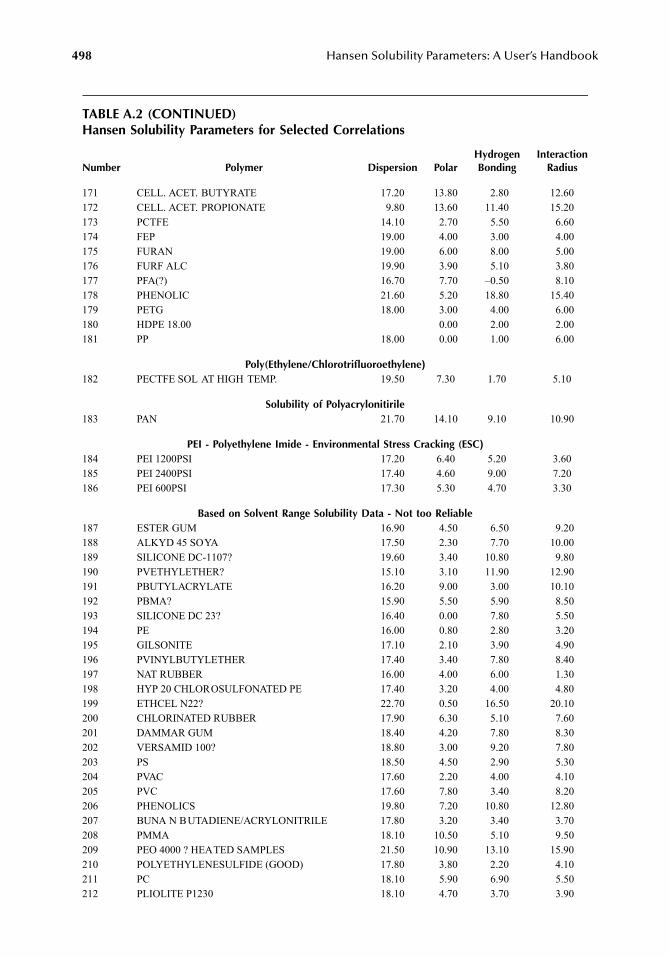
498 Hansen Solubility Parameters: A User’s Handbook
TABLE A.2 (CONTINUED)Hansen Solubility Parameters for Selected Correlations
Number Polymer Dispersion PolarHydrogenBonding
InteractionRadius
171 CELL. ACET. BUTYRATE 17.20 13.80 2.80 12.60172 CELL. ACET. PROPIONATE 9.80 13.60 11.40 15.20173 PCTFE 14.10 2.70 5.50 6.60174 FEP 19.00 4.00 3.00 4.00175 FURAN 19.00 6.00 8.00 5.00176 FURF ALC 19.90 3.90 5.10 3.80177 PFA(?) 16.70 7.70 –0.50 8.10178 PHENOLIC 21.60 5.20 18.80 15.40179 PETG 18.00 3.00 4.00 6.00180 HDPE 18.00 0.00 2.00 2.00181 PP 18.00 0.00 1.00 6.00
Poly(Ethylene/Chlorotrifluoroethylene) 182 PECTFE SOL AT HIGH TEMP. 19.50 7.30 1.70 5.10
Solubility of Polyacrylonitirile183 PAN 21.70 14.10 9.10 10.90
PEI - Polyethylene Imide - Environmental Stress Cracking (ESC)184 PEI 1200PSI 17.20 6.40 5.20 3.60185 PEI 2400PSI 17.40 4.60 9.00 7.20186 PEI 600PSI 17.30 5.30 4.70 3.30
Based on Solvent Range Solubility Data - Not too Reliable187 ESTER GUM 16.90 4.50 6.50 9.20188 ALKYD 45 SOYA 17.50 2.30 7.70 10.00189 SILICONE DC-1107? 19.60 3.40 10.80 9.80190 PVETHYLETHER? 15.10 3.10 11.90 12.90191 PBUTYLACRYLATE 16.20 9.00 3.00 10.10192 PBMA? 15.90 5.50 5.90 8.50193 SILICONE DC 23? 16.40 0.00 7.80 5.50194 PE 16.00 0.80 2.80 3.20195 GILSONITE 17.10 2.10 3.90 4.90196 PVINYLBUTYLETHER 17.40 3.40 7.80 8.40197 NAT RUBBER 16.00 4.00 6.00 1.30198 HYP 20 CHLOROSULFONATED PE 17.40 3.20 4.00 4.80199 ETHCEL N22? 22.70 0.50 16.50 20.10200 CHLORINATED RUBBER 17.90 6.30 5.10 7.60201 DAMMAR GUM 18.40 4.20 7.80 8.30202 VERSAMID 100? 18.80 3.00 9.20 7.80203 PS 18.50 4.50 2.90 5.30204 PVAC 17.60 2.20 4.00 4.10205 PVC 17.60 7.80 3.40 8.20206 PHENOLICS 19.80 7.20 10.80 12.80207 BUNA N BUTADIENE/ACRYLONITRILE 17.80 3.20 3.40 3.70208 PMMA 18.10 10.50 5.10 9.50209 PEO 4000 ? HEATED SAMPLES 21.50 10.90 13.10 15.90210 POLYETHYLENESULFIDE (GOOD) 17.80 3.80 2.20 4.10211 PC 18.10 5.90 6.90 5.50212 PLIOLITE P1230 18.10 4.70 3.70 3.90
7248_A002.fm Page 498 Wednesday, May 23, 2007 12:53 PM
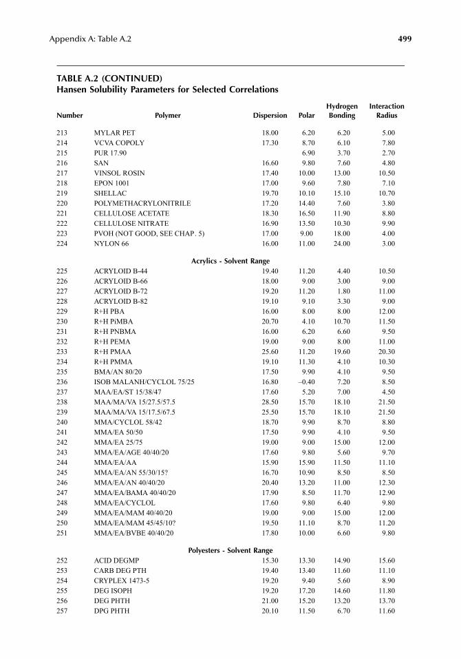
Appendix A: Table A.2 499
TABLE A.2 (CONTINUED)Hansen Solubility Parameters for Selected Correlations
Number Polymer Dispersion PolarHydrogenBonding
InteractionRadius
213 MYLAR PET 18.00 6.20 6.20 5.00214 VCVA COPOLY 17.30 8.70 6.10 7.80215 PUR 17.90 6.90 3.70 2.70216 SAN 16.60 9.80 7.60 4.80217 VINSOL ROSIN 17.40 10.00 13.00 10.50218 EPON 1001 17.00 9.60 7.80 7.10219 SHELLAC 19.70 10.10 15.10 10.70220 POLYMETHACRYLONITRILE 17.20 14.40 7.60 3.80221 CELLULOSE ACETATE 18.30 16.50 11.90 8.80222 CELLULOSE NITRATE 16.90 13.50 10.30 9.90223 PVOH (NOT GOOD, SEE CHAP. 5) 17.00 9.00 18.00 4.00224 NYLON 66 16.00 11.00 24.00 3.00
Acrylics - Solvent Range225 ACRYLOID B-44 19.40 11.20 4.40 10.50226 ACRYLOID B-66 18.00 9.00 3.00 9.00227 ACRYLOID B-72 19.20 11.20 1.80 11.00228 ACRYLOID B-82 19.10 9.10 3.30 9.00229 R+H PBA 16.00 8.00 8.00 12.00230 R+H PiMBA 20.70 4.10 10.70 11.50231 R+H PNBMA 16.00 6.20 6.60 9.50232 R+H PEMA 19.00 9.00 8.00 11.00233 R+H PMAA 25.60 11.20 19.60 20.30234 R+H PMMA 19.10 11.30 4.10 10.30235 BMA/AN 80/20 17.50 9.90 4.10 9.50236 ISOB MALANH/CYCLOL 75/25 16.80 –0.40 7.20 8.50237 MAA/EA/ST 15/38/47 17.60 5.20 7.00 4.50238 MAA/MA/VA 15/27.5/57.5 28.50 15.70 18.10 21.50239 MAA/MA/VA 15/17.5/67.5 25.50 15.70 18.10 21.50240 MMA/CYCLOL 58/42 18.70 9.90 8.70 8.80241 MMA/EA 50/50 17.50 9.90 4.10 9.50242 MMA/EA 25/75 19.00 9.00 15.00 12.00243 MMA/EA/AGE 40/40/20 17.60 9.80 5.60 9.70244 MMA/EA/AA 15.90 15.90 11.50 11.10245 MMA/EA/AN 55/30/15? 16.70 10.90 8.50 8.50246 MMA/EA/AN 40/40/20 20.40 13.20 11.00 12.30247 MMA/EA/BAMA 40/40/20 17.90 8.50 11.70 12.90248 MMA/EA/CYCLOL 17.60 9.80 6.40 9.80249 MMA/EA/MAM 40/40/20 19.00 9.00 15.00 12.00250 MMA/EA/MAM 45/45/10? 19.50 11.10 8.70 11.20251 MMA/EA/BVBE 40/40/20 17.80 10.00 6.60 9.80
Polyesters - Solvent Range252 ACID DEGMP 15.30 13.30 14.90 15.60253 CARB DEG PTH 19.40 13.40 11.60 11.10254 CRYPLEX 1473-5 19.20 9.40 5.60 8.90255 DEG ISOPH 19.20 17.20 14.60 11.80256 DEG PHTH 21.00 15.20 13.20 13.70257 DPG PHTH 20.10 11.50 6.70 11.60
7248_A002.fm Page 499 Wednesday, May 23, 2007 12:53 PM
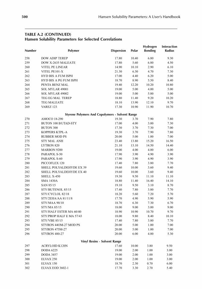
500 Hansen Solubility Parameters: A User’s Handbook
TABLE A.2 (CONTINUED)Hansen Solubility Parameters for Selected Correlations
Number Polymer Dispersion PolarHydrogenBonding
InteractionRadius
258 DOW ADIP TEREP 17.80 10.40 6.80 9.30259 DOW X-2635 MALEATE 17.80 5.60 6.80 4.50260 VITEL PE LINEAR 14.90 10.10 2.90 6.10261 VITEL PE101-X 21.30 6.30 4.70 7.30262 HYD BIS A FUM ISPH 17.00 4.40 6.20 5.00263 HYD BIS A PG FUM ISPH 18.70 8.90 5.50 8.40264 PENTA BENZ MAL 19.40 12.20 10.20 10.80265 SOL MYLAR 49001 19.00 5.00 4.00 5.00266 SOL MYLAR 49002 19.00 5.00 5.00 5.00267 TEG EG MAL TEREP 18.80 11.40 9.20 10.20268 TEG MALEATE 18.10 13.90 12.10 9.70269 VAREZ 123 17.30 10.90 11.90 10.70
Styrene Polymers And Copolymers - Solvent Range 270 AMOCO 18-290 19.30 3.70 7.90 7.80271 BUTON 100 BUTAD-STY 17.00 4.00 3.00 7.30272 BUTON 300 17.30 3.70 7.30 7.00273 KOPPERS KTPL-A 19.30 3.70 7.90 7.80274 RUBBER MOD PS 20.00 5.00 1.00 7.00275 STY MAL ANH 23.40 13.80 15.20 16.50276 LYTRON 820 21.10 13.10 14.50 14.40277 MARBON 9200 19.00 4.00 4.00 6.00278 PARAPOL S-50 17.90 3.90 4.90 3.90279 PARAPOL S-60 17.90 3.90 4.90 3.90280 PICCOFLEX 120 17.40 7.80 3.80 7.70281 SHELL POLYALDEHYDE EX 39 19.60 10.00 3.60 9.40282 SHELL POLYALDEHYDE EX 40 19.60 10.00 3.60 9.40283 SHELL X-450 19.30 9.50 11.10 11.10284 SMA 1430A 18.80 11.40 16.40 14.10285 SAN 85/15 19.10 9.50 3.10 8.70286 STY/BUTENOL 85/15 17.40 7.80 3.80 7.70287 STY/CYCLOL 82/18 18.20 5.60 7.20 5.70288 STY/2EHA/AA 81/11/8 17.70 4.90 5.90 5.90289 STY/MAA 90/10 18.70 6.30 7.30 6.70290 STY/MA 85/15 18.00 9.00 3.00 9.00291 STY/HALF ESTER MA 60/40 18.90 10.90 10.70 9.70292 STY/PROP HALF E MA 57/43 18.00 9.80 8.40 10.10293 STY/VBE 85/15 17.40 7.80 3.80 7.70294 STYRON 44OM-27 MOD PS 20.00 5.00 1.00 7.00295 STYRON 475M-27 20.00 5.00 1.00 7.00296 STYRON 480-27 20.00 6.00 4.00 5.30
Vinyl Resins - Solvent Range297 ACRYLOID K120N 17.60 10.00 3.80 9.50298 DODA 6225 19.00 2.00 1.00 3.00299 DODA 3457 19.00 2.00 1.00 3.00300 ELVAX 250 19.00 2.00 1.00 3.00301 ELVAX 150 18.70 2.30 0.70 6.00302 ELVAX EOD 3602-1 17.70 3.30 2.70 5.40
7248_A002.fm Page 500 Wednesday, May 23, 2007 12:53 PM
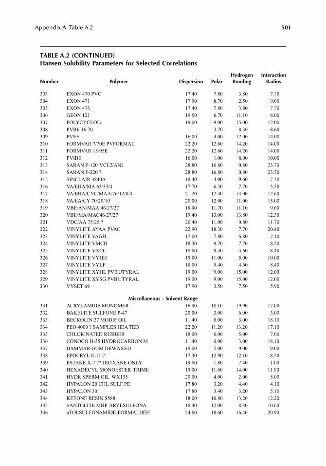
Appendix A: Table A.2 501
TABLE A.2 (CONTINUED)Hansen Solubility Parameters for Selected Correlations
Number Polymer Dispersion PolarHydrogenBonding
InteractionRadius
303 EXON 470 PVC 17.40 7.80 3.80 7.70304 EXON 471 17.90 8.70 2.50 9.00305 EXON 473 17.40 7.80 3.80 7.70306 GEON 121 19.50 6.70 11.10 8.00307 POLYCYCLOLa 19.00 9.00 15.00 12.00308 PVBE 16.70 3.70 8.30 8.60309 PVEE 16.00 4.00 12.00 14.00310 FORMVAR 7/70E PVFORMAL 22.20 12.60 14.20 14.00311 FORMVAR 15/95E 22.20 12.60 14.20 14.00312 PVIBE 16.00 1.00 8.00 10.00313 SARAN F-120 VCL2/AN? 28.80 16.80 0.80 23.70314 SARAN F-220 ? 28.80 16.80 0.80 23.70315 SINCLAIR 3840A 18.40 4.00 9.60 7.30316 VA/EHA/MA 63/33/4 17.70 6.30 7.70 5.30317 VA/EHA/CYC/MAA/76/12/8/4 21.20 12.40 13.00 12.60318 VA/EA/CY 70/20/10 20.00 12.00 11.00 15.00319 VBE/AN/MAA 46/27/27 18.90 11.70 11.10 9.60320 VBE/MA/MAC46/27/27 19.40 13.00 13.80 12.30321 VDC/AA 75/25 ? 20.40 11.00 0.80 11.70322 VINYLITE AYAA PVAC 22.90 18.30 7.70 20.40323 VINYLITE VAGH 17.00 7.80 6.80 7.10324 VINYLITE VMCH 18.30 9.70 7.70 8.50325 VINYLITE VXCC 18.00 9.40 4.60 8.40326 VINYLITE VYHH 19.00 11.00 5.00 10.00327 VINYLITE VYLF 18.00 9.40 4.60 8.40328 VINYLITE XYHL PVBUTYRAL 19.00 9.00 15.00 12.00329 VINYLITE XYSG PVBUTYRAL 19.00 9.00 15.00 12.00330 VYSET 69 17.90 3.50 7.50 5.90
Miscellaneous - Solvent Range331 ACRYLAMIDE MONOMER 16.90 18.10 19.90 17.00332 BAKELITE SULFONE P-47 20.00 3.00 6.00 3.00333 BECKOLIN 27 MODIF OIL 11.40 0.00 3.00 18.10334 PEO 4000 ? SAMPLES HEA TED 22.20 11.20 13.20 17.10335 CHLORINATED RUBBER 18.00 6.00 5.00 7.00336 CONOCO H-35 HYDROCARBON M 11.40 0.00 3.00 18.10337 DAMMAR GUM DEWAXED 19.00 2.00 9.00 9.00338 EPOCRYL E-11 ? 17.30 12.90 12.10 8.50339 ESTANE X-7 ?? DIO XANE ONLY 19.00 1.80 7.40 1.00340 HEXADECYL MONOESTER TRIME 19.00 11.60 14.00 11.90341 HYDR SPERM OIL WX135 20.00 4.00 2.00 5.00342 HYPALON 20 CHL SULF PE 17.80 3.20 4.40 4.10343 HYPALON 30 17.80 3.40 3.20 5.10344 KETONE RESIN S588 18.00 10.80 13.20 12.20345 SANTOLITE MHP ARYLSULFONA 18.40 12.00 8.40 10.60346 pTOLSULFONAMIDE-FORMALDEH 24.60 18.60 16.40 20.90
7248_A002.fm Page 501 Wednesday, May 23, 2007 12:53 PM
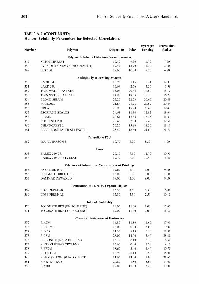
502 Hansen Solubility Parameters: A User’s Handbook
TABLE A.2 (CONTINUED)Hansen Solubility Parameters for Selected Correlations
Number Polymer Dispersion PolarHydrogenBonding
InteractionRadius
Polymer Solubility Data from Various Sources347 VYHH-NIF REPT 17.40 9.90 6.70 7.50348 PVF? (DMF ONLY GOOD SOLVENT) 17.40 13.70 11.30 2.00349 PES SOL 19.60 10.80 9.20 6.20
Biologically Interesting Systems350 LARD 37C 15.90 1.16 5.41 12.03351 LARD 23C 17.69 2.66 4.36 7.98352 1%IN WATER -AMINES 15.07 20.44 16.50 18.12353 1%IN WATER +AMINES 14.96 18.33 15.15 16.22354 BLOOD SERUM 23.20 22.73 30.60 20.48355 SUCROSE 21.67 26.26 29.62 20.44356 UREA 20.90 18.70 26.40 19.42357 PSORIASIS SCALES 24.64 11.94 12.92 19.04358 LIGNIN 20.61 13.88 15.25 11.83359 CHOLESTEROL 20.40 2.80 9.40 12.60360 CHLOROPHYLL 20.20 15.60 18.20 11.10361 CELLULOSE-PAPER STRENGTH 25.40 18.60 24.80 21.70
Polysulfone PSU362 PSU ULTRASON S 19.70 8.30 8.30 8.00
Barex363 BAREX 210 CR 20.10 9.10 12.70 10.90364 BAREX 210 CR-STYRENE 17.70 8.90 10.90 6.40
Polymers of Interest for Conservation of Paintings365 PARALOID B72 17.60 7.40 5.60 9.40366 ESTIMATE DRIED OIL 16.00 6.00 7.00 5.00367 DAMMAR DEWAXED 19.00 2.00 9.00 9.00
Permeation of LDPE by Organic Liquids368 LDPE PERM>80 16.50 4.50 0.50 6.00369 LDPE PERM<0.8 15.30 5.30 2.50 10.10
Tolonate Solubility370 TOLONATE HDT (RH-POULENC) 19.00 11.00 3.00 12.00371 TOLONATE HDB (RH-POULENC) 19.00 11.00 2.00 11.30
Chemical Resistance of Elastomers372 R ACM 16.80 11.80 11.60 17.00373 R BUTYL 18.00 0.00 3.00 9.00374 R ECO 21.30 8.10 6.10 12.00375 R CSM 28.00 14.00 3.40 28.30376 R EBONITE (DATA FIT 0.722) 18.70 6.10 2.70 6.60377 R ETHYLENE/PROPYLENE 16.60 0.00 5.20 9.10378 R EPDM 18.60 –3.40 4.40 10.70379 R FQ FL/SI 15.90 20.10 6.90 16.80380 R FKM (VITON) (0.76 DATA FIT) 11.60 23.00 5.00 21.60381 R NR NAT RUB 20.80 1.80 3.60 14.00382 R NBR 19.80 17.80 3.20 19.00
7248_A002.fm Page 502 Wednesday, May 23, 2007 12:53 PM
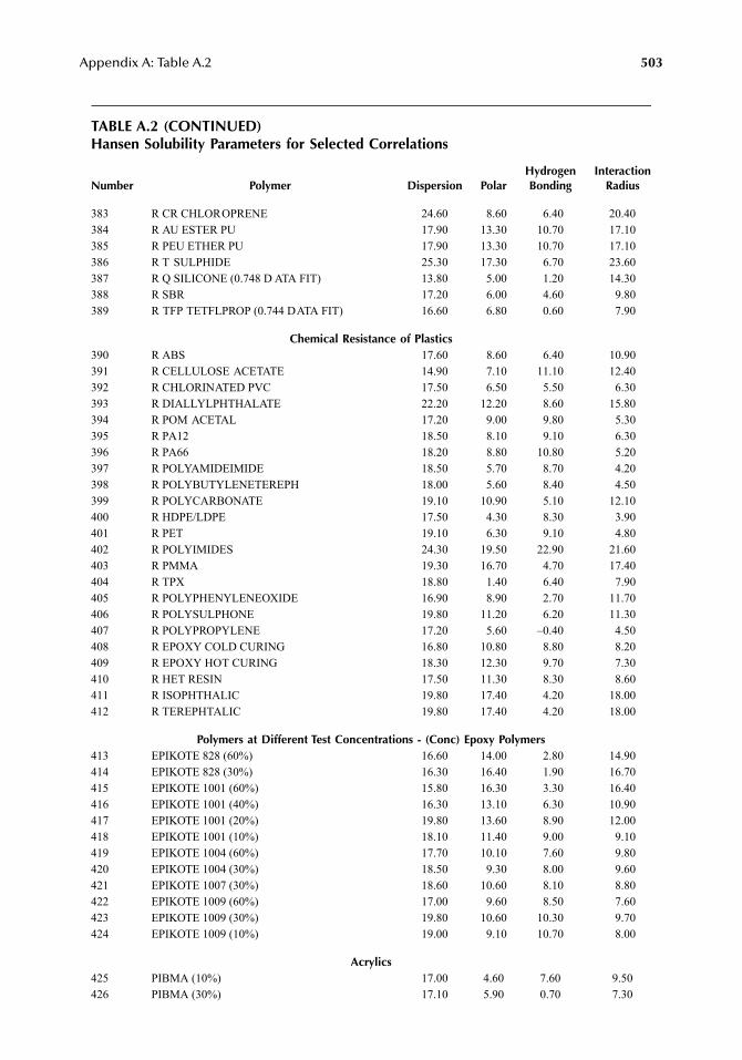
Appendix A: Table A.2 503
TABLE A.2 (CONTINUED)Hansen Solubility Parameters for Selected Correlations
Number Polymer Dispersion PolarHydrogenBonding
InteractionRadius
383 R CR CHLOROPRENE 24.60 8.60 6.40 20.40384 R AU ESTER PU 17.90 13.30 10.70 17.10385 R PEU ETHER PU 17.90 13.30 10.70 17.10386 R T SULPHIDE 25.30 17.30 6.70 23.60387 R Q SILICONE (0.748 D ATA FIT) 13.80 5.00 1.20 14.30388 R SBR 17.20 6.00 4.60 9.80389 R TFP TETFLPROP (0.744 DATA FIT) 16.60 6.80 0.60 7.90
Chemical Resistance of Plastics390 R ABS 17.60 8.60 6.40 10.90391 R CELLULOSE ACETATE 14.90 7.10 11.10 12.40392 R CHLORINATED PVC 17.50 6.50 5.50 6.30393 R DIALLYLPHTHALATE 22.20 12.20 8.60 15.80394 R POM ACETAL 17.20 9.00 9.80 5.30395 R PA12 18.50 8.10 9.10 6.30396 R PA66 18.20 8.80 10.80 5.20397 R POLYAMIDEIMIDE 18.50 5.70 8.70 4.20398 R POLYBUTYLENETEREPH 18.00 5.60 8.40 4.50399 R POLYCARBONATE 19.10 10.90 5.10 12.10400 R HDPE/LDPE 17.50 4.30 8.30 3.90401 R PET 19.10 6.30 9.10 4.80402 R POLYIMIDES 24.30 19.50 22.90 21.60403 R PMMA 19.30 16.70 4.70 17.40404 R TPX 18.80 1.40 6.40 7.90405 R POLYPHENYLENEOXIDE 16.90 8.90 2.70 11.70406 R POLYSULPHONE 19.80 11.20 6.20 11.30407 R POLYPROPYLENE 17.20 5.60 –0.40 4.50408 R EPOXY COLD CURING 16.80 10.80 8.80 8.20409 R EPOXY HOT CURING 18.30 12.30 9.70 7.30410 R HET RESIN 17.50 11.30 8.30 8.60411 R ISOPHTHALIC 19.80 17.40 4.20 18.00412 R TEREPHTALIC 19.80 17.40 4.20 18.00
Polymers at Different Test Concentrations - (Conc) Epoxy Polymers413 EPIKOTE 828 (60%) 16.60 14.00 2.80 14.90414 EPIKOTE 828 (30%) 16.30 16.40 1.90 16.70415 EPIKOTE 1001 (60%) 15.80 16.30 3.30 16.40416 EPIKOTE 1001 (40%) 16.30 13.10 6.30 10.90417 EPIKOTE 1001 (20%) 19.80 13.60 8.90 12.00418 EPIKOTE 1001 (10%) 18.10 11.40 9.00 9.10419 EPIKOTE 1004 (60%) 17.70 10.10 7.60 9.80420 EPIKOTE 1004 (30%) 18.50 9.30 8.00 9.60421 EPIKOTE 1007 (30%) 18.60 10.60 8.10 8.80422 EPIKOTE 1009 (60%) 17.00 9.60 8.50 7.60423 EPIKOTE 1009 (30%) 19.80 10.60 10.30 9.70424 EPIKOTE 1009 (10%) 19.00 9.10 10.70 8.00
Acrylics425 PIBMA (10%) 17.00 4.60 7.60 9.50426 PIBMA (30%) 17.10 5.90 0.70 7.30
7248_A002.fm Page 503 Wednesday, May 23, 2007 12:53 PM
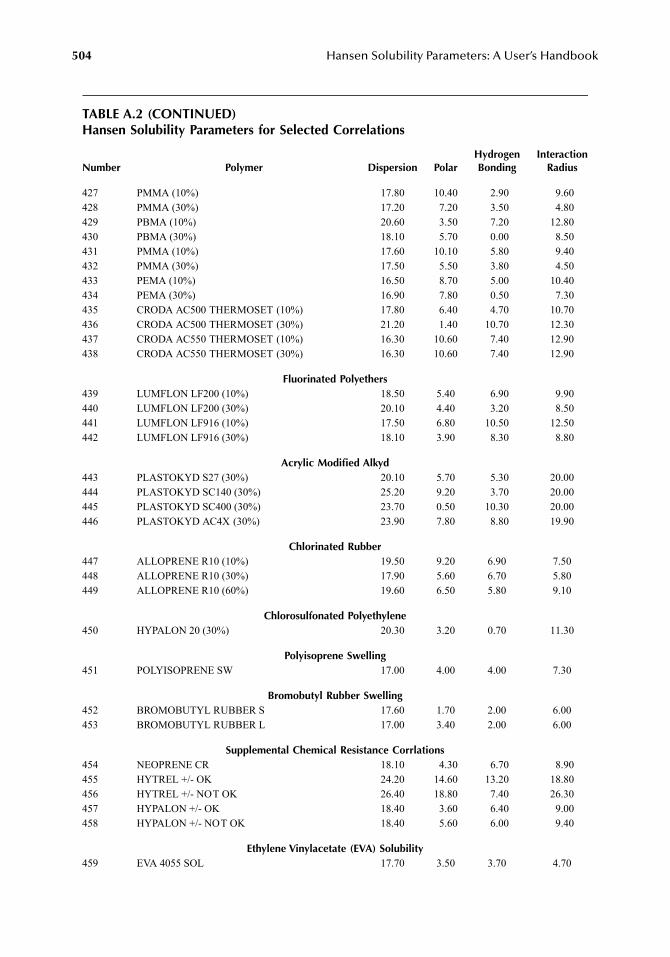
504 Hansen Solubility Parameters: A User’s Handbook
TABLE A.2 (CONTINUED)Hansen Solubility Parameters for Selected Correlations
Number Polymer Dispersion PolarHydrogenBonding
InteractionRadius
427 PMMA (10%) 17.80 10.40 2.90 9.60428 PMMA (30%) 17.20 7.20 3.50 4.80429 PBMA (10%) 20.60 3.50 7.20 12.80430 PBMA (30%) 18.10 5.70 0.00 8.50431 PMMA (10%) 17.60 10.10 5.80 9.40432 PMMA (30%) 17.50 5.50 3.80 4.50433 PEMA (10%) 16.50 8.70 5.00 10.40434 PEMA (30%) 16.90 7.80 0.50 7.30435 CRODA AC500 THERMOSET (10%) 17.80 6.40 4.70 10.70436 CRODA AC500 THERMOSET (30%) 21.20 1.40 10.70 12.30437 CRODA AC550 THERMOSET (10%) 16.30 10.60 7.40 12.90438 CRODA AC550 THERMOSET (30%) 16.30 10.60 7.40 12.90
Fluorinated Polyethers439 LUMFLON LF200 (10%) 18.50 5.40 6.90 9.90440 LUMFLON LF200 (30%) 20.10 4.40 3.20 8.50441 LUMFLON LF916 (10%) 17.50 6.80 10.50 12.50442 LUMFLON LF916 (30%) 18.10 3.90 8.30 8.80
Acrylic Modified Alkyd443 PLASTOKYD S27 (30%) 20.10 5.70 5.30 20.00444 PLASTOKYD SC140 (30%) 25.20 9.20 3.70 20.00445 PLASTOKYD SC400 (30%) 23.70 0.50 10.30 20.00446 PLASTOKYD AC4X (30%) 23.90 7.80 8.80 19.90
Chlorinated Rubber447 ALLOPRENE R10 (10%) 19.50 9.20 6.90 7.50448 ALLOPRENE R10 (30%) 17.90 5.60 6.70 5.80449 ALLOPRENE R10 (60%) 19.60 6.50 5.80 9.10
Chlorosulfonated Polyethylene450 HYPALON 20 (30%) 20.30 3.20 0.70 11.30
Polyisoprene Swelling451 POLYISOPRENE SW 17.00 4.00 4.00 7.30
Bromobutyl Rubber Swelling452 BROMOBUTYL RUBBER S 17.60 1.70 2.00 6.00453 BROMOBUTYL RUBBER L 17.00 3.40 2.00 6.00
Supplemental Chemical Resistance Corrlations454 NEOPRENE CR 18.10 4.30 6.70 8.90455 HYTREL +/- OK 24.20 14.60 13.20 18.80456 HYTREL +/- NOT OK 26.40 18.80 7.40 26.30457 HYPALON +/- OK 18.40 3.60 6.40 9.00458 HYPALON +/- NOT OK 18.40 5.60 6.00 9.40
Ethylene Vinylacetate (EVA) Solubility459 EVA 4055 SOL 17.70 3.50 3.70 4.70
7248_A002.fm Page 504 Wednesday, May 23, 2007 12:53 PM
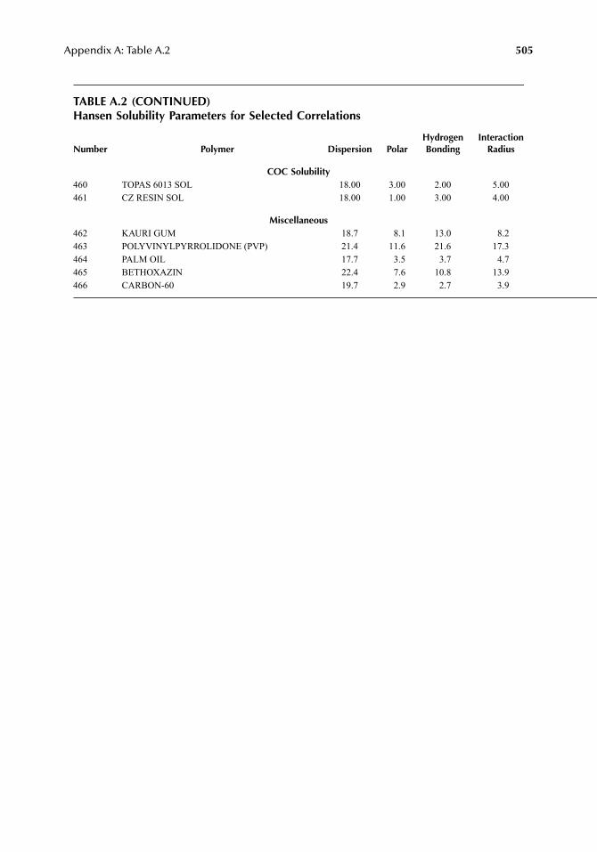
Appendix A: Table A.2 505
TABLE A.2 (CONTINUED)Hansen Solubility Parameters for Selected Correlations
Number Polymer Dispersion PolarHydrogenBonding
InteractionRadius
COC Solubility460 TOPAS 6013 SOL 18.00 3.00 2.00 5.00461 CZ RESIN SOL 18.00 1.00 3.00 4.00
Miscellaneous462 KAURI GUM 18.7 8.1 13.0 8.2463 POLYVINYLPYRROLIDONE (PVP) 21.4 11.6 21.6 17.3464 PALM OIL 17.7 3.5 3.7 4.7465 BETHOXAZIN 22.4 7.6 10.8 13.9466 CARBON-60 19.7 2.9 2.7 3.9
7248_A002.fm Page 505 Wednesday, May 23, 2007 12:53 PM

7248_A002.fm Page 506 Wednesday, May 23, 2007 12:53 PM
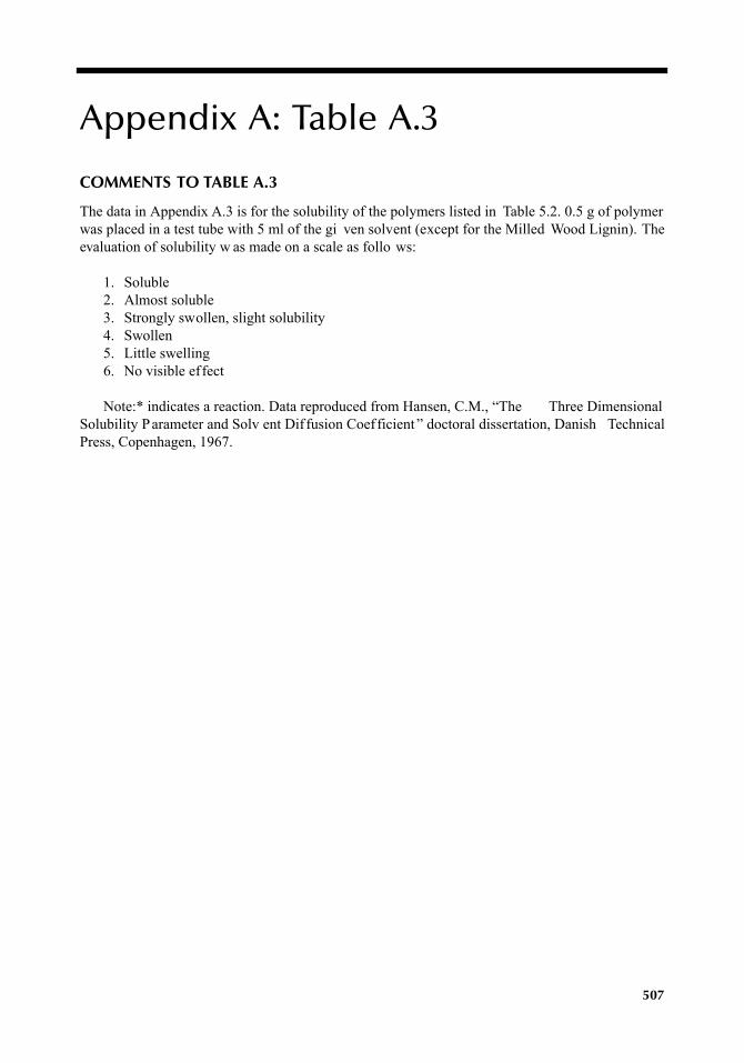
507
Appendix A: Table A.3
COMMENTS TO TABLE A.3
The data in Appendix A.3 is for the solubility of the polymers listed in Table 5.2. 0.5 g of polymerwas placed in a test tube with 5 ml of the gi ven solvent (except for the Milled Wood Lignin). Theevaluation of solubility w as made on a scale as follo ws:
1. Soluble2. Almost soluble3. Strongly swollen, slight solubility4. Swollen5. Little swelling6. No visible effect
Note:* indicates a reaction. Data reproduced from Hansen, C.M., “The Three DimensionalSolubility Parameter and Solv ent Dif fusion Coefficient ” doctoral dissertation, Danish TechnicalPress, Copenhagen, 1967.
7248_A003.fm Page 507 Wednesday, May 23, 2007 12:57 PM
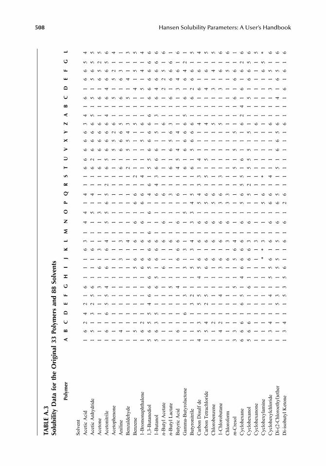
508
Hansen Solubility Parameters: A User’s Handbook
TAB
LE A
.3So
lubi
lity
Dat
a fo
r th
e O
rigi
nal
33 P
olym
ers
and
88 S
olve
nts
Poly
mer
AB
CD
EF
GH
IJ
KL
MN
OP
QR
ST
UV
XY
ZA
BC
DE
FG
L
Solv
ent
Ace
tic A
cid
16
24
21
61
11
63
14
41
41
16
66
66
34
16
16
65
4A
cetic
Anh
ydrid
e1
51
32
56
11
16
11
15
14
11
62
66
66
51
51
56
55
Ace
tone
11
11
11
31
61
31
11
31
11
16
16
66
61
16
16
52
5A
ceto
nitri
le1
61
65
54
16
16
41
55
65
21
65
66
66
41
64
66
56
Ace
toph
enon
e1
11
11
11
11
11
11
11
11
11
11
55
26
11
51
52
14
Ani
line
14
11
11
11
13
13
11
11
11
16
16
66
51
16
16
31
1B
enza
ldeh
yde
11
11
11
11
11
14
11
11
11
12
15
54
31
15
14
11
3B
enze
ne1
51
11
11
15
61
61
61
66
12
11
11
15
11
14
15
15
1-B
rom
onap
htha
lene
16
21
11
11
66
16
16
16
61
41
11
51
61
11
51
41
41,
3-B
utan
edio
l5
65
54
66
65
66
66
16
14
61
55
66
66
61
66
66
66
1-B
utan
ol5
63
51
16
51
66
61
11
16
43
66
61
51
31
64
66
66
n
-But
yl A
ceta
te1
11
11
11
16
11
61
61
16
11
11
11
16
11
12
25
16
n
-But
yl L
acta
te1
11
11
15
11
11
61
11
13
11
61
65
63
11
61
66
61
But
yric
Aci
d1
61
11
14
11
66
61
61
16
11
45
41
41
11
13
46
16
Gam
ma-
But
yrol
acto
ne1
11
61
31
13
13
11
15
11
11
61
66
66
51
61
64
21
But
yron
itrile
11
11
32
11
51
34
13
34
51
16
15
66
61
16
26
61
5C
arbo
n D
isul
fde
45
31
55
14
56
16
16
15
43
31
41
11
41
11
61
61
4C
arbo
n Te
trach
lorid
e1
54
12
51
16
61
61
61
56
15
15
11
14
11
14
16
15
Chl
orob
enze
ne1
12
11
11
11
61
61
61
56
11
11
11
15
11
13
14
15
1-C
hlor
obut
ane
14
21
14
11
36
16
16
13
61
31
11
11
51
11
31
61
6C
hlor
ofor
m1
11
11
11
11
61
31
61
33
11
11
11
11
11
11
15
16
m
-Cre
sol
33
11
11
51
15
64
11
11
11
15
15
15
11
16
16
61
1C
yclo
hexa
ne6
66
16
51
46
66
61
61
56
55
16
11
16
24
16
16
26
Cyc
lohe
xano
l5
66
11
16
11
66
31
61
15
21
55
51
51
11
51
66
56
Cyc
lohe
xano
ne1
11
11
11
11
11
31
11
11
11
11
11
16
11
11
11
15
Cyc
lohe
xyla
min
e1
11
11
11
11
**
31
11
56
1*
11
11
11
11
11
16
5*
Cyc
lohe
xylc
hlor
ide
13
41
14
15
56
16
16
16
61
41
11
11
61
11
31
51
6D
i-(2-
Chl
oroe
thyl
)eth
er1
11
15
31
15
51
51
61
65
11
51
66
56
11
41
65
16
Di-i
sobu
tyl K
eton
e1
34
11
53
56
11
61
61
26
11
11
11
16
11
16
16
16
7248_A003.fm Page 508 Wednesday, May 23, 2007 12:57 PM
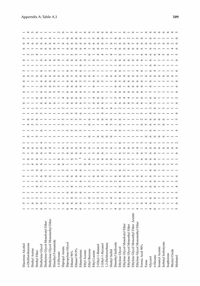
Appendix A: Table A.3
509
Dia
ceto
ne A
lcoh
ol1
51
11
15
11
13
41
11
11
11
61
66
66
31
61
66
51
o
-Dic
hlor
oben
zene
11
21
11
11
26
16
16
14
61
11
11
11
61
11
31
41
4D
ieth
yl A
min
e1
61
11
11
54
55
61
11
55
11
11
11
15
11
12
16
15
Die
thyl
Eth
er3
63
14
53
46
66
61
51
36
53
16
11
16
11
14
16
16
Die
thyl
ene
Gly
col
66
15
35
66
41
66
41
61
15
16
66
66
66
16
16
66
1D
ieth
ylen
e G
lyco
l Mon
obut
yl E
ther
33
11
11
41
11
16
11
11
11
16
45
56
61
16
16
61
1D
ieth
ylen
e G
lyco
l Mon
omet
hyl E
ther
11
11
11
61
11
44
11
11
11
16
36
66
65
16
16
64
1D
imet
hyl F
orm
amid
e1
11
11
11
11
11
11
11
11
11
61
55
66
41
61
64
11
1,4-
Dio
xane
11
11
11
11
66
11
11
11
11
11
14
51
61
14
15
31
2D
ipro
pyl A
min
e1
61
11
11
56
55
61
11
55
12
14
11
16
11
13
16
16
Dip
ropy
lene
Gly
col
66
16
15
65
11
66
11
51
15
16
66
66
66
16
16
66
1Et
hano
l 96%
46
46
41
61
16
66
11
51
55
16
66
66
55
16
56
66
5Et
hano
l 99.
9%5
63
51
16
41
36
61
15
15
41
66
66
66
41
65
66
66
Etha
nola
min
e6
61
62
66
65
*6
41
15
15
61
66
66
56
66
61
66
61
Ethy
l Ace
tate
11
11
11
11
61
15
11
11
11
13
15
15
61
14
14
61
6Et
hyl B
enze
ne1
54
12
31
14
61
61
61
66
13
11
11
16
11
16
16
16
Ethy
l Lac
tate
11
11
11
61
11
51
11
11
11
16
46
66
63
16
16
65
32-
Ethy
l-1-B
utan
ol3
25
31
16
51
66
61
61
16
33
66
61
61
11
54
66
66
2-Et
hyl-1
-Hex
anol
42
51
11
65
16
66
16
11
64
46
65
15
11
11
45
66
61,
2-D
ichl
oroe
than
e1
11
11
11
11
61
51
61
45
11
11
11
16
11
11
23
16
Die
thyl
Sul
fid1
44
11
51
35
61
61
61
56
14
11
11
16
11
14
16
16
Dim
ethy
l Sul
foxi
de4
11
31
26
11
11
11
14
11
11
65
66
66
61
61
62
61
Ethy
lene
Gly
col
66
64
66
66
66
66
61
66
65
26
46
65
66
66
66
66
1Et
hyle
ne G
lyco
l Mon
obut
yl E
ther
15
11
11
62
11
26
11
11
11
16
46
16
41
16
16
61
6Et
hyle
ne G
lyco
l Mon
oeth
yl E
ther
15
11
11
51
11
56
11
11
11
16
46
66
61
16
16
62
1Et
hyle
ne G
lyco
l Mon
oeth
yl E
ther
Ace
tate
11
11
11
11
51
14
11
11
11
15
16
66
61
16
16
51
6Et
hyle
ne G
lyco
l Mon
omet
hyl E
ther
43
11
11
61
11
64
11
21
11
16
56
66
64
16
16
65
1Fo
rmic
Aci
d 90
%1
65
36
16
11
66
15
15
62
51
66
66
63
61
66
66
61
Fura
n1
41
11
11
13
63
61
61
55
11
11
11
16
11
14
16
16
Gly
cero
l4
66
56
66
66
66
66
66
66
43
66
56
66
66
66
66
66
n
-Hex
ane
65
61
66
36
66
66
16
55
65
63
61
11
64
61
62
65
6Is
oam
yl A
ceta
te1
11
11
11
15
11
61
61
56
11
11
11
16
11
14
15
16
Isob
utyl
Isob
utyr
ate
15
51
55
15
51
16
16
16
61
31
11
11
61
11
51
61
6Is
opho
rone
11
11
11
11
11
16
11
11
11
11
11
11
61
11
61
61
6M
esity
l Oxi
de1
11
11
11
15
11
61
11
11
11
11
11
16
11
11
42
14
Met
hano
l5
64
54
56
13
16
62
14
15
41
65
66
65
61
65
66
65
7248_A003.fm Page 509 Wednesday, May 23, 2007 12:57 PM
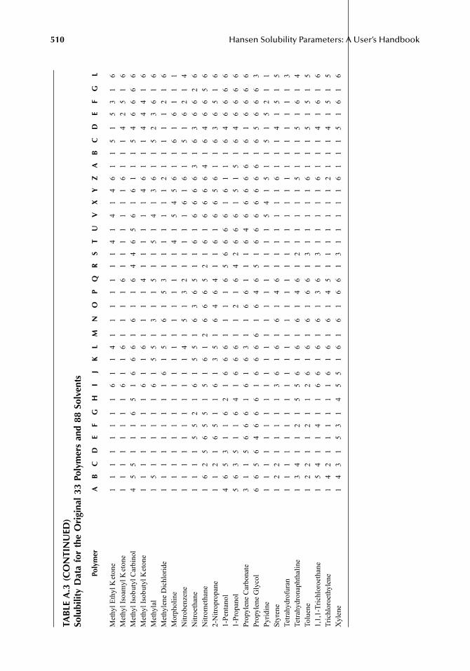
510
Hansen Solubility Parameters: A User’s Handbook
TAB
LE A
.3 (
CO
NTI
NU
ED)
Solu
bilit
y D
ata
for
the
Ori
gina
l 33
Pol
ymer
s an
d 88
Sol
vent
s
Poly
mer
AB
CD
EF
GH
IJ
KL
MN
OP
QR
ST
UV
XY
ZA
BC
DE
FG
L
Met
hyl E
thyl
Ket
one
11
11
11
11
61
14
11
11
11
14
14
14
61
15
15
31
6M
ethy
l Iso
amyl
Ket
one
11
11
11
11
61
16
11
11
61
11
11
11
61
11
42
51
6M
ethy
l Iso
buty
l Car
bino
l4
55
11
16
51
66
61
61
16
44
65
61
61
11
54
66
66
Met
hyl I
sobu
tyl K
eton
e1
11
11
11
16
11
61
11
14
11
11
11
46
11
14
44
16
Met
hyla
l1
51
11
11
16
15
51
31
15
11
51
41
36
11
52
36
16
Met
hyle
ne D
ichl
orid
e1
11
11
11
11
61
51
61
53
11
11
11
12
11
11
12
16
Mor
phol
ine
11
11
11
11
11
11
11
11
11
14
15
45
61
16
16
11
1N
itrob
enze
ne1
11
11
11
11
11
41
51
32
11
11
16
16
11
51
62
14
Nitr
oeth
ane
11
11
55
21
61
55
16
36
51
16
16
66
63
16
36
62
6N
itrom
etha
ne1
62
56
55
15
16
12
66
65
21
61
66
66
41
64
66
56
2-N
itrop
ropa
ne1
12
16
51
16
13
51
64
64
11
61
66
56
11
63
65
16
1-Pe
ntan
ol4
65
31
16
21
66
61
11
16
56
66
61
61
11
64
66
66
1-Pr
opan
ol5
63
51
16
41
66
61
12
16
42
66
61
51
51
64
66
66
Prop
ylen
e C
arbo
nate
31
15
66
61
61
63
11
66
11
16
46
66
66
16
16
66
6Pr
opyl
ene
Gly
col
66
56
46
66
16
66
61
64
65
16
66
66
66
16
56
66
3Py
ridin
e1
11
11
11
11
11
11
11
11
11
11
54
15
11
51
52
11
Styr
ene
12
21
11
11
36
16
16
14
61
11
11
11
61
11
41
51
5Te
trahy
drof
uran
11
11
11
11
11
11
11
11
11
11
11
11
11
11
11
11
3Te
trahy
dron
apht
halin
e1
34
11
21
55
61
61
61
46
12
11
11
15
11
15
16
14
Tolu
ene
12
21
12
11
26
16
16
16
61
31
11
11
61
11
51
51
51,
1,1-
Tric
hlor
oeth
ane
15
41
14
11
66
16
16
13
61
31
11
11
61
11
41
61
6Tr
ichl
oroe
thyl
ene
14
21
11
11
16
16
16
14
51
11
11
11
21
11
41
51
5X
ylen
e1
43
15
31
45
51
61
61
66
13
11
11
16
11
15
16
16
7248_A003.fm Page 510 Wednesday, May 23, 2007 12:57 PM
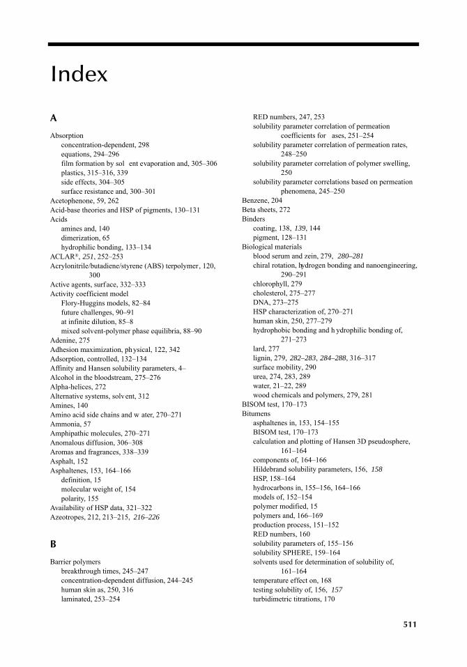
511
Index
A
Absorptionconcentration-dependent, 298equations, 294–296film formation by sol ent evaporation and, 305–306plastics, 315–316, 339side effects, 304–305surface resistance and, 300–301
Acetophenone, 59, 262Acid-base theories and HSP of pigments, 130–131Acids
amines and, 140dimerization, 65hydrophilic bonding, 133–134
ACLAR
®
,
251
, 252–253Acrylonitrile/butadiene/styrene (ABS) terpolymer, 120,
300Active agents, surface, 332–333Activity coefficient model
Flory-Huggins models, 82–84future challenges, 90–91at infinite dilution, 85–8mixed solvent-polymer phase equilibria, 88–90
Adenine, 275Adhesion maximization, physical, 122, 342Adsorption, controlled, 132–134Affinity and Hansen solubility parameters, 4–Alcohol in the bloodstream, 275–276Alpha-helices, 272Alternative systems, solvent, 312Amines, 140Amino acid side chains and w ater, 270–271Ammonia, 57Amphipathic molecules, 270–271Anomalous diffusion, 306–308Aromas and fragrances, 338–339Asphalt, 152Asphaltenes, 153, 164–166
definition, 15molecular weight of, 154polarity, 155
Availability of HSP data, 321–322Azeotropes, 212, 213–215,
216–226
B
Barrier polymersbreakthrough times, 245–247concentration-dependent diffusion, 244–245human skin as, 250, 316laminated, 253–254
RED numbers, 247, 253solubility parameter correlation of permeation
coefficients for ases, 251–254solubility parameter correlation of permeation rates,
248–250solubility parameter correlation of polymer swelling,
250solubility parameter correlations based on permeation
phenomena, 245–250Benzene, 204Beta sheets, 272Binders
coating, 138,
139
, 144pigment, 128–131
Biological materialsblood serum and zein, 279,
280–281
chiral rotation, hydrogen bonding and nanoengineering, 290–291
chlorophyll, 279cholesterol, 275–277DNA, 273–275HSP characterization of, 270–271human skin, 250, 277–279hydrophobic bonding and h ydrophilic bonding of,
271–273lard, 277lignin, 279,
282–283
,
284–288
, 316–317surface mobility, 290urea, 274, 283, 289water, 21–22, 289wood chemicals and polymers, 279, 281
BISOM test, 170–173Bitumens
asphaltenes in, 153, 154–155BISOM test, 170–173calculation and plotting of Hansen 3D pseudosphere,
161–164components of, 164–166Hildebrand solubility parameters, 156,
158
HSP, 158–164hydrocarbons in, 155–156, 164–166models of, 152–154polymer modified, 15polymers and, 166–169production process, 151–152RED numbers, 160solubility parameters of, 155–156solubility SPHERE, 159–164solvents used for determination of solubility of,
161–164temperature effect on, 168testing solubility of, 156,
157
turbidimetric titrations, 170
7248_Index.fm Page 511 Wednesday, May 9, 2007 10:49 AM
512
Hansen Solubility Parameters: A User’s Handbook
uses, 151, 160Blanc fi e, 131Blistering of coatings, 141, 281Blood serum, 279,
280–281
Boundaries of solubility, 7–8Breakthrough times, HSP correlations of, 245–247Butadiene block copolymer (SBS), 168Butyl rubber, 246
C
Calculationsversus experimental
χ
12
parameters, 34–39polymer HSP, 97–98
Carbon dioxide, 57, 252Hildebrand parameters of, 187–190HSP of, 336–337ideal solubility of g ases in liquids and, 199–201pressure effects on solubility parameters of, 187,
191–196solubility data in v arious solvents, 178–186,
187
solubility in liquid solv ents, 185–186solubility parameters, 141–142temperature effects on solubility parameters of,
190–191three-component solubility parameters, 189–190
Carbon disulfide, 16–1Carbon fiber sur ace characterization, 131–132,
133
Carbon tetrachloride, 35–36, 204Carcinogens, 312Castor oil, 214Cellulose, 281,
289
acetate, 303Challenge
®
5100, 246Chemical protective clothing, 315Chemical resistance
acceptable-or-not data on, 232effects of solvent molecular size on, 232–233HSP characterization of, 231–232, 339plastics, 234–237special effects with water, 238–239tank coatings, 233–234tensile strength and, 237–238
Chiral rotation and HSP, 290–291Chlorobenzene, 245, 305Chloroform, 35–36Chlorophyll, 279Cholesterol, 275–277Cleaning solvents
application of HSP methodology to, 212–213azeotropes, 212, 213–215,
216–226
calculating HSP of composites and, 205–206HSP of multiple-component soils and, 204–205identification of designe , 208method for choice of suitable, 206–208pathology of soils and, 204performance, 210–212reference soils, 208,
209–210
variety of chemicals used in, 204
Coatingsamines added to, 140binders, 138,
139,
144blistering in, 141, 281chemical resistance and, 231–239,
240
gases as solvents in, 141–142for hazardous materials, 312PET film, 234, 23polymer compatibility in, 145–146RED numbers, 142–143, 144self-stratifying, 120–121solvents, 137–142
and surface phenomena in, 144–145SPHERE and, 143surface mobility, 333–334tank, 233–234water-reducible, 139–140
Cohesion energy parameters, 2, 5, 13–18, 113Cohesive energy density, carbon dioxide, 187Cohesive energy difference, 27
polymer segments and solvents, 30–32Composite soils, 204–206Compound formation, 9Concentration-dependent diffusion, 244–245, 297–298,
304–305Constant diffusion coefficients, 296–29Controlled adsorption, 132–134Controlled release of drugs, 339–340Cooling, rapid, 19Corresponding states theory (CST), 3, 6
HSP and, 30–32predicting the
χ
12
parameter using, 28Critical chi parameter, 32Critical surface tensions, 116–117Crude oils
BISOM test, 170–173HSP of molecules in, 169–170origins and structure, 152–153uses, 151–152
Cyclic olefinic copolymer (COC), 120, 300–30Cyclohexanone, 185
D
Danish MAL system, 313–315Data, HSP
availability, 321–322quality, 324, 326
Dendrimers, 90–91Designer solvents.
See also
Cleaning solventsanalysis of capability of, 213–215application of HSP methodology to, 212–213azeotropes, 212, 213–215,
216–226
cleaning performance of, 210–212defined, 20identification of, 20variety of chemicals used in, 204
Desirability function, 20Dextran C, 101–102, 322,
323–324,
325–326
Dibasic esters (DBE), 315
7248_Index.fm Page 512 Wednesday, May 9, 2007 10:49 AM
Index
513
1,2-dibromoethane, 185Dichloromethane, 185Diethyl ether, 17, 262Diffusion
anomalous, 306–308concentration-dependent, 244–245, 297–298, 304–305constant coefficients, 296–29equations, 294–296film formation by sol ent evaporation and, 305–306side effects, 304–305steady state permeation, 296surface effects and, 302–304surface resistance and, 298–305time-dependent, 308vapor, 301–302
Dilution, infinite, 85–8Dimerization, acid, 65Dimethyl sulfoxide, 2891,4-dioxane, 262Dipolar interactions, 50–52, 66Dipole moments, 8–9
zero, 16–17Dispersion solubility parameters, 5, 13–16
hydrogen bonding, 52–59Distance, solubility parameter, 7DNA, 273–275Dynamic shear rheometer (DSR), 152
E
Elastomers, 245, 333Electron exchange parameters, 5, 29Electrostatic repulsion, 140Energy
density, cohesive, 13–16Gibbs, 92–93polar cohesive, 5relative difference, 8surface free, 113–114of vaporization, 13–16
Entropic group contribution model, 78–79, 83Environmental impact of solv ents, 208Environmental stress cracking (ESC), 107, 120
incidence of, 259–260interpreted using HSP, 260–262mechanism for, 259–260, 264–267with nonabsorbing stress cracking initiators, 263–264RED number and, 260–262
EPDM rubber, 141Epon
®
1001, 233Epoxies, 138, 141, 233–234Equation-of-state framework, 46–50, 60–62
carbon dioxide, 188–189Ethanol, 4–5, 276Ethyl acetate, 262Ethylene glycol monomethyl ether (EGMME), 245Ethylene vinyl alcohol copolymers (EV OH), 253–254Evaporation, solvent, 305–306
F
Fickian diffusion, 306–308Field ionization mass spectrometry (FIMS), 154Fillers and fibers, 147–14Film formation by solv ent evaporation, 305–306Films, PET, 234, 235First-order and second-order groups in solubility parameter
prediction, 66–73Floating rates of particles in pigments, 126–127Flocculation, 153Flory-Huggins model, 27–28, 77, 341
versus the GC methods, 84–90for multicomponent mixtures, 92–93regular solution theory and, 80–82using Hildebrand and HSP, 82–84
Fluoropolymers, 16–17Formamide, 274Fragrances and aromas, 338–339Free-volume-based models for polymers, 77–79
solvent selection for paints, 85–88Fresh Air Numbers (FAN/MAL) system, 313–315
G
Gasescharacterization problems, 336–337HSP of, 336–337ideal solubility in liquids, 199–201permeation through polymers, 243solubility parameter correlation of permeation
coefficients fo , 251–254as solvents, 141–142
Gibbs energy, 92–93Glycol ethers, 138, 140–141Group-contribution method
applications, 76–77entropic model, 78–79, 83Flory-Huggins/Hansen model versus, 84–90Flory-Huggins model and re gular solution theory,
80–82free-volume-based models for polymers, 77reliability of calculation procedures for , 328UNIFAC model, 76–78, 83
Guggenheim expression, 47
H
Halar
®
, 235,
236
Hansen 3D pseudosphere, 161–164Hansen solubility parameters (HSP)
acid-base theories and, 130–131aromas and fragrances, 338–339biological materials, 269–291bitumen, 158–164blood serum and zein, 279,
280–281
carbon dioxide, 177–201for chemical protective clothing, 315
7248_Index.fm Page 513 Wednesday, May 9, 2007 10:49 AM
514
Hansen Solubility Parameters: A User’s Handbook
chemical resistance characterization using, 231–239,
240,
339chiral rotation and, 290–291chlorophyll, 279cholesterol, 275–277coatings, 145–146composite soils, 204–206controlled release drugs, 339–340correlation of permeation coef ficients for ases,
251–254correlation of permeation rates, 248–250correlation of polymer swelling, 250correlation of zeta potential for blanc fi e, 131correlations for chemical resistance, 234–236correlations of breakthrough times, 245–247correlations with surface tension, 113–114corresponding states theories and, 30–32data
availability, 321–322quality, 324, 326
defined, 1, 4–Dextran C, 322,
323–324,
325–326
electron exchange energy and, 29environmental stress cracking (ESC) and, 260–267fillers and fibers, 147–1first-order and second-order groups contri ution to,
66–73Flory-Huggins model and, 81–82gases, 336–337GC methods versus the FH/, 84–90human skin, 277–279, 316hydrogen bonding and, 290–291inorganic salts, 337lard, 277lignin, 279,
282–283,
284–288
methodology applied to cleaning operations, 212–213methods and problems in determination of, 6–13mixtures, 205–206molecules in crude oils, 169–170multiple-component soils, 204–206nanoengineering and, 290–291, 340–341organic compounds, 177–178organic salts, 337organometallic compounds, 338pigments, 128–131
fillers and fibers, 125–1plastics, 315–316, 339polymers, 29–30, 95–109solvents, 29–30, 40–41, 137–143special effects with water, 238–239surface
characterization, 113–122, 131–132, 330–332liquid adhesion, 342mobility and, 263–264, 290
tensile strength and, 237–238three-component, 189–190urea, 283, 289water, 21–22, 289, 326, 334–336wood chemicals and polymers, 279, 281
χ
12
parameter and, 32–39
Hazardous materialschemical protective clothing for, 315Danish MAL system, 313–315skin penetration of, 316solvent formulation and personal protection for least
risk from, 313substitutions for, 311–312transport phenomena, 316–317uptake by plastic containers, 315–316
Heat of vaporization, 50Hemicelluloses, 281,
289
Henry's law coefficient, 17Hexane, 116, 120, 204Hildebrand parameters, 2–4
of bitumen, 155, 156,
158
of carbon dioxide, 187–190solvent selection for paints, 85–88
χ
12
coefficient and, 28, 3Hoy dispersion parameter, 9, 13Human skin
HSP of, 277–279, 316penetration of hazardous materials, 316as polymeric barrier, 250
Hydrocarbonsin bitumen, 155–156, 164–166carbon dioxide solubility parameters and, 192–194,
336–337coatings applications, 138–139and corresponding states theories, 29in crude oils, 153ether solvents partially based on silicon, 208
Hydrochlorides, 339–340Hydrofluoroethers (HFEs), 20Hydrogen bonding, 5, 7
acid dimerization and, 65coatings, 138cohesive energy differences and, 31–32defined, 26dipole moments and, 9DNA, 273–275HSP and, 290–291lattice-fluid, 4nonrandom, 46, 50–59polymer surfaces, 115self-stratifying coatings, 120–121solubility parameters, 17, 52–59techniques for data treatment, 142–143temperature increases and, 140–141water temperature and, 141
Hydrophilic bonding, 133–134, 271–273, 333–334Hydrophobic bonding, 271–273, 332
I
Inorganic salts, 337Interaction radius, 184Internal pressure, 187Intrinsic viscosity of polymers, 107–109
7248_Index.fm Page 514 Wednesday, May 9, 2007 10:49 AM
Index
515
J
Joffé effect, 342
K
Keratin, 277, 317Ketones, 138,
140
L
Laminates, 253–254Lard, 277Lattice-fluid ydrogen bonding (LFHB), 46Lignin, 279,
282–283,
284–288,
316–317Liquid-liquid phase separation (LLE), 75Liquids
absorption by plastic containers, 315–316adhesion phenomena, 342cohesion energy parameters and surf ace
characterization of, 114–116environmental stress cracking (ESC) and, 262first-order and second-order groups in, 66–7ideal solubility of g ases in, 199–201solubility parameters for, 17–21, 32–33, 52–59solvents, CO
2
solubility in, 185–186spontaneous spreading, 115–118surface tension, 116–117
Lithium, 338Lorenz-Berthelot mixtures, 41Low density polyethylene (LDPE), 249Lower critical solution temperature, 28Lydersen group constants, 12–13t, 15
M
MAL system, Danish, 313–315Maltenes, 153, 164–165MATLAB platform, 163Melting points of polymers, 106–107Metallic bonding, 338Methanol, 19, 141, 238–2392-methylcyclohexanone, 185Methylene chloride,
140
Methyl ethyl ketone,
140
Methyl iodide-cellulose acetate, 303Methyl isobutyl ketone, 262Methyl methacrylate, 277Mixtures, solubility parameters of, 205–206, 283, 289Mobility, surface, 263–264, 290, 333–334Molar volume and solubility parameters, 7Molecular size and solubility parameters, 19–20, 32–33,
232–233, 243Morpholine, 108Multicomponent mixtures, Flory-Huggins model for ,
92–93Multiple-component soils, 204–206Multivariable analysis and solubility parameters, 8
N
Nanoengineering, 290–291, 340–341
n
-butanol, 138,
140n
-butyl acetate, 262Neoprene
®
, 235New Flory theory, 27–28
n
-heptane, 153, 154, 165–166
n
-hexane, 243, 262Nitrates, 337Nitrile rubber, 246Nitromethane, 4–5N-methyl-morpholine-N-oxide, 279
N
-methyl-2-pyrrolidone, 204Nonabsorbing stress cracking initiators, 263–264Nonbiodegradable substances, 312Nonpolar interactions in or ganic materials, 5Nonrandom hydrogen bonding, 46, 50–59Normal diffusion, 306–308Nylon-6, 303
O
Octyl alcohol, 277Oleic acid, 185Olive oil, 277One-component Hildebrand parameter as a function of
temperature and pressure, 187–189Organic compounds, HSP and solv ents for, 177–178Organic salts, 337Organoclays, 340–341Organometallic compounds, 338Ostwald coefficient, 17Ozone depletion potentials (ODP), 208
P
Paintshydrophilic bonding in, 272older, dried, 142–143self-stratifying coatings, 120–121solvent selection for, 85–88
Partial solubility parameters determination, 6–13dipolar interactions and, 50–52for liquids, 17–21, 52–59
Particle suspensions, 126–127Pathology of soils, 204
P
-dioxane, 303Peat moss, 333Pentachlorophenol, 316Permeation
of liquid or g as through polymers, 243rates, 248–250size and shape and dependence of diffusion coefficient,
255–256solubility parameter correlation of permeation
coefficients for ases, 251–254solubility parameter correlations based on, 245–250steady state, 296
7248_Index.fm Page 515 Wednesday, May 9, 2007 10:49 AM
516
Hansen Solubility Parameters: A User’s Handbook
surface resistance in, 301–302through human skin, 277–279, 316
PET film coating, 234, 23Phase equilibria, mixed solvent-polymer, 88–90Phenyl acetate, 262Physical adhesion maximization, 122Pigments, fillers, and fibe
binders, 128–131carbon fibe , 131–132,
133
cohesion parameter characterization study , 125controlled adsorption, 132–134manufacturing, 128organic versus inorganic, 130–131sedimentation rates, 126–127,
129
solvents, 128–131, 144–145surface characterization methods, 126–127
Plasticizers, 21, 142, 244Plastics
absorption of chemicals in, 315–316, 339bitumen in, 167chemical resistance, 234–237containers uptake, 315–316environmental stress cracking and, 107HSP correlations acceptable or not, 234–237SWEAT and, 141
Plastomers, 167Points, polymers as, 328, 330Polar bonding and cohesi ve energy
acid groups, 132–134differences, 31–32
Polarity of asphaltenes, 155Polar solubility parameters, 5, 16–17Polyacrylonitrile (PAN), 39, 100, 132, 252Polyamides (PA), 253–254, 260Polybutadiene, 35–36Polycarbonate (PC), 120, 260, 300Poly(chlorotrifluoroet ylene), 252Polydimethyl siloxane (PDMS), 77Polydimethylsiloxanes, 264Polyesterimide, 108–109Polyesters (TPU), 333Polyether ether ketone (PEEK), 260Polyether/polyamide block copolymer (PEB A), 333Polyether sulfone, 141Polyethersulfone (PES), 167–168, 238Poly(ethylene co-chlorotrifluoroet ylene) (ECTFE), 235,
236
Polyethylene (PE),
118,
246, 260, 303low density, 249Polyethylenesulfide, 167–168,
327–328,
329–330
Polyethylene terephthalate (PET), 252, 253–254Polyisobutylene, 36–38Polymer modified bitumen (PMB), 15Polymers
barrierconcentration-dependent diffusion and, 244–245human skin as, 250, 316laminated, 253–254RED numbers, 247, 253solubility parameter correlation of permeation
coefficients for ases, 251–254
solubility parameter correlation of permeation rates, 248–250
solubility parameter correlations based on permeation, 245–250
swelling, 250bitumen and, 166–169calculated versus experimental
χ
12
parameters, 34–39coatings, 139–140cohesive energy differences between solvents and,
30–32compatibility in coatings, 145–146concentration and
χ
12
,
39
concentration-dependent diffusion of, 244–245dendrimer, 90–91environmental stress cracking, 107experimental evaluation of behavior of, 95–97Flory-Huggins models using Hildebrand and HSP ,
82–84group contribution
applications, 76–77entropic model, 78–79Flory-Huggins model and re gular solution theory,
80–82free-volume-based models for polymers, 77UNIFAC-FV model, 77–78
high temperature solvents, 140–141HSP for, 29–30
calculation of, 97–98solubility and, 98–106SPHERE program and, 95–96, 99–106, 108–109two-dimensional plot of, 96–97
intrinsic viscosity of, 107–109melting point determinations, 106–107permeation of liquid or g as through, 243as points, 328, 330RED number, 98–100rigid, 245solubility, 341solution thermodynamics, 2–4, 19, 75–76-solvent mixtures phase equilibria, 88–90SPHERE program and, 95–96, 99–106, 108–109swelling of, 106wood, 279, 281
Polymethyl methacrylate (PMMA), 243, 260Polyolefins, 252, 253–25Polyphenylene sulfide (PPS), 20, 141, 23Polypropylene, 59, 106, 302Polystyrene (PS), 38, 260Polytetrafluoroet ylene (PTFE), 252, 260Polyurethanes, 333Polyvinylacetate, 39Polyvinyl acetate, 243Polyvinylacetate, 305Polyvinyl alcohol, 252Polyvinyl chloride (PVC), 116–117, 243Polyvinylchloride (PVC), 260Polyvinyl chloride (PVC), 264–267Polyvinylidine chloride (PVDC), 106–107Pressure effects on carbon dioxide solubility parameters,
187, 191–196Pressure-volume-temperature (PVT) data, 52–59
7248_Index.fm Page 516 Wednesday, May 9, 2007 10:49 AM
Index
517
Prigogine corresponding states theory (CST), 3, 6HSP and, 30–32predicting the
χ
12
parameter using, 28Prigogine-Patterson theory, 31, 40–41Propylene bromide, 185Protective clothing, chemical, 315Proteins in blood serum, 279,
280–281
Pyrimidine, 275
Q
Quasi-chemical condition, 47–49
R
Rapid cooling, 19Rates, permeation, 248–250RED (relative energy difference) numbers, 8, 21, 40
barrier polymers, 247, 253bitumen, 160carbon dioxide, 185coatings, 142–143, 144environmental stress cracking and, 260–262polymer solubility and, 98–100solvent quality and, 142transport phenomena and, 316
Reference soils, 208,
209–210
Refrigerants, 208Regular solution theory and Flory-Huggins model, 80–82Rehbinder effect, 120, 342Relative energy difference, 8Resins, 153Resistance, surface
in absorption experiments, 300–301mathematical background, 298–299measuring diffusion coefficients with, 304–30in permeation experiments, 301–302skin layer effect, 302–303
Rhodamin FB,
331,
334–335Rigid polymers, 245RNA, 274
S
Safety and health issues.
See
Hazardous materialsSalts
inorganic, 337organic, 337
SARA analysis, 153Sedimentation rates, 126–127,
129,
130Self-assembly (controlled adsorption), 132–134, 341Self-stratifying coatings, 120–121Side effects, 304–305Silicon, hydrocarbon ether solvent partially based on, 208Similia similibus solvuntur, 45–46Skin, human.
See
Human skinSkin layer effects, 302–303Soils
composite, 204–206, 213–215
HSP of multiple-component, 204–205method for choice of suitable solv ents for, 206–208mixtures with solvents, 205–206pathology of, 204reference, 208,
209–210
Solubility parameters.
See also
Hansen solubility parameters (HSP); Hildebrand parameters
of bitumen, 155–161boundaries and, 7–8carbon dioxide, 141–142dipolar interactions and, 50–52dispersion, 13–16distance equation, 7first-order and second-order groups contri ution to,
66–73hydrogen bonding, 17introduction to, 1–2for liquids, 17–21partial, 6–13, 17–21polar, 5, 16–17polymers, 341of solvent-solute combinations, 3–4study of, 45–46surface science, 6temperature dependence and, 18–19for water, 21–22
Solubility sphere, 184Solvents
absorption, 300–301alternatives, 312azeotropes, 212, 213–215,
216–226
biological materials as, 274–275carbon dioxide solubility in v arious, 178–186,
187
cleaninganalysis of capability of, 213–215application of HSP methodology to, 212–213calculating HSP of mixtures of soil and, 205–206HSP of multiple-component soils and, 204–205method for choice of suitable, 206–208pathology of soils and, 204performance, 210–212reference soils, 208,
209–210
variety of chemicals used in, 204coating applications, 137–148cohesive energy differences between polymers and,
30–32diffusion coefficients, 244–24environmental impact of, 208evaporation film formation, 305–30formulation and personal protection for least risk, 313gases as, 141–142for hazardous materials, 312high temperature, 140–141HSP for, 29–30, 32–33, 40–41, 137–142for human skin, 277–279hydrocarbon base, 138–139, 208for lard, 277mixtures with soils, 205–206molecular size and solubility parameters, 19–20,
232–233permeation rates, 248–250
7248_Index.fm Page 517 Wednesday, May 9, 2007 10:49 AM
518
Hansen Solubility Parameters: A User’s Handbook
pigments adsorption and, 128–131, 144–145polymer compatibility in coatings, 145–146-polymer mixtures phase equilibria, 88–90selection for paints, 85–88solubility of bitumens in, 156,
157–158
solute-combination solubility parameters, 3–4as spheres, 328, 330and surface phenomena in coatings, 144–145titration tests, 170–173used as refrigerants, 208used for determination of solubility of bitumens,
161–164vegetable oils in, 142viscosity, 145–146
SPHERE and SPHERE1 analysis, 20–21bitumen solubility and, 159–164cholesterol, 275–276coatings and, 143Hansen 3D pseudo-, 161–164polymers and, 95–96, 99–106, 108–109
Spheres, solvents as, 328, 330Spontaneous spreading of liquid droplets, 115–118, 120Steady state permeation, 296Stress corrosion cracking (SCC), 260Styrene, 277Styrene-acrylonitrile copolymer (SAN), 260Styrene/butadiene/styrene block copolymer (SBS), 333Substitutions, 311–312Sulfur trioxide, 253Super Case II beha vior, 306–308Surfaces
active agents, 332–333-active agents in coatings, 140carbon fibe , 131–132characterizations and comparisons using HSP, 118–120,
131–132, 330–332cohesion energy parameters evaluation for,
114–116film formation by sol ent evaporation and,
305–306free energy, 113–114HSP for, 113–122liquid adhesion phenomena, 342mobility, 263–264, 290, 333–334phenomena in coatings, 144–145physical adhesion maximization, 122pigment, fillers, and fib , 126–131resistance, 298–305self-stratifying coatings, 120–121tension correlations with HSP, 113–114tensions, critical, 116–117wetting tension, 115–116, 117–118
Surfactants, 332–333SWEAT (soluble water exuded at lower temperatures), 141,
238–240Swelling
polypropylene, 106solubility parameter correlation of polymer , 250
T
Tank coatings, 233–234Tar, 152Temperature
bitumen fl xibility and, 168chiral rotation and, 290dependence and solubility parameter calcuation, 18–19effect on chemical resistance, 235effects on solubility parameters of carbon dioxide,
190–196hydrocarbon solvents and, 337hydrogen-bonding parameters in coatings and, 140–141melting point of polymers and, 106–107one-component Hildebrand parameter as a function of
pressure and, 187–189SWEAT phenomena, 141, 238–240water absorption versus, 238–240
Tensile strength, 237–238Tetrabromobisphenol A (TBBPA), 316–317Tetrahydrofurane, 290Tetrahydrofuran (THF), 59,
140
Thermoplastic elastomers (TPE), 333Three-component solubility parameters, 189–190Thymine, 275Titration
BISOM test, 170–173turbidimetric, 170
Toluene, 245, 277, 290, 314Toxic substances, 312Transport phenomena, 316–317Trichloroethylene, 253, 277Trichloromethane, 185Tricresyl phosphate, 214Turbidimetric titrations, 170
U
ULTEM
®
1000, 237–238UNIFAC model, 76–78, 83Urea, 274, 283, 289
V
Van der Waals volume, 77, 79Van Krevelen dispersion parameters, 13Vapor degreasing operations, 210–212Vapor diffusion, 301–302Vapor phase osmometry (VPO), 154Vegetable oils in solv ent cleaners, 142Vinyl acetate, 243Vinyl chloride, 243Viscosity
crude oil, 169–170intrinsic, 107–109
solvent, 145–146V iton
®
, 106, 246, 250Volatile organic compounds (VOC), 137, 142
7248_Index.fm Page 518 Wednesday, May 9, 2007 10:49 AM
Index
519
W
Waterabsorption versus temperature, 238–240amino acid side chains and, 270–271characterization problems with, 334–336chemical resistance and HSP correlations with,
238–239as a cleaning solv ent, 204HSP for, 21–22, 289, 326hydrogen-bonding parameter and temperature of, 141polymer softening using, 244–245-reducible coatings, 139–140surface mobility, 263–264, 290urea mixtures, 283, 289
Wetting tension, 115–116, 117–118Wood chemicals and polymers, 279, 281,
289
X
χ
12
parameters
comparison of calculated and e xperimental, 34–39defined, 27–2HSP and, 32–39polyacrylonitrile, 39polybutadiene, 35–36polyisobutylene, 36–38polymer concentration and, 39polystyrene, 38polyvinylacetate, 39scatter, 39–40
X-ray photoelectron spectroscopy (XPS) analysis, 132Xylene, 138,
140,
314
Z
Zein, 279,
280–281
Zero dipole moments, 16–17Zeta potential, 130, 131
7248_Index.fm Page 519 Wednesday, May 9, 2007 10:49 AM

7248_Index.fm Page 520 Wednesday, May 9, 2007 10:49 AM