Embed Size (px)
Citation preview
Dharmapuri – 636 703
Regulation : 2013
Branch : B.E. – ECE
Year & Semester : III Year / V Semester
ICAL ENG
EC6511EC6511EC6511EC6511----DIGITAL SIGNAL PROCESSING LABORATORYDIGITAL SIGNAL PROCESSING LABORATORYDIGITAL SIGNAL PROCESSING LABORATORYDIGITAL SIGNAL PROCESSING LABORATORY
LAB MANUAL
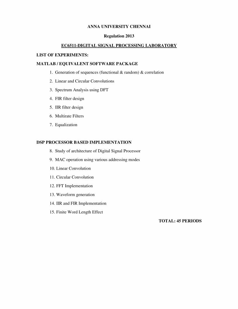
ANNA UNIVERSITY CHENNAI
Regulation 2013
EC6511-DIGITAL SIGNAL PROCESSING LABORATORY
LIST OF EXPERIMENTS:
MATLAB / EQUIVALENT SOFTWARE PACKAGE
1. Generation of sequences (functional & random) & correlation
2. Linear and Circular Convolutions
3. Spectrum Analysis using DFT
4. FIR filter design
5. IIR filter design
6. Multirate Filters
7. Equalization
DSP PROCESSOR BASED IMPLEMENTATION
8. Study of architecture of Digital Signal Processor
9. MAC operation using various addressing modes
10. Linear Convolution
11. Circular Convolution
12. FFT Implementation
13. Waveform generation
14. IIR and FIR Implementation
15. Finite Word Length Effect
TOTAL: 45 PERIODS
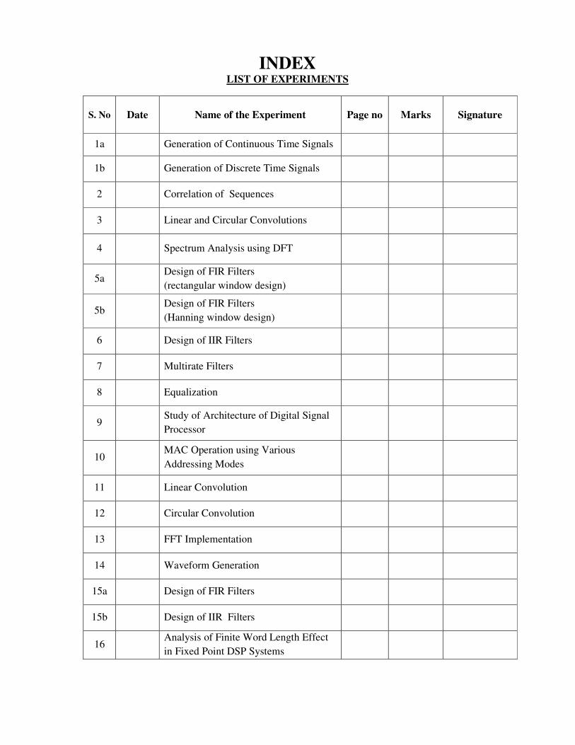
INDEX LIST OF EXPERIMENTS
S. No Date Name of the Experiment Page no Marks Signature
1a Generation of Continuous Time Signals
1b Generation of Discrete Time Signals
2 Correlation of Sequences
3 Linear and Circular Convolutions
4 Spectrum Analysis using DFT
5a Design of FIR Filters
(rectangular window design)
5b Design of FIR Filters
(Hanning window design)
6 Design of IIR Filters
7 Multirate Filters
8 Equalization
9 Study of Architecture of Digital Signal
Processor
10 MAC Operation using Various
Addressing Modes
11 Linear Convolution
12 Circular Convolution
13 FFT Implementation
14 Waveform Generation
15a Design of FIR Filters
15b Design of IIR Filters
16 Analysis of Finite Word Length Effect
in Fixed Point DSP Systems
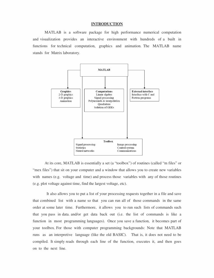
INTRODUCTION
MATLAB is a software package for high performance numerical computation
and visualization provides an interactive environment with hundreds of a built in
functions for technical computation, graphics and animation. The MATLAB name
stands for Matrix laboratory.
At its core, MATLAB is essentially a set (a “toolbox”) of routines (called “m files” or
“mex files”) that sit on your computer and a window that allows you to create new variables
with names (e.g. voltage and time) and process those variables with any of those routines
(e.g. plot voltage against time, find the largest voltage, etc).
It also allows you to put a list of your processing requests together in a file and save
that combined list with a name so that you can run all of those commands in the same
order at some later time. Furthermore, it allows you to run such lists of commands such
that you pass in data. and/or get data back out (i.e. the list of commands is like a
function in most programming languages). Once you save a function, it becomes part of
your toolbox. For those with computer programming backgrounds: Note that MATLAB
runs as an interpretive language (like the old BASIC). That is, it does not need to be
compiled. It simply reads through each line of the function, executes it, and then goes
on to the next line.
DSP Development System
• Testing the software and hardware tools with Code Composer Studio
• Use of the TMS320C6713 DSK
• Programming examples to test the tools
Digital signal processors such as the TMS320C6x (C6x) family of processors are like
fast special-purpose microprocessors with a specialized type of architecture and an
instruction set appropriate for signal processing. The C6x notation is used to designate a
member of Texas Instruments’ (TI) TMS320C6000 family of digital signal processors. The
architecture of the C6x digital signal processor is very well suited for numerically intensive
calculations. Based on a very-long-instruction-word (VLIW) architecture, the C6x is
considered to be TI’s most powerful processor. Digital signal processors are used for a wide
range of applications, from communications and controls to speech and image processing.
The general-purpose digital signal processor is dominated by applications in communications
(cellular). Applications embedded digital signal processors are dominated by consumer
products. They are found in cellular phones, fax/modems, disk drives, radio, printers, hearing
aids, MP3 players, high-definition television (HDTV), digital cameras, and so on. These
processors have become the products of choice for a number of consumer applications, since
they have become very cost-effective. They can handle different tasks, since they can be
reprogrammed readily for a different application.
DSP techniques have been very successful because of the development of low-cost
software and hardware support. For example, modems and speech recognition can be less
expensive using DSP techniques.DSP processors are concerned primarily with real-time
signal processing. Real-time processing requires the processing to keep pace with some
external event, whereas non-real-time processing has no such timing constraint. The external
event to keep pace with is usually the analog input. Whereas analog-based systems with
discrete electronic components such as resistors can be more sensitive to temperature
changes, DSP-based systems are less affected by environmental conditions.
DSP processors enjoy the advantages of microprocessors. They are easy to use,
flexible, and economical. A number of books and articles address the importance of digital
signal processors for a number of applications .Various technologies have been used for real-
time processing, from fiber optics for very high frequency to DSPs very suitable for the
audio-frequency range. Common applications using these processors have been for
frequencies from 0 to 96kHz. Speech can be sampled at 8 kHz (the rate at which samples are
acquired), which implies that each value sampled is acquired at a rate of 1/(8 kHz) or
0.125ms. A commonly used sample rate of a compact disk is 44.1 kHz. Analog/digital (A/D)-
based boards in the megahertz sampling rate range are currently available.
EC6511-Digital Signal Processing Laboratory
1 Department of Electronics and Communication Engineering
Varuvan Vadivelan Institute of Technology, Dharmapuri – 636 703
Ex. No: 1a
Date:
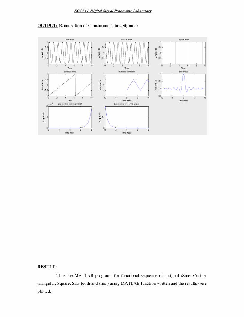
GENERATION OF CONTINUOUS TIME SIGNALS
AIM:
To generate a functional sequence of a signal (Sine, Cosine, triangular, Square, Saw
tooth and sinc ) using MATLAB function.
APPARATUS REQUIRED:
HARDWARE : Personal Computer
SOFTWARE : MATLAB R2014a
PROCEDURE:
1. Start the MATLAB program.
2. Open new M-file
3. Type the program
4. Save in current directory
5. Compile and Run the program
6. If any error occurs in the program correct the error and run it again
7. For the output see command window\ Figure window
8. Stop the program.
PROGRAM: (Generation of Continuous Time Signals)
%Program for sine wave
t=0:0.1:10;
y=sin(2*pi*t);
subplot(3,3,1);
plot(t,y,'k');
xlabel('Time');
ylabel('Amplitude');
title('Sine wave');
%Program for cosine wave
t=0:0.1:10;
y=cos(2*pi*t);
subplot(3,3,2);
plot(t,y,'k');
xlabel('Time');
ylabel('Amplitude');
title('Cosine wave');
%Program for square wave
t=0:0.001:10;
y=square(t);
subplot(3,3,3);
EC6511-Digital Signal Processing Laboratory
2 Department of Electronics and Communication Engineering
Varuvan Vadivelan Institute of Technology, Dharmapuri – 636 703
plot(t,y,'k');
xlabel('Time');
ylabel('Amplitude');
title('Square wave');
%Program for sawtooth wave
t=0:0.1:10;
y=sawtooth(t);
subplot(3,3,4);
plot(t,y,'k');
xlabel('Time');
ylabel('Amplitude');
title('Sawtooth wave');
%Program for Triangular wave
t=0:.0001:20;
y=sawtooth(t,.5); % sawtooth with 50% duty cycle
(triangular)
subplot(3,3,5);
plot(t,y);
ylabel ('Amplitude');
xlabel ('Time Index');
title('Triangular waveform');
%Program for Sinc Pulse
t=-10:.01:10;
y=sinc(t);
axis([-10 10 -2 2]);
subplot(3,3,6)
plot(t,y)
ylabel ('Amplitude');
xlabel ('Time Index');
title('Sinc Pulse');
% Program for Exponential Growing signal
t=0:.1:8;
a=2;
y=exp(a*t);
subplot(3,3,7);
plot(t,y);
ylabel ('Amplitude');
xlabel ('Time Index');
title('Exponential growing Signal');
% Program for Exponential Growing signal
t=0:.1:8;
a=2;
y=exp(-a*t);
subplot(3,3,8);
plot(t,y);
ylabel ('Amplitude');
xlabel ('Time Index');
title('Exponential decaying Signal');
EC6511-Digital Signal Processing Laboratory
OUTPUT: (Generation of Continuous
RESULT:
Thus the MATLAB progr
triangular, Square, Saw tooth and sinc
plotted.
Digital Signal Processing Laboratory
Generation of Continuous Time Signals)
Thus the MATLAB programs for functional sequence of a signal (Sine, Cosine,
and sinc ) using MATLAB function written and the results were
functional sequence of a signal (Sine, Cosine,
written and the results were
EC6511-Digital Signal Processing Laboratory
4 Department of Electronics and Communication Engineering
Varuvan Vadivelan Institute of Technology, Dharmapuri – 636 703
Ex. No: 1b
Date:
GENERATION OF DISCRETE TIME SIGNALS
AIM:
To generate a discrete time signal sequence (Unit step, Unit ramp, Sine, Cosine,
Exponential, Unit impulse) using MATLAB function.
APPARATUS REQUIRED:
HARDWARE : Personal Computer
SOFTWARE : MATLAB R2014a
PROCEDURE:
1. Start the MATLAB program.
2. Open new M-file
3. Type the program
4. Save in current directory
5. Compile and Run the program
6. If any error occurs in the program correct the error and run it again
7. For the output see command window\ Figure window
8. Stop the program.
EC6511-Digital Signal Processing Laboratory
5 Department of Electronics and Communication Engineering
Varuvan Vadivelan Institute of Technology, Dharmapuri – 636 703
PROGRAM: (Generation of Discrete Time Signals) %Program for unit step sequence
clc;
N=input('Enter the length of unit step sequence(N)= ');
n=0:1:N-1;
y=ones(1,N);
subplot(3,2,1);
stem(n,y,'k');
xlabel('Time')
ylabel('Amplitude')
title('Unit step sequence');
%Program for unit ramp sequence
N1=input('Enter the length of unit ramp sequence(N1)= ');
n1=0:1:N1-1;
y1=n1;
subplot(3,2,2);
stem(n1,y1,'k');
xlabel('Time');
ylabel('Amplitude');
title('Unit ramp sequence');
%Program for sinusoidal sequence
N2=input('Enter the length of sinusoidal sequence(N2)=
');
n2=0:0.1:N2-1;
y2=sin(2*pi*n2);
subplot(3,2,3);
stem(n2,y2,'k');
xlabel('Time');
ylabel('Amplitude');
title('Sinusoidal sequence');
%Program for cosine sequence
N3=input('Enter the length of the cosine sequence(N3)=');
n3=0:0.1:N3-1;
y3=cos(2*pi*n3);
subplot(3,2,4);
stem(n3,y3,'k');
xlabel('Time');
ylabel('Amplitude');
title('Cosine sequence');
%Program for exponential sequence
N4=input('Enter the length of the exponential
sequence(N4)= ');
n4=0:1:N4-1;
a=input('Enter the value of the exponential sequence(a)=
');
y4=exp(a*n4);
subplot(3,2,5);
stem(n4,y4,'k');
xlabel('Time');
ylabel('Amplitude');
title('Exponential sequence');
%Program for unit impulse
n=-3:1:3;
y=[zeros(1,3),ones(1,1),zeros(1,3)];
EC6511-Digital Signal Processing Laboratory
subplot(3,2,6);
stem(n,y,'k');
xlabel('Time');
ylabel('Amplitude');
title('Unit impulse');
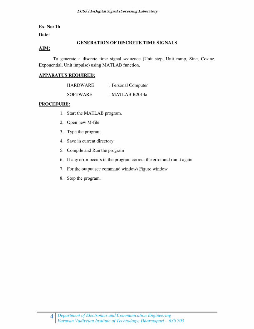
OUTPUT: (Generation of Discrete Time Signals
RESULT:
Thus the MATLAB progr
ramp, Sine, Cosine, Exponential, Unit impulse) using MATLAB function
results were plotted.
Digital Signal Processing Laboratory
ylabel('Amplitude');
title('Unit impulse');
Generation of Discrete Time Signals)
MATLAB programs for discrete time signal sequence (Unit step, Unit
ramp, Sine, Cosine, Exponential, Unit impulse) using MATLAB function written and the
discrete time signal sequence (Unit step, Unit
written and the
EC6511-Digital Signal Processing Laboratory
7 Department of Electronics and Communication Engineering
Varuvan Vadivelan Institute of Technology, Dharmapuri – 636 703
Ex. No: 2
Date:
CORRELATION OF SEQUENCES
AIM:
To write MATLAB programs for auto correlation and cross correlation.
APPARATUS REQUIRED:
HARDWARE : Personal Computer
SOFTWARE : MATLAB R2014a
PROCEDURE:
1. Start the MATLAB program.
2. Open new M-file
3. Type the program
4. Save in current directory
5. Compile and Run the program
6. If any error occurs in the program correct the error and run it again
7. For the output see command window\ Figure window
8. Stop the program.
EC6511-Digital Signal Processing Laboratory
8 Department of Electronics and Communication Engineering
Varuvan Vadivelan Institute of Technology, Dharmapuri – 636 703
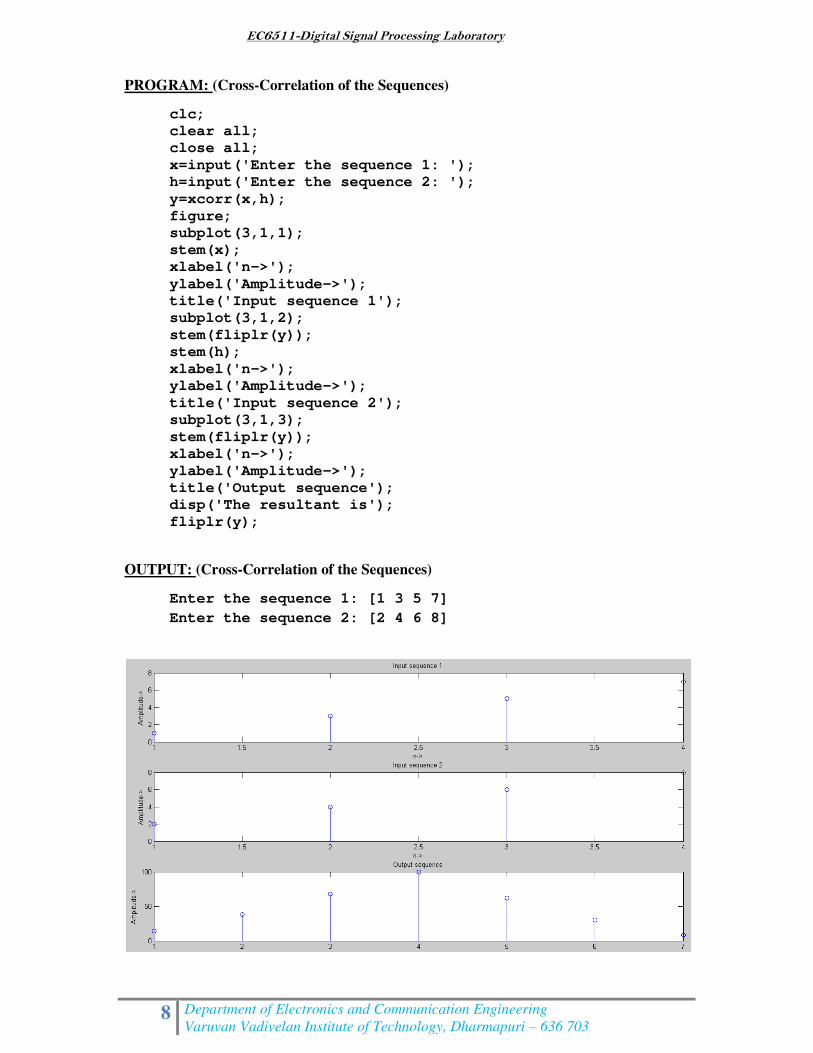
PROGRAM: (Cross-Correlation of the Sequences)
clc;
clear all;
close all;
x=input('Enter the sequence 1: ');
h=input('Enter the sequence 2: ');
y=xcorr(x,h);
figure;
subplot(3,1,1);
stem(x);
xlabel('n->');
ylabel('Amplitude->');
title('Input sequence 1');
subplot(3,1,2);
stem(fliplr(y));
stem(h);
xlabel('n->');
ylabel('Amplitude->');
title('Input sequence 2');
subplot(3,1,3);
stem(fliplr(y));
xlabel('n->');
ylabel('Amplitude->');
title('Output sequence');
disp('The resultant is');
fliplr(y);
OUTPUT: (Cross-Correlation of the Sequences)
Enter the sequence 1: [1 3 5 7]
Enter the sequence 2: [2 4 6 8]
EC6511-Digital Signal Processing Laboratory
9 Department of Electronics and Communication Engineering
Varuvan Vadivelan Institute of Technology, Dharmapuri – 636 703
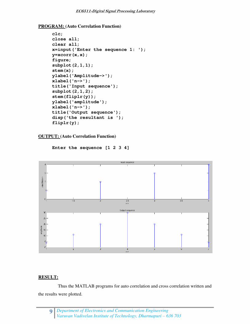
PROGRAM: (Auto Correlation Function)
clc;
close all;
clear all;
x=input('Enter the sequence 1: ');
y=xcorr(x,x);
figure;
subplot(2,1,1);
stem(x);
ylabel('Amplitude->');
xlabel('n->');
title('Input sequence');
subplot(2,1,2);
stem(fliplr(y));
ylabel('amplitude');
xlabel('n->');
title('Output sequence');
disp('the resultant is ');
fliplr(y);
OUTPUT: (Auto Correlation Function)
Enter the sequence [1 2 3 4]
RESULT:
Thus the MATLAB programs for auto correlation and cross correlation written and
the results were plotted.
EC6511-Digital Signal Processing Laboratory
10 Department of Electronics and Communication Engineering
Varuvan Vadivelan Institute of Technology, Dharmapuri – 636 703
Ex. No: 3
Date:
LINEAR AND CIRCULAR CONVOLUTIONS
AIM:
To write MATLAB programs to find out the linear convolution and Circular
convolution of two sequences.
APPARATUS REQUIRED:
HARDWARE : Personal Computer
SOFTWARE : MATLAB R2014a
PROCEDURE:
1. Start the MATLAB program.
2. Open new M-file
3. Type the program
4. Save in current directory
5. Compile and Run the program
6. If any error occurs in the program correct the error and run it again
7. For the output see command window\ Figure window
8. Stop the program.
EC6511-Digital Signal Processing Laboratory
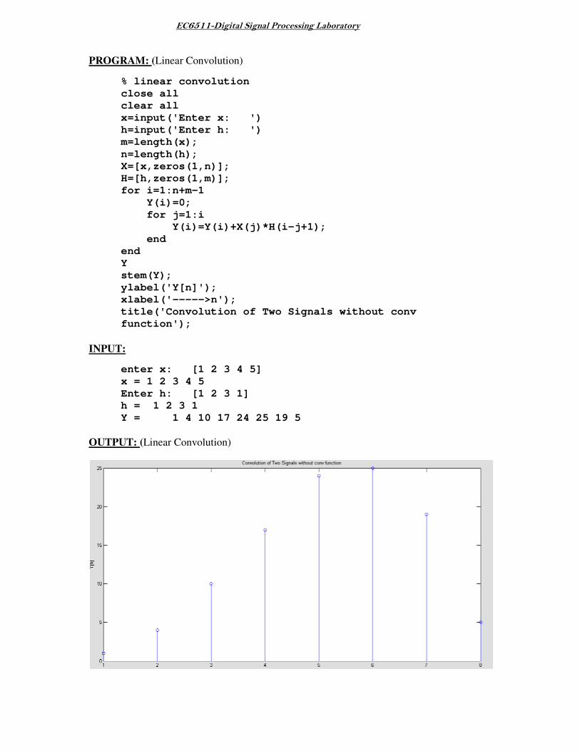
PROGRAM: (Linear Convolution)
% linear convolution
close all
clear all
x=input('Enter x: ')
h=input('Enter h: ')
m=length(x);
n=length(h);
X=[x,zeros(1,n)];
H=[h,zeros(1,m)];
for i=1:n+m-1
Y(i)=0;
for j=1:i
Y(i)=Y(i)+X(j)*H(i
end
end
Y
stem(Y);
ylabel('Y[n]');
xlabel('----->n');
title('Convolution of Two Signals without conv
function');
INPUT:
enter x: [1 2 3 4 5]
x = 1 2 3 4 5
Enter h: [1 2 3 1]
h = 1 2 3 1
Y = 1 4 10 17 24 25 19 5
OUTPUT: (Linear Convolution)
Digital Signal Processing Laboratory
Convolution)
% linear convolution
x=input('Enter x: ')
h=input('Enter h: ')
X=[x,zeros(1,n)];
H=[h,zeros(1,m)];
Y(i)=Y(i)+X(j)*H(i-j+1);
>n');
title('Convolution of Two Signals without conv
enter x: [1 2 3 4 5]
Enter h: [1 2 3 1]
Y = 1 4 10 17 24 25 19 5
Convolution)
EC6511-Digital Signal Processing Laboratory
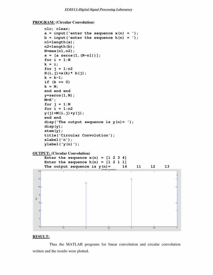
PROGRAM: (Circular Convolution
clc; clear;
a = input('enter the sequence x(n) = ');
b = input('enter the sequence h(n) = ');
n1=length(a);
n2=length(b);
N=max(n1,n2);
x = [a zeros(1,(N
for i = 1:N
k = i;
for j = 1:n2
H(i,j)=x(k)* b(j);
k = k-1;
if (k == 0)
k = N;
end end end
y=zeros(1,N);
M=H';
for j = 1:N
for i = 1:n2
y(j)=M(i,j)+y(j);
end end
disp('The output sequence is y(n)= ');
disp(y);
stem(y);
title('Circular Convolution');
xlabel('n');
ylabel('y(n)');
OUTPUT: (Circular ConvolutionEnter the sequence x(n) =
Enter the sequence h(n) = [1 2 1 1]
The output sequence is y(n)= 14 11 12 13
RESULT:
Thus the MATLAB progr
written and the results were plotted.
Digital Signal Processing Laboratory
Circular Convolution)
a = input('enter the sequence x(n) = ');
b = input('enter the sequence h(n) = ');
x = [a zeros(1,(N-n1))];
H(i,j)=x(k)* b(j);
y(j)=M(i,j)+y(j);
disp('The output sequence is y(n)= ');
title('Circular Convolution');
Circular Convolution) the sequence x(n) = [1 2 3 4]
the sequence h(n) = [1 2 1 1]
The output sequence is y(n)= 14 11 12 13
Thus the MATLAB programs for linear convolution and circular convolution
written and the results were plotted.
The output sequence is y(n)= 14 11 12 13
and circular convolution
EC6511-Digital Signal Processing Laboratory
13 Department of Electronics and Communication Engineering
Varuvan Vadivelan Institute of Technology, Dharmapuri – 636 703
Ex. No: 4
Date:
SPECTRUM ANALYSIS USING DFT
AIM:
To write MATLAB program for spectrum analyzing signal using DFT.
APPARATUS REQUIRED:
HARDWARE : Personal Computer
SOFTWARE : MATLAB R2014a
PROCEDURE:
1. Start the MATLAB program.
2. Open new M-file
3. Type the program
4. Save in current directory
5. Compile and Run the program
6. If any error occurs in the program correct the error and run it again
7. For the output see command window\ Figure window
8. Stop the program.
EC6511-Digital Signal Processing Laboratory
14 Department of Electronics and Communication Engineering
Varuvan Vadivelan Institute of Technology, Dharmapuri – 636 703
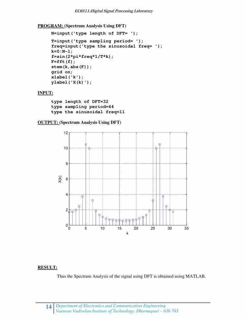
PROGRAM: (Spectrum Analysis Using DFT)
N=input('type length of DFT= ');
T=input('type sampling period= ');
freq=input('type the sinusoidal freq= ');
k=0:N-1;
f=sin(2*pi*freq*1/T*k);
F=fft(f);
stem(k,abs(F));
grid on;
xlabel('k');
ylabel('X(k)');
INPUT:
type length of DFT=32
type sampling period=64
type the sinusoidal freq=11
OUTPUT: (Spectrum Analysis Using DFT)
RESULT:
Thus the Spectrum Analysis of the signal using DFT is obtained using MATLAB.
EC6511-Digital Signal Processing Laboratory
15 Department of Electronics and Communication Engineering
Varuvan Vadivelan Institute of Technology, Dharmapuri – 636 703
Ex. No: 5a
Date:
DESIGN OF FIR FILTERS
(RECTANGULAR WINDOW DESIGN)
AIM:
To write a program to design the FIR low pass, High pass, Band pass and Band stop
filters using RECTANGULAR window and find out the response of the filter by using
MATLAB.
APPARATUS REQUIRED:
HARDWARE : Personal Computer
SOFTWARE : MATLAB R2014a
PROCEDURE:
1. Start the MATLAB program.
2. Open new M-file
3. Type the program
4. Save in current directory
5. Compile and Run the program
6. If any error occurs in the program correct the error and run it again
7. For the output see command window\ Figure window
8. Stop the program.

EC6511-Digital Signal Processing Laboratory
16 Department of Electronics and Communication Engineering
Varuvan Vadivelan Institute of Technology, Dharmapuri – 636 703
PROGRAM: (Rectangular Window)
clear all;
rp=input('Enter the PB ripple rp =');
rs=input('Enter the SB ripple rs =');
fp=input('Enter the PB ripple fp =');
fs=input('Enter the SB ripple fs =');
f=input('Enter the sampling frequency f =');
wp=2*fp/f;
ws=2*fs/f;
num=-20*log10(sqrt(rp*rs))-13;
den=14.6*(fs-fp)/f;
n=ceil(num/den);
n1=n+1;
if(rem(n,2)~=0)
n=n1;
n=n-1;
end;
y=boxcar(n1);
%LPF b=fir1(n,wp,y);
[h,o]=freqz(b,1,256);
m=20*log10(abs(h));
subplot(2,2,1);
plot(o/pi,m);
xlabel('Normalized frequency------>');
ylabel('Gain in db--------.');
title('MAGNITUDE RESPONSE OF LPF');
%HPF b=fir1(n,wp,'high',y);
[h,o]=freqz(b,1,256);
m=20*log10(abs(h));
subplot(2,2,2);
plot(o/pi,m);
xlabel('Normalized frequency------>');
ylabel('Gain in db--------.');
title('MAGNITUDE RESPONSE OF HPF');
%BPF wn=[wp ws];
b=fir1(n,wn,y);
[h,o]=freqz(b,1,256);
m=20*log10(abs(h));
subplot(2,2,3);
plot(o/pi,m);
xlabel('Normalized frequency------>');
ylabel('Gain in db--------.');
title('MAGNITUDE RESPONSE OF BPF');
%BSF b=fir1(n,wn,'stop',y);
[h,o]=freqz(b,1,256);
m=20*log10(abs(h));
subplot(2,2,4);
plot(o/pi,m);
EC6511-Digital Signal Processing Laboratory
17 Department of Electronics and Communication Engineering
Varuvan Vadivelan Institute of Technology, Dharmapuri – 636 703
xlabel('Normalized frequency------>');
ylabel('Gain in db--------.');
title('MAGNITUDE RESPONSE OF BSF');
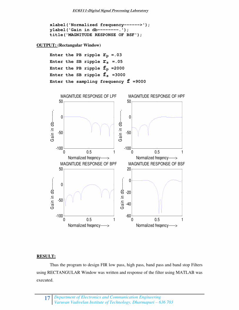
OUTPUT: (Rectangular Window)
Enter the PB ripple rp =.03
Enter the SB ripple rs =.05
Enter the PB ripple fp =2000
Enter the SB ripple fs =3000
Enter the sampling frequency f =9000
RESULT:
Thus the program to design FIR low pass, high pass, band pass and band stop Filters
using RECTANGULAR Window was written and response of the filter using MATLAB was
executed.
0 0.5 1-100
-50
0
50
Normalized freqency------>
Ga
in i
n d
b--
----
--.
MAGNITUDE RESPONSE OF LPF
0 0.5 1-100
-50
0
50
Normalized freqency------>
Ga
in i
n d
b--
----
--.
MAGNITUDE RESPONSE OF HPF
0 0.5 1-100
-50
0
50
Normalized freqency------>
Ga
in i
n d
b--
----
--.
MAGNITUDE RESPONSE OF BPF
0 0.5 1-60
-40
-20
0
20
Normalized freqency------>
Ga
in i
n d
b--
----
--.
MAGNITUDE RESPONSE OF BSF
EC6511-Digital Signal Processing Laboratory
18 Department of Electronics and Communication Engineering
Varuvan Vadivelan Institute of Technology, Dharmapuri – 636 703
Ex. No: 5b
Date:
DESIGN OF FIR FILTERS
(HANNING WINDOW DESIGN)
AIM:
To write a program to design the FIR low pass, High pass, Band pass and Band stop
filters using HANNING window and find out the response of the filter by using MATLAB.
APPARATUS REQUIRED:
HARDWARE : Personal Computer
SOFTWARE : MATLAB R2014a
PROCEDURE:
1. Start the MATLAB program.
2. Open new M-file
3. Type the program
4. Save in current directory
5. Compile and Run the program
6. If any error occurs in the program correct the error and run it again
7. For the output see command window\ Figure window
8. Stop the program.
EC6511-Digital Signal Processing Laboratory
19 Department of Electronics and Communication Engineering
Varuvan Vadivelan Institute of Technology, Dharmapuri – 636 703
PROGRAM: (Hanning Window)
clear all;
rp=input('Enter the PB ripple rp =');
rs=input('Enter the SB ripple rs =');
fp=input('Enter the PB ripple fp =');
fs=input('Enter the SB ripple fs =');
f=input('Enter the sampling frequency f =');
wp=2*fp/f;
ws=2*fs/f;
num=-20*log10(sqrt(rp*rs))-13;
den=14.6*(fs-fp)/f;
n=ceil(num/den);
n1=n+1;
if(rem(n,2)~=0)
n=n1;
n=n-1;
end;
y=hanning(n1);
%LPF b=fir1(n,wp,y);
[h,O]=freqz(b,1,256);
m=20*log10(abs(h));
subplot(2,2,1);
plot(O/pi,m);
xlabel('Normalized freqency------>');
ylabel('Gain in db--------.');
title('MAGNITUDE RESPONSE OF LPF');
%HPF b=fir1(n,wp,'high',y);
[h,O]=freqz(b,1,256);
m=20*log10(abs(h));
subplot(2,2,2);
plot(O/pi,m);
xlabel('Normalized freqency------>');
ylabel('Gain in db--------.');
title('MAGNITUDE RESPONSE OF HPF');
%BPF wn=[wp ws];
b=fir1(n,wn,y);
[h,O]=freqz(b,1,256);
m=20*log10(abs(h));
subplot(2,2,3);
plot(O/pi,m);
xlabel('Normalized freqency------>');
ylabel('Gain in db--------.');
title('MAGNITUDE RESPONSE OF BPF');
%BSF b=fir1(n,wn,'stop',y);
[h,O]=freqz(b,1,256);
m=20*log10(abs(h));
subplot(2,2,4);
plot(O/pi,m);
EC6511-Digital Signal Processing Laboratory
20 Department of Electronics and Communication Engineering
Varuvan Vadivelan Institute of Technology, Dharmapuri – 636 703
xlabel('Normalized freqency------>');
ylabel('Gain in db--------.');
title('MAGNITUDE RESPONSE OF BSF');
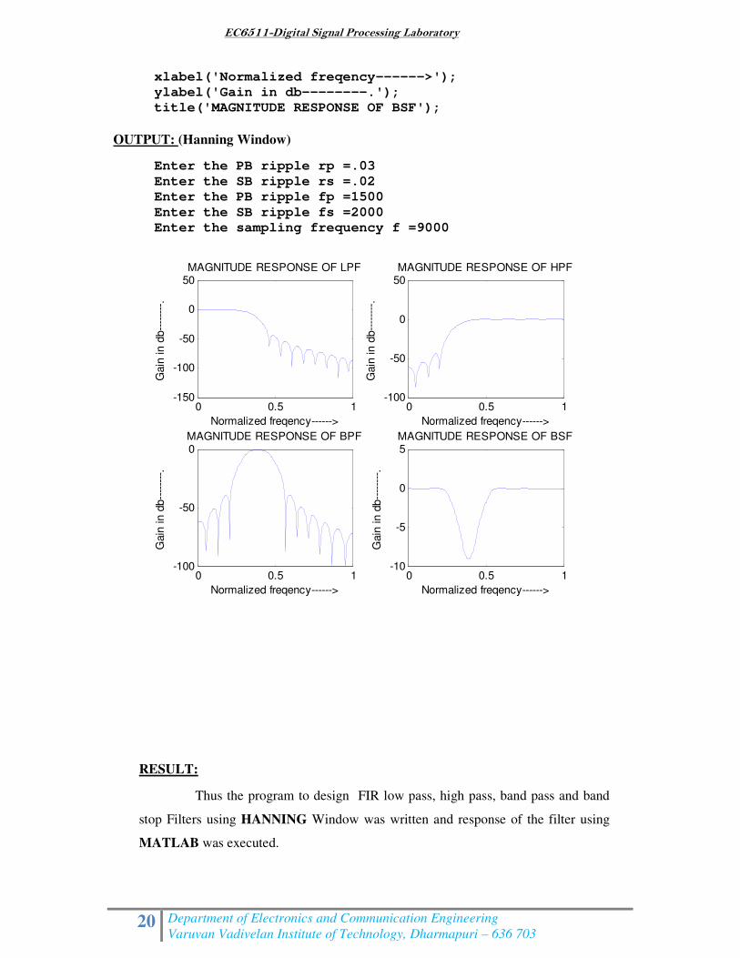
OUTPUT: (Hanning Window)
Enter the PB ripple rp =.03
Enter the SB ripple rs =.02
Enter the PB ripple fp =1500
Enter the SB ripple fs =2000
Enter the sampling frequency f =9000
RESULT:
Thus the program to design FIR low pass, high pass, band pass and band
stop Filters using HANNING Window was written and response of the filter using
MATLAB was executed.
0 0.5 1-150
-100
-50
0
50
Normalized freqency------>
Gain
in d
b--
----
--.
MAGNITUDE RESPONSE OF LPF
0 0.5 1-100
-50
0
50
Normalized freqency------>
Gain
in d
b--
----
--.
MAGNITUDE RESPONSE OF HPF
0 0.5 1-100
-50
0
Normalized freqency------>
Gain
in d
b--
----
--.
MAGNITUDE RESPONSE OF BPF
0 0.5 1-10
-5
0
5
Normalized freqency------>
Gain
in d
b--
----
--.
MAGNITUDE RESPONSE OF BSF
EC6511-Digital Signal Processing Laboratory
21 Department of Electronics and Communication Engineering
Varuvan Vadivelan Institute of Technology, Dharmapuri – 636 703
Ex. No: 6
Date:
DESIGN OF IIR FILTERS
AIM:
To write a program to design the IIR Filter using Impulse Invariant Transformation
method and find out the Magnitude response and Pole Zero Plot by using MATLAB.
APPARATUS REQUIRED:
HARDWARE : Personal Computer
SOFTWARE : MATLAB R2014a
PROCEDURE:
1. Start the MATLAB program.
2. Open new M-file
3. Type the program
4. Save in current directory
5. Compile and Run the program
6. If any error occurs in the program correct the error and run it again
7. For the output see command window\ Figure window
8. Stop the program.
EC6511-Digital Signal Processing Laboratory
22 Department of Electronics and Communication Engineering
Varuvan Vadivelan Institute of Technology, Dharmapuri – 636 703
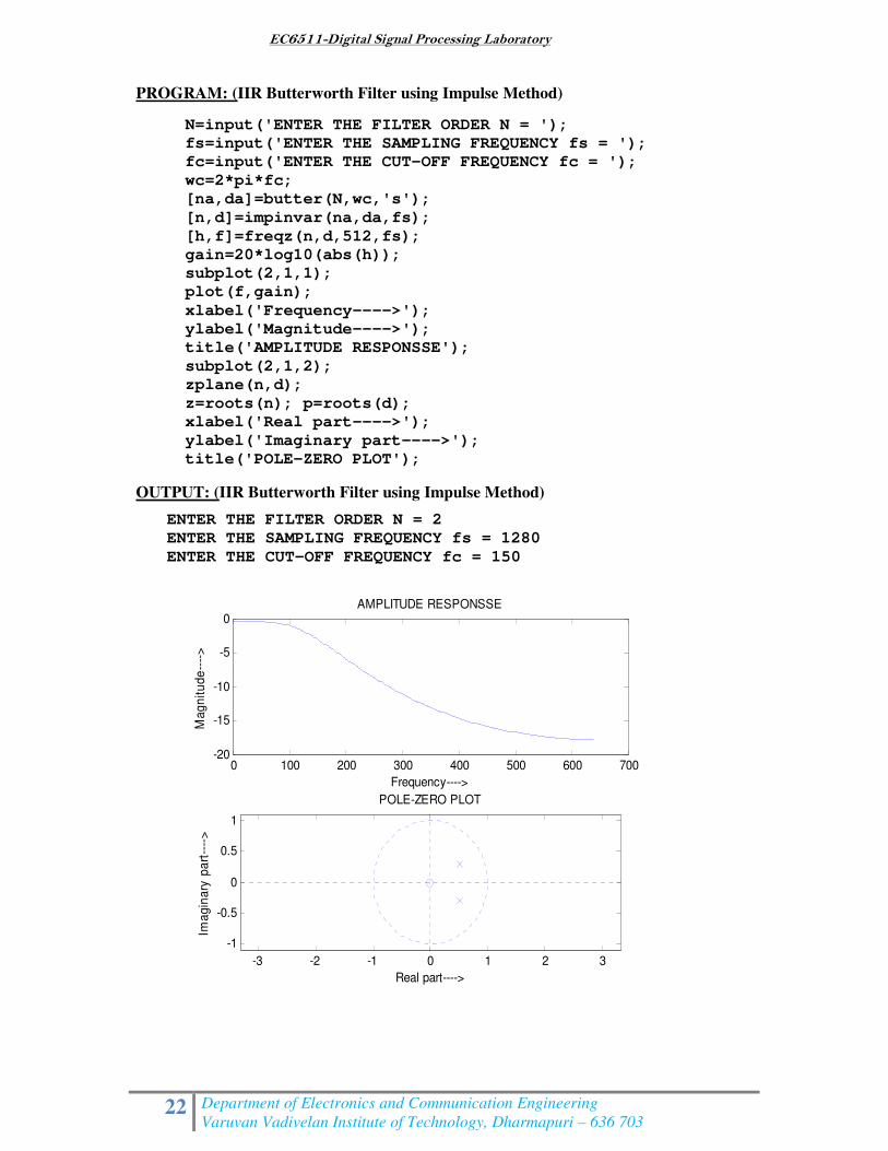
PROGRAM: (IIR Butterworth Filter using Impulse Method)
N=input('ENTER THE FILTER ORDER N = ');
fs=input('ENTER THE SAMPLING FREQUENCY fs = ');
fc=input('ENTER THE CUT-OFF FREQUENCY fc = ');
wc=2*pi*fc;
[na,da]=butter(N,wc,'s');
[n,d]=impinvar(na,da,fs);
[h,f]=freqz(n,d,512,fs);
gain=20*log10(abs(h));
subplot(2,1,1);
plot(f,gain);
xlabel('Frequency---->');
ylabel('Magnitude---->');
title('AMPLITUDE RESPONSSE');
subplot(2,1,2);
zplane(n,d);
z=roots(n); p=roots(d);
xlabel('Real part---->');
ylabel('Imaginary part---->');
title('POLE-ZERO PLOT');
OUTPUT: (IIR Butterworth Filter using Impulse Method)
ENTER THE FILTER ORDER N = 2
ENTER THE SAMPLING FREQUENCY fs = 1280
ENTER THE CUT-OFF FREQUENCY fc = 150
0 100 200 300 400 500 600 700-20
-15
-10
-5
0
Frequency---->
Ma
gn
itu
de
----
>
AMPLITUDE RESPONSSE
-3 -2 -1 0 1 2 3
-1
-0.5
0
0.5
1
Real part---->
Ima
gin
ary
pa
rt--
-->
POLE-ZERO PLOT
EC6511-Digital Signal Processing Laboratory
23 Department of Electronics and Communication Engineering
Varuvan Vadivelan Institute of Technology, Dharmapuri – 636 703
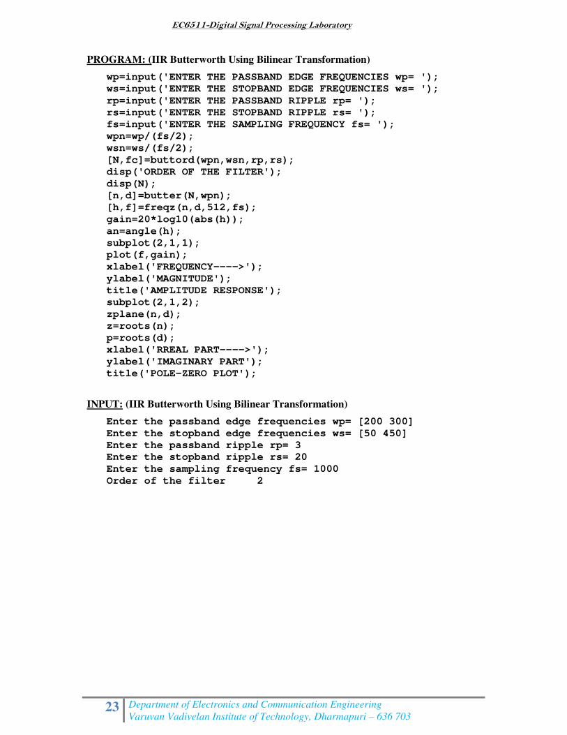
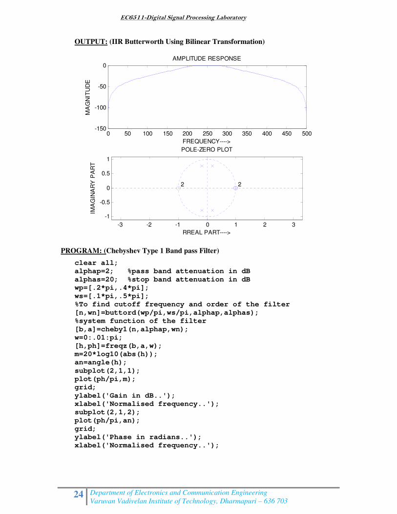
PROGRAM: (IIR Butterworth Using Bilinear Transformation)
wp=input('ENTER THE PASSBAND EDGE FREQUENCIES wp= ');
ws=input('ENTER THE STOPBAND EDGE FREQUENCIES ws= ');
rp=input('ENTER THE PASSBAND RIPPLE rp= ');
rs=input('ENTER THE STOPBAND RIPPLE rs= ');
fs=input('ENTER THE SAMPLING FREQUENCY fs= ');
wpn=wp/(fs/2);
wsn=ws/(fs/2);
[N,fc]=buttord(wpn,wsn,rp,rs);
disp('ORDER OF THE FILTER');
disp(N);
[n,d]=butter(N,wpn);
[h,f]=freqz(n,d,512,fs);
gain=20*log10(abs(h));
an=angle(h);
subplot(2,1,1);
plot(f,gain);
xlabel('FREQUENCY---->');
ylabel('MAGNITUDE');
title('AMPLITUDE RESPONSE');
subplot(2,1,2);
zplane(n,d);
z=roots(n);
p=roots(d);
xlabel('RREAL PART---->');
ylabel('IMAGINARY PART');
title('POLE-ZERO PLOT');
INPUT: (IIR Butterworth Using Bilinear Transformation)
Enter the passband edge frequencies wp= [200 300]
Enter the stopband edge frequencies ws= [50 450]
Enter the passband ripple rp= 3
Enter the stopband ripple rs= 20
Enter the sampling frequency fs= 1000
Order of the filter 2
EC6511-Digital Signal Processing Laboratory
24 Department of Electronics and Communication Engineering
Varuvan Vadivelan Institute of Technology, Dharmapuri – 636 703
OUTPUT: (IIR Butterworth Using Bilinear Transformation)
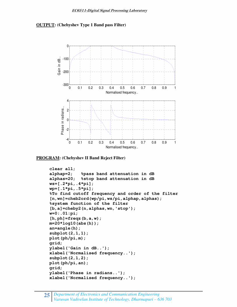
PROGRAM: (Chebyshev Type 1 Band pass Filter)
clear all;
alphap=2; %pass band attenuation in dB
alphas=20; %stop band attenuation in dB
wp=[.2*pi,.4*pi];
ws=[.1*pi,.5*pi];
%To find cutoff frequency and order of the filter
[n,wn]=buttord(wp/pi,ws/pi,alphap,alphas);
%system function of the filter
[b,a]=cheby1(n,alphap,wn);
w=0:.01:pi;
[h,ph]=freqz(b,a,w);
m=20*log10(abs(h));
an=angle(h);
subplot(2,1,1);
plot(ph/pi,m);
grid;
ylabel('Gain in dB..');
xlabel('Normalised frequency..');
subplot(2,1,2);
plot(ph/pi,an);
grid;
ylabel('Phase in radians..');
xlabel('Normalised frequency..');
0 50 100 150 200 250 300 350 400 450 500-150
-100
-50
0
FREQUENCY---->
MA
GN
ITU
DE
AMPLITUDE RESPONSE
-3 -2 -1 0 1 2 3
-1
-0.5
0
0.5
1
2 2
RREAL PART---->
IMA
GIN
AR
Y P
AR
T
POLE-ZERO PLOT
EC6511-Digital Signal Processing Laboratory
25 Department of Electronics and Communication Engineering
Varuvan Vadivelan Institute of Technology, Dharmapuri – 636 703
OUTPUT: (Chebyshev Type 1 Band pass Filter)
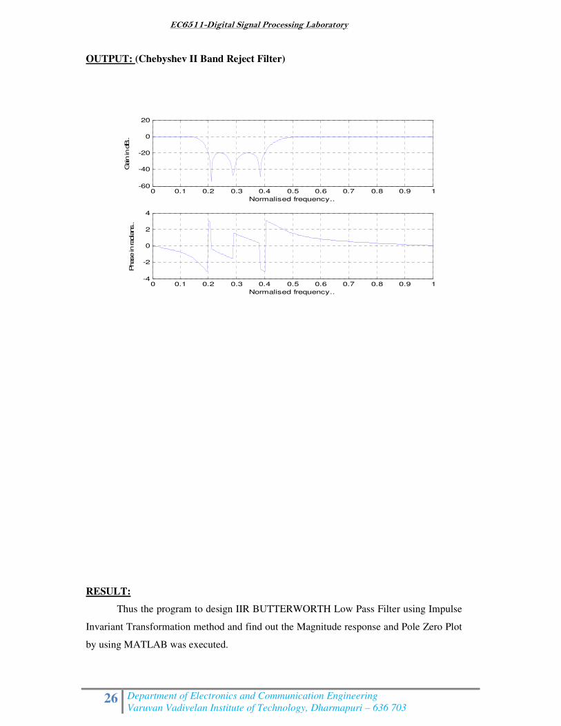
PROGRAM: (Chebyshev II Band Reject Filter)
clear all;
alphap=2; %pass band attenuation in dB
alphas=20; %stop band attenuation in dB
ws=[.2*pi,.4*pi];
wp=[.1*pi,.5*pi];
%To find cutoff frequency and order of the filter
[n,wn]=cheb2ord(wp/pi,ws/pi,alphap,alphas);
%system function of the filter
[b,a]=cheby2(n,alphas,wn,'stop');
w=0:.01:pi;
[h,ph]=freqz(b,a,w);
m=20*log10(abs(h));
an=angle(h);
subplot(2,1,1);
plot(ph/pi,m);
grid;
ylabel('Gain in dB..');
xlabel('Normalised frequency..');
subplot(2,1,2);
plot(ph/pi,an);
grid;
ylabel('Phase in radians..');
xlabel('Normalised frequency..');
0 0.1 0.2 0.3 0.4 0.5 0.6 0.7 0.8 0.9 1-300
-200
-100
0
Ga
in i
n d
B..
Normalised frequency..
0 0.1 0.2 0.3 0.4 0.5 0.6 0.7 0.8 0.9 1-4
-2
0
2
4
Ph
as
e i
n r
ad
ian
s..
Normalised frequency..
EC6511-Digital Signal Processing Laboratory
26 Department of Electronics and Communication Engineering
Varuvan Vadivelan Institute of Technology, Dharmapuri – 636 703
OUTPUT: (Chebyshev II Band Reject Filter)
RESULT:
Thus the program to design IIR BUTTERWORTH Low Pass Filter using Impulse
Invariant Transformation method and find out the Magnitude response and Pole Zero Plot
by using MATLAB was executed.
0 0.1 0.2 0.3 0.4 0.5 0.6 0.7 0.8 0.9 1-60
-40
-20
0
20G
ain in d
B..
Normalised frequency..
0 0.1 0.2 0.3 0.4 0.5 0.6 0.7 0.8 0.9 1-4
-2
0
2
4
Phase in radians..
Normalised frequency..
EC6511-Digital Signal Processing Laboratory
27 Department of Electronics and Communication Engineering
Varuvan Vadivelan Institute of Technology, Dharmapuri – 636 703
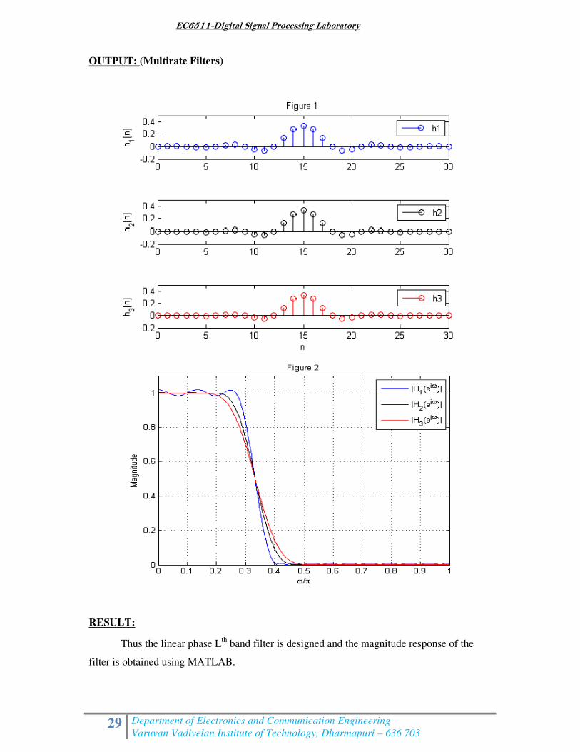
Ex. No: 7
Date:
MULTIRATE FILTERS
AIM:
To design linear-phase FIR Lth
-band filters of the length N =31, with L = 3 and with
the roll-off factors: ρ = 0.2, 0.4, and 0.6. Plot the impulse responses and the magnitude
responses for all designs.
APPARATUS REQUIRED:
HARDWARE : Personal Computer
SOFTWARE : MATLAB R2014a
PROCEDURE:
1. Start the MATLAB program.
2. Open new M-file
3. Type the program
4. Save in current directory
5. Compile and Run the program
6. If any error occurs in the program correct the error and run it again
7. For the output see command window\ Figure window
8. Stop the program.
EC6511-Digital Signal Processing Laboratory
28 Department of Electronics and Communication Engineering
Varuvan Vadivelan Institute of Technology, Dharmapuri – 636 703
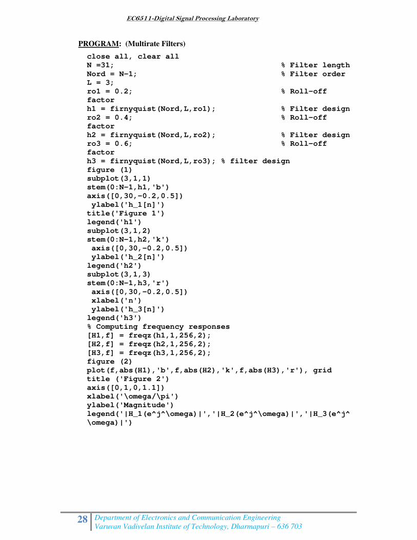
PROGRAM: (Multirate Filters)
close all, clear all
N =31; % Filter length
Nord = N-1; % Filter order
L = 3;
ro1 = 0.2; % Roll-off
factor
h1 = firnyquist(Nord,L,ro1); % Filter design
ro2 = 0.4; % Roll-off
factor
h2 = firnyquist(Nord,L,ro2); % Filter design
ro3 = 0.6; % Roll-off
factor
h3 = firnyquist(Nord,L,ro3); % filter design
figure (1)
subplot(3,1,1)
stem(0:N-1,h1,'b')
axis([0,30,-0.2,0.5])
ylabel('h_1[n]')
title('Figure 1')
legend('h1')
subplot(3,1,2)
stem(0:N-1,h2,'k')
axis([0,30,-0.2,0.5])
ylabel('h_2[n]')
legend('h2')
subplot(3,1,3)
stem(0:N-1,h3,'r')
axis([0,30,-0.2,0.5])
xlabel('n')
ylabel('h_3[n]')
legend('h3')
% Computing frequency responses
[H1,f] = freqz(h1,1,256,2);
[H2,f] = freqz(h2,1,256,2);
[H3,f] = freqz(h3,1,256,2);
figure (2)
plot(f,abs(H1),'b',f,abs(H2),'k',f,abs(H3),'r'), grid
title ('Figure 2')
axis([0,1,0,1.1])
xlabel('\omega/\pi')
ylabel('Magnitude')
legend('|H_1(e^j^\omega)|','|H_2(e^j^\omega)|','|H_3(e^j^
\omega)|')
EC6511-Digital Signal Processing Laboratory
29 Department of Electronics and Communication Engineering
Varuvan Vadivelan Institute of Technology, Dharmapuri – 636 703
OUTPUT: (Multirate Filters)
RESULT:
Thus the linear phase Lth
band filter is designed and the magnitude response of the
filter is obtained using MATLAB.
EC6511-Digital Signal Processing Laboratory
30 Department of Electronics and Communication Engineering
Varuvan Vadivelan Institute of Technology, Dharmapuri – 636 703
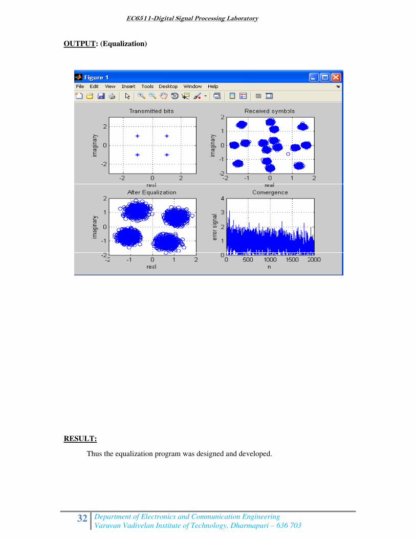
Ex. No: 8
Date:
EQUALIZATION
AIM:
To write MATLAB programs for equalization.
APPARATUS REQUIRED:
HARDWARE : Personal Computer
SOFTWARE : MATLAB R2014a
PROCEDURE:
1. Start the MATLAB program.
2. Open new M-file
3. Type the program
4. Save in current directory
5. Compile and Run the program
6. If any error occurs in the program correct the error and run it again
7. For the output see command window\ Figure window
8. Stop the program.
EC6511-Digital Signal Processing Laboratory
31 Department of Electronics and Communication Engineering
Varuvan Vadivelan Institute of Technology, Dharmapuri – 636 703
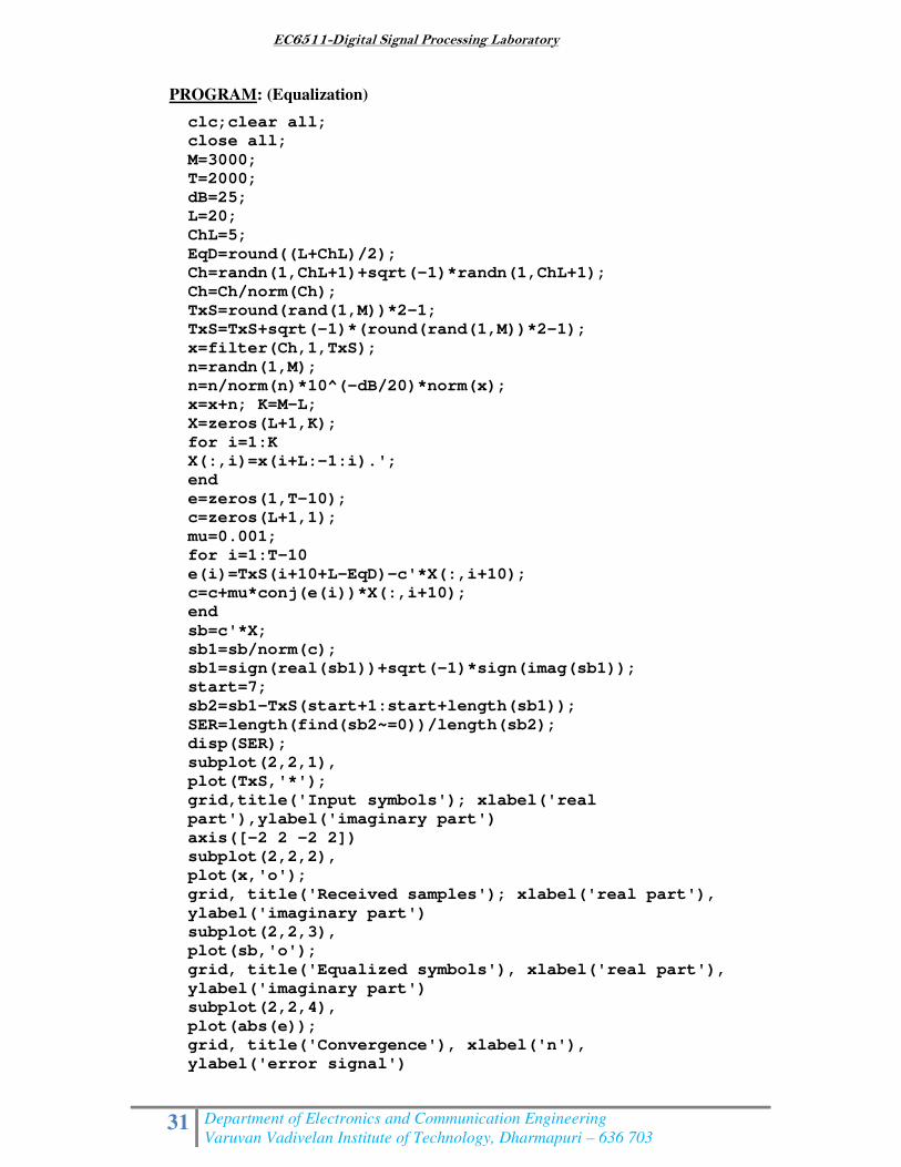
PROGRAM: (Equalization)
clc;clear all;
close all;
M=3000;
T=2000;
dB=25;
L=20;
ChL=5;
EqD=round((L+ChL)/2);
Ch=randn(1,ChL+1)+sqrt(-1)*randn(1,ChL+1);
Ch=Ch/norm(Ch);
TxS=round(rand(1,M))*2-1;
TxS=TxS+sqrt(-1)*(round(rand(1,M))*2-1);
x=filter(Ch,1,TxS);
n=randn(1,M);
n=n/norm(n)*10^(-dB/20)*norm(x);
x=x+n; K=M-L;
X=zeros(L+1,K);
for i=1:K
X(:,i)=x(i+L:-1:i).';
end
e=zeros(1,T-10);
c=zeros(L+1,1);
mu=0.001;
for i=1:T-10
e(i)=TxS(i+10+L-EqD)-c'*X(:,i+10);
c=c+mu*conj(e(i))*X(:,i+10);
end
sb=c'*X;
sb1=sb/norm(c);
sb1=sign(real(sb1))+sqrt(-1)*sign(imag(sb1));
start=7;
sb2=sb1-TxS(start+1:start+length(sb1));
SER=length(find(sb2~=0))/length(sb2);
disp(SER);
subplot(2,2,1),
plot(TxS,'*');
grid,title('Input symbols'); xlabel('real
part'),ylabel('imaginary part')
axis([-2 2 -2 2])
subplot(2,2,2),
plot(x,'o');
grid, title('Received samples'); xlabel('real part'),
ylabel('imaginary part')
subplot(2,2,3),
plot(sb,'o');
grid, title('Equalized symbols'), xlabel('real part'),
ylabel('imaginary part')
subplot(2,2,4),
plot(abs(e));
grid, title('Convergence'), xlabel('n'),
ylabel('error signal')
EC6511-Digital Signal Processing Laboratory
32 Department of Electronics and Communication Engineering
Varuvan Vadivelan Institute of Technology, Dharmapuri – 636 703
OUTPUT: (Equalization)
RESULT:
Thus the equalization program was designed and developed.
EC6511-Digital Signal Processing Laboratory
33 Department of Electronics and Communication Engineering
Varuvan Vadivelan Institute of Technology, Dharmapuri – 636 703
DSP PROCESSOR EXPERIMENTS
EC6511-Digital Signal Processing Laboratory
34 Department of Electronics and Communication Engineering
Varuvan Vadivelan Institute of Technology, Dharmapuri – 636 703
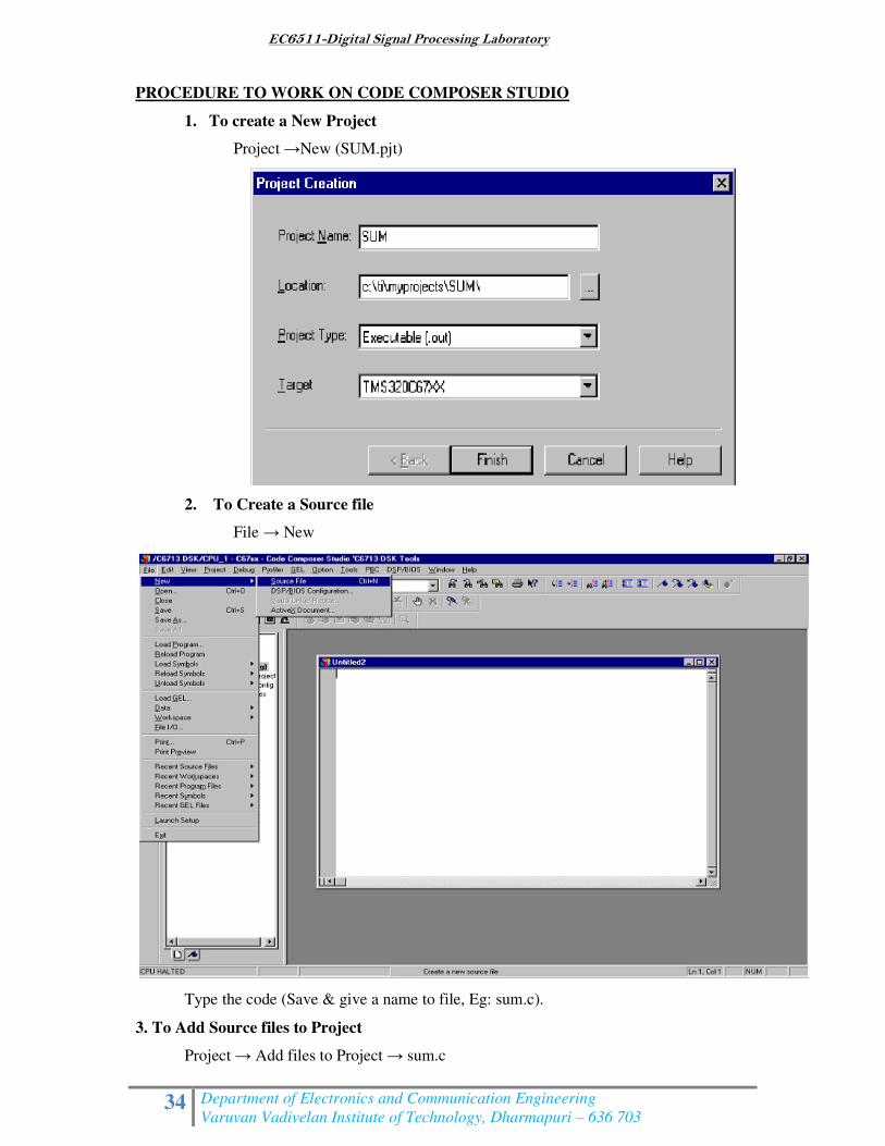
PROCEDURE TO WORK ON CODE COMPOSER STUDIO
1. To create a New Project
Project →New (SUM.pjt)
2. To Create a Source file
File → New
Type the code (Save & give a name to file, Eg: sum.c).
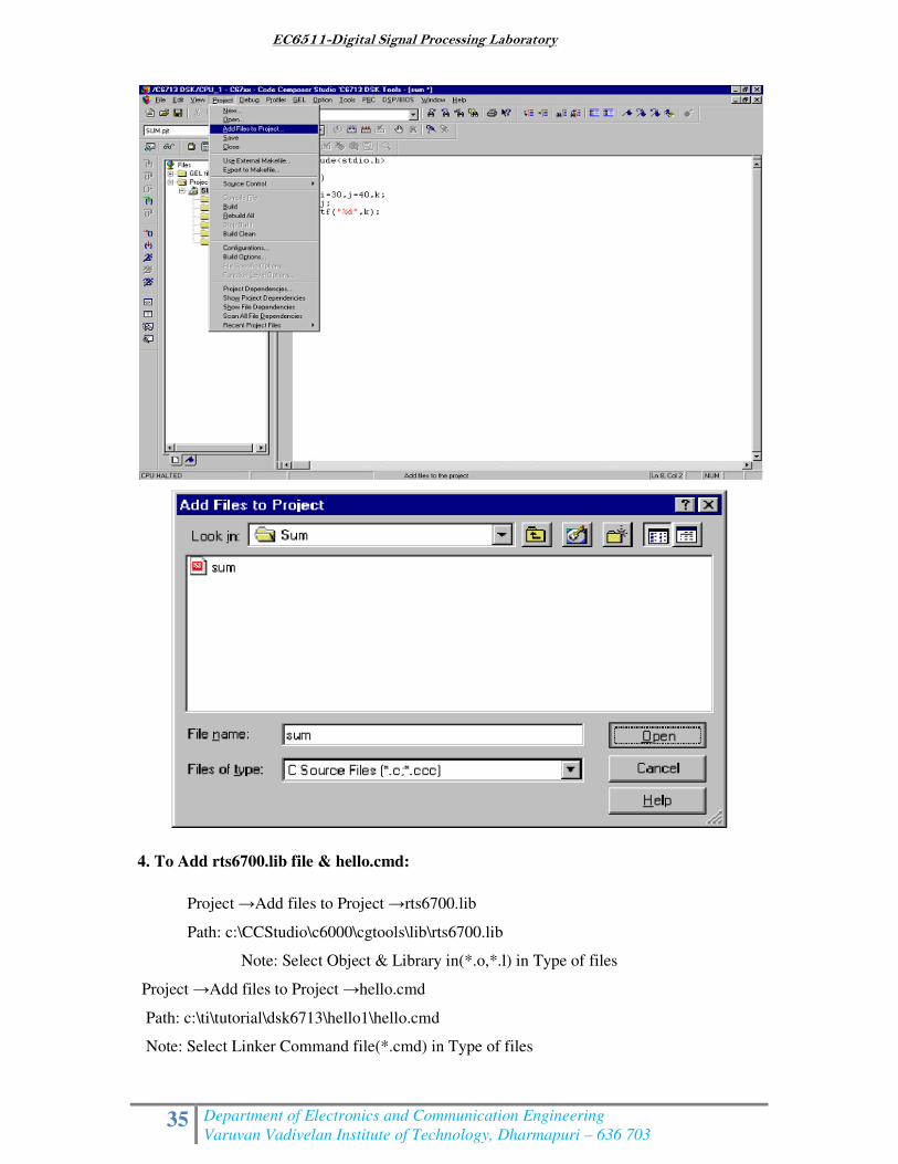
3. To Add Source files to Project
Project → Add files to Project → sum.c
EC6511-Digital Signal Processing Laboratory
35 Department of Electronics and Communication Engineering
Varuvan Vadivelan Institute of Technology, Dharmapuri – 636 703
4. To Add rts6700.lib file & hello.cmd:
Project →Add files to Project →rts6700.lib
Path: c:\CCStudio\c6000\cgtools\lib\rts6700.lib
Note: Select Object & Library in(*.o,*.l) in Type of files
Project →Add files to Project →hello.cmd
Path: c:\ti\tutorial\dsk6713\hello1\hello.cmd
Note: Select Linker Command file(*.cmd) in Type of files
EC6511-Digital Signal Processing Laboratory
36 Department of Electronics and Communication Engineering
Varuvan Vadivelan Institute of Technology, Dharmapuri – 636 703
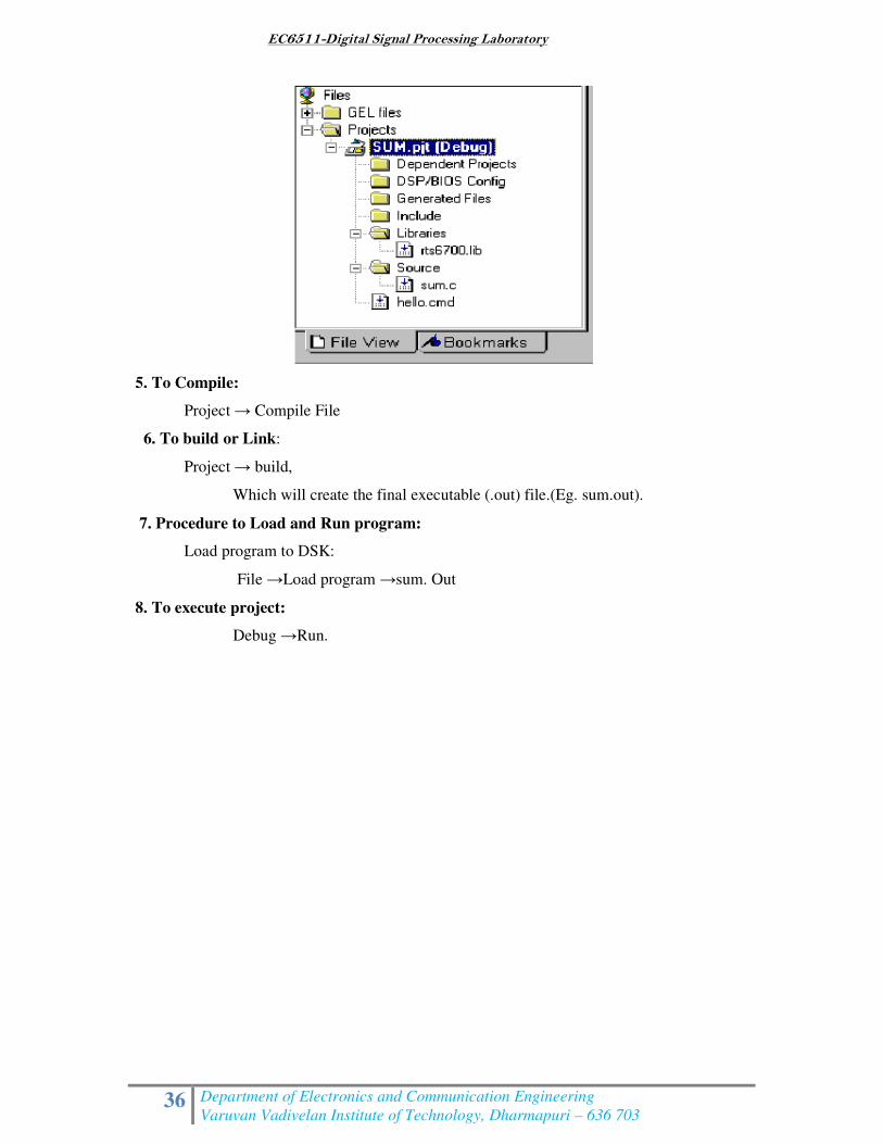
5. To Compile:
Project → Compile File
6. To build or Link:
Project → build,
Which will create the final executable (.out) file.(Eg. sum.out).
7. Procedure to Load and Run program:
Load program to DSK:
File →Load program →sum. Out
8. To execute project:
Debug →Run.
EC6511-Digital Signal Processing Laboratory
37 Department of Electronics and Communication Engineering
Varuvan Vadivelan Institute of Technology, Dharmapuri – 636 703
Ex. No: 9
Date:
STUDY OF ARCHITECTURE OF DIGITAL SIGNAL PROCESSOR
AIM: To study the Architecture of TMS320VC67XX DSP processor.
INTRODUCTION
The hardware experiments in the DSP lab are carried out on the Texas Instruments
TMS320C6713 DSP Starter Kit (DSK), based on the TMS320C6713 floating point DSP
running at 225MHz. The basic clock cycle instruction time is 1/(225 MHz)= 4.44
nanoseconds. During each clock cycle, up to eight instructions can be carried out in parallel,
achieving up to 8×225 = 1800 million instructions per second (MIPS). The DSK board
includes a 16MB SDRAM memory and a 512KB Flash ROM. It has an on-board 16-bit audio
stereo codec (the Texas Instruments AIC23B) that serves both as an A/D and a D/A
converter. There are four 3.5 mm audio jacks for microphone and stereo line input, and
speaker and headphone outputs. The AIC23 codec can be programmed to sample audio inputs
at the following sampling rates: fs = 8, 16, 24, 32, 44.1, 48, 96 kHz
The ADC part of the codec is implemented as a multi-bit third-order noise-shaping
delta-sigma converter) that allows a variety of oversampling ratios that can realize the above
choices of fs. The corresponding oversampling decimation filters act as anti-aliasing pre-
filters that limit the spectrum of the input analog signals effectively to the Nyquist interval
[−fs/2,fs/2]. The DAC part is similarly implemented as a multi-bit second-order noise-
shaping delta-sigma converter whose oversampling interpolation filters act as almost ideal
reconstruction filters with the Nyquist interval as their pass band.
The DSK also has four user-programmable DIP switches and four LEDs that can be
used to control and monitor programs running on the DSP. All features of the DSK are
managed by the Code Composer Studio (CCS). The CCS is a complete integrated
development environment (IDE) that includes an optimizing C/C++ compiler, assembler,
linker, debugger, and program loader. The CCS communicates with the DSK via a USB
connection to a PC. In addition to facilitating all programming aspects of the C6713 DSP, the
CCS can also read signals stored on the DSP‟s memory, or the SDRAM, and plot them in the
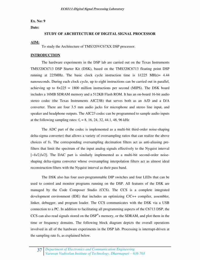
time or frequency domains. The following block diagram depicts the overall operations
involved in all of the hardware experiments in the DSP lab. Processing is interrupt-driven at
the sampling rate fs, as explained below.
EC6511-Digital Signal Processing Laboratory
38 Department of Electronics and Communication Engineering
Varuvan Vadivelan Institute of Technology, Dharmapuri – 636 703
TMS320C6713 floating point DSP
The AIC23 codec is configured (through CCS) to operate at one of the above
sampling rates fs. Each collected sample is converted to a 16-bit two’s complement integer (a
short data type in C). The codec actually samples the audio input in stereo, that is, it collects
two samples for the left and right channels
ARCHITECTURE
The 67XX DSPs use an advanced, modified Harvard architecture that maximizes
processing power by maintaining one program memory bus and three data memory buses.
These processors also provide an arithmetic logic unit (ALU) that has a high degree of
parallelism, application-specific hardware logic, on-chip memory, and additional on-chip
peripherals. These DSP families also provide a highly specialized instruction set, which is the
basis of the operational flexibility and speed of these DSPs. Separate program and data
spaces allow simultaneous access to program instructions and data, providing the high degree
of parallelism. Two reads and one write operation can be performed in a single cycle.
Instructions with parallel store and application-specific instructions can fully utilize this
architecture. In addition, data can be transferred between data and program spaces. Such
parallelism supports a powerful set of arithmetic, logic, and bit-manipulation operations that
can all be performed in a single machine cycle. Also included are the control mechanisms to
manage interrupts, repeated operations, and function calls.
EC6511-Digital Signal Processing Laboratory
39 Department of Electronics and Communication Engineering
Varuvan Vadivelan Institute of Technology, Dharmapuri – 636 703
EC6511-Digital Signal Processing Laboratory
40 Department of Electronics and Communication Engineering
Varuvan Vadivelan Institute of Technology, Dharmapuri – 636 703
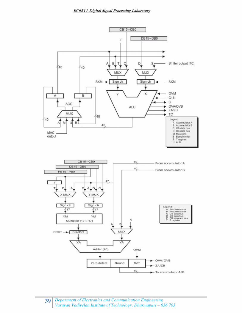
1. Central Processing Unit (CPU)
The CPU of the ‟67XX devices contains:
• A 40-bit arithmetic logic unit (ALU)
• Two 40-bit accumulators
• A barrel shifter
• A 17 -bit multiplier/adder
• A compare, select, and store unit (CSSU)
2. Arithmetic Logic Unit (ALU)
The ‟67XX devices perform 2s-complement arithmetic using a 40-bit ALU
and two 40-bit accumulators (ACCA and ACCB). The ALU also can perform
Boolean operations. The ALU can function as two 16-bit ALUs and perform two 16-
bit operations simultaneously when the C16 bit in status register 1 (ST1) is set.
3. Accumulators
The accumulators, ACCA and ACCB, store the output from the ALU or the
multiplier / adder block; the accumulators can also provide a second input to the ALU
or the multiplier / adder. The bits in each accumulator are grouped as follows:
• Guard bits (bits 32–39)
• A high-order word (bits 16–31)
• A low-order word (bits 0–15)
Instructions are provided for storing the guard bits, the high-order and the low-
order accumulator words in data memory, and for manipulating 32-bit accumulator
words in or out of data memory. Also, any of the accumulators can be used as
temporary storage for the other.
4. Barrel Shifter
The ‟67XX‟s barrel shifter has a 40-bit input connected to the accumulator or
data memory (CB, DB) and a 40-bit output connected to the ALU or data memory
(EB). The barrel shifter produces a left shift of 0 to 31 bits and a right shift of 0 to 16
bits on the input data. The shift requirements are defined in the shift-count field
(ASM) of ST1 or defined in the temporary register (TREG), which is designated as a
shift-count register. This shifter and the exponent detector normalize the values in an
accumulator in a single cycle. The least significant bits (LSBs) of the output are filled
with 0s and the most significant bits (MSBs) can be either zero-filled or sign-
extended, depending on the state of the sign-extended mode bit (SXM) of ST1.
EC6511-Digital Signal Processing Laboratory
41 Department of Electronics and Communication Engineering
Varuvan Vadivelan Institute of Technology, Dharmapuri – 636 703
Additional shift capabilities enable the processor to perform numerical scaling, bit
extraction, extended arithmetic, and overflow prevention operations
5. Multiplier/Adder
The multiplier / adder perform 17-bit 2s-complement multiplication with a 40-
bit accumulation in a single instruction cycle. The multiplier / adder block consists of
several elements: a multiplier, adder, signed/unsigned input control, fractional control,
a zero detector, a rounder (2s-complement), overflow/saturation logic, and TREG.
The multiplier has two inputs: one input is selected from the TREG, a data memory
operand, or an accumulator; the other is selected from the program memory, the data
memory, an accumulator, or an immediate value. The fast on-chip multiplier allows
the C67XX to perform operations such as convolution, correlation, and filtering
efficiently. In addition, the multiplier and ALU together execute multiply/accumulate
(MAC) computations and ALU operations in parallel in a single instruction cycle.
This function is used in determining the Euclid distance, and in implementing
symmetrical and least mean square (LMS) filters, which are required for complex
DSP algorithms.
6. Compare, Select, and Store Unit (CSSU)
The compare, select, and store unit (CSSU) performs maximum comparisons
between the accumulator’s high and low words, allows the test/control (TC) flag bit of
status register 0 (ST0) and the transition (TRN) register to keep their transition
histories, and selects the larger word in the accumulator to be stored in data memory.
The CSSU also accelerates Viterbi-type butterfly computation with optimized on-chip
hardware.
7. Program Control
Program control is provided by several hardware and software mechanisms:
The program controller decodes instructions, manages the pipeline, stores the
status of operations, and decodes conditional operations. Some of the hardware
elements included in the program controller are the program counter, the status and
control register, the stack, and the address-generation logic.
Some of the software mechanisms used for program control includes branches,
calls, and conditional instructions, are peat instruction, reset, and interrupt.
The C67XX supports both the use of hardware and software interrupts for
program control. Interrupt service routines are vectored through a re-locatable
interrupt vector table. Interrupts can be globally enabled / disabled and can be
EC6511-Digital Signal Processing Laboratory
42 Department of Electronics and Communication Engineering
Varuvan Vadivelan Institute of Technology, Dharmapuri – 636 703
individually masked through the interrupt mask register (IMR). Pending interrupts are
indicated in the interrupt flag register (IFR). For detailed information on the structure
of the interrupt vector table, the IMR and the IFR, see the device-specific data sheets.
8. Status Registers (ST0, ST1)
The status registers, ST0 and ST1, contain the status of the various conditions
and modes for the ‟67XX devices. ST0 contains the flags (OV, C, and TC) produced
by arithmetic operations and bit manipulations in addition to the data page pointer
(DP) and the auxiliary register pointer (ARP) fields. ST1 contains the various modes
and instructions that the processor operates on and executes.
9. Auxiliary Registers (AR0–AR7)
The eight 16-bit auxiliary registers (AR0–AR7) can be accessed by the central
arithmetic logic unit (CALU) and modified by the auxiliary register arithmetic units
(ARAUs). The primary function of the auxiliary registers is generating 16-bit
addresses for data space. However, these registers also can act as general-purpose
registers or counters.
10. Temporary Register (TREG)
The TREG is used to hold one of the multiplicands for multiply and
multiply/accumulate instructions. It can hold a dynamic (execution-time
programmable) shift count for instructions with a shift operation such as ADD, LD,
and SUB. It also can hold a dynamic bit address for the BITT instruction. The EXP
instruction stores the exponent value computed into the TREG, while the NORM
instruction uses the TREG value to normalize the number. For ACS operation of
Viterbi decoding, TREG holds branch metrics used by the DADST and DSADT
instructions.
11. Transition Register (TRN)
The TRN is a 16-bit register that is used to hold the transition decision for the
path to new metrics to perform the Viterbi algorithm. The CMPS (compare, select,
max, and store) instruction updates the contents of the TRN based on the comparison
between the accumulator high word and the accumulator low word.
12. Stack-Pointer Register (SP)
The SP is a 16-bit register that contains the address at the top of the system
stack. The SP always points to the last element pushed onto the stack. The stack is
manipulated by interrupts, traps, calls, returns, and the PUSHD, PSHM, POPD, and
POPM instructions. Pushes and pops of the stack pre decrement and post increment,
respectively, all 16 bits of the SP.
EC6511-Digital Signal Processing Laboratory
43 Department of Electronics and Communication Engineering
Varuvan Vadivelan Institute of Technology, Dharmapuri – 636 703
13. Circular-Buffer-Size Register (BK)
The 16-bit BK is used by the ARAUs in circular addressing to specify the data
block size.
14. Block-Repeat Registers (BRC, RSA, REA)
The block-repeat counter (BRC) is a 16-bit register used to specify the number
of times a block of code is to be repeated when performing a block repeat. The block-
repeat start address (RSA) is a 16-bit register containing the starting address of the
block of program memory to be repeated when operating in the repeat mode. The 16-
bit block-repeat end address (REA) contains the ending address if the block of
program memory is to be repeated when operating in the repeat mode.
15. Interrupt Registers (IMR, IFR)
The interrupt-mask register (IMR) is used to mask off specific interrupts
individually at required times. The interrupt-flag register (IFR) indicates the current
status of the interrupts.
16. Processor-Mode Status Register (PMST)
The processor-mode status registers (PMST) controls memory configurations
of the 67XX devices.
17. Power-Down Modes
There are three power-down modes, activated by the IDLE1, IDLE2, and
IDLE3 instructions. In these modes, the ‟67XX devices enter a dormant state and
dissipate considerably less power than in normal operation. The IDLE1instruction is
used to shut down the CPU. The IDLE2 instruction is used to shut down the CPU and
on-chip peripherals. The IDLE3 instruction is used to shut down the ‟67XX processor
completely. This instruction stops the PLL circuitry as well as the CPU and
peripherals.
RESULT
Thus the study of architecture TMS320VC67XX and its functionalities has been
identified.
EC6511-Digital Signal Processing Laboratory
44 Department of Electronics and Communication Engineering
Varuvan Vadivelan Institute of Technology, Dharmapuri – 636 703
Ex. No: 10
Date:
MAC OPERATION USING VARIOUS ADDRESSING MODES
AIM:
To Study the various addressing modes of TMS320C67XX DSP processor.
THEORY:
Addressing Modes The TMS320C67XX DSP supports three types of addressing
modes that enable flexible access to data memory, to memory-mapped registers, to register
bits, and to I/O space:
The absolute addressing mode allows you to reference a location by supplying all or
part of an address as a constant in an instruction.
The direct addressing mode allows you to reference a location using an address offset.
The indirect addressing mode allows you to reference a location using a pointer.
Each addressing mode provides one or more types of operands. An instruction that
supports an addressing-mode operand has one of the following syntax elements listed below.
Baddr
When an instruction contains Baddr, that instruction can access one or two bits in an
accumulator (AC0–AC3), an auxiliary register (AR0–AR7), or a temporary register (T0–T3).
Only the register bit test/set/clear/complement instructions support Baddr. As you write one
of these instructions, replace Baddr with a compatible operand.
Cmem
When an instruction contains Cmem, that instruction can access a single word (16
bits)of data from data memory. As you write the instruction, replace Cmem with a compatible
operand.
Lmem
When an instruction contains Lmem, that instruction can access a long word (32 bits)
of data from data memory or from a memory-mapped registers. As you write the instruction,
replace Lmem with a compatible operand.
Smem
When an instruction contains Smem, that instruction can access a single word (16
bits) of data from data memory, from I/O space, or from a memory-mapped register. As you
write the instruction, replace Smem with a compatible operand.
EC6511-Digital Signal Processing Laboratory
45 Department of Electronics and Communication Engineering
Varuvan Vadivelan Institute of Technology, Dharmapuri – 636 703
Xmem and Ymem
When an instruction contains Xmem and Ymem, that instruction can perform two
simultaneous 16-bit accesses to data memory. As you write the instruction, replace Xmem
and Ymem with compatible operands.
Absolute Addressing Modes k16 absolute
This mode uses the 7-bit register called DPH (high part of the extended data page
register) and a 16-bit unsigned constant to form a 23-bit data space address. This mode is
used to access a memory location or a memory-mapped register.
k23 absolute
This mode enables you to specify a full address as a 23-bit unsigned constant. This
mode is used to access a memory location or a memory-mapped register.
I/O absolute
This mode enables you to specify an I/O address as a 16-bit unsigned constant. This
mode is used to access a location in I/O space.
Direct Addressing Modes DP direct
This mode uses the main data page specified by DPH (high part of the extended data
page register) in conjunction with the data page register (DP).This mode is used to access a
memory location or a memory-mapped register.
SP direct
This mode uses the main data page specified by SPH (high part of the extended stack
pointers) in conjunction with the data stack pointer (SP). This mode is used to access stack
values in data memory.
Register-bit direct
This mode uses an offset to specify a bit address. This mode is used to access one
register bit or two adjacent register bits.
PDP direct
This mode uses the peripheral data page register (PDP) and an offset to specify an I/O
address. This mode is used to access a location in I/O space. The DP direct and SP direct
addressing modes are mutually exclusive. The mode selected depends on the CPL bit in
status register ST1_67: 0 DP direct addressing mode 1 SP direct addressing mode The
register-bit and PDP direct addressing modes are independent of the CPL bit.
Indirect Addressing Modes
You may use these modes for linear addressing or circular addressing.
EC6511-Digital Signal Processing Laboratory
46 Department of Electronics and Communication Engineering
Varuvan Vadivelan Institute of Technology, Dharmapuri – 636 703
AR indirect
This mode uses one of eight auxiliary registers (AR0–AR7) to point to data. The way
the CPU uses the auxiliary register to generate an address depends on whether you are
accessing data space (memory or memory-mapped registers), individual register bits, or I/O
space.
Dual AR indirect
This mode uses the same address-generation process as the AR indirect addressing
mode. This mode is used with instructions that access two or more data-memory locations.
CDP indirect
This mode uses the coefficient data pointer (CDP) to point to data. The way the CPU
uses CDP to generate an address depends on whether you are accessing data space (memory
or memory-mapped registers), individual register bits, or I/O space.
Coefficient indirect
This mode uses the same address-generation process as the CDP indirect addressing
mode. This mode is available to support instructions that can access a coefficient in data
memory at the same time they access two other data-memory values using the dual AR
indirect addressing mode.
Circular Addressing
Circular addressing can be used with any of the indirect addressing modes. Each of
the eight auxiliary registers (AR0–AR7) and the coefficient data pointer (CDP) can be
independently configured to be linearly or circularly modified as they act as pointers to data
or to register bits, see Table 3−10. This configuration is done with a bit (ARnLC) in status
register ST2_67. To choose circular modification, set the bit. Each auxiliary register ARn has
its own linear/circular configuration bit in ST2_67: 0 Linear addressing 1 Circular addressing
The CDPLC bit in status register ST2_67 configures the DSP to use CDP for linear
addressing or circular addressing: 0 Linear addressing 1 Circular addressing You can use the
circular addressing instruction qualifier, .CR, if you want every pointer used by the
instruction to be modified circularly, just add .CR to the end of the instruction mnemonic (for
example, ADD.CR). The circular addressing instruction qualifier overrides the linear/circular
configuration in ST2_67.
EC6511-Digital Signal Processing Laboratory
47 Department of Electronics and Communication Engineering
Varuvan Vadivelan Institute of Technology, Dharmapuri – 636 703
ADDITION:
INP1 .SET 0H
INP2 .SET 1H
OUT .SET 2H
.mmregs
.text
START:
LD #140H,DP
RSBX CPL
NOP
NOP
NOP
NOP
LD INP1,A
ADD INP2,A
STL A,OUT
HLT: B HLT
INPUT:
Data Memory: A000h 0004h
A001h 0004h
OUTPUT: Data Memory: A002h 0008h
SUBTRACTION: INP1 .SET 0H
INP2 .SET 1H
OUT .SET 2H
.mmregs
.text
START:
LD #140H,DP
RSBX CPL
NOP
NOP
NOP
NOP
LD INP1,A
SUB INP2,A
STL A,OUT
HLT: B HLT
INPUT: Data Memory: A000h 0004h
A001h 0002h
OUTPUT:
Data Memory: A002h 0002h
RESULT:
Thus, the various addressing mode of DSP processor TMS320C67XX was studied.
EC6511-Digital Signal Processing Laboratory
49 Department of Electronics and Communication Engineering
Varuvan Vadivelan Institute of Technology, Dharmapuri – 636 703
Ex. No: 11
Date:
LINEAR CONVOLUTION
AIM:
To perform the Linear Convolution of two given discrete sequence in
TMS320C67XX.
APPARATUS REQUIRED:
HARDWARE : Personal Computer & TMS320C67XX kit
SOFTWARE : Code Composer Studio version4
PROCEDURE:
1. Open Code Composer Studio v4.
2. To create the New Project
Project→ New (File Name. pjt, Eg: vvits.pjt)
3. To create a Source file
File →New→ Type the code (Save & give file name, Eg: sum.c).
4. To Add Source files to Project
Project→ Add files to Project→ sum.c
5. To Add rts.lib file & Hello.cmd:
Project→ Add files to Project→ rts6700.lib
Library files: rts6700.lib (Path: c:\ti\c6000\cgtools\lib\ rts6700.lib)
Note: Select Object& Library in (*.o,*.l) in Type of files
6. Project→ Add files to Project →hello.cmd
CMD file - Which is common for all non real time programs.
(Path: c:\ti \ tutorial\dsk6713\hello1\hello.cmd)
Note: Select Linker Command file (*.cmd) in Type of files
Compile:-
1. To Compile: Project→ Compile
2. To Rebuild: project → rebuild,
Which will create the final .out executable file. ( Eg. vvit.out).
3. Procedure to Lode and Run program:
Load the Program to DSK: File→ Load program →vvit.out
To Execute project: Debug → Run
EC6511-Digital Signal Processing Laboratory
50 Department of Electronics and Communication Engineering
Varuvan Vadivelan Institute of Technology, Dharmapuri – 636 703
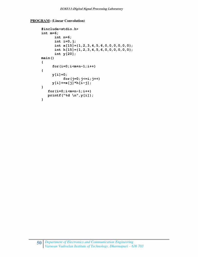
PROGRAM: (Linear Convolution)
#include<stdio.h>
int m=6;
int n=6;
int i=0,j;
int x[15]={1,2,3,4,5,6,0,0,0,0,0,0};
int h[15]={1,2,3,4,5,6,0,0,0,0,0,0};
int y[20];
main()
{
for(i=0;i<m+n-1;i++)
{
y[i]=0;
for(j=0;j<=i;j++)
y[i]+=x[j]*h[i-j];
}
for(i=0;i<m+n-1;i++)
printf("%d \n",y[i]);
}
EC6511-Digital Signal Processing Laboratory
51 Department of Electronics and Communication Engineering
Varuvan Vadivelan Institute of Technology, Dharmapuri – 636 703
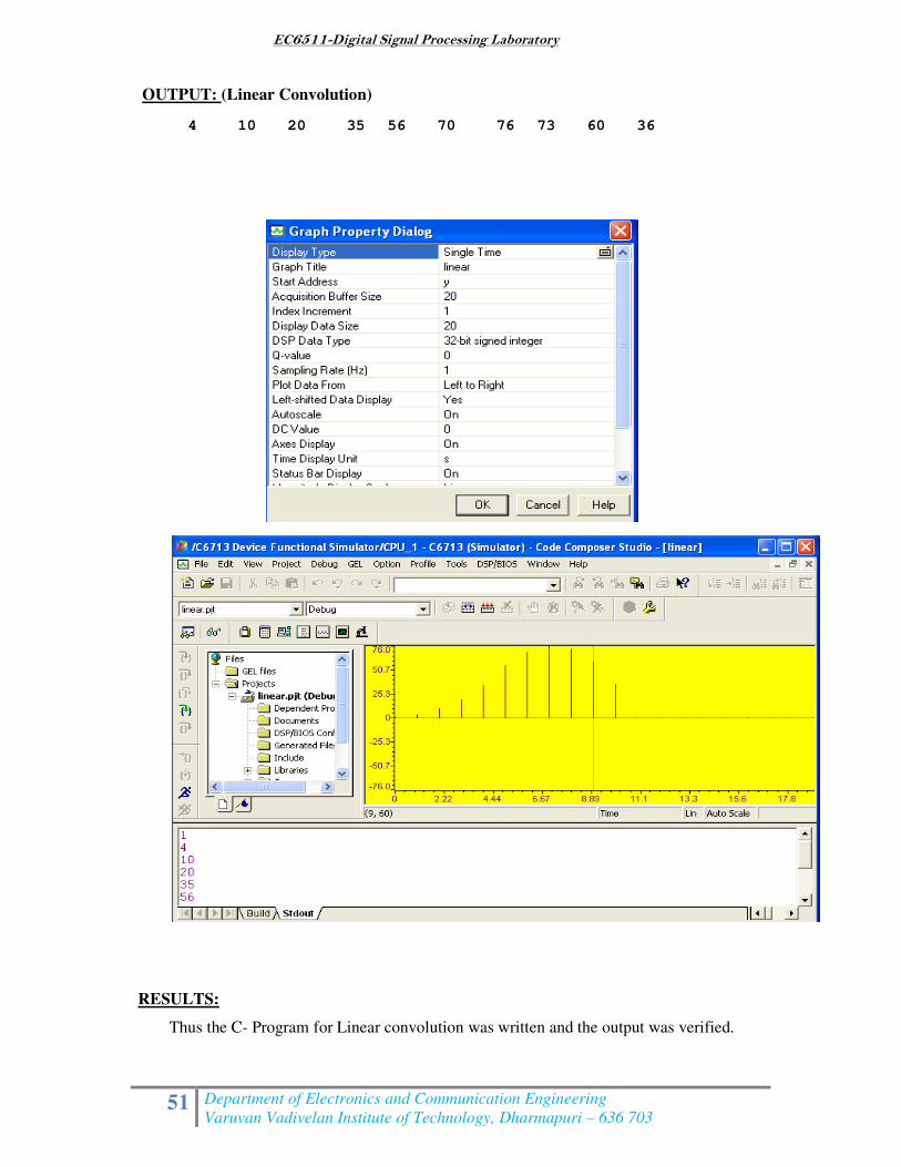
OUTPUT: (Linear Convolution)
4 10 20 35 56 70 76 73 60 36
RESULTS:
Thus the C- Program for Linear convolution was written and the output was verified.

EC6511-Digital Signal Processing Laboratory
52 Department of Electronics and Communication Engineering
Varuvan Vadivelan Institute of Technology, Dharmapuri – 636 703
Ex. No: 12
Date:
CIRCULAR CONVOLUTION
AIM:
To perform the circular Convolution of two given discrete sequences in
TMS320C67XX.
APPARATUS REQUIRED:
HARDWARE : Personal Computer & TMS320C67XX kit
SOFTWARE : Code Composer Studio version4
PROCEDURE:
1. Open Code Composer Studio v4.
2. To create the New Project
Project→ New (File Name. pjt, Eg: vvits.pjt)
3. To create a Source file
File →New→ Type the code (Save & give file name, Eg: sum.c).
4. To Add Source files to Project
Project→ Add files to Project→ sum.c
5. To Add rts.lib file & Hello.cmd:
Project→ Add files to Project→ rts6700.lib
Library files: rts6700.lib (Path: c:\ti\c6000\cgtools\lib\ rts6700.lib)
Note: Select Object& Library in (*.o,*.l) in Type of files
6. Project→ Add files to Project →hello.cmd
CMD file - Which is common for all non real time programs.
(Path: c:\ti \ tutorial\dsk6713\hello1\hello.cmd)
Note: Select Linker Command file (*.cmd) in Type of files
COMPILE:
1. To Compile: Project→ Compile
2. To Rebuild: project → rebuild,
Which will create the final .out executable file. ( Eg. vvit.out).
3. Procedure to Lode and Run program:
Load the Program to DSK: File→ Load program →vvit.out
To Execute project: Debug → Run
EC6511-Digital Signal Processing Laboratory
53 Department of Electronics and Communication Engineering
Varuvan Vadivelan Institute of Technology, Dharmapuri – 636 703
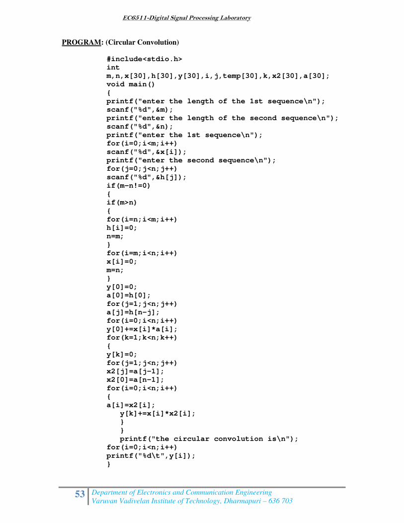
PROGRAM: (Circular Convolution)
#include<stdio.h>
int
m,n,x[30],h[30],y[30],i,j,temp[30],k,x2[30],a[30];
void main()
{
printf("enter the length of the 1st sequence\n");
scanf("%d",&m);
printf("enter the length of the second sequence\n");
scanf("%d",&n);
printf("enter the 1st sequence\n");
for(i=0;i<m;i++)
scanf("%d",&x[i]);
printf("enter the second sequence\n");
for(j=0;j<n;j++)
scanf("%d",&h[j]);
if(m-n!=0)
{
if(m>n)
{
for(i=n;i<m;i++)
h[i]=0;
n=m;
}
for(i=m;i<n;i++)
x[i]=0;
m=n;
}
y[0]=0;
a[0]=h[0];
for(j=1;j<n;j++)
a[j]=h[n-j];
for(i=0;i<n;i++)
y[0]+=x[i]*a[i];
for(k=1;k<n;k++)
{
y[k]=0;
for(j=1;j<n;j++)
x2[j]=a[j-1];
x2[0]=a[n-1];
for(i=0;i<n;i++)
{
a[i]=x2[i];
y[k]+=x[i]*x2[i];
}
}
printf("the circular convolution is\n");
for(i=0;i<n;i++)
printf("%d\t",y[i]);
}
EC6511-Digital Signal Processing Laboratory
54 Department of Electronics and Communication Engineering
Varuvan Vadivelan Institute of Technology, Dharmapuri – 636 703
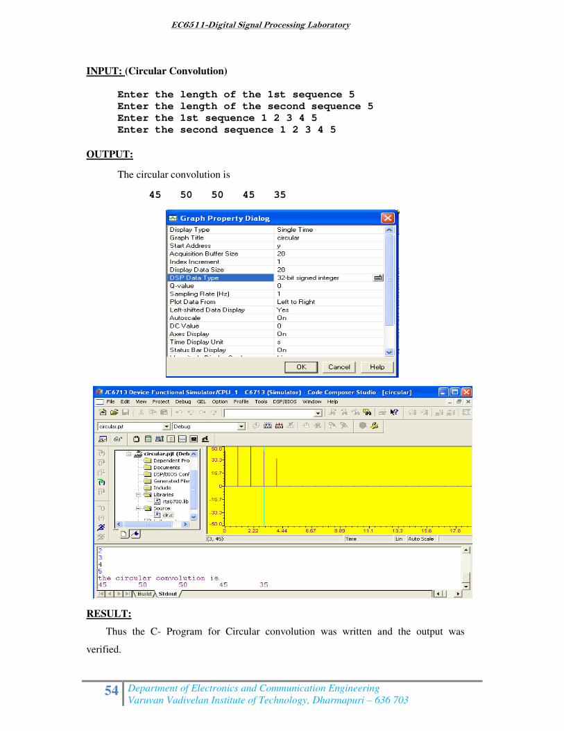
INPUT: (Circular Convolution)
Enter the length of the 1st sequence 5
Enter the length of the second sequence 5
Enter the 1st sequence 1 2 3 4 5
Enter the second sequence 1 2 3 4 5
OUTPUT:
The circular convolution is
45 50 50 45 35
RESULT:
Thus the C- Program for Circular convolution was written and the output was
verified.
EC6511-Digital Signal Processing Laboratory
55 Department of Electronics and Communication Engineering
Varuvan Vadivelan Institute of Technology, Dharmapuri – 636 703
Ex. No: 13
Date:
FFT IMPLEMENTATION
AIM:
To write a C- program to compute 8 – FFT of given sequences using DIF – FFT
algorithm in TMS320C67XX.
APPARATUS REQUIRED:
HARDWARE : Personal Computer & TMS320C67XX kit
SOFTWARE : Code Composer Studio version4
PROCEDURE:
1. Open Code Composer Studio v4.
2. To create the New Project
Project→ New (File Name. pjt, Eg: vvits.pjt)
3. To create a Source file
File →New→ Type the code (Save & give file name, Eg: sum.c).
4. To Add Source files to Project
Project→ Add files to Project→ sum.c
5. To Add rts.lib file & Hello.cmd:
Project→ Add files to Project→ rts6700.lib
Library files: rts6700.lib (Path: c:\ti\c6000\cgtools\lib\ rts6700.lib)
Note: Select Object& Library in (*.o,*.l) in Type of files
6. Project→ Add files to Project →hello.cmd
CMD file - Which is common for all non real time programs.
(Path: c:\ti \ tutorial\dsk6713\hello1\hello.cmd)
Note: Select Linker Command file (*.cmd) in Type of files
COMPILE:
1. To Compile: Project→ Compile
2. To Rebuild: project → rebuild,
Which will create the final .out executable file. ( Eg. vvit.out).
3. Procedure to Lode and Run program:
Load the Program to DSK: File→ Load program →vvit.out
To Execute project: Debug → Run
EC6511-Digital Signal Processing Laboratory
56 Department of Electronics and Communication Engineering
Varuvan Vadivelan Institute of Technology, Dharmapuri – 636 703
PROGRAM: (FFT Implementation)
#include<stdio.h>
#include<math.h>
#define N 8
#define PI 3.14159
typedef struct
{
float real,imag;
}
complex;
main()
{
int i;
complex w[N];
complex
x[8]={0,0.0,1,0.0,2,0.0,3,0.0,4,0.0,5,0.0,6,0.0,7,0.0};
complex temp1,temp2;
int j,k,upper_leg,lower_leg,leg_diff,index,step;
for(i=0;i<N;i++)
{
w[i].real=cos((2*PI*i)/(N*2.0));
w[i].imag=-sin((2*PI*i)/(N*2.0));
}
leg_diff=N/2;
step=2;
for(i=0;i<3;i++)
{
index=0;
for(j=0;j<leg_diff;j++)
{
for(upper_leg=j;upper_leg<N;upper_leg+=(2*leg_diff))
{
lower_leg=upper_leg+leg_diff;
temp1.real=(x[upper_leg]).real+(x[lower_leg]).real;
temp1.imag=(x[upper_leg]).imag+(x[lower_leg]).imag;
temp2.real=(x[upper_leg]).real-(x[lower_leg]).real;
temp2.imag=(x[upper_leg]).imag-(x[lower_leg]).imag;
(x[lower_leg]).real=temp2.real*(w[index]).real-
temp2.imag*(w[index]).imag;
(x[lower_leg]).imag=temp2.real*(w[index]).imag+temp2.imag
*(w[index]).real;
(x[upper_leg]).real=temp1.real;
(x[upper_leg]).imag=temp1.imag;
}
index+=step;
}
leg_diff=(leg_diff)/2;
step=step*2;
}
j=0;
for(i=1;i<(N-1);i++)
{
EC6511-Digital Signal Processing Laboratory
57 Department of Electronics and Communication Engineering
Varuvan Vadivelan Institute of Technology, Dharmapuri – 636 703
k=N/2;
while(k<=j)
{
j=j-k;
k=k/2;
}
j=j+k;
if(i<j)
{
temp1.real=(x[j]).real;
temp1.imag=(x[j]).imag;
(x[j]).real=(x[i]).real;
(x[j]).imag=(x[i]).imag;
(x[i]).real=temp1.real;
(x[i]).imag=temp1.imag;
}
}
printf("the fft of the given input sequence is \n");
for(i=0;i<8;i++)
{
printf("%f %f \n",(x[i]).real,(x[i]).imag);
}
}
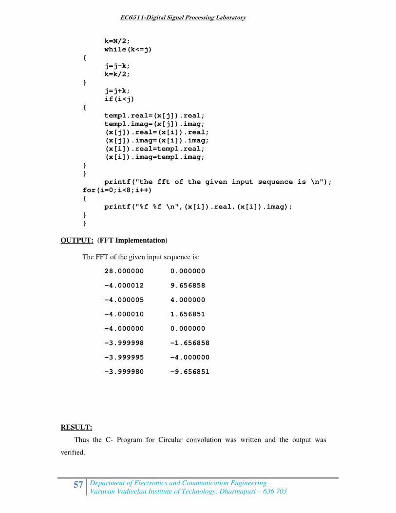
OUTPUT: (FFT Implementation)
The FFT of the given input sequence is:
28.000000 0.000000
-4.000012 9.656858
-4.000005 4.000000
-4.000010 1.656851
-4.000000 0.000000
-3.999998 -1.656858
-3.999995 -4.000000
-3.999980 -9.656851
RESULT:
Thus the C- Program for Circular convolution was written and the output was
verified.
EC6511-Digital Signal Processing Laboratory
58 Department of Electronics and Communication Engineering
Varuvan Vadivelan Institute of Technology, Dharmapuri – 636 703
Ex. No: 14
Date:
WAVEFORM GENERATION
AIM:
To generate a sine wave and square wave using TMS320C67XX DSP KIT.
APPARATUS REQUIRED:
HARDWARE : Personal Computer & TMS320C67XX kit
SOFTWARE : Code Composer Studio version4
PROCEDURE:
1. Open Code Composer Studio v4.
2. To create the New Project
Project→ New (File Name. pjt, Eg: vvits.pjt)
3. To create a Source file
File →New→ Type the code (Save & give file name, Eg: sum.c).
4. To Add Source files to Project
Project→ Add files to Project→ sum.c
5. To Add rts.lib file & Hello.cmd:
Project→ Add files to Project→ rts6700.lib
Library files: rts6700.lib (Path: c:\ti\c6000\cgtools\lib\ rts6700.lib)
6. Project→ Add files to Project →hello.cmd
CMD file - Which is common for all non real time programs.
(Path: c:\ti \ tutorial\dsk6713\hello1\hello.cmd)
Note: Select Linker Command file (*.cmd) in Type of files
COMPILE:
1. To Compile: Project→ Compile
2. To Rebuild: project → rebuild,
Which will create the final .out executable file. ( Eg. vvit.out).
3. Procedure to Lode and Run program:
Load the Program to DSK: File→ Load program →vvit.out
To Execute project: Debug → Run
EC6511-Digital Signal Processing Laboratory
59 Department of Electronics and Communication Engineering
Varuvan Vadivelan Institute of Technology, Dharmapuri – 636 703
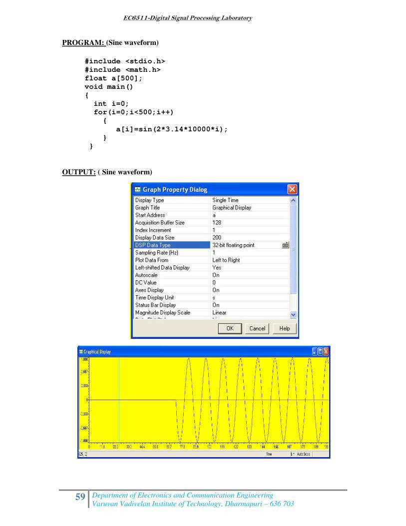
PROGRAM: (Sine waveform)
#include <stdio.h>
#include <math.h>
float a[500];
void main()
{
int i=0;
for(i=0;i<500;i++)
{
a[i]=sin(2*3.14*10000*i);
}
}
OUTPUT: ( Sine waveform)
EC6511-Digital Signal Processing Laboratory
60 Department of Electronics and Communication Engineering
Varuvan Vadivelan Institute of Technology, Dharmapuri – 636 703
PROGRAM: ( Square waveform)
#include <stdio.h>
#include <math.h>
int a[1000];
void main()
{
int i,j=0;
int b=5;
for(i=0;i<10;i++)
{
for (j=0;j<=50;j++)
{
a[(50*i)+j]=b;
}
b=b*(-1) ;
}
}
OUTPUT: ( Square waveform)
RESULT:
Thus, the sine wave and square waveform was generated displayed at graph.

EC6511-Digital Signal Processing Laboratory
61 Department of Electronics and Communication Engineering
Varuvan Vadivelan Institute of Technology, Dharmapuri – 636 703
Ex. No: 15a
Date:
DESIGN OF FIR FILTERS
AIM:
To write a C program for the design of FIR Filter, also plots the magnitude responses
for the same.
APPARATUS REQUIRED:
HARDWARE : Personal Computer & TMS320C67XX kit
SOFTWARE : Code Composer Studio version4
PROCEDURE:
1. Open Code Composer Studio v4.
2. To create the New Project
Project→ New (File Name. pjt, Eg: vvits.pjt)
3. To create a Source file
File →New→ Type the code (Save & give file name, Eg: sum.c).
4. To Add Source files to Project
Project→ Add files to Project→ sum.c
5. To Add rts.lib file & Hello.cmd:
Project→ Add files to Project→ rts6700.lib
Library files: rts6700.lib (Path: c:\ti\c6000\cgtools\lib\ rts6700.lib)
Note: Select Object& Library in (*.o,*.l) in Type of files
6. Project→ Add files to Project →hello.cmd
CMD file - Which is common for all non real time programs.
(Path: c:\ti \ tutorial\dsk6713\hello1\hello.cmd)
Note: Select Linker Command file (*.cmd) in Type of files
COMPILE:
1. To Compile: Project→ Compile
2. To Rebuild: project → rebuild,
Which will create the final .out executable file. ( Eg. vvit.out).
3. Procedure to Lode and Run program:
Load the Program to DSK: File→ Load program →vvit.out
To Execute project: Debug → Run
EC6511-Digital Signal Processing Laboratory
62 Department of Electronics and Communication Engineering
Varuvan Vadivelan Institute of Technology, Dharmapuri – 636 703
PROGRAM: (FIR Filters)
#include<stdio.h>
#include<math.h>
#define pi 3.1415
int n,N,c;
float wr[64],wt[64];
void main()
{
printf("\n enter no. of samples,N= :");
scanf("%d",&N);
printf("\n enter choice of window function\n 1.rect
\n 2. triang \n c= :");
scanf("%d",&c);
printf("\n elements of window function are:");
switch(c)
{
case 1:
for(n=0;n<=N-1;n++)
{
wr[n]=1;
printf(" \n wr[%d]=%f",n,wr[n]);
}
break;
case 2:
for(n=0;n<=N-1;n++)
{
wt[n]=1-(2*(float)n/(N-1));
printf("\n wt[%d]=%f",n,wt[n]);
}
break;
}
}
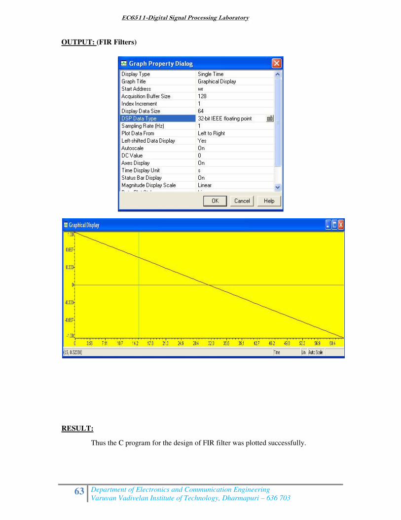
EC6511-Digital Signal Processing Laboratory
63 Department of Electronics and Communication Engineering
Varuvan Vadivelan Institute of Technology, Dharmapuri – 636 703
OUTPUT: (FIR Filters)
RESULT:
Thus the C program for the design of FIR filter was plotted successfully.
EC6511-Digital Signal Processing Laboratory
64 Department of Electronics and Communication Engineering
Varuvan Vadivelan Institute of Technology, Dharmapuri – 636 703
Ex. No: 15b
Date:
DESIGN OF IIR FILTERS
AIM:
To write a C program for the design of IIR Filter, also plots the magnitude responses
for the same.
APPARATUS REQUIRED:
HARDWARE : Personal Computer & TMS320C67XX kit
SOFTWARE : Code Composer Studio version4
PROCEDURE:
1. Open Code Composer Studio v4.
2. To create the New Project
Project→ New (File Name. pjt, Eg: vvits.pjt)
3. To create a Source file
File →New→ Type the code (Save & give file name, Eg: sum.c).
4. To Add Source files to Project
Project→ Add files to Project→ sum.c
5. To Add rts.lib file & Hello.cmd:
Project→ Add files to Project→ rts6700.lib
Library files: rts6700.lib (Path: c:\ti\c6000\cgtools\lib\ rts6700.lib)
Note: Select Object& Library in (*.o,*.l) in Type of files
6. Project→ Add files to Project →hello.cmd
CMD file - Which is common for all non real time programs.
(Path: c:\ti \ tutorial\dsk6713\hello1\hello.cmd)
Note: Select Linker Command file (*.cmd) in Type of files
COMPILE:
1. To Compile: Project→ Compile
2. To Rebuild: project → rebuild,
Which will create the final .out executable file. ( Eg. vvit.out).
3. Procedure to Lode and Run program:
Load the Program to DSK: File→ Load program →vvit.out
To Execute project: Debug → Run
EC6511-Digital Signal Processing Laboratory
65 Department of Electronics and Communication Engineering
Varuvan Vadivelan Institute of Technology, Dharmapuri – 636 703
PROGRAM: (IIR Filters)
#include<stdio.h>
#include<math.h>
int i,w,wc,c,N;
float H[100];
float mul(float,int);
void main()
{
printf("\n Enter order of filter");
scanf("%d",&N);
printf("\n Enter the cut off frequency");
scanf("%d",&wc);
printf("\n Enter the choice for IIR Filter 1.LPF 2.HPF");
scanf("%d",&c);
switch(c)
{
case 1:
for(w=0;w<100;w++)
{
H[w]=1/sqrt(1+mul((w/(float)wc),2*N));
printf("H[%d]=%f\n",w,H[w]);
}
break;
case 2:
for(w=0;w<=100;w++)
{
H[w]=1/sqrt(1+mul((float)wc/w,2*N));
printf("H[%d]=%f\n",w,H[w]);
}
break;
}
}
float mul(float a,int x)
{
for(i=0;i<x-1;i++)
a*=a;
return(a); }
INPUT: (IIR Filters)
Enter order of filter 2
Enter the cut off frequency 50
Enter the choice for IIR Filter 1.LPF 2.HPF: 1
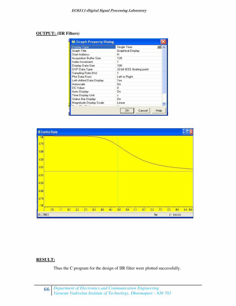
EC6511-Digital Signal Processing Laboratory
66 Department of Electronics and Communication Engineering
Varuvan Vadivelan Institute of Technology, Dharmapuri – 636 703
OUTPUT: (IIR Filters)
RESULT:
Thus the C program for the design of IIR filter were plotted successfully.
EC6511-Digital Signal Processing Laboratory
67 Department of Electronics and Communication Engineering
Varuvan Vadivelan Institute of Technology, Dharmapuri – 636 703
Ex. No:16
Date:
ANALYSIS OF FINITE WORD LENGTH EFFECT IN
FIXED POINT DSP SYSTEMS
AIM:
To study the functions of finite word length effect in fixed point DSP systems.
APPARATUS REQUIRED:
HARDWARE : Personal Computer & TMS320C67XX kit
SOFTWARE : Code Composer Studio version4
FUNCTIONS:
function ADCNoiseGain=ADCNoise(b,a,n,FM)
[B,A] = sos2tf([b a]); %form A(z) and B(z)
[h,t] = impz(B,A,n);
ADCNoiseGain = sum(h.^2)/12.0;
fprintf('ADC noise gain is %f\n\n',ADCNoiseGain);
if FM~=1
fprintf('ADC noise is %g^2*%g*q^2\n',[FM ADCNoiseGain]);
else
fprintf('ADC noise is %g*q^2\n',ADCNoiseGain);
end
function CoeffQuantizeErr(b,a,maxbits,ftype,f,Fs)
%COEFFICIENT QUANTIZATION ERROR ANALYSIS n=256;
for nbits=2:maxbits
[B,A]=QuantizeCoeff(b,a,nbits);
[B,A] = sos2tf([B A]);
[h,w] = freqz(B,A,n);
amag = abs(h);
amag = amag/max(amag); response
dev(nbits-1,:) = RippleAtten(ftype,f,amag,n,Fs);
fprintf('nbits\tband1\t\tband2\t\tband3\n');
fprintf('%d\t%f\t%f\t%f\n',reshape([(2:maxbits)'
dev]',maxbits-1,4));
fprintf('\nfrequency response with quantization noise for
desired wordlength:\n');
nbits=input(' wordlength (32 for unquantized
coefficients): ');
[B,A] = sos2tf([b a]);
freqz(B,A,n);
hold on;
[B,A] = QuantizeCoeff(b,a,nbits); [B,A] = sos2tf([B A]);
freqz(B,A,n);
title('Frequency Response for Desired Wordlength');
function Stability(b,a,maxbits)
format long;
EC6511-Digital Signal Processing Laboratory
68 Department of Electronics and Communication Engineering
Varuvan Vadivelan Institute of Technology, Dharmapuri – 636 703
fprintf('\n\nnbits\tstage\tA1\tA2\tradius1\tangle1\tradiu
s2\tangle2\n');
for nbits=2:maxbits
[B,A]=QuantizeCoeff(b,a,nbits);
for i=1:size(b,1)
r1 = sqrt(abs(A(i,3)));
angle1 = 180/pi*acos(A(i,2)/(-2.0*r1));
r2 = sqrt(abs(a(i,3)));
angle2 = 180/pi*acos(a(i,2)/(-2.0*r2));
fprintf('%d\t%d\t%-7.4f\t%-7.4f\t%-7.4f\t%-7.2f\t%-
7.4f\t%-
7.2f\n',nbits,i,A(i,2),A(i,3),r1,angle1,r2,angle2);
end
end
format;
function ScaleFactor(b,a,nstep,size,structure)
norm0 = DirectScale(b,a,0,nstep);
norm1 = DirectScale(b,a,1,nstep);
norm2 = DirectScale(b,a,2,size);
else
norm0 = CanonicScale(b,a,0,nstep);
norm1 = CanonicScale(b,a,1,nstep);
norm2 = CanonicScale(b,a,2,size);
end
disp('L1-norms of the second order sections:'); disp(norm0);
disp('L2-norms of the second order sections:'); disp(norm1);
disp('Loo-norms of the second order sections:');disp(norm2);
function s = DirectScale(b,a,iopt,n)
if(iopt>=3)
s = ones(1,size(b,1));
return;
else
A = 1; B = 1;
for i=1:size(b,1) %loop for each stage
A = conv(A,a(i,:));
B = conv(B,b(i,:));
s(i) = GetScaleFactor(B,A,iopt,n);
end
end
function s = CanonicScale(b,a,iopt,n)
if(iopt>=3)
s = ones(1,size(b,1));
return;
else
A = 1; B = 1;
for i=1:size(b,1)
A = conv(A,a(i,:));
if i>1
B = conv(B,b(i-1,:));
end
s(i) = GetScaleFactor(B,A,iopt,n);
end end
EC6511-Digital Signal Processing Laboratory
69 Department of Electronics and Communication Engineering
Varuvan Vadivelan Institute of Technology, Dharmapuri – 636 703
RESULT:
Thus the function of finite word length effect in fixed point DSP processor is studied.


![ECE-V-DIGITAL SIGNAL PROCESSING [10EC52] …vtusolution.in/.../digital-signal-processing-10ec52.pdfDigital vtusolution.in Signal Processing 10EC52 TEXT BOOK: 1. DIGITAL SIGNAL PROCESSING](https://img.pdfslide.net/doc/110x75/5afe42bb7f8b9a256b8ccd2e/ece-v-digital-signal-processing-10ec52-signal-processing-10ec52-text-book.jpg)