ECE 4750 Computer Architecture, Fall 2014 T02 FSM …€¦ · · 2016-03-22ECE 4750 Computer Architecture, Fall 2014 T02 FSM Processors School of Electrical and Computer Engineering

ECE 4750 Computer Architecture, Fall 2014

T02 FSM Processors

School of Electrical and Computer EngineeringCornell University

revision: 2014-09-10-14-15

1 Finite-State-Machine Processors 2

2 Implementing FSM Control Units 13

2.1. Hardwired FSMs . . . . . . . . . . . . . . . . . . . . . . . . 13

2.2. Horizontally Microcoded FSM . . . . . . . . . . . . . . . . 15

2.3. Vertically Microcoded FSM . . . . . . . . . . . . . . . . . . 17

3 Analyzing Processor Performance 18

4 Case Study: Transition from CISC to RISC 20

1

1 Finite-State-Machine Processors

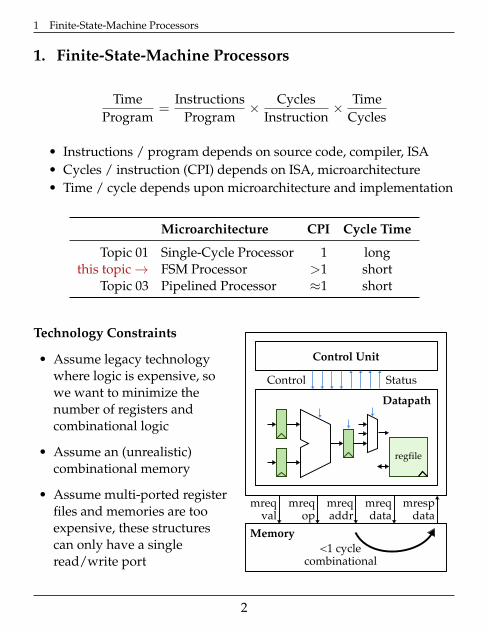
1. Finite-State-Machine Processors

TimeProgram

=Instructions

Program× Cycles

Instruction× Time

Cycles

• Instructions / program depends on source code, compiler, ISA• Cycles / instruction (CPI) depends on ISA, microarchitecture• Time / cycle depends upon microarchitecture and implementation

Microarchitecture CPI Cycle Time

Topic 01 Single-Cycle Processor 1 longthis topic→ FSM Processor >1 short

Topic 03 Pipelined Processor ≈1 short

Technology Constraints

• Assume legacy technologywhere logic is expensive, sowe want to minimize thenumber of registers andcombinational logic

• Assume an (unrealistic)combinational memory

• Assume multi-ported registerfiles and memories are tooexpensive, these structurescan only have a singleread/write port

Control Status

Control Unit

Datapath

mreqval

mreqop

mrespdata

<1 cyclecombinational

Memory

regfile

mreqaddr

mreqdata

2


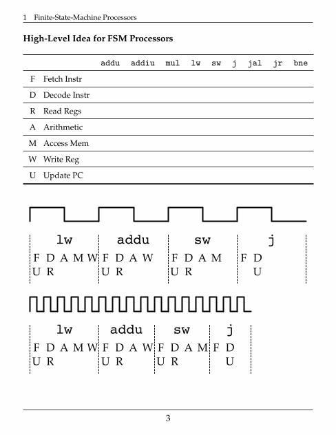
High-Level Idea for FSM Processors

addu addiu mul lw sw j jal jr bne

F Fetch Instr

D Decode Instr

R Read Regs

A Arithmetic

M Access Mem

W Write Reg

U Update PC

F D A M WU R

lw

F D A WU R

addu

F D A MU R

sw

F DU

j

F D A M WU R

lw

F D A WU R

addu

F D A MU R

sw

F DU

j

3


Implementing Fetch Sequence

PC IR

ir_enpc_en

Dat

apat

h B

us

pc_bus_en

A

a_en

+4

alu_bus_en

mrespdata

mreqaddr

RD

rd_bus_en

To control unit

F0

F1

F2

(pseudo-control-signal syntax)

4


Implementing ADDU Instruction

PC IR

ir_enpc_en

Dat

apat

h B

us

pc_bus_en

A

a_en

+4

alu_bus_en

mrespdata

mreqaddr

RD

rd_bus_en

To control unit

B

b_en

RFrf_wen

rf_bus_en

alu_func

alu func

A + 4

A + B

alu

rf_addr_sel

rsrtrd

F0

F1

F2

A0

A1

A2


5


Implementing ADDIU Instruction

PC IR

ir_enpc_en

Dat

apat

h B

us

pc_bus_en

A

a_en

+4

alu_bus_en

mrespdata

mreqaddr

RD

rd_bus_en

To control unit

B

b_en

RFrf_wen

rf_bus_en

alu_func

alu func

A + 4

A + B

alu

rf_addr_sel

rsrtrd

sextimm

iau_bus_en

F0

F1

F2

A0

A1

A2

AI0

AI1

AI2


6


Full Datapath for PARCv1 FSM Processor

PC IR

ir_enpc_en

Dat

apat

h B

us

pc_bus_en

A

a_en

+4

alu_bus_en

mrespdata

mreqaddr

RD

rd_bus_en

To control unit

B

b_en

RFrf_wen

rf_bus_en

alu_func

alu func

A + 4

A + B

alu

rf_addr_sel

rsrtrd

sextimm

iau_bus_en

>>

b_sel

>>C

c_selc_en

A +? B mreqdata

WD

wd_en

iau_func

A jt B

iau func

IR.sext_imm

IR.target_sll2

iau31

IR.sext_imm_sll2

alu_bus_en

eq

MUL Instruction Pseudo-Control-Assembly Fragment

F0

F1

F2

A0

A1

A2

AI0

AI1

AI2

M0

M1

M2

M34

M3

M0: A <- RF[0]M1: B <- RF[rs]M2: C <- RF[rt]M3: A <- A +? B;

B <- B << 1; C <- C >> 1M4: A <- A +? B;

B <- B << 1; C <- C >> 1...

M35: R[rd] <- A +? B;B <- B << 1; C <- C >> 1goto F0

7


LW Instruction Pseudo-Control-Assembly Fragment

F0

F1

F2

A0

A1

A2

AI0

AI1

AI2

M0

M1

M2

M34

M3

L0

L1

L2

L3

L0: A <- RF[rs]L1: B <- IR.sext_immL2: mreq_addr <- A + BL3: R[rt] <- MRD; goto F0

SW Instruction Pseudo-Control-Assembly Fragment

F0

F1

F2

A0

A1

A2

AI0

AI1

AI2

M0

M1

M2

M34

M3

L0

L1

L2

L3

S0

S1

S2

S3

S0: WD <- RF[rt]S1: A <- RF[rs]S2: B <- IR.sext_immS3: mreq_addr <- A + B;

goto F0

8


J Instruction Pseudo-Control-Assembly Fragment

F0

F1

F2

A0

A1

A2

AI0

AI1

AI2

M0

M1

M2

M34

M3

L0

L1

L2

L3

S0

S1

S2

S3

J0

J1

J0: B <- IR.target_sll2J1: PC <- A jt B; goto F0

JAL Instruction Pseudo-Control-Assembly Fragment

F0

F1

F2

A0

A1

A2

AI0

AI1

AI2

M0

M1

M2

M34

M3

L0

L1

L2

L3

S0

S1

S2

S3

J0

J1

JA0

JA1

JA2

JA0: R[31] <- PCJA1: B <- IR.target_sll2JA2: PC <- A jt B; goto F0

9


JR Instruction Pseudo-Control-Assembly Fragment

F0

F1

F2

A0

A1

A2

AI0

AI1

AI2

M0

M1

M2

M34

M3

L0

L1

L2

L3

S0

S1

S2

S3

J0

J1

JA0

JA1

JA2

JR0

JR0: PC <- R[rs]; goto F0

BNE Instruction Pseudo-Control-Assembly Fragment

F0

F1

F2

A0

A1

A2

AI0

AI1

AI2

M0

M1

M2

M34

M3

L0

L1

L2

L3

S0

S1

S2

S3

J0

J1

JA0

JA1

JA2

JR0 B0

B1

B2

B3

B4

B0: A <- R[rs]B1: B <- R[rt]B2: A <- IR.sext_imm_sll2;

goto F0 if A == BB3: B <- PCB4: PC <- A + B; goto F0

10


Adding a Complex Instruction

FSM processors simplify adding complex instructions, since new instruc-tions usually do not require datapath modifications, only additional states.

addu.mm rd, rs, rt

M[ R[rd] ]←M[ R[rs] ] + M[ R[rt] ]

PC IR

ir_enpc_en

Dat

apat

h B

us

pc_bus_en

A

a_en

+4

alu_bus_en

mrespdata

mreqaddr

RD

rd_bus_en

To control unit

B

b_en

RFrf_wen

rf_bus_en

alu_func

alu func

A + 4

A + B

alu

rf_addr_sel

rsrtrd

sextimm

iau_bus_en

>>

b_sel

>>C

c_selc_en

A +? B mreqdata

WD

wd_en

iau_func

A jt B

iau func

IR.sext_imm

IR.target_sll2

iau31

IR.sext_imm_sll2

alu_bus_en

eq

11


Adding a New Auto-Incrementing Load Instruction

Implement the following auto-incrementing load instruction using pseudo-control-sign syntax. Modify the datapath if necessary.

lw.ai rt, imm(rs)

R[rt]←M[ R[rs] + sext(imm) ]; R[rs]← R[rs] + 4

PC IR

ir_enpc_en

Dat

apat

h B

us

pc_bus_en

A

a_en

+4

alu_bus_en

mrespdata

mreqaddr

RD

rd_bus_en

To control unit

B

b_en

RFrf_wen

rf_bus_en

alu_func

alu func

A + 4

A + B

alu

rf_addr_sel

rsrtrd

sextimm

iau_bus_en

>>

b_sel

>>C

c_selc_en

A +? B mreqdata

WD

wd_en

iau_func

A jt B

iau func

IR.sext_imm

IR.target_sll2

iau31

IR.sext_imm_sll2

alu_bus_en

eq

12

2 Implementing FSM Control Units

2. Implementing FSM Control Units

F0

F1

F2

A0

A1

A2

AI0

AI1

AI2

M0

M1

M2

M34

M3

L0

L1

L2

L3

S0

S1

S2

S3

J0

J1

JA0

JA1

JA2

JR0 B0

B1

B2

B3

B4

We will study three techniquesfor implementing FSM controlunits:

• Hardwired control units arehigh-performance, butinflexible

• Horizontal µcodingincreases flexibility, requireslarge control store

• Vertical µcoding is anintermediate design point

2.1. Hardwired FSMs

State

ControlSignalLogic

StateTransition

Logic

Control Signals(22)

Status Signals(1)

13

2 Implementing FSM Control Units 2.1. Hardwired FSMs

Control signal output table for hardwired control unit

PC IR

ir_enpc_en

Dat

apat

h B

us

pc_bus_en

A

a_en

+4

alu_bus_en

mrespdata

mreqaddr

RD

rd_bus_en

To control unit

B

b_en

RFrf_wen

rf_bus_en

alu_func

alu func

A + 4

A + B

alu

rf_addr_sel

rsrtrd

sextimm

iau_bus_en

>>

b_sel

>>C

c_selc_en

A +? B mreqdata

WD

wd_en

iau_func

A jt B

iau func

IR.sext_imm

IR.target_sll2

iau31

IR.sext_imm_sll2

alu_bus_en

eq

F0: mreq_addr <- PC; A <- PC

F1: IR <- RD

F2: PC <- A + 4; A <- A + 4

goto inst

A0: A <- RF[rs]

A1: B <- RF[rt]

A2: R[rd] <- A + B

goto F0

Bus Enables Register Enables Mux Func RF MReq

state PC IAU ALU RF RD PC IR A B C WD A B IAU ALU sel wen val op

14

2 Implementing FSM Control Units 2.2. Horizontally Microcoded FSM

2.2. Horizontally Microcoded FSM

• Use memory array (called the control store) instead of random logicto encode both the control signal logic and the state transition logic

• Enables a more systematic approach to implementing complexmulti-cycle instructions

• Microcoding can produce good performance if accessing the controlstore is much faster than accessing main memory

• Read-only control stores might be replaceable enabling in-fieldupdates, while read-write control stores can simplify diagnosticsand microcode patches

15

2 Implementing FSM Control Units 2.2. Horizontally Microcoded FSM

Handling micro-control flow with horizontal microcoding

F0

F1

F2

A0

A1

A2

AI0

AI1

AI2

index csigs (22b) next state (2b)

00

01

10

11

index csigs (22b) next state (3b)

0000

0001

0010

0011

0100

0101

0110

0111

1000

1001

1010

1011

1100

1101

1110

1111

16

2 Implementing FSM Control Units 2.3. Vertically Microcoded FSM

2.3. Vertically Microcoded FSM

• Horizontal microcode has wider micro-instructions

– Multiple parallel operations per micro-instruction– Fewer microcode steps per macroinstruction– Sparser encoding = more bits, but less decoding logic

• Vertical microcode has narrower micro-instructions

– Typically a single datapath operation per micro-instruction– More microcode steps per macroinstruction– More compact = less bits, but more decoding logic

17

3 Analyzing Processor Performance

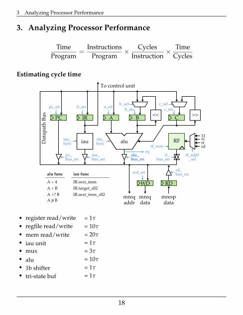
3. Analyzing Processor Performance

TimeProgram

=Instructions

Program× Cycles

Instruction× Time

Cycles

Estimating cycle time

PC IR

ir_enpc_en

Dat

apat

h B

us

pc_bus_en

A

a_en

+4

alu_bus_en

mrespdata

mreqaddr

RD

rd_bus_en

To control unit

B

b_en

RFrf_wen

rf_bus_en

alu_func

alu func

A + 4

A + B

alu

rf_addr_sel

rsrtrd

sextimm

iau_bus_en

>>

b_sel

>>C

c_selc_en

A +? B mreqdata

WD

wd_en

iau_func

A jt B

iau func

IR.sext_imm

IR.target_sll2

iau31

IR.sext_imm_sll2

alu_bus_en

eq

• register read/write = 1τ

• regfile read/write = 10τ

• mem read/write = 20τ

• iau unit = 1τ

• mux = 3τ

• alu = 10τ

• 1b shifter = 1τ

• tri-state buf = 1τ

18

3 Analyzing Processor Performance

Estimating execution time

Using our first-order equation for processor performance, how long inns will it take to execute the vvadd example assuming n is 64?

loop:lw r12, 0(r4)lw r13, 0(r5)addu r14, r12, r13sw r14, 0(r6)addiu r4, r4, 4addiu r5, r5, 4addiu r6, r6, 4addiu r7, r7, -1bne r7, r0, loopjr r31

Using our first-order equation for processor performance, how long inns will it take to execute the mystery program assuming n is 64 and thatwe find a match on the 10th element.

addiu r12, r0, 0loop:lw r13, 0(r4)bne r13, r6, fooaddiu r2, r12, 0jr r31

foo:addiu r4, r4, 4addiu r12, r12, 1bne r12, r5, loopaddiu r2, r0, -1jr r31

19

4 Case Study: Transition from CISC to RISC

4. Case Study: Transition from CISC to RISC

• Microcoding thrived in the 1970’s

– ROMs significantly faster than DRAMs– For complex instruction sets, microcode was cheaper and simpler– New instructions supported without modifying datapath– Fixing bugs in controller is easier– ISA compatibility across models relatively straight-forward

— Maurice Wilkes, 1954

20


IBM 360 Microprogramming

M30 M40 M50 M65

Datapath width (bits) 8 16 32 64µinst width (bits) 50 52 85 87µcode size (1K µinsts) 4 4 2.75 2.75µstore technology CCROS TCROS BCROS BCROSµstore cycle (ns) 750 625 500 200Memory cycle (ns) 1500 2500 2000 750Rental fee ($K/month) 4 7 15 35

TROS = transformer read-only storage (magnetic storage)BCROS = balanced capacitor read-only storage (capacitive storage)

CCROS = card capacitor read-only storage (metal punch cards, replace in field)

Only the fastest models (75,95) were hardwired

IBM 360/M30 microprogram for register-register logical OR

OR

Fetch first byteof operands

Instruction Fetch

Writeback Result

Prepare for Next Byte

21


IBM 360/M30 microprogram for register-register binary ADD

Analyzing Microcoded Machines

• John Cocke and group at IBM

– Working on a simple pipelined processor, 801, and advanced compilers

– Ported experimental PL8 compiler to IBM 370, and only used simpleregister-register and load/store instructions similar to 801

– Code ran faster than other existing compilers that used all 370instructions! (up to 6 MIPS, whereas 2 MIPS considered good before)

• Joel Emer and Douglas Clark at DEC

– Measured VAX-11/780 using external hardware– Found it was actually a 0.5 MIPS machine, not a 1 MIPS machine– 20% of VAX instrs = 60% of µcode, but only 0.2% of the dynamic execution

• VAX 8800, high-end VAX in 1984

– Control store: 16K×147b RAM, Unified Cache: 64K×8b RAM– 4.5×more microstore RAM than cache RAM!

22


From CISC to RISC

• Key changes in technology constraints

– Logic, RAM, ROM all implemented with MOS transistors– RAM ≈ same speed as ROM

• Use fast RAM to build fast instruction cache of user-visibleinstructions, not fixed hardware microfragments

– Change contents of fast instruction memory to fit what app needs

• Use simple ISA to enable hardwired pipelined implementation

– Most compiled code only used a few of CISC instructions– Simpler encoding allowed pipelined implementations– Load/Store Reg-Reg ISA as opposed to Mem-Mem ISA

• Further benefit with integration

– Early 1980’s→ fit 32-bit datapath, small caches on single chip– No chip crossing in common case allows faster operation

μPC

ROM for

μInst

Small

Decoder

User PC

RAM for

Instr Cache

"Larger"

Decoder

Vertical μCode

ControllerRISC

Controller

23


Ratio of

MIPS

to

VAX

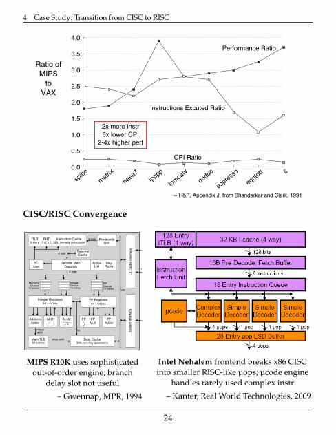
-- H&P, Appendix J, from Bhandarkar and Clark, 1991

Performance Ratio

Instructions Excuted Ratio

CPI Ratio

4.0

3.5

3.0

2.5

2.0

1.5

1.0

0.5

0.0

spice

matri

x

nasa7

fpppp

tom

catv

doduc

espre

sso

eqntott li

2x more instr

6x lower CPI

2-4x higher perf

CISC/RISC Convergence

by Linley Gwennap

Not to be left out in the move to thenext generation of RISC, MIPS Tech-nologies (MTI) unveiled the design ofthe R10000, also known as T5. As thespiritual successor to the R4000, thenew design will be the basis of high-end

MIPS processors for some time, at least until 1997. Byswapping superpipelining for an aggressively out-of-order superscalar design, the R10000 has the potentialto deliver high performance throughout that period.

The new processor uses deep queues decouple theinstruction fetch logic from the execution units. Instruc-tions that are ready to execute can jump ahead of thosewaiting for operands, increasing the utilization of the ex-ecution units. This technique, known as out-of-order ex-ecution, has been used in PowerPC processors for sometime (see 081402.PDF ), but the new MIPS design is themost aggressive implementation yet, allowing more in-structions to be queued than any of its competitors.

Taking advantage of its experience with the 200-MHz R4400, MTI was able to streamline the design andexpects it to run at a high clock rate. Speaking at theMicroprocessor Forum, MTI’s Chris Rowen said that thefirst R10000 processors will reach a speed of 200 MHz,50% faster than the PowerPC 620. At this speed, he ex-pects performance in excess of 300 SPECint92 and 600SPECfp92, challenging Digital’s 21164 for the perfor-mance lead. Due to schedule slips, however, the R10000has not yet taped out; we do not expect volume ship-ments until 4Q95, by which time Digital may enhancethe performance of its processor.

Speculative Execution Beyond BranchesThe front end of the processor is responsible for

maintaining a continuous flow of instructions into thequeues, despite problems caused by branches and cachemisses. As Figure 1 shows, the chip uses a two-way set-associative instruction cache of 32K. Like other highlysuperscalar designs, the R10000 predecodes instructionsas they are loaded into this cache, which holds four extra

bits per instruction. These bits reducethe time needed to determine the ap-propriate queue for each instruction.

The processor fetches four instruc-tions per cycle from the cache and de-codes them. If a branch is discovered, itis immediately predicted; if it is pre-dicted taken, the target address is sentto the instruction cache, redirecting thefetch stream. Because of the one cycleneeded to decode the branch, takenbranches create a “bubble” in the fetchstream; the deep queues, however, gen-erally prevent this bubble from delay-ing the execution pipeline.

The sequential instructions thatare loaded during this extra cycle arenot discarded but are saved in a “re-sume” cache. If the branch is later de-termined to have been mispredicted, thesequential instructions are reloadedfrom the resume cache, reducing themispredicted branch penalty by onecycle. The resume cache has four entriesof four instructions each, allowing spec-ulative execution beyond four branches.

The R10000 design uses the stan-dard two-bit Smith method to predict

M I C R O P R O C E S S O R R E P O R T

MIPS R10000 Uses Decoupled Architecture Vol. 8, No. 14, October 24, 1994 © 1994 MicroDesign Resources

MIPS R10000 Uses Decoupled ArchitectureHigh-Performance Core Will Drive MIPS High-End for Years

1 9 9 4

FORUMMICROPROCESSOR

Figure 1. The R10000 uses deep instruction queues to decouple the instruction fetch logicfrom the five function units.

Instruction Cache32K, two-way associative

PC

Unit

Predecode

Unit

ITLB8 entry

Decode, Map,

DispatchActive

ListMapTable

Main TLB64 entries

ALU1

Data Cache32K, two-way associative

FP

Adder

4 instr

4 instr

4 instr

MemoryQueue

16 entries

IntegerQueue16 entries

FPQueue16 entries

ALU2 FP

Mult÷!

FP÷"

virtualaddr

phys addr

64

DataSRAM

128

512K-16M

Avala

nche B

us (

64 b

it a

ddr/

data

)

L2 C

ache Inte

rface

128

Syste

m Inte

rface

TagSRAM

BHT512 x 2

Resume

Cache

Address

Adder

Integer Registers64 ! 64 bits

FP Registers64 ! 64 bits

MIPS R10K uses sophisticatedout-of-order engine; branch

delay slot not useful

– Gwennap, MPR, 1994

Intel Nehalem frontend breaks x86 CISCinto smaller RISC-like µops; µcode engine

handles rarely used complex instr

– Kanter, Real World Technologies, 2009

24


Microprogamming Today

• Microprogramming is far from extinct

• Played a crucial role in microprocessors of the 1980s(DEC VAX, Motorola 68K series, Intel 386/486)

• Microprogramming plays assisting role in many modern processors(AMD Phenom, Intel Nehalem, Intel Atom, IBM Z196)

– 761 Z196 instructions executed with hardwired control– 219 Z196 “complex” instructions always executed with microcode– 24 Z196 instructions conditionally executed with microcode

• Patchable microcode common for post-fabrication bug fixes (Intelprocessors load µcode patches at bootup)

25

Documents

ECE 4750 Computer Architecture, Fall 2014 T02 FSM …€¦ · · 2016-03-22ECE 4750 Computer Architecture, Fall 2014 T02 FSM Processors School of Electrical and Computer Engineering