ECE 600: Introduction to Shape Analysis Convex Hull … 600/Project...University of Louisville Instructor Dr. Aly A. Farag Electrical and Computer Engineering Summer 2009 ECE 600:

University of Louisville Instructor Dr. Aly A. Farag

Electrical and Computer Engineering Summer 2009

EC

E 6

00: In

tro

duct

ion

to

Sh

ape

An

alys

is L

ab #

4 –

Co

nvex

Hull in

2D

1

ECE 600: Introduction to Shape Analysis

Lab #4 – Convex Hull in 2D

(Assigned Thursday 6/11/09 – Due Thursday 6/18/09)

In this lab, we will discuss the details of computing convex hull using Graham's algorithm, refer to lecture

notes for more theoretical details. We start with data structures, then tackle the sorting step, and finally

present the code.

Table of Contents Table of Code Snippets ................................................................................................................................ 1

1. Data Representation ................................................................................................................................ 3

2. Sorting ........................................................................................................................................................ 6

2.1 FindLowest. ................................................................................................................................... 6

2.2 Sorting Relation ............................................................................................................................. 7

2.3 Slopes .............................................................................................................................................. 7

2.4 Using Left Predicate ..................................................................................................................... 8

2.5 Compare ......................................................................................................................................... 8

2.6 QuickSort ..................................................................................................................................... 10

3. Graham Algorithm ................................................................................................................................ 14

Task 12: ........................................................................................................................................... 18

Table of Code Snippets

Code 1 - Vertex2D class after modification to compute the convex hull ................................................. 3

Code 2 – Stack functions added Vertex2D class .......................................................................................... 5

Code 3 – Example how to use stack data structure ...................................................................................... 5

Code 4 - FindLowest function ......................................................................................................................... 6

ECE 600 - Su 09; Dr. Farag



EC

E 6

00: In

tro

duct

ion

to

Sh

ape

An

alys

is L

ab #

4 –

Co

nvex

Hull in

2D

2

Code 5 – Swap function .................................................................................................................................... 6

Code 6 - Compare function .............................................................................................................................. 8

Code 7 - QuickSort function .......................................................................................................................... 13

Code 8 - Partition function, Version 2 ......................................................................................................... 14




EC

E 6

00: In

tro

duct

ion

to

Sh

ape

An

alys

is L

ab #

4 –

Co

nvex

Hull in

2D

3

1. Data Representation

As usual, we have a choice between storing the points in an array or a list. We choose in this

instance to use an array, anticipating using a sorting routine that expects its data in a contiguous

section of memory. Each point will be represented by a structure paralleling that used for vertices in

polygon triangulation lab, i.e. Vertex2D, however it will be modified to serve the purpose of convex

hull computation.

The points are stored in an array (rather than a linked list) called P with P(1),P(1),...,P(n)

corresponding to 𝑝0, 𝑝1, … , 𝑝𝑛−1, note that Matlab arrays are one-based indexed. Each P(i) is a

structure with fields for its coordinates, a unique identifying number, vertexID, and a flag to mark

deletion, isDeleted, such member will be added to the Vertex2D class.

Thus, we are given an array of points P, where P(i) is of type Vertex2D, and optimally we are

required to extract from them the following:

(1) All points on the hull in arbitrary order (array of points subset of P can be used)

(2) The extreme points in arbitrary order (array of points subset of P can be used)

(3) All the points on the hull in boundary traversal order ( a linked list containing such

(4) The extreme points in boundary traversal order

Where an array of points which is subset of P is sufficient to represent the first two outputs, while a

linked list structure can be used to represented the last two outputs to maintain the boundary

traversal order. See Code 1 to see the modification done for Vertex2D class.

Code 1 - Vertex2D class after modification to compute the convex hull

classdef Vertex2D < handle

% in this class we will define the basic building block of a polygon

properties

vertexID % index or id number assigned to the current vertex

% which reveals its order within the polygon

point % point coordinates for this vertex

% members used for polygon triangulation, i.e. if Vertex2D is

% used as a linked list of vertices to define the

% boundary of a polygon

isEar % ear status, true if this vertex is an ear

isAdded = 0 % a flag to indicate whether this vertex is

% added to the vertex list of the polygon or not

index_in_vertexList = 0;

% members used for convex hull computation (Graham's Algorithm)

isDeleted % a flag which mark point deletion

% members used to used Vertex2D as a node in either a linked list

% or a stack




EC

E 6

00: In

tro

duct

ion

to

Sh

ape

An

alys

is L

ab #

4 –

Co

nvex

Hull in

2D

4

next % next vertex

prev % previous vertex

end

methods

%% constructor,

% take care to modify the constructor to add the added

% member (isDeleted)

%% get/set access methods

% don’t forget to add a set and get access function for isDeleted

%% disp function

% modify the function to display isDeleted

end

end

Now, throughout the computation of the convex hull of the given set of points P, we need to

maintain a stack of so-far added points to the convex hull boundary. In Lab 3 we have implemented

Vertex2D as a doubly linked list to represent a polygon, however to compute the convex hull, we

need to view it as a stack, hence we will add some functionalities on Vertex2D class to enable using

it as a node in a stack.

Conceptually, a stack is simple: a data structure that allows adding and removing elements in a

particular order. Every time an element is added, it goes on the top of the stack; the only element

that can be removed is the element that was at the top of the stack. Consequently, a stack is said to

have "first in last out" behavior (or "last in, first out"). The first item added to a stack will be the last

item removed from a stack.

Stacks have some useful terminology associated with them:

1. Push To add an element to the stack, such element will be the head/top of the stack, hence

this addition can be thought of inserting a node at the end of a linked list.

2. Pop To remove an element from the stack, this element is the last one, hence moving the

head/top of the stack one step down, thus this removal can be thought of deleting the last

node from a linked list.

3. Peek To look at (traverse) elements in the stack without removing them

4. LIFO Refers to the last in, first out behavior of the stack

5. FILO Equivalent to LIFO

Thus, the stack is most naturally represented by a singly linked list of cells, each of which "contains"

a vertex, such that we always have the access to the top of the stack which is the last element being

pushed in such a single linked list. See Code 2 for the functions added to Vertex2D class to allowing

the implementation of stack functions.




EC

E 6

00: In

tro

duct

ion

to

Sh

ape

An

alys

is L

ab #

4 –

Co

nvex

Hull in

2D

5

Code 2 – Stack functions added Vertex2D class

%% functions related to stack implementation

function stackTop = Push(stackTop,newNode)

newNode.insertAfter(stackTop);

stackTop = newNode;

end

function [stackTop, popedNode] = Pop(stackTop)

popedNode = Vertex2D(stackTop.vertexID,stackTop.point);

stackTop = stackTop.prev;

stackTop.next = [];

end

function Peek(stackTop)

% loop backward from the stacktop till the first element being

% pushed and display node info

while(1)

disp(stackTop);

% termination condition

if isempty(stackTop.prev)

break

end


end

end

See Code 3 for an example how to use the stack

Code 3 – Example how to use stack data structure

% test stack

x = [0 10 12 20 13 10 12 14 8 6 10 7 0 1 3 5 -2 5];

y = [0 7 3 8 17 12 14 9 10 14 15 18 16 13 15 8 9 5];

% let's fill a stack of vertices for the previous coordinates

% the first point will be the starting head/top of the stack

starting_point = Point2D(x(1),y(1));

stackTop = Vertex2D(0,starting_point);

for i = 2 : length(x)

curPoint = Point2D(x(i),y(i));

curVertex = Vertex2D(i-1,curPoint);

stackTop = stackTop.Push(curVertex);

end

% go over the stack element and display node information without removing

% them

stackTop.Peek();




EC

E 6

00: In

tro

duct

ion

to

Sh

ape

An

alys

is L

ab #

4 –

Co

nvex

Hull in

2D

6

% remove the last pushed node in the stack

stackTop = stackTop.Pop();

2. Sorting

2.1 FindLowest.

We first start with the easiest aspect of the sorting step: finding the rightmost lowest point in the set.

The function FindLowest (Code 4) accomplishes this and swaps the point into P(1) (note that

Matlab arrays are one-based indexed). The straightforward Swap is shown in Code 5. Note that

these functions are utility functions hence they are not included in any class definition.

Code 4 - FindLowest function

function P = FindLowest(P)

% this function finds the rightmost lowest point in a given array of vertices

each of type Vertex2D.

% this function accomplishes this and swaps the point into P(0).

lowestIndex = 1;

lowestPoint = P(lowestIndex).point;

for i = 2 : length(P)

curPoint = P(i).point;

if (curPoint.y < lowestPoint.y) || ...

((curPoint.y == lowestPoint.y)&&(curPoint.x > lowestPoint.x))

lowestIndex = i;

lowestPoint = P(lowestIndex).point;

end

end

P = Swap(P,1,lowestIndex);

Code 5 – Swap function

function P = Swap(P,i,j)

% this function will swap array element at index i with array element at

% index j and return the array P after swap has been occured

tempElement = P(i);

P(i) = P(j);

P(j) = tempElement;




EC

E 6

00: In

tro

duct

ion

to

Sh

ape

An

alys

is L

ab #

4 –

Co

nvex

Hull in

2D

7

2.2 Sorting Relation

The sorting step seems straightforward, but there are hidden pitfalls if we want to guarantee an

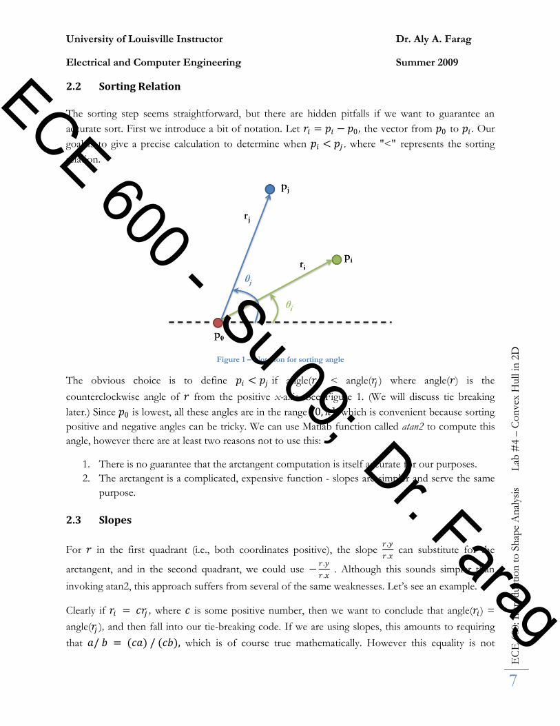
accurate sort. First we introduce a bit of notation. Let 𝑟𝑖 = 𝑝𝑖 − 𝑝0, the vector from 𝑝0 to 𝑝𝑖 . Our

goal is to give a precise calculation to determine when 𝑝𝑖 < 𝑝𝑗 , where "<" represents the sorting

relation.

Figure 1 – Notation for sorting angle

The obvious choice is to define 𝑝𝑖 < 𝑝𝑗 if angle(𝑟𝑖) < angle(𝑟𝑗 ) where angle(𝑟) is the

counterclockwise angle of 𝑟 from the positive x-axis. See Figure 1. (We will discuss tie breaking

later.) Since 𝑝0 is lowest, all these angles are in the range (0, 𝜋], which is convenient because sorting

positive and negative angles can be tricky. We can use Matlab function called atan2 to compute this

angle, however there are at least two reasons not to use this:

1. There is no guarantee that the arctangent computation is itself accurate for our purposes.

2. The arctangent is a complicated, expensive function - slopes are simpler and serve the same

purpose.

2.3 Slopes

For 𝑟 in the first quadrant (i.e., both coordinates positive), the slope 𝑟 .𝑦

𝑟 .𝑥 can substitute for the

arctangent, and in the second quadrant, we could use −𝑟 .𝑦

𝑟 .𝑥 . Although this sounds simpler than

invoking atan2, this approach suffers from several of the same weaknesses. Let’s see an example.

Clearly if 𝑟𝑖 = 𝑐𝑟𝑗 , where 𝑐 is some positive number, then we want to conclude that angle(𝑟𝑖) =

angle(𝑟𝑗 ), and then fall into our tie-breaking code. If we are using slopes, this amounts to requiring

that 𝑎/ 𝑏 = (𝑐𝑎) / (𝑐𝑏), which is of course true mathematically. However this equality is not




EC

E 6

00: In

tro

duct

ion

to

Sh

ape

An

alys

is

L

ab #

4 –

Co

nvex

Hull in

2D

8

guaranteed to hold for floating-point division. It depends on the machine. Some machines performs

division by reciprocating and multiplying, and the two operations sometimes lead to small errors.

2.4 Using Left Predicate

The solution is already in hand: the Left predicate, the function to determine whether a point is left

of a line determined by two other points, is precisely what we need to compare 𝑟𝑖 and 𝑟𝑗 .

Recall that Left was itself a simple test on the value of getTriangleArea, which computes the signed

area of the triangle determined by three points. We will use this area function rather than Left, as it

is then easier to distinguish ties.

2.5 Compare

Now, given two points, 𝑝𝑖 and 𝑝𝑗 , we want to compare them, i.e. 𝑝𝑖 < 𝑝𝑗 ? with respect to 𝑝0. If 𝑝𝑗

is on the left of the directed line 𝑝0𝑝𝑖 , then 𝑝𝑖 < 𝑝𝑗 , i.e. 𝑝𝑖 < 𝑝𝑗 if 𝑎𝑟𝑒𝑎 𝑝0, 𝑝𝑖 , 𝑝𝑗 > 0, hence -1 is

returned to indicate less than. When the area is zero, we fall into a sorting collinearity. To decide

which point is closer to 𝑝0, we can avoid computing the distance by noting that if 𝑝𝑖 is closer, then

𝑟𝑖 = 𝑝𝑖 − 𝑝0 projects to a shorter length than does 𝑟𝑗 = 𝑝𝑗 − 𝑝0 . If 𝑝𝑖 is closer, we mark it for later

deletion, if 𝑝𝑗 is closer, mark it instead. If 𝑝𝑖 = 𝑝𝑗 then we mark the one with lower index for later

deletion (which one we choose to delete does not matter, however consistency is needed). In all

cases, either -1, 0 or 1 is returned according to the angular sorting rule. For implementation issues, it

was found that it is preferred to separate the comparison code (Code 6) from the part related to

marking a point for deletion (Code 7), where the later is called after sorting the vertices.

Code 6 - Compare function

function decision = compare(p0,pi,pj)

% this function compares pi and pj with respect to p0 using the angular

% sorting rule

% getting the area of the triangle of vertices po,pi and pj

A = area(p0,pi,pj);

if A > 0

decision = -1; % less than

else if A < 0

decision = 1; % greater than

else

% points are collinear with p0

% compute the projections of ri = pi-po and rj = pj-po

x = abs(pi.point.x - p0.point.x) - abs(pj.point.x - p0.point.x);

y = abs(pi.point.y - p0.point.y) - abs(pj.point.y - p0.point.y);

if (x<0)||(y<0)




EC

E 6

00: In

tro

duct

ion

to

Sh

ape

An

alys

is L

ab #

4 –

Co

nvex

Hull in

2D

9

decision = -1;

else if (x>0) || (y>0)

decision = 1;

else

% points are coincident

decision = 0;

end

end

end

end

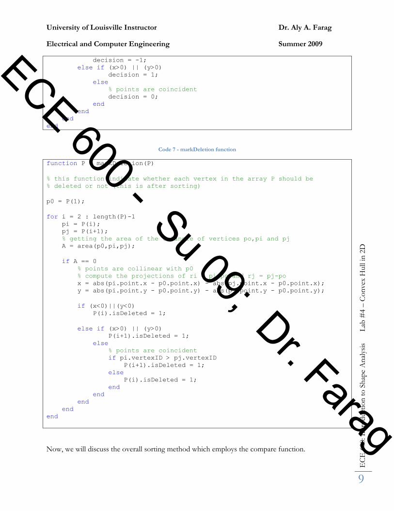
Code 7 - markDeletion function

function P = markDeletion(P)

% this function indicate whether each vertex in the array P should be

% deleted or not (this is after sorting)

p0 = P(1);

for i = 2 : length(P)-1

pi = P(i);

pj = P(i+1);

% getting the area of the triangle of vertices po,pi and pj

A = area(p0,pi,pj);

if A == 0

% points are collinear with p0

% compute the projections of ri = pi-po and rj = pj-po

x = abs(pi.point.x - p0.point.x) - abs(pj.point.x - p0.point.x);

y = abs(pi.point.y - p0.point.y) - abs(pj.point.y - p0.point.y);

if (x<0)||(y<0)

P(i).isDeleted = 1;

else if (x>0) || (y>0)

P(i+1).isDeleted = 1;

else

% points are coincident

if pi.vertexID > pj.vertexID

P(i+1).isDeleted = 1;

else

P(i).isDeleted = 1;

end

end

end

end

end

Now, we will discuss the overall sorting method which employs the compare function.




EC

E 6

00: In

tro

duct

ion

to

Sh

ape

An

alys

is L

ab #

4 –

Co

nvex

Hull in

2D

10

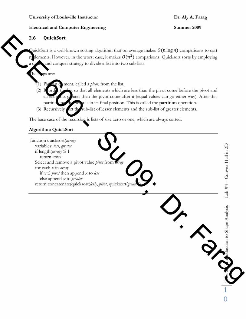
2.6 QuickSort

QuickSort is a well-known sorting algorithm that on average makes 𝑂(𝑛 log 𝑛) comparisons to sort

𝑛 elements. However, in the worst case, it makes 𝑂(𝑛2) comparisons. Quicksort sorts by employing

a divide and conquer strategy to divide a list into two sub-lists.

The steps are:

(1) Pick an element, called a pivot, from the list.

(2) Reorder the list so that all elements which are less than the pivot come before the pivot and

all elements greater than the pivot come after it (equal values can go either way). After this

partitioning, the pivot is in its final position. This is called the partition operation.

(3) Recursively sort the sub-list of lesser elements and the sub-list of greater elements.

The base case of the recursion is lists of size zero or one, which are always sorted.

Algorithm: QuickSort

function quicksort(array) variables: less, greater if length(array) ≤ 1 return array Select and remove a pivot value pivot from array for each x in array if x ≤ pivot then append x to less else append x to greater return concatenate(quicksort(less), pivot, quicksort(greater))




EC

E 6

00: In

tro

duct

ion

to

Sh

ape

An

alys

is L

ab #

4 –

Co

nvex

Hull in

2D

11

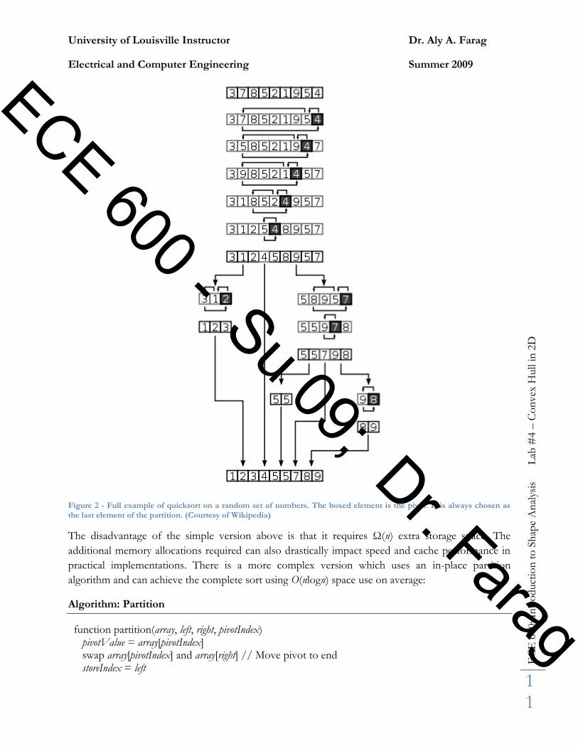
Figure 2 - Full example of quicksort on a random set of numbers. The boxed element is the pivot. It is always chosen as the last element of the partition. (Courtesy of Wikipedia)

The disadvantage of the simple version above is that it requires Ω(n) extra storage space. The

additional memory allocations required can also drastically impact speed and cache performance in

practical implementations. There is a more complex version which uses an in-place partition

algorithm and can achieve the complete sort using O(nlogn) space use on average:

Algorithm: Partition

function partition(array, left, right, pivotIndex) pivotValue = array[pivotIndex] swap array[pivotIndex] and array[right] // Move pivot to end storeIndex = left




EC

E 6

00: In

tro

duct

ion

to

Sh

ape

An

alys

is L

ab #

4 –

Co

nvex

Hull in

2D

12

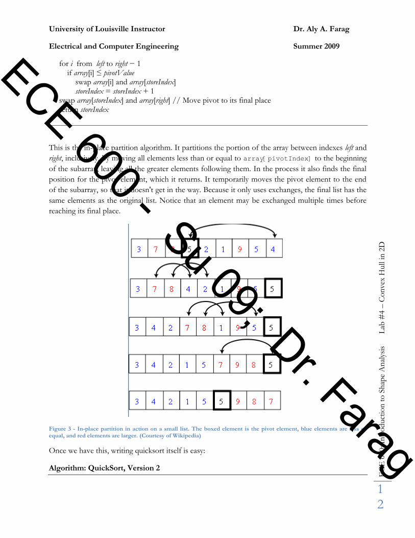
for i from left to right − 1 if array[i] ≤ pivotValue swap array[i] and array[storeIndex] storeIndex = storeIndex + 1 swap array[storeIndex] and array[right] // Move pivot to its final place return storeIndex

This is the in-place partition algorithm. It partitions the portion of the array between indexes left and

right, inclusively, by moving all elements less than or equal to array[pivotIndex] to the beginning

of the subarray, leaving all the greater elements following them. In the process it also finds the final

position for the pivot element, which it returns. It temporarily moves the pivot element to the end

of the subarray, so that it doesn't get in the way. Because it only uses exchanges, the final list has the

same elements as the original list. Notice that an element may be exchanged multiple times before

reaching its final place.

Figure 3 - In-place partition in action on a small list. The boxed element is the pivot element, blue elements are less or equal, and red elements are larger. (Courtesy of Wikipedia)

Once we have this, writing quicksort itself is easy:

Algorithm: QuickSort, Version 2




EC

E 6

00: In

tro

duct

ion

to

Sh

ape

An

alys

is L

ab #

4 –

Co

nvex

Hull in

2D

13

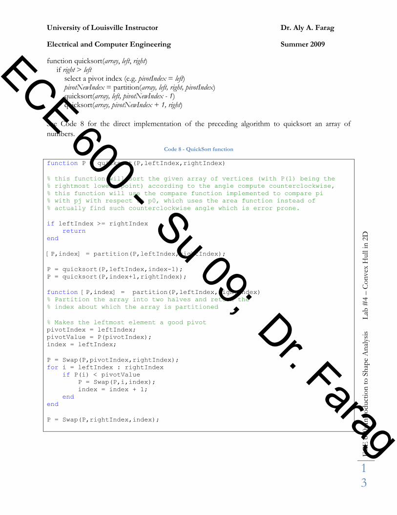
function quicksort(array, left, right) if right > left select a pivot index (e.g. pivotIndex = left) pivotNewIndex = partition(array, left, right, pivotIndex) quicksort(array, left, pivotNewIndex - 1) quicksort(array, pivotNewIndex + 1, right)

See Code 8 for the direct implementation of the preceding algorithm to quicksort an array of

numbers.

Code 8 - QuickSort function

function P = quicksort(P,leftIndex,rightIndex)

% this function will sort the given array of vertices (with P(1) being the

% rightmost lowest point) according to the angle compute counterclockwise,

% this function will use the compare function implemented to compare pi

% with pj with respect to p0, which uses the area function instead of

% actually find such counterclockwise angle which is error prone.

if leftIndex >= rightIndex

return

end

[P,index] = partition(P,leftIndex,rightIndex);

P = quicksort(P,leftIndex,index-1);

P = quicksort(P,index+1,rightIndex);

function [P,index] = partition(P,leftIndex,rightIndex)

% Partition the array into two halves and return the

% index about which the array is partitioned

% Makes the leftmost element a good pivot

pivotIndex = leftIndex;

pivotValue = P(pivotIndex);

index = leftIndex;

P = Swap(P,pivotIndex,rightIndex);

for i = leftIndex : rightIndex

if P(i) < pivotValue

P = Swap(P,i,index);

index = index + 1;

end

end

P = Swap(P,rightIndex,index);




EC

E 6

00: In

tro

duct

ion

to

Sh

ape

An

alys

is L

ab #

4 –

Co

nvex

Hull in

2D

14

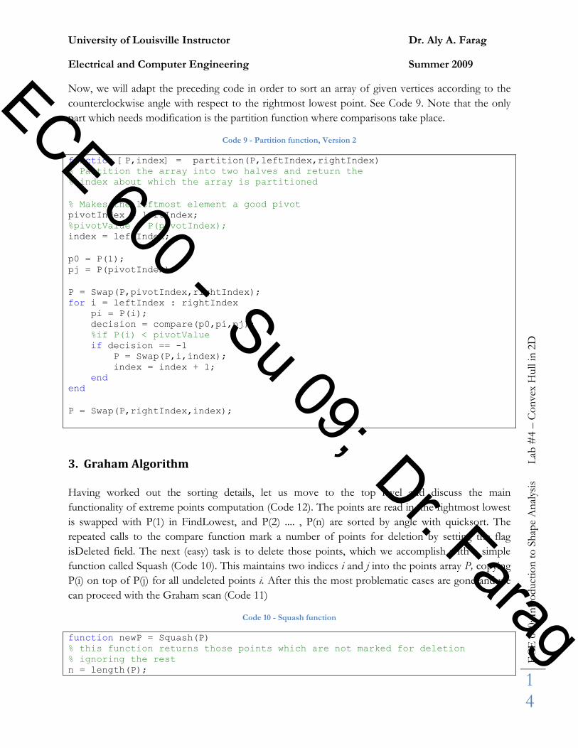
Now, we will adapt the preceding code in order to sort an array of given vertices according to the

counterclockwise angle with respect to the rightmost lowest point. See Code 9. Note that the only

part which needs modification is the partition function where comparisons take place.

Code 9 - Partition function, Version 2

function [P,index] = partition(P,leftIndex,rightIndex)

% Partition the array into two halves and return the

% index about which the array is partitioned

% Makes the leftmost element a good pivot

pivotIndex = leftIndex;

%pivotValue = P(pivotIndex);

index = leftIndex;

p0 = P(1);

pj = P(pivotIndex);

P = Swap(P,pivotIndex,rightIndex);

for i = leftIndex : rightIndex

pi = P(i);

decision = compare(p0,pi,pj);

%if P(i) < pivotValue

if decision == -1

P = Swap(P,i,index);

index = index + 1;

end

end

P = Swap(P,rightIndex,index);

3. Graham Algorithm

Having worked out the sorting details, let us move to the top level and discuss the main

functionality of extreme points computation (Code 12). The points are read in, the rightmost lowest

is swapped with P(1) in FindLowest, and P(2) .... , P(n) are sorted by angle with quicksort. The

repeated calls to the compare function mark a number of points for deletion by setting the flag

isDeleted field. The next (easy) task is to delete those points, which we accomplish with a simple

function called Squash (Code 10). This maintains two indices i and j into the points array P, copying

P(i) on top of P(j) for all undeleted points i. After this the most problematic cases are gone and we

can proceed with the Graham scan (Code 11)

Code 10 - Squash function

function newP = Squash(P)

% this function returns those points which are not marked for deletion

% ignoring the rest

n = length(P);




EC

E 6

00: In

tro

duct

ion

to

Sh

ape

An

alys

is L

ab #

4 –

Co

nvex

Hull in

2D

15

j = 0;

for i = 1 : n

if ~P(i).isDeleted % if not marked for deletion

j = j +1;

newP(j) = P(i);

end

end

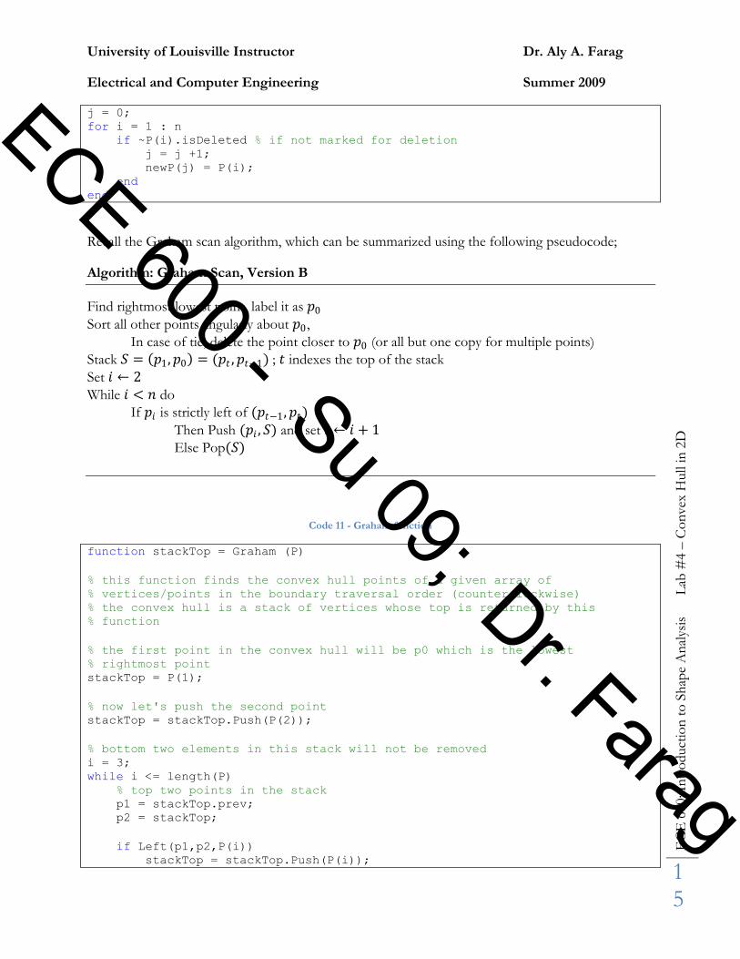
Recall the Graham scan algorithm, which can be summarized using the following pseudocode;

Algorithm: Graham Scan, Version B

Find rightmost lowest point, label it as 𝑝0

Sort all other points angularly about 𝑝0,

In case of tie, delete the point closer to 𝑝0 (or all but one copy for multiple points)

Stack 𝑆 = 𝑝1,𝑝0 = (𝑝𝑡 , 𝑝𝑡−1) ; 𝑡 indexes the top of the stack

Set 𝑖 ← 2

While 𝑖 < 𝑛 do

If 𝑝𝑖 is strictly left of (𝑝𝑡−1, 𝑝𝑡)

Then Push (𝑝𝑖 , 𝑆) and set 𝑖 ← 𝑖 + 1

Else Pop(𝑆)

Code 11 - Graham function

function stackTop = Graham (P)

% this function finds the convex hull points of a given array of

% vertices/points in the boundary traversal order (counterclockwise)

% the convex hull is a stack of vertices whose top is returned by this

% function

% the first point in the convex hull will be p0 which is the lowest

% rightmost point

stackTop = P(1);

% now let's push the second point

stackTop = stackTop.Push(P(2));

% bottom two elements in this stack will not be removed

i = 3;

while i <= length(P)

% top two points in the stack

p1 = stackTop.prev;

p2 = stackTop;

if Left(p1,p2,P(i))

stackTop = stackTop.Push(P(i));




EC

E 6

00: In

tro

duct

ion

to

Sh

ape

An

alys

is L

ab #

4 –

Co

nvex

Hull in

2D

16

i = i + 1;

else

stackTop = stackTop.Pop();

end

end

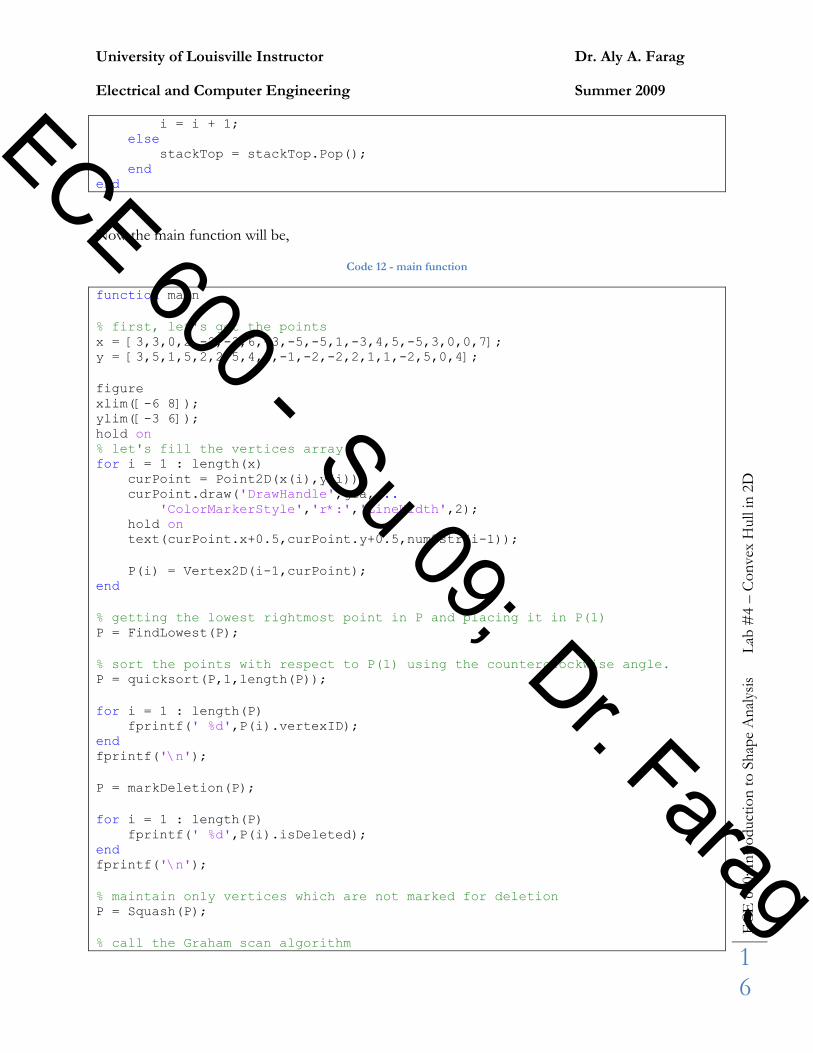
Now the main function will be,

Code 12 - main function

function main

% first, let's get the points

x = [3,3,0,2,-2,-3,6,-3,-5,-5,1,-3,4,5,-5,3,0,0,7];

y = [3,5,1,5,2,2,5,4,2,-1,-2,-2,2,1,1,-2,5,0,4];

figure

xlim([-6 8]);

ylim([-3 6]);

hold on

% let's fill the vertices array

for i = 1 : length(x)

curPoint = Point2D(x(i),y(i));

curPoint.draw('DrawHandle',gca,...

'ColorMarkerStyle','r*:','LineWidth',2);

hold on

text(curPoint.x+0.5,curPoint.y+0.5,num2str(i-1));

P(i) = Vertex2D(i-1,curPoint);

end

% getting the lowest rightmost point in P and placing it in P(1)

P = FindLowest(P);

% sort the points with respect to P(1) using the counterclockwise angle.

P = quicksort(P,1,length(P));


fprintf(' %d',P(i).vertexID);

end

fprintf('\n');

P = markDeletion(P);


fprintf(' %d',P(i).isDeleted);

end

fprintf('\n');

% maintain only vertices which are not marked for deletion

P = Squash(P);

% call the Graham scan algorithm




EC

E 6

00: In

tro

duct

ion

to

Sh

ape

An

alys

is L

ab #

4 –

Co

nvex

Hull in

2D

17

stackTop = Graham(P);

% now let's visualize the outputs

while(1)

curPoint = stackTop.point;

curPoint.draw('DrawHandle',gca,...

'ColorMarkerStyle','b*:','LineWidth',2);

hold on

pause(0.5);

% termination condition

if isempty(stackTop.prev)

break

end


end

Task 1: Examine the preceding code using the given set of points which include all types of collinearities,

then do the following:

(a) Tabulate the points after angular sorting each with its delete flag and vertex ID.

(b) Tabulate the points after apply the Squash function.

(c) Show the stack (with vertexID’s only) and the value of 𝑖 at the top of the while loop.

(d) Visualize the intermediate results (each pop and push) throughout consecutive iterations.

Task 2: Graham Algorithm is mainly used to obtain the extreme points of a given set of points, with some

minor changes in the given code we can obtain all points on the hull’s boundary with boundary traversal

order, in this task you are required to analyze the given code and indicate these minor changes then develop

another version of this code to obtain points on the hull, experiment your modifications using the given set

of points and report any difficulties/special cases encountered during such modification, in particular when

applied on the given set of point.

Task 3: All points collinear. What will the code output if all input points are collinear?

Task 4: Best case. How many iterations of the scan's while loop (in Graham Algorithm version B)

occur if the input points are all already on the hull?

Task 5: Worst case. Construct a set of points for each n that causes the largest number of iterations of

the while loop of the scan (in Graham Algorithm version B).

Task 6: Graham's algorithm has no obvious extension to three dimensions: It depends crucially on

angular sorting, which has no direct counterpart in three dimensions. In the lecture notes we have

discussed the Incremental Algorithm to compute convex hull, your task is to implement this

algorithm using linked lists to represent points on the hull.




EC

E 6

00: In

tro

duct

ion

to

Sh

ape

An

alys

is L

ab #

4 –

Co

nvex

Hull in

2D

18

Task 7: Degenerate tangents. Modify the incremental algorithm as presented to output the correct hull

when a tangent line from p includes an edge of Q. The "correct" hull should not have three collinear

vertices.

Task 8: Collinearities. Modify the incremental algorithm to work with sets of points that may include

three or more collinear points, hint extend task 7.

Task 9: Optimal incremental algorithm. Presort the points by their x coordinate, so that 𝑝 ∉ 𝒬 at each

step. Now try to arrange the search for tangent lines in such a manner that the total work over the

life of the algorithm is O(n). This then provides an O(n logn) algorithm.

Task 10: Write a report to summarize the theoretical background needed for this lab and your experimental

results. Your report should begin with a cover page introducing the project title and group members. It is

important to note that all figure axes should be labeled properly. You are required to submit your MATLAB

codes (fully commented) with a readme file describing your files and how to use them in terms of input and

output.

Good Luck


Documents

ECE 600: Introduction to Shape Analysis Convex Hull … 600/Project...University of Louisville Instructor Dr. Aly A. Farag Electrical and Computer Engineering Summer 2009 ECE 600: