Embed Size (px)
Citation preview
E&CE 710 Wireless Communications Networks
Lecture Notes: #2
Xuemin (Sherman) ShenOffice: EIT 4155Phone: x 32691
Email: [email protected]
2018/2/28 1ECE710 Wireless Communications Networks
3. Traffic characterization
• Communication Networks are expected to carry a
variety of traffic types in integrated fashion.
• With traffic characterization, the statistical resource requirements, in terms of link and buffer capacities can be obtained.
• With traffic characterization, the queue wait times, blocking
probabilities, etc. can be determined.
2018/2/28 2ECE710 Wireless Communications Networks

Type of Traffic (M. Schwartz, 1996)• The importance of the traffic characterization
Ex. 3.1: 1 ATM cell = 53×8 = 424bits.
2018/2/28 3ECE710 Wireless Communications Networks
Cells are delivered to the network in FIFO order.B— buffer size E(W)— average waiting time S— service rate
Q: Determine the buffer size B required, in units of cells, and theaverage time E(W) a typical cell must wait.

Type of Traffic• Solution:
(1) The utilization factor ,B= 4 is suffice to handle
the cell arrivals. With nD/D/1 queue, Loss
probability = 0.
(2) with M/D/1, = 35.6 , B= 249 with loss probability= 10−9.
2018/2/28 4ECE710 Wireless Communications Networks
• Traffic characterization is not only important when designing buffers, but also in studying admission, access, and flow control.
• Three types of traffic:Voice: Continuous (Constant ) bit rate;Video: Variable bit rate;Bursty data;

Type of Traffic
5
Voice communication: interactive communication
Video: variable length of video frames
Bob speaks
Dave speaks
Frame 1 Frame 2 Frame 3 Frame 4
Video = moving picture (30 pics/s)
picture (frame) size depends on motion in pictures

Type of Traffic
2018/2/28 6ECE710 Wireless Communications Networks
Voice (audio) — real time traffic, in which bits are periodically generated.Video (Compression) — real time trafficImages, bursty data — non real-time traffic (Available bit rate)Images, bursty data (Unspecified bit rate)
Objectives: Characterize each traffic; using the models obtained to determine buffer occupancy statistics queue wait times, and blocking probabilities.
Voice service requires a peak cell rate traffic descriptor;Video service requires a peak cell rate, a average cell rate and an intrinsic burst tolerance traffic descriptor; ABR service requires a peak cell rate and a minimum cell rate traffic descriptor;UBR or “best-effort” service has no pre-specified traffic descriptor

Packet Voice Modeling
2018/2/28 7ECE710 Wireless Communications Networks
A single voice source can be well presented by a two-state process (on - off model).
— the rate of transition out of the silent state;
— the rate of transition out of talk spurt.
The speaker activity factor

Packet Voice Modeling
2018/2/28 8ECE710 Wireless Communications Networks
Suppose there are voice sources; their initiations of calls areindependent of each other.
It is clear that the parameter must satisfy the low bound inequality
i.e., the utilization factor
The probability of active voices (out of N) follows binomial distribution
Packet Voice Modeling
2018/2/28 9ECE710 Wireless Communications Networks
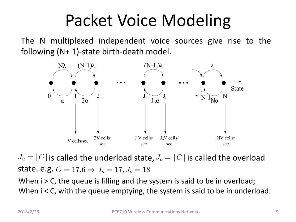
The N multiplexed independent voice sources give rise to thefollowing (N+ 1)-state birth-death model.
is called the underload state, is called the overload state. e.g.
When i > C, the queue is filling and the system is said to be in overload;When i < C, with the queue emptying, the system is said to be in underload.

Packet Voice Modeling
2018/2/28 10ECE710 Wireless Communications Networks
By setting up the balance equations at each state
Let , then
where
Q: how to calculate the performance and design parameters such as delay and loss statistics and buffer size required?

Fluid Source Modeling of Packet Voice
2018/2/28 11ECE710 Wireless Communications Networks
Assume N sources each generating cells/sec during a talkspurt.The service capacity is cells/sec. When N and are very largerelative to the small cell size, it can be superimposed upon/on thecell arriving process during a talkspurt as one information unitflowing into the system. Thus the discreteness of the cell is removed(like a continuous flow of fluid).
Let be the average length of talk spurt and define the number of cells arriving during a talk spurt as a “unit of information”. The service capacity is normalized into by .

Fluid Source Modeling of Packet Voice
2018/2/28 12ECE710 Wireless Communications Networks
X (continuous RV) — buffer occupancyThe units of x are defined to be the number of unit of informationarriving during a talk spurt.Let be the state of the buffer in units of cells.
, Then,
Find the probability distribution of x (which can be converted to buffer cell distribution).

Fluid Source Modeling of Packet Voice
2018/2/28 13ECE710 Wireless Communications Networks
Assume an exponentially distributed on-off process for each source,and there are sources in talk spurt.
Define as the cumulative probability distribution of x, then,
P{one source moves from “off” to “on” during system isin state at }
P{one source moves from “on” to “off” during system isin state at }
P{no source changes state during system is in state at }

Fluid Source Modeling of Packet Voice
2018/2/28 14ECE710 Wireless Communications Networks
Add both side of the equation by and divide by
Letting , we get
Under steady state condition , , we have
Here , with
( is the net gain of the buffer in a small period to )

Fluid Source Modeling of Packet Voice
2018/2/28 15ECE710 Wireless Communications Networks
The solution of this set of equations is readily obtained by firstwriting them out in their complete form:
Define , then
With an (N+1)×(N+1) diagonal matrix defined as
and an (N+1)×(N+ 1) matrix defined as follows:

Fluid Source Modeling of Packet Voice
2018/2/28 16ECE710 Wireless Communications Networks
Multiplying by on both sides, we get
The general solution of the above equation is
with the i-th eigenvalue, the corresponding eigenvector given as the solution to the eigenvector equation
and the set of undetermined coefficients.
Since , is a diagonal matrix, then

Fluid Source Modeling of Packet Voice
2018/2/28 17ECE710 Wireless Communications Networks
Let ,
with the j-th component of eigenvector

Fluid Source Modeling of Packet Voice
2018/2/28 18ECE710 Wireless Communications Networks
• Procedure of finding
and are the eigenvalues and eigenvectors of the matrix . They can be calculated by using Matlab.
Since (for the infinite-buffer case)
Let , we get . By setting ,
It has been proved that the number of negative eigenvalues is which is also the number values of that have to be found.

Fluid Source Modeling of Packet Voice
2018/2/28 19ECE710 Wireless Communications Networks
Since , for (When the system is in overload state, theprobability that the buffer is empty is zero), we have
e.g., . (5 overload states)
The probability for the buffer occupancy to be less than or equal to is
( )

Fluid Source Modeling of Packet Voice
2018/2/28 20ECE710 Wireless Communications Networks
The complementary probability cumulative distribution function
is also called the survivor function. It can be used to find the buffer size required for a given loss probability.
The buffer occupancy will exceed cells is given by
• Approximate Approach:D. Anick, et al. “Stochastic Theory of a Data Handling System withMultiple Sources”, Bell System tech. J. Vol. 61, No. 8, pp. 1871-
1894, 1982.Since the probability distribution is given by the sum of negativeexponentials, the exponential with the smallest negative eigenvaluewill dominate.
Fluid Source Modeling of Packet Voice
2018/2/28 21ECE710 Wireless Communications Networks
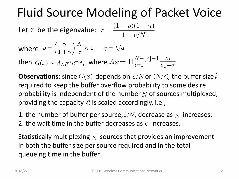
Let be the eigenvalue:
where
then where
Observations: since depends on or , the buffer size required to keep the buffer overflow probability to some desire probability is independent of the number of sources multiplexed, providing the capacity is scaled accordingly, i.e.,
Statistically multiplexing sources that provides an improvement in both the buffer size per source required and in the total queueing time in the buffer.
1. the number of buffer per source, , decrease as increases;2. the wait time in the buffer decreases as increases.

Fluid Source Modeling of Packet Voice
2018/2/28 22ECE710 Wireless Communications Networks
Example 3.2 Consider the special case of voice sources, sec and
sec .a) Find for the two cases and .
Indicate all three value on the (N+1)-state diagram.
Solution: Using , we have
N+ 1 state diagram:

Fluid Source Modeling of Packet Voice
2018/2/28 23ECE710 Wireless Communications Networks
b) Find and compare the eigenvalues of for the two cases (and ).
Solution:
for eigenvalues:
Note that: i) one eigenvalue is 0 in both cases; ii) the number of negative eigenvalues equals to the number of overload states.

Fluid Source Modeling of Packet Voice
2018/2/28 24ECE710 Wireless Communications Networks
c). Find the eigenvectors for the two cases
(i)
(ii)
Note: both parts (b) and (c) are solved using MATLAB.
d). Calculate and plot , where cells/sec.
Thus,
(ii) it can be calculated that

Fluid Source Modeling of Packet Voice
2018/2/28 25ECE710 Wireless Communications Networks
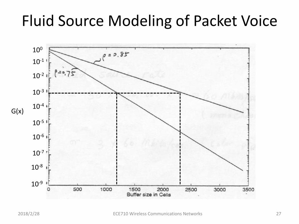
f). How large a buffer size is needed to have the buffer overflow probability equal to 10−2 for each of the two cases? Repeat for an overflow probability of 10−3.
• Observations:1. For the different overflow probability, the required buffer size
increases for lower overflow probability (with the same ).
2. As the traffic intensity increases, the required buffer size to meet the overflow probability constraint also increases.
Solution: From the plot of G(x), we get the buffer size in cells for overflow probability of 10−2 and 10−3.

Fluid Source Modeling of Packet Voice
2018/2/28 26ECE710 Wireless Communications Networks
Fluid Source Modeling of Packet Voice
2018/2/28 27ECE710 Wireless Communications Networks
G(x)
100
10-1
10-2
10-3
10-4
10-5
10-6
10-7
10-8
10-9
Fluid source modeling of video traffic
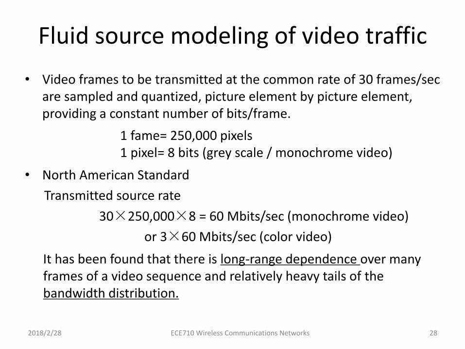
• Video frames to be transmitted at the common rate of 30 frames/sec are sampled and quantized, picture element by picture element, providing a constant number of bits/frame.
• North American Standard
Transmitted source rate
30×250,000×8 = 60 Mbits/sec (monochrome video)
or 3×60 Mbits/sec (color video)
2018/2/28 ECE710 Wireless Communications Networks 28
1 fame= 250,000 pixels 1 pixel= 8 bits (grey scale / monochrome video)
It has been found that there is long-range dependence over many frames of a video sequence and relatively heavy tails of the bandwidth distribution.

Fluid source modeling of video traffic
2018/2/28 ECE710 Wireless Communications Networks 29
Compression (using a variety of coding techniques) can obtain0.5bit/pixel, i.e., source rate= 30×250,000×0.5 = 3.75Mbits/sec .
The compressed video traffic is with variable bit rate. (frame byframe) If independent video sources are multiplexed together,the average bit rate per second, and the autocovariancefunction are used to describe each source.
(continuous time)
(discrete time)
is the frame number, represents a frame n units (frames)away.

Fluid source modeling of video traffic
2018/2/28 ECE710 Wireless Communications Networks 30
Statistical multiplexer, N video sources (M >> N)

Fluid source modeling of video traffic
2018/2/28 ECE710 Wireless Communications Networks 31
is the multiplexed (time varying) rate. Actually changes at frame intervals (30 frames/sec) rather than continuously. The time-varying bit rate has been quantized to have the values 0, A, 2A, ···, mA bits/pixel only. The original N sources multiplexed model can be represented by an (m+ 1)-state Markov chain with state-dependent transition rates.
Markov chain representation, equivalent process

Fluid source modeling of video traffic
2018/2/28 ECE710 Wireless Communications Networks 32
Question: How does one choose the three minisource model parameter and ?
Answer: Since
then,
The parameter represents the variance of video source , while is used to represent the variance of composite signal.

Fluid source modeling of video traffic
2018/2/28 ECE710 Wireless Communications Networks 33
Proof:
Note that for wide-sense stationary process,
autocorrelation

Fluid source modeling of video traffic
2018/2/28 ECE710 Wireless Communications Networks 34
Special case: independent sources with identical moments
It can be proved that the autocovariance function of the two-state minisource model is given by
Let be probability the minisource is in the ”on” state,is in the ”off” state.
Note: the two-state covariance of the two-state minisource exhibitsthe desired exponential behavior.

Fluid source modeling of video traffic
2018/2/28 ECE710 Wireless Communications Networks 35
For stationary 2-state Markov Chain:
Define

Fluid source modeling of video traffic
2018/2/28 ECE710 Wireless Communications Networks 36
where

Fluid source modeling of video traffic
2018/2/28 ECE710 Wireless Communications Networks 37

Fluid source modeling of video traffic
2018/2/28 ECE710 Wireless Communications Networks 38
Since
Fluid source modeling of video traffic
2018/2/28 ECE710 Wireless Communications Networks 39
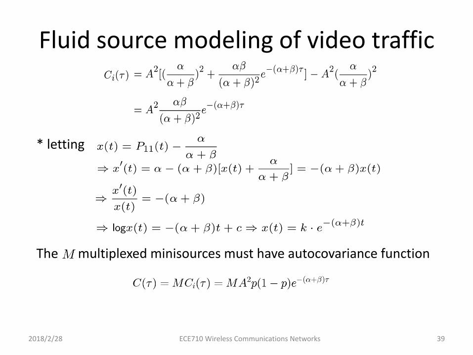
* letting
The multiplexed minisources must have autocovariance function

Fluid source modeling of video traffic
2018/2/28 ECE710 Wireless Communications Networks 40
The average number of minisources ”on” is just , the average bit rate of the equivalent minisource model is .
If we can measure from video traffic (data) that
then,

Fluid source modeling of video traffic
2018/2/28 ECE710 Wireless Communications Networks 41
We obtain
If , we have
With the composite minisource model for the video determined,one can use this video source model and the fluid-flow approachto calculate (to design the access buffer) to provide a specifiedprobability of cell loss, and to determine the resultant video accessdelay.
Define
where

Fluid source modeling of video traffic
2018/2/28 ECE710 Wireless Communications Networks 42
Following the same analysis procedure as to voice model, we get the following equation
is the net gain of the buffer in a small timeperiod to
Re-arrange, let and use the steady state conditionwe get

Fluid source modeling of video traffic
2018/2/28 ECE710 Wireless Communications Networks 43
Rewriting the above equation
Define
we have
where
Fluid source modeling of video traffic
2018/2/28 ECE710 Wireless Communications Networks 44
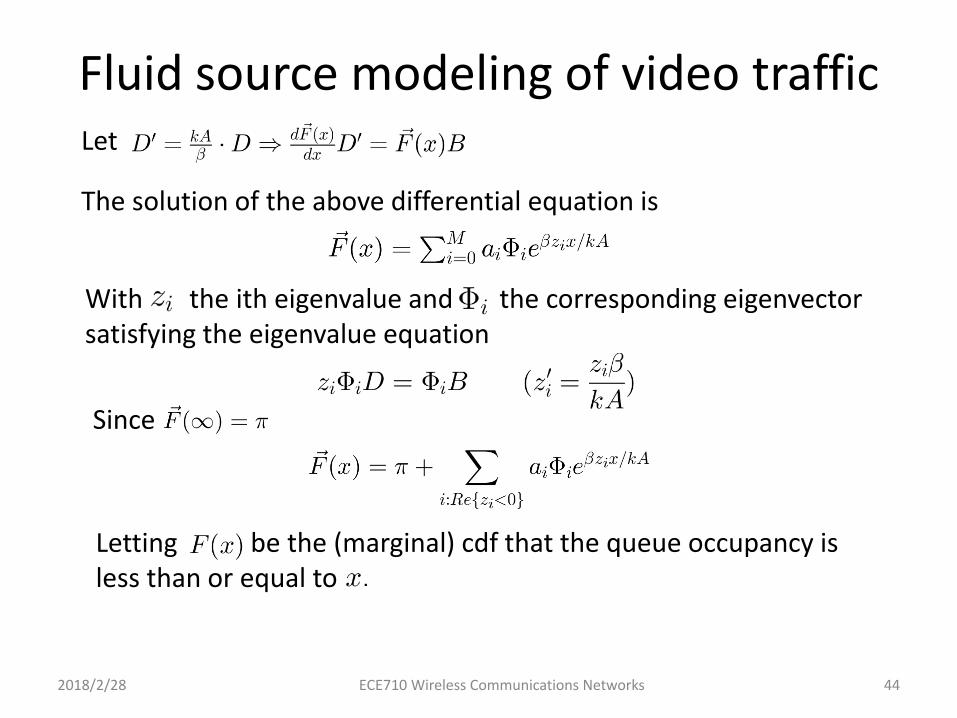
Let
The solution of the above differential equation is
With the ith eigenvalue and the corresponding eigenvector satisfying the eigenvalue equation
Since
Letting be the (marginal) cdf that the queue occupancy is less than or equal to

Fluid source modeling of video traffic
2018/2/28 ECE710 Wireless Communications Networks 45
The solution of the above differential equation is
The survivor function (the probability the queue occupancyis greater than x) is given by
Note that the overload states are those for which the queue istending to fill. For these states, we must have ; i.e., thebuffer cannot be empty. When or (overloadstate), the number of overload states is which is thenumber of negative eigenvalues.

Fluid source modeling of video traffic
2018/2/28 ECE710 Wireless Communications Networks 46
Setting for the overload states, we can find
Approximate approach:
where and
(approximating the survivor function by the dominant (asymptotic)eigenvalue term only).
Example 2.3(Maglaris, B., et. al., ”Performance Models of Statistical Multiplexingin Packet Video Communications”, IEEE Trans. on Commun., vol. 36,No. 7. pp. 834-844, 1988)
Let video source be approximated by minisources.The average source bit rate is

Fluid source modeling of video traffic
2018/2/28 ECE710 Wireless Communications Networks 47
The transmission capacity
The utilization is then 3.9/4.875 = 0.8, we get:
Approximating the survivor function by the dominant eigenvalue term only,
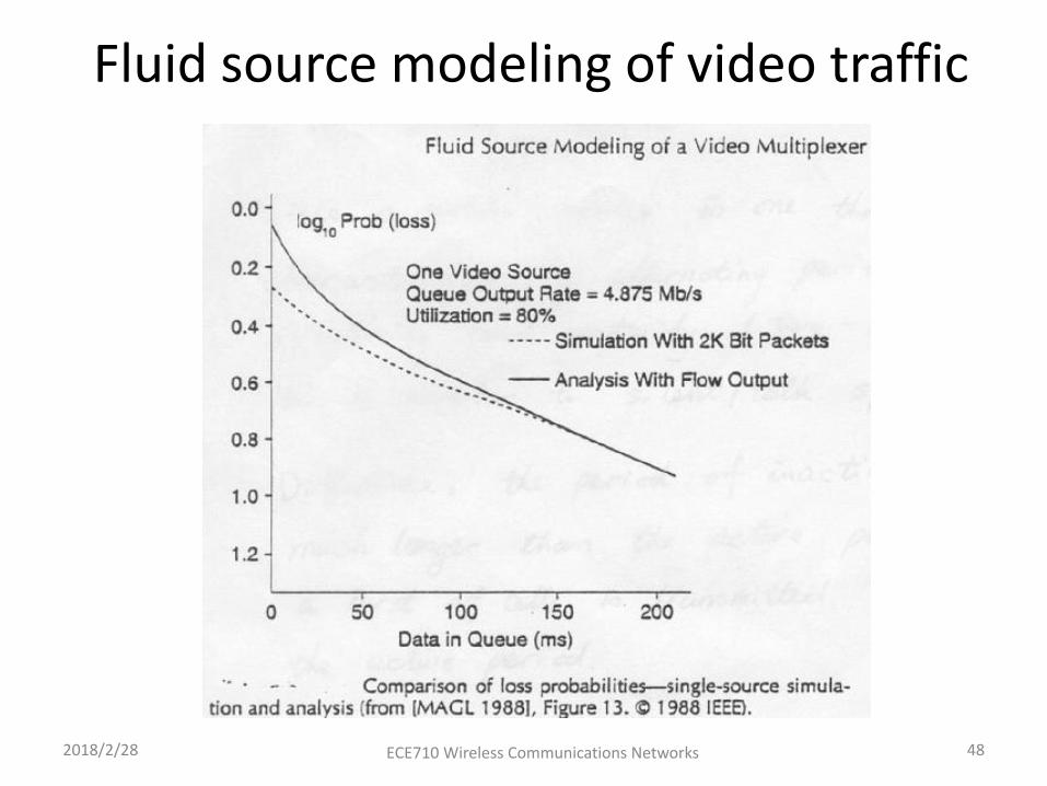
Fluid source modeling of video traffic
2018/2/28 ECE710 Wireless Communications Networks 48

Fluid source modeling of video traffic
2018/2/28 ECE710 Wireless Communications Networks 49

Bursty traffic model
2018/2/28 ECE710 Wireless Communications Networks 50
Since a bursty source is one that is characterized by alternatingperiods of inactivity and activity (two-state model), this is similar tosilent/talk spurt of voice.
Difference: the period of inactivity is much longer than the activeperiod; a burst of cells is transmitted during the active period.
Two-state, on-off model for bursty traffic source
If the active period is much shorter than the inactivity period, aPoisson arrival process (bulk arrival process) can be used to modelbursty traffic.


![d200403-4-01.ppt [호환 모드] - CHERIC · 2013-12-19 · Table 3. Sample buffer와running buffer. Running buffer [Laemmli Tray Buffer] Sample buffer [4X Laemmli Tray Buffer] Tris(1.5M)](https://img.pdfslide.net/doc/110x75/5f9066bc067eff27fe2ab824/d200403-4-01ppt-eeoe-cheric-2013-12-19-table-3-sample-bufferrunning.jpg)