ECE201 Lect-11 1

Nodal and Loop Analysis cont’d (8.8)

Dr. Holbert

March 1, 2006

ECE201 Lect-11 2

Advantages of Nodal Analysis

• Solves directly for node voltages.

• Current sources are easy.

• Voltage sources are either very easy or somewhat difficult.

• Works best for circuits with few nodes.

• Works for any circuit.

ECE201 Lect-11 3

Advantages of Loop Analysis

• Solves directly for some currents.

• Voltage sources are easy.

• Current sources are either very easy or somewhat difficult.

• Works best for circuits with few loops.

ECE201 Lect-11 4

Disadvantages of Loop Analysis

• Some currents must be computed from loop currents.

• Does not work with non-planar circuits.

• Choosing the supermesh may be difficult.

• FYI: PSpice uses a nodal analysis approach

ECE201 Lect-11 5

Where We Are

• Nodal analysis is a technique that allows us to analyze more complicated circuits than those in Chapter 2.

• We have developed nodal analysis for circuits with independent current sources.

• We now look at circuits with dependent sources and with voltage sources.

ECE201 Lect-11 6

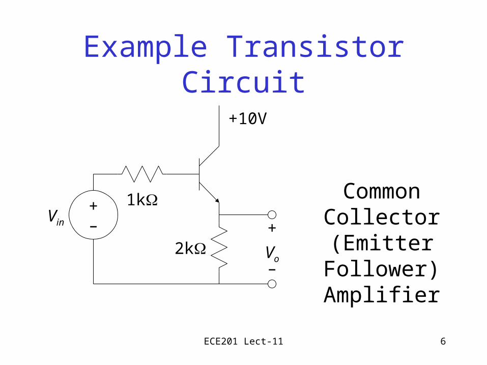
Example Transistor Circuit

1k+–

Vin

2k

+10V

+

–Vo

Common Collector (Emitter Follower)

Amplifier

ECE201 Lect-11 7

Why an Emitter Follower Amplifier?

• The output voltage is almost the same as the input voltage (for small signals, at least).

• To a circuit connected to the input, the EF amplifier looks like a 180k resistor.

• To a circuit connected to the output, the EF amplifier looks like a voltage source connected to a 10 resistor.

ECE201 Lect-11 8

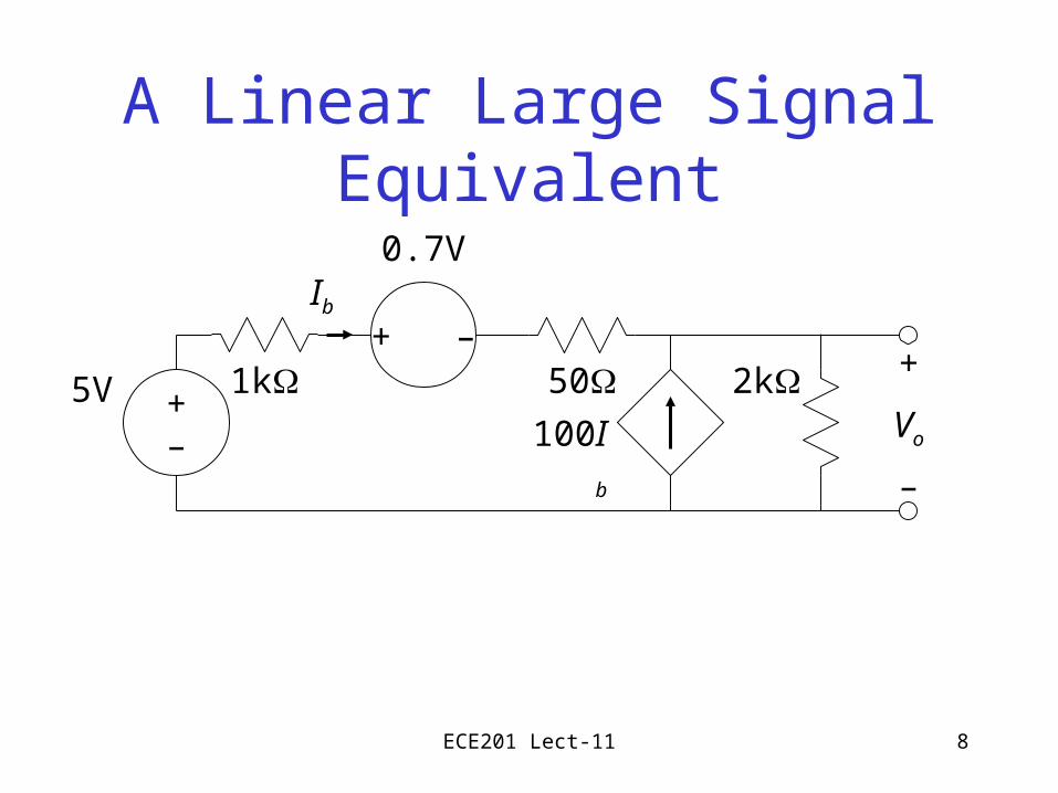
A Linear Large Signal Equivalent

5V100Ib

+

–

Vo

50

Ib

2k1k+–

+ –

0.7V

ECE201 Lect-11 9

Steps of Nodal Analysis

1. Choose a reference node.

2. Assign node voltages to the other nodes.

3. Apply KCL to each node other than the reference node; express currents in terms of node voltages.

4. Solve the resulting system of linear equations.

ECE201 Lect-11 10

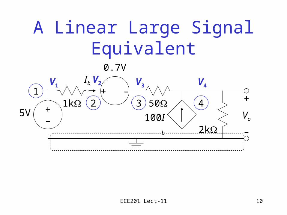
A Linear Large Signal Equivalent

5V 100Ib

+

–

Vo

50

Ib

2k

1k

0.7V

12 3 4

V1 V2 V3 V4

+–

+ –

ECE201 Lect-11 11

Steps of Nodal Analysis

1. Choose a reference node.

2. Assign node voltages to the other nodes.

3. Apply KCL to each node other than the reference node; express currents in terms of node voltages.

4. Solve the resulting system of linear equations.

ECE201 Lect-11 12

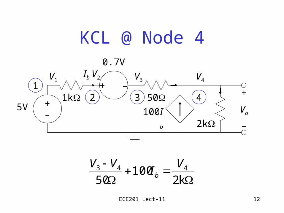
KCL @ Node 4

k2100

50443 V

IVV

b

100Ib

+

–

Vo

50

Ib

2k

1k+–

0.7V

12 3 4

V1V2 V3 V4

5V

+ –

ECE201 Lect-11 13

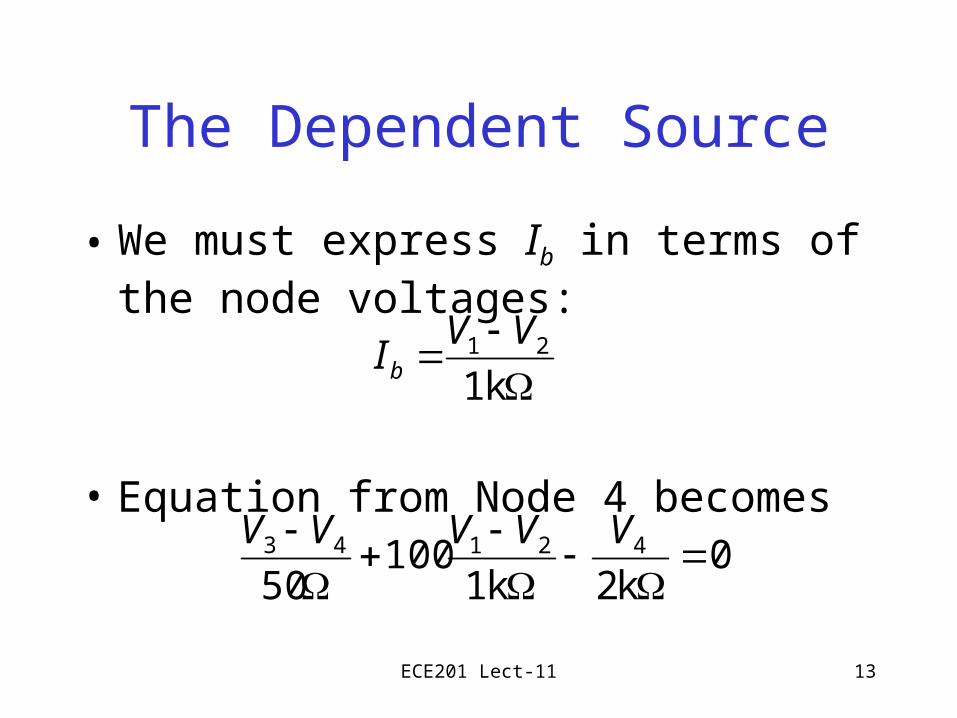
The Dependent Source

• We must express Ib in terms of the node voltages:

• Equation from Node 4 becomes

k1

21 VVIb

0k2k1

10050

42143

VVVVV

ECE201 Lect-11 14

How to Proceed?

• The 0.7V voltage supply makes it impossible to apply KCL to nodes 2 and 3, since we don’t know what current is passing through the supply.

• We do know that

V2 - V3 = 0.7V

ECE201 Lect-11 15

100Ib

+

–

Vo

50

Ib

2k

1k

0.7V

14

V1V2 V3 V4

+–

+ –

ECE201 Lect-11 16

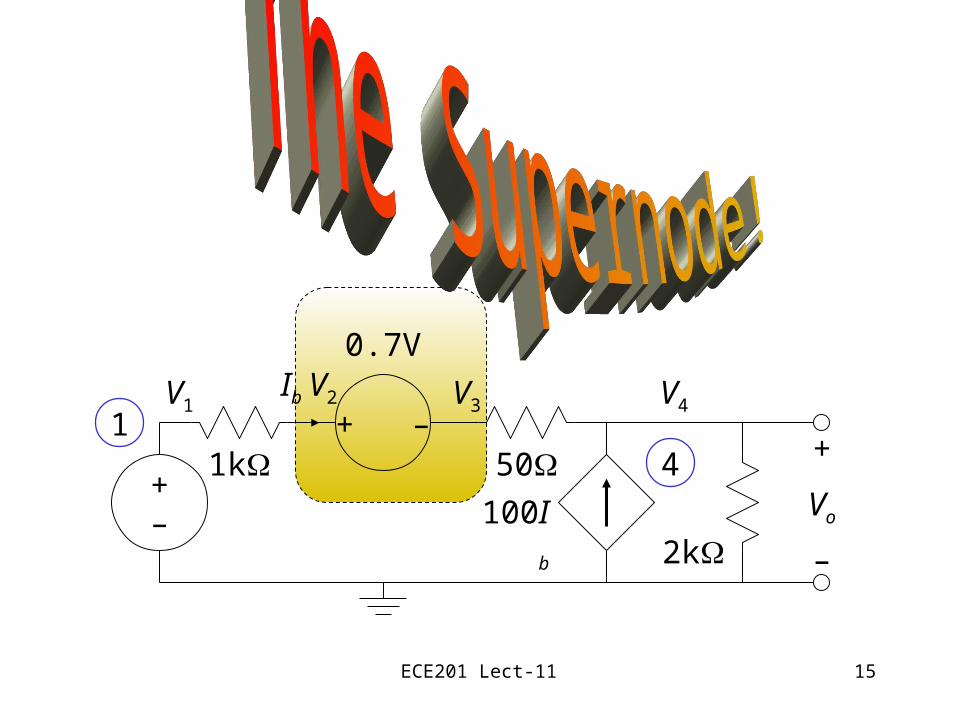
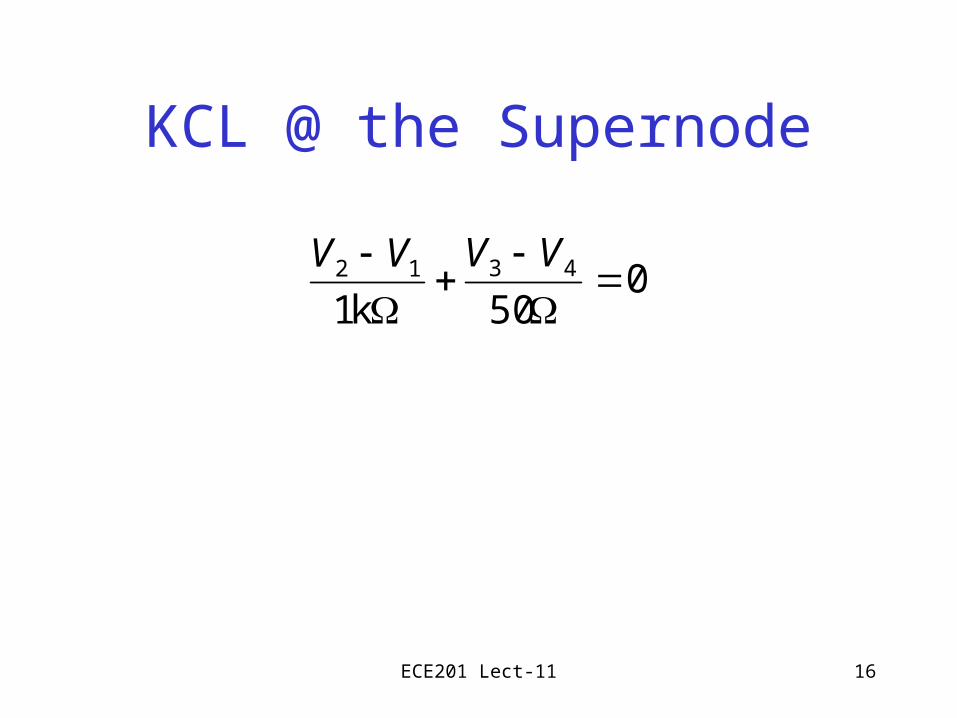
KCL @ the Supernode

050k1

4312

VVVV

ECE201 Lect-11 17

Another Analysis Example

• We will analyze a possible implementation of an AM Radio IF amplifier. (Actually, this would be one of four stages in the IF amplifier.)

• We will solve for output voltages using nodal (and eventually) mesh analysis.

• This circuit is a bandpass filter with center frequency 455kHz and bandwidth 40kHz.

ECE201 Lect-11 18

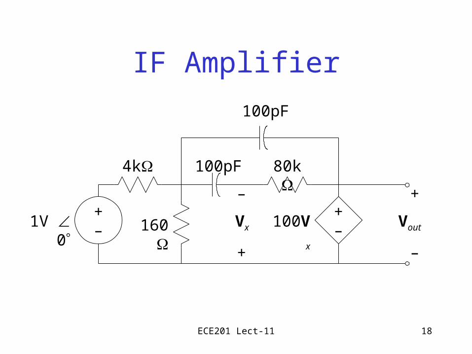
IF Amplifier

4k

1V 0

+

–

Vout

100pF

160

100pF

80k

–

+

Vx 100Vx

+–

+–

ECE201 Lect-11 19

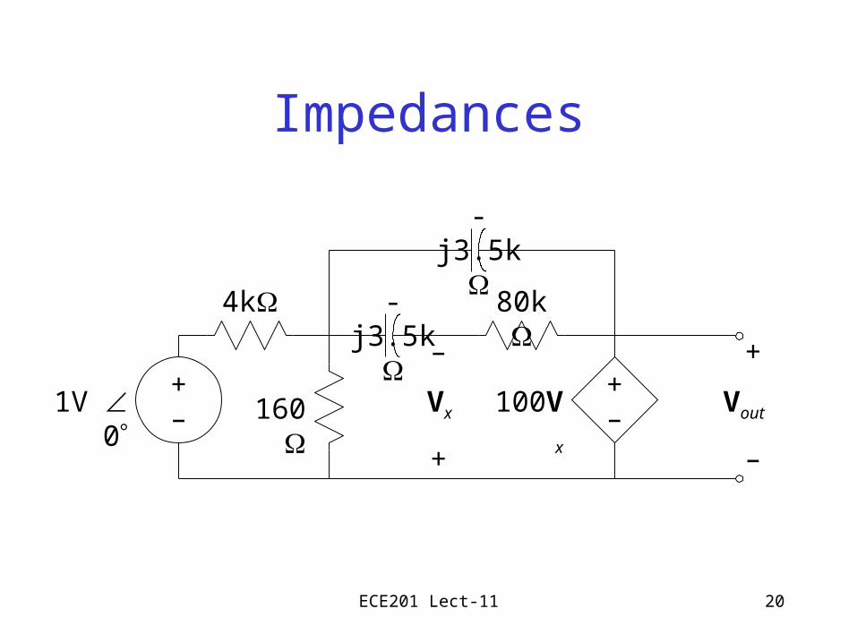
Nodal AC Analysis

• Use AC steady-state analysis.

• Start with a frequency of =2 455,000.

ECE201 Lect-11 20

Impedances

4k

1V 0

+

–

Vout160

80k

–

+

Vx 100Vx

-j3.5k

-j3.5k

+–

+–

ECE201 Lect-11 21

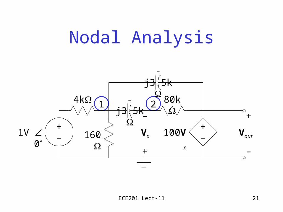
Nodal Analysis

1 24k

1V 0

+

–

Vout160

80k

–

+

Vx 100Vx

-j3.5k

-j3.5k

+–

+–

ECE201 Lect-11 22

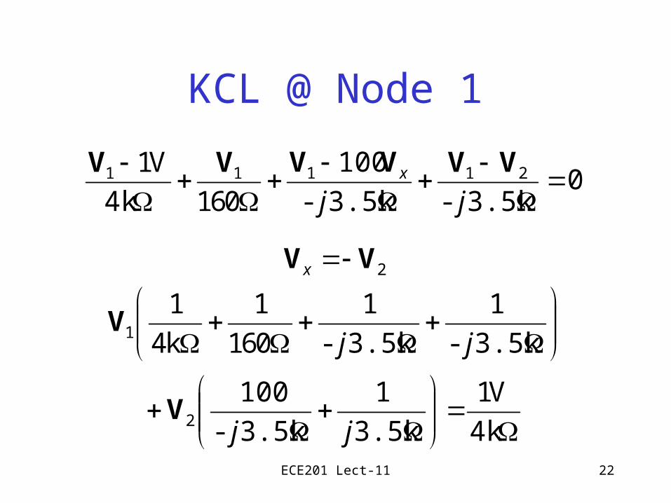
KCL @ Node 1

03.5k-3.5k-

100

0614k

V1 21111

jj

x VVVVVV

4k

V1

3.5k

1

3.5k-

100

3.5k-

1

3.5k-

1

061

1

k4

1

2

1

jj

jj

V

V

2VV x

ECE201 Lect-11 23

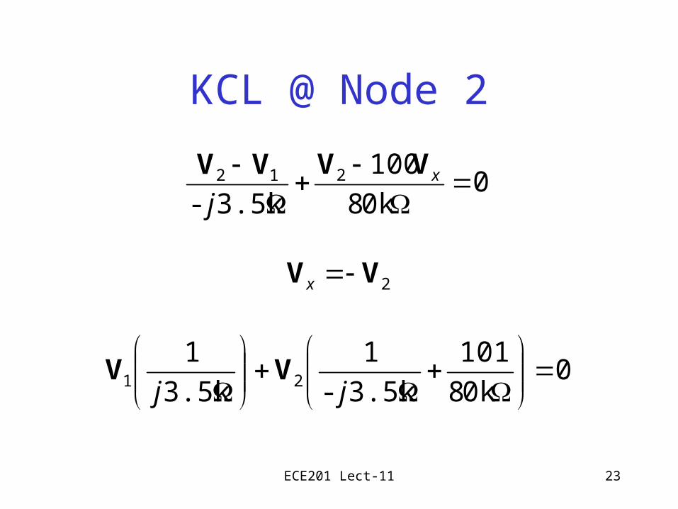
KCL @ Node 2

00k8

100

3.5k-212

x

j

VVVV

00k8

101

3.5k-

1

3.5k

121

jj

VV

2VV x

ECE201 Lect-11 24

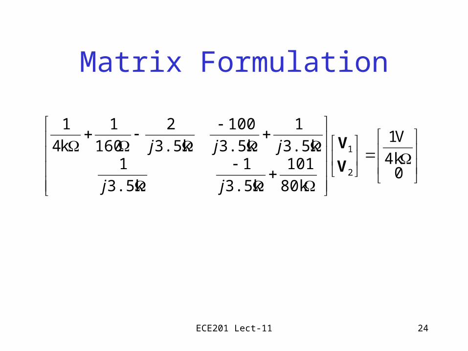
04k

V1

80k

101

3.5k

1

3.5k

13.5k

1

3.5k

100

3.5k

2

160

1

k4

1

2

1

V

V

jj

jjj

Matrix Formulation

ECE201 Lect-11 25

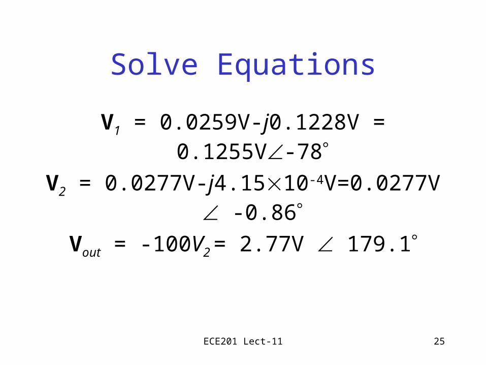
Solve Equations

V1 = 0.0259V-j0.1228V = 0.1255V-78

V2 = 0.0277V-j4.1510-4V=0.0277V -0.86

Vout = -100V2 = 2.77V 179.1

ECE201 Lect-11 26

Class Examples

• Learning Extension E3.6

• Learning Extension E8.13

• Learning Extension E8.14(a)