Embed Size (px)
Citation preview

ECE6604
PERSONAL & MOBILE COMMUNICATIONS
GORDON L. STUBER
School of Electrical and Computer EngineeringGeorgia Institute of TechnologyAtlanta, Georgia, 30332-0250
Ph: (404) 894-2923Fax: (404) 894-7883
E-mail: [email protected]: http://www.ece.gatech.edu/users/stuber/6604
1

COURSE OBJECTIVES
• The course treats the underlying principles of mobile communications thatare applicable to a wide variety of wireless systems and standards.
– Focus is on the physical layer (PHY), medium access control layer(MAC), and connection layer.
– Consider elements of digital baseband processing as opposed to analogradio frequency (RF) processing.
• Mathematical modeling, statistical characterization and simulation of wire-less channels, signals, noise and interference.
• Design of digital waveforms and associated receiver structures for recov-ering channel corrupted message waveforms.
– Single-carrier and multi-carrier signaling schemes and their performanceanalysis on wireless channels.
– Methods for mitigating wireless channel impairments and co-channelinterference.
• Architectures and deployment of wireless systems, including link budgetand frequency planning.
2

TOPICAL OUTLINE
1. INTRODUCTION TO CELLULAR RADIO SYSTEMS
2. MULTIPATH-FADING CHANNEL MODELLING AND SIMULATION
3. SHADOWING AND PATH LOSS
4. CO-CHANNEL INTERFERENCE AND OUTAGE
5. SINGLE- AND MULTI-CARRIER MODULATION TECHNIQUESAND THEIR POWER SPECTRUM
6. BASIC DIGITAL SIGNALING ON FLAT FADING CHANNELS
7. MULTI-ANTENNA TECHNIQUES
8. MULTI-CARRIER TECHNIQUES
3
ECE6604
PERSONAL & MOBILE COMMUNICATIONS
Week 1
Introduction,
Path Loss, Co-channel Interference
4
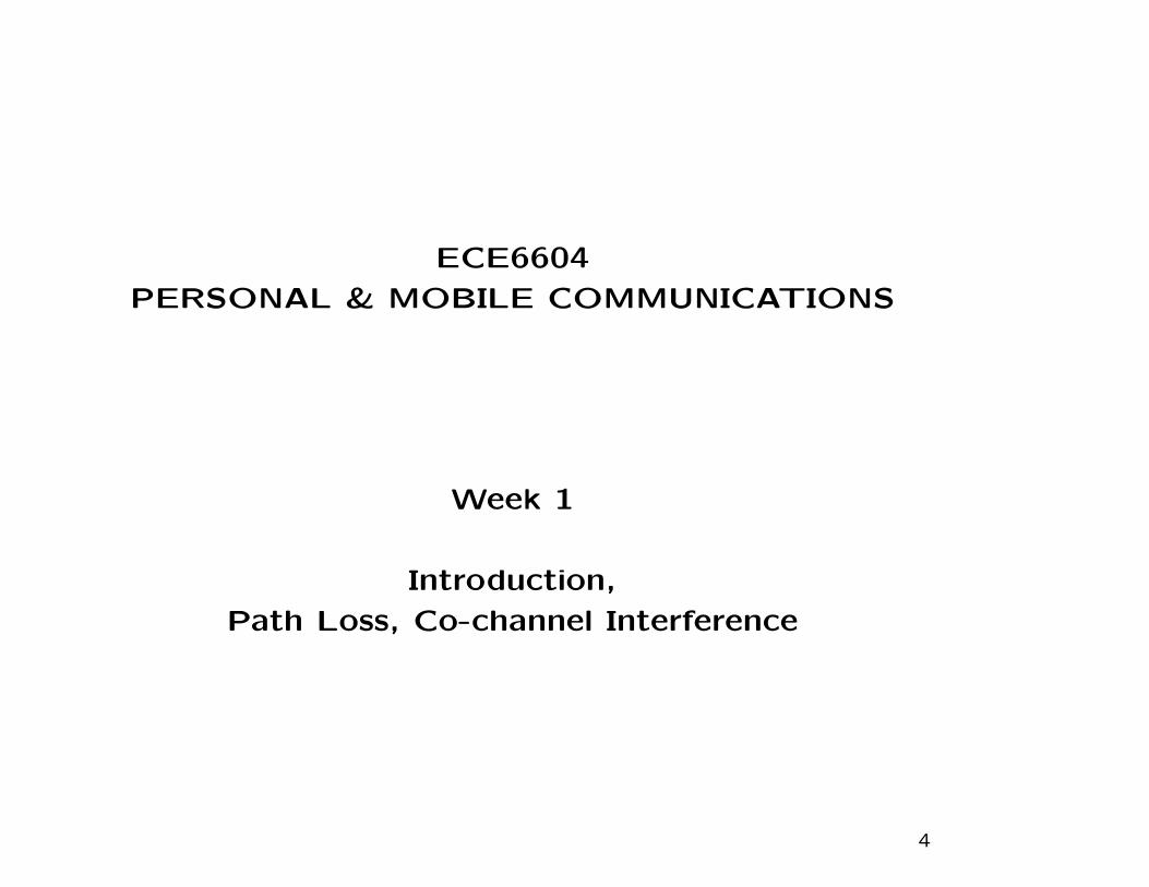
CELLULAR CONCEPT
• Base stations (BSs) transmit to and receive from mobile stations (MSs)using assigned licensed spectrum.
• Multiple BSs use the same spectrum (frequency reuse).
• The service area of each BS is called a “cell.”
• Each MS is typically served by the “closest” BSs.
• Handoffs or handovers occur when MSs move from one cell to the next.
5

CELLULAR FREQUENCIES
Cellular frequencies (USA):
700MHz: 698-806 (3G, 4G, MediaFLO (defunct), DVB-H)GSM800: 806-824, 851–869 (SMR iDEN, CDMA (future), LTE (future))GSM850: 824-849, 869-894 (GSM, IS-95 (CDMA), 3G)GSM1900 or PCS: 1,850-1,910, 1,930-1,990 (GSM, IS-95 (CDMA), 3G, 4G)AWS: 1,710-1,755, 2,110–2,155 (3G, 4G)BRS/EBS: 2,496-2,690 (4G)600MHz: 84 MHz, 10 MHz unlicensed (incentive auction)
6

Cellular Technologies
• 0G: Briefcase-size mobile radio telephones (1970s)
• 1G: Analog cellular telephony (1980s)
• 2G: Digital cellular telephony (1990s)
• 3G: High-speed digital cellular telephony, including video telephony(2000s)
• 4G: All-IP-based anytime, anywhere voice, data, and multimediatelephony at faster data rates than 3G (2010s)
• 5G: Gbps, low latency, wireless based on mm-wave small cell tech-nology, massive MIMO, heterogeneous networks (2020s).
7

0G and 1G Cellular
• 1979 — Nippon Telephone and Telegraph (NTT) introduces thefirst cellular system in Japan.
• 1981 — Nordic Mobile Telephone (NMT) 900 system introduced byEricsson Radio Systems AB and deployed in Scandinavia.
• 1984 — Advanced Mobile Telephone Service (AMPS) introducedby AT&T in North America.
8
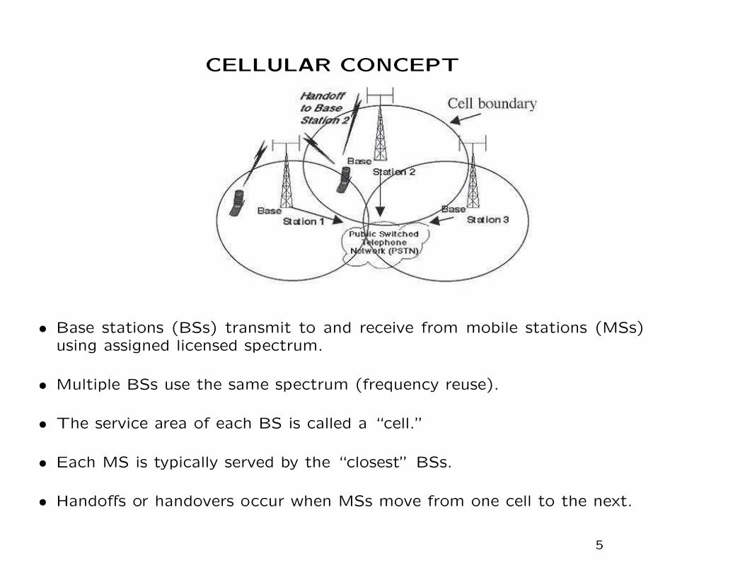
2G Cellular
• 1987 — Europe produces very first agreed GSM Technical Specifi-cation
• 1990 — Interim Standard IS-54 (USDC) standardized by TIA.
• 1991 — Japanese Ministry of Posts and Telecommunications stan-dardizes Personal Digital Cellular (PDC)
• 1993 — Interim Standard IS-95A (CDMA) standardized by TIA.
• 1994 — Interim Standard IS-136 standardized by TIA.
• 1998 — IS-95B standardized by TIA.
• 1998 — GSM Phase 2+ (GPRS) standardized by ETSI.
9

3G Cellular
• 2000 — South-Korean Telecom (SKT) launches cdma2000-1X net-work (DL/UL: 153 kbps)
• 2001 — NTT DoCoMo deploys commercial UMTS network in Japan
• 2002 — cdma2000 1xEV-DO (UL: 153 kbps, DL: 2.4 Mb/s)
• 2003 — WCDMA (UL/DL: 384 kbps)
• 2006 — HSDPA (UL: 384 kbps, DL: 7.2 Mbps)
• 2007 — cdma2000 1xEV-DO Rev A (UL: 1.8 Mbps, DL: 3.1 Mbps)
• 2010 — HSDPA/HSUPA (UL: 5.8 Mbps, DL: 14.0 Mbps), cdma20001xEV-DO Rev A (UL: 1.8 Mbps, DL: 3.1 Mbps)
10

4G Cellular
• LTE: Seeing rapid deployment (DL 299.6 Mbit/s, UL 75.4 Mbit/s)
– There are 591 LTE networks in 189 countries
– 2.1 billion subscribers worldwide 2017Q1
• LTE-A: is a true 4G system (DL 3 Gbps, UL 1.5 Gbps)
– There are 194 LTE-A networks.
• VoLTE in 100 networks in 55 countries; 540 million subscribers.
• 9 billion mobile subscriptions by 2022 with 8.3 billion smartphoneusers, 6.2 billion unique mobile subscribers.
• 1.5 billion IoT devices with cellular connections by 2022 (total 29billion connected IoT devices).
11

Cellular growth rates by technology.
12

4G Cellular Deployment Worldwide.
13

World’s Fastest 4G Networks
Robert Triggs, “State of the worlds 4G LTE networks June 2017,” Android
Authority
14
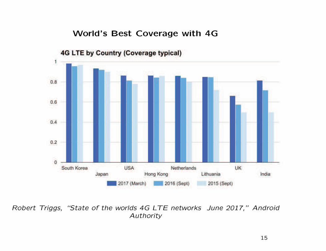
World’s Best Coverage with 4G
Robert Triggs, “State of the worlds 4G LTE networks June 2017,” Android
Authority
15
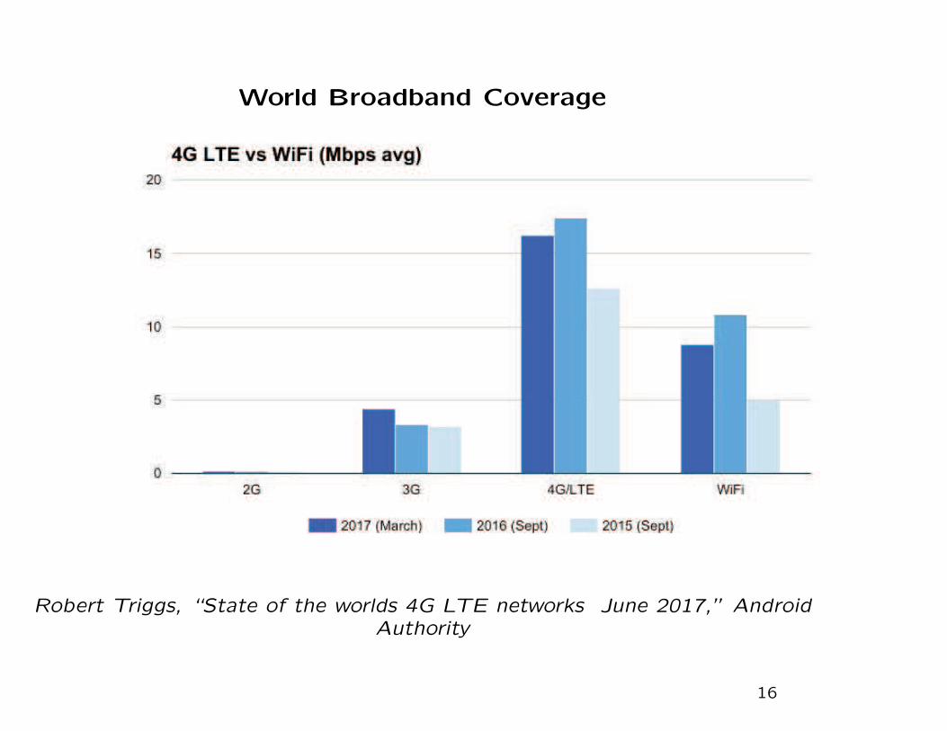
World Broadband Coverage
Robert Triggs, “State of the worlds 4G LTE networks June 2017,” Android
Authority
16

Evolution of Cellular Networks
1G 2G 3G 4G2.5G
Evolution of Cellular Standards.
17

5G Cellular
• 1000 times more data volume than 4G.
• 10 to 100 times faster than 4G with an expected speed of 1 to10 Gbps.
• 10-100 times higher number of connected devices.
• 5 times lower end-to-end latency (1 ms delay).
• 10 times longer battery life for low-power devices.
18
5G Cellular Enabling Technologies
• Massive MIMO
• Ultra-Dense Networks
• Moving Networks
• Higher Frequencies (mm-wave)
• D2D Communications
• Ultra-Reliable Communications
• Massive Machine Communications
19

FREQUENCY RE-USE AND THE CELLULAR
CONCEPT
CD
B
A
4-Cell
C
AB
3-Cell 7-Cell
A
C
F
D
GE
B
Commonly used hexagonal cellular reuse clusters.
• Tessellating hexagonal cluster sizes, N , satisfy
N = i2 + ij + j2
where i, j are non-negative integers and i ≥ j.
– hence N = 1, 3, 4, 7, 9, 12, . . . are allowable.
20

B
G
F
G
D
B
C
G
A
F
B
G
D
E
C
A
E
C
A
F
B
A
F
G
D
D
E
C
A
F
G
B
Cellular layout using 7-cell reuse clusters.
• Real cells are not hexagonal, but irregular and overlapping.
• Frequency reuse introduces co-channel interference and adjacent chan-nel interference.
21
CO-CHANNEL REUSE FACTOR
A
AD
R
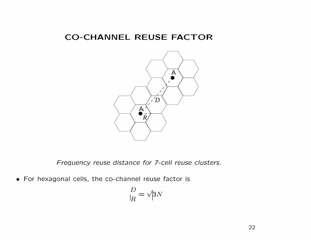
Frequency reuse distance for 7-cell reuse clusters.
• For hexagonal cells, the co-channel reuse factor is
D
R=
√3N
22
RADIO PROPAGATION MECHANISMS
• Radio propagation is by three mechanisms:
– Reflections off of objects larger than a wavelength, sometimes calledscatterers.
– Diffractions around the edges of objects
– Scattering by objects smaller than a wavelength
• A mobile radio environment is characterized by three nearly independentpropagation factors:
– Path loss attenuation with distance.
– Shadowing caused by large obstructions such as buildings, hills andvalleys.
– Multipath-fading caused by the combination of multipath propagationand transmitter, receiver and/or scatterer movement.
23
FREE SPACE PATH LOSS (FSPL)
• Equation for free-space path loss is
LFS =
(
4πd
λc
)2
.
and encapsulates two effects.
1. The first effect is that spreading out of electromagnetic energy in freespace is determined by the inverse square law, i.e.,
µΩr(d) = Ωt
1
4πd2,
where
– Ωt is the transmit power
– µΩr(d) is the received power per unit area or power spatial density
(in watts per meter-squared) at distance d. Note that this term isnot frequency dependent.
24

FREE SPACE PATH LOSS (FSPL)
• Second effect
2. The second effect is due to aperture, which determines how well anantenna picks up power from an incoming electromagnetic wave. Foran isotropic antenna, we have
µΩp(d) = µΩr
(d)λ2c
4π= Ωt
(
λc
4πd
)2
,
where µΩp(d) is the received power. Note that aperature is entirely
dependent on wavelength, λc, which is how the frequency-dependentbehavior arises in the free space path loss.
• The free space propagation path loss is
LFS (dB) = 10log10
Ωt
µΩp(d)
= 10log10
(
4πd
λc
)2
= 10log10
(
4πd
c/fc
)2
= 20log10fc + 20log10d− 147.55 dB .
25

PROPAGATION OVER A FLAT SPECULAR SURFACE
d1
d2
BS
MS
d
hb
hm
26

• The length of the direct path is
d1 =
√
d2 + (hb − hm)2
and the length of the reflected path is
d2 =
√
d2 + (hb + hm)2
d = distance between mobile and base stations
hb = base station antenna height
hm = mobile station antenna height
• Given that d ≫ hbhm, we have d1 ≈ d and d2 ≈ d.
• However, since the wavelength is small, the direct and reflected paths mayadd constructively or destructively over small distances. The carrier phasedifference between the direct and reflected paths is
φ2 − φ1 =2π
λc(d2 − d1) =
2π
λc∆d
27

• Taking into account the phase difference, the received signal power is
µΩp(d) = Ωt
(
λc
4πd
)2 ∣∣
∣1+ ae−jbej
2π
λc∆d
∣
∣
∣
2
,
where a and b are the amplitude attenuation and phase change introducedby the flat reflecting surface.
• If we assume a perfect specular reflection, then a = 1 and b = π for smallθ. Then
µΩp(d) = Ωt
(
λc
4πd
)2 ∣∣
∣1− ej(
2π
λc∆d)
∣
∣
∣
2
= Ωt
(
λc
4πd
)2 ∣∣
∣
∣
1− cos
(
2π
λc∆d
)
− j sin
(
2π
λc∆d
)∣
∣
∣
∣
2
= Ωt
(
λc
4πd
)2 [
2− 2 cos
(
2π
λc∆d
)]
= 4Ωt
(
λc
4πd
)2
sin2
(
π
λc∆d
)
28

• Given that d ≫ hb and d ≫ hm, and applying the Taylor series approximation√1+ x ≈ 1+ x/2 for small x, we have
∆d ≈ d
(
1+(hb + hm)2
2d2
)
− d
(
1+(hb − hm)2
2d2
)
=2hbhm
d.
• This approximation yields the received signal power as
µΩp(d) ≈ 4Ωt
(
λc
4πd
)2
sin2
(
2πhbhm
λcd
)
• Often we will have the condition d ≫ hbhm, such that the above approxi-mation further reduces to
µΩp(d) ≈ Ωt
(
hbhm
d2
)2
where we have invoked the small angle approximation sin x ≈ x for small x.
• Propagation over a flat specular surface differs from free space propagationin two important respects
– it is not frequency dependent
– signal strength decays with the with the fourth power of the distance,rather than the square of the distance.
29
10 100 1000 10000Path Length, d (m)
10
100
1000
Path
Los
s (d
B)
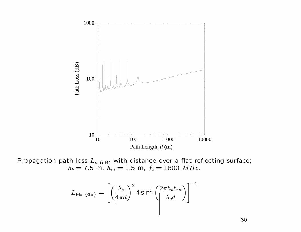
Propagation path loss Lp (dB) with distance over a flat reflecting surface;hb = 7.5 m, hm = 1.5 m, fc = 1800 MHz.
LFE (dB) =
[
(
λc
4πd
)2
4 sin2
(
2πhbhm
λcd
)
]−1
30

• In reality, the earth’s surface is curved and rough, and the signal strengthtypically decays with the inverse β power of the distance, and the receivedpower at distance d is
µΩp(d) =
µΩp(do)
(d/do)β
where µΩp(do) is the received power at a reference distance do.
• Expressed in units of dBm, the received power is
µΩp (dBm)(d) = µΩp (dBm)
(do)− 10β log10(d/do) (dBm)
• β is called the path loss exponent. Typical values of µΩp (dBm)(do) and β
have been determined by empirical measurements for a variety of areas
Terrain µΩp (dBm)(do = 1.6 km) β
Free Space -45 2Open Area -49 4.35North American Suburban -61.7 3.84North American Urban (Philadelphia) -70 3.68North American Urban (Newark) -64 4.31Japanese Urban (Tokyo) -84 3.05
31

Co-channel Interference
Worst case co-channel interference on the forward channel.
32

Worst Case Co-Channel Interference
• For N = 7, there are six first-tier co-channel BSs, located at distances√13R,4R,
√19R,5R,
√28R,
√31R from the MS.
• Assuming that the BS antennas are all the same height and all BSs transmitwith the same power, the worst case carrier-to-interference ratio, Λ, is
Λ =R−β
(√13R)−β + (4R)−β + (
√19R)−β + (5R)−β + (
√28R)−β + (
√31R)−β
=1
(√13)−β + (4)−β + (
√19)−β + (5)−β + (
√28)−β + (
√31)−β
.
• With a path loss exponent β = 3.5, the worst case Λ is
Λ(dB) =
14.56 dB for N = 79.98 dB for N = 47.33 dB for N = 3
.
– Shadows will introduce variations in the worst case Λ.
33
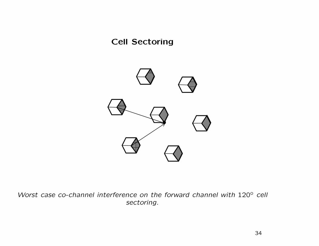
Cell Sectoring
Worst case co-channel interference on the forward channel with 120o cell
sectoring.
34

• 120o cell sectoring reduces the number of co-channel base stations fromsix to two. For N = 7, the two first tier interferers are located at distances√19R,
√28R from the MS.
• The carrier-to-interference ratio becomes
Λ =R−β
(√19R)−β + (
√28R)−β
=1
(√19)−β + (
√28)−β
.
• Hence
Λ(dB) =
20.60 dB for N = 717.69 dB for N = 413.52 dB for N = 3
.
• For N = 7, 120o cell sectoring yields a 6.04 dB C/I improvement overomni-cells.
• The minimum allowable cluster size is determined by the threshold Λ, Λth,of the radio receiver. For example, if the radio receiver has Λth = 15.0 dB,then a 4/12 reuse cluster can be used (4/12 means 4 cells or 12 sectorsper cluster).
35