Embed Size (px)
Citation preview
http://www.ee.unlv.edu/~b1morris/ecg782/
Professor Brendan Morris, SEB 3216, [email protected]
ECG782: Multidimensional
Digital Signal Processing
Spring 2014
TTh 14:30-15:45 CBC C313
Lecture 09
Morphology
14/02/25
Outline
• Mathematical Morphology
• Erosion/Dilation
• Opening/Closing
• Grayscale Morphology
• Morphological Operations
• Connected Components
2
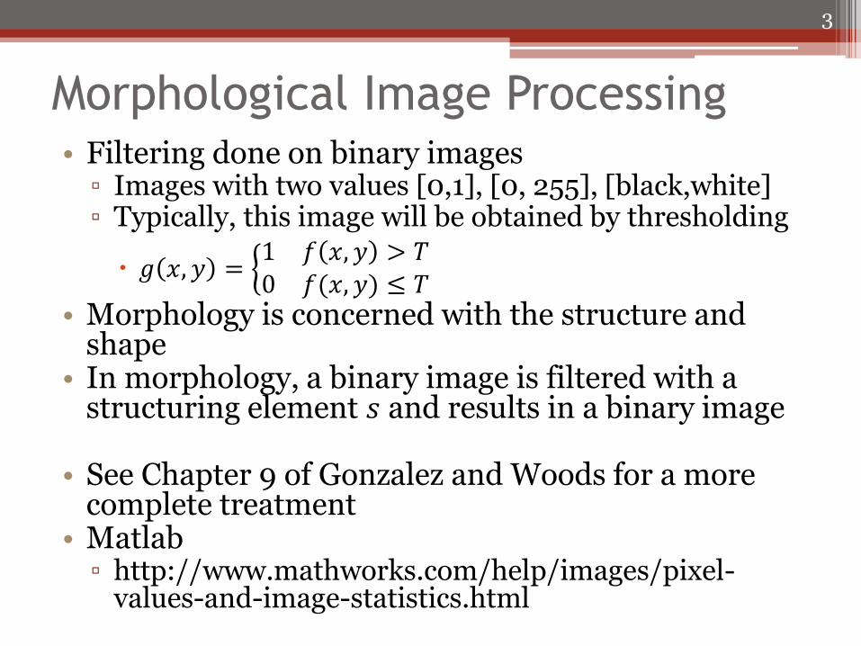
Morphological Image Processing • Filtering done on binary images
▫ Images with two values [0,1], [0, 255], [black,white] ▫ Typically, this image will be obtained by thresholding
𝑔 𝑥, 𝑦 = 1 𝑓 𝑥, 𝑦 > 𝑇0 𝑓(𝑥, 𝑦) ≤ 𝑇
• Morphology is concerned with the structure and shape
• In morphology, a binary image is filtered with a structuring element 𝑠 and results in a binary image
• See Chapter 9 of Gonzalez and Woods for a more complete treatment
• Matlab ▫ http://www.mathworks.com/help/images/pixel-
values-and-image-statistics.html
3
Mathematical Morphology
• Tool for image simplification while maintaining shape characteristics of objects
▫ Image pre-processing
Noise filtering, shape simplification
▫ Enhancing object structure
Skeletonizing, thinking, thickening, convex hull
▫ Segmenting objects from background
▫ Quantitative description of objects
Area, perimeter, moments
4
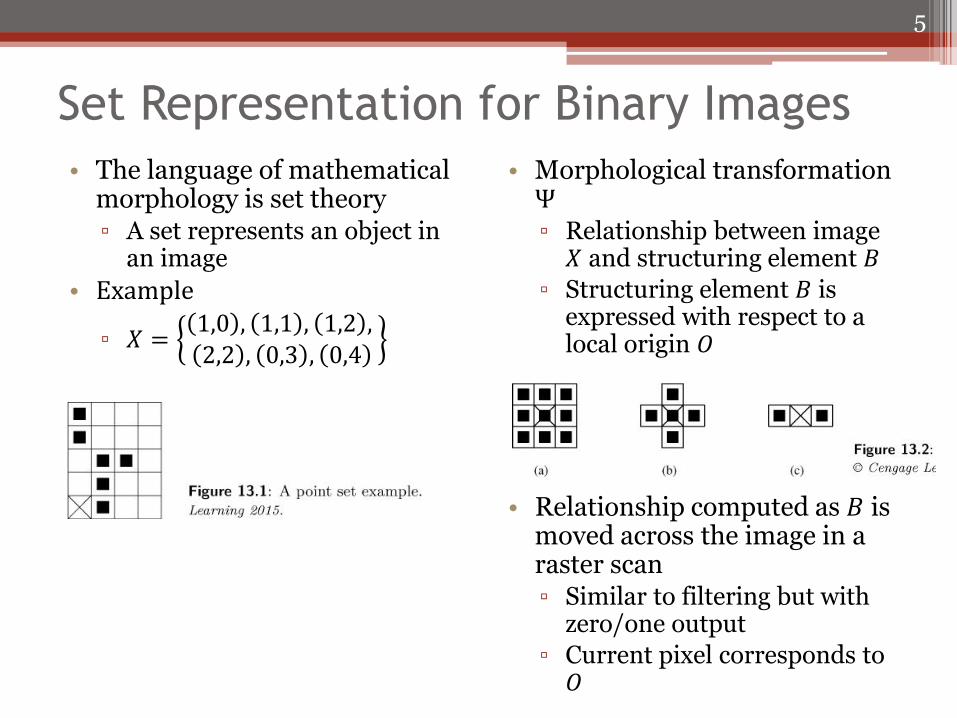
Set Representation for Binary Images
• The language of mathematical morphology is set theory ▫ A set represents an object in
an image
• Example
▫ 𝑋 =1,0 , 1,1 , 1,2 ,
2,2 , 0,3 , 0,4
• Morphological transformation Ψ ▫ Relationship between image
𝑋 and structuring element 𝐵
▫ Structuring element 𝐵 is expressed with respect to a local origin 𝑂
• Relationship computed as 𝐵 is moved across the image in a raster scan ▫ Similar to filtering but with
zero/one output
▫ Current pixel corresponds to 𝑂
5
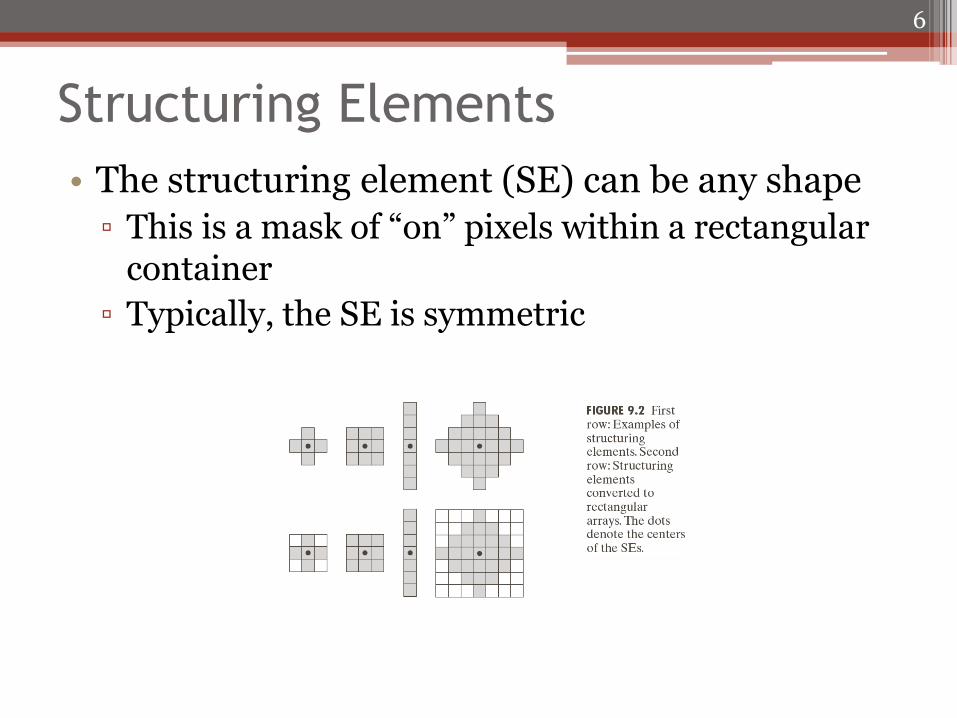
Structuring Elements
• The structuring element (SE) can be any shape
▫ This is a mask of “on” pixels within a rectangular container
▫ Typically, the SE is symmetric
6
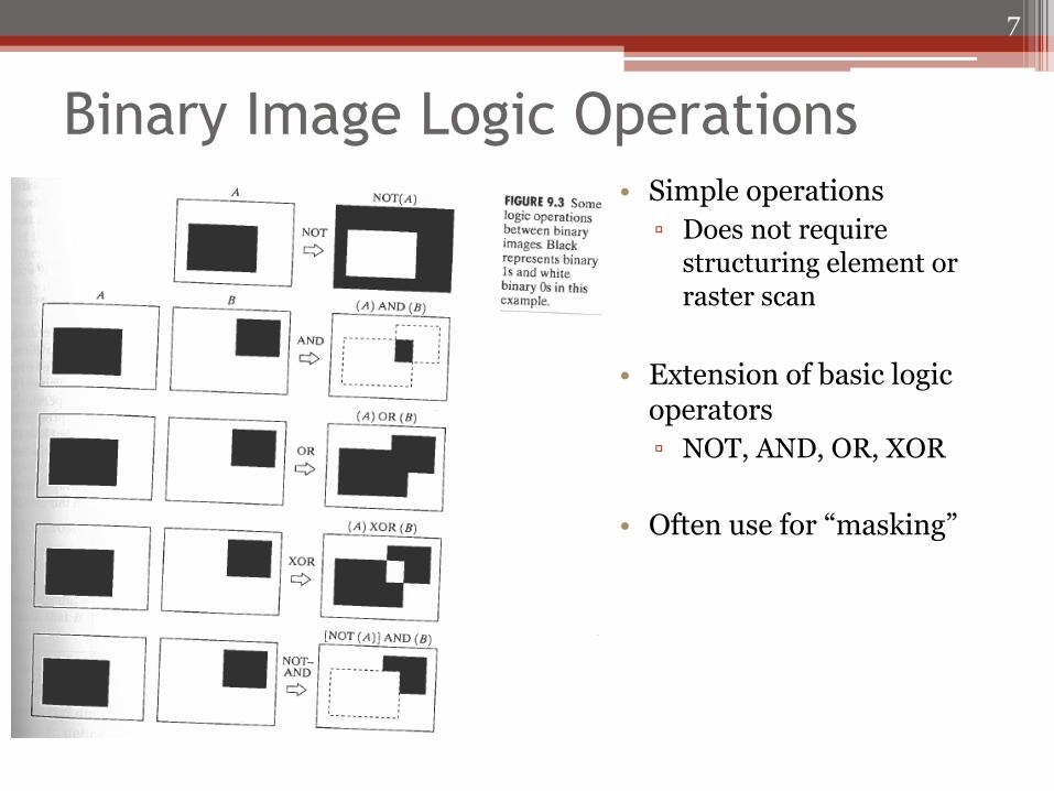
Binary Image Logic Operations • Simple operations
▫ Does not require structuring element or raster scan
• Extension of basic logic operators
▫ NOT, AND, OR, XOR
• Often use for “masking”
7
Basic Morphology Operations
• Erosion
• Dilation
• Opening
• Closing
8
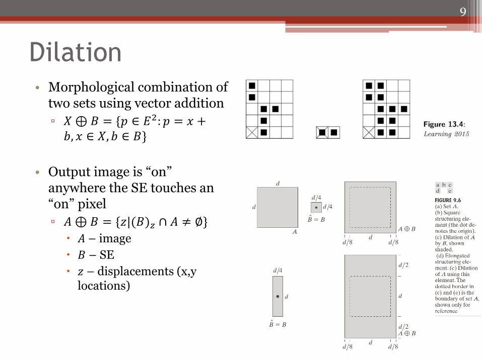
Dilation • Morphological combination of
two sets using vector addition
▫ 𝑋 ⊕ 𝐵 = {𝑝 ∈ 𝐸2: 𝑝 = 𝑥 +𝑏, 𝑥 ∈ 𝑋, 𝑏 ∈ 𝐵}
• Output image is “on” anywhere the SE touches an “on” pixel
▫ 𝐴 ⊕ 𝐵 = {𝑧|(𝐵)𝑧 ∩ 𝐴 ≠ ∅}
𝐴 – image
𝐵 – SE
𝑧 – displacements (x,y locations)
9
Dilation Properties
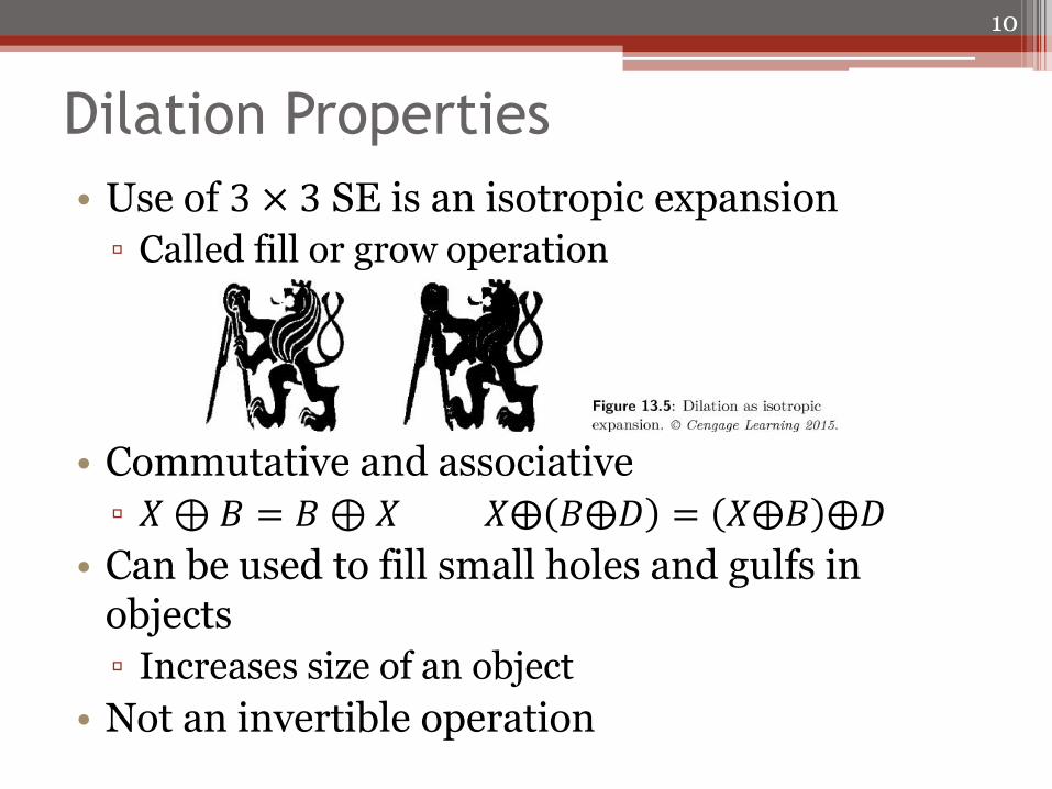
• Use of 3 × 3 SE is an isotropic expansion
▫ Called fill or grow operation
• Commutative and associative
▫ 𝑋 ⊕ 𝐵 = 𝐵 ⊕ 𝑋 𝑋⨁ 𝐵⨁𝐷 = 𝑋⨁𝐵 ⨁𝐷
• Can be used to fill small holes and gulfs in objects
▫ Increases size of an object
• Not an invertible operation
10
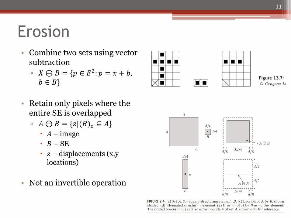
Erosion • Combine two sets using vector
subtraction
▫ 𝑋 ⊖ 𝐵 = {𝑝 ∈ 𝐸2: 𝑝 = 𝑥 + 𝑏,𝑏 ∈ 𝐵}
• Retain only pixels where the entire SE is overlapped
▫ 𝐴 ⊖ 𝐵 = {𝑧|(𝐵)𝑧 ⊆ 𝐴}
𝐴 – image
𝐵 – SE
𝑧 – displacements (x,y locations)
• Not an invertible operation
11
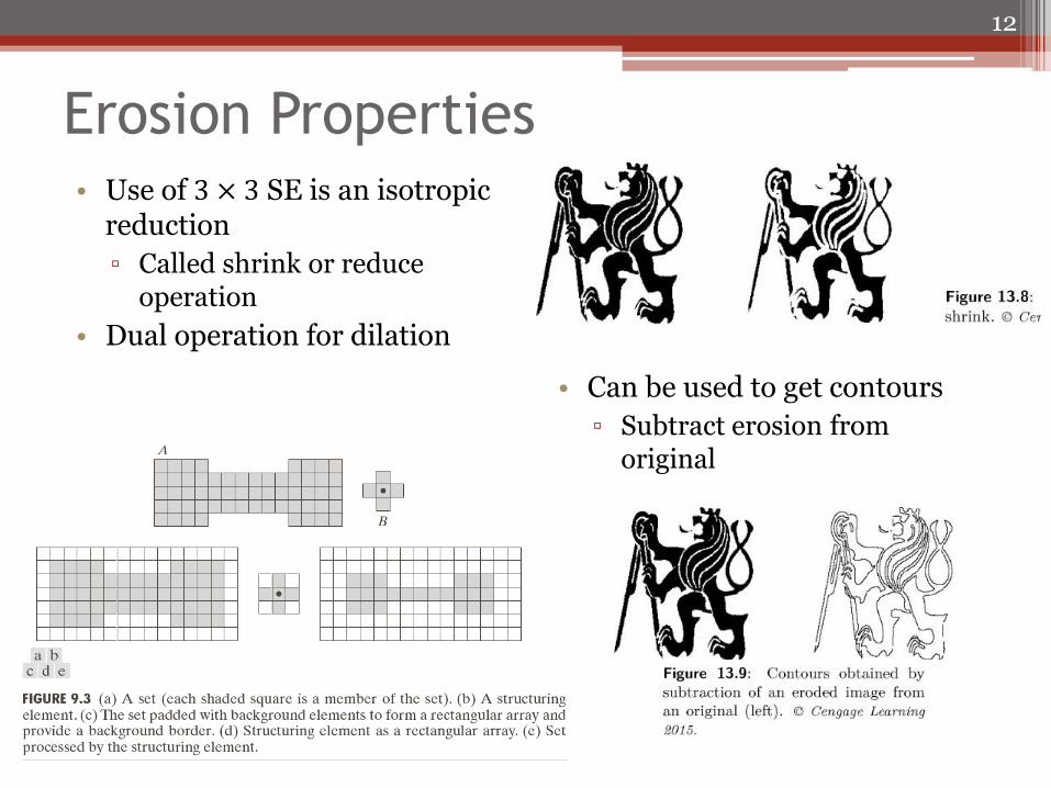
Erosion Properties • Use of 3 × 3 SE is an isotropic
reduction
▫ Called shrink or reduce operation
• Dual operation for dilation
• Can be used to get contours
▫ Subtract erosion from original
12
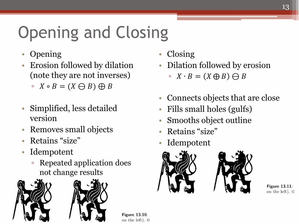
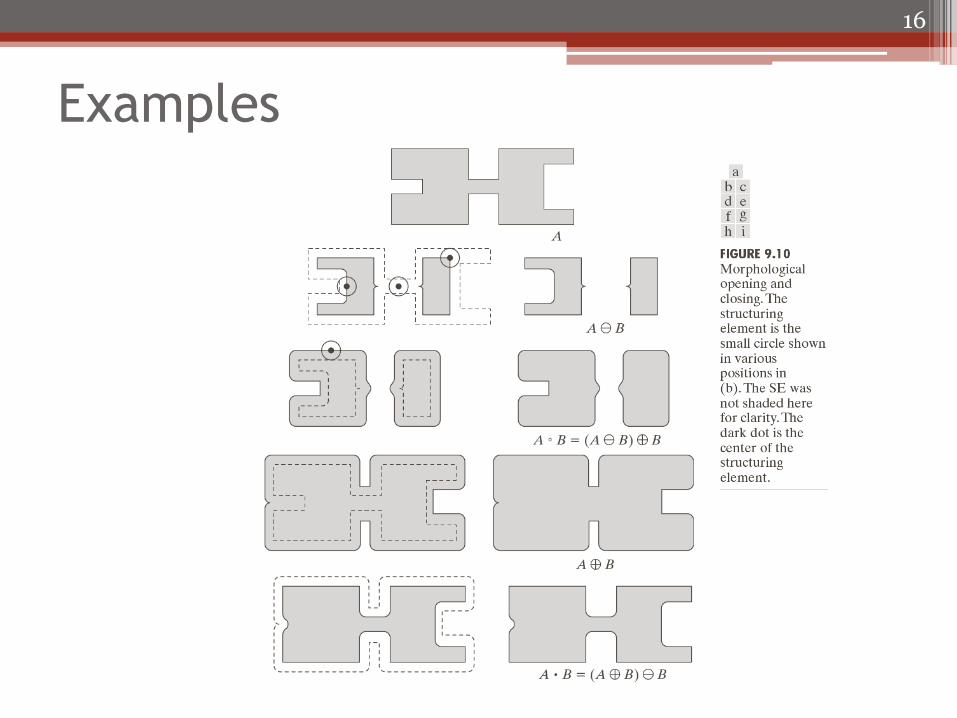
Opening and Closing • Opening
• Erosion followed by dilation (note they are not inverses)
▫ 𝑋 ∘ 𝐵 = (𝑋 ⊖ 𝐵) ⊕ 𝐵
• Simplified, less detailed version
• Removes small objects
• Retains “size”
• Idempotent
▫ Repeated application does not change results
• Closing
• Dilation followed by erosion
▫ 𝑋 ∙ 𝐵 = 𝑋⨁𝐵 ⊖ 𝐵
• Connects objects that are close
• Fills small holes (gulfs)
• Smooths object outline
• Retains “size”
• Idempotent
13
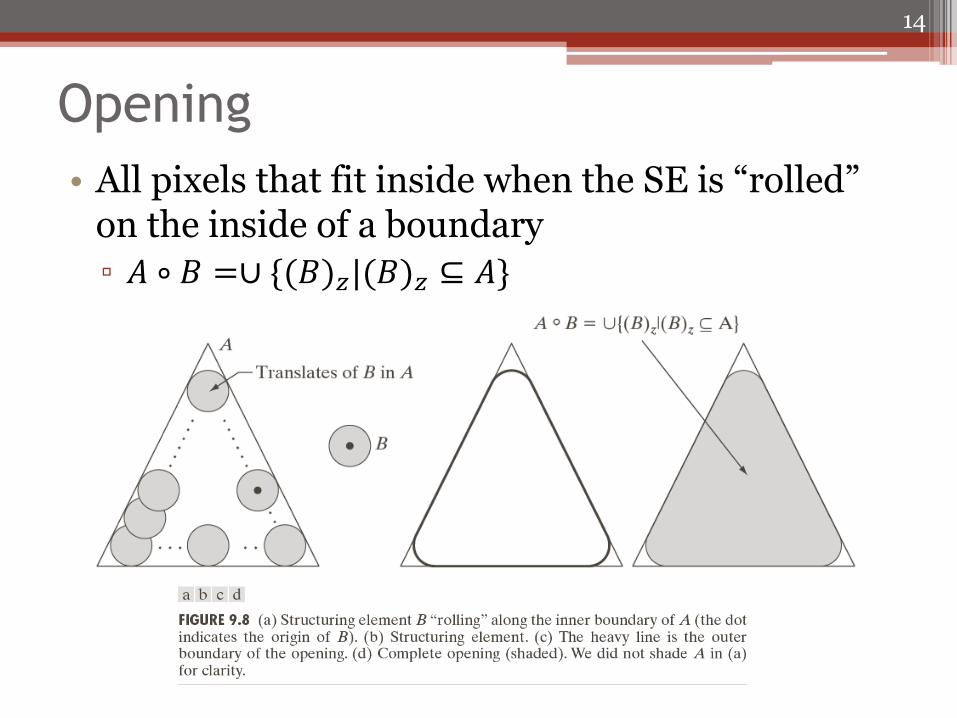
Opening
• All pixels that fit inside when the SE is “rolled” on the inside of a boundary
▫ 𝐴 ∘ 𝐵 =∪ {(𝐵)𝑧|(𝐵)𝑧 ⊆ 𝐴}
14
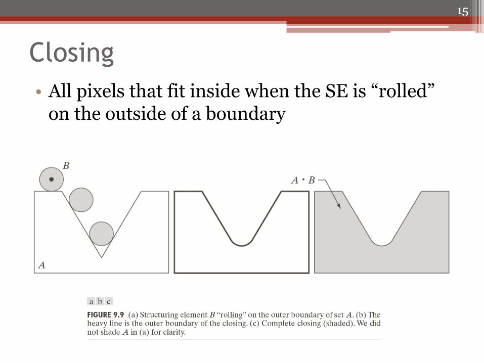
Closing
• All pixels that fit inside when the SE is “rolled” on the outside of a boundary
15
Examples
16
Grayscale Morphology
• Can extent binary morphology to grayscale images
▫ Min operation – erosion
▫ Max operation – dilation
• The structuring element not only specifies the neighborhood relationship
• It specifies the local intensity property
• Must consider image as a surface in 2D plane
17
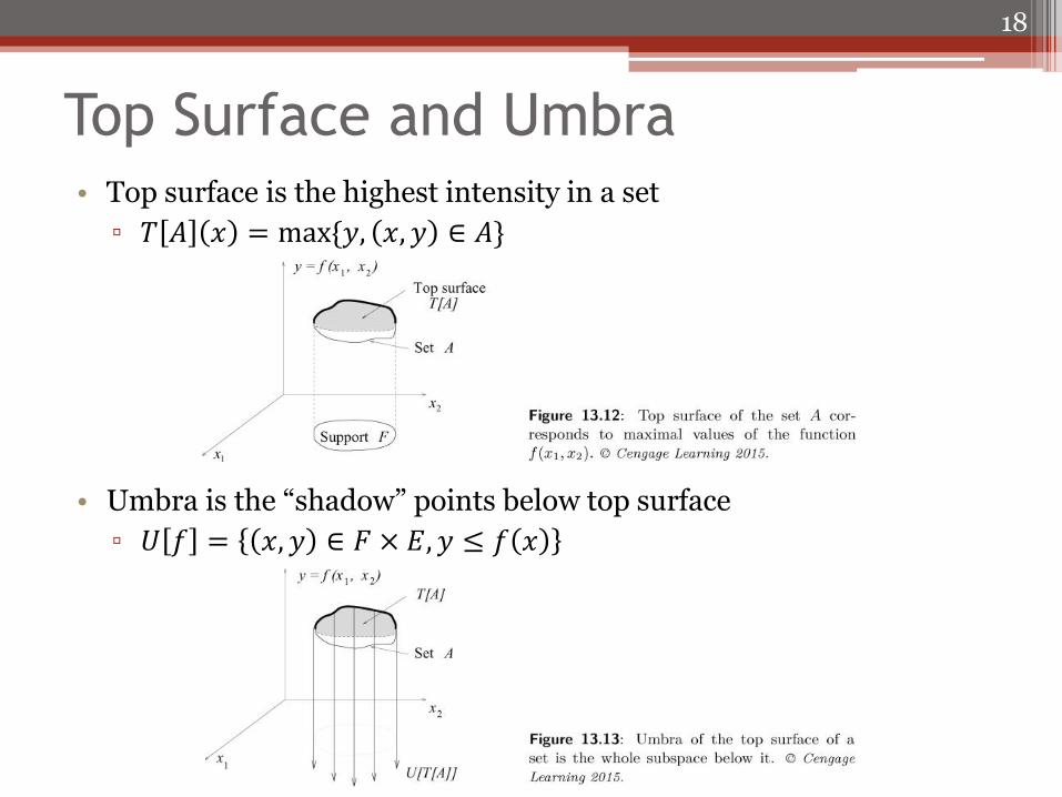
Top Surface and Umbra • Top surface is the highest intensity in a set
▫ 𝑇 𝐴 𝑥 = max {𝑦, 𝑥, 𝑦 ∈ 𝐴}
• Umbra is the “shadow” points below top surface
▫ 𝑈 𝑓 = 𝑥, 𝑦 ∈ 𝐹 × 𝐸, 𝑦 ≤ 𝑓 𝑥
18
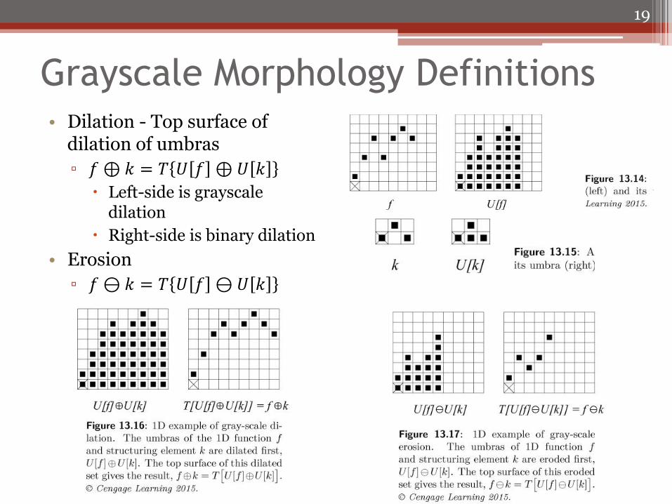
Grayscale Morphology Definitions • Dilation - Top surface of
dilation of umbras
▫ 𝑓 ⊕ 𝑘 = 𝑇 𝑈 𝑓 ⊕ 𝑈 𝑘
Left-side is grayscale dilation
Right-side is binary dilation
• Erosion
▫ 𝑓 ⊖ 𝑘 = 𝑇 𝑈 𝑓 ⊖ 𝑈 𝑘
19
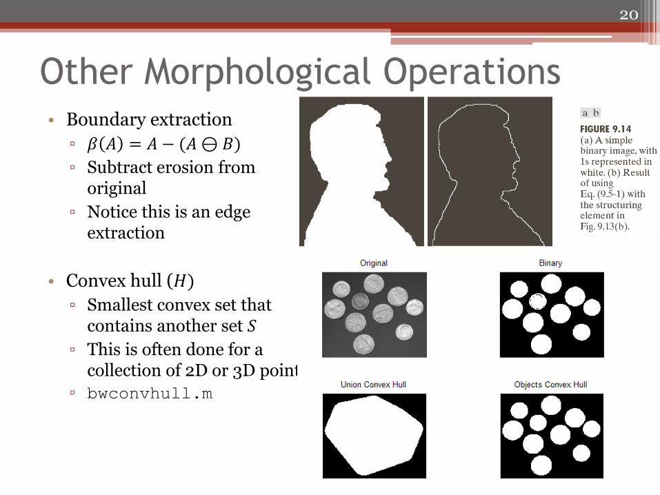
Other Morphological Operations • Boundary extraction
▫ 𝛽 𝐴 = 𝐴 − (𝐴 ⊖ 𝐵)
▫ Subtract erosion from original
▫ Notice this is an edge extraction
• Convex hull (𝐻)
▫ Smallest convex set that contains another set 𝑆
▫ This is often done for a collection of 2D or 3D points
▫ bwconvhull.m
20
More Morphological Operations • Definitions from Szeliski book
• Threshold operation
▫ 𝜃 𝑓, 𝑡 = 1 𝑓 ≥ 𝑡0 else
• Structuring element ▫ 𝑠 – e.g. 3 x 3 box filter (1’s indicate
included pixels in the mask)
▫ 𝑆 – number of “on” pixels in 𝑠
• Count of 1s in a structuring element
▫ 𝑐 = 𝑓 ⊗ 𝑠
▫ Correlation (filter) raster scan procedure
• Basic morphological operations can be extended to grayscale images
• Dilation
▫ dilate 𝑓, 𝑠 = 𝜃(𝑐, 1)
▫ Grows (thickens) 1 locations
• Erosion
▫ erode 𝑓, 𝑠 = 𝜃(𝑐, 𝑆)
▫ Shrink (thins) 1 locations
• Opening
▫ open 𝑓, 𝑠 = dilate(erode 𝑓, 𝑠 , 𝑠)
▫ Generally smooth the contour of an object, breaks narrow isthmuses, and eliminates thin protrusions
• Closing
▫ close 𝑓, 𝑠 = erode(dilate 𝑓, 𝑠 , 𝑠)
▫ Generally smooth the contour of an object, fuses narrow breaks/separations, eliminates small holes, and fills gaps in a contour
21
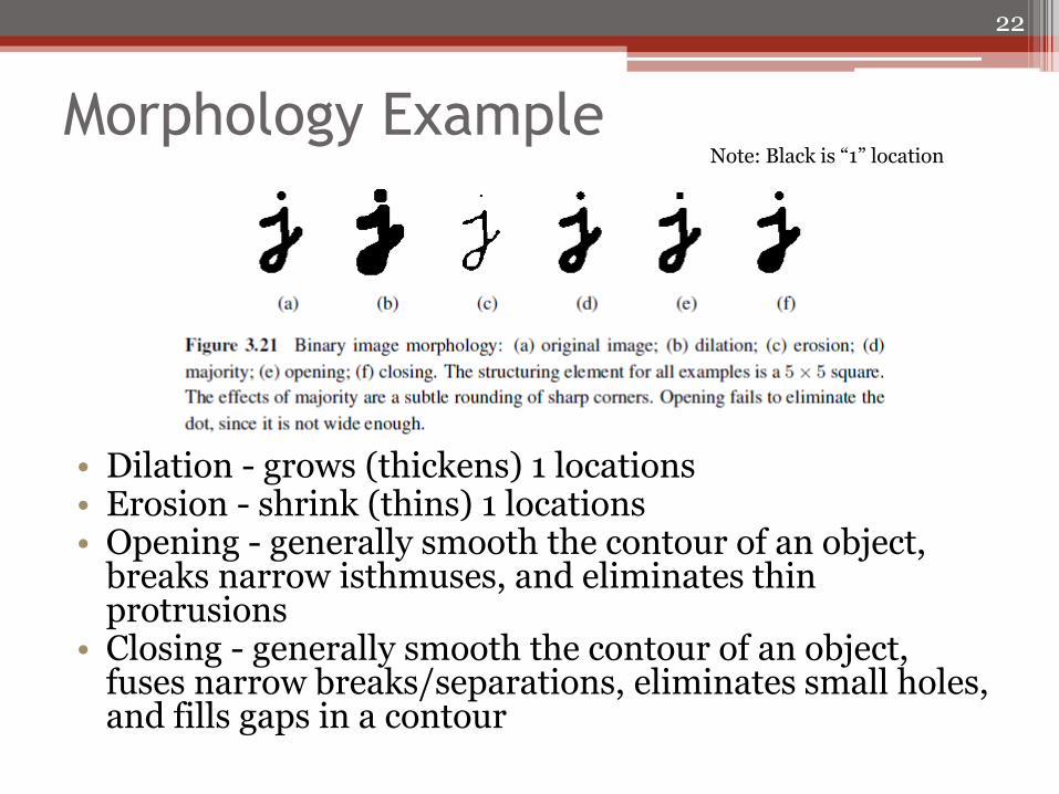
Morphology Example
• Dilation - grows (thickens) 1 locations • Erosion - shrink (thins) 1 locations • Opening - generally smooth the contour of an object,
breaks narrow isthmuses, and eliminates thin protrusions
• Closing - generally smooth the contour of an object, fuses narrow breaks/separations, eliminates small holes, and fills gaps in a contour
22
Note: Black is “1” location
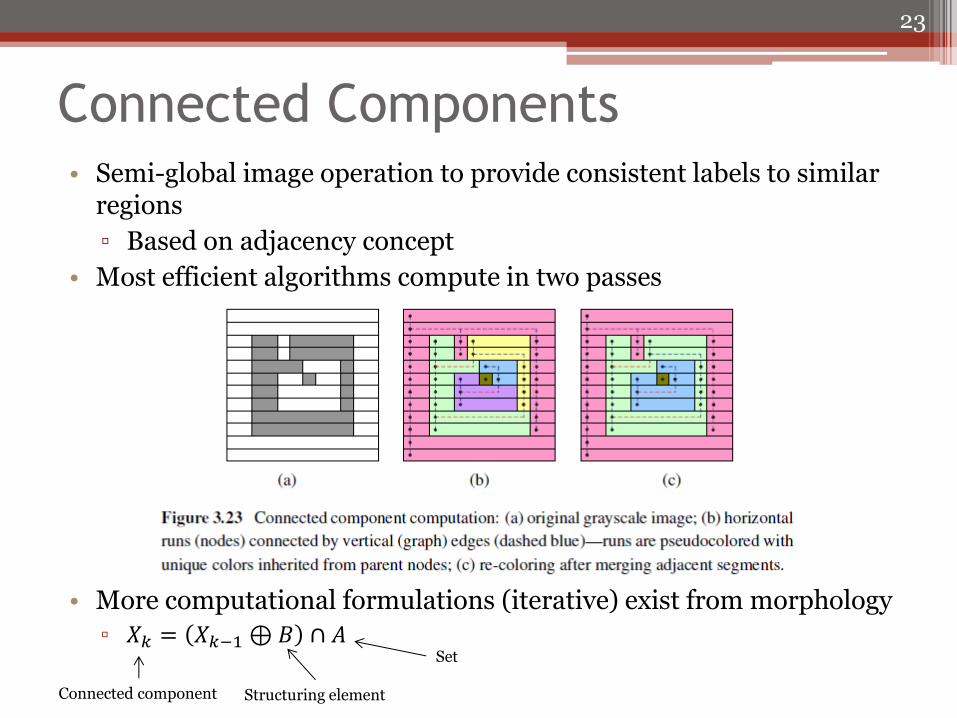
Connected Components • Semi-global image operation to provide consistent labels to similar
regions
▫ Based on adjacency concept
• Most efficient algorithms compute in two passes
• More computational formulations (iterative) exist from morphology
▫ 𝑋𝑘 = 𝑋𝑘−1 ⊕ 𝐵 ∩ 𝐴
23
Connected component Structuring element
Set
More Connected Components
• Typically, only the “white” pixels will be considered objects ▫ Dark pixels are background and do not get counted
• After labeling connected components, statistics from each region can be computed ▫ Statistics describe the region – e.g. area, centroid,
perimeter, etc.
• Matlab functions
▫ bwconncomp.m, labelmatrix.m (bwlabel.m)- label image
▫ label2rgb.m – color components for viewing ▫ regionprops.m – calculate region statistics
24
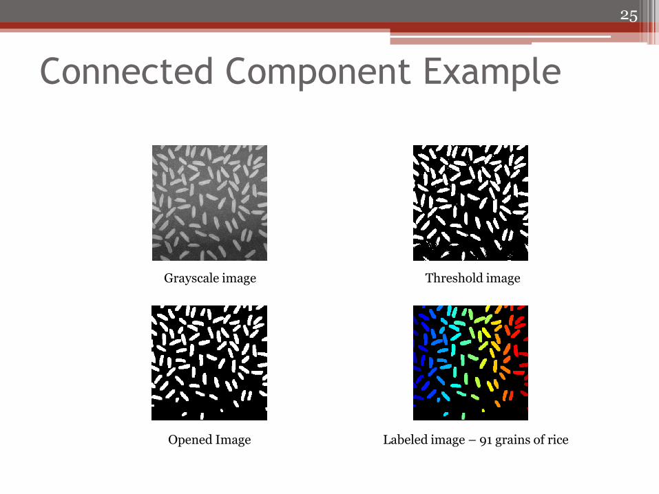
Connected Component Example
25
Grayscale image Threshold image
Opened Image Labeled image – 91 grains of rice