Embed Size (px)
Citation preview

B.Sc. Engg. Thesis
Efficient Enumeration of Combinatorial Objects
By
Muhammad Abdullah Adnan
Student No.: 0005010
Submitted to
Department of Computer Science and Engineering
in partial fulfilment of the requirements for the degree of
Bachelor of Science in Computer Science and Engineering
Department of Computer Science and Engineering
Bangladesh University of Engineering and Technology (BUET)
Dhaka-1000
November 13, 2006

i
Certificate
This is to certify that the work presented in this thesis entitled “Study of Enumeration
Problems” is the outcome of the investigation carried out by me under the supervision of
Professor Dr. Md. Saidur Rahman in the Department of Computer Science and Engineering,
Bangladesh University of Engineering and Technology (BUET), Dhaka. It is also declared that
neither this thesis nor any part thereof has been submitted or is being currently submitted
anywhere else for the award of any degree or diploma.
(Supervisor) (Author)
Dr. Md. Saidur Rahman Muhammad Abdullah Adnan
Professor Student No.: 0005010
Department of Computer Science Department of Computer Science
and Engineering (BUET), Dhaka-1000. and Engineering (BUET), Dhaka-1000.
Contents
Certificate i
Acknowledgements ix
Abstract x
1 Introduction 1
1.1 Enumeration Problems . . . . . . . . . . . . . . . . . . . . . . . . . . . . . . . . 3
1.1.1 Order of output . . . . . . . . . . . . . . . . . . . . . . . . . . . . . . . . 4
1.1.2 Applications . . . . . . . . . . . . . . . . . . . . . . . . . . . . . . . . . . 5
1.1.3 Goals of an Enumeration Algorithm . . . . . . . . . . . . . . . . . . . . . 7
1.2 Challenges . . . . . . . . . . . . . . . . . . . . . . . . . . . . . . . . . . . . . . . 7
1.2.1 Time Complexity . . . . . . . . . . . . . . . . . . . . . . . . . . . . . . . 7
1.2.2 Avoiding Duplications . . . . . . . . . . . . . . . . . . . . . . . . . . . . 8
1.2.3 I/O Operations . . . . . . . . . . . . . . . . . . . . . . . . . . . . . . . . 8
1.2.4 Exhaustive Generation . . . . . . . . . . . . . . . . . . . . . . . . . . . . 8
1.3 Algorithms for Enumeration Problems . . . . . . . . . . . . . . . . . . . . . . . 9
1.3.1 Combinatorial Gray Code Approach . . . . . . . . . . . . . . . . . . . . 9
1.3.2 Family Tree Approach . . . . . . . . . . . . . . . . . . . . . . . . . . . . 11
1.4 Scope of this Thesis . . . . . . . . . . . . . . . . . . . . . . . . . . . . . . . . . . 12
1.4.1 Distribution of Objects to Bins . . . . . . . . . . . . . . . . . . . . . . . 12
1.4.2 Distribution of Distinguishable Objects to Bins . . . . . . . . . . . . . . 13
1.4.3 Evolutionary Trees . . . . . . . . . . . . . . . . . . . . . . . . . . . . . . 13
ii

CONTENTS iii
1.4.4 Labeled and Ordered Evolutionary Trees . . . . . . . . . . . . . . . . . . 14
1.5 Summary . . . . . . . . . . . . . . . . . . . . . . . . . . . . . . . . . . . . . . . 14
2 Preliminaries 17
2.1 Basic Terminology . . . . . . . . . . . . . . . . . . . . . . . . . . . . . . . . . . 17
2.1.1 Graphs . . . . . . . . . . . . . . . . . . . . . . . . . . . . . . . . . . . . . 17
2.1.2 Paths and Cycles . . . . . . . . . . . . . . . . . . . . . . . . . . . . . . . 18
2.1.3 Trees . . . . . . . . . . . . . . . . . . . . . . . . . . . . . . . . . . . . . . 18
2.1.4 Binary Trees . . . . . . . . . . . . . . . . . . . . . . . . . . . . . . . . . . 19
2.1.5 Family Trees . . . . . . . . . . . . . . . . . . . . . . . . . . . . . . . . . 20
2.1.6 Recursion Trees . . . . . . . . . . . . . . . . . . . . . . . . . . . . . . . . 20
2.1.7 Evolutionary Trees . . . . . . . . . . . . . . . . . . . . . . . . . . . . . . 21
2.1.8 Integer Partition . . . . . . . . . . . . . . . . . . . . . . . . . . . . . . . 21
2.1.9 Set Partition . . . . . . . . . . . . . . . . . . . . . . . . . . . . . . . . . 21
2.1.10 Multiset . . . . . . . . . . . . . . . . . . . . . . . . . . . . . . . . . . . . 21
2.1.11 Simpleset . . . . . . . . . . . . . . . . . . . . . . . . . . . . . . . . . . . 22
2.2 Algorithms and Complexity . . . . . . . . . . . . . . . . . . . . . . . . . . . . . 22
2.2.1 The notation O(n) . . . . . . . . . . . . . . . . . . . . . . . . . . . . . . 22
2.2.2 Polynomial algorithms . . . . . . . . . . . . . . . . . . . . . . . . . . . . 22
2.2.3 Constant Time . . . . . . . . . . . . . . . . . . . . . . . . . . . . . . . . 23
2.2.4 Average Constant Time . . . . . . . . . . . . . . . . . . . . . . . . . . . 23
2.2.5 Amortized Time . . . . . . . . . . . . . . . . . . . . . . . . . . . . . . . 23
2.3 Graph Traversal Algorithm . . . . . . . . . . . . . . . . . . . . . . . . . . . . . . 24
2.4 Catalan Families . . . . . . . . . . . . . . . . . . . . . . . . . . . . . . . . . . . 25
3 Distribution of Objects to Bins 26
3.1 Introduction . . . . . . . . . . . . . . . . . . . . . . . . . . . . . . . . . . . . . . 26
3.2 Preliminaries . . . . . . . . . . . . . . . . . . . . . . . . . . . . . . . . . . . . . 30
3.3 Generating Distribution of Objects to Bins . . . . . . . . . . . . . . . . . . . . . 32
3.3.1 The Family Tree . . . . . . . . . . . . . . . . . . . . . . . . . . . . . . . 32

CONTENTS iv
3.3.2 The Algorithm . . . . . . . . . . . . . . . . . . . . . . . . . . . . . . . . 36
3.4 Efficient Tree Traversal . . . . . . . . . . . . . . . . . . . . . . . . . . . . . . . . 37
3.4.1 Relationship Between Left Sibling and Right Sibling . . . . . . . . . . . . 37
3.4.2 Leaf-Ancestor Relationship . . . . . . . . . . . . . . . . . . . . . . . . . . 38
3.4.3 The Efficient Algorithm . . . . . . . . . . . . . . . . . . . . . . . . . . . 40
3.5 Distributions in Anti-lexicographic Order . . . . . . . . . . . . . . . . . . . . . . 43
3.6 Generating Distributions with Priorities to Bins . . . . . . . . . . . . . . . . . . 44
3.7 Conclusion . . . . . . . . . . . . . . . . . . . . . . . . . . . . . . . . . . . . . . . 44
4 Distribution of Distinguishable Objects to Bins 45
4.1 Introduction . . . . . . . . . . . . . . . . . . . . . . . . . . . . . . . . . . . . . . 45
4.2 Preliminaries . . . . . . . . . . . . . . . . . . . . . . . . . . . . . . . . . . . . . 49
4.3 Generating Distribution of Distinguishable Objects . . . . . . . . . . . . . . . . 51
4.3.1 The Family Tree . . . . . . . . . . . . . . . . . . . . . . . . . . . . . . . 52
4.3.2 The Algorithm . . . . . . . . . . . . . . . . . . . . . . . . . . . . . . . . 56
4.4 Efficient Tree Traversal . . . . . . . . . . . . . . . . . . . . . . . . . . . . . . . . 57
4.4.1 Relationship Between Left Sibling and Right Sibling . . . . . . . . . . . . 58
4.4.2 Leaf-Ancestor Relationship . . . . . . . . . . . . . . . . . . . . . . . . . . 59
4.4.3 Representation of a Distribution in D(n,m, k) . . . . . . . . . . . . . . . 61
4.4.4 The Efficient Algorithm . . . . . . . . . . . . . . . . . . . . . . . . . . . 62
4.5 Generating Distributions with Priorities to Bins . . . . . . . . . . . . . . . . . . 64
4.6 Conclusion . . . . . . . . . . . . . . . . . . . . . . . . . . . . . . . . . . . . . . . 64
5 Evolutionary Trees 66
5.1 Introduction . . . . . . . . . . . . . . . . . . . . . . . . . . . . . . . . . . . . . . 66
5.2 Preliminaries . . . . . . . . . . . . . . . . . . . . . . . . . . . . . . . . . . . . . 68
5.3 Generating Labeled Evolutionary Trees . . . . . . . . . . . . . . . . . . . . . . . 69
5.4 The Recursion Tree . . . . . . . . . . . . . . . . . . . . . . . . . . . . . . . . . . 71
5.4.1 Parent-Child Relationship . . . . . . . . . . . . . . . . . . . . . . . . . . 73
5.4.2 Child-Parent Relationship . . . . . . . . . . . . . . . . . . . . . . . . . . 74

CONTENTS v
5.4.3 The Recursion Tree . . . . . . . . . . . . . . . . . . . . . . . . . . . . . . 75
5.5 The Algorithm . . . . . . . . . . . . . . . . . . . . . . . . . . . . . . . . . . . . 76
5.6 Conclusion . . . . . . . . . . . . . . . . . . . . . . . . . . . . . . . . . . . . . . . 78
6 Labeled and Ordered Evolutionary Trees 79
6.1 Introduction . . . . . . . . . . . . . . . . . . . . . . . . . . . . . . . . . . . . . . 79
6.2 Preliminaries . . . . . . . . . . . . . . . . . . . . . . . . . . . . . . . . . . . . . 82
6.3 Representation of Evolutionary Trees . . . . . . . . . . . . . . . . . . . . . . . . 84
6.4 The Family Tree . . . . . . . . . . . . . . . . . . . . . . . . . . . . . . . . . . . 85
6.4.1 Parent-Child Relationship . . . . . . . . . . . . . . . . . . . . . . . . . . 86
6.4.2 Child-Parent Relationship . . . . . . . . . . . . . . . . . . . . . . . . . . 87
6.4.3 The Family Tree . . . . . . . . . . . . . . . . . . . . . . . . . . . . . . . 87
6.5 Algorithm . . . . . . . . . . . . . . . . . . . . . . . . . . . . . . . . . . . . . . . 89
6.6 Conclusion . . . . . . . . . . . . . . . . . . . . . . . . . . . . . . . . . . . . . . . 91
7 Conclusion 92
References 94
List of Publications 97
Index 98

List of Figures
1.1 Lexicographic order vs Gray code order for binary strings. . . . . . . . . . . . . 5
1.2 Generating permutations using gray code approach: Johnson-Trotter scheme. . 10
1.3 Illustration of the family tree for all set partitions. . . . . . . . . . . . . . . . . 12
2.1 Illustration of a graph. . . . . . . . . . . . . . . . . . . . . . . . . . . . . . . . 18
2.2 Illustration of a tree. . . . . . . . . . . . . . . . . . . . . . . . . . . . . . . . . . 19
2.3 Illustration of a binary tree. . . . . . . . . . . . . . . . . . . . . . . . . . . . . . 20
2.4 Illustration of a family tree of 15 nodes. . . . . . . . . . . . . . . . . . . . . . . . 20
3.1 The Family Tree T4,3. . . . . . . . . . . . . . . . . . . . . . . . . . . . . . . . . . 29
3.2 Representation of a distribution of 4 objects to 3 bins. . . . . . . . . . . . . . . 31
3.3 Efficient Traversal of the family tree T4,4. . . . . . . . . . . . . . . . . . . . . . . 38
3.4 Efficient Traversal of T4,3 keeping extra information. . . . . . . . . . . . . . . . . 40
3.5 Use of stack for tree traversal (T4,4). . . . . . . . . . . . . . . . . . . . . . . . . . 41
3.6 A Gray code for D(4, 3). . . . . . . . . . . . . . . . . . . . . . . . . . . . . . . . 43
3.7 Illustration of generation of D(4, 3) in anti-lexicographic order. . . . . . . . . . . 43
4.1 The Family Tree T3,3,2. . . . . . . . . . . . . . . . . . . . . . . . . . . . . . . . . 48
4.2 Representation of a distribution of 3 objects to 2 bins where the objects fall into
two classes and 2 objects from class 1 and 1 object from class 2. . . . . . . . . . 50
4.3 The sequence ((0, 0), (2, 1)) has five children. . . . . . . . . . . . . . . . . . . . . 54
4.4 Efficient Traversal of the family tree T3,3,2. . . . . . . . . . . . . . . . . . . . . . 58
4.5 Efficient Traversal of T4,3 keeping extra information. . . . . . . . . . . . . . . . . 61
vi

LIST OF FIGURES vii
4.6 Illustration of data structure that we use to represent a distribution for distin-
guishable objects. . . . . . . . . . . . . . . . . . . . . . . . . . . . . . . . . . . . 61
4.7 A Gray code for D(3, 3, 2). . . . . . . . . . . . . . . . . . . . . . . . . . . . . . . 64
5.1 The evolutionary tree having four species. . . . . . . . . . . . . . . . . . . . . . 67
5.2 All possible evolutionary trees having three species. . . . . . . . . . . . . . . . . 67
5.3 Representation of evolutionary tree in terms of complete binary tree. . . . . . . 69
5.4 Two evolutionary trees of (a) and (b) are mirror image of one another. . . . . . 70
5.5 Two evolutionary trees of (a) and (b) are sibling equivalent to one another. . . . 70
5.6 The Recursion Tree R4. . . . . . . . . . . . . . . . . . . . . . . . . . . . . . . . . 71
5.7 Illustration of a sequence of subtree A ∈ S(6). . . . . . . . . . . . . . . . . . . . 72
5.8 Illustration of Type I and Type II child of a sequence of subtree A ∈ S(6). . . . 74
6.1 The evolutionary tree having four species. . . . . . . . . . . . . . . . . . . . . . 80
6.2 The Family Tree F4. . . . . . . . . . . . . . . . . . . . . . . . . . . . . . . . . . 82
6.3 Representation of evolutionary tree in terms of complete binary tree. . . . . . . 83
6.4 Representation of an evolutionary tree having five species. . . . . . . . . . . . . 84
6.5 Illustration of Family Tree F5. . . . . . . . . . . . . . . . . . . . . . . . . . . . . 88
6.6 Representation of Family Tree F5. . . . . . . . . . . . . . . . . . . . . . . . . . . 88

List of Tables
1.1 Results on distribution of identical objects to bins. . . . . . . . . . . . . . . . . 15
1.2 Results on distribution of distinguishable objects to bins. . . . . . . . . . . . . . 15
1.3 Results on generating evolutionary trees. . . . . . . . . . . . . . . . . . . . . . . 15
viii

Acknowledgments
First of all, I would like to thank my supervisor Professor Dr. Md. Saidur Rahman for
introducing me to the field of enumeration of combinatorial objects, and for teaching me how
to carry on a research work. I have learned from him how to write, speak and present well. I
thank him for his patience in reviewing my so many inferior drafts, for correcting my proofs and
language, suggesting new ways of thinking and encouraging me to continue my research work.
I again express my heart-felt and most sincere gratitude to him for his constant supervision,
valuable advice and continual encouragement, without which this thesis would have not been
possible.
I would like to express my utmost gratitude to Professor Shin-ichi Nakano for encouraging
me to work in this area and for giving us valuable comments on the manuscripts of my papers.
I would like to thank Shin-ichiro Kawano for helpful discussions.
I would also want to thank Professor Dr. Muhammad Masroor Ali, Head, Department of
Computer Science and Engineering, BUET, for the provision of laboratory facilities.
I would like to acknowledge with sincere thanks the all-out cooperation and services rendered
by the members of our research group for many things. They gave me valuable suggestions and
listened to all of my presentations.
ix

Abstract
One of the problems addressed in the area of combinatorial algorithms is to enumerate all
items of a particular combinatorial class efficiently in such a way that each item is generated
exactly once. Enumeration algorithms have many applications in optimizations, clustering,
data mining, and machine learning, thus we need developments of efficient algorithms, in the
sense of both theory and practice. In this thesis, we study different enumeration problems and
approaches to solve them. In particular, we focus on the applications of enumeration algorithms
to Bioinformatics and Combinatorics. We concentrate on the efficiency improvement of the
algorithms and invent new approaches to solve enumeration problems such that each solution
is generated in constant time in ordinary sense.
A well known counting problem in combinatorics is counting the number of ways objects
can be distributed among bins. In this thesis, we consider it as an enumeration problem
and give efficient algorithms to generate all distributions of n objects to m bins. We gave
elegant algorithms for both identical and distinguishable objects. Generating all distributions
has practical applications in computer networks, distributed architecture, CPU scheduling,
memory management, etc. Our algorithms generate each distribution in constant time without
repetition. We also introduce a new elegant and efficient tree traversal algorithm that generates
each solution in O(1) time in ordinary sense.
In this thesis, we also deal with the problem of generating all evolutionary trees. Generating
all evolutionary trees among different species have many applications in Bioinformatics, Genetic
Engineering, Archaeology, Biochemistry and Molecular Biology. In these applications, to find
a better prediction, sometimes it is necessary to generate all possible evolutionary trees among
different species. We give an algorithm to generate all such probable evolutionary trees having
n ordered species without repetition. We also find out an efficient representation of such
evolutionary trees such that each tree is generated in constant time on average.
x
Chapter 1
Introduction
In computer science, we frequently need to count things and generate solutions. The science of
enumerating is captured by a branch of mathematics called combinatorics . One of the problems
addressed in the area of combinatorial algorithms is to generate all items of a particular combi-
natorial class efficiently in such a way that each item is generated exactly once. To solve many
practical problems it is required to generate samples of random objects from a combinatorial
class. Sometimes a list of objects of a particular class is useful to search for a counter-example
to some conjecture, to find the best solution among all solutions, or to experimentally measure
the average performance of an algorithm over all possible inputs. Early works in combinatorics
focused on counting; because generating all objects requires huge computation. With the aid
of fast computers it now has become feasible to list the objects in combinatorial classes. How-
ever, in order to generate entire list of objects from a class of moderate size, extremely efficient
algorithms are required even with the fastest computers. Due to the reason mentioned above,
recently many researchers have concentrated their attention for developing efficient algorithms
to generate all objects of a particular class without repetitions [JWW80, S97]. Examples of
such exhaustive generation of combinatorial objects include generating all integer partition
and set partitions, enumerating all binary trees, generating permutations and combinations,
enumerating spanning trees, etc. [J63, KN05, NU03, NU04, NU05, ZS98].
In this thesis, we study different enumeration problems and approaches to solve them.
1

Chapter 1. Introduction 2
In particular, we focus on the applications of generation algorithms to Bioinformatics and
Combinatorics . We also give some efficient algorithms to solve two of them. We concentrate
on the efficiency improvement of the algorithms and invent new approaches to solve enumeration
problems such that each solution is generated in constant time (in ordinary sense). The main
feature of our algorithms is that they are constant time solution which is a very important
requirement for generation problems.
A well known counting problem in combinatorics is counting the number of ways objects
can be distributed among bins [AU95, R00, AR06]. The paradigm problem is counting the
number of ways of distributing fruits to children. For example, Kathy, Peter and Susan are
three children. We have four fruits to distribute among them without cutting the fruits into
parts. In how many ways the children receive fruits? The fruits or the objects, that we want
to distribute, may be identical or of different kinds. Based on this criterion, the problem can
be subdivided into two parts - identical case and non-identical case. In this thesis, we consider
it as an enumeration problem and give algorithms to generate all distributions without repeti-
tion. Generating all distributions has practical applications in channel allocation in computer
networks, client-server broker distributed architecture, CPU scheduling, memory management,
etc. [T02, T04]. Our algorithms generate each distribution in constant time with linear space
complexity. We also present an efficient tree traversal algorithm that generates each solution in
O(1) time. To the best of our knowledge, our algorithm is the first algorithm which generates
each solution in O(1) time in ordinary sense. By modifying our algorithm, we can generate
the distributions in anti-lexicographic order. Finally, we extend our algorithms for the case
when the bins have priorities associated with them. As a byproduct of our algorithm, we get
a new algorithm to enumerate all set partitions when the number of partitions is fixed and the
partitions are numbered. The main feature of all our algorithms is that all of them are constant
time solution which is very important requirement for enumeration problems.
In this thesis, we also deal with the problem of generating all evolutionary trees. Gener-
ating all evolutionary trees among different species have many applications in Bioinformatics
[JP04], Genetic Engineering [KR03], Archaeology, Biochemistry and Molecular Biology. In
1.1. Enumeration Problems 3
these applications, to find a better prediction, sometimes it is necessary to generate all possible
evolutionary trees among different species. To a mathematician, such a tree is simply a cycle-
free connected graph, but to a biologist it represents a series of hypotheses about evolutionary
events. In this thesis, we are concerned with generating all such probable evolutionary trees
that will guide biologists to research in all biological subdisciplines. We give an algorithm to
generate all evolutionary trees having n species without repetition. We also find out an efficient
representation of such evolutionary trees such that each tree is generated in constant time on
average. For the purposes of biologists, we also give a new algorithm to generate evolutionary
trees having ordered species.
In this chapter we provide the necessary background and motivation for this study on
enumeration problems. Section 1.1 serves as an introduction to the enumeration problems.
Section 1.2 addresses the algorithmic challenges that any efficient enumeration algorithm must
resolve. Section 1.3 deals with the well known techniques for solving enumeration problems.
In Section 1.4 we describe the scope of this thesis. Finally, Section 1.5 gives a summary of the
results we have found and compares our algorithms with other related algorithms.
1.1 Enumeration Problems
In this section we discuss about enumeration problems and its applications in different areas.
In mathematics and theoretical computer science, an enumeration of a set is a procedure
for listing all members of the set in some definite sequence. An enumeration algorithm is an
algorithm that exhaustively lists all members of a set, so that each instance is listed exactly
once. Often the set under consideration is the set of all solutions of a practical problem and
hence has huge amount of members. Since an enumeration algorithm must list huge amount
solutions without repetition, to devise an enumeration algorithm we must have the following
considerations:
• Representation (how do we represent the object?)
• Efficiency (how fast is the algorithm?)
Chapter 1. Introduction 4
• Order of output (Lexicographic, Gray code, etc.)
First, we must be able to represent the object that we want to generate. The representation
must be simple and must require least memory. Then we must concentrate on the efficiency i.e.
the time complexity of our algorithm must be minimized. Finally, we must determine an order
in which our listing of objects will be generated. The former two are more problem specific and
hence we discuss them with the description of the problems in the following chapters. In the
following subsections we describe the order of output for enumeration problems and also the
applications of enumeration problems.
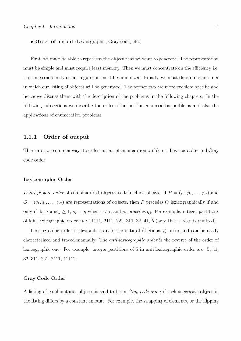
1.1.1 Order of output
There are two common ways to order output of enumeration problems. Lexicographic and Gray
code order.
Lexicographic Order
Lexicographic order of combinatorial objects is defined as follows. If P = (p1, p2, . . . , ps′) and
Q = (q1, q2, . . . , qs′′) are representations of objects, then P precedes Q lexicographically if and
only if, for some j ≥ 1, pi = qi when i < j, and pj precedes qj. For example, integer partitions
of 5 in lexicographic order are: 11111, 2111, 221, 311, 32, 41, 5 (note that + sign is omitted).
Lexicographic order is desirable as it is the natural (dictionary) order and can be easily
characterized and traced manually. The anti-lexicographic order is the reverse of the order of
lexicographic one. For example, integer partitions of 5 in anti-lexicographic order are: 5, 41,
32, 311, 221, 2111, 11111.
Gray Code Order
A listing of combinatorial objects is said to be in Gray code order if each successive object in
the listing differs by a constant amount. For example, the swapping of elements, or the flipping
1.1. Enumeration Problems 5
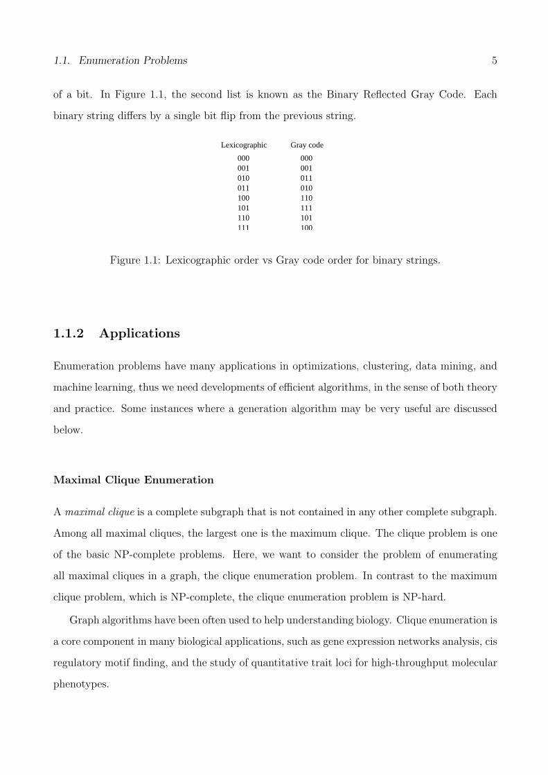
of a bit. In Figure 1.1, the second list is known as the Binary Reflected Gray Code. Each
binary string differs by a single bit flip from the previous string.
Lexicographic Gray code
000000001 001010 011
010011110100
101 111101110
111 100
Figure 1.1: Lexicographic order vs Gray code order for binary strings.
1.1.2 Applications
Enumeration problems have many applications in optimizations, clustering, data mining, and
machine learning, thus we need developments of efficient algorithms, in the sense of both theory
and practice. Some instances where a generation algorithm may be very useful are discussed
below.
Maximal Clique Enumeration
A maximal clique is a complete subgraph that is not contained in any other complete subgraph.
Among all maximal cliques, the largest one is the maximum clique. The clique problem is one
of the basic NP-complete problems. Here, we want to consider the problem of enumerating
all maximal cliques in a graph, the clique enumeration problem. In contrast to the maximum
clique problem, which is NP-complete, the clique enumeration problem is NP-hard.
Graph algorithms have been often used to help understanding biology. Clique enumeration is
a core component in many biological applications, such as gene expression networks analysis, cis
regulatory motif finding, and the study of quantitative trait loci for high-throughput molecular
phenotypes.

Chapter 1. Introduction 6
Generating Subsets
A subset describes a selection of objects, where the order among them does not matter. Many
algorithmic problems seek the best subset of a group of things: vertex cover seeks the smallest
subset of vertices to touch each edge in a graph; knapsack seeks the most profitable subset of
items of bounded total size; and set packing seeks the smallest subset of subsets that together
cover each item exactly once. There are 2n distinct subsets of an n-element set, including the
empty set as well as the set itself. This grows exponentially, but at a considerably smaller rate
than the n! permutations of n items. For example, the set {1, 2, 3} has 8 subsets:
{}, {1}, {2}, {3}, {1, 2}, {2, 3}, {1, 3}, {1, 2, 3}
Generating Partitions
There are two different types of combinatorial objects denoted by the term “partition”, namely
integer partitions and set partitions. These terms are described below:
• Integer partitions of n are sets of nonzero integers that add up to exactly n. For exam-
ple, the seven distinct integer partitions of 5 are {5}, {4, 1}, {3, 2}, {3, 1, 1}, {2, 2, 1},{2, 1, 1, 1}, and {1, 1, 1, 1, 1}. An interesting application that requires the generation of
integer partitions is in a simulation of nuclear fission. When an atom is smashed, the
nucleus of protons and neutrons is broken into a set of smaller clusters. The sum of the
particles in the set of clusters must equal the original size of the nucleus. As such, the
integer partitions of this original size represent all the possible ways to smash the atom.
• Set partitions divide the elements 1, . . . , n into nonempty subsets. For example, there
are fifteen distinct set partitions of n = 4: {1234}, {123, 4}, {124, 3}, {12, 34}, {12, 3, 4},{134, 2}, {13, 24}, {13, 2, 4}, {14, 23}, {1, 234}, {1, 23, 4}, {14, 2, 3}, {1, 24, 3}, {1, 2, 34},and {1, 2, 3, 4}. The problem of set partitions have many applications in vertex coloring,
connected components, etc.

1.2. Challenges 7
1.1.3 Goals of an Enumeration Algorithm
Any algorithm for generating all objects of a particular combinatorial class has to achieve a
number of goals or aims. We list the most important ones below.
• Reduce the time complexity,
• Minimize the usage of memory,
• Reduce the amount of output,
• Avoid duplications, and
• Avoid omissions.
In this thesis, we have considered each of these goals while we develop our algorithms. To
achieve the goals, we have developed efficient representations of objects, efficient data structure
for storage, and clever algorithmic techniques. We will address the issues mentioned above
while we describe our algorithms in detail in later chapters.
1.2 Challenges
In this section we discuss the main challenges that any algorithm for enumerating combinatorial
objects must face [S97]. We have considered all these challenges while developing our algorithms
in this thesis and have given algorithmic techniques that successfully resolve the difficulties
mentioned in the following subsections.
1.2.1 Time Complexity
The number of different objects is very large in many cases. For example, the number of
different permutations of n numbers is exponential. Therefore, to generate all the objects of
a particular combinatorial class, we may have to find an exponential number of objects. That
means, the overall time complexity of the algorithm is at best exponential, which means the

Chapter 1. Introduction 8
generation of individual objects must be very efficient. There are a number of techniques that
accomplish the task. We mention some of those techniques in Section 1.4.
1.2.2 Avoiding Duplications
In any enumeration algorithm, we must have a way to avoid generation of redundant objects.
One way to avoid duplications of objects is to store each object generated so far and check each
newly generated object with all the previous one to find whether the newly generated one is a
duplication. This way of checking duplications has two problems. First, the time complexity
goes up. Second, the space requirement becomes very high. We mention some alternatives for
avoiding duplications in Section 1.4.
1.2.3 I/O Operations
Algorithms that solve enumeration problems are generally I/O intensive and the output of the
algorithm dominates the running time. This is because the number of objects generated is
exponential in many cases and each of these objects must be output to an output device. Since
I/O is slower than computation, the more I/O operations an algorithm performs the slower it
becomes. For this reason reducing the amount of output is essential.
1.2.4 Exhaustive Generation
While we exhaustively generate combinatorial objects, we must have an efficient way to deter-
mine the end of generation. One solution to this problem is that we count the number of objects
generated so far and check whether we have explored all the possibilities. But this works only
in the case where we know in advance the total number of distinct objects to be generated and
have an efficient way for detecting repetitions. For many problems, it may be difficult to know
or calculate the exact number objects that will be generated. For example, it is not trivial to
count the number of different triangulations of a given arbitrary plane graph.

1.3. Algorithms for Enumeration Problems 9
1.3 Algorithms for Enumeration Problems
There are a number of standard methods that are in use for solving enumeration problems. As
mentioned in previous sections, there are some difficulties that any enumeration algorithm must
resolve somehow. These challenges include reducing the amount of output, efficient checking
for duplications and omissions, space complexity etc. Different methods have different ways of
dealing with these challenges.
Classical method algorithms first generate combinatorial objects allowing duplications, but
output only if the object has not been output yet. These methods require huge space to store
the list of objects generated so far. Furthermore, checking whether the newly generated object
will be output takes a lot of time.
Orderly methods algorithms [M98] need not to store the list of objects generated so far,
they output an object only if it is a canonical representation of an isomorphism class.
Reverse search method algorithms also need not to store the list. The idea is to implicitly
define a connected graph H such that the vertices of H correspond to the graphs with the given
property, and the edges of H correspond to some relation between the graphs. By traversing
an implicitly defined spanning tree of H, one can find all the vertices of H, which correspond
to all the graphs with the given property.
In the following two subsections, we describe in more detail two other methods for solving
enumeration problems and address the techniques employed by these methods for resolving the
challenges mentioned above.
1.3.1 Combinatorial Gray Code Approach
To generate all the objects of a particular class, one approach is to try to generate the objects as
a list in which successive elements differ only in a small way. The term Combinatorial Gray Code
first appeared in [JWW80] and is now used to refer to any method for generating combinatorial
objects so that successive objects differ in some prespecified, usually small, way. Savage [S97]
gives a description of the state of the art of the area. The advantages anticipated by such

Chapter 1. Introduction 10
gray code approach are manifold. First, generation of successive objects is faster, since each
object is generated from the preceding one by making constant number of changes. Secondly,
the number of objects in a particular class is generally exponential. Generating algorithms
thus produce huge outputs in general, and the output dominates the running time. If we can
reduce the amount of output, the efficiency of the algorithm improves considerably. So in gray
code approach, each object is output as a difference from the preceding one, thus removing the
necessity to output the entire object. Thirdly, gray codes typically involve elegant recursive
constructions provide new insights into the structure of combinatorial families.
There are many problems that can be solved using combinatorial gray code approach. We
list some of them below.
1. Listing all permutations of 1, . . . , n.
2. Listing all k element subsets of an n element set,
3. Listing all binary trees,
4. Listing all spanning trees of a graph,
5. Listing all partitions of an integer n, and
6. Listing linear extensions of certain posets etc.
n=3
123132312321231213
n=2
1221
n=4
1234 432134213241
1243142341234132143213421324314234124312
23142341243142314213241321432134
Figure 1.2: Generating permutations using gray code approach: Johnson-Trotter scheme.

1.3. Algorithms for Enumeration Problems 11
One particular algorithm for generating all permutations of n elements, based on combinato-
rial gray code approach, is the Johnson-Trotter algorithm. Johnson and Trotter independently
showed that it is possible to generate permutations by transpositions even the two elements
exchanged are required to be in adjacent positions [T62, J63]. The recursive scheme, as shown
in Figure 1.2, inserts into each permutation on the list for n1 the element ’n’ in each of the
possible n positions, moving alternately from right to left, then from left to right.
1.3.2 Family Tree Approach
In the family tree or genealogical tree approach, a hierarchical structure or tree structure es-
tablished among the members of a particular combinatorial class. The idea is to find a unique
parent-child relationship among the objects such that one object can be generated from its
parent by making a minimal amount of changes. The main feature of this approach is that the
entire list of objects need not be in the memory at once for checking duplications. The objects
are generated in the order they are present in the family tree and generation rule itself ensures
that no omissions occur. The space complexity for this approach is also linear in the size of
an individual object. The main challenge in solving an enumeration problem by family tree
approach is to establish a unique parent-child relationship among the objects of interest. For
many problems, finding a suitable parent-child relationship may be extremely difficult.
There are a number of problems that have been solved by the family tree approach [KN05,
NU03, NU04]. Figure 1.3 illustrates the family tree developed by Kawano and Nakano [KN05]
for their algorithm for generating all set partitions.
The drawback of family tree approach is that to build a family tree we have to define both
parent-child and child-parent relationship. Moreover, the recursive traversal of family tree
yields an average constant time algorithm. But for enumeration problems, most of the cases
we want a constant time solution in ordinary sense. Hence intensive research has been made
on the traversal of family tree. Kawano and Nakano [KN05] gave a tree traversal algorithm
which generates each solution in constant time but the overall time complexity is same as the
ordinary traversal. In this thesis we present a new elegant tree traversal algorithm which is

Chapter 1. Introduction 12
11123
1122311213
1212311231 11233
12133
12313
12213
12231
12132
12312 12232 12233
12332 12333
12223
11232
12331
12113
12131
12311
12321 12322 12323
Figure 1.3: Illustration of the family tree for all set partitions.
constant time per solution and also overall time complexity of the algorithm is less than that
of ordinary traversal.
1.4 Scope of this Thesis
In this section we list the algorithms we have developed in this thesis. We follow the family
tree approach of solving enumeration problems. We invent new approaches to establish gray
code among the solutions using family tree approach for solving enumeration problems. We
concentrate on the efficiency improvement of the algorithms and invent new approaches to solve
enumeration problems such that each solution is generated in constant time (in ordinary sense).
1.4.1 Distribution of Objects to Bins
The first problem that we consider is to generate all distributions of n identical objects to m
bins. In this thesis, we give an algorithm to generate all such distributions without repetition.
Our algorithm generates each distribution in constant time with linear space complexity. We
also present an efficient tree traversal algorithm that generates each solution in O(1) time. To
the best of our knowledge, our algorithm is the first algorithm which generates each solution

1.4. Scope of this Thesis 13
in O(1) time in ordinary sense. By modifying our algorithm, we can generate the distributions
in anti-lexicographic order. Finally, we extend our algorithm for the case when the bins have
priorities associated with them. Overall space complexity of our algorithm is O(m), where m
is the number of bins. We give the detailed algorithms in Chapter 3.
1.4.2 Distribution of Distinguishable Objects to Bins
The second problem that we consider in this thesis is to generate all distributions of distin-
guishable objects to bins. Our algorithm generates each distribution in constant time without
repetition. To the best of our knowledge, our algorithm is the first algorithm which generates
each solution in O(1) time in ordinary sense. As a byproduct of our algorithm, we get a new
algorithm to enumerate all multiset partitions when the number of partitions is fixed and the
partitions are numbered. In this case, our algorithm generates each multiset partition in con-
stant time (in ordinary sense). Finally, we extend our algorithm for the case when the bins have
priorities associated with them. Overall space complexity of our algorithm is O(km), where
there are m bins and the objects fall into k different classes. We give the detailed algorithm in
Chapter 4.
1.4.3 Evolutionary Trees
In this thesis, we also deal with the problem of generating all evolutionary trees. Generating
all evolutionary trees among different species have many applications in Bioinformatics [JP04],
Genetic Engineering [KR03], Archaeology, Biochemistry and Molecular Biology. We first give
an algorithm to generate all such evolutionary trees with n species. Our algorithm is simple
and generates each tree in linear time without repetition (O(1) time in amortized sense). We
give the detailed algorithm in Chapter 5.

Chapter 1. Introduction 14
1.4.4 Labeled and Ordered Evolutionary Trees
In this thesis, we also give an efficient algorithm to generate all evolutionary trees with fixed
and ordered number of leaves. The order of the species is based on evolutionary relationship
and phylogenetic structure. A species is more related to its preceding and following species
in the sequence of species than other species in the sequence. We also find out a suitable
representation of such trees. We represent a labeled and ordered evolutionary tree with n
leaves by a sequence of (n − 2) numbers. Our algorithm generates all such trees in constant
time (on average) without repetition. We give the detailed algorithm in Chapter 6.
1.5 Summary
In this thesis we develop efficient algorithms for generating all distributions of objects to bins.
We generate distributions of both identical and distinguishable objects in O(1) time per distri-
bution. We also develop a technique for efficient family tree traversal such that each solution
is generated in constant time in ordinary sense). We also give an algorithm to generate all
evolutionary trees having n species without repetition. We find out an efficient representation
of such evolutionary trees such that each tree is generated in constant time on average. For the
purposes of biologists, we also give two new algorithms to generate evolutionary trees having
ordered species and satisfying some distance constraints. Our main results can be divided into
three parts.
The first part of the results is about the distributions of identical objects to bins. We give
an efficient algorithm that generates all distributions of n objects to m bins where the objects
are identical. The algorithm generates each distribution in constant time (in ordinary sense).
We also present an efficient tree traversal algorithm that generates each solution in O(1) time.
Our new results together with known ones are listed in Table 1.1.
The second part of the results deals with generating all distributions of n distinguishable
objects to m bins where the objects fall into k different classes. The algorithms generates each
distribution in constant time (in ordinary sense) from its previous one using linear space only.

1.5. Summary 15
Criteria Klingsberg Our algorithm
[K82]
Generation time Average constant Ordinary Constant
per object
Space complexity O(m) O(m)
Requires searching? YES NO
Table 1.1: Results on distribution of identical objects to bins.
Criteria Kawano and Nakano Our algorithm
[KN06]
Generates Multiset partitions Distributions of distinguishable
objects to bins
Generation time O(k) Ordinary Constant
per object
Space complexity O(km) O(km)
Table 1.2: Results on distribution of distinguishable objects to bins.
Criteria Nakano and Uno Our algorithm
[NU04]
Generates Rooted trees Labeled and ordered
with n nodes evolutionary trees
Generation time Average constant Average constant
per object
Redundant Objects YES NO
Table 1.3: Results on generating evolutionary trees.

Chapter 1. Introduction 16
This new result together with known ones is listed in Table 1.2.
The third part of our results is on bioinformatics. We give a linear time algorithm to
generate all evolutionary trees. We also find out an efficient representation of an evolutionary
tree having ordered species. We give a new algorithm to generate all evolutionary trees having
n ordered species. The algorithm is simple, generates each tree in constant time on average.
Our new results together with known ones are listed in Table 1.3.

Chapter 2
Preliminaries
In this chapter we define some basic terms of graph theory and algorithms. Definitions which
are not included in this chapter will be introduced as they are needed. We start, in Section 2.1,
by giving definitions of some standard graph theoretical terms used throughout the remainder
of this thesis. We describe some notions from complexity theory in Section 2.2. Sections 2.3
deals with a well known graph traversal algorithm. Finally, Section 2.4 deals with the Catalan
Families of combinatorial objects.
2.1 Basic Terminology
In this section we give definitions of some theoretical terms used throughout the remainder of
this thesis.
2.1.1 Graphs
A graph G is a structure (V,E) which consists of a finite set of vertices V and a finite set of
edges E; each edge is an unordered pair of distinct vertices. We denote the set of vertices of
G by V (G) and the set of edges by E(G). Figure 2.1 illustrates an example of a graph. An
edge connecting vertices vi and vj in V is denoted by (vi, vj). An edge (vi, vj) is called a loop if
17

Chapter 2. Preliminaries 18
vi = vj. A graph is called a simple graph if there is no loop or multiple edges between any two
vertices in G. The degree of a vertex v is the number of edges incident to v in G.
Figure 2.1: Illustration of a graph.
2.1.2 Paths and Cycles
A v0−vl walk, v0, e1, v1, . . . , vl−1, el, vl, in G is an alternating sequence of vertices and edges of G,
beginning and ending with a vertex, in which each edge is incident to two vertices immediately
preceding and following it. If the vertices v0, v1, . . . , vl are distinct (except possibly v0, vl), then
the walk is called a path and usually denoted either by the sequence of vertices v0, v1, . . . , vl or
by the sequence of edges e1, e2, . . . , el. The length of the path is l, one less than the number of
vertices on the path. A path or walk is closed if v0 = vl. A closed path containing at least one
edge is called a cycle.
2.1.3 Trees
A tree is a connected graph containing no cycle. Figure 2.2 is an example of a tree. The
vertices in a tree are usually called nodes . A rooted tree is a tree in which one of the nodes is
distinguished from the others. The distinguished node is called the root of the tree. The root
of a tree is generally drawn at the top. In Figure 2.2, the root is v1. Every node u other than
the root is connected by an edge to some other node p called the parent of u. We also call u
a child of p. We draw the parent of a node above that node. For example, in Figure 2.2, v1 is
the parent of v2, v3 and v4, while v2 is the parent of v5 and v6; v2, v3 and v4 are children of v1,

2.1. Basic Terminology 19
while v5 and v6 are children of v2. A leaf is a node of a tree that has no children. An internal
node is a node that has one or more children. Thus every node of a tree is either a leaf or an
internal node. In Figure 2.2, the leaves are v4, v5, v6, v7 and v8, and the nodes v1, v2 and v3
are internal nodes.
v1
v2 v3 v4
v6 v7 v8v5
Figure 2.2: Illustration of a tree.
The parent child relationship can be extended naturally to ancestors and descendants. Sup-
pose that u1, u2, . . . , ul is a sequence of nodes in a tree such that u1 is the parent of u2, which
is a parent of u3, and so on. Then node u1 is called an ancestor of ul and node ul a descendant
of u1. The root is an ancestor of every node in a tree and every node is a descendant of the
root. In Figure 2.2, all seven nodes are descendants of v1, and v1 is an ancestor of all nodes.
The height of a node u in a tree is the length of a longest path from u to a leaf. The height
of the tree is the height of the root. The depth of a node u in a tree is the length of a path from
the root to u. The level of a node u in a tree is the height of the tree minus the depth of u. In
Figure 2.2, for example, node v2 is of height 1, depth 1 and level 1. The tree in Figure 2.2 has
height 2.
2.1.4 Binary Trees
A binary tree is either a single node or consists of a node and two subtrees rooted at the node,
both of the subtrees are binary trees. Figure 2.3 illustrates a binary tree of 15 nodes.
A complete binary tree is a rooted tree with each internal node having exactly two children.
Chapter 2. Preliminaries 20
v1
v3v2
v4 v5 v6 v7
Figure 2.3: Illustration of a binary tree.
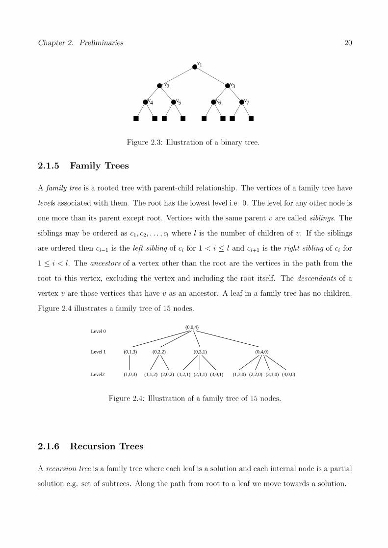
2.1.5 Family Trees
A family tree is a rooted tree with parent-child relationship. The vertices of a family tree have
levels associated with them. The root has the lowest level i.e. 0. The level for any other node is
one more than its parent except root. Vertices with the same parent v are called siblings. The
siblings may be ordered as c1, c2, . . . , cl where l is the number of children of v. If the siblings
are ordered then ci−1 is the left sibling of ci for 1 < i ≤ l and ci+1 is the right sibling of ci for
1 ≤ i < l. The ancestors of a vertex other than the root are the vertices in the path from the
root to this vertex, excluding the vertex and including the root itself. The descendants of a
vertex v are those vertices that have v as an ancestor. A leaf in a family tree has no children.
Figure 2.4 illustrates a family tree of 15 nodes.
Level 0
Level 1
Level2 (4,0,0)(3,1,0)(2,2,0)(1,3,0)(2,0,2)(1,1,2)
(0,3,1)(0,2,2)
(0,0,4)
(1,2,1) (2,1,1) (3,0,1)
(0,4,0)
(1,0,3)
(0,1,3)
Figure 2.4: Illustration of a family tree of 15 nodes.
2.1.6 Recursion Trees
A recursion tree is a family tree where each leaf is a solution and each internal node is a partial
solution e.g. set of subtrees. Along the path from root to a leaf we move towards a solution.

2.1. Basic Terminology 21
2.1.7 Evolutionary Trees
An evolutionary tree is a graphical representation of the evolutionary relationship among three
or more species. In a rooted evolutionary tree, the root corresponds to the most ancient ancestor
in the tree and the path from the root to a leaf in the rooted tree is called an evolutionary
path. Leaves of evolutionary trees correspond to the existing species while internal vertices
correspond to hypothetical ancestral species.
2.1.8 Integer Partition
Given an integer n, it is possible to represent it as the sum of one or more positive integers xi,
i.e., n = x1 + x2 + . . . + xm for 1 ≤ m ≤ n. This representation is called an integer partition if
x1 ≥ x2 ≥ . . . ≥ xm. For example, there are seven distinct partitions of the integer 5:
5, 4+1, 3+2, 3+1+1, 2+2+1, 2+1+1+1, 1+1+1+1+1.
2.1.9 Set Partition
For a positive integer n and k < n, set partition is the set of all partitions of {1, 2, . . . , n} into
k non-empty subsets. For instance, for n = 4 and k = 2 there are seven such partitions:
{1, 2, 3}∪ {4}, {1, 2, 4}∪ {3}, {1, 3, 4}∪ {2}, {2, 3, 4}∪ {1}, {1, 2}∪ {3, 4}, {1, 3}∪{2, 4}, {1, 4} ∪ {2, 3}, {1, 4} ∪ {2, 3}.
2.1.10 Multiset
A multiset is a set of elements where all the elements are not identical. The elements of a
multiset fall into different classes where the elements in the same class are identical but are
distinguishable from those of other classes. For example, {1,1,2,3,1,3,2,2} is an example of
multiset.

Chapter 2. Preliminaries 22
2.1.11 Simpleset
A simple set is a set of elements where all the elements are identical. By simple set we naturally
mean a set. For example, a set of apples, a set of graphs etc.
2.2 Algorithms and Complexity
In this section we briefly introduce some terminologies related to complexity of algorithms.
The most widely accepted complexity measure for an algorithm is the running time, which
is expressed by the number of operations it performs before producing the final answer. The
number of operations required by an algorithm is not the same for all problem instances. Thus,
we consider all inputs of a given size together, and we define the complexity of the algorithm
for that input size to be the worst case behavior of the algorithm on any of these inputs. Then
the running time is a function of size n of the input.
2.2.1 The notation O(n)
In analyzing the complexity of an algorithm, we are often interested only in the ”asymptotic
behavior”, that is, the behavior of the algorithm when applied to very large inputs. To deal
with such a property of functions we shall use the following notations for asymptotic running
time. Let f(n) and g(n) are the functions from the positive integers to the positive reals, then
we write f(n) = O(g(n)) if there exists positive constants c1 and c2 such that f(n) ≤ c1g(n)+c2
for all n. Thus the running time of an algorithm may be bounded from above by phrasing like
”takes time O(n2)”.
2.2.2 Polynomial algorithms
An algorithm is said to be polynomially bounded (or simply polynomial) if its complexity is
bounded by a polynomial of the size of a problem instance. Examples of such complexities are
O(n), O(nlogn), O(n100), etc. The remaining algorithms are usually referred as exponential or
2.2. Algorithms and Complexity 23
non-polynomial. Example of such complexity are O(2n), O(n!), etc.
When the running time of an algorithm is bounded by O(n), we call it a linear time algorithm
or simply a linear algorithm.
2.2.3 Constant Time
In computational complexity theory, constant time refers to the computation time of a problem
when the time needed to solve that problem doesn’t depend on the size of the data that is given
as input. Constant time is notated as O(1).
For example, accessing the elements in the array takes constant time as we can pick up an
element using the index and start working with it. However finding the minimum value in an
array is not a constant time operation as we need to scan each element of the array and then
decide the minimum of those elements. Hence it is a linear time operation and takes O(n) time.
2.2.4 Average Constant Time
In computational complexity theory, average constant time refers to the computation time of
a problem when the time needed to generate all the solutions of that problem depends on the
size of the data that is given as input but the computational time per solution is constant when
averaged over all solutions.
For example, in depth first search(DFS) traversal of a tree, the time required to visit all
nodes in the tree depends on the size of the tree. The computation time per node is constant
if averaged over all nodes. Hence DFS traversal is average constant.
2.2.5 Amortized Time
In analysis of algorithms, amortized analysis refers to finding the average running time per
operation over a worst-case sequence of operations. Amortized analysis differs from average-
case performance in that probability is not involved; amortized analysis guarantees the time
per operation over worst-case performance.

Chapter 2. Preliminaries 24
2.3 Graph Traversal Algorithm
When designing algorithms on graphs, we often need a method for exploring the vertices and
edges of a graph. In this section we describe such a method named depth first search (DFS). In
DFS each edge is traversed exactly once in the forward and reverse directions and each vertex
is visited. Thus DFS runs in linear time on average. We now describe the method.
Consider visiting the vertices of a graph G in the following way. We select and visit a
starting vertex v. Then we select any edge (v, w) incident on v and visit w. In general, suppose
x is the most recent visited vertex. The search is continued by selecting some unexplored edge
(x, y) incident on x. If y has been previously visited, we find another new edge incident on
x. If y has not been visited previously, then we visit y and begin a new search starting at
y. After completing the search through all paths beginning at y, the search returns to x, the
vertex from which y was first reached. The process of selecting unexplored edges incident to x
is continued until the list of these edges is exhausted. This method is called depth first search
since we continue searching in the deeper direction as long as possible.
If the graph G is a tree, then we can order the vertices based on the way the edges are
chosen to be traversed. Consider a vertex v from which a new edge would be explored and
another vertex would be reached. We mark a vertex u when we first reach u and call the label
of u the rank of u. The rank of the root of the tree is 0. So the rank of a vertex u is the
number of vertices explored before u is reached for the first time. Such a traversal is called a
pre-order traversal of the vertices of the tree. If a vertex u is labeled after all vertices located
in the subtree rooted at u are labeled, then the traversal is called post-order traversal. In case
of a binary tree, if the vertex u is labeled after all vertices located in the left subtree rooted at
u are labeled, but before all vertices located in the right subtree rooted at u are labeled, then
the traversal is called in-order traversal.

2.4. Catalan Families 25
2.4 Catalan Families
In several families of combinatorial objects, the size of the class is bounded by the Catalan
Numbers, defined for n ≥ 0 by
Cn =1
n + 12nCn (2.1)
These include binary trees on n vertices, well formed sequence of 2n parentheses, and
triangulations of a labeled convex polygon with n + 2 vertices. There exist bijections between
the members of the Catalan family [CLR90]. Therefore, enumeration algorithm for one member
of the family gives implicitly a listing scheme for every other member of the family.

Chapter 3
Distribution of Objects to Bins
3.1 Introduction
In computer science, we frequently need to count things and generate solutions. The science of
counting is captured by a branch of mathematics called combinatorics. A well known counting
problem is counting the number of ways objects can be distributed among bins [AU95, R00].
The paradigm problem is counting the number of ways of distributing fruits to children. For
example, Kathy, Peter and Susan are three children. We have four apples to distribute among
them without cutting apples into parts. In how many ways the children receive apples?
To solve the counting problem mentioned above, we have four letters A’s representing apples
and two *’s which will represent partitions between the apples belonging to different children.
We order the A’s and *’s as we like and interpret all A’s before the first * as being apples
belonging to Kathy. Those A’s between two *’s belonging to Peter, and the A’s after the
second * are apples belonging to Susan. For instance, AA*A*A represents the distribution
(2, 1, 1), where Kathy gets two apples and the other two children gets one each. Thus, each
distribution of apples to bins is associated with a unique string of four A’s and two *’s. How
many such strings are there? The number of such string is equal to the number of permutations
of those 6 letters. This number is 6!4!2!
. So, the solution for m bins and n objects is (n+m−1)!n!(m−1)!
[AU95, R00]. Thus we count the number of distributions. However, in this thesis we are not
26

3.1. Introduction 27
interested in counting the number of distributions, rather we are interested in generating all
distributions.
Let, D(n,m) represents the set of all distributions of n objects to m bins where each bin gets
zero or more objects. For the previous example, we have D(4, 3) representing all distributions.
Now, let, (i, j, k) represent the situation in which Kathy receives i apples, Peter receives j, and
Susan receives k. The 6!4!2!
= 15 possibilities are -
(0,0,4) (0,1,3) (0,2,2) (0,3,1) (0,4,0) (1,0,3) (1,1,2) (1,2,1) (1,3,0) (4,0,0) (2,0,2)
(2,1,1) (2,2,0) (3,0,1) (3,1,0)
It is useful to have the complete list of all solutions. One can use such a list to search
for a counter-example to some conjecture, to find best solution among all solutions or to test
and analyze an algorithm for its correctness or computational complexity. Many algorithms
to generate a particular class of objects without repetition, are already known [KN05, ZS98,
NU03, YN04, FL79, NU04, NU05, BS94].
There are many applications of distribution of objects to bins. In these days of automa-
tion, machines may require to distribute objects among candidates optimally. Generating all
distribution has many applications in computer science also. In computer networks suppose
there are several communication channels and several processes wants to use the channels. We
can think of communication channels as our symbolic objects and the processes as bins. To
find out which distribution is better taking into account congestion, QoS, channel capacity and
different factors, we may need to calculate these values for each solution. Then we may choose
the optimal one and the next distributions may depend on this distribution i.e. we may want
associate priority with processes. Generating all distributions has also applications in client-
server broker distributed architecture, CPU scheduling, memory management, multiprocessor
systems, etc. [T02, T04].
In this thesis we first consider the problem of generating all possible distributions. The
main challenges in finding algorithms for enumerating all distributions are as follows. Firstly,
the number of such distributions is exponential in general and hence listing all of them requires
huge time and computational power. Secondly, generating algorithms produce huge outputs

Chapter 3. Distribution of Objects to Bins 28
and the outputs dominate the running time. For this reason, reducing the amount of output is
essential. Thirdly, checking for any repetitions must be very efficient. Storing the entire list of
solutions generated so far will not be efficient, since checking each new solution with the entire
list to prevent repetition would require huge amount of memory and overall time complexity
would be very high. So, if we can compress the outputs, then it considerably improves the
efficiency of the algorithm. Therefore, many generating algorithms output objects in an order
such that each object differs from the preceding one by a very small amount, and output each
object as the “difference” from the preceding one. Such orderings of objects are known as Gray
codes [S97, KN05, R00].
The problem of generating all distributions of n objects to m bins can be viewed as generat-
ing integer partition of the integer n when there are m partitions, and the partitions are “fixed”,
“numbered” and “ordered”. That means the number of partitions is fixed, the partitions are
numbered and the assigned numbers are not altered. Zoghbi and Stojmenovic [ZS98] gave an
algorithm to generate integer partitions with a specified order of generation (lexicographic and
anti-lexicographic) but their partitions are not fixed, numbered and ordered. Moreover, their
algorithm does not allow empty partitions. Kawano and Nakano [KN05] generated all set par-
titions where the number of partitions are fixed but the subsets are not numbered or ordered.
They used efficient generation method based on the family tree structure of the solutions. If
we apply their method to this problem then we have to number the subsets. Then we have to
permutate the numbers that we have assigned to the subsets. Since the objects in this problem
are identical, permutating the assigned numbers leads to repetition when any two of the subsets
contain same number of objects. Thus modifying their algorithm we cannot solve our problem
of generating distributions.
Klingsberg [K82] gave an algorithm for sequential listing of the composition of an integer
n into k parts. The algorithm keeps pointers to the first and second nonzero elements in the
sequence. Then by incrementing and decrementing the proper elements in the sequence their
algorithm generates solutions. Their method is straight forward but requires searching for the
second nonzero element in the sequence, for the solutions having a nonzero as the first element.

3.1. Introduction 29
Hence their algorithm cannot generate each solution in O(1) time in ordinary sense, rather the
cost per generation is constant averaging over all solutions in D(n,m).
In this thesis we first give a new algorithm to generate all distributions of n objects to m bins
without repetition. Here, the number of bins are fixed and the bins are numbered and ordered.
The algorithm is simple and generates each distribution in constant time on average without
repetition. Our algorithm, generates a new distribution from an existing one by making a
constant number of changes and outputs each distribution as the difference from the preceding
one. The main feature of our algorithm is that we define a tree structure, that is parent-child
relationships, among those distributions (see Figure 3.1). In such a “tree of distributions”, each
node corresponds to a distribution of objects to bins and each node is generated from its parent
in constant time. In our algorithm, we construct the tree structure among the distributions in
such a way that the parent-child relation is unique, and hence there is no chance of producing
duplicate distributions. Our algorithm also generates the distributions in place, that means,
the space complexity is only O(m).
Level 0
Level 1
Level2 (4,0,0)(3,1,0)(2,2,0)(1,3,0)(2,0,2)(1,1,2)
(0,3,1)(0,2,2)
(0,0,4)
(1,2,1) (2,1,1) (3,0,1)
(0,4,0)
(1,0,3)
(0,1,3)
Figure 3.1: The Family Tree T4,3.
Later, we give a new algorithm to traverse the tree efficiently. This algorithm outputs
each distributions in constant time in ordinary sense (not in average sense). Thus we can
regard the derived sequence of the outputs as a combinatorial Gray code [S97, KN05, R00] for
distributions. To the best of our knowledge, our algorithm is the first algorithm to generate all
distribution in constant time per distribution in ordinary sense. Our algorithm also generates
distributions with a specified order of generation. By using this algorithm we can generate
integer partitions in anti-lexicographic order when the partitions are fixed and ordered. Then,
we extend our algorithm for the case when the bins have priorities associated with them. In

Chapter 3. Distribution of Objects to Bins 30
this case, the bins are numbered in the order of priority. The sequence of generations maintain
an order so that the generations maintain priority.
The rest of the chapter is organized as follows. Section 3.2 gives some definitions. Sec-
tion 3.3 deals with generating all distributions of objects to bins. In Section 3.4, we present
the improved tree traversal algorithm that generates each solution in O(1) time. Section 3.5
generates distributions in anti-lexicographic order. In Section 3.6, we consider the case when
priorities are associated with bins. Finally Section 3.7 is a conclusion. Our results presented in
this chapter are to appear in [AR06].
3.2 Preliminaries
In this section we define some terms used in this chapter.
Let G be a connected graph with n vertices. A tree is a connected graph without cycles.
A rooted tree is a tree with one vertex r chosen as root. A leaf in a tree is a vertex of degree
1. Each vertex in a tree is either an internal vertex or a leaf. A family tree is a rooted tree
with parent-child relationship. The vertices of a rooted tree have levels associated with them.
The root has the lowest level i.e. 0. The level for any other node is one more than its parent
except root. Vertices with the same parent v are called siblings. The siblings may be ordered
as c1, c2, . . . , cl where l is the number of children of v. If the siblings are ordered then ci−1 is the
left sibling of ci for 1 < i ≤ l and ci+1 is the right sibling of ci for 1 ≤ i < l. The ancestors of a
vertex other than the root are the vertices in the path from the root to this vertex, excluding
the vertex and including the root itself. The descendants of a vertex v are those vertices that
have v as an ancestor. A leaf in a family tree has no children.
Given an integer n, it is possible to represent it as the sum of one or more positive integers
xi, i.e., n = x1 + x2 + . . . + xm for 1 ≤ m ≤ n. This representation is called an integer partition
if x1 ≥ x2 ≥ . . . ≥ xm. For example, there are seven distinct partitions of the integer 5:
5, 4+1, 3+2, 3+1+1, 2+2+1, 2+1+1+1, 1+1+1+1+1.

3.2. Preliminaries 31
For a positive integer n and k < n, set partition is the set of all partitions of {1, 2, . . . , n}into k non-empty subsets. For instance, for n = 4 and k = 2 there are seven such partitions:
{1, 2, 3}∪ {4}, {1, 2, 4}∪ {3}, {1, 3, 4}∪ {2}, {2, 3, 4}∪ {1}, {1, 2}∪ {3, 4}, {1, 3}∪{2, 4}, {1, 4} ∪ {2, 3}, {1, 4} ∪ {2, 3}.
For positive integers n and m, let, A ∈ D(n,m) be a distribution of n objects to m bins.
The bins are ordered and numbered as B1, B2, . . . , Bm. For each A ∈ D(n,m), we define a
unique sequence of positive integers (a1, a2, . . . , am), where ai represents number of objects in
ith bin Bi, for 1 ≤ i ≤ m. The sequence for A is unique for each distribution because the
bins are ordered and numbered. For example, (0, 0, 4) represents there are 3 bins and 4 objects
and third bin contains 4 objects and the rest of the bins are empty (see Figure 3.2). We can
observe that for each sequence a1 + a2 + . . . + am = n. This equality holds because the number
of objects are fixed and we have to place every object to some bins.
����
����
���
������
���
(0,0,4)
Figure 3.2: Representation of a distribution of 4 objects to 3 bins.
Lexicographic order for distribution of objects is defined as follows. If P = (p1, p2, . . . , pm)
and Q = (q1, q2, . . . , qm) are sequences for two distributions, then P precedes Q lexicographically
if and only if, for some k, pk < qk and pi = qi for all 1 ≤ i ≤ (k − 1). For example,
the distributions of 4 objects to 3 bins in lexicographic order are: (0, 0, 4), (0, 1, 3), (0, 2, 2),
(0, 3, 1), (0, 4, 0) and so on. The anti-lexicographic order is the reverse of lexicographic one. The
distributions in antilexicographic order are: (4, 0, 0), (3, 1, 0), (3, 0, 1), (2, 2, 0), (2, 1, 1) and so
on.
A listing of distributions is said to be in gray code order if each successive sequences for
distributions in the listing differs by a constant amount. For example, the swapping of elements,
or the flipping of a bit. In this chapter, we establish such an ordering of all distribution of objects

Chapter 3. Distribution of Objects to Bins 32
to bins so that each distribution can be generated by making constant amount of changes to
the preceding distribution in the order.
3.3 Generating Distribution of Objects to Bins
In this section we give an algorithm to generate all distributions of identical objects to bins. For
that purpose we define a unique parent-child relationship among the distributions in D(n,m)
so that the relationship among the distributions can be represented by a tree with a suitable
distribution as the root. Figure 3.1 shows such a tree of distributions of 4 objects and 3 bins.
Once such a parent-child relationship is established, we can generate all the distributions in
D(n,m) using the relationship. We do not need to build or store the entire tree of distributions
at once, rather we generate each distribution in the order it appears in the tree structure.
In Section 3.3.1 we define a tree structure among distributions in D(n,m) and in Section
3.3.2 we present our algorithm which generates each solution in O(1) time on average.
3.3.1 The Family Tree
In this section we define a tree structure Tn,m among distributions in D(n,m).
For positive integers n and m, let, A ∈ D(n,m) be a distribution of n objects to B1, B2, . . . , Bm
bins. For each A ∈ D(n,m) we get a unique sequence (a1, a2, . . . , am) where ai represents num-
ber of objects in ith bin, for 1 ≤ i ≤ m. Note that, for each sequence a1 + a2 + · · ·+ am = n.
Now we define the family tree Tn,m as follows. Each node of Tn,m represents a distribution. If
there are m bins then there are m levels in Tn,m. A node is in level i in Tn,m if a1, a2, . . . , am−i−1 =
0 and am−i 6= 0 for 0 ≤ i < m. As the level increases the number of leftmost 0 decreases and
vice versa. Thus a node at level m − 1 has no leftmost 0 before leftmost nonzero integer i.e.
a1 6= 0. Since Tn,m is a rooted tree we need a root and the root is a node at level 0. One can
observe that a node is at level 0 in Tn,m if a1, a2, . . . , am−1 = 0 and am 6= 0. In this case, am = n
and there can be exactly one such node. We thus take the sequence (0, 0, . . . , 0, n) as the root
of Tn,m. Clearly, the number of leftmost 0 before any nonzero integer in root is greater than

3.3. Generating Distribution of Objects to Bins 33
that of any other sequence for any distribution in D(n,m).
To construct Tn,m, we define two types of relations among the distributions in D(n,m):
(a) Parent-child relationship and
(b) Child-parent relationship.
We define the parent-child relationships among the distributions in D(n,m) with two goals
in mind. First, the difference between a distribution A and its child C(A) should be minimum,
so that C(A) can be generated from A by minimum effort. Second, every distribution in
D(n,m) must have a parent except the root and only one parent in Tn,m. We achieve the first
goal by ensuring that the child C(A) of a distribution A can be found by simple subtraction.
That means A can also be generated from its child C(A) by simple addition. The second goal,
that is the uniqueness of the parent-child relationship is illustrated in the following subsections.
Parent-Child Relationship
Let A ∈ D(n,m) be a sequence (a1, a2, . . . , am) and it corresponds to a node of level i, 0 ≤ i < m
of Tn,m. So, we have a1, a2, . . . , am−i−1 = 0 and am−i 6= 0 for 0 ≤ i < m. The number of children
it has is equal to am−i. The sequence of the children are defined in such a way that to generate
a child from its parent we have to deal with only two integers in the sequence and the rest of the
integers remain unchanged. The two integers are determined by the level of parent sequence in
Tn,m. The operations we apply to these two integers are only subtraction and assignment. The
number of leftmost 0 decreases in the child sequence by applying parent-child relationship.
Let Cj(A) ∈ D(n,m) be the sequence of jth child, 1 ≤ j ≤ am−i of A. Note that A is in
level i of Tn,m and Cj(A) will be in level i + 1 of Tn,m. We define the sequence for Cj(A) as
(c1, c2, . . . , cm−i−1, cm−i, . . . , cm), where 0 ≤ i < m, c1 = c2 = . . . = cm−i−2 = 0, cm−i−1 = j,
cm−i = am−i− j and ck = ak for m− i+1 ≤ k ≤ m. Thus, we observe that Cj is a node of level
i + 1, 0 ≤ i < m − 1 of Tn,m and so c1, c2, . . . , cm−i−2 = 0 and cm−i−1 6= 0 for 0 ≤ i < m − 1.
So, for each consecutive level we only deal with two numbers am−i−1 and am−i and the rest of
the integers remain unchanged. For example, the solution (0, 0, 4), for n = 4 and m = 3, is a

Chapter 3. Distribution of Objects to Bins 34
node of level 0 because a1 = 0, a2 = 0 and a3 6= 0. Here, am−i = 4 so it has 4 children and the
four children are shown in Figure 3.1.
Child-Parent Relationship
The child-parent relation is just the reverse of parent-child relation. Let, A ∈ D(n,m) be a
sequence (a1, a2, . . ., am) and it corresponds to a node of level i, 1 ≤ i < m of Tn,m. So, we
have a1, a2, . . . , am−i−1 = 0 and am−i 6= 0 for 0 < i < m. We define a unique parent sequence
of A at level i − 1 of Tn,m. Like the parent-child relationship here we also deal with only two
integers in the sequence. The operations we apply to these two integers are only addition and
assignment. The number of leftmost 0 increases in the parent sequence by applying child-parent
relationship.
Let P (A) ∈ D(n,m) be the parent sequence of A. We define the sequence for P (A) as (p1, p2,
. . ., pm−i, pm−i+1, . . ., pm) where 1 ≤ i < m, p1 = p2 = . . . = pm−i = 0, pm−i+1 = am−i +am−i+1,
and pj = aj for m − i + 1 < j ≤ m. Thus, we observe that P (A) is a node of level i − 1,
1 ≤ i < m of Tn,m and so p1, p2, . . . , pm−i = 0 and pm−i+1 6= 0 for 1 ≤ i < m. For example, the
solution (0, 3, 1), for n = 4 and m = 3, is a node of level 1 because a1 = 0 and a2 6= 0. It has a
unique parent (0, 0, 4) as shown in Figure 3.1.
The Family Tree
From the above definitions we can construct Tn,m. We take the sequence Ar = a1, a2, . . . , am
as root where a1, a2, . . . , am−1 = 0 and am = n as we mentioned before. The family tree
Tn,m for the distributions in D(n,m) is shown in Figure 3.1. Based on the above parent-child
relationship, the following lemma proves that every distribution in D(n,m) is present in Tn,m.
Lemma 3.3.1 For any distribution A ∈ D(n,m), there is a unique sequence of distributions
that transforms A into the root Ar of Tn,m.
Proof. Let A ∈ D(n,m) be a sequence, where A is not the root sequence. By applying
child-parent relationship, we find the parent sequence P (A) of the sequence A. Now if P(A)
3.3. Generating Distribution of Objects to Bins 35
is the root sequence, then we stop. Otherwise, we apply the same procedure to P (A) and
find its parent P (P (A)). By continuously applying this process of finding the parent sequence
of the derived sequence, we have the unique sequence A,P (A), P (P (A)), . . . of sequences in
D(n,m) which eventually ends with the root sequence Ar of Tn,m. We observe that P (A) has
at least one zero more than A in its sequence. Thus A,P (A), P (P (A)), . . . never lead to a cycle
and the level of the derived sequence decreases which ends up with the level of root sequence
Ar. Q.E .D.
Lemma 3.3.1 ensures that there can be no omission of distributions in the family tree Tn,m.
Since there is a unique sequence of operations that transforms a distribution A ∈ D(n,m) into
the root Ar of Tn,m, by reversing the operations we can generate that particular distribution,
staring from root. Now we have to make sure that Tn,m represents distributions without rep-
etition. Based on the parent-child and child-parent relationships, the following lemma proves
this property of Tn,m.
Lemma 3.3.2 The family tree Tn,m represents distributions in D(n,m) without repetition.
Proof. Given a sequence A ∈ D(n,m), the children of A are defined in such a way that
no other sequence in D(n,m) can generate same child. For contradiction let two sequences
A,B ∈ D(n,m) are at level i of Tn,m and generate same child C. So, C is a sequence of
level i + 1 of Tn,m. The sequences for A, B and C are aj, bj and cj for 1 ≤ j ≤ m. Clearly,
ak = bk = 0 for 1 ≤ k ≤ m− i−1. According to parent-child relationship, we have ak = bk = ck
for m−i+1 ≤ k ≤ m because only two integers in the sequence are changed and the rest remain
unchanged. From the above two equations we have ak = bk for k 6= m − i and 1 ≤ k ≤ m.
Note that, a1 + a2 + . . . + am = n = b1 + b2 + . . . + bm. Substituting the values for ak and bk
for k 6= m− i and 1 ≤ k ≤ m and simplifying yields am−i = bm−i. So, ak = bk for 1 ≤ k ≤ m.
This implies that A and B are same sequence. By contradiction, every sequence has a single
and unique parent. Q.E .D.

Chapter 3. Distribution of Objects to Bins 36
3.3.2 The Algorithm
In this section we give an algorithm to construct Tn,m and generate all distributions.
If we can generate all child sequences of a given sequence in D(n, m), then in a recursive
manner we can construct Tn,m and generate all sequence in D(n,m). We have the root sequence
Ar = (0, . . . , 0, n). We get the child sequence Ac by using the parent to child relation discussed
above.
Procedure Find-All-Child-Distributions(A = (a1, a2, . . . , am), i)
{ A is the current sequence, i indicates the current level and Ac is the child sequence }begin
1 Output A {Output the difference from the previous distribution}2 for j = 1 to am−i
3 Find-All-Child-Distributions( Ac = (a1, a2, . . . , am−i−2, j, (am−i−j), . . . , am), i+1)
4 end;
5 Algorithm Find-All-Distributions(n,m)
6 begin
7 Find-All-Child-Distributions( Ar = (0, . . . , 0, n), 0 )
8 end.
The following theorem describes the performance of the algorithm Find-All-Distributions.
Theorem 3.3.3 The algorithm Find-All-Distributions runs in O(|D(n,m)|) time and uses
O(m) space.
Proof. In our algorithm we only use the simple addition or subtraction operation to
generate a new distribution from an old one. Thus each distribution is generated in constant
time without computational overhead. Since we traverse the family tree Tn,m and output each
sequence at each corresponding vertex of Tn,m we can generate all the sequences in D(n,m)
without repetition. By applying parent to child relation we can generate every child in O(1)

3.4. Efficient Tree Traversal 37
time. Then by using child to parent relation we go back to the parent sequence. Hence, the
algorithm takes O(|D(n,m)|) time i.e. constant time on average for each output.
Our algorithm outputs each distribution as the difference from the previous one. The data
structure that we use to represent the distribution is a sequence of integers where each integer
represents the number of objects in a particular bin. Therefore, the memory requirement is
O(m), where m is the number of bins. Q.E .D.
3.4 Efficient Tree Traversal
The algorithm in Section 3.3 generates all sequences in D(n,m) in O(|D(n,m)|) time. Thus
the algorithm generates each sequence in O(1) time “on average”. However, after generating
a sequence corresponding to the last vertex in the largest level in a large subtree of Tn,m, we
have to merely return from the deep recursive call without outputting any sequence and hence
we cannot generate each sequence in O(1) time (in ordinary sense). In this section we present
the improved tree traversal algorithm that generates each solution in O(1) time (in ordinary
sense).
To make the algorithm efficient we introduce two additional types of relations:
(i) Relationship between left sibling and right sibling and
(ii) Leaf-ancestor relationship.
In Section 3.4.1 we define the relationship between left sibling and right sibling, in Section
3.4.2, we illustrate the leaf-ancestor relationship and in Section 3.4.3 we present our efficient
tree traversal algorithm.
3.4.1 Relationship Between Left Sibling and Right Sibling
The relationship between left sibling and right sibling is defined with two goals in mind. First,
the difference between a distribution A and its right sibling As should be minimum if right
sibling exists, so that As can be generated from A by minimum effort. Second, the steps

Chapter 3. Distribution of Objects to Bins 38
needed to go back to parent and then generate next child must be reduced. We achieve the first
goal by ensuring that the right sibling As of a distribution A can be found by simple increment
and decrement operation. The second goal, that is reduction of steps is achieved by directly
moving to next child sequence from the current sequence. That means, we do not have to go
back to parent to generate the next child. This saves two extra steps needed to generate the
next child.
Let A ∈ D(n,m) be a sequence (a1, a2, . . . , am) and it corresponds to a node of level i,
1 ≤ i < m of Tn,m. So, we have a1, a2, . . . , am−i−1 = 0 and am−i 6= 0 for 1 ≤ i < m. We say the
right sibling As ∈ D(n,m) of node A exists if am−i+1 6= 0 at level i of Tn,m. Then we call the
sequence A the left sibling of As.
We define the sequence for As as (s1, s2, . . . , sm−i, sm−i+1, . . . , sm), 1 ≤ i < m, where s1 =
s2 = . . . = sm−i−1 = 0, sm−i = am−i−1, sm−i+1 = am−i+1 +1 and sj = aj for m− i+2 ≤ j ≤ m.
That means, to obtain As from A, we decrement am−i by one and increment am−i+1 by one and
the rest of the integers remain unchanged. For example, in Figure 3.3 the solution (0, 0, 3, 1) is
a node of level 1 and it has a right sibling (0, 0, 4, 0).
Level 0
Level 1
Level2
Level 3
(0,0,1,3)
(0,1,0,3)
(1,0,0,3) (3,0,0,1)(2,1,0,1)(1,2,0,1)(2,0,1,1)(1,1,1,1)(1,0,2,1) (4,0,0,0)
(0,0,4,0)
(0,3,0,1)(0,1,2,1) (0,2,1,1)
(0,0,3,1)
(0,1,1,2)
(1,0,1,2) (2,0,0,2)(1,1,0,2)
(0,0,2,2)
(0,2,0,2)
(0,0,0,4)
Figure 3.3: Efficient Traversal of the family tree T4,4.
3.4.2 Leaf-Ancestor Relationship
To avoid returning from deep recursive call without outputting any sequence, we define leaf-
ancestor relationship. After generating the sequence Al of the last vertex in the largest level
i.e. rightmost leaf, we do not return to parent. Instead, we return to the nearest ancestor

3.4. Efficient Tree Traversal 39
Aa which has right sibling. By rightmost leaf we mean that leaf which has no right sibling.
Thus this leaf-ancestor relation saves many non generation steps. Another reason of defining
leaf-ancestor relationship is that the nearest ancestor can be generated from the leaf sequence
by a simple swap operation between two integers in the sequence. The other integers in the
sequence remain unchanged.
Let Al ∈ D(n,m) be a sequence (a1, a2, . . . , am) of leaf and it corresponds to a node of level
m − 1 of Tn,m. So, we have a1 6= 0. We say that the ancestor sequence Aa ∈ D(n,m) of node
Al exists if a2 = 0 i.e. A has no right sibling. We define the ancestor sequence Aa of Al at level
m − 1 − k if a2 = a3 = . . . = ak+1 = 0 and ak+2 6= 0. The sequence for nearest ancestor Aa
is determined by the number of consecutive 0’s after a1 in the sequence for Al. We denote the
number such 0’s in the sequence Al as k. This k will determine the level and sequence of the
nearest ancestor Aa which has right sibling.
We define the sequence for Aa as (s1, s2, . . . , sk, sk+1, . . . , sm), where s1 = s2 = . . . = sk = 0
and sk+1 = a1 and sj = aj for k + 1 < j ≤ m. In other words, to obtain Aa from Al, we swap
a1 and ak+1 and the rest of the integers remain unchanged. One can observe that the sequence
Aa is at level m− 1− k of Tn,m. For example, in Figure 3.3 the solution (3,0,0,1) is a node of
level 3 and it has a nearest ancestor (0,0,3,1) which is obtained by swapping first integer 3 and
third integer 0. We have the following lemma on the nearest ancestor Aa of Al.
Lemma 3.4.1 Let Al be a leaf sequence of Tn,m having no right sibling. Then Al has a unique
ancestor sequence Aa in Tn,m. Furthermore, either Aa has a right sibling in Tn,m or Aa is the
root Ar of Tn,m.
Proof. Let the sequence for Al ∈ D(n,m) be (a1, a2, . . . , am) and it corresponds to a node
of level m− 1 of Tn,m. Note that a1 6= 0 and a2 = 0. We get the sequence for Aa by swapping
a1 and ak+1 where k is the number of consecutive 0’s after a1. Clearly Aa is an ancestor of
Al. Note that Aa is at level m− 1− k. By Lemma 3.2, parent-child relation is unique. Hence
by repeatedly applying child-parent relation on Al, we will reach a unique ancestor at level
m − 1 − k. For k = m − 1, one can observe that we get the root sequence Ar by swapping

Chapter 3. Distribution of Objects to Bins 40
a1 and am. For 1 ≤ k < m − 1, we get the unique ancestor sequence Aa which has a right
sibling. Q.E .D.
Lemma 3.4.1 ensures that Al has a unique ancestor Aa. As we see later Aa plays an
important role in our algorithm. Note that, we may need to return to ancestor Aa if current
node is a leaf Al and for a leaf sequence Al we have a1 6= 0. Aa is obtained from Al by swapping
a1 and ak+1 where k is the number of consecutive 0’s after a1. Now, to find out k we have
to search the sequence Al from a1 to ak+1 such that a2 = a3 = . . . = ak+1 = 0 and a1 6= 0,
ak+2 6= 0. We reduce the complexity of searching by keeping extra information as shown in
Figure 3.4 (for simplicity we omit the separators). The information consists of the number of
subsequences of consecutive 0’s and the number of 0’s in each subsequence after am−i, where i
is the current level. For this we keep a stack of size m/2. The top of the stack determines the
current k. Initially the stack is empty. As soon as we find a zero, when moving from parent
to child or left sibling to right sibling, we push a 1 on the stack. We increment the top of the
stack for consecutive 0’s. We make a pop operation when we apply the leaf-ancestor relation.
The stack operations are shown in Figure 3.5. One can observe that there can be at most m/2
subsequences of consecutive 0’s in a sequence of size m. Therefore, in worst case we need a
stack of size m/2.
Level 0
Level 1
Level2 400,2310,1301,1
013,_
103,1 112,_ 202,1
022,_ 031,_ 040,1
220,1130,1211,_
004,_
121,_
Figure 3.4: Efficient Traversal of T4,3 keeping extra information.
3.4.3 The Efficient Algorithm
In this section we present an efficient algorithm to generate all distributions in D(n,m). We
use three relations in this algorithm, they are parent-child relation, relation between left sibling

3.4. Efficient Tree Traversal 41
0040,
0130,
1030,
0004,
1
1
11
Level 0
Level 1
Level2
Level 3 4000,3100,2200,1300,
0220, 0310, 0400,1 1 2
2 2 2 3
Figure 3.5: Use of stack for tree traversal (T4,4).
and right sibling and leaf-ancestor relation. By applying parent-child relation, we go from root
down the family tree Tn,m until we reach leaf at level m − 1. Then we apply the relationship
between left sibling and right sibling to traverse horizontally until we reach a node which has
no right sibling. Then by applying leaf-ancestor relation, we return to that nearest ancestor
which has sibling. Then we again apply relation between left sibling and right sibling. The
sequence of applying relationships and generating distributions continues until we reach root.
This algorithm thus reduces non-generation steps and generates each sequence in O(1) time (in
ordinary sense).
Procedure Find-All-Child-Distributions2(A = (a1, a2, . . . , am), i)
{ A is the current sequence }begin
1 Output A {Output the difference from the previous distribution}2 if A has child then
3 Generate first child Ac;
4 Find-All-Child-Distributions2(Ac, i + 1);
5 else if A has right sibling then
6 Generate right sibling As;
7 Find-All-Child-Distributions2(As, i);
8 else
9 Generate that ancestor Aa at level i− k which has right sibling or which is root;

Chapter 3. Distribution of Objects to Bins 42
10 if Aa is root at level 0
11 then done
12 else
13 Generate right sibling Aas of Aa;
14 Find-All-Child-Distributions2(Aas, i− k);
15 end;
16 Algorithm Find-All-Distributions2(n,m)
17 begin
18 Find-All-Child-Distributions2( Ar = (0, . . . , 0, n), 0 );
19 end.
The tree traversal according to the efficient algorithm is depicted in Figure 3.3. For a
sequence we need O(m) space and additional m/2 space is required for stack manipulation.
Hence the algorithm takes O(m) space. One can observe that the algorithm generates all
sequences such that each sequence in Tn,m can be obtained from the preceding one by at most
two operations. Note that if A corresponds to a vertex v of Tn,m, which has no child and no
sibling, we need two steps, one for tracing its ancestor and the other for tracing ancestor’s right
sibling. Otherwise, we need only one step to generate the next sequence. Thus the algorithm
generates each sequence in O(1) time per sequence. Note that each sequence is similar to the
preceding one, since it can be obtained by at most two operations (see Figure 3.6). Thus, we can
regard the derived sequence of the sequences as a combinatorial Gray code [S97, KN05, R00]
for distributions. Thus we have the following theorem.
Theorem 3.4.2 The algorithm Find-All-Distributions2 uses O(m) space and generates
each distribution in D(n,m) in constant time (in ordinary sense).

3.5. Distributions in Anti-lexicographic Order 43
(0,0,4)
(0,1,3)
(1,0,3)
(0,2,2)
(1,1,2)
(2,0,2)
(0,3,1)
(1,2,1)
(2,1,1)
(3,0,1)
(0,4,0)
(1,3,0)
(2,2,0)
(3,1,0)
(4,0,0)
Figure 3.6: A Gray code for D(4, 3).
3.5 Distributions in Anti-lexicographic Order
In this section we describe how our algorithm generates distributions in anti-lexicographic order.
By using this technique, we can also generate integer partitions in anti-lexicographic order when
the partitions are fixed and ordered.
Our algorithm generates distributions with a specified order of generation. For positive
integers n and m, let A ∈ D(n,m) be a distribution of n objects to m bins. The bins are
ordered and numbered as B1, B2, . . . , Bm. We generate the distributions in an order such that
the rightmost bin gets the highest number of objects at first and the leftmost bin gets the
lowest. The number of objects in the rightmost bin decreases with the sequence of generations.
In the last distribution, the leftmost bin gets the highest number of objects and the rightmost
bin gets lowest. We find that in our generation if we reverse the order of the bins then we will
get the generation in anti-lexicographic order. The algorithm will be same as the previous case
but only the order of the bins will reverse. The anti-lexicographic order of generation is shown
in Figure 3.7.
Level 0
Level 1
Level2 004013103
310
301 211 202
220 130 040
022031121 112
400
Figure 3.7: Illustration of generation of D(4, 3) in anti-lexicographic order.

Chapter 3. Distribution of Objects to Bins 44
3.6 Generating Distributions with Priorities to Bins
In this section we consider the case when priorities are associated with bins. The sequence of
generations will maintain an order such that the bin with highest priority gets highest objects
at first and then the priorities of the bins are decreased one by one. The sequence of generations
maintain an order so that generations can maintain priority.
Our algorithm generates distributions with a specified order of generation. For positive
integers n and m, let A ∈ D(n,m) be a distribution of n objects to m bins. The bins are
ordered and numbered as B1, B2, . . . , Bm which have priorities as p1, p2, . . . , pm. Our order of
generation is such that the rightmost bin gets the highest number of objects at first and the
leftmost bin gets the lowest. The number of objects in the rightmost bin decreases with the
sequence of generations. The last distribution ensures that the leftmost bin gets the highest
number of objects and the rightmost bin gets lowest. We find that in our generation if the
bins are ordered according to their priorities in ascending order then we will get the generation
that maintains priority. That means the highest priority bin gets the highest objects at first
and the number of objects decreases with the generations. The algorithm will be same as the
previous case but only the order of the bins will be such that the following inequality holds:
p1 ≤ p2 ≤ . . . ≤ pm. The generation is similar to Figure 3.3.
3.7 Conclusion
In this chapter we give a simple algorithm to generate all distributions in D(n,m). The al-
gorithm generates each distribution in constant time with linear space complexity. We also
present an efficient tree traversal algorithm that generates each solution in O(1) time. Then,
we describe a method to generate distributions in anti-lexicographic order. Finally, we extend
our algorithms for the case when the bins have priorities associated with them. The main
feature of our algorithms is that they are constant time solution which is a very important
requirement for generation problems.

Chapter 4
Distribution of Distinguishable Objects
to Bins
4.1 Introduction
In the previous chapter, we gave efficient algorithms to generate all distributions of objects to
bins where the objects where identical. In this chapter we generalize the problem by considering
non-identical objects. Non-identical objects fall into different classes and we call such objects
as “distinguishable objects”.
Let there are m bins and n distinguishable objects where the objects fall into k different
classes. Objects within a class are identical with each other, but are distinguishable from those
of other classes. Let, nj represent the number of objects in the jth class where 1 ≤ j ≤ k. The
paradigm problem is distributing different types of fruits to children. Suppose we have three
apples, two pears and a banana to distribute to Kathy, Peter and Susan. Then m = 3, which
is the number of children. There are k = 3 groups, with n1 = 3, n2 = 2, and n3 = 1. Since
there are 6 objects in total, so n = 6.
Now the question is - Can we count the number of solutions? For identical objects, the
number of distributions for m bins and n identical objects is (n+m−1)!n!(m−1)!
[AU95, R00, AR06]. To
45

Chapter 4. Distribution of Distinguishable Objects to Bins 46
solve the counting problem for distinguishable objects, we use this formula. For distinguishable
objects, we first distribute the fruits of class 1 to all the bins. The number of such distributions
with n1 objects and m bins is (n1+m−1)!n1!(m−1)!
. Then we distribute the objects of second class and
so on upto kth class. Thus the total number of distributions will be the product of all these
solutions as in the following expression:
(n1 + m− 1)!
n1!(m− 1)!.(n2 + m− 1)!
n2!(m− 1)!. . . .
(nk + m− 1)!
nk!(m− 1)!
Let D(n,m, k) represents the set of all distributions of n objects to m bins where the
objects fall into k different classes and each bin gets zero or more objects. For the previous
example, we have D(6, 3, 3) representing all distributions where the number of distribution
is 8!3!2!
. 7!2!2!
. 6!1!2!
= 1524096000. Thus we count the number of distributions. However, in this
thesis we are not interested in counting the number of distributions, rather we are interested
in generating all distributions.
It is useful to have the complete list of all solutions. One can use such a list to search
for a counter-example to some conjecture, to find best solution among all solutions or to test
and analyze an algorithm for its correctness or computational complexity. Many algorithms
to generate a particular class of objects without repetition, are already known [AR06, KN05,
ZS98, NU03, YN04, FL79, NU04, NU05, BS94].
There are many applications of distribution of objects to bins. In these days of automa-
tion, machines may require to distribute objects among candidates optimally. Generating all
distribution has many applications in computer science also. In computer networks suppose
there are several communication channels and several processes wants to use the channels. We
can think of communication channels with different bandwidth as our symbolic objects and
the processes as bins. To find out which distribution is better taking into account congestion,
QoS, channel capacity and different factors, we may need to calculate these values for each
solution. Then we may choose the optimal one and the next distributions may depend on this
distribution i.e. we may want associate priority with processes. Generating all distributions
has also applications in client-server broker distributed architecture, CPU scheduling, memory
management, multiprocessor systems, etc. [T02, T04].

4.1. Introduction 47
Generally, generating algorithms produce huge outputs, and the outputs dominate the run-
ning time of the generating algorithms. So, if we can compress the outputs, then it considerably
improves the efficiency of the algorithm. Therefore, many generating algorithms output solu-
tions in an order such that each solution differs from the preceding one by a very small amount,
and output each solution as the “difference” from the preceding one. Such orderings of solutions
are known as Gray codes [S97, KN05, AR06].
Klingsberg [K82] gave an average constant time algorithm for sequential listing of the com-
position of an integer n into k parts. Using efficient tree traversal technique, we improved the
time complexity to constant time (in ordinary sense) and gave an efficient algorithm to generate
all distribution of identical objects to bins in the previous chapter. We used efficient generation
method based on the family tree structure of the distributions. However, in this chapter we
are interested in generating all distributions of distinguishable objects. This problem becomes
more difficult than the identical case since the solution space is large. If we apply the algorithm
for identical objects for distinguishable objects, there will be omission of distributions. Hence
the algorithm for generating identical objects is not applicable for distinguishable objects.
The problem of generating all distribution of distinguishable objects can be viewed as gen-
erating multiset partitions when the partitions are “fixed”, “numbered” and “ordered”. That
means the number of partitions is fixed, the partitions are numbered and the assigned numbers
to bins are not altered. There is no known algorithm that generates all multiset partitions
in constant time. So, our algorithm is the first algorithm that generates multiset partitions
in constant time when the partitions are fixed, numbered and ordered. Kawano and Nakano
[KN06] gave an algorithm to generate multiset partition but the algorithm is complex and does
not give solutions in constant time in ordinary sense. Their algorithm is based on family tree
recombination and generates solutions in O(k) time where there are k types of elements in the
set. Their method is not applicable here since the partitions are fixed, ordered and numbered.
On the other hand, our algorithm is simple and generates each solution in constant for fixed,
numbered and ordered partitions.
In this chapter we give an algorithm to generate all distributions of n distinguishable objects

Chapter 4. Distribution of Distinguishable Objects to Bins 48
to m bins where the objects fall into k different classes. Here, the number of bins is fixed and
the bins are numbered and ordered. The algorithm is simple and generates each distribution
in constant time on average without repetition. Our algorithm, generates a new distribution
from an existing one by making a constant number of changes and outputs each distribution
as the difference from the preceding one. The main feature of our algorithm is that we define
a tree structure, that is parent-child relationships, among those distributions (see Figure 4.1).
In such a “tree of distributions”, each node corresponds to a distribution of objects to bins and
each node is generated from its parent in constant time. In our algorithm, we construct the tree
structure among the distributions in such a way that the parent-child relation is unique, and
hence there is no chance of producing duplicate distributions. Our algorithm also generates the
distributions in place, that means, the space complexity is linear.
Level 1
((1,0),(1,0),(0,1))
((1,0),(0,1),(1,0)) ((0,1),(1,0),(1,0)) ((1,1),(0,0),(1,0))
Level 0 ((0,0),(0,0),(2,1))
((0,0),(1,0),(1,1))
((1,0),(0,0),(1,1))
((0,0),(2,0),(0,1)) ((0,0),(2,1),(0,0))
((2,0),(0,0),(0,1)) ((0,1),(0,0),(2,0))
((0,0),(0,1),(2,0)) ((0,0),(1,1),(1,0))
((2,0),(0,1),(0,0)) ((0,1),(2,0),(0,0))((1,0),(1,1),(0,0)) ((1,1),(1,0),(0,0)) ((2,1),(0,0),(0,0))
Level 2
Figure 4.1: The Family Tree T3,3,2.
Later, we give a new algorithm to traverse the tree efficiently. This algorithm outputs each
distributions in constant time in ordinary sense (not in average sense). Thus we can regard the
derived sequence of the outputs as a combinatorial Gray code [S97, KN05, R00] for distributions.
To the best of our knowledge, our algorithm is the first algorithm to generate all distribution
in constant time per distribution in ordinary sense. Then, we extend our algorithm for the

4.2. Preliminaries 49
case when the bins have priorities associated with them. In this case, the bins are numbered
in the order of priority. The sequence of generations maintain an order so that the successive
generations maintain priority.
The rest of the chapter is organized as follows. Section 4.2 gives some definitions. Section
4.3 deals with generating all distributions of distinguishable objects to bins. In Section 4.4, we
present the improved tree traversal algorithm that generates each solution in O(1) time. In
Section 4.5, we consider the case when priorities are associated with bins. Finally Section 4.6
is a conclusion.
4.2 Preliminaries
In this section we define some terms used in this chapter.
Let G be a connected graph with n vertices. A tree is a connected graph without cycles.
A rooted tree is a tree with one vertex r chosen as root. A leaf in a tree is a vertex of degree
1. Each vertex in a tree is either an internal vertex or a leaf. A family tree is a rooted tree
with parent-child relationship. The vertices of a rooted tree have levels associated with them.
The root has the lowest level i.e. 0. The level for any other node is one more than its parent
except root. Vertices with the same parent v are called siblings. The siblings may be ordered
as c1, c2, . . . , cl where l is the number of children of v. If the siblings are ordered then ci−1 is the
left sibling of ci for 1 < i ≤ l and ci+1 is the right sibling of ci for 1 ≤ i < l. The ancestors of a
vertex other than the root are the vertices in the path from the root to this vertex, excluding
the vertex and including the root itself. The descendants of a vertex v are those vertices that
have v as an ancestor. A leaf in a family tree has no children.
For a positive integer n and k < n, set partition is the set of all partitions of {1, 2, . . . , n}into k non-empty subsets. For instance, for n = 4 and k = 2 there are seven such partitions:
{1, 2, 3}∪ {4}, {1, 2, 4}∪ {3}, {1, 3, 4}∪ {2}, {2, 3, 4}∪ {1}, {1, 2}∪ {3, 4}, {1, 3}∪{2, 4}, {1, 4} ∪ {2, 3}, {1, 4} ∪ {2, 3}.
A simple set is a set of elements where all the elements are identical. A multiset is a set of

Chapter 4. Distribution of Distinguishable Objects to Bins 50
elements where all the elements are not identical. The elements of a multiset fall into different
classes where the elements in the same class are identical but are distinguishable from those of
other classes. For example, {1,1,2,3,1,3,2,2} is an example of multiset.
For positive integers n, m and k, let A ∈ D(n,m, k) be a distribution of n objects to m
bins where the objects fall into k classes. Let, nj represent the number of objects in the jth
class where 1 ≤ j ≤ k. Clearly, n1 + n2 + . . . + nk = n since every object must be in a class.
The bins are ordered and numbered as B1, B2, . . . , Bm. Each bin contains objects of different
classes. We order the different types of objects in a bin so that we can keep track of objects
of different classes. For each A ∈ D(n, m, k), we define a unique sequence (a1, a2, . . . , am),
where ai represents an inner sequence of positive integers (ti1, ti2, . . . , tik) where tij represents
the number of objects of jth type in ith bin Bi, for 1 ≤ i ≤ m, 1 ≤ j ≤ k. The sequence for A
is unique for each distribution because the bins are ordered and numbered and also the objects
of different types are ordered. For example, the sequence ((0, 0), (2, 1)) represents there are 2
bins because there are 2 sequence of sequences of integers and 3 objects which is sum of all the
integers in the sequence and there are 2 classes of objects where 2 objects are from class 1 and
1 object from class 2. Also the second bin contains 3 objects i.e. 2 objects from class 1 and 1
object from class 2 and the first bin is empty (see Figure 4.2).
������
������������
������
���
��� ((0,0),(2,1))
Figure 4.2: Representation of a distribution of 3 objects to 2 bins where the objects fall into
two classes and 2 objects from class 1 and 1 object from class 2.
For each such sequence of sequences in D(n,m, k), we have the following equations:
m∑
i=1
k∑
j=1
tij = n, (4.1)
m∑
i=1
tij = nj, for,1 ≤ j ≤ k, and (4.2)

4.3. Generating Distribution of Distinguishable Objects 51
k∑
j=1
nj = n. (4.3)
Equation 4.1 describes that the sum of all the integers in the sequence of sequences in equal
to the total number of objects. This holds because the number of objects are fixed and every
object is distributed somewhere in some bin. In Equation 4.2, we describe that every object
of same kind are present in the sequence. Since every object must be in a class Equation 4.3
holds.
For positive integer k, let a be a sequence of positive integers t1, t2, . . . , tk where tj ≥ 0 for
1 ≤ j ≤ k. We call a as zero sequence if t1 = t2 = · · · = tk = 0. That means all the integers
in a zero sequence are 0. We call a as nonzero sequence if there exists an index j, 1 ≤ j ≤ k,
such that tj 6= 0. That means a sequence is nonzero if at least one of the integers in the
sequence is nonzero. Let b be another sequence of positive integers u1, u2, . . . , uk for 1 ≤ j ≤ k.
By addition of two sequences a + b we mean the addition of corresponding elements tj + uj
where 1 ≤ j ≤ k. Similarly, by subtraction of two sequences a − b we mean the subtraction
of corresponding elements tj − uj where 1 ≤ j ≤ k and by equality of two sequences a = b we
mean the equality of corresponding elements tj = uj where 1 ≤ j ≤ k.
A listing of combinatorial objects is said to be in gray code order if each successive com-
binatorial objects in the listing differs by a constant amount. For example, the swapping of
elements, or the flipping of a bit. In this chapter, we establish such an ordering of all distribu-
tion of objects to bins so that each distribution can be generated by making constant amount
of changes to the preceding distribution in the order.
4.3 Generating Distribution of Distinguishable Objects
In this section we give an algorithm to generate all distributions of distinguishable objects to
bins. For that purpose we define a unique parent-child relationship among the distributions in
D(n,m, k) so that the relationship among the distributions can be represented by a tree with
a suitable distribution as the root. Figure 4.1 shows such a tree of distributions where each

Chapter 4. Distribution of Distinguishable Objects to Bins 52
distribution in the tree is in D(3, 3, 2). Once such a parent-child relationship is established,
we can generate all the distributions in D(n,m, k) using the relationship. We do not need to
build or store the entire tree of distributions at once, rather we generate each distribution in
the order it appears in the tree structure.
In Section 4.3.1 we define a tree structure among distributions in D(n,m, k) and in Section
4.3.2 we present our algorithm which generates each solution in O(1) time on average.
4.3.1 The Family Tree
In this section we define a tree structure Tn,m,k among distributions in D(n,m, k).
For positive integers n, m and k, let, A ∈ D(n,m, k) be a distribution of n objects to
B1, B2, . . . , Bm bins where the objects fall into k classes. Let, nj represent the number of
objects in the jth class where 1 ≤ j ≤ k. From Equation 4.3, n1 + n2 + . . . + nk = n. For each
A ∈ D(n,m, k), we define a unique sequence of sequences of positive integers (a1, a2, . . . , am),
where ai represents a sequence of integers (ti1, ti2, . . . , tik) where tij represents the number of
objects of jth type in ith bin Bi, for 1 ≤ i ≤ m, 1 ≤ j ≤ k.
Now we define the family tree Tn,m,k as follows. Each node in Tn,m,k represents a distribution
in D(n,m, k). If there are m bins then there are m levels in Tn,m,k. A node is in level i, 0 ≤ i < m
in Tn,m,k if tlj = 0 for 1 ≤ j ≤ k, 1 ≤ l < (m− i) and a(m−i) is nonzero sequence. So, a node at
level m− 1 has no leftmost inner zero sequence before leftmost inner nonzero sequence. As the
level increases the number of leftmost inner zero sequence decreases and vice versa. Since the
family tree is a rooted tree we need a root and the root is a node at level 0. One can observe
that a node is at level 0 in Tn,m,k if tlj = 0 for 1 ≤ j ≤ k, 1 ≤ l < (m) and tmj 6= 0 for 1 ≤ j ≤ k.
We also have from Equation 4.1 that∑m
i=1
∑kj=1 tij = n. Substituting the values for tlj for
1 ≤ j ≤ k, 1 ≤ l < (m) we find that∑k
j=1 tmj = n. By using Equation 4.2 and Equation 4.3, we
get tmj = nj where 1 ≤ j ≤ k. Thus we can say that there can be exactly one such node which
is our root. So, the sequence for root is ((0, . . . , 0), (0, . . . , 0), . . . , (0, . . . , 0), (n1, n2, . . . , nk)).
In other words, we can say that the number of leftmost inner zero sequence before any inner
nonzero sequence in root is greater than any other sequence for any distribution in D(n,m, k).

4.3. Generating Distribution of Distinguishable Objects 53
To construct Tn,m,k, we define two types of relationships: (a) Parent-child relationship and
(b) Child-parent relationship among the distributions in D(n,m, k) which are discussed in the
following sections.
Child-Parent Relationship
It is convenient to consider the child-parent relationship before the parent-child relationship.
Let, A ∈ D(n,m, k) be a sequence of sequences (a1, a2, . . . , am) which is not a root sequence,
where al represents a sequence of integers tlj for 1 ≤ j ≤ k, 1 ≤ l ≤ m. The sequence A
corresponds to a node of level i, 1 ≤ i < m. So, we have tlj = 0 for 1 ≤ j ≤ k, 1 ≤ l < (m− i)
and t(m−i) is nonzero sequence. We now define a unique parent sequence of A at level i− 1.
Let, P (A) ∈ D(n,m, k) be the parent sequence of A. We define the sequence for P (A) as
(p1, p2, . . ., pm−i, pm−i+1, . . . ,pm), 1 ≤ i < m where p1 = p2 = . . . = pm−i are zero sequences
and pm−i+1 = am−i + am−i+1 and pl = al for m− i + 1 < l ≤ m. Thus, we observe that P (A) is
a node of level i−1, 1 ≤ i < m and so p1, p2, . . . , pm−i are zero sequences and pm−i+1 is nonzero
sequence for 1 ≤ i < m. Thus for each consecutive level we only deal with two sequences am−i−1
and am−i and the rest of the sequences remain unchanged. The number of leftmost inner zero
sequence increases in the parent sequence by applying child-parent relationship. For example,
the solution ((1, 1), (1, 0)), for n = 3, m = 2, k = 2 and n1 = 2, n2 = 1, is a node of level 1
because a1 is a nonzero sequence. It has a unique parent ((0, 0), (2, 1)) as shown in Figure 4.3.
Parent-Child Relationship
The parent-child relationship is just the reverse of child-parent relationship. Let, A ∈ D(n,m, k)
be a sequence (a1, a2, . . . , am), where al represents a sequence of integers tlj for 1 ≤ j ≤ k,
1 ≤ l ≤ m. The sequence A corresponds to a node of level i, 0 ≤ i < m. So, we have
tlj = 0 for 1 ≤ j ≤ k, 1 ≤ l < (m − i) and a(m−i) is a nonzero sequence. Like the child-
parent relationship here we also deal with only two inner sequences in the sequence. From
the child-parent relationship, one can observe that the number of children of A is equal to
(∏k
j=1(t(m−i)j + 1))− 1.

Chapter 4. Distribution of Distinguishable Objects to Bins 54
Let, Cp(A) ∈ D(n,m, k) be the sequence of pth child, 1 ≤ p ≤ (∏k
j=1(t(m−i)j + 1)) − 1
of A. We define the sequence for Cp(A) as ( c1, c2, . . ., cm−i−1, cm−i, . . ., cm ), 0 ≤ i < m
where c1, c2, . . . , cm−i−2 are zero sequences and cm−i−1 = f(p, am−i), cm−i = am−i − f(p, am−i)
and cl = al for m − i + 1 ≤ l ≤ m, where f(p, am−i) is a sequence of integer dependent
on p and am−i. We define the sequence for f(p, am−i) as i1, i2, . . . , ik and f(p, am−i) generates
(∏k
j=1(t(m−i)j +1))−1 sequences. Thus, we observe that Cp is a node of level i+1, 0 ≤ i < m−1
and so c1, c2, . . . , cm−i−2 are zero sequences and cm−i−1 is nonzero sequence for 0 ≤ i < m− 1.
So, for each consecutive level we only deal with two sequences am−i−1 and am−i and the rest of
the sequences remain unchanged. The number of leftmost zero sequence decreases in the child
sequence by applying parent-child relationship. For example, the solution ((0, 0), (2, 1)), for
n = 3, m = 2, k = 2 and n1 = 2, n2 = 1, is a node of level 0 because a1 is a zero sequence, a2 is
not a zero sequence. Here, (∏k
j=1(t(m−i)j + 1))− 1 = (2 + 1).(1 + 1)− 1 = 5 so it has 5 children
and the five children are ((1,0),(1,1)), ((2,0),(0,1)), ((0,1),(2,0)), ((1,1),(1,0)) and ((2,1),(0,0))
as shown in Figure 4.3.
((1,0),(1,1))
Level 0
Level 1 ((2,0),(0,1)) ((0,1),(2,0)) ((1,1),(1,0)) ((2,1),(0,0))
((0,0),(2,1))
Figure 4.3: The sequence ((0, 0), (2, 1)) has five children.
The Family Tree
From the above definitions we can construct the family tree Tn,m,k. We take the sequence
Ar = a1, a2, . . . , am as root where a1, a2, . . . , am−1 are zero sequences and am = (n1, n2, . . . , nk)
as we mentioned before. The family tree Tn,m,k for the distributions in D(n,m, k) is shown
in Figure 4.1. Based on the above parent-child relationship, the following lemma proves that
every distribution in D(n,m, k) is present in Tn,m,k.
Lemma 4.3.1 For any distribution A ∈ D(n,m, k), there is a unique sequence of distributions
that transforms A into the root Ar of Tn,m,k.

4.3. Generating Distribution of Distinguishable Objects 55
Proof. Let, A ∈ D(n,m, k) be a sequence, where A is not the root sequence. We determine
the level of A in the family tree Tn,m,k. Then by applying child-parent relationship, we find the
parent sequence P (A) of A. Now if P(A) is the root sequence, then we stop. Otherwise, we
apply the same procedure to P (A) and find its parent P (P (A)). By continuously applying this
process of finding the parent sequence of the derived sequence, we have the unique sequence
A,P (A), P (P (A)), . . . of sequences in D(n,m, k) which eventually ends with the root sequence
Ar of Tn,m,k. We observe that P (A) has at least one zero more than A in its sequence. Thus
A,P (A), P (P (A)), . . . never lead to a cycle and the level of the derived sequence decreases
which ends up with the level of root sequence Ar. Q.E .D.
Lemma 4.3.1 ensures that there can be no omission of distributions in the family tree Tn,m,k.
Since there is a unique sequence of operations that transforms a distribution A ∈ D(n,m, k) into
the root Ar of Tn,m,k, by reversing the operations we can generate that particular distribution,
staring from root. We now have to make sure that the family tree Tn,m,k represents distributions
without repetition. Based on the parent-child and child-parent relationships, the following
lemma proves this property of Tn,m,k.
Lemma 4.3.2 The family tree Tn,m,k represents distributions in D(n,m, k) without repetition.
Proof. Given a sequence A ∈ D(n,m, k), the children of A are defined in such a way that no
other sequence in D(n,m, k) can generate same child. Let A,B ∈ D(n, m, k) be two different
sequences at level i of Tn,m,k. For a contradiction, assume that A and B generate the same
child C. Then C is a sequence of level i + 1 of Tn,m,k. The sequences for A, B and C are aj, bj
and cj for 1 ≤ j ≤ m. Clearly, al=bl for 1 ≤ l ≤ m − i − 1 and the parent-child relationship
yields al = bl = cl for m− i + 1 ≤ l ≤ m. Therefore al = bl for l 6= m− i and 1 ≤ l ≤ m. But
we have a1 + a2 + . . . + am = b1 + b2 + . . . + bm by Equation 4.1. Then al must be equal to
bl, for 1 ≤ l ≤ m. This implies that A and B are the same sequence, a contradiction. Hence
every sequence has a single and unique parent. Q.E .D.

Chapter 4. Distribution of Distinguishable Objects to Bins 56
4.3.2 The Algorithm
In this section, we give an algorithm to construct Tn,m,k and generate all distributions.
If we can generate all child sequences of a given sequence in D(n,m, k), then in a recursive
manner we can construct Tn,m,k and generate all sequence in D(n,m, k). We have the root
sequence Ar = ((0, . . . , 0), (0, . . . , 0), . . . , (0, . . . , 0), (n1, n2, . . . , nk)). We get the child sequence
Ac by using the parent to child relation discussed above.
Procedure Find-All-Child-Distributions(A = ( ( t11, t12, . . ., t1k ), ( t21, t22, . . .,
t2k ), . . ., ( tm1, tm2, . . ., tmk ) ), i)
{ A is the current sequence, i indicates the current level, Ac is the child sequence }begin
1 Output A {Output the difference from the previous distribution}2 for ik = 0 to t(m−i)k
3 for ik − 1 = 0 to t(m−i)(k−1)
4 . . .
5 for i1 = 0 to t(m−i)1
6 Find-All-Child-Distributions( Ac = ( ( t11, t12, . . ., t1k ), ( t21, t22, . . ., t2k
), . . ., ( t(m−i−2)1, t(m−i−2)2, . . ., t(m−i−2)k ), ( i1, i2, . . ., ik ), ( t(m−i)1− i1, t(m−i)2− i2,
. . ., t(m−i)k − ik ), . . ., ( tm1, tm2, . . ., tmk ) ), i + 1)
7 end;
8 Algorithm Find-All-Distributions(n,m)
9 begin
10 Find-All-Child-Distributions( Ar = ((0, . . . , 0),(0, . . . , 0),. . .,(0, . . . , 0),(n1,n2,. . . ,
nk)), 0 )
11 end.
Lemma 4.3.1 and 4.3.2 ensure that Algorithm Find-All-Distributions generates all
distributions without repetition. We now have the following theorem.

4.4. Efficient Tree Traversal 57
Theorem 4.3.3 The algorithm Find-All-Distributions runs in O(|D(n,m, k)|) time and
uses O(mk) space.
Proof. We traverse the family tree Tn,m,k and output each sequence at each correspond-
ing vertex of Tn,m,k when we visit the vertex for the first time. Hence, the algorithm takes
O(|D(n,m, k)|) time i.e. constant time on average for each output. Our algorithm outputs
each distribution as the difference from the previous one. The data structure that we use to
represent the distribution is a sequence of sequences of integers where each integer represents
the number of objects a particular class in a particular bin. Therefore, the memory requirement
is O(mk), where k is the number of types of objects and m is the number of bins. Q.E .D.
4.4 Efficient Tree Traversal
The algorithm in Section 4.3 generates all sequences in D(n,m, k) in O(|D(n,m, k)|) time. Thus
the algorithm generates each sequence in O(1) time “on average”. However, after generating
a sequence corresponding to the last vertex in the largest level in a large subtree of Tn,m,k, we
have to merely return from the deep recursive call without outputting any sequence and hence
we cannot generate each sequence in O(1) time (in ordinary sense). In this section we present
the improved tree traversal algorithm that generates each solution in O(1) time (in ordinary
sense).
To make the algorithm efficient we introduce two additional types of relations:
(i) Relationship between left sibling and right sibling and
(ii) Leaf-ancestor relationship.
In Section 4.4.1 we define the relationship between left sibling and right sibling. In Section
4.4.2, we illustrate the leaf-ancestor relationship. Section 4.4.3 shows the data structure that
we use to represent a distribution A ∈ D(n, m, k). Finally, in Section 4.4.4 we present our
efficient tree traversal algorithm.

Chapter 4. Distribution of Distinguishable Objects to Bins 58
4.4.1 Relationship Between Left Sibling and Right Sibling
The relationship between left sibling and right sibling is defined so that the difference between
a distribution A and its right sibling As should be minimum if right sibling exists. Thus As
can be generated from A by minimum effort. To generate right sibling sequence As, if it exists,
from left sibling sequence A using constant number of steps we generate parent from the left
sibling using child-parent relationship. Then we generate the next child using parent-child
relationship. Thus we will always require 2 steps to generate right sibling from left sibling
which is a constant time solution.
Let, A ∈ D(n,m, k) be a sequence of sequences (a1, a2, . . . , am) which is not a root sequence,
where al represents a sequence of integers tlj for 1 ≤ j ≤ k, 1 ≤ l ≤ m. The sequence A
corresponds to a node of level i, 0 ≤ i < m. So, we have tlj = 0 for 1 ≤ j ≤ k, 1 ≤ l < (m− i)
and a(m−i) is not a zero sequence. We say the right sibling, As ∈ D(n,m, k) of this node A
exists if t(m−i+1)j 6= 0 for 1 ≤ j ≤ k at level i. Then we call the sequence A left sibling of As.
We define the sequence for As as s1, s2, . . . , sm−i, sm−i+1, . . . , sm, 1 ≤ i < m where s1, s2,
. . . , sm−i−1 are zero sequences and sj = aj for m− i + 2 ≤ j ≤ m and to find sm−i, sm−i+1 we
apply child-parent relationship and then parent-child relationship. Thus, we observe that As
is a node of level i, 1 ≤ i < m and so s1, s2, . . . , sm−i−1 are zero sequences and sm−i is nonzero
sequence for 1 ≤ i < m. For example, the solution ((0, 0), (1, 0), (1, 1)), for n = 3, m = 3, k = 2
and n1 = 2, n2 = 1, is a node of level 1 because a1 is a nonzero sequence. It has a unique right
sibling ((0, 0), (2, 0), (0, 1)) as shown in Figure 4.4.
Level 1
Level 0
((0,0),(1,0),(1,1))
((1,0),(0,0),(1,1))Level2 ((1,0),(1,0),(0,1)) ((2,0),(0,0),(0,1)) ((0,1),(0,0),(2,0))
((0,0),(0,1),(2,0)) ((0,0),(1,1),(1,0)) ((0,0),(2,1),(0,0))((0,0),(2,0),(0,1))
((0,0),(0,0),(2,1))
Figure 4.4: Efficient Traversal of the family tree T3,3,2.
4.4. Efficient Tree Traversal 59
4.4.2 Leaf-Ancestor Relationship
To avoid returning from deep recursive call without outputting any sequence, we define leaf-
ancestor relationship. After generating the sequence Al of the last vertex in the largest level
i.e. rightmost leaf, we do not return to parent. Instead, we return to the nearest ancestor
Aa which has right sibling. By rightmost leaf we mean that leaf which has no right sibling.
Thus this leaf-ancestor relation saves many non generation steps. Another reason of defining
leaf-ancestor relationship is that the nearest ancestor can be generated from the leaf sequence
by just a simple swap operation between two inner sequences in the sequence. This is possible
due to the data structure that we use for this case (as described in the following subsection).
For the swap operation we just swap the pointers to sequences. The other inner sequences
remain unchanged.
Let, Al ∈ D(n,m, k) be a sequence of sequences (a1, a2, . . . , am) of leaf, where ap represents
a sequence of integers tpj for 1 ≤ j ≤ k, 1 ≤ p ≤ m. The sequence A corresponds to a node
of level m − 1. So, we have a(m−i) is a nonzero sequence. We say that the ancestor sequence
Aa ∈ D(n,m, k) of this node Al exists if a2 is a zero sequence that is it has no right sibling.
We define a unique ancestor sequence of Al at level m − 1 − q where a2, a3, . . . , aq+1 are zero
sequence and aq+2 is a nonzero sequence. This means we want to skip the long sequence of
inner zero sequence in the sequence for Al. The nearest ancestor sequence is determined by the
number of zero sequence in this sequence. We denote the number of inner zero sequence as q.
This q will determine the level and sequence of the nearest ancestor Aa which has sibling.
We define the sequence for Aa as s1, s2, . . . , sq, sq+1, . . . , sm, where s1, s2, . . . , sq are zero
sequence and sq+1 = a1 and sj = aj for q + 1 < j ≤ m. In other words, we just swap the
sequences a1 and aq+1 in the sequence and the rest of the inner sequences remain unchanged.
For example, in Figure 4.4 the solution ((2,0),(0,0),(0,1)), for n = 3, m = 3, k = 2 and
n1 = 2, n2 = 1, is a node of level 1 because a1 is a nonzero sequence. It has a unique ancestor
((0, 0), (2, 0), (0, 1)) which is obtained by swapping first and second sequences. We have the
following lemma on the nearest ancestor Aa of Al.
Lemma 4.4.1 Let Al be a leaf sequence of Tn,m,k having no right sibling. Then Al has a unique

Chapter 4. Distribution of Distinguishable Objects to Bins 60
ancestor sequence Aa in Tn,m,k. Furthermore, either Aa has a right sibling in Tn,m,k or Aa is
the root Ar of Tn,m,k.
Proof. Let the sequence for Al ∈ D(n,m, k) be (a1, a2, . . . , am) and it corresponds to a node
of level m− 1 of Tn,m,k. Note that a1 is a nonzero sequence and a2 is a zero sequence. We get
the sequence for Aa by swapping a1 and aq+1 where q is the number of consecutive inner zero
sequence after a1. Clearly Aa is an ancestor of Al. Note that Aa is at level m − 1 − q. By
Lemma 4.2, parent-child relation is unique. Hence by repeatedly applying child-parent relation
on Al, we will reach a unique ancestor at level m− 1− q. For q = m− 1, one can observe that
we get the root sequence Ar by swapping a1 and am. For 1 ≤ q < m − 1, we get the unique
ancestor sequence Aa which has a right sibling. Q.E .D.
Lemma 4.4.1 ensures that Al has a unique ancestor Aa. As we see later Aa plays an
important role in our algorithm. Note that, we may need to return to ancestor Aa if current
node is a leaf Al and for a leaf sequence Al we have a1 is a nonzero sequence. Aa is obtained
from Al by swapping a1 and aq+1 where q is the number of consecutive zero sequence after a1.
Now, to find out q we have to search the sequence Al from a1 to aq+1 such that a2, a3, . . . , aq+1
are inner zero sequence and a1, aq+2 are inner nonzero sequence. We reduce the complexity
of searching by keeping extra information as shown in Figure 4.5. The information consists of
the number of subsequences of consecutive inner zero sequence and the number of inner zero
sequence in each subsequence after am−i, where i is the current level. For this we keep a stack
of size m/2. The top of the stack determines the current q. Initially the stack is empty. As soon
as we find a zero sequence, when moving from parent to child or left sibling to right sibling, we
push a 1 on the stack. We increment the top of the stack for consecutive zero sequence. We
make a pop operation when we apply the leaf-ancestor relation. The stack operations are shown
in Figure 4.5. One can observe that there can be at most m/2 subsequences of consecutive
inner zero sequence in a sequence of size m. Therefore, in worst case we need a stack of size
m/2.

4.4. Efficient Tree Traversal 61
Level 1 ((0,0),(1,0),(1,1))
Level2
((0,0),(0,1),(2,0)) ((0,0),(1,1),(1,0)) ((0,0),(2,1),(0,0))((0,0),(2,0),(0,1))
Level 0 ((0,0),(0,0),(2,1))
((1,0),(0,0),(1,1)) 1
1
2
Figure 4.5: Efficient Traversal of T4,3 keeping extra information.
4.4.3 Representation of a Distribution in D(n,m, k)
In this section we describe the data structure that we use to represent a distribution in
D(n,m, k) that will help us to generate each distribution in constant time.
The operations that we use to generate distributions are addition, subtraction, increment,
decrement and swap. The index of the two operands for all of this operations are known.
So, we might think of keeping of array of integers. Since for distinguishable objects we deal
with sequence of sequences, we may want to use array of array of integers that means two-
dimensional array of integers. But note that for applying leaf-ancestor relationship we need
to swap enter sequence of integers. By keeping 2D-array of integers it will take O(k) time to
swap such array of integer. This is not efficient. To do swap operation in constant time, we
use a special data structure as shown in Figure 4.6. We keep an array of pointers for each
bins pointing to an array of integers. The array of integers represents the inner sequence that
is the sequence of different types of objects in a particular bin. The structure may be viewed
as array of objects where each object is an array of integers in object-oriented sense. Thus by
swapping the pointers we will be able to swap entire array in O(1) time.
t 11 t t21 m112t 1kt 22t t 2k m2t t mk
Figure 4.6: Illustration of data structure that we use to represent a distribution for distinguish-
able objects.

Chapter 4. Distribution of Distinguishable Objects to Bins 62
Now we examine the memory requirement of the data structure that we use. There are a
sequence of pointers of O(m) size where m is the number of bins. Each pointer points to an
array of integers of size O(k) where k is the number of types of objects. Thus, the memory
requirement is O(mk). The other operations addition, subtraction, increment and decrement
operations remain constant time and are not hampered by the modification of the data structure
since the array structure is also kept intact.
4.4.4 The Efficient Algorithm
In this section we present an efficient algorithm to generate all distributions in D(n,m, k). We
use three relations in this algorithm, they are parent-child relation, relation between left sibling
and right sibling and leaf-ancestor relation. By applying parent-child relation, we go from root
down the family tree Tn,m,k until we reach leaf at level m− 1. Then we apply the relationship
between left sibling and right sibling to traverse horizontally until we reach a node which has
no right sibling. Then by applying leaf-ancestor relation, we return to that nearest ancestor
which has sibling. Then we again apply relation between left sibling and right sibling. The
sequence of applying relationships and generating distributions continues until we reach root.
This algorithm thus reduces non-generation steps and generates each sequence in O(1) time (in
ordinary sense).
Procedure Find-All-Child-Distributions2( A = ( ( t11, t12, . . ., t1k ), ( t21, t22,
. . ., t2k ), . . ., ( tm1, tm2, . . ., tmk ) ) , i)
{ A is the current sequence }begin
1 Output A {Output the difference from the previous distribution}2 if A has child then
3 Generate first child Ac;
4 Find-All-Child-Distributions2(Ac, i + 1);
5 else if A has right sibling then
6 Generate right sibling As;

4.4. Efficient Tree Traversal 63
7 Find-All-Child-Distributions2(As, i);
8 else
9 Generate that ancestor Aa at level i− q which has right sibling or which is root;
10 if Aa is root at level 0
11 then done
12 else
13 Generate right sibling Aas of Aa;
14 Find-All-Child-Distributions2(Aas, i− q);
15 end;
16 Algorithm Find-All-Distributions2(n,m)
17 begin
18 Find-All-Child-Distributions2( Ar = ((0, . . . , 0),(0, . . . , 0),. . .,(0, . . . , 0),(n1, n2, . . .,
nk)), 0 );
19 end.
The tree traversal according to the efficient algorithm is depicted in Figure 4.4. For a
sequence we need O(mk) space and additional m/2 space is required for stack manipulation.
Hence the algorithm takes O(mk) space. One can observe that the algorithm generates all
sequences such that each sequence in Tn,m,k can be obtained from the preceding one by at most
two operations. Note that if A corresponds to a vertex v of Tn,m,k, which has no child and no
sibling, we need two steps, one for tracing its ancestor and the other for tracing ancestor’s right
sibling. Otherwise, we need only one step to generate the next sequence. Thus the algorithm
generates each sequence in O(1) time per sequence. Note that each sequence is similar to the
preceding one, since it can be obtained by at most two operations (see Figure 4.7). Thus, we can
regard the derived sequence of the sequences as a combinatorial Gray code [S97, KN05, R00]
for distributions. Thus we have the following theorem.
Theorem 4.4.2 The algorithm Find-All-Distributions2 uses O(mk) space and generates
each distribution in D(n,m, k) in constant time (in ordinary sense).

Chapter 4. Distribution of Distinguishable Objects to Bins 64
((0,0),(2,1),(0,0))
((1,0),(1,1),(0,0))
((2,0),(0,1),(0,0))
((0,1),(2,0),(0,0))
((1,1),(1,0),(0,0))
((2,1),(0,0),(0,0))
((0,0),(0,0),(2,1))
((0,0),(1,0),(1,1))
((1,0),(0,0),(1,1))
((0,0),(2,0),(0,1))
((1,0),(1,0),(0,1))
((2,0),(0,0),(0,1))
((0,0),(0,1),(2,0))
((0,1),(0,0),(2,0))
((0,0),(1,1),(1,0))
((1,0),(0,1),(1,0))
((0,1),(1,0),(1,0))
((1,1),(0,0),(1,0))
Figure 4.7: A Gray code for D(3, 3, 2).
4.5 Generating Distributions with Priorities to Bins
In this section, we consider the case when priorities are associated with bins. The sequence of
generations will maintain an order such that the bin with highest priority gets highest objects
at first and then the priorities of the bins are decreased one by one. The sequence of generations
maintain an order so that generations maintain priority.
Our algorithm generates distributions with a specified order of generation. For positive
integers n, m and k, let, A ∈ D(n,m, k) be a distribution of n distinguishable objects to m bins.
The bins are ordered and numbered as B1, B2, . . . , Bm which have priorities as p1, p2, . . . , pm.
Our order of generation is such that the rightmost bin gets the highest number of objects at
first and the leftmost bin gets the lowest. The number of objects in the rightmost bin decreases
with the sequence of generations. At the last distribution ensures that the leftmost bin gets the
highest number of objects and the rightmost bin gets lowest. We find that in our generation if
we order the bins according to their priorities in ascending order then we will get the generation
maintaining priority. That means the highest priority bin gets the highest objects at first and
the number of objects decreases with the generations. The algorithm will be same as the
previous case but only the order of the bins will be such that the following inequality holds:
p1 ≥ p2 ≥ . . . ≥ pm. The generation is similar to Figure 4.4.
4.6 Conclusion
In this chapter we give a simple algorithm to generate all distributions in D(n,m, k). The
algorithm generates each distribution in constant time with linear space complexity. We also

4.6. Conclusion 65
present an efficient tree traversal algorithm that generates each solution in O(1) time. Then,
we extend our algorithms for the case when the bins have priorities associated with them. The
main feature of our algorithms is that they are constant time solution which is a very important
requirement for generation problems.

Chapter 5
Evolutionary Trees
5.1 Introduction
In bioinformatics, we frequently need to establish evolutionary relationship between different
types of species [JP04, KR03]. Biologists often represent this relationship in the form of binary
trees. Such complete binary trees having different types of species in its leaves are known
as evolutionary trees (see Figure 5.1). In a rooted evolutionary tree, the root corresponds to
the most ancient ancestor in the tree. Leaves of evolutionary trees correspond to the existing
species while internal vertices correspond to hypothetical ancestral species.
Evolutionary trees are used to predict predecessors of existing species, to comment about
future generations, DNA sequence matching, etc. Prediction of ancestors can be easy if all
possible trees are generated. Moreover, it is useful to have the complete list of evolutionary
trees having different types of species. One can use such a list to search for a counter-example
to some conjecture, to find best solution among all solutions or to experimentally measure an
average performance of an algorithm over all possible input evolutionary trees. Many algorithms
to generate a given class of graphs without repetition, are already known [KN05, ZS98, NU03,
YN04, FL79, NU04, NU05, BS94, LBR93]. Many nice textbooks have been published on the
subject [AU95, R00, GKP94].
Let E(n) represents the set of all evolutionary trees with n distinct species. The number
66
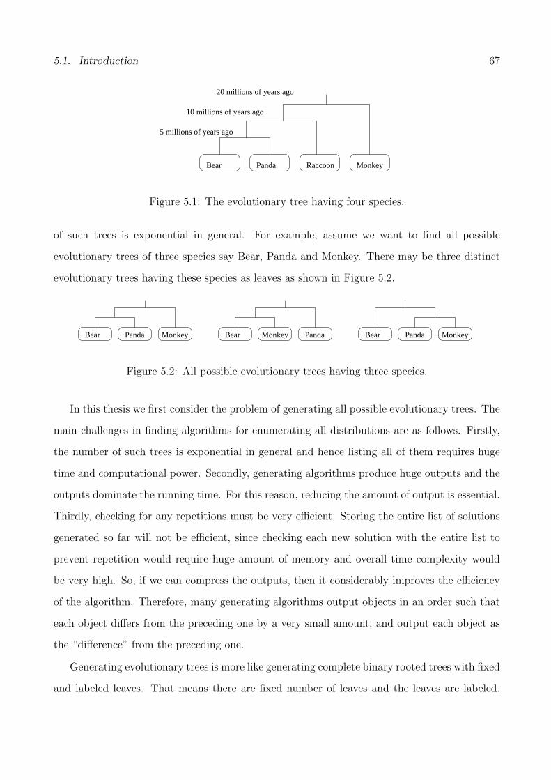
5.1. Introduction 67
Panda Raccoon MonkeyBear
5 millions of years ago
10 millions of years ago
20 millions of years ago
Figure 5.1: The evolutionary tree having four species.
of such trees is exponential in general. For example, assume we want to find all possible
evolutionary trees of three species say Bear, Panda and Monkey. There may be three distinct
evolutionary trees having these species as leaves as shown in Figure 5.2.
Bear Panda Monkey Bear Monkey Panda Bear Panda Monkey
Figure 5.2: All possible evolutionary trees having three species.
In this thesis we first consider the problem of generating all possible evolutionary trees. The
main challenges in finding algorithms for enumerating all distributions are as follows. Firstly,
the number of such trees is exponential in general and hence listing all of them requires huge
time and computational power. Secondly, generating algorithms produce huge outputs and the
outputs dominate the running time. For this reason, reducing the amount of output is essential.
Thirdly, checking for any repetitions must be very efficient. Storing the entire list of solutions
generated so far will not be efficient, since checking each new solution with the entire list to
prevent repetition would require huge amount of memory and overall time complexity would
be very high. So, if we can compress the outputs, then it considerably improves the efficiency
of the algorithm. Therefore, many generating algorithms output objects in an order such that
each object differs from the preceding one by a very small amount, and output each object as
the “difference” from the preceding one.
Generating evolutionary trees is more like generating complete binary rooted trees with fixed
and labeled leaves. That means there are fixed number of leaves and the leaves are labeled.
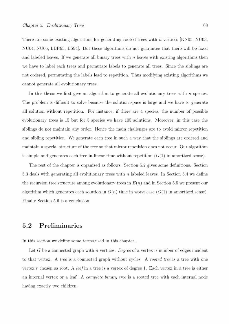
Chapter 5. Evolutionary Trees 68
There are some existing algorithms for generating rooted trees with n vertices [KN05, NU03,
NU04, NU05, LBR93, BS94]. But these algorithms do not guarantee that there will be fixed
and labeled leaves. If we generate all binary trees with n leaves with existing algorithms then
we have to label each trees and permutate labels to generate all trees. Since the siblings are
not ordered, permutating the labels lead to repetition. Thus modifying existing algorithms we
cannot generate all evolutionary trees.
In this thesis we first give an algorithm to generate all evolutionary trees with n species.
The problem is difficult to solve because the solution space is large and we have to generate
all solution without repetition. For instance, if there are 4 species, the number of possible
evolutionary trees is 15 but for 5 species we have 105 solutions. Moreover, in this case the
siblings do not maintain any order. Hence the main challenges are to avoid mirror repetition
and sibling repetition. We generate each tree in such a way that the siblings are ordered and
maintain a special structure of the tree so that mirror repetition does not occur. Our algorithm
is simple and generates each tree in linear time without repetition (O(1) in amortized sense).
The rest of the chapter is organized as follows. Section 5.2 gives some definitions. Section
5.3 deals with generating all evolutionary trees with n labeled leaves. In Section 5.4 we define
the recursion tree structure among evolutionary trees in E(n) and in Section 5.5 we present our
algorithm which generates each solution in O(n) time in worst case (O(1) in amortized sense).
Finally Section 5.6 is a conclusion.
5.2 Preliminaries
In this section we define some terms used in this chapter.
Let G be a connected graph with n vertices. Degree of a vertex is number of edges incident
to that vertex. A tree is a connected graph without cycles. A rooted tree is a tree with one
vertex r chosen as root. A leaf in a tree is a vertex of degree 1. Each vertex in a tree is either
an internal vertex or a leaf. A complete binary tree is a rooted tree with each internal node
having exactly two children.
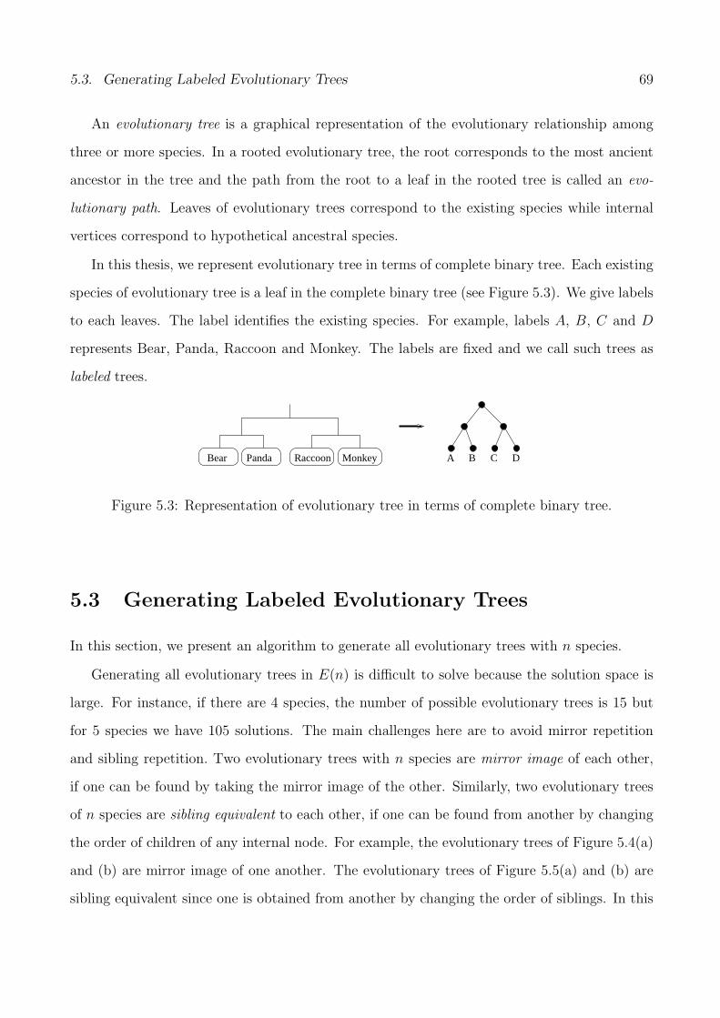
5.3. Generating Labeled Evolutionary Trees 69
An evolutionary tree is a graphical representation of the evolutionary relationship among
three or more species. In a rooted evolutionary tree, the root corresponds to the most ancient
ancestor in the tree and the path from the root to a leaf in the rooted tree is called an evo-
lutionary path. Leaves of evolutionary trees correspond to the existing species while internal
vertices correspond to hypothetical ancestral species.
In this thesis, we represent evolutionary tree in terms of complete binary tree. Each existing
species of evolutionary tree is a leaf in the complete binary tree (see Figure 5.3). We give labels
to each leaves. The label identifies the existing species. For example, labels A, B, C and D
represents Bear, Panda, Raccoon and Monkey. The labels are fixed and we call such trees as
labeled trees.
A B DCPanda MonkeyRaccoonBear
Figure 5.3: Representation of evolutionary tree in terms of complete binary tree.
5.3 Generating Labeled Evolutionary Trees
In this section, we present an algorithm to generate all evolutionary trees with n species.
Generating all evolutionary trees in E(n) is difficult to solve because the solution space is
large. For instance, if there are 4 species, the number of possible evolutionary trees is 15 but
for 5 species we have 105 solutions. The main challenges here are to avoid mirror repetition
and sibling repetition. Two evolutionary trees with n species are mirror image of each other,
if one can be found by taking the mirror image of the other. Similarly, two evolutionary trees
of n species are sibling equivalent to each other, if one can be found from another by changing
the order of children of any internal node. For example, the evolutionary trees of Figure 5.4(a)
and (b) are mirror image of one another. The evolutionary trees of Figure 5.5(a) and (b) are
sibling equivalent since one is obtained from another by changing the order of siblings. In this

Chapter 5. Evolutionary Trees 70
section, we present our algorithm of generating all evolutionary trees in E(n) which avoids such
repetitions.
A B
C D
E AB
CD
E
(b)(a)
Figure 5.4: Two evolutionary trees of (a) and (b) are mirror image of one another.
A B
C D
E B A
D C
E
(b)(a)
Figure 5.5: Two evolutionary trees of (a) and (b) are sibling equivalent to one another.
The main idea of our algorithm is to generate all possible subtrees of the evolutionary trees
in E(n). Then we assign numbers to the subtrees in a way that mirror repetition does not occur.
We call the set of subtrees that make up an evolutionary tree e ∈ E(n), the partial solution of
e. Then we recombine the subtrees in the set in an efficient manner such that sibling repetition
does not occur. For that purpose we define a recursion tree structure among the set of all
subtrees. A recursion tree is a family tree where each leaf is a solution and each internal node
is a partial solution e.g. set of subtrees. Along the path from root to a leaf we move towards a
solution. Hence to generate solutions we define a unique parent-child relationship among the
set of all subtrees of all evolutionary trees in E(n) so that the relationship among the set of
subtrees can be represented by a recursion tree with a suitable set as the root. Figure 5.6 shows
such a recursion tree of 4 species. Once such a parent-child relationship is established, we can
generate all the evolutionary trees in E(n) using the relationship. We do not need to build or

5.4. The Recursion Tree 71
store the entire recursion tree at once, rather we generate each evolutionary tree in the order
it appears in the recursion tree structure.
A B
D
C
A B
C
D
A B C D
A C
D
B
A C
B
D
A C B D
A D
C
B
A D
B
C
A DB C
B C
A
D
B C
D
A
B D
A
C
B D
C
A
C D
A
B
C D
B
A
A B
C
D
A B
D
C
BA C D
A C
B
D
A C
D
B
CA B D
A D
B
C
A D
C
B
DA B C
B C
A
D
B C
D
A
B D
A
C
B D
C
A
C D
A
B
C D
B
A
B C
A D
A C
B D
A B
C D
B D
A C
C D
A B
A B C D
A D
B C
Figure 5.6: The Recursion Tree R4.
5.4 The Recursion Tree
In this section we define a recursion tree structure Rn among the evolutionary trees in E(n).
For that purpose we assign numbers 1, 2, . . . , n to the species so that each species has identity.
This in turn helps us avoid repetitions.
For positive integer n, let S(n) be the set of all sets of subtrees that make up all evolutionary
trees in E(n). Let A ∈ S(n) be a set of subtree t1, t2, . . . , tk where k denotes the number of
subtrees in the set A. The set is ordered so we call A a sequence of subtree. We assign a number
ai to a subtree ti for 1 ≤ i ≤ k. Thus we get a sequence of integers a1, a2, . . . , ak associated
with A. The ais are calculated from the numbers assigned to the species. If there are m
species numbered s1, s2, . . . , sm in a subtree ti, then ai = min{s1, s2, . . . , sm} for 1 ≤ i ≤ k
and m ≤ n − k + 1. That means ai is the lowest numbered species in the subtree ti. For
example, Figure 5.7) shows a sequence of subtrees where the ais for each subtree are shown in
the internal nodes. Note that, for a leaf of the subtree ai = si.
Now we define the recursion tree Rn as follows. Each node of Rn represents a sequence
of subtree. If there are n species then there are n levels in Rn. A node is in level i in Rn if

Chapter 5. Evolutionary Trees 72
32
2 5 6
1 4
1
Figure 5.7: Illustration of a sequence of subtree A ∈ S(6).
there are n − i subtrees in the sequence of subtree for 0 ≤ i < n. As the level increases, the
number of subtree in the sequence decreases and vice versa. Thus a node at level n − 1 has
only one subtree which is an evolutionary tree. Since Rn is a rooted tree we need a root and
the root is a node at level 0. One can observe that a node is at level 0 in Rn if there are n
subtrees in the sequence of subtrees and there can be exactly one such node. In this case, all
the subtrees are the species itself i.e. aj = sj for 1 ≤ j ≤ n. For the root sequence we order the
subtrees according to the numbers assigned to the species. Thus for a root sequence we have
a1 < a2 < · · · < an. Clearly, the number of subtrees in root is greater than that of any other
sequence of subtrees in S(n).
To construct Rn, we define two types of relations among the sequence of subtrees in S(n):
(a) Parent-child relationship and
(b) Child-parent relationship.
We define the parent-child relationships among the sequence of subtrees in S(n) with two
goals in mind. First, the difference between a sequence of subtree A and its child C(A) should
be minimum, so that C(A) can be obtained from A by minimum effort. Second, every sequence
in S(n) must have a parent except the root and only one parent in Rn. We achieve the first
goal by ensuring that the child C(A) of a sequence A can be found by simply combining two
subtrees. That means A can also be generated from its child C(A) by simple decomposition.
The second goal, that is the uniqueness of the parent-child relationship is illustrated in the
following subsections.

5.4. The Recursion Tree 73
5.4.1 Parent-Child Relationship
Let A ∈ S(n) be a set of subtree t1, t2, . . . , tk where k denotes the number of subtrees in the
set A. Thus it corresponds to a node of level n− k, 1 ≤ k ≤ n of Rn. We have the numbers ai
associated with each ti for 1 ≤ i ≤ k. The sequence of subtrees of the children are defined in
such a way that to generate a child from its parent we have to deal with only two subtrees in the
sequence and the rest of the subtrees remain unchanged. The number of subtrees 0 decreases
in the child sequence by applying parent-child relationship.
Let C(A) ∈ S(n) be the sequence c1, c2, . . . , ck−1 of a child of A resulting from recombination
of ti and tj in the sequence for A, 1 ≤ i, j ≤ k. After recombination ti becomes the left child of
the root and tj becomes the right child of the root and the new subtree is denoted ti + tj. ti + tj
becomes the first subtree in the sequence for C(A) i.e. c1 = ti + tj. The rest of the subtrees in
the sequence remain unchanged in the order. We only recombine those ti and tj that do not
lead to repetition in the recursion tree. We have the following two cases based on whether ti
recombines with tj or not.
Case 1: i = 1
In this case t1 recombines with tj, for 1 < j ≤ n. Thus the number of such child is
n − 1 and we call these child as Type I child. We compute new a1 for c1 for this case as
a1(new) = mina1, aj. For example, in Figure 5.8 the first three children are obtained by the
recombination of t1 + t2, t1 + t3 and t1 + t3.
Case 2: i > 1
In this case ti recombines with tj only if a1 < ai and ai < aj, for i < j ≤ n. We call such
child as Type II child. One can observe that this case helps us avoid the sibling repetition. We
compute new a1 for c1 for this case as a1(new) = ai. For example, the fourth child in Figure 5.8
in generated by the recombination of t3 + t4.

Chapter 5. Evolutionary Trees 74
5 6
32 1 4
12
1
32
2
2
5
1 4
1 6
32
2
2
6
1 4
1 5
32
2 5 6
1 4
1
65
5
2 3
2
1 4
1
Type I Type II
Figure 5.8: Illustration of Type I and Type II child of a sequence of subtree A ∈ S(6).
5.4.2 Child-Parent Relationship
The child-parent relation is just the reverse of parent-child relation. Let A ∈ S(n) be a set of
subtree t1, t2, . . . , tk where k denotes the number of subtrees in the set A. Thus it corresponds
to a node of level n − k, 1 ≤ k ≤ n of Rn. We have the numbers ai associated with each
ti for 1 ≤ i ≤ k. We define a unique parent sequence of A at level n − k − 1 of Rn. Like
the parent-child relationship here we also deal with only two subtrees in the sequence. The
operations we apply to these two integers are only addition and assignment. The number of
subtrees 0 increases in the parent sequence by applying child-parent relationship.
Let P (A) ∈ S(n) be the sequence p1, p2, . . . , pk−1 of the parent of A. We get the sequence
for the parent by the decomposition of the subtree t1 in the sequence for A. Let pi and pj be
the resulting subtrees after decomposition. So, pi is the left child of t1 and pj is the right child
of t1. We compute ai and aj for the subtrees pi and pj. Now the following two cases occur
depending on the values of ai and aj that are associated with pi and pj.
Case 1: ai = a1(old) or aj = a1(old)
In this case p1 recombines with some pj and so we get i = 1. Hence A is a Type I child of
P (A). We place pj in the sequence for P (A) so that the subsequence from p2 to pn is sorted in
ascending order. The rest of the subtrees in the sequence remain unchanged in the order (see

5.4. The Recursion Tree 75
Figure 5.8).
Case 2: ai 6= a1(old) or aj 6= a1(old)
In this case A is a Type II child of P (A). We place pi and pj in the sequence for P (A) so
that the subsequence from p2 to pn is sorted in ascending order. The rest of the subtrees in the
sequence remain unchanged in the order (see Figure 5.8).
5.4.3 The Recursion Tree
From the above definitions we can construct Rn. We take the sequence t1, t2, . . . , tn of numbered
species as the root Ar as we mentioned before. The recursion tree Rn for the sequence of
subtrees in S(n) is shown in Figure 5.6. Based on the above parent-child relationship, the
following lemma proves that every sequence of subtrees in S(n) is present in Rn.
Lemma 5.4.1 For any sequence of subtree A ∈ S(n), there is a unique sequence of sequences
of subtrees that transforms A into the root Ar of Rn.
Proof. Let A ∈ S(n) be a sequence, where A is not the root sequence. By applying
child-parent relationship, we find the parent sequence P (A) of the sequence A. Now if P(A)
is the root sequence, then we stop. Otherwise, we apply the same procedure to P (A) and find
its parent P (P (A)). By continuously applying this process of finding the parent sequence of
the derived sequence, we have the unique sequence A,P (A), P (P (A)), . . . of sequences in S(n)
which eventually ends with the root sequence Ar of Rn. We observe that P (A) has at least
one subtree more than A in its sequence. Thus A,P (A), P (P (A)), . . . never lead to a cycle
and the level of the derived sequence decreases which ends up with the level of root sequence
Ar. Q.E .D.
Lemma 5.4.1 ensures that there can be no omission of sequence of subtrees in the recursion
tree Rn. Since there is a unique sequence of operations that transforms a sequence A ∈ S(n) into
the root Ar of Rn, by reversing the operations we can generate that particular sequence, staring
from root. Now we have to make sure that Rn represents sequences without repetition. Based

Chapter 5. Evolutionary Trees 76
on the parent-child and child-parent relationships, the following lemma proves this property of
Rn.
Lemma 5.4.2 The recursion tree Rn represents sequences of subtrees in S(n) without repeti-
tion.
Proof. Given a sequence A ∈ S(n), the children of A are defined in such a way that no other
sequence in S(n) can generate same child. For contradiction let two sequences A,B ∈ S(n) are
at level i of Rn and generate same child C. So, C is a sequence of level i + 1 of Rn. Since A
and B are at level i, they have same number of subtrees in the sequence and at least two of
the subtrees are different. According to child-parent relationship, we get P(C) by decomposing
t1 in the sequence for C. Decomposing t1 always results in two subtrees and the rest of the
subtrees in the sequence remain unchanged. Hence by applying child-parent relationship we
always get only one parent at level i. By contradiction, every sequence has a single and unique
parent. Q.E .D.
5.5 The Algorithm
In this section we give an algorithm to construct Rn and generate all evolutionary tree in E(n).
If we can generate all child sequences of a given sequence in S(n), then in a recursive manner
we can construct Rn and generate all evolutionary trees in E(n). We have the root sequence
Ar = (s1, s2, . . . , sn) where si are numbered species and s1 < s2 < · · · < sn . We get the child
sequence Ac by using the parent to child relation discussed above.
Procedure Find-All-Child-Subtrees(T = (t1, t2, . . . , tn−i), A = (a1, a2, . . . , an−i), i)
{ T is the current sequence of subtrees, i indicates the current level, A is the sequence of
assigned numbers and Tc is the child sequence of subtrees}begin
1 if i = n− 1 then
begin
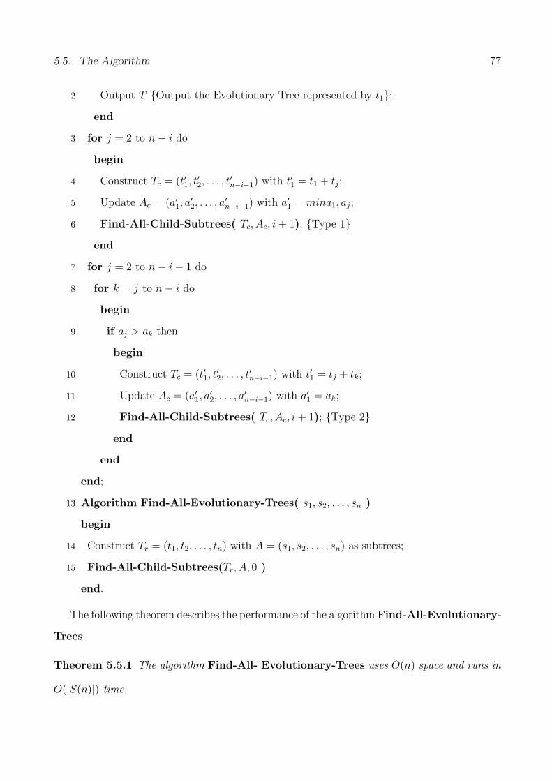
5.5. The Algorithm 77
2 Output T {Output the Evolutionary Tree represented by t1};end
3 for j = 2 to n− i do
begin
4 Construct Tc = (t′1, t′2, . . . , t
′n−i−1) with t′1 = t1 + tj;
5 Update Ac = (a′1, a′2, . . . , a
′n−i−1) with a′1 = mina1, aj;
6 Find-All-Child-Subtrees( Tc, Ac, i + 1); {Type 1}end
7 for j = 2 to n− i− 1 do
8 for k = j to n− i do
begin
9 if aj > ak then
begin
10 Construct Tc = (t′1, t′2, . . . , t
′n−i−1) with t′1 = tj + tk;
11 Update Ac = (a′1, a′2, . . . , a
′n−i−1) with a′1 = ak;
12 Find-All-Child-Subtrees( Tc, Ac, i + 1); {Type 2}end
end
end;
13 Algorithm Find-All-Evolutionary-Trees( s1, s2, . . . , sn )
begin
14 Construct Tr = (t1, t2, . . . , tn) with A = (s1, s2, . . . , sn) as subtrees;
15 Find-All-Child-Subtrees(Tr, A, 0 )
end.
The following theorem describes the performance of the algorithm Find-All-Evolutionary-
Trees.
Theorem 5.5.1 The algorithm Find-All- Evolutionary-Trees uses O(n) space and runs in
O(|S(n)|) time.

Chapter 5. Evolutionary Trees 78
Proof. In our algorithm we only use the recombination or decomposition of subtrees to
generate a new sequence of subtrees from an old one. Thus each sequence is generated in
constant time without computational overhead. Since we traverse the recursion tree Rn and
generate each sequence at each corresponding vertex of Rn we can generate all the sequences
in S(n) without repetition. By applying parent to child relation we can generate every child in
O(1) time. Then by using child to parent relation we go back to the parent sequence. Hence,
the algorithm takes O(|S(n)|) time i.e. constant time on average for each sequence. Moreover,
each evolutionary tree is at the leaf of the recursion tree Rn. Hence to output each evolutionary
tree in E(n), we to traverse the path from root to leaf in the worst case. Thus the algorithm
Find-All- Evolutionary-Trees outputs each evolutionary tree in E(n) in linear time (in
worst case).
Our algorithm generates each sequence of subtree in place i.e. we apply recombination and
decomposition to the current sequence. Therefore, the memory requirement is O(n), where n
is the number of species. Q.E .D.
5.6 Conclusion
In this chapter, we give a simple algorithm to generate all evolutionary trees having n species.
The algorithm is simple, generates each tree in constant time on average, and clarifies a simple
relation among the trees, that is a recursion tree of the trees.
Chapter 6
Labeled and Ordered Evolutionary
Trees
6.1 Introduction
In the previous chapter, we gave an algorithm to generate all labeled evolutionary trees. In
this chapter, we deal with the problem of generating all labeled and ordered evolutionary trees.
Generating all labeled and ordered evolutionary trees among different species have many appli-
cations in Bioinformatics [JP04], Genetic Engineering [KR03], Archaeology, Biochemistry and
Molecular Biology. In these applications, to find a better prediction, sometimes it is necessary
to generate all possible evolutionary trees among different species. To a mathematician, such a
tree is simply a cycle-free connected graph, but to a biologist it represents a series of hypotheses
about evolutionary events. In this chapter, we are concerned with generating all such probable
evolutionary trees that will guide biologists to research in all biological subdisciplines. We give
an algorithm to generate all evolutionary trees having n ordered species without repetition.
We also find out an efficient representation of such evolutionary trees such that each tree is
generated in constant time on average.
In bioinformatics, we frequently need to establish evolutionary relationship between different
79

Chapter 6. Labeled and Ordered Evolutionary Trees 80
types of species [JP04, KR03]. Biologists often represent this relationship in the form of binary
trees. Such complete binary trees having different types of species in its leaves are known as
evolutionary trees (see Figure 6.1). In a rooted evolutionary tree, the root corresponds to
the most ancient ancestor in the tree. Leaves of evolutionary trees correspond to the existing
species while internal vertices correspond to hypothetical ancestral species.
Evolutionary trees are used to predict predecessors of existing species, to comment about
future generations, DNA sequence matching, etc. Prediction of ancestors can be easy if all
possible trees are generated. Moreover, it is useful to have the complete list of evolutionary
trees having different types of species. One can use such a list to search for a counter-example
to some conjecture, to find best solution among all solutions or to experimentally measure an
average performance of an algorithm over all possible input evolutionary trees. Many algorithms
to generate a given class of graphs without repetition, are already known [AR06, BS94, FL79,
KN05, NU03, NU04, NU05, S97, YN04, ZS98].
PandaBear
20 millions of years ago
Raccoon Monkey
5 millions of years ago
10 millions of years ago
Figure 6.1: The evolutionary tree having four species.
In this thesis we first consider the problem of generating all possible evolutionary trees.
The main challenges in finding algorithms for enumerating all evolutionary trees are as follows.
Firstly, the number of such trees is exponential in general and hence listing all of them requires
huge time and computational power. Secondly, generating algorithms produce huge outputs
and the outputs dominate the running time. For this reason, reducing the amount of output is
essential. Thirdly, checking for any repetitions must be very efficient. Storing the entire list of
solutions generated so far will not be efficient, since checking each new solution with the entire
list to prevent repetition would require huge amount of memory and overall time complexity
would be very high. So, if we can compress the outputs, then it considerably improves the
efficiency of the algorithm. Therefore, many generating algorithms output objects in an order

6.1. Introduction 81
such that each object differs from the preceding one by a very small amount, and output each
object as the “difference” from the preceding one.
Generating evolutionary trees is more like generating complete binary rooted trees with
’fixed’ and ’labeled’ leaves. That means there are fixed number of leaves and the leaves are
labeled. There are some existing algorithms for generating rooted trees with n vertices [BS94,
KN05, NU03, NU04, NU05]. But these algorithms do not guarantee that there will be fixed
and labeled leaves. If we generate all binary trees with n leaves with existing algorithms then
we have to label each trees and permutate labels to generate all trees. Since the siblings are
not ordered, permutating the labels lead to repetition. Thus modifying existing algorithms we
cannot generate all evolutionary trees.
In this chapter we first give an efficient algorithm to generate all evolutionary trees with fixed
and ordered number of leaves. The order of the species is based on evolutionary relationship
and phylogenetic structure. For instance, Bear is more related to Panda than Monkey and
Raccoon is more related to Panda than Bear. Thus a species is more related to its preceding
and following species in the sequence of species than other species in the sequence. The order
of labels maintains this property. This property implies that each species in the sequence share
a common ancestor either with the preceding species or with the following species. We apply
the above restriction on the order of leaves with two goals in mind. First, the solution space
is reduced so that more probable solutions are available for the biologists to predict quickly
and easily. Second, each such probable evolutionary tree must be generated in constant time.
We also find out a suitable representation of such trees. We represent a labeled and ordered
complete binary tree with n leaves by a sequence of (n− 2) numbers. Our algorithm generates
all such trees without repetition.
Furthermore the algorithm for generating labeled and ordered trees is simple and generates
each tree in constant time on average without repetition. Our algorithm generates a new tree
from an existing one by making a constant number of changes and outputs each tree as the
difference from the preceding one. The main feature of our algorithm is that we define a tree
structure, that is parent-child relationships, among those trees (see Figure 6.2). In such a

Chapter 6. Labeled and Ordered Evolutionary Trees 82
“tree of evolutionary trees”, each node corresponds to an evolutionary tree and each node is
generated from its parent in constant time. In our algorithm, we construct the tree structure
among the evolutionary trees in such a way that the parent-child relation is unique, and hence
there is no chance of producing duplicate evolutionary trees. Our algorithm also generates the
trees in place, that means, the space complexity is only O(n).
B
D
C
A
B
A
C
D
BA C D B
A
C D
A B
C
D
Figure 6.2: The Family Tree F4.
The rest of the chapter is organized as follows. Section 6.2 gives some definitions. Section
6.3 depicts the representation of evolutionary trees. Section 6.4 shows a tree structure among
evolutionary trees. In Section 6.5 we present our algorithm which generates each solution in
O(1) time on average. Finally, section 6.6 is a conclusion.
6.2 Preliminaries
In this section we define some terms used in this chapter.
In mathematics and computer Science, a tree is a connected graph without cycles. A rooted
tree is a tree with one vertex r chosen as root. A leaf in a tree is a vertex of degree 1. Each
vertex in a tree is either an internal vertex or a leaf. A complete binary tree is a rooted tree
with each internal node having exactly two children.
A family tree is a rooted tree with parent-child relationship. The vertices of a rooted tree
have levels associated with them. The root has the lowest level i.e. 0. The level for any
other node is one more than its parent except root. Vertices with the same parent v are called
siblings. The siblings may be ordered as c1, c2, . . . , cl where l is the number of children of v.

6.2. Preliminaries 83
If the siblings are ordered then ci−1 is the left sibling of ci for 1 < i ≤ l and ci+1 is the right
sibling of ci for 1 ≤ i < l. The ancestors of a vertex other than the root are the vertices in
the path from the root to this vertex, excluding the vertex and including the root itself. The
descendants of a vertex v are those vertices that have v as an ancestor. A leaf in a family tree
has no children.
An evolutionary tree is a graphical representation of the evolutionary relationship among
three or more species. In a rooted evolutionary tree, the root corresponds to the most ancient
ancestor in the tree and the path from the root to a leaf in the rooted tree is called an evo-
lutionary path. Leaves of evolutionary trees correspond to the existing species while internal
vertices correspond to hypothetical ancestral species.
In this chapter, we represent evolutionary tree in terms of complete binary tree. Each
existing species of evolutionary tree is a leaf in the complete binary tree (see Figure 6.3). We
give labels to each leaves. The label identifies the existing species. For example, labels A, B,
C and D represents Bear, Panda, Raccoon and Monkey. The labels are fixed and ordered.
The order of the species is based on evolutionary relationship and phylogenetic structure. For
instance, Bear is more related to Panda than Monkey and Raccoon is more related to Panda
than Bear. So, a species is more related to its preceding and following species in the sequence
of species than other species in the sequence. The order of labels maintains this property. This
property implies that each species in the sequence share a common ancestor either with the
preceding species or with the following species. Our complete binary tree will maintain this
property and we will generate all such trees with exactly n leaves.
A B DCPanda MonkeyRaccoonBear
Figure 6.3: Representation of evolutionary tree in terms of complete binary tree.

Chapter 6. Labeled and Ordered Evolutionary Trees 84
6.3 Representation of Evolutionary Trees
In this section we give an efficient representation of a labeled and ordered evolutionary tree in
T (n). We represent such trees with n species with a sequence of (n− 2) numbers.
Let T (n) be the set of all evolutionary trees with n labeled and ordered leaves. Now, we
find out a representation of each evolutionary tree t ∈ T (n). Our idea here is to represent a
tree with a sequence of numbers. For this, we find out an intermediate representation of each
tree t ∈ T (n). A complete binary tree with n labeled leaves can be represented with a string of
valid parenthesization of n labels l1, l2, . . . , ln. Figure 6.4 shows the representation of complete
binary tree having 5 leaves. Thus the number of such trees corresponds directly to Catalan
number. Thus the total number of complete binary trees with n fixed and labeled leaves is
given by2(n−1)C(n−1)
n.
����
A B
C D
E
2
( ( A B ) ( ( C D ) E ) )
2244442
Figure 6.4: Representation of an evolutionary tree having five species.
We now count the number of opening parenthesis ’(’ before each label li, 1 ≤ i ≤ (n−2) in the
string of valid parenthesis of each intermediate representation. This gives us a sequence of (n−2)
numbers a1, a2, . . ., an−2 where ai represents the number of ’(’ before label li, for 1 ≤ i ≤ (n−2).
Since the labels are fixed and ordered, we do not need to count for ln−1 and ln and so we omit
these two numbers in the sequence. For example, the sequence 244 represents a evolutionary
tree with 5 leaves which corresponds to the string of valid parenthesis ((l1((l2l3)l4))l5). One can
observe that for each sequence a1 ≤ a2 ≤ · · · ≤ an−2 and 1 ≤ ai ≤ (n− 1) for 1 ≤ i ≤ (n− 2).
Thus, we say that a sequence of (n− 2) numbers uniquely represents a evolutionary tree with
labeled and ordered leaves as shown in Figure 6.4.
Let S(n) denote the set of all such sequence. Each sequence s ∈ S(n) uniquely identifies a
tree t ∈ T (n). We have the following lemma.

6.4. The Family Tree 85
Lemma 6.3.1 A sequence s ∈ S(n) of (n − 2) numbers uniquely represents an evolutionary
tree t ∈ T (n).
Proof. In an evolutionary tree t ∈ T (n) the labeled leaves l1, l2, . . . , ln are ordered. A leaf
li, 1 < i < n can only be paired with either with li−1 or li+1 in the sequence of labels. We take
any two labels, li and lj, 1 < i ≤ n− 2 and j ∈ {i− 1, i + 1}. If li and lj are paired, the count
of the ’(’ is same for both of them. This implies that si = sj. If li and lj are not paired, their
count of the ’(’ is different which implies si 6= sj.
For any two trees t1 ∈ T (n) and t2 ∈ T (n), t1 6= t2, we will find at least two labels li
and lj which are paired in one and not paired in another. Thus, their count is different i.e.
si 6= sj. Hence the sequence s ∈ S(n) of (n − 2) numbers represents exactly one evolutionary
tree t ∈ T (n). Q.E .D.
6.4 The Family Tree
In this section we define a tree structure Fn among evolutionary trees in T (n).
For positive integer n, let t ∈ T (n) be an evolutionary tree with n leaves having l1, l2, . . . , ln
labels. For each t ∈ T (n), we get unique sequence s ∈ S(n) of (n− 2) numbers a1, a2, . . . , an−2
where ai represents the number of ’(’ before label li, for 1 ≤ i ≤ (n−2). Also, for each sequence
a1 ≤ a2 ≤ · · · ≤ an−2 and 1 ≤ ai ≤ (n− 1) for 1 ≤ i ≤ (n− 1).
Now we define the family tree Fn as follows. Each node of Fn represents an evolutionary
tree. If there are n species then there are (n − 1) levels in Fn. A node is in level i in Fn if
a1 ≤ a2 ≤ . . . ≤ ai < (n− 1) and ai+1 = . . . = an−2 = (n− 1) for 1 < i ≤ (n− 1). For example,
the sequence 224 is at level 2. As the level increases the number of rightmost (n− 1) decreases
and vice versa. Thus a node at level n− 2 has no rightmost (n− 1) number i.e. an−2 < (n− 1).
Since Fn is a rooted tree we need a root and the root is a node at level 0. One can observe that
a node is at level 0 in Fn if a1, a2, . . . , an−2 = (n− 1) and there can be exactly one such node.
We thus take the sequence (n − 1, n − 1, . . . , n − 1) as the root of Fn. Clearly, the number of
rightmost (n − 1) in root is greater than that of any other sequence for any evolutionary tree

Chapter 6. Labeled and Ordered Evolutionary Trees 86
in T (n).
To construct Fn, we define two types of relations among the evolutionary trees in T (n):
(a) Parent-child relationship and
(b) Child-parent relationship.
We define the parent-child relationships among the evolutionary trees in T (n) with two
goals in mind. First, the difference between an evolutionary tree s and its child C(s) should be
minimum, so that C(s) can be generated from A by minimum effort. Second, every evolutionary
tree in T (n) must have a parent except the root and only one parent in Fn. We achieve the
first goal by ensuring that the child C(s) of an evolutionary tree A can be found by simple
subtraction. That means s can also be generated from its child C(s) by simple addition. The
second goal, that is the uniqueness of the parent-child relationship is illustrated in the following
subsections.
6.4.1 Parent-Child Relationship
Let t ∈ T (n) be an evolutionary tree with n ordered leaves having l1, l2, . . . , ln labels and
s ∈ S(n) be the sequence of numbers a1, a2, . . . , an−2 corresponding to t. s corresponds to a
node of level i, 0 ≤ i ≤ (n − 2) of Fn. Thus we have a1 ≤ a2 ≤ · · · ≤ ai < (n − 1) and
ai+1 = · · · = an−2 = (n − 1) for 1 < i ≤ (n − 2). The number of children it has is equal to
(ai+1 − ai). The sequence of the children are defined in such a way that to generate a child
from its parent we have to deal with only one integer in the sequence and the rest of the
integers remain unchanged. The integer is determined by the level of parent sequence in Fn.
The operation we apply is only subtraction and assignment. The number of rightmost (n− 1)
decreases in the child sequence by applying parent-child relationship.
Let Cj(s) ∈ S(n) be the sequence of jth child, 1 ≤ j ≤ (ai+1−ai) of s. Note that s is in level
i of Fn and Cj(s) will be in level i+1 of Fn. We define the sequence for Cj(s) as c1, c2, . . . , cn−2
where ck = ak for k 6= j and cj = (ai+1 − j). Thus, we observe that Cj is a node of level i + 1,
0 ≤ i < n − 2 of Fn and so c1 ≤ c2 ≤ · · · ≤ ci+1 < (n − 1) and ci+2 = · · · = cn−2 = (n − 1)

6.4. The Family Tree 87
for 0 ≤ i < (n− 2). Thus for each consecutive level we only deal with the integer ai+1 and the
rest of the integers remain unchanged. For example, 244 for n = 5 is a node of level 1 because
a1 < 4 and a2 = a3 = 4. Here, a2 − a1 = 2 so it has two children and the two children are
shown in Figure 6.6.
6.4.2 Child-Parent Relationship
The child-parent relation is just the reverse of parent-child relation. Let t ∈ T (n) be an
evolutionary tree with n ordered leaves having l1, l2, . . . , ln labels and s ∈ S(n) be the sequence
of numbers a1, a2, . . . , an−2 corresponding to t. s corresponds to a node of level i, 0 ≤ i ≤ (n−2)
of Fn. Thus we have a1 ≤ a2 ≤ . . . ≤ ai < (n − 1) and ai+1 = . . . = an−2 = (n − 1) for
1 < i ≤ (n− 1). We define a unique parent sequence of s at level i− 1. Like the parent-child
relationship here we also deal with only one integer in the sequence. The operations we apply
here is only addition and assignment. The number of rightmost n − 1 increases in the parent
sequence by applying child-parent relationship.
Let P (s) ∈ S(n) be the parent sequence of s. We define the sequence for P (s) as p1, p2, . . .,
pn−2 where pj = aj for j 6= (i − 1) and pi−1 = (n − 1). Thus, we observe that P (s) is a
node of level i − 1, 1 ≤ i < (n − 2) of Fn and so p1 ≤ p2 ≤ · · · ≤ pi−1 < (n − 1) and
pi = · · · = pn−2 = (n− 1) for 1 ≤ i ≤ (n− 2). For example, 224 for n = 5 is a node of level 2
because a1 ≤ a2 ≤ 4 and a3 = 4. It has a unique parent 244 as shown in Figure 6.6.
6.4.3 The Family Tree
From the above definitions we can construct Fn. We take the sequence sr = a1, a2, . . . , an−2
as root where a1, a2, . . . , an−2 = n − 1 as we mentioned before. The family tree Fn for the
evolutionary trees in T (n) is shown in Figure 6.5 and Figure 6.6 shows the representation of
family tree Fn.
Based on the above parent-child relationship, the following lemma proves that every evolu-
tionary tree in T (n) is present in Fn.

Chapter 6. Labeled and Ordered Evolutionary Trees 88
C
E
D
B
A
C D
E
A
B
C
E
A
B
D
C
A
B D E
CA B
D E
D E
B C
A
A B
C D E
C
A B
D
E
C
A
E
B
D
BA C D
E
A
B C
D
E
B
A
C
D
E
B
D
C
A
E
A B
C
D
ELevel 0
Level 1
Level 2
Level 3
Figure 6.5: Illustration of Family Tree F5.
244
Level 0
Level 1
334 234 134224
144
Level 2
344
Level 3
124
333 233 223 133 123
444
Figure 6.6: Representation of Family Tree F5.
Lemma 6.4.1 For any evolutionary tree t ∈ T (n), there is a unique sequence of evolutionary
trees that transforms t into the root tr of Fn.
Proof. Let s ∈ S(n) be a sequence, where s is not the root sequence, representing
an evolutionary tree t ∈ T (n). By applying child-parent relationship, we find the parent
sequence P (s) of the sequence s. Now if P(s) is the root sequence, then we stop. Otherwise, we
apply the same procedure to P (s) and find its parent P (P (s)). By continuously applying this
process of finding the parent sequence of the derived sequence, we have the unique sequence
s, P (s), P (P (s)), . . . of sequences in S(n) which eventually ends with the root sequence sr of
Tn,m. We observe that P (s) has at least one (n− 1) number more than s in its sequence. Thus
s, P (s), P (P (s)), . . . never lead to a cycle and the level of the derived sequence decreases which
6.5. Algorithm 89
ends up with the level of root sequence sr. Q.E .D.
Lemma 6.4.1 ensures that there can be no omission of evolutionary trees in the family
tree Fn. Since there is a unique sequence of operations that transforms an evolutionary tree
t ∈ T (n) into the root tr of Fn, by reversing the operations we can generate that particular
evolutionary tree, staring from root. Now we have to make sure that Fn represents evolutionary
trees without repetition. Based on the parent-child and child-parent relationships, the following
lemma proves this property of Fn.
Lemma 6.4.2 The family tree Fn represents evolutionary trees in T (n) without repetition.
Proof. Given a sequence s ∈ S(n), representing a t ∈ T (n), the children of s are defined in
such a way that no other sequence in S(n) can generate same child. For contradiction let two
sequences A,B ∈ S(n) are at level i of Fn and generate same child C. Thus C is a sequence of
level i + 1 of Fn. The sequences for A, B and C are aj, bj and cj for 1 ≤ j ≤ n − 2. Clearly,
ak = bk = n − 1 for i + 1 ≤ k ≤ n − 2 and we will get at least one j such that aj 6= bj for
1 ≤ j ≤ i. According to parent-child relationship, to generate C from its parent A or B, only
one integer ai+1 or bi+1 is changed in the sequence. Thus child of A, C(A) and child of B, C(B)
are different since ai+1 = bi+1 and aj 6= bj for 1 ≤ j < i + 1. Thus A and B does not generate
same child C. By contradiction, every sequence has a single and unique parent. Q.E .D.
6.5 Algorithm
In this section, we give an algorithm to construct the family tree Fn and generate all trees.
If we can generate all child sequences of a given sequence in S(n), then in a recursive
manner we can construct Fn and generate all sequence in S(n). We have the root sequence
sr = (n − 1) . . . (n − 1). We get the child sequence sc by using the parent to child relation
discussed above.
Procedure Find-All-Child-Trees(s = a1a2 . . . an−1, i)

Chapter 6. Labeled and Ordered Evolutionary Trees 90
{ s is the current sequence, i indicates the current level and sc is the child sequence }begin
Output s {Output the difference from the previous evolutionary tree};for j = 1 to (ai+1 − ai)
Find-All-Child-Trees( sc = a1a2 . . . (ai+1 − j) . . . an−2), i + 1);
end;
Algorithm Find-All-Evolutionary-Trees(n)
begin
Find-All-Child-Trees( sr = (n− 1) . . . (n− 1), 0 );
end.
The following theorem describes the performance of the algorithm Find-All- Evolutionary-
Trees.
Theorem 6.5.1 The algorithm Find-All-Evolutionary-Trees uses O(n) space and runs in
O(|T (n)|) time.
Proof. In our algorithm we only use the simple addition or subtraction operation to generate
a new evolutionary tree from an old one. Thus each evolutionary tree is generated in constant
time without computational overhead. Since we traverse the family tree Fn and output each
sequence at each corresponding vertex of Fn we can generate all the evolutionary trees in T (n)
without repetition. By applying parent to child relation we can generate every child in O(1)
time. Then by using child to parent relation we go back to the parent sequence. Hence, the
algorithm takes O(|T (n)|) time i.e. constant time on average for each output.
Our algorithm outputs each evolutionary tree as the difference from the previous one. The
data structure that we use to represent the evolutionary trees is a sequence of n − 2 integers.
Therefore, the memory requirement is O(n), where n is the number of species. Q.E .D.

6.6. Conclusion 91
6.6 Conclusion
In this chapter, we find out an efficient representation of an evolutionary tree having ordered
species. We also give an algorithm to generate all evolutionary trees having n ordered species.
The algorithm is simple, generates each tree in constant time on average, and clarifies a simple
relation among the trees that is a family tree of the trees.
Chapter 7
Conclusion
This thesis deals with algorithms for generating all solutions of a combinatorial problem. We
have presented efficient algorithms to generate all distributions of n objects (both identical and
distinguishable) to m bins. We have introduced a new elegant efficient family tree traversal
algorithm that generates each solution in O(1) time (in ordinary sense). In this thesis, we
also deal with the problem of generating all evolutionary trees. We have given an algorithm to
generate all evolutionary trees having n species without repetition. We also find out an efficient
representation of such evolutionary trees such that each tree is generated in constant time on
average. For the purposes of biologists, we also give a new algorithm to generate evolutionary
trees having ordered species.
We first summarize each chapter and its contributions. In Chapter 1 we have discussed
about enumeration problems and its applications in different areas. We also have described the
main algorithmic challenges that any enumerations algorithm has to face and reviewed some of
the existing literature.
In Chapter 2 we have introduced graph theoretical terminologies that have been used
throughout this thesis.
In Chapter 3 we have given an elegant algorithm to generate all distributions of identical
objects to bins without repetition. Our algorithm generates each distribution in constant time
with linear space complexity. We also present an efficient tree traversal algorithm that generates
92

93
each solution in O(1) time (in ordinary sense). To the best of our knowledge, our algorithm is
the first algorithm which generates each solution in O(1) time in ordinary sense. By modifying
our algorithm, we can generate the distributions in anti-lexicographic order. Finally, we extend
our algorithm for the case when the bins have priorities associated with them. Overall space
complexity of our algorithm is O(m), where m is the number of bins.
In Chapter 4 we have given a simple algorithm to generate all distributions of distinguishable
objects to bins. The algorithm generates each distribution in constant time with linear space
complexity. We also present an efficient tree traversal algorithm that generates each solution in
O(1) time. Then, we extend our algorithms for the case when the bins have priorities associated
with them.
In Chapter 5 we have given a simple algorithm to generate all evolutionary trees having n
species. The algorithm is simple, generates each tree in linear time (O(1) time in amortized
sense) and clarifies a simple relation among the trees, that is a recursion tree of the trees.
In Chapter 6 we find out an efficient representation of an evolutionary tree having ordered
species. We also give an algorithm to generate all evolutionary trees having n ordered species.
The algorithm is simple, generates each tree in constant time on average, and clarifies a simple
relation among the trees that is a family tree of the trees.
In this thesis we have given many efficient algorithms for generating all solutions of different
enumeration problems. However, the following problems are still open.
1. Develop an algorithm that generates all distributions of distinguishable objects to bins
when the objects are weighted and the bins have maximum capacity.
2. Is there any constant time algorithm that generates each evolutionary tree in constant
time?
3. We have obtained a average constant-time algorithm for generating all labeled and ordered
evolutionary trees. Is it possible to obtain a constant time algorithm that generates each
evolutionary tree in O(1) time in ordinary sense?

References
[AR06] M. A. Adnan and M. S. Rahman, Distribution of objects to bins: generating all dis-
tributions, Proc. of International Conference on Computer and Information Technology
(ICCIT’06), 2006 (to appear).
[AU95] A. V. Aho and J. D. Ullman, Foundation of Computer Science, Computer Science
Press, New York, 1995.
[BS94] M. Belbaraka and I. Stojmenovic, On generating B-trees with constant average delay
and in lexicographic order, Information Processing Letters, 49, pp. 27-32, 1994.
[CLR90] T. M. Cormen, C. E. Leiserson and R. L. Rivest, Introduction to Algorithms, MIT
Press, 1990.
[FL79] T. I. Fenner and G. Loizou, A binary tree representation and related algorithms for
generating integer partitions, The Computer Journal, 23, pp. 332-337, 1979.
[GKP94] R. Graham, D.E. Knuth and O. Patashnik, Concrete Mathematics, Addision-Wesley,
(1994).
[HS93] J. Hershberger and S. Suri, Morphing Binary Trees, Journal of Algorithms, 1993.
[J63] S. M. Johnson, Generation of permutations by adjacent transpositions, Mathematics of
Computation, 17, pp. 282-285, 1963.
[JP04] N. C. Jones and P. A. Pevzner, An Introduction to Bioinformatics Algorithms, The MIT
Press, Cambridge, Massachusetts, London, England, 2004.
94
References 95
[JWW80] J. T. Joichi, D. E. White and S. G. Williamson, Combinatorial Gray codes, SIAM
Journal on Computing, 9(1), pp. 130-141, 1980.
[K06] D. E. Knuth, The Art of Computer Programming, Vol.4, url:
http://www.cs.utsa.edu/ wagner/knuth/, 2006.
[K82] P. Klingsberg, A gray code for compositions, Journal of Algorithms, 3, pp. 41-44, 1982.
[KN05] S. Kawano and S. Nakano, Constant time generation of set partition, IEICE Trans.
Fundamentals, E88-A, 4, pp. 930-934, 2005.
[KN06] S. Kawano and S. Nakano, Generating Multiset Partitions, (on private communication),
2006.
[KR03] D. E. Krane and Michael L. Raymer, Fundamental Concepts of BioInformatics, Pearson
Education, San Francisco, 2003.
[LBR93] J. M. Lucas , D. R. Baronaigien and F. Ruskey, On Rotations and the Generation of
binary Trees, Journal of Algorithms, 9, pp. 503-535, 1993.
[M98] B. D. Mckay, Isomorph-free exhaustive generation, Journal of Algorithms, 26, pp. 306-
324, 1998.
[NU03] S. Nakano and T. Uno, Efficient generation of rooted trees, NII Technical Report, NII-
2003-005E, July 2003.
[NU04] S. Nakano and T. Uno, Constant time generation of trees with specified diameter, Proc.
of WG 2004, LNCS 3353, pp. 33-45, 2004.
[NU05] S. Nakano and T. Uno, Generating colored trees, Proc. of WG 2005, LNCS 3787, pp.
249-260, 2005.
[NW78] A. Nijenhuis and H. Wilf, Combinatorial Algorithms, Academic press, New York, 1978.
[R00] K. H. Rosen, Discrete Mathematics and Its Applications, WCB/McGraw-Hill, Singapore,
2000.

References 96
[S97] C. Savage, A survey of combinatorial gray codes, SIAM Review, 39, pp. 605-629, 1997.
[T02] A. S. Tanenbaum, Computer Networks, Prentice Hall, Upper Saddle River, New Jersey,
2002.
[T04] A. S. Tanenbaum, Modern Operating Systems, Prentice Hall, Upper Saddle River, New
Jersey, 2004.
[T62] H. F. Trotter, PERM (Algorithm 115), Communications of the ACM, 5, pp. 434-435,
1962.
[W96] D. B. West, Introduction to Graph Theory, Prentice-Hall, Upper Saddle River, New
Jersey, 1996.
[YN04] K. Yamanaka and S. Nakano, Generating all realizers, IEICE Trans. Inf. and Syst.,
J87-DI, 12, pp. 1043-1050, 2004.
[ZS98] A. Zoghbi and I. Stojmenovic, Fast algorithm for generating integer partitions, Interna-
tional Journal of Computer Mathematics, 70, pp. 319-332, 1998.

List of Publications
1. Muhammad Abdullah Adnan and Md. Saidur Rahman, Distribution of objects to bins:
generating all distributions, Proc. of International Conference on Computer and Infor-
mation Technology (ICCIT’06), 2006 (to appear).
2. Muhammad Abdullah Adnan and Md. Saidur Rahman, Distribution of distinguishable
objects to bins: generating all distributions, submitted to a Journal, 2006.
3. Muhammad Abdullah Adnan and Md. Saidur Rahman, Efficient Generation of Evolu-
tionary Trees, submitted to a Journal, 2006.
97

Index
algorithm, 22
amortized time, 23
average constant time, 23
constant time, 23
exponential, 22
linear, 23
linear time, 23
non-polynomial, 23
polynomial, 22
polynomially bounded, 22
run time, 22
anti-lexicographic order, 4
binary tree
complete binary tree, 19
bioinformatics, 2
Catalan Numbers, 25
child-parent relation, 34
combinatorial gray code, 9
combinatorics, 1, 2, 26
combinatorial algorithms, 1
depth first search(DFS), 24
distinguishable objects, 45
edge
loop, 17
enumeration, 3
enumeration algorithm , 3
evolutionary tree, 21, 83
evolutionary path, 21, 83
labeled trees, 69
family tree, 11, 30
ancestor, 20
descendant, 20
level, 20
rightmost leaf, 59
sibling, 20, 30
genealogical tree, 11
generation
in place, 29
graph, 17
cycle, 18
degree, 18
edge, 17
path, 18
rank, 24
simple graph, 18
98

INDEX 99
vertex, 17
walk, 18
Gray code, 28, 47
gray code approach, 10
gray code order, 4, 51
integer partition, 6, 21, 30
Johnson-Trotter algorithm, 11
lexicographic order, 4
maximal clique, 5
multiset, 21
node
level, 19
objects
identical objects, 45
non-identical objects, 45
parent-child relationship, 33
partition, 6
recursion tree, 70
rightmost leaf, 38, 59
sequence
inner sequence, 50
nonzero sequence, 51
zero sequence, 51
set partition, 6, 21, 31
sibling
left sibling, 20, 30
right sibling, 20, 30
simple set, 22
subset, 6
traversal, 24
in-order, 24
post-order, 24
pre-order, 24
tree, 18, 30
ancestor, 19
binary tree, 19
child, 18
depth, 19
descendant, 19
family tree, 20
height, 19
internal node, 19
leaf, 19, 30
level, 30
nodes, 18
parent, 18
root, 18
rooted tree, 18, 30