1

Journal of Economic Entomology, FORUM 1

2

3

Ecoinformatics for integrated pest management: expanding the applied 4

insect ecologist‟s tool-kit 5

6

7

8

Jay A. Rosenheim1,6

, Soroush Parsa2, Andrew A. Forbes

1,3, William A. Krimmel

1, Yao 9

Hua Law1, Michal Segoli

1, Moran Segoli

1, Frances S. Sivakoff

1, Tania Zaviezo

1,4, and 10

Kevin Gross5 11

12

13

1Department of Entomology, University of California, Davis, CA 95616. 14

2CIAT (Centro Internacional de Agricultura Tropical) A.A. 6713, Cali, Colombia. 15

3Current address: Department of Biology, University of Iowa, Iowa City, IA 52242. 16

4Departamento de Fruticultura y Enología, Pontificia Universidad Catolica Chile, 17

Santiago 30622, Chile. 18

5Department of Statistics, North Carolina State University, Raleigh NC 27695. 19

6Corresponding author, e-mail: jarosenheim@ucdavis.edu. 20

21

22

2

ABSTRACT Experimentation has been the cornerstone of much of IPM research. 23

Here we aim to open a discussion on the possible merits of expanding the use of 24

observational studies, and in particular the use of data from farmers or private pest 25

management consultants in „ecoinformatics‟ studies, as tools that might complement 26

traditional, experimental research. The manifold advantages of experimentation are 27

widely appreciated: experiments provide definitive inferences regarding causal 28

relationships between key variables, can produce uniform and high quality data sets, and 29

are highly flexible in the treatments that can be evaluated. Perhaps less widely 30

considered, however, are the possible disadvantages of experimental research. Using the 31

yield-impact study to focus the discussion, we address some reasons why observational 32

or ecoinformatics approaches might be attractive as complements to experimentation. A 33

survey of the literature suggests that many contemporary yield-impact studies lack 34

sufficient statistical power to resolve the small, but economically important, effects on 35

crop yield that shape pest management decision-making by farmers. Ecoinformatics-36

based data sets can be substantially larger than experimental data sets, and therefore hold 37

out the promise of enhanced power. Ecoinformatics approaches also address problems at 38

the spatial and temporal scales at which farming is conducted, can achieve higher levels 39

of „external validity‟, and can allow researchers to efficiently screen a large number of 40

variables during the initial, exploratory phases of research projects. Experimental, 41

observational, and ecoinformatics-based approaches may, if used together, provide more 42

efficient solutions to problems in pest management than can any single approach, used in 43

isolation. 44

45

3

46

KEY WORDS Ecoinformatics, observational studies, statistical power, economic 47

injury level, causal inference 48

49

50

51

52

53

54

4

INTEGRATED PEST management (IPM) research is highly diverse in the questions 55

addressed and the research approaches employed. Some subdisciplines of IPM research 56

rely heavily on observational studies, including for example research in the landscape 57

ecology of insect herbivores and their natural enemies (e.g., Thies & Tscharntke 1999; 58

Gardiner et al. 2009; Bahlai et al. 2010). Nevertheless, experimentation remains the 59

foundation of most pest management research. The goal of this paper is to open a 60

discussion on the possible utility of expanding the toolkit of the applied insect ecologist 61

to include a greater role for observational studies, and in particular to evaluate critically 62

the potential for ecoinformatics to contribute to our science. 63

What is ecoinformatics? Perhaps because the field is so new, usage of the term 64

„ecoinformatics‟ is not uniform (e.g., Recknagel 2006; Williams et al. 2006; Vos et al. 65

2006; Bekker et al. 2007; McIntosh et al. 2007; Sucaet et al. 2008; Hale and Hollister 66

2009), but ecoinformatics studies often: (1) use pre-existing data sets („data mining‟) 67

instead of data sets gathered by the researchers themselves; (2) integrate data sets from 68

multiple sources to create a composite data set; (3) use observational data, rather than 69

experimental data; (4) address ecological questions at a larger spatial and temporal scale 70

than is typically feasible within an experimental framework; (5) use larger amounts of 71

data than are typically feasible within an experimental framework; and (6) necessitate 72

novel applications of data management, database design, and statistical analysis tools 73

because of the large, observational, and often heterogeneous data sets involved. Thus, 74

ecoinformatics is an interdisciplinary field in which computer scientists, statisticians, and 75

ecologists work hand in hand to grapple with large-scale ecological questions. 76

5

Is there a relevant body of pre-existing data that can be mined by IPM 77

researchers? We suggest that a bountiful opportunity to employ ecoinformatics exists in 78

IPM, because private pest management consultants and farm staff generate large 79

quantities of data on insect densities and crop performance as part of their routine, but 80

extensive, sampling efforts in commercial agriculture. Insect scouting data can be 81

combined with additional data streams from farmers, other private consultants (e.g., 82

agronomy consultants), and governmental sources, including data on plant growth and 83

performance, pesticide use, agronomic practices, and landscape context, to address a 84

wide range of questions relevant to agricultural insect ecology. 85

We begin with a small survey of recently published studies to characterize the 86

current state of research practices. We then review and discuss the most salient strengths 87

of experimental research, followed by a consideration of some particular strengths of 88

observational or ecoinformatics-based research that may allow them to complement 89

traditional experimental work. Finally we provide a brief introduction to statistical tools 90

that may be particularly useful for the analysis of observational studies. Our views have 91

been influenced by our recent efforts to conduct observational studies (Rosenheim et al. 92

2006; Parsa 2010; Parsa et al. 2010) and to use ecoinformatics to address pest 93

management problems in California cotton (Forbes and Rosenheim 2010; unpublished). 94

We will allude to these experiences below. 95

96

Literature Survey: Studies of Pest Impact on Crop Yield. To make our discussion more 97

focused and tangible, we propose to view the field of IPM through the lens of one 98

particular type of study: the yield-impact study, in which the relationship between insect 99

6

densities and crop yield is characterized. The yield impact study is one of the 100

foundations of modern pest management programs, because it is used to estimate the 101

economic injury level: the number of insects that reduces yield sufficiently that 102

management intervention is economically advantageous (Pedigo 2002). We 103

acknowledge, however, that other types of agricultural pest management research may 104

employ quite different research methodologies. Our goal, then, is to ask whether 105

observational and ecoinformatics-based approaches can contribute to progress in areas of 106

IPM research that have traditionally relied heavily upon experimentation. 107

To describe current research practices within the community of IPM researchers, 108

we reviewed all yield-impact studies conducted in the field or in greenhouses and 109

published in Journal of Economic Entomology or Environmental Entomology between 110

January 2007 and June 2010. Thirty-six papers satisfied our criteria for inclusion in the 111

review, namely (i) that the study include a measure of crop yield in response to variation 112

in densities of an herbivorous arthropod, and (ii) that the variation in herbivore densities 113

either be natural or the result of an experimental manipulation of some kind, but not 114

solely a response to different crop plant genotypes. We characterized each study using 115

four basic descriptors: (1) was the study observational or experimental (we define a study 116

as experimental if the researcher manipulated arthropod densities by applying a treatment 117

to each experimental unit either randomly, or at least without regard to other traits 118

expressed by that experimental unit); (2) were the data collected by the researcher or by 119

other persons (e.g., farmers, consultants, etc.); (3) was the research conducted on a 120

commercial farm or on a research farm; and (4) what was the size of each replicate plot 121

(in m2) within the overall study layout. In addition, to quantify the statistical power of 122

7

those studies that employed an experimental approach (see below for details), we 123

attempted to gather five further metrics for each study: (1) the mean and SD of crop yield 124

observed in the treatment with the lowest level of herbivory (henceforth, the “arthropod-125

free control”); (2) the number of replicates for the arthropod-free control treatment; (3) 126

the number of replicates for the treatment with the next lowest level of herbivory 127

(henceforth, the “lowest damage treatment”); (4) the value of the crop (dollars/acre); and 128

(5) the cost of a single application of the pesticide most commonly used to suppress the 129

arthropod that was the focus of the paper (cost of the material plus the cost of the 130

application; dollars/acre). Papers that did not report the needed crop yield data (mean 131

and SD) or replicate numbers were excluded from further analysis. In cases where the 132

authors did not provide estimates of crop value, we obtained these data from other 133

sources, including primarily the USDA National Agricultural Statistics Service 134

(http://www.nass.usda.gov/). Data on the current commonest pesticide use practices and 135

costs were obtained either from each paper or, if not reported there, from university 136

extension web-sites or from personal communications with specialists; the full data set 137

with references is available from JAR. 138

The survey shows that experimentation is the dominant means by which 139

researchers study the effects of herbivory on crop yield. Thirty-five of the 36 reviewed 140

studies (97%) were experimental, with just the one remaining study (3%) employing an 141

observational, correlative approach. Of the 27 studies that provided all the data needed to 142

conduct the power analysis, data were collected by the researchers in all cases (100%); 143

none of the studies involved mining data collected by non-researchers. Studies were 144

usually conducted on experimental farms (22/27 studies, 81%) and much less frequently 145

8

in the fields of cooperating farmers (3/27, 11%; in the remaining three studies, the 146

location of the field plots was not specified). We discuss further these and other results 147

of the literature survey below. 148

149

Strengths of experimental approaches/weaknesses of observational or 150

ecoinformatics approaches 151

152

In this section, we summarize briefly views that we expect are already widely understood 153

and assimilated within the research community regarding the manifold strengths of 154

experimental science and the corresponding weaknesses of observational studies. We use 155

the yield impact study as an exemplar to focus the discussion. 156

157

Experiments produce definitive inferences of causal relationships; observational studies 158

cannot. Assume that in a well-replicated experiment, a researcher generates one or 159

more treatments by manipulating some variable, A, while holding other conditions as 160

nearly constant as possible; assigns those treatments randomly to experimental units; and 161

then measures a response variable, B. If the response variable B differs significantly 162

across treatments, then the experimenter can infer with a high degree of confidence that a 163

change in A causes a change in B. This ability of experiments to reveal the causal 164

structure of the environment is their most singular strength (e.g., Diamond 1983; Paine 165

2010). In contrast, when a researcher observes a correlation between natural, pre-existing 166

variation in variables C and D, it is difficult to know whether the correlation reflects a 167

causal influence of C on D, of D on C, or whether C and D are not causally related to 168

9

each other at all, and instead are both influenced by some other variable(s) E, F, etc., 169

which may or may not have been measured by the experimenter. 170

A yield impact experiment that employed only observational data but that 171

attempted to infer a causal relationship between herbivore densities and crop yield could 172

probably run afoul in several different ways, but two seem particularly likely. First, some 173

herbivores may prefer to attack weak or stressed host plants (e.g., bark beetles; the „plant 174

stress hypothesis‟; White 1984; Mattson and Haack 1987; Huberty and Denno 2004), 175

which are likely to produce less yield than vigorous, unstressed host plants, irrespective 176

of herbivore load. Herbivores that prefer to attack low-vigor host plants are thus likely to 177

be negatively correlated with crop yield, even if the damage that they generate actually 178

has no effect on yield. In this case, it is instead the variable(s) that caused the plant stress 179

in the first place that is the causal factor (e.g., for the bark beetle Scolytus rugulosus 180

attacking almond trees in California, the causal agent for both decreased almond yield 181

and increased bark beetle populations might be a soil-borne pathogen in the genus 182

Phytophthora; University of California 2002). Second, other herbivores may prefer to 183

attack particularly vigorously growing host plants (e.g., gall-inducing herbivores, cicadas; 184

the „plant vigor hypothesis‟; Price 1991; Cornelissen et al. 2008; Yang and Karban 2009). 185

If vigorous plants are high yielding plants, then the result could be a spurious positive 186

correlation between herbivore densities and crop yield or the masking or distortion of 187

what could be a true underlying negative effect of herbivores on yield. Thus, purely 188

observational data sets linking herbivore densities to crop performance must be 189

approached with great caution, especially when the herbivore does not select host plants 190

10

at random with respect to the host plant‟s yield potential, or else we must adopt some 191

means of controlling for underlying variation in plant vigor. 192

193

By reducing between-replicate variation, experiments augment statistical power. Many 194

experiments are conducted in a „common garden‟ setting, in which all environmental 195

conditions that might influence the dependent variable B are held as nearly constant as 196

possible, except for the one variable, A, that is to be manipulated experimentally. By 197

doing this, experimenters reduce the magnitude of unexplained variation, and thereby 198

enhance the experiment‟s ability to resolve the influence of variable A on variable B. 199

Moreover, many alternative experimental designs are available to reduce unexplained 200

variation when common-garden experiments are unfeasible. For example, blocking is a 201

familiar technique in which experimental units are grouped by a known source of 202

variation that could impact the response, such as soil fertility. By manipulating the 203

experimental variable within blocks, variability attributable to the external source cancels 204

out, allowing a more direct assessment of the effect of the manipulated variable. 205

Measurable differences in experimental units or environmental conditions can also be 206

controlled statistically with regression designs. Regression designs require stronger 207

assumptions than blocking designs (namely, that the effect of the measurable extraneous 208

variation can be modeled mathematically), but return enhanced statistical power for 209

detecting the effect of the manipulated variable when those assumptions are viable. 210

211

Experiments are flexible; in principle, any treatment can be generated; observational 212

studies are limited to extant variation. Experiments are the ultimate intellectual 213

11

playground in which researchers can attempt to implement any manipulation that they 214

can imagine. In contrast, observational studies are restricted to conditions that actually 215

occur in the field. This is not a profound observation, but it is one with important 216

implications for using observational data to assess the relationship between herbivore 217

densities and crop yield. In particular, if farmers manage a particular pest in a uniformly 218

aggressive manner, maintaining its densities at low levels, then an observational study 219

will be unable to explore the effects of higher densities of the herbivore on plant 220

performance. Furthermore, the costs and benefits of any universally-adopted farming 221

practice will be recalcitrant to study with purely observational approaches. For example, 222

sulfur is applied to nearly 100% of all commercial grape production in California to 223

suppress the fungal pathogen Erisiphe necator (powdery mildew); therefore, a strictly 224

observational approach cannot be used to evaluate the hypothesis that sulfur exacerbates 225

problems with Tetranychus spp. spider mites or Erythroneura spp. leafhoppers (Costello 226

2007; Jepsen et al. 2007), because there are virtually no sulfur-free vineyards with which 227

sulfur-treated vineyards can be compared. 228

229

Data uniformity, completeness, and quality may be higher for data collected by 230

researchers than for data used in ecoinformatics studies. Researchers who gather their 231

own data have a high degree of control over the quality of their observations. Uniform 232

data collection protocols, the option to measure all variables thought to be relevant to the 233

question being addressed, and the ability to adjust sampling intensity to achieve the 234

desired level of sampling precision are all available to the researcher. In contrast, data 235

mining always involves giving up some of this control over data uniformity, 236

12

completeness, and, possibly, quality. In the context of IPM research, private pest control 237

consultants may use a variety of different sampling methods to estimate the density of a 238

given focal pest species, creating challenges in integrating multiples sources of data into 239

one composite data set. Research comparing different sampling methods may allow 240

different types of data to be inter-converted (e.g., Musser et al. 2007), but such studies are 241

not always available. In many cases, density estimates may be qualitative (e.g., densities 242

may be recorded as “trace”, “low”, “moderate”, or “high”) rather than quantitative. The 243

sampling effort efficiencies demanded by the highly competitive workplace may not 244

always be compatible with research objectives, and variables not thought to be critical to 245

immediate management decisions are often not measured, even if they may be needed in 246

a research context. On the other hand, it should not be forgotten that consultants are 247

professional arthropod samplers: their livelihoods depend on producing useful estimates 248

of pest densities, and they often have more experience in sampling than even the most 249

seasoned researcher. 250

251

Pest control consultants and farmers may not wish to share data. An absolute 252

prerequisite of using ecoinformatics to address IPM research objectives is to establish a 253

collaborative relationship with the consultants and farmers whose data will form the core 254

of the ecoinformatics data set. There are two primary obstacles to establishing this 255

collaboration. First, essentially all of the data typically needed for IPM research (e.g., 256

insect densities, crop yield, pesticide use) are „sensitive‟ for the persons who might 257

provide those data. Consultants may be reluctant to divulge information about fields in 258

which pest populations escaped control and generated substantial damage. Farmers are 259

13

notoriously, and understandably, secretive about the yields that they obtain; yield data 260

and details of agronomic practices may represent important competitive edges in the 261

marketplace. Finally, pesticide use data are often very sensitive, due to the sometimes 262

considerable blurring of the boundaries between legal use, consistent with labeled 263

restrictions, and illegal use. Promises to treat all data confidentially may ameliorate these 264

concerns, but rarely eliminate them. Second, requests for data sharing invariably impose 265

a time burden on collaborating consultants and farmers; records must be located and 266

organized, and sampling methods and recording practices must be explained in detail to 267

the researcher. We have discovered that by working during the winter, when farmers and 268

consultants are generally less pressured by immediate crop management responsibilities, 269

it is often easier to secure active cooperation. Furthermore, we have found that the single 270

most important element in securing active collaboration from farmers and consultants is 271

to ensure that the ecoinformatics study addresses questions that they view as important to 272

their livelihoods. In that way, farmers and consultants can expect a fair return on their 273

very real investment in the conduct of the research. Finally, it is important to note that 274

any time some farmers choose to participate in data sharing while others do not, it creates 275

a possible filtering of the data set that may introduce various biases. 276

277

Weaknesses of experimental approaches/strengths of observational or 278

ecoinformatics approaches 279

280

Given the many strengths of experimental science, as summarized above, it might seem 281

strange indeed to consider alternative approaches to IPM research. In this section, 282

14

however, we present views that may not be as widely considered within the research 283

community regarding the limitations of experimental science and the corresponding 284

strengths of observational or ecoinformatics-based studies. We again use the yield 285

impact study as an exemplar to focus the discussion. 286

287

Traditional experimental designs may not have sufficient power; large ecoinformatics 288

data sets may provide greater power. As noted above, experimenters may augment 289

their ability to detect the effects of causal variable A on response variable B by holding as 290

nearly constant as possible all other environmental variables (the „common garden‟ 291

approach). Nevertheless, we suggest that traditional agricultural experimentation may 292

often fail to produce sufficiently precise estimates of key crop performance variables to 293

guide many pest management decisions that farmers must make in their daily operations. 294

The problem is that effects on yield that are small (perhaps too small to be resolved by 295

traditional experimentation) may still be economically important to a farmer whose profit 296

margin may be quite thin (e.g., see http://coststudies.ucdavis.edu/current.php). For 297

example, a farmer who works with a 10% profit margin will be strongly motivated to 298

avoid even a 2% loss of yield from herbivory, especially when that farmer can do so by 299

applying an inexpensive pesticide. But, can we measure such small effects on yield? 300

We first explore the hypothesis that traditional experimentation may lack 301

sufficient power by examining a case-study co-authored by one of us; in so doing, we lay 302

out the methodology that we use below in a broader, literature-survey based test of the 303

hypothesis. Rosenheim et al. (1997) examined the yield impact of the cotton aphid, 304

Aphis gossypii, feeding on seedling upland cotton plants, Gossypium hirsutum, in 305

15

California. Cotton grown in California is not an unusually high value crop: mean yields 306

in 2009 were 1,613 pounds/acre, and the average price received by growers was $0.715 307

per pound, generating a crop value of $1,153 per acre. A farmer faced with a potentially 308

damaging aphid population on seedling cotton is faced with a simple decision: should I 309

apply an insecticide or not? A single application of an insecticide commonly used to 310

suppress aphids currently costs approximately $18.25 per acre ($8.50 per acre for the 311

insecticide itself and $9.75 per acre for the aerial application). To maximize profits, 312

farmers should apply an insecticide only if the application cost is less than the value of 313

the crop yield that would be sacrificed if the insect populations were not suppressed. 314

Thus, assuming that a single application of insecticide will completely eliminate any 315

potential effect of aphids on seedling cotton, farmers will maximize their profits by 316

applying an insecticide if the aphids would otherwise cause a loss of ($18.25/$1153)% of 317

yield, or 1.58%. Did the experiments reported by Rosenheim et al. (1997) have sufficient 318

power to resolve effects of this size? 319

We can think of an idealized yield-impact study as including a key contrast 320

between two treatments: an “arthropod-free” control, replicated n1 times, and a “threshold 321

damage” treatment, replicated n2 times, that generates the amount of yield loss that 322

corresponds to the point at which the profit-maximizing farmer would switch from not 323

intervening to intervening to suppress pest densities (the “economic injury level”). Note 324

that it is not a trivial challenge for the researcher to create this threshold damage 325

treatment; before conducting preliminary trials, the insect density that produces this level 326

of damage will generally be unknown. Furthermore, the function relating the intensity of 327

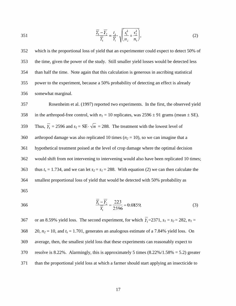
herbivore damage to plant performance (the compensation function) is highly variable in 328

16

form, and is frequently non-linear (Dyer et al. 1993; Huhta et al. 2003; Gao et al. 2008). 329

As a result, whereas treatments that generate greater amounts of yield loss can help to 330

define the complete form of the compensation function and can allow researchers to 331

resolve statistically significant yield effects, they are largely uninformative regarding the 332

yield effects of lower levels of damage. For the farmer, then, the key problem is to 333

identify the economic injury level: at what pest density does the amount of protectable 334

yield loss equal the cost of the pesticide application? To answer this question, we need to 335

be able to resolve a statistically significant yield loss for the threshold damage treatment. 336

In the simplest possible case, this yield loss can be evaluated as a t-test, 337

338

, (1) 339

where ts is the critical t-value for a contrast with n1 + n2 – 2 degrees of freedom, is the 340

mean yield in the arthropod-free control, is the mean yield in the threshold damage 341

treatment, and s1 and s2 are the sample standard deviations observed for the two 342

treatments. To be as generous as possible in evaluating the power of yield impact 343

experiments, we can consider the test to be 1-tailed (i.e., excluding the possibility of 344

overcompensation). Because not all studies include a “threshold damage” treatment (i.e., 345

one corresponding closely to an amount of damage that represents the point at which a 346

farmer‟s optimal behavior switches from „don‟t intervene‟ to „intervene‟), we can 347

conservatively estimate and s1 from the reported arthropod-free control treatment data 348

and assume that s2 = s1. Equation (1) can then be rearranged to calculate 349

350

17

, (2) 351

which is the proportional loss of yield that an experimenter could expect to detect 50% of 352

the time, given the power of the study. Still smaller yield losses would be detected less 353

than half the time. Note again that this calculation is generous in ascribing statistical 354

power to the experiment, because a 50% probability of detecting an effect is already 355

somewhat marginal. 356

Rosenheim et al. (1997) reported two experiments. In the first, the observed yield 357

in the arthropod-free control, with n1 = 10 replicates, was 2596 ± 91 grams (mean ± SE). 358

Thus, = 2596 and s1 = = 288. The treatment with the lowest level of 359

arthropod damage was also replicated 10 times (n2 = 10), so we can imagine that a 360

hypothetical treatment poised at the level of crop damage where the optimal decision 361

would shift from not intervening to intervening would also have been replicated 10 times; 362

thus ts = 1.734, and we can let s2 = s1 = 288. With equation (2) we can then calculate the 363

smallest proportional loss of yield that would be detected with 50% probability as 364

365

, (3) 366

or an 8.59% yield loss. The second experiment, for which =2371, s1 = s2 = 282, n1 = 367

20, n2 = 10, and ts = 1.701, generates an analogous estimate of a 7.84% yield loss. On 368

average, then, the smallest yield loss that these experiments can reasonably expect to 369

resolve is 8.22%. Alarmingly, this is approximately 5 times (8.22%/1.58% = 5.2) greater 370

than the proportional yield loss at which a farmer should start applying an insecticide to 371

18

suppress a damaging pest. To encapsulate this problem, we define a study‟s „power ratio‟ 372

as 373

374

. (4) 375

Clearly, and in contrast to this first example, it will be highly desirable to conduct 376

experiments that achieve power ratios < 1. Power ratios >1 suggest that a fundamental 377

disconnect exists between the effect sizes that researchers can detect and the effect sizes 378

that drive the pest management decisions of profit-maximizing farmers. 379

We are not the first to identify this possible problem with statistical power. 380

Ragsdale et al. (2007) noted emphatically that, even working with a relatively low-value 381

crop (soybeans), where the power problem should be less acute, the economic injury 382

level was associated with a yield loss that was so small that it was “immeasurable”. How 383

widespread is this problem of insufficient power? 384

We used our survey of recently-published yield impact studies to try to address 385

this question. Twenty-seven of the 36 studies surveyed presented the needed data on 386

crop yield (mean plus some measure of variability). For crops with multiple harvests per 387

year, crop value for just a single harvest was used. Any time the authors of the original 388

studies collapsed observations across multiple experiments or treatments to produce 389

larger sample sizes, we used these aggregate yield estimates to achieve the greatest 390

possible statistical power. Many studies reported multiple experiments individually and 391

did not collapse results; in these cases, we calculated a power ratio for each experiment, 392

19

and then averaged across the different power ratio estimates to obtain a single 393

observation per study. 394

Our survey suggests that the problem of insufficient power is a general one (Fig. 395

1); indeed, none of the 27 studies achieved a mean power ratio <1 (the lowest value was 396

1.49; see Table 1). If we look instead at the distribution of power ratios for each 397

experiment reported within the 27 published studies, our sample size increases (N = 159), 398

but the result is not much more encouraging: the median power ratio is 8.0 (range: 0.60-399

578.2), and only 4 of the 159 experiments (2.5%) achieved a power ratio < 1.0. 400

It appears then that experimental yield impact studies only very rarely have the 401

statistical power needed to resolve the economic injury level, and thus to guide one of the 402

most basic decisions that farmers must make in their daily pest management practices. 403

How can this problem be overcome? We suggest four possible approaches. First, for at 404

least a subset of the pests that directly attack the marketed portion of the crop („direct 405

pests‟), it is possible to evaluate yield loss directly, by quantifying the damaged or 406

destroyed portion of the crop. This may greatly ameliorate the power problem. For 407

example, increased herbivory by the navel orangeworm, Amyelois transitella, on almond 408

nuts may generate a very small loss of yield (say, 1%), representing a small „signal‟ that 409

may be lost in the abundant „noise‟ generated by the many other factors that cause 410

variation in almond yield (e.g., variation in soil quality, water or nutrient availability, 411

pollinator efficacy, presence of pathogens, etc.). In contrast, even a similarly small 412

absolute increase in the proportion of the harvested almond nuts bearing distinctive A. 413

transitella feeding damage (e.g., increasing from 1% to 2%), as detected in the packing 414

20

house, may be easier to resolve statistically, because whereas the „signal‟ is still small, 415

the „noise‟ is reduced, since A. transitella is the sole source of such damage. 416

A second approach is to retain the same commitment to experimentation, but to 417

increase the number of replicate plots. This suggestion is tempered by the recognition 418

that feasibility concerns regularly constrain the number of replicates possible in any 419

single experiment. However, an approach that is being used increasingly frequently and, 420

we think, with excellent results, is to pool research effort across multiple workers, 421

creating consortia of researchers capable of producing experiments that are heavily 422

replicated across space and time (e.g., Ragsdale et al. 2007; Chapman et al. 2009; 423

Johnson et al. 2009; Musser et al. 2009a,b). Because statistical power increases only as 424

the square root of replicate number, however, in most cases very large increases in 425

research effort are required to push the power ratio into the desired range (e.g., a 25-fold 426

increase in replicate number is needed to bring the power ratio from 5.0 1.0). The 427

huge labor and capital requirements of such extensive experimentation is the most 428

significant obstacle to further adoption of this approach to augmenting power. Analyses 429

that combine observations across different places and times may also sacrifice some of 430

the advantages of experiments over observational studies discussed above. For example, 431

some authors have created composite data sets by combined data across experiments and 432

then employing regression analyses relating pest density to yield; such analyses do 433

enhance power very substantially, but also sacrifice some of the interpretational rigor 434

associated with experimental data. 435

A third possible approach again derives extra statistical power by pooling data 436

across multiple experiments, but now in a strictly post hoc manner through formal meta-437

21

analysis. This differs from the creation of consortia of researchers in that the experiments 438

to be pooled will generally have been performed by different researchers without any 439

original coordination of effort. Meta-analysis is now used widely in biology, in large part 440

because it effectively increases sample sizes by synthesizing data across multiple studies 441

(Harrison in press), thereby decreasing the likelihood of failing to reject a null hypothesis 442

(e.g., that a pest has no effect on yield), even when it is false (i.e., Type II error). In 443

agricultural pest management, meta-analysis will be feasible only for pest-crop 444

combinations that have been studied repeatedly. 445

A fourth possible means of realizing the needed statistical power is to seek out 446

much larger data sets, capitalizing on the substantial data collection efforts made by the 447

community of private consultants and farm employees who routinely scout fields, i.e., 448

ecoinformatics. Ecoinformatics approaches, although still in their infancy, hold the 449

promise of data sets that are orders of magnitude larger than those generated in a 450

traditional experiment. Although assembling farmer- and consultant-derived data into a 451

usable database can require a significant investment of time and labor, it can still be much 452

more efficient than generating the data de novo. 453

454

The spatial and temporal scales of many experimental studies do not match the scales of 455

commercial agriculture; ecoinformatics studies generally achieve the appropriate match. 456

Experimental studies are generally performed in small research plantings, employing 457

relatively small treatment plots. Our survey of published yield impact studies revealed a 458

median plot size of just 36.9 m2 (Table 1), roughly equivalent to a square plot 6 m on a 459

side. Ecologists have long discussed the problems of extending experimental results 460

22

observed at one spatial scale to another (Diamond 1983; Addicott et al. 1987; Willis and 461

Whittaker 2002; Paine 2010). In the case of IPM research, this problem is likely to be 462

acute, because the difference in spatial scale may be large (often ≈2 orders of magnitude). 463

We offer one example of the problems that may be encountered in attempting to scale up. 464

One of the commonest problems encountered in agricultural pest management is the 465

potential of broad-spectrum insecticide applications to elicit pest resurgences or 466

secondary pest outbreaks as a result of suppressing natural enemy populations (Hardin et 467

al. 1995). Experimentation examining pest suppression with pesticides in small research 468

plots may be unlikely to reveal the full scope of possible problems with resurgences or 469

secondary pest outbreaks, because it is easy for natural enemies to move just the handful 470

of meters required to re-colonize sprayed plots from adjacent unsprayed plots. In 471

contrast, when natural enemy populations in a large commercial field are suppressed by a 472

pesticide, re-colonization requires beneficial insects to travel much farther, and thus may 473

take too long to prevent pest population eruptions. 474

The problem with temporal scale is different. Most yield impact studies 475

conducted with annual crops are indeed performed at the appropriate temporal scale (a 476

whole cropping cycle). But yield impact studies for perennial crops may require 477

experimental manipulations to be maintained for several years to quantify the cumulative 478

effects of herbivore stress, and then crop performance must be observed for years 479

following the removal of herbivory to assess the possibility for lagged effects. Such 480

multi-year yield-impact studies have been successfully conducted (Welter et al. 1989, 481

1991; Hare et al. 1999; Fournier et al. 2006), but the requirement for multiple years of 482

experimentation makes the work very costly. These costs discourage researchers from 483

23

updating economic injury levels as agronomic practices change (e.g., introductions of 484

new crop cultivars) and limit yield impact studies to only a small handful of the most 485

important pests. It is probably not just a coincidence that none of the 36 studies reviewed 486

in our survey dealt with a perennial crop. 487

Observational studies performed in farmers‟ fields and ecoinformatics-based 488

approaches largely avoid these problems of spatial and temporal scale. When data are 489

collected in the real commercial farming setting, there is no need to translate to a 490

different spatial scale. Ecoinformatics approaches also hold out the hope of capturing 491

quickly and efficiently multiple years of data on pest densities and performance of both 492

annual and perennial crops when cooperating consultants and farmers have adequate 493

record keeping. Although record-keeping practices vary, our experience has been that 494

many consultants do retain their pest monitoring data for several years. The 495

ecoinformatics approach will not be a panacea for all problems of temporal scale; for 496

example, a crop rotation scheme that led to gradual soil acidification and the 497

establishment of an acid-loving soil-borne pathogen did not emerge until years 40-80 of a 498

long-term experiment conducted by scientists at the Rothamsted Agricultural Research 499

Station (Denison 2011). Such problems are, hopefully, exceptional in the context of 500

arthropod management. 501

502

The narrowly controlled environmental conditions of experimental studies give strong 503

‘internal validity,’ but may restrict the ability to extend conclusions to situations of 504

different environmental conditions (i.e., limited ‘external validity’). As noted above, 505

researchers often augment the statistical power of their experiments by holding 506

24

environmental conditions as nearly constant as possible. Although this approach has 507

obvious merits, it does raise the question of whether or not the conclusions derived from 508

the experiment are relevant to farming operations that are conducted under other 509

conditions (e.g., different crop cultivars, soil types, microclimates, or agronomic 510

practices; presence of other members of a frequently speciose food web centered on the 511

crop plant, including other herbivores, plant pathogens, omnivores, and predators). The 512

spatial and temporal scale issues discussed above are just one expression of this more 513

general problem. The importance of choosing research methods that recognize the trade-514

off between internal and external validity has been discussed in diverse fields (e.g., 515

community ecology: Diamond 1983; Miller 1986; economics: Roe and Just 2009). 516

Of course, repeating experiments at different locations and at different times helps 517

to build confidence that conclusions are more broadly relevant. But simply repeating 518

experiments does not solve all aspects of this problem. For example, 22 out of the 25 519

(88%) of our surveyed yield-impact studies that specified where the experiments were 520

conducted were performed in research farms, with only the remaining 3 studies (12%) 521

performed in cooperating farmers‟ fields (Table 1). This may reflect the prevalence 522

within the journals we surveyed of studies performed in North America, where research 523

farms are commonplace; in other regions of the world, research in commercial farmers‟ 524

fields may be more common. Although research farms do offer potential advantages for 525

experimentation, research farms also differ in many ways from the commercial setting. 526

Farmers are often reluctant to adopt pest management recommendations derived from 527

small experiments performed on research farms; this is a major reason why cooperative 528

25

extension specialists often establish demonstration plots in farmers‟ fields – to show 529

farmers that practices actually work when applied in the commercial setting. 530

As noted by Jiménez et al. (2009), observational studies conducted in commercial 531

fields and ecoinformatics-based data sets can largely avoid these problems, because the 532

data can be collected from many commercial fields. With careful planning, the data can 533

reflect a representative range of the diverse conditions under which the crop is farmed. 534

This purposeful „heterogenization‟ of the data set (see Richter et al. 2009, 2010) can 535

increase the confidence with which farmers view a study‟s conclusions. 536

537

Observational or ecoinformatics-based approaches may be particularly valuable as a 538

means of screening a large number of potentially important variables during the early, 539

exploratory phase of a research project. IPM research often involves highly focused 540

research questions; the yield-impact study that has guided this opinion piece is one such 541

example, in which the relationship between just two variables (herbivore density and crop 542

yield) is to be examined. But, in some cases, IPM research may begin with more open-543

ended or ill-defined questions, which necessitate an initial, highly exploratory phase of 544

research in which a large number of candidate variables are screened to identify a smaller 545

set of variables that is amenable to experimental analysis (e.g., Jiménez et al. 2009). 546

Whereas experimental designs capable of screening a larger number of variables do exist 547

(e.g., fractional factorial designs), they necessitate a larger-than-usual number of 548

experimental plots, may be taxing because the experimenter may need to devise novel 549

means of manipulating many variables, and have limited abilities to explore interactions 550

between multiple factors. Observational and ecoinformatics-based studies may be 551

26

particularly valuable during the early stages of a highly exploratory research program, 552

when the main goal is to shorten the list of variables and generate hypotheses for further, 553

more narrowly focused testing. In this regard, ecoinformatics data sets that represent a 554

large range of commercial farming conditions also provide enhanced opportunities to 555

screen the effects of multiple variables on a pest-crop interaction. 556

One example should make clear the potential complementarity of an initial 557

observational phase of research followed by a subsequent, more narrowly focused 558

experimental phase of research. Cotton farmers in California have long noted that the 559

short-term appearance of crop damage produced by Lygus hesperus feeding on cotton is 560

highly enigmatic: in some fields with many Lygus, little damage (the shedding of young 561

flower buds) is seen, whereas in other fields with few Lygus, high damage is observed. 562

Why? The list of possible explanations was dauntingly large; under the broad headings 563

of (i) observer error; (ii) variable insect behavior; (iii) variable plant response; and (iv) 564

crop damage produced by some other insect; 23 variables were screened in an 565

observational study conducted in farmers‟ fields (Rosenheim et al. 2006). The 566

observational study allowed us to cast a wide net, and suggested a completely unexpected 567

underlying mechanism for enigmatic crop damage, namely that it was the cotton plant‟s 568

phosphorus content, itself a reflection of the field‟s crop rotation history, that controlled 569

the plant‟s response to Lygus feeding damage (i.e., the key effect was an interaction of 570

phosphorus and Lygus herbivory). Subsequent manipulative experimentation confirmed 571

a direct causal role for phosphorus (Forbes and Rosenheim, unpubl. ms.). Because 572

manipulating phosphorus proved to be very difficult (a large field experiment failed to 573

establish the desired nutrient level treatments; it took three successive tries in the 574

27

greenhouse to produce the right nutrient and damage treatments), this result likely would 575

never have been obtained if all 23 variables had to be explored experimentally from the 576

start. With no reason to suspect a role for phosphorus (no such suggestion existed in the 577

extensive literature on flower bud abscission in cotton; Addicott 1982; Weir et al. 1996), 578

such an ambitious set of experiments to screen for a phosphorus effect would have been 579

unthinkable. Thus, while the observational study alone was not sufficient in this case to 580

generate any confidence that the correlation was real or reflected a causal relationship, 581

the combination of observational and experimental approaches answered a long-standing 582

question that otherwise would likely have remained a mystery. 583

584

Researchers and farmers may use different sampling methods, and translating research 585

results into decision tools that farmers can use may be challenging. In each of the 27 586

studies that provided the data needed for the power analysis, all data were collected by 587

the researchers themselves. As discussed above, when researchers gather their own data, 588

they may secure the benefits of high data uniformity and quality. However, it is also 589

often the case that researchers use sampling methods that differ from those used in 590

commercial pest scouting operations. In such cases, it may be difficult to „translate‟ 591

research-based recommendations, generated with one sampling methodology, to a 592

farmer-ready decision tool that will be implemented with a different sampling method. 593

This is not an insurmountable problem, but is one that may mandate additional research 594

effort. Ecoinformatics-based approaches, on the other hand, use farmer-generated data to 595

produce decision rules that are immediately ready to be implemented in the same 596

„language‟ as the original data set; nothing should be lost in translation. 597

28

598

Statistical tools for observational and ecoinformatics data sets 599

600

As we have seen, observational data can be used to elucidate and quantify relationships 601

between key variables in IPM. However, merely detecting an association in 602

observational data provides no evidence that the association is causal, that is, that 603

variation in one variable generates variation in the other. This limitation of observational 604

data is broadly appreciated. Despite this limitation, observational data can still provide a 605

basis for scientific learning, especially when observational studies are coupled with 606

experiments. The example of phosphorous content mediating Lygus damage to cotton 607

described above illustrates this possibility. Thus, observational data complement 608

experimental data, and together the two can foster learning about causal relationships in 609

IPM. 610

However, and perhaps surprisingly, causal learning with observational data does 611

not always have to be informal. In fact, there is a restricted set of circumstances under 612

which observational data themselves can be used to draw inferences about cause-and-613

effect relationships in a mathematically rigorous way. These circumstances, and the 614

statistical methods that can be used for causal inference when they prevail, are the topics 615

to which we now turn. Statistical methods for drawing causal inferences from 616

observational data have been developed largely in the context of disciplines that study 617

human welfare, namely the behavioral sciences (particularly economics: Rosenbaum 618

2002; Imbens and Wooldridge 2009; Gangl 2010) and public health (Little and Rubin 619

2000; Jewell 2004). In these settings, the notion of experimentally manipulating the 620

29

putative causal variable of interest (e.g., wages, or exposure to an environmental toxicant) 621

is either unfeasible, unethical, or both. Consequently, investigators in these fields have 622

pioneered the development of methodologies for eliciting causal inferences from 623

observational data. We suggest that some of these methods can be fruitfully applied to 624

observational data in the natural sciences as well. 625

A comprehensive survey of statistical methods for causal inference is beyond the 626

scope of this article. Instead, our goal in this section is to discuss general insights that 627

have emerged from this literature, and to provide references that may serve as a gateway 628

for the interested reader. Among the references cited in this section, Imbens and 629

Wooldridge (2009) provide a particularly readable and comprehensive review of the 630

field. We plan to present a more detailed case study of causal inference in IPM in a 631

future contribution. 632

The key insight to emerge from the causal-inference literature is that causal 633

inference from observational data is only possible if covariates are available that 634

eliminate confounding between the putative cause and response variables. This 'no 635

unmeasured confounders' condition is perhaps not surprising, and it is also not 636

necessarily discouraging – an understanding of the conditions required for formal causal 637

inference does not prohibit informal learning under any circumstance, and indeed opens 638

the door to formal causal inference in those scenarios where the condition is met. 639

Evaluating the 'no unmeasured confounders' assumption also requires clearly articulating 640

the conditions under which a covariate qualifies as a confounder. In short, a covariate is 641

a confounder if it is causally associated with both the putative causal variable and the 642

putative response (Jewell 2004). For example, in a yield-impact study, plant vigor is a 643

30

confounder if vigor either attracts or deters arthropod herbivores and simultaneously 644

impacts yield through other pathways unrelated to arthropod feeding. Jewell (2004) 645

describes graphical approaches that can be used to identify confounding variables. 646

Clearly, evaluating the 'no unmeasured confounders' condition requires a deep and 647

thorough knowledge of the system under study. Although this condition will surely need 648

to be evaluated on a case-by-case basis, it is conceivable to us that some IPM questions 649

may lend themselves to satisfying this condition more naturally than others. In particular, 650

identifying confounders may be more feasible when the number of recognized 651

management options available to IPM practitioners is small, and when managers or 652

farmers record and make available the scouting information (e.g., arthropod densities, 653

weather conditions) that they use to decide which of these options to pursue. 654

If the no unmeasured confounders condition is met, methods exist for drawing 655

causal inferences about the relationship between the causal variable and the response. 656

We provide the briefest of introductions to two of these methods here, and point the 657

interested reader to references that provide a more thorough description. A versatile 658

method for eliciting causal relationships is multiple regression. Here, one builds a 659

regression model in which the putative cause, the confounder(s) and their statistical 660

interactions are included as predictors in the regression model. Multiple regression 661

models are attractive when the number of confounders is large, and/or when the 662

confounders are continuous variables. A subtlety here is that the causal effect of the 663

putative causal variable on the response is not in general equal to the partial regression 664

coefficient associated with the causal effect. Instead, the causal effect is estimated by 665

evaluating the fitted regression model for different values of the causal variable and all 666

31

the observed values of the confounders. Regression methods can also be used when the 667

causal effect depends on the value of one or more covariates. Regression methods for 668

causal inference are described in Imbens and Wooldridge (2009). 669

A second but related approach entails the use of propensity scores (Rosenbaum 670

and Rubin 1983). Propensity scores are especially useful when the putative causal 671

variable is binary, such as whether or not a particular management intervention was used. 672

Use of propensity scores entails two stages of modeling. In the first stage, one builds a 673

statistical model in which the confounders serve as predictors and the putative causal 674

variable serves as the response. Propensity scores are the fitted values from that model, 675

and reflect the information about the treatment assignment contained in the confounders. 676

A variety of estimators are then available to quantify the causal effect of the treatment, 677

either by stratifying on or weighting by the propensity score. Recent reviews of 678

propensity score methods can be found in D'Agostino (1998) and Lunceford and 679

Davidian (2004). 680

Consideration of statistical methods for causal inference also brings to light useful 681

principles that can inform the design of an observational study. First, the 'no unmeasured 682

confounders' assumption clearly limits the type of questions for which observational data 683

can be used to measure causality directly. In particular, 'no unmeasured confounders' 684

demands that the investigator possess sufficient expertise to knowledgably assess whether 685

or not the variables in hand capture all possible sources of confounding. Second, a 686

'greedy' approach in which one amasses as much data as possible and hopes that learning 687

will ensue is not necessarily wise or efficient. Intelligent construction of observational 688

data sets requires that the data gathered span the range of interesting variability for both 689

32

the causal variable of interest and any confounders. For example, in yield-impact studies, 690

selection of an appropriate 'control' that allows one to quantify yield when the arthropod 691

is absent (or at least minimally present) is vital. Haphazard or random collection of 692

observational data does not ensure that a suitable control will be included, and offers no 693

benefit equivalent to random assignment of treatments in controlled experiments. Thus, 694

much like experimental studies, observational studies also benefit from careful 695

forethought in the planning stages, and well-constructed observational data sets will 696

strengthen the analyst's ability to draw causal inferences about the IPM system under 697

study. 698

699

Conclusions 700

701

The advantages of experimental research are well appreciated by applied insect 702

ecologists; foremost among these is the ability to make definitive inferences regarding 703

causal relationships between variables. Nevertheless, our analysis suggests that 704

experimental science, like any approach to science, has both strengths and weaknesses. 705

We have argued that a key weakness of experimentation in agricultural pest management 706

research is the frequent lack of sufficient statistical power to resolve the small but 707

economically important yield effects that dictate farmer pest management decisions. 708

Observational approaches to science, while clearly at a disadvantage in determining 709

causal relationships, have strengths that can largely complement the weaknesses of 710

experimental science. In particular, ecoinformatics-based approaches can produce data 711

sets that are substantially larger than typical experimental data sets, producing 712

33

opportunities for improved power. Observational and ecoinformatics studies can also 713

more readily address questions at the true spatial and temporal scale of commercial 714

agriculture and can embrace a large range of the natural variation in commercial farming 715

conditions. For these reasons, observational studies are growing in their importance 716

within IPM research (e.g., Rochester et al. 2002; Carrière et al. 2004; Cattaneo et al. 717

2006; Gardiner et al. 2009; Jiménez et al. 2009; de Valpine et al. 2010). A vigorous 718

analysis and discussion of the relative strengths and weaknesses of different research 719

approaches can, we suggest, encourage researchers to combine the complementary 720

strengths of different approaches (Diamond 1983), thereby helping to accelerate progress 721

in IPM research and the agricultural sciences more broadly. 722

723

724

34

Acknowledgements 725

726

For helpful feedback on an earlier draft of the manuscript, we thank Irina Shapiro. 727

Funding for this project was provided by the California State Support Board of Cotton 728

Incorporated and by the USDA-NRICGP, grant 2006-01761. 729

730

731

732

35

References Cited 733

734

Addicott, F. T. 1982. Abscission. University of California Press, Berkeley, CA. 735

Addicott, J. F., J. M. Aho, M. F. Antolin, D. K. Padilla, J. S. Richardson, and D. A. 736

Soluk. 1987. Ecological neighborhoods: scaling environmental patterns. Oikos 737

49:340-346. 738

Bahlai, C. A., S. Sikkema, R. H. Hallett, J. Newman, and A. W. Schaafsma. 2010. 739

Modeling distribution and abundance of soybean aphid in soybean fields using 740

measurements from the surrounding landscape. Environ. Entomol. 39:50-56. 741

Bekker, R. M., E. van der Maarel, H. Bruelheide, and K. Woods. 2007. Long-term 742

datasets: from descriptive to predictive data using ecoinformatics. J. Veg. Sci. 743

18:458-462. 744

Carrière, Y., P. Dutilleul, C. Ellers-Kirk, B. Pedersen, S. Haller, L. Antilla, T. J. 745

Dennehy, and B. E. Tabashnik. 2004. Sources, sinks, and the zone of influence of 746

refuges for managing insect resistance to Bt crops. Ecol. Appl. 14:1615-1623. 747

Cattaneo, M. G., C. Yafuso, C. Schmidt, C.-Y. Huang, M. Rahman, C. Olson, C. Ellers-748

Kirk, B. J. Orr, S. E. Marsh, L. Antilla, P. Dutilleul, and Y. Carrière. 2006. Farm-749

scale evaluation of the impacts of transgenic cotton on biodiversity, pesticide use, and 750

yield. Proc. Natl. Acad. Sci. USA 103:7571-7576. 751

Chapman, A. V., T. P. Kuhar, P. B. Schultz, T. W. Leslie, S. J. Fleischer, G. P. Dively, 752

and J. Whalen. 2009. Integrating chemical and biological control of European corn 753

borer in bell pepper. J. Econ. Entomol. 102:287-295. 754

36

Cornelissen, T., G. W. Fernandes, and J. Vasconcellos-Neto. 2008. Size does matter: 755

variation in herbivory between and within plants and the plant vigor hypothesis. 756

Oikos 117:1121-1130. 757

Costello, M. J. 2007. Impact of sulfur on density of Tetranychus pacificus (Acari: 758

Tetranychidae) and Galendromus occidentalis (Acari: Phytoseiidae) in a central 759

California vineyard. Exp. Appl. Acarol. 42:197-208. 760

D'Agostino, R.B. 1998. Propensity score methods for bias reduction in the comparison 761

of a treatment group to a non-randomized control group. Stat. Med. 17:2265-2281. 762

de Valpine, P., K. Scranton, and C. P. Ohmart. 2010. Synchrony of population dynamics 763

of two vineyard arthropods occurs at multiple spatial and temporal scales. Ecol. 764

Appl. 20:1926-1935. 765

Denison, R. F. 2011. Darwinian agriculture: where does nature‟s wisdom lie? Princeton 766

University Press, Princeton, NJ. 767

Diamond, J. M. 1983. Laboratory, field and natural experiments. Nature 304:586-587. 768

Dyer, M. I., C. L. Turner, and T. R. Seastedt. 1993. Herbivory and its consequences. 769

Ecol. Appl. 3:10-16. 770

Forbes, A. A., and J. A. Rosenheim. Phosphorus nutrition modulates plant responses to 771

insect herbivore damage. (unpubl. ms.) 772

773

774

775

Gangl, M. 2010. Causal inference in sociological research. Ann. Rev. Soc. 36:21-47. 776

37

Gao, Y., D. Wang, L. Ba, Y. Bai, and B. Liu. 2008. Interactions between herbivory and 777

resource availability on grazing tolerance of Leymus chinensis. Environ. Exp. Bot. 778

63:113-122. 779

Gardiner, M. M., D. A. Landis, C. Gratton, C. D. DiFonzo, M. O‟Neal, J. M. Chacon, M. 780

T. Wayo, N. P. Schmidt, E. E. Mueller, and G. E. Heimpel. 2009. Landscape 781

diversity enhances biological control of an introduced crop pest in north-central USA. 782

Ecol. Appl. 19:143-154. 783

Hale, S. S., and J. W. Hollister. 2009. Beyond data management: how ecoinformatics 784

can benefit environmental monitoring programs. Environ. Monit. Assess. 150:227-785

235. 786

Hare, J. D., M. Rakha, and P. A. Phillips. 1999. Citrus bud mite (Acari: Eriophyidae): 787

an economic pest of California lemons? J. Econ. Entomol. 92:663-675. 788

Hardin, M. R., B. Benrey, M. Coll, W. O. Lamp, G. K. Roderick, and P. Barbosa. 1995. 789

Arthropod pest resurgence: an overview of potential mechanisms. Crop Prot. 14:3-790

18. 791

Huberty, A. F., and R. F. Denno. 2004. Plant water stress and its consequences for 792

herbivorous insects: a new synthesis. Ecology 85:1383-1398. 793

794

795

796

797

798

38

799

800

801

Jewell, N.P. 2004. Statistics for epidemiology. Chapman & Hall, Boca Raton, FL, 802

USA. 803

Jiménez, D., J. Cock, H. F. Satizábal, M. A. Barreto, A. Pérez-Uribe, A. Jarvis, and P. 804

Van Damme. 2009. Analysis of Andean blackberry (Rubus glaucus) production 805

models obtained by means of artificial neural networks exploiting information 806

collected by small-scale growers in Colombia and publicly available meteorological 807

data. Comp. Electron. Agric. 69:198-208. 808

Johnson, K. D., M. E. O‟Neal, D. W. Ragsdale, C. D. DiFonzo, S. M. Swinton, P. M. 809

Dixon, B. D. Potter, E. W. Hodgson, and A. C. Costamagna. 2009. Probability of 810

cost-effective management of soybean aphid (Hemiptera: Aphididae) in North 811

America. J. Econ. Entomol. 102:2101-2108. 812

Little, R.J., and D.B. Rubin. 2000. Causal effects in clinical and epidemiological studies 813

via potential outcomes: concepts and analytical approaches. Ann. Rev. Pub. Health 814

21:121-145. 815

Lunceford, J.K., and M. Davidian. 2004. Stratification and weighting via the propensity 816

score in estimation of causal treatment effects: a comparative study. Stat. Med. 817

23:2937-2960. 818

Mattson, W. J., and R. A. Haack. 1987. The role of drought in outbreaks of plant-eating 819

insects. BioScience 37:110-118. 820

39

McIntosh, A. C. S., J. B. Cushing, N. M. Nadkarni, and L. Zeman. 2007. Database 821

design for ecologists: composing core entities with observations. Ecol. Inform. 822

2:224-236. 823

Miller, J. 1986. Manipulations and interpretations in tests for competition in streams: 824

"controlled" vs "natural" experiments. Oikos 47:120-123. 825

Musser, F., S. Stewart, R. Bagwell, G. Lorenz, A. Catchot, E. Burris, D. Cook, J. 826

Robbins, J. Greene, G. Studebaker, and J. Gore. 2007. Comparison of direct and 827

indirect sampling methods for tarnished plant bug (Hemiptera: Miridae) in flowering 828

cotton. J. Econ. Entomol. 100:1916-1923. 829

Musser, F. R., A. L. Catchot, S. D. Stewart, R. D. Bagwell, G. M. Lorenz, K. V. Tindall, 830

G. E. Studebaker, B. R. Leonard, D. S. Akin, D. R. Cook, and C. A. Daves. 2009a. 831

Tarnished plant bug (Hemiptera: Miridae) thresholds and sampling comparisons for 832

flowering cotton in the midsouthern United States. J. Econ. Entomol. 102:1827-1836. 833

Musser, F. R., G. M. Lorenz, S. D. Stewart, R. D. Bagwell, B. R. Leonard, A. L. Catchot, 834

K. V. Tindall, G. E. Studebaker, D. S. Akin, D. R. Cook, and C. A. Daves. 2009b. 835

Tarnished plant bug (Hemiptera: Miridae) thresholds for cotton before bloom in the 836

midsouth of the United States. J. Econ. Entomol. 102:2109-2115. 837

Paine, R. T. 2010. Macroecology: does it ignore or can it encourage further ecological 838

syntheses based on spatially local experimental manipulations? Amer. Nat. 176:385-839

393. 840

Parsa, S. 2010. Native herbivore becomes key pest after dismantlement of a traditional 841

farming system. Am. Entomol. (in press). 842

40

Parsa, S., R. Ccanto, and J. A. Rosenheim. 2010. Resource concentration dilutes a key 843

pest in indigenous potato agriculture. Ecol. Appl. (in press). 844

Pedigo, L. P. 2002. Entomology and pest management, 4th

ed. Prentice Hall, New Jersey. 845

846

847

848

849

850

851

852

853

854

855

856

857

858

Roe, B., and D. Just. 2009. Internal and external validity in economics research: 859

tradeoffs between experiments, field experiments, natural experiments, and field data. 860

Am. J. Agric. Econ. 91:1266-1271. 861

Rosenbaum, P., and D. Rubin. 1983. The central role of the propensity score in 862

observational studies for causal effects. Biometrika 70:41-55. 863

41

864

865

866

867

868

869

870

871

872

873

874

875

876

877

878

879

880

881

882

883

884

885

886

42

887

888

889

890

891

892

893

894

895

Williams, R. J., N. D. Martinez, and J. Golbeck. 2006. Ontologies for ecoinformatics. J. 896

Web Seman. 4:237-242. 897

Willis, K. J., and R. J. Whittaker. 2002. Species diversity – scale matters. Science 898

295:1245-1248. 899

Yang, L. H., and R. Karban. 2009. Long-term habitat selection and chronic root 900

herbivory: explaining the relationship between periodical cicada density and tree 901

growth. Am. Nat. 173:105-112. 902

903

43

Table 1. Summary statistics for the survey of recently published studies (2007-2010) 904

examining the relationship between pest density and crop yield (N = 36 total studies, 27 905

of which provided the data needed to calculate a power ratio). For each of the variables 906

described in the table, each study provided a single observation (when multiple 907

experiments were reported in a single publication, the mean value of the variable across 908

the experiments is reported). 909

A. Categorical variables %

Type of study: 35/36 experimental

1/36 observational

97.2

2.8

Persons responsible for data collection: 27/27 researchers

0/27 others

100.0

0.0

Location of field trial: 2/27 not stated

3/27 commercial farms

22/27 experimental farm

74.1

11.1

81.5

B. Continuous variables Median (Mean; SD) Range

Plot size (m2) 36.9 (486.7; 1058.8) 2.0-4000

Number of replicates for lowest

herbivory treatment

4 (11.7; 21.1) 2-90

Number of replicates for next lowest

herbivory treatment

4 (11.8; 21.1) 2-90

Crop value (dollars/acre) 555 (4,348; 11,649) 145.7-56,089

Cost of a single pesticide application 14.5 (18.2; 18.5) 6.0-102.2

44

(dollars/acre)

Smallest proportional yield loss

detectable with 50% probability

0.109 (0.186; 0.173) 0.042-0.691

Smallest proportional yield loss that

would motivate a farmer to suppress

the pest population

0.020 (0.021; 0.014) 0.00037-0.048

Power ratio 4.69 (41.6; 113.8) 1.49-578.2

910

45

Figure 1. Survey of recently published studies (2007-2010; N = 27) examining the 911

relationship between pest density and crop yield. For each study the mean power ratio 912

was calculated as (the smallest proportional yield loss that would be detected with a 913

probability of 50%)/(the smallest proportional yield loss that would motivate a farmer to 914

suppress the focal pest population). Each study contributed one observation (power 915

ratios were averaged across experiments for studies reporting multiple experiments). 916

This ratio should be <1 for the study to have sufficient power to resolve the economic 917

injury level for the pest, and thus to guide pest management practices; however, none of 918

the studies achieved this desired level of statistical power. 919

920

921

46

922