ECOI,OGY - Pace University Webspacewebpage.pace.edu/dnabirahni/rahnidocs/law802/Chapter 23 from... · ECOI,OGY The Experimental ... P 514 PART FOUR DISTRIBUTION AND ABUNDANCE AT THE

ECOI,OGYThe Experimental AnahsisJ

ofDistribution and Abundance

Third Edition

Charles J. KrebsInstitute of Animal Resource Ecology,

The University of British Columbia

1817

EFI

HARPER 81 ROW, PUBLISHERS, New York

Cambridge, Phiiadelphia, San Francisco,

London, Mexico City, SBo Paula, Singapore, Sydney

Chapter 23

Species Diversity I: Theory

Ecological communities do not all contain the same number of species, and one ofthe Lurrently.active areas-of research in community ecology is the study of speciesrichness or diversity. A.J. Wallace (1878) recognized that animal life was on thewhole more abundant and varied in the tropics than in other parts of the globe, andthe same applies to planrs. Other patterns of variation have long been known onislands; small or remote islands have fewer species than large islands or those nearercontinents (MacArthur and Wilson 1967). The regularity of these patterns for manytaxonomic groups suggests that they have been produced in conformity with a set ofbasic principles rather than as accidents of history. How can we explain these trendsin species diversity?

MEASUREMENT OF SPECIES DIVERSITY

The simplest measure of species diversity is to count the number ofrpccies. In such acount we should include only resident species,’ not accidental or temporaryimmigrants. It may not ahvays be easy to decide which species are accidentals: Is abottomland tree species gro\\-in,0 on a ridge top an accidental species or a residentone? The n_u_mber of sp~~cles_isth_e~fir~~~n_c!pldesrcoIlcept of species diversity-and iscalled sp+eg &-hness..

A second concept of species diversity is that ofjJetevogeneity. Qneprobh-m?vithcounting the number of species as a measure of diversity is that it treats rare speciesand common species as equals. A community with two species might be divided in

-two extreme ways:

513

:P 514 PART FOUR DISTRIBUTION AND ABUNDANCE AT THE COMMUNITY LEVEL CHAPTER 23 SPECIES DIVERSITY I: THEORY 515

Community 1 Community 2

Species A 99 50Species B 1 50

The second community would seem intuitively to be more diverse than the first. Peer(1974) suggested that we combme the concepts of number of species and relativeabundance into a single concept of &euogenelty. Heterogeneity .is .-higher in acommunity when there are more species and when the species are equally abundant.

A difficult problem arises in try?ng to determine the number of species in a-- biological community: Species counts depend on sample siz_e. Adequate samplingI~ -~ ~~ -~ ~~

can usually get around this difficulty, particularly with vertebrate species, butnot always with insects and other arthropods, in which species counts cannotbe complete.

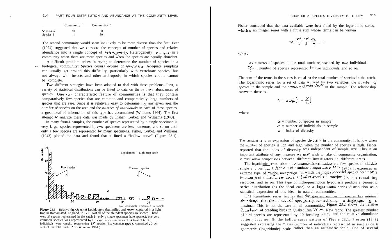
T&o different strategies have been adopted to deal with these problems. First, avariety of statistical distributions can be fitted to data on the relative abundances ofspecies. One v2~ characteristic feature of communities is that they containcomparatively few species that are common and comparatively large numbers ofspecies that are rare. Since it is relatively easy to determine for any given area thenumber of species on the area and the number of individuals in each of these species,a great deal of information of this type has accumulated (Williams 1964). The firstattempt to analyze these data was made by Fisher, Corbet, and Williams (1943).

In many fauna1 samples, the number of species represented by a single specimen isvery large, species represented by two specimens are less numerous, and so on untilonly a few species are represented by many specimens. Fisher, Corbet, and Williams(1943) plotted the data and found that it fitted a “hollow curve” (Figure 23.1).

Lepidoptera - Light trap catch

Common speciesI4 Rare species

No. individuals represented in sampleFipre 23.1 Relative abundance oi Lepidoptera (butterflies and moths) captured in a lighttrap in Rothamsted. England, in 1935. Not all of the abundant species are shown. Therewere 37 species represenred in the catch br only a single specimen (rare species); one verycommon species was represented by 1799lndiriduals in the catch. h total of 6814individuals were caught, representing 19: species. Six common species comprised 50 per-cent of the total catch. (.After Willlams 1964.)

Fisher concluded that the data available were best fitted by the logarithmic series,lvhich is an integer series with a finite sum whose terms can be written

lvhere

cs = number of species in the total catch represented by one individuala$-=2

number of species represented by two individuals, and so on.

The sum of the terms in the series is equal to the total number of species in the catch.The logarithmic series for a set of data is fixed by two variables, the number ofspecies in the sample and the number of indiz,iduals in the sample. The relationshipbenveen these is

s = alog, 1 + !Y‘c 1c k

where

.S = number of species in sampleN = number of individuals in sample

(Y = index of diversity

The constant LY is an expression of species diversi? in the community. It is low whenthe number of species is Ion and high when the number of species is high. Fisherreported that the index of diversity was independent of sample size. This is an

important attribute of any measure we ma)- wish to take of community organization;it must allow comparisons between different investigators in different areas.

The logarithmic series arises inmmunities wi&r.el_a_tivelv few species &&i&a-./-single en~ironmentalfacroriLoidamrr-lan~Q~~e-(May 1975). It expresses an- -extreme type of “niche preemption” in which the most succe_&! speciesgJerEpJ> afractio_n_k ofth&otal resclurres,-t~~~~e~~~~~fraction k~ of.the remainingresources, and so on. This type of niche-preemption hypothesis predicts a geometricseries distribution (as the ideal case) or a .logarithmic series distribution as astatistical expression of this ideal in natural communities.

The logarithmic series implies that th_e greatest number of species has minimal

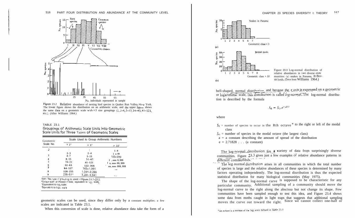
abundance,~lhal~tbe_~number_of _spscies represgnJe3 b y a sjcg!e-_speclmen I---_-m.-_----maximal. This is not the case in all communities. Figure 23.2 shows the relative

ab-&dance of breeding birds in Quaker Run iTalley, New York. The greatest numberoi bird species are represented by 10 breeding p airs, and the relative abundance

pat tern does not f i t the hol low-curve pat tern of Figure 23.1. Preston (1948)suggested expressing the s axis (number of individuals represented in sample) on ageometric (logarithmic) scale rather than an arithmetic scale. One of several

516 PART FOUR DISTRIBUTION AND ABUNDANCE AT THE COMMUNITY LEVEL CHAPTER 23 SPECIES DIVERSITY I: THEORY 517

I II I I Ill,1 1 J/l--+

,5 I I15 I25 35 45 55 6.5

Figure 23.2Ko. individuals represented in sample

Relative abundance of nesting bird species in Quaker Run Valley New York.The lower figure shows the distribution on an arithmetic scale, and rhe upper kgnre showsthe same dara on a geometric scale ivirh x3 size groupings (1, .?.A, 5-13, 14-40, 41-121,etc.). (After Williams 1964.)

TABLE 23.1Groupings of Arithmetic Scale Units into GeometricScale Units for Three Types of Geometric Scales

Scale Used to Group Arithmetic Numbers

x 2" x 3" x 10’

GeometricScale No.

7; I 1

2-3 2-43 4-7 5-134 8-15 14-40

l-91 o-99

100-9991 ,ooo-9,999

1 o,ooo-99,9991 oo,ooo-999,999

-

5 16-31 41-1216 32-63 122-3647 64-1278

365-1,093128-255

91,094-3,280

256511 3.281-9,841

h’ote. The tYPe of groupmg is used m Fhgures 23.2-23.5.aOctave scaie of Preston (1948). equivalent to log2 scale“Equivalent to ICJQ scaie.

-

Wwaient to logic scale.

geometric scales can be used, since they differ only by a constant multiplier; a few

scales are indicated in Table 23.1.When this conversion of scale is done, relative abundance data take the form of a

Snakes in Panama

01 2 3 4 5 6 7

Geometric class X 3(a)

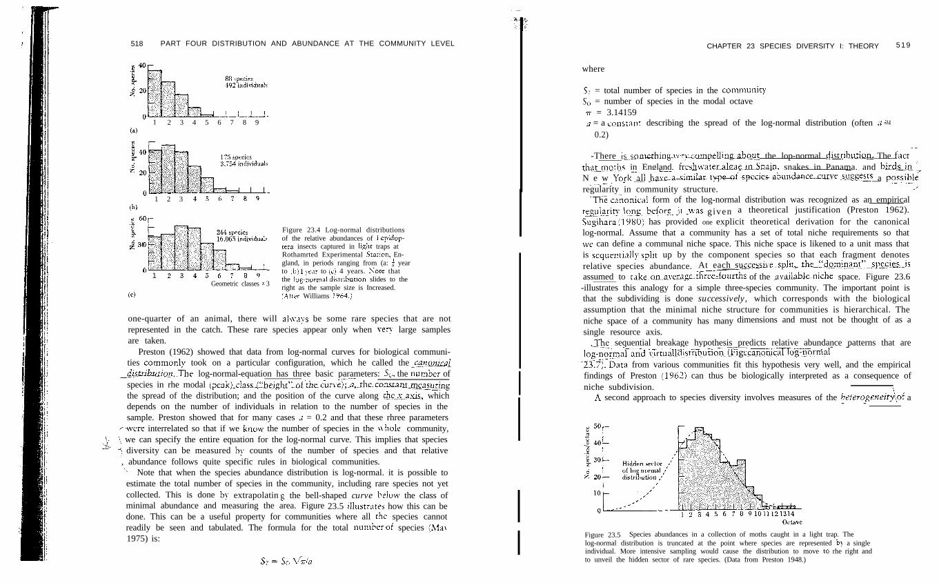
1 2 3 4 5 6 7 8Figure 23.3 Log-normal distribution ofrelative abundances in rwo diverse com-

(b)

Geometric class X 10 munities: (a) snakes in Panama, (b) Brit-ish birds. {Dara from Williams 1964.)

bell-shaped, normal distribution, and because the x-a.~jsI~-exp.ressed_on_a.gqqmetricT_-a7---------or iG@&mic scale, &&tr~butlon is called log-normaLThe log-normal distribu-tion is described by the formula

_... ~. .--.

where

,SR = number of species to occur in the Rth octave * to the right or left of the modal

classSo = number of species in the modal octave (the largest class)a = a constant describing the amount of spread of the distributione = 2.71828 . . . (a constant)

The log-nqr_maLdistribution _fi_t_s-__--a variety of data from surprisingly diverse~~~communities. Figure -33.3 gives just a few examples of relative abundance patterns in

_--- .__.__ _ _~ ._.. --~-.. ~~Y!lIff&ent commumtles.-_~._--~

The-log-normal distriburion arises in all communities in which the total numberof species is large and the relative abundances of these species is determined by manyfactors operating independently. The log-normal disrribution is thus the expectedstatistical distribution for many biological communities (May 1975).

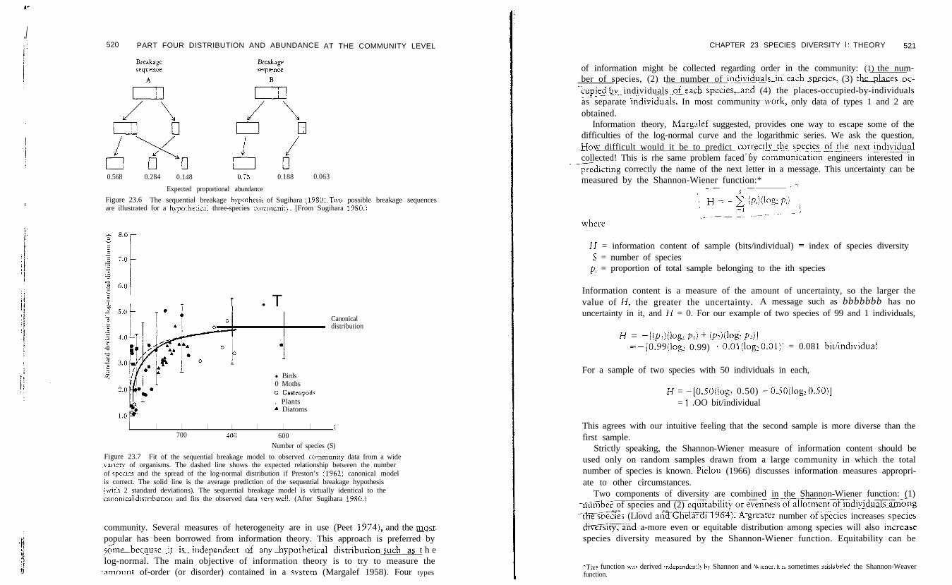
The shape of the log-normal curve is supposed to be characteristic for any

particular community. Additional sampling of a community should move the

log-normal curve to the right along the abscissa but not change its shape. Fewcommunities have been sampled enough to test this idea, and Figure 23.4 showssome data from moths caught in light traps that suggests that additional samplingmoves the curve out toward the right. Since we cannot collect one-half or

518 PART FOUR DISTRIBUTION AND ABUNDANCE AT THE COMMUNITY LEVEL

” 1 2 3 4 5 6 7 8 9(4

1 2 3 456789(b)

cc 60r

%

..:;;< :..: ,.._ :::,: ; .: ..:.c:..$ 3. ,..+ Q.::, >.::..:; :<;::.p

~~du:

” 1 23456;89Geometric classes x 3

Cc)

Figure 23.4 Log-normal distributionsof the relative abundances of Lepidop-tera insects captured in ii&h: traps atRothamrted Experimental Starion, En-gland, in periods ranging from (a: f yearto :b) 1 year to (c) 4 years. Nore thatthe log-normai distribution slides to theright as the sample size is Increased.(.Uter Williams 1964.1

one-quarter of an animal, there will ahvays be some rare species that are notrepresented in the catch. These rare species appear only when very large samplesare taken.

Preston (1962) showed that data from log-normal curves for biological communi-ties commoniy took on a particular configuration, which he called the canon&J

&hbwiotz. The- log-normal-equation has three basic parameters: 5s. the &Y&r of-._ x----species in rhe modal (peak)_classi~eight’Lof thecurr,e);~a,~rheconsrant_measurigthe spread of the distribution; and the position of the curve along rhex.asis, whichdepends on the number of individuals in relation to the number of species in thesample. Preston showed that for many cases 1 = 0.2 and that these rhree parameters

/-were interrelated so that if we know the number of species in the lvhole community,‘: we can specify the entire equation for the log-normal curve. This implies that species: diversity can be measured by counts of the number of species and that relative, abundance follows quite specific rules in biological communities.

‘,- Note that when the species abundance distribution is log-normal. it is possible toestimate the total number of species in the community, including rare species not yetcollected. This is done by extrapolatin g the bell-shaped curve below the class ofminimal abundance and measuring the area. Figure 23.5 illustrsres how this can bedone. This can be a useful property for communities where all rhc species cannotreadily be seen and tabulated. The formula for the total number of species (Ma\1975) is:

CHAPTER 23 SPECIES DIVERSITY I: THEORY 5 1 9

where

ST = total number of species in the communitvSo = number of species in the modal octave

57 = 3.14159a = a constant describing the spread of the log-normal distribution (often u z

0.2)

-There issomething VPW ~ornpelling~out the lop-normal distr!UQn. The fact--thaLmoths in England, freshlater algaeinSpa& snakes in Panama, and bird& ‘iN e w ~ork-~ll_~~~~-s~il~f--species-abundancerurve~_s_u_ggests a poSsib)e_m_-~-.-_- -regularity in community structure. /

Thecanonical form of the log-normal distribution was recognized as an empiricalregularity J.gng_-befqre- Jt -Was g iven a theoretical justification (Preston 1962).Sugihara (19~0) has provided one explicit theoretical derivation for the canonicallog-normal. Assume that a community has a set of total niche requirements so thatwe can define a communal niche space. This niche space is likened to a unit mass thatis sequentiall!T split up by the component species so that each fragment denotesrelative species abundance. At each succe~siusplit~he~d.~~~n~~~.~~~~i~~~assumed to take~on.a~er~ge-~ourths of the ~availableniche space. Figure 23.6-illustrates this analogy for a simple three-species community. The important point isthat the subdividing is done successively, which corresponds with the biologicalassumption that the minimal niche structure for communities is hierarchical. Theniche space of a community has many dimensions and must not be thought of as asingle resource axis.Jhe sequential breakage hypothesis predicts relative abundance patterns that are_- _--~_

log-~~rn~-~ent~c~-~~t~~----_-. - -

d$triKZion~~ure._ca_npnical~log-norm-TL>yData from various communities fit this hypothesis very well, and the empirical

findings of Preston (1962j can thus be biologically interpreted as a consequence ofniche subdivision.

A second approach to species diversity involves measures of the h~teroge~2ri~$~of a- -

Figure 23.5 Species abundances in a collection of moths caught in a light trap. Thelog-normal distribution is truncated at the point where species are represented b!- a singleindividual. More intensive sampling would cause the distribution to move to rhe right andto unveil the hidden sector of rare species. (Data from Preston 1948.)

./i’


0.568 0.284 0.148 O.i5 0.188 0.063

Expected proportional abundance

Figure 23.6 The sequential breakage hyporhests of Sugihara (19’20). TLVO possible breakage sequencesare illustrated for a h!-potherical three-species communi~. [From Sugihara 19SO.j

I T T l T

l Birds0 Moths0 Gastropods. PlantsA Diatoms

Canonicaldistribution

I I I I I I I I700 100 600

Number of species (S)

Figure 23.7 Fit of the sequential breakage model to observed community data from a widerariery of organisms. The dashed line shows the expected relationship between the numberof spectes and the spread of the log-normal distribution if Preston’s (1962) canonical modelis correct. The solid line is the average prediction of the sequential breakage hypothesis!\vith 2 standard deviations). The sequential breakage model is virtually identical to thecanomcal distriburton and fits the observed data yer)- ~~11. (After Sugihara 19SO.)

community. Several measures of heterogeneity are in use (Peet 1974), and the m_l9st.popular has been borrowed from information theory. This approach is preferred by&aebecause_it_iss independ~otanyhypatheric~distribution suchas t h elog-normal. The main objective of information theory is to try to measure the

mamnunt of-order (or disorder) contained in a system (Margalef 1958). Four types

CHAPTER 23 SPECIES DIVERSITY I: THEORY 521

of information might be collected regarding order in the community: (1) the num-ber of species, (2) the number of indivi-cJua!tich+ecies, (3) t-c-

‘cupied bv individuals oj_each_species+nd (4) the places-occupied-by-individuals_ _.___ -------.: -_--as separate mdlvrduals. In most community lvork, only data of types 1 and 2 areobtained.

Information theory, Margalef suggested, provides one way to escape some of thedifficulties of the log-normal curve and the logarithmic series. We ask the question,

.HQW difficult would it be to predict .cozecth-thes?ecCeL ofthe- next indiviclualcollected! This is rhe same problem faced by coimmumcation engineers interested in

3icting correctly the name of the next letter in a message. This uncertainty can bemeasured by the Shannon-Wiener function:* .,-,~_-.- - ~.

T

H = information content of sample (bits/individual) = index of species diversityS = number of species

p, = proportion of total sample belonging to the ith species

Information content is a measure of the amount of uncertainty, so the larger thevalue of H, the greater the uncertainty. A message such as bbbbbbb has nouncertainty in it, and H = 0. For our example of two species of 99 and 1 individuals,

H = -[(p,)(logr pd + $4(log: P2)l= - [0.99(logz 0.99) -t O.Ol(log. O.Ol)] = 0.081 bit/individual

For a sample of two species with 50 individuals in each,

H = -[0.50(logz 0.50) + 0.50(logz 0.50)]= 1 .OO bit/individual

This agrees with our intuitive feeling that the second sample is more diverse than thefirst sample.

Strictly speaking, the Shannon-Wiener measure of information content should beused only on random samples drawn from a large community in which the totalnumber of species is known. Pielou (1966) discusses information measures appropri-ate to other circumstances.

Two components of diversity are combined in the Shannon-Wiener function: (1)-n%iiber of species and (2) equiFas;li~ore~f~~~~~ent-dft~i~~~s-~~ong

--- --. ----th?$ecres (Llovd anbCh~iar-dl~9617~--A-greater number of$ecies increases species-d&@%it~nd a-more even or equitable distribution among species will also in&easespecies diversity measured by the Shannon-Wiener function. Equitability can be

*Thus function was derived mdependenrly by Shannon and Wiener. It IS sometimes mtslabeled the Shannon-Weaverfunction.


measured in several ways. The simplest approach is to ask, What would bethe species diversity of this sample if all S species were equal in abundance? In thiscase,

where

Hma?. = species diversity under condiGons of maximal equitabilityS = number of species in the communin

Thus, for example, in a community with two species only,

Hmax =log: 2 = 1.00 bit/individual

as we observed earlier. Equitability can now be defined as the ratio

where

E = equitability (range O-l)H = observed species diversity

Hmax = maximum species diversity = log1 S

Table 23.2 presents a sample calculation illustrating the use of these formu-las.

Other measures of diversity can be derived from probability theory. Simpson(1949) suggested this question: What is the probability that two specimens picked atrandom in a community of infinite size will be the same species? If a person went intothe boreal forest in northern Canada and picked two trees at random, there is a fairlyhigh probability that they would be the same species. If a person went into thetropical rain forest, by contrast, two trees picked at-random would have a lowprobability of being the same species. We can use this approach to determine anindex of diversity:

Simpson’s index of diversiry = probability of picking two organisms at randomthat are differenr species

= 1 - (probability of picking two organisms thatare the same species)

If a particular species i is represented in the community by p, (proportion ofindividuals), the probability of picking two of these at random is the jointprobability [(pJ(p,)] or pt. If we sum these probabilities for all the i species in thecommunity, we get Simpson’s diversity (D):


D = 1 - i iPr)’i=,

where

D = Simpson’s index of diversityp, = proportion of individuals of species i in the community

For example, for our two-species communiy lvith 99 and 1 individuals,

D = 1 - I(O.99): + (0.01)2] = 0.02

Simpson’s index gives relatively little weighr to the rare species and more weight tothe common species. It ranges in value from 0 (low diversity) to a maximum of (1 -l/S), bvhere S is the number of species.

In practice it seems to matter ver! little which of these different measures ofspecies diversity we use, and rhe combination of two measures-( 1) of the number of

TABLE 23.2Sample Calculations of Species Diversityand Equitability Through the Use of theShannon-Wiener Function

Tree Species

HemlockBeech~eliow birchSugar mapleBlack birchRed map!eBlack cherry\&We ashBasswoodYellow poplarMagnolia

Total

Proportional Abundance

(P3 GoXlOL22P,)”0.521 0.4900.324 0.5270.046 0.2040.035 0 1730.026 0 1370.025 0.1330 009 0.0610 006 0.0440.004 0.0320.002 0.0180.001 0010

1 000 H = 1 829

hm = log2 5 = log: 11 = 3 453

Eaultablllty = E = 2~ = 3.45g =l.szq

0.53

Note that there is no speed theorexa’ reasol to “se bg; lnSt?adof log, or loglo The log2 usage ;“,es US !nformat~on unlfs in“b,ts” (binary d,glts) and IS preferred by mformatlon !heoris?sSee PIelou (1969. p 2291.Source bough (1936)


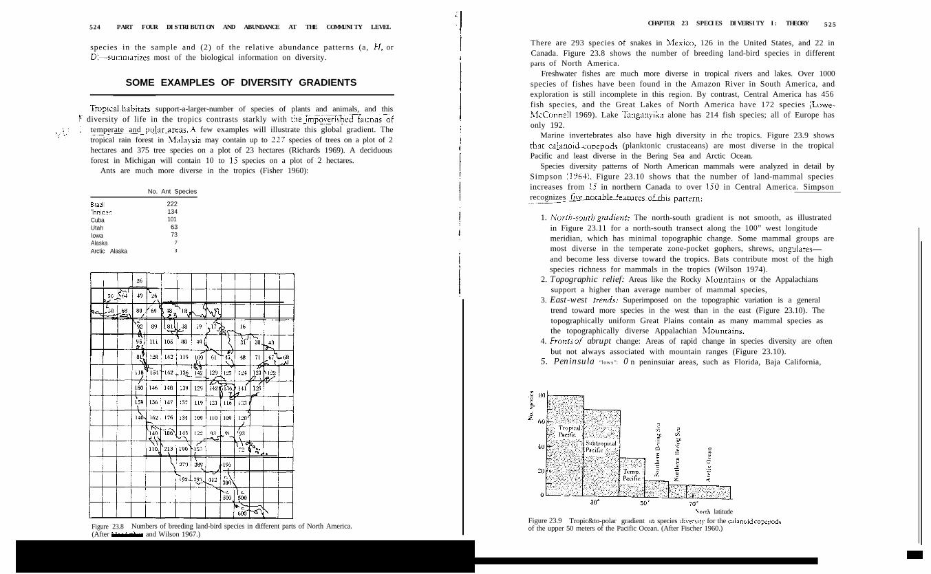
species in the sample and (2) of the relative abundance patterns (a, H, orD)-summarizes most of the biological information on diversity.

SOME EXAMPLES OF DIVERSITY GRADIENTS

Tropicaihabitats support-a-larger-number of species of plants and animals, and this[ diversity of life in the tropics contrasts starkly with the,&Y$ZZs&~f~~~<f

a,\: 1 temperate and polaqareas. X few examples will illustrate this global gradient. TheI_~-.-__ ~~tropical rain forest in 12/lalaysia may contain up to 227 species of trees on a plot of 2hectares and 375 tree species on a plot of 23 hectares (Richards 1969). A deciduousforest in Michigan will contain 10 to 15 species on a plot of 2 hectares.

Ants are much more diverse in the tropics (Fisher 1960):

No. Ant Species

Btazll 222Tmdad 134Cuba 101Utah 63Iowa 73Alaska 7

Arctic Alaska 3

I

Figure 23.8 Numbers of breeding land-bird species in different parts of North America.(After !&cr\rthur and Wilson 1967.)


There are 293 species of snakes in 1Iexico, 126 in the United States, and 22 inCanada. Figure 23.8 shows the number of breeding land-bird species in differentparts of North America.

Freshwater fishes are much more diverse in tropical rivers and lakes. Over 1000species of fishes have been found in the Amazon River in South America, andexploration is still incomplete in this region. By contrast, Central America has 456fish species, and the Great Lakes of North America have 172 species (Lowe-hlcConnel1 1969). Lake Tanganyika alone has 214 fish species; all of Europe hasonly 192.

Marine invertebrates also have high diversity in the tropics. Figure 23.9 showsthat~cajanoidiopepods (planktonic crustaceans) are most diverse in the tropicalPacific and least diverse in the Bering Sea and Arctic Ocean.

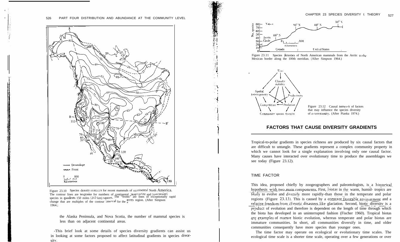
Species diversity patterns of North American mammals were analyzed in detail bySimpson (1964). Figure 23.10 shows that the number of land-mammal speciesincreases from 15 in northern Canada to over 150 in Central America. Simpsonrecognizes fi~_e4atablefeatures_ofthis_pattern:_.---

1. No&-so& ,o)~ldielzt: The north-south gradient is not smooth, as illustratedin Figure 23.11 for a north-south transect along the 100” west longitudemeridian, which has minimal topographic change. Some mammal groups aremost diverse in the temperate zone-pocket gophers, shrews, ungulates-and become less diverse toward the tropics. Bats contribute most of the highspecies richness for mammals in the tropics (Wilson 1974).

2. Topographic relief: Areas like the Rocky hlountains or the Appalachianssupport a higher than average number of mammal species,

3. East-west trends: Superimposed on the topographic variation is a generaltrend toward more species in the west than in the east (Figure 23.10). Thetopographically uniform Great Plains contain as many mammal species asthe topographically diverse Appalachian &fountains.

4. Fronts of abrupt change: Areas of rapid change in species diversity are oftenbut not always associated with mountain ranges (Figure 23.10).

5. Peninsula “lows”: 0 n peninsuiar areas, such as Florida, Baja California,

Sorth latitudeFigure 23.9 Tropic&to-polar gradient m species diversity for the calanoid copepodsof the upper 50 meters of the Pacific Ocean. (After Fischer 1960.)


- Downslope

- Front

0 800

itli&Gs

II

Figure 23.10 Species densitv conrours for recent mammals of contmental North America.The contour lines are isograms for numbers of continental {nonmarine and noninsularjspecies in quadrats 150 miles (240 km) square. The “fronts” are lines of exceptionally rapid

change that are multiples of the contour Interval for the cmiven region. (After Simpson

1964.;

the Alaska Peninsula, and Nova Scotia, the number of mammal species isless than on adjacent continental areas.

-This brief look at some details of species diversity gradients can assist usin looking at some factors proposed to affect latitudinal gradients in species diver-Lsitv.


Kilometers

Canada I Llnited States I

Figure 23.11 Species densities of North American mammals from the Arctic ro theMexican border along the 100th meridian. {After Simpson 1964.)

Compt:tltion -Prrdation

I

Communitv species dnrreit\

Figure 23.12 Causal network of factorsthat may influence the species diversityof a community. (After Pianka 1974.)

FACTORS THAT CAUSE DIVERSITY GRADIENTS

Tropical-to-polar gradients in species richness are produced by six causal factors thatare difficult to untangle. These gradients represent a complex community property inwhich we cannot look for a single explanation involving only one causal factor.Many causes have interacted over evolutionary time to produce the assemblages wesee today (Figure 23.12).

TIME FACTOR

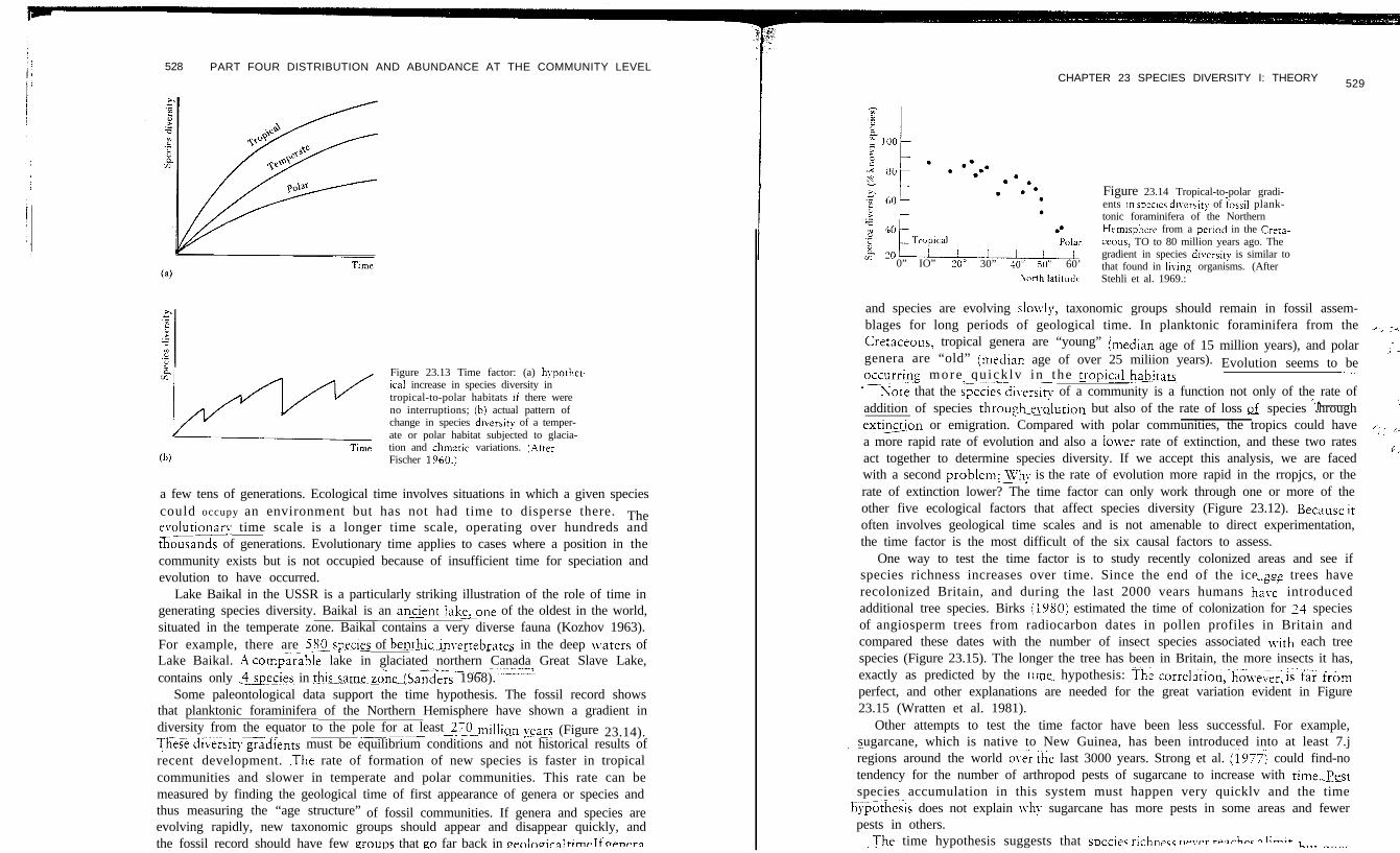
This idea, proposed chiefly by zoogeographers and paleontologists, is a historia!.- -hypothesis A&two-mamcomponents. First, biotas~ in the warm, humid- tropics areXi&l,; to evolve and diver+ more rapidly-than those in the temperate and polarregions (Figure 23113). This is caused by a c_onstant-iauarable_.s~~~~onrnent and a~. __rela-fre-edom from-climanc.disasters.like glaciation. Second, biotic diversitv is a---_c_

product of evolution and therefore is dependent on the length of time through whichthe biota has developed in an uninterrupted fashion (Fischer 1960). Tropical biotasare--examples of ~mature biotic evolution, whereas temperate and polar biotas areimmature communities. In short, all communities diversify in time, and oldercommunities consequently have more species than younger ones.

The time factor may operate on ecological or evolutionary time scales. Theecological time scale is a shorter time scale, operating over a few generations or over


Figure 23.13 Time factor: (a) hypother-icai increase in species diversity intropical-to-polar habitats if there wereno interruptions; ib) actual pattern ofchange in species diversity of a temper-ate or polar habitat subjected to glacia-tion and chmatic variations. (AfterFischer 1960.)

a few tens of generations. Ecological time involves situations in which a given speciescould occupy an environment but has not had time to disperse there. Theevolutiona_n- time scale is a longer time scale, operating over hundreds andt&&sands of generations. Evolutionary time applies to cases where a position in thecommunity exists but is not occupied because of insufficient time for speciation andevolution to have occurred.

Lake Baikal in the USSR is a particularly striking illustration of the role of time ingenerating species diversity. Baikal is an ancientJake,one of the oldest in the world,situated in the temperate zone. Baikal contains a very diverse fauna (Kozhov 1963).For example, there are 58O.spe.cies of benthic_invertebrates in the deep waters of- - - -Lake Baikal. AY comparable lake in glaciated northern Canada Great Slave Lake,

-------.--------.-.__Imcontains only aecies in thissame_zone_iSanders 1968).

Some paleontological data support the time hypothesis. The fossil record showsthat planktonic foraminifera of the Northern Hemisphere have shown a gradient indiversity from the equator to the pole for at least 270 million~pe~s--__~-~ ~~-~ ~-- (Figure 23.14).ThZse~diverYitj~dients must be equilibrium conditions and not historical results ofrecent development. .The rate of formation of new species is faster in tropicalcommunities and slower in temperate and polar communities. This rate can bemeasured by finding the geological time of first appearance of genera or species andthus measuring the “age structure” of fossil communities. If genera and species areevolving rapidly, new taxonomic groups should appear and disappear quickly, andthe fossil record should have few ,groups that go far back in wnlnoiral rime If opnprg


0” IO” zoo 30” 10” 50” 60’\orth latitudr

Figure 23.14 Tropical-to-polar gradi-ents m species d]verLity of iossii plank-tonic foraminifera of the NorthernHemisphere from a period in the Crera-ceous, TO to 80 million years ago. Thegradient in species diversi? is similar tothat found in Iking organisms. (AfterStehli et al. 1969.:

and species are evolving slovvly, taxonomic groups should remain in fossil assem-blages for long periods of geological time. In planktonic foraminifera from the <. 3Cretaceous, tropical genera are “young” ’genera are “old” ’

,median age of 15 million years), and polar,median age of over 25 miliion years).

>‘>-

occurring~ more qu ick lv in the tropicalJabitatsEvolution seems to be-

‘-Note that the s~e~ieshiversity of a community is a function not only of the rate ofaddition of species throug&&.rtian but also of the rate of loss ok species through

,,I ;

ext*on or emigration. Compared with polar communities, the tropics could havea more rapid rate of evolution and also a lovver rate of extinction, and these two rates

‘:: +

act together to determine species diversity. If we accept this analysis, we are facedG,

with a second problem:Jyhy is the rate of evolution more rapid in the rropjcs, or therate of extinction lower? The time factor can only work through one or more of theother five ecological factors that affect species diversity (Figure 23.12). Because itoften involves geological time scales and is not amenable to direct experimentation,the time factor is the most difficult of the six causal factors to assess.

One way to test the time factor is to study recently colonized areas and see ifspecies richness increases over time. Since the end of the ice aoe trees haverecolonized Britain, and during the last 2000 vears humans ha:.: introducedadditional tree species. Birks (1980) estimated the time of colonization for 24 speciesof angiosperm trees from radiocarbon dates in pollen profiles in Britain andcompared these dates with the number of insect species associated vvith each treespecies (Figure 23.15). The longer the tree has been in Britain, the more insects it has,exactly as predicted by the tnme. hypothesis: The~correlation,~h&,~ev~er~ is far-fromperfect, and other explanations are needed for the great variation evident in Figure23.15 (Wratten et al. 1981).

Other attempts to test the time factor have been less successful. For example,sugarcane, which is native to New Guinea, has been introduced into at least 7.j- .~regions around the world o<er-the last 3000 years. Strong et al. (i977) could find-notendency for the number of arthropod pests of sugarcane to increase with time.,Pxstspecies accumulation in this system must happen very quicklv and the time

hj;j5othesis does not explain why sugarcane has more pests in some areas and fewerpests in others.

-The time hypothesis suggests that snecies richnecc np1.p~ rP9rh-c = I;-;* I..,, ---^


.

.. ’ . . Figure 23.15 Tnne factor: the time an-

.;h, ,*: ;-*, ; , giosperm tree species hale been continu-ousl~ present in Britain in relation to thenumber of msect species associated witheach tree species. Species richness growsover time, as suggested by the clme hy-

0 2 1 6 8 10 12 14 pothesis, hut the relationship is far fromTime pa-in; in Britain (thousands of years) perfect. (Data from Birks 1980.)

record or not (Gould 1981). Because the time factor is so difficult to test, we shoulduse it only after we have exhausted simpler hypotheses to explain diversity trends.

~_. -_ -a--.-I ___. _ -. _. - --

SPATIAL HETEROGENEITY FACTOR.---__- ___. .-..~ -- -- .-

There-couXbe-a general increase .in environmental complexity as one proceeds- - - ~_._ .--.--.-----toward the tropics. The m_oreheterogeneous and come!eklhe.p~~:stcaTpn.v_rqnment,.the more complex-&--plant and animal commumties and the higher the species

diversity. This factor can be considered on both a macro and a micro scale..Topographic relief, or mac~ospatial heteI~~e2zsit~,certainlJi has a strong effect on

species diversity. Simpson (1964) has shown that the highest diversities of mammalsin the United States occur in the mountain areas (Figure 23.10). The explanation forthis seems quite simple: Areas of high topographic relief contain many differenthabitats and hence more species. Also, mountainous areas produce more geographicisolation of populations and so may promote speciation.

MacArthur (1965) suggests that we should recognize two components in trying toanalyze latitudinal gradients in species diversity: d-diversity, andbetween-balzitiatdiversit~. \‘ie can illustrate this distinction by two simple schemes to- -explain tropical diversity:

iScheme ATemperate Tropical

-w

Country CountryI

8’ No. speaes per habitat 10 10No. different habitats 19 50

All the increase in tropical diversity is caused by between-habitat diversity in this Tropical habitats would contain more bird species if there were more foliage-hypothetical scheme. height diversity in tropical forests and if birds recognized the same vegetation layers


Scheme B

No. species per habitatNo. different habltats

TemperateCountry

1010

TropicalC o u n t r y i

5010

In this oversimplified scheme, all the increase in tropical diversity is due toMithin-habitat diversity.

-----Can the facror oftopographic relief provide some explanationfor_.latitudin_alvariation in species diversir)? There is some evidence that this is part of the reasonthat the tropics are so rich in species. MacArthur (1969) showed that, for land birds,2 hectares of Panama forest supported 21 times as many bird species as 2 hectares ofVermont forest. But larger areas in the tropics support proportionately even morespecies. Ecuador has c_7 tirnes~~.~~rnber-~-~~~ds..~~~es as New En-land, even__ --._ ---a___though &?ZZZZoth approximately 260,000 km?. For land birds, there areboth more species per habitat in the tropics and also more habitats per unit of area.

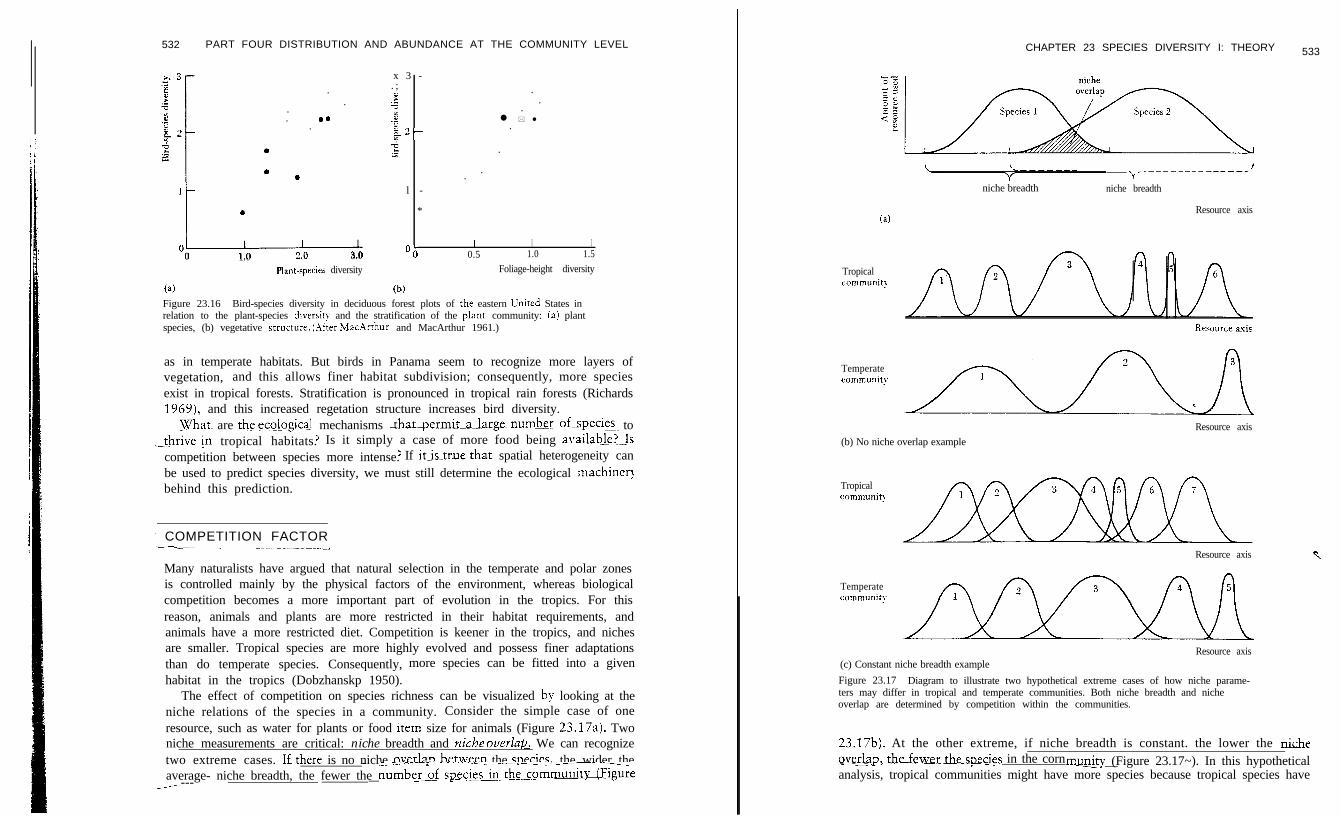
: Mi’~~j~~~o~~~efers to a local scale of organism-sized objects such asi_- ~~~rocks and vegetation. The most difficult problem here is to determine which of themany things that we as humans see in a habitat are really important to the particularorganisms under study. Birds have been studied more in this regard than othergroups. lZlacArthur and MacArthur (1961) measured bird-species diversity on aseries of study areas and attempted to relate this to two aspects of the vegetation:p lan t - spec ies divers i ty andfoliage-height divetity. Foliage-height diversity is ameasure of stratification and evenness in the vertical distribution of vegetation;highb strarifiedco.mmunitie~ave high foliage-height.divers~ti~e~-~~~ith..d~.~~.e.~r~~~~.&&anches and-lea\ies~~~ds..fo~~~~e- ground ~0 the tsp of the canopy.. It doesnot matter Lvhether the strata are contributed by a variety of species or by a varietyof age classes of one species. MacArthur. found that bird-species-pivqrsity-was not j:correlated so much with plant-species diversity as it was with foliage-height diversit!(Figure 23.16). This suggests that we can predict the %-d-shecies diversity on aforested area without any knowledge of the plant species that make up thecommunity. Vegetation structure, ~r~t_r~~fication,~se~s~to_be mo_re_ impg,rtant to -.A<---_--birds than planEspecIes_co@tin.

-~---in shrub and Prassland ha.bitars, vertical stratification is less important indetermining bird-species diversity than it is in forested habitats. In the SonoranDesert, for example, bird diversity is related to the densitv of particu=st plantssuch as saguaro and ch&ac_ti (Tomoff 1974). Many different trees providesuitable nest sites in a forest, but in a desert habitat onlv a few growth-forms may b,e

,di.c.aLas -nesting--s&. Vertical stratification in shrub and grassland habitats 1slimited and may be less important than horizontal structure or patchiness. Birddi\Lersir!r.may-bepredicted moreaccuratelv from a krm$Tdge on&ih horizon-

& and vertical structure in vepetatioa(Roth 1976). Some of the scatter of points--czFigure 23.16 might be removed if we considered both horizontal and

vertical structure.


.

..

.

. 0..

.

. .

O/0 1.0 3.0Plant-species diversity

x 3 -. ;0 .

Lz ..

R.g l * l

$2- .

G;=” .

..

l -

*

OOI I I

0.5 1.0 1.5

Foliage-height diversity

(a) (b)Figure 23.16 Bird-species diversity in deciduous forest plots of the eastern United States inrelation to the plant-species diversi? and the stratification of the plant community: (a) plantspecies, (b) vegetative strucrure. (.kfter MacArrhur and MacArthur 1961.)

as in temperate habitats. But birds in Panama seem to recognize more layers ofvegetation, and this allows finer habitat subdivision; consequently, more speciesexist in tropical forests. Stratification is pronounced in tropical rain forests (Richards1969), and this increased regetation structure increases bird diversity.

JVhat~ are the eco!ogical mechanisms ~rhat~per_mit_a_large_nwm~~_ofspecies~ to.-th:i& in tropical habitats.j Is it simply a case of more food being availabE&

competition between species more intense.3 If it&truethat spatial heterogeneity canbe used to predict species diversity, we must still determine the ecological machiner)behind this prediction.

( COMPETITION FACTOR- - -~ ~~__..~ -.m.__---.._,

Many naturalists have argued that natural selection in the temperate and polar zonesis controlled mainly by the physical factors of the environment, whereas biologicalcompetition becomes a more important part of evolution in the tropics. For thisreason, animals and plants are more restricted in their habitat requirements, andanimals have a more restricted diet. Competition is keener in the tropics, and nichesare smaller. Tropical species are more highly evolved and possess finer adaptationsthan do temperate species. Consequently, more species can be fitted into a givenhabitat in the tropics (Dobzhanskp 1950).

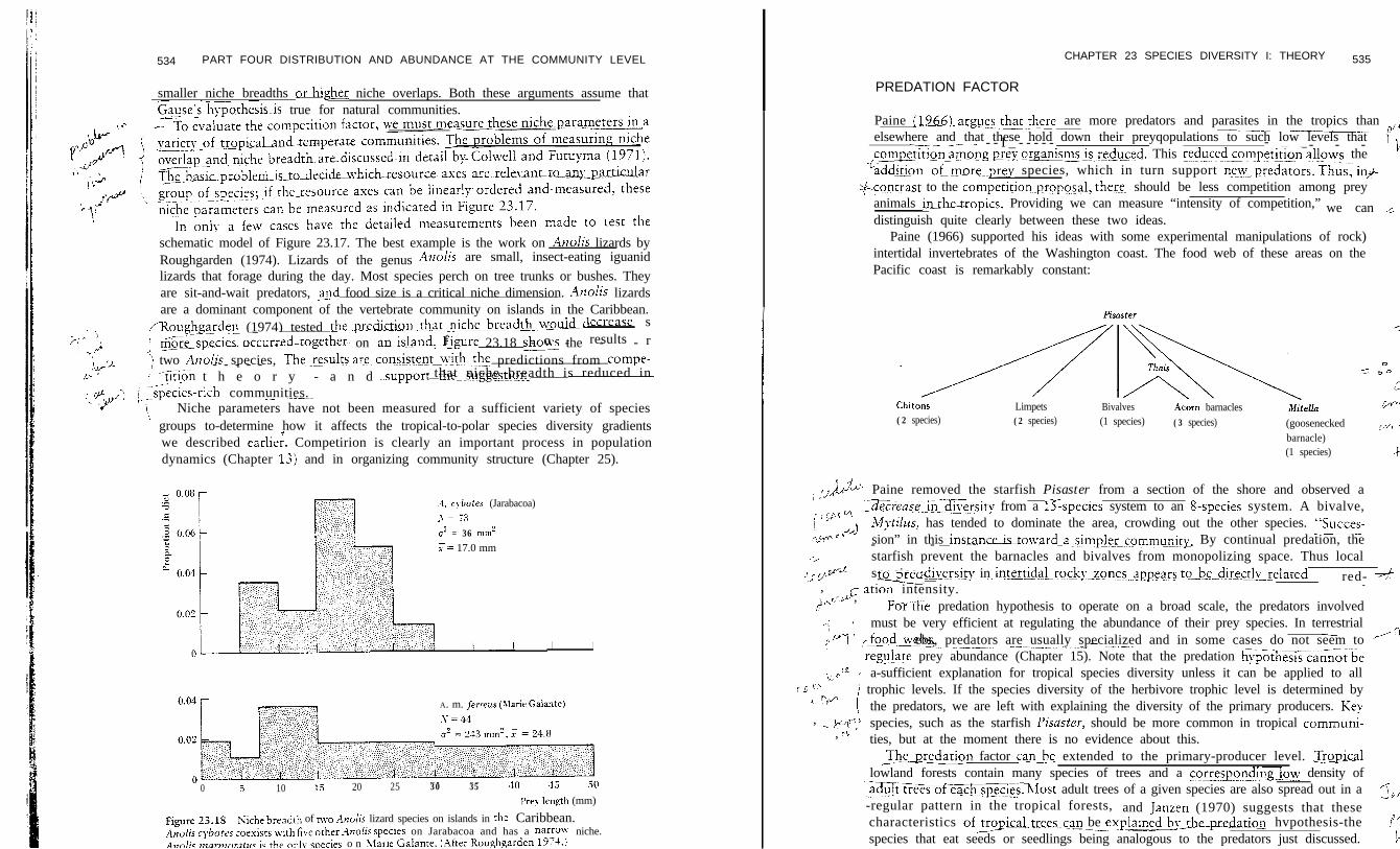
The effect of competition on species richness can be visualized by looking at theniche relations of the species in a community. Consider the simple case of oneresource, such as water for plants or food irem size for animals (Figure 23.17aj. Twoniche measurements are critical: niche breadth and vziche overlu~. We can recognizetwo extreme cases. ILthere is no niche oxerlapbetween the spsees, the wider the- -average- niche breadth, the fewer the nurnberf.speCiesinthec~-~-rn~~~e___- ---


\c------- ___ ___v

\” ,_________ ----_/niche breadth niche breadth

Resource axis

Tropicalcommunit>

Temperatecommunit!-

(b) No niche overlap example

Resource axis

Tropicalcommunit)

Resource axis t

Temperatecommunit!-

Resource axis(c) Constant niche breadth example

Figure 23.17 Diagram to illustrate two hypothetical extreme cases of how niche parame-ters may differ in tropical and temperate communities. Both niche breadth and nicheoverlap are determined by competition within the communities.

23.17b). At the other extreme, if niche breadth is constant. the lower the nicheoverlapdmemtipecies in the corn- - - munity (Figure 23.17~). In this hypotheticalanalysis, tropical communities might have more species because tropical species have


PREDATION FACTOR

Paine (1966.Larggcstkrhere are more predators and parasites in the tropics than o/’----~ -.-_ ~._elsewhere and that these hold down their preyqopulations to such low levels thatz-y- - - I _ - - - - - - _ _ - - --mtion anlong prey orgsnisEjSr_educed. This r~&cedcl~mp+tit.~ a&ws the

1 i/oadd_iuun- ofrmre--prey species, which in turn support neu-predators. Thus, in+

+contrast to the competitions-proposa!, there should be less competition among preyanimals in-thetropics. Providing we can measure “intensity of competition,” we can 4distinguish quite clearly between these two ideas.

Paine (1966) supported his ideas with some experimental manipulations of rock)intertidal invertebrates of the Washington coast. The food web of these areas on thePacific coast is remarkably constant:


smaller niche breadths odgher niche overlaps. Both these arguments assume thatGause’sxypothesis~is true for natural communities.

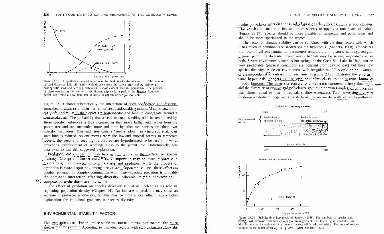
schematic model of Figure 23.17. The best example is the work on il120lis lizards byRoughgarden (1974). Lizards of the genus 4nolis are small, insect-eating iguanidZlizards that forage during the day. Most species perch on tree trunks or bushes. Theyare sit-and-wait predators, and food size is a critical niche dimension. ilnolis lizardsare a dominant component of the vertebrate community on islands in the Caribbean.

a secrease,/Roug&arden (1974) tested t_he_ps.e_dicrio~j ~~~species_o~~~d-rogether- on .an..isl_and,Figure 23.18 shows thef o rresults- - - -

J&A ) two Arzolis species, Thq_rrsults ace. consist-ent_-t_h__t predictions from compe-- - - - -P ’ ’ 5tioti t h e o r y - a n d -.support the_-sugg&o_nthat niche breadth is reduced in

--~1.->becies-rich communities.-.. ~----

Niche parameters have not been measured for a sufficient variety of species’ groups to-determine how it affects the tropical-to-polar species diversity gradients

we described earlie;. Competirion is clearly an important process in populationdynamics (Chapter 13) and in organizing community structure (Chapter 25).

B. cybotes (Jarabacoa).Y= ;3

0' = 36 mm'

I- = 17.0 mm

I I

A. m. ferrets (brie Galante)

0 .i 10 15 20 25 30 35 40 45 50

Pry length (mm)

Figure 23.18 Siche breadth of n~o A~zoIis lizard species on islands in the Caribbean.4,2a/is cvbotes coexists with five orher Abzolis species on Jarabacoa and has a narrox niche.bwn/;c &ilmlnr;ltIlc ic the o&r species o n Klarle Galanre. (hfter Roughgarden 19?4.)

I Pimter

Chitons Limpets Bivalves .4corn barnacles(2 species) (2 species) (1 species) (3 species)

Miella(gooseneckedbarnacle)(1 species)

I ,,.J&- Paine removed the starfish Pisaster from a section of the shore and observed a:

: i ;p ylaase-_incl&erslty from a 15-species system to an 8-species system. A bivalve,

I c ,4/JMptilus, has tended to dominate the area, crowding out the other species. “Succes-

~~,‘/Y- sion” in this instancels_to~vard_a_sl_m_p~e_r_comm_u_n_i_ty, By continual predation, the- --5

/‘Jstarfish prevent the barnacles and bivalves from monopolizing space. Thus local

<is: & species divErsi! in intertidalrod<yzon~s..~~pears tQ_b-~-~~~~c~ly_relatedtc --__ red- 4c ation intensity. _~,

i;,;* ,p - hY.the predation hypothesis to operate on a broad scale, the predators involved,/ g

EPA-l ’

must be very efficient at regulating the abundance of their prey species. In terrestrial

.fobL.. ~___~__~ ___.__.__.... -- -.-. -~-ebs, predators are usually specialized and in some cases do not seem to- -(Tt

,C! regu!ate prey abundance (Chapter 15). Note that the predation hypZ&Z&&g&e

*uA .- (1 :’rJ CL

a-sufficient explanation for tropical species diversity unless it can be applied to all

2, y.fli trophic levels. If the species diversity of the herbivore trophic level is determined by( the predators, we are left with explaining the diversity of the primary producers. Key

, _ yq, ri

species, such as the starfish Pisastev, should be more common in tropical communi-ties, but at the moment there is no evidence about this.

zburedation factor can-be extended to the primary-producer level. meallowland forests contain many species of trees and a correTond&glow density of

%-lu~trZ~-t!!.hpecles. lZiost adult trees of a given species are also spread out in a-regular pattern in the tropical forests,

2,rand Janzen (1970) suggests that these

characteristics OfsiLaLtrees~can be explainedmdation hvpothesis-the ‘“I1--2_ __-

species that eat seeds or seedlings being analogous to the predators just discussed. !+

PART FOUR DISTRIBUTION AND ABUNDANCE AT THE COMMUNITY LEVEL

”Distance from parent tree

Figure 23.19 Hypothetical model ro account for high tropical-forest diversiry. The amountof seed dispersed falls off rapidly with distance from the parent tree; and the activity oihost-speufic seed and seedling herbivores is most evident near rhe parent tree. The productof these two factors determmes a recruitment curve with a peak at the dlsrznx from theparent tree where a next adult tree is likely to appear. (After Janzen 1970.1

Figure 23.19 shows schematically the interaction of seed p_r~ductio~ and dispersalfrom the p- - - arenurPeandthe~act&~ity of se-eaters- lb&u&kiSLhl~e~e&andJrulIs in the tro.pics-are host-specific and tend to congregate around a

saurce-ofseeds. The probability that a seed or small seedling n-ill be overlooked by\ these specific herbivores is thus increased as they move farther and farther from the I

5 parent tree and are surrounded more and more by other tree species nirh their own1 specific herbivores. Thus each tree casts a “seed shadow, ” in which_survjvaL&ts1 own kind is reduced. As one moves tram the lowland tropical forests to temperate

--‘forests, the seed and seedling herbivores are hypothesized ro be less efficienr atpreventing establishment of seedlings close to the parent tree. Unfortunately, fewdata exist to test this suggested explanation.

PredatLon-and competition may be com$&nentary in their effects on species-d~t~.iMeI?ge_andSurherland-~~6),Cam~~o~-~-y -be more imp-maintaining-high-diversity-.arnong..par.asites and predators. while the process of_---~Jredation is more-important~ among herbivores_Superimposed-on -these effect&

another pattern:- In complex-communities-with many--species, predation is probablythe dominant interaction affecting diversity, whereas in

~~pet~iri~i~~~nafi~~~~a~~. -~simple~cornmumities,

The effect of predation on species diversity is just as unclear as its role inregulating population density (Chapter 14). i\n increase in predation may cause anincrease in prey-species diversity, but this may be more a local effect than a globalexplanation for latitudinal gradients in species diversity.

ENVIRONMENTAL STABILITY FACTOR

This &&pkaes-tIrmhemore-stable the e-n-,

species will-bypresent. According to this idea, regions with stabJe-climates allo-Mv,rhe_~____._. --


evolution of~pecrali7ationsand.a~ap~a~i~h~~ doareaswith erratic climates.- -‘TKresults in smaller niches and more species occupying a unit space of habitat(Figure 23.17). Species should be more flexible in temperate and polar areas andshould be more specialized in the tropics.

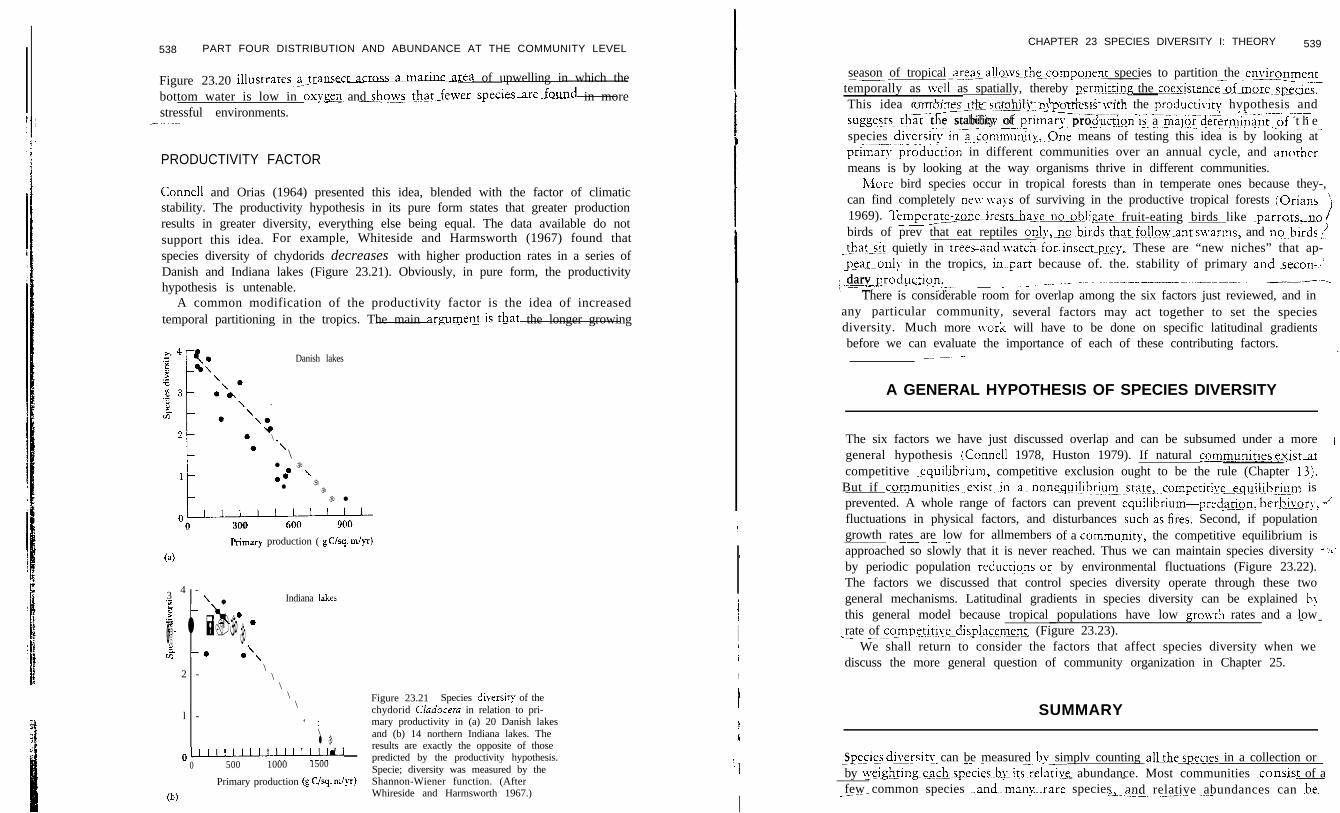
The factor of climatic stability can be combined with the time factor, with whichit has much in common. The stabzlrty-time hypothesis (Sanders 1968) emphasizesthe role of all environmental parameters-temperature, moisture, salinity, oxygen,pH-in permitting diversity. Low-diversity habitats may be severe, unpredictable, orboth. Severe environments, such as hot springs or the Great Salt Lake in Utah, can bevery predictable (physical conditions are constant from day to day) but have lowspecies diversity. A desert environment with irregular rainfall would-be-au example,&a+uupred’ KZI can setereenvir%n&nt~ F i g u r er d - 7 23.20 illustrates the stability-time hypothesis-Sanders (1968) apgiied the hypothesisarine fauna ofmuddy bottoms. The deep sea represegtsa stable.enrrironmentoflong time span,\& &------_and the diversity of bivalve andpolychaete.species-in. botmm sampleein-the-deep-sea. _m.----- _~ --was almost equal to that in-tropical. shallow-water.areas..This surprising-disrsity%r deep-sea-bottom organisms is difficult to reconcile with other hypotheses.. - .- -- ~-- __-_. _I-___-_ -

Gradient of ph\siolo&al stres

High LOW

Environmentalforces

Predominantlyphysical factors

Predominantlybiolotical rek&mshiDs

20

LOW

Species diversity>

High

Marine benthic invertebrates

/

-I

Il i .

I.

<Stress gradient

I I I I I I I0 20 40 60.

Oxygen saturation (56)

Figure 23.20 Stability-time hypothesis of Sanders (1968). The numbers of species (stip-pling) will decrease continuously along a stress gradient. The lower figure illustrates thisidea for marine invertebrates of a bottom transect off Sourhwest Africa. The area of oxygenstress is in the center of an upwelling area. (After Sanders 1968.)


Figure 23.20 illustratessansmdrea of upwelling in which the

bottom water is low in oxBen and sho~~that.-few~:rspeciesarefound in more__- _.__.stressful environments.

__-.

PRODUCTIVITY FACTOR

Connell and Orias (1964) presented this idea, blended with the factor of climaticstability. The productivity hypothesis in its pure form states that greater productionresults in greater diversity, everything else being equal. The data available do notsupport this idea. For example, Whiteside and Harmsworth (1967) found thatspecies diversity of chydorids decreases with higher production rates in a series ofDanish and Indiana lakes (Figure 23.21). Obviously, in pure form, the productivityhypothesis is untenable.

A common modification of the productivity factor is the idea of increasedtemporal partitioning in the tropics. The main argument-&that the longer growing

Danish lakes

.

.*Y

\‘\

\l \

.t �

l \\\ l

OI0 300

(4

himary production ( g C/sq. miyr)

3 4 -‘B \ l Indiana l&z

$ -\4 0

$ 3 - l =.\ 0

�3 \L?2 -0 42 -

\\

\\

\Figure 23.21 Species diversiry of the

l -‘ :

chydorid CIadorem in relation to pri-mary productivity in (a) 20 Danish lakes

\l \

and (b) 14 northern Indiana lakes. The

0.““““““““”results are exactly the opposite of those

0 500 1000 1500predicted by the productivity hypothesis.Specie; diversity was measured by the

Primary production (g C/sq. m/yr) Shannon-Wiener function. (After

(b) Whireside and Harmsworth 1967.)

!11

1I/I,11i

!.I

I


season of tropical areas.allavsrhecomppnent species to partition the enanment--_-temporally as Ivell as spatially, thereby perrminirting the coexistenrpof~_o_rR__s~~c~-This idea combines the stabilitv hv othesis nith the productivity hvpothesis and-.~-.:-----TJ-T-.-m ..- .___.___suggests--that t e stability of primarv pro

.I.-.-..;----------------_... --_L_ uctron is a malor determinam~of t h e__~_.. .~ -_-._ - ._. _. _...

species divers--inac6~m~ty..~One means of testing this idea is by looking atprim%t.~prohuction in different communities over an annual cycle, and annthermeans is by looking at the way organisms thrive in different communities.

h4ore bird species occur in tropical forests than in temperate ones because they-,can find completely ne\v Ivays of surviving in the productive tropical forests {Orians ‘j1969). Twrestshavemdbligate fruit-eating birds like ~parrots,-no !birds of prev that eat reptiles only~nobirds~ r.ha_t_fo!low_ant sivarms, and nqbirds :’

_t_hat_sir quietly in treesand watch-for.insect-pley,. These are “new niches” that ap-g-emair-only in the tropics, &part because of. the. stability of primary and..secon-,,’i-.--.-P.FPductjp.~.__darv __ __~_. _ _ ~.~- _._ _~--~-.-.__---.-----.---.--_ --.

There is considerable room for overlap among the six factors just reviewed, and inany particular community,diversity. Much

several factors may act together to set the speciesmore Ivork will have to be done on specific latitudinal gradients

before we can evaluate the importance of each of these contributing factors. .~~____. - ~-~ -

A GENERAL HYPOTHESIS OF SPECIES DIVERSITY

The six factors we have just discussed overlap and can be subsumed under a more !general hypothesis (Connell 1978, Huston 1979). If natural cmmunities existatjcompetitive .equilibrium, competitive exclusion ought to be the rule (Chapter 13).But if communitiesserist~ina_ nane_qui!ib-.~-~state,..c_ornpetitive_e_Elu_il:lbriurn isprevented. A whole range of factors can prevent equilibrium-predati_on, herb&ry? -cfluctuations in physical factors, and disturbances such-as&es. Second, if populationgrowth rates are low for allmembers__- .- ~-~~~~ ~~~ of a co-mmmunity, the competitive equilibrium isapproached so slowly that it is never reached. Thus we can maintain species diversity .+i-by periodic population reductions.or by environmental fluctuations (Figure 23.22).The factors we discussed that control species diversity operate through these twogeneral mechanisms. Latitudinal gradients in species diversity can be explained bythis general model because tropical populations have low gro\vth rates and a low- -rate of competiti\-e_displ;l~.~.~~~~ (Figure 23.23).+__--------- .~~

We shall return to consider the factors that affect species diversity when wediscuss the more general question of community organization in Chapter 25.

SUMMARY

.p_e-_m-_ ~,S ties diversitv can be measured bv simplv counting albhmecies in a collection or~~-~~ . ~~~ ---.~pi-by ~~i~h__tin~~~h_species~~b~-lrs~-r.e!~~~~ abundance. Most communities ~consist of a- -few common species -and.manyrare species_---- and relative abundances can .be..1_.___. ~_-.- .~...


No reduction Periodic reductions Frequent reductions

Time(b)

Frequency of reduction

Time(4

Population growth rate

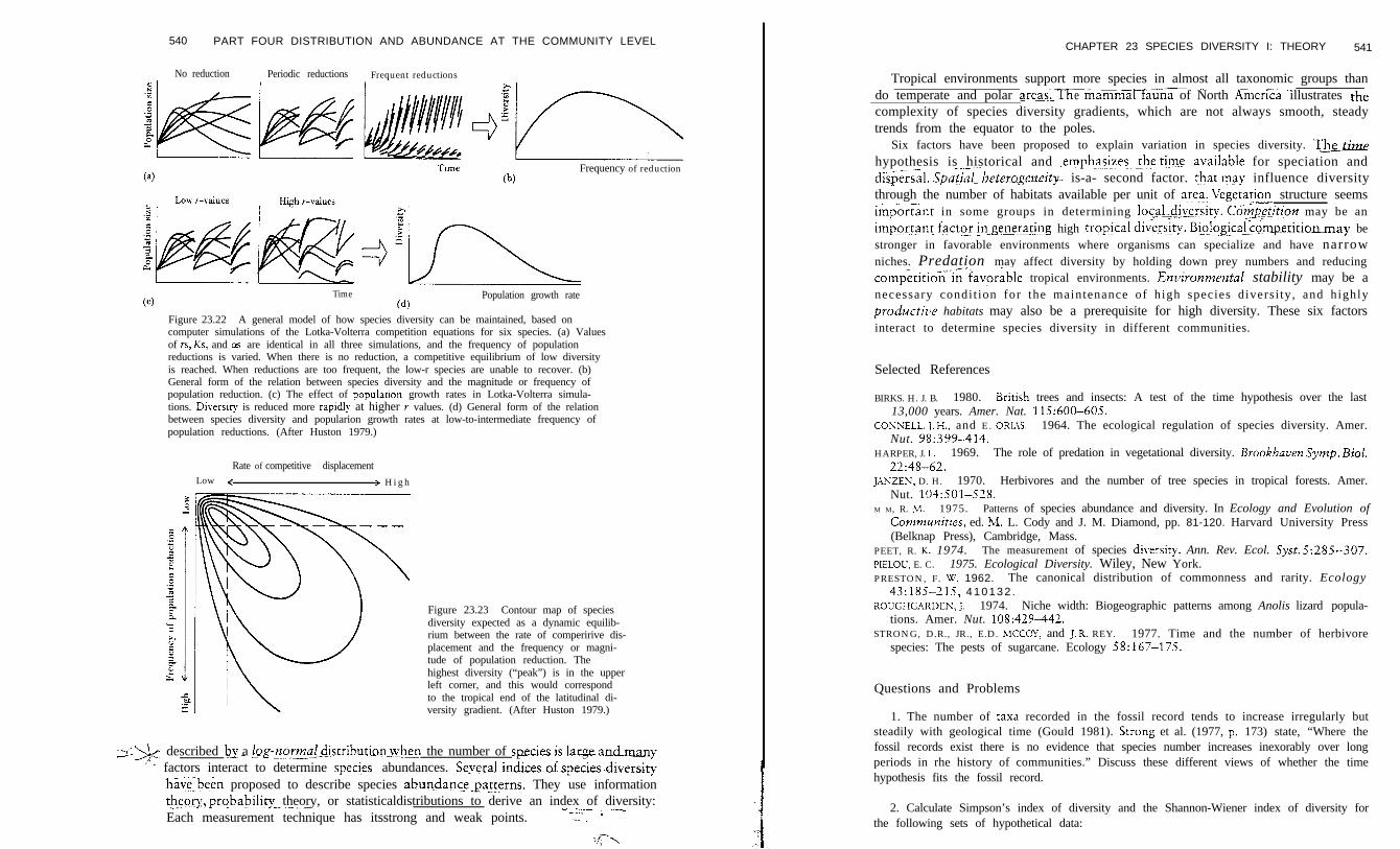
Figure 23.22 A general model of how species diversity can be maintained, based oncomputer simulations of the Lotka-Volterra competition equations for six species. (a) Valuesof TS, k’s? and as are identical in all three simulations, and the frequency of populationreductions is varied. When there is no reduction, a competitive equilibrium of low diversityis reached. When reductions are too frequent, the low-r species are unable to recover. (b)General form of the relation between species diversity and the magnitude or frequency ofpopulation reduction. (c) The effect of populanon growth rates in Lotka-Volterra simula-tions. Diversiry is reduced more rapidly at higher T values. (d) General form of the relationbetween species diversity and popularion growth rates at low-to-intermediate frequency ofpopulation reductions. (After Huston 1979.)

Rate of competitive displacementLow < > H i g h

Figure 23.23 Contour map of speciesdiversity expected as a dynamic equilib-rium between the rate of comperirive dis-placement and the frequency or magni-tude of population reduction. Thehighest diversity (“peak”) is in the upperleft corner, and this would correspondto the tropical end of the latitudinal di-versity gradient. (After Huston 1979.)

z:% described by a log-normaI_distrihurio.n_\vhen the number of specitidarmy- - - ~-~__” - factors interact to determine species. abundances. Se.~eralindices~ofspecies-diwrsity

J&.been proposed to describe species abundancepatlerns. They use information&pry, prqbabiiity theory, or statisticaldistributions to derive an index of diversity:.- ~.-__- -.---__Each measurement technique has itsstrong and weak points. -z‘- ’ -L-

:;c--.,


Tropical environments support more species in almost all taxonomic groups thando temperate and polar am,Th

.__ - ---_-_e mammahZna of North ,4merlca illustrates the

complexity of species diversity gradients, which are not always smooth, steadytrends from the equator to the poles.

Six factors have been proposed to explain variation in species diversity. Twhypothesis is historical and .emp&zes- Ihe ti_me-_aeailable for speciation and._ ~~-~.-di$$&%l. Spatial~ heterogezzeity- is-a- second factor. t-hat may influence diversitythrough the number of habitats available per unit of are_a. Vegetat& structure seemsitiportant in some groups in determining loc&~~~\~rsity. Cowzg@i_tion may be animportan! facter~-ge~~e~.~~~~~g high tropical d&&y. Biolo&al competitionmay bestronger in favorable environments where organisms can specialize and have narrowniches. Predation may affect diversity by holding down prey numbers and reducingcomp&itioXiZfav-orable tropical environments. Erzuironmental stability may be anecessary condit ion for the maintenance of high species diversi ty, and highlyprodtlrtive habitats may also be a prerequisite for high diversity. These six factorsinteract to determine species diversity in different communities.

Selected References

BIRKS. H. J. B. 1980. British trees and insects: A test of the time hypothesis over the last13,000 years. Amer. Nat. 115:600-605.

CONNELL. J.H., and E . ORIAS. 1964. The ecological regulation of species diversity. Amer.Nut. 98:399-414.

HARPER, J. 1. 1969. The role of predation in vegetational diversity. Brookhaven Symp. Biol.22:48-62.

JANZEN, D. H. 1970. Herbivores and the number of tree species in tropical forests. Amer.Nut. 104:501-528.

M M, R. M. 1975. Patterns of species abundance and diversity. In Ecology and Evolution ofCommtinities, ed. M. L. Cody and J. M. Diamond, pp. 81-120. Harvard University Press(Belknap Press), Cambridge, Mass.

PEET, R. K. 1974. The measurement of species diversit). Ann. Rev. Ecol. Syst. 5:2&S-307.PIELOU, E. C. 1975. Ecological Diversity. Wiley, New York.PRESTON, F. U’. 1962. The canonical distribution of commonness and rarity. Ecology

43:185-215, 4 1 0 1 3 2 .ROLIGHGARDEX, J. 1974. Niche width: Biogeographic patterns among Anolis lizard popula-

tions. Amer. Nut. 108~4291142.STRONG, D.R., JR., E.D. hlCCOY, and J.R. REY. 1977. Time and the number of herbivore

species: The pests of sugarcane. Ecology 583167-175.

Questions and Problems

1. The number of taxa recorded in the fossil record tends to increase irregularly butsteadily with geological time (Gould 1981). Strong et al. (1977, p. 173) state, “Where thefossil records exist there is no evidence that species number increases inexorably over longperiods in rhe history of communities.” Discuss these different views of whether the timehypothesis fits the fossil record.

2. Calculate Simpson’s index of diversity and the Shannon-Wiener index of diversity forthe following sets of hypothetical data:

Documents

ECOI,OGY - Pace University Webspacewebpage.pace.edu/dnabirahni/rahnidocs/law802/Chapter 23 from... · ECOI,OGY The Experimental ... P 514 PART FOUR DISTRIBUTION AND ABUNDANCE AT THE