Ecological Impacts of Stream Bank Stabilization in a Great Plains River

University of Nebraska - LincolnDigitalCommons@University of Nebraska - Lincoln

Dissertations & Theses in Natural Resources Natural Resources, School of

Fall 12-3-2010

Ecological Impacts of Stream Bank Stabilization ina Great Plains RiverChristopher M. PracheilUniversity of Nebraska - School of Natural Resources, [email protected]

Follow this and additional works at: http://digitalcommons.unl.edu/natresdiss

Part of the Environmental Indicators and Impact Assessment Commons, EnvironmentalMonitoring Commons, and the Natural Resources and Conservation Commons

This Article is brought to you for free and open access by the Natural Resources, School of at DigitalCommons@University of Nebraska - Lincoln. Ithas been accepted for inclusion in Dissertations & Theses in Natural Resources by an authorized administrator of DigitalCommons@University ofNebraska - Lincoln.

Pracheil, Christopher M., "Ecological Impacts of Stream Bank Stabilization in a Great Plains River" (2010). Dissertations & Theses inNatural Resources. 16.http://digitalcommons.unl.edu/natresdiss/16

http://digitalcommons.unl.edu?utm_source=digitalcommons.unl.edu%2Fnatresdiss%2F16&utm_medium=PDF&utm_campaign=PDFCoverPages

http://digitalcommons.unl.edu/natresdiss?utm_source=digitalcommons.unl.edu%2Fnatresdiss%2F16&utm_medium=PDF&utm_campaign=PDFCoverPages

http://digitalcommons.unl.edu/natres?utm_source=digitalcommons.unl.edu%2Fnatresdiss%2F16&utm_medium=PDF&utm_campaign=PDFCoverPages

http://digitalcommons.unl.edu/natresdiss?utm_source=digitalcommons.unl.edu%2Fnatresdiss%2F16&utm_medium=PDF&utm_campaign=PDFCoverPages

http://network.bepress.com/hgg/discipline/1015?utm_source=digitalcommons.unl.edu%2Fnatresdiss%2F16&utm_medium=PDF&utm_campaign=PDFCoverPages




http://digitalcommons.unl.edu/natresdiss/16?utm_source=digitalcommons.unl.edu%2Fnatresdiss%2F16&utm_medium=PDF&utm_campaign=PDFCoverPages

ECOLOGICAL IMPACTS OF STREAM BANK STABILIZATION

IN A GREAT PLAINS RIVER

by

Christopher M. Pracheil

A THESIS

Presented to the Faculty of

The Graduate College at the University of Nebraska

In Partial Fulfillment of Requirements

For the Degree of Master of Science

Major: Natural Resources Sciences

Under the Supervision of Professor Steven A. Thomas

Lincoln, Nebraska

December, 2010

ECOLOGICAL IMPACTS OF STREAM BANK STABILIZATION IN A

GREAT PLAINS RIVER

Christopher M. Pracheil, M.S.

University of Nebraska, 2010

Adviser: Steven A. Thomas

Reduced ecological complexity, decreased water quality, and accelerated stream bank

erosion are common disturbances in rivers with agriculturally dominated watersheds.

Massive bank failures, increased sediment loads, and decreased riverine habitat are

current problems in the agriculturally dominated Cedar River of central Nebraska. In an

effort to slow erosion and prevent further ecological degradation, 20 reach scale stream

bank stabilization projects were installed on the Cedar River from 2001 to 2004. The

objective of this study was to determine the impact of the Cedar River stream bank

stabilization projects on the ecological conditions within the Cedar River. Stream bank

erosion, suspended sediment load, aquatic chemistry, in-stream metabolism, riparian

macrophytes, macroinvertebrates, and fish data from seven stabilized and three

unstabilized reaches were monitored from the spring of 2007 through to fall of 2008 to

assess the ecological condition of each site. Stabilized sites experienced significantly less

stream bank erosion than unstabilized sites. Suspended sediment and dissolved nutrient

concentrations general increased in the downstream direction, irrespective of treatment.

Riparian macrophyte diversity and density was significantly higher at stabilized sites.

Stabilized sites were found to have greater numbers of macroinvertebrate families and

individuals, as well as greater numbers of the sensitive EPT families and individuals.

More fish species and native fish species were captured at the stabilized sites, and a

greater number of fish per m2 were captured at the stabilized sites. The results of this

study demonstrate that stream bank stabilization projects can positively impact plant,

invertebrate, and fish communities, while not impacting water quality parameters.

iii

Table of Contents

Introduction ......................................................................................................................... 1

The Cedar River .................................................................................................................. 4

Site Description ............................................................................................................... 4

Study Reaches ................................................................................................................. 5

Methods............................................................................................................................... 9

Topographical Surveys ................................................................................................... 9

Water Column Sediment and Nutrients Analyses ........................................................ 10

Stream Metabolism ....................................................................................................... 12

Riparian Vegetation ...................................................................................................... 13

Macroinvertebrate Collections ...................................................................................... 14

Fish Collections ............................................................................................................ 14

Statistical Analysis ........................................................................................................ 15

Results ............................................................................................................................... 16

Stream Bank Erosion .................................................................................................... 16

Water Chemistry ........................................................................................................... 17

Stream Metabolism ....................................................................................................... 21

Macroinvertebrates ....................................................................................................... 22

Macrophytes .................................................................................................................. 25

Fish ................................................................................................................................ 26

Multivariate Assessments ............................................................................................. 27

Discussion ......................................................................................................................... 29

Conclusion ........................................................................................................................ 40

Literature Cited ................................................................................................................. 41

iv

Tables and Figures Table 1 Characteristics of the 10 monitored sites in the Cedar River……………47

Table 2 Stream bank characteristics and erosion estimates……………………....48

Table 3 Stream bank erosion rates and treatment comparisons…………………. 49

Table 4 Summary of 2007 water chemistry parameters by site…………………. 50

Table 5 Summary of 2008 water chemistry parameters by site…………………. 51

Table 6 Summary of summer 2007 water chemistry parameters by site………... 52

Table 7 Summary of 2007 water chemistry parameters by stream segment……. 53

Table 8 Summary of 2008 water chemistry parameters by stream segment……. 54

Table 9 Summary of daily ecosystem metabolism parameters………………….. 55

Table 10 Summary of 2007 macroinvertebrates captured by treatment………...... 56

Table 11 Summary of May 2007 macroinvertebrates captured by site…………....57

Table 12 Summary of July 2007 macroinvertebrates captured by site…………… 58

Table 13 Summary of September 2007 macroinvertebrates captured by site…..… 59

Table 14 Summary of 2007 macroinvertebrates captured by site………………….60

Table 15 Summary of 2008 macroinvertebrates captured by site………………….61

Table 16 Summary of 2007 macrophytes collected by site………………………..62

Table 17 Summary of 2008 macrophytes collected by site………………………..63

Table 18 Summary of 2007 fish collected by site………………………………….64

Table 19 Summary of 2008 fish collected by site………………………………….65

Table 20 Lateral erosion rates of other Midwestern streams………………………66

Table 21 Summary of 2007 sediment chlorophyll a by site……………………… 67

Figure 1 Location of study site and study reaches………………………………...68

Figure 2 Cedar River basin land use………………………………………………69

Figure 3 Description of dominant stabilization structures………………………...70

Figure 4 2007 conductivity, NH4, NO3, and SRP and river km…………………...71

Figure 5 2007 DOC, TSS, SOM and river km………………………………….....72

Figure 6 2008 NH4, NO3, SRP, TP and river km…………………….…………....73

Figure 7 2008 DOC, TSS, SOM and river km………………………………….....74

Figure 8 2007 Cedar River discharge at river km 90 and 10……………………...75

v

Tables and Figures continued

Figure 9 2008 Cedar River discharge at river km 90 and 10……………………...75

Figure 10 2007 NH4, NO3, SRP, TP and discharge...………………….…………...76

Figure 11 2007 DOC, TSS, SOM, conductivity and discharge..........................…...77

Figure 12 2008 NH4, NO3, SRP, TP and discharge ……………………….……….78

Figure 13 2008 DOC, TSS, SOM and discharge………………………..………….79

Figure 14 NMDS ordination for water chemisty data pooled by site………………80

Figure 15 2007 Riparian macrophyte species richness and wetland class………….81

Figure 16 2008 Riparian macrophyte species richness and wetland class………….81

Figure 17 NMDS ordination for 2007 & 2008 riparian macrophytes………………82

Figure 18 Number of fish captured per meter in 2007 and 2008…………………...82

Figure 19 NMDS ordination for erosion rate and water chemisty data…………….83

Figure 20 NMDS ordination for 2007 & 2008 invertebrates and macrophytes…….83

Figure 21 NMDS ordination for erosion rate, 2007 & 2008 invertebrates and

macrophytes……………………………………………………………...84

Figure 22 NMDS ordination for erosion rate, water chemisty data, 2007

& 2008 invertebrates and macrophytes…………………………………..84

Figure 23 NMDS ordination for erosion rate, water chemisty data, 2007

& 2008 invertebrates and macrophytes…………………………………..85

Appendix

Table 1 Scientific and common name of macroinvertebrates collected………….86

Table 2 Scientific and common name of fish collected…………………………..88

1

Introduction

Anthropogenic alterations of landscapes and geomorphic processes are well

documented drivers of ecosystem degradation. The conversion of arable landscapes into

agricultural fields alters hydrologic and ecological processes across several spatial and

temporal scales that directly impact aquatic ecosystem health (Karr and Schlosser, 1978;

Karr et al. 1985; Allen 2004). Agricultural land use removes native vegetation, decreases

hydrologic retention times, reduces stream sinuosity, and confines riparian corridors

(Shields et al. 1994; Peterson and Kwak, 1999). These landscape modifications alter the

natural flow regime resulting in flashier storm flows and increased water velocities (Allen

et al. 1997; Poff et al. 1997; Allen 2004). To accommodate more intense flow events

stream channels widen, stream banks erode, and riverbeds are scoured, resulting in

homogenous stream channels with little in-stream habitat, unstable stream banks, and

degraded water quality conditions (Shields et al. 1995; Richards et al. 1996; Allan et al.

1997; Shields et al. 2000a).

Agricultural land use has been negatively correlated with water quality, biological

diversity, and habitat complexity in numerous studies (Skaggs et al. 1994; Wichert and

Rapport, 1998; Stewart et al. 2002). Streams with the greatest amounts of agricultural

activity within their watersheds had the highest nutrient concentrations, suspended solids,

and turbidity levels in studies that compared streams across a gradient of agricultural

intensities (Omernik et al. 1981; Johnson et al. 1997; Harding et al. 1999). Agricultural

land use is also negatively correlated with macroinvertebrate and fish indices scores and

was the only significant predictor of the bioassessment scores in studies by Roth et al.

2

(1996), Walser and Bart (1999), and Nerbonne and Vondracek (2001). In-stream and

riparian habitat is significantly more homogenous in agriculturally dominated streams

(Walser and Bart, 1999; Wood and Armitage, 1999) and the lack of woody debris in

agriculturally streams leads to less channel, substrate, and velocity heterogeneity

(Schlosser, 1991).

Recent studies showing a precipitous drop in biological diversity of freshwater

ecosystems (Sala et al. 2000; Dudgeon et al. 2006) have stimulated attempts to mitigate

the impacts of anthropogenic land use on riverine systems. While catchment scale land

use drives lotic ecosystem degradation, mitigation or restoration at the catchment scale

can be logistically difficult and financially burdensome and as a result most stream and

river restoration projects are focused at the reach scale (Brown 2000). Accelerated

stream bank erosion is a commonly observed reach-scale disturbance in agricultural

streams and is often the focus of mitigation and restoration practices (Brookes and

Shields 1996; Abbe et al. 1997). The ecological impact of accelerated bank erosion is

well documented and includes increased sediment loads, decreased autochthonous

production, reduced biological diversity, and loss of aquatic habitat (Quinn and Hickey

1990; Waters 1995, Wood and Armitage 1997; Walser and Bart 1999).

Accelerated rates of stream bank erosion have been directly linked to

anthropogenic land use (Shields et al. 1994; Richards et al. 1996; Allen et al. 1997) and

the effectiveness of reach-scale stream bank stabilization projects at mitigating the

impacts of catchment level land use is an area of active debate. For example, stabilized

stream banks may experience less erosion (Shields et al. 2004; Sudduth and Meyer 2006)

3

and have greater autochthonous production than unstabilized reaches within the same

stream (Osborn and Kovacic, 1993). Numerous studies conducted by the USDA-

Agricultural Research Service have documented improved aquatic habitat (Shields et al.

1998, 2000b, 2003), increased macroinvertebrate diversity (Smiley and Dibble, 2007),

and increased fish densities and diversity (Shields et al. 1998, 2000b, 2003; Smiley et al.

1999) at reaches with stream bank stabilization structures compared to unstabilized

reaches. However, other studies indicate that reaches with stabilization projects have the

same suspended sediment load (Riley 1998; Li and Eddleman, 2002), macroinvertebrate

diversity (Sudduth and Meyer, 2006), and fish diversity (Moerke and Lamberti, 2004) as

reaches without stabilization structures. Furthermore, streams with stabilization projects

were physically and biological indistinguishable from streams without stabilization

projects when compared at the river segment or stream system scale (Allen et al. 1997;

Larson et al. 2001; Roni et al. 2002). Therefore, there remains considerable uncertainty

regarding the ecological benefits of these structures in agriculturally dominated streams.

The objective of this study was to assess the impact of bank stabilization projects

on erosion rates and ecological conditions within an agricultural river in central

Nebraska. To determine rates of stream bank erosion, high resolution topographic maps

were made of the same seven stabilized and three unstabilized reaches over two

consecutive summers. The suspended sediment load, aquatic chemistry, riparian

macrophytes, macroinvertebrates, benthic chlorophyll a, and fish data of these same ten

reaches were monitored from the spring of 2007 through to fall of 2008 to assess the

ecological condition of each site. Consistent with the aims of the agencies that installed

4

the stabilization structures, these data were collected to test the following hypothesis:

Stabilized reaches experience less stream bank erosion than unstabilized reaches,

resulting in greater macrophyte, macroinvertebrate, and fish diversities compared to

unstabilized reaches.

The Cedar River

Site Description

This study was conducted on the Cedar River, a fourth order river system that

begins as a series of springs and wetlands in the Nebraska Sandhills. Vast quantities of

shallow groundwater, porous eolian sediments, and limited anthropogenic disturbance

allow for large wetland complexes to exist throughout the Sandhills. These wetlands

complexes form the headwaters of several Nebraska rivers including the Calamus, Cedar,

Dismal, Elkhorn, Middle and North Loup and provide some of the most stable base flow

conditions in the world (Huntzinger and Ellis, 1993).

The intersection of the Ogallala aquifer with the linear dunes of the eastern

Sandhills creates a network of wet meadows and interdunal wetlands that coalesce to

form the Big Cedar and Little Cedar Creeks in southern Holt and northern Garfield

Counties. The confluence of Big and Little Cedar Creeks in eastern Garfield County

marks the beginning of the 200 km long Cedar River. The Cedar River continues for

88km through the eastern Sandhills before transitioning into the loess plains of central

Nebraska where it joins the Loup River near Fullerton (Fig. 1).

The Cedar River drains a 323,300 ha watershed that is naturally divided into two

distinct regions. The upper half of the catchment is largely undeveloped rangeland and

5

wetlands along the eastern edge of the Sandhills, while the lower half of the watershed

traverses the loess plains of east-central Nebraska where row-crop agriculture is the

dominate land use (Fig. 2). The Sandhills sub-watershed is 196,200 ha, of which less

than 10% is in intensive agricultural production (17,870 ha), whereas the lower loess

plains sub-watershed drains 127,100 ha, of which nearly 40% is in intensive agricultural

production (46,000 ha).

The amount of land dedicated to row-crop agriculture in the three counties that

contain the lower half of the Cedar basin has increased substantially over the past 30

years. In these three counties (Boone, Greeley, and Nance) a combined 142,000 ha of

corn and soybeans were planted in 1980. In 2007, more than 194,700 ha of corn and

soybeans were planted, an increase of 27% (USDA, National Agricultural Statistics

Service). The increase in land dedicated to row crop agriculture corresponds with a 17%

increase in mean daily stream flows in the Cedar River near Fullerton, when mean daily

stream flow data from 1990-2008 is compared against daily data from 1960-1980 (USGS

Water Resources, NDNR Streamflow Data).

Study Reaches

In the agriculturally dominated sub-watershed, stream bank erosion has led to

massive bank failures and decreased riverine habitat complexity. To stem the loss of

valuable farm land and prevent further ecological degradation, 20 stream bank

stabilization projects were installed on the Cedar River. These reach-scale stabilization

projects were designed to direct flow away from the eroding banks by extending several

wooden or rock jetties into the stream. The Cedar River stabilization project

6

predominately used three types of stabilization structures: pole jetties, cottonwood

jetties, and riprap vanes (Fig. 3). Stabilized study reaches were chosen to ensure that the

three dominate stabilization structures were represented and that treatment reaches were

distributed throughout the stabilized region of the river. Three unstabilized bends were

selected for monitoring to serve as control reaches that provided ambient physical and

biological data. The unstabilized bends selected for monitoring were chosen because

they were representative of the current channel morphology and land use in the

surrounding area (Table 1) and were also distributed across the stabilized region (Fig. 1).

The most upstream reach (Site 1) in this study was a stabilized bend three km

west of Spalding, in the transitional area between the Sandhills and loess plains. This

340m bend had an average bank height of 3.47m, an average bank slope of 45 degrees

and a bend angle of 190 degrees. Stabilization efforts at this site consisted of a 10m wide

buffer strip and five riprap vanes. The riprap vanes were centered on the inflection point

of the concave bank and were spaced approximately 35m apart, so that the first vane was

located 70m upstream, and the last vane 70m downstream of the inflection point. The

riprap vanes for this project were designed to extend into the channel 10% of the channel

width.

Site 2 was a control reach located approximately 8 km southeast of Spalding on

the edge of an irrigated alfalfa field. This site was located on a 320m bend with a bend

angle of 160 degrees, an average bank height of 1.13m, and an average bank slope of 57

degrees. While this site was not part of the stabilization effort the landowner had left a

15m riparian buffer around this site in an effort to slow stream bank erosion.

7

Site 3 was a stabilized site located on the 225m bend, immediately downstream of

Site 2. This bend curved 170 degrees and had banks that averaged 1.3m high and had a

slope of 48 degrees. This site was located on the edge of a no-till field in a corn/soybean

crop rotation program. Stabilization efforts for this site included a 5m vegetated buffer,

1 rip-rap vane and 3 pole jetties; with the stabilization structures located on the

downstream half of the bend. The most upstream structure was the rip-rap vane, which

was located 25m downstream of the inflection point, followed by the three pole jetties

spaced 25m apart.

The next study reach (Site 4) was a stabilized reach on a gradual 800m bend that

curved 100 degrees. This site was along the edge of no-till field in a corn/soybean crop

rotation program 3km downstream from Site 3. This site had seven rip-rap vane

structures that were centered around the inflection point of the bend and spaced

approximately 25m apart. This site had lowest banks (0.4m) and the smallest bank slope

(16.1 degrees) of any site in the study. However, it was apparent that before stabilization

efforts began at this site erosion was a problem because the historic bank was 2-3m tall

and had a slope of >45 degrees.

Twenty two river km downstream of Site 4 was Site 5, an unstabilized 370m bend

that curved 200 degrees. This site was located in the loess plains at the edge of a

traditional tillage field in a corn/soybean rotation with no buffer. The banks at this site

averaged 3.3m and showed obvious signs of erosion with steep banks (59.3 degrees) and

bank slumping.

8

Site 6 was a stabilized reach located 5.5km downstream of Site 5 on a 580m bend

that curved 260 degrees. This reach had banks that averaged 1.6m high, with an average

slope of 55 degrees. This site was located on the edge of a hay field that remained

vegetated year round. Seven pole jetties were used to stabilize this site, with all jetties

located downstream of the inflection point of the bend. The jetties were spaced

approximately 30m apart in the bottom 250m of the bend.

The stabilized Site 7 was located 500m downstream of Site 6 on the next river

bend. This bend was 720m long and the bend angle was 170 degrees. The concave bank

at this reach averaged 1.34m in height and had an average slope of 29 degrees. The

stabilization efforts at this site included a 30m buffer strip and 12 pole jetties. The jetties

at this site were centered around the inflection point of the bend and covered

approximately 150m upstream and downstream of the inflection point.

Site 8 was an unstabilized reach located 350m downstream of Site 7. This 325m

bend was on the edge of a riparian forest that extended the entire length of the concave

bank and had a bend angle of 150 degrees. The banks at this site averaged 2.0m high and

had a slope of 43 degrees.

Site 9 was a stabilized reach located 2.5km downstream of Site 8 on an 800m

river bend that curved 280 degrees. The bank at this site had an average height of 4m and

an average bank slope of 51 degrees. The upper half of this bend was buffered by a 40m

wide riparian forest, while the lower half had a 5m grass buffer on the edge of a no-till

field in a corn/soybean rotation. Stabilization efforts at this site included the buffer strip

and 10 pole jetties, with the first jetty being located just downstream of the inflection

9

point of the bend. The jetties were space approximately 35m apart and covered the lower

400m of this bend.

The study reach furthest downstream was Site 10, located approximately 11 km

from the river’s confluence and 18 river km downstream from Site 9. This stabilized site

had four cottonwood (Populus deltoides L.) jetties on a 250 m bend in a cattle pasture

with no riparian buffer. The banks on this site averaged 2.5m high and had a slope of 50

degrees.

Methods

Topographical Surveys

High resolution three-dimensional surveys of each study reach were conducted

during the late summer of 2007 and again in 2008 using a Sokkia SET3B Total Station

(electronic theodolite and distance meter) and stadia rod. Local benchmarks were

installed at each study reach to mark the location of the total station during the 2007

survey. These benchmarks were then used to place the total station in the exact same

location for the 2008 survey. A marker was also placed at a “back site” location for each

study reach; the back site was used to set the horizontal and vertical angle for each

survey, as well as, serve as a control point between the 2007 and 2008 surveys.

While the surveys were conducted to gather topographical information on the

entire study reach of each site, the surveys focused on capturing data on the concave

(eroding) bank. On the eroding bank, transects were conducted on both the top of the

bank and at the river’s edge, with measurements being collected every 1.5m for the

10

length of the bank. In addition to the horizontal transects, vertical transects were

collected on the bank every 15 to 20m to get a profile of the bank.

The survey data were imported into ArcGIS (ESRI, 2008) and point based

shapefiles were created. From the shapefiles a series of measurements (reach length,

bank height, stream width, bend radius, average stream depth) were performed to

characterize each study reach. New shapefiles that only contained points from the

eroding bank were then created to make digital elevation maps (DEM) to estimate

erosion. These shapefiles were edited to clearly define the stream bank boundaries so

that the DEMs did not extend beyond the extent of the surveyed area.

To determine the changes in stream bank erosion from the DEMs, stream bank

angle was measured at 10m intervals for the length of each DEM and averaged to get a

mean stream bank angle. The 2007 DEM from each site was then overlaid with the

corresponding 2008 DEM and the difference in bank position between 2007 and 2008 at

the top and bottom of the bank was measured at 5m intervals. To estimate whole bank

erosion the average change in position between the top and bottom bank measurements

were multiplied by the average bank height for that site.

Water Column Sediment and Nutrients Analyses

Water samples were collected bi-monthly from May through September, 2007

and 2008 at each of the monitoring sites. Water temperature, dissolved oxygen (DO),

pH, and specific conductance were measured in situ using a YSI 556MPS probe (YSI

2006). Water samples for chemical analyses were collected from the thalweg and

filtered immediately through pre-weighed glass-fiber filters (Whatman GF/F) into rinsed

11

polyethylene bottles. Filtered water samples were placed on ice until analyzed or frozen

for future analyses.

Water column total suspended solids (TSS) and suspended organic matter (SOM)

were determined by drying (55ºC, 48 hr), weighing, combusting (550ºC – 30 min.), and

reweighing pre-weighed filters that water samples were filtered through. Total suspended

solids were calculated as the difference between the original weight of the filter and the

weight of the dried, used filter divided by the volume of water filtered (mg/L).

Suspended organic matter was calculated as the difference between the weight of the

dried filter and the combusted filter divided by the volume of water filtered (mg/L).

Water samples were analyzed for major nutrients, including nitrate-nitrogen

(NO3-N), ammonium nitrogen (NH4-N), soluble reactive phosphorus (SRP), total

phosphorus (TP), and dissolved organic carbon (DOC). Ammonium (NH4) was

determined using the Holmes et al. (1999) fluorometric method with a Turner 10-AU

fluorometer. Nitrate samples were frozen until analyzed using an ion chromatograph

(Dionex ICS-90). Dissolved organic carbon was processed using the wet persulfate

digestion method (McDowell et al. 1997) and measured on a total carbon analyzer

(Latchat IL500 TOC). Soluble reactive phosphorus was determined using the ascorbic

acid method (American Public Health Association, 1998) and measured on a

spectrophotometer (Varian Cary 300). Total phosphorus samples were put through a

digestion process following the persulfate-sulfuric acid autoclave technique (American Public

Health Association, 1998) before also being analyzed using the ascorbic acid method.

12

Stream Metabolism

Whole stream metabolism was calculated following the single station, diurnal dissolved

oxygen change method (Odum 1956; Bott 2006). This technique allows rates of in-stream gross

primary production and stream community respiration to be estimated from changes in in-stream

dissolved oxygen concentration. To account for gas exchange between stream water and the

atmosphere the oxygen reaeration coefficient was calculated using a regressional analysis

technique that determined the relationship between oxygen saturation deficit and dissolved

oxygen concentration rate of change at dusk (Bott, 2006).

Metabolism data were collected from two stations at three stabilized sites between July

27, 2007 and August 29, 2007. At each station continuous dissolved oxygen, water temperature,

and barometric pressure measurements were collected every 5 minutes for 26 hrs. Measurements

were collected using YSI 6600 sondes (YSI, 2007) deployed in the thalweg of the river channel

approximately one foot off the river bottom. Two sondes, one upstream of the stabilization

structures and one downstream, were deployed at the same site, on the same day to determine the

impact of stabilization efforts on stream metabolism.

Whole stream rates of gross primary production (GPP) and community respiration (CR)

were calculated for each station by determining the rate of change in dissolved oxygen (DO)

concentration (Bott, 2006). An hourly rate of change in DO concentration �∆DO� was used to

calculate stream metabolism and the hourly rate of change was determined for each DO

measurement. This created an hourly rate of change dataset that had data points every five

minutes. The rate of change in DO concentration within a stream is dependant upon GPP, CR,

and atmospheric oxygen exchange (AE) as demonstrated by the following equation:

∆DO � GPP CR � AE

Atmospheric oxygen exchange was calculated for every rate of change calculation by

first determining the dissolved oxygen surplus or deficit in the stream. This was determined as

13

the difference between the DO concentration at saturation, based on atmospheric pressure and

water temperature, and the measured DO concentration. The difference between saturation and

observed DO concentrations was then multiplied by the oxygen reaeration coefficient to

determine the atmospheric oxygen exchange (AE). The AE value was then subtracted from the

∆DO to correct for atmospheric exchange and leave metabolic activity as the driver ∆DO.

Community respiration (CR) occurs at a consistent rate during both the day and night but

is most easily measured at night when the confounding effects of light dependent photosynthesis

are absent. To accurately calculate daily CR rates, ∆DO was summed during the night and added

with extrapolated daytime CR values. Daytime CR values were extrapolated between the ∆DO

one hour predawn and the ∆DO one hour post dusk (Mullholland et al., 2001). The daily rate of

GPP was then determined as the summed difference between the measured ∆DO and the

extrapolated daytime CR values. Rates of GPP and CR were original determined as a volumetric

rate (g O2* L-1

*day-1

) and converted to an areal rate by multiplying the mean stream depth of each

site by the volumetric rate.

Riparian Vegetation

Measurements to determine riparian vegetation canopy-coverage were conducted

using a modified Daubenmire technique at each study reach (Daubenmire 1959). At ten

random points along the outside riverbank a 1-m sampling quadrant was placed and the

percentage of the ground covered by live vegetation in the quadrant was estimated. The

percent coverage was then converted into one of seven possible ranks using the

Daubenmire method. The Daubenmire ranking system focused emphasis on plots with

very little (0-5%) and very dense (95-100%) vegetation coverage because these coverage

estimates are the least susceptible to estimation error.

14

All plants within each quadrant were identified to species, clipped at ground level,

and collected. Collected samples were washed, dried at 55oC for 10 d and weighed.

Canopy coverage, species richness and diversity, number of wetland species, percent of

wetland taxa, and above ground biomass were determined for each site.

Macroinvertebrate Collections

Macroinvertebrates were collected from each monitoring site in May, July and

September of 2007 and July of 2008. At each site the three most abundant habitat types

were identified, and three replicate samples were collected from each habitat type,

resulting in nine samples per site per collection. When possible samples were collected

using a 30 cm wide D-frame dip net with 500 µm netting, sweeping approximately 2.0 m2

of surface area per sample. In rock stabilized study sites the riffle habitat created by the

rocks was sampled by scrapping rocks until approximately 2.0 m2 of surface area was

sampled. Macroinvertebrate samples were rinsed, transferred to polyethylene bottles, and

preserved in 95% ethanol until analyzed in the lab. The entire contents of each sample

were hand-picked under a dissecting scope and macroinvertebrates were identified to the

family taxonomic level.

Fish Collections

Fish collections were conducted at two reference and five stabilized sites in

October 2007 and 2008. Fish were collected using a portable electrofisher floating in a

small raft. To standardize collections between sites only the area within 3m of the bank

was sampled and the concave bank was sampled from upstream to downstream of each

reach and the convex bank was sampled downstream to upstream. Fish were collected in

15

nets and placed in buckets of river water until identified or euthanized for laboratory

identification. Fish were identified to species level before being released or were

euthanized and identified in the lab. Fish relative abundance (fish per meter sampled),

species richness, and species diversity of each site were calculated for use in site

comparisons.

Statistical Analysis

Univariate statistical analyses were conducted using SAS 5.0.2 (SAS Institute

Inc.). Most analysis were conducted by comparing individual study reaches or by

grouping the study reaches by treatment, however for water chemistry data additional

analysis were conducted that group sites by location regardless of treatment. All data

was tested for normality before analysis and log(x+1) transformed when necessary.

Parameter differences between sites and/or groups were determined using paired t-tests or

ANOVAs. Significant differences for ANOVAs and t-tests were determined at α = 0.05.

All significant ANOVAs were further analyzed using the Student-Newman-Kuhl (SNK)

post-hoc analysis.

Multivariate Non-metric Multi-Dimensional Scaling (NMDS) analyses were

conducted on water chemistry, macroinvertebrate, and vegetation, as well as

combinations of these data in Primer-E (Primer-E Ltd.). Water chemistry NMDS were

conducted on both the bi-monthly and pooled yearly data, analysis of biological data was

conducted for each year of collection. One-way analysis of similarity (ANOSIM) was

conducted on all NMDS data with river location and treatment used as the explanatory

factors.

16

Diversity of plants, macroinvertebrates, and fish were calculated using Shannon’s

H’. The three 2007 invertebrate collections were analyzed separately and then pooled

and analyzed. Taxonomic richness, abundance, and density for plants and fish for each

site were calculated and analyzed each year.

Results

Stream Bank Erosion

Yearly rates of stream bank erosion in the Cedar River ranged from

11.4 cm*year-1

at Site 4 (S) to 107.1 cm*year-1

at Site 5 (C) (Table 2). Stabilized sites

were found to experience significantly less stream bank erosion than control sites when

pooled erosion data from all stabilized sites was compared to pooled data from all control

sites (t(273) = 11.15, p < 0.01). To determine if location (river km) in the river was

impacting erosion rates, the erosion rates for the most proximate stabilized and control

site pairs were also compared. Erosion rates at the stabilized site for each paired

comparison were also significantly lower than control site (Table 2.)

Total volume (m3) of stream bank lost at the study reaches ranged from 7.5 m

3 at

Site 4 (S) to 1030.6 m3 at Site 5 (C), and total mass of stream bank lost ranged from

11.6 Mg at Site 4 to 1597.4 Mg at Site 5 (Table 3). Neither total volume nor total mass

of stream bank lost were statistically compare between treatments because both measures

are dependent upon measured length of stream bank and stream bank height which varied

considerably between sites and were not influenced by streambank treatment (Table 3).

17

Water Chemistry

Analyses were conducted on each bi-monthly water chemistry data set and on

data sets pooled by year to determine if stabilization treatment influenced water

chemistry parameters. No analysis conducted on bi-monthly or yearly data found

stabilization treatments to have a significant effect on water chemistry nor did treatment

serve as useful predictor of water chemistry patterns. However, the concentrations of

several analytes, pooled by year, tended to increase with downstream distance,

irrespective of stabilization treatment in 2007 and 2008 (Table 4 & 5, and Figs 4-7).

Linear regressions of pooled 2007 data found significant relationships between

conductivity (r2

= 0.97, d.f. = 7, p < 0.01 ), NH4-N (r2

= 0.60, d.f. = 7, p = 0.01), SRP

( r2

= 0.44, d.f. = 7, p = 0.05), TSS (r2

= 0.89, d.f. = 7, p < 0.01), SOM (r2

= 0.88, d.f. = 7,

p < 0.01) and river km. Similar results were found for 2008 pooled water chemistry

linear regressions with NO3-N (r2

= 0.39, d.f. = 7, p = 0.05), SRP (r2

= 0.63, d.f. = 7,

p = 0.01), TP (r2

= 0.94, d.f. = 7, p < 0.01), TSS (r2

= 0.79, d.f. = 7, p < 0.01) and SOM

( r2

= 0.92, d.f. = 7, p < 0.01) concentrations being significantly related to river km.

Linear regressions on bi-monthly water chemistry data revealed a tendency for solute and

seston concentrations to increase in the downstream direction, however, variability in

discharge along the stream during individual sampling events confounded these analyses

(Fig. 8 & 9).

To determine the relationship between stream flow and water chemistry

concentrations, analytes were pooled by date and the mean analyte value of that date was

compared to the mean daily discharge on that date by simple linear regression. The 2007

data showed strong relationships between analyte concentration and stream flow (Fig. 10

18

& 11) with NH4-N (r2

= 0.94, d.f. = 8, p < 0.01), NO3-N (r2

= 0.46, d.f. = 6, p = 0.04),SRP

(r2

= 0.79, d.f. = 8, p < 0.01), TP (r2

= 0.93, d.f. = 8, p < 0.01), TSS (r2

= 0.95, d.f. = 7,

p < 0.01), and SOM (r2

= 0.79, d.f. = 7, p < 0.01). DOC and conductivity were the only

analytes in 2007 where the concentration was not significantly related to discharge. The

2008 water chemistry data did not show the same strong relationship with stream flow

(Fig. 12 & 13). Only 2008 DOC concentrations (r2

= 0.77, d.f. = 5, p = 0.01) showed a

significant positive relationship with stream discharge.

To account for the influence of stream flow on analyte concentrations, when

statistically comparing sites, we attempted to run analyses of covariance (ANCOVAs)

with mean daily discharge as the covariate, analyte concentration as the dependant

variable, and river km as the independent variable. In all ANCOVAs conducted the

interaction between the covariate (discharge) and the independent variable (river km) was

significant and the ANCOVA model could not be used.

Analyte concentration varied with both flow and location, and statistically

distinguishing between sites on the bi-monthly data was not possible. Therefore, site

based statistical comparisons were restricted to yearly averaged site data. In 2007, mean

conductivity was lowest at the uppermost site and steadily increased downstream so that

Site 10 had the highest value and was significantly different from upstream sites

(ANOVA, F = 25.79, p < 0.01) (Table 4). Mean NO3-N concentrations significantly

differed between sites (ANOVA, F =3.52, p < 0.01) (Table 4) with the lowest values in

the middle study reaches and Site 10 having the highest mean concentration. Similar to

conductivity, NH4-N concentrations were significantly lower at Site 1 than they were at

19

Site 10 (ANOVA, F = 2.06, p = 0.03) with most of the middle study reaches showing no

difference between either site. There were no differences in pooled SRP, DOC, TSS, or

SOM between sites, though there were large differences between Site 1 and Site 10 for

both TSS and SOM (Table 4). The site pooled 2008 data analysis found only mean NO3-

N concentrations differed significantly between sites (ANOVA, F =3.52, p < 0.01) (Table

5). There were no differences in NH4-N, SRP, DOC, TSS, or SOM concentrations,

though there were again large differences between the upper and lower site for TSS and

SOM (Table 5).

The first four water chemistry sampling events in 2007 corresponded with high

stream flow events that influenced water chemistry data (Fig. 8). To determine if water

chemistry differences between sites could be detected at base flow, the first four sampling

events of 2007 were removed from the data set and the remainder of the data was then

pooled by site and analyzed. The results of some of these analyses are more consistent

with the results of the river km linear regressions. For example, conductivity (ANOVA,

F = 11.42, P <0.01), TSS (ANOVA, F = 8.37, P <0.01), and SOM (ANOVA, F = 5.36, P

<0.01) increased significantly from the upper sites to the lower sites (Table 6). However,

both NO3-N (ANOVA, F = 2.23, P = 0.03) and NH4-N (ANOVA, F = 5.91, P <0.01)

showed very different trends with some of the highest concentrations occurring at the

upper sites (Table 6). There were no differences in DOC or SRP concentrations between

sites. Sampling events in 2008 happen to correspond more closely to runoff events (Fig.

9) and prevented us from conducting the same type of analysis on the 2008 data.

20

Due to the lack of treatment effects, the significant relationship between several

analytes and river km, and the inconclusive results of the site comparisons, it was decided

to group the study reaches into three blocks (upper segment, mid segment, lower

segement), based on river km. The data for all sites within a segment, for the entire year,

was pooled and then the segments were statistically compared (Table 7 & 8). In 2007,

conductivity was significantly lower in the upper segment than in the mid and lower

segments (ANOVA, F = 3.72, p =0.04). NO3-N (ANOVA, F = 4.70, p =0.01), NH4-N

(ANOVA, F =7.04, p <0.01 ), TSS (ANOVA, F =8.00 , p < 0.01 ), and SOM (ANOVA,

F =7.04, p < 0.01 ) all had significantly lower concentrations at the upper segment than

the lower segment (Table 7). There were no differences detected in DOC or SRP

concentrations and stream segment.

Analysis of variance on the blocked 2008 data revealed similar trends to 2007

for both TSS (ANOVA, F =3.89 , p =0.03 ), and SOM (ANOVA, F =4.13 , p=0.02), with

concentrations increasing significantly from upper to lower segments (Table 8). Also like

2007, there were no differences between segments for SRP or DOC (Table 8). However,

the blocked 2008 NO3-N (ANOVA, F = 15.18, p < 0.01), and NH4-N (ANOVA, F =7.81,

p < 0.01) show unique differences. NO3-N concentrations are again lowest in the upper

segment but are not different from the lower segment concentration and the mid segment

had the highest values (Table 8). Lastly, NH4-N analyses found the mid segment to have

the lowest concentrations with no difference being detected between the upper and lower

segments.

21

Due to the multivariate nature of the water chemistry data, Non-metric Multi-

Dimensional Scaling (NMDS) was conducted on log transformed bi-monthly and site

pooled water chemistry data sets. NMDS results, using Euclidian distance to measure

similarity found a relationship between site location in the river and its water chemistry.

The results of the NMDS ordinations showed clear groupings of sites by location within

the river (Fig. 14). The results of the pooled 2007 data (Fig. 14a) shows three distinct

groups, with clustering of the four sites of the upper segment and five sites of the mid

segment. The site representing the lower segment is clearly separated from the other two

groups. One-way analysis of similarity (ANOSIM) conducted on the 2007 data with river

location as the explanatory factor found significantly more similarity within a group than

between groups (R = 0.944, p < 0.01) which agrees with the results of the univariate tests

and the visual inspection of the NMDS ordination. Similar ordination and ANOSIM

results were found on the pooled 2008 data (Fig. 14a, R = 0.845, p < 0.01) and the 2007-

2008 pooled data (Fig. 14c, R = 0.879, p < 0.01). The ordinations for the 2008 and 2007-

2008 data sets both placed site 5 outside of the middle reach cluster, which may be

reflective of the large longitudinal separation between site 5 and the remainder of the mid

segment sites (Fig. 1).

Stream Metabolism

Rates of gross primary production (GPP) in the Cedar River ranged from

2.24 g O2 m-2

day-1

to 5.07 g O2 m-2

day-1

while rates of community respiration (CR)

ranged from 1.92 g O2 m-2

day-1

to 6.51 g O2 m-2

day-1

(Table 9). When the six

measurements of diurnal metabolism in the Cedar River are considered together they find

22

the river to be slightly heterotrophic, with CR consuming more oxygen than GPP

produced in the stream. However, all estimates of net ecosystem production (NEP)

showed positive rates of NEP at all six sites for some portion of the day.

Stream metabolism experiments were designed to determine the impact of bank

stabilization on ecosystem production. Measurements were conducted in pairs with data

being collected upstream and downstream of the same stabilized study reach on the same

date. Examination of the paired data finds that at Site 4 and Site 9, CR and GPP were

greater downstream of the stabilization structures than they were upstream (Table 9).

The opposite was true at Site 7 with both CR and GPP being higher upstream of the

stabilization structures (Table 9). Net ecosystem production (NEP) was negative above

and below Site 7 (-1.44 g O2 m-2

day-1

and -0.27 g O2 m-2

day-1

, respectively) whereas

NEP was positive above and below Site 9 (0.32 g O2 m-2

day-1

and 0.37 g O2 m-2

day-1

,

respectively). Site 4 was the only site where the NEP was negative (-0.45 g O2 m-2

day-1

)

above the stabilization structures and positive (1.04 above) below, this may be due to a

reaeration effect cause by water flowing across the seven rip-rap vanes. At all three sites

both NEP and the GPP to CR ratios were greater downstream of the stabilization

structures than they were upstream, documenting increased production at the stabilization

structures.

Macroinvertebrates

A total of 44,884 macroinvertebrates from 67 families were collected in May,

July, and September, 2007 and July 2008 (Appendix Table 1). The most common taxa

were chironomidae, baetidae, oligochaetes, and copepods. All analyses of

23

macroinvertebrate individuals required log transformation to achieve normal distribution,

whereas analyses of macroinvertebrate families did not required transformation. When

variances were unequal Satterthwaite’s approximation for degrees of freedom was used

to approximate the t statistic.

In May 2007, the stabilized sites had more invertebrate families (t(47) = 2.37, p =

0.02), and EPT families (t(47) = 3.53, p < 0.01) (Table 10). However, the total number

of macroinvertebrates, the number of Ephemeroptera-Plecoptera-Trichoptera (EPT)

individuals, the number of diptera captured, and Shannon’s diversity did not differ

between control and stabilized sites (Table 10).

In July 2007, the total number of individuals (t(88) = 1.75, p =0.04), number of

EPT individuals (t(88) = 1.68, p = 0.05), number of diptera individuals (t(88) = 2.33, p =

0.01), and Shannon’s diversity (t(8) = 1.97, p = 0.03) were significantly greater at the

stabilized sites (Table 10). However, no differences between treatments were detected in

the total number of families or the number of EPT families.

Stabilized sites had more total families (t(70) = 2.12, p = 0.02) and EPT families

(t(88) = 1.86, p = 0.04) in September 2007 than control sites (Table 10). Treatment did

not affect total numbers of individuals, EPT individuals, diptera individuals, or

Shannon’s diversity.

Comparisons of treatments for the pooled 2007 macroinvertebrate data revealed

that the stabilized sites had more total individuals (t(163) = 2.10, p = 0.0187), EPT

individuals (t(250) = 1.90, p = 0.04), diptera individuals (t(164) = 2.12, p = 0.02, total

24

families (t(186) = 3.21, p < 0.01), and EPT families (t(179) = 3.53, p < 0.01)(Table 10),

but no difference in Shannon’s diversity was observed.

Between site comparisons were also made on the monthly and pooled 2007

invertebrate data to determine if differences existed between stabilization types. In May

2007, ANOVA results found between site differences in total number of families

(ANOVA, F =2.60, p = 0.01) and number of EPT families (ANOVA, F =2.52, p = 0.01)

with stabilized site 3 having the fewest total families and EPT families (Table 11). No

between-site differences were found for total number of individuals, EPT individuals, or

diptera individuals.

There were between site differences for total individuals (ANOVA, F = 2.52, p =

0.01), EPT individuals (ANOVA, F =2.20, p = 0.03), diptera individuals (ANOVA, F =

2.34, p = 0.02) and EPT families (ANOVA, F =2.23, p = 0.03) in July 2007, but post hoc

SNK tests did not reveal any differences. The total number of families differed between

sites (ANOVA, F = 3.24, p < 0.01) with stabilized site 1 having the greatest number of

families (Table 12).

In September 2007, between-site comparisons revealed difference in total

individuals (ANOVA, F =3.11, p < 0.01), EPT individuals (ANOVA, F = 3.63, p < 0.01),

total number of families (ANOVA, F =2.49, p = 0.02), EPT families (ANOVA, F =3.27,

p < 0.01) and dipteran individuals (ANOVA, F =2.97, p <0.01) with stabilized site 3 and

control site 5 having the lowest values for most parameters (Table 13).

Between-site comparisons on the pooled 2007 invertebrate date revealed

difference for all parameters: total individuals (ANOVA, F =4.30, p < 0.01), EPT

25

individuals (ANOVA, F = 4.81, p < 0.01), total number of families (ANOVA, F =4.72, p

< 0.01), EPT families (ANOVA, F =5.52, p < 0.01) and dipteran individuals (ANOVA, F

=2.61, p < 0.01)(Table 14).

In July 2008, significantly more diptera individuals (t(88) =1.94 p = 0.03) were

captured at the stabilized sites than at the controls sites. No treatment effects were

detected for total individuals, EPT individuals, total families, or EPT families. However,

there were differences between sites for all of assessed parameters: total individuals

(ANOVA, F =4.93, p < 0.01), EPT individuals (ANOVA, F = 3.07, p < 0.01), total

number of families (ANOVA, F =10.32, p < 0.01), EPT families (ANOVA, F =4.28, p <

0.01) and dipteran individuals (ANOVA, F =5.46, p < 0.01) (Table 15).

Non-metric Multi-Dimensional Scaling (NMDS) analyses, using Bray-Curtis

measures of similarity, were conducted on the May, July, and September 2007

macroinvertebrate data, the pooled 2007 data, and the 2008 data. The NMDS ordinations

revealed no distinct patterns due to treatment or location. Similarly, ANOSIM analyses

on the 2007 and 2008 macroinvertebrate data failed to detect any significant treatment or

location effects on the macroinvertebrate community.

Macrophytes

Macrophyte species richness, wetland status, and coverage were closely

associated with stream bank treatment. In 2007 there were significantly more plant

species (t(8) = 3.79, p < 0.01) and greater plant coverage (t(8) = 7.96, p < 0.01) at the

stabilized sites (Table 16). Greater numbers of obligate wetland plant species (OBL)

(t(8) = 3.73, p < 0.01) and facultative wetland plant species (FACW) (t(8) = 2.23, p =

26

0.04) also occurred at the stabilized sites in 2007 (Fig. 15). The 2008 plant data also

show significantly more species (t(8) = 4.49, p < 0.01) and greater vegetative cover (t(8)

= 6.3, p <0.01) at the stabilized sites (Table 17). There were also greater numbers of

OBL plants (t(8) = 3.83, p < 0.01) and FACW plants (t(8) = 2.68, p =0.03) at the

stabilized sites (Fig. 16).


measures of similarity, on the 2007 and 2008 macrophyte species data revealed a

relationship between stabilization treatment and the riparian plant community. The

NMDS ordination on the pooled 2007 and 2008 plant species data show a clear

separation of the stabilized sites from the control sites with the three control sites

clustering together (Fig. 17). One-way analysis of similarity (ANOSIM) conducted on

the 2007 plant species data, with treatment as the explanatory factor, found significantly

more similarity within treatment groups than between groups (R = 0.562, p = 0.03).

Similar results were found when ANOSIM were conducted on the 2008 plant species

data (R = 0.792, p < 0.01), and the pooled 2007 and 2008 plant species data (R = 0.714,

p < 0.01).

Fish

A total of 17 fish species were captured during this study (Appendix Table 2) with

the number of fish species collected per site in 2007 ranging from six to 14 (Table 18)

and the number of individual caught ranged from 2.1 to 27.4 per m2

in 2007 (Fig. 18a).

In 2008 the number of fish species ranged from six to 13 (Table 19), and the number of

individuals caught ranged from 2.2 to 13.4 per m2

(Fig. 18b). In 2007, more native fish

27

species (t(5) = 5.48, p < 0.01) were collected at the stabilized sites than at the control

sites. No between treatments differences were found in the number of fish per m2,

number of fish species, or Shannon’s diversity. In 2008 there were significantly more

fish species (t(5) = 3.05, p = 0.03), more native fish species (t(5) = 3.77, p = 0.01), and

more fish per m2

(t(5) = 3.25, p = .03) at the stabilized sites. No difference was found in

Shannon’s diversity.

Multivariate Assessments

The ecological condition of a stream reach is determined by physical, chemical,

and biological parameters at multiple spatial and temporal scales. The data collected in

this study found that both longitudinal position and stabilization treatment significantly

impacted environmental variables in the Cedar River. We analyzed combinations of the

physical, chemical, and biological data using NMDS and ANOSIM in an effort to

elucidate the factors most influential to the ecological condition of the study reaches.

Non-metric Multi-Dimensional Scaling (NMDS) analyses, using Euclidian

measures of similarity, on the lateral erosion rates and the log transformed 2007 and 2008

mean water chemistry data did not reveal a clear relationship between site location or

treatment and the erosion and chemistry data (Fig. 19). One-way analysis of similarity

(ANOSIM) conducted on the erosion and chemistry data, with location as the explanatory

factor, found more similarity within treatment groups than between groups (R = 0.78, p =

0.01). The results of the ANOSIM with treatment as the explanatory factor failed to find

any differences within or between groups (R = 0.10, p = 0.31).

28


measures of similarity, on all 2007 and 2008 macroinvertebrate and macrophyte data

revealed a clear relationship between site treatment and the invertebrate and plant data

(Fig. 20). The ordination plot shows a clear separation between the control sites and the

stabilized sites and the ANOSIM results, with treatment as the explanatory variable,

found between group differences were greater than among group differences (R = 0.98, p

< 0.01). Lateral erosion rates, as well as all macroinvertebrate and macrophyte data was

than analyzed using NMDS with Bray-Curtis measures of similarity. Clear separation

between the control sites and stabilized sites was again seen in the ordination plot (Fig.

21) with the treatment sites now clustering more closely together. The ANOSIM results

support the visual interpretation of the ordination plot with between group differences

being significantly greater than within group differences (R = 0.98, p < 0.01).

Lastly, lateral erosion rates, log transformed 2007 and 2008 mean water chemistry

data, all 2007 and 2008 macroinvertebrate data, and all 2007 and 2008 macrophyte data

were analyzed using NMDS with both Bray-Curtis and Euclidian measures of similarity.

Both ordination plots show a clear separation between the control and stabilized

treatments and both show clustering of proximate stabilized pairs (Figs. 22 & 23). Both

the Euclidean based and Bray-Curtis based ANOSIM models, with treatment as the

explanatory factor, agreed with the visual inspection of ordination plots and found

significantly more similarity within a treatment group than between treatment groups (R

= 0.79, p = 0.01) and (R = 0.96, p < 0.01) respectively.

29

Discussion

Stream bank stabilization projects in the Cedar River significantly reduced rates

of stream bank erosion observed in this study (Tables 2 & 3). The stabilization

treatments also had significant positive effects on the fish, plant, and macroinvertebrate

communities of the Cedar River. However, the biological response to the stabilization

structures varied. The macrophyte and fish communities showed a strong positive

response to the stabilization treatment at all sites (Fig. 15-17) while the macroinvertebrate

community was influenced by stabilization type, site location, and treatment (Tables 11-

15). Primary production to community respiration ratios downstream of stabilized

treatments increased in all three paired comparisons, though GPP was not always greatest

downstream of the stabilization treatment (Table 9). Water quality data showed clear

longitudinal patterns, irrespective of stabilization treatment (Figs 4-7) and was also

influenced by stream discharge for portions of both years (Figs 10-13). While

stabilization treatments clearly had an ecological impact on the Cedar River, the

interactions between treatment, stabilization type, site location, and discharge influenced

the components of the Cedar River ecosystem differently.

Bank erosion:

The most obvious impact of the stream bank stabilization project in the Cedar

River was the significant reduction in yearly rates of stream bank erosion at the stabilized

sites (t(273) = 11.15, p < 0.01). While stream bank erosion is an integral component to

healthy riverine ecosystems (Gregory et al. 1991; Naiman et al. 1993), anthropogenic

alterations to agricultural watersheds have converted stream bank erosion, a historic pulse

disturbance critical to maintain habitat heterogeneity and species diversity, into a press

30

disturbance that alters channel dynamics, creating incised streams with steep banks and

homogenous depths (Sheilds et al.1994; Richards et al. 1996; Wood and Armitage, 1997).

In the lower half of the Cedar River the majority of the floodplain was converted to row

crop agriculture (Fig. 2), which reduced hydrologic residence times and created

homogenous stream banks with little perennial vegetation (Tables 16 & 17). The altered

hydrology and lack of vegetation accelerated bank erosion in this section of the river, and

without large woody debris to redirect stream flow or provide sites for sediment

deposition, erosion continued unchecked. These conditions eventually created steep

stream banks with little vegetation and lateral erosion rates of more than a meter per year

(Table 3), which is common in agriculturally dominated Midwestern streams (Table 20).

The installation of stabilization structures on these highly eroding bends were

intended to dissipate stream energy, direct flow away from the eroding bank, and provide

in-stream structures to facilitate sediment deposition (Abbe et al. 1997; Shields et al.

2000b; Li and Eddleman 2002). In the Cedar River, the physical impacts of the

stabilization structures significantly reduced stream bank erosion, as well as, increased

sediment deposition, increased stream depth heterogeneity, and decreased stream bank

slope. At the three control sites the thalweg ran adjacent to the eroding bank creating a

homogenous hardpan channel of deep water with little habitat, however at all of the

stabilized sites the thalweg was directed away from the eroding bank and sediment was

accumulating downstream of the stabilization structures. The accumulation of sediment

created variation in stream depth because deep pools from the old thalweg were adjacent

to shallow sand/mud flat that were being formed from sediment deposition. At portions

31

of three of the stabilized sites (S4, S7, and S9) enough sediment had accumulated that it

breached the water line during base flow, changing both the shape and angle of the

concave bank. At the lower end of all three of these sites sediment accumulation created

flat point bar banks that extended 0.5 to 1 meter from the historic bank and were

colonized by riparian plants. Several other studies have also found bank stabilization

efforts increased sediment deposition and depth heterogeneity (Abbe et al. 1997; Shields

et al. 1998, 2000b, 2003, and 2004; Smiley et al. 1999; Larson et al. 2001). In fact,

Shields et al. (1998) and Larson et al. (2001) both suggested that the increase in depth

heterogeneity and bank stability provided by the stabilization structures encouraged the

colonization of the stabilized sites by members of the stream community.

Water chemistry:

Water chemistry in the Cedar River was clearly influenced by hydrology and

position in the watershed but not by stabilization treatment, at least over the spatial scales

assessed in this study. While base flow in the Cedar River is fairly consistent, due to

connection with the Ogallala aquifer, the Cedar watershed often receives intense rainfall

events in May and June which more than quadruple daily mean discharge (Figs. 8 & 9).

Simple linear regression found stream flow had significant influence on NH4-N, SRP, TP,

Conductivity, TSS, and SOM concentrations in 2007 (Figs. 10 & 11). In 2008, isolated

rain events occurred throughout the sampling season (Fig. 9) and fewer samples were

collected, resulting in a less apparent relationship between discharge and analyte

concentration (Fig. 12 & 13). However the trends seen in TSS and SOM for 2008 do

imply that stream discharge influenced water chemistry values during the 2008 sampling

season as well.

32

The location of a study reach within the river was also an important predictor of

water quality characteristics. Mean annual NH4-N, SRP, TSS, and SOM concentrations

in 2007 were significantly related to river km (Figs 4 & 5). A similar pattern was

observed in 2008 with NO3, SRP, TP, TSS, and SOM concentrations all being

significantly related river km (Fig. 6 & 7). When an NMDS analysis was performed on

the water chemistry data, study sites that were located in the same river segment (Upper,

Mid, Lower) clustered together on the NMDS ordination regardless of treatment (Fig.

14). The lack of a treatment effect on water chemistry values is not surprising given the

size of the river, hydrologic residence time in the reaches examined, and the

concentration of the analytes considered. The Cedar River is a fourth order river with a

base flow of 3300 liters sec-1

at Site 1, with mean nutrient concentrations (Tables 4 &5)

an order of magnitude greater than the 30µg L-1

TP and 40µg L-1

TN concentrations

determined by Dodds et al. (2002) to limit stream production. Due to the nutrient load in

the Cedar River an unachievable amount of production at the stabilized sites would be

required to reduce the nutrient concentrations sufficiently to detect a change in

concentration. These observations are consistent with several other studies in Great

Plains Rivers that have documented nutrients well in excess of production requirements

(Minshall, 1978; Kemp and Dodds, 2001; Dodds et al. 2004)

Stream metabolism:

While water chemistry parameters were not influenced by stabilization treatment,

direct measures of ecosystem productivity did exhibit treatment effects. At sites 4 and 9

both community respiration and gross primary production rates were greater downstream

of the stabilization treatments than observed upstream (Table 9). The majority of the

33

Cedar River streambed in the study area was shallow shifting sands that supported sparse

algal communities (Table 21). Field observations at sites 4 and 9 found the in-stream

structures supported periphyton communities and facilitated sediment deposition. At

Site 4 the seven rip-rap vanes had dense algal growth on the rocks and sediment was

collecting between the rocks (Table 21), at Site 9 the 10 pole jetties had algae growing on

the submerged portions of the jetties and had sediment, algae, and macrophytes

accumulating in the cedar trees behind the jetties (Fig. 3). The stabilization structures at

these sites also facilitated the formation of point bars and shallow sand/mud flats that

were actively being colonized algae and macrophytes (Table 21). Stream sediment

chlorophyll a concentrations were substantially higher at the sand/mud flats that

occurring behind stabilization structures than they were in the sand substrate at any site

(Table 21). The increase in primary productivity downstream of stabilization treatments

at sites 4 and 9 was likely due to the increased algal biomass that the stabilization

structures supported. The increase in community respiration may also be caused by the

accumulation of both algae and organic sediments on and behind the stabilization

structures. While sand bars formed at all study reaches at some point in the study,

sustained sediment accumulation and perennial algal communities were only observed at

the stabilized sites. During the collection of subsurface water chemistry data it was

apparent that the sediment accumulating behind the stabilization structures contained

more organic material and were more biologically active than the bars that would form in

the stream channel (personal observations). While no other studies have measured the

impacts of bank stabilization on stream metabolism, several studies have documented

34

increased algal production and fine sediment deposition at stabilized sites (Shields et al.

2000b, 2003; Larson et al. 2001; Sudduth and Meyer, 2006) which could lead to the

results observed in this study.

The metabolism data at Site 7 is more difficult to explain because both

community respiration and gross primary production were higher above the stabilized site

than below it. Site 7 also had the highest rates of both heterotrophic and autotrophic

activity. Site 7 was probably a poor choice for upstream/downstream metabolic

comparisons because stabilized Site 6 was only 1 km upstream of Site 7 which may have

impacted my observations. Also, a large cottonwood tree had fallen into the river

between Site 6 and Site 7 creating a large sand/mud flat. However, Site 7 had 12 pole

jetties that created numerous shallow, stable sites for algal and microbial activity and we

expected a substantial increase in both GPP and CR associated with these structures. One

possible explanation for the decreased metabolic activity below the stabilization

structures that may also account for the high CR and GPP rates, both above and below

the treatment, is the possibility that algal production had peak prior to our measurements

and algal sloughing had began (Biggs and Close, 1989). The collection at Site 7 occurred

after a month of stable flow and numerous studies (Power and Stewart, 1987; Biggs and

Close, 1989; Grimm and Fisher 1989) document peak algal production under stable flow

is followed by self-shading and sloughing events. Algal production may have peaked

earlier at the stabilized site because colonization occurred earlier and accrual was

typically greater at the stable sites. The high rates of CR during this collection also

suggest an algal peak was the probable; there was no significant runoff event to supply

35

the allochthonous carbon needed produce the 0.78 production to respiration ratio,

however an algal peak followed by sloughing could support the increased respiration

(Fisher et al. 1982).

When all three metabolism data sets are considered together a pattern does

emerge; the sites downstream of the stabilization structures all had greater production to

respiration ratios and higher rates of net ecosystem production than the upstream sites.

This observation is consistent with the reduced rates of streambank erosion and the

increased sediment deposition at stabilized sites that the topographical surveys detected.

The increase in GPP is also consistent with the chlorophyll a data collected and the

observations of algal growth and the stabilized and control sites. In the Cedar River the

streambank stabilization structures support enough primary production to make the reach

of river where they are found autotrophic.

Riparian vegetation:

The Cedar River bank stabilization project had a significant positive impact on the

riparian plant community. An average of 13.2% of the riverbank was covered with

vegetation at the three unstabilized sites in 2007 and 17.0% in 2008 (Tables 16 &17). At

the seven stabilized sites vegetation covered an average of 58.8% of the riverbank in

2007 and 63.2% in 2008 (Tables 16 &17). The stabilized sites also had more total plant

species, and more wetland plant species unstabilized sites (Figs. 15 & 16). Previous

studies have also documented more complex riparian plant communities at stabilized

sites (Shields et al. 1998; Larson et al. 2001). In these studies, as in the Cedar River,

stabilization structures reduced stream bank erosion and created permanent sites of

sediment deposition that were colonized by hydrophilic plant species, allowing

36

establishment of a more complex plant community (Shields et al. 1998; Larson et al.

2001). While plant species richness and coverage varied across stabilized sites, these

differences were not significantly linked to restoration method or river km. In fact, both

the greatest bank coverage (S9, 84%) and the lowest bank coverage (S6, 34%) occurred

at “pole jetty” sites in same river segment.

Macroinvertebrates:

Stabilization structures have been shown to increase macroinvertebrate density

and diversity by both providing habitat and increasing organic matter stocks and aquatic

vegetation at the stabilized sites (Roni et al. 2002; Sudduth and Meyer 2007). Visual

inspection of each reach during invertebrate sampling revealed a greater diversity of

habitat types and improved habitat condition at the stabilized sites. The pooled 2007

macroinvertebrate results support the visual habitat inspections and demonstrate that the

stabilized sites provided superior macroinvertebrate habitat compared to the unstabilized

sites. For example, stabilized sites averaged more macroinvertebrates (n = 142) per

sampling effort than unstabilized sites (n = 62) (Table 10), demonstrating that stabilized

sites support greater macroinvertebrate densities.

Macroinvertebrate functional feeding class data are often used to determine

habitat availability in aquatic ecosystem assessments (Quinn and Hickey, 1990; Osborn

and Kovacic, 1993; Walser and Bart, 1999). More macroinvertebrate families were

collected at the stabilized sites in this study and functional feeding class data from the

taxa collected suggest more habitat types are available at the stabilized sites than at the

control sites (Table 10). These results are similar to the findings of Sudduth and Meyer

37

(2007), who attributed higher taxa richness to greater habitat heterogeneity at stabilized

sites.

Ephemeroptera, Trichoptera, and Plectoptera (EPT) taxa have long been used as

bioindicators of aquatic ecosystem health because they employ a diverse set of life

strategies and habitat requirements while remaining sensitive to many types of pollution

(Merritt and Cummins, 1996; Plefkin et al. 1999). In 2007 the greatest number of EPT

individuals and EPT families were collected from S1, S4, S7, and S9 all stabilized sites.

Most of the EPT taxa found at these sites were categorized as scrappers or

gatherer/collectors, both of which survive by eating periphyton that grows on submerged

rocks and logs (Merritt and Cummins, 1996). The stabilization structures at these sites

created large amounts of stable, submerged habitat on which algae was observed. Many

EPT taxa are sensitive to degradation in water quality and our data show that most water

chemistry analyte values are lowest in the upper segment of the Cedar, yet Site 9 had the

most EPT families. This demonstrates that stable habitat may be more critical to

macroinvertebrate survival in the Cedar River than water quality.

Fish:

More native fish species were captured at the stabilized sites during the 2007 and

2008 collections than at the unstabilized sites. The 2008 collection also captured more

total fish species and more fish per m2 at the stabilized sites than at the unstabilized sites.

Because stabilized sites had significantly more macrophytes and macroinvertebrates it

would have been surprising if the stabilized sites did not support more fish. Fish often

use flooded riparian wetlands for spawning and foraging in the spring (Sheilds et al 1995,

2000b; Peterson and Kwak, 1999; Walser and Bart, 1999). In the lower half of the Cedar

38

River, only the stabilized sites provide this much needed habitat category. Most of the

fish species collected in this study feed on algae and/or invertebrates (Pflieger, 1997)

which occur at greater densities at the stabilized sites. In-stream structures also provide

shelter for smaller fish species and foraging grounds for larger fish species (Shields et al.,

1998, 2003; Smiley et al. 1999) and it would be reasonable to expect the structures within

the Cedar River are providing similar benefits. The fact that larger differences between

stabilization treatments were not observed is a bit surprising and may be explained by

poor sampling efficiency. It was quite difficult to thoroughly sample the area around

both the riprap vanes and the pole jetties due to deep water and submerged snags. At

these locations fish were often observed evading our collection efforts.

Multivariate Assessments:

Multivariate analyses found both reach location and stabilization treatment

influenced the ecological condition of the study reaches in the Cedar River. For example,

water chemistry parameters were found to be strongly influenced by longitudinal position

with study sites grouping together based on proximity (Figure 14), while riparian

vegetation was influenced by stabilization treatment, with study sites from different

stream segments grouping together based on treatment (Figure 17). By analyzing

combinations of the physical, chemical, and biological data using NMDS and ANOSIM

we were able to determine that stabilization treatment had a greater impact on study reach

ecological condition than site location.

When stream bank erosion was considered along with the water chemistry data

longitudinal patterns were still present in the ordination (Fig. 19) but the relationships

were less obvious and control sites no longer clustered as closely with the stabilized sites

39

from the same stream segment. However, when stream bank erosion data was analyzed

with the macroinvertebrate and macrophyte data, the NMDS revealed a greater separation

of the stabilized sites from the control sites than when the macroinvertebrate and

macrophyte data were considered alone (Figs. 20 & 21). The ordination that included

erosion also showed an obvious grouping of S7 with S9 and S1 with S3 and the unique

positions of S4 and S6 (Fig. 21). The arrangement of the stabilized sites in the ordination

are in agreement with the age, location, and type of stabilization structure (Table 1 & Fig.

1) which were not included in the NMDS analysis, as well as, in agreement with the

physical and biological data (Tables 2, 14-17).

When erosion rate, pooled water chemistry, macroinvertebrate, and macrophyte

data are analyzed together in an NMDS, using either Euclidean or Bray-Curtis measures

of similarity, the ordination results document a distinct separation of the stabilized sites

from the control sites with no obvious longitudinal patterns (Figs. 22 & 23). The

arrangement of the stabilized sites in both ordinations showed the grouping of S1 with S3

and S7 with S9 while S4 and S6 were again positioned by themselves. This arrangement

is in agreement with the history, location, size, and type of stabilization structure, as well

as, with the physical, chemical, and biological data. For example, S6, S7 and S9 are all

pole jetty stabilized sites in the middle segment of the river yet the NMDS shows a clear

separation of S6 from S7 and S9. Closer inspection of the data reveals that S7 and S9 are

the largest, oldest and most intact of the pole jetty sites, while S6 is a newly constructed

site that received substantial ice damage in the winter of 2007-2008.

40

The stabilization structures in the Cedar River are not homogenous and their

impact on the ecology of the river can vary greatly depending on the variable of interest

and the scale at which it is measured. But based on the analyses conducted in this study,

when the ecological data is considered together, the stabilized sites are significantly

different than the control sites.

Conclusion

Stream bank erosion often acts as a press disturbance in agricultural streams,

continually scouring banks until little habitat heterogeneity remains. This constant

removal of habitat resets the ecological community until very little of the original

community remains (Allen, 2004). Mitigating stream bank erosion at an individual reach

can stop the continual degradation at that site and allow re-establishment of the riverine

community. In this study, stabilization efforts significantly reduced rates of stream bank

erosion, creating stable sites that were actively colonized by algal, macrophytes,

macroinvertebrates, and fish. This study demonstrates that local biological conditions

within a river can be positively influenced by reach scale stream bank stabilization and

that the reestablishment of a complex riverine ecosystem may be possible at reach scale

despite catchment scale disturbances.

41

Literature Cited

Abbe, T. B., D. R. Montgomery, and C. Petroff. 1997. Design of stable in-channel wood

debris structures for bank protection and habitat restoration, and example from the

Cowlitz River, Wa. Pages 809-815 in S. S. Y. Wang, E. Langendoen, and F. D.

Shields Jr., editors. Management of landscapes disturbed by channel incision:

stabilization, rehabilitation, and restoration. University of Mississippi Press,

Oxford, MS.

Allen, J. D. 2004. Landscapes and riverscapes: the influence of land use on stream

ecosystems. The Annual Review of Ecology, Evolution, and Systematics 35:257-

284.

Allen, J. D., D. L. Erickson, and J. Fay. 1997. The influence of catchment land use on

stream integrity across multiple spatial scales. Freshwater Biology 37:149-161.

American Public Health Association, American Water Works Association, and Water

Environment Foundation. 1998. Standard methods for the examination of water

and wastewater, 20th

ed. American Public Health Association, Washington, D.C.

Brookes, A. and F. D. Shields Jr. 1996. River channel restoration: guiding principles for

sustainable projects. Wiley, Chichester, U.K.

Brown, K. 2000. Urban stream restoration practices: an initial assessment. US EPA

Office of Wetlands, Ellicott City, MD. 87 pp.

Daubenmire, R. 1959. A canopy-coverage method of vegetational analysis. Northwest

Science 33:43-64.

42

Dodds, W. K., V. H. Smith, K. Lohman. 2002. Nitrogen and phosphorus relationships to

benthic algal biomass in temperate streams. Canadian Journal of Fisheries and

Aquatic Sciences 55: 865-874.

Dudgeon, D., A. H. Arthingon, M. O. Gessner, Z. Kawabata, D. J. Knowler, C. Leveque,

R. J. Naiman, A. H. Prieur-Richard, D. Soto, M. L. Stiassny, and C. A. Sullivan.

2006. Freshwater biodiversity: importance, threats, status and conservation

challenges. Biological Reviews 81:163-182.

Holmes, R. A., A. Aminot, R. Kerouel, B.A. Hooker, and B.J. Peterson. 1999, A simple

and precise method for measuring ammonium in marine and freshwater

ecosystems. Canadian Journal of Fisheries and Aquatic Sciences 56:1801-1808.

Larson, M. G., D. B. Booth, and S. A. Morley. 2001. Effectiveness of large woody debris

in stream rehabilitation projects in urban basins. Ecological Engineering 18:211-

226.

Li, M.-H., and K. E. Eddleman. 2002. Biotechnical engineering as an alternative to

traditional engineering methods: a biotechnical streambank stabilization design

approach. Landscape and Urban Planning 60:225-242.

Merritt, R.W., K.W. Cummings. 1996. An introduction to the aquatic insects of North

America. 3rd

Edition. Kendall Hunt Publishing. New York, NY. USA

Moerke A. H., and G. A. Lamberti. 2004. Restoring stream ecosystems: lessons from a

Midwestern state. Restoration Ecology 12:327-334.

Osborn, L. L., and D. A. Kovacic. 1993. Riparian vegetated buffer strips in water-quality

restoration and stream management. Freshwater Biology 29:243-258.

43

Nebraska Department of Natural Resources, Streamflow Daily Data. URL

http://dnrdata.dnr.ne.gov/streamflow/DailyMeanByStation.aspx?WiskiID=12901

41andBeginYear=1980andEndYear=2007andStationID=6792000 [ accessed 13,

February 2009 ]

Peterson J. T., and T. J. Kwak. 1999. Modeling the effects of land use and climate change

on riverine smallmouth bass. Ecological Application 9:1391-1404.

Plafkin, J. L., M. T.Barbour, K. D. Porter, S. K. Gross, and R. M. Hughes. 1999. Rapid

bioassessment protocols for use in streams and rivers: benthic macro-invertebrates

and fish. EPA/444/ 4-89-001. United States Environmental Protection Agency,

Washington, D.C.

Pflieger, W.L. 1997. Fishes of Missouri. Missouri Department of Conservation. Jefferson

City, MO. USA.

Poff, N. L., J. D. Allen, M. B. Bain, J. R. Karr, and K. L. Prestegarrd. 1997. The natural

flow regime: a paradigm for conservation and restoration of riverine ecosytems.

Bioscience 47:769-84.

Quinn, J. M., and C. W. Hickey. 1990. The magnitude of the effects of substrate particle

size, recent flooding, and catchment development on benthic invertebrates in 88

New Zealand rivers. New Zealand Journal of Marine and Freshwater Research

24:411-427.

Richards, C., L. B. Johnson, and G. E. Host. 1996. Landscape-scale influences on stream

habitats and biota. Canadian Journal of Fisheries and Aquatic Sciences 53:295-

311.

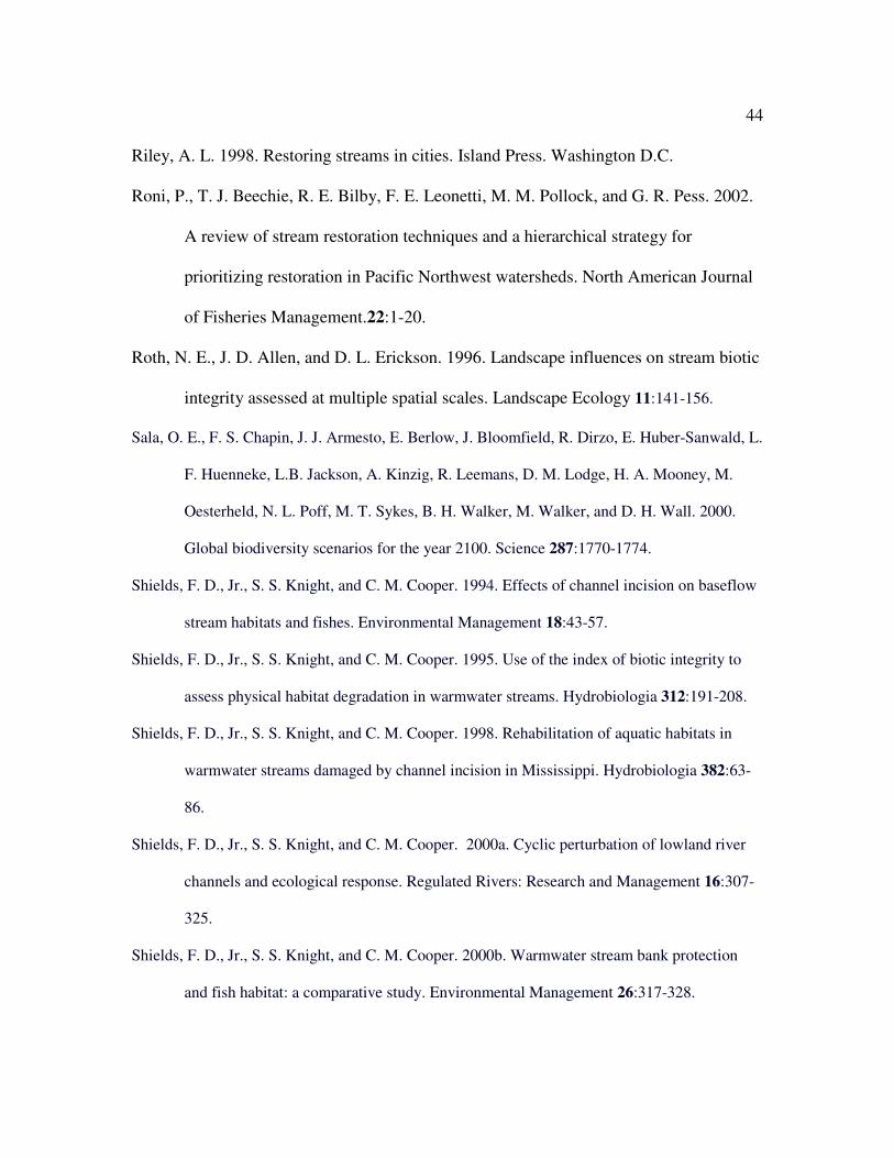
44

Riley, A. L. 1998. Restoring streams in cities. Island Press. Washington D.C.

Roni, P., T. J. Beechie, R. E. Bilby, F. E. Leonetti, M. M. Pollock, and G. R. Pess. 2002.

A review of stream restoration techniques and a hierarchical strategy for

prioritizing restoration in Pacific Northwest watersheds. North American Journal

of Fisheries Management.22:1-20.

Roth, N. E., J. D. Allen, and D. L. Erickson. 1996. Landscape influences on stream biotic

integrity assessed at multiple spatial scales. Landscape Ecology 11:141-156.

Sala, O. E., F. S. Chapin, J. J. Armesto, E. Berlow, J. Bloomfield, R. Dirzo, E. Huber-Sanwald, L.

F. Huenneke, L.B. Jackson, A. Kinzig, R. Leemans, D. M. Lodge, H. A. Mooney, M.

Oesterheld, N. L. Poff, M. T. Sykes, B. H. Walker, M. Walker, and D. H. Wall. 2000.

Global biodiversity scenarios for the year 2100. Science 287:1770-1774.

Shields, F. D., Jr., S. S. Knight, and C. M. Cooper. 1994. Effects of channel incision on baseflow

stream habitats and fishes. Environmental Management 18:43-57.

Shields, F. D., Jr., S. S. Knight, and C. M. Cooper. 1995. Use of the index of biotic integrity to

assess physical habitat degradation in warmwater streams. Hydrobiologia 312:191-208.

Shields, F. D., Jr., S. S. Knight, and C. M. Cooper. 1998. Rehabilitation of aquatic habitats in

warmwater streams damaged by channel incision in Mississippi. Hydrobiologia 382:63-

86.

Shields, F. D., Jr., S. S. Knight, and C. M. Cooper. 2000a. Cyclic perturbation of lowland river

channels and ecological response. Regulated Rivers: Research and Management 16:307-

325.

Shields, F. D., Jr., S. S. Knight, and C. M. Cooper. 2000b. Warmwater stream bank protection

and fish habitat: a comparative study. Environmental Management 26:317-328.

45

Shields, F. D., Jr., S. S. Knight, N. Morin, and J. C. Blank. 2003. Response of fishes and aquatic

habitats to sand-bed stream restoration using large woody debris. Hydrobiologia 494:251-

257.

Shields, F. D., Jr., N. Morin, C. M. Cooper. 2004. Large woody debris structures for sand-bed

channels. Journal of Hydraulic Engineering 130:208-217.

Smiley P. C., Jr. and E. D. Dibble. 2007. Influence of spatial resolution on assessing

channelization impacts on fish and macroinvertebrate communities in a warmwater

stream in the southeastern United States. Environmental Monitoring and Assessment

138:17-29.

Smiley, P. C. Jr., S. S. Knight, C. M. Cooper, and K. W. Kallies. 1999. Fish richness

and abundance in created riparian habitats of channelized northern Mississippi

streams. Southeastern Fishes Council Proceedings 39: 7-12.

Sudduth, E. B., and . L. Meyer. 2006. Effects of bioengineered streambank stabilization on bank

habitat and macroinvertebrates in urban streams. Environmental Management 38:218-

226.

United States Department of Agriculture, National Agricultural Statistics Services, County Crops

Data. URL

http://usda.mannlib.cornell.edu/MannUsda/viewDocumentInfo.do?documentID=1270

[ accessed 12 February, 2009 ]

Valett, H. M., J. A. Morrice, and C. N. Dahm. 1996. Parent lithology, surface-

groundwater exhange, and nitrate retention in headwater streams. Limnol.

Oceanogr. 41: 333-345.

46

Walser, C. A., H. L. Bart. 1999. Influence of agriculture on in-stream habitat and fish community

structure in Piedmont watersheds of the Chattahoochee River system. Ecology of

Freshwater Fish 8:237-246.

Wang, L., J. Lyons, P. Kanehl, and R. Gatti. 1997. Influences of watershed land use on habitat

quality and biotic integrity in Wisconsin streams. Fisheries 22:6-12.

Waters, T. F. 1995. Sediments in streams: sources, biological effects, and control. American

Fisheries Society. Bethesda, MD.

Wood, P. J., and P. D. Armitage. 1997. Biological effects of fine sediment in the lotic

environment. Environmental Management 21:203-217.

47

5 riprap vanes

------------

1 riprap vane & 3 pole jetties

7 riprap vanes

------------

7 pole jetties

12 pole jetties

------------

10 pole jetties

4 cottonwood jetties

SiteMapped

length (m)

Number & type

of structure

Vegetated buffer

width (m)

200

150

100

200

300

200

350

175

400

225

Site 1(S)

Site 2 (C)

Site 3 (S)

Site 4 (S)

Site 5 (C)

Site 6 (S)

Site 7 (S)

Site 8 (C)

Site 9 (S)

Site 10 (S)

10

15

5

5

0

0

30

30

5

0

Table 1. Characteristics of the 10 monitored sites in the Cedar River, Nebraska.

S or C following each site name indicates the treatment, (S) sites have stabilization

structures, (C) sites are control sites with no stabilization structures.

River km

88

75

74

71

49

44

43

42

39

11

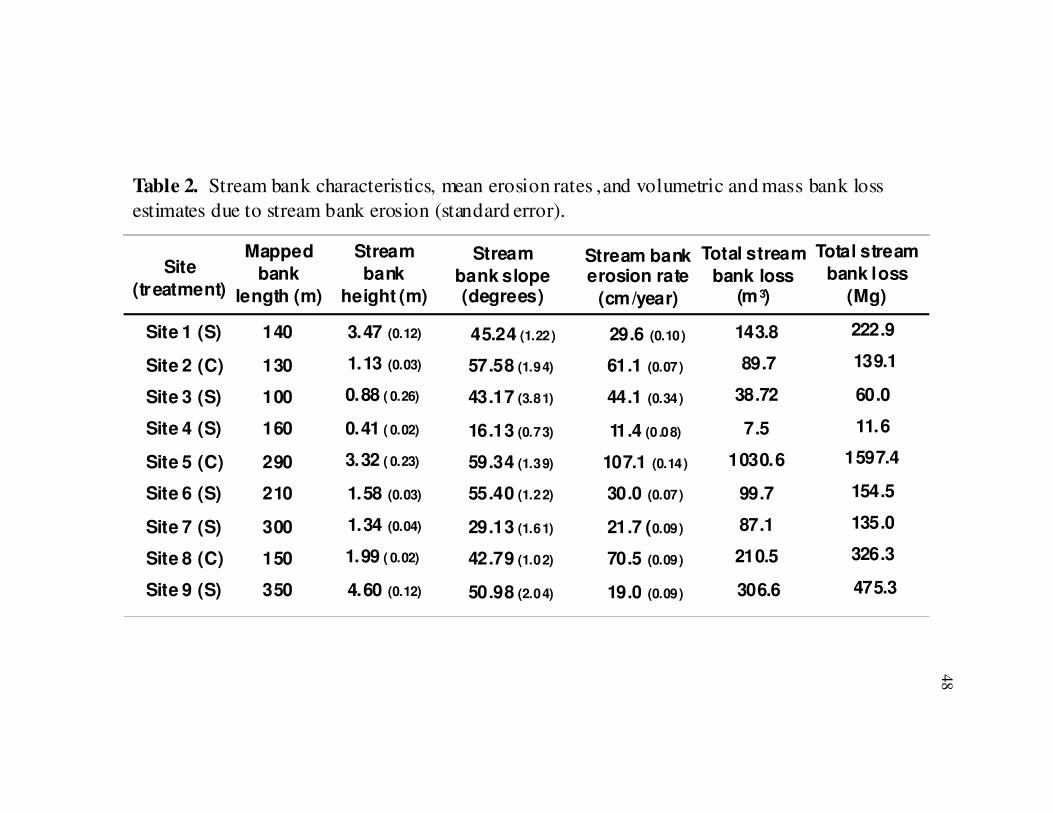
48

Table 2. Stream bank characteristics, mean erosion rates ,and volumetric and mass bank loss

estimates due to stream bank erosion (standard error).

Total stream

bank loss

(Mg)

Stream

bank

height (m)

Stream

bank slope (degrees)

Total stream

bank loss (m 3)

Site

(treatment)

Mapped

bank

length (m)

140

130

100

160

290

210

300

150

350

Site 1 (S)

Site 2 (C)

Site 3 (S)

Site 4 (S)

Site 5 (C)

Site 6 (S)

Site 7 (S)

Site 8 (C)

Site 9 (S)

3.47 (0.12)

1.13 (0.03)

0.88 ( 0.26)

0.41 ( 0.02)

3.32 ( 0.23)

1.58 (0.03)

1.34 (0.04)

1.99 ( 0.02)

4.60 (0.12)

143.8

89.7

38.72

7.5

1030.6

99.7

87.1

210.5

306.6

222.9

139.1

60.0

11.6

1597.4

154.5

135.0

326.3

475.3

Stream bank erosion rate

(cm/year)

29.6 (0.10)

61.1 (0.07)

44.1 (0.34)

11.4 (0.08)

107.1 (0.14)

30.0 (0.07)

21.7 (0.09)

70.5 (0.09)

19.0 (0.09)

45.24 (1.22)

57.58 (1.94)

43.17 (3.81)

16.13 (0.73)

59.34 (1.39)

55.40 (1.22)

29.13 (1.61)

42.79 (1.02)

50.98 (2.04)

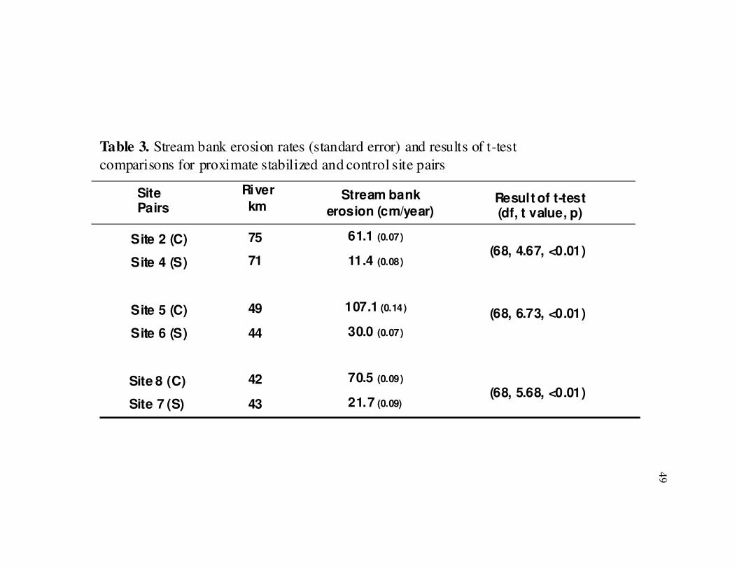
49

Site Pairs

Result of t-test(df, t value, p)

61.1 (0.07)

11.4 (0.08)

107.1 (0.14)

30.0 (0.07)

70.5 (0.09)

21.7 (0.09)

Site 2 (C)

Site 4 (S)

Site 5 (C)

Site 6 (S)

Site 8 (C)

Site 7 (S)

Table 3. Stream bank erosion rates (standard error) and results of t-test

comparisons for proximate stabilized and control site pairs

River

km

75

71

49

44

42

43

(68, 4.67, <0.01)

(68, 6.73, <0.01)

(68, 5.68, <0.01)

Stream bank

erosion (cm/year)

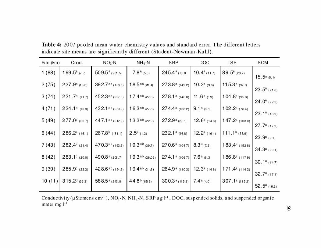
50

Site (km) Cond. NO3-N NH4-N SRP DOC TSS SOM

199.5a (7. 7)

237.9b (18.0)

231.7b (11.7)

234.1b (10.9)

277.0c (20. 7)

286.2c(16. 1)

282.4c(21. 4)

283.1c (20. 0)

285.9c (22. 3)

315.2d (33.3)

509.5 a (201. 5)

392.7 ab (138.5)

452.3 ab (227.6)

432.1 ab (269.2)

447.1 ab (212.9)

267.8 b(181.1)

470.3 ab (192.6)

490.8 a (208. 7)

428.6 ab (154.6)

588.5 a (242. 8)

7.8a (5.3)

18.5ab (28. 4)

17.4ab (27.3)

16.3ab (27.6)

13.3ab (22.9)

2.5a(1.2)

19.3ab(29.7)

19.3ab (26.02)

19.4ab (31.6)

44.8b (65. 8)

245.4 a (78. 0)

273.8 a (149.2)

278.1 a (146.8)

274.4 a (138.2)

272.9 a (89. 1)

232.1 a(46.8)

270.6 a(104.7)

274.1 a (106.7)

264.9 a (110.3)

300.3 a (115.3)

10.4a (11.7)

10.3a (9.6)

11.6 a (8.9)

9.1 a (8. 1)

12.6a (14. 8)

12.2a(16. 1)

8.3 a (7. 2)

7.6 a (6. 3)

12.3a (14. 6)

7.4 a (4. 0)

89.5a (23.7)

115.3 a (97. 3)

104.8a (95.8)

102.2a (78.4)

147.2a (103. 0)

111.1a(38. 9)

183.4a(152. 8)

186.8a (117. 9)

171.4a (114. 2)

307.1a (115.2)

15.5a (5. 1)

23.5a(21.6)

24.0a(22.2)

23.1a(18.9)

27.7a (17.9)

23.9a (9.1)

34.3a (29.1)

30.1a(14.7)

32.7a(17.1)

52.5a (16.2)

Table 4: 2007 pooled mean water chemistry values and standard error. The different letters

indicate site means are significantly different (Student-Newman-Kuhl).

1 (88)

2 (75)

3 (74)

4 (71)

5 (49)

6 (44)

7 (43)

8 (42)

9 (39)

10 (11)

Conductivi ty (µ Siemens cm-1 ), NO3-N, NH4-N, SRP µ g l-1 , DOC, susp ended solids, and suspended organic

mater mg l-1

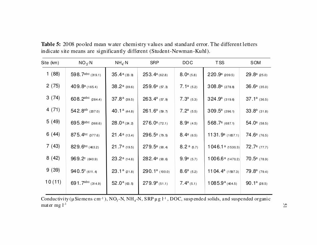
51

Site (km) NO 3-N NH4-N SRP DOC T SS SOM

Table 5: 2008 pooled mean water chemistry values and standard error. The different letters


598.7abc (319.1)

409.8a (165. 4)

608.2abc(284.4)

542.8ab(207.0)

695.8abc (366.6)

875.4bc (377.6)

829.6bc (463.2)

969.2c (640.9)

940.5c (611. 4)

691.7abc (314.9)

35.4a (33.9)

38.2a (39.6)

37.8a(39.5)

40.1a(44.8)

28.0a (24.2)

21.4a (13.4)

21.7a (19.5)

23.2a (14.6)

23.1a(21.8)

52.0a (63.5)

253.4a (62.8)

259.6a (57.3)

263.4a(57.9)

261.6a(59.7)

276.0a (72.1)

296.5a (79.5)

279.5a (90.4)

282.4a (90.6)

290.1a(100.0)

279.9a (51.1)

8.0a (5.8)

7.1a (5.2)

7.3a(5.3)

7.2a(5.5)

8.9a (4.5)

8.4a (6.5)

8.2 a (5.7)

9.9a (5.7)

8.6a(5.2)

7.4a (5.1)

220.9a (209.5)

308.8a (278. 8)

324.9a(319. 6)

309.5a(296. 1)

568.7a (687. 1)

1131.9a (1657.1)

1046.1 a (1530.3)

1006.6 a (1470.2)

1104.4a(1597.3)

1085.9 a (404.5)

29.8a (25.0)

36.6a (35.0)

37.1a(36.5)

33.8a(31.8)

54.0a (58.5)

74.6a (76.5)

72.7a (77.7)

70.5a (78.9)

79.8a(79.4)

90.1a (28.5)

1 (88)

2 (75)

3 (74)

4 (71)

5 (49)

6 (44)

7 (43)

8 (42)

9 (39)

10 (11)

Conductivi ty (µ Siemens cm-1 ), NO3-N, NH4-N, SRP µ g l-1 , DOC, susp ended solids, and suspended organic

mater mg l-1

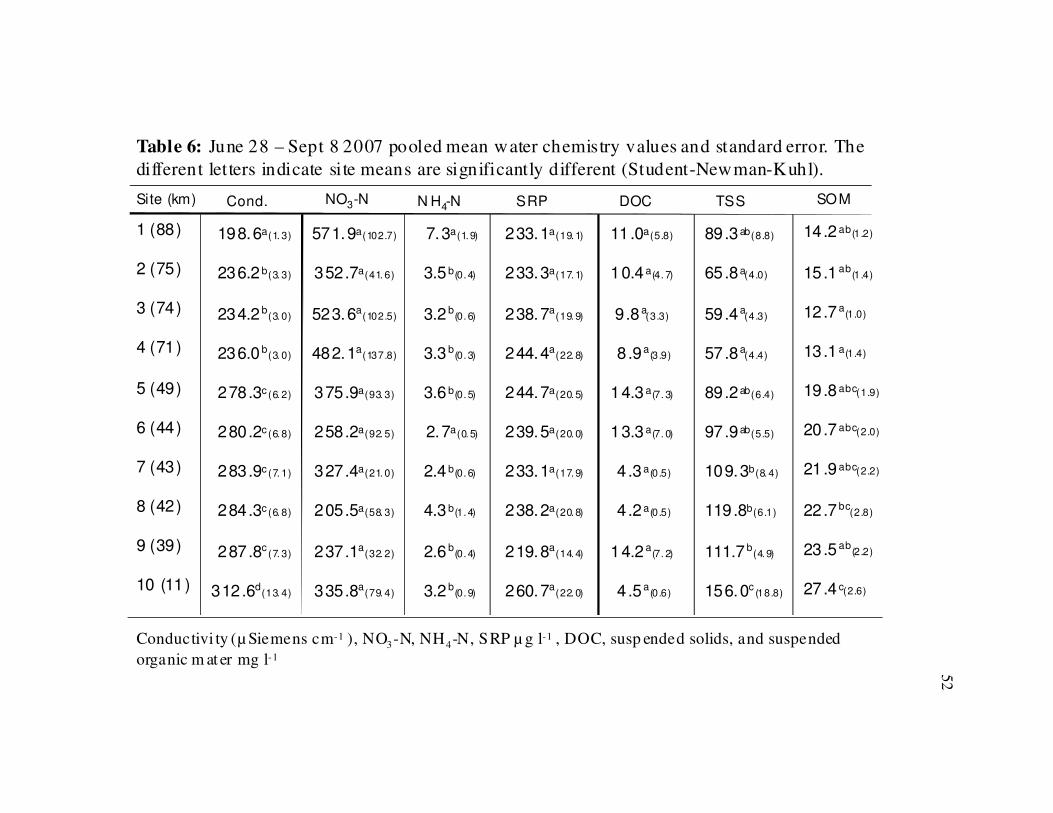
52

Site (km) Cond. NO3-N N H4-N SRP DOC TSS SOM

1 (88)

2 (75)

3 (74)

4 (71)

5 (49)

6 (44)

7 (43)

8 (42)

9 (39)

10 (11)

198.6a(1. 3)

236.2 b(3. 3)

234.2 b(3. 0)

236.0 b(3. 0)

278.3c (6. 2)

280.2c (6. 8)

283.9c (7. 1)

284.3c (6. 8)

287.8c(7. 3)

312.6d(13. 4)

571.9a(102.7)

352.7a(41. 6)

523.6a(102.5)

482.1a(137.8)

375.9a(93. 3)

258.2a(92. 5)

327.4a(21. 0)

205.5a(58. 3)

237.1a(32. 2)

335.8a(79. 4)

7.3a(1. 9)

3.5 b(0. 4)

3.2 b(0. 6)

3.3 b(0. 3)

3.6 b(0. 5)

2.7a(0. 5)

2.4 b(0. 6)

4.3 b(1. 4)

2.6 b(0. 4)

3.2 b(0. 9)

233.1a(19. 1)

233.3a(17. 1)

238.7a(19. 9)

244.4a(22. 8)

244.7a(20. 5)

239.5a(20. 0)

233.1a(17. 9)

238.2a(20. 8)

219.8a(14. 4)

260.7a(22. 0)

11.0a(5.8)

10.4 a(4. 7)

9.8 a(3.3)

8.9a(3.9)

14.3 a(7. 3)

13.3 a(7. 0)

4.3a(0.5)

4.2a(0.5)

14.2 a(7. 2)

4.5a(0.6)

89.3ab(8.8)

65.8a(4.0)

59.4a(4.3)

57.8a(4.4)

89.2ab(6.4)

97.9ab(5.5)

109.3b(8. 4)

119.8b(6.1)

111.7 b(4. 9)

156.0c(18.8)

14.2 ab(1.2)

15.1 ab(1.4)

12.7 a(1.0)

13.1 a(1.4)

19.8 abc(1.9)

20.7 abc(2.0)

21.9 abc(2.2)

22.7 bc(2.8)

23.5 ab(2.2)

27.4 c(2.6)

Table 6: June 28 – Sept 8 2007 pooled mean water chemistry values and standard error. The

different letters indicate site means are significantly different (Student-Newman-Kuhl).

Conductivi ty (µ Siemens cm-1 ), NO3-N, NH4-N, SRP µ g l-1 , DOC, susp ended solids, and suspended

organic m at er mg l-1

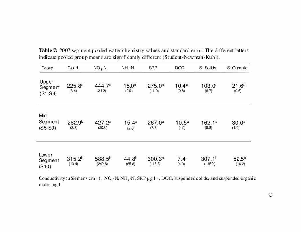
53

Group Cond. NO3-N NH4-N SRP DOC S. Solids S. Organic

UpperSegment

(S1-S4)

Mid

Segment

(S5-S9)

LowerSegment

(S10)

Table 7: 2007 segment pooled water chemistry values and standard error. The different letters

indicate pooled group means are significantly different (Student-Newman-Kuhl).

225.8a

(3.4)

282.9b

(3.3)

315.2b

(13.4)

444.7a

(21.2)

427.2a

(20.8)

588.5b

(242 .8)44.8b

(65.8)

15.4a

(2.6)

15.0a

(2.0 )275.0a

(11.0)

267.0a

(7.6)

300.3a

(115.3)

10.4 a

(0.8)

10.5a

(1.0)

7.4a

(4.0)

103.0a

(6.7)

162.1a

(8.8)

307.1b

(115.2 )

21.6a

(0.6)

30.0a

(1.0)

52.5b

(16.2)

Conductivity (µ Siemens cm-1 ), NO3-N, NH4-N, SRP µ g l-1 , DOC, suspended solids, and suspended organic

mater mg l-1

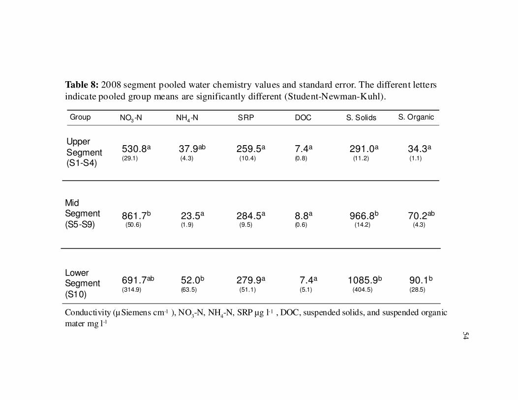
54

Group S. Organic

Upper

Segment(S1-S4)

MidSegment

(S5-S9)

LowerSegment

(S10)

Table 8: 2008 segment pooled water chemistry values and standard error. The different letters

indicate pooled group means are significantly different (Student-Newman-Kuhl).

NO3 -N

530.8a

(29.1)

861.7b

(50.6)

691.7ab

(314.9)

NH4 -N

52.0b

(63.5)

23.5a

(1.9)

37.9ab

(4.3)

SRP

259.5a

(10.4)

284.5a

(9.5)

279.9a

(51.1)

8.8a

(0.6)

DOC

7.4a

(0.8)

7.4a

(5.1)

S. Solids

291.0a

(11.2)

966.8b

(14.2)

1085.9b

(404.5)

34.3a

(1.1)

70.2ab

(4.3)

90.1b

(28.5)

Conductivity (µSiemens cm-1 ), NO3-N, NH

4-N, SRP µg l-1 , DOC, suspended solids, and suspended organic

mater mg l-1

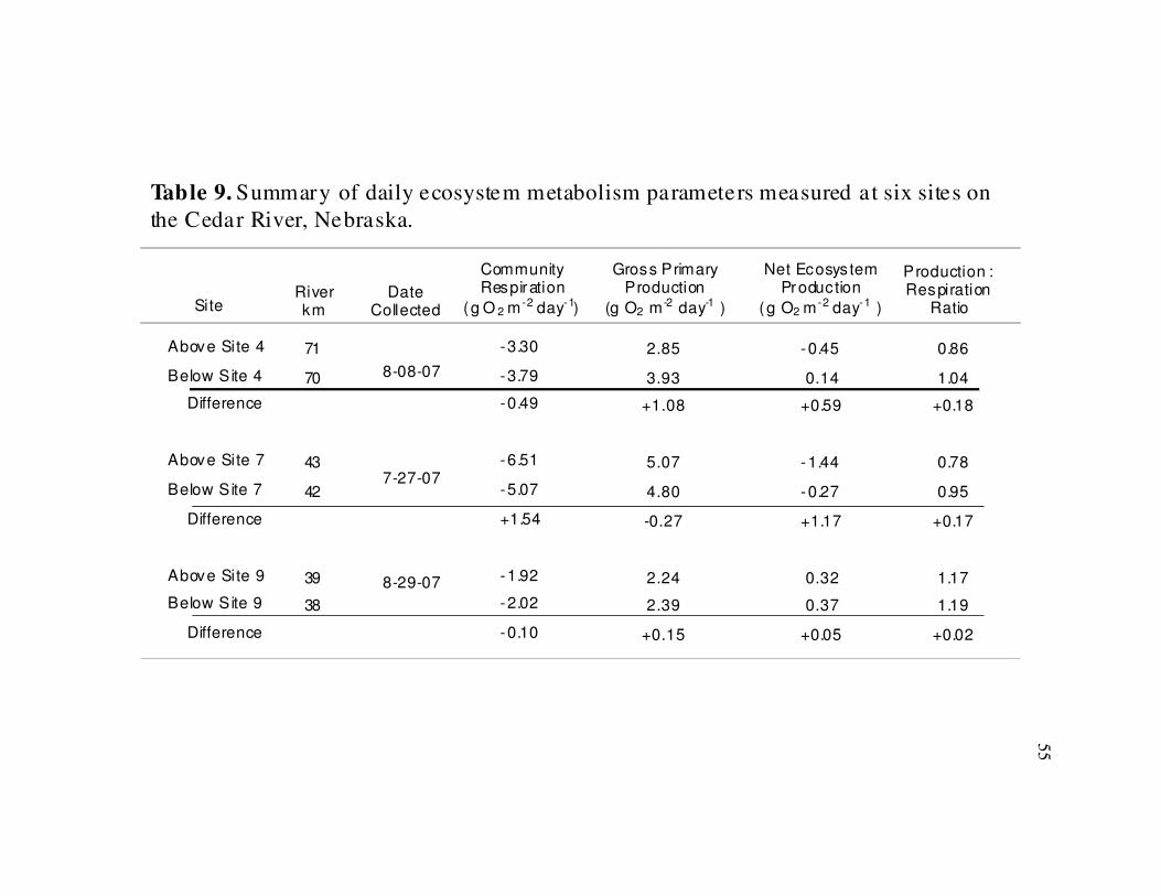
55

Site

Community Respiration

( g O 2 m -2 day-1)

Gross Primary Production

(g O2 m -2 day-1 )

Net Ecosys tem Production

( g O2 m -2 day-1 )

-3.30

-3.79

-0.49

-6.51

-5.07

+1.54

-1.92

-2.02

-0.10

Above Site 4

Below Site 4

Difference

Above Site 7

Below Site 7

Difference

Above Site 9

Below Site 9

Difference

Table 9. Summary of daily ecosystem metabolism parameters measured at six sites on

the Cedar River, Nebraska.

River km

71

70

43

42

39

38

Production : Respiration

Ratio

2.85

3.93

+1.08

5.07

4.80

-0.27

2.24

2.39

+0.15

-0.45

0.14

+0.59

-1.44

-0.27

+1.17

0.32

0.37

+0.05

0.86

1.04

+0.18

0.78

0.95

+0.17

1.17

1.19

+0.02

DateCollected

8-08-07

7-27-07

8-29-07

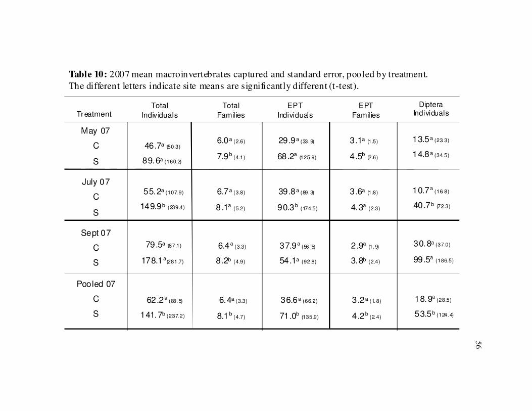
56

TreatmentTotal

Individuals

Total

Families

EPT

Individuals

Table 10: 2007 mean macroinvertebrates captured and standard error, pooled by treatment.

The different letters indicate site means are significantly different (t-test).

46.7a (50.3)

89.6a (160.2)

55.2a (107. 9)

149.9b (239.4)

79.5a (87.1)

178.1a(281.7)

62.2a (88. 5)

141.7b (237.2)

May 07

C

S

July 07

C

S

Sept 07

C

S

Pooled 07

C

S

EPT

Families

DipteraIndividuals

6.0a (2.6)

7.9b (4.1)

6.7a (3.8)

8.1a(5.2)

6.4a (3.3)

8.2b (4.9)

6.4a (3.3)

8.1b (4.7)

29.9a (33.9)

68.2a (125.9)

39.8a (89.3)

90.3b(174.5)

37.9a (56. 5)

54.1a (92.8)

36.6a (66.2)

71.0b (135.9)

3.1a (1.5)

4.5b (2.6)

3.6a (1.8)

4.3a(2.3)

2.9a (1.9)

3.8b (2.4)

3.2a (1. 8)

4.2b (2. 4)

13.5a (23.3)

14.8a (34.5)

10.7a (16.8)

40.7b (72.3)

30.8a (37.0)

99.5a(186.5)

18.9a (28.5)

53.5b (124. 4)

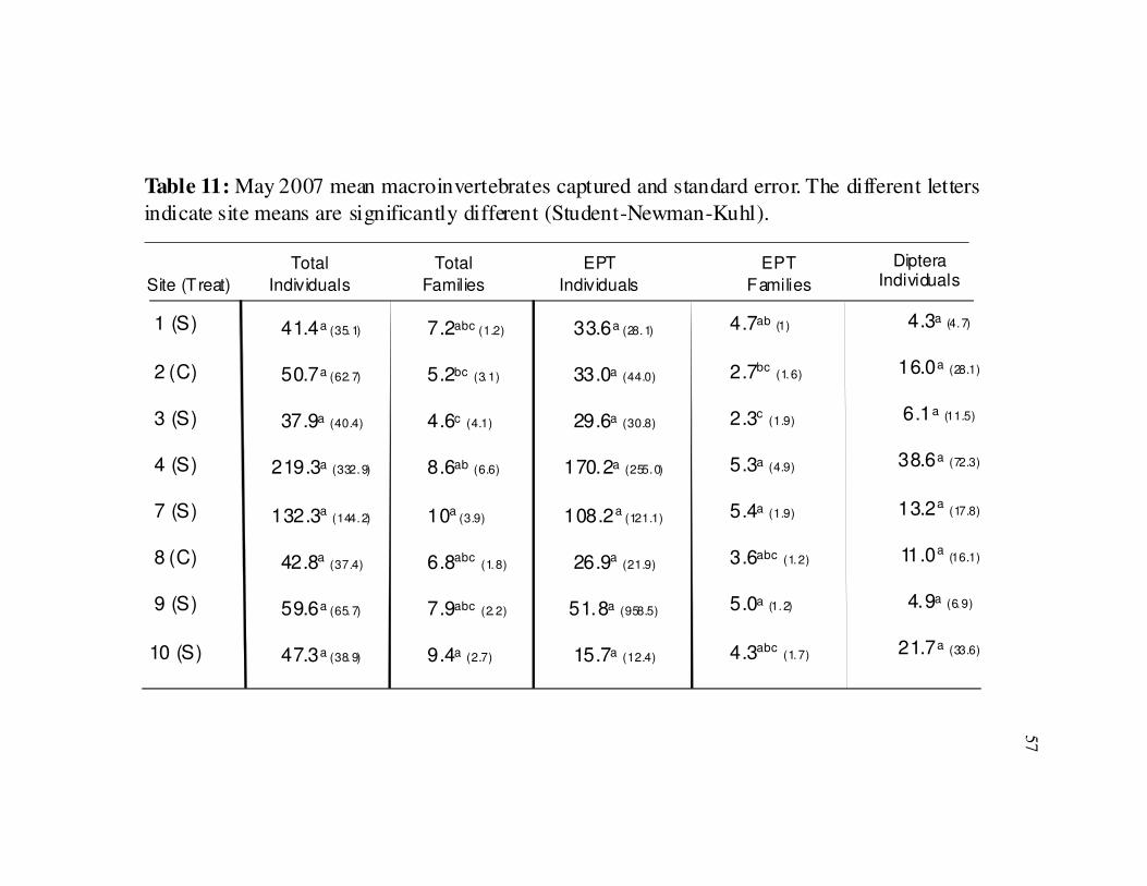
57

Site (Treat)

Total

Individuals

Total

Families

EPT

Individuals

Table 11: May 2007 mean macroinvertebrates captured and standard error. The different letters


41.4a (35.1)

50.7a (62.7)

37.9a (40.4)

219.3a (332.9)

132.3a(144.2)

42.8a(37.4)

59.6a (65.7)

47.3a (38.9)

7.2abc (1.2)

5.2bc (3.1)

4.6c (4.1)

8.6ab (6.6)

10a (3.9)

6.8abc(1.8)

7.9abc (2.2)

9.4a (2.7)

33.6a (28.1)

33.0a (44.0)

29.6a (30.8)

170.2a (255.0)

108.2a (121.1)

26.9a(21.9)

51.8a (958.5)

15.7a (12.4)

4.7ab (1)

2.7bc(1.6)

2.3c(1.9)

5.3a (4.9)

5.4a (1.9)

3.6abc (1.2)

5.0a (1.2)

4.3abc(1.7)

4.3a (4.7)

16.0a (28.1)

6.1a (11.5)

38.6a (72.3)

13.2a(17.8)

11.0a(16.1)

4.9a (6.9)

21.7a (33.6)

1 (S)

2 (C)

3 (S)

4 (S)

7 (S)

8 (C)

9 (S)

10 (S)

EPT

Families

DipteraIndividuals

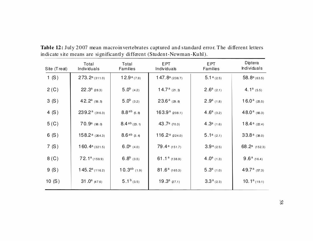
58

Site (T reat)Total

Indiv idualsTotal

Famil iesEPT

Indiv iduals

Table 12: July 2007 mean macroinvertebrates captured and standard error. The different letters


273.2a (311. 0)

22.3a (28.3)

42.2a(56. 5)

239.2 a(316.3)

70.9a (98. 0)

158.2 a (264.3)

160.4a (321. 5)

72.1a (159. 9)

145.2a (116. 2)

31.0a (47.6)

12.9 a (7.9)

5 .0b(4.2)

5 .0b(3.2)

8.8 ab(5. 8)

8.4 ab (23. 1)

8.6 ab (3. 4)

6 .0b (4.0)

6 .8b(3.5)

10.3ab(1. 9)

5 .1 b (3. 5)

147.8a (238. 7)

14.7 a(21. 3)

23.6 a(29. 8)

163.9 a(208.1)

43 .7a (70.3)

116 .2 a (224.0)

79 .4 a (151.7)

61 .1 a(138.9)

81 .6 a(165.3)

19 .3a (27.1)

5.1 a (2. 5)

2 .6a(2.1)

2 .9a(1.8)

4 .6a(3.2)

4 .3a (1.6)

5 .1a (2.1)

3.9 a (2. 5)

4 .0a(1.3)

5 .3a(1.0)

3.3 a (2. 3)

58.8a (63.5)

4.1a(5. 5)

16.0 a(25.5)

48.0 a(66.3)

18.4 a (22.4)

33.8 a (38.0)

68 .2a (152. 3)

9 .6 a(16.4)

49.7 a(57.3)

10.1a (19.1)

1 (S )

2 (C)

3 (S )

4 (S )

5 (C)

6 (S )

7 (S )

8 (C)

9 (S )

10 (S )

EPT Famil ies

Diptera

Individuals

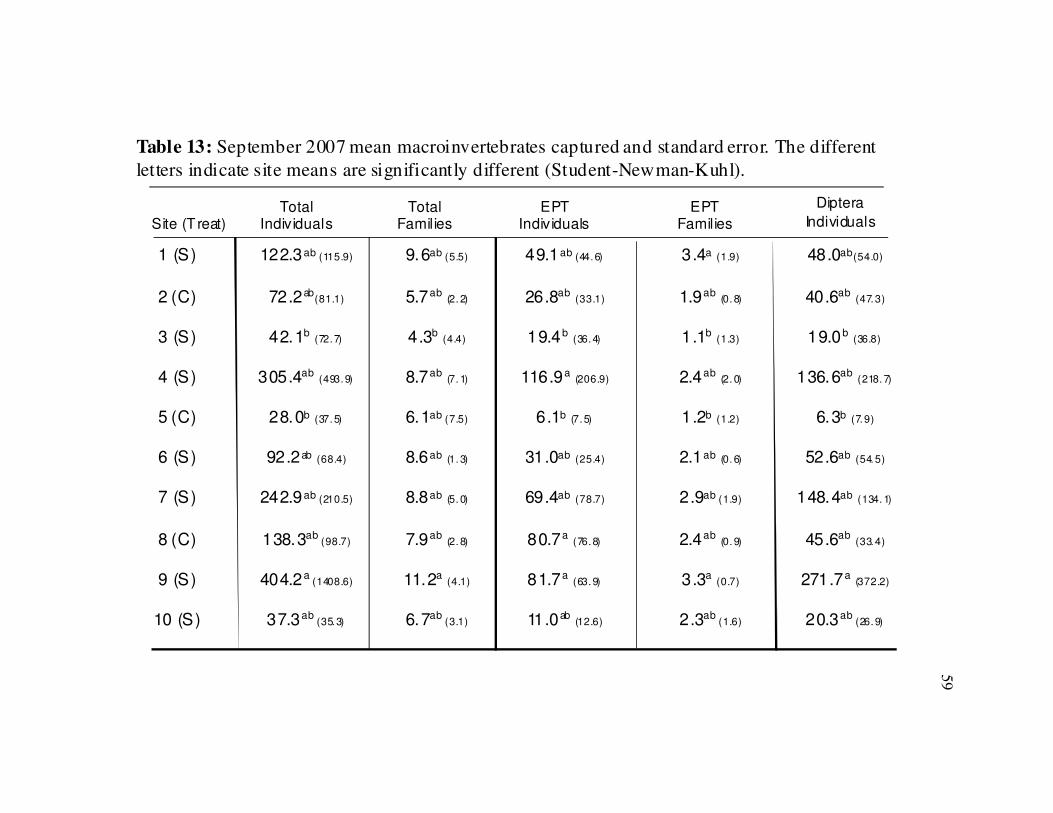
59

Site (T reat)Total

IndividualsTotal

FamiliesEPT

Individuals

Table 13: September 2007 mean macroinvertebrates captured and standard error. The different

letters indicate site means are significantly different (Student-Newman-Kuhl).

122.3ab (115.9)

72.2ab(81.1)

42.1b(72.7)

305.4ab(493.9)

28.0b (37.5)

92.2ab (68.4)

242.9ab (210.5)

138.3ab (98.7)

404.2a (1408.6)

37.3ab (35. 3)

9.6ab (5.5)

5.7ab(2. 2)

4.3b(4.4)

8.7ab(7. 1)

6.1ab (7.5)

8.6ab (1. 3)

8.8ab (5. 0)

7.9ab(2. 8)

11.2a(4.1)

6.7ab (3.1)

49.1ab (44.6)

26.8ab(33.1)

19.4b(36.4)

116.9a(206.9)

6.1b (7.5)

31.0ab (25.4)

69.4ab (78.7)

80.7a(76.8)

81.7a(63.9)

11.0ab (12.6)

3.4a (1.9)

1.9ab(0. 8)

1.1b(1.3)

2.4ab(2. 0)

1.2b (1.2)

2.1ab (0. 6)

2.9ab (1.9)

2.4ab(0. 9)

3.3a(0.7)

2.3ab (1.6)

48.0ab(54.0)

40.6ab(47.3)

19.0b(36.8)

136.6ab(218. 7)

6.3b (7.9)

52.6ab (54.5)

148.4ab (134. 1)

45.6ab(33.4)

271.7a(372.2)

20.3ab (26.9)

1 (S)

2 (C)

3 (S)

4 (S)

5 (C)

6 (S)

7 (S)

8 (C)

9 (S)

10 (S)

EPT Families

Diptera

Individuals

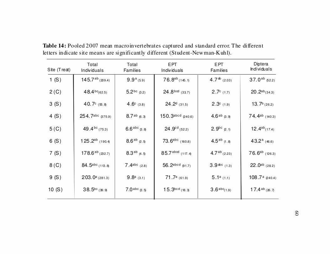
60

Site (T reat)Total

Indiv iduals

Total

Families

EPT

Indiv iduals

Table 14: Pooled 2007 mean macroinvertebrates captured and standard error. The different

letters indicate site means are significantly different (Student-Newman-Kuhl).

145.7ab (209.4)

48.4bc(62.5)

40.7c (55. 8)

254.7abc (375.9)

49.4 bc(75.3)

125.2ab(190. 4)

178.6ab (232.7)

84.5abc (113. 8)

203.0a (281. 3)

38.5bc (39. 9)

9.9 a (5. 9)

5.2 bc (3.2)

4.6c (3.8)

8.7 ab (6. 3)

6.6abc (3. 8)

8.6 ab(2. 5)

8.3 ab(4. 5)

7.4abc (2.8)

9.8a (3.1)

7.0abc (3. 5)

76.8ab (145. 1)

24.8bcd (33. 7)

24.2d (31.5)

150.3abc d (240.6)

24.9c d (52.2)

73.6abc(160.8)

85.7 abcd(117. 4)

56.2abcd (91.7)

71.7a (61.9)

15.3bc d (18. 3)

4.7 ab(2.03)

2.7c (1.7)

2.3c (1.9)

4.6ab (3. 9)

2.9bc(2. 1)

4.5ab(1. 8)

4.7 ab (2.23)

3.9 abc (1.3)

5.1a (1.1)

3.6abc(1.9)

37.0ab(52.2)

20.2ab(34.3)

13.7b (26.2)

74.4ab (140.3)

12.4ab(17.4)

43.2a(46.6)

76.6ab(126.3)

22.0ab (28.2)

108.7 a (240.4)

17.4ab (26.7)

1 (S)

2 (C)

3 (S)

4 (S)

5 (C)

6 (S)

7 (S)

8 (C)

9 (S)

10 (S)

EPT

Families

DipteraIndividuals

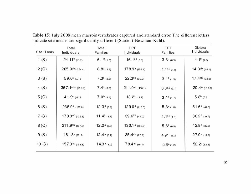
61

Site (T reat)Total

Indiv iduals

Total

Families

EPT

Indiv iduals

Table 15: July 2008 mean macroinvertebrates captured and standard error. The different letters


24.11c(11.7)

205.9abc(274.4)

59.6c (77. 8)

367.1abc (535.2)

41.9c (46. 8)

235.9 a(139.0)

170.0 ab (135.3)

211.9ab (207.3)

181.8 a (90. 9)

157.3 ab (153.3)

6.1 b (1. 8)

8.8b (2.6)

7.3b (2.0)

7.4b (3.6)

7.0 b (3. 1)

12.3a(2.7)

11.4a(3.1)

12.2a (2.3)

12.4a (2.4)

14.3a (3.0)

16.1ab (8.8)

178.9 a (258.1)

22.3ab (32.2)

211.0ab (406.1)

13.2b (13.2)

129.0 a(118.3)

39.6ab(42.0)

130.1 a (168.6)

35.4ab (28.2)

78.4ab (86. 4)

3.3b (0.9)

4.4ab(0. 9)

3.1b(1.5)

3.8ab (2. 1)

3.1b (1.7)

5.3a (1.8)

4.1ab (1.5)

5.6a(0.9)

4.9ab(1. 3)

5.6 a (1. 2)

4.1b (3. 0)

14.3ab (16. 1)

17.4ab (32. 2)

120.4a (156.0)

5.8b (5. 3)

51.6 a(43.7)

36.2 a(39.7)

42.8 a (35.6)

27.0 a (15.5)

52.2a (62.2)

1 (S )

2 (C)

3 (S )

4 (S )

5 (C)

6 (S )

7 (S )

8 (C)

9 (S )

10 (S )

EPT

Families

DipteraIndividuals

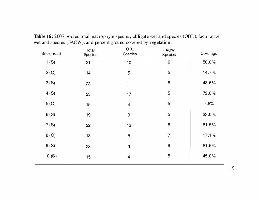
62

Site (Treat)Total

Species

OBL

SpeciesFACW

Species

Table 16: 2007 pooled total macrophyte species, obligate wetland species (OBL), facultative

wetland species (FACW), and percent ground covered by vegetation.

21

14

23

23

15

19

22

13

23

15

10

5

11

17

4

9

13

5

9

4

6

5

8

5

5

5

8

7

9

5

50.0%

14.7%

48.6%

72.0%

7.8%

33.0%

81.5%

17.1%

81.6%

45.0%

1 (S)

2 (C)

3 (S)

4 (S)

5 (C)

6 (S)

7 (S)

8 (C)

9 (S)

10 (S)

Coverage

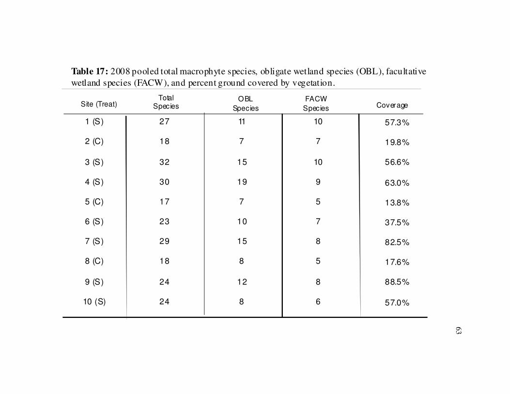
63

Site (Treat)Total

SpeciesOBL

Species

FACW

Species

Table 17: 2008 pooled total macrophyte species, obligate wetland species (OBL), facultative

wetland species (FACW), and percent ground covered by vegetation.

27

18

32

30

17

23

29

18

24

24

11

7

15

19

7

10

15

8

12

8

10

7

10

9

5

7

8

5

8

6

57.3%

19.8%

56.6%

63.0%

13.8%

37.5%

82.5%

17.6%

88.5%

57.0%

1 (S)

2 (C)

3 (S)

4 (S)

5 (C)

6 (S)

7 (S)

8 (C)

9 (S)

10 (S)

Coverage

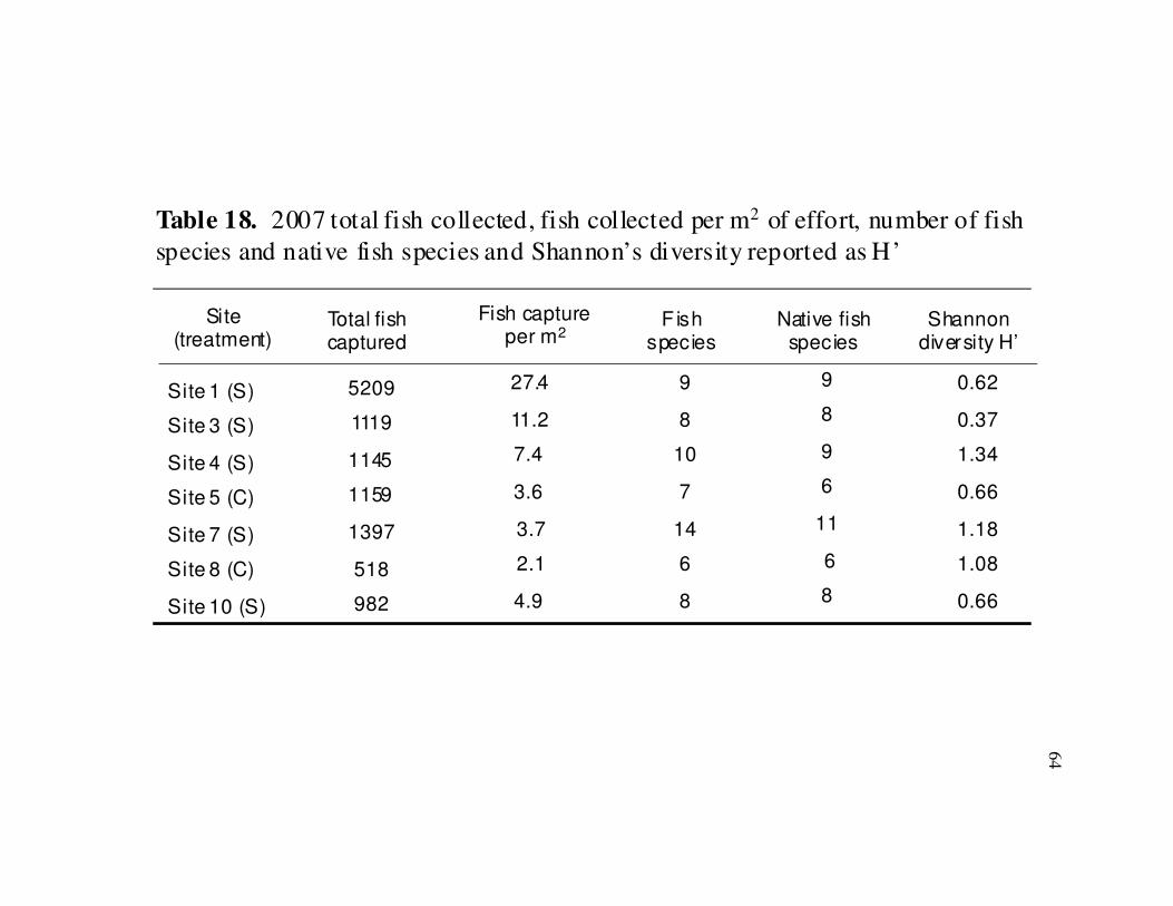
64

Table 18. 2007 total fish collected, fish collected per m2 of effort, number of fish

species and native fish species and Shannon’s diversity reported as H’

Native fish species

Fish capture per m2

Fish species

Shannondiversity H’

Site (treatment)

Total fish captured

5209

1119

1145

1159

1397

518

982

Site 1 (S)

Site 3 (S)

Site 4 (S)

Site 5 (C)

Site 7 (S)

Site 8 (C)

Site 10 (S)

9

8

9

6

11

6

8

27.4

11.2

7.4

3.6

3.7

2.1

4.9

9

8

10

7

14

6

8

0.62

0.37

1.34

0.66

1.18

1.08

0.66

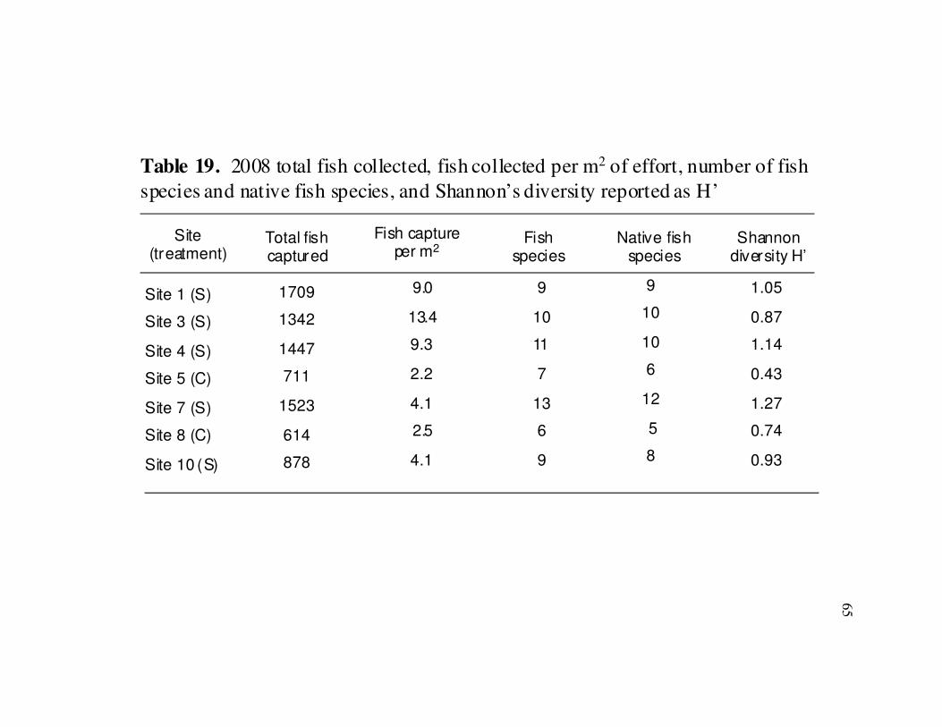
65

Native fish species

Fish capture per m2

Fish species

Shannondiversity H’

Site (treatment)

Total fish captured

1709

1342

1447

711

1523

614

878

Site 1 (S)

Site 3 (S)

Site 4 (S)

Site 5 (C)

Site 7 (S)

Site 8 (C)

Site 10 (S)

9

10

10

6

12

5

8

9.0

13.4

9.3

2.2

4.1

2.5

4.1

9

10

11

7

13

6

9

1.05

0.87

1.14

0.43

1.27

0.74

0.93

Table 19. 2008 total fish collected, fish collected per m2 of effort, number of fish

species and native fish species, and Shannon’s diversity reported as H’

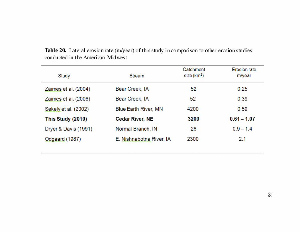
66

Table 20. Lateral erosion rate (m/year) of this study in comparison to other erosion studies

conducted in the American Midwest

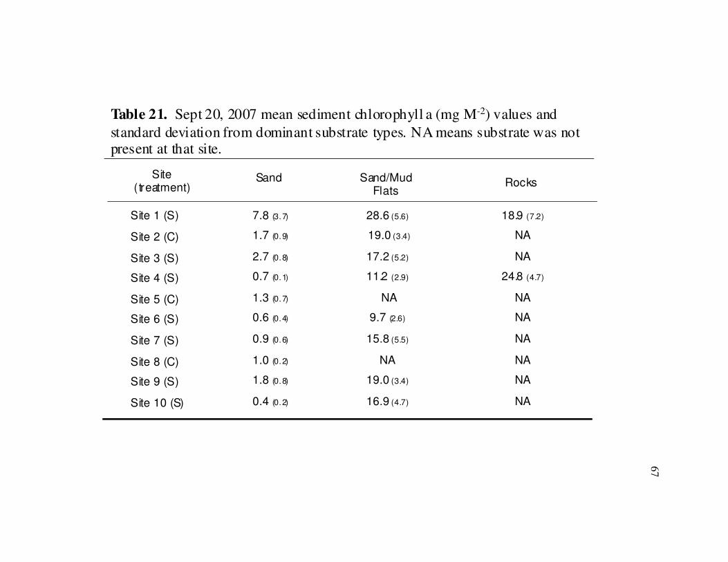
67

Sand/Mud Flats

RocksSite

( treatment) Sand

7.8 (3.7)

1.7 (0.9)

2.7 (0.8)

0.7 (0.1)

1.3 (0.7)

0.6 (0.4)

0.9 (0.6)

1.0 (0.2)

1.8 (0.8)

0.4 (0.2)

Site 1 (S)

Site 2 (C)

Site 3 (S)

Site 4 (S)

Site 5 (C)

Site 6 (S)

Site 7 (S)

Site 8 (C)

Site 9 (S)

Site 10 (S)

28.6 (5.6)

19.0 (3.4)

17.2 (5.2)

11.2 (2.9)

NA

9.7 (2.6)

15.8 (5.5)

NA

19.0 (3.4)

16.9 (4.7)

18.9 (7.2)

NA

NA

24.8 (4.7)

NA

NA

NA

NA

NA

NA

Table 21. Sept 20, 2007 mean sediment chlorophyll a (mg M-2) values and

standard deviation from dominant substrate types. NA means substrate was not present at that site.

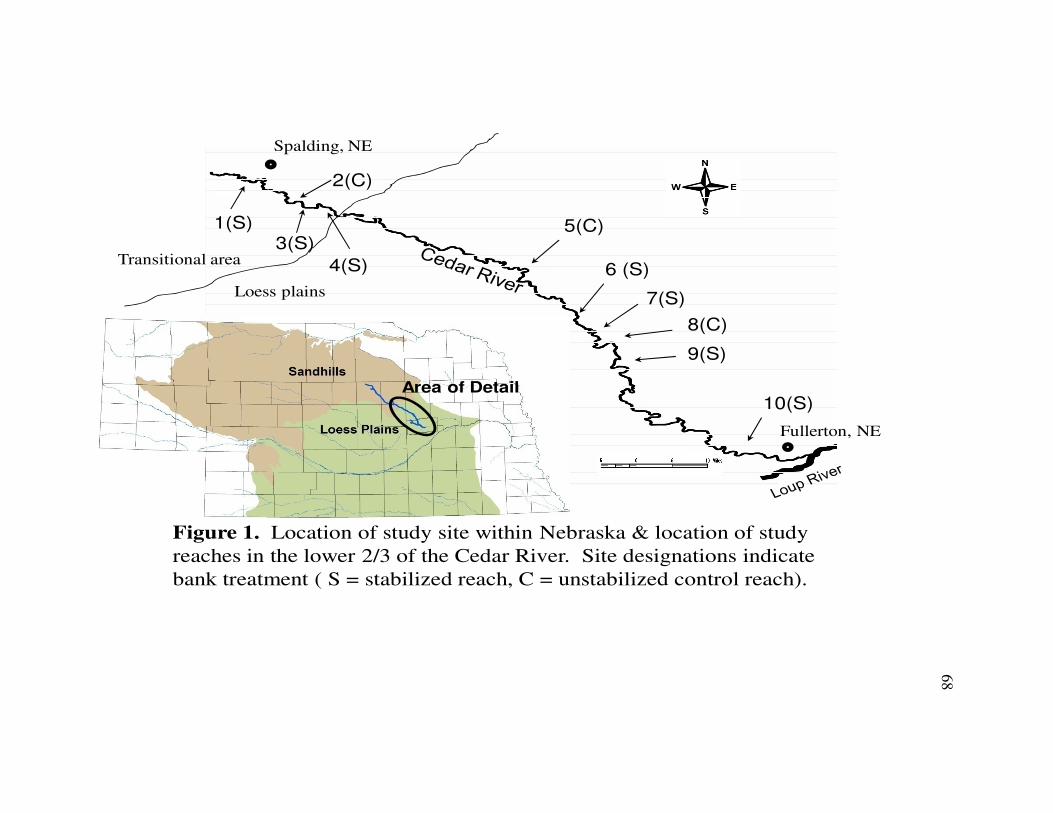
68

1(S)

2(C)

3(S)

4(S) 6 (S)

5(C)

7(S)

9(S)

8(C)

10(S)

Figure 1. Location of study site within Nebraska & location of study

reaches in the lower 2/3 of the Cedar River. Site designations indicate

bank treatment ( S = stabilized reach, C = unstabilized control reach).

Area of Detail

Spalding, NE

Fullerton, NE

Transitional area

Loess plains

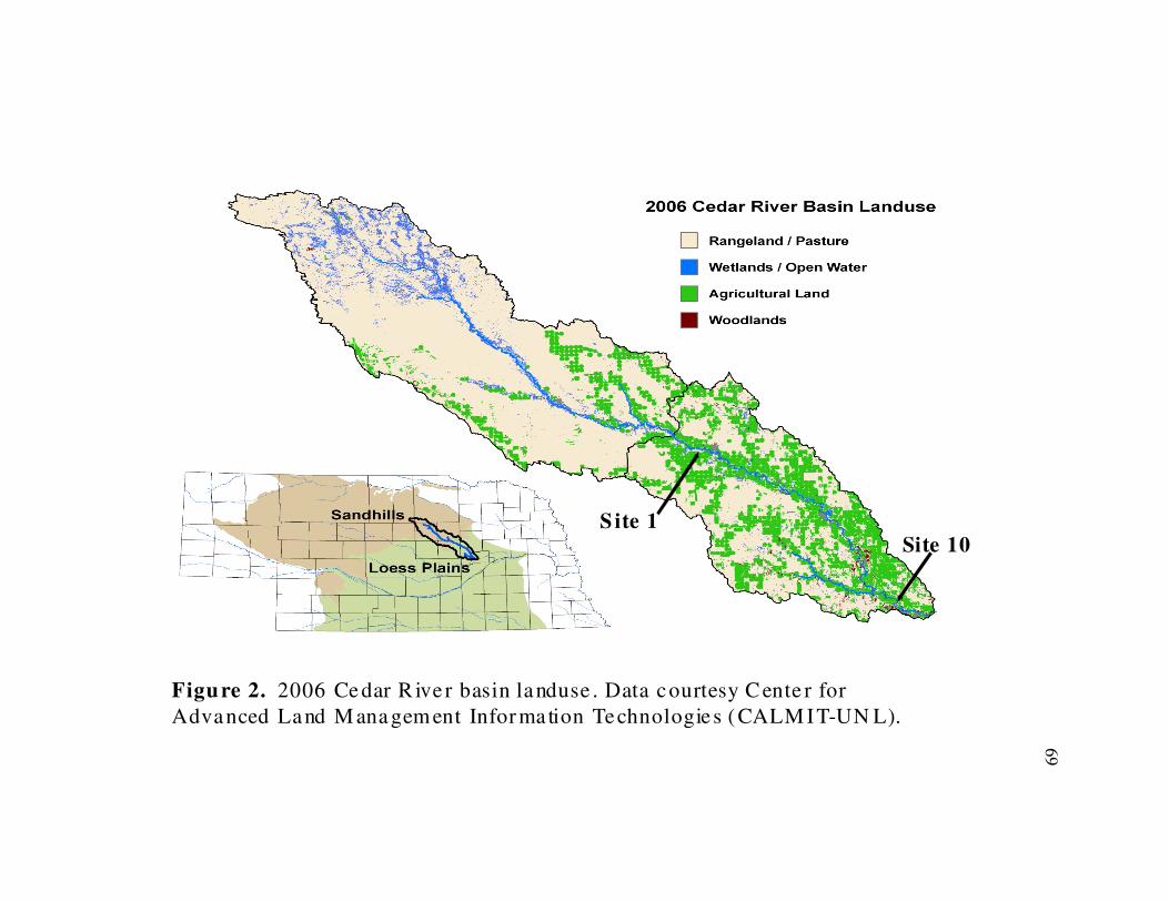
69

Figure 2. 2006 Ce dar R ive r basin landuse . Data courtesy C ente r for

Advanced Land M ana gem ent Informa tion Technologies (CALM IT-UN L).

Site 1Site 10

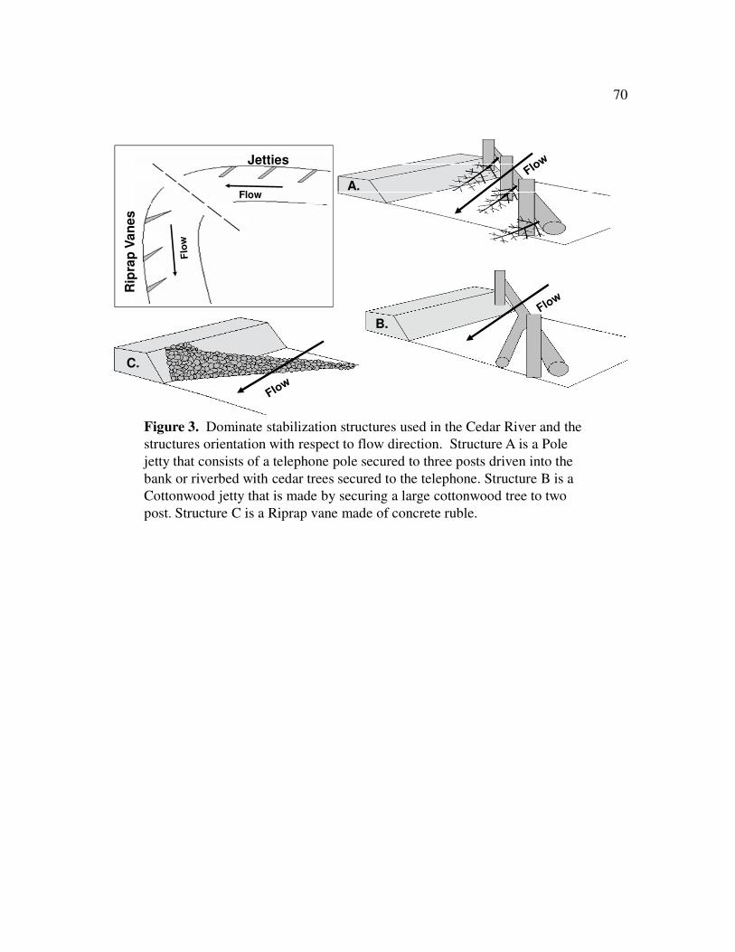
70

A.

B.

C.

Figure 3. Dominate stabilization structures used in the Cedar River and the

structures orientation with respect to flow direction. Structure A is a Pole

jetty that consists of a telephone pole secured to three posts driven into the

bank or riverbed with cedar trees secured to the telephone. Structure B is a

Cottonwood jetty that is made by securing a large cottonwood tree to two

post. Structure C is a Riprap vane made of concrete ruble.

Flow

Jetties

Rip

rap

Va

ne

s

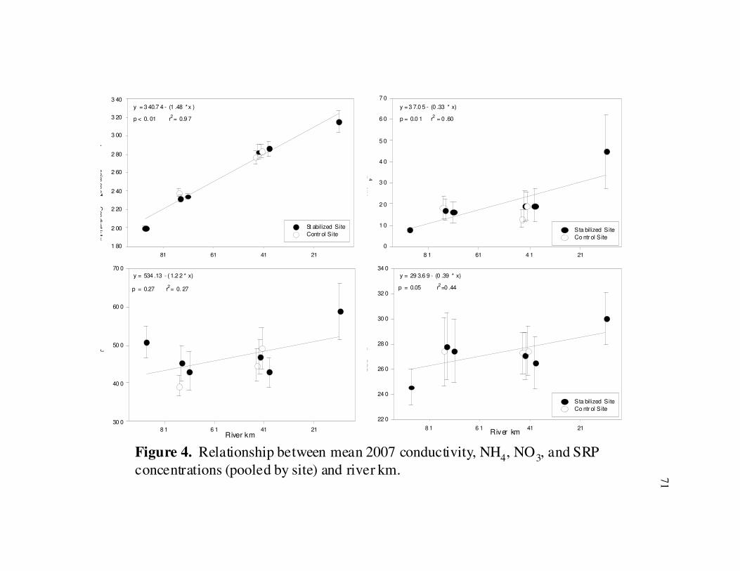
71

Figure 4. Relationship between mean 2007 conductivity, NH4, NO3, and SRP

concentrations (pooled by site) and river km.

214 1618 1

NH

4

µg

*L-1

0

1 0

2 0

3 0

4 0

5 0

6 0

7 0

p = 0.0 1

y = 3 7.0 5 - (0 .33 * x)

r2

= 0 .60

Sta bilized Site

Co ntr ol Site

21416181

Con

ductiv

ity

µseim

an

s*L

-1

1 80

2 00

2 20

2 40

2 60

2 80

3 00

3 20

3 40

St abilized Site

Contr ol Site

y = 3 40.7 4 - (1 .48 * x )

p < 0. 01 r2 = 0.9 7

River km21416 18 1

SR

P

µg

*L-1

22 0

24 0

26 0

28 0

30 0

32 0

34 0

r2=0 .44p = 0.05

y = 29 3.6 9 - (0 .39 * x)

Sta bilized Site

Co ntr ol Site

River km21416 18 1

ΝΟ

3

µg

*L

30 0

40 0

50 0

60 0

70 0

r2 = 0. 27p = 0.27

y = 534 .13 - ( 1.2 2 * x)

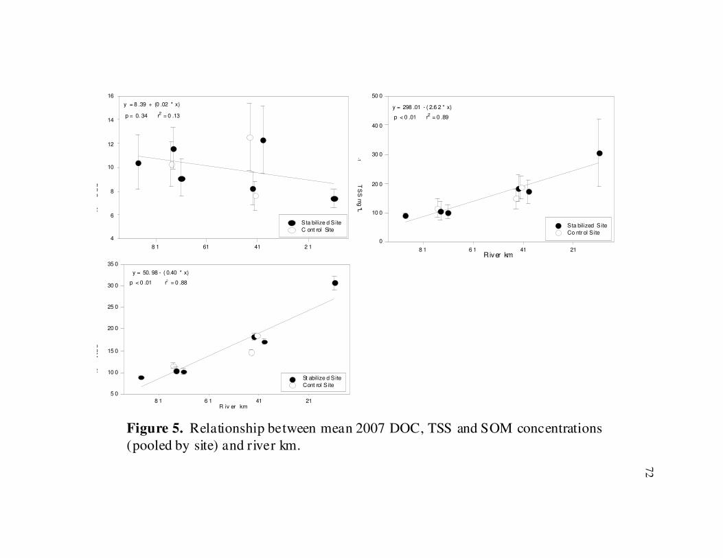
72

Figure 5. Relationship between mean 2007 DOC, TSS and SOM concentrations

(pooled by site) and river km.

2 141618 1

DO

C m

g*L

4

6

8

10

12

14

16

r2

= 0 .13p = 0. 34

y = 8 .39 + (0 .02 * x)

Sta bilize d Site

C ont rol Site

River km21416 18 1

TS

S m

g*L

-1

0

10 0

20 0

30 0

40 0

50 0

r2

= 0 .89p < 0 .01

y = 298 .01 - ( 2.6 2 * x)

Sta bilized Site

Co ntr ol Site

R iv er km21416 18 1

SO

M m

g*L

5 0

10 0

15 0

20 0

25 0

30 0

35 0

r2

= 0 .88p < 0 .01

y = 50. 98 - ( 0.40 * x)

St abilize d Site

Cont rol Site

73

Figure 4. Relationship between mean 2007 conductivity, NH4, NO3, and SRP

concentrations (pooled by site) and river km.

214 1618 1

NH

4

µg

*L-1

0

1 0

2 0

3 0

4 0

5 0

6 0

7 0

p = 0.0 1

y = 3 7.0 5 - (0 .33 * x)

r2

= 0 .60

Sta bilized Site

Co ntr ol Site

21416181

Con

ductiv

ity

µseim

an

s*L

-1

1 80

2 00

2 20

2 40

2 60

2 80

3 00

3 20

3 40

St abilized Site

Contr ol Site

y = 3 40.7 4 - (1 .48 * x )

p < 0. 01 r2 = 0.9 7

River km21416 18 1

SR

P

µg

*L-1

22 0

24 0

26 0

28 0

30 0

32 0

34 0

r2=0 .44p = 0.05

y = 29 3.6 9 - (0 .39 * x)

Sta bilized Site

Co ntr ol Site

River km21416 18 1

ΝΟ

3

µg

*L

30 0

40 0

50 0

60 0

70 0

r2 = 0. 27p = 0.27

y = 534 .13 - ( 1.2 2 * x)

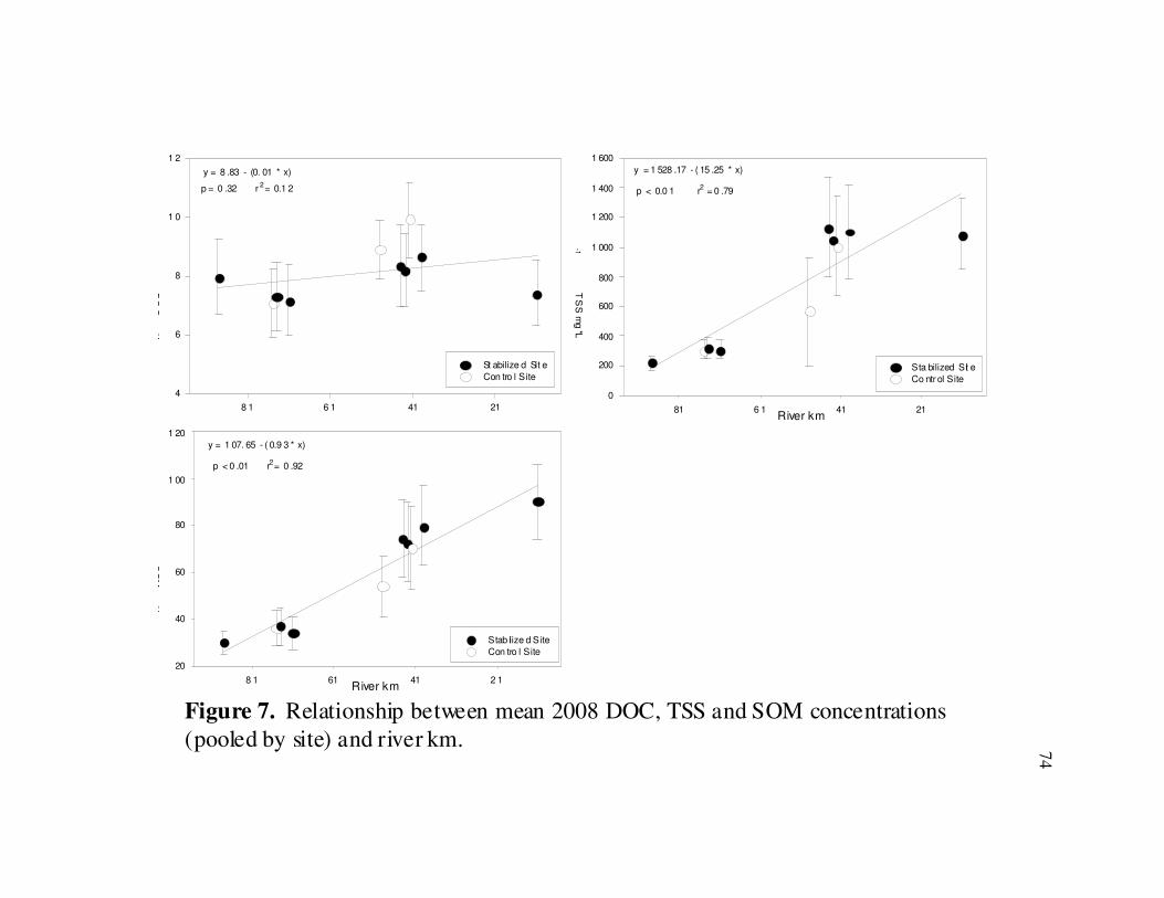
74

Figure 7. Relationship between mean 2008 DOC, TSS and SOM concentrations

(pooled by site) and river km.

21416 18 1

DO

C m

g*L

4

6

8

1 0

1 2

r2 = 0.1 2p = 0 .32

y = 8 .83 - (0. 01 * x)

St abilize d Sit e

Con tro l Site

River km21416 181

TS

S m

g*L

-1

0

200

400

600

800

1 000

1 200

1 400

1 600

r2

= 0 .79p < 0.0 1

y = 1 528 .17 - ( 15 .25 * x)

Sta bilized Sit e

Co ntr ol Site

River km2 141618 1

SO

M m

g*L

20

40

60

80

1 00

1 20

r2 = 0 .92p < 0 .01

y = 1 07. 65 - ( 0.9 3 * x)

Stab ilize d Site

Con tro l Site

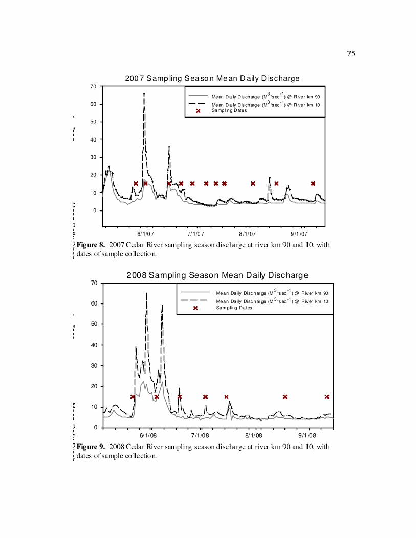
75

200 7 Samp ling Sea so n Me an D aily D ischarge

6/ 1/0 7 7/ 1/0 7 8 /1/ 07 9 /1 /07

Mea

n D

aily D

isch

arg

e M

3*s

ec

-1

0

10

20

30

40

50

60

70

Mean Dai ly D is charge (M3

*s ec-1

) @ River km 90

Mean Dai ly D is charge (M3

*s ec-1

) @ River km 10Sampling Dates

Figure 8. 2007 Cedar River sampling season discharge at river km 90 and 10, with

dates of sample collection.

2008 Sampling Season Mean Daily Discharge

6/1/08 7/1/08 8/1/08 9/1/08

Me

an

Da

ily D

isc

ha

rge

M3

*se

c-1

0

10

20

30

40

50

60

70

Mean Da i ly Disc har ge (M3

*s ec-1

) @ Riv er km 90

Mean Da i ly Disc har ge (M3

*s ec-1

) @ Riv er km 10

Sam pling Dates

Figure 9. 2008 Cedar River sampling season discharge at river km 90 and 10, with

dates of sample collection.

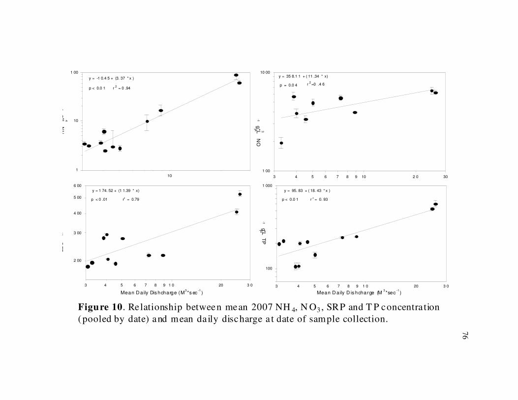
76

Figure 10. Relationship between mean 2007 NH 4, N O3 , SRP and T P concentra tion

(pooled by date) and mean daily discharge a t date of sample collection.

10

NH

4

µ g*L-1

1

10

1 00

r2 = 0 .94 p < 0.0 1

y = -1 0.4 5 + (3. 37 * x )

3 4 5 6 7 8 9 2 0 3010

NO

3

µg

*L-1

1 00

10 00

r2

=0 .4 6 p = 0.0 4

y = 35 8.1 1 + ( 11 .34 * x)

Mean D aily Dis hcharge (M3*s ec

-1)

3 4 5 6 7 8 9 20 3 01 0

SR

P

µ g*L

2 00

3 00

4 00

5 00

6 00

r2

= 0.79p < 0 .01

y = 1 74. 52 + (1 1.39 * x)

Mean D aily D is hcharge (M3*sec

-1)

3 4 5 6 7 8 9 20 3 01 0

TP

µ g*L

-1

100

1 000

r2 = 0. 93 p < 0.0 1

y = 95. 83 + ( 18. 43 * x )

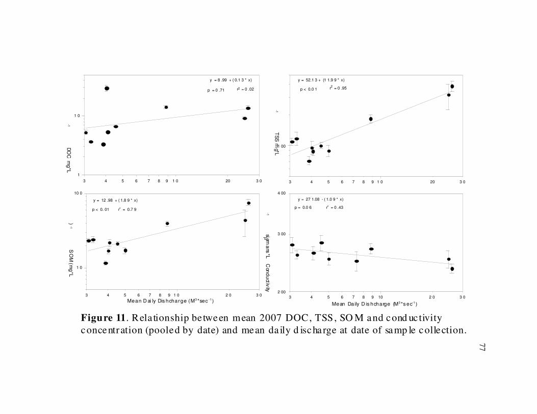
77

Figure 11. Rela tionship between mean 2007 DOC, TSS, SO M and cond uctivity

concentration (pooled by date) and mean da ily d ischarge at date of samp le collection.

3 4 5 6 7 8 9 20 3 01 0

DO

C m

g*L

-1

1

1 0

r2 = 0 .02 p = 0 .71

y = 8 .99 + ( 0.1 3 * x)

3 4 5 6 7 8 9 20 3 01 0

TS

S m

g*L-1

1 00

r2

= 0 .95 p < 0.0 1

y = 52.1 3 + (1 1.9 9 * x)

Mean D ai ly Dis hcharge (M3 *sec -1 )3 4 5 6 7 8 9 2 0 3 01 0

SO

M (m

g*L

-1)

1 0

10 0

r2 = 0.7 9 p < 0. 01

y = 12 .98 + ( 1.8 9 * x)

Mean Daily D is hcharge (M3 *s ec-1 )

3 4 5 6 7 8 9 2 0 3 010

Con

du

ctivity

µ

siema

ns*L

-1

2 00

3 00

4 00

r2

= 0 .43 p = 0.0 6

y = 27 1.08 - ( 1.0 9 * x)

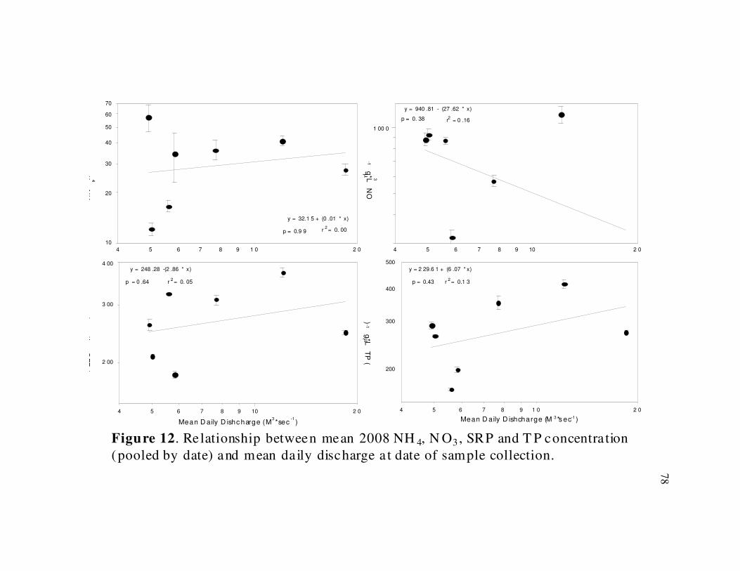
78

Figure 12. Relationship between mean 2008 NH 4, N O3 , SRP and T P concentra tion


4 5 6 7 8 9 2 01 0

NH

4

µg

*L

20

30

40

50

60

70

10

r2 = 0. 00p = 0.9 9

y = 32.1 5 + (0 .01 * x)

4 5 6 7 8 9 2 010

NO

3

µ g*L-1

1 00 0

r2

= 0 .16p = 0. 38

y = 940 .81 - (27 .62 * x)

Mean D aily D ishc harge (M3*sec

-1)

4 5 6 7 8 9 2 010

SR

P (

µg

*L)

2 00

3 00

4 00

r2 = 0. 05p = 0 .64

y = 248 .28 -(2 .86 * x)

Mean D aily D ishcharge (M 3 *s ec-1)

4 5 6 7 8 9 2 01 0

TP

(µ

g*L

-1)

200

300

400

500

r2 = 0.1 3p = 0.43

y = 2 29.6 1 + (6 .07 * x)

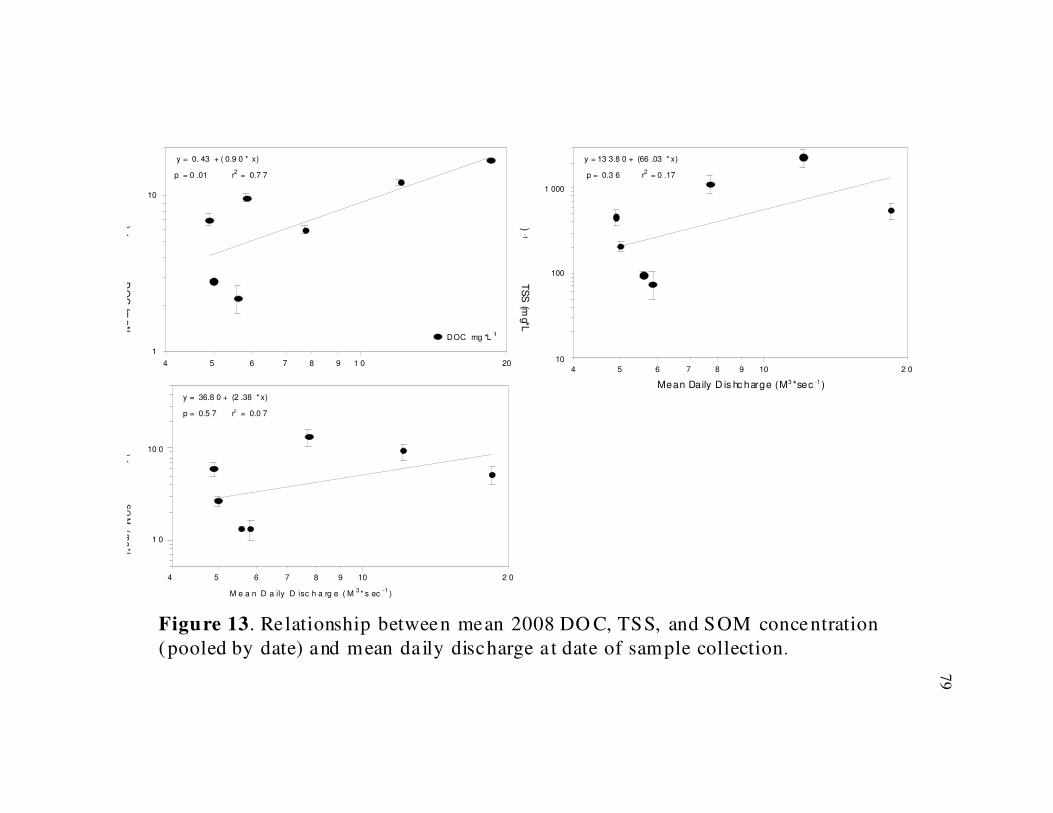
79

Figure 13. Relationship between mean 2008 DO C, TSS, and SOM concentration


4 5 6 7 8 9 201 0

DO

C (m

g*L

-1)

1

10

DOC mg *L-1

r2 = 0.7 7p = 0 .01

y = 0. 43 + ( 0.9 0 * x)

Mean Daily D is hc harge (M3 *sec -1 )

4 5 6 7 8 9 2 010

TS

S (m

g*L-1

)

10

100

1 000

r2

= 0 .17p = 0.3 6

y = 13 3.8 0 + (66 .03 * x)

M e a n D a ily D isc h a rg e ( M3* s ec

-1)

4 5 6 7 8 9 2 010

SO

M (m

g*L

-1)

1 0

10 0

r2 = 0.0 7p = 0.5 7

y = 36.8 0 + (2 .38 * x)

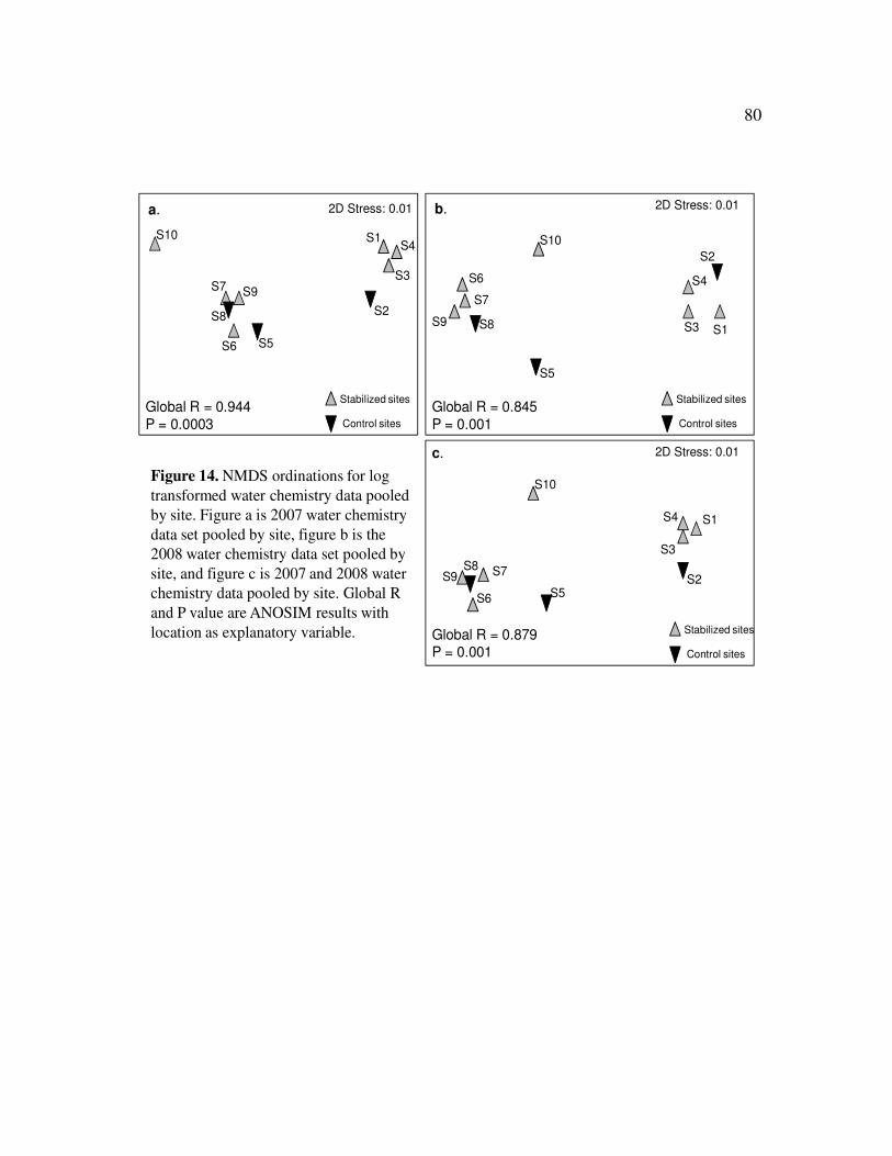
80

2D Stress: 0.01

S1S4

S3

S2S8

S7 S9

S6 S5

S10

Global R = 0.944

P = 0.0003 Control sites

Stabilized sites

a. b. 2D Stress: 0.01

Global R = 0.845

P = 0.001

S10

S7

S9

S6

S5

S8 S1

S4

S3

S2

Control sites

Stabilized sites

c. 2D Stress: 0.01

Global R = 0.879P = 0.001 Control sites

Stabilized sites

S7S9

S6 S5

S8

S10

S1S4

S3

S2

Figure 14. NMDS ordinations for log

transformed water chemistry data pooled

by site. Figure a is 2007 water chemistry

data set pooled by site, figure b is the

2008 water chemistry data set pooled by

site, and figure c is 2007 and 2008 water

chemistry data pooled by site. Global R

and P value are ANOSIM results with

location as explanatory variable.

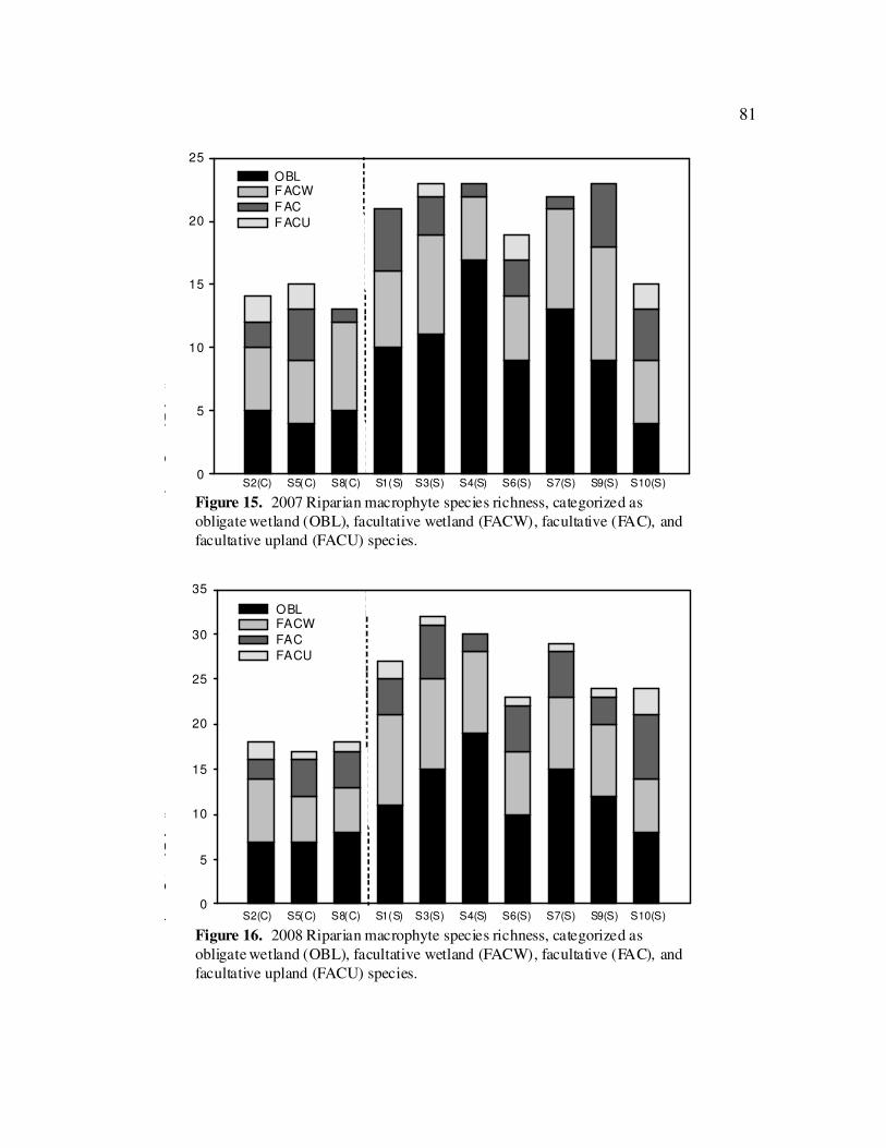
81

2008 Riparian macrophyte

# o

f Pla

nt S

pe

cie

s

0

5

10

15

20

25

30

35

OBLFACW

FAC

FACU

Figure 16. 2008 Riparian macrophyte species richness, categorized as

obligate wetland (OBL), facultative wetland (FACW), facultative (FAC), and

facultative upland (FACU) species.

S2(C) S5(C) S8(C) S1(S) S3(S) S4(S) S6(S) S7(S) S9(S) S10(S)

2007 Riparian macrophytes

# o

f Pla

nt S

pe

cie

s

0

5

10

15

20

25

OBLFACW

FAC

FACU

Figure 15. 2007 Riparian macrophyte species richness, categorized as

obligate wetland (OBL), facultative wetland (FACW), facultative (FAC), and

facultative upland (FACU) species.

S2(C) S5(C) S8(C) S1(S) S3(S) S4(S) S6(S) S7(S) S9(S) S10(S)

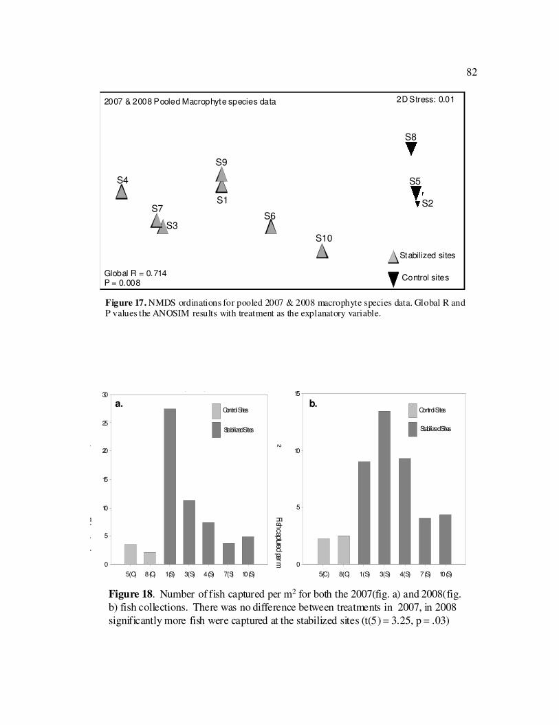
82

2007 & 2008 Pooled Macrophyte species data 2D Stress: 0.01

Global R = 0.714P = 0.008

Control sites

Stabilized sites

S6S3

S1S7

S9

S4

S8

S2

S10

S5

Figure 17. NMDS ordinations for pooled 2007 & 2008 macrophyte species data. Global R and P values the ANOSIM results with treatment as the explanatory variable.

sdfg

2007 Fish captured per m2

5 (C) 8 (C) 1 (S) 3 (S) 4 (S) 7 (S) 10 (S)

Fish captured per m2

0

5

10

15

20

25

30

Control Sites

Stabilized Sites

2008 Fish captured per m2

5 (C) 8 (C) 1 (S) 3 (S) 4 (S) 7 (S) 10 (S)

Fish captured per m2

0

5

10

15

Control Sites

Stabilized Sites

Figure 18. Number of fish captured per m2 for both the 2007(fig. a) and 2008(fig.

b) fish collections. There was no difference between treatments in 2007, in 2008

significantly more fish were captured at the stabilized sites (t(5) = 3.25, p = .03)

a. b.

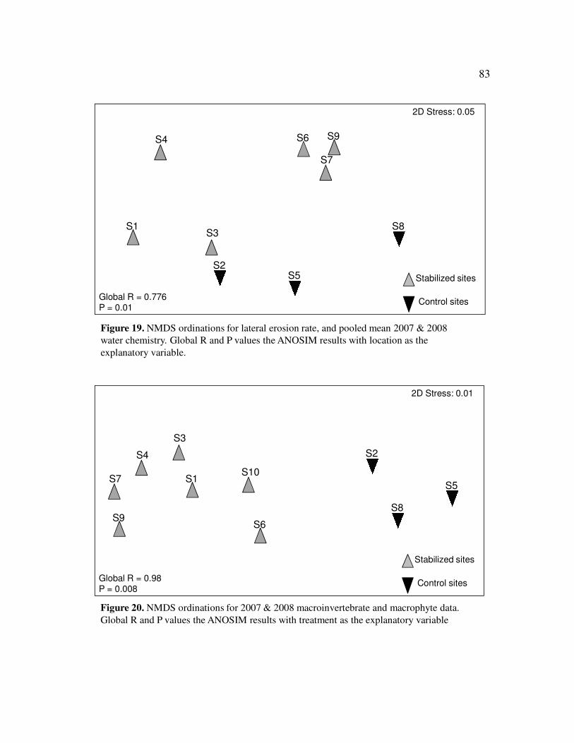
83

2D Stress: 0.05

Global R = 0.776P = 0.01

Control sites

Stabilized sites

S6

S3S1

S7

S9S4

S8

S2S5

Figure 19. NMDS ordinations for lateral erosion rate, and pooled mean 2007 & 2008

water chemistry. Global R and P values the ANOSIM results with location as the

explanatory variable.

2D Stress: 0.01

Global R = 0.98P = 0.008

Control sites

Stabilized sites

S6

S3

S1S7

S9

S4

S8

S2

S10

S5

Figure 20. NMDS ordinations for 2007 & 2008 macroinvertebrate and macrophyte data.

Global R and P values the ANOSIM results with treatment as the explanatory variable

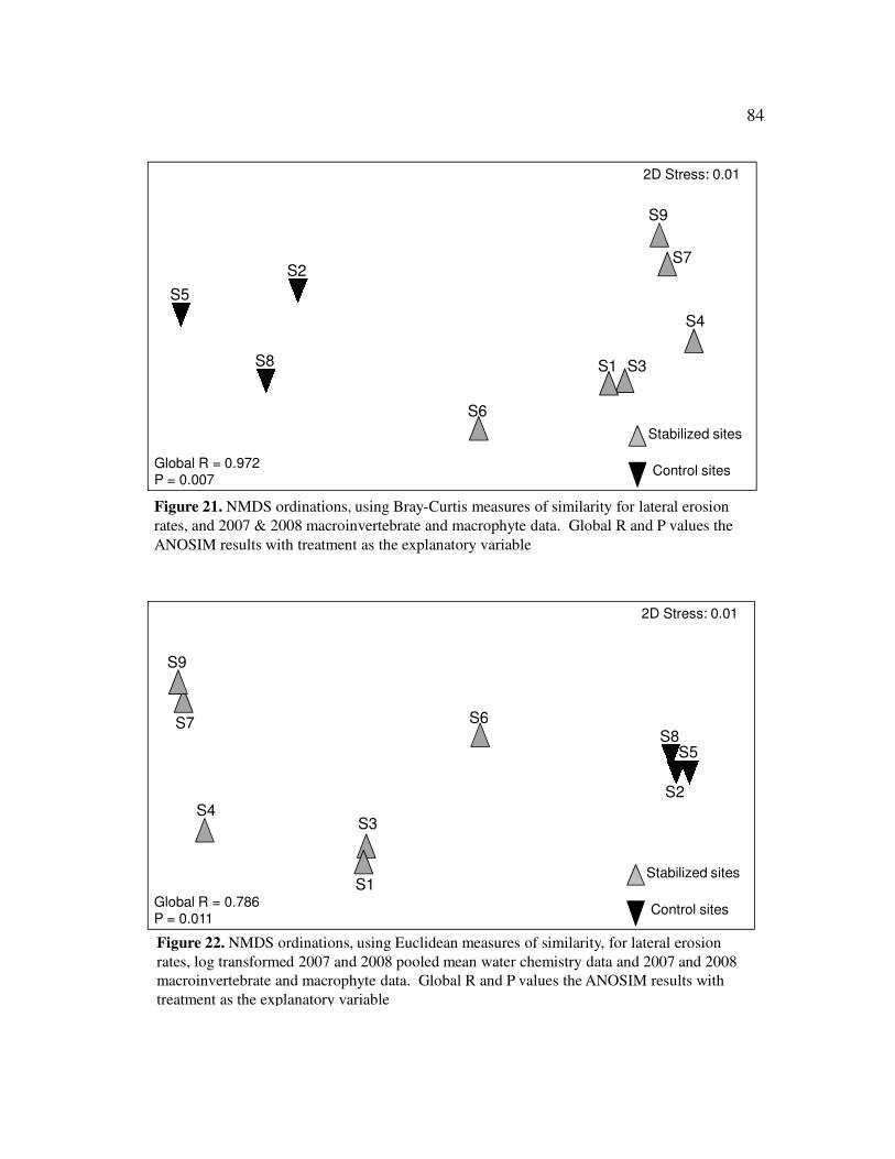
84

2D Stress: 0.01

Global R = 0.972P = 0.007

Control sites

Stabilized sites

S6

S3S1

S7

S9

S4

S8

S2

S5

Figure 21. NMDS ordinations, using Bray-Curtis measures of similarity for lateral erosion

rates, and 2007 & 2008 macroinvertebrate and macrophyte data. Global R and P values the

ANOSIM results with treatment as the explanatory variable

2D Stress: 0.01

Global R = 0.786P = 0.011

Control sites

Stabilized sites

S6

S3

S1

S7

S9

S4

S8

S2

S5

Figure 22. NMDS ordinations, using Euclidean measures of similarity, for lateral erosion

rates, log transformed 2007 and 2008 pooled mean water chemistry data and 2007 and 2008

macroinvertebrate and macrophyte data. Global R and P values the ANOSIM results with

treatment as the explanatory variable

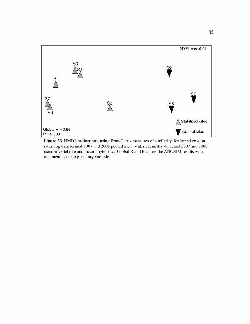
85

2D Stress: 0.01

Global R = 0.96P = 0.008

Control sites

Stabilized sites

S6

S3

S1

S7

S9

S4

S8

S2

S5

Figure 23. NMDS ordinations, using Bray-Curtis measures of similarity, for lateral erosion

rates, log transformed 2007 and 2008 pooled mean water chemistry data, and 2007 and 2008

macroinvertebrate and macrophyte data. Global R and P values the ANOSIM results with

treatment as the explanatory variable

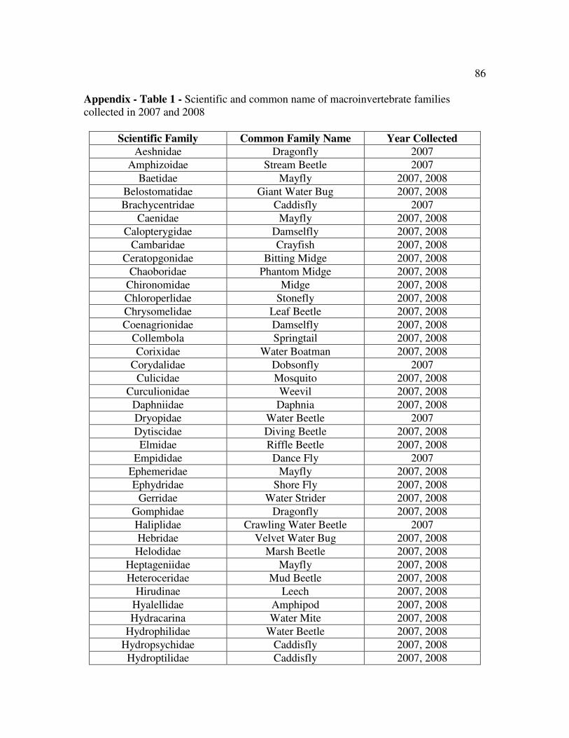
86

Appendix - Table 1 - Scientific and common name of macroinvertebrate families

collected in 2007 and 2008

Scientific Family Common Family Name Year Collected

Aeshnidae Dragonfly 2007

Amphizoidae Stream Beetle 2007

Baetidae Mayfly 2007, 2008

Belostomatidae Giant Water Bug 2007, 2008

Brachycentridae Caddisfly 2007

Caenidae Mayfly 2007, 2008

Calopterygidae Damselfly 2007, 2008

Cambaridae Crayfish 2007, 2008

Ceratopgonidae Bitting Midge 2007, 2008

Chaoboridae Phantom Midge 2007, 2008

Chironomidae Midge 2007, 2008

Chloroperlidae Stonefly 2007, 2008

Chrysomelidae Leaf Beetle 2007, 2008

Coenagrionidae Damselfly 2007, 2008

Collembola Springtail 2007, 2008

Corixidae Water Boatman 2007, 2008

Corydalidae Dobsonfly 2007

Culicidae Mosquito 2007, 2008

Curculionidae Weevil 2007, 2008

Daphniidae Daphnia 2007, 2008

Dryopidae Water Beetle 2007

Dytiscidae Diving Beetle 2007, 2008

Elmidae Riffle Beetle 2007, 2008

Empididae Dance Fly 2007

Ephemeridae Mayfly 2007, 2008

Ephydridae Shore Fly 2007, 2008

Gerridae Water Strider 2007, 2008

Gomphidae Dragonfly 2007, 2008

Haliplidae Crawling Water Beetle 2007

Hebridae Velvet Water Bug 2007, 2008

Helodidae Marsh Beetle 2007, 2008

Heptageniidae Mayfly 2007, 2008

Heteroceridae Mud Beetle 2007, 2008

Hirudinae Leech 2007, 2008

Hyalellidae Amphipod 2007, 2008

Hydracarina Water Mite 2007, 2008

Hydrophilidae Water Beetle 2007, 2008

Hydropsychidae Caddisfly 2007, 2008

Hydroptilidae Caddisfly 2007, 2008

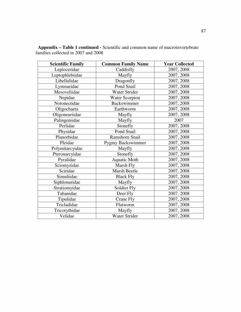
87

Appendix – Table 1 continued - Scientific and common name of macroinvertebrate

families collected in 2007 and 2008


Leptoceridae Caddisfly 2007, 2008

Leptophlebiidae Mayfly 2007, 2008

Libellulidae Dragonfly 2007, 2008

Lymnaeidae Pond Snail 2007, 2008

Mesoveliidae Water Strider 2007, 2008

Nepidae Water Scorpion 2007, 2008

Notonectidae Backswimmer 2007, 2008

Oligochaeta Earthworm 2007, 2008

Oligoneuriidae Mayfly 2007, 2008

Palingeniidae Mayfly 2007

Perlidae Stonefly 2007, 2008

Physidae Pond Snail 2007, 2008

Planorbidae Ramshorn Snail 2007, 2008

Pleidae Pygmy Backswimmer 2007, 2008

Polymitarcyidae Mayfly 2007, 2008

Pteronarcyidae Stonefly 2007, 2008

Pyralidae Aquatic Moth 2007, 2008

Sciomyzidae Marsh Fly 2007, 2008

Sciridae Marsh Beetle 2007, 2008

Simuliidae Black Fly 2007, 2008

Siphlonuridae Mayfly 2007, 2008

Stratiomyidae Soldier Fly 2007, 2008

Tabanidae Deer Fly 2007, 2008

Tipulidae Crane Fly 2007, 2008

Tricladidae Flatworm 2007, 2008

Tricorythidae Mayfly 2007, 2008

Velidae Water Strider 2007, 2008

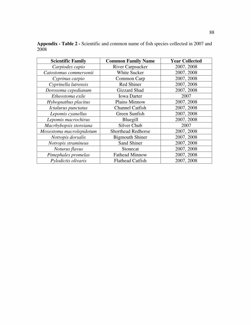
88

Appendix - Table 2 - Scientific and common name of fish species collected in 2007 and

2008


Carpiodes capio River Carpsucker 2007, 2008

Catostomus commersonii White Sucker 2007, 2008

Cyprinus carpio Common Carp 2007, 2008

Cyprinella lutrensis Red Shiner 2007, 2008

Dorosoma cepedianum Gizzard Shad 2007, 2008

Etheostoma exile Iowa Darter 2007

Hybognathus placitus Plains Minnow 2007, 2008

Ictalurus punctatus Channel Catfish 2007, 2008

Lepomis cyanellus Green Sunfish 2007, 2008

Lepomis macrochirus Bluegill 2007, 2008

Macrhybopsis storeiana Silver Chub 2007

Moxostoma macrolepidotum Shorthead Redhorse 2007, 2008

Notropis dorsalis Bigmouth Shiner 2007, 2008

Notropis stramineus Sand Shiner 2007, 2008

Noturus flavus Stonecat 2007, 2008

Pimephales promelas Fathead Minnow 2007, 2008

Pylodictis olivaris Flathead Catfish 2007, 2008

Documents

Ecological Impacts of Stream Bank Stabilization in a Great Plains River