Embed Size (px)
Citation preview

Ecologically sustainable development of the regional marine and estuarine resources of NSW: Modelling of the NSW continental shelf ecosystem CSIRO Wealth from Oceans Flagship: Marie Savina, Beth Fulton, Scott Condie University of British Columbia: Robyn Forrest NSW Department of Primary Industries James Scandol, Karen Astles, Philip Gibbs March 2009
i

Ecologically sustainable development of the regional marine and estuarine resources of NSW: Modelling of the NSW continental shelf ecosystem CSIRO Wealth from Oceans Flagship: Marie Savina, Beth Fulton, Scott Condie University of British Columbia: Robyn Forrest NSW Department of Primary Industries James Scandol, Karen Astles, Philip Gibbs March 2009
ii

Enquiries should be addressed to:
Scott Condie CSIRO Wealth from Oceans Flagship GPO Box 1538, Hobart, TAS 7000 Ph. 03 6232 5025 [email protected] Distribution list
Project Manager √
On-line approval to publish
Client √
Authors √
Other CSIRO Staff
National Library
State Library
CMAR Library as pdf (Meredith Hepburn)
√
CMAR Web Manager as pdf (Diana Reale)
Important Notice
© Copyright Commonwealth Scientific and Industrial Research Organisation (‘CSIRO’) Australia 2005
All rights are reserved and no part of this publication covered by copyright may be reproduced or copied in any form or by any means except with the written permission of CSIRO.
The results and analyses contained in this Report are based on a number of technical, circumstantial or otherwise specified assumptions and parameters. The user must make its own assessment of the suitability for its use of the information or material contained in or generated from the Report. To the extent permitted by law, CSIRO excludes all liability to any party for expenses, losses, damages and costs arising directly or indirectly from using this Report.
Use of this Report
The use of this Report is subject to the terms on which it was prepared by CSIRO. In particular, the Report may only be used for the following purposes.
this Report may be copied for distribution within the Client’s organisation;
the information in this Report may be used by the entity for which it was prepared (“the Client”), or by the Client’s contractors and agents, for the Client’s internal business operations (but not licensing to third parties);
extracts of the Report distributed for these purposes must clearly note that the extract is part of a larger Report prepared by CSIRO for the Client.
The Report must not be used as a means of endorsement without the prior written consent of CSIRO.
The name, trade mark or logo of CSIRO must not be used without the prior written consent of CSIRO.
iii

iv

CONTENTS
EXECUTIVE SUMMARY ................................................................................... 1
1. INTRODUCTION ....................................................................................... 3
1.1 Marine resource issues in NSW..................................................... 3
1.2 Objectives of the study................................................................... 3
1.3 Approach ......................................................................................... 4
1.4 Focus systems ................................................................................ 5
2. MODELLING FRAMEWORK .................................................................... 7
2.1 Spatial and temporal representation ............................................. 7
2.2 Ecosystem model............................................................................ 8 Physical and chemical components ...............................................8 Biological components....................................................................9
2.3 Human sector models................................................................... 10 Pollution........................................................................................10 Fishing ..........................................................................................10 Habitat modification ......................................................................11 Exotic species introductions .........................................................12 Climate change.............................................................................12
2.4 Sampling and assessment model................................................ 12
2.5 Management model....................................................................... 12
2.6 Model outputs................................................................................ 13
3. MODEL IMPLEMENTATION................................................................... 14
3.1 Spatial and temporal representation ........................................... 14
3.2 Ecosystem model.......................................................................... 16 3.2.1 Physical and chemical components .........................................16 3.2.2 Biological components ..............................................................17
Nutrients .......................................................................................19 Detritus .........................................................................................19 Plants............................................................................................19 Bacteria ........................................................................................19 Invertebrates.................................................................................19 Vertebrates ...................................................................................21
3.3 Model scenarios ............................................................................ 25 3.3.1 Fisheries scenarios ....................................................................26
v

vi
3.3.2 Marine reserve scenarios .......................................................... 27
4. MODEL RESULTS .................................................................................. 29
4.1 Calibration of historic simulations............................................... 29
4.2 Historical changes in ecosystem structure ................................ 32
4.3 Impacts of harvest strategies....................................................... 32
4.4 Impacts of marine parks ............................................................... 38 Comparing the pre-existing and expanded reserve systems ....... 38 Effects of redistributing catch displaced by reserves ................... 43
5. CONCLUSIONS ...................................................................................... 46
ACKNOWLEDGEMENTS................................................................................ 47
6. REFERENCES ........................................................................................ 48
APPENDIX A – DESCRIPTION OF BONY FISH GROUPS ............................ 50 Shallow demersal herbivorous fish (FDE) .................................... 50 Shallow demersal territorial fish (FDP)......................................... 50 Shallow demersal omnivorous fish (FDS) .................................... 51 Shallow pelagic small planktivorous fish (FPS)............................ 51 Shallow pelagic large planktivorous fish (FPL) ............................ 52 Shallow pelagic piscivorous fish (FVS) ........................................ 52 Deep demersal fish (FDD)............................................................ 53 Oceanic piscivorous fish (FVT) .................................................... 53 Oceanic planktivorous fish (FVD)................................................. 54 Migratory and non-migratory mesopelagics (FMM/FMN)............. 54
APPENDIX B – DESCRIPTION OF COMMERCIAL DEEP-WATER FISH SPECIES ................................................................................................. 56
Eastern Gemfish (Rexea solandri- FVV) ...................................... 56 Morwongs (Nemadactylus sp – FPO) .......................................... 56 Warehous and Trevalla (FDF)...................................................... 57 Blue Grenadier (Macruronus novaezelandiae - FBP) .................. 57 Pink Ling (Genypterus blacodes - FDC)....................................... 58 Redfish (Centroberyx affinis - FDM)............................................. 58 Eastern School whiting (Sillago flindersi – FVO).......................... 59
APPENDIX C – DESCRIPTION OF SHARK AND RAY GROUPS.................. 60 Pelagic sharks (SHP) ................................................................... 60 Demersal sharks (SHD) ............................................................... 60 Skates and Rays (SSK)................................................................ 61 Dogsharks (SHB) ......................................................................... 61 Spiky dogshark (Squalus megalops – SHC) ................................ 62 Grey nurse shark (Carcharias taurus) .......................................... 62

EXECUTIVE SUMMARY
This report describes results from a modelling study of the NSW marine ecosystem and its associated resources. It forms part of a broader collaborative study between CSIRO and the NSW Department of Primary Industries on ecologically sustainable development of the regional marine and estuarine resources of NSW.
This component of the study aimed to develop tools that could help address issues emerging along the NSW coast, particularly related to the ecological impacts of fisheries and the potential role of specific harvest strategies or conservation strategies. The tool that was adopted for these purposes was the Atlantis model incorporating: (i) a deterministic ecosystem model incorporating physical, biogeochemical, and higher
trophic level components and processes; (ii) a deterministic sector model that emulates the effects of fisheries and other human
activities on the ecosystem; (iii) a sampling model that collects data from the ecosystem and sector models and calculates
indicators; and (iv) a management model that regulates the sector model.
The Atlantis model was implemented as a series of interconnected polygonal boxes extending from the NSW coastline offshore to the upper continental slope. The box structure was designed to reflect the biogeographical distributions of the region, as well as coastal characteristics such geomorphology, major rivers and bays, and human land-uses. The model was also resolved into a series of vertical layers to account for depth zonation. Physical exchanges between boxes were estimated from oceanographic model results.
The model calculated the distributions of various forms of nutrients and detritus over time, as well as the biomasses of 54 biological groups. These groups included plants, bacteria, invertebrates, finfish, sharks, marine mammals and birds. While most were broad functional groups, a significant number of commercial fish were represented at the level of individual species.
The main conclusions from the model runs were: (i) The Ocean Trawl Fishery is already fully exploited. (ii) Reduced fishing would allow a significant proportion of overfished predatory groups to
recover with an accompanying decline in their prey (e.g. forage groups and juveniles). (iii) Fishing levels seen in the 1970s and 1980s achieved biodiversity levels (of the groups
represented in the model) that are equal to or better than other harvest strategies (a result that can be understood in terms of the intermediate disturbance hypothesis).
(iv) Marine reserves have a very positive impact on sharks and rays and a mainly negative impact on their prey groups. Shallow demersals and their prey can be impacted positively or negatively depending on whether fishing effort previously in the reserve areas is removed (e.g. buy-outs) or displaced to neighbouring areas.
(v) Marine reserves cause a decline in the biodiversity of the groups represented in the model irrespective of whether historical fishing effort is entirely removed (low disturbance) or redistributed into neighbouring areas outside the reserve (leading to excessive disturbance).
It is envisioned that the model will continue be used to support management of the NSW coastal and shelf system through scenario exploration and management strategy evaluation.
1

2

1. INTRODUCTION
In 2004 the NSW Department of Primary Industries sought assistance from CSIRO in developing and evaluating a range of tools to assist with implementation of ecosystem management for their aquatic resources. The specific aim was to assess the likely performance of existing and proposed managerial and institutional arrangements for future scenarios of the development of coastal NSW. A five-year collaborative project between NSW DPI and CSIRO was officially launched at Darling Harbour on the 22nd August 2004, with work beginning in the following July. This report summarises results from one component of the study focusing on the NSW continental shelf ecosystem and associated fisheries.
1.1 Marine resource issues in NSW
There are a range of issues emerging along the NSW coast that are associated with management of fisheries and conservation initiatives. Examples include:
– Impacts on marine biota and habitats from multi-sector and multi-species commercial fisheries and recreational angling, including non-sustainable harvesting, bycatch, seafloor disturbance, and translocation of aquatic pests.
– Impacts of the incremental establishment of a system of marine reserves, fishing closures, and other conservation measures.
There is also significant potential for these impacts to interact and potentially lead to unforseen consequences.
1.2 Objectives of the study
The high level objectives of the study are to:
(i) Identify key management issues, potential management strategies, likely development scenarios, and modelling frameworks for a study of multiple-use management of NSW coastal environments.
(ii) Develop and apply models of the ecosystem and human activities for selected NSW coastal systems within a framework suitable for evaluating management strategies across a range of sectors.
(iii) Design and evaluate potential monitoring programs for these systems to underpin ecosystem-based management.
(iv) Collect baseline data for a set of agreed socio-economic and environmental indicators within these systems to support the implementation of changed management strategies.
(v) Develop communication tools to support engagement of key stakeholders and uptake of project outcomes.
This is the first report from the study and focuses on the first three of these objectives as applied to the NSW continental shelf.
3

1.3 Approach
The nature of the issues listed in Section 1.1 underlines the strong need for integrated ecosystem-based management. This is likely to be the dominant national and international model of natural resource management within ten years. It involves the application of a range of management strategies that aim to maintain the structure and function of ecosystems, whilst recognising the human use and values of ecosystems. Ecosystem-based management is not a single management strategy, but a collection of integrated policies that give primary regard to the ecosystems that sustain industries.
The current initiative builds on management strategy evaluation (MSE) techniques developed for fisheries around Australia and other parts of the world since the 1980s and recently extended to address a wider range of human uses on the North West Shelf off Western Australia (Fulton et al. 2006, Little et al. 2006). MSE is a simulation based framework that can be used to test, compare and evaluate the outcomes of management strategies against defined performance measures derived from the objectives of management. It explicitly includes uncertainty in the dynamics of the ecosystem or socio-economic system, the effects of human uses or activities, and the implementation of monitoring and management measures. This is achieved by running ensemble simulations covering the range of model structures and model parameter values consistent with current understanding of the system. Such an approach can reveal the robustness of existing or proposed strategies to deliver management objectives despite recognised uncertainties.
MSE techniques attempt to close the adaptive management loop as depicted in figure 1.3.1. This requires explicitly modelling of the following elements:
– the natural ecosystem and human activities;
– our ability to observe these systems and make management decisions on the basis of these observations; and
– responses of users of the system to the changes in management and changes in the state of the system.
Details of the modelling framework will be presented in Section 2 of this report.
The desired outcomes of the MSE approach are:
– predicted ranges of ecosystem and human responses to management strategies;
– associated trade-offs in the values associated with such systems; and
– identification of robust observational and management strategies capable of achieving objectives associated with ecologically sustainable development.
The results of the current study will demonstrate these outcomes in the contexts of both
fisheries and conservation.
4
Sectors
impacts
Ecosystem regulation
Sampling & assessment
Management
Figure 1.3.1: Model components for evaluating management strategies in aquatic environments exposed to multiple human uses.
1.4 Focus systems
The models being developed in the study can be applied to a diversity of aquatic systems functioning across a range of scales. Selection of systems for detailed study has been largely determined by the management needs of NSW agencies, with an initial focus on fisheries related issues.
The first model has been developed for the entire NSW continental shelf and slope. It is designed to both address larger scale issues and provide the context for other more geographically focused models, such as that being developed for the Clarence River Estuary. The large spatial coverage of such a model is essential when considering processes that span such scales, such as ocean currents and eddies (figure 1.4.1), migration of marine populations, and regionally coordinated management of fisheries (figure 1.4.2).
Issues that have been addressed within the NSW coastal seas model include:
– the impacts of historical and future fisheries management and practices; and
– the effectiveness of marine reserves in maintaining the health of the broader shelf ecosystem.
5

Figure 1.4.1: Examples of satellite sea surface temperature off northern NSW from 13-12-2002 (left) and satellite chlorophyll estimates (SeaWiFS) off southern NSW from 12-12-1997 (right). Both reveal the complex eddy structures generated by the East Australian Current in this region.
Figure 1.4.2: Ocean trawler operating off northern NSW (photograph byJonathan Rhodes, CSIRO).
6

2. MODELLING FRAMEWORK
CSIRO has developed technically advanced and conceptually powerful modelling frameworks that capture the intricacies of multiple-use natural resource management. These models range from qualitative conceptual frameworks through to fully quantitative models that resolve key processes both temporally and spatially. They enable representation of physical, biological, ecological, economic, social and institutional processes. For this project, an MSE approach to the NSW coastal environment is being developed within the Atlantis modelling framework (Fulton et al. 2004) that evolved from earlier spatially-resolved biogeochemical models (Murray and Parslow 1999).
The Atlantis modelling framework incorporates four major components:
– a deterministic ecosystem model incorporating physical, biogeochemical, and higher trophic level components and processes;
– a deterministic sector model that emulates the effects of fisheries and other human activities on the ecosystem;
– a sampling model that collects data from the ecosystem and sector models and calculates indicators; and
– a management model that regulates the sector model.
These components correspond to those depicted in figure 1.3.1, which also indicates how they are linked through both information flow and biophysical interactions.
2.1 Spatial and temporal representation
Atlantis is a box model, meaning that all model variables are computed within a finite number of horizontally layered polygonal boxes with horizontal and vertical exchanges between adjoining boxes. It supports arbitrary spatial and temporal scales, although in practice the number of boxes and the model time-step are limited by the available computing capacity.
The model uses a polygonal spatial grid in the horizontal and a series of layers in the vertical. The design of the spatial structure of the model is based on a wide range of considerations, but typically includes the geometry of the water body and the distributions of:
– habitats (benthic and pelagic);
– organisms (species, populations and communities);
– physical processes (e.g. current patterns, water masses, tidal exchanges); and
– human influences (e.g. resource utilisation, contaminant inputs, management zones).
Coarse resolution models have previously been developed for the entire Commonwealth South East Fishery (Fulton et al. 2004, Fulton and Smith 2004) and where appropriate the models developed for NSW will be nested within this larger-scale framework (figure 2.1.1).
The temporal resolution of any model is largely determined by the types of processes that need to be represented. For example, within the oceanic realm, a model time-step of a few days is
7

adequate to capture the evolving influences of synoptic weather systems, ocean eddies and coastally trapped waves. However, if say diurnal migration of micronekton were a key process that needed to be explicitly represented in the model, then a time-step of half a day might be required. In estuarine systems, tidal flushing needs to be represented and many key biogeochemical processes also operate on timescales of a day or less.
The timeframe over which the models are run is determined mostly by the issues being addressed, particularly with respect to changes in sectoral activities and associated ecosystem responses. The longest period that will be considered in this study is 1950 to 2030, which captures the historical period of rapid regional development and environmental change in NSW, as well as a manageable projection period of interest to policy makers.
0
150 50
250
700
1800
Figure 2.1.1: Horizontal and indicative vertical spatial structure for the South East Fishery model (Fulton et al. 2004, 2007) into which finer-scale models will be nested for regions of NSW.
2.2 Ecosystem model
The ecosystem model is a nutrient-based (i.e. biomass units of mg N m-3) biogeochemical model that includes physical forcing, biogeochemical cycling, trophic interactions, and human influences on the ecosystem.
Physical and chemical components
The physical component of the model replicates spatial exchanges of material (dissolved or particulate) between boxes as a result of oceanic or estuarine flows. Time series of exchange fluxes are estimated and stored prior to running other model components. These can be computed directly from three-dimensional flow fields, such as those generated by ocean circulation models, or from stream-flow data often measured in rivers and estuaries or generated by catchment models. Local or diffuse inflows entering from outside the model domain can also be represented by one or more point source time-series.
Water temperature and salinity can be specified directly or allowed to vary dynamically in response to water exchanges (i.e. advection and mixing), solar irradiance, heat exchange
8

through the air-water interface, or precipitation and evaporation. The physical properties of the seabed, such as porosity, can also evolve through resuspension and deposition of sediments.
Chemical forcing may include nutrient inputs from point sources, and atmospheric deposition of dissolved inorganic nitrogen (DIN). In regions of the model where the deepest water column boxes contact the seafloor, a sediment chemistry submodel can calculate nutrient remineralisation and oxygen exchange. Where model boxes do not extend to the seafloor, the base of the deepest box is treated as an open boundary with no epibenthic or sediment layers.
Biological components
The biologically relevant components of Atlantis include various classes of:
– nutrients (nitrogen, silica);
– detritus (labile, refractory, carrion);
– primary producers;
– bacteria;
– invertebrates; and
– vertebrates (fish, mammals and birds).
Multiple functional groups can be defined within each of these components. The selection of groups is largely determined by the need to capture key ecosystem functional characteristics (taxonomy, size, turnover rate, shared predators and prey) while also addressing identified management issues (commercial and conservation related). Grouping organisms with vastly different characteristics usually leads to erroneous model system dynamics. Typically, higher trophic levels are better resolved than lower trophic levels, with a small number of key species potentially being explicitly represented. While other functional groups are typically treated as aggregated biomass pools, vertebrate groups are represented as numbers of individuals. Vertebrate groups and some invertebrate groups can be further resolved into age-structures to capture behavioural differences.
Functional groups are linked through trophic interactions and are also influenced by environmental and habitat conditions in the water column and bottom sediments. The main biological processes that can be explicitly represented in the model are:
– consumption and growth;
– waste production and decomposition;
– reproduction;
– habitat dependency (preferences and refuges);
– movements and large-scale migrations;
– bioturbation and bioirrigation;
– predation and other forms of natural mortality such as disease.
The key biological information needs of the model are summarised in Table 2.2.1.
9

Table 2.2.1: Summary of key biological information.
Primary producers
Benthic invertebrates
Planktonic invertebrates
Nektonic invertebrates
Vertebrates
Period of activity √ √ √ √ Habitat dependency √ √ √ √ √ Distributions and abundances
√ √ √ √ √
Swimming speeds √ Migration times, routes, participation
√ √ √
Diets √ √ √ √ Growth rates √ √ √ √ √ Length-weight relationships
√
Mortality rates √ √ √ √ √ Maximum age √ Age at maturity √ Spawning area, season √ √ √ Larval or gestation period
√ √
Location of recruits √ Number of recruits √ √ Size of recruits √ √
2.3 Human sector models
A wide range of human activities can be represented including pollution, commercial and recreational fishing, habitat modification, introductions of exotic species, and climate change. Because Atlantis represents many components of the ecosystem and human uses, it is also well suited to the exploration of cumulative impacts arising from multiple-uses.
Pollution
Inputs of pollutants are usually specified as time-series of contaminant flux from a single point source, as is appropriate for a factory or sewage treatment plant outfall; or from multiple sources, as is appropriate for diffuse inputs such as agricultural run-off or groundwater sources. While Atlantis can currently deal with anomalous temperature, salinity or nutrient inputs, more exotic contaminants require development of new submodels describing transmission through the foodweb and the biological responses of each of the affected functional groups.
Fishing
Atlantis has been used to explore a wide range of fisheries issues and a wide range of options are available for the type of fleet, the fishing method, and the allocation of effort. For example, the commercial and recreational gears include:
– dive;
– jig;
– bottom trawl;
– midwater trawl;
– trap;
10

– gillnet;
– Danish seine; and
– recreational.
By selecting different combinations of characteristics, a wide range of fleets can be represented. Multiple fleets can operate within a single fishery so as to cover different targeting preferences and can be further subdivided to examine explicit economic concerns.
Within each fleet, alternative fishing methods can be selected on the basis of:
– target species;
– discarding;
– gear type (and associated selectivity curve and habitat impacts); and
– habitat accessibility to gear type.
Each fleet can use only one of the alternative fishing method formulations at any given time, but the formulation can switch through time so as to represent changes in fishing practices, advances in gear, or alternative management strategies. Different fleets can also use different formulations, allowing multiple combinations of the various methods to be activated within any one model scenario.
Alternative effort allocation algorithms currently available range from simple prescribed rates (as used in the current study) to sophisticated dynamic fleet models driven by socio-economic factors:
– prescribed fishing pressure (constant or varying in space and/or time);
– prescribed effort (constant or varying in space and/or time based on historical CPUE);
– dynamic effort based on historical distribution of CPUE;
– fleet dynamics model incorporating ports (with capacity developing over time), distance (with a fuel penalty), exploratory fishing, and the historical distribution of CPUE;
– full economic and updating subfleet-based fleet dynamics;
– human population based recreational fishing effort (ports and boat-ramps); and
– effort changing through time at a steady rate or in pulses.
The more elaborate effort formulations in Atlantis can represent the dynamics of aggregate fleets and allow for behavioural responses to effects such as effort displacement due to the depletion of local stocks or the creation of marine reserves.
Habitat modification
Degradation of habitats through activities such as trawling and dredging can be represented through changes in coverage of habitat forming groups, such as seagrasses and macroalgae. The effectiveness of habitat protection, through limits on such activities or declaration of spatial reserves, can also be explored within this context.
11

Exotic species introductions
Populations of exotic species can be introduced at any time and locality in the model domain, provided groups have been defined with characteristics corresponding to the introduced species. Scenarios could focus on the impacts of a small number of successful introductions (based on recent history or existing risk assessments) or impose a statistical distribution of introductions and allow the model dynamics to determine which are ultimately successful.
Climate change
The physical and chemical trends associated with climate change can be represented in Atlantis through changes in water temperatures, flow patterns, or freshwater inputs. These fields may be imposed by adding a background trend to the model forcing, or alternatively, may be imported from the outputs of global climate change models. The effects of increasing ocean acidity might also be explored once sub-models have been developed to describe the biological responses of each of the affected functional groups.
2.4 Sampling and assessment model
The sampling and assessment model selectively extracts data from the outputs of the ecosystem model and the sector model based on the sampling design to be tested. It then adds sampling error, misreporting where appropriate, and other stochastic elements so that the final data sets resemble those collected by environmental monitoring programs, industry monitoring programs, or scientific surveys. It thereby allows the effectiveness of particular monitoring strategies and assessment processes to be explored and tested against management objectives.
The sampled dataset can be analysed by a variety of assessment sub-models. In the fisheries context, these range from simple catch curve analysis to more complicated approaches such as Virtual Population Analysis and Bayesian models. Indeed any adaptive management strategy trialled in Atlantis can be based on assessment models intended for operational use.
Assessment models that move beyond fisheries target species to consider broader environmental values and other sectors are relatively immature. They continue to rely mainly on comparisons between indicator values and targets based on traditional monitoring and some socio-economic considerations rather than key ecological components and processes.
2.5 Management model
The results of the sampling and assessment model feed into the management model, which includes a wide range of management options that can be applied with or without an adaptive feedback:
– restrictions on point source inputs of contaminants;
– spatial or temporal closures to specified activities (including declaration of reserves);
– restrictions on fishing gear, discarding, vessel numbers or trip numbers;
– fishing by-catch mitigation;
12

– fishing quotas (total, basket, companion or regional); and
– target species or protected species considerations.
The management actions can change with time. They can also be employed to vary from region-to-region or fleet-to-fleet within the sector model and include non-compliance of sectors, such as unauthorised discharges or illegal fishing.
2.6 Model outputs
Model outputs are in the form of:
– aggregate time-series of selected physical, biological and anthropogenic component of the modelled system; and
– time series of spatial distributions of selected physical, biological and anthropogenic component of the modelled system;
These outputs can be used to derive other statistics, such as time-series of indicator values that may be used as part of the assessment model.
13

3. MODEL IMPLEMENTATION
3.1 Spatial and temporal representation
The model domain covered the region from the NSW coastline offshore to the upper continental slope (figure 3.1.1). This area was been divided into a total of 43 polygons resolving the following features:
– 8 bays and estuaries;
– a coastal strip delimited by the 50 m isobath;
– a shelf strip, delimited by the 200 m isobath;
– an upper slope strip, approximately delimited by the 800 m isobath; and
– a set of boundary boxes that specify the model boundary conditions.
The three alongshore strips were also been subdivided across-shore on the basis of the pelagic provinces identified by the IMCRA pelagic bioregionalisation (Interim Marine and Coastal Regionalisation for Australia Technical Group 1998, Lyne and Hayes 2005) and by further consideration of the coastal morphology, as well as the location and character of major rivers and bays, and human land-use (figure 3.1.1).
Vertically, the model resolved a single sediment layer and five water layers selected on the basis of the general vertical zonation of water properties and pelagic organisms in the region. The interfaces between the water layers were set at depths of 20, 50, 100 and 200 m (figure 3.1.1).
The model time-step was set at 0.5 days. This was considered sufficient to resolve key physical processes such as large-scale current and eddy transports; key biological processes such as diurnal vertical migration of plankton and development of phytoplankton blooms; and key sector activities such as relocation of fish catch.
14

Figure 3.1.1: The polygonal box structure of the NSW coastal seas model. The dynamical boxes are represented in blue and the boundary boxes in light blue. The vertical division of the water column is indicated in meters (bottom right). Rivers considered in terms of freshwater and nutrient inputs are listed to the left of the coastline. Bays and estuaries represented by separate boxes are listed to the right of the model domain.
15

3.2 Ecosystem model
3.2.1 Physical and chemical components
Temperatures and salinities within each box were prescribed at every time-step utilising output from a global ocean circulation model referred to as the Bluelink Reanalysis or BRAN (Figure 3.2.1, Brassington et al. 2005, Oke et al. 2008). This model solved the three-dimensional equations describing the hydrodynamics, while also assimilating observations such as expendable bathythermographs, ARGO profiling floats and satellite derived sea surface heights. Results from these simulations were available for the period from 1991 to 2004 (and could be recycled to generate longer time-series for extended scenarios). Since BRAN fields were computed on a much finer grid than Atlantis, the BRAN temperatures and salinities were averaged within each box at each time-step.
Figure 3.2.1: Example of the surface temperature and current fields (left) and vertical temperature sections (right) from the BlueLink Reanalysis (BRAN) that was used to estimate temperatures, salinities and exchanges in the NSW coastal seas model. BRAN is based on the Modular Ocean Model (MOM) software and the same system is being used for ocean forcing by the Bureau of Meteorology. It has a horizontal resolution of approximately 10 km around Australia. The vertical grid employs 47 levels with uniform 10m resolution over the top 200m, gradually increasing to a maximum depth of 5000 m. Further examples of the output can be found at http://www.cmar.csiro.au/bluelink/exproducts/index.htm.
16

Physical exchanges between boxes were calculated from ocean currents also taken from BRAN (figure 3.2.1). At each time-step, the weekly averaged flows normal to each surface of the box were calculated from the more finely resolved BRAN currents. The resulting horizontal fluxes were corrected to account for the numerical diffusion typically associated with coarse grids such as that used in Atlantis. However, because vertical exchanges in coastal areas are known to be underestimated by BRAN, they were enhanced to provide more realistic ecological responses in Atlantis.
Since BRAN doesn’t consider estuarine inputs, water exchanges between the ocean and the eight bays and estuaries explicitly represented in the model were estimated from data available on the NSW Department of Natural Resources website (http://www.naturalresources.nsw.gov.au/estuaries). Fresh water inputs from rivers were represented by point sources with flow rates for 1976 to 1996 taken from the NSW Department of Infrastructure, Planning and Natural Resources PINEENA database. Nutrient inputs were similarly represented where data were available.
3.2.2 Biological components
The high-level biological structure of the NSW coastal seas model is shown in figure 3.2.2, while the individual groups are specified in Table 3.2.1. Each component and their interaction with other components will be briefly described in the following sub-sections (at the sub-category levels listed in Table 3.2.1).
Figure 3.2.2: Components of the ecosystem represented in the NSW coastal seas model. The number of functional groups considered within each category is indicated in parentheses.
air Birds (1)
water Zooplankton (4) Phytoplankton (2)Bacteria (1)
Nutrients (3)Detritus (4) Mammals (4)
Fish (21) Sharks (6)
Nekton (2)
Zoobenthos (10) Phytobenthos (2)sediment Bacteria (1)
Detritus (4) Nutrients (3)
17

Table 3.2.1: The biological groups used in the NSW coastal seas model (concentration unit is mg N m-3).
Categories Sub-categories Groups Symbol Description
Reduced nitrogen (NHx) NH Ammonia (NH3), ammonium (NH4) Oxidised nitrogen (NOx) NO Nitrate (NO3), nitrite (NO2)
NUTRIENTS (3 groups)
Dissolved silica Si Labile detritus DL Rapidly decomposing detritus Refractory detritus DR Slowly decomposing detritus Detrital silica DSi Biogenic silica
DETRITUS (4 groups)
Carrion DC Benthic bacteria BB BACTERIA
(2 groups) Pelagic bacteria PB Large phytoplankton PL Diatoms Phytoplankton Small phytoplankton PS Macroalgae MA
PLANTS (4 groups) Phytobenthos Seagrass SG
Gelatinous zooplankton ZG Salps and medusa Large zooplankton ZL Krill, Chaetognaths Mesozooplankton ZM Copepods Zooplankton
Small zooplankton ZS Heterotrophic flagellates Cephalopods CEP Squids and calamari Nekton Prawns PWN Eastern king and school prawns Meiobenthos BO Benthic carnivores BC Polychaetes mainly Benthic deposit feeders BD Echinoderms, holothurians, bivalves Deep filter-feeders BFD Sponges, corals, crinoids, bivalves Shallow filter-feeders BFF Sponges, corals, crinoids, bivalves Commercial filter-feeders BFS Scallops and oysters Benthic grazers BG Abalone, gastropods, echinoderms Macrozoobenthos BMD Crustaceans, Asteroids, molluscs Commercial macrozoobenthos BMS Octopus and commercial crabs
INVERTEBRATES (16 groups)
Zoobenthos
Lobsters BML Shovelnosed and rock lobsters Demersal shallow herbivorous FDE Mullets, Luderick, Garfish
Demersal shallow territorials FDP Pipefish, seahorses, gobies, damselfish Demersal shallow other fish FDS Flounders, gurnards, wrasses, flatheads Ocean perch FVB Whiting spp. FVO Tiger flathead FDB Trevallies FDO Demersal deep fish FDD Dories, whiptails, cardinalfish, hapuku Morwongs FPO Blue Grenadier FBP Pink ling FDC Warehous and trevalla FDF Redfish FDM Gemfish FVV Pelagic small planktivores FPS Pilchards, anchovy, scad Pelagic large planktivores FPL Mackerels Pelagic shallow piscivores FVS Bonito, Mulloway, Teraglin, Australian salmon Mesopelagic migratory FMM Myctophids, frostfish, lancetfish Mesopelagic non-migratory FMN Sternophychids, cyclothene (lightfish) Oceanic planktivores FVD Flying fish, sauries, redbait
Bony Fish
Oceanic piscivores FVT Tunas, swordfish, billfish Demersal sharks SHD Gummy, school, wobbegong, sawsharks Grey nurse shark SHR Skates and Rays SSK Pelagic sharks SHP Whalers, blue, mako, white, hammerhead, tiger Dogsharks SHB
Sharks
Spiky dogshark SHC Baleen whales WHB Dolphins WHS Toothed whales WHT Orca Mammals
Pinnipeds PIN Australian and New Zealand fur seals
VERTEBRATES (32 groups)
Birds Sea birds SB Albatross, shearwaters, gulls, gannets
18

Nutrients
Nitrogen was considered the most important nutrient limiting primary production in the system and was represented in the model in both its reduced form (NHx) and its oxidised form (NOx). Silica was also included as a critical element in the simulation of large phytoplankton (diatoms).
Detritus
Detritus was represented in a labile form that rapidly decomposes through remineralisation, and a refractory form that was more resistive to decomposition and subsequent biological assimilation. A detrital form of silica was also included because of its role in diatom production. Carrion was represented separately because it can be consumed directly by larger invertebrates and vertebrates.
Plants
Two classes of phytoplankton were represented. Large phytoplankton (diatoms) grow rapidly in response to the availability of nitrate and silicate (and light) and are responsible for most of the new production in the system. Small phytoplankton (picoplankton) can recycle remineralised nutrients (ammonium) when new production is nitrate limited and hence tend to be ubiquitous throughout the system.
Two classes of phytobenthos were represented. Seagrasses are flowering plants that draw their nutrients from the soft sediments in which they grow. Macroalgae (seaweeds) on the other hand, do not have roots and draw their nutrients from the water column while fastened onto harder substrates.
Bacteria
Bacteria play a primary role in decomposing detritus and making recycled nutrients available through remineralisation. Two broad bacteria groups were represented: benthic bacteria decompose material in the bottom sediments, while pelagic bacteria decompose material in the water column.
Invertebrates
Four classes of zooplankton were represented mainly on the basis of size (and associated trophic dependencies). Small zooplankton consume bacteria, detritus, small phytoplankton and other small zooplankton. Mesozooplankton (copepods) consume detritus and associated bacteria, phytoplankton, small zooplankton and other mesozooplankton. Large zooplankton (krill, chaetognaths, invertebrate larvae) consume detritus and associated bacteria, phytoplankton and other zooplankton.
19

Two nekton groups were represented, both of which are targeted by commercial fisheries. Species of cephalopod and prawn are listed in Table 3.2.2 along with their model functional groupings. Both groups were represented as biomass pools similar to the other invertebrates. However, their juvenile and adult stages were represented separately due to the significant changes in distribution, behaviour and trophic interactions that occur through their life-histories. Catch rates for these species have been extracted from NSW fisheries databases. While all the prawn species were included in estimates of biomass and catch, other functional group characteristics were based on the commercially important eastern king prawn and school prawn.
Table 3.2.2: Commercial species of prawns and cephalopods (appearing in NSW fisheries databases) and their associated functional grouping.
Species Functional group Symbol
Cuttlefish Squid Southern Calamari
Cephalopods CEP
School prawn Eastern King prawn Greasyback prawn Tiger prawn Scarlet prawn Endeavour prawn Royal red prawn Carid prawn Racek prawn Unspecified prawns
Prawns PWN
Zoobenthos are a functionally diverse sub-category and have been represented by ten groups. These include various filter feeders, deposit feeders, benthic grazers, and benthic carnivores, as well as a number of commercial groups. All the commercial zoobenthos species are listed in the Table 3.2.3 with their model functional grouping. Because of their habitat preferences, octopus were included here with macrozoobenthos, rather than with the other cephalopods listed in Table 3.2.2. Catch rates for these species were extracted from NSW fisheries databases.
20

Table 3.2.3: Commercial zoobenthos (appearing in NSW fisheries databases) and their associated functional groups. ‘Unspecified shellfish” were equally distributed into the three groups to which they were most likely to belong.
Species Functional group Symbol Abalone Urchins Benthic grazers BG
Mud crab Sand crab Blue swimmer crab Coral crab Giant Tasmanian crab Spanner crab Hermit crab Redspot crab Unspecified crab Bugs Octopus
Commercial macrozoobenthos BMS
Lobsters Crayfish Lobsters BML
Blue mussel Scallops Drift oysters Unspecified shellfish
Commercial filter-feeders BFS
Unspecified shellfish Shallow filter-feeders BFF Unspecified shellfish Benthic deposivores BD
Vertebrates
Vertebrates have been functionally grouped according to their habitats, predators and prey, growth characteristics (mainly size and longevity) and movement patterns. This information was extracted from standard reference books and reports such as Australian Fisheries Resources, The fish of Australia's South coast, Environmental Impact statement on the Ocean Hauling Fishery and the Kapala report (Andrew et al, 1997), as well as from websites such as FishBase (www.fishbase.org), Australian Museum Fish Site (www.austmus.gov.au/fishes) and NSW-DPI-fisheries (www.dpi.nsw.gov.au/fisheries). Because of the diversity and patchiness of the available information, groups were defined through expert judgement rather than through more objective clustering approaches.
A total of 18 bony fish groups have been defined. These included 11 multi-species groups containing some minor commercial species (the dominant species are listed in Table 3.2.4 with more detailed descriptions in Appendix A) and 7 individual species groups, all of which had particular significance to commercial fisheries of the region (listed in Table 3.2.5 with more detailed descriptions in Appendix B).
21

Table 3.2.4: Bony fish species and their associated functional groups.
Species Functional group Symbol Black Trevally (Silver) Drummer Eastern sea garfish Old maid Rock blackfish Luderick Fantail mullet Sea mullet Sand mullet Other mullets
shallow demersal herbivorous FDE
Seahorses and sea dragons Pipefish Gobies Damselfishes Diamond fish
shallow demersal territorial FDP
Leatherjackets Flounders and flat fish Toadfishes Emperors Stargazers Eels Gurnards Wrasses Blue groper (eastern) Dusky flathead Sand flathead Other flatheads Grass whiting King George Whiting Sand whiting Trumpeter whiting Tarwhine Red codling Southern rock cod Giant Queensland groper Estuary cod Black bream Snapper Yellowfin bream Trumpeter John dory sergeant baker Mangrove jack Latchet
shallow demersal omnivorous FDS
Anchovy Pilchard Sandy sprat (whitebait) Glassfish (whitebait)
shallow pelagic small planktivorous FPS
22

Table 3.2.4 (continued): Bony fish species and their associated functional groups.
Species Functional group Symbol Blue mackerel Peruvian jack mackerel Jack mackerel Yellowtail (scad)
Shallow pelagic large planktivorous FPL
Australian salmon (eastern) Barracouta Tailor Snook/barracuda Dolphinfish (mahi mahi) (Yellowtail) kingfish Mulloway Teraglin Spanish mackerel Spotted mackerel Mackerel tuna Bonito
Shallow pelagic piscivorous FVS
Mirror dory king dory other dories hapuku cucumber fish painted gurnard long-finned gemfish silverside Whiptails Beryx (imperador and alfonsino) Cardinalfish spiny flathead Ribaldo
Deep demersal FDD
Leadenall (frigate mackerel or tuna) Skipjack tuna Albacore tuna Yellowfin tuna Bigeye tuna Southern Bluefin Tuna Striped marlin Black marlin Blue marlin Swordfish
Oceanic piscivorous FVT
Sauries Flying fish Redbait
Oceanic plantivorous FVD
lanternfish frostfish or ribbonfish lancetfish pomfret oilfish
Migratory mesopelagics FMM
Sternoptychids Lightfish (cyclothene) rudderfish
Non-migratory mesopelagics FMN
Table 3.2.5: Commercial fish species and their associated functional groups.
23

Species Functional group Symbol Eastern gemfish Eastern gemfish FVV Morwongs Morwongs FPO Warehous & Trevalla Warehous & Trevalla FDF School whiting School whiting FVO Blue grenadier Blue grenadier FBP Pink ling Pink ling FDC Redfish Redfish FDM
Sharks and rays were represented by four multi-species groups: pelagic sharks, demersal sharks, skates and rays, and dogsharks. Two single-species groups were also included. The spiky dogshark was treated separately because its distribution extends beyond the upper slope habitat of other dogsharks onto the mid and outer shelf and its historical response to fishing has been quite different from other dogsharks. The grey nurse shark was treated separately because of its unique status both as the only significant reef shark in New South Wales and also as a protected species since 1984 (Otway and Parker, 2000). The dominant species for each of the shark groups are listed in Table 3.2.6 and more detailed descriptions of the group characteristics are given in Appendix C.
Table 3.2.6: Shark species and their associated functional groups.
Species Functional group Symbol bronze whaler dusky whaler blue shark tiger shark mako shark white pointer hammerhead shark
pelagic sharks SHP
gummy Shark school Shark wobbegong Herbsts nurse shark Port Jackson shark green sawfish sawshark
demersal sharks SHD
Angel shark Stingray Stingaree Fiddler Tasmanian numbfish skate
skates and rays SSK
Harrisson dogfish Southern dogfish Endeavour dogshark Shovelnose spiny dogfish Longsnout dogfish Greeneye dogshark
dogsharks SHB
spiky dogshark spiky dogshark SHC grey nurse shark grey nurse shark SHR
24

Mammals were represented by a baleen whale group, dolphins, other toothed whales, and a pinniped group (fur seals), all of which are protected. The dominant species for each of the mammal groups are listed in Table 3.2.7.
Table 3.2.7: Mammal species and their associated functional groups.
Species Functional group Symbol Humpback whale Blue whale Southern Right whale
baleen whales WHB
Sperm whale Southern bottlenose whale Long-finned pilot whale
toothed whales WHT
short beaked common dolphin Bottlenose dolphin dolphins WHS
Australian fur seal New Zealand fur seal pinnipeds PIN
A single group of birds represented all seabirds and penguins. The dominant species for the bird group are listed in Table 3.2.8. The parameters and initial conditions associated with the mammal and bird groups were adapted from the South East Fishery implementation of Atlantis developed by Fulton et al 2004 (Figure 2.1.1).
Table 3.2.8: Bird species and their associated functional group.
Species Functional group Symbol silver gull albatross shearwaters gannets penguins
birds SB
3.3 Model scenarios
A standard historical scenario has been developed and run based on the most realistic achievable representation of recent historical trends in the region. The total period of the run was 1966 to 1996 inclusive. The first 10 years used constant fishing pressure within each box (based on 1976 data) to allow the model to adjust from (often highly uncertain) initial conditions towards a more dynamically balanced state with realistic population structures. Subsequent fishing pressure was prescribed based on the temporal and spatial distributions of historical catches (including discards) from the combined commercial fisheries operating in the region.
25

3.3.1 Fisheries scenarios
Additional scenarios have been designed to explore how alternative fisheries management strategies might have changed ecological and industry outcomes over the reference historical period. These scenarios were developed by Robyn Forrest (University of British Columbia) using the Ecosim modelling suite’s policy search interface (Pauly et al., 2000) to search for fishing policies that address the specific goals listed in Table 3.3.1. These policies were in the simple form of fishing pressure held constant through time. They were derived using data from the Ocean Trawl Fishery (OTF), which accounts for a large proportion of the total landed catch from the NSW shelf. However, Atlantis model runs used the full dataset for the NSW shelf incorporating both the Commonwealth Trawl Fishery off NSW and the NSW State fisheries (Ocean Prawl Trawl, Ocean Fish Trawl, and Ocean Trap and Line).
Table 3.3.1: Constant fishing pressure F (relative to the historical 1976 fishing pressure) needed to achieve each goal (according to the Ecosim policy search interface).
OTF Goal Symbol F
Maximum total yield Ai 62.79
Maximum total yield without extinctions Aii 1.81
Maximum total catch value Aiii 1.19
Maximum total catch value without fishery running at a loss Aiv 1.05
Maintain biomasses of vulnerable stocks above maximum sustainable yield B 0.61
Maximise biodiversity as defined by Kempton’s Q biodiversity index C 1.26
Maintain ecosystem structure by maximising biomass to production ratios D 0.025
Each of the fisheries strategies in Table 3.3.1 was applied as a model scenario using output from the standard historical scenario at the start of 1976 as initial conditions and running for 30 years. While the nominal end date is 2006, it should be remembered that as these simulations use constant fishing pressure (rather than historical fishing pressure) they are not intended to mimic a particular historical period.
In addition to time series of catch and biomass, metrics used to measure the performance of each strategy included:
– the value of the catch;
– the number of overfished species (i.e. 1996 biomass < 40% of 1976 biomass);
– the number of extinct species; and
– a biodiversity index.
While many biodiversity indices depend on occurrence and abundance of taxonomic species, Kempton’s index (Kempton and Taylor 1976) is dependent on relative biomasses of species or groups and so is well suited to simulations in which the number of groups typically does not change (Ainsworth and Pitcher 2006). Kempton’s Q index is defined as:
26

)log(275.0
25.075
S
S
NN
SQ×
= (3.3.1.1)
where S is the number of functional groups with a trophic level of three or more and Nxs is the total biomass of the xS most abundant groups. The Q75 index thus describes the slope of the cumulative species-abundance curve between the lowest and the highest quartiles. A sample with high biodiversity will have a low slope, so an increase in the diversity will manifest itself through a lower Q75 index. A relative index can then be defined as:
baserun
run
Q −= 2 , Qrun < 2 Qbaserun (3.3.1.2a)
0=Q , Qrun > 2 Qbaserun (3.3.1.2b)
where Qrun is the value of Q75 for the model run of interest and Qbaserun is the value of Q75 for the standard historical scenario. This relative index increases with diversity (i.e. opposite to Q75). Like Q75 it is sensitive to the number of functional groups and so its main value is in expressing relative changes for a given model or across models with the same group structure.
3.3.2 Marine reserve scenarios
The marine reserve scenarios explored the broad-scale impacts of marine parks on ecological values and fisheries over a 30 year period. Like for the fisheries scenarios, these simulations are not intended to mimic a particular historical period.
The individual scenarios (Table 3.3.2) considered options with no marine parks, only the marine parks existing in 2005, and existing plus Port Stephens Great Lakes and Batemans Marine Parks (http://www.mpa.nsw.gov.au/).
The fishing scenarios considered in the marine reserve context were:
- fishing pressure held at 1976 levels unhindered by marine parks;
- removal of fishing pressure within marine parks without displacement of pressure to neighbouring regions (e.g. achieved through buy-outs);
- removal of realised catches within marine parks without displacement of catch to neighbouring regions (e.g. achieved through quota reductions);
- removal of realised catches within marine parks but with catches displaced to neighbouring regions;
Effort within the parks was assumed to be negligible (i.e. no-take zones). However, since the model cells did not usually coincide with the dimensions of the marine park, the percentage of the area of each model cell open to fishing was specified (Figure 3.3.1).
27

Table 3.3.2: Names and defining characteristics of the five scenarios used to explore the effects of marine parks. F = fishing pressure, C = realised catch, and any redistribution is applied in boxes neighbouring the reserves.
Marine parks included in scenario
No displaced fishing
pressure
F forced and not redistributed
C forced and not redistributed
C forced and redistributed
None MP0 Existing: – Cape Byron – Solitary Islands – Jervis Bay
MPA1
Existing plus 2007 declarations: – Cape Byron – Solitary Islands – Port Stephens - Great
Lakes – Jervis Bay – Batemans
MPA2 MPA3 MPA4
Figure 3.3.1: Percentage of model cells open to fishing as a consequence of existing marine parks (left, used for runs MP1 and MP3) plus the 2007 declarations (right, used for runs MP2 and MP4).
28

4. MODEL RESULTS
This section provides examples of the key results from the standard historical scenario and those relating to a range of harvest strategies and networks of marine reserves.
4.1 Calibration of historic simulations
The first ten years of the historical scenarios (1966–1975) allowed the model to equilibrate under 1976 fishing pressure and then model calibration was focused on the historical period of 1976-1996. On the basis of validation procedures undertaken elsewhere, it was assumed that the physical and chemical forcing provided an adequate representation (Oke et al. 2008). These were used to drive the model and produce spatially resolved outputs for all the biological groups (see examples in figure 4.1.1).
Given the focus on vertebrate fisheries and the very limited information available on lower tropic groups, model calibrations have focussed on the demersal shelf and upper slope vertebrates. The associated biological and fisheries parameters were tuned on the basis of available abundance estimates from stock assessments and Kapala’s catch rates, while keeping all parameters within realistic ranges suggested by the relevant literature and expert knowledge. Satisfactory model-data comparisons were achieved for most of the commercial species (figure 4.1.2). Notable features evident in the individual comparisons include:
– Variability associated with migrations to areas outside of the model domain was unlikely to be reproduced by the model. For example, the small oscillations observed in the Blue Grenadier stock are thought to be associated with environmental variability and subsequent juvenile prey availability around the spawning grounds off western Tasmania (Fulton et al. 2007).
– It has not been possible to emulate the persistent decline of morwongs evident in the stock assessment. The current Atlantis model and the Ecopath model (Robin Forrest, pers. com.) both show recovery from the early 1990s, suggesting that some aspect of their dynamics is absent or misrepresented in these models (e.g. recreational fishing impacts).
– There were two catch time-series available for gemfish that had significant differences. Neither on its own produced a satisfactory biomass trend with the higher of the two causing rapid extinction and the lower not reproducing the observed decline. Intermediate catches, generated by increasing the lower catch rate by 30%, produced a satisfactory model calibration.
– Data suggest that the spiky dogshark has not experienced the same level of decline as other dogshark species. Similar tendencies in the model (albeit less pronounced) result from the broader distribution of the spiky dogshark onto the shelf, where food is more abundant and fishing pressure less intense than in the upper slope environment inhabited the other dogshark species.
29

Figure 4.1.1: Examples of the distributions of selected model groups at the end of 1996. All biomasses are depth integrated. Seagrass and shallow demersal herbivores were limited to the coastal strip as expected, with seagrass exhibiting some alongshore variability. Blue Grenadier was restricted to southern NSW with highest concentrations over the upper slope. The range of dogshark was confined entirely to the upper slope (excluding spiky dogshark) and extended over the full length of NSW with lowest biomass off central NSW.
30

Blue Grenadier (FBP)
05000
1000015000
20000250003000035000400004500050000
1976 1980 1984 1988 1992 19960510152025303540
Redfish (FDM)
05000
1000015000
200002500030000350004000045000
1976 1980 1984 1988 1992 19960
50
100
150
200
250
Pink Ling (FDC)
0
5000
10000
15000
1976 1980 1984 1988 1992 1996051015202530354045
Warehous and trevalla (FDF)
0
5000
10000
1976 1980 1984 1988 1992 1996
Morw ongs (FPO)
0
5000
10000
15000
20000
1976 1980 1984 1988 1992 19960
5
10
15
20
25
Gemfish (FVV)
0
5000
10000
15000
20000
25000
1976 1980 1984 1988 1992 19960
2
4
6
8
10
12
Spiky dogshark (SHC)
0
5000
10000
15000
20000
1976 1980 1984 1988 1992 199655
60
65
70
75
80
Dogsharks (SHB)
0
5000
10000
15000
20000
25000
30000
35000
1976 1980 1984 1988 1992 19960
50
100
150
200
250
300
Tiger f lathead (FDB)
0
5000
10000
1976 1980 1984 1988 1992 1996
Trevallies (FDO)
0
5000
10000
15000
20000
1976 1980 1984 1988 1992 1996
Biom
ass
(T)
Figure 4.1.2: Evolution of the biomass of deep commercial species between 1976 and 1996. The blue line is the model output and the red line is the estimated biomass from the stock assessment data (tons). Green points correspond to the 76/77 – 96/97 Kapala CPUE comparison and the yellow points to the 76/77 – 79/81 – 96/97 comparison (kg hr-1).
31

4.2 Historical changes in ecosystem structure
Results from the calibrated model have been used to indicate how the NSW marine ecosystem may have changed over the 20 year period from 1976 and 1996 (figure 4.2.1). In the absence of any obvious shift in environmental forcing, there was little change in detritus levels or in the lower trophic groups such as the plankton.
The most significant changes were in species under direct fishing pressure, where both the proportion of adults and total biomass typically decreased. The most notable examples are school whiting (FVO) and deep demersals (FDD), which become invisible on the scale of the figure. (Note that other whiting species represented among shallow demersal omnivores (FDS) do not decline and that the modelled decline in FVO appears to be excessive and warranting further investigation.) There were also very significant declines in billfish and tunas (FVT), skates and rays (SSK), trevallies (FDO), redfish (FDM), and shallow large planktivores (FPL).
Some non-harvested species, such as oceanic planktivores (FVD) and mesopelagics (FMM and FMN), showed an increase in the proportion of adults related to lower predation pressure from the heavily fished groups. Whales and sharks showed little variation, despite the protected species status of Grey Nurse Shark (SHR) over the modelling period.
4.3 Impacts of harvest strategies
Scenario harvest strategies in the form of the set fishing mortalities (Table 3.3.1) were derived using ECOSIM’s policy search interface to meet various management objectives (Section 3.3.1). Results from applying these scenarios within the Atlantis model are summarised in Figure 4.3.1. In many instances the stated management objective used to derive the scenario in Ecosim was not achieved in the Atlantis results. For example, the extremely high fishing pressure associated with scenario Ai produced one of the lowest catches over the long-term rather than successfully maximising total catch (Figure 4.3.1c). It also resulted in many overfished species and a number of extinctions (Figure 4.3.1b).
The remaining scenarios were characterised by much lower fishing (Table 3.3.1). The relative insensitivity of catch to fishing pressure (compare BL and Aii in figure 4.3.1c) suggests that the OTF is fully exploited. Lower harvest rates (scenarios B and D) successfully reduced the number of overfished stocks (figure 4.3.1b) and provided some protection for highly vulnerable groups such as dogsharks. However, they were also associated with a decline in biodiversity (as defined by Kempton’s index) compared to the historical scenario (figure 4.3.2). The third highest fishing pressure (scenario C) was chosen to maximise biodiversity, but in this respect was significantly outperformed by the intermediate harvest rates of the historical scenario and scenario Aiv (Figure 4.3.2).
32

19761976
Pelagic piscivores
Pelagic plantivores
Mesopelagics
Zooplankton
Phytoplankton Detritus Phytobenthos
Zoobenthos
Demersals
19961996
Figure 4.2.1: Comparison of the NSW marine ecosystem states in 1976 and 1996. Plant and invertebrate groups are represented by squares with area proportional to their group biomass. Vertebrate groups are represented by polygons with width proportional to the log of the biomass of the group and height distribution proportional to the log of the number of individuals in each age class (age increasing to the right). Note that the apparent decrease in the biomass of macroalgae (MA) is an artefact of a slow adjustment from the initial biomass assumed for 1966.
33

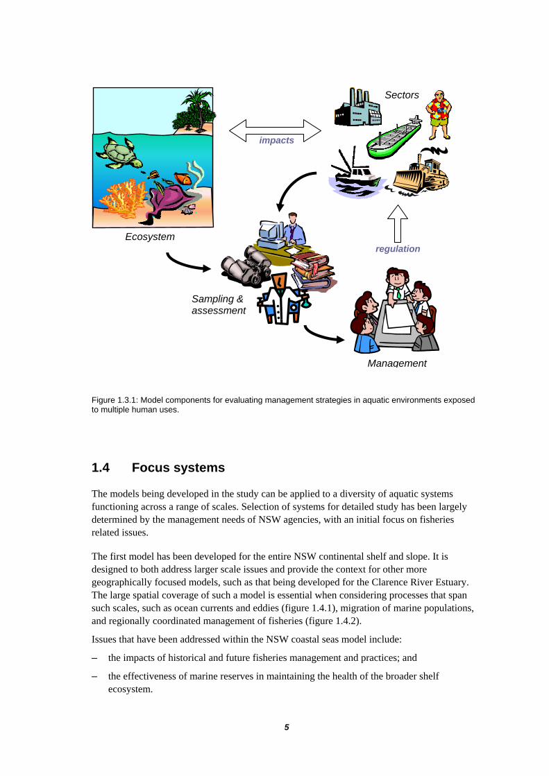
The nonlinear dependence on fishing pressure evident in figure 4.3.2 is consistent with the intermediate disturbance hypothesis. This hypothesis proposes that the greatest biodiversity occurs when the disturbance rate is not too high or too low. Reductions in biodiversity at high levels of disturbance can usually be explained by direct impacts - fishing mortality in our case. Reductions in biodiversity at low levels of disturbance are often attributed to competitive exclusion by a dominant species (Grime 1973, Connell 1978). However, increased predation has been proposed as a alternative mechanism (Menge and Sutherland 1987) and this appears to be the situation in our model results where populations of sharks and rays rise markedly as fishing pressure diminishes (figure 4.3.3).
While it is clear that an extreme harvest strategy such as scenario Ai fails on all accounts, identifying a preferred strategy involves trade-offs and is clearly dependent on management priorities. For example, if the only objective was to reduce the number of over-fished species, then very low harvest rates would be imposed. However, if objectives focused on high biodiversity and sustaining the economic benefits of the fishery, then intermediate harvest rates (baseline or scenario Aiv) would be more attractive.
The model results also provide an indication of the specific groups that are most vulnerable to fishing (Table 4.3.1, Figure 4.3.3). Among the 16 groups mainly harvested by the OTF (>85 % of the landing), the majority show a final biomass inversely correlated to the fishing effort (Figure 4.3.3a). Under extreme fishing pressure (scenario Ai) five groups were driven to extinction in the model - gemfish (FVV), Tiger flathead (FDB), deep demersal fish (FDD), demersal sharks (SHD) and pelagic sharks (SHP).
Apart from the extremely high harvest rates of scenario Ai, the final biomasses of Pink Ling (FDC), whiting (FVO), and deep demersals (FDD) tend to be inversely correlated to the fishing effort, reflecting the beneficial effects of reduced predation by sharks (Figure 4.3.3b). Blue eye and Trevala (FDF) and Blue Grenadier (FBP) show little variation in the final biomass except in the case of the scenario Ai.
The groups partially harvested by the OTF, such as Trevallies (FDO), shallow demersal omnivorous (FDS) and shallow pelagic large planktivores (FPL), seem to benefit from an increased fishing effort in the OTF (Figure 4.3.3b). The exception is again the extremely high harvest rates of scenario Ai. Even oceanic piscivores (FVT), which are otherwise completely insensitive the OTF, show a sharp decline under scenario Ai.
The commercial groups not harvested in the OTF generally benefit from the increase in the OTF fishing effort. For example, the final biomass of shallow demersal herbivores (FDE) is highly correlated to the OTF fishing effort (Figure 4.3.3c). Shallow pelagic small planktivorous (FPS) and prawns (PWN) are mostly insensitive to the OTF, except in scenario Ai where they take advantage of the significant decline in predators (Figure 4.3.3c). Many other non-fished groups, such as small demersal territorial (FDP) and mesopelagics (FMM, FMN) also benefit from reduced predation (Figure 4.3.3d). However, carnivorous mammals (WHS, WHT, PIN) suffer as a result of extremely high fishing effort due to loss of prey (scenario Ai).
34

(a) 0
1
2
3
4
5
6
D B BL Aiv Aiii C Aii AiR
elat
ive
U
(b)
02468
1012141618
D B BL Aiv Aiii C Aii Ai
Num
ber o
f gro
ups
overf ished groups extinct groups
(c)
0
0.2
0.4
0.6
0.8
1
1.2
D B BL Aiv Aiii C Aii Ai
Fina
l yea
r cat
ch re
lativ
e to
BL
OTF Total
(d)
0
0.2
0.4
0.6
0.8
1
1.2
D B BL Aiv Aiii C Aii Ai
Fina
l yea
r val
ue re
lativ
e to
BL
OTF Total
Figure 4.3.1: Summary results after applying each of the fisheries scenarios for 30 years: (a) applied harvest rate relative to the 1976 harvest rate (from Table 3.3.1); (b) number of over-fished and extinct groups; (c) catch relative to 1976 catch; and (d) value of catch relative to 1976 value.
35

0.9
0.95
1
1.05
1.1
0 0.5 1 1.5
biod
iver
sity
inde
x
2
Aii
Aiii C
Aiv
BD
BL
Figure 4.3.2: Kempton’s Q biodiversity index (after 30 years) plotted as a function of fishing pressure relative to the historical 1976 level for each of the harvest strategy scenarios. Scenario Ai with F = 62.79 is off the scale (Table 3.3.1).
Table 4.3.1: Vulnerability of the groups to harvesting based on results from all eight scenarios. *: groups for which the proportion of the total landing landed in the offshore trawling fishery is below 90%. **: groups for which the proportion of the total landing landed in the offshore trawling fishery is below 50%. Groups between parentheses are not landed in the offshore trawl fishery. The deep demersal fish group was the only group that was overfished (< 0.4B0 where B0 is the 1976 biomass) in all scenarios. However, a number of groups were vulnerable to overfishing including skates and rays (SSK), and the dogsharks (SHB).
Vulnerability Groups landed in the Offshore Fishery
Always above 0.4 B0 FPO – FBP – FDC – FDO – CEP (FPS – FVS – FDE – PWN)
Once overfished (Ai) FVB – FVO – FDM – FDB – FDF – SHC – FPL* - FVT *
Once extinct (Ai) FVV
Twice overfished or extinct SHP – SHD* - FDS**
6 times overfished SHB
7 times overfished or extinct SSK
Always overfished FDD
36
(a)0
0.5
1
1.5
2
2.5
3
SHB SHP SSK FVV SHD FDB FDM FPO FVB SHC
AiAiiCAiiiAivBD
(b)0
0.25
0.5
0.75
1
1.25
1.5
1.75
2
FDC FVO FDO FDS FDD FPL FBP FDF
AiAiiCAiiiAivBD
(c)0.0000
0.2500
0.5000
0.7500
1.0000
1.2500
1.5000
1.7500
2.0000
FVT CEP FVS FPS PWN FDE
AiAiiCAiiiAivBD
(d)0
0.25
0.5
0.75
1
1.25
1.5
1.75
2
FDP FM M FM N FVD SHR WHB PIN WHS WHT
AiAiiCAiiiAivBD
Figure 4.3.3: Ratio between the final biomass obtained for each harvest strategy scenario and the final biomass in the baseline case for each group.
37

4.4 Impacts of marine parks
The modelled impacts of marine parks have been explored using the four scenarios summarised in Table 3.3.1 and Figure 3.3.1.
Comparing the pre-existing and expanded reserve systems
The implementation of a series of marine parks closed to fishing significantly affected the total biomass of approximately half of the 32 groups of the model. When fishing pressure or realised catch was removed and not redistributed (MPA1 and MPA2), the biomass changes increased with the size of the area protected (Figure 4.4.1). In the case of the more extensive marine park system (MPA2) biomass increases of up to 15% and decreases of up to 6% occurred over the 30 year simulation (Figure 4.4.1a).
The strongest effects were found in groups that live almost exclusively in the coastal habitat types protected by the marine parks (Figure 4.4.1a). Strong positive effects were experienced by shallow demersal herbivores (FDE), piscivore bony fish (FDB, FDS, FVS), a number of the vulnerable shark groups including grey nurse sharks (SHR), pelagic sharks (SHP), demersal sharks (SHD), and the skates and rays group (SSK). For migratory sharks, such as the grey nurse, these effects necessarily pertain to the entire NSW population. However, even in the case of more sedentary groups, such as the shallow demersal herbivores, the positive effects tend to diffuse along the entire NSW coast rather than being restricted to the marine park areas (Figure 4.4.2a-c).
The increases in predatory shark and bony fish groups tended to have a negative impact on prey groups that live in these environments, such as shallow pelagic large planktivores (FPL), trevallies (FDO) and particularly shallow demersal territorials (FDP) (Figure 4.4.1a). These impacts are evident along the entire NSW coastline, consistent with the widespread increase in predators (Figure 4.4.3a-c). Even redfish (FDM), that only spend their juvenile phase in bays and coastal areas, are impacted by the increased predation (Figure 4.4.1b). Smaller impacts on exclusively offshore species, such as pink ling (FDC), ocean perch (FVB) and morwongs (FPO), again reflect the spread of shark populations benefiting from the marine parks (Figure 4.4.1c).
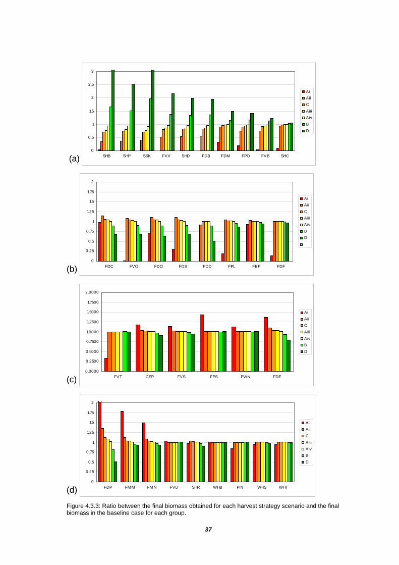
The harvest strategy results, described in the previous section, suggested that fishing rates significantly less than the baseline case may result in increased predation pressure and reduced biodiversity (Figure 4.3.2). The same trend is seen when fishing is reduced by imposing reserves without redistributing fishing effort outside reserves (MPA1 and MPA2 in Figure 4.4.4). However, the reductions in both catch and biodiversity are relatively small compared to the changes considered in the harvest strategy scenarios.
Imposed reductions in catches associated with reserves lead to reductions in both overall catches and catch value (Figure 4.4.5). The largest impacts tend to be on the estuarine fishery (14% loss in value), where the reserve coverage is most comprehensive.
38

(a) 0.9
0.95
1
1.05
1.1
1.15
1.2
SSK FDE SHP SHD SHR FDB FDS FVS PWN FVO FVT FPS WHT WHB WHS PIN FPL FDO FDP
(b) 0.9
0.95
1
1.05
1.1
1.15
1.2
FDD FDF FBP FDM
baselineMPA1MPA2
(c) 0.9
0.95
1
1.05
1.1
1.15
1.2
CEP FM N FM M FVD SHB SHC FVV FDC FVB FPO
Figure 4.4.1: Ratio between the final biomass obtained for MPA1 and MPA2 and the final biomass obtained for MPA0 (i.e. no marine parks): (a) groups that live in bays and coastal areas; (b) groups whose juveniles live in bays and coastal areas while the adults live out on the shelf; and (c) groups that live their entire life out on the shelf and deeper ocean.
39

(a) FDE under MPA0
(b) FDE under MPA1
(c) FDE under MPA2
(c) FDE under MPA3
(d) FDE under MPA4
Figure 4.4.2: Biomass distribution of shallow demersal herbivores (FDE) under scenarios with (a) no marine parks (MPA0); (b) existing marine parks with removal of fishing effort (MPA1); (c) existing plus new marine parks with removal of fishing effort (MPA2); (d) existing marine parks with redistribution of fishing effort (MPA3); and (e) existing plus new marine parks with redistribution of fishing effort (MPA4).
40

(a) FDP under MPA0
(b) FDP under MPA1
(c) FDP under MPA2
(d) FDP under MPA3
(e) FDP under MPA4
Figure 4.4.3: Biomass distribution of shallow demersal territorials (FDP) under scenarios with (a) no marine parks (MPA0); (b) existing marine parks with removal of fishing effort (MPA1); (c) existing plus new marine parks with removal of fishing effort (MPA2); (d) existing marine parks with redistribution of fishing effort (MPA3); and (e) existing plus new marine parks with redistribution of fishing effort (MPA4). Note different colour scales in (d) and (e).
41
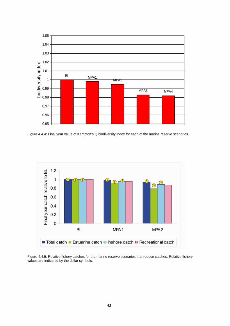
BL MPA1MPA2
MPA3 MPA4
0.95
0.96
0.97
0.98
0.99
1
1.01
1.02
1.03
1.04
1.05bi
odiv
ersi
ty in
dex
Figure 4.4.4: Final year value of Kempton’s Q biodiversity index for each of the marine reserve scenarios.
Figure 4.4.5: Relative fishery catches for the marine reserve scenarios that reduce catches. Relative fishery values are indicated by the dollar symbols.
42
Effects of redistributing catch displaced by reserves
The remaining scenarios (MPA3 and MPA4) looked at the potential impacts of those catches displaced by the expanded marine reserve system being redistributed in neighbouring areas around the reserves. For groups spending at least part of their time within reserves, three main responses were obtained (Figure 4.4.6):
(1) Shark groups (SSK, SHP, SHD, SHR) benefited from the implementation of reserves irrespective of the catch redistribution.
(2) Demersal groups (FDS, FDE, FVO, FDB) as well as the shallow pelagic piscivores (FVS) only benefited when there was no redistribution of catches. When catches were redistributed there was a net decline in these groups, with FDS experiencing the most significant decline.
(3) Groups such as shallow pelagic large planktivores (FPL) and trevallies (FDO) always declined when reserves were implemented due to increased predation. Shallow demersal territorials (FDP) and small pelagic planktivores (FPS) also declined when fishing was removed due to large increases in predators such as shallow demersal omnivores (FDS). However, redistribution of catches reversed these trends through a decline in these predators (Figure 4.4.3).
The influence of coastal reserves on the groups living outside the coastal areas, or living there only as juveniles, was generally quite low (figure 4.4.6). Groups such as pink ling (FDC), ocean perch (FVB) and morwongs (FPO) showed minor declines mainly due to increased predation. The significant anomaly was redfish (FDM), which declined with the introduction of reserves and then declined further when catches were redistributed. This response suggests that the effects of fishing and increased predation were compounded in the case of redfish. Coastal reserves had little influence on oceanic piscivores (FVT) or marine mammals (WHT, WHB, WHS and PIN) irrespective of catch redistribution (not shown).
When catches were redistributed, the biodiversity index decreased. At first this might seem contradictory to the earlier results showing that reducing fishing pressure with reserves also reduced the biodiversity index. However, it appears that the concentration of catches around reserves moves these areas into a high disturbance regime where, according to the intermediate disturbance hypothesis (Grime 1973), biodiversity starts to decline again in response to fisheries impacts (figure 4.3.2). In this case, fishing pressure in the absence of reserves corresponds to an “intermediate” level of disturbance.
Allowing catches to be redistributed removed the impact of reserves on overall catches and catch value (Figure 4.4.7). However, this analysis does not take into account factors such as the economic costs of redistributing catches in response to the introduction of reserves.
The main regional impacts of marine reserves have been summarised schematically in Figure 4.4.8. This emphasises that the key difference between totally removing the fishing effort that was previously applied to the reserve area compared to reallocating it outside the reserve area is the decline of shallow demersal omnivores in the latter case and its associated trophic impacts.
43

(a) 0.75
0.8
0.85
0.9
0.95
1
1.05
1.1
1.15
1.2
SSK SHP SHD SHR FDS FDE FVS FVO FDB PWN FVT WHT WHB WHS PIN FPS FDP FPL FDO
(b) 0.75
0.8
0.85
0.9
0.95
1
1.05
1.1
1.15
1.2
FDD FDF FBP FDM
baseline_catchMPA3MPA4
(c) 0.75
0.8
0.85
0.9
0.95
1
1.05
1.1
1.15
1.2
CEP FM N FM M FVD SHB SHC FVV FDC FVB FPO
Figure 4.4.6: Ratio between the final biomass obtained for MPA3 and MPA4 and the final biomass obtained for MPA0 (i.e. no marine parks): (a) groups that live in bays and coastal areas; (b) groups whose juveniles live in bays and coastal areas while the adults live out on the shelf; and (c) groups that live their entire life out on the shelf and deeper ocean.
44

Figure 4.4.7: Relative fishery catches for the marine reserve scenarios that redistribute catches. Relative fishery values are indicated by the dollar symbols.
Fishing inside
reserve
Sharks & rays
Redfish
Marine reserve
Shallow demersals
Shallow demersal territorial
Trevallies
Sharks & rays
Redfish
Marine reserve
Shallow demersals
Positive effect
Negative effect
Lesser effect
Net increase
Net decrease
Fishing outside reserve
Fishing inside
reserve Biodiversity Biodiversity
Shallow demersal territorial
Trevallies
Fishing displaced Fishing removed
Figure 4.4.8: Schematic representation of the main impacts of marine parks with all of the displaced fishing removed (left) and the displaced fishing redistributed outside of the reserve area (right). Smaller changes in biomass (< 5%) have not been represented in this figure (e.g. morwongs, tiger flathead, ocean perch, whiting and some of the pelagic groups).
45

5. CONCLUSIONS
The main conclusions of the NSW shelf seas modelling completed to date can be summarised as follows:
– The Ocean Trawl Fishery is already fully exploited.
– Reduced fishing would allow a significant proportion of overfished predatory groups (i.e. 1996 biomass < 40% of 1976 biomass) to recover. However, the forage groups and juveniles that form their prey may see a significant decline.
– Fishing levels seen in the 1970s and 1980s achieved biodiversity levels (as measured by Kempton’s Q index applied to the model functional groups) that are equal to or better than other harvest strategies. This result can be understood in terms of the intermediate disturbance hypothesis with very high fishing pressure reducing biodiversity through direct fishing mortality and very low fishing pressure resulting in high predation and reduced biodiversity.
– Marine reserves had a very positive impact on sharks and rays and a mainly negative impact on their prey groups. Shallow demersals and their prey could be impacted positively or negatively depending on whether fishing effort previously in the reserve areas was removed (e.g. buy-outs) or displaced to neighbouring areas.
– Marine reserves caused a decline in biodiversity of the groups represented in the model irrespective of whether historical fishing effort was entirely removed (low disturbance) or redistributed into neighbouring areas outside the reserve (leading to excessive disturbance). This result can also be understood in terms of the intermediate disturbance hypothesis with these two cases pushing the system to either extreme (biodiversity limited by direct fishing pressure or high predation) rather than the intermediate position where biodiversity is thought to peak.
Future work might include extending the historical model runs beyond 1996. This would provide a contemporary view of the system under the most recent management arrangements. It would also allow the model to be run forward into the future to explore the impacts of proposed new management regimes or climate change scenarios.
46

ACKNOWLEDGEMENTS
This research was funded by NSW Department of Primary Industries and the CSIRO Wealth from Oceans Flagship as part of the project Ecologically sustainable development of the regional marine and estuarine resources of NSW. Robyn Forrest received additional support from the University of British Columbia. The co-chairs of the Project Management Committee, Dr Keith Sainsbury and Dr Steve Kennelly, and Dr Bob Creese are thanked for their input and oversight of the project. Dr Matthew Ives and Dr Leo Dutra provided valuable comments on the report.
47

6. REFERENCES
Ainsworth CH, Pitcher TJ, 2006. Modifying Kempton’s species diversity index for use with ecosystem simulation models. Ecological Indicators 6, 623–630.
Andrew NL, Graham KJ, Hodgson KE, Gordon GNG, 1997. Changes after twenty years in relative abundance and size composition of commercial fishes caught during fishery independent surveys on SEF trawl grounds. NSW Fisheries Research Institute - FRDC 96/139, 109 pp.
Brassington GB, Warren, G, Smith N, Schiller A, Oke PR, 2005. Progress on operational ocean prediction for Australia. Bulletin of the Australian Meteorological and Oceanographic Society, 18, 104–109.
Connell, JH, 1978. Diversity in tropical rain forests and coral reefs. Science 199,1302–1310. Daley R, Stevens J, Graham K, 2002. Catch analysis and productivity of the deepwater dogfish
resource in Southern Australia. FRDC project 1998/108, 106 pp. Fulton EA, Fuller M, Smith ADM, Punt A, 2004. Ecological Indicators of the Ecosystem effects
of fishing: Final report 31/7/2004.CSIRO. AFMA Final Research Report R99/1546. Fulton E, Sainsbury K, McDonald D, Hayes D, Lyne V, Little R, Fuller M, Condie S, Gray R,
Scott R., Webb H, Hatfield B, Martin M, 2006. Management strategy evaluation specification for Australia’s North West Shelf. NWSJEMS Technical Report No. 15.
Fulton EA, Smith ADM, 2004. Lessons learnt from a comparison of three ecosystem models for Port Phillip Bay, Australia. Ecosystems approaches to fisheries in the Southern Benguela. African Journal of Marine Science 26, 219-243.
Fulton EA., Smith ADM, Smith DC, 2007. Alternative Management Strategies for Southeast Australian Commonwealth Fisheries: Stage 2: Quantitative Management Strategy Evaluation. Australian Fisheries Management Authority Report.
Graham KJ, 2005. Distribution, population structure and biological aspects of Squalus spp. (Chondrichtyes: Squaliformes) from New South Wales and adjacent waters. Marine and Freshwater Research 56, 405-416.
Grime JP, 1973. Competitive exclusion in herbaceous vegetation. Nature 242, 344-347 Interim Marine and Coastal Regionalisation for Australia Technical Group, 1998. Interim
Marine and Coastal Regionalisation for Australia: An Ecosystem-Based Classification for Marine and Coastal Environments. Version 3.3. Environment Australia, Commonwealth Department of the Environment: Canberra.
Kempton RA, Taylor LR, 1976. Models and statistics for species diversity. Nature 262, 818–820.
Little R, Fulton E, Gray R, Hayes D, Lyne V, Scott R, Sainsbury K, McDonald D, 2006. Management strategy evaluation results and discussion for Australia’s North West Shelf. NWSJEMS Technical Report No. 14.
Lyne V, Hayes D, 2005. Pelagic Regionalisation. National Marine Bioregionalisation Integration Project. CSIRO Marine Research, Hobart, Australia.
Menge BA, Sutherland JP, 1987. Community regulation: Variation in disturbance, competition, and predation in relation to environmental stress and recruitment. The American Naturalist 130, 730-757.
Murray A, Parslow J, 1999. Modelling of nutrient impacts in Port Philip bay - A semi enclosed marine Australian ecosystem. Marine and Freshwater Research 50, 597-611
Oke PR, Brassington GB, Griffin DA, Schiller A, 2008. The Bluelink ocean data assimilation system (BODAS). Ocean Modelling 21, 46-70.
Otway NM, Burke AL, 2004. Mark-recapture population estimate and movements of Grey Nurse Shark. NSW Fisheries Report Series no. 63, 53pp.
Otway NM, Parker PC, 2000. The biology, ecology, distribution, abundance and identification of marine protected areas for the conservation of threatened Grey Nurse sharks in south east Australian waters. NSW Fisheries Final Report Series no. 19, 101pp.
48

49
Otway NM, Burke AL, Morrison NS, Parker PC, 2003. Monitoring and identification of NSW Critical Habitat Sites for conservation of Grey Nurse Sharks. NSW Fisheries Final Report Series no. 47, 62pp.
Pauly D, Christensen V, Walters C, 2000. Ecopath, Ecosim, and Ecospace as tools for evaluating ecosystem impact of fisheries. ICES Journal of Marine Science 57, 697–706.
Punt AE, 2000. Bayesian assessments of the eastern stock of Gemfish using data for the 2000 winter fishing season. CSIRO Marine Research, 19pp.
Punt AE, Rowling K, Prince J, 2000. Summary of the data use in the assessments of the eastern Stock of Gemfish based on the 1999 fishing season. 18pp.
Taylor B, Smith D, 2004. Stock assessment of spotted warehou (Seriolella punctata) in the South East Fishery. PIRVic, Queenscliff, august 2004, 8pp.
Thomson RB, 2002. Integrated Analysis of redfish in the South East Fishery, including the 2001 fishing data. Presented to the Redfish Assessment Group, Bermagui, 27-28 June 2002. 32pp.
Tuck GN, 2006. Stock Assessment for the Southern and Eastern Scalefish and Shark Fishery 2004-2005. Australian Fisheries Management Authority and CSIRO Marine Research, Hobart, 222 pp.
Tuck GN, Smith ADM, 2004. Stock Assessment for South East and Southern Shark Fishery Species. Fisheries Research and Development Corporation and CSIRO Marine Research, Hobart, 412pp.
Tuck GN, Smith D, Talman S, 2004. Update stock assessment for Blue Grenadier (Macruronus novaezelandiae) in the South East Fishery: August 2004. SESSF Quantitative Analysis Group, 33pp.
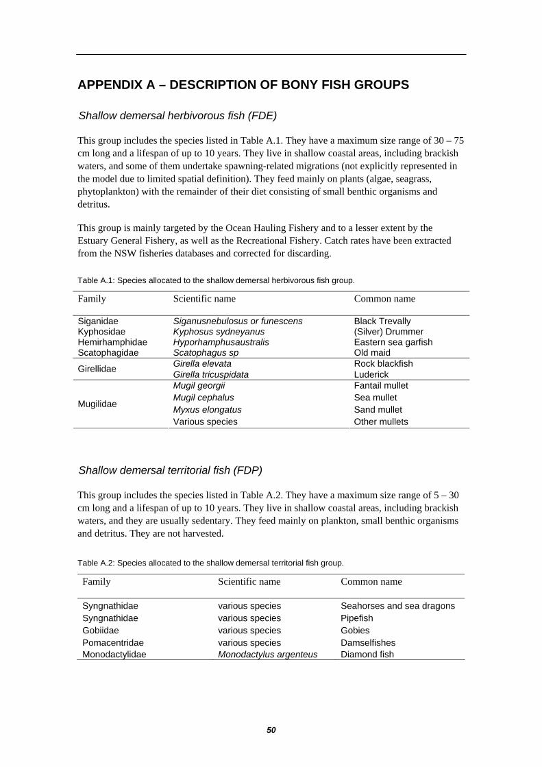
APPENDIX A – DESCRIPTION OF BONY FISH GROUPS
Shallow demersal herbivorous fish (FDE)
This group includes the species listed in Table A.1. They have a maximum size range of 30 – 75 cm long and a lifespan of up to 10 years. They live in shallow coastal areas, including brackish waters, and some of them undertake spawning-related migrations (not explicitly represented in the model due to limited spatial definition). They feed mainly on plants (algae, seagrass, phytoplankton) with the remainder of their diet consisting of small benthic organisms and detritus.
This group is mainly targeted by the Ocean Hauling Fishery and to a lesser extent by the Estuary General Fishery, as well as the Recreational Fishery. Catch rates have been extracted from the NSW fisheries databases and corrected for discarding.
Table A.1: Species allocated to the shallow demersal herbivorous fish group.
Family Scientific name Common name
Siganidae Siganusnebulosus or funescens Black Trevally Kyphosidae Kyphosus sydneyanus (Silver) Drummer Hemirhamphidae Hyporhamphusaustralis Eastern sea garfish Scatophagidae Scatophagus sp Old maid
Girella elevata Rock blackfish Girellidae Girella tricuspidata Luderick Mugil georgii Fantail mullet Mugil cephalus Sea mullet Myxus elongatus Sand mullet Mugilidae
Various species Other mullets
Shallow demersal territorial fish (FDP)
This group includes the species listed in Table A.2. They have a maximum size range of 5 – 30 cm long and a lifespan of up to 10 years. They live in shallow coastal areas, including brackish waters, and they are usually sedentary. They feed mainly on plankton, small benthic organisms and detritus. They are not harvested.
Table A.2: Species allocated to the shallow demersal territorial fish group.
Family Scientific name Common name
Syngnathidae various species Seahorses and sea dragons Syngnathidae various species Pipefish Gobiidae various species Gobies Pomacentridae various species Damselfishes Monodactylidae Monodactylus argenteus Diamond fish
50
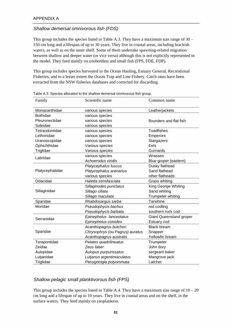
APPENDIX A
Shallow demersal omnivorous fish (FDS)
This group includes the species listed in Table A.3. They have a maximum size range of 30 – 150 cm long and a lifespan of up to 30 years. They live in coastal areas, including brackish waters, as well as on the inner shelf. Some of them undertake spawning-related migration between shallow and deeper water (or vice versa) although this is not explicitly represented in the model. They feed mainly on zoobenthos and small fish (FPS, FDE, FDP).
This group includes species harvested in the Ocean Hauling, Estuary General, Recreational Fisheries, and to a lesser extent the Ocean Trap and Line Fishery. Catch rates have been extracted from the NSW fisheries databases and corrected for discarding.
Table A.3: Species allocated to the shallow demersal omnivorous fish group.
Family Scientific name Common name
Monacanthidae various species Leatherjackets Bothidae various species Pleuronectidae various species Soleidae various species
flounders and flat fish
Tetraodontidae various species Toadfishes Lethrinidae various species Emperors Uranoscopidae various species Stargazers Ophichthidae Various species Eels Triglidae Various species Gurnards
various species Wrasses Labridae Achoerodus viridis Blue groper (eastern) Platycephalus fuscus Dusky flathead Platycephalus arenarius Sand flathead Platycephalidae various species other flatheads
Odacidae Haletta semifasciata Grass whiting Sillaginodes punctatus King George Whiting Sillago ciliata Sand whiting Sillaginidae Sillago maculata Trumpeter whiting
Sparidae Rhabdosargus sarba Tarwhine Pseudophycis bachus red codling Moridae
Pseudophycis barbata southern rock cod Epinephelus lanceolatus Giant Queensland groper Serranidae Epinephelus coioides Estuary cod Acanthopagrus butcheri Black bream Chrysophrys (ou Pagrus) auratus Snapper Sparidae Acanthopagrus australis Yellowfin bream
Terapontidae Pelates quadrilineatus Trumpeter Zeidae Zeus faber John dory Aulopidae Aulopus purpurissatus sergeant baker Lutjanidae Lutjanus argentimaculatus Mangrove jack Triglidae Pterygotrigla polyommata Latchet
Shallow pelagic small planktivorous fish (FPS)
This group includes the species listed in Table A.4. They have a maximum size range of 10 – 20 cm long and a lifespan of up to 10 years. They live in coastal areas and on the shelf, in the surface waters. They feed mainly on zooplankton.
51

They are harvested in the Ocean Hauling Fishery, while pilchards are also caught in the South East Non Trawl Fishery (Commonwealth) and as bait in the Eastern Tuna and Billfish Fishery (Commonwealth). Catch rates have been extracted from the NSW fisheries databases and corrected for discarding.
Table A.4: Species allocated to the shallow pelagic small planktivorous fish group.
Family Scientific name Common name
Engraulidae Engraulis australis Anchovy Sardinops sagax or neopilchardus Pilchard Hyperlophus vittatus Sandy sprat (whitebait) Clupeidae Spratelloides robustus or Hyperlophus translucidus Glassfish (whitebait)
Shallow pelagic large planktivorous fish (FPL)
This group includes the species listed in Table A.5. They have a maximum size range of 50 – 70 cm long and a lifespan of up to 30 years. They live in the surface waters of coastal areas and the shelf. They feed mainly on zooplankton and small fish (FPS and FMM/FMN).
In New South Wales they are harvested by the Ocean Hauling, Ocean Trap and Line, and Recreational Fisheries. They are also caught in Commonwealth fisheries such as the Small Pelagic Fishery, South East Non Trawl Fishery, and the Eastern Tuna and Billfish Fishery as bait. Catch rates have been extracted from the NSW fisheries databases and corrected for discarding.
Table A.5: Species allocated to the shallow pelagic large planktivorous fish group.
Family Scientific name Common name
Scombridae Scomber australasicus Blue mackerel Trachurus murphyi Peruvian jack mackerel Trachurus declivis Jack mackerel Carangidae
Trachurus novaezelandiae Yellowtail (scad)
Shallow pelagic piscivorous fish (FVS)
This group includes the species listed in Table A.6. They have a maximum size range of 90 – 200 cm long and a lifespan of up to 10 years. They live in coastal areas and on the shelf. They are pelagic, but species such as Teraglin and Mulloway can feed close to the sea bed at certain time of the day. Migration pattern have been detected for species such as Tailor and Teraglin, although this behaviour is again not explicitly represented in the model.
They are harvested in the Ocean Hauling, Ocean Trap and Line, and Recreational Fisheries. Catch rates have been extracted from the NSW fisheries databases and corrected for discarding.
Table A.6: Species allocated to the shallow pelagic piscivorous fish group.
52

APPENDIX A
53
Family Scientific name Common name
Arripididae Arripis trutta Australian salmon (eastern) Gempylidae Thyrsites atun Barracouta Pomatomidae Pomatomus saltatrix Tailor Sphyraenidae Sphyraena novaehollandiae Snook/barracuda Coryphaenidae Coryphaena hippurus Dolphinfish (or mahi mahi) Carangidae Seriola lalandi (Yellowtail) kingfish
Argyrosomus hololepidotus Mulloway Sciaenidae Atractoscion aequidens Teraglin Scomberomorus commerson Spanish mackerel Scomberomorus munroi Spotted mackerel Euthynnus affinis Mackerel tuna
Scombridae
Sarda australis Bonito
Deep demersal fish (FDD)
This group includes the species listed in Table A.7. They have a maximum size range of 15 – 180 cm long and a lifespan of up to 40 years. They live close to the seabed on the outer shelf and upper slope. They feed on fish (other deep fish, FMM/FMN), benthos, cephalopods and gelatinous zooplankton.
They are harvested in the Ocean Trap and Line, Ocean Trawl, and Ocean Prawn Trawl fisheries as well as in the Commonwealth South East Fishery. Catch rates have been extracted from the NSW fisheries databases and corrected for discarding.
Table A.7: Species allocated to the deep demersal fish group.
Family Scientific name Common name
Zenopsis nebulosus Mirror dory Cyttus traversi king dory Zeidae
various sp other dories Percichthyidae Polyprion oxygeneios hapuku Paraulopidae Paraulopus or Chlorophthalmus nigripinnis cucumber fish Triglidae Pterygotrigla andertoni painted gurnard Gempylidae Rexea antefurcata long-finned gemfish Argentinidae Argentina australiae silverside Macrouridae various sp Whiptails
Berycidae Berycidae beryx spp Beryx (imperador and alfonsino)
Apogonidae various species Cardinalfish Hoplichthyidae Hoplichthys haswelli spiny flathead Moridae Mora moro Ribaldo
Oceanic piscivorous fish (FVT)
This group includes the species listed in Table A.8. They have a maximum size range of 100 – 450 cm long and typically a lifespan of up to 10 years. They live in the epipelagic zone (surface
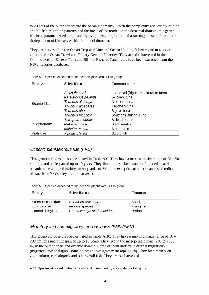
54
to 200 m) of the outer neritic and the oceanic domains. Given the complexity and variety of tuna and billfish migration patterns and the focus of the model on the demersal domain, this group has been parameterised simplistically by ignoring migration and assuming constant recruitment (independent of biomass within the model domain).
They are harvested in the Ocean Trap and Line and Ocean Hauling fisheries and to a lesser extent in the Ocean Trawl and Estuary General Fisheries. They are also harvested in the Commonwealth Eastern Tuna and Billfish Fishery. Catch rates have been extracted from the NSW fisheries databases.
Table A.8: Species allocated to the oceanic piscivorous fish group.
Family Scientific name Common name
Auxis thazard Leadenall (frigate mackerel or tuna) Katsuwonus pelamis Skipjack tuna Thunnus alalunga Albacore tuna Thunnus albacares Yellowfin tuna Thunnus obesus Bigeye tuna
Scombridae
Thunnus maccoyii Southern Bluefin Tuna Tetrapturus audax Striped marlin Makaira indica Black marlin Istiophoridae Makaira mazara Blue marlin
Xiphiidae Xiphias gladius Swordfish
Oceanic planktivorous fish (FVD)
This group includes the species listed in Table A.9. They have a maximum size range of 25 – 50 cm long and a lifespan of up to 10 years. They live in the surface waters of the neritic and oceanic zone and feed mainly on zooplankton. With the exception of minor catches of redbait off southern NSW, they are not harvested.
Table A.9: Species allocated to the oceanic planktivorous fish group.
Family Scientific name Common name
Scomberesocidae Scomberesox saurus Sauries Exocoetidae various species Flying fish Emmelichthyidae Emmelichthys nitidus nitidus Redbait
Migratory and non-migratory mesopelagics (FMM/FMN)
This group includes the species listed in Table A.10. They have a maximum size range of 10 – 200 cm long and a lifespan of up to 10 years. They live in the mesopelagic zone (200 to 1000 m) in the outer neritic and oceanic domain. Some of them undertake diurnal migrations (migratory mesopelagics) some do not (non-migratory mesopelagics). They feed mainly on zooplankton, cephalopods and other small fish. They are not harvested.
A.10: Species allocated to the migratory and non-migratory mesopelagics fish group.

APPENDIX A
55
Migration Family Scientific name Common name
Myctophidae Diaphus sp lanternfish Trichiuridae various species frostfish or ribbonfish Alepisauridae Alepisaurus sp lancetfish Bramidae Brama brama pomfret
yes
Gempylidae Ruvettus pretiosus oilfish Sternoptychidae various species Sternoptychids Gonostomatidae various species Lightfish (cyclothene) no Centrolophidae Centrolophus niger rudderfish

56
APPENDIX B – DESCRIPTION OF COMMERCIAL DEEP-WATER FISH SPECIES
The species ecological information presented below is from the book Australian Fisheries Resources, unless otherwise stated. Abundances were based on detailed stock assessments where available. Catch rates have been extracted from the NSW fisheries databases and corrected for discarding, unless otherwise stated.
Eastern Gemfish (Rexea solandri- FVV)
Eastern gemfish inhabit deeper continental shelf and upper slope waters from 100 m to 700 m. They spend most of their time close to the seabed, occasionally moving into the mid-water. They are distributed from Cape Moreton in southern Queensland to eastern Bass Strait.
The mature eastern gemfish undergo an annual spawning migration which begins with fish aggregating off north-eastern Bass Strait in autumn, then moving north. The migrating schools usually reach the Sydney to Wollongong region by the end of June and typically peak in abundance during July. Most fish reach the spawning grounds off central and northern NSW to spawn in August. They appear to disperse after spawning with at least some of the stock returning to southern waters. Parts of the migration that fall within the model domain have been explicitly represented in the model.
Because the eastern gemfish stock and the associated fishery catch are mainly distributed off NSW (Punt et al. 2000), it was assumed that the model gemfish abundance corresponded to the whole eastern gemfish stock. The stock assessment of Punt (2000) suggested that official catch statistics do not reflect the true magnitude of the annual landing. Two alternative catch time series (considered equally plausible) were therefore used in the assessment to account for discarding. These alternatives have both been tested using the Atlantis model.
Morwongs (Nemadactylus sp – FPO)
This group represents both Jackass morwong (Nemadactylus macropterus) and Rubberlip or Grey morwong (Nemadactylus douglasii). However, given the scarcity of information about the second species, the parameterisation has been mainly based on Jackass morwong ecology.
Jackass morwong is a demersal fish with adults living over open grounds between 40 and 400 m depth and juveniles near shallow reefs. They are distributed throughout southern Australia from Moreton Bay in Queensland to Perth in Western Australia. There is no evidence of separate stocks in Australian waters. However, given the differences among Jackass morwong in the eastern zones and western zones, a single stock is assumed for the fishing zones east to Bass Strait (Tuck and Smith, 2004).
Jackass morwong spawn from late summer to autumn (February to May). The only known nursery areas for juvenile jackass morwong are in Bass Strait and the coastal waters of Tasmania. Tagging and genetic studies have shown little movement by adults, so it appears that older juveniles disperse from the nursery areas to their adult habitats.
Given the location of the nursery areas, we assumed a gradual southward increase in adults along the NSW coast during the spawning season. While the recruitment of Jackass morwong

APPENDIX B 57
57
was assumed to be proportional to the NSW population (as for the other fish), juveniles started their life outside the model domain with gradual immigration after a year of development.
Abundance estimates for Jackass morwong were based on assessments for the Commonwealth South East Fishery (Tuck 2006), with a proportional increase to account for the additional habitat available in NSW waters outside of the South East Fishery area. Because there was no information available on the abundance of Grey morwong in NSW, it was roughly estimated on the basis of available catch time series.
Warehous and Trevalla (FDF)
This group includes blue Warehou (Seriolella brama) and spotted warehou (Seriolella punctata), as well as blue-eye trevalla (Hyperoglyphe antartica). Adult warehous and blue-eye trevalla inhabit continental shelf and slope waters from a depth of 50 m to 900 m (blue warehou : 50-400 m, spotted warehou: 50-600 m, blue-eye: 200-900 m). They mainly reside close to the sea bed, moving into the mid-water at night following prey.
Blue-eye trevalla are present along the southern continental margin from Moreton Island in Queensland to around 30ºS in Western Australia. Preliminary studies indicate that blue eye trevalla off south-eastern Australia belong to a common stock. Warehous are found in the South East corner of Australia, including around Tasmania, and there is increasing evidence for separate stocks of blue warehou to the east and west of Bass Strait (Tuck and Smith, 2004). No studies have been done on the stock structure of spotted warehou in Australian waters and there is little anecdotal evidence of any stock structure. Consequently the species is managed in the South East Fishery as a single stock (Taylor and Smith, 2004).
From April to June, mature blue eye move up the continental slope into shallow depths (320-400 m) where they aggregate on their spawning grounds. Juveniles inhabit surface waters, sometimes in association with floating debris, before moving to deeper demersal habitats at around 2 years of age. Warehous spawn from late winter to early spring. The small juveniles are pelagic, inhabiting offshore areas and often associated with jellyfish. Older juvenile warehou move inshore with large numbers found in bays and inlets.
Abundances of warehous were based on stock assessments (Taylor and Smith, 2004, Tuck, 2006) with a correction to take into account the area of habitat available off NSW compared to that available over the entire assessment area. Since no quantitative assessments were available for blue-eye trevalla, it was assumed be 50% of the warehou biomass.
Blue Grenadier (Macruronus novaezelandiae - FBP)
Adult blue grenadier inhabit continental slope waters between 200 and 700 m. They form dense schools near the seabed during the day and disperse into the water column at dusk, ascending to within 50 m of the surface.
Blue Grenadier is distributed through southern Australian waters from Broken Bay in NSW to the western Great Australian Bight. Data support the hypothesis of a single breeding population in Australian waters (Tuck et al. 2004).
The main spawning ground is off the west coast of Tasmania and is thought to attract adults from throughout the species Australian distribution. Spawning occurs in winter and early spring.

58
Most larvae probably settle off the Tasmanian west and south coast. Juveniles are common in the estuaries and bays of southern Tasmania.
In the model, the whole NSW population migrates away from the model domain during the second half of each year. However, the abundance of juveniles arriving in the model domain is assumed to be proportional to the NSW blue grenadier population.
Abundances of blue grenadier were based on stock assessments (Tuck, 2006) with a correction to take into account the area of habitat available off NSW compared to that available over the entire assessment area. Given that the species is limited to the area south of Broken Bay, this abundance has not been further corrected. Catch rates were not available on the NSW fisheries databases for this species, therefore a fishing mortality time series has been used instead (Tuck, pers. com.).
Pink Ling (Genypterus blacodes - FDC)
Pink ling are demersal, inhabiting depths of 20 to 800 m with highest abundance between 300 and 550 m depth. They occur over a variety of substrate, from rocky ground to soft sand and mud in which they burrow. They inhabit the continental shelf and slope of temperate Australia, from Crowdy Head in NSW to Albany in Western Australia. One stock is assumed throughout South East Australia.
There is little information on spawning of pink ling. To the west of Bass Strait spawning probably takes place in late winter to early spring. There are no records of regular migrations of pink ling. A shift into deeper water in winter and spring is suggested by catch data, which has been incorporated into the model. Juveniles are found in shallower shelf waters.
Abundances were based on stock assessments (Tuck, 2006) with a correction to take into account the area of habitat available off NSW compared to that available over the entire assessment area. This biomass has then been further corrected to account for the available habitat north to the assessment area (to Crowdy head).
Redfish (Centroberyx affinis - FDM)
Redfish are demersal with most adults found over reefs and mud substrates in continental shelf and slope waters to a depth of 450 m. Trawl catches are highest in depth of 100 m to 300 m with large schools forming near the sea bed around dawn and dusk. Juveniles inhabit estuaries and shallow coastal waters.
The species is most abundant off the NSW coast, although the distribution extends from Moreton Bay in Queensland to Western Bass Strait and north-eastern Tasmanian. Tagging studies indicate a single stock off NSW. However, the stock assessments distinguish areas north and south of Montague Island due to their different growth rates (Thomson, 2002).
Spawning takes place in late summer and autumn and is thought to occur throughout the species distribution.
The abundance of redfish has been estimated from a stock assessment (Thomson, 2002) assuming that the biomass estimate for the area north of Montague Island corresponds to the NSW biomass.

APPENDIX B 59
59
Eastern School whiting (Sillago flindersi – FVO)
The eastern school whiting is a demersal fish inhabiting depths from the surf zone to about 80 m. They are distributed from Moreton Bay in Queensland, through New South Wales and Victoria to Anxious Bay in South Australia. They are also present on the east coast of Tasmania. Genetic studies of eastern school whiting have identified 4 separate stocks. Fish from northern NSW are distinct from southern NSW fish, which appear to be part of a larger stock extending through eastern and central Bass Strait. Other stocks are present off Tasmania and from Western Victoria to Anxious Bay.
Off northern NSW, spawning activity peaks in winter. In southern NSW and eastern Bass Strait spawning occurs from spring to late summer. Juveniles inhabit inshore waters.
Abundances of school whiting were based on stock assessments (Tuck, 2006) with a correction to take into account the area of habitat available off NSW compared to that available over the entire assessment area. This abundance was then increased by 50% to account for the stock off northern NSW, which was not included in the assessment. The two stocks were not treated separately in the model.

APPENDIX C – DESCRIPTION OF SHARK AND RAY GROUPS
Unless otherwise stated, the species ecological information presented below is from Australian Fisheries Resources, The Fish of Australia's South Coast, the Kapala report (Andrew et al, 1997) and the websites FishBase and Australian Museum Fish Site. Abundances were based on detailed stock assessments where available. Catch rates have been estimated from Kapala unless otherwise stated.
Pelagic sharks (SHP)
This group includes the species listed in Table C1. They have a maximum size range of 300 – 800 cm long and a lifespan of up to 30 years. They are pelagic and can be found in all environments from shallow coastal to oceanic. They are opportunistic carnivores, feeding on a wide variety of fish and invertebrates. Their migration patterns are likely to be driven by seasonal conditions and we have assumed southward movement during spring and northward movement during autumn.
No data on pelagic shark biomass or catch were available. The initial biomass was assumed to be 1400-1500 tons with a fishing mortality of 0.2 yr-1 to account for commercial fishing, recreational fishing, and mortality associated with shark nets.
Table C1: Species allocated to the pelagic shark group.
Family Scientific name Common name
Carcharhinus brachyurus Bronze whaler Carcharhinus obscurus Dusky whaler Prionace glauca Blue shark
Carcharhinidae
Galeocerdo cuvier Tiger shark Isurus oxyrinchus Mako Lamnidae Carcharodon carcharias White pointer or great white shark
Sphyrnidae Sphyrna zygaena Hammerhead shark
Demersal sharks (SHD)
This group includes the species listed in Table C2. They have a maximum size range of 150 – 500 cm long and a lifespan of up to 20 years. They are demersal and live in coastal areas and on the shelf. They feed on a wide variety of fish, as well as cephalopods and benthic invertebrates.
On the basis of the 1976-77 Kapala catch rates, the initial biomass was set at 10,000 tons and a fishing mortality of 0.18 yr-1 was assumed.
60

APPENDIX C 61
61
Table C2: Species allocated to the demersal shark group.
Family Scientific name Common name
Mustelus antarcticus Gummy Shark Triakidae Galeorhinus galeus School Shark
Orectolobidae Orectolobus spp Wobbegong Odontaspidae Odontaspis ferox Herbsts nurse shark Heterodontidae Heterodontus portusjacksoni Port Jackson shark Pristidae Pristis zijsron Green sawfish Pristiophoridae Pristiophorus sp sawshark
Skates and Rays (SSK)
This group includes the species listed in Table C3. They have a maximum size range of 50 – 400 cm long and a lifespan of up to 30 years. They are demersal and can be found in all environments from the coast to the continental slope. They feed on demersal fish and benthic invertebrates.
On the basis of the 1976-77 Kapala catch rates, the initial biomass was set at 20,000 tons and a fishing mortality of 0.2 yr-1 was assumed.
Table C3: Species allocated to the skates and rays group.
Family
Scientific name Common name
Squatinidae Squatina tergocellata or Squatina australis Angel shark Dasyatidae various sp Stingray Urolophidae various sp Stingaree Rhinobatidae Trygonorrhina fasciata Eastern fiddler ray Torpedinidae Narcine tasmaniensis Tasmanian numbfish Rajidae various species skate
Dogsharks (SHB)
This group includes the species listed in Table C4. They have a maximum size range of 180 – 200 cm long and a typical lifespan of up to 40 years. They are demersal and live on the continental slope. They feed on deep demersal and mesopelagic fish, as well as cephalopods and benthic invertebrates (Daley et al, 2002).
On the basis of the 1976-77 Kapala catch rates, the initial biomass was set at 30,000 tons. The fishing mortality time series has been estimated from Daley et al. (2002).

62
Table C4: Species allocated to the dogsharks group.
Family Scientific name Common name
Centrophorus harrissoni Harrisson dogfish Centrophorus uyato Southern dogfish Centrophorus moluccensis Endeavour dogshark Deania calcea Shovelnose spiny dogfish
Centrophoridae
Deania quadrispinosa Longsnout dogfish Squalidae Squalus mitsukurii Greeneye dogshark
Spiky dogshark (Squalus megalops – SHC)
The spiky dogshark is up to 70 cm long and is assumed to have a lifespan of up to 30 years. It is a demersal species occurring on the outer shelf and upper slope (60-500 m depth), while the juveniles are pelagic (Graham, 2005). The species can be found throughout southern Australia, NSW and Queensland (Graham, 2005). They feed on teleost fish and benthic invertebrates.
This species has been considered separately from the other dogsharks because it is the only one that showed no statistically significant change in overall catch rates between the 1976-77 and 1996-97 Kapala surveys. The size composition data obtained during these surveys also suggested little change in population structure after 20 years. This apparent robustness compared to other dogsharks may be associated with its distribution, which includes large areas of the outer continental shelf that are only lightly impacted by commercial fishing (Graham, 2005).
On the basis of the 1976-77 Kapala catch rates, the initial biomass was set at 17,000 tons. The fishing mortality time series has been estimated from Daley et al. (2002).
Grey nurse shark (Carcharias taurus)
The grey nurse shark is up to 320 cm long (Otway and Parker, 2000) and is assumed to have a lifespan of up to 30 years (Otway et al, 2003). It is a coastal species, present from the surf zone down to at least 190 m. Individuals are often found in or near deep sandy-bottomed gutters or in rocky caves around inshore rocky reefs and islands at depth between 15 and 25 meters. They feed on a large variety of teleost fishes, smaller sharks, cephalopods and benthic invertebrates (Otway and Parker, 2000).
The grey nurse shark is distributed through from Mooloolaba in southern Queensland, around the southern half of the continent, and northwards to Shark Bay in Western Australia. They are rare in Tasmanian waters (Otway and Parker, 2000) and recent studies suggest that the eastern and western populations are distinct.
In New South Wales, according to the results of a diving survey carried out in 1998-1999, sexually mature males move into shallow water in early autumn to mate, before migrating northwards to appear at the most northerly sites in Southern Queensland around July or August. Sexually mature females and immature sharks of both sexes move to south in spring and early summer, returning to sites north of Foster in the autumn and winter months (Otway and Parker, 2000). These patterns are yet to be confirmed by recent tagging studies. Because females and males are not considered separately in the model, their migration patterns have effectively been merged.

APPENDIX C 63
63
The grey nurse shark has been considered separately due to its status as a protected species since 1984 (Otway and Parker, 2000) and as the most significant reef shark in New South Wales. The NSW beach meshing program records suggest that the number of grey nurse sharks declined significantly more than the other shark species over the period 1950-1990.
A mark-recapture study performed in 2003 (Otway and Burke, 2004), has estimated the population at 410 to 460 individuals. In the absence of other indications of the absolute abundance of the grey nurse shark in NSW, it has been assumed in the model that the initial abundance in 1976 was 100 times greater at 44000 individuals with a total biomass of 2370 tonnes. A fishing mortality of 0.11 yr-1 has been used to represent the impact of recreational fishing prior to 1984, with a reduced rate of 0.03 yr-1 post 1984 to represent accidental fishing and meshing.